Author response:

The following is the authors’ response to the original reviews.

Public Reviews:

Reviewer #1 (Public Review):

In the manuscript by Su et al., the authors present a massively parallel reporter assay (MPRA) measuring the stability of in vitro transcribed mRNAs carrying wild-type or mutant 5' or 3' UTRs transfected into two different human cell lines. The goal presented at the beginning of the manuscript was to screen for effects of disease-associated point mutations on the stability of the reporter RNAs carrying partial human 5' or 3' UTRs. However, the majority of the manuscript is dedicated to identifying sequence components underlying the differential stability of reporter constructs. This shows that TA dinucleotides are the most predictive feature of RNA stability in both cell lines and both UTRs.

The effect of AU rich elements (AREs) on RNA stability is well established in multiple systems, and the present study confirms this general trend but points out variability in the consequence of seemingly similar motifs on RNA stability. For example, the authors report that a long stretch of Us has extreme opposite effects on RNA stability depending on whether it is preceded by an A (strongly destabilizing) or followed by an A (strongly stabilizing). While the authors interpretation of a context- dependence of the effect is certainly well-founded, it seems counterintuitive that the preceding or following A would be the (only) determining factor. This points to a generally reductionist approach taken by the authors in the analysis of the data and in their attempt to dissect the contribution of "AU rich sequences" to RNA stability, with a general tendency to reduce the size and complexity of the features (e.g. to dinucleotides). While this certainly increases the statistical power of the analysis due to the number of occurrences of these motifs, it limits the interpretability of the results. How do TA dinucleotides per se contribute to destabilizing the RNA, both in 5' and 3' UTRs, but (according to limited data presented) not in coding sequences? What is the mechanism? RBPs binding to TA dinucleotide containing sequences are suggested to "mask" the destabilizing effect, thereby leading to a more stable RNA. Gain of TA dinucleotides is reported to have a destabilizing effect, but again no hypothesis is provided as to the underlying molecular mechanism. In addition to reducing the motif length to dinucleotides, the notion of "context dependence" is used in a very narrow sense; especially when focusing on simple and short motifs, a more extensive analysis of the interdependence of these features (beyond the existing analysis of the relationship between TA- diNTs and GC content) could potentially reveal more of the context dependence underlying the seemingly opposite behavior of very similar motifs.

(We have used UA instead of TA, as per the reviewer's suggestion)

The contribution of coding region sequence to RNA stability has been extensively discussed (For example: doi.org/10.1016/j.molcel.2022.03.032; doi.org/10.1186/s13059-020-02251-5; doi.org/10.15252/embr.201948220; doi.org/10.1371/journal.pone.0228730; doi.org/10.7554/eLife.45396). While UA content at the third codon position (wobble position) has been implicated as a pro-degradation signal, codon optimality has emerged as the most prominent determinant for RNA stability. This indicates that the role of coding regions in RNA stability differs from that of UTRs due to the involvement of translation elongation. We did not intend to suggest that UA-dinucleotides in UTRs and coding regions have the same effect. 

To ensure the representativeness of the features entered into the LASSO model, we pre-selected those with an occurrence greater than 10% among all UTRs. As a result, while motifs with very low occurrences were excluded from the analysis, there is no evidence to indicate a preference for dinucleotides by the LASSO model.

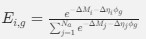
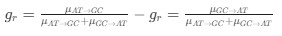
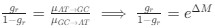
We hypothesize that UA-dinucleotide may recruit endonucleases RNase A family, whose catalytic pockets exhibit a strong bias for UA dinucleotide (doi.org/10.1016/j.febslet.2010.04.018). Structures or protein bindings that block this recognition might stabilize RNAs. To gain further insight into the motif interactions, we investigated the interactions between UA and other 15 dinucleotides through more detailed analyses. We conducted a linear regression analysis investigating interactions between UA and the other 15 dinucleotides. The formula used below includes UA:

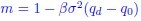
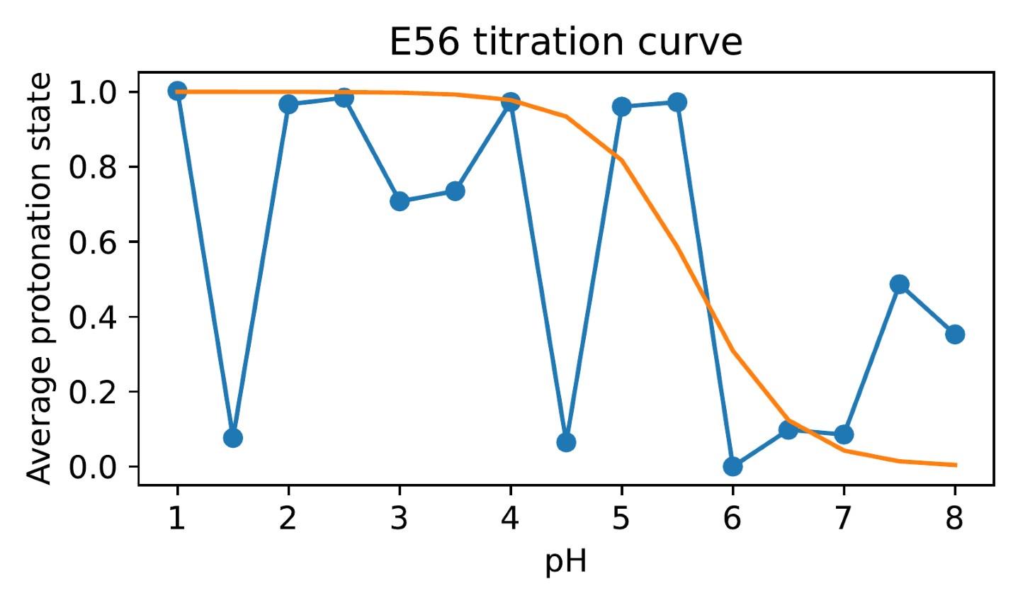
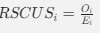
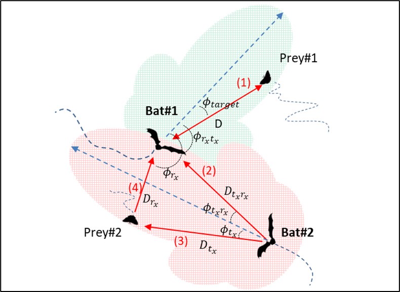
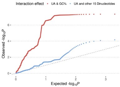
, where all 𝛽 terms represent the regression coefficients, and , , and represent the number of UA dinucleotides, the number of other dinucleotides (other than UA), and the GC content of the i^th UTR, respectively, and 𝜖_i denotes the error term. For each dinucleotide, we tested the significance of 𝛽_UAxGC% and 𝛽_UAxDiNT, and compared their p-values using a quantile-quantile (QQ) plot. Author response image 1 shows that the interaction effect of UA dinucleotides with GC% is much more significant than interactions with the other 15 dinucleotides, as indicated by the inflated QQ plot of p-values. This suggests that GC content is a more critical contextual factor influencing UA dinucleotides' impact on RNA stability.

Author response image 1.

The present MPRAs measures the effect of UTR sequences in one specific reporter context and using one experimental approach (following the decay of in vitro transcribed and transfected RNAs). While this approach certainly has its merits compared to other approaches, it also comes with some caveats: RNA is delivered naked, without bound RBPs and no nuclear history, e.g. of splicing (no EJCs), editing and modifications. One way to assess the generalizability of the results as well as the context dependence of the effects is to perform the same analysis on existing datasets of RNA stability measurements obtained through other methods (e.g. transcription inhibition). Are TA dinucleotides universally the most predictive feature of RNA half-lives?

Our system studies the stability control of RNA synthesized in vitro and delivered into human cells. While we did not intend to generalize our conclusions to endogenous RNAs, our approach contributes to the understanding of in vitro synthesized RNA used for cellular expression, such as in vaccines. It is known that endogenous RNAs undergo very different regulation. The most prominent factors controlling endogenous RNA stability are the density of splice junctions and the length of UTRs (doi.org/10.1186/s13059-022-02811-x; doi.org/10.1186/s12915-021-00949-x). To decipher the sequence regulation, these factors are controlled in our experiments. Therefore, we do not expect the dinucleotide features found by our approach to be generalized as the most predictive feature of RNA half-life in vivo. 

The authors conclude their study with a meta-analysis of genes with increased TA dinucleotides in 5' and 3'UTRs, showing that specific functional groups are overrepresented among these genes. In addition, they provide evidence for an effect of disease-associated UTR mutations on endogenous RNA stability. While these elements link back to the original motivation of the study (screening for effects of point mutations in 5' and 3' UTRs), they provide only a limited amount of additional insights.

We utilized the Taiwan Biobank to investigate whether mutations significantly affecting RNA stability also impact human biochemical measurements. Our findings indicate that these mutations indeed have a significant effect on various biochemical indices. This highlights the importance of our study, as it bridges basic science with potential applications in precision medicine. By linking specific UTR mutations with measurable changes in biochemical indices, our research underscores the potential for these findings to inform targeted medical interventions in the future.

In summary, this manuscript presents an interesting addition to the long-standing attempts at dissecting the sequence basis of RNA stability in human cells. The analysis is in general very comprehensive and sound; however, at times the goal of the authors to find novelty and specificity in the data overshadows some analyses. One example is the case where the authors try to show that TA-dinucleotides and GC content are decoupled and not merely two sides of the same coin.

They claim that the effect of TA dinucleotides is different between high- and low-GC content contexts but do not control for the fact that low GC-content regions naturally will contain more TA dinucleotides and therefore the effect sizes and the resulting correlation between TA-diNT rate and stability will be stronger (Fig. 5A). A more thorough analysis and greater caution in some of the claims could further improve the credibility of the conclusions.

Low GC content implies a higher UA content but does not directly equate to a high UA-dinucleotide ratio. For instance, the sequence AUUGAACCUU has a lower GC content (0.3) compared to UAUAGGCCGC (0.6), yet it also has a lower UA-dinucleotide ratio (0 vs. 0.22). To address this concern more rigorously, we performed a stratified analysis based on UA-diNT rate. As shown in our Fig. S7C, even after stratifying by UA- dinucleotide ratio (upper panel high UA- dinucleotide ratio / lower panel low UA- dinucleotide ratio), we still observe that the destabilizing effect of UA is stronger in the low GC content group.

Reviewer #2 (Public Review):

Summary of goals:

Untranslated regions are key cis-regulatory elements that control mRNA stability, translation, and translocation. Through interactions with small RNAs and RNA binding proteins, UTRs form complex transcriptional circuitry that allows cells to fine-tune gene expression. Functional annotation of UTR variants has been very limited, and improvements could offer insights into disease relevant regulatory mechanisms. The goals were to advance our understanding of the determinants of UTR regulatory elements and characterize the effects of a set of "disease-relevant" UTR variants.

Strengths:

The use of a massively parallel reporter assay allowed for analysis of a substantial set (6,555 pairs) of 5' and 3' UTR fragments compiled from known disease associated variants. Two cell types were used.

The findings confirm previous work about the importance of AREs, which helps show validity and adds some detailed comparisons of specific AU-rich motif effects in these two cell types.

Using a Lasso regression, TA-dinucleotide content is identified as a strong regulator of RNA stability in a context dependent manner based on GC content and presence of RNA binding protein binding motifs. The findings have potential importance, drawing attention to a UTR feature that is not well characterized.

The use of complementary datasets, including from half-life analyses of RNAs and from random sequence library MRPA's, is a useful addition and supports several important findings. The finding the TA dinucleotides have explanatory power separate from (and in some cases interacting with) GC content is valuable.

The functional enrichment analysis suggests some new ideas about how UTRs may contribute to regulation of certain classes of genes.

Weaknesses:

It is difficult to understand how the calculations for half-life were performed. The sequencing approach measures the relative frequency of each sequence at each time point (less stable sequences become relatively less frequent after time 0, whereas more stable sequences become relatively more frequent after time 0). Since there is no discussion of whether the abundance of the transfected RNA population is referenced to some external standard (e.g., housekeeping RNAs), it is not clear how absolute (rather than relative) half-lives were determined.

We estimated decay constant λ and half-life (t_1/2) by the following equations:

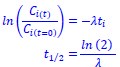
where C_i(t) and C_i(t=0) are read count values of the ith replicate at time points 𝑡 and 0 (see also Methods). The absolute abundance was not required for the half-life calculation. 

Fig. S1A and B are used to assess reproducibility. They show that read counts at a given time point correlate well across replicate experiments. However, this is not a good way to assess reproducibility or accuracy of the measurements of t1/2 are. (The major source of variability in read counts in these plots - especially at early time points - is likely the starting abundance of each RNA sequence, not stability.) This creates concerns about how well the method is measuring t1/2. Also creating concern is the observation that many RNAs are associated with half-lives that are much longer than the time points analyzed in the study. For example, based upon Figure S1 and Table S1 correctly, the median t1/2 for the 5' UTR library in HEK cells appears to be >700 minutes. Given that RNA was collected at 30, 75, and 120 minutes, accurate measurements of RNAs with such long half lives would seem to be very difficult.

We estimated the half-life based on the following equations:

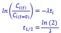
where C_i(t) and C_i(t=0) are read count values of the ith replicate at time points 𝑡 and 0 (see also Methods). The calculation of the half-life involves first determining the decay constant 𝜆, which represents a constant rate of decay. Since 𝜆 is a constant, it is possible to accurately calculate it without needing data over the entire decay range. Our experimental design considers this by selecting appropriate time points to ensure a reliable estimation of 𝜆, and thus, the half-life. To determine the most suitable time points, we conducted preliminary experiments using RT-PCR.

These experiments indicated that 30, 75, and 120 minutes provided an effective range for capturing the decay dynamics of the transcripts.

There is no direct comparison of t1/2 between the two cell types studied for the full set of sequences studied. This would be helpful in understanding whether the regulatory effects of UTRs are generally similar across cell lines (as has been shown in some previous studies) or whether there are fundamental differences. The distribution of t1/2's is clearly quite different in the two cell lines, but it is important to know if this reflects generally slow RNA turnover in HEK cells or whether there are a large number of sequence-specific effects on stability between cell lines. A related issue is that it is not clear whether the relatively small number of significant variant effects detected in HEK cells versus SH-SY5Y cells is attributable to real biological differences between cell types or to technical issues (many fewer read counts and much longer half lives in HEK cells).

For both cell lines, we selected oligonucleotides with R² > 0.5 and mean squared error (MSE) < 1 for analysis when estimating half-life (λ) by linear regression. This selection criterion was implemented to minimize the effect of experimental noise. After quality control, we selected common UTRs and compared the RNA half-lives of the two cell lines using a scatter plot. Author response image 2 shows that RNA half-lives are quite different between the cell lines, with a moderate similarity observed in the 5' UTRs (R = 0.21), while the correlation in the 3' UTRs is non-significant.

Author response image 2.

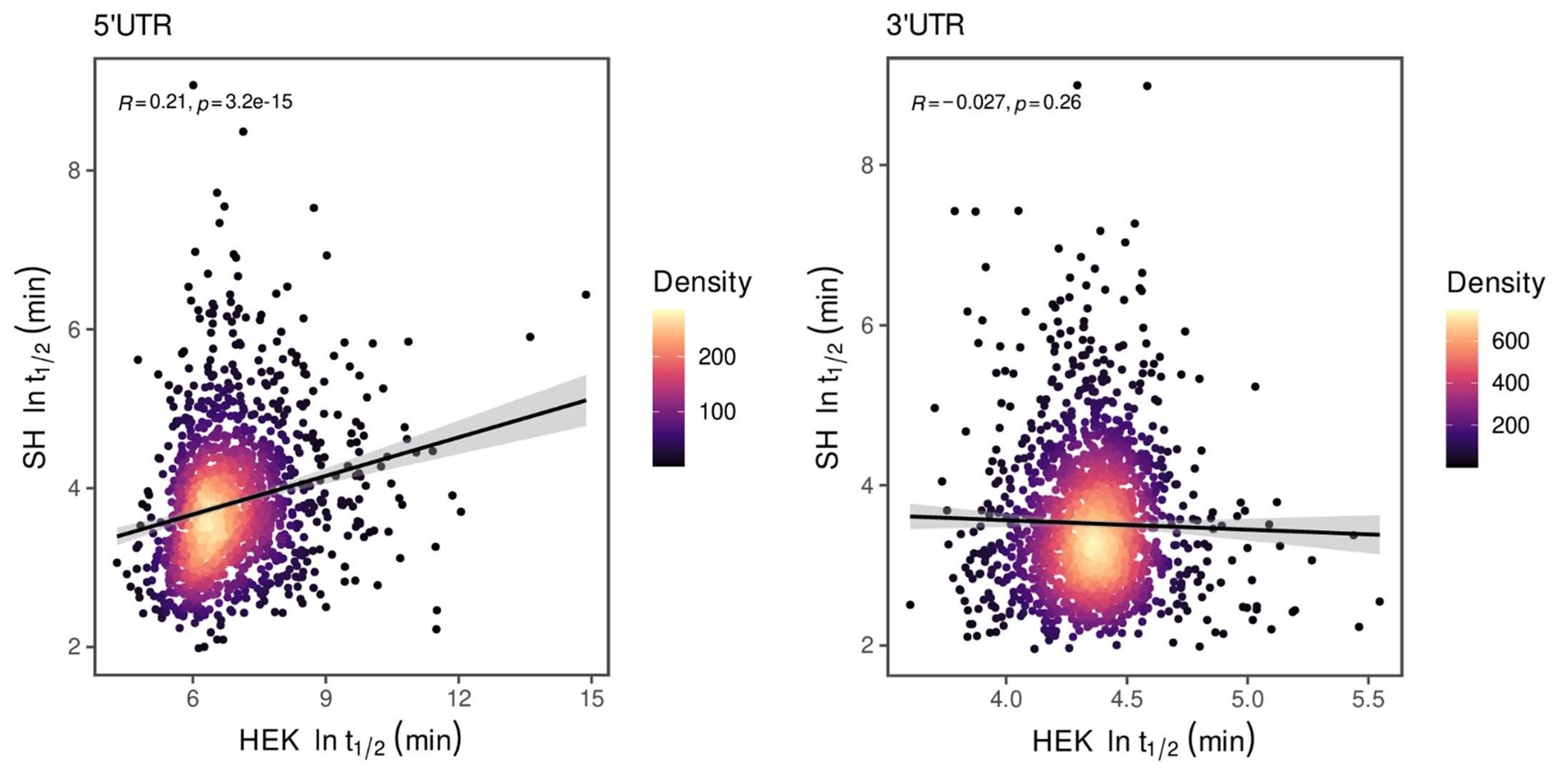
Despite the low correlation of mRNA half-life between the two cell lines, UA-dinucleotide and UA-rich sequences consistently emerge as the most significant destabilizing features, suggesting a shared regulatory mechanism across diverse cellular environments.

The general assertion is made in many places that TA dinucleotides are the most prominent destabilizing element in UTRs (e.g., in the title, the abstract, Fig. 4 legend, and on p. 12). This appears to be true for only one of the two cell lines tested based on Fig. 3.

UA-dinucleotides and other UA-rich sequences exhibit similar effects on RNA stability, as illustrated in Fig. S5A-C. In two cell lines, UA-dinucleotide and WWWWWW sequences were representatives of the same stability-affecting cluster. While the impact of UA-dinucleotides can be generalized, we have rephrased some statements for clarification to avoid any potential misunderstanding. For examples: 

Abstract: “...We found that UA dinucleotides and UA-rich motifs are the most prominent destabilizing element.“

p.10: “UA dinucleotides and UA-rich motifs are the most common and effective RNA destabilizing factor” 

Figure 4: “The UTR UA dinucleotides and UA-rich motifs are the most common and influential RNA destabilizing factor.”

Appraisal and impact:

The work adds to existing studies that previously identified sequence features, including AREs and other RNA binding protein motifs, that regulate stability and puts a new emphasis on the role of "TA" (better "UA") dinucleotides. It is not clear how potential problems with the RNA stability measurements discussed above might influence the overall conclusions, which may limit the impact unless these can be addressed.

It is difficult to understand whether the importance of TA dinucleotides is best explained by their occurrence in a related set of longer RBP binding motifs (see Fig 5J, these motifs may be encompassed by the "WWWWWW cluster") or whether some other explanation applies. Further discussion of this would be helpful. Does the LASSO method tend to collapse a more diverse set of longer motifs that are each relatively rare compared to the dinucleotide? It remains unclear whether TA dinucleotides are associated with less stability independent of the presence of the known larger WWWWWWW motif. As noted above, the importance of TA dinucleotides in the HEK experiments appears to be less than is implied in the text.

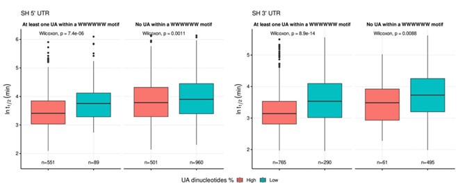
To ensure the representativeness of the features entered into the LASSO model, we pre-selected those with an occurrence greater than 10% among all UTRs. There is no evidence to support a preference for dinucleotides by LASSO. To address whether the destabilizing effect of UA dinucleotides is part of the broader WWWWWW motif, we divided UA dinucleotides into two groups: those within the WWWWWW motif and those outside of it. Specifically, we divided UTRs into two categories: 'at least one UA within a WWWWWW motif' and 'no UA within a WWWWWW motif,' and visualized the results using a boxplot. As shown in Author response image 3, the destabilizing trend still remains for UA dinucleotides outside of the WWWWWW motif, although the effect appears to be more pronounced when UA is within the WWWWWW motif. This suggests that while UA dinucleotides have a destabilizing effect independently, their impact is amplified when they are part of the broader WWWWWW motif.

Author response image 3.

The inclusion of more than a single cell type is an acknowledgement of the importance of evaluating cell type-specific effects. The work suggests a number of cell type-specific differences, but due to technical issues (especially with the HEK data, as outlined above) and the use of only two cell lines, it is difficult to understand cell type effects from the work.

The inclusion of both 3' and 5' UTR sequences distinguishes this work from most prior studies in the field. Contrasting the effects of these regions on stability is of interest, although the role of these UTRs (especially the 5' UTR) in translational regulation is not assessed here.

We examined the role of UTR and UTR variants in translation regulation using polysome profiling. By both univariate analysis and an elastic regression model, we identified motifs of short repeated sequences, including SRSF2 binding sites, as mutation hotspots that lead to aberrant translation. Furthermore, these polysome-shifting mutations had a considerable impact on RNA secondary structures, particularly in upstream AUG-containing 5’ UTRs. Integrating these features, our model achieved high accuracy (AUROC > 0.8) in predicting polysome-shifting mutations in the test dataset. Additionally, metagene analysis indicated that pathogenic variants were enriched at the upstream open reading frame (uORF) translation start site, suggesting changes in uORF usage underlie the translation deficiencies caused by these mutations. Illustrating this, we demonstrated that a pathogenic mutation in the IRF6 5’ UTR suppresses translation of the primary open reading frame by creating a uORF. Remarkably, site-directed ADAR editing of the mutant mRNA rescued this translation deficiency. Because the regulation of translation and stability does not converge, we illustrate these two mechanisms in two separate manuscripts (this one and doi.org/10.1101/2024.04.11.589132).

Reviewer #3 (Public Review):

Summary:

In their manuscript titled "Multiplexed Assays of Human Disease‐relevant Mutations Reveal UTR

Dinucleotide Composition as a Major Determinant of RNA Stability" the authors aim to investigate the effect of sequence variations in 3'UTR and 5'UTRs on the stability of mRNAs in two different human cell lines.

To do so, the authors use a massively parallel reporter assay (MPRA). They transfect cells with a set of mRNA reporters that contain sequence variants in their 3' or 5' UTRs, which were previously reported in human diseases. They follow their clearance from cells over time relative to the matching non-variant sequence. To analyze their results, they define a set of factors (RBP and miRNA binding sites, sequence features, secondary structure etc.) and test their association with differences in mRNA stability. For features with a significant association, they use clustering to select a subset of factors for LASSO regression and identify factors that affect mRNA stability.

They conclude that the TA dinucleotide content of UTRs is the strongest destabilizing sequence feature. Within that context, elevated GC content and protein binding can protect susceptible mRNAs from degradation. They also show that TA dinucleotide content of UTRs affects native mRNA stability, and that it is associated with specific functional groups. Finally, they link disease associated sequence variants with differences in mRNA stability of reporters.

Strengths:

This work introduces a different MPRA approach to analyze the effect of genetic variants. While previous works in tissue culture use DNA transfections that require normalization for transcription efficiency, here the mRNA is directly introduced into cells at fixed amounts, allowing a more direct view of the mRNA regulation.

The authors also introduce a unique analysis approach, which takes into account multiple factors that might affect mRNA stability. This approach allows them to identify general sequence features that affect mRNA stability beyond specific genetic variants, and reach important insights on mRNA stability regulation. Indeed, while the conclusions to genetic variants identified in this work are interesting, the main strength of the work involve general effect of sequence features rather than specific variants.

The authors provide adequate supports for their claims, and validate their analysis using both their reporter data and native genes. For the main feature identified, TA di-nucleotides, they perform follow-up experiments with modified reporters that further strengthen their claims, and also validate the effect on native cellular transcripts (beyond reporters), demonstrating its validity also within native scenarios.

The work provides a broad analysis of mRNA stability, across two mRNA regulatory segments (3'UTR and 5'UTR) and is performed in two separate cell-types. Comparison between two different cell-types is adequate, and the results demonstrate, as expected, the dependence of mRNA stability on the cellular context. Analysis of 3'UTR and 5'UTR regulatory effects also shows interesting differences and similarities between these two regulatory regions.

Weaknesses:

(1) The authors fail to acknowledge several possible confounding factors of their MPRA approach in the discussion.

First, while transfection of mRNA directly into cells allows to avoid the need to normalize for differences in transcription, the introduction of naked mRNA molecules is different than native cellular mRNAs and could introduce biases due to differences in mRNA modifications, protein associations etc. that may occur co-transcriptionally.

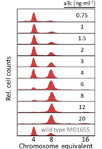
Second, along those lines, the authors also use in-vitro polyadenylation. The length of the polyA tail of the transfected transcripts could potentially be very different than that of native mRNAs and also affect stability.

The transcripts used in our study were polyadenylated in vitro with approximately 100 nucleotides 

(Fig. S1C), similar to the polyA tail lengths typically observed in vivo (dx.doi.org/10.1016/j.molcel.2014.02.007).  Additionally, these transcripts were capped to emulate essential mRNA characteristics and to minimize immune responses in recipient cells. This design allows us to study RNA decay for in vitro-synthesized RNA delivered into human cells, akin to RNA vaccines, but it does not necessarily extend to endogenous RNAs. As mentioned, endogenous RNAs undergo nuclear processing and are decorated by numerous trans factors, resulting in distinct regulatory mechanisms. We therefore provided a more discussion on these differences and their implications in the revised manuscript: “However, while our approach effectively assesses the stability of synthesized RNA in human cells, it may not fully capture the decay dynamics of nuclear-synthesized RNA, which can be influenced by endogenous modifications and trans-acting RNA binding factors. (p. 18)”

(2) The analysis approach used in this work for identifying regulatory features in UTRs was not previously used. As such, lack of in-depth details of the methodology, and possibly also more general validation of the approach, is a drawback in convincing the reader in the validity of this approach and its results.

In particular, a main point that is not addressed is how the authors decide on the set of "factors" used in their analysis? As choosing different sets of factors might affect the results of the analysis. 

In our study, we employed the calculation of the Variance Inflation Factor (VIF) as a basis for selecting variables. This well-established method is widely used to detect variables with high collinearity, thus ensuring the robustness and reliability of our analysis. By identifying and excluding highly collinear variables, we aimed to minimize multicollinearity and improve the accuracy of our regression models. For more detailed information on the use of VIF in regression analysis, please refer to Akinwande, M., Dikko, H., and Samson, A. (2015). Variance Inflation Factor: As a Condition for the Inclusion of Suppressor Variable(s) in Regression Analysis. Open Journal of Statistics, 5, 754-767. doi: 10.4236/ojs.2015.57075. We have included the method details in the revised manuscript (p. 28) :”… to avoid multicollinearity caused by similar features that perturb feature selection, all features were clustered using single-linkage hierarchical clustering with the distance metric defined as one minus the absolute value of the Spearman correlation coefficient. We cut the tree at a specific height, and the feature that had the greatest influence on RNA stability, which was examined using a simple linear regression model, was selected to be the representative of each cluster. Then we calculated the variance inflation factor (VIF) value of the representative features. The VIFs were obtained by the following linear model and equations:

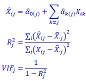
where and are the estimated value of the jth feature and the value of the kth feature of the ith UTR (note that the kth feature is a feature other than the jth feature), and are the intercept and the regression coefficients of the linear model that regressed the jth feature on the other remaining features, and is the mean level of the jth feature of all UTRs.”

For example, the choice to use 7-mer sequences within the factors set is not explained, particularly when almost all motifs that are eventually identified (Figure 3B-E) are shorter.

The known RBP motifs are primarily 6-mer. To explore the possibility of discovering novel motifs that could significantly impact our model, we started with 7-mer sequences. However, our analysis revealed that including these additional variables did not improve the explanatory power of the model; instead, it reduced it. Consequently, our final model focuses on motifs shorter than 7-mer. We explained the motif selections in the revised manuscript (p. 9): “Given our discovery that the effect of AREs is heavily dependent on sequence content, we decided to further explore the effects of other sequence elements, i.e., beyond known regulatory motifs, in more detail. Since most reported RBP motifs are 6-mers, we initiated a search for novel motifs by analyzing the presence of all 7-mers in our massively parallel reporter assay (MPRA) library, correlating their occurrence with mRNA half-life.”

In addition, the authors do not perform validations to demonstrate the validity of their approach on simulated data or well-established control datasets. Such analysis would be helpful to further convince the reader in the usefulness and robustness of the analysis.

We acknowledge the importance of validating our approach on simulated data or well-established control datasets to demonstrate its robustness and reliability. However, to the best of our knowledge, there are currently no well-established control datasets available that perfectly correspond to our specific study context. Despite this, we will continue to search for any relevant datasets that could be utilized for this purpose in future work. This effort will help to further reinforce the confidence in our methodology and its findings.

(3) The analysis and regression models built in this work are not thoroughly investigated relative to native genes within cells. The effect of sequence "factors" on native cellular transcripts' stability is not investigated beyond TA di-nucleotides, and it is unclear to what degree do other predicted factors also affect native transcripts.

Our system studies the stability control of RNA synthesized in vitro and delivered into human cells. While we validated the UTR UA-dinucleotide effect in vivo, we did not intend to conclude that this is the most influential regulation for endogenous RNAs. It is known that endogenous RNAs undergo very different regulation. The most prominent factors controlling endogenous RNA stability are the density of splice junctions and the length of UTRs (doi.org/10.1186/s13059-022-02811-x; doi.org/10.1186/s12915-021-00949-x). To decipher the sequence regulation, we controlled for these factors in our experiments. Therefore, we acknowledge that several endogenous features, which were excluded by our approach, may serve as predictive features of RNA half-life in vivo. 

Recommendations for the authors:

Reviewer #1 (Recommendations For The Authors):

Specific comments:  

Some references are missing, e.g for the sentence:

Please see the response below.

"Similarly, point mutation of the GFPT1 3' UTR results in congenital myasthenic syndrome." (p5)

The reference has been added to the text:

Dusl, M., Senderek, J., Muller, J. S., Vogel, J. G., Pertl, A., Stucka, R., Lochmuller, H., David, R., & Abicht, A. (2015). A 3'-UTR mutation creates a microRNA target site in the GFPT1 gene of patients with congenital myasthenic syndrome. Human Molecular Genetics, 24(12), 34183426. https://doi.org/10.1093/hmg/ddv090 

"...but there have been no systematic assessments of the explicit effects of variants of both UTRs on stability regulation." (not true in the current phrasing; e.g. PMIDs 32719458, 36156153, 34849835)

These references have been added to the text. However, we have to point out that these studies do not focus on the effects of the disease-relevant variants. To clarify, we modified the sentence to "... systematic assessments of the explicit effects of disease-relevant variants in both UTRs on stability regulation are still absent."

"Multiple approaches have revealed AREs as exerting a destabilizing effect on RNA stability (Barreau et al., 2005). (p8)

The reference has been added to the text:

Barreau, C., Paillard, L., & Osborne, H. B. (2005). AU-rich elements and associated factors: are there unifying principles? Nucleic Acids Research, 33(22), 7138-7150. https://doi.org/10.1093/nar/gki1012 

"This effect is specific, as such ratios in the coding region are inconsequential." (p12)

This refers to our findings of Fig. 4G and Supplemental Fig. S5F.

What are the sequences at the 5' and 3'UTR without insertion of a library? 5'UTR library (especially in SH) has much longer half-life compared to 3'utr library (Fig S1D).

There is no designed 5’UTR of the 3’UTR library, only the Kozak sequence derived from the pEGFPC1 vector. This may partially underlie the shorter half-life of the 3’ UTR library.

Fig2A: What are the units? "half-life (log)" Do the numbers correspond to log10(min)?

It represents ln (min). To clarify, we now use ‘ln t_1/2 (min)’ in all figures.

Fig 2 and 3: This was done only on the wild-type sequences? Or all tested sequences together, wt and mut?

It was done only on the wild-type sequences. To clarify, we modified the text to “we examined the effect of AREs on RNA stability of the ref alleles according to specific sequence content….(p.8)” and “We considered as many factors as possible to explain the half-life of our ref UTR libraries,…. (p.9)”. ‘ref’ stands for reference.

"Furthermore, to avoid collinearity confounding our model, e.g., the effects of very similar factors (such as 'AA' and 'AAA' sequences), we clustered the factors according to their properties, and then only one representative factor from within a cluster (i.e., the one with the highest correlation to halflife within a cluster) was subjected to LASSO regression": Given the observed context dependence, e.g. in the case of poly-U stretches: Isn't this clustering leading to similar/identical motifs with different context being grouped together (such as polyU preceded by an A (strongly destabilizing, according to Fig 2B) or followed by one (strongly stabilizing, according to Fig 2B), resulting in ignoring the context or using one potential outcome while a motif from the same cluster can have the opposite effect?

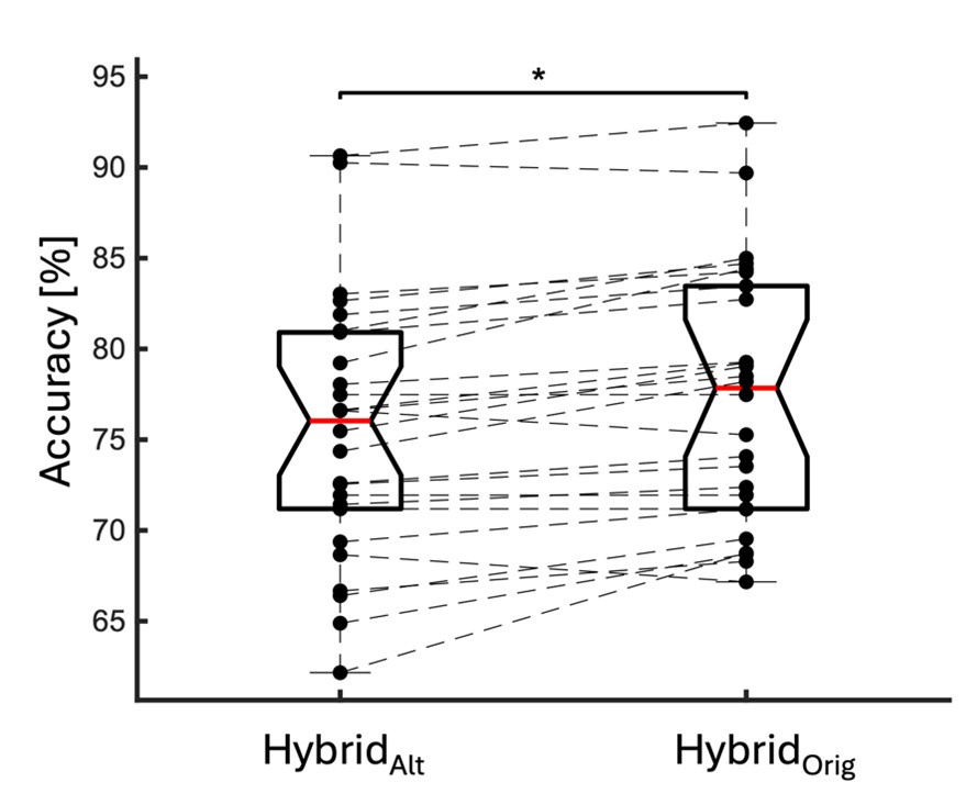
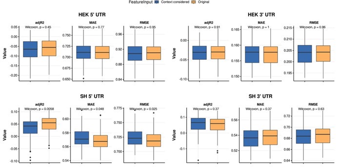
Thank you very much for pointing this out. To determine if considering different contextual effects within each feature cluster would enhance model performance, we modified our feature selection by choosing both the feature with the largest positive and the largest negative effect on RNA half-life in Step III of Figure 3A. We then split the data into a 2:1 training and testing set and repeated this process 100 times. Model performance was evaluated using mean average error (MAE), root mean squared error (RMSE), and adjusted R-squared. From Author response image 4, we observed no significant improvement in model performance using this new approach. Notably, in the SH-SY5Y 5' UTR model, our original method even outperformed the modified one, with statistically lower MAE and RMSE and a higher adjusted R-squared. Therefore, we believe our current approach remains appropriate.

Author response image 4.

"Overall, motifs that are at least two nucleotides long proved critical for RNA stability, supporting the sequence specificity of the decay process." Unclear why this supports the "sequence specificity"

No monomers were selected as an explanatory factor. On the contrary, specific sequence combinations and order are important for the regulation. These findings suggest sequence-specific recognition for the decay process.

Fig3: The same features were used in both cell lines? If yes: Since they were selected for their highest correlation with half-life, how was a common set chosen? If no: problematic to compare.

Thank you for your question regarding feature selection across cell lines. Initially, the features were collected uniformly for both cell lines. However, subsequent feature selection steps were cell-type specific, focusing on identifying features with the greatest impact on RNA half-life in each context. This approach allows us to still compare model performance and discuss the similarities and differences in selected features across cell types. By maintaining a consistent starting point, we ensure that any observed differences reflect cell-specific regulatory dynamics.

uORFs were not used as features?

Thank you for pointing this out. At the beginning of our study, we investigated the impact of Kozak sequence strength (categorized as weak, moderate, strong, or optimal) on RNA half-life. However, we found that this feature performed poorly in predicting RNA stability, and as a result, we decided not to include upstream open reading frames (uORFs) or Kozak sequences in our subsequent analyses.

Experimental reproducibility: Only correlations between replicates for the same time point is shown, but no comparison between time points or between decay rates. How reproducible were the paired differences between mut/wt?

The decay rate was calculated by modeling the slope of a linear regression of all time points. Therefore, there is only one decay rate associated with a genotype. To rule out inconsistent data, we excluded any regression with a mean square error greater than 1, as this indicates a poor fit of the data points. 

Fig 7C/p17: This does not establish a "causal relationship" as the authors claim.

We agree with the reviewer’s suggestion. We have modified the text on p.17 to “to establish a correlation between UTR variants and health outcomes,…..”

In the discussion, the authors claim that TA-diNTs are not only an opposite of the GC percentage and base this on Fig 5A.

Fig 5A: The range of TA-diNTs is naturally much higher in the low GC group. To make the high and low GC content comparable (as the authors aim to do), the correlation should be assessed for the same range of TA dint in both cases.

To address this concern more rigorously, we performed a stratified analysis based on UA-diNT rate. As shown in our Fig. S7C, even after stratifying by UA- dinucleotide ratio (upper panel high UA- dinucleotide ratio / lower panel low UA- dinucleotide ratio), we still observe that the destabilizing effect of UA is stronger in the low GC content group.

Supplemental Figure S7. Interplay of GC content and TA dinucleotide on stability regulation, related to Figure 5. (C) Stratifications of both TA dinucleotide ratio and GC content showed that the destabilizing effect of TA dinucleotide is the most prominent under conditions of low TA dinucleotide ratio and low GC content. The same trend was observed for 5’ UTR (left) and 3’ UTR (right).

The injection of in vitro transcribed and polyA/capped RNA certainly has advantages over other methods, but delivering naked mRNA without nuclear history might also lead to artifacts. The caveats of the approach should be discussed more extensively.

We appreciate the suggestion and have hence added the following in the Discussion (p.18): “However, while our approach effectively assesses the stability of synthesized RNA in human cells, it may not fully capture the decay dynamics of nuclear-synthesized RNA, which can be influenced by endogenous modifications and trans-acting RNA binding factors.”

"We unexpectedly identified many crucial regulatory features in 5' UTRs." Why was this unexpected?

We initially thought the 3’ UTR would play a major role in stability regulation. To avoid confusion, we have removed the word ‘unexpected’ from the text (p. 20): "We identified many crucial regulatory features in 5' UTRs."

"...a massively parallel reporter assay in which coding regions and human 5'/3' UTRs with diseaserelevant mutations were generated in vitro and then directly transfected into human cell lines to assess their decay patterns by next‐generation sequencing": also coding regions?

Thanks for the question. Indeed, the coding region was not synthesized together with the UTR library. Therefore, we modified the text of p. 6 to “…we developed a massively parallel reporter assay in which human 5’/3’ UTRs with disease-relevant mutations were generated in vitro, ligated with the enhanced green fluorescence protein (EGFP) coding region, and then directly transfected into human cell lines to assess their decay patterns by next-generation sequencing.”

Reviewer #2 (Recommendations For The Authors):

Nomenclature: When discussing RNA sequences, "U" should be used in place of "T" (e.g., "UA dinucleotide").

We have replaced the RNA sequence “T” with “U” of the text and figures.

Abstract: "We examined the RNA degradation patterns mediated by the UTR library in multiple cell lines" - It would be clearer to state that two cell lines (rather than multiple) were used.

We appreciate the suggestion. We have modified the abstract as suggested: “We examined the RNA degradation patterns mediated by the UTR library in two cell lines…"

The manuscript refers to "wild-type (WT) and mutant (mt) alleles." (p. 7 and elsewhere). It would be better to use "reference" instead of "wild type" given that these are human populations.

We appreciate the suggestion. All instances of ‘wild-type’ or ‘WT’ in the text and figures have been replaced with ‘reference’ or ‘ref’.

In the introduction, it is stated that traditional MPRAs "cannot differentiate the effect of the UTRs on transcription, stability and, in some cases, even protein production, greatly limiting scientific interpretation." This is confusing, since these assays can and have been used in association with both RNA decay measurements and measurements of reporter protein levels that allow assessment of effects on stability and protein production (including in the cited references).

We reason that the RNA steady-state level (e.g., sequencing the overall RNA normalized to DNA) or protein steady-state level (e.g., detecting the fluorescence signal) does not precisely reveal the decay kinetics of the RNA. Steady-state level is a result of production and decay, both of which UTRs contribute to. Similarly, the protein level is not a perfect estimate of the RNA decay.

To clarify, we have modified the introduction (p. 5) to “Nevertheless, because the steady-state level is a result of production and decay, these approaches cannot differentiate the effect of the UTRs on transcription, stability and, in some cases, even protein production, greatly limiting scientific interpretation.” 

Adding raw and normalized read count data from individual experiments (e.g., to Table S1) would make it more likely for others to use this dataset to address additional questions.

All raw and processed sequencing data generated in this study have been submitted to the NCBI Gene Expression Omnibus (GEO; https://www.ncbi.nlm.nih.gov/geo/) under accession number GSE217518 (reviewer token snspaakujtsdpcv).

The manuscript would benefit from further clarification about model selection. Additional details regarding how the features were clustered, and the actual clusters themselves should be included.

It should be discussed why Lasso was chosen vs Ridge or Elastic Net, in the context of handling multicollinearity. Often, data is subsetted for training and validation, and model performance metrics are presented.

Thank you for pointing out the need for further clarification on model selection. The features were clustered using single-linkage hierarchical clustering with the distance metric defined as one minus the absolute value of the Spearman correlation coefficient (this information has been added to the manuscript on p. 28: “…to avoid multicollinearity caused by similar features that perturb feature selection, all features were clustered using single-linkage hierarchical clustering with the distance metric defined as one minus the absolute value of the Spearman correlation coefficient.”). The resulting feature clusters are available in Supplemental Table S3. 

Regarding model selection, we chose LASSO over ridge and elastic net primarily for feature selection, as ridge does not perform feature selection. Elastic net is essentially a hybrid of ridge regression and LASSO regularization, but we opted for LASSO for its simplicity and effectiveness in selecting a sparse set of important features.

We also performed a 2:1 training and testing set analysis and have included these details in the manuscript. Model performance metrics, including correlation coefficient between observed and predicted values in the testing set, mean absolute error (MAE), root mean squared error (RMSE), mean absolute percentage error (MAPE), and R-squared, are provided in new Supplemental Table S4.

Recommend reviewing and correcting verb tenses in the methods section.

We appreciate the reviewer’s suggestion. We have corrected verb tenses in the methods section, which includes “The UTRs were defined by NCBI RefSeq and ENCODE V27. (p.21)”, “The variant was placed in the middle of the sequence….(p.22)”, and “eCLIP signals with value < 1 or p value > 0.05 were removed. (p.26)”

Please add information about which cell type(s) are being used in each of the figure legends (e.g., in Figs. 2B and 5).

We appreciate the reviewer’s suggestion. We have added the cell type information in the figure legends: “Figure 2…. (B) The ten most influential AREs in terms of RNA stability in SH-SY5Y cells.” And “Figure 5…..(A) MPRA data of SH-SY5Y cells stratified according to the GC content (GC%) of UTRs.”

Recommend review of axis labels and consistency in formatting the log(half-lives) and including the base of the log and the time unit (minutes). Even better, converting axis labels from log minutes to minutes would make this easier to understand.

Thank you for the suggestion regarding axis labels and consistency. We have unified the half-life label to ‘ln t_1/2 (min)’ in all figures. We chose not to convert the axis from logarithmic minutes to minutes because the original scale is highly skewed, which would hinder clear data visualization.

The discussion refers to Figure 1D but Figure 1 only has A-C

Thank you for pointing out this mistake. ‘Fig. 1D’ has been changed to ‘Fig. 1B’ in the text (p. 7 and p. 20).

The analyses in Fig. 2 are interpreted as demonstrating that AREs destabilize RNAs. These analyses are examining associations, so it would be more appropriate to say that AREs are associated with destabilization (since it is formally possible that other sequences that are present in these UTR fragment cause destabilization). A similar issue arises on p. 10: "TA dinucleotides alone can negatively regulate RNA stability, with a Pearson's correlation coefficient of ‐0.287 for 5' UTRs and ‐0.377 for 3' UTRs (Fig. 4A,C)." This is an association and does not establish causation. Again on p. 17: "We identified several SNPs in UTRs that induce aberrant RNA expression and/or protein expression (Supplemental Table S7)." These may be causal but may simply be in LD with other variants that are causal.

We agree that the association observed is not proven to be causal. Therefore, we modified the text as suggested: 

“AUUUA/AUUA-containing AREs are associated with RNA destabilization.” (p. 8)

“UA dinucleotides alone present a negative correlation with RNA stability, with a Pearson’s correlation coefficient of -0.287 for 5’ UTRs and -0.377 for 3’ UTRs.”  (p.10)

“We identified several SNPs in UTRs that correlated with aberrant RNA expression and/or protein expression.”  (p. 17)

Figure 4C is important in that it examines whether variant sequences that differ in a manner that changes the number of dinucleotide repeats affect stability. Please show the number (not just the percentage) of sequences in each category.

Thank you for your insightful comment. We believe the figure you referred to is Figure 4E. We have updated the figure to include the number of sequences in each category.

Figure 6A and B: The horizontal axes appear to be misaligned since the dotted vertical lines do not cross at 0. ?

The dotted vertical lines represent the genomic background of the UA-diNT ratio. To clarify it, we have modified the legend to: “Figure 6……(A) The top ten biological processes for which the 5’ UTR UA-dinucleotide ratio most significantly deviated from the genomic background (dashed line).”

It may be helpful to state what the dashed and solid lines represent on Figure 6 E/F. Please correct spelling of "Biological" in 6E.

As per the reviewer’s suggestions, we have modified the legend of Figure 6 to: “………..(E) Biological processes for RNAs in which the UA-dinucleotide ratios of both 5’ and 3’ UTRs are significantly different from the genomic background (dashed lines). (F) Molecular functions for RNAs in which the UA-dinucleotide ratios of both 5’ and 3’ UTRs are significantly different from the genomic background (dashed lines). The thin solid lines represent the standard deviation of the UAdinucleotide ratio within the gene group.” 

In addition, the spelling of “Biological” in Fig. 6E has been corrected.

Reviewer #3 (Recommendations For The Authors):

I have 3 points that I think could improve science and its presentation within the manuscript.

(1) Most importantly, how well do LASSO regression models predict the stability of native transcripts? Such analysis can also be useful for comparison between two different cell-types. How well does the regression model learned (on reporters) within one cell-type predict mRNA stability (of reporters and native genes) in this cell-type and in the other cell-type? Similarly, models can also help to analyze the effects of 5'UTR and 3'UTR sequences on mRNA stability. In particular, how well does the regression model of each separate regulatory sequence (3'UTR or 5'UTR) is able to predict the stability of native genes in the cell? Can the predictions be improved by combining both 3'UTR and 5'UTR sequence features within the regression models?

The decay model for native transcripts has been established in prior research (doi.org/10.1186/s13059-022-02811-x; doi.org/10.1186/s12915-021-00949-x), which indicates that exon junction density and transcript length are the primary determinants of RNA stability. Based on these findings, we designed the MPRA with fixed length and without splicing to focus on the contribution of primary sequences. We validated the destabilizing effect of UA dinucleotide on endogenous RNAs (Fig. 4G and Supplemental Fig. S5F) but do not recommend using our model to fully explain or predict the stability of native transcripts.

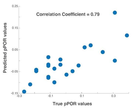
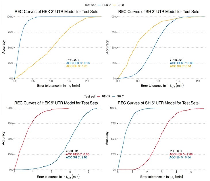
To assess the model's cross-cell type predictive performance for RNA half-life, we employed the Regression Error Characteristic (REC) curve (Bi & Bennett, 2003). Similar to the receiver operating characteristic (ROC) curve, the REC curve illustrates the trade-off between error tolerance and accuracy, with better performance indicated by curves trending toward the upper left. We also computed the Area Over the Curve (AOC) as a performance metric, where lower values indicate better predictive ability. From Author response image 5, the REC curves reveal that cross-cell type prediction performance is suboptimal. The y-axis represents prediction accuracy, while the x-axis denotes error tolerance for the natural logarithm of RNA half-life (ln(𝑡_1/2), in minutes).

Author response image 5.

In response to the suggestion of combining 5' and 3' UTR sequence features in the regression model, we believe this approach may not be ideal. As shown in Figure S1D, the distribution of RNA half-lives between 5' and 3' UTRs is significantly different, reflecting their distinct regulatory roles. Additionally, the base composition differs, with 5' UTRs having a higher GC content compared to 3' UTRs. Combining these datasets would likely make the origin of the sequence (5' or 3' UTR) the most predictive feature, thereby reducing the model's interpretability. Furthermore, our MPRA results, derived from separate 5’ or 3’ UTR library, do not support a combined model, further suggesting this approach may not be suitable with our data.

The conclusions regarding genetic variants are interesting, yet the main strength of the work involves identifying general sequence features that affect mRNA stability rather than specific variants. I wonder if the authors have considered to shift the focus of the motivation part to reflect that?

We appreciated the reviewer’s suggestion. We have revised the abstract and introductions to emphasize the general UTR regulation. Here is the revised abstract:

UTRs contain crucial regulatory elements for RNA stability, translation and localization, so their integrity is indispensable for gene expression. Approximately 3.7% of genetic variants associated with diseases occur in UTRs, yet a comprehensive understanding of UTR variant functions remains limited due to inefficient experimental and computational assessment methods. To systematically evaluate the effects of UTR variants on RNA stability, we established a massively parallel reporter assay on 6,555 UTR variants reported in human disease databases. We examined the RNA degradation patterns mediated by the UTR library in two cell lines, and then applied LASSO regression to model the influential regulators of RNA stability. We found that UA dinucleotides and UA-rich motifs are the most prominent destabilizing element. Gain of UA dinucleotide outlined mutant UTRs with reduced stability. Studies on endogenous transcripts indicate that high UA-dinucleotide ratios in UTRs promote RNA degradation. Conversely, elevated GC content and protein binding on UA dinucleotides protect high-UA RNA from degradation. Further analysis reveals polarized roles of UA-dinucleotide-binding proteins in RNA protection and degradation. Furthermore, the UA-dinucleotide ratio of both UTRs is a common characteristic of genes in innate immune response pathways, implying a coordinated stability regulation through UTRs at the transcriptomic level. We also demonstrate that stability-altering UTRs are associated with changes in biobank-based health indices, underscoring the importance of precise UTR regulation for wellness. Our study highlights the importance of RNA stability regulation through UTR primary sequences, paving the way for further exploration of their implications in gene networks and precision medicine.

Plots presenting correlations (e.g., Figure 4A, 4C) are more informative when plotted as density plots (i.e., using colorscale to show density of the dots at each part of the plot).

We greatly appreciate the reviewer's insightful suggestion regarding the use of density plots for presenting correlations. We have modified Figures 4A and 4C in the revised manuscript to implement density plotting. The updated figures now utilize a colorscale that highlights areas of high and low data density.

Author Response

The following is the authors’ response to the original reviews.

Public Reviews:

Reviewer #1 (Public Review):

Qin et al. set out to investigate the role of mechanosensory feedback during swallowing and identify neural circuits that generate ingestion rhythms. They use Drosophila melanogaster swallowing as a model system, focusing their study on the neural mechanisms that control cibarium filling and emptying in vivo. They find that pump frequency is decreased in mutants of three mechanotransduction genes (nompC, piezo, and Tmc), and conclude that mechanosensation mainly contributes to the emptying phase of swallowing. Furthermore, they find that double mutants of nompC and Tmc have more pronounced cibarium pumping defects than either single mutants or Tmc/piezo double mutants. They discover that the expression patterns of nompC and Tmc overlap in two classes of neurons, md-C and md-L neurons. The dendrites of md-C neurons warp the cibarium and project their axons to the subesophageal zone of the brain. Silencing neurons that express both nompC and Tmc leads to severe ingestion defects, with decreased cibarium emptying. Optogenetic activation of the same population of neurons inhibited filling of the cibarium and accelerated cibarium emptying. In the brain, the axons of nompC∩Tmc cell types respond during ingestion of sugar but do not respond when the entire fly head is passively exposed to sucrose. Finally, the authors show that nompC∩Tmc cell types arborize close to the dendrites of motor neurons that are required for swallowing, and that swallowing motor neurons respond to the activation of the entire Tmc-GAL4 pattern.

Strengths:

• The authors rigorously quantify ingestion behavior to convincingly demonstrate the importance of mechanosensory genes in the control of swallowing rhythms and cibarium filling and emptying

• The authors demonstrate that a small population of neurons that express both nompC and Tmc oppositely regulate cibarium emptying and filling when inhibited or activated, respectively

• They provide evidence that the action of multiple mechanotransduction genes may converge in common cell types

Thank you for your insightful and detailed assessment of our work. Your constructive feedback will help to improve our manuscript.

Weaknesses:

• A major weakness of the paper is that the authors use reagents that are expressed in both md-C and md-L but describe the results as though only md-C is manipulated-Severing the labellum will not prevent optogenetic activation of md-L from triggering neural responses downstream of md-L. Optogenetic activation is strong enough to trigger action potentials in the remaining axons. Therefore, Qin et al. do not present convincing evidence that the defects they see in pumping can be specifically attributed to md-C.

Thank you for your comments. This is important point that we did not adequately address in the original preprint. We have obtained imaging and behavioral results that strongly suggest md-C, rather than md-L, are essential for swallowing behavior.

36 hours after the ablation of the labellum, the signals of md-L were hardly observable when GFP expression was driven by the intersection between Tmc-GAL4 & nompC-QF (see F Figure 3—figure supplement 1A). This observation indicates that the axons of md-L likely degenerated after 36 hours, and were unlikely to influence swallowing. Moreover, the projecting pattern of Tmc-GAL4 & nompC-QF>>GFP exhibited no significant changes in the brain post labellum ablation.

Furthermore, even after labellum ablation for 36 hours, flies exhibited responses to light stimulation (see Figure 3—figure supplement 1B-C, Video 5) when ReaChR was expressed in md-C. We thus reasoned that md-C but not md-L, plays a crucial role in the swallowing process.

• GRASP is known to be non-specific and prone to false positives when neurons are in close proximity but not synaptically connected. A positive GRASP signal supports but does not confirm direct synaptic connectivity between md-C/md-L axons and MN11/MN12.

In this study, we employed the nSyb-GRASP, wherein the GRASP is expressed at the presynaptic terminals by fusion with the synaptic marker nSyb. This method demonstrates an enhanced specificity compared to the original GRASP approach.

Additionally, we utilized +/ UAS-nSyb-spGFP1-10, lexAop-CD4-spGFP11 ; + / MN-LexA fruit flies as a negative control to mitigate potential false signals originating from the tool itself (Author response image 1, scale bar = 50μm). Beside the genotype Tmc-Gal4, Tub(FRT. Gal80) / UAS-nSyb-spGFP1-10, lexAop-CD4-spGFP11 ; nompC-QF, QUAS-FLP / MN-LexA fruit flies discussed in this manuscript, we also incorporated genotype Tmc-Gal4, Tub(FRT. Gal80) / lexAop-nSyb-spGFP1-10, UAS-CD4-spGFP11 ; nompC-QF, QUAS-FLP / MN-LexA fruit flies as a reverse control (Author response image 2). Unexpectedly, similar positive signals were observed, indicating that, positive signals may emerge due to close proximity between neurons even with nSyb-GRASP.

Author response image 1.

It should be noted that the existence of synaptic projections from motor neurons (MN) to md-C cannot be definitively confirmed at this juncture. At present, we can only posit the potential for synaptic connections between md-C and motor neurons. A more conclusive conclusion may be attainable with the utilization of comprehensive whole-brain connectome data in future studies.

Author response image 2.

• As seen in Figure 2—figure supplement 1, the expression pattern of Tmc-GAL4 is broader than md-C alone. Therefore, the functional connectivity the authors observe between Tmc expressing neurons and MN11 and 12 cannot be traced to md-C alone

It is true that the expression pattern of Tmc-GAL4 is broader than that of md-C alone. Our experiments, including those flies expressing TNT in Tmc+ neurons, demonstrated difficulties in emptying (Figure 2A, 2D). Notably, we encountered challenges in finding fly stocks bearing UAS>FRT-STOP-P2X2. Consequently, we opted to utilize Tmc-GAL4 to drive UAS-P2X2 instead. We believe that the results further support our hypothesis on the role of md-C in the observed behavioral change in emptying.

Overall, this work convincingly shows that swallowing and swallowing rhythms are dependent on several mechanosensory genes. Qin et al. also characterize a candidate neuron, md-C, that is likely to provide mechanosensory feedback to pumping motor neurons, but the results they present here are not sufficient to assign this function to md-C alone. This work will have a positive impact on the field by demonstrating the importance of mechanosensory feedback to swallowing rhythms and providing a potential entry point for future investigation of the identity and mechanisms of swallowing central pattern generators.

Reviewer #2 (Public Review):

In this manuscript, the authors describe the role of cibarial mechanosensory neurons in fly ingestion. They demonstrate that pumping of the cibarium is subtly disrupted in mutants for piezo, TMC, and nomp-C. Evidence is presented that these three genes are co-expressed in a set of cibarial mechanosensory neurons named md-C. Silencing of md-C neurons results in disrupted cibarial emptying, while activation promotes faster pumping and/or difficulty filling. GRASP and chemogenetic activation of the md-C neurons is used to argue that they may be directly connected to motor neurons that control cibarial emptying.

The manuscript makes several convincing and useful contributions. First, identifying the md-C neurons and demonstrating their essential role for cibarium emptying provides reagents for further studying this circuit and also demonstrates the important of mechanosensation in driving pumping rhythms in the pharynx. Second, the suggestion that these mechanosensory neurons are directly connected to motor neurons controlling pumping stands in contrast to other sensory circuits identified in fly feeding and is an interesting idea that can be more rigorously tested in the future.

At the same time, there are several shortcomings that limit the scope of the paper and the confidence in some claims. These include:

a) the MN-LexA lines used for GRASP experiments are not characterized in any other way to demonstrate specificity. These were generated for this study using Phack methods, and their expression should be shown to be specific for MN11 and MN12 in order to interpret the GRASP experiments.

Thanks for the suggestion. We have checked the expression pattern of MN-LexA, which is similar to MN-GAL4 used in previous work (Manzo et al., PNAS., 2012, PMID:22474379) . Here is the expression pattern:

Author response image 3.

b) There is also insufficient detail for the P2X2 experiment to evaluate its results. Is this an in vivo or ex vivo prep? Is ATP added to the brain, or ingested? If it is ingested, how is ATP coming into contact with md-C neuron if it is not a chemosensory neuron and therefore not exposed to the contents of the cibarium?

The P2X2 experimental preparation was done ex vivo. We immersed the fly in the imaging buffer, as described in the Methods section under Functional Imaging. Following dissection and identification of the subesophageal zone (SEZ) area under fluorescent microscopy, we introduced ATP slowly into the buffer, positioned at a distance from the brain

c) In Figure 3C, the authors claim that ablating the labellum will remove the optogenetic stimulation of the md-L neuron (mechanosensory neuron of the labellum), but this manipulation would presumably leave an intact md-L axon that would still be capable of being optogenetically activated by Chrimson.

Please refer to the corresponding answers for reviewer 1 and Figure 3—figure supplement 1.

d) Average GCaMP traces are not shown for md-C during ingestion, and therefore it is impossible to gauge the dynamics of md-C neuron activation during swallowing. Seeing activation with a similar frequency to pumping would support the suggested role for these neurons, although GCaMP6s may be too slow for these purposes.

Profiling the dynamics of md-C neuron activation during swallowing is crucial for unraveling the operational model of md-C and validating our proposed hypothesis. Unfortunately, our assay faces challenges in detecting probable 6Hz fluorescent changes with GCaMP6s.

In general, we observed an increase of fluorescent signals during swallowing, but movement of alive flies during swallowing influenced the imaging recording, so we could not depict a decent tracing for calcium imaging for md-C neurons. To enhance the robustness of our findings, patching the md-C neurons would be a more convincing approach. As illustrated in Figure 2, the somata of md-C neurons are situated in the cibarium rather than the brain. patching of the md-C neuron somata in flies during ingestion is difficult.

e) The negative result in Figure 4K that is meant to rule out taste stimulation of md-C is not useful without a positive control for pharyngeal taste neuron activation in this same preparation.

We followed methods used in the previous work (Chen et al., Cell Rep., 2019, PMID:31644916), which we believe could confirm that md-C do not respond to sugars.

In addition to the experimental limitations described above, the manuscript could be organized in a way that is easier to read (for example, not jumping back and forth in figure order).

Thanks for your suggestion and the manuscript has been reorganized.

Reviewer #3 (Public Review):

Swallowing is an essential daily activity for survival, and pharyngo-laryngeal sensory function is critical for safe swallowing. In Drosophila, it has been reported that the mechanical property of food (e.g. Viscosity) can modulate swallowing. However, how mechanical expansion of the pharynx or fluid content sense and control swallowing was elusive. Qin et al. showed that a group of pharyngeal mechanosensory neurons, as well as mechanosensory channels (nompC, Tmc, and Piezo), respond to these mechanical forces for regulation of swallowing in Drosophila melanogaster.

Strengths:

There are many reports on the effect of chemical properties of foods on feeding in fruit flies, but only limited studies reported how physical properties of food affect feeding especially pharyngeal mechanosensory neurons. First, they found that mechanosensory mutants, including nompC, Tmc, and Piezo, showed impaired swallowing, mainly the emptying process. Next, they identified cibarium multidendritic mechanosensory neurons (md-C) are responsible for controlling swallowing by regulating motor neuron (MN) 12 and 11, which control filling and emptying, respectively.

Weaknesses:

While the involvement of md-C and mechanosensory channels in controlling swallowing is convincing, it is not yet clear which stimuli activate md-C. Can it be an expansion of cibarium or food viscosity, or both? In addition, if rhythmic and coordinated contraction of muscles 11 and 12 is essential for swallowing, how can simultaneous activation of MN 11 and 12 by md-C achieve this? Finally, previous reports showed that food viscosity mainly affects the filling rather than the emptying process, which seems different from their finding.

We have confirmed that swallowing sucrose water solution activated md-C neurons, while sucrose water solution alone could not (Figure 4J-K). We hypothesized that the viscosity of the food might influence this expansion process.

While we were unable to delineate the activation dynamics of md-C neurons, our proposal posits that these neurons could be activated in a single pump cycle, sequentially stimulating MN12 and MN11. Another possibility is that the activation of md-C neurons acts as a switch, altering the oscillation pattern of the swallowing central pattern generator (CPG) from a resting state to a working state.

In the experiments with w1118 flies fed with MC (methylcellulose) water, we observed that viscosity predominantly affects the filling process rather than the emptying process, consistent with previous findings. This raises an intriguing question. Our investigation into the mutation of mechanosensitive ion channels revealed a significant impact on the emptying process. We believe this is due to the loss of mechanosensation affecting the vibration of swallowing circuits, thereby influencing both the emptying and filling processes. In contrast, viscosity appears to make it more challenging for the fly to fill the cibarium with food, primarily attributable to the inherent properties of the food itself.

Reviewer #4 (Public Review):

A combination of optogenetic behavioral experiments and functional imaging are employed to identify the role of mechanosensory neurons in food swallowing in adult Drosophila. While some of the findings are intriguing and the overall goal of mapping a sensory to motor circuit for this rhythmic movement are admirable, the data presented could be improved.

The circuit proposed (and supported by GRASP contact data) shows these multi-dendritic neurons connecting to pharyngeal motor neurons. This is pretty direct - there is no evidence that they affect the hypothetical central pattern generator - just the execution of its rhythm. The optogenetic activation and inhibition experiments are constitutive, not patterned light, and they seem to disrupt the timing of pumping, not impose a new one. A slight slowing of the rhythm is not consistent with the proposed function.

Motor neurons implicated in patterned motions can be considered effectors of Central Pattern Generators (CPGs)(Marder et al., Curr Biol., 2001, PMID: 11728329; Hurkey et al., Nature., 2023, PMID:37225999). Given our observation of the connection between md-C neurons and motor neurons, it is reasonable to speculate that md-C neurons influence CPGs. Compared to the patterned light (0.1s light on and 0.1s light off) used in our optogenetic experiments, we noted no significant changes in their responses to continuous light stimulation. We think that optogenetic methods may lead to overstimulation of md-C neurons, failing to accurately mimic the expansion of the cibarium during feeding.

Dysfunction in mechanosensitive ion channels or mechanosensory neurons not only disrupts the timing of pumping but also results in decreased intake efficiency (Figure 1E). The water-swallowing rhythm is generally stable in flies, and swallowing is a vital process that may involve redundant ion channels to ensure its stability.

The mechanosensory channel mutants nompC, piezo, and TMC have a range of defects. The role of these channels in swallowing may not be sufficiently specific to support the interpretation presented. Their other defects are not described here and their overall locomotor function is not measured. If the flies have trouble consuming sufficient food throughout their development, how healthy are they at the time of assay? The level of starvation or water deprivation can affect different properties of feeding - meal size and frequency. There is no description of how starvation state was standardized or measured in these experiments.

Defects in mechanosensory channel mutants nompC, piezo, and TMC, have been extensively investigated (Hehlert et al., Trends Neurosci., 2021, PMID:332570000). Mutations in these channels exhibit multifaceted effects, as illustrated in our RNAi experiments (see Figure 2E). Deprivation of water and food was performed in empty fly vials. It's important to note that the duration of starvation determines the fly's willingness to feed but not the pump frequency (Manzo et al., PNAS., 2012, PMID:22474379).

In most cases, female flies were deprived water and food in empty vials for 24 hours because after that most flies would be willing to drink water. The deprivation time is 12 hours for flies with nompC and Tmc mutated or flies with Kir2.1 expressed in md-C neurons, as some of these flies cannot survive 24h deprivation.

The brain is likely to move considerably during swallow, so the GCaMP signal change may be a motion artifact. Sometimes this can be calculated by comparing GCaMP signal to that of a co-expressed fluorescent protein, but there is no mention that this is done here. Therefore, the GCaMP data cannot be interpreted.

We did not co-express a fluorescent protein with GCaMP for md-C. The head of the fly was mounted onto a glass slide, and we did not observe significant signal changes before feeding.

Recommendations for the authors:

Reviewer #1 (Recommendations For The Authors):

.>Abstract: I disagree that swallow is the first step of ingestion. The first paragraph also mentions the final checkpoint before food ingestion. Perhaps sufficient to say that swallow is a critical step of ingestion.

Indeed, it is not rigorous enough to say “first step”. This has been replaced by “early step”.

Introduction:

Line 59: "Silence" should be "Silencing"

This has been replaced.

Results:

Lines 91-92: I am not clear about what this means. 20% of nompC and 20% of wild-type flies exhibit incomplete filling? So nompC is not different from wild-type?

Sorry for the mistake. Viscous foods led to incomplete emptying (not incomplete filling), as displayed in Video 4. The swallowing behavior differs between nompC mutants and wild-type flies, as illustrated in Figure 1C, Figure 1—figure supplement 1A-C and video 1&5.

When fed with 1% MC water solution (Figure 1—figure supplement 1E-H). We found that when fed with 1% MC watere solution, Tmc or piezo mutants displayed incomplete emptying, which could constitute a long time proportion of swallowing behavior; while only 20% of nompC flies and 20% of wild-type flies sporadically exhibit incomplete emptying, which is significantly different. Though the percent of flies displaying incomplete pump is similar between nompC mutant and wild-type files, you can find it quite different in video 1 and 5.

Line 94: Should read: “while for foods with certain viscosity, the pump of Tmc or piezo mutants might"

What evidence is there for weakened muscle motion? The phenotypes of all three mutants is quite similar, so concluding that they have roles in initiation versus swallowing strength is not well supported -this would be better moved to the discussion since it is speculative.

Muscles are responsible for pumping the bolus from the mouth to the crop. In the case of Tmc or piezo mutants, as evidenced by incomplete filling for viscous foods (see Video 4), we speculate that the loss of sensory stimuli leads to inadequate muscle contraction. The phenotypes observed in Tmc and piezo mutants are similar yet distinct from those of the wild-type or nompC mutant, as shown in Video 1 and 4. The phrase "due to weakened muscle motion" has been removed for clarity.

Line 146: If md-L neurons are also labeled by this intersection, then you are not able to know whether the axons seen in the brain are from md-L or md-C neurons. Line 148: cutting the labellum is not sufficient to ablate md-L neurons. The projections will still enter the brain and can be activated with optogenetics, even after severing the processes that reside in the labellum.

Please refer to the responses for reviewer #1 (Public Review):” A major weakness of the paper…” and Figure 4.

Line 162: If the fly head alone is in saline, do you know that the sucrose enters the esophagus? The more relevant question here is whether the md-C neurons respond to mechanical force. If you could artificially inflate the cibarium with air and see the md-C neurons respond that would be a more convincing result. So far you only know that these are activated during ingestion, but have not shown that they are activated specifically by filling or emptying. In addition, you are not only imaging md-C (md-L is also labeled). This caveat should be mentioned.

We followed the methods outlined in the previous work (Chen et al., Cell Rep., 2019, PMID:31644916), which suggested that md-C neurons do not respond to sugars. While we aimed to mechanically stimulate md-C neurons, detecting signal changes during different steps of swallowing is challenging. This aspect could be further investigated in subsequent research with the application of adequate patch recording or two-photon microscopy (TPM).

Figure 3: It is not clear what the pie charts in Figure 3 A refer to. What are the three different rows, and what does blue versus red indicate?

Figure 3A illustrates three distinct states driven by CsChrimson light stimulation of md-C neurons, with the proportions of flies exhibiting each state. During light activation, flies may display difficulty in filling, incomplete filling, or a normal range of pumping. The blue and red bars represent the proportions of flies showing the corresponding state, as indicated by the black line.

Figure 4: Where are the example traces for J? The comparison in K should be average dF/F before ingestion compared with average dF/F during ingestion. Comparing the in vitro response to sucrose to the in vivo response during ingestion is not a useful comparison.

Please refer to the answers for reviewer #2 question d).

Reviewer #2 (Recommendations For The Authors):

Suggested experiments that would address some of my concerns listed in the public review include:

a) high resolution SEZ images of MN-LexA lines crossed to LexAop-GFP to demonstrate their specificity

b) more detail on the P2X2 experiment. It is hard to make suggestions beyond that without first seeing the details.

c) presenting average GCaMP traces for all calcium imaging results

d) to rule out taste stimulation of md-C (Figure 4K) I would suggest performing more extensive calcium imaging experiments with different stimuli. For example, sugar, water, and increasing concentrations of a neutral osmolyte (e.g. PEG) to suppress the water response. I think that this is more feasible than trying to get an in vitro taste prep to be convincing.

Please refer to the responses for public review of reviewer #2.

Reviewer #3 (Recommendations For The Authors):

Below I list my suggestions as well as criticisms.

(1) It would be excellent if the authors could demonstrate whether varying levels of food viscosity affect md-C activation.

That is a good point, and could be studied in future work.

(2) It is not clear whether an intersectional approach using TMC-GAL4 and nompC-QF abolishes labelling of the labellar multidendritic neurons. If this is the case, please show labellar multidendritic neurons in TMC-GAL4 only flies and flies using the intersectional approach. Along with this question, I am concerned that labellum-removed flies could be used for feeding assay.

Intersectional labelling using TMC-GAL4 and nompC-QF could not abolish labelling of the labellar multidendritic neurons (Author response image 4). Labellum-removed flies could be used for feeding assay (Figure 3—figure supplement 1B-C, video 5), but once LSO or cibarium of fly was damaged, swallowing behavior would be affected. Removing labellum should be very careful.

Author response image 4.

(3) Please provide the detailed methods for GRASP and include proper control.

Please refer to the responses for public review of reviewer #1.

(4) The authors hypothesized that md-C sequentially activates MN11 and 12. Is the time gap between applying ATP on md-C and activation of MN11 or MN12 different? Please refer to the responses for public review of reviewer #3. The time gap between applying ATP on md-C and activation of MN11 or MN12 didn’t show significant differences, and we think the reason is that the ex vivo conditions could not completely mimic in vivo process.

I found the manuscript includes many errors, which need to be corrected.

(1) The reference formatting needs to be rechecked, for example, lines 37, 42, and 43.

(2) Line 44-46: There is some misunderstanding. The role of pharyngeal mechanosensory neurons is not known compared with chemosensory neurons.

(3) Line 49: Please specify which type of quality of food. Chemical or physical?

(4) Line 80 and Figure 1B-D Authors need to put filling and emptying time data in the main figure rather than in the supplementary figure. Otherwise, please cite the relevant figures in the text(S1A-C).

(5) Line 84-85; Is "the mutant animals" indicating only nompC? Please specify it.

(6) Figure 1a: It is hard to determine the difference between the series of images. And also label filling and emptying under the time.

(7) S1E-H: It is unclear what "Time proportion of incomplete pump" means. Please define it.

(8) Please reorganize the figures to follow the order of the text, for example, figures 2 and 4

(9) Figure 4A. There is mislabelling in Figure 4A. It is supposed to be phalloidin not nc82.

(10) Figure 4K: It does not match the figure legend and main text.

(11) Figure 4D and G: Please indicate ATP application time point.

Thanks for your correction and all the points mentioned were revised.

Reviewer #4 (Recommendations For The Authors):

The figures need improvement. 1A has tiny circles showing pharynx and any differences are unclear.

The expression pattern of some of these drivers (Supplement) seems quite broad. The tmc nompC intersection image in Figure 1F is nice but the cibarium images are hard to interpret: does this one show muscle expression? What are "brain" motor neurons? Where are the labellar multi-dendritic neurons?

Tmc nompC intersection image show no expression in muscles. Somata of motor neurons 12 or 11 situated at SEZ area of brain, while somata of md-C neurons are in the cibarium. Image of md-L neurons was posted in response for reviewer #3 (Recommendations For The Authors):

Why do the assays alternate between swallowing food and swallowing water?

Thank for your suggestion, figure 1A has been zoomed-in. The Tmc nompC intersection image in Figure 2F displayed the position of md-C neurons in a ventral perspective, and muscles were not labelled. We stained muscles in cibarium by phalloidin and the image is illustrated in Figure 4A, while we didn’t find overlap between md-C neurons and muscles. Image of md-L neurons were posted as Author response image 4.

In the majority of our experiments, we employed water to test swallowing behavior, while we used methylcellulose water solution to test swallowing behavior of mechanoreceptor mutants, and sucrose solution for flies with md-C neurons expressing GCaMP since they hardly drank water when their head capsules were open.

How starved or water-deprived were the flies?

One day prior to the behavioral assays, flies were transferred to empty vials (without water or food) for 24 hours for water deprivation. Flies who could not survive 24h deprivation would be deprived for 12h.

How exactly was the pumping frequency (shown in Fig 1B) measured? There is no description in the methods at all. If the pump frequency is scored by changes in blue food intensity (arbitrary units?), this seems very subjective and maybe image angle dependent. What was camera frame rate? Can it capture this pumping speed adequately? Given the wealth of more quantitative methods for measuring food intake (eg. CAFE, flyPAD), it seems that better data could be obtained.

How was the total volume of the cibarium measured? What do the pie charts in Figure 3A represent?

The pump frequency was computed as the number of pumps divided by the time scale, following the methodology outlined in Manzo et al., 2012. Swallowing curves were plotted using the inverse of the blue food intensity in the cibarium. In this representation, ascending lines signify filling, while descending lines indicate emptying (see Figure 2D, 3B). We maintain objectivity in our approach since, during the recording of swallowing behavior, the fly was fixed, and we exclusively used data for analysis when the Region of Interest (ROI) was in the cibarium. This ensures that the intensity values accurately reflect the filling and emptying processes. Furthermore, we conducted manual frame-by-frame checks of pump frequency, and the results align with those generated by the time series analyzer V3 of ImageJ.

For the assessment of total volume of ingestion, we referred the methods of CAFE, utilizing a measurable glass capillary. We then calculated the ingestion rate (nL/s) by dividing the total volume of ingestion by the feeding time.

The changes seem small, in spite of the claim of statistical significance.

The observed stability in pump frequency within a given genotype underscores the significance of even seemingly small changes, which is statistically significant. We speculate that the stability in swallowing frequency suggests the existence of a redundant mechanism to ensure the robustness of the process. Disruption of one channel might potentially be partially compensated for by others, highlighting the vital nature of the swallowing mechanism.

How is this change in pump frequency consistent with defects in one aspect of the cycle - either ingestion (activation) or expulsion (inhibition)?

Please refer to Figure 2, 3. Both filling and emptying process were affects, while inhibition mainly influences emptying time (Figure 1—figure supplement 1).

for the authors:

Line 48: extensively

Line 62 - undiscovered.

Line 107, 463: multi

Line 124: What is "dysphagia?" This is an unusual word and should be defined.

Line 446: severe

Line 466: in the cibarium or not?

Thanks for your correction and all the places mentioned were revised.

Author Response

The following is the authors’ response to the original reviews.

Thank you for organizing the reviews for our manuscript: Behavioral entrainment to rhythmic auditory stimulation can be modulated by tACS depending on the electrical stimulation field properties,” and for the positive eLife assessment. We also thank the reviewers for their constructive comments. We have addressed every comment, which has helped to improve the transparency and readability of the manuscript. The main changes to the manuscript are summarized as follows:

1. Surrogate distributions were created for each participant and session to estimate the effect of tACS-phase lag on behavioral entrainment to the sound that could have occurred by chance or because of our analysis method (R1). The actual tACS-amplitude effects were normalized relative to the surrogate distribution, and statistical analysis was performed on the normalized (z-score) values. This analysis did not change our main outcome: that tACS modulates behavioral entrainment to the sound depending on the phase lag between the auditory and the electrical signals. This analysis has now been incorporated into the Results section and in Fig. 3c-d.

2. Two additional supplemental figures were created to include the single-participant data related to Fig. 3b and 3e (R2).

3. Additional editing of the manuscript has been performed to improve the readability.

Below, you will find a point-by-point response to the reviewers’ comments.

Reviewer #1 (Public Review):

We are grateful for the reviewer’s positive assessment of the potential impact of our study. The reviewer’s primary concerns were 1) the tACS lag effects reported in the manuscript might be noise because of the realignment procedure, and 2) no multiple comparisons correction was conducted in the model comparison procedure.

In response to point 1), we have reanalyzed the data in exactly the manner prescribed by the reviewer. Our effects remain, and the new control analysis strengthens the manuscript. 2) In the context of model comparison, the model selection procedure was not based on evaluating the statistical significance of any model or predictor. Instead, the single model that best fit the data was selected as the model with the lowest Akaike’s information criterion (AIC), and its superiority relative to the second-best model was corroborated using the likelihood ratio test. Only the best model was evaluated for significance and analyzed in terms of its predictors and interactions. This model is an omnibus test and does not require multiple comparison correction unless there are posthoc decompositions. For similar approaches, see (Kasten et al., 2019).

Below, we have responded to each comment specifically or referred to this general comment.

Summary of what the authors were trying to achieve.

This paper studies the possible effects of tACS on the detection of silence gaps in an FM-modulated noise stimulus. Both FM modulation of the sound and the tACS are at 2Hz, and the phase of the two is varied to determine possible interactions between the auditory and electric stimulation. Additionally, two different electrode montages are used to determine if variation in electric field distribution across the brain may be related to the effects of tACS on behavioral performance in individual subjects.

Major strengths and weaknesses of the methods and results.

The study appears to be well-powered to detect modulation of behavioral performance with N=42 subjects. There is a clear and reproducible modulation of behavioral effects with the phase of the FM sound modulation. The study was also well designed, combining fMRI, current flow modeling, montage optimization targeting, and behavioral analysis. A particular merit of this study is to have repeated the sessions for most subjects in order to test repeat-reliability, which is so often missing in human experiments. The results and methods are generally well-described and well-conceived. The portion of the analysis related to behavior alone is excellent. The analysis of the tACS results is also generally well described, candidly highlighting how variable results are across subjects and sessions. The figures are all of high quality and clear. One weakness of the experimental design is that no effort was made to control for sensation effects. tACS at 2Hz causes prominent skin sensations which could have interacted with auditory perception and thus, detection performance.

The reviewer is right that we did not control for the sensation effects in our paradigm. We asked the participants to rate the strength of the perceived stimulation after each run. However, this information was used only to assess the safety and tolerability of the stimulation protocol. Nevertheless, we did not consider controlling for skin sensations necessary given the within-participant nature of our design (all participants experienced all six tACS–audio phase lag conditions, which were identical in their potential to cause physical sensations; the only difference between conditions was related to the timing of the auditory stimulus). That is, while the reviewer is right that 2-Hz tACS can indeed induce skin sensation under the electrodes, in this study, we report the effects that depend on the tACS-phase lag relative to the FM-stimulus. Note that the starting phase of the FM-stimulus was randomized across trials within each block (all six tACS audio lags were presented in each block of stimulation). We have no reason to expect the skin sensation to change with the tACS-audio lag from trial to trial, and therefore do not consider this to be a confound in our design. We have added some sentences with this information to the Discussion section:

Pages 16-17, lines 497-504: “Note that we did not control for the skin sensation induced by 2-Hz tACS in this experiment. Participants rated the strength of the perceived stimulation after each run. However, this information was used only to assess the safety and tolerability of the stimulation protocol. It is in principle possible that skin sensation would depend on tACS phase itself. However, in this study, we report effects that depend on the relationship between tACS-phase and FM-stimulus phase, which changed from trial to trial as the starting phase of the FM-stimulus was randomized across trials. We have no reason to expect the skin sensation to change with the tACS-audio lag and therefore do not consider this to be a confound in our data.”

Appraisal of whether the authors achieved their aims, and whether the results support their conclusions.

Unfortunately, the main effects described for tACS are encumbered by a lack of clarity in the analysis. It does appear that the tACS effects reported here could be an artifact of the analysis approach. Without further clarification, the main findings on the tACS effects may not be supported by the data.

Likely impact of the work on the field, and the utility of the methods and data to the community.

The central claim is that tACS modulates behavioral detection performance across the 0.5s cycle of stimulation. However, neither the phase nor the strength of this effect reproduces across subjects or sessions. Some of these individual variations may be explainable by individual current distribution. If these results hold, they could be of interest to investigators in the tACS field.

The additional context you think would help readers interpret or understand the significance of the work.

The following are more detailed comments on specific sections of the paper, including details on the concerns with the statistical analysis of the tACS effects.

The introduction is well-balanced, discussing the promise and limitations of previous results with tACS. The objectives are well-defined.

The analysis surrounding behavioral performance and its dependence on the phase of the FM modulation (Figure 3) is masterfully executed and explained. It appears that it reproduces previous studies and points to a very robust behavioral task that may be of use in other studies.

Again, we would like to thank the reviewer for the positive assessment of the potential impact of our work and for the thoughtful comments regarding the methodology. For readability in our responses, we have numbered the comments below.

1. There is a definition of tACS(+) vs tACS(-) based on the relative phase of tACS that may be problematic for the subsequent analysis of Figures 4 and 5. It seems that phase 0 is adjusted to each subject/session. For argument's sake, let's assume the curves in Fig. 3E are random fluctuations. Then aligning them to best-fitting cosine will trivially generate a FM-amplitude fluctuation with cosine shape as shown in Fig. 4a. Selecting the positive and negative phase of that will trivially be larger and smaller than a sham, respectively, as shown in Fig 4b. If this is correct, and the authors would like to keep this way of showing results, then one would need to demonstrate that this difference is larger than expected by chance. Perhaps one could randomize the 6 phase bins in each subject/session and execute the same process (fit a cosine to curves 3e, realign as in 4a, and summarize as in 4b). That will give a distribution under the Null, which may be used to determine if the contrast currently shown in 4b is indeed statistically significant.

We agree with the reviewer’s concerns regarding the possible bias induced by the realignment procedure used to estimate tACS effects. Certainly, when adjusting phase 0 to each participant/session’s best tACS phase (peak in the fitting cosine), selecting the positive phase of the realigned data will be trivially larger than sham (Fig. 4a). This is why the realigned zero-phase and opposite phase (trough) bins were excluded from the analysis in Fig. 4b. Therefore, tACS(+) vs. tACS(-) do not represent behavioral entrainment at the peak positive and negative tACS lags, as both bins were already removed from the analysis. tACS(+) and tACS(-) are the averages of two adjacent bins from the positive and negative tACS lags, respectively (Zoefel et al., 2019). Such an analysis relies on the idea that if the effect of tACS is sinusoidal, presenting the auditory stimulus at the positive half cycle should be different than when the auditory stimulus lags the electrical signal by the other half. If the effect of tACS was just random noise fluctuations, there is no reason to assume that such fluctuations would be sinusoidal; therefore, any bias in estimating the effect of tACS should be removed when excluding the peak to which the individual data were realigned. Similar analytical procedures have been used previously in the literature (Riecke et al., 2015; Riecke et al., 2018). We have modified the colors in Fig. 4a and 4c (former 4b) and added a new panel to the figure (new 4b) to make the realignment procedure, including the exclusion of the realigned peak and trough data, more visually obvious.

Moreover, we very much like the reviewer’s suggestion to normalize the magnitude of the tACS effect using a permutation strategy. We performed additional analyses to normalize our tACS effect in Fig. 4c by the probability of obtaining the effect by chance. For each subject and session, tACS-phase lags were randomized across trials for a total of 1000 iterations. For each iteration, the gaps were binned by the FM-stimulus phase and tACS-lag. For each tACS-lag, the amplitude of behavioral entrainment to the FM-stimulus was estimated (FM-amplitude), as shown in Fig. 3. Similar to the original data, a second cosine fit was estimated for the FM-amplitude by tACS-lag. Optimal tACS-phase was estimated from the cosine fit and FM-amplitude values were realigned. Again, the realigned phase 0 and trough were removed from the analysis, and their adjacent bins were averaged to obtain the FM-amplitude at tACS(+) and tACS(−), as shown in Fig. 4c. We then computed the difference between 1) tACS(+) and sham, 2) tACS(-) and sham, and 3) tACS(+) and tACS (-), for the original data and the permuted datasets. This procedure was performed for each participant and session to estimate the size of the tACS effect for the original and surrogate data. The original tACS effects were transformed to z-scores using surrogate distributions, providing us with an estimate of the size of the real effect relative to chance. We then computed one-sample t-tests to compare whether the effects of tACS were statistically significant. In fact, this analysis showed that the tACS effects were still statistically significant. This analysis has been added to the Results and Methods sections and is included in Figure 4d.

Page 10, lines 282-297: “In order to further investigate whether the observed tACS effect was significantly larger than chance and not an artifact of our analysis procedure (33), we created 1000 surrogate datasets per participant and session by permuting the tACS lag designation across trials. The same binning procedure, realignment, and cosine fits were applied to each surrogate dataset as for the original data. This yielded a surrogate distribution of tACS(+) and tACS(-) values for each participant and session. These values were averaged across sessions since the original analysis did not show a main effect of session. We then computed the difference between tACS(+) and sham, tACS(-) and sham, and tACS(+) and tACS(-), separately for the original and surrogate datasets. The obtained difference for the original data where then z-scored using the mean and standard deviation of the surrogate distribution. Note that in this case we used data of all 42 participants who had at least one valid session (37 participants with both sessions). Three one-sample t-tests were conducted to investigate whether the size of the tACS effect obtained in the original data was significantly larger than that obtained by chance (Fig. 4d). This analysis showed that all z-scores were significantly higher than zero (all t(41) > 2.36, p < 0.05, all p-values corrected for multiple comparisons using the Holm-Bonferroni method).”

Page 31, lines 962-972: “To further control that the observed tACS effects were not an artifact of the analysis procedure, the difference between the tACS conditions (sham, tACS(+), and tACS(-)) were normalized using a permutation approach. For each participant and session, 1000 surrogate datasets were created by permuting the tACS lag designation across trials. The same binning procedure, realignment, and cosine fits were applied to each surrogate dataset as for the original data (see above). FM-amplitude at sham, tACS(+) and tACS(-) were averaged across sessions since the original analysis did not show a main effect of session. Difference between tACS conditions were estimated for the original and surrogate datasets and the resulting values from the original data were z-scored using the mean and standard deviation from the surrogate distributions. One-sample t-tests were conducted to test the statistical significance of the z-scores. P-values were corrected for multiple comparisons using the Holm-Bonferroni method.”

1. Results of Fig 5a and 5b seem consistent with the concern raised above about the results of Fig. 4. It appears we are looking at an artifact of the realignment procedure, on otherwise random noise. In fact, the drop in "tACS-amplitude" in Fig. 5c is entirely consistent with a random noise effect.

Please see our response to the comment above.

1. To better understand what factors might be influencing inter-session variability in tACS effects, we estimated multiple linear models ..." this post hoc analysis does not seem to have been corrected for multiple comparisons of these "multiple linear models". It is not clear how many different things were tried. The fact that one of them has a p-value of 0.007 for some factors with amplitude-difference, but these factors did not play a role in the amplitude-phase, suggests again that we are not looking at a lawful behavior in these data.

We suspect that the reviewer did not have access to the supplemental materials where all tables (relevant here is Table S3) are provided. This post hoc analysis was performed as an exploratory analysis to better understand the factors that could influence the inter-session variability of tACS effects. In Table S3, we provide the formula for each of the seven models tested, including their Akaike information criteria corrected for small samples (AICc), R2, F, and p-values. As described in the methods section, the winning model was selected as the model with the smallest AICc. A similar procedure has been previously used in the literature (Kasten et al., 2019). Moreover, to ensure that our winning model was better at explaining the data than the second-best unrestricted model, we used the likelihood ratio test. After choosing the winning model and before reporting the significance of the predictors, we examined the significance of the model in and of itself, taking into account its R2 as well as F- and p-values relative to a constant model. Thus, only one model is being evaluated in terms of statistical significance. Therefore, to our understanding, there are no multiple comparisons to correct for. We added the information regarding the selection procedure, hoping this will make the analysis clearer.

See page 12, lines 354-360: “This model was selected because it had the smallest Akaike’s information criterion (corrected for small samples), AICc. Moreover, the likelihood ratio test showed no evidence for choosing the more complex unrestricted model (stat = 2.411, p = 0.121). Following the same selection criteria, the winning model predicting inter-session variability in tACS-phase, included only the factor gender (Table S4). However, this model was not significant in and of itself when compared to a constant model (F-statistic vs. constant model: 3.05, p = 0.09, R2 = 0.082).”

1. "So far, our results demonstrate that FM-stimulus driven behavioral modulation of gap detection (FM-amplitude) was significantly affected by the phase lag between the FM-stimulus and the tACS signal (Audio-tACS lag) ..." There appears to be nothing in the preceding section (Figures 4 and 5) to show that the modulation seen in 3e is not just noise. Maybe something can be said about 3b on an individual subject/session basis that makes these results statistically significant on their own. Maybe these modulations are strong and statistically significant, but just not reproducible across subjects and sessions?

Please see our response to the first comment regarding the validity of our analysis for proving the significant effect of tACS lag on modulating behavioral entrainment to the FM-stimulus (FM-amplitude), and the new control analysis. After performing the permutation tests, to make sure the reported effects are not noise, our statistical analysis still shows that tACS-lag does significantly modulate behavioral entrainment to the sound (FM-amplitude). Thus, the reviewer is right to say “these modulations are strong and statistically significant, just not reproducible across subjects and sessions”. In this regard, we consider our evaluation of session-to-session reliability of tACS effects is of high relevance for the field, as this is often overlooked in the literature.

1. "Inter-individual variability in the simulated E-field predicts tACS effects" Authors here are attempting to predict a property of the subjects that was just shown to not be a reliable property of the subject. Authors are picking 9 possible features for this, testing 33 possible models with N=34 data points. With these circumstances, it is not hard to find something that correlates by chance. And some of the models tested had interaction terms, possibly further increasing the number of comparisons. The results reported in this section do not seem to be robust, unless all this was corrected for multiple comparisons, and it was not made clear?

We thank the reviewer very much for this comment. While the reviewer is right that in these models, we are trying to predict an individual property (tACS-amplitude) that was not test–retest reliable across sessions, we still consider this to be a valid analysis. Here, we take the tACS-amplitude averaged across sessions, trying to predict the probability of a participant to be significantly modulated by tACS, in general, regardless of day-to-day variability. Regarding the number of multiple regression models, how we chose the winning model and the appropriateness/need of multiple-comparisons correction in this case, please see our explanation under “Reviewer 1 (Public review)” and our response to comment 3.

1. "Can we reduce inter-individual variability in tACS effects ..." This section seems even more speculative and with mixed results.

We agree with the reviewer that this section is a bit speculative. We are trying to plant some seeds for future research can help move the field forward in the quest for better stimulation protocols. We have added a sentence at the end of the section to explicitly say that more evidence is needed in this regard.

Page 14, lines 428-429: “At this stage, more evidence is needed to prove the superiority of individually optimized tACS montages for reducing inter-individual variability in tACS effects.”

Given the concerns with the statistical analysis above, there are concerns about the following statements in the summary of the Discussion:

1. "2) does modulate the amplitude of the FM-stimulus induced behavioral modulation (FM-amplitude)"

This seems to be based on Figure 4, which leaves one with significant concerns.

Please see response to comment 1. We hope the reviewer is satisfied with our additional analysis to make sure the effect of tACS here reported is not noise.

1. "4) individual variability in tACS effect size was partially explained by two interactions: between the normal component of the E-field and the field focality, and between the normal component of the E-field and the distance between the peak of the electric field and the functional target ROIs."

The complexity of this statement alone may be a good indication that this could be the result of false discovery due to multiple comparisons.

We respectfully disagree with the reviewer’s opinion that this is a complex statement. We think that these interaction effects are very intuitive as we explain in the results and discussion sections. These significant interactions show that for tACS to be effective, it matters that current gets to the right place and not to irrelevant brain regions. We believe this finding is of great importance for the field, since most studies on the topic still focus mostly on predicting tACS effects from the absolute field strength and neglect other properties of the electric field.

For the same reasons as stated above, the following statements in the Abstract do not appear to have adequate support in the data:

"We observed that tACS modulated the strength of behavioral entrainment to the FM sound in a phase-lag specific manner. ... Inter-individual variability of tACS effects was best explained by the strength of the inward electric field, depending on the field focality and proximity to the target brain region. Spatially optimizing the electrode montage reduced inter-individual variability compared to a standard montage group."

Please see response to all previous comments

In particular, the evidence in support of the last sentence is unclear. The only finding that seems related is that "the variance test was significant only for tACS(-) in session 2". This is a very narrow result to be able to make such a general statement in the Abstract. But perhaps this can be made clearer.

We changed this sentence in the abstract to:

Page 2, lines 41-43: “Although additional evidence is necessary, our results also provided suggestive insights that spatially optimizing the electrode montage could be a promising tool to reduce inter-individual variability of tACS effects.”

Reviewer #3 (Public Review):

In "Behavioral entrainment to rhythmic auditory stimulation can be modulated by tACS depending on the electrical stimulation field properties" Cabral-Calderin and collaborators aimed to document 1) the possible advantages of personalized tACS montage over standard montage on modulating behavior; 2) the inter-individual and inter-session reliability of tACS effects on behavioral entrainment and, 3) the importance of the induced electric field properties on the inter-individual variability of tACS.

To do so, in two different sessions, they investigated how the detection of silent gaps occurring at random phases of a 2Hz- amplitude modulated sound could be enhanced with 2Hz tACS, delivered at different phase lags. In addition, they evaluated the advantage of using spatially optimized tACS montages (information-based procedure - using anatomy and functional MRI to define the target ROI and simulation to compare to a standard montage applied to all participants) on behavioral entrainment. They first show that the optimized and the standard montages have similar spatial overlap to the target ROI. While the optimized montage induced a more focal field compared to the standard montage, the latter induced the strongest electric field. Second, they show that tACS does not modify the optimal phase for gap detection (phase of the frequency-modulated sound) but modulates the strength of behavioral entrainment to the frequency-modulated sound in a phase-lag specific manner. However, and surprisingly, they report that the optimal tACS lag, and the magnitude of the phasic tACS effect were highly variable across sessions. Finally, they report that the inter-individual variability of tACS effects can be explained by the strength of the inward electric field as a function of the field focality and on how well it reached the target ROI.

The article is interesting and well-written, and the methods and approaches are state-of-the-art.

Strengths:

• The information-based approach used by the authors is very strong, notably with the definition of subject-specific targets using a fMRI localizer and the simulation of electric field strength using 3 different tACS montages (only 2 montages used for the behavioral experiment).

• The inter-session and inter-individual variability are well documented and discussed. This article will probably guide future studies in the field.

Weaknesses:

• The addition of simultaneous EEG recording would have been beneficial to understand the relationship between tACS entrainment and the entrainment to rhythmic auditory stimulation.

We are grateful for the Reviewer’s positive assessment of our work and for the reviewer’s recommendations. We agree with the reviewer that adding simultaneous EEG or MEG to our design would have been beneficial to understand tACS effects. However, as the reviewer might be familiar with, such combination also possesses additional challenges due to the strong artifacts induced by tACS in the EEG signals, which is at the frequency of interest and several orders of magnitude higher than the signal of interest. Unfortunately, the adequate setup for simultaneous tACS-EEG was not available at the moment of the study. Nevertheless, since we are using a paradigm that we have repeatedly studied in the past and have shown it entrains neural activity and modulates behavior rhythmically, we are confident our results are of interest on their own. For readability of our answers, we numbered to comments below.

1. It would have been interesting to develop the fact that tACS did not "overwrite" neural entrainment to the auditory stimulus. The authors try to explain this effect by mentioning that "tACS is most effective at modulating oscillatory activity at the intended frequency when its power is not too high" or "tACS imposes its own rhythm on spiking activity when tACS strength is stronger than the endogenous oscillations but it decreases rhythmic spiking when tACS strength is weaker than the endogenous oscillations". However, it is relevant to note that the oscillations in their study are by definition "not endogenous" and one can interpret their results as a clear superiority of sensory entrainment over tACS entrainment. This potential superiority should be discussed, documented, and developed.

We thank the reviewer very much for this remark. We completely agree that our results could be interpreted as a clear superiority of sensory entrainment over tACS entrainment. We have now incorporated this possibility in the discussion.

Page 16, line 472-478: “Alternatively, our results could simply be interpreted as a clear superiority of the auditory stimulus for entrainment. In other words, sensory entrainment might just be stronger than tACS entrainment in this case where the stimulus rhythm was strong and salient. It would be interesting to further test whether this superiority of sensory entrainment applies to all sensory modalities or if there is a particular advantage for auditory stimuli when they compete with electrical stimulation. However, answering this question was beyond the scope of our study and needs further investigations with more appropriate paradigms.”

1. The authors propose that "by applying tACS at the right lag relative to auditory rhythms, we can aid how the brain synchronizes to the sounds and in turn modulate behavior." This should be developed as the authors showed that the tACS lags are highly variable across sessions. According to their results, the optimal lag will vary for each tACS session and subtle changes in the montage could affect the effects.

We thank the reviewer for this remark. We believe that the right procedure in this case would be using close-loop protocols where the optimal tACS-lag is estimated online as we discuss in the summary and future directions sub-section. We tried to make this clearer in the same sentence that the reviewer mentioned.

Page 17, line 506-508: “Since optimal tACS phase was variable across participants and sessions, this approach would require closed-loop protocols where the optimal tACS lag is estimated online (see next section).”

1. In a related vein, it would be very useful to show the data presented in Figure 3 (panels b,d,e) for all participants to allow the reader to evaluate the quality of the data (this can be added as a supplementary figure).

Thank you very much for the suggestion. We have added two new supplemental figures (Fig S1 and S2) to show individual data for Fig. 3b and 3e. Note that Fig. 3d already shows the individual data as each circle represents optimal FM-phase for a single participant.

Reviewer #1 (Recommendations For The Authors):

Minor comments:

"was optimized in SimNIBS to focus the electric field as precisely as possible at the target ROI" It appears that some form of constrained optimization was used. It would be good to clarify which method was used, including a reference.

Indeed, SimNIBS implements a constrained optimization approach based on pre-calculated lead fields. We have added the corresponding reference. All parameters used for the optimization are reported in the methods (see sub-section Electric field simulations and montage optimization). Regarding further specifics, the readers are invited to check the MATLAB code that was used for the optimization which is made available at: https://osf.io/3yutb

"Thus, each montage has its pros and cons, and the choice of montage will depend on which of these dependent measures is prioritized." Well put. It would be interesting to know if authors considered optimizing for intensity on target. That would give the strongest predicted intensity on target, which seems like an important desideratum. Individualizing for something focal, as expected, did not give the strongest intensity. In fact, the method struggled to achieve the desired intensity of 0.1V/m in some subjects. It would be interesting to have a discussion about why this particular optimization method was selected.

The specific optimization method used in this study was somewhat arbitrary, as there is no standard in the field. It was validated in prior studies, where it was also demonstrated that it performs favorably compared to alternative methods (Saturnino et al., 2019; Saturnino et al., 2021). The underlying physics of the head volume conductor generally limits the maximally achievable focality, and requires a tradeoff between focality and the desired intensity in the target. This tradeoff depends on the maximal amount of current that can be injected into the electrodes due to safety limits (4 mA in total in our case). Further constraints of the optimization in our application were the simultaneous targeting of two areas, and achieving field directions in the targets roughly parallel to those of auditory dipoles. Given the combination of these constraints, as the reviewer noticed, we could not even achieve the desired intensity of .1V/m in some subjects. As we wanted to stimulate both auditory cortices equally, our priority was to have the E-fields as similar as possible between hemispheres. Future studies optimizing for only one target would be easier to optimize for target intensity (assuming the same maximal total current injection). Alternatively, relaxing the constraint on direction and optimizing only for field intensity would help to increase the field intensities in the targets, but would lead to differing field directions in the two targets. As an example, see Rev. Fig.1 below. We extensively discuss some of these points in the discussion section: “Are individually optimized tACS montage better?” (Pages 21-22).

Additionally, we added a few sentences in the Results and Methods giving more details about the optimization approach.

Page 5, lines 115-116: “Using individual finite element method (FEM) head models (see Methods) and the lead field-based constrained optimization approach implemented in SimNIBS (31)”

Page 27, lines 819-822: “The optimization pipeline employed the approach described in (31) and was performed in two steps. First, a lead field matrix was created per individual using the 10-10 EEG virtual cap provided in SimNIBS and performing electric field simulations based on the default tissue conductivities listed below.”

Author response image 1.

E-field distributions for one example participant. Brain maps show the results from the same optimization procedure described in the main manuscript but with no constraint for the current direction (top) or constraining the current direction (bottom). Note that the desired intensity of .1 V/m can be achieved when the current direction is not constrained.

The terminology of "high-definition HD" used here is unconventional and may confuse some readers. The paper cited for ring electrodes (18) does not refer to it as HD. A quick search for high-definition HD yields mostly papers using many small electrodes, not ring electrodes. They look more like what was called "individualized". More conventional would be to call the first configuration a "ring-electrode", and the "individualized" configuration might be called "individualized HD".

We thank the reviewer for this remark. We changed the label of the high-definition montage to ring-electrode. Regarding the individualized configuration, we prefer not to use individualized HD as it has the same number of electrodes as the standard montage.

"So far, we have evaluated whether tACS at different phase lags interferes with stimulus-brain synchrony and modulates behavioral signatures of entrainment" The paper does not present any data on stimulus-brain synchrony. There is only an analysis of behavior and stimulus/tACS phase.

We agree with the reviewer. To be more careful with such statement we now modified the sentence to say:

Page 10, lines 303-304: “So far, we have evaluated whether tACS at different phase lags modulates behavioral signatures of entrainment: FM-amplitude and FM-phase.”

"However, the strength of the tACS effect was variable across participants." and across sessions, and the phase also was variable across subjects and sessions.

"tACS-amplitude estimates were averaged across sessions since the session did not significantly affect FM-amplitude (Fig. 5a)." More importantly, the authors show that "tACS-amplitude" was not reproducible across sessions.

Unfortunately, we did not understand what the reviewer is suggesting here, and would have to ask the reviewer in this case to provide us with more information.

References

Kasten FH, Duecker K, Maack MC, Meiser A, Herrmann CS (2019) Integrating electric field modeling and neuroimaging to explain inter-individual variability of tACS effects. Nat Commun 10:5427. Riecke L, Sack AT, Schroeder CE (2015) Endogenous Delta/Theta Sound-Brain Phase Entrainment Accelerates the Buildup of Auditory Streaming. Curr Biol 25:3196-3201.

Riecke L, Formisano E, Sorger B, Baskent D, Gaudrain E (2018) Neural Entrainment to Speech Modulates Speech Intelligibility. Curr Biol 28:161-169 e165.

Saturnino GB, Madsen KH, Thielscher A (2021) Optimizing the electric field strength in multiple targets for multichannel transcranial electric stimulation. J Neural Eng 18.

Saturnino GB, Siebner HR, Thielscher A, Madsen KH (2019) Accessibility of cortical regions to focal TES: Dependence on spatial position, safety, and practical constraints. Neuroimage 203:116183.

Zoefel B, Davis MH, Valente G, Riecke L (2019) How to test for phasic modulation of neural and behavioural responses. Neuroimage 202:116175.

Author response:

The following is the authors’ response to the original reviews

Public Reviews:  

Reviewer #1 (Public review):  

Summary:  

This work examines the binding of several phosphonate compounds to a membrane-bound pyrophosphatase using several different approaches, including crystallography, electron paramagnetic resonance spectroscopy, and functional measurements of ion pumping and pyrophosphatase activity. The work attempts to synthesize these different approaches into a model of inhibition by phosphonates in which the two subunits of the functional dimer interact differently with the phosphonate.  

Strengths:  

This study integrates a variety of approaches, including structural biology, spectroscopic measurements of protein dynamics, and functional measurements. Overall, data analysis was thoughtful, with careful analysis of the substrate binding sites (for example calculation of POLDOR omit maps).  

Weaknesses:  

Unfortunately, the protein did not crystallize with the more potent phosphonate inhibitors. Instead, structures were solved with two compounds with weak inhibitory constants >200 micromolar, which limits the molecular insight into compounds that could possibly be developed into small molecule inhibitors. Likewise, the authors choose to focus the spectroscopy experiments on these weaker binders, missing an opportunity to provide insight into the interaction between more potent binders and the protein. 

We acknowledge the reviewer concern regarding the choice of weaker inhibitors. We attempted cocrystallization with all available inhibitors, including those with higher potency. However, despite numerous efforts, these potent inhibitors yielded low-resolution crystals, making them unsuitable for detailed structural analysis. Therefore, we chose to focus on the weaker binders, as we were able to obtain high-quality crystal structures for these compounds. This allowed us to perform DEER spectroscopy and monitor conformational TmPPase state ensembles in solution with the added advantage of accurately analysing the data against structural models derived from X-ray crystallography. Using these weaker inhibitors enabled a more precise interpretation of the DEER data, thus providing reliable insights into the conformational dynamics and inhibition mechanism. As suggested by the reviewer, in the revised version, we add new DEER experiments, conditions and analysis on two of the more potent inhibitors (alendronate and pamidronate) to provide additional insight into their interactions. Furthermore, we also implemented additional DEER data on the cytoplasmic side of TmPPase; at a new site we identified (with the advantage of being an endogenous cysteine residue) and spin labelled (C599R1), given the DEER data for the previous T211R1cytoplasmic site were difficult to interpret owing to the highly dynamic nature of this region. The new pair C599R1 yielded high-quality DEER traces and indicated more clearly than T211R1, distance distributions consistent with asymmetry across the sampled conditions.  Again, as suggested by the reviewer, alendronate and pamidronate DEER measurements were also recorded for this site (cytoplasmic side; C599R1) as well as the periplasmic side (525R1).

In general, the manuscript falls short of providing any major new insight into membrane-bound pyrophosphatases, which are a very well-studied system. Subtle changes in the structures and ensemble distance distributions suggest that the molecular conformations might change a little bit under different conditions, but this isn't a very surprising outcome. It's not clear whether these changes are functionally important, or just part of the normal experimental/protein ensemble variation. 

We respectfully disagree with the reviewer. The scale of motions particularly seen in solution (and now on a new reliable spin pair (C599R1) located on the cytoplasmic side) correspond to those seen in the full panoply of crystal structures of mPPases. Some proteins undergo very large conformational changes during catalysis – such as the rotary ATPase. This one does not, meaning that the precise motions we describe here are relevant and observed in solution for the first time. Conformational changes in the ensemble, whether large or small, represent essential protein motions which underlie key mPPase catalytic function. These dynamic transitions are extremely challenging to monitor, especially in so many conditions and our DEER spectroscopy data demonstrate the sensitivity and resolution necessary to monitor these subtle changes in equilibria, even if these are only a few Angstroms. For several of the conditions we investigated by DEER in solution, corresponding X-ray structures have been solved, with the derived distances agreeing well with the DEER distributions. This further validates the biological relevance of the structures, and reveals the complete conformational ensemble, intractable using other current approaches. Indeed, some conformational states were previously seen using serial time-resolved X-ray static structures and were consistent with asymmetry.

The ZLD-bound crystal structure doesn't predict the DEER distances, and the conformation of Na+ binding site sidechains in the ZLD structure doesn't predict whether sodium currents occur. This might suggest that the ZLD structure captures a conformation that does not recapitulate what is happening in solution/ a membrane. 

We agree with the reviewer that the ZLD-bound crystal structure does not predict the DEER distances. However, we believe this discrepancy arises from the steric bulkiness of ZLD inhibitor, which prevents the closure of the hydrolytic centre. Additionally, the absence of Na+ at the ion gate in the ZLD-bound structure suggests that Na+ transport does not occur, a conclusion further supported by our electrometric measurements. We agree with the reviewer; distances observed in the DEER experiments might represent a potential new conformation in solution, not captured by the static X-ray structure, thereby offering new insights into the dynamic nature of the protein under physiological conditions. This serves to emphasize the complementarity of the DEER approach to Xray crystallography and redoubles the importance of using both techniques. Finally, the static X-ray structures have not captured the asymmetric conformations that must exist to explain half-of-thesites reactivity, where DEER yields distance distributions, across all 16 cases tested here (two mutants with eight conditions each), that are consistent with asymmetry.

Reviewer #2 (Public review):  

Summary:  

Crystallographic analysis revealed the asymmetric conformation of the dimer in the inhibitor-bound state. Based on this result, which is consistent with previous time-resolved analysis, authors verified the dynamics and distance between spin introduced label by DEER spectroscopy in solution and predicted possible patterns of asymmetric dimer.  

Strengths:  

Crystal structures with inhibitor bound provide detailed coordination in the binding pocket thus useful information for the mPPase field and maybe for drug development.  

Weaknesses:  

The distance information measured by DEER is advantageous for verifying the dynamics and structure of membrane protein in solution. However, regarding T211 data, which, as the authors themselves stated, lacks measurement precision, it is unclear for readers how confident one can judge the conclusion leading from these data for the cytoplasmic side. 

We thank the reviewer for acknowledging the advantageous use of the DEER methodology for identifying dynamic states of membrane proteins in solution. In our original manuscript, we used two sites in our analysis: S525 (periplasm) and T211 (cytoplasm), in which S525R1 yielded highquality DEER data, while T211R1 yielded weak (or no) visual oscillations, leading to broad distributions for the several conditions tested. In the revised manuscript, we now added a third site at the cytoplasmic side (C599R1 located at TMH14), which yielded high-quality DEER data and comparable to S525R1. Both C599R1 and C525R1 spin pairs generated distance distributions for all 16 conditions (two mutants of eight conditions each) that were described well by the solution-state ensemble adopting a predominantly asymmetric conformation.  

Furthermore, we have tailored our interpretation of the T211R1 DEER data, and refrain from using the data to draw conclusions about the TmPPase conformational ensemble in the presence of different inhibitors. However, we still opted to include the T211R1 data in the SI because they confirm an important structural feature of mPPase in solution conditions; the intrinsically dynamic behaviour of the loop5-6 where T211 is located. This observation in solution is also consistent with our previous (Kellosalo et al., Science, 2012; Li et al., Nat. Commun, 2016; Vidilaseris et al., Sci. Adv., 2019; Strauss et al., EMBO Rep., 2024) and current X-ray crystallography data. To reiterate, we excluded T211R1 from any analysis relating to mPPase asymmetry and our conclusions were entirely based on the S525R1 and new C599R1 DEER data, which allowed us to monitor both sides on the membrane.  

The distance information for the luminal site, which the authors claim is more accurate, does not indicate either the possibility or the basis for why it is the ensemble of two components and not simply a structure with a shorter distance than the crystal structure.  

We thank the reviewer for pointing out this possibility and alternative interpretation of our DEER data. We now provide further analysis to show that our DEER data from both membrane sides reporters are highly consistent with (although they cannot completely exclude) asymmetry and rephrase to be inclusive of other possibilities. Importantly, this additional possibility does not affect the current interpretation of the data in our manuscript. Furthermore, we have removed Fig. 6 from the manuscript, and we now include a direct comparison of the in silico predicted distribution coming from the asymmetric hybrid structure with the 8 conditions tested, for both mutants (i.e. S525R1 and C599R1).

Reviewer #3 (Public review):  

Summary:  

Membrane-bound pyrophosphatases (mPPases) are homodimeric proteins that hydrolyze pyrophosphate and pump H+/Na+ across membranes. They are attractive drug targets against protist pathogens. Non-hydrolysable PPi analogue bisphosphonates such as risedronate (RSD) and pamidronate (PMD) serve as primary drugs currently used. Bisphosphonates have a P-C-P bond, with its central carbon can accommodate up to two substituents, allowing a large compound variability. Here the authors solved two TmPPase structures in complex with the bisphosphonates etidronate (ETD) and zoledronate (ZLD) and monitored their conformational ensemble using DEER spectroscopy in solution. These results reveal the inhibition mechanism of these compounds, which is crucial for developing future small molecule inhibitors.  

Strengths:  

The authors show that seven different bisphosphonates can inhibit TmPPase with IC50 values in the micromolar range. Branched aliphatic and aromatic modifications showed weaker inhibition.  

High-resolution structures for TmPPase with ETD (3.2 Å) and ZLD (3.3 Å) are determined. These structures reveal the binding mode and shed light on the inhibition mechanism. The nature of modification on the bisphosphonate alters the conformation of the binding pocket.  

The conformational heterogeneity is further investigated using DEER spectroscopy under several conditions.  

Weaknesses:  

The authors observed asymmetry in the TmPPase-ELD structure above the hydrolytic center. The structural asymmetry arises due to differences in the orientation of ETD within each monomer at the active site. As a result, loop5-6 of the two monomers is oriented differently, resulting in the observed asymmetry. The authors attempt to further establish this asymmetry using DEER spectroscopy experiments. However, the (over)interpretation of these data leads to more confusion than any further understanding. DEER data suggest that the asymmetry observed in the TmPPase-ELD structure in this region might be funneled from the broad conformational space under the crystallization conditions. 

We respectfully disagree with the reviewer. The asymmetry was previously established using serial time crystallography (Strauss et al., EMBO Rep, 2024) and biochemical assays (e.g. Malinen et al., Prot. Sci., 2022; Artukka et al., Biochem J, 2018; Luoto et al., PNAS, 2013) and partially seen in one static structure (Vidilaseris et al., Sci Adv 2019). DEER data here also show that the previously proposed asymmetry is also present (and this presence of asymmetry is consistent across all DEER data) within the TmPPase conformational ensemble in solution conditions. Although we cannot rule out the possibility that the TmPPase monomers adopt a metastable intermediate state, in such a case we would expect the distance changes reported by DEER to be symmetric across both membrane sides. However, we observe a symmetry breaking between the cytoplasmic and periplasmic TmPPase sites. Indeed, DEER data yield distance distributions similar to that of the hybrid asymmetric structure under all: apo, +Ca, +Ca/ETD, +ETD, +ZLD, +IDP, +PAM, +ALE conditions.

DEER data for position T211R1 at the enzyme entrance reveal a highly flexible conformation of loop56 (and do not provide any direct evidence for asymmetry, Figure EV8).

Please see relevant response above. We acknowledge that T211 is indeed situated on a highly dynamic loop, which is important for gating and our DEER data confirm the high flexibility of this protein region. Given we have not observed dipolar oscillations, leading to broad distributions, we have stated in the original manuscript that we will not establish the presence of any asymmetry in solution on the basis of T211, rather relying on the S525R1 and the new C599R1 sites, for which we have acquired high-quality DEER data, as was also pointed out and has been commented on by all reviewers. We have provided data at the C599R1 position (same cytoplasmic side as 211 for which we have now limited our analysis to a minimum) which further provides evidence for asymmetry, including two new conditions.

Similarly, data for position S521R1 near the exit channel do not directly support the proposed asymmetry for ETD.  

The reviewer appears to suggest that we hold the S525R1 DEER data as direct proof of asymmetry; this is combative on the grounds that to directly prove asymmetry would require time-resolved DEER measurements, far beyond the scope of this work. Rather, we have applied DEER measurements to explore whether asymmetry (observed previously via time-resolved X-ray crystallography) is also present (or indeed a possibility) in solution. All our S525R1 and C599R1 DEER data (recorded for eight conditions) are consistent with asymmetry (see also detailed response above).

Despite the high quality of the data, they reveal a very similar distance distribution. The reported changes in distances are very small (+/- 0.3 nm), which can be accommodated by a change of spin label rotamer distribution alone. Further, these spin labels are located on a flexible loop, thereby making it difficult to directly relate any distance changes to the global conformation

We thank the reviewer for recognising the high quality of our DEER data for the S525R1 site which we now complement with a new pair on the cytoplasmic facing membrane side (C599R1) with DEER data of comparable quality as for S525R1, where visual oscillations in the raw traces for both spin pairs, as in our case, reportedly lead to highly accurate and reliable distributions, able to separate (in fortuitous cases) helical movements of only a few Angstroms (Peter et al., Nature Comms 13:4396, 2022; Klose et al., Biophys J 120:4842-4858, 2021). The ability of DEER/PELDOR offering near Angstrom resolution was also previously demonstrated by the acquisition and solution of highresolution multi-subunit spin-labelled membrane protein structures (Pliotas at al., PNAS, 2012; Pliotas et al., Nat Struct Mol Biol, 2015; Pliotas, Methods Enzymol, 2017) as well as its ability in detecting small (and of similar to mPPase magnitude) conformational changes in different integral membrane protein systems (Kapsalis et al., Nature Comms, 2019; Kubatova et al., PNAS, 2023; Schmidt et al., JACS, 2024; Lane et al., Structure, 2024; Hett et al., JACS, 2021; Zhao et al., Nature, 2024), occurring under different conditions and/or stimuli in solution and/or lipid environment. The changes here are not below the detection sensitivity of DEER (e.g. ~ 7 Angstroms between the two modal distance extremes (+Ca vs +IDP for S525R1), and with all other conditions showing intermediate changes.  

We agree with the reviewer that these changes are relatively small, but they are expected for membrane ion pumps. Indeed, none of the mPPase structures show helical movements of greater than half a turn, and that only in helices 6 and 12. There appear to be larger-scale loop closing motions of the 5-6 loop that includes T211, due to the presence of E217 which binds to one of the Mg²⁺ ions that coordinate the leaving group phosphate. This is, inter alia, the reason that this loop is so flexible: it cannot order before substrate is bound.  

The reviewer suggests that the subtle distance shifts detected arise only from changes of label rotamer distribution. However, the concerted nature of the modal distance shifts with respect to multiple different conditions at a single labelling site strongly suggests that preferential rotamer orientations are not the cause. Indeed, for so many spin labels to undergo an arbitrary shift that the modal distance of the entire distribution changes – and in the absence of any conformational change – appears improbable. Here we have the resolution to detect such subtle differences by DEER, given there are unambiguous shifts in our time domain data (i.e. the position of the minimum of the first dipolar oscillation) (Fig 4) and these are reflected in the modal distances in the distributions. We also refrain from performing any quantitative analysis and use qualitative trends in modal distance shifts only; all which support our proposed model of a symmetry breaking across the membrane face. To further belabour this point, we do not quantify the DEER data (for instance through parametric fitting) to extract populations of different conformational states and we appreciate that to do so would be highly prone to error; however we do (and can, we feel without over-interpretation) assert that the modal distances shift.  

The interpretations listed below are not supported by the data presented:  

(1) 'In the presence of Ca2+, the distance distribution shifts towards shorter distances, suggesting that the two monomers come closer at the periplasmic side, and consistent with the predicted distances derived from the TmPPase:Ca structure.'

Problem: This is a far-stretched interpretation of a tiny change, which is not reliable for the reasons described in the paragraph above. 

While the authors overall agree with the reviewer assessment that ±0.3 nm is a small (not a minor) change, there are literature examples quantifying (or using for quantification) distribution peaks separated by similar Δr. (Kubatova et al., PNAS, 2023; Schmidt et al., JACS, 2024; Hett et al., JACS, 2021; Zhao et al., Nature, 2024). However, the time-domain data clearly indicate the position of the first minimum of the dipolar oscillation shifts to shorter dipolar evolution time. The sensitivity of the time-domain data to subtle changes in dipolar coupling frequency is significantly improved compared to the distance distributions.

Importantly, we have fitted Gaussians to the experimental distance distributions of 525R1 output by the Comparative Deer Analyzer 2.0 and observed a change in the distribution width in presence of Ca2+, implying the rotameric freedom of the spin label is restricted. However, the CW-EPR for 525R1 indicate that the rotational correlation time of the spin label is highly consistent between conditions (the spectra are almost identical); this cannot be explained simply by rotameric preference of the spin label (as asserted by the reviewer 3), as there is no (further) immobilisation observed from the CW-EPR of apo-state (Figure EV9) to that in presence of Ca2+. Furthermore, in the absence of conformational changes, it is reasonable to assume (and demonstrable from the CW-EPR data) that the rotamer cloud should not significantly change between conditions. However, Gaussian fits of the two extreme cases yielding the longest (i.e., in presence of IDP) and shortest (in presence of ZLD) modal distances for the 525R1 DEER data indicated significant (i.e., above the noise floor after Tikhonov validation) probability density for the IDP condition at 50 Å (P(r) = 0.18). This occurs at four standard deviations above the mean of the Guassian fit to the +ZLD condition, which by random chance should occur with <0.007% probability.  

As in previous response, the method can detect changes of such magnitude which are not small, but physiologically relevant and expected for integral membrane proteins, such as mPPases. Indeed, even in equal (or more) complex systems such as heptameric mechanosensitive channel proteins DEER provided sub-Angstrom accuracy, when a spin labelled high resolution XRC structure was solved (Pliotas et al., PNAS, 2012; Pliotas et al., Nat Struct Mol Biol, 2015). Despite this being an ideal case where DEER accuracy was experimentally validated another high-resolution structural method on modified membrane protein and is not very common it demonstrates the power of the method, especially when strong oscillations are present in the raw DEER data (as here for mPPase S525R1, and C599R1), even when multiple distances are present, Angstrom resolution is achievable in such challenging protein classes.

(2) 'Based on the DEER data on the IDP-bound TmPPase, we observed significant deviations between the experimental and the in silico distances derived from the TmPPase:IDP X-ray structure for both cytoplasmic- (T211R1) and periplasmic-end (S525R1) sites (Figure 4D and Figure EV8D). This deviation could be explained by the dimer adopting an asymmetric conformation under the physiological conditions used for DEER, with one monomer in a closed state and the other in an open state.'  

Problem: The authors are trying to establish asymmetry using the DEER data. Unfortunately, no significant difference is observed (between simulation and experiment) for position 525 as the authors claim (Figure 4D bottom panel). The observed difference for position 112 must be accounted for by the flexibility and the data provide no direct evidence for any asymmetry.  

Reviewer 3 is incorrect in suggesting that we are trying to prove asymmetry through the DEER data. That is a well-known fact in the literature (e.g. Vidilaseris et al, Sci Adv 2019) where we show (1) that the exit channel inhibitor ATC (i.e. close to S525R1) binds better in solution to the TmPPase:PPi complex than the TmPPase:PPi₂ complex, and (2) that ATC binds in an asymmetric fashion to the TmPPase:IDP₂ complex with just one ATC dimer on one of the exit channels. We merely use the DEER data to support this well-established fact.  

However, because we agree that the DEER data in presence of IDP does not provide direct proof for asymmetry; particularly for the cytoplasmic facing mutant T211R1, we have refrained from interpreting T211R1 data beyond being a highly dynamic loop region (as evidenced by the broad distributions). As pointed out by the reviewer, the differences in distance distributions between conditions observed for T211R1 likely arise from conformational heterogeneity in solution. Furthermore, we now report DEER data on another new site (C599R1), which is also on the cytoplasmic side and yields high quality DEER data comparable to the S525R1 data (commended for their quality by both the reviewers). The C599R1 measurements show that in all conditions tested, highly similar distributions are observed, inconsistent with the in silico predicted distance distributions from the symmetric X-ray structures, but consistent with an asymmetric hybrid structure (i.e. open-closed) in solution. Importantly, the difference between the fully open (6.8 nm modal distance) and fully closed (4.8 nm modal distance) states of the C599R1 dimer is larger than for the S525R1 dimer pair. Thus, delineating the asymmetric hybrid conformation from the symmetric conformations is more robust.

(3) 'Our new structures, together with DEER distance measurements that monitor the conformational ensemble equilibrium of TmPPase in solution, provide further solid experimental evidence of asymmetry in gating and transitional changes upon substrate/inhibitor binding.'  

Problem: See above. The DEER data do not support any asymmetry. 

We feel that the reviewer comments here are somewhat unfounded. All the DEER data (for 525R1 periplasmic and C599R1 cytoplasmic sites are described, most parsimoniously, using an asymmetric hybrid structure. In particular, the new C599R1 distance distributions are poorly described by the symmetric X-ray crystal structures, with a conserved modal distance of approx. 5.8 nm throughout the tested conditions that aligns nicely with the in silico predictions from the asymmetric hybrid structure. Additionally, all S525R1 and C599R1 data well exceed the relevant criteria of the recent white paper (Schiemann et al., 2021, JACS) from the EPR community to be considered reliably interpretable (strong visual oscillations in the raw traces; signal-to-noise ratio .r.t modulation depth of > 20 in all cases; replicates have been performed and added into the maintext or supplementary; near quantitative labelling efficiency (evidenced by lack of free spin label signal in the CW-EPR spectra); analysed using the CDA (now Figure EV10) to avoid confirmation bias).

While the DEER data do not prove asymmetry, we do not claim proof of asymmetry in the above sentence. We concede to rephrase the offending sentence above as: “Our new structures, together with DEER distance measurements that monitor the conformational ensemble of TmPPase in solution, do not exclude asymmetry in gating and transitional changes upon substrate/inhibitor binding and are consistent with our proposed model.” We feel that this reframed conjecture of asymmetry is well founded; indeed, comparing all the 16 experimentally derived DEER distance distributions for the 525R1 and 599R1 sites with in-silico modelling performed on the hybridised asymmetric structure (i.e., comprised of one monomer bound to Ca2+ and another bound to IDP) yields overlap coefficients (Islam and Roux, JPC B, 2015) of >0.85. This implies the envelope of the modelled distance distribution is quantitatively inside the envelope of the experimental distance distributions. Thus, the DEER data support asymmetry (previously observed by time-resolved XRC) in solution, and while we appreciate that ideally one would measure time-resolved DEER to directly correlate kinetics of conformational changes within the ensemble to the catalytic cycle of mPPase, (and this is something we aim to do in the future), it is far beyond the scope of this study.

Indeed, half-of-the-sites reactivity has been demonstrated in at least the following papers

(Vidilaseris et al, Sci Acv. ,2019, Strauss et al, EMBO Rep. 2024, Malinen et al Prot Sci, 2022, Artukka et al Biochem J, 2018; Luoto et al, PNAS, 2013). Half-of-the sites activity requires asymmetry in the mechanism, and therefore asymmetric motions in the active site (viz 211) and exit channel (viz 525). As mentioned above, we have demonstrated this for other inhibitors (Vidilaseris et al 2019) and as part of a time-resolved experiment (Strauss et al 2024). In fact, given the wealth of evidence showing that the symmetrical crystal structures sample a non- or less-productive conformation of the protein, it would be quixotic to propose the DEER experiments - in solution - do not generate asymmetric conformations. It certainly doesn’t obey Occam’s razor of choosing the simplest possible explanation that covers the data.

(4) Based on these observations, and the DEER data for +IDP, which is consistent with an asymmetric conformation of TmPPase being present in solution, we propose five distinct models of TmPPase (Figure 7).  

Problem: Again, the DEER data do not support any asymmetry and the authors may revisit the proposed models. 

We have redressed the proposed models and limited them to four asymmetric models to clearly illustrate the apo/+Ca/+Ca:ETD-state (model 1) and highlight the distinct binding patterns of various inhibitors (ETD, ZLD and IDP; model 2-4), which result in a variety of closed/open-open states. In this version, we clarify that the proposed models are not solely based on the DEER data but all DEER data recorded for multiple conditions, inhibitors and for two opposite membrane side facing reporters are highly consistent, and are grounded in both current and previously solved structures, with the DEER data providing additional consistency with these models.

(5) 'In model 2 (Figure 7), one active site is semi-closed, while the other remains open. This is supported by the distance distributions for S525R1 and T211R1 for +Ca/ETD informed by DEER, which agrees with the in silico distance predictions generated by the asymmetric TmPPase:ETD X-ray structure'  

Problem: Neither convincing nor supported by the data 

We respectfully disagree with the reviewer. However, owing to the conformational heterogeneity of T211R1, we now exclude T211R1 data from quantitative interpretation of changes to the conformational ensemble. Instead, we include new DEER data from site C599R1, which provides high-quality and convincing data that is consistent with asymmetry at the cytoplasmic face, and inconsistent with in silico distance distributions derived from symmetric X-ray crystal structures. Furthermore, the S525R1 distance distributions for the +ETD (corresponding to +Ca/ETD) and +ZLD conditions were directly compared with both the apo-state distance distribution (corresponding to a fully open, symmetric conformation) and the in silico predicted distributions of the asymmetric hybrid structure (corresponding to an open-closed conformation). Overlap coefficients were calculated (given in the main text) that indicated the +ETD (corresponding to +Ca/ETD) and +ZLD S525R1 distributions were more consistent with the apo-state distance distribution. This suggests that while on the cytosolic face of the membrane, an open-closed conformation is favoured, on the periplasmic face, a symmetric open-open conformation is favoured.

Recommendations for the authors:  

Reviewer #1 (Recommendations for the authors):   

(1) The DEER experiments were performed with the two crystallized inhibitors, ETD and ZLD, along with previously characterized IDP. It would increase the impact of a tighter-binding phosphonate was examined since the inhibitory mechanism of these molecules is of greater interest. 

We acknowledge the reviewer concern regarding the choice of weaker inhibitors. We chose to focus on the weaker binders, as we were able to obtain high-quality crystal structures for these compounds. This allowed us to perform DEER spectroscopy with the added advantage of accurately analysing the data against structural models derived from X-ray crystallography. In the revised version, we also include results from alendronate and pamidronate, two of the tighter inhibitors, which show similar and consistent results to the others.

(2) I'm not able to find the concentrations of ETD and ZLD used for the DEER experiments. This information should be added to the Methods section on sample prep for EPR. 

The information is already mentioned in the Method section on sample preparation for EPR spectroscopy (page 24), where we indicated that the protein aliquots were incubated with a final concentration of 2 mM inhibitors or 10 mM CaCl2 (30 min, RT). However, we recognise that this may not have been sufficiently clear. To clarify, we now explicitly state that the concentration of ETD and ZLD (amongst other inhibitors) used for the DEER experiments is 2 mM.  

(3) There should be additional detail about the electrometry replicates. Does "triplicate" mean three measurements on the same sensor, three different sensors, and different protein preparations? At a minimum, data should be collected from three different sensors to ensure that the negative results (lack of current) for ETD and ZLD are not due to a failed sensor prep. In addition, Data from the other replicates should be shown in a supplementary figure, either the traces, or in a summary figure. Are the traces shown collected on the same sensor? They could be, in principle, since the inhibitor is washed away after each perfusion. 

Yes, by 'triplicate', we mean three measurements taken on the same sensor. All traces shown were collected from a single sensor. Thank you for your advice; we now show here additional data from other sensors that display the same pattern. As for the possibility of a failed sensor preparation, this is unlikely since we always ensure the sensor quality with the substrate (PPi) as a positive control after each measurement.

Author response image 1.

(4) I'm confused by the NEM modification assay, and I don't think there is enough information in this manuscript for a reader to figure out what is happening. Why is the protein active if an inhibitor is present? I understand that there is a conformational change in the presence of the inhibitor that buries a cysteine, but the inhibitor itself should diminish function, correct? Is the inhibitor removed before testing the function? In addition, it would be clearer if the cysteines that are modified are indicated in the main text. I don't understand what is being shown in Figure Ev2. Shouldn't the accessible cysteines in the apo form be shown? Finally, the sentence "IDP has been reported to prevent the NEM modification..." does not make sense to me. Should the word "by" be removed from this sentence? 

We apologize for the confusion. Yes, the inhibitors were removed before testing the protein function. In Figure EV2, the accessible cysteines are shown for both the apo and IDP-bound states. As seen, the accessible cysteines in the IDP-bound states are fewer than those in the apo state, meaning fewer cysteines are available for modification. Consequently, more activity is retained when IDP binds due to the reduction in accessible cysteines. We have addressed this in the manuscript (see the method section on the NEM modification assay).

(5) Why does the model in Figure 7 show the small molecules bound to only one subunit, when they are crystallized in both subunits? 

We propose that the small molecules bound to the two subunits in the crystal structure is likely a result of substrate inhibition, given the excess inhibitor used during crystallisation (e.g. Artukka, et al., Biochemical Journal, 2018; Vidilaseris, et al., Science Advances, 2022). Our PELDOR data indicate that in solution, the small molecules bound to TmPPase are in an intermediate state between both subunits being closed and both being open, most likely with at least one subunit in an open state. This is also consistent with previous kinetic studies (Anashkin, V. A., et al., International Journal of Molecular Sciences, 22, 2021), which showed that the binding constant of IDP to the second subunit is around 120 times higher than that of the first subunit.

(6) The authors argue that the two ETDs bound in the two protomers adopt distinct conformations. Can this be further supported, for example, by swapping the position of the two ETDs between the two protomers and calculating a difference map (there should be corresponding negative/positive density if the modelling of the two different conformations is robust)? 

As per the reviewer suggestion, we swapped the positions of the two ETDs between the protomers and calculated the difference electron density map. This analysis, presented in Figure EV3, reveals corresponding negative and positive electron density peaks, indicating that the ETDs indeed adopt distinct conformations in each protomer, supporting the accuracy of our modeling.

(7) Are the changes in loop conformation possibly due to crystal packing differences for the two protomers? 

We examined the crystal packing of the two protomers and found no interactions at the loop regions (red coloured in Author response image 2 below) that could be attributed to crystal packing differences. Therefore, we rule out this possibility.

Author response image 2.

(8) Typos:  

Legend for Figure EV2 cystine - cysteine  

Page 14, last sentence of the first paragraph: further - further  

Figure 6 legend: there is no reference to panel B.  

Thanks for pointing out the typos, now they are fixed.

Reviewer #2 (Recommendations for the authors):  

(1) T211 is located on the same loop where ligand/inhibitor-coordinating side chains (E217, D218) are located. It has not been tested whether spin labeling here would affect inhibitor binding. 

We test all the mutant(s) activity before spin labelling, but not the activity of the spin-labelled mutants. MTSSL spin labels are typically not structurally perturbing. In particular, the T211R1 site that the reviewer is referring to is now not included in our interpretation of conformational changes occurring during mPPase’s functional cycle.

(2) Why should the spin label be introduced to T211, which is recognized as a flexible region in the crystal structure? Authors should search for suitable residues except for T211 and other residues in this loop to evaluate the cytoplasmic distance. 

We acknowledge the reviewer’s concern regarding the flexibility of the T211 region for spin labelling. Given the challenges associated with TmPPase, including reduced protein expression, loss of function, or inaccessibility upon spin labelling at certain sites, we have explored alternative residues. After extensive testing, we identified C599 as a suitable site for spin labelling resulting in high-quality DEER data. The results from spin labelling at C599 have been incorporated into the revised manuscript.

(3) On the other hand, DEER data for S525 is solid, as the authors stated. This residue is located on the luminal side of the enzyme. However, the description of the luminal side structure and the comparison of symmetric/asymmetric dimer in this par are missing in the paper. 

We thank the viewer for their positive assessment of the S525R1 DEER data. The data for 525 and now also for 599 spin pairs are indeed solid given the strong visual oscillation we observed particularly in such a challenging system.   

We presented the periplasmic sites in the crystal structure dimer (Figure 4A), highlighting both the symmetrical region and the asymmetric model in Figure 4. In the revised version, we include additional details about this region and our rationale for labeling at position S525.

(4) The conclusion models (Figure 7) are misleading. In the crystal structure, the 5-6Loop distance between each monomer should be close given the location of the dimer interface, and the actual distance between T211 in the structure (for example, in 5lzq) is about 10A. Nevertheless, the model depicts this distance longer than S525 (40.7A in 5LZQ), which would give a false impression. 

We would like to apologize for the misleading model. We have now corrected the models to ensure they are consistent with their respective regions in the crystal structures.

(5) P8 last paragraph  

It is hard to imagine that in a crystal lattice, the straight inhibitor always binds to monomer A, and the neighboring monomer is always attached to a slightly tilted inhibitor, which causes asymmetry. For example, wouldn't it mean that it would first bind to one of them, which would then affect the neighboring monomer via 5-6 Loop, which would then affect its binding pose? So in this case, the inhibitor did not ARAISE asymmetry, and this is where it is misleading for readers. 

We apologize for the confusion. What we intended to convey is that the first inhibitor binds to one protomer, which then affects the conformation of the neighbouring monomer, ultimately influencing its binding pose. This is required for half-of-the-sites reactivity, which is well-established in this system. This is reflected in our crystal structure, where we observed asymmetry in the loop 5-6 region and the ETD orientation between the two protomers. We have addressed this in the manuscript accordingly.

(6) P11 L4 EV10 instead of EV8? 

Thanks for pointing out. We have corrected it accordingly.

(7) P11 L5 It is difficult to determine whether the peak is broad or sharp. Should be evaluated quantitatively by showing the half-value width of the peak. This may also be helpful to judge whether the peak is a mixture of two components or a single one. 

We have taken this analysis out and rephrased the offending sentence. We have also added the FWHM values as the Reviewer suggested, and corresponding standard deviations for the distance distributions (under approximation as Gaussian distribution).   

(8) Throughout the paper, the topology of the enzyme may be difficult to follow for readers who are not experts in this field. Please indicate the membrane plane's location or a figure's viewpoint in the caption. 

We acknowledge the importance of making our figures accessible to all readers. In the revised manuscript, we have enhanced the clarity of our figures by explicitly indicating the membrane plane’s location and specifying the viewpoint in each figure caption. For example, we have added annotations such as “Top view of the superposition of chain A (cyan) and chain B (wheat), showing the relative movements (black arrow) of helices. The membrane plane is indicated by dashed lines.”

(9) Figure 2B Check the color of the helix.  

IDP and ETD are almost the same color, so it is difficult to see the superposition. It would be easier to understand the reading by, for example, using a lighter or transparent color set only for IDPs.  

We acknowledge the reviewer concern regarding the colour similarity between the IDP and ETD in Figure 2B, which hinders clear differentiation. To enhance visual distinction, we have adjusted the colour scheme by changing the TmPPase:IDP structure colour to light blue. This modification improves the clarity of the superposition, making the structural differences more discernible.

(10) Figure 2C Check the coordination state (dotted line), there appears to be coordination between E217Cg and Mg. Also, water that is located near N492 appears to be a bit distant from Mg, why does this act as a ligand? Stereo view or view from different angles, and distance information would help the reader understand the bonding state in more detail.  

Yes, we confirm that Mg²⁺ is coordinated by the oxygen atoms from both the side chain and main chain of residue E217. The water molecule near N492 is not directly coordinated with Mg²⁺ but interacts with the O5 atom of one of the phosphate groups in ETD. To enhance clarity, we have updated Figure 2C (and other related figures) to include stereo views.  

(11) Figure 5A: in the Bottom view (lower left), the symmetric dimer does not look symmetric. Better to view from a 2-fold axis exactly.  

We have taken this figure out entirely and instead add a direct comparison to the in silico predicted distribution from the asymmetric hybrid structure to all 16 experimental DEER distributions. We have added the symmetric and asymmetric structures to Fig. 4A and view the symmetric structure along the 2-fold axis, as suggested.   

(12) Figure 5B: Indicate which data is plotted in the caption.  

As mentioned above, we have taken this figure out, as we felt quantifying two overlapping populations from a single Gaussian was over-interpretation of the data, and at the suggestion of reviewer 3, we have tailored our interpretation here.  

(13) Figure EV8:  

Because the authors discuss a lot about their conclusive model based on this data, Figure EV8 should be treated as a main figure, not a supplement. However, this reviewer has serious concerns about the measurement in this figure. Because DEER for T211 is too noisy, I don't see the point in discussing this in detail. For example, in the Ca/ETD data, there is a peak near 50A, but it would be difficult for TM5 to move away from this distance unless the protein unfolds. I do not find it meaningful to discuss using measurement results in which such an impossible distance is detected as a peak.  

A: Show top view as in Figure 5  

D: 2nd row dotted line. Regarding the in silico model that is used as a reference to compare the distance information, the distance of 40-50 A for T211 in the Ca-bound form is hard to imagine. PDB 4av6 model shows that T211 is disordered and not visible, but given the position of the TM5 helix, it does not appear to be that different from the IDR binding structure (5LZQ, 10A between two T211). The structures of in silico models are not shown in the figure, as it is only mentioned as modeled in Rossetafold. Please indicate their structures, especially focused on the relative orientation of T211 and S525 in the dimer, which would allow readers to determine the distances.  

We acknowledge the reviewer’s concerns regarding Figure EV8 and the DEER data for T211R1. Upon re-evaluation, we recognize that the non-oscillating nature of the DEER data for T211R1 leads to broad distributions, indicating increased conformational dynamics, which is expected for a highly dynamic loop. Consequently, we have limited the discussion and interpretation of T211R1 in the revised manuscript and focused more on C599R1.

Reviewer #3 (Recommendations for the authors):  

A careful interpretation of the data in view of these limitations and without directly linking to asymmetry could solve the problem of the over-interpretation of the DEER data.  

We respectfully disagree with the reviewer. Please see our detailed response above.  

Additional comments:  

(1) Did the authors use a Cys-less construct for spin labeling and DEER experiments?  

We utilized a nearly Cys-less construct in which all native cysteines were mutated to serine, except for Cys183, which was retained due to its buried location and functional importance. We then introduced single cysteine mutations for spin labelling. For C599, Ser599 was reverted to cysteine.

(2) The time data for position T211R1 is too short for most cases (Figure EV8D) for a reliable distance determination. No confidence interval is given for the '+Ca' sample distance distributions.  

We recorded longer time traces for two of the conditions to better assign the background. We did not use the 211R1 data to reach any conclusions regarding asymmetry, which were based on the 525R1 and the 599R1 data. We now simply include T211R1 data to indicate the high mobility observed at loop5-6. We have added the confidence interval for the +Ca condition.  

(3) It is recommended to mention the 2+1 artefact obvious at the end of the DEER data. 

In the methods section, we have mentioned that the “2+1” artefact present at the end of the S525R1, and T211R1 DEER data likely arises from using a 65 MHz offset, rather than an 80 MHz offset (as for the C599R1 data), which avoids significant overlap of the pump and detection pulses. We also mention in the methods section that owing to the intense “2+1” artefact, the decision was made to truncate the artefact away, to minimise the impact on data treatment. As for motivation to use the lower offset of 65 MHz, we did so to maximise the achievable signal-to-noise ratio (SNR), as particularly for the T211R1 data, the detected echo was quite weak. This was further exacerbated by the poor transverse relaxation time observed at that site.  

(4) Please check the number of significant digits for all the reported values. 

We have addressed the number of significant digits as requested.

(5) Please report the mean distances from DEER experiments with the standard deviation or FWHM.

We have addressed this in the revised manuscript, we report modal distances rather than the mean distances and provide the FWHM and standard deviation.

Author response:

The following is the authors’ response to the original reviews

Reviewer #1:

Weaknesses:

(1) Only Experiment 1 of Rademaker et al (2019) is reanalyzed. The previous study included another experiment (Expt 2) using different types of distractors which did result in distractor-related costs to neural and behavioral measures of working memory. The Rademaker et al (2019) study uses these two results to conclude that neural WM representations are protected from distraction when distraction does not impact behavior, but conditions that do impact behavior also impact neural WM representations. Considering this previous result is critical for relating the present manuscript's results to the previous findings, it seems necessary to address Experiment 2's data in the present work

We thank the reviewer for the proposal to analyze Experiment 2 where subjects completed the same type of visual working memory task, but instead had either a flashing orientation distractor or a naturalistic (gazebo or face) distractor present during two-thirds of the trials. As the reviewer points out, unlike Experiment 1, these two conditions in Experiment 2 had a behavioral impact on recall accuracy, when compared to the blank delay. We have now run the temporal cross-decoding analysis, temporally-stable neural subspace analysis, and condition cross-decoding analysis in Experiment 2. The results from the stable subspace analysis are present in Figure 3, while the results from the temporal cross-decoding analysis and condition cross-decoding analysis are present in the Supplementary Data.

First, we are unable to draw strong conclusions from the temporal cross-decoding analysis, as the decoding accuracies across time in Experiment 2 are much lower compared to Experiment 1. In some ROIs of the naturalistic distractor condition we see that some diagonal elements are not part of the above-chance decoding cluster, making it difficult to draw any conclusions regarding dynamic clusters. We do see some dynamic coding in the naturalistic condition in V3 where the off-diagonals do not show above-chance decoding. Since the temporal cross-decoding provides low accuracies, we do not examine the dynamics of neural subspaces across time.

We do, however, run the stable subspace analysis on the flashing orientation distractor condition. Just like in Experiment 1, we examine temporally stable target and distractor subspaces. When projecting the distractor onto the working memory target subspace, we see a higher overlap between the two as compared to Experiment 1. A similar pattern is seen also when projecting the target onto the distractor subspace. We still see an above-chance principal angle between the target and distractor; however, this angle is qualitatively smaller compared to Experiment 1. This shows that the degree of separation between the two neural subspaces is impacted by behavioral performance during recall.

(2) Primary evidence for 'dynamic coding', especially in the early visual cortex, appears to be related to the transition between encoding/maintenance and maintenance/recall, but the delay period representations seem overall stable, consistent with previous findings

We agree with the reviewer that we primarily see dynamic coding between the encoding/maintenance and at the end of the maintenance periods, implying the WM representations are stable in most ROIs. The only place where we argue that we might see more dynamic coding during the delay itself is in V1 during the noise distractor trials in Experiment 1.

(3) Dynamicism index used in Figure 1f quantifies the proportion of off-diagonal cells with significant differences in decoding performance from the diagonal cell. It's unclear why the proportion of time points is the best metric, rather than something like a change in decoding accuracy. This is addressed in the subsequent analysis considering coding subspaces, but the utility of the Figure 1f analysis remains weakly justified.

We agree that other metrics can also provide a summary of dynamics; here, the dynamicism index just acts as a summary visualizing the dynamic elements. It offers an intuitive way to visualize peaks and troughs of the dynamic code across the extent of the trial.

(4) There is no report of how much total variance is explained by the two PCs defining the subspaces of interest in each condition, and timepoint. It could be the case that the first two principal components in one condition (e.g., sensory distractor) explain less variance than the first two principal components of another condition.

We thank the reviewer for this comment. We have now included the percent variance explained for the two PCs in both the temporally-stable target and distractor subspace and the dynamic subspace analysis. The percent-explained is comparable across analyses; the first PC ranges from 43-50% and the second ranges from 28-37%. The PCs within each analysis (dynamic no-distractor, orientation and noise distractor; temporally-stable target and distractor) are even closer in range (Figure 2c and 3d).

(5) Converting a continuous decoding metric (angular error) to "% decoding accuracy" serves to obfuscate the units of the actual results. Decoding precision (e.g., sd of decoding error histogram) would be more interpretable and better related to both the previous study and behavioral measures of WM performance.

We thank the reviewer for the comments. FCA is a linear function of the angular error that uses the following equation:

We think that the FCA does not obfuscate the results, but instead provides an intuitive scale where 0% accuracy corresponds to a 180° error, 50% to a 90° error and so on. This also makes it easy to reverse-calculate the absolute error if need be. Our lab has previously used this method in other neuroimaging papers with continuous variables (Barbieri et al. 2023, Weber et al. 2024).

We do, however, agree that “% decoding accuracy” does not provide an accurate reflection of the metric used. We have thus now changed “% decoding accuracy” to “Accuracy (% FCA)”.

(6) This report does not make use of behavioral performance data in the Rademaker et al (2019) dataset.

We have now analyzed Experiment 2 which, as previously mentioned by the reviewer and unlike Experiment 1, showed a decrease in recall accuracy during the two distractor conditions. We address the results from Experiment 2 in a previous response (please see Weaknesses 1).

We do not, however, relate single subject behavioral performance to neural measurements, as we do not think there is enough power to do so with a small number of subjects in both Experiment 1 and 2. 

(7) Given there were observed differences between individual retinotopic ROIs in the temporal cross-decoding analyses shown in Figure 1, the lack of data presented for the subspace analyses for the corresponding individual ROIs is a weakness

We have now included an additional supplementary figure that shows individual plots of each ROI for the temporally stable subspace analysis for both Experiment 1 and Experiment 2 (Supplementary Figure 5). 

Reviewer #1 (Recommendations For The Authors):

(1) Is there any relationship between stable/dynamic coding properties and aspects of behavioral performance? This seems like a major missed opportunity to better understand the behavioral relevance or importance of the proposed dynamic and orthogonal coding schemes. For example, is it the case that participants who have more orthogonal coding subspaces between orientation distractor and remembered orientation show less of a behavioral consequence to distracting orientations? Less induced bias? I know these differences weren't significant at the group level in the original study, but maybe individual variability in the metrics of this study can explain differences in performance between participants in the reported dataset

As mentioned in the previous response, we do not run individual correlations between dynamic or orthogonal coding metrics and behavioral performance, because of the small number of subjects in both experiments. We believe that for a brain-behavior correlation between average behavioral error of subjects and an average brain measure, we would need a larger sample size.  

(2) The voxel selection procedure differs from the original study. The authors should add additional detail about the number of voxels included in their analyses, and how this number of voxels compares to that used in the original study.

We have now added a figure summarizing the number of voxels selected across participants. We do select fewer voxels compared to Rademaker et al. 2019 (see their Supplementary Tables 9 and 10 and our Supplementary Figure 8). For example we have ~500 voxels on average in V1 in Experiment 1, while the original study had ~1000. As mentioned in the methods, we aimed to select voxels that reliably responded to both the perception localizer conditions and the working memory trials.

(3) Lines 428-436 specify details about how data is rescaled prior to decoding. The procedure seems to estimate rescaling factors according to some aspect of the training data, and then apply this rescaling to the training and testing data. Is there a possibility of leakage here? That is - do aspects of the training data impact aspects of the testing data, and could a decoder pick up on such leakage to change decoding? It seems this is performed for each training/testing timepoint pair, and so the temporal unfolding of results may depend on this analysis choice.

Thank you for the suggestion. To prevent data leakage, the mean and standard deviation are computed exclusively from the training set. These scaling parameters are then applied to the test set, ensuring that no information from the test set influences the training process. This transformation simply adjusts the test set to the same scale as the training data, without exposing the model to unseen test data during training.

(4) Figure 1d, V1: it looks like the 'dynamics' are a bit non-symmetric - perhaps the authors could comment on this detail of the results? Why would we expect there would be a dynamic cluster on one side of the diagonal, but not the other? Given that this region, condition is the primary evidence for a dynamic code that's not related to the beginning/end of delay (see other comments), figuring this out is of particular importance.

We thank the reviewer for this question. We think that this is just due to small numerical differences in the upper and lower triangles of the matrix, rather than a neuroscientifically interesting effect. However, this is only a speculative observation.

(5) I think it's important to address the issue I raised in "weaknesses" about variance explained by the top N principal components in each condition. What are we supposed to learn from data projected into subspaces fit to different conditions if the subspaces themselves are differently useful?

Thank you, this has now been addressed in a previous comment (please see Weakness 4). 

Reviewer #2:

Weaknesses:

(1) An alternative interpretation of the temporal dynamic pattern is that working memory representations become less reliable over time. As shown by the authors in Figure 1c and Figure 4a, the on-diagonal decoding accuracy generally decreased over time. This implies that the signal-to-noise ratio was decreasing over time. Classifiers trained with data of relatively higher SNR and lower SNR may rely on different features, leading to poor generalization performance. This issue should be addressed in the paper.

We thank the reviewer for raising this issue and we have now run three simulations that aim to address whether a changing SNR across time might create dynamic clusters. 

In the first simulation we created a dataset of 200 voxels that have a sine or cosine response function to orientations between 1° to 180°, the same orientations as the remembered target. A circular shift is applied to each voxel to vary preferred (or maximal) responses of each simulated voxel. We then assess the decoding performance under different SNR conditions during training and testing. For each of the seven iterations we selected 108 responses (out of 180) to train on and 108 to test on. To increase variability the selected trials differed in each iteration. Random white noise was applied to the data and thus the SNR was independently scaled according to the specified levels for train and test data. We then use the same pSVR decoder as in the temporal cross decoding analysis to train and test. 

The second and third simulations more directly address whether increased noise levels  would induce the decoder to rely on different features of the no-distractor and noise distractor data. We use empirical data from the primary visual cortex (V1; where dynamic coding was seen in the noise distractor trials) under the no-distractor and noise distractor conditions for the second and third simulations, respectively. Data from time points 5.6–8.8 seconds after stimulus onset are averaged across five TRs. As in the first simulation, SNR is systematically manipulated by adding white noise. Additionally, to see whether the initial decrease in SNR and subsequent increase would result in dynamic coding clusters, we initially increased and subsequently decreased the amplitude of added noise. The same pSVR decoder was used to train and test on the data with different levels of added noise.

We see an absence of dynamic elements in the SNR cross-decoding matrices, as the decoding accuracy primarily depends on the training data rather than test data. This results in some off-diagonal values in the decoding matrix that are higher, rather than smaller, than corresponding on-diagonal elements.

We have now added a Methods section explaining the simulations in more detail and Supplementary Figure 9 showing the SNR cross-decoding matrices. 

(2) The paper tests against a strong version of stable coding, where neural spaces representing WM contents must remain identical over time. In this version, any changes in the neural space will be evidence of dynamic coding. As the paper acknowledges, there is already ample evidence arguing against this possibility. However, the evidence provided here (dynamic coding cluster, angle between coding spaces) is not as strong as what prior studies have shown for meaningful transformations in neural coding. For instance, the principal angle between coding spaces over time was smaller than 8 degrees, and around 7 degrees between sensory distractors and WM contents. This suggests that the coding space for WM was largely overlapping across time and with that for sensory distractors. Therefore, the major conclusion that working memory contents are dynamically coded is not well-supported by the presented results.

We thank the reviewer for this comment. The principal angles we calculate are above-baseline, meaning that we subtract the within-subspace principal angles from the between-subspace principal angles and take the average. Thus a 7 degree difference does not imply that there are only 7 degrees separating e.g. the sensory distractor from the target; it just indicates that the separation is 7 degrees above chance. 

(3) Relatedly, the main conclusions, such as "VWM code in several visual regions did not generalize well between different time points" and "VWM and feature-matching sensory distractors are encoded in separable coding spaces" are somewhat subjective given that cross-condition generalization analyses consistently showed above chance-level performance. These results could be interpreted as evidence of stable coding. The authors should use more objective descriptions, such as 'temporal generalization decoding showed reduced decoding accuracy in off-diagonals compared to on-diagonals.

Thank you, we agree that our previous claims might have been too strong. We have now toned down our statements in the Abstract and use “did not fully generalize” and “VWM and feature-matching sensory distractors are encoded in coding spaces that do not fully overlap.”

Reviewer #2 (Recommendations For The Authors):

Weakness 1 can potentially be addressed with data simulations that fix the signal pattern, vary the noise pattern, and perform the same temporal generalization analysis to test whether changes in SNR can lead to seemingly dynamic coding formats.

Thank you for the great suggestion. We have now run the suggested simulations. Please see above (response to Weakness 1).

There are mismatches in the statistical symbols shown in Figure 4 and Supplementary Table 2. It seems that there was a swap between the symbols for the noise between-condition and noise within-condition.

Thank you, this has now been fixed.

Author response:

The following is the authors’ response to the original reviews.

Public Reviews:

Reviewer #1 (Public Review): 

(1) In Figure 1, the authors show that TF3C binds to the amino terminus of MYCN (Myc box I region), as shown previously. The data in Figure 1 B-D support, but do not rigorously confirm a 'direct' interaction because it has not been ruled out that accessory proteins mediating the association may be present in the mixture.

In Figure 1B-D we have purified MYCN and the TFIIIC/TauA complex separately and then mixed the purified preparations, demonstrating that the purified proteins interact. We have additionally performed mass spectrometry, which shows that the TauA/MYCN complex is formed without further accessory proteins, as the molecular weight would be higher. Based on the Coomassie stained SDS-PAGE gels, there is no plausible contaminating band in the purified complex that could be mediating the interaction between MYCN and TauA, either in the purified complex (Figure 1C), or in the purified protein used to reconstitute the complex (Figure S1A & S1B).

(2) The authors indicate in Figure 2 that TF3C has essentially no effect on MYCNdependent gene expression and/or transcription elongation. Yet a previous study (PMID: 29262328) associated with several of the same authors concluded that TF3C positively affects transcription elongation. The authors make no attempt to reconcile these disparate results and need to clarify this point.

We agree that the data in this manuscript do not support the role on transcription elongation. This point was also raised by Reviewer 3. Comparing our new results to the data published previously we can summarize that the data sets in the two studies show three key results: First, the traveling ratio of RNAPII changes upon induction of MYCN. Second, RNAPII decreases at the transcription start side and third, it increases towards the end side.

We agree that in the previous study we linked the traveling ratio directly to elongation. However performing ChIP-seq with different RNAPII antibodies showed us that for example RNAPII (N20), which is unfortunately discontinued, gives different results compared to RNAPII (A10). Combining our new results using the RNAPII (8WG16) antibody shows that the traveling ratio is not only reflecting transcription elongation but also includes that the RNAPII is kicked-off chromatin at the start side.

(3) Figures 2B and C show that unphosphorylated pol2 is TSS-centered, and Ser2-P pol2 occupation is centered beyond the TES. From this data, however, the reader can't tell how much of the phospho-Ser2- pol2 is centered on the TSS. The authors should include overall plots over TSS and TES, and also perhaps the gene-body to allow a better comparison for TSS and TES plotted for both antibodies over the collected gene sets.

We focused on the TSS for unphosphorylated RNAPII and the TES for pSer2-RNAPII, as these are the regions with specific enrichment of the respective antibodies. As requested for comparison, we now include metagenes showing TSS, gene-body, and TES for both antibodies as new Figure S2A and B. Additionally, we included density plots for unphosphorylated RNAPII at the TES as well as for pSer2-RNAPII at the TSS as a Figure for the Reviewers (Figure 1).

(4) The authors see more TF3C at promoters in cells with MYCN (Figure 2F). What are the levels of TF3C in the absence and presence of MYCN?

As shown in the immunoblot in Figure S1E, TF3C5 levels do not change upon induction of MYCN. We therefore think that MYCN helps to recruit TFIIIC5 to RNAPII promoter sites. This is also in accordance to what we previously reported 1.

(5) The finding that TF3C is increased at TSS (Figure 2F) doesn't necessarily indicate that 1) MYCN is recruiting TF3C there, and 2) that this is due to the phosphorylation status of pol2. It could mean many other things. The logic of conflating these 3 points based on the data shown is questionable.

We showed previously that knock-down of MYCN affects TFIIIC5 binding, showing that MYCN is required for binding of TFIIIC5 at promoter sites 1.

Additionally, we included data with DRB treated cells (Figure 2F), which prevents RNAPII loading by preventing downstream de novo elongation. Those data show that TFIIIC5 binding at the TSS is massively increased upon induction of MYCN and additionally upon treatment with DRB. Conversely, we observed that the major effect of TFIIIC knock-down was at the nonphosphorylated RNAPII at the TSS on MYCN induction (Figure 2B). Therefore, we would argue that our assumption fits well to the data presented in the manuscript.

(6) Figure 3A doesn't add much to the paper, as it is overplotted and no relationship is clear, except that Pol2 and MYCN occupy many of the same sites. Perhaps a less complex or different type of plot would allow the interactions to be better visible.

We agree with the comment and since in another comment we were asked to show the same window for all shown Hi-ChIP data plots, we changed Figure 3A.

(7) That depletion of TF3C leads to increased promoter hubs may or may not have anything to do with its association with MYCN (Figure 4E). This could be a direct consequence of its known structural function in cohesin complexes, and the MYCN changes as a secondary consequence of this (also see point 4, above).

As shown in Büchel et al. (2017) 1 MYCN is needed to recruit RAD21 and depletion of RAD21 has no impact on the recruitment of MYCN. Since RAD21 is part of the cohesin complex we would exclude that the MYCN changes are a secondary consequence.

(8) Depletion of TF3C5 results in a loss of EXOSC5 (exosome) at TSS in the presence and absence of MYCN (Figure 5B). As TF3C5 is a cohesin, could this simply be a consequence of genomic structure changes?

We agree that the discovered changes in EXOSC5 can be due to depletion of TFIIIC5. TFIIIC has been shown to recruit cohesin 1 and condensin complexes 2, as well as inducing chromatin architectural changes 3. However, MYCN is needed to recruit TFIIIC and depletion of TFIIIC had no impact on MYCN recruitment 1. Furthermore, MYCN has been shown to recruit exosome 4. Therefore, we would argue that either MYCN can directly play a role or thru chromatin architectural changes.

(9) The authors suggest that RNA dynamics are affected by changes in exosome function (RNA degradation, etc). What effect, if any does TF3C depletion have on the overall gene expression profile?

We show in the manuscript that TFIIIC depletion in unperturbed cells has no effect on the global gene expression profile in the time frame analyzed (Figure 2E and S2B).

Reviewer #2 (Public Review):

(1) Dynamic inferences are made without kinetic experiments.

While we agree that we did not collect kinetic data to study the dynamics of RNA polymerase we would argue that the integration of our different data sets make it possible to draw conclusions about dynamic interferences. The transcription cycle and its sequential steps have been well described. In this sense, we use the non-phosphorylated RNAPII data that is situated between RNAPII recruitment and initiation and RNAPII-pSer2 that shows pause-release to elongation to draw conclusions on the dynamic. Likewise, we also made use of our previous published datasets.

Reviewer #2 (Recommendations For The Authors):  

(1) A number of changes are reported in hub size, expression, etc. upon treatment with tamoxifen to activate MCN-ER. But MYC is already present in the SHEP cells, so why doesn't MYC support these same phenomena? It would seem that either the ability to cooperate with TFIIIC to clear non-productive polymerase complexes from promoters is particular to MYCN, or else it reflects a quantitative increase in total MYC proteins due to the entry of MYCN-ER into the nucleus with tamoxifen. The authors should address or discuss this issue.

It could be that protein levels are the limiting factor between MYC and MYCN observed effects in this system. This interpretation would be in accordance with the results of Lorenzin et al. 5, which reported that different levels of MYC had different targets based on the affinity to Eboxes and protein level. A similar profile of MYC levels compared to function was also reported regarding SPT5 6. Those high protein levels mimic what is found in certain tumors in contrast to physiological levels. In this sense, the observed differences can also be between physiological and oncological levels of MYC proteins.

On the other hand, it has been described both a core MYC- and an isoform specific-signature of target genes. MYCN is described to be involved in gene expression during the S-phase of the cell cycle 7. This suggests that there are differences between MYC and MYCN other than gene sets. The interaction with TFIIIC appears to be one of these differences. We have found multiple TFIIIC subunits as part of the MYCN interactome, but the interaction of TFIIIC with MYC is weaker and we are uncertain how relevant it is 7,8. We show here that depletion of different subunits of the TFIIIC complex show a MYCN-dependent growth defect (Figure 1 E). Similarly, nuclear exosome is a MYCN-specific dependence 4, and we show here that MYCNdependent recruitment of the exosome requires TFIIIC5. We take this as an indication that there is an intrinsic difference between MYC and MYCN and that MYCN engages TFIIIC for this pathway.

(2) Reciprocal to TFIIIC recruitment to MYCN- rRNA, and other RNAPIII genes. Does this happen targets would be MYCN association with tRNA genes, 5S, and if so, is this association TFIIIC dependent? What happens to the expression of these genes?

We did observe MYCN in interactions involving tRNA and other RNAPIII sites, such as SINE elements and tRNAs (Figure 4B, 4D, S3F, and S4B). There was no relevant number of 5S rRNA involved in interactions – either because the difficulty to properly map these repetitive regions or due to biology. In any case, none of those regions appeared to be specifically dependent on TFIIIC as the overall number of interactions increased in TFIIIC depletion regardless of the genomic annotation (Figure S4B). Regarding the expression of RNAPIII genes, we are constrained by technical limitations of poly(A) enrichment RNA-seq to globally analyze it in an unbiased way. However, we addressed this point for tRNAs expression in an earlier work 1 and found that tRNA levels do not change upon TFIIIC depletion. We think this is because tRNAs are stable transcripts and RNAPIII recycling can occur in a TFIIICindependent manner 9. Conversely, we reported no significant expression changes in RNAPII genes upon TFIIIC depletion in this work.

(3) The authors show that TFIIIC depletion does not alter the RNA-expression profile; how do they account for this? Can they comment on "background" transcription that it would seem should be suppressed by TFIIIC-dependent removal of various hypofunctional polymerases?

Since TFIIIC is important for the removal of non-functional RNAPII we would not expect changes to the gene expression profile upon depletion of TFIIIC in the time frame analyzed. Monitoring the elongating form of RNAPII by measuring pSer2 indeed shows us that transcription elongation is not affected.

(4) Global changes in expression are difficult to assess with DESEQ2. This hypernormalizing algorithm is not really suited to distinguish differential, but universal upregulation from some targets being truly upregulated while others are downregulated. The authors should comment.

The authors acknowledge that DESEQ2 relies on the conjecture that genewise estimates of dispersion are generally unchanged among samples. We address this comment in two different ways. We include those in the Figure for the Reviewers (Figure 2). The first was to sequence samples deeper to avoid any bias created by random effect of lower coverage, the range of total reads increased from 6.8-9.3 to 16.5-20.7 million reads. The second was to compare the fold average bin dot plot for RNA-seq of SH-EP-MYCN-ER showing mRNA expression normalized by control per bin using the DESEQ2 (Figure 2A) normalization to TMM in edgeR (Figure 2B) and to quantile normalization (Figure 2C). No major differences were found from the original data or using the different methods, but we updated the Figure 2E in the manuscript to include the deeper sequencing dataset, we also adjusted it to show -/+ MYCN and transformed to log2 to make it more intuitive. Overall, it enhances our original understanding that gene expression remains largely unaffected by TFIIIC5 knockdown.

(5) On page 7, the authors claim that MYCN-ER increased Ser-2 can reflect MYCN-stimulated transcription elongation. In fact, without kinetic studies, this is not fully supported. Accumulation of Ser-2 RNAPII along a gene can reflect increased initiation of full-speed RNAPs or a pile-up of RNAPs slowing down. This should be resolved or qualified.

While we agree that we did not collect kinetic data to study the dynamics of RNA polymerase we would argue that the integration of our different data sets make it possible to draw conclusions about dynamic interferences. We showed on the one side that pSer-2 accumulates on the TES and on the other side the induction of MYCN-ER up-regulates gene expression which proves productive transcription elongation.

(6) pLHiChIP needs to be better described, the Mumbach reference is not sufficient.

We have reformulated the pLHiChIP in the method section and hope that this will provide now a better description of the method.

(7) Can the authors recheck all the labels in Figure 2D-I believe there is an error involving + or - MYCN.

We carefully rechecked all the labels in Figure 2 and it was correct as it was. We understand the confusion that may have created comparing Figure 2D and Figure 2E. To avoid confusion, we updated Figure 2E to show the same direction of Figure 2D. We also log2 transformed the y-axis of Figure 2E to foster a more intuitive reading.

(8) Why are there different scales for the regions of chromosome 17 shown in Figures 3 and 4? It would be easier to compare if the examples were all shown at the same scale (about 2 MB is shown in another Figure).

We now show the same region of chromosome 17 in Figure 3 and 4.

Reviewer #3 (Public Review):

(1) The connection between the three major findings presented in this study regarding the role of TFIIIC in the regulation of MYCN function remains unclear. Specifically, how the TFIIICdependent restriction of MYCN localization to promoter hubs enhances the association of factors involved in nascent RNA degradation to prevent the accumulation of inactive RNA polymerase II at promoters is not apparent. As they are currently presented, these findings appear as independent observations. Cross-comparison of the different datasets obtained may provide some insight into addressing this question.

We previously observed that TFIIIC does not affect MYCN recruitment, while MYCN affects TFIIIC binding 1. Moreover, our group reported that MYCN recruits exosome 4 and BRCA1 to promoter-proximal regions 10 to clear out non-functional RNAPII. We are currently reporting that MYCN-TFIIIC complexes exclude non-functional RNAPII. However, MYCN-active promoter hubs have more RNAPII and more transcription than MYCN-active promoter outside hubs. Furthermore, TFIIIC binding occurs upstream of BRCA1 and exosome recruitments as depletion of TFIIIC leads to recruitment decrease of both factors. Therefore, we argue that TFIIIC is required for the proper function of those MYCN-active promoter hubs.

(2) Another concern involves the disparities in RNA polymerase II ChIP-seq results between this study and earlier ones conducted by the same group. In Figure 2, the authors demonstrate that activation of MYCN results in a reduction of non-phosphorylated RNA polymerase II across all expressed genes. This discovery contradicts prior findings obtained using the same methodology, where it was concluded that the expression of MYCN had no significant effect on the chromatin association of hypo-phosphorylated RNA polymerase II (Buchel et al, 2017). In this regard, the choice of the 8WG16 antibody raises concern, as fluctuations in the signal may be attributed to changes in the phosphorylation levels of the Cterminal domain. It remains unclear why the authors decided against using antibodies targeting the N-terminal domain of RNA polymerase II, which are unaffected by phosphorylation and consistently demonstrated a significant signal reduction upon MYCN activation in their previous studies (Buchel et al, 2017) (Herold et al, 2019). Similarly, the authors previously proposed that depletion of TFIIIC5 abrogates the MYCN-dependent increase of Ser2phosphorylated RNA polymerase II (Buchel et al, 2017), whereas they now show that it has no obvious impact. These aspects need clarification.

We politely disagree that our discoveries are contradicting each other. Comparing our new results to the data published previously we can summarize that the data sets in the two studies show three key results: First, the traveling ratio of RNAPII changes upon induction of MYCN. Second, RNAPII decreases at the transcription start side and third, it increases towards the end side.

We agree that in the previous study we linked the traveling ratio directly to elongation. However performing ChIP-seq with different RNAPII antibodies showed us that for example RNAPII (N20), which is unfortunately discontinued, gives different results compared to RNAPII (A10). Combining our new results using the RNAPII (8WG16) antibody shows that the traveling ratio is not only reflecting transcription elongation but also includes that the RNAPII is kicked-off chromatin at the start side.

In the previous study we only performed manual ChIP experiments for RNAPII (8WG16) and pSer2. Now we did a global analysis which is more meaningful and is also reflected in the RNA sequencing data.

(3) Finally, the varied techniques employed to explore the role of TFIIIC in MYCNdependent recruitment of nascent RNA degradation factors make it challenging to draw definitive conclusions about which factor is affected and which one is not. While conducting ChIPseq experiments for all factors may be beyond the scope of this manuscript, incorporating proximity ligation assays (PLA) or ChIP-qPCR assays with each factor would have enabled a more direct and comprehensive comparison.

We understand the criticism that we are comparing different assays. We have performed PLAs with different antibodies. Since the controls of the PLAs were not sufficient for us, we refrain from using them. ChIP-qPCR experiments are much more challenging to do side by side compared to PLAs, which is why we decided against looking at all factors with this method.

Recommendations For The Authors:

Reviewer #3 (Recommendations For The Authors):

(1) Figure 2: Why did the authors choose the 8WG16 antibody? Does TFIIIC5 depletion suppress the MYCN-dependent reduction of total RNA polymerase II binding to promoters that they consistently showed in previous studies? Given that phosphorylation of the CTD impacts 8WG16 recognition, including Ser5-phosphorylated RNA polymerase II ChIPseq experiments might clarify this issue.

We used the RNAPII (8WG16) antibody to exactly map non-phosphorylated RNAPII which shows us the binding of non-functional RNAPII.

(2) Figures 3 and 4: As it stands, the manuscript does not convincingly establish a functional connection between the results in Figures 2, 3, and 4 or elucidate potential mechanisms. Are changes in RNA polymerase II levels upon MYCN activation more pronounced at promoters located at MYCN hubs? Do changes in MYCN-enriched chromatin contacts upon TFIIIC5 depletion somehow correlate with alterations in RNA polymerase II levels? Performing similar cross-comparisons as in Figure 3C may help address this issue. Furthermore, it not clear how the authors concluded that MYCN/TFIIIC5-bound genes are not part of these so-called promoter hubs.

In Figure 3C we show that RNAPII levels are more pronounced upon MYCN activation at promoters located at MYCN hubs. Additionally, we show non-phosphorylated ChIP-seq on TSS and RNAPII-pSer2 ChIP-seq on TES density plots for promoters with MYCN interactions in the Figure for the Reviewers (Figure 3). We found no other difference than binding compared to the overall global analysis for all expressed genes showed in Figure 2B and Figure 2C. This goes on the same direction of the high expression observed of those genes in MYCN interactions observed in Figure 3C.

The changes observed in Figures 2B and 2C are global and do include the promoters with MYCN interactions. At the same time, it is required a higher number of replicates to statistically distinguish the MYCN interaction differences between TFIIIC5 presence and depletion. We acknowledge this limitation, and we therefore restrain any attempt towards this end. We base our conclusions on the other parts of the manuscript and on our previous studies that show that MYCN recruits TFIIIC, BRCA1, and the exosome to promoter proximal regions 1,4,10.

(3) Figure 5: According to the PLA results, activation of MYCN could enhance RNA polymerase II-NELFE interaction in a TFIIC5-dependent manner. Considering the raised issues regarding the use of the 8WG16 antibody, this result might be of relevance.

Nevertheless, PLA does not seem to be the optimal technique to address these questions, and I would rather suggest performing ChIP-qPCR experiments for all the factors to be compared. Finally, do the authors conclude that the TFIIIC5 effect on MYCN-dependent changes in RNA polymerase II depends upon the recruitment of EXOSC5 and BRCA1? If so, it would be interesting to determine whether depletion of these factors phenocopies the effects observed with TFIIC5.

We understand the criticism that we are comparing different assays. We have performed PLAs with different antibodies. Since the controls of the PLAs were not sufficient for us, we refrain from using them.

(4) In Figure S2 the labels should be EtOH, 4-OHT, and Input.

We changed this accordingly.

(5) On page 7, the sentence "We have shown previously that TFIIIC5 depletion does not cause significant changes in expression of multiple tRNA genes that are transcribed by RNAPIII (Buchel et al., 2017)" appears to lack a connection.

We agree with the reviewer and we deleted this sentence from the manuscript.

Author response image 1.

(A) Density plot of ChIP-Rx signal for non-phosphorylated RNAPII. Data show mean (line) ± standard error of the mean (SEM indicated by the shade) of different gene sets based on an RNA-seq of SH-EP-MYCN-ER cells ± 4-OHT. The y-axis shows the number of spike-in normalized reads and it is centered to the TES ± 2 kb. N = number of genes in the gene set defined in the methods. (B) Density plot of ChIP-Rx signal for RNAPII pSer2 as described for panel A. The signal is centered to the TSS ± 2 kb.

Author response image 2.

Bin dot plot for RNA-seq of SH-EP-MYCN-ER showing mRNA expression normalized by control per bin comparing the fold average using DESEQ2 (A), normalization to TMM in edgeR (B) and to quantile normalization (C).

Author response image 3.

Average density plot of ChIP-Rx signal for non-phosphorylated RNAPII (A) or RNAPII pSer2 (B) at promoters with MYCN interactions.

References

(1) Büchel, G., Carstensen, A., Mak, K.-Y., Roeschert, I., Leen, E., Sumara, O., Hofstetter, J., Herold, S., Kalb, J., and Baluapuri, A. (2017). Association with Aurora-A controls NMYC-dependent promoter escape and pause release of RNA polymerase II during the cell cycle. Cell reports 21, 3483-3497.

(2) Yuen, K.C., Slaughter, B.D., and Gerton, J.L. (2017). Condensin II is anchored by TFIIIC and H3K4me3 in the mammalian genome and supports the expression of active dense gene clusters. Sci Adv 3, e1700191. 10.1126/sciadv.1700191.

(3) Ferrari, R., de Llobet Cucalon, L.I., Di Vona, C., Le Dilly, F., Vidal, E., Lioutas, A., Oliete, J.Q., Jochem, L., Cutts, E., Dieci, G., et al. (2020). TFIIIC Binding to Alu Elements Controls Gene Expression via Chromatin Looping and Histone Acetylation. Mol Cell 77, 475-487 e411. 10.1016/j.molcel.2019.10.020.

(4) Papadopoulos, D., Solvie, D., Baluapuri, A., Endres, T., Ha, S.A., Herold, S., Kalb, J., Giansanti, C., Schulein-Volk, C., Ade, C.P., et al. (2021). MYCN recruits the nuclear exosome complex to RNA polymerase II to prevent transcription-replication conflicts. Mol Cell. 10.1016/j.molcel.2021.11.002.

(5) Lorenzin, F., Benary, U., Baluapuri, A., Walz, S., Jung, L.A., von Eyss, B., Kisker, C., Wolf, J., Eilers, M., and Wolf, E. (2016). Different promoter affinities account for specificity in MYC-dependent gene regulation. Elife 5. 10.7554/eLife.15161.

(6) Baluapuri, A., Hofstetter, J., Dudvarski Stankovic, N., Endres, T., Bhandare, P., Vos, S.M., Adhikari, B., Schwarz, J.D., Narain, A., Vogt, M., et al. (2019). MYC Recruits SPT5 to RNA Polymerase II to Promote Processive Transcription Elongation. Mol Cell 74, 674-687 e611. 10.1016/j.molcel.2019.02.031.

(7) Baluapuri, A., Wolf, E., and Eilers, M. (2020). Target gene-independent functions of MYC oncoproteins. Nat Rev Mol Cell Biol. 10.1038/s41580-020-0215-2.

(8) Koch, H.B., Zhang, R., Verdoodt, B., Bailey, A., Zhang, C.D., Yates, J.R., 3rd, Menssen, A., and Hermeking, H. (2007). Large-scale identification of c-MYCassociated proteins using a combined TAP/MudPIT approach. Cell Cycle 6, 205-217. 10.4161/cc.6.2.3742.

(9) Ferrari, R., Rivetti, C., Acker, J., and Dieci, G. (2004). Distinct roles of transcription factors TFIIIB and TFIIIC in RNA polymerase III transcription reinitiation. Proc Natl Acad Sci U S A 101, 13442-13447. 10.1073/pnas.0403851101.

(10) Herold, S., Kalb, J., Büchel, G., Ade, C.P., Baluapuri, A., Xu, J., Koster, J., Solvie, D., Carstensen, A., and Klotz, C. (2019). Recruitment of BRCA1 limits MYCN-driven accumulation of stalled RNA polymerase. Nature 567, 545-549.

Author response:

The following is the authors’ response to the original reviews.

Reviewer #1 (Public Review):

Summary:

The manuscript by Dubicka and co-workers on calcification in miliolid foraminifera presents an interesting piece of work. The study uses confocal and electron microscopy to show that the traditional picture of calcification in porcelaneous foraminifera is incorrect.

Strengths:

The authors present high-quality images and an original approach to a relatively solid (so I thought) model of calcification.

Weaknesses:

There are several major shortcomings. Despite the interesting subject and the wonderful images, the conclusions of this manuscript are simply not supported at all by the results. The fluorescent images may not have any relation to the process of calcification and should therefore not be part of this manuscript. The SEM images, however, do point to an outdated idea of miliolid calcification. I think the manuscript would be much stronger with the focus on the SEM images and with the speculation of the physiological processes greatly reduced.

We agree that fluorescence studies presented in the paper are not an unequivocal proof by itself for calcification model utilised by studied Miliolida species. However, fluorescence data combined with SEM studies, especially overlap of the elements that show autofluorescence upon excitation at 405 nm (emission 420–480 nm) and acidic vesicles marked by p_H-_sensitive LysoGlow84, may be a hint indicating ACC-bearing vesicles.

We will tone down the the physiological interpretation based on fluorescence studies in the revised version of the manuscript.

Nevertheless, we think that our fluorescent life-imaging experiments provides important observations in miliolida, which is scarce in the existing literature, and therefore are worth being presented as they might be very helpful in better understanding of full calcification model in the future.

Reviewer #2 (Public Review):

Summary:

Dubicka et al. in their paper entitled " Biocalcification in porcelaneous foraminifera" suggest that in contrast to the traditionally claimed two different modes of test calcification by rotallid and porcelaneous miliolid formaminifera, both groups produce calcareous tests via the intravesicular mineral precursors (Mg-rich amorphous calcium carbonate). These precursors are proposed to be supplied by endocytosed seawater and deposited in situ as mesocrystals formed at the site of new wall formation within the organic matrix. The authors did not observe the calcification of the needles within the transported vesicles, which challenges the previous model of miliolid mineralization. Although the authors argue that these two groups of foraminifera utilize the same calcification mechanism, they also suggest that these calcification pathways evolved independently in the Paleozoic.

We do not argue that Miliolida and Rotallida utilize exactly the same calcification mechanism but the both groups use less divergent crystallization pathways, where mesocrystalline chamber walls are created by accumulating and assembling particles of pre-formed liquid amorphous mineral phase.

Strengths:<br /> The authors document various unknown aspects of calcification of Pseudolachlanella eburnea and elucidate some poorly explained phenomena (e.g., translucent properties of the freshly formed test) however there are several problematic observations/interpretations which in my opinion should be carefully addressed.

Weaknesses:

(1) The authors (line 122) suggest that "characteristic autofluorescence indicates the carbonate content of the vesicles (Fig. S2), which are considered to be Mg-ACCs (amorphous MgCaCO3) (Fig. 2, Movies S4 and S5)". Figure S2 which the authors refer to shows only broken sections of organic sheath at different stages of mineralization. Movie S4 shows that only in a few regions some vesicles exhibit red autofluorescence interpreted as Mg-ACC (S5 is missing but probably the authors were referring to S3). In their previous paper (Dubicka et al 2023: Heliyon), the authors used exactly the same methodology to suggest that these are intracellularly formed Mg-rich amorphous calcium carbonate particles that transform into a stable mineral phase in rotaliid Aphistegina lessonii. However, in Figure 1D (Dubicka et al 2023) the apparently carbonate-loaded vesicles show the same red autofluorescence as the test, whereas in their current paper, no evidence of autofluorescence of Mg-ACC grains accumulated within the "gel-like" organic matrix is given. The S3 and S4 movies show circulation of various fluorescing components, but no initial phase of test formation is observable (numerous mineral grains embedded within the o rganic matrix - Figures 3A and B - should be clearly observed also as autofluorescence of the whole layer). Thus the crucial argument supporting the calcification model (Figure 5) is missing.

This is correct that we did not observe the initial phase of test formation in vivo. Therefore, it is not our crucial argument supporting novel components of the new calcification model. We suspect that vesicles preparing and transporting Mg-ACC are produced way before their docking and deposition into the new wall, because such seawater vesicles were observed between the chamber formation stages (Goleń and Tyszka, 2024, personal communication based on independent experiments on a closely related miliolid taxon). It means that our in vivo experiments most likely represent a long, dynamic stage of vesicles formation via seawater endocytosis, their modification (incl. Mg-ACC formation) before the stage of exocytosis during the new chamber formation. Our crucial arguments supporting the calcification model come from the SEM imaging of the specimens fixed during chamber formation, as well as from the transparency of the new chamber wall during its progressive calcification.

There is no support for the following interpretation (lines 199-203) "The existence of intracellular, vesicular intermediate amorphous phase (Mg-ACC pools), which supply successive doses of carbonate material to shell production, was supported by autofluorescence (excitation at 405 nm; Fig. 2; Movies S3 and S4; see Dubicka et al., 2023) and a high content of Ca and Mg quantified from the area of cytoplasm by SEM-EDS analysis (Fig. S6)."

We used laser line 405nm and multiphoton excitaton to detect ACCs. These wavelengths (partly) permeate the shell to excite ACCs autofluorescence. The autofluorescence of the shells is present as well but not clearly visible in movieS4 as the fluorescence of ACCs is stronger. This may be related to the plane/section of the cell which is shown. The laser permeates the shell above the ACCs (short distance) but to excite the shell CaCO3 around foraminifera in the same three-dimensional section where ACCs are shown, the light must pass a thick CaCO3 area due to the three-dimensional structure of the foraminiferan shell. Therefore, the laser light intensity is reduced. In a revised version a movie/image with reduced threshold is shown.

Author response image 1.

Autofluorescence image of studied Miliolida species (exc. 405 nm) showing algal chlorophyll (blue) and CaCO3 (red), both ACC and calcite shell.

It would be very convenient if it was possible to visualize ACC by illumination with a blacklight, but there are very many organic molecules that have an autofluorescence excited by ~405 nm. One of the examples is NADH (Lee et al., 2015. Kor J Physiol Pharmac 19(4): 373-382), an omnipresent molecule in any cell (couldn't copy the appropriate picture here, but the reference has a figure with the em/exc spectra).

The paper of Lee et al. 2015 shows that the excitation spectrum of NADH is ending close to 400 nm. This means that NADH is not or only very weakly excitable at 405nm, what we used as the excitation laser line. 

(2) The authors suggest that "no organic matter was detected between the needles of the porcelain structures (Figures 3E; 3E; S4C, and S5A)". Such a suggestion, which is highly unusual considering that biogenic minerals almost by definition contain various organic components, was made based only on FE-SEM observation. The authors should either provide clearcut evidence of the lack of organic matter (unlikely) or may suggest that intense calcium carbonate precipitation within organic matrix gel ultimately results in a decrease of the amount of the organic phase (but not its complete elimination), alike the pure calcium carbonate crystals are separated from the remaining liquid with impurities ("mother liquor"). On the other hand, if (249-250) "organic matrix involved in the biomineralization of foraminiferal shells may contain collagen-like networks", such "laminar" organization of the organic matrix may partly explain the arrangement of carbonate fibers parallel to the surface as observed in Fig. 3E1.

We agree with the reviewer that biogenic minerals should by definition contain some organic components. We just wrote that "no organic matter was detected between the needles of the porcelain structures” that means that we did not detect any organic structures based only on our FE-SEM observations. We will rephrase this part of the text to avoid further confusion.

(3) The author's observations indeed do not show the formation of individual skeletal crystallites within intracellular vesicles, however, do not explain either what is the structure of individual skeletal crystallites and how they are formed. Especially, what are the structures observed in polarized light (and interpreted as calcite crystallites) by De Nooijer et al. 2009? The author's explanation of the process (lines 213-216) is not particularly convincing "we suspect that the OM was removed from the test wall and recycled by the cell itself".

Thank you for this comment. We will do our best to supplement our explanations. We are aware about the structures observed in polarized light by De Nooijer et al. (2009). However, Goleń et al. (2022, Prostist; + 2 other citations) showed that organic polymers may also exhibit light polarization. Additional experimental studies are needed to separate these types of polarization. We will try to investigate this issue in our future research.

(4) The following passage (lines 296-304) which deals with the concept of mesocrystals is not supported by the authors' methodology or observations. The authors state that miliolid needles "assembled with calcite nanoparticles, are unique examples of biogenic mesocrystals (see Cölfen and Antonietti, 2005), forming distinct geometric shapes limited by planar crystalline faces" (later in the same passage the authors say that "mesocrystals are common biogenic components in the skeletons of marine organisms" (are they thus unique or are they common)? It is my suggestion to completely eliminate this concept here until various crystallographic details of the miliolid test formation are well documented.

Our intension was to express that mesocrystals are common biogenic components in the skeletons of marine organisms however such a miliolid needles forming distinct geometric shapes limited by planar crystalline faces are unique.

Reviewer #1 (Recommendations For The Authors):

Below, I have summarized my main criticisms.

(1) The movies S1-S4 do not indicate what is described. The videos show indeed seawater (S1), cell membranes (S2), and autofluorescence and acidic vesicles (S3 and S4). The presence of all these intracellular structures is not surprising: any eukaryotic cell will have those. The authors, however, claim that they participate in the process of calcification, which is simply not shown. One of the main arguments seems the presence of 'carbonate pools', in the caption these are even claimed to be 'Mg-ACC pools', but this is by no means revealed by an excitation of 405nm/ emission between 420 and 490 nm. It would be very convenient if it was possible to visualize ACC by illumination with a blacklight, but there are very many organic molecules that have an autofluorescence excited by ~405 nm. One of the examples is NADH (Lee et al., 2015. Kor J Physiol Pharmac 19(4): 373-382), an omnipresent molecule in any cell (couldn't copy the appropriate picture here, but the reference has a figure with the em/exc spectra).

The paper of Lee et al. 2015 shows that the excitation spectrum of NADH is ending close to 400 nm. This means that NADH is not or only very weakly excitable at 405nm, what we used as the excitation laser line. 

The fluorescence by this excitation/ emission couple unlikely indicates the vesicles in which these foraminifera calcify. Therefore, most of the interpretation of the authors on what happens with the calcitic needles is not based on results but remains pure speculation.

The fluorescence autofluorescence upon excitation at 405 nm (emission 420–480 nm is typical for CaCO3 both for biocalcite and amorphous calcium carbonate, what was proven by laboratory synthesis of amorphous calcium carbonate (Dubicka et al., in preparation).

(2) The results mention 'granules', which are the supposed Mg-ACC-containing vesicles, but the movies simply don't show any granules. Only fluorescence. Again, the results show a lot of vesicles with autofluorescence, but these are not necessarily related to calcification. Proof could be supplied by showing that the same fluorescent vesicles are 'used up' when the specimens under observation are making a new chamber, but until that is done, the fate of all these vesicles remains uncertain and once more, may not be involved in calcification at all.

We suspect that vesicles preparing and transporting Mg-ACC are produced way before their docking and deposition into the new wall, because such seawater vesicles were observed between the chamber formation stages (Goleń and Tyszka, 2024, personal communication based on independent experiments on a closely related miliolid taxon). It means that our in vivo experiments most likely represent a long, dynamic stage of vesicles formation via seawater endocytosis, their modification (incl. Mg-ACC formation) before the stage of exocytosis during the new chamber formation. Our crucial arguments supporting the calcification model come from the SEM imaging of the specimens fixed during chamber formation, as well as from the transparency of the new chamber wall during its progressive calcification.

(3) The Methods are unclear. How long were the foraminifers kept before being placed under the microscope? Were they fed with anything? This is important since the chlorophyll should not be from any food source. I didn't know that this foraminiferal species has photosynthetic symbionts: genera like Quinqueloculina don't. Is there any reference for this? Normally, I wouldn't care that much, but the authors find the presence of (facultative) symbionts important (lines 305-336). I am a bit suspicious about this since the only evidence for the presence of photosynthetic symbionts is because of the autofluorescence. As the authors said, commonly these miliolid species are regarded as symbiont-barren, so additional proof for these symbionts is necessary.

We agree that additional proof is needed for the presence of photosynthetic symbionts. We rephrased the manuscript accordingly.

(4) It is also unclear (Methods) at what stage the miliolids were photographed (Figure 3). How did chamber formation proceed, what was the timing of the photographs, etc. These pictures are to me the most interesting finding of this study, but need to be described much better.

All individuals of living foraminifera were fixed at the overall stage of chamber formation. However, every individual presents a complete set of successive steps (substages) of chamber wall calcification fixed at once. Fig. 3A and B present nearly the most proximal (youngest) part of the new chamber with a thick wall of calcite nanograins within a gel-like organic matrix. Fig. 3C and D present a bit more distal (intermediate) part of the calcified chamber. Fig. 3E shows the most distal part of the new chamber. This part is anchored to the older, underlying solid calcified chamber (not shown in this figure). All these steps are synchronous, however, represent gradual successive stages of calcification. The main text and Figs 4 and 5 explain this phenomenon in details.

There are many small issues with the text too. These include:

Line 28/29: in many other groups, calcification is thought to be polyphyletic (e.g. sponges: Chombard et al., 1997. Biol Bull 193: 359-367).

Corrected

Line 29/30: there may be even more 'types of shells'. The first author has shown in earlier papers that nodosarids have a unique shell architecture. Spirillinids also seem to have their own way of calcification. It is unclear what is meant here by 'two contrasting models'.

By now there are known only two models of foraminiferal calcification. Lagenida biocalcification has not been studied.

Line 33: 'Both groups'? This paper only shows calcification in miliolids.

However, we refer to previous study.

Line 42: Perhaps, but there is no data on the pseudopodial network in this manuscript.

We refer to Angell, 1980 studies

Line 43: Likely, but that is not what this manuscript is showing.

Line 42-44: The authors should make a choice and be clear. The point of this paper is that miliolids and rotalids calcify in ways that are actually not as different as they seemed previously. Still, they are said to have different 'chamber formation modes'. If they are calcifying in a similar way (which I think is not necessarily supported by the results), isn't calcification in these groups like variations on the same theme? How does this relate to the independent origins of calcification within these two groups?

Our intension is to show that Miliolida and Rotaliida utilize less divergent calcification pathways, following the recently discovered biomineralization principles.

Line 49-51: is this a well-established distinction? If so, please add a reference. If not: what is fundamentally different between B and C? Does only the size of the intracellular vesicle matter?

Rephrased

Line 60: please include a reference for the intracellular calcification by coccolithophores.

Added

Line 67: this is wrong. It is the alignment of the needles at the surface that makes them all reflect light in the same way and gives the shells a porcelaneous appearance. A close-up of the miliolid's shell surface shows this arrangement. Underneath this layer, the orientation of the needles is more random.

We referred to Johan Hohenegger papers.

Line 114: how else?

Line 114-116: I don't see the relevance here. If seawater is taken up, the vesicle containing this seawater has to have a membrane around it. By definition. The text here ('These vesicles') suggests that Calcein and FM1-43 were combined (which they easily could have), but the methods describe that they are used successively.

Yes, we used two dyes separately.

Lines 122-130: I think the interpretation of this autofluorescence signal is wrong. Even if it was true, these lines belong to the Discussion.

This paragraph has been placed within discussion

Line 138: What are 'mobile clusters'? I don't see a relation between the location of the symbionts and the other vesicles (Figure 2).

Line 147-148: How can an SEM image show the absence of organic matter?

We meant the absence of the gel-like OM visible in the previous stages of the chamber formation

Line 148: Should be 'Figs. 3E; 3E1; S4C'.

Corrected

Lines 143-150: this can be merged with the following paragraph.

Done

Lines 151-169: why is there no indication of the time? Figures 3 and 4 link the pictures in time to show the development of the growing chamber wall. However, neither here nor in the methods, is there any recording of the time after the beginning of chamber formation. Now, the images are linked (Figure 4) as if they were taken at regular intervals, but this is not documented.

Lines 170-184: this should go to the Discussion.

Done

Line 193-195: this is likely, but not visible in Figure 1.

It was visible by optical microscopy and described by Angell, 1980

Line 199-201: I don't understand this: the fluorescent vesicles were not observed during chamber formation so any link between the SEM and CLSM scans remains pure speculation.

Line 203-204: needed for what?

For better documentation of Miliolid ACC-bearing granules

Line 220: is this shown in any of the images? 

Angell, 1980

Line 230: It sounds nice, but I don't think a 'paradigm shift' is appropriate here. However interesting and important foraminiferal biomineralization is, the authors show that the crystals of miliolids are likely formed differently than previously thought. If this is a 'paradigm shift', then most scientific findings are.

In our opinion this is definitely a shift of paradigm

Line 231: I don't think anyone suggested miliolids and coccolithophores share 'the same' pathway. They are shown (cocco's) and thought (miliolids) to secrete their calcite intracellularly.

Changed to similar, intracellular

Line 258: References should only be to peer-reviewed studies.

Line 430: Burgers'

Corrected

Reviewer #2 (Recommendations For The Authors):

Please separate clearly the results (observations) from the discussion (interpretations): various interpretational/commentary phrases should be removed from the Results section to Discussion e.g., lines 124-130, 131-135.

Interpretation have been separated from results as suggested by Reviewer.

[line 49] " living cells have evolved three major skeleton crystallization pathways". I would rather say "organisms" not "cells" as the coordination of the calcification process in multicellular organisms clearly involves processes that are beyond the individual cell activity.

Corrected

Author response:

The following is the authors’ response to the original reviews.

Response to the Reviewer #1 (Public review):

We greatly appreciate the reviewer’s high evaluation of our paper and helpful comments. As expected, we revealed that the CCL17/CCL22–CCR4 axes play an important role in guiding Tregs to the atherosclerotic aorta. Interestingly, we also demonstrated that these axes are critical for Treg-dependent regulation of proinflammatory T cell responses in lymphoid tissues and atherosclerotic aortas, which is a previously unrecognized role for CCR4 in regulating inflammatory immune responses. However, the role of the CCL17/CCL22–CCR4 axes in regulating inflammatory immune responses and atherosclerosis has not been fully elucidated and further investigation is needed.

Response to the reviewer #2 (Public review):

We greatly appreciate the reviewer’s high evaluation of our paper and helpful comments and suggestions. We isolated CD4⁺CD25⁺ T cells and used them as Tregs in several experiments. As the reviewer pointed out, we realize that CD4⁺CD25⁺ T cell population contains some activated effector T cells. However, in consideration of the high expression levels of the most reliable Treg marker Foxp3 in isolated CD4⁺CD25⁺ T cells determined by flow cytometry, we believe that our method for separating Tregs would be acceptable.

Regarding the role of Th17 cells in atherosclerosis, conflicting results have been reported. Therefore, it is unclear whether augmented Th17 cell immune responses contribute to accelerated atherosclerosis in Ccr4^-/-Apoe^-/- mice.

As the reviewer pointed out, it is important to consider the clinical relevance of our findings. We analyzed public database to determine if Ccr4 single nucleotide polymorphisms correlate with a higher incidence of atherosclerotic cardiovascular disease. However, no evidence supporting the clinical relevance of our findings was found.

Response to the Reviewer #3 (Public review):

We greatly appreciate the reviewer’s high evaluation of our paper and helpful comments and suggestions. In accordance with the reviewer’s suggestion, we described the detailed methods and carefully performed data analysis regarding flow cytometry, which would strengthen the conclusion of this study.

We understood the importance of reviewer’s claim that CCR4 deficiency does not shift the Th1 cell/Treg balance toward Th1 cell responses in all lymphoid tissues. CCR4 deficiency promoted the accumulation of Th1 cells but did not affect the accumulation of Tregs in the atherosclerotic aorta, which led to the shift of the Th1 cell/Treg balance toward Th1 cell responses. The frequencies of both Tregs and Th1 cells in peripheral lymphoid tissues were increased by CCR4 deficiency, while these CCR4-deficient Tregs exhibited impaired suppressive function. Given this, we speculate that CCR4 deficiency may shift the Th1 cell/Treg balance toward Th1 cell responses in peripheral lymphoid tissues. However, it is difficult to clearly show this. We revised the manuscript accordingly.

Although the reviewer pointed out the possibility that modulation of the Th1 cell/Th17 cell balance might be responsible for the changes in aortic inflammatory cells in Ccr4^-/-Apoe^-/- mice, the role of Th17 cells in atherosclerosis remain controversial. However, we cannot completely exclude the possibility of the involvement of the Th17 response modulation in accelerated atherosclerosis in Ccr4^-/-Apoe^-/- mice.

As the limitation of this study, the phenotypic heterogeneity and dynamics of aortic leukocytes could not be revealed by flow cytometric analysis. Single-cell proteomic and transcriptomic approaches would provide additional important information on various aortic cells including immune cells and vascular cells.

Reviewer #1 (Recommendations for the authors):

Issue (1) Ideally, CCR4 could be deleted on Foxp3+ cells and some staining on double positive Rorg+Foxp3+ done. On the other side, a whole gene expression of infiltrated Foxp3 and effector could be also helpful. More challenging, it would be important to see whether those CCR4-specific Trges could or not regulate effector infiltrating cells.

As the reviewer suggested, single-cell proteomic and transcriptomic approaches would be helpful to reveal the phenotypic heterogeneity and dynamics of aortic leukocytes including Tregs. Also, the use of conditional knockout mice would reveal the precise role of CCR4-expressing Tregs in regulating aortic immune cell infiltration and atherosclerosis.

Reviewer #2 (Recommendations for the authors):

Minor Suggestions:

Issue (1) In supplementary Figure 1, CCR4 expression would be better represented by dot plots rather than histograms.

We revised Supplementary Figure 1A through 1C.

Issue (2) The reduction in CD103 expression shown in Figure 2E at 8 weeks should be discussed.

In Figure 2E, we found that the expression of CD103 in peripheral LN Tregs was slightly lower in 8-week-old Ccr4^-/-Apoe^-/- mice than in age-matched Apoe^-/- mice, while there was no difference in its expression levels between 18-week-old Apoe^-/- and Ccr4^-/-Apoe^-/- mice. In addition, there was no significant difference in the mRNA expression of this molecule in splenic Tregs between 8-week-old Apoe^-/- and Ccr4^-/-Apoe^-/- mice. Based on the minor effect of CCR4 deficiency on CD103 expression in Tregs, reduced CD103 expression in Ccr4^-/-Apoe^-/- mice does not seem to be an important change.

Issue (3) The increased expression of CD86 by DCs should be discussed.

The upregulated CD86 expression on DCs in Ccr4^-/-Apoe^-/- mice might be explained by the data on a Treg-DC coculture experiment showing the impaired cell–cell contacts between CCR4-deficient Tregs and DCs. On the other hand, the expression of another important costimulatory molecule CD80 on DCs was not altered in these mice, which is not consistent with the data on the above coculture experiment. The reason why only CD86 expression on DCs was upregulated in Ccr4^-/-Apoe^-/- mice remains unclear.

Issue (4) In Figures 5F-H, using larger dots would enhance visibility.

We revised the graphs in Figure 5F-H.

Issue (5) In Figure 5I, since the data is normalized, a one-sample t-test is more appropriate.

In accordance with the reviewer’s suggestion, we reconsidered the data analysis. Because there was a dramatic difference in the absolute number of Kaede-expressing Tregs accumulated in the aorta among experiments, we were worried that the statistical analysis of the combined data from multiple experiments might draw a wrong conclusion. We have decided to show the representative data from 3 independent experiments in Figure 5I.

Issue (6) On page 11, line 256, the text mentions IL4 and IL10 being detected by cytokine array; however, the figures do not show these cytokines.

We are afraid that the reviewer might have misunderstood the data. The cytokine levels of IL-4 and IL-10 could not be detected by cytokine array analysis. Accordingly, we carefully revised the text in the manuscript.

Issue (7). On page 14, lines 326-330, the text should be revised for clarity.

We revised the text in the manuscript.

Issue (8) Several data are marked as "not shown"; some of this information is relevant and should be included in the supplementary figures.

We showed the data on CCL17 and CCL22 expression in peripheral LNs in Supplementary Figure 2.

Major Suggestions:

Issue (1) FoxP3 expression should be evaluated post-isolation of CD4⁺CD25⁺ T cells, and FoxP3- CD4⁺CD25⁺ T cells should be characterized. Tregs could be more effectively isolated using FoxP3eGFP mice.

After isolation of CD4⁺CD25⁺ T cells (the purity was >95%), we examined Foxp3 expression by flow cytometry and found that most of these cells express Foxp3 (Supplementary Figure 10). Therefore, CD4⁺CD25⁺ T cells without Foxp3 expression, which are considered contaminated effector T cells, are minor cells and would not substantially affect the results. Nonetheless, the use of Foxp3-eGFP mice would enable us to isolate Tregs more accurately.

Issue (2) In Figure 3, it would be interesting to evaluate whether there are RORgt+Tbet+ (IL17+IFNg+) cells. These cells would be pathogenic, whereas RORgt+CD73+ cells would be non-pathogenic.

We analyzed CD4⁺ T cells producing both IL-17 and IFN-γ in the peripheral lymphoid tissues of Apoe^-/- and Ccr4^-/-Apoe^-/- mice. We found that this cell population was quite rare and that there was no significant difference its proportion between the 2 groups, suggesting the possible minor contribution of this cell population to the atherosclerosis phenotype.

Author response image 1.

Issue (3) Different time points after adoptive cell transfer should be evaluated to confirm reduced migration to the atherosclerotic aorta.

It would be interesting to evaluate Treg migration to the atherosclerotic aorta at different time points after Treg transfer. However, it seems difficult to accurately evaluate the migration of Tregs at later time points because they would proliferate in the aorta.

Issue (4) The authors could evaluate whether Ccr4 SNPs correlate with an increased risk of atherosclerosis.

As the reviewer pointed out, it is important to consider the clinical relevance of our findings. However, there is no evidence supporting that Ccr4 single nucleotide polymorphisms correlate with a higher incidence of atherosclerotic cardiovascular disease.

Issue (5) The authors could evaluate if the transfer of Apoe^-/- Tregs rescues early atherosclerosis development in Ccr4^-/-Apoe^-/- mice.

To confirm whether transfer of CCR4-intact Tregs rescues the development of early atherosclerotic lesions in Ccr4^-/-Apoe^-/- mice, we injected Ccr4^-/-Apoe^-/- mice with saline or Tregs from Apoe^-/- or Ccr4^-/-Apoe^-/- mice and analyzed the aortic root atherosclerotic lesions of recipient Ccr4^-/-Apoe^-/- mice. However, we found no significant difference in the aortic sinus plaque area among the 3 groups. We described this result in the results section and included the data in Supplementary Figure 8.

Reviewer #3 (Recommendations for the authors):

Analysis of TCD4⁺ cell populations in different tissues:

Issue (1) The description of flow cytometry analysis is incomplete and requires clarification. Please detail the use of controls to ensure correct analysis, including the following: i) cell viability; ii) staining controls to define positive and negative cells; iii) the gating strategy used to identify cell populations in each lymphoid tissue and aorta (please provide them as supplementary figures).

As we thought that most of the prepared cells would be viable, we did not check their viability. Based on our previous work where various immune cells including Tregs, effector memory T cells, and helper T cell subsets were clearly detected, in this study we performed flow cytometric analysis of these immune cells without preparing negative controls stained with isotype control antibodies. The gating strategy of flow cytometric analysis of various immune cells in peripheral lymphoid tissues was reported in our previous report (J Am Heart Assoc 2024; 13: e031639). We provided the gating strategy of flow cytometric analysis of helper T cells and Tregs in the aorta in Supplementary Figure 9.

Issue (2) The phenotype/differentiation markers used for analysing T CD4⁺ cell subsets differ between lymphoid tissues and aortic lesions; might this influence results? If so, please comment on that.

As the number of aortic T cells was quite few compared with that in peripheral lymphoid tissues, it seemed difficult to precisely detect aortic T cells including various helper T cell subsets and Tregs by intracellular cytokine staining. Therefore, we decided to analyze these cells by evaluating transcription factors specific for helper T cell subsets. The difference in the markers used for analyzing T cell subsets would not considerably influence the results.

Issue (3) Considering my observations about the effect of CCR4 deficiency on the T CD4⁺ differentiation profile in different tissues, I suggest comparing Th1/Treg and Th17/Treg ratios in all examined tissues. The modulation of the Th17/Th1 balance could shape inflammation.

The Th1 cell/Treg balance is shifted toward Th1 cell responses in the atherosclerotic aorta of Ccr4^-/-Apoe^-/- mice, while this balance would not be altered in the peripheral lymphoid tissues. It remains unclear whether CCR4 deficiency affects the Th17 cell/Treg ratio. We do not think that it is important to investigate the effect of CCR4 deficiency on the balance of Th17 cell/Treg or Th17 cell/Th1 cell because the role of Th17 cell responses in atherosclerosis remains controversial.

Issue (4) Cell numbers of recovered Treg from para-aortic lymphoid nodes and aortic tissues might not allow Treg functional assays. Analysis by flow cytometry of biomarkers of Treg activation state would be more informative than by quantifying mRNA expression levels. In particular, TGFβ analysis at the mRNA level does not provide much more information about the suppressive activity of Treg, and even at the protein level, the recognition of the active form of this cytokine is required. Analysis of PD1 (for exhausted cell phenotype) and Treg apoptosis along the stages of atherosclerosis could also yield useful information.

We performed flow cytometric analysis of activation markers CTLA-4 and CD103, cell exhaustion marker PD1, and apoptosis in Tregs in the para-aortic LNs of Apoe^-/- or Ccr4^-/-Apoe^-/- mice, and found no major differences in the expression levels of these molecules or the proportion of apoptotic cells between the 2 groups. We showed these data below.

Author response image 2.

Unfortunately, we failed to evaluate the activity of TGF-β in Tregs because an appropriate experimental method for precisely detecting its active form was unavailable.

Issue (5) Regarding the result´s interpretation, I recommend being precise when concluding to avoid misunderstanding. A shift in the T CD4⁺ response in lymphoid tissues might be interpreted as a modulation of the T cell differentiation process, which strongly depends on signals derived from DCs, which were not the focus of this study.

There are two possible mechanisms for the altered CD4⁺ T cell responses in peripheral lymphoid tissues, which include the modulation of their differentiation and proliferation processes. These processes are substantially regulated by DCs whose function could be favorably modulated by CCR4-expressing Tregs as described in the manuscript. Therefore, we think that the interactions between Tregs and DCs are crucial for shifting the CD4⁺ T cell responses in peripheral lymphoid tissues, though it remains unclear which process plays a major role in regulating CD4⁺ T cell polarization.

Suppression studies:

Issue (1) In vitro assays. According to the methodology suppression studies were performed using Treg collected from peripheral lymphoid nodes and spleen, but it is unclear whether these cells were analysed separately or as a pool (this was not clarified in the legend of Figure 5 either). Besides, be precise about which cells were used as antigen-presenting cells in the Treg suppression assay.

In in vitro Treg suppression assay, we used Tregs purified from peripheral lymph nodes and spleen as a pool. We used splenocytes as antigen-presenting cells in Treg suppression assay. We revised the manuscript accordingly.

Issue (2) Obtaining CD4⁺CD25⁺ and CD4⁺CD25-. The control of the purity and viability of cell preparations from CCR4 deficient and CCR4 sufficient Apoe^-/- mice should be included as a supplementary material; these purified cells were used in in vitro suppressive assays and in vivo cell transfer experiments, being relevant information to guarantee results. Since this control was performed by flow cytometry, I wonder whether Foxp3 levels were also checked.

We included the data on the purity and viability of CD4⁺CD25⁺ Tregs and CD4⁺CD25^- T cells from Apoe^-/- or Ccr4^-/-Apoe^-/- mice in Supplementary Figure 10. After the isolation of CD4⁺CD25⁺ T cells, we examined Foxp3 expression by flow cytometry and found that most of these cells express Foxp3.

Issue (3) For in vitro assays, IL-2, IL-10, and TGFβ measurement in culture supernatants could confirm and provide more information about Treg function.

As both CD4⁺CD25⁺ Tregs and CD4⁺CD25^- T cells would produce various cytokines in in vitro Treg suppression assay, it is difficult to determine which cells mainly produce the above cytokines. Therefore, measurement of these cytokines would not provide more information about Treg function.

Issue (4) It would be interesting to assess whether CCR4-mediated DC-Treg interaction is equally important to regulate Th1 than Th17 and Th2 activation; this likely requires using different settings to favour each activation profile.

Based on our findings, we speculate that CCR4 may play an important role in regulating not only Th1 cell responses but also Th2 and Th17 cell responses by maintaining the interactions between Tregs and DCs. However, it may not be meaningful to investigate the effect of CCR4 deficiency on these T cell responses because the roles of Th2 and Th17 cell responses in atherosclerosis remain controversial.

Issue (5) The authors showed that the presence of Treg decreased CD80 and CD86 surface levels in DCs in vitro, remarking a lower capacity of Treg derived from CCR4-deficient mice (Figure 5B). However, the fact that CD86 on splenic CD11c+MHC-II+ DCs in 8-week-old Ccr4^-/-Apoe^-/- mice was significantly higher than in Apoe^-/- was underestimated (Supplementary Figure 4). This data needs reconsideration as it might indicate an in vivo more permissive activation state of DCs in Ccr4^-/-Apoe^-/- mice than in Apoe^-/- mice, explaining the augmented effector T cell response observed in these mice (Figure 2).

Our finding of the upregulated CD86 expression on DCs in Ccr4^-/-Apoe^-/- mice could be explained by the data on a Treg-DC coculture experiment showing the impaired ability of CCR4-deficient Tregs to downregulate CD80 and CD86 expression on DCs. As the reviewer pointed out, our data may indicate more permissive activation state of DCs and subsequent augmentation of effector T cell responses in Ccr4^-/-Apoe^-/- mice, which may be derived from impaired Treg suppressive function.

Assays for chemokine levels and influence on T cell activation and traffic:

Issue (1) Considering the findings described by Döring et al. (reference 24 in the paper), monitoring CCL22, CCL17, and CCL3 levels in the aorta and lymph nodes along atherosclerosis development would help in understanding when and how CCL17/CCL20-CCR4 might influence T cell activation and traffic. I wonder whether these chemokines were assayed by qPCR in lymphoid nodes and aorta from CCR4-deficient and sufficient Apoe^-/- mice. The authors report that CCR8 (capable also of binding CCL17) was unaltered by CCR4 deficiency in splenic and para-aortic lymph nodes Treg from 8 and 18 weeks-old mice, respectively (Supplementary Figure 5 and 6), although a trend towards a high-level was observed for splenic Treg. It would be informative to evaluate CCR8 Treg levels along with atherosclerosis progress.

As it is considered that the mRNA expression levels of chemokines do not necessarily reflect their protein expression levels, we did not analyze the mRNA expression of Ccl17 or Ccl22 by quantitative reverse transcription PCR. Instead of this, we evaluated the protein expression of CCL17 and CCL22 not only in the aorta but also in the peripheral lymph nodes of 18-week-old wild-type, Apoe^-/-, and Ccr4^-/-Apoe^-/- mice by immunohistochemistry. We found no marked differences in their expression levels in peripheral lymph nodes among these mice and included the data in Supplementary Figure 2.

As we focused on the role of the CCL17/CCL22–CCR4 axes in atherosclerosis, we did not examine the expression of CCL3 that is not directly related to these axes. The evaluation of CCR8+ Treg proportion is beyond the scope of this study, though we are interested in the change of this population by CCR4 deficiency associated with atherosclerotic lesion development.

Issue (2) According to IFNγ and IL-17 expressing TCD4⁺ subclasses, Th1 and Th17 cell subset levels increase in the spleen (Figure 3B-D) and para-aortic lymphoid nodes (Figure 4E) in CCR4 absence. A comparison of the CCR4 dependence for the migration of Th17 and Th1 cell subsets to the aorta was not performed in this atherosclerosis model; this study could help to understand the mechanisms associated with the aortic inflammation development.

To evaluate the migration of Th1 or Th17 cells in the aorta, we need to specifically isolate them from the peripheral lymphoid tissues of Apoe^-/- or Ccr4^-/-Apoe^-/- mice and adoptively transfer them into recipient Apoe^-/- mice. However, it is impossible to isolate alive Th1 or Th17 cells because specific cell surface markers that enable us to separate these cells are unavailable.

Issue (3) The numbers of Kaede Treg cells detected in the aorta were extremely low in both Apoe^-/- and Ccr4^-/-Apoe^-/- mice (Figure 5I), opening results to question. Besides, the flow cytometry assay used for determining Kaede Treg cells in tissues was not well described. How were cell viability and formation of doublets examined to avoid artefacts? The gating strategy used to ensure a confident analysis of Kaede Tregs, particularly in the aorta, should be included as supplementary material.

The extremely low number of Kaede-expressing Tregs migrated in the aorta of Apoe^-/- and Ccr4^-/-Apoe^-/- mice may be derived from the small number of the transferred Tregs. As another explanation for this finding, Tregs may rarely migrate in the aorta under hypercholesterolemic conditions. We did not check the viability or doublets of Kaede-expressing Tregs because we thought that such experimental procedures would not considerably affect the results. We provided the gating strategy of flow cytometric analysis of Kaede-expressing Tregs in peripheral lymphoid tissues and aortas in Supplementary Figure 11.

Other comments:

Issue (1) As an alternative for statistical data analysis from independent experiments, two-way ANOVA with Tukey's post hoc (for data normally distributed) or the Mack Skillings exact test with Conover´s post hoc multiple comparison test (for a two-way layout in non-parametric conditions) could improve analysis.

We performed statistical analysis in Figure 5A according to the reviewer’s suggestion.

Issue (2) For future work, employing recombinant pseudo-receptor proteins capable of neutralizing chemokines (doi: 10.1016/j.jhep.2021.08.029) might help as an alternative to complete knockout mice.

We thank the reviewer for giving us the information on an interesting approach as an alternative to CCR4-deficient mice.

Author Response

The following is the authors’ response to the original reviews.

REVIEWER 1

The claim that olivooid-type feeding was most likely a prerequisite transitional form to jet-propelled swimming needs much more support or needs to be tailored to olivooids. This suggests that such behavior is absent (or must be convergent) before olivooids, which is at odds with the increasing quantities of pelagic life (whose modes of swimming are admittedly unconstrained) documented from Cambrian and Neoproterozoic deposits. Even among just medusozoans, ancestral state reconstruction suggests that they would have been swimming during the Neoproterozoic (Kayal et al., 2018; BMC Evolutionary Biology) with no knowledge of the mechanics due to absent preservation.

Thanks for your suggestions. Yes, we agree with you that the ancestral swimming medusae may appear before the early Cambrian, even at the Neoproterozoic deposits. However, discussions on the affinities of Ediacaran cnidarians are severely limited because of the lack of information concerning their soft anatomy. So, it is hard to detect the mechanics due to absent preservation. Olivooids found from the basal Cambrian Kuanchuanpu Formation can be reasonably considered as cnidarians based on their radial symmetry, external features, and especially the internal anatomies (Bengtson and Yue 1997; Dong et al. 2013; 2016; Han et al. 2013; 2016; Liu et al. 2014; Wang et al. 2017; 2020; 2022). The valid simulation experiment here was based on the soft tissue preserved in olivooids.

While the lack of ambient flow made these simulations computationally easier, these organisms likely did not live in stagnant waters even within the benthic boundary layer. The absence of ambient unidirectional laminar current or oscillating current (such as would be found naturally) biases the results.

Many thanks for your suggestion concerning the lack of ambient flow in the simulations. We revised the section “Perspectives for future work and improvements” (lines 381-392 in our revised version of manuscript). Conducting the simulations without ambient flow can reduce the computational cost and, of course, making the simulation easier, while adding ambient flow can lead to poorer convergency and more technical issues. Meanwhile, we strongly agreed that these (benthic) organisms did not live in stagnant waters, as discussed in Liu et al. 2022. However, reducing computational complexity is not the main reason that the ambient flow was not incorporated in the simulations. As we discussed in section “Perspectives for future work and improvements”, our work focuses on the theoretical effect caused by the dynamics (based on fossil observation and hypothesis) of polyp on ambient environment (i.e., how fast the organism inhales water from ambient environment) rather than effect caused by ambient flow on organism (e.g., drag forces), which was what previous palaeontological CFD simulations mainly focused based on fossil morphology and hydrodynamics. To this end, we mainly concern the flow velocity above or near peridermal aperture (and vorticity computed in this paper) generated only by polyp’s dynamics itself without the interference of ambient flow (as many CFD simulations for modern jellyfish, i.e., McHenry & Jed 2003; Gemmell et al. 2013; Sahin et al. 2009. All those simulations were conducted under hydrostatic conditions). Adding ambient flow to our simulations “biases” the flow velocity profiles we expect to obtain in this case.

Nevertheless, we do agree that the ambient unidirectional laminar current or oscillating current plays an important role in feeding and respiration behavior of Quadrapyrgites. Further investigations need to be realized by designing a set of new insightful simulations and is beyond the scope of this work. We conducted CFD simulations incorporated with a randomly generated surface that imitated uneven seabed, where unidirectional laminar current and oscillating current (or vortex) were formed and exerted on Quadrapyrgites located in different places on the surface (Zhang et al. 2022). We assumed that combining the method we used in Zhang et al. 2022 and the velocity profiles collected in this work to conduct new simulations may be a promising way to further investigate the effect of the ambient current on organisms’ active feeding behavior.

There is no explanation for how this work could be a breakthrough in simulation gregarious feeding as is stated in the manuscript.

Thanks for your suggestion. We revised the section “Perspectives for future work and improvements” (lines 396-404 in our revised version of manuscript).

Conducting simulations of gregarious active feeding behavior generally need to model multi (or clustered) organisms, which is beyond the present computational capability. However, exploiting the simulation result and thus building a simplified model can be possible to realize that, as we may apply an inlet or outlet boundary condition to the peridermal aperture of Quadrapyrgites with corresponding exhale or inhale flow velocity profiles collected in this work. By doing this we can obtain a simplified version of an active feeding Quadrapyrgites model without using computational expensive moving mesh feature. Such a model can be used solely or in cluster to investigate gregarious feeding behavior incorporated with ambient current. Those above are explicit explanations for how this work could be a “breakthrough” in simulation gregarious feeding. However, we modified the corresponding description in section “Perspectives for future work and improvements” to make it more appropriate.

Throughout the manuscript there are portions that are difficult to digest due to grammar, which I suspect is due to being written in a second language. This is particularly problematic when the reader is attempting to understand if the authors are stating an idea is well documented versus throwing out hypotheses/interpretations.

Thanks. Our manuscript was checked and corrected by a native speaker of English again.

Line-by-line:

L023: "Although fossil evidence suggests..."

L026: "demonstrated" instead of "proven"

We corrected them accordingly.

L030: "The hydrostatic simulations show that the..." Maybe I'm confused by the wording, but shouldn't this be the case since it's a set part of the model?

As is demonstrated in our manuscript, all the simulations were conducted under “hydrostatic” environment. We originally intend to use the description “hydrostatic” here to emphasize the simulation condition we set in our work. However, it can literally lead to misunderstanding that some of the simulations we conducted are “hydrostatic” while the others are not. To this end, deleting the word “hydrostatic” here (line 30) may be appropriate to eliminate confusion.

L058: "lacking soft tissue" Haootia preservation suggests it is soft tissue (Liu et al., 2014), unless the preceding sentence is not including Haootia, in which case this section is confusingly worded

Thank you. We deleted the sentence “However, their affinities are not without controversy as the lacking soft tissue.”

L085: change "proxy"

Yes, we changed to “Considering their polypoid shape and cubomedusa-type anatomy, the hatched olivooids appear to a type of periderm-bearing polyp-shaped medusa (Wang et al. 2020) (lines 86-88).”

L092: "assist in feeding" has this been stated before? Citation needed, else this interpretation should primarily be in the discussion

Yes, you are right. We cited the reference at the end of the mentioned sentence (lines 91-94).

L095: Remove "It is suggested that"

Thanks for your suggestions. We corrected it.

L100: "Probably the..." here to the end belongs in the discussion and not introduction.

Thanks for your suggestions. We corrected the sentences.

L108: "an abapical"

Thanks for your suggestions. We revised it in line 107.

L112: "for some distance" be specific or remove

Yes, we deleted “for some distance” in line 111.

L133: I can't find a corresponding article to Zhang et al., 2022. Is this the correct reference?

The article Zhang et al. 2022 (entitled “Effect of boundary layer on simulation of microbenthic fossils in coastal and shallow seas”.) was in press at the time when we first submitted this manuscript. We complemented the corresponding term in References with the doi (10.13745/j.esf.sf.2023.5.32), which may help readers to locate this article easier.

L138: You can't be positive that your simulations "provide a good reproduction of the movement." You have attempted to reconstruct said movement, but the language here is overly firm - as is "pave a new way"

Thanks for your suggestions. We corrected the corresponding description (lines 138-140) to make it more rigorous.

L149: "No significant change" implies statistics were computed that are not presented here.

The statistics were computed by using built-in function of Excel and presented in Table supplement 2 (deposited in figshare, https://doi.org/10.6084/m9.figshare.23282627.v2) rather than in manuscript. To be specific, the error computations are followed by the formula of relative error, which is defined by:

where u_z denotes the velocity profile collected on each cut point z with the current mesh parameters, u_z^* denotes the velocity profile collected on each cut point z with the next finer mesh parameters, i denotes each time step (from 0.01 to 4.0). In this case, the total average error was computed by averaging the sum of each 〖error〗_i on corresponding time step. The results are red marked in Table supplement 2. We revised the corresponding description in lines 140-146

L152: "line graphs" >> "profiles"

Thanks for your suggestions. We corrected it in line 144.

L159: remove "significant" unless statistics are being reported, in which case those need to be explained in detail.

Thanks for your suggestions. We removed "significant" and corrected the corresponding sentences in lines 150-153 to make them more rigorous.

L159: I would recommend including a supplemental somewhere that shows how tall the modeled Quadrapyrgites is and where the cut lines exist above it.

Many thanks for your suggestions. Corresponding complementation was made in the last paragraph of section “Computational fluid dynamics” (line 455 and line 535). We agree that it is appropriate to elucidate the height of modeled Quadrapyrgites and the position of each cut point. Hence, we add a supplementary figure (entitled Figure supplement 1) to illustrate those above.

L183: "The maximum vorticity magnitude was set..." I do not follow what this threshold is based on the current phrasing.

The vorticity magnitude mentioned here is the visualisation range of the color scalebar, which can be set manually set in the software. The positive number represent the vortex rotated counterclockwise, while the negative number represent that rotated clockwise on the cut plane. In this case, the visualisation range is [-0.001,0.001] (i.e., the absolute value of 0.001 is the threshold), as the color scalebar in Figure 7. Decreasing the threshold, for example, setting the visualisation range to [-0.0001,0.0001], can capture smaller vorticity on the cut plane, as the figure below on the left. Otherwise, setting the range to [-0.01,0.01] will focus on bigger vorticity, as the figure below on the right. We found [-0.001,0.001] could be an appropriate parameter to visualize the vortex near periderm based on our trial. To be more rigorous and to avoid confusion, we modified the description in the corresponding place of the manuscript (lines 172-174).

Author response image 1.

L201: "3.9-4 s"

Thanks, we corrected it in line 191.

L269: "Sahin et al.,..." add to the next paragraph

Yes, we rearranged the corresponding two paragraphs (lines 258-289).

L344: "Higher expansion-contraction..." this needs references and/or more justification.

Thanks. We deleted the sentence.

L446: two layers of hexahedral elements is a very low number for meshing boundary layer flow

Many thanks for your question. We agree that an appropriate hexahedral elements mesh for boundary layer is essential to recover boundary flow, especially in cases where turbulence model incorporated with wall function is adopted such as the standard k-epsilon model. In this case, the boundary flow is not the main point since the velocity profile was collected above periderm aperture rather than near no-slip wall region. What else, we do not need drag (related to sheer stress and pressure difference) computations in this case, which requires a more accurate flow velocity reconstruction near no-slip walls as what previous palaeontological CFD simulations have done. Thus, we think two layers of hexahedral elements are enough. What else, hexahedral elements added to periderm aperture domain, as illustrated in figure below, can let the velocity near wall vary smoothly and thus can benefit the convergency of simulations.

Author response image 2.

L449: similar to comments regarding lines 146-148, key information is missing here. Figure 3C appears to be COMSOL's default meshing routine. While it is true that the domain is discretized in a non-uniform manner, no information is provided as to what mesh parameters were "tuned" to determine "optimal settings" or what those settings are (or how they are optimal).

Many thanks for your question. Specific mesh parameters were listed in Table supplement 3 and corresponding descriptions and modifications were made both in lines 475-479 and lines 542-549. In most CFD cases, the mesh parameters need to be tuned to ensure a balance between computational cost and accuracy. If the difference of the result obtained from present mesh and that obtained from the next finer mesh ranges from 5% -10%, the present mesh is expected to be “optimal”. To achieve this, we prescribed several sets of different mesh (mainly concerning maximum and minimum element size) to each subdomain (domain of the inner cavity, domain of the peridermal aperture and domain outside of fossil model) of the whole computational domain in the test model. Subsequently, we refined the mesh step by step as much as possible and adjust the element size of subdomains to find suitable mesh parameters, that is how the mesh parameters were "tuned". We agree that we should explicit what mesh parameters were tuned and what those settings are.

Figure 7 should have the timesteps included and the scaling of the arrows should be explicit in the caption

Many thanks for your suggestions. We intended to use the white arrows to represent the velocity orientation rather than true velocity scale in Figure 7 (Instead, the white arrows in Animation supplement 1 represent a normalized velocity profile). To avoid confusion, we revised Figure 7 with timesteps and arrows represent a normalized velocity profile, making it consistent with Animation supplement 1. Corresponding modification is also made in the caption of Figure 7.

The COMSOL simulation files (raw data) are missing from the supplemental data. These should be posted to Dryad or here.

We uploaded the files to Dryad (https://datadryad.org/stash/share/QGDSqLh8HOll7ofl6JWVrqM57Rp62ZPjvZU0AQQHwTY), and added the corresponding link to section “Data Availability Statement”.

REVIEWER 2

Lines 319-334: The omission in this paragraph of Paraconularia ediacara Leme, Van Iten and Simoes (2022) from the terminal Ediacaran of Brazil is a serious matter, as (1) the medusozoan affinities of this fossil are every bit as well established as those of anabaritids, Sphenothallus, Cambrorhytium and Byronia, and (2) P. ediacara was a large (centimetric) polyp, the presence of which in Precambrian times is thus a problem for the simple evolutionary scenario (very small polyps followed later in evolutionary history by large polyps) outlined in the paragraph. Thus, Paraconularia ediacara must be mentioned in this paper, both in connection with the early evolution of size in cnidarian polyps and in other places where the early evolution of cnidarians is discussed.

Thanks for your important suggestions. We added some sentences in lines 323-326 as following: “Significantly, the large-bodied, skeletonized conulariids-like Paraconularia found from the terminal Ediacaran Tamengo Formation of Brazil confirmed their ancient predators like the extant medusozoans and suggested the origin of cnidarians even farther into the deep evolutionary scenario (Leme et al. 2022).”

Line 23. Delete the word, been.

Line 25. Replace conjecture with conjectural.

Line 26. Delete the word, the before calyx-like.

Line 32. Replace consisting with consistent.

Thanks for your suggestions. We all corrected them.

Author Response

The following is the authors’ response to the original reviews.

Thanks for your comments and suggestions concerning our manuscript entitled “miR-252 targeting temperature receptor CcTRPM to mediate the transition from summer-form to winter-form of Cacopsylla chinensis”. These comments are all of great important and extremely helpful for revising and improving our manuscript. We have revised the manuscript carefully according to all your comments. Our point-by-point responses to the comments are listed below.

Reviewer #1 (Recommendations For The Authors):

1) If the authors wish to improve their phylogenetic analysis, I strongly suggest using their hemipteran sequences alongside the Drosophila homolog and at least all of the human paralogs. This should be generally sufficient to recapitulate the generally accepted TRPM phylogeny. If the authors contend that this is in fact a separate lineage from other insect TRPMs, a phylogeny that is as taxonomically inclusive as possible, and as methodologically rigorous as possible, would be ideal.

Thanks for your great suggestion. We have redid the phylogenetic analysis in Figure S1B using CcTRPM sequence with homologs from other 16 species, including 8 human paralogs, 1 Mus musculus homolog, 1 Drosophila homolog, and 6 insect homologs. The relative description was added in Line 489-491 and Line 1044-1049 of our revised manuscript.

2) If the authors wish to conclude that this is a cold-sensitive ion channel, I strongly suggest repeating at least the Ca2+ imaging with a cold stimulus. In the absence of this experiment, I think that the conclusions need to be significantly softened/hedged, making it clear that the only evidence of cold sensitivity is indirect (resulting from the knockdown experiments).

Thanks for your excellent suggestion. We have performed Ca2+ imaging with a cold stimulus of 10°C. As expected, there was a clear increase of Ca2+ concentration was observed when treated with cold stimulus of 10°C, which was similar with menthol treatment. So, we could get the solid conclusion that CcTRPM is a direct cold-sensitive ion channel in C. chinensis. We also have added the Ca2+ imaging result with a cold stimulus of 10°C in Figure 2D and moved the results of Ca2+ imaging with menthol treatment to Figure S2I. The related results and methods were added in Line 193-200, Line 919-923, and Line 1065-1069 of our revised manuscript.

3) Lines 173 and 181: The method used to identify the putative transmembrane domains was not described (although the 3D model does have the correct TRP structure, these methodological details would be appreciated).

Thanks for your great suggestion. We used an online software of SMART (a Simple Modular Architecture Research Tool) to identify the putative transmembrane domains of CcTRPM, and have added these methodological details in Line 485-487 of Materials and Methods of our revised manuscript.

4) Lines 176-178: The authors state that "phylogenetic analysis revealed that CcTRPM was most closely related to the DcTRPM homologue (Diaphorina citri, XP_017299512.2), which was consistent with the evolutionary relationships predicted from the multiple alignment of amino acid sequences." The meaning of this sentence is unclear to me. I'm not sure what it means to be "consistent with the evolutionary relationships predicted from the multiple alignment of amino acid sequences."

Thanks for your excellent suggestion. We have revised this sentence in Line176 to 179 of our revised manuscript.

5) Lines 474-475: The authors state that the NCBI database was used to identify homologous sequences, but there isn't sufficient methodological detail to repeat the search. For example, was this a BLASTP search? Was it taxonomically restricted? What statistical thresholds for homology inference were used? These details would be much appreciated.

Thanks for your great suggestion. We used BLASTP of NCBI database to identify homologous sequences and preferred the representative species that TRPM sequences have been reported. We have added more description about the methodological detail of phylogenetic analysis in Line 489 to 491 of our revised manuscript.

6) It would be very interesting, but not critical, to know if menthol and borneol alone have an effect on cuticle thickness.

Thanks for your excellent suggestion. Actually, we performed the experiments of menthol and borneol alone on cuticle thickness at the beginning. Under 25°C condition, treatment of menthol and borneol alone induced 30-40% transition of 1st instar nymphs from summer-form to winter-form, but only had some slight effect on cuticle thickness, not strong as 10°C of low temperature, because of the opposite effect of 25°C. However, under 10°C condition, we could not know whether the effect on cuticle thickness is from 10°C of low temperature, or direct from menthol and borneol alone.

7) It would be interesting, but not critical, to confirm the authors' ab initio protein folding by comparing their model to the AlphaFold2-derived model, either by folding it themselves or extracting it from the AlphaFold Protein Structure Database, if it has already been folded by DeepMind.

Thanks for your great suggestion. We have predicted the tertiary protein structures of CcTRPM with AlphaFold2 software and the result was shown in Author response image 1. Compared with the result in Figure 2A, the conserved ankyrin repeats (ANK) and six transmembrane domains were almost similar.

Author response image 1.

The tertiary structures of CcTRPM predicted with AlphaFold2 software.

8) Figures 1F-G, 3F, 4A-B, 5G-J, S6C, and S7C-D do not plot replicates (although these are plotted in other figures).

Thanks for your excellent suggestion. Besides Figure 1F-G was stacked grouped graph type and could not add the plot replicates, we have added the plot replicates in Figures 3F, 4A-B, 5G-J, S6C, and S7C-D of our revised manuscript.

9) Figure 5A-C, and associated text: The significance of these findings is somewhat lost on me, coming from a position of general naivety concerning chitin biosynthesis. My interpretation of Figure 5A was that each of these steps was a necessary component of chitin biosynthesis. It was thus surprising that not all of the steps were required. I think it would be exceptionally helpful if the authors spent more time describing this pathway, alternative pathways to generating the intermediate steps, and ultimately, their hypothesis of why only two steps seem critical.

Thanks for your great suggestion. The signal pathway of chitin biosynthesis in Figure 5A was modified from the paper of Doucet and Retnakaran, 2012. De novo biosynthesis of chitin has eight enzymatic steps, including 1 Trehalose, 2 enzymes in Glycolysis, 4 enzymes in Hexosamine pathway, and 1 Chitin synthesis. Glycolysis and hexosamine pathway are two complex cellular metabolic processes within organisms. We supposed that there are two reasons for not all of these steps were required: (1) the function of some enzymes may be replaced or supplemented by other enzymes, for examples, function of hexokinase and glucokinase was similar. (2) The reason for no obviously phenotypic defects might be cause by insufficient interference efficiency of RNAi. So, it’s worth to further study the functions of these chitin biosynthesis enzymes by CRISPR-Cas9 in future. We have added more describing about this chitin biosynthesis pathway in Line 379-390 of our revised manuscript.

Reviewer #2 (Recommendations For The Authors):

1) Line 19, should be morphological transition.

Thanks for your excellent suggestion. We have changed “behavioral transition” to “morphological transition” in Line 19 of our revised manuscript.

2) Line 21, delete the novel.

Thanks for your excellent suggestion. We have deleted the word of “novel” in Line 21 of our revised manuscript.

3) Fig. 2B, did authors examine the CcTRPM expression level before 3 d? Given that CcTRPM acts as a cold sensor, it is supposed to respond to temperature change quickly.

Thanks for your excellent suggestion. We have examined the CcTRPM expression level in 1 d and 2 d after 10°C treatment compared with 25°C treatment. As expected, CcTRPM expression levels were also obviously increased in 1 d and 2 d after 10°C treatment. We have added the relative results in Figure S2F and relative description in Line 184-185, Line 500, and Line 1059-1060 of our revised manuscript.

4) Fig. 2I, from the figure legend and the text in the panel, it's hard for readers to understand what the authors intend to say. This data is important since knockdown of CcTRPM decreases the winter-form from 90% to 30% at 10℃. Provide more information in the figure legend.

Thanks for your excellent suggestion. We have added more information in the figure legend of Figure 2I in Line 933-939 of our revised manuscript.

5) Line 224, ...CcTRPM functions as a molecular switch to modulate the transition from .... The phrase 'molecular switch' is inappropriate because knockdown of CcTRPM partially decreases the form ratio as shown in Fig.2I instead of reversing the effect completely. So, use other words instead of 'molecular switch'.

Thanks for your excellent suggestion. We have changed “a molecular switch” to “an essential molecular signal” in Line 225 of our revised manuscript.

6) Fig. 4G, this data is important. It's nice to see that this data is provided.

Thanks for your excellent suggestion. We have provided the data of Figure 4G in Table S2 of our revised manuscript.

7) Authors showed that CcTRPM functions as a cold receptor to regulate the transition of C. chinensis from summer-form to winter-form. Does this mean that a heat receptor gene functions oppositely by transiting winter-form into summer-form? Did the authors test the function of a heat TRP in the form transition? At least, discuss this in the discussion part.

Thanks for your excellent suggestion. TRPV ion channel has been reported to function as a heat receptor in mammals by David Julius (Caterina et al., 1997; Cao et al., 2013). So, we supposed TRPV maybe function as a heat receptor to induce the transition from winter-form to summer-form in C. chinensis. The relative tests are on going. We have added two references in Line 681-686 and some discussion about the heat receptor in Line 341-345 of our revised manuscript.

8) Line 433, which tissue was used for transmission electron microscopy?

Thanks for your excellent suggestion. The thorax was used for transmission electron microscopy, and we have added the information in Line 448 and Line 453 of our revised manuscript.

9) How is the conservation of miR-252? Does the regulatory role of CcTRPM and miR-252 apply to the psylla family in addition to C. chinensis?

Thanks for your excellent suggestion. Besides C. chinensis, the phenomenon of summer-form and winter-form also existed in other psylla species, like Cyamophila willieti. Because of no genomic information was reported in most psylla species, we could not evaluate the conservation of miR-252 between different psylla species. However, it is worth and interesting to clarify whether the function of TRPM and miR-252 were conserved in the future.

Author response:

The following is the authors’ response to the original reviews.

eLife assessment

This is a valuable study in which the authors provide an expression profile of the human blood fluke, Schistosoma mansoni. A strength of this solid study is in its inclusion of in situ hybridisation to validate the predictions of the transcript analysis.

We thank the reviewers and the editor for their effort and expertise in reviewing our manuscript. We have made changes based on the reviews and believe this has greatly strengthened our manuscript. We appreciate their insightful comments and suggestions.

Public Reviews:

Reviewer #1 (Public Review):

In this work, the authors provide a valuable transcriptomic resource for the intermediate free-living transmission stage (miracidium larva) of the blood fluke. The single-cell transcriptome inventory is beautifully supplemented with in situ hybridization, providing spatial information and absolute cell numbers for many of the recovered transcriptomic states. The identification of sex-specific transcriptomic states within the populations of stem cells was particularly unexpected. The work comprises a rich resource to complement the biology of this complex system, however falls short in some technical aspects of the bioinformatic analyses of the generated sequence data.

(1) Four sequencing libraries were generated and then merged for analysis, however, the authors fail to document any parameters that would indicate that the clustering does not suffer from any batch effects.

We thank the reviewer for this comment which has given us the opportunity to elaborate on this interesting point. Consequently, we have added evidence to show that the data do not suffer from batch effects between samples (e.g. between sorted samples 1 and 4, and unsorted samples 2 and 3). We now show that there are contributions to all clusters from sorted and unsorted samples and highlight the benefits to using both conditions in a cell atlas with unknown cell types.

Accordingly, we have now added the following paragraph to line 153:

There were contributions from sorted and unsorted samples in almost all clusters (except ciliary plates). We found that some cell/tissue types had similar recovery from both methods (e.g. Stem A, Muscle 2, and Tegument), others were preferentially recovered by sorting (e.g Neuron 1, Neuron 4, and Stem E), and some were depleted by sorting (e.g. Parenchyma 1, Protonephridia, and Ciliary plates) (Supplementary Figure 1) , Supplementary Table 4). This variation in recovery, therefore, enabled us to maximise the discovery and inclusion of different cell types in the atlas.

We have now added a Supplementary Figure 1 showing the contribution of sorted and unsorted cells to the Seurat clusters. We have also included a Supplementary Table 4 detailing the cell number contribution for both conditions and the percentages in order to easily compare differential recovery between cell types.

These are added to the manuscript.

(2) Additionally, the authors switch between analysis platforms without a clear motivation or explanation of what the fundamental differences between these platforms are. While in theory, any biologically robust observation should be recoverable from any permutation of analysis parameters, it has been recently documented that the two popular analysis platforms (Seurat - R and scanPy python) indeed do things slightly differently and can give different results (https://www.biorxiv.org/content/10.1101/2024.04.04.588111v1). For this reason, I don't think that one can claim that Seurat fails to find clusters resolved by SAM without running a similar pipeline on the cluster alone as was done with SAM/scanPy here. The manuscript itself needs to be checked carefully for misleading statements in this regard.

We thank the reviewer for this comment and agree that it’s important to increase the clarity on this matter. We have added additional detail to explain that results of subclustering Neuron 1 using Seurat and SAM/ScanPy were broadly similar, but that we presented the results from the SAM/ScanPy analysis due to the strengths of SAM in detecting small differences in gene expression (Tarashanky et al., 2019 PMID: 31524596). We have included here the UMAP showing subclustering of Neuron 1 in Seurat for comparison.

Author response image 1.

UMAP showing subclustering of Neuron 1 cluster in Seurat (SCT normalisation, PC = 19, resolution = 0.3).

We’ve added this additional text to the ‘Neuron abundance and diversity’ section on line 220:

We explored whether Neuron 1 could be further subdivided into transcriptionally distinct cells by subclustering (Supplementary Figure 2; Supplementary Table 6) using the self-assembling manifold (SAM) algorithm (Tarashansky et al., 2019) with ScanPy (Wolf et al., 2018), given its reported strength in discerning subtle variation in gene expression (Tarashansky et al., 2019), although a similar topology was subsequently found using Seurat.

(3) Similarly, the manuscript contains many statements regarding clusters being 'connected to', or forming a 'bridge' on the UMAP projection. One must be very careful about these types of statements, as the relative position of cells on a reduced-dimension cell map can be misleading (see Chari and Pachter 2023). To support these types of interpretations, the authors should provide evidence of gene expression transitions that support connectivity as well as stability estimates of such connections under different parameter conditions. Otherwise, these descriptors hold little value and should be dropped and the transcriptomic states simply defined as clusters with no reference to their positions on the UMAP.

We thank the reviewer for this thoughtful comment. We agree and have rephrased those statements accordingly e.g. line numbers 218, 439, 543, and 557.

(4) The underlying support for the clusters as transcriptomically unique identities is not well supported by the dot plots provided. The authors used very permissive parameters to generate marker lists, which hampers the identification of highly specific marker genes. This permissive approach can allow for extensive lists of upregulated genes for input into STRING/GO analyses, this is less useful for evaluating the robustness of the cluster states. Running the Seurat::FindAllMarkers with more stringent parameters would give a more selective set of genes to display and thereby increase the confidence in the reader as to the validity of profiles selected as being transcriptomically unique.

The Reviewer is correct in noting that we used a permissive approach to enable a better understanding of the biology of each cluster, based on analysing enriched functions. However, we disagree about the suitability of the approach for finding markers. First, the permissive approach produced longer candidate lists, but those with the best AUC scores for each cluster are at the top of the list for each cluster. Second, some of the markers with lower expression also revealed interesting biology (e.g. Notum in the muscles). Furthermore, we used filtering on the marker genes lists to increase the minimum marker gene scores for analyses such as the GO analyses (details in the GO section of the methods). It’s important to stress that our approach also utilised validation by FISH for top marker genes, as well as biologically informative genes that were lower down the marker gene list.

(5) Figure 5B shows a UMAP representation of cell positions with a statement that the clustering disappears. As a visual representation of this phenomenon, the UMAP is a very good tool, however, to make this statement you need to re-cluster your data after the removal of this gene set and demonstrate that the data no longer clusters into A/B and C/D.

We’ve added Supplementary Figure 13 to show that after removing WSR and ZSR genes and reclustering, the data no longer clusters in A/B and C/D, even at a higher resolution where clusters appear oversplit.

Also, as a reader, these data beg the question: which genes are removed here? Is there an over-representation of any specific 'types' of genes that could lead to any hypotheses of the function? Perhaps the STRING/GO analyses of this gene set could be informative.

We have performed GO-enrichment analyses on W-specific genes, Z-specific genes and both together compared to the rest of the genome, but we did not find very informative results (see Supplementary Table 13 that we have now added, line 464). This may be due to the large difference in size. There are approx 900 Z-specific genes (males two copy, females one copy), while approx 30 W-specific genes many of which have homologs in the Z-specific region of the genome. Instead we suggest that tissue-specific regulation of gene dosage compensation is the more likely explanation as reported for other species (Valsecchi et al. 2018).

(6) How do the proportions of cell types characterized via in situ here compare to the relative proportions of clusters obtained? It does not correspond to the percentages of the clusters captured (although this should be quantified in a similar manner in order to make this comparison direct: 10,686/20,478 = ~50% vs. 7%), how do you interpret this discrepancy? While this is mentioned in the discussion, there is no sufficient postulation as to why you have an overabundance of the stem cells compared to their presence in the tissue. While it is true that you could have a negative selection of some cell types, for example as stated the size of the penetration glands exceeds both that of the 10x capabilities (40uM), and the 30uM filters used in the protocol, this does not really address why over half of the captured cells represent 'stem cells'. A more realistic interpretation would be biological rather than merely technical. For example, while the composition of the muscle cells and the number of muscle transcriptomes captured are quite congruent at ~20%, the organism is composed of more than 50% of neurons, but only 15% of the transcriptomic states are assigned to neuronal. Could it be that a large fraction of the stem cells are actually neural progenitors? Are there other large inconsistencies between the cluster sizes and the fraction of expected cells? Could you look specifically at early transcription factors that are found in the neurons (or other cell types) within the various stem cell populations to help further refine the precursor/cell type relationships?

Yes, it is really interesting that more than 50% of cells in the animal are neurons whereas more than 50% of cells in scRNAseq data are stem cells. This dataset provides a unique opportunity to compare tissue composition in the whole animal to the corresponding single cell RNAseq dataset.

The table (in Supplementary Table 17) shows the percentage of cells from each tissue type in the miracidium (identified via in situ hybridisation of tissue-type marker genes) and in the scRNAseq to understand this phenomenon.

This table shows that the single cell protocol used in this study negatively selected for nerves and tegument, and positively selected for stem and parenchyma. The composition of the muscle and protonephridia cells and the number of muscle and protonephridia transcriptomes captured are quite congruent.

This technical finding is also biologically consistent. For instance, the tegument cells span the body wall muscles, with the cell bodies below and a syncytial layer above. It is not known how the tegument fragments during the dissociation process, and which parts of the cells get packaged by the 10X GEMs. Because of tegumental structure, the cells are likely prone to damage, and therefore we speculate that is why the tegument cells are under-represented in our 10X data. Unusually shaped fragments may not have been captured in 10X GEMs and of those that were, damaged or distressed tegument cells/fragments may have been excluded post-sequencing, by QC filters including cell calling, mitochondrial percentage and low transcript count (e.g. if there there was a tegumental fragment with 100 transcripts it would have not passed QC). Stem cells are spherical with a large nucleus:cytoplasm ratio, likely making them more robust during dissociation and more likely to be captured in 10X GEMs.

We don’t think that a large fraction of the stem cells are actually neural progenitors because:

(1) we used previously reported marker genes of different tissue types to identify the single cell RNAseq clusters, e.g. Ago2-1 for stem cells, which has been used in multiple life stages.

(2) The stem cell transcriptomes express many previously reported stem cell marker genes.

(3) We found that the stem cells from the single cell data generally had higher numbers of transcripts than the other cell types which is consistent with the Wang et al. 2013 observation that RNA marker POPO-1 could distinguish germinal (stem) cells from other cell types as they are RNA rich.

(4) We also found higher numbers of ribosomal related transcripts in our stem cell transcriptomes, which is consistent with Pan’s observation that part of the distinct morphology of stem cells is densely packed ribosomes in the cytoplasm.

In order to elaborate on this discussion we have generated new visualisations:

(1) A UMAP of the stem cell marker ago2-1 (Supplementary figure 10), to further illustrate our evidence in classifying the stem cell clusters

(2) A co-expression plot of the stem cell marker ago2-1 with neural marker complexin to confirm that there is little coexpression (the most coexpression being in Neuron 1 and Stem F). We identified that 15.56% of cells in the Stem F cluster show some expression of complexin (neural marker), suggesting that a small fraction of Stem F may be early/precursor neurons, but the gene expression indicates that the majority of cells in Stem F are more likely to be stem cells than any other tissue type. There is little to no complexin expression in the other stem clusters.

(3) Expression plots of the 5 neurogenins (TFs involved in neuronal differentiation) we could identify using WormBase ParaSite in these data. Four of the five showed very little expression, and not in specific clusters. The fifth (Smp_072470) showed slightly more expression, though still sparse, mostly across the stem and neural clusters not enough to indicate that any of the stem clusters are neural progenitors.

Author response image 2.

Coexpression UMAP showing the expression of stem cell marker Ago2-1 and neural marker complexin.

Author response image 3.

UMAPs showing the expression five putative neurogenins of S.mansoni.

Reviewer #2 (Public Review):

Summary:

In this manuscript the authors have generated a single-cell atlas of the miracidium, the first free-living stage of an important human parasite, Schistosoma mansoni. Miracidia develop from eggs produced in the mammalian (human) host and are released into freshwater, where they can infect the parasite's intermediate snail host to continue the life cycle. This study adds to the growing single-cell resources that have already been generated for other life-cycle stages and, thus, provides a useful resource for the field.

Strengths:

Beyond generating lists of genes that are differentially expressed in different cell types, the authors validated many of the cluster-defining genes using in situ hybridization chain reaction. In addition to providing the field with markers for many of the cell types in the parasite at this stage, the authors use these markers to count the total number of various cell types in the organism. Because the authors realized that their cell isolation protocols were biasing the cell types they were sequencing, they applied a second method to help them recover additional cell types.

Schistosomes have ZW sex chromosomes and the authors make the interesting observation that the stem cells at this stage are already expressing sex (i.e. W)-specific genes.

Weaknesses:

The sample sizes upon which the in situ hybridization results and cell counts are based are either not stated (in most cases) or are very small (n=3). This lack of clarity about biological replicates and sample sizes makes it difficult for the reader to assess the robustness of the results and the extremely small sample sizes (when provided) are a missed opportunity to explore the variability of the system, or lack thereof.

We have now added more details about the methods we used for validating cell type marker genes by in situ hybridisation. We have added to the methods that ‘We carried out at least three in situ hybridisation experiments for each marker gene we validated (each experiment was a biological replicate). From each experiment we imaged (by confocal microscopy) at least 10 miracidia (technical replicates) per marker gene experiment.’ on line 1036.

In the figure legends we have added the number of miracidia that were screened, and documented the percentage of the screened larvae that showed the in situ gene expression pattern that is seen in the images in the figures, and that we described in the text.

We manually segmented the nuclei of pan tissue marker genes, and we did this for one miracidium in the case of all tissues, except stem cells where we segmented stem cells in five larvae. Manual segmentation of gene expression in a confocal z-stack is very time consuming. We consider that the variability of different cell and tissue types (stereotypy) between miracidia is beyond the scope of this paper and can be investigated in future work.

Although assigning transcripts to a given cell type is usually straightforward via in situ experiments, the authors fail to consider the potential difficulty of assigning the appropriate nuclei to cells with long cytoplasmic extensions, like neurons. In the absence of multiple markers and a better understanding of the nervous system, it seems likely that the authors have overestimated the number of neurons and misassigned other cell types based on their proximity to neural projections.

This is a valid point, and we acknowledge the difficulties of assigning a nucleus to a cell using mRNA expression only and in the absence of a cell membrane marker. We tried to address this issue by labelling the cell membranes using an antibody against beta catenin after the HCR in situ protocol. This method has been used successfully on sections on slides (Schulte et al., 2024), but we failed to get usable results in our miracidia whole-mounts. The beta catenin localisation marked the membranes of the gland cells but didn’t do the same for the neurons or other cell types (see image below).

Author response image 4.

Image showing a maximum intensity projection of a subvolume of a confocal z-stack of a miracidia wholemount in situ hybridisation (by HCR) for paramyosin counterstained with a beta catenin antibody (1:600 concentration of Sigma C2206). The cell membrane of a lateral gland is clearly labelled, but those of the neurons of the brain and the paramyosin+ muscle cells are not.

Our observation that 57% of the cells in a miracidium are nerves is high compared to the C.elegans hermaphrodite adult in which 302 out of 959 cells are neurons (Hobert et al., 2016), few studies have equivalent data with which to make comparisons. Despite this, and the limitation described above, we believe that we have not overestimated the number of neural cells. During the process of validating the marker genes and closely examining gene expression in hundreds of miracidia, we noted that the nuclei of different tissue types are distinct and recognisable (see figure below). The nuclei of stem, tegument and parenchymal cells are comparatively large and spherical with obvious nucleoli (i). The four nuclei of the apical gland cell are angular, pentagonal in shape and sit adjoining each other (inside red dashed circle, i-iii), those of the two lateral glands are bilaterally symmetrical and surrounded by flask shaped cytoplasm (arrows, iv). The nuclei of the body wall muscle cells are peripheral and flattened on the outer edge (iii). The notum+ muscle cell nuclei are anterior of the apical gland (manuscript Figure 2E). The only other two tissue types are the nerves and protonephridia, and their nuclei are smaller and more compact/condensed. In situ expression of the protonephridia marker suggests that 6 cells make up the protonephridial system (manuscript Figure 4 B&E). Therefore, by process of elimination, the remaining nuclei should belong to neurons. The complexin expression pattern supports this and we counted 209 nuclei that were surrounded by cpx transcript expression. To help the reader interpret this for themselves we have added confocal z-stacks of miracidia where tissue level markers have been multiplexed (supplementary videos 18-20). We counted all tissue type cells individually and the tissue type cell numbers added up to the overall cell count.

Author response image 5.

Image showing the diversity of nucleus morphology between tissue types in the miracidium.

Biologically, it is not surprising that this larva is dominated by neural cells. It must navigate a complex aquatic environment and identify a suitable mollusc host in less than 12 hours. It is a non-feeding vehicle that must deliver the stem cells to a suitable environment where they can develop into the subsequent life cycle stage. Accordingly, the cell type composition reflects this challenge.

The conclusion that germline genes are expressed in the miracidia stem cells seems greatly overstated in the absence of any follow-up validation. The expression scales for genes like eled and boule are more than 3 orders of magnitude smaller than those used for any of the robustly expressed genes presented throughout the paper. These scales are undefined, so it isn't entirely clear what they represent, but neither of these genes is detected at levels remotely high (or statistically significant) enough to survive filters for cluster-defining genes.

Given that germ cells often develop early in embryogenesis and arrest the cell cycle until later in development, and that these transcripts reveal no unspliced forms, it seems plausible that the authors are detecting some maternally supplied transcripts that have yet to be completely degraded.

We agree that the expression of genes such as eled and boule are low. We made this clear in the figure legends and text, and have now added scale information to the figure legends. We did not explore these genes as cluster-defining genes, partly due to their comparatively low levels of expression, but as genes already reported to be important in germ line specification. We found the expression of these genes to be consistent with our hypothesis that the Kappa stem cells may include germ line segregated cells, but our hypothesis does not rest on these lower-expressed genes.

It is certainly possible that we have detected some maternally supplied transcripts in the miracidia stem cells. However experiments to distinguish between zygotic and maternal transcripts using metabolic labelling of zygotic transcripts (e.g. Fishman et al. 2023) would be hard in this species due to the hard egg capsule and its ectolethical embryogenesis. Therefore this is out of scope for this work, but this would be a very interesting topic to follow up on and develop tools for.

We have added these sentences to the Discussion ln 746 ‘Intriguingly, the presence of spliced-only copies of the germline defining genes eled and boule could suggest that they are maternal transcripts that have been restricted to the primordial germ cells during embryogenesis, as is the case in Zebrafish embryos (Fishman et al., 2023). An alternative explanation is that unspliced transcripts exist for these lowly expressed genes but their abundance was below our threshold for detection.’

Reviewer #1 (Recommendations For The Authors):

Ln 138: specify the version of Seurat used, and reference the primary papers for this software. Also, from the dot plot shown here, these do not all appear to be supported by unique gene sets. How was the final clustering determined? This information is in the methods section, but a summary here could make it more robust for the readership.

In addition to the details in the methods section, we have added the version and referenced the version-specific primary paper for Seurat when it is first mentioned. We have also summarised the methods used to select the final clustering when we first present the results to aid in clarity.

We added to line 140 ‘Using Seurat (version 4.3.0) (Hao et al., 2021), 19 distinct clusters of cells were identified, along with putative marker genes best able to discriminate between the populations (Figure 1C & D and Supplementary Table 2 and 3). We used Seurat’s JackStraw and ElbowPlot, along with molecular cross-validation to select the number of principal components, and Seurat’s clustree to select a resolution where clusters were stable (Hao et al., 2021).’

Ln 147: isn't seven stem cell clusters a lot? See comment in public review.

We did not have preconceived expectations of the number of stem cell clusters, and were guided by the data and gene expression. In doing so we also discovered that four of those clusters were likely only two ‘biologically or functionally distinct’ clusters, but these split into four clusters based on the expression of genes on the sex-specific regions of the chromosomes, which was both unexpected and interesting.

Figure 1D: gene model names are un-informative for the general reader. Can you provide any putative gene identities here to render this plot interpretable? For example in the main text you state that Smp-085540 is paramyosin; please use this annotation in all your visual material (as is used in Figure 2A).

We have added gene names to the dotplots in all figures with the locus identifier (minus the ‘Smp’ prefix) in brackets after the gene name.

Ln 191:196 Identification of the two muscle clusters as circular and longitudinal muscles is very well supported. However, it would be interesting to look specifically at the genes that are different here. Did the authors attempt to specifically pull out genes differentially expressed between these two groups, or only examine the output of FindAllMarkers at this point?

We did indeed look specifically for genes differentially expressed between the muscle clusters, the results of which can be found in Supplementary Table 5 (Line 206). This analysis revealed “Wnt-11-1 (circular) and MyoD (longitudinal) were among the most differentially expressed genes”, which were important findings in our understanding of the muscle cells in the miracidium.

Ln 207: "connected to stem F" - does this refer specifically to their relative positions on the UMAP in Figure 1C? One must be very careful about these types of statements, as the relative position of cells on a reduced-dimension cell map can be misleading (public review).

We agree, and have rephrased accordingly.

Ln 209:211: Here the authors switch from Seurat (R) as an analysis package, to SAM (python) for subset analysis of one large neural cluster. The results indicate that there may be small populations of transcriptomically distinct neural subtypes also within the neural1 cluster, but that the vast majority of these cells do not express unique transcriptomic profiles. Also in the supplementary material for this (SF1) there is a question of whether or not there is any clustering according to batch effects.

In general, I find the neuronal section a little difficult to follow and it is unclear how many unique profiles are present and which are documented with in situ. I would recommend re-running the analysis on the entire neural subset (n1:5: complexin positive) and generating an inventory of putatively unique neural states with the associated in situ validation altogether in a main figure.

In response to comments above we have both clarified our reasoning for using SAM analysis, and presented more details on possible batch effects. We have gone through the neural system results in order to make it clearer for the reader to follow.

Ln 236: here the authors introduce a STRING analysis for the first time. Also, this method requires some introduction for the general audience in terms of its goals and general functionality and output.

We used STRING analysis on some well defined clusters to provide additional clues about function. At the first mention of STRING (neuron 3 results) we have added the following statement to give more introduction to the reader: “STRING analysis of the top 100 markers of Neuron 3 predicted two protein interaction networks with functional enrichment: ….”

Ln. 280:281. It is unclear why Steger et al is referenced here. In what way does a description of neural and glandular cell transcriptomic similarity in a Cnidarian inform your data on a member of the playhelmenthes? (which should also be referenced in the introduction: to which phylogenetic lineage does Schistosoma belong).

We have now added that the Schistosoma belong to the Platyhelminths on the first line of the introduction.

Ln 295 we have added ‘We expected to find a discrete cluster(s) for the penetration glands, and that it would show similarities to the neural clusters (as glandular cells arise from neuroglandular precursor cells in other animals, such as the sea anemone, Nematostella vectensis, Steger et al., 2022).’

Ln 339: explain the motivation for generating a further plate-based scRNA of the ciliary plates.

We wished to include the ciliary plates alongside the gland cells for plate based RNAseq as they are unique to the miracidium stage and wanted to make sure we had captured them in this study.

Ln 345: Define the tegumental cells for the general reader.

We have added further description on tegument cells in the introduction and tegument results section, e.g. on line 61, 366).

Ln 365: "this cluster" is imprecise. Which cluster are we looking at here?' Also: were flame cells already described morphologically at this stage, or is this the first description of the protonephridial system for this stage of the life cycle?

We have now clarified which cluster we are talking about in the text. The flame cells have been described using TEM before (Pan, 1980).

Stem Cells: also here you refer to cells as 'bridge' which refers to the configuration of the UMAP. While this is likely a biological representation of a different differentiation state, the nomination of this based solely on the UMAP representation should be avoided.

We have rephrased this.

Figure 5B: What is neuron 6? This was Neuron 3 in Figure 1.

Thank you for spotting these mistakes in the labelling, we have corrected them now.

Ln 421:438 - Here you represent a UMAP representation of the cell positions, but state that the clustering disappears. See comment in Public Review.

Modified accordingly, see response in public review.

Ln 472 "Cells in stem E, F, and G in silico clusters might be stressed/damaged/dying cells or cells in transcriptionally transitional states." Is there any evidence supporting either of these conclusions?

We found that 15.56% of the cells in Stem F expressed the neural marker complexin, leading us to consider the possibility that a fraction of these cells may be neural precursors. Stem F also had some cells with a mitochondrial % near the maximum threshold we set, suggesting they could be experiencing some stress. Since we could not identify clear markers for these clusters, their function and a more specific identity, beyond ‘stem’, is not yet known.

That the two stem cell populations contribute to different parts of the next life cycle stage is interesting. The combined analysis suffers from the same issues as the previous analysis in terms of sample distribution; are the 'grey' sporocyst cells also contributing to the stem A/B (kappa) C/D (delta/phi) clusters? This is not possible to tell from the plot as the miracidia may simply be plotted on the top. A different representation of sample contribution to clusters is warranted.

We have made an alternative visualisation here to demonstrate that the miracidia cells are not plotted on top of the sporocyst stem cells. Unfortunately this visual is hampered as there is not a straightforward way to split the panels. In the figure below, the left pane shows the miracidia cells, and the right pane shows the sporocyst cells. Below that, we have included the original figure for comparison. It can be clearly seen that there are three miracidia tegument cells in the sporocyst tegument cluster, and one sporocyst cell in the miracidia stem cells (Stem E), but the miracidia A/B and C/D stem cells are not plotted on top of any sporocyst cells.

Author response image 6.

Methods: Why is the multiplet rate estimate at >50% for the unsorted sample?

We have added more detail on this: “The estimated doublet rate was calculated based on 10X loading guidelines and adjusted for our sample concentrations”.

Reviewer #2 (Recommendations For The Authors):

(1) The manuscript would benefit from a more careful consideration of what was already known based on previous literature, which would help the authors to better put their results in context. For example, previous work suggested that one of the sporocyst stem cell populations (phi) gives rise to tegument and other temporary larval structures; this appears not to be mentioned here. The model in Figure 7 suggests that two of the stem cell populations are gone at day 15 post-infection; the literature shows that those cells can still be detected at this stage (there are just far fewer of them).

We have added the definition of Kappa, Delta and Phi as per Wang et al (2018) in the stem cell results p13 ln 428.

We have amended Figure 7 to include further elements from the Wang et al (2018) paper that show that mother sporocyst stem cells classified as delta and phi are still detectable on day 15 post-infection in mother sporocysts.

We intentionally didn’t put too much emphasis on fitting our data to the model of Wang et al (2018), because a) it’s a different life cycle stage and b) the single cell data the model was based on was from 35 stem cells and gathered using a different method, c) more recent data (Diaz, Attenborough et al. 2024) with 119 stem cells from sporocysts did not recover the same populations of stem cells. We therefore linked our data to previous literature where it was relevant but focused on being led by the data we gathered (>10,000 stem cells).

(2) To add some detail to the public comment about the lack of clarity about sample sizes and biological replicates, and how this leads to questions about the robustness of the results, Figures 4 B and F show the expression pattern for the same parenchyma marker (Smp_318890) in two different samples. The patterns appear quite distinctive. In B, the cell bodies are so clearly labeled that the signal appears oversaturated. In F the cell bodies are barely apparent. Based on the single-cell clustering, it should be possible to distinguish between Parenchyma clusters 1 and 2 based on the levels of this transcript. Careful quantification of signal intensity from multiple samples across multiple experiments might enable the authors to detect such differences.

The reason the expression patterns look different between panels 4Bii and 4F is that in 4Bii we have manually segmented the nuclei of the parenchymal cells in order to count them, whereas in the images in 4F there is no segmentation. We have made this more clear in this legend now, and also in the legends of Figures 2,3, and 5. If there was any signal intensity difference between parenchyma 1 and 2 cells based on expression of the marker gene, Smp_318890, it was not obvious. We carried out 6 experiments for parenchyma markers, multiplexing the pan-parenchyma marker, Smp_318890, with markers for parenchyma 2 but we were unable to distinguish between the two populations.

(3) The authors find that the "somatic" stem cells in miracidia seem to combine attributes of the previously defined delta and phi stem cells from sporocysts. Because the 3 classes of sporocyst stem cells were defined by expression of nanos-2 and fgfrA, using those probes in in-situ experiments could have helped them resolve whether or not the miracidial cells represent precursors that can adopt either fate or if the heterogeneity is already present in miracidia.

In silico expression of the marker genes for the 3 classes of sporocyst stem cells didn’t support those three classes in the miracidia stem cells (See supplementary table 10). We further subclustered the delta/phi cells to see if we could recover separate delta and phi populations but we were unable to do so. We therefore did not pursue in situ experiments of these genes. We instead prioritised cluster-defining genes in the miracidia stem cell populations rather than cluster defining genes in the sporocyst (defined by Wang et al., 2018), but we still explored these in silico. For example, instead of using klf to define Kappa (Wang et al 2018), we used UPPA to validate the Kappa population as it showed similar expression to klf but higher expression levels and was specific to that population. However, like Wang et al 2018, we did use p53, which is a cluster marker of delta and phi in sporocysts, as it showed clear and high expression in our miracidia delta/phi population. We were guided by our data and our knowledge of the literature. More in depth single cell RNAseq is needed from the mother and daughter sporocyst stages to understand the heterogeneity and fates of these stem populations.

(4) Scale bars should be included throughout the figures and the scale should be defined either on the figure or in the legend. Similarly, all the scales used for velocity and expression analysis should be defined.

We have added scale bars to all figures and legends.

The statements “Gene expression has been log-normalised and scaled using Seurat(v. 4.3.0)”, “Gene expression has been normalised (CPM) and log-transformed using scvelo(v. 0.2.4)”, or “Library size was normalised and gene expression values were log-normalised using SAM (v1.0.1) and Scanpy (v1.8.2)” has been added to all figures as appropriate.

(5) The table entitled In situ hybridization probes (Supplementary Table 15) contains no probe sequences, so any interested reader wishing to use these probes would have to design their own. To ensure the reproducibility of the results presented here, the authors should provide the probe sequences they used.

In Supplementary Table 15 we have added the Molecular Instruments Lot number of all the probes used. Anyone wanting to repeat the experiment can order the same probes from the company.

(6) It is unclear how useful the supplemental figures showing the STRING enrichment analyses will be for readers. Unannotated Smp gene identifiers provide no way to help readers digest the information in these hairballs. It would probably be best to replace the Smp names with useful annotations based on their orthologs; if not, these figures could probably be dropped entirely. (Also, the bottom panel of Supplementary Figure 7 has the word "Lorem" embedded on one of the connecting nodes.)

“Lorem” has been removed.

Many of the genes in these analyses do not have short descriptions, therefore we have used Smp gene identifiers in the STRING analysis supplementary figures. These ‘Smp_’ numbers can be used to search WormBase Parasite, where a description can be found and the history of the gene ID traced. This latter function facilitates searching for these genes in the literature and consistency between versions as gene models are updated.

Minor edits

(1) Figures 4A-D aren't cited in the text until after 4E-F are. It seems like moving the section on protonephridial cells (line 364) before the section on tegumental cells (line 345) better reflects the order of the figures.

Thank you for flagging this, we have updated the in-text citations of Figure 4.

(2) In-text references to Sarfati et al, 2021 should be to Nanes Sarfati, as listed in the references. Poteaux et al 2023 is cited in the text, but not in the reference list.

Both of these have been fixed.

Author response:

The following is the authors’ response to the original reviews

Public Reviews:

Reviewer #1 (Public review):

The authors track the motion of multiple consortia of Multicellular Magnetotactic Bacteria moving through an artificial network of pores and report a discovery of a simple strategy for such consortia to move fast through the network: an optimum drift speed is attained for consortia that swim a distance comparable to the pore size in the time it takes to align the with an external magnetic field. The authors rationalize their observations using dimensional analysis and numerical simulations. Finally, they argue that the proposed strategy could generalize to other species by demonstrating the positive correlation between the swimming speed and alignment time based on parameters derived from literature.

Strengths:

The underlying dimensional analysis and model convincingly rationalize the experimental observation of an optimal drift velocity: the optimum balances the competition between the trapping in pores at large magnetic fields and random pore exploration for weak magnetic fields.

Weaknesses:

The convex pore geometry studied here creates convex traps for cells, which I expect enhances their trapping. The more natural concave geometries, resulting from random packing of spheres, would create no such traps. In this case, whether a non-monotonic dependence of the drift velocity on the Scattering number would persist is unclear.

We agree that convex walls increase the time that consortia remain trapped in pores at high magnetic fields. Since the non-monotonic behavior of the drift velocity with the Scattering number arises largely due to these long trapping times, we agree that experiments using concave pores are likely to show a peak drift velocity that is diminished or erased.

However, we disagree that a random packing of spheres or similar particles provides an appropriate model for natural sediment, which is not composed exclusively of hard particles in a pure fluid. Pore geometry is also influenced by clogging. Biofilms growing within a network of convex pillars in two-dimensional microfluidic devices have been observed to connect neighboring pillars, thereby forming convex pores. Similar pore structures appear in simulations of biofilm growth between spherical particles in three dimensions. Moreover, the salt marsh sediment in which MMB live is more complex than simple sand grains, as cohesive organic particles are abundant. Experiments in microfluidic channels show that cohesive particles clog narrow passageways and form pores similar to those analyzed here. Thus, we expect convex pores to be present and even common in natural sediment where clogging plays a role.

The concentration of convex pores in the experiments presented here is almost certainly much higher than in nature. Nonetheless, since magnetotactic bacteria continuously swim through the pore space, they are likely to regularly encounter such convexities. Efficient navigation of the pore space thus requires that magnetotactic bacteria be able to escape these traps. In the original version of this manuscript, this reasoning was reduced to only one or two sentences. That was a mistake, and we thank the reviewer for prompting us to expand on this point. As the reviewer notes, this reasoning is central to the analysis and should have been featured more prominently. In the final version, we will devote considerable space to this hypothesis and provide references to support the claims made above.

The reviewer suggests that the generality of this work depends on our finding a ”positive correlation between the swimming speed and alignment [rate] based on parameters derived from literature.” We wish to emphasize that, in addition to predicting this correlation, our theory also predicts the function that describes it. The black line in Figure 3 is not fitted to the parameters found in the literature review; it is a pure prediction.

Reviewer #2 (Public review):

The authors have made microfluidic arrays of pores and obstacles with a complex shape and studied the swimming of multicellular magnetotactic bacteria through this system. They provide a comprehensive discussion of the relevant parameters of this system and identify one dimensionless parameter, which they call the scattering number and which depends on the swimming speed and magnetic moment of the bacteria as well as the magnetic field and the size of the pores, as the most relevant. They measure the effective speed through the array of pores and obstacles as a function of that parameter, both in their microfluidic experiments and in simulations, and find an optimal scattering number, which they estimate to reflect the parameters of the studied multicellular bacteria in their natural environment. They finally use this knowledge to compare different species to test the generality of this idea.

Strengths:

This is a beautiful experimental approach and the observation of an optimal scattering number (likely reflecting an optimal magnetic moment) is very convincing. The results here improve on similar previous work in two respects: On the one hand, the tracking of bacteria does not have the limitations of previous work, and on the other hand, the effective motility is quantified. Both features are enabled by choices of the experimental system: the use the multicellular bacteria which are larger than the usual single-celled magnetotactic bacteria and the design of the obstacle array which allows the quantification of transition rates due to the regular organization as well as the controlled release of bacteria into this array through a clever mechanism.

Weaknesses:

Some of the reported results are not as new as the authors suggest, specifically trapping by obstacles and the detrimental effect of a strong magnetic field have been reported before as has the hypothesis that the magnetic moment may be optimized for swimming in a sediment environment where there is a competition of directed swimming and trapping. Other than that, some of the key experimental choices on which the strength of the approach is based also come at a price and impose some limitations, namely the use of a non-culturable organism and the regular, somewhat unrealistic artificial obstacle array.

In the “Recommendations for the Authors,” this reviewer drew our attention to a manuscript that absolutely should have been prominently cited. As the reviewer notes, our manuscript meaningfully expands upon this work. We are pleased to learn that the phenomena discussed here are more general than we initially understood. It was an oversight not to have found this paper earlier. The final version will better contextualize our work and give due credit to the authors. We sincerely appreciate the reviewer for bringing this work to our attention.

We disagree that the use of non-culturable organisms and our unrealistic array should be considered serious weaknesses. While any methodological choice comes with trade-offs, we believe these choices best advance our aims. First, the goal of our research, both within and beyond this manuscript, is to understand the phenotypes of magnetotactic bacteria in nature. While using pure cultures enables many useful techniques, phenotypic traits may drift as strains undergo domestication. We therefore prioritize studying environmental enrichments.

Clearly, an array of obstacles does not fully represent natural heterogeneity. However, using regular pore shapes allows us to average over enough consortium-wall collisions to enable a parameter-free comparison between theory and experiment. Conducting an analysis like this with randomly arranged obstacles would require averaging over an ensemble of random environments, which is practically challenging given the experimental constraints. Since we find good agreement between theory and experiment in simple geometries, we are now in a position to justify extending our theory to more realistic geometries. Additionally, we note that a microfluidic device composed of a random arrangement of obstacles would also be a poor representation of environmental heterogeneity, as pore shape and network topology differ between two and three dimensions.

Recommendations for the Authors: 

Reviewer #1 (Recommendations for the authors):

My main suggestion is for the authors to describe the limitations of their approach in the case of concave pores.

As we noted in our public comments, this was a very useful comment to hear from you and one that has been repeated as we have spoken about these results to colleagues. Convexities here represent an experimentally simple way to force bacteria to back track through the maze, as they must through natural sediment. We have greatly expanded this discussion to clarify this reasoning (lines 84–105). We provide references to three types of physical processes that may lead to such traps. First, as in figure 1 of Kurz et al, biofilm (white) can fill the spaces between convex pillars to create covexities. Additionally, clogging by cohesive particles can make narrow passageways between convex particles impassible. An example of clogging is shown in figure 6 of Dressaire & Sauret 2017. Finally, air bubbles trapped in the sediment can create pore-scale dead ends that require bacteria to backtrack. The full references are provided in the main text.

Small points:

(1) How many trajectories were used to produce Figures 2 b and c?

We have modified the caption to note that these data represent the measured transition rates of a total 938 consortia at various Scattering numbers. Each consortium may pass between pores many times.

(2) Can the authors describe in more detail how Equation (3) is derived? Why doesn’t it depend on the gap size between the pores?

We have provided a derivation of this equation in Appendix 2 of the new version. This derivation shows that the drift velocity U_drift is proportional to the pore diameter and difference between the transition rates.

The proportionality constant α depends on how the pores are connected together in space. In the original version, we wanted to highlight the role of the asymmetry of the transition rates, so we imagined a one dimensional network of pores without gaps. In this case, α \= 1. This reasoning was poorly explained in the previous version and we thank the reviewer for pointing this deficiency out. In the new version, we include the gap size and use the layout of pores in a square lattice with gaps, which is shown in figure 1. The proportionality constant for a square lattice in the absence of gaps√ would be 1/2. The limitations of photolithography require some gap that increase the proportionality constant to α \= 0.8344.

We have updated the text, equation (3), and the figures to account for the finite gap sizes.

(3) I found the second part of the abstract, related to the comparison between diverse bacteria, to be slightly misleading. Upon first reading, my expectation was that the authors carried out experiments with different species.

We have modified the abstract to make clear that we rely on values taken from a literature review.

(4) More information is needed on how many trajectories were used to produce the probability densities in Figures 1b-d. How were the densities computed?

The probability distributions give the probability that a pixel in a pore is covered by a consortium. They reflect between 1.2 and 7 million measurements (depending on the panel) of the instantaneous positions of consortia. We have added a section (Lines 453–469) to Materials and Methods that describes exactly how these distributions were calculated.

Reviewer #2 (Recommendations for the authors):

(1) As mentioned under Weaknesses in the Public review, some results are less new than claimed here. The existence of an optimal magnetic moment has been shown by Codutti et al eLife eLife13:RP98001 in very similar experiments, where it was also proposed that this may be an evolutionary adaptation to the sediment habitat. The paper here provides additional evidence for this, and with better tracking and quantification, but previous work should be discussed. Likewise, the work by Dekharghani et al. that is mentioned rather suddenly in the Results section appears to be a crucial previous state of the art and could already be mentioned in the introduction.

We thank the reviewer for bringing this paper, which came out as we were writing this manuscript, to our attention. The hypothesis that there is an optimal phenotype that balances magnetotaxis with obstacle avoidance—and that natural selection could guide organisms to this optimum—goes back to at least 2022. It seems that Codutti et al independently came up with this same hypothesis and provided the first test.

We have substantively rewritten the introduction (Lines 46–58) to better contextualize our work and give due attention to Dekharghani et al.

(2) The first paragraph of Results also contains background information and could be moved into the introduction.

As part of the rewrite to better contextualize our work, we moved the first two paragraphs of results to the introduction.

(3) I found Figure 1 a bit confusing and it took me some time to understand the geometry. I think the black obstacles are very dominant to the viewer’s eye and draw attention away from the essentially circular shape of the pores. Likewise, I am not sure that cutting the neighboring pores off in a circular fashion in Figures 1b-d was the best choice. The authors should think about whether the presentation can be improved. Likewise, when describing the direction of the field in the text, I would suggest adding that it is along the horizontal direction in Figure 1.

We have modified the figure and the text as the reviewer suggests.

(4) That collisions with a pore wall are an important mechanism of changing direction is clear and it is nice to see the paper demonstrate that this mechanism is dominant over rotational diffusion. However, this may not be universal, as (i) rotational diffusion is more important for smaller cells and (ii) interaction with walls can result in all kinds of different behaviors than complete randomization (e.g. swimming along the walls as shown in microfluidic chambers, Ostapenko et al. Phys Rev Lett 2018, Codutti et al. eLife 2022, or reversals, Kuhn et al PNAS 2017). Here, it appears that complete randomization of the direction is an assumption, but this could be tested/quantified by analyzing the trajectories.

This is an excellent point. We have modified the text to describe qualitatively how these tendencies would shift the Critical Scattering number. We also note in the text that there is evidence of these differences in Fig 3. The Desulfobacterota are shifted upwards in Fig 3 relative to the α-proteobacteria. This shift indicates that Desulfobacterota tend to live at slightly greater scattering numbers of 0.9±0.3 than the α-proteobacteria, which live at scattering number 0.37 ± 0.03. It is likely that this difference reflects taxonomic differences in rotational diffusion and cell-wall interactions.

It is true that total randomization of the direction is indeed an assumption, and it is stated as such in line 189. We performed all of the numerics to find the solid curves in Fig 2 before we got any experimental data and so, at the time, total randomization seemed like a fair choice. Looking at Fig 2b, it is clear that these numerics systematically overestimate k₋. We believe that this error is do to the assumption of total randomization.

As this effect is small and does not change any of the conclusions of the paper and Codutti et al were able to publish their paper in the time that we were writing ours, we feel some urgency to move forward.

(5) From the manuscript it is not fully clear to what extent experiments and simulations are or can be quantitatively compared. For example: is the curve (“fit”) in Figure 2c based on the simulations? Is there an explicit expression or is this just a spline or something like that? Why does Figure 5 (simulation) show the velocity as a function of Sc⁻¹and Figure 2 (experiment) as a function of Sc? It looks to me as if a quantitative comparison could be achieved.

The original version of Figure 2 shows a quantitative comparison between theory and experiment with no fit parameters. The data points are the result of experiments in which consortia are tracked as they as they move between connected pores. The solid line is a found by interpolating a smooth curve through the data from simulations. As we make clear in the new version (Lines 537–551), this blue curve is the most probable smooth curve that explains the simulations.

We have added the simulations to figure 2 so that a single panel includes the data, the simulations, and the smooth curve. To further make clear that this comparison is quantitative and parameter free, we have added a panel to Figure 2. This panel directly compares the prediction to observation and is independent of the blue curve.

As was noted (deep within the methods section) in the original version, our numerics can exactly simulate Sc = ∞. Consequently, it was reasonable to simulate parameters that are uniformly spaced in Sc⁻¹.

(6) While I like the idea behind Figure 3, the data shown here is not as convincing as suggested. If one looks at the data without the black line, I think one gets a weaker dependence. The correlation between U₀ and γ_geo is likely not as strong as it seems. Calculating a correlation coefficient might be helpful here. In any case, the assumptions going into this figure should be discussed more explicitly and the results should in my opinion be phrased more cautiously (I tend to believe what the authors claim, but I don’t think the evidence for this point is very strong).

We appreciate the reviewer’s skepticism. However, we believe that the data are stronger than one might understand from the previous text. We have rewritten the text (Lines 219–291) and included new analysis, figures, and explanation to make three points clear.

(a) It is surprising that speed, magnetic moment, and mobility all vary tremendously(between one and three orders of magnitude) across taxa and environment, however, their dimensionless combination Sc is narrowly distributed. We have added a panel to Fig. 3 to show the measured Scattering numbers.

It is notable that there are no adjusted parameters in the calculation of the Scattering numbers: it is a simple dimensionless combination of phenotypic and environmental parameters. All but one of these parameters (the pore size) is measured either by us or by other authors. The pore radius is likely narrowly distributed. We measure it at our field site and, when it is not reported, we use a value typical of the geological and fluvial environment. Just as the size of sand grains does not vary greatly between the beaches of Australia, Africa, and California, it is a good assumption that the pore spaces that host these magnetotactic bacteria do not vary tremendously in size.

(b) In the new version we compare the Scattering number statistics to a parameterfree null model of phenotypic diversity. We argue in the text that it is appropriate to bootstrap over the phenotypic diversity of species. This null model provides the correct method to calculate p-values as the variability in the Scattering numbers is neither identically distributed nor normally distributed.

We use this null model to show that—given the measured phenotypic diversity across species—the probability that fifteen random species would fall within the measured range of Scattering numbers that is consistent with optimal navigation is ∼ 10⁻⁶. This result is strong evidence that the phenotypic variables exhibit the correlations that are predicted by our analysis.

(c) The correlation between U₀/r and γ_geo is reasonably strong. I think that our choice of axes in Fig 3, which were chosen to fit the legend, make the data look flatter than then they actually are. Here are the same data plotted without the line with tighter axes:

Author response image 1.

With the exception of the very first point and the very last point, the data appear to our eyes to be pretty correlated. This impression is born out by a calculation of the correlation coefficient which gives 0.77. The p-value is 4 × 10⁻⁴. We have included these values in the main text to clarify that this correlation is both statistically significant and of primary importance.

(7) There is a comment at the end of the discussion that the evolutionary hypothesis could be tested by transferring the magnetotaxis genes to nonmagnetotactic organisms. This would indeed be highly desirable, but this is very difficult as indicated by the successful efforts in that direction (which often are only moderately magnetic/magnetotactic), see Kolinko et al Nature Nanotech 2014, Dziuba et al Nature Nanotech 2024.

Thank you for highlighting these references, which we have included. We agree that these experiments will be challenging. Our results make a prediction about the evolution of these strains, so it seems worth mentioning this fact. We feel that this manuscript is not the correct space for a detailed description of challenges that we will encounter should we pursue this direction of study.

(8) A section on how the bacterial samples were obtained could be added in Methods.

We have done so.

Additional Changes

(1) In the original version, we feared that the consortia in the microfluidic device arepoorly representative of the natural population. Consequently, we used the values from previous experiments, which we performed using consortia taken from the same pond. Since submitting this manuscript we have undertaken new experiments that allowed us to measure the Scattering number of individual consortia. It turns out the effect is smaller than we worried. We have included these measurements in the new version. We find that even as the most common phenotypes vary over the course of time, the Scattering number remains constant. This result is additional evidence that there is strong selective pressure to optimally navigate.

As a result of these additions, we have added an author, Julia Hernandez, who contributed to these experiments and analysis.

(2) We have expanded the table of phenotypic variable in Appendix 1 to make it easier forother researchers to reproduce our analysis.

Author response:

The following is the authors’ response to the original reviews

Public Reviews:

Reviewer #1 (Public review):

Hearing and balance rely on specialized ribbon synapses that transmit sensory stimuli between hair cells and afferent neurons. Synaptic adhesion molecules that form and regulate transsynaptic interactions between inner hair cells (IHCs) and spiral ganglion neurons (SGNs) are crucial for maintaining auditory synaptic integrity and, consequently, for auditory signaling. Synaptic adhesion molecules such as neurexin-3 and neuroligin-1 and -3 have recently been shown to play vital roles in establishing and maintaining these synaptic connections ( doi: 10.1242/dev.202723 and DOI: 10.1016/j.isci.2022.104803). However, the full set of molecules required for synapse assembly remains unclear.

Karagulan et al. highlight the critical role of the synaptic adhesion molecule RTN4RL2 in the development and function of auditory afferent synapses between IHCs and SGNs, particularly regarding how RTN4RL2 may influence synaptic integrity and receptor localization. Their study shows that deletion of RTN4RL2 in mice leads to enlarged presynaptic ribbons and smaller postsynaptic densities (PSDs) in SGNs, indicating that RTN4RL2 is vital for synaptic structure. Additionally, the presence of "orphan" PSDs-those not directly associated with IHCs-in RTN4RL2 knockout mice suggests a developmental defect in which some SGN neurites fail to form appropriate synaptic contacts, highlighting potential issues in synaptic pruning or guidance. The study also observed a depolarized shift in the activation of CaV1.3 calcium channels in IHCs, indicating altered presynaptic functionality that may lead to impaired neurotransmitter release. Furthermore, postsynaptic SGNs exhibited a deficiency in GluA2/3 AMPA receptor subunits, despite normal Gria2 mRNA levels, pointing to a disruption in receptor localization that could compromise synaptic transmission. Auditory brainstem responses showed increased sound thresholds in RTN4RL2 knockout mice, indicating impaired hearing related to these synaptic dysfunctions.

The findings reported here significantly enhance our understanding of synaptic organization in the auditory system, particularly concerning the molecular mechanisms underlying IHC-SGN connectivity. The implications are far-reaching, as they not only inform auditory neuroscience but also provide insights into potential therapeutic targets for hearing loss related to synaptic dysfunction.

We would like to thank the reviewer for appreciating the work and the advice that helped us to further improve the manuscript. We have carefully addressed all concerns, please see our point-per-point response below and the revised manuscript.

Reviewer #2 (Public review):

Summary:

Kargulyan et al. investigate the function of the transsynaptic adhesion molecule RTN4RL2 in the formation and function of ribbon synapses between type I spiral ganglion neurons (SGNs) and inner hair cells. For this purpose, they study constitutive RTN4RL2 knock-out mice. Using immunohistochemistry, they reveal defects in the recruitment of protein to ribbon synapses in the knockouts. Serial block phase EM reveals defects in SGN projections in mutants. Electrophysiological recordings suggest a small but statistically significant depolarized shift in the activation of Cav1.3 Ca²⁺ channels. Auditory thresholds are also elevated in the mutant mice. The authors conclude that RTN4RL2 contributes to the formation and function of auditory afferent synapses to regulate auditory function.

We would like to thank the reviewer for appreciating the work and the advice that helped us to further improve the manuscript. We have carefully addressed all concerns, please see our point-per-point response below and the revised manuscript.

Strengths:

The authors have excellent tools to analyze ribbon synapses.

Weaknesses:

However, there are several concerns that substantially reduce my enthusiasm for the study.

(1) The analysis of the expression pattern of RTN4RL2 in Figure 1 is incomplete. The authors should show a developmental time course of expression up into maturity to correlate gene expression with major developmental milestones such as axon outgrowth, innervation, and refinement. This would allow the development of models supporting roles in axon outgrowth versus innervation or both.

We agree that it would be valuable to show the developmental time course of RTN4RL2 expression. In response to the reviewer’s comment, we are providing RNAscope data from developmental ages E11.5, E12.5 and E16 in Figure 1. RTN4RL2 shows expression at E11.5/E12.5 both in the spiral ganglion and hair cell region, with first onset in the hair cells. We conclude that RTN4RL2 is expressed highest during fiber growth at embryonic stages and is downregulated during postnatal development maintaining low levels of expression during adulthood.

(2) It would be important to improve the RNAscope data. Controls should be provided for Figure 1B to show that no signal is observed in hair cells from knockouts. The authors apparently already have the sections because they analyzed gene expression in SGNs of the knock-outs (Figure 1C).

In Figure 1C gene expression in SGNs was assessed at p40, while the expression in hair cells is provided for p1 animals. Unfortunately, we do not have KO controls for p1 animals. However, as indicated in our manuscript, previously published RNA expression datasets do find RTN4RL2 expression in hair cells. Therefore, we think it is unlikely that our results are unspecific.

(3) It is unclear from the immunolocalization data in Figure 1D if all type I SGNs express RTN4RL2. Quantification would be important to properly document the presence of RTN4RL2 in all or a subset of type I SGNs. If only a subset of SGNs express RTN4RL2, it could significantly affect the interpretation of the data. For example, SGNs selectively projecting to the pillar or modiolar side of hair cells could be affected. These synapses significantly differ in their properties.

According to already published single cell RNAseq dataset from Shrestha et al., 2018, RTN4RL2 expression does not seem to show a clear type I SGN subtype specificity (Author response image 1). In response to the reviewer’s comment, we have further performed anti-Parvalbumin (PV) and anti-calretinin (CR) immunostainings in mid-modiolar cryosections of RTN4RL2^+/+ and RTN4RL2^-/- cochleae. Parvalbumin was chosen to label all SGNs and CALB2 was chosen primarily as a type Ia SGN marker (Sun et al., 2018). We present the data from all analyzed samples below (figure 2 of this rebuttal letter). Cell segmentation masks of PV positive cells were obtained using Cellpose 2.0 and the average CR intensity was calculated in those masks. While the distributions of CR intensity and the ratio of CR and PV intensities are slightly shifted in RTN4RL2^-/- cochleae, we take the data to suggest that the composition of the spiral ganglion by molecular type I SGN subtypes is largely unchanged in RTN4RL2^-/- mice.

Author response image 1.

Author response image 1 cites single cell RNAseq data of Brikha R Shrestha, Chester Chia, Lorna Wu, Sharon G Kujawa, M Charles Liberman, Lisa V Goodrich. Sensory neuron diversity in the inner ear is shaped by activity. Cell. 2018 Aug 23; 174(5):1229-1246.e17. doi: 10.1016/j.cell/2018.07.007

Author response image 2.

Calretinin intensity distribution in spiral ganglion of RTN4RL2^+/+ and RTN4RL2^-/- mice. (A) Mid-modiolar cochlear cryosections from RTN4RL2^+/+ (top) and RTN4RL2^-/- (bottom) mice immunolabeled against Parvalbumin (PV) and Calretinin (CR). Scale bar = 20 mm. (B) Distribution of CR intensity in PV positive cells (N = 3 for each genotype). (C) Distribution of the ratio of CR and PV intensities (N = 3 for each genotype).

(4) It is important to show proper controls for the RTN4RL2 immunolocalization data to show that no staining is observed in knockouts.

Unfortunately, our recent attempts to perform RTN4RL2 immunostainings on cryosections failed and therefore, we decided to remove the RTNr4RL2 immunostainings from Figure 1. We have adjusted the results section accordingly.

(5) The authors state in the discussion that no staining for RTN4RL2 was observed at synaptic sites. This is surprising. Did the authors stain multiple ages? Was there perhaps transient expression during development? Or in axons indicative of a role in outgrowth, not synapse formation?

We thank the reviewer for the comment. We have now tried RTN4RL2 immunostainings on cryosections at several developmental stages, but unfortunately this time did not succeed to obtain reproducible and reliable results. Therefore, we decided to also remove the previous immunostainings from Figure 1. We have adjusted the results section as well as removed our statement of not detecting RTN4RL2 near the synaptic regions from the discussion.

(6) In Figure 2 it seems that images in mutants are brighter compared to wildtypes. Are exposure times equivalent? Is this a consistent result?

Yes, the samples were prepared in parallel, imaged and analyzed in the same manner.

No, we did not observe consistent differences in brightness and also did not find it in the exemplary images of figure 2.

(7) The number of synaptic ribbons for wildtype in Figure 2 is at 10/IHCs, and in Figure 2 Supplementary Figure 2 at 20/IHCs (20 is more like what is normally reported in the literature). The value for mutant similarly drastically varies between the two figures. This is a significant concern, especially because most differences that are reported in synaptic parameters between wild-type and mutants are far below a 2-fold difference.

The key message is that there is no difference in the numbers of ribbons and synapses between the genotypes for the cochlear apex (~10 ribbons/IHCs, Figure 2 and Figure 2-figure supplement 2) and the mid- and base of the cochlea (more ribbons/IHCs, Figure 2-figure supplement 2). Figure 2-figure supplement 3 (now Figure 3) shows that there is a massive reduction of postsynaptic GluA2, while both Figure 2 and Figure 2-figure supplement 2 indicate that the number synapses is normal. These are two different data sets and while we closely collaborated and also shared the Moser lab protocols and analysis routines, we agree that there is a difference in the absolute synapse count, which most likely was an observer difference and different choice of tonotopic positions of analysis. In Figure 2 only the apical hair cells have been analyzed. The Moser lab, since establishing the immunofluorescence-based quantification of synapse number (Khimich et al., 2005) reported tonotopic differences in synapse counts (focus of Meyer et al., 2009 and reported by others: e.g. Kujawa and Liberman, 2009): apical and basal IHCs lower synapse numbers than mid-cochlear IHCs.

(8) The authors report differences in ribbon volume between wild-type and mutant. Was there a difference between the modiolar/pillar region of hair cells? It is known that synaptic size varies across the modiolar-pillar axis. Maybe smaller synapses are preferentially lost?

We thank the reviewer for the comment. Unfortunately, our already acquired datasets from 3-week-old mice did not allow us to check whether the previously described modiolar-pillar gradient of the ribbon size was collapsed in RTN4RL2^-/- mice due to the not so well-preserved morphology of the inner hair cells in our preparations. However, since the number of the ribbons is not changed in the RTN4RL2 KO mice, we do not think that the increase in the ribbon size is due to the loss of small ribbons. In response to the reviewers comment we have analyzed the modiolar-pillar gradient of the ribbon size in IHCs of middle turn of the cochlea form a newly acquired dataset of 14-week-old mice. We took the fluorescence intensity of Ctbp2 positive puncta as a proxy for the ribbon size. In these older mice we found a preserved modiolar-pillar gradient of the ribbon size (larger ribbons at the modiolar side). We summarized the results in the below Author response image 3.

Author response image 3.

The modiolar-pillar gradient of ribbon size is preserved in RTN4RL2^-/- IHCs. (A) Maximum intensity projections of approximately 2 IHCs stained against Vglut3 and Ctbp2 from 14-week-old RTN4RL2^+/+ (left) and RTN4RL2^-/- (right) mice. Scale bar = 5 mm. (B) Synaptic ribbons on the modiolar side show higher fluorescence intensity than the ones on the pillar side of mid-cochlear IHCs in both RTN4RL2^+/+ (left, N=2) RTN4RL2^-/- (right, N=2) mice. (C) Average fluorescence intensity of modiolar ribbons per IHC is higher than the average fluorescence intensity of pillar ribbons (paired t-test, p < 0.001).

(9) The authors show in Figure 2 - Supplement 3 that GluA2/3 staining is absent in the mutants. Are GluA4 receptors upregulated? Otherwise, synaptic transmission should be abolished, which would be a dramatic phenotype. Antibodies are available to analyze GluA4 expression, the experiment is thus feasible. Did the authors carry out recordings from SGNs?

In response to the reviewer’s comment, we have performed GluA4 stainings in RTN4LR2^-/- mice and did not detect any GluA4 positive signal in the mutants (new Figure 3-figure supplement 1). Unfortunately, our animal breeding license was expired at the time we received the reviews and that is why our results are from 14-week-old animals. To verify that the absence of GluA4 signal is not due to potential PSD loss in 14-week-old RTN4RL2^-/-, we have additionally performed anti-Ctbp2, anti-Homer1 and anti-Vglut3 stainings in 14-week-old animals. Despite the reduced number, we still observed juxtaposing pre- and postsynaptic puncta. We assume that the reviewer asks for patch-clamp recordings from SGNs, which are, as we are confident the reviewer is aware of, technically very challenging and beyond the scope of the present study but an important objective for future studies.  In response to the reviewers comment we have added a statement to the discussion pointing to these patch-clamp recordings from SGNs as important objective for future studies.

(10) The authors use SBEM to analyze SGN projections and synapses. The data suggest that a significant number of SGNs are not connected to IHCs. A reconstruction in Figure 3 shows hair cells and axons. It is not clear how the outline of hair cells was derived, but this should be indicated. Also, is this a defect in the formation of synapses and subsequent retraction of SGN projections? Or could RTN4RL2 mutants have a defect in axonal outgrowth and guidance that secondarily affects synapses? To address this question, it would be useful to sparsely label SGNs in mutants, for example with AAV vectors expression GFP, and to trace the axons during development. This would allow us to distinguish between models of RTN4RL2 function. As it stands, it is not clear that RTN4RL2 acts directly at synapses.

We agree with the reviewer on the value of a developmental study of afferent connectivity but consider this beyond the scope of the present study. In response to the reviewer's comment, we have replaced the IHC outlines with volume-reconstructed IHCs in Figure 3B (now Figure 4B). Moreover, as shown in Figure 3F (now Figure 4F), most if not all type-I SGNs (both with and without ribbon) were unbranched in the mutants just like in wildtype (also shown for a larger sample in Hua et al., 2021), arguing against morphological abnormality during development.

(11) The authors observe a tiny shift in the operation range of Ca²⁺ channels that has no effect on synaptic vesicle exocytosis. It seems very unlikely that this difference can explain the auditory phenotype of the mutant mice.

We assume that the statement refers to the normal exocytosis of mutant IHCs at the potential of maximal Ca²⁺ influx (Figure 3G and H, now Figure 4G and H). We would like to note that this experiment was performed to probe for a deficit of synapse function beyond that of the Ca²⁺ channel activation, but did not address the impact of the altered voltage—dependence of Ca²⁺ channel activation. In response to the reviewer’s comment, we have now added further discussion to more clearly communicate that for the range of receptor potentials achieved near sound threshold we expect impaired IHC exocytosis as the Ca²⁺ channels require slightly more depolarization for activation in the mutant IHCs.

(12) ABR recordings were conducted in whole-body knockouts. Effects on auditory thresholds could be a secondary consequence of perturbation along the auditory pathway. Conditional knockouts or precisely designed rescue experiments would go a long way to support the authors' hypothesis. I realize that this is a big ask and floxed mice might not be available to conduct the study.

Thanks for this helpful comment and, indeed, unfortunately, we do not have conditional KO mice at our disposal. We totally agree that this will be important also for clarifying the role of IHC vs. SGN expression of RTN4RL2. In response to the reviewer’s comment, we now discussed the shortcoming of using constitutive RTN4RL2^-/- mice and added this important experiment on IHC and SGN specific deletion of RTN4RL2 as an objective of future studies.

Reviewer #3 (Public review):

In this study, the authors used RNAscope and immunostaining to confirm the expression of RTN4RL2 RNA and protein in hair cells and spiral ganglia. Through RTN4RL2 gene knockout mice, they demonstrated that the absence of RTN4RL2 leads to an increase in the size of presynaptic ribbons and a depolarized shift in the activation of calcium channels in inner hair cells. Additionally, they observed a reduction in GluA2/3 AMPA receptors in postsynaptic neurons and identified additional "orphan PSDs" not paired with presynaptic ribbons. These synaptic alterations ultimately resulted in an increased hearing threshold in mice, confirming that the RTN4RL2 gene is essential for normal hearing. These data are intriguing as they suggest that RTN4RL2 contributes to the proper formation and function of auditory afferent synapses and is critical for normal hearing. However, a thorough understanding of the known or postulated roles of RTN4Rl2 is lacking.

We would like to thank the reviewer for appreciating the work and the advice that helped us to further improve the manuscript. We have carefully addressed all concerns, please see our point-per-point response below and the revised manuscript.

While the conclusions of this paper are generally well supported by the data, several aspects of the data analysis warrant further clarification and expansion.

(1) A quantitative assessment is necessary in Figure 1 when discussing RNA and protein expression. It would be beneficial to show that expression levels are quantitatively reduced in KO mice compared to wild-type mice. This suggestion also applies to Figure 2-supplement 3.D, which examines expression levels.

The processing of our control and KO samples for RNAscope was not strictly done in parallel and therefore we would like to refrain from quantitative comparison.

(2) In Figure 2, the authors present a morphological analysis of synapses and discuss the presence of "orphan PSDs." I agree that Homer1 not juxtaposed with Ctbp2 is increased in KO mice compared to the control group. However, in quantifying this, they opted to measure the number of Homer1 juxtaposed with Ctbp2 rather than directly quantifying the number of Homer1 not juxtaposed with Ctbp2. Quantifying the number of Homer1 not juxtaposed with Ctbp2 would more clearly represent "orphan PSDs" and provide stronger support for the discussion surrounding their presence.

We appreciate the reviewer’s comment. We did not perform this analysis primarily because “orphan” Homer1 puncta, as seen in our immunostainings, are distributed away from hair cells in diverse morphologies and sizes. This makes distinguishing them from unspecific immunofluorescent spots—also present in wild-type samples—challenging. In response to the reviewer’s request, we analyzed the number of “orphan” Homer1 puncta in our previously acquired RTN4RL2^+/+ and RTN4RL2^-/- samples. Using the surface algorithm in Imaris software, we applied identical parameters across all samples to create surfaces for Homer1-positive puncta (total Homer1 puncta). We quantified “orphan” Homer1 puncta as the difference between total and ribbon-juxtaposing Homer1 puncta and normalized this number to the IHC count. Our results showed 4.3 vs. 26.8 “orphan” Homer1 puncta per IHC in RTN4RL2^+/+ and RTN4RL2^-/- samples, respectively. We note that variations in acquired volumes between samples may introduce confounding effects.

(3) In Figure 2, Supplementary 3, the authors discuss GluA2/3 puncta reduction and note that Gria2 RNA expression remains unchanged. However, there is an issue with the lack of quantification for Gria2 RNA expression. Additionally, it is noted that RNA expression was measured at P4. While the timing for GluA2/3 puncta assessment is not specified, if it was assessed at 3 weeks old as in Figure 2's synaptic puncta analysis, it would be inappropriate to link Gria2 RNA expression with GluA2/3 protein expression at P4. If RNA and protein expression were assessed at P4, please indicate this timing for clarity.

GluA2/3 immunostainings were performed in 1 to 1.5-month-old animals. We apologize for not indicating this before and have now included it in Figure 3 legend. The processing of our control and KO samples for RNAscope was not strictly done in parallel and therefore we would like to refrain from quantitative comparison.

(4) In Figure 3, the authors indicate that RTN4RL2 deficiency reduces the number of type 1 SGNs connected to ribbons. Given that the number of ribbons remains unchanged (Figure 2), it is important to clearly explain the implications of this finding. It is already known that each type I SGN forms a single synaptic contact with a single IHC. The fact that the number of ribbons remains constant while additional "orphan PSDs" are present suggests that the overall number of SGNs might need to increase to account for these findings. An explanation addressing this would be helpful.

In Figure 3 (now Figure 4), we found additional type-1 SGNs that are unconnected to IHC, in good agreement with “orphan PSDs” observed under the light microscope. Indeed, we also confirmed monosynaptic, unbranched fiber morphology (Figure 3F, now Figure 4F). Together, these results imply about a 20% increase in the overall number of SGNs, which however we did not observe in SGN soma counting.

(5) In Figure 4F and 5Cii, could you clarify how voltage sensitivity (k) was calculated? Additionally, please provide an explanation for the values presented in millivolts (mV).

Voltage sensitivity (k) was calculated as the slope of the Boltzmann fit to the fractional activation curves: , Where G is conductance, G_max is the maximum conductance, V_m is the membrane potential, V_half is the voltage corresponding to the half maximal activation of Ca²⁺ channels and k (slope of the curve) is the voltage sensitivity of Ca²⁺ channel activation. We have now added this to our Materials and Methods section.

(6) In Figure 6, the author measured the threshold of ABR at 2-4 months old. Since previous figures confirming synaptic morphology and function were all conducted on 3-week-old mice, it would be better to measure ABR at 3 weeks of age if possible.

ABR measurements for comparisons in a cohort of age-matched mice require fully developed individuals. 3 weeks is the minimum age that is regarded for a mature ear. However, variation in developmental differences among one litter is very frequent that affects normal hearing thresholds. From our own experience we do not regard the ear fully functional before 6 weeks of age. Then hearing thresholds are lowest indicating full functionality. Since the C57BL/6 background strain has a genetic defect in the Cadherin 23-coding gene (Cdh23) at the ahl locus of mouse chromosome 10 these mice exhibit early onset and progression of age-related hearing loss starting at 5–8 months (Hunter & Willott, 1987). Therefore, we chose a “safe” time window for stable and unaffected ABR recordings of 2-4 months to provide most representative data.

Recommendations for the authors:

Reviewer #1 (Recommendations for the authors):

(1) Please include information on the validation of all the antibodies used in this study, or reference the relevant work where the antibodies were previously validated.

In response to the reviewer’s comment, we have now included a table listing all primary antibodies used in this study. Where possible, we provide references for knockout (KO) validation. Otherwise, we refer to the manufacturer’s information, as provided in the respective datasheets.

(2) Figure 2 illustrates the pre- and postsynaptic changes observed in RTN4RL2 knockout (KO) mice. Please specify the age of the mice and the cochlear region depicted and analyzed in Figure 2.

We thank the reviewer for the comment. The IHCs of apical cochlear region were analyzed in mice at 3 weeks of age. We have now added this to the figure legend.

(3) The discovery of orphan SGN neurites in RTN4RL2 KO mice is particularly intriguing. I wonder whether the additional Homer1-positive puncta illustrated in Figure 2 are present in these orphan SGN neurites, which would suggest that they may be functional. Conducting immunohistochemistry (IHC) labeling for type I SGN neurites using an anti-Tuj1 antibody, along with Homer1, would help localize the additional Homer1 puncta shown in Figure 2. Additionally, the "extra" Homer1 puncta appears less striking in the data presented in Figure 2-Supplement 2. Quantifying the number of Homer1 puncta in wild-type versus KO mice across different cochlear regions will help visualize the Figure 2-Supplement 2 data and relate the presence of extra neurites to the increased auditory brainstem response (ABR) thresholds observed at all frequencies.

We thank the reviewer for the comment and we agree that localizing orphan PSDs on the SGN neurites would be very useful. Unfortunately, the animal breeding license in the Göttingen lab had expired. At the time we received the reviews we only had access to 14-week-old animals and could not perform the stainings in animals which would have comparable age range to the rest of the study (3-4 weeks). The phenotype of extra Homer1 puncta was not as drastic in 14-week-old animals as it was in previously stained 3-week-old animals. Nevertheless, we still tried NF200, Homer1 and Vglut3 immunostainings in 14-week-old animals. We present representative single imaging planes of NF200, Homer1 and Vglut3 stainings in Author response image 4. Additionally, we provide exemplary images from 7-week-old RTN4RL2^-/-, where it looks like that the orphan Homer1 puncta are found on calretinin positive neurites.

Author response image 4.

Attempts to localize “orphan” Homer1 patches on type I SGN neurites. (A) Single exemplary imaging planes of apical IHC region from RTN4RL2^+/+ (left) and RTN4RL2^-/- (right) mice immunolabeled against NF200, Vglut3 and Homer1. White arrows show putative “orphan” Homer1 puncta on NF200 positive neurites. Scale bar = 5 mm. (B) Maximum intensity projections of representative confocal stacks of IHCs from RTN4RL2^-/- mice immunolabeled against Calretinin and Homer1. Scale bars = 5 mm. White arrows show possible “orphan” Homer1 puncta on Calretinin positive boutons.

(4) The authors noted a reduction in the number of GluA2/3-positive puncta in RTN4RL2 KOs, as shown in Figure 2-Supplement 3. However, in the Results section (page 5, line 124), it is unclear whether the authors refer to a reduction in fluorescence intensity or the number of puncta. Please clarify this.

We thank the reviewer for the comment. We refer to the number and have now added this to the manuscript.

(5) I find it particularly interesting that, despite the presence of smaller but synaptically engaged Homer1-positive SGN neurites, these appear to lack or present a reduction in the number of GluA2/3 puncta, and that GluA2/3 puncta are observed in non-ribbon juxtaposed neurites. Therefore, I suggest including GluA2/3 (Fig2 supplement 3) data in the main figure. It would be valuable to determine whether the orphan neurites express both Homer1 and GluA2/3, which could indicate that the defect is not solely due to reduced GluA2/3 expression at the formed synapses, but also to the presence of additional orphan synapses. I would also mention in the discussion how the phenotype of the RTN4L2 KO compares to the GluA2/3 KO and if the lack of GluA2/3 at the AZ could explain the increase in ABR threshold. Quantification of GluA2/3 puncta at the apical, middle, and basal region would also help understand the auditory phenotype of the KO mice.

We have changed Figure2-figure supplement 3 to become a main figure (Figure 3) based on the recommendation of the reviewer. We agree, that it would be valuable to perform immunohistochemistry combining anti-GluA2/3 and anti-Homer1 and anti-Ctbp2 antibodies to see if the “orphan” Homer1 patches house GluA2/3 not juxtaposing synaptic ribbons. Unfortunately, as mentioned above, due to the expiration of our animal breeding and experimentation licenses we did not manage to do those experiments. We have however performed stainings with anti-GluA4 antibodies and could not detect GluA4 signal in RTN4RL2^-/- mice (Figure 3-figure supplement 1). This potentially could explain the more drastic ABR threshold elevation in RTN4RL2^-/- mice compared to e.g. GluA3 KO mice. We have now made this clearer in our discussion.

(6) I suggest considering the use of color-blind friendly palettes for figures and graphs in this manuscript to enhance clarity and ensure that the findings are accessible to a wider audience and improve the overall effectiveness of the presentation. Please use color-blind-friendly schemes in Figure 1 and Figure 2 Supplement 3.

Done.

(7) Could you please explain what "XX {plus minus} Y, SD = W" means in the figure legends?

Mean ± SEM (standard error of the mean), SD (standard deviation) are indicated in the legends. In response to the reviewer comment we have now added an explanation in the Materials and Methods –> Data analysis and statistics section.

(8) Please include information about the ear tested (left or right or both).

Both ears were tested. Since there was no significant difference between right and left ear we did not further consider this factor. We will add this fact more precisely in the Material and methods section.

Reviewer #3 (Recommendations for the authors):

(1) Line 90: Why not show this control, it is a nice control.

Unfortunately, our recent attempts to perform RTN4RL2 immunostaining on cryosections were unsuccessful. Therefore, we decided to remove RTN4RL2 immunostaining from Figure 1 and have adjusted the results section accordingly.

(2) Line 94: Please provide a reference for these interactions.

Done.

Author Response

The following is the authors’ response to the original reviews.

Reviewer #1 (Public Review):

The Hedgehog (HH) protein family is important for embryonic development and adult tissue maintenance. Deregulation or even temporal imbalances in the activity of one of the main players in the HH field, sonic hedgehog (SHH), can lead to a variety of human diseases, ranging from congenital brain disorders to diverse forms of cancers. SHH activates the GLI family of transcription factors, yet the mechanisms underlying GLI activation remain poorly understood. Modification and activation of one of the main SHH signalling mediators, GLI2, depends on its localization to the tip of the primary cilium. In a previous study the lab had provided evidence that SHH activates GLI2 by stimulating its phosphorylation on conserved sites through Unc-51-like kinase 3 (ULK3) and another ULK family member, STK36 (Han et al., 2019). Recently, another ULK family member, ULK4, was identified as a modulator of the SHH pathway (Mecklenburg et al. 2021). However, the underlying mechanisms by which ULK4 enhances SHH signalling remained unknown. To address this question, the authors employed complex biochemistry-based approaches and localization studies in cell culture to examine the mode of ULK4 activity in the primary cilium in response to SHH. The study by Zhou et al. demonstrates that ULK4, in conjunction with STK36, promotes GLI2 phosphorylation and thereby SHH pathway activation. Further experiments were conducted to investigate how ULK4 interacts with SHH pathway components in the primary cilium. The authors show that ULK4 interacts with a complex formed between STK36 and GLI2 and hypothesize that ULK4 functions as a scaffold to facilitate STK36 and GLI2 interaction and thereby GLI2 phosphorylation by STK36. Furthermore, the authors provide evidence that ULK4 and STK36 co-localize with GLI2 at the ciliary tip of NIH 3T3 cells, and that ULK4 and STK36 depend on each other for their ciliary tip accumulation. Overall, the described ULK4-mediated mechanism of SHH pathway modulation is based on detailed and rigorous Co-IP experiments and kinase assays as well as confocal imaging localization studies. The authors used various mutated and wild-type constructs of STK36 and ULK4 to decipher the mechanisms underlying GLI2 phosphorylation at the tip of the primary cilium. These novel results on SHH pathway activation add valuable insight into the complexity of SHH pathway regulation. The data also provide possible new strategies for interfering with SHH signalling which has implications in drug development (e.g., cancer drugs).

However, it will be necessary to explore additional model systems, besides NIH3T3, HEK293 and MEF cell cultures, to conclude on the universality of the mechanisms described in this study. Ultimately, it needs to be addressed whether ULK4 modulates SHH pathway activity in vivo. Is there evidence that genetic ablation of ULK4 in animal models leads to less efficient SHH pathway induction? It also remains to be resolved how ULK3 and ULK4 act in distinct or common manners to promote SHH signalling. Another remaining question is, whether cell type- and tissue-specific features exist, that play a role in ULK3- versus ULK4-dependent SHH pathway modulation. In particular for the studies on ciliary tip localization of factors, relevant for SHH pathway transduction, a higher temporal resolution will be needed in the future as well as a deeper insight into tissue/ cell type-specific mechanisms. These caveats, mentioned here, don't have to be addressed in new experiments for the revision of this manuscript but could be discussed.

We agree with the reviewer that it would be important to investigate in the future the in vivo function Ulk4 in Shh signaling, the relationship between Ulk3 and Ulk4/Stk36, and possible cell type/tissue specificity of these two kinase systems. This will need the generation of single and double knockout mice and examine Hh related phenotypes in different tissues and developmental stages. The precise mechanism by which Ulk4 and Stk36 are translocated to the ciliary tip is also an important and unsolved issue. We include several paragraphs in the “discussion” section to address these outstanding questions for future study.

Reviewer #2 (Public Review):

The authors provide solid molecular and cellular evidence that ULK4 and STK36 not only interact, but that STK36 is targeted (transported?) to the cilium by ULK4. Their data helps generate a model for ULK4 acting as a scaffold for both STK36 and its substrate, Gli2, which appear to co-localise through mutual binding to ULK4. This makes sense, given the proposed role of most pseuodkinases as non-catalytic signaling hubs. There is also an important mechanistic analysis performed, in which ULK4 phosphorylation in an acidic consensus by STK36 is demonstrated using IP'd STK36 or an inactive 'AA' mutant, which suggests this phosphorylation is direct.

The major strength of the study is the well-executed combination of logical approaches taken, including expression of various deletion and mutation constructs and the careful (but not always quantified in immunoblot) effects of depleting and adding back various components in the context of both STK36 and ULK3, which broadens the potential impact of the work. The biochemical analysis of ULK4 phosphorylation appears to be solid, and the mutational study at a particular pair of phosphorylation sites upstream of an acidic residue (notably T2023) is further strong evidence of a functional interaction between ULK4/STK36. The possibility that ULK4 requires ATP binding for these mechanisms is not approached, though would provide significant insight: for example it would be useful to ask if Lys39 in ULK4 is involved in any of these processes, because this residue is likely important for shaping the ULK4 substrate-binding site as a consequence of ATP binding; this was originally shown in PMID 24107129 and discussed more recently in PMID: 33147475 in the context of the large amount of ULK4 proteomics data released.

The reviewer raised an interesting question of whether ATP binding to the pseudokinase domain of Ulk4 might be required for its function, i.e., by regulating the interaction with its binding partner. In a recent study (Preuss et al. 2020;PMID: 33147475), the critical Lys39 for ATP binding was converted to Arg (KR mutation); however, unlike in most kinases the KR mutation affect ATP binding, the K39R mutation in the Ulk4 pseudokinase did not affect ATP binding although it slightly increased ADP binding (PMID: 33147475). Another mutation made by Preuss et al(PMID: 33147475), N239L, affected protein stability, making it impossible to determine whether this mutation affect ATP binding. Therefore, in the absence of clear approach to perturb ATP binding without affecting the overall structure of Ulk4, it would be challenging to address whether ATP binding regulates the ability of Ulk4 to bind its substrates. Nevertheless, we discuss the possibility that ATP binding might regulate Ulk4/Stk36 interaction and Shh signaling.

The discussion is excellent, and raises numerous important future work in terms of potential transportation mechanisms of this complex. It also explains why the ULK4 pseudokinase domain is linked to an extended C-terminal region. Does AF2 predict any structural motifs in this region that might support binding to Gli2?

The extended C-terminal domain of Ulk4 contains Arm/HEAT repeats (protein-protein interacting domain), which are predicted by AF2 to form alpha helixes.

A weakness in the study, which is most evident in Figure 1, where Ulk4 siRNA is performed in the NIH3T3 model (and effects on Shh targets and Gli2 phosphorylation assessed), is that we do not know if ULK4 protein is originally present in these cells in order to actually be depleted. Also, we are not informed if the ULK4 siRNA has an effect on the 'rescue' by HA-ULK4; perhaps the HA-ULK4 plasmid is RNAi resistant, or if not, this explains why phosphorylation of Gli2 never reaches zero? Given the important findings of this study, it would be useful for the authors to comment on this, and perhaps discuss if they have tried to evaluate endogenous levels of ULK4 (and Stk36) in these cells using antibody-based approaches, ideally in the presence and absence of Shh. The authors note early on the large number of binding partners identified for ULK4, and siRNA may unwittingly deplete some other proteins that could also be involved in ULK4 transport/stability in their cellular model.

Due to the lack of reliable Ulk4 and Stk36 antibodies, we were unable to confirm knockdown efficiency by western blot analysis. Therefore, we relied on the measure Ulk4 and STk36 mRNA expression by RT-qPCR to estimate the knockdown efficiency (Fig 1- figure supplement 1). We used mouse Ulk4 shRNA to carry out the knockdown experiments in NIH3T3 and MEF cells while the human version of Ulk4 (hUlk4) was used for the rescue experiments (Fig 1- figure supplement 2; Fig. 8). We have confirmed that the mUlk4 shRNA targeting sequence is not conserved in hUlk4; therefore, the hULK4 construct is RNAi resistant. The rescue experiments strongly argue that the effect of Ulk4 RNAi on Shh signaling is due to loss of endogenous Ulk4. This argument is further strengthened by the observations that mutations that affected Ulk4 and Stk36 ciliary tip localization also affected Shh signaling such as Gli2 phosphorylation and Ptch1/Gli expression (Fig. 8).

The sequence of ULK4 siRNAs is not included in the materials and methods as far as I can see.

We have added the mouse Ulk4 RNAi target sequence in the revised version.

Reviewer #3 (Public Review):

In this manuscript, Zhou et al. demonstrate that the pseudokinase ULK4 has an important role in Hedgehog signaling by scaffolding the active kinase Stk36 and the transcription factor Gli2, enabling Gli2 to be phosphorylated and activated.

Through nice biochemistry experiments, they show convincingly that the N-terminal pseudokinase domain of ULK4 binds Stk36 and the C-terminal Heat repeats bind Gli2.

Lastly, they show that upon Sonic Hedgehog signaling, ULK4 localizes to the cilia and is needed to localize Stk36 and Gli2 for proper activation.

This manuscript is very solid and methodically shows the role of ULK4 and STK36 throughout the whole paper, with well controlled experiments. The phosphomimetic and incapable mutations are very convincing as well. I think this manuscript is strong and stands as is, and there is no need for additional experiments.

Overall, the strengths are the rigor of the methods, and the convincing case they bring for the formation of the ULK4-Gli2-Stk36 complex. There are no weaknesses noted. I think a little additional context for what is being observed in the immunofluorescence might benefit readers who are not familiar with these cell types and structures.

We thank this reviewer for the positive comments.

Recommendations For the Authors

Reviewer #1 (Recommendations For The Authors):

This elegant study has been thoroughly and thoughtfully designed and the dataset is solid. The biochemistry results are overall very convincing. Some data lack quantification and there needs to be more information on data analyses and statistics. The following suggestions and comments aim at strengthening the manuscript.

1. Please provide quantification normalized to input for IP experiments (Figures 1 E - F; Figure 8 C). More information on data analyses and statistics should be provided and included as information in the figure legends.

Thanks for the suggestions, we have done the quantification and statistics analyses for Figures 1E-G and Figure8 C as requested.

1. Did the authors investigate whether overexpressing hULK4 in the control NIH3T3 cells leads to an increase in pS230/232 (related to Figure 1E)? This would nicely support the notion of a promoting effect of ULK4 on GLI2 phosphorylation.

We did not. We speculated that overexpressing hULK4 may not significantly promote GLI2 phosphorylation because Ulk4 is a pseudokinase and endogenous Stk36 (the kinase partner of Ulk4) is limited.

1. The CO-IP experiments to show GLI2 activation were performed in NIH3T3 cells, whereas HEK293 cells were used for the experiments shown in Figure 2. Is there a specific reason for switching between cell lines also for experiments shown in Figures 3 C- I? Did the authors repeat some of the key experiments in both cell lines?

In mammalian cells, Shh-induced activation of GLI2 depends on primary cilia (Han et al., 2019). NIH3T3 cells form the primary cilia but HEK293T cells do not. Therefore, we used NIH3T3 cells to examine the processes that are regulated by the Shh treatment assay (e.g., the Shh-induced phosphorylation of GLI2 and STK36). The HEK293 cells were used to map binding domain between ULK4 and STK36/GLI2/SUFU due to the high transfection efficiency.

1. In Figure 2 D-E the authors nicely showed that hUlk4N-HA interacted with CFP-Stk36 but not with Myc-Gli2/Fg-Sufu whereas hUlk4C-HA formed a complex with Myc-Gli2/Fg-Sufu but not with CFP-Stk36. In Figure 4E the authors showed in their Co-IP experiments that Fg-Stk36 and Myc-Gli2 form a complex independent of SHH treatment. Did the authors see some pull down of Stk36, still in complex with Gli2, using hUlk4C IP and pull down of Gli2, still in complex with Stk36, using hUlk4N IP?

We did not test that. As we have shown in Figures 4A and 4E, knockdown of endogenous ULK4 nearly abolished the interaction between Myc-GLi2 and Fg-Stk36, suggesting that Ulk4 is the major scaffold to bring Skt36 and Gli2 together, and that there is little if any direct interaction between GLi2 and Stk36.

1. Another method to verify hULK4-Stk36-Gli2 complex formation (Figure 4) would be helpful. For example, proximity ligation assays, tripartite split GFP assays, or colocalization based on expansion STED immunofluorescence microscopy could be performed to temporally and spatially resolve localization of Ulk4, Stk36 and Gli2 upon SHH stimulation in the primary cilium

Thanks for the suggestions. We think that our current study using biochemical and cell biology approaches have provide sufficient evidence that Ulk4, Stk36 and Gli2 form complexes. We will keep in mind of those more sophisticated methods in our future endeavors.

1. Please provide more representative images of Ulk4, Stk36 and Gli2 localization in NIH3T3 cells or lower magnification overview images showing more than one cell (Figure 5).

We have provided more representative images in Figure 5- figure supplement 1A-F of the revised manuscript.

1. Confirmation of the results shown in Figure 5 in a second cell line would strengthen the data.

We have confirmed the results in MEFs (see Figure 5- figure supplement 1G-J)

1. Did the authors add immunofluorescence for tubulin as a ciliary base marker to ensure correct assignment of ciliary tip versus ciliary base localization for quantification experiments (Figures 5 - 8)?

It has been well documented that GLi2 is accumulated at the ciliary tip in respond to Shh treatment; therefore, we used Gli2 as a marker for ciliary tip where both Ulk4 and Stk36 were also accumulated. γ tubulin staining could be another marker to assign the ciliary tip vs base; however, the antibody combination we have did not allow us to simultaneously stain γ tubulin and acetylated tubulin (Ac-Tub).

1. SMO localization as a further readout of SHH pathway activation might be considered to be added for some of the key results (e.g., Figure 6). Is SMO trafficking affected after depletion or overexpression of ULK4?

Due to the lack of a workable antibody to detect endogenous Smo in our hands, we did not determine whether the trafficking of SMO is affected after depletion or overexpression of ULK4. However, we noticed that a recent study reported that the SHH-induced ciliary SMO accumulation was impaired in Ulk4 siRNA treated cells (Mecklenburg et al. 2021). We include this information and its implication in the discussion section

1. Do the authors see ULK4 only at the ciliary tip after SHH stimulation or is there also a dynamic time-dependent localization along the ciliary shaft? The image in Figure 6E (dKO + Stk36 WT) seems to show ULK4 also in the shaft.

Unlike Smo that is evenly distributed alone the axoneme of primary cilia, ULK4 is mainly accumulated at ciliary tips upon Shh stimulation. Ulk4 is also located at low levels outside the cilia and sometimes in the ciliary shaft during its transit to the ciliary tip (e.g., see Figure 5- figure supplement 1F1-2; J1-2).

1. Is the immunofluorescence signal for Ulk4 significantly reduced after shRNA treatment to deplete Ulk4 (Figure 6A)?

We constructed a cell line that stably expressed ULK4 shRNA. The knockdown efficiency was determined by measuring Ulk4 mRNA expression (Fig 1_figure supplement 1). Because we were unable to obtain a reliable ULK4 antibody for immunostaining, we did not examine by whether ULK4 signal was depleted by Ulk4 shRNA.

1. The labelled ciliary tip resembles in some cases images seen for ciliary abscission. The authors could use membrane/ciliary membrane markers to ensure "intraciliary" localization of the investigated factors.

Thanks for the suggestion. We will try that in our future experiments.

1. How many replicates were used in the three independent quantitative RT-PCR experiments (Figure 1 A-D)?

We used 3 replicates in each independent quantitative RT-PCR assay.

1. Please provide p values or statement on no significance for the comparison between Ulk3 single and Ulk3/Ulk4 double knockdown (Figure 1C) and between Stk36 single and Stk36/Ulk4 double knockdown (Figure 1D; Fig1_Figure Supplement 2).

Thanks for the suggestion, we have added the p value or “ns” as asked.

1. Figure legends in general are a bit short could have some more detailed information.

Thank you for the suggestion, we have revised the Figure legends as asked.

1. What do the asterisks present in Figure 4 C-D?

Thanks for the suggestion. The asterisks in Figure 4C-D indicated the full length STK36 and truncated form STK36N and STK36C fragments. We that included this information in the figure legend.

1. The authors state that a previous study described ULK4 as a genetic modifier for holoprosencephaly and that this raised the possibility that ULK4 may participate in HH signal transduction. Primary ciliary localization of ULK4 in mouse neuronal tissue and SHH pathway modulation by ULK4 in cell culture have been shown by Mecklenburg et al. 2021 before. Maybe the authors could rephrase their introduction and discussion accordingly.

Thanks for the suggestion, we have changed the introduction and discussion accordingly.

1. Overexpression studies in heterologous systems using tagged proteins can potentially have an influence on their subcellular localization and function. Please discuss this caveat.

We have mentioned this caveat in the “discussion” section of the revised manuscript. However, we have tried to express the transgene at low levels using the lentiviral vector containing a weak promoter to ensure that the exogenously expressed proteins are still regulated by Hh signaling. We have also confirmed that the tagged Ulk4 and Stk36 can rescue the loss of endogenous genes.

1. More details in the Methods section should be provided on the SHH induction in NIH3T3 cells, HEK293 cells and MEFs.

We have revised the methods section on Shh induction.

1. ULK4 is known to have at least three isoforms that exhibit varying abundance across developmental stages in mice and humans (Lang et al., 2014) (DOI:10.1242/jcs.137604). Can the authors speculate on potential common and distinct functions of the different ULK4 isoforms on SHH pathway modulation based on their present results?

It is interesting that Ulk4 has multiple isoforms in both mouse and human. Several short isoforms in both mouse and human lack the pseudokinase domain while one short isoform in mouse lacks the C-terminal region essential for Ulk4 ciliary tip localization. We speculate that the C-terminally deleted isoform may not have a function in the Shh pathway based on our results shown in Fig. 7 and 8 but might still have functions in other cellular processes.

Reviewer #2 (Recommendations For The Authors):

The paper is well written, and clear throughout, with excellent (up-to-date) citations to the field.

We thank reviewer #2 for the positive comments.

Reviewer #3 (Recommendations For The Authors):

My only quibble is that the immunofluorescence images are a little confusing, especially to people outside of the field. Please include an image of the whole field and improve the captions. Is that a single cell for each cilia? Why are there so few cilia? The DAPI makes it seem like What are we looking at? Are those multiple nuclei in Figure 6? They seem a little small if that's the 5 uM scale bar

We provide uncropped images of Figure 5E to show the entire cells (below). We have added some context to improve the captions. Most of the mammalian cells such as MEF and NIH3T3 cells contain a single primary cilium; however, mutilated cells do exist. The DAPI staining indicated the nuclei. The cells shown in Figure 6 have single nucleus (the scale should be 2 µM). Due to the unevenness of DAPI signals in the nuclei, only the strong signals (puncta) were shown for individual nuclei.

Author response image 1.

One small typo: GLL2 instead of GLI2 on line 363

Thanks, we have corrected this spelling mistake.

Author Response

The following is the authors’ response to the original reviews.

Reviewer #1 (Public Review):

The present work establishes 14-3-3 proteins as binding partners of spastin and suggests that this binding is positively regulated by phosphorylation of spastin. The authors show evidence that 14-3-3 >- spastin binding prevents spastin ubiquitination and final proteasomal degradation, thus increasing the availability of spastin. The authors measured microtubule severing activity in cell lines and axon regeneration and outgrowth as a prompt to spastin activity. By using drugs and peptides that separately inhibit 14-3-3 binding or spastin activity, they show that both proteins are necessary for axon regeneration in cell culture and in vivo models in rats.

The following is an account of the major strengths and weaknesses of the methods and results.

Major strengths

-The authors performed pulldown assays on spinal cord lysates using GST-spastin, then analyzed pulldowns via mass spectrometry and found 3 peptides common to various forms of 14-3-3 proteins. In co-expression experiments in cell lines, recombinant spastin co-precipitated with all 6 forms of 14-3-3 tested.

-By protein truncation experiments they found that the Microtubule Binding Domain of spastin contained the binding capability to 14-3-3. This domain contained a putative phosphorylation site, and substitutions that cannot be phosphorylated cannot bind to spastin.

-spastin overexpression increased neurite growth and branching, and so did the phospho null spastin. On the other hand, the phospho mimetic prevents all kinds of neurite development.

-Overexpression of GFP-spastin shows a turn-over of about 12 hours when protein synthesis is inhibited by cycloheximide. When 14-3-3 is co-overexpressed, GFP-spastin does not show a decrease by 12 hours. When S233A is expressed, a turn-over of 9 hours is observed, indicating that the ability to be phosphorylated increases the stability of the protein.

-In support of that notion, the phospho-mimetic S233D makes it more stable, lasting as much as the over-expression of 14-3-3.

-Authors show that spastin can be ubiquitinated, and that in the presence of ubiquitin, spastin-MT severing activity is inhibited.

-By combining FCA with Spastazoline, the authors claim that FCA increased regeneration is due to increased spastin Activity in various models of neurite outgrowth and regeneration in cell culture and in vivo, the authors show impressive results on the positive effect of FCA in regeneration, and that this is abolished when spastin is inhibited.

Major weaknesses

-However convincing the pull-downs of the expressed proteins, the evidence would be stronger if a co-immunoprecipitation of the endogenous proteins were included.

We thank the reviewer for their succinct summary of the main results and strengths of our study. We acknowledge the reviewers' valuable suggestions and agree that performing endogenous co-immunoprecipitation (co-IP) experiments in neurons is crucial for supporting our conclusions. To address this question, cortical neurons were cultured in vitro for endogenous IP experiment. The cortical neurons were cultured using a neurobasal medium supplemented with 2% B27, and using cytarabine to inhibit the proliferation of glial cells. The proteins were then extracted and subjected to the immunoprecipitation experiments using antibodies against spastin. The results, as shown in Fig.1C in the revised manuscript, clearly demonstrate that 14-3-3 protein indeed interacts with spastin within neurons.

-To better establish the impact of spastin phosphorylation in the interaction, there is no indication that the phosphomimetic (S233D) can better bind spastin, and this result is contradicting to the conclusion of the authors that spastin-14-3-3 interaction is necessary for (or increases) spastin function.

Thank you for your valuable and constructive comments. We agree with your consideration. To reinforce the importance of phosphorylated spastin in this binding model, we conducted additional experiments by transfecting S233D into 293T cells and performed immunoprecipitation experiments (Fig.2H). The results clearly demonstrate that spastin (S233D) exhibits enhanced binding to spastin, indicating that phosphorylation at the S233 site is critical for this interaction. Additionally, we observed that spastin (S233D) maintains its binding to 14-3-3 even in the presence of staurosporine. This data further supports and strengthens our conclusions.

-To fully support the authors' suggestion that 14-3-3 and spastin work in the same pathway to promote regeneration, I believe that some key observations are missing.

1-There is no evidence showing that 14-3-3 overexpression increases the total levels of spastin, not only its turnover.

Thank you for your consideration and valuable input. We have previously demonstrated that overexpression of 14-3-3 leads to an increase in the protein levels of spastin in the absence of CHX (Fig.3E&F). Furthermore, we also observed an upregulated protein levels of spastin S233D compared to the wild-type (Fig.3G). We have now included these results in the revised manuscript.

2- There is no indication that increasing the ubiquitination of spastin decreases its levels. To suggest that proteasomal activity is affecting the levels of a protein, one would expect that proteasomal inhibition (with bortezomib or epoxomycin), would increase its levels.

Thanks for your concern. We believe that this evidence is critical. Indeed, another study by our team is working to elucidate the ubiquitination degradation pathway of spastin. In addition, a previous study has shown that phosphorylation of the S233 site of spastin can affect its protein stability (Spastin recovery in hereditary spastic paraplegia by preventing neddylation-dependent degradation, doi:10.26508/lsa.202000799.). To better support our conclusions, we have supplemented the results in Fig.3L&M. The results showed that the proteasome inhibitor MG132 could significantly increase the protein level of spastin, whereas CHX could significantly decrease the protein level of spastin, and the degradation of spastin is significantly hindered in the presence of both CHX and MG132. This experiment also further showed that ubiquitination of spastin reduced its protein level.

3- Authors show that S233D increases MT severing activity, and explain that it is related to increased binding to 14-3-3. An alternative explanation is that phosphorylation at S233 by itself could increase MT severing activity. The authors could test if purified spastin S233D alone could have more potent enzymatic activity.）

We appreciate the reviewer’s consideration. After investigating the interaction between 14-3-3 and spastin, we first aimed to determine whether the S233 phosphorylation mutation of spastin influenced its microtubule-severing activity. We found that overexpression of both S233A and S233D mutants resulted in significant microtubule severing (as indicated by a significant decrease in microtubule fluorescence intensity) (Fig.S2). Furthermore, it is noteworthy that S233 is located outside the microtubule-binding domain (MTBD, 270-328 amino acids) and the AAA region (microtubule-severing region, 342-599 amino acids) of spastin. Based on our initial observations, we believe that the phosphorylation of the S233 residue in spastin does not impact its microtubule-severing function. Additionally, under the same experimental conditions, we observed that the green fluorescence intensity of GFP-spastin S233D was significantly higher than that of GFP-spastin S233A. Based on these phenomena, we speculated that phosphorylation of the S233 residue of spastin might affect its protein stability, leading us to conduct further experiments. Furthermore, we fully acknowledge the reviewer's concern; however, due to technical limitations, we were unable to perform an in vitro assay to test the microtubule-severing activity of spastin. We have provided an explanation for this consideration in the revised version.

-Finally, I consider that there are simpler explanations for the combined effect of FC-A and spastazoline. FC-A mechanism of action can be very broad, since it will increase the binding of all 14-3-3 proteins with presumably all their substrates, hence the pathways affected can rise to the hundreds. The fact that spastazoline abolishes FC-A effect, may not be because of their direct interaction, but because spastin is a necessary component of the execution of the regeneration machinery further downstream, in line with the fact that spastizoline alone prevented outgrowth and regeneration, and in agreement with previous work showing that normal spastin activity is necessary for regeneration.

We appreciate the considerations raised by the reviewer. It is evident that spastin is not the exclusive substrate protein for 14-3-3, and it is challenging to demonstrate that 14-3-3 promotes nerve regeneration and recovery of spinal cord injury directly through spastin in vivo. However, we have identified the importance of 14-3-3 and spastin in the process of nerve regeneration. Importantly, we have conducted supplementary experiments to support the stabalization of spastin by FC-A treatment within neurons (Fig.4M), as well as the repair process of spinal cord injury in vivo (Fig.5D). The results showed that FC-A treatment in cortical neurons could enhance the stability of spastin protein levels, and we also demonstrated a consistent trend of upregulated protein levels of spastin and 14-3-3 following spinal cord injury. Moreover, the protein levels were significantly elevated in the the FC-A group of mice. These results also support that 14-3-3 enhances spastin protein stability to promote spinal cord injury repair. The manuscript was revised accordingly.

Reviewer #2 (Public Review):

Summary:

The idea of harnessing small molecules that may affect protein-protein interactions to promote axon regeneration is interesting and worthy of study. In this manuscript, Liu et al. explore a 14-3-3-spastin complex and its role in axon regeneration.

Strengths:

Some of the effects of FC-A on locomotor recovery after spinal cord contusion look interesting.

Weaknesses:

The manuscript falls short of establishing that a 14-3-3-spastin complex is important for any FC-A-dependent effects and there are several issues with data quality that make it difficult to interpret the results. Importantly, the effects of the spastin inhibitor have a major impact on neurite outgrowth suggesting that cells simply cannot grow in the presence of the inhibitor and raising serious questions about any selectivity for FC-A - dependent growth. Aspects of the histology following spinal cord injury were not convincing.

We sincerely appreciate the reviewer for evaluating our manuscript. Given the multitude of substrates that interact with 14-3-3, and considering spastin's indispensable role in neuroregeneration, it is indeed challenging to experimentally establish that FC-A's neuroregenerative effect is directly mediated through spastin in vivo. Therefore, we have provided additional crucial evidence regarding the changes in spastin protein levels following spinal cord injury, as well as the application of FC-A after spinal cord injury. Furthermore, we have made relevant adjustments to the uploaded images to enhance the resolution of the presented figures, as detailed in the subsequent response.

Reviewer #3 (Public Review):

Summary: The current manuscript c laims that 14-3-3 interacts with spastin and that the 14-3-3/spastin interaction is important to regulate axon regeneration after spinal cord injury.

Strengths:

In its present form, this reviewer identified no clear strengths for this manuscript.

Weaknesses:

In general, most of the figures lack sufficient quality to allow analyses and support the author's claims (detailed below). The legends also fail to provide enough information on the figures which makes it hard to interpret some of them. Most of the quantifications were done based on pseudo-replication. The number of independent experiments (that should be defined as n) is not shown. The overall quality of the written text is also low and typos are too many to list. The original nature of the spinal cord injury-related experiments is unclear as the role of 14-3-3 (and spastin) in axon regeneration has been extensively explored in the past.

We sincerely appreciate the careful consideration and rigorous evaluation provided by the reviewer. In the revised version, we have made effort to present high-resolution figures and provide more detailed figure legends. Furthermore, we have made relevant adjustments to the statistical methods in accordance with the reviewer's suggestions. The manuscript has also undergone a thorough review and correction process to eliminate any writing-related errors. Please refer to the following response.

To the best of our knowledge, there has been no clear reports on the efficacy of 14-3-3 in the repair of spinal cord injury. Kaplan A et al. (doi: 10.1016/j.neuron.2017.02.018) reported a reduction in die-back of the corticospinal tract following spinal cord injury using FC-A as a filler in situ in the lesion site. However, the specific effects of FC-A on spinal cord injury, such as motor function and neural reactivity, as well as the expression characteristic of 14-3-3 after spinal cord injury, have not been extensively elucidated. Additionally, prior research on spastin's role in axon regeneration primarily focused on the effects in Drosophila, and its regenerative effects in the central nervous system of adult mammals after injury have not been reported. Therefore, our study provides crucial insights into the importance of 14-3-3 and spastin in the process of spinal cord injury repair in mammals.

Reviewer #1 (Recommendations For The Authors):

There are many spelling and grammar errors, please revise. Examples:

-approach revealed14-3-3

-We have detected different many 14-3-3 peptides

-Line 1057 (D) 14-3-3 agnoist FC-A

-There is a discrepancy between panel names and figure legend in Figure 4.

-There is another discrepancy between the color coding of treatments in Figure 7. All panels show "injury" in red and FC-A in orange, but in panel E, these are swapped. This is confusing to readers.

Thank you for the thorough and rigorous review. We have re-colored the relevant chart. The manuscript has also undergone a thorough review to eliminate any writing-related errors.

Most images from confocal microscopy are blurred or low resolution. They should be sharper for the type of microscopy used.

We have adjusted and re-uploaded the images with higher resolution. Additionally, we have enlarged the relevant images.

The list of all peptides retrieved in the Mass-Spec analyses of the GST-spastin pulldown must be publicly available, according to eLife rules.

Thank you for your suggestion. We have now uploaded the mass spectrometry data.

To determine where the 14-3-3/spastin protein142 complex functions in neurons, we double stained hippocampal neurons with spastin143 and 14-3-3 antibody, and found that 14-3-3 was colocalized with spastin in the entire144 cell compartment (Figure 1C).

Colocalization by confocal fluorescence microscopy is not evidence for protein complexes.

While co-localization experiments may not directly demonstrate protein-protein interactions, they can still provide valuable insights into the cellular localization of the proteins and suggest potential interactions between them. Therefore, we adjusted the statement.

Fig1F- Co-immunoprecipitation assay results confirmed that all 14-3-3 isoforms could form direct complexes with spastin.

CoIP in cells overexpressing the proteins is not evidence that it is direct. That they can interact directly with each other can be extracted from the evidence in vitro with purified proteins.

We agree with this and we have changed our statement accordingly.

For a broad audience to have a better understanding, the authors have to explain their a.a. subtitucions of Serine233, one being mimicking phosphorylation (S233D) and the other rendering the protein not being able to be phosphorylated in that position (S233A).

We appreciate the suggestion. We have provided a more detailed explanation in revised manuscript.

The panel of neuronas in Fig2G is mislabeled, because it is twice spastin S233A, instead of S233D.

We apologize for this mistake and we have corrected it in the panel.

FCA may increase the interaction of 14-3-3 with any of its substrates, including spastin. One would appreciate evidence that FCA increases the MT-severing activity of spastin, as assumed by authors

We appreciate the reviewer’s suggestion. In this study, we overexpressed spastin to investigate its microtubule severing activity. It is important to note that overexpressing spastin significantly exceeds the normal physiological concentration of the protein. Using excessive amounts of FC-A to enhance the interaction between 14-3-3 and spastin in cells can lead to cell toxicity. Therefore, we chose to overexpress 14-3-3 instead of employing excessive FC-A.

In Fig2F, the interaction of 14-3-3 with Spas-S233D would have been very informative.

Thank you for the constructive suggestions from the reviewer. We have supplemented the corresponding co-immunoprecipitation experiments (Fig.).

The functional effect of S233A and S233D does not correlate with a function of 14-3-3 in neurite outgrowth. This is because S233A does not interact with 14-3-3, however, it is as good as WT spastin... meaning that binding of 14-3-3 with spastin is not necessary...

We appreciate the reviewer's consideration. The observed phenomenon of spastin WT and S233A promoting axon growth do not align with the physiological state within neurons. This may mask the true effects of S233A or S233D on neuronal axon growth. It is documented that the proper dosage of spastin is essential for neuronal growth and regeneration, as excessive or insufficient amounts can hinder axon growth. Excessive spastin levels can disrupt the overall cellular MTs. Therefore, spastin were moderately expressed by adjusting the transfection dosage and duration. Nevertheless, we were unable to precisely control the expression levels of spastin for both WT and S233A, also resulting in an overexpression state compared to the physiological state. As a result, the crucial role of spastin S233 in neural growth under physiological conditions may be masked. We have addressed this issue in the revised version of our manuscript.

In panels 3C and D it is not clear if it does contain 14-3-3.... it seems it does not... but clarify.

We apologize for any confusion. Since there is endogenous 14-3-3 present in the cells, we utilized spastin S233A and S233D to mimic the binding pattern with 14-3-3 according to the established interaction model. This information has been clarified in the original manuscript.

Line 217 should indicate Figure 3, not Figure 5

We have made the corresponding corrections.

In F3G, it is intriguing that the input blot shows a decrease in Ubiquitin proteins when there is expression of flag ubiquitin...

We apologize for the error in our presentation. In the control group, we actually overexpressed Flag-ubiquitin and GFP instead of Flag and GFP-spastin. Additionally, to further elucidate the impact of different phosphorylation states on spastin ubiquitination and degradation, we have conducted additional ubiquitination experiments (Fig.3N), which are now included in the revised version of our manuscript.

S233 mutations seem to affect the effective turnover of spastin, but does not seem to change the levels of the spastin protein...hence, the conclusion that 14-3-3 protects from degradation is overstated.

We thank the reviewers for the careful review and we have revised the statement accordingly.

The mode of action of R18 FCA should be introduced earlier in the text.

Thank you for the reviewer's correction. We have provided a corresponding description of the effects of FC-A and R18 on the interaction between 14-3-3 and spastin in the ubiquitination experiments section of the manuscript.

Line 296 reads: Our results revealed that levels of 14-3-3 protein remained high even at 30 DPI, indicating that 14-3-3 plays an important role in the recovery of spinal cord injury.

This is overstated since it can well be that an upregulated protein is inhibitory. We thank the reviewers for their consideration and we have made adjustments accordingly.

It is not clear if 14-3-3 prevents ubiquitination of spastin, then its levels should be higher... it is noteworthy that they did not measure its levels in nerve tissue after injury. For example, in experiments shown in Figure 5A, it would have been very useful the observation of the levels of spastin.

We appreciate the reviewer's consideration. We have now included the assessment of spastin protein levels following spinal cord injury. Additionally, we have collected the injured spinal cord lysates in mice treated with FC-A for western blot analysis. The results revealed that the expression trend of 14-3-3 protein is largely consistent with spastin after spinal cord injury. Furthermore, the treatment with FC-A was found to enhance the expression of spastin after spinal cord injury (Fig. 5C&D)."

Panel 5G reads "nerve regeneration across the lesion site", but it actually measured NF levels, according to the legend.

Thanks to the reviewers for the critical review. We have revised the chart accordingly.

361 "BMS" should be explained in the results section for a better understanding of the results by non-experts.

Thank you to the reviewers for their suggestions. We have explained this in the results section accordingly.

Reviewer #2 (Recommendations For The Authors):

1. The results of the mass spec and co-IP in Figure 1 are unclear.

a) Are all of the peptides in Fig. 1A from 14-3-3 and were there only 3 14-3-3 peptides that were identified?

The mass spectrum results did identify only three 14-3-3 peptides, and these three peptides were highly conserved across all isoforms.

b) The blot in panel B needs to show the input band for spastin and 14-3-3 from the same gel and not spliced so that the level of enrichment can be evaluated in the co-IP.

Thanks to the reviewer's comments, we have presented the whole gel (Fig.1B)

c) Further, does an IP for 14-3-3 co-precipitate spastin?

Thank you for your concern. We appreciate your feedback. Our 14-3-3 antibody is capable of Western blot experiments and recognizes all subtypes (Pan 14-3-3, Cell Signaling Technology, Cat #8312). Unfortunately, it is not suitable for immunoprecipitation (IP) experiments. Therefore, we have employed additional approaches, namely immunoprecipitation and pull-down assays, to further investigate the interaction between 14-3-3 and spastin.

1. It is difficult to say anything about 14-3-3 - spastin co-localization in hippocampal neurons (1c) since 14-3-3 labels the entire hippocampal neuron so any protein will co-localize.

We appreciate the comments. The co-localization experiments have provided evidence of the relative expression of both 14-3-3 and spastin in neurons, suggesting their potential interaction within neuronal cells. We have made the necessary revisions to accurately describe the results of the co-localization experiments in the manuscript.

To further investigate the interaction between 14-3-3 and spastin within neurons, we have conducted additional co-immunoprecipitation (Co-IP) experiments using cortical neuron lysates (Fig.1C).

1. The molecular weight of 14-3-3 is 25-28 kDa but the band in panel 1B and in subsequent figures it is below 15 kDa. Fig. 1F - the spastin band also seems to be low compared to predicted molecular weight and other W. Blot reports in the literature so some indication of how the antibody was validated would be important.

Apologies for the mistakes. We have carefully re-evaluated the western blot images (See Author response image 1). We have confirmed that the molecular weight of the 14-3-3 protein is approximately 33 kDa. In the case of spastin, its molecular weight is around 55-70 kDa. Additionally, the GFP-spastin fusion protein has an estimated molecular weight of approximately 90 kDa. We have conducted a thorough verification and made appropriate adjustments to the molecular weight labels in all western blot images.

Author response image 1.

1. Fig 1G is a co-immunoprecipitation and it is not clear what the authors mean by "direct complexes" as claimed in line 150 of the results since this does not show direct binding between 14-3-3 and spastin. None of the assays in Fig. 1 assess "direct" binding between the two proteins and the authors should be clear in their interpretation.

We agree with the reviewer's comments and have removed the word "direct" from the text.

1. Fig. 1D - there is no validation that staurosporine (protein kinase inhibitor, not protein kinase as per typo in Line 167) affects the phosphorylation levels of spastin.

Thank you for your valuable comments. In our group, we have conducted another study that has confirmed the involvement of CAMKII in mediating spastin phosphorylation. Furthermore, we have found that the addition of staurosporine significantly reduces the phosphorylation levels of spastin (unpublished results). In response to the reviewer's comment, we are pleased to provide western blot experiments demonstrating the effect of staurosporine on reducing spastin phosphorylation. The phosphorylation levels of spastin were assessed using a Pan Phospho antibody (Fig.2D).

1. Fig. 2F - it would be important to test if spastin S233D interacts more robustly with 14-3-3 and if this is insensitive to staurosporine.

Thank you for your comments. The suggestion provided by the reviewer is highly significant for supporting our conclusion that "phosphorylation of spastin is a prerequisite for its interaction with 14-3-3." Therefore, we have conducted additional immunoprecipitation experiments to further supplement our findings (Fig.2H). The experimental results demonstrate that the binding affinity between spastin S233D and 14-3-3 is stronger compared to spastin WT.

1. Line 179 "Next, we transfected Ser233 mutation of spastin (spastin S233A or spastin S233D) with flag tagged 14-3-3 and generated Pearson's correlation coefficients. Results revealed that spastin 181 S233D was markedly colocalized with 14-3-3, with minimal colocalization with spastin S233A (Figure 2A-B)." Assuming the authors are referring to supplemental Figure 2, the 14-3-3 covers the entire cell thus I think measures of co-localization are uninterpretable.

We agree with the reviewer's comment. We realize that 14-3-3θ exhibits a ubiquitous cellular distribution, which renders the measurement of its co-localization coefficients inconclusive. Therefore, we have decided to remove Supplementary Figure 2 from the manuscript.

1. Line 189 "Consistent with earlier results, spastin promoted neurite outgrowth, as evidenced by both the length and total branches of neurite." - It is unclear what earlier results the authors are referring to. The authors should clarify how they determined the "moderate" expression level.

We thank the review’s suggestions. The "earlier results" mentioned here refers to previously published articles, we now have added relevant references. Existing literature indicates that an appropriate dosage of spastin is necessary for neuronal growth and regeneration. However, both excessive and insufficient amounts of spastin are detrimental to axonal growth. Excessive spastin disrupts the overall microtubule network within cells. We controlled plasmid transfection dosage and transfection durations to achieve moderate expression. We have provided an explanation of these details in the revised version.

1. The effects of WT spastin and spastin S233A were similar in spite of the fact that S233A does not bind to 14-3-3, which is inconsistent with the author's model that spastin-14-3-3 binding promotes growth. Line 191 - the authors mention that spastin S233D was toxic but I do not see any cell death measurements. I assume the bottom right panel in Fig. 2G labelled as spastin S233A is mislabeled and should be S233D.

In response to comment 8, the transfection of both wild-type (WT) spastin and S233A mutant failed to precisely control the expression levels around the physiological concentration. Consequently, we observed an overexpression of spastin in both cases, which obscured the critical role of S233 phosphorylation in neurite outgrowth. We have addressed this issue in the revised version of the manuscript.

1. Fig. 3. Does spastin(S233D) bind constitutively to 14-3-3? Why is spastin S233A not less stable than WT spastin based on the author's model?

We propose that 14-3-3 is more likely to interact with spastin S233D in a non-constitutive manner. The instability of the S233A protein is attributed to the disruption of its ubiquitination degradation process due to the absence of 14-3-3 binding.

1. The ubiquitin blot in Fig. 3G is not convincing and not quantified.

We acknowledge the mislabeling in our figures. In the control group, Flag-Ubiquitin was also overexpressed, and we transfected GFP as a control instead of GFP-spastin. To further enhance the reliability, we conducted additional ubiquitination experiments (Fig.3N), which revealed a significant increase in spastin (S233A) ubiquitination levels compared to the WT group, consistent with previous research findings (Spastin recovery in hereditary spastic paraplegia by preventing neddylation-dependent degradation, doi:10.26508/lsa.202000799). Additionally, we observed that the addition of R18 could partially enhance spastin ubiquitination levels, as quantitatively illustrated in the figure (Fig.3O). This result further underscores the inhibitory role of 14-3-3 in the ubiquitination degradation pathway of spastin.

1. I do not understand how the glutamate injury fits with the narrative (Fig. 4C).

Excessive glutamate exposure can induce severe intracellular oxidative stress reactions, leading to the disruption of physiological processes such as mitochondrial energy production. This, in turn, results in the swelling and lysis of neuronal processes, a phenomenon known as neuronal necrosis. During this state, neurite maintenance is obstructed, and neurites exhibit swelling and breakage (Glutamate-induced neuronal death: a succession of necrosis or apoptosis depending on mitochondrial function. Neuron. 1995 Oct;15(4):961-73). We have provided a more comprehensive explanation of this phenomenon in the revised version of our manuscript.

1. Some commentary about the selectivity of spastazoline to inhibit spastin should be included - it would be helpful if the authors could explain that this is a spastin inhibitor in the manuscript. FC-A still seems to promote growth in the presence of spastazoline suggesting that the FC-A effects are not dependent on spastin (Fig. 4E). The statistical analysis section of the materials and methods indicates that multiple groups were analyzed by one-way ANOVA. This seems unusual since the controls for cellular transfection are different than for small molecules (FC-A) and for peptides such as R18. As such, there is no vehicle control for the FC-A condition and it is difficult to assess the FC-A vs Spastazoline vs FA-A + Spastoazoline. The authors should clarify (Fig. 4E-J)

Thank you for the reviewer’s suggestions. In the revised version, we have provided a more detailed explanation of the specific inhibition of spastin's severing function by spastazoline.

We observed that FC-A, in combination with spastazoline, still exhibited a certain degree of promotion in neurite growth compared to the injury group under the glutamate circumstances. Evidently, spastin is not the exclusive substrate for 14-3-3, and FC-A might delay cellular oxidative stress reactions by facilitating the interaction of 14-3-3 with other substrates, such as the FOXO transcription factors as mentioned in the introduction. Nevertheless, our results still demonstrate that the addition of spastazoline significantly diminishes the promoting effect of FC-A on neurite growth, indicating that FC-A affects neuronal growth by impacting spastin.

Furthermore, in the drug-treated groups, we overexpressed GFP to trace the morphology of neurons. Culture media were exchanged following transfection, and during media exchange, drugs were added. And an equivalent amount of DMSO or ethanol were added as controls to rule out the influence of solvents on neurons.

1. There is a good possibility that spastin is required for all axon regeneration and that there is no selectivity for the FC-A pathway and this is a major issue with the interpretation of the manuscript (Fig 4K-L).

We acknowledge this point. Clearly, spastin is not the exclusive substrate for 14-3-3, and our experimental evidence does not establish that 14-3-3 solely promotes neuronal regeneration through spastin. Nevertheless, we have identified the significance of 14-3-3 and spastin in the process of neural regeneration. Furthermore, we conducted complementary experiments to support the stability of spastin by FC-A treatment both in vitro and in vivo. We found an enhanced protein expression in cortical neurons after FC-A treatment (Fig.4M). Also, the results indicate a consistent elevation trend in the protein levels of spastin and 14-3-3 following spinal cord injury (Fig.5C&H). Moreover, in the FC-A group of mice, there was a significant increase in spastin protein levels (Fig.5D&I). These results also support that 14-3-3 promotes spinal cord injury repair by enhancing spastin protein stability.

1. Fig. 5C- it is unclear where the photomicrographs were taken relative to the lesion.

We obtained tissue sections from the lesion core and the above segments for histological analysis. Given the scarcity of neural compartment at the injury center, we select tissue slices as close as possible to lesion core to illustrate the relationship between 14-3-3 and the injured neurons. We have provided an explanation of this in the revised version of the manuscript.

1. The authors need to provide some evidence that the FC-A and spastazoline compounds are accessing the CNS following IP injection.

We thank the review’s suggestion. Although direct visualization evidence of FC-A and spastazoline entering the CNS is challenging to obtain, several indicators suggest drug penetration into spinal cord tissue. Firstly, behavioral and electrophysiological experiments in vivo demonstrate that drug injections indeed affect the neural activity of mice. Secondly, following spinal cord injury, the blood-spinal cord barrier was disrupted at the injury site, combined with the fact that both FC-A (molecular weight: 680.82 Da) and spastazoline (molecular weight: 382.51 Da) are small molecule drugs, these increases the likelihood of these small molecules entering the injured spinal cord tissue. Furthermore, our microtubule staining results indicated that FC-A and spastazoline did influence the acetylation ratio of microtubules. These findings support the drug penetration into spinal cord tissue.

1. Some quantification of Fig. 5D would be important to support the contention that the lesion site is impacted by FC-A treatment.

Thank you for the suggestion. We have included quantitative analysis for Figure 5D (Figure) as recommended.

1. The NF and 5-HT staining in Fig. 5D and in Fig. 7A and B does not clearly define fibers and is not convincing.

We appreciate the concerns. While we did not present whole nerve fibers, we therefore employed NF and 5-HT immunoreactive fluorescence intensity as an indicator to assess the regeneration of nerve fibers as previously described, but not axons per square millimeter (Baltan S, et, al. J Neurosci. 2011 Mar 16;31(11):3990-9; Iwai M, et, al. Stroke. 2010 May;41(5):1032-7; Wang Y, et, al. Elife. 2018 Sep 12;7:e39016; Altmann C, et, al. Mol Neurodegeneration. 2016 Oct 22;11(1):69).

Our results showed that in the spinal cord injury group, there was strongly decreased NF-positive stainning (with a slight increase in 5-HT). In contrast, the FC-A treatment group exhibited a significant higher abundance of NF-positive signals (or an increased 5-HT signal) in the lesion site, which also suggests the reparative effect of FC-A on nerves. We also intend to refine our immunohistochemical methods in future experiments.

Minor Comments: 1. Line 80 -84. To my knowledge the only manuscripts examining the effects of spastin in axon regeneration models includes the analysis in drosophila (i.e. ref 15 and 16) and a study in sciatic nerve that reported an index of functional recovery but did not perform any histology to assess axon regeneration phenotypes. The literature should be more accurately reflected in the introduction.

We appreciate the suggestions from the reviewer. In the revised version, we have provided further clarification on the novelty of spastin in the spinal cord injury repair process.

1. Line 73: The meaning of the following statement needs to be clarified: "spastin has two major isoforms, namely M1 and M87, coded form different initial sites."

We have provided additional elaboration for this statement in the revised version.

1. Line 216: Results indicated that GFP-spastin could be ubiquitinated, while inhibiting the 217 binding of 14-3-3/spastin promoted spastin ubiquitination (Figure 5G)." - Should be Fig 3G

Sorry about the mistake. We have made the corresponding changes in the revised version.

1. Line 255: "Briefly, we established a neural injury model as previously described(31)" - the basics of the injury model need to be described in this manuscript.

In the revised version, we have provided further elaboration on the glutamate-induced neuronal injury model.

Reviewer #3 (Recommendations For The Authors):

Figure 1: A- Both legend and text fail to provide detail on this specific panel.

We have provided a more detailed and comprehensive description of the legend and results in this section.

B- Is the contribution of non-neuronal cells for co-IPs relevant? Co-IP with isolated neuronal extracts (instead of spinal cord tissue) should be performed.

We thank the review’s suggestion. To further elucidate their interaction within neurons, cortical neurons were cultured (Cultured in Neurobasal medium supplemented with 2%B27 and cytarabine was used to inhibit glial cell growth) and cells were lysed for co-IP experiments (Fig.1C), and the results demonstrated the interaction between 14-3-3 and spastin within neurons.

C- Both spastin and 14-3-3 appear to label the entire neuron with similar intensities throughout the entire cell which is rather unusual. Conditions of immunofluorescence should be improved and z-projections should be provided to support co-localization.

Thanks for the comment. Our dual-labeling experiments indicated that 14-3-3 exhibits a characteristic pattern of whole-cell distribution. Therefore, this result cannot confirm the interaction between 14-3-3 and spastin within neurons, but it does provide evidence regarding the intracellular distribution patterns of 14-3-3 and spastin. Consequently, we supplemented neuronal endogenous co-IP experiments to further demonstrate the direct interaction between 14-3-3 and spastin within neurons, and we have modified the wording in the revised version accordingly.

D- xx and yy axis information is either lacking or incomplete.

We have made the corrections to the figures.

E- It would be useful to show the conservation between the different 14-3-3 isoforms.

We appreciate the suggestions. We have included a conservation analysis of 14-3-3 to assist readers in better understanding these results (Fig.1F).

Figure 2:

D- The experiment using a general protein kinase inhibitor does not allow concluding that the specific phosphorylation of spastin is sufficient for binding to 14-3-3. An alternative phosphorylated protein might be involved in the process.

We appreciate the reviewer's consideration. We believe this serves as a prerequisite condition to demonstrate that "14-3-3 binding to spastin requires spastin phosphorylation." In fact, another project in our group has confirmed that CAMK II can mediate spastin phosphorylation, and the addition of staurosporine significantly reduces spastin phosphorylation levels (unpublished results). Here, we provide the western blot experiment showing the decrease in spastin phosphorylation under staurosporine treatment, with phosphorylation levels detected using the Pan Phospho antibody (Fig.2D).

H and I- Pseudo-replication. Only independent experiments should be plotted and not data on multiple cells obtained in the same experiment. Please indicate the number of independent experiments.

We appreciate the reviewer's correction. We now have included the mean value of three independent experiments and we have made relevant revisions to the statistical charts.

Figure 3:

The rationale for the hypothesis that spastin S233D transfection might upregulate the expression of spastin relative to WT and spastin S233A is unclear.

We appreciate the reviewer's consideration. We have supplemented the relevant results, as depicted in the Fig.3G, which demonstrates that 14-3-3 can enhance the protein levels of spastin, and phosphorylated spastin (S233D) exhibits a significantly increased protein level compared to wild-type spastin. These findings indicate that 14-3-3 not only inhibits the degradation of spastin but also increases its protein levels.

I- pseudo-replication. Please plot and do statistical analysis of independent experiments.

Thank you for the reviewer's corrections. We have made the necessary revisions.

Figure 4: E-J: I- pseudo-replication. Please plot and do statistical analysis of independent experiments.

Thank you for the reviewer's corrections. We have made the necessary revisions.

Figure 5:

B- Please show individual data points.

Thank you for the reviewer's corrections. We have made the necessary revisions.

D- Longitudinal images of spinal cords where spastazoline was used cannot correspond to contusion as there is a very sharp discontinuity between the rostral and caudal spinal cord tissue. A full transection seems to have occurred. Alternatively, technical problems with tissue collection/preservation might have occurred.

Thank you for the reviewer's consideration. The sharp discontinuity observed in the spastazoline group is not due to modeling issues but rather a result of the drug's effects on the injury site. This is primarily because spastin plays a crucial role not only in neuronal development but also in mitosis. Since the highly active proliferation of stromal cells at the injury site, . spastazoline may inhibit the proliferation of injury site-related stormal cells, thereby impeding the wound healing process following spinal cord injury, resulting in the observed discontinuous injury gap. We have made the corresponding revision accordingly.

E- Images do not have the quality to allow analysis. 5HT staining should not be considered as a clear axonal labeling is not seen. This is also the case for neurofilament staining.

We appreciate the concerns. While we did not present whole nerve fibers, we therefore employed NF and 5-HT immunoreactive fluorescence intensity as an indicator to assess the regeneration of nerve fibers as previously described, but not axons per square millimeter (Baltan S, et, al. J Neurosci. 2011 Mar 16;31(11):3990-9; Iwai M, et, al. Stroke. 2010 May;41(5):1032-7; Wang Y, et, al. Elife. 2018 Sep 12;7:e39016; Altmann C, et, al. Mol Neurodegeneration. 2016 Oct 22;11(1):69).

Our results showed that in the spinal cord injury group, there was strongly decreased NF-positive stainning (with a slight increase in 5-HT). In contrast, our FC-A treatment group exhibited a significant higher abundance of NF-positive signals (or an increased 5-HT signal) in the lesion site, which also suggests the reparative effect of FC-A on nerves. We also intend to refine our immunohistochemical methods in future experiments.

F- Images do not allow analysis. Higher magnifications are needed.

Thank you for the reviewer's consideration. We have now included higher-magnification images (Fig.5M) to address this concern.

Figure 7:

Same issues as in Figure 5.

A- Images do not have the quality to allow analysis. 5HT staining should not be considered as a clear axonal labeling is not seen.

B- Images do not have the quality to allow analysis. Neurofilament staining should not be considered as clear axonal labeling is not seen. MBP staining does not have a pattern consistent with myelin staining

We appreciate the concerns. While we did not present whole nerve fibers, we therefore employed NF and 5-HT immunoreactive fluorescence intensity as an indicator to assess the regeneration of nerve fibers as previously described, but not axons per square millimeter (Baltan S, et, al. J Neurosci. 2011 Mar 16;31(11):3990-9; Iwai M, et, al. Stroke. 2010 May;41(5):1032-7; Wang Y, et, al. Elife. 2018 Sep 12;7:e39016; Altmann C, et, al. Mol Neurodegeneration. 2016 Oct 22;11(1):69). In this study, sagittal slices were used. MBP covers the axonal surface, indicating its co-localization with the axons. However, as we did not present intact nerve fibers, so we were unable to show the typical myelin staining of MBP.

Author Response:

The following is the authors' response to the original reviews.

We were pleased with the overall enthusiastic comments of the reviewers:

• Reviewer #1: “This manuscript by Mahlandt, et al. presents a significant advance in the manipulation of endothelial barriers with spatiotemporal precision”

• Reviewer #2: “The immediate and repeatable responses of barrier integrity changes upon light-on and light-off switches are fascinating and impressive.”

• Reviewer #3: “, these molecular tools will be of broad interest to cell biologists interested in this family of GTPases.”

We thank the reviewers for their fair and constructive comments that helped us to improve the manuscript.

Reviewer #1 (Recommendations For The Authors):

1) This paper is likely to attract a diverse audience. However, the order of data presented in this manuscript can be confusing or challenging to follow for the naive reader. This is because the tool characterization is split into two parts: before the barrier strength assay (selection of optogenetic platform and tool expression) and after (characterization of cell morphology with global and local optogenetic stimulation). Reorganizing the results such that the barrier strength results follows from an understanding of individual cell responses to stimulation may improve the ability of this readership to understand the factors at play in the changes in barrier strength observed when opto-RhoGEFs are activated.

We appreciate this idea, and we initially structured the paper in the proposed order and then decided, that we wanted to put more focus on the barrier strength results by already presenting them in the second figure. Therefore, we prefer to keep this order of figures.

2) While the description of the selection of iLID as the study's optogenetic platform is clear, a better job could be done motivating the need for engineering new optogenetic tools for the control of GEF recruitment. Given that iLID-based tools for GEFs of RhoA, Rac1, and Cdc42 already exist, some of which are cited in the introduction, more information on why these tools were not used would be helpful-were these tools tested in endothelial cells and found lacking.

The original system has the domain structure DHPH-tagRFP-SspB. But we wanted to work with a SspB-FP-GEF construct, which would allow easy exchange of the FP and the DHPH domain. This modular approach allowed us to generate and compare the mCherry, iRFP647 and HaloTag version. We don’t want to claim that we engineered an entirely new optogenetic tool but rather optimized an existing one with different tags. To make this more clear we added : ‘The membrane tag of the original iLID was changed to an optimized anchor. In addition, we modified the sequence of the domains to SspB, tag, GEF to simplify the exchange of GEF and genetically encoded tag. A set of plasmids with different fluorescent tags was created for more flexibility in co-imaging.’

3) Comment on the reason behind using DHPH vs. DH domains for each GEF is needed.

We have previously found (and this is supported by biochemical analysis of GEF activity) that the selected domains provide the best activity. We will add reference and the following to the text: ‘Their catalytic active DHPH domains were used for ITSN1 and TIAM1 (Reinhard et al., 2019).  In case of p63 the DH domain only was used, because the PH domain of p63 inhibits the GEF activity (Van Unen et al., 2015) (Fig. 1E).’

4) Since multiple Rho GTPases (e.g., RhoA, RhoB, RhoC) exist and Rho is used as the name of the GTPase family, please use RhoA where applicable for clarity.

Since the RhoGEFp63 will activate RhoA/B/C we would rather not refer to RhoA only. We will clarify this in the text: ‘Three GEFs were selected, ITSN1, TIAM1 and RhoGEFp63, which are known to specifically activate respectively Cdc42, Rac and Rho and their isoforms.’

5) A brief comment on the use of HeLa cells for protein engineering and characterization (versus the endothelial cells motivated in the introduction) may be helpful.

We added the following to the text: ‘HeLa cells were used for the tool optimization because of easier handling and  higher transfection rate in comparison to endothelial cells.’

Minor suggestions:

In figure 1C, line sections showing intensity profiles before and after protein dimerization might further emphasize the change in biosensor localization.

We are not a fan of intensity profiles as the profile depends strongly on the position of the line and it basically turns a 2D image in 1D data, for a single image. So, we prefer to stick to the quantification as shown in panel 1B (which shows data from multiple cells).

Reviewer #2 (Recommendations For The Authors):

1)The study has analyzed the effects of light-induced activation of the three optogenetic constructs in endothelial cells on their barrier function (electrical resistance) at high cell density and correlated the findings with the cellular overlap-producing effects on endothelial cells cultured at sparse cell density. It should be tried to show these effects at a cell density where these light-induced effects increase electrical resistance. Lifeact with different chromophores in adjacent cells might be useful.

We had attempted to measure the overlap in a monolayer by taking advantage of the Halotag and the variety of dyes available by staining one pool of cells red with JF 552 nm and the other far red with the JF 635 nm dye. However, the cells need at least 24 h to form a monolayer and by then they had exchanged the dye and red and far red pool could not be distinguished any longer.

Therefore, we used the Lck-mTq2-iLID construct, which already marks the plasma membrane of the cells. We created a mosaic monolayer of cells expressing mScarlet-CaaX and cells expressing Lck-mTq2-iLID + SspB-HaloTag-TIAM(DHPH). We observed and increase in the overlap between cells under this condition. The results have been added to figure 4 - figure supplement 2I&J. To the text we added:

'Additionally, cell-cell membrane overlap increased about 20 %, up on photo-activation of OptoTIAM, in a mosaic expression monolayer (figure 4 - figure supplement 2I,J, Animation 22)‘

2) The authors correctly state that some reports have shown that S1P can increase endothelial barrier function in VE-cadherin independent ways and these are related to Rac and Cdc42. This was also shown for Tie-2 in vitro and even in vitro in the absence of VE-cadherin and should also be mentioned.

We added the following to the text: ‘Not only S1P promotes endothelial barrier independent from VE-cadherin, also Tie2 can increase barrier resistance in the absence of VE-cadherin (Frye et al. 2015).’

Since a blocking antibody against VE-cadherin was used, a negative control antibody should be tested which also binds to endothelial cells.

To visualize the cell-cell junctions in the experiment shown in Supplemental Fig 3.1, we added a non-blocking VE-cadherin antibody that is directly labeled with ALEXA 647 and shows normal junction morphology. These experiments already give an indication that the live labeling antibody of VE-cadherin does not disturb the junction morphology. However, when we added the blocking antibody against VE-cadherin, known to interfere with the trans-interactions of VE-cadherin, a rapid disruption of the junctions is observed.

Additionally, previous work has shown, that VE-cadherin labeling antibody does not interfere with junction dynamics and function (see Figure 2.A, Kroon et al. 2014 ‘Real-time imaging of endothelial cell-cell junctions during neutrophil transmigration under physiological flow’, jove.). We have added the figures below, showing that addition of the control IgG and VE-cadherin 55-7H1 Abs at the timepoint where the dotted line is, did not interfere with the resistance whereas the blocking Ab drastically reduced resistance. We have added this reference to the results. ‘Previous work has shown the specific blocking effect of this antibody in comparison to the VE-cadherin (55-7H1) labeling antibody (Kroon et al., 2014).’

Author response image 1.

Reviewer #3 (Recommendations For The Authors):

Additional comments for the authors:

1) The introduction is very long and would benefit from a more concise emphasis on the information required to put the work and results in context and understand their importance.

Comment: we appreciate the comment of the reviewer. However, we wish to introduce the topic and the tools thoroughly and therefore we chose to keep the introduction as it is.

2) The N-terminal membrane-binding domain does not homogeneously translocate to the plasma membrane, since lck is a raft-associated kinase. Please comment on this.

In our hands, the Lck is among the most selective and efficient tags for plasma membrane localization (https://doi.org/10.1101/160374). We do observe homogeneous translocation, but our resolution is limited to ~200 nm and so we cannot exclude that the Lck concentrates in structures smaller than 200 nm. Given the robust performance of the lck-based iLID anchor in the optogenetics experiments, we think that the Lck anchor is a good choice.

3) Figure 1D is not very clear. What does 25 or 36% change mean? If iLID tg is conjugated to these sequences, its cytosolic localization should be reduced versus iLID alone. Is this what the graph wants to express? If so, please, label properly the ordinate axis in the graph (% of non-tagged iLID values?)

The graph is representing the recruitment efficiency of SspB to the plasma membrane for the two different membrane tags, targeting iLID to the plasma membrane. The recruitment efficiency was measured by the depletion of SspB-mScarlet intensity in the cytosol, up on light activation, and represented as a change in percentage.

We added the following to the title of the graph_: SspB recruitment efficiency for Plasma Membrane tagged iLID._

4) Supplemental figures in the main text. Fig S1D in the text refers to data in Fig S1E and Fig S1E is supposed to be Fig S1F? (page 11).

That is correct. The mistakes have been corrected (and this is now renamed to figure 1 - figure supplement 1E and 1F).

5) Figure 3. Contribution of VE-cadherin. Other junctional complexes, such as tight junctions may also intervene. However, these results would also suggest that cell-substrate adhesion rather than cell-cell junctions may modulate the barrier properties, as it has been previously demonstrated for example by imatinib-mediated activation of Rac1 (Aman et al. Circulation 2012). The ECIS system used to measure TEER in the quantitative barrier function assays can modulate these measurements and discriminate between paracellular permeability (Rb) and cell-substrate adhesion (alpha). Please, provide whether the optogenetic modulation of these GTPases does indeed regulate Rb or alpha.

The measured impedance is made up of two components: capacitance and resistance. At relatively high AC frequencies (> 32,000 Hz) more current capacitively couples directly through the plasma membranes. At relatively low frequencies (≤ 4000 Hz), the current flows in the solution channels under and between adjacent endothelial cells’ (https://www.biophysics.com/whatIsECIS.php).

Therefore, the high frequency impedance is representing cell-substrate adhesion whereas the low frequency responds more strongly to changes in cell-cell junction connections.

We only measured at 4000 Hz, representing the paracellular permeability. We chose a single frequency to maximize time resolution.

We have added this extra comment to the legend of the figure: ‘(B) Resistance of a monolayer of BOECs stably expressing Lck-mTurquoise2-iLID, solely as a control (grey), and either SspB-HaloTag-TIAM1(DHPH)(purple)/ ITSN1(DHPH) (blue) or p63RhoGEF(DH) (green) measured with ECIS at 4000 Hz, representing paracellular permeability, every 10 s.’

Author response:

The following is the authors’ response to the original reviews.

We appreciate your comments and suggestions on our manuscript.

In particular, we have measured the affinity between the middle tail domain of myosin-5a (Myo5a-MTD) and the actin-binding domain of melanophilin (Mlph-ABD) using microscale thermophoresis, and obtained the Kd of ~0.56 uM, which is similar to the Kd of the globular tail domain of myosin-5a (Myo5a-GTD) to the GTD-binding motif of melanophilin (Mlph-GTBM). Moreover, we have performed Western blot of the lysate of transfected cells, showing that the proteins of the dominant negative construct and the negative control were expressed at similar lever without noticeable degradation.

We appreciate the editors’ and reviewers’ comment on how melanophilin might be regulated in binding to the exon-G of myosin-5 and to actin filaments. Phosphorylation of melanophilin by protein kinase A is one possible mechanism. We will investigate this issues in our future study.

We also took this opportunity to correct several minor errors in the manuscript. Textual alterations can be viewed in the “tracked change” version of the manuscript. Below is the comments from the editors and the two reviewers together with our point-by-point responses.

eLife assessment

This study represents a useful description of a third interaction site between melanophilin and myosin-5a which is important in regulating the distribution of pigment granules in melanocytes. While much of the data forms a solid case for this interaction, the inclusion of important controls for the cellular studies and measurement of interaction affinities would have been helpful.

Public Reviews:

Reviewer #1 (Public Review):

Interactions known to be important for melanosome transport include exon F and the globular tail domain (GTD) of MyoVa with Mlph. Motivated by a discrepancy between in vitro and cell culture results regarding necessary interactions for MyoVa to be recruited to the melanosome, the authors used a series of pull-down and pelleting assays experiments to identify an additional interaction that occurs between exon G of MyoVa and Mlph. This interaction is independent of and synergistic with the interaction of Mlph with exon F. However, the interaction of the actin-binding domain of Mlph can occur either with exon G or with the actin filament, but not both simultaneously. These data lead to a modified recruitment model where both exon F and exon G enhance the binding of Mlph to auto-inhibited MyoVa, and then via an unidentified switch (PKA?) the actin-binding domain of Mlph dissociates from MyoVa and interacts with the actin filament to enhance MyoVa processivity.

The only weakness noted is that the authors could have had a more complete story if they pursued whether PKA phosphorylation/dephosphorylation of Mlph is indeed the switch for the actin-binding domain of Mlph to interact with exon G versus the actin filament.

We thank Reviewer #1 for careful reading of the manuscript and appreciation of the study. We agree with the Reviewer that it is important to understand how the actin-binding domain of Mlph switch its interaction with the exon-G of Myo5a and actin filament. We would like to pursue this direction in our future research.

Reviewer #2 (Public Review):

The authors identify a third component in the interaction between myosin Va and melanophilin- an interaction between a 32-residue sequence encoded by exon-g in myosin Va and melanophilin's actin-binding domain. This interaction has implications for how melanosome motility may be regulated.

While this work is largely well done and certainly publishable following needed revisions (e.g. some affinity measurements, necessary controls for the dominant negative experiments), I believe that additional work would be required to make a more compelling case. First, the study provides just one more piece to a well-developed story (the role of exon-F and the GTD in myosin Va: melanophilin (Mlph) interaction), much of which was published 20 years ago by several labs. Second, the study does not demonstrate a physiological significance for their findings other than that exon-G plays an auxiliary role in the binding of myosin Va to Mlph. For example, what dictates the choice between Mlph's actin binding domain (ABD) binding to actin or to exon-G. Is it a PTM or local actin concentration? It is unlikely to be alternative splicing as exon-G is present in all spliced isoforms of myosin Va. And what changes re melanosome dynamics in cells between these two alternatives? Similarly, the paper does not provide any in vitro evidence that binding to exon-G instead of actin effects the processivity of a Rab27a/Myosin Va/Mlph transport complex. For example, if the ABD sticks to exon-G instead of actin, does that block Mlph's ability to promote processivity through its interaction with the actin filament during transport? In summary, given that the authors did not directly test their model either in vitro or in cells, I do not think this story represent a significant conceptual advance.

We thank Reviewer #2 for careful reading of the manuscript and the suggestions of improving the manuscript. As suggested by the reviewer, we have measured the affinity between the middle tail domain of Myo5a (Myo5a-MTD) and Mlph-ABD (Kd ~0.562 uM), which is similar to that between the globular tail domain of Myo5a (Myo5a-GTD) and the GTBM of Mlph. In addition, we have performed additional experiments showing the integrity and the expression level of the dominant negative constructs in the transfected cells.

We believe more extensive experiments are required to address other questions raised by the reviewer. For example, what dictates the choice between Mlph's actin binding domain (ABD) binding to actin or to exon-G is an open question. As we proposed, phosphorylation by protein kinase A is only one possible mechanism. We would like to pursue them in our future research.

Recommendations for the authors:

The reviewing editor feels strongly that addressing some of the points raised by the reviewers would make this a more compelling manuscript. In particular, a measurement of the affinity of the relevant fragments from melanophilin and myosin-5a would indicate that the interaction might be physiologically relevant. Concerning the dominant negative experiments, the lack of effect of an expressed fragment could be that the expressed fragments were simply degraded or expressed at too low of a level to be competing. The reviewer gives guidelines on how to address this. Reviewer #2 made a point that it would be compelling if the effect of phosphorylation as suggested in the model was tested, but we all agree that this could well be the subject of a later study. In addition, the authors make a very interesting proposal for how protein kinase A could be involved in this regulation as has been suggested previously. Perhaps the use of phosphomimetic mutations could give some insight into this. Such experiments, if consistent with the proposed model would certainly raise the impact of this study. Finally, a very clear periodicity in hydrophobic amino acids is apparent in the interacting sequences of both Myo5 (yrisLykrMidLmeqLekqdktVrkLkkqLkvFakkIgeLevgqmen) and Mlph (tdeeLseMedrVamtAseVqqAeseIsdIesrIaaLra). This is strongly suggesting a leucine-zipper-like coiled coil, rather than an interaction mediated solely by charge. Recent softwares (and easily accessible too) like AlphaFold multimer might yield important structural insight into the binding configuration and might help rationalize the effect of the mutations herein.

We thank the editors and the reviewers for their suggestions of improving the manuscript. We have performed the several essential experiments to address the concerns raised by the reviewers.

(1) Regarding the affinity of the relevant fragments from melanophilin and myosin-5a. We have measured the affinity between Mlph-ABD and Myo5a-MTD using MST (Kd ~562 nM) (see revised Figure 3A).

(2) Regarding the concerns on the dominant negative experiments. We have examined the molecular sizes and expression levels of  Mlph or Myo5a constructs by Western blots. First, we show that all constructs have correct molecular size in transfected cells (see revised Figure 6C and 7D), indicating that the inability of Myo5a or Mlph truncations to generate dilute-like phenotypes was not due to the intracellular degradation of the EGFP fusion protein. Second, by correcting for the percentage of transfected cells, we show that the overall expression levels of the wild-type construct and the mutants are roughly equal. Third, we categorized the expression levels into high and low, and calculated percentage of the DN phenotype in high and low expression levels. The results are consistent with the percentage of DN phenotype in total EGFP fusion protein cells.

(3) Regarding the suggestion to investigate the effect of phosphorylation by protein kinase A on Mlph-ABD’s interaction with Myo5a and actin filament. We understand that it is important to elucidate the mechanism by which the actin-binding domain of Mlph switch its interaction with the exon-G of Myo5a and actin filament. However, as we proposed, phosphorylation by protein kinase A is one possible mechanism, and more extensive experiments are required to address this question. Therefore, we would like to pursue it in our future research.

(4) Regarding the suggestion to predict the interaction between the exon-G of myosin-5a and Mlph-ABD using AlphaFold. We have used AlphaFold multimer to predict the Myo5a-MTD/Mlph-ABD interaction. Remarkably, the AlphaFold predicted that the binding of Myo5a-MTD with Mlph-ABD is mediated by an antiparallel coiled-coil formed by Myo5a (1430-1467) and Mlph (450-481), just as predicted by the editors. This prediction is also consistent with our finding that the exon-G of Myo5a interacts with Mlph-ABD. However, the predicted model cannot explain our mutagenesis results. We will pursue this point in the future research. Nevertheless, we are grateful to the editors for bringing this idea to our attention, because it will help us to design experiments to investigate the nature of Myo5a-exon-G/Mlph-ABD interaction.

Reviewer #1 (Recommendations For The Authors):

Specific minor comments

Q1: In figs 6-7 an overlay between DAPI and EGFP would be helpful for the reader to see perinuclear distribution.

As suggested, we have added the merged images of DAPI and EGFP in the revised Figure 6 and 7.

Q2: The delta symbol in the pdf text was corrupted.

The corrupted delta symbol has been fixed in the revised manuscript.

Reviewer #2 (Recommendations For The Authors):

Q1: Please explain in detail early in the text what exon-G is - length, position in the tail, and evidence that it is a coiled coil (CC). Of note, is it only long enough for about 4 heptad repeats? Has it been shown biochemically to form a CC? Is the CC irreversible? What would be the consequence of removing the exon-G CC on the ability of surrounding regions to bind Mlph (exon-F and the GTD)?

We thank the reviewer for this suggestion. In the revision, we added a new paragraph (the first paragraph in the results section) and revised Figure 1A to introduce the middle tail domain and alternatively spliced exons of Myo5a.

Exon-G is 32 amino acids in length, located at the C-terminal region of the middle tail domain, immediately before the globular tail domain. Exon-G region was predicted to form a short coiled-coil by using on-line tools (such as paircoil), and this prediction has not been tested biochemically. Moreover, we do not know whether the exon-G coiled-coil is reversible or not.

We have not examined the effect of removing the whole exon-G on the interaction between the GTD and Mlph-GTBM. The exon-G (residues 1436-1467) and the GTD core (residues 1498-1877) are separated by a long loop of 31 residues. We therefore expect that the removing the exon-G will not affect the GTD/Mlph-GTBM interaction.

Physically, exon-F is immediately followed by exon-G, and those two regions might interfere with each other. In our preliminary study, we found that removing the whole exon-G abolished the interaction between exon-F and Mlph-EFBD. On the other hand, removing the C-terminal half (residues 1454-1467) of exon-G had little effect the interaction between exon-F and Mlph-EFBD (see Figure 2C). In this work, we intentionally selected the later construct for functional analysis of the exon-G/Mlph-ABD interaction, because removing the C-terminal half of exon-G abolishes the interaction with Mlph-ABD, but does not affect the exon-F/Mlph-EFBD interaction.

Q2: Figures 1-3. While the pulldown experiments demonstrating an interaction between Mlph-ABD residues 446-571 and Myo5a-MTD are a good start, one would like to see affinity measurements to gauge the likelihood that this interaction is physiologically relevant. The same goes for the pulldown experiments demonstrating an interaction between (i) the C-terminal half of exon-G (residues 1453-1467) and the Mlph-ABD, (ii) between residues 1411-1467 (a short peptide containing exon-F and exon-G) and the Mlph-ABD, and (iii) between residues 1436-1467 (a short peptide containing exon-G) and the Mlph-ABD. This would also apply to the pulldowns in 3C-3E where versions of the proteins with charge residue changes were tested.

We agree the reviewer’s opinion that determination of the affinities between Mlph-ABD and Myo5a-MTD and their variants will be helpful in understanding the physiological relevance of Exon-G/Mlph-ABD interaction. However, the extensive experiments suggested by the reviewer require many high quality, purified proteins, which are not trivial.

Nevertheless, we think it is important to know the affinity between Myo5a-MTD and Mlph-ABD (both wild-type), as this parameter can be used for the comparison of the three interactions between Myo5a and Mlph. Therefore, we have obtained the affinity between Myo5a-MTD and Mlph-ABD using microscale thermophoresis (MST). The dissociation constant (Kd) of Myo5a-MTD to Mlph-ABD is 0.562±0.169 uM, which is similar to that between Myo5a-GTD and Mlph-GTBM (~1 uM) (Geething & Spudich (2007) JBC 282:21518). Consistent with GST pulldown results, MST shows that deletion of C-terminal half of exon-G (1453-1467) greatly decreases the MST signals (see revised Figure 3A).

Q3: While the domain negative (DN) approach to testing functional significance is OK, rescuing dilute/myosin Va null melanocytes with full-length myosin Va containing the various deletions would have been more convincing. Also, the authors must show (i) that the DN constructs are the correct size in transfected cells (i.e. are not degraded), and (ii) that they are expressed at roughly equal levels (either by doing Westerns and correcting for the percent of transfected cells, or by measuring total cellular fluorescence in transfected cells). Without this information, it remains possible that constructs not exhibiting a DN effect are simply degraded or poorly expressed. This applies to all the DN data in Figures 6 and 7.

We agree with the reviewer that Myo5a null melanocytes is ideal for investigating exon G function. Unfortunately, we do not have Myo5a null melanocytes derived from dilute mice.

To confirm the integrity of the overexpressed proteins in the transfected cells, we performed Western blot of those proteins, including  EGFP-Mlph-RBD (wild-type and two mutants) and Myo5a-Tail (wild-type and G mutant), in the lysate of the transfected cells. Western blots show that all those proteins have correct molecular masses, indicating no degradation of those overexpressed proteins (see revised Figure 6C and 7C). Moreover, by correcting for the percentage of transfected cells, we show that the overall expression levels in each transfected cell of the wild-type construct and the mutants are roughly equal. This information is included in the revised manuscript (Line 222-225; 237-241).

Q4: The authors scored the DN phenotype as yes/no but it mostly likely varies depending on the degree of over-expression. Showing that the degree of melanosome centralization scales with the degree of overexpression, and that the correlation between expression level and phenotype varies depending on the construct would strengthen the results.

We agree with the reviewer’s prediction that the degree of DN phenotype should depend on the of over-expression level. We analyzed the EGFP signals of transfected cells and found very few cells with medium expression level. Therefore, we simply categorized the expression levels into high and low, and calculated the DN phenotype in each categories as shown in the table below. These results are consistent with the expectation that the degree of DN phenotype depends on the over-expression level of the transfected constructs.

Author response table 1.

Percentage of the EGFP-expressing cells with perinuclear aggregation of melanosomes

Q5: The conclusion from the data in Figure 8A- "the presence of both exon-F and exon-G is insufficient for binding to the Mlph occupied by Myo5a, but sufficient for binding to the unoccupied Mlph"- should be verified by also doing the experiment in myosin Va knockdown cells.

We agree. Unfortunately, our RNAi knockdown of Myo5a in melanocytes by RNAi is not ideal and we do not have Myo5a knockout melanocytes. We will pursue this point in the future.

Q6: Line 213 "three Mlph-binding regions, i.e., exon-F, exon-F, and GTD (Figure 7A)" has a typo.

This typo has been corrected.

Q7: The authors should provide high mag insets for the images in Figure 8.

As suggested, we have revised Figure 8 by including high mag insets for the images.

Author response:

The following is the authors’ response to the original reviews.

Reviewer #1:

In this manuscript by Napoli et al, the authors study the intracellular function of Cytosolic S100A8/A9 a myeloid cell soluble protein that operates extracellularly as an alarmin, whose intracellular function is not well characterized. Here, the authors utilize state-of-the-art intravital microscopy to demonstrate that adhesion defects observed in cells lacking S100A8/A9 (Mrp14-/-) are not rescued by exogenous S100A8/A9, thus highlighting an intrinsic defect. Based on this result subsequent efforts were employed to characterize the nature of those adhesion defects.

The authors thank reviewer #1 for his/her insightful comments and suggestions. Please find our point to point responses below.

(1) Ex vivo characterization of the function of S100A8/A9 in adhesion, spreading, and calcium signaling requires at least one rescue experiment to support the direct role of these proteins in the biological processes under study.

We thank the reviewer for this comment. We agree that rescue experiments would be helpful to confirm the direct role of intracellular S100A8/A9 in adhesion, spreading, and Ca2+ signaling. Although transfection of primary cells, especially neutrophils, poses challenges due to their short half-life, we now have undertaken additional in vitro rescue experiments. Specifically, we used extracellular S100A8/A9 and coated Ibidi flow chambers with E-selectin, ICAM-1 and CXCL1 alone or alongside S100A8/A9, and measured rolling and adhesion of blood neutrophils. Our data reveal that extracellular S100A8/A9 can induce increased adhesion in WT neutrophils but fails to rescue the adhesion defect in Mrp14-/- neutrophils (Author response image 1). This result corroborates our in vivo findings, emphasizing that the observed adhesion defect is due to the lack of intracellular S100A8/A9.

Author response image 1.

Extracellular S100A8/A9 does not rescue the adhesion defect in Mrp14/- neutrophils. Analysis of number of adherent leukocytes FOV-1 normalized to the WBC of WT and Mrp14-/- mice. Whole blood was harvested through a carotid artery catheter and perfused with a high precision pump at constant shear rate using flow cambers coated with either E-selectin, ICAM-1 and CXCL1 or E-selectin, ICMA-1, CXCL1 and S100A8/A9. [mean+SEM, n=5 mice per group, 12 (WT) and 14 (Mrp14-/-) flow chambers, 2way ANOVA, Sidak’s multiple comparison]. ns, not significant; *p≤0.05, **p≤0.01, ***p≤0.001.

(2) There is room for improvement in the analysis of signaling pathways presented in Figures 3 H and I. Western blots and analyses are not convincing, in particular for p-Pax.

We acknowledge the reviewer's concern regarding the clarity of the signaling pathway analysis, particularly the western blots for p-Paxillin. To address this, we have repeated the western blot experiments using murine neutrophils. Our new data confirm the defective paxillin phosphorylation upon CXCL1 stimulation and ICAM-1 binding in the absence of cytosolic S100A8/A9. We have now integrated these new findings with the original data and included the updated results in the manuscript (Figure 3I revised). These enhanced analyses provide a more robust and convincing demonstration of the signaling defects in Mrp14-/- neutrophils.

(3) At least one western blot showing a knockdown of S100A8/A9 should be included towards the beginning of the result section.

We appreciate the reviewer's suggestion to include a western blot demonstrating the knockout of S100A8/A9 early in the results section. In a recent publication by our group, we have already demonstrated the absence of S100A8/A9 at the protein level in Mrp14-/- neutrophils via western blotting ([1], please refer to Extended Data Fig. 1h). We agree that visual confirmation of the absence of S100A8/A9 protein is crucial for establishing the validity of our study.

(4) The Ca2+ measurements at LFA-1 nanoclusters using the Mrp14-/- Lyz2xGCamP5 are interesting; It is understood that the authors are correcting calcium levels by normalizing by LFA-1 cluster areas and that seems fine to me. The issue is that the total calcium signal seems decreased in Mrp14-/- cells compared to WT cells (Fig. 4E)...why is totalCa2+ low? Please discuss.

We thank the reviewer for this insightful comment. Indeed, our observations reveal reduced overall Ca2+ levels in Mrp14-/- neutrophils compared to WT neutrophils. Initially, we noticed a general decrease in Ca2+ intensity (Author response image 2A-B) and lifetime in Mrp14-/- neutrophils (Author response image 2C-D). Further analysis indicated that these differences in Ca2+ levels are localized specifically to the LFA-1 nanocluster sites. In contrast, the cytosolic Ca2+ levels outside of the LFA-1 nanocluster areas were comparable between Mrp14-/- and WT neutrophils (Figure 4H-J). This suggests that the reduced total Ca2+ levels observed in Mrp14-/- neutrophils are primarily due to the impaired Ca2+ supply at the LFA-1 nanocluster areas. Our data support the notion that cytosolic S100A8/A9 plays a crucial role in actively supplying Ca2+ to LFA-1 nanoclusters during neutrophil crawling. In the absence of S100A8/A9, the increase in overall Ca2+ levels (summing both inside and outside LFA-1 nanocluster areas) is minimal, further highlighting the specific role of S100A8/A9 in maintaining localized Ca2+ concentrations at these crucial sites.

Author response image 2.

Overall Ca2+ levels in WT and Mrp14-/- neutrophils (A) Representative confocal images of neutrophils from WT Lyz2xGCaMP5 and Mrp14-/- Lyz2xGCaMP5 mice, labeled with Lyz2 td Tomato marker. The images illustrate overall cytosolic Ca2+ levels during neutrophil crawling flow chambers coated with E-selectin, ICAM-1, and CXCL1 (scale bar=10μm). (B) Quantitative analysis of total cytosolic Ca2+ intensity in single cells from WT Lyz2xGCaMP5 and Mrp14-/- Lyz2xGCaMP5 neutrophils measured over three time intervals: min 0-1, 5-6 and 9-10 [mean+SEM, n=5 mice per group, 56 (WT) and 54 (Mrp14-/-) neutrophils, 2way ANOVA, Sidak’s multiple comparison]. (C) Representative traces and (D) single cell analysis of total Ca2+ lifetime over the first 5 minutes in WT Lyz2xGCaMP5 and Mrp14-/- Lyz2xGCaMP5 neutrophils crawling on Eselectin, ICAM-1, and CXCL1 coated flow chambers recorded with FLIM microscopy [mean+SEM, n=3 mice per group, 111 (WT) and 95 (Mrp14-/-) neutrophils, 2way ANOVA, Sidak’s multiple comparison]. ns, not significant; *p≤0.05, **p≤0.01, ***p≤0.001.

(5) Even if the calcium level outside LFA-1 nanoclusters is not significant (Figure 4J), the data at min 9-10 in Figure 4J seems to be affected by a single event that may be an outlier. Additional data may be needed here.

We appreciate the reviewer’s attention to this detail. To address the concern regarding a potential outlier in the Ca2+ level measurements at 9-10 minutes in Figure 4J, we rigorously tested the dataset using the GraphPad outlier calculator. The analysis revealed that no data point was statistically identified as an outlier. Given that the current dataset is robust and the statistical analysis confirms the integrity of the data, we believe that the results accurately reflect the biological variability observed in our experiments. Therefore, we have not added additional data points at this stage but remain open to discussing this further.

(6) Finally, even though there is less calcium at LFA-1 clusters, that does not necessarily mean that "cytosolic S100A8/A9 plays an important role in Ca2+ "supply" at LFA-1 adhesion spots" as proposed. S100A8/A9 may play an indirect role in calcium availability. The analysis of the subcellular localization of S100A8/A9 at LFA-1 clusters together with calcium dynamics in stimulated WT cells would help support the authors' interpretation, which although possibly correct, seems speculative at this point.

We thank the reviewer for this insightful comment and fully agree that additional evidence regarding the subcellular localization of S100A8/A9 would strengthen our conclusions. Although live cell imaging of intracellular S100A8/A9 was initially challenging due to technical limitations, we have now performed additional experiments to address this issue. We conducted end-point measurements where we allowed WT neutrophils to crawl on E-selectin, ICAM-1, and CXCL1 coated flow chambers for 10 minutes. Following this, we fixed and permeabilized the cells to stain intracellular S100A9, along with LFA-1 and a cell tracker for segmentation. Confocal microscopy and subsequent single-cell analysis revealed a significant enrichment of S100A8/A9 at LFA-1 positive nanocluster areas compared to the surrounding cytosol (Figure 4K and 4L, new). This finding supports our hypothesis that S100A8/A9 plays a direct role in the localized supply of Ca2+ at LFA-1 adhesion spots, thus facilitating efficient neutrophil crawling under shear stress. These new data have been included in the revised manuscript, providing stronger evidence for our proposed mechanism.

Reviewer #2:

Napoli et al. provide a compelling study showing the importance of cytosolic S100A8/9 in maintaining calcium levels at LFA-1 nanoclusters at the cell membrane, thus allowing the successful crawling and adherence of neutrophils under shear stress. The authors show that cytosolic S100A8/9 is responsible for retaining stable and high concentrations of calcium specifically at LFA-1 nanoclusters upon binding to ICAM-1, and imply that this process aids in facilitating actin polymerisation involved in cell shape and adherence. The authors show early on that S100A8/9 deficient neutrophils fail to extravasate successfully into the tissue, thus suggesting that targeting cytosolic S100A8/9 could be useful in settings of autoimmunity/acute inflammation where neutrophil-induced collateral damage is unwanted.

The authors appreciate reviewer #2's insightful comments and suggestions. Below are our detailed responses:

(1) Extravasation is shown to be a major defect of Mrp14-/- neutrophils, but the Giemsa staining in Figure 1H seems to be quite unspecific to me, as neutrophils were determined by nuclear shape and granularity. It would have perhaps been more clear to use immunofluorescence staining for neutrophils instead as seen in Supplementary Figure 1A (staining for Ly6G or other markers instead of S100A9).

We acknowledge the reviewer's concern. However, Giemsa staining is a well-established method in hematology, histology, cytology, and bacteriology, widely recognized for its ability to distinguish leukocyte subsets based on nuclear shape and cytoplasmic characteristics. This method is extensively documented in the literature [2-5]. Its advantages are the easy morphological discrimination of leukocytes based on nuclear and cytoplasmic shape and conformation (Author response image 3).

Author response image 3.

Giemsa staining of extravasated leukocyte subsets. (A) Representative image of Giemsa-stained cremaster muscle tissue post-TNF stimulation. The image clearly differentiates leukocyte subsets (white arrow = neutrophils, yellow arrow = eosinophils, red arrow = monocytes). Scale bar = 50µm.

(2) The representative image for Mrp14-/- neutrophils used in Figure 4K to demonstrate Ripley's K function seems to be very different from that shown above in Figures 4C and 4F.

The reviewer correctly observed that the cell in Figure 4K is different from those in Figures 4C and 4F. This is intentional, as Figure 4K is meant to show a representative image that accurately reflects the overall results of the experiments. We assure the reviewer that all cells analyzed in Figures 4C and 4F were also included in the analysis for Figure 4K.

(3) Although the authors have done well to draw a path linking cytosolic S100A8/9 to actin polymerisation and subsequently the arrest and adherence of neutrophils in vitro, the authors can be more explicit with the analysis - for example, is the F-actin co-localized with the LFA-1 nanoclusters? Does S100A8/9 localise to the membrane with LFA-1 upon stimulation? Lastly, I think it would have been very useful to close the loop on the extravasation observation with some in vitro evidence to show that neutrophils fail to extravasate under shear stress.

We thank the reviewer for this comment and questions. 

Concerning the co-localization of F-actin with LFA-1 nanoclusters and S100A8/9 localization: We appreciate the reviewer's interest in the co-localization between F-actin and LFA-1. Unfortunately, due to the limitations of our GCaMP5 mouse model (with neutrophils labeled with td-Tomato and eGFP for LyzM and Ca2+), we could only stain for either LFA-1 or F-actin at a time. However, in our F-actin movies, we observed that F-actin predominantly localizes at the rear of the cell, while LFA-1 is more uniformly distributed at the plasma membrane.

Regarding S100A8/A9 localization, as mentioned in response to Reviewer 1's sixth point, we now conducted endpoint measurements. We stained neutrophils with cell tracker green CMFDA and LFA-1, allowed them to crawl on E-selectin, ICAM-1, and CXCL1-coated flow chambers, and then performed intracellular S100A9 staining after fixation and permeabilization. Our analysis shows higher S100A9 intensity at LFA-1 positive areas compared to LFA-1 negative areas (Figure 4K and 4L, new). This indicates that S100A8/A9 indeed concentrates Ca2+ at LFA-1 nanoclusters, supporting adhesion and post-arrest modification events under flow.

Regarding the extravasation defect under shear stress: To address the reviewer's suggestion, we performed transwell migration assays under static conditions. Our results show no significant difference in transmigration between WT and Mrp14-/- neutrophils without flow, indicating that the extravasation defect in Mrp14-/- neutrophils is shear-dependent. This supports our hypothesis that S100A8/A9-mediated Ca2+ supply at LFA-1 nanoclusters is critical under flow conditions (Author response image 4).

Author response image 4.

Static Transmigration assay. (a) Transmigration of WT and Mrp14-/- neutrophils in static transwell assays (3um pore size, 45min migration time) showing spontaneously migration (PBS) or migration towards CXCL1. [mean+SEM, n=3 mice per group, 2way ANOVA, Sidak’s multiple comparison]. ns, not significant; *p≤0.05, **p≤0.01, ***p≤0.001.

Additional References

(1) Pruenster, M., et al., E-selectin-mediated rapid NLRP3 inflammasome activation regulates S100A8/S100A9 release from neutrophils via transient gasdermin D pore formation. Nature Immunology, 2023. 24(12): p. 2021-2031.

(2) Kuwano, Y., et al., Rolling on E- or P-selectin induces the extended but not high-affinity conformation of LFA-1 in neutrophils. Blood, 2010. 116(4): p. 617-24.

(3) Porse, B., Mouse Hematology – A Laboratory Manual. European Journal of Haematology, 2010. 84(6): p. 554-554.

(4) Frommhold, D., et al., Protein C concentrate controls leukocyte recruitment during inflammation and improves survival during endotoxemia after efficient in vivo activation. Am J Pathol, 2011. 179(5): p. 2637-50.

(5) Braach, N., et al., RAGE Controls Activation and Anti-Inflammatory Signalling of Protein C. PLOS ONE, 2014. 9(2): p. e89422.

Author response:

The following is the authors’ response to the original reviews.

Reviewer #1 (Public review):

In the presented study, the authors aim to explore the role of nociceptors in the fine particulate matter (FPM) mediated Asthma phenotype, using rodent models of allergic airway inflammation. This manuscript builds on previous studies and identify transcriptomic reprogramming and an increased sensitivity of the jugular nodose complex (JNC) neurons, one of the major sensory ganglia for the airways, on exposure to FPM along with Ova during the challenge phase. The authors then use OX-314 a selectively permeable form of lidocaine, and TRPV1 knockouts to demonstrate that nociceptor blocking can reduce airway inflammation in their experimental setup. The authors further identify the presence of Gfra3 on the JNC neurons, a receptor for the protein Artemin, and demonstrate their sensitivity to Artemin as a ligand. They further show that alveolar macrophages release Artemin on exposure to FPM.

We thank the reviewer for their valuable comments, which have significantly enhanced the quality of our manuscript. A point-by-point rebuttal is provided below.

Strength

The study builds on results available from multiple previous work and presents important results which allow insights into the mixed phenotypes of Asthma seen clinically. In addition, by identifying the role of nociceptors, they identify potential therapeutic targets which bear high translational potential.

Weakness

While the results presented in the study are highly relevant, there is a need for further mechanistic dissection to allow better inferences. Currently certain results seem associative. Also, certain visualisations and experimental protocols presented in the manuscript need careful assessment and interpretation. While Asthma is a chronic disease, the presented results are particularly important to explore Asthma exacerbations in response to acute exposure to air pollutants. This is relevant in today's age of increasing air pollution and increasing global travel.

Major

The JNC is a major group of neurons responsible for receiving sensory inputs from the airways. However, the DRG also contains nociceptors and is known to receive afference from the upper airways. An explanation of why the study was restricted to the JNC would be important.

We acknowledge that some afferents to the upper airways do arise from the DRG, specifically in the upper thoracic segments (T1–T5). We have added a statement in the text to note this subset of nociceptive and spinally mediated pathways. However, the preponderance of evidence indicates that the majority of airway and lung afferents (70–80%, sometimes up to 90%) originate from the jugular–nodose complex (JNC). Given this large imbalance—and because our study focuses on the mechanosensory, and chemosensory functions mediated primarily by the JNC—we restricted our analysis to this main vagal pathway. By contrast, DRG innervation, though functionally important for nociception and irritation-related reflexes, accounts for a smaller yet significant (~20–30%) fraction of the total afferent pool. The referenced tracing studies[1,2] support this distribution and are cited to clarify our rationale for emphasizing the JNC in our work.

Similarly, the role of the Artemin in the study remains associative. The study results present that Artemin sensitize nociceptors to lead to an increased inflammatory response (Supplementary Figure 2), however, both upstream and downstream evidence for this inference needs to be dissected further. For instance, the evidence for the role of Artemin in the model comes from ex vivo experiments with alveolar macrophages, but not in the experimental model created. Blocking or activation experiments could be performed, along with investigating the change in the total number of nociceptors with Artemin exposure. Similarly, the downstream effects of the potential Artemin-mediated JNC stimulation should be explored in the context of this experimental setup. A detailed dissection of the mechanisms is important. Additionally, it is also important to discuss the hypothesis leading to the selection of Artemin as a target, which currently seems arbitrary.

Our data show that exogenous i) OVA-FPM exposed AM secrete Artemin and that ii) recombinant Artemin can sensitize nociceptors, potentially heightening the inflammatory response. As suggested, we agree that more upstream and downstream evidence is needed for definitive mechanistic insight. In response, we have expanded our experiments to include intravital microscopy, which demonstrates impaired motility of alveolar macrophages and neutrophils in nociceptor-ablated mice, suggesting a bidirectional crosstalk between AMs and nociceptor neurons.  

In future studies, we will perform blocking or activation studies to clarify Artemin’s in vivo effects and confirm its role in modulating airway nociceptors. We also recognize the importance of examining whether Artemin exposure alters the phenotype of these neurons and lung innervation density. As recommended, we plan targeted interventions (e.g., Artemin-neutralizing antibodies or overexpression strategies) to delineate the mechanisms by which Artemin-mediated nociceptor stimulation influences the local inflammatory environment.

We have expanded our discussion to clarify that Artemin is a recognized growth factor known to sensitize certain sensory neurons, including those responsive to tissue injury and inflammation. This literature-based rationale guided our hypothesis that Artemin might increase nociceptor reactivity in the lung and thereby influence alveolar macrophage function. By combining ex vivo and intravital approaches, we have begun to map these interactions but agree that further in vivo studies are necessary to confirm causality, dissect signal transduction pathways, and fully validate Artemin’s contributions to AM–nociceptor crosstalk. We have revised our manuscript accordingly to highlight these limitations.

A deeper exploration of the inflammatory parameters could be performed. The multiplex analysis of the cytokine analysis shows a reduction in certain cytokines like IL-6 and MCP (figure 3F), which needs to be discussed. Additionally, investigating the change in proportions of the different immune cell populations is important, which currently restricts the eosinophil and neutrophil counts in the BAL. This is also important as the study builds on work from Prof. Chang's group, which also identified the expansion of an invariant iNKT cell population by FPM, regulatory in nature. Adding data on airway hyperresponsiveness, if possible, would be a welcome addition, considering Asthma as the disease context.

We thank the reviewer for highlighting the need for a more comprehensive exploration of inflammatory parameters. To address these concerns:

(1) Cytokine Analysis: We re-ran all statistical analyses, including the CBA and ELISA assays, and confirmed that TNFα and Artemin are the only differentially expressed cytokines across experimental groups. We have expanded the Discussion to emphasize TNFα’s role in this context.

(2) Immune Cell Profiling in BALF: Our data show that co-exposure with FPM exacerbates CD45+ cells, eosinophil, neutrophil, T-cells and monocyte infiltration. Notably, CD45+ cells and neutrophils were the only population reduced under nociceptor neuron loss-of-function conditions (QX314–treated or TRPV1-DTA mice, Author response image 1).

Of note, we also confirmed these data using intravital imaging and in a second line of nociceptor ablated mice (NaV1.8DTA). We are aware of Prof. Chang’s work suggesting expansion of an invariant iNKT cell population this population in future

(3) Airway Hyperresponsiveness (AHR): We recognize that adding AHR data would strengthen the asthma-related context. Unfortunately, we are not currently equipped to perform AHR measurements, but we intend to include this in future experiments to provide a more complete assessment of airway function.

Author response image 1.

The authors could revisit the data presented in terms of visualization. For instance, the pooled data presented in some of the figures is probably leading to a wide variation which makes interpretation more difficult. Presenting data separately for each experimental replicate might help the reader. This is also important considering the possible variation seen between experiments (for instance, in Figure 3A and 3C and 3B and 3D, the neutrophil and eosinophil panels for the same groups seem to have an almost 2-fold difference.). Similarly, in the cytokine analysis, the authors have used a common axis for depicting all cytokine values which leads to difficulties in interpretation (Figure 3F). Analysis of the RNA seq results and the DEGs could be revisited to include pathway analysis etc (Figure 2), and the supplementary information could include detailed lists of the major target genes.

To address this query, we have completely reformatted all graphs and included both gene lists and lists of enriched pathways for all three comparisons in Supplementary Table 1. We also confirmed our flow cytometry analysis functionally by performing intravital imaging.

The authors should also consider citing the previous experimental setup used for some particular protocols. For instance, the use of the specified protocol for OVA in a C57 background needs to be justified, as there are various protocols reported in the literature. Additionally, doses used in some experiments seem arbitrary (The FPM and Artemin exposure in Figure 4). Depicting the dose-response curve or citing previous literature for the same would be important. Similarly, different sample sizes seen in experiments should be explained, whether they are due to mortality, failure to exhibit phenotypes, or due to technical failures. The RNA seq experiment mentions only 2 biological replicates in one of the groups which should be addressed either by increasing the sample size or by replicating the experiment. Moreover, nested comparisons in experiments performed for Figure 1 need to be performed. Neurons isolated from each mouse should be maintained and analysed separately to retain biological replicates to better represent the heterogeneity.

We appreciate the request for clarity regarding the experimental protocols and sample sizes:

OVA Model in C57BL/6 Mice: We adapted a previously published OVA protocol in C57BL/6 mice[3-5] (PMID: 39661516), which uses two doses of sensitization to compensate for the lower Th2 response compared to BALB/c[6]. We increased the dose of OVA (100 µg) because our initial experiments produced low eosinophil infiltration. Although this dosage is on the higher side, some studies have noted local IFNγ induction in C57BL/6 mice; however, we did not detect IFNγ in our setup.

FPM and Artemin Doses: We did not perform a full dose-response assay for FPM and Artemin but used 100 ng/mL as reported in prior literature, where TRPA1 and TRPV1 mRNA were upregulated after 18 hours of incubation[7]. This reference has been added for clarity.

Sample Sizes and Exclusions: One control mouse was excluded from the RNA-seq experiment because a parallel PCA analysis indicated it was an outlier. This was the only exclusion in the study, and this have been indicated in the method section of the article.  

Nested Comparisons and Biological Replicates: We reanalyzed the relevant data with a nested one-way ANOVA and updated the figures accordingly. Neurons isolated from each mouse were first averaged to preserve biological replicates and capture potential heterogeneity; and data was analysed on the per mouse averages.

The manuscript should be more detailed regarding the statistics employed. Currently, there is a section mentioned in the methods section, but details of corrections employed and specific stats for specific experiments should be described. There are also some minor grammatical errors and incomplete sentences in the manuscript which should be corrected. The authors should also consider a more expansive literature review in the introduction/discussion sections.

We have updated the figure legends and methods to include more detailed information on the specific statistical tests used for each experiment. In addition, we have fixed minor grammatical errors and incomplete sentences throughout the manuscript. Finally, we have expanded our Introduction and Discussion to include additional references and a broader literature context.

Reviewer #2 (Public review):

The authors sought to investigate the role of nociceptor neurons in the pathogenesis of pollutionmediated neutrophilic asthma.

We thank the reviewer for their valuable comments, which have significantly enhanced the quality of our manuscript. A point-by-point rebuttal is provided below.

Strength

The authors utilize TRPV1 ablated mice to confirm effects of intranasally administered QX-314 utilized to block sodium currents. The authors demonstrate that via artemin, which is upregulated in alveolar macrophages in response to pollution, sensitizes JNC neurons thereby increasing their responsiveness to pollution. Ablation or inactivity of nociceptor neurons prevented the pollution induced increase in inflammation.

Weakness

While neutrophilic, the model used doesn't appear to truly recapitulate a Th2/Th17 phenotype.  No IL-17A is visible/evident in the BALF fluid within the model. (Figure 3F). Unclear of the relevance of the RNAseq dataset, none of the identified DEGs were evaluated in the context of mechanism. The authors overall achieved the aim of demonstrating that nociceptor neurons are important to the pathogenesis of pollutionexacerbated asthma. Their results support their conclusions overall, although there are ways the study findings can be strengthened. This work further evaluates how nociceptor neurons contribute to asthma pathogenesis important for consideration while proposing treatment strategies for undertreated asthma endotypes.

Major

Utilizing a different model, one using house dust mite or alternaria alternata or similar that is able to induce a true Th2/th17 type response that is also more translatable to humans for confirmation.

We appreciate the suggestion to use additional allergen models. In a pilot study, we did observe increased Artemin in the BALF of house dust mite–treated mice, although the levels were low under our current dosing schedule (20 µg/dose daily from Day 0–4 and Day 7–9, with sacrifice on Day 10; Auhtor response image 2). Conversely, using an Alternaria alternata model at 100 µg/dose daily from Day 0–2 (sacrificed on Day 3) did not yield a detectable increase in Artemin. We suspect these findings may reflect the specific dose and timing used. We plan to refine our protocols (e.g., longer exposures or higher doses) for HDM and/or Alternaria to better model a Th2/Th17 response and further validate our observations in a setting more translatable to human asthma.

Author response image 2.

Additional analysis, maybe pathway analysis on the RNAseq dataset presented in Figure 2. Unclear how these genes are relevant/how they affect functionality. At present it is acceptable to say they are transcriptionally reprogramed, but no protein evaluation is provided which would get more at function, however, the authors do show some functional data in Figure 1, so maybe this could somehow be discussed/related to Figure 2.

We have expanded our RNA-seq analysis to include gene lists and enriched pathways for all three comparisons in Supplementary Table 1. We have also revised our discussion to align these transcriptomic changes with the functional data shown in Figure 1. While we have not yet performed protein-level validation for all identified genes, the patterns observed in our RNA-seq dataset suggest pathways potentially tied to nociceptor activation and the downstream inflammatory response. We plan to conduct targeted protein analyses in future studies to further substantiate these findings.

Histology and localization of neutrophils/nociceptor neurons/alveolar macrophages would enhance the study findings.

We appreciate the reviewer’s suggestion to include histological data showing the distribution of neutrophils, nociceptor neurons, and alveolar macrophages. While we have not yet performed detailed histological staining of these cell types, we have added live in-vivo intravital microscopy data (Figure 4) that illustrate impaired AM and neutrophil motility in nociceptor-ablated mice. We plan to include additional histological analyses in future studies to further localize these cells in the lung tissue.

Minor:

The first 3 figures are small and hard to read.

We have enlarged Figures 1 and 3 in the revised manuscript to improve readability. We have also added the corresponding gene lists and enriched pathways to Supplementary Table 1 for clarity.

The figures are mislabeled in the text. Figure 2 is discussed twice in two different contexts; the second mention is supposed to be labeled as Figure 2.

We corrected the mislabeled figures in the text, ensuring that each figure is referenced accurately.

Figure 4 isn't cited in the text. I think it is supposed to be referenced in the paragraph before the discussion starts and is currently labeled as Figure 1.

We have updated the text to properly cite Figure 4 in the relevant paragraph before the Discussion begins, rather than labeling it as Figure 1.

Notating which statistical analysis was used with each figure/subfigure would be beneficial. Also, it's important to notate if the data was analyzed for multiple comparisons.

We have revised each figure/subfigure legend to specify the statistical tests used, including information on whether corrections for multiple comparisons were applied. This provides a clearer understanding of how each dataset was analyzed.

Reviewer #3 (Public review):

Asthma is a complex disease that includes endogenous epithelial, immune, and neural components that respond awkwardly to environmental stimuli. Small airborne particles with diameters in the range of 2.5 micrometers or less, so-called PM2.5, are generally thought to contribute to some forms of asthma. These forms of asthma may have increased numbers of neutrophils and/or eosinophils present in bronchoalveolar lavage fluid and are difficult to treat effectively as they tend to be poorly responsive to steroids. Here, Wang and colleagues build on a recent model that incorporated PM2.5 which was found to have a neutrophilic component. Wang altered the model to provide an extra kick via the incorporation of ovalbumin. Building on their prior expertise linking nociceptors and inflammation, they find that silencing TRPV1-expressing neurons either pharmacologically or genetically, abrogated inflammation and the accumulation of neutrophils. By examining bronchoalveolar lavage fluid, they found not only that levels of the number of cytokines were increased, but also that artemin, a protein that supports neuronal development and function, was elevated, which did not occur in nociceptor-ablated mice. They also found that alveolar macrophages exposed to PM2.5 particles had increased artemin transcription, suggesting a further link between pollutants, and immune and neural interactions.

We thank the reviewer for their valuable comments, which have significantly enhanced the quality of our manuscript. A point-by-point rebuttal is provided below.

Weakness

There are substantial caveats that must be attached to the suggestions by the authors that targeting nociceptors might provide an approach to the treatment of neutrophilic airway inflammation in pollutiondriven asthma in general and wildfire-associated respiratory problems in particular.  

These caveats include the uncertainty of the relevance of the conventional source of PM2.5, to pollution and asthma. According to the National Institute of Standards and Technology (NIST), the standard reference material (SRM) 2786 is a mix obtained from an air intake system in the Czech Republic. It is not clear exactly what is in the mix, and a recent bioRxiv preprint, https://www.biorxiv.org/content/10.1101/2023.08.18.553903v3.full.pdf reveals the presence of endotoxin. Care should thus be taken in interpreting data using particulate matter. Regarding wildfires, there is data that indicates that such exposure is toxic to macrophages. What impact might that then have on the production of cytokines, and artemin, in humans?

We recognize the potential limitations of using SRM2786 (obtained from a Czech air-intake system) as a model for realworld PM2.5 exposure. Our rationale for choosing SRM2786 is that it is commercially available and represents a broad spectrum of ambient air pollutants, in contrast to more specialized sources like diesel exhaust particles. However, we acknowledge in the discussion the presence of endotoxin in SRM2786, as suggested by recent reports, and agree that this may influence immune responses and should be considered when interpreting our data.

Regarding wildfire-associated exposure, we are aware that certain components of wildfire smoke can be toxic to macrophages. We do not think this play a significant role in the current study design as number of AMs, as determined by flow cytometry and intravital microscopy, are similar when comparing OVA-exposed mice to OVA-FPM exposed animals. Thus, these results rule out significant AM toxicity by FPM.

Ultimately, while our findings suggest that modulating nociceptor activity may reduce neutrophilic inflammation, we emphasize that additional research—including different PM2.5 sources, validation of endotoxin levels, and in vivo confirmation in human-relevant models—is necessary before drawing definitive conclusions about treating pollutiondriven asthma or wildfire-induced respiratory problems.

The Introductory paragraph implies links between wildfire events, particular exposure, and neutrophilic asthma. I am not aware of such a link having been established, in which case the paragraph needs revision. In the paragraph that begins with 'Urban pollution', it is suggested that eosinophilic asthma is treatment responsive in comparison to the neutrophilic form. That may not be the case, and they may often these cellular components may occur together. In much of the manuscript, there is a mismatch between the text and the figure numbers. For example, in the Results, Figure 2 should be Figure 3 some of the time, and Figure 3 is actually Figure 4, while the reference to Figure 1F-H is Figure 4H. Please check carefully.

(a) Introduction Paragraph and Wildfire–Neutrophilic Asthma Link

We add references to the introduction to support the link between wildfire, respiratory symptoms and the link to neutrophilic asthma [8-12].

(b) Distinction Between Eosinophilic and Neutrophilic Asthma

We recognize that eosinophilic and neutrophilic airway infiltrates can co-occur in the same individual and that treatment responsiveness can vary considerably. Our intention was to note that conventional asthma therapies (e.g., inhaled corticosteroids) are generally more effective for eosinophilic-driven disease than for neutrophilic phenotypes, but we agree that these inflammatory endotypes often overlap in clinical practice. We have revised the text in the “Urban pollution” section to acknowledge this complexity and to clarify that inflammatory cell populations in asthma are not always discrete.

Figure Numbering and Text–Figure Mismatch

We sincerely apologize for the confusion caused by mismatched figure labels and references in the Results section. We have carefully reviewed and corrected all figure references throughout the manuscript to ensure accuracy.

References

(1) Kim, S. H. et al. Mapping of the Sensory Innervation of the Mouse Lung by Specific Vagal and Dorsal Root Ganglion Neuronal Subsets. eNeuro 9 (2022). https://doi.org/10.1523/ENEURO.0026-22.2022

(2) McGovern, A. E. et al. Evidence for multiple sensory circuits in the brain arising from the respiratory system: an anterograde viral tract tracing study in rodents. Brain Struct Funct 220, 3683-3699 (2015). https://doi.org/10.1007/s00429-014-0883-9

(3) Shen, C.-C., Wang, C.-C., Liao, M.-H. & Jan, T.-R. A single exposure to iron oxide nanoparticles attenuates antigen-specific antibody production and T-cell reactivity in ovalbumin-sensitized BALB/c mice. International journal of nanomedicine, 1229-1235 (2011).  

(4) Delayre-Orthez, C., De Blay, F., Frossard, N. & Pons, F. Dose-dependent effects of endotoxins on allergen sensitization and challenge in the mouse. Clinical & Experimental Allergy 34, 1789-1795 (2004).  

(5) Morokata, T., Ishikawa, J. & Yamada, T. Antigen dose defines T helper 1 and T helper 2 responses in the lungs of C57BL/6 and BALB/c mice independently of splenic responses. Immunology letters 72, 119-126 (2000).  

(6) Li, L., Hua, L., He, Y. & Bao, Y. Differential effects of formaldehyde exposure on airway inflammation and bronchial hyperresponsiveness in BALB/c and C57BL/6 mice. PLoS One 12, e0179231 (2017).  

(7) Ikeda-Miyagawa, Y. et al. Peripherally increased artemin is a key regulator of TRPA1/V1 expression in primary afferent neurons. Molecular pain 11, s12990-12015-10004-12997 (2015).  

(8) Baan, E. J. et al. Characterization of Asthma by Age of Onset: A Multi-Database Cohort Study. J Allergy Clin Immunol Pract 10, 1825-1834 e1828 (2022). https://doi.org/10.1016/j.jaip.2022.03.019

(9) de Nijs, S. B., Venekamp, L. N. & Bel, E. H. Adult-onset asthma: is it really different? Eur Respir Rev 22, 44-52 (2013). https://doi.org/10.1183/09059180.00007112

(10) Gianniou, N. et al. Acute effects of smoke exposure on airway and systemic inflammation in forest firefighters. J Asthma Allergy 11, 81-88 (2018). https://doi.org/10.2147/JAA.S136417

(11) Noah, T. L., Worden, C. P., Rebuli, M. E. & Jaspers, I. The Effects of Wildfire Smoke on Asthma and Allergy. Curr Allergy Asthma Rep 23, 375-387 (2023). https://doi.org/10.1007/s11882-023-01090-1

(12) Wilgus, M. L. & Merchant, M. Clearing the Air: Understanding the Impact of Wildfire Smoke on Asthma and COPD. Healthcare (Basel) 12 (2024). https://doi.org/10.3390/healthcare12030307

Author Response

The following is the authors’ response to the current reviews.

We thank the editors and reviewers for their helpful comments, which have allowed us to improve the manuscript.

Response to reviewer 2

We thank the reviewer for this positive feedback, which requires no further revision.

Response to reviewer 3

We thank the reviewer for highlighting these additional points and provide further explanations on these below.

Firstly, we started the analysis from a baseline of year 2000 because the largest international donor (the Global Fund) uses baseline malaria levels in the period 2000-2004 as the basis of their current allocation calculations (The Global Fund, Description of the 2020-2022 Allocation Methodology, December 2019). In the paper we compare our optimal strategy to a simplified version of this method, represented by our “proportional allocation” strategy.

Even if our simulations started in the year 2015, a direct comparison with the Global Technical Strategy for Malaria 2016-2030 would not be possible due to the different approaches taken. The GTS was developed to progress towards malaria elimination globally and set ambitious targets of at least 90% reduction in malaria case incidence and mortality rates and malaria elimination in at least 35 countries by 2030 compared to 2015. Mathematical modelling at the time suggested that 90% coverage of WHO-recommended interventions (vector control, treatment and seasonal malaria chemoprevention) would be needed to approach this target (Griffin et al. 2016, Lancet Infectious Diseases). The global annual investment requirements to meet GTS targets were estimated at US$6.4 billion by 2020 and US$8.7 billion by 2030 (Patouillard et al. 2017, BMJ Global Health). This strategy therefore considers what resources would be required to achieve a specific global target, but not the optimized allocation of resources.

Investments into malaria control have consistently been below the estimated requirements for the GTS milestones (World Health Organization 2022, World Malaria Report 2022). In our study, we therefore take a different perspective on how limited budgets can be optimally allocated to a single intervention (insecticide-treated nets) across countries/settings to achieve the best possible outcome for two objectives that are different to the GTS milestones (either minimizing the global case burden, or minimizing both the global case burden and the number of settings not having yet reached a pre-elimination phase). As stated in the discussion, our estimate of allocating 76% of very low budgets to high-transmission settings was similar to the global investment targets estimated for the GTS, where the 20 countries with the highest burden in 2015 were estimated to require 88% of total investments (Patouillard et al. 2017, BMJ Global Health). Nevertheless, we also show that if higher budgets were available, allocating the majority to low-transmission settings co-endemic for P. falciparum and P. vivax would achieve the largest reduction in global case burden. We acknowledge the modelling of a single intervention as one of the key limitations of this analysis, but this simplification was necessary in order to perform the complex optimisation problem. Computationally it would not have been feasible to optimize across a multitude of intervention and coverage combinations.

A further limitation raised by the reviewer is the lack of cross-species immunity between P. falciparum and P. vivax in our model. While cross-reactivity between antibodies against these two species has been observed in previous studies and the potential implications of this would be important to explore in future work, we did not include it here as little is known to date about the epidemiological interactions between different malaria parasite species (Muh et al. 2020, PLoS Neglected Tropical Diseases).

Lastly, we did not assume that transmission was homogenous within the four transmission settings in our study (very low, low, moderate, high); transmission dynamics were simulated separately in each country, accounting for heterogeneous mosquito bite exposure. However, results were summarised for the broader transmission settings since many other country-specific factors were not accounted for (see discussion) and the findings should not be used to inform individual country allocation decisions.

The following is the authors’ response to the original reviews.

Author response to peer review

We thank the reviewers for their insightful comments, which raise several important points regarding our study. As the reviewers have recognised, we introduced a number of simplifications in order to perform this complex optimisation problem, such as by restricting the analysis to a single intervention (insecticide-treated nets) and modelling countries at a national level. Despite their clear relevance to the study, computationally it would not have been feasible to run the multitude of scenarios suggested by reviewer 1, which we recognise as a limitation. As such we agree with the assessment that this study primarily represents a thought experiment, based on substantive modelling and aggregate scenario-based analysis, to assess whether current policies are aligned with an optimal allocation strategy or whether there might be a need to consider alternative strategies. The findings are relevant primarily to global funders and should not be used to inform individual country allocation decisions, and also point to avenues for further research. This perspective also underlies our decision to start the analysis from a baseline of year 2000 as opposed to modelling the current 2023 malaria situation: the largest international donor (the Global Fund) uses baseline malaria levels in the period 2000-2004 as the basis of their allocation calculations (The Global Fund, Description of the 2020-2022 Allocation Methodology, December 2019) (1). A simplified version of this method is represented by our “proportional allocation” strategy. We have made several revisions to the manuscript to address the points raised by the reviewers, as detailed below.

Reviewer #1 (Public Review):

1. The authors present a back-of-the-envelope exploration of various possible resource allocation strategies for ITNs. They identify two optimal strategies based on two slightly different objective functions and compare 3 simple strategies to the outcomes of the optimal strategies and to each other. The authors consider both P falciparum and P vivax and explore this question at the country level, using 2000 prevalence estimates to stratify countries into 4 burden categories. This is a relevant question from a global funder perspective, though somewhat less relevant for individual countries since countries are not making decisions at the global scale.

Thank you for this summary of the paper. We agree that our analysis is of relevance to global funders, but is not meant to inform individual country allocation decisions. In the discussion, we now state:

p. 12 L19: “Therefore, policy decisions should additionally be based on analysis of country-specific contexts, and our findings are not informative for individual country allocation decisions.”

1. The authors have made various simplifications to enable the identification of optimal strategies, so much so that I question what exactly was learned. It is not surprising that strategies that prioritize high-burden settings would avert more cases.

Thank you for raising this point. Indeed, several simplifying assumptions were necessary to ensure the computational feasibility of this complex optimization problem. As a result, our study primarily represents a thought experiment to assess whether current policies are aligned with an optimal allocation strategy or whether there might be a need to consider alternative strategies. As now further outlined in the introduction, approaches to this have differed over time and it remains a relevant debate for malaria policy.

p. 2 L22: “However, there remains a lack of consensus on how best to achieve this longer-term aspiration. Historically, large progress was made in eliminating malaria mainly in lower-transmission countries in temperate regions during the Global Malaria Eradication Program in the 1950s, with the global population at risk of malaria reducing from around 70% of the world population in 1950 to 50% in 2000 (2). Renewed commitment to malaria control in the early 2000s with the Roll Back Malaria initiative subsequently extended the focus to the highly endemic areas in sub-Saharan Africa (3).”

We believe our findings not only confirm an “expected” outcome – that prioritizing high-burden settings would avert more cases – but also clearly illustrate various consequences of different allocation strategies that are implemented or considered in reality, which may not be so obvious. For example, we found that initially allocating a larger share of the budget to high-transmission countries could be both almost optimal in terms of reducing clinical cases and maximising the number of countries reaching pre-elimination. We also observed a trade-off between reducing burden and reducing the global population at risk (“shrinking the map”) through a focus on near-elimination settings, and estimate the loss in burden reduction when following an elimination target.

1. Generally, I found much of the text confusing and some concepts were barely explained, such that the logic was difficult to follow.

Thank you for bringing this to our attention, and we regret to hear the manuscript was confusing to read. We believe that the revisions made as a result of the reviewer comments have now made the manuscript much easier to follow. We additionally passed the manuscript to a colleague to identify confusing passages, and have added a number of sentences to clarify key concepts and improve the structure.

1. I am not sure why the authors chose to stratify countries by 2000 PfPR estimates and in essence explore a counterfactual set of resource allocation strategies rather than begin with the present and compare strategies moving forward. I would think that beginning in 2020 and modeling forward would be far more relevant, as we can't change the past. Furthermore, there was no comparison with allocations and funding decisions that were actually made between 2000 and 2020ish so the decision to begin at 2000 is rather confusing.

Thank you for pointing this out. We have now made the rationale for this choice clearer in the manuscript. Our main reason for this was to allow comparison with the Global Fund funding allocation, which is largely based on malaria disease burden in 2000-2004. As stated in the paper, malaria prevalence estimates in the year 2000 are commonly considered to represent a “baseline” endemicity level, before large-scale implementation of interventions in the following decades. In the manuscript, the transmission-related element of the Global Fund allocation algorithm is represented in our “proportional allocation” strategy. Previously this was only mentioned in the methods, but we have now added the following in the results to address this comment of the reviewer:

p. 6 L12: “Strategies prioritizing high- or low-transmission settings involved sequential allocation of funding to groups of countries based on their transmission intensity (from highest to lowest EIR or vice versa). The proportional allocation strategy mimics the current allocation algorithm employed by the Global Fund: budget shares are mainly distributed according to malaria disease burden in the 2000-2004 period. To allow comparison with this existing funding model, we also started allocation decisions from the year 2000.”

The Global Fund framework additionally considers economic capacity and other specific factors, and we have now also included a direct comparison with the 2020-2022 Global Fund allocation in Supplementary Figure S12 (see Author response image 1).

We agree that looking at allocation decisions from 2020 onward would also constitute a very interesting question. However, the high dimensionality in scenarios to consider for this would currently make it computationally infeasible to run on the global level. Not only would it have to include all interventions currently implemented and available for malaria at different levels of coverage, but also the option of scaling down existing interventions. Instead, our priority in this paper was to conduct a thought experiment including both P. falciparum and P. vivax on a large geographical scale.

Author response image 1.

Impact of the proportional allocation strategy and the 2020-2022 Global Fund allocation on global malaria cases (panel A) and the total population at risk of malaria (panel B) at varying budgets. Both strategies use the same algorithm for budget share allocation based on malaria disease burden in 2000-2004, but the Global Fund allocation additionally involves an economic capacity component and specific strategic priorities.

1. I realize this is a back-of-the-envelope assessment (although it is presented to be less approximate than it is, and the title does not reveal that the only intervention strategy considered is ITNs) but the number and scope of modeling assumptions made are simply enormous. First, that modeling is done at the national scale, when transmission within countries is incredibly heterogeneous. The authors note a differential impact of ITNs at various transmission levels and I wonder how the assumption of an intermediate average PfPR vs modeling higher and lower PfPR areas separately might impact the effect of the ITNs.

Thank you for this comment. We agree the title could be more specific and have changed this to “Resource allocation strategies for insecticide-treated bednets to achieve malaria eradication”.

Regarding the scale of ITN allocation, it is true that allocation at a sub-national scale could affect the results. However, considering this at a national scale is most relevant for our analysis because this is the scale at which global funding allocation decisions are made in practice. A sentence explaining this has been added in the methods.

p. 15 L8: “The analysis was conducted on the national level, since this scale also applies to funding decisions made by international donors (1).”

Further considering different geographical scales would also require introducing other assumptions, for example about how different countries would distribute funding sub-nationally, whether specific countries would take cooperative or competitive approaches to tackle malaria within a region or in border areas, and about delays in the allocation of bednets in specific regions. These interesting questions were outside of the scope of this work, but certainly require further investigation.

1. Second, the effect of ITNs will differ across countries due to variations in vector and human behavior and variation in insecticide resistance and susceptibility to the ITNs. The authors note this as a limitation but it is a little mind-boggling that they chose not to account for either factor since estimates are available for the historical period over which they are modeling.

Thank you for pointing this out. We did consider this and mentioned it as a limitation. Nevertheless, the complexity of accounting for this should also be recognised; for example, there is substantial uncertainty about the precise relationship between insecticide resistance and the population-level effect of ITNs (Sherrard-Smith et al., 2022, Lancet Planetary Health) (4). Additionally, our simulations extend beyond the 2000-2023 period so further assumptions about future changes to these factors would also be required. Simplifying assumptions are inherent to all mathematical modelling studies and we consider these particular simplifications acceptable given the high-level nature of the analysis.

1. Third, the assumption that elimination is permanent and nothing is needed to prevent resurgence is, as the authors know, a vast oversimplification. Since resources will be needed to prevent resurgence, it appears this assumption may have a substantial impact on the authors' results.

Thank you for this comment. In the discussion, we have now expanded on this:

p. 13 L3: “While our analysis presents allocation strategies to progress towards eradication, the results do not provide insight into allocation of funding to maintain elimination. In practice, the threat of malaria resurgence has important implications for when to scale back interventions.”

We believe that from a global perspective, the questions of funding allocation to achieve elimination vs to maintain it can currently still be considered separately given the large time-scales involved. The cost of preventing resurgence is not known, and one major problem in accounting for this would also be to identify relevant timescales to quantify this over.

1. The decision to group all settings with EIR > 7 together as "high transmission" may perhaps be driven by WHO definitions but at a practical level this groups together countries with EIR 10 and EIR 500. Why not further subdivide this group, which makes sense from a technical perspective when thinking about optimal allocation strategies?

Thank you for pointing this out. The WHO categories used are better interpreted in terms of the corresponding prevalence, which places countries with a prevalence of over 35% in the high transmission categories (WHO Guidelines for malaria, 31 March 2022) (5). We felt this is appropriate given that we are looking at theoretical global allocation patterns and do not aim to make recommendations for specific groups of countries or individual countries within sub-Saharan Africa that would be distinguished through the use of higher cut-offs. In our analysis, all 25 countries in the high transmission category were located in sub-Saharan Africa.

1. The relevance of this analysis for elimination is a little questionable since no one eliminates with ITNs alone, to the best of my understanding.

Thank you for this comment. We indeed state in the paper that ITNs alone are not sufficient to eliminate malaria. However, we still think that our analysis is relevant for elimination by taking a more theoretical perspective on reducing transmission using interventions. Starting from the 2000 baseline (or current levels) globally, large-scale transmission reductions such as those achieved by mass ITN distribution still represent the first key step on the path to malaria eradication, as shown in previous modelling work (Griffin et al., 2016, Lancet Infectious Diseases) (6). In the final phase of elimination, the WHO also recommends the addition of more targeted and reactive interventions (WHO Guidelines for malaria, 31 March 2022) (5). Our changes to the title of the article (“Resource allocation strategies for insecticide-treated bednets to achieve malaria eradication”) should now better reflect that we consider ITNs as just one necessary component to achieve malaria eradication.

Reviewer #2 (Public Review):

1. Schmit et al. analyze and compare different strategies for the allocation of funding for insecticide-treated nets (ITNs) to reduce the global burden of malaria. They use previously published models of Plasmodium falciparum and Plasmodium vivax malaria transmission to quantify the effect of ITN distribution on clinical malaria numbers and the population at risk. The impact of different resource allocation strategies on the reduction of malaria cases or a combination of malaria cases and achieving pre-elimination is considered to determine the optimal strategy to allocate global resources to achieve malaria eradication.

Strengths:

Schmit et al. use previously published models and optimization for rigorous analysis and comparison of the global impact of different funding allocation strategies for ITN distribution. This provides evidence of the effect of three different approaches: the prioritization of high-transmission settings to reduce the disease burden, the prioritization of low-transmission settings to "shrink the malaria map", and a resource allocation proportional to the disease burden.

Thank you for providing this summary and outline of the strengths of the paper.

1. Weaknesses:

The analysis and optimization which provide the evidence for the conclusions and are thus the central part of this manuscript necessitate some simplifying assumptions which may have important practical implications for the allocation of resources to reduce the malaria burden. For example, seasonality, mosquito species-specific properties, stochasticity in low transmission settings, and changing population sizes were not included. Other challenges to the reduction or elimination of malaria such as resistance of parasites and mosquitoes or the spread of different mosquito species as well as other beneficial interventions such as indoor residual spraying, seasonal malaria chemoprevention, vaccinations, combinations of different interventions, or setting-specific interventions were also not included. Schmit et al. clearly state these limitations throughout their manuscript.

The focus of this work is on ITN distribution strategies, other interventions are not considered. It also provides a global perspective and analysis of the specific local setting (as also noted by Schmit et al.) and different interventions as well as combinations of interventions should also be taken into account for any decisions.

Thank you for raising these points. As outlined at the beginning of our response, for computational reasons we indeed had to introduce several simplifying assumptions to perform this complex optimisation problem. As a result of these factors you highlighted, our study should primarily be interpreted as a thought experiment to assess whether current policies are aligned with an optimal allocation strategy or whether there might be a need to consider alternative strategies. The findings are relevant primarily to global funders and should not be used to inform individual country allocation decisions, which we have further clarified in the manuscript.

1. Nonetheless, the rigorous analysis supports the authors' conclusions and provides evidence that supports the prioritization of funding of ITNs for settings with high Plasmodium falciparum transmission. Overall, this work may contribute to making evidence-based decisions regarding the optimal prioritization of funding and resources to achieve a reduction in the malaria burden.

Thank you for this positive assessment of our work.

Reviewer #1 (Recommendations For The Authors):

1. L144: last paragraph, the focus on endemic equilibrium: I did not really understand this, when 39 years is mentioned later is that a different analysis? How are cases averted calculated in a time-agnostic endemic equilibrium analysis? Perhaps a little more detail here would be helpful.

A further explanation of this has been added in the results and methods.

p. 8 L 22: “To evaluate the robustness of the results, we conducted a sensitivity analysis on our assumption on ITN distribution efficiency. Results remained similar when assuming a linear relationship between ITN usage and distribution costs (Figure S10). While the main analysis involves a single allocation decision to minimise long-term case burden (leading to a constant ITN usage over time in each setting irrespective of subsequent changes in burden), we additionally explored an optimal strategy with dynamic re-allocation of funding every 3 years to minimise cases in the short term.”

p. 17 L25: “To ensure computational feasibility, 39 years was used as it was the shortest time frame over which the effect of re-distribution of funding from countries having achieved elimination could be observed.”

p. 18 L 9: “Global malaria case burden and the population at risk were compared between baseline levels in 2000 and after reaching an endemic equilibrium under each scenario for a given budget.”

1. L148: what is proportional allocation by disease burden and how is that different from prioritizing high-transmission settings?

Further details have been added in the text.

p. 6 L12: “Strategies prioritizing high- or low-transmission settings involved sequential allocation of funding to groups of countries based on their transmission intensity (from highest to lowest EIR or vice versa). The proportional allocation strategy mimics the current allocation algorithm employed by the Global Fund: budget shares are mainly distributed according to malaria disease burden in the 2000-2004 period. To allow comparison with this existing funding model, we also started allocation decisions from the year 2000.”

1. L198-9: did low transmission settings get the majority of funding at intermediate and maximum budgets because they have the most population (I think so, based on Fig 1)?

Yes, this is correct. We state in the results: “the optimized distribution of funding to minimize clinical burden depended on the available global budget and was driven by the setting-specific transmission intensity and the population at risk”.

1. L206: what is ITN distribution efficiency? This is not explained. What is the 39-year period? Why this duration?

Further explanations have been added in the results section, which were previously only detailed in the methods:

p. 8 L 22: “To evaluate the robustness of the results, we conducted a sensitivity analysis on our assumption on ITN distribution efficiency. Results remained similar when assuming a linear relationship between ITN usage and distribution costs (Figure S10)."

p. 17 L25: “To ensure computational feasibility, 39 years was used as it was the shortest time frame over which the effect of re-distribution of funding from countries having achieved elimination could be observed.”

1. L218: what is "no intervention with a high budget"? is this a phrasing confusion?

Yes, this has been changed.

p. 9 L14: “We estimated that optimizing ITN allocation to minimize global clinical incidence could, at a high budget, avert 83% of clinical cases compared to no intervention.”

1. L235-7: on comparing these results to previous work on the 20 highest-burden countries: is the definition of "high" similar enough across these studies that this is a relevant comparison?

We believe this is reasonably comparable, as looking at the 20 highest-burden countries encompasses almost the entire high-transmission group in our work (25 countries in total), on which the comparison is made.

1. L267-70: I didn't understand this sentence at all.

Thanks for flagging this. The sentence referred to is: “Allocation proportional to disease burden did not achieve as great an impact as other strategies because the funding share assigned to settings was constant irrespective of the invested budget and its impact, and we did not reassign excess funding in high-transmission settings to other malaria interventions.”

The previously mentioned added details on the proportional allocation strategy in the manuscript should now make this clearer, together with this clarification:

p. 11 L17: “In modelling this strategy, we did not reassign excess funding in high-transmission settings to other malaria interventions, as would likely occur in practice.”

For proportional allocation, a fixed proportion of the budget is calculated for each country based on disease burden, as described in the Global Fund allocation documentation (see Methods). However, since ITNs are the only intervention considered, this leads to a higher budget being allocated than is needed in some countries (i.e. where more funding doesn’t translate into further health gains).

1. L339 EIR range: 80 is high at the country level but areas within countries probably went as high as 500 back in 2000. How does this affect the modeled estimates of ITN impact?

The question of sub-national differences in transmission has been addressed in the public review comments. Briefly, we consider the national scale to be most relevant for our analysis because this is the scale at which global funding allocation decisions are made in practice. Although, as you correctly point out, the EIR affects ITN impact, it is not possible to conclude what the average effect of this would be on the country level without considering the following factors and introducing further assumptions on these: how would different countries distribute funding sub-nationally? Which countries would take cooperative or competitive approaches to tackle malaria within a region or in border areas? Would there be delays in the allocation of bednets in specific regions? These interesting questions were outside of the scope of this work, but certainly require further investigation.

1. L347 population size constant: births and deaths are still present, is that right? Unclear from this sentence

Yes, this is correct. Full details on the model can be found in the Supplementary Materials.

1. L370 estimating ITN distribution required to achieve simulated population usage: is this a single relationship for all of Africa? Is it based on ITNs distributed 2:1 -> % access -> % usage? So it accounts for allocation inefficiency?

Yes, this is represented by a single relationship for all of Africa to account for allocation inefficiency and is based on observed patterns across the continent and methodology developed in a previous publication (Bertozzi-Villa et al., 2021, Nature Communications) (7). Full details can be found in the Supplementary Materials (“Relationship between distribution and usage of insecticide-treated nets (ITNs)”, p. 21).

1. L375: the ITN unit cost is assumed constant across countries and time (I think, it doesn't say explicitly), is this a good assumption?

Yes, this is correct. We consider this a reasonable assumption within the scope of the paper. While delivery costs likely vary across countries, international funders usually have pooled procurement mechanisms for ITNs (The Global Fund, 2023, Pooled Procurement Mechanism Reference Pricing: Insecticide-Treated Nets).

1. L399: "single allocation of a constant ITN usage" it is not explained what exactly this means

Further explanations have been added in the manuscript.

p. 8 L24: “While the main analysis involves a single allocation decision to minimise long-term case burden (leading to a constant ITN usage over time in each setting irrespective of subsequent changes in burden), we additionally explored an optimal strategy with dynamic re-allocation of funding every 3 years to minimise cases in the short term.”

Reviewer #2 (Recommendations For The Authors):

1. Additionally to the public comments, the only major comment is that in this reviewer's opinion, the focus on ITNs as the only intervention should be made clearer at different places in the manuscript (e.g. in the discussion lines 303-304). Otherwise, there are only some minor comments (see below).

We have now modified the following sentence and also included this suggestion in the title (“Resource allocation strategies for insecticide-treated bednets to achieve malaria eradication”).

p. 13 L8: “Our analysis demonstrates the most impactful allocation of a global funding portfolio for ITNs to reduce global malaria cases.”

1. Minor comments:
2. It may be of interest to compare the maximum budget obtained from the optimization with other estimates of required funding and actual available funding.

Thank you for this interesting suggestion. Our maximum budget estimates are similar to the required investments projected for the WHO Global Technical Strategy: US$3.7 billion for ITNs in our analysis compared to between US$6.8 and US$10.3 billion total annual resources between 2020 and 2030, of which an estimated 55% would be required for (all) vector control (US$3.7 - US$5.7 billion) (Patouillard et al., 2016, BMJ Global Health) (8). However, it is well known that current spending is far below these requirements: total investments in malaria were estimated to be about US$3.1 billion per year in the last 5 years (World Health Organization, 2022, World Malaria Report 2022) (9).

1. Line 177: should "Figure S7" be bold?

Yes, this has been corrected.

1. Line 218: what does "no intervention with high budget" mean? Should this simply be "no intervention"?

This has been changed.

p. 9 L14: “We estimated that optimizing ITN allocation to minimize global clinical incidence could, at a high budget, avert 83% of clinical cases compared to no intervention.”

1. In this reviewer's opinion it would be easier for the reader if the weighting term in the objective function would be added in the Materials and Methods section. The weighting could be added without extending the section substantially and the explanation in lines 390-393 may be easier to understand.

Thank you for this suggestion. We agree and have added this in the main manuscript.

References

1. The Global Fund. Description of the 2020-2022 Allocation Methodology 2019 [Available from: https://www.theglobalfund.org/media/9224/fundingmodel_2020-2022allocations_methodology_en.pdf.

2. Hay SI, Guerra CA, Tatem AJ, Noor AM, Snow RW. The global distribution and population at risk of malaria: past, present, and future. Lancet Infect Dis. 2004;4(6):327-36.

3. Feachem RGA, Phillips AA, Hwang J, Cotter C, Wielgosz B, Greenwood BM, et al. Shrinking the malaria map: progress and prospects. The Lancet. 2010;376(9752):1566-78.

4. Sherrard-Smith E, Winskill P, Hamlet A, Ngufor C, N'Guessan R, Guelbeogo MW, et al. Optimising the deployment of vector control tools against malaria: a data-informed modelling study. The Lancet Planetary Health. 2022;6(2):e100-e9.

5. World Health Organization. WHO Guidelines for malaria, 31 March 2022. Geneva: World Health Organization; 2022. Contract No.: Geneva WHO/UCN/GMP/ 2022.01 Rev.1.

6. Griffin JT, Bhatt S, Sinka ME, Gething PW, Lynch M, Patouillard E, et al. Potential for reduction of burden and local elimination of malaria by reducing Plasmodium falciparum malaria transmission: a mathematical modelling study. The Lancet Infectious Diseases. 2016;16(4):465-72.

7. Bertozzi-Villa A, Bever CA, Koenker H, Weiss DJ, Vargas-Ruiz C, Nandi AK, et al. Maps and metrics of insecticide-treated net access, use, and nets-per-capita in Africa from 2000-2020. Nature Communications. 2021;12(1):3589.

8. Patouillard E, Griffin J, Bhatt S, Ghani A, Cibulskis R. Global investment targets for malaria control and elimination between 2016 and 2030. BMJ global health. 2017;2(2):e000176.

9. World Health Organization. World malaria report 2022. Geneva: World Health Organization; 2022. Report No.: 9240064893.

Author Response

The following is the authors’ response to the original reviews.

eLife assessment

This work presents H3-OPT, a deep learning method that effectively combines existing techniques for the prediction of antibody structure. This work is important because the method can aid the design of antibodies, which are key tools in many research and industrial applications. The experiments for validation are solid.

Comments to Author:

Several points remain partially unclear, such as:

1). Which examples constitute proper validation;

Thank you for your kind reminder. We have modified the text of the experiments for validation to identify which examples constitute proper validation. We have corrected the “Finally, H3-OPT also shows lower Cα-RMSDs compared to AF2 or tFold-Ab for the majority of targets in an expanded benchmark dataset, including all antibody structures from CAMEO 2022” into “Finally, H3-OPT also shows lower Cα-RMSDs compared to AF2 or tFold-Ab for the majority (six of seven) of targets in an expanded benchmark dataset, including all antibody structures from CAMEO 2022” and added the following sentence in the experimental validation section of our revised manuscript to clarify which examples constitute proper validation: “AlphaFold2 outperformed IgFold on these targets”.

2) What the relevance of the molecular dynamics calculations as performed is;

Thank you for your comment, and I apologize for any confusion. The goal of our molecular dynamics calculations is to compare the differences in binding affinities, an important issue of antibody engineering, between AlphaFold2-predicted complexes and H3-OPT-predicted complexes. Molecular dynamics simulations enable the investigation of the dynamic behaviors and interactions of these complexes over time. Unlike other tools for predicting binding free energy, MM/PBSA or MM/GBSA calculations provide dynamic properties of complexes by sampling conformational space, which helps in obtaining more accurate estimates of binding free energy. In summary, our molecular dynamics calculations demonstrated that the binding free energies of H3-OPT-predicted complexes are closer to those of native complexes. We have included the following sentence in our manuscript to provide an explanation of the molecular dynamics calculations: “Since affinity prediction plays a crucial role in antibody therapeutics engineering, we performed MD simulations to compare the differences in binding affinities between AF2-predicted complexes and H3-OPT-predicted complexes.”.

3) The statistics for some of the comparisons;

Thank you for the comment. We have incorporated statistics for some of the comparisons in the revised version of our manuscript and added the following sentence in the Methods section: “We conducted two-sided t-test analyses to assess the statistical significance of differences between the various groups. Statistical significance was considered when the p-values were less than 0.05. These statistical analyses were carried out using Python 3.10 with the Scipy library (version 1.10.1).”.

4) The lack of comparison with other existing methods.

We appreciate your valuable comments and suggestions. Conducting comparisons with a broader set of existing methods can further facilitate discussions on the strengths and weaknesses of each method, as well as the accuracy of our method. In our study, we conducted a comparison of H3-OPT with many existing methods, including AlphaFold2, HelixFold-Single, ESMFold, and IgFold. We demonstrated that several protein structure prediction methods, such as ESMFold and HelixFold-Single, do not match the accuracy of AlphaFold2 in CDR-H3 prediction. Additionally, we performed a detailed comparison between H3-OPT, AlphaFold2, and IgFold (the latest antibody structure prediction method) for each target.

We sincerely thank the comment and have introduced a comparison with OmegaFold. The results have been incorporated into the relevant sections (Fig 4a-b) of the revised manuscript.

Author response image 1.

Public Reviews

Comments to Author:

Reviewer #1 (Public Review):

Summary:

The authors developed a deep learning method called H3-OPT, which combines the strength of AF2 and PLM to reach better prediction accuracy of antibody CDR-H3 loops than AF2 and IgFold. These improvements will have an impact on antibody structure prediction and design.

Strengths:

The training data are carefully selected and clustered, the network design is simple and effective.

The improvements include smaller average Ca RMSD, backbone RMSD, side chain RMSD, more accurate surface residues and/or SASA, and more accurate H3 loop-antigen contacts.

The performance is validated from multiple angles.

Weaknesses:

1) There are very limited prediction-then-validation cases, basically just one case.

Thanks for pointing out this issue. The number of prediction-then-validation cases is helpful to show the generalization ability of our model. However, obtaining experimental structures is both costly and labor-intensive. Furthermore, experimental validation cases only capture a limited portion of the sequence space in comparison to the broader diversity of antibody sequences.

To address this challenge, we have collected different datasets to serve as benchmarks for evaluating the performance of H3-OPT, including our non-redundant test set and the CAMEO dataset. The introduction of these datasets allows for effective assessments of H3-OPT’s performance without biases and tackles the obstacle of limited prediction-then-validation cases.

Reviewer #2 (Public Review):

This work provides a new tool (H3-Opt) for the prediction of antibody and nanobody structures, based on the combination of AlphaFold2 and a pre-trained protein language model, with a focus on predicting the challenging CDR-H3 loops with enhanced accuracy than previously developed approaches. This task is of high value for the development of new therapeutic antibodies. The paper provides an external validation consisting of 131 sequences, with further analysis of the results by segregating the test sets into three subsets of varying difficulty and comparison with other available methods. Furthermore, the approach was validated by comparing three experimentally solved 3D structures of anti-VEGF nanobodies with the H3-Opt predictions

Strengths:

The experimental design to train and validate the new approach has been clearly described, including the dataset compilation and its representative sampling into training, validation and test sets, and structure preparation. The results of the in-silico validation are quite convincing and support the authors' conclusions.

The datasets used to train and validate the tool and the code are made available by the authors, which ensures transparency and reproducibility, and allows future benchmarking exercises with incoming new tools.

Compared to AlphaFold2, the authors' optimization seems to produce better results for the most challenging subsets of the test set.

Weaknesses:

1) The scope of the binding affinity prediction using molecular dynamics is not that clearly justified in the paper.

We sincerely appreciate your valuable comment. We have added the following sentence in our manuscript to justify the scope of the molecular dynamics calculations: “Since affinity prediction plays a crucial role in antibody therapeutics engineering, we performed MD simulations to compare the differences in binding affinities between AF2-predicted complexes and H3-OPT-predicted complexes.”.

2) Some parts of the manuscript should be clarified, particularly the ones that relate to the experimental validation of the predictions made by the reported method. It is not absolutely clear whether the experimental validation is truly a prospective validation. Since the methodological aspects of the experimental determination are not provided here, it seems that this may not be the case. This is a key aspect of the manuscript that should be described more clearly.

Thank you for the reminder about experimental validation of our predictions. The sequence identities of the wild-type nanobody VH domain and H3 loop, when compared with the best template, are 0.816 and 0.647, respectively. As a result, these mutants exhibited low sequence similarity to our dataset, indicating the absence of prediction bias for these targets. Thus, H3-OPT outperformed IgFold on these mutants, demonstrating our model's strong generalization ability. In summary, the experimental validation actually serves as a prospective validation.

Thanks for your comments, we have added the following sentence to provide the methodological aspects of the experimental determination: “The protein expression, purification and crystallization experiments were described previously. The proteins used in the crystallization experiments were unlabeled. Upon thawing the frozen protein on ice, we performed a centrifugation step to eliminate any potential crystal nucleus and precipitants. Subsequently, we mixed the protein at a 1:1 ratio with commercial crystal condition kits using the sitting-drop vapor diffusion method facilitated by the Protein Crystallization Screening System (TTP LabTech, mosquito). After several days of optimization, single crystals were successfully cultivated at 21°C and promptly flash-frozen in liquid nitrogen. The diffraction data from various crystals were collected at the Shanghai Synchrotron Research Facility and subsequently processed using the aquarium pipeline.”

3) Some Figures would benefit from a clearer presentation.

We sincerely thanks for your careful reading. According to your comments, we have made extensive modifications to make our presentation more convincing and clearer (Fig 2c-f).

Author response image 2.

Reviewer #3 (Public Review):

Summary:

The manuscript introduces a new computational framework for choosing 'the best method' according to the case for getting the best possible structural prediction for the CDR-H3 loop. The authors show their strategy improves on average the accuracy of the predictions on datasets of increasing difficulty in comparison to several state-of-the-art methods. They also show the benefits of improving the structural predictions of the CDR-H3 in the evaluation of different properties that may be relevant for drug discovery and therapeutic design.

Strengths:

The authors introduce a novel framework, which can be easily adapted and improved. The authors use a well-defined dataset to test their new method. A modest average accuracy gain is obtained in comparison to other state-of-the art methods for the same task while avoiding testing different prediction approaches.

Weaknesses:

1) The accuracy gain is mainly ascribed to easy cases, while the accuracy and precision for moderate to challenging cases are comparable to other PLM methods (see Fig. 4b and Extended Data Fig. 2). That raises the question: how likely is it to be in a moderate or challenging scenario? For example, it is not clear whether the comparison to the solved X-ray structures of anti-VEGF nanobodies represents an easy or challenging case for H3-OPT. The mutant nanobodies seem not to provide any further validation as the single mutations are very far away from the CDR-H3 loop and they do not disrupt the structure in any way. Indeed, RMSD values follow the same trend in H3-OPT and IgFold predictions (Fig. 4c). A more challenging test and interesting application could be solving the structure of a designed or mutated CDR-H3 loop.

Thank you for your rigorous consideration. When the experimental structure is unavailable, it is difficult to directly determinate whether the target is easy-to-predict or challenging. We have conducted our non-redundant test set in which the number of easy-to-predict targets is comparable to the other two groups. Due to the limited availability of experimental antibody structures, especially nanobody structures, accurately predicting CDR-H3 remains a challenge. In our manuscript, we discuss the strengths and weakness of AlphaFold2 and other PLM-based methods, and we introduce H3-OPT as a comprehensive solution for antibody CDR3 modeling.

We also appreciate your comment on experimental structures. We fully agree with your opinion and made attempts to solve the experimental structures of seven mutants, including two mutants (Y95F and Q118N) which are close to CDR-H3 loop. Unfortunately, we tried seven different reagent kits with a total of 672 crystallization conditions, but were unable to obtain crystals for these mutants. Despite the mutants we successfully solved may not have significantly disrupted the structures of CDR-H3 loops, they have still provided valuable insights into the differences between MSA-based methods and MSA-free methods (such as IgFold) for antibody structure modeling.

We have further conducted a benchmarking study using two examples, PDBID 5U15 and 5U0R, both consisting of 18 residues in CDR-H3, to evaluate H3-OPT's performance in predicting mutated H3 loops. In the first case (target 5U15), AlphaFold2 failed to provide an accurate prediction of the extended orientation of the H3 loop, resulting in a less accurate prediction (Cα-RMSD = 10.25 Å) compared to H3-OPT (Cα-RMSD = 5.56 Å). In the second case (target 5U0R, a mutant of 5U15 in CDR3 loop), AlphaFold2 and H3-OPT achieved Cα-RMSDs of 6.10 Å and 4.25 Å, respectively. Additionally, the Cα-RMSDs of OmegaFold predictions were 8.05 Å and 9.84 Å, respectively. These findings suggest that both AlphaFold2 and OmegaFold effectively captured the mutation effects on conformations but achieved lower accuracy in predicting long CDR3 loops when compared to H3-OPT.

2) The proposed method lacks a confidence score or a warning to help guide the users in moderate to challenging cases.

We appreciate your suggestions and we have trained a separate module to predict confidence scores. We used the MSE loss for confidence prediction, where the label error was calculated as the Cα deviation of each residue after alignment. The inputs of this module are the same as those used for H3-OPT, and it generates a confidence score ranging from 0 to 100.

3) The fact that AF2 outperforms H3-OPT in some particular cases (e.g. Fig. 2c and Extended Data Fig. 3) raises the question: is there still room for improvements? It is not clear how sensible is H3-OPT to the defined parameters. In the same line, bench-marking against other available prediction algorithms, such as OmegaFold, could shed light on the actual accuracy limit. We totally understand your concern. Many papers have suggested that PLM-based models are computationally efficient but may have unsatisfactory accuracy when high-resolution templates and MSA are available (Fast, accurate antibody structure prediction from deep learning on massive set of natural antibodies, Ruffolo, J. A. et al, 2023). However, the accuracy of AF2 decreased substantially when the MSA information is limited. Therefore, we directly retained high-confidence structures of AF2 and introduced a PSPM to improve the accuracy of the targets with long CDR-H3 loops and few sequence homologs. The improvement in mean Cα-RMSD demonstrated the room for accurately predicting CDR-H3 loops.

We also appreciate your kind comment on defined parameters. In fact, once a benchmark dataset is established, determining an optimal cutoff value through parameter searching can indeed further improve the performance of H3-OPT in CDR3 structure prediction. However, it is important to note that this optimal cutoff value heavily depends on the testing dataset being used. Therefore, we provide a recommended cutoff value and offer a program interface for users who wish to manually define the cutoff value based on their specific requirements. Here, we showed the average Cα-RMSDs of our test set under different confidence cutoffs and the results have been added in the text accordingly.

Author response table 1.

We also appreciate your reminder, and we have conducted a benchmark against OmegaFold. The results have been included in the manuscript (Fig 4a-b).

Author response image 3.

Reviewer #1 (Recommendations For The Authors):

1) In Fig 3a, please also compare IgFold and H3-OPT (merge Fig. S2 into Fig 3a)

In Fig 3b, please separate Sub2 and Sub3, and add IgFold's performance.

Thank you very much for your professional advice. We have made revisions to the figures based on your suggestions.

Author response image 4.

2) For the three experimentally solved structures of anti-VEGF nanobodies, what are the sequence identities of the VH domain and H3 loop, compared to the best available template? What is the length of the H3 loop? Which category (Sub1/2/3) do the targets belong to? What is the performance of AF2 or AF2-Multimer on the three targets?

We feel sorry for these confusions. The sequence identities of the VH domain and H3 loop are 0.816 and 0.647, respectively, comparing with the best template. The CDR-H3 lengths of these nanobodies are both 17. According to our classification strategy, these nanobodies belong to Sub1. The confidence scores of these AlphaFold2 predicted loops were all higher than 0.8, and these loops were accepted as the outputs of H3-OPT by CBM.

3) Is AF2-Multimer better than AF2, when using the sequences of antibody VH and antigen as input?

Thanks for your suggestions. Many papers have benchmarked AlphaFold2-Multimer for protein complex modeling and demonstrated the accuracy of AlphaFold2-Multimer on predicting the protein complex is far from satisfactory (Benchmarking AlphaFold for protein complex modeling reveals accuracy determinants, Rui Yin, et al., 2022). Additionally, there is no significantly difference between AlphaFold2 and AlphaFold2-Multimer on antibody modeling (Structural Modeling of Nanobodies: A Benchmark of State-of-the-Art Artificial Intelligence Programs, Mario S. Valdés-Tresanco, et al., 2023)

From the data perspective, we employed a non-redundant dataset for training and validation. Since these structures are valuable, considering the antigen sequence would reduce the size of our dataset, potentially leading to underfitting.

4) For H3 loop grafting, I noticed that only identical target and template H3 sequences can trigger grafting (lines 348-349). How many such cases are in the test set?

We appreciate your comment from this perspective. There are thirty targets in our database with identical CDR-H3 templates.

Reviewer #2 (Recommendations For The Authors):

• It is not clear to me whether the three structures apparently used as experimental confirmation of the predictions have been determined previously in this study or not. This is a key aspect, as a retrospective validation does not have the same conceptual value as a prospective, a posteriori validation. Please note that different parts of the text suggest different things in this regard "The model was validated by experimentally solving three structures of anti-VEGF nanobodies predicted by H3-OPT" is not exactly the same as "we then sought to validate H3-OPT using three experimentally determined structures of anti-VEGF nanobodies, including a wild-type (WT) and two mutant (Mut1 and Mut2) structures, that were recently deposited in protein data bank". The authors are kindly advised to make this point clear. By the way, "protein data bank" should be in upper case letters.

We gratefully thank you for your feedback and fully understand your concerns. To validate the performance of H3-OPT, we initially solved the structures of both the wild-type and mutants of anti-VEGF nanobodies and submitted these structures to Protein Data Bank. We have corrected “that were recently deposited in protein data bank” into “that were recently deposited in Protein Data Bank” in our revised manuscript.

• It would be good to clarify the goal and importance of the binding affinity prediction, as it seems a bit disconnected from the rest of the paper. Also, it would be good to include the production MD runs as Sup, Mat.

Thanks for your valuable comment. We have added the following sentence in our manuscript to clarify the goal and importance of the molecular dynamics calculations: “Since affinity prediction plays a crucial role in antibody therapeutics engineering, we performed MD simulations to compare the differences in binding affinities between AF2-predicted complexes and H3-OPT-predicted complexes.”. The details of production runs have been described in Method section.

• Has any statistical test been performed to compare the mean Cα-RMSD values across the modeling approaches included in the benchmark exercise?

Thanks for this kind recommendation. We conducted a statistical test to assess the performance of different modeling approaches and demonstrated significant improvements with H3-OPT compared to other methods (p<0.001). Additionally, we have trained H3-OPT with five random seeds and compared mean Cα-RMSD values with all five models of AF2. Here, we showed the average Cα-RMSDs of H3-OPT and AlphaFold2.

Author response table 1.

• In Fig. 2c-f, I think it would be adequate to make the ordering criterion of the data points explicit in the caption or the graph itself.

We appreciate your comment and suggestion. We have revised the graph in the manuscript accordingly.

Author response image 5.

• Please revise Figure S2 caption and/or its content. It is not clear, in parts b and c, which is the performance of H3-OPT. Why weren´t some other antibody-specific tools such as IgFold included in this comparison?

Thanks for your comments. The performance of H3-OPT is not included in Figure S2. Prior to training H3-OPT, we conducted several preliminary studies, and the detailed results are available in the supplementary sections. We showed that AlphaFold2 outperformed other methods (including AI-based methods and TBM methods) and produced sub-angstrom predictions in framework regions. The comparison of IgFold with other methods was discussed in a previous work (Fast, accurate antibody structure prediction from deep learning on massive set of natural antibodies, Ruffolo, J. A. et al, 2023). In that study, we found that IgFold largely yielded results comparable to AlphaFold2 but with lower prediction cost. Additionally, we have also conducted a detailed comparison of CDR-H3 loops with IgFold in our main text.

• It is stated that "The relative binding affinities of the antigen-antibody complexes were evaluated using the Python script...". Which Python script?

Thank you for your comments, and I apologize for the confusion. This python script is a module of AMBER software, we have corrected “The relative binding affinities of the antigen-antibody complexes were evaluated using the python script” into “The relative binding affinities of the antigen-antibody complexes were evaluated using the MMPBSA module of AMBER software”.

Reviewer #3 (Recommendations For The Authors):

Does H3-OPT improve the AF2 score on the CDR-H3? It would be interesting to see whether grafted and PSPM loops improve the pLDDT score by using for example AF2Rank [https://doi.org/10.1103/PhysRevLett.129.238101]. That could also be a way to include a confidence score into H3-OPT.

We are so grateful for your kind question. H3-OPT could not provide a confidence score for output in current version, so we did not know whether H3-OPT improve the AF2 score or not.

We appreciate your kind recommendations and have calculated the pLDDT scores of all models predicted by H3-OPT and AF2 using AF2Rank. We showed that the average of pLDDT scores of different predicted models did not match the results of Cα-RMSD values.

Author response table 3.

Therefore, we have trained a separate module to predict the confidence score of the optimized CDR-H3 loops. We hope that this module can provide users with reliable guidance on whether to use predicted CDR-H3 loops.

The test case of Nb PDB id. 8CWU is an interesting example where AF2 outperforms H3-OPT and PLMs. The top AF2 model according to ColabFold (using default options and no template [https://doi.org/10.1038/s41592-022-01488-1]) shows a remarkably good model of the CDR-H3, explaining the low Ca-RMSD in the Extended Data Fig. 3. However, the pLDDT score of the 4 tip residues (out of 12), forming the hairpin of the CDR-H3 loop, pushes down the average value bellow the CBM cut-off of 80. I wonder if there is a lesson to learn from that test case. How sensible is H3-OPT to the CBM cut-off definition? Have the authors tried weighting the residue pLDDT score by some structural criteria before averaging? I guess AF2 may have less confidence in hydrophobic tip residues in exposed loops as the solvent context may not provide enough support for the pLDDT score.

Thanks for your valuable feedback. We showed the average Cα-RMSDs of our test set under different confidence cutoffs and the results have been added in the text accordingly.

Author response table 4.

We greatly appreciate your comment on this perspective. Inspired on your kind suggestions, we will explore the relationship between cutoff values and structural information in related work. Your feedback is highly valuable as it will contribute to the development of our approach.

A comparison against the new folding prediction method OmegaFold [https://doi.org/10.1101/2022.07.21.500999] is missed. OmegaFold seems to outperform AF2, ESM, and IgFold among others in predicting the CDR-H3 loop conformation (See [https://doi.org/10.3390/molecules28103991] and [https://doi.org/10.1101/2022.07.21.500999]). Indeed, prediction of anti-VEGF Nb structure (PDB WT_QF_0329, chain B in supplementary data) by OmegaFold as implemented in ColabFold [https://colab.research.google.com/github/sokrypton/ColabFold/blob/main/beta/omegafold.ipynb] and setting 10 cycles, renders Ca-RMSD 1.472 Å for CDR-H3 (residues 98-115).

We appreciate your valuable suggestion. We have added the comparison against OmegaFold in our manuscript. The results have been included in the manuscript (Fig 4a-b).

Author response image 6.

In our test set, OmegaFold outperformed ESMFold in predicting the CDR-H3 loop conformation. However, it failed to match the accuracy of AF2, IgFold, and H3-OPT. We discussed the difference between MSA-based methods (such as AlphaFold2) and MSA-free methods (such as IgFold) in predicting CDR-H3 loops. Similarly, OmegaFold provided comparative results with HelixFold-Single and other MSA-free methods but still failed to match the accuracy of AlphaFold2 and H3-OPT on Sub1.

The time-consuming step in H3-OPT is the AF2 prediction. However, most of the time is spent in modeling the mAb and Nb scaffolds, which are already very well predicted by PLMs (See Fig. 4 in [https://doi.org/10.3390/molecules28103991]). Hence, why not use e.g. OmegaFold as the first step, whose score also correlates to the RMSD values [https://doi.org/10.3390/molecules28103991]? If that fails, then use AF2 or grafting. Alternatively, use a PLM model to generate a template, remove/mask the CDR loops (at least CDR-H3), and pass it as a template to AF2 to optimize the structure with or without MSA (e.g. using AF2Rank).

Thanks for your professional feedbacks. It is really true that the speed of MSA searching limited the application of high-throughput structure prediction. Previous studies have demonstrated that the deep learning methods performed well on framework residues. We once tried to directly predict the conformations of CDR-H3 loops using PLM-based methods, but this initial version of H3-OPT lacking the CBM could not replicate the accuracy of AF2 in Sub1. Similarly, we showed that IgFold and OmegaFold also provide lower accuracy in Sub1 (average Cα-RMSD is 1.71 Å and 1.83 Å, respectively, whereas AF2 predicted an average of 1.07 Å). Therefore, The predictions of AlphaFold2 not only produce scaffolds but also provide the highest quality of CDR-H3 loops when high-resolution templates and MSA are available.

Thank you once again for your kind recommendation. In the current version of H3-OPT, we have highlighted the strengths of H3-OPT in combining the AF2 and PLM models in various scenarios. AF2 can provide accurate predictions for short loops with fewer than 10 amino acids, and PLM-based models show little or no improvement in such cases. In the next version of H3-OPT, as the first step, we plan to replace the AF2 models with other methods if any accurate MSA-free method becomes available in the future.

Line 115: The statement "IgFold provided higher accuracy in Sub3" is not supported by Fig. 2a.

We are sorry for our carelessness. We have corrected “IgFold provided higher accuracy in Sub3” into “IgFold provided higher accuracy in Sub3 (Fig. 3a)”.

Lines 195-203: What is the statistical significance of results in Fig 5a and 5b?

Thank you for your kind comments. The surface residues of AF2 models are significantly higher than those of H3-OPT models (p < 0.005). In Fig. 5b, H3-OPT models predicted lower values than AF2 models in terms of various surface properties, including polarity (p <0.05) and hydrophilicity (p < 0.001).

Lines 212-213: It is not easy to compare and quantify the differences between electrostatic maps in Fig. 5d. Showing a Dmap (e.g. mapmodel - mapexperiment) would be a better option. Additionally, there is no methodological description of how the maps were generated nor the scale of the represented potential.

Thank you for pointing this out. We have modified the figure (Fig. 5d) according to your kind recommendation and added following sentences to clarify the methodological description on the surface electrostatic potential:

“Analysis of surface electrostatic potential

We generated two-dimensional projections of CDR-H3 loop’s surface electrostatic potential using SURFMAP v2.0.0 (based on GitHub from February 2023: commit: e0d51a10debc96775468912ccd8de01e239d1900) with default parameters. The 2D surface maps were calculated by subtracting the surface projection of H3-OPT or AF2 predicted H3 loops to their native structures.”

Author response image 7.

Lines 237-240 and Table 2: What is the meaning of comparing the average free energy of the whole set? Why free energies should be comparable among test cases? I think the correct way is to compare the mean pair-to-pair difference to the experimental structure. Similarly, reporting a precision in the order of 0.01 kcal/mol seems too precise for the used methodology, what is the statistical significance of the results? Were sampling issues accounted for by performing replicates or longer MDs?

Thanks for your rigorous advice and pointing out these issues. We have modified the comparisons of free energies of different predicted methods and corrected the precision of these results. The average binding free energies of H3-OPT complexes is lower than AF2 predicted complexes, but there is no significant difference between these energies (p >0.05).

Author response table 4.

Comparison of binding affinities obtained from MD simulations using AF2 and H3-OPT.

Thanks for your comments on this perspective. Longer MD simulations often achieve better convergence for the average behavior of the system, while replicates provide insights into the variability and robustness of the results. In our manuscript, each MD simulation had a length of 100 nanoseconds, with the initial 90 nanoseconds dedicated to achieving system equilibrium, which was verified by monitoring RMSD (Root Mean Square Deviation). The remaining 10 nanoseconds of each simulation were used for the calculation of free energy. This approach allowed us to balance the need for extensive sampling with the verification of system stability.

Regarding MD simulations for CDR-H3 refinement, its successful application highly depends on the starting conformation, the force field, and the sampling strategy [https://doi.org/10.1021/acs.jctc.1c00341]. In particular, the applied plan MD seems a very limited strategy (there is not much information about the simulated times in the supplementary material). Similarly, local structure optimizations with QM methods are not expected to improve a starting conformation that is far from the experimental conformation.

Thank you very much for your valuable feedback. We fully agree with your insights regarding the limitations of MD simulations. Before training H3-OPT, we showed the challenge of accurately predicting CDR-H3 structures. We then tried to optimize the CDR-H3 loops by computational tools, such as MD simulations and QM methods (detailed information of MD simulations is provided in the main text). Unfortunately, these methods were not expected to improve the accuracy of AF2 predicted CDR-H3 loops. These results showed that MD simulations and QM methods not only are time-consuming, but also failed to optimize the CDR-H3 loops. Therefore, we developed H3-OPT to tackle these issues and improve the accuracy of CDR3-H3 for the development of antibody therapeutics.

Text improvements

Relevant statistical and methodological parameters are presented in a dispersed manner throughout the text. For example, the number of structures in test, training, and validation datasets is first presented in the caption of Fig. 4. Similarly, the sequence identity % to define redundancy is defined in the caption of Fig. 1a instead of lines 87-88, where authors define "we constructed a non-redundant dataset with 1286 high-resolution (<2.5 Å)". Is the sequence redundancy for the CDR-H3 or the whole mAb/Nb?

Thank you for pointing out these issues. We have added the number of structures in each subgroup in the caption of Fig. 1a: “Clustering of the filtered, high-resolution structures yielded three datasets for training (n = 1021), validation (n = 134), and testing (n = 131).” and corrected “As data quality has large effects on prediction accuracy, we constructed a non-redundant dataset with 1286 high-resolution (<2.5 Å) antibody structures from SAbDab” into “As data quality has large effects on prediction accuracy, we constructed a non-redundant dataset (sequence identity < 0.8) with 1286 high-resolution (<2.5 Å) antibody structures from SAbDab” in the revised manuscript. The sequence redundancy applies to the whole mAb/Nb.

The description of ablation studies is not easy to follow. For example, what does removing TGM mean in practical terms (e.g. only AF2 is used, or PSPM is applied if AF2 score < 80)? Similarly, what does removing CBM mean in practical terms (e.g. all AF2 models are optimized by PSPM, and no grafting is done)? Thanks for your comments and suggestions. We have corrected “d, Differences in H3-OPT accuracy without the template module. e, Differences in H3-OPT accuracy without the CBM. f, Differences in H3-OPT accuracy without the TGM.” into “d, Differences in H3-OPT accuracy without the template module. This ablation study means only PSPM is used. e, Differences in H3-OPT accuracy without the CBM. This ablation study means input loop is optimized by TGM and PSPM. f, Differences in H3-OPT accuracy without the TGM. This ablation study means input loop is optimized by CBM and PSPM.”.

Authors should report the values in the text using the same statistical descriptor that is used in the figures to help the analysis by the reader. For example, in lines 223-224 a precision score of 0.75 for H3-OPT is reported in the text (I assume this is the average value), while the median of ~0.85 is shown in Fig. 6a.

Thank you for your careful checks. We have corrected “After identifying the contact residues of antigens by H3-OPT, we found that H3-OPT could substantially outperform AF2 (Fig. 6a), with a precision of 0.75 and accuracy of 0.94 compared to 0.66 precision and 0.92 accuracy of AF2.” into “After identifying the contact residues of antigens by H3-OPT, we found that H3-OPT could substantially outperform AF2 (Fig. 6a), with a median precision of 0.83 and accuracy of 0.97 compared to 0.64 precision and 0.95 accuracy of AF2.” in proper place of manuscript.

Minor corrections

Lines 91-94: What do length values mean? e.g. is 0-2 Å the RMSD from the experimental structure?

We appreciate your comment and apologize for any confusion. The RMSD value is actually from experimental structure. The RMSD value evaluates the deviation of predicted CDR-H3 loop from native structure and also represents the degree of prediction difficulty in AlphaFold2 predictions. We have added following sentence in the proper place of the revised manuscript: “(RMSD, a measure of the difference between the predicted structure and an experimental or reference structure)”.

Line 120: is the "AF2 confidence score" for the full-length or CDR-H3?

We gratefully appreciate for your valuable comment and have corrected “Interestingly, we observed that AF2 confidence score shared a strong negative correlation with Cα-RMSDs (Pearson correlation coefficient =-0.67 (Fig. 2b)” into “Interestingly, we observed that AF2 confidence score of CDR-H3 shared a strong negative correlation with Cα-RMSDs (Pearson correlation coefficient =-0.67 (Fig. 2b)” in the revised manuscript.

Line 166: Do authors mean "Taken" instead of "Token"?

We are really sorry for our careless mistakes. Thank you for your reminder.

Line 258: Reference to Fig. 1 seems wrong, do authors mean Fig. 4?

We sincerely thank the reviewer for careful reading. As suggested by the reviewer, we have corrected the “Fig. 1” into “Fig. 4”.

Author response image 7.

Point out which plot corresponds to AF2 and which one to H3-OPT

Thanks for pointing out this issue. We have added the legends of this figure in the proper positions in our manuscript.

Author Response

The following is the authors’ response to the current reviews.

We thank both reviewers for their detailed and positive assessment of our work.

To Reviewer #2, we have now explicated the pattern -- (QXQXQX>3)4 where X>3 denotes any length of three or more residues of any composition -- in the first paragraph of the discussion.

To Reviewer #3, we have made slight modifications to the text in the “Q zippers poison themselves” results section, to attempt to further clarify the mechanism of self-poisoning.

Briefly, the reviewer questions if an alternative model -- where inhibition involves non-structured rather than Q-zipper containing oligomers -- better explains the data. We provided two lines of evidence that we believe exclude this alternative model. First, we point out in the first paragraph of the “Q zippers poison themselves” section that the cells that unexpectedly lack amyloid in the high concentration regime have negligible levels of AmFRET, indicating that the inhibitory oligomers themselves occur at low concentrations regardless of the total concentration, and are therefore limited by a kinetic barrier. Second, we point out in the third paragraph of the section that the severity of amyloid inhibition with respect to concentration has a sequence dependence that matches the expectation of converging phase boundaries for crystal polymorphs -- specifically, inhibition is most severe for sequences that have a local Q density just high enough to form a Q zipper on both sides of each strand. Inhibition relaxed for sequences having more or less Qs than that threshold. In contrast, disordered oligomerization is not expected to have such a dependence on the precise pattern of Qs and Ns.

The following is the authors’ response to the original reviews.

We are pleased that the editors find our study valuable. We find that the reviewers’ criticisms largely arise from misunderstandings inherent to the conceptually challenging nature of the topic, rather than fundamental flaws, as we will elaborate here. We are grateful for the opportunity afforded by eLife to engage reviewers in what we intend to be a constructive public dialogue.

Response to Reviewer 1

This review is highly critical but lacks specifics. The reviewer’s criticisms reflect a position that seems to dismiss a critical role for (or perhaps even the existence of) conformational ordering in polyQ amyloid, which is untenable.

The reviewer states that our objective to characterize the amyloid nucleus “rests on the assertion that polyQ forms amyloid structures to the exclusion of all other forms of solids”. We do not fully agree with this assertion because our findings show that detectable aggregation is rate-limited by conformational ordering, as evident by 1) its discontinuous relationship to concentration, 2) its acceleration by a conformational template, and 3) its strict dependence on very specific sequence features that are consistent with amyloid structure but not disordered aggregation).

We strongly disagree with the reviewer’s subjective statement that we have not critically assessed our findings and that they do not stand up to scrutiny. This statement seems to rest on the perceived contradiction of our findings with that of Crick et al. 2013. Contrary to the reviewer’s assessment, we argue here that the conclusions of Crick et al. do more to support than to refute our findings. Briefly, Crick et al. investigated the aggregation of synthetic Q30 and Q40 peptides in vitro, wherein fibrils assembled from high concentrations of peptide were demonstrated to have saturating concentrations in the low micromolar range. As explained below, this finding of a saturating concentration does not refute our results. More relevant to the present work are their findings that “oligomers” accumulated over an hours-long timespan in solutions that are subsaturated with respect to fibrils, and these oligomers themselves have (nanomolar) critical concentrations. The authors postulated that the oligomers result from liquid–liquid demixing of intrinsically disordered polyglutamine. However, phase separation by a peptide is expected to fix its concentration in both the solute and condensed phases, and, because disordered phase separation is faster than amyloid formation, the postulated explanation removes the driving force for any amyloid phase with a critical solubility greater than that of the oligomers. In place of this interpretation that truly does appear to -- in the reviewer’s words -- “contradict basic physical principles of how homopolymers self-assemble”, we interpret these oligomers as evidence of Q zipper-containing self-poisoned multimers, rounded as an inherent consequence of self-poisoning (Ungar et al., 2005), and plausibly akin to semicrystalline spherulites that have been observed in other polymer crystal and amyloid-forming systems (Crist and Schultz, 2016; Vetri and Foderà, 2015). Importantly, the physical parameters governing the transition between amyloid spherulites and fibrils have been characterized in the case of insulin (Smith et al. 2012), where it was found that spherulites form at lower protein concentrations than fibrils. This mirrors the observation by Crick et al. that fibrils have a higher solubility limit than the spherical oligomers. . Further rebuttal to the perceived incompatibility of monomeric nucleation with the existence of a critical concentration for amyloid

We appreciate that the concept of a monomeric nucleus can superficially appear inconsistent with the fact that crystalline solids such as polyQ amyloid have a saturating concentration, but this is only true if one neglects that polyQ amyloids are polymer crystals with intramolecular ordering. The perceived discrepancy is perhaps most easily dispelled by the fact that folded proteins can form crystals, and the folded state of the protein. These crystals have critical concentrations, and the protein subunits within them each have intramolecular crystalline order (in the form of secondary structure). When placed in a subsaturated solution, the protein crystals dissolve into the constituent monomers, and yet those monomers still retain intramolecular order. Our present findings for polyQ are conceptually no different.

To further extrapolate this simple example to polyQ, one can also draw on the now well-established phenomenon of secondary nucleation, whereby transient interactions of soluble species with ordered species leads to their own ordering (Törnquist et al., 2018). Transience is important here because it implies that intramolecular ordering can in principle propagate even in solutions that are subsaturated with respect to bulk crystallization. This is possible in the present case because the pairing of sufficiently short beta strands (equivalent to “stems” in the polymer crystal literature) will be more stable intramolecularly than intermolecularly, due to the reduced entropic penalty of the former. Our elucidation that Q zipper ordering can occur with shorter strands intramolecularly than intermolecularly (Fig. S4C-D) demonstrates this fact. It is also evident from published descriptions of single molecule “crystals” formed in sufficiently dilute solutions of sufficiently long polymers (Hong et al., 2015; Keller, 1957; Lauritzen and Hoffman, 1960).

In suggesting that a saturating concentration for amyloid rules out monomeric nucleation, the reviewer assumes that the Q zipper-containing monomer must be stable relative to the disordered ensemble. This is not inherent to our claim. The monomeric nucleating structure need not be more stable than the disordered state, and monomers may very well be disordered at equilibrium at low concentrations. To be clear, our claim requires that the Q zipper-containing monomer is both on pathway to amyloid and less stable than all subsequent species that are on pathway to amyloid. The former requirement is supported by our extensive mutational analysis. The latter requirement is supported by our atomistic simulations showing the Q zipper-containing monomer is stabilized by dimerization (included in our 2021 preprint). Hence, requisite ordering in the nucleating monomer is stabilized by intermolecular interactions. We provide in Author response image 1 an illustration to clarify what we believe to be the discrepancy between our claim and the reviewer’s interpretation.

Author response image 1.

That the rate-limiting fluctuation for a crystalline phase can occur in a monomer can also be understood as a consequence of Ostwald’s rule of stages, which describes the general tendency of supersaturated solutes, including amyloid forming proteins (Chakraborty et al., 2023), to populate metastable phases en route to more stable phases (De Yoreo, 2022; Schmelzer and Abyzov, 2017). Our findings with polyQ are consistent with a general mechanism for Ostwald’s rule wherein the relative stabilities of competing polymorphs differ with the number of subunits (De Yoreo, 2022; Navrotsky, 2004). As illustrated in Fig. 6 of Navrotsky, a polymorph that is relatively stable at small particle sizes tends to give way to a polymorph that -- while initially unstable -- becomes more stable as the particles grow. The former is analogous to our early stage Q zipper composed of two short sheets with an intramolecular interface, while the latter is analogous to the later stage Q zipper composed of longer sheets with an intermolecular interface. Subunit addition stabilizes the latter more than the former, hence the initial Q zipper that is stabilized more by intra- than intermolecular interactions will mature with growth to one that is stabilized more by intermolecular interactions.

We have added a new figure (Fig. 6) to the manuscript to illustrate qualitative features of the amyloid pathway we have deduced for polyQ.

Rebuttal to the perceived necessity of in vitro experiments

The overarching concern of this reviewer and reviewing editor is whether in-cell assays can inform on sequence-intrinsic properties. We understand this concern. We believe however that the relative merit of in-cell assays is largely a matter of perspective. The truly sequence-intrinsic behavior of polyQ, i.e. in a vacuum, is less informative than the “sequence-intrinsic” behaviors of interest that emerge in the presence of extraneous molecules from the appropriate biological context. In vitro experiments typically include a tiny number of these -- water, ions, and sometimes a crowding agent meant to approximate everything else. Obviously missing are the myriad quinary interactions with other proteins that collectively round out the physiological solvent. The question is what experimental context best approximates that of a living human neuron under which the pathological sequence-dependent properties of polyQ manifest. We submit that a living yeast cell comes closer to that ideal than does buffer in a test tube.

The reviewer’s statements that our findings must be validated in vitro ignores the fact -- stressed in our introduction -- that decades of in vitro work have not yet generated definitive evidence for or against any specific nucleus model. In addition to the above, one major problem concerns the large sizes of in vitro systems that obscure the effects of primary nucleation. For example, a typical in vitro experimental volume of e.g. 1.5 ml is over one billion-fold larger than the femtoliter volume of a cell. This means that any nucleation-limited kinetics of relevant amyloid formation are lost, and any alternative amyloid polymorphs that have a kinetic growth advantage -- even if they nucleate at only a fraction the rate of relevant amyloid -- will tend to dominate the system (Buell, 2017). Novel approaches are clearly needed to address these problems. We present such an approach, stretch it to the limit (as the reviewer notes) across multiple complementary experiments, and arrive at a novel finding that is fully and uniquely consistent with all of our own data as well as the collective prior literature.

That the preceding considerations are collectively essential to understand relevant amyloid behavior is evident from recent cryoEM studies showing that in vitro-generated amyloid structures generally differ from those in patients (Arseni et al., 2022; Bansal et al., 2021; Radamaker et al., 2021; Schmidt et al., 2019; Schweighauser et al., 2020; Yang et al., 2022). This is highly relevant to the present discourse because each amyloid structure is thought to emanate from a different nucleating structure. This means that in vitro experiments have broadly missed the mark in terms of the relevant thermodynamic parameters that govern disease onset and progression. Note that the rules laid out via our studies are not only consistent with structural features of polyQ amyloid in cells, but also (as described in the discussion) explain why the endogenous structure of a physiologically relevant Q zipper amyloid differs from that of polyQ.

A recent collaboration between the Morimoto and Knowles groups (Sinnige et al.) investigated the kinetics of aggregation by Q40-YFP expressed in C. elegans body wall muscle cells, using quantitative approaches that have been well established for in vitro amyloid-forming systems of the type favored by the reviewer. They calculate a reaction order of just 1.6, slightly higher than what would be expected for a monomeric nucleus but nevertheless fully consistent with our own conclusions when one accounts for the following two aspects of their approach. First, the polyQ tract in their construct is flanked by short poly-Histidine tracts on both sides. These charges very likely disfavor monomeric nucleation because all possible configurations of a four-stranded bundle position the beginning and end of the Q tract in close proximity, and Q40 is only just long enough to achieve monomeric nucleation in the absence of such destabilization. Second, the protein is fused to YFP, a weak homodimer (Landgraf et al., 2012; Snapp et al., 2003). With these two considerations, our model -- which was generated from polyQ tracts lacking flanking charges or an oligomeric fusion -- predicts that amyloid nucleation by their construct will occur more frequently as a dimer than a monomer. Indeed, their observed reaction order of 1.6 supports a predominantly dimeric nucleus. Like us and others, Sinnige et al. did not observe phase separation prior to amyloid formation. This is important because it not only argues against nucleation occurring in a condensate, it also suggests that the reaction order they calculated has not been limited by the concentration-buffering effect of phase separation.

While we agree that our conclusions rest heavily on DAmFRET data (for good reason), we do provide supporting evidence from molecular dynamics simulations, SDD-AGE, and microscopy.

To summarize, given the extreme limitations of in vitro experiments in this field, the breadth of our current study, and supporting findings from another lab using rigorous quantitative approaches, we feel that our claims are justified without in vitro data.

Rebuttals to other critiques

We do not deny that flanking domains can modulate the kinetics and stability of polyQ amyloid. However, as stated and referenced in the introduction, they do not appear to change the core structure. We have also added a paragraph concerning flanking domains to the discussion, and acknowledged that “the extent to which our findings will translate in these different contexts remains to be determined.” Nevertheless, that the intrinsic behavior of the polyQ tract itself is central to pathology is evident from the fact that the nine pathologic polyQ proteins have similar length thresholds despite different functions, flanking domains, interaction partners, and expression levels.

The reviewer states that we found nucleation potential to require 60 Qs in a row. Our data are collectively consistent with nucleation occurring at and above approximately 36 Qs, a point repeated in the paper. The reviewer may be referring to our statement, ”Sixty residues proved to be the optimum length to observe both the pre- and post-nucleated states of polyQ in single experiments”. The purpose of this statement is simply to describe the practical consideration that led us to use 60 Qs for the bulk of our assays. We do appreciate that the fraction of AmFRET-positive cells is very low for lengths just above the threshold, especially Q40. They are nevertheless highly significant (p = 0.004 in [PIN+] cells, one-tailed T-test), and we have modified the figure and text to clarify this.

The reviewer characterizes self-poisoning as the hallmark of crystallization from polymer melts, which would be problematic for our conclusions if self-poisoning were limited to this non-physiological context. In fact the term was first used to describe crystallization from solution (Organ et al., 1989), wherein the phenomenon is more pronounced (Ungar et al., 2005).

Response to Reviewer 2

We thank the reviewer for their detailed and helpful critique.

The reviewer correctly notes that the majority of our manipulations were conducted with 60-residue long tracts (which corresponds to disease onset in early adulthood), and this length facilitates intramolecular nucleation. However, we also analyzed a length series of polyQ spanning the pathological threshold, as well as a synthetic sequence designed explicitly to test the model nucleus structure with a tract shorter than the pathological threshold, and both experiments corroborate our findings.

The reviewer mentions “several caveats” that come with our result, but their subsequent elaboration suggests they are to be interpreted more as considerations than caveats. We agree that increasing sequence complexity will tend to increase homogeneity, but this is exactly the motivation of our approach. We explicitly set out to determine the minimal complexity sequence sufficient to specify the nucleating conformation, which we ultimately identified in terms of secondary and tertiary structure. We do not specify which parts of a long polyQ tract correspond to which parts of the structure, because, as the reviewer points out, they can occur at many places. Hence, depending on the length of the polyQ tract, the nucleus we describe may have any length of sequence connecting the strand elements. We do not think that the effects of N-residue placement can be interpreted as a confounding influence on hairpin position because the striking even-odd pattern we observe implicates the sides of beta strands rather than the lengths. Moreover, we observe this pattern regardless of the residue used (Gly, Ser, Ala, and His in addition to Asn).

We thank the reviewer for noting the novelty and plausibility of the self-poisoning connection. We would like to elaborate on our finding that self-poisoning inhibits nucleation (in addition to elongation), as this will be confusing to many readers. While self-poisoning is claimed to inhibit primary nucleation in the polymer crystal literature (Ungar et al., 2005; Zhang et al., 2018), the semantics of “nucleation” in this context warrants clarification. Technically, the same structure can be considered a nucleus in one context but not in another. The Q zipper monomer, even if it is rate-limiting for amyloid formation at low concentrations (and is therefore the “nucleus”), is not necessarily rate-limiting when self-poisoned at high concentrations. Whether it comprises the nucleus in this case depends on the rates of Q zipper formation relative to subunit addition to the poisoned state. If the latter happens slower than Q zipper formation de novo, it can be said that self-poisoning inhibits nucleation, regardless of whether the Q zipper formed. We suspect this to be the mechanism by which preemptive oligomerization blocks nucleation in the case of polyQ, though other mechanisms may be possible.

We believe the revised text also now incorporates the remaining suggestions of this reviewer, with two exceptions. 1) We retain the phrase “hidden pattern”, because we believe our data argue for a nucleus whose formation requires that Qs occur in a pattern that we now elaborate as (QXQXQX>3)4 where X>3 denotes any length of three or more residues of any composition. In amyloids formed from long polyQ molecules, the nucleus will involve any subset of 12 Qs that match this pattern. 2) We decided not to re-order the mansucript to discuss self-poisoning after establishing the monomer nucleus (even though we agree that doing so would improve the logical flow) because the interpretation of the data with respect to self-poisoning helps to establish critical strand lengths, and self-poisoning creates an anomaly in the DAmFRET data that is difficult to ignore. We add text clarifying that high local concentrations “effectively shifts the rate-limiting step to the growth of a higher order relatively-disordered species”.

Response to Reviewer 3

We thank the reviewer for their helpful comments.

We opted to retain Figures 1A and B because we think they are important for comprehending the subject and objectives of the study. We modified the former to attempt to make it more clear. We have also elaborated on DAmFRET as it is a relatively new approach that may be unfamiliar to many readers. Beyond this, we refer the reviewer and readers to our cited prior work describing the theory and interpretation of DAmFRET. Note that the y-axes of DAmFRET plots are not raw FRET but rather “AmFRET”, a ratio of FRET to total expression level. As explained thoroughly in our cited prior work, the discontinuity of AmFRET with expression level indicates that the high AmFRET-population formed via a disorder-to-order transition. When the query protein is predicted to be intrinsically disordered, the discontinuous transition to high AmFRET invariably (among hundreds of proteins tested in prior published and unpublished work) signifies amyloid formation as corroborated by SDD-AGE and tinctorial assays.

When performed using standard flow cytometry as in the present study, every AmFRET measurement corresponds to a cell-wide average, and hence does not directly inform on the distribution of the protein between different stoichiometric species. As there is only one fluorophore per protein molecule, monomeric nuclei have no signal. DAmFRET can distinguish cells expressing monomers from stable dimers from higher order oligomers (see e.g. Venkatesan et al. 2019), and we are therefore quite confident that AmFRET values of zero correspond to cells in which a vast majority of the respective protein is not in homo-oligomeric species (i.e. is monomeric or in hetero-complexes with endogenous proteins). The exact value of AmFRET, even for species with the same stoichiometry, will depend both on the effect of their respective geometries on the proximity of mEos3.1 fluorophores, and on the fraction of protein molecules in the species. Hence, we only attempt to interpret the plateau values of AmFRET (where the fraction of protein in an assembled state approaches unity) as directly informing on structure, as we did in Fig. S3A.

We believe that AmFRET decreases with longer polyQ because the mass fraction of fluorophore decreases in the aggregate, simply because the extra polypeptide takes up volume in the aggregate.

Yes, the fraction of positive cells in a discontinuous DAmFRET plot does increase with time. However, given the more laborious data collection and derivation of nucleation kinetics in a system with ongoing translation, especially across hundreds of experiments with other variables, ours is a snapshot measurement to approximately derive the relative contributions of intra- and intermolecular fluctuations to the nucleation barrier, rather than the barrier’s magnitude.

We have revised the tautological statement by removing “non-amyloid containing”.

Concerning the correlation of our data with the pathological length threshold -- as we state in the first results section, “Our data recapitulated the pathologic threshold -- Q lengths 35 and shorter lacked AmFRET, indicating a failure to aggregate or even appreciably oligomerize, while Q lengths 40 and longer did acquire AmFRET in a length and concentration-dependent manner”. Hence, most of our experiments were conducted with 60Q not because it resembles the pathological threshold, but rather because it was most convenient for DAmFRET experiments.

Self-poisoning is a widely observed and heavily studied phenomenon in polymer crystal physics, though it seems not yet to have entered the lexicon of amyloid biologists. We were new to this concept before it emerged as an extremely parsimonious explanation for our results. As described in the text, two pieces of evidence exclude the alternative mechanism suggested by the reviewer -- that non-structured oligomers form and subsequently engage and inhibit the template. Specifically, 1) inhibition occurs without any detectable FRET, even at high total protein concentration, indicating the species do not form in a concentration-dependent manner that would be expected of disordered oligomers; and 2) inhibition itself has strict sequence requirements that match those of Q zippers. Hence our data collectively suggest that inhibition is a consequence of the deposition of partially ordered molecules onto the templating surface.

We have softened the subheading and text of the relevant section in the discussion to more clearly indicate the speculative nature of our statements concerning the possible role of self-poisoned oligomers in toxicity.

We stand by our statement 'that kinetically arrested aggregates emerge from the same nucleating event responsible for amyloid formation', as this follows directly from self-poisoning.

Regarding the arguments for lateral and axial growth, we agree that the data are indirect. However, that polyQ forms lamellar amyloids both in vitro and in vivo is now established, so we do not feel it necessary to rigorously show that here. Nevertheless, we need to include this section primarily because it introduces the fact that ordering in polyQ amyloid occurs in the lateral as well as axial dimensions, and the onset of lateral ordering (lamellar growth) explains the very different behaviors of QU and QB sequences apparent on the DAmFRET plots. Ultimately, the two dimensions of growth are important to understand self-poisoning and maturation of the short nucleating zipper to amyloid.

References

Arseni D, Hasegawa M, Murzin AG, Kametani F, Arai M, Yoshida M, Ryskeldi-Falcon B. 2022. Structure of pathological TDP-43 filaments from ALS with FTLD. Nature 601:139–143. doi:10.1038/s41586-021-04199-3

Bansal A, Schmidt M, Rennegarbe M, Haupt C, Liberta F, Stecher S, Puscalau-Girtu I, Biedermann A, Fändrich M. 2021. AA amyloid fibrils from diseased tissue are structurally different from in vitro formed SAA fibrils. Nat Commun 12:1013. doi:10.1038/s41467-021-21129-z

Buell AK. 2017. The Nucleation of Protein Aggregates - From Crystals to Amyloid Fibrils. Int Rev Cell Mol Biol 329:187–226. doi:10.1016/bs.ircmb.2016.08.014

Chakraborty D, Straub JE, Thirumalai D. 2023. Energy landscapes of Aβ monomers are sculpted in accordance with Ostwald’s rule of stages. Sci Adv 9:eadd6921. doi:10.1126/sciadv.add6921 Crist B, Schultz JM. 2016. Polymer spherulites: A critical review. Prog Polym Sci 56:1–63. doi:10.1016/j.progpolymsci.2015.11.006

De Yoreo JJ. 2022. Casting a bright light on Ostwald’s rule of stages. Proc Natl Acad Sci USA 119. doi:10.1073/pnas.2121661119

Hong Y, Yuan S, Li Z, Ke Y, Nozaki K, Miyoshi T. 2015. Three-Dimensional Conformation of Folded Polymers in Single Crystals. Phys Rev Lett 115:168301. doi:10.1103/PhysRevLett.115.168301 Keller A. 1957. A note on single crystals in polymers: Evidence for a folded chain configuration. Philosophical Magazine 2:1171–1175. doi:10.1080/14786435708242746

Landgraf D, Okumus B, Chien P, Baker TA, Paulsson J. 2012. Segregation of molecules at cell division reveals native protein localization. Nat Methods 9:480–482. doi:10.1038/nmeth.1955

Lauritzen JI, Hoffman JD. 1960. Theory of Formation of Polymer Crystals with Folded Chains in Dilute Solution. J Res Natl Bur Stand A Phys Chem 64A:73–102. doi:10.6028/jres.064A.007

Navrotsky A. 2004. Energetic clues to pathways to biomineralization: precursors, clusters, and nanoparticles. Proc Natl Acad Sci USA 101:12096–12101. doi:10.1073/pnas.0404778101

Ohhashi Y, Ito K, Toyama BH, Weissman JS, Tanaka M. 2010. Differences in prion strain conformations result from non-native interactions in a nucleus. Nat Chem Biol 6:225–230. doi:10.1038/nchembio.306

Organ SJ, Ungar G, Keller A. 1989. Rate minimum in solution crystallization of long paraffins. Macromolecules 22:1995–2000. doi:10.1021/ma00194a078

Radamaker L, Baur J, Huhn S, Haupt C, Hegenbart U, Schönland S, Bansal A, Schmidt M, Fändrich M. 2021. Cryo-EM reveals structural breaks in a patient-derived amyloid fibril from systemic AL amyloidosis. Nat Commun 12:875. doi:10.1038/s41467-021-21126-2

Sahoo B, Singer D, Kodali R, Zuchner T, Wetzel R. 2014. Aggregation behavior of chemically synthesized, full-length huntingtin exon1. Biochemistry 53:3897–3907. doi:10.1021/bi500300c

Schmelzer JWP, Abyzov AS. 2017. How do crystals nucleate and grow: ostwald’s rule of stages and beyond In: Šesták J, Hubík P, Mareš JJ, editors. Thermal Physics and Thermal Analysis, Hot Topics in Thermal Analysis and Calorimetry. Cham: Springer International Publishing. pp. 195–211. doi:10.1007/978-3-319-45899-1_9

Schmidt M, Wiese S, Adak V, Engler J, Agarwal S, Fritz G, Westermark P, Zacharias M, Fändrich M. 2019. Cryo-EM structure of a transthyretin-derived amyloid fibril from a patient with hereditary ATTR amyloidosis. Nat Commun 10:5008. doi:10.1038/s41467-019-13038-z

Schweighauser M, Shi Y, Tarutani A, Kametani F, Murzin AG, Ghetti B, Matsubara T, Tomita T, Ando T, Hasegawa K, Murayama S, Yoshida M, Hasegawa M, Scheres SHW, Goedert M. 2020. Structures of α-synuclein filaments from multiple system atrophy. Nature 585:464–469. doi:10.1038/s41586-020-2317-6

Snapp EL, Hegde RS, Francolini M, Lombardo F, Colombo S, Pedrazzini E, Borgese N, Lippincott-Schwartz J. 2003. Formation of stacked ER cisternae by low affinity protein interactions. J Cell Biol 163:257–269. doi:10.1083/jcb.200306020

Törnquist M, Michaels TCT, Sanagavarapu K, Yang X, Meisl G, Cohen SIA, Knowles TPJ, Linse S. 2018. Secondary nucleation in amyloid formation. Chem Commun 54:8667–8684. doi:10.1039/c8cc02204f

Ungar G, Putra EGR, de Silva DSM, Shcherbina MA, Waddon AJ. 2005. The Effect of Self-Poisoning on Crystal Morphology and Growth Rates In: Allegra G, editor. Interphases and Mesophases in Polymer Crystallization I, Advances in Polymer Science. Berlin, Heidelberg: Springer Berlin Heidelberg. pp. 45–87. doi:10.1007/b107232

Vetri V, Foderà V. 2015. The route to protein aggregate superstructures: Particulates and amyloid-like spherulites. FEBS Lett 589:2448–2463. doi:10.1016/j.febslet.2015.07.006

Wild EJ, Boggio R, Langbehn D, Robertson N, Haider S, Miller JRC, Zetterberg H, Leavitt BR, Kuhn R, Tabrizi SJ, Macdonald D, Weiss A. 2015. Quantification of mutant huntingtin protein in cerebrospinal fluid from Huntington’s disease patients. The Journal of Clinical Investigation.

Yang Y, Arseni D, Zhang W, Huang M, Lövestam S, Schweighauser M, Kotecha A, Murzin AG, Peak-Chew SY, Macdonald J, Lavenir I, Garringer HJ, Gelpi E, Newell KL, Kovacs GG, Vidal R, Ghetti B, Ryskeldi-Falcon B, Scheres SHW, Goedert M. 2022. Cryo-EM structures of amyloid-β 42 filaments from human brains. Science 375:167–172. doi:10.1126/science.abm7285

Zhang X, Zhang W, Wagener KB, Boz E, Alamo RG. 2018. Effect of Self-Poisoning on Crystallization Kinetics of Dimorphic Precision Polyethylenes with Bromine. Macromolecules 51:1386–1397. doi:10.1021/acs.macromol.7b02745

Author Response

eLife assessment

In this valuable study, the authors investigate the mechanism of amyloid nucleation in a cellular system using their novel ratiometric measurements and uncover interesting insights regarding the role of polyglutamine length and the sequence features of glutamine-rich regions on amyloid formation. Overall, the problem is significant and being able to assess nucleation in cells is of considerable relevance. The data, as presented and analyzed, are currently still incomplete. The specific claims would be stronger if based on in vitro measurements that avoid the intricacies of specific cellular systems and that are more suitable for assessing sequence-intrinsic properties.

We are pleased that the editors find our study valuable. We find that the reviewers’ criticisms largely arise from misunderstandings inherent to the conceptually challenging nature of the topic, rather than fundamental flaws, as we will elaborate here. We are grateful for the opportunity afforded by eLife to engage reviewers in a constructive public dialogue.

Reviewer #1 (Public Review):

The authors take on the challenge of defining the core nucleus for amyloid formation by polyglutamine tracts. This rests on the assertion that polyQ forms amyloid structures to the exclusion of all other forms of solids. Using their unique assay, deployed in yeast, the authors attempt to infer the size of the nucleus that templates amyloid formation by polyQ. Further, through a series of sequence titrations, all studied using a single type of assay, the authors converge on an assertion stating that a single polyQ molecule is the nucleus for amyloid formation, that 12-residues make up the core of the nucleus, that it takes ca. 60 Qs in a row to unmask this nucleation potential, and that polyQ amyloid formation belongs to the same universality class as self-poisoned crystallization, which is the hallmark of crystallization from polymer melts formed by large, high molecular weight synthetic polymers. Unfortunately, the authors have decided to lean in hard on their assertions without a critical assessment of whether their findings stand up to scrutiny. If their findings are truly an intrinsic property of polyQ molecules, then their findings should be reconstituted in vitro. Unfortunately, careful and rigorous experiments in vitro show that there is a threshold concentration for forming fibrillar solids. This threshold concentration depends on the flanking sequence context on temperature and on solution conditions. The existence of a threshold concentration defies the expectation of a monomer nucleus. The findings disagree with in vitro data presented by Crick et al., and ignored by the authors. Please see: https://doi.org/10.1073/pnas.1320626110. These reports present data from very different assays, the importance of which was underscored first by Regina Murphy and colleagues. The work of Crick et al., provides a detailed thermodynamic framework - see the SI Appendix. This framework dove tails with theory and simulations of Zhang and Muthukumar, which explains exactly how a system like polyQ might work (https://doi.org/10.1063/1.3050295). The picture one paints is radically different from what the authors converge upon. One is inclined to lean toward data that are gleaned using multiple methods in vitro because the test tube does not have all the confounding effects of a cellular milieu, especially when it comes to focusing on sequence-intrinsic conformational transitions of a protein. In addition to concerns about the limitations of the DAmFRET method, which based on the work of the authors in their collaborative paper by Posey et al., are being stretched to the limit, there is the real possibility that the cellular milieu, unique to the system being studied, is enabling transitions that are not necessarily intrinsic to the sequence alone. A nod in this direction is the work of Marc Diamond, which showed that having stabilized the amyloid form of Tau through coacervation, there is a large barrier that limits the loss of amyloid-like structure for Tau. There may well be something similar going on with the polyQ system. If the authors could show that their data are achievable in vitro without anything but physiological buffers one would have more confidence in a model that appears to contradict basic physical principles of how homopolymers self-assemble. Absent such additional evidence, numerous statements seem to be too strong. There are also several claims that are difficult to understand or appreciate.

Rebuttal to the perceived necessity of in vitro experiments

The overarching concern of this reviewer and reviewing editor is whether in-cell assays can inform on sequence-intrinsic properties. We understand this concern. We believe however that the relative merit of in-cell assays is largely a matter of perspective. The truly sequence-intrinsic behavior of polyQ, i.e. in a vacuum, is less informative than the “sequence-intrinsic” behaviors of interest that emerge in the presence of extraneous molecules from the appropriate biological context. In vitro experiments typically include a tiny number of these -- water, ions, and sometimes a crowding agent meant to approximate everything else. Obviously missing are the myriad quinary interactions with other proteins that collectively round out the physiological solvent. The question is what experimental context best approximates that of a living human neuron under which the pathological sequence-dependent properties of polyQ manifest. We submit that a living yeast cell comes closer to that ideal than does buffer in a test tube.

The reviewer’s statements that our findings must be validated in vitro ignores the fact -- stressed in our introduction -- that decades of in vitro work have not yet generated definitive evidence for or against any specific nucleus model. In addition to the above, one major problem concerns the large sizes of in vitro systems that obscure the effects of primary nucleation. For example, a typical in vitro experimental volume of e.g. 1.5 ml is over one billion-fold larger than the femtoliter volume of a cell. This means that any nucleation-limited kinetics of relevant amyloid formation are lost, and any alternative amyloid polymorphs that have a kinetic growth advantage -- even if they nucleate at only a fraction the rate of relevant amyloid -- will tend to dominate the system (Buell, 2017). Novel approaches are clearly needed to address these problems. We present such an approach, stretch it to the limit (as the reviewer notes) across multiple complementary experiments, and arrive at a novel finding that is fully and uniquely consistent with all of our own data as well as the collective prior literature.

That the preceding considerations are collectively essential to understand relevant amyloid behavior is evident from recent cryoEM studies showing that in vitro-generated amyloid structures generally differ from those in patients (Arseni et al., 2022; Bansal et al., 2021; Radamaker et al., 2021; Schmidt et al., 2019; Schweighauser et al., 2020; Yang et al., 2022). This is highly relevant to the present discourse because each amyloid structure is thought to emanate from a different nucleating structure. This means that in vitro experiments have broadly missed the mark in terms of the relevant thermodynamic parameters that govern disease onset and progression. Note that the rules laid out via our studies are not only consistent with structural features of polyQ amyloid in cells, but also (as described in the discussion) explain why the endogenous structure of a physiologically relevant Q zipper amyloid differs from that of polyQ.

A recent collaboration between the Morimoto and Knowles groups (Sinnige et al.) investigated the kinetics of aggregation by Q40-YFP expressed in C. elegans body wall muscle cells, using quantitative approaches that have been well established for in vitro amyloid-forming systems of the type favored by the reviewer. They calculate a reaction order of just 1.6, slightly higher than what would be expected for a monomeric nucleus but nevertheless fully consistent with our own conclusions when one accounts for the following two aspects of their approach. First, the polyQ tract in their construct is flanked by short poly-Histidine tracts on both sides. These charges very likely disfavor monomeric nucleation because all possible configurations of a four-stranded bundle position the beginning and end of the Q tract in close proximity, and Q40 is only just long enough to achieve monomeric nucleation in the absence of such destabilization. Second, the protein is fused to YFP, a weak homodimer (Landgraf et al., 2012; Snapp et al., 2003). With these two considerations, our model -- which was generated from polyQ tracts lacking flanking charges or an oligomeric fusion -- predicts that amyloid nucleation by their construct will occur more frequently as a dimer than a monomer. Indeed, their observed reaction order of 1.6 supports a predominantly dimeric nucleus. Like us and others, Sinnige et al. did not observe phase separation prior to amyloid formation. This is important because it not only argues against nucleation occurring in a condensate, it also suggests that the reaction order they calculated has not been limited by the concentration-buffering effect of phase separation.

While we agree that our conclusions rest heavily on DAmFRET data (for good reason), we do provide supporting evidence from molecular dynamics simulations, SDD-AGE, and microscopy.

To summarize, given the extreme limitations of in vitro experiments in this field, the breadth of our current study, and supporting findings from another lab using rigorous quantitative approaches, we feel that our claims are justified without in vitro data.

Rebuttal to the perceived incompatibility of monomeric nucleation with the existence of a critical concentration for amyloid

We appreciate that the concept of a monomeric nucleus can superficially appear inconsistent with the fact that crystalline solids such as polyQ amyloid have a saturating concentration, but this is only true if one neglects that polyQ amyloids are polymer crystals with intramolecular ordering. The perceived discrepancy is perhaps most easily dispelled by protein crystallography. Folded proteins form crystals. These crystals have critical concentrations, and the protein subunits within them each have intramolecular crystalline order (in the form of secondary structure). To extrapolate these familiar examples to our present finding with polyQ, one need only appreciate the now well-established phenomenon of secondary nucleation, whereby transient interactions of soluble species with the ordered species leads to their own ordering (Törnquist et al., 2018). Transience is important here because it implies that intramolecular ordering can in principle propagate even in solutions that are subsaturated with respect to bulk crystallization. This is possible in the present case because the pairing of sufficiently short beta strands (equivalent to “stems” in the polymer crystal literature) will be more stable intramolecularly than intermolecularly, due to the reduced entropic penalty of the former. Our elucidation that Q zipper ordering can occur with shorter strands intramolecularly than intermolecularly (Fig. S4C-D) demonstrates this fact. It is also evident from published descriptions of single molecule “crystals” formed in sufficiently dilute solutions of sufficiently long polymers (Hong et al., 2015; Keller, 1957; Lauritzen and Hoffman, 1960).

In suggesting that a saturating concentration for amyloid rules out monomeric nucleation, the reviewer assumes that the Q zipper-containing monomer must be stable relative to the disordered ensemble. This is not inherent to our claim and in fact opposes the definition of a nucleus. The monomeric nucleating structure need not be more stable than the disordered state, and monomers may very well be disordered at equilibrium at low concentrations. To be clear, our claim requires that the Q zipper-containing monomer is both on pathway to amyloid and less stable than all subsequent species that are on pathway to amyloid. The former requirement is supported by our extensive mutational analysis. The latter requirement is supported by our atomistic simulations showing the Q zipper-containing monomer is stabilized by dimerization (see our 2021 preprint). Hence, requisite ordering in the nucleating monomer is stabilized by intermolecular interactions. We provide in Author response image 1 an illustration to clarify what we believe to be the discrepancy between our claim and the reviewer’s interpretation.

Author response image 1.

That the rate-limiting fluctuation for a crystalline phase can occur in a monomer can also be understood as a consequence of Ostwald’s rule of stages, which describes the general tendency of supersaturated solutes, including amyloid forming proteins (Chakraborty et al., 2023), to populate metastable phases en route to more stable phases (De Yoreo, 2022; Schmelzer and Abyzov, 2017). Our findings with polyQ are consistent with a general mechanism for Ostwald’s rule wherein the relative stabilities of competing polymorphs differ with the number of subunits (De Yoreo, 2022; Navrotsky, 2004). As illustrated in Fig. 6 of Navrotsky, a polymorph that is relatively stable at small particle sizes tends to give way to a polymorph that -- while initially unstable -- becomes more stable as the particles grow. The former is analogous to our early stage Q zipper composed of two short sheets with an intramolecular interface, while the latter is analogous to the later stage Q zipper composed of longer sheets with an intermolecular interface. Subunit addition stabilizes the latter more than the former, hence the initial Q zipper that is stabilized more by intra- than intermolecular interactions will mature with growth to one that is stabilized more by intermolecular interactions.

We apologize to the Pappu group for neglecting to cite Crick et al. 2013 in the current preprint. Contrary to the reviewer’s assessment, however, we find that the conclusions of this valuable study do more to support than to refute our findings. Briefly, Crick et al. investigated the aggregation of synthetic Q30 and Q40 peptides in vitro, wherein fibrils assembled from high concentrations of peptide were demonstrated to have saturating concentrations in the low micromolar range. As explained above, this finding of a saturating concentration does not refute our results. More relevant to the present work are their findings that “oligomers” accumulated over an hours-long timespan in solutions that are subsaturated with respect to fibrils, and these oligomers themselves have (nanomolar) critical concentrations. The authors postulated that the oligomers result from liquid–liquid demixing of intrinsically disordered polyglutamine. However, phase separation by a peptide is expected to fix its concentration in both the solute and condensed phases, and, because disordered phase separation is inherently faster than amyloid formation, the postulated explanation removes the driving force for any amyloid phase with a critical solubility greater than that of the oligomers. In place of this interpretation that truly does appear to -- in the reviewer’s words -- “contradict basic physical principles of how homopolymers self-assemble”, we interpret these oligomers as evidence of our Q zipper-containing self-poisoned multimers, rounded as an inherent consequence of self-poisoning (Ungar et al., 2005), and likely akin to semicrystalline spherulites that have been observed in other polymer crystal and amyloid-forming systems (Crist and Schultz, 2016; Vetri and Foderà, 2015). That Crick et al. also observed the formation of a relatively labile amyloid phase when the reactions were started with 50 uM peptide is unsurprising in light of the aforementioned kinetic advantage that large reaction volumes can confer to labile polymorphs, and that high concentrations (in this case, orders of magnitude higher than the likely physiological concentration of polyQ (Wild et al., 2015)) can favor the formation of labile amyloid polymorphs (Ohhashi et al., 2010). Indeed, a contemporaneous study by the Wetzel group using very similar peptide constructs and polyQ lengths -- but beginning with lower concentrations -- found that the relevant saturating concentrations for amyloid lie below their limit of detection of 100 nM (Sahoo et al., 2014).

Rebuttals to other critiques

The reviewer states that we found nucleation potential to require 60 Qs in a row. Our data are collectively consistent with nucleation occurring at and above approximately 36 Qs, a point repeated in the paper. The reviewer may be referring to our statement, ”Sixty residues proved to be the optimum length to observe both the pre- and post-nucleated states of polyQ in single experiments”. The purpose of this statement is simply to describe the practical consideration that led us to use 60 Qs for the bulk of our assays. We do appreciate that the fraction of AmFRET-positive cells is very low for lengths just above the threshold, especially Q40. They are nevertheless highly significant (p = 0.004 in [PIN+] cells, one-tailed T-test), and we will modify the figure and text to clarify this.

The reviewer characterizes self-poisoning as the hallmark of crystallization from polymer melts, which would be problematic for our conclusions if self-poisoning were limited to this non-physiological context. In fact the term was first used to describe crystallization from solution (Organ et al., 1989), wherein the phenomenon is more pronounced (Ungar et al., 2005).

Reviewer #2 (Public Review):

Numerous neurodegenerative diseases are thought to be driven by the aggregation of proteins into insoluble filaments known as "amyloids". Despite decades of research, the mechanism by which proteins convert from the soluble to insoluble state is poorly understood. In particular, the initial nucleation step is has proven especially elusive to both experiments and simulation. This is because the critical nucleus is thermodynamically unstable, and therefore, occurs too infrequently to directly observe. Furthermore, after nucleation much faster processes like growth and secondary nucleation dominate the kinetics, which makes it difficult to isolate the effects of the initial nucleation event. In this work Kandola et al. attempt to surmount these obstacles using individual yeast cells as microscopic reaction vessels. The large number of cells, and their small size, provides the statistics to separate the cells into pre- and post-nucleation populations, allowing them to obtain nucleation rates under physiological conditions. By systematically introducing mutations into the amyloid-forming polyglutamine core of huntingtin protein, they deduce the probable structure of the amyloid nucleus. This work shows that, despite the complexity of the cellular environment, the seemingly random effects of mutations can be understood with a relatively simple physical model. Furthermore, their model shows how amyloid nucleation and growth differ in significant ways, which provides testable hypotheses for probing how different steps in the aggregation pathway may lead to neurotoxicity.

In this study Kandola et al. probe the nucleation barrier by observing a bimodal distribution of cells that contain aggregates; the cells containing aggregates have had a stochastic fluctuation allowing the proteins to surmount the barrier, while those without aggregates have yet to have a fluctuation of suitable size. The authors confirm this interpretation with the selective manipulation of the PIN gene, which provides an amyloid template that allows the system to skip the nucleation event.

In simple systems lacking internal degrees of freedom (i.e., colloids or rigid molecules) the nucleation barrier comes from a significant entropic cost that comes from bringing molecules together. In large aggregates this entropic cost is balanced by attractive interactions between the particles, but small clusters are unable to form the extensive network of stabilizing contacts present in the larger aggregates. Therefore, the initial steps in nucleation incur an entropic cost without compensating attractive interactions (this imbalance can be described as a surface tension). When internal degrees of freedom are present, such as the conformational states of a polypeptide chain, there is an additional contribution to the barrier coming from the loss of conformational entropy required to the adopt aggregation-prone state(s). In such systems the clustering and conformational processes do not necessarily coincide, and a major challenge studying nucleation is to separate out these two contributions to the free energy barrier. Surprisingly, Kandola et al. find that the critical nucleus occurs within a single molecule. This means that the largest contribution to the barrier comes from the conformational entropy cost of adopting the beta-sheet state. Once this state is attained, additional molecules can be recruited with a much lower free energy barrier.

There are several caveats that come with this result. First, the height of the nucleation barrier(s) comes from the relative strength of the entropic costs compared to the binding affinities. This balance determines how large a nascent nucleus must grow before it can form interactions comparable to a mature aggregate. In amyloid nuclei the first three beta strands form immature contacts consisting of either side chain or backbone contacts, whereas the fourth strand is the first that is able to form both kinds of contacts (as in a mature fibril). This study used relatively long polypeptides of 60 amino acids. This is greater than the 20-40 amino acids found in amyloid-forming molecules like ABeta or IAPP. As a result, Kandola et al.'s molecules are able to fold enough times to create four beta strands and generate mature contacts intramolecularly. The authors make the plausible claim that these intramolecular folds explain the well-known length threshold (L~35) observed in polyQ diseases. The intramolecular folds reduce the importance of clustering multiple molecules together and increase the importance of the conformational states. Similarly, manipulating the sequence or molecular concentrations will be expected to manipulate the relative magnitude of the binding affinities and the clustering entropy, which will shift the relative heights of the entropic barriers.

The reviewer correctly notes that the majority of our manipulations were conducted with 60-residue long tracts (which corresponds to disease onset in early adulthood), and this length facilitates intramolecular nucleation. However, we also analyzed a length series of polyQ spanning the pathological threshold, as well as a synthetic sequence designed explicitly to test the model nucleus structure with a tract shorter than the pathological threshold, and both experiments corroborate our findings.

The authors make an important point that the structure of the nucleus does not necessarily resemble that of the mature fibril. They find that the critical nucleus has a serpentine structure that is required by the need to form four beta strands to get the first mature contacts. However, this structure comes at a cost because residues in the hairpins cannot form strong backbone or zipper interactions. Mature fibrils offer a beta sheet template that allows incoming molecules to form mature contacts immediately. Thus, it is expected that the role of the serpentine nucleus is to template a more extended beta sheet structure that is found in mature fibrils.

A second caveat of this work is the striking homogeneity of the nucleus structure they describe. This homogeneity is likely to be somewhat illusory. Homopolymers, like polyglutamine, have a discrete translational symmetry, which implies that the hairpins needed to form multiple beta sheets can occur at many places along the sequence. The asparagine residues introduced by the authors place limitations on where the hairpins can occur, and should be expected to increase structural homogeneity. Furthermore, the authors demonstrate that polyglutamine chains close to the minimum length of ~35 will have strict limitations on where the folds must occur in order to attain the required four beta strands.

We are unsure how to interpret the above statements as a caveat. We agree that increasing sequence complexity will tend to increase homogeneity, but this is exactly the motivation of our approach. We explicitly set out to determine the minimal complexity sequence sufficient to specify the nucleating conformation, which we ultimately identified in terms of secondary and tertiary structure. We do not specify which parts of a long polyQ tract correspond to which parts of the structure, because, as the reviewer points out, they can occur at many places. Hence, depending on the length of the polyQ tract, the nucleus we describe may have any length of sequence connecting the strand elements. We do not think that the effects of N-residue placement can be interpreted as a confounding influence on hairpin position because the striking even-odd pattern we observe implicates the sides of beta strands rather than the lengths. Moreover, we observe this pattern regardless of the residue used (Gly, Ser, Ala, and His in addition to Asn).

A novel result of this work is the observation of multiple concentration regimes in the nucleation rate. Specifically, they report a plateau-like regime at intermediate regimes in which the nucleation rate is insensitive to protein concentration. The authors attribute this effect to the "self-poisoning" phenomenon observed in growth of some crystals. This is a valid comparison because the homogeneity observed in NMR and crystallography structures of mature fibrils resemble a one-dimensional crystal. Furthermore, the typical elongation rate of amyloid fibrils (on the order of one molecule per second) is many orders of magnitude slower than the molecular collision rate (by factors of 10^6 or more), implying that the search for the beta-sheet state is very slow. This slow conformational search implies the presence of deep kinetic traps that would be prone to poisoning phenomena. However, the observation of poisoning in nucleation during nucleation is striking, particularly in consideration of the expected disorder and concentration sensitivity of the nucleus. Kandola et al.'s structural model of an ordered, intramolecular nucleus explains why the internal states responsible for poisoning are relevant in nucleation.

We thank the reviewer for noting the novelty and plausibility of the self-poisoning connection. We would like to elaborate on our finding that self-poisoning inhibits nucleation (in addition to elongation), as this could prove confusing to some readers. While self-poisoning is claimed to inhibit primary nucleation in the polymer crystal literature (Ungar et al., 2005; Zhang et al., 2018), the semantics of “nucleation” in this context warrants clarification. Technically, the same structure can be considered a nucleus in one context but not in another. The Q zipper monomer, even if it is rate-limiting for amyloid formation at low concentrations (and is therefore the “nucleus”), is not necessarily rate-limiting when self-poisoned at high concentrations. Whether it comprises the nucleus in this case depends on the rates of Q zipper formation relative to subunit addition to the poisoned state. If the latter happens slower than Q zipper formation de novo, it can be said that self-poisoning inhibits nucleation, regardless of whether the Q zipper formed. We suspect this to be the mechanism by which preemptive oligomerization blocks nucleation in the case of polyQ, though other mechanisms may be possible.

To achieve these results the authors used a novel approach involving a systematic series of simple sequences. This is significant because, while individual experiments showed seemingly random behavior, the randomness resolved into clear trends with the systematic approach. These trends provided clues to build a model and guide further experiments.

Reviewer #3 (Public Review):

Kandola et al. explore the important and difficult question regarding the initiating event that triggers (nucleates) amyloid fibril growth in glutamine-rich domains. The researchers use a fluorescence technique that they developed, dAMFRET, in a yeast system where they can manipulate the expression level over several orders of magnitude, and they can control the length of the polyglutamine domain as well as the insertion of interfering non-glutamine residues. Using flow cytometry, they can interrogate each of these yeast 'reactors' to test for self-assembly, as detected by FRET.

In the introduction, the authors provide a fairly thorough yet succinct review of the relevant literature into the mechanisms of polyglutamine-mediated aggregation over the last two decades. The presentation as well as the illustrations in Figure 1A and 1B are difficult to understand, and unfortunately, there is no clear description of the experimental technique that would allow the reader to connect the hypothetical illustrations to the measurement outcomes. The authors do not explain what the FRET signal specifically indicates or what its intensity is correlated to. FRET measures distance between donor and acceptor, but can it be reliably taken as an indicator of a specific beta-sheet conformation and of amyloid? Does the signal increase with both nucleation and with elongation, and is the signal intensity the same if, e.g., there were 5 aggregates of 10 monomers each versus 50 monomeric nuclei? Is there a reason why the AmFRET signal intensity decreases at longer Q even though the number of cells with positive signal increases? Does the number of positive cells increase with time? The authors state later that 'non-amyloid containing cells lacked AmFRET altogether', but this seems to be a tautology - isn't the lack of AmFRET taken as a proof of lack of amyloid? Overall, a clearer description of the experimental method and what is actually measured (and validation of the quantitative interpretation of the FRET signal) would greatly assist the reader in understanding and interpreting the data.

We believe the difficulty in understanding the illustrations in Figure 1A and 1B is inherent to the subject. We agree that elaborating how DAmFRET works would help the reader, and will add a few sentences to this end. Beyond this, we refer the reviewer and readers to our cited prior work describing the theory and interpretation of DAmFRET. Note that the y-axes of DAmFRET plots are not raw FRET but rather “AmFRET”, a ratio of FRET to total expression level. As explained thoroughly in our cited prior work, the discontinuity of AmFRET with expression level indicates that the high AmFRET-population formed via a disorder-to-order transition. When the query protein is predicted to be intrinsically disordered, the discontinuous transition to high AmFRET invariably (among hundreds of proteins tested in prior published and unpublished work) signifies amyloid formation as corroborated by SDD-AGE and tinctorial assays.

When performed using standard flow cytometry as in the present study, every AmFRET measurement corresponds to a cell-wide average, and hence does not directly inform on the distribution of the protein between different stoichiometric species. As there is only one fluorophore per protein molecule, monomeric nuclei have no signal. DAmFRET can distinguish cells expressing monomers from stable dimers from higher order oligomers (see e.g. Venkatesan et al. 2019), and we are therefore quite confident that AmFRET values of zero correspond to cells in which a vast majority of the respective protein is not in homo-oligomeric species (i.e. is monomeric or in hetero-complexes with endogenous proteins). The exact value of AmFRET, even for species with the same stoichiometry, will depend both on the effect of their respective geometries on the proximity of mEos3.1 fluorophores, and on the fraction of protein molecules in the species. Hence, we only attempt to interpret the plateau values of AmFRET (where the fraction of protein in an assembled state approaches unity) as directly informing on structure, as we did in Fig. S3A.

We believe that AmFRET decreases with longer polyQ because the mass fraction of fluorophore decreases in the aggregate, simply because the extra polypeptide takes up volume in the aggregate.

Yes, the fraction of positive cells in a discontinuous DAmFRET plot does increase with time. However, given the more laborious data collection and derivation of nucleation kinetics in a system with ongoing translation, especially across hundreds of experiments with other variables, ours is a snapshot measurement to approximately derive the relative contributions of intra- and intermolecular fluctuations to the nucleation barrier, rather than the barrier’s magnitude.

We will revise the tautological statement by removing “non-amyloid containing”.

The authors demonstrate that their assay shows that the fraction of cells with AmFRET signal increases strongly with an increase in polyQ length, with a 'threshold around 50-60 glutamines. This roughly correlates with the Q-length dependence of disease. The experiments in which asparagine or other amino acids are inserted at variable positions in the glutamine repeat are creative and thorough, and the data along with the simulations provide compelling support for the proposed Q zipper model. The experiments shown in Figure 5 are strongly supportive of a model where formation of the beta-sheet nucleus is within a monomer. This is a potentially important result, as there are conflicting data in the literature as to whether the nucleus in polyQ is monomer.

We thank the reviewer for these comments. We wish to clarify one important point, however, concerning the correlation of our data with the pathological length threshold. As we state in the first results section, “Our data recapitulated the pathologic threshold -- Q lengths 35 and shorter lacked AmFRET, indicating a failure to aggregate or even appreciably oligomerize, while Q lengths 40 and longer did acquire AmFRET in a length and concentration-dependent manner”. Hence, most of our experiments were conducted with 60Q not because it resembles the pathological threshold, but rather because it was most convenient for DAmFRET experiments.

I did not find the argument, that their data shows the Q zipper grows in two dimensions, compelling; there are more direct experimental methods to answer this question. I was also confused by the section that Q zippers poison themselves. It would be easier for the reader to follow if the authors first presented their results without interpretation. The data seem more consistent with an argument that, at high concentrations, non-structured polyQ oligomers form which interfere with elongation into structured amyloid assemblies - but such oligomers would not be zippers.

Self-poisoning is a widely observed and heavily studied phenomenon in polymer crystal physics, though it seems not yet to have entered the lexicon of amyloid biologists. We were new to this concept before it emerged as an extremely parsimonious explanation for our results. As described in the text, two pieces of evidence exclude the alternative mechanism suggested by the reviewer -- that non-structured oligomers form and subsequently engage and inhibit the template. Specifically, 1) inhibition occurs without any detectable FRET, even at high total protein concentration, indicating the species do not form in a concentration-dependent manner that would be expected of disordered oligomers; and 2) inhibition itself has strict sequence requirements that match those of Q zippers. Hence our data collectively suggest that inhibition is a consequence of the deposition of partially ordered molecules onto the templating surface.

Although some speculation or hypothesizing is perfectly appropriate in the discussion, overall the authors stretch this beyond what can be supported by the results. A couple of examples: The conclusion that toxicity arises from 'self-poisoned polymer crystals' is not warranted, as there is no relevant data presented in this manuscript. The authors refer to findings 'that kinetically arrested aggregates emerge from the same nucleating event responsible for amyloid formation', but I cannot recall any evidence for this statement in the results section.

We restricted any mention of toxicity to the introduction and a section in the discussion that is not worded as conclusive. Nevertheless, we will soften the subheading and text of the relevant section in the discussion to more clearly indicate the speculative nature of the statements.

We stand by our statement 'that kinetically arrested aggregates emerge from the same nucleating event responsible for amyloid formation', as this follows directly from self-poisoning.

Bibliography

Arseni D, Hasegawa M, Murzin AG, Kametani F, Arai M, Yoshida M, Ryskeldi-Falcon B. 2022. Structure of pathological TDP-43 filaments from ALS with FTLD. Nature 601:139–143. doi:10.1038/s41586-021-04199-3

Bansal A, Schmidt M, Rennegarbe M, Haupt C, Liberta F, Stecher S, Puscalau-Girtu I, Biedermann A, Fändrich M. 2021. AA amyloid fibrils from diseased tissue are structurally different from in vitro formed SAA fibrils. Nat Commun 12:1013. doi:10.1038/s41467-021-21129-z

Buell AK. 2017. The Nucleation of Protein Aggregates - From Crystals to Amyloid Fibrils. Int Rev Cell Mol Biol 329:187–226. doi:10.1016/bs.ircmb.2016.08.014

Chakraborty D, Straub JE, Thirumalai D. 2023. Energy landscapes of Aβ monomers are sculpted in accordance with Ostwald’s rule of stages. Sci Adv 9:eadd6921. doi:10.1126/sciadv.add6921 Crist B, Schultz JM. 2016. Polymer spherulites: A critical review. Prog Polym Sci 56:1–63. doi:10.1016/j.progpolymsci.2015.11.006

De Yoreo JJ. 2022. Casting a bright light on Ostwald’s rule of stages. Proc Natl Acad Sci USA 119. doi:10.1073/pnas.2121661119

Hong Y, Yuan S, Li Z, Ke Y, Nozaki K, Miyoshi T. 2015. Three-Dimensional Conformation of Folded Polymers in Single Crystals. Phys Rev Lett 115:168301. doi:10.1103/PhysRevLett.115.168301

Keller A. 1957. A note on single crystals in polymers: Evidence for a folded chain configuration. Philosophical Magazine 2:1171–1175. doi:10.1080/14786435708242746

Landgraf D, Okumus B, Chien P, Baker TA, Paulsson J. 2012. Segregation of molecules at cell division reveals native protein localization. Nat Methods 9:480–482. doi:10.1038/nmeth.1955

Lauritzen JI, Hoffman JD. 1960. Theory of Formation of Polymer Crystals with Folded Chains in Dilute Solution. J Res Natl Bur Stand A Phys Chem 64A:73–102. doi:10.6028/jres.064A.007

Navrotsky A. 2004. Energetic clues to pathways to biomineralization: precursors, clusters, and nanoparticles. Proc Natl Acad Sci USA 101:12096–12101. doi:10.1073/pnas.0404778101

Ohhashi Y, Ito K, Toyama BH, Weissman JS, Tanaka M. 2010. Differences in prion strain conformations result from non-native interactions in a nucleus. Nat Chem Biol 6:225–230. doi:10.1038/nchembio.306

Organ SJ, Ungar G, Keller A. 1989. Rate minimum in solution crystallization of long paraffins. Macromolecules 22:1995–2000. doi:10.1021/ma00194a078

Radamaker L, Baur J, Huhn S, Haupt C, Hegenbart U, Schönland S, Bansal A, Schmidt M, Fändrich M. 2021. Cryo-EM reveals structural breaks in a patient-derived amyloid fibril from systemic AL amyloidosis. Nat Commun 12:875. doi:10.1038/s41467-021-21126-2

Sahoo B, Singer D, Kodali R, Zuchner T, Wetzel R. 2014. Aggregation behavior of chemically synthesized, full-length huntingtin exon1. Biochemistry 53:3897–3907. doi:10.1021/bi500300c

Schmelzer JWP, Abyzov AS. 2017. How do crystals nucleate and grow: ostwald’s rule of stages and beyond In: Šesták J, Hubík P, Mareš JJ, editors. Thermal Physics and Thermal Analysis, Hot Topics in Thermal Analysis and Calorimetry. Cham: Springer International Publishing. pp. 195–211. doi:10.1007/978-3-319-45899-1_9

Schmidt M, Wiese S, Adak V, Engler J, Agarwal S, Fritz G, Westermark P, Zacharias M, Fändrich M. 2019. Cryo-EM structure of a transthyretin-derived amyloid fibril from a patient with hereditary ATTR amyloidosis. Nat Commun 10:5008. doi:10.1038/s41467-019-13038-z

Schweighauser M, Shi Y, Tarutani A, Kametani F, Murzin AG, Ghetti B, Matsubara T, Tomita T, Ando T, Hasegawa K, Murayama S, Yoshida M, Hasegawa M, Scheres SHW, Goedert M. 2020. Structures of α-synuclein filaments from multiple system atrophy. Nature 585:464–469. doi:10.1038/s41586-020-2317-6

Snapp EL, Hegde RS, Francolini M, Lombardo F, Colombo S, Pedrazzini E, Borgese N, Lippincott-Schwartz J. 2003. Formation of stacked ER cisternae by low affinity protein interactions. J Cell Biol 163:257–269. doi:10.1083/jcb.200306020

Törnquist M, Michaels TCT, Sanagavarapu K, Yang X, Meisl G, Cohen SIA, Knowles TPJ, Linse S. 2018. Secondary nucleation in amyloid formation. Chem Commun 54:8667–8684. doi:10.1039/c8cc02204f

Ungar G, Putra EGR, de Silva DSM, Shcherbina MA, Waddon AJ. 2005. The Effect of Self-Poisoning on Crystal Morphology and Growth Rates In: Allegra G, editor. Interphases and Mesophases in Polymer Crystallization I, Advances in Polymer Science. Berlin, Heidelberg: Springer Berlin Heidelberg. pp. 45–87. doi:10.1007/b107232

Vetri V, Foderà V. 2015. The route to protein aggregate superstructures: Particulates and amyloid-like spherulites. FEBS Lett 589:2448–2463. doi:10.1016/j.febslet.2015.07.006

Wild EJ, Boggio R, Langbehn D, Robertson N, Haider S, Miller JRC, Zetterberg H, Leavitt BR, Kuhn R, Tabrizi SJ, Macdonald D, Weiss A. 2015. Quantification of mutant huntingtin protein in cerebrospinal fluid from Huntington’s disease patients. The Journal of Clinical Investigation.

Yang Y, Arseni D, Zhang W, Huang M, Lövestam S, Schweighauser M, Kotecha A, Murzin AG, Peak-Chew SY, Macdonald J, Lavenir I, Garringer HJ, Gelpi E, Newell KL, Kovacs GG, Vidal R, Ghetti B, Ryskeldi-Falcon B, Scheres SHW, Goedert M. 2022. Cryo-EM structures of amyloid-β 42 filaments from human brains. Science 375:167–172. doi:10.1126/science.abm7285

Zhang X, Zhang W, Wagener KB, Boz E, Alamo RG. 2018. Effect of Self-Poisoning on Crystallization Kinetics of Dimorphic Precision Polyethylenes with Bromine. Macromolecules 51:1386–1397. doi:10.1021/acs.macromol.7b02745

Author response:

The following is the authors’ response to the original reviews.

Public Reviews:

Reviewer 1:

(1) In Figure 1, it is curious that the authors only chose E.coli and staphytlococcus sciuri to test the induction of Chi3l1. What about other bacteria? Why does only E.coli but not staphytlococcus sciuri induce chi3l1 production? It does not prove that the gut microbiome induces the expression of Chi3l1. If it is the effect of LPS, does it trigger a cell death response or inflammatory responses that are known to induce chi3l1 production? What is the role of peptidoglycan in this experiment? Also, it is recommended to change WT to SPF in the figure and text, as no genetic manipulation was involved in this figure.

Thank you for your valuable feedback and insightful suggestions. In our study, we tried to identify bacteria from murine gut contents and feces using 16S sequencing. However, only E. coli and Staphylococcus sciuri were identified (Figure 1D). Consequently, our experiments were limited to these two bacterial strains. While we have not tested other bacteria, our data suggest that not all bacteria can induce the expression of Chi3l1. Given that E. coli is Gram-negative and Staphylococcus sciuri is Gram-positive, we hypothesized that the difference in their ability to induce Chi3l1 expression might be due to variations between Gram-negative and Gram-positive bacteria, such as the presence of lipopolysaccharides (LPS).

To test this hypothesis, we used LPS to induce Chi3l1 expression. Consistent with our hypothesis, LPS successfully induced Chi3l1 expression (Figure 1F&G). Additionally, we observed that Chi3l1 expression is significantly upregulated in specific pathogen-free (SPF) mice compared to germ-free mice (Figure 1A), demonstrating that the gut microbiome induces the expression of Chi3l1.

Although we have not examined cell death or inflammatory responses, the protective role of Chi3l1 shown in Figure 5 suggests that any such responses would be mild and negligible. Regarding the role of peptidoglycan in the induction of Chi3l1 expression in DLD-1 cells, we have not yet explored this aspect. However, we agree with your suggestion that it would be worthwhile to investigate this in future experiments.

We have also made the suggested modifications to the labeling (Figure 1A) and the clarification in the revised manuscript accordingly (page 3, Line 95-96; Line 102-106).

Thank you again for your constructive feedback.

(2) In Figure 2, the binding between Chi3l1 and PGN needs better characterization, regarding the affinity and how it compares with the binding between Chi3l1 and chitin. More importantly, it is unclear how this interaction could facilitate the colonization of gram-positive bacteria.

Thank you for your insightful suggestions and we have performed the suggested experiments and included the results in the revised manuscript (Figure 2E-G, page 3-4, Line 132-146).

Our results indicate that Chi3l1 interact with PGN in a dose-increase manner (Figure 2E). In contrast, the binding between Chi3l1 and chitin did not exhibit dose dependency (Figure 2E). These findings suggest a specific and distinct binding mechanism for Chi3l1 with PGN compared to chitin.

We conducted DLD-1 cell-bacteria adhesion experiments, using GlmM mutant (PGN synthesis mutant) and K12 (wild-type) bacteria to test their adhesion capabilities. The results showed that the adhesion ability of the GlmM mutant to cells significantly decreased (Figure 2F). Additionally, after knocking down Chi3l1 in DLD-1 cells, we observed a decreased bacterial adhesion (Figure 2G). These findings suggest that Chi3l1 and PGN interaction plays a crucial role in bacterial adhesion.

(3) In Figure 3, the abundance of furmicutes and other gram-positive species is lower in the knockout mice. What is the rationale for choosing lactobacillus in the following transfer experiments?

We appreciate your thorough review. Among the Gram-positive bacteria that we have sequenced and analyzed, Lactobacillus occupies the largest proportion. Given the significant presence and established benefits of Lactobacillus, we chose it for the subsequent transfer experiments to leverage its known properties and availability, thereby ensuring the robustness and reproducibility of our findings.This is supported by the study referenced below.

Lamas B, Richard ML, Leducq V, Pham HP, Michel ML, Da Costa G, Bridonneau C, Jegou S, Hoffmann TW, Natividad JM, Brot L, Taleb S, Couturier-Maillard A, Nion-Larmurier I, Merabtene F, Seksik P, Bourrier A, Cosnes J, Ryffel B, Beaugerie L, Launay JM, Langella P, Xavier RJ, Sokol H. CARD9 impacts colitis by altering gut microbiota metabolism of tryptophan into aryl hydrocarbon receptor ligands. Nat Med. 2016 Jun;22(6):598-605. doi: 10.1038/nm.4102. Epub 2016 May 9. PMID: 27158904; PMCID: PMC5087285.

(4) FDAA-labeled E. faecalis colonization is decreased in the knockouts. Is it specific for E. faecalis, or it is generally true for all gram-positive bacteria? What about the colonization of gram-negative bacteria?

Thank you for your insightful suggestions and we have investigated the colonization of gram-negative bacteria, OP50-mcherry (a strain of E.coli that express mCherry) and included the results in the updated manuscript (Supplementary Figure 3B, page 5, Line 197-200). We performed rectal injection of both wildtype and Chi11-/- mice with mCherry-OP50, and found that Chi11-/- mice had much higher colonization of E. coli compared to wildtype mice.

(5) In Figure 5, the fact that FMT did not completely rescue the phenotype may point to the role of host cells in the processes. The reason that lactobacillus transfer did completely rescue the phenotypes could be due to the overwhelming protective role of lactobacillus itself, as the experiments were missing villin-cre mice transferred with lactobacillus.

Thank you for your valuable feedback and thorough review. In our study, pretreatment with antibiotics in mice to eliminate gut microbiota demonstrated that IEC∆Chil1 mice exhibited a milder colitis phenotype (Supplementary Figure 4). This suggests that Chi3l1-expressing host cells are likely to play a detrimental role in colitis. Consequently, the failure of FMT to completely rescue the phenotype is likely due to the incomplete preservation of bacteria in the feces during the transfer experiment.

We agree with your assessment of the protective role of lactobacillus. This also explains the significant difference in colitis phenotype between Villin-cre and IEC∆Chil1 mice (Figure 5B-E), as lactobacillus levels are significantly lower in IEC∆Chil1 mice (Figure 4F). Given the severity of colitis in Villin-cre mice at 7 days post-DSS, even if lactobacillus were transferred back to these mice, it is unlikely to result in a significant improvement.

(6) Conflicting literature demonstrating the detrimental roles of Chi3l1 in mouse IBD model needs to be acknowledged and discussed.

Thank you for your insightful suggestions and we have included additional discussions in the revised manuscript (page 6-7, Line 258-274).

Reviewer #2 (Public Review):

(1) Images are of great quality but lack proper quantification and statistical analysis. Statements such as "substantial increase of Chi3l1 expression in SPF mice" (Fig.1A), "reduced levels of Firmicutes in the colon lumen of IEC ∆ Chil1" (Fig.3F), "Chil1-/- had much lower colonization of E.faecalis" (Fig.4G), or "deletion of Chi3l1 significantly reduced mucus layer thickness" (Supplemental Figure 3A-B) are subjective. Since many conclusions were based on imaging data, the authors must provide reliable measures for comparison between conditions, as long as possible, such as fluorescence intensity, area, density, etc, as well as plots and statistical analysis.

Thank you for your insightful suggestions and we have performed the suggested statistical analysis on most of the figures and included the analysis in the revised manuscript (Figure 1A, Figure 3E&F, Supplementary Figure 3B&C).Given large quantity of dietary fiber intertwined with bacteria, it is challenging to make a reliable quantification of bacteria in Figure 4G. However, it is easy to distinguish bacteria from dietary fiber under the microscope. We have exclusively analyzed gut sections from six mice in each group, and the results are consistent between the two groups.

(2) In the fecal/Lactobacillus transplantation experiments, oral gavage of Lactobacillus to IECChil1 mice ameliorated the colitis phenotype, by preventing colon length reduction, weight loss, and colon inflammation. These findings seem to go against the notion that Chi3l1 is necessary for the colonization of Lactobacillus in the intestinal mucosa. The authors could speculate on how Lactobacillus administration is still beneficial in the absence of Chi3l1. Perhaps, additional data showing the localization of the orally administered bacteria in the gut of Chi3l1 deficient mice would clarify whether Lactobacillus are more successfully colonizing other regions of the gut, but not the mucus layer. Alternatively, later time points of 2% DSS challenge, after Lactobacillus transplantation, would suggest whether the gut colonization by Lactobacillus and therefore the milder colitis phenotype, is sustained for longer periods in the absence of Chi3l1.

Thank you for your thorough review and insightful suggestions. Since we pretreated mice with antibiotics, the intestinal mucus layer is likely damaged according to a previous study (PMID: 37097253). Therefore, gavaged Lactobacillus cannot colonize in the mucus layer. Moreover, existing studies have shown that the protective effect of Lactobacillus is mainly derived from its metabolites or thallus components, rather than the living bacteria itself (PMID: 36419205, PMID: 27516254).

Zhan M, Liang X, Chen J, Yang X, Han Y, Zhao C, Xiao J, Cao Y, Xiao H, Song M. Dietary 5-demethylnobiletin prevents antibiotic-associated dysbiosis of gut microbiota and damage to the colonic barrier. Food Funct. 2023 May 11;14(9):4414-4429. doi: 10.1039/d3fo00516j. PMID: 37097253.

Montgomery TL, Eckstrom K, Lile KH, Caldwell S, Heney ER, Lahue KG, D'Alessandro A, Wargo MJ, Krementsov DN. Lactobacillus reuteri tryptophan metabolism promotes host susceptibility to CNS autoimmunity. Microbiome. 2022 Nov 23;10(1):198. doi: 10.1186/s40168-022-01408-7. PMID: 36419205.

Piermaría J, Bengoechea C, Abraham AG, Guerrero A. Shear and extensional properties of kefiran. Carbohydr Polym. 2016 Nov 5;152:97-104. doi: 10.1016/j.carbpol.2016.06.067. Epub 2016 Jun 23. PMID: 27516254.

Reviewer #3 (Public Review):

The claim that mucus-associated Ch3l1 controls colonization of beneficial Gram-positive species within the mucus is not conclusive. The study should take into account recent discoveries on the nature of mucus in the colon, namely its mobile fecal association and complex structure based on two distinct mucus barrier layers coming from proximal and distal parts of the colon (PMID: ). This impacts the interpretation of how and where Ch3l1 is expressed and gets into the mucus to promote colonization. It also impacts their conclusions because the authors compare fecal vs. tissue mucus, but most of the mucus would be attached to the feces. Of the mucus that was claimed to be isolated from the WT and IEC Ch3l1 KO, this was not biochemically verified. Such verification (e.g. through Western blot) would increase confidence in the data presented. Further, the study relies upon relative microbial profiling, which can mask absolute numbers, making the claim of reduced overall Gram-positive species in mice lacking Ch3l1 unproven. It would be beneficial to show more quantitative approaches (e.g. Quantitative Microbial Profiling, QMP) to provide more definitive conclusions on the impact of Ch3l1 loss on Gram+ microbes.

You raise an excellent point about the data interpretation, and we appreciate your insightful suggestions. We have included the discussion regarding the recent discoveries in the revised manuscript (page 7-8, Line 304-312). According to the recent discovery, the mucus in the proximal colon forms a primary encapsulation barrier around fecal material, while the mucus in the distal colon forms a secondary barrier. Our findings indicate that Chi3l1 is expressed throughout the entire colon, including the proximal, middle, and distal sections (See Author response image 1 below, P.S. Chi3l1 detection in colon presented in the manuscript are from the middle section). This suggests that Chi3l1 likely promotes bacterial colonization across the entire colon. Despite most mucus being expelled with feces, the

constant production of mucus and the minimal presence of Chi3l1 in feces (Figure 4C) indicate that Chi3l1 continuously plays a role in promoting the colonization of microbiota.

Author response image 1.

Chi3l1 express in the proximal and distal colon. Immunofluoresence staining on proximal and distal colon sections to detect Chi3l1 （Red） expression. Nuclei were detected with DAPI (blue). Scale bars, 50um.

Given the isolation method of the mucus layer, we followed the paper titled "The Antibacterial Lectin RegIIIγ Promotes the Spatial Segregation of Microbiota and Host in the Intestine" (PMID: 21998396). Although we did not find a suitable marker representative of the mucus layer for western blotting, we performed protein mass spectrometry on the isolated mucus layers and analyzed the data by comparing it with established research ("Proteomic Analyses of the Two Mucus Layers of the Colon Barrier Reveal That Their Main Component, the Muc2 Mucin, Is Strongly Bound to the Fcgbp Protein," PMID: 19432394). Our data showed a high degree of overlap with the proteins identified in established studies (see Author response image 2 below).

Author response image 2.

Comparison of mucus layer proteins identified by mass spectrometry between Our team and the Hansson team Mucus layer proteins identified by mass spectrometry between our team and the Hansson team (PMID: 19432394) are compared.

Due to a lack of expertise, it has been challenging for us to perform reliable QMP experiments. However, since QMP involves qPCR combined with bacterial sequencing, we conducted 16S rRNA sequencing and confirmed the quantity of certain bacteria by qPCR (revised manuscript, Figure 3B, H, Figure 4E, F, Supplementary Figure 3A). Therefore, our data is reliable to some extent.

Other weaknesses lie in the execution of the aims, leaving many claims incompletely substantiated. For example, much of the imaging data is challenging for the reader to interpret due to it being unfocused, too low of magnification, not including the correct control, and not comparing the same regions of tissues among different in vivo study groups. Statistical rigor could be better demonstrated, particularly when making claims based on imaging data. These are often presented as single images without any statistics (i.e. analysis of multiple images and biological replicates). These images include the LTA signal differences, FISH images, Enterococcus colonization, and mucus thickness.

Thank you for your thorough review and insightful suggestions. We have performed the recommended statistical analysis on most of the figures and included the analysis in the revised manuscript (Figure 1A, Figure 3E&F, Supplementary Figure 3B&C). We have also added arrows in Figure 2B to make the figure easier to understand. Additionally, we repeated some key experiments to show the same regions of tissues among different groups. We will upload higher resolution figures during the revision. Thank you again for your constructive feedback.

Recommendations for the authors:

Reviewer #1 (Recommendations For The Authors):

It is recommended to change WT to SPF in the figure and text, as no genetic manipulation was involved in Figure 1.

Thank you for your insightful suggestion. We have also made the suggested modifications to the labeling (revised manuscript, Figure 1A).

Reviewer #2 (Recommendations For The Authors):

The manuscript is well-written, but it would benefit from a critical reading to correct some typos and small grammar issues. Histological and IF images would be more informative if they contained arrows and labels guiding the reader's attention to what the authors want to show. More details about the structures shown in the figures should be included in the legends.

Thank you for your thorough review and insightful suggestions. We have revised the manuscript to correct noticeable typos and grammar issues. Arrows have been added to Figure 2A&B to make the figures easier to understand. Additionally, we have included a detailed description of the structural similarities and differences between chitin and peptidoglycan in the figure legend ( revised manuscript, page 19, line 730-733).

Minor points:

• Page 1, line 36: Please correct "mice models" to "mouse models".

Thank you for your insightful suggestion and we have made the suggested correction in the revised manuscript (page 1, line 41).

• Page 3, line 110: "by comparing the structure of chitin with that of peptidoglycan (PGN), a component of bacterial cells walls, we observed that they have similar structures (Fig.2A)". Although both structures are shown side-by-side, no similarities are mentioned or highlighted in the text, figure, or legend.

Thank you for your insightful suggestion and we have included a detailed description of the structural similarities and differences between chitin and peptidoglycan in the figure legend (revised manuscript, page 19, line 730-733).

• Fig.5C and Fig.5G: y axis brings "weight (%)". I believe the authors mean "weight change (%)"?

We agrees with your suggestion and has corrected the labeling according to your suggestion (revised manuscript, Figure 5C and G)

• Page 8: Genotyping method is described as a protocol. Please modify it.

Thank you for your constructive suggestion and we have modified the genotyping method in the revised manuscript (page 8, line 339-349)

• Please expand on the term "scaffold model" used in the abstract and discussion.

Thank you for your thorough review. In this model, Chi3l1 acts as a key component of the scaffold. By binding to bacterial cell wall components like peptidoglycan, Chi3l1 helps anchor and organize bacteria within the mucus layer. This interaction facilitates the colonization of beneficial bacteria such as Lactobacillus, which are important for gut health. We included more descriptions regarding scaffold model in the revised manuscript (page 6, line 248-250)

• Discussion session often recapitulates results description, which makes the text repetitive.

Thank you for your constructive suggestion and we have removed unnecessary results description in the discussion session in the revised manuscript.

Reviewer #3 (Recommendations For The Authors):

Major comments

(1) Figure 1A. The staining is very faint, and hard to see. The reader cannot be certain those are Ch311-positive cells. Higher Mag is needed.

Thank you for your insightful suggestion and we have included the higher resolution figures in the revised manuscript Figure 1A.

(2) The mucus is produced largely by the proximal colon, is adherent to the feces, and mobile with the feces (PMID: 33093110). Therefore it is important to determine where the Ch311 is being expressed to be released into the lumen. Further Ch3l1 expression studies are needed to be done in both proximal and distal colon.

Thank you for your thorough review and insightful suggestions. We have addressed this part in our public review. Additionally, we agree with your suggestions and will conduct further studies on Chi3l1 expression in both the proximal and distal colon.

(3) Figure 1B. The image is out of focus for the Ileum, and the DAPI signal needs to be brought up for the colon. Which part of the colon is this? The UEA1+ cells do not really look like goblet cells. A better image with clearer goblet cells is needed.

Thank you for your constructive suggestions. In the revised manuscript, we have included higher-resolution images (Figure 1B). The middle colon (approximately 3 to 4 cm distal from the cecum) was harvested for staining. In addition to UEA-1, we utilized anti-MUC2 antibody to label goblet cells in this colon segment (see Author response image 3 below). The patterns of goblet cells identified by UEA-1 or MUC2 antibodies are similar. The UEA-1-positive cells shown in Figure 1B are presumed to be goblet cells.

Author response image 3.

Goblet Cell Distribution in the Middle Colon. Goblet cells in the middle segment of the colon (approximately 3 to 4 cm distal from the cecum) were detected using immunofluorescence with antibodies against UEA-1 (green) and MUC2 (red). Scale bar=50μm. Representative images are shown from three mice individually stained for each antibody.

(4) Figure 1G. There needs to be some counterstain or contrast imaging to show evidence that cells are present in the untreated sample.

Thank you for your insightful suggestions. We have annotated the cells present in the untreated sample based on the overexposure in the revised manuscript (Figure 1G).

(5) Figure 3B. Is this absolute quantification? How were the data normalized to allow comparison of microbial loads?

Thank you for your thorough review. Figure 3B presents absolute quantification data based on the methodology described in the paper titled "The Antibacterial Lectin RegIIIγ Promotes the Spatial Segregation of Microbiota and Host in the Intestine" (PMID: 21998396). Briefly, we amplified a short segment (179 bp) of the 16S rRNA gene using conserved 16S rRNA-specific primers and OP50 (a strain of E. coli) as the template. After gel extraction and concentration measurement, the PCR products were diluted to gradient concentrations (0.16, 0.32, 0.64, 1.28, 2.56, 5.12, 10.24, 20.48 pg/µl). These gradient concentrations were used as templates for qPCR to generate a standard curve based on Ct values and bacterial concentration. The standard curve is used to calculate bacterial concentration in the samples. The data presented in Figure 3B represent the weight of bacteria/milligram sample, calculated as (bacterial concentration x bacterial volume) / (weight of feces or gut content).

(6) Figure 3D. The major case is made for a dramatic reduction in Gram+ species, but Figure 1D does not show a dramatic change. Is this difference significant?

Thank you for your thorough review. We don’t think we are clear about your question. However, there was no significant difference in Figure 3D. The dramatic reduction in Gram+ species are made based on the LTA, Firmicutes FISH, individual species comparison between WT and KO mice, bacterial QPCR results together (Figure 3E-H).

(7) Figures 3E and 3F. These stainings are alone not convincing of reduced Gram+ in the KOs. Some stats are required for these images. An independent complementary method is also needed to quantify these with statistics since this data is so central to the study's conclusions.

Thank you for your constructive suggestions. We have included statistical analysis in the revised manuscript (Figure 3E and F). Given large quantity of dietary fiber intertwined with bacteria, it is challenging to make a reliable quantification of bacteria in Figure 3E. However, it is easy to distinguish bacteria from dietary fiber under the microscope. We have exclusively analyzed gut sections from six mice in each group, and the results are consistent with the Firmicutes FISH results. Complementary method such as bacterial QPCR have been employed to quantify these (Figure 4E, F). Due to a lack of expertise, it has been challenging for us to perform reliable QMP experiments.

(8) Figure 3G. To make quantitative conclusions, the authors need to do quantitative microbial profiling (QMP) of the microbiota. Relative abundance masks absolute numbers, which could be increased. There are qPCR-based QMP platforms the authors could use (PMID: PMIDs: 31940382, 33763385).

Thank you for your constructive suggestions. Due to a lack of expertise, it has been challenging for us to perform reliable QMP experiments. However, since QMP involves qPCR combined with bacterial sequencing, we conducted 16S rRNA sequencing and confirmed the quantity of certain bacteria by qPCR (revised manuscript, Figure 3B, H, Figure 4E, F, Supplementary Figure 3A). In addition to the original bacterial qPCR data presented in the manuscript, we included another bacterial species, Turicibater. Consistent with the 16S rRNA sequencing analysis data, qPCR results showed that Turicibacter was more abundant in IECΔChil1 mice than Villin-cre mice (revised manuscript, supplementary Figure 3A, page 4, line 171-173) Therefore, our data is reliable to some extent.

(9) Figure 4B. The data nicely shows Ch3l1 in mucus. However, no data supports the authors' main claim Ch3h1 binds Gram-positive bacteria in situ. Dual staining of Ch3l1 with Firmicutes probe would be supportive to show this interaction is happening in vivo.

You raise an excellent point, and we agree with your suggestion that we should confirm Chi3l1 binding to Gram-positive bacteria in situ. During the study, we attempted dual staining of Chi3l1 with a universal bacterial 16S FISH probe several times, but we were unsuccessful. Despite various optimizations of the protocol, we were only able to detect bacteria, not Chi3l1. It appears that the antibody is not suitable for this method.

(10) Figures 4D - F. Because mucus is associated with feces (PMID: ), the data with feces likely contains both Muc2/mucus and Feces. Therefore, it is unclear what the "mucus" is referring to in these figures. To support the authors' conclusions, there needs to be some validation that mucus was purified in the assays. This must be confirmed at a minimum by PAS staining on SDS PAGE gel (should be very high molecular weight) or Western blot with UEA lectin.

Thank you for your insightful suggestions. As mentioned in the public review, the mucus layer was isolated following the protocol described in the paper titled "The Antibacterial Lectin RegIIIγ Promotes the Spatial Segregation of Microbiota and Host in the Intestine" (PMID: 21998396). Briefly, after harvesting the middle colon from the mice, we cut open the colon longitudinally. After removing the gut contents, the lumen was vigorously rinsed in PBS while holding one end with forceps. The pellet obtained after centrifuging the rinsate was used as our mucus sample. Fresh feces were collected immediately after the mice defecated in a new, empty cage. We performed Western blot analysis to detect UEA lectin but were unsuccessful.

However, as noted in the public review, we conducted protein mass spectrometry on the isolated mucus layers and analyzed the data by comparing it with established research ("Proteomic Analyses of the Two Mucus Layers of the Colon Barrier Reveal That Their Main Component, the Muc2 Mucin, Is Strongly Bound to the Fcgbp Protein," PMID: 19432394). Our data showed a high degree of overlap with the proteins identified in these established studies.

(11) Figure 4E/F: The units of measurement are in pg/cm2, implying picogram per area. Can the authors please explain what this unit is referring to?

We are grateful for your thorough review. The unit pg/cm ² represents picograms per square centimeter. Figures 4E and 4F present absolute quantification data based on the methodology described in the paper titled "The Antibacterial Lectin RegIIIγ Promotes the Spatial Segregation of Microbiota and Host in the Intestine" (PMID: 21998396). Briefly, we harvested a 3x0.5 cm section of colon and a 9x0.4 cm section of ileum. And then we collected the mucus layer as previously described (responses to question 10). We measured bacterial concentration as described in response to question 5 using the equation (y = -1.53ln(x) + 13.581), where x represents the bacterial concentration and y represents the Ct value. After obtaining the bacterial concentration, we multiplied it by the volume of the rinsate and divided it by the area to obtain the values for pg/cm² used in the figures.

(12) Figure 5E. Normal tissues appear to be from different colon regions from colitis tissues: the "Normal" looks like the proximal colon, while "Colitis" looks like the Distal colon. They cannot be directly compared.

Thank you for your insightful suggestion. We have now included the updated image in the revised manuscript as Figure 5E to compare the same region of the colons.

(13) Similarly, in Figure 5I it appears different colon regions are being compared between groups: Proximal colon in the bottom panels, and distal in the top panels. Since the proximal colon is less damaged by DSS, this data could be misleading.

Thank you for your insightful suggestion. We have now included the updated image in the revised manuscript as Figure 5I to compare the same region of the colons.

(14) In the DSS studies, are the VillinCre and IEC Chit3l1 mice co-housed littermates?

Thank you for your insightful suggestion. In the DSS studies, the Villin-Cre and IECΔChil1 mice are not co-housed littermates. However, they are derived from the same lineage and are housed in the same rack within the same room of the animal facility.

(15) Supplementary Figure 3: Mucus thickness images; are they representative? Stats are needed on multiple mice to support the claim that the mucus is thinner.

Thank you for your insightful suggestion. The images are representative of 4 mice each group. We have now included the statistical analysis in the revised manuscript Supplementary Figure 3C&D.

Minor

(1) Introduction: Reference to "mucosal layer": "Mucosal" and "Mucus" are different things. "Mucosal" refers to the epithelium, lamina propria, and muscularis mucosa. "Mucus" refers to the secreted mucus gel, the focus of the authors' study. Therefore, the statement "mucosal layer" is not proper. "Mucosal layer" should be changed to "mucus layer."

Thank you for your constructive suggestions and we have learned a lot from it. We have made the replacement of “mucosal layer” to “mucus layer in the revised manuscript.

(2) Line 366 and related lines: Feces cannot be "dissolved". "Resuspended" is a better term.

Thank you for your constructive suggestion and we have made the changes of “dissolved” to “resuspended” in the revised manuscript.

(3) Lines 36-37 and 43-44 are redundant to each other.

Thank you for your constructive suggestion and we have removed the lines 36-37 in the revised manuscript.

Author response:

The following is the authors’ response to the current reviews.

Reviewer #1:

Summary:

The authors study age-related changes in the excitability and firing properties of sympathetic neurons, which they ascribe to age-related changes in the expression of KCNQ (Kv7, "M-type") K+ currents in rodent sympathetic neurons, whose regulation by GPCRs has been most thoroughly studied for over 40 years.

Strengths:

The strengths include the rigor of the current-clamp and voltage-clamp experiments and the lovely, crisp presentation of the data, The separation of neurons into tonic, phasic and adapting classes is also interesting, and informative. The ability to successfully isolate and dissociate peripheral ganglia from such older animals is also quite rare and commendable! There is much useful detail here.

Thank you for recognizing the effort we put on presenting the data and analyzing the neuronal populations. I also believe the ability to isolate neurons from old animals is worth communicating to the scientific community.

Weaknesses:

Where the manuscript becomes less compelling is in the rapamycin section, which does not provide much in the way of mechanistic insights. As such, the effect is more of an epi-phenomenon of unclear insight, and the authors cannot ascribe a signaling mechanism to it that is supported by data. Thus, this latter part rather undermines the overall impact and central advance of the manuscript. The problem is exacerbated by the controversial and anecdotal nature of the entire mTor/aging field, some of whose findings have very unfortunately had to be recently retracted.

I would strongly recommend to the authors that they end the manuscript with their analysis of the role of M current/KCNQ channels in the numerous age-related changes in sympathetic neuron function that they elegantly report, and save the rapamycin, and possible mTor action, for a separate line of inquiry that the authors could develop in a more thorough and scholarly way.

Whereas the description of the data are very nice and useful, the manuscript does not provide much in the way of mechanistic insights. As such, the effect is more of an epi-phenomenon of unclear insight, and the authors cannot ascribe changes in signaling mechanisms, such as that of M1 mAChRs to the phenomena that is supported by data.

I appreciate the new comment. We had agreed that our rapamycin experiments did not allow to ascribe the mechanism to the signaling pathway of mTOR. The new comment mentions M1 mAChRs signaling as another potential signaling mechanism. Our work centered on determining whether aging altered the function of sympathetic motor neurons and defining the mechanism. We presented evidence showing that the mechanism is a reduction of the M-current. We did not attempt to identify the signaling mechanism linking aging to a reduction in M-current. Therefore, we agree with the reviewer that we do not provide further details on the mechanism and that that remains an open question. However, I find it harsh to say that “the effect is more of an epiphenomenon of unclear insight”. How could we possibly test that the effect of aging on the excitability of these neurons only arises as a secondary effect or that is not causal? How could we test for sufficiency and necessity of aging? How could we modify the state of aging to test for causality? We would have to reverse aging and show that the effect on the excitability is gone. And that is exactly what we tried to do with the rapamycin experiment.

Reviewer #1 (Recommendations For The Authors):

(1) The significance values greater than p < 0.05 do not add anything and distract focus from the results that are meaningful. Fig. 5 is a good example. What does p = 0.7 mean? Or p = 0.6? Does this help the reader with useful information?

I thank Reviewer 1 for raising this question. We have attempted different versions of how we report p values, as we want to make sure to address rigor and transparency in reporting data. As corresponding author, I favor reporting p values for all statistical comparisons. To help the reader identifying what we considered statistically significant, we color coded the p values, with red for p-value<0.05 and black for p-value>0.05. As a reader, seeing a p-value=0.7 allows me to know that the authors performed an analysis comparing these conditions and found the mean not to be different. Not presenting the p-value makes me wonder whether the authors even analyzed those groups. In other words, I value more the ability to analyze the data seeing all p-values than not being distracted by not-significant p-values. This is just my preference.

(2) Fig. 1 is not informative and should be removed.

I thank Reviewer 1 for the suggestion. In previous drafts of the manuscript, this figure was included only as a panel. However, we decided it was better to guide the reader into the scope of our work. This is part of our scientific style and, therefore, we prefer to keep the figure.

(3) The emphasis on a particular muscarinic agonist favored by many ion channel physiologists, oxotremorine, is not meaningful (lines 192, 198). The important point is stimulation of muscarinic AChRs, which physiologically are stimulated by acetylcholine. The particular muscarinic agonist used is unimportant. Unless mandated by eLife, "cholinergic type 1 muscarinic receptors" are usually referred to as M1 mAChRs, or even better is "Gq-coupled M1 mAChRs." I don't think that Kruse and Whitten, 2021 were the first to demonstrate the increase in excitability of sympathetic neurons from stimulation of M1 mAChRs. Please try and cite in a more scholarly fashion.

A) I have modified lines 192 and 198 removing mention to oxotremorine.

B) I have modified the nomenclature used to refer to cholinergic type 1 muscarinic receptors.

C) I cited references on the role of M current on sympathetic motor neuron excitability. I also removed the reference (Kruse and Whitten, 2021) referring only on the temporal correlation between the decrease of KCNQ current with excitability.

(4) The authors may want to use the term "M current" (after defining it) as the current produced by KCNQ2&3-containing channels in sympathetic neurons, and reserve "KCNQ" or "Kv7" currents as those made by cloned KCNQ/Kv7 channels in heterologous systems. A reason for this is to exclude currents KCNQ1-containing channels, which most definitely do not contribute to the "KCNQ" current in these cells. I am not mandating this, but rather suggesting it to conform with the literature.

Thank you for the suggestion. I have modified the text to use the term M current. I maintain the use of KCNQ only when referring to KCNQ channel, such as in the section describing the abundance of KCNQ2.

(5) The section in the text on "Aging reduces KCNQ current" is confusing. Can the authors describe their results and their interpretation more directly?

I am not sure to understand the request. I assumed point 5 and 6 are related and decided to answer point 6.

(6) Please explain the meaning of the increase in KCNQ2 abundance with age in Fig. 6G. How is this increase in KCNQ2 expression consistent with an increase in excitability? The explanation of "The decrease in KCNQ current and the increase in the abundance of KCNQ2 protein suggest a potential compensatory mechanism that occurs during aging, which we are actively investigating in an independent study." is rather odd, considering that the entire thesis of this paper is that changes in excitability and firing properties are underlied by changes in KCNQ2/3 channel expression/density. Suddenly, is this not the case?? What about KCNQ3? It would be very enlightening if the authors would just quantify the ratio of KCNQ2:KCNQ3 subunits in M-type channels in young and old mice using simple TEA dose/response curves (see Shapiro et al., JNS, 2000; Selyanko et al., J. Physiol., Hadley et al., Br. J. Pharm., 2001 and a great many more). It is also surprising that the authors did not assess or probe for differences in mAChR-induced suppression of M current between SCG neurons of young and old mice. This would seem to be a fundamental experiment in this line of inquiry.

A. Please explain the meaning of the increase in KCNQ2 abundance with age in Fig. 6G. How is this increase in KCNQ2 expression consistent with an increase in excitability? The explanation of "The decrease in KCNQ current and the increase in the abundance of KCNQ2 protein suggest a potential compensatory mechanism that occurs during aging, which we are actively investigating in an independent study." is rather odd, considering that the entire thesis of this paper is that changes in excitability and firing properties are underlied by changes in KCNQ2/3 channel expression/density. Suddenly, is this not the case?? Our interpretation is that the decrease in M current is not caused by a decrease in the abundance of KCNQ (2) channels. We do not claim that changes in excitability are underlied by a reduction in the expression or density of KCNQ2 channels. On the contrary, our working hypothesis is that the reduction in M current is caused by changes in traffic, degradation, posttranslational modifications, or cofactors for KCNQ2 or KCNQ3 channels. We have modified the description in the results section to clarify this concept.

B. What about KCNQ3? Unfortunately, we did not find an antibody to detect KCNQ3 channels. I have added a sentence to state this.

C. KCNQ2:KCNQ3 subunits in M-type channels in young and old mice using simple TEA dose/response curves. This is a great idea. Thank you for the suggestion. Is this a necessary experiment for the acceptance of this manuscript?

D. It is also surprising that the authors did not assess or probe for differences in mAChR-induced suppression of M current between SCG neurons of young and old mice. This would seem to be a fundamental experiment in this line of inquiry. Reviewer 1 is correct. We did not assess for differences in the suppression of M current by mAChR activation. We do not see the connection of this experiment with the scope of the current investigation.

(7) Why do the authors use linopirdine instead of XE-991? Both are dirty drugs hardly specific to KCNQ channels at 25 uM concentrations, but linopirdine less so. The Methods section lists the source of XE991 used in the study, not linopirdine. Is there an error?

A. Why do the authors use linopirdine instead of XE-991? After validation of KCNQ2/3 inhibition by Linopirdine, we found the effect on membrane potential recordings to be reproducible. Linopirdine has also been reported to be reversible. We wanted to assess reversibility on the excitability of young neurons. We did not find the effect to be reversible. We performed experiments applying XE-991 while recording the membrane potential. XE-991 did not show a clear effect. I was not surprised by this. It is very likely that the pharmacological inhibition of one channel leads to the activation of other channel types. This is highlighted in the work by Kimm, Khaliq, and Bean, 2015. “Further experiments revealed that inhibiting either BK or Kv2 alone leads to recruitment of additional current through the other channel type during the action potential as a consequence of changes in spike shape.” In fact, it was quite remarkable that the aged and young phenotypes were mimicked by targeting KCNQ pharmacologically.

B. Both are dirty drugs hardly specific to KCNQ channels at 25 uM concentrations, but linopirdine less so. I have added a sentence to point out that linopirdine is less potent than XE-991. It reads: “We want to point out that linopirdine is less potent than XE-991 and that it has been reported to activate TRPV1 channels (Neacsu and Babes, 2010). Despite this limitation, the application of linopirdine to young sympathetic motor neurons led to depolarization and firing of action potentials.”

C. The Methods section lists the source of XE991 used in the study, not linopirdine. Is there an error? Thank you for pointing out this. I have added information for both retigabine and linopirdine in the Methods section, both were missing.

(8) Can the authors use a more scientific explanation of RTG action than "activating KCNQ channels?" For instance, RTG induces both a negative-shift in the voltage-dependance of activation and a voltage-independent increase in the open probability, both of which differing in detail between KCNQ2 and KCNQ3 subunits. The authors are free to use these exact words. Thus, the degree of "activation" is very dependent upon voltage at any voltages negative to the saturating voltages for channel activation.

I have modified the text to reflect your suggestion.

(9) Methods: did the authors really use "poly-l-lysine-coated coverslips?" Almost all investigators use poly-D-lysine as a coating for mammalian tissue-culture cells and more substantial coatings such as poly-D-lysine + laminin or rat-tail collagen for peripheral neurons, to allow firm attachment to the coverslip.

That is correct. We used poly-L-lysine-coated coverslips. Sympathetic motor neurons do not adhere to poly-D-Lysine.

(10) As a suggestion, sampling M-type/KCNQ/Kv7 current at 2 kHz is not advised, as this is far faster than the gating kinetics of the channels. Were the signals filtered?

It is correct. Currents were sampled at 2KHz. Data were low-pass filtered at 3 KHz. Our conditions are not far from what is reported by others. Some sample at 10KHz and even 50 KHz. Others do not report the sample frequency.

Reviewer #2:

Weaknesses:

None, the revised version of the manuscript has addressed all my concerns.

I am glad we were able to satisfy previous concerns.

Reviewer #3:

The main weakness is that this study is a descriptive tabulation of changes in the electrophysiology of neurons in culture, and the effects shown are correlative rather than establishing causality.

Allow me to clarify our previous responses and determine how this aligns with your concerns. In the previous revision, Reviewer 3 wrote: “It is difficult to know from the data presented whether the changes in KCNQ channels are in fact directly responsible for the observed changes in membrane excitability.” And suggested to “use of blockers and activators to provide greater relevance.” I assumed these comments were the main concern and that doing such experiments was enough to satisfy the criticism. It is discouraging to see that our experiments did not satisfy the concerns of the reviewer of being correlative.

If Reviewer 3 is referring to stablishing causality between aging and a reduction in M current, I would like to emphasize that such endeavor is complicated as there is not a clear experiment to solve that issue. Our best attempt was to reverse aging with rapamycin, but the recommendation was to remove those experiments.

… but the specifics of the effects and relevance to intact preparations are unclear. Additional experiments in slice cultures would provide greater significance on the potential relevance of the findings for intact preparations.

I apologize for missing this point in the previous revision. The proposed experiments will require an upward microscope coupled to an electrophysiology rig. Unfortunately, I do not have the equipment to do these experiments.

Summary of recommendations from the three reviewers:

Please make corrections as suggested by reviewer 1 to improve the manuscript. Specifically, reviewer 1 suggests making changes to p values in Figure 5,

It is not clear what the suggested changes are. The comment from Reviewer 1 says: The significance values greater than p < 0.05 do not add anything and distract focus from the results that are meaningful. If the suggested change is to remove p values > 0.05, I have explained my rational for keeping those values. If the Journal has a specific format on how to report p-values, I will be happy to make appropriate changes.

and the importance of citing original scholarly works related to effects of increase in excitability of sympathetic neurons by M1 receptors, and the terminology for M currents and KCNQ currents. These changes will improve the manuscript and are strongly recommended.

I cited original papers on that area, and changed the terminology for M current. I kept KCNQ when referring to the channel protein or abundance.

The section dealing with Aging Reduces KCNQ currents seems to contain a lot of extraneous information especially in the last part of the long paragraph and this section should be rewritten for improved clarity… and - the implications or lack thereof - of the correlation of KCNQ with AP firing rates.

A. I removed extraneous information in that section. It now reads: Previous work by our group and others demonstrated that cholinergic stimulation leads to a decrease in M current and increases the excitability of sympathetic motor neurons at young ages \cite{RN67,RN68,RN69,RN71, RN72, RN73, RN74, RN75}. The molecular determinants of the M current are channels formed by KCNQ2 and KCNQ3 in these neurons \cite{RN76, RN77, RN70}. Thus, Figure 6A shows a voltage response (measured in current-clamp mode) and a consecutive M current recording (measured in voltage-clamp mode) in the same neuron upon stimulation of cholinergic type 1 muscarinic receptors. It illustrates the temporal correlation between the decrease of M current with the increase in excitability and firing of APs upon activation with oxotremorine. This strong dependence led us to hypothesize that aging decreases M current, leading to a depolarized RMP and hyperexcitability (Figure 6B). For these experiments, we measured the RMP and evoked activity using perforated patch, followed by the amplitude of M current using a whole-cell voltage clamp in the same cell. We also measured the membrane capacitance as a proxy for cell size. Interestingly, M current density was smaller by 29\% in middle age (7.5 ± 0.7 pA/pF) and by 55\% in old (4.8 ± 0.7 pA/pF) compared to young (10.6 ± 1.5 pA/pF) neurons (Figure 6C-D). The average capacitance was similar in young (30.8 ± 2.2 pF), middle-aged (27.4 ± 1.2 pF), and old (28.8 ± 2.3 pF) neurons (Figure 6E), suggesting that aging is not associated with changes in cell size of sympathetic motor neurons, and supporting the hypothesis that aging alters the levels of M current. Next, we tested the effect on the abundance of the channels mediating M current. Contrary to our expectation, we observed that KCNQ2 protein levels were 1.5 ± 0.1 -fold higher in old compared to young neurons (Figure 6F-G). Unfortunately, we did not find an antibody to detect consistently KCNQ3 channels. We concluded that the decrease in M current is not caused by a decrease in the abundance of KCNQ2 protein.

B. and - the implications or lack thereof - of the correlation of KCNQ with AP firing rates. I am not sure to understand the request on the section of the correlation of KCNQ with AP firing rate. I divided the long paragraph.

The apparent lack of correlation between KCNQ current and KCNQ2 protein needs to be better explained. This is a central part of the study and this result undercuts the premise of the paper.

Indeed, total KCNQ2 protein abundance increases while M current decreases. We do not claim in our work that changes in excitability are caused by a reduction in the expression or density of KCNQ2 channels. On the contrary, our current working hypothesis is that the reduction in M current is caused by changes in traffic, degradation, posttranslational modifications, or cofactors for KCNQ2 or KCNQ3 channels. I have modified the description in the results section and discussion to clarify this concept.

Additionally, the poor specificity of Linordipine for KCNQ should be pointed out in the limitations.

I pointed this limitation. It reads: We want to point out that linopirdine is less potent than XE-991 and that it has been reported to activate TRPV1 channels (Neacsu and Babes, 2010). Despite this limitation, the application of linopirdine to young sympathetic motor neurons led to depolarization and firing of action potentials.

Finally, the editor notes that the author response should not contain ambiguities in what was addressed in the revision. In the original summary of consolidated revisions that were requested, one clearly and separately stated point (point 4) was that experiments in slice cultures should be strongly considered to extend the significance of the work to an intact brain preparation. The author response letter seems to imply that this was done, but this is not the case. The author response seems to have combined this point with another separate point (point 3) about using KCNQ drugs, and imply that all concerns were addressed. Authors should be clear about what revisions were in fact addressed.

As corresponding author, and direct responsible of the document provided for the reply to the reviewers, I apologize for my mistake. After reviewing this comment, I realized I did not respond to the Major points in the section of the Recommendations for the authors from Reviewer 3. I missed that entire section. My previous responses addressed the Public review of reviewer 3. When doing so, I did not separate the sentences, omitting the request on performing the experiment in slices.

The following is the authors’ response to the original reviews.

Reviewer #1

Summary:

The authors study age-related changes in the excitability and firing properties of sympathetic neurons, which they ascribe to age-related changes in the expression of KCNQ (Kv7, "M-type") K+ currents in rodent sympathetic neurons, whose regulation by GPCRs has been most thoroughly studied for over 40 years. The authors suggest the ingestion of rapamycin may partially reverse the age-related decrease in M-channel expression. With the rapamycin part included, it is unclear how this work will impact the field of age-related neuronal dysfunction, as the mechanistic information is not strong.

Strengths:

The strengths include the rigor of the current-clamp and voltage-clamp experiments, the lovely, crisp presentation of the data, and the expert statistics. The separation of neurons into tonic, phasic, and adapting classes is also interesting, and informative. The writing is also elegant, and crisp. The above is especially true of the manuscript up until the part dealing with the effects of rapamycin, which becomes less compelling.

We appreciate the thoughtful comments and constructive feedback to improve the impact of the manuscript.

Weaknesses:

Where the manuscript becomes less compelling is in the rapamycin section, which does not provide much in the way of mechanistic insights. As such, the effect is more of an epi-phenomenon of unclear insight, and the authors cannot ascribe a signaling mechanism to it that is supported by data. Thus, this latter part rather undermines the overall impact and central advance of the manuscript. The problem is exacerbated by the controversial and anecdotal nature of the entire mTor/aging field, some of whose findings have very unfortunately had to be recently retracted.

I would strongly recommend to the authors that they end the manuscript with their analysis of the role of M current/KCNQ channels in the numerous age-related changes in sympathetic neuron function that they elegantly report, and save the rapamycin, and possible mTor action, for a separate line of inquiry that the authors could develop in a more thorough and scholarly way.

We agree with the reviewer in that we cannot ascribe a signaling mechanism to the reversibility observed with rapamycin. Therefore, we are following the recommendation of the reviewer and have removed the rapamycin section.

We want to emphasize that, in the aging field, any advancement in the knowledge of how drugs such as rapamycin reverse age-associated phenotypes is of crucial importance. These drugs, commonly referred to as aging interventions, include rapamycin, calorie restriction, elamipretide, and metformin. We could have used any of these interventions. And yet, the cellular and molecular mechanisms for each one of these anti-aging drugs are unknown.

We want to note that, although the nature of the mTOR field is controversial, the effect of rapamycin in extending lifespan and improving health is not. At least these authors have not been able to find retracted papers on that subject or notices from the NIA alerting on this issue. We kindly request the reviewer to provide the references related to rapamycin that were retracted so we can evaluate how that affects the rigor of the premise for our future work.

As authors, we also find it important to note that we are confident of our observations regarding the effect of rapamycin, and that we are not removing this section because we are retracting our claims. We will use these data to continue our research of the mechanism behind the effect of aging on sympathetic motor neurons.

Reviewer #2:

Summary:

This research shows compelling and detailed evidence showing that aging influences intrinsic membrane properties of peripheral sympathetic motor neurons such that they become more excitable. Furthermore, the authors present convincing evidence that the oral administration of the anti-aging drug Rapamycin partially reversed hyperexcitability in aged neurons. This study also investigates the molecular mechanisms underlying age-associated hyperexcitability in mouse sympathetic motor neurons. In that regard, the authors found an age-associated reduction of an outward current having properties similar to KCNQ2/Q3 potassium current. They suggested a reduction of KCNQ2/Q3 current density in aged neurons as a potential mechanism behind their overactivity.

Strengths:

Detailed and rigorous analysis of electrical responses of peripheral sympathetic motor neurons using electrophysiology (perforated patch and whole-cell recordings). Most of the conclusions of this paper are well supported by the data.

We thank the reviewer for valuing our effort to present a detailed and rigorous analysis.

Weaknesses:

(1) The identity of the age-associated reduced current as KCNQ2/Q3 is not corroborated by pharmacology (blocking the current with the specific blocker XE-991).

We have performed experiments using blockers of KCNQ channels. See responses below.

(2) The manuscript does not include a direct test of the reduction of KCNQ current as the mechanism behind age-induced hyperexcitability.

Thank you for raising this point. We have performed experiments blocking KCNQ channels with Linopiridine in young neurons and found that the pharmacological reduction of KCNQ current was enough to depolarize the cell and, in some cases, elicit the firing of action potentials. We present the results in a new figure. We also added the description in the Results section.

Reviewer #3:

This is a descriptive study of membrane excitability and Na+ and K+ current amplitudes of sympathetic motor neurons in culture. The main findings of the study are that neurons isolated from aged animals show increased membrane excitability manifested as increased firing rates in response to electrical stimulation and changes in related membrane properties including depolarized resting membrane potential, increased rheobase, and spontaneous firing. By contrast, neuron cultures from young mice show little to no spontaneous firing and relatively low firing rates in response to current injection. These changes in excitability correlate with significant reductions in the magnitude of KCNQ currents in aged neurons compared to young neurons. Treating cultures with the immunosuppressive drug, rapamycin, which has known antiaging effects in model animals appears to reverse the firing rates in aged neurons and enhance KCNQ current. The authors conclude that aging promotes hyperexcitability of sympathetic motor neurons.

The electrophysiological cataloging of the neuronal properties is generally well done, and the experiments are performed using perforated patch recordings which preserve the internal constituents of neurons, providing confidence that the effects seen are not due to washout of regulators from the cells.

The main weakness is that this study is a descriptive tabulation of changes in the electrophysiology of neurons in culture, and the effects shown are correlative rather than establishing causality. It is difficult to know from the data presented whether the changes in KCNQ channels are in fact directly responsible for the observed changes in membrane excitability.

We appreciate the constructive criticism. In an attempt to assess whether changes in KCNQ are in fact directly responsible for the changes in membrane excitability, we have performed experiments blocking KCNQ channels with Linopirdine in young neurons and found that the pharmacological reduction of KCNQ current was enough to depolarize the cell and, in some cases, elicit the firing of action potentials. Conversely, we activated KCNQ channels in old neurons with retigabine and found that the pharmacological activation was enough to hyperpolarize the membrane potential and stop the firing of action potentials. This effect was reversible. These two experiments provide solid evidence to our statement that age-associated reduction of KCNQ activity is responsible for the hyperexcited state in sympathetic motor neurons. We present the results in a new figure (Figure 8). We also added the description in the Results section.

Furthermore, a notable omission seems to be the analysis of Ca2+ currents which have been widely linked to alterations in membrane properties in aging.

We thank the reviewer for the comment. We did omit to include data on our studies of calcium currents. We agree that the study of the effect of calcium currents is relevant as it can influence the afterhyperpolarization. Furthermore, we believe that potential effects on calcium currents need to be studied in relation to other physiological processes that depend on calcium, including excitation-transcription coupling, calcium handling, and neurotransmitter release. Adding this information to this manuscript would only contribute to the tabulation of effects that we observe in sympathetic motor neurons with aging. As our main goal was to determine the ion channels responsible for the hyperexcited state, voltage-gated calcium channels or other calcium sources could have reflected a more indirect mechanism as compared to changes in sodium or potassium currents. We will continue our investigation on calcium currents and report our observations in the future, but for now, we have decided to leave it out of this work.

As well, additional experiments in slice cultures would provide greater significance on the potential relevance of the findings for intact preparations. Finally, experiments using KCNQ blockers and activators could provide greater relevance that the observed changes in KCNQ are indeed connected to changes in membrane excitability.

We are happy to report that we have performed these experiments and that the results strengthen the conclusion that changes in KCNQ are connected to changes in membrane excitability.

Recommendations for the authors:

We recommend the following essential revisions summarized from the reviews:

(1) Is the change in KCNQ current responsible for the altered membrane excitability? What happens to membrane excitability when KCNQ is partially blocked (see reviewer 2 comment below)? Conversely, what happens to the excitability of aged neurons if KCNQ is activated (e.g., with retigabine)? (see reviewer 3 comment below). Results of these important experiments are needed to support the argument that KCNQ underlies the alterations in firing and membrane excitability.

We have responded to this point. Thank you for the suggested experiments. In summary, the new experiments show that blocking KCNQ channels in young neurons lead to depolarization, and in some cases, the firing of action potentials. Conversely, the activation of KCNQ channels in aged neurons leads to hyperpolarization and a cease of firing. We have added a new figure and reported the results in the Results section.

(2) Rapamycin experiments are underdeveloped and weak. These should be further developed by examining the effects of KCNQ blockers to see if their effects on membrane excitability are reversed. Also, see comment 2 from reviewer 1.

We have followed the recommendation by reviewer 1 and removed the section on rapamycin.

(3) The study should examine voltage-gated calcium currents to determine potential changes in these currents with aging. See reviewer 3 comments.

We thank the reviewer for the comment. We performed preliminary experiments and found that aging impacts calcium currents. However, we omitted to include the data. In our opinion, the changes in calcium currents are outside the scope of this work, as the changes could be related to physiological processes that go beyond the control of firing. Effects on calcium currents need to be studied in relation to other physiological processes that depend on calcium, including excitation-transcription coupling, calcium handling, and neurotransmitter release. The study of the relationship between changes in calcium currents and those physiological processes would require multiple experiments and detailed analysis. We will continue our investigation on calcium currents and report our observations in the future, but for now, we have decided to leave it out of this work.

We have also edited suggestions in the Figures and Legends.

(2) In Fig.4 panel H, Y-axis must be # AP at 100 pA.

We corrected the axis in Figure 4H.

(3) In Legend Fig. 5, the number of cells for each subpopulation (n) needs to be corrected. In plots F-I, n= 9, 7, and 3 seem to be the number of adapting cells for 12-, 64- and 115w-old, respectively, instead of the number of single, phasic, and old cells for 12-week-old mice. A similar correction seems to be needed for 64-week-old and 115-week-old.

We corrected the n number in Figure 5.

(4) In Figure 6 panel C, it would be helpful for a reader to align the voltage protocol depicted with the current shown.

We have aligned the voltage protocol to the current traces.

(5) In the legend of Figure 7, the description of panel A ends with "Magnitude of voltage step to elicit each trace is shown in black", however in panel A there is no voltage depiction. In the description of panel D, "N = X animals, n=x cells" must be corrected.

We have modified the legend to clarify. It now reads: “Text at the right of each current trace corresponds to the voltage used to elicit that current.”

New Figure 8

Author response image 1.

Pharmacological inhibition and activation of KCNQ channels mimic the age-dependent phenotype. A. Membrane potential recordings from two young neurons treated with 25 μM linopirdine during the time illustrated by the light gray box. No holding current was applied. B. Left: Summary of the resting membrane potential measured before (light orange) and after (dark orange) the application of linopirdine. Right: Summary of the depolarization produced by linopirdine calculated by subtracting the post-drug voltage from the pre-drug voltage (V). Data points are from N = 2 animals, n = 8 cells, 14-week-old mice. C. Membrane potential recordings from two aged neurons treated with 10 μM retigabine during the time illustrated by the light gray box. No holding current was applied. D. Left: Summary of the resting membrane potential measured before (light purple) and after (dark purple) the application of retigabine. Right: Summary of the hyperpolarization produced by retigabine calculated by subtracting the post-drug voltage from the pre-drug voltage (V). Data points are from N = 2 animals, n = 7 cells, 120-week-old mice. P-values are shown at the top of the graphs.

Author Response

The following is the authors’ response to the current reviews.

Joint Public Review

This study is concerned with the general question as to how pools of synaptic vesicles are organized in presynaptic terminals to support different types of transmitter release, such as fast synchronous and asynchronous release. To address this issue, the authors employed the classical method of load- ing synaptic vesicle membranes with FM-styryl dyes and assessing dye destaining during repetitive synapse stimulation by live imaging as a readout of the mobilization of vesicles for fusion. Among other 1ndings, the authors provide evidence indicating that there are multiple reserve vesicle pools, that quickly and slowly mobilized reserves do not mix, and that vesicle fusion does not follow a mono-exponential time course, leading to the notion that two separate reserve pools of vesicles - slowly vs. rapidly mobilizing - feed two distinct releasable pools - reluctantly vs. rapidly releasing. These 1ndings are valuable to the 1eld of synapse biology, where the organization of synaptic vesicle pools that support synaptic transmission in different temporal and stimulation regimes has been a focus of intense experimentation and discussion for more than two decades.

On the other hand, the present study has limitations, so that the authors’ key conclusions remain incompletely supported by the data, and alternative interpretations of the data remain possible. The approach of using bulk FM-styryl dye destaining as a readout of precise vesicle arrangements and pools in a population of functionally very diverse synapses bears problems. In essence, the approach is ’blind’ to many additional processes and confounding factors that operate in the back- ground, from other forms of release to inter-synaptic vesicle exchange. Further, averaging signals over many - functionally very diverse - synapses makes it diicult to distinguish the dynamics of separate vesicle pools within single synapses from a scenario where different kinetics of release originate from different types of synapses with different release probabilities.

We thank the editors and reviewers for their time and patience, and are happy that they found our results valuable.

We do not have a clear understanding of what the alternative interpretations might be - beyond those already addressed - but would like to. At present, we believe that the evidence for parallel processing of slowly and quickly mobilized reserve vesicles is solid and hope that people who are open to the possibility will evaluate the reasoning described within our report. The hypothesis that reserves are kept separate because they feed distinct subdivisions of the readily releasable pool remains to be tested.

Beyond that, we have used FM-dye de-staining as a bulk measurement of sub-synaptic events in the sense that we have made no attempt to measure mobilization of isolated individual vesicles. We do not see how this necessarily leaves viable alternative interpretations, but this is diZcult to evaluate without knowing what the alternatives might be. On the other hand, the FM-dye technique has had good resolution at the level of distinguishing between individual synapses since at least Murthy et al. (2001). For our part, we are con1dent that our analysis in Figure 3 combined with the results in Figures 4-11 shows that the multiple reserve pools co-occur in many individual presynaptic terminals. We did not use electron microscopy to con1rm that all of the punctae analyzed in Figure 3 were indeed single synapses, but the reviewers did not recommend this, and we believe there is already enough published about the spatial distribution of synapses in cell culture to be con1dent that many of the punctae that are smaller than 1.5 µm were individuals.

Overall, we have attempted to address all of the individual concerns raised by reviewers, and our understanding is that these concerns and our responses will be available on the eLife website. The reviewers were not convinced on every point, but these are cases where the nature of the concern was not clear to us. We hope that people who share these concerns will check out our responses and contact us with any further questions or alternative interpretations.

(1) The authors sincerely addressed many of the previous concerns, mainly by clari1cation. The data are consistent with the authors’ hypothesis. The pool concept is somewhat similar to that of Richards et al (2000) and Rey et al (2015). The authors further propose that two reserve pools feed vesicles to two readily-releasable pools independently.

To clarify further: The possibility that distinct reserve pools feed distinct readily releasable pools is predicted by our working model, and is something that we would like to test in the future, but is not a conclusion of the present study. Instead, in the present study, we tested the prediction that quickly and slowly mobilized reserve vesicles are processed in parallel without making assumptions about the the underlying mechanism.

Unfortunately, the heterogeneity among individual synapses remains a concern as shown in (some of) the raw data (Fig. 3 and supplements).

We emphasize that we have not attempted to minimize the extensive heterogeneity among synapses, but actually highlight this. In fact, we chose the image in Figure 3 for an example in part because of the lower left region replicated in Figure 3 supplement 2 demonstrating extensive heterogeneity along what appears to be a single axon. We are not the 1rst to notice the heterogeneity (see Waters and Smith, 2002), but we do provide a new possible explanation which, if correct, might be impor- tant for understanding biological computation (see our Discussion). At the same time, we believe that our evidence for multiple reserve pools within individual synapses with heterogenous properties is compelling. We see no contradiction, and indeed, our conclusion that the ratio of slowly to quickly mobilized varies extensively between synapses can only be correct if individual synapses contain mul- tiple types. We hope that people who are interested in our conclusions will evaluate the evidence and reasoning presented in our report.

Bulk imaging of FM de-staining does not really measure the fraction of non-stained vesicles, which changes dynamically during stimulation, so that the situation calls for an independent readout of stained and non-stained vesicles. Moreover, direct correspondence between two speci1c stimulation frequencies (with long stimulation) and vesicle pools is not straightforward. These issues make the experimentally measured pools not well-de1ned.

We think that the reviewer is suggesting an alternative scenario where decreases in the fractional rate of FM-dye de-staining seen during 1 Hz stimulation might be caused by a large (4-fold) increase in the total size of the reserve pool that dilutes the stained vesicles by mixing. This scenario is consis- tent with the results in Figures 2 and 4-7, and initially seems plausible because previous studies have shown that many vesicles are not mobilized, and therefore are not stained, during our standard load- ing protocol of 100 s at 20 Hz (Harata et al., 2001). However, liberation of this "deep reserve" as an explanation for the decrease in fractional destaining is not compatible with the results in Figures 10-11 that rule out mixing. For example, liberation of the deep reserve would cause fractional destaining to appear equally depressed during subsequent 20 Hz stimulation, and Figure 10 shows that this is not the case. The scenario cannot be rescued by postulating that the subsequent 20 Hz stimulation caused the deep reserve to quickly recapture the liberated vesicles because Figure 11D-E shows that fractional de-staining continues to be depressed at the very beginning of a second 1 Hz train that follows the 20 Hz stimulation.

(2) The authors’ latest round of responses did not alleviate most of my major previous concerns. The additional data now shown in Fig 3 rely on conceptually the same type of bulk measurements and thus suffer from the same limitations as outlined in the earlier review.

We believe that the new evidence in Figure 3 for multiple reserve pools at individual synapses is strong when evaluated in combination with the results in Figures 4-11. We do not, at present, see how the fact that FM-dye destaining is used as a bulk measurement at the sub-synaptic level could undercut our logic.

Moreover, the image of neuronal cultures shown in Fig. 3 might be problematic. It shows very bright staining with large round lumps, which may be indicative of unhealthy cultures.

Unhealthy cultures are not a concern because we used strict quantitative criteria to assess health that are better than we have seen elsewhere (details below). We think the reviewer might be reacting to the way we rendered the image; i.e., as “overexposed”. We did this to highlight the dimmest punctae, which is a key element of the analysis. The same image rendered with less contrast is now displayed in Author response image 1 (3rd panel from left).

Author response image 1.

Image to left is a reproduction of the example image in Figure 3, which was the average of 120 time lapse raw data images; scale bar is 20 µm. The second image is a replicate except all 69 punctae that were included in the study are occluded by 1.5 µm × 1.5 µm yellow squares. The third image is another replicate except with a different brightness setting. The rightmost image is one of the raw data images with brightness matched to the third image.

More details (relevance to in vivo is in point 4):

(1) Identifying unhealthy cultures is straightforward with our technique because synapses in un- healthy cultures destain spontaneously. Our criteria for accepting experiments for further analy- sis was less than 1.5 % spontaneous rundown/minute. This is a better way to judge health than we have seen elsewhere because it eliminates subjective decisions, and would be equally appli- cable for microscopes and imaging software of any quality. For our part, we used a 25X objective with a low numerical aperture and low intensity illumination that allowed us to completely avoid photobleaching. The images will look worse to some compared to when acquired with a higher quality microscope, but the absence of photobleaching is an important bene1t because it allowed us to avoid complicated corrections.

(2) Stained areas larger than 1.5 µm across - such as the ones noted by the reviewer - were expressly excluded from our study because they could have been clusters of multiple synapses. The size criteria are detailed in the Legend of Figure 3. Punctae and larger areas that were excluded are the ones that are not occluded by yellow squares in the 2nd image from the left, above; at least two of the largest were likely clusters of synapses that were out of focus. Nevertheless, despite being excluded, it is unlikely that the stained areas larger than 1.5 µm in the image in Figure 3 were characteristic of unhealthy cultures because these areas did not de-stain spontaneously, but instead de-stained in response to 1 and 20 Hz electrical stimulation much like the small punctae that were included in the analysis.

(3) Electron microscopy results have shown that individual synapses vary >10-fold in size, so a large range of brightness is expected (Murthy et al., 2001). The large range would either make the brighter punctae and clusters appear to be overexposed in a printed image, or render the dimmer punctae invisible. We have opted to present an image with overall brightness adjusted so that the dimmest punctae are visible. This is appropriate because one of the concerns was that analyzing the dimmest punctae would reveal underlying populations where the rate of fractional destaining was constant. In the end, no evidence for underlying populations emerged, which supports the conclusion that the decreases in fractional destaining occur at individual synapses. Note that adjusting brightness for example images was unavoidable; we used the camera in a range that was far below saturation and, because of this, images presented without adjusting brightness would appear to be completely black.

(4) Primary cell cultures are non-physiological by de1nition, so the concept of health is intrinsically arbitrary, and relevance to synapses in brains is questioned routinely. However, the new 1ndings in the present report are that: (1) individual hippocampal synapses contain multiple reserve pools; (2) the reserves remain separate but are not distinguishable by the timing of mobilization when the frequency of stimulation is high; and (3) the reserves are nevertheless processed in parallel even when the frequency of stimulation is high. Of these, 1nding (1) has been reported previously for other synapse types, but 1ndings (2) and (3) were both unexpected, and 1nding (3) was not compatible with current concepts. Nevertheless, all three 1ndings were predicted by a model that was developed to explain orthogonal results from studies of intact synapses in ex vivo slices that did not 1t with current concepts either, as referenced in the Introduction. Because of this, we think that the parallel processing of quickly and slowly mobilized reserve vesicles likely occurs in individual Schaffer collateral synapses in vivo, and is not a cell culture artifact; the alternative would be too much of an unlikely coincidence.

References

Harata N, Pyle JL, Aravanis AM, Mozhayeva M, Kavalali ET & Tsien RW (2001). Limited numbers of recycling vesicles in small CNS nerve terminals: implications for neural signaling and vesicular cycling. Trends in Neurosciences 24, 637–43.

Murthy VN, Schikorski T, Stevens CF & Zhu Y (2001). Inactivity produces increases in neurotransmitter release and synapse size. Neuron 32, 673–82.

Waters J & Smith SJ (2002). Vesicle pool partitioning in2uences presynaptic diversity and weighting in rat hippocampal synapses. Journal of Physiology 541, 811–23.

The following is the authors’ response to the original reviews.

Reviewer 1

Mahfooz et al. investigated the time course of synaptic vesicle fusion of cultured mouse hippocampal synapses using FM-styryl dyes. The major finding is that the FM destaining time course deviates from a mono-exponential function during 1 Hz, but not 20 Hz stimulation. The deviation from a mono-exponential function was also seen during a second stimulus train applied after recovery periods of several minutes, or after depletion of the readily-releasable vesicle pool. Furthermore, this "decreased fractional destaining" was unlikely due to long-term synaptic depression, or incomplete dye clearance. Fractional destaining was enhanced when the dye was loaded with 1 Hz compared with 20 Hz stimulation, suggesting that vesicles recycled during 1 Hz stimulation are predominantly sorted into a rapidly mobilized pool. Finally, they show that 20 Hz stimulation does not affect the decrease in fractional destaining induced and recorded during 1 Hz stimulation. Based on these observations, they put forward a model in which slowly and quickly resupplied synaptic vesicles are mobilized in parallel.

The demonstration that FM destaining time courses deviate from single exponentials during 1 Hz stimulation (Figs 2-3) is a starting point used to rule out simple models where vesicles intermix freely and to introduce a mathematical technique for quantifying the extent of the deviations that is essential for the analysis of later experiments, where curve fitting could not be used. We then:

1) Show that the deviation from simple models is not caused by depletion of the readily releasable pool, as noted by the reviewer;

2) rule out a number of explanations for the deviation that do not involve reserve pools at all, again as noted;

3) provide affirmative evidence for the presence of multiple reserve pools by labeling them with distinct colors;

4) show that the vesicles within the distinct reserve pools do not intermix even when activity is intense enough to drive destaining with single exponential kinetics.

We believe that the 4th point - documented in Figs 10-11 - is a key element.

Beyond that, we note that our working model arose from previous studies, as referenced in the Introduction, not from the present results. The model did predict the parallel processing of quickly and slowly mobilized reserves, and the present study was designed to test this prediction. In that sense, the evidence in the current study supports our working model, not the other way around.

In any case, most readers in the near term will be more interested in the serial versus parallel question, and less in precisely what the present results mean for evaluating our working model. Because of this, we emphasize that evidence for parallel processing of separate reserve pools depends solely on experimental results within the study, and not on modeling. As a consequence, the evidence will continue to be equally strong even if problems with our working model arise later on (lines 382-386).

We do have additional unpublished evidence for the working model that does not bear directly on the parallel versus serial question. Some of this was removed from an earlier version of the manuscript and some has been newly gathered since the original submission. We will publish the additional evidence at a later point. We decided not to include it in the present manuscript expressly to avoid confusion about the relationship between modeling and the evidence for parallel processing in general.

The paper addresses an interesting question - the relationship between the resupply and release of synaptic vesicles. The study is based on a lot of data of high quality. Most data are solid. However, some of the major conclusions are not well supported by the data. Moreover, it remains unclear how speci1c the findings are to the experimental design.

The following points should be addressed:

1) Most traces display a decrease in fluorescence intensity before stimulation. Data with a decrease in baseline fluorescence intensity of up to 1.5 % were considered for the analysis (Fig 2-supplement 2). I may have missed it, but were the data corrected for the observed decrease in baseline fluorescence intensity? (In the model shown in Appendix 1 Figure 1, they correct for "rundown"). For instance, are the residuals shown in Fig 2D, E based on corrected data? In case the data would not be corrected for a decrease in baseline fluorescence, would the decay kinetics also deviate from a single exponential after correction?

We did not correct for rundown - as now noted on lines 96-97 - except in the figure in the Appendix, noted by the reviewer, where the uncorrected and corrected time courses are plotted side by side for easy comparison. However, our study includes an analysis showing that correcting for rundown during 1 Hz stimulation would increase - not decrease - the deviation from a single exponential (2 bars in rightmost panel in Fig 2C, and lines 113-116 of Results), so the absence of a correction does not weaken our conclusions.

2) The analysis of "fractional destaining" is not clear to me. How many intervals of which length were chosen and why? For instance, the intervals often differ in length, number and do not cover the complete decay (e.g., Fig 2B).

We calculated fractional destaining from longer intervals at later times because the overall amount of stain was less, meaning signal/noise was less, and scatter was more. We did this because increased scatter at later times could be counteracted by estimating the slope of destaining from longer intervals. An additional bene1t is that elongating the later intervals allowed us to plot only 6 bars for 25 min of 1 Hz destaining, which works better visually than 17.

Increasing the interval length for later times is mathematically sound because the key factor causing distortions related to deviations from linearity is not the length of the interval per se but, instead, the fractional destaining over the interval. The fractional destaining is greater at the start of 1Hz stimulation, thus requiring shorter intervals.

It would be possible to choose inappropriately long intervals that would distort estimates of the change in fractional destaining. However, we now include Fig 2-supplement 6 – which includes all 17 1.5 min intervals - to con1rm that any distortions after the first interval were minimal. The Appendix predicts a biologically important distortion for the first interval which we are following up, but this would underestimate the true deviation from quickly mixing pools, so would not be problematic for the present conclusions.

Sometimes, only the interval right after stimulation onset was considered (e.g., Fig 7, 8).

Figs 7, 8 in the previous version are now Figs 8, 9.

This is appropriate because the goal was to estimate the fractional destaining at the very start, before the quickly mobilized fraction has destained.

How quickly fractional destaining is expected to revert to the lowest value seen after 15 min of 1Hz stimulation in Fig 2 (and elsewhere) depends very much on assumptions - such as the number of reserve pools, etc. We sought to avoid this kind of additional analysis because we are keen to avoid the impression that our main conclusions depend on the speci1cs of modeling.

How sensitive are the changes in fractional destaining to the choice of the intervals?

Minimally. This can be seen by eye because the magenta lines in Fig 2B 1t the data well, but see Fig 2-supplement 6 for a quantitative comparison.

For instance, would fractional destaining be increased if later intervals would have been chosen for the second 20 Hz stimulus in the experiment shown in Fig 9B?

Previous Fig 9B is now Fig 10B.

We cannot be certain, but think it probably would not be different. Neither an increase nor a decrease would be problematic for our conclusions.

More detail: There is not enough data to evaluate this specifically for Fig 10B because the total amount of stain remaining at later intervals is little, meaning signal/noise is low, which causes extensive experimental scatter. However, synapses were even more extensively destained prior to time course c of Figure2-supplement 2C, which nevertheless matches time courses a, b, and d.

I propose fitting all baseline-corrected data with a single and a double-exponential function (as well as single exponential plus line?) and reporting the corresponding time constants (slopes) and amplitudes.

As noted above, we purposefully do not baseline correct data in a way that would make this possible. However, we do include exponential fits when appropriate, in Fig 2D-E, Fig 2- supplement 1, Fig 2-supplement-7, Fig 2-supplement-8, and Fig 12B.

Indeed, the absence of any change in the weighting parameter despite substantial changes for both time constants seen after raising the temperature to 35C (Fig 2-supplement-8 vs Fig12B) is notable because it suggests that the contents of the reserve pools are not altered by changing temperature, even though vesicle trafficking is accelerated. Fig 2-supplement-8 is a supplementary figure because the result is outside the scope of the main point, not because the quality is lower than for other figures.

Beyond that, exponential fits would not be adequate for most of the study because many experiments - including the core experiments in Figs 10-11 - require discontinuous stimulation, such as when we stop stimulating at 1 Hz, rest for minutes, and then start up again at 1 or 20 Hz. And, although widely used, exponentials are non-linear equations after all. Even when they can be used to quantify time courses, the fractional destaining measurement is almost always more informative, in the technical sense, because it avoids complications when estimating the importance of deviations occurring at the two extremes versus deviations in the middle of the time course.

3) Along the same lines, is the average slow time constant indeed around 40 min? (Are the data shown in Fig 2 S7 based on an average?) If this would be the case, I suggest conducting a control experiment with a recording time > 40 min. Would fitting an exponential or a line to baseline data (without stimulation) also give a similar slow component?

Fig 2-supplement 7 in the previous version is now Fig 2-supplement 8.

First, yes, the time course shown in Fig 2-supplement 8 is the mean across preparations. The time courses of the individual preparations were quanti1ed as the median value of the individual ROIs before averaging.

Second, no, fitting baseline data would give an approximately 3-fold greater time constant (i.e., 120 min) because fractional destaining decreases by about 3-fold when we stop stimulating after 25 min of 1 Hz stimulation (i.e., Fig 2C, 3B, and many others).

The key point is that fractional destaining decreases greatly over long trains of 1 Hz stimulation.

For Fig 2, we saw a 2.7+/-0.1-fold decrease before accounting for baseline destaining (lines 106-110), which increased to a 4.4-fold decrease when we did account for baseline destaining (lines 113-116). Overall, the 2.7-fold value is simultaneously a safe minimum boundary, and much greater than the value of 1.0 expected from models where vesicles mix freely.

Note that future studies will show that even the 4.4-fold value is probably an underestimate because 1 Hz stimulation misses a fast component at the very beginning of the time courses, as predicted in the Appendix.

4) How speci1c are the findings to 1 Hz (and 20 Hz) stimulation? From which frequency onward can a decrease in fractional destaining be no longer observed?

Our logic depends only on the premise that we are able to find some frequency where fractional destaining no longer decreases. We knew that 20 Hz was a good place to start because of previous electrophysiological experiments - frequency jumps (Fig 1 of Wesseling and Lo, 2002 and Fig 2C of Garcia-Perez and Wesseling, 2008), and trains of action potentials followed by osmotic shocks (Fig 2A of Garcia-Perez et al., 2008) - showing that 20 Hz stimulation is enough to nearly completely exhaust the readily releasable pool. This is noted in lines 202-203, and Box 2.

would previous stimulation with frequencies <20 Hz interfere with fractional destaining? These control experiments would help assessing how general/speci1c the findings are.

Yes (Figs 4 and 11A at 1 Hz). Also, we have done experiments at 0.1 Hz, which will be published later; some of these were actually removed from an earlier version of the manuscript because the results are primarily relevant to deciding between particular parallel models, and are not relevant to the conclusion of the present study that quickly and slowly mobilized reserves are processed in parallel.

Similarly, a major conclusion of the paper - the parallel mobilization of two vesicle pools - is largely based on these two stimulation frequencies. Can they exclude that mixing between the two pools occurs at other frequencies?

We cannot exclude the possibility of breakdown at a higher frequency, but this would not undercut our conclusions. We do not have plans to try this experiment because: (1) a positive result would be open to concerns about non-physiologically heavy stimulation; and (2) a negative result would be difficult to interpret because of the possibility that the axons cannot follow at higher frequencies.

6) Some information in the methods section is lacking. For instance, which species is the cell culture based on?

Mice from both sexes were used. This is now speci1ed in the Methods.

Reviewer 2

By using optical monitoring of synaptic vesicles with FM1-43 at hippocampal synapses, the authors try to show the evidence for two parallel reserve pools of synaptic vesicles, which feed the vesicles to the readily releasable pool. The major strength of the study is the use of a quantitative model, which can be readily testable by experiments: in the course of the study, the authors propose the best vesicle pool model, which fits the experimental data "averaged over synapses" nicely. On the other hand, the weak point of the study comes from the optical method and the data: bulk imaging of vesicle dynamics monitored at each synapse is noisy and the signals vary considerably among synapses. Therefore, the average signals over many synapses may not reflect the vesicle dynamics of two reserve pools within a synapse, but something else, such as the different kinetics of release from multiple synapses with different release probability. Nevertheless, a new framework of two reserve pools offers a testable hypothesis of vesicle dynamics, and the use of single vesicle tracking and EM may allow one to give a de1nitive answer in the future studies Therefore, the study may be of interest to the community of synaptic neurobiology.

1) The current version includes a new figure (Fig 3) showing that the deviations from single pool models seen in populations are caused by deviations occurring at the level of single synapses. The heterogeneity between synapses actually causes population statistics to underestimate - not overestimate - the mean and median size of the deviations at individuals.

We think the new evidence in Fig 3 and supplements is conclusive without follow-on EM of the same punctae given the substantial body of already published EM on similar cultures. Essentially, the only way to explain the results without invoking multiple reserve pools in individual synapses would be to say that individual synapses ALWAYS come in clumps containing multiple types and are NEVER separated from neighbors by more than 1.5 microns - even when the clumps are separated from each other by 5 microns. There is already clear evidence against this.

2) No new model is proposed here, see the first response to the first reviewer.

3) We are not aware of alternative hypotheses that could account for our results, so cannot evaluate if single vesicle tracking and EM could add meaningful additional support.

1) The existence of non-stained vesicles complicates the interpretation of the data. Because the release by 20 Hz and 1 Hz stimulation do not entirely reflect the release from fast and slow vesicle pools. the estimation of non-stained vesicles using synaptopHluorin (+ba1lomycin) and EPSCs would be helpful to examine fraction of non-stained / stained vesicles over time (with stimulation, the ratio may change dynamically, which may bring complications).

Non-stained vesicles are not a complication, but instead a key element of our logic which is included in the diagrams in Boxes 1 and 2 and Figure 9. That is, quickly and slowly mobilized reserves can be distinguished at 1 Hz precisely because 1 Hz is not intense enough to exhaust the readily releasable pool (Box 2). The corollary is that stained vesicles must be replaced by non-stained vesicles, because otherwise 1 Hz stimulation would exhaust the readily releasable pool. And this is why FM-dyes (plus a beta-cyclodextrin during washing) are ideal for the current questions whereas other techniques, such as electrophysiology or synaptopHluorin imaging are obviously indispensable for other questions, but could not replace the FM-dyes in the current study. This is now noted on lines 86-89.

We are aware that synaptopHluorin + ba1lomycin could, in principle, accomplish some of the same goals. However, ba1lomycin ended up being toxic when applied for tens of minutes, as it would have to be in our experiments. And, we do not see what critical question is not already answered with strong evidence using FM dyes.

2) Individual synapses show marked differences in the time course of de-staining, suggesting differences in release probability. The averaging of the whole data may reflect "average" behavior of synapses, but for example, bi-exponential time course may reflect high Pr and low Pr synapses, rather than vesicle recruitment.

The authors may comment on this issue.

See newly added Fig 3, and responses above.

3) Some differences are very small (Fig 10, the same amplitude as bleaching time course), and I am not certain if the observed differences are meaningful, given low signal to noise ratio in each synapse.

Fig 10 in the previous version is Fig 11 in the current version.

Even if correct, this would not be problematic because 20 Hz stimulation clearly did not cause fractional destaining to return to the initial value when stimulation was resumed at 1 Hz (compare d and f in Fig 11E). In any case, Figs 2C, 3B, 5B, 7B, and Fig 10-supplement 2A all show that the minimum fractional destaining value during 1 Hz stimulation is about 3-fold greater than during subsequent rest intervals, which is not a small difference. Also, note that Fig 2-supplement 3 shows that photobleaching likely did not play a role.

Reviewer 3

Reviewer #3 (Recommendations For The Authors):

This study attempts to conceptualize the long-standing question of vesicle pool organization in presynaptic terminals. Authors used classical FM dye release experiments to support a hypothesis that rapidly and slowly releasing vesicles are mobilized in parallel without intermixing. This modular model is also supported indirectly by the authors’ recent findings of molecular links that connect a subset of vesicles in linear chains (published elsewhere).

Our study should be seen as a test of the hypothesis that quickly and slowly mobilized reserves are processed in parallel. The evidence is independent of any modeling, and would continue to be equally strong if our working model turns out to be incorrect (lines 382-386).

The scope of the original model was limited by a number of caveats. The main concerns included a limited data set measured in bulk from a highly heterogeneous synapse population, and a complex interrelationship between vesicle mobilization and the bulk FM dye de-staining kinetics. The second major limitation was measurements being performed at room temperature, which inhibits or alters a number of critical synaptic processes that are being modeled. This includes the efficiency of exo/endocytosis coupling, vesicle mobility and release site refractory period, which are stimulus- and temperature-dependent, but were not accounted for in the original model.

The present study contains experiments at body temperature (Fig 12 and Fig 12-supplement 1 in the current version) and analyses of individual synapses (especially Fig 3 in the current version). To our knowledge all results are consistent with everything that is known about the efficiency of exo/endocytosis coupling, vesicle mobility and release site refractory periods.

The authors made strong efforts to address previous concerns. However, the main conceptual point, i.e. linking the bulk FM dye de-staining kinetics with precise arrangement of vesicle pools, is not well supported and is generally highly problematic because it ignores many additional processes and confounding factors.

For example, vesicle exchange between neighboring synapses constitutes from 15% to over 50% of total recycling vesicle population, and therefore is a major contributing factor to FM dye loss/redistribution, but is not considered in this study. Additionally, this vesicle exchange process undergoes calcium/activity-dependent changes, contributing to difficulty in interpreting the current experiments comparing FM de-staining at different stimulation frequencies.

We do not see how exchange of vesicles between synapses could be a problem for our logic, so cannot evaluate this without a more detailed description of the concern. Instead, our results rule out random inter-synaptic exchange between quickly and slowly mobilized reserve pools because this would show up in our assays as mixing, which does not occur. We think there are three remaining possibilities:

1) vesicles are exchanged primarily between quickly mobilized reserve pools

2) vesicles are exchanged primarily between slowly mobilized reserve pools

3) vesicles in quickly mobilized reserve pools are targeted to quickly mobilized reserve pools in other synapses and vesicles in slowly mobilized reserve pools are targeted to slowly mobilized reserve pools in other synapses.

It would be interesting to know which of these is correct, but this is outside the scope of the current study.

Moreover, other forms of release, such as asynchronous release, contribute a large fraction of released vesicles, but are not factored in. Asynchronous release varies widely in synapse population from 0.1 to >0.4 of synchronous release, but is entirely ignored. Spontaneous release may also contribute to FM dye loss over extended 25min recordings used.

Spontaneous release and asynchronous release are not caveats.

First, spontaneous: We suspect that spontaneous release contributes to the background destaining rate, but this is 3-fold slower than the minimum during 1 Hz stimulation on average (Figs 2C, 3C, 5B etc), so we know that the slowly mobilized reserve is mobilized by low frequency trains of action potentials (lines 410-412). Note that a different outcome - where the rate of destaining decreased to a very low level during long trains of 1 Hz stimulation - would not have been consistent with the idea that slowly mobilized vesicles are only released spontaneously because the remaining fluorescence can always be destained rapidly by increasing the stimulation intensity to 20 Hz (e.g., see examples in Fig 3).

Second, asynchronous: We know that slowly mobilized reserves must be released synchronously at 35C because the asynchronous component is eliminated at this temperature (Huson et al., 2019), without altering the quantity of slowly mobilized reserves that are mobilized by 1 Hz stimulation (lines 350-360 of Results, and 445-452 of Discussion; we can con1rm from our own unpublished experiments that the disappearance of asynchronous release at 35C is a robust phenomenon in these cell cultures). Asynchronous release of slowly mobilized vesicles might occur at room temperature, but this would not argue against the conclusion that slowly mobilized vesicles are processed in parallel with quickly mobilized.

Speci1c comments:

Points 1-4 are already addressed above.

5) The notion of the chained vesicles is somewhat confusing: how does the "first" vesicle located at the plasma membrane/release site get released if it is attached to the chain? Wouldn’t this "first" vesicle be non-immediately releasable since it must first be liberated? Since all vesicles shown in the Figure 1 have chains attached to them, what vesicle population then give rise to sub-millisecond release?

This is not a concern relevant to the present study because none of the conclusions rely on the model in any way (see Introduction, and lines 382-386 of the Discussion). Beyond that: We previously published clear evidence that docked vesicles are tethered to non-docked vesicles (Figure 8 of Wesseling et al., 2019). We see no reason to suspect that a tether to an internal vesicle would prevent the docked vesicle from priming for release.

7) Model: For fitting de-staining during 20 Hz stimulation, authors state that it was necessary to allow >5-fold Facilitation. This seems to be non-physiologically relevant, since previous studies found only very mild facilitation at room temperature (typically below a factor of 1.5-2.0) and the authors themselves state that, at most, a 1.3 fold facilitation was found.

If the 1.3-fold facilitation estimate comes from us, it must have been in a different context.

Most estimates of facilitation that are published are heavily convolved with simultaneous depression, and there is additionally a saturation mechanism for readily releasable vesicles with high release probability that is not widely known (Garcia-Perez and Wesseling, 2008). The standard method for eliminating the depression is to lower the probability of release by lowering extracellular [Ca2+], which additionally relieves occlusion by the saturation mechanism. And, lowering [Ca2+] uncovers an enormous amount facilitation at synapses in hippocampal cell culture. For example, see Figure 2B of Stevens and Wesseling (1999), which shows a 7-fold enhancement during 9 Hz stimulation, and Figure 3 of the same study, which shows a linear relationship with frequency. Taken together these two results suggest 15-fold enhancement during 20 Hz stimulation, which far exceeds the 5-fold value needed at inefficient release sites to make our working model 1t the FM-dye destaining results.

References

Garcia-Perez E, Lo DC & Wesseling JF (2008). Kinetic isolation of a slowly recovering component of short-term depression during exhaustive use at excitatory hippocampal synapses. Journal of Neurophysiology 100, 781–95.

Garcia-Perez E & Wesseling JF (2008). Augmentation controls the fast rebound from depression at excitatory hippocampal synapses. Journal of Neurophysiology 99, 1770–86.

Huson V, van Boven MA, Stuefer A, Verhage M & Cornelisse LN (2019). Synaptotagmin-1 enables frequency coding by suppressing asynchronous release in a temperature dependent manner. Scienti1c reports 9, 11341.

Stevens CF & Wesseling JF (1999). Augmentation is a potentiation of the exocytotic process. Neuron 22, 139–46.

Wesseling JF & Lo DC (2002). Limit on the role of activity in controlling the release-ready supply of synaptic vesicles. Journal of Neuroscience 22, 9708–20.

Wesseling JF, Phan S, Bushong EA, Siksou L, Marty S, Pérez-Otaño I & Ellisman M (2019). Sparse force-bearing bridges between neighboring synaptic vesicles. Brain Structure and Function 224, 3263–3276.

Author Response

The following is the authors’ response to the original reviews.

Recommendations

Recommendation #1: Address potential confounds in the experimental design:

(1a) Confounding factors between baseline to early learning. While the visual display of the curved line remains constant, there are at least three changes between these two phases: 1) the presence of reward feedback (the focus of the paper); 2) a perturbation introduced to draw a hidden, mirror-symmetric curved line; 3) instructions provided to use reward feedback to trace the line on the screen (intentionally deceitful). As such, it remains unclear which of these factors are driving the changes in both behavior and bold signals between the two phases. The absence of a veridical feedback phase in which participants received reward feedback associated with the shown trajectory seems like a major limitation.

(1b) Confounding Factors Between Early and Late Learning. While the authors have focused on interpreting changes from early to late due to the explore-exploit trade-off, there are three additional factors possibly at play: 1) increasing fatigue, 2) withdrawal of attention, specifically related to individuals who have either successfully learned the perturbation within the first few trials or those who have simply given up, or 3) increasing awareness of the perturbation (not clear if subjective reports about perturbation awareness were measured.). I understand that fMRI research is resource-intensive; however, it is not clear how to rule out these alternatives with their existing data without additional control groups. [Another reviewer added the following: Why did the authors not acquire data during a control condition? How can we be confident that the neural dynamics observed are not due to the simple passage of time? Or if these effects are due to the task, what drives them? The reward component, the movement execution, increased automaticity?]

We have opted to address both of these points above within a single reply, as together they suggest potential confounding factors across the three phases of the task. We would agree that, if the results of our pairwise comparisons (e.g., Early > Baseline or Late > Early) were considered in isolation from one another, then these critiques of the study would be problematic. However, when considering the pattern of effects across the three task phases, we believe most of these critiques can be dismissed. Below, we first describe our results in this context, and then discuss how they address the reviewers’ various critiques.

Recall that from Baseline to Early learning, we observe an expansion of several cortical areas (e.g., core regions in the DMN) along the manifold (red areas in Fig. 4A, see manifold shifts in Fig. 4C) that subsequently exhibit contraction during Early to Late learning (blue areas in Fig. 4B, see manifold shifts in Fig. 4D). We show this overlap in brain areas in Author response image 1 below, panel A. Notably, several of these brain areas appear to contract back to their original, Baseline locations along the manifold during Late learning (compare Fig. 4C and D). This is evidenced by the fact that many of these same regions (e.g., DMN regions, in Author response image 1 panel A below) fail to show a significant difference between the Baseline and Late learning epochs (see Author response image 1 panel B below, which is taken from supplementary Fig 6). That is, the regions that show significant expansion and subsequent contraction (in Author response image 1 panel A below) tend not to overlap with the regions that significantly changed over the time course of the task (in Author response image 1 panel B below).

Author response image 1.

Note that this basic observation above is not only true of our regional manifold eccentricity data, but also in the underlying functional connectivity data associated with individual brain regions. To make this second point clearer, we have modified and annotated our Fig. 5 and included it below. Note the reversal in seed-based functional connectivity from Baseline to Early learning (leftmost brain plots) compared to Early to Late learning (rightmost brain plots). That is, it is generally the case that for each seed-region (A-C) the areas that increase in seed-connectivity with the seed region (in red; leftmost plot) are also the areas that decrease in seed-connectivity with the seed region (in blue; rightmost plot), and vice versa. [Also note that these connectivity reversals are conveyed through the eccentricity data — the horizontal red line in the rightmost plots denote the mean eccentricity of these brain regions during the Baseline phase, helping to highlight the fact that the eccentricity of the Late learning phase reverses back towards this Baseline level].

Author response image 2.

Critically, these reversals in brain connectivity noted above directly counter several of the critiques noted by the reviewers. For instance, this reversal pattern of effects argues against the idea that our results during Early Learning can be simply explained due to the (i) presence of reward feedback, (ii) presence of the perturbation or (iii) instructions to use reward feedback to trace the path on the screen. Indeed, all of these factors are also present during Late learning, and yet many of the patterns of brain activity during this time period revert back to the Baseline patterns of connectivity, where these factors are absent. Similarly, this reversal pattern strongly refutes the idea that the effects are simply due to the passage of time, increasing fatigue, or general awareness of the perturbation. Indeed, if any of these factors alone could explain the data, then we would have expected a gradual increase (or decrease) in eccentricity and connectivity from Baseline to Early to Late learning, which we do not observe. We believe these are all important points when interpreting the data, but which we failed to mention in our original manuscript when discussing our findings.

We have now rectified this in the revised paper, where we now write in our Discussion:

“Finally, it is important to note that the reversal pattern of effects noted above suggests that our findings during learning cannot be simply attributed to the introduction of reward feedback and/or the perturbation during Early learning, as both of these task-related features are also present during Late learning. In addition, these results cannot be simply explained due to the passage of time or increasing subject fatigue, as this would predict a consistent directional change in eccentricity across the Baseline, Early and Late learning epochs.”

However, having said the above, we acknowledge that one potential factor that our findings cannot exclude is that they are (at least partially) attributable to changes in subjects’ state of attention throughout the task. Indeed, one can certainly argue that Baseline trials in our study don’t require a great deal of attention (after all, subjects are simply tracing a curved path presented on the screen). Likewise, for subjects that have learned the hidden shape, the Late learning trials are also likely to require limited attentional resources (indeed, many subjects at this point are simply producing the same shape trial after trial). Consequently, the large shift in brain connectivity that we observe from Baseline to Early Learning, and the subsequent reversion back to Baseline-levels of connectivity during Late learning, could actually reflect a heightened allocation of attention as subjects are attempting to learn the (hidden) rewarded shape. However, we do not believe that this would reflect a ‘confound’ of our study per se — indeed, any subject who has participated in a motor learning study would agree that the early learning phase of a task is far more cognitively demanding than Baseline trials and Late learning trials. As such, it is difficult to disentangle this ‘attention’ factor from the learning process itself (and in fact, it is likely central to it).

Of course, one could have designed a ‘control’ task in which subjects must direct their attention to something other than the learning task itself (e.g., divided attention paradigm, e.g., Taylor & Thoroughman, 2007, 2008, and/or perform a secondary task concurrently (Codol et al., 2018; Holland et al., 2018), but we know that this type of manipulation impairs the learning process itself. Thus, in such a case, it wouldn’t be obvious to the experimenter what they are actually measuring in brain activity during such a task. And, to extend this argument even further, it is true that any sort of brain-based modulation can be argued to reflect some ‘attentional’ process, rather than modulations related to the specific task-based process under consideration (in our case, motor learning). In this regard, we are sympathetic to the views of Richard Andersen and colleagues who have eloquently stated that “The study of how attention interacts with other neural processing systems is a most important endeavor. However, we think that over-generalizing attention to encompass a large variety of different neural processes weakens the concept and undercuts the ability to develop a robust understanding of other cognitive functions.” (Andersen & Cui, 2007, Neuron). In short, it appears that different fields/researchers have alternate views on the usefulness of attention as an explanatory construct (see also articles from Hommel et al., 2019, “No one knows what attention is”, and Wu, 2023, “We know what attention is!”), and we personally don’t have a dog in this fight. We only highlight these issues to draw attention (no pun intended) that it is not trivial to separate these different neural processes during a motor learning study.

Nevertheless, we do believe these are important points worth flagging for the reader in our paper, as they might have similar questions. To this end, we have now included in our Discussion section the following text:

“It is also possible that some of these task-related shifts in connectivity relate to shifts in task-general processes, such as changes in the allocation of attentional resources (Bédard and Song, 2013; Rosenberg et al., 2016) or overall cognitive engagement (Aben et al., 2020), which themselves play critical roles in shaping learning (Codol et al., 2018; Holland et al., 2018; Song, 2019; Taylor and Thoroughman, 2008, 2007; for a review of these topics, see Tsay et al., 2023). Such processes are particularly important during the earlier phases of learning when sensorimotor contingencies need to be established. While these remain questions for future work, our data nevertheless suggest that this shift in connectivity may be enabled through the PMC.”

Finally, we should note that, at the end of testing, we did not assess participants' awareness of the manipulation (i.e., that they were, in fact, being rewarded based on a mirror image path). In hindsight, this would have been a good idea and provided some value to the current project. Nevertheless, it seems clear that, based on several of the learning profiles observed (e.g., subjects who exhibited very rapid learning during the Early Learning phase, more on this below), that many individuals became aware of a shape approximating the rewarded path. Note that we have included new figures (see our responses below) that give a better example of what fast versus slower learning looks like. In addition, we now note in our Methods that we did not probe participants about their subjective awareness re: the perturbation:

“Note that, at the end of testing, we did not assess participants’ awareness of the manipulation (i.e., that they were, in fact, being rewarded based on a mirror image path of the visible path).”

Recommendation #2: Provide more behavioral quantification.

(2a) The authors chose to only plot the average learning score in Figure 1D, without an indication of movement variability. I think this is quite important, to give the reader an impression of how variable the movements were at baseline, during early learning, and over the course of learning. There is evidence that baseline variability influences the 'detectability' of imposed rotations (in the case of adaptation learning), which could be relevant here. Shading the plots by movement variability would also be important to see if there was some refinement of the moment after participants performed at the ceiling (which seems to be the case ~ after trial 150). This is especially worrying given that in Fig 6A there is a clear indication that there is a large difference between subjects' solutions on the task. One subject exhibits almost a one-shot learning curve (reaching a score of 75 after one or two trials), whereas others don't seem to really learn until the near end. What does this between-subject variability mean for the authors' hypothesized neural processes?

In line with these recommendations, we have now provided much better behavioral quantification of subject-level performance in both the main manuscript and supplementary material. For instance, in a new supplemental Figure 1 (shown below), we now include mean subject (+/- SE) reaction times (RTs), movement times (MTs) and movement path variability (our computing of these measures are now defined in our Methods section).

As can be seen in the figure, all three of these variables tended to decrease over the course of the study, though we note there was a noticeable uptick in both RTs and MTs from the Baseline to Early learning phase, once subjects started receiving trial-by-trial reward feedback based on their movements. With respect to path variability, it is not obvious that there was a significant refinement of the paths created during late learning (panel D below), though there was certainly a general trend for path variability to decrease over learning.

Author response image 3.

Behavioral measures of learning across the task. (A-D) shows average participant reward scores (A), reaction times (B), movement times (C) and path variability (D) over the course of the task. In each plot, the black line denotes the mean across participants and the gray banding denotes +/- 1 SEM. The three equal-length task epochs for subsequent neural analyses are indicated by the gray shaded boxes.

In addition to these above results, we have also created a new Figure 6 in the main manuscript, which now solely focuses on individual differences in subject learning (see below). Hopefully, this figure clarifies key features of the task and its reward structure, and also depicts (in movement trajectory space) what fast versus slow learning looks like in the task. Specifically, we believe that this figure now clearly delineates for the reader the mapping between movement trajectory and the reward score feedback presented to participants, which appeared to be a source of confusion based on the reviewers’ comments below. As can be clearly observed in this figure, trajectories that approximated the ‘visible path’ (black line) resulted in fairly mediocre scores (see score color legend at right), whereas trajectories that approximated the ‘reward path’ (dashed black line, see trials 191-200 of the fast learner) resulted in fairly high scores. This figure also more clearly delineates how fPCA loadings derived from our functional data analysis were used to derive subject-level learning scores (panel C).

Author response image 4.

Individual differences in subject learning performance. (A) Examples of a good learner (bordered in green) and poor learner (bordered in red). (B) Individual subject learning curves for the task. Solid black line denotes the mean across all subjects whereas light gray lines denote individual participants. The green and red traces denote the learning curves for the example good and poor learners denoted in A. (C) Derivation of subject learning scores. We performed functional principal component analysis (fPCA) on subjects’ learning curves in order to identify the dominant patterns of variability during learning. The top component, which encodes overall learning, explained the majority of the observed variance (~75%). The green and red bands denote the effect of positive and negative component scores, respectively, relative to mean performance. Thus, subjects who learned more quickly than average have a higher loading (in green) on this ‘Learning score’ component than subjects who learned more slowly (in red) than average. The plot at right denotes the loading for each participant (open circles) onto this Learning score component.

The reviewers note that there are large individual differences in learning performance across the task. This was clearly our hope when designing the reward structure of this task, as it would allow us to further investigate the neural correlates of these individual differences (indeed, during pilot testing, we sought out a reward structure to the task that would allow for these intersubject differences). The subjects who learn early during the task end up having higher fPCA scores than the subjects who learn more gradually (or learn the task late). From our perspective, these differences are a feature, and not a bug, and they do not negate any of our original interpretations. That is, subjects who learn earlier on average tend to contract their DAN-A network during the early learning phase whereas subjects who learn more slowly on average (or learn late) instead tend to contract their DAN-A network during late learning (Fig. 7).

(2b) In the methods, the authors stated that they scaled the score such that even a perfectly traced visible path would always result in an imperfect score of 40 patients. What happens if a subject scores perfectly on the first try (which seemed to have happened for the green highlighted subject in Fig 6A), but is then permanently confronted with a score of 40 or below? Wouldn't this result in an error-clamp-like (error-based motor adaptation) design for this subject and all other high performers, which would vastly differ from the task demands for the other subjects? How did the authors factor in the wide between-subject variability?

We think the reviewers may have misinterpreted the reward structure of the task, and we apologize for not being clearer in our descriptions. The reward score that subjects received after each trial was based on how well they traced the mirror-image of the visible path. However, all the participant can see on the screen is the visible path. We hope that our inclusion of the new Figure 6 (shown above) makes the reward structure of the task, and its relationship to movement trajectories, much clearer. We should also note that, even for the highest performing subject (denoted in Fig. 6), it still required approximately 20 trials for them to reach asymptote performance.

(2c) The study would benefit from a more detailed description of participants' behavioral performance during the task. Specifically, it is crucial to understand how participants' motor skills evolve over time. Information on changes in movement speed, accuracy, and other relevant behavioral metrics would enhance the understanding of the relationship between behavior and brain activity during the learning process. Additionally, please clarify whether the display on the screen was presented continuously throughout the entire trial or only during active movement periods. Differences in display duration could potentially impact the observed differences in brain activity during learning.

We hope that with our inclusion of the new Supplementary Figure 1 (shown above) this addresses the reviewers’ recommendation. Generally, we find that RTs, MTs and path variability all decrease over the course of the task. We think this relates to the early learning phase being more attentionally demanding and requiring more conscious effort, than the later learning phases.

Also, yes, the visible path was displayed on the screen continuously throughout the trial, and only disappeared at the 4.5 second mark of each trial (when the screen was blanked and the data was saved off for 1.5 seconds prior to commencement of the next trial; 6 seconds total per trial). Thus, there were no differences in display duration across trials and phases of the task. We have now clarified this in the Methods section, where we now write the following:

“When the cursor reached the target distance, the target changed color from red to green to indicate that the trial was completed. Importantly, other than this color change in the distance marker, the visible curved path remained constant and participants never received any feedback about the position of their cursor.”

(2d) It is unclear from plots 6A, 6B, and 1D how the scale of the behavioral data matches with the scaling of the scores. Are these the 'real' scores, meaning 100 on the y-axis would be equivalent to 40 in the task? Why then do all subjects reach an asymptote at 75? Or is 75 equivalent to 40 and the axis labels are wrong?

As indicated above, we clearly did a poor job of describing the reward structure of our task in our original paper, and we now hope that our inclusion of Figure 6 makes things clear. A ‘40’ score on the y-axis would indicate that a subject has perfectly traced the visible path whereas a perfect ‘100’ score would indicate that a subject has perfectly traced the (hidden) mirror image path.

The fact that several of the subjects reach asymptote around 75 is likely a byproduct of two factors. Firstly, the subjects performed their movements in the absence of any visual error feedback (they could not see the position of a cursor that represented their hand position), which had the effect of increasing motor variability in their actions from trial to trial. Secondly, there appears to be an underestimation among subjects regarding the curvature of the concealed, mirror-image path (i.e., that the rewarded path actually had an equal but opposite curvature to that of the visible path). This is particularly evident in the case of the top-performing subject (illustrated in Figure 6A) who, even during late learning, failed to produce a completely arched movement.

(2e) Labeling of Contrasts: There is a consistent issue with the labeling of contrasts in the presented figures, causing confusion. While the text refers to the difference as "baseline to early learning," the label used in figures, such as Figure 4, reads "baseline > early." It is essential to clarify whether the presented contrast is indeed "baseline > early" or "early > baseline" to avoid any misinterpretation.

We thank the reviewers for catching this error. Indeed, the intended label was Early > Baseline, and this has now been corrected throughout.

Recommendation #3. Clarify which motor learning mechanism(s) are at play.

(3a) Participants were performing at a relatively low level, achieving around 50-60 points by the end of learning. This outcome may not be that surprising, given that reward-based learning might have a substantial explicit component and may also heavily depend on reasoning processes, beyond reinforcement learning or contextual recall (Holland et al., 2018; Tsay et al., 2023). Even within our own data, where explicit processes are isolated, average performance is low and many individuals fail to learn (Brudner et al., 2016; Tsay et al., 2022). Given this, many participants in the current study may have simply given up. A potential indicator of giving up could be a subset of participants moving straight ahead in a rote manner (a heuristic to gain moderate points). Consequently, alterations in brain networks may not reflect exploration and exploitation strategies but instead indicate levels of engagement and disengagement. Could the authors plot the average trajectory and the average curvature changes throughout learning? Are individuals indeed defaulting to moving straight ahead in learning, corresponding to an average of 50-60 points? If so, the interpretation of brain activity may need to be tempered.

We can do one better, and actually give you a sense of the learning trajectories for every subject over time. In the figure below, which we now include as Supplementary Figure 2 in our revision, we have plotted, for each subject, a subset of their movement trajectories across learning trials (every 10 trials). As can be seen in the diversity of these trajectories, the average trajectory and average curvature would do a fairly poor job of describing the pattern of learning-related changes across subjects. Moreover, it is not obvious from looking at these plots the extent to which poor learning subjects (i.e., subjects who never converge on the reward path) actually ‘give up’ in the task — rather, many of these subjects still show some modulation (albeit minor) of their movement trajectories in the later trials (see the purple and pink traces). As an aside, we are also not entirely convinced that straight ahead movements, which we don’t find many of in our dataset, can be taken as direct evidence that the subject has given up.

Author response image 5

Variability in learning across subjects. Plots show representative trajectory data from each subject (n=36) over the course of the 200 learning trials. Coloured traces show individual trials over time (each trace is separated by ten trials, e.g., trial 1, 10, 20, 30, etc.) to give a sense of the trajectory changes throughout the task (20 trials in total are shown for each subject).

We should also note that we are not entirely opposed to the idea of describing aspects of our findings in terms of subject engagement versus disengagement over time, as such processes are related at some level to exploration (i.e., cognitive engagement in finding the best solution) and exploitation (i.e., cognitively disengaging and automating one’s behavior). As noted in our reply to Recommendation #1 above, we now give some consideration of these explanations in our Discussion section, where we now write:

“It is also possible that these task-related shifts in connectivity relates to shifts in task-general processes, such as changes in the allocation of attentional resources (Bédard and Song, 2013; Rosenberg et al., 2016) or overall cognitive engagement (Aben et al., 2020), which themselves play critical roles in shaping learning (Codol et al., 2018; Holland et al., 2018; Song, 2019; Taylor and Thoroughman, 2008, 2007; for a review of these topics, see Tsay et al., 2023). Such processes are particularly important during the earlier phases of learning when sensorimotor contingencies need to be established. While these remain questions for future work, our data nevertheless suggest that this shift in connectivity may be enabled through the PMC.”

(3b) The authors are mixing two commonly used paradigms, reward-based learning, and motor adaptation, but provide no discussion of the different learning processes at play here. Which processes were they attempting to probe? Making this explicit would help the reader understand which brain regions should be implicated based on previous literature. As it stands, the task is hard to interpret. Relatedly, there is a wealth of literature on explicit vs implicit learning mechanisms in adaptation tasks now. Given that the authors are specifically looking at brain structures in the cerebral cortex that are commonly associated with explicit and strategic learning rather than implicit adaptation, how do the authors relate their findings to this literature? Are the learning processes probed in the task more explicit, more implicit, or is there a change in strategy usage over time? Did the authors acquire data on strategies used by the participants to solve the task? How does the baseline variability come into play here?

As noted in our paper, our task was directly inspired by the reward-based motor learning tasks developed by Dam et al., 2013 (Plos One) and Wu et al., 2014 (Nature Neuroscience). What drew us to these tasks is that they allowed us to study the neural bases of reward-based learning mechanisms in the absence of subjects also being able to exploit error-based mechanisms to achieve learning. Indeed, when first describing the task in the Results section of our paper we wrote the following:

“Importantly, because subjects received no visual feedback about their actual finger trajectory and could not see their own hand, they could only use the score feedback — and thus only reward-based learning mechanisms — to modify their movements from one trial to the next (Dam et al., 2013; Wu et al., 2014).”

If the reviewers are referring to ‘motor adaptation’ in the context in which that terminology is commonly used — i.e., the use of sensory prediction errors to support error-based learning — then we would argue that motor adaptation is not a feature of the current study. It is true that in our study subjects learn to ‘adapt’ their movements across trials, but this shaping of the movement trajectories must be supported through reinforcement learning mechanisms (and, of course, supplemented by the use of cognitive strategies as discussed in the nice review by Tsay et al., 2023). We apologize for not being clearer in our paper about this key distinction and we have now included new text in the introduction to our Results to directly address this:

“Importantly, because subjects received no visual feedback about their actual finger trajectory and could not see their own hand, they could only use the score feedback — and thus only reward-based learning mechanisms — to modify their movements from one trial to the next (Dam et al., 2013; Wu et al., 2014). That is, subjects could not use error-based learning mechanisms to achieve learning in our study, as this form of learning requires sensory errors that convey both the change in direction and magnitude needed to correct the movement.”

With this issue aside, we are well aware of the established framework for thinking about sensorimotor adaptation as being composed of a combination of explicit and implicit components (indeed, this has been a central feature of several of our other recent neuroimaging studies that have explored visuomotor rotation learning, e.g., Gale et al., 2022 PNAS, Areshenkoff et al., 2022 elife, Standage et al., 2023 Cerebral Cortex). However, there has been comparably little work done on these parallel components within the domain of reinforcement learning tasks (though see Codol et al., 2018; Holland et al., 2018, van Mastrigt et al., 2023; see also the Tsay et al., 2023 review), and as far as we can tell, nothing has been done to date in the reward-based motor learning area using fMRI. By design, we avoided using descriptors of ‘explicit’ or ‘implicit’ in our study because our experimental paradigm did not allow a separate measurement of those two components to learning during the task. Nevertheless, it seems clear to us from examining the subjects’ learning curves (see supplementary figure 2 above), that individuals who learn very quickly are using strategic processes (such as action exploration to identify the best path) to enhance their learning. As we noted in an above response, we did not query subjects after the fact about their strategy use, which admittedly was a missed opportunity on our part.

Author response image 6.

With respect to the comment on baseline variability and its relationship to performance, this is an interesting idea and one that was explored in the Wu et al., 2014 Nature Neuroscience paper. Prompted by the reviewers, we have now explored this idea in the current data set by testing for a relationship between movement path variability during baseline trials (all 70 baseline trials, see Supplementary Figure 1D above for reference) and subjects’ fPCA score on our learning task. However, when we performed this analysis, we did not observe a significant positive relationship between baseline variability and subject performance. Rather, we actually found a trend towards a negative relationship (though this was non-significant; r=-0.2916, p=0.0844). Admittedly, we are not sure what conclusions can be drawn from this analysis, and in any case, we believe it to be tangential to our main results. We provide the results (at right) for the reviewers if they are interested. This may be an interesting avenue for exploration in future work.

Recommendation #4: Provide stronger justification for brain imaging methods.

(4a) Observing how brain activity varies across these different networks is remarkable, especially how sensorimotor regions separate and then contract with other, more cognitive areas. However, does the signal-to-noise ratio in each area/network influence manifold eccentricity and limit the possible changes in eccentricity during learning? Specifically, if a region has a low signal-to-noise ratio, it might exhibit minimal changes during learning (a phenomenon perhaps relevant to null manifold changes in the striatum due to low signal-to-noise); conversely, regions with higher signal-to-noise (e.g., motor cortex in this sensorimotor task) might exhibit changes more easily detected. As such, it is unclear how to interpret manifold changes without considering an area/network's signal-to-noise ratio.

We appreciate where these concerns are coming from. First, we should note that the timeseries data used in our analysis were z-transformed (mean zero, 1 std) to allow normalization of the signal both over time and across regions (and thus mitigate the possibility that the changes observed could simply reflect mean overall signal changes across different regions). Nevertheless, differences in signal intensity across brain regions — particularly between cortex and striatum — are well-known, though it is not obvious how these differences may manifest in terms of a task-based modulation of MR signals.

To examine this issue in the current data set, we extracted, for each subject and time epoch (Baseline, Early and Late learning) the raw scanner data (in MR arbitrary units, a.u.) for the cortical and striatal regions and computed the (1) mean signal intensity, (2) standard deviation of the signal (Std) and (3) temporal signal to noise ratio (tSNR; calculated by mean/Std). Note that in the fMRI connectivity literature tSNR is often the preferred SNR measure as it normalizes the mean signal based on the signal’s variability over time, thus providing a general measure of overall ‘signal quality’. The results of this analysis, averaged across subjects and regions, is shown below.

Author response image 7.

Note that, as expected, the overall signal intensity (left plot) of cortex is higher than in the striatum, reflecting the closer proximity of cortex to the receiver coils in the MR head coil. In fact, the signal intensity in cortex is approximately 38% higher than that in the striatum (~625 - 450)/450). However, the signal variation in cortex is also greater than striatum (middle plot), but in this case approximately 100% greater (i.e., (~5 - 2.5)/2.5)). The result of this is that the tSNR (mean/std) for our data set and the ROI parcellations we used is actually greater in the striatum than in cortex (right plot). Thus, all else being equal, there seems to have been sufficient tSNR in the striatum for us to have detected motor-learning related effects. As such, we suspect the null effects for the striatum in our study actually stem from two sources.

The first likely source is the relatively lower number of striatal regions (12) as compared to cortical regions (998) used in our analysis, coupled with our use of PCA on these data (which, by design, identifies the largest sources of variation in connectivity). In future studies, this unbalance could be rectified by using finer parcellations of the striatum (even down to the voxel level) while keeping the same parcellation of cortex (i.e., equate the number of ‘regions’ in each of striatum and cortex). The second likely source is our use of a striatal atlas (the Harvard-Oxford atlas) that divides brain regions based on their neuroanatomy rather than their function. In future work, we plan on addressing this latter concern by using finer, more functionally relevant parcellations of striatum (such as in Tian et al., 2020, Nature Neuroscience). Note that we sought to capture these interrelated possible explanations in our Discussion section, where we wrote the following:

“While we identified several changes in the cortical manifold that are associated with reward-based motor learning, it is noteworthy that we did not observe any significant changes in manifold eccentricity within the striatum. While clearly the evidence indicates that this region plays a key role in reward-guided behavior (Averbeck and O’Doherty, 2022; O’Doherty et al., 2017), there are several possible reasons why our manifold approach did not identify this collection of brain areas. First, the relatively small size of the striatum may mean that our analysis approach was too coarse to identify changes in the connectivity of this region. Though we used a 3T scanner and employed a widely-used parcellation scheme that divided the striatum into its constituent anatomical regions (e.g., hippocampus, caudate, etc.), both of these approaches may have obscured important differences in connectivity that exist within each of these regions. For example, areas such the hippocampus and caudate are not homogenous areas but themselves exhibit gradients of connectivity (e.g., head versus tail) that can only be revealed at the voxel level (Tian et al., 2020; Vos de Wael et al., 2021). Second, while our dimension reduction approach, by design, aims to identify gradients of functional connectivity that account for the largest amounts of variance, the limited number of striatal regions (as compared to cortex) necessitates that their contribution to the total whole-brain variance is relatively small. Consistent with this perspective, we found that the low-dimensional manifold architecture in cortex did not strongly depend on whether or not striatal regions were included in the analysis (see Supplementary Fig. 6). As such, selective changes in the patterns of functional connectivity at the level of the striatum may be obscured using our cortex x striatum dimension reduction approach. Future work can help address some of these limitations by using both finer parcellations of striatal cortex (perhaps even down to the voxel level)(Tian et al., 2020) and by focusing specifically on changes in the interactions between the striatum and cortex during learning. The latter can be accomplished by selectively performing dimension reduction on the slice of the functional connectivity matrix that corresponds to functional coupling between striatum and cortex.”

(4b) Could the authors clarify how activity in the dorsal attention network (DAN) changes throughout learning, and how these changes also relate to individual differences in learning performance? Specifically, on average, the DAN seems to expand early and contract late, relative to the baseline. This is interpreted to signify that the DAN exhibits lesser connectivity followed by greater connectivity with other brain regions. However, in terms of how these changes relate to behavior, participants who go against the average trend (DAN exhibits more contraction early in learning, and expansion from early to late) seem to exhibit better learning performance. This finding is quite puzzling. Does this mean that the average trend of expansion and contraction is not facilitative, but rather detrimental, to learning? [Another reviewer added: The authors do not state any explicit hypotheses, but only establish that DMN coordinates activity among several regions. What predictions can we derive from this? What are the authors looking for in the data? The work seems more descriptive than hypothesis-driven. This is fine but should be clarified in the introduction.]

These are good questions, and we are glad the reviewers appreciated the subtlety here. The reviewers are indeed correct that the relationship of the DAN-A network to behavioral performance appears to go against the grain of the group-level results that we found for the entire DAN network (which we note is composed of both the DAN-A and DAN-B networks). That is, subjects who exhibited greater contraction from Baseline to Early learning and likewise, greater expansion from Early to Late learning, tended to perform better in the task (according to our fPCA scores). However, on this point it is worth noting that it was mainly the DAN-B network which exhibited group-level expansion from Baseline to Early Learning whereas the DAN-A network exhibited negligible expansion. This can be seen in Author response image 8 below, which shows the pattern of expansion and contraction (as in Fig. 4), but instead broken down into the 17-network parcellation. The red asterisk denotes the expansion from Baseline to Early learning for the DAN-B network, which is much greater than that observed for the DAN-A network (which is basically around the zero difference line).

Author response image 8.

Thus, it appears that the DAN-A and DAN-B networks are modulated to a different extent during the task, which likely contributes to the perceived discrepancy between the group-level effects (reported using the 7-network parcellation) and the individual differences effects (reported using the finer 17-network parcellation). Based on the reviewers’ comments, this seems like an important distinction to clarify in the manuscript, and we have now described this nuance in our Results section where we now write:

“...Using this permutation testing approach, we found that it was only the change in eccentricity of the DAN-A network that correlated with Learning score (see Fig. 7C), such that the more the DAN-A network decreased in eccentricity from Baseline to Early learning (i.e., contracted along the manifold), the better subjects performed at the task (see Fig. 7C, scatterplot at right). Consistent with the notion that changes in the eccentricity of the DAN-A network are linked to learning performance, we also found the inverse pattern of effects during Late learning, whereby the more that this same network increased in eccentricity from Early to Late learning (i.e., expanded along the manifold), the better subjects performed at the task (Fig. 7D). We should note that this pattern of performance effects for the DAN-A — i.e., greater contraction during Early learning and greater expansion during Late learning being associated with better learning — appears at odds with the group-level effects described in Fig. 4A and B, where we generally find the opposite pattern for the entire DAN network (composed of the DAN-A and DAN-B subnetworks). However, this potential discrepancy can be explained when examining the changes in eccentricity using the 17-network parcellation (see Supplementary Figure 8). At this higher resolution level we find that these group-level effects for the entire DAN network are being largely driven by eccentricity changes in the DAN-B network (areas in anterior superior parietal cortex and premotor cortex), and not by mean changes in the DAN-A network. By contrast, our present results suggest that it is the contraction and expansion of areas of the DAN-A network (and not DAN-B network) that are selectively associated with differences in subject learning performance.”

Finally, re: the reviewers’ comments that we do not state any explicit hypotheses etc., we acknowledge that, beyond our general hypothesis stated at the outset about the DMN being involved in reward-based motor learning, our study is quite descriptive and exploratory in nature. Such little work has been done in this research area (i.e., using manifold learning approaches to study motor learning with fMRI) that it would be disingenuous to have any stronger hypotheses than those stated in our Introduction. Thus, to make the exploratory nature of our study clear to the reader, we have added the following text (in red) to our Introduction:

“Here we applied this manifold approach to explore how brain activity across widely distributed cortical and striatal systems is coordinated during reward-based motor learning. We were particularly interested in characterizing how connectivity between regions within the DMN and the rest of the brain changes as participants shift from learning the relationship between motor commands and reward feedback, during early learning, to subsequently using this information, during late learning. We were also interested in exploring whether learning-dependent changes in manifold structure relate to variation in subject motor performance.”

We hope these changes now make it obvious the intention of our study.

(4c) The paper examines a type of motor adaptation task with a reward-based learning component. This, to me, strongly implicates the cerebellum, given that it has a long-established crucial role in adaptation and has recently been implicated in reward-based learning (see work by Wagner & Galea). Why is there no mention of the cerebellum and why it was left out of this study? Especially given that the authors state in the abstract they examine cortical and subcortical structures. It's evident from the methods that the authors did not acquire data from the cerebellum or had too small a FOV to fully cover it (34 slices at 4 mm thickness 136 mm which is likely a bit short to fully cover the cerebellum in many participants). What was the rationale behind this methodological choice? It would be good to clarify this for the reader. Related to this, the authors need to rephrase their statements on 'whole-brain' connectivity matrices or analyses - it is not whole-brain when it excludes the cerebellum.

As we noted above, we do not believe this task to be a motor adaptation task, in the sense that subjects are not able to use sensory prediction errors (and thus error-based learning mechanisms) to improve their performance. Rather, by denying subjects this sensory error feedback they are only able to use reinforcement learning processes, along with cognitive strategies (nicely covered in Tsay et al., 2023), to improve performance. Nevertheless, we recognize that the cerebellum has been increasingly implicated in facets of reward-based learning, particularly within the rodent domain (e.g., Wagner et al., 2017; Heffley et al., 2018; Kostadinov et al., 2019, etc.). In our study, we did indeed collect data from the cerebellum but did not include it in our original analyses, as we wanted (1) the current paper to build on prior work in the human and macaque reward-learning domain (which focuses solely on striatum and cortex, and which rarely discusses cerebellum, see Averbeck & O’Doherty, 2022 & Klein-Flugge et al., 2022 for recent reviews), and, (2) allow this to be a more targeted focus of future work (specifically we plan on focusing on striatal-cerebellar interactions during learning, which are hypothesized based on the neuroanatomical tract tracing work of Bostan and Strick, etc.). We hope the reviewers respect our decisions in this regard.

Nevertheless, we acknowledge that based on our statements about ‘whole-brain’ connectivity and vagueness about what we mean by ‘subcortex,’ that this may be confusing for the reader. We have now removed and/or corrected such references throughout the paper (however, note that in some cases it is difficult to avoid reference to “whole-brain” — e.g., “whole-brain correlation map” or “whole-brain false discovery rate correction”, which is standard terminology in the field).

In addition, we are now explicit in our Methods section that the cerebellum was not included in our analyses.

“Each volume comprised 34 contiguous (no gap) oblique slices acquired at a ~30° caudal tilt with respect to the plane of the anterior and posterior commissure (AC-PC), providing whole-brain coverage of the cerebrum and cerebellum. Note that for the current study, we did not examine changes in cerebellar activity during learning.”

(4d) The authors centered the matrices before further analyses to remove variance associated with the subject. Why not run a PCA on the connectivity matrices and remove the PC that is associated with subject variance? What is the advantage of first centering the connectivity matrices? Is this standard practice in the field?

Centering in some form has become reasonably common in the functional connectivity literature, as there is considerable evidence that task-related (or cognitive) changes in whole-brain connectivity are dwarfed by static, subject-level differences (e.g., Gratton, et al, 2018, Neuron). If covariance matrices were ordinary scalar values, then isolating task-related changes could be accomplished simply by subtracting a baseline scan or mean score; but because the space of covariance matrices is non-Euclidean, the actual computations involved in this subtraction are more complex (see our Methods). However, fundamentally (and conceptually) our procedure is simply ordinary mean-centering, but adapted to this non-Euclidean space. Despite the added complexity, there is considerable evidence that such computations — adapted directly to the geometry of the space of covariance matrices — outperform simpler methods, which treat covariance matrices as arrays of real numbers (e.g. naive substraction, see Dodero et al. & Ng et al., references below). Moreover, our previous work has found that this procedure works quite well to isolate changes associated with different task conditions (Areshenkoff et al., 2021, Neuroimage; Areshenkoff et al., 2022, elife).

Although PCA can be adapted to work well with covariance matrix valued data, it would at best be a less direct solution than simply subtracting subjects' mean connectivity. This is because the top components from applying PCA would be dominated by both subject-specific effects (not of interest here), and by the large-scale connectivity structure typically observed in component based analyses of whole-brain connectivity (i.e. the principal gradient), whereas changes associated with task-condition (the thing of interest here) would be buried among the less reliable components. By contrast, our procedure directly isolates these task changes.

References cited above:

Dodero, L., Minh, H. Q., San Biagio, M., Murino, V., & Sona, D. (2015, April). Kernel-based classification for brain connectivity graphs on the Riemannian manifold of positive definite matrices. In 2015 IEEE 12th international symposium on biomedical imaging (ISBI) (pp. 42-45). IEEE.

Ng, B., Dressler, M., Varoquaux, G., Poline, J. B., Greicius, M., & Thirion, B. (2014). Transport on Riemannian manifold for functional connectivity-based classification. In Medical Image Computing and Computer-Assisted Intervention–MICCAI 2014: 17th International Conference, Boston, MA, USA, September 14-18, 2014, Proceedings, Part II 17 (pp. 405-412). Springer International Publishing.

(4e) Seems like a missed opportunity that the authors just use a single, PCA-derived measure to quantify learning, where multiple measures could have been of interest, especially given that the introduction established some interesting learning-related concepts related to exploration and exploitation, which could be conceptualized as movement variability and movement accuracy. It is unclear why the authors designed a task that was this novel and interesting, drawing on several psychological concepts, but then chose to ignore these concepts in the analysis.

We were disappointed to hear that the reviewers did not appreciate our functional PCA-derived measure to quantify subject learning. This is a novel data-driven analysis approach that we have previously used with success in recent work (e.g., Areshenkoff et al., 2022, elife) and, from our perspective, we thought it was quite elegant that we were able to describe the entire trajectory of learning across all participants along a single axis that explained the majority (~75%) of the variance in the patterns of behavioral learning data. Moreover, the creation of a single behavioral measure per participant (what we call a ‘Learning score’, see Fig. 6C) helped simplify our brain-behavior correlation analyses considerably, as it provided a single measure that accounts for the natural auto-correlation in subjects’ learning curves (i.e., that subjects who learn quickly also tend to be better overall learners by the end of the learning phase). It also avoids the difficulty (and sometimes arbitrariness) of having to select specific trial bins for behavioral analysis (e.g., choosing the first 5, 10, 20 or 25 trials as a measure of ‘early learning’, and so on). Of course, one of the major alternatives to our approach would have involved fitting an exponential to each subject’s learning curves and taking measures like learning rate etc., but in our experience we have found that these types of models don’t always fit well, or derive robust/reliable parameters at the individual subject level. To strengthen the motivation for our approach, we have now included the following text in our Results:

“To quantify this variation in subject performance in a manner that accounted the auto-correlation in learning performance over time (i.e., subjects who learned more quickly tend to exhibit better performance by the end of learning), we opted for a pure data-driven approach and performed functional principal component analysis (fPCA; (Shang, 2014)) on subjects’ learning curves. This approach allowed us to isolate the dominant patterns of variability in subject’s learning curves over time (see Methods for further details; see also Areshenkoff et al., 2022).”

In any case, the reviewers may be pleased to hear that in current work in the lab we are using more model-based approaches to attempt to derive sets of parameters (per participant) that relate to some of the variables of interest described by the reviewers, but that we relate to much more dynamical (shorter-term) changes in brain activity.

(4f) Overall Changes in Activity: The manuscript should delve into the potential influence of overall changes in brain activity on the results. The choice of using Euclidean distance as a metric for quantifying changes in connectivity is sensitive to scaling in overall activity. Therefore, it is crucial to discuss whether activity in task-relevant areas increases from baseline to early learning and decreases from early to late learning, or if other patterns emerge. A comprehensive analysis of overall activity changes will provide a more complete understanding of the findings.

These are good questions and we are happy to explore this in the data. However, as mentioned in our response to query 4a above, it is important to note that the timeseries data for each brain region was z-scored prior to analysis, with the aim of removing any mean changes in activity levels (note that this is a standard preprocessing step when performing functional connectivity analysis, given that mean signal changes are not the focus of interest in functional connectivity analyses).

To further emphasize these points, we have taken our z-scored timeseries data and calculated the mean signal for each region within each task epoch (Baseline, Early and Late learning, see panel A in figure below). The point of showing this data (where each z-score map looks near identical across the top, middle and bottom plots) is to demonstrate just how miniscule the mean signal changes are in the z-scored timeseries data. This point can also be observed when plotting the mean z-score signal across regions for each epoch (see panel B in figure below). Here we find that Baseline and Early learning have a near identical mean activation level across regions (albeit with slightly different variability across subjects), whereas there is a slight increase during late learning — though it should be noted that our y-axis, which measures in the thousandths, really magnifies this effect.

To more directly address the reviewers’ comments, using the z-score signal per region we have also performed the same statistical pairwise comparisons (Early > Baseline and Late>Early) as we performed in the main manuscript Fig. 4 (see panel C in Author response image 9 below). In this plot, areas in red denote an increase in activity from Baseline to Early learning (top plot) and from Early to Late learning (bottom plot), whereas areas in blue denote a decrease for those same comparisons. The important thing to emphasize here is that the spatial maps resulting from this analysis are generally quite different from the maps of eccentricity that we report in Fig. 4 in our paper. For instance, in the figure below, we see significant changes in the activity of visual cortex between epochs but this is not found in our eccentricity results (compare with Fig. 4). Likewise, in our eccentricity results (Fig. 4), we find significant changes in the manifold positioning of areas in medial prefrontal cortex (MPFC), but this is not observed in the activation levels of these regions (panel C below). Again, we are hesitant to make too much of these results, as the activation differences denoted as significant in the figure below are likely to be an effect on the order of thousandths of a z-score (e.g., 0.002 > 0.001), but this hopefully assuages reviewers’ concerns that our manifold results are solely attributable to changes in overall activity levels.

We are hesitant to include the results below in our paper as we feel that they don’t add much to the interpretation (as the purpose of z-scoring was to remove large activation differences). However, if the reviewers strongly believe otherwise, we would consider including them in the supplement.

Author response image 9.

Examination of overall changes in activity across regions. (A) Mean z-score maps across subjects for the Baseline (top), Early Learning (middle) and Late learning (bottom) epochs. (B) Mean z-score across brain regions for each epoch. Error bars represent +/- 1 SEM. (C) Pairwise contrasts of the z-score signal between task epochs. Positive (red) and negative (blue) values show significant increases and decreases in z-score signal, respectively, following FDR correction for region-wise paired t-tests (at q<0.05).

Author response:

The following is the authors’ response to the original reviews.

Reviewer 1:

In the article titled "Polyphosphate discriminates protein conformational ensembles more efficiently than DNA promoting diverse assembly and maturation behaviors," Goyal and colleagues investigate the role of negatively charged biopolymers, i.e., polyphosphate (polyP) and DNA, play in phase separation of cytidine repressor (CytR) and fructose repressor (FruR). The authors find that both negative polymers drive the formation of metastable protein/polymer condensates. However, polyPdriven condensates form more gel- or solid-like structures over time while DNA-driven condensates tend to dissipate over time. The authors link this disparate condensate behavior to polyP-induced structures within the enzymes. Specifically, they observe the formation of polyproline II-like structures within two tested enzyme variants in the presence of polyP. Together their results provide a unique insight into the physical and structural mechanism by which two unique negatively charged polymers can induce distinct phase transitions with the same protein. This study will be a welcomed addition to the condensate field and provide new molecular insights into how binding partner-induced structural changes within a given protein can affect the mesoscale behavior of condensates. The concerns outlined below are meant to strengthen the manuscript.

Recommendation:

We value the reviewer’s positive comments and appreciate time taken to provide detailed feedback that has certainly helped improve our manuscript.

Major Concerns:

(1) The biggest concern in this manuscript lies with experiments comparing polyP45, which has a net negative charge of -47, and double-stranded DNA of 45 base pairs (as stated in the methods), which will have a net negative charge of -90. Given the dependence of phase separation and phase transitions on not only net charge but charge density, this is an important factor to consider when comparing the effect of these molecules. It is unclear how or if the authors considered these factors in the design of their experiments. Because of the factor of 2 difference in net charge over the same number of polymer chain components, i.e. a chain of 45 pi vs. a chain of 45 double-stranded base pairs, it is unclear if the results from polyP vs. DNA are directly comparable. One solution would be to repeat all DNA experiments using single-stranded DNA so that the net charge is similar to polyP over the same chain length. Another possibility would be to repeat DNA experiments using a doublestranded DNA of 23 base pairs. This would allow for a nearly equal net charge (-46 vs. -47 for polyP), but the charge density would still be 2X polyP. As it stands now, the perceived differences in DNA vs. polyP behavior may be an artifact arising from the difference in net charge and charge density between DNA and polyP.

To address the reviewer’s concerns regarding charge density differences between polyP and DNA, we conducted an experiment using a higher DNA concentration (11.24 µM) to obtain charge equivalence between the two experiments (i.e. the total concentration of charges). As shown in Figure S5, even at higher DNA concentration, the condensates undergo progressive dissolution over time. This observation indicates that the differential maturation of condensates, arising from distinct initial protein ensembles, are governed by the intrinsic properties of polyP. Charge density (i.e. the number of charges per unit volume of the polymer), on the other hand, is an intrinsic feature of the polymer which is naturally different between DNA and polyP. In fact, the primary result of our work is our observation that polyP can discern the starting ensembles more efficiently, likely through actively engaging and interacting with the ensemble while DNA appears to be a passive player. The differences are not an artifact as they arise from fundamental features of two natural anionic polymers found within cells. In other words, the outcomes could be very different if the concentration of one polymer dominates over the other (see the response below).

(2) One outstanding question the authors do not address relates to how mixtures of CytR or FruR, DNA, and polyP behave. In the bacterial cytoplasm, these molecules are all in the same compartment (admittedly that compartment is not well mixed due to unique condensate-driven organization). Would the authors expect to see similar effects of polyP and DNA if they were in the same solution? Perhaps the authors could run a set of experiments where they vary the ratios of DNA and polyP to probe how increased levels of "stress", i.e. increased levels of polyP vs. DNA, alter the formation and behavior of enzymatic condensates.

Following this comment, we investigated the phase separation behavior of CytR WT in the presence of different charge ratios of polyP-DNA mixtures. As seen in Author response image 1,panel A below, the outcomes are highly sensitive to the starting concentrations: at higher charge concentration of polyP (left panel), the OD and ThT fluorescence intensity is high at lower time points, both decrease and increase again. Fluorescence microscopy images (panel B) reveal similar trends, but the more fascinating outcome are the FRAP recovery profiles which recover extremely fast and fully at zero time point (panel C) despite aggregation-like tendencies observed in ThT fluorescence assays. However, at longer time points (20 and 40 mins) the FRAP recovery is significantly weaker but recovers to ~65% at 1 hour (panel C). At high relative polyP concentrations with respect to DNA, droplets are formed first which then transition into aggregates (liquid-to-solid transition; middle image in panel A). At relatively high DNA concentrations it appears that both droplets and aggregates co-exist as both OD and ThT fluorescence are moderately high. Given these complex behaviors, we have not included the same in the current manuscript as we still do not fully understand the origins of these differences. In fact, we are planning to extend this study by exploring the combinations in detail to understand the relative roles played by the two polymers in ternary mixtures.

Author response image 1.

(3) In Figure 1H, the recovery trace shows the fractional recovery of DM to near WT levels. It is clear from the images that recovery of the bleached region occurs, but the overall fluorescence intensity of DM is much lower than WT, even when accounting for the difference in starting condensate sizes in the Pre-Bleach images. Shouldn't this qualitative difference in total fluorescence be reflected in the quantitative trace?

In Figure 2H, as the reviewer rightly points out, there is a clear difference in the absolute fluorescence intensity between WT and DM condensates. We would like to clarify that the recovery traces shown in Figure 2I were normalized to the pre-bleach intensity of each individual condensate to reflect fractional recovery. This normalization is intended to highlight the relative mobility of the protein within each condensate, but it does not capture the difference in total fluorescence intensity between WT and DM.

(4) A description of the molten-globular variant Y19A FruR should be included in the main text where the variant is introduced. There is currently no additional description of the molten-globular variant in the Supplement as suggested by the manuscript.

Figure 6A depicts the three-dimensional structure of FruR WT, with tyrosine residues Y19 and Y28, shown in red, forming stacking interactions. In the Y19A mutant, the loss of these interactions results in little changes in secondary structure (as shown in Figure 6E) but disrupts the protein’s tertiary structure, resulting in a molten globular state. The FruR work is now published in JPCB and can be found at https://doi.org/10.1021/acs.jpcb.4c03895, and is also appropriately cited in the revised version (reference 53).

(5) Throughout the manuscript, the authors discuss polyP and DNA being able (or unable) to "distinguish" between different variants of CytR and FruR. This is confusing and suggests that DNA or polyP can choose to bind one form over another. The authors should re-work the language in this section to better reflect their direct observations for the behavior of protein in CD experiments and condensate behavior in imaging and turbidity experiments.

We have now modified the text where necessary. The experiments were not done in the presence of both polyP and DNA, but in isolation (protein + polyP or protein + DNA). Hence, our aim is to convey that polyP is the polymer that leads to variable outcomes because of its ability to ‘interact’ differently with the different starting ensembles.

Minor Concerns:

(1) For all Figures, please include the number of measurements, i.e., N = ...

We have updated all figure legends to include the number of measurements, indicated as N = ..., as suggested.

(2) For all Figures, please place panel labels, i.e., A, B, C, etc., in the same respective location for each panel. As currently mapped out, it is difficult to easily determine which data are associated with each panel because the IDs are in various locations.

Due to variations in data presentation and spacing within individual plots, it was challenging to place all labels in exactly the same position without obscuring important details. We have therefore maintained the labels as they were before.

(3) In the introduction, it would be helpful for the authors to specify exactly what is meant by chaperone. Given the context, it seems that the authors refer to the chaperone activity as one that prevents aggregation. Is this correct?

We refer to chaperone activity specifically as the ability to prevent aggregation of proteins. We have now clarified this definition in the Introduction section of the revised manuscript.

(4) The results for experiments shown in Figure 3 need additional setup in the text. Were these measurements taken immediately after mixing WT, DM, or P33A with polyP? If so, why do condensates immediately appear and then dissipate before ThT-detected aggregates begin forming? Or were condensates allowed to form and then transferred to a different buffer, after which measurements were taken? Without a brief description of the experimental setup, interpreting the results is difficult.

The condensates appear immediately after adding polyP to protein solutions, indicating that the condensate phase is kinetically accessible on mixing polyP with DM or the WT. As illustrated in Figure 3A and 3B, for WT protein, the condensates undergo liquid to solid transition over the time as this likely is the most thermodynamically stable phase. Effectively, this work is to convey that it is important to look at time-dependence of even droplets when formed as they may not be the most stable phase.

(5) Please include images of P33A over the time course of the experiment in Figure 3B.

We have included the representative images of P33A in presence of polyP over the time in Figure 3B in the revised manuscript.

(6) In Figures 3D, E, G, and H, please plot each measurement separately with mean and standard deviation to enable the reader to see each data point.

We have now revised Figures 3D, E, G, and H to show individual data points along with the mean and standard deviation.

(7) In the top paragraph on page 12, "fast-moving molecules" can be replaced with "dynamic molecules", as this offers a better description of the FRAP data.

We have incorporated the suggested changes.

(8) In the "Structural changes within the condensates spans over three hours" results section on page 15, the conclusion reads "In summary, we find that both the WT and the DM 'unfold' on forming condensates with polyP..." The way this is written suggests that WT and DM behave in a similar manner. Given the CD data, however, it seems that by 4 hours, DM forms alpha helices while the WT does not. This suggests that while each unfolds, the conformation at 4 hours is different. The summary should reflect these differences.

We fully agree with the reviewer on this. The summary is now modified to include the fact the DM forms alpha helices at 4 hours while the WT does not.

(9) At the end of the first paragraph of the results section "DNA does not discriminate the conformational ensembles" the authors should refer to Figure 2G, where they show the altered morphology of polP-P33A condensates.

We have now included the reference to Figure 2G.

(10) The authors refer to droplets "solubilizing" throughout the manuscript. It seems that dissolve is a better term to use. Solubilize is better associated with individual biomolecules while dissolve is better associated with condensate behavior.

We thank the reviewer for pointing this out. We have revised the manuscript to replace “solubilize” with “dissolve”.

(11) In Figures 5L and 5N, please change the Y-axis scale so that each curve is visible on the plot.

We have adjusted the Y-axis scale in Figures 5L, 5M, and 5N to ensure that each curve is clearly visible and for easier comparison among the variants.

(12) The authors should show an image of FruR WT and Y19A with DNA for a direct comparison with experiments in which FruR and polyP were used. The addition of turbidity measurements of samples shown in Figure 6D will offer another direct comparison. As written, there is no way for the author to directly compare the effects of polyP and DNA on FruR phase transitions.

As suggested, we have now included representative images of FruR WT and Y19A with DNA (Figure 6K and 6L) to enable a direct comparison with the FruR–polyP experiments. Also, we have already shown turbidity measurements in Figure 6B and 6C corresponding to the samples shown in Figure 6D.

Reviewer 2:

In this study, Goyal et al demonstrate that the assembly of proteins with polyphosphate into either condensates or aggregates can reveal information on the initial protein ensemble. They show that, unlike DNA, polyphosphate is able to effectively discriminate against initial protein ensembles with different conformational heterogeneity, structure, and compactness. The authors further show that the protein native ensemble is vital on whether polyphosphate induces phase separation or aggregation, whereas DNA induces a similar outcome regardless of the initial protein ensemble. This work provides a way to improve our mechanistic understanding of how conformational transitions of proteins may regulate or drive LLPS condensate and aggregate assemblies within biological systems.

We thank the reviewer for the favorable comments on the manuscript.

Major Concerns:

(1) The authors are using bacterial proteins (CytR and FruR) and solely represent polyphosphates as polyP45 (a polyphosphate with 45 Pi units). However, in bacterial systems, polyphosphates can be significantly longer (in the order of 100s to 1000 Pi units). Additionally, the experiments were run at neutral pH (7.0), and though this is fairly appropriate for the cytoplasm, volutin granules (where polyphosphates often accumulate) are typically considered slightly acidic (pH 5.5-6.5). From a physiological perspective, understanding how pH and the length of polyphosphate influence the ability to induce condensates or aggregates could be of importance.

We appreciate the reviewer’s insightful comments regarding the physiological relevance of polyphosphate length and pH. In our current study, we used polyP45 as it is easily available commercially and we conducted our experiments at pH 7 to mimic the general cytoplasm conditions. We agree that polyphosphates in bacterial cells can be significantly longer (hundreds to thousands of Pi units) and conducting experiments at slightly more acidic environment would be physiologically relevant. We plan to use longer polyP from Regene Tiss Inc. and acidic pH to explore how polyphosphate-induced phase separation of CytR vary with pH as a part of a future study. One could imagine doing all the experiments listed in the manuscript at different pH conditions for the different variants, but this could not be a part of the current work which has a specific focus on the differences in maturation properties depending on the nature of starting ensemble. However, the pKa values of the internal hydroxyl groups is ~2.2 (DOI:10.2147/IJN.S389819) indicating that the polyP carries near identical charges in the pH range between 4-7, and hence we expect little change in the charged status of polyP. On the other hand, the protonation states of charged amino acids within CytR could vary with pH, thus influencing its assembly properties.

(2) In the study, the longest metastable condensate induced by polyphosphate lasted approximately 3 hours before resolubilizing. It would be nice if the authors were able to generate a longer-lived condensate phase that would enable further mechanistic studies (e.g., NMR).

We agree that generating longer-lived condensates would be highly valuable for mechanistic studies. However, the formation and stability of condensates is an intrinsic property of protein, and optimizing different conditions for a longer-lived condensate phase is beyond the scope of the current study. It is possible that the condensates are long-lived with longer polyP, but it is not clear if this would indeed be the case. We would also like to state here that while it is common to report on the liquid-to-solid transition in condensates, the intrinsic metastability of droplets (when there is no aggregation) is rarely reported. One possibility is to mutationally introduce cysteine residues and induce the formation of disulphide bridges (as done in a recent work, doi: 10.1021/jacs.4c09557) that make the condensate highly stable kinetically; however, this would also complicate the interpretation as the mechanism of condensate formation might be very different. We have therefore reported our results as an observation arising from differences in the nature of the poly-anionic polymers.

(3) The authors showed that CytR DM (fully folded), CytR WT (minor state folded), and CytR P33A (highly disordered) with polyphosphates lead to longer-lived condensates that resolubilize, shorterlived condensates that aggregate, and immediate aggregating, respectively. Whereas FruR (folded) and FruR Y19A (molten globular) with polyphosphate induce spontaneous aggregation and short-lived condensates, respectively. I would expect FruR to be more similar to CytR DM and FruR Y19A more similar to CytR WT in terms of structure and conformational dynamics and plasticity, yet they have opposing results. This raises a bit of concern. Meaning, that though polyphosphate discriminates between the different ensembles, is it actually possible to obtain information on the initial ensemble composition?

In the current study, we show that CytR WT (less structured) and FruR Y19A (molten globule) form short-lived condensates that aggregate. We agree with the reviewer that while CytR DM (fully folded) forms condensates that dissolve over time, FruR WT (fully folded) variant forms aggregates immediately upon polyP addition. The observations show that polyP can discriminate between different protein conformations, in contrast to DNA, which does not show such selectivity. However, we acknowledge that while polyP-induced behavior reflects aspects of protein ensemble properties, it does not provide direct insight into the nature of the initial conformational ensemble.

(4) In the case of FruR with polyphosphate, no CD for the secondary structure analysis was provided as it was for CytR. It would be useful to see if the polyphosphate-induced structural changes observed for CytR hold true for FruR as well.

We thank the reviewer for the suggestion. In response, we have performed far-UV CD experiments on FruR variants in the presence of polyP. Similar to the CytR WT, FruR WT shows unfolding upon polyP addition. A similar outcome is noted for the Y19A variant though there is significant residual helix content in the condensate unlike the WT. The CD spectra of FruR variants have been added to Figure 6.

Minor Concerns/Suggestions:

Under conclusion, third paragraph, first sentence. This sentence reads, "Our observations thus establish that polyP efficiently discriminates the conformational features of proteins than DNA, contributing to the diverse outcomes."

We thank the reviewer for pointing this out. The sentence has been revised for clarity. It now reads “Our observations establish that polyP is more sensitive to the conformational features of proteins than DNA, thereby contributing to the diverse outcomes.”

One experimental suggestion. Seeing that protein dynamics and plasticity seem to play a role. For either CytR WT or DM, it would be interesting to see the influence of temperature. Altering the temperature is a good way to perturb the population distribution of conformation sub-states and to alter kinetics. It may be that at a lower temperature (maybe 5C) for the WT you reduce conformational dynamics and you obtain results more similar to that of the DM. Alternatively, heating the DM would be another option. Obviously, there are additional challenges that may arise with changing the temperature, but if it were to work I think it could add some value.

We thank the reviewer for the thoughtful suggestion. Due to limitations in our current experimental setup (as the reviewer notes as ‘challenges’)- the confocal set up does not have a temperature controller - we will not be to perform temperature-controlled assays. However, the ‘structure’ of CytR variants do not vary much between 280 – 298 K, and this is one of the reasons for choosing three variants without altering any other thermodynamic property. If temperature were varied, the dynamics of polyP would also change and hence the true molecule origins of any differences we might observe will be confounded by the dynamic effects on polyP as well. In this work, we have eliminated any dynamic differences in polyP by performing the experiments at a fixed temperature.

Author response:

The following is the authors’ response to the current reviews.

Reviewer #1 (Public Review):

Summary:

This manuscript explores the impact of serotonin on olfactory coding in the antennal lobe of locusts and odor-evoked behavior. The authors use serotonin injections paired with an odorevoked palp-opening response assay and bath application of serotonin with intracellular recordings of odor-evoked responses from projection neurons (PNs).

Strengths:

The authors make several interesting observations, including that serotonin enhances behavioral responses to appetitive odors in starved and fed animals, induces spontaneous bursting in PNs, directly impacts PN excitability, and uniformly enhances PN responses to odors.

Weaknesses:

The one remaining issue to be resolved is the theoretical discrepancy between the physiology and the behavior. The authors provide a computational model that could explain this discrepancy and provide the caveat that while the physiological data was collected from the antennal lobe, but there could be other olfactory processing stages involved. Indeed other processing stages could be the sites for the computational functions proposed by the model. There is an additional caveat which is that the physiological data were collected 5-10 minutes after serotonin application whereas the behavioral data were collected 3 hours after serotonin application. It is difficult to link physiological processes induced 5 minutes into serotonin application to behavioral consequences 3 hours subsequent to serotonin application. The discrepancy between physiology and behavior could easily reflect the timing of action of serotonin (i.e. differences between immediate and longer-term impact).

For our behavioral experiments, we waited 3 hours after serotonin injection to allow serotonin to penetrate through the layers of air sacks and the sheath, and for the locusts to calm down and recover their baseline POR activity levels. For the physiology experiments, we noticed that the quality of the patch decreased over time after serotonin introduction. Hence, it was difficult to hold cells for that long. However, the point raised by the reviewer is well-taken. We have performed additional experiments to show that the changes in POR levels to different odorants are rapid and can be observed within 15 minutes of injecting serotonin (Author response image 2) and that the physiological changes in PNs (bursting spontaneous activity, maintenance of temporal firing patterns, and increase odor-evoked responses) persists when the cells are held for longer duration (i.e. 3 hours akin to our behavioral experiments). It is worth noting that 3-hour in-vivo intracellular recordings are not easily achievable and come with many experimental constraints. So far, we have managed to record from two PNs that were held for this long and add them to this rebuttal to support our conclusions. (Author response image 1).

Author response image 1.

Spontaneous and odor-evoked responses in individual PNs remain consistent for three hours after serotonin introduction into the recording chamber/bath. (A) Representative intracellular recording showing membrane potential fluctuations in a projection neuron (PN) in the antennal lobe. Spontaneous and odor-evoked responses to four odorants (pink color bars, 4 s duration) are shown before (control) and after serotonin application (5HT). Voltage traces 30 minutes (30min), 1 hour (1h), 2 hours (2h), and 3 hours (3h) after 5HT application are shown to illustrate the persisting effect of serotonin during spontaneous and odor-evoked activity periods. (B) Rasterized spiking activities in two recorded PNs are shown. Spontaneous and odor-evoked responses are shown in all 5 consecutive trials. Note that the odor-evoked response patterns are maintained, but the spontaneous activity patterns are altered after serotonin introduction.

Author response image 2.

Palp-opening response (POR) patterns to different odorants remain consistent following serotonin introduction. The probability of PORs is shown as a bar plot for four different odorants; hexanol (green), benzaldehyde (blue), linalool (red), and ammonium (purple). PORs before serotonin injection (solid bars) are compared against response levels after serotonin injection (striped bars). As can be noted, PORs to the four odorants remain consistent when tested 15 minutes and 3 hours after (5HT) serotonin injection.

Overall, the study demonstrates the impact of serotonin on odor-evoked responses of PNs and odor-guided behavior in locusts. Serotonin appears to have non-linear effects including changing the firing patterns of PNs from monotonic to bursting and altering behavioral responses in an odor-specific manner, rather than uniformly across all stimuli presented.

We thank the reviewer for again providing very useful feedback for improving our manuscript.

Reviewer #2 (Public Review):

Summary:

The authors investigate the influence of serotonin on feeding behavior and electrophysiological responses in the antennal lobe of locusts. They find that serotonin injection changes behavior in an odor-specific way. In physiology experiments, they can show that projection neurons in the antennal lobe generally increase their baseline firing and odor responses upon serotonin injection. Using a modeling approach the authors propose a framework on how a general increase in antennal lobe output can lead to odor-specific changes in behavior.

Strengths:

This study shows that serotonin affects feeding behavior and odor processing in the antennal lobe of locusts, as serotonin injection increases activity levels of projection neurons. This study provides another piece of evidence that serotonin is a general neuromodulator within the early olfactory processing system across insects and even phyla.

Weaknesses:

I still have several concerns regarding the generalizability of the model and interpretation of results. The authors cannot provide evidence that serotonin modulation of projection neurons impacts behavior.

This is true and likely to be true for any study linking neural responses to behavior. There are multiple circuits and pathways that would get impacted by a neuromodulator like serotonin. What we showed with our physiology is how spontaneous and odor-evoked responses in the very first neural network that receives olfactory sensory neuron input are altered by serotonin. Given the specificity of the changes in behavioral outcomes (i.e. odor-specific increase and decrease in an appetitive behavior) and non-specificity in the changes at the level of individual PNs (general increase in odor-evoked spiking activity), we presented a relatively simple computational model to address the apparent mismatch between neural and behavioral responses. (Author response image 4).

The authors show that odor identity is maintained after 5-HT injection, however, the authors do not show if PN responses to different odors were differently affected after serotonin exposure.

The PN responses to different odorants changed in a qualitatively similar fashion. (Author response image 3)

Author response image 3.

PN activity before and after 5HT application are compared for different cellodor combinations. As can be noted, the changes are qualitatively similar in all cases. After 5HT application, the baseline activity became more bursty, but the odor-evoked response patterns were robustly maintained for all odorants.

Regarding the model, the authors show that the model works for odors with non-overlapping PN activation. However, only one appetitive, one neutral, and one aversive odor has been tested and modeled here. Can the fixed-weight model also hold for other appetitive and aversive odors that might share more overlap between active PNs? How could the model generate BZA attraction in 5-HT exposed animals (as seen in behavior data in Figure 1) if the same PNs just get activated more?

Author response image 4.

Testing the generality of the proposed computational model. To test the generality of the model proposed we used a published dataset [Chandak and Raman, 2023]: Neural dataset – 89 PN responses to a panel of twenty-two odorants; Behavioral dataset – probability of POR responses to the same twenty-two odorants. We built the model using just the three odorants overlapping between the two datasets: hexanol, benzaldehyde and linalool. The true probability of POR values of the twenty odorants and the POR probability predicted by the model are shown for all twenty-two odorants as a scatter plot. As can be noted, there is a high correlation (0.79) between the true and the predicted values.

The authors should still not exclude the possibility that serotonin injections could affect behavior via modulation of other cell types than projection neurons. This should still be discussed, serotonin might rather shut down baseline activation of local inhibitory neurons - and thus lead to the interesting bursting phenotypes, which can also be seen in the baseline response, due to local PN-to-LN feedback.

As we agreed, there could be other cells that are impacted by serotonin release. Our goal in this study was to characterize how spontaneous and odor-evoked responses in the very first neural network that receives olfactory sensory neuron input are altered by serotonin. Within this circuit, there are local inhibitory neurons (LNs), as correctly indicated by this reviewer. Surprisingly, our preliminary data indicates that LNs are not shut down but also have an enhanced odor-evoked neural response. (Author response image 5.) Further data would be needed to verify this observation and determine the mechanism that mediate the changes in PN excitability. Irrespective, since PN activity should incorporate the effects of changes in the local neuron responses and is the sole output from the antennal lobe that drives all downstream odor-evoked activity, we focused on them in this study.

Author response image 5.

Representative traces showing intracellular recording from a local neuron in the antennal lobe. Five consecutive trials are shown. Note that LNs in the locust antennal lobe are non-spiking. The LN activity before, during, and after the presentation of benzaldehyde and hexanol (colored bar; 4s) are shown. The Left and Right panels show LN activity before and after the application of 5HT. As can be noted, 5HT did not shut down odor-evoked activity in this local neuron.

The authors did not fully tone down their claims regarding causality between serotonin and starved state behavioral responses. There is no proof that serotonin injection mimics starved behavioral responses.

Specific minor issues:<br /> It is still unclear how naturalistic the chosen odor concentrations are. This is especially important as behavioral responses to different concentrations of odors are differently modulated after serotonin injection (Figure 2: Linalool and Ammonium). The new method part does not indicate the concentrations of odors used for electrophysiology.

All odorants were diluted to 0.01-10% concentration by volume in either mineral oil or distilled water. This information is included in the Methods section. For most odorants used in the study, the lower concentrations only evoked a very weak neural response, and the higher concentrations evoked more robust responses. The POR responses for these odorants at various concentrations chosen are included in Figure 2. Note, that the responses to linalool and ammonium remained weak throughout the concentration changes, compared to hexanol and benzaldehyde.

Did all tested PNs respond to all odorants?

No, only a subset of them responses to each odorant. These responses have been well characterized in earlier publications [included refs].

The authors do not show if PN responses to different odors were differently affected after serotonin exposure. They describe that ON responses were robust, but OFF responses were less consistent after 5-HT injection. Was this true across all odors tested? Example traces are shown, but the odor is not indicated in Figure 4A. Figure 4D shows that many odor-PN combinations did not change their peak spiking activity - was this true across odorants? In Figure 5 - are PNs ordered by odor-type exposure?

Also, Figure 6A only shows example trajectories for odorants - how does the average look? Regarding the data used for the model - can the new dataset from the 82 odor-PN pairs reproduce the activation pattern of the previously collected dataset of 89 pairs?

What is shown in Figure 6A is the trial-averaged response trajectory combining activities of all 82 odor-PN pairs. 82 odor-PN pair was collected intracellularly examining the responses to four odorants before and after 5HT application. The second dataset involving 89 PN responses to 22 odorants was collected extracellularly. They have qualitative similarities in each odorant activate a unique subset of those neurons.

The authors toned down their claims that serotonin injection can mimic the starved state behavioral response. However, some sentences still indicate this finding and should also be toned down:

last sentence of introduction - "In sum, our results provide a more systems-level view of how a specific neuromodulator (serotonin) alters neural circuits to produce flexible behavioral outcomes."

We believe we showed this with our computational model, how uniform changes in the neural responses could lead to variable and odor-specific changes in behavioral PORs.

discussion: "Finally, fed locusts injected with serotonin generated similar appetitive responses to food-related odorants as starved locusts indicating the role of serotonin in hunger statedependent modulation of odor-evoked responses." This claim is not supported.

Figure 7 shows that the fed locusts had lower POR to hex and bza. The POR responses significantly increased after the 5HT application. However, we have rephrased this sentence to limit our claims to this result. "Finally, fed locusts injected with serotonin generated similar appetitive palp-opening responses to food-related odorants as observed in starved locusts”

last results: "However, consistent with results from the hungry locusts, the introduction of serotonin increased the appetitive POR responses to HEX and BZA. Intriguingly, the appetitive responses of fed locusts treated with 5HT were comparable or slightly higher than the responses of hungry locusts to the same set of odorants."

Again this sentence simply describes the result shown in Figure 7.

In Figure 7 - BZA response seems unchanged in hungry and fed animals and only 5-HT injection enhances the response. There is only one example where 5-HT application and starvation induce the same change in behavior - N=1 is not enough to conclude that serotonin influences food-driven behaviors.

The reviewer is ignoring the lack of changes to PORs to linalool and ammonium. Taken together, serotonin increased PORs to only two of the four odorants in starved locusts. The responses after 5HT modulation to these four odorants were similar in fed locusts treated with 5HT and starved locusts.

Also, this seems to be wrongly interpreted in Figure 7: "It is worth noting that responses to LOOL and AMN, non-food related odorants with weaker PORs, remained unchanged in fed locusts treated with 5HT." The authors indicate a significant reduction in POR after 5-HT injection on LOOL response in Figure 7.

Revised.<br /> It is worth noting that responses to LOOL and AMN, non-food related odorants with weaker PORs, and reduced in fed locusts treated with 5HT."

Also, the newly added sentence at the end of the discussion does not make sense: "However, since 5HT increased behavioral responses in both fed and hungry locusts, the precise role of 5HT modulation and whether it underlies hunger-state dependent modulation of appetitive behavior still remains to be determined."<br /> The authors did not test 5-HT injection in starved animals

The results shown in Figure 1 compare the POR responses of starved locusts before and after 5HT introduction.

We again thank the reviewer for useful feedback to further improve our manuscript.

The following is the authors’ response to the original reviews.

Reviewer #1 (Public Review):

Summary:

This manuscript explores the impact of serotonin on olfactory coding in the antennal lobe of locusts and odor-evoked behavior. The authors use serotonin injections paired with an odor-evoked palp-opening response assay and bath application of serotonin with intracellular recordings of odor-evoked responses from projection neurons (PNs).

Strengths:

The authors make several interesting observations, including that serotonin enhances behavioral responses to appetitive odors in starved and fed animals, induces spontaneous bursting in PNs, and uniformly enhances PN responses to odors. Overall, I had no technical concerns. Weaknesses:

While there are several interesting observations, the conclusions that serotonin enhanced sensitivity specifically and that serotonin had feeding-state-specific effects, were not supported by the evidence provided. Furthermore, there were other instances in which much more clarification was needed for me to follow the assumptions being made and inadequate statistical testing was reported.

Major concerns.

• To enhance olfactory sensitivity, the expected results would be that serotonin causes locusts to perceive each odor as being at a relatively higher concentration. The authors recapitulate a classic olfactory behavioral phenomenon where higher odor concentrations evoke weaker responses which is indicative of the odors becoming aversive. If serotonin enhanced the sensitivity to odors, then the dose-response curve should have shifted to the left, resulting in a more pronounced aversion to high odor concentrations. However, the authors show an increase in response magnitude across all odor concentrations. I don't think the authors can claim that serotonin enhances the behavioral sensitivity to odors because the locusts no longer show concentration-dependent aversion. Instead, I think the authors can claim that serotonin induces increased olfactory arousal.

The reviewer makes a valid point. Bath application of serotonin increased POR behavioral responses across all odor concentrations, and concentration-dependent aversion was also not observed. Furthermore, the monotonic relationship between projection neuron responses and the intensity of current injection is altered when serotonin is exogenously introduced (see Author response image 1; see below for more explanation). Hence, our data suggests that serotonin alters the dose-response relationship between neural/behavioral responses and odor intensity. As recommended, we have followed what the reviewer has suggested and revised our claim to serotonin inducing increase in olfactory arousal. The new physiology data has been added as Supplementary Figure 3 to the revised manuscript.

• The authors report that 5-HT causes PNs to change from tonic to bursting and conclude that this stems from a change in excitability. However, excitability tests (such as I/V plots) were not included, so it's difficult to disambiguate excitability changes from changes in synaptic input from other network components.

To confirm that the PN excitability did indeed change after serotonin application, we performed a new set of current-clamp recordings. In these experiments, we monitored the spiking activities in individual PNs as we injected different levels of current injections (200 – 1000 pico Amperes). Note that locust LNs that provide recurrent inhibition arborize and integrate inputs from a large number of sensory neurons and projection neurons. Therefore, activating a single PN should not activate the local neurons and therefore the antennal lobe network.

We found that the total spiking activity monotonically increased with the magnitude of the current injection in all four PNs recorded (Author response image 1). However, after serotonin injection, we found that the spiking activity remained relatively stable and did not systematically vary with the magnitude of the current injection. While the changes in odor-evoked responses may incorporate both excitability changes in individual PNs and recurrent feedback inhibition through GABAergic LNs, these results from our current injection experiments unambiguously indicate that there are changes in excitability at the level of individual PNs. We have added this result to the revised manuscript.

Author response image 1.

Current-injection induced spiking activity in individual PNs is altered after serotonin application. (A) Representative intracellular recordings showing membrane potential fluctuations as a function of time for one projection neuron (PNs) in the locust antennal lobe. A two-second window when a positive 200-1000pA current was applied is shown. Firing patterns before (left) and after (right) serotonin application are shown for comparison. Note, the spiking activity changes after the 5HT application. The black bar represents the 20mV scale. (B) Dose-response curves showing the average number of action potentials (across 5 trials) during the 2second current pulse before (green) and after (purple) serotonin for each recorded PN. Note that the current intensity was systematically increased from 200 pA to 1000 pA. The (C) The mean number of spikes across the four recorded cells during current injection is shown. The color progression represents the intensity of applied current ranging 200pA (leftmost bar) to 1000pA (rightmost bar). The dose-response trends before (green) and after (purple) 5HT application are shown for comparison. The error bars represent SEM across the four cells.

• There is another explanation for the theoretical discrepancy between physiology and behavior, which is that odor coding is further processing in higher brain regions (ie. Other than the antennal lobe) not studied in the physiological component of this study. This should at least be discussed.

This is a valid argument. For our model of neural mapping onto behavior to work, we only need the odorant that evokes or suppresses PORs to activate a distinct set of neurons. Having said that, our extracellular recording results (Fig. 6E) indicate that hexanol (high POR) and linalool (low POR) do activate highly non-overlapping sets of PNs in the antennal lobe. Hence, our results suggest that the segregation of neural activity based on behavioral relevance already begins in the antennal lobe. We have added this clarification to the discussion section.

• The authors cannot claim that serotonin underlies a hunger state-dependent modulation, only that serotonin impacts responses to appetitive odors. Serotonin enhanced PORs for starved and fed locusts, so the conclusion would be that serotonin enhances responses regardless of the hunger state. If the authors had antagonized 5-HT receptors and shown that feeding no longer impacts POR, then they could make the claim that serotonin underlies this effect. As it stands, these appear to be two independent phenomena.

This is also a valid point. We have clarified this in the revised manuscript.

Reviewer #2 (Public Review):

Summary:

The authors investigate the influence of serotonin on feeding behavior and electrophysiological responses in the antennal lobe of locusts. They find that serotonin injection changes behavior in an odorspecific way. In physiology experiments, they can show that antennal lobe neurons generally increase their baseline firing and odor responses upon serotonin injection. Using a modeling approach the authors propose a framework on how a general increase in antennal lobe output can lead to odorspecific changes in behavior. The authors finally suggest that serotonin injection can mimic a change in a hunger state.

Strengths:

This study shows that serotonin affects feeding behavior and odor processing in the antennal lobe of locusts, as serotonin injection increases activity levels of antennal lobe neurons. This study provides another piece of evidence that serotonin is a general neuromodulator within the early olfactory processing system across insects and even phyla. Weaknesses:

I have several concerns regarding missing control experiments, unclear data analysis, and interpretation of results.

A detailed description of the behavioral experiments is lacking. Did the authors also provide a mineral oil control and did they analyze the baseline POR response? Is there an increase in baseline response after serotonin exposure already at the behavioral output level? It is generally unclear how naturalistic the chosen odor concentrations are. This is especially important as behavioral responses to different concentrations of odors are differently modulated after serotonin injection (Figure 2: Linalool and Ammonium).

POR protocol: Sixth instar locusts (Schistocera americana) of either sex were starved for 24-48 hours before the experiment or taken straight from the colony and fed blades of grass for the satiated condition. Locusts were immobilized by placing them in the plastic tube and securing their body with black electric tape (see Author response image 2). Locusts were given 20 - 30 minutes to acclimatize after placement in the immobilization tube. As can be noted, the head of the locusts along with the antenna and maxillary palps protruded out of this immobilization tube so they can be freely moved by the locusts. Note that the maxillary palps are sensory organs close to the mouth parts that are used to grab food and help with the feeding process.

It is worth noting that our earlier studies had shown that the presentation of ‘appetitive odorants’ triggers the locust to open their maxillary palps even when no food is presented (Saha et al., 2017; Nizampatnam et al., 2018; Nizampatnam et al., 2022; Chandak and Raman, 2023.) Furthermore, our earlies results indicate that the probability of palp opening varies across different odorants (Chandak and Raman, 2023). We chose four odorants that had a diverse range of palp-opening: supra-median (hexanol), median (benzaldehyde), and sub-median (linaool). Therefore, each locust in our experiments was presented with one concentration of four odorants (hexanol, benzaldehyde, linalool, and ammonium) in a pseudorandomized order. The odorants were chosen based on our physiology results such that they evoked different levels of spiking activities.

The odor pulse was 4 s in duration and the inter-pulse interval was set to 60 s. The experiments were recorded using a web camera (Microsoft) placed right in front of the locusts. The camera was fully automated with the custom MATLAB script to start recording 2 seconds before the odor pulse and end recording at odor termination. An LED was used to track the stimulus onset/offset. The POR responses were manually scored offline. Responses to each odorant were scored a 0 or 1 depending on if the palps remained closed or opened. A positive POR was defined as a movement of the maxillary palps during the odor presentation time window as shown on the locust schematic (Main Paper Figure 1).

Author response image 2.

Pictures showing the behavior experiment setup and representative palp-opening responses in a locust.

As the reviewer inquired, we performed a new series of POR experiments, where we explored POR responses to mineral oil and hexanol, before and after serotonin injection. For this study, we used 10 locusts that were starved 24-48 hours before the experiment. Note that hexanol was diluted at 1% (v/v) concentration in mineral oil. Our results reveal that locusts PORs to hexanol (~ 50% PORs) were significantly higher than those triggered by mineral oil (~10% PORs). Injection of serotonin increased the POR response rate to hexanol but did not alter the PORs evoked by mineral oil (Author response image 3).

Author response image 3.

Serotonin does not alter the palp-opening responses evoked by paraffin oil. The PORs before and after (5HT) serotonin injection are summarized and shown as a bar plot for hexanol and paraffin oil. Striped bars signify the data collected after 5HT injection. Significant differences are identified in the plot (one-tailed paired-sample t-test; (*p<0.05).

Regarding recordings of potential PNs - the authors do not provide evidence that they did record from projection neurons and not other types of antennal lobe neurons. Thus, these claims should be phrased more carefully.

In the locust antennal lobe, only the cholinergic projection neurons fire full-blown sodium spikes. The GABAergic local neurons only fire calcium ‘spikelets’ (Laurent, TINS, 1996; Stopfer et al., 2003; see Author response image 4 for an example). Hence, we are pretty confident that we are only recording from PNs. Furthermore, due to the physiological properties of the LNs, their signals being too small, they are also not detected in the extracellular recordings from the locust antennal lobe. Hence, we are confident with our claims and conclusion.

Author response image 4.

PN vs LN physiological differences: Left: A representative raw voltage traces recorded from a local neuron before, during, and after a 4-second odor pulse are shown. Note that the local neurons in the locust antennal lobe do not fire full-blown sodium spikes but only fire small calcium spikelets. On the right: A representative raw voltage trace recorded from a representative projection neuron is shown for comparison. Clear sodium spikes are clearly visible during spontaneous and odor-evoked periods. The gray bar represents 4 seconds of odor pulse. The vertical black bar represents the 40mV.

The presented model suggests labeled lines in the antennal lobe output of locusts. Could the presented model also explain a shift in behavior from aversion to attraction - such as seen in locusts when they switch from a solitarious to a gregarious state? The authors might want to discuss other possible scenarios, such as that odor evaluation and decision-making take place in higher brain regions, or that other neuromodulators might affect behavioral output. Serotonin injections could affect behavior via modulation of other cell types than antennal lobe neurons. This should also be discussed - the same is true for potential PNs - serotonin might not directly affect this cell type, but might rather shut down local inhibitory neurons.

There are multiple questions here. First, regarding solitary vs. gregarious states, we are currently repeating these experiments on solitary locusts. Our preliminary results (not included in the manuscript) indicate that the solitary animals have increased olfactory arousal and respond with a higher POR but are less selective and respond similarly to multiple odorants. We are examining the physiology to determine whether the model for mapping neural responses onto behavior could also explain observations in solitary animals.

Second, this reviewer makes the point raised by Reviewer 1. We agree that odor evaluation and decisionmaking might take place in higher brain regions. All we could conclude based on our data is that a segregation of neural activity based on behavioral relevance might provide the simplest approach to map non-specific increase in stimulus-evoked neural responses onto odor-specific changes in behavioral outcome. Furthermore, our results indicate that hexanol and linalool, two odorants that had an increase and decrease in PORs after serotonin injection, had only minimal neural response overlap in the antennal lobe. These results suggest that the formatting of neural activity to support varying behavioral outcomes might already begin in the antennal lobe. We have added this to our discussion.

Third, regarding serotonin impacting PNs, we performed a new set of current-clamp experiments to examine this issue (Author response image 1). Our results clearly show that projection neuron activity in response to current injections (that should not incorporate feedback inhibition through local neurons) was altered after serotonin injection. Therefore, the observed changes in the odor-evoked neural ensemble activity should incorporate modulation at both individual PN level and at the network level. We have added this to our discussion as well.

Finally, the authors claim that serotonin injection can mimic the starved state behavioral response. However, this is only shown for one of the four odors that are tested for behavior (HEX), thus the data does not support this claim.

We note that Hex is the only appetitive odorant in the panel. But, as reviewer 1 has also brought up a similar point, we have toned down our claims and will investigate this carefully in a future study.

Recommendations for the authors:

Reviewer #1 (Recommendations For The Authors):

• Was the POR of the locusts towards linalool and ammonium higher than towards a blank odor cartridge? I ask because the locusts appear to be less likely to respond to these odors and so I am concerned that this assay is not relevant to the ecological context of these odors. In other words, perhaps serotonin did not enhance the responses to these odors in this assay, because this is not a context in which locusts would normally respond to these odors.

The POR response to linalool and ammonium is lower and comparable to that of paraffin oil. Serotonin does not increase POR responses to paraffin oil but does increase response to hexanol (an appetitive odorant). We have clarified this using new data (Author response image 5).

• It seems to me that Figure 5C is the crux for understanding the potential impact of 5-HT on odor coding, but it is somewhat confusing and underutilized. Is the implication that 5-HT decorrelates spontaneous activity such that when an odor stimulus arrives, the odor-evoked activity deviates to a greater degree? The authors make claims about this figure that require the reader to guess as to the aspect of the figure to which they are referring.

The reviewer makes an astute observation. Yes, the spontaneous activity in the antennal lobe network before serotonin introduction is not correlated with the ensemble spontaneous activity after serotonin bath application. Remarkably, the odor-evoked responses were highly similar, both in the reduced PCA space and when assayed using high-dimensional ensemble neural activity vectors. Whether the changes in network spontaneous activity have a function in odor detection and recognition is not fully understood and cannot be convincingly answered using our data. But this is something that we had pondered.

• The modeling component summarized in Figure 6 needs clarification and more detail. Perhaps example traces associated with positive weighting within neural ensemble 1 relative to neural ensemble 2? I struggled to understand conceptually how the model resolved the theoretical discrepancy between physiology and behavior.

As recommended, here is a plot showing the responses of four PNs that had positive weights to hexanol and linalool. As can be expected, each PN in this group had higher responses to hexanol and no response to linalool. Further, the four PNs that received negative weights had response only to linalool.

Author response image 5.

Odor-evoked responses of four PNs that received positive weights in the model (top panel), and four PNs that were assigned negative weights in the model (bottom).

• Was there a significant difference between the PORs of hungry vs. fed locusts? The authors state that they differ and provide statistics for the comparisons to locusts injected with 5-HT, but then don't provide any statistical analyses of hungry vs. fed animals.

The POR responses to HEX (an appetitive odorant) were significantly different between the hungry and starved locusts.

Author response image 6.

A bar plot summarizing PORs to all four odors for satiated locust (highlighted with stripes), before (dark shade), and after 5HT injection (lighter shade). To allow comparison before 5HT injection for starved locust plotted as well (without stripes). The significance was determined using a one-tailed paired-sample ttest(*p<0.05).

• Were any of the effects of 5-HT on odor-evoked PN responses significant? No statistics are provided.

We examined the distribution of odor-evoked responses in PNs before and after 5HT introduction. We found that the overall distribution was not significantly different between the two (one-tailed pairedsample t-test; p = 0.93).

Author response image 7.

Comparison of the distribution of odor-evoked PN responses before (green) and after (purple) 5HT introduction. One-tailed paired sample t-test was used to compare the two distributions.

• The authors interchangeably use "serotonin", "5HT" and "5-HT" throughout the manuscript, but this should be consistent.

This has been fixed in the revised manuscript.

• On page 2 the authors provide an ecological relevance for linalool as being an additive in pesticides, however, linalool is a common floral volatile chemical. Is the implication that locusts have learned to associate linalool with pesticides?

Linalool is a terpenoid alcohol that has a floral odor but has also been used as a pesticide and insect repellent [Beier et al., 2014]. As shown in Author response image 2, it evoked the least POR responses amongst a diverse panel of 22 odorants that were tested. We have clarified how we chose odorants based on the prior dataset in the Methods section.

• In Figure 1, there should be a legend in the figure itself indicating that the black box indicates the absence of POR and the white box indicates presence, rather than just having it in the legend text.

Done.

• In Figure 2, the raw data from each animal can be moved to the supplements. The way it is presented is overwhelming and the order of comparisons is difficult to follow.

Done.

• For the induction of bursting in PNs by the application of 5-HT, were there any other metrics observed such as period, duration of bursts, or peak burst frequency? The authors rely on ISI, but there are other bursting metrics that could also be included to understand the nature of this observation. In particular, whether the bursts are likely due to changes in intrinsic biophysical properties of the PNs or polysynaptic effects.

We could use other metrics as the reviewer suggests. Our main point is that the spontaneous activity of individual PNs changed. We have added a new current-injection experiments to show that the PNs output to square pulses of current becomes different after serotonin application (Author response image 1)

• Were 4-vinyl anisole, 1-nonanol, and octanoic acid selected as additional odors because they had particular ecological relevance, or was it for the diversity of chemical structure?

These odorants were selected based on both, chemical structure and ecological relevance. The logic behind this was to have a very diverse odor panel that consisted of food odorant – Hexanol, aggregation pheromone – 4-vinyl anisole, sex pheromone – benzaldehyde, acid – octanoic acid, base – ammonium, and alcohol – 1-nonanol. Additionally, we selected these odors based on previous neural and behavioral data on these odorants (Chandak and Raman, 2023, Traner and Raman, 2023, Nizampatnam et al, 2022 & 2018; Saha et al., 2017 & 2013).

Reviewer #2 (Recommendations For The Authors):

The electrophysiology dataset combines all performed experiments across all tested different PN-odor pairs. How many odors have been tested in a single PN and how many PNs have been tested for a single odor? This information is not present in the current manuscript. Can the authors exclude that there are odor-specific modulations?

In total, our dataset includes recordings from 19 PNs. Seven PNs were tested on a panel of seven odorants (4-vinyl anisole, 1-nonanol, octanoic acid, Hex, Bza, Lool, and Amn), and the remaining twelve were tested with the four main odorants used in the study (Hex, Bza, Lool, and Amn). This information has been added to the Methods section

How did the authors choose the concentrations of serotonin injections and bath applications - is this a naturalistic amount?

The serotonin concentration for ephys experiments was chosen based on trial-error experiments:

0.01mM was the highest concentration that did not cause cell death. For the behavioral experiments, we increased the concentration (0.1 M) due to the presence of anatomical structures in the locust's head such as air sacks, sheath as well as hemolymph which causes some degree of dilution that we cannot control.

Behavior experiments were performed 3 hours after injection - ephys experiments 5-10 minutes following bath application. Can the authors exclude that serotonin affects neural processing differently on these different timescales?

We cannot exclude this possibility. We did ePhys experiments 5-10 minutes after bath application as it would be extremely hard to hold cells for that long.

A longer delay was required for our behavioral experiments as the locusts tended to be a bit more agitated with larger spontaneous movements of palps as well as exhibited unprompted vomiting. A 3hour period allowed the locust to regain its baseline level movements after 5HT introduction. [This information has been added to the methods section of the revised manuscript]

Concerning the analysis of electrophysiological data. The authors should correct for changes in the baseline before performing PCA analysis. And how much of the variance is explained by PC1 and PC2?

We did not correct for baseline changes or subtract baseline as we wanted to show that the odor-evoked neural responses still robustly encoded information about the identity of the odorant.

The authors should perform dye injections after recordings to visualize the cell type they recorded from. Serotonin might affect also other cell types in the antennal lobe.

As mentioned above, in the locust antennal lobe only PNs fire full-blown sodium spikes, and LNs only fire calcium spikelets (Author response image 4). Since these signals are small, they will be buried under the noise floor when using extracellular recording electrodes for monitoring responses in the AL antennal lobe.

Hence we are pretty certain what type of cells we are recording from.

There were several typos in the manuscript, please check again.

We have fixed many of the grammatical errors and typos in the revised version.

Author response:

The following is the authors’ response to the original reviews

Public Reviews:

Reviewer #1 (Public Review):

Summary:

Most studies in sensory neuroscience investigate how individual sensory stimuli are represented in the brain (e.g., the motion or color of a single object). This study starts tackling the more difficult question of how the brain represents multiple stimuli simultaneously and how these representations help to segregate objects from cluttered scenes with overlapping objects.

Strengths

The authors first document the ability of humans to segregate two motion patterns based on differences in speed. Then they show that a monkey's performance is largely similar; thus establishing the monkey as a good model to study the underlying neural representations.

Careful quantification of the neural responses in the middle temporal area during the simultaneous presentation of fast and slow speeds leads to the surprising finding that, at low average speeds, many neurons respond as if the slowest speed is not present, while they show averaged responses at high speeds. This unexpected complexity of the integration of multiple stimuli is key to the model developed in this paper.

One experiment in which attention is drawn away from the receptive field supports the claim that this is not due to the involuntary capture of attention by fast speeds.

A classifier using the neuronal response and trained to distinguish single-speed from bi-speed stimuli shows a similar overall performance and dependence on the mean speed as the monkey. This supports the claim that these neurons may indeed underlie the animal's decision process.

The authors expand the well-established divisive normalization model to capture the responses to bi-speed stimuli. The incremental modeling (eq 9 and 10) clarifies which aspects of the tuning curves are captured by the parameters.

We thank the Reviewer for the thorough summary of the findings and supportive comments.

Weaknesses

While the comparison of the overall pattern of behavioral performance between monkeys and humans is important, some of the detailed comparisons are not well supported by the data. For instance, whether the monkey used the apparent coherence simply wasn't tested and a difference between 4 human subjects and a single monkey subject cannot be tested statistically in a meaningful manner. I recommend removing these observations from the manuscript and leaving it at "The difference between the monkey and human results may be due to species differences or individual variability" (and potentially add that there are differences in the task as well; the monkey received feedback on the correctness of their choice, while the humans did not.)

Thanks for the suggestion. We agree and have modified the text accordingly. We now state on page 8, lines 189-191, "The difference between the monkey and human results may be due to species differences or individual variability. The differences in behavioral tasks may also play a role – the monkey received feedback on the correctness of the choice, whereas human subjects did not."

A control experiment aims to show that the "fastest speed takes all" behavior is general by presenting two stimuli that move at fast/slow speeds in orthogonal directions. The claim that these responses also show the "fastest speed takes all" is not well supported by the data. In fact, for directions in which the slow speed leads to the largest response on its own, the population response to the bi-speed stimulus is the average of the response to the components (This is fine. One model can explain all direction tuning curve, which also explain averaging at the slower speed stronger directions). Only for the directions where the fast speed stimulus is the preferred direction is there a bias towards the faster speed (Figure 7A). The quantification of this effect in Figure 7B seems to suggest otherwise, but I suspect that this is driven by the larger amplitude of Rf in Figure 8, and the constraint that ws and wf are constant across directions. The interpretation of this experiment needs to be reconsidered.

The Reviewer raised a good question. Our model with fixed weights for faster and slower components across stimulus directions provided a parsimonious explanation for the whole tuning curve, regardless of whether the faster component elicited a stronger response than the slower component. Because the model can be well constrained by the measured direction-tuning curves, we did not restrain 𝑤 and 𝑤 to sum to one, which is more general. The linear weighted summation (LWS) model fits the neuronal responses to the bi-speed stimuli very well, accounting for an average of 91.8% (std = 7.2%) of the response variance across neurons. As suggested by the Reviewer, we now use the normalization model to fit the data with fixed weights across all motion directions. The normalization model also provides a good fit, accounting for an average of 90.5% (std = 7.1%) of the response variance across neurons.

Note that in the new Figure 8A, at the left side of the tuning curve (i.e., at negative vector average (VA) directions), where the slower component moving in a more preferred direction of the neurons than the faster component, the bi-speed response (red curve) is slightly lower than the average of the component response (gray curve), indicating a bias toward the weaker faster component. Therefore, the faster speed bias does not occur only when the faster component moves in the more preferred direction. This can also be seen in the direction-tuning curves of an example neuron that we added to the figure (new Fig. 8B). The peak responses to the slower and faster component were about the same, but the neuron still showed a faster-speed bias. At negative VA directions, the red curve is lower than the response average (gray curve) and is biased toward the weaker (faster) component.  

The faster-speed bias also occurs when the peak response to the slower component is stronger than the faster component. As a demonstration, Author response image 1 1 shows an example MT neuron that has a slow preferred speed (PS = 1.9 deg/s) and was stimulated by two speeds of 1.2 and 4.8 deg/s. The peak response to the faster component (blue) was weaker than that to the slower component (green). However, this neuron showed a strong bias toward the faster component. A normalization model fit with fixed weights for the faster and slower components (black curve) described the neuronal response to both speeds (red) well. This neuron was not included in the neuron population shown in Figure 8 because it was not tested with stimulus speeds of 2.5 and 10 deg/s.

Author response image 1.

An example MT neuron was tested with stimulus speeds of 1.2 and 4.8 deg/s. The preferred speed of this neuron was 1.9 deg/s. Fixed weights of 0.59 for the faster component and 0.12 for the slower component described the responses to the bispeed stimuli well using a normalization model. The neuron showed a faster-speed bias although its peak response to the slower component was higher than that of the faster component.

We modified the text to clarify these points:

Page 19, lines 405 – 410, “The bi-speed response was biased toward the faster component regardless of whether the response to the faster component was stronger (in positive VA directions) or weaker (in negative VA directions) than that to slower component (Fig. 8A). The result from an example neuron further demonstrated that, even when the peak firing rates of the faster and slower component responses were similar, the response elicited by the bi-speed stimuli was still biased toward the faster component (Fig. 8B). ”

Page 19, lines 421 – 427, “Because the model can be well constrained by the measured direction-tuning curves, it is not necessary to require 𝑤 and 𝑤 to sum to one, which is more general. An implicit assumption of the model is that, at a given pair of stimulus speeds, the response weights for the slower and faster components are fixed across motion directions. The model fitted MT responses very well, accounting for an average of 91.8% of the response variance (std = 7.2%, N = 21) (see Methods). The success of the model supports the assumption that the response weights are fixed across motion directions.”

Reviewer #2 (Public Review):

Summary:

This is a paper about the segmentation of visual stimuli based on speed cues. The experimental stimuli are random dot fields in which each dot moves at one of two velocities. By varying the difference between the two speeds, as well as the mean of the two speeds, the authors estimate the capacity of observers (human and non-human primates) to segment overlapping motion stimuli. Consistent with previous work, perceptual segmentation ability depends on the mean of the two speeds. Recordings from area MT in monkeys show that the neuronal population to compound stimuli often shows a bias towards the faster-speed stimuli. This bias can be accounted for with a computational model that modulates single-neuron firing rates by the speed preferences of the population. The authors also test the capacity of a linear classifier to produce the psychophysical results from the MT data.

Strengths:

Overall, this is a thorough treatment of the question of visual segmentation with speed cues. Previous work has mostly focused on other kinds of cues (direction, disparity, color), so the neurophysiological results are novel. The connection between MT activity and perceptual segmentation is potentially interesting, particularly as it relates to existing hypotheses about population coding.

We thank the Reviewer for the summary and comments.

Weaknesses:

Page 10: The relationship between (R-Rs) and (Rf-Rs) is described as "remarkably linear". I don't actually find this surprising, as the same term (Rs) appears on both the x- and y-axes. The R^2 values are a bit misleading for this reason.

The Reviewer is correct that subtracting a common term Rs from R and Rf would introduce correlation between (R-Rs) and (Rf-Rs). To address this concern, we conducted an additional analysis. We showed that, at most speed pairs, the R^2 values between (R-Rs) and (Rf-Rs) based on the data are significantly higher than the R^2 values between (R’-Rs) and (RfRs), in which R’ was a random combination of Rs and Rf. Since the same Rs was commonly subtracted in calculating R^2 (data) and R^2 (simulation), the difference between R^2 (data) and R^2 (simulation) suggests that the response pattern of R contributes to the additional correlation.

We now acknowledge this confounding factor and describe the new analysis results on page 14, lines 309 – 326. Please also see the response to Reviewer 3 about a similar concern.

Figure 9: I'm confused about the linear classifier section of the paper. The idea makes sense - the goal is to relate the neuronal recordings to the psychophysical data. However the results generally provide a poor quantitative match to the psychophysical data. There is mention of a "different paper" (page 26) involving a separate decoding study, as well as a preprint by Huang et al. (2023) that has better decoding results. But the Huang et al. preprint appears to be identical to the current manuscript, in that neither has a Figure 12, 13, or 14. The text also says (page 26) that the current paper is not really a decoding study, but the linear classifier (Figure 9F) is a decoder, as noted on page 10. It sounds like something got mixed up in the production of two or more papers from the same dataset.

We apologize for the confusion regarding the reference of Huang et al. (2023, bioRxiv). We referred to an earlier version of this bioRxiv manuscript (version 1), which included decoding analysis. In the bibliography, we provided two URLs for this pre-print. While the second link was correct, the first URL automatically links to the latest version (version 2), which did not have the abovementioned decoding analysis.

The analysis in Figure 9 is to apply a classifier to discriminate two-speed from singlespeed stimuli, which is a decoding analysis as the Reviewer pointed out. We revised the result section about the classifier to make it clear what the classifier can and cannot explain (pages 2223, lines 516-534). We also included a sentence at the end of this section that leads to additional decoding analysis to extract motion speed(s) from MT population responses (page 23, lines 541543), “To directly evaluate whether the population neural responses elicited by the bi-speed stimulus carry information about two speeds, it is important to conduct a decoding analysis to extract speed(s) from MT population responses.”

In any case, I think that some kind of decoding analysis would really strengthen the current paper by linking the physiology to the psychophysics, but given the limitations of the linear classifier, a more sophisticated approach might be necessary -- see for example Zemel, Dayan, and Pouget, 1998. The authors might also want to check out closely related work by Treue et al. (Nature Neuroscience 2000) and Watamaniuk and Duchon (1992).

We thank the Reviewer for the suggestion and agree that it is useful to incorporate additional decoding analysis that can better link physiology results to psychophysics. The decoding analysis we conducted was motivated by the framework proposed by Zemel, Dayan, and Pouget (1998), and also similar to the idea briefly mentioned in the Discussion of Treue et al. (2000). We have added the decoding analysis to this paper on pages 25-32.  

What do we learn from the normalization model? Its formulation is mostly a restatement of the results - that the faster and slower speeds differentially affect the combined response. This hypothesis is stated quantitatively in equation 8, which seems to provide a perfectly adequate account of the data. The normalization model in equation 10 is effectively the same hypothesis, with the mean population response interposed - it's not clear how much the actual tuning curve in Figure 10A even matters, since the main effect of the model is to flatten it out by averaging the functions in Figure 10B. Although the fit to the data is reasonable, the model uses 4 parameters to fit 5 data points and is likely underconstrained; the parameters other than alpha should at least be reported, as it would seem that sigma is actually the most important one. And I think it would help to examine how robust the statistical results are to different assumptions about the normalization pool.

In the linear weighted summation model (LWS) model (Eq. 8), the weights Ws and Wf are free parameters. We think the value of the normalization model (Eq. 9) is that it provides an explanation of what determines the response weights. We agree with the Reviewer that using the normalization model (Eq. 9) with 4 parameters to fit 5 data points of the tuning curves to bispeed stimuli of individual neurons is under-constrained. We, therefore, removed the section using the normalization model to fit overlapping stimuli moving in the same direction at different speeds.

A better way to constrain the normalization model is to use the full direction-tuning curves of MT neurons in response to two stimulus components moving in different directions at different speeds, as shown in Figure 8. We now use the normalization model (Eq. 9) to fit this data set (also suggested by Reviewer 1), in addition to the LWS model. We now report the median values of the model parameters of the normalization model, including the exponent n, sigma, alpha, and the constant c. We also compared the normalization model fit with the linear summation (LWS) model. We discuss the limitations of our data set and what needs to be done in future studies. The revisions are on page 20, lines 434-467 in the Results, and pages 34-35, lines 818-829 in Discussion.

Reviewer #3 (Public Review):

Summary:

This study concerns how macaque visual cortical area MT represents stimuli composed of more than one speed of motion.

Strengths:

The study is valuable because little is known about how the visual pathway segments and preserves information about multiple stimuli. The study presents compelling evidence that (on average) MT neurons represent the average of the two speeds, with a bias that accentuates the faster of the two speeds. An additional strength of the study is the inclusion of perceptual reports from both humans and one monkey participant performing a task in which they judged whether the stimuli involved one vs two different speeds. Ultimately, this study raises intriguing questions about how exactly the response patterns in visual cortical area MT might preserve information about each speed, since such information could potentially be lost in an average response as described here, depending on assumptions about how MT activity is evaluated by other visual areas.

Weaknesses:

My main concern is that the authors are missing an opportunity to make clear that the divisive normalization, while commonly used to describe neural response patterns in visual areas (and which fits the data here), fails on the theoretical front as an explanation for how information about multiple stimuli can be preserved. Thus, there is a bit of a disconnect between the goal of the paper - how does MT represent multiple stimuli? - and the results: mostly averaging responses which, while consistent with divisive normalization, would seem to correspond to the perception of a single intermediate speed. This is in contrast to the psychophysical results which show that subjects can at least distinguish one from two speeds. The paper would be strengthened by grappling with this conundrum in a head-on manner.

We thank the Reviewer for the constructive comments. We agree with the Reviewer that it is important to connect the encoding of multiple speeds with the perception. The Reviewer also raised an important question regarding whether multiple speeds can be extracted from population neural responses, given the encoding rules characterized in this study.

It is a hard problem to extract multiple stimulus values from the population neural response. Inspired by the theoretical framework proposed by Zemel et al. (1998), we conducted a detailed decoding study to extract motion speed(s) from MT population responses. We used the decoded speed(s) to perform a discrimination task similar to our psychophysics task and compared the decoder's performance with perception. We found that, at X4 speed difference, we could decode two speeds based on MT response, and the decoder's performance was similar to that of perception. However, at X2 speed difference, except at the slowest speeds of 1.25 and 2.5 deg/s, the decoder cannot extract two speeds and cannot differentiate between a bi-speed stimulus and a single log-mean speed stimulus. We have added the decoding analysis to this paper on pages 25-32. We also discuss the implications and limitations of these results (pages 35-36, lines 852-884).

Recommendations for the authors:

Reviewer #1 (Recommendations For The Authors):

Classifier:

One question I have is how the classifier's performance scales with the number of neurons used in the analysis. Here that number is set to the number that was recorded, but it is a free parameter in this analysis. Why does the arbitrary choice of 100 neurons match the animals' performance?

We apologize for the unclearness of this point. The decoding using the classifier was based on the neural responses of 100 recorded MT neurons in our data set. The number of 100 neurons was not a free parameter. We need to reconstruct the population neural response based on the responses of the recorded neurons and their preferred speeds (red and black dots in Figure 9A-E).  

We spline-fitted the reconstructed population neural responses (red and black curves in Figure 9-E). One way to change the number of neurons used for the decoding is to resample N points along the spline-fitted population responses, using N as a free parameter. However, we think it is better to conduct decoding based on the responses from the recorded neurons rather than based on interpolated responses. We now clarify on page 22, lines 520-522, that we based on the responses of the 100 recorded neurons in our dataset to do the classification (decoding).

Normalization Model:

Although the model is phenomenological, a schematic circuit diagram could help the reader understand how this could work (I think this is worthwhile even though the data cannot distinguish among different implementations of divisive normalization).

Thanks for this suggestion. We agree that a circuit diagram would help the readers understand how the model works. However, as the Reviewer pointed out, our data cannot distinguish between different implementations of the model. For example, divisive normalization can occur on the inputs to MT neurons or on MT neurons themselves. The circuit mechanism of weighting the component responses is not clear either. A schematic circuit diagram then mainly serves to recapitulate the normalization model in Equation 9. We, therefore, choose not to add a schematic circuit diagram at this time. We are interested in developing a circuit model to account for how visual neurons represent multiple stimuli in future studies.

Another suggestion is that the time courses could be used to constrain the model; the fact that it takes a while after the onset of the slow-speed response for averaging to reveal itself suggests the presence of inertia/hysteresis in the circuit).

We agree that the time course of MT responses could be used to constrain the model. This is also why we think it is important to document the time course in this paper. We now state in the Results, page 17, lines 354-357:

“At slow speeds, the very early faster-speed bias suggests a likely role of feedforward inputs to MT on the faster-speed bias. The slightly delayed reduction (normalization) in the bispeed response relative to the stronger component response also helps constrain the circuit model for divisive normalization.”

Two-Direction Experiment:

Applying the normalization model to this dataset could help determine its generality.

This is a good point. We now apply the normalization model (Eq. 9) to fit this data set with the full direction tuning curves in response to two stimuli moving in different directions at different speeds. Please also see the response to Reviewer 2 about the normalization model fit.

The results of the normalization model fit are now described on page 20 and Figure 8A, B, D.

Reviewer #2 (Recommendations For The Authors):

In terms of impact, I would say that the presentation is geared largely toward people who go to VSS. To broaden the appeal, the authors might consider a more general formulation of the four hypotheses stated at the bottom of page 3. These are prominent ideas in systems neuroscience - population encoding, Bayesian inference, etc.

We thank the Reviewer for the suggestion. We have revised the Introduction accordingly on pages 3-4, lines 43-69. Please also see the response to Reviewer 3 about the Introduction.

Figure 5: It might be helpful to show the predictions for different hypotheses. If the response to the transparent stimulus is equal to that of the faster stimulus, you will have a line with slope 1. If it is equal to the response to the slow stimulus, all points will lie on the x-axis. In between you get lines with slopes less than 1.

In Figures 5F1 and 5F2, we show dotted lines indicating faster-all (i.e., faster-componenttake-all), response averaging, and slower-all (i.e., slower-component-take-all) on the X-axis. We show those labels in between Figs. 5F1 and F2.

Figure 6: The analysis is not motivated by any particular question, and the results are presented without any quantitation. This section could be better motivated or else removed.

We now better motivate the section about the response time course on page 16, lines 336 – 339: “The temporal dynamics of the response bias toward the faster component may provide a useful constraint on the neural model that accounts for this phenomenon. We therefore examined the timecourse of MT response to the bi-speed stimuli. We asked whether the faster-speed bias occurred early in the neuronal response or developed gradually.”

On page 17, lines 354-357, we also state that “At slow speeds, the very early faster-speed bias suggests a likely role of feedforward inputs to MT on the faster-speed bias. The slightly delayed reduction (normalization) in the bi-speed response relative to the stronger component response also helps constrain the circuit model for divisive normalization.”

Equation (9): There appears to be an "S" missing in the denominator.

We double-checked and did not see a missing "S" in Equation 9, on page 20.  

Reviewer #3 (Recommendations For The Authors):

This is an impressive study, with the chief strengths being the computational/theoretical motivation and analyses and the inclusion of psychophysics together with primate neurophysiology. The manuscript is well-written and the figures are clear and convincing (with a couple of suggestions detailed below).

We thank the Reviewer for the comments.

Specific suggestions:

(1) Intro para 3

"It is conceivable that the responses of MT neurons elicited by two motion speeds may follow one of the following rules: (1) averaging the responses elicited by the individual speed components; (2) bias toward the speed component that elicits a stronger response, i.e. "soft-max operation" (Riesenhuber and Poggio, 1999); (3) bias toward the slower speed component, which may better represent the more probable slower speeds in nature scenes (Weiss et al., 2002); (4) bias toward the faster speed component, which may benefit the segmentation of a faster-moving stimulus from a slower background."

This would be a good place to point out which of these options is likely to preserve vs. lose information and how.

It seems to me that only #2 is clearly information-preserving, assuming that there are neurons with a variety of different speed preferences such that different neurons will exhibit different "winners". #1 would predict subjects would perceive only an intermediate speed, whereas #3 would predict perceiving only/primarily the slower speed and #4 would predict only/primarily perceiving the faster speed.

The difference between "only" and "primarily" would depend on whether the biases are complete or only partial. I acknowledge that the behavioral task in the study is not a "report all perceived speeds" task, but rather a 1 vs 2 speeds task, so the behavioral assay is not a direct assessment of the question I'm raising here, but I think it should still be possible to write about the perceptual implications of these different possibilities for encoding in an informative way.

Thanks for the suggestions. We have revised this paragraph in the Introduction on pages 3 – 4, lines 43 – 69.

(2) Analysis clarifications

The section "Relationship between the responses to bi-speed stimuli and constituent stimulus components" could use some clarification/rearrangement/polish. I had to read it several times. Possibly, rearrangement, simplification/explanation of nomenclature, and building up from a simpler to a more complex case would help. If I understand correctly, the outcome of the analysis is to obtain a weight value for every combination of slow and fast speeds used. The R's in equation 5 are measured responses, observed on the single stimulus and combined stimulus trials. It was not clear to me if the R's reflect average responses or individual trial responses; this should be clarified. Ws = 1- wf so in essence only 1 weight is computed for each combination. Then, in the subsequent sections of the manuscript, the authors explore whether the weight computed for each stimulus combination is the same or does it vary across conditions. If I have this right, then walking through these steps will aid the reader.

The Reviewer is correct. We now walk through these steps and better state the rationale for this approach. The R's in Equation 5 are trial-averaged responses, not trial-by-trial responses.

We have clarified these points on page 13.

To take a particular example, the sentence "Using this approach to estimate the response weights for individual neurons can be inaccurate because, at each speed pair, the weights are determined only by three data points" struck me as a rather backdoor way to get at the question. Is the estimate noisy? Or does the weighting vary systematically across speeds? I think the authors are arguing the latter; if so, it would be valuable to say so.

We wanted to estimate the weighting for each speed pair and determine whether the weights change with the stimulus speeds. Indeed, we found that the weights change systematically across speed pairs. The issue was not because the estimate was noisy (see below in response to the second paragraph for point 3.  

We have clarified this point in the text, on page 13, lines 273 – 280: “Our goal was to estimate the weights for each speed pair and determine whether the weights change with the stimulus speeds. In our main data set, the two speed components moved in the same direction. To determine the weights of 𝑤 and w_f for each neuron at each speed pair, we have three data points R, R_s, and R_f, which are trial-averaged responses. Since it is not possible to solve for both variables, 𝑤 and w_f, from a single equation (Eq. 5) with three data values, we introduced an additional constraint: 𝑤 + w_f =1. While this constraint may not yield the exact weights that would be obtained with a fully determined system, it nevertheless allows us to characterize how the relative weights vary with stimulus speed.”

(3) Figure 5

Related to the previous point, Figures 5A-E are subject to a possible confound. When plotting x vs y values, it is critical that the x and y not depend trivially on the same value. Here, the plots are R-Rs and Rf-Rs. Rs, therefore, is contained in both the x and y values. Assume, for the sake of argument, that R and Rf are constants, whereas Rs is drawn from a distribution of random noise. When Rs, by chance, has an extreme negative value, R-Rs and Rf-Rs will be large positive values. The solution to this artificial confound is to split the trials that generate Rs into two halves and subtract one half from R and the other half from Rf. Then, the same noisy draw will not be contributing to both x and y. The above is what is needed if the authors feel strongly about including this analysis.

The Reviewer is correct that subtracting a common term (Rs) would introduce a correlation between (R-Rs) and (Rf-Rs) (Reviewer 2 also raised this point). R's in Equations 5, 6, 7 (and Figure 5A-E) are trial-averaged responses. So, we cannot address the issue by dividing R’s into two halves. Our results showed that the regression slope (W_f) changed from near 1 to about 0.5 as the stimulus speeds increased, and the correlation coefficient between (R – Rs) and (R_f – Rs) was high at slow stimulus speeds. To determine whether these results can be explained by the confounding factor of subtracting a common term Rs, rather than by the pattern of R in representing two speeds, we did an additional analysis. We acknowledged the issue and described the new analysis on page 13, lines 303 – 326:

“Our results showed that the bi-speed response showed a strong bias toward the faster component when the speeds were slow and changed progressively from a scheme of ‘fastercomponent-take-all’ to ‘response-averaging’ as the speeds of the two stimulus components increased (Fig. 5F1). We found similar results when the speed separation between the stimulus components was small (×2), although the bias toward the faster component at low stimulus speeds was not as strong as x4 speed separation (Fig. 5A2-F2 and Table 1).  

In the regression between (𝑅 – 𝑅_s) and (𝑅_f – 𝑅_s), 𝑅_s was a common term and therefore could artificially introduce correlations. We wanted to determine whether our estimates of the regression slope (𝑤_f) and the coefficient of determination (𝑅²) can be explained by this confounding factor. At each speed pair and for each neuron from the data sample of the 100 neurons shown in Figure 5, we simulated the response to the bi-speed stimuli (𝑅 _e) as a randomly weighted sum of 𝑅_f and 𝑅_s of the same neuron.

𝑅_e = 𝑎𝑅_f + (1 − 𝑎)𝑅_s,

in which 𝑎 was a randomly generated weight (between 0 and 1) for 𝑅_f, and the weights for 𝑅_f and 𝑅_s summed to one. We then calculated the regression slope and the correlation coefficient between the simulated 𝑅_e - 𝑅_s and 𝑅_f - 𝑅_s across the 100 neurons. We repeated the process 1000 times and obtained the mean and 95% confidence interval (CI) of the regression slope and the 𝑅². The mean slope based on the simulated responses was 0.5 across all speed pairs. The estimated slope (𝑤_f) based on the data was significantly greater than the simulated slope at slow speeds of 1.25/5, 2.5/10 (Fig. 5F1), and 1.25/2.5, 2.5/5, and 5/10 degrees/s (Fig. 5F2) (bootstrap test, see p values in Table 1). The estimated 𝑅² based on the data was also significantly higher than the simulated 𝑅² for most of the speed pairs (Table 1). These results suggest that the faster-speed bias at the slow stimulus speeds and the consistent response weights across the neuron population at each speed pair are not analysis artifacts.”

However, I don't see why the analysis is needed at all. Can't Figure 5F be computed on its own? Rather than computing weights from the slopes in 5A-E, just compute the weights from each combination of stimulus conditions for each neuron, subject to the constraint ws=1-wf. I think this would be simpler to follow, not subject to the noise confound described in the previous point, and likely would make writing about the analysis easier.

We initially tried the suggested approach to determine the weights of the individual neurons. The weights from each speed combination for each neuron are calculated by:  𝑤_s = , 𝑤_f , and 𝑤_s and 𝑤_f sum to 1. 𝑅, 𝑅_f and  𝑅_s are the responses to the same motion direction. Using this approach to estimate response weights for individual neurons can be unreliable, particularly when 𝑅_f and 𝑅_s are similar. This situation often arises when the two speeds fall on opposite sides of the neuron's preferred speed, resulting in a small denominator (𝑅_f - 𝑅_s) and, consequently, an artificially inflated weight estimate. We therefore used an alternative approach. We estimated the response weights for the neuronal population at each speed pair (𝑅_f - 𝑅_s) using linear regression of (𝑅 - 𝑅_s) against (𝑅_f - 𝑅_s). The slope is the weight for the faster component for the population. This approach overcame the difficulty of determining the response weights for single neurons.

Nevertheless, if the data provide better constraints, it is possible to estimate the response weights for each speed pair for individual neurons. For example, we can calculate the weights for single neurons by using stimuli that move in different directions at two speeds. By characterizing the full direction tuning curves for R, R_f, and Rs, we have sufficient data to constrain the response weights for single neurons, as we did for the speed pair of 2.5 and 10º/s in Figure 8. In future studies, we can use this approach to measure the response weights for single neurons at different speed pairs and average the weights across the neuron population.  

We explain these considerations in the Results (pages 13–14, lines 265-326) and Discussion (pages 34-35, lines 818-829).

(4) Figure 7

Bidirectional analysis. It would be helpful to have a bit more explanation for why this analysis is not subject to the ws=1-wf constraint. In Figure 7B, a line could be added to show what ws + wf =1 would look like (i.e. a line with slope -1 going from (0,1) to (1,0); it looks like these weights are a little outside that line but there is still a negative trend suggesting competition.

For the data set when visual stimuli move in the same direction at different speeds, we included a constraint that W_s and W_f sum to 1. This is because one cannot solve two independent variables (Ws and Wf) using one equation R = W_s · R_s + W_f R_f, with three data values (R, Rs, Rf).

In the dataset using bi-directional stimuli (now Fig. 8), we can use the full direction tuning curves to constrain the linear weighted (LWS) summation model and the normalization model. So, we did not need to impose the additional constraint that Ws and Wf sum to one, which is more general. We now clarify this in the text, on page 19, lines 421-423.

As suggested, we added a line showing Ws + Wf = 1 for the LWS model fit (Fig. 8C) and the normalization model fit (Fig. 8D) (also see page 21, lines 482-484). Although 𝑤 and 𝑤 are not constrained to sum to one in the model fits, the fitted weights are roughly aligned with the dashed lines of Ws + Wf = 1.

(5) Attention task

General wording suggestions - a caution against using "attention" as a causal/mechanistic explanation as opposed to a hypothesized cognitive state. For example, "We asked whether the faster-speed bias was due to bottom-attention being drawn toward the faster stimulus component". This could be worded more conservatively as whether the bias is "still present if attention is directed elsewhere" - i.e. a description of the experimental manipulation.

We intended to test the hypothesis of whether the faster-speed bias can be explained by attention automatically drawn to the faster component and therefore enhance the contribution of the faster component to the bi-speed response. We now state it as a possible explanation to be tested. We changed the subtitle of this section to be more conservative: “Faster-speed bias still present when attention was directed away from the RFs”, on page 18, line 363.

We also modified the text on page 18, lines 364-367: “One possible explanation for the faster-speed bias may be that bottom-up attention is drawn toward the faster stimulus component, enhancing the response to the faster component. To address this question, we asked whether the faster-speed bias was still present if attention was directed away from the RFs.”

Relatedly, in the Discussion, the section on "Neural mechanisms", the sentence "The faster-speed bias was not due to an attentional modulation" should be rephrased as something like 'the bias survived or was still present despite an attentional modulation requiring the monkey to attend elsewhere'.

Our motivation for doing the attention-away experiment was to determine whether a bottom-up attentional modulation can explain the faster-speed bias. We now describe the results as suggested by the Reviewer. But we’d also like to interpret the implications of the results. In Discussion, page 34, lines 789-790, we now state: “We found that the faster-speed bias was still present when attention was directed away from the RFs, suggesting that the faster-speed bias cannot be explained by an attentional modulation.”  

(6) "A model that accounts for the neuronal responses to bi-speed stimuli". This section opens with: "We showed that the neuronal response in MT to a bi-speed stimulus can be described by a weighted sum of the neuron's responses to the individual speed components". "Weighted average" would be more appropriate here, given that ws = 1-wf.

As mentioned above, the added constraint of Ws+Wf = 1 was only a practical solution for determining the weights for the data set using visual stimuli moving in the same direction. More generally, Ws and Wf do not need to sum to one. As such, we prefer the wording of weighted sum.

(7) "As we have shown previously using visual stimuli moving transparently in different directions, a classifier's performance of discriminating a bi-directional stimulus from a singledirection stimulus is worse when the encoding rule is response-averaging than biased toward one of the stimulus components" - this is important! Can this be worked into the Introduction?

Yes, we now also mention this point in the Introduction regarding response averaging on page 4, lines 54-57: “While decoding two stimuli from a unimodal response is theoretically possible (Zemel et al., 1998; Treue et al., 2000), response averaging may result in poorer segmentation compared to encoding schemes that emphasize individual components, as demonstrated in neural coding of overlapping motion directions (Xiao and Huang, 2015).” Also, please see the response to point 1 above.

(8) Minor, but worth catching now - is the use of initials for human participants consistent with best practices approved at your institution?

Thanks for checking. The letters are not the initials of the human subjects. They are coded characters. We have clarified it in the legend of Figure 1, on page 7, line 168.

Author Response

Reviewer #1 (Public Review):

Summary:

In this paper, the effects of two sensory stimuli (visual and somatosensory) on fMRI responsiveness during absence seizures were investigated in GEARS rats with concurrent EEG recordings. SPM analysis of fMRI showed a significant reduction in whole-brain responsiveness during the ictal period compared to the interictal period under both stimuli, and this phenomenon was replicated in a structurally constrained whole-brain computational model of rat brains.

The conclusion of this paper is that whole-brain responsiveness to both sensory stimuli is inhibited and spatially impeded during seizures.

I also suggest the manuscript should be written in a way that is more accessible to readers who are less familiar with animal experiments. In addition, the implementation and interpretation of brain simulations need to be more careful and clear.

Several sections of the manuscript were clarified and simplified to be more accessible. Also, implementation and interpretations of brain simulations were modified to be more precise.

Strengths:

1) ZTE imaging sequence was selected over traditional EPI sequence as the optimal way to perform fMRI experiments during absence seizures.

2) A detailed classification of stimulation periods is achieved based on the relative position in time of the stimulation period with respect to the brain state.

3) A whole-brain model embedded with a realistic rat connectome is simulated on the TVB platform to replicate fMRI observations.

We thank the reviewer for indicating the strengths of our manuscript.

Weaknesses:

1) The analysis in this paper does not directly answer the scientific question posed by the authors, which is to explore the mechanisms of the reduced brain responsiveness to external stimuli during absence seizures (in terms of altered information processing), but merely characterizes the spatial involvement of such reduced responsiveness. The same holds for the use of mean-field modeling, which merely reproduces experimental results without explaining them mechanistically as what the authors have claimed at the head of the paper.

We agree with the reviewer that the manuscript does not answer specifically about the mechanisms of reduced brain responsiveness. The main scientific question addressed in the manuscript was to compare whole-brain responsiveness of stimulus between ictal and interictal states. The sentence that can lead to misinterpretations in the manuscript abstract: “The mechanism underlying the reduced responsiveness to external stimulus remains unknown.” was therefore modified to the following “The whole-brain spatial and temporal characteristics of reduced responsiveness to external stimulus remains unknown”.

2) The implementations of brain simulations need to be more specific.

Contribution:

The contribution of this paper is performing fMRI experiments under a rare condition that could provide fresh knowledge in the imaging field regarding the brain's responsiveness to environmental stimuli during absence seizures.

Reviewer #2 (Public Review):

Summary:

This study examined the possible effect of spike-wave discharges (SWDs) on the response to visual or somatosensory stimulation using fMRI and EEG. This is a significant topic because SWDs often are called seizures and because there is non-responsiveness at this time, it would be logical that responses to sensory stimulation are reduced. On the other hand, in rodents with SWDs, sensory stimulation (a noise, for example) often terminates the SWD/seizure.

In humans, these periods of SWDs are due to thalamocortical oscillations. A certain percentage of the normal population can have SWDs in response to photic stimulation at specific frequencies. Other individuals develop SWDs without stimulation. They disrupt consciousness. Individuals have an absent look, or "absence", which is called absence epilepsy.

The authors use a rat model to study the responses to stimulation of the visual or somatosensory systems during and in between SWDs. They report that the response to stimulation is reduced during the SWDs. While some data show this nicely, the authors also report on lines 396-8 "When comparing statistical responses between both states, significant changes (p<0.05, cluster-) were noticed in somatosensory auditory frontal..., with these regions being less activated in interictal state (see also Figure 4). That statement is at odds with their conclusion.

We thank the reviewer for noting this discrepancy. The statement should have been written vice versa and it has been corrected as: “When comparing statistical responses between both states, significant changes (p<0.05, cluster-level corrected) were noticed in the somatosensory, auditory and frontal cortices: these regions were less activated in ictal than in interictal state (see also Figure 4).”

They also conclude that stimulation slows the pathways activated by the stimulus. I do not see any data proving this. It would require repeated assessments of the pathways in time.

We agree with the reviewer that there are no data showing slowing of the pathways in response to stimulus. However, we are a bit confused about this comment, as to what part in conclusion section it refers to. We did not intentionally claim that stimulation slows the activated pathways in the manuscript.

The authors also study the hemodynamic response function (HRF) and it is not clear what conclusions can be made from the data.

Hemodynamic response functions were studied for two reasons:

• To account for possible change in HRF during the detection of activated regions. Indeed, a physiological change in HRF can mask the detection of an activation when the software uses a standard HRF to convolve the design matrix (David et al. 2008).

• To characterize the shape and polarity of fMRI activations in brain regions that we noticed to be differently activated between ictal and interictal states and evaluate whether alteration in activation was associated to alteration in hemodynamic.

The observed HRF decreases (rather than increases) in the cortex when stimulation was applied during SWD, was discussed in section 4.4., where we speculated that neuronal suppression caused by SWD can prevent responsiveness. In this case, the decreased HRF could either be a consequence or a cause of the observed neuronal suppression. The assumption that the HRF reduction is causal would be supported by a possible vascular steal effect from other activation regions. However, in the conclusion section we did not state this and therefore the following sentence was added to conclusions: “Moreover, the detected decreases in the cortical HRF when sensory stimulation was applied during spike-and-wave discharges, could play a role in decreased sensory perception. Further studies are required to evaluate whether this HRF change is a cause or a consequence of the reduced neuronal response”.

Finally, the authors use a model to analyze the data. This model is novel and while that is a strength, its validation is unclear. The conclusion is that the modeling supports the conclusions of the study, which is useful.

Details about the model were added.

Strengths:

Use of fMRI and EEG to study SWDs in rats.

Weaknesses:

Several aspects of the Methods and Results are unclear.

Reviewer #3 (Public Review):

Summary:

This is an interesting paper investigating fMRI changes during sensory (visual, tactile) stimulation and absence seizures in the GAERS model. The results are potentially important for the field and do suggest that sensory stimulation may not activate brain regions normally during absence seizures. However the findings are limited by substantial methodological issues that do not enable fMRI signals related to absence seizures to be fully disentangled from fMRI signals related to the sensory stimuli.

Strengths:

Investigating fMRI brain responses to sensory stimuli during absence seizures in an animal model is a novel approach with the potential to yield important insights.

The use of an awake, habituated model is a valid and potentially powerful approach.

Weaknesses:

The major difficulty with interpreting the results of this study is that the duration of the visual and auditory stimuli was 6 seconds, which is very close to the mean seizure duration per Table 1. Therefore the HRF model looking at fMRI responses to visual or auditory stimuli occurring during seizures was simultaneously weighting both seizure activity and the sensory (visual or auditory) stimuli over the same time intervals on average. The resulting maps and time courses claiming to show fMRI changes from visual or auditory stimulation during seizures will therefore in reality contain some mix of both sensory stimulation-related signals and seizure-related signals. The main claim that the sensory stimuli do not elicit the same activations during seizures as they do in the interictal period may still be true. However the attempts to localize these differences in space or time will be contaminated by the seizure-related signals.

The claims that differences were observed for example between visual cortex and superior colliculus signals with visual stim during seizures vs. interictal are unconvincing due to the above.

We understand this concern expressed by the reviewer and agree that seizure-related signals must be considered in the analysis when studying stimulation responses. Therefore, in modelling the responses in the SPM framework, we considered both stimulation and seizure-only states as regressors of interest and used seizure-only responses as nuisance regressors to account for error variance. Thereby, the effects caused by the stimulation should be, in theory, separated as much as possible from the effects caused by the seizure itself. Additionally, the cases where stimulations occurred fully inside a seizure (included in Figure 3, “...stimulation during ictal state) actually had a longer average seizure duration of 45 ± 60 s, therefore being much longer than 6s which an average duration taken from all seizures.

However, we acknowledge that there is a potential that some leftover effects from a seizure are still present, and we have noted this caution in the “Physiologic and methodologic considerations” section: “We note a caution that presented maps and time courses showing fMRI changes from visual or whisker stimulation during seizures may contain mixture of both sensory stimulation-related signals and seizure-related signals. To minimize this contamination, we considered in SPM both stimulation and seizure-only states as regressors of interest and used seizure-only responses as nuisance regressors to account for error variance. Thereby, the effects caused by the seizure itself should be separated as much as possible from the effects caused by stimulation.”

The maps shown in Figure 3 do not show clear changes in the areas claimed to be involved.

We clarified the overall appearance of Figure 3, by enlarging the selected cross sections for better anatomical differentiation and added anterior and posterior directions on all images.

Reviewer #1 (Recommendations For The Authors):

1) The implementations of brain simulations need to be more specific: How is the stimulation applied in the mean-field model in terms of its mathematical expression? The state variable of the model is the rate of neuronal firing, but how is it subsequently converted into fMRI responses? How are the statistical plots calculated? How much does this result depend on the model parameter?

Further details and explanations about the model have now been added to the manuscript. The stimulation of a specific region is simulated as an increase in the excitatory input to the specific node. In particular we use a square function for representing the stimulus (see for example panel A in Figure 6–figure supplement 1). As the referee mentions, the model describes the dynamics of the neuronal firing rates. This provides direct information about neuronal activity and responsiveness for which all the statistical analyses of the simulations shown in the paper were performed using the firing rates. For these analyses, no conversion to fMRI was needed. To build the statistical maps, an ANOVA (analysis of variance) test was used. The ANOVA test is originally designed to assess the significance of the change in the mean between two samples, and is calculated via an F-test as the ratio of the variance between and within samples. In our case it allowed us to assess the impact of the stimulation on the ongoing neuronal activity by performing a comparison of the timeseries of the firing rate with and without stimulation (this was performed independently for each state). For the results presented in this paper, the ANOVA analysis was performed using the “f_oneway” function of the scipy.stats. module in python. Regarding the dependence on the model parameter, the main results obtained in our paper are related with the responsiveness of the system under two quantitatively different types of ongoing dynamics: an asynchronous irregular activity (interictal period) and an oscillatory SWD type of dynamics (ictal period). In particular, we show how for the SWD dynamics the activity evoked by the stimulus is overshadowed by the ongoing activity which imposes a strong limitation in the response of the system and the propagation of the stimulus. In this sense, the main results of the simulations are very general, and no significant dependence on specific cellular or network parameters was observed within a physiologically relevant range or should be expected. Nevertheless, we point out that, as mentioned in the text, the key parameter that triggers the transition between the two types of dynamics is the strength of the adaptation current (in particular the strength of the spike-triggered adaptation parameter ‘b’ described in the Supplementary information), which in addition has the capacity of controlling the frequency of the oscillations. In the paper, this parameter was set such that the SWD frequency falls within the range observed in the GAERS (between 7-12Hz). We believe that further analysis around the region of transition between states, in particular from a dynamical point of view, could be of relevance for future work.

2) In the abstract, what exactly does "typical information flow in functional pathways" mean and which part of the results does this refer to?

We note that this sentence was overly complicated. By “typical information flow”, we were referring to sensory responsiveness during interictal state. Therefore, we made the following modifications to the abstract: “These results suggest that sensory processing observed during an interictal state can be hindered or even suppressed by the occurrence of an absence seizure, potentially contributing to decreased responsiveness.”

3) Figure 4 - Figure Supplement 1 performed an analysis of comparing states between 'when stimulation ended a seizure' and 'stimulation during an ictal period'. The authors should explain more clearly in the manuscript what is the reason and significance of considering the state of 'when stimulation ended a seizure'. And how is a seizure considered to be terminated by stimulation rather than ending spontaneously?

We have now added explanations to the manuscript section 2.5.3 as why this state was also of interest: “The case when stimulation ended a seizure is particularly interesting for studying the spatial and temporal aspects explaining shift from ictal, i.e. non-responsiveness state, to non-ictal, i.e. responsiveness state.” We agree that there is a possibility that seizures ended spontaneously at the same time as stimulus was applied but argue that seizures most probably end due to stimulation, based on results published previously (https://doi.org/10.1016/j.brs.2012.05.009).

4) In Section 3.1, some detailed descriptions of methods should be moved to Section 2, e.g. how the spatial and temporal SNR is obtained and the description of bad quality data. Also, I suggest the significance of selecting the optimal MRI sequence be stated earlier in the paper, as Section 3.1 cannot be expected from reading the abstract and introduction.

We moved some technical explanations of SNRs from section 3.1. to section 2.4.1. Significance of the selection of the MRI sequence is also now stated earlier in the introduction section: “For this purpose, the functionality of ZTE sequence was first piloted, and selected over traditional EPI sequence for its lower acoustic noise and reduced magnetic susceptibility artefacts. The selected MRI sequence thus appeared optimal for awake EEG-fMRI measurements.”

Some minor issues:

1) How is ROI defined in this paper? What type of atlas is used?

Anatomical ROIs were drawn based on Paxinos and Watson rat brain atlas 7th edition. Region was selected if there were statistically significant activations detected inside that region, based on activation maps. We clarified the definition of ROI as the following: “Anatomical ROIs, based on Paxinos atlas (Paxinos and Watson rat brain atlas 7th edition), were drawn on the brain areas where statistical differences were seen in activation maps.”

2) Section 4.3.2, "In addition, some responses were seen in the somatosensory cortex during the seizure state, which may be due to the fact that the linear model used did not completely remove the effect of the seizure itself" What is the reason for the authors to make such comments?

This claim was made because we saw similar trend of responses (deactivation) in F-contrast maps in the somatosensory cortex, when comparing “stimulation during ictal state” maps to "seizure map", leading us to assume that the effect of seizure was still apparent in the maps (even though “seizure only” states were used as nuisance regressors). However, as this claim is highly speculative, we have decided to delete this sentence in the manuscript.

3) Abbreviations such as SPM, HRF, CBF, etc. are not defined in the manuscript.

Definitions for these abbreviations were added.

4) Supplementary information-AdEx mean-field model, 've and vi', e and i should be subscripted.

Subscripts were added.

Reviewer #2 (Recommendations For The Authors):

Below are more detailed questions and concerns. Many questions are about the Methods, which seem to be written by a specialist. However, there are also questions about the experimental approach and conclusions.

One of the strengths of the study is the use of fMRI and EEG. However, to allow rats to be still in the magnet, isoflurane was used, and then as soon as rats recovered they were imaged. However isoflurane has effects on the brain long after the rats have appeared to wake up. Moreover, to train rats to be still, repetitive isoflurane sessions had to be used. Repetitive isoflurane should have a control of some kind, or be discussed as a limitation.

The repetitive use of isoflurane is indeed an important limiting factor that was not yet discussed in the manuscript. We have added the following sentences to the “Physiologic and methodologic considerations” section:

“As the used awake habituation and imaging protocol didn’t allow us to avoid the usage of isoflurane during the preparation steps, we cannot rule out the possible effect of using repetitive anesthesia on brain function. However, duration (~15 min) and concentration of anesthesia (~1.5%) during these steps were still moderate, whereas extended durations (1-3 h) of either single or repetitive isoflurane exposures have been used in previous studies where long-term effects on brain function have been observed (Long II et al., 2016; Stenroos et al., 2021). Moreover, there was a 5-15 min waiting period between the cessation of anesthesia and initiation of fMRI scan, to avoid the potential short-term effects of isoflurane that has been found to be most prominent during the 5 min after isoflurane cessation (Dvořáková et al., 2022).

An assumption of the study is that interictal periods are normal. However, they may not be. A control is necessary. One also wants to know how often GAERS have spontaneous spike-wave discharges (SWDs), what the authors call seizures. The reason is that the more common the SWDs, the less likely interictal periods are normal. It seems from the Methods that rats were selected if they had frequent seizures so many could be captured in a recording session. Those without frequent seizures were discarded.

A good control would be a normal rat that has spontaneous SWDs, since almost all rat strains have them, especially with age and in males (PMID: 7700522). However, whether they are frequent enough might be a problem. Alternatively, animals could be studied with rare seizures to assess the normal baseline, and compared to interictal states in GAERS.

We appreciate this concern raised by the Reviewer. Even though it would be interesting to study different strains and SWD frequency dependence, the aim of this study was to compare interictal vs ictal states in this specific animal model. We also understand that interictal periods could not necessarily model “normal” state and therefore went through the manuscript again to remove any claims referring to this.

About the mechanisms of SWDs, the authors should update their language which seems imprecise and lacks current citations (starting on line 71):

"Although the origin of absence seizures is not fully understood, current studies on rat models of absence seizures suggest that they arise from atypical excitatory-inhibitory patterns in the barrel field of the somatosensory cortex (Meeren et al. 2002; Polack et al. 2007) and lead to synchronous cortico-thalamic activity (Holmes, Brown, and Tucker 2004)."

Some of the best explanations for SWDs that I know of are from the papers of John Huguenard. His reviews are excellent. They discuss the mechanisms of thalamocortical oscillations.

We have reformatted the sentences discussing the mechanism of SWDs and included the explanations provided by manuscripts from Huguenard and McCafferty et al.: “Although the origin of absence seizures is not fully understood, current studies on rat models of absence seizures suggest that they arise from excitatory drive in the barrel field of the somatosensory cortex (Meeren et al. 2002; Polack et al. 2007, 2009, David et al., 2008) and then propagate to other structures (David et al., 2008) including thalamus, knowing to play an essential role during the ictal state (Huguenard, 2019). Notably, the thalamic subnetwork is believed to play a role in coordinating and spacing SWDs via feedforward inhibition together with burst firing patterns. These lead to the rhythms of neuronal silence and activation periods that are detected in SWD waves and spikes (McCafferty et al., 2018; Huguenard, 2019).”

The following also is not precise:

"Although seizures are initially triggered by hyperactive somatosensory cortical neurons, the majority of neuronal populations are deactivated rather than activated during the seizure, resulting in an overall decrease in neuronal activity during SWD (McCafferty et al. 2023)." What neuronal populations? Cortex? Which neurons in the cortex? Those projecting to the thalamus? What about thalamocortical relay cells? Thalamic gabaergic neurons?

Lines 85-8: "In addition, a previous fMRI study on GAERS, which measured changes in cerebral blood volume, found both deactivated and activated brain areas during seizures (David et al. 2008). Which areas and conditions led to reduced activity? Increased activity? How was it surmised?

"concurrent stimuli and therefore could contribute to the alterations in behavioral responsiveness" - This idea has been raised before by others (Logthetis, Barth). Please discuss these as the background for this study.

The particular section was modified to the following:

“Previous results on GAERS have indicated that, during an absence seizure, hyperactive electrophysiological activity in the somatosensory cortex can contribute to bilateral and regular SWD firing patterns in most parts of the cortex. These patterns propagate to different cortical areas (retrosplenial, visual, motor and secondary sensory), basal ganglia, cerebellum, substantia nigra and thalamus (David et al. 2008; Polack et al. 2007). Although SWDs are initially triggered by hyperactive somatosensory cortical neurons, neuronal firing rates, especially in majority of frontoparietal cortical and thalamocortical relay neurons, are decreased rather than increased during SWD, resulting in an overall decrease in activity in these neuronal populations (McCafferty et al. 2023). Previous fMRI studies have demonstrated blood volume or BOLD signal decreases in several cortical regions including parietal and occipital cortex, but also, quite surprisingly, increases in subcortical regions such as thalamus, medulla and pons (David et al., 2008; McCafferty et al., 2023). In line with these findings, graph-based analyses have shown an increased segregation of cortical networks from the rest of the brain (Wachsmuth et al. 2021). Altogether, alterations in these focal networks in the animal models of epilepsy impairs cognitive capabilities needed to process specific concurrent stimuli during SWD and therefore could contribute to the lack of behavioral responsiveness (Chipaux et al. 2013; Luo et al. 2011; Meeren et al. 2002; Studer et al. 2019), although partial voluntary control in certain stimulation schemes can be still present (Taylor et al., 2017).”

Please discuss the mean-field model more. What are its assumptions? What is its validation? Do other models also provide the same result?

We have now extended the discussion and explanation of the mean-field model, both in the main text and in the Supplementary information. The mean-field model is a statistical tool to estimate the mean activity of large neuronal populations, and as such its main assumptions are centered around the size of the population analyzed and the characteristic times of the neuronal dynamics under study. It has been shown that the formalism is valid for characteristic times of neuronal dynamics with a lower bond in the order of few milliseconds and with population size of in the order thousands of neurons (see El Boustani and Destexhe, Neural computation 2009; and Di Volo et al, Neural computation 2019), with both conditions satisfied in the simulations made for this work. Regarding the validation, the model has been extensively validated and used for simulating different brain states (Di Volo et al. 2009; Goldman et al. 2023), signal propagation in cortical circuits (Zerlaut et al, 2018) and to perform whole-brain simulations (Goldman et al, 2023). The standard validation of the mean-field implies its comparison with the activity obtained from the corresponding spiking neural network. For completeness we show in Author response image 1 an example of the SWD type of dynamics obtained from a spiking neural network together with the one obtained from the mean-field. This figure has been added now to the Supplementary information of the paper. Regarding the extension of the results to other models, we think that the generality of our results is an interesting point from our work. The main results obtained from our simulation are related with the responsiveness of the system during two different type of ongoing activity: in the interictal state there is a significant variation on the ongoing activity evoked by the stimulation that is propagated to other regions, while in the SWD state the evoked activity is overshadowed by the ongoing activity which imposes a strong limit to the responsiveness of the system and the propagation of the signal. In this sense, the results of the simulations are very general and should be extensible to other models. Of course, the advantage of using a model like ours is the capability of reproducing the different states, its applicability to large scale simulations, and the fact that it is built from biologically relevant single-cell models (AdEx).

Author response image 1.

Comparison of the SWD dynamics in the mean-field model and the underlying spiking-neural network of AdEx neurons. A) Raster plot (top) and mean firing rate (bottom) from an SWD type of dynamics obtained from the spiking- network simulations. The network is made of 8000 excitatory neurons and 2000 inhibitory neurons. Neurons in the network are randomly connected with probability p=0.05 for inhibitory-inhibitory and excitatory-inhibitory connections, and p=0.06 for excitatory-excitatory connections. Cellular parameters correspond to the ones used in the mean-field, with spike-triggered adaptation for excitatory neurons set to b=200pA. We show the results for excitatory (green) and inhibitory (red) neurons. B) Mean-firing rate obtained from a single mean-field model. We see that, although the amplitude of oscillations is larger in the spiking-network, the mean-field can correctly capture the general dynamics and frequency of the oscillations.

Line 11: "rats were equally divided by gender." Given n=11, does that mean 5 males and 6 females or the opposite?

Out of 11 animals, 6 were males, and 5 females. This is now mentioned in the manuscript.

What was the type of food?

Type of food was added to the manuscript (Extrudat, vitamin-fortified, irradiated > 25 kGy)

What were the electrodes?

This was provided in the manuscript. Carbon fiber filament was produced by World Precision Instruments. The tips of this filament were spread to brush-like shape to increase the contact surface above the skull.

"low noise zero echo time (ZTE) MRI sequence"- please explain for the non-specialist or provide references.

Reference added.

Lines 148-150: "The length of habituation period was selected based on pilot experiments and was sufficient for rats to be in low-stress state and produce absence seizures inside the magnet." How do the authors know the rats were in a low-stress state?

This claim was based on two factors. At the end of the habituation protocol, the motion of animals was considerably decreased according to previous study using similar restraint/habituation protocol (DOI: 10.3389/fnins.2018.00548). In this study the decreased motion is also correlated with decreased blood corticosterone levels which reduced to baseline levels (indicating low-stress state) after 4 days of habituation. Another factor is when epileptic rodents are continuously recorded for 24h, most SWDs occur during a state of passive wakefulness or drowsiness (Lannes et al. 1988, Coenen et al. 1991) . Either way, as we don’t have a way to provide direct evidence of low-stress state, we modified the sentence to the following:

“The length of habituation period was selected based on pilot experiments to provide low-motion data therefore giving rats a better chance to be in a low-stress state and thus produce absence seizures inside the magnet.”

Lines 150-2: "Respiration rate and motion were monitored during habituation sessions using a pressure pillow and video camera to estimate stress level." What were the criteria for a high stress level?

Criteria for high (or low) stress levels were based mostly on motion levels according to previous study (DOI: 10.1016/s0149-7634(05)80005-3). Still, as we didn’t measure direct measures of stress, we modified the sentence to the following:

“Pressure pillow and video camera were used to estimate physiological state, via breathing rate, and motion level, respectively.”

Lines 152-3: "During the last habituation session, EEG was measured to confirm that the rats produced a sufficient amount of absence seizures (10 or more per session)." If 10 min, the rats would basically be seizing the entire session, leading to doubt about what the interictal state was.

The length of the last habituation session was 60min and the fMRI scan 45min. Given that rats produced ~40-50 seizures during fMRI scan, on average they produced ~1 seizures/min, and one seizure lasting on average of 5-6s, giving ~45s periods for interictal states. 10 or more seizures were used as a threshold to give statistically meaningful findings based on pilot experiments.

Line 153: "Total of 2-5 fMRI experiments were conducted per rat within a 1-3-week period." What was the schedule for each animal? A table would be useful. If it varied, how do the authors know this was justified?

Please see Figure 1–figure supplement 2 for examples of habituation timelines for individual rats:

We found an error when stating 2-5 fMRI experiments, but it should be 3-5 fMRI experiments. This was corrected. We had an aim to acquire 12-14 sessions per stimulation condition and once a sufficient number of sessions were acquired, part of the animals was not used further. Two of the animals that were found to have good quality EEG and produced sufficient amounts of SWDs were kept, and briefly retrained for later second stimulation condition experiments. This was done to replace animals that needed to be excluded in the second stimulation condition due to bad quality EEG or lost implant. Extended use of some animals could theoretically bring slight variation to results but could actually be an advantage as animals were already well trained providing low-motion data.

"Before and after each habituation session, rats were given a treat of sugar water and/or chocolate cereals as positive reinforcement. " How much and what was the concentration of sugar water; chocolate cereal?

Rats were given 3 chocolate cereals and/or 1% sugar water. This was added to the manuscript now.

Line 188: "We relied on pilot calibration of the heated water to maintain the body temperature" Please explain.

Sentence was clarified:

“We relied on pilot calibration of the temperature of heated water circulating inside animal bed to maintain the normal body temperature of ~37 °C"

Line 190: "After manual tuning and matching of the transmit-receive coil, shimming and anatomical imaging" Please explain for the non-specialist.

Sentence was simplified:

“After routine preparation steps in the MRI console were done"

Lines 199-201: "Anatomical imaging was conducted with a T1-FLASH sequence (TR: 530 ms, TE: 4 ms, flip angle 196 18{degree sign}, bandwidth 39,682 kHz, matrix size 128 x 128, 51 slices, field-of-view 32 x 32 mm², resolution 0.25 x 0.25 x 0.5 mm3). fMRI was performed with a 3D ZTE sequence (TR: 0.971 ms, TE: 0 ms, flip angle 4{degree sign}, pulse length 1 µs, bandwidth 150 kHz, oversampling 4, matrix size 60 x 60 x 60, field-of-view 30 x 30 x 60 mm3 , resolution of 0.5 x 0.5 x 1 mm3 , polar under sampling factor 5.64 nr. of projections 2060 resulting to a volume acquisition time of about 2 s). A total of 1350 volumes (45 min) were acquired." Please explain for the non-specialist.

These technical parameters are provided for the sake of repeatability. Section was however clarified as the following and citation was added:

Anatomical imaging was conducted with a T1-FLASH sequence (repetition time: 530 ms, echo time: 4 ms, flip angle 18°, bandwidth 39,682 kHz, matrix size 128 x 128, 51 slices, field-of-view 32 x 32 mm², spatial resolution 0.25 x 0.25 x 0.5 mm3). fMRI was performed with a 3D ZTE sequence (repetition time: 0.971 ms, TE: 0 ms, flip angle 4°, pulse length 1 µs, bandwidth 150 kHz, oversampling 4, matrix size 60 x 60 x 60, field-of-view 30 x 30 x 60 mm3, spatial resolution of 0.5 x 0.5 x 1 mm3, polar under sampling factor 5.64, number of projections 2060 resulting to a volume acquisition time of about 2 s (look Wiesinger & Ho, 2022 for parameter explanations)). A total of 1350 volumes (45 min) were acquired.

"Visual (n=14 sessions, 5 rats) and somatosensory whisker (n=14 sessions, 4 rats)" - Please explain how multiple sessions were averaged for a single rat. Please justify the use of different numbers of sessions per rat.

All the sessions belonging to the same stimulus scheme (multiple sessions per rat) were put at the once as sessions in SPM analysis together with all the stimulus conditions belonging to these sessions. Justifications for using a different number of sessions per rat, were given above.

Lines 205-206: "For the visual stimulation, light pulses (3 Hz, 6 s total length, pulse length 166 ms) were produced by a blue led, and light was guided through two optical fibers to the front of the rat's eyes. What wavelength of blue? Why blue? Is the stimulation strong? Weak?

Wavelength was 470 nm and brightness 7065 mcd with a current of 20mA. Blue was selected as it is in the frequency range that rat can differentiate and this color has been used in previous literature ( https://doi.org/10.1016/j.neuroimage.2020.117542, https://doi.org/10.1016/j.jneumeth.2021.109287)

Line 212: "Stimulation parameters were based on previous rat stimulation fMRI studies to produce robust responses" What is a robust response? One where a lot of visual cortical voxels are activated?

Sentence was corrected as the following:

“Stimulation parameters were based on previous rat stimulation fMRI studies and chosen to activate voxels widely in visual and somatosensory pathways, correspondingly.”

Line 245: "Seizures were confirmed as SWDs if they had a typical regular pattern, had at least double the amplitude compared to baseline signal..." What was the "typical" pattern? What baseline signal was it compared to? Was the baseline measured as an amplitude? Peak to trough?

Sentence was corrected to the following:

“Seizures were confirmed as SWDs if they had a typical regular spike and wave pattern with 7-12 Hz frequency range and had at least double the amplitude compared to baseline signal. All other signals were classified as baseline i.e. signal absent of a distinctive 7-12 Hz frequency power but spread within frequencies from 1 to 90 Hz.”

"using rigid, affine, and SYN registrations" Please explain for the non-specialist.

Corrected as the following:

“using rigid, affine (linear) and SYN (non-linear) registrations”

Line 274-5: "However, there were also intermediate cases where the seizure started or ended during the stimulation block (Figure 1 - Figure Supplement 1). These intermediate cases were modeled as confounds" Why confounds? They could be very interesting because the stimulation may not be affected if timed at the end of the seizure. What was the definition of start and end? Defining the onset and end of seizures is tricky.

We agree that these cases are also highly interesting. Indeed, all the intermediate cases were also analyzed separately but not included in the manuscript (other than the case when stimulation immediately ended a seizure) as no statistical findings were found when comparing these cases to the baseline. E.g. for the case when stimulation was applied towards the end of seizure, it provided weakened responses but still stronger compared to case when stimulation was applied fully during a seizure (indicating some responsiveness after the cessation of seizure). As these intermediate cases led to results with higher variance, we considered them as confounds in the general linear model (i.e. reducing unwanted variance from the results of interests).

Definition of onset and end of seizure can be difficult in some cases. When looking at the signal itself, especially towards the end of seizure the amplitude of SWDs can get weaker and thus the shift from seizure to baseline signal can be more problematic to differentiate. However, when looking at the power spectrum the boundaries were more easily detectable. Thus, in the definitions of onsets and ends of seizure we relied on both the signal and power spectrum (stated in the manuscript).

"in the SPM analysis" Please explain for the non-specialist.

Definition of SPM together with a link to software site was added.

Line 276: "of fMRI data (see 2.5.3.) and thus explained variance that was not accounted for by the main effects of interest. " Please clarify.

Clarified as:

“Intermediate cases, where the seizure started or ended during the stimulation block (Figure 1–figure supplement 1), were considered as confounds of no-interest in the SPM analysis of fMRI data and the explained variance caused by the confounds were reduced from the main effects of interests”

Line 277: "Additionally, a contrast..." What is meant?

This chapter in 2.5.3. was modified as a whole to be more clear.

Line 278-9: "...was given to two cases: i) when stimulation ended a seizure (0-2 s between stimulation start and seizure end)..." Again, how is the seizure onset and end defined?

Look comment above.

Lines 281-2: "Stimulations that did not fully coincide with a seizure were considered as nuisance regressors in the second level analysis." What is meant by nuisance regressor?

Reference to SPM 12 manual was given for technical terms referring to analysis software.

Lines 283-8: "Motion periods were also included as multiple regressors (not convolved with a basis function) to be used as nuisance regressors. Stimulations that coincided with a motion above 0.3% of the voxel size were not considered stimulation inputs. Stimulation and seizure inputs were convolved with "3 gamma distribution basis functions" (i.e. 3rd 285 order gamma) in SPM (option: basis functions, gamma functions, order: 3), to account for temporal and dispersion variations in the hemodynamic response. The choice of 3rd order gamma was based on the expectation that time-to peak and shape of HRFs of seizure could vary across voxels (David et al. 2008)." Please explain the technical terms.

Reference for SPM 12 manual was given for technical terms referring to analysis software, and HRF was defined.

"BAMS rat connectome" - Please explain the technical terms.

Modified as:

“…connection matrix of the rat nervous system (BAMS rat connectome, Bota, Dong, and Swanson 2012).”

Results

After removing problematic animals and sessions, was there sufficient power? There probably wasn't enough to determine sex differences.

After removing problematic sessions, we found statistically significant results (multiple comparison corrected) results in both activation maps, and hemodynamic responses. To determine sex differences, there were not enough animals for statistical findings (p>0.05).

Figure 2 - I don't understand "tSNR" here. What is the point here?

B vs C. Are these different brain areas or the same but SNR was adjusted?

D. Where is FD explained? I think explaining what the parts of the figure show would be helpful.

tSNR, the temporal signal-to-noise ratio, demonstrates the behavior of noise through time. Readers who are planning to mimic the used awake fMRI protocol together with the single loop coil, might be interested on data quality aspect, and ability for the coil to capture signal from noise, as it is one of the most important factors in fMRI designs where small signal changes have to be distinguished from the background noise.

B and C illustrate the same brain area, but B was acquired with high resolution anatomical scanning (T1 FLASH), and C was acquired with low resolution ZTE scanning. We clarified the figure legend to the following:

“…spatial signal-to-noise ratios of an illustrative high resolution anatomical T1-FLASH (B), and low resolution ZTE image (C)

FD was explained in section 2.5.1. Some parts of the explanation were clarified: “Framewise displacement (FD) (Figure 2E) was calculated as follows. First, the differential of successive motion parameters (x, y, z translation, roll, pitch, yaw rotation) was calculated. Then absolute value was taken from each parameter and rotational parameters were divided by 5 mm (as estimate of the rat brain radius) to convert degrees to millimeters (Power et al. 2012). Lastly, all the parameters were summed together.”

Table 1 has no statistical comparisons.

Table 1 is purely an illustration of stimulation and seizure occurrence. There is no specific interest to compare stimulation types (in what state of seizure it occurred) as it does not provide any meaningful inferences to the study.

Statistical activation maps - it is not clear how this was done.

Creation of statistical maps are explained in section 2.5.3.

Line 384-5: "In addition, some responses were observed in the somatosensory cortex during a seizure state, probably due to incomplete nuisance removal of the effect of the seizure itself by the linear model used." I don't see why the authors would not suggest that the result is logical given that stimuli should activate the somatosensory cortex.

Sentence was modified as the following:

“In addition, responses were observed in the somatosensory cortex during a seizure state”

Fig 3 "F-contrast maps." Please explain.

Creation of statistical maps are explained in section 2.5.3.

HRF- please define. The ROI selection is unclear - it "was based on statistical differences seen in activation maps." But how were ROIs drawn? Also, why were HRFs examined at the end of seizures?

HRF was defined, and definitions of HRF and ROI were moved from results section 3.3. to method section 2.5.3.

Definition of ROI was clarified:

“Anatomical ROIs, based on Paxinos atlas (Paxinos and Watson rat brain atlas 7th edition), were drawn on the brain areas where statistical differences were seen in activation maps.”

HRFs were estimated additionally at the end of seizure as it was specifically interesting to study brain state shifts from ictal to interictal. This shift was also providing us statistically significant findings in means that brain responses differed from ictal stimulation.

Line 421: "Interestingly, the response amplitude was higher when the stimulation ended a seizure compared to when it did not" Why is this interesting?

Word “interestingly” was changed to “additionally” to avoid any inferences in the results section.

Line 427: "Notably, HRFs amplitudes were both negatively and positively signed during the ictal 427 state, depending on the brain region." Why is this notable?

Word “notably” was removed to avoid any inferences in the results section.

Please explain the legends of Figures 4 and 6 more clearly.

Figure 4, and figure 4 – figure supplement 1, legends were clarified:

“HRFs was calculated in selected ROI, belonging to visual or somatosensory area, by multiplying gamma basis functions (Figure 1–figure supplement 1, B) with their corresponding average beta values over a ROI and taking a sum of these values.”

Using the comments above as a guide, please revise the Discussion to be more precise and more clear about what was shown and what can be concluded in light of limitations. Please ensure the literature is cited where appropriate.

Some parts of the discussion and conclusion sections were modified.

Reviewer #3 (Recommendations For The Authors):

Minor comments:

Formatting: fMRI maps in Figures 3 and 5 should be more clearly labeled, indicating anterior and posterior directions on all images, and the cross sections should be enlarged to enable anatomical areas to be more clearly differentiated.

Anterior and posterior directions were added, and cross sections were enlarged.

The Methods section 2.41 and other places in the text, and Figure 2 - Figure Supplement 1 say that there was less artifact on the EEG with ZTA than with GE-EPI. However the EEG shown in Figure 2 - Figure Supplement 1 Part C shows much more artifact in the left (ZTE) trace than the right (GE-EPI) trace. This apparent contradiction should be resolved.

The figure was actually demonstrating the relative change to the signal when MRI sequences were on, and by this standard, the ZTE produced both less amplitude and frequency changes than EPI. In the example figure, the baseline fluctuations in the EEG trace in the left were higher in amplitude than in the right, and this could potentially lead to misconception of ZTE producing more noise. Figure legend was clarified to highlight relative change:

“ZTE also caused relatively less artificial noise on EEG signal, keeping both amplitude of the signal and frequencies relatively more intact, which improved live detection of absence seizures.”

Figure 2 - Supplement 1, part B horizontal axis should provide units.

Units were added.

Figure 2 - Supplement 1, legend last sentence says arrows mark the beginning of each "sequence." Is this a typo and should this instead say "each seizure"?

Should state “each fMRI sequence” which was corrected.

Line 307, Methods "to reveal brain areas where ictal stimulation provided higher amplitude response than interictal" - should this be reversed, ie weren't the authors analyzing a contrast to determine where interictal signals were higher than ictal signals?

This should be reversed, and was corrected, thank you for noting this.

Figure 6 - Figure Supplement 1, the scales are very different for many of the plots so they are hard to compare. Especially in the ictal periods (D, E, F) it is hard to see if any changes are happening during ictal stimulation similar to interictal stimulation due to very different scales. The activity related to SWD is so large that it overshadows the rest and perhaps should be subtracted out.

We point out that Figure 6 - Figure Supplement 1 reproduces with a higher level of detail the results shown of Figure 6 from the main text, where all signals are plotted in the same scale. The difference between scales used in this figure is intended, and its purpose is to show and highlight the large differences observed on the ongoing activity and the evoked response between the two states (ictal and interictal). In interictal periods the ongoing activity is characterized by fluctuations around a baseline level whose variance is highly affected by the application of the stimulus. On the contrary, ictal periods are characterized by large oscillations, with periods of high and synchronized activity followed by periods of nearly no activity, where the effect of the stimulus on the dynamics is overshadowed by the ongoing dynamics (both from local and from afferent nodes) as the referee mentions, and which imposes a strong limit to the responsiveness of the system and the propagation of the signal.

Author Response

The following is the authors’ response to the original reviews.

Reviewer #1 (Public Review):

Assessment:

The manuscript titled 'Rab7 dependent regulation of goblet cell protein CLCA1 modulates gastrointestinal 1 homeostasis' by Gaur et al discusses the role of Rab7 in the development of ulcerative colitis by regulating the lysosomal degradation of Clca1, a mucin protease. The manuscript presents interesting data and provides a potential molecular mechanism for the pathological alterations observed in ulcerative colitis. Gaur et al demonstrate that Rab7 levels are lowered in UC and CD. However, a similar analysis of Rab7 levels in ulcerative colitis (UC) and Crohn's disease (CD) patient samples was conducted recently (Du et al, Dev Cell, 2020) which showed that Rab7 levels are found to be elevated under these conditions. While Gaur et al have briefly mentioned Du et al's paper in passing in the discussion, they need to discuss these contradictory results in their paper and clarify these differences. Additionally, Du et al are not included in the list of references.

Strengths:

The manuscript used a multi-pronged approach and compares patient samples, mouse models of DSS, and protocols that allow differentiation of goblet cells. They also use a nanogel-based delivery system for siRNAs, which is ideal for the knockdown of specific genes in the gut.

Weaknesses:

(1) Du et al, Dev Cell 2020 (https://doi.org/10.1016/j.devcel.2020.03.002) have previously shown that Rab7 levels are elevated in a similar set of colonic samples (age group, number etc.) from UC and CD patients. Gaur et al have not discussed this paper or its findings in detail, which directly contradicts their results. Clarification regarding this should be provided.

We thank and appreciate the reviewer for bringing this point.

The results shown by Du et al, Dev Cell, 2020 depict elevated expression of Rab7 in UC and CD patients compared to controls. In first occurrence, these results appear contradictory, but there may be a few possible explanations for this.

Firstly, Rab7 expression levels may fluctuate in the tissue depending on the degree of the gut inflammation. This can be concluded from our observations in DSS-mice dynamics model and the human patient samples with mild and moderate UC. Furthermore, Du et al provide no information of the severity of the condition among the patients employed in the study. Our motive, in the current work, was to emphasize this aspect. This point was mentioned in the discussion section of the manuscript. However, in view of the reviewer’s concern, we have now added a detailed comment on this in the main text of the revised version of the manuscript.

Secondly, the control biopsies in our investigation were acquired from non-IBD patients, and not what was done by Du et al., wherein biopsies from the normal para-carcinoma region of the colorectal cancer patients were used. One cannot overlook the fact that physiological and molecular changes are apparent even in non-inflamed regions in the gut of an IBD or CRC patient. It is possible that the observed discrepancy arises due to the differences in the sample type used for comparing the Rab7 expression.

Finally, the main sub-tissue region showing a decrease in Rab7 expression in UC samples, appeared to be the Goblet cells which was not covered by Du et al.

Keeping these points in mind we do not think that there is a contradiction in our findings with that of Du et al., 2020. In the revised submission some of these explanations are incorporated (Lines 106-109).

This was an oversight from our side. We have actually mentioned Du et al., 2020 in the discussion (line number 345) but somehow the reference was missing in the main list. We have ensured that the reference is included in the revised version and that their findings are included both in main text and in the discussion.

Reviewer #2 (Public Review):

Summary:

In this work, the authors report a role for the well-studied GTPase Rab7 in gut homeostasis. The study combines cell culture experiments with mouse models and human ulcerative colitis patient tissues to propose a model where, Rab7 by delivering a key mucous component CLCA1 to lysosomes, regulates its secretion in the goblet cells. This is important for the maintenance of mucous permeability and gut microbiota composition. In the absence of Rab7, CLCA1 protein levels are higher in tissues as well as the mucus layer, corroborating with the anticorrelation of Rab7 (reduced) and CLCA1 (increased) from ulcerative colitis patients. The authors conclude that Rab7 maintains CLCA1 level by controlling its lysosomal degradation, thereby playing a vital role in mucous composition, colon integrity, and gut homeostasis.

Strengths:

The biggest strength of this manuscript is the combination of cell culture, mouse model, and human tissues. The experiments are largely well done and, in most cases, the results support their conclusions. The authors go to substantial lengths to find a link, such as alteration in microbiota, or mucus proteomics.

Weaknesses:

(1) There are also some weaknesses that need to be addressed. The association of Rab7 with UC in both mice and humans is clear, however, claims on the underlying mechanisms are less clear. Does Rab7 regulate specifically CLCA1 delivery to lysosomes, or is it an outcome of a generic trafficking defect?

We thank the reviewer for the insightful comment. We would like to bring forth the following explanation for each these concerns:

Our immunofluorescence imaging experiments revealed co-localization of Rab7 protein with CLCA1 and the lysosomes (Fig 7I). In addition, the absence of Rab7 affects the transport of CLCA1 to lysosomes (Fig 7J). This demonstrates that Rab7 may be involved in regulation of CLCA1 transport (presumably along with other cargo), to lysosomes selectively. However, we do recognize that the point raised by the reviewer about possible effect of a generic trafficking defect is valid.

(2) CLCA1 is a secretory protein, how does it get routed to lysosomes, i.e., through Golgi-derived vesicles, or by endocytosis of mucous components? Mechanistic details on how CLCA1 is routed to lysosomes will add substantial value.

As mentioned in the manuscript, the trafficking of CLCA1 protein or CLCA1-containing vesicles within the goblet cell is unknown, with no information on the proteins involved in its mobility. The switching of CLCA1 containing vesicles from the secretory route to lysosomes needs extensive investigation involving overall trafficking of the protein. Taken together, the complete answer to both these important questions will need a series of experiments and those may be interesting avenues for future research.

(3) Why does the level of Rab7 fluctuate during DSS treatment (Fig 1B)?

This is a very thoughtful point from the reviewer. We detected a distinct pattern of Rab7 expression fluctuation in intestinal epithelial cells after DSS-dynamics treatment in mice. Perhaps, these changes are the result of complex cellular signaling in response to the DSS treatment. Rab7, being a fundamental protein involved in protein sorting pathway, is expected to undergo alteration based on cells requirement. Presently there are no reports suggesting the regulatory mechanisms that govern Rab7 levels in the gut.

(4) Does the reduction seen in Rab7 levels (by WB) also reflect in reduced Rab7 endosome numbers?

We observed reduction in Rab7 expression both at RNA and protein levels. To confirm whether this alteration will lead to reduced Rab7 positive endosome numbers may require detailed investigations.

(5) Are other late endosomal (and lysosomal) populations also reduced upon DSS treatment and UC? Is there a general defect in lysosomal function?

There are no direct evidences showing reduction in the late endosomal and lysosomal population during gut inflammation, but few studies link lysosomal dysfunction with risk for colitis (doi: 10.1016/j.immuni.2016.05.007).

(6) The evidence for lysosomal delivery of CLCA1 (Fig 7 I, J) is weak. Although used sometimes in combination with antibodies, lysotracker red is not well compatible with permeabilization and immunofluorescence staining. The authors can substantiate this result further using lysosomal antibodies such as Lamp1 and Lamp2. For Fig 7J, it will be good to see a reduction in Rab7 levels upon KD in the same cell.

We used Lysotracker red in live cells followed by fixation. So, permeabilization issues were resolved. Lamp1, as suggested by the reviewer, is definitely a better marker for lysosomes in immunofluorescence studies, but is also shown to mark late endosomes (doi: 10.1083/jcb.132.4.565). As Rab7 protein also marks the late endosomes, using Lamp1 may leave the ambiguity of CLCA1 in Rab7 positive late endosomes versus lysosomes. Nevertheless, we have carried out this experiment, as suggested by the reviewer, by staining the cells with LAMP1 (author response image 1). As demonstrated in our previous data, the colocalization of CLCA1 with LAMP1 positive vesicles decreased upon Rab7 knockdown. Also, we observed a decrease in the intensity of LAMP1 staining in cells with Rab7 knockdown. Additionally, we noted a reduction in the LAMP1 staining intensity in cells where Rab7 was knocked down. This observation can be attributed to the decrease in the presence of Rab7-positive vesicles or late endosomes which also exhibit LAMP1 staining.

Author response image 1.

(A) Representative confocal images of HT29-MTX-E12 cells transfected with either scrambled siRNA (control) or Rab7 siRNA (Rab7Knockdown). Cells are stained with CLCA1 (green) using antiCLCA1 antibody and lysosomes with LAMP1. (B) Graph shows quantitation of colocalization between CLCA1 and LAMP1 from images (n=20) using Mander’s overlap coefficient. Inset shows zoomed areas of the image with colocalization puncta (yellow) marked with arrows.

(7) In this connection, Fig S3D is somewhat confusing. While it is clear that the pattern of Muc2 in WT and Rab7-/- cells are different, how this corroborates with the in vivo data on alterations in mucus layer permeability -- as claimed -- is not clear.

The data in Fig. S3D suggest the involvement of Rab7 in packaging of Muc2. The whole idea for doing this experiment was to support our observation in the Rab7KD-mice model where mucus layer was seen to be loose and more permeable in Rab7 deficient mice.

(8) Overall, the work shows a role for a well-studied GTPase, Rab7, in gut homeostasis. This is an important finding and could provide scope and testable hypotheses for future studies aimed at understanding in detail the mechanisms involved.

We thank the reviewer for this comment.

Recommendations for the authors:

Reviewer #1 (Recommendations For The Authors):

Specific questions to the authors:

(1) Why is the dotted line in Fig. 1c at -7.5? What does this signify?

Response: The dotted line was intended to represent the baseline; in the revised manuscript it is corrected and placed at y=0.

(2) Du et al should be cited. Fig 6 K-Q from Du et al should be discussed and reasons for contradictory findings should be given in greater detail, rather than a single sentence in the discussion.

Response: The reference for Du et al is included in the list and the possible reasons the findings of the current work are discussed in the main text (Line 106-109).

(3) Fig1. Why are Rab7 levels low even in remission patient samples? Can DSS be withdrawn to induce remission followed by analysis of colonic samples?

Response: A possible explanation for this observation could be that the restoration of Rab7 levels may not immediately follow the resolution of clinical symptoms in remission patients. After the remission initiation, the normalization of cellular processes, including the regulation of Rab7 expression, might exhibit a time lag. A thorough investigation of Rab7 levels and the allied pathways at different time points during the remission phase could provide deeper insights into the gradual dynamics of recovery. As suggested by the reviewer, DSS withdrawal induced recovery model can be utilized for understanding the same and could be a good approach for future investigations.

(4) Fig. 2: Single-channel fluorescence should be shown.

Response: The single channel fluorescence images are incorporated in Fig. S2.

(5) Line 456 should be modified. 'Blind pathologist' does not read well!

Response: The line has been modified with ‘Blinded pathologist’.

(6) Other inflammatory markers, cytokine levels should be looked at in addition to TNF alpha.

Response: TNF-α is a crucial mediator in intestinal inflammation, actively contributing to the development of IBD. Elevated levels of TNF-α are observed in patients of IBD (Billmeier U. et al, World J Gastroenterol. 2016). In the current work, while probing for TNF-α our primary objective was to examine this significant indicator of colitis following Rab7 knockdown in mice, aiming to gain insights into heightened gut inflammation.

(7) Quantitation of S3D should be provided.

Response: The dispersed expression of Muc2 was observed in n=20 cells per sample and it was a qualitative observation. The aim was to identify any changes in Muc2 packaging under Rab7 knockout conditions.

(8) Microbiota analysis should include Rab7KD+DSS mice.

Response: We understand the importance of this point, however, in the current work our primary objective was to specifically investigate changes in microbial diversity and abundance in Rab7KD mice compared to both DSS+CScr and CScr mice. Rab7KD+DSS mice is expected to show higher dysbiosis in comparison to DSS+CScr.

(9) Fig 6 H and I, G. How do Clca1 levels reduce in Rab7kd +DSS relative to Scr+DSS while they are higher in Rab7kd compared to Scr. Comment.

Response: The decreased expression of CLCA1 in the mucus of DSS+Rab7KD mice can be attributed to a consequence of significant reduction in goblet cell numbers in these mice, as evidenced by the observed loss of these cells (Fig.S3 B and Fig. S3C). CLCA1 is exclusively secreted by goblet cells, so a decline in their numbers directly affects CLCA1 levels.

(10) How are Rab7 levels downregulated? What is the predicted mechanism?

Response: While our current study didn't explore this aspect, it's worth noting that Rab7 protein levels undergo regulation through various mechanisms, including post-translational modifications such as Ubiquitination and SUMOylation. These modifications are known to regulate Rab7 stability, transport and recycling. Specific experiments conducted during this study (work not included in the manuscript) indicated the participation of SENP7, a deSUMOylase, in controlling the stability of Rab7 protein, particularly in the context of colitis. Additionally, goblet cell specific mechanisms are also likely to be controlling the Rab7 in the gut.

(11) What is the explanation for opposite changes in CLCa1 RNA (down) and protein (up).

Response: The reduction in CLCA1 at the RNA level could be associated with the decrease in goblet cell numbers during colitis. Our investigation indicates that Rab7 predominantly influences CLCA1 at the protein level by impacting its degradation pathway. It is important to acknowledge that not all the alterations in CLCA1 observed during colitis can be solely attributed to Rab7, but our study has identified a connection between Rab7 and CLCA1.

(12) In light of Du et al, it would be interesting to see how the number of peroxisomes changes upon alteration of Rab7 levels.

Response: The suggestion by the reviewer is noteworthy. Since, being an altogether different domain, it deviates from the primary objectives of current work. Here, our goal was specifically on exploring the role of Rab7 in goblet cell functioning. Thus is an attractive theme for future investigations.

(13) While Gaur et al suggest in their discussion that Du et al may have observed an upregulation in Rab7 levels in different cell types of the intestine, this is not apparent from the data provided. Tissue sections should be carefully analysed to provide data supporting this observation. Differences in reagents used (antibodies) should also be considered. As far as the human patient data is concerned, it does not appear that the sample stages are very different across the two manuscripts (based on age, inclusion criteria etc.).

Response: This has been explained in detail in our public comments.

Reviewer #2 (Recommendations For The Authors):

(1) In general, image-based measurements could be done better (for example, object-based statistics than pixel-based overlaps) and represented differently. It is difficult to appreciate the reduction in Rab7 levels in goblet cells in Fig 2 A, C. It might be good to show the channels separately, and perhaps use an intensity gradient LUT for the Rab7 channel.

Response: The single channel fluorescence images are incorporated in Fig. S2.

(2) The EM images, and particularly Fig 2F are not convincing, with an oddly square-shaped vesicle. I'm not sure what value they are adding to the interpretation.

Response: The observed square-shaped vesicle in Fig. 2F could be attributed to the dynamic nature of vesicles within a cell. This dynamicity allows them to adopt various shapes depending on their state and function within the cell. The presence of Rab7 near vacuoles of goblet cells signify its probable involvement in the regulation of secretory function of these cells which is the key aspect being covered in this work.

(3) A general method question concerns the definition of the distal colon. How is this decided, particularly when colon lengths are reduced upon DSS treatment?

Response: The murine colon is divided into proximal and distal colon of mouse and has a visual difference of inner folds which are quite prominent in proximal colon. Additionally, the portion towards the rectum (predominantly distal colon) was majorly utilized for the experiments. In each case the various experimental groups were matched for the respective areas.

(4) The use of an in vivo intestine-specific Rab7 silencing model is good. Why does Rab7 KD itself not capitulate aspects of DSS treatment, rather it seems to exacerbate it.

Response: Our objective was to determine whether the downregulation of Rab7 during colitis was the cause or consequence of gut inflammation. Interestingly, our investigation using the murine Rab7 knockdown model revealed that the reduction of Rab7 expression in the intestine exacerbates inflammation. Subsequent analysis demonstrated that the absence of Rab7 disrupts goblet cell secretory function, consequently contributing to heightened inflammation. Our findings overall suggest that Rab7 downregulation is not merely a consequence but plays a contributory role in aggravating inflammation in the context of colitis.

(5) The axes labels in Fig 5 are not readable. It is unclear how Rab7 KD is more similar in gut microbiota phenotypes to DSS than to CScr.

Response: The microbial analysis revealed an abnormal composition of gut microbiota in Rab7KD mice compared to CScr. Interestingly, this composition exhibited some similarity to the inflamed gut microbiota observed in DSSScr mice. The analysis further demonstrated a shift in microbial diversity in Rab7KD mice, showcasing characteristics akin to those observed in inflamed mice. This similarity in gut microbiota phenotypes between Rab7KD and DSSScr suggests a potential link or influence of Rab7 downregulation on the microbiota, contributing to the observed similarities with DSS-induced inflammation.

(6) The use of mucous proteomics to identify mechanisms of Rab7-mediated phenotype is a good approach. The replicates in the proteomics dataset (Fig 6F) do not seem to match. Detailing of methodology used for analysis will help to overcome these doubts.

Response: The identified proteins in different samples of mucus proteomics were subjected to label free quantification. Subsequently, the significantly altered proteins were subjected to analysis with the False Discovery Rate (FDR) to control for potential false positives and ascertain the validity of the findings.

(7) It will be good to see the immunoblots showing the negative correlation between Rab7 and CLCL1 in Fig 7D.

Response: Fig. 7C shows western blot for protein expression of CLCA1of the same control and UC samples which were used in Fig. 1F to show Rab7 expression. Fig. 7D is the quantitative correlation plot for Fig. 1F (Rab7 expression) and Fig. 7C (CLCA1 expression).

(8) Why is UC different from the DSS model for Rab7 gene expression but not protein levels? Endosomal counts could help address this.

Response: We encountered challenges in accurately counting the individual puncta of Rab7 expression in immunofluorescence images due to the nature of tissue samples. Locating endosomes within a single cell proved to be challenging, and the proximity of many puncta made it difficult to delineate them individually. Despite these technical difficulties, the intriguing prospect of correlating Rab7 expression with endosomal counts remains a compelling aspect that may well be area for future investigations.

Author response:

(1) General Statements

As you will see in our attached rebuttal to the reviewers, we have added several new experiments and revised manuscript to fully address their concerns.

(2) Point-by-point description of the revisions

Reviewer #1:

Evidence, reproducibility and clarity

Summary:

The manuscript by Yang et al. describes a new CME accessory protein. CCDC32 has been previously suggested to interact with AP2 and in the present work the authors confirm this interaction and show that it is a bona fide CME regulator. In agreement with its interaction with AP2, CCDC32 recruitment to CCPs mirrors the accumulation of clathrin. Knockdown of CCDC32 reduces the amount of productive CCPs, suggestive of a stabilisation role in early clathrin assemblies. Immunoprecipitation experiments mapped the interaction of CCDC42 to the α-appendage of the AP2 complex α-subunit. Finally, the authors show that the CCDC32 nonsense mutations found in patients with cardio-facial-neuro-developmental syndrome disrupt the interaction of this protein to the AP2 complex. The manuscript is well written and the conclusions regarding the role of CCDC32 in CME are supported by good quality data. As detailed below, a few improvements/clarifications are needed to reinforce some of the conclusions, especially the ones regarding CFNDS.

We thank the referee for their positive comments. In light of a recently published paper describing CCDC32 as a co-chaperone required for AP2 assembly (Wan et al., PNAS, 2024, see reviewer 2), we have added several additional experiments to address all concerns and consequently gained further insight into CCDC32-AP2 interactions and the important dual role of CCDC32 in regulating CME. 

Major comments:

(1) Why did the protein could just be visualized at CCPs after knockdown of the endogenous protein? This is highly unusual, especially on stable cell lines. Could this be that the tag is interfering with the expressed protein function rendering it incapable of outcompeting the endogenous? Does this points to a regulated recruitment?

The reviewer is correct, this would be unusual; however, it is not the case. We misspoke in the text (although the figure legend was correct) these experiments were performed without siRNA knockdown and we can indeed detect eGFP-CCDC32 being recruited to CCPs in the presence of endogenous protein. Nonetheless, we repeated the experiment to be certain (see Author response image 1).  

Author response image 1.

Cohort-averaged fluorescence intensity traces of CCPs (marked with mRuby-CLCa) and CCP-enriched eGFPCCDC32(FL).

(2) The disease mutation used in the paper does not correspond to the truncation found in patients. The authors use an 1-54 truncation, but the patients described in Harel et al. have frame shifts at the positions 19 (Thr19Tyrfs*12) and 64 (Glu64Glyfs*12), while the patient described in Abdalla et al. have the deletion of two introns, leading to a frameshift around amino acid 90. Moreover, to be precisely test the function of these disease mutations, one would need to add the extra amino acids generated by the frame shift. For example, as denoted in the mutation description in Harel et al., the frameshift at position 19 changes the Threonine 19 to a Tyrosine and ads a run of 12 extra amino acids (Thr19Tyrfs*12).

The label of the disease mutant p.(Thr19Tyrfs12) and p.(Glu64Glyfs12) is based on a 194aa polypeptide version of CCDC32 initiated at a nonconventional start site that contains a 9 aa peptide (VRGSCLRFQ) upstream of the N-terminus we show. Thus, we are indeed using the appropriate mutation site (see: https://www.uniprot.org/uniprotkb/Q9BV29/entry). The reviewer is correct that we have not included the extra 12 aa in our construct; however as these residues are not present in the other CFNDS mutants, we think it unlikely that they contribute to the disease phenotype.  Rather, as neither of the clinically observed mutations contain the 78-98 aa sequence required for AP2 binding and CME function, we are confident that this defect contributed to the disease. Thus, we are including the data on the CCDC32(1-54) mutant, as we believe these results provide a valuable physiological context to our studies. 

(3) The frameshift caused by the CFNDS mutations (especially the one studied) will likely lead to nonsense mediated RNA decay (NMD). The frameshift is well within the rules where NMD generally kicks in. Therefore, I am unsure about the functional insights of expressing a diseaserelated protein which is likely not present in patients.

We thank the reviewer for bringing up this concern. However, as shown in new Figure S1, the mutant protein is expressed at comparable levels as the WT, suggesting that NMD is not occurring.

(4) Coiled coils generally form stable dimers. The typically hydrophobic core of these structures is not suitable for transient interactions. This complicates the interpretation of the results regarding the role of this region as the place where the interaction to AP2 occurs. If the coiled coil holds a stable CCDC32 dimer, disrupting this dimer could reduce the affinity to AP2 (by reduced avidity) to the actual binding site. A construct with an orthogonal dimeriser or a pulldown of the delta78-98 protein with of the GST AP2a-AD could be a good way to sort this issue.

We were unable to model a stable dimer (or other oligomer) of this protein with high confidence using Alphafold 3.0. Moreover, we were unable to detect endogenous CCDC32 coimmunoprecipitating with eGFP-CCDC32 (Fig. S6C). Thus, we believe that the moniker, based solely on the alpha-helical content of the protein is a misnomer.  We have explained this in the main text.

Minor comments:

(1) The authors interchangeably use the term "flat CCPs" and "flat clathrin lattices". While these are indeed related, flat clathrin lattices have been also used to refer to "clathrin plaques". To avoid confusion, I suggest sticking to the term "flat CCPs" to refer to the CCPs which are in their early stages of maturation.

Agreed. Thank you for the suggestion. We have renamed these structures flat clathrin assemblies, as they do not acquire the curvature needed to classify them as pits, and do not grow to the size that would classify then as plaques. 

Significance

General assessment:

CME drives the internalisation of hundreds of receptors and surface proteins in practically all tissues, making it an essential process for various physiological processes. This versatility comes at the cost of a large number of molecular players and regulators. To understand this complexity, unravelling all the components of this process is vital. The manuscript by Yang et al. gives an important contribution to this effort as it describes a new CME regulator, CCDC32, which acts directly at the main CME adaptor AP2. The link to disease is interesting, but the authors need to refine their experiments. The requirement for endogenous knockdown for recruitment of the tagged CCDC32 is unusual and requires further exploration.

Advance:

The increased frequency of abortive events presented by CCDC32 knockdown cells is very interesting, as it hints to an active mechanism that regulates the stabilisation and growth of clathrin coated pits. The exact way clathrin coated pits are stabilised is still an open question in the field.

Audience:

This is a basic research manuscript. However, given the essential role of CME in physiology and the growing number of CME players involved in disease, this manuscript can reach broader audiences.

We thank the referee for recognizing the ‘interesting’ advances our studies have made and for considering these studies as ‘an important contribution’ to ‘an essential process for various physiological processes’ and able ‘to reach broader audiences’. We have addressed and reconciled the reviewer’s concerns in our revised manuscript. 

Field of expertise of the reviewer:

Clathrin mediated endocytosis, cell biology, microscopy, biochemistry.

Reviewer #2:

Evidence, reproducibility and clarity

In this manuscript, the authors demonstrate that CCDC32 regulates clathrin-mediated endocytosis (CME). Some of the findings are consistent with a recent report by Wan et al. (2024 PNAS), such as the observation that CCDC32 depletion reduces transferrin uptake and diminishes the formation of clathrin-coated pits. The primary function of CCDC32 is to regulate AP2 assembly, and its depletion leads to AP2 degradation. However, this study did not examine AP2 expression levels. CCDC32 may bind to the appendage domain of AP2 alpha, but it also binds to the core domain of AP2 alpha.

We thank the reviewer for drawing our attention to the Wan et al. paper, that appeared while this work was under review.  However, our in vivo data are not fully consistent with the report from Wan et al. The discrepancies reveal a dual function of CCDC32 in CME that was masked by complete knockout vs siRNA knockdown of the protein, and also likely affected by the position of the GFP-tag (C- vs N-terminal) on this small protein. Thus:

-  Contrary to Wan et al., we do not detect any loss of AP2 expression (see new Figure S3A-B) upon siRNA knockdown. Most likely the ~40% residual CCDC32 present after siRNA knockdown is sufficient to fulfill its catalytic chaperone function but not its structural role in regulating CME beyond the AP2 assembly step.  

- Contrary to Wan et al., we have shown that CCDC32 indeed interacts with intact AP2 complex (Figure S3C and 6B,C) showing that all 4 subunits of the AP2 complex co-IP with full length eGFP-CCDC32. Interestingly, whereas the full length CCDC32 pulls down the intact AP2 complex, co-IP of the ∆78-98 mutant retains its ability to pull down the β2-µ2 hemicomplex, its interactions with α:σ2 are severely reduced.  While this result is consistent with the report of Wan et al that CCDC32 binds to the α:σ2 hemi-complex, it also suggests that the interactions between CCDC32 and AP2 are more complex and will require further studies.

- Contrary to Wan et al., we provide strong evidence that CCDC32 is recruited to CCPs. Interestingly, modeling with AlphaFold 3.0 identifies a highly probably interaction between alpha helices encoded by residues 66-91 on CCDC32 and residues 418-438 on α. The latter are masked by µ2-C in the closed confirmation of the AP2 core, but exposed in the open confirmation triggered by cargo binding, suggesting that CCDC32 might only bind to membrane-bound AP2.

Thus, our findings are indeed novel and indicate striking multifunctional roles for CCDC32 in CME, making the protein well worth further study. 

(1) Besides its role in AP2 assembly, CCDC32 may potentially have another function on the membrane. However, there is no direct evidence showing that CCDC32 associates with the plasma membrane.

We disagree, our data clearly shows that CCDC32 is recruited to CCPs (Fig. 1B) and that CCPs that fail to recruit CCDC32 are short-lived and likely abortive (Fig. 1C). Wan et al. did not observe any colocalization of C-terminally tagged CCDC32 to CCPs, whereas we detect recruitment of our N-terminally tagged construct, which we also show is functional (Fig. 6F).  Further, we have demonstrated the importance of the C-terminal region of CCDC32 in membrane association (see new Fig. S7).  Thus, we speculate that a C-terminally tagged CCDC32 might not be fully functional. Indeed, SIM images of the C-terminally-tagged CCDC32 in Wan et al., show large (~100 nm) structures in the cytosol, which may reflect aggregation. 

(2) CCDC32 binds to multiple regions on AP2, including the core domain. It is important to distinguish the functional roles of these different binding sites.

We have localized the AP2-ear binding region to residues 78-99 and shown these to be critical for the functions we have identified. As described above we now include data that are complementary to those of Wan et al. However, our data also clearly points to additional binding modalities. We agree that it will be important and map these additional interactions and identify their functional roles, but this is beyond the scope of this paper.  

(3) AP2 expression levels should be examined in CCDC32 depleted cells. If AP2 is gone, it is not surprising that clathrin-coated pits are defective.

Agreed and we have confirmed this by western blotting (Figure S3A-B) and detect no reduction in levels of any of the AP2 subunits in CCDC32 siRNA knockdown cells. As stated above this could be due to residual CCDC32 present in the siRNA KD vs the CRISPR-mediated gene KO.

(4) If the authors aim to establish a secondary function for CCDC32, they need to thoroughly discuss the known chaperone function of CCDC32 and consider whether and how CCDC32 regulates a downstream step in CME.

Agreed. We have described the Wan et al paper, which came out while our manuscript was in review, in our Introduction.  As described above, there are areas of agreement and of discrepancies, which are thoroughly documented and discussed throughout the revised manuscript.  

(5) The quality of Figure 1A is very low, making it difficult to assess the localization and quantify the data.

The low signal:noise in Fig. 1A the reviewer is concerned about is due to a diffuse distribution of CCDC32 on the inner surface of the plasma membrane. We now, more explicitly describe this binding, which we believe reflects a specific interaction mediated by the C-terminus of CCDC32; thus the degree of diffuse membrane binding we observe follows: eGFP-CCDC32(FL)> eGFPCCDC32(∆78-98)>eGFP-CCDC32(1-54)~eGFP/background (see new Fig. S7). Importantly, the colocalization of CCDC32 at CCPs is confirmed by the dynamic imaging of CCPs (Fig 1B).

(6) In Figure 6, why aren't AP2 mu and sigma subunits shown?

Agreed. Not being aware of CCDC32’s possible dual role as a chaperone, we had assumed that the AP2 complex was intact.  We have now added this data in Figure 6 B,C and Fig. S3C, as discussed above. 

Page 5, top, this sentence is confusing: "their surface area (~17 x 10 nm²) remains significantly less than that required for the average 100 nm diameter CCV (~3.2 x 103 nm²)."

Thank you for the criticism. We have clarified the sentence and corrected a typo, which would definitely be confusing.  The section now reads,  “While the flat CCSs we detected in CCDC32 knockdown cells were significantly larger than in control cells (Fig. 4D, mean diameter of 147 nm vs. 127 nm, respectively), they are much smaller than typical long-lived flat clathrin lattices (d≥300 nm)(Grove et al., 2014). Indeed, the surface area of the flat CCSs that accumulate in CCDC32 KD cells (mean ~1.69 x 10⁴ nm²) remains significantly less than the surface area of an average 100 nm diameter CCV (~3.14 x 10⁴ nm²). Thus, we refer to these structures as ‘flat clathrin assemblies’ because they are neither curved ‘pits’ nor large ‘lattices’. Rather, the flat clathrin assemblies represent early, likely defective, intermediates in CCP formation.” 

Significance

Overall, while this work presents some interesting ideas, it remains unclear whether CCDC32 regulates AP2 beyond the assembly step.

Our responses above argue that we have indeed established that CCDC32 regulates AP2 beyond the assembly step. We have also identified several discrepancies between our findings and those reported by Wan et al., most notably binding between CCDC32 and mature AP2 complexes and the AP2-dependent recruitment of CCDC32 to CCPs.  It is possible that these discrepancies may be due to the position of the GFP tag (ours is N-terminal, theirs is C-terminal; we show that the N-terminal tagged CCDC32 rescues the knockdown phenotype, while Wan et al., do not provide evidence for functionality of the C-terminal construct). 

Reviewer #3: 

Evidence, reproducibility and clarity (Required): 

In this manuscript, Yang et al. characterize the endocytic accessory protein CCDC32, which has implications in cardio-facio-neuro-developmental syndrome (CFNDS). The authors clearly demonstrate that the protein CCDC32 has a role in the early stages of endocytosis, mainly through the interaction with the major endocytic adaptor protein AP2, and they identify regions taking part in this recognition. Through live cell fluorescence imaging and electron microscopy of endocytic pits, the authors characterize the lifetimes of endocytic sites, the formation rate of endocytic sites and pits and the invagination depth, in addition to transferrin receptor (TfnR) uptake experiments. Binding between CCDC32 and CCDC32 mutants to the AP2 alpha appendage domain is assessed by pull down experiments. Together, these experiments allow deriving a phenotype of CCDC32 knock-down and CCDC32 mutants within endocytosis, which is a very robust system, in which defects are not so easily detected. A mutation of CCDC32, known to play a role in CFNDS, is also addressed in this study and shown to have endocytic defects.

We thank the reviewer for their positive remarks regarding the quality of our data and the strength of our conclusions.  

In summary, the authors present a strong combination of techniques, assessing the impact of CCDC32 in clathrin mediated endocytosis and its binding to AP2, whereby the following major and minor points remain to be addressed: 

- The authors show that CCDC32 depletion leads to the formation of brighter and static clathrin coated structures (Figure 2), but that these were only prevalent to 7.8% and masked the 'normal' dynamic CCPs. At the same time, the authors show that the absence of CCDC32 induces pits with shorter life times (Figure 1 and Figure 2), the 'majority' of the pits.

Clarification is needed as to how the authors arrive at these conclusions and these numbers. The authors should also provide (and visualize) the corresponding statistics. The same statement is made again later on in the manuscript, where the authors explain their electron microscopy data. Was the number derived from there? 

These points are critical to understanding CCDC32's role in endocytosis and is key to understanding the model presented in Figure 8. The numbers of how many pits accumulate in flat lattices versus normal endocytosis progression and the actual time scales could be included in this model and would make the figure much stronger. 

Thank you for these comments.  We understand the paradox between the visual impression and the reality of our dynamic measurements. We have been visually misled by this in previous work (Chen et al., 2020), which emphasizes the importance of unbiased image analysis afforded to us through the well-documented cmeAnalysis pipeline, developed by us (Aguet et al., 2013) and now used by many others (e.g. (He et al., 2020)). 

The % of static structures was not derived from electron microscopy data, but quantified using cmeAnalysis, which automatedly provides the lifetime distribution of CCPs. We have now clarified this in the manuscript and added a histogram (Fig. S4) quantifying the fraction of CCPs in lifetime cohorts  <20s, 21-60s, 61-100s, 101-150s and >150s (static). 

- In relation to the above point, the statistics of Figure 2E-G and the analysis leading there should also be explained in more detail: For example, what are the individual points in the plot (also in Figures 6G and 7G)? The authors should also use a few phrases to explain software they use, for example DASC, in the main text. 

Each point in these bar graphs represents a movie, where n≥12. These details have been added to the respective figure legend. We have also added a brief description of DASC analysis in the text. 

-  There are several questions related to the knock-down experiments that need to be addressed:

Firstly, knock-down of CCDC32 does not seem to be very strong (Figure S2B). Can the level of knock-down be quantified? 

We have now quantified the KD efficiency. It is ~60%. This turns out to be fortuitous (see responses to reviewer 2), as a recent publication, which came out after we completed our study, has shown by CRISPR-mediated knockout, that CCD32 also plays an essential chaperone function required for AP2 assembly.  We do not see any reduction in AP2 levels or its complex formation under our conditions (see new Supplemental Figure S3), which suggests that the effects of CCDC32 on CCP dynamics are more sensitive to CCDC32 concentration than its roles as a chaperone. Our phenotypes would have been masked by more efficient depletion of CCDC32.  

In page 6 it is indicated that the eGFP-CCDC32(1-54) and eGFP-CCDC32(∆78-98) constructs are siRNA-resistant. However in Fig S2B, these proteins do not show any signal in the western blot, so it is not clear if they are expressed or simply not detected by the antibody. The presence of these proteins after silencing endogenous CCDC32 needs to be confirmed to support Figures 6 and Figures 7, which critically rely on the presence of the CCDC32 mutants. 

Unfortunately, the C-terminally truncated CCDC32 proteins are not detected because they lack the antibody epitope, indeed even the ∆78-98 deletion is poorly detected (compare the GFP blot in new S1A with the anti-CCDC32 blot in S1B).  However, these constructs contain the same siRNA-resistance mutation as the full length protein. That they are expressed and siRNA resistant can be seen in Fig. S2A (now Fig. S1A) blotting for GFP.

In Figures 6 and 7, siRNA knock-down of CCDC32 is only indicated for sub-figures F to G. Is this really the case? If not, the authors should clarify. The siRNA knock-down in Figure 1 is also only mentioned in the text, not in the figure legend. The authors should pay attention to make their figure legends easy to understand and unambiguous. 

No, it is not the case.  Thank you for pointing out the uncertainty. We have added these details to the Figure legends and checked all Figure legends to ensure that they clearly describe the data shown.  

- It is not exactly clear how the curves in Figure 3C (lower panel) on the invagination depth were obtained. Can the authors clarify this a bit more? For example, what are kT and kE in Figure 3A? What is I0? And how did the authors derive the logarithmic function used to quantify the invagination depth? In the main text, the authors say that the traces were 'logarithmically transformed'. This is not a technical term. The authors should refer to the actual equation used in the figure. 

This analysis was developed by the Kirchhausen lab (Saffarian and Kirchhausen, 2008). We have added these details and reference them in the Figure legend and in the text. We also now use the more accurate descriptor ‘log-transformed’.

- In the discussion, the claim 'The resulting dysregulation of AP2 inhibits CME, which further results in the development of CFNDS.' is maybe a bit too strong of a statement. Firstly, because the authors show themselves that CME is perturbed, but by no means inhibited. Secondly, the molecular link to CFNDS remains unclear. Even though CCDC32 mutants seem to be responsible for CFNDS and one of the mutant has been shown in this study to have a defect in endocytosis and AP2 binding, a direct link between CCDC32's function in endocytosis and CFNDS remains elusive. The authors should thus provide a more balanced discussion on this topic. 

We have modified and softened our conclusions, which now read that the phenotypes we see likely “contribute to” rather than “cause” the disease.

- In Figure S1, the authors annotate the presence of a coiled-coil domain, which they also use later on in the manuscript to generate mutations. Could the authors specify (and cite) where and how this coiled-coil domain has been identified? Is this predicted helix indeed a coiled-coil domain, or just a helix, as indicated by the authors in the discussion?

See response to Reviewer 1, point 4.  We have changed this wording to alpha-helix. The ‘coiled-coil’ reference is historical and unlikely a true reflection of CCDC32 structure. AlphaFold 3.0 predictions were unable to identify with certainly any coiled-coil structures, even if we modelled potential dimers or trimers; and we find no evidence of dimerization of CCDC32 in vivo. We have clarified this in the text.

Minor comments

- In general, a more detailed explanation of the microscopy techniques used and the information they report would be beneficial to provide access to the article also to non-expert readers in the field. This concerns particularly the analysis methods used, for example: 

How were the cohort-averaged fluorescence intensity and lifetime traces obtained? 

How do the tools cmeAnalysis and DASC work? A brief explanation would be helpful. 

We have expanded Methods to add these details, and also described them in the main text. 

- The axis label of Figure 2B is not quite clear. What does 'TfnR uptake % of surface bound' mean? Maybe the authors could explain this in more detail in the figure legend? Is the drop in uptake efficiency also accessible by visual inspection of the images? It would be interesting to see that. 

This is a standard measure of CME efficiency. 'TfnR uptake % of surface bound' = Internalized TfnR/Surface bound TfnR. Again, images may be misleading as defects in CME lead to increased levels of TfnR on the cell surface, which in turn would result in more Tfn uptake even if the rate of CME is decreased.

- Figure 4: How is the occupancy of CCPs in the plasma membrane measured? What are the criteria used to divide CCSs into Flat, Dome or Sphere categories? 

We have expanded Methods to add these details. Based on the degree of invagination, the shapes of CCSs were classified as either: flat CCSs with no obvious invagination; dome-shaped CCSs that had a hemispherical or less invaginated shape with visible edges of the clathrin lattice; and spherical CCSs that had a round shape with the invisible edges of clathrin lattice in 2D projection images. In most cases, the shapes were obvious in 2D PREM images. In uncertain cases, the degree of CCS invagination was determined using images tilted at ±10–20 degrees. The area of CCSs were measured using ImageJ and used for the calculation of the CCS occupancy on the plasma membrane.

- Figure 5B: Can the authors explain, where exactly the GFP was engineered into AP2 alpha? This construct does not seem to be explained in the methods section. 

We have added this information. The construct, which corresponds to an insertion of GFP into the flexible hinge region of AP2, at aa649, was first described by (Mino et al., 2020) and shown to be fully functional.  This information has been added to the Methods section.

- Figure S1B: The authors should indicate the colour code used for the structural model.

We have expanded our structural modeling using AlphaFold 3.0 in light of the recent publication suggesting the CCDC32 interacts with the µ2 subunit and does not bind full length AP2. These results are described in the text. The color coding now reflects certainty values given by AlphaFold 3.0 (Fig. S6B, D). 

- The list of primers referred to in the materials and methods section does not exist. There is a Table S1, but this contains different data. The actual Table S1 is not referenced in the main text. This should be done. 

We apologize for this error. We have now added this information in Table S2.

Significance (Required):

In this study, the authors analyse a so-far poorly understood endocytic accessory protein, CCDC32, and its implication for endocytosis. The experimental tool set used, allowing to quantify CCP dynamics and invagination is clearly a strength of the article that allows assessing the impact of an accessory protein towards the endocytic uptake mechanism, which is normally very robust towards mutations. Only through this detailed analysis of endocytosis progression could the authors detect clear differences in the presence and absence of CCDC32 and its mutants. If the above points are successfully addressed, the study will provide very interesting and highly relevant work allowing a better understanding of the early phases in CME with implication for disease. 

The study is thus of potential interest to an audience interested in CME, in disease and its molecular reasons, as well as for readers interested in intrinsically disordered proteins to a certain extent, claiming thus a relatively broad audience. The presented results may initiate further studies of the so-far poorly understood and less well known accessory protein CCDC32.

We thank the reviewer for their positive comments on the significance of our findings and the importance of our detailed phenotypic analysis made possible by quantitative live cell microscopy. We also believe that our new structural modeling of CCDC32 and our findings of complex and extensive interactions with AP2 make the reviewers point regarding intrinsically disordered proteins even more interesting and relevant to a broad audience.  We trust that our revisions indeed address the reviewer’s concerns. 

The field of expertise of the reviewer is structural biology, biochemistry and clathrin mediated endocytosis. Expertise in cell biology is rather superficial.

References:

Aguet, F., Costin N. Antonescu, M. Mettlen, Sandra L. Schmid, and G. Danuser. 2013. Advances in Analysis of Low Signal-to-Noise Images Link Dynamin and AP2 to the Functions of an Endocytic Checkpoint. Developmental Cell. 26:279-291.

Chen, Z., R.E. Mino, M. Mettlen, P. Michaely, M. Bhave, D.K. Reed, and S.L. Schmid. 2020. Wbox2: A clathrin terminal domain–derived peptide inhibitor of clathrin-mediated endocytosis. Journal of Cell Biology. 219.

Grove, J., D.J. Metcalf, A.E. Knight, S.T. Wavre-Shapton, T. Sun, E.D. Protonotarios, L.D. Griffin, J. Lippincott-Schwartz, and M. Marsh. 2014. Flat clathrin lattices: stable features of the plasma membrane. Mol Biol Cell. 25:3581-3594.

He, K., E. Song, S. Upadhyayula, S. Dang, R. Gaudin, W. Skillern, K. Bu, B.R. Capraro, I. Rapoport, I. Kusters, M. Ma, and T. Kirchhausen. 2020. Dynamics of Auxilin 1 and GAK in clathrinmediated traffic. J Cell Biol. 219.

Mino, R.E., Z. Chen, M. Mettlen, and S.L. Schmid. 2020. An internally eGFP-tagged α-adaptin is a fully functional and improved fiduciary marker for clathrin-coated pit dynamics. Traffic. 21:603-616.

Saffarian, S., and T. Kirchhausen. 2008. Differential evanescence nanometry: live-cell fluorescence measurements with 10-nm axial resolution on the plasma membrane. Biophys J. 94:23332342.

Author response:

Reviewer #1 (Evidence, reproducibility and clarity):

Minor comments:

In the results section (lines 498-499), the authors describe free kinetochores in many cells without associated spindle microtubules. However, some nuclei appear to have kinetochores, as presented in Figure 6. Could the authors clarify how this conclusion was derived using transmission electron microscopy (TEM) without serial sectioning, as this is not explicitly mentioned in the materials and methods?

We observed free kinetochores in the ALLAN-KO parasites with no associated spindle microtubules (see Fig. 6Gh), while kinetochores are attached to spindle microtubules in WT-GFP cells (see Fig. 6Gc). To provide further evidence we analysed additional images and found that ALLAN-KO cells have free kinetochores in the centre of nucleus, unattached to spindle microtubules. We provide some more images clearly showing free kinetochores in these cells (new supplementary Fig. S11).

However, in the ALLAN mutant, this difference is not absolute: in a search of over 50 cells, one example of a cell with a “normal” nuclear spindle and attached kinetochores was observed.

The use of serial sectioning has limitations for examining small structures like kinetochores in whole cells. The limitations of the various techniques (for example, SBF-SEM vs tomography) are highlighted in our previous study (Hair et al 2022; PMID: 38092766), and we consider that examining a population of randomly sectioned cells provides a better understanding of the overall incidence of specific features.

Discussion Section:

Could the authors expand on why SUN1 and ALLAN are not required during asexual replication, even though they play essential roles during male gametogenesis?

We observed no phenotype in asexual blood stage parasites associated with the sun1 and allan gene deletions. Several other Plasmodium berghei gene knockout parasites with a phenotype in sexual stages, for example CDPK4 (PMID: 15137943), SRPK (PMID: 20951971), PPKL (PMID: 23028336) and kinesin-5 (PMID: 33154955) have no phenotype in blood stages, so perhaps this is not surprising. One explanation may be the substantial differences in the mode of cell division between these two stages. Asexual blood stages produce new progeny (merozoites) over 24 hours with closed mitosis and asynchronous karyokinesis during schizogony, while male gametogenesis is a rapid process, completed within 15 min to produce eight flagellated gametes. During male gametogenesis the nuclear envelope must expand to accommodate the increased DNA content (from 1N to 8N) before cytokinesis. Furthermore, male gametogenesis is the only stage of the life cycle to make flagella, and axonemes must be assembled in the cytoplasm to produce the flagellated motile male gametes at the end of the process. Thus, these two stages of parasite development have some very different and specific features.

Lines 611-613 states: "These loops serve as structural hubs for spindle assembly and kinetochore attachment at the nuclear MTOC, separating nuclear and cytoplasmic compartments." Could the authors elaborate on the evidence supporting this statement?

We observed the loops/folds in the nuclear envelope (NE) as revealed by SUN1-GFP and 3D TEM images during male gametogenesis. These folds/loops occur mainly in the vicinity of the nuclear MTOC where the spindles are assembled (as visualised by EB1 fluorescence) and attached to kinetochores (as visualised by NDC80 fluorescence). These loops/folds may form due to the contraction of the spindle pole back to the nuclear periphery, inducing distortion of the NE. Since there is no physical segregation of chromosomes during the three rounds of mitosis (DNA increasing from 1N to 8N), we suggest that these folds provide additional space for spindle and kinetochore dynamics within an intact NE to maintain separation from the cytoplasm (as shown by location of kinesin-8B).

In lines 621-622, the authors suggest that ALLAN may have a broader role in NE remodelling across the parasite's lifecycle. Could they reflect on or remind readers of the finding that ALLAN is not essential during the asexual stage?

ALLAN-GFP is expressed throughout the parasite life cycle but as the reviewer points out, a functional role is more pronounced during male gametogenesis. This does not mean that it has no role at other stages of the life cycle even if there is no obvious phenotype following deletion of the gene during the asexual blood stage. The fact that ALLAN is not essential during the asexual blood stage is noted in lines 628-29.

Reviewer #2 (Evidence, reproducibility and clarity):

Introduction

Line 63: The authors stat: "NE is integral to mitosis, supporting spindle formation, kinetochore attachment, and chromosome segregation..". Seemingly at odds, they also say (Line 69) that 'open' "mitosis is "characterized by complete NE disassembly".

The authors could explain better the ideas presented in their quoted review from Dey and Baum, which points out that truly 'open' and 'closed' topologies may not exist and that even in 'open' mitosis, remnants of the NE may help support the mitotic spindle.

We have modified the sentence in which we discuss current opinions about ‘open’ and ‘closed’ mitosis. It is believed that there is no complete disassembly of the NE during open mitosis and no completely intact NE during closed mitosis, respectively. In fact, the NE plays a critical role in the different modes of mitosis during MTOC organisation and spindle dynamics. Please see the modified lines 64-71.

Results

Fig 7 is the final figure; but would be more useful upfront.

We have provided a new introductory figure (Fig 1) showing a schematic of conventional /canonical LINC complexes and evidence of SUN protein functions in model eukaryotes and compare them to what is known in apicomplexans.

Fig 1D. The authors generated a C-terminal GFP-tagged SUN1 transfectants and used ultrastructure expansion microscopy (U-ExM) and structured illumination microscopy (SIM) to examine SUN1-GFP in male gametocytes post-activation. The immuno-labelling of SUN1-GFP in these fixed cells appears very different to the live cell images of SUN1-GFP. The labelling profile comprises distinct punctate structures (particularly in the U-ExM images), suggesting that paraformaldehyde fixation process, followed by the addition of the primary and secondary antibodies has caused coalescing of the SUN1-GFP signal into particular regions within the NE.

We agree with the reviewer. Fixation with paraformaldehyde (PFA) results in a coalescence of the SUN1-GFP signal. We have also tried methanol fixation (see new Fig. S2), but a similar problem was encountered.

Given these fixation issues, the suggestion that the SUN1-GFP signal is concentrated at the BB/ nuclear MTOC and "enriched near spindle poles" needs further support.

These statements seem at odd with the data for live cell imaging where the SUN1-GFP seems evenly distributed around the nuclear periphery. Can the observation be quantitated by calculating the percentage of BB/ nuclear MTOC structures with associated SUN1-GFP puncta? If not, I am not convinced these data help understand the molecular events.

We agree with the reviewer that whilst the live cell imaging showed an even distribution of SUN1-GFP signal, after fixation with either PFA or methanol, then SUN1-GFP puncta are observed in addition to the peripheral location around the stained DNA (Hoechst) (See Fig. S2; puncta are indicated by arrows). These SUN1-GFP labelled puncta were observed at the junction of the nuclear MTOC and the basal body (Fig. 2F). Quantification of the distribution showed that these SUN1-GFP puncta are associated with nuclear MTOC in more than 90 % of cells (18 cells examined). Live cell imaging of the dual labelled parasites; SUN1xkinesin-8B (Fig. 2H) and SUN1x EB1 (Fig. 2I) provides further support for the association of SUN1-GFP puncta with BB (kinesin-8B) /nuclear MTOC (EB1).

The authors then generated dual transfectants and examined the relative locations of different markers in live cells. These data are more informative.

The authors state; " ..SUN1-GFP marked the NE with strong signals located near the nuclear MTOCs situated between the BB tetrads". The nuclear MTOCs are not labelled in this experiment. The SUN1-GFP signal between the kinesin-8B puncta is evident as small puncta on regions of NE distortion. I would prefer to not describe this signal as "strong". The signal is stronger in other regions of the NE.

We have modified the sentence on line 213 to accommodate this suggestion.

Line 219. The authors state; "..SUN1-GFP is partially colocalized with spindle poles as indicated by EB1,.. it shows no overlap with kinetochores (NDC80)." The authors should provide an analysis of the level of overlap at a pixel by pixel level to support this statement.

We now provide the overlap at a pixel-by-pixel level for representative images, and we have quantified more cells (n>30), as documented in the new Fig. S4A. We have also modified the sentence on line 219 to reflect these additions.

The SUN1 construct is C-terminally GFP-tagged. By analogy with human SUN1, the C-terminal SUN domain is expected to be in the NE lumen. That is in a different compartment to EB1, which is located in the nuclear lumen (on the spindle). Thus, the overlap of signal is expected to be minimal.

We agree with the reviewer that the overlap between EB1 and Sun1 signals is expected to be minimal. We have quantified the data and included it in Supplementary Fig. S4A.

Similarly, given that EB1 and NDC80 are known to occupy overlapping locations on the spindle, it seems unlikely that SUN1 can overlap with one and not the other.

We agree with the reviewer’s analysis that EB1 and NDC80 occupy overlapping locations on the spindle, although the length of NDC80 is less at the ends of spindles (see Author response image 1A) as shown in our previous study where we compared the locations of two spindle proteins, ARK2 and EB1, with that of NDC80 (Zeeshan et al, 2022; PMID: 37704606). In the present study we observed that Sun1-GFP partially overlaps with EB1 at the ends of the spindle, but not with NDC80. Please see Author response image 1B.

Author response image 1.

I note on Line 609, the authors state "Our study demonstrates that SUN1 is primarily localized to the nuclear side of the NE.." As per Fig 7D, and as discussed above, the bulk of the protein, including the SUN1 domain, is located in the space between the INM and the ONM.

We appreciate the reviewer’s correction; we have now modified the sentence to indicate that the protein is largely localized in the space between the INM and the ONM on line 617.

Interestingly, as the authors point out, nuclear membrane loops are evident around EB1 and NDC80 focal regions. The data suggests that the contraction of the spindle pole back to the nuclear periphery induces distortion of the NE.

We agree with the reviewer’s suggestion that the data indicate that contraction of spindle poles back to the nuclear periphery may induce distortion of the NE.

The author should discuss further the overlap of findings of this study with that from a recent manuscript (https://doi.org/10.1016/j.cels.2024.10.008). That Sayers et al. study identified a complex of SUN1 and ALLC1 as essential for male fertility in P. berghei. Sayers et al. also provide evidence that this complex particulate in the linkage of the MTOC to the NE and is needed for correct mitotic spindle formation during male gametogenesis.

We thank the reviewer for this suggestion. The study by Sayers et al, (2024) was published while our manuscript was under preparation. It was interesting to see that these complementary studies have similar findings about the role of SUN1 and the novel complex of SUN1-ALLAN. Our study contains a more detailed, in-depth analysis both by Expansion and TEM of SUN1. We include additional studies on the role of ALLAN.  We discuss the overlap in the findings of the two studies in lines 590-605.

While the work is interesting, the conclusions may need to be tempered. The authors suggestion that in the absence of KASH-domain proteins, the SUN1-ALLAN complex forms a non-canonical LINC complex (that is, a connection across the NE), that "achieves precise nuclear and cytoskeletal coordination".

We have toned down the wording of this conclusion in lines 665-677.

In other organisms, KASH interacts with the C-terminal domain on SUN1, which as mentioned above is located between the INM and ONM. By contrast, ALLAN interacts with the N-terminal domain of SUN1, which is located in the nuclear lumen. The SUN1-ALLAN interaction is clearly of interest, and ALLAN might replace some of the roles of lamins. However, the protein that functionally replaces KASH (i.e. links SUN1 to the ONM) remains unidentified.

We agree with reviewer, and future studies will need to focus on identifying the KASH replacement that links SUN1 to the ONM.

It may also be premature to suggest that the SUN1-ALLAN complex is promising target for blocking malaria transmission. How would it be targeted?

We have deleted the sentence that raised this suggestion.

While the above datasets are interesting and internally consistent, there are two other aspects of the manuscript that need further development before they can usefully contribute to the molecular story.

The authors undertook a transcriptomic analysis of Δsun1 and WT gametocytes, at 8 and 30 min post-activation, revealing moderate changes (~2-fold change) in different genes. GO-based analysis suggested up-regulation of genes involved in lipid metabolism. Given the modest changes, it may not be correct to conclude that "lipid metabolism and microtubule function may be critical functions for gametogenesis that can be perturbed by sun1 deletion." These changes may simply be a consequence of the stalled male gametocyte development.

Following the reviewer’s suggestion we have moved these data to the supplementary information (Fig. S5D-I) and toned down their discussion in the results and discussion sections.

The authors have then undertaken a detailed lipid analysis of the Δsun1 and WT gametocytes, before and after activation. Substantial changes in lipid metabolites might not be expected in such a short period of time. And indeed, the changes appear minimal. Similarly, there are only minor changes in a few lipid sub-classes between Δsun1 and WT gametocytes. In my opinion, the data are not sufficient to support the authors conclusion that "SUN1 plays a crucial role, linking lipid metabolism to NE remodelling and gamete formation."

In agreement with the reviewer’s comments we have moved  these data to supplementary information (Fig. S6) and substantially toned down the conclusions based on these findings.

Reviewer #3 (Evidence, reproducibility and clarity):

Major comments:

My main concern with this manuscript is that the authors do conclude not only that SUN1 is important for spindle formation and basal body segregation, but also that it influences for lipid metabolism and NE dynamics. I don't think the data supports this conclusion, for several reasons listed below. I would suggest to remove this claim from the manuscript or at least tone it down unless more supporting data are provided, in particular showing any change in NE dynamics in the SUN1-KO. Instead I would recommend to focus on the more interesting role of SUN1-ALLAN in bipartite MTOC organisation, which likely explains all observed phenotypes (including those in later stages of the parasite life cycle). In addition, some aspects of the knockout phenotype should be quantified to a bit deeper level.

In more detail:

- The lipidomics analysis is clearly the weakest point of the manuscript: The authors state that there are significant changes in some lipid populations between WT and sun1-KO, and between activated and non-activated cells, yet no statistical analysis is shown and the error bars are quite high compared to only minor changes in the means. For some discussed lipids, the result text does not match the graphs, e.g. PA, where the increase upon activation is more pronounced in the SUN1-KO vs WT (contrary to the text), or MAG, which is reduced in the SUN1-KO vs WT (contrary to the text). I don't see the discussed changes in arachidonic acid levels and myristic acid levels in the data either. Even if the authors find after analysis some statistically significant differences between some groups, they should carefully discuss the biological significance of these differences. As it is, I do not think the presented data warrants the conclusion that deletion of SUN1 changes lipid homeostasis, but rather shows that overall lipid homeostasis is not majorly affected by gametogenesis or SUN1 deletion. As a minor comment, if you decide to keep the lipidomics analysis in the manuscript, please state how many replicates were done.

As detailed above we have moved the lipidomics data to supplementary information (Fig. S6) and substantially toned down the discussion of these data in the results and discussion sections.

- I can't quite follow the logic why the authors performed transcriptomic analysis of the SUN1 and how they chose their time points. Their data up to this point indicate that SUN1 has a structural or coordinating role in the bipartite MTOC during male gametogenesis. Based on that it is rather unlikely that SUN1 KO directly leads to transcriptional changes within the 8 min of exflagellation. Isn't it more likely that transcriptional differences are purely a downstream effect of incomplete/failed gametogenesis? This is particularly true for the comparison at 30 min, which compares a mixture of exflagellated/emerged gametes and zygotes in WT to a mixture of aberrant, arrested gametes in the knockout, which will likely not give any meaningful insight. The by far most significant GO-term is then also nuclear-transcribed mRNA catabolic process, which is likely not related at all to SUN1 function (and the authors do not even comment on this in the main text). I would therefore suggest removing the 30 min data set from this manuscript. As a minor point, I would suggest highlighting some of the top de-regulated gene IDs in the volcano plots and stating their function. Also, please state how you prepared the cells for the transcriptomes and in how many replicates this was done.

As suggested by the reviewer we have removed the 30 min post activation data from the manuscript. We have also moved the rest of the transcriptomics data to supplementary information (Fig. S5) and toned down the presentation of this aspect of the work in the results and discussion sections.

- Live-cell imaging of SUN1-GFP does nicely visualise the NE during gametogenesis, showing a highly dynamic NE forming loops and folds, which is very exciting to see. It would be beneficial to also show a video from the life-cell imaging.

We have now added videos to the manuscript as suggested by the reviewer. Please see the supplementary Videos S1 and S2.

In their discussion, the authors state multiple times that NE dynamics are changed upon SUN1 KO. Yet, they do not provide data supporting this claim, i.e. that the extended loops and folds found in the nuclear envelope during gametogenesis are affected in any way by the knockout of SUN1 or ALLAN. What happens to the NE in absence of SUN1? Are there less loops and folds? In absence of a reliable NE marker this may not be entirely easy to address, but at least some SBF-SEM images of the sun1-KO gametocytes could provide insight.

It was difficult to provide SBF-SEM images as that work is beyond the scope of this manuscript. We will consider this approach in our future work. We re-examined many of our TEM images of SUN1-KO and ALLAN-KO parasites and did find some micrographs showing aberrant nuclear membrane folding (<5%) (Please see Author response image 2). However, we also observed similar structures in some of the WT-GFP samples (<5%), so we do not think this is a strong phenotype of the SUN1 or ALLAN mutants.

Author response image 2.

- I think the exciting part of the manuscript is the cell biological role of SUN1 on male gametogenesis, which could be carved out a bit more by a more detailed phenotyping. Specifically it would be good to quantify

(1) If DNA replication to an octoploid state still occurs in SUN1-KO and ALLAN-KO,

DNA replication is not affected in the SUN1-KO and ALLAN-KO mutants: DNA content increases to 8N (data added in Fig. 3J and Fig. S10F).

(2) The proportion of anucleated gametes in WT and the KO lines

We have added these data in Fig. 3K and Fig. S10G

(3) A quantification of the BB clustering phenotype (in which proportion of cells do the authors see this phenotype). This could be addressed by simple fixed immunofluorescence images of the respective WT/KO lines at various time points after activation (or possibly by reanalysis of the already obtained images) and would really improve the manuscript.

We have reanalysed the BB clustering phenotype and added the quantitative data in Fig. 4E and Fig. S7.

Especially the claim that emerged SUN1-KO gametes lack a nucleus is currently only based on single slices of few TEM cells and would benefit from a more thorough quantification in both SUN1- and ALLAN-Kos

We have examined many microgametes (100+ sections). In WT parasites a small proportion of gametes can appear to lack a nucleus if it does not extend all the way to the apical and basal ends (Hair et al. 2022). However, the proportion of microgametes that appear to lack a nucleus (no nucleus seen in any section) was much higher in the SUN1 mutant. In contrast, this difference was not as clear cut in the ALLAN mutant with a small proportion of intact (with axoneme and nucleus) microgametes being observed.

We have done additional analysis of male gametes, looking for the presence of the nucleus by live cell imaging after DNA staining with Hoechst. These data are added in Fig. 3K (for Sun1-KO) and Fig. S10G (for Allan-KO).

- The TEM suggests that in the SUN1-KO, kinetochores are free in the nucleus. Are all kinetochores free or do some still associate to a (minor/incorrectly formed) spindle? The authors could address this by tagging NDC80 in the KO lines.

Our observation and quantification of the data indicated that 100% of kinetochores were attached to spindle microtubules and that 0% were unattached kinetochores in the WT parasites. However, the exact opposite was found for the SUN1 mutant with 100% unattached kinetochores and 0% attached. The result was not quite as clear cut in the ALLAN mutant, with 98% unattached and 2% attached. An important observation was the lack of separation of the nuclear poles and any spindle formation. Spindle formation was never or very rarely observed in the mutants.

- Finally, I think it is curious that in contrast to SUN1, ALLAN seems to be less important, with some KO parasite completing the life cycle. Maybe a more detailed phenotyping as above gives some more hints to where the phenotypic difference between the two proteins lies. I would assume some ALLAN-KO cells can still segregate the basal body. Can the authors speculate/discuss in more detail why these two proteins seems to have slightly different phenotypes?

We agree with the reviewer. Overall, the ALLAN-KO has a less prominent phenotype than that of the Sun1-KO. The main difference is that in the ALLAN-KO mutant some basal body segregation can occur, leading to the production of some fertile microgametocytes, and ookinetes, and oocyst formation (Fig. 8). Approximately 5% of oocysts sporulated to release infective sporozoites that could infect mice in bite back experiments and complete the life cycle. In contrast the Sun1-KO mutant made no healthy oocysts, or infective sporozoites, and could not complete the life cycle in bite back experiments. We have analysed the phenotype in detail and provide quantitative data for gametocyte stages by EM and ExM in Figs. 4 and S8 (SUN1) and Figs. 7 and S11 (ALLAN). We have also performed detailed analysis of oocyst and sporozoite stages and included the data in Fig. 3 (SUN1) and S10 (ALLAN).

Based on the location, and functional and interactome data, we think that SUN1 plays a central role in coordinating nucleoplasm and cytoplasmic events as a key component of the nuclear membrane lumen, whereas ALLAN is located in the nucleoplasm. Deleting the SUN1 gene may disrupt the connection between INM and ONM whereas the deletion of ALLAN may affect only the INM.

Some additional points where the data is not entirely sound yet or could be improved:

- Localisation of SUN1: There seems to be a discrepancy between SUN1-GFP location as observed by live cell microscopy, and by Expansion Microscopy (ExM), similar for ALLAN-GFP. By live-cell microscopy, the SUN1 localisation is much more evenly distributed around the NE, while the localisation in ExM is much more punctuated, and e.g. in Figure 1E seems to be within the nucleus. Do the authors have an explanation for this? Also, in Fig. 1D there are two GFP foci at the cell periphery (bottom left of the image), which I would think are not SUN1-Foci, as they seem to be outside of the cell. Is the antibody specific? Was there a negative control done for the antibody (WT cells stained with GFP antibodies after ExM)?

High resolution SIM and expansion microscopy showed that the SUN1-GFP molecules coalesce to form puncta, in contrast to the more uniform distribution observed by live cell imaging. This apparent difference may be due to a better resolution that could not be achieved by live cell imaging. We agree with the reviewer that the two green foci are outside of the cell. As a negative control we have used WT-ANKA cells (which contain no GFP) and the anti-GFP antibody, which gave no signal. This confirms the specificity of the antibody (please see the new Fig. S3). 

- The authors argue that SIM gave unexpected results due to PFA fixation leading to collapse of the NE loops. However, they also fix their ExM cells and their EM cells with PFA and do not observe a collapse, at least from what I see in the two presented images and in the 3D reconstruction. Is there something else different in the sample preparation?

There was no difference in the fixation process for samples examined by SIM and ExM, but we used an anti-GFP antibody in ExM to visualise the SUN1-GFP, while in SIM the images of GFP signal were collected directly after fixation.  We used both PFA and methanol as fixative, and both methods showed a coalescing of the SUN1-GFP signal (please see the new Fig. S2 and S3).

Can the authors trace their NE in ExM according to the NHS-Ester signal?

We could trace the NE in the ExM by the NHS-ester signal and observed that the SUN1-GFP signal was largely coincident with the NE (Please see the new Fig. S3B).

- Fig 2D: It would be good to not just show images of oocysts but actually quantify their size from images. Also, have the authors determined the sporozoite numbers in SUN1-KO?

We have measured oocyst size (data added in new Fig. 3) and added the sporozoite quantification data in Fig. 3D.

- Line 481-483: the authors state that oocyst size is reduced in ALLAN-KO but do not show the data. Please quantify oocyst size or at least show representative images. Also the drastic decrease in sporozoite numbers (Fig. 6D, E) is not mentioned in the text. Please add reference to Fig S7D when talking about the bite back data.

We have added the oocyst size data in Fig. S10. We mention the changes in sporozoite numbers (now  shown in Fig. 7D, E), and refer to  the bite back data shown in current Fig. 7E.

- Fig S1C, 6C: Both WB images are stitched, but this is not clearly indicated e.g. by leaving a small gap between the lanes. Also please show a loading control along with the western blots. Also there seems to be a (unspecific?) band in the control, running at the same height as Allan-GFP WB. What exactly is the control?

We have provided the original blot showing the bands of ALLAN-GFP and SUN1-GFP. As a positive control, we used an RNA associated protein (RAP-GFP) that is highly expressed in Plasmodium and regularly used in our lab for this purpose.

- Regarding the crossing experiment: The authors conclude from this cross that SUN1 is only needed in males, yet for this conclusion they would need to also show that a cross with a female line does not rescue the phenotype. The authors should repeat the cross with a male-deficient line to really test if the phenotype is an exclusively male phenotype. In addition, line 270-272 states that no oocysts/sporozoites were detected in sun1-ko and nek4-ko parasites. However, the figure 2E shows only oocysts, not sporozoites, and shows also that sun1-ko does form oocysts, albeit dead ones.

We have now performed the experiment of crossing the Sun1-KO parasite line with a male deficient line (Hap2-KO) and added the data in Fig. 3I. We have added images showing sporozoites in oocysts.

- In Fig S1 the authors show that they also generated a SUN1-mCherry line, yet they do not use it in any of the presented experiments (unless I missed it). Would it be beneficial to cross the SUN1-mCherry line with the Allan1-GFP line to test colocalisation (possibly also by expansion microscopy)?

We did generate a SUN1-mCherry line, with the intent to cross ALLAN-GFP and SUN1-mCherry lines and observe the co-location of the proteins. Despite multiple attempts this cross was unsuccessful. This may have been due to their close proximity such that the addition of both GFP and mCherry was difficult to facilitate a proper protein-protein interaction between either of the proteins.

- Line 498: "In a significant proportion of cells" - What was the proportion of cells, and what does significant mean in this context?

Approximately 67% of cells showed the clumping of BBs. We have now added the numbers in Figs. 6H and S11I.

- The authors should discuss a bit more how their work relates to the work of Sayers et al. 2024, which also identified the SUN1-ALLAN complex. The paper is cited, but only very briefly commented on.

We have extended this discussion now in lines 590-605.

Suggestions how to improve the writing and data presentation.

- General presentation of microscopy images: Considering that large parts of the manuscript are based on microscopy data, their presentation could be improved. Single-channel microscopy images would benefit from being depicted in gray scale instead of color, which would make it easier to see the structures and intensities (especially for blue channels).

Whilst we agree with the reviewer, sometimes it is difficult to see the features in the merged images. Therefore, we would like to request to be allowed to retain the colours, which can be easily followed in both individual and merged images.

Also, it would be good to harmonize in which panels arrows are shown (e.g. Fig 1G, where some white arrows are in the SUN1-GFP panel, while others are in the merge panel, but they presumably indicate the same thing.). At the same time, Fig 1H doesn't have any with arrows, even though the figure legend states so.

We apologise for this lack of consistency, and we have now added arrows wherever they are missing to harmonise in the presentations.

Fig 3A and S4 show the same experiment but are coloured in different colours (NHS-Eester in green vs grey scale).

- Are the scale bars of all expansion microscopy images adjusted for the expansion factor?

Yes, the scale bars are adjusted accordingly.

- The figure legends would benefit from streamlining, as they have very different style between figures (eg Fig. 6 which has a concise figure legend vs microscopy figures where figure legends are very long and describe not only the figure but the results)

The figure legends have been streamlined, with removal of the description of results.

- Line 155-156: The text makes it sound like the expression only happens after activation. is that the case? Are these images activated or non-activated gametocytes?

They are expressed before activation, but the signal intensifies after activation. Images from before and after activation of gametocytes have been added in Fig. S1F.

- Line 267: Reference to the original nek4-KO paper missing

This reference is now included.

- Line 301: The reference to Figure 2J seems to be a bit arbitrarily placed. Also, this schematic of lipid metabolism is never discussed in relation to the transcriptomic or lipidomic data.

We have moved these data to supplementary information and modified the text.

- Line 347-349 states that gametes emerged, but the referenced figure shows activated gametocytes before exflagellation.

We have corrected the text to the start of exflagellation.

- Line 588: Spelling mistake in SUN1-domain

Corrected.

- Line 726/731: i missing in anti-GFP

Corrected.

- Line 787-789: statement of scale bar and number of cells imaged is not at the right position in the figure legend.

Moved to right place

- Line 779, 783: "shades of green" should be just "green". Same goes for line 986, 989 with "shades of grey"

Changed.

- Line 974, 976: please correct to WT-GFP and dsun1

Corrected.

- Line 1041, 1044: WT-GFP instead of WTGFP.

Corrected to WT-GFP.

- Fig 1B, D, E, Fig S1G, H: What are the time points of imaging?

We have added the time points to the images in these figures.

- Fig 1D/Line 727: the scale of the scale bar on the inset is missing.

We have added the scale bar.

- Fig 3 E-G and 6H-J: Please indicate total number of cells/images analysed per quantification, either in the graphs themselves or in the figure legend.

We indicate now the number of cells analysed in individual figures and also in Fig. S5C and S8C, respectively.

- Fig 5B: What is NP

Nuclear Pole (NP), also known as the nuclear/acentriolar MTOC (Zeeshan et al 2022; PMID: 35550346).

- Fig S1B/D: The legend states that there is an arrow indicating the band, but there is none.

We have added the arrow.

- Fig S2C: Is the scale bar really the same for the zygote and the ookinete?

We have checked this and used the same for both zygote and ookinete.

- Fig S3C, S7C: which stages was qRT-PCR done on?

Gametocytes activated for 8 min.

- Fig. S3D, S7D: According to the figure legend, three independent experiments were performed. How many mice were used per experiment? It would be good to depict the individual data points instead of the bar graph. For S7D, 3 data points are depicted (one in WT, two in allan-KO), what do they mean?

The bite back experiment was performed using 15-20 mosquitoes infected with WT-GFP and gene knockout lines to feed on one naïve mouse each, in three different experiments. We have now included the data points in the bar diagrams.

- Fig S3: Panel letters E and G are missing

We have updated the lettering in current Fig. S5

- Fig 3D: Please indicate what those boxes are. I presume that these are the insets show in b, e and j, but it is never mentioned. J is not even larger than i. Also, f is quite cropped, it would be good to see the large-scale image it comes from to see where in the nucleus these kinetochores are placed. Were there unbound kinetochores found in WT?

We mention the boxes in the figure legends. It is rare to find unbound kinetochores in WT parasite. We provide large scale and zoomed-in images of free kinetochores in Fig. S8.

- Fig S4: Insets are not mentioned in the figure legend. Please add scale bar to zoom-ins

We now describe the insets in the figure legends and have added scale bars to the zoomed-in images.

- Fig S5A, B: Please indicate which inset belongs to which sub-panel. Where does Ac stem from?

We have now included the full image showing the inset (new Fig. S8).

- Fig S5C and S8C: Change "DNA" to "Nucleus".

We have changed “DNA” to “Nucleus”. Now they are Fig. S8K and S11I.

Reviewer #3 (Significance):

Yet, the statement that SUN1 is also important for lipid homoeostasis and NE dynamics is currently not backed up by sufficient data. I believe that the manuscript would benefit from removing the less convincing transcriptomic and lipidomic datasets and rather focus on more deeply characterising the cell biology of the knockouts. This way, the results would be interesting not only for parasitologists, but also for more general cell biologists.

We have moved the lipidomics and transcriptomics data to supplementary information and toned down the emphasis on these data to make the manuscript more focused on the cell biology and analysis of the genetic KO data.

Author response:

eLife assessment

This study is a detailed investigation of how chromatin structure influences replication origin function in yeast ribosomal DNA, with focus on the role of the histone deacetylase Sir2 and the chromatin remodeler Fun30. Convincing evidence shows that Sir2 does not affect origin licensing but rather affects local transcription and nucleosome positioning which correlates with increased origin firing. However, the evidence remains incomplete as the methods employed do not rigorously establish a key aspect of the mechanism, fully address some alternative models, or sufficiently relate to prior results. Overall, this is a valuable advance for the field that could be improved to establish a more robust paradigm.

Public Reviews:

Reviewer #1 (Public Review):

Summary:

This paper presents a mechanistic study of rDNA origin regulation in yeast by SIR2. Each of the ~180 tandemly repeated rDNA gene copies contains a potential replication origin. Early-efficient initiation of these origins is suppressed by Sir2, reducing competition with origins distributed throughout the genome for rate-limiting initiation factors. Previous studies by these authors showed that SIR2 deletion advances replication timing of rDNA origins by a complex mechanism of transcriptional de-repression of a local PolII promoter causing licensed origin proteins (MCMcomplexes) to re-localize (slide along the DNA) to a different (and altered) chromatin environment. In this study, they identify a chromatin remodeler, FUN30, that suppresses the sir2∆ effect, and remarkably, results in a contraction of the rDNA to about one-quarter it's normal length/number of repeats, implicating replication defects of the rDNA. Through examination of replication timing, MCM occupancy and nucleosome occupancy on the chromatin in sir2, fun30, and double mutants, they propose a model where nucleosome position relative to the licensed origin (MCM complexes) intrinsically determines origin timing/efficiency. While their interpretations of the data are largely reasonable and can be interpreted to support their model, a key weakness is the connection between Mcm ChEC signal disappearance and origin firing. While the cyclical chromatin association-dissociation of MCM proteins with potential origin sequences may be generally interpreted as licensing followed by firing, dissociation may also result from passive replication and as shown here, displacement by transcription and/or chromatin remodeling.

While it is true that both transcription and passive replication can cause the signal of MCM-ChEC to disappear, neither can cause selective disappearance of the displaced complex without affecting the non-displaced complex.  Indeed, in the case of transcription, RNA polymerase transcribing C-pro would have to first dislodge the normally positioned MCM complex before even reaching the displaced complex.  Furthermore, deletion of FUN30 leads to both more C-pro transcription and less disappearance of the displaced MCM complex.  It is important to keep in mind that this cannot somehow reflect continuous replenishment of displaced MCMs with newly loaded MCMs, since the cells are in S phase and licensing is restricted to G1. 

Moreover, linking its disappearance from chromatin in the ChEC method with such precise resolution needs to be validated against an independent method to determine the initiation site(s). Differences in rDNA copy number and relative transcription levels also are not directly accounted for, obscuring a clearer interpretation of the results.

Copy number reduction of the magnitude caused by deletion of SIR2 and FUN30 does not suppress the sir2D effect (i.e. early replication of the rDNA), but rather exacerbates it.  In particular, deletion of SIR2 and FUN30 causes the rDNA to shrink to approximately 35 copies.  Kwan et al., 2023 (PMID: 36842087) have shown that reduction of rDNA copy number to 35 causes a dramatic acceleration of rDNA replication in a SIR2 strain.  Thus, the effect of rDNA size on replication timing reinforces our conclusion that deletion of FUN30 suppresses rDNA replication.

However, to address this concern directly, in the revision we will include 2 D gels in fob1 strains with equal number of repeats that allows to conclude that the effect of FUN30 deletion in suppressing rDNA origin firing is independent of either rDNA size or FOB1. The figure of the critical 2 D gels is shown below in the reply to reviewer 2.

Nevertheless, this paper makes a valuable advance with the finding of Fun30 involvement, which substantially reduces rDNA repeat number in sir2∆ background. The model they develop is compelling and I am inclined to agree, but I think the evidence on this specific point is purely correlative and a better method is needed to address the initiation site question. The authors deserve credit for their efforts to elucidate our obscure understanding of the intricacies of chromatin regulation. At a minimum, I suggest their conclusions on these points of concern should be softened and caveats discussed. Statistical analysis is lacking for some claims.

Strengths are the identification of FUN30 as suppressor, examination of specific mutants of FUN30 to distinguish likely functional involvement. Use of multiple methods to analyze replication and protein occupancies on chromatin. Development of a coherent model.

Weaknesses are failure to address copy number as a variable; insufficient validation of ChEC method relationship to exact initiation locus; lack of statistical analysis in some cases. 

The two potential initiation sites that one would monitor (non-displaced and displaced) are separated by less than 150 base pairs, and other techniques simply do not have the resolution necessary to distinguish such differences.  Furthermore, as we suggest in the manuscript, our results are consistent with a model in which it is only the displaced MCM complex that is activated, whether in sir2 or WT.  If no genotype-dependent difference in initiation sites is even expected, it would be hard to interpret even the most precise replication-based assays.  However, the reviewer is correct that this is a novel technique and that confirmation with a well-established technique is comforting, therefore we are performing ChIP experiments to corroborate, to the extent possible, the conclusions that we reached with ChEC. 

We appreciate the reviewer pointing out that some statistical analyses were lacking, and we will correct this in a revised manuscript.

Additional background and discussion for public review:

This paper broadly addresses the mechanism(s) that regulate replication origin firing in different chromatin contexts. The rDNA origin is present in each of ~180 tandem repeats of the rDNA sequence, representing a high potential origin density per length of DNA (9.1kb repeat unit). However, the average origin efficiency of rDNA origins is relatively low (~20% in wild-type cells), which reduces the replication load on the overall genome by reducing competition with origins throughout the genome for limiting replication initiation factors. Deletion of histone deacetylase SIR2, which silences PolII transcription within the rDNA, results in increased early activation or the rDNA origins (and reduced rate of overall genome replication). Previous work by the authors showed that MCM complexes loaded onto the rDNA origins (origin licensing) were laterally displaced (sliding) along the rDNA, away from a well-positioned nucleosome on one side. The authors' major hypothesis throughout this work is that the new MCM location(s) are intrinsically more efficient configurations for origin firing. The authors identify a chromatin remodeling enzyme, FUN30, whose deletion appears to suppress the earlier activation of rDNA origins in sir2∆ cells. Indeed, it appears that the reduction of rDNA origin activity in sir2∆ fun30∆ cells is severe enough to results in a substantial reduction in the rDNA array repeat length (number of repeats); the reduced rDNA length presumably facilitates it's more stable replication and maintenance.

Analysis of replication by 2D gels is marginally convincing, using 2D gels for this purpose is very challenging and tricky to quantify. The more quantitative analysis by EdU incorporation is more convincing of the suppression of the earlier replication caused by SIR2 deletion.

To address the mechanism of suppression, they analyze MCM positioning using ChEC, which in G1 cells shows partial displacement of MCM from normal position A to positions B and C in sir2∆ cells and similar but more complete displacement away from A to positions B and C in sir2fun30 cells. During S-phase in the presence of hydroxyurea, which slows replication progression considerably (and blocks later origin firing) MCM signals redistribute, which is interpreted to represent origin firing and bidirectional movement of MCMs (only one direction is shown), some of which accumulate near the replication fork barrier, consistent with their interpretation. They observe that MCMs displaced (in G1) to sites B or C in sir2∆ cells, disappear more rapidly during S-phase, whereas the similar dynamic is not observed in sir2∆fun30∆. This is the main basis for their conclusion that the B and C sites are more permissive than A. While this may be the simplest interpretation, there are limitations with this assay that undermine a rigorous conclusion (additional points below). The main problem is that we know the MCM complexes are mobile so disappearance may reflect displacement by other means including transcription which is high is the sir2∆ background. Indeed, the double mutant has greater level of transcription per repeat unit which might explain more displaced from A in G1. Thus, displacement might not always represent origin firing. Because the sir2 background profoundly changes transcription, and the double mutant has a much smaller array length associated with higher transcription, how can we rule out greater accessibility at site A, for example in sir2∆, leading to more firing, which is suppressed in sir2 fun30 due to greater MCM displacement away from A?

I think the critical missing data to solidly support their conclusions is a definitive determination of the site(s) of initiation using a more direct method, such as strand specific sequencing of EdU or nascent strand analysis. More direct comparisons of the strains with lower copy number to rule out this facet. As discussed in detail below, copy number reduction is known to suppress at least part of the sir2∆ effect so this looms over the interpretations. I think they are probably correct in their overall model based on the simplest interpretation of the data but I think it remains to be rigorously established. I think they should soften their conclusions in this respect.

Reviewer #2 (Public Review):

Summary:

In this manuscript, the authors follow up on their previous work showing that in the absence of the Sir2 deacetylase the MCM replicative helicase at the rDNA spacer region is repositioned to a region of low nucleosome occupancy. Here they show that the repositioned displaced MCMs have increased firing propensity relative to non-displaced MCMs. In addition, they show that activation of the repositioned MCMs and low nucleosome occupancy in the adjacent region depend on the chromatin remodeling activity of Fun30.

Strengths:

The paper provides new information on the role of a conserved chromatin remodeling protein in the regulation of origin firing and in addition provides evidence that not all loaded MCMs fire and that origin firing is regulated at a step downstream of MCM loading.

Weaknesses:

The relationship between the author's results and prior work on the role of Sir2 (and Fob1) in regulation of rDNA recombination and copy number maintenance is not explored, making it difficult to place the results in a broader context. Sir2 has previously been shown to be recruited by Fob1, which is also required for DSB formation and recombination-mediated changes in rDNA copy number. Are the changes that the authors observe specifically in fun30 sir2 cells related to this pathway? Is Fob1 required for the reduced rDNA copy number in fun30 sir2 double mutant cells? 

Strains lacking SIR2 have unstable rDNA size, and FOB1 deletion stabilizes rDNA size in sir2 background. Likewise, FOB1 deletion influences the kinetics  rDNA size reduction in sir2 fun30 cells. However, the main effect of Fun30 in sir2 cells we were interested in, suppression of rDNA replication, is preserved in fob1 background, arguing that the observed effect is independent of Fob1 (see figure below). Given that the main focus of the paper is regulation of rDNA origins activity and that these changes were independent of Fob1, we had elected not to include these results in the original manuscript but will gladly include them in the revision.

Besides refuting the possible role of Fob1 in the FUN30-mediated activation of rDNA origin firing in sir2 cells, the use of fob1 background enabled us compare the activation of rDNA origins in the sir2 and sir2 fun30 strains with equally short rDNA size. The 2-D gels demonstrate a dramatic suppression of rDNA origin activity upon deletion of FUN30 in the sir2 fob1 strains with 35 rDNA copies.

Author response image 1.

The deletion of FUN30 diminishes the replication bubble signal in a fob1 sir2 strain with 35 rDNA copies by more than tenfold. The single rARS signal, marked with the arrow, originates from the rightmost rDNA repeat. This specific rightmost rDNA NheI fragment is approximately 25 kb in size, distinctly larger than the 4.7 kb NheI 1N rARS-containing fragments that originate from the internal rDNA repeats.

Reviewer #3 (Public Review):

Summary:

Heterochromatin is characterized by low transcription activity and late replication timing, both dependent on the NAD-dependent protein deacetylase Sir2, the founding member of the sirtuins. This manuscript addresses the mechanism by which Sir2 delays replication timing at the rDNA in budding yeast. Previous work from the same laboratory (Foss et al. PLoS Genetics 15, e1008138) showed that Sir2 represses transcription-dependent displacement of the Mcm helicase in the rDNA. In this manuscript, the authors show convincingly that the repositioned Mcms fire earlier and that this early firing partly depends on the ATPase activity of the nucleosome remodeler Fun30. Using read-depth analysis of sorted G1/S cells, fun30 was the only chromatin remodeler mutant that somewhat delayed replication timing in sir2 mutants, while nhp10, chd1, isw1, htl1, swr1, isw2, and irc5 had not effect. The conclusion was corroborated with orthogonal assays including two-dimensional gel electrophoresis and analysis of EdU incorporation at early origins. Using an insightful analysis with an Mcm-MNase fusion (Mcm-ChEC), the authors show that the repositioned Mcms in sir2 mutants fire earlier than the Mcm at the normal position in wild type. This early firing at the repositioned Mcms is partially suppressed by Fun30. In addition, the authors show Fun30 affects nucleosome occupancy at the sites of the repositioned Mcm, providing a plausible mechanism for the effect of Fun30 on Mcm firing at that position. However, the results from the MNAse-seq and ChEC-seq assays are not fully congruent for the fun30 single mutant. Overall, the results support the conclusions providing a much better mechanistic understanding how Sir2 affects replication timing at rDNA.

The reason that the results for the fun30 single mutant appear incongruent, with a larger signal of the +2 nucleosome in the MNase-seq plot but a negligible signal in the ChEC-seq plot is the paucity of displaced Mcm in the fun30 single mutant. Given the relative absence of displaced MCMs, the MCM-MNase fusion protein can't "light up" the +2 nucleosome.  We will comment on this in the revision to clarify this. 

Strengths

(1) The data clearly show that the repositioned Mcm helicase fires earlier than the Mcm in the wild type position.

(2) The study identifies a specific role for Fun30 in replication timing and an effect on nucleosome occupancy around the newly positioned Mcm helicase in sir2 cells.

Weaknesses

(1) It is unclear which strains were used in each experiment.

(2) The relevance of the fun30 phospho-site mutant (S20AS28A) is unclear.

(3) For some experiments (Figs. 3, 4, 6) it is unclear whether the data are reproducible and the differences significant. Information about the number of independent experiments and quantitation is lacking. This affects the interpretation, as fun30 seems to affect the +3 nucleosome much more than let on in the description.

We appreciate the reviewer pointing out places in which our manuscript omitted key pieces of information (items 1 and 3), and we will fix these oversights in our revision. 

With regard to point 2, we had written: 

“Fun30 is also known to play a role in the DNA damage response; specifically, phosphorylation of Fun30 on S20 and S28 by CDK1 targets Fun30 to sites of DNA damage, where it promotes DNA resection (Chen et al. 2016; Bantele et al. 2017). To determine whether the replication phenotype that we observed might be a consequence of Fun30's role in the DNA damage response, we tested non-phosphorylatable mutants for the ability to suppress early replication of the rDNA in sir2; these mutations had no effect on the replication phenotype (Figure 2B), arguing against a primary role for Fun30

in DNA damage repair that somehow manifests itself in replication.”

We will expand on this to clarify our point in the revision.

Author rsponse:

Public Reviews:

Reviewer #1 (Public review):

Summary:

In this paper, the authors have performed an antigenic assay for human seasonal N1 neuraminidase using antigens and mouse sera from 2009-2020 (with one avian N1 antigen). This shows two distinct antigen groups. There is poorer reactivity with sera from 2009-2012 against antigens from 2015-2019, and poorer reactivity with sera from 2015-2020 against antigens from 2009-2013. There is a long branch separating these two groups. However, 321 and 423 are the only two positions that are consistently different between the two groups. Therefore these are the most likely cause of these antigenic differences.

Strengths:

(1) A sensible rationale was given for the choice of sera, in terms of the genetic diversity.

(2) There were two independent batches of one of the antigens used for generating sera, which demonstrated the level of heterogeneity in the experimental process.

(3) Replicate of the Wisconsin/588/2019 antigen (as H1 and H6) is another useful measure of heterogeneity.

(4) The presentation of the data, e.g. Figure 2, clearly shows two main antigenic groups.

(5) The most modern sera are more recent than other related papers, which demonstrates that has been no major antigenic change.

Weaknesses:

(1) Issues with experimental methods

As I am not an experimentalist, I cannot comment fully on the experimental methods. However, I note that BALB/c mice sera were used, whereas outbred ferret sera are typically used in influenza antigenic characterisation, so the antigenic difference observed may not be relevant in humans. Similarly, the mice were immunised with an artificial NA immunogen where the typical approach would be to infect the ferret with live virus intra-nasally.

Indeed, ferrets are the gold standard model for the study of influenza. The main reason for this is the susceptibility of ferrets to infection with primary human influenza virus isolates and their ability to transmit human influenza A and B viruses. Although mouse models often require the use of mouse-adapted influenza virus strains, it is still the most used model to study new developments on influenza vaccine.

In our previous publication we performed a parallel analysis of sera of ferrets that were primed by infection and boosted by recombinant protein, as well as mice that, like in this study that focuses on N1 NA, were prime-boosted with purified recombinant NA proteins in the presence of an adjuvant. Our data indicate that the NAI responses in immune sera from infected ferrets after infection and after boost enables similar antigenic classification and correlated strongly with those induced in mice that had been prime-boosted with adjuvanted recombinant NA (Catani et al., eLife 2024). To a large extend, the immunogenicity of an antigen relies on epitope accessibility, which may dictate a universal rule of immunogenicity and antigenicity (Altman et al., 2015).

(2) Five mice sera were generated per immunogen and then pooled, but data was not presented that demonstrated these sera were sufficiently homogenous that this approach is valid.

Although individual sera was not tested here. Based on previous studies from our group we are confident that a prime-boost schedule with 1 µg of adjuvanted soluble tetrameric NA, induces a highly homogeneous response in mice (Catani et al., 2022).

(3) There were no homologous antigens for most of the sera. This makes the responses difficult to interpret as the homologous titre is often used to assess the overall reactivity of a serum. The sequence of the antigens used is not described, which again makes it difficult to interpret the results.

The absence of homologous antigens may indeed make interpretation more difficult. However, we have observed that homologous sera do not always coincide with the highest reactivity, although highest reactivity is always found within an antigenic cluster. A sequence comparison would be appropriate to improve interpretability of the data. Therefore, a sequence alignment and a pairwise comparison will be provided in the revised manuscript as supplement. 

(4) To be able to untangle the effects of the individual substitutions at 321, 386, and 432, it would have been useful to have included the naturally occurring variants at these positions, or to have generated mutants at these positions. Gao et al clearly show an antigenic difference with ferret sera correlated separately with N386K and I321V/K432E.

The prevalence of single amino acid substitutions in N1 NA of clinical H1N1 virus strains isolated between 2009 and 2024 is minimal, which may indicate reduced fitness (see Author response image 1) in strains with these substitutions in NA. Nevertheless, we agree that the rescue of single mutants would provide important evidence to untangle those individual impacts on antigenicity. We plan to generate mutants with substitution at these positions in NA of A/Wisconsin/588/2019 H1N1 and determine the NAI against our panel of sera.

Author response image 1.

Prevalence of the indicated N1 NA substitutions in all clinical human H1N1 isolates with unique sequences deposited in the GISAID data bank since 2009.

(5) The challenge experiments in Gao et al showed that NI titre was not a good correlate of protection, so that limits the interpretation of these results.

On the contrary, challenges experiments confirmed that drift occurred in NA from H1N1 viruses isolated between 2009 (CA/09) and 2015 (MI/15). The dilution of transferred sera to equal inhibitory titers indicate that the homologous ferret sera (shown in figure 5e-f)(Gao et al., 2019) is still effective in protecting against infection while heterologous sera are not. This result emphasises that the nature of the homologous NAI response is well-suited for protection against a homologous challenge, although mechanistic data was not provided.

Issues with the computational methods

(6) The NAI titres were normalised using the ELISA results, and the motivation for this is not explained. It would be nice to see the raw values.

Mice were immunized with different batches of recombinant protein. Each of those batches may have distinct intrinsic immunogenicity, as observed in Figure 1d. For that reason, NAI values were normalized using homologous ELISA titers induced by each respective NA antigen. A table with the raw values will be included in the revised manuscript.

(7) It is not clear what value the random forest analysis adds here, given that positions 321 and 432 are the only two that consistently differ between the two groups.

The substitutions at position 321 and 432 are indeed the only 2 consistently differing amino acids among the tested N1s. Although their correlation with antigenic clustering may be obvious after analysis, a random forest analysis would enable to reveal less obvious substitutions that contribute to the antigenic diversity. In the future, we intend to expand this methodology to strains that are not currently included in the panel. A random forest model is a relatively simple and performant method to deal with a new dataset.

(8) As with the previous N2 paper, the metric for antigenic distance (the root mean square of the difference between the titres for two sera) is not one that would be consistent when different sera are included. More usual metrics of distance are Archetti-Horsfall, fold down from homologous, or fold down from maximum.

The antigenic distances calculated prior to our random forest does use fold-difference as metrics as log2(max(EC50) / EC50). After having obtained the fold-difference values, a pairwise dissimilarity matrix was calculated to obtain the average antigenic distance between pairs of sera. A more detailed description of the methodology will be included in the methods session, including the R-code.

(9) Antigenic cartography of these data is fraught. I wonder whether 2 dimensions are required for what seems like a 1-dimensional antigenic difference - certainly, the antigens, excluding the H5N1, are in a line. The map may be skewed by the high reactivity Brisbane/18 antigen. It is not clear if the column bases (normalisation factors for calculating antigenic distance) have been adjusted to account for the lack of homologous antigens. It is typical to present antigenic maps with a 1:1 x:y ratio.

Antigenic cartography will be repeated excluding H5N1 and/or Brisbane/18 antigen. Data will be provided in the final rebuttal letter.

Issues with interpretation

(10) Figure 2 shows the NAI titres split into two groups for the antigens, however, A/Brisbane is an outlier in the second antigenic group with high reactivity.

Indeed, A/Brisbane/02/2018 has overall higher IC50 values. However, it still falls into the same cluster that we called AG2. Highlighting A/Brisbane/02/2018 may lead to the misinterpretation of a non-existent antigenic group. 

(11) Following Gao et al, I think you can claim that it is more likely that the antigenic change is due to K432E than I321V, based on a comparison of the amino acid change.

Indeed, we would expect that substitution of the basic arginine to an acidic glutamate is more likely to impact antigenicity than the isoleucine-to-valine apolar substitution. Testing of mutant reassortants with single mutations may provide the definitive answer for that question.

Appraisal:

Taking into account the limitations of the experimental techniques (which I appreciate are due to resource constraints), this paper meets its aim of measuring the antigenic relationships between 2009-2020 seasonal N1s, showing that there were two main groups. The authors discovered that the difference between the two antigenic groups was likely attributable to positions 321 and 432, as these were the only two positions that were consistently different between the two groups. They came to this finding by using a random forest model, but other simpler methods could have been used.

Impact:

This paper contributes to the growing literature on the potential benefit of NA in the influenza vaccine.

Reviewer #2 (Public review):

Summary:

In this study, Catani et al. have immunized mice with 17 recombinant N1 neuraminidases (NAs) from human isolates circulating between 2009-2020 to investigate antigenic diversity. NA inhibition (NAI) titers revealed two groups that were antigenically and phylogenetically distinct. Machine learning was used to estimate the antigenic distances between the N1 NAs and mutations at residues K432E and I321V were identified as key determinants of N1 NA antigenicity.

Strengths:

Observation of mutations associated with N1 antigenic drift.

Weaknesses:

Validation that K432E and I321V are responsible for antigenic drift was not determined in a background strain with native K432 and I321 or the restitution of antibody binding by reversion to K432 and I321 in strains that evaded sera.

Reassortant A/Wisconsin/588/2019 with E432K, V321I and also K386N single mutations will be rescued and tested against the panel of sera.

Author response:

eLife Assessment

This valuable study presents a theoretical model of how punctuated mutations influence multistep adaptation, supported by empirical evidence from some TCGA cancer cohorts. This solid model is noteworthy for cancer researchers as it points to the case for possible punctuated evolution rather than gradual genomic change. However, the parametrization and systematic evaluation of the theoretical framework in the context of tumor evolution remain incomplete, and alternative explanations for the empirical observations are still plausible.

We thank the editor and the reviewers for their thorough engagement with our work. The reviewers’ comments have drawn our attention to several important points that we have addressed in the updated version. We believe that these modifications have substantially improved our paper.

There were two major themes in the reviewers’ suggestions for improvement. The first was that we should demonstrate more concretely how the results in the theoretical/stylized modelling parts of our paper quantitatively relate to dynamics in cancer.

To this end, we have now included a comprehensive quantification of the effect sizes of our results across large and biologically-relevant parameter ranges. Specifically, following reviewer 1’s suggestion to give more prominence to the branching process, we have added two figures (Fig S3-S4) quantifying the likelihood of multi-step adaptation in a branching process for a large range of mutation rates and birth-death ratios. Formulating our results in terms of birth-death ratios also allowed us to provide better intuition regarding how our results manifest in models with constant population size vs models of growing populations. In particular, the added figure (Fig S3) highlights that the effect size of temporal clustering on the probability of successful 2-step adaptation is very sensitive to the probability that the lineage of the first mutant would go extinct if it did not acquire a second mutation. As a result, the phenomenon we describe is biologically likely to be most effective in those phases during tumor evolution in which tumor growth is constrained. This important pattern had not been described sufficiently clearly in the initial version of our manuscript, and we thank both reviewers for their suggestions to make these improvements.

The second major theme in the reviewers’ suggestions was focused on how we relate our theoretical findings to readouts in genomic data, with both reviewers pointing to potential alternative explanations for the empirical patterns we describe.

We have now extended our empirical analyses following some of the reviewers’ suggestions. Specifically, we have included analyses investigating how the contribution of reactive oxygen species (ROS)-related mutation signatures correlates with our proxies for multi-step adaptation; and we have included robustness checks in which we use Spearman instead of Pearson correlations. Moreover, we have included more discussion on potential confounds and the assumptions going into our empirical analyses as well as the challenges in empirically identifying the phenomena we describe.

Below, we respond in detail to the individual comments made by each reviewer.

Public Reviews:

Reviewer #1 (Public review):

Summary:

Grasper et al. present a combined analysis of the role of temporal mutagenesis in cancer, which includes both theoretical investigation and empirical analysis of point mutations in TCGA cancer patient cohorts. They find that temporally elevated mutation rates contribute to cancer fitness by allowing fast adaptation when the fitness drops (due to previous deleterious mutations). This may be relevant in the case of tumor suppressor genes (TSG), which follow the 2-hit hypothesis (i.e., biallelic 2 mutations are necessary to deactivate TS), and in cases where temporal mutagenesis occurs (e.g., high APOBEC, ROS). They provide evidence that this scenario is likely to occur in patients with some cancer types. This is an interesting and potentially important result that merits the attention of the target audience. Nonetheless, I have some questions (detailed below) regarding the design of the study, the tools and parametrization of the theoretical analysis, and the empirical analysis, which I think, if addressed, would make the paper more solid and the conclusion more substantiated.

Strengths:

Combined theoretical investigation with empirical analysis of cancer patients.

Weaknesses:

Parametrization and systematic investigation of theoretical tools and their relevance to tumor evolution.

We sincerely thank Reviewer 1 for their comments. As communicated in more detail in the point-by-point replies to the “Recommendations for the authors”, we have revised the paper to address these comments in various ways. To summarize, Reviewer 1 asked for (1) more comprehensive analyses of the parameter space, especially in ranges of small fitness effects and low mutation rates; (2) additional clarifications on details of mechanisms described in the manuscript; and (3) suggested further robustness checks to our empirical analyses. We have addressed these points as follows: we have added detailed analyses of dynamics and effect sizes for branching processes (see Sections SI2 and SI3 in the Supplementary Information, as well as Figures S3 and S4). As suggested, these additions provide characterizations of effect sizes in biologically relevant parameter ranges (low mutation rates and smaller fitness effect sizes), and extend our descriptions to processes with dynamically changing population sizes. Moreover, we have added further clarifications at suggested points in the manuscript, e.g. to elaborate on the non-monotonicities in Fig 3. Lastly, we have undertaken robustness checks using Spearman rather than Pearson correlation coefficients to quantify relations between TSG deactivation and APOBEC signature contribution, and have performed analyses investigating dynamics of reactive oxygen species-associated mutagenesis instead of APOBEC.

Reviewer #2 (Public review):

This work presents theoretical results concerning the effect of punctuated mutation on multistep adaptation and empirical evidence for that effect in cancer. The empirical results seem to agree with the theoretical predictions. However, it is not clear how strong the effect should be on theoretical grounds, and there are other plausible explanations for the empirical observations.

Thank you very much for these comments. We have now substantially expanded our investigations of the parameter space as outlined in the response to the “eLife Assessment” above and in the detailed comments below (A(1)-A(3)) to convey more quantitative intuition for the magnitude of the effects we describe for different phases of tumor evolution. We agree that there could be potential additional confounders to our empirical investigations besides the challenges regarding quantification that we already described in our initial version of the manuscript. We have thus included further discussion of these in our manuscript (see replies to B(1)-B(3)), and we have expanded our empirical analyses as outlined in the response to the “eLife Assessment”.

For various reasons, the effect of punctuated mutation may be weaker than suggested by the theoretical and empirical analyses:

(A1) The effect of punctuated mutation is much stronger when the first mutation of a two-step adaptation is deleterious (Figure 2). For double inactivation of a TSG, the first mutation--inactivation of one copy--would be expected to be neutral or slightly advantageous. The simulations depicted in Figure 4, which are supposed to demonstrate the expected effect for TSGs, assume that the first mutation is quite deleterious. This assumption seems inappropriate for TSGs, and perhaps the other synergistic pairs considered, and exaggerates the expected effects.

Thank you for highlighting this discrepancy between Figure 2 and Figure 4. For computational efficiency and for illustration purposes, we had opted for high mutation rates and large fitness effects in Figure 2; however, our results are valid even in the setting of lower mutation rates and fitness effects. To improve the connection to Figure 4, and to address other related comments regarding parameter dependencies, we have now added more detailed quantification of the effects we describe (Figures SF3 and SF4) to the revised manuscript. These additions show that the effects illustrated in Figure 2 retain large effect sizes when going to much lower mutation rates and much smaller fitness effects. Indeed, while under high mutation rates we only see the large relative effects if the first mutation is highly deleterious, these large effects become more universal when going to low mutation rates.

In general, it is correct that the selective disadvantage (or advantage) conveyed by the first mutation affects the likelihood of successful 2-step adaptations. It is also correct that the magnitude of the ‘relative effect’ of temporal clustering on valley-crossing is highest if the lineage with only the first of the two mutations is vanishingly unlikely to produce a second mutant before going extinct. If the first mutation is strongly deleterious, the lineage of such a first mutant is likely to quickly go extinct – and therefore also more likely to do so before producing a second mutant.

However, this likelihood of producing the second mutant is also low if the mutation rate is low. As our added figure (Figure SF3) illustrates, at low mutation rates appropriate for cancer cells, is insensitive to the magnitude of the fitness disadvantage for large parts of the parameter space. Especially in populations of constant size (approximated by a birth/death ratio of 1), the relative effects for first mutations that reduce the birth rate by 0.5 or by 0.05 are indistinguishable (Figure SF3f).

Moreover, the absolute effect (f_k - f₁), as we discuss in the paper (Figures SF2 and SF3) is largest in regions of the parameter space in which the first mutant is not infinitesimally unlikely to produce a second mutant (and f_k  and f₁ would be infinitesimally small), but rather in parameter regions in which this first mutant has a non-negligible chance to produce a second mutant. The absolute effect (f_k - f₁) therefore peaks around fitness-neutral first mutations. While the next comment (below) says that our empirical investigations more closely resemble comparisons of relative effects and not absolute effects, we would expect that the observations in our data come preferentially from multi-step adaptations with large absolute effect since the absolute effect is maximal when both f_k and f₁ are relatively high.

In summary, we believe Figure 2, while having exaggerated parameters for very defendable reasons, is not a misleading illustration of the general phenomenon or of its applicability in biological settings, as effect sizes remain large when moving to biologically realistic parameter ranges. To clarify this issue, we have largely rewritten the relevant paragraphs in the results section and have added two additional figures (Figures SF3 and SF4) as well as a section in the SI with detailed discussion (SI2).

(A2) More generally, parameter values affect the magnitude of the effect. The authors note, for example, that the relative effect decreases with mutation rate. They suggest that the absolute effect, which increases, is more important, but the relative effect seems more relevant and is what is assessed empirically.

Thank you for this comment. As noted in the replies to the above comments, we have now included extensive investigations of how sensitive effect sizes are to different parameter choices. We also apologize for insufficiently clearly communicating how the quantities in Figure 4 relate to the findings of our theoretical models.

The challenge in relating our results to single-timepoint sequencing data is that we only observe the mutations that a tumor has acquired, but we do not directly observe the mutation rate histories that brought about these mutations. As an alternative readout, we therefore consider (through rough proxies: TSGs and APOBEC signatures) the amount of 2-step adaptations per acquired/retained mutation. While we unfortunately cannot control for the average mutation rate in a sample, we motivate using this “TSG-deactivation score” by the hypothesis that for any given mutation rate, we expect a positive relationship between the amount of temporal clustering and the amount of 2-step adaptations per acquired/retained mutation. This hypothesis follows directly from our theoretical model where it formally translates to the statement that for a fixed μ, f_k is increasing in k.

However, while both quantities f_k/f₁ or f_k - f₁ from our theoretical model relate to this hypothesis – both are increasing in k –, neither of them maps directly onto the formulation of our empirical hypothesis.