Author Response
Reviewer #1 (Public Review):
The study by Akter et al demonstrates that astrocyte-derived L-lactate plays a key role in schema memory formation and promotes mitochondrial biogenesis in the Anterior Cingulate Cortex (ACC).
The main tool used by the authors is the DREADD technology that allows to pharmacologically activate receptors in a cell-specific manner. In the study, the authors used the DREADD technique to activate appropriately transfected astrocytes, a subtype of muscarinic receptor that is not normally present in cells. This receptor being coupled to a Gi-mediated signal transduction pathway inhibiting cAMP formation, the authors could demonstrate cell-(astrocyte) specific decreases in cAMP levels that result in decreased L-lactate production by astrocytes.
Behaviorally this pharmacological manipulation results in impairments of schema memory formation and retrieval in the ACC in flavor-place paired associate paradigms. Such impairments are prevented by co-administration of L-lactate.
The authors also show that activation of Gi signaling resulting in L-lactate decreased release by astrocytes impairs mitochondrial biogenesis in neurons in an L-lactate reversible manner.
By using MCT 2 inhibitors and an NMDAR antagonist the authors conclude that the molecular mechanisms underlying the observed effects are mediated by L-lactate entering neurons through MCT2 transporters and involve NMDAR.
Overall, the article's conclusions are warranted by the experimental evidence, but some weak points could be addressed which would make the conclusions even stronger.
The number of animals in some of the experiments is on the low side (4 to 6).
In the revised manuscript, we have increased the animal numbers in two key experimental groups (hM4Di-CNO and Control groups) of behavioral experiments. Now the animal numbers in different groups are as follows:
• 15 rats in hM4Di-CNO group
o Further divided into two subgroups for probe tests (PT1-4) conducted during flavor-place paired associate training; 8 rats in the hM4Di-CNO (saline) and 7 rats in the hM4Di-CNO (CNO) subgroups receiving I.P. saline or I.P. CNO, respectively, before these PTs.
• 8 rats in the Control group
• 7 rats in the Rescue group (hM4Di-CNO+L-lactate)
• 4 rats in the Control-CNO group. Animal number in this group was not increased as it was apparent from these 4 rats that CNO alone was not impairing the PA learning and memory retrieval in these rats (AAV8-GFAP-mCherry injected). Their result was very similar to the control group. Additionally, in a previous study (Liu et al., 2022), we showed that CNO administration in the rats injected with AAV8-GFAP-mCherry into the hippocampus does not show any impairments in schema.
Also, in the newly added open field test experiments to investigate the locomotor activity as suggested by the Reviewer #2, 8 rats were used in each group.
The use of CIN to inhibit MCT2 is not optimal. Authors may want to decrease MCT2 expression by using antisense oligonucleotides.
In the revised manuscript, we have conducted the experiment using MCT2 antisense oligodeoxynucleotide (ODN) as suggested.
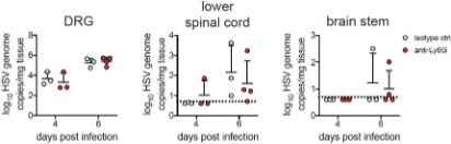
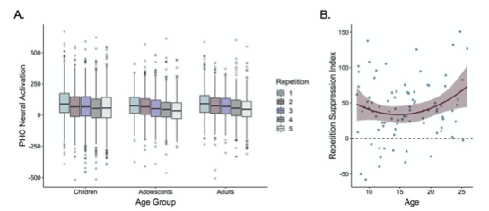
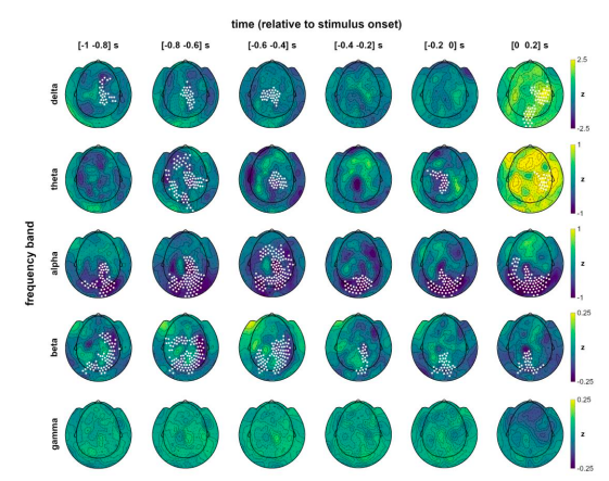
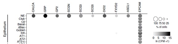
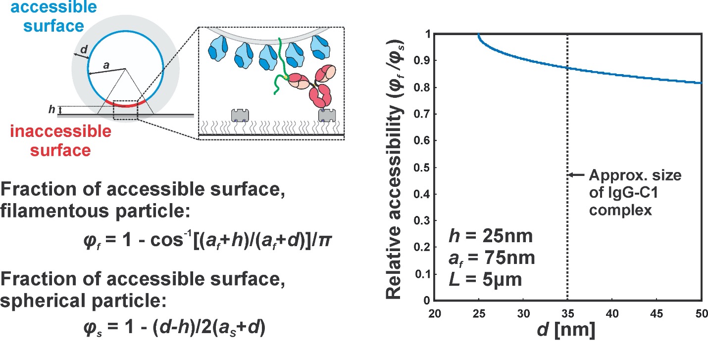
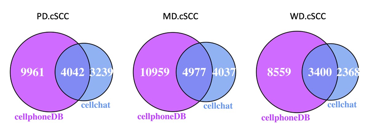
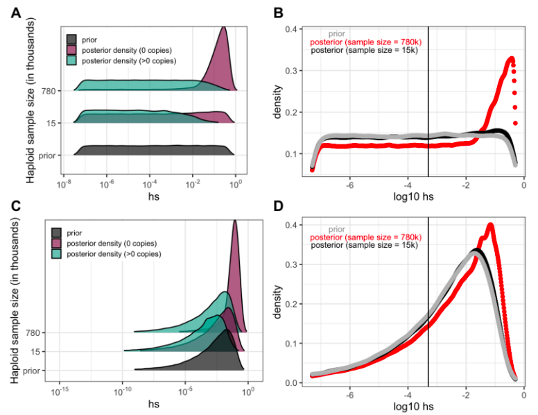
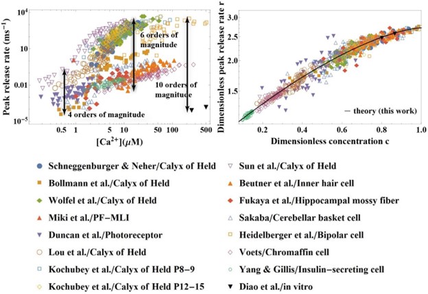
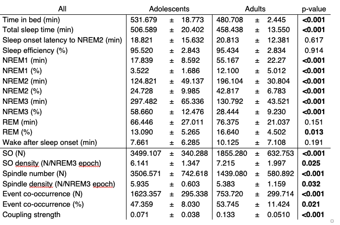
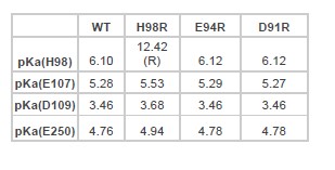
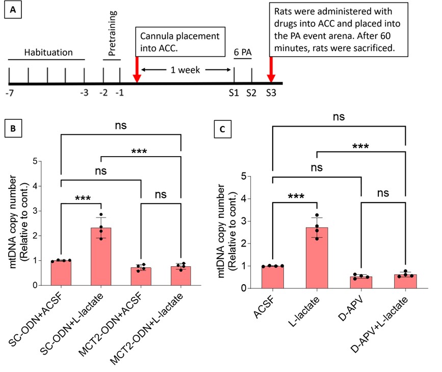
To test whether the L-lactate-induced neuronal mitochondrial biogenesis is dependent on MCT2, we bilaterally injected MCT2 antisense oligodeoxynucleotide (MCT2-ODN, n=8 rats, 2 nmol in 1 μl PBS per ACC) or scrambled ODN (SC-ODN, n=8 rats, 2 nmol in 1 μl PBS per ACC) into the ACC. After 11 hours, bilateral infusion of L-lactate (10 nmol, 1 μl) or ACSF (1 μl) was given into the ACC and the rats were kept in the PA event arena. After 60 mins (12 hours from MCT2-ODN or SC-ODN administration), the rats were sacrificed. As shown in Author response image 1B, SC-ODN+L-lactate group showed significantly increased relative mtDNA copy number compared to the SC-ODN+ACSF group (p<0.001, ANOVA followed by Tukey's multiple comparisons test). However, this effect was completely abolished in MCT2-ODN+L-lactate group, suggesting that MCT2 is required for the L-lactate-induced mitochondrial biogenesis in the ACC.
We have integrated this new data and results in the revised manuscript.
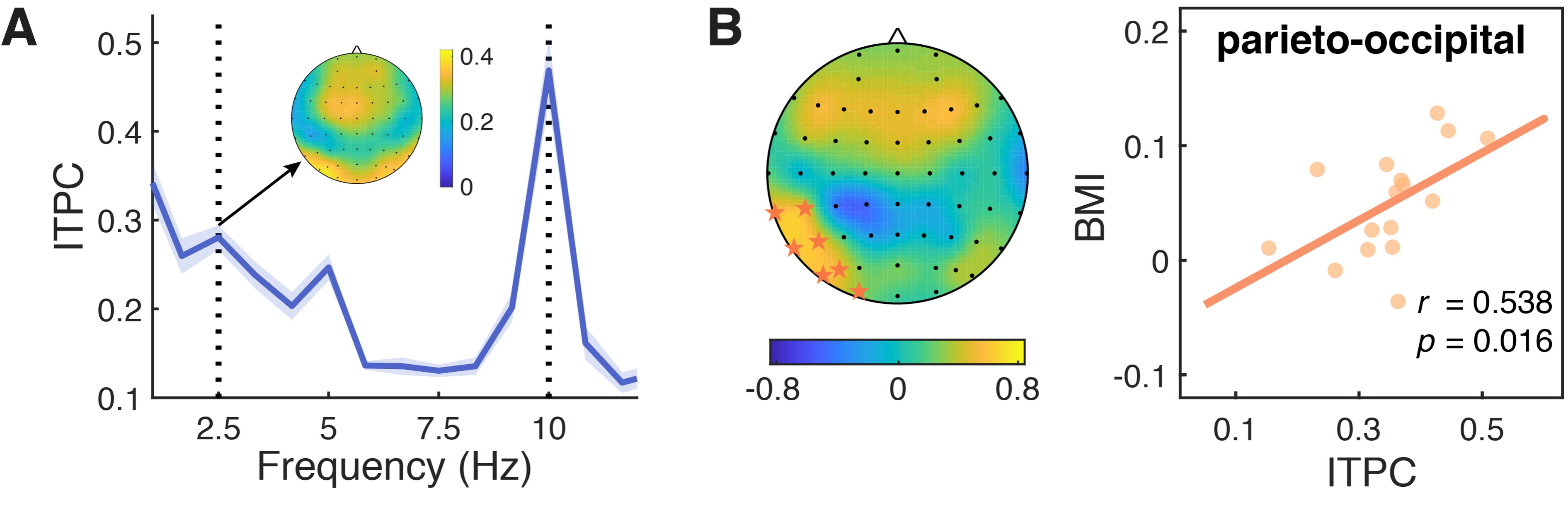
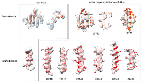
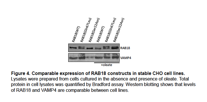
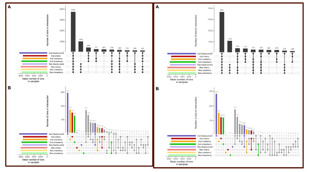
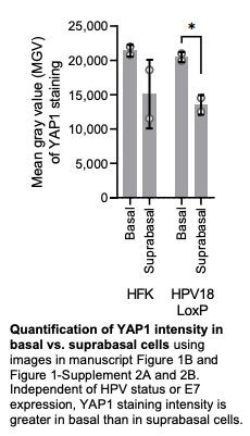
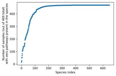
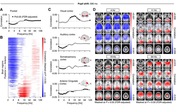
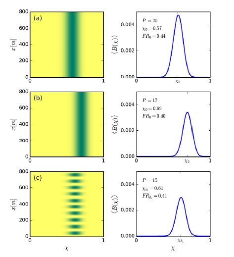
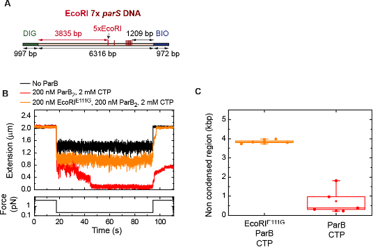
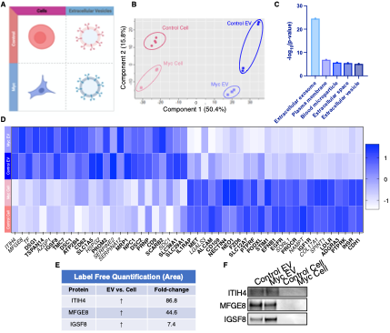
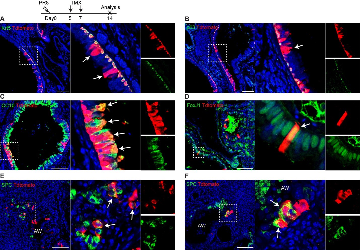
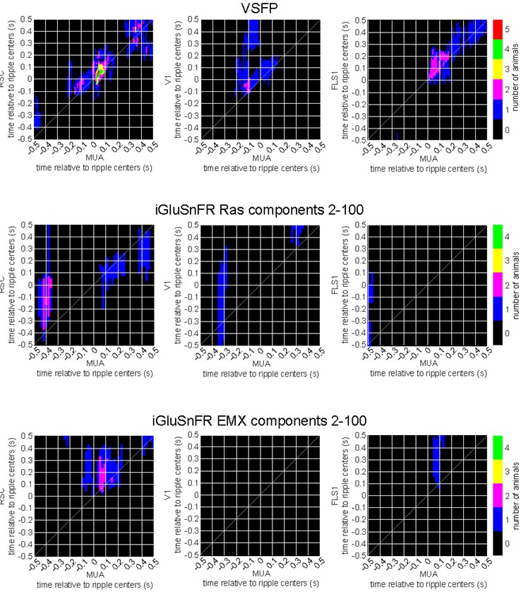
Author response image 1.
Mitochondrial biogenesis by L-lactate is dependent on MCT2 and NMDAR. A. Experimental design to investigate whether MCT2 and NMDAR activity are required for L-lactate-induced mitochondrial biogenesis. B and C. mtDNA copy number abundance in the ACC of different rat groups relative to nDNA. Data shown as mean ± SD (n=4 rats in each group). ***p<0.001, ANOVA followed by Tukey's multiple comparisons test.
The experiment using AVP to block NMDAR only partially supports the conclusions. Indeed, blocking NMDAR will knock down any response that involves these receptors, whether L-lactate is necessary or not.
In the current study we found that Astrocytic Gi activation in the ACC reduced L-lactate level in the ECF of ACC which was also associated with decreased PGC-1α/SIRT3/ATPB/mtDNA abundance suggesting downregulation of mitochondrial biogenesis pathway. We also found that exogenous administration of L-lactate into the ACC of astrocytic Gi-activated rats rescued this downregulation. In line with this, in a recently published study (Akter et al., 2023), we found upregulation of mitochondrial biogenesis pathway in the hippocampus neurons of exogenous L-lactate-treated anesthetized rats. Another recent study has demonstrated that exercise-induced L-lactate release from skeletal muscle or I.P. injection of L-lactate can induce hippocampal PGC-1α (which is a master regulator of mitochondrial biogenesis) expression and mitochondrial biogenesis in mice (Park et al., 2021). Together, these results provide compelling evidence that L-lactate promotes mitochondrial biogenesis.
L-lactate is known to promote expression of synaptic plasticity genes like Arc, c-Fos, and Zif268 in neurons (Yang et al., 2014). After entry into the neuronal cytoplasm, mainly through MCT2, it is converted into pyruvate by lactate dehydrogenase 1 (LDH1). This conversion also produces NADH, affecting the redox state of the neuron. NADH positively modulates the activity of NMDAR resulting in enhanced Ca2+ currents, the activation of intracellular signaling cascades, and the induction of the expression of plasticity-associated genes (Yang et al., 2014; Magistretti & Allaman, 2018). The study demonstrated that L-lactate–induced plasticity gene expression was abolished in the presence of NMDAR antagonists including D-APV (Yang et al., 2014). These results suggested that the MCT2 and NMDAR are key players in the regulation of L-lactate induced plasticity gene expression.
In the current study, we investigated whether similar mechanisms might be involved in L-lactate-induced neuronal mitochondrial biogenesis. We now used MCT2 antisense oligodeoxynucleotide to decrease the expression of MCT2 (as mentioned in the previous response and Author response image 1B) and showed that MCT2 is necessary for L-lactate-induced mitochondrial biogenesis to manifest, indicating that L-lactate’s entry into the neuron is required. As mentioned before, after entry into neuron, L-lactate is converted into pyruvate by LDH, which also produce NADH, which in turn potentiates NMDAR activity. Therefore, we investigated whether NMDAR activity is required for L-lactate-induced mitochondrial biogenesis. We used D-APV to inhibit NMDAR (Author response image 1C) and found that L-lactate does not increase mtDNA copy number abundance if D-APV is given, suggesting that NMDAR activity is required for L-lactate to promote mitochondrial biogenesis.
NMDAR serves diverse functions. Therefore, as mentioned by the reviewer, blocking NMDAR may knock down many such functions. While our current data only suggests the involvement of MCT2 and NMDAR in the upregulation of mitochondrial biogenesis by L-lactate, we have not investigated other mechanisms and pathways modulating mitochondrial biogenesis that are either dependent or independent of MCT2 and NMDAR activity. Further studies are needed in future to dissect and better understand this interesting observation. We have now clarified this in the discussion section of the manuscript.
Is inhibition of glycogenolysis involved in the observed effects mediated by Gi signaling? Indeed, L-lactate is formed both by glycolysis and glycogenolysis. The authors could test whether the glycogen metabolism-inhibiting drug DAB would mimic the effects of Gi activation.
In this study we have shown that astrocytic Gi activation in the ACC leads to a decrease in the cAMP and L-lactate. L-lactate is produced by glycogenolysis and glycolysis. cAMP in astrocytes acts as a trigger for L-lactate production (Choi et al., 2012; Horvat, Muhič, et al., 2021; Horvat, Zorec, et al., 2021; Zhou et al., 2021) by promoting glycogenolysis and glycolysis (Vardjan et al., 2018; Horvat, Muhič, et al., 2021; Horvat, Zorec, et al., 2021). Therefore, one promising explanation of reduced L-lactate level observed in our study is the reduction of L-lactate production in the astrocyte due to decreased glycogen metabolism as a result of decreased cAMP. We have now mentioned this in the discussion.
DAB is an inhibitor of glycogen phosphorylase that suppresses L-lactate production. It was shown to impair memory by decreasing L-lactate (Newman et al., 2011; Suzuki et al., 2011; Iqbal et al., 2023). As we found that the impairment in the schema memory and mitochondrial biogenesis was associated with decreased L-lactate level in the ACC and that the exogenous L-lactate administration can rescue the impairments, it is likely that DAB will mimic the effect of Gi activation in terms of schema memory and mitochondrial biogenesis. However, further study is needed to confirm this.
Reviewer #2 (Public Review):
The manuscript of Akter et al is an important study that investigates the role of astrocytic Gi signaling in the anterior cingulate cortex in the modulation of extracellular L-lactate level and consequently impairment in flavor-place associates (PA) learning. However, whereas some of the behavioral observations and signaling mechanism data are compelling, the conclusions about the effect on memory are inadequate as they rely on an experimental design that does not allow to differentiate acute or learning effect from the effect outlasting pharmacological treatments, i.e. effect on memory retention. With the addition of a few experiments, this paper would be of interest to the larger group of researchers interested in neuron-glia interactions during complex behavior.
• Largely, I agree with the authors' conclusion that activating Gi signaling in astrocytes impairs PA learning, however, the effect on memory retrieval is not that obvious. All behavioral and molecular signaling effects described in this study are obtained with the continuous presence of CNO, therefore it is not possible to exclude the acute effect of Gi pathway activation in astrocytes. What will happen with memory on retrieval test when CNO is omitted selectively during early, middle, or late session blocks of PA learning?
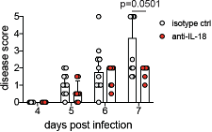
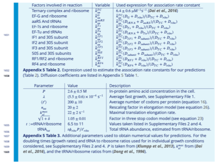
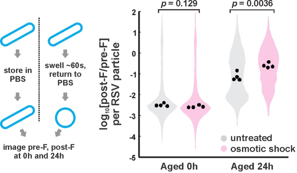
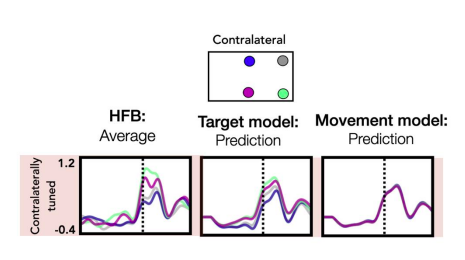
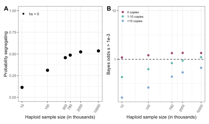
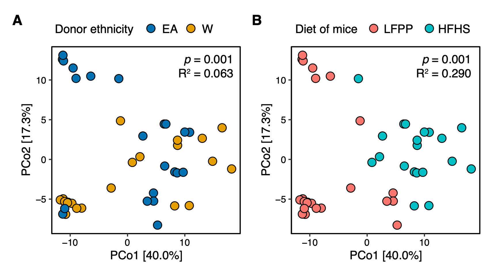
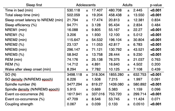
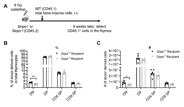
We have now added 8 more rats to the hM4Di-CNO group (i.e., the group with astrocytic Gi activation) to clarify the memory retrieval. These rats underwent flavor-place paired associate (PA) training similar to the previously described rats (n=7) of this group, that is they received CNO 30 minutes before and 30 minutes after the PA training sessions (S1-2, S4-8, S10-17). However, contrasting to the previous rats of this group which received CNO before PTs (PT1, PT2, PT3), we omitted the CNO (instead administered I.P. saline) selectively on these PTs conducted at the early, middle, and late stage of PA training, as suggested by the reviewer. These newly added rats did not show memory retrieval in these PTs, suggesting that the rats were not learning the PAs from the PA training sessions. See Author response image 2C-E, where this subgroup is denoted as hM4Di-CNO (Saline).
We then continued more PA training sessions (S21 onwards, Author response image 2B) for these rats without CNO. They gradually learned the PAs. PTs (PT5, PT6, PT7; Author response image 2G-I) were done during this continuation phase of PA training; once without CNO (i.e., with I.P. saline instead), and another one with CNO. As seen in the Author response image 2H and 2I, they retrieved the memory when PT6 and PT7 were done without CNO. However, if these PTs were done with CNO, they could not retrieve the memory. Together these results suggest that ACC astrocytic Gi activation by CNO during PT can impair memory retrieval in rats which have already learned the PAs.
As shown in the Author response image 2B, we replaced two original PAs with two new PAs (NPA 9 and 10) at S34. This was followed by PT8 (S35). As seen in Author response image 2J, these rats retrieved the NPA memory if the PT is done without CNO. However, they could not retrieve the NPA memory if the PT was done with CNO. This result suggests that ACC astrocytic Gi activation by CNO during PT can impair NPA memory retrieval.
In summary, these data show that astrocytic Gi activation in the ACC can impair PA memory retrieval. We have integrated this new data and results in the revised manuscript.
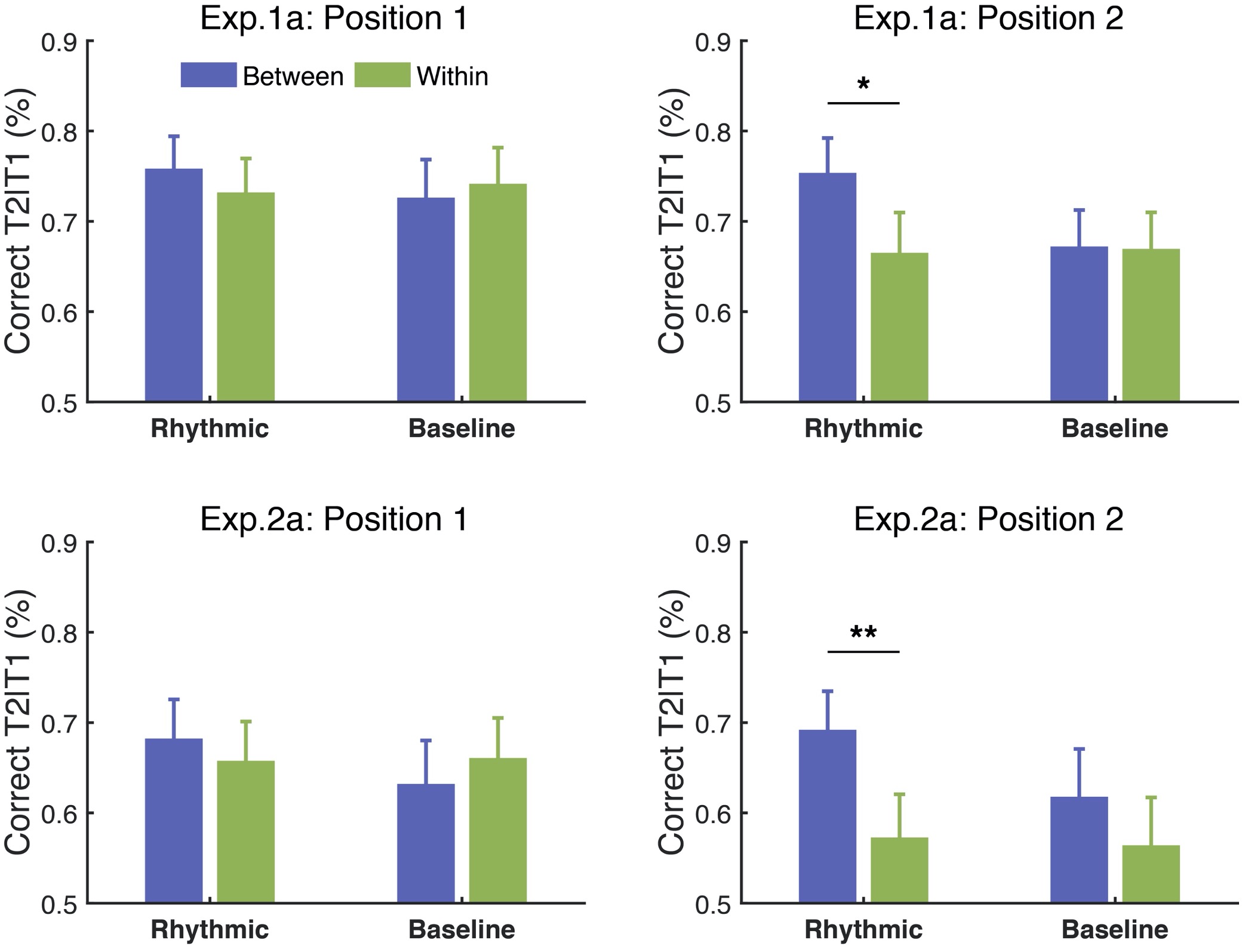
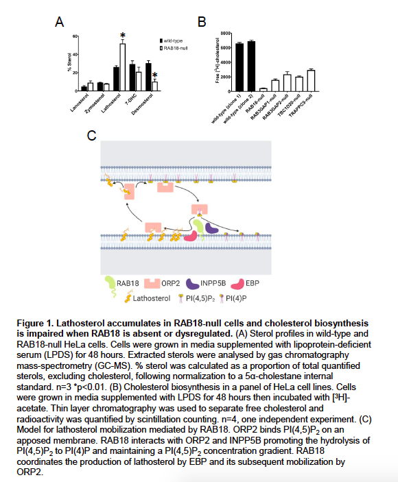
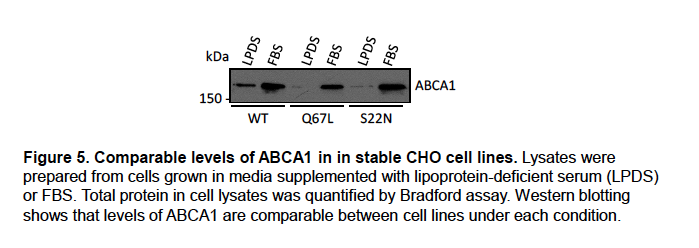
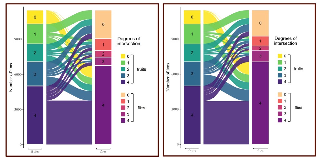
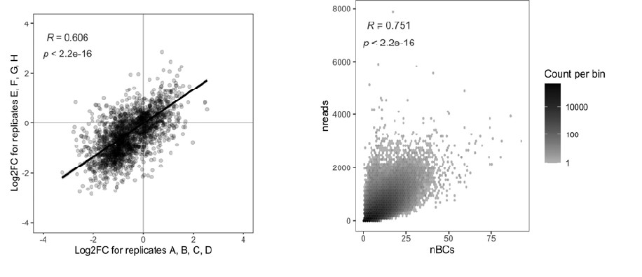
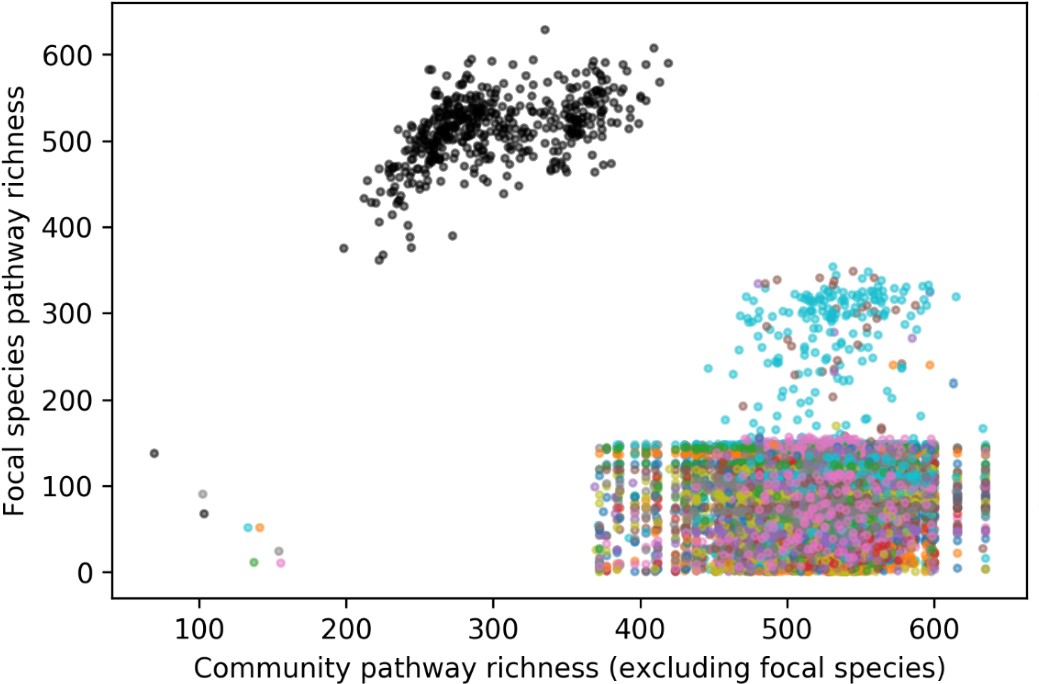
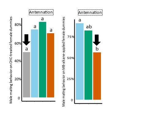
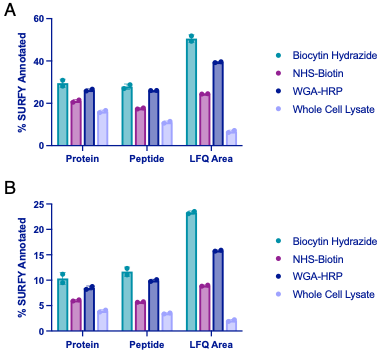
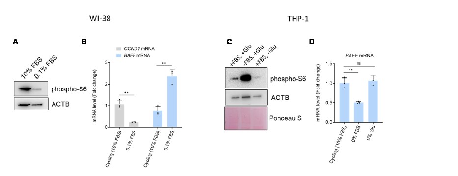
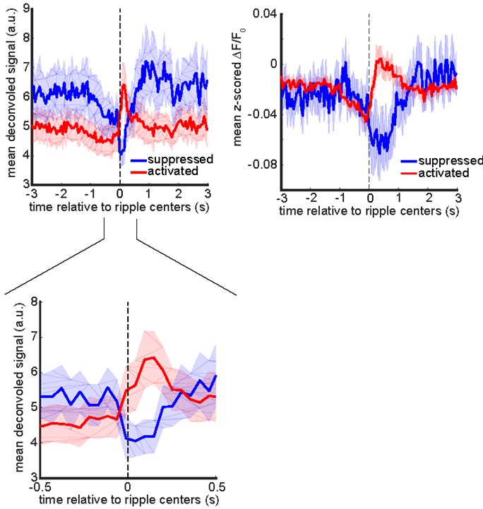
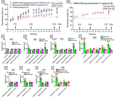
Author response image 2.
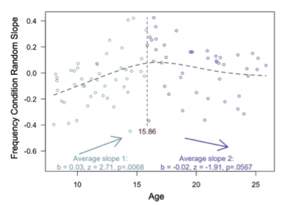
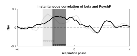
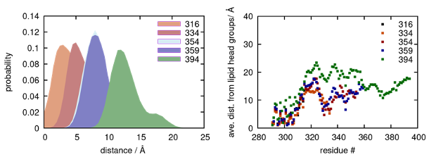
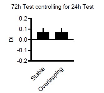
A. PI (mean ± SD) during the acquisition of the six original PAs (OPAs) (S1-2, 4-8, 10-17) and new PAs (NPAs) (S19) of the control (n=8), hM4Di-CNO (n=15), and rescue (hM4Di-CNO+L-lactate) (n=7) groups. From S6 onwards, hM4Di-CNO group consistently showed lower PI compared to control. However, concurrent L-lactate administration into the ACC (rescue group) can rescue this impairment. B. PI (mean ± SD) of hM4Di-CNO group (n=8) from S21 onwards showing gradual increase in PI when CNO was withdrawn. C, D, and E. Non-rewarded PTs (PT1, PT2, and PT3 conducted on S3, S9, and S18, respectively) to test memory retrieval of OPAs for the control, hM4Di-CNO, and rescue groups. The percentage of digging time at the cued location relative to that at the non-cued locations are shown (mean ± SD). In both PT2 and PT3, the control group spent significantly more time digging the cued sand well above the chance level, indicating that the rats learned OPAs and could retrieve it. Contrasting to this, hM4Di-CNO group did not spend more time digging the cued sand well above the chance level irrespective of CNO administration before the PTs. The rescue group showed results similar to the hM4Di-CNO group if CNO is given without L-lactate. On the other hand, they showed results similar to the control group if L-lactate is concurrently given with CNO, indicating that this group learned OPAs and could retrieve it. p < 0.05, p < 0.01, p < 0.001, one-sample t-test comparing the proportion of digging time at the cued sand well with the chance level of 16.67%. F. Non-rewarded PT4 (S20) which was conducted after replacing two OPAs with two NPAs (NPA 7 & 8) in S19 for the control, hM4Di-CNO, and rescue groups. Results show that the control group spent significantly more time digging the new cued sand well above the chance level indicating that the rats learned the NPAs from S19 and could retrieve it in this PT. Contrasting to this, hM4Di-CNO group did not spend more time digging the new-cued sand well above the chance level irrespective of CNO administration before the PT. The rescue group showed results similar to the hM4Di-CNO group if CNO is given without L-lactate. On the other hand, they showed results similar to the control group if L-lactate is concurrently given with CNO indicating that this group learned NPAs from S19 and could retrieve it. p < 0.001, one-sample t-test comparing the proportion of digging time at the new cued sand well with the chance level of 16.67%. G, H, and I. Non-rewarded PTs (PT5, PT6, and PT7 conducted on S23, S27, and S33, respectively) to test memory retrieval of OPAs for the hM4Di-CNO group. In both PT6 and PT7, the rats spent significantly more time digging the cued sand well above the chance level if the tests are done without CNO, indicating that the rats learned the OPAs and could retrieve it. However, CNO prevented memory retrieval during these PTs. p < 0.001, one-sample t-test comparing the proportion of digging time at the cued sand well with the chance level of 16.67%.
J. Non-rewarded PT4 (S35) which was conducted after replacing two OPAs with two NPAs (NPA 9 & 10) in S34 for the hM4Di-CNO group. Results show that the rats spent significantly more time digging the new cued sand well above the chance level if CNO was not given before the PT, indicating that the rats learned the NPAs from S34 and could retrieve it in this PT. However, if CNO is given before the PT, the retrieval is impaired. *p < 0.001, one-sample t-test comparing the proportion of digging time at the new cued sand well with the chance level of 16.67%.
• I found it truly exciting that the administration of exogenous L-lactate is capable to rescue CNO-induced PA learning impairment, when co-applied. Would it be possible that this treatment has a sensitivity to a particular stage of learning (acquisition, consolidation, or memory retrieval) when L-lactate administration would be the most efficacious?
The hM4Di-CNO group, when continued with PA training without CNO (S21-S32) (Author response image 2B), was able to learn the six original PAs (OPAs). In the PT7 done at S33 (Author response image 2I), this group of rats was able to retrieve the memory if the test was done without CNO but could not retrieve the memory if CNO was given. Similarly, the Rescue group (hM4Di-CNO+L-lactate) (Author response image 2A), which received both CNO and L-lactate during PA training sessions (S1-S17), they were able to learn the OPAs. And at PT3 done at S18 (Author response image 2E), these rats were able to retrieve the memory when the test was done with CNO+L-lactate but not if the test is done with only CNO. Together, these results clearly show that ACC astrocytic Gi activation with CNO impairs memory retrieval and exogenous L-lactate can rescue the impairment. Therefore, it can be concluded that the memory retrieval is sensitive to L-lactate.
The PA learning is hippocampus-dependent. Over the course of repeated PA training, systems consolidation occurs in the ACC, after which the already learned PA memory (schema) becomes hippocampus-independent (Tse et al., 2007; Tse et al., 2011). A higher activation (indicated by expression of c-Fos) in the hippocampus relative to the ACC during the early period of schema development, and the reverse at the late stage was observed in our previous study (Liu et al., 2022). However, rapid assimilation of new PA into the ACC requires simultaneous activation/retrieval of previous schema from ACC and hippocampus dependent new PA learning (Tse et al., 2007; Tse et al., 2011). During new PA learning, increase of c-Fos neurons in both CA1 and ACC was detected (Liu et al., 2022).
Our hM4Di-CNO group received CNO 30 mins before and after each PA training session in S1-S17 (Author response image 2A). Also, the Rescue group similarly received CNO+L-lactate before and after each PA training session in S1-S17. Therefore, while this study design allowed us to conclude that ACC astrocytic Gi activation impairs PA learning and that exogenous L-lactate can rescue the impairment, it does not allow clear differentiation of the effects of these treatments on memory acquisition and consolidation. Further studies are needed to investigate this.
• The hypothesis that observed learning impairments could be associated with diminished mitochondrial biogenesis caused by decreased l-lactate in the result of astrocytic Gi-DREADDS stimulation is very appealing, but a few key pieces of evidence are missing. So far, the hypothesis is supported by experiments demonstrating reduced expression of several components of mitochondrial membrane ATP synthase and a decrease in relative mtDNA copy numbers in ACC of rats injected with Gi-DREADDs. L-lactate injections into ACC restored and even further increased the expression of the above-mentioned markers. Co-administration of NMDAR antagonist D-APV or MCT-2 (mostly neuronal) blocker 4-CIN with L-lactate, prevented L-lactate-induced increase in relative mtDNA copy. I am wondering how the interference with mitochondrial biogenesis is affecting neuronal physiology and if it would result in impaired PA learning or schema memory.
The observation of diminished mitochondrial biogenesis in the astrocytic Gi-activated rats that showed impaired PA learning is exciting. However, our study does not provide experimental data on how mitochondrial biogenesis could be associated with impaired PA learning and schema memory. Results from several previous studies linked mitochondrial biogenesis and its regulators such as PGC-1α and SIRT3 to diverse neuronal and cognitive functions as described in the discussion section of the manuscript. In the revised manuscript, we have provided further discussion as follows to discuss potential mechanisms:
“In this study, we have demonstrated that ACC astrocytic Gi activation impairs PA learning and schema formation, PA memory retrieval, and NPA learning and retrieval by decreasing L-lactate level in the ACC. Although we have shown that these impairments are associated with diminished expression of proteins of mitochondrial biogenesis, the precise mechanisms of how astrocytic Gi activation affects neuronal functions and schema memory remain to be elucidated. We previously demonstrated that neuronal inhibition in either the hippocampus or the ACC impairs PA learning and schema formation (Hasan et al., 2019). In another recent study (Liu et al., 2022), we showed that astrocytic Gi activation in the CA1 impaired PA training-associated CA1-ACC projecting neuronal activation. Yao et al. recently showed that reduction of astrocytic lactate dehydrogenase A (an enzyme that reversibly catalyze L-lactate production from pyruvate) in the dorsomedial prefrontal cortex reduces L-lactate levels and neuronal firing frequencies, promoting depressive-like behaviors in mice (Yao et al., 2023). These impairments could be rescued by L-lactate infusion. It is possible that the impairment in PA learning and schema observed in our study might have involved a similar functional consequence of reduced neuronal activity in the ACC neurons upon astrocytic Gi activation.
Schema consolidation is associated with synaptic plasticity-related gene expression (such as Zif268, Arc) in the ACC (Tse et al., 2011). L-lactate, after entry into neurons, can be converted to pyruvate during which NADH is also produced, promoting synaptic plasticity-related gene expression by potentiating NMDA signaling in neurons (Yang et al., 2014; Margineanu et al., 2018). Furthermore, L-lactate acts as an energy substrate to fuel learning-induced de novo neuronal translation critical for long-term memory (Descalzi et al., 2019). On the other hand, mitochondria play crucial role in fueling local translation during synaptic plasticity (Rangaraju et al., 2019). Therefore, it could be hypothesized that the rescue of astrocytic Gi activation-mediated impairment of schema by exogenous L-lactate could have been mediated by facilitating synaptic plasticity-related gene expression by directly fueling the protein translation, potentiating NMDA signaling, as well as increasing mitochondrial capacity for ATP production by promoting mitochondrial biogenesis. Furthermore, the potential involvement of HCAR1, a receptor for L-lactate that may regulate neuronal activity (Bozzo et al., 2013; Tang et al., 2014; Herrera-López & Galván, 2018; Abrantes et al., 2019), cannot be excluded. Future research could explore these potential mechanisms, examining the interactions among them, and determining their relative contributions to schema.
Our previous study also showed that ACC myelination is necessary for PA learning and schema formation, and that repeated PA training is associated with oligodendrogenesis in the ACC (Hasan et al., 2019). Oligodendrocytes facilitate fast, synchronized, and energy efficient transfer of information by wrapping axons in myelin sheath. Furthermore, they supply axons with glycolysis products, such as L-lactate, to offer metabolic support (Fünfschilling et al., 2012; Lee et al., 2012). The association of oligodendrogenesis and myelination with schema memory may suggest an adaptive response of oligodendrocytes to enhance metabolic support and neuronal energy efficiency during PA learning. Given the impairments in PA learning observed in the ACC astrocytic Gi-activated rats in the current study, it is reasonable to conclude that the direct metabolic support to axons provided by oligodendrocytes is not sufficient to rescue the schema impairments caused by decreased L-lactate levels upon astrocytic Gi activation. On the other hand, L-lactate was shown to be important for oligodendrogenesis and myelination (Sánchez-Abarca et al., 2001; Rinholm et al., 2011; Ichihara et al., 2017). Therefore, it is tempting to speculate that a decrease in L-lactate level may also impede oligodendrogenesis and myelination, consequently preventing the enhanced axonal support provided by oligodendrocytes and myelin during schema learning. Recently, a study has demonstrated that upon demyelination, mitochondria move from the neuronal cell body to the demyelinated axon (Licht-Mayer et al., 2020). Enhancement of this axonal response of mitochondria to demyelination, by targeting mitochondrial biogenesis and mitochondrial transport from the cell body to axon, protects acutely demyelinated axons from degeneration. Given the connection between schema and increased myelination, it remains an open question whether L-lactate-induced mitochondrial biogenesis plays a beneficial role in schema through a similar mechanism. Nevertheless, our results contribute to the mounting evidence of the glial role in cognitive functions and underscores the new paradigm in which glial cells are considered as integral players in cognitive functions alongside neurons. Disruption of neurons, myelin, or astrocytes in the ACC can disrupt PA learning and schema memory.”
Reviewer #3 (Public Review):
Akter et al. investigated how the astroglial Gi signaling pathway in the rat anterior cingulate cortex (ACC) affects cognitive functions, in particular schema memory formation. Using a stereotactic approach they intracranially introduced AAV8 vectors carrying mCherry-tagged hM4Di DREADD (Designer Receptor Exclusively Activated by Designer Drugs) under astrocyte selective GFAP promotor (AAV8-GFAP-hM4Di-mCherry) into the AAC region of the rat brain. hM4Di DREADD is a genetically modified form of the human M4 muscarinic (hM4) receptor insensitive to endogenous acetylcholine but is activated by the inert clozapine metabolite clozapine-N-oxide (CNO), triggering the Gi signaling pathway. The authors confirmed that hM4Di DREADD is selectively expressed in astrocytes after the application of the AAV8 vector by analysing the mCherry signals and immunolabeling of astrocytes and neurons in the ACC region of the rat brain. They activated hM4Di DREADD (Gi signalling) in astrocytes by intraperitoneal administration of CNO and measured cognitive functions in animals after CNO administration. Activation of Gi signaling in astrocytes by CNO application decreased paired-associate (PA) learning, schema formation, and memory retrieval in tested animals. This was associated with a decrease in cAMP in astrocytes and L-lactate in extracellular fluid as measured by immunohistochemistry in situ and in awake rats by microdialysis, respectively. Administration of exogenous L-lactate rescued the astroglial Gi-mediated deficits in PA learning, memory retrieval, and schema formation, suggesting that activation of astroglial Gi signalling downregulates L-lactate production in astrocytes and its transport to neurons affecting memory formation. Authors also show that expression level of proteins involved in mitochondrial biogenesis, which is associated with cognitive functions, is decreased in neurons, when Gi signalling is activated in astrocytes, and rescued when exogenous L-lactate is applied, suggesting the implication of astrocyte-derived L-lactate in the maintenance of mitochondrial biogenesis in neurons. The latter depended on lactate MCT2 transporter activity and glutamate NMDA receptor activity.
The paper is very well written and discussed. The conclusions of this paper are well supported by the data. Although this is a study that uses established and previously published methodologies, it provides new insights into L-lactate signalling in the brain, particularly in AAC, and further confirms the role of astroglial L-lactate in learning and memory formation. It also raises new questions about the molecular mechanisms underlying astrocyte-derived L-lactate-mediated mitochondrial biogenesis in neurons and its contribution to schema memory formation.
• The authors discuss astrocytic L-lactate signalling without considering the recently discovered L-lactate-sensitive Gs and Gi protein-coupled receptors in the brain, which are present in both astrocytes and neurons. The use of nonendogenous L-lactate receptor agonists (Compound 2, 3-chloro-5-hydroxybenzoic acid) would clarify the implication of L-lactate receptor signalling in schema memory formation.
In the revised manuscript, we have included this point in the discussion section to mention the potential role of HCAR1 in schema memory as follows:
“Schema consolidation is associated with synaptic plasticity-related gene expression (such as Zif268, Arc) in the ACC (Tse et al., 2011). L-lactate, after entry into neurons, can be converted to pyruvate during which NADH is also produced, promoting synaptic plasticity-related gene expression by potentiating NMDA signaling in neurons (Yang et al., 2014; Margineanu et al., 2018). Furthermore, L-lactate acts as an energy substrate to fuel learning-induced de novo neuronal translation critical for long-term memory (Descalzi et al., 2019). On the other hand, mitochondria play crucial role in fueling local translation during synaptic plasticity (Rangaraju et al., 2019). Therefore, it could be hypothesized that the rescue of astrocytic Gi activation-mediated impairment of schema by exogenous L-lactate could have been mediated by facilitating synaptic plasticity-related gene expression by directly fueling the protein translation, potentiating NMDA signaling, as well as increasing mitochondrial capacity for ATP production by promoting mitochondrial biogenesis. Furthermore, the potential involvement of HCAR1, a receptor for L-lactate that may regulate neuronal activity (Bozzo et al., 2013; Tang et al., 2014; Herrera-López & Galván, 2018; Abrantes et al., 2019), cannot be excluded. Future research could explore these potential mechanisms, examining the interactions among them, and determining their relative contributions to schema.”
• The use of control animals transduced with an "empty" AAV9 vector (AAV8-GFAP-mCherry) compared with animals transduced with AAV8-GFAP-hM4Di-mCherry throughout the study would strengthen the results of this study, since transfection itself, as well as overexpression of the mCherry protein, may affect cell function.
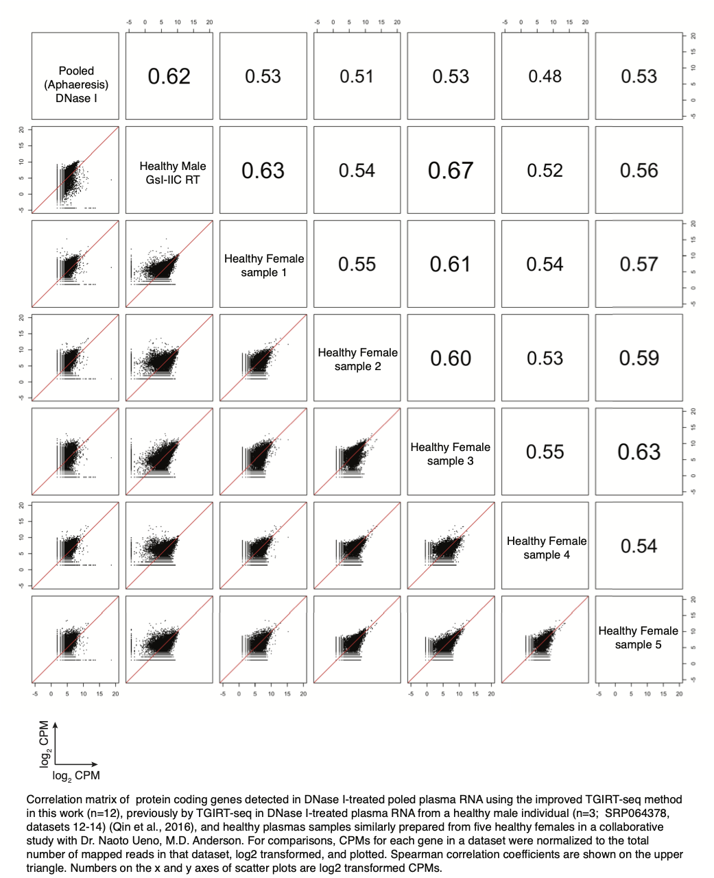
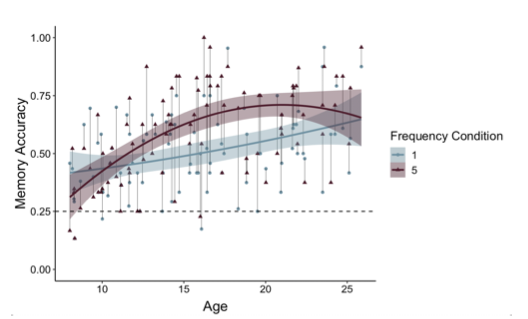
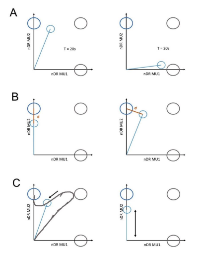
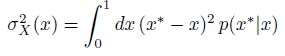
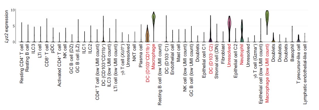
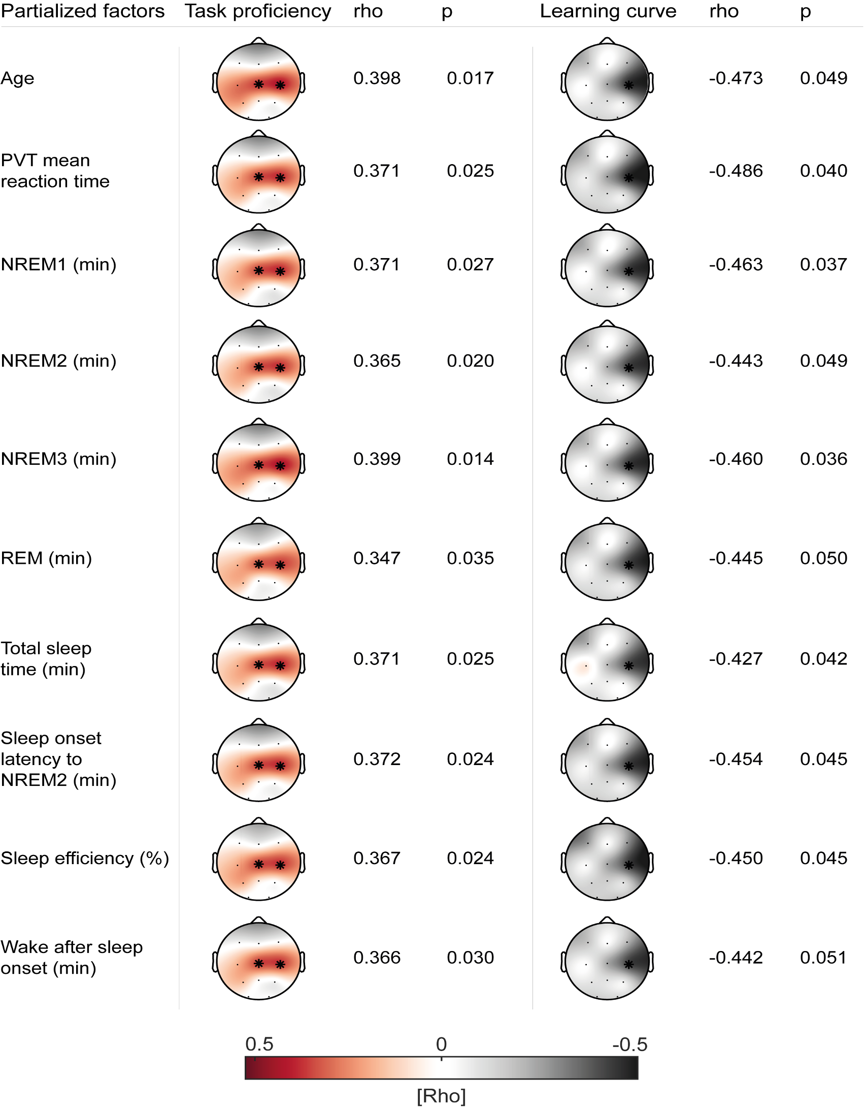
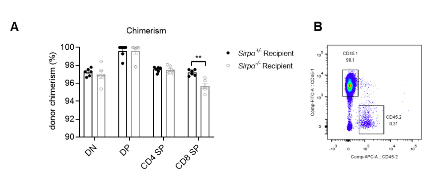
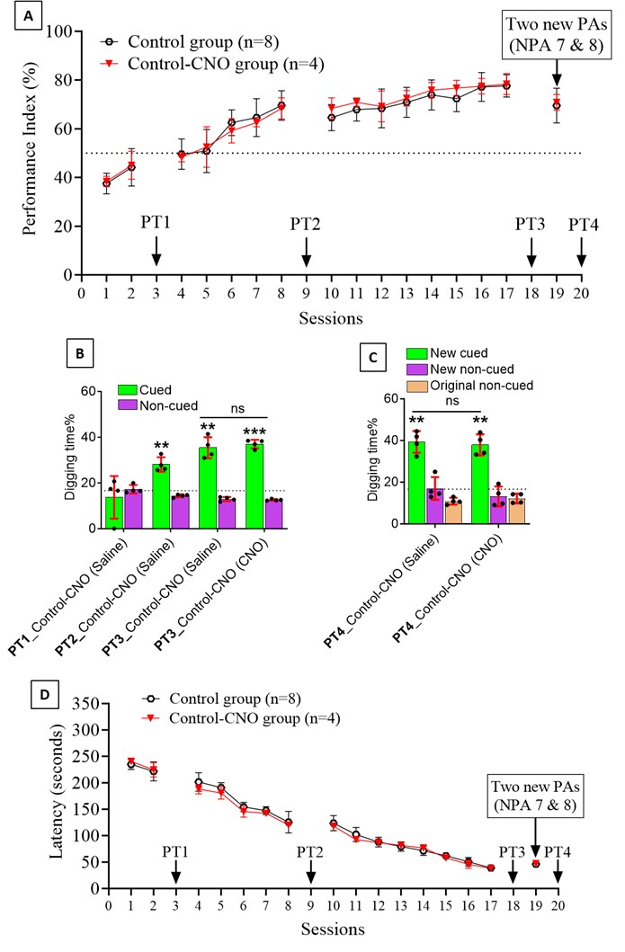
We thank the reviewer for pointing this. The schema experiment includes a control group (Control-CNO group) of rats injected with AAV8-GFAP-mCherry bilaterally into the ACC. As shown in Author response image 3, after habituation and pretraining, these rats were trained for PA learning similarly to the other groups. Before 30 mins and after 30 mins of each PA training session, they received I.P. CNO. The PA learning, schema formation, memory retrieval, NPA learning and retrieval, and latency (time needed to commence digging at the correct well) were similar to the control group of rats. This result is consistent with our previous study where rats bilaterally injected with AAV8-GFAP-mCherry into CA1 of hippocampus did not show impairments in PA learning and schema formation upon CNO treatment (Liu et al., 2022).
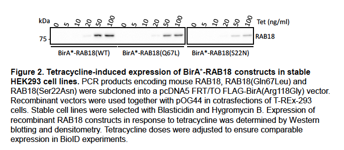
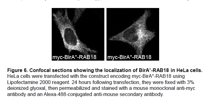
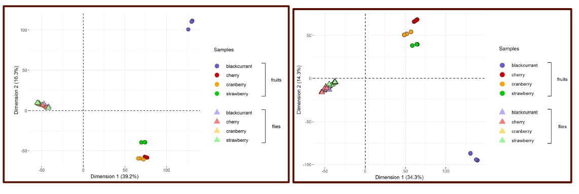
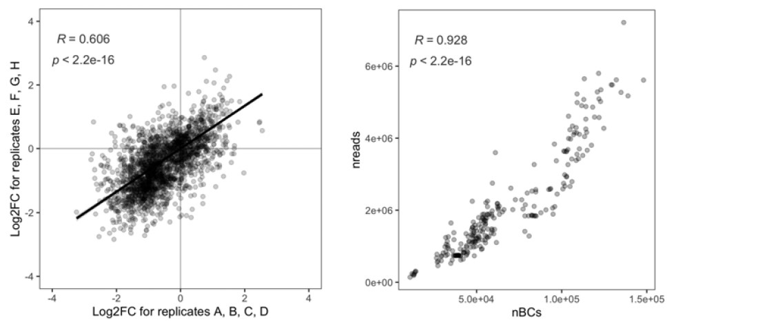
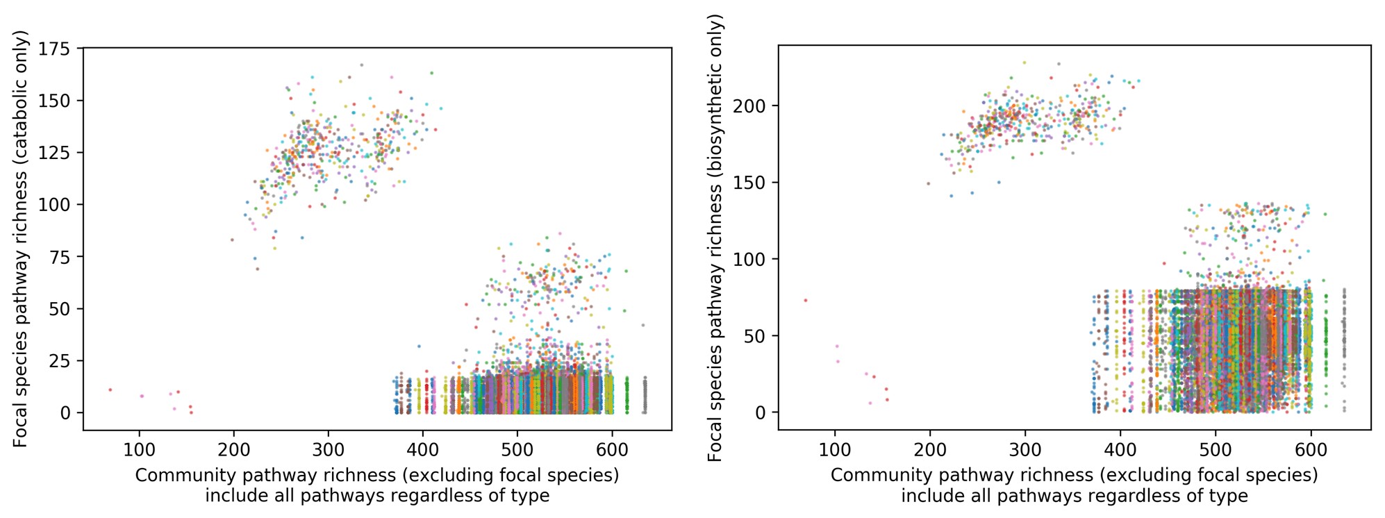
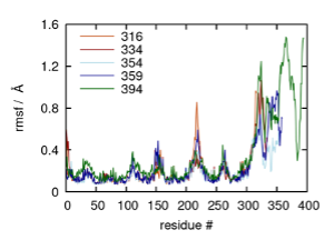
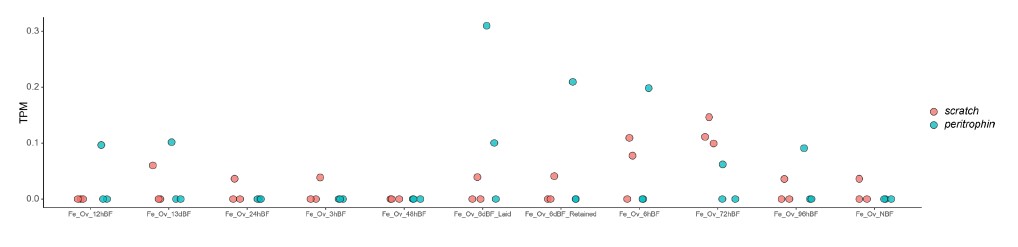
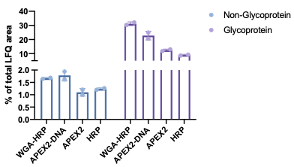
Author response image 3.
A. PI (mean ± SD) during the acquisition of the original six PAs (OPAs) (S1-2, 4-8, 10-17) and new PAs (NPAs) (S19) of the control (n=6) and control-CNO (n=4) groups. B. Non-rewarded PTs (PT1, PT2, and PT3 done on S3, S9, and S18, respectively) to test memory retrieval of OPAs for the control-CNO group. C. Non-rewarded PT4 (S20) which was done after replacing two OPAs with two NPAs (NPA 7 & 8) in S19 for the control-CNO group. D. Latency (in seconds) before commencing digging at the correct well for control and control-CNO groups. Data shown as mean ± SD.
References
Abrantes, H. d. C., Briquet, M., Schmuziger, C., Restivo, L., Puyal, J., Rosenberg, N., Rocher, A.-B., Offermanns, S., & Chatton, J.-Y. (2019). The Lactate Receptor HCAR1 Modulates Neuronal Network Activity through the Activation of Gα and Gβγ Subunits. The Journal of Neuroscience, 39(23), 4422-4433. https://doi.org/10.1523/jneurosci.2092-18.2019
Akter, M., Ma, H., Hasan, M., Karim, A., Zhu, X., Zhang, L., & Li, Y. (2023). Exogenous L-lactate administration in rat hippocampus increases expression of key regulators of mitochondrial biogenesis and antioxidant defense [Original Research]. Frontiers in Molecular Neuroscience, 16. https://doi.org/10.3389/fnmol.2023.1117146
Bozzo, L., Puyal, J., & Chatton, J.-Y. (2013). Lactate Modulates the Activity of Primary Cortical Neurons through a Receptor-Mediated Pathway. PLoS One, 8(8), e71721. https://doi.org/10.1371/journal.pone.0071721
Choi, H. B., Gordon, G. R., Zhou, N., Tai, C., Rungta, R. L., Martinez, J., Milner, T. A., Ryu, J. K., McLarnon, J. G., Tresguerres, M., Levin, L. R., Buck, J., & MacVicar, B. A. (2012). Metabolic communication between astrocytes and neurons via bicarbonate-responsive soluble adenylyl cyclase. Neuron, 75(6), 1094-1104. https://doi.org/10.1016/j.neuron.2012.08.032
Covelo, A., Eraso-Pichot, A., Fernández-Moncada, I., Serrat, R., & Marsicano, G. (2021). CB1R-dependent regulation of astrocyte physiology and astrocyte-neuron interactions. Neuropharmacology, 195, 108678. https://doi.org/https://doi.org/10.1016/j.neuropharm.2021.108678
Descalzi, G., Gao, V., Steinman, M. Q., Suzuki, A., & Alberini, C. M. (2019). Lactate from astrocytes fuels learning-induced mRNA translation in excitatory and inhibitory neurons. Communications Biology, 2(1), 247. https://doi.org/10.1038/s42003-019-0495-2
Endo, F., Kasai, A., Soto, J. S., Yu, X., Qu, Z., Hashimoto, H., Gradinaru, V., Kawaguchi, R., & Khakh, B. S. (2022). Molecular basis of astrocyte diversity and morphology across the CNS in health and disease. Science, 378(6619), eadc9020. https://doi.org/10.1126/science.adc9020
Fünfschilling, U., Supplie, L. M., Mahad, D., Boretius, S., Saab, A. S., Edgar, J., Brinkmann, B. G., Kassmann, C. M., Tzvetanova, I. D., Möbius, W., Diaz, F., Meijer, D., Suter, U., Hamprecht, B., Sereda, M. W., Moraes, C. T., Frahm, J., Goebbels, S., & Nave, K.-A. (2012). Glycolytic oligodendrocytes maintain myelin and long-term axonal integrity. Nature, 485(7399), 517-521. https://doi.org/10.1038/nature11007
Harris, R. A., Lone, A., Lim, H., Martinez, F., Frame, A. K., Scholl, T. J., & Cumming, R. C. (2019). Aerobic Glycolysis Is Required for Spatial Memory Acquisition But Not Memory Retrieval in Mice. eNeuro, 6(1). https://doi.org/10.1523/ENEURO.0389-18.2019
Hasan, M., Kanna, M. S., Jun, W., Ramkrishnan, A. S., Iqbal, Z., Lee, Y., & Li, Y. (2019). Schema-like learning and memory consolidation acting through myelination. FASEB J, 33(11), 11758-11775. https://doi.org/10.1096/fj.201900910R
Herrera-López, G., & Galván, E. J. (2018). Modulation of hippocampal excitability via the hydroxycarboxylic acid receptor 1. Hippocampus, 28(8), 557-567. https://doi.org/https://doi.org/10.1002/hipo.22958
Horvat, A., Muhič, M., Smolič, T., Begić, E., Zorec, R., Kreft, M., & Vardjan, N. (2021). Ca2+ as the prime trigger of aerobic glycolysis in astrocytes. Cell Calcium, 95, 102368. https://doi.org/https://doi.org/10.1016/j.ceca.2021.102368
Horvat, A., Zorec, R., & Vardjan, N. (2021). Lactate as an Astroglial Signal Augmenting Aerobic Glycolysis and Lipid Metabolism [Review]. Frontiers in Physiology, 12. https://doi.org/10.3389/fphys.2021.735532
Ichihara, Y., Doi, T., Ryu, Y., Nagao, M., Sawada, Y., & Ogata, T. (2017). Oligodendrocyte Progenitor Cells Directly Utilize Lactate for Promoting Cell Cycling and Differentiation. J Cell Physiol, 232(5), 986-995. https://doi.org/10.1002/jcp.25690
Iqbal, Z., Liu, S., Lei, Z., Ramkrishnan, A. S., Akter, M., & Li, Y. (2023). Astrocyte L-Lactate Signaling in the ACC Regulates Visceral Pain Aversive Memory in Rats. Cells, 12(1), 26. https://www.mdpi.com/2073-4409/12/1/26
Jourdain, P., Rothenfusser, K., Ben-Adiba, C., Allaman, I., Marquet, P., & Magistretti, P. J. (2018). Dual action of L-Lactate on the activity of NR2B-containing NMDA receptors: from potentiation to neuroprotection. Sci Rep, 8(1), 13472. https://doi.org/10.1038/s41598-018-31534-y
Kofuji, P., & Araque, A. (2021). G-Protein-Coupled Receptors in Astrocyte-Neuron Communication. Neuroscience, 456, 71-84. https://doi.org/10.1016/j.neuroscience.2020.03.025
Lee, Y., Morrison, B. M., Li, Y., Lengacher, S., Farah, M. H., Hoffman, P. N., Liu, Y., Tsingalia, A., Jin, L., Zhang, P. W., Pellerin, L., Magistretti, P. J., & Rothstein, J. D. (2012). Oligodendroglia metabolically support axons and contribute to neurodegeneration. Nature, 487(7408), 443-448. https://doi.org/10.1038/nature11314
Licht-Mayer, S., Campbell, G. R., Canizares, M., Mehta, A. R., Gane, A. B., McGill, K., Ghosh, A., Fullerton, A., Menezes, N., Dean, J., Dunham, J., Al-Azki, S., Pryce, G., Zandee, S., Zhao, C., Kipp, M., Smith, K. J., Baker, D., Altmann, D., Anderton, S. M., Kap, Y. S., Laman, J. D., Hart, B. A. t., Rodriguez, M., Watzlawick, R., Schwab, J. M., Carter, R., Morton, N., Zagnoni, M., Franklin, R. J. M., Mitchell, R., Fleetwood-Walker, S., Lyons, D. A., Chandran, S., Lassmann, H., Trapp, B. D., & Mahad, D. J. (2020). Enhanced axonal response of mitochondria to demyelination offers neuroprotection: implications for multiple sclerosis. Acta Neuropathologica, 140(2), 143-167. https://doi.org/10.1007/s00401-020-02179-x
Liu, S., Wong, H. Y., Xie, L., Iqbal, Z., Lei, Z., Fu, Z., Lam, Y. Y., Ramkrishnan, A. S., & Li, Y. (2022). Astrocytes in CA1 modulate schema establishment in the hippocampal-cortical neuron network. BMC Biol, 20(1), 250. https://doi.org/10.1186/s12915-022-01445-6
Magistretti, P. J., & Allaman, I. (2018). Lactate in the brain: from metabolic end-product to signalling molecule. Nat Rev Neurosci, 19(4), 235-249. https://doi.org/10.1038/nrn.2018.19
Margineanu, M. B., Mahmood, H., Fiumelli, H., & Magistretti, P. J. (2018). L-Lactate Regulates the Expression of Synaptic Plasticity and Neuroprotection Genes in Cortical Neurons: A Transcriptome Analysis. Front Mol Neurosci, 11, 375. https://doi.org/10.3389/fnmol.2018.00375
Netzahualcoyotzi, C., & Pellerin, L. (2020). Neuronal and astroglial monocarboxylate transporters play key but distinct roles in hippocampus-dependent learning and memory formation. Progress in Neurobiology, 194, 101888. https://doi.org/https://doi.org/10.1016/j.pneurobio.2020.101888
Newman, L. A., Korol, D. L., & Gold, P. E. (2011). Lactate produced by glycogenolysis in astrocytes regulates memory processing. PLoS One, 6(12), e28427. https://doi.org/10.1371/journal.pone.0028427
Park, J., Kim, J., & Mikami, T. (2021). Exercise-Induced Lactate Release Mediates Mitochondrial Biogenesis in the Hippocampus of Mice via Monocarboxylate Transporters. Front Physiol, 12, 736905. https://doi.org/10.3389/fphys.2021.736905
Peterson, S. M., Pack, T. F., & Caron, M. G. (2015). Receptor, Ligand and Transducer Contributions to Dopamine D2 Receptor Functional Selectivity. PLoS One, 10(10), e0141637. https://doi.org/10.1371/journal.pone.0141637
Rangaraju, V., Lauterbach, M., & Schuman, E. M. (2019). Spatially Stable Mitochondrial Compartments Fuel Local Translation during Plasticity. Cell, 176(1), 73-84.e15. https://doi.org/10.1016/j.cell.2018.12.013
Rinholm, J. E., Hamilton, N. B., Kessaris, N., Richardson, W. D., Bergersen, L. H., & Attwell, D. (2011). Regulation of oligodendrocyte development and myelination by glucose and lactate. J Neurosci, 31(2), 538-548. https://doi.org/10.1523/JNEUROSCI.3516-10.2011
Sánchez-Abarca, L. I., Tabernero, A., & Medina, J. M. (2001). Oligodendrocytes use lactate as a source of energy and as a precursor of lipids. Glia, 36(3), 321-329. https://doi.org/10.1002/glia.1119
Suzuki, A., Stern, S. A., Bozdagi, O., Huntley, G. W., Walker, R. H., Magistretti, P. J., & Alberini, C. M. (2011). Astrocyte-neuron lactate transport is required for long-term memory formation. Cell, 144(5), 810-823.
Tang, F., Lane, S., Korsak, A., Paton, J. F. R., Gourine, A. V., Kasparov, S., & Teschemacher, A. G. (2014). Lactate-mediated glia-neuronal signalling in the mammalian brain. Nature Communications, 5(1), 3284. https://doi.org/10.1038/ncomms4284
Tauffenberger, A., Fiumelli, H., Almustafa, S., & Magistretti, P. J. (2019). Lactate and pyruvate promote oxidative stress resistance through hormetic ROS signaling. Cell Death Dis, 10(9), 653. https://doi.org/10.1038/s41419-019-1877-6
Tse, D., Langston, R. F., Kakeyama, M., Bethus, I., Spooner, P. A., Wood, E. R., Witter, M. P., & Morris, R. G. (2007). Schemas and memory consolidation. Science, 316(5821), 76-82. https://doi.org/10.1126/science.1135935
Tse, D., Takeuchi, T., Kakeyama, M., Kajii, Y., Okuno, H., Tohyama, C., Bito, H., & Morris, R. G. (2011). Schema-dependent gene activation and memory encoding in neocortex. Science, 333(6044), 891-895. https://doi.org/10.1126/science.1205274
Vardjan, N., Chowdhury, H. H., Horvat, A., Velebit, J., Malnar, M., Muhič, M., Kreft, M., Krivec, Š. G., Bobnar, S. T., Miš, K., Pirkmajer, S., Offermanns, S., Henriksen, G., Storm-Mathisen, J., Bergersen, L. H., & Zorec, R. (2018). Enhancement of Astroglial Aerobic Glycolysis by Extracellular Lactate-Mediated Increase in cAMP [Original Research]. Frontiers in Molecular Neuroscience, 11. https://doi.org/10.3389/fnmol.2018.00148
Vezzoli, E., Cali, C., De Roo, M., Ponzoni, L., Sogne, E., Gagnon, N., Francolini, M., Braida, D., Sala, M., Muller, D., Falqui, A., & Magistretti, P. J. (2020). Ultrastructural Evidence for a Role of Astrocytes and Glycogen-Derived Lactate in Learning-Dependent Synaptic Stabilization. Cereb Cortex, 30(4), 2114-2127. https://doi.org/10.1093/cercor/bhz226
Wang, J., Tu, J., Cao, B., Mu, L., Yang, X., Cong, M., Ramkrishnan, A. S., Chan, R. H. M., Wang, L., & Li, Y. (2017). Astrocytic l-Lactate Signaling Facilitates Amygdala-Anterior Cingulate Cortex Synchrony and Decision Making in Rats. Cell Rep, 21(9), 2407-2418. https://doi.org/10.1016/j.celrep.2017.11.012
Yang, J., Ruchti, E., Petit, J. M., Jourdain, P., Grenningloh, G., Allaman, I., & Magistretti, P. J. (2014). Lactate promotes plasticity gene expression by potentiating NMDA signaling in neurons. Proc Natl Acad Sci U S A, 111(33), 12228-12233. https://doi.org/10.1073/pnas.1322912111
Yao, S., Xu, M.-D., Wang, Y., Zhao, S.-T., Wang, J., Chen, G.-F., Chen, W.-B., Liu, J., Huang, G.-B., Sun, W.-J., Zhang, Y.-Y., Hou, H.-L., Li, L., & Sun, X.-D. (2023). Astrocytic lactate dehydrogenase A regulates neuronal excitability and depressive-like behaviors through lactate homeostasis in mice. Nature Communications, 14(1), 729. https://doi.org/10.1038/s41467-023-36209-5
Yu, X., Zhang, R., Wei, C., Gao, Y., Yu, Y., Wang, L., Jiang, J., Zhang, X., Li, J., & Chen, X. (2021). MCT2 overexpression promotes recovery of cognitive function by increasing mitochondrial biogenesis in a rat model of stroke. Anim Cells Syst (Seoul), 25(2), 93-101. https://doi.org/10.1080/19768354.2021.1915379
Zhou, Z., Okamoto, K., Onodera, J., Hiragi, T., Andoh, M., Ikawa, M., Tanaka, K. F., Ikegaya, Y., & Koyama, R. (2021). Astrocytic cAMP modulates memory via synaptic plasticity. Proc Natl Acad Sci U S A, 118(3), e2016584118. https://doi.org/10.1073/pnas.2016584118
Zhu, J., Hu, Z., Han, X., Wang, D., Jiang, Q., Ding, J., Xiao, M., Wang, C., Lu, M., & Hu, G. (2018). Dopamine D2 receptor restricts astrocytic NLRP3 inflammasome activation via enhancing the interaction of β-arrestin2 and NLRP3. Cell Death Differ, 25(11), 2037-2049. https://doi.org/10.1038/s41418-018-0127-2