Author response:
The following is the authors’ response to the original reviews.
Public Reviews:
Reviewer #1 (Public review):
In this manuscript, Qin and colleagues aim to delineate a neural mechanism by which the internal satiety levels modulate the intake of sugar solution. They identified a three-step neuropeptidergic system that downregulates the sensitivity of sweet-sensing gustatory sensory neurons in sated flies. First, neurons that release a neuropeptide Hugin (which is an insect homolog of vertebrate Neuromedin U (NMU)) are in an active state when the concentration of glucose is high. This activation does not require synaptic inputs, suggesting that Hugin-releasing neurons sense hemolymph glucose levels directly. Next, the Hugin neuropeptides activate Allatostatin A (AstA)-releasing neurons via one of Hugin's receptors, PK2-R1. Finally, the released AstA neuropeptide suppresses sugar response in sugar-sensing Gr5a-expressing gustatory sensory neurons through AstA-R1 receptor. Suppression of sugar response in Gr5a-expressing neurons reduces the fly's sugar intake motivation (measured by proboscis extension reflex). They also found that NMU-expressing neurons in the ventromedial hypothalamus (VMH) of mice (which project to the rostral nucleus of the solitary tract (rNST)) are also activated by high concentrations of glucose, independent of synaptic transmission, and that injection of NMU reduces the glucose-induced activity in the downstream of NMU-expressing neurons in rNST. These data suggest that the function of Hugin neuropeptide in the fly is analogous to the function of NMU in the mouse.
Generally, their central conclusions are well-supported by multiple independent approaches. The parallel study in mice adds a unique comparative perspective that makes the paper interesting to a wide range of readers. It is easier said than done: the rigor of this study, which effectively combined pharmacological and genetic approaches to provide multiple lines of behavioral and physiological evidence, deserves recognition and praise.
A perceived weakness is that the behavioral effects of the manipulations of Hugin and AstA systems are modest compared to a dramatic shift of sugar solution-induced PER (the behavioral proxy of sugar sensitivity) induced by hunger, as presented in Figure 1B and E. It is true that the mutation of tyrosine hydroxylase (TH), which synthesizes dopamine, does not completely abolish the hunger-induced PER change, but the remaining effect is small. Moreover, the behavioral effect of the silencing of the Hugin/AstA system (Figure Supplement 13B, C) is difficult to interpret, leaving a possibility that this system may not be necessary for shifting PER in starved flies. These suggest that the Hugin-AstA system accounts for only a minor part of the behavioral adaptation induced by the decreased sugar levels. Their aim to "dissect out a complete neural pathway that directly senses internal energy state and modulates food-related behavioral output in the fly brain" is likely only partially achieved. While this outcome is not a shortcoming of a study per se, the depth of discussion on the mechanism of interactions between the Hugin/AstA system and the other previously characterized molecular circuit mechanisms mediating hunger-induced behavioral modulation is insufficient for readers to appreciate the novelty of this study and future challenges in the field.
We thank the reviewer for the thoughtful comment. We agree that the behavioral effects of manipulating the Hugin–AstA system alone were considerably weaker than the pronounced PER shifts induced by starvation. We have revised our Discussion to address it by positioning our findings within the broader context of energy regulation.
More specifically, we discuss that feeding behavior is controlled by two distinct, yet synergistic, types of mechanisms:
(1) Hunger-driven 'accelerators': as the reviewer notes, pathways involving dopamine and NPF are powerful drivers of sweet sensitivity. These systems are strongly activated by hunger to promote food-seeking and consumption.
(2) Satiety-driven 'brakes': our study identifies the counterpart to those systems above, aka. a satiety-driven 'brake'. The Hugin–AstA pathway acts as a direct sensor of high internal energy (glucose), which is specifically engaged during satiety to actively suppress sweet sensation and prevent overconsumption.
This framework explains the seemingly discrepancy in effect size. The dramatic PER shift seen upon starvation is a combined result of engaging the 'accelerators' (hunger pathways like TH/NPF) while simultaneously releasing the 'brake' (our Hugin–AstA pathway being inactive).
Our manipulations, which specifically target only the 'brake' system, are therefore expected to have a more modest effect than this combined physiological state. Thus, rather than being a "minor part," the Hugin–AstA pathway is a mechanistically defined, satiety-specific circuit that is essential for the precise "braking" required for energy homeostasis. We will update our Discussion to emphasize how these 'accelerator' and 'brake' circuits must work in concert to ensure precise energy regulation.
In this context, authors are encouraged to confront a limitation of the study due to the lack of subtype-level circuit characterization, despite their intriguing finding that only a subtype of Hugin- and AstA-releasing neurons are responsive to the elevated level of bath-applied glucose.
We thank the reviewer for highlighting the critical issue of subtype-level specialization within the Hugin and AstA populations.
We fully agree that the Hugin system is known for its functional heterogeneity (pleiotropy), with different Hugin neuron subclusters implicated in regulating a variety of behaviors, including feeding, aversion, and locomotion (e.g., Anna N King, Curr Biol, 2017, Andreas PLoS Biol, Sebastian et al., 2016, Nat Comm). Our finding that only a specific subcluster of Hugin neurons is responsive to glucose elevation provides a crucial first step in functionally dissecting this complexity.
we have added a dedicated paragraph to elaborate on this functional partitioning in the discussion. We propose that this subtype-level specialization allows the Hugin system to precisely link specific physiological states (like high circulating glucose) to appropriate behavioral outputs (like the suppression of sweet taste), demonstrating an elegant solution to coordinating multiple survival behaviors. Future work using high-resolution tools such as split-GAL4 and single-cell sequencing will be invaluable in fully mapping the specific functional roles corresponding to each Hugin and AstA subcluster.
Reviewer #2 (Public review):
Summary:
The question of how caloric and taste information interact and consolidate remains both active and highly relevant to human health and cognition. The authors of this work sought to understand how nutrient sensing of glucose modulates sweet sensation. They found that glucose intake activates hugin signaling to AstA neurons to suppress feeding, which contributes to our mechanistic understanding of nutrient sensation. They did this by leveraging the genetic tools of Drosophila to carry out nuanced experimental manipulations and confirmed the conservation of their main mechanism in a mammalian model. This work builds on previous studies examining sugar taste and caloric sensing, enhancing the resolution of our understanding.
Strengths:
Fully discovering neural circuits that connect body state with perception remains central to understanding homeostasis and behavior. This study expands our understanding of sugar sensing, providing mechanistic evidence for a hugin/AstA circuit that is responsive to sugar intake and suppresses feeding. In addition to effectively leveraging the genetic tools of Drosophila, this study further extends their findings into a mammalian model with the discovery that NMU neural signaling is also responsive to sugar intake.
Weaknesses:
The effect of Glut1 knockdown on PER in hugin neurons is modest, and does not show a clear difference between fed and starved flies as might be expected if this mechanism acts as a sensor of internal energy state. This could suggest that glucose intake through Glut1 may only be part of the mechanism.
We thank the reviewer for this insightful comment and agree that the modest behavioral effect of Glut1 knockdown is a critical finding that warrants further clarification. This observation strongly supports the idea that internal energy state is monitored by a sophisticated and robust network, not a single, fragile component. We believe the effect size is modest for two main reasons, which we have addressed in revised Discussion.
Firstly, the effect size is likely attenuated by technical and molecular redundancy. Specifically, the RNAi-mediated knockdown of Glut1 may be incomplete, leaving residual transporter function. Furthermore, Glut1 is likely only one part of the Hugin neuron's intrinsic sensing mechanism; other components, such as alternative glucose transporters or downstream K<sub>ATP</sub> channel signaling, may provide molecular redundancy, meaning that the full energy-sensing function is not easily abolished by a single manipulation.
Secondly, and more importantly, the final feeding decision is an integrated output of competing circuits. While hunger-sensing pathways like the dopamine and NPF circuits act as powerful "accelerators" to drive sweet consumption, the Hugin–AstA pathway serves as a satiety-specific "brake." The modest effect of partially inhibiting just one component of this 'brake' system is the hallmark of a precisely regulated, multi-layered homeostatic system. We have clarified in the Discussion that the Hugin pathway represents one essential inhibitory circuit within this cooperative network that works together with the hunger-promoting systems to ensure precise control over energy intake.
Reviewer #3 (Public review):
Summary:
This study identifies a novel energy-sensing circuit in Drosophila and mice that directly regulates sweet taste perception. In flies, hugin+ neurons function as a glucose sensor, activated through Glut1 transport and ATP-sensitive potassium channels. Once activated, hugin neurons release hugin peptide, which stimulates downstream Allatostatin A (AstA)+ neurons via PK2-R1 receptors. AstA+ neurons then inhibit sweet-sensing Gr5a+ gustatory neurons through AstA peptide and its receptor AstA-R1, reducing sweet sensitivity after feeding. Disrupting this pathway enhances sweet taste and increases food intake, while activating the pathway suppresses feeding.
The mammalian homolog of neuromedin U (NMU) was shown to play an analogous role in mice. NMU knockout mice displayed heightened sweet preference, while NMU administration suppressed it. In addition, VMH NMU+ neurons directly sense glucose and project to rNST Calb2+ neurons, dampening sweet taste responses. The authors suggested a conserved hugin/NMU-AstA pathway that couples energy state to taste perception.
Strengths:
Interesting findings that extend from insects to mammals. Very comprehensive.
Weaknesses:
Coupling energy status to taste sensitivity is not a new story. Many pathways appear to be involved, and therefore, it raises a question as to how this hugin-AstA pathway is unique.
The reviewer is correct that several energy-sensing pathways are known. However, we now clarify that these previously established mechanisms, such as the dopaminergic and NPF pathways, primarily function as hunger-driven "accelerators." They are activated by low-energy states to promote sweet sensitivity and drive consumption.
The crucial, missing piece of the puzzle—which our study provides—is the satiety-specific "brake" mechanism. We identify the Hugin–AstA circuit as one of the “brakes”: a dedicated, central sensor that responds directly to high circulating glucose (satiety) to suppress sweet sensation and prevent overconsumption.
Thus, our work is unique because it defines the essential counterpart to the hunger pathways. In the revised Discussion, we have explained how these 'accelerator' (hunger) and 'brake' (satiety) systems work in concert to allow for the precise, bidirectional regulation of energy intake. Furthermore, by demonstrating that this Hugin/NMU 'brake' circuit is evolutionarily conserved in mice, our findings reveal a fundamental energy-sensing strategy and suggest that this pathway could represent a promising new therapeutic target for managing conditions of excessive food intake.
Recommendations for the authors:
Reviewing Editor Comments:
Considering the comments from all three reviewers, new experiments are not necessary, but the authors are welcome to provide new pieces of evidence that would strengthen their conclusions. To assist the authors with their revisions, the comments have been categorized from the highest to lowest priority based on the concerns raised by reviewers 1, 2, and 3.
High priority:
(1) Acknowledgement of partial phenotypes by the genetic manipulations, especially relative to other neuromodulators that are involved in the adjustment of sugar sensitivity after starvation (1, 2).
Please see our responses to the Public Review 1 for details.
(2) Detailed discussion on the novelty of the present work, also in light of previous studies both in flies and mammals (known Drosophila modulators, as well as NMU-rNST circuit on sugar sensation) (1, 2, 3).
Please see our responses to the Public Review 3 for details.
(3) Medium priority:
• Discussions on the subtype-specific function of hugin neurons (1).
Please see our responses to the Public Review 1 for details.
• Discussions on the pleiotropic effect of changes in the level of circulating sugar (including release of other sugar types) (2, 3).
We agree that circulating sugars represent a complex, systemic signal with broad, pleiotropic effects, and we have expanded our Discussion to address this.
We will discuss the functional distinction between key hemolymph sugars, such as trehalose (the main circulating sugar, critical for stress/flight) and glucose (the primary, rapidly mobilized energy currency). While various sugars collectively influence metabolic status, our study’s unique focus is on the direct neural link between internal energy and sweet taste modulation. We clarify that our work precisely identifies glucose as the direct, key ligand for the Hugin satiety circuit, thus providing a concrete, mechanistically defined link from systemic energy complexity to the specific regulation of sweet sensation.
• Illustration or clear explanations of sugar application methods in mouse experiments (ex. Figure 5F vs Figure 5M), as well as discussion on the concentration of sugar solutions used (3).
We have added the relevant details in the figure legends and explain the rationale for using this concentration of sugar in the results.
• Less saturated image for Figure 5K (3).
We have adjusted Figure 5K to reduce image saturation for clarity.
• Discussions on the modest effect of NMU on rNST neurons (Figure 5M) (3).
In the revised results, we have discussed that the modest suppression of rNST activity likely reflects partial peptide diffusion and the heterogeneous composition of sweet-responsive rNST neurons.
(4) Low priority:
• Systematic quantification of multiple types of sugars after starvation (3).
We agree that circulating sugars represent a complex metabolic milieu, and a fully systematic biochemical quantification of individual hemolymph sugars after starvation would be informative. While such analyses are beyond the scope of the present study, we have addressed this point at the functional level by systematically pre-feeding flies with different types of dietary sugars prior to PER assays.
We find that multiple sugars are capable of suppressing PER, indicating that satiety-related behavioral inhibition is not unique to a single carbohydrate source. Notably, sucrose produces the strongest suppression, consistent with its rapid metabolic conversion and effectiveness in elevating internal glucose levels. These results support the notion that diverse dietary sugars converge on a common satiety-signaling mechanism, while our mechanistic analyses specifically identify glucose as the key ligand engaging the Hugin satiety circuit.
We now clarify this distinction in the revised Discussion.
• Testing Gr64f neurons or mutants (3).
Our results indicate that energy sensing in the CNS suppresses sweet-sensing neuron activity (e.g., via hyperpolarization) rather than directly blocking sugar binding to receptors. Thus, sweet perception—not sugar detection—is inhibited. As evidence, in Figure supplementary4 we measured the PER to fructose and trehalose. Although Gr5a and Gr64a differ in their sensitivity to these sugars, the CNS energy state consistently suppresses sweet perception for both. As Reviewer 3 noted, Gr5a and Gr64f are co-expressed in sweet neurons; while they respond to different sugars, their labeling of the neurons is largely equivalent.
• Testing sugar preference (glucose vs. other sugars) (3)
Since our primary goal was to identify a direct satiety-sensing and sensory-modulating circuit—the "brake" mechanism—PER served as the most suitable and mechanistically specific readout. While manipulation of the Hugin–AstA circuit influences internal state, and therefore likely alters long-term sugar preference, investigating the integration of this pathway with reward and post-ingestive signaling is a critical question that lies beyond the scope of the current study.
• Cell type-specific knockout of NMU (3).
Achieving a cell type-specific knockout of NMU using the Cre approach is not feasible in the short term. While previous studies have reported the role of NMU in the VMH region in regulating feeding, our contribution lies in revealing how these neurons sense energy. We also show that these neurons project to the vicinity of Calb2 neurons and that the neuropeptide can suppress Calb2 neuronal activity. This essentially demonstrates that the hugin–Gr5a pathway in Drosophila is conserved in mice. We believe that a detailed dissection of the precise circuitry in mice is more appropriate to address in a subsequent study.
• Explanation of NMU detection in Figure 5K (3): this is GFP expressed by the Cre-dependent virus.
We have revised the Figure 5K legend to clarify that NMU<sup>+</sup> neurons are labeled by GFP expression from a Cre-dependent AAV2/1-DIO-GFP, which undergoes anterograde trans-synaptic transfer. We further explain that GFP expression in rNST neurons requires local AAV-Cre injection, enabling identification of postsynaptic Calb2<sup>+</sup> target neurons.
• Neuronal manipulation of NMU neurons by optogenetics or DREADD.
Please see our responses to the question “Cell type-specific knockout of NMU.”
Reviewer #1 (Recommendations for the authors):
A major concern about the study is that the effect of genetic manipulations on Hugin/AstA system appears to account for only a small part of the dramatic shift of PER probability toward smaller concentrations of sucrose solutions among starved flies. In Figure 1B and E, PER probability is significantly higher among starved flies in response to 10-200mM of sucrose solutions than fed flies. Compared to this, RNAi knockdown of glucose transporter in hugin neurons (Figure 2C), PK2-R1 pan-neuronally (Figure 3C) or in AstA-releasing neurons (Figure 3G), AstA-R1 in Gr5a neurons (Figure 4E), systemic mutation of PK-R2 (Figure Supplement 10) and AstA-R1 (Figure Supplement 12) all produce relatively minor behavioral changes. Consistent with previous works, the mutation of TH causes a robust decrease of PER across the entire range of sucrose concentration tested (Figure Supplement 1).
These discrepancies can be caused by many technical limitations that cannot be readily addressed. For instance, the large effect of TH can be confounded by the pleiotropic behavioral effect of the lack of dopamine. RNAi can suffer from incomplete elimination of targeted genes. However, the relatively small behavioral effect size of these manipulations cannot be entirely ignored in light of previous publications, which point to the importance of other neuromodulators such as dopamine, serotonin, Akh, and NPF, on sugar sensitivity (Marella et al., 2012; Inagaki et al., 2014; Yao et al., 2022), as well as other potentially parallel glucose-sensing systems, including Gr43a-expressing cells (Miyamoto et al., 2012) and sNPF-expressing CN neurons (Oh et al., 2019). While the neuropeptides initially tested (Figure 1) are not poor choices, it is a missed opportunity that so many other neuromodulators were excluded from the initial search.
We appreciate the reviewer’s detailed analysis and agree that the magnitude of behavioral effects produced by manipulating the hugin–AstA pathway is smaller than the dramatic shift in PER observed under starvation conditions. This comparison is important and highlights a central conceptual point of our study.
Starvation represents a compound physiological state that simultaneously engages multiple hunger-promoting neuromodulatory systems—most prominently dopaminergic and NPF pathways—while also releasing satiety-associated inhibitory signals. As shown previously and confirmed here (Figure supplementary 1), manipulation of dopamine synthesis produces a broad and robust reduction in PER across sucrose concentrations, consistent with its role as a powerful hunger-driven modulator.
By contrast, our genetic manipulations specifically target a satiety-associated inhibitory circuit—the hugin–AstA pathway—that is selectively engaged by high internal glucose levels. Manipulating this pathway alone therefore isolates a single “brake” component of feeding regulation, rather than recapitulating the full physiological state of starvation, which combines both accelerator activation and brake release. Accordingly, the more modest behavioral effects we observe are an expected consequence of dissecting one defined regulatory module from a larger, cooperative network.
We agree that multiple neuromodulators, including dopamine, serotonin, Akh, NPF, and others, as well as parallel glucose-sensing systems such as Gr43a-expressing cells and sNPF-expressing CN neurons, contribute to the regulation of sugar sensitivity. Rather than aiming to exhaustively screen all neuromodulators, our study was designed to identify and mechanistically define a central, glucose-responsive satiety sensor that directly links internal energy state to sweet taste modulation. In the revised discussion, we now explicitly position the hugin–AstA circuit as one essential, satiety-specific component within this broader regulatory landscape and discuss how it functionally complements previously characterized hunger-driven pathways.
I am also confused by the results of Shibirets1-mediated silencing of Hugin and AstA neurons (Figure Supplement 13B, C). It is unclear to me why a feeding assay was used instead of PER, like the activation experiments. Feeding (ingestion) and PER are qualitatively different types of behavior, which cannot be directly compared. Moreover, the definition of "fold change" is not provided either in the figure legend or in the Materials and Methods section, making it difficult to understand what the figure means.
We thank the reviewer for pointing out this important issue regarding the interpretation of the Shibire^ts1-mediated silencing experiments. We agree that proboscis extension reflex (PER) and feeding/ingestion assays reflect qualitatively different behavioral processes and should not be directly compared.
In the original submission, feeding assays were used to assess the effect of neuronal silencing, which led to ambiguity when comparing these results with PER-based activation experiments. To directly address this concern and ensure consistency across behavioral readouts, we have now performed additional PER experiments under the same Shibire^ts1-mediated silencing conditions.
These new data demonstrate that acute silencing of hugin neurons significantly enhances PER responses to sucrose (Figure supplementary 13B), indicating increased sweet sensitivity. This result is fully consistent with our activation experiments and supports the conclusion that the hugin–AstA pathway suppresses sweet taste perception under satiety conditions.
In addition, we have revised the figure legend to explicitly define the “fold change” metric used in the behavioral analysis, clarifying how the values were calculated and normalized. Together, these changes resolve the ambiguity raised by the reviewer and strengthen the behavioral consistency of our conclusions.
Of note, Marella et al. (2012) reported that silencing of Hugin-releasing neurons did not affect PER. It is therefore possible that the Hugin system is sufficient, but not necessary, for modulating PER under food deprivation.
We agree that their observation—that silencing Hugin-releasing neurons does not alter PER in starved flies—is consistent with a state-dependent role of the Hugin system in feeding regulation.
In starved animals, dopaminergic TH<sup>+</sup> neurons are strongly activated and promote high PER responsiveness, while circulating glucose levels are low, placing Hugin neurons in a relatively inactive state. Under such conditions, further silencing of Hugin neurons would be expected to produce minimal additional effects on PER, which likely explains the results reported by Marella et al.
Importantly, our data show that preventing the starvation-associated reduction in Hugin neuronal activity—by thermogenetic activation of Hugin<sup>+</sup> neurons (Hugin–TrpA1; Figure 1D)—significantly suppresses the hunger-induced enhancement of PER. These results indicate that dynamic downregulation of Hugin neuronal activity is a critical component of the normal behavioral shift in sweet sensitivity in response to food deprivation. Thus, while Hugin neurons may not be required to further modulate PER once animals are already in a strongly starved state, their regulated activity change is essential for mediating state-dependent modulation of sweet taste behavior. We have added discussion in the revised manuscript.
While no new experiments are requested, it is important for authors to acknowledge the limited effect size of Hugin/AstA manipulation. In the current manuscript, the authors briefly mention the previous works (lines 460-462, 472-474), which is insufficient. Discussions must include how the Hugin/AstA system may "complement these established mechanisms (line 460)" (described in the references listed above), under what situations this novel Hugin/AstA system can be relevant for controlling PER, and why the fly is equipped with seemingly redundant systems for sensing internal glucose levels and controlling feeding behavior. Without these discussions, it is difficult to recognize the novelty of the presented work. The data appears largely to be a minor and incremental progress on an already mature field.
In the revised manuscript, we have substantially expanded the Discussion to explicitly acknowledge this limited effect size and to clarify the functional role of the Hugin–AstA pathway within the broader energy-regulatory network. We now emphasize that this circuit represents a satiety-specific inhibitory branch that complements, rather than replaces, previously described hunger-promoting systems such as dopaminergic, NPF, and AKH circuits.
Importantly, we discuss the specific physiological conditions under which the Hugin–AstA system is most relevant—namely, post-feeding and high-glucose states. Unlike hunger circuits that amplify sweet sensitivity during starvation, the Hugin–AstA pathway directly senses circulating glucose and rapidly suppresses sweet taste perception when energy is sufficient, thereby acting as a brake to prevent overconsumption.
We further address the apparent redundancy among internal sugar-sensing systems. Rather than being redundant, these pathways form a coordinated and layered network with distinct sugar specificities, temporal dynamics, and functional roles. For example, Gr43a<sup>+</sup> neurons primarily detect fructose, whereas hemolymph glucose represents the principal energetic currency in Drosophila. The use of multiple internal sugar sensors allows flies to fine-tune feeding decisions across different nutritional contexts and timescales.
Finally, we expand the Discussion to highlight that although the Hugin–AstA circuit constitutes only one branch of the energy-sensing network, its disruption leads to excessive energy intake (Figure supplementary 13C-E, G) and increased fat accumulation (Figure S13F), underscoring its physiological relevance. We also discuss how this pathway likely interacts with other neuromodulatory systems, including TH<sup>+</sup> dopaminergic and NPF<sup>+</sup> neurons, to collectively orchestrate adaptive feeding behavior and energy homeostasis.
Together, these additions clarify that our work does not simply add another neuromodulator to an already mature field, but instead identifies a distinct glucose-sensing, satiety-linked mechanism that fills a conceptual gap between internal energy state detection and sensory modulation.
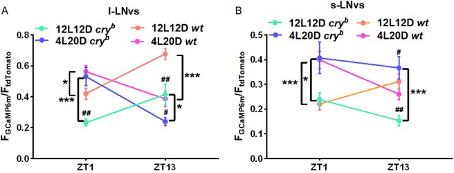
Another perceived weakness is the lack of subtype-level dissection among Hugin- and AstA-releasing neurons. I make a justified request to narrow down the behaviorally relevant neuron to one (or one type), which is based on a widespread but unreasonable and dangerous assumption that every behavior must be controlled by one neuron. However, the authors present very interesting data that only a subset of Hugin- and AstA-releasing neurons responds to higher levels of sucrose (Figure 1H, Figure Supplement 7A, B), which leads to a hypothesis that a specific subtype within each peptidergic neuronal group is responsible for starvation-induced behavioral change. The authors only briefly touch upon this (lines 217-218), but this is an important hypothesis that requires further discussion.
We thank the reviewer for highlighting the importance of neuronal heterogeneity within the Hugin- and AstA-releasing populations. We fully agree that the observation that only a subset of Hugin<sup>+</sup> and AstA<sup>+</sup> neurons responds to elevated sucrose levels (Figure 1H; Figure Supplement 7A, B) strongly suggests functional specialization within these peptidergic groups.
In the revised Discussion, we now explicitly propose that distinct subtypes of Hugin and AstA neurons differentially contribute to energy sensing and feeding modulation. We suggest that glucose-responsive subpopulations may be specifically engaged in satiety signaling, whereas other neurons within the same genetic classes may participate in additional physiological or behavioral processes. This heterogeneity provides a plausible explanation for the partial behavioral effects observed following population-level manipulations. Although we did not perform subtype-specific perturbations in this study, our findings provide a foundation for identifying these subtypes in future work using split-GAL4 lines and connectomic datasets.
These issues are more important than the sprawling and unfocused review of various hunger and satiety-controlling systems across species in the Introduction. Lines 53-108 contain only tangential information to the main conclusion of the paper. Both the Introduction and Discussion sections must be completely restructured so that readers understand what is already known about hunger-induced changes in feeding-related behavior, what is a missing gap of knowledge in neural mechanisms controlling behavioral adaptation under starvation, and why Hugin/NMU is an interesting target in this context.
We thank the reviewer for this important structural critique. We agree that, in the original manuscript, the Introduction placed disproportionate emphasis on a broad survey of hunger- and satiety-regulating systems across species, which may have obscured the central conceptual advance of this study.
In the revised manuscript, we have substantially restructured both the Introduction and the Discussion to sharpen the narrative focus and clarify the specific knowledge gap addressed by our work.
First, the Introduction has been streamlined to focus on what is already known about hunger-induced modulation of feeding-related behaviors, particularly sweet taste sensitivity and PER in Drosophila. We now emphasize that prior studies have predominantly characterized hunger-activated, feeding-promoting pathways (e.g., dopaminergic, NPF, AKH systems) that act as accelerators of food-seeking behavior.
Second, we explicitly define the missing gap in knowledge: while hunger-driven mechanisms are well studied, it remains unclear how satiety states—specifically elevated internal glucose levels—are directly sensed by central neurons and translated into suppression of sensory gain and feeding behavior.
Third, we reposition Hugin/NMU as an attractive and conceptually distinct target because of its peptidergic nature, evolutionary conservation, and previously reported but mechanistically unresolved links to feeding regulation. This framing motivates our central question: whether Hugin/NMU neurons function as a direct internal energy sensor that actively implements a satiety-specific inhibitory control over taste perception.
In parallel, the Discussion has been reorganized to avoid an unfocused review of feeding circuits across species and instead to interpret our findings within a clear conceptual framework. We now emphasize that the Hugin–AstA (and NMU) pathway represents a satiety-driven “brake” that complements, rather than duplicates, established hunger-driven “accelerator” circuits. This restructuring clarifies both the novelty of our findings and their relevance within the existing literature.
Reviewer #2 (Recommendations for the authors):
When discussing the results of Figure 1, such as lines 203-204, "These results demonstrate that sugar intake inhibits sweet sensation, probably via increasing circulating sugar levels" it may be worth discussing the known impact of sweet sensation experience on future sweet taste responses. With the data shown here, it is difficult to conclusively separate blood glucose levels from the sweet sensation that happens during the re-feeding. The "normal diet minus sucrose" does not blunt the starved PER effect, but that could potentially be impacted by either/both sugar intake or sweet taste.
We thank the reviewer for this thoughtful and important point. We agree that sweet taste experience itself can influence subsequent sweet sensitivity, and that separating the contribution of sensory experience from nutrient-derived internal energy is non-trivial.
In the revised manuscript, we have clarified the experimental timing by explicitly stating that PER was assessed 15 minutes after refeeding. At this time point, hemolymph glucose levels have returned to baseline (Figure supplementary 5), supporting the physiological relevance of glucose-dependent activation of Hugin neurons under our experimental conditions.
We also acknowledge that sweet taste exposure can induce sensory adaptation and modulate future taste responses. To directly address this potential confound, we performed additional control experiments during revision (Figure supplementary 4B) in which starved flies were refed with sorbitol (caloric but not sweet) or arabinose (sweet but non-nutritive). We found that both manipulations partially reduced PER, but neither recapitulated the full suppressive effect of sucrose refeeding.
These results indicate that sweet taste experience and metabolic energy contribute in parallel to the regulation of sweet sensitivity. Importantly, the incomplete effects of sorbitol or arabinose alone suggest that neither sensory adaptation nor caloric value is sufficient by itself to fully account for the observed PER suppression.
Accordingly, we have revised the Discussion to clarify that the Hugin–AstA pathway likely operates within a broader, multi-layered regulatory framework, integrating internal metabolic state with sensory experience, rather than acting as a sole determinant of post-feeding sweet sensitivity. This clarification avoids over-attribution of the behavioral effect to circulating glucose alone while preserving the central conclusion that internal energy state is a key modulator of sweet perception.
Blocking cellular sugar intake or metabolism could be impacting the ability of neurons to function, distinct from any specific intracellular regulatory mechanism that glucose or its derivatives might be involved with. That may be a caveat worth mentioning in the results or discussion.
We thank the reviewer for raising this important caveat. We agree that blocking cellular sugar uptake or metabolism could, in principle, impair neuronal function in a nonspecific manner, independent of any dedicated intracellular glucose-sensing mechanism.
In the revised manuscript, we now explicitly acknowledge this possibility and clarify the scope of our interpretation. Several features of our data argue against a generalized loss of neuronal function as the primary explanation. First, the behavioral and physiological effects observed upon manipulation of glucose transport or K<sub>ATP</sub> channel activity are rapid and reversible, consistent with state-dependent modulation rather than chronic metabolic failure. Second, these manipulations selectively affect sweet sensitivity and feeding-related behaviors, without causing gross deficits in proboscis extension or neuronal responsiveness.
Accordingly, we have revised the Results to emphasize that while intracellular glucose metabolism is required for normal neuronal activity, our findings specifically support a role for glucose-dependent modulation of neuronal excitability in satiety signaling, rather than a nonspecific energetic impairment.
Minor suggestions:
(1) Figure 2G: "Pryuvate" -> "Pyruvate."
We have corrected “Pryuvate” to “Pyruvate”
(2) "Fly" methods section: it says that flies were kept on 2% agar for 12 hours for starvation, but in the Figure 1A description, it says 24 hours.
We have corrected the description in Figure 1A.
Reviewer #3 (Recommendations for the authors):
(1) SEZ Hugin+ and AstA+ neurons were activated by glucose (Figures 1G, 1I), yet hemolymph also contains trehalose and fructose. For instance, DH44 neurons respond broadly to all hemolymph sugars (Dus et al., 2015), while Gr43a neurons specifically detect fructose (Miyamoto et al., 2012). The present study does not clarify whether Hugin+ or AstA+ neurons are similarly sugar-specific or more broadly tuned. A systematic analysis is needed to determine whether these circuits are selective for glucose.
We thank the reviewer for raising this important question regarding sugar specificity. We agree that hemolymph contains multiple sugars, including trehalose and fructose, and that distinct neural systems have been shown to differ in their tuning breadth. To address this issue, we performed additional experiments during revision in which starved wild-type flies were refed with different sugars—including sucrose, fructose, trehalose, and sorbitol—followed by PER measurements. We found that sucrose refeeding produced the strongest suppression of PER, whereas fructose, trehalose, and sorbitol induced weaker effects (Figuresupplementary 4A).
We interpret these results as suggesting a preferential sensitivity of the Hugin/AstA pathway to glucose availability rather than a broad responsiveness to all circulating sugars. One plausible explanation is that fructose, trehalose, and sorbitol require peripheral metabolic conversion before contributing to intracellular glucose levels in neurons, whereas sucrose feeding rapidly restores hemolymph glucose within the 15-minute time window used in our experiments (Figure supplementary 5).
Importantly, we now clarify in the revised Results and Discussion that our data support a functional preference for glucose under physiological conditions, rather than excluding the possibility that other sugars may influence this circuit indirectly or on longer timescales.
(2) The authors state that SEZ, but not VNC, Hugin+ neurons regulate AstA activity (lines 318-319). However, comparison of Figure Supplement 8B with the severing sample in Figure Supplement 11B shows a more pronounced reduction of sweet sensation under hug>TrpA1 activation. Although the absolute response in Figure 3F (in vivo) is higher than that in the cut-off preparation (Figure S11), comparison of Figure S11C with Figure 3F indicates that hug+ neurons drive an AstA+ calcium transient more than fourfold greater in the presence of VNC neurons. Thus, the contribution of Hugin+ VNC neurons cannot be dismissed, and the conclusion should be revised accordingly.
We thank the reviewer for this careful and quantitative comparison. We agree that our original wording overstated the exclusivity of SEZ Hugin<sup>+</sup> neurons in regulating AstA activity.
Upon closer examination of the data, we now acknowledge that VNC Hugin<sup>+</sup> neurons likely contribute to AstA activation. As the reviewer points out, the AstA<sup>+</sup> calcium response evoked by Hugin activation is substantially larger when VNC neurons are intact (Figure supplementary11C) compared with the cut preparation (Figure 3F), indicating that descending inputs from the VNC can potentiate AstA neuronal activity.
Accordingly, we have revised the manuscript to state that SEZ Hugin<sup>+</sup> neurons play a predominant role in driving AstA responses relevant to sweet sensation, while VNC Hugin<sup>+</sup> neurons provide additional modulatory input that enhances the overall magnitude of Hugin signaling. These revisions have been made in the Results to more accurately reflect the contributions of distinct Hugin subpopulations.
(3) In Figure 4D, you show AstA-R1 co-localized with Gr5a-expressing cells. However, Gr5a-expressing cells also co-express Gr64f in labellum (Fuji et al., 2015, Current Biology). Are the authors sure that the sweet sensation they described is Gr5a-specific? Testing Gr64f is essential. Moreover, Fuji et al. demonstrated that Gr5a loss-of-function mutation impairs not only sucrose but also maltose, fructose, and trehalose sensation. This raises a question of whether the Hug+ and AstA+ neurons identified in the current study contribute to sensing sugars beyond sucrose. Additional experiments are required to clarify this point.
Please see our responses to the Reviewing Editor Comments (4).
(4) While nutritive sugar sensors such as Dh44 neurons have been directly implicated in sugar preference (Dus et al., 2015, Neuron), this study examines the hug+,AstA+, Gr5a neuronal circuit only in the context of PER responses. Why is sugar preference not assessed here, especially given that in mice, the comparison was made using preference tests?
We thank the reviewer for this insightful question. We agree that sugar preference assays provide important information about feeding decisions and reward-based behavior. In the present study, however, we deliberately focused on the proboscis extension reflex (PER) because it offers a direct, quantitative, and temporally precise readout of sweet sensory sensitivity at the sensory–motor level.
PER allows us to isolate changes in taste perception itself, largely independent of post-ingestive reinforcement, learning, or motivational state, all of which strongly influence preference-based assays. This distinction is particularly important given our central goal of identifying a circuit that directly links internal energy sensing to modulation of peripheral sweet-sensing neurons.
By contrast, sugar preference reflects an integrated behavioral outcome combining sensory input, internal state, and post-ingestive reward signals, including those mediated by DH44 neurons and other nutritive sensing pathways. We therefore chose PER as the most mechanistically specific assay to dissect the Hugin–AstA–Gr5a pathway. We now explicitly acknowledge in the revised Discussion that determining how this satiety-linked sensory modulation interacts with reward and post-ingestive circuits to shape long-term sugar preference will be an important direction for future studies.
Several other concerns:
(5) The intraperitoneal injection of NMU is interpreted as reflecting a brain-specific NMU effect, but such systemic delivery cannot exclude peripheral actions. In Figure 5D, the use of whole-body KO mice is insufficient; targeted manipulations (e.g., NMU-Cre-driven inactivation) are required to establish circuit-specific behavioral roles.
Please see our responses to the Reviewing Editor Comments (Low priority)
(6) In Figure 5F and 5M, neural activity is measured under different conditions: gastric glucose infusion in 5F versus glucose licking in 5M. To establish that NMU VMH neurons and Calb2 rNST neurons belong to the same circuit, this discrepancy in stimulation timing must be resolved to support the conclusions.
We thank the reviewer for pointing out this important issue regarding stimulation paradigms in Figures 5F and 5M. We agree that the difference between gastric glucose infusion and glucose licking requires explicit clarification.
In the revised manuscript, we now clearly state that these two paradigms were intentionally designed to probe complementary levels of the same NMU–Calb2 circuit. In Figure 5F, gastric glucose infusion was used to isolate the internal energy-sensing property of VMH NMU<sup>+</sup> neurons, independent of oral sensory input, motor behavior, or reward expectation. This experiment establishes that NMU<sup>+</sup> neurons are directly activated by elevated circulating glucose.
By contrast, Figures 5M examined how activation of this NMU pathway modulates downstream Calb2<sup>+</sup> rNST neurons under physiologically relevant feeding conditions, in which sweet taste signals are naturally evoked by licking. This design allows us to test the functional consequence of NMU signaling on sweet-responsive rNST neurons during normal sensory processing.
Although the route and timing of glucose delivery differ, both paradigms converge on a unified circuit model: internal glucose elevation activates VMH NMU<sup>+</sup> neurons, and NMU signaling suppresses sweet-driven activity in Calb2<sup>+</sup> rNST neurons. We have revised the Results and figure legends to explicitly describe this layered experimental logic and to clarify that Figures 5F and 5M together establish distinct but connected nodes of the same circuit.
(7) Figure 5I-J. The glucose concentration used appears excessively high. In mammals, blood glucose in the sated state is ~7-8 mM. It is unclear whether the observed responses represent physiological effects or artifacts of supraphysiological stimulation. Additional experiments with lower glucose concentrations would strengthen the study.
We thank the reviewer for raising this important concern regarding the glucose concentration used in Figure 5I–J. We agree that the concentration applied in ex vivo slice experiments exceeds the typical physiological range of circulating glucose.
This higher concentration was intentionally chosen to ensure reliable neuronal activation in acute brain slices, where glucose diffusion, uptake, and metabolic access are substantially slower than in vivo. Similar approaches have been widely used in studies of glucose-sensitive hypothalamic neurons to overcome these technical limitations (e.g., Kim et al., 2025., Neuron).
Importantly, the physiological relevance of our findings is supported by in vivo fiber photometry experiments, which demonstrate that VMH NMU⁺ neurons are robustly activated following normal sugar ingestion under physiological conditions. Thus, while supraphysiological glucose was used to establish glucose responsiveness ex vivo, our in vivo data confirm that NMU⁺ neurons respond to glucose elevations within the normal physiological range.
(8) Figure 5K. The VMH images are inconsistently oriented compared with Figure 5E, lacking a 3v landmark. The NMU detection method (IHC or FISH) is not specified in the legend. The GFP-Calb2 signal is heavily saturated, making it difficult to distinguish true signals from artifacts. These issues undermine interpretability.
We thank the reviewer for pointing out these issues. In the revised manuscript, VMH images in Figure 5K have been reoriented to match Figure 5E, and the third ventricle (3v) is now indicated as an anatomical landmark. The figure legend has been revised to clarify that NMU<sup>+</sup> neurons are identified by GFP expression from a Cre-dependent AAV2/1-DIO-GFP injected into NMU-Cre mice, rather than by NMU immunohistochemistry or FISH. In addition, GFP–Calb2 images have been reprocessed to clearly distinguish true signals from background and imaging artifacts.
(9) Figure 5L-M. Details of the NMU injection method are absent (route, dose, delivery parameters). The number of animals (n) is also not reported. Furthermore, AUC reduction alone is not sufficient evidence of robust inhibition. To convincingly demonstrate causality, NMU-IRES-Cre mice should be combined with DREADD or optogenetic approaches to directly inhibit NMU neurons and test whether rNST Calb2 activity is reduced.
We thank the reviewer for these helpful comments. We have revised the manuscript to include all missing methodological details. These details are now clearly described in the Methods section and figure legend.
We fully acknowledge that cell-type–specific manipulations, such as DREADD or optogenetic inhibition of NMU neurons, would provide more definitive causal evidence. However, our main goal in the mouse experiments was to demonstrate that NMU<sup>+</sup> neurons can directly sense glucose and modulate sweet sensitivity, thereby supporting the evolutionary conservation of the Hugin mechanism identified in Drosophila. Detailed dissection of the downstream circuit architecture and behavioral consequences in mammals is indeed an important direction for future research, but it lies beyond the current study’s primary focus on cross-species conservation.
(10) In Drosophila, hugin neurons respond selectively to nutritive glucose (Fig. 2H), but whether NMU neurons share this property is unknown. Notably, Calb2 neurons in the rNST respond to the artificial sweetener AceK (Hao Jin et al., 2021, Cell), leaving open whether the NMU-rNST circuit is calorie-dependent or calorie-independent.
We have added a statement in the Discussion acknowledging this limitation and emphasizing that future work will be needed to test whether the NMU–Calb2 circuit is selectively engaged by metabolically active sugars or also by sweet taste signals independent of caloric value.
Minor comments
(11) All bar graphs should include individual data points.
We have added individual data points to all bar graphs.
(12) In Figures 3E, 4C, and 4D, it appears that a combination of GAL4 and LexA was used, but the information about the fly lines is missing.
We have now included the complete list of fly lines used for these experiments, including their genotypes and sources.
(13) The source for PK2-R1 KO, AstA-R1 KO fly lines and NMU-IRES-Cre, Calb2-IRES-Cre mice is missing.
We have added the complete source information for all genetic lines mentioned.
(14) Figure 5B-D, This is a sucrose preference test, so why is the y-axis labeled as glucose? Is this an error, or were the values converted to glucose equivalents?
We thank the reviewer for catching this mistake. The assay shown in Figure 5B–D measured sucrose preference, not glucose preference. The inconsistency resulted from a typographical error in the Methods description. In the revised manuscript, we have corrected this error to clearly state that sucrose was used in the preference test,
(15) Supplementary Figure 15. The NMU images are of poor quality and should be improved.
The punctate appearance of NMU signals in Supplementary Figure 15 is not due to poor image quality but rather reflects the physiological distribution of the NMU neuropeptide. As NMU is stored in secretory vesicles within neuronal terminals and somata, its immunostaining typically appears as discrete puncta rather than diffuse cytoplasmic labeling.
Editor's note:
Should you choose to revise your manuscript, if you have not already done so, please include full statistical reporting including exact p-values wherever possible alongside the summary statistics (test statistic and df) and, where appropriate, 95% confidence intervals. These should be reported for all key questions and not only when the p-value is less than 0.05 in the main manuscript.<br />
Readers would also benefit from noting that the mice were male and discussion of the exclusion of females.
In the revised manuscript, we have included full statistical reporting for all key experiments in the resource data. Regarding animal sex, we confirm that all mouse experiments were conducted using male mice. This choice was made to minimize variability caused by hormonal cycles in females, which can influence feeding behavior and glucose metabolism. We have now explicitly stated this information in the Methods section and included a brief discussion noting that sex-specific differences in NMU–Calb2 circuitry and feeding regulation represent an important question for future investigation.