7,368 Matching Annotations
  1. Last 7 days
    1. In what situations would impromptu speaking be used? Since we’ve already started thinking of the similarities between public speaking and conversations, we can clearly see that most of our day-to-day interactions involve impromptu speaking. When your roommate asks you what your plans for the weekend are, you don’t pull a few note cards out of your back pocket to prompt your response. This type of conversational impromptu speaking isn’t anxiety inducing because we’re talking about our lives, experiences, or something we’re familiar with. This is also usually the case when we are asked to speak publicly with little to no advance warning. For example, if you are at a meeting for work and you are representing the public relations department, a colleague may ask you to say a few words about a recent news story involving a public relations misstep of a competing company. In this case, you are being asked to speak on the spot because of your expertise. A competent communicator should anticipate instances like this when they might be called on to speak, so they won’t be so surprised. Of course, being caught completely off guard or being asked to comment on something unfamiliar to you creates more anxiety. In such cases, do not pretend to know something you don’t, as that may come back to hurt you later. You can usually mention that you do not have the necessary background information at that time but will follow up later with your comments.

      This reading explains that each delivery method—impromptu, manuscript, and memorized—has specific strengths and weaknesses depending on the speaking situation. I found it interesting that impromptu speaking, although anxiety-inducing, can actually strengthen public speaking skills because it forces speakers to think quickly and organize ideas on the spot. However, it also carries the risk of rambling or overstating knowledge. Manuscript delivery, on the other hand, offers precision and consistency, especially for complex information, but often reduces audience engagement because the speaker may sound like they are reading rather than speaking naturally.

    1. Author response:

      The following is the authors’ response to the original reviews

      Public Reviews:

      Reviewer #1 (Public review):

      This work shows that resistance profiles to a variety of drugs are variable between different mycobacterial species and are not correlated with growth rate or intrabacterial compound concentration (at least for linezolid, bedaquiline, and Rifampicin). Note that intrabacterial compound concentration does not distinguish between cytosolic and periplasmic/cell wall-associated drugs. The susceptibility profiles for a wide range of mycobacteria tested under the same conditions against 15 commonly used antimycobacterial drugs provide the first recorded cross-species comparison which will be a valuable resource for the scientific community. To understand the reasons for the high Rifampicin resistance seen in many mycobacteria, the authors confirm the presence of the arr gene known to encode a Rif ribosyltransferase involved in Rif resistance in M. smegmatis in the resistant mycobacteria after confirming the absence of on-target mutations in the RpoB RRDR. Metabolomic analyses confirm the presence of ribosylated Rif in some of the naturally resistant mycobacteria which may not be entirely surprising but an important confirmation. Presumably M. branderi is highly resistant despite lacking the arr homolog due to the rpoB S45N mutation. M. flavescens has an MIC similar to that of M. smegmatis, despite having both Arr-1 and Arr-X. Various Arr-1 and Arr-X proteins are expressed and characterized for catalytic activity which shows that Arr-X is a faster enzyme,, especially with respect to more hydrophobic rifamycins. M. flavescens has similar MIC values to Rifapentine and Rifabutin to M. smegmatis. Thus, the Arr-1 versus Arr-X comparison does not provide a complete explanation for the underlying reasons driving natural Rif resistance in mycobacteria. Downregulation of Arr-X expression in M. conceptionense confers increased sensitivity to Rifabutin confirming its role as a rifamycin-inactivating enzyme.

      Overall, the comparison of cross-species susceptibility profiles is novel; the demonstration that MIC is not correlated with intracellular drug concentration is important but not sufficiently interrogated, the demonstration that Arr-X is also a Rif ADP-ribosyltransferase is a good confirmation and shows that it is more efficient than Arr-1 on hydrophobic rifamycins is interesting but maybe not entirely surprising. The manuscript seems to have two parts that are related, but the rifamycin modification aspect of the work is not strongly linked to the first part since it interrogates the modification of one drug but not the common cause of natural resistance for other drugs.

      Reviewer #2 (Public review):

      Summary:

      The authors use a variety of methods to investigate the mechanisms of innate drug resistance in mycobacteria. They end up focusing on two primary determinants - drug accumulation, which correlates rather poorly with resistance for many species, and, for the rifamycins, ADP-ribosyltransferases. The latter enzymes do appear to account for a good deal of resistance, though it is difficult to extrapolate quantitatively what their relative contributions are.

      Overall, they make excellent use of biochemical methods to support their conclusions. Though they set out to draw very broad lessons, much of the focus ends up being on rifamycins. This is still a very interesting set of conclusions.

      Strengths:

      (1) A very interesting approach and set of questions.

      (2) Outstanding technical approaches to measuring intracellular drug concentrations and chemical modification of rifamycins.

      (3) Excellent characterization of variant rifamycin ADP-ribosyltransferases

      Weaknesses:

      (1) Figure 3c/d: These panels show the same experiment done twice, yet they display substantially different results in certain cases. For instance, M. smegmatis appears to show an order of magnitude lower RIF accumulation in panel d compared to M. flavescens, despite them displaying equal accumulation in panel c. The authors should provide justification for this variation, particularly as quantitative intra-species comparisons are central to the conclusions of this figure.

      The data in panels 3c and 3d are from different sets of experiments. The reviewer is correct with regards to M. smegmatis. The data indeed is ~ 1 order of magnitude different. However, the data for other species is very similar. The reviewer may also have noticed that the error bars are also larger in 3d, compared to 3c, indicating a greater variation between independent experiments use in 3d. We do not have a good explanation for this, other than the experiments shown in 3d were associated with greater biological variability.

      (2) There are several technical concerns with Figure 3 that affect how to interpret the work. According to the methods, the authors did not appear to normalize to an internal standard, only to an external antibiotic standard (which may account for some of the technical variation alluded to above).

      We agree that using a labeled drug as an internal standard (IS) would be ideal. However, the experiment initially followed an untargeted metabolomics approach, which later shifted to relative drug quantification. At that stage, normalizing with IS was impractical because proper implementation would require multiple IS across the chromatographic range. Therefore, we opted for total ion current (TIC) normalization, which accounts for variability in overall metabolite abundance—even though the experimental setup was already adjusted for each bacterial species’ growth rate. Additionally, we prepared external standard curves for each drug to enable quantification, and the amount of drug added to each plate was considered when reporting these values.

      Second, the authors used different concentrations of drug for each species to try to match the species' MICs. I appreciate the authors' thinking on this, but I think for an uptake experiment it would be more appropriate to treat with the same concentration of drug since uptake is likely saturable at higher drug concentrations. In the current setup, for the species with higher MIC, they have to be able to uptake substantially more antibiotics than the species with low MIC in order to end up with the same normalized uptake value in Figure 3d. It would be helpful to repeat this experiment with a single drug concentration in the media for all species and test whether that gives the same results seen here.

      We respectfully disagree with the reviewer. Experiments such as the one proposed by the review work well when MIC values are a few fold apart, for strains of the same species, but have not been tested when MIC values are 100-1000-fold apart, with different species. Furthermore, what would be the interpretation of compound uptake at 1000-fold the MIC for one species and MIC level for another? By using antibiotic concentrations at the respective MIC for each species we are at least under conditions where we know the biological effect of the antibiotic across species is the same, based on its potency.

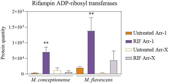
      (3) Figure 4f: This panel seems to argue against the idea that the efficacy of RIF ribosylation is what's driving drug susceptibility. M. flavescens is similarly resistant to RIF as M. smegmatis, yet M. flavescens has dramatically lower riboslyation of RIF. This is perhaps not surprising, as the authors appropriately highlight the number of different rif-modifying enzymes that have been identified that likely also contribute to drug resistance. However, I do think this means that the authors can't make the claim that the resistance they observe is caused by rifamycin modification, so those claims in the text and figure legend should be altered unless the authors can provide further evidence to support them. This experiment also has results that are inconsistent with what appears to be an identical experiment performed in Supplemental Figure 5b. The authors should provide context for why these results differ.

      In regard to enzyme efficiency, the apparent rate of all Arr-1 is relatively similar in converting RIF into ADP-Ribosyl-Rif between species. However, Arr-X is much more efficient when compared to Arr-1 in both M. flavescents and M. conceptionense. This is indicated by the apparent rate measured and displayed on figure 5c.

      Proteomics data shows that there is upregulation of Arr-1 and Arr-X upon rifampicin treatment in M. flavescens and M. conceptionense. However, the same experiment was not performed in Arr-1 KD. Therefore, we can’t verify through this approach if the activity observed in vivo directly correlates with a higher expression of Arr-X alone. Of note, likely both enzymes contribute to resistance to rifamycins, as per our results with the Arr-X KD and sensitization of M. conceptionense to RIF.

      Author response image 1.

      It is also worth mentioning that there are other enzymes in the pathway of RIF ribosylation and their efficiency is unknown (Author response image 2). Therefore ADP-Ribosyl-RIF It is not an “end-metabolite” and maybe not the sole determinant of RIF resistance via ADP-ribosylation. Downstream enzymes can also account for the difference observed between M. flavescens and M. smegmatis.

      Author response image 2.

      It is correct that the Rifampicin MIC for M. flavescens is the same as M. smegmatis.

      (4) Fig 4f/5c: M. flavescens has both Arr-1 and Arr-X, yet it appears to not have ribosylated RIF. This result seems to undermine the authors' reliance on the enzyme assay shown in Fig 5c - in that assay, M. flavescens Arr-X is very capable of modifying rifampicin, yet that doesn't appear to translate to the in vivo setting. This is of importance because the authors use this enzyme assay to argue that Arr-X is a fundamentally more powerful RIF resistance mechanism than Arr-1 and that it has specificity for rifabutin. However, the result in Figure 4f would argue that the enzyme assay results cannot be directly translated to in vivo contexts. For the authors to claim that Arr-X is most potent at modifying rifabutin, they could test their CRISPRi knockdowns of Arr-X and Arr-1 under treatment with each of the rifamycins they use in the enzyme assay. The authors mentioned that they didn't do this because all the strains are resistant to those compounds; however, if Arr-X is important for drug resistance, it would be reasonable to expect to see sensitization of the bacteria to those compounds upon knockdown.

      The reviewer is reading Fig. 4f incorrectly, probably because it is plotted in a linear scale instead of logarithmic scale. Ribosylated Rif is present in M. flavescens, just at lower levels than M. conceptionense and M. smegmatis. In species where there is no Arr-1 or Arr-3, ribosylated RIF is not detected at all (e.g. M. tuberculosis), i.e., concentration is zero. Therefore, any detection of ribosylated RIF can be considered significant. In addition, as mentioned before, ADP-ribosylation of RIF is not the final product of the reaction and further studies need to be undertaken to understand subsequent reactions.

      (5) Figure 5d: The authors use this CRISRPi experiment to claim that ArrX from M. conceptionanse is more potent at inactivating rifabutin than Arr-1. This claim depends on there being equal degrees of knockdown of Arr-1 and Arr-X, so the authors should validate the degree of knockdown they get. This is particularly important because, to my knowledge, nobody has used this system in M. conceptionanse before.

      We agree with the reviewer that a qPCR should have been performed to define the extent of interference in the strain. generated Unfortunately, at this time a qPCR was not performed in the strains tested to confirm the extent of down regulation. Although it is the best practice to validate the strain KD, there is no indication that the effect observed is due to unspecific downregulation. The genetic environment in which Arr-X is positioned is different from Arr-1 and the targeting oligonucleotides are specific and would not promiscuously bind to Arr-1. Said that, this is indeed a fault in our setup.

      (6) The authors' arguments about Arr-X and Arr-1 would be strengthened by showing by LC/MS that Arr-X knockdown in M. conceptionense results in more loss of ribosyl-rifabutin than knockdown of Arr-1.

      We agree with the reviewer that performing the LC-MS analysis of the Arr-x knockdown would have strengthened the argument of our paper. Unfortunately, this experiment was not performed.

      Reviewer #3 (Public review):

      This manuscript presents a macroevolutionary approach to the identification of novel high-level antibiotic resistance determinants that takes advantage of the natural genetic diversity within a genus (mycobacteria, in this case) by comparing antibiotic resistance profiles across related bacterial species and then using computational, molecular, and cellular approaches to identify and characterize the distinguishing mechanisms of resistance. The approach is contrasted with "microevolutionary" approaches based on comparing resistant and susceptible strains of the same species and approaches based on ecological sampling that may not include clinically relevant pathogens or related species. The potential for new discoveries with the macroevolution-inspired approach is evident in the diversity of drug susceptibility profiles revealed amongst the selected mycobacterial species and the identification and characterization of a new group of rifamycin-modifying ADP-ribosyltransferase (Arr) orthologs of previously described mycobacterial Arr enzymes. Additional findings that intra-bacterial antibiotic accumulation does not always predict potency within this genus, that M. marinum is a better proxy for M. tuberculosis drug susceptibility than the commonly used saprophyte M. smegmatis, and that susceptibility to semi-synthetic antibiotic classes is generally less variable than susceptibility to antibiotics more directly derived from natural products strengthen the claim that the macroevolutionary lens is valuable for elucidating general principles of susceptibility within a genus.

      There are some limitations to the work. The argument for the novelty of the approach could be better articulated. While the opportunities for new discoveries presented by the identification of discrepant susceptibility results between related species are evident, it is less clear how the macroevolutionary approach is further leveraged for the discovery of truly novel resistance determinants. The example of the discovery of Arr-X enzymes presented here relied upon foundational knowledge of previously characterized Arr orthologs. There is little clarity on what the pipeline for identifying more novel resistance determinants would look like. In other words, what does the macroevolutionary perspective contribute to discovery from the point of finding interspecies differences in susceptibility? Does the framework still remain distinct from other discovery frameworks and approaches? If so, how?

      Thanks for pointing this out, as this is a critical feature of our study and method. Our approach relies on inter-species comparative genomics and phenotypes, and therefore, it is distinct from inter-strains comparison. This difference is dramatic, and it becomes clearer when we are comparing the core genome of M. tuberculosis (one species) 92% with the core genome of the genus, circa of 1%. While we focus on rifamycin in this manuscript, future manuscripts will investigate many of the other dozens of “inconsistencies” observed between the genetic makeup of different mycobacterial species and there actual performance in the presence of different antibiotics.

      While the experimentation and analyses performed appear well-designed and rigorous, there are a few instances in which broad claims are based on inferences from sample sets or data sets that are too limited to provide robust support. For example, the claim that rifampicin modification, and precisely ADP-ribosylation, is the dominant mechanism of resistance to rifampicin in mycobacteria may be a bit premature or an over-generalization, as other enzymatic modification mechanisms and other mechanisms such as helR-mediated dissociation of rifampicin-stalled RNA polymerases, efflux, etc were not examined nor were CRISPRi knockdown experiments conducted beyond an experiment to tease out the role of Arr-X and Arr-1 in one strain. The general claim that intra-bacterial antibiotic accumulation does not predict potency in mycobacteria may be another over-generalization based on the limited number of drugs and species studied, but perhaps the intended assertion was that antibiotic accumulation ALONE does not predict potency.

      Recommendations for the authors:

      Reviewer #1 (Recommendations for the authors):

      Major comments

      (1) The metabolomics is done using mycobacteria grown on filters. Initially, mycobacterial cells are grown on the filters for 5 doublings before being transferred to drug-containing (or free) agar for one doubling. Is this based on calculated doubling time in liquid culture or a true determination of the fact that the biomass increases to what would amount to 5 doublings?

      The doubling time used is the one determined in liquid media. Although it is possible that the growth kinetics in solid media is slightly different from liquid (±10%), this experimental design is well established for M. tuberculosis (since Proc Natl Acad Sci U S A. 2010 May 25;107(21):9819-24.) and M. smegmatis (unpublished). Therefore, we used the growth rate as a proxy for having the same biomass of cells for each species tested. A maximum difference of 10% was observed between M. tuberculosis growth in liquid and in solid media, however, cells grow exponentially for much longer in filters. This makes filter-based experiments more reliable, as few growth phase-derived differences are present.

      (2) The demonstration that intrabacterial drug concentrations vary between mycobacterial species in a manner not related to MIC for at least LZD and RIF, is an important finding. However, intrabacterial does not mean cytoplasmic since a considerable fraction could be present in the periplasmic/cell wall layers. Ideally, this would need to be determined but would of course be a massive undertaking since the method needs validation & optimization for each mycobacterial species. Nevertheless, this has to be mentioned. In addition, three drugs are limiting. Measuring additional drug concentrations in these 5 mycobacteria would at least establish some confirmation about the extent of this lack of correlation. Thus, could the authors measure concentrations of additional drugs with intracellular targets?

      Testing additional drugs can be beneficial and would be an expansion of our paper, which will definitely be on future plans for further studies focusing on other antibiotics described here. It would also provide new insights into other possible mechanisms of resistance in mycobacterial species. However, in this study we aimed to first determine the antibiotic response profile in different mycobacterial species, and once we identified interesting resistance phenotypes that could not be readily explained by known mechanisms of resistance, we narrowed it down to certain drugs and species that would potentially provide insights into new mechanisms of antibiotic resistance. Finally, exploring drug concentration across multiple bacterial compartments is a dauting task and it has not been done extensively with any species, not to mention with multiple species, many of which are still lacking any study of their actual cell envelope.

      (3) CRISPRi was used to reduce transcription in M. conceptionense. What was the level of gene downregulation?

      As mentioned previously, a setback from our setup is that the level of KD was not measured at this instance.

      Minor comments:

      (1) The introduction mentions the fast and slow-growing mycobacteria which are classified based on the time that it takes to observe colonies on solid agar. However, in liquid medium, there is less correlation between the reported growth on agar and doubling time in liquid (Figure 1b, Figure 2d). This could be mentioned in the results section. In Figure 2d, the filled circles represent fast-growers but this does not hold well for liquid culture and it might make more sense to not distinguish between fast- and slow-growers in these graphs. A small complication would also be the fact that the doubling time represents growth in a liquid medium with Tyloxapol as a detergent whereas the MIC and metabolomics are done on solid agar with no detergent. The metabolomics is done after a doubling but for those where agar growth and liquid growth have large discrepancies in growth rate, there could be some differences.

      Apologies for this misunderstanding. Fast- and slow-growth phenotypes are determined in Lowenstein-Jensen (LJ) agar, not in 7H10 agar (used in our study and most studies of mycobacteria). Furthermore, this is a qualitative definition, not a quantitative one. Therefore, our measurements do not need to correlate with fast- and slow-growth phenotypes, unless we had used that one specific medium. Furthermore, in liquid medium, we determined growth rate directly, which is never done with LJ medium.

      In addition to adding the same amount of cells to each filter, we also perform TIC normalization, which should account for how rich the samples were – and therefore how much material we had. Therefore, we do not observe discrepancies due to differences in growth rate and the presence/absence of detergent in the media.

      It is also worth mentioning that this experimental set up has been well established in many M. tuberculosis labs that study metabolism. Importantly, the use of detergent drastically affects mass spectrometry, and therefore cannot be used.

      (2) Figure 1g in the text should be Figure 1f.

      Apologies, it has been fixed.

      (3) Figure S1 would be ideal to have in (supplementary) table format.

      This data is now being provided in a table format.

      (4) Table S1 - ethambutol misspelt.

      Spelling has been corrected.

      (5) MIC for species such as M. abscessus could depend on medium (7H9-based medium can give different MIC values than CAMH).

      Indeed, different media can significantly change MIC values, and this is true for many bacterial species, if not all. For this study we used only species that could be grown in 7H9 broth containing 10 % ADC, 0.05% glycerol 0.05% tyloxapol and 7H10 plates containing 10% OADC and 0.05% glycerol. MIC<sub>99</sub> was determined in the latter as we found more efficient and robust to do our tests it in solid media. The goal of our experiment was not to the determined the “true” MIC for the antibiotics tested, as this value does not exist. It was to find lack of correlations between relative values and the presence of genes that can account for it.

      (6) The statement "the experiment was performed at a concentration of antibiotic equal to its MIC" initially seems confusing. It was not equal to the MIC but performed at 6-fold the respective MIC of the species in question. Maybe re-phrasing this would help.

      Apologies for this oversight. It has been corrected.

      (7) Note that some mutations outside the RRDR (eg. V170F and I491F) can also cause Rif resistance.

      Author response image 3.

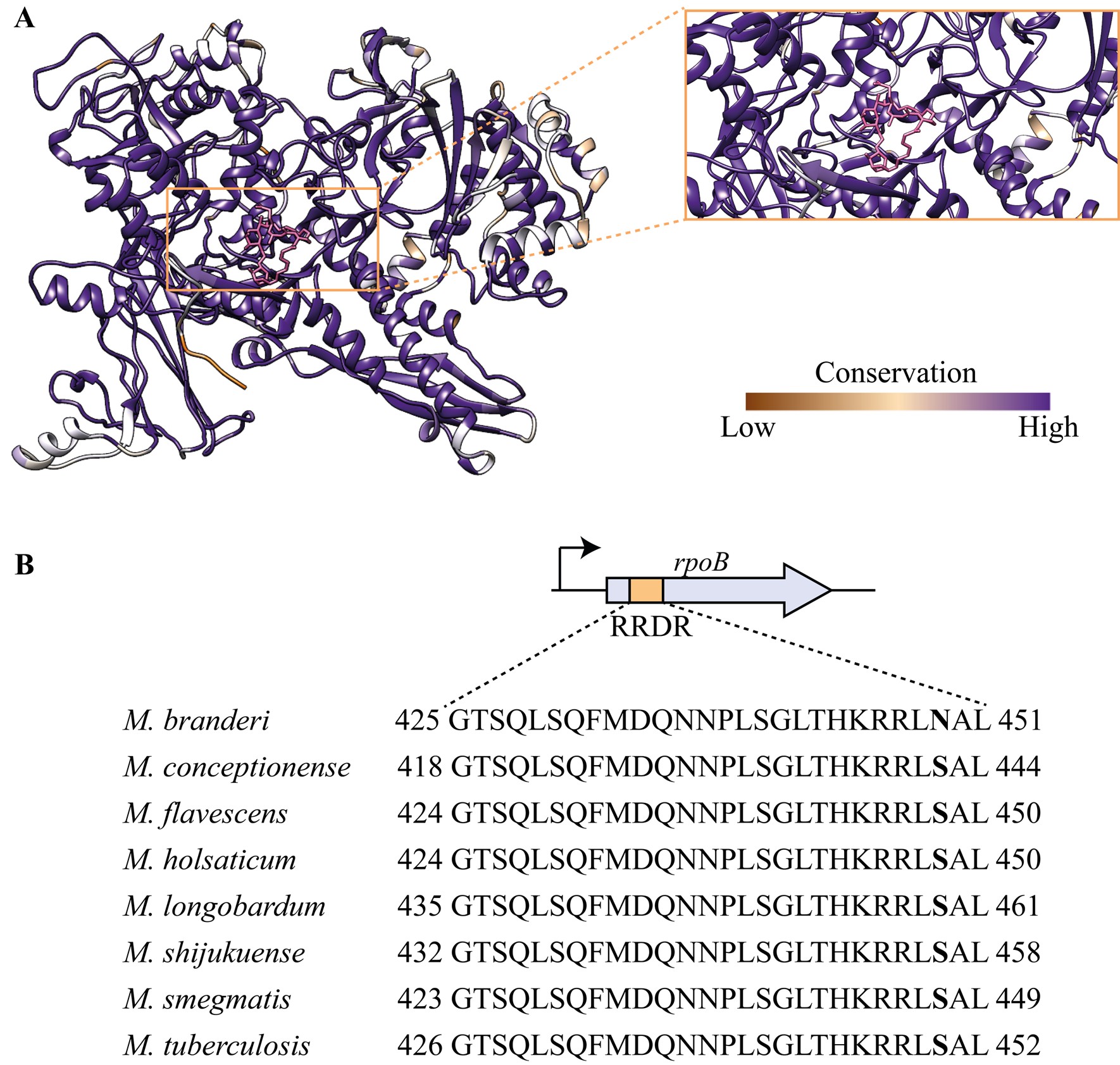
      A Rainbow diagram of RpoB X-Ray structure coloured according to sequence conservation. Dark purple indicates high conservation, whereas dark orange indicates low conservation. RIF (showed in magenta) is bound to RpoB. Zoomed view displays that the RIF-binding pocket is considerably conserved. B RpoB protein sequence has an 81bp region called Rifampicin Resistance Determining Region (RRDR) that is known to be important for RIF binding and is where most mutations occur in drug-resistant TB. Sequence alignment displays that the RRDR region is conserved with the exception of M. branderi, which has an Asn instead of a Ser residue in position 456 (numbering is related to the M. tuberculosis sequence), highlighted in bold.

      Attached we have a structural alignment of RpoB of the species highlighted on this paper. Although there is variability within the sequences, which is also displayed in Author response image 3 with the conservation analysis, the residues that have been implicated with resistance (including V170 and I491) are conserved. Alignment sent on .fasta file that can be opened in jalview.

      (8) Discuss how the RpoB S450N mutation in M. branderi confers the observed level of resistance.

      That’s a great point, thank you. Now it reads as:

      “The rifampicin (RIF) binding pocket is generally conserved, but Mycobacterium branderi has an S450N mutation in the RRDR region. While this specific mutation hasn't been found in clinical isolates, it's located at the binding site and may confer resistance (273). Although both serine (S) and asparagine (N) have similar side chains, related mutations like S450Q have been linked to resistance (156). Thus, M. branderi may be RIF-resistant due to this mutation. In contrast, M. conceptionense, M. flavescens, and M. smegmatis show no target sequence differences that explain their resistance”

      (9) The statement that the three tested NTM are sensitive to rifabutin ("resistant to all rifamycins except for rifabutin") needs to be interpreted considering what sensitivity means. The MIC is still high (1.6-3.1 ug/mL) when compared to that of Mtb. The 2-fold differences in MIC between M. smegmatis and M. conceptionense do not really prove or disprove the role of Arr-X in rifabutin resistance.

      We fixed the sentence to be more careful with the language on the text. We agree, but it is worth mentioning that generally with bacteria there is a regulation by the CLSI. Each bacterial species has a range that is considered sensitive or resistant, but these are not available for the species used in this study. In general, bacteria with MIC values above 8 µg/mL are considered resistant to rifampin (J Antibiot 2014 67:625).

      (10) Figure 1d: It's hard to quantify the sensitivity of the plates. Can this be done by MIC? Was only rifabutin tested or also rifampicin?

      The initial experiments described on the paper were all performed using Rifampicin only. Then, the MIC for the remaining rifamycins was determined for M. smegmatis, M. flavescens and M. conceptionense, and can be perused on “Supplementary table 4”. Figure 5d is to illustrate the effect of the KD in M. conceptionense sensitivity to rifabutin.

      (11) Is there data to show the ADP-ribosylation of rifabutin in M. conceptionense and the CRISPRi strains?

      Unfortunately, we did not perform LC-MS analysis on M. conceptionense CRISPRi strains exposed to rifabutin to measure potential ADP-ribosylation.

      Reviewer #2 (Recommendations for the authors):

      (1) It would be useful if the authors would complete Figure 1A by determining growth rates for the remaining 18 strains that they currently omitted.

      These growth rates were obtained using roller bottles and in at least 3 independent experiments, unfortunately the throughput is far ideal. The goal of the experiment was to highlight difference in growth rate, beyond fast- and slow-growth, which we did. Adding the remaining values would not change this conclusion. Growth rate variation in 7H9 is significant and the point is made in our figure.

      (2) The authors should justify their choice of species used in Figures 3-4. It would be useful to know, for instance, if the authors chose these species in an unbiased fashion, or if they were chosen because the authors had already determined that they possess rifamycin-modifying enzymes of interest. In that case, they wouldn't necessarily be a representative sample to use for the correlation analysis of antibiotic uptake and potency in Figure 3.

      They were chosen because of their resistance profile for BDQ, LZD and RIF. This has been addressed in the text, which now reads “Given the antibiotic response profiles observed, we selected BDQ, LZD and RIF to explore the molecular causes of these dramatic changes in antibiotic potency observed across the Mycobacterium genus.”

      (3) Figure 4b: The data in this panel appear inconsistent - for instance, M. houstonense appears to grow at 10X Mtb MIC, but fails to grow at 1X Mtb MIC. Repeating this experiment would better establish the validity of the authors' claims about the relative susceptibility of these strains to RIF.

      The figures got rotated when exported from illustrator. Corrected figure is uploaded, and original plate photos are also uploaded for clarity.

      (4) Figure 4e: Does Arr-X get upregulated in these proteomic datasets? The authors' argument that proteomic upregulation correlates with important drug resistance genes would imply that it might be, so that would be useful information to provide.

      Arr-X is slightly upregulated, but not statistically significant – this could be due to the native expression of Arr-1. Data is displayed in a previous answer.

      (5) I wasn't able to find the supplementary tables that the authors allude to - not sure if that was a file mixup, but those tables would be useful for interpreting the manuscript.

      We are sorry that you couldn’t access the table. It must be a file corruption issues, as the other reviewers were able to. We will make sure that all tables are available and accessible.

      (6) For LC/MS, the authors use peak height instead of peak area, which they argue correlates better with the amount of drug in cells because of the poor peak shape they observed for linezolid. This is not standard practice, so the authors should provide evidence to support this claim by running an LC/MS standard curve, then showing the correlation between peak height and amount of compound added as well as the correlation between peak area and compound.

      Thank you for pointing that out, accuracy calculated and displayed. Both peak area and height can be used, but indeed area is standard practice.

      (7) The authors should provide methods information about the LC column and the gradient settings used for LC-MS, as well as the settings of the MS.

      The full method has been added to the paper.

      Reviewer #3 (Recommendations for the authors):

      I have only minor comments aside from the information in the Public Review:

      (1) Results, section on Intra-bacterial antibiotic accumulation, line 8: "experiment was performed at a concentration of antibiotic PROPORTIONAL to its MIC" would be more accurate?

      Agreed and adjusted according to Reviewer’s suggestion.

      (2) Results, section on A minor role for pre-existing target modification, last sentence: the mere presence of RIF-ribosylating enzymes does not, in and of itself indicate that "RIF modification, and precisely ADP-ribosylation, is the dominant mechanism of resistance to RIF in mycobacteria", as other mechanisms and other forms of modifying enzymes are known to confer rifamycin resistance, with redundancy (e.g., other rifampicin-modifying enzymes, or helR-mediated dissociation of rifampicin-stalled RNA polymerases from DNA). It would be more appropriate to suggest the results presented to this point indicate RIF modification is common among mycobacteria. The evidence from the CRISPRi knockdown of Arrs shown in Fig 5d is the kind of evidence that suggests ribosylation as a dominant mechanism, at least against rifabutin in this particular species.

      Absolutely, there are other possible modifying enzymes that could be encoded by these mycobacterial species. There is a possibility that M. flavescens and M. smegmatis encode for a putative helR (attached alignment) but further experiments would need to be carried out to confirm its ability to displace RIF in the RNAP. Interestingly, the presence of both Arr and HelR has been studied in M. abscessus and those mechanisms of resistance are independent from each other (Molecular Cell 2022 82(17):3166-3177.e5).

      (3) Discussion, 2nd sentence needs grammatical editing.

      Rephrased and it reads “Using our mycobacterial library, we identified for the first time high- and ultra-high-level intrinsic resistance (3) to many of the antibiotics tested. Of note, the resistant phenotype is naturally occurring and not a result of mutations due to exposure to the antibiotic in the clinic – which is the more traditional approach for probing mechanisms of antibiotic resistance. Our observations revealed that resistance profiles are highly variable across the genus and do not follow phylogeny, implicating HGT as the key mechanism for acquisition of resistance determinants and evolution of antibiotic resistance in mycobacteria (42).”

      (4) Discussion, page 7, first line: the inclusion of LZD and BDQ in this statement seems at odds with Figure 2c and the statements in the first paragraph of page 5 highlighting these as examples of drugs to which most mycobacteria are susceptible.

      Indeed, many of the species are susceptible, however the MIC<sub>99</sub> levels observed have never been reported before, and therefore we found it to be an interesting finding to highlight. From a treatment perspective, knowing which species are sensitive to which drugs is of course the most useful outcome of our study.

      (5) The next sentence..."We found that resistance to these antibiotics in mycobacteria cannot be explained by uptake/efflux mechanisms..." is a bit of an over-generalization and conflicts with the evidence presented earlier that efflux could be playing a role in BDQ resistance and the published evidence establishing a clinically significant role for efflux-mediated BDQ resistance in M. tuberculosis, M. avium complex and M. abscessus complex.

      We rephrased it to make it more specific to our findings. It reads “We found that resistance to these antibiotics in mycobacteria do not correlate with by uptake/efflux mechanisms in the species tested and it does not correlate with growth rate. Identification of mycobacterial species highly resistant to BDQ and LZD is worrisome as most of this species, if not all, have never been exposed to these drugs.”

      (6) Methods, section on In vitro activity assay of Arr enzymes, line 1: reference(s) should be provided for previously reported methods.

      Reference now added.

      (7) Figure 2d: the low end of the susceptibility range is not well defined.

      In this figure the susceptibility is not defined as the lowest area of the graph, but the lower concentrations are indeed harder to be defined. Hopefully supplementary figure 1 and the additional table containing the MIC can be informative to address this comment.

      (8) Figures 3c,d: the presentation of the relative antibiotic concentrations could be harmonized between the graphs in 3c and those in 3d to enable a more ready comparison.

      We disagree. The goal of these different panels is exactly to illustrate two distinct points. C gives the relative concentration of antibiotic, while D correlates relative concentration with MIC99. The use of log scale in D further clarifies that there is no correlation between intracellular antibiotic concentration and potency (MIC). This information is not present in C.

      (9) Figure 4f and Supplementary Figure 5b: it is difficult to understand the limited amount of ribsosyl-RIF in M. flavescens in Fig 4f relative to Supplementary Figure 5b (esp. when considering M. smeg as a common comparator); and, further, to understand the seeming lack of correlation between RIF susceptibility, ribosylation and Arr number and catalytic efficiency for these two strains without considering additional resistance mechanisms.

      In reality the difference between figure 4f and Supplementary figure 5b is mainly due to M. smegmatis – that has an apparent lower production of ribosyl-RIF in the experiment described in the supplementary figure. The values for M. flavescens are relatively similar. In addition, the ADP-Ribosyl-RIF is not the final metabolite of the pathway.

      In regards of having the entire picture, it is true that we were unable to completely unravel and correlate MIC value, expression of Arr-1, expression of Arr-3, efficiency of each enzyme, production of ADP-Ribosyl-RIF and the presence of other possible mechanisms of resistance and this is indeed a setback in our study, and of most studies ever published, which usually focus on one resistant determinant.

    1. Author response:

      The following is the authors’ response to the original reviews

      Many thanks for your helpful and constructive comments for our work examining the effect of inhibiting both the insulin receptor (IR) and IGF1 receptor (IGF1R) in the podocyte. We are pleased to submit an updated manuscript addressing your concerns.

      (1) A major concern was a lack of mechanistic insight into how deletion (or knock-down) of both receptors caused the spliceosomal phenotype (Reviewer 1 and Reviewer 3).

      We now think this is due to the lack of a network of insulin/IGF phospho-signalling events to a variety of spliceosomal proteins and kinases. The reasons for this are as follows:

      A. Since submitting our paper Turewicz et al have published a comprehensive phospho-proteomic paper examining the effects of 100nM insulin on human primary myotubes (DOI: 10.1038/s41467-025-56335-6). They discovered that multiple post-translational phosphorylation events occur in a variety of spliceosomal proteins at differing time points (1 minute to 60 minutes). Furthermore, they show that mRNA splicing is rapidly modified in response to insulin stimulation in their cells. This follows elegant work from Bastista et al who studied diabetic and non-diabetic iPSC derived human myositis and also detected a spliceosome phosphorylation signature (DOI: 10.1016/j.cmet.2020.08.007).

      B. We have examined phospho-proteosome changes that occur in wild -type podocytes (expressing both the IR and IGF1R) compared to double (IR and IGF1R) knockout cells using phosho-proteomics. We have done this 3 days after inducing receptor knockdown, before major cell loss, and have stimulated the cells with either 10nM insulin or 100mg IGF1.

      Interestingly, we detected several post-translational modifications (PTM) in our data set that are also present in Turewicz’s studies. Of note, 100nM insulin (as used by Turewicz) will signal through both the insulin and IGF1 receptor (and hybrid Insulin/IGF1 receptors) which is relevant to our studies.

      Our work shows a cascade of phospho- signalling events affecting multiple components of the spliceosomal complex and evidence of kinase modulation (phosphorylation) (New Figure 7 and supplementary Figure 5). Also new results section in paper (lines 391-425 in track changes version). We acknowledge that we only studied a single time point after stimulation (10 minutes) and could have missed other PTM in the spliceosomal complex and other kinases. This is mentioned in our new limitations of study section (lines 595-606). This will be a focus of future work. We did not find major PTM differences when stimulating with either insulin or IGF1 in our studies and suspect that the doses of insulin (10nM) and IGF1 (100mg) used are still able to signal through cognate receptors.

      Furthermore, we have examined the relative contributions of the insulin and IGF1 receptor in detail in the model (addressed in point 13 below).

      (2) The phenotype of the mouse is only superficially addressed. The main issues are that the completeness of the mouse KO is never assessed nor is the completeness of the KO in cell lines. The absence of this data is a significant weakness. (Reviewer 1)

      We apologise for not making this clear, but we did assess the level of receptor knockdown in both the animal and cell models. The in vivo model showed variable and non-complete levels of insulin receptor and IGF1 receptor podocyte knock down (shown in supplementary Figure 1C). This is why we made the in vitro floxed podocyte cell lines in which we could robustly knockdown both the IR and IGF1R. We show this using Western blotting (shown in Figure 2A). We agree that calling the models knockout is misleading and have changed all to knock down (KD) now.

      (3) The mouse experiments would be improved if the serum creatinine’s were measured to provide some idea how severe the kidney injury is. (Reviewer 1)

      There is variability in creatinine levels which is not uncommon in transgenic mouse models (probably partly due to variability in receptor knock down levels with cre-lox system). This is part of rationale of developing the robust double receptor knockout cell models where we robustly knocked out both receptors by >80%. We have added measured creatinine levels in a subset of mice in supplementary data (New Supplementary Figure 1E) and mention this in the text (lines 285-286). As some mice died we expect they may have developed acute kidney injury, but we did not serially measure the creatinine’s in every mouse over time. We could have assessed the GFR in a more sensitive way to look at differences. However, we consider the highly significant levels of albuminuria and histological damage observed in our models show a significant kidney phenotype.

      (4) An attempt to rescue the phenotype by overexpression of SF3B4 would also be useful. If this didn't work, an explanation in the text would suffice. (Reviewer 1).

      We did consider doing this but on reflection think it is very unlikely to rescue the phenotype as an array of different spliceosomal proteins quantitatively changed and were differentially phosphorylated / dephosphorylated throughout the complex (as we hope our revised work illustrates now). We think a single protein rescue is highly unlikely to work. We hope this is an appropriate explanation for this action. We have mentioned this in the text now in our discussion (lines 601-602).

      (5) As insulin and IGF are regulators of metabolism, some assessment of metabolic parameters would be an optional add-on. (Reviewer 1).

      Thank you for this suggestion. We did not extensively examine the metabolism of the mice however we did perform blood glucose measurement and weight which are included in the paper (Figure 1A and Figure 1B).

      (6) The authors should caveat the cell experiments by discussing the ramifications of studying the 50% of the cells that survive vs the ones that died. (Reviewer 1).

      We appreciate this and this was the rationale behind cells being studied after 3 days differentiation for total and phospho-proteomics before significant cell loss to avoid the issue of studying the 50% of cells that survive (which happened at 7 days). We have made this clearer in the manuscript. We also have added the data showing less cell death at 3 days in the cell model (New Supp Figure 2B).

      (7) It would be helpful to say that tissue scoring was performed by an investigator masked to sample identity. (Reviewer 2)

      We did this and have added to manuscript (line 113).

      (8) Data are presented as mean/SEM. In general, mean/SD or median/IQR are preferred to allow the reader to evaluate the spread of the data. There may be exceptions where only SEM is reasonable. (Reviewer 2)

      All graphs have now been changed to SD rather than SEM.

      (9) It would be useful to for the reader to be told the number of over-lapping genes (with similar expression between mouse groups) and the results of a statistical test comparing WT and KO mice. The overlap of intron retention events between experimental repeats was about 30% in both knock-out podocytes. This seems low and I am curious to know whether this is typical for this method; a reference could be helpful. (Reviewer 2)

      This is an excellent question. We had 30% overlap as the parameters used for analysis were very stringent. We suspect we could get more than 30% by being less stringent, which still be considered as similar events if requested. Our methods were based on FLAIR analysis (PMID: 32188845). We have added this reference to the manuscript (Line 242 & 680).

      (10) With the GLP1 agonists providing renal protection, there is great interest in understanding the role of insulin and other incretins in kidney cell biology. It is already known that Insulin and IGFR signaling play important roles in other cells of the kidney. So, there is great interest in understanding these pathways in podocytes. The major advance is that these two pathways appear to have a role in RNA metabolism, the major limitations are the lack of information regarding the completeness of the KO's. If, for example, they can determine that in the mice, the KO is complete, that the GFR is relatively normal, then the phenotype they describe is relatively mild. (Reviewer 1)

      Thank you. The receptor knock-out (KO) in the mice is highly unlikely to be complete (Please see comments above and Supplementary Figure 1C). There are many examples of “KO” animal models targeting other tissues showing that complete KO of these receptors seems difficult to achieve, particularly in reference to the IGF1 receptor. In the brain, which also contains terminally differentiated cells, barely 50% of IGF1R knockdown was achieved in the target cells (PMID:28595357). In ovarian granulosa cells (PMID:28407051) -several tissue specific drivers tried but couldn't achieve any better than 80%. The paper states that 10% of IGF1R is sufficient for function in these cells so they conclude that their knockdown animals are probably still responding to IGF1. Finally, in our recent IGF1R podocyte knockdown model we found Cre levels were important for excision of a single homozygous floxed gene (PMID: 38706850) hence we were not surprised that trying to excise two homozygous floxed genes (insulin receptor and IGF1 receptor) was challenging. This was the rationale for making the double receptor knockout cell lines to understand processes / biology in more detail. As stated earlier, we have changed our description of the mice and cell lines from knock-out to knock-down throughout the revised manuscript as this is more accurate.

      (11) For the in vivo studies, the only information given is for mice at 24 weeks of age. There needs to be a full-time course of when the albuminuria was first seen and the rate of development. Also, GFR was not measured. Since the podocin-Cre utilized was not inducible, there should be a determination of whether there was a developmental defect in glomeruli or podocytes. Were there any differences in wither prenatal post-natal development or number of glomeruli? (Reviewer 3)

      We have added further urinary Albumin:creatinine ratio (uACR) data at 12, 16 and 20 weeks to manuscript. We do not think there was a major developmental phenotype as albuminuria did not become significantly different until several months of age (new Supp Figure 1B). We did consider using a doxycycline inducible model but we know the excision efficiency is much less than the constitutive podocin-cre driven model Author response image 1. This would likely give a very mild (if any) phenotype when attempting to knockout both receptors and not reveal the biology adequately. We acknowledge the weaknesses of the animal model and this was the rationale for generating the cell models.

      (12) Although the in vitro studies are of interest, there are no studies to determine if this is the underlying mechanism for the in vivo abnormalities seen in the mice. Cultured podocytes may not necessarily reflect what is occurring in podocytes in vivo. (Reviewer 3)

      This is a good point. We have now immune-stained the DKD and WT mice for Sf3b4 (a spliceosomal change in our in vitro proteomics) and also find a significant reduction in this protein in podocytes of the DKD mice (New Figure 3F).

      (13) Given that both receptors are deleted in the podocyte cell line, it is not clear if the spliceosome defect requires deletion of both receptors or if there is redundancy in the effect. The studies need to be repeated in podocyte cell lines with either IR or IGFR single deletions. (Reviewer 3)

      We have now performed proteomics and phospho-proteomics in all 4 cell types (Wild-type, Insulin receptor knock down, IGF1R knockdown and double knockdown) at 3 days (New Figure 8 and supplementary Figure 6. Also new results section lines 425 to 450). This shows that both receptors contribute to the pathways (and hence there is a high level of compensation built into the system). For total proteins we detected that spliceosomal tri-snRNP was only reduced when both receptors were lacking but other proteins / pathways had an incremental effect of losing the insulin or IGF1 receptor. Likewise, the spliceosomal phospho-signaling events can go through either the insulin or igf1 receptors predominantly or through both. We think this reflects the complexity of this system and how evolutioatily it has developed in mammals to protect against its loss.

      Finally in revision we have rewritten the discussion with a “limitations of the study” section and hopefully in an easier to read fashion for the readership.

      Author response image 1.

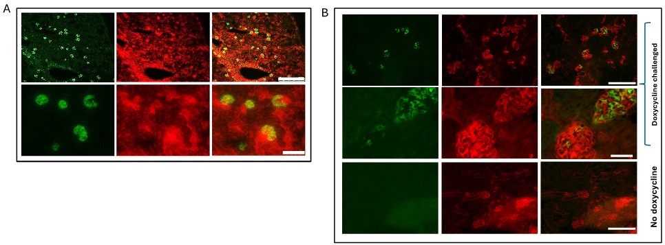
      (A) mT/mG reporter mouse crossed to constitutional podocin Cre heterozygous mouse. Illustrates podocyte specificity for Cre driver and excision Of reporter Figure shows GFP expression in Cre producing cells (top panel scale bar=250vm; bottom panel scale bar=50pm). Cre expression causes GFP to be switched on. (B) mT/mG reporter mouse crossed to podocin RtTA— tet-o-cre heterozygous mouse shows podocyte specificity for driver and approximately 60% excision. (top and bottom panels scale bar=250pm; middle panel scale bar=50pm). Doxycycline required for expression showing not leaky.

    1. Capulet. When the sun sets, the air doth drizzle dew; But for the sunset of my brother's son It rains downright. 2235How now! a conduit, girl? what, still in tears? Evermore showering? In one little body Thou counterfeit'st a bark, a sea, a wind; For still thy eyes, which I may call the sea, Do ebb and flow with tears; the bark thy body is, 2240Sailing in this salt flood; the winds, thy sighs; Who, raging with thy tears, and they with them, Without a sudden calm, will overset Thy tempest-tossed body. How now, wife! Have you deliver'd to her our decree? 2245 Lady Capulet. Ay, sir; but she will none, she gives you thanks. I would the fool were married to her grave! Capulet. Soft! take me with you, take me with you, wife. How! will she none? doth she not give us thanks? Is she not proud? doth she not count her blest, 2250Unworthy as she is, that we have wrought So worthy a gentleman to be her bridegroom? Juliet. Not proud, you have; but thankful, that you have: Proud can I never be of what I hate; But thankful even for hate, that is meant love. 2255 Capulet. How now, how now, chop-logic! What is this? 'Proud,' and 'I thank you,' and 'I thank you not;' And yet 'not proud,' mistress minion, you, Thank me no thankings, nor, proud me no prouds, But fettle your fine joints 'gainst Thursday next, 2260To go with Paris to Saint Peter's Church, Or I will drag thee on a hurdle thither. Out, you green-sickness carrion! out, you baggage! You tallow-face! Lady Capulet. Fie, fie! what, are you mad? 2265 Juliet. Good father, I beseech you on my knees, Hear me with patience but to speak a word. Capulet. Hang thee, young baggage! disobedient wretch! I tell thee what: get thee to church o' Thursday, Or never after look me in the face: 2270Speak not, reply not, do not answer me; My fingers itch. Wife, we scarce thought us blest That God had lent us but this only child; But now I see this one is one too much, And that we have a curse in having her: 2275Out on her, hilding! Nurse. God in heaven bless her! You are to blame, my lord, to rate her so. Capulet. And why, my lady wisdom? hold your tongue, Good prudence; smatter with your gossips, go. 2280 Nurse. I speak no treason. Capulet. O, God ye god-den. Nurse. May not one speak? Capulet. Peace, you mumbling fool! Utter your gravity o'er a gossip's bowl; 2285For here we need it not. Lady Capulet. You are too hot. Capulet. God's bread! it makes me mad: Day, night, hour, tide, time, work, play, Alone, in company, still my care hath been 2290To have her match'd: and having now provided A gentleman of noble parentage, Of fair demesnes, youthful, and nobly train'd, Stuff'd, as they say, with honourable parts, Proportion'd as one's thought would wish a man; 2295And then to have a wretched puling fool, A whining mammet, in her fortune's tender, To answer 'I'll not wed; I cannot love, I am too young; I pray you, pardon me.' But, as you will not wed, I'll pardon you: 2300Graze where you will you shall not house with me: Look to't, think on't, I do not use to jest. Thursday is near; lay hand on heart, advise: An you be mine, I'll give you to my friend; And you be not, hang, beg, starve, die in 2305the streets, For, by my soul, I'll ne'er acknowledge thee, Nor what is mine shall never do thee good: Trust to't, bethink you; I'll not be forsworn. [Exit]

      lord Capulet enters and mocks Juliet's grief however after he learns that Juliet is rejecting the wedding he gets enraged saying that he would drag her to the church himself he then gives juliet a ultimatium saying if he doesnt marry paris he would disown juliet and leave her a beggar on the streets

    2. Tybalt. Well, peace be with you, sir: here comes my man. Mercutio. But I'll be hanged, sir, if he wear your livery: 1555Marry, go before to field, he'll be your follower; Your worship in that sense may call him 'man.' Tybalt. Romeo, the hate I bear thee can afford No better term than this,—thou art a villain. Romeo. Tybalt, the reason that I have to love thee 1560Doth much excuse the appertaining rage To such a greeting: villain am I none; Therefore farewell; I see thou know'st me not. Tybalt. Boy, this shall not excuse the injuries That thou hast done me; therefore turn and draw. 1565 Romeo. I do protest, I never injured thee, But love thee better than thou canst devise, Till thou shalt know the reason of my love: And so, good Capulet,—which name I tender As dearly as my own,—be satisfied. 1570 Mercutio. O calm, dishonourable, vile submission! Alla stoccata carries it away. [Draws] Tybalt, you rat-catcher, will you walk? Tybalt. What wouldst thou have with me? 1575 Mercutio. Good king of cats, nothing but one of your nine lives; that I mean to make bold withal, and as you shall use me hereafter, drybeat the rest of the eight. Will you pluck your sword out of his pitcher by the ears? make haste, lest mine be about your 1580ears ere it be out. Tybalt. I am for you.

      tybalt spots romeo and challenges him to a fight but romeo refuses and says that we are closer than you think mercutio sees romeo as a coward and decide to draw his sword challenging tybalt in romeos place

    1. Author response:

      The following is the authors’ response to the original reviews.

      eLife Assessment

      This valuable study examines the role of E2 ubiquitin enzyme, Uev1a in tissue resistance to oncogenic RasV12 in Drosophila melanogaster polyploid germline cells and human cancer cell lines. The incomplete evidence suggests that Uev1a works with the E3 ligase APC/C to degrade Cyclin A, and the strength of evidence could be increased by addressing the expression of CycA in the ovaries and the uev1a loss of function in human cancer cells. This work would be of interest to researchers in germline biology and cancer.

      Thank you for your valuable assessment. The requested data on CycA expression (Figure 4E-G) and uev1a loss-of-function in human cancer cells (Figure 8 and Figure 8-figure supplement 2) have been added to the revised manuscript.

      Public Reviews:

      Reviewer #1 (Public review):

      Summary:

      This study uncovers a protective role of the ubiquitin-conjugating enzyme variant Uev1A in mitigating cell death caused by over-expressed oncogenic Ras in polyploid Drosophila nurse cells and by RasK12 in diploid human tumor cell lines. The authors previously showed that overexpression of oncogenic Ras induces death in nurse cells, and now they perform a deficiency screen for modifiers. They identified Uev1A as a suppressor of this Ras-induced cell death. Using genetics and biochemistry, the authors found that Uev1A collaborates with the APC/C E3 ubiquitin ligase complex to promote proteasomal degradation of Cyclin A. This function of Uev1A appears to extend to diploid cells, where its human homologs UBE2V1 and UBE2V2 suppress oncogenic Ras-dependent phenotypes in human colorectal cancer cells in vitro and in xenografts in mice.

      Strengths:

      (1) Most of the data is supported by a sufficient sample size and appropriate statistics.

      (2) Good mix of genetics and biochemistry.

      (3) Generation of new transgenes and Drosophila alleles that will be beneficial for the community.

      We greatly appreciate your comments.

      Weaknesses:

      (1) Phenotypes are based on artificial overexpression. It is not clear whether these results are relevant to normal physiology.

      Downregulation of Uev1A, Ben, and Cdc27 together significantly increased the incidence of dying nurse cells in normal ovaries (Figure 5-figure supplement 2), indicating that the mechanism we uncovered also protects nurse cells from death during normal oogenesis.

      (2) The phenotype of "degenerating ovaries" is very broad, and the study is not focused on phenotypes at the cellular level. Furthermore, no information is provided in the Materials and Methods on how degenerating ovaries are scored, despite this being the most important assay in the study.

      Thank you for pointing out this issue. We quantified the phenotype of nurse cell death using “degrading/total egg chambers per ovary”, not “degenerating ovaries”. Normal nurse cell nuclei exhibit a large, round morphology in DAPI staining (see the first panel in Figure 1D). During early death, they become disorganized and begin to condense and fragment (see the second panel in Figure 1D). In late-stage death, they are completely fragmented into small, spherical structures (see the third panel in Figure 1D), making cellular-level phenotypic quantification impossible. Since all nurse cells within the same egg chamber are interconnected, their death process is synchronous. Thus, quantifying the phenotype at the egg-chamber level is more practical than at the cellular level. We have added the description of this death phenotype and its quantification to the main text (Lines 104-108).

      (3) In Figure 5, the authors want to conclude that uev1a is a tumor-suppressor, and so they over-express ubev1/2 in human cancer cell lines that have RasK12 and find reduced proliferation, colony formation, and xenograft size. However, genes that act as tumor suppressors have loss-of-function phenotypes that allow for increased cell division. The Drosophila uev1a mutant is viable and fertile, suggesting that it is not a tumor suppressor in flies. Additionally, they do not deplete human ubev1/2 from human cancer cell lines and assess whether this increases cell division, colony formation, and xenograph growth.

      We apologize for any misleading description. We aimed to demonstrate that UBE2V1/2, like Uev1A in Drosophilanos>Ras<sup>G12V</sup>+bam-RNAi” germline tumors, suppress oncogenic KRAS-driven overgrowth in diploid human cancer cells. Importantly, this function of Uev1A and UBE2V1/2 is dependent on Ras-driven tumors; there is no evidence that they act as broad tumor suppressors in the absence of oncogenic Ras. Drosophila uev1a mutants were lethal, not viable (see Lines 135-137), and germline-specific knockdown of uev1a (nos>uev1a-RNAi) caused female sterility without inducing tumors. These findings suggest that Uev1A lacks tumor-suppressive activity in the Drosophila female germline in the absence of Ras-driven tumors. We have revised the manuscript to prevent misinterpretation. Furthermore, we have added data demonstrating that the combined knockdown of UBE2V1 and UBE2V2 significantly promotes the growth of KRAS-mutant human cancer cells, as suggested (Figure 8 and Figure 8-figure supplement 2).

      (4) A critical part of the model does not make sense. CycA is a key part of their model, but they do not show CycA protein expression in WT egg chambers or in their over-expression models (nos.RasV12 or bam>RasV12). Based on Lilly and Spradling 1996, Cyclin A is not expressed in germ cells in region 2-3 of the germarium; whether CycA is expressed in nurse cells in later egg chambers is not shown but is critical to document comprehensively.

      We appreciate your critical comment. CycA is a key cyclin that partners with Cdk1 to promote cell division (Edgar and Lehner, 1996). Notably, nurse cells are post-mitotic endocycling cells (Hammond and Laird, 1985) and typically do not express CycA (Lilly and Spradling, 1996) (see the last sentence, page 2518, paragraph 3 in this 1996 paper). However, their death induced by oncogenic Ras<sup>G12V</sup> is significantly suppressed by monoallelic deletion of either cycA or cdk1 (Zhang et al., 2024). Conversely, ectopic CycA expression in nurse cells triggers their death (Figure 4C, D). These findings suggest that polyploid nurse cells exhibit high sensitivity to aberrant division-promoting stress, which may represent a distinct form of cellular stress unique to polyploid cells. In the revised manuscript, we have provided the CycA-staining data, comparing its expression in normal nurse cells versus cells undergoing oncogenic Ras<sup>G12V</sup>-induced death (Figure 4E-G).

      (5) The authors should provide more information about the knowledge base of uev1a and its homologs in the introduction.

      Thank you for your suggestion. In the revised introduction, we have provided a more detailed description of Uev1A (Lines 72-79). Additionally, we have introduced its human homologs, UBE2V1 and UBE2V2, in the main text (Lines 143-145).

      Reviewer #2 (Public review):

      Summary:

      The authors performed a genetic screen using deficiency lines and identified Uev1a as a factor that protects nurse cells from RasG12V-induced cell death. According to a previous study from the same lab, this cell death is caused by aberrant mitotic stress due to CycA upregulation (Zhang et al.). This paper further reveals that Uev1a forms a complex with APC/C to promote proteasome-mediated degradation of CycA.

      In addition to polyploid nurse cells, the authors also examined the effect of RasG12V-overexpression in diploid germline cells, where RasG12V-overexpression triggers active proliferation, not cell death. Uev1a was found to suppress its overgrowth as well.

      Finally, the authors show that the overexpression of the human homologs, UBE2V1 and UBE2V2, suppresses tumor growth in human colorectal cancer xenografts and cell lines. Notably, the expression of these genes correlates with the survival of colorectal cancer patients carrying the Ras mutation.

      Strength:

      This paper presents a significant finding that UBE2V1/2 may serve as a potential therapy for cancers harboring Ras mutations. The authors propose a fascinating mechanism in which Uev1a forms a complex with APC/C to inhibit aberrant cell cycle progression.

      We greatly appreciate your comments.

      Weakness:

      The quantification of some crucial experiments lacks sufficient clarity.

      Thank you for highlighting this issue. We have provided more details regarding the quantification data in the revised manuscript.

      References

      Edgar, B.A., and Lehner, C.F. (1996). Developmental control of cell cycle regulators: a fly's perspective. Science 274, 1646-1652.

      Hammond, M.P., and Laird, C.D. (1985). Chromosome structure and DNA replication in nurse and follicle cells of Drosophila melanogaster. Chromosoma 91, 267-278.

      Lilly, M.A., and Spradling, A.C. (1996). The Drosophila endocycle is controlled by Cyclin E and lacks a checkpoint ensuring S-phase completion. Genes Dev 10, 2514-2526.

      Zhang, Q., Wang, Y., Bu, Z., Zhang, Y., Zhang, Q., Li, L., Yan, L., Wang, Y., and Zhao, S. (2024). Ras promotes germline stem cell division in Drosophila ovaries. Stem Cell Reports 19, 1205-1216.

      Recommendations for the authors:

      Reviewer #1 (Recommendations for the authors):

      (1) The figure legends insufficiently describe the figures. One example is Figure 3, where there are no details in the figure legend about what conditions apply to each panel and each lane of the gels.

      For clarity and brevity, detailed experimental conditions are described in the Materials and Methods section. Figure legends therefore focus on summarizing the key findings. Thank you for your understanding!

      (2) The font size on the figure is too small.

      Thank you for your constructive suggestion. In response, we have enlarged all font sizes to improve readability.

      (3) There are places where the authors overstate their results, and there are issues with the clarity of the text:

      (3a) Lines 170: "excessive" is not appropriate. Their prior study showed a mild increase in proliferation.

      “Excessive” has been removed in the revised manuscript (Lines 215-216).

      (3b) Line 187-8: The authors should restate this sentence. Here's a possibility. Over-expression of Uev1a suppressed the phenotypes caused by CycA over-expression.

      This sentence has been restated as “Notably, this cell death was suppressed by co-overexpression of CycA and Uev1A, indicating a genetic interaction between them”. (Lines 229-231).

      (3c) Lines 266-7: The properties of Uev1a (ie, lacking a conserved Cys) should be in the introduction.

      This information has been added to the revised introduction (Lines 74-76).

      (3d) Line 318: "markedly" is an overstatement of the prior results.

      Our quantification data revealed that “nos>Ras<sup>G12V</sup>; bam<sup>-/-</sup>” ovaries are three times larger than “nos>GFP; bam<sup>-/-</sup>” control ovaries (see Figure 4A-C in Zhang et al., Stem Cell Reports 19, 1205-1216). Given this substantial difference, we think that using "markedly" is not an overstatement.

      (4) Data not shown occurs in a few places in the text. Given the ability to supply supplemental information in eLife preprints, these data should be shown.

      Thanks for your suggestion. All “not shown” data have been added to the revised manuscript.

      Reviewer #2 (Recommendations for the authors):

      Major Comments

      (1) Cyclin A (CycA) is a key player in this study, but the authors do not provide evidence showing the upregulation of CycA following Ras overexpression in either polyploid or diploid cells. Data on CycA expression should be included.

      Thank you for your constructive suggestion. These data have been added to the revised manuscript (Figure 4E-G).

      (2) DNA replication stress, cellular senescence, and cell death should be assessed under Ras overexpression (RasOE) and RasOE + Uev1A RNAi conditions to support the model proposed in Figure 4F.

      We apologize for any confusion caused by our initial model. We do not have evidence that DNA replication stress and cellular senescence occur under these conditions. Cell death can be readily detected through the presence of fragmented nuclei and condensed DNA (see Figure 1D). The model has been updated accordingly (Figure 9E).

      (3) Appropriate controls should be performed alongside the experimental sets. The same nos>Ras+GFPi data set was repeatedly used in Figures 1I, 2B, 2H, and Figures 2, S2B, which is not ideal.

      All these experiments were performed under identical conditions. Therefore, we deem it appropriate to use the same control data across these analyses.

      (4) Overall, the microscopic images are too small and hard to see.

      Thank you for raising this important point. In the revised manuscript, all images and the font size on figures have been enlarged for improved clarity.

      (5) Figure 1H

      Why is the frequency of egg chamber degradation quite less in nos>RasG12V+GFP-RNAi (about 40%) than nos > RasG12V (about 80%)? And the authors do not show that there is a significant difference between those two conditions, although it should be there. We will need the explanation from the authors on why there is a difference here.

      These overexpression experiments were conducted using the GAL4/UAS system. While both “nos>Ras<sup>G12V</sup>+GFP-RNAi” and “nos>Ras<sup>G12V</sup>” contain a single nos-GAL4 driver, they differ in UAS copy number: the former incorporates two UAS elements compared to only one in the latter (see the detailed genotypes in Source data 2). These results demonstrate that UAS copy number impacts experimental outcomes in our system.

      In the previous paper (Zhang et al. (2024), Figure 7H shows that the frequency of egg chambers in nos>RasG12V is 33%, although this paper shows it as about 80%. There seems to be a difference in flies' age (previous paper: 7d, this paper: 3d), but this data raises the question of why nos>RasG12V shows more egg chamber degradation this time.

      We greatly appreciate your careful observation. The nurse-cell-death phenotype exhibits a spectrum from mild to severe manifestations [see Figure 1D and our response to weekness (2) in Reviewer #1’s public reviews]. While our 2024 paper exclusively quantified egg chambers with severe phenotypes as degrading, the current study included both mild and severe cases in this classification. We do not think fly age could account for this substantial phenotypic difference. A detailed description of the nurse-cell-death phenotype and its quantification have been added to the revised manuscript (Lines 104-108).

      In the following experiments, only nos>RasG12V+GFP-RNAi is used as a control (Figures 2B, H, S2B). I wonder if these results would give us a different conclusion if nos>RasG12V were used as a control.

      As explained above, the UAS copy number does matter in our analyses, so it is important to keep them identical for comparison.

      (6) In the abstract, the authors mention that uev1a is an intrinsic factor to protect cells from RasG12V-induced cell death. RasG12V does not induce much cell death of cystocytes with bam-gal4, whereas it induces a lot of nurse cells' death. Does it mean the intrinsic expression level of uev1a is low in nurse cells (or polyploid cells) compared to cystocytes (or diploid cells)?

      Overexpression of Ras<sup>G12V</sup> driven by bam-GAL4 exhibited only minimal nurse cell death (Figure 1D, E). Additionally, Uev1A exhibited low intrinsic expression levels in both cystocytes and nurse cells (Figure 3E and Figure 5-figure supplement 1).

      (7) Is uev1a-RNAi alone sufficient to induce egg chamber degradation? Or does it have any effect on ovarian development? (Related to question #1 in minor comments)

      While nos>uev1a-RNAi resulted in female sterility, it alone was insufficient to induce egg chamber degradation. However, simultaneous downregulation of Uev1A, Ben, and Cdc27 triggered significant egg chamber degradation (Figure 5-figure supplement 2).

      (8) Which stages of egg chambers get degraded with RasG12V induction?

      This is a good question. In our analyses, we noted that degrading egg chambers exhibited considerable size variability (Figure 1D). Because degradation disrupts normal morphological cues, precise staging of these egg chambers is nearly impossible.

      (9) I suggest testing the cellular senescence marker as well if the authors mention that CycA-degradation by Uev1a-APC/C complex prevents cellular senescence induced by RasG12V in a schematic image of Figure 4 (e.g., Dap/p21, SA-β-gal).

      As addressed in our response to your Major Comment (2), we lacked experimental evidence to support cellular senescence in this context. We have therefore revised the model accordingly (Figure 9E). While this study focuses specifically on cell death, investigating potential roles of cellular senescence remains an important direction for future research. Thank you for your suggestion!

      Minor Comments

      (1) Figure 1D: Df#7584

      It seems that the late-stage egg chamber is missing in this condition. Why does this occur without egg chamber degradation? Is there a possibility that we do not see egg chamber degradation because this deficiency line does not have a properly developed egg chamber that can have a degradation?

      While this image represents only a single sample, we have confirmed the presence of late-stage egg chambers in other samples. If “Df#7584/+” females were unable to support late-stage egg chamber development, complete sterility would be expected due to the lack of mature eggs. However, as shown in this image (Figure 1D), the ovary contains mature eggs, and the “Df#7584/+” fly strain remains fertile.

      (2) Based on the results that DDR signaling functions as keeping egg chambers from degradation, the authors may be better to check the DNA-damage markers in nos>RasG12V, nos>RasG12V +uev1a. (e.g. γ-H2AX)

      Thank you for your constructive recommendation. These data have been added to the revised manuscript (Figure 3C).

    1. Author response:

      eLife Assessment

      Using genome databases, the authors performed solid bioinformatic analyses to trace the genomic history of the clinically relevant Staphylococcus aureus tetracycline resistance plasmid pT181 over the last seven decades. They discovered that this element has transitioned from a multicopy plasmid to a chromosomally integrated element, and the work represents a valuable demonstration of the use of publicly available data to investigate plasmid biology and inform clinical epidemiology. This work will appeal to researchers interested in staphylococcal evolution and plasmid biology.

      Thank you, we agree with this overview. We also think this work is interesting to people interested in antimicrobial resistance and bacterial genome structure.

      Public Reviews:

      Reviewer #1 (Public review):

      The study provides a robust bioinformatic characterization of the evolution of pT181. My main criticism of the work is the lack of experimental validation for the hypotheses proposed by the authors.

      Comments on the study:

      (1) One potential reason for the decline in pT181 copy number over time may be a high cost associated with the multicopy state. In this sense, it would be interesting if the authors could use (or construct) isogenic strains differing only in the state of the plasmid (multicopy/integrated). With this system, the authors could measure the fitness of the strains in the presence and absence of tetracycline, and they could be able to understand the benefit associated with the plasmid transition. The authors discuss these ideas, but it would be nice to test them.

      We agree that the relative fitness of integrated versus multicopy plasmids is interesting and a costly multicopy state could explain the transition of independent pT181 replicons to chromosomal integration. This is a project we are exploring for a future study. However, we think that this additional experimental work goes beyond the scope of the paper.

      (2) It would be interesting to know the transfer frequencies of the multicopy mobilizable pT181 plasmid, compared to the transfer frequency of the plasmid integrated into the SSCmec element (which can be co-transferred, integrated in conjugative plasmids, or by transduction).

      We agree with the reviewer that this is an interesting question. However, we think inferring these rates from natural sequence data is not feasible in this case given the low heterogeneity of the plasmid sequence. A laboratory-based experimental study could not address the real transfers we observe over the course of decades, as in vitro S. aureus transfer rates are often not good proxies for in vivo (McCarthy et al., 2014). In addition, we do not know what is moving the integrated plasmid. pT181 could be moved by a phage or plasmid, so we are uncertain what the correct experiment would be to explore this.

      (3) One important limitation of the study that should be mentioned is that inferring pT181 PCN from whole genome data can be problematic. For example, some DNA extraction methods may underestimate the copy number of small plasmids because the small, circular plasmids are preferentially depleted during the process (see, for example, https://www.nature.com/articles/srep28063).

      We will investigate this issue further in the revisions. The kits used to extract DNA for the earlier-collected samples may possibly yield more plasmid DNA relative to the chromosome compared to newer ones on average; however, we think this is not driving the decline that we observe in multicopy pT181 copy number. Multiple BioProjects find the same result, where earlier samples have higher copy number compared to later samples. We expect extraction methods to be consistent within a BioProject, suggesting that this decline is genuine and not technical. In revisions, we intend to evaluate the effect of date of sequencing and additional metadata on copy number.

      Reviewer #2 (Public review):

      Summary:

      The authors performed bioinformatic analyses to trace the genomic history of the clinically relevant pT181 plasmid. Specifically, they:

      (1) Tracked the presence of pT181 across different S. aureus strain backgrounds through time. It was first found in one, later multiple strains, though this may reflect changes in sampling over time.

      (2) Estimated the mutation rate of the chromosome and plasmid.

      (3) Estimated the plasmid copy number of pT181, and found that it decreased over time. The latter was supported by two sets of statistical analyses, first showing that the number of single-copy isolates increased over time, and second, that the multicopy isolates demonstrated a lower PCN over time.

      (4) Reported the different integration sites at which pT181 integrated into the genome.

      As a caveat, they mentioned that identical plasmid sequences have variable plasmid copy numbers across different genomes in their dataset.

      Strengths:

      This is a very solid, well-considered bioinformatic study on publicly available data. I greatly appreciate the thoughtful approach the authors have taken to their subject matter, neither over- nor underselling their results. It is a strength that the authors focused on a single plasmid in a single bacterial species, as it allowed them to take into account unique knowledge about the biology of this system and really dive deep into the evolution of this specific plasmid. It makes for a compelling case study. At the same time, I think the introduction and discussion can be strengthened to demonstrate what lessons might be drawn from this case study for other plasmids.

      Weaknesses:

      The finding that the pT181 copy number declined over time is the most interesting claim of the paper to me, and not something that I have seen done before. While the authors have looked at some confounders in this analysis, I think this could be strengthened further in a revision.

      In the revisions, we will further explore the impact that technical variation could have in contributing to copy number variation and update our claims for the decline in copy number of the independent replicon over time and variation for the same plasmid sequence accordingly. Multiple BioProjects show earlier samples have higher copy number compared to later samples; we expect extraction methods to be consistent within a BioProject, supporting our initial findings that this decline over time is not due to technical variation.

      For the flow of the storyline, I also think the estimation of mutation rates (starting L181) and integration into the chromosome (starting L255) could be moved to the supplement or a later position in the main text.

      We will revisit the text organization for flow and clarity of storyline.

      Clearly, the use of publicly available data prevents the authors from controlling the growth and sequencing conditions of the isolates. It is striking that they observe a clear signal in spite of this, but I would have loved to see more discussion of the metadata that came with the publicly available sequences and even more use of that metadata to control for confounding.

      In revisions, we will further investigate possible contributors to the observed decline in copy number of multicopy pT181 over time. We have incorporated the date of sample collection and BioProject in our analysis, but not the date of sequencing or extraction technique.

      References

      McCarthy, A. J., Loeffler, A., Witney, A. A., Gould, K. A., Lloyd, D. H., & Lindsay, J. A. (2014). Extensive horizontal gene transfer during Staphylococcus aureus co-colonization in vivo. Genome Biology and Evolution, 6(10), 2697–2708. https://doi.org/10.1093/gbe/evu214

    1. ord itself imilieu in which records are creattermined by all these factors: fustructures, as well as records-creaobservation I am not abandoninggrounding in the evidence, structuway. I am asserting, however, thatcircumstances of creation a

      When I think about this passage alongside the rise of artificial intelligence (AI), Cook’s emphasis on context feels even more urgent. Terry Cook argues that records are shaped by the functional and structural environments in which they are created. In an AI-driven world, where systems generate, sort, and analyze massive volumes of data automatically, understanding that broader context becomes essential. AI can process content at scale, but without contextual grounding, it risks misinterpreting records or reinforcing surface-level patterns. I see AI as both an opportunity and a challenge for appraisal theory. On one hand, AI tools can help identify patterns across enormous bureaucratic systems, making macro-level analysis more feasible. They can cluster records, detect trends, and even suggest appraisal priorities. This could strengthen Cook’s top-down approach by giving archivists analytical support in mapping institutional functions. On the other hand, AI systems are trained on existing data, which may already reflect institutional biases and power imbalances. If archivists rely too heavily on AI-driven selection, we risk automating those biases. Cook stresses that archivists must actively and consciously shape the archival record. AI does not remove that responsibility—it arguably heightens it. I cannot simply defer judgment to an algorithm.

    1. Author response:

      The following is the authors’ response to the original reviews.

      Public Reviews:

      Reviewer #1 (Public review):

      Summary:

      Abdelmageed et al. investigate age-related changes in the subcellular localization of DNA polymerase kappa (POLK) in the brains of mice. POLK has been actively investigated for its role in translesion DNA synthesis and involvement in other DNA repair pathways in proliferating cells, very little is known about POLK in a tissue-specific context, let alone in post-mitotic cells. The authors investigated POLK subcellular distribution in the brains of young, middle-aged, and old mice via immunoblotting of fractioned tissue extracts and immunofluorescence (IF). Immunoblotting revealed a progressive decrease in the abundance of nuclear POLK, while cytoplasmic POLK levels concomitantly increased. Similar findings were present when IF was performed on brain sections. Further, IF studies of the cingulate cortex (Cg1), the motor cortex (M1, M2), and the somatosensory (S1) cortical regions all showed an age-related decline in nuclear POLK. Nuclear speckles of POLK decrease in each region, meanwhile, the number of cytoplasmic POLK granules decreases in all four regions, but granule size is increasing. The authors report similar findings for REV1, another Y-family DNA polymerase.

      The authors then investigate the colocalization of POLK with other DNA damage response (DDR) proteins in either pyramidal neurons or inhibitory interneurons. At 18 months of age, DNA damage marker gH2AX demonstrated colocalization with nuclear POLK, while strong colocalization of POLK and 8-oxo-dG was present in geriatric mice. The authors find that cytoplasmic POLK granules colocalize with stress granule marker G3BP1, suggesting that the accumulated POLK ends up in the lysosome.

      Brain regions were further stained to identify POLK patterns in NeuN+ neurons, GABAergic neurons, and other non-neuronal cell types present in the cortex. Microglia associated with pyramidal neurons or inhibitory interneurons were found to have a higher abundance of cytoplasmic POLK. The authors also report that POLK localization can be regulated by neuronal activity induced by Kainic acid treatment. Lastly, the authors suggest that POLK could serve as an aging clock for brain tissue, but POLK deserves further characterization and correlation to functional changes before being considered as a biomarker.

      Strengths:

      Investigation of TLS polymerases in specific tissues and in post-mitotic cells is largely understudied. The potential changes in sub-cellular localization of POLK and potentially other TLS polymerases open up many questions about DNA repair and damage tolerance in the brain and how it can change with age.

      Weaknesses:

      The work is quite novel and interesting, and the authors do suggest some potentially interesting roles for POLK in the brain, but these are in and of themselves a bit speculative. The majority of the findings of this paper draw upon findings from POLK antibody and its presumed specificity for POLK. However, this antibody has not been fully validated and needs further work. Further validation experiments using Polk-deficient or knocked-down cells to investigate antibody specificity for both immunoblotting and immunofluorescence should be performed. More mechanistic investigation is needed before POLK could be considered as a brain aging clock.

      We are thankful for the overall enthusiasm and positive comments.

      (a) Concern over POLK antibody characterization in mouse:

      We performed siRNA and shRNA knock downs in mouse primary cortical neurons as well as efficiently transfectable murine lines like 4T1 and Neuro-2A showing knock down of 99kDa and 120kDa bands recognized by sc-166667 anti-POLK antibody (exact figure number Figure 1 and S1). We show that in IF sc-166667 and A12052 (Figure S1G) shows similar immunostaining patterns and we used sc-166667 in all reported figures and western blots.

      (b) More mechanistic investigation is needed before POLK could be considered as a brain aging clock:

      We sincerely appreciate the valuable suggestion. We agree as a terminal assay POLK nucleo-cytoplasmic status is not practical for longitudinal studies. However, we believe it may serve an investigative/correlative endogenous signal for determining tissue age, that may be useful to "date" brain sections, since not many such cell biological markers exist. We have added clarification texts to address this.

      Reviewer #2 (Public review):

      Summary:

      Abdelmageed et al., demonstrate POLK expression in nervous tissue and focus mainly on neurons. Here they describe an exciting age-dependent change in POLK subcellular localization, from the nucleus in young tissue to the cytoplasm in old tissue. They argue that the cytosolic POLK is associated with stress granules. They also investigate the cell-type specific expression of POLK, and quantitate expression changes induced by cell-autonomous (activity) and cell nonautonomous (microglia) factors.

      I think it is an interesting report but requires a few more experiments to support their findings in the latter half of the paper. Additionally, a more mechanistic understanding of the pathways regulating POLK dynamics between the nucleus and cytosol, what is POLK doing in the cytosol, and what is it interacting with; would greatly increase the impact of this report. However, additional mechanistic experiments are mostly not needed to support much of the currently presented results, again, it would simply increase the impact.

      (a) Concern on more mechanistic understanding of the pathways regulating POLK dynamics between the nucleus and cytosol:

      We sincerely appreciate the reviewer’s enthusiasm and valuable guidance in helping us better understand the mechanism of nuclear-cytoplasmic POLK dynamics. Previously, we developed a modified aniPOND (accelerated native isolation of proteins on nascent DNA) protocol, which we termed iPoKD-MS (isolation of proteins on Pol kappa synthesized DNA followed by mass spectrometry), to capture proteins bound to nascent DNA synthesized by POLK in human cell lines (bioRxiv https://www.biorxiv.org/content/10.1101/2022.10.27.513845v3). In this dataset, we identified potential candidates that may regulate nuclear/cytoplasmic POLK dynamics. These candidates are currently undergoing validation in human cell lines, and we are preparing a manuscript on these findings. Among these, some candidates, including previously identified proteins such as exportin and importin (Temprine et al., 2020, PMID: 32345725), are being explored further as potential POLK nuclear/cytoplasmic shuttles. We are also conducting tests on these candidates in mouse cortical primary neurons to assess their role in POLK dynamics. In the revised version of the manuscript, we have included a discussion of our current understanding.

      (b) Question on “… what is POLK doing in the cytosol, and what is it interacting with …”: Our data so far indicate that POLK accumulates in stress granules and lysosomes. We are very grateful for the reviewer’s insightful suggestions and will make every effort to incorporate them in the revised manuscript. We characterized POLK accumulation in the cytoplasm using six additional endo-lysosomal markers, as recommended by the reviewer. This data is now part of entirely new Figure 3.

      Reviewer #3 (Public review):

      Summary:

      In this study, the authors show that DNA polymerase kappa POLK relocalizes in the cytoplasm as granules with age in mice. The reduction of nuclear POLK in old brains is congruent with an increase in DNA damage markers. The cytoplasmic granules colocalize with stress granules and endo-lysosome. The study proposes that protein localization of POLK could be used to determine the biological age of brain tissue sections.

      Strengths:

      Very few studies focus on the POLK protein in the peripheral nervous system (PNS). The microscopy approach used here is also very relevant: it allows the authors to highlight a radical change in POLK localization (nuclear versus cytoplasmic) depending on the age of the neurons. 

      The conclusions of the study are strong. Several types of neurons are compared, the colocalization with several proteins from the NHEJ and BER repair pathways is tested, and microscopy images are systematically quantified.

      Weaknesses:

      The authors do not discuss the physical nature of POLK granules. There is a large field of research dedicated to the nature and function of condensates: in particular numerous studies have shown that some condensates but not all exhibit liquid-like properties (https://www.nature.com/articles/nrm.2017.7, https://pubmed.ncbi.nlm.nih.gov/33510441/ https://www.mdpi.com/2073-4425/13/10/1846). The change of physical properties of condensates is particularly important in cells undergoing stress and during aging. The authors should discuss this literature.

      We highly appreciate the reviewer bringing up the context of biomolecular condensates. Our iPoKD-MS data referenced above suggests candidates from various biomolecular condensates that we are currently investigating. We appreciate the reviewer providing important literature cited these articles in text and potential biomolecular condensates are discussed in the revised version. 

      Recommendations for the authors:

      Reviewer #1 (Recommendations for the authors):

      The work is quite novel and interesting, and the authors do suggest some potentially interesting roles for POLK in the brain, but these are in of themselves a bit speculative. The majority of the findings of this paper rely upon the POLK antibody and its specificity for POLK, which is not fully characterized and needs further work (validation of antibodies using immunoblots of Polk KO cells or siRNA KD of POLK in murine cells) to provide confidence in the authors' findings. 

      Points

      siRNA knockdown of Polk in primary neurons showed a dramatic reduction in signal by IF even though qPCR analysis showed a reduction of only ~35% at the transcript level. Typically many DNA repair genes need to be knocked down by 80% or more to see discernable differences at the protein level. siRNA knockdown in a murine cell line (MEFs, neurons, or some other easily transfectable cell type) needs to be performed with immunoblotting with whole cell and fractionated (nuclear/cytoplasmic) lysates in order to better validate the anti-POLK antibodies and which bands that are visualized during immunoblotting are specific to POLK.

      We performed siRNA and shRNA knock downs in mouse primary cortical neurons as well as efficiently transfectable murine lines like 4T1 and Neuro-2A showing knock down of 99kDa and 120kDa bands recognized by sc-166667 anti-POLK antibody (exact figure number Figure 1 and S1). We show that in IF sc-166667 and A12052 (Figure S1G) shows similar immunostaining patterns and we used sc-166667 in all reported figures and western blots.

      Figure 1B and C, it is not clear which antibody(ies) are used for the immunoblotting of nuclear and cytoplasmic fractions and for a blot with whole tissue lysates. Please place the antibody vendor or clone next to the corresponding blot or describe it in the figure legend. Bands of varying sizes are present in 1B (and Figure S1) but only a band at 99 kDa was shown in 1C. Because there are no bands of equivalent size present in the nuclear and cytoplasmic fractions in Figure 1B, please describe or denote which bands were used for quantification purposes for nuclear and cytoplasmic POLK.

      This has been clarified by using only one antibody throughout the manuscript sc-166667. We observed in whole cell lysate an intense ~99kDa and a faint ~120kDa band, which gets intense in nuclear fraction and is absent in cytoplasmic fraction. We have noted this in multiple human cell lines and hiPSC-derived neurons, which is our ongoing work. We do not know yet if the ~120kDa is a modification or isoform of POLK. We have hints from our proteomics data that it may be SUMOylated or ubiquitinylated or other post translational modifications. We added this in the discussion section.

      Figure 1I, is there a quantification beyond just the representative image? There is no green staining pattern outside the cytoplasm in the 1-month-old M1 images that is present in all the other images in the panel.

      Fig 1I is now Fig S1G in the revised manuscript. Since REV1 and POLH were not central to the study that focused on POLK, they were meant to be exploratory data panels and as such we did not quantify beyond the qualitative evaluation, which broadly resembled POLK’s disposition with age. We have noted there are some sample to sample variability in the background signal. In general, outside the cytoplasm as subcellularly segmented by fluorescent nissl expression, tends to be variable by brain areas but also higher in older brains

      "Association with PRKDC further suggests POLK's role in the "gap-filling" step in the NHEJ repair pathway in neurons." There is no strong evidence in the literature for mammalian POLK playing a role in NHEJ. Some description of a role in HR has been described, however. The reference regarding the iPoKD-MS data set that provides evidence of POLK associating with BER and NHEJ factors is listed as Paul, 2022 but is in the reference list as Shilpi Paul 2022.

      We removed this speculative statement and citation fixed.

      Figure 4A, what is the age of the mouse for the representative images?

      19 months and now mentioned in the figure legend

      Figure 4C, Could the data from the different ages be plotted side by side to better evaluate the differences for each cell type/region?

      Data is plotted side by side

      Why was the one-month time point chosen as this could still represent the developing and not mature murine brain? 

      Reviewer correctly noted that a 1 month brain is still developing, but mostly from the behavioral and circuit maturation standpoint. However, from cell division and neurogenesis perspective, that is considered to be complete by first postnatal month, with neuron production thereafter largely restricted to specialized adult niches in the dentate gyrus and subventricular zone–olfactory bulb pathway; these adult neurogenic stem cells are embryonically derived and are regulated in ways that are distinct from the early, expansionary developmental waves of neurogenesis. In our study we performed our measurements in the cortical areas only. (Caviness et al., 1995, PMID: 7482802; Ansorg et al., 2012, PMID: 22564330; Ming & Song, 2011, PMID: 21609825; Bond et al., 2015, PMID: 26431181; Bond et al., 2021, PMID: 33706926; Bartkowska et al., 2022, PMID: 36078144). Also, in Figure 6A it was incorrectly mentioned to be just 1month, we rechecked our metadata and noted that young brains were comprised of 1 and 2 month old brains and now it has been corrected.

      Furthermore, can the authors describe which sex of mice was used in these experiments and the justification if a single sex was used? If both sexes were used, were there any dimorphic differences in POLK localization patterns?

      This is an important aspect, but in the beginning to keep mice numbers within manageable limits, we were focusing more on the age component. While both males and female brains were assayed but due to uneven sample distribution between sexes, we could not estimate if there were any statistically significant sexual dimorphic differences in IN, PN and NNs. Future studies will investigate the sex component as a function of age.

      The suggestion of POLK as a brain aging clock may be a bit premature as the functional and behavioral consequences of cytoplasmic POLK sequestration are not fully known. Furthermore, investigation of POLK levels in other genetic models of neurodegeneration or with gerotherapeutics would be needed to establish if the POLK brain clock is responsive to changes that shift brain aging. Lastly, this clock may be impractical and not useful for longitudinal studies due to the terminal nature of assessing POLK levels.

      We agree as a terminal assay POLK nucleo-cytoplasmic status is not practical for longitudinal studies. However, we believe it may serve an investigative/correlative endogenous signal for determining tissue age, that may be useful to "date" brain sections, since not many such cell biological markers exist. We have added clarification text.

      Some discussion of the Polk-null mice is warranted, as they only have a slightly shortened lifespan, and any disease phenotypes were not reported. This stands in contrast to other DNA repair-deficient mice that mimic premature aging and show behavioral and motor deficits. This calls into question the role of POLK in brain aging.

      Discussion statements on Polk-null mice has been added.

      Please correct the catalog number for the SCBT anti-POLK antibody to sc-166667

      Typographical error has been corrected

      Reviewer #2 (Recommendations for the authors):

      Results:

      Figure by figure 

      (1) A progressive age-associated shift in subcellular localization of POLK The authors state that POLK has not been studied in nervous tissue before and they want to see if it is expressed, and if it changes subcellular location as a function of age. The authors argue age = stress like that seen in previous models using genotoxic agents and cancer cells. Indeed, POLK seems to convincingly change subcellular location from the nucleus to larger cytosolic puncta. 

      (2) Nuclear POLK co-localizes with DNA damage response and repair proteins This was a difficult dataset for me to decipher. To me, it appears as though POLK colocalizes with these examined proteins in the CYTOSOL, not the nucleus. Especially, in the oldest mice.

      We added in the discussion that DNA repair proteins were observed to be present in the cytoplasm and biomolecular condensates citing relevant reviews and primary references.

      (3) POLK in the cytoplasm is associated with stress granules and lysosomes in old brains LAMP1 has some issues as a lysosome marker. The authors even state it can be on endosomes. It would be nice to use a marker for mature lysosomes, some fluorescent reporter that is activated only by lysosomal proteases or pH. It is also of interest if POLK is localized to the membrane or the inside of these structures. The authors have access to an airyscan which is sufficient to examine luminal vs membrane localization on larger organelles like lysosomes.

      We thank the reviewer for pushing us to investigate the nature of cytoplasmic POLK in endo-lysosomal compartments. We have now added a full-page figure on the cell biological results from six different markers, subset (Cathepsin B and D) are known to present in the lumens of endo-lysosomes, in Figure 3. Further high-resolution membrane vs lumen was not pursued, which is perhaps better suited in cultured neurons rather than thick fixed tissues.

      (4) Differentially altered POLK subcellular expression amongst excitatory, inhibitory, and nonneuronal cells in the cortex.

      This seems fine. I don't see anything wrong with the author's statement that there is more POLK in neurons vs non-neuronal cells. 

      (5) Microglia associated with IN and PN have significantly higher levels of cytoplasmic POLK I don't see really any convincing evidence of the author's claim here. They find a difference at early-old age, but not at old-old, or other ages. This is explained by "However, this effect is lost in late-old age (Figure 5D), likely due to the MG-mediated removal of the INs.". But no trend being observed, no experiment to show sufficiency, and no experiment to uncover a directional relationship; this is a tough claim to stand by.

      Changes made in text to reflect speculative nature of this observation

      (6) Subcellular localization of POLK is regulated by neuronal activity

      Interesting and fairly difficult experiment. Can the authors talk more about what these values mean? I am confused as to why there is a decline in nuclear puncta at 80 min. Also, why are POLK counts in 6c similar at baseline between young and early-old? In Figures 5 and 6 I also worry about statistical analysis. Are all assumptions checked to use t-tests? Why not always use a test that has fewer assumptions?

      We have explained in the text the artificial nature of few hour long acute slice preparations is very different and inherently a stressful environment, especially for the old brains, compared to the vascular perfused PFA fixed brain tissues tested between young and old ages.

      We don’t have a proper explanation for the initial dip in nuclear puncta in both young and old brains at 80min of very similar magnitude. It could be a separate biological phenomenon that occurs at much shorter time scales that would not otherwise be captured in a fixed tissue assay and needs careful investigation using live tissue fluorescence imaging that is beyond the scope of this manuscript.

      We apologize for the typographical error in the figure legend. We rechecked our R code and the tests were all Wilcoxon rank-sum (Mann–Whitney U) two-sided nonparametric.

      Figure 6B & E had absurdly small p values due to large sample numbers. So, we implemented random sampling of 100 cells repeating for 200 times and presented the distribution of p values and Cohen’s d in the supplement and reported the median p value and Cohen’s in the main plot.

      (7) POLK as an endogenous "aging clock" for brain tissue

      Trainable model. What are the criteria for the model, and how does it work? The cutoffs it uses to classify each age group might be interesting in that the model may have identified a trait the researchers were unaware of. Otherwise, it is not especially useful. Maybe as an independent 'blind' analysis of the data?

      We have added a better description of the models, assumptions and how two different unsupervised approaches converge on the same set of features with high AUROCs.

      Minor questions:

      The cartoons (1a, 2a-b, 5a, 6a) help a lot. However, I still had to work a bit to understand some of the graphs (e.g., 5d, 6b-e, fig 7). Is there a simpler way to present them? Maybe simply additional labelling? I'm not sure.

      A more thorough discussion of statistical tests is warranted I think. I am not very clear why some were chosen (t-test vs nonparametric with fewer assumptions). Infinitesimally small p values also make me think maybe incorrect tests were done or no power analysis was performed beforehand. A fix for this is just discussing what went into the testing methods and why they were chosen.

      Statistical analysis for Fig2 (using Generalized Estimating Equations), and Fig6 (with random repeated subsampling; method explained in text, figure legend updated and supplementary data on the distribution of p values and cohen’s d are added) to address the very small p values. Descriptions rewritten in relevant text.

      In the absence of further mechanistic experiments, it would still be interesting to hear what the authors think is going on and what the significance of this altered subcellular location means. How do the authors think this is occurring? I think they are arguing that cytosolic localization of POLK is 100% detrimental to the neuron. ("The reduction of nuclear POLK in old brains is congruent with an increase in DNA damage markers") Do they have any idea what the 'bug' is in the POLK system then?

      Statements in the discussion has been added.

      Reviewer #3 (Recommendations for the authors):

      POLK is detected as small " as small "speckles" inside the nucleus at a young age (1-2 months) and larger "granules" can be seen in the cytoplasm at progressively older time points (>9 months). In the nucleus, is POLK bound to DNA? In the cytoplasm, how are the POLK molecules organized: are they bound to a substrate or are they just organized as a proteins condensate without DNA?

      In human U2OS cell line Dnase1 treatment leads to loss of POLK from the nucleus as well as its activity as reported in Fig5 of Paul, S. et. al. 2023 bioRxiv. While we haven’t reproduced these results in mouse primary neurons, we anticipate a similar situation which will be tested in the future. We have addressed limited aspects of the POLK in the cytoplasm in all new Fig3 with six endo-lysosomal markers, and added text.

      When POLK proteins accumulate in the cytoplasm in aging cells, do they also repair condensates in the cytoplasm? What is the function of cytoplasmic POLK granules? More generally, is it known if other granules or foci, such as repair foci are found in the cytoplasms in aging cells, or in cells under stress?

      Six markers for endo-lysosomes were tested to characterize the cytoplasmic granules now shown in Fig3.

      While the authors quantify the number and sizes of the POLK signal, they don't discuss their physical nature. Some membrane-less condensates exhibit liquid-like properties, such as stress granules, P-bodies, or in the nucleus some repair condensates. In some diseased tissues, some condensates lose their liquid properties and become solid-like. Is it known if POLK condensates behave like liquid condensates or they are simply formed by bound molecules on DNA? Since they are larger and fewer in the cytoplasm, is it because several small puncta fused together to form a larger one? It would be worthwhile to discuss these points.

      Discussion statements on the nature of condensates in context of the POLK cytoplasmic signal has been added.

    1. Author response:

      Public Reviews:

      Reviewer #1 (Public review):

      Summary:

      The manuscript titled, "Sleep-Wake Transitions Are Impaired in the AppNL-G-F Mouse Model of Early Onset Alzheimer's Disease", is about a study of sleep/wake phenomena in a knockin mouse strain carrying "three mutations in the human App gene associated with elevated risk for early onset AD". Traditional, in-depth characterization of sleep/wake states, EEG parameters, and response to sleep loss are employed to provide evidence, "supporting the use of this strain as a model to investigate interventions that mitigate AD burden during early disease stages". The sleep/wake findings of earlier studies (especially Maezono et al., 2020, as noted by the authors) were extended by several important, genotype-related observations, including age-related hyperactivity onset that is typically associated with increased arousal, a normal response to loss of sleep and to multiple sleep latency testing, and a stronger AD-like phenotype in females. The authors conclude that the AppNL-G-F mice demonstrate many of the human AD prodromal symptoms and suggest that this strain may serve as a model for prodromal AD in humans, confirming the earlier results and conclusions of Maezono et al. Finally, based on state bout frequency and duration analyses, it is suggested that the AppNL-G-F mice may develop disruptions in mechanism(s) involved in state transition.

      Strengths:

      The study appears to have been, technically, rigorously conducted with high quality, in-depth traditional assessment of both state and EEG characteristics, with the concordant addition of activity and temperature. The major strengths of this study derive from observations that the AppNL-G-F mice: (1) are more hyperactive in association with decreased transitions between states; (2) maintain a normal response to sleep deprivation and have normal MSLT results; and (3) display a sex specific, "stronger" insomnia-like effect of the knockin in females.

      Weaknesses:

      The weaknesses stem from the study's impact being limited due to its being largely confirmatory of the Maezono et al. study, with advances of importance to a potentially more focused field. Further, the authors conclude that AppNL-G-F mice have disrupted mechanism(s) responsible for state transition; however, these were not directly examined. The rationale for this conclusion is stated by the authors as based on the observations that bouts of both W and NREM tend to be longer in duration and decreased in frequency in AppNL-G-F mice. Although altered mechanism(s) of state transition (it is not clear what mechanisms are referenced here) cannot be ruled out, other explanations might be considered. For example, increased arousal in association with hyperactivity would be expected to result in increased duration of W bouts during the active phase. This would also predictably result in greater sleep pressure that is typically associated with more consolidated NREM bouts, consistent with the observations of bout duration and frequency.

      Reviewer 1 succinctly summarizes the advances of this study beyond the ground-breaking Maezono et al (2020) study of this “humanized” mouse model exhibiting amyloid deposition. Whereas Maezono et al. conducted sleep/wake studies on male App<sup>NL-G-F</sup> mice at 6 and 12 months of age, we had the unusual opportunity to study both sexes of homozygous App<sup>NL-G-F</sup> mice and WT littermates at 14-18 months of age and to conduct a longitudinal assessment of many of the same individuals at 18-22 months. In addition to baseline sleep/wake and EEG spectral analyses, we (1) measured subcutaneous body temperature and activity to obtain a broader picture of the physiology and behavior of this strain at advanced ages; (2) assessed baseline sleepiness in this strain using the murine version of the clinically-relevant Multiple Sleep Latency Test (MSLT); (3) evaluated the response of App<sup>NL-G-F</sup> mice and WT littermates to a perturbation of the sleep homeostat; (4) compared the sleep/wake characteristics of male vs. female App<sup>NL-G-F</sup> mice at 18-22 months and, (5) to assess the stability of the phenotypes, analyzed these data over a continuous 14-d recording rather than the conventional 24h recordings typical of most sleep/wake studies including Maezono et al. We found that a long wake/short sleep phenotype was characteristic of homozygous App<sup>NL-G-F</sup> mice at these advanced ages which is also evident in the Maezono et al. (2020) study at 12 months of age (but not at 6 months), although the authors do not comment on this phenotype and instead focus on the reduced REM sleep which is particularly evident in female App<sup>NL-G-F</sup> mice in our study. Remarkably, despite being awake ~20% longer per day, we find that App<sup>NL-G-F</sup> mice are no sleepier than WT mice as determined by the MSLT and that their sleep homeostat is intact when challenged by 6-h sleep deprivation. At both advanced ages, the long wake/short sleep phenotype is due primarily to longer Wake bouts and shorter bouts of both NREM and REM sleep during the dark phase. Moreover, hyperactivity develops in older in App<sup>NL-G-F</sup> mice, particularly females, which contributes to this phenotype. We agree with Reviewer 1 that “hyperactivity would be expected to result in increased duration of W bouts during the active phase” and that this could result in more consolidated NREM bouts and we will modify the manuscript to discuss this alternative. However, the suggestion of greater sleep pressure is not borne out by the MSLT studies as we did not observe the shorter sleep latencies and increased sleep during the nap opportunities on the MSLT that we have observed in other mouse strains. Moreover, due to their short sleep phenotype, App<sup>NL-G-F</sup> mice would be entering the sleep deprivation study with a greater sleep debt than WT mice, yet we did not observe greater EEG Slow Wave Activity in this strain during recovery from sleep deprivation. Thus, we have suggested that App<sup>NL-G-F</sup> mice are unable to transition from Wake to sleep as readily as their WT littermates. Our observations summarized above set the stage for subsequent mechanistic studies in aged App<sup>NL-G-F</sup> mice, although realistically, mice of this age and genotype are a rare commodity.

      Reviewer #2 (Public review):

      Summary:

      The authors have used a knock-in mouse model to explore late-in-life amyloid effects on sleep. This is an excellent model as the mutated genes are regulated by the endogenous promoter system. The sleep study techniques and statistical analyses are also first-rate.

      The group finds an age-dependent increase in motor activity in advanced age in the NLGF homozygous knock-in mice (NLGF), with a parallel age-dependent increase in body temperature, both effects predominate in the dark period. Interestingly, the sleep patterns do not quite follow the sleep changes. Wake time is increased in NLGF mice, and there is no progression in increased wake over time. NREMS and REM sleep are both reduced, and there is no progression. Sleep-wake effects, however, show a robust light:dark effect with larger effects in the dark period. These findings support distinct effects of this mutation on activity and temperature and on sleep. This is the first description of the temporal pattern of these effects. NLGF mice show wake stability (longer bout durations in the dark period (their active period) and fewer brief arousals from sleep. Sleep homeostasis across the lights-on period is normal. Wake power spectral density is unaffected in NLGF mice at either age. Only REM power spectra are affected, with NLGF mice showing less theta and more delta. There are interesting sex differences, with females showing no gene difference in wake bout number, while males show a gene effect. Similarly, gene effects on NREM bout number seem larger in males than in females. Although there was no difference in homeostatic response, there was normalization of sleep-wake activity after sleep deprivation.

      Strengths:

      Approach (model extent of sleep phenotyping), analysis.

      Weaknesses:

      The weaknesses are summarized below and are viewed as "addressable".

      (1) The term insomnia. Insomnia is defined as a subjective dissatisfaction with sleep, which cannot be ascertained in a mouse model. The findings across baseline sleep in NLGF mice support increased wake consolidation in the active period. The predominant sleep period (lights on) is largely unaffected, and the active period (lights off) shows increased activity and increased wake with longer bouts. There is a fantastic clue where NLGF effects are consistent with increased hypocretinergic (orexinergic) neuron activity in the dark period, and/or increased drive to hypocretin neurons from PVH.

      (2) Sleep-wake transitions are impaired: This should not be termed an impairment. It could actually be beneficial to have greater state stability, especially wake stability in the dark or active period. There is reduced sleep in the model that can be normalized by short-term sleep loss. It is fascinating that recovery sleep normalized sleep in the NLGF in the immediate lights-on and light-off period. This is a key finding.

      Reviewer 2 suggests a provocative hypothesis to test. Curiously, although a recent Science paper suggests that hyperexcitable hypocretin/orexin neurons in aging mice results in greater sleep/wake fragmentation, hyperexcitability of this system could result in hyperactivity and longer wake bouts in aged App<sup>NL-G-F</sup> mice.

      Reviewer #3 (Public review):

      Summary:

      In this study, Tisdale et al. studied the sleep/wake patterns in the biological mouse model of Alzheimer's disease. The results in this study, together with the established literature on the relationship of sleep and Alzheimer's disease progression, guided the authors to propose this mouse model for the mechanistic understanding of sleep states that translates to Alzheimer's disease patients. However, the manuscript currently suffers from a disconnect between the physiological data and the mechanistic interpretations. Specifically, the claim of "impaired transitions" is logically at odds with the observed increase in wake-state stability or possible hyperactivity. Additionally, the description of the methods, the quantification, and the figure presentation could be substantially improved. I detail some of my concerns below.

      Strengths:

      The selection of the knock-in model is a notable strength as it avoids the artifacts associated with APP overexpression and more closely mimics human pathology. The study utilizes continuous 14-day EEG recordings, providing a unique dataset for assessing chronic changes in arousal states. The assessment of sex as a biological variable identifies a more severe "insomniac-like" phenotype in females, which aligns with the higher prevalence and severity of Alzheimer's disease in women.

      Weaknesses:

      The study seems to lack a clear hypothesis-driven approach and relies mostly on explorative investigations. Moreover, lack of quantitative analytical methods as well as shaky logical conclusions, possibly not supported by data in its current form, leaves room for major improvement.

      Since this paper studied sleep states, the "Methods" section is quite unclear on what specific criteria were used to classify sleep states. There is no quantitative description of classifying sleep based on clear, reproducible procedures. There are many reasonably well-characterized sleep scoring systems used in rat electrophysiological literature, which could be useful here. The authors are generally expected to describe movement speed and/or EMG and/or EEG (theta/delta/gamma) criteria used to classify these epochs. The subjective (manual) nature of this procedure provides no verifiable validation of the accuracy and interpretability of the results.

      One of the bigger claims is that "state transition mechanism(s)" are impaired. However, Figure 7 shows that model mice exhibit significantly more long wake bouts (>260s) and fewer short wake bouts (<60s). Logically, an "impaired switch" (the flip-flop model, Saper et al., 2010) results in state fragmentation. The data here show the opposite: the wake state has become too stable. This suggests the primary defect is not in the transition mechanism itself, but possibly in a pathological increase in arousal drive (hyper-arousal), likely linked to the dark-phase hyperactivity shown in Figures 4 and 5. Also, a point to note is that this finding is not new.

      Figure 3 heatmaps lack color bars and units. Spectral power must be quantitatively defined and methods well-explained in the Methods section. Without these, the reader cannot discern if the "reduced power" in females is a global suppression of signal or a frequency-specific shift. Additionally, the representative example used to claim shorter sleep bouts lacks the statistical weight required for a major physiological conclusion. How does a cooler color (not clear what range and what the interpretation is) mean shorter sleep bout in female mice? The authors should clearly mark the frequency ranges that support their claims. In this figure, there is a question mark following the theta/delta range. The authors should avoid speculation and state their claims based on facts. They should also add the theta and delta ranges in the plot, such that readers can draw their own conclusions.

      Figure 8 and the MSLT results show that model mice are "no sleepier than WT mice" and have a functional homeostatic rebound. This presents a logical flaw in the "insomnia" narrative. True insomnia in AD patients typically involves a failure of the homeostatic process or a debilitating accumulation of sleep debt. If these mice do not show increased sleepiness (shorter latency) despite ~19% less sleep, the authors might be describing a "reduced need" for sleep or a "hyper-aroused" state, possibly not a clinical insomnia phenotype.

      In Figure 9, LFP power shown and compared in percentages is problematic, as LFP power distribution is known to be skewed (follows power law). This is particularly problematic here because all the frequencies above ~20 Hz seem to be totally flattened or nonexistent, which makes this comparison of power severely limited and biased towards the relative frequency in the highly skewed portion of the LFP power spectrum, i.e., very low frequency ranges like delta, theta, and possibly beta. This ignores low, mid, and high gamma as well as ripple band frequencies. NREM sleep is known to have relatively greater ripple band (100-250 Hz) power bursts in hippocampal regions, and REM sleep is known to have synchronous theta-gamma relationships.

      We agree with the reviewer that the “Classification of arousal states” section was missing the key description of how we scored the recordings into arousal states based on EEG, EMG and locomotor activity; this was an oversight as the corresponding text exists in all our previous sleep/wake studies published over several decades. Reviewer 1 also points out the alternative interpretation that “the wake state has become too stable.” However, I think we are using different words to say the same thing: that the transition from wake to sleep is impaired whether it is due to hyperarousal or to a defect in the flip/flop switch that results in greater Wake stability. We will revise Fig 3 (Reviewer 2 suggests combining with Fig 14) but note that the X-axis is labelled 0-25 Hz and that this figure was intended to be descriptive -- illustrating how unusual the female App<sup>NL-G-F</sup> mice are relative to WT -- rather than a quantitative analysis of spectral power as in Fig. 14. Both Reviewer 2 and 3 suggest that we are using “insomnia” incorrectly, which we have simply used to describe less sleep per 24h period. Reviewer 2 states that “Insomnia is defined as a subjective dissatisfaction with sleep” and Reviewer 3 suggests a narrow definition of insomnia as due only to “a failure of the homeostatic process or a debilitating accumulation of sleep debt.” In a revised manuscript, we will define “insomnia” as an operational term to succinctly mean “less sleep”. Regarding the problem of presenting spectral power in percentages, we completely agree with the reviewer. However, we intentionally presented spectral power density, a measure of relative power, as in Figure 3A and 3B of Maezono et al. (2020). At the risk of making Fig. 9 even more busy, we will revise Fig. 9 to add labels for all Y-axes.

      In addition to a revised Fig. 9, in the revised manuscript, we will reformat Tables 1-3, Figs. S1 and S2 for legibility and correct an error in Fig. 7.

    1. Author response:

      The following is the authors’ response to the original reviews.

      Public Reviews:

      Reviewer #1 (Public review):

      Summary:

      The study by Wu et al. uses endogenous bruchpilot expression in a cell-type-specific manner to assess synaptic heterogeneity in adult Drosophila melanogaster mushroom body output neurons. The authors performed genomic on locus tagging of the presynaptic scaffold protein bruchpilot (BRP) with one part of splitGFP (GFP11) using the CRISPR/Cas9 methodology and co-expressed the other part of splitGFP (GFP1-10) using the GAL4/UAS system. Upon expression of both parts of splitGFP, fluorescent GFP is assembled at the N-terminus of BRP, exactly where BRP is endogenously expressed in active zones. For manageable analysis, a high-throughput pipeline was developed. This analysis evaluated parameters like location of BRP clusters, volume of clusters, and cluster intensity as a direct measure of the relative amount of BRP expression levels on site, using publicly available 3D analysis tools that are integrated in Fiji. Analysis was conducted for different mushroom body cell types in different mushroom body lobes using various specific GAL4 drivers. To test this new method of synapse assessment, Wu et al. performed an associative learning experiment in which an odor was paired with an aversive stimulus and found that, in a specific time frame after conditioning, the new analysis solidly revealed changes in BRP levels at specific synapses that are associated with aversive learning.

      Strengths:

      Expression of splitGFP bound to BRP enables intensity analysis of BRP expression levels as exactly one GFP molecule is expressed per BRP. This is a great tool for synapse assessment. This tool can be widely used for any synapse as long as driver lines are available to co-express the other part of splitGFP in a cell-type-specific manner. As neuropils and thus the BRP label can be extremely dense, the analysis pipeline developed here is very useful and important. The authors have chosen an exceptionally dense neuropil - the mushroom bodies - for their analysis and convincingly show that BRP assessment can be achieved with such densely packed active zones. The result that BRP levels change upon associative learning in an experiment with odor presentation paired with punishment is likewise convincing, and strongly suggests that the tool and pipeline developed here can be used in an in vivo context.

      Weaknesses:

      Although BRP is an important scaffold protein and its expression levels were associated with function and plasticity, I am still somewhat reluctant to accept that synapse structure profiling can be inferred from only assessing BRP expression levels and BRP cluster volume. Also, is it guaranteed that synaptic plasticity is not impaired by the large GFP fluorophore? Could the GFP10 construct that is tagged to BRP in all BRP-expressing cells, independent of GAL4, possibly hamper neuronal function? Is it certain that only active zones are labeled? I do see that plastic changes are made visible in this study after an associative learning experiment with BRP intensity and cluster volume as read-out, but I would be reassured by direct measurement of synaptic plasticity with splitGFP directly connected to BRP, maybe at a different synapse that is more accessible.

      We appreciate the reviewer’s comments. In the revised manuscript, we have clarified that Brp is an important, but not the only player in the active zone. We have included new data to demonstrate that split-GFP tagging does not severely affect the localization and plasticity of Brp and the function of synapses by showing: (1) nanoscopic localization of Brp::rGFP using STED imaging; (2) colocalization between Brp::rGFP and anti-Brp signals/VGCCs; (3) activity-dependent Brp remodeling in R8 photoreceptors; (4) no defect in memory performance when labeling Brp::rGFP in KCs; These four lines of additional evidence further corroborate our approach to characterize endogenous Brp as a proxy of active zone structure.

      Reviewer #2 (Public review):

      Summary:

      The authors developed a cell-type specific fluorescence-tagging approach using a CRISPR/Cas9 induced spilt-GFP reconstitution system to visualize endogenous Bruchpilot (BRP) clusters as presynaptic active zones (AZ) in specific cell types of the mushroom body (MB) in the adult Drosophila brain. This AZ profiling approach was implemented in a high-throughput quantification process, allowing for the comparison of synapse profiles within single cells, cell types, MB compartments, and between different individuals. The aim is to analyse in more detail neuronal connectivity and circuits in this centre of associative learning. These are notoriously difficult to investigate due to the density of cells and structures within a cell. The authors detect and characterize cell-type-specific differences in BRP-dependent profiling of presynapses in different compartments of the MB, while intracellular AZ distribution was found to be stereotyped. Next to the descriptive part characterizing various AZ profiles in the MB, the authors apply an associative learning assay and detect consequent AZ re-organisation.

      Strengths:

      The strength of this study lies in the outstanding resolution of synapse profiling in the extremely dense compartments of the MB. This detailed analysis will be the entry point for many future analyses of synapse diversity in connection with functional specificity to uncover the molecular mechanisms underlying learning and memory formation and neuronal network logics. Therefore, this approach is of high importance for the scientific community and a valuable tool to investigate and correlate AZ architecture and synapse function in the CNS.

      Weaknesses:

      The results and conclusions presented in this study are, in many aspects, well-supported by the data presented. To further support the key findings of the manuscript, additional controls, comments, and possibly broader functional analysis would be helpful. In particular:

      (1) All experiments in the study are based on spilt-GFP lines (BRP:GFP11 and UAS-GFP1-10).The Materials and Methods section does not contain any cloning strategy (gRNA, primer, PCR/sequencing validation, exact position of tag insertion, etc.) and only refers to a bioRxiv publication. It might be helpful to add a Materials and Methods section (at least for the BRP:GFP11 line). Additionally, as this is an on locus insertion the in BRP-ORF, it needs a general validation of this line, including controls (Western Blot and correlative antibody staining against BRP) showing that overall BRP expression is not compromised due to the GFP insertion and localizes as BRP in wild type flies, that flies are viable, have no defects in locomotion and learning and memory formation and MB morphology is not affected compared to wild type animals.

      We thank the reviewer for suggesting these important validations. We included details of the design of the construct and insertion site to the Methods section, performed several new experiments to validate the split-GFP tagging of Brp, and present the data in the revision.

      First, to examine whether the transcription of the brp gene is unaffected by the insertion of GFP<sub>11</sub>, we conducted qRT-PCR to compare the brp mRNA levels between brp::GFP<sub>11</sub>, UAS-GFP1-10 and UAS-GFP1-10 and found no difference (Figure 1 - figure supplement 1A).

      To further verify the effect of GFP<sub>11</sub> tagging at the protein level, we performed anti-Brp (nc82) immunohistochemistry of brains where GFP is reconstituted pan-neuronally. We found unaltered neuropile localization of nc82 signals (Figure 1 - figure supplement 1C). In presynaptic terminals of the mushroom body calyx, we found integration of Brp::rGFP to nc82 accumulation (Figure 1D). We performed super-resolution microscopy to verify the configuration of Brp::rGFP and confirmed the donut-shape arrangement of Brp::rGFP in the terminals of motor neurons (see Wu, Eno et al., 2025 PLOS Biology), corroborating the nanoscopic assembly of Brp::rGFP at active zones (Kittel et al., 2006 Science).

      Furthermore, co-expression of RFP-tagged voltage-gated calcium channel alpha subunit Cacophony (Cac) and Brp::rGFP in PAM-γ5 dopaminergic neurons revealed strong presynaptic colocalization of their punctate clusters (Figure 1E), suggesting that rGFP tagging of Brp did not damage key protein assembly at active zones (Kawasaki et al., 2004 J Neuroscience; Kittel et al., Science).

      These lines of evidence suggest that the localization of endogenous Brp is barely affected by the C-terminal GFP<sub>11</sub> insertion or GFP reconstitution therewith. This is in line with a large body of studies confirming that the N-terminal region and coiled-coil domains, but not the C-terminal, region of Brp are necessary and sufficient for active zone localization (Fouquet et al., 2009 J Cell Biol; Oswald et al., 2010 J Cell Biol; Mosca and Luo, 2014 eLife; Kiragasi et al., 2017 Cell Rep; Akbergenova et al., 2018 eLife; Nieratschker et al., 2009 PLoS Genet; Johnson et al., 2009 PLoS Biol; Hallermann et al., 2010 J Neurosci). We nevertheless report homozygous lethality and found the decreased immunoreactive signals in flies carrying the GFP<sub>11</sub> insertion (Figure 1 - figure supplement 1B).

      For these reasons, we always use heterozygotes for all the experiments therefore there is no conspicuous defect in locomotion as reported in the original study (Wagh et al., 2005 Neuron). To functionally validate the heterozygotes, we measured the aversive olfactory memory performance of flies where GFP reconstitution was induced in Kenyon cells using R13F02-GAL4. We found that all these transgenes did not alter mushroom body morphology (Figure 7 - figure supplement 1) or memory performance as compared to wild-type flies (Figure 7 - figure supplement 2), suggesting the synapse function required for short-term memory formation is not affected by split-GFP tagging of Brp.

      (2) Several aspects of image acquisition and high-throughput quantification data analysis would benefit from a more detailed clarification.

      (a) For BRP cluster segmentation it is stated in the Materials and Methods state, that intensity threshold and noise tolerance were "set" - this setting has a large effect on the quantification, and it should be specified and setting criteria named and justified (if set manually (how and why) or automatically (to what)). Additionally, if Pyhton was used for "Nearest Neigbor" analysis, the code should be made available within this manuscript; otherwise, it is difficult to judge the quality of this quantification step.

      (b) To better evaluate the quality of both the imaging analysis and image presentation, it would be important to state, if presented and analysed images are deconvolved and if so, at least one proof of principle example of a comparison of original and deconvoluted file should be shown and quantified to show the impact of deconvolution on the output quality as this is central to this study.

      We thank the reviewer for suggesting these clarifications. We have included more description to the revised manuscript to clarify the setting of segmentation, which was manually adjusted to optimize the F-score (previous Figure 1D, now moved to Figure 1 -figure supplement 5). We have included the code used for analyzing nearest neighbor distance, AZ density and local Brp density in the revised manuscript (Supplementary file 1), together with a pre-processed sample data sheet (Supplementary file 2).

      Regarding image deconvolution, we have clarified the differential use of deconvolved and not-deconvolved images in the revised manuscript. We have also included a quantitative evaluation of Richardson-Lucy iterative deconvolution (Figure 1 - figure supplement 4). We used 20 iterations due to only marginal FWHM improvement beyond this point (Figure 1 - figure supplement 4).

      (3) The major part of this study focuses on the description and comparison of the divergent synapse parameters across cell-types in MB compartments, which is highly relevant and interesting. Yet it would be very interesting to connect this new method with functional aspects of the heterogeneous synapses. This is done in Figure 7 with an associative learning approach, which is, in part, not trivial to follow for the reader and would profit from a more comprehensive analysis.

      (a) It would be important for the understanding and validation of the learning induced changes, if not (only) a ratio (of AZ density/local intensity) would be presented, but both values on their own, especially to allow a comparison to the quoted, previous AZ remodelling analysis quantifying BRP intensities (ref. 17, 18). It should be elucidated in more detail why only the ratio was presented here.

      We thank the reviewer for the suggestion on the presentation of learning-induced Brp remodeling. The reported values in Figure 7C are the correlation coefficient of AZ density and local intensity in each compartment, but not the ratio. These results suggest that subcompartment-sized clusters of AZs with high Brp accumulation (Figure 6) undergo local structural remodeling upon associative learning (Figure 7). For clarity, we have included a schematic of this correlation and an example scatter plot to Figure 6. Unlike the previous studies (refs 17 and 18), we did not observe robust learning-dependent changes in the Brp intensity, possibly due to some confounding factors such as overall expression levels and conditioning protocols as described in the previous and following points, respectively.

      (b) The reason why a single instead of a dual odour conditioning was performed could be clarified and discussed (would that have the same effects?).

      (c) Additionally, "controls" for the unpaired values - that is, in flies receiving neither shock nor odour - it would help to evaluate the unpaired control values in the different MB compartments.

      We use single odor conditioning because it is the simplest way to examine the effect of odor-shock association by comparing the paired and unpaired group. Standard differential conditioning with two odors contains unpaired odor presentation (CS-) even in the ‘paired’ group. We now show that single-odor conditioning induces memory that lasts one day as in differential conditioning (Figure 7B; Tully and Quinn, J Comp Phys A 1985).

      (d) The temporal resolution of the effect is very interesting (Figure 7D), and at more time points, especially between 90 and 270 min, this might raise interesting results.

      The sampling time points after training was chosen based on approximately logarithmic intervals, as the memory decay is roughly exponential (Figure 7B). This transient remodeling is consistent with the previous studies reporting that the Brp plasticity was short-lived (Zhang et al., 2018 Neuron; Turrel et al., 2022 Current Biol).

      (e) Additionally, it would be very interesting and rewarding to have at least one additional assay, relating structure and function, e.g. on a molecular level by a correlative analysis of BRP and synaptic vesicles (by staining or co-expression of SV-protein markers) or calcium activity imaging or on a functional level by additional learning assays.

      We thank the reviewer for raising this important point. We have performed calcium imaging of KC presynaptic terminals to correlate the structure and function in another study (see Figure 2 in Wu, Eno et al., 2025 PLOS Biology for more detail). The basal presynaptic calcium pattern along the γ compartments is strikingly similar to the compartmental heterogeneity of Brp accumulation (see also Figure 2 in this study). Considering colocalization of other active-zone components, such as Cac (Figure 1E), we propose that the learning-induced remodeling of local Brp clusters should transiently modulate synaptic properties.

      As a response to other reviewers’ interest, we used Brp::rGFP to measure different forms of Brp-based structural plasticity upon constant light exposure in the photoreceptors and upon silencing rab3 in KCs. Since these experiments nicely reproduced the results of previous studies (Sugie et al., Neuron 2013; Graf et al., Neuron 2009), we believe the learning-induced plasticity of Brp clustering in KCs has a transient nature.

      Reviewer #3 (Public review):

      Summary:

      The authors develop a tool for marking presynaptic active zones in Drosophila brains, dependent on the GAL4 construct used to express a fragment of GFP, which will incorporate with a genome-engineered partial GFP attached to the active zone protein bruchpilot - signal will be specific to the GAL4-expressing neuronal compartment. They then use various GAL4s to examine innervation onto the mushroom bodies to dissect compartment-specific differences in the size and intensity of active zones. After a description of these differences, they induce learning in flies with classic odour/electric shock pairing and observe changes after conditioning that are specific to the paired conditioning/learning paradigm.

      Strengths:

      The imaging and analysis appear strong. The tool is novel and exciting.

      Weaknesses:

      I feel that the tool could do with a little more characterisation. It is assumed that the puncta observed are AZs with no further definition or characterisation.

      We performed additional validation on the tool, including (1) nanoscopic localization of Brp::rGFP using STED imaging; (2) colocalization between Brp::rGFP and anti-Brp signals/VGCCs (Figure 1D-E); 3) activity-dependent active zone remodeling in R8 photoreceptors (Figure 1F). These will be detailed in our point-by-point response below.

      Recommendations for the authors:

      Reviewer #1 (Recommendations for the authors):

      (1) The authors keep stating, they profile or assess synaptic structure by analyzing BRP localization, cluster volume, and intensity. However, I do not think that BRP cluster volume and intensity warrant an educated statement about presynaptic structure as a whole. I do not challenge the usefulness of BRP cluster analysis for synapse evaluation, but as there are so many more players involved in synaptic function, BRP analysis certainly cannot explain it all. This should at least be discussed.

      It is correct that Brp is not the only player in the active zone. We have included more discussion on the specific role of Brp (line 84 to 89) and other synaptic markers (line 250) and edited potentially misunderstanding text.

      (2) I do see that changes in BRP expression were observed following associative learning, but is it certain, that synaptic plasticity is generally unaffected by the large GFP fluorophore? BRP is grabbing onto other proteins, both with its C- and N-termini. As the GFP is right before the stop codon, it should be at the N-terminus. How far could BRP function be hampered by this? Is there still enough space for other proteins to interact?

      We thank the reviewer for sharing the concerns. We here provided three lines of evidence to demonstrate that the Brp assembly at active zones required for synaptic plasticity is unaffected by split-GFP tagging.

      First, we assessed olfactory memory of flies that have Brp::rGFP labeled in Kenyon cells and found the performance comparable to wild-type (Figure 7 - figure supplement 2), suggesting the Brp function required for olfactory memory (Knapek et al., J Neurosci 2011) is unaffected by split-GFP tagging.

      Second, we measured Brp remodeling in photoreceptors induced by constant light exposure (LL; Sugie et al., 2015 Neuron). Consistent with the previous study, we found that LL decreased the numbers of Brp::rGFP clusters in R8 terminals in the medulla, as compared to constant dark condition (DD). This result validates the synaptic plasticity involving dynamic Brp rearrangement in the photoreceptors. We have included this result into the revised manuscript (Figure 1F).

      To further validate protein interaction of Brp::rGFP, we focused on Rab3, as it was previously shown to control Brp allocation at active zones (Graf et al., 2009 Neuron). To this end, we silenced rab3 expression in Kenyon cells using RNAi and measured the intensity of Brp::rGFP clusters in γ Kenyon cells. As previously reported in the neuromuscular junction, we found that rab3 knock-down increased Brp::rGFP accumulation to the active zones, suggesting that Brp::rGFP represents the interaction with Rab3. We have included all the new data to the revised manuscript (Figure 1 - figure supplement 3).

      (3) It may well be that not only active-zone-associated BRP is labeled but possibly also BRP molecules elsewhere in the neuron. I would like to see more validation, e.g., the percentage of tagged endogenous BRP associated with other presynaptic proteins.

      To answer to what extent Brp::rGFP clusters represent active zones, we double-labelled Brp::rGFP and Cac::tdTomato (Cacophony, the alpha subunit of the voltage-gated calcium channels). We found that 97% of Brp::rGFP clusters showed co-localization with Cac::tdTomato in PAM-γ5 dopamine neurons terminals (Figure 1E), suggesting most Brp::rGFP clusters represent functional AZs.

      (4) Z-size is ~200 nm, while x/y pixel size is ~75 nm during acquisition. How far down does the resolution go after deconvolution?

      The Z-step was 370 nm and XY pixel size was 79 nm for image acquisition. We performed 20 iterations of Richarson-Lucy deconvolution using an empirical point spread function (PSF). We found that the effect of deconvolution on the full-width at half maximum (FWHM) of Brp::rGFP clusters improves only marginally beyond 20 iterations, when the XY FWHM is around 200 nm and the XZ FWHM is around 450 nm (Figure 1 - figure supplement 4).

      (5) Figure Legend 7: What is a "cytoplasm membrane marker"? Does this mean membrane-bound tdTom is sticking into the cytoplasm?

      We apologize for the typo and have corrected it to “plasma membrane marker”.

      (6) At the end of the introduction: "characterizing multiple structural parameters..." - which were these parameters? I was under the assumption that BRP localization, cluster volume, and intensity were assessed. I do not see how these are structural parameters. Please define what exactly is meant by "structural parameters".

      We apologize for the confusion. By "structural parameters”, we indeed referred to the volume, intensity and molecular density of Brp::rGFP clusters. We have revised the sentence to “Characterizing the distinct parameters and localization of Brp::rGFP cluster.”

      (7) Next to last sentence of the introduction: "Characterizing multiple structural parameters revealed a significant synaptic heterogeneity within single neurons and AZ distribution stereotypy across individuals." What do the authors mean by "significant synaptic heterogeneity"?

      By “synaptic heterogeneity”, we refer to the intracellular variability of active zone cytomatrices reported by Brp clusters. For instance, the intensities of Brp::rGFP clusters within Kenyon cell subtypes were variable among compartments (Figure 2). Intracellular variability of the Brp concentration of individual active zones was higher in DPM and APL neurons than Kenyon cells (Figure 3). These variabilities demonstrate intracellular synaptic heterogeneity. We have revised the sentence to be more specific to the different characters of Brp clusters.

      (8) I do not understand the last sentence of the introduction. "These cell-type-specific synapse profiles suggest that AZs are organized at multiple scales, ranging from neighboring synapses to across individuals." What do the authors mean by "ranging from neighboring synapses to across individuals"? Does this mean that even neighboring synapses in the same cell can be different?

      We have revised the sentence to “These cell-type-specific synapse profiles suggest that AZs are spatially organized at multiple scales, ranging from interindividual stereotypy to neighboring synapses in the same cells.”

      By “neighboring synapses", we refer to the nearest neighbor similarity in Brp levels in some cell-types (Figure 6A-C), and also the sub-compartmental dense AZ clusters with high Brp level in Kenyon cells (Figure 6D-H). By “across individuals”, we refer to the individually conserved active zone distribution patterns in some neurons (Figure 5).

      (9) The title talks about cell-type-specific spatial configurations. I do not understand what is meant by "spatial configurations"? Do you mean BRP cluster volume? I think the title is a little misleading.

      By “spatial configuration”, we refer to the arrangement of Brp clusters within individual mushroom body neurons. This statement is based on our findings on the intracellular synaptic heterogeneity (see also response to comment #7). We have streamlined the text description in the revised manuscript for clarity.

      Reviewer #2 (Recommendations for the authors):

      (1) For Figure 3A: exemplary two AZs are compared here, a histogram comparing more AZs would aid in making the point that in general, AZ of similar size have different BRP level (intensities) and how much variation exists.

      We have included histograms for Brp::rGFP intensity and cluster volumes to Figure 3 in the revised manuscript.

      (2) Line 52: "endogenous synapses" is a confusing term; it's probably meant that the protein levels within the synapse are endogenous and not overexpressed. 

      We apologize for the confusion and have revised the term to “endogenous synaptic proteins.”

      (3) It is not clear from the Materials and Methods section, whether and where deconvolved or not-deconvolved images were used for the quantification pipeline. Please comment on this. 

      We have now revised the Method section to clarify how deconvolved or not-deconvolved images were differently used in the pipeline.

      (4) Line 664 (C) not bold.

      We have corrected the error.

      (5) 725 "Files" should be Flies.

      We have corrected the error.

      (6) 727 two times "first".

      We have corrected the error.

      (7) Figure 7. All (A) etc., not bold - there should be consistent annotation. 

      We want to thank the reviewer for the detailed proof and have corrected all the errors spotted.

      Reviewer #3 (Recommendations for the authors):

      (1) Has there been an expression of the construct in a non-neuronal cell? Astrocyte-like cell? Any glia? As some sort of control for background and activity?

      As the reviewer suggested, we verified the neuronal expression specificity of Brp::rGFP. Using R86E01-GAL4 and Amon-GAL4, we compared Brp::rGFP in astrocyte-like glia and neuropeptide-releasing neurons. We found no Brp::rGFP puncta in the neuropils in astrocyte-like glia compared to neurons, suggesting Brp::rGFP is specific to neurons. We have included this new dataset to the revised manuscript (Figure 1 - figure supplement 2).

      (2) Similarly, expression of the construct co-expressed with a channelrhodopsin, and induction of a 'learning'-like regime of activity, similarly in a control type of experiment, expression of an inwardly rectifying channel (e.g. Kir2.1) to show that increases in size of the BRP puncta are truly activity dependent? The NMJ may be an optimal neuron to use to see the 'donut' structures of the AZs and their increase with activity. Also, are these truly AZs we are seeing here? Perhaps try co-expressing cacophony-dsRed? If the GFP Puncta are active zones, then they should be surrounded by cacophony.

      We would like to clarify that we did not find Brp::rGFP size increase upon learning. Instead, we demonstrated that associative training transiently remodelled sub-compartment-sized AZ “hot spots” in Kenyon cells, indicated by the correlation of local intensity and AZ density (Figure 6-7).

      To demonstrate split-GFP tagging does not affect activity-dependent plasticity associated with Brp, we measured Brp remodeling in photoreceptors induced by constant light exposure (LL; Sugie et al., 2015 Neuron). Consistent with the previous study, we found that LL decreased the numbers of Brp::rGFP clusters in R8 terminals in the medulla, as compared to constant dark condition (DD). This result validates the synaptic plasticity involving dynamic Brp rearrangement in the photoreceptors (Figure 1F).

      As the reviewer suggested, we performed the STED microscopy for the larval motor neuron and confirmed the donut-shape arrangement of Brp::rGFP (Wu, Eno et al., PLOS Biol 2025).

      Also following the reviewer’s suggestion, we double-labelled Brp::rGFP and Cac::tdTomato (Cacophony, the alpha subunit of the voltage-gated calcium channels). We found that 97% Brp::rGFP clusters showed co-localization with Cac::tdTomato in PAM-γ5 dopamine neurons terminals (Figure 1E), suggesting most Brp::rGFP clusters represent functional AZs.

      (3) In the introduction: Intro, a sentence about BRP - central organiser of the active zone, so a key regulator of activity.

      We have included a few more sentences about the role Brp in the active zones to the revised manuscript.

      (4) Figure 1 E, line 650 'cite the resource here'. 

      We thank the reviewer for pointing out the error and we have corrected it.

      (5) Many readers may not be MB aficionados, and to make the data more accessible, perhaps use a cartoon of an MB with the cell bodies of the neurons around the MB expressing the constructs highlighted so that the reader can have a wider idea of the anatomy in relation to the MB.

      We appreciate these comments and have appended cartoons of the MB to figures to help readers understand the anatomy.

    1. Reviewer #1 (Public review):

      Summary:

      This study focuses on characterizing the EEG correlates of item-specific proportion congruency effects. Two types of learned associations are characterized, one being associations between stimulus features and control states (SC), and the other being stimulus features and responses (SR). Decoding methods are used to identify time-resolved SC and SR correlates, which are used to test properties of their dynamics.

      The conclusion is reached that SC and SR associations can independently and simultaneously guide behavior. This conclusion is based on results showing SC and SR correlates are: (1) not entirely overlapping in cross-decoding; (2) simultaneously observed on average over trials in overlapping time bins; (3) independently correlate with RT; and (4) have a positive within-trial correlation.

      Strengths:

      Fearless, creative use of EEG decoding to test tricky hypotheses regarding latent associations.

      Nice idea to orthogonalize ISPC condition (MC/MI) from stimulus features.

      Weaknesses:

      I still have my concern from the first round that the decoders are overfit to temporally structured noise. As I wrote before, the SC and SR classes are highly confounded with phase (chunk of session). I do not see how the control analyses conducted in the revision adequately deal with this issue.

      In the figures, there are several hints that these decoders are biased. Unfortunately, the figures are also constructed in such a way that hides or diminishes the salience of the clues of bias. This bias and lack of transparency discourage trust in the methods and results.

      I have two main suggestions:

      (1) Run a new experiment with a design that properly supports this question.

      I don't make this suggestion lightly, and I understand that it may not be feasible to implement given constraints; but I feel that this suggestion is warranted. The desired inferences rely on successful identification of SC and SR representations. Solidly identifying SC and SR representations necessitates an experimental design wherein these variables are sufficiently orthogonalized, within-subject, from temporally structured noise. The experimental design reported in this paper unfortunately does not meet this bar, in my opinion (and the opinion of a colleague I solicited).

      An adequate design would have enough phases to properly support "cross-phase" cross-validation. Deconfounding temporal noise is a basic requirement for decoding analyses of EEG and fMRI data (see e.g., leave-one-run-out CV that is effectively necessary in fMRI; in my experience, EEG is not much different, when the decoded classes are blocked in time, as here). In a journal with a typical acceptance-based review process, this would be grounds for rejection.

      Please note that this issue of decoder bias would seem to weaken the rest of the downstream analyses that are based on the decoded values. For instance, if the decoders are biased, in the within-trial correlation analysis, how can we be sure that co-fluctuations along certain dimensions within their projected values are driven by signal or noise? A similar issue clouds the LMM decoding-RT correlations.

      (2) Increase transparency in the reporting of results throughout main text.

      Please do not truncate stimulus-aligned timecourses at time=0. Displaying the baseline period is very useful to identify bias, that is, to verify that stimulus-dependent conditions cannot be decoded pre-stimulus. Bias is most expected to be revealed in the baseline interval when the data are NOT baseline-corrected, which is why I previously asked to see the results omitting baseline correction. (But also note that if the decoders are biased, baseline-correcting would not remove this bias; instead, it would spread it across the rest of the epoch, while the baseline interval would, on average, be centered at zero.)

      Please use a more standard p-value correction threshold, rather than Bonferroni-corrected p<0.001. This threshold is unusually conservative for this type of study. And yet, despite this conservativeness, stimulus-evoked information can be decoded from nearly every time bin, including at t=0. This does not encourage trust in the accuracy of these p-values. Instead, I suggest using permutation-based cluster correction, with corrected p<0.05. This is much more standard and would therefore allow for better comparison to many other studies.

      I don't think these things should be done as control analyses, tucked away in the supplemental materials, but instead should be done as a part of the figures in the main text -- including decoding, RSA, cross-trial correlations, and RT correlations.

      Other issues:

      Regarding the analysis of the within-trial correlation of RSA betas, and "Cai 2019" bias:

      The correction that authors perform in the revision -- estimating the correlation within the baseline time interval and subtracting this estimate from subsequent timepoints -- assumes that the "Cai 2019" bias is stationary. This is a fairly strong assumption, however, as this bias depends not only on the design matrix, but also on the structure of the noise (see the Cai paper), which can be non-stationary. No data were provided in support of stationarity. It seems safer and potentially more realistic to assume non-stationarity.

      This analysis was included in the supplemental material. However, given that the correlation analysis presented in the Results is subject to the "Cai 2019" bias, it would seem to be more appropriate to replace that analysis, rather than supplement it.

      Regardless, this seems to be a moot issue, given that the underlying decoders seem to be overfit to temporally structured noise (see point above regarding weakening of downstream analyses based on decoder bias).

      Outliers and t-values:

      More outliers with beta coefficients could be because the original SD estimates from the t-values are influenced more by extreme values. When you use a threshold on the median absolute deviation instead of mean +/-SD, do you still get more outliers with beta coefficients vs t-values?

      Random slopes:

      Were random slopes (by subject) for all within-subject variables included in the LMMs? If not, please include them, and report this in the Methods.

    2. Author response:

      The following is the authors’ response to the original reviews.

      eLife Assessment

      This useful study uses creative scalp EEG decoding methods to attempt to demonstrate that two forms of learned associations in a Stroop task are dissociable, despite sharing similar temporal dynamics. However, the evidence supporting the conclusions is incomplete due to concerns with the experimental design and methodology. This paper would be of interest to researchers studying cognitive control and adaptive behavior, if the concerns raised in the reviews can be addressed satisfactorily.

      We thank the editors and the reviewers for their positive assessment of our work and for providing us with an opportunity to strengthen this manuscript. Please see below our responses to each comment raised in the reviews.

      Public Reviews:

      Reviewer #1 (Public review):

      Summary:

      This study focuses on characterizing the EEG correlates of item-specific proportion congruency effects. In particular, two types of learned associations are characterized. One being associations between stimulus features and control states (SC), and the other being stimulus features and responses (SR). Decoding methods are used to identify SC and SR correlates and to determine whether they have similar topographies and dynamics.

      The results suggest SC and SR associations are simultaneously coactivated and have shared topographies, with the inference being that these associations may share a common generator.

      Strengths:

      Fearless, creative use of EEG decoding to test tricky hypotheses regarding latent associations. Nice idea to orthogonalize the ISPC condition (MC/MI) from stimulus features.

      Thank you for acknowledging the strength in EEG decoding and design. We have addressed all your concerns raised below point by point.

      Weaknesses:

      (1a) I'm relatively concerned that these results may be spurious. I hope to be proven wrong, but I would suggest taking another look at a few things.

      While a nice idea in principle, the ISPC manipulation seems to be quite confounded with the trial number. E.g., color-red is MI only during phase 2, and is MC primarily only during Phase 3 (since phase 1 is so sparsely represented). In my experience, EEG noise is highly structured across a session and easily exploited by decoders. Plus, behavior seems quite different between Phase 2 and Phase 3. So, it seems likely that the classes you are asking the decoder to separate are highly confounded with temporally structured noise.

      I suggest thinking of how to handle this concern in a rigorous way. A compelling way to address this would be to perform "cross-phase" decoding, however I am not sure if that is possible given the design.

      Thank you for raising this important issue. To test whether decoding might be confounded by temporally structured noise, we performed a control decoding analysis. As the reviewer correctly pointed out, cross-phase decoding is not possible due to the experimental design. Alternatively, to maximize temporal separation between the training and test data, we divided the EEG data in phase 2 and phase 1&3 into the first and second half chronologically. Phase 1 and 3 were combined because they share the same MC and MI assignments. We then trained the decoders on one half and tested them on the other half. Finally, we averaged the decoding results across all possible assignments of training and test data. The similar patterns (Supplementary Fig.1) observed confirmed that the decoding results are unlikely to be driven by temporally structured noise in the EEG data. The clarification has been added to page 13 of the revised manuscript.

      (1b) The time courses also seem concerning. What are we to make of the SR and SC timecourses, which have aggregate decoding dynamics that look to be <1Hz?

      As detailed in the response to your next comment, some new results using data without baseline correction show a narrower time window of above-chance decoding. We speculate that the remaining results of long-lasting above-chance decoding could be attributed to trials with slow responses (some responses were made near the response deadline of 1500 ms). Additionally, as shown in Figure 6a, the long-lasting above-chance decoding seems to be driven by color and congruency representations. Thus, it is also possible that the binding of color and congruency contributes to decoding. This interpretation has been added to page 17 of the revised manuscript.

      (1c) Some sanity checks would be one place to start. Time courses were baselined, but this is often not necessary with decoding; it can cause bias (10.1016/j.jneumeth.2021.109080), and can mask deeper issues. What do things look like when not baselined? Can variables be decoded when they should not be decoded? What does cross-temporal decoding look like - everything stable across all times, etc.?

      As the reviewer mentioned, baseline-corrected data may introduce bias to the decoding results. Thus, we cited the van Driel et al (2021) paper in the revised manuscript to justify the use of EEG data without baseline-correction in decoding analysis (Page 27 of the revised manuscript), and re-ran all decoding analysis accordingly. The new results revealed largely similar results (Fig. 2, 4, 6 and 8 in the revised manuscript) with the following exceptions: narrower time window for separatable SC subspace and SR subspace (Fig. 4b), narrower time window for concurrent representations of SC and SR (Fig. 6a-b), and wider time window for the correlations of SC/SR representations with RTs (Fig. 8).

      (2) The nature of the shared features between SR and SC subspaces is unclear.

      The simulation is framed in terms of the amount of overlap, revealing the number of shared dimensions between subspaces. In reality, it seems like it's closer to 'proportion of volume shared', i.e., a small number of dominant dimensions could drive a large degree of alignment between subspaces.

      What features drive the similarity? What features drive the distinctions between SR and SC? Aside from the temporal confounds I mentioned above, is it possible that some low-dimensional feature, like EEG congruency effect (e.g., low-D ERPs associated with conflict), or RT dynamics, drives discriminability among these classes? It seems plausible to me - all one would need is non-homogeneity in the size of the congruency effect across different items (subject-level idiosyncracies could contribute: 10.1016/j.neuroimage.2013.03.039).

      Thank you for this question. To test what dimensions are shared between SC and SR subspaces, we first identify which factors can be shared across SC and SR subspaces. For SC, the eight conditions are the four colors × ISPC. Thus, the possible shared dimensions are color and ISPC. Additionally, because the four colors and words are divided into two groups (e.g., red-blue and green-yellow, counterbalanced across subjects, see Methods), the group is a third potential shared dimension. Similarly, for SR decoders, potential shared dimensions are word, ISPC and group. Note that each class in SC and SR decoders has both congruent and incongruent trials. Thus, congruency is not decodable from SC/SR decoders and hence unlikely to be a shared dimension in our analysis. To test the effect of sharing for each of the potential dimensions, we performed RSA on decoding results of the SC decoder trained on SR subspace (SR | SC) (Supplementary Fig. 4a) and the SR decoder trained on SC subspace (SC | SR) (Supplementary Fig. 4b), where the decoders indicated the decoding accuracy of shared SC and SR representations. In the SC classes of SR | SC, word red and blue were mixed within the same class, same were word yellow and green. The similarity matrix for “Group” of SR | SC (Supplementary Fig. 4a) shows the comparison between two word groups (red & blue vs. yellow & green). The similarity matrix for “Group” of SC | SR (Supplementary Fig. 4b) shows the comparison between two color groups (red & blue vs. yellow & green).

      The RSA results revealed that the contributions of group to the SC decoder (Supplementary Fig. 5a) and the SR decoder (Supplementary Fig. 5b) were significant. Meanwhile, a wider time window showed significant effect of color on the SC decoder (approximately 100 - 1100 ms post-stimulus onset, Supplementary Fig. 5a) and a narrower time window showed significant effect of word on SR decoder (approximately 100 - 500 ms post-stimulus onset, Supplementary Fig. 5b). However, we found no significant effect of ISPC on either SC or SR decoders. We also performed the same analyses on response-locked data from the time window -800 to 200 ms. The results showed shared representation of color in the SC decoder (Supplementary Fig. 5c) and group in both decoders (Supplementary Fig. 5c-d). Overall, the above results demonstrated that color, word and group information are shared between SC and SR subspaces.

      Lastly, we would like to stress that our main hypothesis for the cross-subspace decoding analysis is that SR and SC subspaces are not identical. This hypothesis was supported by lower decoding accuracy for cross-subspace than within-subspace decoders and enables following analyses that treated SC and SR as separate representations.

      We have added the interpretation to page 13-14 of the revised manuscript.

      (3) The time-resolved within-trial correlation of RSA betas is a cool idea, but I am concerned it is biased. Estimating correlations among different coefficients from the same GLM design matrix is, in general, biased, i.e., when the regressors are non-orthogonal. This bias comes from the expected covariance of the betas and is discussed in detail here (10.1371/journal.pcbi.1006299). In short, correlations could be inflated due to a combination of the design matrix and the structure of the noise. The most established solution, to cross-validate across different GLM estimations, is unfortunately not available here. I would suggest that the authors think of ways to handle this issue.

      Thank you for raising this important issue. Because the bias comes from the covariance between the regressors and the same GLM was applied to all time points in our analysis, we assume that the inflation would be similar at different time points. Therefore, we calculated the correlation of SC and SR betas ranging from -200 to 0 ms relative to stimulus onset as a baseline (i.e., no SC or SR representation is expected before the stimulus onset) and compared the post-stimulus onset correlation coefficients against this baseline. We hypothesized that if the positively within-trial correlation of SC and SR betas resulted from the simultaneous representation instead of inflation, we should observe significantly higher correlation when compared with the baseline. To examine this hypothesis, we first performed the linear discriminant analysis (Supplementary Fig. 7a) and RSA regression (Supplementary Fig. 7b) on the -200 - 0 ms window relative to stimulus onset. We then calculated the average r<sub>baseline</sub> of SC and SR betas on that time window for each participant (group results at each time point are shown in Supplementary Fig. 7c) and computed the relative correlation at each post-stimulus onset time point using (fisher-z (r) - fisher-z (r<sub>baseline</sub>)). Finally, we performed a simple t test at the group level on baseline-corrected correlation coefficients with Bonferroni correction. The results (Fig. 6c) showed significantly more positive correlation from 100 - 500 ms post-stimulus onset compared with baseline, supporting our hypothesis that the positive within-trial correlation of SC and SR betas arise from simultaneous representation rather than inflation. The related interpretation was added to page 17 of the revised manuscript.

      (4) Are results robust to running response-locked analyses? Especially the EEG-behavior correlation. Could this be driven by different RTs across trials & trial-types? I.e., at 400 ms poststim onset, some trials would be near or at RT/action execution, while others may not be nearly as close, and so EEG features would differ & "predict" RT.

      Thanks for this question. We now pair each of the stimulus-locked EEG analysis in the manuscript with response-locked analysis. To control for RT variations among trial types, when using the linear mixed model (LMM) to predict RTs from trial-wise RSA results, we included a separate intercept for each of the eight trial types in SC or SR. Furthermore, at each time point, we only included trials that have not generated a response (for stimulus-locked analysis) or already started (for response-locked analysis). All the results (Fig. 3, 5, 7, 9 in the revised manuscript) are in support of our hypothesis. We added these detailed to page 31 of the revised manuscript.

      (5) I suggest providing more explanation about the logic of the subspace decoding method - what trialtypes exactly constitute the different classes, why we would expect this method to capture something useful regarding ISPC, & what this something might be. I felt that the first paragraph of the results breezes by a lot of important logic.

      In general, this paper does not seem to be written for readers who are unfamiliar with this particular topic area. If authors think this is undesirable, I would suggest altering the text.

      To improve clarity, we revised the first paragraph of the SC and SR association subspace analysis to list the conditions for each of the SC and SR decoders and explain more about how the concept of being separatable can be tested by cross-decoding between SC and SR subspaces. The revised paragraph now reads:

      “Prior to testing whether controlled and non-controlled associations were represented simultaneously, we first tested whether the two representations were separable in the EEG data.

      In other words, we reorganized the 16 experimental conditions into 8 conditions for SC (4 colors × MC/MI, while collapsing across SR levels) and SR (4 words × 2 possible responses per word, while collapsing across SC levels) associations separately. If SC and SR associations are not separable, it follows that they encode the same information, such that both SC and SR associations can be represented in the same subspace (i.e., by the same information encoded in both associations). For example, because (1) the word can be determined by the color and congruency and (2) the most-likely response can be determined by color and ISPC, the SR association (i.e., association between word and most-likely response) can in theory be represented using the same information as the SC association. On the other hand, if SC and SR associations are separable, they are expected to be represented in different subspaces (i.e., the information used to encode the two associations is different). Notably, if some, but not all, information is shared between SC and SR associations, they are still separable by the unique information encoded. In this case, the SC and SR subspaces will partially overlap but still differ in some dimensions. To summarize, whether SC and SR associations are separable is operationalized as whether the associations are represented in the same subspace of EEG data. To test this, we leveraged the subspace created by the LDA (see Methods). Briefly, to capture the subspace that best distinguishes our experimental conditions, we trained SC and SR decoders using their respective aforementioned 8 experimental conditions. We then projected the EEG data onto the decoding weights of the LDA for each of the SC and SR decoders to obtain its respective subspace. We hypothesized that if SC and SR subspaces are identical (i.e., not separable), SC/SR decoding accuracy should not differ by which subspace (SC or SR) the decoder is trained on. For example, SC decoders trained in SC subspace should show similar decoding performance as SC decoders trained in SR subspace. On the other hand, if SC and SR association representations are in different subspaces, the SC/SR subspace will not encode all information for SR/SC associations. As a result, decoding accuracy should be higher using its own subspace (e.g., decoding SC using the SC subspace) than using the other subspace (e.g., decoding SC using the SR subspace). We used cross-validation to avoid artificially higher decoding accuracy for decoders using their own subspace (see Methods).” (Page 11-12).

      We also explicitly tested what information is shared between SC and SR representations (see response to comment #2). Lastly, to help the readers navigate the EEG results, we added a section “Overview of EEG analysis” to summarize the EEG analysis and their relations in the following manner:

      “EEG analysis overview. We started by validating that the 16 experimental conditions (8 unique stimuli × MC/MI) were represented in the EEG data. Evidence of representation was provided by above-chance decoding of the experimental conditions (Fig. 2-3). We then examined whether the SC and SR associations were separable (i.e., whether SC and SR associations were different representations of equivalent information). As our results supported separable representations of SC and SR association (Fig. 4-5), we further estimated the temporal dynamics of each representation within a trial using RSA. This analysis revealed that the temporal dynamics of SC and SR association representations overlapped (Fig. 6a-b, Fig. 7a-b). To explore the potential reason behind the temporal overlap of the two representations, we investigated whether SC and SR associations were represented simultaneously as part of the task representation, independently from each other, or competitively/exclusively (e.g., on some trials only SC association was represented, while on other trials only SR association was represented). This was done by assessing the correlation between the strength of SC and SR representations across trials (Fig. 6c, Fig. 7c). Lastly, we tested how SC and SR representations facilitated performance (Fig.8-9).” (Page 8-9).

      Minor suggestions:

      (6) I'd suggest using single-trial RSA beta coefficients, not t-values, as they can be more stable (it's a t-value based on 16 observations against 9 or so regressors.... the SE can be tiny).

      Thank you for your suggestion. To choose between using betas and t-values, we calculate the proportion of outliers (defined as values beyond mean ± 5 SD) for each predictor of the design matrix and each subject. We found that outliers were less frequent for t-values than for beta coefficients (t-values: mean = 0.07%, SD = 0.009%; beta-values: mean = 0.19%, SD = 0.033%). Thus, we decided to stay with t-values.

      (7) Instead of prewhitening the RTs before the HLM with drift terms, try putting those in the HLM itself, to avoid two-stage regression bias.

      Thank you for your suggestion. Because our current LMM included each of the eight trial types in SC or SR as separate predictors with their own intercepts (as mentioned above), adding regressors of trial number and mini blocks (1-100 blocks) introduced collinearity (as ISPC flipped during the experiment). We therefore excluded these regressors from the current LMM (Page 31).

      (8) The text says classical MDS was performed on decoding *accuracy* - is this accurate?

      We now clarify in the manuscript that it is the decoders’ probabilistic classification results (Page 28).

      (9) At a few points, it was claimed that a negative correlation between SC and SR would be expected within single trials, if the two were temporally dissociable. Wouldn't it also be possible that they are not correlated/orthogonal?

      We agree with the reviewer and revised the null hypothesis in the cross-trial correlation analysis to include no correlation as SC and SR association representations may be independent from each other (Page 17, 22).

      Reviewer #2 (Public review):

      Summary:

      In this EEG study, Huang et al. investigated the relative contribution of two accounts to the process of conflict control, namely the stimulus-control association (SC), which refers to the phenomenon that the ratio of congruent vs. incongruent trials affects the overall control demands, and the stimulus-response association (SR), stating that the frequency of stimulusresponse pairings can also impact the level of control. The authors extended the Stroop task with novel manipulation of item congruencies across blocks in order to test whether both types of information are encoded and related to behaviour. Using decoding and RSA, they showed that the SC and SR representations were concurrently present in voltage signals, and they also positively co-varied. In addition, the variability in both of their strengths was predictive of reaction time. In general, the experiment has a solid design, but there are some confounding factors in the analyses that should be addressed to provide strong support for the conclusions.

      Strengths:

      (1) The authors used an interesting task design that extended the classic Stroop paradigm and is potentially effective in teasing apart the relative contribution of the two different accounts regarding item-specific proportion congruency effect, provided that some confounds are addressed.

      (2) Linking the strength of RSA scores with behavioural measures is critical to demonstrating the functional significance of the task representations in question.

      Thank you for your positive feedback. We hope our responses below address your concerns.

      Weakness:

      (1) While the use of RSA to model the decoding strength vector is a fitting choice, looking at the RDMs in Figure 7, it seems that SC, SR, ISPC, and Identity matrices are all somewhat correlated. I wouldn't be surprised if some correlations would be quite high if they were reported. Total orthogonality is, of course, impossible depending on the hypothesis, but from experience, having highly covaried predictors in a regression can lead to unexpected results, such as artificially boosting the significance of one predictor in one direction, and the other one to the opposite direction. Perhaps some efforts to address how stable the timed-resolved RSA correlations for SC and SR are with and without the other highly correlated predictors will be valuable to raising confidence in the findings.

      Thank you for this important point. The results of proportion of variability explained shown in the Author response table 1 below, indicated relatively higher correlation of SC/SR with Color and Identity. We agree that it is impossible to fully orthogonalize them. To address the issue of collinearity, we performed a control RSA by removing predictors highly correlated with others. Specifically, we calculated the variance inflation factor (VIF) for each predictor. The Identity predictor had a high VIF of 5 and was removed from the RSA. All other predictors had VIFs < 4 and were kept in the RSA. The results (Supplementary Fig. 6) showed patterns similar to the results with the Identity predictor, suggesting that the findings are not significantly influenced by collinearity. We have added the interpretation to page 17 of the revised manuscript.

      Author response table 1.

      Proportion of variability explained (r<sup>2</sup>) of RSA predictors.

      (2) In "task overview", SR is defined as the word-response pair; however, in the Methods, lines 495-496, the definition changed to "the pairing between word and ISPC" which is in accordance with the values in the RDMs (e.g., mccbb and mcirb have similarity of 1, but they are linked to different responses, so should they not be considered different in terms of SR?). This needs clarification as they have very different implications for the task design and interpretation of results, e.g., how correlated the SC and SR manipulations were.

      Thank you for pointing out this important issue with how our operationalization captures the concept in questions. In the revised manuscript, we clarified the stimulus-response (SR) association is the link between the word and the most-likely response (i.e., not necessarily the actual response on the current trial). This association is likely to be encoded based on statistical learning over several trials. On each trial, the association is updated based on the stimulus and the actual response. Over multiple trials, the accumulated association will be driven towards the most-common (i.e., most-likely) response. In our ISPC manipulation, a color is presented in mostly congruent/incongruent (MC/MI) trials, which will also pair a word with a most-likely response. For example, if the color blue is MC, the color blue, which leads to the response blue, will co-occur with the word blue with high frequency. In other words, the SR association here is between the word blue and the response blue. As the actual response is not part of the SR association, in the RDM two trial types with different responses may share the same SR association, as long as they share the same word and the same ISPC manipulation, which, by the logic above, will produce the same most-likely response. These clarifications have been added to page 4 and 29 of the revised manuscript.

      In the revised manuscript (Page 17), we addressed how much the correlated SC and SR predictors in the RDM could affect the correlation analysis between SC and SR association representation strength. Specifically, we conducted the RSA using the same GLM on EEG data prior to stimulus onset (Supplementary Fig. 7a-b). As no SC and SR associations are expected to be present before stimulus onset, the correlation between SC and SR representation would serve as a baseline of inflation due to correlated predictors in the GLM (Supplementary Fig. 7c, also see comment #3 of R1). The SC-SR correlation coefficients following stimulus onset was then compared to the baseline to control for potential inflation (Fig. 6c). Significantly above-baseline correlation was still observed between ~100-500 ms post-stimulus onset, providing support for the hypothesis that SC and SR are encoded in the same task representation.

      Minor suggestions:

      (3) Overall, I find that calling SC-controlled and SR-uncontrolled representations unwarranted. How is the level controlledness defined? Both are essentially types of statistical expectation that provide contextual information for the block of tasks. Is one really more automatic and requires less conscious processing than the other? More background/justification could be provided if the authors would like to use these terms.

      Following your advice, we have added more discussion on how controlledness is conceptualized in this work and in the literature, which reads:

      “We consider SC and SR as controlled and uncontrolled respectively based on the literature investigating the mechanism of ISPC effect. The SC account posits that the ISPC effect results from conflict and involves conflict adaptation, which requires the regulation of attention or control (Bugg & Hutchison, 2013; Bugg et al., 2011; Schmidt, 2018; Schmidt & Besner, 2008). On the other hand, the SR account argues that ISPC effect does not require conflict adaptation but instead reflects contingency leaning. That is, the response can be directly retrieved from the association between the stimulus and the most-likely response without top-down regulation of attention or control. As more empirical evidence emerged, researchers advocating control view began to acknowledge the role of associative learning in cognitive control regarding the ISPC effect (Abrahamse et al., 2016). SC association has been thought to include both automatic that is fast and resource saving and controlled processes that is flexible and generalizable (Chiu, 2019). Overall, we do not intend to claim that SC is entirely controlled or SR is completely automatic. We use SC-controlled and SR-uncontrolled representations to align with the original theoretical motivation and to highlight the conceptual difference between SC and SR associations.” (Page 24-25)

      (4) Figures 3c and d: the figures could benefit from more explanation of what they try to show to the readers. Also for 3d, the dimensions were aligned with color sets and congruencies, but word identities were not linearly separable, at least for the first 3 axes. Shouldn't one expect that words can be decoded in the SR subspace if word-response pairs were decodable (e.g., Figure 3b)?

      Thank you for the insightful observation. We now clarified that Fig. 3c and d in the original manuscript (Fig. 4c and d in the current manuscript) aim to show how each of the 8 trial types in the SC and SR subspaces are represented. The MDS approach we used for visualization tries to preserve dissimilarity between trial types when projecting from data from a high dimensional to a low dimensional space. However, such projection may also make patterns linearly separatable in high dimensional space not linearly separatable in low dimensional space. For example, if the word blue has two points (-1, -1) and (1, 1) and the word red has two points (-1, 1) and (1, -1), they are not linearly separatable in the 2D space. Yet, if they are projected from a 3D space with coordinates of (-1, -1, -0.1), (1, 1, -0.1), (-1, 1, 0.1) and (1, -1, 0.1), the two words can be linearly separatable using the 3<sup>rd</sup> dimension. Thus, a better way to test whether word can be linearly separated in SR subspace is to perform RSA on the original high dimensional space. We performed the RSA with word (Supplementary Fig. 2) on the SR decoder trained on the SR subspace. Note that in Fig. 3c and d of the original script (Fig. 4c and d in the current manuscript) there are two pairs of words that are not linearly separable: red-blue and yellow-green. Thus, we specifically tested the separability within the two pairs using the one predictor for each pair, as shown in Supplementary Fig. 2. The results showed that within both word pairs individual words were presented above chance level (Supplementary Fig. 3). Considering that the decoders are linear, this finding indicates linear separability of the word pairs in the original SR subspace. The clarification has been added to page 13 (the end of the second paragraph) of the revised manuscript.

      References

      Abrahamse, E., Braem, S., Notebaert, W., & Verguts, T. (2016). Grounding cognitive control in associative learning. Psychological Bulletin, 142(7), 693-728.doi:10.1037/bul0000047.

      Bugg, J. M., & Hutchison, K. A. (2013). Converging evidence for control of color-word Stroop interference at the item level. Journal of Experimental Psychology:Human Perception and Performance, 39(2), 433-449. doi:10.1037/a0029145.

      Bugg, J. M., Jacoby, L. L., & Chanani, S. (2011). Why it is too early to lose control in accounts of item-specific proportion congruency effects. Journal of Experimental Psychology: Human Perception and Performance, 37(3), 844-859. doi:10.1037/a0019957.

      Chiu, Y.-C. (2019). Automating adaptive control with item-specific learning. In Psychology of Learning and Motivation (Vol. 71, pp. 1-37).

      Schmidt, J. R. (2018). Evidence against conflict monitoring and adaptation: An updated review. Psychonomic Bulletin & Review, 26(3), 753-771. doi:10.3758/s13423018-1520-z.

      Schmidt, J. R., & Besner, D. (2008). The Stroop effect: Why proportion congruent has nothing to do with congruency and everything to do with contingency. Journal of Experimental Psychology: Learning, Memory, and Cognition, 34(3), 514-523. doi:10.1037/0278-7393.34.3.514.

    1. Note: This response was posted by the corresponding author to Review Commons. The content has not been altered except for formatting.

      Learn more at Review Commons


      Reply to the reviewers

      General Response to Review

      We would like to thank all three reviewers for their encouraging comments on our manuscript. We now submit our revised study after considerable efforts to address each of the reviewer concerns. I will first provide a response related to a major change we have made in the revision that addressed a concern common to all three reviewers, followed by a point-by-point response to individual comments.

      Replacing LRRK2ARM data with a LRRK2 specific type II kinase inhibitor: The most critical issue for all 3 reviewers was the use of our new CRISPR-generated truncation mutant of LRRK2 that we called LRRK2ARM. We had not provided direct evidence of the protein product of this truncation, which was a significant limitation. To address this we performed proteomics analysis of all clones, and to our surprise, we identified 7 peptides that were C-terminal to our "predicted" stop codon we had engineered into the CRISPR design. A repeat of the deep sequencing analysis in both directions then more clearly revealed site specific mutations leading to 4 amino acid changes at the junction of exon 19, without introducing a stop codon. Given that we could not detect the protein by western blot (even though proteomics now indicated the region of LRRK2 recognized by our antibodies was present) we decided to remove this clone from the manuscript. In the meantime we had compared the ineffectiveness of MLi-2 to block Rab8 phosphorylation during iron overload in the LRRK2G2019S cells with a type II kinase inhibitor called rebastinib. The data showed very clearly that treatment with rebastinib reversed the iron-induced phospho-Rab8 at the plasma membrane (and by western blot, in new Fig 3). Since this inhibitor is very broad spectrum inhibiting ~30% of the kinome we reached out to Sam Reck-Peterson and Andres Leschziner, experts in LRRK2 structure/function, who recently developed a much more selective LRRK2-specific type II kinase inhibitor they called RN341 and RN277 (developed with Stefan Knapp PMID: 40465731). These compounds effectively coupled the MLi-2 compound through an indole ring to a rebastinib type II compound to provide LRRK2 binding specificity to the efficient DYG "out" type II inhibitor. As with rebastinib, the new LRRK-specific kinase inhibitors also effectively reversed the cell surface p-Rab8 seen in LRRK2G2019S, iron loaded cells. These new data provide the first biological paradigm where the kinase activity of LRRK2 is resistant to type I MLi-2, yet remains highly sensitive to type II inhibitors. While the loss of our LRRK2ARM clone marks a significant change in the manuscript we believe the main message is stronger with the addition of the new LRRK2 specific type II kinase inhibitor. Our data show that it is indeed the active kinase function of LRRK2G2019S that is impacting the iron phenotypes we observe but highlight the conformational specificity upon iron overload such that MLi-2 is ineffective. The overall phenotypes we observe in LRRK2G2019S macrophages remain unchanged and are now expanded within the manuscript. We hope reviewers will agree that our work provides important new insights into LRRK2 function in iron homeostasis while opening new avenues of research in future studies.

      Given this new information we have changed the title from "LRRK2G2019S acts as a dominant interfering mutant in the context of iron overload" to the more accurate "LRRK2G2019S interferes with NCOA4 trafficking in response to iron overload leading to oxidative stress and ferroptotic cell death."

      Response to Reviewer 1

      Reviewer 1 (R1): There are two major concerns with the data in their present form. In brief, first, the G2019S cells express much less LRRK2 and more Rab8 that the WT cells and this severely affects interpretability.

      Heidi McBride (HM): We agree that the LRRK2G2019S lines express lower levels of LRRK2 than wild type, which is a previously documented phenomenon, presumably as the cell attempts to downregulate the increased kinase activity by reducing protein expression. However, the levels of Rab8 across 10s of experiments do not consistently show any differences between the wild type, G2019S and KO. We have provided more comprehensive quantifications of the blots in the revised version, and the Rab8 levels are consistent across all the blots presented in the manuscript (Figure 1A and 1B).

      R1: Second, the investigators used CRISPR to truncate the endogenous LRRK2 locus to produce a hypothetical truncated LRRK2-ARM polypeptide. This appears to have robust effects on NCOA4, in particular, which drives the overall interpretation of the data. However, the expression of this novel LRRK2 species is not confirmed nor compared to WT or G2019S in these cells (although admittedly the investigators did seek to address this with subsequent KO in the ARM cells). It would be premature to account for the changes reported without evidence of protein expression. This latter issue may be more easily addressed and could provide very strong support for a novel function/finding, see more detailed comments below, most seeking clarifications beyond the above.

      HM: As described in my common response above, we have removed the LRRK2ARM data from the manuscript.

      R1: Need to make clear in the results whether the G2019S CRISPR mutant is heterozygous or homozygous (presumably homozygous, same for ARM)

      HM: The RAW cell line we generated is homozygous for the G2019S and the KO alleles. We added this to the beginning of the results section and methods.

      R1: The text of the results implies that MLi2 was used in both WT and G2019S Raw cells, but it's only shown for G2019S. Given the premise for the use of RAW cells, it's important to show that there is basal LRRK2 kinase activity in WT cells to go along with its high protein expression. This is particularly important as the G2019S blot suggests minor LRRK2-independent phosphorylation of Rab8a (and other detected pRabs). One would imagine that pRab8 levels in both WT and G2019S would reduce to the same base line or ratio of total Rab in the presence of MLi2, but WT untreated is similar to G2019S with MLi2. This suggests no basal LRRK2 activity in the Raw cells, but I don't think that is the case.

      HM: We have included the data from MLi-2 treatment of wild type cells in Fig 3C quantified in D. Again, the baseline levels of Rab8 are unchanged across the genotypes. However, the reviewer is correct that there is some baseline LRRK2 kinase activity that is sensitive to MLi2 in wild type cells. This is seen most clearly on the autophosphorylation of LRRK2 at S1292 in Fig 3C. The pRab8 blots is not as clear in wild type cells. It is likely that LRRK2 must be actively recruited to membranes (as seen by others with LLOME, etc) to easily visualize p-Rabs in wild type cells. Nevertheless, we do clearly see the activity of autophosphorylation in wild type cells. Therefore while we understand the reviewers point that there should be some Rab8 phosphorylation in wild type cells, we don't see a significant, or very convincing, amount of it in our RAW macrophages.

      R1: Also, in terms of these cells, the levels of LRRK2 are surprisingly unmatched (Fig 1A, 1D, 1H, S1D, etc.) as are total levels of Rab8 (but in opposite directions) between the WT and G2019S. This is not mentioned in the Results text and is clearly reproducible and significant. Why do the investigators think this is? If Rab8 plays a role in iron, how do these differences affect the interpretation of the G2019S cells (especially given that MLi2 does not rescue)? Are other LRRK2-related Rabs affected at the protein (not phosphorylation level)? Could reduced levels of LRRK2 or increase Rab 8 alone or together account for some of these differences? Substantial further characterization is required as this seriously affects the interpretability of the data. Since pRab8 is not normalized to total Rab8, this G2019S model may not reflect a total increase in LRRK2 kinase activity, and could in fact have both less LRRK2 protein and less cellular kinase activity than WT (in this case).

      HM: In our hands, the RAW cells with homozygous LRRK2G2019S mutations show clearly that the total protein levels of LRRK2 is reduced compared to wild type, which is likely a compensatory effect to reduce cellular kinase activity overall. We understand that some of our previous blots were not so clear on the total Rab8 levels across the different experiments. We have repeated many of these experiments and hope the reviewer can see in Figs 1A, 3C, 3E, 3J, and Sup3A that the total Rab8 levels are stable across the conditions. We also present quantifications from 3 independent experiments normalizing the pRab8/Rab8 levels in all three genotypes in untreated and iron-loaded conditions (Supp Fig 3A and B), and upon MLi2 treatment (Fig 3C). In 3C and D the data show the effectiveness of MLi-2 to reduce pRab8 in control conditions, but the resistance to MLi-2 in FAS treated cells.

      R1: Presumably, the blots in 1H are whole cell lysates and account for the pooled soluble and insoluble NCOA4 (increased in G2019S), as there is no difference in soluble NCOA4 (Fig 2H). I suspect the prior difference is nicely reflected in the insoluble fraction (Fig 2H). This should be better explained in the Results text. This is a very interesting finding and I wonder what the investigators believe is driving this phenotype? Is the NCOA4 partitioning into a detergent-inaccessible compartment? Does this replicate with other detergents, those perhaps better at solubilizing lipid rafts? Is this a phenotype reversible with MLi2? Very interesting data.

      HM: We apologize for not being clearer in the text describing the behavior of NCOA4. The reviewer is correct that the major change in G2019S is the increased triton-X100 insoluble NCOA4. Previous work has established that NCOA4 segregates into detergent-insoluble foci upon iron overload as a way to release it from ferritin cages, and this fraction is then internalized into lysosomes through a microautophagy pathway (see Mizushima's work PMID: 36066504). In Fig 1I we show that the elevation in NCOA4 and ferritin heavy chain seen in untreated G2019S cells can be cleared upon iron chelation with DFO, indicating that the canonical NCOA4 mediated ferritinophagy (macroautophagy) pathway remains intact to recycle the iron in conditions of iron starvation. However in Figure 2 we show that conditions of iron overload, when NCOA4 segregates from ferritin (to allow cytosolic storage of iron), this form of NCOA4 cannot be degraded within the lysosome through the microautophagy pathway, and begins to accumulate. We see this with our live and fixed imaging compared to wild type cells (Fig 2A,D), and by the lack of clearance seen by western blot (Fig 2E). As for the impact of MLi-2, we observe some reversal of NCOA4 accumulation in untreated cells at 4 and 8 hrs after MLi-2 treatment (Supp Fig 2F). However, in iron loaded conditions the high NCOA4 levels in G2019S cells are MLi2 insensitive, while the elevated NCOA4 in wild type cells is reduced upon MLi2 addition (Fig. 2F, compare lates 3vs4 in wt with lanes 7vs8 in G2019S). This is consistent with a block in the microautophagy pathway of phase-separated NCOA4 degradation in G2019S cells.

      R1: Figure 2 describes the increased NCOA4-positive iron structures after iron load, but does not emphasize that the G2019S cells begin preloaded with more NCOA4. How do the investigators account for differential NCOA4 in this interpretation? Is this simply a reflection of more NCOA4 available in G2019S cells? This seems reasonable.

      HM: The reviewer is correct, we showed that there is some turnover of NCOA4 in untreated conditions through canonical ferritinophagy, but in iron overload this appears to be blocked, the NCOA4 segregates from ferritin and remains within insoluble, phase-separated structures that cannot be degraded through microautophagy. We have written the text to be more clear on these points.

      R1: These are very long exposures to iron, some as high as 48 hr which will then take into account novel transcriptomic and protein changes. Did the investigators evaluate cell death? Iron uptake would be trackable much quicker.

      HM: We agree that many things will change after our FAS treatments and now provide a full proteomics dataset on wild type and G2019S cells with and without iron overload, which is presented in Figure 4A-B. Indeed Figure 4 is entirely new to this revised submission. The proteomics highlighted a series of cellular changes that reflect major cell stress responses including the upregulation of HMOX1 (western blots to validate in Supp Fig 4A), an NRF2 transcriptional target consistent with our observation that NRF2 is stabilized and translocated to the nucleus in G2019S iron loaded cells (Sup Fig 4B,C). There are several interesting changes, and we highlighted the three major nodes, which are changes in iron response proteins, lysosomal proteins - particularly a loss of catalytic enzymes like lysozymes and granzymes consistent with the loss of hydrolytic capacity we show in Fig. 4C,D. We also noted changes in cytoskeletal proteins we suspect is consistent with the "blebbing" of the plasma membrane we see decorated with pRab8 in Fig 3. To test the activation of lipid oxidation likely resulting from the elevation in Fe2+ and oxidation signatures we employed the C11-bodipy probe and observe strong signal specific to the G2019 iron-loaded cells, particularly labelling endocytic compartments and the cell surface (Fig. 4E-G).

      Lastly, an analysis of SYTOX green uptake experiments was done to monitor the uptake of the dye into cells that have died of cell membrane rupture, commonly used to examine ferroptotic cell death. We now show the G2019S cells are very susceptible to this form of death (Fig 4H,I). These data add new functional evidence for the consequence of the G2019S mutation in an increased susceptibility to iron stress.

      R1: The legend for 2F is awkward (BSADQRED)

      HM: We have changed this to BSA-DQRed, which is a widely used probe to monitor the hydrolytic capacity of the lysosome.

      R1: Why are WT cells not included in Fig 2G?

      HM: We have now included new panels in Fig 3C,D showing wild type and G2019S +/- FAS and +/-ML-i2 with quantifications of pRab8/Rab8.

      R1: The biochemical characterization of NCOA4 in the LRRK2-arm cells is a great experiment and strength of the paper. The field would benefit by a bit further interrogation, other detergents, etc.

      HM: We have removed all of the LRRK2ARM data given our confusion over the impact of the 4 amino acid changes in exon 19 and our inability to monitor this protein by western blot. The concept that NCOA4 enters into TX100 insoluble, phase separated compartments has been well established, so we didn't explore other detergents at this point.

      R1: Have the investigators looked for aberrant Rab trafficking to lysosomes in the LRRK2-arm cells? Is pRab8 mislocalized compared to WT? Other pRabs?

      HM: We did initially show that pRab8 was also at the plasma membrane in the LRRK2ARM cells, and we still focus on this finding for the G2019S, seen in Fig 3A,B,F,H. We did try to look at other p-Rabs known to be targets of LRRK2 but none of them worked in immunofluorescence so we couldn't easily monitor specific traffic and/or localization changes for them.

      R1: The expression levels and therefore stability of the ARM fragment is not shown. This is necessary for interpretation. While very intriguing, the data in Aim 3 rely on the assumption that the ARM fragment is expressed, and at comparable levels to G2019S to account for phenotypes. The generation of second clone is admirable, but the expression of the protein must be characterized. This is especially true because of the different LRRK2 levels between WT and G2019S. One could easily conceive of exogenous expression of a tagged-ARM fragment into LRRK2 KO cells, for example, as another proof-of-concept experiment. If it is truly dominant, does this effect require or benefit from some FL LRRK2? It seems easy enough to express the LRRK2-ARM in at least WT and KO RAW cells.

      HM: We agree and our attempts to understand this clone resulted in its removal from the manuscript. We did also express cDNA encoding our ARM domain (up to exon 19), but it didn't phenocopy the CRISPR clone, which of course made sense once we had better proteomics and repeated our deep sequencing.

      In our further efforts to understand why our phenotype was MLi-2 resistant upon iron overload we expanded to examine the impact of pan-specific TypeII kinase inhibitors, and then reached out to the Reck-Peterson and Leschziner labs to obtain a newly developed LRRK2 selective type II kinase inhibitor. These all very efficiently reversed the pRab8 signals seen at the plasma membrane of G2019S cells upon iron overload (Fig 3E-K). Therefore the G2019S is not dominant negative, as we had initially supposed, rather there is a specific conformation of LRRK2 in high iron that potentially opens the ATP binding pocket to bind the type II inhibitors, but not MLi2. We do not understand exactly what this conformation is but likely involves new protein interactions specific to high iron, or perhaps LRRK2 binds iron directly as a sensor somehow that ultimately leads to the differential sensitivity we observe between type I and type II kinase inhibitors. Our data indicate that MLi-2 treatment in clinic will not be protective against iron toxicity phenotypes that may contribute to PD, where these newer selective type II LRRK2 kinase inhibitors would be effective in this conformation-specific context of iron toxicity.

      R1: Does iron overload induce Rab8a phosphorylation in a LRRK2 KO cell? This would be a solid extension on the ARM data and support the important finding that an additional kinase(s) can phosphorylate Rab8a under these conditions, and while not unexpected, this may not have been demonstrated by others as clearly. It also addresses whether the ARM domain is important to this other putative kinase(s), which may add value to the authors' model.

      HM: Iron overload does not induce pRab8 in LRRK2 KO cells, as seen by immunofluorescence in Fig 3A,B, and western blot in Supp Fig 3 A,B. With our new type II kinase inhibitor data we can confirm that the plasma membrane localized Rab8 is indeed phosphorylated by LRRK2.

      R1: Minor concern - the abstract but not the introduction emphasizes a hypothesis that loss of neuromelanin may promote cell loss in PD (through loss of iron chelation), while post mortem studies are by definition only correlative, early works suggested that the higher melanized DA neurons were preferentially lost when compared to poorly melanized neurons in PD. This speculation in the abstract is not necessary to the novel findings of the paper.

      HM: We appreciate that the links to iron in PD are correlative, we have maintained some of our discussion on this point within the manuscript given the lack of attention the field has paid to the cell biology of iron homeostasis in PD models. If there is a cell autonomous nature to the loss of DA neurons in PD, iron is very likely to be a part of this specificity in our opinion. Most of the newer MRI studies looking at iron levels in patient brains are showing higher free iron and working on this as potential biomarkers of disease. The precise timing of this relative to the stability/loss of neuromelanin is, I agree, not really clear.

      R1: (Significance (Required)): This study could shed light on a both novel and unexpected behavior of the LRRK2 protein, and open new insights into how pathogenic mutations may affect the cell. While studied in one cell line known for unusually high LRRK2 expression levels, data in this cell type have been broadly applicable elsewhere. Give the link to Parkinson's disease, Rab-dependent trafficking, and iron homeostasis, the findings could have import and relevance to a rather broad audience.

      HM: We are so very appreciative that reviewer 1 feels our work will be of interest to the PD and cell biology communities.

      Response to Reviewer 2

      Reviewer 2 (R2): Major: Please confirm that the observed phenotype is conserved within bone marrow-derived macrophages of LRRK2 G2019S mice. These mice are widely available within the community and frozen bone marrow could be sent to the labs. The main reason for this experiment is that CRISPR macrophage cell lines do sometimes acquire weird phenotypes (at least in our lab they sometimes do!) and it would strengthen the validity of the observations.

      HM: We did a series of experiments on primary BMDM derived from 3 pairs of wild type, LRRK2G2019S and LRRK2KO mice. We examined levels of ferritin heavy and light chains in steady state and withFAS treatment experiments. Unfortunately the data did not phenocopy the RAW macrophage lines we present here since FTL and FTH were mostly unchanged. We did observe an increase in NCOA4 levels, consistent with potential issues with microautophagy as observed in our RAW system.

      While we understand the danger that our phenotypes are nonspecific and linked to a CRISPR-based anomaly, there are a number of arguments we would make that these data and pathways are potentially very important to our understanding of LRRK2 mutant phenotypes and pathology. The first point is that we now include a LRRK2-specific type II kinase inhibitor that reverses the iron-overload pRab8 accumulation at the plasma membrane in LRRK2G2019S cells, showing that this is at least directly linked to LRRK2 kinase activity, even though it is resistant to MLi2.

      Second, Suzanne Pfeffer recently published their single cell RNAseq datasets from brains of untreated LRRK2G2019S mice (PMID: 39088390). She reported major changes in Ferritin heavy chain (it is lost) in very specific cell types of the brain, astrocytes, microglia and oligodendrocytes, with no changes in other cell types at all (her Fig 6 included left). This is consistent with a very context specific impact of LRRK2 on iron homeostasis that we don't yet understand.

      Third, the labs of both Cookson, Mamais and Lavoie have been working on the impact of LRRK2 mutations on iron handling in a few different model systems, including iPSCs, and see changes in transferrin recycling and iron accumulation. Those studies did not go into much detail on ferritin, NCOA4 and other readouts of iron homeostasis but are roughly in agreement with our work here. In the last biorxiv study submitted after we sent this work for review they concluded their phenotypes were reversed by MLi2 treatment, however they required 7 days of treatment for a ~20% restoration in iron levels. Given our work it would seem the impact of LRRK2G019S in high iron conditions is also very resistant to MLi2 treatment. In all these studies we do not yet know for sure whether iron overload in the brain may be a precursor to DA neuron cell death, which could be exacerbated in G2019S carriers. But we hope the reviewer will agree that our approach and findings will be useful for the field to expand on these concepts within different models of PD.

      R2: Minor comments: Supplementary Fig 1: I don't think one should normalize all controls to 1 and then do a statistical test as obviously the standard deviation of control is 0.

      HM: We agree with the reviewer that statistical testing is not appropriate when the WT control is fixed to a value of 1, as this necessarily eliminates variance in that group; accordingly, we have removed both statistical comparisons and standard deviation from the WT control while retaining variability measures for all experimental conditions. Raw densitometry values could not be pooled across independent experiments due to substantial inter-blot variability, and therefore normalization to the WT control was used solely to allow relative comparison within experiments, acknowledging the inherent quantitative limitations of Western blot densitometry. Ultimately the magnitude of the changes relative to the control lanes in each biological replicate was consistent across experiments, even if the absolute density of the bands between experiments was not always the same.

      R2: The raw data needs to be submitted to PRIDE or similar.

      HM: All of our data is being uploaded to the GEO databases, protocols to protocols.io and raw data deposited on Zenodo site in compliance with our ASAP funding requirements and the journals.

      R2: Some of the western blots could be improved. If these are the best shown, I am a little concerned about the reproducibility. How often has they been done?

      HM: We now ensure there is quantification of all the blots for at least 3 independent experiments and have worked to improve the quality of them throughout the revision period.

      R2: (Significance (Required)): Considering the importance of LRRK2 biology in Parkinson's and the new biology shown, this paper will be of great interest to the community and wider research fields.

      HM: We are so very grateful that the reviewer appreciates that the LRRK2 and PD community will find our work of interest. We hope our revisions will prove satisfactory even in the absence of ferritin changes in primary G2019S BMDM.

      Response to Reviewer 3

      Reviewer 3 (R3): What is missing in the study is the physiological relevance of these findings, mainly whether this effect actually results in higher cell death during iron overload. Since iron overload is known to result in ferroptosis, it is surprising that the authors have not checked whether the LRRK2 G2019S and ARM cells undergo more ferroptosis relative to LRRK2 WT cells.

      HM: We thank the reviewer for pushing us to monitor the functional implications of the iron mishandling upon iron overload in the G2019S RAW cell system. We now add a completely new Figure 4 to get to these functional points. We employed two tools to look at established aspects of ferroptosis, first the C11-bodipy probe that labels oxidized lipids and we see significant signals specific to the G2019S iron loaded cells, where it labels endocytic membranes and the cell surface (Fig 4 E-G). This is consistent with the elevation of free iron 2+. We also used the SYTOX green death assay where the dye is internalized into cells when the cell surface is ruptured and show that G2019S cells die upon iron overload, but not the LRRK2KO or wild type cells (Fig 4 H,I). Lastly, we performed full proteomics analysis of the wt and G2019S RAW cells in iron overload conditions. These data provide a better view of the full stress response initiated in the G2019S cells, including the upregulation of HMOX1 (an NRF2 target gene), changes in lysosomal hydrolytic enzymes consistent with the reduction in BSA-DQRed signals, and in cytoskeleton, which is consistent with the plasma membrane blebbing phenotypes we see in G2019S (Fig. 4A-D and Supp. Fig 4 data). We hope these new data help to position the phenotype into a more physiological output.

      R3: Moreover, their conclusion of the findings as "resistant to LRRK2 kinase inhibitors" is not convincing, since in most of the studies, they have removed the kinase domain, and this description implies the use of pharmacological kinase inhibition which has not been done in this paper.

      HM: We took this comment to heart and, as explained in the general response we removed the LRRK2ARM clones from the study. To understand the kinase function in the iron overload conditions we first explored the pan-specific type II kinase inhibitor rebastinib, shown to inhibit LRRK2. In contrast to MLi2, this drug effectively blocked p-Rab8 in G2019S cells exposed to high iron. However, since it is not specific and likely inhibits about 30-40% of all kinases we reached out to the Reck-Peterson and Leschziner labs who have developed a LRRK2 specific type II kinase inhibitor (published in June 2025 PMID: 40465731). They provided these to us (along with a great deal of discussion) and the two drugs both blocked the effect of LRRK2G2019 on p-Rab8 at the plasma membrane. These data show that the phenotypes we observe are indeed linked to the increased kinase activity of LRRK2, even though they are fully resistant to MLi-2. It suggests that high iron results in some alteration in LRRK2 conformation that alters the ability of MLi2 to block the kinase activity, while still allowing the type II kinase inhibitors that bind deeper in the ATP-binding pocket, to functionally block activity. We believe that these new data remove a great deal of confusion we had in the initial submission to explain the MLi-2 resistance.

      R3: There is lower LRRK2 expression in LRRK2 G2019S cells, have the authors checked Rab phosphorylation to validate the mutation?

      HM: We agree that the G2019S mutation leads a reduction in total LRRK2 levels in the cell, which is likely a compensatory effect to lower kinase activity in the cell. We do show that the G2019S mutation has clear activation of phosphorylation on both Rab8 and at the autophosphorylation site S1292 of LRRK2, as seen in Fig 1A, quantified in Fig 1B. In untreated conditions, these phosphorylation events are reversible upon treatment with MLi-2. We also provide the sequencing data in the supplement to confirm the presence of the G2019S mutation in this clone, shown in Supp Fig. 1A.

      R3: The authors should specify if their cells are heterozygous or homozygous since they are discussing a dominant interfering mutant.

      HM: The G2019S and LRRK2 KO are both homozygous. We state this early in the results section and the methods.

      R3: The transferrin phenotype validated through proteomics and western blot is solid. HM: We agree, thank you very much!

      R3: Quantification in figure 1F-G is problematic, not clear what they mean by "diffuse and lysosomal". Puncta is either colocalising with lysosomes or not colocalising. This needs to be clarified and re-analysed.

      HM: We apologize for the confusion. In control cells the Cherry tagged FTL is efficiently cycling through the lysosomes and we don't see a strong cytosolic (diffuse) pool, which likely reflects the relatively iron-poor culture conditions. However, in G2019S cells, there is a highly elevated amount of FTL, with a strong cytosolic/diffuse stain in steady state, with some flux into lysosomes. In this experiment we chelated iron to test whether this cytosolic pool of FTL was capable of clearing through the lysosomes (ferritinophagy). While there is a cytosolic (diffuse) pool that remains, the pool that fluxes into the lysosome increases in G2019S chelated cells. This is also seen by the reduction in total FTL seen by western blot (endogenous FTL). Our conclusion here is that the general ferritinophagy machinery remains functional in G2019S cells. We have changed the term "diffuse" to "cytosolic" and improved our description of this experiment in the text.

      R3: Text in the first results part called "LRRK2G2019S RAW macrophages have altered iron homeostasis" is very long. It could be divided into more sections to improve readability. HM: We have improved the text to be more descriptive of the conclusions and added new sections

      R3: If the effect is armadillo-dependent, where does LRRK2 G2019S is implicated since there is no kinase domain in these cells?

      HM: Our new data employing the LRRK2-specific type II kinase inhibitors now confirm that the effects of the G2019S on iron overload are indeed kinase dependent, it's just insensitive to MLi2.

      R3: The authors do not show any controls (PCR, sequencing) confirming knockout or truncation. HM: We did higher resolution proteomics and deep sequencing and learned that the "Arm" mutation was not a truncation but a series of 4 point mutations around exon 19. Therefore we removed all data referring to this clone and replaced it with the use of the type II kinase inhibitor experiments. We feel this removed a lot of confusion and provides much clearer conclusions on the role of the kinase activity in iron overload. We may continue to explore what the 4 amino acid mutations created such strong phenotypes, as it could reflect a critical conformational change that impacts the kinase activity. But that is for future work. We now include the sequencing files of the G2019 and KO as Supplementary Data Files 1 and 2.

      R3: The data is interesting and the image quality with the insets is very high. HM: We thank the reviewer for their positive comments!

      R3: Mutant not clearly described in text, did the authors remove just the kinase and ROC-COR domains or all the domains downstream of the Armadillo domain? This is not clear. HM: We have removed the clone from the manuscript.

      R3: The authors cannot conclude that their phenotype is due to the independence of the kinase domain specifically as they are also interfering with the GTPase activity by removing the ROC-COR domains. HM: We agree and our new drugs allow us to confirm that the phenotypes are due to kinase activity, but there is a new conformation of LRRK2 induced in high iron that renders the kinase domain resistant to MLi-2 inhibition. We discuss this in the manuscript now.

      R3: In Figure 3E, is the difference between the "ARM CTRL" and the "ARM FAS" conditions significant? A trend appears to be there, but the p-value is not shown. HM: these data are now removed.

      R3: In figure 4A, it would have been important to check if Rab8 phosphorylation is also observed in LRRK2 KO cells after administration of FAS to further evaluate the mechanism through which this Rab8 phosphorylation is occurring.

      HM: We show that the pRab8 is specific to the G2019S lines and not seen in LRRK2 KO (Fig 3A,B, Supp. Fig. 3A,B).

      R3: The vinculin bands in figure 4A are misaligned with the rest of the bands.

      HM: We now provide new blots for all of these experiments (in Fig 3) as we removed the LRRK2ARM data from the manuscript and the appropriate loading controls are all included.

      R3: The authors do not have any controls to validate the pRab8 staining in IF. This is an important caveat and needs to be addressed. HM: We now include siRNA validation of Rab8 (vs Rab10) to confirm the specificity of the antibody to pRab8 in IF where it labels the plasma membrane in G2019S iron loaded cells.

      R3: The authors should have checked if FAS administration in the LRRK2 G2019S and the ARM cells is leading to ferroptotic cell death (or cell death in general). This is key to validate the link between the altered iron homeostasis in LRRK2 G2019S cells and increased cytotoxicity observed during neurodegeneration.

      HM: As mentioned above, we have added extensively to our new Fig 4 to include full proteomics analysis of the changes in iron loaded G2019S cells, we use C11-Bodipy probes to monitor lipid oxidation, and SYTOX green assays to monitor cell death through cell surface rupture (consistent with ferroptosis). We thank the reviewer for pushing us to do these experiments and provide further relevance to the potential for LRRK2 mutations to promote cell toxicity during neurodegeneration.

      R3: Regarding the literature, the authors are missing some important papers that are preprinted and these studies need to be discussed. This includes a report with opposite findingshttps://www.biorxiv.org/content/10.1101/2025.09.26.678370v1.full and a report showing kinase independent cell death in macrophages https://www.biorxiv.org/content/10.1101/2023.09.27.559807v1.abstract

      HM: We thank the reviewers for alerting us to the biorxiv papers, one of which was submitted after we sent our manuscript to review. We are excited to see the growing interest in the impact of LRRK2 function in iron homeostasis and hope our work will contribute to this. Upon reading the study from the LaVoie lab they do show some sensitivity of the iron loaded phenotype in G2019S cells, however they see a ~20% reduction in lysosomal iron after 7 days of MLi treatment in Astrocytes (their Fig 2L). To us, this is very likely an indication of a relatively high resistance to the drug. I'm sure if they tried these new Type II inhibitors the iron load would be much more rapidly reversed. The specificity of their phenotype to Rab8 is also very interesting considering the cell surface localization we see for pRab8 in our iron loaded system. Similar comments for the Guttierez study in macrophages. We have included the findings of these papers within the manuscript and thank the reviewer for pointing them out.

    1. Author response:

      The following is the authors’ response to the original reviews.

      Public Reviews:

      Reviewer #1 (Public review): 

      Summary:

      In this study, Lamberti et al. investigate how translation initiation and elongation are coordinated at the single-mRNA level in mammalian cells. The authors aim to uncover whether and how cells dynamically adjust initiation rates in response to elongation dynamics, with the overarching goal of understanding how translational homeostasis is maintained. To this end, the study combines single-molecule live-cell imaging using the SunTag system with a kinetic modeling framework grounded in the Totally Asymmetric Simple Exclusion Process (TASEP). By applying this approach to custom reporter constructs with different coding sequences, and under perturbations of the initiation/elongation factor eIF5A, the authors infer initiation and elongation rates from individual mRNAs and examine how these rates covary.

      The central finding is that initiation and elongation rates are strongly correlated across a range of coding sequences, resulting in consistently low ribosome density ({less than or equal to}12% of the coding sequence occupied). This coupling is preserved under partial pharmacological inhibition of eIF5A, which slows elongation but is matched by a proportional decrease in initiation, thereby maintaining ribosome density. However, a complete genetic knockout of eIF5A disrupts this coordination, leading to reduced ribosome density, potentially due to changes in ribosome stalling resolution or degradation.

      Strengths:

      A key strength of this work is its methodological innovation. The authors develop and validate a TASEP-based Hidden Markov Model (HMM) to infer translation kinetics at single-mRNA resolution. This approach provides a substantial advance over previous population-level or averaged models and enables dynamic reconstruction of ribosome behavior from experimental traces. The model is carefully benchmarked against simulated data and appropriately applied. The experimental design is also strong. The authors construct matched SunTag reporters differing only in codon composition in a defined region of the coding sequence, allowing them to isolate the effects of elongation-related features while controlling for other regulatory elements. The use of both pharmacological and genetic perturbations of eIF5A adds robustness and depth to the biological conclusions. The results are compelling: across all constructs and conditions, ribosome density remains low, and initiation and elongation appear tightly coordinated, suggesting an intrinsic feedback mechanism in translational regulation. These findings challenge the classical view of translation initiation as the sole rate-limiting step and provide new insights into how cells may dynamically maintain translation efficiency and avoid ribosome collisions.

      We thank the reviewer for their constructive assessment of our work, and for recognizing the methodological innovation and experimental rigor of our study.

      Weaknesses:

      A limitation of the study is its reliance on exogenous reporter mRNAs in HeLa cells, which may not fully capture the complexity of endogenous translation regulation. While the authors acknowledge this, it remains unclear how generalizable the observed coupling is to native mRNAs or in different cellular contexts.

      We agree that the use of exogenous reporters is a limitation inherent to the SunTag system, for which there is currently no simple alternative for single-mRNA translation imaging. However, we believe our findings are likely generalizable for several reasons.

      As discussed in our introduction and discussion, there is growing mechanistic evidence in the literature for coupling between elongation (ribosome collisions) and initiation via pathways such as the GIGYF2-4EHP axis (Amaya et al. 2018, Hickey et al. 2020, Juszkiewicz et al. 2020), which might operate on both exogenous and endogenous mRNAs.

      As already acknowledged in our limitations section, our exogenous reporters may not fully recapitulate certain aspects of endogenous translation (e.g., ER-coupled collagen processing), yet the observed initiation-elongation coupling was robust across all tested constructs and conditions.

      We have now expanded the Discussion (L393-395) to cite complementary evidence from Dufourt et al. (2021), who used a CRISPR-based approach in Drosophila embryos to measure translation of endogenous genes. We also added a reference to Choi et al. 2025, who uses a ER-specific SunTag reporter to visualize translation at the ER (L395-397).

      Additionally, the model assumes homogeneous elongation rates and does not explicitly account for ribosome pausing or collisions, which could affect inference accuracy, particularly in constructs designed to induce stalling. While the model is validated under low-density assumptions, more work may be needed to understand how deviations from these assumptions affect parameter estimates in real data.

      We agree with the reviewer that the assumption of homogeneous elongation rates is a simplification, and that our work represents a first step towards rigorous single-trace analysis of translation dynamics. We have explicitly tested the robustness of our model to violations of the low-density assumption through simulations (Figure 2 - figure supplement 2). These show that while parameter inference remains accurate at low ribosome densities, accuracy slightly deteriorates at higher densities, as expected. In fact, our experimental data do provide evidence for heterogeneous elongation: the waiting times between termination events deviate significantly from an exponential distribution (Figure 3 - figure supplement 2C), indicating the presence of ribosome stalling and/or bursting, consistent with the reviewer's concern. We acknowledge in the Limitations section (L402-406) that extending the model to explicitly capture transcript-dependent elongation rates and ribosome interactions remains challenging. The TASEP is difficult to solve analytically under these conditions, but we note that simulation-based inference approaches, such as particle filters to replace HMMs, could provide a path forward for future work to capture this complexity at the single-trace level.

      Furthermore, although the study observes translation "bursting" behavior, this is not explicitly modeled. Given the growing recognition of translational bursting as a regulatory feature, incorporating or quantifying this behavior more rigorously could strengthen the work's impact.

      While we do not explicitly model the bursting dynamics in the HMM framework, we have quantified bursting behavior directly from the data. Specifically, we measure the duration of translated (ON) and untranslated (OFF) periods across all reporters and conditions (Figure 1G for control conditions and Figure 4G-H for perturbed conditions), finding that active translation typically lasts 10-15 minutes interspersed with shorter silent periods of 5-10 minutes. This empirical characterization demonstrates that bursting is a consistent feature of translation across our experimental conditions. The average duration of silent periods is similar to what was inferred by Livingston et al. 2023 for a similar SunTag reporter; while the average duration of active periods is substantially shorter (~15 min instead of ~40 min), which is consistent with the shorter trace duration in our system compared to theirs (~15 min compared to ~80 min, on average). Incorporating an explicit two-state or multi-state bursting model into the TASEP-HMM framework would indeed be computationally intensive and represents an important direction for future work, as it would enable inference of switching rates alongside initiation and elongation parameters. We have added this point to the Discussion (L415-417).

      Assessment of Goals and Conclusions:

      The authors successfully achieve their stated aims: they quantify translation initiation and elongation at the single-mRNA level and show that these processes are dynamically coupled to maintain low ribosome density. The modeling framework is well suited to this task, and the conclusions are supported by multiple lines of evidence, including inferred kinetic parameters, independent ribosome counts, and consistent behavior under perturbation.

      Impact and Utility:

      This work makes a significant conceptual and technical contribution to the field of translation biology. The modeling framework developed here opens the door to more detailed and quantitative studies of ribosome dynamics on single mRNAs and could be adapted to other imaging systems or perturbations. The discovery of initiation-elongation coupling as a general feature of translation in mammalian cells will likely influence how researchers think about translational regulation under homeostatic and stress conditions.

      The data, models, and tools developed in this study will be of broad utility to the community, particularly for researchers studying translation dynamics, ribosome behavior, or the effects of codon usage and mRNA structure on protein synthesis.

      Context and Interpretation:

      This study contributes to a growing body of evidence that translation is not merely controlled at initiation but involves feedback between elongation and initiation. It supports the emerging view that ribosome collisions, stalling, and quality control pathways play active roles in regulating initiation rates in cis. The findings are consistent with recent studies in yeast and metazoans showing translation initiation repression following stalling events. However, the mechanistic details of this feedback remain incompletely understood and merit further investigation, particularly in physiological or stress contexts. 

      In summary, this is a thoughtfully executed and timely study that provides valuable insights into the dynamic regulation of translation and introduces a modeling framework with broad applicability. It will be of interest to a wide audience in molecular biology, systems biology, and quantitative imaging.

      We appreciate the reviewer's thorough and positive assessment of our work, and that they recognize both the technical innovation of our modeling framework and its potential broad utility to the translation biology community. We agree that further mechanistic investigation of initiation-elongation feedback under various physiological contexts represents an important direction for future research.

      Reviewer #2 (Public review):

      Summary:

      This manuscript uses single-molecule run-off experiments and TASEP/HMM models to estimate biophysical parameters, i.e., ribosomal initiation and elongation rates. Combining inferred initiation and elongation rates, the authors quantify ribosomal density. TASEP modeling was used to simulate the mechanistic dynamics of ribosomal translation, and the HMM is used to link ribosomal dynamics to microscope intensity measurements. The authors' main conclusions and findings are:

      (1) Ribosomal elongation rates and initiation rates are strongly coordinated.

      (2) Elongation rates were estimated between 1-4.5 aa/sec. Initiation rates were estimated between 0.5-2.5 events/min. These values agree with previously reported values.

      (3) Ribosomal density was determined below 12% for all constructs and conditions.

      (4) eIF5A-perturbations (KO and GC7 inhibition) resulted in non-significant changes in translational bursting and ribosome density.

      (5) eIF5A perturbations resulted in increases in elongation and decreases in initiation rates.

      Strengths:

      This manuscript presents an interesting scientific hypothesis to study ribosome initiation and elongation concurrently. This topic is highly relevant for the field. The manuscript presents a novel quantitative methodology to estimate ribosomal initiation rates from Harringtonine run-off assays. This is relevant because run-off assays have been used to estimate, exclusively, elongation rates.

      We thank the reviewer for their careful evaluation of our work and for recognizing the novelty of our quantitative methodology to extract both initiation and elongation rates from harringtonine run-off assays, extending beyond the traditional use of these experiments.

      Weaknesses:

      The conclusion of the strong coordination between initiation and elongation rates is interesting, but some results are unexpected, and further experimental validation is needed to ensure this coordination is valid. 

      We agree that some of our findings need further experimental investigation in future studies. However, we believe that the coordination between initiation and elongation is supported by multiple results in our current work: (1) the strong correlation observed across all reporters and conditions (Figure 3E), and (2) the consistent maintenance of low ribosome density despite varying elongation rates. While additional experimental validation would be valuable, we note that directly manipulating initiation or elongation independently in mammalian cells remains technically challenging. Nevertheless, our findings are consistent with emerging mechanistic understanding of collision-sensing pathways (GIGYF2-4EHP) that could mediate such coupling, as discussed in our manuscript.

      (1) eIF5a perturbations resulted in a non-significant effect on the fraction of translating mRNA, translation duration, and bursting periods. Given the central role of eIF5a, I would have expected a different outcome. I would recommend that the authors expand the discussion and review more literature to justify these findings.

      We appreciate this comment. This finding is indeed discussed in detail in our manuscript (Discussion, paragraphs 6-7). As we note there, while eIF5A plays a critical role in elongation, the maintenance of bursting dynamics and ribosome density upon perturbation can be explained by compensatory feedback mechanisms. Specifically, the coordinated decrease in initiation rates that counterbalances slower elongation to maintain homeostatic ribosome density. We also discuss several factors that complicate interpretation: (1) potential RQC-mediated degradation masking stronger effects in proline-rich constructs, (2) differences between GC7 treatment and genetic knockout suggesting altered stalling resolution kinetics, and (3) the limitations of using exogenous reporters that lack ER-coupled processing, which may be critical for eIF5A function in endogenous collagen translation (as suggested by Rossi et al., 2014; Mandal et al., 2016; Barba-Aliaga et al., 2021). The mechanistic complexity and tissue-specific nature of eIF5A function in mammals, which differs substantially from the better-characterized yeast system, likely contributes to the nuanced phenotype we observe. We believe our Discussion adequately addresses these points.

      (2) The AAG construct leading to slow elongation is very surprising. It is the opposite of the field consensus, where codon-optimized gene sequences are expected to elongate faster. More information about each construct should be provided. I would recommend more bioinformatic analysis on this, for example, calculating CAI for all constructs, or predicting the structures of the proteins.

      We agree that the slow elongation of the AAG construct is counterintuitive and indeed surprising. Following the reviewer's suggestion, we have now calculated the Codon Adaptation Index (CAI) for all constructs (Renilla 0.89, Col1a1 0.78, Col1a1 mutated 0.74). It is therefore unlikely that codon bias explains the slow translation, particularly since we designed the mutated Col1a1 construct with alanine codons selected to respect human codon usage bias, thereby minimizing changes in codon optimality. As we discuss in the manuscript, we hypothesize that the proline-to-alanine substitutions disrupted co-translational folding of the collagen-derived sequence. Prolines are critical for collagen triple-helix formation (Shoulders and Raines, 2009), and their replacement with alanines likely generates misfolded intermediates that cause ribosome stalling (Barba-Aliaga et al., 2021; Komar et al., 2024). This interpretation is supported by the high frequency (>30%) of incomplete run-off traces for AAG, suggesting persistent stalling events. Our findings thus illustrate an important potential caveat: "optimizing" a sequence based solely on codon usage can be detrimental when it disrupts functionally important structural features or co-translational folding pathways.

      This highlights that elongation rates depend not only on codon optimality but also on the interplay between nascent chain properties and ribosome progression.

      (3) The authors should consider using their methodology to study the effects of modifying the 5'UTR, resulting in changes in initiation rate and bursting, such as previously shown in reference Livingston et al., 2023. This may be outside of the scope of this project, but the authors could add this as a future direction and discuss if this may corroborate their conclusions. 

      We thank the reviewer for this excellent suggestion. We agree that applying our methodology to 5'-UTR variants would provide a complementary test of initiation-elongation coupling, and we have now added this as a future direction in the Discussion (L417-420).

      (4) The mathematical model and parameter inference routines are central to the conclusions of this manuscript. In order to support reproducibility, the computational code should be made available and well-documented, with a requirements file indicating the dependencies and their versions. 

      We have added the Github link in the manuscript (https://github.com/naef-lab/suntag-analysis) and have also deposited the data (.ome.tif) on Zenodo (https://zenodo.org/records/17669332).

      Reviewer #3 (Public review):

      Disclaimer:

      My expertise is in live single-molecule imaging of RNA and transcription, as well as associated data analysis and modeling. While this aligns well with the technical aspects of the manuscript, my background in translation is more limited, and I am not best positioned to assess the novelty of the biological conclusions.

      Summary:

      This study combines live-cell imaging of nascent proteins on single mRNAs with time-series analysis to investigate the kinetics of mRNA translation.

      The authors (i) used a calibration method for estimating absolute ribosome counts, and (ii) developed a new Bayesian approach to infer ribosome counts over time from run-off experiments, enabling estimation of elongation rates and ribosome density across conditions.

      They report (i) translational bursting at the single-mRNA level, (ii) low ribosome density (~10% occupancy

      {plus minus} a few percents), (iii) that ribosome density is minimally affected by perturbations of elongation (using a drug and/or different coding sequences in the reporter), suggesting a homeostatic mechanism potentially involving a feedback of elongation onto initiation, although (iv) this coupling breaks down upon knockout of elongation factor eIF5A.

      Strengths:

      (1) The manuscript is well written, and the conclusions are, in general, appropriately cautious (besides the few improvements I suggest below).

      (2) The time-series inference method is interesting and promising for broader applications. 

      (3) Simulations provide convincing support for the modeling (though some improvements are possible). 

      (4) The reported homeostatic effect on ribosome density is surprising and carefully validated with multiple perturbations.

      (5) Imaging quality and corrections (e.g., flat-fielding, laser power measurements) are robust.

      (6) Mathematical modeling is clearly described and precise; a few clarifications could improve it further.

      We thank the reviewer for recognizing the novelty of the approach and its rigour, and for providing suggestions to improve it further.

      Weaknesses:

      (1) The absolute quantification of ribosome numbers (via the measurement of $i_{MP}$ ) should be improved.This only affects the finding that ribosome density is low, not that it appears to be under homeostatic control. However, if $i_{MP}$ turns out to be substantially overestimated (hence ribosome density underestimated), then "ribosomes queuing up to the initiation site and physically blocking initiation" could become a relevant hypothesis. In my detailed recommendations to the authors, I list points that need clarification in their quantifications and suggest an independent validation experiment (measuring the intensity of an object with a known number of GFP molecules, e.g., MS2-GFP MS2-GFP-labeled RNAs, or individual GEMs).

      We agree with the reviewer that the estimation of the number of ribosomes is central to our finding that translation happens at low density on our reporters. This result derives from our measurement of the intensity of one mature protein (i<sub>MP</sub>), that we have achieved by using a SunTag reporter with a RH1 domain in the C terminus of the mature protein, allowing us to stabilise mature proteins via actin-tethering. In addition, as suggested by the reviewer, we already validated this result with an independent estimate of the mature protein intensity (Figure 5 - figure supplement 2B), which was obtained by adding the mature protein intensity directly as a free parameter of the HMM. The inferred value of mature protein intensity for each construct (10-15 a.u) was remarkably close to the experimental calibration result (14 ± 2 a.u.). Therefore, we have confidence that our absolute quantification of ribosome numbers is accurate.

      (2) The proposed initiation-elongation coupling is plausible, but alternative explanations, such as changes in abortive elongation frequency, should be considered more carefully. The authors mention this possibility, but should test or rule it out quantitatively. 

      We thank the reviewer for the comment, but we consider that ruling out alternative explanations through new perturbation experiments is beyond the scope of the present work.

      (3) The observation of translational bursting is presented as novel, but similar findings were reported by Livingston et al. (2023) using a similar SunTag-MS2 system. This prior work should be acknowledged, and the added value of the current approach clarified.

      We did cite Livingston et al. (2023) in several places, but we recognized that we could add a few citations in key places, to make clear that the observation of bursting is not novel but is in agreement with previous results. We now did so in the Results and Discussion sections.

      (4) It is unclear what the single-mRNA nature of the inference method is bringing since it is only used here to report _average_ ribosome elongation rate and density (averaged across mRNAs and across time during the run-off experiments - although the method, in principle, has the power to resolve these two aspects).

      While decoding individual traces, our model infers shared (population-level) rates. Inferring transcript-specific parameters would be more informative, but it is highly challenging due to the uncertainty on the initial ribosome distribution on single transcripts. Pooling multiple transcripts together allows us to use some assumptions on the initial distribution and infer average elongation and initiation-rate parameters, while revealing substantial mRNA-to-mRNA variability in the posterior decoding (e.g. Figure 3 - figure Supplement 2C). Indeed, the inference still informs on the single-trace run-off time distribution (Figure 3 A) and the waiting time between termination events (Figure 3 - figure supplement 2C), suggesting the presence of stalling and bursting. In addition, the transcript-to-transcript heterogeneity is likely accounted for by our model better than previous methods (linear fit of the average run-off intensity), as suggested by their comparison (Figure 3 - figure supplement 2 A). In the future the model could be refined by introducing transcript-specific parameters, possibly in a hierarchical way, alongside shared parameters.

      (5) I did not find any statement about data availability. The data should be made available. Their absence limits the ability to fully assess and reproduce the findings.

      We have added the Github link in the manuscript (https://github.com/naef-lab/suntag-analysis) and have also deposited the data (.ome.tif) on Zenodo (https://zenodo.org/records/17669332).

      Recommendations for the authors:

      Reviewer #1 (Recommendations for the authors): 

      Major Comments:

      (1) Lack of Explicit Bursting Model

      Although translation "bursts" are observed, the current framework does not explicitly model initiation as a stochastic ON/OFF process. This limits insight into regulatory mechanisms controlling burst frequency or duration. The authors should either incorporate a two-state/more-state (bursting) model of initiation or perform statistical analysis (e.g., dwell-time distributions) to quantify bursting dynamics. They should clarify how bursting influences the interpretation of initiation rate estimates.

      We agree with the reviewer that an explicit bursting model (e.g., a two-state telegraph model) would be the ideal theoretical framework. However, integrating such a model into the TASEP-HMM inference framework is computationally intensive and complex. As a robust first step, we have opted to quantify bursting empirically based on the decoded single-mRNA traces. As shown in Figure 1G (control) and Figure 4G (perturbed conditions), we explicitly measured the duration of "ON" (translated) and "OFF" (untranslated) periods. This statistical analysis provides a quantitative description of the bursting dynamics without relying on the specific assumptions of a telegraph model. We have clarified this in the text (L123-125) and, as suggested, added a discussion (L415-417) on the potential extensions of the model to include explicit switching kinetics in the Outlook section.

      (2) Assumption of Uniform Elongation Rates

      The model assumes homogeneous elongation across coding sequences, which may not hold for stalling-prone inserts (e.g., PPG). This simplification could bias inference, particularly in cases of sequence-specific pausing. Adding simulations or sensitivity analysis to assess how non-uniform elongation affects the accuracy of inferred parameters. The authors should explicitly discuss how ribosome stalling, collisions, or heterogeneity might skew model outputs (see point 4).

      A strong stalling sequence that affects all ribosomes equally should not deteriorate the inference of the initiation rate, provided that the low-density assumption holds. The scenario where stalling events lead to higher density, and thus increased ribosome-ribosome interactions, is comparable to the conditions explored in Figure 2E. In those simulations, we tested the inference on data generated with varying initiation and elongation rates, resulting in ribosome densities ranging from low to high. We demonstrated that the inference remains robust at low ribosome densities (<10%). At higher densities, the accuracy of the initiation rate estimate decreases, whereas the elongation rate estimate remains comparatively robust. Additionally, the model tends to overestimate ribosome density under high-density conditions, likely because it neglects ribosome interference at the initiation site (Figure 2 figure supplement 2C). We agree that a deeper investigation into the consequences of stochastic stalling and bursting would be beneficial, and we have explicitly acknowledged this in the Limitations section.

      (3) Interpretation of eIF5A Knockout Phenotype

      The observation that eIF5A KO reduces initiation more than elongation, leading to decreased ribosome density, is biologically intriguing. However, the explanation invoking altered RQC kinetics is speculative and not directly tested. The authors should consider validating the RQC hypothesis by monitoring reporter mRNA stability, ribosome collision markers, or translation termination intermediates.

      We thank the reviewer for the comment, but we consider that ruling out alternative explanations through new experiments is beyond the scope of the present work.

      (4) To strengthen the manuscript, the authors should incorporate insights from three studies.

      - Livingston et al. (PMC10330622) found that translation occurs in bursts, influenced by mRNA features and initiation factors, supporting the coupling of initiation and elongation.

      - Madern et al. (PMID: 39892379) demonstrated that ribosome cooperativity enhances translational efficiency, highlighting coordinated ribosome behavior.

      - Dufourt et al. (PMID: 33927056) observed that high initiation rates correlate with high elongation rates, suggesting a conserved mechanism across cell cultures and organisms.

      Integrating these studies could enrich the manuscript's interpretation and stimulate new avenues of thought.

      We thank the reviewer for the valuable comment. We added citations of Livingston et al. in the context of translational bursting. We already cited Madern et al. in multiple places and, although its observations of ribosome cooperativity are very compelling, they cannot be linked with our observations of a feedback between initiation and elongation, and it would be very challenging to see a similar effect on our reporters. This is why we did not expressly discuss cooperativity. We also integrated Dufourt et al. in the Discussion about the possibility of designing genetically-encoded reporter. We also added a sentence about the possibility of using an ER-specific SunTag reporter, as done recently in Choi et al., Nature (2025) (https://doi.org/10.1038/s41586-025-09718-0).

      Minor Comments:

      (1) Use consistent naming for SunTag reporters (e.g., "PPG" vs "proline-rich") throughout.

      Thank you for the comment. However, the term proline-rich always appears together with PPG, so we believe that the naming is clear and consistent.

      (2) Consider a schematic overview of the experimental design and modeling pipeline for accessibility.

      Thank you for the suggestion. We consider that experimental design and modeling is now sufficiently clearly described and does not justify an additional scheme. 

      (3) Clarify how incomplete run-off traces are handled in the HMM inference.

      Incomplete run-off traces are treated identically to complete traces in our HMM inference. This is possible because our model relies on the probability of transitions occurring per time step to infer rates. It does not require observing the final "empty" state to estimate the kinetic parameters ɑ and λ. The loss of signal (e.g., mRNA moving out of the focal volume or photobleaching) does not invalidate the kinetic information contained in the portion of the trace that was observed. We have clarified this in the Methods section.

      Reviewer #2 (Recommendations for the authors):

      (1) Reproducibility:

      (1.1) The authors should use a GitHub repository with a timestamp for the release version.

      The code is available on GitHub (https://github.com/naef-lab/suntag-analysis).

      (1.2) Make raw images and data available in a figure repository like Figshare.

      The raw images (.ome.tif) are now available on Zenodo (https://zenodo.org/records/17669332).

      (2) Paper reorganization and expansion of the intensity and ribosome quantification:

      (2.1) Given the relevance of the initiation and elongation rates for the conclusions of this study, and the fact that the authors inferred these rates from the spot intensities. I recommend that the authors move Figure 1 Supplement 2 to the main text and expand the description of the process to relate spot intensity and number of ribosomes. Please also expand the figure caption for this image.

      We agree with the importance of this validation. We have expanded the description of the calibration experiment in the main text and in the figure caption.

      (2.2) I suggest the authors explicitly mention the use of HMM in the abstract.

      We have now explicitly mentioned the TASEP-based HMM in the abstract.

      (2.3) In line 492, please add the frame rate used to acquire the images for the run-off assays.

      We have added the specific frame rate (one frame every 20 seconds) to the relevant section.

      (3) Figures and captions:

      (3.1) Figure 1, Supplement 2. Please add a description of the colors used in plots B, C. 

      We have expanded the caption and added the color description.

      (3.2) In the Figure 2 caption. It is not clear what the authors mean by "traceseLife". Please ensure it is not a typo.

      Thank you for spotting this. We have corrected the typo.

      (3.3) Figure 1 A, in the cartoon N(alpha)->N-1, shouldn't the transition also depend on lambda?

      The transition probability was explicitly derived in the “Bayesian modeling of run-off traces” section (Eqs. 17-18), and does not depend on λ, but only on the initiation rate under the low-density assumption.

      (3.4) Figure 3, Supplement 2. "presence of bursting and stalling.." has a typo.

      Corrected.

      (3.5) Figure 5, panel C, the y-axis label should be "run-off time (min)."

      Corrected.

      (3.6) For most figures, add significance bars.

      (3.7) In the figure captions, please add the total number of cells used for each condition.

      We have systematically indicated the number of traces (n<sub>t</sub>) and the number of independent experiments (n<sub>e</sub>) in the captions in this format (n<sub>t</sub>, n<sub>e</sub>).

      (4) Mathematical Methods:

      We greatly thank the reviewer for their detailed attention to the mathematical notation. We have addressed all points below.

      (4.1) In lines 555, Materials and Methods, subsection, Quantification of Intensity Traces, multiple equations are not numbered. For example, after Equation (4), no numbers are provided for the rest of the equations. Please keep consistency throughout the whole document.

      We have ensured that all equations are now consistently numbered throughout the document.

      (4.2) In line 588, the authors mention "$X$ is a standard normal random variable with mean $\mu$ and standard deviation $s_0$". Please ensure this is correct. A standard normal random variable has a 0 mean and std 1. 

      Thank you for the suggestion, we have corrected the text (L678).

      (4.3) Line 546, Equation 2. The authors use mu(x,y) to describe a 2d Gaussian function. But later in line 587, the authors reuse the same variable name in equation 5 to redefine the intensity as mu = b_0 + I.

      We have renamed the 2D Gaussian function to \mu_{2D}(x,y) in the spot tracking section

      (4.4) For the complete document, it could be beneficial to the reader if the authors expand the definition of the relationship between the signal "y" and the spot intensity "I". Please note how the paragraph in lines 582-587 does not properly introduce "y".

      We have added an explicit definition of y and its relationship to the underlying spot intensity I in the text to improve readability and clarity.

      (4.5) Please ensure consistency in variable names. For example, "I" is used in line 587 for the experimental spot intensity, then line 763 redefines I(t) as the total intensity obtained from the TASEP model; please use "I_sim(t)" for simulated intensities. Please note that reusing the variable "I" for different contexts makes it hard for the reader to follow the text. 

      We agree that this was confusing. We have implemented the suggestion and now distinguish simulated intensities using the notation I<sub>S</sub> .

      (4.6) Line 555 "The prior on the total intensity I is an "uninformative" prior" I ~ half_normal(1000). Please ensure it is not "I_0 ~ half_normal(1000)."? 

      We confirm that “I” is the correct variable representing the total intensity in this context; we do not use an “I<sub>0</sub>” variable here.

      (4.7) In lines 595, equation 6. Ensure that the equation is correct. Shouldn't it be: s_0^2 = ln ( 1 + (sigma_meas^2 / ⟨y⟩^2) )? Please ensure that this is correct and it is not affecting the calculated values given in lines 598.

      Thank you for catching this typo. We have corrected the equation in the manuscript. We confirm that the calculations performed in the code used the correct formula, so the reported values remain unchanged.

      (4.8) In line 597, "the mean intensity square ^2". Please ensure it is not "the square of the temporal mean intensity."

      We have corrected the text to "the square of the temporal mean intensity."

      (4.9) In lines 602-619, Bayesian modeling of run-off traces, please ensure to introduce the constant "\ell". Used to define the ribosomal footprint?

      We have added the explicit definition of 𝓁 as the ribosome footprint size (length of transcript occupied by one ribosome) in the "Bayesian modeling of run-off traces" section.

      (4.10) Line 687 has a minor typo "[...] ribosome distribution.. Then, [...]"

      We have corrected the punctuation.

      (4.11) In line 678, Equation 19 introduces the constant "L_S", Please ensure that it is defined in the text.

      We have added the explicit definition of L<sub>S</sub> (the length of the SunTag) to the text surrounding Equation 19.

      (4.12) In line 695, Equation 22, please consider using a subscript to differentiate the variance due to ribosome configuration. For example, instead of "sigma (...)^2" use something like "sigma_c ^2 (...)". Ensure that this change is correctly applied to Equation 24 and all other affected equations.

      Thank you, we have implemented the suggestions.

      (4.13) In line 696, please double-check equations 26 and 27. Specifically, the denominator ^2. Given the previous text, it is hard to follow the meaning of this variable. 

      We have revised the notation in Equations 26 and 27 to ensure the denominator is consistent with the definitions provided in the text.

      (4.14) In lines 726, the authors mention "[...], but for the purposes of this dissertation [...]", it should be "[...], but for the purposes of this study [...]"

      Thank you for spotting this. We have replaced "dissertation" with "study."

      (4.15) Equations 5, 28, 37, and the unnumbered equation between Equations 16 and 17 are similar, but in some, "y" does not explicitly depend on time. Please ensure this is correct. 

      We have verified these equations and believe they are correct.

      (4.16) Please review the complete document and ensure that variables and constants used in the equations are defined in the text. Please ensure that the same variable names are not reused for different concepts. To improve readability and flow in the text, please review the complete Materials and Methods sections and evaluate if the modeling section can be written more clearly and concisely. For example, Equation 28 is repeated in the text.

      We have performed a comprehensive review of the Materials and Methods section. To improve conciseness and flow, we have merged the subsection “Observation model and estimation of observation parameters” with the “Bayesian modeling of run-off traces” section. This allowed us to remove redundant definitions and repeated equations (such as the previous Equation 28). We have also checked that all variables and constants are defined upon first use and that variable names remain consistent throughout the manuscript.

      Reviewer #3 (Recommendations for the authors):

      (1) Data Presentation

      (1.1) In main Figures 1D and 4E, the traces appear to show frequent on-off-on transitions ("bursting"), but in supplementary figures (1-S1A and 4-S1A), this behavior is seen in only ~8 of 54 traces. Are the main figure examples truly representative?

      We acknowledge the reviewer's point. In Figure 1D, we selected some of the longest and most illustrative traces to highlight the bursting dynamics. We agree that the term "representative" might be misleading if interpreted as "average." We have updated the text to state "we show bursting traces" to more accurately reflect the selection.

      (1.2) There are 8 videos, but I could not identify which is which.

      Thank you for pointing this out. We have renamed the video files to clearly correspond to the figures and conditions they represent.

      (2) Data Availability:

      As noted above, the data should be shared. This is in accordance with eLife's policy: "Authors must make all original data used to support the claims of the paper, or that are required to reproduce them, available in the manuscript text, tables, figures or supplementary materials, or at a trusted digital repository (the latter is recommended). [...] eLife considers works to be published when they are posted as preprints, and expects preprints we review to meet the standards outlined here." Access to the time traces would have been helpful for reviewers.

      We have now added the Github link for the code (https://github.com/naef-lab/suntag-analysis) and deposited the raw data (.ome.tif files) on Zenodo (10.5281/zenodo.17669332).

      (3) Model Assumptions:

      (3.1) The broad range of run-off times (Figure 3A) suggests stalling, which may be incompatible with the 'low-density' assumption used on the TASEP model, which essentially assumes that ribosomes do not bump into each other. This could impact the validity of the assumptions that ribosomes behave independently, elongate at constant speed (necessary for the continuum-limit approximation), and that the rate-limiting step is the initiation. How robust are the inferences to this assumption?

      We agree that the deviation of waiting times from an exponential distribution (Figure 3 - figure supplement 2C) suggests the presence of stalling, which challenges the strict low-density assumption and constant elongation speed. We explicitly explored the robustness of our model to higher ribosome densities in simulations. As shown in Figure 2 - figure supplement 2, while the model accuracy for single parameters deteriorates at very high densities (overestimating density due to neglected interference), it remains robust for estimating global rates in the regime relevant to our data. We have expanded the discussion on the limitations of the low density and homogeneous elongation rate assumptions in the text (L404-408).

      (3.2) Since all constructs share the same SunTag region, elongation rates should be identical there and diverge only in the variable region. This would affect $\gamma (t)$ and hence possibly affect the results. A brief discussion would be helpful.

      This is a valid point. Currently, our model infers a single average elongation rate that effectively averages the behavior over the SunTag and the variable CDS regions. Modeling distinct rates for these regions would be a valuable extension but adds significant complexity. While our current "effective rate" approach might underestimate the magnitude of differences between reporters, it captures the global kinetic trend. We have added a brief discussion acknowledging this simplification (L408-412).

      (3.3) A similar point applies to the Gillespie simulations: modeling the SunTag region with a shared elongation rate would be more accurate.

      We agree. Simulating distinct rates for the SunTag and CDS would increase realism, though our current homogeneous simulations serve primarily to benchmark the inference framework itself. We have noted this as a potential future improvement (L413-414).

      (3.4) Equation (13) assumes that switching between bursting and non-bursting states is much slower than the elongation time. First, this should be made explicit. Second, this is not quite true (~5 min elongation time on Figure 3-s2A vs ~5-15min switching times on Figure 1). It would be useful to show the intensity distribution at t=0 and compare it to the expected mixture distribution (i.e., a Poisson distribution + some extra 'N=0' cells). 

      We thank the reviewer for this insightful comment. We have added a sentence to the text explicitly stating the assumption that switching dynamics are slower than the translation time. While the timescales are indeed closer than ideal (5 min vs. 5-15 min), this assumption allows for a tractable approximation of the initial conditions for the run-off inference. Comparing the intensity distribution at t=0 to a zero-inflated Poisson distribution is an excellent suggestion for validation, which we will consider for future iterations of the model.

      (4) Microscopy Quantifications:

      (4.1) Figure 1-S2A shows variable scFv-GFP expression across cells. Were cells selected for uniform expression in the analysis? Or is the SunTag assumed saturated? which would then need to be demonstrated. 

      All cell lines used are monoclonal, and cells were selected via FACS for consistent average cytoplasmic GFP signal. We assume the SunTag is saturated based on the established characterization of the system by Tanenbaum et al. (2014), where the high affinity of the scFv-GFP ensures saturation at expression levels similar to ours.

      (4.2) As translation proceeds, free scFv-GFP may become limiting due to the accumulation of mature SunTag-containing proteins. This would be difficult to detect (since mature proteins stay in the cytoplasm) and could affect intensity measurements (newly synthesized SunTag proteins getting dimmer over time).

      This effect can occur with very long induction times. To mitigate this, we optimized the Doxycycline (Dox) incubation time for our harringtonine experiments to prevent excessive accumulation of mature protein. We also monitor the cytoplasmic background for granularity, which would indicate aggregation or accumulation.

      (4.3) The statements "for some traces, the mRNA signal was lost before the run-off completion" (line 195) and "we observed relatively consistent fractions of translated transcripts and trace duration distributions across reporters" (line 340) should be supported by a supplementary figure.

      The first statement is supported by Figure 2 - figure supplement 1, which shows representative run-off traces for all constructs, including incomplete ones.

      The second statement regarding consistency is supported by the quantitative data in Figure 1E and G, which summarize the fraction of translated transcripts and trace durations across conditions.

      (4.4) Measurements of single mature protein intensity $i_{MP}$:

      (4.4.1) Since puromycin is used to disassemble elongating ribosomes, calibration may be biased by incomplete translation products (likely a substantial fraction, since the Dox induction is only 20min and RNAs need several minutes to be transcribed, exported, and then fully translated).

      As mentioned in the “Live-cell imaging” paragraph, the imaging takes place 40 min after the end of Dox incubation. This provides ample time for mRNA export and full translation of the synthesized proteins. Consequently, the fraction of incomplete products generated by the final puromycin addition is negligible compared to the pool of fully synthesized mature proteins accumulated during the preceding hour.

      (4.4.2) Line 519: "The intensity of each spot is averaged over the 100 frames". Do I understand correctly that you are looking at immobile proteins? What immobilizes these proteins? Are these small aggregates? It would be surprising that these aggregates have really only 1, 2, or 3 proteins, as suggested by Figure 1-S2A.

      We are visualizing mature proteins that are specifically tethered to the actin cytoskeleton. This is achieved using a reporter where the RH1 domain is fused directly to the C-terminus of the Renilla protein (SunTag-Renilla-RH1). The RH1 domain recruits the endogenous Myosin Va motor, which anchors the protein to actin filaments, rendering it immobile. Since each Myosin Va motor interacts with one RH1 domain (and thus one mature protein), the resulting spots represent individual immobilized proteins rather than aggregates. We have now revised the text and Methods section to make this calibration strategy and the construct design clearer (L130-140).

      (4.4.3) Estimating the average intensity $i_{MP}$ of single proteins all resides in the seeing discrete modes in the histogram of Figure 1-S2B, which is not very convincing. A complementary experiment, measuring *on the same microscope* the intensity of an object with a known number of GFP molecules (e.g., MS2-GFP labeled RNAs, or individual GEMs https://doi.org/10.1016/j.cell.2018.05.042 (only requiring a single transfection)) would be reassuring to convince the reader that we are not off by an order of magnitude.

      While a complementary calibration experiment would be valuable, we believe our current estimate is robust because it is independently validated by our model. When we inferred i<sub>MP</sub> as a free parameter in the HMM (Figure 5 - figure supplement 2B), the resulting value (10-15 a.u.) was remarkably consistent with our experimental calibration (14 ± 2 a.u.). We have clarified this independent validation in the text to strengthen the confidence in our quantification (L264-272).

      (4.4.4) Further on the histogram in Figure 1-S2B:

      - The gap between the first two modes is unexpectedly sharp. Can you double-check? It means that we have a completely empty bin between two of the most populated bins.

      We have double-checked the data; the plot is correct, though the sharp gap is likely due to the small sample size (n=29).

      - I am surprised not to see 3 modes or more, given that panel A shows three levels of intensity (the three colors of the arrows).

      As noted below, brighter foci exist but fall outside the displayed range of the histogram.

      - It is unclear what the statistical test is and what it is supposed to demonstrate.

      The Student's t-test compares the means of the two identified populations to confirm they are statistically distinct intensity groups.

      - I count n = 29, not 31. (The sample is small enough that the bars of the histogram show clear discrete heights, proportional to 1, 2, 3, 4, and 5 --adding up all the counts, I get 29). Is there a mistake somewhere? Or are some points falling outside of the displayed x-range?

      You are correct. Two brighter data points fell outside the displayed range. The total number of foci in the histogram is 29. We have corrected the figure caption and the text accordingly.

      (5) Miscellaneous Points: 

      (5.1) Panel B in Figure 2-s1 appears to be missing.

      The figure contains only one panel.

      (5.2) In Equation (7), $l$ is not defined (presumably ribosome footprint length?). Instead, $J$ is defined right after eq (7), as if it were used in this equation.

      Thank you for pointing this out, we have corrected it.

      (5.3) Line 703, did you mean to write something else than "Equation 26" (since equation 26 is defined after)?

      Yes, this was a typo. We have corrected the cross-reference.

    1. Author response:

      The following is the authors’ response to the original reviews.

      Public Reviews:

      Reviewer #1 (Public review):

      Summary:

      Here, the authors aim to investigate the potential improvements of ANNs when used to explain brain data using top-down feedback connections found in the neocortex. To do so, they use a retinotopic and tonotopic organization to model each subregion of the ventral visual (V1, V2, V4, and IT) and ventral auditory (A1, Belt, A4) regions using Convolutional Gated Recurrent Units. The top-down feedback connections are inspired by the apical tree of pyramidal neurons, modeled either with a multiplicative effect (change of gain of the activation function) or a composite effect (change of gain and threshold of the activation function).

      To assess the functional impact of the top-down connections, the authors compare three architectures: a brain-like architecture derived directly from brain data analysis, a reversed architecture where all feedforward connections become feedback connections and vice versa, and a random connectivity architecture. More specifically, in the brain-like model the visual regions provide feedforward input to all auditory areas, whereas auditory areas provide feedback to visual regions.

      First, the authors found that top-down feedback influences audiovisual processing and that the brain-like model exhibits a visual bias in multimodal visual and auditory tasks. Second, they discovered that in the brain-like model, the composite integration of top-down feedback, similar to that found in the neocortex, leads to an inductive bias toward visual stimuli, which is not observed in the feedforward-only model. Furthermore, the authors found that the brain-like model learns to utilize relevant stimuli more quickly while ignoring distractors. Finally, by analyzing the activations of all hidden layers (brain regions), they found that the feedforward and feedback connectivity of a region could determine its functional specializations during the given tasks.

      Strengths:

      The study introduces a novel methodology for designing connectivity between regions in deep learning models. The authors also employ several tasks based on audiovisual stimuli to support their conclusions. Additionally, the model utilizes backpropagation of error as a learning algorithm, making it applicable across a range of tasks, from various supervised learning scenarios to reinforcement learning agents. Conversely, the presented framework offers a valuable tool for studying top-down feedback connections in cortical models. Thus, it is a very nice study that also can give inspiration to other fields (machine learning) to start exploring new architectures.

      We thank the reviewer for their accurate summary of our work and their kind assessment of its strengths.

      Weaknesses:

      Although the study explores some novel ideas on how to study the feedback connections of the neocortex, the data presented here are not complete in order to propose a concrete theory of the role of top-down feedback inputs in such models of the brain.

      (1) The gap in the literature that the paper tries to fill in the ability of DL algorithms to predict behavior: "However, there are still significant gaps in most deep neural networks' ability to predict behavior, particularly when presented with ambiguous, challenging stimuli." and "[...] to accurately model the brain."

      It is unclear to me how the presented work addresses this gap, as the only facts provided are derived from a simple categorization task that could also be solved by the feedforward-only model (see Figures 4 and 5). In my opinion, this statement is somewhat far-fetched, and there is insufficient data throughout the manuscript to support this claim.

      We can see now that the way the introduction was initially written led to some confusion about our goal in this study. Our goal here was not to demonstrate that top-down feedback can enable superior matches to human behaviour. Rather, our goal was to determine if top-down feedback had any real implications for processing ambiguous stimuli. The sentence that the reviewer has highlighted was intended as an explanation for why top-down feedback, and its impact on ambiguous stimuli, might be something one would want to examine for deep neural networks. But, here, we simply wanted to (1) provide an overview of the code base we have created, (2) demonstrate that top-down feedback does impact the processing of ambiguous stimuli.

      We agree with the reviewer that if our goal was to improve our ability to predict behaviour, then there was a big gap in the evidence we provided here. But, this was not our goal, and we believe that the data we provide here does convincingly show that top-down feedback has an impact on processing of ambiguous stimuli. We have updated the text in the introduction to make our goals more clear for the reader and avoid this misunderstanding of what we were trying to accomplish here. Specifically, the end of the introduction is changed to:

      “To study the effect of top-down feedback on such tasks, we built a freely available code base for creating deep neural networks with an algorithmic approximation of top-down feedback. Specifically, top-down feedback was designed to modulate ongoing activity in recurrent, convolutional neural networks. We explored different architectural configurations of connectivity, including a configuration based on the human brain, where all visual areas send feedforward inputs to, and receive top-down feedback from, the auditory areas. The human brain-based model performed well on all audiovisual tasks, but displayed a unique and persistent visual bias compared to models with only driving connectivity and models with different hierarchies. This qualitatively matches the reported visual bias of humans engaged in audio-visual tasks. Our results confirm that distinct configurations of feedforward/feedback connectivity have an important functional impact on a model's behavior. Therefore, top-down feedback captures behaviors and perceptual preferences that do not manifest reliably in feedforward-only networks. Further experiments are needed to clarify whether top-down feedback helps an ANN fit better to neural data, but the results show that top-down feedback affects the processing of stimuli and is thus a relevant feature that should be considered for deep ANN models in computational neuroscience more broadly.”

      (2) It is not clear what the advantages are between the brain-like model and a feedforward-only model in terms of performance in solving the task. Given Figures 4 and 5, it is evident that the feedforward-only model reaches almost the same performance as the brain-like model (when the latter uses the modulatory feedback with the composite function) on almost all tasks tested. The speed of learning is nearly the same: for some tested tasks the brain-like model learns faster, while for others it learns slower. Thus, it is hard to attribute a functional implication to the feedback connections given the presented figures and therefore the strong claims in the Discussion should be rephrased or toned down.

      Again, we believe that there has been a misunderstanding regarding the goals of this study, as we are not trying to claim here that there are performance advantages conferred by top-down feedback in this case. Indeed, we share the reviewer’s assessment that the feedforward only model seems to be capable of solving this task well. To reiterate: our goal here was to demonstrate that top-down feedback alters the computations in the network and, thus, has distinct effects on behaviour that need to be considered by researchers who use deep networks to model the brain. But we make no claims of “superiority” of the brain-like model.

      In-line with this, we’re not completely sure which claims in the discussion the reviewer is referring to. We note that we were quite careful in our claims. For example, in the first section of the discussion we say:

      “Altogether, our results demonstrate that the distinction between feedforward and feedback inputs has clear computational implications, and that ANN models of the brain should therefore consider top-down feedback as an important biological feature.”

      And later on:

      “In summary, our study shows that modulatory top-down feedback and the architectural diversity enabled by it can have important functional implications for computational models of the brain. We believe that future work examining brain function with deep neural networks should therefore consider incorporating top-down modulatory feedback into model architectures when appropriate.”

      If we have missed a claim in the discussion that implies superiority of the brain-like model in terms of task performance we would be happy to change it.

      (3) The Methods section lacks sufficient detail. There is no explanation provided for the choice of hyperparameters nor for the structure of the networks (number of trainable parameters, number of nodes per layer, etc). Clarifying the rationale behind these decisions would enhance understanding. Moreover, since the authors draw conclusions based on the performance of the networks on specific tasks, it is unclear whether the comparisons are fair, particularly concerning the number of trainable parameters. Furthermore, it is not clear if the visual bias observed in the brain-like model is an emerging property of the network or has been created because of the asymmetries in the visual vs. auditory pathway (size of the layer, number of layers, etc).

      We thank the reviewer for raising this issue, and want to provide some clarifications: First, the number of trainable parameters are roughly equal, since we were only switching the direction of connectivity (top-down versus bottom-up), not the number of connections. We confirmed the biggest difference in size is between models with composite and multiplicative feedback; models with composite feedback have roughly ~1K more parameters, and all models are within the 280K parameter range. We now state this in the methods.

      Second, because superior performance was not the goal of this study, as stated above, we conducted limited hyperparameter tuning. Given the reviewer’s comment, we wondered whether this may have impacted our results. Therefore, we explored different hyperparameters for the model during the multimodal auditory tasks, which show the clearest example of the visual dominance in the brainlike model (Figure 3).

      We explored different hidden state sizes, learning rates and processing times, and examined whether the core results were different. We found that extremely high learning rates (0.1) destabilize all models and that some models perform poorly under different processing times. But overall, the core results are evident across all hyperparameters where the models learn i.e the different behaviors of models with different connectivities and the visual dominance observed in the brainlike model. We now provide these results in a supplementary figure (Fig. S2, showing larger models trained with different learning rates, and Fig S3, which shows the effect of processing time on AS task performance).

      Reviewer #2 (Public review):

      Summary:

      This work addresses the question of whether artificial deep neural network models of the brain could be improved by incorporating top-down feedback, inspired by the architecture of the neocortex.

      In line with known biological features of cortical top-down feedback, the authors model such feedback connections with both, a typical driving effect and a purely modulatory effect on the activation of units in the network.

      To assess the functional impact of these top-down connections, they compare different architectures of feedforward and feedback connections in a model that mimics the ventral visual and auditory pathways in the cortex on an audiovisual integration task.

      Notably, one architecture is inspired by human anatomical data, where higher visual and auditory layers possess modulatory top-down connections to all lower-level layers of the same modality, and visual areas provide feedforward input to auditory layers, whereas auditory areas provide modulatory feedback to visual areas.

      First, the authors find that this brain-like architecture imparts the models with a light visual bias similar to what is seen in human data, which is the opposite in a reversed architecture, where auditory areas provide a feedforward drive to the visual areas.

      Second, they find that, in their model, modulatory feedback should be complemented by a driving component to enable effective audiovisual integration, similar to what is observed in neural data.

      Last, they find that the brain-like architecture with modulatory feedback learns a bit faster in some audiovisual switching tasks compared to a feedforward-only model.

      Overall, the study shows some possible functional implications when adding feedback connections in a deep artificial neural network that mimics some functional aspects of visual perception in humans.

      Strengths:

      The study contains innovative ideas, such as incorporating an anatomically inspired architecture into a deep ANN, and comparing its impact on a relevant task to alternative architectures.

      Moreover, the simplicity of the model allows it to draw conclusions on how features of the architecture and functional aspects of the top-down feedback affect the performance of the network.

      This could be a helpful resource for future studies of the impact of top-down connections in deep artificial neural network models of the neocortex.

      We thank the reviewer for their summary and their recognition of the innovative components and helpful resources therein.

      Weaknesses:

      Overall, the study appears to be a bit premature, as several parts need to be worked out more to support the claims of the paper and to increase its impact.

      First, the functional implication of modulatory feedback is not really clear. The "only feedforward" model (is a drive-only model meant?) attains the same performance as the composite model (with modulatory feedback) on virtually all tasks tested, it just takes a bit longer to learn for some tasks, but then is also faster at others. It even reproduces the visual bias on the audiovisual switching task. Therefore, the claims "Altogether, our results demonstrate that the distinction between feedforward and feedback inputs has clear computational implications, and that ANN models of the brain should therefore consider top-down feedback as an important biological feature." and "More broadly, our work supports the conclusion that both the cellular neurophysiology and structure of feed-back inputs have critical functional implications that need to be considered by computational models of brain function" are not sufficiently supported by the results of the study. Moreover, the latter points would require showing that this model describes neural data better, e.g., by comparing representations in the model with and without top-down feedback to recorded neural activity.

      To emphasize again our specific claims, we believe that our data shows that top-down feedback has functional implications for deep neural network behaviour, not increased performance or neural alignment. Indeed, our results demonstrate that top-down feedback alters the behaviour of the networks, as shown by the differences in responses to various combinations of ambiguous stimuli. We agree with the reviewer that if our goal was to claim either superior performance on these tasks, or better fit to neural data, we would need to actually provide data supporting that claim.

      Given the comments from the reviewer, we have tried to provide more clarity in the introduction and discussion regarding our claims. In particular, we now highlight that we are not trying to demonstrate that the models with top-down feedback exhibit superior performance or better fit to neural data.

      As one final note, yes, the reviewer understood correctly that the “only feedforward” model is a model with only driving inputs. We have renamed the feedforward-only models to drive only models and added additional emphasis in the text to ensure that the distinction is clear for all readers.

      Second, the analyses are not supported by supplementary material, hence it is difficult to evaluate parts of the claims. For example, it would be helpful to investigate the impact of the process time after which the output is taken for evaluation of the model. This is especially important because in recurrent and feedback models the convergence should be checked, and if the network does not converge, then it should be discussed why at which point in time the network is evaluated.

      This is an excellent point, and we thank the reviewer for raising it. We allowed the network to process the stimuli for seven time-steps, which was enough for information from any one region to be transmitted to any other. We found in some initial investigations that if we shortened the processing time some seeds would fail to solve the task. But, based on the reviewer’s comment, we have now also run additional tests with longer processing times for the auditory tasks where we see the clearest visual bias (Figure 3). We find that different process times do not change the behavioral biases observed in our models, but may introduce difficulties ignoring visual stimuli for some models. Thus, while process time is an important hyperparameter for optimal performance of the model, the central claim of the paper remains. We include this new data in a supplementary figure S3.

      Third, the descriptions of the models in the methods are hard to understand, i.e., parameters are not described and equations are explained by referring to multiple other studies. Since the implications of the results heavily rely on the model, a more detailed description of the model seems necessary.

      We agree with the reviewer that the methods could have been more thorough. Therefore, we have greatly expanded the methods section. We hope the model details are now more clear.

      Lastly, the discussion and testable predictions are not very well worked out and need more details. For example, the point "This represents another testable prediction flowing from our study, which could be studied in humans by examining the optical flow (Pines et al., 2023) between auditory and visual regions during an audiovisual task" needs to be made more precise to be useful as a prediction. What did the model predict in terms of "optic flow", how can modulatory from simple driving effect be distinguished, etc.

      We see that the original wording of this prediction was ambiguous, thank you for pointing this out. In the study highlighted (Pines et al., 2023) the authors use an analysis technique for measuring information flow between brain regions, which is related to analysis of optical flow in images, but applied to fMRI scans. This is confusing given the current study, though. Therefore, we have changed this sentence to make clear that we are speaking of information flow here. 

      Reviewer #3 (Public review):

      Summary:

      This study investigates the computational role of top-down feedback in artificial neural networks (ANNs), a feature that is prevalent in the brain but largely absent in standard ANN architectures. The authors construct hierarchical recurrent ANN models that incorporate key properties of top-down feedback in the neocortex. Using these models in an audiovisual integration task, they find that hierarchical structures introduce a mild visual bias, akin to that observed in human perception, not always compromising task performance.

      Strengths:

      The study investigates a relevant and current topic of considering top-down feedback in deep neural networks. In designing their brain-like model, they use neurophysiological data, such as externopyramidisation and hierarchical connectivity. Their brain-like model exhibits a visual bias that qualitatively matches human perception.

      We thank the reviewer for their summary and evaluation of our paper’s strengths.

      Weaknesses:

      While the model is brain-inspired, it has limited bioplausibility. The model assumes a simplified and fixed hierarchy. In the brain with additional neuromodulation, the hierarchy could be more flexible and more task-dependent.

      We agree, there are still many facets of top-down feedback that we have not captured here, and the modulation of hierarchy is an interesting example. We have added some consideration of this point to the limitations section of the discussion.

      While the brain-like model showed an advantage in ignoring distracting auditory inputs, it struggled when visual information had to be ignored. This suggests that its rigid bias toward visual processing could make it less adaptive in tasks requiring flexible multimodal integration. It hence does not necessarily constitute an improvement over existing ANNs. It is unclear, whether this aspect of the model also matches human data. In general, there is no direct comparison to human data. The study does not evaluate whether the top-down feedback architecture scales well to more complex problems or larger datasets. The model is not well enough specified in the methods and some definitions are missing.

      We agree with the reviewer that we have not demonstrated anything like superior performance (since the brain-like network is quite rigid, as noted) nor have we shown better match to human data with the brain-like network. This was not our intended claim. Rather, we demonstrated here simply that top-down feedback impacts behavior of the networks in response to ambiguous stimuli. We have now added statements to the introduction and discussion to make our specific claims (which are supported by our data, we believe) clear.

      Recommendations for the authors:

      Reviewer #1 (Recommendations for the authors):

      I believe that the work is very nice but not so mature at this stage. Below, you can find some comments that eventually could improve your manuscript.

      (1) Intro, last sentence: "Therefore, top-down feedback is a relevant feature that should be considered for deep ANN models in computational neuroscience more broadly." I don't understand what the authors refer to with this sentence. There are numerous models (deep ANNs) that have been used to model the neural activity and are much simpler than the one proposed here which contains very complex models and connectivity. Although I do agree that the top-down connections are very important there is no data to support their importance for modeling the brain.

      Respectfully, we disagree with the reviewer that we don’t provide data to demonstrate the importance of top-down feedback for modelling. Indeed, we provided a great deal of data to show that top-down feedback in the networks has real functional implications for behaviour, e.g., it can induce a human-like visual bias. Thus, top-down feedback is a factor that one should care about when modelling the brain. But, we agree with the reviewer that more demonstration of the utility of using top-down feedback for achieving better fits to neural data would be an important next step. 

      (2) I suggest adding some extra supplementary simulations where, for example, the number of data for visual and auditory pathways is equal in size (i.e., the same number of examples), the number of layers is identical (3 per pathway), and also the number of parameters. Doing this would help strengthen the claims presented in the paper.

      In fact, all of the hyperparameters the reviewer mentions here were identical for the different networks, so the experiments the reviewer is requesting here were already part of the paper. We now clarify this in the text.

      (3) Results: I suggest adding Tables with quantifications of the presented results. For example, best performance, epochs to converge, etc. As it is now, it is very hard to follow the evidence shown in Figures.

      This is a good suggestion, we have now added this table to the start of the supplemental figures.

      (4) Figure 2e, 3e: Although VS3, and AS3 have been used only for testing, the plot shows alignments with respect to training epochs. The authors should clarify in the Methods if they tested the network with all intermediate weights during VS1/VS2 or AS1/AS2 training.

      Testing scenarios in this context meant that the model was never shown the scenario/task during training, but the models were indeed evaluated on the VS3 and AS3 after each training epoch. We have added clarifications to the figure legends.

      (5) Methods: It would be beneficial to discuss how specific hyperparameters were selected based on prior research, empirical testing, or theoretical considerations. Also, it is not clear how the alignment (visual or audio) is calculated. Do the authors use the examples that have been classified correctly for both stimuli or do they exclude those from the analysis (maybe I have missed it).

      As noted above, because superior performance was not the goal of this study, we conducted limited hyperparameter tuning. But we have extended the results with additional hyperparameter tuning in a supplementary figure, and describe the hyperparameter choices more thoroughly in the methods. As well, all data includes all model responses, regardless of whether they were correct or not. We now clarify this in the methods.

      (6) Code: The code repository lacks straightforward examples demonstrating how to utilize the modeling approach. Given that it is referred to as a "framework", one would expect it to facilitate easy integration into various models and tasks. Including detailed instructions or clear examples would significantly improve usability and help users effectively apply the proposed methodology.

      We agree with the reviewer, this would be beneficial. We have revised the README of the codebase to explain the model and its usage more clearly and included an interactive jupyter notebook with example training on MNIST.

      Some minor comments are given below. Generally speaking, the Figures need to be more carefully checked for consistent labels, colors, etc.

      (1) Page 4, 1st paragraph - grammar correction: "a larger infragranular layer" or "larger infragranular layers"

      Thank you for catching this, we have fixed the text.

      (2) Page 4, 2nd para - rephrase: "In three additional control ANNs" → "In the third additional control ANN"

      In fact, we did mean three additional control ANNs, each one representing a different randomized connectivity profile. We now clarify this in the text and provide the connectivity of the two other random graphs in the supplemental figures.

      (3) Page 4, VAE acronym needs to be defined before its first use

      The variational autoencoder is introduced by its full name in the text now.

      (4) Page 4: Fig. 2c reference should be Fig. 2b, Fig. 2d should be Fig. 2c, Fig. 2b should be Fig. 2d, VS4; Fig. 2b, bottom should be VS4; Fig. 2f, Fig. 2f to Fig. 2g. Double check the Figure references in the text. Here is very confusing for the reader.

      We have now fixed this, thank you for catching it.

      (5) Page 5, 1st para: "Altogether, our results demonstrated both" → "Altogether, our results demonstrated that both"

      This has been updated.

      (6) Figure 2: In the e and g panels the x label is missing.

      This was actually because the x-axis were the same across the panels, but we see how this was unclear, so we have updated the figure.

      (7) Figure 3: There is no panel g (the title is missing); In panels b, c, e, and g the y label is missing, and in panels e and g the x label is missing. Also, the Feedforward model is shown in panel g but it is introduced later in the text. Please remove it from Figure 3. Also in legend: "AV Reverse graph" → "Reverse graph". Also, "Accuracy" and "Alignment" should be presented as percentages (as in Figure 2).

      This has been corrected.

      (8) Figure 4; x labels are missing.

      As with point (6), this was actually because the x-axis were the same across the panels, but we see how this was unclear, so we have updated the figure.

      (9) Page 7; I can’t find the cited Figure S1.

      Apologies, we have added the supplemental figure (now as S4). It shows the results of models with multiplicative feedback on the task in Fig 5 (as opposed to models with composite feedback shown in the main figure).

      Reviewer #2 (Recommendations for the authors):

      (1) Discussion Section 3.1 is only a literature review, and does not really add any value.

      Respectfully, we think it is important to relate our work to other computational work on the role of top-down feedback, and to make clear what our specific contribution is. But, we have updated the text to try to place additional emphasis on our study’s contribution, so that this section is more than just a literature review.

      “Our study adds to this previous work by incorporating modulatory top-down feedback into deep, convolutional, recurrent networks that can be matched to real brain anatomy. Importantly, using this framework we could demonstrate that the specific architecture of top-down feedback in a neural network has important computational implications, endowing networks with different inductive biases.”

      (2) Including ipython notebooks and some examples would be great to make it easier to use the code.

      We now provide a demo of how to use the code base in a jupyter notebook.

      (3) The description of the model is hard to comprehend. Please name and describe all parameters. Also, a figure would be great to understand the different model equations.

      We have added definitions of all model terms and parameters.

      (4) The terminology is not really clear to me. For example "The results further suggest that different configurations of top-down feedback make otherwise identically connected models functionally distinct from each other and from traditional feedforward only recurrent models." The feedforward and only recurrent seem to contradict each other. Would maybe driving and modulatory be a better term here? I also saw in the code that you differentiate between three types of inputs, modulatory, threshold offset and basal (like feedforward). How about you only classify connections based on these three type? I was also confused about the feedforward only model, because I was unsure whether it is still feedback connections but with "basal" quality, or whether feedback connections between modalities and higher-to-lower level layers were omitted altogether.

      We take the reviewer’s point here. To clarify this, we have updated the text to refer to “driving only” rather than “feedforward only”, to make it obvious that what we change in these models is simply whether the connection has any modulatory impact on the activity. 

      (5) "incorporating it into ANNs can affect their behavior and help determine the solutions that the network can discover." -> Do you mean constrain? Overall, I did not really get this point.

      Yes, we mean that it constrains the solutions that the network is likely to discover.

      (6) "ignore the auditory inputs when they visual inputs were unambiguous" -> the not they

      This has been fixed. Thank you for catching it.

      (7) xlabel in Figure 4 is missing.

      This has been fixed, thank you for catching it.

      Reviewer #3 (Recommendations for the authors):

      Major:

      (1) How alignment is computed is not defined. In addition to a proper definition in the methods section, it would be nice to briefly define it when it first appears in the results section.

      We’ve added an explicit definition of how alignment is calculated in the methods and emphasized the calculation when its first explained in the results

      (2) A connectivity matrix for the feedforward-only model is missing and could be added.

      We have added this to Figure 1.

      (3) The connectivity matrix for each random model should also be shown.

      We’ve shown each of the random model configurations in the new supplemental figure S1.

      (4) Initial parameters are not defined, such as W, b etc. A table with all model parameters would be great.

      We have added a table to the methods listing all of the parameters.

      (5) Would be nice to show the t-sne plots (not just the NH score) for each model and each task in the appendix.

      We can provide these figures on request. They massively increase the file size of the paper pdf, as there’s 49 of them for each task and each model, 980 in total. An example t-SNE plot is provided in figure 6.

      Minor:

      (1) Page 4:

      "we refer to this as Visual-dominant Stimulus case 1, or VS1; Fig. 1a, top)." This should be Fig. 2a.

      (2) "In stimulus condition VS1, all of the models were able to learn to use the auditory clues to disambiguate the images (Fig. 2c)."

      This should be Fig. 2b.

      (3) "In comparison, in VS2, we found that the brainlike model learned to ignore distracting audio inputs quickly and consistently compared to the random models, and a bit more rapidly than the auditory information (Fig 2d)."

      This should be Fig. 2c.

      (4) "VS3; Fig. 2b, top"

      This should be Fig. 2d

      (5) "while all other models had to learn to do so further along in training (Fig. 2e)."

      It is not stated explicitly, but this suggests that the image-aligned target was considered correct, and that weight updates were happening.

      (6) "VS4; Fig. 2b, bottom"

      This should be Fig. 2f

      (7) "adept at learning (Fig. 2f)."

      This should be Fig. 2g

      (8) Figure 3:b,c,e y-labels are missing

      3f: both x and y labels are missing

      (9) Figure labeling in the text is not consistent (Fig. 1A versus Fig. 2a)

      (10) Doubled "the" in ""This shows that the inductive bias towards vision in the brainlike model depended on the presence of the multiplicative component of the the feedback"

      (11) Page 9 Figure 6: The caption says b shows the latent spaces for the VS2 task, whereas the main text refers to 6b as showing the latent space for the AS2 task. Please correct which task it is.

      (12) Methods 4.1 page 13

      "which is derived from the feedback input (h_{l−1})"

      This should be h_{l+1}

      (13) r_l, u_l, u and c are not defined to which aspects of the model they refer to

      Even though this is based on a previous model, the methods section should completely describe the model.

      Equations 1,2,3: the notation [x;y] is unclear and should be defined.

      Equation 5: u should probably be u_l.

      (14) Page 14 typo: externopyrmidisation.

      (15) It is confusing to use different names for the same thing: the all-feedforward model, the all feedforward network, the feedforward network, and the feedforward-only model are probably all the same? Consistent naming would help here.

      Thank you for the detailed comments! We’ve fixed the minor errors and renamed the feedforward models to drive-only models.

    1. Reviewer #1 (Public review):

      Summary:

      This manuscript presents findings on the adaptation mechanisms of Saccharomyces cerevisiae under extreme stress conditions. The authors try to generalize this to adaptation to stress tolerance. A major finding is that S. cerevisiae evolves a quiescence-like state with high trehalose to adapt to freeze-thaw tolerance independent of their genetic background. The manuscript is comprehensive, and each of the conclusions is well supported by careful experiments.

      Strengths:

      This is excellent interdisciplinary work.

      I have commented on the response of the authors, in-line, below. This is to maintain the conversation thread with the authors.

      Comment 1:

      Earlier papers have shown that loss of ribosomal proteins, that slow growth, leads to better stress tolerance in S. cerevisiae. Given this, isn't it expected that any adaptation that slows down growth would, overall, increase stress tolerance? Even for other systems, it has been shown that slowing down growth (by spore formation in yeast or bacteria/or dauer formation in C. elegans) is an effective strategy to combat stress and hence is a likely route to adaptation. The authors stress this as one of the primary findings. I would like the authors to explain their position, detailing how their findings are unexpected in the context of the literature.

      Response:

      We agree that the link between slower growth and higher stress tolerance has been well stud-ied. What is distinctive here is that repeated, near-lethal freeze-thaw selected not only for a tolerant/quiescent-like state but also for a shorter lag on re-entry. In this regime of freeze-thaw-regrowth, cells that are tolerant but slow to restart would be outcompeted by naive fast growers. Our quiescence-based selection simulations reproduce exactly this constraint. We have added this explanation to the Results to make clear that the novelty is the co-evolution of a tolerant, trehalose-rich state together with rapid regrowth under an alternating regime.

      Comment to Response: I get the point. I believe that the outcome is highly dependent on how selection pressure is administered. So, generalizing this over all stresses (as done in the abstract) may not be accurate.

      Comment 2:

      Convergent evolution of traits: I find the results unsurprising. When selecting for a trait, if there is a major mode to adapt to that stress, most of the strains would adapt to that mode, independent of the route. According to me, finding out this major route was the objective of many of the previous reports on adaptive evolution. The surprising part in the previous papers (on adaptive evolution of bacteria or yeast) was the resampling of genes that acquired mutations in multiple replicates of an evolution experiments, providing a handle to understand the major genetic route or the molecular mechanism that guides the adaptation (for example in this case it would be - what guides the over-accumulation of trehalose). I fail to understand why the authors find the results surprising, and I would be happy to understand that from the authors. I may have missed something important.

      Response:

      Our surprise was precisely that we did not see the classical pattern of "phenotypic convergence + repeated mutations in the same locus/module." All independently evolved lines converged on a trehalose-rich, mechanically reinforced, quiescence-like phenotype, but population sequencing across lines did not reveal a single repeatedly hit gene or small shared pathway, even when we increased selection stringency (1-3 freeze-thaw cycles per round). We have now stated in the manuscript that this decoupling (strong phenotypic convergence, non-overlapping genetic routes) is the central inference: selection is acting on a physiologically defined state that multiple genotypes can reach.

      Comment to Response: You indeed saw a case of phenotypic convergence. Converging towards trehalose-rich, mechanically reinforced, quiescent like - are phenotypes that have converged. This is what prevented lysis. The same locus need not be mutated over and over again, if the trehalose pathway is controlled by many processes (it is, and many are still unknown as I point in the next comment), many different mutations on different loci can result in the same regulation! I do not see the decoupling between phenotypic convergence and decoupling of genetic mutations as surprising or novel; molecular and cellular biology is replete with such examples where deletion(mutation) of hundreds of different genes can have the same phenotypic outcome (yeast deletion library screening, indirect effects etc). If this was a specific question unsolved in evolutionary biology, then the matter is different.

      A minor point: Here I would also like to point out that the three phenotypes you measure may be linked to each other, so their independent evolution may just be a cause-effect relationship. For example Trehalose accumulation may drive the other two. This has not been deconvoluted in this manuscript.

      Comment 3:

      Adaptive evolution would work on phenotype, as all of selective evolution is supposed to. So, given that one of the phenotypes well-known in literature to allow free-tolerance is trehalose accumulation, I think it is not surprising that this trait is selected. For me, this is not a case of "non-genetic" adaptation as the authors point out: it is likely because perturbation of many genes can individually result in the same outcome - up-regulation of trehalose accumulation. Thereby, although the adaptation is genetic, it is not homogeneous across the evolving lines - the end result is. Do the authors check that the trait is actually a non-genetic adaptation, i.e., if they regrow the cells for a few generations without the stress, the cells fall back to being similarly only partially fit to freeze-thaw cycles? Additionally, the inability to identify a network that is conserved in the sequencing does not mean that there is no regulatory pathway. A large number of cryptic pathways may exist to alter cellular metabolic states.<br /> This is a point in continuation of point #2, and I would like to understand what I have missed.

      Response:

      We agree, and we have removed the wording "non-genetic adaptation." The evolved populations retain high survival even after regrowth for {greater than or equal to}25 generations without freeze-thaw, so the adaptation is clearly genetically maintained. What our data show is that there is no single genetic route to the shared phenotype; different mutations can all drive cells into the same trehalose-rich, quiescence-like, mechanochemically reinforced state. We now describe this as "genetic diversification with phenotypic convergence."

      Comment to Response: While the last term does explain what is going on, isn't it an outcome that is routine in cell biology (as pointed out in my previous comment to your response)? I apologize for not understanding the punchline that is provided in the last few sentences of the abstract.

      Comment 4:

      To propose the convergent nature, it would be important to check for independently evolved lines and most probably more than 2 lines. It is not clear from their results section if they have multiple lines that have evolved independently.

      Response:

      We indeed evolved four independent lines and maintained two independent controls. We have added this information at the start of the Results so that the level of replication is immediately clear.

      Comment to Response: Previous large scale studies have done hundreds of sequencing to oversample the pathway and figure out reproducible loci. With pooled sequencing (as mentioned below) and only 4 sample evolution, I am not sure that you would have the power in your study to conclude in the loci are sampled or not! If there were 10 gene LOFs that control Trehalose levels (which you can find from the published deletion screening experiment), then four of the experiments are likely to go through one of these routes; what is the likely event that you would identify the same route in two pools? It is unlikely, and therefore, sequencing of 4 pools cannot tell you if the mutation path is repeatedly sampled or not.

      Comment 5:

      For the genomic studies, it is not clear if the authors sequenced a pool or a single colony from the evolved strains. This is an important point, since an average sequence will miss out on many mutations and only focus on the mutations inherited from a common ancestral cell. It is also not clear from the section.

      Response:

      We sequenced population samples from the evolved lines. Our specific question was whether independently evolved lines would show the same high-frequency genetic solution, as is often seen in parallel evolution. Pool sequencing may under-sample rare/private variants, but it is appropriate for detecting such shared, high-frequency routes - and we do not find any. We have clarified this rationale in the Methods/Results.

      Comment to Response: Please provide the average sequencing depth of each sequencing run. It is essential to understand the power of this study in identifying mutations. What coverage was used in Xgenome size?

    2. Author response:

      The following is the authors’ response to the original reviews.

      We thank the editor and the reviewers for the detailed and constructive comments. In revising the manuscript we have: (i) clarified what is new relative to prior stress tolerance work, (ii) made explicit that we observe phenotypic convergence without a shared genetic route, (iii) stated upfront that we evolved four independent lines plus two controls, and (iv) corrected figure legends, statistics, and the missing citations. Below we respond point-by-point.

      Public Reviews:

      Reviewer #1 (Public review):

      Summary:

      This manuscript presents findings on the adaptation mechanisms of Saccharomyces cerevisiae under extreme stress conditions. The authors try to generalize this to adaptation to stress tolerance. A major finding is that S. cerevisiae evolves a quiescence-like state with high trehalose to adapt to freeze-thaw tolerance independent of their genetic background. The manuscript is comprehensive, and each of the conclusions is well supported by careful experiments.

      Strengths:

      This is excellent interdisciplinary work.

      Weaknesses:

      I have questions regarding the overall novelty of the proposal, which I would like the authors to explain.

      (1) Earlier papers have shown that loss of ribosomal proteins, that slow growth, leads to better stress tolerance in S. cerevisiae. Given this, isn’t it expected that any adaptation that slows down growth would, overall, increase stress tolerance? Even for other systems, it has been shown that slowing down growth (by spore formation in yeast or bacteria/or dauer formation in C. elegans) is an effective strategy to combat stress and hence is a likely route to adaptation. The authors stress this as one of the primary findings. I would like the authors to explain their position, detailing how their findings are unexpected in the context of the literature.

      We agree that the link between slower growth and higher stress tolerance has been well studied. What is distinctive here is that repeated, near-lethal freeze–thaw selected not only for a tolerant/quiescent-like state but also for a shorter lag on re-entry. In this regime of freeze–thaw–regrowth, cells that are tolerant but slow to restart would be outcompeted by naive fast growers. Our quiescence-based selection simulations reproduce exactly this constraint. We have added this explanation to the Results to make clear that the novelty is the co-evolution of a tolerant, trehaloserich state together with rapid regrowth under an alternating regime.

      (2) Convergent evolution of traits: I find the results unsurprising. When selecting for a trait, if there is a major mode to adapt to that stress, most of the strains would adapt to that mode, independent of the route. According to me, finding out this major route was the objective of many of the previous reports on adaptive evolution. The surprising part in the previous papers (on adaptive evolution of bacteria or yeast) was the resampling of genes that acquired mutations in multiple replicates of an evolution experiments, providing a handle to understand the major genetic route or the molecular mechanism that guides the adaptation (for example in this case it would be - what guides the overaccumulation of trehalose). I fail to understand why the authors find the results surprising, and I would be happy to understand that from the authors. I may have missed something important.

      Our surprise was precisely that we did not see the classical pattern of “phenotypic convergence + repeated mutations in the same locus/module.” All independently evolved lines converged on a trehalose-rich, mechanically reinforced, quiescence-like phenotype, but population sequencing across lines did not reveal a single repeatedly hit gene or small shared pathway, even when we increased selection stringency (1–3 freeze–thaw cycles per round). We have now stated in the manuscript that this decoupling (strong phenotypic convergence, non-overlapping genetic routes) is the central inference: selection is acting on a physiologically defined state that multiple genotypes can reach.

      (3) Adaptive evolution would work on phenotype, as all of selective evolution is supposed to. So, given that one of the phenotypes well-known in literature to allow free-tolerance is trehalose accumulation, I think it is not surprising that this trait is selected. For me, this is not a case of ”non-genetic” adaptation as the authors point out: it is likely because perturbation of many genes can individually result in the same outcome - up-regulation of trehalose accumulation. Thereby, although the adaptation is genetic, it is not homogeneous across the evolving lines - the end result is. Do the authors check that the trait is actually a non-genetic adaptation, i.e., if they regrow the cells for a few generations without the stress, the cells fall back to being similarly only partially fit to freeze-thaw cycles? Additionally, the inability to identify a network that is conserved in the sequencing does not mean that there is no regulatory pathway. A large number of cryptic pathways may exist to alter cellular metabolic states.

      This is a point in continuation of point #2, and I would like to understand what I have missed.

      We agree, and we have removed the wording “non-genetic adaptation.” The evolved populations retain high survival even after regrowth for ≥25 generations without freeze–thaw, so the adaptation is clearly genetically maintained. What our data show is that there is no single genetic route to the shared phenotype; different mutations can all drive cells into the same trehalose-rich, quiescencelike, mechanochemically reinforced state. We now describe this as “genetic diversification with phenotypic convergence.”

      (4) To propose the convergent nature, it would be important to check for independently evolved lines and most probably more than 2 lines. It is not clear from their results section if they have multiple lines that have evolved independently.

      We indeed evolved four independent lines and maintained two independent controls. We have added this information at the start of the Results so that the level of replication is immediately clear.

      (5) For the genomic studies, it is not clear if the authors sequenced a pool or a single colony from the evolved strains. This is an important point, since an average sequence will miss out on many mutations and only focus on the mutations inherited from a common ancestral cell. It is also not clear from the section.

      We sequenced population samples from the evolved lines. Our specific question was whether independently evolved lines would show the same high-frequency genetic solution, as is often seen in parallel evolution. Pool sequencing may under-sample rare/private variants, but it is appropriate for detecting such shared, high-frequency routes — and we do not find any. We have clarified this rationale in the Methods/Results.

      Reviewer #2 (Public review):

      Summary:

      The authors used experimental evolution, repeatedly subjecting Saccharomyces cerevisiae populations to rapid liquid-nitrogen freeze-thaw cycles while tracking survival, cellular biophysics, metabolite levels, and whole-genome sequence changes. Within 25 cycles, viability rose from ~2 % to ~70 % in all independent lines, demonstrating rapid and highly convergent adaptation despite distinct starting genotypes. Evolved cells accumulated about threefold more intracellular trehalose, adopted a quiescence-like phenotype (smaller, denser, non-budding cells), showed cytoplasmic stiffening and reduced membrane damage, and re-entered growth with shorter lag traits that together protected them from ice-induced injury. Whole-genome sequencing indicated that multiple genetic routes can yield the same mechano-chemical survival strategy. A population model in which trehalose controls quiescence entry, growth rate, lag, and freeze-thaw survival reproduced the empirical dynamics, implicating physiological state transitions rather than specific mutations as the primary adaptive driver. The study therefore concludes that extreme-stress tolerance can evolve quickly through a convergent, trehalose-rich quiescence-like state that reinforces membrane integrity and cytoplasmic structure.

      Strengths:

      The strengths of the paper are the experimental design, data presentation and interpretation, and that it is well-written.

      (1) While the phenotyping is thorough, a few more growth curves would be quite revealing to determine the extent of cross-stress protection. For example, comparing growth rates under YPD vs. YPEG (EtOH/glycerol), and measuring growth at 37ºC or in the presence of 0.8 M KCl.

      We thank the referee for the interesting suggestions. However, growth rates alone may be difficult to interpret since WT strains also show different growth rates under these conditions. Therefore, comparing the relative fitness or survival of the evolved strains versus the WT under these stresses would be more informative. In the present study we limited growth/survival measurements to what was needed to parameterize the adaptation model in YPD under the freeze–thaw regime. We have now added a statement in the Discussion that, given the shared trehalose/mechanical mechanism, such cross-stress assays are an expected and straightforward follow-up.

      (2) Is GEMS integrated prior to evolution? Are the evolved cells transformable?

      Yes. GEMs were integrated prior to evolution, because the non-integrated evolved population showed low transformation efficiency, likely due to altered cell-wall properties.

      (3) From the table, it looks like strains either have mutations in Ras1/2 or Vac8. Given the known requirements of Ras/PKA signaling for the G1/S checkpoint (to make sure there are enough nutrients for S phase), this seems like a pathway worth mentioning and referencing. Regarding Vac8, its emerging roles in NVJ and autophagy suggest another nutrient checkpoint, perhaps through TORC1. The common theme is rewired metabolism, which is probably influencing the carbon shuttling to trehalose synthesis.

      We appreciate the reviewer’s suggestion to consider pathways like Ras/PKA (linked to Ras1/2) and autophagy/TORC1 (linked to Vac8) as potential upstream modulators. While these pathways are involved in nutrient sensing and metabolic regulation, we choose not to emphasize them specifically. This is because (i) some evolved lines lack Ras1/2 or Vac8 variants, and (ii) none of the variants lies directly in trehalose synthesis/degradation pathways. Furthermore, direct links to trehalose accumulation are not well established for these specific variants in this context, and pathways like Ras are global regulators with broad effects. Together with the strongly convergent phenotype, this supports our main inference that multiple genetic/metabolic routes can feed into the same trehalose-rich, mechanochemically reinforced, quiescence-like state. We have added a note in the discussion regarding metabolic rewiring and trehalose.

      Recommendations for the authors:

      Reviewer #1 (Recommendations for the authors):

      Generally, the results sections should have more details. The figures should be corrected, and the legends should be checked for correctness. The manuscript seems to have been assembled in haste?

      We have expanded the relevant Results subsections with one-sentence motivations (why each measurement was performed) and we have corrected the figure legends for ordering and consistency.

      Figure 3: It will be good to have the correct p-values on the figure itself. P-values are typically less than 1, unless there is some special method (here the values presented are , etc). Please explain how the P-values were obtained in the figure legend itself.

      Figure 3 now shows the actual p-values. The legend specifies the details and the sample sizes used.

      Figure 5: It is not clear what the error bars show in 5B, E (different evolved population/ clones/ cells?). All the figure legends are mixed up, please correct them. It is difficult to follow the paper.

      Figure 5 legends now state clearly what the error bars represent (biological replicates) and which panels are from single-cell measurements. We have checked the panel lettering and legend order for consistency with the flow of the main text.

      Reviewer #3 (Recommendations for the authors):

      Overall, the paper is outstanding, well-written, and insightful.

      A point to address is that there are missing citations on lines 60, 91.

      We have added the missing citations at both locations. We apologize for the omission, which was due to a compilation error. This error has been fixed, and the bibliography has been corrected (now containing 74 references).

    1. Author response:

      The following is the authors’ response to the original reviews.

      Public reviews:

      Reviewer #1 (Public review):

      Summary:

      Schafer et al. tested whether the hippocampus tracks social interactions as sequences of neural states within an abstract social space defined by dimensions of affiliation and power, using a task in which participants engaged in narrative-based social interactions. The findings of this study revealed that individual social relationships are represented by unique sequences of hippocampal activity patterns. These neural trajectories corresponded to the history of trial-to-trial affiliation and power dynamics between participants and each character, suggesting an extended role of the hippocampus in encoding sequences of events beyond spatial relationships.

      The current version has limited information on details in decoding and clustering analyses which can be improved in the future revision.

      Strengths:

      (1) Robust Analysis: The research combined representational similarity analysis with manifold analyses, enhancing the robustness of the findings and the interpretation of the hippocampus's role in social cognition.

      (2) Replicability: The study included two independent samples, which strengthens the generalizability and reliability of the results.

      Weaknesses:

      I appreciate the authors for utilizing contemporary machine-learning techniques to analyze neuroimaging data and examine the intricacies of human cognition. However, the manuscript would benefit from a more detailed explanation of the rationale behind the selection of each method and a thorough description of the validation procedures. Such clarifications are essential to understand the true impact of the research. Moreover, refining these areas will broaden the manuscript's accessibility to a diverse audience.

      We thank the reviewer for these comments and have addressed them in various ways.

      First, we removed the spline-based decoding and spectral clustering analyses. As we detail in our response to the recommendations, these approaches were complex and raised legitimate interpretational concerns, making it unclear how they supported our core claims. The revised manuscript now focuses on a set of representational similarity analyses to show representations consistent with social dimension similarity (affiliation vs. power decision trials) and social location similarity (trajectory/map-like coding based on participant choices).

      Second, we expanded the Methods and Results to more clearly explain the analyses, the questions they address, and associated controls and robustness tests. The dimension similarity analysis tests whether hippocampal patterns differentiate affiliation and power decisions in a way consistent with an abstract dimension representation. The location similarity RSAs test whether within-character neural pattern distances scale with Euclidean distance in social space (relationship-specific trajectories), and whether pattern distances across all characters scale with location distances when distances are globally standardized, consistent with a shared map-like coordinate system.

      Third, we emphasize new controls. For the dimension similarity RSA, we test for potential confounds such as word count, text sentiment, and reaction time differences between affiliation and power trials. For the location similarity RSA, we control for temporal distance between trials and show (in the Supplement) that the reported effects cannot be explained by temporal autocorrelation in the fMRI data or by the relationship between temporal distance and behavioral location distance.

      We believe that these changes address the reviewer’s request for clearer rationale and validation.

      Reviewer #2 (Public review):

      Summary:

      Using an innovative task design and analysis approach, the authors set out to show that the activity patterns in the hippocampus related to the development of social relationships with multiple partners in a virtual game. While I found the paper highly interesting (and would be thrilled if the claims made in the paper turned out to be true), I found many of the analyses presented either unconvincing or slightly unconnected to the claims that they were supposed to support. I very much hope the authors can alleviate these concerns in a revision of the paper.

      Strengths & Weaknesses:

      (1) The innovative task design and analyses, and the two independent samples of participants are clear strengths of the paper.

      We thank the reviewer for this comment.

      (2) The RSA analysis is not what I expected after I read the abstract and tile of the result section "The hippocampus represents abstract dimensions of affiliation and power". To me, the title suggests that the hippocampus has voxel patterns, which could be read out by a downstream area to infer the affiliation and power value, independent of the exact identity of the character in the current trial. The presented RSA analysis however presents something entirely different - namely that the affiliation trials and power trials elicit different activity patterns in the area indicated in Figure 3. What is the meaning of this analysis? It is not clear to me what is being "decoded" here and alternative explanations have not been considered. How do affiliation and power trials differ in terms of the length of sentences, complexity of the statements, and reaction time? Can the subsequent decision be decoded from these areas? I hope in the revision the authors can test these ideas - and also explain how the current RSA analysis relates to a representation of the "dimensions of affiliation and power".

      We agree that this analysis needed to be better justified and explained. We have revised the text to clarify that by “represents the interaction decision trials along abstract social dimensions” we mean that hippocampal multivoxel patterns differentiate affiliation and power decisions in a way consistent with the conceptual framework of underlying latent dimensions. The analysis tests one simple prediction of this view – that on average these trial types are separable in the neural patterns. We have added details to the Methods, showing how the affiliation and power trials do not differ in word count or in sentiment, but do differ in their semantics, as assessed by a Large Language Model, as we expect from our task assumptions. Thanks to the reviewer’s comment, we also tested for and found a reaction time difference between affiliation and power trials, that we now control for.

      (3) Overall, I found that the paper was missing some more fundamental and simpler RSA analyses that would provide a necessary backdrop for the more complicated analyses that followed. Can you decode character identity from the regions in question? If you trained a simple decoder for power and affiliation values (using the LLE, but without consideration of the sequential position as used in the spline analysis), could you predict left-out trials? Are affiliation and power represented in a way that is consistent across participants - i.e. could you train a model that predicts affiliation and power from N-1 subjects and then predict the Nth subject? Even if the answer to these questions is "no", I believe that they are important to report for the reader to get a full understanding of the nature of the neural representations in these areas. If the claim is that the hippocampus represents an "abstract" relationship space, then I think it is important to show that these representations hold across relationships. Otherwise, the claim needs to be adjusted to say that it is a representation of a relationship-specific trajectory, but not an abstract social space.

      We appreciate this comment and agree on the value of clear, conceptually simple analyses. To address this concern, we have simplified our main analysis significantly by removing the spline-based analysis and substituting it with a multiple regression representational similarity analysis approach. We test whether within-character neural pattern distances scale with distance in social space (relationship-specific trajectories), and whether pattern distances across all characters scale with location distances when distances are globally standardized. We find evidence for both, consistent with a shared map-like coordinate system.

      We agree that decoding character identity and an across-participant decoding approach could be informative. However, our current task is not well designed for such analyses and as such would complicate the paper. Although we agree that these questions are interesting, they would test questions that are outside the scope of this paper. 

      (4) To determine that the location of a specific character can be decoded from the hippocampal activity patterns, the authors use a sequential analysis in a lowdimensional space (using local linear embedding). In essence, each trial is decoded by finding the pair of two temporally sequential trials that is closest to this pattern, and then interpolating the power/affiliation values linearly between these two points. The obvious problem with this analysis is that fMRI pattern will have temporal autocorrelation and the power and affiliation values have temporal autocorrelation. Successful decoding could just reflect this smoothness in both time series. The authors present a series of control analyses, but I found most of them to not be incisive or convincing and I believe that they (and their explanation of their rationale) need to be improved. For example, the circular shifting of the patterns preserves some of the autocorrelation of the time series - but not entirely. In the shifted patterns, the first and last items are considered to be neighboring and used in the evaluation, which alone could explain the poor performance. The simplest way that I can see is to also connect the first and last item in a circular fashion, even when evaluating the veridical ordering. The only really convincing control condition I found was the generation of new sequences for every character by shuffling the sequence of choices and re-creating new artificial trajectories with the same start and endpoint. This analysis performs much better than chance (circular shuffling), suggesting to me that a lot of the observed decoding accuracy is indeed simply caused by the temporal smoothness of both time series.

      We thank the reviewer for emphasizing this important concern; we agree that we did not sufficiently address this in the initial submission. This concern is one main reason we removed the spline-based analysis and now use regression-based representational similarity analyses in its place. In the revision, we report autocorrelation-related analyses in the supplement, and via controls and additional analysis show that temporal distance (or its square) cannot explain the location-like effects. This substantially improves our ability to interpret the findings.

      (5) Overall, I found the analysis of the brain-behavior correlation presented in Figure 5 unconvincing. First, the correlation is mostly driven by one individual with a large network size and a 6.5 cluster. I suspect that the exclusion of this individual would lead to the correlation losing significance. Secondly, the neural measure used for this analysis (determining the number of optimal clusters that maximize the overlap between neural clustering and behavioral clustering) is new, non-validated, and disconnected from all the analyses that had been reported previously. The authors need to forgive me for saying so, but at this point of the paper, would it not be much more obvious to use the decoding accuracy for power and affiliation from the main model used in the paper thus far? Does this correlate? Another obvious candidate would be the decoding accuracy for character identity or the size of the region that encodes affiliation and power. Given the plethora of candidate neural measures, I would appreciate if the authors reported the other neural measures that were tried (and that did not correlate). One way to address this would have been to select the method on the initial sample and then test it on the validation sample - unfortunately, the measure was not pre-registered before the validation sample was collected. It seems that the correlation was only found and reported on the validation sample?

      We agree that this analysis was too complicated and under constrained, and thus not convincing. We think that removing this cluster-based analysis is the most conservative response to the reviewer’s concerns and have removed it from the revised paper.

      Recommendations to the authors:

      Reviewer #1 (Recommendations for the authors):

      The manuscript's description of the shuffling analysis performed during decoding is currently ambiguous, particularly concerning the control variables. This ambiguity is present only in the Figure 4 legends and requires a more detailed explanation within the methods section. It is essential to clarify whether the permutation process was conducted within each character's data set or across multiple characters' data sets. If permutations were confined to within-character data, the conclusion would be that the hippocampus encodes context-specific information rather than providing a twodimensional common space.

      We thank the reviewer for this comment. We have now removed the spline analysis due to these and other problems and have replaced it with representational similarity analyses that are both more rigorous and easier to interpret. We think these analyses allow us to make the claim that the characters are represented in a common space. 

      In the methods, we explain the analyses (page 23-24, lines 475-500):

      “We also expected the hippocampus to represent the different characters’ changing social locations, which are implicit in the participant’s choices. We used multiple regression searchlight RSA to test whether hippocampal pattern dissimilarity increases with social location distance, based on participant-specific trial-wise beta images where boxcar regressors spanned each trial’s reaction time.”

      “We ran two complementary regression analyses to address two related questions. First, we asked whether the hippocampus represents how a specific relationship changes over time. For this analysis, for each participant and each searchlight, we computed character-specific (i.e., only for same character trial pairs) correlation distances between trial-wise beta patterns and Euclidean distances between the social location behavioral coordinates. Distances were zscored within character trial pairs to isolate character-specific changes. The second analysis asked whether the there is a common map-like representation, where all trials, regardless of relationship, are represented in a shared coordinate system. Here, we included all trial pairs and z-scored the distances globally. For both regression analyses, we included control distances to control for possible confounds. To account for generic time-related changes, we controlled for absolute scan-time difference, as this correlated with location distance across participants (see Temporal autocorrelation of hippocampal beta patterns in the supplement). Although the square of this temporal distance did not explain any additional variance in behavioral distances, we ran a robustness analysis including both temporal distance and its square and saw qualitatively the same clusters with similar effect sizes. As such, we report the main analysis only. We included binary dimension difference (0 = trial pairs of different dimension, 1 = trials pairs of the same dimension), to ensure effects could not be explained by dimension-related effects. In the group-level model, we controlled for sample and the average reaction time between affiliation and power decisions.”

      In the results, we describe the results and our interpretation (pages 11-12, lines 185208):

      “We have shown that the left hippocampus represents the affiliation and power trials differently, consistent with an abstract dimensional representation. Does it also represent the changing social coordinates of each character? To test this, we multiple-regression RSA searchlight to test whether left hippocampus patterns represent the characters’ changing social locations across interactions (see Figure 3). We restricted the distances to those from trial pairs from the same character and standardized the distances within character (see Figure 3BD). We controlled for temporal distance to ensure the effect was not explainable by the time between trials, and for whether the trials shared the same underlying dimension (affiliation or power; see Location similarity searchlight analyses for more details). At the group level, we controlled for sample and the average reaction time difference between affiliation and power trials. Using the same testing logic as the dimensionality similarity analysis, we first tested our hypothesis in the bilateral hippocampus and found widespread effects in both the left (peak voxel MNI x/y/z = -35/-22/-15, cluster extent = 1470 voxels) and right (peak voxel MNI x/y/z = 37/-19/-14, cluster extent = 1953 voxels) hemispheres. The whole-brain searchlight analysis revealed additional clusters in the left putamen (-27/-3/14, cluster extent = 131 voxels) and left posterior cingulate cortex (-10/-28/41, cluster extent = 304 voxels).”

      “We then asked a second, complementary question: does the hippocampus represent all interactions, across characters, within a shared map? To test for this map-like structure, we repeated the analysis but now included all trial pairs, z-scoring distances globally rather than within character (Figure 3E-F). The remainder of the procedure followed the same logic as the preceding analysis. The hippocampus analysis revealed an extensive right hippocampal cluster (27/27/-14, cluster extent = 1667 voxels). The whole-brain analysis did not show any significant clusters.”

      We also describe the results in the discussion (page 12, lines 220-226): 

      “Then, we show that the hippocampus tracks the changing social locations (affiliation and power coordinates), above and beyond the effects of dimension or time; the hippocampus seemed to reflect both the changing within-character locations, tracking their locations over time, and locations across characters, as if in a shared map. Thus, these results suggest that the hippocampus does not just encode static character-related representations but rather tracks relationship changes in terms of underlying affiliation and power.”

      The manuscript's description of the decoding analysis is unclear regarding the variability of the decoded positions. The authors appear to decode the position of a character along a spline, which raises the question of whether this position correlates with time, since characters are more likely to be located further from the center in later trials. There is a concern that the decoded position may not solely reflect the hippocampal encoding of spatial location, but could also be influenced by an inherent temporal association. Given that a character's position at time t is likely to be similar to its positions at t−1 and t+1, it is crucial that the authors clearly articulate their approach to separating spatial representation from temporal autocorrelation. While this issue may have been addressed in the construction of the test set, the manuscript does not seem to adequately explain how such biases were mitigated in the training set.

      We agree that temporal confounding needs to be better accounted for, as our claims depend on space-like signals being separable from time-like ones. We address this in several ways in the revised manuscript.

      First, we emphasize that this is a narrative-based task, where temporal structure is relevant. As such, our analyses aim to demonstrate that effects go beyond simple temporal confounds, like trial order or time elapsed.

      Despite the temporal structure to the task, the decisions for the same character are spaced in time, and interleaved with other characters’ decisions, reducing the chance that a simple temporal confound could explain trajectory-related effects. We now describe the task better in the revised methods (page 16, lines 314-318):

      “All six characters’ decision trials are interleaved with one another and with narrative slides. On average, after a decision trial for a given character, participants view ~11 narrative slides and complete ~3 decisions for other characters before returning to that same character, such that each character’s choices are separated by an average of ~20 seconds (range 12 seconds to 10 min).”

      To address temporal autocorrelation in the fMRI time series, we used SPM’s FAST algorithm. Briefly, FAST models temporal autocorrelation as a weighted combination of candidate correlation functions, using the best estimate to remove autocorrelated signal.

      We also now report the temporal autocorrelation profile of the hippocampal beta series in the supplement, including (pages 29-31, lines 593-656):

      “The Social Navigation Task is a narrative-based task, where the relationships with characters evolve over time; trial pairs that are close in time may have more similar fMRI patterns for reasons unrelated to social mapping (e.g., slow drift). It is important to account for the role of time in our analyses, to ensure effects go beyond simple temporal confounds, like the time between decision trials. To aid in this, we quantified how fMRI signals change over time using a pattern autocorrelation function across decision trial lags. We defined the left and right hippocampus and the left and right intracalcarine cortex using the HarvardOxford atlas and thresholded them at 50% probability. We chose intracalcarine corex as an early visual control region that largely corresponds to primary visual cortex (V1), as it is likely to be driven by the visually presented narrative. We used the same trial-wise beta images as in the location similarity RSA (boxcar regressors spanning each decision trial’s reaction time). For each participant and region-of-interest (ROI), we extracted the decision trial-by-voxel beta matrix and quantified three kinds of temporal dependence: beta autocorrelation, multivoxel pattern correlation and multivoxel pattern correlation after regressing out temporal distance.”

      “To estimate the temporal autocorrelation of the trial-wise beta values, we treated each voxel’s beta values as a time series across trials and measured how much a voxel’s response on one trial correlated (Pearson) with its response on previous trials. We averaged these voxel wise autocorrelations within each ROI. At one trial apart (lag 1), both the hippocampus and V1 showed small positive autocorrelations, indicating modest trial-to-trial carryover in response amplitude (see Supplemental figure 1) that by three trials apart was approximately 0.”

      “Because our representational similarity analyses depend on trial-by-trial pattern similarity, we also estimated how multivoxel patterns were autocorrelated over time. For each lag, we computed the Pearson correlation between each trial’s voxelwise pattern and the pattern from the trial that many trials earlier, then averaged those correlations to obtain a single autocorrelation value for that lag. At one trial apart, both regions showed positive autocorrelation, with V1 having greater autocorrelation than the hippocampus; pattern correlations between trials 3 or 4 trials apart reduced across participants, settling into low but positive values. Then, for each participant and ROI, we regressed out the effect of absolute trial onset differences from all pairwise pattern correlations, to mirror the effects of controlling for these temporal distances in regressions. After removing this temporal distance component, the short lag pattern autocorrelation dropped substantially in both regions. The similarity in autocorrelation profiles between the two regions suggests that significant similarity effects in the hippocampus are unlikely to be driven by generic temporal autocorrelation.”

      “Relationship between behavioral location distance and temporal distance “

      “We also quantified how temporal distances between trials relates to their behavioral location distances, participant by participant. Our dimension similarity analysis controls for temporal distance between trials by design (see Social dimension similarity searchlight analysis), but our location similarity analysis does not. To decide on covariates to include in the analysis, we tested whether temporal distances can explain behavioral location distances. For each participant, we computed the correlations between trial pairs’ Euclidean distances in social locations and their linear temporal distances (“linear”) and the temporal distances squared (“quadratic”), to test for nonlinear effects. We then summarized the correlations using one-sample t-tests. The linear relationship was statistically significant (t<sub>49</sub> = 12.24, p < 0.001), whereas the quadratic relationship was not (t<sub>49</sub> = -0.55, p = 0.586). Similarly, in participant specific regressions with both linear and quadratic temporal distances, the linear effect was significant (t<sub>49</sub> = 5.69, p < 0.001) whereas the quadratic effect was not (t<sub>49</sub> = 0.20, p = 0.84). Based on this, we included linear temporal distances as a covariate in our location similarity analyses (see Location similarity searchlight analyses), and verified that adding a quadratic temporal distance covariate does not alter the results. Thus, the reported location-related pattern similarity effects go beyond what can be explained by temporal distance alone.”

      How the free parameter of spectral clustering was determined, if there is any?

      The interpretation of the number of hippocampal activity clusters is ambiguous. It is suggested that this number could fluctuate due to unique activity patterns or the fit to behaviorally defined trajectories. A lower number of clusters might indicate either a noisier or less distinct representation, raising the question of the necessity and interpretability of such a complex analysis. This concern is compounded by the potential sensitivity of the clustering to the variance in Euclidean distances of each trial's position relative to the center. If a character's position is consistently near the center, this could artificially reduce the perceived number of clusters. Furthermore, the manuscript should address whether there is any correlation between the number of clusters and behavioral performance. Specifically, what are the implications if participants are able to perform the task adequately with a smaller number of distinct hippocampal representation states?

      The rationale for conducting both cluster analysis and position decoding as separate analyses remains unclear. While cluster analysis can corroborate the findings of position decoding, it is not apparent why the authors chose to include trials across characters for cluster analysis but not for decoding analysis. An explanation of the reasoning behind this methodological divergence would help in understanding the distinct contributions of each analysis to the study's findings.

      The paper by Cohen et al. (1997), which provides the questionnaire for measuring the social network index, is not cited in the references. Upon reviewing the questionnaire that the author may have used, it appears that the term "social network size" does not refer to the actual size but to a score or index derived from the questionnaire responses. It may be more appropriate to replace the term "size" with a different term to more accurately reflect this distinction.

      Thank you for seeking these clarifications. Given the complexity of this analysis, we have decided to drop it to focus instead on our dimension and location representational similarity analysis results.

      Reviewer #2 (Recommendations for the authors):

      How did the participants' decisions on previous trials influence the future trials that the subjects saw? If the different participants were faced with different decision trials, then how did you compare their decision? If two participants made the same decisions, would they have seen exactly the same sequence of trials (see point X on how the trial sequence was randomized).

      All participants experience the same narrative, with the same decisions (i.e., the same available options); their choices (i.e., the options they select) are what implicitly shape each character’s affiliation and power locations, and thus each character’s trajectory. In other words, the narrative is fixed; what changes is the social coordinates assigned to each trial’s outcome depending on the participant’s choice of how to interact from the two narrative options. This means that we can meaningfully compare participants' neural patterns, given that every participant received the same text and images throughout.

      We have now added details on the narrative structure, replacing more ambiguous statements with a clearer description (page 16, lines 309-318):

      “The sequence of trials, including both narrative and decision trials, were fixed across participants; all that differs are the choices that the participants make. Narrative trials varied in duration, depending on the content (range 2-10 seconds), but were identical across participants. Decision trials always lasted 12 seconds, with two options presented until the participant made a choice, after which a blank screen was presented for the remainder of the duration. All six characters’ decision trials are interleaved with one another, and with the narrative slides. On average, after a decision trial for a given character, participants view ~11 narrative slides and complete ~3 decisions for other characters before returning to another decision with the same character, such that each character’s choices are separated by an average of ~20 seconds (ranging from 12 seconds to 10 min).”

      Figure 2B: I assume that "count" is "count of participants"? It would be good to indicate this on the axis/caption.

      Thank you for noting this. We have now removed this figure to improve the clarity of our figures. 

      We have shown that the hippocampus represents the interaction decision trials along abstract social dimensions, but does it track each relationship's unique sequence of abstract social coordinates?". Please clarify what you mean by "represents the interaction decision trials”.

      By “represents the interaction decision trials along abstract social dimensions”, we mean that when the participant makes a choice during the social interactions the hippocampal patterns represent the current social dimension of the choice (affiliation vs power). In other words, the hippocampal BOLD patterns differentiate affiliation and power decisions, consistent with our hypothesis of abstract social dimension representation in the hippocampus. We have clarified this (page 11, lines 185-187):

      “We have shown that the left hippocampus represents the affiliation and power trials differently, consistent with an abstract dimensional representation.”

      Page 8: "Hippocampal sequences are ordered like trajectories": It is not entirely clear to me what is meant by the split midpoint. Is this the midpoint of the piece-wise linear interpolation between two points, or simply the mean of all piecewise splines from one character? If the latter, is the null model the same as simply predicting the mean affiliation and power value for this character? If yes, please clarify and simplify this for the reader.

      Page 8: "Hippocampal sequences track relationship-specific paths". First, I was misled by the "relationship-specific". I first understood this to mean that you wanted to test whether two relationships (i.e. the identity of the partner) had different representations in Hippocampus, even if the power/affiliation trajectories are the same. I suggest changing the title of this section.

      The analysis in this section also breaks any temporal autocorrelation of measured patterns - so I am not sure if this is a strong analysis that should be interpreted at all. This analysis seems to not address the claim and conclusion that is drawn from it. I assume that the random trajectories have different choices and different affiliation/power values than the true trajectories. So the fact that the true trajectories can be better decoded simply shows that either choices or affiliation and power (or both) are represented in the neural code - but not necessarily anything beyond this.

      Page 9: "Neural trajectories reflect social locations, not just choices". The motivation of this analysis is not clear to me. As I understand this analysis, both social location and choices are changed from the real trajectories. How can it then show that it reflects social locations, not just the choices?

      Figure 4 caption: "on the -based approximation" Is there a missing "point"-[based] here?

      We agree with the reviewer that this analysis is hard to interpret and does not adequately address concerns regarding temporal autocorrelation, and as such we have removed it from the manuscript. We describe the new results that include controlling for temporal distance between trials (pages 11-12, lines 185-208):

      “We have shown that the left hippocampus represents the affiliation and power trials differently, consistent with an abstract dimensional representation. Does it also represent the changing social coordinates of each character? To test this, we multiple-regression RSA searchlight to test whether left hippocampus patterns represent the characters’ changing social locations across interactions (see Figure 3). We restricted the distances to those from trial pairs from the same character and standardized the distances within character (see Figure 3BD). We controlled for temporal distance to ensure the effect was not explainable by the time between trials, and for whether the trials shared the same underlying dimension (affiliation or power; see Location similarity searchlight analyses for more details). At the group level, we controlled for sample and the average reaction time difference between affiliation and power trials. Using the same testing logic as the dimensionality similarity analysis, we first tested our hypothesis in the bilateral hippocampus and found widespread effects in both the left (peak voxel MNI x/y/z = -35/-22/-15, cluster extent = 1470 voxels) and right (peak voxel MNI x/y/z = 37/-19/-14, cluster extent = 1953 voxels) hemispheres. The whole-brain searchlight analysis revealed additional clusters in the left putamen (-27/-3/14, cluster extent = 131 voxels) and left posterior cingulate cortex (-10/-28/41, cluster extent = 304 voxels).”

      “We then asked a second, complementary question: does the hippocampus represent all interactions, across characters, within a shared map? To test for this map-like structure, we repeated the analysis but now included all trial pairs, z-scoring distances globally rather than within character (Figure 3E-F). The remainder of the procedure followed the same logic as the preceding analysis. The hippocampus analysis revealed an extensive right hippocampal cluster (27/27/-14, cluster extent = 1667 voxels). The whole-brain analysis did not show any significant clusters.”

      We emphasize that the results are robust to the inclusion of temporal distance squared, in the methods (pages 23-24, lines 493-496):

      “Although the square of this temporal distance did not explain any additional variance in behavioral distances, we ran a robustness analysis including both temporal distance and its square and saw qualitatively the same clusters with similar effect sizes.”

      Page 8: last paragraph: The text sounds like you have already shown that you can decode character identity from the patterns - but I do not believe you have it this point. I would consider this would be an interesting addition to the paper, though.

      This section has been removed, and we have been careful to not imply this in the current version of the manuscript. While we agree a character identity decoding would enrich our argument, we do not believe our task is well-suited to capture a character identity effect. Each character only has 12 decision trials, and these trials are partially clustered in time - this is one problem of temporal autocorrelation that we thank the reviewers for pushing us to consider in more detail. Dimension and location patterns, on the other hand, are more natural to analyze in our task, especially in representational similarity analyses that test whether the relevant differences scale with neural distances.

      Page 14ff: Why is "Analysis section" not part of "Materials and Methods"? I believe adding the analysis after a careful description of the methods would improve the clarity of this section.

      We agree with the reviewer and have now consolidated these two sections.

      Two or three examples of Affiliation and Power decision trials should be provided, so the reader can form a more thorough understanding of how these dimensions were operationalized. For the RSA analysis, it is important to consider other differences between these two types of trials.

      We agree that adding examples will clarify the operationalization of these dimensions. We now include example affiliation and power trials in a table (page 17-18).

      We thank the reviewer for noting the need to rule out alternative hypotheses; we have added several such tests. Affiliation and power trials were not different in word count (page 17, lines 329-332):

      “To ensure that any observed neural or behavioral differences were not confounded by trivial features of the text, we tested for differences between the affiliation and power trials (where the two options are concatenated). There were no differences in word count (affiliation average = 26.6, power average = 25.6; t-test p = 0.56).”

      They were also not different in their sentiment, as assessed by a Large Language Model (LLM) analysis (page 17, lines 332-335): 

      “The text’s sentiment also did not differ between these trial types (t-test p = 0.72), as quantified by comparing sentiment compound scores (from most negative, −1, to most positive, +1), using a Large Language Model (LLM) specialized for sentiment analysis [26]. “

      The affiliation and power trials were different in terms of semantic content, consistent with our assumptions (page 17, lines 337-347):

      “Our framework assumes that affiliation and power trials differ in their semantic content–that is, in the conceptual meaning of the text, beyond word count or sentiment. To test this assumption, we used an LLM-based semantic embedding analysis. Each decision trial was embedded into a semantic vector. We then measured the cosine similarity between pairs of trials and calculated the difference between average within-dimension similarity (affiliation-affiliation and power-power comparisons) and average between-dimension similarity (affiliationpower comparisons) and assessed its statistical significance with permutation testing (1,000 shuffles of trial labels). As expected, decision trials of the same dimension were more similar to each other than trials of different dimension, across multiple LLMs (OpenAI’s text-embedding-3-small [27]: similarity difference = 0.041, p < 0.001; all-MiniLM-L12-v2 [28]: similarity difference = 0.032, p < 0.001).”

      The affiliation and power trials were different in average reaction time. To control for this difference in the dimension RSA analysis, we added each participant’s absolute value reaction time difference between the trial types as a covariate. The results were nearly identical to what they were before. We updated the text to reflect this new control (page 23, lines 471-474):

      “However, there was a significant difference in the average reaction time between affiliation and power decisions across participants (t<sub>49</sub> = 6.92, p < 0.001; affiliation mean = 4.92 seconds (s), power mean = 4.51 s), so we controlled for this in the group-level analysis.”

      The exact implementation and timing of the behavioral tasks should be described better. How many narrative trials were intermixed with the decision trials? Which characters were they assigned to? How was the sequence of trials determined? Was it fixed across participants, or randomized?

      We agree that additional details are helpful. In the Methods, we now describe this with more detail (page 16, lines 301-318):

      “There are two types of trials: “narrative” trials where background information is provided or characters talk or take actions (a total of 154 trials), and “decision” trials where the participant makes decisions in one-on-one interactions with a character that can change the relationship with that character (a total of 63 trials). On each decision, participants used a button response box to select between the two options. The options (1 or 2, assigned to the index and middle fingers) choice directions (+/-1 arbitrary unit on the current dimension) were counterbalanced.”

      “The sequence of trials, including both narrative and decision trials, were fixed across participants; all that differs are the choices that the participants make. Narrative trials varied in duration, depending on the content (range 2-10 seconds), but were identical across participants. Decision trials always lasted 12 seconds, with two options presented until the participant made a choice, after which a blank screen was presented for the remainder of the duration. All six characters’ decision trials are interleaved with one another, and with the narrative slides. On average, after a decision trial for a given character, participants view ~11 narrative slides and complete ~3 decisions for other characters before returning to another decision with the same character, such that each character’s choices are separated by an average of ~20 seconds (ranging from 12 seconds to 10 min).”

      What is the exact timing of trials during fMRI acquisition - i.e. how long were the trials, what was the ITI, were there long phases of rest to determine the resting baseline? These are all important factors that will determine the covariance between regressors and should be reported carefully. Ideally, I would like to see the trial-by-trial temporal auto-correlation structure across beta-weights to be reported.

      We thank the reviewer for asking for this clarification. We have added the following text to clarify the trial timing (page 16, lines 314-318):

      “All six characters’ decision trials are interleaved with one another and with narrative slides. On average, after a decision trial for a given character, participants view ~11 narrative slides and complete ~3 decisions for other characters before returning to that same character, such that each character’s choices are separated by an average of ~20 seconds (range 12 seconds to 10 min).”

      We now describe the temporal autocorrelation patterns in the supplement, including how we decided on how to control for temporal distance in representational similarity analyses (pages 29-31, lines 593-656):

      “The Social Navigation Task is a narrative-based task, where the relationships with characters evolve over time; trial pairs that are close in time may have more similar fMRI patterns for reasons unrelated to social mapping (e.g., slow drift). It is important to account for the role of time in our analyses, to ensure effects go beyond simple temporal confounds, like the time between decision trials. To aid in this, we quantified how fMRI signals change over time using a pattern autocorrelation function across decision trial lags. We defined the left and right hippocampus and the left and right intracalcarine cortex using the HarvardOxford atlas and thresholded them at 50% probability. We chose intracalcarine corex as an early visual control region that largely corresponds to primary visual cortex (V1), as it is likely to be driven by the visually presented narrative. We used the same trial-wise beta images as in the location similarity RSA (boxcar regressors spanning each decision trial’s reaction time). For each participant and region-of-interest (ROI), we extracted the decision trial-by-voxel beta matrix and quantified three kinds of temporal dependence: beta autocorrelation, multivoxel pattern correlation and multivoxel pattern correlation after regressing out temporal distance.”

      “To estimate the temporal autocorrelation of the trial-wise beta values, we treated each voxel’s beta values as a time series across trials and measured how much a voxel’s response on one trial correlated (Pearson) with its response on previous trials. We averaged these voxel wise autocorrelations within each ROI. At one trial apart (lag 1), both the hippocampus and V1 showed small positive autocorrelations, indicating modest trial-to-trial carryover in response amplitude (see Supplemental figure 1) that by three trials apart was approximately 0.”

      “Because our representational similarity analyses depend on trial-by-trial pattern similarity, we also estimated how multivoxel patterns were autocorrelated over time. For each lag, we computed the Pearson correlation between each trial’s voxelwise pattern and the pattern from the trial that many trials earlier, then averaged those correlations to obtain a single autocorrelation value for that lag. At one trial apart, both regions showed positive autocorrelation, with V1 having greater autocorrelation than the hippocampus; pattern correlations between trials 3 or 4 trials apart reduced across participants, settling into low but positive values. Then, for each participant and ROI, we regressed out the effect of absolute trial onset differences from all pairwise pattern correlations, to mirror the effects of controlling for these temporal distances in regressions. After removing this temporal distance component, the short lag pattern autocorrelation dropped substantially in both regions. The similarity in autocorrelation profiles between the two regions suggests that significant similarity effects in the hippocampus are unlikely to be driven by generic temporal autocorrelation.”

      “Relationship between behavioral location distance and temporal distance “

      “We also quantified how temporal distances between trials relates to their behavioral location distances, participant by participant. Our dimension similarity analysis controls for temporal distance between trials by design (see Social dimension similarity searchlight analysis), but our location similarity analysis does not. To decide on covariates to include in the analysis, we tested whether temporal distances can explain behavioral location distances. For each participant, we computed the correlations between trial pairs’ Euclidean distances in social locations and their linear temporal distances (“linear”) and the temporal distances squared (“quadratic”), to test for nonlinear effects. We then summarized the correlations using one-sample t-tests. The linear relationship was statistically significant (t<sub>49</sub> = 12.24, p < 0.001), whereas the quadratic relationship was not (t<sub>49</sub> = -0.55, p = 0.586). Similarly, in participant specific regressions with both linear and quadratic temporal distances, the linear effect was significant (t<sub>49</sub> = 5.69, p < 0.001) whereas the quadratic effect was not (t<sub>49</sub> = 0.20, p = 0.84). Based on this, we included linear temporal distances as a covariate in our location similarity analyses (see Location similarity searchlight analyses), and verified that adding a quadratic temporal distance covariate does not alter the results. Thus, the reported location-related pattern similarity effects go beyond what can be explained by temporal distance alone.”

    1. Author response:

      The following is the authors’ response to the original reviews.

      Public Reviews:

      Reviewer #1 (Public review):

      Summary:

      This study by Howe and colleagues investigates the role of the posterolateral cortical amygdala (plCoA) in mediating innate responses to odors, specifically attraction and aversion. By combining optogenetic stimulation, single-cell RNA sequencing, and spatial analysis, the authors identify a topographically organized circuit within plCoA that governs these behaviors. They show that specific glutamatergic neurons in the anterior and posterior regions of plCoA are responsible for driving attraction and avoidance, respectively, and that these neurons project to distinct downstream regions, including the medial amygdala and nucleus accumbens, to control these responses.

      Strengths:

      The major strength of the study is the thoroughness of the experimental approach, which combines advanced techniques in neural manipulation and mapping with high-resolution molecular profiling. The identification of a topographically organized circuit in plCoA and the connection between molecularly defined populations and distinct behaviors is a notable contribution to understanding the neural basis of innate motivational responses. Additionally, the use of functional manipulations adds depth to the findings, offering valuable insights into the functionality of specific neuronal populations.

      Weaknesses:

      There are some weaknesses in the study's methods and interpretation. The lack of clarity regarding the behavior of the mice during head-fixed imaging experiments raises the possibility that restricted behavior could explain the absence of valence encoding at the population level.

      We agree with idea that head-fixation may alter the state of the animal and the neural encoding of odor. To address this, we have provided further analysis of walking behavior during the imaging sessions, which is provided in Figure S2. Overall, we could not identify any clear patterns in locomotor behavior that are odor-specific. Moreover, when neural activity was sorted depending on the behavioral state (walking, pausing or fleeing) we didn’t observe any apparent patterns in odor-evoked neural activity. This is now discussed in the Results and Limitations sections of the manuscript.

      Furthermore, while the authors employ chemogenetic inhibition of specific pathways, the rationale for this choice over optogenetic inhibition is not fully addressed, and this could potentially affect the interpretation of the results.

      The rationale was logistical. First, inhibition of over a timescale of minutes is problematic with heat generation during prolonged optical stimulation. Second, our behavioral apparatus has a narrow height between the ceiling and floor, making tethering difficult. This is now explained the results section. The trade-off of using chemogenetics is that we are silencing neurons and not specific projections. However, because we find that NAc- and MeA- projecting neurons have little shared collateralization, we believe the conclusion of divergent pathways still stands. This is now discussed in the Limitations section.

      Additionally, the choice of the mplCoA for manipulation, rather than the more directly implicated anterior and posterior subregions, is not well-explained, which could undermine the conclusions drawn about the topographic organization of plCoA.

      We targeted the middle region of plCoA because it contains a mixture of cell types found in both the anterior and posterior plCoA, allowing us to test the hypothesis that cell types, not intra plCoA location, elicit different responses. Had we targeted the anterior or posterior regions, we would expect to simply recapitulate the result from activation of random cells in each region. As a result, we think stimulation in the middle plCoA is a better test for the contribution of cell types. We have now clarified this in the text.

      Despite these concerns, the work provides significant insights into the neural circuits underlying innate behaviors and opens new avenues for further research. The findings are particularly relevant for understanding the neural basis of motivational behaviors in response to sensory stimuli, and the methods used could be valuable for researchers studying similar circuits in other brain regions. If the authors address the methodological issues raised, this work could have a substantial impact on the field, contributing to both basic neuroscience and translational research on the neural control of behavior.

      Reviewer #2 (Public review):

      Summary:

      The manuscript by the Root laboratory and colleagues describes how the posterolateral cortical amygdala (plCoA) generates valenced behaviors. Using a suite of methods, the authors demonstrate that valence encoding is mediated by several factors, including spatial localization of neurons within the plCoA, glutamatergic markers, and projection. The manuscript shows convincingly that multiple features (spatial, genetic, and projection) contribute to overall population encoding of valence. Overall, the authors conduct many challenging experiments, each of which contains the relevant controls, and the results are interpreted within the framework of their experiments.

      Strengths:

      - For a first submission the manuscript is well constructed, containing lots of data sets and clearly presented, in spite of the abundance of experimental results.

      - The authors should be commended for their rigorous anatomical characterizations and posthoc analysis. In the field of circuit neuroscience, this is rarely done so carefully, and when it is, often new insights are gleaned as is the case in the current manuscript.

      - The combination of molecular markers, behavioral readouts and projection mapping together substantially strengthen the results.

      - The focus on this relatively understudied brain region in the context is valence is well appreciated, exciting and novel.

      Weaknesses:

      - Interpretation of calcium imaging data is very limited and requires additional analysis and behavioral responses specific to odors should be considered. If there are neural responses behavioral epochs and responses to those neuronal responses should be displayed and analyzed.

      We have now considered this, see response above.

      - The effect of odor habituation is not considered.

      We considered this, but we did not find any apparent differences in valence encoding as measured by the proportion of neurons with significant valence scores across trials (see Figure 1J).

      - Optogenetic data in the two subregions relies on very careful viral spread and fiber placement. The current anatomy results provided should be clear about the spread of virus in A-P, and D-V axis, providing coordinates for this, to ensure readers the specificity of each sub-zone is real.

      We were careful to exclude animals for improper targeting. The spread of virus is detailed in Figures S3, S8 & S9.

      - The choice of behavioral assays across the two regions doesn't seem balanced and would benefit from more congruency.

      The choice of the 4-quadrant assay was used because this study builds off of our prior experiments that demonstrate a role for the plCoA in innate behavior. It is noteworthy that the responses to odor seen in this assay are generally in agreement with other olfactory behavioral assays, so one wouldn’t predict a different result. Moreover, the approach and avoidance responses measured in this assay are precisely the behaviors we wish to understand. We did examine other non-olfactory behavioral readouts (Figures S3, S8), and didn’t observe any effect of manipulation of these pathways.

      - Rationale for some of the choices of photo-stimulation experiment parameters isn't well defined.

      The parameters for photo-stimulation were based on those used in our past work (Root et al., 2014). We used a gradient of frequency from 1-10 Hz based on the idea that odor likely exists in a gradient and this was meant to mimic a potential gradient, though we don’t know if it exists. The range in stimulation frequencies appears to align with the actual rate of firing of plCoA neurons (Iurilli et al., 2017).

      Reviewer #3 (Public review):

      Summary:

      Combining electrophysiological recording, circuit tracing, single cell RNAseq, and optogenetic and chemogenetic manipulation, Howe and colleagues have identified a graded division between anterior and posterior plCoA and determined the molecular characteristics that distinguish the neurons in this part of the amygdala. They demonstrate that the expression of slc17a6 is mostly restricted to the anterior plCoA whereas slc17a7 is more broadly expressed. Through both anterograde and retrograde tracing experiments, they demonstrate that the anterior plCoA neurons preferentially projected to the MEA whereas those in the posterior plCoA preferentially innervated the nucleus accumbens. Interestingly, optogenetic activation of the aplCoA drives avoidance in a spatial preference assay whereas activating the pplCoA leads to preference. The data support a model that spatially segregated and molecularly defined populations of neurons and their projection targets carry valence specific information for the odors. The discoveries represent a conceptual advance in understanding plCoA function and innate valence coding in the olfactory system.

      Strengths:

      The strongest evidence supporting the model comes from single cell RNASeq, genetically facilitated anterograde and retrograde circuit tracing, and optogenetic stimulation. The evidence clear demonstrates two molecularly defined cell populations with differential projection targets. Stimulating the two populations produced opposite behavioral responses.

      Weaknesses:

      There are a couple of inconsistencies that may be addressed by additional experiments and careful interpretation of the data.

      Stimulating aplCoA or slc17a6 neurons results in spatial avoidance, and stimulating pplCoA or slc17a7 neurons drives approach behaviors. On the other hand, the authors and others in the field also show that there is no apparent spatial bias in odor-driven responses associated with odor valence. This discrepancy may be addressed better. A possibility is that odor-evoked responses are recorded from populations outside of those defined by slc17a6/a7. This may be addressed by marking activated cells and identifying their molecular markers. A second possibility is that optogenetic stimulation activates a broad set of neurons that and does not recapitulate the sparseness of odor responses. It is not known whether sparsely activation by optogenetic stimulation can still drive approach of avoidance behaviors.

      We agree that marking specific genetic or projection defined neurons could help to clarify if there are some neurons have more selective valence responses. However, we are not able to perform these experiments at the moment. We have included new data demonstrating that sparser optogenetic activation evokes behaviors similar in magnitude as the broader activation (see Figure S4).

      The authors show that inhibiting slc17a7 neurons blocks approaching behaviors toward 2-PE. Consistent with this result, inhibiting NAc projection neurons also inhibits approach responses. However, inhibiting aplCOA or slc17a6 neurons does not reduce aversive response to TMT, but blocking MEA projection neurons does. The latter two pieces of evidence are not consistent with each other. One possibility is that the MEA projecting neurons may not be expressing slc17a6. It is not clear that the retrogradely labeling experiments what percentage of MEA- and NACprojecting neurons express slc17a6 and slc17a7. It is possible that neurons expressing neither VGluT1 nor VGluT2 could drive aversive or appetitive responses. This possibility may also explain that silencing slc17a6 neurons does not block avoidance.

      We have now performed RNAscope staining on retrograde tracing to better define this relationship. Although the VGluT1 and VGluT2 neurons have biased projections to the MeA and NAc, respectively, there is some nuance detailed in Figure S10. Generally, MeA projecting neurons are predominately VGluT2+, whereas NAc projecting have about 20% that express both. Some (less than 35%) retrogradely labeled neurons were not detected as VGluT1 or VGluT2 positive, suggesting that other populations could also contribute. We agree that the discrepancy between MeA-projection and VGluT2 silencing is likely due to incomplete targeting of the MeA-projecting population with the VGluT2-cre line. This is included in the Discussion section.

      Recommendations for the authors:

      Reviewer #1 (Recommendations for the authors):

      Main:

      (1) For the head-fixed imaging experiments, what is the behavior of the mice during odor exposure? Could the weak reliability of individual neurons be due to a lack of approach or avoidance behavior? Could restricted behavior also explain the lack of valence encoding at the population level?

      We agree that this is a limitation of head-fixed recordings. In the revised manuscript we did attempt to characterize their behavioral response, and look for correlations in odor representation. Although we did find different patterns of odor-evoked walking behavior, these patterns were not reliable or specific to particular odors (Figure S2). For example, one might expect aversive odors to pause walking or elicit a fast fleeing-like response, but we did not observe any apparent differences for locomotion between odors as all odors evoked a mixture of responses (Figure S2A-D, text lines 208-232). We then examined responses to odor depending on the behavioral state (walking, pausing or fleeing) and didn’t observe any apparent patterns in odor responses (Figure S2E,F). Lastly, we acknowledge in the text that the lack of valence encoding may be an artifact of head-fixation (see lines 849-857).

      (2) For the optogenetic manipulations of Vglut1 and Vglut2 neurons, why was the injection and fiber targeted to the medial portion of the plCoA, if the hypothesis was that these glutamatergic neuron populations in different regions (anterior or posterior) are responsible for approach and avoidance? 

      We targeted the middle region of plCoA because it contains a mixture of cell types found in both the anterior and posterior plCoA, allowing us to test the hypothesis that cell types, not intraplCoA location, elicit different responses. Had we targeted the anterior or posterior regions, we would expect to simply recapitulate the result from activation of random cells in each region. As a result, we think stimulation in the middle plCoA is a better test for the contribution of cell types. We have clarified this in the text (Lines 417-419).

      Could this explain the lack of necessity with the DREADD experiments? 

      For the loss of function experiments, a larger volume of virus was injected to cover a larger area and we did confirm targeting of the appropriate areas. Though, it is always possible that the lack of necessity is due to incomplete silencing.

      Further, why was an optogenetic inhibition approach not utilized? 

      Although optogenetic inhibition could have plausibly been used instead, we chose chemogenetic inhibition for two reasons: First, for minutes-long periods of inhibition, optical illumination poses the risk of introducing heat related effects (Owen et al., 2019). In fact, we first tried optical inhibition but controls were exhibited unusually large variance. Second, it is more feasible in our assay as it has a narrow height between the floor and lid that complicates tethering to an optic fiber. Past experiments overcame this with a motorized fiber retraction system (Root et al., 2014), but this is highly variable with user-dependent effects, so we found chemogenetics to be a more practical strategy. We have added a sentence to explain the rationale (see lines 561-563).

      (3) The specific subregion of the nucleus accumbens that was targeted should be named, as distinct parts of the nucleus accumbens can have very different functions. 

      We attempted to define specific subregions of the nucleus accumbens and found that plCoA projection is not specific to the shell or core, anterior or posterior, rather it broadly innervates the entire structure. We have added a note about this in manuscript (see lines 470-471). Given that we did not find notable subregion-specific outputs within the NAc, targeting was directed to the middle region of NAc, with coordinates stated in the methods. 

      (4) Why was an intersectional DREADD approach used to inhibit the projection pathways, as opposed to optogenetic inhibition? The DREADD approach could potentially affect all projection targets, and the authors might want to address how this could influence the interpretation of the results.

      This is partly addressed above in point 2. As for interpretation, we acknowledge that the intersectional approach silences the neurons projecting to a given target and not the specific projection and we have been careful with the wording. Although this may complicate the conclusion, we did map the collaterals for NAc and MeA projecting neurons and find that neurons do not appreciably project to both targets and have minimal projections to other targets. We have now taken care to state that we silence the neurons projecting to a structure, not silencing the projection, and we acknowledge this caveat. However, since the MeA- and NAcprojecting neurons appear to be distinct from each other (largely not collateralizing to each other), the conclusion that these divergent pathways are required still stands. We have added discussion of this in the Limitations section (see lines 859-863).

      Minor:

      (1) Line 402 needs a reference.

      We have added the missing reference (now line 441).

      (2) The Supplemental Figure labeling in the main text should be checked carefully.

      Thank you for pointing this out. We have fixed the prior errors.

      (3) Panel letter D is missing from Figure 2.

      This has been fixed.

      Reviewer #2 (Recommendations for the authors):

      Major Concerns, additional experiments:

      - In the calcium imaging experiments mice were presented with the same odor many times. Overall responses to odor presentations were quite variable and appear to habituate dramatically (Figure S1F). The general conclusion from these experiments are a lack of consistent valence-specific responses of individual neurons, but I wonder if this conclusion is slightly premature. A few potential explanatory factors that may need additional attention are: -First, despite recording video of the mouse's face during experiments, no behavioral response to any odor is described. Is it possible these odors when presented in head-fixed conditions do not have the same valence?

      Yes, we agree that this is a possibility. We have added a discussion in the Limitations section (see lines 849-857). We have also added additional behavioral analysis discussed below.

      On trials with neural responses are there behavioral responses that could be quantified? 

      We have now added data in which we attempt to characterize their behavioral response, to look for correlations in odor representation (see lines 208-228). Although we did observe different patterns of odor-evoked walking behavior, these patterns were not reliable or specific to particular odors (Figure S2). One might expect aversive odors to pause walking or elicit a fast fleeing-like response, but we did not observe any apparent differences for locomotion between odors (Figure S2A-D). Next, we examined responses to odor depending on the behavioral state (walking, pausing or fleeing) and didn’t observe any meaningful differences in odor responses (Figure S2E,F). Lastly, we acknowledge that the odor representation may be different in freely moving animals that exhibit dynamic responses to odor (see lines 859-857).

      - Habituation seems to play a prominent role in the neural signals, is there a larger contribution of valence if you look only at the first delivery (or some subset of the 20 presentations) of an odor type for a given trial? 

      Indeed, we considered this, but we did not find any apparent differences in valence encoding as measured by the proportion of neurons with significant valence scores across trials (see Figure 1J).

      - Is it reasonable to exclude valence encoding as a possibility when largely neurons were unresponsive to the positive valence odors (2PE and peanut) chosen when looking at the average cluster response (Figure 1F)? 

      It is true that we see fewer neurons responding to the appetitive odors (Figure 1H) and smaller average responses within the cluster, but some neurons do respond robustly. If these were valence responses, we would predict that neural responses should be similarly selective, but we do not observe any such selectivity. The sparseness of responses to appetitive odors does cause the average cluster analysis (Figure 1F) to show muted responses to these odors, consistent with the decreased responsivity to appetitive odors. Moreover, single neuron response analysis reveals that a given neuron is not more likely to respond to appetitive or aversive odors with any selectivity greater than chance. For these reasons, we think it is reasonable to conclude an absence of valence responses, which is consistent with the conclusion from another report (Iurilli et al., 2017).

      - While the preference and aversion assay with 4 corners is an interesting set-up and provides a lot of data for this particular manuscript. It would be helpful to test additional behaviors to determine whether these circuits are more conserved. As it stands the current manuscript relies on very broad claims using a single behavioral readout. Some attempts to use head-fixed approaches with more defined odor delivery timelines and/or additional valenced behavioral readouts is warranted.

      We appreciate the suggestion, but are not able to perform these experiments at the moment. The choice of the 4-quadrant assay was used because it built off of our prior experiments that demonstrate a role for the plCoA in innate behavior. It is noteworthy that the responses to odor seen in this assay are generally in agreement with other olfactory behavioral assays, so one wouldn’t predict a different result. The approach and avoidance responses measured in this assay are precisely the behaviors we wish to understand. Moreover, we did examine other nonolfactory behavioral readouts (Figures S3, S8), and didn’t observe any effect of manipulation of these pathways. Lastly, we have tried to define parameters for head-fixed behavior that would permit correlation of neural responses with behavior, including longer stimulations and closed loop locomotion control of odor concentration, but were unsuccessful at establishing parameters that generated reliable behavioral responses. We acknowledge that one limitation of the study is the limited behavioral tests with two odors and whether the circuits are more broadly necessary for other odors. 

      Minor comments:

      • Please define PID in the Results when it is first introduced.

      Done (see line 154)

      • Line 412 Figure S5C-N should be Figure S6C-N.

      Fixed. Now Figure S8C-N due to additional figures (see line 451).

      • Throughout the Discussion it would be helpful if the authors referred to specific Figure panels that support their statements (e.g. lines 654-656 "[...] which is supported by other findings presented here showing that both VGluT2+ and VGluT1+ neurons project to MeA, while the projection to NAc is almost entirely composed of VGluT1+ neurons".

      Thank you for the suggestion. We have added figure references in the discussion.

      • Line 778 "producing" should be "produce".

      Corrected (see line 840)

      • The figures are very busy, especially all the manipulations. The authors are commended for including each data point, but they might consider a more subtle design (translucent lines only for each animal, and one mean dot for the SEM), just to reduce the overall clutter of an already overwhelming figure set. But this is ultimately left to the authors to resolve and style to their liking. 

      Thank you for the suggestion. We have tried some different styles but like the original best.

      Reviewer #3 (Recommendations for the authors):

      If within reach, I suggest that the author determine the percentage of retrogradely labeled neurons to NAc or MEA that expresses GluT1 and GluT2. 

      We have done this for the middle region plCoA that has the greatest mixture of cell types (See Figure S10, lines 504-517). We find that the MeA projecting neurons are mostly VGluT2+ with a minority that express both VGluT1 and VGlut2. NAc-projecting neurons are primarily VGluT1+ with about 20% expressing VGlut2 as well.

      It would also be nice to sparse label of aplCoA and pplCoA using ChR2 to see if sparse activation drives approach or avoidance. 

      We agree that it would be useful to vary the sparseness of the ChR2 expression, to see if produces similar results. We examined this using sparsely labeled odor ensembles, as previously done (Root et al., 2014). Briefly, we used the Arc-CreER mouse to label TMT responsive neurons with a cre-dependent ChR2 AAV vector targeted to the anterior or posterior regions, while previously we had broadly targeted the entirety of plCoA. We had established that this labeling method captures about half of the active cells detected by Arc expression, which is on the order of hundreds of neurons rather than thousands by broad cre-independent expression. Remarkably, we get effects similar in magnitude that are not significantly different from that with broader activation of the anterior or posterior domains (see new Figure S4, lines 267-288). It still remains possible that there is a threshold number of neurons that are necessary to elicit behavior, but that is beyond the scope of the current study. However, these data indicate that the effect of activating anterior and posterior domains is not an artifact of broad stimulation.

    1. Author response:

      The following is the authors’ response to the original reviews.

      eLife Assessment

      We appreciate the positive assessment. We recognize that since all of the work in this manuscript was done in vitro, there are reasonable concerns about the translatability of these data to clinical settings. These results should not directly inform malaria policy, but we hope that these data bring new considerations to the approach for choosing strategic antimalarial combinations. We have modified the manuscript to clarify this distinction.

      Public Reviews

      Reviewer #1 (Public Review):

      We thank the reviewer for their thoughtful summary of this manuscript. It is important to note that DHA-PPQ did show antagonism in RSAs. In this modified RSA, 200 nM PPQ alone inhibited growth of PPQ-sensitive parasites approximately 20%. If DHA and PPQ were additive, then we would expect that addition of 200 nM PPQ would shift the DHA dose response curve to the left and result in a lower DHA IC50. Please refer to Figure 4a and b as examples of additive relationships in dose-response assays. We observed no significant shift in IC50 values between DHA alone and DHA + PPQ. This suggests antagonism, albeit not to the extent seen with CQ. We have modified the manuscript to emphasize this point. As the reviewer pointed out, it is fortunate that despite being antagonistic, clinically used artemisinin-4-aminoquinoline combinations are effective, provided that parasites are sensitive to the 4-aminoquinoline. It is possible that superantagonism is required to observe a noticeable effect on treatment efficacy (Sutherland et al. 2003 and Kofoed et al. 2003), but that classical antagonism may still have silent consequences. For example, if PPQ blocks some DHA activation, this might result in DHA-PPQ acting more like a pseudo-monotherapy. However, as the reviewer pointed out, while our data suggest that DHA-PPQ and AS-ADQ are “non-optimal” combinations, the clinical consequences of these interactions are unclear. We have modified the manuscript to emphasize the later point.

      While the Ac-H-FluNox and ubiquitin data point to a likely mechanism for DHA-quinoline antagonism, we agree that there are other possible mechanisms to explain this interaction.  We have addressed this limitation in the discussion section. Though we tried to measure DHA activation in parasites directly, these attempts were unsuccessful. We acknowledge that the chemistry of DHA and Ac-H-FluNox activation is not identical and that caution should be taken when interpreting these data. Nevertheless, we believe that Ac-H-FluNox is the best currently available tool to measure “active heme” in live parasites and is the best available proxy to assess DHA activation in live parasites. These points are now addressed in the discussion section. Both in vitro and in parasite studies point to a roll for CQ in modulating heme, though an exact mechanism will require further examination. Similar to the reviewer, we were perplexed by the differences observed between in vitro and in parasite assays with PPQ and MFQ. We proposed possible hypotheses to explain these discrepancies in the discussion section. Interestingly, our data corelate well with hemozoin inhibition assays in which all three antimalarials inhibit hemozoin formation in solution, but only CQ and PPQ inhibit hemozoin formation in parasites. In both assays, in-parasite experiments are likely to be more informative for mechanistic assessment.

      It remains unclear why K13 genotype influences RSA values, but not early ring DHA IC50 values. In K13<sup>WT</sup> parasites, both RSA values and DHA IC50 values were increased 3-5 fold upon addition of CQ. This suggests that CQ-mediated resistance is more robust than that conferred by K13 genotype. However, this does not necessarily suggest a different resistance mechanism. We acknowledge that in addition to modulating heme, it is possible that CQ may enhance DHA survival by promoting parasite stress responses. Future studies will be needed to test this alternative hypothesis. This limitation has been acknowledged in the manuscript. We have also addressed the reviewer’s point that other factors, including poor pharmacokinetic exposure, contributed to OZ439-PPQ treatment failure.

      Reviewer #2 (Public Review):

      We appreciate the positive feedback. We agree that there have been previous studies, many of which we cited, assessing interactions of these antimalarials. We also acknowledge that previous work, including our own, has shown that parasite genetics can alter drug-drug interactions. We have included the author’s recommended citations to the list of references that we cited. Importantly, our work was unique not only for utilizing a pulsing format, but also for revealing a superantagonistic phenotype, assessing interactions in an RSA format, and investigating a mechanism to explain these interactions. We agree with the reviewer that implications from this in vitro work should be cautious, but hope that this work contributes another dimension to critical thinking about drug-drug interactions for future combination therapies. We have modified the manuscript to temper any unintended recommendations or implications.

      The reviewer notes that we conclude “artemisinins are predominantly activated in the cytoplasm”. We recognize that the site of artemisinin activation is contentious. We were very clear to state that our data combined with others suggest that artemisinins can be activated in the parasite cytoplasm. We did not state that this is the primary site of activation. We were clear to point out that technical limitations may prevent Ac-H-FluNox signal in the digestive vacuole, but determined that low pH alone could not explain the absence of a digestive vacuole signal.

      With regard to the “reproducibility” and “mechanistic definition” of superantagonism, we observed what we defined as a one-sided superantagonistic relationship for three different parasites (Dd2, Dd2 PfCRT<sup>Dd2</sup>, and Dd2 K13<sup>R539T</sup>) for a total of nine independent replicates. In the text, we define that these isoboles are unique in that they had mean ΣFIC50 values > 2.4 and peak ΣFIC50 values >4 with points extending upward instead of curving back to the axis. As further evidence of the reproducibility of this relationship, we show that CQ has a significant rescuing effect on parasite survival to DHA as assessed by RSAs and IC50 values in early rings.

      Reviewer #3 (Public Review):

      We thank the reviewer for their positive feedback. We acknowledge that no combinations tested in this manuscript were synergistic. However, two combinations, DHA-MFQ and DHA-LM, were additive, which provides context for contextualizing antagonistic relationships. We have previously reported synergistic and additive isobolograms for peroxide-proteasome inhibitor combinations using this same pulsing format (Rosenthal and Ng 2021). These published results are now cited in the manuscript.

      We believe that these findings are specific to 4-aminoquinoline-peroxide combinations, and that these findings cannot be generalized to antimalarials with different mechanisms of action. Note that the aryl amino alcohols, MFQ and LM, were additive with DHA. Since the mechanism of action of MFQ and LM are poorly understood, it is difficult to speculate on a mechanism underlying these interactions.

      We agree with the reviewer that while the heme probe may provide some mechanistic insight to explain DHA-quinoline interactions, there is much more to learn about CQ-heme chemistry, particularly within parasites.

      The focus of this manuscript was to add a new dimension to considerations about pairings for combination therapies. It is outside the scope of this manuscript to suggest alternative combinations. However, we agree that synergistic combinations would likely be more strategic clinically.

      An in vitro setup allows us to eliminate many confounding variables in order to directly assess the impact of partner drugs on DHA activity. However, we agree that in vivo conditions are incredibly more complex, and explicitly state this.

      We agree that in the future, modeling studies could provide insight into how antagonism may contribute to real-world efficacy. This is outside the scope of our studies.

      Recommendations for the Authors:

      Reviewer #1 (Recommendations for the Authors):

      The key weaknesses identified in this manuscript are described in the 'weaknesses' section of the public review. The major one is the inconsistency around the H-FluNox response in the chemical vs biological experiments. I can't think of a simple experiment to resolve this issue, but it is good that this data is openly provided in the manuscript. I believe there could be more discussion to clarify this limitation with the current study, and the conclusions, and particularly the title, should be softened regarding the mechanism of antagonism being based on heme reactivity.

      We have softened the title and conclusions to take into account the limitations of our studies.

      (1) Please double-check the definitions for isobologram interpretation. In most antimicrobial interaction studies, I see the threshold for antagonism at sumFIC50 of 1.5, or even 2. 1.25 is often interpreted as additive in many studies.

      We acknowledge that different studies use various cutoff values. Our interpretations for additive versus antagonistic versus superantagonistic were based not only on mean ΣFIC50 values, but also isobologram shape. For example, the flat isoboles for MFQ-DHA were clearly distinct from the curved isoboles of PPQ-DHA. It is unclear what cutoff value(s) would be most clinically relevant.

      (2) For the MFQ-PPQ interaction study, please make it clear that these drugs have very long half-lives (weeks), so the 4 h pulse assay isn't really relevant to their overall activity. It probably shows a slower onset of action, but there is plenty of drug remaining for many days in the clinical scenario, so perhaps the data from the traditional 48h assay is more relevant. The same consideration applies to OZ439, which may impact the interpretation of that data.

      We have now included the half-lives of these compounds in the discussion section. Our intent was to use a pulsing format to make these isobolograms comparable with the other assays. It is important to note that pulses can reveal stronger phenotypes that might be missed with traditional methods. Thus, while 48 h assays may better mimic in vivo conditions, they could also mask important phenotypes.

      Reviewer #3 (Recommendations for the Authors):

      I have included most of my concerns in the public review. Below are some additional specific points for consideration:

      (1) It is expected to include a synergistic combination as a control (e.g., artemisinin + lumefantrine) to contextualize the degree of antagonism observed. The experimental design should show some synergistic profiles in comparison. Adding a few experiments by including a synergistic control is needed.

      Both MFQ-DHA and LM-DHA combinations were additive, which provides context for antagonistic combinations. This is now stated in the results section pertaining to Figure 1. We have also included a reference to our previous publication in which we demonstrated that proteasome inhibitor-peroxide combinations are synergistic to additive using this same pulsing format.

      (2) Consider in vivo validation or pharmacokinetic/pharmacodynamic modeling to strengthen the translational relevance of the findings when it comes to doses and the IC50 correlations.

      We agree that this would be useful to do in future, but it is outside the scope of the current study.

      (3) It would be beneficial to include a discussion section on how the findings are generalizable to different Plasmodium falciparum genotypes (3D7, Dd2, MRA-1284) and their relevance.

      Findings were consistent across three parasite backgrounds depending on PfCRT genotype. This point has been included in the discussion section. The background of these parasites is also provided in Table 1.

      (4) Potential evaluation criteria to understand where certain combinations should be reconsidered can be included as a suggestion for the wider audience.

      Our in vitro studies suggest that pulsing isobolograms would be a useful assay to include when evaluating combination therapies. While we believe that synergistic combinations would be more strategic than antagonistic combinations, we cannot provide evaluation criteria or make recommendations for reconsidering currently used combinations.

      (5) Further elaborate on the mechanistic basis of heme inactivation by quinolines. If data are available, please include more data on the specificity of the process.

      Despite our best efforts, we were unable to evaluate quinoline-heme interactions in parasites. Even in vitro, this interaction has remined elusive for decades. We agree that this would be an important future step towards supporting a specific mechanism for quinoline-DHA antagonism.

  2. Feb 2026
    1. The idea of change over time is perhaps the easiest of the C’s to grasp. Students readily acknowledge that we employ and struggle with technologies unavailable to our forebears, that we live by different laws, and that we enjoy different cultural pursuits. Moreover, students also note that some aspects of life remain the same across time.

      It is very important to understand that things are different in both time a culture. Realizing cultural roots can also help better attach ideas and goals to the things we view as different. For example we may not make an old recipe using the exact same methods but rather make it with modern appliances. So in some ways the recipe is different but the root is the same.

    1. Note: This response was posted by the corresponding author to Review Commons. The content has not been altered except for formatting.

      Learn more at Review Commons


      Reply to the reviewers

      Manuscript number: RC-2025-03280

      Corresponding author(s): Stephan Gruber

      1. General Statements [optional]

      First, we would like to thank the editor at Review Commons for the efficient handling of our manuscript. We also apologize for our delayed response.

      We are grateful to all three reviewers for their careful evaluation of our work and for their constructive feedback, which will provide a valuable basis for improving the figures and the text, as described below. We expect to be able to complete the revision following the plan described below quickly.

      We note that the reviewer reports (Rev. #1 and Rev. #3) made us realize that the manuscript text was misleading on the following point. Although we used the purified ATP hydrolysis–deficient Smc protein for sybody isolation, this does not restrict the selection to a specific conformation. As described in detail in Vazquez-Nunez et al. (Figure 5), this mutant displays the ATP-engaged conformation only in a smaller fraction of complexes (~25% in the presence of ATP and DNA), consistent with prior in vivo observations reported by Diebold-Durand et al. (Figure 5). Rather than limiting the selection to a particular configuration, our aim was to reduce the prevalence of the predominant rod state in order to broaden the range of conformations represented during sybody selection. Consistent with this interpretation, only a small number of isolated sybodies show strong conformation-specific binding in the presence or absence of ATP/DNA, as observed by ELISA (now included in the manuscript). We will revise the manuscript text accordingly to clarify this point.

      2. Description of the planned revisions

      Insert here a point-by-point reply that explains what revisions, additional experimentations and analyses are planned to address the points raised by the referees.

      • *

      Reviewer #1 (Evidence, reproducibility and clarity (Required)):

      Gosselin et al., develop a method to target protein activity using synthetic single-domain nanobodies (sybodies). They screen a library of sybodies using ribosome/ phage display generated against bacillus Smc-ScpAB complex. Specifically, they use an ATP hydrolysis deficient mutant of SMC so as to identify sybodies that will potentially disrupt Smc-ScpAB activity. They next screen their library in vivo, using growth defects in rich media as a read-out for Smc activity perturbation. They identify 14 sybodies that mirror smc deletion phenotype including defective growth in fast-growth conditions, as well as chromosome segregation defects. The authors use a clever approach by making chimeras between bacillus and S. pnuemoniae Smc to narrow-down to specific regions within the bacillus Smc coiled-coil that are likely targets of the sybodies. Using ATPase assays, they find that the sybodies either impede DNA-stimulated ATP hydrolysis or hyperactivate ATP hydrolysis (even in the absence of DNA). The authors propose that the sybodies may likely be locking Smc-ScpAB in the "closed" or "open" state via interaction with the specific coiled-coil region on Smc. I have a few comments that the authors should consider:

      Major comments: 1. Lack of direct in vitro binding measurements: The authors do not provide measurements of sybody affinities, binding/ unbinding kinetics, stoichiometries with respect to Smc-ScpAB. Additionally, do the sybodies preferentially interact with Smc in ATP/ DNA-bound state? And, do the sybodies affect the interaction of ScpAB with SMC? It is understandable that such measurements for 14 sybodies is challenging, and not essential for this study. Nonetheless, it is informative to have biochemical characterization of sybody interaction with the Smc-ScpAB complex for at least 1-2 candidate sybodies described here.

      We agree with the reviewer that adding such data would be reassuring and that obtaining solid data using purified components is not easy even for a smaller selection of sybodies. We have data that show direct binding of Smc to sybodies by various methods including ELISA, pull-downs and by biophysical methods (GCI). Initially, we omitted these data from the manuscript as we are convinced that the mapping data obtained with chimeric SMC proteins is more definitive and relevant. During the revision we will incorporate the ELISA data showing direct binding and also indicating a lack of preference for a specific state of Smc.

      Many modes of sybody binding to Smc are plausible The authors provide an elaborate discussion of sybodies locking the Smc-ScpAB complex in open/ closed states. However, in the absence of structural support, the mechanistic inferences may need to be tempered. For example, is it also not possible for the sybodies to bind the inner interface of the coiled-coil, resulting in steric hinderance to coiled-coil interactions. It is also possible that sybody interaction disrupts ScpAB interaction (as data ruling this possibility out has not been provided). Thus, other potential mechanisms would be worth considering/ discussing. In this direction, did AlphaFold reveal any potential insights into putative binding locations?

      We have attempted to map the binding by structure prediction, however, so far, even the latest versions of AlphaFold are not able to clearly delineate the binding interface. Indeed, many ways of binding are possible, including disruption of ScpAB interaction. However, since the main binding site is located on the SMC coiled coils, the later scenario would likely be an indirect consequence of altered coiled coil configuration, consistent with our current interpretation.

      1. Sybody expression in vivo Have the authors estimated sybody expression in vivo? Are they all expressed to similar levels?

      We have tagged selected sybodies with gfp and performed live cell imaging. This showed that they are all roughly equally expressed and that they localize as foci in the cell presumably by binding to Smc complexes loaded onto the chromosome at ParB/parS sites. We will include this data in the revised version of the manuscript.

      1. Sybodies should phenocopy ATP hydrolysis mutant of Smc The sybodies were screened against an ATP hydrolysis deficient mutant of Smc, with the rationale that these sybodies would interfere this step of the Smc duty cycle. Does the expression of the sybodies in vivo phenocopy the ATP hydrolysis deficient mutant of Smc? Could the authors consider any phenotypic read-outs that can indicate whether the sybody action results in an smc-null effect or specifically an ATP hydrolysis deficient effect?

      As eluded to above, we think that our selection gave rise to sybodies that bind various, possibly multiple Smc conformations. Consistent with this idea, the phenotypes are similar to null mutant rather than the ATP-hydrolysis defective EQ mutant, which display even more severe growth phenotypes. We will add the following notes to the text:

      “These conditions favour ATP-engaged particles alongside the typically predominant ATP-disengaged rod-shaped state (add Vazquez Nunez et al., 2021).”

      “ELISA data confirm that nearly all clones bind Smc-ScpAB; however, their binding shows little or no dependence on the presence of ATP or DNA.”

      Minor comments: 1. It was surprising that no sybodies were found that could target both bacillus and spneu Smc. For example, sybodies targeting the head regions of Smc that might work in a more universal manner. Could the authors comment on the coverage of the sybodies across the protein structure?

      It is rather common that sybodies (like antibodies and nanobodies) exhibit strong affinity differences between highly conserved proteins (> 90 % identity). The underlying reasons for such strong discrimination are i) location of less conserved residues primarily at the target protein surface and ii) the large interaction interface between sybody and target which offers multiple vulnerabilities for disturbance, in particular through bulky side chains resulting in steric clashes. Another frequently observed phenomenon is sybody binding to a dominant epitope, which also often applies to nanobodies and antibodies. A great example for this are the dominant epitopes on SARS-CoV-2 RBDs.

      Growth curves (Fig. S3) show a large jump in recovery in growth under sybody induction conditions. Could the authors address this observation here and in the text?

      We suppose that this recovery represents suppressor mutants and/or (more likely) improved growth in the absence of functional Smc during nutrient limitation (see Gruber et al., 2013 and Wang et al., 2013). We will add this statement to the text.

      L41- Sentence correction: Loop can be removed. Ah, yes, sorry for this confusing error. Thank you. 4. L525 - bsuSmc 'E' :extra E can be removed. To do. Thank you. 5. References need to be properly formatted. To do. Thank you. 6. The authors should add in figure legend for Fig 1i) details on representation of the purple region, and explain the grey strokes for orientation of the loop. To do. 7. How many cells were analysed in the cell biological assays? Legends should include these information. To Be Included.

      Reviewer #1 (Significance (Required)):

      Overall, this is an impressive study that uses an elegant strategy to find inhibitors of protein activity in vivo. The manuscript is clearly written and the experiments are logical and well-designed. The findings from the study will be significant to the broad field of genome biology, synthetic biology and also SMC biology. Specifically, the coiled coil domain of SMC proteins have been proposed to be of high functional value. The authors have elegantly identified key coiled-coil regions that may be important for function, and parallelly exhibited potential of the use of synthetic sybody/designed binders for inhibition of protein activity.

      Reviewer #2 (Evidence, reproducibility and clarity (Required)):

      Review: "Single Domain Antibody Inhibitors Target the Coiled Coil Arms of the Bacillus subtilis SMC complex" by Ophélie Gosselin et al, Review Commons RC-2025-03280 Structural Maintenance of Chromosome proteins (SMCs), a family of proteins found in almost all organisms, are organizers of DNA. They accomplish this by a process known as loop extrusion, wherein double-stranded DNA is actively reeled in and extruded into loops. Although SMCs are known to have several DNA binding regions, the exact mechanism by which they facilitate loop extrusion is not understood but is believed to entail large conformational changes. There are currently several models for loop extrusion, including one wherein the coiled coil (CC) arms open, but there is a lack of insightful experimentation and analysis to confirm any of these models. The work presented aims to provide much-needed new tools to investigate these questions: conformation-selective sybodies (synthetic nanobodies) that are likely to alter the CC opening and closing reactions. The authors produced, isolated, and expressed sybodies that specifically bound to Bacillus subtilis Smc-ScpAB. Using chimeric Smc constructs, where the coiled coils were partly replaced with the corresponding sequences from Streptococcus pneumoniae, the authors revealed that the isolated sybodies all targeted the same 4N CC element of the Smc arms. This region is likely disrupted by the sybodies either by stopping the arms from opening (correctly) or forcing them to stay open (enough). Disrupting these functional elements is suggested to cause the Smc-dependent chromosome organization lethal phenotype, implying that arm opening and closing is a key regulatory feature of bacterial Smc-ScpAB. In summary, the authors present a new method for trapping bacterial Smc's in certain conformations using synthetic antibodies. Using these antibodies, they have pinpointed the (previously suggested) 4N region of the coiled coils as an essential site for the opening and closing of the Smc coiled coil arms and that hindering these reactions blocks Smc-driven chromosomal organization. The work has important implications for how we might elucidate the mechanism of DNA loop extrusion by SMC complexes. Some specific comments: Line 75: "likely stabilizing otherwise rare intermediates of the conformational cycle." - sorry, why is that being concluded? Why not stabilizing longer-lived oncformations? We will clarify this statement!

      Line 89: Sorry, possibly our lack of understanding: why first ribosome and then phage display?

      Ribosome display offers to screen around 10^12 sybodies per selection round (technically unrestricted library size), while for phage display, the library size is restricted to around 10^9 sybodies due to the fact that production of a phage library requires transformation of the phagemid plasmid into E. coli, thereby introducing a diversity bottleneck. This is why the sybody platform starts off with ribosome display. It switches to phage display from round 2 onwards because the output of the initial round of ribosome display is around 10^6 sybodies, which can be easily transferred into the phage display format. Phage display is used to minimize selection biases. For more information, please consult the original sybody paper (PMID: 29792401).

      Line 100: Why was only lethality selected? Less severe phenotypes not clear enough?

      Yes, colony size is more difficult to score robustly, as the sizes of individual transformant colonies can vary quite widely. The number of isolated sybodies was at the limit of further analysis.

      Line 106: Could it be tested somehow if convex and concave library sybodies fold in Bs?

      We did not focus on the non-functional sybody candidates and only sybodies of the loop library turned out to cause functional consequences at the cellular level. Notably, we will include gfp-imaging showing that non-lethal sybodies are expressed to similar levels that toxic sybodies. Given the identical scaffold of concave and loop sybodies (they only differ in their CDR3 length), we expect that the concave sybodies fold in the cytoplasm of B. subtilis. For the convex sybodies exhibiting a different scaffold, this will be tested.

      Line 125: Could Pxyl be repressed by glucose?

      To our knowledge and experience, repression by glucose (catabolite repression) does not work well in this context in B. subtilis.

      Line 131: The SMC replacement strain is a cool experiment and removes a lot of doubts!

      Thank you! (we agree 😊)

      Line 141: The mapping is good and looks reliable, but looks and feels like a tour de force? Of course, some cryo-EM would have been lovely (lines 228-229 understood, it has been tried!).

      Yes, we have made several attempts at structural biology. Unfortunately, Smc-ScpAB is not well suited for cryo-EM in our hands and crystallography with Smc fragments and sybodies did not yield well-diffracting crystals.

      Line 179: Mmmh. Do we not assume DNA binding on top of the dimerised heads to open the CC (clamp)?

      We will clarify the text here.

      Line 187: Having sybodies that presumably keep the CC together (closing) and some that do not allow them to come together correctly (opening) is really cool and probably important going forward.

      Thank you!

      Figure 1 Ai is not very colour-blind friendly.

      We are sorry for this oversight. We will try to make the color scheme more inclusive. Thank you for the notification.

      Optional: did the authors see any spontaneous mutations emerge that bypass the lethal phenotype of sybody expression?

      No, we did not observe spontaneous mutations suppressing the phenotype, possibly due to the limited number of cell generations observed. We tried to avoid suppressors by limiting growth, but this may indeed be a good future approach for further fine map the binding sites and to obtain insights into the mechanism of inhibition.

      Optional: we think it would be nice to try some biochemical experiment with BMOE/cysteine-crosslinked B. subtilis Smc in the mid-region (4N or next to it) of the Smc coiled coils to try to further strengthen the story. Some of the authors are experts in this technique and strains might already exist?

      We have indeed tried to study the impact of sybody binding on Smc conformation by cysteine cross-linking. However, we were not convinced by the results and thus prefer not to draw any conclusions from them. We will add a corresponding note to the text.

      Reviewer #2 (Significance (Required)):

      The authors present a new method for trapping bacterial Smc's in certain conformations using synthetic antibodies. Using these antibodies, they have pinpointed the (previously suggested) 4N region of the coiled coils as an essential site for the opening and closing of the Smc coiled coil arms and that hindering these reactions blocks Smc-driven chromosomal organization. The work has important implications for how we might elucidate the mechanism of DNA loop extrusion by SMC complexes. Thank you!

      Reviewer #3 (Evidence, reproducibility and clarity (Required)):

      Gosselin et al. use the sybody technology to study effects of in vivo inhibition oft he Bacillus subtilis SMC complex. Smc proteins are central DNA binding elements of several complexes that are vital for chromosome dynamics in almost all organisms. Sybodies are selected from three different libraries of the single domain antibodies, using the „transition state" mutant Smc. They identify 14 such mutant sybodies that are lethal when expressed in vivo, because they prevent proper function of Smc. The authors present evidence suggesting that all obtained sybodies bind to a coiled-coil region close to the Smc „neck", and thereby interfere with the Smc activity cycle, as evidenced by defective ATPase activity when Smc is bound to DNA. The study is well done and presented and shows that the strategy is very potent in finding a means to quickly turn off a protein's function in vivo, much quicker than depleting the protein.

      The authors also draw conclusions on the molecular mode of action of the SMC complex. The provide a number of suggestive experiments, but in my view mostly indirect evidence for such mechanism.

      My main criticism ist hat the authors have used a single - and catalytically trapped form of SMC. They speculate why they only obtain sybodies from one library, and then only idenfity sybodies that bind to a rather small part oft he large Smc protein. While the approach is definitely valuable, it is biassed towards sybodies that bind to Smc in a quite special way, it seems. Using wild type Smc would be interesting, to make more robust statements about the action of sybodies potantially binding to different parts of Smc.

      As explained above, we are quite confident the Smc ATPase mutation did not bias the selection in an obvious way. The surprising bias towards coiled coil binding sites has likely other explanations, as they likely form a preferred epitope recognized by sybodies.

      Line 105: Alternatively, the other libraries did not produce good binders or these sybodies were 106 not stably expressed in B. subtilis. This could be tested using Western blotting - I am assuming sybody antibodies are commercially avalable. However, this test is not important for the overall study, it would just clarify a minor point.

      While there are antibody fragments available to augment the size of sybodies (PMID: 40108246), these recognize 3D-epitopes and are thus not suited for Western blotting. We did not follow up on the negative results much, but would like to point out again that there are several biases that likely emerge for the same reason (bias to library, bias to coiled coil binding site). If correct, then likely few other sybodies are effectively lethal in B. subtilis, with the exception of the ones isolated and characterized. We have added this notion to the manuscript. We have also tested the expression of non-lethal sybodies by gfp-tagging and imaging. These results will be included in the revision.

      Fig. 2B: is is odd to count Spo0J foci per cells, as it is clear from the images that several origins must be present within the fluorescent foci. I am fine with the „counting" method, as the images show there is a clear segregation defect when sybodies are expressed, I believe the authors should state, though, that this is not a replication block, but failure to segregate origins.

      We agree that this is an important point and will add a corresponding comment to the text.

      Testing binding sites of sybodies tot he SMC complex is done in an indirect manner, by using chimeric Smc constructs. I am surprised why the authors have not used in vitro crosslinking: the authors can purify Smc, and mass spectrometry analyses would identify sites where sybodies are crosslinked to Smc. Again, I am fine with the indirect method, but the authors make quite concrete statements on binding based on non-inhibition of chimeric Smc; I can see alternative explanations why a chimera may not be targeted.

      We have made several attempts of testing direct binding with mixed outcomes and decided to not include those results in the light of the stronger and more relevant in vivo mapping. However, we will add ELISA results and briefly discuss grating coupled interferometry (GCI) data and pull-downs.

      Smc-disrupting sybodies affect the ATPase activity in one of two ways. Again, rather indirect experiments. This leads to the point Revealing Smc arm dynamics through synthetic binders in the discussion. The authors are quite careful in stating that their experiments are suggestive for a certain mode of action of Smc, which is warranted.

      In line 245, they state More broadly, the study demonstrates how synthetic binders can trap, stabilize, or block transient conformations of active chromatin-associated machines, providing a powerful means to probe their mechanisms in living cells. This is off course a possible scenario for the use of sybodies, but the study does not really trap Smc in a transient conformation, at least this is not clearly shown.

      We agree and will carefully rephrase this statement. Thank you.

      Overall, it is an interesting study, with a well-presented novel technology, and a limited gain of knowledge on SMC proteins. We respectfully disagree with the last point, since our unique results highlight the importance of the Smc coiled coils, which are otherwise largely neglected in the SMC literature, likely (at least in part) due the mild effect of single point mutations on coiled coil dynamics.

      Reviewer #3 (Significance (Required)):

      The work describes the gaining and use of single-binder antibodies (sybodies) to interfere with the function of proteins in bacteria. Using this technology for the SMC complex, the authors demonstrate that they can obtain a significant of binders that target a defined region is SMC and thereby interfere with the ATPase cycle.

      The study does not present a strong gain of knowledge of the mode of action of the SMC complex.

      As pointed out above, we respectfully disagree with this assertion.

      • *

      3. Description of the revisions that have already been incorporated in the transferred manuscript

      Please insert a point-by-point reply describing the revisions that were already carried out and included in the transferred manuscript. If no revisions have been carried out yet, please leave this section empty.

      • *

      4. Description of analyses that authors prefer not to carry out

      Please include a point-by-point response explaining why some of the requested data or additional analyses might not be necessary or cannot be provided within the scope of a revision. This can be due to time or resource limitations or in case of disagreement about the necessity of such additional data given the scope of the study. Please leave empty if not applicable.

      As pointed out above, there are a few minor points that we prefer not to experimentally address. In particular, we do not consider it as necessary to determine the expression levels of sybodies which were non-inhibitory. We also wish to note that we attempted to obtain structural additional biochemical data and to that end performed cryo-EM, crystallography and cysteine cross-linking experiments. Unfortunately, we did not obtain sybody complex structures and the cross-linking data were unfortunately not conclusive. We also wish to note that the first author has finished her PhD and left the lab, which limits our capacity to add additional experiments. However, as the reviewers also pointed out, the main conclusions are well supported by the data already.

    1. Note: This response was posted by the corresponding author to Review Commons. The content has not been altered except for formatting.

      Learn more at Review Commons


      Reply to the reviewers

      Response to Reviewers

      We thank the Reviewers for their appreciative comments (Reviewer 1: “first time that a well-established existing mathematical model of signaling response extended and applied to heterogeneous ligand mixtures”)and constructive suggestions for improvement. In this extensive revision, we have not only addressed the suggestions comprehensively but also extended our analysis of signaling antagonism to all doses and at the single-cell level using novel computational workflows. This resulted in the discovery of several mechanismsof antagonism and synergy that are dose-dependent, and dependent on the cell-specific state of the signaling network, thereby manifesting in only a subset of cells.

      We have addressed Reviewer comments: we have made substantial revisions to improve clarity, rigor, and biological interpretation. Below we briefly summarize the main concerns raised by Reviewers 1-3 and how we have addressed them.

      • We have rewritten the Methods section to clarify our approaches. We have also added the explanation of methodology and the rationale in the main text to improve readability and comprehensiveness (Addressing Reviewer #1 comments). This includes explaining and justifying the signaling codon approaches (Reviewer 1), our core-module parameter matching methodology and discussion (Reviewer #1, point 11, Reviewer #2, point 1), and the model schematic (Reviewer #1, point 5).
      • For one of our major conclusions – that macrophages may distinguish stimuli in the context of ligand mixtures – we have validated these results with experiments, which increases confidence in this conclusion (Reviewer #2, point 3, Reviewer #3, point 2).
      • We have updated the model for CpG-pIC competition using Michaelis–Menten kinetics without any additional parameters, rather than introducing new free parameters. This change removes parameter freedom for fitting combinatorial conditions, leading to a more constrained and mechanistically grounded model whose predictions align better with experimental data (Updated Figures 2 and S2; Reviewer #2, point 2).
      • We have addressed all other editorial and clarification-related concerns as well, as detailed in our point-by-point response below. In addition, we have extended the scope of the manuscript. We have extended our analysis of ligand combinations across a broad dose range, from non-responsive to saturated conditions. This led to several additional discoveries. For example, we show that ultrasensitive IKK activation can underlie synergistic combinations of ligands at low doses. In contrast, beyond the CpG-poly(I:C) antagonism, we identify that competition for CD14 uptake by LPS and Pam can generate antagonism between these ligands within specific dose ranges.

      Importantly, such antagonism or synergy is not evident in all cells in the population. It may also not be picked up by studies of the mean behavior. With our new computational workflow that allows for single-cell resolution we identify the conditions that must be met by the signaling network state, for antagonism or synergy to take place.

      Further, we examine the hypothesis that such signaling pathway interactions affect stimulus-response specificity in combinatorial stimulus conditions. By comparing models with and without this antagonism, we demonstrate that antagonistic interactions can improve stimulus-response specificity in complex ligand mixtures.

      These additional analyses provide a new mechanistic understanding of cellular information processing and elucidate how synergy and antagonism can mechanistically shape signaling fidelity in response to complex ligand mixtures.

      Point-by-Point Response

      Reviewer #1

      Evidence, reproducibility and clarity

      The authors extend an existing mathematical model of NFkB signalling under stimulation of various single receptors, to model that describes responses to stimulation of multiple receptors simultaneously. They compare this model to experimental data derived from live-cell imaging of mouse macrophages, and modify the model to account for potential antagonism between TLR3 and TLR9 response due to competition for endosomal transport. Using this framework they show that, despite distinguishability decreasing with increasing numbers of heterogenous stimuli, macrophages are still able in principle to distinguish these to a statistically significant degree. I congratulate the authors on an interesting approach that extends and validates an existing mathematical model, and also provides valuable information regarding macrophage response.

      Response: We thank the reviewer for this appreciative assessment and for the careful reading of our work. The constructive comments helped us substantially improve the rigor and clarity of the manuscript.

      In addition to revising the text for clarity, we have extended our analysis to systematically investigate dose-response behavior for each pair of ligand combination. Using the experimentally validated model, we explored 10 ligand pairs across a range of doses from non-responsive to saturating. This allowed us to identify mechanistic regimes in which synergy and antagonism arise at the single-cell level. In particular, we found that low-dose synergy can be explained by ultrasensitive IKK activation (Figure 4 and corresponding supplementary figures), while antagonism can emerge from competition for shared components such as CD14 (Figure 5 and corresponding supplementary figures). We further show that antagonism can enhance condition distinguishability in ligand mixtures, thereby contributing to stimulus-response specificity (Figure 5 and corresponding supplementary figures).

      There are no major issues affecting the scientific conclusions of the paper, however the lack of detail surrounding the mathematical model and the 'signaling codons' that are used throughout the paper make it difficult to read. This is exacerbated by the fact that I was unable to find Ref 25 which apparently describes the model, however I was able to piece together the essential components from the description in Ref 8 and the supplementary material.

      Response: This comment helped us to improve the writing. We apologize that the key reference 25 was still not publicly available. It is now published in Nature Communications. In addition, we have added more details to clarify the mathematical model as well as the signaling codons, in results and in methods. Please see below for details.

      Lots of the minor comments below stem from this, however there are also a few other places that could benefit from some additional clarification and explanation.

      Significance: 1. '...it remains unclear complex...' -> '...it remains unclear whether complex...' Response: We have rewritten the Significance (now it is Synopsis).

      Introduction: 2. 'temporal dynamics of NFkB' - it would be good to be more concrete regarding the temporal dynamics of what aspect of this (expression, binding, conformation, etc), if possible. Response: It refers to the presence of NFκB into nucleus, which represents active NFκB capable of activating gene expression. We have clarified this (Lines 59-61 in introduction paragraph 2). “Upon stimulation, NFκB translocates into the nucleus, … activating immune gene expression (10, 15–19).

      'signaling codons' - the behaviour of these is key to the entire paper, so even if they are well described in the reference, it would be good to have a short description as early as possible so that the reader can get an idea in their mind what exactly is being discussed here. Later, it would be good to have concrete description of exactly what these capture.

      Response: We thank the reviewer for this comment. We have added one whole paragraph in the early introduction to describe the concept of Signaling Codons which allow quantitative characterization of NFkB stimulus-response-specific dynamics (Lines 60-67). We have also added more concrete description of Signaling Codons in the results as well as adding an illustration for the signaling codons (Lines 169-175, Figure S2B).

      'This challenge...population of macrophages' - this seems a bit out of place, and is a bit of a run on sentence, so I suggest moving this to the next paragraph and working it into the first sentence there '...regulatory mechanisms, and this challenge could be addressed with a model parameterised to account for heterogeneous...Early models ...', or something similar.

      Response: We thank the reviewer for this suggestion, we have revised this as suggested. This improves the logic flow (Lines 87-88).

      Ref 25: I can't find a paper with this title anywhere, so if it's an accepted preprint then it would be good to have this available as well. That said, I still think it would be difficult to grasp the work done in this paper without some description of the mathematical model here, at least schematically, if not the full set of ODEs. For example, there are numerous references to how this incorporates heterogeneous responses, the 'core module', etc, and the reader has no context of these if they aren't familiar with the structure of the model. Response: We apologize that Ref 25 was not on PubMed. Now it’s published, and we have updated the corresponding information. This comment also helped us to improve the writing by adding a description of the mathematical model in the Introduction (Lines 95-105), the results (Lines 129-141), and a detailed description of the model in the Methods (Simulation of heterogenous NFκB dynamical responses.)

      We have also added the schematic of the model topology in Figure S1 (adapted from previous publications Guo et al 2025, Adelaja et al 2021) to make sure the paper is self-contained.

      'A key challenge which is...' -> 'A key challenge is...' Response: We have revised the Introduction and removed this sentence.

      'With model simulation ...' -> a bit of a run on sentence, I suggest breaking after 'conditions'. Response: We have revised the introduction and removed this sentence.

      Results:

      1. This section would benefit from a more in-depth description of the model and experimental setup. In particular for the experiment, the reader never really knows what this workflow for this is, nor what the model ingests as input, and what the predictions are of. Response: This comment helped us to improve clarity by adding an in-depth description of the model and experimental setup. We have revised the Results as suggested (Lines 129-141). We also appended the corresponding revision here for reviewer reference.

      This mechanistic model was trained on single-ligand response experimental datasets, capturing the single-ligand stimulus-response specificity of the population of macrophages while accounting for cellular heterogeneity. Specifically, quantitative NFκB dynamic trajectory data from hundreds of single macrophages responding to five single ligands (TNF, pIC, Pam, CpG, LPS) at 3-5 doses was obtained from live cell imaging experiments. The mathematical model (Figure S1) consists of a 52-dimensional system of ordinary differential equations, including 52 intracellular species, 101 reactions and 133 parameters, and is divided into five receptor modules, which respond to the corresponding ligands respectively, and the IKK-NFκB core module that contains the prominent IκBα negative feedback loop. By fitting the single-cell experimental data set with a non-linear mixed effect statistical model (coupling with 52-dimensional NFκB ODE model), the parameter distributions for the single-cell population were inferred. Analyzing the resulting simulated NFκB trajectories with Information theoretic and machine learning classification analyses confirmed that the virtual cell model simulations reproduced key SRS performance characteristics of live macrophages.”

      '..mechanistic model was trained...' - trained in this study, or in the previous referenced study? Response: The mechanistic model was trained in a previous study (Guo et al 2025 Nature Comm), and we have clarified this in the revision (Lines 127 - 129).

      1. 'determined parameter distributions' - this is where it would be good to have more background on the model. What parameters are these, and what do they correspond to biologically? It would also be nice to see in the methods or supplementary material how this is done (maximum likelihood, etc). Response: This comment helps us to clarify the predetermined parameter distributions. We have revised the methods to include this information (Simulation of heterogenous NFκB dynamical responses, paragraph 3). We have appended the corresponding text here for reviewer’s convenience.

      “The ODE model was then fitted to the population of single-cell trajectories to recapitulate the cell-to-cell heterogeneity in the experimental data (2). This is achieved by solving the non-linear mixed effects model (NLME) through stochastic approximation of expectation maximation algorithm (SAEM) (3–6). Seventeen parameters were estimated. Within the core module, the estimated parameters included the rates governing TAK1 activation (k52, k65), the time delays of IκBα transcription regulated by NFκB (k99, k101), and the total cellular NFκB abundance (tot NFκB). Within the receptor module, receptor synthesis rates (k54 for TNF, k68 for Pam, k85 for CpG, k35 for LPS, k77 for pIC), degradation rates of the receptor–ligand complexes (k56, k61, k64 for TNF; k75 for Pam; k93 for CpG; k44 for LPS; k83 for pIC), and endosomal uptake rates (k87 for CpG; k36 and k40 for LPS; k79 for pIC) were fitted. All remaining parameters were fixed at literature-suggested values (1). The single-cell parameters inferred from experimental individualcell trajectories then served as empirical distributions for generating the new dataset (see SupplementaryDataset2).”

      'matching cells with similar core model...' - it's difficult to follow the logic as to why this is done, so I think this needs to be a little clearer. My guess would be that the assumption is that simulated cells with similar 'core' parameters have a similar downstream signalling response, and therefore the receptors can be 'transplanted'. So it would be nice to see exactly what these distributions are and what the effect of a bad match would be. Response: We thank the reviewer for this comment. In the revision, we have explained the rationale for matching cells with similar core module (Lines 145-152).

      Previous work determined parameter distributions for only the cognate receptor module (and the core module) that provided the best fit for the relevant single ligand experimental data (Figure 1A, Step 1), but other receptor modules’ parameter values were not determined. To simulate stimulus responses to more than two ligands, we imputed the other ligand-receptor module parameters using shared core-module parameters as common variables and employing nearest-neighbor hot-deck imputation (35). In this setup, the core module functions as an “anchor” to harmonize two or more receptor-specific parameter distributions.

      This nearest-neighbor hot-deck imputation approach (the core module matching method) was shown to outperform other approaches, including random matching and rescaled-similarity matching (Guo et al. 2025, Supplementary Figure S11). For the reviewer’s convenience, we have also appended the corresponding figure below.

      Figure S11 from (Guo et al., 2025). Assessment of matching techniques for predicting single-cell responses to various ligand stimuli (a-d). Heatmaps illustrating the Wasserstein distance between the signaling codon distributions predicted by the model and those observed in experiments. The analysis employs four distinct matching methods to align the five ligand-receptor module parameters: (a) “Random Matching”, (b) “Similarity Matching” (the method used in our study), (c) “Rescaled-Similarity Matching”, and (d) “Sampling Approximated Distribution”. In the heatmaps, rows represent signaling codons, columns denote ligands, and the color intensity indicates the Wasserstein distance, providing a visual metric of similarity between model predictions and experimental data. e-f. Histogram of the average Wasserstein distance between the model-predicted and experimentally observed signaling codon distributions, summarized across signaling codons (e) and ligands (f).

      Some explanation of how this relates to the experimental data the parameters are fit on would also be useful. (a) Is there a correspondence between individual simulated cells and the experimental data for the single ligand stimulation, and then the smallest set of these is taken? Is there also a matching from the simulated multi-receptor modules and the multi-receptor data, and if so, is this done in the same way? Response: This comment to help us clarify the correspondence relationship between model simulations and experimental data.

      Yes—there is a correspondence between individual simulated cells and the previously published experimental data (Guo et al., 2025b) for single-ligand stimulation. We have revised the first paragraph of the Results (Lines 136–148) and the Methods (Lines 544-557) to clarify how the model simulations were fit to the previous experimental dataset. See Reviewer 1, Comments 10 for the updates in Methods. We have pasted in the revised Results section below for the reviewer’s reference.

      By fitting the single-cell experimental data set with a non-linear mixed effect statistical model (coupling with 52-dimensional NFκB ODE model), the parameter distributions for the single cell population were inferred.

      'six signaling codons' - here it would be good to recapitulate what these represent, but also what the 'strength' and 'activity' correspond to (total integrated value, maximum value, etc) Response: We thank the reviewer for the suggestion and have clarified this point (Lines 169-175, Figure S2B).

      'pre-defined thresholds' - no need to state these numerically in the text (although giving some sense of how/why these were chosen would give some context), but I couldn't find the values of these, nor values corresponding to the signaling codons. Response: We appreciate the reviewer’s comment. We have added this information in the figure legend (Figure 1B-C) and Method -- “Responder fraction” (Lines 666-672). Specifically, for the model simulation data, the integral thresholds are 0.4 (µM·h), 0.5 (µM·h), and 0.6 (µM·h). The peak thresholds are 0.12 (µM), 0.14 (µM), and 0.16 (µM). For the experimental data, the integral thresholds are 0.2 (A.U.·h), 0.3 (A.U.·h), and 0.4 (A.U.·h). The peak thresholds are 0.14 (A.U.), 0.18 (A.U.), and 0.22 (A.U.). Thresholds were selected so that the medium threshold yields 50% responder cells under single-ligand conditions, while the responder ratio remains unsaturated under three-ligand stimulation.

      'non-responder cells are likely a result of cellular heterogeneity in receptor modules rather than the core module' - is this the 'ill health' referenced earlier? If so make this clear. Response: Yes, this is the ‘ill health’ referenced earlier, and we have clarified this (Lines 198-199).

      It's also very difficult to follow this chain of logic, given that the reader at this point doesn't have any knowledge of what the 'core' module is, nor the significance of the thresholds on the signaling codons. I would suggest making this much clearer, with reference to each of these. Response: We apologize for the poor explanation. We have now explained in the Introduction (Lines 95-106) and the results (Lines 129-141) how the model is structured into receptor-proximal modules that converge on the common core module. We have also added a schematic for clarity (Figure S1). For further clarification of the math models, we have significantly revised the Methods (Simulation of heterogenous NFκB dynamical responses). The defined thresholds are clarified in the Methods -- “Responder fraction”.

      '...but the model represented these as independent mass action reactions' - the significance of this may not be clear to someone not familiar with biophysical models, so probably better to make it explicit. Response: We thank the reviewer for this reminder, and we have added a description of the significance of this point (Lines 225-227).

      '...we trained a random forest classifier...' - is this trained on the 'raw' experimental time series data, or on the signaling codons? Response: It is trained on the signaling codons calculated from model simulations of NFκB trajectories. We have clarified this (Lines 260-261).

      'We also applied a Long Short-Term Memory (LSTM) machine learning model...' - it might be good to reference these three approaches at the beginning of this section, otherwise they seem to come out of the blue a little. Response: We have added the references of these three approaches in the beginning of this section (Lines 242-246).

      'We then used machine learning classifiers...' - random forests, LSTMs, or a different model? Response: We have clarified that this as random forest classifier (Line 276).

      Discussion:

      1. '...over statistical models...' - suggest maybe 'purely statistical models' Response: We thank the reviewer for this suggestion. We have rewritten the whole Discussion to include the new insights of antagonism and synergy and their roles in maintaining unexpectedly high SRS performance. Thus, this sentence was removed.

      'We found that endosomal transport...' - A paper by Huang, et. al. (https://www.jneurosci.org/content/40/33/6428) observed a synergistic phagocytic response between CpC and pIC stimulation in microglia. This is still consistent with a saturation effect dependent on dose, but may be worth a mention. Response: We thank the reviewer for referring this interesting paper to us, and this comment helps us to improve the Discussion of inflammatory signaling pathways besides NFκB. This paper demonstratessynergistic effects between CpG and pIC in inhibiting tumor growth and promoting cytokine production(Huang et al., 2020), such as IFN-β and TNF-α, whose expression is also regulated by the IRF and MAPK signaling pathways (Luecke et al., 2021; Sheu et al., 2023). This finding does not contradict our findings that CpG and pIC act antagonistically in the NFκB signaling pathway because of the combinatorial pathways that act on gene expression: CpG can activate the MAPK signaling pathway (Luecke et al., 2024) but not the IRF signaling pathway, whereas pIC activates the IRF signaling pathway (Akira and Takeda, 2004) but only weakly the MAPK pathway. Therefore, their combination can synergistically regulate inflammatory responses. We have added this to the discussion (Lines 515-522).

      '...features termed...' -> 'features, termed' Response: We thank the reviewer for their carefully reading, and we have rewritten the Discussion.

      '...we applied a Long Short-Term Memory (LSTM) machine learning model..' - maybe make clear that this is on the time-series data (also LSTM has already been defined). Response: We thank the reviewer for their carefully reading, and we have rewritten the Discussion.

      Materials and methods:

      1. The descriptions in this section are quite vague, so I would suggest expanding this with more detail from the supplementary material, where things are quite well explained. Response: We thank the reviewer for this suggestion, and we have rewritten the whole Methods as suggested.

      'sampling distribution' - not clear what this refers to in this context Response: We have clarified this in the revision (Methods -- Simulation of heterogenous NFκB dynamical responses, paragraph 3). The single-cell signaling-pathway parameter values used for bootstrapping sampling to generate model simulations are given in Supplementary dataset 2.

      'RelA-mVenus mouse strain' - it would be good to mention the relevance of the reporter for NFkB signaling Response: We have added the relevance of the reporter for NFkB signaling (Methods, Lines 624-626).

      '...A random forest classifier...' -> a random forest classifier

      Response: We have rewritten the methods.

      Significance

      This study provides mechanistically interpretable insight on the important question of how immune cells perform target recognition in realistic scenarios, and also provides validation of existing mathematical models by extending these beyond their original domain. The paper uses 'signaling codons' as a proxy for information processing, however in this instance it is cross-validated with an LSTM model that is applied directly to the time series data. Nevertheless, the scope of the paper is such that it does not deal with the question of how these signals are transmitted or used in a downstream immune response. To my knowledge, this is the first time that a well established existing mathematical model of signalling response has been extended and applied to heterogeneous ligand mixtures. These results will be of interest to those studying immune cell responses, and to those interested in basic research on mathematical models of signaling and cellular information processing more generally.

      My background is in biophysical models, machine learning, and signaling in cancer. I have a basic understanding of immunology, but no experience in experimental cell biology.

      Response: We thank the reviewer for highlighting the novelty of our study. We appreciate the reviewer’s recognition that our work advances the understanding of cellular information processing in the context of ligand mixtures, particularly as the first to extend computational models to investigate signaling fidelity under mixed-ligand conditions.

      We agree that this work will interest computational biologists focused on signaling network modeling and information processing. In addition, we believe it will also be valuable for all signaling biologists, as we provide fundamental insights. For experimental biologists in particular, our model provides an efficient, quantitative framework for exploring and generating testable hypotheses.

      We would also like to gently emphasize that evaluating specificity within signaling pathways is as essential as studying downstream functional responses. While immune function outcomes are certainly important, they rely on the upstream signaling pathways that first respond to environmental cues. Understanding how these signaling pathways achieve specificity and discriminability is therefore crucial. For example, this is particularly relevant for drug development targeting pathways such as NFκB, where assessing the direct signaling output—NFκB activation dynamics—can provide valuable insight into the effects of pharmacological interventions.

      Reviewer #2

      Evidence, reproducibility and clarity

      Guo et al. developed a heterogeneous, single-cell ODE model of NFκB signaling parameterized on five individual ligands (TNF, Pam, LPS, CpG, pIC) and extended it, via core-module parameter matching, to predict responses to all 31 combinations of up to five ligands. They found that simulated responder fractions and signaling codon features generally agreed with live-cell imaging data. A notable discrepancy emerged for the CpG (TLR9) + pIC (TLR3) pair: experiments exhibited non-integrative antagonism unpredicted by the original model. This issue was resolved by incorporating a Hill-type term for competitive, limited endosomal trafficking of these ligands. Finally, by decomposing NFκB trajectories into six "signaling codons" and applying Wasserstein distances plus random-forest and LSTM classifiers, the authors showed that stimulus-response specificity (SRS) declines with ligand complexity but remains statistically significant even for quintuple mixtures. This is a well written and scientifically sound manuscript about complexities of cellular signaling, especially considering the limitations of in vitro experiments in recapitulating in vivo dynamics.

      Response: We thank the reviewer for carefully reading the manuscript and for this endorsement. We have significantly improved the manuscript thanks to the reviewer’s insightful comments (see below for point-to-point responses).

      Besides addressing the reviewer’s questions, we have further extended our work to investigate how ligand pairs interact across all doses and how those interactions affect stimulus-response specificity. As the reviewer pointed out, experimental studies are limited in recapitulating the multitude of complex physiological contexts. The model is helpful to explore more complex scenarios beyond the feasibility of in-vitro experimental setups. Using computational simulations, we have further explored 360 conditions generated from 10 ligand pairs, each evaluated at 6 doses spanning non-responsive to saturating levels, and with each condition considered 1000 cells to capture the heterogeneity of the population.

      From this extended analysis, we identified the mechanistic bases for observations of both synergy and antagonism. Synergy for certain low-dose ligand combinations can be explained by ultrasensitive IKK activation (Figure 4), while antagonism between LPS and Pam arises from competition for the cofactor CD14 (Figure 5). We show that these phenomena are dependent on the signaling network state and therefore are not observed in all cells of the population. We define the network conditions that must be met for antagonism and synergy to occur. Importantly, we then show that antagonism can contribute to stimulus-response specificity in ligand mixtures (Figure 5).

      Here are a few comments and recommendations:

      1. The modeling approach used in this manuscript, while interesting, might need further validation. Inferring multi-ligand receptor parameters by matching single-ligand cells on core-module similarity may not capture true co-variation in receptor expression or adaptor availability. Single cell measurements of receptor expressions could be done (e.g. via flow cytometry) to ground this assumption in real data. If the authors think this is out of scope for this manuscript, they could fit core-matched single cell models with two receptor modules from scratch to the two-ligand experimental data. Would this fitted model produce similar receptor parameters compared to the presented approach? At least the authors should add a bit more explanation for why their modeling approach is better (or valid) than fitting the models with 2/3/4/5 receptor modules from scratch to the experimental data.

      Response: We thank the reviewer for this comment, this helped us improve the explanation of the methodology, the rationale, and the validation. The methodology is based on the well-established statistical method of nearest-neighbor hot-deck imputation (Andridge and Little, 2010). In this implementation, the core module functions as a stabilizing “anchor” (common variables) to harmonize various receptor-specific parameter distributions. Similar methodologies have been successfully applied to correct batch effects or integrate single-cell RNAseq datasets using anchor cell types (Stuart et al., 2019). Our workflow has been validated on single-ligand stimuli conditions in a previous study (Guo et al., 2025) (See below 3rdparagraph). Here, we used this method to generate predictions for ligand mixtures and have validated them with experimental studies of the dual-ligand stimuli, and we found that our predictions align well with the experimental data. As the reviewer suggested in point 3, in the revision, we also added experimental validation on the binary classifiers of macrophage determines whether specific stimuli are presented in the ligand mixture. The question we are interested in in this work is how macrophage process ligand-specific information in the context of ligand mixtures. For this question, the experimental results align with the model predictions, reaching consistent conclusions.

      In the revision, we have explained the rationale for using the nearest-neighbor hot-deck imputation by matching cells with similar core module (Lines 143-150).

      Previous work determined parameter distributions for only the cognate receptor module (and the core module) that provided the best fit for the single ligand experimental data (Figure 1A, Step 1), and other receptor modules parameter information is missing. To simulate stimulus responses to more than two ligands, we imputed the other ligand–receptor module parameters using shared core-module parameters as common variables and employing nearest-neighbor hot-deck imputation (35). In this setup, the core module functions as an “anchor” to harmonize two or more receptor-specific parameter distributions. This was achieved by by minimizing Euclidean distance between the core module parameters associated with the independently parameterized single-ligand models (Figure 1A, Step 2).

      In Guo et al. (2025) (see Supplementary Figure S11), the nearest-neighbor hot-deck imputation approach (core module similarity matching method) was compared with other approaches, including random matching and rescaled-similarity matching. The results show that, after matching, the core module method best preserves the single-ligand stimulus signaling codon distributions. For the reviewer’s convenience, we have also appended the figure in the response to Reviewer 1, Comment 11.

      The advantage of our workflow is that it does not need to be fit to new experimental data and still gives reliable predictions on signaling dynamics. For the reviewer’s interest, we have tried to fit core-matched single cell models with two receptor modules. As fitting parameters require sufficiently large and high-quality datasets, single-ligand stimulation data with more than 1,000 cells can be adequate to estimate 6~7 parameters (Guo et al., 2025) (approx. 1400 cells to 2000 cells per ligand). However, our current experimental dataset for combinatorial-ligand conditions contains only 500~1,000 cells, and we have tested these datasets but results show a poor fit of heterogeneous signaling dynamics. This is due to an insufficient number of cells for estimating 8~10 parameters. We estimate that at least ~1,500 cells would be needed for reliable parameter estimation under dual-ligand stimulation (and more cells may be needed for combinatorial ligand stimuli involving more ligands). This is currently not feasible to obtain for mixed ligands given the large number of combinatorial conditions.

      Overall, in this paper, the nearest-neighbor hot-deck imputation approach is presented as a feasible and acceptable approach that best reflects our current understanding of the signaling network. Importantly, it helps identify potential gaps by highlighting discrepancies between model predictions and experimental observations.

      (a) The refined model posits competitive, saturable endosomal transport for CpG and pIC, but no direct measurements of endosomal uptake rates or compartmental saturation thresholds are provided, leaving the Hill parameters under-constrained. The authors could produce dose-response curves for CpG and pIC individually and in combination across a range of concentrations to fit the Hill parameters for competitive uptake. (b) If this is out of scope for this paper, the authors should at least comment on why the endosome hypothesis is better than others e.g. crosstalks and other parallel pathway activations. Especially given that even the refined model simulations with Hill equations for CpG and pIC do not quite match with the experimental data (Fig 2 B,E).

      Response: (a) The reviewer’s comments helped us to improve our work by employing the Michaelis-Menten Kinetics for substrate competition reactions, which increases the mathematic rigor of the CpG-pIC competition model. In this updated model, there is no free parameters to tune, as all the Vmax, Kd, should be consistent with the single-ligand scenario. And the Hill is same as single-ligand case, equal to 1.

      The comments on examining dose-response curves for CpG and pIC inspired us to extend the dose-response curves for all ligand pair combination, allowing us to identify the synergy in low-dose ligand pairs and antagonism for high-dose LPS-Pam, besides CpG-pIC (new Figure 4 & 5).

      (b) Regarding alternative hypotheses for antagonism—such as crosstalk or parallel-pathway activation: any antagonistic effect would have to arise from negative regulation acting within the first 30 min. However, IκBα-mediated feedback only becomes appreciable after ~30 min (Hoffmann et al., 2002), and A20-dependent attenuation requires ≥2 h (Werner et al., 2005). Beyond these delayed feedback, NFκB activation depends primarily on phosphorylation and K63-linked ubiquitination, for which no mechanism produces true antagonism; at most, combinatorial inputs saturate the response to the level of the strongest single ligand. We have added this rationale to the Discussion to explain why we favor the endosome saturation hypothesis over other mechanisms (Lines 459-465). While this may not capture every nuance, it represents the simplest model extension capable of reproducing the observed antagonism.

      Authors asses the distinguishability of single-ligand stimuli and combinatorial ligands stimuli using the simulations from the refined model. While this is informative, the simulated data could propagate deviations from the experimental data to the classifiers. How would the classifiers fare when the experimental data is used to assess the single-stimulus distinguishability? The authors could use the experimental data they already have and confirm their main claim of the paper, that cells retain stimulus-response specificity even with multiple ligand exposure. In short, how would Fig 3E look when trained/validated on available experimental data?

      Response: We thank the reviewer’s valuable comments, and they helped us strengthen the rigor of our analysis by incorporating cross-model testing. Specifically, we refined our analysis of ligand presence/absence classification by including ROC AUC and balanced accuracy metrics. This adjustment accounts for the fact that the experimental data did not cover all combinatorial conditions, thereby mitigating potential biases from data imbalance and threshold choice. The experimental results are qualitatively consistent with the simulations, though—as expected—they show somewhat lower ligand distinguishability compared to the noise-free simulated dataset. We have updated Figures 3E–F (previously Figure 3E), added Figure S8, and revised the manuscript accordingly (Lines 292–301). For the reviewer’s convenience, we have also pasted in the revised manuscript text below.

      “Classifiers trained to distinguish TNF-present from TNF-absent conditions achieved a Receiver Operating Characteristic-Area Under the Curve (ROC AUC) of 0.96, significantly above the 0.5 baseline (Figure 3D, Figure S8A). Extending this analysis to other ligands, cells detected LPS (0.85), Pam (0.84), pIC (0.73), and CpG (0.63) in mixtures (Figure 3D, S8A). Using experimental data from double- and triple-ligand stimuli (Figure 1D), ROC AUC values were TNF 0.74, LPS 0.74, Pam 0.66, pIC 0.75, and CpG 0.66 (Figure 3E, S8B). Classifier accuracies yielded consistent results (Figure S8C-D). These results indicated a remarkable capability of preserving ligand-specific dynamic features within complex NFκB signal trajectories that enable nuclear detection of extracellular ligands even in complex stimulus mixtures.”

      While the approach of presented here with multiple simultaneous ligand exposures is a major step towards the in vivo-like conditions, the temporal aspect is still missing. That is, temporal phasing i.e. sequential exposure to multiple ligands as one would expect in vivo rather than all at once. This is probably out of scope for this paper but the authors could comment how how their work could be taken forward in such direction and would the SRS be better or worse in such conditions. Response: We thank the reviewer for this insightful comment. We have added “the temporal aspect of multiple ligand exposures” to the discussion (Lines 503-510), and we pasted the corresponding paragraph here for reviewer’s references (black fonts are previous version, and blue fonts is the revised new texts):

      Cells may be expected to interpret not only the combination of signals but also their timing and duration to mount appropriate transcriptional responses (58, 59). For example, acute inflammation integrates pathogen-derived cues with pro- and anti-inflammatory signals over a timeframe of hours to days (58), to coordinate the pathogen removal and tissue repairing process. Investigating sequential stimulus combinations in our model is therefore crucial for understanding how cells process complex physiological inputs. Simulations that account for longer timescales may require additional feedback mechanisms, as described in some of our previous studies for NFκB (15, 60). **

      There is no caption for Figure 3F in the figure legend nor a reference in the main text.

      Response: In the revised manuscript we actually removed Figure 3F.

      Significance

      General assessment: This is a good manuscript in it's present form which could get better with revision. There needs more supporting data and validation to back the main claim presented in the manuscript.

      Significance/impact/readership: When revised this manuscript could be of interest to a broad community involving single cells biology, cell and immune signaling, and mathematical modeling. Especially the models presented here could be used a starting point to more complex and detailed modeling approaches.

      Response: We thank the reviewer for this endorsement. The reviewer’s constructive suggestion helped us significantly improve the clarity and rigor of our main conclusion.

      In summary, we have strengthened the computational framework in several ways. We improved the model’s fit to experimental single-ligand training data and reformulated the antagonistic CpG-pIC model using Michaelis–Menten kinetics, thereby reducing parameter arbitrariness and increasing mechanistic interpretability. These changes led to better agreement between model predictions and experimental observations for combinatorial ligand responses (Updated Figure 2 and Figure S2), which we hope will further increase experimentalists’ confidence in the modeling results. We have also validated one key conclusion (“cells retain stimulus-response specificity even with multiple ligand exposure”) using the experimental dataset, and it aligns with the model predictions.

      In addition, we have further extended our analysis and the scope. Inspired by the reviewer’s advice (and Reviewer 3’s comment 1b) on dose-combination study for CpG-pIC pair, we expanded our research to dose-response relationships for all dual-ligand combinations (Lines 302-406, Figure 4-5). This additional comprehensive analysis allowed us to identify the mechanism of synergistic and antagonistic effects in single-cell responses and to pinpoint the corresponding dose ranges among different ligand pairs.

      Interestingly, we found that IKK ultrasensitive activation may lead to low-dose ligand combinations synergistic response for single cells. We also found that CD14 uptake competition between LPS and Pam may lead to antagonistic/non-integrative combination. Our simulation-based finding of non-integrative combination of LPS-Pam stimuli aligns with previous independent experimental finding of non-integrative response for LPS and Pam combination (Kellogg et al., 2017), and this independent experimental study validated our model prediction.

      We further analyzed stimulus-response specificity under conditions predicted to exhibit synergy or antagonism. Our results indicate that antagonistic combinations of ligands can increase stimulus-response specificity in the context of ligand mixtures.

      Reviewer #3

      Evidence, reproducibility and clarity

      The authors investigate experimentally single macrophages' NF-kB responses to five ligands, separately and to 3 pairs of ligands. Using the single ligand stimulations, they train an existing mathematical model to replicate single-cell NF-kB nuclear trajectories. From what I understand, for each single cell trajectory in response to a given ligand, the best fit parameters of the core module and the receptor module (specific for the given ligand) are found.

      Then (again, from what I understand), single ligand models are used to generate responses to combinations of ligands. The parametrizations of single ligand models (to be combined) are chosen to have the most similar core modules. It is not described how the responses to more than one ligand are calculated - I expect that respective receptor modules work in parallel, providing signals to the core module. After observing that the response to CpG+pIC is lower (in terms of duration and total) than for CpG alone, the model is modified to account for competition for endosomal transport required by both ligands.

      Having the trained model, simulations of responses to all 31 combinations of ligands are performed, and each NF-κB trajectory is described by six signaling codons-Speed, Peak, Duration, Total, Early vs. Late, and Oscillations. Next, these codons are used to reconstruct (using a random forest model) the stimuli (which may be the combination of ligands). The single and even the two ligand stimuli are relatively well recognized, which is interpreted as the ability of macrophages to distinguish ligands even if present in combination.

      We thank the reviewer for careful reading of the manuscript.

      Major comments

      1) The demonstrated ability to recognize stimuli is based on several key assumptions that can hardly be met in reality.

      Response: We thank the reviewer for this comment, which prompted us to carefully reflect on the rigor of our work, inspired us to extend our analysis to a broad range of ligand-dose combinations, and helped us improve clarifying the limitations of our approach. Please see our detailed responses below.

      a) The cell knows the stimulation time, and then it can use speed as a codon. Look on fig. S4A: The trajectories in response to plC are similar to those in response to TNF, but just delayed. Response: We thank the reviewer for this comment. We updated the model parameterization to better fit to the single-ligand pIC condition (Lines 557-559). In the updated model, the simulated responses to TNF and pIC are quite different (Fig. S2A-B, Fig. S5A-B). Specifically, the Peak, Duration, EarlyVsLate, and Total signaling codons have different values. In addition, the literature suggests that timing difference of NFκB activation are sufficient to elicit differences in downstream gene expression responses, especially for the early response genes (ERG) and intermediate response genes (ING) (Figure 1 in Ando, et al, 2021). For reviewer’s convenience, we have also appended the figures. Specifically, within the first 60 minutes, ctrl exhibit higher Speed of NFκB activation, and the NFκB regulated ERG and ING show differences in the first 60 minutes (Below Fig 1a,b). Ando et al then identified the gene regulatory mechanism that is able to distinguish between differences in the Speed codon. Importantly, this mechanism does not require knowledge of t=0, i.e. when the timer was started.

      The signaling codon Speed, which is based on derivatives, is one way to quantify such timing differences in activation. It was selected from a library of more than 900 different dynamic features using an information maximizing algorithm (Adelaja et al., 2021). It is possible that other ways of measuring time, e.g. time to half-max, might not be distinguished that well by these regulatory mechanisms.

      b) The increase of stimulus concentration typically increases Peak, Duration, and Total, so a similar effect can be achieved by changing the ligand or concentration. Response: This (“the increase of stimulus concentration typically increases Peak, Duration, and Total”) is not an assumption. What the reviewer described (“a similar effect can be achieved by changing the ligand or concentration”) may occur or may not. The six informative signaling codons can vary under different ligands or doses. For example, with increasing doses of Pam, the NFκB response shows a higher peak, potentially making it appear more like LPS stimulation. However, as the Pam dose increases, the response duration decreases, which distinguishes it from LPS stimulation (See experimental data shown in Figure 4A, second row, and Figure 3A, second row in Luecke et al., (2024), we also pasted the corresponding figure below for reviewer’s convenience).

      Figure 4A and Figure 3A from Luecke et al., (2024). Figure 4A: NFκB activity dynamics in the single cells in response to 0, 0.01, 0.1, 1, 10, and 100 ng/ml P3C4 stimulation. Eight hours were measured by fluorescence microscopy of reporter hMPDMs. Each row of the heatmap represents the p38 or NFκB signaling trajectory of one cell. Trajectories are sorted by the maximum amplitude of p38 activity. Data from two pooled biological replicates are depicted. Total # of cells: 898, 834, 827, 787, 778, and 923. Figure 3A: NFκB activity dynamics in the single cells in response to 100 ng/ml LPS stimulation. Eight hours were measured by fluorescence microscopy of reporter hMPDMs. Each row of the heatmap represents the NFκB signaling trajectory of one cell (with p38 measured shown in the original paper). Trajectories are sorted by the maximum amplitude of p38 activity. Data from two pooled biological replicates are depicted.

      Inspired by the reviewer’s comment (and also Reviewer 2’s comments), in the revision, we expanded our research to dose-response relationships for all dual-ligand combinations (Lines 302-406, Figure 4-5). This additional comprehensive analysis allowed us to identify the mechanism of synergistic and antagonistic effects in single-cell responses and to pinpoint the corresponding dose ranges among different ligand pairs.

      Interestingly, we found that IKK ultrasensitive activation may lead to synergistic responses to low-dose ligand combinations but only in a subset of single cells. We also found that CD14 uptake competition between LPS and Pam may lead to antagonistic/non-integrative combination. Our simulation-based finding of non-integrative combination of LPS-Pam stimuli aligns with previous independent experimental findings of non-integrative response for LPS and Pam combination (Kellogg et al., 2017).

      c) Distinguishing a given ligand in the presence of some others, even stronger bases, on the assumption that these ligands were given at the same time, which is hardly justified. Response: We agree with the reviewer that ligands could be given at different times. Considering time delays between ligands (the inset and also removal) dramatically adds to the combinatorial complexity. Some initial studies by the Tay lab are beginning to explore some scenarios of time-shifted ligand pairs (Wang et al 2025). Here we focus on a systematic exploration of all ligand combinations at 6 different doses. The fact that we do not consider time delays is not an assumption but admittedly a limitation that may well be addressed in future studies. We have included a brief discussion of this issue in the discussion (Lines 503-514). We’ve appended here for reviewer’s convenience.

      Cells may be expected to interpret not only the combination of signals but also their timing and duration to mount appropriate transcriptional responses (Kumar et al., 2004; Son et al., 2023). For example, acute inflammation integrates pathogen-derived cues with pro- and anti-inflammatory signals over a timeframe of hours to days (Kumar et al., 2004), to coordinate the pathogen removal and tissue repairing process. Investigating sequential stimulus combinations in our model is therefore crucial for understanding how cells process complex physiological inputs. Simulations that account for longer timescales may require additional feedback mechanisms, as described in some of our previous studies for NFκB (Werner et al., 2008, 2005).

      We would like to suggest that despite (or maybe because) limiting our study to coincident stimuli, we made some noteworthy discoveries.

      2) For single ligands, it would be nice to see how the random forest classifier works on experimental data, not only on in silico data (even if generated by a fitted model).

      Response: This comment and Reviewer 2 comment 3 have helped us strengthen the rigor of our analysis by incorporating cross-model testing. We pasted the response below.

      Specifically, we refined our analysis of ligand presence/absence classification by including ROC AUC and balanced accuracy metrics. This adjustment accounts for the fact that the experimental data did not cover all combinatorial conditions, thereby mitigating potential biases from data imbalance and threshold choice. The experimental results are qualitatively consistent with the simulations, though—as expected—they show somewhat lower ligand distinguishability compared to the noise-free simulated dataset. We have updated Figures 3E–F (previously Figure 3E), added Figure S8, and revised the manuscript accordingly (Lines 292–301). For the reviewer’s convenience, we have also included the revised manuscript text below.

      “Classifiers trained to distinguish TNF-present from TNF-absent conditions achieved a Receiver Operating Characteristic-Area Under the Curve (ROC AUC) of 0.96, significantly above the 0.5 baseline (Figure 3D, Figure S8A). Extending this analysis to other ligands, cells detected LPS (0.85), Pam (0.84), pIC (0.73), and CpG (0.63) in mixtures (Figure 3D, S8A). Using experimental data from double- and triple-ligand stimuli (Figure 1D), ROC AUC values were TNF 0.74, LPS 0.74, Pam 0.66, pIC 0.75, and CpG 0.66 (Figure 3E, S8B). Classifier accuracies yielded consistent results (Figure S8C-D). These results indicated a remarkable capability of preserving ligand-specific dynamic features within complex NFκB signal trajectories that enable nuclear detection of extracelular ligands even in complex stimulus mixtures.”

      3) My understanding of ligand discrimination is such that it is rather based on a combination of pathways triggered than solely on a single transcription factor response trajectory, which varies with ligand concentration and ligand concentration time profile (no reason to assume it is OFF-ON-OFF). For example, some of the considered ligands (plC and CpG) activate IRF3/IRF7 in addition to NF-kB, which leads to IFN production and activation of STATs. This should at least be discussed.

      Response: We thank the reviewer for this comment and fully agree. In the previous version, we discussed different signaling pathways combinatorically distinguishing stimulus. In the revision, we have extended this discussion to include the example of pIC and CpG activation, as suggested (Lines 515-522). We pasted the corresponding text below.

      Furthermore, innate immune responses do not solely rely on NFκB but also involve the critical functions of AP1, p38, and the IRF3-ISGF3 axis. The additional pathways are likely activated in a coordinated manner and provide additional information (Luecke et al., 2021). This is exemplified by the studies demonstrating synergistic effects between CpG and pIC in inhibiting tumor growth and promoting cytokine production (Huang et al., 2020), such as IFNβ and TNFα, whose expression is also regulated by the IRF and MAPK signaling pathways (Luecke et al., 2021; Sheu et al., 2023). Therefore the inclusion of parallel pathways of AP1 and MAPK, as well as the type I interferon network (Cheng et al., 2015; Davies et al., 2020; Hanson and Batchelor, 2022; Luecke et al., 2024; Paek et al., 2016; Peterson et al., 2022) are next steps for expanding the mathematical models presented here.”

      Technical comments

      1) Reference 25: X. Guo, A. Adelaja, A. Singh, W. Roy, A. Hoffmann, Modeling single-cell heterogeneity in signaling dynamics of macrophages reveals principles of information transmission. Nature Communications (2025) does not lead to any paper with the same or a similar title and author list. This Ref is given as a reference to the model. Fortunately, Ref 8 is helpful. Nevertheless, authors should include a schematic of the model.

      Response: We apologize for the paper not being accessible on time. It is now. We have also added a schematic of the model as suggested (Figure S1) and have added detailed description of the model and simulations in introduction (Lines 95-106), results (Lines 129-141), and methods (Simulation of heterogenous NFκB dynamical responses).

      2) Also Mendeley Data DOI:10.17632/bv957x6frk.1 and GitHub https://github.com/Xiaolu-Guo/Combinatorial_ligand_NFkB lead to nowhere.

      Response: We thank the reviewer for this comment, and we have made the GitHub codes public. Mendeley Data DOI:10.17632/bv957x6frk.1 can be accessed via the shared link: https://data.mendeley.com/preview/bv957x6frk?a=6d56e079-d7b0-482e-951f-8a8e06ee8797

      and will be public once the paper accepted.

      3) Dataset 1 is not described. Possibly it contains sets of parameters of receptor modules (different numbers of sets for each module, why?), but the names of parameters never appear in the text, which makes it impossible to reproduce the data.

      Response: We thank the reviewer for this comment, and we have added the description of the dataset (S3 SupplementaryDataset2_NFkB_network_single_cell_parameter_distribution.xlsx) and added the parameter names in the methods (Simulation of heterogenous NFκB dynamical responses).


      4) It is difficult to understand how the simulations in response to more than one ligand are performed.

      Response: We thank the reviewer for this comment, and we have improved the explanation of the methods (Results, Lines 145-152) and included a detailed description of the model and simulations for combinatorial ligands (Methods, Predicting heterogeneous single-cell responses to combinatorial-ligand stimulation).

      Significance

      A lot of work has been done, the methodology is interesting, but the biological conclusions are overstated.

      Response: We thank the reviewer for their interest in the methodology. We have revised the title, the abstract, and added the discussion about our finding to more accurately document what we have found. In the revision, we have increased the clarity and rigor of the work. For the key conclusion that macrophages maintain some level of NFκB signaling fidelity in response to ligand mixtures, we have validated the binary classifier results on experimental data as reviewer suggested.

      In the revision, we have also extended our methodology to explore further, the dose-response curves for different dosage combination for ligand pairs. This further work allowing us identified the synergistic and antagonistic regimes. By comparing the stimulus response specificity for antagonistic model vs the non-antagonistic model, we demonstrated that signaling antagonism may increase the distinguishability of presence or absence of specific ligands within complex ligand mixtures. This provides a mechanism of how signaling fidelity is maintained to the surprising degree we reported.

      REFERENCES

      Adelaja, A., Taylor, B., Sheu, K.M., Liu, Y., Luecke, S., Hoffmann, A., 2021. Six distinct NFκB signaling codons convey discrete information to distinguish stimuli and enable appropriate macrophage responses. Immunity 54, 916-930.e7. https://doi.org/10.1016/j.immuni.2021.04.011

      Akira, S., Takeda, K., 2004. Toll-like receptor signalling. Nat Rev Immunol 4, 499–511. https://doi.org/10.1038/nri1391

      Andridge, R.R., Little, R.J.A., 2010. A Review of Hot Deck Imputation for Survey Non-response. Int Stat Rev 78, 40–64. https://doi.org/10.1111/j.1751-5823.2010.00103.x

      Cheng, Z., Taylor, B., Ourthiague, D.R., Hoffmann, A., 2015. Distinct single-cell signaling characteristics are conferred by the MyD88 and TRIF pathways during TLR4 activation. Sci Signal 8, ra69. https://doi.org/10.1126/scisignal.aaa5208

      Davies, A.E., Pargett, M., Siebert, S., Gillies, T.E., Choi, Y., Tobin, S.J., Ram, A.R., Murthy, V., Juliano, C., Quon, G., Bissell, M.J., Albeck, J.G., 2020. Systems-Level Properties of EGFR-RAS-ERK Signaling Amplify Local Signals to Generate Dynamic Gene Expression Heterogeneity. Cell Systems 11, 161-175.e5. https://doi.org/10.1016/j.cels.2020.07.004

      Guo, X., Adelaja, A., Singh, A., Roy, W., Hoffmann, A., 2025a. Modeling single-cell heterogeneity in signaling dynamics of macrophages reveals principles of information transmission. Nature Communications.

      Guo, X., Adelaja, A., Singh, A., Wollman, R., Hoffmann, A., 2025b. Modeling heterogeneous signaling dynamics of macrophages reveals principles of information transmission in stimulus responses. Nat Commun 16, 5986. https://doi.org/10.1038/s41467-025-60901-3

      Hanson, R.L., Batchelor, E., 2022. Coordination of MAPK and p53 dynamics in the cellular responses to DNA damage and oxidative stress. Molecular Systems Biology 18, e11401. https://doi.org/10.15252/msb.202211401

      Huang, Y., Zhang, Q., Lubas, M., Yuan, Y., Yalcin, F., Efe, I.E., Xia, P., Motta, E., Buonfiglioli, A., Lehnardt, S., Dzaye, O., Flueh, C., Synowitz, M., Hu, F., Kettenmann, H., 2020. Synergistic Toll-like Receptor 3/9 Signaling Affects Properties and Impairs Glioma-Promoting Activity of Microglia. J. Neurosci. 40, 6428–6443. https://doi.org/10.1523/JNEUROSCI.0666-20.2020

      Kellogg, R.A., Tian, C., Etzrodt, M., Tay, S., 2017. Cellular Decision Making by Non-Integrative Processing of TLR Inputs. Cell Rep 19, 125–135. https://doi.org/10.1016/j.celrep.2017.03.027

      Kumar, R., Clermont, G., Vodovotz, Y., Chow, C.C., 2004. The dynamics of acute inflammation. Journal of Theoretical Biology 230, 145–155. https://doi.org/10.1016/j.jtbi.2004.04.044

      Luecke, S., Guo, X., Sheu, K.M., Singh, A., Lowe, S.C., Han, M., Diaz, J., Lopes, F., Wollman, R., Hoffmann, A., 2024. Dynamical and combinatorial coding by MAPK p38 and NFκB in the inflammatory response of macrophages. Molecular Systems Biology 20, 898–932. https://doi.org/10.1038/s44320-024-00047-4

      Luecke, S., Sheu, K.M., Hoffmann, A., 2021. Stimulus-specific responses in innate immunity: Multilayered regulatory circuits. Immunity 54, 1915–1932. https://doi.org/10.1016/j.immuni.2021.08.018

      Paek, A.L., Liu, J.C., Loewer, A., Forrester, W.C., Lahav, G., 2016. Cell-to-Cell Variation in p53 Dynamics Leads to Fractional Killing. Cell 165, 631–642. https://doi.org/10.1016/j.cell.2016.03.025

      Peterson, A.F., Ingram, K., Huang, E.J., Parksong, J., McKenney, C., Bever, G.S., Regot, S., 2022. Systematic analysis of the MAPK signaling network reveals MAP3K-driven control of cell fate. Cell Systems 13, 885-894.e4. https://doi.org/10.1016/j.cels.2022.10.003

      Sheu, K.M., Guru, A.A., Hoffmann, A., 2023. Quantifying stimulus-response specificity to probe the functional state of macrophages. Cell Systems 14, 180-195.e5. https://doi.org/10.1016/j.cels.2022.12.012

      Son, M., Wang, A.G., Keisham, B., Tay, S., 2023. Processing stimulus dynamics by the NF-κB network in single cells. Exp Mol Med 55, 2531–2540. https://doi.org/10.1038/s12276-023-01133-7

      Stuart, T., Butler, A., Hoffman, P., Hafemeister, C., Papalexi, E., Mauck, W.M., Hao, Y., Stoeckius, M., Smibert, P., Satija, R., 2019. Comprehensive Integration of Single-Cell Data. Cell 177, 1888-1902.e21. https://doi.org/10.1016/j.cell.2019.05.031

      Werner, S.L., Barken, D., Hoffmann, A., 2005. Stimulus Specificity of Gene Expression Programs Determined by Temporal Control of IKK Activity. Science 309, 1857–1861. https://doi.org/10.1126/science.1113319

      Werner, S.L., Kearns, J.D., Zadorozhnaya, V., Lynch, C., O’Dea, E., Boldin, M.P., Ma, A., Baltimore, D., Hoffmann, A., 2008. Encoding NF-kappaB temporal control in response to TNF: distinct roles for the negative regulators IkappaBalpha and A20. Genes Dev 22, 2093–2101. https://doi.org/10.1101/gad.1680708

    2. Note: This preprint has been reviewed by subject experts for Review Commons. Content has not been altered except for formatting.

      Learn more at Review Commons


      Referee #1

      Evidence, reproducibility and clarity

      The authors extend an existing mathematical model of NFkB signalling under stimulation of various single receptors, to model that describes responses to stimulation of multiple receptors simultaneously. They compare this model to experimental data derived from live-cell imaging of mouse macrophages, and modify the model to account for potential antagonism between TLR3 and TLR9 response due to competition for endosomal transport. Using this framework they show that, despite distinguishability decreasing with increasing numbers of heterogenous stimuli, macrophages are still able in principle to distinguish these to a statistically significant degree. I congratulate the authors on an interesting approach that extends and validates an existing mathematical model, and also provides valuable information regarding macrophage response.

      There are no major issues affecting the scientific conclusions of the paper, however the lack of detail surrounding the mathematical model and the 'signaling codons' that are used throughout the paper make it difficult to read. This is exacerbated by the fact that I was unable to find Ref 25 which apparently describes the model, however I was able to piece together the essential components from the description in Ref 8 and the supplementary material.

      Lots of the minor comments below stem from this, however there are also a few other places that could benefit from some additional clarification and explanation.

      Significance:

      '...it remains unclear complex...' -> '...it remains unclear whether complex...'

      Introduction: 'temporal dynamics of NFkB' - it would be good to be more concrete regarding the temporal dynamics of what aspect of this (expression, binding, conformation, etc), if possible.

      'signaling codons' - the behaviour of these is key to the entire paper, so even if they are well described in the reference, it would be good to have a short description as early as possible so that the reader can get an idea in their mind what exactly is being discussed here. Later, it would be good to have concrete description of exactly what these capture.

      'This challenge...population of macrophages' - this seems a bit out of place, and is a bit of a run on sentence, so I suggest moving this to the next paragraph and working it into the first sentence there '...regulatory mechanisms, and this challenge could be addressed with a model parameterised to account for heterogeneous...Early models ...', or something similar.

      Ref 25: I can't find a paper with this title anywhere, so if it's an accepted preprint then it would be good to have this available as well. That said, I still think it would be difficult to grasp the work done in this paper without some description of the mathematical model here, at least schematically, if not the full set of ODEs. For example, there are numerous references to how this incorporates heterogeneous responses, the 'core module', etc, and the reader has no context of these if they aren't familiar with the structure of the model.

      'A key challenge which is...' -> 'A key challenge is...'

      'With model simulation ...' -> a bit of a run on sentence, I suggest breaking after 'conditions'.

      Results:

      This section would benefit from a more in-depth description of the model and experimental setup. In particular for the experiment, the reader never really knows what this workflow for this is, nor what the model ingests as input, and what the predictions are of.

      '..mechanistic model was trained...' - trained in this study, or in the previous referenced study?

      'determined parameter distributions' - this is where it would be good to have more background on the model. What parameters are these, and what do they correspond to biologically? It would also be nice to see in the methods or supplementary material how this is done (maximum likelihood, etc).

      'matching cells with similar core model...' - it's difficult to follow the logic as to why this is done, so I think this needs to be a little clearer. My guess would be that the assumption is that simulated cells with similar 'core' parameters have a similar downstream signalling response, and therefore the receptors can be 'transplanted'. So it would be nice to see exactly what these distributions are and what the effect of a bad match would be.

      Some explanation of how this relates to the experimental data the parameters are fit on would also be useful. Is there a correspondence between individual simulated cells and the experimental data for the single ligand stimulation, and then the smallest set of these is taken? Is there also a matching from the simulated multi-receptor modules and the multi-receptor data, and if so, is this done in the same way?

      'six signaling codons' - here it would be good to recapitulate what these represent, but also what the 'strength' and 'activity' correspond to (total integrated value, maximum value, etc)

      'pre-defined thresholds' - no need to state these numerically in the text (although giving some sense of how/why these were chosen would give some context), but I couldn't find the values of these, nor values corresponding to the signaling codons.

      'non-responder cells are likely a result of cellular heterogeneity in receptor modules rather than the core module' - is this the 'ill health' referenced earlier? If so make this clear.

      It's also very difficult to follow this chain of logic, given that the reader at this point doesn't have any knowledge of what the 'core' module is, nor the significance of the thresholds on the signaling codons. I would suggest making this much clearer, with reference to each of these.

      '...but the model represented these as independent mass action reactions' - the significance of this may not be clear to someone not familiar with biophysical models, so probably better to make it explicit.

      '...we trained a random forest classifier...' - is this trained on the 'raw' experimental time series data, or on the signaling codons?

      'We also applied a Long Short-Term Memory (LSTM) machine learning model...' - it might be good to reference these three approaches at the beginning of this section, otherwise they seem to come out of the blue a little.

      'We then used machine learning classifiers...' - random forests, LSTMs, or a different model?

      Discussion:

      '...over statistical models...' - suggest maybe 'purely statistical models'

      'We found that endosomal transport...' - A paper by Huang, et. al. (https://www.jneurosci.org/content/40/33/6428) observed a synergistic phagocytic response between CpC and pIC stimulation in microglia. This is still consistent with a saturation effect dependent on dose, but may be worth a mention.

      '...features termed...' -> 'features, termed'

      '...we applied a Long Short-Term Memory (LSTM) machine learning model..' - maybe make clear that this is on the time-series data (also LSTM has already been defined).

      Materials and methods:

      The descriptions in this section are quite vague, so I would suggest expanding this with more detail from the supplementary material, where things are quite well explained.

      'sampling distribution' - not clear what this refers to in this context

      'RelA-mVenus mouse strain' - it would be good to mention the relevance of the reporter for NFkB signaling

      '...A random forest classifier...' -> a random forest classifier

      Significance

      This study provides mechanistically interpretable insight on the important question of how immune cells perform target recognition in realistic scenarios, and also provides validation of existing mathematical models by extending these beyond their original domain. The paper uses 'signaling codons' as a proxy for information processing, however in this instance it is cross-validated with an LSTM model that is applied directly to the time series data. Nevertheless, the scope of the paper is such that it does not deal with the question of how these signals are transmitted or used in a downstream immune response. To my knowledge, this is the first time that a well established existing mathematical model of signalling response has been extended and applied to heterogeneous ligand mixtures. These results will be of interest to those studying immune cell responses, and to those interested in basic research on mathematical models of signaling and cellular information processing more generally.

      My background is in biophysical models, machine learning, and signaling in cancer. I have a basic understanding of immunology, but no experience in experimental cell biology.

    1. Arguments for Utilitarianismfunction togglePlayOrPause(){document.getElementById("player-container").classList.add("show-player"),document.getElementById("audio-icon").outerHTML=""}Table of ContentsIntroduction: Moral Methodology & Reflective EquilibriumArguments for UtilitarianismWhat Fundamentally MattersThe Veil of IgnoranceEx Ante ParetoExpanding the Moral CircleThe Poverty of the AlternativesThe Paradox of DeontologyThe Hope ObjectionSkepticism About the Distinction Between Doing and AllowingStatus Quo BiasEvolutionary Debunking ArgumentsConclusionResources and Further ReadingIntroduction: Moral Methodology & Reflective EquilibriumYou cannot prove a moral theory. Whatever arguments you come up with, it’s always possible for someone else to reject your premises—if they are willing to accept the costs of doing so. Different theories offer different advantages. This chapter will set out some of the major considerations that plausibly count in favor of utilitarianism. A complete view also needs to consider the costs of utilitarianism (or the advantages of its competitors), which are addressed in Chapter 8: Objections to Utilitarianism. You can then reach an all-things-considered judgment as to which moral theory strikes you as overall best or most plausible.To this end, moral philosophers typically use the methodology of reflective equilibrium. 1 1 This involves balancing two broad kinds of evidence as applied to moral theories:Intuitions about specific cases (thought experiments).General theoretical considerations, including the plausibility of the theory’s principles or systematic claims about what matters.General principles can be challenged by coming up with putative counterexamples, or cases in which they give an intuitively incorrect verdict. In response to such putative counterexamples, we must weigh the force of the case-based intuition against the inherent plausibility of the principle being challenged. This could lead you to either revise the principle to accommodate your intuitions about cases or to reconsider your verdict about the specific case, if you judge the general principle to be better supported (especially if you are able to “explain away” the opposing intuition as resting on some implicit mistake or confusion).As we will see, the arguments in favor of utilitarianism rest overwhelmingly on general theoretical considerations. Challenges to the view can take either form, but many of the most pressing objections involve thought experiments in which utilitarianism is held to yield counterintuitive verdicts.There is no neutral, non-question-begging answer to how one ought to resolve such conflicts. 2 2 It takes judgment, and different people may be disposed to react in different ways depending on their philosophical temperament. As a general rule, those of a temperament that favors systematic theorizing are more likely to be drawn to utilitarianism (and related views), whereas those who hew close to common sense intuitions are less likely to be swayed by its theoretical virtues. Considering the arguments below may thus do more than just illuminate utilitarianism; it may also help you to discern your own philosophical temperament!While our presentation focuses on utilitarianism, it’s worth noting that many of the arguments below could also be taken to support other forms of welfarist consequentialism (just as many of the objections to utilitarianism also apply to these related views). This chapter explores arguments for utilitarianism and closely related views over non-consequentialist approaches to ethics.Arguments for UtilitarianismWhat Fundamentally MattersMoral theories serve to specify what fundamentally matters, and utilitarianism offers a particularly compelling answer to this question.Almost anyone would agree with utilitarianism that suffering is bad, and well-being is good. What could be more obvious? If anything matters morally, human well-being surely does. And it would be arbitrary to limit moral concern to our own species, so we should instead conclude that well-being generally is what matters. That is, we ought to want the lives of sentient beings to go as well as possible (whether that ultimately comes down to maximizing happiness, desire satisfaction, or other welfare goods).Could anything else be more important? Such a suggestion can seem puzzling. Consider: it is (usually) wrong to steal. 3 3 But that is plausibly because stealing tends to be harmful, reducing people’s well-being. 4 4 By contrast, most people are open to redistributive taxation, if it allows governments to provide benefits that reliably raise the overall level of well-being in society. So it’s not that individuals just have a natural right to not be interfered with no matter what. When judging institutional arrangements (such as property and tax law), we recognize that what matters is coming up with arrangements that tend to secure overall good results, and that the most important factor in what makes a result good is that it promotes well-being. 5 5Such reasoning may justify viewing utilitarianism as the default starting point for moral theorizing. 6 6 If someone wants to claim that there is some other moral consideration that can override overall well-being (trumping the importance of saving lives, reducing suffering, and promoting flourishing), they face the challenge of explaining how that could possibly be so. Many common moral rules (like those that prohibit theft, lying, or breaking promises), while not explicitly utilitarian in content, nonetheless have a clear utilitarian rationale. If they did not generally promote well-being—but instead actively harmed people—it’s hard to see what reason we would have to still want people to follow them. To follow and enforce harmful moral rules (such as rules prohibiting same-sex relationships) would seem like a kind of “rule worship”, and not truly ethical at all. 7 7 Since the only moral rules that seem plausible are those that tend to promote well-being, that’s some reason to think that moral rules are, as utilitarianism suggests, purely instrumental to promoting well-being.Similar judgments apply to hypothetical cases in which you somehow know for sure that a typically reliable rule is, in this particular instance, counterproductive. In the extreme case, we all recognize that you ought to lie or break a promise if lives are on the line. In practice, of course, the best way to achieve good results over the long run is to respect commonsense moral rules and virtues while seeking opportunities to help others. (It’s important not to mistake the hypothetical verdicts utilitarianism offers in stylized thought experiments with the practical guidance it offers in real life.) The key point is just that utilitarianism offers a seemingly unbeatable answer to the question of what fundamentally matters: protecting and promoting the interests of all sentient beings to make the world as good as it can be.The Veil of IgnoranceHumans are masters of self-deception and motivated reasoning. If something benefits us personally, it’s all too easy to convince ourselves that it must be okay. We are also more easily swayed by the interests of more salient or sympathetic individuals (favoring puppies over pigs, for example). To correct for such biases, it can be helpful to force impartiality by imagining that you are looking down on the world from behind a “veil of ignorance”. This veil reveals the facts about each individual’s circumstances in society—their income, happiness level, preferences, etc.—and the effects that each choice would have on each person, while hiding from you the knowledge of which of these individuals you are. 8 8 To more fairly determine what ideally ought to be done, we may ask what everyone would have most personal reason to prefer from behind this veil of ignorance. If you’re equally likely to end up being anyone in the world, it would seem prudent to maximize overall well-being, just as utilitarianism prescribes. 9 9How much weight we should give to the verdicts that would be chosen, on self-interested grounds, from behind the veil? The veil thought experiment highlights how utilitarianism gives equal weight to everyone’s interests, without bias. That is, utilitarianism is just what we get when we are beneficent to all: extending to everyone the kind of careful concern that prudent people have for their own interests. 10 10 But it may seem question-begging to those who reject welfarism, and so deny that interests are all that matter. For example, the veil thought experiment clearly doesn’t speak to whether non-sentient life or natural beauty has intrinsic value. It’s restricted to that sub-domain of morality that concerns what we owe to each other, where this includes just those individuals over whom our veil-induced uncertainty about our identity extends: presently existing sentient beings, perhaps. 11 11 Accordingly, any verdicts reached via the veil of ignorance will still need to be weighed against what we might yet owe to any excluded others (such as future generations, or non-welfarist values).Still, in many contexts other factors will not be relevant, and the question of what we morally ought to do will reduce to the question of how we should treat each other. Many of the deepest disagreements between utilitarians and their critics concern precisely this question. And the veil of ignorance seems relevant here. The fact that some action is what everyone affected would personally prefer from behind the veil of ignorance seems to undermine critics’ claims that any individual has been mistreated by, or has grounds to complain about, that action.Ex Ante ParetoA Pareto improvement is better for some people, and worse for none. When outcomes are uncertain, we may instead assess the prospect associated with an action—the range of possible outcomes, weighted by their probabilities. A prospect can be assessed as better for you when it offers you greater well-being in expectation, or ex ante. 12 12 Putting these concepts together, we may formulate the following principle:Ex ante Pareto: in a choice between two prospects, one is morally preferable to another if it offers a better prospect for some individuals and a worse prospect for none.This bridge between personal value (or well-being) and moral assessment is further developed in economist John Harsanyi’s aggregation theorem. 13 13 But the underlying idea, that reasonable beneficence requires us to wish well to all, and prefer prospects that are in everyone’s ex ante interests, has also been defended and developed in more intuitive terms by philosophers. 14 14A powerful objection to most non-utilitarian views is that they sometimes violate ex ante Pareto, such as when choosing policies from behind the veil of ignorance. Many rival views imply, absurdly, that prospect Y could be morally preferable to prospect X, even when Y is worse in expectation for everyone involved.Caspar Hare illustrates the point with a Trolley case in which all six possible victims are stuffed inside suitcases: one is atop a footbridge, five are on the tracks below, and a train will hit and kill the five unless you topple the one on the footbridge (in which case the train will instead kill this one and then stop before reaching the others). 15 15 As the suitcases have recently been shuffled, nobody knows which position they are in. So, from each victim’s perspective, their prospects are best if you topple the one suitcase off the footbridge, increasing their chances of survival from 1/6 to 5/6. Given that this is in everyone’s ex ante interests, it’s deeply puzzling to think that it would be morally preferable to override this unanimous preference, shared by everyone involved, and instead let five of the six die; yet that is the implication of most non-utilitarian views. 16 16Expanding the Moral CircleWhen we look back on past moral atrocities—like slavery or denying women equal rights—we recognize that they were often sanctioned by the dominant societal norms at the time. The perpetrators of these atrocities were grievously wrong to exclude their victims from their “circle” of moral concern. 17 17 That is, they were wrong to be indifferent towards (or even delight in) their victims’ suffering. But such exclusion seemed normal to people at the time. So we should question whether we might likewise be blindly accepting of some practices that future generations will see as evil but that seem “normal” to us. 18 18 The best protection against making such an error ourselves would be to deliberately expand our moral concern outward, to include all sentient beings—anyone who can suffer—and so recognize that we have strong moral reasons to reduce suffering and promote well-being wherever we can, no matter who it is that is experiencing it.While this conclusion is not yet all the way to full-blown utilitarianism, since it’s compatible with, for example, holding that there are side-constraints limiting one’s pursuit of the good, it is likely sufficient to secure agreement with the most important practical implications of utilitarianism (stemming from cosmopolitanism, anti-speciesism, and longtermism).The Poverty of the AlternativesWe’ve seen that there is a strong presumptive case in favor of utilitarianism. If no competing view can be shown to be superior, then utilitarianism has a strong claim to be the “default” moral theory. In fact, one of the strongest considerations in favor of utilitarianism (and related consequentialist views) is the deficiencies of the alternatives. Deontological (or rule-based) theories, in particular, seem to rest on questionable foundations. 19 19Deontological theories are explicitly non-consequentialist: instead of morally assessing actions by evaluating their consequences, these theories tend to take certain types of action (such as killing an innocent person) to be intrinsically wrong. 20 20 There are reasons to be dubious of this approach to ethics, however.The Paradox of DeontologyDeontologists hold that there is a constraint against killing: that it’s wrong to kill an innocent person even if this would save five other innocent people from being killed. This verdict can seem puzzling on its face. 21 21 After all, given how terrible killing is, should we not want there to be less of it? Rational choice in general tends to be goal-directed, a conception which fits poorly with deontic constraints. 22 22 A deontologist might claim that their goal is simply to avoid violating moral constraints themselves, which they can best achieve by not killing anyone, even if that results in more individuals being killed. While this explanation can render deontological verdicts coherent, it does so at the cost of making them seem awfully narcissistic, as though the deontologist’s central concern was just to maintain their own moral purity or “clean hands”.Deontologists might push back against this characterization by instead insisting that moral action need not be goal-directed at all. 23 23 Rather than only seeking to promote value (or minimize harm), they claim that moral agents may sometimes be called upon to respect another’s value (by not harming them, even as a means to preventing greater harm to others), which would seem an appropriately outwardly-directed, non-narcissistic motivation.The challenge remains that such a proposal makes moral norms puzzlingly divergent from other kinds of practical norms. If morality sometimes calls for respecting value rather than promoting it, why is the same not true of prudence? (Given that pain is bad for you, for example, it would not seem prudent to refuse a painful operation now if the refusal commits you to five comparably painful operations in future.) Deontologists may offer various answers to this question, but insofar as we are inclined to think, pre-theoretically, that ethics ought to be continuous with other forms of rational choice, that gives us some reason to prefer consequentialist accounts. 24 24Deontologists also face a tricky question about where to draw the line. Is it at least okay to kill one person to prevent a hundred killings? Or a million? Absolutists never permit killing, no matter the stakes. But such a view seems too extreme for many. Moderate deontologists allow that sufficiently high stakes can justify violations. But how high? Any answer they offer is apt to seem arbitrary and unprincipled. Between the principled options of consequentialism or absolutism, many will find consequentialism to be the more plausible of the two.The Hope ObjectionImpartial observers should want and hope for the best outcome. Non-consequentialists claim, nonetheless, that it’s sometimes wrong to bring about the best outcome. Putting the two claims together yields the striking result that you should sometimes hope that others act wrongly.Suppose it would be wrong for some stranger—call him Jack—to kill one innocent person to prevent five other (morally comparable) killings. Non-consequentialists may claim that Jack has a special responsibility to ensure that he does not kill anyone, even if this results in more killings by others. But you are not Jack. From your perspective as an impartial observer, Jack’s killing one innocent person is no more or less intrinsically bad than any of the five other killings that would thereby be prevented. You have most reason to hope that there is only one killing rather than five. So you have reason to hope that Jack acts “wrongly” (killing one to save five). But that seems odd.More than merely being odd, this might even be taken to undermine the claim that deontic constraints matter, or are genuinely important to abide by. After all, to be important just is to be worth caring about. For example, we should care if others are harmed, which validates the claim that others’ interests are morally important. But if we should not care more about Jack’s abiding by the moral constraint against killing than we should about his saving five lives, that would seem to suggest that the constraint against killing is not in fact more morally important than saving five lives.Finally, since our moral obligations ought to track what is genuinely morally important, if deontic constraints are not in fact important then we cannot be obligated to abide by them. 25 25 We cannot be obliged to prioritize deontic constraints over others’ lives, if we ought to care more about others’ lives than about deontic constraints. So deontic constraints must not accurately describe our obligations after all. Jack really ought to do whatever would do the most good overall, and so should we.Skepticism About the Distinction Between Doing and AllowingYou might wonder: if respect for others requires not harming them (even to help others more), why does it not equally require not allowing them to be harmed? Deontological moral theories place great weight on distinctions such as those between doing and allowing harm, or killing and letting die, or intended versus merely foreseen harms. But why should these be treated so differently? If a victim ends up equally dead either way, whether they were killed or “merely” allowed to die would not seem to make much difference to them—surely what matters to them is just their death. Consequentialism accordingly denies any fundamental significance to these distinctions. 26 26Indeed, it’s far from clear that there is any robust distinction between “doing” and “allowing”. Sometimes you might “do” something by remaining perfectly still. 27 27 Also, when a doctor unplugs a terminal patient from life support machines, this is typically thought of as “letting die”; but if a mafioso, worried about an informant’s potentially incriminating testimony, snuck in to the hospital and unplugged the informant’s life support, we are more likely to judge it to constitute “killing”. 28 28 Jonathan Bennett argues at length that there is no satisfactory, fully general distinction between doing and allowing—at least, none that would vindicate the moral significance that deontologists want to attribute to such a distinction. 29 29 If Bennett is right, then that might force us towards some form of consequentialism (such as utilitarianism) instead.Status Quo BiasOpposition to utilitarian trade-offs—that is, benefiting some at a lesser cost to others—arguably amounts to a kind of status quo bias, prioritizing the preservation of privilege over promoting well-being more generally.Such conservatism might stem from the Just World fallacy: the mistake of assuming that the status quo is just, and that people naturally get what they deserve. Of course, reality offers no such guarantees of justice. What circumstances one is born into depends on sheer luck, including one’s endowment of physical and cognitive abilities which may pave the way for future success or failure. Thus, even later in life we never manage to fully wrest back control from the whimsies of fortune and, consequently, some people are vastly better off than others despite being no more deserving. In such cases, why should we not be willing to benefit one person at a lesser cost to privileged others? They have no special entitlement to the extra well-being that fortune has granted them. 30 30 Clearly, it’s good for people to be well-off, and we certainly would not want to harm anyone unnecessarily. 31 31 However, if we can increase overall well-being by benefiting one person at the lesser cost to another, we should not refrain from doing so merely due to a prejudice in favor of the existing distribution. 32 32 It’s easy to see why traditional elites would want to promote a “morality” which favors their entrenched interests. It’s less clear why others should go along with such a distorted view of what (and who) matters.It can similarly be argued that there is no real distinction between imposing harms and withholding benefits. The only difference between the two cases concerns what we understand to be the status quo, which lacks moral significance. Suppose scenario A is better for someone than B. Then to shift from A to B would be a “harm”, while to prevent a shift from B to A would be to “withhold a benefit”. But this is merely a descriptive difference. If we deny that the historically given starting point provides a morally privileged baseline, then we must say that the cost in either case is the same, namely the difference in well-being between A and B. In principle, it should not matter where we start from. 33 33Now suppose that scenario B is vastly better for someone else than A is: perhaps it will save their life, at the cost of the first person’s arm. Nobody would think it okay to kill a person just to save another’s arm (that is, to shift from B to A). So if we are to avoid status quo bias, we must similarly judge that it would be wrong to oppose the shift from A to B—that is, we should not object to saving someone’s life at the cost of another’s arm. 34 34 We should not care especially about preserving the privilege of whoever stood to benefit by default; such conservatism is not truly fair or just. Instead, our goal should be to bring about whatever outcome would be best overall, counting everyone equally, just as utilitarianism prescribes.Evolutionary Debunking ArgumentsAgainst these powerful theoretical objections, the main consideration that deontological theories have going for them is closer conformity with our intuitions about particular cases. But if these intuitions cannot be supported by independently plausible principles, that may undermine their force—or suggest that we should interpret these intuitions as good rules of thumb for practical guidance, rather than as indicating what fundamentally matters.The force of deontological intuitions may also be undermined if it can be demonstrated that they result from an unreliable process. For example, evolutionary processes may have endowed us with an emotional bias favoring those who look, speak, and behave like ourselves; this, however, offers no justification for discriminating against those unlike ourselves. Evolution is a blind, amoral process whose only “goal” is the propagation of genes, not the promotion of well-being or moral rightness. Our moral intuitions require scrutiny, especially in scenarios very different from our evolutionary environment. If we identify a moral intuition as stemming from our evolutionary ancestry, we may decide not to give much weight to it in our moral reasoning—the practice of evolutionary debunking. 35 35Katarzyna de Lazari-Radek and Peter Singer argue that views permitting partiality are especially susceptible to evolutionary debunking, whereas impartial views like utilitarianism are more likely to result from undistorted reasoning. 36 36 Joshua Greene offers a different psychological debunking argument. He argues that deontological judgments—for instance, in response to trolley cases—tend to stem from unreliable and inconsistent emotional responses, including our favoritism of identifiable over faceless victims and our aversion to harming someone up close rather than from afar. By contrast, utilitarian judgments involve the more deliberate application of widely respected moral principles. 37 37Such debunking arguments raise worries about whether they “prove too much”: after all, the foundational moral judgment that pain is bad would itself seem emotionally-laden and susceptible to evolutionary explanation—physically vulnerable creatures would have powerful evolutionary reasons to want to avoid pain whether or not it was objectively bad, after all! 38 38However, debunking arguments may be most applicable in cases where we feel that a principled explanation for the truth of the judgment is lacking. We do not tend to feel any such lack regarding the badness of pain—that is surely an intrinsically plausible judgment if anything is. Some intuitions may be over-determined: explicable both by evolutionary causes and by their rational merits. In such a case, we need not take the evolutionary explanation to undermine the judgment, because the judgment also results from a reliable process (namely, rationality). By contrast, deontological principles and partiality are far less self-evidently justified, and so may be considered more vulnerable to debunking. Once we have an explanation for these psychological intuitions that can explain why we would have them even if they were rationally baseless, we may be more justified in concluding that they are indeed rationally baseless.As such, debunking objections are unlikely to change the mind of one who is drawn to the target view (or regards it as independently justified and defensible). But they may help to confirm the doubts of those who already felt there were some grounds for scepticism regarding the intrinsic merits of the target view.ConclusionUtilitarianism can be supported by several theoretical arguments, the strongest perhaps being its ability to capture what fundamentally matters. Its main competitors, by contrast, seem to rely on dubious distinctions—like “doing” vs. “allowing”—and built-in status quo bias. At least, that is how things are apt to look to one who is broadly sympathetic to a utilitarian approach. Given the flexibility inherent in reflective equilibrium, these arguments are unlikely to sway a committed opponent of the view. For those readers who find a utilitarian approach to ethics deeply unappealing, we hope that this chapter may at least help you to better understand what appeal others might see in the view.However strong you judge the arguments in favor of utilitarianism to be, your ultimate verdict on the theory will also depend upon how well the view is able to counter the influential objections that critics have raised against it.The next chapter discusses theories of well-being, or what counts as being good for an individual.Next Chapter: Theories of Well-BeingHow to Cite This PageChappell, R.Y. and Meissner, D. (2023). Arguments for Utilitarianism. In R.Y. Chappell, D. Meissner, and W. MacAskill (eds.), An Introduction to Utilitarianism, <https://www.utilitarianism.net/arguments-for-utilitarianism>, accessed document.write((new Date).toLocaleDateString("en-US"))2/13/2026.
    1. HICS, Peirce has said, depends onaesthetics, i.e., judgments of oughtdepend on the delineation of anideal, of what is admirable and what isnot.' Existentialism has given to the ad-mirable a new location-and hence byimplication has relocated judgments ofmoral value. What the existentialist ad-mires is not the happiness of a man's life,the goodness of his disposition, or therightness of his acts but the authenticityof his existence. This is, I think, theunique contribution of existentialism toethical theory. There are, of course, otherethical principles involved in existentialphilosophy, but they are principles whichit has in common with other ethical sys-tems. For example, the existentialistdenies the practical supremacy of reason,he denies the universality of moralvalues, he asserts the all-importance,ethically, of the historic individual in hisunique situation-all these tenets theexistentialist shares with numerous othermoralists, past and present. They aretenets which will appear obvious truthsto those who believe them and obviousfalsehoods to those who disbelieve them;in either event they are not unique. Butthe stress on authenticity is, I think, aunique existentialist emphasis-and animportant one.There are, in contemporary existen-tialism, two principal versions of thisnew ethical concept. For Heidegger,genuine existence is existence whichdares to face death: rising from the dis-sipating and deceptive consolations of to-day's concerns to the inner realizationthat its own past must take shape and sig-nificance in relation to its inevitable lasttomorrow. Contrasted with such genuineexistence is Verfallen, the distraction orscattering of one's freedom in the cares ofeveryday, where not the true individual,but das man, the indifferent "they," issovereign. In Sartre, on the other hand,genuine existence is conceived of as free,not in facing death so much as in facingthe meaningless ground of its own tran-scendence; that is, the fact that thevalues by which I live depend not ondivine fiat or metaphysical necessity buton myself alone. Contrasted with suchawareness is bad faith, the stultificationof freedom in the enslavement to an "ob-jective" truth or a consuming passion.In both versions, the concept ofauthenticity is rooted in the existentialinterpretation of freedom. We live frombirth to death under the compulsion ofbrute fact; yet out of the mere givennessof situation it is we ourselves who shapeourselves and our world. And in thisshaping we succeed or fail. To succeed isnot to escape compulsion but to tran-scend it-to give it significance andmeaning by our own projection of the ab-surdly given past into a directed future.But such shaping of contingency, suchimposition of meaning on the meaning-less, is possible only through the veryrecognition of meaninglessness-of thenothingness that underlies our lives.Such recognition means, for Sartre, theawareness, in dread, that the values bywhich I live are totally, absurdly mine;the contingency, the compulsion I mustface is the irrevocable givenness of myown creation. In the more radical concep-266AUTHENTICITY: AN EXISTENTIAL VIRTUE 267tion of Heidegger it is not the absurdity,the nothingness, of life which must befaced but the ultimate nothingness, thelast and total contingency of death,which must inwardly determine as it out-wardly delimits my existence. Thus forSartre it is a peculiar attitude towardfreedom in its relation to value that de-fines authentic existence; for Heideggerit is the orientation to the end of life, theresolve to death, that is essential toauthenticity. In both cases authenticityis a kind of honesty or a kind of courage;the authentic individual faces somethingwhich the unauthentic individual isafraid to face.If, in authentic existence, freedom caninform necessity and give meaning to themeaningless, it may also fail of its tran-scendence, it may succumb to the mul-tiplicity and absurdity of fact, it mayseek escape in the fiction of a supportingcosmic morality or in the domination ofa blind passion or in the nagging distrac-tions of its everyday concerns. In otherwords, freedom is not an abstraction tobe generically applied to "man" as such,but a risk, a venture, a demand. In asense we are all free, but we are free toachieve our freedom or to lose it. Thereare no natural slaves, but most of us haveenslaved ourselves. Existentialism is, inthis, a kind of inverse Spinozism. LikeSpinoza, it sees man as bond or free; only,unlike Spinoza, it finds in reason not aliberator but one of the possible enslaversand in imagination of a sort the sourcenot of enslavement but of emancipationfrom it.It should be noticed, however, that inHeidegger's conception the sphere of thenonauthentic, of Verfallen, is always withus. There is no easy distinction betweenthose who, leaving the fraudulent behindthem, achieve the level of genuine exist-ence and those who do not. We are all,always, a prey to the cares of here andnow; of a thousand and one trivialitiesall our days are made. Yet there is an es-sential, qualitative, recognizable differ-ence, a total difference, morally, betweenthe existence for which the trivialitiesare the whole and the existence for whichthe manifold of experience is transcendedin a unity not, like the Kantian, abstractand universal but intensely personal andconcrete.What does it mean to say, as Heideg-ger does, that what constitutes this unityis a "resolve to death," that it is "beingto death" or "freedom to death" whichemancipates the individual from bondageto the "they"? The arguments by whichHeidegger develops this thesis cannot betaken seriously as arguments. Like mostof his arguments they consist principallyin inversions of ground and consequentand in the kind of word play in whichGerman philosophy from Hegel onabounds. For example, if empirically it isfound that various peoples and individu-als face death in various ways, he can de-fine personal existence as "being todeath" and say that it is not the case thatdeath is essential to existence becausepeople die and face the fact of dying but,much more profoundly, people die andface the fact of dying because existenceis being to death. In other words, a pos-terioris are turned into a prioris: and,presto, there is the philosopher possessedof a foresight far finer than the hindsightof the ordinary man. Or, for instance, hecan play, much as Aristotle does withtelos in the Politics, with the meaning of"end": death is the end of life, and there-fore the end of life, etc.Yet, although Sein und Zeit is a tissueof this sort of pseudo-definition and re-definition, there is in its central thesis aserious truth. For the individual de-prived of supernatural support, cast268 ETHICSalone into his world, the dread of deathis a haunting if suppressed theme thatruns through life. What is more, if at alltimes communication between men istattered and fragile, it is in the face ofdeath that each man stands most strik-ingly and irrevocably alone. For thisEveryman there is after all no guide inhis most need to go by his side; and there-fore, more intensely than for his medievalcounterpart, his relation to death marksas nothing else does the integrity and in-dependence of his life. Thus, if authen-ticity is rare, authenticity in youth onemay expect to find extremely rare, for itis a virtue that flowers only in andthrough dread, in the living presence ofits own mortality.Yet whether "being to death" is thesole content and meaning of existentialauthenticity, as Heidegger makes it, isanother question. That the awareness ofdeath is a significant factor in any con-scious life is certain-and to have shownthis is an extremely important service ofSein und Zeit to contemporary thought.For this is, so far as I know, the first timesince Plato that death has been givencentral philosophic significance in the in-terpretation of life. In the case of Lucre-tius, for example, the fear of death and inthat of Hobbes the fear of violent deathare hinges, so to speak, on which theirphilosophic systems are hung; but theyare not, like Heidegger's "resolve todeath," internal to the analysis of life it-self. Whatever moralists wish to do here-after with this concept, they must cer-tainly reckon with it.On the other hand, in the fashion inwhich Heidegger presents it, the empha-sis on death involves an inescapable nar-rowness which warps the total concep-tion of the authentic individual. It isonly a man's death, Heidegger says,which is irreplaceably his own, which isnot interchangeable with the experienceof others; and therefore it is only in "be-ing to death" that he escapes the claimsof the public and corrupting "they" andis genuinely himself, genuinely free. His"freedom to death," the confrontationwith this one fact which is really his own,is the whole content and meaning of hisfreedom, and the existence of otherselves as of the world is for him only ameans to the achievement of this grimand lonely triumph. But this is not onlyemancipation from the bewildering dis-traction of the anonymous "they"; it isemancipation from all that might, by ourown creation, be made meaningful. It isindeed a transcendence of the meaning-less manifold, but a transcendence toodearly bought, for the very oneness andintensity of the achievement make it it-self almost empty of meaning. This isagain the Nullpunktsexistenz of Kierke-gaard, from which even God himself hasvanished. Personal authenticity is a sig-nificant ethical concept, and the relationof the individual to death is an essentialaspect of it, but it is not an aspect whichcan stand alone as Heidegger makes itdo. If nothing else, some relation toothers in their authenticity, some livingcommunication or the attempt at it,must play a part. But Heidegger'sauthentic individual wanders his solitary"wood paths," and they are not after allvery admirable roads to follow nor is it avery admirable sort of man who followsthem.If, then, Heidegger's definition ofauthentic existence is inadequate, that ofSartre may at first glance appear morefruitful. For Sartre, again, the honesty ofthe authentic person consists in his facingthe nature of his own freedom. This de-scription, since it is tied to life ratherthan to its cessation, does not seem, es-sentially, to entail the same narrownessAUTHENTICITY: AN EXISTENTIAL VIRTUE 269as does Heidegger's version. Yet as theFrench existentialists have developedtheir theory they have, I think, impover-ished as much as they have enriched theconcept of authenticity.For one thing, instead of amplifyingthe concept of das Sein zum Tode or pro-ceeding from it, Sartre has, in his theo-retical statements, dismissed it rathercavalierly. My death, he says, since itcan never become part of my own experi-ence, is more real to others than to me. Itis true, of course, that the death ofothers, of those near to me in particular,forms an essential part of my experiencein a fashion which Heidegger ought tobut does not recognize. But my own rela-tion to my own death does also, in itsparadoxical fashion, constitute an essen-tial element in my experience. Sartrehimself has given a brilliant account ofthe most dramatic and visible kind of"being to death" in his moving tributeto the Resistance, The Republic ofSilence:Exile, captivity and especially death (whichwe usually shrink from facing at all in happiertimes) became for us the habitual objects of ourconcern. We learned that they were neitherinevitable accidents, nor even constant and exte-rior dangers, but that they must be consideredas our lot itself, our destiny, the profound sourceof our reality as men.. . . Thus the basicquestion of liberty was posed, and we werebrought to the verge of the deepest knowledgethat man can have of himself. For the secretof a man is not his Oedipus complex or his in-feriority complex: it is the limit of his ownliberty, his capacity for resisting torture anddeath.2And he has, though perhaps less success-fully, dealt with similar themes in suchworks as The Wall or The Unburied Dead.But theoretically, it seems, he is toomuch interested in what is called the"open future"-or perhaps the indefiniteextent of open futures which the existen-tial revolutionary needs to envisage-tobe much concerned, philosophically, withthe individual's awareness of death. Yetthe concept of authenticity needs thissharp edge to mark it. Genuine existenceis revealed for what it is in relation towhat Jaspers called Grenzsituationen, andthe dreadful awareness of my own crea-tion of myself in indeed such a situation.But my death is the most dramatic ofsuch boundary situations-and in fact itis more than that; it is the essential anddetermining boundary situation. If it isterrible that I am responsible for what Ihave become, it is always hopeful to re-flect that tomorrow I may do better. Butwhat is most terrible is that I cannot doso forever, that in fact if I have bungledand cheated and generally made a fool ofmyself, there is only a little while, per-haps not all of today even, in which to doit all over. Kierkegaard's favorite maxim,"over 70,000 fathoms, miles and milesfrom all human help, to be glad," is anessential constituent of existentialism,and in particular of the concept of theauthentic individual.And perhaps one may call on Kierke-gaard to support a second criticism ofSartre's conception of authenticity. Thistime it is the "knight of infinite resigna-tion" whom I should like to recall. It isnot necessary here to attempt to under-stand this character, let alone to endorsehim, so to speak, as a moral model, butthere is this about him which is impor-tant-though he is extremely differentfrom the ordinary sort of person, he may,Kierkegaard says, look and act just likehim. That, we have noticed, is true alsoof Heidegger's authentic person. In thecase of Sartre, however, those who liveby mauvaise foi are marked off from anelusive but admirable sort of individualwho presumably has left bad faith behindand lives entirely in the separate and dis-270 ETHICStinct area of authenticity. Now the con-cept of bad faith has in fact served as akey for some brilliant portraits of varioussorts of depravity as, for example, in thePortrait of the Anti-Semite. Yet if onelooks, for instance, at the masterly pic-ture of life by mauvaisefoi painted in theopening episode of The Room, one getsthe feeling that the life of bad faith is theconventional one and, by implication,that of good faith unconventional. Infact this is, implicitly at least, the themeof the whole story-the story of a youngwoman who chooses to share the life ofher mad husband, even to try earnestlyand tragically to share his hallucina-tions, rather than to return to the va-cantly respectable existence of her horri-fied bourgeois parents. And here again, ifone equates convention with bourgeoisconvention, the interest of the existentialrevolutionary demands such a view. Lib-eration is the existential keynote allalong the line. It is the shackles of con-vention, of beliefs imposed from outside,that bind us personally, just as the eco-nomic interests of those who foster theconventions bind us socially. To cast offthe expressions of false privilege in ourprivate lives is to become authentic, tobecome ourselves, just as political revo-lution will, in this view, cast off for us theshackes that bind us in our economic andpolitical lives.Now of course it is true that theauthentic person is seldom a convention-al person. The concept of authenticity isnot a concept of adjustment-in factwith respect to the current ideal of thewell-adjusted member of society it istruly and deeply a heresy. One can evensay that some societies almost demandrebellion of a sort as the price of authen-ticity. Yet there may be authentic indi-viduals who live all their lives, like theknight of infinite resignation, as highlyrespectable members of highly respect-able societies. Elizabeth Bennett is anauthentic individual, though she neverdid anything more unconventional thanto walk three miles on a rather muddyday. Sartre's authentic existent, on theother hand, deprived of all the triviali-ties and all the substance of Verfallen andgiven only a highly mechanical un-Marxist Marxianism by which to live, re-mains a mere ideal, or a ghost of a per-son. Mathieu, for example, who in TheAge of Reason is a real person, has notachieved authenticity but is constantlyand desperately seeking it. He is unableto survive the Grenzsitucation which theFrench existentialists in their own per-sons met so courageously. Absurdly anddefiantly, he is killed during the fall ofFrance in 1940. The trouble is that anauthentic existent, as Sartre conceiveshim, has no end given him except his ownauthenticity; but authenticity is not somuch an end of acts as a value which isrealized as a by-product of acts. The fail-ure to recognize this essential complexityof the ethical situation is a serious lack ofexistentialism, as it is of most other sys-tematic moralities. Moralists seek to de-scribe the end of human action, but manyvalues, and perhaps the highest, are pro-duced as Hartmann puts it "on the backof the act." The self-consciousness in-volved in seeking them makes them im-possible to find. And authenticity is sucha value. Those who attain it are doingand seeking what others are doing andseeking; the unique and in a sense time-less value their life exhibits is a qualifyof, but not an end for, that life itself.But this lack of complexity reflects adeeper lack, for the central difficultywhich underlies all these errors or omis-sions of existentialism is the narrownessof the existential view of the free act. Itis because of that narrowness that theAUTHENTICITY: AN, EXISTENTIAL VIRTUE 271existential hero has nothing to seek buthis own authentic act. The existentialisthas rightly seen that, "thrown into theworld," always already "engaged," weare nevertheless each totally responsiblefor our own destinies. But by singling outthe act alone by which a man faces hisown "condemnation to be free," theexistentialist isolates part of a complexsituation which cannot in fact be so iso-lated. It is true that it is I who have-al-ways-already-chosen the values by whichI live. But I have chosen, not createdthem; if they were not in some sensethere to be chosen, if they did not some-how compel me to choose them, theywould not be values at all. I could noteven, like Kirillov, choose suicide as thenegation of all values. Sartre says thatvalues "start up like partridges beforeour acts." That is how it looks in the re-flective moment of dread-but the aspectof total responsibility is only one aspectof a more complex situation. The choiceis my choice, yet it is also the choice ofsomething-and of something thatobliges me to choose it. For Sartre, how-ever, there is a crude and absolute dis-junction between the free act of genuineexistence and the bad faith of belief invalues as metaphysically self-existent orsupernaturally revealed. Either I myself,all alone, simply act or I enslave myselfto a falsely hypostatized being; hence thedesperate endeavor to make of the act it-self-of my freedom as such or the hones-ty to face my freedom-the whole endand object of the free man. But there areno pure acts. An act involves a referenceto values which in some way make aclaim on the agent and perhaps, at leastindirectly, bind him to other agents or tothose affected by his acts.It is probably in some such context,moreover, that the problems of the rela-tions between individuals need to betreated. And that brings me to my finalcriticism, that is, the all too familiar butnecessary objection that the authenticindividual, while facing with admirablecourage the ultimate loneliness of humanlife, is nevertheless even lonelier than cir-cumstances warrant. To be sure, Sartreand, presumably with his knowledge andassent, Beauvoir have tried in variousways to meet this common objection,but, in my opinion at least, with verylittle success.They try to relate one self to others inaccordance with two favorite maxims(each of which is the slogan for a Beau-voir novel): Hegel's "Every conscious-ness wants the death of another" andDostoevski's "We are all responsible forall." The Hegelian maxim serves as aguiding principle for Sartre's detailedanalysis of the circle of conflicts in L'Etreet le Neant, and it also serves as a basis forthe description of class-consciousness andtherefore as a bridge to his theory of revo-lution. That it is not an adequate prin-ciple for a complete or essential analysisof human relationships has been saidoften enough, and that some uneasinessis felt about it even at headquarters isevidenced by the extremely crude argu-ments with which Beauvoir has since at-tempted to dismiss it in The Ethics ofAmbiguity. The first view one takes ofanother, that the other consciousnesswants the death of mine, is naive, shesays, for one at once realizes that ofcourse, as we all know, if anyone takesanything away from me, he is really giv-ing it to me all the while. This is un-doubtedly one of the worst philosophicalarguments ever penned-not to mentionthe shocking fact that there are in thiscase four hundred pages of naivete in themaster's masterpiece. Nor have other at-tempts to get from the first to the secondmaxim had better success. Sartre and,272 ETHICSfollowing him, Beaufrom my concrete, indom to freedom as aalways with curious sophistry-exceptperhaps in the argument that I cannot befree unless others are so. It is true thatminimal requirements of civil and eco-nomic freedom are the sine qua non of myfreedom. Yet we believe in freedom forothers not only because it facilitates ourown. This argument, though valid, is in-sufficient. And what is worse, the politicswhich is developed on this basis has,despite its opposition to dialectical ma-terialism, the same lifeless and mechani-cal quality as the article it seeks to re-place. One need only instance the longseries of articles called What Is Litera-ture? in which, after a rather ingeniousanalysis of the differences between thearts, Sartre embarks on a completelystock Marxian account of the functionsof the prose writer, in which RichardWright becomes the greatest Americannovelist and Flaubert is no good becausehe did not take his political responsibili-ties seriously, and so on.Yet it does seem likely that somehowand in some sense the concept of authen-ticity does involve not only the winningof freedom but the respect for freedom,not only the achievement of dignity inthe individual but the acceptance of theKantian maxim of the dignity of all indi-viduals. Some such connection does seemto exist; one cannot imagine an authenticindividual who really has no respect forthe liberty of others, and one cannotimagine the existence of authenticitywhere some sort of liberty does not exist,in idea even if not in fact. But there hasbeen, so far as I know, no convincingphilosophic statement why this should beso. Certainly to take away substantivevalues as mauvaise foi and then to putfreedom back in as a substantive value isnot good enough. But on the other hand,like Heidegger, to view the existence ofothers only as a means to my freedom isworse than not good enough-it is posi-tively evil. Yet it is difficult, at least inexistential language, to say why.Perhaps this failure of existentialism-its failure adequately to relate my free-dom to freedom in general-is connectedwith the more limited or more concreteproblem which it equally fails to treat,that is, the problem of the manner inwhich authenticity is determined or de-fined or influenced by the direct relationof one individual to another in his free-dom. Both Jaspers and Marcel have in-troduced concepts of communication intoexistentialism, but in both cases thetreatment is so vague and sentimental asto contribute little. Yet it is here, in thequestion of communication as well as inthe implications of the concept of authen-tic existence for the general concept ofliberty, that more needs to be said.Is it wholly in loneliness that authen-ticity is achieved? If genuine existence istranscendence successfully accomplished,giving form and meaning to the meaning-less succession of hours and needs, does itnot, in transcending contingency andnothingness, in some sense transcendloneliness as well? Is not-sometimes, atleast-the transcendence of lonelinessneeded for the very achievement ofauthenticity? True, authenticity itself,the core of genuine existence, is a valuewhich must center in the individual whobears it; the inner dissipation of the selfin seeming devotion to other selves is,existentially speaking, deeply immoral.Even the "self-sacrifice" of an authenticperson perfects and dignifies the individ-ual and inalienable person that is him-self. Yet, if one can distinguish betweena fraudulent and an authentic aspect ofthe self, may one not distinguish also be-AUTHENTICITY: AN EXISTENTIAL VIRTUE 273tween a fraudulent and an authentic rela-tion between selves? The quality of theconcern with others on the distractivelevel is evident in all gregariousness; itsmost extreme expression, perhaps, is thecozy friendliness of radio announcers totheir disembodied audience. But, in theprojection toward one's own freedomwhich focuses distraction into authen-ticity, the bewildered and bewilderingdiffusion of everyday sociability wouldseem likewise to be, if not replaced, atleast reoriented in the direction of a gen-uine and decisive reaching-out to the fewothers whose existence shows a signifi-cant kinship to one's own. Even ifauthenticity is in an essential aspect "be-ing to death," it is in that very aspect, inthe light of the ultimate dissolution ofthe person loved or loving, that the ur-gency and the reality of communicationare most strikingly exhibited. In short,between the two Beauvoir maxims, be-tween the sadism of the Hegelian masterand the sainthood of Zossima, there lies awhole range of kinds of and endeavors atcommunication-of times and places inwhich, fleetingly and in devious ways,perhaps, but still truly, minds do meet.And, without the actuality and possibili-ty of such meetings, the irrevocableloneliness of human life, however authen-tic, would be indeed too great to bear.But whether existential philosophy assuch can produce an adequate solutionfor this problem-whether it can buildagain the bridge it has broken-is an-other question. Every philosophy "ex-plains" only such phenomena as itspremises already include; it can onlyamplify what its basic beliefs already as-sert. So, for example, Descartes's failureto understand the living-both animallife and human passion-is determinedby the concept of "clear and distinctidea" with which he starts. If, then, forthe existentialists the beginning is the in-dividual in loneliness and peril, the wholecontent of their doctrine is the elabora-tion and expansion of this same theme:and, to go further, to describe the ties ofmen as well as their isolation, their loyal-ties as well as their momentary decisions,demands at least, as we have suggestedearlier, a recognition of the complexity ofthe free act, of the element in every actof submission to a claim as well as re-sponsibility for choosing to submit.This is not to deny the significance ofthe existential insight but to demand itsinterpretation in a wider, other thanexistential, setting. Without some suchimmersion in a more inclusive view ofman's nature, existentialism remains asignificant but static insight into one as-pect of human consciousness. True, it isan aspect peculiarly characteristic of ourpresent mentality, and existentialism is aphilosophy peculiarly descriptive of thecrisis of our time. But it is the kind ofphilosophy which sees something thatmust be seen and goes no further. And togo further, or rather to go back, to makea new and richer beginning, is no longerexistentialism. Yet if, for the existential-ist, freedom is transcendence, he shouldperhaps be willing to acknowledge that,in the projective creation of the future,existentialism itself is among the data tobe transcended
    1. Author response:

      The following is the authors’ response to the original reviews.

      Public Reviews:

      Reviewer #1 (Public review):

      Summary:

      This paper presents maRQup, a Python pipeline for automating the quantitative analysis of preclinical cancer immunotherapy experiments using bioluminescent imaging in mice. maRQup processes images to quantify tumor burden over time and across anatomical regions, enabling large-scale analysis of over 1,000 mice. The study uses this tool to compare different CAR-T cell constructs and doses, identifying differences in initial tumor control and relapse rates, particularly noting that CD19.CD28 CAR-T cells show faster initial killing but higher relapse compared to CD19.4-1BB CAR-T cells. Furthermore, maRQup facilitates the spatiotemporal analysis of tumor dynamics, revealing differences in growth patterns based on anatomical location, such as the snout exhibiting more resistance to treatment than bone marrow.

      Strengths:

      (1) The maRQup pipeline enables the automatic processing of a large dataset of over 1,000 mice, providing investigators with a rapid and efficient method for analyzing extensive bioluminescent tumor image data.

      (2) Through image processing steps like tail removal and vertical scaling, maRQup normalizes mouse dimensions to facilitate the alignment of anatomical regions across images. This process enables the reliable demarcation of nine distinct anatomical regions within each mouse image, serving as a basis for spatiotemporal analysis of tumor burden within these consistent regions by quantifying average radiance per pixel.

      Weaknesses:

      (1) While the pipeline aims to standardize images for regional assessment, the reliance on scaling primarily along the vertical axis after tail removal may introduce limitations to the quantitative robustness of the anatomically defined regions. This approach does not account for potential non-linear growth across dimensions in animals of different ages or sizes, which could result in relative stretching or shrinking of subjects compared to an average reference.

      Our answer to this comment is included in the Supplemental Methods. The standard deviation of the mouse pixels was calculated to ensure that the image processing steps did not alter the shape or size of the mice. Such consistency is particularly striking because our dataset was accrued by nine lab members over the last five years, before we conceived and carried out our analysis (c.f., answer to point #2). In fact, it is the very consistency of this IVIS measurement that led us to conceive our pipeline. As seen from Supplemental Figure 4G, there is minimal difference in the shape or size of the mice across 7,534 images. A total of 99 images were removed either due to being too slanted (91/7663, 1.2%) or due to processing errors (8/7633, 0.1%). Also, the vertical scaling was conducted while keeping the aspect ratio unchanged to prevent any non-anatomical scaling. Hence, we did not record any nonlinear growth of the mice that would warrant more convoluted alignment and/or batch correction for our images.

      (2) Furthermore, despite excluding severely slanted images, the pipeline does not fully normalize for variations in animal pose during image acquisition (e.g., tucked body, leaning). This pose variability not only impacts the precise relative positioning of internal anatomical regions, potentially making their definition based on relative image coordinates more qualitative than truly quantitative for precise regional analysis, but it also means that the bioluminescent light signal from the tumor will not propagate equally to the camera, as photons will travel differentially through the tissue. This differing light path through tissues due to variable positioning can introduce large variability in the measured radiance that was not accounted for in the analysis algorithm. Achieving more robust anatomical and quantitative normalization might require methods that control animal posture using a rigid structure during imaging.

      Reviewer #1 is correct that different mouse postures would be an issue when aligning the images and normalizing for size. However, all experiments are conducted for luminescence measurements in the IVIS system (i.e., this requires anesthesia and long integration time for imaging). In our experience and in our 1000+ mouse dataset, we noticed that all experiments (n=37) did place the anesthetized mice in a stretched/elongated position. Of note, these experiments were conducted by nine different researchers who were not instructed on how to place the mice on the machine for ideal image processing, thus showing that the standard protocol of imaging mice on IVIS does not introduce large variations in animal pose during image acquisition. We think the issue raised by Reviewer #1 is moot in the context of classical settings for mouse luminescence imaging.

      Reviewer #2 (Public review):

      Summary:

      The authors developed a method that automatically processes bioluminescent tumor images for quantitative analysis and used it to describe the spatiotemporal distribution of tumor cells in response to CD19-targeting CAR-T cells, comprising CD28 or 4-1BB costimulatory domains. The conclusion highlights the dependence of tumor decay and relapse on the number of injected cells, the type of cells, and the initial growth rate of tumors (where initial is intended from the first day of therapy). The authors also determined the spatiotemporal analysis of tumor response to CAR T therapy in different regions of the mouse body in a model of acute lymphoblastic leukemia (ALL).

      Strengths:

      The analysis is based on a large number of images and accounts for many variables. The results of the analysis largely support their claims that the kinetics of tumor decay and relapse are dependent on the CAR T co-stimulatory domain and number of cells injected and tumor growth rates. 

      Weaknesses:

      The study does not specify how a) differences in mouse positioning (and whether they excluded not-aligned mice) and b) tumor spread at the start of therapy influenced their data. The study does not take into account the potential heterogeneity of CAR T cells in terms of CAR T expression or T cell immunophenotype (differentiation, exhaustion, fitness...).

      See answer #2 to Reviewer #1.

      Author response image 1.

      Author response image 1 shows the average tumor radiance on day zero (when CAR-T cell therapy was administered) for all mice. While there is some spread, most mice had tumor localized to the liver or bone marrow.

      Reviewer #3 (Public review):

      Summary:

      The paper "The 1000+ mouse project: large-scale spatiotemporal parametrization and modeling of preclinical cancer immunotherapies" is focused on developing a novel methodology for automatic processing of bioluminescence imaging data. It provides quantitative and statistically robust insights into preclinical experiments that will contribute to optimizing cell-based therapies. There is an enormous demand for such methods and approaches that enable the spatiotemporal evaluation of cell monitoring in large cohorts of experimental animals.

      Strengths:

      The manuscript is generally well written, and the experiments are scientifically sound. The conclusions reflect the soundness of experimental data. This approach seems to be quite innovative and promising to improve the statistical accuracy of BLI data quantification. 

      This methodology can be used as a universal quantification tool for BLI data for in vivo assessment of adoptively transferred cells due to the versatility of the technology.

      Weaknesses: 

      No weaknesses were identified by this Reviewer. 

      Recommendations for the authors:

      Reviewer #1 (Recommendations for the authors):

      In this paper, the authors propose a significant advancement in optical image data analysis by employing automation. They effectively demonstrate the valuable insights that can be gained from analyzing extensive datasets with a more unbiased methodology. At present, I do not have any specific suggestions for improvement.

      However, it is important to note that this work is limited in its operational scope. Specifically, it relies on predefined ROIs rather than aligning the signal site with anatomical systems. The scaling model and image cropping are simplistic, animal pose is not taken into account, and the data output needs to be called semi-quantitative or qualitative, and would have been stronger utilizing an AI agent. Nevertheless, this work underscores the potential of automated systems in preclinical image analysis, which is a crucial step towards developing more sophisticated approaches to optical image data analysis.

      While our analysis used predefined ROIs, the maRQup pipeline allows users to manually draw ROIs on the mouse image.

      Reviewer #2 (Recommendations for the authors):

      The writing and presentation of data are clear and accurate, but some additional information should be added regarding the imaging protocol used to acquire the original data. 

      The authors mention fluorescence in Figure 1. I expected all the data to be generated from bioluminescent NALM-6 tumors, since bioluminescence is indeed measured in average radiance and can be per pixel (p/sec/cm2/sr/pixel). Fluorescence should be measured using radiance efficiency (p/sec/cm2/sr)/(µW/cm2), a unit that compensates for non-uniform excitation light pattern in the instrument. Would the author find different results if fluorescence data were analyzed separately?

      Reviewer #2 is correct that the unit for fluorescence would be radiance efficiency. The word “fluorescent” was included in the label of Figure 1a  to highlight that our workflow could be applied to other types of light-generating methods (i.e., fluorescence vs. bioluminescence). However, in this study, measurements of bioluminescent tumors only were analyzed. If fluorescence measurements are to be analyzed, our methods of image acquisition and processing would be directly applicable.

      Did the author ever check the signal of the snout in mice with no tumor?

      In mice with no tumor, there is no detectable signal in the snout (or anywhere else, for that matter).

      The urine of mice contains phosphor, and might give a background signal, especially if longer exposure is used at the end of the study.

      For the mice with no tumor injection, the luminescence signal was below background (<10<sup>2</sup> p/sec/cm<sup>2</sup>/sr/pixel). In particular, we do not detect any signal in the bladder/urine. Additionally, as described in the Supplemental Methods and Figure 1b, only pixels that were on the mouse as determined from the brightfield image were used to calculate the tumor burden from the radiance of the luminescent image. This method ensures that any background signal (e.g., from phosphor in mouse urine) would be excluded in the radiance quantification and not bias the results.

      Additionally, as described in the Methods, the exposure time was held constant at 30 seconds for each IVIS measurement across all 37 experiments.

      The data using more than 2 million cells comes from only 10 mice, and maybe the biological relevance of this group is limited since it will not be achievable and translatable in humans (PMID: 33653113).

      We appreciate Reviewer #2’s attention to this issue. The effect observed in our study is large enough to reach statistical significance despite the small number of mice. Note that the dosing regimen used was optimized for the murine NSG model and would require appropriate scaling before clinical application. Nonetheless, NSG mice remain the gold standard for pre‑clinical in vivo evaluation and their use is generally required by regulatory agencies, such as the FDA, for assessing novel CAR‑T cell therapies; thus these findings are relevant for advancing such treatments.

    1. Mary Smith Cranch comments on politics, 1786-87 In the aftermath of the Revolution, politics became a sport consumed by both men and women. In a series of letters sent to her sister, Mary Smith Cranch comments on a series of political events including the lack of support for diplomats, the circulation of paper or hard currency, legal reform, tariffs against imported tea tables, Shays rebellion, and the role of women in supporting the nation’s interests. On foreign policy, pending legislation, and women’s political participation I began to write you last night but my eyes were so poor that I could not continue it. I am now risen with the sun to thank you for the charming budget you have sent me. Such frequent communications shortens the idea of distance by many miles. I believe there have been letters constantly upon the water for each other ever since you left us. The idea of your returning soon to your dear friends here would be a much more joyful one if this country would suffer you first to do all the good your inclinations lead you too, and what they really wish you to do though they put it out of your power to do it. I hope they will come to their senses before winter. The court is adjourned to next January. The House have been disputing half this session whether we should have paper money, any lawyers or any court of common pleas. They voted finally, against paper money, sent up to the Senate a curious bill with regards to lawyers and the inferior court. A committee of five from the Senate have it to consider till next term. Mr. Cranch is one of them. Thus do they spend their time in curtailing tea tables, while they are suffering thousand to be wrested from them for want of giving ampler powers to Congress. It is dreadful to those who see the necessity of different measures to stand by and see such pursued as they fear will ruin their country. Ask no excuse my dear sister for writing politics. It would be such a want of public spirit not to feel interested in the welfare of our country as the wives of ministers and Senators ought to be ashamed off. Let no one say that the ladies are of no importance in the affairs of the nation. Persuade them to renounce all their luxuries and it would be found that they are, and believe me there is not a more effectual way to do it, than to make them acquainted with the causes of the distresses of their country. We do not want spirit. We only want to have it properly directed.  “Mary Smith Cranch to Abigail Adams, 10 July 1786,” Founders Online, National Archives.  Available through the National Archives Her frustration with the Massachusetts state legislature May 22, 1786 “Not one word of politics have I written nor shall I have time to do it now. If I had I would tell you what wonderful things the House are doing with the lawyers, the court of common pleas, &c, but the newspapers will do it for me. I am thankful there is a Senate as well as a House. What has Congress done? Anything to detain you in Europe. I love my country too well to wish you to return yet, much as I wisht to see you. I did design to write to my dear niece by this vessel but fear I shall not have time. My sincere love and good wishes attend her and hers. Tis very late good night my ever dear Sister and believe me, yours affectionately.  “Mary Smith Cranch to Abigail Adams, 22 May 1786,” Founders Online, National Archives.  Available through the National Archives Commenting on Shays’ Rebellion November 26, 1786 There is like to be a great disturbance in Cambridge at the sitting of the Court of Common Pleas this week. There is an express come to the governor to inform him that Shays, one of the heads of the incendiaries, (it is a many headed beast) is determined to come with eighteen hundred men to stop the court. There will be force sent to oppose them I suppose, and I wish there may not be blood shed. Are we not hastening fast to monarchy, to Anarchy? I am sure we are unless the people discover a better spirit soon. We are concerned for our children I assure you. The college company are wishing to be allowed to march out in defence of government but they will not be permitted. Mr Cranch will go tomorrow and take care of them, of our children I mean… “Mary Smith Cranch to Abigail Adams, 26 November 1786,” Founders Online, National Archives Available through the National Archives Further thoughts on Shays’ Rebellion February 9, 1787 “If you have received our Letters by Captain Callahan, you will be in some measure prepared for the accounts which Captain Folger will bring you of the rebellion which exists in this state. It had arisen to such a height that it was necessary to oppose it by force of arms. We are always in this country to do things in an extraordinary manner. The militia were called for, but there was not a copper in the treasury to pay them or to support them upon their march. Town meetings were called in many places and promises were made them that if the would enlist, they would pay them and wait till the money could be collected from the public for their pay. And for their present support people contributed as they were able and in this manner in less than a week was collected an army of five thousand men who marched under the command of General Lincoln to Worcester to protect the court. The result you will see in the papers. The season has been stormy and severe our army have suffered greatly in some of their marches, especially last Saturday night. Many of them were badly froze, they marched thirty miles without stopping to refresh themselves in order to take Shays and his army by surprise. They took about 150 of them. Shays and a number with him scampered off and have gotten to New Hampshire. Shays and his party are a poor deluded people. They have given much trouble and put us and themselves to much expense and have greatly added to the difficulties they complain off. I think you must have been very uneasy about us. Shays has not a small party in Braintree but not many in this parish. They want paper money to cheat with. They called a town meeting about a week since to forbid collection. Thayers attending the general court but they could not get a vote.  “Mary Smith Cranch to Abigail Adams, 9 February 1787,” Founders Online, National Archives.  Available through the National Archives

      Mary Smith Cranch’s letters show that women were deeply engaged in political debates even though they could not vote or hold office. Her discussions of currency policy, legal reforms, and Shays’s Rebellion reveal that she closely followed national issues and believed women had a responsibility to support the country through informed opinions and economic sacrifice.

    1. Introduction Organizational members at workplaces become victims of meaninglessness when they gradually lose their ability to believe in the importance and usefulness of any action, and eventually consider work as a burden or a meaningless chore (Lips-Wiersma and Morris, 2013). Causes of meaninglessness can be multifarious. A concerted effort by the research community can help identify antecedents, outcomes, scope conditions, semantic relationships and mechanisms surrounding this construct. In this paper, we focus on one precursor of meaninglessness – institutional inconsistency. Institutional inconsistencies arise when competing institutional prescriptions clash, for example, during occasions of institutional change. Such occasions require organizational members to think of alternative ideas and values. Frequently, it becomes necessary to identify new means for resolving conflicts (Creed et al., 2010; Goodrick and Reay, 2011; Greenwood and Suddaby, 2006; Greenwood et al., 2011). Not all organizational members cope with the institutional demands in the same manner. Members of an organization differ in their mindsets (Kegan, 1982, 1994). Hence, there arises diversity in experiences of and reactions to institutional inconsistencies. The same situation may lead to certain organizational members developing a sense of meaninglessness, while others experience no such feeling. Extant research has thoroughly investigated the role of conflicting logics behind different institutions (Goodrick and Reay, 2011), the levels of conflict between them (Pache and Santos, 2010), the relative exposure of organizations and organizational members to the institutional inconsistencies (Greenwood and Suddaby, 2006; Reay et al., 2006) and the ways the institutional inconsistencies can be managed at the organizational and field levels (Besharov and Smith, 2014; Reay and Hinings, 2009). But institutional inconsistencies are more cognitive in nature and are better understood at the organizational member level (Creed et al., 2010; Suddaby, 2010; Voronov and Yorks, 2015). The origin and diffusion of meaning-making can be better explained at the organizational member level (Suddaby, 2010). Yet, research on how organizational members experience such conflicting institutional prescriptions differently to develop varied levels of meaninglessness is scarce (except Creed et al., 2010; Hensmans, 2003; Suddaby, 2010). In this paper, we wish to develop this theme. Bartunek et al. (1983) advice that developmental stage theories are well placed to deal with the complex nature of many organizational problems. In the context of our inquiry, Kegan’s (1982, 1994) constructive development theory (hereafter, CDT) fits the bill. The CDT highlights the ways organizational members develop and make sense of their personality and the surroundings in the light of their experiences. In this research, we use the CDT to inquire how institutional inconsistencies experienced by organizational members translate into a feeling of meaninglessness. The CDT helps clarify the mechanism through which institutional inconsistencies translate into different degrees of meaninglessness in various mindsets. We expect that our work shall serve as a guidepost for scholars who attempt to develop strategies that can help managers counter the meaninglessness in their organizations. In the next section, we briefly review the literature on institutional inconsistencies. Then, we examine the conditioning role of institutional conformity pressure and disposition pressure that differently affect the conversion of institutional inconsistencies into meaninglessness in different organizational members. Next, taking the difference in organizational members’ mindsets – as categorized in the CDT – we explain the difference in their understandings and reactions to institutional inconsistencies. We drive some empirically testable propositions. We conclude highlighting some limitations of this work and identifying some avenues for future research. Review of previous research: institutional inconsistencies Institutions are underlying beliefs and dogmas that grow to become rules which monitor organizational members’ actions and activities (Jepperson, 1991; Lammers and Barbour, 2006; Scott, 2001). Institutions are dynamic in nature and evolve gradually (Ansari et al., 2010; Fiss et al., 2012; Gondo and Amis, 2013). The ample extant literature shows how institutions change and diffuse and what mechanisms guide such change and diffusion (Ansari et al., 2010; Fiss et al., 2012; Gondo and Amis, 2013). This change in institutions can be an outcome of certain institutional inconsistencies (Creed et al., 2010; Friedland and Alford, 1991; Greenwood and Suddaby, 2006; Rao et al., 2003; Seo and Creed, 2002). Institutional inconsistencies are “ruptures both among and within the established social arrangements” (Seo and Creed, 2002, p. 225). We accept and base our conceptual framework on this definition. Previous literature suggests following important sources of institutional inconsistencies: presence of potentially incompatible institutional norms (Seo and Creed, 2002); a person’s exposure to conflicting and overlapping institutional logics, which are defined as “overarching sets of principles that […] provide guidelines on how to interpret and function in social situations” (Fan and Zietsma, 2017; Greenwood et al., 2011, p. 318); legitimacy that undermines functional inefficiency; adaptation that undermines adaptability; intra-institutional conformity that creates inter-institutional incompatibilities; isomorphism that conflicts with divergent interests (Seo and Creed, 2002, p. 226); and an outcome of organizational responses (Vermeulen et al., 2016) to some institutional complexity (Fincham and Forbes, 2016), etc. Organizational members, in their routine life, find various examples of institutional inconsistencies originating from conflicting institutional logics. For example, Zilber’s study shows that how a conflict originates when the dominant feminist logic is challenged by the therapeutic logic (Zilber, 2002). Two more examples are depicted in the conflict between development and commercial microfinance logics (Battilana and Dorado, 2010) and between commercial and community logics (Besharov and Smith, 2014). The conflict can be across institutional spheres, where a strong sphere competes to be dominant (Dick, 2006; Ladge et al., 2012). Institutional inconsistencies are the breeding places for change. They can bring about institutional and social change at field and organizational levels (Creed et al., 2010; Friedland and Alford, 1991; Greenwood and Suddaby, 2006; Rao et al., 2003; Whittington, 1992). For example, previous research states that, field-level institutional inconsistencies lead to corporate governance change that: revolutionizes the managerial corporate control; changes the relative political position of various constituents; regulates climate of the market; threatens managerial hegemonic positions in a field; creates dissensus; and results in heterogeneous power and resources distribution for action in the field (Davis and Thompson, 1994). At the organizational level, these consequences of institutional inconsistencies have brought drastic changes in various policies (Scully and Creed, 1998). At an individual level, institutional inconsistencies shape a member’s orientation “from unreflective participation in institutional reproduction to an imaginative critique of existing arrangements” (Seo and Creed, 2002, p. 231). They “may facilitate a change in actors’ consciousness such that the relative dominance of some institutional arrangements is no longer seen as inevitable” (Seo and Creed, 2002, p. 233). They do so by providing a change-conducive environment, which identifies the existing gaps between the ways the things are and the things should be (Sewell, 1997; Swidler, 1986; Weber and Glynn, 2006). Moreover, they motivate the members to carve new means to resolve the conflicts (Creed et al., 2010; Goodrick and Reay, 2011; Greenwood and Suddaby, 2006; Greenwood et al., 2011). Researchers have explored the outcomes of institutional inconsistencies that result, for example, from identity-role incompatibility, e.g. being a “gay” and a “church minister” (Creed et al., 2010), a “devoted Catholic” and a “reformer” (Gutierrez et al., 2010) or a “professional” and a “mother” (Ladge et al., 2012). However, very little is known about organizational members’ experience of and reaction to institutional inconsistencies (except for Greenwood and Suddaby, 2006; Hensmans, 2003). Apparently, members may vary in their experience of and reaction to the tensions and conflicts created by institutional inconsistencies (Seo and Creed, 2002). It is suggested that, in the face of institutional change, organizational members either accept new logic or reinforce the existing ones (Tracy, 2004). More work is required to uncover the mechanism that operates beneath acceptance or rejection of institutional prescription and its outcomes, e.g. in the form of meaninglessness. We contend that institutional members’ experiences of institutional inconsistencies and eventual display of behavioral scripts are not free from the effects of internal and external forces. Therefore, in the lines ahead, we unpack the literature on the institutional pressure of conformity (external) and pressure of disposition (internal) that significantly influence the choices that organizational members make. Institutional pressure of conformity Institutional field is the set of actors (organizational members or organizations) (Hoffman, 1999), governed by approved institutional prescriptions. Institutional field derives its strength from the dominant views of the referent others – “whose perspective constitutes the frame of reference of the actor” (Oshagan, 1996, p. 337). Their views in the form of discourses are the “outward expression of a mental attitude” (Grunig, 1979, p. 741). These views can create, maintain and abandon any institution (Green et al., 2008; Greenwood et al., 2002). It is essential to conform to the dominant socially approved views of referent others, while any violation can lead to social penalties like losing face (Glynn and Huge, 2007; Glynn and Park, 1997; Ho et al., 2013; Kim, 2012; Neuwirth and Frederick, 2004; Oshagan, 1996; Rimal and Real, 2003). This conformity, primarily, relies on the fact that “how widespread a behavior is among referent others” and what are the threats and benefits of compliance or noncompliance (Rimal and Real, 2005, p. 185). The institutional field not only exerts the pressure of conformity, but it also facilitates the deinstitutionalization of the prescriptions with the approval of referent others. In fact, the deinstitutionalization is a two-stage process, whereby a dominant opinion turns hostile to an arrangement, and subsequently exerts pressure on the members to abandon it. Here, it is important to question that, when the organizational members abandon an institutional prescription under social pressure, what extent do they detach themselves mentally and emotionally from the previous institutional prescription. If they find it difficult to detach, how do they experience and behave in this new institutional settlement? Pressure of human disposition In the course of life, organizational members come across various inconsistencies in institutional fields. They respond differently to these conflicts and inconsistencies as per their personal experiences (Creed et al., 2014). These experiences are the product of the institutional practices that are carved in their minds and are internalized in the form of their disposition (Bourdieu, 2000). They result in emotional investment into certain internalized institutional practices (Bourdieu, 2000). Emotional investment can be defined as the emotional attachment of an organizational member to the basic ideals of certain institutional arrangements (Stavrakakis, 2008; Voronov and Vince, 2012; Zizek, 1999) that disciplines the organizational members’ subjectivity and disposition (Creed et al., 2014). Organizational members are considered as more than refined “actors” who initiate and respond to any change in the institutional stimuli (Bechky, 2011; Hallett and Ventresca, 2006). The emotional investment of organizational members’ disposition makes them respond differently to different situations. It may cause them to transcend certain institutional arrangement (Creed et al., 2014; Patriotta and Lanzara, 2006), and alternative institutional arrangements may or may not let them alter their behavioral scripts (Thornton et al., 2012). Even the organizational members may not identify the need to alter their behavior in response to a novel situation (Molinsky, 2013; Swidler, 1986). In a nutshell, the life-long learning process and personal experiences of organizational members impact their perspective to face and understand the institutional inconsistencies (Kegan, 1982, 1994; Mezirow, 2000). On the whole, the field pressure of conformity and pressure of human disposition exert either reinforcing or opposing pressures on organizational members. The disposition sometimes has a counteraction against the pressure of conformity. Thus, apparently, the organizational members exhibit the changed behavioral scripts, but in the very core of mind, the institutional arrangements are still present. This underscores the meaninglessness of newly imposed institutional arrangement. Therefore, to understand the complicity of printed-on-minds institutional arrangements in generating meaninglessness, it is necessary to complement the prior focus on field’s conformity pressure with differences in how organizational members experience the institutional inconsistencies. To explain that how organizational members differ in their experiences of and capacity to understand institutional inconsistencies, we include the CDT in our framework. Constructive developmental theory (CDT) The CDT (Kegan, 1982, 1994) is an extension of Piaget’s pivotal work on life-long progressive psychosocial development, explaining unfolding of mental capacity for complex thoughts throughout childhood and into adolescence (Fisher et al., 2000; Loevinger and Blasi, 1976; McCauley et al., 2006; Rooke and Torbert, 2005). The CDT posits that human cognitive development does not cease once organizational members reach adulthood (Kegan and Lahey, 2009). Rather, their life-long experiences make them differently capable of responding to their surroundings through self-reflection. Mindset development is not necessarily related to age; it means that older people do not have necessarily progressed to the higher mindset stage (Kegan and Lahey, 2009). The CDT (Drago-Severson, 2004; Kegan, 1982, 1994) is an effective tool to understand how organizational members with different mindsets experience institutional inconsistencies differently. Three reasons make the CDT a valuable option to explain the mechanism of translating institutional inconsistencies into different degrees of meaninglessness in various mindsets. First, it supports that people evolve their meaning-making process, which enhances their capacity to reflect on their experiences in a contextual setting they abode (Kegan, 1994; Kegan and Lahey, 2001; McCauley et al. 2006). So, this theory considers the contextual factors affecting organizational members meaning-making of the situations; this brings it close to the institutional theory. Second, the CDT explains that how the process of meaning-making in different mindsets is filtered through organizational members’ emotional experiences like desires, fears and anxieties (Kegan, 1994). Third, the CDT also indicates the differences between the mindset stages and personality variables (Strang and Kuhnert, 2009) in the light of the human actors’ various life-long experiences. Overall, it highlights the difference in organizational members’ capacity of meaning-making of the surroundings. In general, six mindset stages are categorized in Kegan’s CDT (1982, 1994). In this paper, we focus on the three stages, particularly relevant to adults – i.e. socialized mindset, self-authoring mindset and self-transforming mindset. Extant literature also confirms that the vast majority of organizational members’ mindsets fall within these three stages (Kegan, 1994; Kegan and Lahey, 2009; Rooke and Torbert, 2005; Torbert, 1987). Therefore, these three stages better fit the bill (Drago-Severson, 2009; McCauley et al. 2006; Strang and Kuhnert, 2009). Socialized knowers are organizational members who are identified as reliant on valued others for the authentication of their feelings, opinions and actions. They identify with the values and desires of valued others. They cannot externalize view point of valued others as discrete from their own. They avoid concrete conscious deliberation against valued others and feel threatened in case of a conflict that strains valued relations (Drago-Severson, 2004, 2009; Kegan, 1982, 1994; Kegan and Lahey, 2009). Self-authoring knowers can distinguish their feelings from those of others and take responsibility for their judgments. They derive approval of their actions from the trust what they believe is right (Kegan, 1982, 1994). For them, conflict is a constructive opportunity to improve performance (Popp and Portnow, 2001). In the face of conflicts, they deliberate conscious reflection based on their desired identity to take decisions (Kegan, 1994). While, self-transforming knowers can get engaged simultaneously with multiple and often competing value systems. They can maintain a dialectical relationship with differences, seeking more inclusive perspectives to address or transcend differences in a principled way (Kegan, 1982, 1994). Conflict is an opportunity for self-learning. In the face of conflicts, they reflect on the tensions and challenges using their intuition and emotions to act (Voronov and Yorks, 2015). At each mindset stage, people react differently to process events and to make meaning of them. The differences in mindset stages indicate the differences in the capacities to appreciate institutional inconsistencies, while the possibility of mindset stage development proposes that the capacity for appreciating institutional contradictions may change over time. Previous research verifies that, among professionals, more organizational members are either at the socialized mindset stage or at the transitioning stage from socialized to self-authoring or functioning at the self-authoring mindset stage (Kegan and Lahey, 2009). Hardly 1 per cent of them reach the self-transforming mindset stage (Kegan, 1994). However, we will not exclude self-transforming mindset from our analysis, because employees with such mindsets may considerably affect the meaning-making process in other mindsets. As mindset stages represent more or less durable capacities to reflect on the knowledge that is transferable across institutional spheres, the CDT complements the focus of institutional analyses of the field-specific influences on social behavior (Child and Smith, 1987; Hinings and Greenwood, 1988; Kikulis et al., 1995). Our conceptualization acknowledges more fully the sedimented (Creed et al., 2014) or “sticky” (Patriotta and Lanzara, 2006) effects of the various institutional arrangements that not only govern individuals’ lives in specific institutional spheres (Gladwell, 2005) but are internalized and retain their potency even when they are not directly exposed to them (Bourdieu, 2000; Kegan, 2000). Summing up, we expect that organizational members belonging to different mindsets as prescribed by the CDT experience disposition and field conformity pressures differently. The disposition and field conformity pressures condition the translation of institutional inconsistencies into meaningfulness or meaninglessness differently in three different mindsets. In the lines ahead, we explain the construct of meaninglessness and discuss the level at which it is operationalized in our work. Meaninglessness For decades, organizational efforts are being focused to generate meaningful work for their employees (Lips-Wiersma and Morris, 2013). Meaningfulness is defined as “the value of a work goal or purpose, judged to the organizational member’s own ideals or standards” (May et al., 2004, p. 11). In organizations, it is “the sense made of, and significance felt regarding the nature of one’s being and existence” (Steger et al., 2006, p. 81). Meaning-making is intrinsic to people as: […] by nature, a person is involved in his or her being and in his or her becoming (to which alienation is an obstacle): a subject whose whole being is meaning and which has a need of meaning (Aktouf, 1992, p. 415). Previous research suggests that organizational members with the meaningful approach are more creative, productive, committed and collegial in organizations (Amabile and Kramer, 2012). Traditionally, the focus of all management theories is to motivate their employees to get their work done; for this reason, the managers were supposed to adopt the carrot-and-stick approaches. Sometimes they achieve their objective by enhancing their compensations, and sometimes by making a job more enriched. Despite all efforts, the employees are reported to be engaged in counterproductive work behaviors more than any other time before in the history (Aquino et al., 1999; Ball et al., 1994; Bennett and Robinson, 2000; Robinson and O’Leary-Kelly, 1998). The meaning of life at work often has been treated as more philosophical rather than psychological, and scholars attribute it as one of the reasons behind few empirical studies conducted in this domain (Chamberlain and Zika, 1988; Keeva, 1999; Steenkamp, 2012). In the extant literature, there are three different levels to interpret meaning related to work. The first level is “meaning in work” that is about the organizational member’s reason behind working and his/her objective to pursue work-related activities (Isaksen, 2000). The second level is “meaning of work” that indicates the role of work in a society, depicting norms, values and traditions of work in the daily life of people. The meaning of work can be linked to values emanating from the organizational member, religion and society at large (Team, 1987). Nelson and Quick (2000) stated that the meaning of work differs from person to person and from culture to culture. In an increasingly global workplace, it is important to understand and appreciate differences among organizational members and among cultures with regard to the meaning of work. The third level is “meaning at work” which relates to the meaning within the specific context (Chalofsky, 2010). It implies meaning extracted through the relationship between the organizational member and institutional context. This last level of meaning at work is the aggregate of total work experience. Meaning at work is derived from or through the attachment of the employees to the organization, its procedures, their engagement in social relations and the evaluation of the worthiness of their work. In our theory, we are concerned with last two levels of meaning at work. This is because of our special interest in the importance of institutional context that cannot be neglected in the experience of meaningfulness or meaninglessness. Literature views meaninglessness (and its antonym meaningfulness) as an experience (Battista and Almond, 1973; Baumeister, 1991; O’Connor and Chamberlain, 1996; Yalom, 1980), as a perception (Fabry et al. 1979; Hackman and Oldham, 1975; Thompson and Janigian, 1988) and as a feeling (Kahn, 1990). As per Oxford dictionary, a feeling is an emotional state or reaction, an experience is a practical contact with and observation of facts or events and a perception is defined as an awareness of something through senses. In our conceptualization, we treat meaning or its absence as a feeling and experience. Therefore, we adopt the definition of meaninglessness as stated by Shephard (1971) – i.e. “the inability to understand the events in which one is engaged” (Shepherd, 1971, p. 14). The phenomenon of meaninglessness as a form of alienation appears when work roles are perceived lacking integration with organizational goals. In organization and management research, several important antecedents of meaninglessness have been identified. It has been found that meaninglessness can be an outcome of: burnout, apathy and detachment from one’s work (May et al., 2004); physical, psychological and emotional sufferings that leads to stressful life events (Newcomb and Harlow, 1986; Tim Oakley, 2010); a situation when work roles are perceived lacking integration with organizational goals (Casey, 2002); and inefficiency, non-adaptability, institutional inconsistencies and misaligned interests that negate the existing institutions making them meaningless (Seo and Creed, 2002). Keeping in view the aforementioned causes of meaninglessness, knowledge of meaninglessness in employees is essentially necessary for managers. This is because of the fact that meaninglessness is a symptom of several wrongs that might be at work in an organization. Sensing meaninglessness can help managers directly go to the cause and fix it. For example, in a recent intra-organizational level of treatment, Bailey and Madden (2016) have interviewed 135 professionals in 10 different professions and asked them to tell stories about incidents or times when they found their work to be meaningful. The results of the study reveal that meaninglessness is not same as other work attitudes, e.g. commitment or engagement, rather it is intensely personal and individual. Unjust and unfair treatment, pointless and unfitting job descriptions, improper judgment and non-supportive behavior of managers have been identified as causes of meaninglessness (Bailey and Madden, 2016). Therefore, managers play an important role in making work meaningless for their employees; thus, poor management is found to be the top destroyer of meaningfulness. Building on the previous work, we adopt the institutional perspective to propose that institutional inconsistencies breed meaninglessness. In doing so, we also trace a cause–effect path to show that originating from conflicting logics, institutional inconsistencies (cause) can result in the development of a feeling of disconnect (effect) in the organizational members who cannot navigate across different logics equally (Voronov and Yorks, 2015). In fact, their actions are affected by a dominant logic, negating the other logics by making them meaningless. This is apparent in the literature of organizational routines that, even in the presence of other competing logics, how one specific institutional logic embedded, for example, in religion, can control organizational members behavioral script (Creed et al., 2010; Gutierrez et al., 2010). Similarly, Kellogg (2011) and Michel (2011) demonstrate that the institutional logic of professionalism may alone shape organizational members’ behavior. But which logic organizational members shall adhere to and is depicted in their behavioral script depends on their mindsets and the emotional investment there against. For example, socialized knowers emotionally invest in the valued-others; self-authoring knowers invest in the desired identity; and self-transforming knowers invest in the moral identity (Kegan, 1982, 1994). This signifies the importance of analysis of variations in organizational members’ cognitive meaning-making, and therefore makes differences in their mindsets more appealing to us. It is important to clarify that institutional inconsistencies themselves do not trigger a change process. Rather, these are organizational members whose understanding of institutional arrangements can facilitate or impede the change (Emirbayer and Goldberg, 2005; Voronov and Vince, 2012). The reason is that the organizational members’ understanding of the institutional arrangements is a very significant factor in deciding that whether these institutions are meaningful or not (Bourdieu, 2000; Glynos et al., 2012; Mutch, 2007; Voronov and Vince, 2012). Thus, organizational members’ mindsets and understanding of institutional prescriptions are significantly important in meaning-making (Voronov and Yorks, 2015). As organizational members emotionally invest in institutional arrangements (Kegan, 1982, 1994), they are reactive to those factors that tend to attack their emotional investments. Here, we suggest that only those institutional inconsistencies that challenge organizational members’ investment (either in valued others, desired identity or in moral identity) can trigger cognitive micro-processes by which meaninglessness develops. Therefore, when organizational members perceive institutional inconsistencies, this brings a reflective shift in their consciousness, making them evaluate the existing institutions (Benson, 1977). This mobilizes organizational members to search for alternative meanings (Seo and Creed, 2002). Mindset stages and feeling of meaninglessness In this section, we shall discuss the ways the organizational members belonging to different mindsets experience institutional inconsistencies and field conformity pressure. Afterward, we shall put forth the propositions, showing the feelings of meaninglessness are conditioned by the factors of field conformity and disposition in the face of institutional inconsistencies. Socialized knowers Socialized knowers depend on the will of the “valued others” for the construction of reality and meaning-making of their environment. They even make sense of institutional milieu via the cues of valued other (Weber and Glynn, 2006). They do not rely on their own direct experience with the institutional arrangements. Their association with valued others is the source of authentication for them and make socialized knowers feel worthy. They subordinate their own needs to the happiness of others (Drago-Severson, 2009), as the level of sensitivity toward the wills of their valued others is high. Their self-subordination to valued-others is a psychological phenomenon, which postulates that they are strongly prone to be identified with others and be liked (Kegan and Lahey, 2009). This is because they depend on respected authorities as sources of authentication of their own opinions, feelings and actions. They perceive the peril of being shunned by the valued others as a threat to their very sense of self-authentication (Creed et al., 2014; Scheff, 1988; Thoits, 2004). Thus, the values, norms, reasoning and emotional experiences of socialized knowers are embedded in their social context (Kegan, 2000, p. 59). They also conform to the beliefs of the valued others about the institutional arrangements. In the face of any institutional inconsistencies, if the valued others preserve the status quo, then possibly such exposure to the institutional inconsistency may less likely develop the feeling of meaninglessness in socialized knowers. As the thought pattern of socialized knowers is actually conditioned by the cognitive and behavioral script of valued others, so they unconsciously subordinate their own opinions to the wishes of valued others (Drago-Severson, 2004). Thus, they are the one highly affected by the field pressure of conformity, exerted by the beliefs of valued others about institutional prescriptions. When it comes to the phenomenological experience of inconsistencies, socialized knowers have just a raw sensation of these inconsistencies. In terms of apprehension of institutional inconsistencies, if valued others defend the institutional status quo, socialized knowers’ cognitive apprehension is blocked. To fulfill the desire to conform to the desires of the valued others, socialized knowers would not deliberate to reflect on the institutional goals. Though cognitive apprehension of socialized knowers is limited, this apprehension can be facilitated, if the valued others highlight these inconsistencies (Voronov and Yorks, 2015), to develop meaninglessness in them (Figure 1). We, therefore, propose that: P1a. The degree of meaninglessness felt by socialized knowers is decreased to the extent the valued others defend the extant institutional prescription. P1b. The degree of meaninglessness felt by socialized knowers is decreased to the extent the field exerts the conformity pressure to extant institutional prescription. Otherwise, P1c. The degree of meaninglessness felt by socialized knowers is increased to the extent the valued others highlight the institutional inconsistencies. P1d. The degree of meaninglessness felt by socialized knowers is increased to the extent the field withdraws the conformity pressure to the extant institutional prescription. Self-authoring knowers Self-authoring knowers have a high sense of authority and possess the capacity for making deliberate choices between their own beliefs and expectations of others (Drago-Severson, 2009; Kuhnert and Lewis, 1987). They consider other people around as autonomous beings, being different from them having their own distinct values and agendas. Self-authoring knowers internalize certain institutional goals and treat them as their own desires and wishes. Therefore, they heavily invest in institutional goals. The understanding of the context of an institution is prerequisite for attaining this mindset stage. This context helps them to develop internalized capacity to desire certain things and exercise discretionary judgment based on their values. They draw clear symbolic boundaries between institutions; those which belong and those which do not, because institutions: […] exercise pressures on component organizational members to weaken their ties, or not to form any ties with other institutions or persons that might make claims that conflict with their own demands (Coser, 1974, p. 6). They tend to block any competing source of identification and allegiance. Thus, they develop an idealized desired identity which they seek to gain and to maintain (Anteby, 2008; Carr, 1998; Ibarra and Barbulescu, 2010). They evaluate their thoughts, feelings and actions (Ibarra, 1999), using the desired identity as a frame of reference through conscious reflection. Self-authoring knowers invest in institutional arrangements in which their desired identity is rooted. Generally, individuals governed by different logics can navigate multiple institutional spheres such as work and family. For instance, there can be self-authoring knowers who might prioritize different institutional spheres differently – e.g. they might prioritize their religion more than their profession, and this might be reversed for another person. Likewise, for them, some institutional orders are more demanding and dominate their life more strongly (Coser, 1974). The desired identities of self-authoring knowers are more likely to be aligned with one institutional sphere than another. Thus, they prefer to invest in those institutional spheres in which their desired identity is rooted. According to the scholars of the CDT, self-authoring knowers have a greater capacity for leadership and change management (Kuhnert and Lewis, 1987; Strang and Kuhnert, 2009; Valcea et al., 2011). Whenever there is an institutional inconsistency, they tend to act as change agents. However, their reaction to institutional inconsistencies greatly depends on the degree of their emotional investment in those institutions. Exposure to institutional inconsistencies which triggers dissonance against their desired identity tends to develop defense mechanisms in them. They generate a narrative to rationalize their continued emotional investment in particular institutional prescription to reduce dissonance. Conscious reflection and reasoning are their preferred modes of operation for dissonance reduction (Festinger, 1957). They view conflict as potentially constructive (Popp and Portnow, 2001). They have the cognitive awareness of the presence of alternative institutional arrangements, in case of institutional inconsistencies. In terms of apprehension of institutional inconsistencies, those experiences that improve their ability to rationalize inconsistencies facilitate their apprehension, rendering them meaningless. While, institutional inconsistencies which challenge their desired identity block their apprehension (Voronov and Yorks, 2015). Based on the above-mentioned arguments, we propose the following: P2. The degree of meaninglessness felt by the self-authoring knower is increased to the extent the alternative institutional prescriptions successfully challenges the ones attached to his/her desired identity. Self-transforming knowers This mindset stage is the most difficult to attain, thus is rare among the adults (Kegan, 1994; Kegan and Lahey, 2009; Rooke and Torbert, 2005; Strang and Kuhnert, 2009; Torbert, 1987). Self-transforming knowers take their “unique identity itself as an object of reflection”, experiencing “multiple possibilities of the self as a product of interaction with others” (McCauley et al. 2006, p. 638). They are indulged in what Lawrence and Maitlis (2012) call the “ethic of care”. Ethic of care involves seeing others as relational than as bounded actors and independent. Ethic of care allows them to value the growth of an uncertain future, conceive truth as provisional and local and recognize the ubiquity of vulnerability (McCauley et al., 2006). They consider conflict as inevitable and an opportunity for self-development and development of others as well. Self-transforming knowers are akin to Mannheim’s (1985) free-floating intellectuals, whose subjectivities are less constituted by the extant institutional arrangements and their positions in the arrangements. They can adopt a more skeptical orientation toward the institutional arrangements they encounter. This stage is most conducive to perceive institutional inconsistencies because of self-transforming knowers’ sense of self is least conditioned by particular institutional arrangements. They perceive institutional arrangements as potentially arbitrary social constructions (Gergen, 1997). When exposed to institutional inconsistencies, they use intuition and emotions to explore the tensions and challenges through self-reflection (Kegan, 1994). Their capacity to apprehend institutional inconsistencies makes them better evaluate their meaninglessness. Self-transforming knowers prefer to maintain personal integrity and moral identity (Blasi, 1984) to the extent that they evaluate institutional inconsistencies on the basis of what is morally right. It can be inferred that those institutional inconsistencies that trigger their moral identity strongly can make institutional arrangements highly meaningless. They take conflict as an instrument for learning. They do not adopt defense mechanism. Research shows that self-transforming knowers can help employees to resolve the conflict between community and market logics, by highlighting mutual identifications and by mitigating boundaries (Besharov, 2014). Self-transforming knowers identify themselves emotionally with those who are unprivileged and are more directly affected by the institutional inconsistencies. Their apprehension of institutional inconsistencies depends on the degree to which their moral identity is triggered (Khan et al., 2007). It is facilitated when they have increased emotional connection with people impacted by institutional inconsistencies. On the contrary, having little emotional connection with people impacted by institutional inconsistencies, proper apprehension of inconsistencies in self-transforming knowers is blocked (Kegan and Lahey, 2009; Voronov and Yorks, 2015). The case study on child labor in Pakistan soccer industry by Khan et al. (2007) shows that, in an utmost effort to maintain their moral identity, self-transforming knowers, sometimes, feel more meaninglessness in the face of institutional inconsistencies impacting others (Khan et al., 2007). Based on the preceding, we propose the following: P3. The degree of meaninglessness felt by self-transforming knowers is increased to the extent that they relate institutional inconsistency to the experiences of others impacted by it. Discussion In this paper, we suggest that the pressure of conformity (exogenous) and pressure of disposition (endogenous) condition the course of human agents’ actions in the face of institutional inconsistencies, differently in different mindsets. Grounded on the three types of mindsets as proposed in the CDT, we identify the nature and extent of reactions of different mindsets to institutional inconsistencies under the molding impact of the disposition and pressure of conformity. Thus, we argue that, for socialized knowers, the degree of meaninglessness is directly related to how valued others perceive an inconsistent institutional prescription. If the valued others defend that institutional prescription, socialized knowers will feel less degree of meaninglessness, provided the field also exerts high conformity pressure to that institutional prescription. On the contrary, the degree of meaninglessness felt by socialized knowers is enhanced if the valued others highlight the institutional inconsistencies in an institutional prescription, under decreased conformity pressure. Self-authoring knowers react differently in the face of institutional inconsistencies. They feel a heightened extent of meaninglessness if the alternative institutional prescriptions challenge those attached to their desired identity. Self-transforming knowers feel a higher level of meaninglessness when they realize that an institutional inconsistency is strongly related to the experiences of others impacted by it. Keeping in view the fact that meaninglessness is one of the most significant problems facing humanity (Lips-Wiersma and Morris, 2013; Maddi, 1967), we identify some managerial implications. Our work notes the importance of identification and categorization of employees based on their mindsets and behavioral scripts. The subject–object interview developed by Lahey et al. (1988) can be used to assess and categorize the types of mindsets of the employees. This will also inform the managers that, when exposed to institutional inconsistencies, how much and to what extent the employees will develop meaninglessness. However, what strategies managers would use to contain meaninglessness are yet to be explored, and we invite future researchers to advance this area of research. A better understanding of the organizational members’ perception of institutional inconsistencies and the reaction of the meaninglessness can obviously facilitate development and application of such strategies that can help managers to better organize in the face of institutional change – a perpetual phenomenon. In this connection, the managers should first assess whether the change is desirable. Thereafter, they ought to evaluate their own and others’ reaction to it. In particular, managers are required to better understand their own assumptions, beliefs and convictions, along with those of others, to develop a comprehensive perspective to facilitate or resist change. The feelings of meaninglessness by members with different mindsets can be channelized by the managers either to promote or resist a change. At this juncture, it is important to state the scope conditions relating to our work. Scope conditions can be dealt under three major headings: space, time and value (Bacharach, 1989). First, space or level issues are important to be dealt, because incongruence among levels of theory, measurement and analysis may create problems (Suddaby, 2010). We suggest that, depending on the mindset type, an organizational member’s feeling of meaninglessness might be higher to hihe/sher own previous feelings and lower than the group-level feeling and equal to the overall organizational level of feeling. Second, institutional inconsistencies, mindset and meaninglessness like many other organizational phenomena, are temporal in nature and are subject to constraints of time. Therefore, ignoring the temporal limits and assuming invariance in these constructs can be misleading. We recognize that, just as the type of mindset, the experience of meaninglessness is to be viewed as a state of mind that varies over time. We also suggest that meaninglessness is considered to have both the temporal scope condition – it increases as the employee encounters more events that cause it – and also discontinuous temporal scope condition – one particular event increases meaninglessness but over time it subsides. Third, a limit of the value gets relevant as researchers have their own view of the world and the assumptions (Pierce et al., 1989). Therefore, it is necessary to explicate the background assumptions that we have brought to this conceptual work. In this connection, we admit that our work focuses on theorizing feeling of meaninglessness and not on how employees with different mindsets move from such feeling to take action. We believe that this distinction has better served our analytical purpose and helped us better theorize the differential abilities of various mindsets in apprehending institutional inconsistencies with considerable depth. Moreover, we disregard the fact that institutional logics have their own internal contradictions (Greenwood et al., 2011) and focus on the contest between different logics. Future researchers may investigate the extent to which employees with different mindsets apprehend such internal contradictions and develop meaninglessness. In terms of avenues for future research, our work also paves the way for future research endeavors that may involve an interaction of three mindsets in actor’s meaning-making process (Kegan, 1982, 1994). It is suggested that interaction among three mindsets is largely governed by four major factors: degree of investment in institutional arrangements; phenomenological experience of inconsistencies; blockages of apprehension; and facility of apprehension (Drago-Severson, 2004, 2009; Kegan, 1982, 1994; Kegan and Lahey, 2009). We suggest that mutual interaction within and among different mindset groups should be thoroughly analyzed, as it carries a lot of unrealized potentials to advance this field of study. Lastly, Reay and Hinnings (2009) have suggested taking recourse to a multi-level analysis to explain the institutional change process. This should be complemented by a detailed investigation of meaning-making by different mindsets in the face of institutional inconsistencies at multiple levels. Moreover, for a broader understanding of the phenomenon, future researchers may also consider other “control” variables affecting the organizational member meaning-making along with their mindset types. We propose that, along with different mindsets, religiosity, loyalty, identity, demography and career-specific variables should be examined at the organizational member level. Likewise, commitment, structure, climate at the organizational level and the legal system, technology at the macro level can be examined. Figure 1. Institutional inconsistencies and meaninglessness in various mindsets
    1. Author response:

      eLife Assessment

      This useful study examines whether the sugar trehalose, coordinates energy supply with the gene programs that build muscle in the cotton bollworm (Helicoverpa armigera). The evidence for this currently is incomplete. The central claim - that trehalose specifically regulates an E2F/Dp-driven myogenic program - is not supported by the specificity of the data: perturbations and sequencing are systemic, alternative explanations such as general energy or amino-acid scarcity remain plausible, and mechanistic anchors are also limited. The work will interest researchers in insect metabolism and development; focused, tissue-resolved measurements together with stronger mechanistic controls would substantially strengthen the conclusions.

      We thank the reviewer for the thoughtful and constructive evaluation of our work and for recognizing its potential relevance to researchers working on insect metabolism and development. We fully agree that our current evidence is preliminary and that the mechanistic link between trehalose and the E2F/Dp‑driven myogenic program needs to be strengthened.

      Our intention was to present trehalose-E2F/Dp coupling as a working model emerging from our data, rather than as a fully established pathway. We agree that systemic manipulations of trehalose and whole‑larval RNA‑seq cannot fully differentiate global metabolic stress from specific effects on myogenic programs. In the revision, we plan to include additional metabolic readouts (e.g., ATP/AMP ratio, key amino acids where available) to better discuss the overall energetic and nutritional state. We will reanalyze our RNA‑seq data to more clearly distinguish broad stress/metabolic signatures from cell‑cycle/myogenic signatures. Furthermore, we will reframe our discussion to explicitly state that we cannot completely rule out a contribution of general energy or amino‑acid scarcity at this stage.

      We acknowledge that, with our current experiments, the specificity for an E2F/Dp‑driven program is inferred mainly from enrichment of E2F targets among differentially expressed genes, and expression changes in canonical E2F partners and downstream cell‑cycle/myogenic regulators. To address this more rigorously, we are performing targeted qRT-PCR for a panel of well‑characterized E2F/Dp target genes and myogenic markers in larval muscle versus non‑muscle tissues, following trehalose perturbation. Where technically feasible, testing whether partial knockdown of HaE2F or HaDp modifies the effect of trehalose manipulation on selected myogenic markers. These data, even if limited, will help to provide a more direct functional link, and we will include them in the manuscript if completed in time. In parallel, we will soften statements that imply a fully established, trehalose‑specific regulation of E2F/Dp and instead present this as a strong candidate pathway suggested by the current data.

      We fully agree that tissue‑resolved analyses are essential to move from systemic correlations to causality in muscle. We are in the process of standardizing larval muscle dissections and isolating thoracic/abdominal body wall muscle for trehalose, glycogen, and expression assays. Comparing expression of key metabolic and myogenic genes in muscle versus fat body and midgut, under trehalose manipulation. These tissue‑resolved data will directly address whether the transcriptional changes we report are preferentially localized to muscle.

      We are grateful for the reviewer’s critical but encouraging comments. We will moderate our central claims, also explicitly consider and discuss alternative explanations. Further, we will add tissue‑resolved and more focused mechanistic data as far as possible within the current revision. We believe these changes will substantially strengthen the manuscript and better align our conclusions with the evidence we presently have.

      Public Reviews:

      Reviewer #1 (Public review):

      Summary:

      In this work by Mohite et al., they have used transcriptomic and metabolic profiling of H. armigera, muscle development, and S. frugiperda to link energy trehalose metabolism and muscle development. They further used several different bioinformatics tools for network analysis to converge upon transcriptional control as a potential mechanism of metabolite-regulated transcriptional programming for muscle development. The authors have also done rescue experiments where trehalose was provided externally by feeding, which rescues the phenotype. Though the study is exciting, there are several concerns and gaps that lead to the current results as purely speculative. It is difficult to perform any genetic experiments in non-model insects; the authors seem to suggest a similar mechanism could also be applicable in systems like Drosophila; it might be possible to perform experiments to fill some missing mechanistic details.

      A few specific comments below:

      The authors used N-(phenylthio) phthalimide (NPP), a trehalose-6-phosphate phosphatase (TPP) inhibitor. They also find several genes, including enzymes of trehalose metabolism, that change. Further, several myogenic genes are downregulated in bulk RNA sequencing. The major caveat of this experiment is that the NPP treatment leads to reduced muscle development, and so the proportion of the samples from the muscles in bulk RNA sequencing will be relatively lower, which might have led to the results. So, a confirmatory experiment has to be performed where the muscle tissues are dissected and sequenced, or some of the interesting targets could be validated by qRT-PCR. Further to overcome the off-target effects of NPP, trehalose rescue experiments could be useful.

      Thank you for this valuable comment. We will validate the gene expression data using qRT-PCR on muscle tissue samples from both treated and control groups. This will help determine whether the gene expression patterns observed in the RNA-seq data are muscle-specific or systemic.

      Even the reduction in the levels of ADP, NAD, NADH, and NMN, all of which are essential for efficient energy production and utilization, could be due to the loss of muscles, which perform predominantly metabolic functions due to their mitochondria-rich environment. So it becomes difficult to judge if the levels of these energy molecules' reduction are due to a cause or effect.

      We thank the reviewer for this thoughtful comment and agree that reduced levels of ADP, NAD, NADH, and NMN could arise either from a disturbance of energy metabolism or from loss of mitochondria‑rich muscles. Our current data cannot fully separate these two possibilities. Still, several studies support the interpretation that perturbing trehalose metabolism causes a primary systemic energy deficit that is coupled to mitochondrial function, not merely a passive consequence of tissue loss.

      For example:

      (1) Our previous study in H. armigera showed that chemical inhibition of trehalose synthesis results in depletion of trehalose, glucose, glucose‑6‑phosphate, and suppression of the TCA cycle, indicating reduced energy levels and dysregulated fatty‑acid oxidation (Tellis et al., 2023).

      (2) Chang et al. (2022) showed that trehalose catabolism and mitochondrial ATP production are mechanistically linked. HaTreh1 localizes to mitochondria and physically interacts with ATP synthase subunit α. 20‑hydroxyecdysone increases HaTreh1 expression, enhances its binding to ATP synthase, and elevates ATP content, while knockdown of HaTreh1 or HaATPs‑α reduces ATP levels.

      (3) Similarly, our previous study inhibition of Treh activity in H. armigera generates an “energy‑deficient condition” characterized by deregulation of carbohydrate, protein, fatty‑acid, and mitochondria‑related pathways, and a concomitant reduction in key energy metabolites (Tellis et al., 2024).

      (4) The starvation study in H. armigera has shown that reduced hemolymph trehalose is associated with respiratory depression and large‑scale reprogramming of glycolysis and fatty‑acid metabolism (Jiang et al., 2019).

      These findings support a direct coupling between trehalose availability and systemic energy/redox state. Therefore, the coordinated decrease in ADP, NAD, NADH, and NMN following TPS/TPP silencing is consistent with a primary disturbance of systemic energy and mitochondrial metabolism rather than exclusively a secondary consequence of muscle loss. We agree, however, that the present whole‑larva metabolite measurements do not allow a quantitative partitioning between changes due to altered muscle mass and those due to intrinsic metabolic impairment at the cellular level. Thus, tissue-specific quantification of these metabolites would allow us to directly test whether altered energy metabolites are a cause or consequence of muscle loss.

      References:

      (1) Tellis, M. B., Mohite, S. D., Nair, V. S., Chaudhari, B. Y., Ahmed, S., Kotkar, H. M., & Joshi, R. S. (2024). Inhibition of Trehalose Synthesis in Lepidoptera Reduces Larval Fitness. Advanced Biology, 8(2), 2300404.

      (2) Chang, Y., Zhang, B., Du, M., Geng, Z., Wei, J., Guan, R., An, S. and Zhao, W., 2022. The vital hormone 20-hydroxyecdysone controls ATP production by upregulating the binding of trehalase 1 with ATP synthase subunit α in Helicoverpa armigera. Journal of Biological Chemistry, 298(2).

      (3) Tellis, M., Mohite, S. and Joshi, R., 2024. Trehalase inhibition in Helicoverpa armigera activates machinery for alternate energy acquisition. Journal of Biosciences, 49(3), p.74.

      (4) Jiang, T., Ma, L., Liu, X.Y., Xiao, H.J. and Zhang, W.N., 2019. Effects of starvation on respiratory metabolism and energy metabolism in the cotton bollworm Helicoverpa armigera (Hübner)(Lepidoptera: Noctuidae). Journal of Insect Physiology, 119, p.103951.

      The authors have used this transcriptomic data for pathway enrichment analysis, which led to the E2F family of transcription factors and a reduction in the level of when trehalose metabolism is perturbed. EMSA experiments, though, confirm a possibility of the E2F interaction with the HaTPS/TPP promoter, but it lacks proper controls and competition to test the actual specificity of this interaction. Several transcription factors have DNA-binding domains and could bind any given DNA weakly, and the specificity is ideally known only from competitive and non-competitive inhibition studies.

      We thank the reviewer for this important comment and fully agree that EMSA alone, without appropriate competition and control reactions, cannot establish the specificity or functional relevance of a transcription factor-DNA interaction. In our study, we found the E2F family from GRN analysis of the RNA seq data obtained upon HaTPS/TPP silencing, suggesting a potential regulatory connection. After that, we predicted E2F binding sites on the promoter of HaTPS/TPP. The EMSA experiments were intended as preliminary evidence that E2F can associate with the HaTPS/TPP promoter in vitro. We will clarify this in the manuscript by softening our conclusion to indicate that our data support a “possible E2F-HaTPS/TPP interaction”. We also perform EMSA with specific and non‑specific competitors to confirm the E2F binding to the HaTPS/TPP promoter.

      The work seems to have connected the trehalose metabolism with gene expression changes, though this is an interesting idea, there are no experiments that are conclusive in the current version of the manuscript. If the authors can search for domains in the E2F family of transcription factors that can bind to the metabolite, then, if not, a chip-seq is essential to conclusively suggest the role of E2F in regulating gene expression tuned by the metabolites.

      A previous study in D. melanogaster, Zappia et al., (2016) showed vital role of E2F in skeletal muscle required for animal viability. They have shown that Dp knockdown resulted in reduced expression of genes encoding structural and contractile proteins, such as Myosin heavy chain (Mhc), fln, Tropomyosin 1 (Tm1), Tropomyosin 2 (Tm2), Myosin light chain 2 (Mlc2), sarcomere length short (sals) and Act88F, and myogenic regulators, such as held out wings (how), Limpet (Lmpt), Myocyte enhancer factor 2 (Mef2) and spalt major (salm). Also, ChiP-qRT-PCR showed upstream regions of myogenic genes, such as how, fln, Lmpt, sals, Tm1 and Mef2, were specifically enriched with E2f1, E2f2, and Dp antibodies in comparison with a nonspecific antibody. Further, Zappia et al. (2019) reported a chip-seq dataset that suggests that E2F/Dp directly activates the expression of glycolytic and mitochondrial genes during muscle development. Zappia et al., (2023) showed the regulation of one of the glycolytic genes, Phosphoglycerate kinase (Pgk) by E2F during Drosophila development.

      However, the regulation of trehalose metabolic genes by E2F/Dp and vice versa was not studied previously. So here in our study, we tried to understand the correlation of trehalose metabolism and E2F/Dp in the muscle development of H. armigera.

      References:

      (1) Zappia, M.P. and Frolov, M.V., 2016. E2F function in muscle growth is necessary and sufficient for viability in Drosophila. Nature Communications, 7(1), p.10509.

      (2) Zappia, M.P., Rogers, A., Islam, A.B. and Frolov, M.V., 2019. Rbf activates the myogenic transcriptional program to promote skeletal muscle differentiation. Cell reports, 26(3), pp.702-719.

      (3) Zappia, M. P., Kwon, Y.-J., Westacott, A., Liseth, I., Lee, H. M., Islam, A. B., Kim, J., & Frolov, M. V. (2023a). E2F regulation of the Phosphoglycerate kinase gene is functionally important in Drosophila development. Proceedings of the National Academy of Sciences, 120(15), e2220770120.

      Some of the above concerns are partially addressed in experiments where silencing of E2F/Dp shows similar phenotypes as with NPP and dsRNA. It is also notable that silencing any key transcription factor can have several indirect effects, and delayed pupation and lethality could not be definitely linked to trehalose-dependent regulation.

      Yes. It’s true that silencing of any key transcription factor can have several indirect effects. Our intention was not to argue that delayed pupation and lethality are exclusively due to trehalose-dependent regulation, but that E2F/Dp and HaTPS/TPP silencing showed a consistent set of phenotypes and molecular changes, such as (i) transcriptomic enrichment of E2F targets upon trehalose perturbation, (ii) reduced HaTPS/TPP expression following E2F/Dp silencing, (iii) reduced myogenic gene expression that parallels the phenotypes observed with HaTPS/TPP silencing and (iv) restoration of E2F and Dp expression in E2F/Dp‑silenced insects upon trehalose feeding in the rescue assay. Together, these findings support a functional association between E2F/Dp and trehalose homeostasis. At the same time, we fully acknowledge that these results do not exclude additional, trehalose‑independent roles of E2F/Dp in development.

      Trehalose rescue experiments that rescue phenotype and gene expression are interesting. But is it possible that the fed trehalose is metabolized in the gut and might not reach the target tissue? In which case, the role of trehalose in directly regulating transcription factors becomes questionable. So, a confirmatory experiment is needed to demonstrate that the fed trehalose reaches the target tissues. This could possibly be done by measuring the trehalose levels in muscles post-rescue feeding. Also, rescue experiments need to be done with appropriate control sugars.

      Yes, it’s possible that, to some extent, trehalose is metabolized in the gut. Even though trehalase is present in the insect gut, some of the trehalose will be absorbed via trehalose transporters on the gut lining. Trehalose feeding was not rescued in insects fed with the control diet (empty vector and dsHaTPP), which contains chickpea powder, which is composed of an ample amount of amino acids and carbohydrates. Insects fed exclusively on a trehalose-containing diet are rescued, but not on a control diet that contains other carbohydrates. We agree that direct measurement of trehalose in target tissues will provide important confirmation. In the manuscript, we will measure trehalose levels in muscle, gut, and haemolymph after trehalose feeding.

      No experiments are performed with non-target control dsRNA. All the experiments are done with an empty vector. But an appropriate control should be a non-target control.

      Yes, there was no experiment with non-target dsRNA. Earlier, we have optimized a protocol for dsRNA delivery and its effectiveness in target knockdown (concentration, time) experiment, and published several research articles using a similar protocol:

      (1) Chaudhari, B.Y., Nichit, V.J., Barvkar, V.T. and Joshi, R.S., 2025. Mechanistic insights in the role of trehalose transporter in metabolic homeostasis in response to dietary trehalose. G3: Genes, Genomes, Genetics, p. jkaf303.

      (2) Barbole, R.S., Sharma, S., Patil, Y., Giri, A.P. and Joshi, R.S., 2024. Chitinase inhibition induces transcriptional dysregulation altering ecdysteroid-mediated control of Spodoptera frugiperda development. Iscience, 27(3).

      (3) Patil, Y.P., Wagh, D.S., Barvkar, V.T., Gawari, S.K., Pisalwar, P.D., Ahmed, S. and Joshi, R.S., 2025. Altered Octopamine synthesis impairs tyrosine metabolism affecting Helicoverpa armigera vitality. Pesticide Biochemistry and Physiology, 208, p.106323.

      (4) Tellis, M.B., Chaudhari, B.Y., Deshpande, S.V., Nikam, S.V., Barvkar, V.T., Kotkar, H.M. and Joshi, R.S., 2023. Trehalose transporter-like gene diversity and dynamics enhances stress response and recovery in Helicoverpa armigera. Gene, 862, p.147259.

      (5) Joshi, K.S., Barvkar, V.T., Hadapad, A.B., Hire, R.S. and Joshi, R.S., 2025. LDH-dsRNA nanocarrier-mediated spray-induced silencing of juvenile hormone degradation pathway genes for targeted control of Helicoverpa armigera. International Journal of Biological Macromolecules, p.148673.

      The same vector backbone and preparation procedures were used for both control and experimental constructs, allowing us to specifically compare the effects of the target dsRNA. The phenotypes and gene expression changes we observed were specific to the target genes and were not seen in the empty vector controls, suggesting that the effects are not due to nonspecific responses of dsRNA delivery or vector components.<br /> We acknowledge your suggestions, and in future studies, we will keep non-target dsRNA as a control in silencing assays.

      Reviewer #2 (Public review):

      Summary:

      This study shows that the knockdown of the effects of TPS/TPP in Helicoverpa armigera and Spodoptera frugiperda can be rescued by trehalose treatment. This suggests that trehalose metabolism is necessary for development in the tissues that NPP and dsRNA can reach.

      Strengths:

      This study examines an important metabolic process beyond model organisms, providing a new perspective on our understanding of species-specific metabolism equilibria, whether conserved or divergent.

      Weaknesses:

      While the effects observed may be truly conserved across Lepidopterans and may be muscle-specific, the study largely relies on one species and perturbation methods that are not muscle-specific. The technical limitations arising from investigations outside model systems, where solid methods are available, limit the specificity of inferences that may be drawn from the data.

      Thank you for this potting out this experimental weakness. We will validate the gene expression data using qRT-PCR on muscle tissue samples from both treated and control groups. We will also perform metabolite analysis with muscle samples. This will help to determine whether the observed gene expression patterns and metabolite changes are muscle-specific or systemic.

      Reviewer #3 (Public review):

      The hypothesis is that Trehalose metabolism regulates transcriptional control of muscle development in lepidopteran insects.

      The manuscript investigates the role of Trehalose metabolism in muscle development. Through sequencing and subsequent bioinformatics analysis of insects with perturbed trehalose metabolism (knockdown of TPS/TPP), the authors have identified transcription factor E2F, which was validated through RT-PCR. Their hypothesis is that trehalose metabolism regulates E2F, which then controls the myogenic genes. Counterintuitive to this hypothesis, the investigators perform EMSAs with the E2F protein and promoter of the TPP gene and show binding. Their knockdown experiments with Dp, the binding partner of E2F, show direct effect on several trehalose metabolism genes. Similar results are demonstrated in the trehalose feeding experiment, where feeding trehalose leads to partial rescue of the phenotype observed as a result of Dp knockdown. This seems contradictory to their hypothesis. Even more intriguing is a similar observation between paramyosin, a structural muscle protein, and E2F/Dp - they show that paramyosin regulates E2F/Dp and E2F/Dp regulated paramyosin. The only plausible way to explain the results is the existence of a feed-forward loop between TPP-E2F/Dp and paramyosin-E2F/Dp. But the authors have mentioned nothing in this line. Additionally, I think trehalose metabolism impacts amino acid content in insects, and that will have a direct bearing on muscle development. The sequencing analysis and follow-up GSEA studies have demonstrated enrichment of several amino acid biosynthetic genes. Yet authors make no efforts to measure amino acid levels or correlate them with muscle development. Any study aiming to link trehalose metabolism and muscle development and not considering the above points will be incomplete.

      We appreciate the reviewer’s efforts in the careful evaluation of this manuscript and constructive comments. From our and earlier data we found it was difficult to consider linear pathway “trehalose → E2F → muscle,” but rather a regulatory module in which trehalose metabolism and E2F/Dp form an interdependent circuit controlling myogenic genes. E2F/Dp binds and activates trehalose metabolism genes (TPS/TPP, Treh1) and myogenic structural genes, consistent with EMSA (TPS/TPP-E2F) and predicted binding sites of E2F on metabolic genes, Treh1, Pgk, and myogenic genes such as Act88F, Prm, Tm1, Fln, etc. At the same time, perturbing trehalose synthesis reduces E2F/Dp expression and myogenic gene expression, and trehalose feeding partially restores all three. This bidirectional influence is similar to E2F‑dependent control of carbohydrate metabolism and systemic sugar homeostasis described in D. melanogaster, where E2F/Dp both regulates metabolic genes and is itself constrained by metabolic state (Zappia et al., 2023a; Zappia et al., 2021).

      The reciprocal regulation between Prm and E2F/Dp is indeed intriguing. Rather than a paradox, we interpret this as evidence that E2F/Dp couples metabolic genes and structural muscle genes within a shared module, and that key sarcomeric components (such as paramyosin) feed back on this transcriptional program. Similar cross‑talk between E2F‑controlled metabolic programs and tissue function has been documented in D. melanogaster muscle and fat body, where E2F loss in one tissue elicits systemic changes in the other (Zappia et al., 2021). For further confirmation of E2F-regulated Prm, we will perform EMSA on the Prm promoter with appropriate controls.

      We fully agree that amino‑acid metabolism is a critical missing piece. In the manuscript, we will quantify the amino acid levels and include the results: “Amino acids display differential levels showing cysteine, leucine, histidine, valine, and proline showed significant reductions, while isoleucine and lysine showed non-significant reductions upon trehalose metabolism perturbation. These results are consistent with previous reports published by Tellis et al. (2024) and Shi et al. (2016)”. We will reframe our conclusions more cautiously as establishing a trehalose-E2F/Dp-muscle development, while stating that “definitive causal links via amino‑acid metabolism remain to be demonstrated”.

      Reference:

      (1) Zappia, M. P., Kwon, Y.-J., Westacott, A., Liseth, I., Lee, H. M., Islam, A. B., Kim, J., & Frolov, M. V. (2023a). E2F regulation of the Phosphoglycerate kinase gene is functionally important in Drosophila development. Proceedings of the National Academy of Sciences, 120(15), e2220770120.

      (2) Zappia, M.P., Guarner, A., Kellie-Smith, N., Rogers, A., Morris, R., Nicolay, B., Boukhali, M., Haas, W., Dyson, N.J. and Frolov, M.V., 2021. E2F/Dp inactivation in fat body cells triggers systemic metabolic changes. elife, 10, p.e67753.

      (3)Tellis, M., Mohite, S. and Joshi, R., 2024. Trehalase inhibition in Helicoverpa armigera activates machinery for alternate energy acquisition. Journal of Biosciences, 49(3), p.74.

      (4) Shi, J.F., Xu, Q.Y., Sun, Q.K., Meng, Q.W., Mu, L.L., Guo, W.C. and Li, G.Q., 2016. Physiological roles of trehalose in Leptinotarsa larvae revealed by RNA interference of trehalose-6-phosphate synthase and trehalase genes. Insect Biochemistry and Molecular Biology, 77, pp.52-68.

      Author response image 1.

      The result section of the manuscript is quite concise, to my understanding (especially the initial few sections), which misses out on mentioning details that would help readers understand the paper better. While technical details of the methods should be in the Materials and Methods section, the overall experimental strategy for the experiments performed should be explained in adequate detail in the results section itself or in figure legends. I would request authors to include more details in the results section. As an extension of the comment above, many times, abbreviations have been used without introducing them. A thorough check of the manuscript is required regarding this.

      Thank you very much for pointing out this issue. We will revise the manuscript content according to these suggestions.

      The Spodoptera experiments appear ad hoc and are insufficient to support conservation beyond Helicoverpa. To substantiate this claim, please add a coherent, minimal set of Spodoptera experiments and present them in a dedicated subsection. Alternatively, consider removing these data and limiting the conclusions (and title) to H. armigera.

      We thank the reviewer for this helpful comment. We agree that, in this current version of the manuscript, the S. frugiperda experiments are not sufficiently systematic to support strong claims about conservation beyond H. armigera. Our primary focus in this study is indeed on H. armigera, and the addition of the S. frugiperda data was intended only as preliminary, supportive evidence rather than a central component of our conclusions. To avoid over‑interpretation and to keep the manuscript focused and coherent, we will remove all S. frugiperda data from the revised version, including the corresponding text and figures. We will also adjust the title, abstract, and conclusion to clearly state that our findings are limited to H. armigera.

      In order to check the effects of E2F/Dp, a dsRNA-mediated knockdown of Dp was performed. Why was the E2F protein, a primary target of the study, not chosen as a candidate? The authors should either provide justification for this or perform the suggested experiments to come to a conclusion. I would like to point out that such experiments were performed in Drosophila.

      Thank you for this thoughtful comment and the specific suggestion. We agree that directly targeting E2F would, in principle, be an informative complementary approach. In our study, however, we prioritized Dp knockdown for two main reasons. First, E2F is a large family, and E2F-Dp functions as an obligate heterodimer. Previous work in D. melanogaster has shown that depletion of Dp is sufficient to disrupt E2F-dependent transcription broadly, often with more efficient loss of complex activity than targeting individual E2F isoforms (Zappia et al., 2021; Zappia et al., 2016). Second, in our preliminary trials, we performed a dsRNA feeding assay with dsHaE2F, dsHaDp, and combined dsHaE2F plus dsHaDp. In that assay, we did not achieve silencing of E2F in dsRNA targeting HaE2F (dsHaE2F). So here, as E2F is a large family, other E2F isoforms may be compensating for the silencing effect of targeted HaE2F. However, HaE2F showed significantly reduced expression upon dsHaDp and combined dsHaE2F plus dsHaDp feeding (Figure A), whereas HaDp showed a significant reduction in its expression in all three conditions (Figure B).  As we observed reduced expression of both HaE2F and HaDp upon combined feeding of dsHaE2F and dsHaDp, we further performed a rescue assay by exogenous feeding of trehalose. We observed the significant upregulation of HaE2F, HaDp, trehalose metabolic genes (HaTPS/TPP and HaTreh1), and myogenic genes (HaPrm and HaTm2) (Figure C). For these reasons, we focused on Dp silencing as a more reliable way to impair E2F/Dp complex function in H. armigera.

      Author response image 2.

      References:

      (1) Zappia, M.P. and Frolov, M.V., 2016. E2F function in muscle growth is necessary and sufficient for viability in Drosophila. Nature Communications, 7(1), p.10509.

      (2) Zappia, M.P., Guarner, A., Kellie-Smith, N., Rogers, A., Morris, R., Nicolay, B., Boukhali, M., Haas, W., Dyson, N.J. and Frolov, M.V., 2021. E2F/Dp inactivation in fat body cells triggers systemic metabolic changes. elife, 10, p.e67753.

      Silencing of HaDp resulted in a significant decrease in HaE2F expression. I find this observation intriguing. DP is the cofactor of E2F, and they both heterodimerise and sit on the promoter of target genes to regulate them. I would request authors to revisit this result, as it contradicts the general understanding of how E2F/Dp functions in other organisms. If Dp indeed controls E2F expression, then further experiments should be conducted to come to a conclusion convincingly. Additionally, these results would need thorough discussion with citations of similar results observed for other transcription factor-cofactor complexes.

      Thank you for highlighting this point and for prompting us to examine these data more carefully. Silencing HaDp leading to reduced HaE2F mRNA is indeed unexpected if one only considers the canonical view of E2F/Dp as a heterodimer that co-occupies target promoters without strongly regulating each other’s expression. However, several lines of work suggest that transcription factor-cofactor networks frequently include feedback loops in which cofactors influence the expression of their partner TFs. First, in multiple systems, transcription factors and their cofactors are known to regulate each other’s transcription, forming positive or negative feedback loops. For example, in hematopoietic cells, the transcription factor Foxp3 controls the expression of many of its own cofactors, and some of these cofactors in turn facilitate or stabilize Foxp3 expression, forming an interconnected regulatory network rather than a simple one‑way interaction (Rudra et al., 2012). Second, E2F/Dp complexes exhibit non‑canonical regulatory mechanisms and can regulate broad sets of targets, including other transcriptional regulators. Several studies show that E2F/Dp proteins not only control classical cell‑cycle genes but also participate in diverse processes such as DNA damage signaling, mitochondrial function, and differentiation (Guarner et al., 2017; Ambrus et al., 2013; Sánchez-Camargo et al., 2021). In D. melanogaster, complete loss of dDP alters the expression of direct targets E2F/DP, including dATM (Guarner et al., 2017).

      All these reports indicate that the E2F-Dp complex sits at the top of multi‑layer regulatory hierarchies. Such architectures make it plausible that Dp silencing in H. armigera could modulate HaE2F expression in a non-canonical way.

      References:

      (1) Rudra, D., DeRoos, P., Chaudhry, A., Niec, R.E., Arvey, A., Samstein, R.M., Leslie, C., Shaffer, S.A., Goodlett, D.R. and Rudensky, A.Y., 2012. Transcription factor Foxp3 and its protein partners form a complex regulatory network. Nature immunology, 13(10), pp.1010-1019.

      (2) Guarner, A., Morris, R., Korenjak, M., Boukhali, M., Zappia, M.P., Van Rechem, C., Whetstine, J.R., Ramaswamy, S., Zou, L., Frolov, M.V. and Haas, W., 2017. E2F/DP prevents cell-cycle progression in endocycling fat body cells by suppressing dATM expression. Developmental cell, 43(6), pp.689-703.

      (3) Ambrus, A.M., Islam, A.B., Holmes, K.B., Moon, N.S., Lopez-Bigas, N., Benevolenskaya, E.V. and Frolov, M.V., 2013. Loss of dE2F compromises mitochondrial function. Developmental cell, 27(4), pp.438-451.

      (4) Sánchez-Camargo, V.A., Romero-Rodríguez, S. and Vázquez-Ramos, J.M., 2021. Non-canonical functions of the E2F/DP pathway with emphasis in plants. Phyton, 90(2), p.307.

      I consider the overall bioinformatics analysis to remain very poorly described. What is specifically lacking is clear statements about why a particular dry lab experiments were conducted.

      We again thank the reviewer for advising us to give a biological context/motivation for every bioinformatics analysis performed. The bioinformatics analyses devised here, try to explain the systems-level perturbations of HaTPS/TPP silencing to explain the observed phenotype and to discover transcription factors potentially modulating the HaTPS/TPP induced gene regulatory changes.

      (1) Gene set enrichment analyses:

      Differential gene expression analyses of the bulk RNA sequencing data followed by qRT-PCR confirmed the transcriptional changes in myogenic genes and gene expression alterations in metabolic and cell cycle-related genes. These perturbations merely confirmed the effect induced by HaTPS/TPP silencing in obviously expected genes. We wanted to see whether using an “unbiased” system-level statistical analyses like gene set enrichment analyses (GSEA), can reveal both expected and novel biological processes that underlie HaTPS/TPP silencing. GSEA results revealed large-scale transcriptional changes in 11 enriched processes, including amino acid metabolism, energy metabolism, developmental regulatory processes, and motor protein activity. GSEA not only divulged overall transcriptionally enriched pathways but also identified the genes undergoing synchronized pathway-level transcriptional change upon HaTPS/TPP silencing.

      (2) Gene regulatory network analysis:

      Although GSEA uncovered potential pathway-level changes, we were also interested in identifying the gene regulatory network associated with such large-scale process-level transcriptional perturbations. Interestingly, the biological processes undergoing perturbations were also heterogeneous (e.g., motor protein activity, energy metabolism, amino acid metabolism, etc.). We hypothesized that the inference of a causal gene regulatory network associated with the genes associated with GSEA-enriched biological processes should predict core/master transcription factors that might synchronously regulate metabolic and non-metabolic processes related to HaTPS/TPP silencing, thereby providing a broad understanding of the perturbed phenotype. The gene regulatory network analysis statistically inferred an “active” gene regulatory network corresponding to the GSEA-enriched KEGG gene sets. Ranking the transcription factors (TFs) based on the number of outgoing connections (outdegree centrality) within the active gene regulatory network, E2F family TFs were identified to be top-ranking, highly connected transcription factors associated with the transcriptionally enriched processes. This suggests that E2F family TFs are central to controlling the flow of regulatory information within this network. Intriguingly, E2F has been previously implicated in muscle development in insects (Zappia et al., 2016). Further extracting the regulated targets of E2F family TFs within this network revealed the mechanistic connection with the 11 enriched processes. This GRN analysis was crucial in discovering and prioritizing E2F TFs as central transcription factors mediating HaTPS/TPP silencing effects, which was not apparent using trivial analyses like differential gene expression analysis.

      As per the reviewer’s suggestions, we will add these outlined points in the text of the manuscript (Results section) to further give context and clarity to the bioinformatics analyses conducted in this study.

      In my judgement, the EMSA analysis presented is technically poor in quality. It lacks positive and negative controls, does not show mutation analysis or super shifts. Also, it lacks any competition assays that are important to prove the binding beyond doubt. I am not sure why protein is not detected at all in lower concentrations. Overall, the EMSA assays need to be redone; I find the current results to be unacceptable.

      Thank you for pointing out this issue. We will reperform the EMSA analysis with appropriate controls.  Although the gel image was not clear, there was a light band of protein (indicated by the white square) observed in well No. 8, where we used 8 μg of E2F protein and 75 ng of HaTPS/TPP promoter, upon gel stained with SYPRO Ruby protein stain, suggesting weak HaTPS/TPP-E2F complex formation.

      GSEA studies clearly indicate enrichment of the amino acid synthesis gene in TPP knockdown samples. This supports the plausible theory that a lack of Trehalose means a lack of enough nutrients, therefore less of that is converted to amino acids, and therefore muscle development is compromised. Yet the authors make no effort to measure amino acid levels. While nutrients can be sensed through signalling pathways leading to shut shutdown of myogenic genes, a simple and direct correlation between less raw material and deformed muscle might also be possible.

      We quantified amino acid levels as per the suggestion, and we observed differential levels of amino acids upon trehalose metabolism perturbation.

      However, we observed that insect were failed to rescue when fed a control chickpea-based artificial diet that contained nutrients required for normal growth and development. Based on this observation, we conclude that trehalose deficiency is the only possible cause for the defect in muscle development.

      The authors are encouraged to stick to one color palette while demonstrating sequencing results. Choosing a different color palette for representing results from the same sequencing analysis confuses readers.

      Thank you for the comment. We will revise the color palette as per the suggestion.

      Expression of genes, as understood from sequencing analysis in Figure 1D, Figure 2F, and Figure 3D, appears to be binary in nature. This result is extremely surprising given that the qRT-PCR of these genes have revealed a checker and graded expression.

      Thank you for pointing out this issue. We will revise the scale range for these figures to get more insights about gene expression levels and include figures as per the suggestion.

      In several graphs, non-significant results have been interpreted as significant in the results section. In a few other cases, the reported changes are minimal, and the statistical support is unclear; please recheck the analyses and include exact statistics. In the results section, fold changes observed should be discussed, as well as the statistical significance of the observed change.

      We will revise the analyses and include exact statistics as per the suggestion.

      Finally, I would add that trehalose metabolism regulates cell cycle genes, and muscle development genes establish correlation and causation. The authors should ensure that any comments they make are backed by evidence.

      We thank the reviewer for this insightful comment.  Although direct evidence in insects is currently lacking, multiple independent studies in yeast, plants and mammalian systems support a regulatory link between trehalose metabolism and the cell cycle. In budding yeast Saccharomyces cerevisiae, neutral Treh (Nth1) is directly phosphorylated and activated by the major cyclin‑dependent kinase Cdk1 at G1/S, routing stored trehalose into glycolysis to fuel DNA replication and mitosis (Ewald et al., 2016). CDK‑dependent regulation of trehalase activity has also been reported in plants, where CDC28‑mediated phosphorylation channels glucose into biosynthetic pathways necessary for cell proliferation (Lara-núñez et al., 2025). Furthermore, budding yeast cells accumulate trehalose and glycogen upon entry into quiescence and subsequently mobilize these stores to generate a metabolic “finishing kick” that supports re‑entry into the cell cycle (Silljé et al., 1999; Shi et al., 2010). Exogenous trehalose that perturbs the trehalose cycle impairs glycolysis, reduces ATP, and delays cell cycle progression in S. cerevisiae, highlighting a dose‑ and context‑dependent control of growth versus arrest (Zhang, Zhang and Li, 2020). In mammalian systems, trehalose similarly modulates proliferation-differentiation decisions. In rat airway smooth muscle cells, low trehalose concentrations promote autophagy, whereas higher doses induce S/G2–M arrest, downregulate Cyclin A1/B1, and trigger apoptosis, indicating a shift from controlled growth to cell elimination at higher exposure (Xiao et al., 2021). In human iPSC‑derived neural stem/progenitor cells, low‑dose trehalose enhances neuronal differentiation and VEGF secretion, while higher doses are cytotoxic, again highlighting a tunable impact on cell‑fate outcomes (Roose et al., 2025). In wheat, exogenous trehalose under heat stress reduces growth, lowers auxin, gibberellin, abscisic acid and cytokinin levels, and represses CycD2 and CDC2 expression, suggesting that trehalose signalling integrates with hormone pathways and core cell‑cycle regulators to restrain proliferation during stress (Luo, Liu, and Li, 2021). Together, these studies showed the importance of trehalose metabolism in cell‑cycle regulation to decide whether cells and tissues proliferate, differentiate, or remain quiescent.

      With respect to muscle development, previous work has implicated glycolytic metabolism in myogenesis and muscle growth. Tixier et al. (2013) showed that loss of key glycolytic genes results in abnormally thin muscles, while Bawa et al. (2020) demonstrated that loss of TRIM32 decreases glycolytic flux and reduces muscle tissue size. These findings indicate that carbohydrate and energy metabolism pathways are important determinants of muscle structure and growth. However, there are no previous studies about the role of trehalose metabolism in muscle development, other than as an energy source, so here we specifically set out to establish the involvement of trehalose metabolism in muscle development.

      References:

      (1) Ewald, J.C. et al. (2016) “The yeast cyclin-dependent kinase routes carbon fluxes to fuel cell cycle progression,” Molecular cell, 62(4), pp. 532–545.

      (2) Lara-núñez, A. et al. (2025) “The Cyclin-Dependent Kinase activity modulates the central carbon metabolism in maize during germination,” (January), pp. 1–16.

      (3) Silljé, H.H.W. et al. (1999) “Function of trehalose and glycogen in cell cycle progression and cell viability in Saccharomyces cerevisiae,” Journal of bacteriology, 181(2), pp. 396–400.

      (4) Shi, L. et al. (2010) “Trehalose Is a Key Determinant of the Quiescent Metabolic State That Fuels Cell Cycle Progression upon Return to Growth,” 21, pp. 1982–1990.

      (5) Zhang, X., Zhang, Y. and Li, H. (2020) “Regulation of trehalose, a typical stress protectant, on central metabolisms, cell growth and division of Saccharomyces cerevisiae CEN. PK113-7D,” Food Microbiology, 89, p. 103459.

      (6) Xiao, B. et al. (2021) “Trehalose inhibits proliferation while activates apoptosis and autophagy in rat airway smooth muscle cells,” Acta Histochemica, 123(8), p. 151810.

      (7) Roose, S.K. et al. (2025) “Trehalose enhances neuronal differentiation with VEGF secretion in human iPSC-derived neural stem / progenitor cells,” Regenerative Therapy, 30, pp. 268–277.

      (8) Luo, Y., Liu, X. and Li, W. (2021) “Exogenously-supplied trehalose inhibits the growth of wheat seedlings under high temperature by affecting plant hormone levels and cell cycle processes,” Plant Signaling & Behavior, 16(6).

      (9) Tixier, V., Bataillé, L., Etard, C., Jagla, T., Weger, M., DaPonte, J.P., Strähle, U., Dickmeis, T. and Jagla, K., 2013. Glycolysis supports embryonic muscle growth by promoting myoblast fusion. Proceedings of the National Academy of Sciences, 110(47), pp.18982-18987.

      (10) Bawa, S., Brooks, D.S., Neville, K.E., Tipping, M., Sagar, M.A., Kollhoff, J.A., Chawla, G., Geisbrecht, B.V., Tennessen, J.M., Eliceiri, K.W. and Geisbrecht, E.R., 2020. Drosophila TRIM32 cooperates with glycolytic enzymes to promote cell growth. elife, 9, p.e52358.

      Finally, we appreciate the meticulous review of this manuscript and constructive comments. We will perform the recommended experiments, data analysis, and revise the manuscript accordingly.

    1. Author response:

      The following is the authors’ response to the original reviews.

      Public Reviews:

      Reviewer #1 (Public reviews):

      (1) The absence of replicate paired-end datasets limits confidence in peak localization.

      The reviewer was under the impression that that we did not perform biological replicates of our ChIP-seq experiments. All ChIP-seq (and ATAC-seq) experiments were performed with biological replicates and the Pearson’s correlations (all >0.9) between replicates were provided in Supplementary Table 1. We had indicated this in the text and methods but will try to make this even clearer.

      (2) The analyses are primarily correlative, making it difficult to fully assess robustness or to support strong mechanistic conclusions.

      Histone modifications are difficult to alter genetically because of the high copy number of histone genes and inhibition of HATs/HDACs in general leads to alterations in other histone modifications. It is an inherent challenge in establishing causality of histone modifications, especially histone acetylation marks.

      (3) Some claims (e.g., specificity for CpG islands, "dynamic" regulation during differentiation) are not fully supported by the analyses as presented.

      We have modified the text in response to this point. The new text reads: “Non-CGI promoters have lower overall levels of transcription compared to CGI promoters, and for this promoter class H3K115ac enrichment detected by ChIP is only really seen for the highest quartile of transcription (4SU) quartile of expression (Figure 1G). CGI promoters on the other hand, exhibit significant levels of detected H3K115ac even for the lowest quartile of expression. These results suggest a special link between CGI promoters and H3K115ac”.

      (4) Overall, the study introduces an intriguing new angle on globular PTMs, but additional rigor and mechanistic evidence are needed to substantiate the conclusions.

      We agree that the paper does not provide mechanistic details or solid causality of H3K115ac. We have only emphasized the potential role of H3K115ac in nucleosome fragility based on our in vivo data and previously published in-vitro experiments (Manohar et.al., 2009, Chatterjee et. al., 2015). We do provide the evidence that H3K115ac is enriched on subnucleosomal particles via sucrose gradient sedimentation of MNase-digested chromatin (Figure 3C-D).

      Reviewer #2 (Public review):

      (1) I am not fully convinced about the specificity of the antibody. Although the experiment in Figure S1A shows a specific binding to H3K115ac-modified peptides compared to unmodified peptides, the authors do not show any experiment that shows that the antibody does not bind to unrelated proteins. Thus, a Western of a nuclear extract or the chromatin fraction would be critical to show. Also, peptide competition using the H3K115ac peptide to block the antibody may be good to further support the specificity of the antibody. Also, I don't understand the experiment in Figure S1B. What does it tell us when the H3K115ac histone mark itself is missing? The KLF4 promoter does not appear to be a suitable positive control, given that hundreds of proteins/histone modifications are likely present at this region. It is important to clearly demonstrate that the antibody exclusively recognizes H3K115ac, given that the conclusion of the manuscript strongly depends on the reliability of the obtained ChIP-Seq data.

      ChIP-qPCR in S1B includes competition from native chromatin and shows high specificity to its target. We have provided antibody validation in three ways:

      - Western blot with dot-blot of synthetic peptides (Figure S1A).

      - Western blots with Whole cell extracts (Figure 4D).

      - ChIP-qPCR on native chromatin spiked with a cocktail of synthetic mono-nucleosomes, each carrying a single acetylation and a specific barcode (SNAP-ChIP K-AcylStat Panel).

      We could not include H3K115ac marked nucleosomes as they are not available in the panel. Figure S1B shows that the H3K115ac antibody exhibits negligible binding to known K-acyl marks, comparable to an unmodified nucleosome. Because of the absence of a H3K115ac modified barcoded nucleosome, we used the KLF4 promoter from mESCs as a positive control, in agreement with ChIP-seq signal shown in the genome browser profile (Figure 1E), the KLF4 promoter shows a significantly higher signal than the gene body.

      (2) The association of H3K115ac with fragile nucleosomes is based on MNase-sensitivity and fragment length, which are indirect methods and can have technical bias. Experiments that support that the H3K115ac modified nucleosomes are indeed more fragile are missing.

      We have performed ChIP-seq on MNase digested mESC chromatin fractionated on sucrose gradients and this shows that H3K115ac is enriched in fractions containing sub-nucleosomal and fragile nucleosomes but depleted in fractions containing stable nucleosomes (Figure 3D).

      (3) The comparison of H3K115ac with H3K122ac and H3K64ac relies on publicly available datasets. Since the authors argue that these marks are distinct, data generated under identical experimental conditions would be more convincing. At a minimum, the limitations of using external datasets should be discussed.

      H3K64ac and H3K122ac datasets were generated by us in a previous publication (Pradeepa et. al., 2016) using same native MNase ChIP protocol as used here. The ChIP-seq datasets for H3K122ac and H3K27ac are processed in an identical manner, with the same computational pipelines, to the H3K115ac data sets generated in this paper.

      (4) The enrichment of H3K115ac at enhancers and CTCF binding sites is notable but remains descriptive. It would be interesting to clarify whether H3K115ac actively influences transcription factor/CTCF binding or is a downstream correlate.

      We agree with the reviewer’s comment, but we have not claimed causality.

      (5) No information is provided about how H3K115ac may be deposited/removed. Without this information, it is difficult to place this modification into established chromatin regulatory pathways.

      Due to broad target specificity, redundancies and crosstalk among different classes of HATs and HDACs, it is not tractable to answer this question in the current manuscript.

      Reviewer #3 (Public reviews):

      Reviewer 3 is mistaken in thinking our ChIP experiments are performed under cross-linked conditions. As clearly stated in the main text and methods, all our ChIP-seq for histone modifications is done on native MNase-digested chromatin – with no cross-linking. This includes the spike-in experiment shown in Fig S1B to test H3K115ac antibody specificity against the bar-coded SNAP-ChIP® K-AcylStat Panel from Epicypher. We could not include H3K115ac bar-coded nucleosomes in that experiment since they are not available in the panel.

      Recommendations for the authors:

      Reviewer #1 (Recommendations for the authors):

      (1) I have two primary concerns that resound through the entire paper:

      (a) Overall, the manuscript is making strong claims based on entirely correlative datasets. No quantitative analyses are performed to demonstrate co-occupancy/localization. Please see more detailed descriptions below.

      Our responses to specific points are provided against each comment below.

      (b) Lack of paired-end replicates for H3K115ac ChIP-seq. While the reviewer token for the deposited data was not made accessible to me, looking at Supplementary Table 1, it appears there are two H3K115ac ChIP-seq datasets. One is paired-end and is single-read. So are peaks called with only one replicate of PE? Or are inaccurate peaks called with SR datasets? Either way, this is not a rigorous way to evaluate H3K115ac localization.

      We are sorry that this reviewer was not able to access the data – the token for the GEO accession was provided for reviewers at the journal’s request. All ChIP-seq (and ATAC-seq) experiments (paired and single-end) were performed with two biological replicates and the Pearson’s correlations (all >0.9) between replicates were provided in Supplementary Table 1. This was indicated in both the main text and in the methods. In the revised manuscript we have tried to make this even clearer and have put the relevant Pearsons coefficient (r) into the text at the appropriate places. For the reviewer’s information, here is the complete list of data samples in the GEO Accession:

      Author response image 1.

      While I agree that H3K115ac occupancy is high at +CGIs, the authors downplay that H3K122ac and H3K27ac is also more highly enriched at these locations (page 7, last sentence of first paragraph). I imagine this is all due to the more highly transcribed nature of these genes. Sub-stratifying the K27ac and K122ac by transcription (as in Figure 1G) would help to demonstrate a unique nature of H3K115ac. But even better would be to do an analysis that plots H3K115ac enrichment vs transcription for every individual gene rather than aggregate analyses that are biased by single locations. For example, make an XY scatterplot of RNAPII occupancy or 4SU-seq signal vs H3K115ac level, where each point represents a single gene. Because the interpretation that it is CGI-based and not transcription is confounded with the fact that -CGI are more lowly transcribed. So, looking at Figure 1G, even the -CGI occupancy of H3K115ac is correlated with transcription, but it is just more lowly transcribed.

      We thank the reviewer for these suggestions but point out that Figure 1G shows H3K115ac signal for CGI+ and CGI– TSS that are matched for expressions levels (quartiles of 4SU-seq). Fig 1F shows that H3k115ac is much more of a discriminator between CGI+ and – than H3K27ac or H3K122ac.

      (2) H3K115ac, H3K27ac, and H3K122ac are all more enriched (in aggregate) at +CGI locations (Fig 1F); so do these locations just have more positioned nucleosomes? More H3.3? So that these PTMs are just more enriched due to the opportunity?

      Positioned nucleosomes are generally found downstream of the TSS of active CpG island promoters, so what the reviewer suggests may well account for the relative enrichment of H327ac and H3K122ac at CGI+ vs CGI- promoters in Fig.1F. But H3K115ac localisation is distinct, with the peak at the nucleosome-depleted region not the +1 nucleosome. This is also confirmed by the contour plots in Fig 3. Our observation is also not explained by an enrichment of H3.3 at CGI promoters, since we show that H3K115ac is not specific to H3.3 (Fig 4D).

      (3) The authors note in paragraph 2 of page 7 that "H3K115ac does not scale linearly with gene expression..." but the authors never show a quantification of this; stratification in four clusters is not able to make a linear correlation. Furthermore, in the second line of page 7, the authors state that the levels do generally correlate with transcription. To claim it is a specific CGI link and not transcription is tricky, but I encourage the authors to consider more quantifiable ways, rather than correlations, to demonstrate this point, if it is observed.

      We thank the reviewer for this comment, and taking it into consideration, we have decided to re-phrase this paragraph. The new text reads: “Non-CGI promoters have lower overall levels of transcription compared to CGI promoters, and for this promoter class H3K115ac enrichment detected by ChIP is only really seen for the highest quartile of transcription (4SU) quartile of expression (Figure 1G). CGI promoters on the other hand, exhibit significant levels of detected H3K115ac even for the lowest quartile of expression. These results suggest a special link between CGI promoters and H3K115ac”.

      (4) The authors claim on page 7 that "on average, transcription increased from TSS that also gained H3K115ac but to a modest extent, compared with the more substantial loss of H3K115ac from downregulated TSS". However, both upregulated and downregulated are significant; the difference in magnitude could simply be due to more highly or more lowly transcribed locations, meaning that fold change could be more robustly detected. I caution the authors to substantiate claims like this rather than stating a correlation.

      We thank the reviewer for this comment which relates to the data in Fig 2A. It is Fig. 2B shows that the association of H3K115ac loss with downregulation is statistically stronger than H3K115ac gain with upregulation, but only for CGI promoters. With regard to the text on the original pg 7 that is referred to, we have now reworded this to read “Average levels of transcription increased from TSS that also gained H3K115ac, and there was loss of H3K115ac from downregulated TSS (Figure 2A).”

      (5) For Figure 2C, the authors argue that H3K115ac correlate with bivalent locations. So this is all qualitative and aggregate localization; please quantitatively demonstrate this claim.

      Figure S2D provides statistics for this (observed/expected and Fishers exact test).

      (6) The authors claim in Figure 2 that H3115ac is dynamic during differentiation (title of Figure 2). However, there are locations that gain and lose, or maintain H3K115ac. In fact, the most discussed locations are H3K115ac with no change (2C); which means it is NOT dynamic during differentiation. So what is the message for the role during differentiation? From Supplemental Table 1, it appears there is a single ChIP experiment for H3K115ac in NPC, and it is a single read. So this is also a difficult claim with one replicate. Related to this, in S2A, the authors show K115ac where there is no change in transcription; so what is the role of H3K115ac at TSSs relevant to differentiation - it is at both locations changed and unchanged in transcription, but H3K115ac levels itself do not change at these subsets. So, how is this dynamic? This is very confusing, and clearer analyses and descriptions are necessary to deconvolute these data.

      We apologise for the misleading title for Figure 2. This has now been amended to “Changes in H3K115ac during differentiation”. The message of this figure is that whilst changes in H3K115ac at TSS are small (panels A-C), at enhancers the changes are much more dramatic (panel D). The reviewer is incorrect about the number of replicates for NPCs – there are two biological replicates (see response to point 1b).

      (7) The authors go on to examine H3K115ac enrichment on fragile nucleosomes through sucrose gradient sedimentation. A control for H3K27ac or H3K122ac would be nice for comparison.

      We do not have the material available to perform these experiments

      (8) When discussing Figures 3 and SF3, the authors mention performing a different MNase for a second ChIP. Showing the MNase distribution for both the more highly digested and the lowly digested would be nice. a) Related to the above, the authors show input in SF3E to argue that the difference in H3K115ac vs H3K27ac is not due to the library, but they do not show the MNase digestion patterns, which is more important for this argument.

      Input libraries (first two graphs of FigS3E) are the MNase-digested chromatin. Comparison of nucleotide frequencies from millions of reads is more robust method than the fragment length patterns.

      (9) The authors move on to examine H3K115ac at enhancers. Just out of curiosity, given what was found at promoters, is H3K115ac enriched at +CGI enhancers? And what is the correlation with enhancer transcription?

      This is an interesting point, but the number of enhancers associated with CGI is not very high and so we did not focus on this. We have not analysed a correlation with eRNAs in this paper.

      (10) The authors state on page 14 that the most frequent changes in H3K115ac during differentiation are at these enhancers. So do these changes connect with differentiation-specific genes, and/or genes that have altered transcription during differentiation? Just trying to understand the functional role.

      Given the challenges of connecting enhancers with target genes, we have not addressed this question quantitatively. However, we draw the reviewer’s attention to the Genome Browser shots in Figures 2D and S2C, which show clear gain of H3K115ac (and ATAC-seq peaks) at intra and intergenic regions close to genes whose transcription is activated during the differentiation to NPCs.

      (11) Related, at the end of page 14, the authors state that the changes in H3K115ac correlate with changes in ATAC-seq; I imagine this dynamic is not unique for H3K115ac and this is observed for other PTMs (H3K27ac), so assessing and clarifying this, to again get to the specific interest of H3K115ac, would be ideal.

      We have not claimed that chromatin accessibility is unique to H3K115ac. It is the location of H3K115ac which is found inside the ATAC-seq peak region while H3K27ac is found only upstream/downstream of the ATAC peak that is so striking. This is apparent in Fig 4C.

      (12) The authors examine levels of H3K115ac in H3.3 KO cell lines via western blot (Figure 4D), but no replicates and/or quantification are shown.

      We now provide a biological replicate for the Western Blot (new FigS4H) together with an image of the whole gel for the data in Fig 4D

      (13) In Figure S4 and at the end of page 17, the authors are arguing that there is a link to pioneer TF complexes, based on Oct4 binding. First, while Oct4 has pioneering activity, not all Oct4 sites (or motifs) are pioneering; this has been established. So if you want to use Oct4, substratifying by pioneer vs no pioneer is necessary. Second, demonstrating this is unique to pioneer and not to non-pioneer TFs would be an important control.

      In response to the reviewer’s comment, we have removed the term “pioneer” from the manuscript.

      (14) Minor point: Figure 4 A and B, there are some formatting issues with the scale bars.

      We thank the reviewer for pointing this out, and the errors have been corrected in the revised figure.

      (15) Minor point is that it should be clear when single replicates of data are used and when PE/SR sequences are combined or which one is used in each analysis, as this was hard to discern when reading the paper and figure legends.

      We have clearly stated in the text that, after Figure2, we repeated all experiments in paired-end mode. All processing steps are defined separately for single end and paired end datasets in the method section. Details of biological replicates are provided in Sup. Table 1. These concerns are also addressed in our response to Reviewer’s public comment-1.

      (16) Minor point: it is surprising that different MNase and different units were used in the ChIP vs sucrose sedimentation. Could the authors clarify why?

      Chromatin prep for sucrose gradients were done on a much larger scale than for ChIP-seq and required different setups to obtain the right level of MNase digestion.

      (17) The authors note that fragile nucleosomes contain H2A.Z and H3.3, but they never perform an analysis of available data to demonstrate a correlation (or better a quantifiable correlation) between H3K115ac occupancy and these marks at the locations they identify H3K115ac.

      Since have shown (Fig. 4) that depletion of H3.3 does not affect overall levels of H3K115ac, we do not think there is value in further quantitative correlative analyses of H3K115ac and variant histones.

      (18) Minor point: What is the overlap in peaks for H3K115ac, H3K122ac, and H3K27ac (Figure 1C)?

      Nearly all H3K115ac peaks overlap with H3K122ac and/or H3K27ac. Its most distinct properties are its association with CGI promoters, fragile nucleosomes and its unique localisation within the NDRs, three points that the manuscript is focussed on.

      Reviewer #3 (Recommendations for the authors):

      (1) The western blot results in Figure 4D probing for H3, H3.3, and H3K115ac use Ponceau S staining, presumably of an area of the membrane where histones might be expected to migrate, as a measure of loading. However, the Ponceau S bands appear uniformly weaker in the H3.3KO lanes, yet despite this, blotting with H3.3 antibody detects a band in H3.3 knockout ESCs, suggesting that the antibody does not have a high degree of specificity. Again, a blocking experiment with appropriate peptides would instill more confidence in the specificity of these reagents, and/or the authors could provide independent validation of the knockout model to differentiate between a partial knockout or antibody cross-reactivity (e.g., by Sanger sequencing).

      In a revised Fig. S4H we now show the whole gel corresponding to this blot but including co-staining with an antibody for H4 to provide a better loading control. We also provide a biological replicate of this Western blot in the lower panel of Fig. S4H.

      (2) The manuscript would benefit from in vitro follow-up and validation, but if the authors intend to keep the manuscript primarily in silico, I suggest dedicating a few lines in each section to explain the plots, their axes, and their purpose, as well as to assist with interpretation, rather than directly discussing the results. This would make the manuscript more accessible and understandable for a broader audience in the field of epigenetics.

      In the revised version, we have tried to improve the text to make the data more accessible to a broad audience.

    1. Reviewer #4 (Public review):

      I maintain that the images in Figure 12 (new Figure 14) do not support the authors' interpretation that 2-cell embryos resulted from in vitro fertilization (IVF) of Amrc-/- rescued sperm. They are clearly not normal 2-cell embryos and instead look very much like fragmented eggs that can be seen occasionally following in vitro fertilization procedures even when that is done with wild type eggs and sperm. The only portion of current Figure 14 that has normal looking 2-cell embryos is in panel 14A4, where wild type B6D2 sperm were used. Even in that panel, there are some fragmented eggs that the authors identify as 2-cell embryos.

      The authors offer the explanation that CD1 eggs fertilized by B6D2F1 hybrid male sperm do not develop beyond the 2-cell stage, citing a 2008 paper published in Biology of Reproduction by Fernandez-Goonzalez et al. I read through that paper very carefully and even had a colleague read through it in case I missed something, but that paper says nothing at all about strain incompatibilities, much less 2-cell arrest due to them. The only crosses done in that paper are CD1 eggs x CD1 sperm and B6D2 eggs x B6D2 sperm, all by intracytoplasmic sperm injection and not standard in vitro fertilization. [Note that the paper does mention performing in vitro fertilization but says nothing about how it was done or what mouse strains were used.] I even searched the literature for information regarding incompatibility between these strains and could find nothing relevant. But even if the authors are correct and there happens to be a strain incompatibility and 2-cell arrest is expected, what the authors are calling 2-cell embryos are clearly not.

      A second explanation offered by the authors is that they used collagenase to remove the cumulus cells and that this may have affected the appearance of the embryos. This technique is actually used to remove both the cumulus cells and the zona pellucida and has been described as a gentler way to do so than other standard methods (hyaluronidase treatment followed by acid Tyrodes to remove the zona pellucida) (Yamatoya et al., Reprod Med Biol 2011, DOI 10.1007/s12522-011-0075-8). I think it is highly relevant to the current study that the method they used to remove cumulus cells also dissolves the zona, either partially or completely. Given that many of the eggs, fragmented eggs, and 2-cell embryos (from the WT sperm) in Figure 14A are lacking a zona pellucida, it seems very likely that many of the eggs were either zona-free or had partial zona dissolution from the start. In fact, the authors state in the Methods section that "Cumulus-free and zona-free eggs were collected..." for how IVF was done. Partial zona dissolution is standard in some protocols for performing IVF using frozen mouse sperm, which usually have much lower motility and overall efficacy than fresh sperm. In any case, it would improve transparency if the manuscript made clear somewhere other than buried in the Methods that the IVF procedure was done on eggs with partially or fully removed zonas, to allow proper interpretation.

      In the rebuttal, the authors go on to state: "To provide additional functional evidence, we complemented the IVF experiments with ICSI using rescued Armc2-/- sperm and B6D2 oocytes, which allowed embryos to develop to the blastocyst stage. In these experiments, 25% of injected oocytes reached the blastocyst stage with rescued sperm compared to 13% for untreated Armc2-/- sperm (Supplementary Fig. 9) These results support the functional competence of rescued sperm and demonstrate partial recovery of fertilization ability following Armc2 mRNA electroporation."

      Their conclusion that the data support partial recovery of fertilization ability following Armc2 mRNA electroporation in my opinion has no basis. This experiment was done only once, and no information is provided regarding how many eggs underwent ICSI or how many reached the blastocyst stage. The authors claim that the rescued sperm were better than the Armc2-/- sperm in producing blastocysts, but this is based on a simple percentage report of 25% vs 13% without any statistical analysis, even on the results from the single experiment presented.

      Overall, the paper shows rescue of some sperm motility by the new method they use, and the new title is therefore appropriate. The authors have also dealt reasonably with many of the original concerns regarding documenting that their methodology was effective in producing protein (at least the GFP marker) in spermatogenic cells. In my view the authors have, however, not shown any indication of functional recovery over what is already known for the knockout sperm, that ICSI can support blastocyst stage embryo development. They also have not, in my view, justified the claims at the end of the abstract "These motile sperm were able to produce embryos by IVF..." and that "...mRNA electroporation can restore...partially fertilizing ability..."

    1. Following acceptance, authors may pass their manuscript to the journal in any reasonable format (LaTeX or markdown preferred; Word and PDF acceptable).The document will be published in a “web-first” format, such as the Distill version of R Markdown.This allows reflowable text and mobile readability.We currently do not plan to support interactive content, as we do not think the large effort is worth the modest benefit.

      You don't have to host -- why not just evaluate and curte?

      Or you can have a compromise -- a 'traditional summary' in the journal, linking to the interactive version created by the author, the latter being the canonical one

      NB, I think interactive content is high value, but the authors can produce it, especially given Claude code etc

    1. Chapter 1: Introduction to College Writing at CNM This textbook was designed for English 1110 and 1120, Composition I and Composition II, respectively. If you are enrolled in one of these courses, you may be nearing the end of your studies at Central New Mexico Community College (CNM), you may be just starting your studies at CNM, or you may have already taken this class but didn’t finish. The reality is every English 1110 and 1120 course at CNM contains a diverse range of students. If you are enrolled in English 1110 or 1120 at CNM, you are likely a resident of New Mexico (NM). You might have gone to an elementary or secondary school here. You might feel like a part of the unique culture here in NM. Wherever you started, we welcome you to CNM! The graphic below lists the outcomes for English 1110 and 1120, which will be introduced by your instructor and included in your syllabus. Course Outcomes: Composition I & II Composition I: English 1110 Analyze communication through reading and writing skills. Employ writing processes such as planning, organizing, composing, and revising. Express a primary purpose and organize supporting points logically. Use and document research evidence appropriate for college-level writing. Employ academic writing styles appropriate for different genres and audiences. Identify and correct grammatical and mechanical errors in their writing. Composition II: English 1120 Analyze the rhetorical situation for purpose, main ideas, support, audience, and organizational strategies in a variety of genres. Employ writing processes such as planning, organizing, composing, and revising. Use a variety of research methods to gather appropriate, credible information. Evaluate sources, claims, and evidence for their relevance, credibility, and purpose. Quote, paraphrase, and summarize sources ethically, citing and documenting them appropriately. Integrate information from sources to effectively support claims and for other purposes ( to provide background information, evidence/examples, illustrate an alternative view, etc.). Use an appropriate voice ( including syntax and word choice). Did You Know Being a CNM student means that you are enrolled at the largest post-secondary institution in the state. CNM offers resources that can help you not only with your studies but also with managing your responsibilities as well. In this textbook, we’ll cover the conventions of writing, and we’ll also cover some of the resources available to you as a CNM student. And since this book is free and available on the internet, you can keep it…forever! This textbook is an Open Educational Resource (OER) text, which means it was created using free and available sources on the Internet, namely eight different open access books. Our compiled textbook will shift between free, outside writing resources and the plural first pronoun voice, or the we voice, signaling the English teachers who compiled and developed sections of the text. Throughout this text, the writers–all CNM English faculty, some of whom are still paying back student loans–are the we who compiled this textbook. We did so because we believe that a college education should be engaging, enlightening, informative, life-affirming, worldview-upturning and affordable. We believe it shouldn’t cost money to learn how to write, and that is why we are making this book available to you. This project also would not have happened without the support of CNM’s OER initiative and Liberal Arts administration. This textbook will cover ways to communicate effectively as you develop insight into your own style, writing process, grammatical choices, and rhetorical situations. With these skills, you should be able to improve your writing talent regardless of the discipline you enter after completing this course. Knowing your rhetorical situation, or the circumstances under which you communicate, and knowing which tone, style, and genre will most effectively persuade your audience, will help you regardless of whether you are enrolling in history, biology, theater, or music next semester–because when you get to college, you write in every discipline. To help launch our introduction this chapter includes a section from the open access textbook Successful Writing. As you begin this chapter, you may wonder why you need an introduction. After all, you have been writing and reading since elementary school. You completed numerous assessments of your reading and writing skills in high school and as part of your application process for college. You may write on the job, too. Why is a college writing course even necessary? It can be difficult to feel excited about an intro writing course when you are eager to begin the coursework in your major (and if you are an English major, let your teacher know so you can talk about your future education plans). Regardless of your field of study, honing your writing skills—plus your reading and critical-thinking skills—will help you build a solid academic foundation. In college, academic expectations change from what you may have experienced in high school. The quantity of work you are expected to complete increases. When instructors expect you to read pages upon pages or study hours and hours for one particular course, managing your workload can be challenging. This chapter includes strategies for studying efficiently and managing your time. The quality of the work you do also changes. It is not enough to understand course material and summarize it on an exam. You will also be expected to seriously engage with new ideas by reflecting on them, analyzing them, critiquing them, making connections, drawing conclusions, or finding new ways of thinking about a given subject. Educationally, you are moving into deeper waters. A good introductory writing course will help you swim. Infographic comparing various aspects of high school and college, adapted from “Chapter One” of Successful Writing, 2012, used according to Creative Commons 3.0 cc-by-nc-sa. Seeking Help Meeting College Expectations Depending on your education before coming to CNM, you will have varied writing experiences as compared with other students in class. Some students might have earned a GED, some might be returning to school after a decades-long break, and still other students might either be graduating high school, or be freshly graduated. If the latter is the case, you might enter college with a wealth of experience writing five-paragraph essays, book reports, and lab reports. Even the best students, however, need to make big adjustments to learn the conventions of academic writing. College-level writing obeys different rules, and learning them will help you hone your writing skills. Think of it as ascending another step up the writing ladder. Many students feel intimidated asking for help with academic writing; after all, it’s something you’ve been doing your entire life in school. However, there’s no need to feel like it’s a sign of your lack of ability; on the contrary, many of the strongest student writers regularly seek help and support with their writing (that’s why they’re so strong). College instructors are familiar with the ups and downs of writing, and most colleges have support systems in place to help students learn how to write for an academic audience. The following sections discuss common on-campus writing services, what to expect from them, and how they can help you. Tutoring Center CNM students have access to The Learning and Computer Center (TLCc), which is available on six campuses: Advanced Technology Center, Main, Montoya, Rio Rancho, South Valley, and Westside. At these writing centers, trained tutors help students meet college-level expectations. The tutoring centers offer one-on-one meetings, online, and group sessions for multiple disciplines. TLCc also offers workshops on citing and learning how to develop a writing process.   CNM’s Ace Tutoring Lab provides students with resources and support for their academic needs. Student-Led Workshops Some courses encourage students to share their research and writing with each other, and even offer workshops where students can present their own writing and offer constructive comments to their classmates. Independent paper-writing workshops provide a space for peers with varying interests, work styles, and areas of expertise to brainstorm. Writing in drafts makes academic work more manageable. Drafting gets your ideas onto paper, which gives you more to work with than the perfectionist’s daunting blank screen. You can always return later to fix the problems that bother you. Communicating in a College Course Communication courses teach students that communication involves two parties—the sender and the receiver of the communicated message. Sometimes, there is more than one sender and often, there is more than one receiver of the message. The main purpose of communication whether it be email, text, tweet, blog, discussion, presentation, written assignment, or speech is always to help the receiver(s) of the message understand the idea that the sender of the message is trying to share. This section will focus on electronic communication in a college course. Email or message An email or message sent to your instructor is often the result of a question you may have. Many students think contacting their instructor shows that they weren’t paying attention or that they are the only student did not understand something, so they often keep quiet and go on trying to do work that they do not understand. Other students think that their teacher is their own private tutor, so they email or message the teacher several times a day to ask questions that likely have answers in the syllabus and in the learning module instructions. Both of these behaviors are unhelpful and frustrating to the students and the instructor. On the other hand, avoid monopolizing your teacher’s email inbox with dozens of emails and messages per week and expecting her to respond immediately. Nobody enjoys having their inbox blown up with multiple messages by the same person. Try to remember your instructor will likely have many other emails from administrators, staff, and other students. Avoid sending harsh or demanding emails or messages when you are panicked, frustrated, or angry. Walk away from your computer and return at a later time when you feel calmer. Then re-read the instructions, or syllabus, or the course materials you find confusing, and if you still cannot find the answer because it is not there, definitely email or message your instructor. Tips for Emailing Your Instructor Be polite: Address your professor formally, using the title “Professor” or “Instructor” with their last name. Depending on how formal your professor seems, use a salutation (“Dear” or “Hello” followed by your professor’s name/title (Dr. XYZ, Professor XYZ, etc.) Pose a question. Clearly introduce the purpose of your email and the information you are requesting. If you are not asking a specific question, be aware that you may not receive a response to your email. Be concise. Instructors are busy people, and although they are typically more than happy to help you, kindly get to your point quickly. Sign off with your first and last name, the course number, and the class time. This will make it easy for your professor to identify you. Do not ask, “When will you return our papers?” If you MUST ask, make it specific and realistic (e.g., “Will we get our papers back by the end of next week?”). Most Instructors teach multiple classes and could have hundreds of assignments to grade. Do not ask your Instructor if you missed anything important when you were absent. Instructors work diligently to design their coursework, so asking if any of that content was important can be considered rude or dismissive of their hard work. Instead ask if missed anything that was not included on the course schedule. Creating an appropriate tone can feel overwhelming. We know that all emails should be polite, and emails to your instructor may be more formal or professional. Not all Instructors will expect formal emails, but it’s important to remember that your instructor is not your friend and that an email or message is not a text message. It is not appropriate to send an informal or colloquial message and to assume your instructor is your friend or acquaintance and that an email or message is the same as text message. Sample Email to an Instructor Subject: English 1110 Section 102: Absence Dear/Hello Professor [Last name], l was unable to attend class today, so I wanted to ask if there are any handouts or additional assignments I should complete before we meet on Thursday? I did review the syllabus and course outline, and I will complete the quiz and reading homework listed there. Many thanks, [First name] [Last name]   Communication on Public Discussion Boards Whenever you are being asked to communicate or post in a discussion forum or other communication mode, you need to ask yourself if there will be one recipient or several. In other words, who will be your readers? Is the forum private so that only your instructor or only a group of classmates or only a specific classmate can see it or is it public so that everyone, all of your classmates and your instructor can see your post? Check the forum to which you are posting for these settings. The discussion board is a public forum, so you might have a broad audience. Create a post according to the recipient(s). It is nice to address a classmate by name if you are responding to a specific person in a discussion forum.

      post to the whole class

    1. Note: This response was posted by the corresponding author to Review Commons. The content has not been altered except for formatting.

      Learn more at Review Commons


      Reply to the reviewers

      Reviewer #1 (Evidence, reproducibility and clarity (Required)):

      Summary: This manuscript reports the identification of putative orthologues of mitochondrial contact site and cristae organizing system (MICOS) proteins in Plasmodium falciparum - an organism that unusually shows an acristate mitochondrion during the asexual part of its life cycle and then this develops cristae as it enters the sexual stage of its life cycle and beyond into the mosquito. The authors identify PfMIC60 and PfMIC19 as putative members and study these in detail. The authors at HA tags to both proteins and look for timing of expression during the parasite life cycle and attempt (unsuccessfully) to localise them within the parasite. They also genetically deleted both gene singly and in parallel and phenotyped the effect on parasite development. They show that both proteins are expressed in gametocytes and not asexuals, suggesting they are present at the same time as cristae development. They also show that the proteins are dispensible for the entire parasite life cycle investigated (asexuals through to sporozoites), however there is some reduction in mosquito transmission. Using EM techniques they show that the morphology of gametocyte mitochondria is abnormal in the knock out lines, although there is great variation.

      Major comments: The manuscript is interesting and is an intriguing use of a well studied organism of medical importance to answer fundamental biological questions. My main comments are that there should be greater detail in areas around methodology and statistical tests used. Also, the mosquito transmission assays (which are notoriously difficult to perform) show substantial variation between replicates and the statistical tests and data presentation are not clear enough to conclude the reduction in transmission that is claimed. Perhaps this could be improved with clearer text?

      We would like to thank the reviewer for taking the time to review our manuscript. We are happy to hear the reviewer thinks the manuscript is interesting and thank the reviewer for their constructive feedback.

      To clarify the statistical analyses used, we included a new supplementary dataset with all statistical analyses and p-values indicated per graph. Furthermore, figure legends now include the information on the exact statistical test used in each case.

      Regarding mosquito experiments, while we indeed reported a reduction in transmission and oocysts numbers we are aware that this effect might be due to the high variability in mosquito feeding assays. To highlight this point, we deleted the sentence "with the transmission reduction of [numbers]...." and we included the sentence "The high variability encountered in the standard membrane feeding assays, though, partially obstructs a clear conclusion on the biological relevance of the observed reduction in oocyst numbers"

      More specific comments to address: Line 101/Fig1E (and figure legend) - What is this heatmap showing. It would be helpful to have a sentence or two linking it to a specific methodology. I could not find details in the M+M section and "specialized, high molecular mass gels" does not adequately explain what experiments were performed. The reference to Supplementary Information 1 also did not provide information.

      We added the information "high molecular mass gels with lower acrylamide percentage" to clarify methodology in the text. Furthermore, we extended the figure legend to include all relevant information. Further experimental details can be found in the study cited in this context, where the dataset originates from (Evers et al., 2021).

      Line 115 and Supplementary Figure 2C + D - The main text says that the transgenic parasites contained a mitochondrially localized mScarlet for visualization and localization, but in the supplementary figure 2 it shows mitotracker labelling rather than mScarlet. This is very confusing. The figure legend also mentions both mScarlet and MitoTracker. I assume that mScarlet was used to view in regular IFAs (Fig S2C) and the MitoTracker was used for the expansion microscopy (Fig S2D)? Please clarify.

      We thank the reviewer for pointing this out - this was indeed incorrectly annotated. We used the endogenous mito-mScarlet signal in IFA and mitoTracker in U-ExM. The figure annotation has now been corrected.

      Figure 2C - what is the statistical test being used (the methods say "Mean oocysts per midgut and statistical significance were calculated using a generalized linear mixed effect model with a random experiment effect under a negative binomial distribution." but what test is this?)?

      The statistic test is now included in the material and method section with the sentence "The fitted model was used to obtain estimated means and contrasts and were evaluated using Wald Statistics". The test is now also mentioned in the figure legend.

      Also the choice of a log10 scale for oocyst intensity is an unusual choice - how are the mosquitoes with 0 oocysts being represented on this graph? It looks like they are being plotted at 10^-1 (which would be 0.1 oocysts in a mosquito which would be impossible).

      As the data spans three orders of magnitude with low values being biologically meaningful, we decided that a log scale would best facilitate readability of the graph. As the 0 values are also important to show, we went with a standard approach to handle 0s in log transformed data and substituted the 0s with a small value (0.001). We apologize for not mentioning this transformation in the manuscript. To make this transformation transparent, we added a break at the lower end of the log‑scaled y‑axis and relabelled the lowest tick as '0'. This ensures that mosquitoes with zero oocysts are shown along the x‑axis without being assigned an artificial value on the log scale. We would furthermore like to highlight that for statistics we used the true value 0 and not 0.001.

      Figure 2D - it is great that the data from all feeding replicates has been shared, however it is difficult to conclude any meaningful impact in transmission with the knock-out lines when there is so much variation and so few mosquitoes dissected for some datapoints (10 mosquitoes are very small sample sizes). For example, Exp1 shows a clear decrease in mic19- transmission, but then Exp2 does not really show as great effect. Similarly, why does the double knock out have better transmission than the single knockouts? Sure there would be a greater effect?

      We agree with the reviewer and with the new sentence added, as per major point, we hope we clarified the concept. Note that original Figure 2D has been moved to the supplementary information, as per minor comment of another reviewer.

      Figure 3 legend - Please add which statistical test was used and the number of replicates.

      Done

      Figure 4 legend - Please add which statistical test was used and the number of replicates.

      Done. Regarding replicates, note that while we measured over 100 cristae from over 30 mitochondria, these all stem from the same parasite culture.

      Figure 5C - the 3D reconstructions are very nice, but what does the red and yellow coloring show?

      Indeed, the information was missing. We added it to the figure legend.

      Line 352 - "Still, it is striking that, despite the pronounced morphological phenotype, and the possibly high mitochondrial stress levels, the parasites appeared mostly unaffected in life cycle propagation, raising questions about the functional relevance of mitochondria at these stages." How do the authors reconcile this statement with the proven fact that mitochondria-targeted antimalarials (such as atovaquone) are very potent inhibitors of parasite mosquito transmission?

      Our original sentence was reductive. What we wanted to state was related to the functional relevance of crista architecture and overall mitochondrial morphology rather than the general functional relevance of the mitochondria. We changed the sentence accordingly.

      Furthermore, even though we do not discuss this in the article, we are aware of mitochondria targeting drugs that are known to block mosquito transmission. We want to point out that it is difficult to discern the disruption of ETC and therefore an impact on energy conversion with the impact on the essential pathway of pyrimidine synthesis, highly relevant in microgamete formation. Still, a recent paper from Sparkes et al. 2024 showed the essentiality of mitochondrial ATP synthesis during gametogenesis so it is very likely that the mitochondrial energy conversion is highly relevant for transmission to the mosquito.

      Reviewer #1 (Significance (Required)):

      This manuscript is a novel approach to studying mitochondrial biology and does open a lot of unanswered questions for further research directions. Currently there are limitations in the use of statistical tests and detail of methodology, but these could be easily be addressed with a bit more analysis/better explanation in the text. This manuscript could be of interest to readers with a general interest in mitochondrial cell biology and those within the specific field of Plasmodium research. My expertise is in Plasmodium cell biology.

      We thank the reviewer for the praise.

      Reviewer #2 (Evidence, reproducibility and clarity (Required)):

      Major comments: 1) In my opinion, the authors tend to sensationalize or overinterpret their results. The title of the manuscript is very misleading. While MICOS is certainly important for crista formation, it is not the only factor, as ATP synthase dimer rows make a highly significant contribution to crista morphology. Thus, one can argue with equal validity that ATP synthase should be considered the 'architect', as it's the conformation of the dimers and rows modulate positive curvature. Secondly, while cristae are still formed upon mic60/mic19 gene knockout (KO), they are severely deformed, and likely dysfunctional (see below). Thus, I do not agree with the title that MICOS is dispensable for crista formation, because the authors results show that it clearly is essential. So, the title should be changed.

      We thank the reviewer for taking the time to review our manuscript.

      Based on the reviewers' interpretation we conclude the title does not come across as intended. We have changed the title to: "The role of MICOS in organizing mitochondrial cristae in malaria parasites"

      The Discussion section starting from line 373 also suffers from overinterpretation as well as being repetitive and hard to understand. The authors infer that MICOS stability is compromised less in the single KOs (sKO) in compared to the mic60/mic19 double KO (dKO). MICOS stability was never directly addressed here and the composition of the MICOS complex is unaddressed, so it does not make sense to speculate by such tenuous connections. The data suggest to me that mic60 and mic19 are equally important for crista formation and crista junction (CJ) stabilization, and the dKO has a more severe phenotype than either KO, further demonstrating neither is epistatic.

      We do agree with the reviewer's notion that we did not address complex stability, and our wording did not make this sufficiently clear. We shortened and rephrased the paragraph in question.

      The following paragraphs (line 387 to 422) continues with such unnecessary overinterpretation to the point that it is confusing and contradictory. Line 387 mentions an 'almost complete loss of CJs' and then line 411 mentions an increase in CJ diameter, both upon Mic60 ablation. I do not think this discussion brings any added value to the manuscript and should be shortened. Yes, maybe there are other putative MICOS subunits that may linger in the KOS that are further destabilized in the dKO, or maybe Mic60 remains in the mic19 KO (and vice versa) to somehow salvage more CJs, which is not possible in the dKO. It is impossible to say with confidence how ATP synthase behaves in the KOs with the current data.

      We shortened this paragraph.

      2) While the authors went through impressive lengths to detect any effect on lifecycle progression, none was found except for a reduction in oocyte count. However, the authors did not address any direct effect on mitochondria, such as OXPHOS complex assembly, respiration, membrane potential. This seems like a missed opportunity, given the team's previous and very nice work mapping these complexes by complexome profiling. However, I think there are some experiments the authors can still do to address any mitochondrial defects using what they have and not resorting to complexome profiling (although this would be definitive if it is feasible):

      i) Quantification of MitoTracker Red staining in WT and KOs. The authors used this dye to visualize mitochondria to assay their gross morphology, but unfortunately not to assay membrane potential in the mutants. The authors can compare relative intensities of the different mitochondria types they categorized in Fig. 3A in 20-30 cells to determine if membrane potential is affected when the cristae are deformed in the mutants. One would predict they are affected.

      Interesting suggestion. As our staining and imaging conditions are suitable for such analysis (as demonstrated by Sarazin et al., 2025, https://www.biorxiv.org/content/10.1101/2025.11.27.690934v1), we performed the measurements on the same dataset which we collected for Figure 3. We did, however, not detect any difference in mitotracker intensity between the different lines. The result of this analysis is included in the new version of Supplementary figure S6.

      ii) Sporozoites are shown in Fig S5. The authors can use the same set up to track their motion, with the hypothesis that they will be slower in the mutants compared to WT due to less ATP. This assumes that sporozoite mitochondria are active as in gametocytes.

      While theoretically plausible and informative, we currently do not know the relevance of mitochondrial energy conversion for general sporozoite biology or specifically features of sporozoite movement. Given the required resources and time to set this experiment up and the uncertainty whether it is a relevant proxy for mitochondrial functioning, we argue it is out of scope for this manuscript.

      iii) Shotgun proteomics to compare protein levels in mutants compared to WT, with the hypothesis that OXPHOS complex subunits will be destabilized in the mutants with deformed cristae. This could be indirect evidence that OXPHOS assembly is affected, resulting in destabilized subunits that fail to incorporate into their respective complexes.

      While this experiment could potentially further our understanding of the interaction between MICOS and levels of OXPHOS complex subunits we argue that the indirect nature of the evidence does not justify the required investments.

      To expedite resubmission, the authors can restrict the cell lines to WT and the dKO, as the latter has a stronger phenotype that the individual KOs and conclusions from this cell line are valid for overall conclusions about Plasmodium MICOS.

      I will also conclude that complexome/shotgun proteomics may be a useful tool also for identifying other putative MICOS subunits by determining if proteins sharing the same complexome profile as PfMic60 and Mic19 are affected. This would address the overinterpretation problem of point 1.

      3) I am aware of the authors previous work in which they were not able to detect cristae in ABS, and thus have concluded that these are truly acristate. This can very well be true, or there can be immature cristae forms that evaded detection at the resolution they used in their volumetric EM acquisitions. The mitochondria and gametocyte cristae are pretty small anyway, so it not unreasonable to assume that putative rudimentary cristae in ABS may be even smaller still. Minute levels of sampled complex III and IV plus complex V dimers in ABS that were detected previously by the authors by complexome profiling would argue for the presence of miniscule and/or very few cristae.

      I think that authors should hedge their claim that ABS is acrisate by briefly stating that there still is a possibility that miniscule cristae may have been overlooked previously.

      We acknowledge that we cannot demonstrate the absolute absence of any membrane irregularities along the inner mitochondrial membrane. At the same time, if such structures were present, they would be extremely small and unlikely to contain the full set of proteins characteristic of mature cristae. For this reason, we consider it appropriate to classify ABS mitochondria as acristate. To reflect the reviewer's point while maintaining clarity for readers, we have slightly adjusted our wording in the manuscript, changing 'fully acristate' to 'acristate'.

      This brings me to the claim that Mic19 and Mic60 proteins are not expressed in ABS. This is based on the lack of signal from the epitope tag; a weak signal is detected in gametocytes. Thus, one can counter that Mic19 and Mic60 are also expressed, but below the expression limits of the assay, as the protein exhibits low expression levels when mitochondrial activity is upregulated.

      We agree with the reviewer that the absence of a detectable epitope‑tag signal does not definitively exclude low‑level expression, and we have therefore replaced the term 'absent' with 'undetectable' throughout the manuscript. In context with previous findings of low-level transcripts of the proteins in a study by Lopez-Berragan et al. and Otto et al., we also added the sentence "The apparent absence could indicate that transcripts are not translated in ABS or that the proteins' expression was below detection limits of western blot analysis." to the discussion. _At the same time, we would like to clarify that transcript levels for both genes fall within the

      To address this point, the authors should determine of mature mic60 and mic19 mRNAs are detected in ABS in comparison to the dKO, which will lack either transcript. RT-qPCR using polyT primers can be employed to detect these transcripts. If the level of these mRNAs are equivalent to dKO in WT ABS, the authors can make a pretty strong case for the absence of cristae in ABS.

      We appreciate the reviewer's suggestion. As noted in the Discussion, existing transcriptomic datasets already show detectable MIC19 and MIC60 mRNAs in ABS. For this reason, we expect RT-qPCR to reveal low (but not absent) levels of both transcripts, unlike the true loss expected to be observed in the dKO. Because such residual signals have been reported previously and their biological relevance remains uncertain, we do not believe transcript levels alone can serve as a definitive indicator of cristae absence in ABS.

      They should highlight the twin CX9C motifs that are a hallmark of Mic19 and other proteins that undergo oxidative folding via the MIA pathway. Interestingly, the Mia40 oxidoreductase that is central to MIA in yeast and animals, is absent in apicomplexans (DOI: 10.1080/19420889.2015.1094593).

      Searching for the CX9C motifs is a valuable suggestion. In response to the reviewer´s suggestion we analysed the conservation of the motif in PfMIC19 and included this in a new figure panel (Figure 1 F).

      Did the authors try to align Plasmodium Mic19 orthologs with conventional Mic19s? This may reveal some conserved residues within and outside of the CHCH domain.

      In response to this comment we made Figure 1 F, where we show conserved residues within the CHCH domains of a broad range of MIC19 annotated sequences across the opisthokonts, and show that the Cx9C motifs are conserved also in PfMIC19. Outside the CHCH domain, we did not find any meaningful conservation, as PfMIC19 heavily diverges from opisthokont MIC19.

      5) Statistcal significance. Sometimes my eyes see population differences that are considered insignificant by the statistical methods employed by the authors, eg Fig. 4E, mutants compared to WT, especially the dKO. Have the authors considered using other methods such as student t-test for pairwise comparisons?

      The graphs in figures 3, 4 and 5 got a makeover, such that they now are in linear scale and violin plots (also following a suggestion from further down in the reviewer's comments). We believe that this improves interpretability. ANOVA was kept as statistical testing to assure the correction for multiple comparisons that cannot be performed with standard t-test. A full overview of statistics and exact p-values can also be found in the newly added supplementary information 2.

      Minor comments: Line 33. Anaerobes (eg Giardia) have mitochondria that do produce ATP, unlike aerobic mitochondria

      We acknowledge that producing ATP via OXPHOS is not a characteristic of all mitochondria-like organelles (e.g. mitosomes), which is why these are typically classified separately from canonical mitochondria. When not considering mitochondria-like organelles, energy conversion is the function that the mitochondrion is most well-known for and the one associated with cristae.

      Line 56: Unclear what authors mean by "canonical model of mitochondria"

      To clarify we changed this to "yeast or human" model of mitochondria.

      Lines 75-76: This applies to Mic10 only

      We removed the "high degree of conservation in other cristate eukaryotes" statement.

      Line 80: Cite DOI: 10.1016/j.cub.2020.02.053

      Done

      Fig 2D: I find this table difficult to read. If authors keep table format, at least get rid of 'mean' column' as this data is better depicted in 2C. I suggest depicted this data either like in 3B depicting portion of infected vs unaffected flies in all experiments, then move modified Table to supplement. Important to point out experiment 5 appears to be an outlier with reduced infectivity across all cell lines, including WT.

      To clarify: the mean reported in the table indicates the mean per replicate while the mean reported in figure 2C is the overall mean for a given genotype that corrects for variability within experiments. We agree that moving the table to the supplementary data is a good idea. We decided to not include a graph for infected and non-infected mosquitoes as this information would be partially misleading, highlighting a phenotype we argue to be influenced by the strong variability.

      Fig. 3C-G: I feel like these data repeatedly lead to same conclusions. These are all different ways of showing what is depicted in Fig 2B: mitochondria gross morphology is affected upon ablation of MICOS. I suggest that these graphs be moved to supplement and replaced by the beautiful images.

      Thank you for the nice comment on our images. We have now moved part of the graphs to supplementary figure 6 and only kept the Relative Frequency, Sphericity and total mitochondria volume per cell in the main figure.

      Line 180: Be more specific with which tubulin isoform is used as a male marker and state why this marker was used in supplemental Fig S6.

      We have now specified the exact tubulin isoform used as the male gametocyte marker, both in the main text and in Supplementary Fig. S6. This is a commercial antibody previously known to work as an effective male marker, which is why we selected it for this experiment. This is now clearly stated in the manuscript.

      Line 196 and Fig 3C: the word 'intensities' in this context is very ambiguous. Please choose a different term (puncta, elements, parts?). This is related to major point 2i above.

      To clarify the biological effect that we can conclude form the measurement, we added an explanation about it in the respective section of the results, and we decided to replace the raw results of the plug-in readout with the deduced relative dispersion.

      Line 222: Report male/female crista measurements

      We added Supplementary information 2, which contains exact statistical test and outcomes on all presented quantifications as well as a per-sex statistical analysis of the data from figure 4. Correspondingly, we extended supplementary information 2 by a per-sex colour code for the thin section TEM data.

      Fig. 4B-E: depict data as violin plots or scatter plots like Fig. 2C to get a better grasp of how the crista coverage is distributed. It seems like the data spread is wider in the double KO. This would also solve the problem with the standard deviation extending beyond 0%.

      We changed this accordingly.

      Lines 331-333: Please clarify that this applies for some, but not all MICOS subunits. Please also see major point 1 above. Also, the authors should point out that despite their structural divergence, trypanosomal cryptic mitofilins Mic34 and Mic40 are essential for parasite growth, in contrast to their findings with PfMic60 (DOI: https://doi.org/10.1101/2025.01.31.635831).

      This has been changed accordingly.

      Line 320: incorrect citation. Related to point 1above.

      Correct citation is now included in the text.

      Lines 333-335. This is related to the above. Again, some subunits appear to affect cell growth under lab conditions, and some do not. This and the previous sentence should be rewritten to reflect this.

      This has been changed accordingly.

      Line 343-345: The sentence and citation 45 are strange. Regarding the former, it is about CHCHD10, whose status as a bona fide MICOS subunit is very tenuous, so I would omit this. About the phenomenon observed, I think it makes more sense to write that Mic60 ablation results in partially fragmented mitochondria in yeast (Rabl et al., 2009 J Cell Biol. 185: 1047-63). A fragmented mitochondria is often a physiological response to stress. I would just rewrite as not to imply that mitochondrial fission (or fusion) is impaired in these KOs, or at least this could be one of several possibilities.

      The sentence has been substituted following the indication of the reviewer. Though we still include the data of the human cells as this has also been shown in Stephens et al. 2020.

      Line 373: 'This indicates' is too strong. I would say 'may suggest' as you have no proof that any of the KOs disrupts MICOS. This hypothesis can be tested by other means, but not by penetrance of a phenotype.

      Done

      Line 376-377; 'deplete functionality' does not make sense, especially in the context of talking about MICOS subunit stability. In my opinion, this paragraph overinterprets the KO effects on MICOS stability. None of the experiments address this phenomenon, and thus the authors should not try to interpret their results in this context. See major point 1. Other suggestions for added value

      We removed the sentence. Also, the entire paragraph has been shortened, restructured and wording was changed to address major point 1.

      1) Does Plasmodium Sam50 co-fractionate with Mic60 and Mic19 in BN PAGE (Fig. 1E)

      While we did identify SAMM50 in our BN PAGE, the protein does not co-migrate with the MICOS components but instead comigrates with other components of a putative sorting and assembly machinery (SAM) complex. As SAMM50, the SAM complex and the overarching putative mitochondrial membrane space bridging (MIB) complex are not mentioned in the manuscript, we decided to not include the information in the figure.

      Reviewer #2 (Significance (Required)):

      The manuscript by Tassan-Lugrezin is predicated on the idea that Plasmodium represents the only system in which de novo crista formation can be studied. They leverage this system to ask the question whether MICOS is essential for this process. They conclude based on their data that the answer is no, which the authors consider unprecedented. But even if their claim is true that ABS is acristate, this supposed advantage does not really bring any meaningful insight into how MICOS works in Plasmodium.

      First the positives of this manuscript. As has been the case with this research team, the manuscript is very sophisticated in the experimental approaches that are made. The highlights are the beautiful and often conclusive microscopy performed by the authors. Only the localization of Mic60 and Mic19 was inconclusive due to their very low expression unfortunately.

      The examination of the MICOS mutants during in vitro life cycle of Plasmodium falciparum is extremely impressive and yields convincing results. Mitochondrial deformation is tolerated by life cycle stage differentiation, with a modest but significant reduction of oocyte production, being observed.

      However, despite the herculean efforts of the authors, the manuscript as it currently stands represents only a minor advance in our understanding of the evolution of MICOS, which from the title and focus of the manuscript, is the main goal of the authors. In its current form, the manuscript reports some potentially important findings:

      1) Mic60 is verified to play a role in crista formation, as is predicted by its orthology to other characterized Mic60 orthologs.

      2) The discovery of a novel Mic19 analog (since the authors maintain there is no significant sequence homology), which exhibits a similar (or the same?) complexome profile with Mic60. This protein was upregulated in gametocytes like Mic60 and phenocopies Mic60 KO.

      3) Both of these MICOS subunits are essential (not dispensable) for proper crista formation

      4) Surprisingly, neither MICOS subunit is essential for in vitro growth or differentiation from ABS to sexual stages, and from the latter to sporozoites. This says more about the biology of plasmodium itself than anything about the essentiality of Mic60, ie plasmodium life cycle progression tolerates defects to mitochondrial morphology. But yes, I agree with the authors that Mic60's apparent insignificance for cell growth in examined conditions does differ with its essentiality in other eukaryotes. But fitness costs were not assayed (eg by competition between mutants and WT in infection of mosquitoes)

      5) Decreased fitness of the mutants is implied by a reduction of oocyte formation.

      While interesting in their own way, collectively they do not represent a major advance in our understanding of MICOS evolution. Furthermore, the findings bifurcate into categories informing MICOS or Plasmodium biology. Both aspects are somewhat underdeveloped in their current form.

      This is unfortunate because there seem to be many missed opportunities in the manuscript that could, with additional experiments, lead to a manuscript with much wider impact. For me, what is remarkable about Plasmodium MICOS that sets it apart from other iterations is the apparent absence of the Mic10 subunit. Purification of plasmodium MICOS via the epitope tagged Mic60 and Mic19 could have verified that MICOS is assembled without this core subunit. Perhaps Mic60 and Mic19 are the vestiges of the complex, and thus operate alone in shaping cristae. Such a reduction may also suggest the declining importance of mitochondria in plasmodium.

      Another missed opportunity was to assay the impact of MICOS-depletion of OXPHOS in plasmodium. This is a salient issue as maybe crista morphology is decoupled from OXPHOS capacity in Plasmodium, which links to the apparent tolerance of mitochondrial morphology in cell growth and differentiation. I suggested in section A experiments to address this deficit.

      Finally, the authors could assay fitness costs of MICOS-ablation and associated phenotypes by assaying whether mosquito infectivity is reduced in the mutants when they are directly competing with WT plasmodium. Like the authors, I am also surprised that MICOS mutants can pass population bottlenecks represented by differentiation events. Perhaps the apparent robustness of differentiation may contribute plasmodium's remarkable ability to adapt.

      I realize that the authors put a lot of efforts into their study and again, I am very impressed by the sophistication of the methods employed. Nevertheless, I think there is still better ways to increase the impact of the study aside from overinterpreting the conclusions from the data. But this would require more experiments along the lines I suggest in Section A and here.

      We thank the reviewer for their extensive analysis of the significance of our findings, including the compliments on our microscopy images and the sophisticated experimental approaches. We hope we have convincingly argued why we could or could not include some of the additional analyses suggested by the reviewer in section 1 above.

      With regard to the significance statement, we want to point out that our finding that PfMICOS is not needed for initial formation of cristae (as opposed to organization thereof), is a confirmation of something that has been assumed by the field, without being the actual focus of studies. We argue that the distinction between formation and organization of cristae is important and deserves some attention within the manuscript. The result of MICOS not being involved in the initial formation of cristae, we argue to be relevant in Plasmodium biology and beyond. As for the insights into how MICOS works in Plasmodium we have confirmed that the previously annotated PfMIC60 is indeed involved in the organization of cristae. Furthermore, we have identified and characterized PfMIC19. These findings, we argue, are indeed meaningful insights into PfMICOS.

      Reviewer #3 (Evidence, reproducibility and clarity (Required)):

      Summary:

      MICOS is a conserved mitochondrial protein complex responsible for organising the mitochondrial inner membrane and the maintenance of cristae junctions. This study sheds first light on the role of two MICOS subunits (Mic60 and the newly annotated Mic19) in the malaria parasite Plasmodium falciparum, which forms cristae de novo during sexual development, as demonstrated by EM of thin section and electron tomography. By generating knockout lines (including a double knockout), the authors demonstrate that knockout of both MICOS subunits leads to defects in cristae morphology and a partial loss of cristae junctions. With a formidable set of parasitological assays, the authors show that despite the metabolically important role of mitochondria for gametocytes, the knockout lines can progress through the life stages and form sporozoites, albeit with diminished infection efficiency.

      We thank the reviewer for their time and compliment.

      Major comments:

      1) The authors should improve to present their findings in the right context, in particular by:

      (i) giving a clearer description in the introduction of what is already known about the role of MICOS. This starts in the introduction, where one main finding is missing: loss of MICOS leads to loss of cristae junctions and the detachment of cristae membranes, which are nevertheless formed, but become membrane vesicles. This needs to be clearly stated in the introduction to allow the reader to understand the consistency of the authors' findings in P. falciparum with previous reports in the literature.

      We extended the introduction to include this information.

      (ii) at the end to the introduction, the motivating hypothesis is formulated ad hoc "conclusive evidence about its involvement in the initial formation of cristae is still lacking" (line 83). If there is evidence in the literature that MICOS is strictly required for cristae formation in any organism, then this should be explained, because the bona fide role of MICOS is maintenance of cristae junctions (the hypothesis is still plausible and its testing important).

      To clarify we rephrased the sentence to: "Although MICOS has been described as an organizer of crista junctions, its role during the initial formation of nascent cristae has not been investigated."

      2) Line 96-97: "Interestingly, PfMIC60 is much larger than the human MICOS counterpart, with a large, poorly predicted N-terminal extension." This statement is lacking a reference and presumably refers to annotated ORFs. The authors should clarify if the true N-terminus is definitely known - a 120kDa size is shown for the P. falciparum but this is not compared to the expected length or the size in S. cerevisiae.

      To solve the reference issue, we added the uniprot IDs we compared to see that the annotated ORF is bigger in Plasmodium. We also changed the comparison to yeast instead of human, because we realized it is confusing to compare to yeast all throughout the figure, but then talk about human in this specific sentence.

      Regarding whether the true N-terminus is known. Short answer: No, not exactly.

      However, we do know that the Pf version is about double the size of the yeast protein.

      As the reviewer correctly states, we show the size of 120kDa for the tagged protein in Figure 1G. Considering that we tagged the protein C-terminally, and observed a 120kDa product on western blot, it is safe to conclude that the true N-terminus does not deviate massively from the annotated ORF, and hence, that there is a considerable extension of the protein beyond a 60kDa protein. We do not directly compare to yeast MIC60 on our western blots, however, that comparison can be drawn from literature: Tarasenko et al., 2017 showed that purified MIC60 running at ~60kDa on SDS-PAGE actively bends membranes, suggesting that in its active form, the monomer of yeast MIC60 is indeed 60kDa in size.

      To clarify, we now emphasize that we ran the Alphafold prediction on the annotated open reading frame (annotated and sequenced by Bohme et al. and Chapell et al. now cited in the manuscript), and revised the wording to make clear what we are comparing in which sentence.

      3) lines 244-245: "Furthermore, our data indicates the effect size increases with simultaneous ablation of both proteins?". The authors should explain which data they are referring to, as some of the data in Fig 3 and 4 look similar and all significance tests relate to the wild type, not between the different mutants, so it is not clear if any overserved differences are significant. The authors repeat this claim in the discussion in lines 368-369 without referring to a specific significance test. This needs to be clarified.

      As a reply to this and other comments from the reviewers we added the multiple testing within all samples. In addition, to clarify statistics used we included a supplementary dataset with all p-values and statistical tests used.

      4) lines 304-306: "Though well established as the cristae organizing system, the role of MICOS in initial formation of cristae remains hidden in model organisms that constitutively display cristae.". This sentence is misleading since even in organisms that display numerous cristae throughout their life cycle, new cristae are being formed as the cells proliferate. Thus, failure to produce cristae in MICOS knockout lines would have been observable but has apparently not been reported in the literature. Thus, the concerted process in P. falciparum makes it a great model organism, but not fundamentally different to what has been studied before in other organisms.

      We deleted this statement.

      5) lines 373-378. "where ablation of just MIC60 is sufficient to deplete functionality of the entire MICOS (11, 15),". The authors' claim appears to be contrary to what is actually stated in ref 15, which they cite:

      "MICOS subunits have non-redundant functions as the absence of both MICOS subcomplexes results in more severe morphological and respiratory growth defects than deletion of single MICOS subunits or subcomplexes."

      This seems in line with what the authors show, rather than "different".

      This sentence has been removed.

      6) lines 380-385: "... thus suggesting that membrane invaginations still arise, but are not properly arranged in these knockout lines. This suggests that MICOS either isn't fully depleted,...". These conclusions are incompatible with findings from ref. 15, which the authors cite. In that study, the authors generated a ∆MICOS line which still forms membrane invaginations, showing that MICOS is not required at all for this process in yeast. Hence the authors' implication that MICOS needs to be fully depleted before membrane invaginations cease to occur is not supported by the literature.

      This sentence has been deleted in the revised version of the manuscript.

      Minor comments:

      7) The authors should consider if the first part of their title could be seen as misleading: It suggests that MICOS is "the architect" in cristae formation, but this is not consistent with the literature nor their own findings.

      Title is changed accordingly

      Minor comments:

      • Line 43, of the three seminal papers describing the discovery of MICOS in 2011, the authors only cite two (refs 6 and 7), but miss the third paper, Hoppins et al, PMID: 21987634, which should probably be corrected.

      Done, the paper is now cited

      • Page 2, line 58: for a more complete picture the authors should also cite the work of others here which shows that although at very low levels, e.g. complex III (a drug target) and ATP synthase do assemble (Nina et al, 2011, JBC).

      Done

      • Page 3, line 80: "Irrespective of the shape of an organism's cristae, the crista junctions have been described as tubular channels that connect the cristae membrane to the inner boundary membrane (22, 24)." This omits the slit-shaped cristae junctions found in yeast (Davies et al, 2011, PNAS), which the authors should include.

      The paper and concept have been added to the manuscript, though the sentence has been moved up in the introduction, when crista junctions are first introduced.

      • Line 97: "poorly predicted N-terminal extension", as there is no experimental structure, we don't know if the prediction is poor. Presumably the authors mean either poorly ordered or the absence of secondary structure elements, or the poor confidence score for that region in the prediction? This should be clarified or corrected.

      We were referring to the poor confidence score. To address this comment as well as major point 2, we rewrote the respective paragraph. It now clearly states that confidence of the prediction is low, and we mention the tool that was used to identify conserved domains (Topology-based Evolutionary Domains).

      • Line 98: "an antiparallel array of ten β-sheets". They are actually two parallel beta-sheets stacked together. The authors could find out the name of this fold, but the confidence of the prediction is marked a low/very low. So, its existence is unknown, not just its "function".

      We adapted the domain description to "a stack of two parallel beta-sheets" and replaced the statement on unknown function by the statement "Because this domain is predicted solely from computational analysis, both its actual existence in the native protein and its biological function remain unknown."

      Fig 1B: The authors show two alphafold predictions of S. cerevisiae and P. falciparum Mic60 structures. There is however an experimental Mic60/19 (fragment) structure from the former organism (PMID: 36044574), which should be included if possible

      We appreciate the reviewer's suggestion and note that the available structural data indeed provides valuable insight into how MIC60 and MIC19 interact. However, these structures represent fusion constructs of limited protein fragments and therefore capture only a small portion of each protein, specifically the interaction interface. Because our aim in Fig. 1B is to compare the overall domain architecture of the full‑length proteins, we believe that including fragment‑based structures would be less informative in this context.

      Line: 318-321: "The same trend was observed for PfMIC19 and PfMIC60. Although transcriptomic data suggested that low-level transcripts of PfMIC19 and PfMIC60 are present in ABS (38), we did not detect either of the proteins in ABS by western blot analysis. While this statement is true, the authors should comment on the sensitivity of the respective methods - how well was the antibody working in their hands and how do they interpret the absence of a WB band compared to transcriptomics data?

      The HA antibody used in our experiments is a standard commercial reagent that performs reliably in both WB and IFA, although it shows a low background signal in gametocytes. We agree that the sensitivity of the method and the interpretation of weak or absent bands should be addressed explicitly. Transcript levels for both PfMIC19 and PfMIC60 in asexual blood stages fall within the

      • Lines 322-323: would the authors not typically have expected an IFA signal given the strength of the band in Western blot? If possible, the authors should comment if the negative fluorescence outcome can indeed be explained with the low abundance or if technical challenges are an equally good explanation.

      Considering the nature of the investigated proteins (embedded in the IMM and spread throughout the mitochondria) difficulties in achieving a clear signal in IFA or U-ExM are not very surprizing. While epitopes may remain buried in IFA, U-ExM usually increases accessibility for the antibodies. However, U-ExM comes at the cost of being prone to dotty background signals, therefore potentially hiding low abundance, naturally dotty signals such as the signal of MICOS proteins that localize to distinct foci (at the CJ) along the mitochondrion. Current literature suggests that, in both human and yeast, STED is the preferred method for accurate spatial resolution of MICOS proteins (https://www.ncbi.nlm.nih.gov/pubmed/32567732,https://www.ncbi.nlm.nih.gov/pubmed/32067344). Unfortunately, we do not have experience with, nor access to, this particular technique/method.

      Lines 357-365: the authors describe limitations of the applied methods adequately. Perhaps it would be helpful to make a similar statement about the analysis of 3D objects like mitochondria and cristae from 2D sections. E.g. the apparent cristae length depends on whether cristae are straight (e.g. coiled structures do not display long cross sections despite their true length in 3D).

      The limitations of other methods are described in the respective results section.

      We added a clarifying sentence in the results section of Figure 4:

      "Note that such measurements do not indicate the true total length or width of cristae, as the data is two-dimensional. The recorded values are to be considered indicative of possible trends, rather than absolute dimensions of cristae."

      This statement refers to the length/width measurements of cristae.

      In the context of Figure 4 D we mention the following (see preprint lines 229 - 230): "We expect this effect to translate into the third dimension and thus conclude that the mean crista volume increases with the loss of either PfMIC19,PfMIC60, or both."

      For Figure 5, we included a clarifying statement in the results section of the preprint (lines 269 - 273): "Note that these mitochondrial volumes are not full mitochondria, but large segments thereof. As a result of the incompleteness of the mitochondria within the section, and the tomography specific artefact of the missing wedge, we were unable to confirm whether cristae were in fact fully detached from the boundary membrane, or just too long to fit within the observable z-range. "

      Line 404: perhaps undetected or similar would be a better description than "hidden"?

      The sentence does not exist in the revised manuscript

      Reviewer #3 (Significance (Required)):

      The main strength of the study is that it provides the first characterisation of the MICOS complex in P. falciparum, a human parasite in which the mitochondrion has been shown to be a drug target. Mic60 and the newly annotated Mic19 are confirmed to be essential for proper cristae formation and morphology, as well as overall mitochondrial morphology. Furthermore, the mutant lines are characterised for their ability to complete the parasite life cycle and defects in infection effectivity are observed. This work is an important first step for deciphering the role of MICOS in the malaria parasite and the composition and function of this complex in this organism. The limitation of the study stems from what is already known about MICOS and its subunits in

      great detail in yeast and humans with similar findings regarding loss of cristae and cristae defects. The findings of this study do not provide dramatic new insight on MICOS function or go substantially beyond the vast existing literature in terms of the extent of the study, which focuses on parasitological assays and morphological analysis. Exploring the role of MICOS in an early-divergent organism and human parasite is however important given the divergence found in mitochondrial biology and P. falciparum is a uniquely suited model system. One aspect that would increase the impact of the paper would be if the authors could mechanistically link the observed morphological defects to the decreased infection efficiency, e.g. by probing effects on mitochondrial function. This will likely be challenging as the morphological defects are diverse and the fitness defects appear moderate/mild.

      As suggested by Reviewer 2, we examined mitochondrial membrane potential in gametocytes using MitoTracker staining and did not observe any obvious differences associated with the morphological defects. At present, additional assays to probe mitochondrial function in P. falciparum gametocytes are not sufficiently established, and developing and validating such methods would require substantial work before they could be applied to our mutant lines. For these reasons, a more detailed mechanistic link between the observed morphological changes and the reduced infection efficiency is currently beyond reach.

      The advance presented in this study is to pioneer the study of MICOS in P. falciparum, thus widening our understanding of the role of this complex to different model organism. This study will likely be mainly of interest for specialised audiences such as basic research parasitologists and mitochondrial biologists. My own field of expertise is mitochondrial biology and structural biology.

    1. Author response:

      The following is the authors’ response to the original reviews.

      Reviewer #1 (Public review):

      (1) I have to admit that it took a few hours of intense work to understand this paper and to even figure out where the authors were coming from. The problem setting, nomenclature, and simulation methods presented in this paper do not conform to the notation common in the field, are often contradictory, and are usually hard to understand. Most importantly, the problem that the paper is trying to solve seems to me to be quite specific to the particular memory study in question, and is very different from the normal setting of model-comparative RSA that I (and I think other readers) may be more familiar with.

      We have revised the paper for clarity at all levels: motivation, application, and parameterization. We clarify that there is a large unmet need for using RSA in a trial-wise manner, and that this approach indeed offers benefits to any team interested in decoding trial-wise representational information linked to a behavioral responses, and as such is not a problem specific to a single memory study.

      (2) The definition of "classical RSA" that the authors are using is very narrow. The group around Niko Kriegeskorte has developed RSA over the last 10 years, addressing many of the perceived limitations of the technique. For example, cross-validated distance measures (Walther et al. 2016; Nili et al. 2014; Diedrichsen et al. 2021) effectively deal with an uneven number of trials per condition and unequal amounts of measurement noise across trials. Different RDM comparators (Diedrichsen et al. 2021) and statistical methods for generalization across stimuli (Schütt et al. 2023) have been developed, addressing shortcomings in sensitivity. Finally, both a Bayesian variant of RSA (Pattern component modelling, (Diedrichsen, Yokoi, and Arbuckle 2018) and an encoding model (Naselaris et al. 2011) can effectively deal with continuous variables or features across time points or trials in a framework that is very related to RSA (Diedrichsen and Kriegeskorte 2017). The author may not consider these newer developments to be classical, but they are in common use and certainly provide the solution to the problems raised in this paper in the setting of model-comparative RSA in which there is more than one repetition per stimulus.

      We appreciate the summary of relevant literature and have included a revised Introduction to address this bounty of relevant work. While much is owed to these authors, new developments from a diverse array of researchers outside of a single group can aid in new research questions, and should always have a place in our research landscape. We owe much to the work of Kriegeskorte’s group, and in fact, Schutt et al., 2023 served as a very relevant touchpoint in the Discussion and helped to highlight specific needs not addressed by the assessment of the “representational geometry” of an entire presented stimulus set. Principal amongst these needs is the application of trial-wise representational information that can be related to trial-wise behavioral responses and thus used to address specific questions on brain-behavior relationships. We invite the Reviewer to consider the utility of this shift with the following revisions to the Introduction.

      Page 3. “Recently, methodological advancements have addressed many known limitations in cRSA. For example, cross-validated distance measures (e.g., Euclidean distance) have improved the reliability of representational dissimilarities in the presence of noise and trial imbalance (Walther et al., 2016; Nili et al., 2014; Diedrichsen et al., 2021). Bayesian approaches such as pattern component modeling (Diedrichsen, Yokoi, & Arbuckle, 2018) have extended representational approaches to accommodate continuous stimulus features or temporal variation. Further, model comparison RSA strategies (Diedrichsen et al., 2021) and generalization techniques across stimuli (Schütt et al., 2023) have improved sensitivity and inference. Nevertheless, a common feature shared across most of improvements is that they require stimuli repetition to examine the representational structure. This requirement limits their ability to probe brain-behavior questions at the level of individual events”.

      Page 8. “While several extensions of RSA have addressed key limitations in noise sensitivity, stimulus variance, and modeling (e.g., Diedrichsen et al., 2021; Schütt et al., 2023), our tRSA approach introduces a new methodological step by estimating representational strength at the trial level. This accounts for the multi-level variance structure in the data, affords generalizability beyond the fixed stimulus set, and allows one to test stimulus- or trial-level modulations of neural representations in a straightforward way”.

      Page 44. “Despite such prevalent appreciation for the neurocognitive relevance of stimulus properties, cRSA often does not account for the fact that the same stimulus (e.g., “basketball”) is seen by multiple subjects and produces statistically dependent data, an issue addressed by Schütt et al., 2023, who developed cross validation and bootstrap methods that explicitly model dependence across both subjects and stimulus conditions”.

      (3) The stated problem of the paper is to estimate "representational strength" in different regions or conditions. With this, the authors define the correlation of the brain RDM with a model RDM. This metric conflates a number of factors, namely the variances of the stimulus-specific patterns, the variance of the noise, the true differences between different dissimilarities, and the match between the assumed model and the data-generating model. It took me a long time to figure out that the authors are trying to solve a quite different problem in a quite different setting from the model-comparative approach to RSA that I would consider "classical" (Diedrichsen et al. 2021; Diedrichsen and Kriegeskorte 2017). In this approach, one is trying to test whether local activity patterns are better explained by representation model A or model B, and to estimate the degree to which the representation can be fully explained. In this framework, it is common practice to measure each stimulus at least 2 times, to be able to estimate the variance of noise patterns and the variance of signal patterns directly. Using this setting, I would define 'representational strength" very differently from the authors. Assume (using LaTeX notation) that the activity patterns $y_j,n$ for stimulus j, measurement n, are composed of a true stimulus-related pattern ($u_j$) and a trial-specific noise pattern ($e_j,n$). As a measure of the strength of representation (or pattern), I would use an unbiased estimate of the variance of the true stimulus-specific patterns across voxels and stimuli ($\sigma^2_{u}$). This estimator can be obtained by correlating patterns of the same stimuli across repeated measures, or equivalently, by averaging the cross-validated Euclidean distances (or with spatial prewhitening, Mahalanobis distances) across all stimulus pairs. In contrast, the current paper addresses a specific problem in a quite specific experimental design in which there is only one repetition per stimulus. This means that the authors have no direct way of distinguishing true stimulus patterns from noise processes. The trick that the authors apply here is to assume that the brain data comes from the assumed model RDM (a somewhat sketchy assumption IMO) and that everything that reduces this correlation must be measurement noise. I can now see why tRSA does make some sense for this particular question in this memory study. However, in the more common model-comparative RSA setting, having only one repetition per stimulus in the experiment would be quite a fatal design flaw. Thus, the paper would do better if the authors could spell the specific problem addressed by their method right in the beginning, rather than trying to set up tRSA as a general alternative to "classical RSA".

      At a general level, our approach rests on the premise that there is meaningful information present in a single presentation of a given stimulus. This assumption may have less utility when the research goals are more focused on estimating the fidelity of signal patterns for RSA, as in designs with multiple repetitions. But it is an exaggeration to state that such a trial-wise approach cannot address the difference between “true” stimulus patterns and noise. This trial-wise approach has explicit utility in relating trial-wise brain information to trial-wise behavior, across multiple cognitions (not only memory studies, as applied here). We have added substantial text to the Introduction distinguishing cRSA, which is widely employed, often in cases with a single repetition per stimulus, and model comparative methods that employ multiple repetitions. We clarify that we do not consider tRSA an alternative to the model comparative approach, and discuss that operational definitions of representational strength are constrained by the study design.

      Page 3. “In this paper, we present an advancement termed trial-level RSA, or tRSA, which addresses these limitations in cRSA (not model comparison approaches) and may be utilized in paradigms with or without repeated stimuli”.

      Page 4. “Representational geometry usually refers to the structure of similarities among repeated presentations of the same stimulus in the neural data (as captured in the brain RSM) and is often estimated utilizing a model comparison approach, whereas representational strength is a derived measure that quantifies how strongly this geometry aligns with a hypothesized model RSM. In other words, geometry characterizes the pattern space itself, while representational strength reflects the degree of correspondence between that space and the theoretical model under test”.

      Finally, we clarified that in our simulation methods we assume a true underlying activity pattern and a random error pattern. The model RSM is computed based on the true pattern, whereas the brain RSM comes from the noisy pattern, not the model RSM itself.

      Page 9. “Then, we generated two sets of noise patterns, which were controlled by parameters σ<sub>A</sub> and σ<sub>B</sub> , respectively, one for each condition”.

      (4) The notation in the paper is often conflicting and should be clarified. The actual true and measured activity patterns should receive a unique notation that is distinct from the variances of these patterns across voxels. I assume that $\sigma_ijk$ is the noise variances (not standard deviation)? Normally, variances are denoted with $\sigma^2$. Also, if these are variances, they cannot come from a normal distribution as indicated on page 10. Finally, multi-level models are usually defined at the level of means (i.e., patterns) rather than at the level of variances (as they seem to be done here).

      We have added notations for true and measured activity patterns to differentiate it from our notation for variance. We agree that multilevel models are usually defined at the level of means rather than at the level of variances and we include a Figure (Fig 1D) that describes the model in terms of the means. We clarify that the σ ($\sigma$) used in the manuscript were not variances/standard deviations themselves; rather, they were meant to denote components of the actual (multilevel) variance parameter. Each component was sampled from normal distributions, and they collectively summed up to comprise the final variance parameter for each trial. We have modified our notation for each component to the lowercase letter s to minimize confusion. We have also made our R code publicly available on our lab github, which should provide more clarity on the exact simulation process.

      (5) In the first set of simulations, the authors sampled both model and brain RSM by drawing each cell (similarity) of the matrix from an independent bivariate normal distribution. As the authors note themselves, this way of producing RSMs violates the constraint that correlation matrices need to be positive semi-definite. Likely more seriously, it also ignores the fact that the different elements of the upper triangular part of a correlation matrix are not independent from each other (Diedrichsen et al. 2021). Therefore, it is not clear that this simulation is close enough to reality to provide any valuable insight and should be removed from the paper, along with the extensive discussion about why this simulation setting is plainly wrong (page 21). This would shorten and clarify the paper.

      We have added justification of the mixed-effects model given the potential assumption violations. We caution readers to investigate the robustness of their models, and to employ permutation testing that does not make independence assumptions. We have also added checks of the model residuals and an example of permutation testing in the Appendix. Finally, we agree that the first simulation setting does not possess several properties of realistic RDMs/RSMs; however, we believe that there is utility in understanding the mathematical properties of correlations – an essential component of RSA – in a straightforward simulation where the ground truth is known, thus moving the simulation to Appendix 1.

      (6) If I understand the second simulation setting correctly, the true pattern for each stimulus was generated as an NxP matrix of i.i.d. standard normal variables. Thus, there is no condition-specific pattern at all, only condition-specific noise/signal variances. It is not clear how the tRSA would be biased if there were a condition-specific pattern (which, in reality, there usually is). Because of the i.i.d. assumption of the true signal, the correlations between all stimulus pairs within conditions are close to zero (and only differ from it by the fact that you are using a finite number of voxels). If you added a condition-specific pattern, the across-condition RSA would lead to much higher "representational strength" estimates than a within-condition RSA, with obvious problems and biases.

      The Reviewer is correct that the voxel values in the true pattern are drawn from i.i.d. standard normal distributions. We take the Reviewer’s suggestion of “condition-specific pattern” to mean that there could be a condition-voxel interaction in two non-mutually exclusive ways. The first is additive, essentially some common underlying multi-voxel pattern like [6, 34, -52, …, 8] for all condition A trials, and different one such pattern for condition B trials, etc. The second is multiplicative, essentially a vector of scaling factors [x1.5, x0.5, x0.8, …, x2.7] for all condition A trials, and a different one such vector for condition B trials, etc. Both possibilities could indeed affect tRSA as much as it would cRSA.

      Importantly, If such a strong condition-specific pattern is expected, one can build a condition-specific model RDM using one-shot coding of conditions (see example figure; src: https://www.newbi4fmri.com/tutorial-9-mvpa-rsa), to either capture this interesting phenomenon or to remove this out as a confounding factor. This practice has been applied in multiple regression cRSA approaches (e.g., Cichy et al., 2013) and can also be applied to tRSA.

      (7) The trial-level brain RDM to model Spearman correlations was analyzed using a mixed effects model. However, given the symmetry of the RDM, the correlations coming from different rows of the matrix are not independent, which is an assumption of the mixed effect model. This does not seem to induce an increase in Type I errors in the conditions studied, but there is no clear justification for this procedure, which needs to be justified.

      We appreciate this important warning, and now caution readers to investigate the robustness of their models, and consider employing permutation testing that does not make independence assumptions. We have also added checks of the model residuals and an example of permutation testing in the supplement.

      Page 46. “While linear mixed-effects modeling offers a powerful framework for analyzing representational similarity data, it is critical that researchers carefully construct and validate their models. The multilevel structure of RSA data introduces potential dependencies across subjects, stimuli, and trials, which can violate assumptions of independence if not properly modeled. In the present study, we used a model that included random intercepts for both subjects and stimuli, which accounts for variance at these levels and improves the generalizability of fixed-effect estimates. Still, there is a potential for systematic dependence across trials within a subject. To ensure that the model assumptions were satisfied, we conducted a series of diagnostic checks on an exemplar ROI (right LOC; middle occipital gyrus) in the Object Perception dataset, including visual inspection of residual distributions and autocorrelation (Appendix 3, Figure 13). These diagnostics supported the assumptions of normality, homoscedasticity, and conditional independence of residuals. In addition, we conducted permutation-based inference, similar to prior improvements to cRSA (Niliet al. 2014), using a nested model comparison to test whether the mean similarity in this ROI was significantly greater than zero. The observed likelihood ratio test statistic fell in the extreme tail of the null distribution (Appendix 3, Figure 14), providing strong nonparametric evidence for the reliability of the observed effect. We emphasize that this type of model checking and permutation testing is not merely confirmatory but can help validate key assumptions in RSA modeling, especially when applying mixed-effects models to neural similarity data. Researchers are encouraged to adopt similar procedures to ensure the robustness and interpretability of their findings”.

      Exemplar Permutation Testing

      To test whether the mean representational strength in the ROI right LOC (middle occipital gyrus) was significantly greater than zero, we used a permutation-based likelihood ratio test implemented via the permlmer function. This test compares two nested linear mixed-effects models fit using the lmer function from the lme4 package, both including random intercepts for Participant and Stimulus ID to account for between-subject and between-item variability.

      The null model excluded a fixed intercept term, effectively constraining the mean similarity to zero after accounting for random effects:

      ROI ~ 0 + (1 | Participant) + (1 | Stimulus)

      The full model included the same random effects structure but allowed the intercept to be freely estimated:

      ROI ~ 1 + (1 | Participant) + (1 | Stimulus)

      By comparing the fit of these two models, we directly tested whether the average similarity in this ROI was significantly different from zero. Permutation testing (1,000 permutations) was used to generate a nonparametric p-value, providing inference without relying on normality assumptions. The full model, which estimated a nonzero mean similarity in the right LOC (middle occipital gyrus), showed a significantly better fit to the data than the null model that fixed the mean at zero (χ²(1) = 17.60, p = 2.72 × 10⁻⁵). The permutation-based p-value obtained from permlmer confirmed this effect as statistically significant (p = 0.0099), indicating that the mean similarity in this ROI was reliably greater than zero. These results support the conclusion that the right LOC contains representational structure consistent with the HMAXc2 RSM. A density plot of the permuted likelihood ratio tests is plotted along with the observed likelihood ratio test in Appendix 3 Figure 14.

      (8) For the empirical data, it is not clear to me to what degree the "representational strength" of cRSA and tRSA is actually comparable. In cRSA, the Spearman correlation assesses whether the distances in the data RSM are ranked in the same order as in the model. For tRSA, the comparison is made for every row of the RSM, which introduces a larger degree of flexibility (possibly explaining the higher correlations in the first simulation). Thus, could the gains presented in Figure 7D not simply arise from the fact that you are testing different questions? A clearer theoretical analysis of the difference between the average row-wise Spearman correlation and the matrix-wise Spearman correlation is urgently needed. The behavior will likely vary with the structure of the true model RDM/RSM.

      We agree that the comparability between mean row-wise Spearman correlations and the matrix-wise Spearman correlation is needed. We believe that the simulations are the best approach for this comparison, since they are much more robust than the empirical dataset and have the advantage of knowing the true pattern/noise levels. We expand on our comparison of mean tRSA values and matrix-wise Spearman correlations on page 42.

      Page 42. “Although tRSA and cRSA both aim to quantify representational strength, they differ in how they operationalize this concept. cRSA summarizes the correspondence between RSMs as a single measure, such as the matrix-wise Spearman correlation. In contrast, tRSA computes such correspondence for each trial, enabling estimates at the level of individual observations. This flexibility allows trial-level variability to be modeled directly, but also introduces subtle differences in what is being measured. Nonetheless, our simulations showed that, although numerical differences occasionally emerged—particularly when comparing between-condition tRSA estimates to within-condition cRSA estimates—the magnitude of divergence was small and did not affect the outcome of downstream statistical tests”.

      (9) For the real data, there are a number of additional sources of bias that need to be considered for the analysis. What if there are not only condition-specific differences in noise variance, but also a condition-specific pattern? Given that the stimuli were measured in 3 different imaging runs, you cannot assume that all measurement noise is i.i.d. - stimuli from the same run will likely have a higher correlation with each other.

      We recognize the potential of condition-specific patterns and chose to constrain the analyses to those most comparable with cRSA. However, depending on their hypotheses, researchers may consider testing condition RSMs and utilizing a model comparison approach or employ the z-scored approach, as employed in the simulations above. Regarding the potential run confounds, this is always the case in RSA and why we exclude within-run comparisons. We have also added to the Discussion the suggestion to include run as a covariate in their mixed-effects models. However, we do not employ this covariate here as we preferred the most parsimonious model to compare with cRSA.

      Page 46 - 47. “Further, while analyses here were largely employed to be comparable with cRSA, researchers should consider taking advantage of the flexibility of the mixed-effects models and include co variates of non-interest (run, trial order etc.)”.

      (10) The discussion should be rewritten in light of the fact that the setting considered here is very different from the model-comparative RSA in which one usually has multiple measurements per stimulus per subject. In this setting, existing approaches such as RSA or PCM do indeed allow for the full modelling of differences in the "representational strength" - i.e., pattern variance across subjects, conditions, and stimuli.

      We agree that studies advancing designs with multiple repetitions of a given stimulus image are useful in estimating the reliability of concept representations. We would argue however that model comparison in RSA is not restricted to such data. Many extant studies do not in fact have multiple repetitions per stimulus per subject (Wang et al., 2018 https://doi.org/10.1088/1741-2552/abecc3, Gao et al, 2022 https://doi.org/10.1093/cercor/bhac058, Li et al, 2022 https://doi.org/10.1002/hbm.26195, Staples & Graves, 2020 https://doi.org/10.1162/nol_a_00018) that allow for that type of model-comparative approach. While beneficial in terms of noise estimation, having multiple presentations was not a requirement for implementing cRSA (Kriegeskorte, 2008 https://doi.org/10.3389/neuro.06.004.2008). The aim of this manuscript is to introduce the tRSA approach to the broad community of researchers whose research questions and datasets could vary vastly, including but not limited to the number of repeated presentations and the balance of trial counts across conditions.

      (11) Cross-validated distances provide a powerful tool to control for differences in measurement noise variances and possible covariances in measurement noise across trials, which has many distinct advantages and is conceptually very different from the approach taken here.

      We have added language on the value of cross-validation approaches to RSA in the Discussion:

      Page 47. “Additionally, we note that while our proposed tRSA framework provides a flexible and statistically principled approach for modeling trial-level representational strength, we acknowledge that there are alternative methods for addressing trial-level variability in RSA. In particular, the use of cross-validated distance metrics (e.g., crossnobis distance) has become increasingly popular for controlling differences in measurement noise variance and accounting for possible covariance structures across trials (Walther et al., 2016). These metrics offer several advantages, including unbiased estimation of representational dissimilarities under Gaussian noise assumptions and improved generalization to unseen data. However, cross-validated distances are conceptually distinct from the approach taken here: whereas cross-validation aims to correct for noise-related biases in representational dissimilarity matrices, our trial-level RSA method focuses on estimating and modeling the variability in representation strength across individual trials using mixed-effects modeling. Rather than proposing a replacement for cross-validated RSA, tRSA adds a complementary tool to the methodological toolkit—one that supports hypothesis-driven inference about condition effects and trial-level covariates, while leveraging the full structure of the data”.

      (12) One of the main limitations of tRSA is the assumption that the model RDM is actually the true brain RDM, which may not be the case. Thus, in theory, there could be a different model RDM, in which representational strength measures would be very different. These differences should be explained more fully, hopefully leading to a more accessible paper.

      Indeed, the chosen model RSM may not be the true RSM, but as the noise level increases the correlation between RSMs practically becomes zero. In our simulations we assume this to be true as a straightforward way to manipulate the correspondence between the brain data and the model. However, just like cRSA, tRSA is constrained by the model selections the researchers employ. We encourage researchers to have carefully considered theoretically-motivated models and, if their research questions require, consider multiple and potentially competing models. Furthermore, the trial-wise estimates produced by tRSA encourage testing competing models within the multiple regression framework. We have added this language to the Discussion.

      Page 46. ..”choose their model RSMs carefully. In our simulations, we designed our model RSM to be the “true” RSM for demonstration purposes. However, researchers should consider if their models and model alternatives”.

      Pages 45-46. “While a number of studies have addressed the validity of measuring representational geometry using designs with multiple repetitions, a conceptual benefit of the tRSA approach is the reliance on a regression framework that engenders the testing of competing conceptual models of stimulus representation (e.g., taxonomic vs. encyclopedic semantic features, as in Davis et al., 2021)”.

      Reviewer #2 (Public review):

      (1)  While I generally welcome the contribution, I take some issue with the accusatory tone of the manuscript in the Introduction. The text there (using words such as 'ignored variances', 'errouneous inferences', 'one must', 'not well-suited', 'misleading') appears aimed at turning cRSA in a 'straw man' with many limitations that other researchers have not recognized but that the new proposed method supposedly resolves. This can be written in a more nuanced, constructive manner without accusing the numerous users of this popular method of ignorance.

      We apologize for the unintended accusatory tone. We have clarified the many robust approaches to RSA and have made our Introduction and Discussion more nuanced throughout (see also 3, 11 and16).

      (2) The described limitations are also not entirely correct, in my view: for example, statistical inference in cRSA is not always done using classic parametric statistics such as t-tests (cf Figure 1): the rsatoolbox paper by Nili et al. (2014) outlines non-parametric alternatives based on permutation tests, bootstrapping and sign tests, which are commonly used in the field. Nor has RSA ever been conducted at the row/column level (here referred to by the authors as 'trial level'; cf King et al., 2018).

      We agree there are numerous methods that go beyond cRSA addressing these limitations and have added discussion of them into our manuscript as well as an example analysis implementing permutation tests on tRSA data (see response to 7). We thank the reviewer for bringing King et al., 2014 and their temporal generalization method to our attention, we added reference to acknowledge their decoding-based temporal generalization approach.

      Page 8. “It is also important to note that some prior work has examined similarly fine-grained representations in time-resolved neuroimaging data, such as the temporal generalization method introduced by King et al. (see King & Dehaene, 2014). Their approach trains classifiers at each time point and tests them across all others, resulting in a temporal generalization matrix that reflects decoding accuracy over time. While such matrices share some structural similarity with RSMs, they do not involve correlating trial-level pattern vectors with model RSMs nor do their second-level models include trial-wise, subject-wise, and item-wise variability simultaneously”.

      (3) One of the advantages of cRSA is its simplicity. Adding linear mixed effects modeling to RSA introduces a host of additional 'analysis parameters' pertaining to the choice of the model setup (random effects, fixed effects, interactions, what error terms to use) - how should future users of tRSA navigate this?

      We appreciate the opportunity to offer more specific proscriptions for those employing a tRSA technique, and have added them to the Discussion:

      Page 46. “While linear mixed-effects modeling offers a powerful framework for analyzing representational similarity data, it is critical that researchers carefully construct and validate their models and choose their model RSMs carefully. In our simulations, we designed our model RSM to be the “true” RSM for demonstration purposes. However, researchers should consider if their models and model alternatives. However, researchers should always consider if their models match the goals of their analysis, including 1) constructing the random effects structure that will converge in their dataset and 2) testing their model fits against alternative structures (Meteyard & Davies, 2020; Park et al., 2020) and 3) considering which effects should be considered random or fixed depending on their research question”.

      (4) Here, only a single real fMRI dataset is used with a quite complicated experimental design for the memory part; it's not clear if there is any benefit of using tRSA on a simpler real dataset. What's the benefit of tRSA in classic RSA datasets (e.g., Kriegeskorte et al., 2008), with fixed stimulus conditions and no behavior?

      To clarify, our empirical approach uses two different tasks: an Object Perception task more akin to the classic RSA datasets employing passive viewing, and a Conceptual Retrieval task that more directly addresses the benefits of the trialwise approach. We felt that our Object Perception dataset is a simpler empirical fMRI dataset without explicit task conditions or a dichotomous behavioral outcome, whereas the Retrieval dataset is more involved (though old/new recognition is the most common form of memory retrieval testing) and  dependent on behavioral outcomes. However, we recognize the utility of replication from other research groups and do invite researchers to utilize tRSA on their datasets.

      (5) The cells of an RDM/RSM reflect pairwise comparisons between response patterns (typically a brain but can be any system; cf Sucholutsky et al., 2023). Because the response patterns are repeatedly compared, the cells of this matrix are not independent of one another. Does this raise issues with the validity of the linear mixed effects model? Does it assume the observations are linearly independent?

      We recognize the potential danger for not meeting model assumptions. Though our simulation results and model checks suggest this is not a fatal flaw in the model design, we caution readers to investigate the robustness of their models, and consider employing permutation testing that does not make independence assumptions. We have also added checks of the model residuals and an example of permutation testing in the Appendix. See response to R1.

      (6) The manuscript assumes the reader is familiar with technical statistical terms such as Type I/II error, sensitivity, specificity, homoscedasticity assumptions, as well as linear mixed models (fixed effects, random effects, etc). I am concerned that this jargon makes the paper difficult to understand for a broad readership or even researchers currently using cRSA that might be interested in trying tRSA.

      We agree this jargon may cause the paper to be difficult to understand. We have expanded/added definitions to these terms throughout the methods and results sections.

      Page 12. “Given data generated with 𝑠<sub>𝑐𝑜𝑛𝑑,𝐴</sub> = 𝑠<sub>𝑐𝑜𝑛𝑑,B</sub>, the correct inference should be a failure to reject the null hypothesis of ; any significant () result in either direction was considered a false positive (spurious effect, or Type I error). Given data generated with , the inference was considered correct if it rejected the null hypothesis of  and yielded the expected sign of the estimated contrast (b<sub>B-𝐴</sub><0). A significant result with the reverse sign of the estimated contrast (b<sub>B-𝐴</sub><0) was considered a Type I error, and a nonsignificant (𝑝 ≥ 0.05) result was considered a false negative (failure to detect a true effect, or Type II error)”.

      Page 2. “Compared to cRSA, the multi-level framework of tRSA was both more theoretically appropriate and significantly sensitive (better able to detect) to true effects”.

      Page 25.”The performance of cRSA and tRSA were quantified with their specificity (better avoids false positives, 1 - Type I error rate) and sensitivity (better avoids false negatives 1 - Type II error rate)”.

      Page 6. “One of the fundamental assumptions of general linear models (step 4 of cRSA; see Figure 1D) is homoscedasticity or homogeneity of variance — that is, all residuals should have equal variance” .

      Page11. “Specifically, a linear mixed-effects model with a fixed effect  of condition (which estimates the average effect across the entire sample, capturing the overall effect of interest) and random effects of both subjects and stimuli (which model variation in responses due to differences between individual subjects and items, allowing generalization beyond the sample) were fitted to tRSA estimates via the `lme4 1.1-35.3` package in R (Bates et al., 2015), and p-values were estimated using Satterthwaites’s method via the `lmerTest 3.1-3` package (Kuznetsova et al., 2017)”.

      (7) I could not find any statement on data availability or code availability. Given that the manuscript reuses prior data and proposes a new method, making data and code/tutorials openly available would greatly enhance the potential impact and utility for the community.

      We thank the reviewer for raising our oversight here. We have added our code and data availability statements.

      Page 9. “Data is available upon request to the corresponding author and our simulations and example tRSA code is available at https://github.com/electricdinolab”.

      Reviewer #1 (Recommendations for the authors):

      (13) Page 4: The limitations of cRSA seem to be based on the assumption that within each different experimental condition, there are different stimuli, which get combined into the condition. The framework of RSA, however, does not dictate whether you calculate a condition x condition RDM or a larger and more complete stimulus x stimulus RDM. Indeed, in practice we often do the latter? Or are you assuming that each stimulus is only shown once overall? It would be useful at this point to spell out these implicit assumptions.

      We agree that stimulus x stimulus RDMs can be constructed and are often used. However, as we mentioned in the Introduction, researchers are often interested in the difference between two (or more) conditions, such as “remembered” vs. “forgotten” (Davis et al., https://doi.org/10.1093/cercor/bhaa269) or “high cognitive load” vs. “low cognitive load” (Beynel et al., https://doi.org/10.1523/JNEUROSCI.0531-20.2020). In those cases, the most common practice with cRSA is to construct condition-specific RDMs, compute cRSA scores separately for each condition, and then compare the scores at the group level. The number of times each stimulus gets presented does not prevent one from creating a model RDM that has the same rows and columns as the brain RDM, either in the same condition (“high load”) or across different conditions.

      (14) Page 5: The difference between condition-level and stimulus-level is not clear. Indeed, this definition seems to be a function of the exact experimental design and is certainly up for interpretation. For example, if I conduct a study looking at the activity patterns for 4 different hand actions, each repeated multiple times, are these actions considered stimuli or conditions?

      We have added clarifying language about what is considered stimuli vs conditions. Indeed, this will depend on the specific research questions being employed and will affect how researchers construct their models. In this specific example, one would most likely consider each different hand action a condition, treating them as fixed effects rather than random effects, given their very limited number and the lack of need to generalize findings to the broader “hand actions” category.

      Page 5. “Critically, the distinction between condition-level and stimulus level is not always clear as researchers may manipulate stimulus-level features themselves. In these cases, what researchers ultimately consider condition-level and stimulus-level will depend on their specific research questions. For example, researchers intending to study generalized object representation may consider object category a stimulus-level feature, while researchers interested in if/how object representation varies by category may consider the same category variable condition-level”.

      (15) Page 5: The fact that different numbers of trials / different levels of measurement noise / noise-covariance of different conditions biases non-cross-validated distances is well known and repeatedly expressed in the literature. We have shown that cross-validation of distances effectively removes such biases - of course, it does not remove the increased estimation variability of these distances (for a formal analysis of estimation noise on condition patterns and variance of the cross-nobis estimator, see (Diedrichsen et al. 2021)).

      We thank the reviewer for drawing our attention to this literature and have added discussions of these methods.

      (16). Page 5: "Most studies present subjects with a fixed set of stimuli, which are supposedly samples representative of some broader category". This may be the case for a certain type of RSA experiments in the visual domain, but it would be unfair to say that this is a feature of RSA studies in general. In most studies I have been involved in, we use a "stimulus" x "stimulus" RDM.

      We have edited this sentence to avoid the “most” characterization. We also added substantial text to the introduction and discussion distinguishing cRSA, which is nonetheless widely employed, especially in cases with a single repetition per stimulus (Macklin et al., 2023, Liu et al, 2024) and the model comparative method and explicitly stating that we do not consider tRSA an alternative to the model comparative approach.

      (17). Page 5: I agree that "stimuli" should ideally be considered a random effect if "stimuli" can be thought of as sampled from a larger population and one wants to make inferences about that larger population. Sometimes stimuli/conditions are more appropriately considered a fixed effect (for example, when studying the response to stimulation of the 5 fingers of the right hand). Techniques to consider stimuli/conditions as a random effect have been published by the group of Niko Kriegeskorte (Schütt et al. 2023).

      Indeed, in some cases what may be thought of as “stimuli” would be more appropriately entered into the model as a fixed effect; such questions are increasingly relevant given the focus on item-wise stimulus properties (Bainbridge et al., Westfall & Yarkoni). We have added text on this issue to the Discussion and caution researchers to employ models that most directly answer their research questions.

      Page 46. “However, researchers should always consider if their models match the goals of their analysis, including 1) constructing the random effects structure that will converge in their dataset and 2) testing their model fits against alternative structures (Meteyard & Davies, 2020; Park et al., 2020) and 3) considering which effects should be considered random or fixed depending on their research question. An effect is fixed when the levels represent the specific conditions of theoretical interest (e.g., task condition) and the goal is to estimate and interpret those differences directly. In contrast, an effect is random when the levels are sampled from a broader population (e.g., subjects) and the goal is to account for their variability while generalizing beyond the sample tested. Note that the same variable (e.g., stimuli) may be considered fixed or random depending on the research questions”.

      (18) Page 6: It is correct that the "classical" RSA depends on a categorical assignment of different trials to different stimuli/conditions, such that a stimulus x stimulus RDM can be computed. However, both Pattern Component Modelling (PCM) and Encoding models are ideally set up to deal with variables that vary continuously on a trial-by-trial or moment-by-moment basis. tRSA should be compared to these approaches, or - as it should be clarified - that the problem setting is actually quite a different one.

      We agree that PCM and encoding models offer a flexible approach and handle continuous trial-by-trial variables. We have clarified the problem setting in cRSA is distinct on page 6, and we have added the robustness of encoding models and their limitations to the Discussion.

      Page 6. “While other approaches such as Pattern Component Modeling (PCM) (Diedrichsen et al., 2018) and encoding models (Naselaris et al., 2011) are well-suited to analyzing variables that vary continuously on a trial-by-trial or moment-by-moment basis, these frameworks address different inferential goals. Specifically, PCM and encoding models focus on estimating variance components or predicting activation from features, while cRSA is designed to evaluate representational geometry. Thus, cRSA as well as our proposed approach address a problem setting distinct from PCM and encoding models”.

      (19) Page 8: "Then, we generated two noise patterns, which were controlled by parameters 𝜎 𝐴 and 𝜎𝐵, respectively, one for each condition." This makes little sense to me. The noise patterns should be unique to each trial - you should generate n_a + n_b noise patterns, no?

      We clarify that the “noise patterns” here are n_voxel x n_trial in size; in other words, all trial-level noise patterns are generated together and each trial has their own unique noise pattern. We have revised our description as “two sets of noise patterns” for clarity starting on page 9.

      (20) Page 9: First, I assume if this is supposed to be a hierarchical level model, the "noise parameters" here correspond to variances? Or do these \sigma values mean to signify standard deviations? The latter would make little sense. Or is it the noise pattern itself?

      As clarified in 4., the σ values are meant to denote hierarchical components of the composite standard deviation; we have updated our notation to use lower case letter s instead for clarity.

      (21) Page 10: your formula states "𝜎<sub>𝑠𝑢𝑏𝑗</sub>~ 𝙽(0, 0.5^2)". This conflicts with your previous mention that \sigmas are noise "levels" are they the noise patterns themselves now? Variances cannot be normally distributed, as they cannot be negative.

      As clarified in 4., the σ values are meant to denote hierarchical components of the composite standard deviation; we have updated our notation to use lower case letter s instead for clarity.

      (22) Page 13: What was the task of the subject in the Memory retrieval task? Old/new judgements relative to encoding of object perception?

      We apologize for the lack of clarity about the Memory Retrieval task and have added that information and clarified that the old/new judgements were relative to a separate encoding phase, the brain data for which has been reported elsewhere.

      Page 14. “Memory Retrieval took place one day after Memory Encoding and involved testing participants’ memory of the objects seen in the Encoding phase. Neural data during the Encoding phase has been reported elsewhere. In the main Memory Retrieval task, participants were presented with 144 labels of real-world objects, of which 114 were labels for previously seen objects and 30 were unrelated novel distractors. Participants performed old/new judgements, as well as their confidence in those judgements on a four-point scale (1 = Definitely New, 2 = Probably New, 3 = Probably Old, 4 = Definitely Old)”.

      (23) Page 13: If "Memory Retrieval consisted of three scanning runs", then some of the stimulus x stimulus correlations for the RSM must have been calculated within a run and some between runs, correct? Given that all within-run estimates share a common baseline, they share some dependence. Was there a systematic difference between the within-run and the between-run correlations?

      We have clarified in this portion of the methods that within run comparisons were excluded from our analyses. We also double-checked that the within-run exclusion was included in the description of the Neural RSMs.

      Page 14. “Retrieval consisted of three scanning runs, each with 38 trials, lasting approximately 9 minutes and 12 seconds (within-run comparisons were later excluded from RSA analyses)”.

      Page 18. “This was done by vectorizing the voxel-level activation values within each region and calculating their correlations using Pearson’s r, excluding all within-run comparisons.”

      (24) Page 20: It is not clear why the mean estimate of "representational strength" (i.e., model-brain RSM correlations) is important at all. This comes back to Major point #2, namely that you are trying to solve a very different problem from model-comparative RSA.

      We have clarified that our approach is not an alternative to model-comparative RSA, and that depending on the task constraints researchers may choose to compare models with tRSA or other approaches requiring stimulus repetition (see 3).

      (25) Page 21: I believe the problems of simulating correlation matrices directly in the way that the authors in their first simulation did should be well known and should be moved to an appendix at best. Better yet, the authors could start with the correct simulation right away.

      We agree the paper is more concise with these simulations being moved to the appendix and more briefly discussed. We have implemented these changes (Appendix 1). However, we are not certain that this problem is unknown, and have several anecdotes of researchers inquiring about this “alternative” approach in talks with colleagues, thus we do still discuss the issues with this method.

      (26) Page 26: Is the "underlying continuous noise variable 𝜎𝑡𝑟𝑖𝑎𝑙 that was measured by 𝑣𝑚𝑒𝑎𝑠𝑢𝑟𝑒𝑑 " the variance of the noise pattern or the noise pattern itself? What does it mean it was "measured" - how?

      𝜎𝑡𝑟𝑖𝑎𝑙 is a vector of standard deviations for different trials, and 𝜎𝑡𝑟𝑖𝑎𝑙 i would be used to generate the noise patterns for trial i. v_measured is a hypothetical measurement of trial-level variability, such as “memorability” or “heartbeat variability”. We have revised our description to clarify our methods.

      Reviewer #2 (Recommendations for the authors):

      (8) It would be helpful to provide more clarity earlier on in the manuscript on what is a 'trial': in my experience, a row or column of the RDM is usually referred to as 'stimulus condition', which is typically estimated on multiple trials (instances or repeats) of that stimulus condition (or exemplars from that stimulus class) being presented to the subject. Here, a 'trial' is both one measurement (i.e., single, individual presentation of a stimulus) and also an entry in the RDM, but is this the most typical scenario for cRSA? There is a section in the Discussion that discusses repetitions, but I would welcome more clarity on this from the get-go.

      We have added discussion of stimulus repetition methods and datasets to the Introduction and clarified our use of the terms.

      Page 8. “Critically, in single-presentation designs, a “trial” refers to one stimulus presentation, and corresponds to a row or column in the RSM. In studies with repeated stimuli, these rows are often called “conditions” and may reflect aggregated patterns across trials. tRSA is compatible with both cases: whether rows represent individual trials or averaged trials that create “conditions”, tRSA estimates are computed at the row level”.

      (9) The quality of the results figures can be improved. For example, axes labels are hard to read in Figure 3A/B, panels 3C/D are hard to read in general. In Figure 7E, it's not possible to identify the 'dark red' brain regions in addition to the light red ones.

      We thank the reviewer for raising these and have edited the figures to be more readable in the manner suggested.

      (10) I would be interested to see a comparison between tRSA and cRSA in other fMRI (or other modality) datasets that have been extensively reported in the literature. These could be the original Kriegeskorte 96 stimulus monkey/fMRI datasets, commonly used open datasets in visual perception (e.g., THINGS, NSD), or the above-mentioned King et al. dataset, which has been analyzed in various papers.

      We recognize the great utility of replication from other research groups and do invite researchers to utilize tRSA on their datasets.

      (11) On P39, the authors suggest 'researchers can confidently replace their existing cRSA analysis with tRSA': Please discuss/comment on how researchers should navigate the choice of modeling parameters in tRSA's linear mixed effects setting.

      We have added discussion of the mixed-effects parameters and the various and encourage researchers to follow best practices for their model selection.

      Page 46. “However, researchers should always consider if their models match the goals of their analysis, including 1) constructing the random effects structure that will converge in their dataset and 2) testing their model fits against alternative structures (Meteyard & Davies, 2020; Park et al., 2020) and 3) considering which effects should be considered random or fixed depending on their research question”.

      (12) The final part of the Results section, demonstrating the tRSA results for the continuous memorability factor in the real fMRI data, could benefit from some substantiation/elaboration. It wasn't clear to me, for example, to what extent the observed significant association between representational strength and item memorability in this dataset is to be 'believed'; the Discussion section (p38). Was there any evidence in the original paper for this association? Or do we just assume this is likely true in the brain, based on prior literature by e.g. Bainbridge et al (who probably did not use tRSA but rather classic methods)?

      Indeed, memorability effects have been replicated in the literature, but not using the tRSA method. We have expanded our discussion to clarify the relationship of our findings and the relevant literature and methods it has employed.

      Page 38. “Critically, memorability is a robust stimulus property that is consistent across participants and paradigms (Bainbridge, 2022). Moreover, object memorability effects have been replicated using a variety of methods aside from tRSA, including univariate analyses and representational analyses of neural activity patterns where trial-level neural activity pattern estimates are correlated directly with object memorability (Slayton et al, 2025).”

      (13) The abstract could benefit from more nuance; I'm not sure if RSA can indeed be said to be 'the principal method', and whether it's about assessing 'quality' of representations (more commonly, the term 'geometry' or 'structure' is used).

      We have edited the abstract to reflect the true nuisance in the current approaches.

      Abstract. Neural representation refers to the brain activity that stands in for one’s cognitive experience, and in cognitive neuroscience, a prominent method of studying neural representations is representational similarity analysis (RSA). While there are several recent advances in RSA, the classic RSA (cRSA) approach examines the structure of representations across numerous items by assessing the correspondence between two representational similarity matrices (RSMs): usually one based on a theoretical model of stimulus similarity and the other based on similarity in measured neural data.

      (14) RSA is also not necessarily about models vs. neural data; it can also be between two neural systems (e.g., monkey vs. human as in Kriegeskorte et al., 2008) or model systems (see Sucholutsky et al., 2023). This statement is also repeated in the Introduction paragraph 1 (later on, it is correctly stated that comparing brain vs. model is most likely the 'most common' approach).

      We have added these examples in our introduction to RSA.

      Page 3.”One of the central approaches for evaluating information represented in the brain is representational similarity analysis (RSA), an analytical approach that queries the representational geometry of the brain in terms of its alignment with the representational geometry of some cognitive model (Kriegeskorte et al., 2008; Kriegeskorte & Kievit, 2013), or, in some cases, compares the representational geometry of two neural systems (e.g., Kriegeskorte et al., 2008) or two model systems (Sucholutsky et al., 2023)”.

      (15) 'theoretically appropriate' is an ambiguous statement, appropriate for what theory?

      We apologize for the ambiguous wording, and have corrected the text:

      Page 11. “Critically, tRSA estimates were submitted to a mixed-effects model which is statistically appropriate for modeling the hierarchical structure of the data, where observations are nested within both subjects and stimuli (Baayen et al., 2008; Chen et al., 2021)”.

      (16) I found the statement that cRSA "cannot model representation at the level of individual trials" confusing, as it made me think, what prohibits one from creating an RDM based on single-trial responses? Later on, I understood that what the authors are trying to say here (I think) is that cRSA cannot weigh the contributions of individual rows/columns to the overall representational strength differently.

      We thank the reviewer for their clarifying language and have added it to this section of the manuscript.

      “Abstract. However, because cRSA cannot weigh the contributions of individual trials (RSM rows/columns), it is fundamentally limited in its ability to assess subject-, stimulus-, and trial-level variances that all influence representation”.

      (17) Why use "RSM" instead of "RDM"? If the pairwise comparison metric is distance-based (e..g, 1-correlation as described by the authors), RDM is more appropriate.

      We apologize for the error, and have clarified the Methods text:

      Page3-4. First, brain activity responses to a series of N trials are compared against each other (typically using Pearson’s r) to form an N×N representational similarity matrix.

      (18) Figure 2: please write 'Correlation estimate' in the y-axis label rather than 'Estimate'.

      We have edited the label in Figure 2.

      (19) Page 6 'leaving uncertain the directionality of any findings' - I do not follow this argument. Obviously one can generate an RDM or RSM from vector v or vector -v. How does that invalidate drawing conclusions where one e.g., partials out the (dis)similarity in e.g., pleasantness ratings out of another RDM/RSM of interest?

      We agree such an approach does not invalidate the partial method; we have clarified what we mean by “directionality”.

      Page 8. ”For instance, even though a univariate random variable , such as pleasantness ratings, can be conveniently converted to an RSM using pairwise distance metrics (Weaverdyck et al., 2020), the very same RSM would also be derived from the opposite random variable , leaving uncertain of the directionality (or if representation is strongest for pleasant or unpleasant items) of any findings with the RSM (see also Bainbridge & Rissman, 2018)”.

      (20) P7 'sampled 19900 pairs of values from a bi-variate normal distribution', but the rows/columns in an RDM are not independent samples - shouldn't this be included in the simulation? I.e., shouldn't you simulate first the n=200 vectors, and then draw samples from those, as in the next analysis?

      This section has been moved to Appendix 1 (see responses to Reviewer 1.13).

      (21) Under data acquisition, please state explicitly that the paper is re-using data from prior experiments, rather than collecting data anew for validating tRSA.

      We have clarified this in the data acquisition section.

      Page 13. “A pre-existing dataset was analyzed to evaluate tRSA. Main study findings have been reported elsewhere (S. Huang, Bogdan, et al., 2024)”.

      (22) Figure 4 could benefit from some more explanation in-text. It wasn't clear to me, for example, how to interpret the asterisks depicted in the right part of the figure.

      We clarified the meaning of the asterisks in the main text in addition to the existent text in the figure caption.

      Page 26. “see Figure 4, off-diagonal cells in blue; asterisks indicate where tRSA was statistically more sensitive then cRSA)”.

      (23) Page 38 "the outcome of tRSA's improved characterization can be seen in multiple empirical outcomes:" it seems there is one mention of 'outcomes' too many here.

      We have revised this sentence.

      Page 41. “tRSA's improved characterization can be seen in multiple empirical outcomes”.

      (24) Page 38 "model fits became the strongest" it's not clear what aspect of the reported results in the paragraph before this is referring to - the Appendix?

      Yes, the model fits are in the Appendix, we have added this in text citation.

      Moreover, model-fits became the strongest when the models also incorporated trial-level variables such as fMRI run and reaction time (Appendix 3, Table 6).

      References

      Diedrichsen, J., Berlot, E., Mur, M., Schütt, H. H., Shahbazi, M., & Kriegeskorte, N. (2021). Comparing representational geometries using whitened unbiased-distance-matrix similarity. Neurons, Behavior, Data and Theory, 5(3). https://arxiv.org/abs/2007.02789

      Diedrichsen, J., & Kriegeskorte, N. (2017). Representational models: A common framework for understanding encoding, pattern-component, and representational-similarity analysis. PLoS Computational Biology, 13(4), e1005508.

      Diedrichsen, J., Yokoi, A., & Arbuckle, S. A. (2018). Pattern component modeling: A flexible approach for understanding the representational structure of brain activity patterns. NeuroImage, 180, 119-133.

      Naselaris, T., Kay, K. N., Nishimoto, S., & Gallant, J. L. (2011). Encoding and decoding in fMRI. NeuroImage, 56(2), 400-410.

      Nili, H., Wingfield, C., Walther, A., Su, L., Marslen-Wilson, W., & Kriegeskorte, N. (2014). A toolbox for representational similarity analysis. PLoS Computational Biology, 10(4), e1003553.

      Schütt, H. H., Kipnis, A. D., Diedrichsen, J., & Kriegeskorte, N. (2023). Statistical inference on representational geometries. ELife, 12. https://doi.org/10.7554/eLife.82566

      Walther, A., Nili, H., Ejaz, N., Alink, A., Kriegeskorte, N., & Diedrichsen, J. (2016). Reliability of dissimilarity measures for multi-voxel pattern analysis. NeuroImage, 137, 188-200.

      King, M. L., Groen, I. I., Steel, A., Kravitz, D. J., & Baker, C. I. (2019). Similarity judgments and cortical visual responses reflect different properties of object and scene categories in naturalistic images. NeuroImage, 197, 368-382.

      Kriegeskorte, N., Mur, M., Ruff, D. A., Kiani, R., Bodurka, J., Esteky, H., ... & Bandettini, P. A. (2008). Matching categorical object representations in inferior temporal cortex of man and monkey. Neuron, 60(6), 1126-1141.

      Nili, H., Wingfield, C., Walther, A., Su, L., Marslen-Wilson, W., & Kriegeskorte, N. (2014). A toolbox for representational similarity analysis. PLoS computational biology, 10(4), e1003553.

      Sucholutsky, I., Muttenthaler, L., Weller, A., Peng, A., Bobu, A., Kim, B., ... & Griffiths, T. L. (2023). Getting aligned on representational alignment. arXiv preprint arXiv:2310.13018.

    1. Author response:

      The following is the authors’ response to the original reviews.

      Reviewer #1 (Public review): 

      In this manuscript, Dillard and colleagues integrate cross-species genomic data with a systems approach to identify potential driver genes underlying human GWAS loci and establish the cell type(s) within which these genes act and potentially drive disease. Specifically, they utilize a large single-cell RNA-seq (scRNA-seq) dataset from an osteogenic cell culture model - bone marrow-derived stromal cells cultured under osteogenic conditions (BMSC-OBs) - from a genetically diverse outbred mouse population called the Diversity Outbred (DO) stock to discover network driver genes that likely underlie human bone mineral density (BMD) GWAS loci. The DO mice segregate over 40M single nucleotide variants, many of which affect gene expression levels, therefore making this an ideal population for systems genetic and co-expression analyses. The current study builds on previously published work from the same group that used co-expression analysis to identify co-expressed "modules" of genes that were enriched for BMD GWAS associations. In this study, the authors utilize a much larger scRNA-seq dataset from 80 DO BMSC-OBs, infer co-expression-based and Bayesian networks for each identified mesenchymal cell type, focused on networks with dynamic expression trajectories that are most likely driving differentiation of BMSC-OBs, and then prioritized genes ("differentiation driver genes" or DDGs) in these osteogenic differentiation networks that had known expression or splicing QTLs (eQTL/sQTLs) in any GTEx tissue that colocalized with human BMD GWAS loci. The systems analysis is impressive, the experimental methods are described in detail, and the experiments appear to be carefully done. The computational analysis of the single-cell data is comprehensive and thorough, and the evidence presented in support of the identified DDGs, including Tpx2 and Fgfrl1, is for the most part convincing. Some limitations in the data resources and methods hamper enthusiasm somewhat and are discussed below. Overall, while this study will no doubt be valuable to the BMD community, the cross-species data integration and analytical framework may be more valuable and generally applicable to the study of other diseases, especially for diseases with robust human GWAS data but for which robust human genomic data in relevant cell types is lacking. 

      Specific strengths of the study include the large scRNA-seq dataset on BMSC-OBs from 80 DO mice, the clustering analysis to identify specific cell types and sub-types, the comparison of cell type frequencies across the DO mice, and the CELLECT analysis to prioritize cell clusters that are enriched for BMD heritability (Figure 1). The network analysis pipeline outlined in Figure 2 is also a strength, as is the pseudotime trajectory analysis (results in Figure 3). One weakness involves the focus on genes that were previously identified as having an eQTL or sQTL in any GTEx tissue. The authors rightly point out that the GTEx database does not contain data for bone tissue, but the reason that eQTLs can be shared across many tissues - this assumption is valid for many cis-eQTLs, but it could also exclude many genes as potential DDGs with effects that are specific to bone/osteoblasts. Indeed, the authors show that important BMD driver genes have cell-type-specific eQTLs. Furthermore, the mesenchymal cell type-specific co-expression analysis by iterative WGCNA identified an average of 76 co-expression modules per cell cluster (range 26-153). Based on the limited number of genes that are detected as expressed in a given cell due to sparse per-cell read depth (400-6200 reads/cell) and dropouts, it's hard to believe that as many as 153 co-expression modules could be distinguished within any cell cluster. I would suspect some degree of model overfitting here and would expect that many/most of these identified modules have very few gene members, but the methods list a minimum module size of 20 genes. How do the numbers of modules identified in this study compare to other published scRNA-seq studies that use iterative WGCNA? 

      In the section "Identification of differentiation driver genes (DDGs)", the authors identified 408 significant DDGs and found that 49 (12%) were reported by the International Mouse Knockout [sic] Consortium (IMPC) as having a significant effect on whole-body BMD when knocked out in mice. Is this enrichment significant? E.g., what is the background percentage of IMPC gene knockouts that show an effect on whole-body BMD? Similarly, they found that 21 of the 408 DDGs were genes that have BMD GWAS associations that colocalize with GTEx eQTLs/sQTLs. Given that there are > 1,000 BMD GWAS associations, is this enrichment (21/408) significant? Recommend performing a hypergeometric test to provide statistical context to the reported overlaps here. 

      We thank the reviewer for their constructive feedback and thoughtful questions. In regards to the iterativeWGCNA, a larger number of modules is sometimes an outcome of the analysis, as reported in the iterativeWGCNA preprint (Greenfest-Allen et al., 2017). While we did not make a comparison to other works leveraging this tool for scRNA-seq, it has been used broadly across other published studies, such as PMID: 39640571, 40075303, 33677398, 33653874. While model overfitting, as you mention, may be a cause for more modules, our Bayesian network analysis we perform after iterativeWGCNA highlights smaller aspects of coexpression modules, as opposed to focusing on the entirety of any given module.

      We did not perform enrichment or statistical tests as our goal was to simply highlight attributes or unique features of these genes for additional context.

      Reviewer #2 (Public review): 

      Summary: 

      In this manuscript, Farber and colleagues have performed single-cell RNAseq analysis on bone marrow-derived stem cells from DO Mice. By performing network analysis, they look for driver genes that are associated with bone mineral density GWAS associations. They identify two genes as potential candidates to showcase the utility of this approach. 

      Strengths: 

      The study is very thorough and the approach is innovative and exciting. The manuscript contains some interesting data relating to how cell differentiation is occurring and the effects of genetics on this process. The section looking for genes with eQTLs that differ across the differentiation trajectory (Figure 4) was particularly exciting. 

      Weaknesses: 

      The manuscript is in parts hard to read due to the use of acronyms and there are some questions about data analysis that need to be addressed. 

      We thank the reviewer for their feedback and shared enthusiasm for our work. We tried to minimize the use of technical acronyms as much as we could without compromising readability. Additionally, we addressed questions regarding aspects of data analysis. 

      Reviewer #1 (Recommendations for the authors):

      (1) For increased transparency and to allow reproducibility, it would be necessary for the scripts used in the analysis to be shared along with the publication of the preprint. Also, where feasible, sharing the processed data in addition to the raw data would allow the community greater access to the results and be highly beneficial. 

      Thank you for this suggestion. The raw data will be available via GEO accession codes listed in the data availability statement. We will make available scripts for some analyses on our Github (https://github.com/Farber-Lab/DO80_project) and processed scRNA-seq data in a Seurat object (.rds) on Zenodo (https://zenodo.org/records/15299631)

      (2) Lines 55-76: I think the summary of previous work here is too long. I understand that they would like to cover what has been done previously, but this seems like overkill. 

      Good suggestion. We have streamlined some of the summary of our previous work.

      (3) Did the authors try to map QTL for cell-type proportion differences in their BMSC-OBs? While 80 samples certainly limit mapping power, the data shown in Figs 4C/D suggest that you might identify a large-effect modifier of LMP/OB1 proportions. 

      We did try to map QTL for cell type proportion differences, but no significant associations were identified. 

      (4) Methods question: Does the read alignment method used in your analysis account for SNPs/indels that segregate among the DO/CC founder strains? If not, the authors may wish to include this in their discussion of study limitations and speculate on how unmapped reads could affect expression results. 

      The read alignment method we used does not account for SNPs/indels from the DO founder strains that fall in RNA transcripts captured in the scRNA-seq data. We have included this as a limitation in our discussion (line 422-424). 

      (5) Much of the discussion reads as an overview of the methods, while a discussion of the results and their context to the existing BMD literature is relatively lacking in comparison.

      We have added additional explanation of the results and context to the discussion (line 381-382, 396-407). 

      (6) Figure 1E and lines 146-149: Adjusted p values should be reported in the figure and accompanying text instead of switching between unadjusted and adjusted p values. 

      We updated Figure 1e to portray adjusted p-values, listed the adjusted p-values in legend of Figure 1e, and listed them in the main text (line 153-154).

      (7) Why do the authors bring the IMPC KO gene list into the analysis so late? This seems like a highly relevant data resource (moreso than the GTEx eQTLs/sQTLs) that could have been used much earlier to help identify DDGs. 

      Given that our scRNA-seq data is also from mice, we did choose to integrate information from the IMPC to highlight supplemental features of genes in networks (i.e., genes that have an experimentally-tested and significant effect on BMD in mice). However, our primary goal was to inform human GWAS and leverage our previous work in which we identified colocalizations between human BMD GWAS and eQTL/sQTL in a human GTEx tissue, which is why this information was used to guide our network analysis.

      (8) Does Fgfrl1 and/or Tpx2 have a cis-eQTL in your BMSC-OB scRNA-seq dataset? 

      We did not identify cis-eQTL effects for Fgfrl1 and Tpx2.

      (9) Figure 4B-C: These eQTLs may be real, but based on the diplotype patterns in Figure 4C, I suspect they are artifacts of low mapping power that are driven by rare genotype classes with one or two samples having outlier expression results. For example, if you look at the results in Fig 4C for S100a1 expression, the genotype classes with the highest/lowest expression have lower sample numbers. In the case of Pkm eQTL showing a PWK-low effect, the PWK genome has many SNPs that differ from the reference genome in the 3' UTR of this gene, and I wonder if reads overlapping these SNPs are not aligning correctly (see point 4 above) and resulting (falsely) in lower expression values for samples with a PWK haplotype. 

      As mentioned above, our alignment method did not consider DO founder genetic variation that is specifically located in the 3’ end of RNA transcripts in the scRNA-seq data. We have included this as a limitation in our discussion (line 422-424).

      In future studies, we intend to include larger populations of mice to potentially overcome, as you mention, any artifacts that may be attributable to low statistical power, rare genotype classes, or outlier expression.

      Reviewer #2 (Recommendations for the authors):

      Major Points 

      (1) The authors hypothesize "that many genes impacting BMD do so by influencing osteogenic differentiation or possibly bone marrow adipogenic differentiation". However, cell type itself does not correlate with any bone trait. Does this indicate that the hypothesis is not entirely correct, as genes that drive these phenotypes would not be enriched in one particular cell type? The authors have previously identified "high-priority target genes". So, are there any cell types that are enriched for these target genes? If not, this would indicate that all these genes are more ubiquitously expressed and this is probably why they would have a greater effect on the overall bone traits. Furthermore, are the 73 eGenes (so genes with eQTLs in a particular cell type that change around cell type boundaries) or the DDGs (Table 1) enriched for these high-priority target genes? 

      The bone traits measured in the DO mice are complex and impacted by many factors, including the differentiation propensity and abundance of certain cell types, both within and outside of bone. Though we did not identify correlations between cell type abundance and the bone traits we measured, we tailored our investigations to focus on cellular differentiation using the scRNA-seq data. However, future studies would need to be performed to investigate any connections between cellular differentiation, cell type abundance, and bone traits.

      We did not perform enrichment analyses of either the target genes identified from our other work or eGenes identified here, but instead used the target gene list to center our network analysis and the eGenes to showcase the utility of the DO mouse population.

      (2) The readability of the paper could be improved by minimising the use of acronyms and there are several instances of confusing wording throughout the paper. In many cases, this can be solved by re-organising sentences and adding a bit more detail. For example, it was unclear how you arrived at Fgfrl1 or Tpx2.

      One of the goals of our study was to identify genes that have (to our knowledge) little to no known connection to BMD. We chose to highlight Fgfrl1 and Tpx2 because there is minimal literature characterizing these genes in the context of bone, which we speak to in the results (line 296-297). Additionally, we prioritized these genes in our previous work and they were identified in this study by using our network analyses using the scRNA-seq data, which we mention in the results (line 276-279).

      (3) Technical aspects of the assay. In Figure 1d you show that the cell populations vary considerably between different DO mice. It would be useful to give some sense of the technical variance of this assay given that the assay involves culturing the cells in an exogenous environment. This could take the form of tests between mice within the same inbred strain, or even between different legs of the same DO mice to show that results are technically very consistent. It might also be prudent to identify that this is a potential limitation of the approach as in vitro culturing has the potential to substantially change the cell populations that are present. 

      We agree that in vitro culturing, in addition to the preparation of single cells for scRNA-seq, are unavoidable sources of technical variation in this study. However, the total number of cells contributed by each of the 80 DO mice after data processing does not appear to be skewed and the distribution appears normal (see added figures, now included as Supplemental Figure 3). Therefore, technical variation is at least consistent across all samples. Nevertheless, we have mentioned the potential for technical variation artifacts in our study in the discussion (line 414-416).

      (4) Need for permutation testing. "We identified 563 genes regulated by a significant eQTL in specific cell types. In total, 73 genes with eQTLs were also tradeSeq-identified genes in one or more cell type boundaries". These types of statements are fine but they need to be backed up with permutation testing to show that this level of enrichment is greater than one would expect by chance. 

      We did not perform enrichment tests as our only goal was to 1. determine if eQTL could be resolved in the DO mouse population using our scRNA-seq data and 2. predict in what cell type the associated eQTL and associated eGene may have an effect.

      (5) The main novelty of the paper seems to be that you have used single-cell RNA seq (given that you appear to have already detailed the candidates at the end). I don't think this makes the paper less interesting, but I think you need to reframe the paper more about the approach, and not the specific results. How you landed on these candidates is also not clear. So the paper might be improved by more robustly establishing the workflow and providing guidelines for how studies like this should be conducted in the future. 

      We sought to not only devise a rigorous approach to analyze our single cell data, but also showcase the utility of the approach in practice by highlighting targets for future research (i.e., Fgfrl1 and Tpx2).

      Our goal was to identify novel genes and we landed on these candidate genes (Fgfrl1 and Tpx2) because they had substantial data supporting their causality and they have yet to be fully characterized in the context of bone and BMD (line 295-297).

      In regards to establishing the workflow, we have included rationale for specific aspects of our approach throughout the paper. For example, Figure 2 itemizes each step of our network analysis and we explain why each step is utilized throughout various parts results (e.g., lines 168-170, 179-181, 191-193, 202-203, 257-260, 276-277).

      We have added a statement advocating for large-scale scRNA-seq from genetically diverse samples and network analyses for future studies (line 436-438).

      Minor Points 

      (1) In the summary you use the word "trajectory". Trajectories for what? I assume the transition between cell types, but this is not clear. 

      We added text to clarify the use of trajectory in the summary (line 34).

      (2) This sentence: "By 60 identifying networks enriched for genes implicated in GWAS we predicted putatively causal genes 61 for hundreds of BMD associations based on their membership in enriched modules." is also not clear. Do you mean: we predicted putatively causal genes by identifying clusters of co-expressed genes that were enriched for GWAS genes?" It is not clear how you identify the causal gene in the network. Is this just based on the hub gene? 

      The aforementioned sentence has since been removed to streamline the introduction, as suggested by Reviewer 1.

      In regards to causal gene identification, it is not based on whether it is hub gene. We prioritized a DDG (and their associated networks) if it was a causal gene that we identified in our previous work as having eQTL/sQTL in a GTEx tissue that colocalizes with human BMD GWAS.

      (3) Figure 3C. This is good but the labels are quite small. Would be good to make all the font sizes larger. 

      We have enlarged Figure 3C.

      (4) Line 341 in the Discussion should be "pseudotemporal". 

      We have edited “temporal” to “pseduotemporal”.

    1. Note: This preprint has been reviewed by subject experts for Review Commons. Content has not been altered except for formatting.

      Learn more at Review Commons


      Referee #2

      Evidence, reproducibility and clarity

      In their study, Haghighi et al. seek to build upon prior literature linking alterations in mitochondrial network distribution with various kinds of psychosis. Correlations between subcellular mitochondrial localization and different psychological states is an interesting and potentially fruitful frontier and should be explored; however, despite their ambitious strategy to screen 168 skin fibroblasts from patients experiencing psychosis, and examine various online image databases, there is a concerning number of issues related to the image-analysis approach. The foremost of these is a lack of direct measures of mitochondrial distribution, which might serve to validate their proposed MITO-SLOPE protocol. There is also a worrisome lack of robust controls, which are critical in light of how admittedly subtle some of the distribution phenotypes may be. Overall, the aim to screen differences in mitochondrial distribution is a laudable goal and, in the context of psychological disorders, could be helpful in identifying new therapeutic targets; but the methodology employed in this study does not seem to be sufficiently rigorous to be able to leverage this approach for screening purposes.

      I have extensive experience investigating mitochondria with advanced imaging technologies, including super-resolution microscopy as well as high-throughput and 4D imaging modalities. I am also familiar with standard as well as machine-learning approaches for quantifying mitochondrial morphology as well as distribution or trafficking. In my opinion, this study requires substantial revision, both in terms of the indirect and often opaque image-analysis pipeline as well as the inclusion of orthogonal experiments, which could serve to lessen concerns regarding purported differences in mitochondrial distribution, which are so difficult to discern as to be imperceptible. It is worth noting, too, that this study appears to be predicated, in many ways, upon a 2010 study (Cataldo et al.) of mitochondria in patients with bipolar disorder, which appears to reflect its own lack of critical controls for cell size.

      Major comments:

      The authors state, in the first paragraph of the results section: "By eye, we observed that samples from patients in the control and MDD categories show a more fine-grained, dispersed mitochondrial network extending to the edges of the cell, whereas patients in the categories experiencing psychosis tend to show an agglomerated, thicker network more concentrated around the nucleus. The pattern is subtle and heterogeneous across a cell population." The pattern is indeed subtle. I am concerned that it is so subtle as to be imperceptible. Firstly, it is important to note that the mitochondrial reticulum in BP, SZ, and SZA is more difficult to differentiate, by eye, because the signal appears to be saturated in places, such that the boundaries of individual mitochondria are indistinguishable due to differences in contrast or possibly from the fluorescence intensity itself. Although the authors indicate in the legend that the intensity of the mitochondrial fluorescence was adjusted "for visual clarity," it appears that the contrast needs to be decreased in the BP, SZ, and SZA conditions. It is also important to note that MitoTrackers load into mitochondria in a membrane-potential-dependent fashion. Did the authors detect differences in membrane potential between these groups? While imaging, was the same laser power and gain utilized from condition to condition? With this being said, it is not clear that mitochondria in control and MDD categories have different morphologies from the other conditions. It is also not clear what "fine-grained" means in this context. Is this a comment on aspect ratio? If so, it would be better to use standard terminology. (Why are there large red circular structures in the nucleus? These are likely not mitochondria, so why are they showing up in the channel with MitoTracker?) It is also not evident that one condition has more dispersed mitochondria than another. Given that the authors appear to be making this a central claim of their manuscript, it would seem appropriate to highlight specifically the regions of the different cells that they believe exhibit meaningful differences. If I attempt to look at the merged image, which is important because it is really the only way that one can gauge the relative distance of the mitochondrial network from the edge of the cell, there would seem to be no obvious differences between the conditions. Another key point that I think important to mention, given that it is frequently referenced in this manuscript, Cataldo et al., 2010 indicate that mitochondria in patient fibroblasts with bipolar disorder (BD) are more perinuclear than those in control. However, a cursory inspection of the images from this study (e.g., Figure 2A-B; Figure 4A-D; and Figure 6A-H) unambiguously demonstrate that the BD cells are smaller than the control cells. Of course, if the cells are smaller, the distance from the nucleus will tend to be shorter. In Cataldo et al., 2010, the authors state, "We also measured cell area, cell length, cell width, and cell perimeter of the fibroblasts used in this analysis to verify that the observed mitochondrial distributional differences were not simply a result of BD cells being smaller, shorter, or fatter. No significant differences in any of these measurements were seen based on diagnosis after two sample t tests." Notably, the data is not shown, so it is difficult to appreciate what the variance of the population of cells from control and BD would look like, but it must be said, nevertheless, that the representative images in this paper all point to the BD cells being smaller. In light of this, it would be helpful if Haghighi et al. could add scale bars to all the images (e.g., in Figure 2), so readers can ascertain whether all the cells are portrayed at the same scale and are of similar areas.

      As the authors indicate, interpretable measures of mitochondrial morphology include values like size and shape. It is concerning, therefore, that Figure 3 purports to identify a number of significantly different mitochondrial "features" in the patient groups experiencing psychosis, but they do not appear to make an effort to clarify how any of these features might reflect ground truths of mitochondrial architecture, which can be understood directly by values such as aspect ratio, circularity, area, number organelles, number of nodes or branching points in a network, etc. Unless the authors can specifically tie their machine-learning classifications to standard mitochondrial shape descriptors, their classifications will remain opaque and therefore of limited credibility or value. One way to improve the validation of their machine-learning classification methods would be to use empirically sound methods for manipulating a mitochondrial morphology and distribution, which could serve as positive or negative controls. For example, treatment of cells with the uncoupler FCCP would induce mitochondrial fragmentation, treatment with cycloheximide results in stress-induced mitochondrial hyperfusion (SIMH), or treatment with Nocodazole would block mitochondrial trafficking. Treating control cells with these chemicals would help to establish baseline measurements for how far the patient cells are deviating from untreated controls, in one direction or another. Such considerations, I think, are especially important when the mitochondrial phenotypes are so subtle. I agree with the authors' argument that, for the purposes of screening, it is best to focus on a single metric. Based on their apparent discernment of the subtle differences in mitochondrial distribution in patients experiencing psychosis, they opted to examine possible differences in network density. To this end, they developed "MITO-SLOPE." Out of multiple categories of features, they highlight the following as the most powerful for establishing differences in mitochondrial network density:

      "(a) A subset of texture measures in the nuclei and cytoplasm area of the mito channel. (b) A subset of features measuring the intensity of the mitochondria area across the cell."

      Within the concentric bins around the cell nuclei, they measure:

      • FracAtD: Fraction of total stain in an object at a given radius.
      • MeanFrac: Mean fractional intensity at a given radius, calculated as the fraction of total intensity normalized by the fraction of pixels at a given radius.
      • RadialCV: Coefficient of variation of intensity within a ring, calculated across 8 slices."

      While the authors have recommended the use of a single metric for purposes of screening, MITO-SLOPE appears to represent a bundle of metrics, which, in the end, do not amount to a clear readout of what is being measured. From my point of view, if one were interested in measuring mitochondrial distribution, then, in an ideal situation, one would measure the average distance of all the mitochondria from the center of the nucleus. And, since the size of the cell is critical for establishing relative distances to the boundaries or periphery of the cell, one would normalize this metric by cellular area. Thus, the readout would be: [average mitochondrial distance from the nuclear center (µm)]/[cellular area (µm2)]. An even simpler metric could be: [average mitochondrial distance from nuclear center (µm)]/[average cytoplasmic radius (µm)]. When talking about mitochondrial distribution, we typically think in terms of where is the mitochondrial network, on average, in relation to the nucleus (perinuclear) or to the edge of the cell (peripheral). By quantifying the actual mean distance of the mitochondrial network in relation to both the nucleus and the bona fide cell extremities, via the metrics I described above, one can obtain direct measurements of the truly meaningful values related to mitochondrial distribution. It seems deviating from these approaches introduces more and more opportunities for confounding variables.

      However, the MITO-SLOPE analysis does not seem to consider this metric. Is this, or a similar variation, not the most direct way to establish differences in the mitochondrial network distribution? I would, of course, at least want to see a discussion of why the authors have not chosen to use the most direct form of quantification for this purely spatial value. Why opt for a multifaceted measurement of a relatively straightforward quantity, when a simpler form of quantification would not only suffice but arguably be more likely to capture the ground truth? With this being said, it is not clear to me why, within MITO-SLOPE there seems to be a reliance on measuring the "intensity" of the mitochondria. (And what intensity is it? Mean intensity per ROI?) Of course, particularly if MitoTrackers were used for staining mitochondria, there will be heterogeneity in fluorescence intensity from organelle to organelle, which introduces potential confounders into the workflow. Furthermore, as indicated above, to know if the subcellular distribution of mitochondria is truly altered, it is essential to know if the cell size has likewise changed. Therefore, any unbiased measure of mitochondrial distribution must take into consideration the size of the cell; however, based on the information provided about MITO-SLOPE, it does not appear that the authors are accounting for possible variations in cell size that might account for alterations in mitochondrial network distribution - i.e., a smaller cell will have a more constrained area in which mitochondria will be able to disperse - thus, not accounting for cell size (area) will yield ambiguous results. For example, how can we know if mitochondrial motility is impaired or if the cell is simply smaller and there is less space in which to move? Another complexity, here, is if the cell boundaries were not accounted for via staining of actin, etc., then establishing a true cell boundary will be very challenging. How many bins are sufficient to capture the whole cell? Just 12? Furthermore, human fibroblasts have a tendency to be quite large (sometimes several hundred microns from end to end); how can the authors account for the whole cell, particularly in cases where part of the cell is beyond the field of view or cells are growing on top of each other, as is often the case?

      In Figure 6, there is no control image that could be used as a frame of reference. I have extensive experience imaging A549 cells. The mitochondria in these images appear to be highly fragmented. The staining patterns, particularly of the cells treated with divalproex-sodium, are quite dim, indicating mitochondrial depolarization. Of course, depolarization affects the fluorescence intensity of mitochondria stained with vital dyes, such as MitoTrackers, which will, in turn, presumably affect the values obtained from MITO-SLOPE, which appear to rely on intensity gradients, rather than more concrete spatial coordinates. Also, as indicated above, it is unclear how the authors are establishing the edges of cells without a marker of the plasma membrane or cytoskeleton.

      The authors note that "Divalproex-sodium is a benzodiazepine receptor agonist and HDAC inhibitor (Rahman et al. 2025) used to manage a variety of seizure disorders (Willmore 2003) and bipolar disorder(Bond et al. 2010; Cipriani et al. 2013); it shows a positive MITO-SLOPE which is the direction expected to normalize the centralized mitochondrial localization associated with psychosis." Insofar as this recommends the drug for use in "normalizing" perinuclear mitochondria within neurons, it would seem only prudent to mention that this drug also appears to induce mitochondrial depolarization and fragmentation, which are both associated with a range of severe human pathologies. I would caution the authors to not highlight one potential benefit while omitting an obvious side effect involving what appears to be significant perturbation of mitochondrial structure and function. What is the point of normalizing mitochondrial distribution if the mitochondria being redistributed are dysfunctional?

      The authors note, in Figure 7, that their MITO-SLOPE analysis was unable to discern a statistically significant difference in cells with specific knockouts of genes associated with mitochondrial trafficking. If the MITO-SLOPE cannot discern a difference in the context of a substantial abrogation of mitochondrial transport capacity, how is it that it could detect meaningful differences where there is only a "subtle" change in distribution? This result would seem to militate strongly against the efficacy of this analysis pipeline and would not recommend its use for unbiased screening and discovery.

      Minor comments:

      For Figure 6 b and c, "µm" should be "µM."

      The introduction and discussion could be more concise.

      Significance

      This study attempts to fill an important gap in knowledge relating to mitochondrial distribution and psychological disorders. It aims to perform an initial screen to try to validate a novel analysis pipeline called MITO-SLOPE, however, the study appears to lack analytical rigor, both in terms of the underlying cell biology together with the approach for quantification, itself. Conceptually, this study has great promise, but the authors will need to improve their pipeline prior to publication, which will likely require fundamental revisions, including an array of orthogonal measures (largely lacking here) as well as detailed demonstrations of how the segmentation actually works and ultimately yields data reflecting demonstrable mitochondrial trafficking/distribution defects.

    1. Author response:

      eLife Assessment

      This study provides a valuable contribution to understanding how negative affect influences food-choice decision making in bulimia nervosa, using a mechanistic approach with a drift diffusion model (DDM) to examine the weighting of tastiness and healthiness attributes. The solid evidence is supported by a robust crossover design and rigorous statistical methods, although concerns about the interpretation of group differences across neutral and negative conditions limit the interpretability of the results.

      We are grateful for this improved assessment. Below, we provide detailed responses that we believe address the noted concerns about interpreting group differences across conditions. If these clarifications resolve the interpretability concerns, we would be grateful if the editors would consider updating the eLife assessment accordingly.

      Public Reviews:

      Reviewer #1 (Public review):

      Summary:

      Using a computational modeling approach based on the Drift and Diffusion Model (DDM) introduced by Ratcliff and McKoon in 2008, the article by Shevlin and colleagues investigates whether there are differences between neutral and negative emotional states in:

      (1) The timings of the integration in food choices of the perceived healthiness and tastiness of food options in individuals with bulimia nervosa (BN) and healthy participants

      (2)The weighting of the perceived healthiness and tastiness of these options.

      Strengths:

      By looking at the mechanistic part of the decision process, the approach has potential to improve the understanding of pathological food choices.

      Weaknesses:

      I thank the author for reviewing their manuscript.

      However, I still have major concerns.

      The authors say that they removed any causal claims in their revised version of the manuscript. The sentence before the last one of the abstract still says "bias for high-fat foods predicted more frequent subjective binge episodes over three months". This is a causal claim that I already highlighted in my previous review, specifically for that sentence (see my second sentence of my major point 2 of my previous review).

      We appreciate the Reviewer's continued attention to causal language. We acknowledge that our use of the term 'predicted', though intended to refer to statistical prediction in a regression model, could be misinterpreted as implying causation. We have therefore revised this sentence to read: 'bias for high-fat foods was associated with more frequent subjective binge episodes over three months’.

      I also noticed that a comment that I added was not sent to the authors. In this comment I was highlighting that in Figure 2 of Galibri et al., I was uncertain about a difference between neutral and negative inductions of the average negative rating after the induction in the BN group (i.e. comparing the negative rating after negative induction in BN to the negative rating after neutral induction in BN). Figure 2 of Galibri et al. looks to me that:

      (1) The BN participants were more negative before the induction when they came to the neutral session than when they came to the negative session.

      (2) The BN participants looked almost negatively similar (taking into account the error bars reported) after the induction in both sessions

      These observations are of high importance because they may support the fact that BN patients were likely in a similar negative state to run the food decision task in both conditions (negative and neutral). Therefore, the lack of difference in food choices in BN patients is unsurprising and nothing could be concluded from the DDM analyses. Moreover, the strong negative ratings of BN patients in the neutral condition as compared to healthy participants together with almost similar negative ratings after the two inductions contradict the authors' last sentence of their abstract.

      I appreciate that the authors reproduced an analysis of their initial paper regarding the negative ratings (i.e. Table S1). It partly answers my aforementioned point but does not address the fact that BN may have been in a similar negative state in both conditions (neutral and negative) when running the food decision task: if BN patients were similarly negative after both induction (neutral and negative), nothing can be concluded from their differences in their results obtained from the DDM. As the authors put it, "not all loss-ofcontrol eating occurs in the context of negative state", I add that far from all negative states lead to a loss-of-control eating in BN patients. This grounds all my aforementioned remarks and my remarks of my first review.

      A solution for that is to run a paired t-test in BN patients only comparing the score after the induction in the two conditions (neutral and negative) reported in Figure 2 of their initial article.

      We appreciate the reviewer’s concern. We understand how the visual representation in Figure 2, which displays between-subject error bars, might suggest similar post-induction affect levels. However, the within-subject paired comparison (which appropriately accounts for individual differences in baseline affect) reveals a significant difference, which we detail below.

      While BN participants did report higher baseline negative affect than the HC group prior to the mood inductions, this does not negate the effectiveness of the manipulation. The critical comparison is the within-subject change from pre- to post-induction (detailed below) which shows that negative affect was significantly higher after the negative induction than the neutral induction.

      As we reported in the Supplementary Information (Table S1), our initial analyses of self-reported affect ratings used a linear mixed-effects model with group (HC = 0, BN = 1), condition (Neutral = 0, Negative = 1), and time (pre-induction = 0, post-induction = 1) as fixed effects, including all interactions, and random intercepts for participants. This approach accounts for individual differences in baseline affect.

      However, to address the reviewer's concerns, we conducted two simple effects analyses using estimated marginal means. As the reviewer suggested, we directly compared post-induction affect between conditions within the BN group (described in the second analysis below). In the first analysis, we examined the diagnosis × time interaction within each condition separately. In the Negative condition, individuals with BN demonstrated a substantial increase in negative affect from pre- to post-induction (mean difference = 20.36, t = 4.84, p < 0.0001, Cohen’s d = 0.97). In the second analysis, we examined the condition × time interaction within each group separately. Among the BN group, we found that reported affect was significantly higher following the negative mood induction than after the neutral affect induction (mean difference = -17.40, t = -4.13, p = 0.0003, Cohen’s d = 0.83). This difference in post-induction negative affect between conditions within the BN group represents a meaningful and statistically robust difference in affective states. These within-group effects confirm that the negative mood induction was (1) effective in the BN group and (2) produced significantly greater negative affect than the neutral mood induction.

      These findings confirm that participants completed the food decision task under meaningfully different affective states, supporting the interpretability of the subsequent DDM analyses. We now report these analyses in the Supplementary Information.

      I appreciate the analysis that the authors added with the restrictive subscale of the EDE-Q.

      That this analysis does not show any association with the parameters of interest does not show that there is a difference in the link between self reported restrictions and self reported binges. Only such a difference would allow us to claim that the results the authors report may be related to binges.

      We thank the reviewer for raising this important point about specificity. To address this concern, we examined the correlation between self-reported binge frequency (both subjective binge episodes and objective binge episodes over the past three months) and EDE-Q Restraint subscale in our BN sample.

      The correlation between these measures were modest and non-significant (subjective binge frequency: Spearman’s p = 0.21, p = 0.306; objective binge frequency: Spearman’s p = 0.05, p = 0.806), indicating that both binge frequency measures and dietary restraint were relatively independent dimensions of eating pathology in our sample. This dissociation supports the specificity of our findings: the fact that our DDM parameters were associated with binge frequency but not with dietary restraint suggests that the affect-induced changes in decisionmaking we observed are specifically related to binge-eating behavior rather than reflecting a correlate of dietary restraint. We now report this analysis in the Supplementary Information.

      I appreciate the wording of the answer of the authors to my third point: "the results suggest that individuals whose task behavior is more reactive to negative affect tend to be the most symptomatic, but the results do not allow us to determine whether this reactivity causes the symptoms". This sentence is crystal clear and sums very well the limits of the associations the authors report with binge eating frequency. However, I do not see this sentence in the manuscript. I think the manuscript would benefit substantially from adding it.

      We thank the reviewer for the suggestion. We have added the following sentences that convey this information to the end of the third paragraph of the discussion:

      “These results suggest that individuals whose task behavior is more reactive to negative affect tend to be the most symptomatic. However, our correlational design does not allow us to determine whether this reactivity causes the symptoms.”

      Statistical analyses:

      If I understood well the mixed models performed, analyses of supplementary tables S1 and S27 to S32 are considering all measures as independent which means that the considered score of each condition (neutral vs negative) and each time (before vs after induction) which have been rated by the same participants are independent. Such type of analyses does not take into account the potential correlation between the 4 scores of a given participant. As a consequence, results may lead to false positives that a linear mixed model does not address. The appropriate analysis would be to run adapted statistical tests pairing the data without running any mixed model.

      We appreciate the reviewer's attention to the statistical approach. However, we respectfully note that mixed-effects models do account for within-subject correlations, contrary to the reviewer’s interpretation.

      The linear mixed-effects model we employed explicitly accounts for the correlation among repeated measures from the same participant through the random intercept term. This random effect structure models the non-independence of observations within participants, allowing for correlated errors within individuals while assuming independence between individuals. This is a standard and appropriate approach for analyzing repeated-measures data (Bates et al., 2015).

      The mixed-effects model is, in fact, more appropriate than separate paired t-tests for our design because it:

      (1) Simultaneously models all fixed effects (group, condition, time) and their interactions in a single unified framework;

      (2) Properly partitions variance into within-subject and between-subject components;

      (3) Provides greater statistical power and more precise estimates by using all available data simultaneously; and

      (4) Allows for direct testing of three-way interactions that cannot be assessed through pairwise comparisons alone.

      Paired tests (e.g., t-tests), as the reviewer suggests, would require multiple separate analyses and would not allow us to test our primary hypotheses about group × condition × time interactions. The mixed-effects approach provides a more comprehensive and statistically rigorous analysis of our repeated-measures design. To clarify this even further in the manuscript, we have added the following in our methods when describing our model, “participant-level random intercepts were included to account for within-subject correlations across repeated measurements.”

      Notes:

      It is not because specific methods like correlating self reported measures over long periods with almost instantaneous behaviors (like tasks) have been used extensively in studies that these methods are adapted to answer a given scientific question. Measures aggregated over long periods miss the variations in instantaneous behaviors over these periods.

      We acknowledge the reviewer’s concern about the temporal mismatch between our session-level task measures and the 3-month aggregated symptom reports. This is a valid limitation of crosssectional designs, and we agree that examining how task performance fluctuates in relation to real-time symptom variation would provide richer insights into the potential dynamics of these relationships.

      We agree that we cannot capture how daily changes in task performance relate to momentary symptom occurrence. In response to previous rounds of helpful reviews, we added this limitation to the Discussion section, noting that future research employing ecological momentary assessment (EMA) or daily diary methods could examine whether the decision-making processes we identified also fluctuate in relation to real-time symptom occurrence.

      We note that our finding that affect-induced changes in decision-making parameters were associated with subjective binge frequency suggests that this laboratory-measured reactivity may reflect a stable individual difference that manifests across contexts and time periods. While our current study provides initial evidence that individual differences in affect-related decisionmaking are associated with symptom severity, we acknowledge that longitudinal designs with repeated assessments would strengthen causal and temporal inferences.

      Reviewer #2 (Public review):

      Summary:

      Binge eating is often preceded by heightened negative affect, but the specific processes underlying this link are not well-understood. The purpose of this manuscript was to examine whether affect state (neutral or negative mood) impacts food choice decisionmaking processes that may increase the likelihood of binge eating in individuals with bulimia nervosa (BN). The researchers used a randomized crossover design in women with BN (n=25) and controls (n=21), in which participants underwent a negative or neutral mood induction prior to completing a food-choice task. The researchers found that despite no differences in food choices in the negative and neutral conditions, women with BN demonstrated a stronger bias toward considering the 'tastiness' before the 'healthiness' of the food after the negative mood induction.

      Strengths:

      The topic is important and clinically relevant, and the methods are sound. The use of computational modeling to understand nuances in decision-making processes and how that might relate to eating disorder symptom severity is a strength of the study.

      Weaknesses:

      Sample size was relatively small, and participants were all women with BN, which limits generalizability of findings to the larger population of individuals who engage in binge eating. It is likely that the negative affect manipulation was weak and may not have been potent enough to change behavior. These limitations are adequately noted in the discussion.

      We are grateful to Reviewer #2 for their careful and supportive review of our manuscript. We appreciate their recognition that computational modeling can reveal nuanced alterations in decision-making processes that may not be apparent in overt behavioral choices. Their balanced assessment of both the strengths and limitations of our work has been helpful in contextualizing our findings appropriately. We have carefully considered their comments regarding sample size and the potential limitations of our mood induction procedure, both of which we discuss in detail in the manuscript's limitations section.

      Reviewer #3 (Public review):

      Summary:

      The study uses the food choice task, a well-established method in eating disorder research, particularly in anorexia nervosa. However, it introduces a novel analytical approach-the diffusion decision model-to deconstruct food choices and assess the influence of negative affect on how and when tastiness and healthiness are considered in decision-making among individuals with bulimia nervosa and healthy controls.

      Strengths:

      The introduction provides a comprehensive review of the literature, and the study design appears robust. It incorporates separate sessions for neutral and negative affect conditions and counterbalances tastiness and healthiness ratings. The statistical methods are rigorous, employing multiple testing corrections.

      A key finding-that negative affect induction biases individuals with bulimia nervosa toward prioritizing tastiness over healthiness-offers an intriguing perspective on how negative affect may drive binge eating behaviors.

      Weaknesses:

      A notable limitation is the absence of a sample size calculation, which, combined with the relatively small sample, may have contributed to null findings. Additionally, while the affect induction method is validated, it is less effective than alternatives such as image or film-based stimuli (Dana et al., 2020), potentially influencing the results.

      We are grateful to Reviewer #3 for their thoughtful evaluation of our work. We appreciate their recognition that the diffusion decision model provides a novel analytical lens for understanding how negative affect influences the dynamics of food-related decision-making in bulimia nervosa. Their balanced assessment of both the methodological strengths of our design (counterbalancing, rigorous statistical corrections) and its limitations (sample size, mood induction efficacy) has been valuable in ensuring we appropriately contextualize our findings and their implications. Specifically, we have taken their comments regarding sample size and the relative efficacy of different mood induction methods seriously, and we address these important methodological considerations in our discussion of the study's limitations.

      Recommendations for the authors:

      Reviewer #2 (Recommendations for the authors):

      The authors have addressed my previous comments, and I do not have any additional suggestions for improvement.

      We thank the reviewer for their time, effort, and insightful feedback.

      Reviewer #3 (Recommendations for the authors):

      The authors have adequately addressed my feedback. I have no further comments.

      We thank the reviewer for their time, effort, and insightful feedback.

    1. Author response:

      eLife Assessment

      Hoverflies are known for their sexually dimorphic visual systems and exquisite flight behaviors. This valuable study reports how two types of visual descending neurons differ between males and females in their motion- and speed-dependent responses, yet surprisingly, the behavior they control lacks any sexual dimorphism. The results convincingly support these findings, which will be of interest for studies of visuomotor transformations and network-level brain organization.

      This statement perfectly recapitulates our findings.

      Public Reviews:

      Reviewer #1 (Public review):  

      Summary: 

      Hoverflies are known for a striking sexual dimorphism in eye morphology and early visual system physiology. Surprisingly, the male and female flight behaviors show only subtle differences. Nicholas et al. investigate the sensori-motor transformation of sexually dimorphic visual information to flight steering commands via descending neurons. The authors combined intra- and extracellular recordings, neuroanatomy, and behavioral analysis. They convincingly demonstrate that descending neurons show sexual dimorphisms - in particular at high optic flow velocities - while wing steering responses seem relatively monomorphic. The study highlights a very interesting discrepancy between neuronal and behavioral response properties.

      Thank you for this summary. Most of the statement perfectly recapitulates the main findings of our paper. However, we want to emphasize that some hoverfly flight behaviors are strongly sexually dimorphic, especially those related to courtship and mating. Indeed, only male hoverflies pursue targets at high speed, chase away territorial intruders, and pursue females for mating. However, other flight behaviours, such as those related to optomotor responses and flights between flowers when feeding, are not sexually dimorphic. We will amend the Introduction to make the difference between flight behaviors clear.

      More specifically, the authors focused on two types of descending neurons that receive inputs from well-characterized wide-field sensitive tangential cells: OFS DN1, which receives inputs from so-called HS cells, and OFS DN2, which receives input from a set of VS cells. Their likely counterparts in Drosophila connect to the neck, wing, and haltere neuropils. The authors characterized the visual response properties of these two neuronal classes in both male and female hoverflies and identified several interesting differences. They then presented the same set of stimuli, tracked wing beat amplitude, and analyzed the sum and the difference of right and left wing beat amplitude as a readout of lift or thrust, and yaw turning, respectively. Behavioral responses showed little to no sexual dimorphism, despite the observed neuronal differences.

      Thank you for this very nice summary of our work. We want to clarify that LPTC input to DN1 and DN2 has not been shown directly in hoverflies using e.g. dye coupling, or dual recordings. Instead, the presumed HS and VS input is inferred from morphological and physiological DN evidence, and comparisons to similar data in Drosophila and blowflies. We will amend the Introduction to clarify this. The rest of the paragraph perfectly recapitulates the main findings of our paper.

      Strengths:

      I find the question very interesting and the results both convincing and intriguing. A fundamental goal in neuroscience is to link neuronal responses and behavior. The current study highlights that the transformations - even at the level of descending neurons to motoneurons - are complex and less straightforward than one might expect.

      Thank you.

      Weaknesses:

      The authors investigated two types of descending neurons, but it was not clear to me how many other descending neurons are thought to be involved in wing steering responses to wide-field motion. I would suggest providing a more in-depth overview of what is known about hoverflies and Drosophila, since the conclusions drawn from the study would be different if these two types were the only descending neurons involved, as opposed to representing a subset of the neurons conveying visual information to the wing neuropil.

      This is a great point. There are around 1000 fly DNs, of which many could respond to widefield motion, without being specifically tuned to widefield motion. For example, many looming sensitive neurons also respond to widefield motion, and could therefore be involved in the WBA movements that we measured here. In addition, there are many multimodal neurons that could be involved in optomotor responses in free flight, but these may not have been stimulated when we only provided visual input. Furthermore, many visual neurons are modulated by proprioceptive feedback, which is lacking in immobilized physiology preps. Finally, in blowflies, up to 5 optic flow sensitive DNs have been identified morphologically, and in Drosophila 3 have been identified morphologically and physiologically. In summary, it is more than likely that other neurons project visual widefield motion information to the wing neuropil. We will amend our Introduction and Discussion to make this important point clear to the readers.

      Both neuronal classes have counterparts in Drosophila that also innervate neck motor regions. The authors filled the hoverfly DNs in intracellular recordings to characterize their arborization in the ventral nerve cord. In my opinion, these anatomical data could be further exploited and discussed a bit more: is the innervation in hoverflies also consistent with connecting to the neck and haltere motor regions? Are there any obvious differences and similarities to the Drosophila neurons mentioned by the authors? If the arborization also supports a role in neck movements, the authors could discuss whether they would expect any sexual dimorphism in head movements.

      These are all great points. We did not see any clear arborizations to the frontal nerve, where we would expect to find the neck motor neurons (NMNs). In addition, while we did see fine arborizations throughout the length of the thoracic ganglion, we saw no strong outputs projecting directly to the haltere nerve (HN). In the revised version of the MS we will modify figure 4 (morphological characterization) to clarify.

      There are important differences between the morphology of DN1 and DN2 in hoverflies and DNHS1 and DNOVS2 in Drosophila, in terms of their projections in the thoracic ganglion. For example, In Drosophila DNOVS2, there are several fine branches along the length of the neuron in the thoracic ganglia. Similarly, we found fine branches in Eristalis tenax DN2, however, in addition, we found a wide branch projecting to the area of the thoracic ganglion where the prothoracic and pterothoracic nerves likely get their inputs (Figure 4), suggesting that the neuron could contribute to controlling the wings and/or the forelegs (which is why we quantified the WBA). In Drosophila DNHS1, there is a similar fat branch to the prothoracic and pterothoracic nerves, which we also found in Eristalis tenax OFS DN1 (Figure 4). Indeed, while Drosophila DNHS1 and DNOVS2 have quite strikingly different morphology, DN1 and DN2 in Eristalis looked quite similar. We will modify the Results section to make this clear.

      In addition, to investigate this further, in the revised version of the MS we will include analysis of the movement of different body parts (including the head) to investigate the presence of any potential sexual dimorphism. Unfortunately, however, this will not include the halteres, as they cannot be seen well in the videos.

      Reviewer #2 (Public review):

      Summary:

      Many fly species exhibit male-specific visual behaviors during courtship, while little is known about the circuit underlying the dimorphic visuomotor transformations. Nicholas et al focus on two types of visual descending neurons (DNs) in hoverflies, a species in which only males exhibit high-speed pursuit of conspecifics. They combined electrophysiology and behavior analysis to identify these DNs and characterize their response to a variety of visual stimuli in both male and female flies. The results show that the neurons in both sexes have similar receptive fields but exhibit speed-dependent dimorphic responses to different optic flow stimuli.

      This statement perfectly recapitulates the main findings of our paper. However, as mentioned above, while hoverfly flight behaviors related to courtship and mating are strongly sexually dimorphic, other flight behaviours, such as those related to optomotor responses and flights between flowers when feeding, are not. We will amend the Introduction to make the difference between flight behaviors clear.

      Strengths:

      Hoverflies, though not a common model system, show very interesting dimorphic behaviors and provide a unique and valuable entry point to explore the brain organization behind sexual dimorphism. The findings here are not only interesting on their own right but will also likely inspire those working in other systems, particularly Drosophila.

      Thank you.

      The authors employed rigorous morphology, electrophysiology, and behavior methods to deliver a comprehensive characterization of the neurons in question. The precision of the measurements allowed for identifying a subtle and nuanced neuronal dimorphism and set a standard for future work in this area.

      Thank you.

      Weaknesses:

      Cell-typing using receptive field preferred directions (RFPDs): if I understood correctly, this classification method mostly relies on the LPDs near the center of the receptive field (median within the contour in Fig.1). I have two concerns here. First, this method is great if we are certain there are only two types of visual DNs as described in the manuscript. But how certain is this? Given the importance of vision in flight control, I would expect many DNs that transmit optic flow information to the motor center. I'd also like to point out that there are other lobula plate tangential cells (LPTCs) than HS and VS cells, which are much less studied and could potentially contribute to dimorphic behaviors.

      This is very true, and an important point. As mentioned above, in blowflies, up to 5 optic flow sensitive DNs have been identified morphologically, however, if these correspond to 5 different physiological types remain unclear. In both blowflies and Drosophila 3 have been identified morphologically and physiologically (DNHS1, DNOVS1, DNOVS2). Importantly, in both blowflies and fruitflies DNOVS1 gives graded responses, and no action potentials, meaning that we would not be able to record from it using extracellular electrophysiology.

      We previously used clustering techniques to show that in Eristalis, we can reliably distinguish two types of optic flow sensitive DNs from extracellular electrophysiological data, based on a range of receptive field parameters, and we think that these correspond to DNHS1 and DNOVS2 in Drosophila (Nicholas et al, J Comp Physiol A, 2020, cited in paper). As mentioned above in response to Reviewer 1, this does not mean that there are no other neurons that could respond to widefield optic flow, and which might be involved in the WBA we recorded in the paper. However, the point of this paper was not to conclusively show that there are only two optic flow sensitive descending neurons. The point was to say that there are two quite distinct optic flow sensitive neurons that have similar receptive fields in males and females, while the responses to widefield motion show differences between males and females.

      We will modify the Introduction and Discussion to make these important points clear to the Reader, including the discussion of the 45-60 LPTCs that exist in the lobula plate, and what their role might be.

      Second, this method feels somewhat impoverished given the richness of the data. The authors have nicely mapped out the directional tuning for almost the entire visual field. Instead of reducing this measurement to 2 values (center and direction), I was wondering if there is a better method to fully utilize the data at hand to get a better characterization of these DNs. As the authors are aware, local features alone can be ambiguous in characterizing optic flows. What's more, taking into account more global features can be useful for discovering potentially new cell types.

      This is a great point, and we did an extensive analysis of other receptive field properties in this study (shown in supp fig 1). In addition, and as mentioned above, we have published a clustering analysis across receptive field properties of these neurons (Nicholas et al, J Comp Physiol A, 2020, cited in paper). The point that we attempted to make in this paper was that by using two strikingly simple metrics, we can reliably distinguish which of the two neuron types we are recording from (if we accept that there are two main types that we are likely to record from) simply based on location and overall directional preference. This makes automated analysis very easy and straightforward. Indeed, we now use this routinely to ID what neuron we are recording from, rather than making a human-based assumption.

      However, we agree that further in depth analysis is warranted. Therefore, to address this, we will provide additional receptive field analysis and clustering in the revised version of the MS. In addition, we want to highlight that all data is uploaded to DataDryad for anyone interested in doing additional in-depth analyses.

      Line 131, it wasn't clear to me why full-screen stimuli were used for comparison here, instead of the full receptive field maps. Male flies exhibit sexual dimorphic behaviors only during courtship, which would suggest that small-sized visual stimuli (mimicking an intruder or female conspecific) would be better suited to elicit dimorphic neuronal responses. A similar comment applies to the later results as well. Based on the receptive field mapping in Figure 1, I'm under the impression that these 2 DN types are more suited to detect wide-field optic flows, those induced by self-motion as mentioned in the manuscript. The results are still very interesting, but it's good to make this point clear early on to help set appropriate expectations. Conversely, this would also suggest that there are other visual DN types that are responsible for the courtship-related sexually dimorphic behaviors.

      Thank you for mentioning these important points. Our reasoning for using full-screen stimuli for the analysis on line 131 was that since we used the small sinusoidal gratings for mapping the receptive fields, and to subsequently classify the neurons, it would be unfair to use the same data to investigate potential sexual dimorphism. I.e., we selected neurons that fulfilled certain criteria, and then we cannot rightfully use the same criteria to determine differences. This was not explicitly mentioned in the paper, so we will modify the text to make this clear to the Reader.

      However, in Supp Figure 1d/e we show that there are no striking receptive field differences between males and females in terms of receptive field center nor directional preference. In Supp Figure 1f we show that there is no difference between male and female receptive field height and width. We will modify the text to draw the Reader’s attention to this figure, and also mention the additional analysis done in response to the comment above.

      As a side note, I personally expected at least DNHS1 to have a smaller receptive field in males, as the hoverfly HSN is strikingly sexually dimorphic (Nordström et al, Curr Biol 2008), and also very sensitive to small objects. However, while optic flow sensitive DNs do respond to small objects (see e.g. the J Comp Physiol paper mentioned above) we did not detect any obvious sexual dimorphism in receptive field properties. Indeed, we think that a different subset of DNs control target pursuit behavior (target selective DNs (TSDNs)). This will be addressed in the modified version of the paper.

    1. 12.7. Activity: Value statements in what goes viral# 12.7.1. Choose three scenarios# When content goes viral there may be many people with a stake in it’s going viral, such as: The person (or people) whose content or actions are going viral, who might want attention, or get financial gain, or might be embarrassed or might get criticism or harassment, etc. Different people involved might have different interests. Some may not have awareness of it happening at all (like a video of an infant). Different audiences might have interests such as curiosity or desire to bring justice to a situation or desire to get attention for themselves or their ideas based on engaging the viral content, or desire to troll or harass others. Social networking platforms might have interests such as increased attention to their platform or increased advertising, or increased or decreased reputation (in views of different audiences). List at least three different scenarios of content going viral and list out the interests of different groups and people in the content going viral. 12.7.2. Create value statements# Social media platforms have some ability to influence what goes viral and how (e.g., recommendation algorithms, what actions are available, what data is displayed, etc.), though they only have partial control, since human interaction and organization also play a large role. Still, regardless of whether we can force any particular outcome, we can still consider of what you think would be best for what content should go viral, how much, and in what ways. Create a set of value statements for when and how you ideally would want content to go viral. Try to come up with at least 10 value statements. We encourage you to consider different ethics frameworks as you try to come up with ideas.

      This section clearly shows that virality isn’t neutral and always involves tradeoffs between different groups. I liked how the examples highlight that what benefits platforms or audiences can still harm individuals, especially through misinformation or loss of privacy. It also made me think more about how recommendation systems should reflect ethical values, not just engagement metrics

    1. 11.4.1. Filter Bubbles# One concern with how recommendation algorithms is that they can create filter bubbles (or “epistemic bubbles” or “echo chambers”), where people get filtered into groups and the recommendation algorithm only gives people content that reinforces and doesn’t challenge their interests or beliefs. These echo chambers allow people in the groups to freely have conversations among themselves without external challenge. The filter bubbles can be good or bad, such as forming bubbles for: Hate groups, where people’s hate and fear of others gets reinforced and never challenged Fan communities, where people’s appreciation of an artist, work of art, or something is assumed, and then reinforced and never challenged Marginalized communities can find safe spaces where they aren’t constantly challenged or harassed (e.g., a safe space) 11.4.2. Amplifying Polarization and Negativity# There are concerns that echo chambers increase polarization, where groups lose common ground and ability to communicate with each other. In some ways echo chambers are the opposite of context collapse, where contexts are created and prevented from collapsing. Though others have argued that people do interact across these echo chambers, but the contentious nature of their interactions increases polarization. Along those lines, ff social media sites simply amplify content that gets strong reactions, they will often amplify the most negative and polarizing content. Recommendation algorithms can make this even works. For example: At one point, Facebook counted the default “like” reaction less than the “anger” reaction, which amplified negative content. On Twitter, one study found (full article on archive.org): “Whereas Google gave higher rankings to more reliable sites, we found that Twitter boosted the least reliable sources, regardless of their politics.” According to another study on Twitter: “An analysis […] suggested that when users swarm tweets to denounce them with quote tweets and replies, they might be cueing Twitter’s algorithm to see them as particularly engaging, which in turn might be prompting Twitter to amplify those tweets. The upshot is that when people enthusiastically gather to denounce the latest Bad Tweet of the Day, they may actually be ensuring more people see it than had they never decided to pile on in the first place. That possibility raises serious questions of what constitutes responsible civic behavior on Twitter and whether the platform is in yet another way incentivizing combative behavior.” Though this is a big concern about Internet-based social media, traditional media sources also play into this: For example, this study: Cable news has a much bigger effect on America’s polarization than social media, study finds Note: polarization itself is not necessarily bad (do we want to make everyone believe the exact same thing?), and some argue that in some situations polarization is even a good thing. 11.4.3. Radicalization# Building off of the amplification polarization and negativity, there are concerns (and real examples) of social media (and their recommendation algorithms) radicalizing people into conspiracy theories and into violence. Rohingya Genocide in Myanmar# A genocide of the Rohingya people in Myanmar started in 2016, and in 2018 Facebook admitted it was used to ‘incite offline violence’ in Myanmar. In 2021, the Rohingya sued Facebook for £150bn over how Facebook amplified hate speech and didn’t take down inflammatory posts. The Flat Earth Movement# The flat earth movement (an absurd conspiracy theory that the earth is actually flat, and not a globe) gained popularity in the 2010s. As YouTuber Dan Olson explains it in his (rather long) video In Search of a Flat Earth: Modern Flat Earth [movement] was essentially created by content algorithms trying to maximize retention and engagement by serving users suggestions for things that are, effectively, incrementally more concentrated versions of the thing they were already looking at. Bizarre cranks peddling random theories are an aspect of civilization that has always been with us, so it was inevitable that they would end up on YouTube, but the algorithm made sure they found an audience. These systems were accidentally identifying people susceptible to conspiratorial and reactionary thinking and sending them increasingly deeper into Flat Earth evangelism. Dan Oleson then explained that by 2020, the flat earth content was getting less views: The bottom line is that Flat Earth has been slowly bleeding support for the last several years. Because they’re all going to QAnon. See also: YouTube aids flat earth conspiracy theorists, research suggests 11.4.4. Discussion Questions# What responsibilities do you think social media platforms should have in regards to larger social trends? Consider impact vs. intent. For example, consequentialism only cares about the impact of an action. How do you feel about the importance of impact and intent in the design of recommendation algorithms? What strategies do you think might work to improve how social media platforms use recommendations?

      This section does a great job showing how recommendation algorithms can unintentionally amplify polarization and even contribute to radicalization. The examples (Facebook reactions, Twitter quote-tweet dynamics, and the flat earth → QAnon pipeline) clearly illustrate how engagement-based systems can reward negativity and extreme content. I also appreciate the nuance at the end that polarization itself isn’t always bad, which keeps the discussion balanced rather than alarmist. Overall, this is a clear, well-supported explanation of why algorithmic design choices have serious social consequences beyond individual user intent.

    1. The Examined Life is Wise Living: The Relationship Between Mindfulness, Wisdom, and the Moral Foundations.Published in:Journal of Adult Development, Dec2020,Academic Search CompleteBy:Verhaeghen, PaulVerhaeghen, Paul The Examined Life is Wise Living: The Relationship Between Mindfulness, Wisdom, and the Moral Foundations  This correlational study of two independent samples (260 college students and 173 Mechanical Turk workers aged 21–74) examined whether and how mindfulness (broadly construed as a manifold of self-awareness, self-regulation, and self-transcendence), influences wisdom about the self (Adult Self-Transcendence Inventory and Self-Assessed Wisdom Scale) and wisdom about the (social) world (Three-Dimensional Wisdom Scale), and how mindfulness and wisdom impact ethical sensitivities (the five moral foundations). Mindfulness predicted wisdom about the self, and wisdom about the self was linked to an emphasis on the individualizing moral foundations of care/harm avoidance and fairness and, to a lesser degree, on the binding moral foundations of loyalty, authority, and purity. Wisdom about the (social) world was not associated with either mindfulness or the moral foundations. Age was a significant positive predictor for wisdom about the self once the self-awareness component of mindfulness was taken into account. Keywords: Wisdom; Mindfulness; Moral foundations; Ethics This paper investigates the links between trait mindfulness, wisdom, and ethical sensitivities (operationalized as sensitivity to the five moral foundations) in two independent samples, one of college students and one of adults spanning ages 21–74. Two principal ideas guided the study. The first idea is that wisdom, whether one conceptualizes it as a form of expertise or as a virtue or personality characteristic, might be well served by the specific quality or qualities of attention the individual brings to their experiences. It makes sense to expect that a habitual mindful attitude (i.e., taking an open, non-judgmental, reflective, self-regulatory, and sometimes self-transcendent stance towards life) might be a good indicator or exemplifier of such qualities. The second idea is that most, if not all, current adult-developmental theories consider wisdom to be of practical consequence, in the sense that wise people are expected to generally display prosocial attitudes and behavior (for a review, see Bangen et al. [10]). Consequentially, one might expect this wise stance to give rise to ethical sensitivities that are compatible with the characteristics of wisdom (as defined within these theories). Wisdom It is probably fair to say that within the field of psychology the study of wisdom started from an adult development perspective (e.g., Clayton and Birren [20]; Erikson [26]; Kramer [44]; Pascual-Leone [54]). Initial conceptualizations tended to view wisdom primarily from a cognitive angle, that is, as an advanced form of postformal thought. For instance, Baltes and Staudinger ([ 9 ]) define wisdom as 'expertise in the conduct and meaning of life' (p. 124). In this approach, wisdom is conceptualized as a form of crystallized intelligence, more specifically 'expert knowledge in the fundamental pragmatics of life that permits exceptional insight, judgment, and advice about complex and uncertain matters' (Pasupathi et al. [56], p. 351). Other approaches—Glück and Bluck ([31]) label these 'integrative views'—have supplemented this cognitive view by additionally emphasizing the reflective, affective, and conative qualities of the wise person, making wisdom more akin to a personality characteristic or a virtue (e.g., Ardelt [ 3 ]; Mitchell et al. [52])—wisdom as 'personal, concrete, applied, and involved' (Ardelt [ 3 ], p. 262). The different conceptualizations of wisdom do have a common core. From a review of 24 different key theories or definitions of wisdom, Bangen et al. ([10]) concluded that five subcomponents were present in at least half of the papers: (a) social decision making and pragmatic knowledge of life; (b) prosocial attitudes and values; (c) reflection and self-understanding (including a desire to learn); (d) acknowledgement of and coping with uncertainty; and (e) emotional homeostasis. Although there are qualitative, performance-based measures of wisdom, such as the Berlin wisdom paradigm (Baltes and Smith [ 8 ]), where participants describe how they would solve a particular life problem and answers are scored along a series of dimensions, self-report measures were used here, simply because quantitative measures allow for more efficient data collection and scoring, which in turn allows to query a larger sample of respondents. Specifically, I used the three quantitative self-report measures for wisdom recommended by Glück ([30]), Glück et al. ([34]), and Staudinger and Glück ([64])—Ardelt's Three-Dimensional Wisdom Scale (3D-WS; [ 2 ]), Levenson's Adult Self-Transcendence Inventory (ASTI; Levenson et al. [47]), and Webster's Self-Assessed Wisdom Scale (SAWS; [71], [72]). These three scales have different emphases. The 3D-WS measures wisdom as the integration of cognitive, reflective, and affective/compassionate personal characteristics; the SAWS gauges five dimensions, namely critical life experience, emotional regulation, reminiscence and reflectiveness, humor, and openness; the ASTI taps into self-transcendent wisdom, defined as a self-expansive process entailing decreased self-concern and increased empathy, understanding, spirituality, and feelings of connectedness with past and future generations. Not all of these scales cover all five subcomponents mentioned above: Arguably, the 3D-WS does; the SAWS covers social decision making, self-reflection, and emotional homeostasis; and the ASTI includes items about prosocial attitudes, self-reflection, and emotional homeostasis. Glück et al. ([34]) and Staudinger and Glück ([64]) additionally make a distinction between personal and general wisdom. The former refers to a person's insight into themselves and their own lives; the latter to insights into life and the world in general. The assumption is that personal wisdom is obtained through actual personal experience, whereas general wisdom does not have personal experience as a necessary condition. In Glück's conceptualization, all three scales mentioned above measure personal wisdom; only performance-based measures tap into general wisdom. Glück et al. ([34]) also posit a third, often underappreciated facet of wisdom, namely other-related wisdom, which they define as 'an empathy-based caring concern for both concrete other people and humankind at large' (p. 5); it is most evident in two of the three 3D-WS scales, namely the cognitive and reflective scales, and is possibly a subcomponent of personal wisdom. In (partial) confirmation of this view, Glück et al. found that all three 3D-WS scales loaded on a different factor than the two other quantitative scales. Given that the cognitive scale of the 3D-WS contains items that are indeed about the other (e.g., 'People are either good or bad' and 'You can classify almost all people as either honest or crooked'—both items are reverse-scored), but also items that are often general and external (e.g., 'ignorance is bliss' and 'It is better not to know too much about things that cannot be changed'—both items are reverse-scored), it seems to us that this dimension could be labeled more accurately as 'wisdom about the (social) world', in contrast with the 'wisdom about the self' tapped in personal-wisdom scales. Mindfulness Mindfulness is often defined as a particular way of paying attention—the ability or propensity to engage in "nonelaborative, non-judgmental, present-centered awareness in which each thought, feeling, or sensation that arises in the attentional field is acknowledged" (Bishop et al. [12], p. 232); this awareness requires cultivation (Nilsson and Kazemi [53]). One corollary is that "thought or events are observed as events in the mind without over-identifying with them and without reacting to them in an automatic, habitual pattern of reactivity", thus "introducing a 'space' between one's perception and response" and allowing one "to respond to situations more reflectively (as opposed to reflexively)" (Bishop et al. [12], p. 232). Mindfulness has been found to be broadly beneficial to the individual—mindfulness interventions lead to positive outcomes regarding stress, well-being, anxiety, depression, negative emotions, emotion regulation, rumination, self-compassion, and empathy (Eberth and Sedlmeier [25]; Verhaeghen [68]). These relationships are at least partially causal: changes in dispositional mindfulness after meditation training correlate with changes in self-perceived stress, anxiety, depressed mood, positive affect, negative affect, rumination, and general well-being (Gu et al. [40]; Khoury et al. [43]). Recent theoretical work within the field has converged on the conclusion that mindfulness is a complex concept, more akin to a manifold (or even a cascade of processes) than to a singular construct. The starting point of this work has been an examination of the reasons why mindfulness interventions lead to such a wide array of positive outcomes. Many models have been advanced to explain the translation of mindfulness into positive outcomes (e.g., Baer [ 5 ]; Brown et al. [16]; Chiesa et al. [19]; Creswell and Lindsay [21]; Grabovac et al. [35]; Hölzel et al. [42]; Segal et al. [59]; Shapiro et al. [60]; Vago and Silbersweig [67]), each with their own emphases and levels of complexity. Although details of the different proposed models vary, the list of proposed mechanisms generally contains three categories, as Vago and Silbersweig ([67]) point out. A first proposed mechanism is a change in self-awareness. This involves recognizing automatic habits and automatic patterns of reactivity, as well as an increased awareness of momentary states of body and mind—what is typically meant by mindfulness. A second proposed mechanism is a change in self-regulation. This includes better regulation of emotions, heightened self-compassion, increased emotional and cognitive flexibility, decreased rumination and worry, and increased nonattachment and acceptance. A final proposed mechanism is increased self-transcendence . This implies increased decentering, a stronger awareness of interdependence between self and others, and heightened compassion. Vago and Silbersweig label this common-denominator model the S-ART model, after its three components: self-awareness, self-regulation, and self-transcendence. Our own empirical work on the subject (Verhaeghen [69]; Verhaeghen and Aikman [70]), based on exploratory and confirmatory factor analysis as well as structural equation modeling on 3 independent samples of about 300 subjects each has indeed confirmed the plausibility of this S-ART mindfulness manifold, suggesting a flow of influence from self-awareness over self-regulation to self-transcendence, and then outward to well-being and other aspects of psychological health (for a schematic representation, see Fig. 1). Factor analysis showed that additional subdivisions were present within the components of self-awareness and self-regulation: self-awareness incorporated reflective awareness (the more active, deliberate, probing aspect of mindfulness) and controlled sense-of-self in the moment (the more passive, equanimous, non-judgmental aspect of mindfulness) (for more details on these components and how they are measured, see the "Methods" section below); self-regulation was tapped by (the opposite of) self-preoccupation and by self-compassion. Graph: Fig. 1 The S-ART mindfulness manifold as obtained in Verhaeghen ([69]) Mindfulness and Wisdom There are obvious points of contact between this conceptualization of mindfulness and those of wisdom, suggesting they operate in the same nomological space. First, some of the common-core wisdom subcomponents align with the mindfulness manifold. Clearly, the reflection and self-understanding subcomponent of common-core wisdom has a natural affinity (if not identity) with the reflective awareness component in the mindfulness manifold. A few examples from specific theories illustrate this quite nicely. For instance, Ardelt ([ 3 ]) explicitly claims that '[t]he development of wisdom requires the transcendence of one's subjectivity and projections, which can be accomplished through self-examination, self-awareness, and a reflection on one's own behavior and one's interactions with others' (p. 269). Likewise, Glück and Bluck's ([32]) MORE (mastery, openness, reflectivity, and emotion regulation) model of wisdom posits that wisdom-related knowledge develops through an interaction of life experiences with the four MORE resources, and that therefore wisdom should manifest itself in how people reflect upon past experiences. As a third example, Brown and Greene's model of Wisdom Development ([14]) states that wisdom ripens when individuals go through a core 'learning-from-life' process, comprised of reflection, integration, and application. Pascual-Leone ([55]), as a final example, considers meditation (one possible cultivator of mindfulness) as a path towards wisdom, through its fostering of insight, self-insight, and self-transcendence. Second, emotional homeostasis can be understood as an aspect or outcome of self-regulation. Third, some wisdom researchers explicitly view self-transcendence as a critical component of wisdom (see the Ardelt quote above; also Curnow [22]; Levenson [46]). There are a few empirical indications of a mindfulness-wisdom link as well. One study (Brienza et al. [13]) used its own process-based measure of wisdom, and found correlations with mindfulness scales, especially observing and orienting. Two studies used a training approach to foster wisdom by incorporating mindfulness either explicitly (Sharma and Dewangan [61]) or implicitly (as reflective awareness through a self-reflection journal and a life experience journal; Bruya and Ardelt [17]). The former study did not find intervention effects on either mindfulness or wisdom, but did find significant correlations at pretest between mindfulness (measured by the Mindful Attention Awareness Scale, MAAS; Brown and Ryan [15]) and the affective and reflective components of wisdom. The latter study obtained an intervention effect of the reflective exercises over and beyond those of attending a cognitively oriented class on wisdom, but did not include a measure of mindfulness to verify the proximal cause of the effect. These intervention studies, then, are somewhat suggestive of (but far from definitive about) a positive relationship between mindfulness and wisdom. Wisdom and Ethical Sensitivities The psychological study of ethical sensitivities and attitudes (e.g., Greene [37]; Haidt [41]) has converged on the conclusion that ethical actions are not always the product of the careful application of rational thought, but instead tend to be largely (although not exclusively) based on intuitions—evolved, automatic responses, inaccessible to awareness, which sometimes operate in contradiction with logical constraints. Researchers in this field often consider the vessels for these intuitions to be innate—for instance, Haidt's Moral Foundations Theory (MFT; Graham et al. [36]) posits that ethical sensitivities ultimately boil down to the five dimensions of promoting care/avoiding harm, fairness, ingroup loyalty, (respect for) authority, and purity (or sanctity). The former two are often combined into an 'individualizing' foundation, because they focus on the provision and protection of individual rights; the remaining three into a 'binding' foundation, because they focus on ingroup cohesion. The idea is that every individual is sensitive to these five aspects, but that the intuitions themselves are built through experience, and are thus open to individual and cultural differences through a tuning up or down of the emotional responses due to experiences that fit into these vessels (Flanagan and Williams [28]). In our previous study (Verhaeghen and Aikman [70]), where we adopted the Moral Foundations framework, we found clear links between the mindfulness manifold and ethical sensitivities, which possibly might be mediated through wisdom. Specifically, we found that reflective awareness and self-transcendence were directly related to the individualizing aspects of morality (i.e., an emphasis on care and fairness); only self-transcendence was related to the binding aspects of morality (i.e., an emphasis on loyalty, authority, and sanctity). One reason to suspect that wisdom might play a role in the individualizing foundation stems from its very definition—prosocial attitudes and values are the second most cited key component in Bangen et al.'s ([10]) literature review (21 out of 24 theories or models incorporated this component). A key mechanism may be the self-transcendental character of wisdom, which it has in common with mindfulness. There are empirical reasons to suspect that wisdom is implicated in moral attitudes (for a review of empirical and theoretical links between wisdom and ethics, see Sternberg and Glück [65]). For instance, wisdom has been found to correlate positively with other-oriented values such as well-being of friends, societal engagement, and ecological protection (Kunzmann and Baltes [45]; Webster [73]). Implicit lay theories of wisdom also include value orientations that align, in Haidt's model, with care and fairness (Glück et al. submitted). The Present Study The literature reviewed suggests that mindfulness, wisdom, and ethical sensitivities are related, but the pieces of this puzzle have not yet been fit together. One wide-open question is how the different components of mindfulness, broadly defined as self-awareness, self-regulation, and self-transcendence relate to wisdom; another whether (or how) wisdom might be a mediator translating, and perhaps crystalizing, mindfully experienced events into ethical attitudes. From the literature reviewed above, I expect that all three aspects of mindfulness would be positively related to wisdom. To assess wisdom, I used the three scales most commonly used in quantitative research—the 3D-WS, the ASTI, and the SAWS. After Glück et al. ([34]), I expect that a factor analysis of these measures will yield two dimensions: wisdom about the self (ASTI and SAWS) and wisdom about the (social) world (3D-WS). Given that mindfulness is primarily associated with knowledge of the self, I would expect that the mindfulness-wisdom connection would be stronger for wisdom about the self than for wisdom about the (social) world. Extending our prior work on mindfulness and ethical sensitivities, as well as building on Glück et al. (submitted), I expect that wisdom will be positively connected to the individualizing moral foundations—care and fairness. For the binding foundations—authority, loyalty, and sanctity/purity—the connection is likely less strong. Because wisdom is very often considered an aspect of adult development, I included a group of adults sampled across a large sweep of the adult life span (Sample B, age 25–74), aside from the more usual sample of college students (Sample A). Adding the former sample allows me, first, to check if the results from the first sample replicate, and second, to test whether or not any of the wisdom or ethical components are age-sensitive, as has sometimes been claimed (e.g., Ardelt [ 1 ]; Baltes and Kunzmann [ 7 ]; but see, e.g., Grossmann and Kross [39]; Mickler and Staudinger [51]). Methods Participants Sample A consisted of 260 undergraduate students from the Georgia Institute of Technology, who received course credit in return for their participation. They were invited to participate in a study on 'mindfulness, acceptance, and psychology'. They were aged 18–26 (mean = 19.7, SD = 1.5); 54% were women. Sample B consisted of 173 participants recruited from Mechanical Turk. They were invited to participate in a study on 'mindfulness, acceptance, and psychology', and offered $4 in return for their time. Workers needed to be highly qualified in order to participate—more than 5000 Human Intelligence Tasks (HIT; i.e., surveys or other online tasks) completed to the requesters' satisfaction, and at least 98% of all lifetime HITs approved by the requester. They were aged 21–74 (mean = 39.8, SD = 11.7); 44% were women. The age distribution was as follows: age 21–30: 38 participants; age 31–40: 69 participants; age 41–50: 33 participants; age 51–60: 18 participants; age 61–74: 12 participants. On average, participants had completed 14.9 years of education (SD = 1.9). Although Mechanical Turk is generally considered to be a useful, valid, and reliable tool for behavioral researchers (e.g., Mason and Suri [49]), we found it prudent to assess potential differences in data quality between the two samples. We did this by comparing Cronbach's α values for all subscales (see the "Measures and Procedure" section below for all α values). Sample B (Mechanical Turk) tended to have higher reliability values (median = 0.84, ranging from 0.41 to 0.93) than Sample A (students) (median = 0.71, ranging from 0.48 to 0.90). The correlation between Fisher z -transformed reliability values between the samples was 0.78 (this transformation was applied to linearize the measurement scale), suggesting that both groups were about equally sensitive to differences in the item characteristics that drive reliability. Measures and Procedure Participants filled out all questionnaires online; they took about 45–60 min to complete. Below, questionnaires are grouped thematically; the mindfulness measures (i.e., self-awareness, self-regulation, and self-transcendence) are presented as they resulted from the set of factor analyses (an exploratory analysis on 488 participants, and a confirmatory analysis on an independent sample of 222 participants) in Verhaeghen ([69]); this structure was replicated in Verhaeghen and Aikman ([70]). All measures were collected from both samples. Cronbach's α values reported are the values obtained in the present study, reported separately for Samples A and B, respectively. Note that some scales (notably the subscales of the Self-Compassion Scale) contain a very small number of items, possibly depressing the α values. Control Variables The Mini-IPIP (Donnellan et al. [23]) is a 20-item measurement of the Big Five personality factors , 4 items for each factor: Extraversion (sample item: 'I am the life of the party', Cronbach's α = 0.83 and 0.87), Agreeableness (sample item: 'I sympathize with others' feelings', Cronbach's α = 0.77 and 0.85), Conscientiousness (sample item: 'I get chores done right away', Cronbach's α = 0.68 and 0.78), Openness (which the IPIP labels Intellect/Imagination; sample item: 'I have a vivid imagination', Cronbach's α = 0.71 and 0.84), and Neuroticism (sample item: 'I have frequent mood swings', Cronbach's α = 0.74 and 0.78). Additionally, participants were asked for their age and gender . Social Conservatism Social conservatism was measured via the Social Conservatism subscale (6 items; sample item: 'Please indicate the extent to which you feel positive or negative towards each issue: ... Abortion'; Cronbach's α = 0.62 and 0.69) of the Social and Economic Conservatism Scale (SECS; Everett [27]). Self-awareness Two constructs were assessed within self-awareness. The first, reflective awareness , is the unit-weighted composite of the z -scores of three scales: (a) the Observing subscale of the Five Facets Mindfulness Questionnaire (FFMQ; Baer et al. [ 6 ]) (8 items; sample item: 'When I'm walking, I deliberately notice the sensations of my body moving', Cronbach's α = 0.73 and 0.87); (b) the Reflectiveness subscale of the Broad Rumination Scale (BRS; Trani et al. in preparation) (4 items; sample item: 'It is important for me to understand why I feel a certain way', Cronbach's α = 0.81 and 0.81); and (c) Search for Insight/Wisdom of the Aspects of Spirituality scale (ASP; Büssing et al. [18]) (7 items; sample item: 'I strive for insight and truth', Cronbach's α = 0.84 and. 90). In both samples, the composite was normally distributed, as ascertained via a Kolmogorov–Smirnov test ( p > 0.2). The second construct, controlled sense-of-self in the moment , is the unit-weighted composite of the z -scores of three scales: (a) the Acting with Awareness subscale from the FFMQ (8 items, sample item: the reverse of 'When I'm doing things, my mind wanders off and I'm easily distracted', Cronbach's α = 0.87 and 0.91); (b) the Sense-of-self Scale (SOSS; Flury and Ickes [29]) (12 items, sample item: 'I have a clear and definite sense of who I am and what I'm all about'; Cronbach's α = 0.86 and 0.88); and (c) the Non-judging of inner experience subscale of the FFMQ (8 items, sample item: the reverse of 'I criticize myself for having irrational or inappropriate emotions', Cronbach's α = 0.90 and 0.93). In both samples, the composite was normally distributed, as ascertained via a Kolmogorov–Smirnov test ( p > 0.2). Self-regulation Two constructs were assessed within self-regulation. The first, self-preoccupation , is the unit-weighted composite of the z -scores of two subscales from the BRS, namely Compulsivity (5 items; sample item: 'When I start to worry, it's very hard for me to stop', Cronbach's α = 0.79 and 0.87) and Worrying (3 items; sample item: 'Uncertainty about the future bothers me', Cronbach's α = 0.58 and 0.68), as well as two subscales from the Self-Compassion Scale, Short Form (SCS; Raes et al. [57]), namely Isolation (2 items; sample item: 'When I'm feeling down, I tend to feel like most other people are probably happier than I am', Cronbach's α = 0.56 and 0.63) and Over-Identified (2 items; sample item: 'When I fail at something important to me I become consumed by feelings of inadequacy', Cronbach's α = 0.66 and 0.58). In both samples, the composite was normally distributed, as ascertained via a Kolmogorov–Smirnov test ( p > 0.2). In our previous work, as here, self-preoccupation correlated negatively with other aspects of mindfulness, as one would expect—better self-regulation implies lower, not higher, levels of self-preoccupation. This may be confusing for some readers. Because the construct is, however, measured by scales that tap explicitly into the self-preoccupation aspect, and not its absence or opposite, we preferred to keep the self-preoccupation label. The second, self-compassion , was measured as the unit-weighted composite of the z -scores of three subscales from the SCS, namely Self-Kindness (2 items; sample item: 'I try to be understanding and patient towards those aspects of my personality I don't like', Cronbach's α = 0.61 and 0.60), Common humanity (2 items; sample item: 'I try to see my failings as part of the human condition', Cronbach's α = 0.49 and 0.57), and Mindfulness (2 items; sample item: 'When something painful happens I try to take a balanced view of the situation', Cronbach's α = 0.66 and 0.68), as well as the Decentering subscale of the Experiences Questionnaire (EQ; Fresco et al. 2007) (13 items, sample item: 'I am better able to accept myself as I am'; Cronbach's α = 0.84 and 0.93). The composite was normally distributed in Sample A, Kolmogorov–Smirnov = 0.042, p > 0.2, but not Sample B, Kolmogorov–Smirnov = 0.075, p = 0.034. Self-transcendence Self-transcendence was measured as the unit-weighted composite of the z -scores of 2 subscales from the Dispositional Positive Emotion Scale (DPES; Shiota et al. [62]), namely Joy (6 items; sample item: 'I am an intensely cheerful person', Cronbach's α = 0.84 and 0.90), and Love (6 items; sample item: 'I develop strong feelings of closeness to people easily', Cronbach's α = 0.82 and 0.90), and 1 subscale from the Resilience Scale (RS; Lundman et al. [48]), namely Meaningfulness (7 items, sample item: 'My life has meaning', Cronbach's α = 0.81 and 0.91). The composite was normally distributed in Sample A, Kolmogorov–Smirnov = 0.042, p > 0.2, but not Sample B, Kolmogorov–Smirnov = 0.072, p = 0.046. Moral Foundations This construct was measured using the 5 subscales of the Moral Foundations Questionnaire (Graham et al. [36]): (a) Care/harm (6 items; sample item: 'When you decide whether something is right or wrong, to what extent are the following considerations relevant to your thinking? – Whether or not someone suffered emotionally'; Cronbach's α = 0.52 and 0.76); (b) Fairness (6 items; sample item: '... Whether or not some people were treated differently than others'; Cronbach's α = 0.56 and 0.64); (c) Ingroup loyalty (6 items; sample item: '... Whether or not someone's action showed love for his or her country'; Cronbach's α = 0.48 and 0.84); (d) Authority (6 items; sample item: '... Whether or not someone showed a lack of respect for authority'; Cronbach's α = 0.61 and 0.85); and (e) Purity (6 items; sample item: '... Whether or not someone violated standards of purity and decency'; Cronbach's α = 0.69 and 0.92). Wisdom Scales Participants filled out three self-report wisdom surveys. The Adult Self-Transcendence Inventory (ASTI; Levenson et al. [47]) measures, in the words of the authors, "a decreasing reliance on externals for definition of the self, increasing interiority and spirituality, and a greater sense of connectedness with past and future generations" (p. 127). After factor analysis, Levenson et al. derived a more focused self-transcendence scale, which is used here (Factor 1 of their Table 1; 10 items; sample item: 'My peace of mind is not so easily upset as it used to be'; Cronbach's α = 0.67 and 0.79). The Self-Assessed Wisdom Scale (SAWS; Webster [71]) measures 5 interrelated dimensions of wisdom: experience (8 items; sample item: 'I have experienced many painful events in my life'; Cronbach's α = 0.81 and 0.84), emotions (8 items; sample item: 'I am good at identifying subtle emotions within myself'; Cronbach's α = 0.83 and 0.86), reminiscence (8 items; sample item: 'Reviewing my past helps gain perspective on current concerns'; Cronbach's α = 0.86 and 0.91), openness (8 items; sample item: 'I like to read books which challenge me to think differently about issues'; Cronbach's α = 0.71 and 0.80), and humor (8 items; sample item: 'I can chuckle at personal embarrassments'; Cronbach's α = 0.86 and 0.91). The Three-Dimensional Wisdom Scale (3D-WS; Ardelt [ 2 ]) consists of 3 subscales, tapping the cognitive (14 items, sample item: 'It is better not to know too much about things that cannot be changed'; Cronbach's α = 0.78 and 0.86), reflective (12 items, sample item: 'When I'm upset at someone, I usually try to "put myself in his or her shoes" for a while'; Cronbach's α = 0.55 and 0.54), and affective (13 items, sample item: 'I can be comfortable with all kinds of people'; Cronbach's α = 0.49 and 0.41) components of wisdom. Factor analysis of the nine wisdom scales in both samples; principal axis analysis with oblimin rotation Sample ASample BFactor 1 wisdom about the selfFactor 2 wisdom about the social worldFactor 1 wisdom about the selfFactor 2 wisdom about the social worldASTI (total).67.80SAWS-emotion regulation.72.78SAWS-experience.79.75SAWS-humor.71.77SAWS-openness.65.74SAWS-reminisce-reflect.80.733D-WS-affective.71.803D-WS-cognitive.57.683D-WS-reflective.76.68 N = 260 for Sample A and 173 for Sample B. For legibility reasons, factor loadings below.30 are not represented Measures Collected but Not Included in the Analyses Additionally, participants filled out the Nonattachment Scale (NAS; Sahdra et al. [58]), the Emotional Resilience Scale (ERS; Gross and John [38]); the QUEST scale (Batson and Schoenrade [11]), the Varieties of Inner Speech Questionnaire (VISQ; McCarthy-Jones and Fernyhough [50]), and the Self-Verbalization Scale (SVS; Duncan and Cheyne [24]). Some of those measures were remnants of an earlier (Verhaeghen [69]) attempt at casting a wide net of mindfulness measures; these measures failed to make the final cut after the factor analysis described in that paper (NAS, ERS, and QUEST); others were are not relevant to the present project (VISQ and SVS). Results Factor Analysis of the Wisdom Scales Two exploratory factor analyses (principal axis analysis with oblimin rotation), one for each sample, were conducted on the nine wisdom scales (i.e., the ASTI scale, the three 3D-WS scales and the five SAWS scales). Scale or subscale scores (i.e., not item scores) were the unit of analysis. Eigenvalues and the scree plot suggested a 2-factor solution in both samples. This solution is presented in Table 1; it explains 55% of the variance in Sample A, and 57% of the variance in Sample B. Both analyses converged on the same solution: the ASTI and all the SAWS scales loaded on one factor, and all three 3D-WS scales loaded on another. As mentioned in the introduction, the ASTI and the SAWS scale have in common that they survey wisdom from an intrapersonal perspective, that is, they appear to tap self-knowledge and self-acceptance; the 3D-WS arguably captures skills and wisdom about how to deal with the social world and with external circumstances. Consequently, I will label the first factor wisdom about the self , and the second wisdom about the ( social ) world . The two factors are relatively independent: Their intercorrelation was 0.18 in Sample A and 0.07 in Sample B. Wisdom and the Mindfulness Manifold To examine how the mindfulness manifold is related to self-assessed wisdom, as well as to control for the effects of the set of background variables (personality, age, and gender), hierarchical multiple regression analysis was applied to the data, separated by sample, with the two types of wisdom (wisdom about the self and wisdom about the [social] world) as the final outcome. For these analyses, a unit-weighted composite was constructed from the z -scores for the ASTI and the different SAWS scales to represent wisdom about the self. The unit-weighted composite of the z -scores of the three 3D-WS scales represented wisdom about the (social) world. Both unit-weighted wisdom composites were normally distributed in both samples; highest Kolmogorov–Smirnov = 0.057, p > 0.200. In the first step, the background variables—the five IPIP scales, age, and gender—were entered. The next step added the two self-awareness composites (reflective awareness and controlled sense-of-self in the moment); the step after that the two self-regulation composites (self-preoccupation and self-compassion); the final step added self-transcendence. Pearson correlations between all variables are reported in Table 2; results from the regression analyses in Table 3. Note that in these analyses, self-preoccupation is scored as defined above, that is, higher values indicate higher levels of self-preoccupation, which indicates a low level of self-regulation. Because of the potential conceptual overlap between the mindfulness concept of self-transcendence and wisdom as defined through the ASTI, analyses were rerun after removing the ASTI from the composite measuring wisdom about the self. The wisdom about the self variable and the wisdom about the self variable with the ASTI removed were virtually identical ( r = 0.98 in Sample A and 0.99 in Sample B); the pattern of the regression results was identical (i.e., variables that were significant remained significant and variables that were not remained non-significant). Correlation matrix for the background variables, mindfulness variables, and wisdom factors; Sample A data presented above the diagonal, Sample B below 12345678910111213141516171 IPIP extraversion1.00.29**.01 −.12*.13*.09.10.03.12.22** −.22**.13*.40**.31**.19**.06.062 IPIP agreeableness.25**1.00.17** −.02.25**.18**.03.28**.36**.19**.00.20**.51**.38**.23**.31**.063 IPIP conscientiousness.12.30**1.00 −.16**.05.18**.03.11.09.34** −.11.18**.27**.10 −.02.05.19**4 IPIP neuroticism −.43** −.34** −.36**1.00 −.09 −.04 −.03.24**.08 −.53**.60** −.48** −.34** −.18** −.11.06 −.045 IPIP intellect/imagination.29**.18* −.02 −.20**1.00.07.04 −.15*.35**.08 −.08.07.20**.36**.03.04 −.116 Social conservatism −.04.14.23** −.19* −.111.00 −.05.07.16*.15* −.02.14*.24**.18*.03.11.54**7 Age −.05.13.07 −.08 −.08.30**1.00 −.07.05.03.03 −.02 −.03.03.07 −.03.088 Gender.05 −.31** −.17* −.02.03 −.07 −.21**1.00.04 −.03.21** −.05.13*.05.13*.30**.009 Reflective awareness.22**.34**.26** −.18*.43** −.02 −.12 −.141.00 −.08.22**.23**.35**.60**.15*.37**.23**10 Controlled sense-of-self in the moment.33**.40**.37** −.62**.21**.05.17* −.10.17*1.00 −.54**.42**.43**.22**.14* −.03.0111 Self-preoccupation −.37** −.22** −.23**.57** −.19* −.08 −.17* −.08 −.02 −.56**1.00 −.44** −.27** −.08 −.14*.30**.1112 Self-compassion.06.16* −.07 −.20**.03.05.04 −.04.17* −.01.17*1.00.48**.41**.21**.14*.17**13 Self-transcendence.52**.59**.34** −.66**.16*.26**.04 −.12.43**.54** −.47**.21**1.00.57**.27**.35**.24**14 Wisdom about the self.34**.51**.32** −.47**.40**.10.11 −.14.66**.45** −.28**.22**.68**1.00.28**.41**.26**15 Wisdom about the (social) world.11.06.08 −.08.08 −.05.05 −.06.10.05 −.06.00.11.101.00.18**.1016 Individualizing foundation.09.38**.09 −.13.17* −.08.06 −.15.31**.13 −.02.03.29**.43**.111.00.33**17 Binding foundation −.04.20**.20* −.12 −.20*.77**.13 −.10 −.01 −.02.09.07.31**.16*.01.071.00 N = 260 for Sample A and 173 for Sample B IPIP International Personality Item Pool (https://ipip.ori.org/) * p <.05 Results from hierarchical regression analyses to predict the wisdom factors Step 1Step 2Step 3Step 4Sample ASample BSample ASample BSample ASample BSample ASample BWisdom about the self IPIP extraversion0.19**0.080.16**0.020.17**0.030.11* − 0.06 IPIP agreeableness0.24**0.26**0.080.17**0.060.17** − 0.010.05 IPIP conscientiousness0.010.07* − 0.060.01 − 0.060.03 − 0.080.02 IPIP neuroticism − 0.16** − 0.21** − 0.15** − 0.19** − 0.10 − 0.17* − 0.06 − 0.05 IPIP intellect/imagination0.28**0.31**0.13**0.110.16**0.110.14*0.18** Age − 0.010.08 − 0.020.13* − 0.010.12*0.010.13* Gender0.07 − 0.060.080.010.070.020.050.02 Reflective awareness0.52**0.50**0.46**0.49**0.40**0.38** Controlled sense-of-self in the moment0.15*0.120.120.130.070.09 Self-preoccupation0.04 − 0.010.050.05 Self-compassion0.19**0.060.14*0.03 Self-transcendence0.28**0.41**R2.296.455.506.622.526.625.561.673R2 change.296**.455**.210**.167**.020**.003.035**.048**Wisdom about the (social) world IPIP extraversion0.130.120.100.130.090.130.060.12 IPIP agreeableness0.21** − 0.010.16*0.000.16*0.000.16 − 0.01 IPIP conscientiousness − 0.090.03 − 0.130.04 − 0.120.04 − 0.13*0.04 IPIP neuroticism − 0.17** − 0.02 − 0.13 − 0.08 − 0.07 − 0.09 − 0.05 − 0.08 IPIP intellect/imagination − 0.050.06 − 0.080.06 − 0.080.06 − 0.080.07 Age0.050.040.050.040.060.050.070.05 Gender0.11 − 0.070.10 − 0.070.11 − 0.070.10 − 0.07 Reflective awareness0.110.040.130.040.100.02 Controlled sense-of-self in the moment0.12 − 0.120.07 − 0.110.05 − 0.12 Self-preoccupation − 0.120.03 − 0.110.04 Self-compassion0.03 − 0.000.01 − 0.08 Self-transcendence0.130.06R2.116.033.132.043.140.043.148.044R2 change.116*.033.016.009.008.000.008.001 N = 260 for Sample A and 173 for Sample B IPIP International Personality Item Pool (ipip.ori.org) * p <.05, ** p <.01 Ethical Sensitivity as Consequence of Mindfulness and Wisdom Hierarchical regression was applied to investigate how wisdom and the mindfulness manifold potentially shape ethical sensitivity, operationalized here as the moral foundations. To keep the number of analyses manageable, the two individualizing foundations were collapsed into a single construct by taking the average of the z -scores of the Care/Harm and Fairness scales (the correlation between the two individualizing foundations was 0.50 in Sample A, and 0.57 in Sample B); likewise, a unit-weighted z -score composite was built from the three binding foundations, namely Ingroup loyalty, Authority, and Purity (intercorrelations between the three binding foundations ranged from 0.59 to 0.64 in Sample A, and from 0.63 to 0.78 in Sample B). As is usual (because individuals generally tend to skew towards the ethical side of the distribution), these composites were not normally distributed, Kolmogorov–Smirnov = 0.109, 0.112, 0.139, and 0.073, for individualizing in Samples A and B and binding in sample A and B, respectively, p = 0.000, 0.000, 0.000, and 0.040, respectively. Pearson correlations are reported in Table 2; results from the regression analyses in Table 4. Rerunning the regression analyses with the alternate measure of wisdom about the self, that is, with the ASTI removed, yielded an identical pattern as obtained for the original wisdom about the self concept (i.e., variables that were significant remained significant and variables that were not remained non-significant). Results from hierarchical regression analyses to predict the moral foundations Step 1Step 2Step 3Step 4Step 5Sample ASample BSample ASample BSample ASample BSample ASample BSample ASample BIndividualizing foundation IPIP extraversion − 0.06 − 0.02 − 0.04 − 0.03 − 0.01 − 0.03 − 0.06 − 0.11 − 0.10 − 0.09 IPIP agreeableness0.23**0.34**0.110.33**0.100.34**0.050.25*0.030.23* IPIP conscientiousness0.060.010.01 − 0.02 − 0.00 − 0.04 − 0.03 − 0.040.01 − 0.05 IPIP neuroticism − 0.04 − 0.03 − 0.10 − 0.10 − 0.21* −.16 − 0.17 − 0.07 − 0.17* − 0.05 IPIP intellect/imagination0.15*0.080.040.020.070.020.040.08 − 0.030.03 Social conservatism0.01 − 0.15 − 0.00 − 0.16 − 0.01 − 0.16 − 0.03 − 0.22* − 0.02 − 0.20* Age − 0.060.05 − 0.050.09 − 0.080.11 − 0.060.13 − 0.070.07 Gender0.21** − 0.060.25** − 0.030.21** − 0.030.18* − 0.020.17* − 0.02 Reflective awareness0.33**0.190.22**0.20*0.17*0.110.03 − 0.05 Controlled sense-of-self in the moment − 0.05 − 0.120.05 − 0.110.02 − 0.15 − 0.00 − 0.17 Self-preoccupation0.38**0.100.39**0.170.39**0.13 Self-compassion0.10 − 0.110.04 − 0.15 − 0.01 − 0.15 Self-transcendence0.27**0.35*0.160.17 Wisdom about the self0.42**0.41** Wisdom about the self (ASTI excluded)(NA)(NA) Wisdom about the (social) world0.010.04R2.158.160.233.191.300.202.329.232.404.285R2 stepwise change.158**.160**01,075**.033.067**.011.029**.031*.075**.053**Binding foundation IPIP extraversion − 0.020.030.000.040.030.050.00 − 0.02 − 0.01 − 0.02 IPIP agreeableness − 0.080.09 − 0.120.10 − 0.130.11 − 0.15*0.04 − 0.15*0.03 IPIP conscientiousness0.21**0.030.22**0.040.21**0.020.20**0.030.21**0.02 IPIP neuroticism0.070.07 − 0.020.02 − 0.05 − 0.06 − 0.030.00 − 0.030.02 IPIP intellect/imagination0.02 − 0.10 − 0.03 − 0.10 − 0.01 − 0.11 − 0.02 − 0.06 − 0.06 − 0.09 Social conservatism0.54**0.80**0.54**0.80**0.54**0.80**0.53**0.74**0.53**0.75** Age0.02 − 0.100.02 − 0.110.00 − 0.090.01 − 0.060.01 − 0.09 Gender − 0.13 − 0.04 − 0.10 − 0.05 − 0.13* − 0.03 − 0.14* − 0.02 − 0.14* − 0.02 Reflective awareness0.130.000.040.010.02 − 0.06 − 0.06 − 0.13 Controlled sense-of-self in the moment − 0.15* − 0.08 − 0.12 − 0.06 − 0.13 − 0.09 − 0.15 − 0.10 Self-preoccupation0.21*0.15*0.22**0.20**0.21*0.19** Self-compassion0.14 − 0.090.12 − 0.11*0.09 − 0.12* Self-transcendence0.100.28**0.050.22* Wisdom about the self0.23**0.15 Wisdom about the self (ASTI excluded)(NA)(NA) Wisdom about the (social) world − 0.040.04R2.361.651.391.655.419.668.423.690.447.698R2 stepwise change.361**.651**.030*.004.029*.013.004.024**.023*.008 N = 260 for Sample A and 173 for Sample B IPIP International Personality Item Pool (https://ipip.ori.org/) * p <.05, ** p <.01 Discussion In the present study, I investigated if and how wisdom might be related to dispositional mindfulness, broadly construed as a manifold of self-awareness, self-regulation, and self-transcendence, and if and how it might promote ethical sensitivities. Wisdom was measured using the three self-report surveys most often used in quantitative research on the topic—the 3D-WS, the ASTI, and the SAWS. Two independent samples were included: A sample of college students (Sample A), and one of adult workers on Mechanical Turk with a much wider age range (viz., 21–74; Sample B). The Structure of Wisdom A first expectation (after Glück et al. [34]) was that factor analysis on the subscales of the three surveys would reveal a bifurcation between wisdom about the self (ASTI and SAWS) and wisdom about the (social) world (3D-WS). Factor analysis indeed confirmed this divergence, in both samples. The correlation between the two dimensions was small, 0.18 in Sample A and 0.07 in Sample B, underscoring the relative independence of these two aspects of wisdom. This result replicates that of Glück et al., who obtained a correlation of 0.11. The present study is the first to also show functional independence between the two constructs, in that both types of wisdom have different correlates, as explicated in the next two sections. Predicting Wisdom About the Self From the literature reviewed in the Introduction, I expected that all three aspects of mindfulness—self-awareness, self-regulation, and self-transcendence—would be positively related to wisdom. Regression analysis suggested that this is (partially) true, but only for wisdom about the self. Before I detail these results, note that the background variables explained a fair amount of variance in wisdom about the self: it was negatively related to neuroticism, and positively related to agreeableness and intellect/imagination in both samples, and additionally to extraversion in the college sample and conscientiousness in the Mechanical Turk sample. After taking mindfulness into account, only the influence of intellect/imagination (in both groups) and extraversion (in the college sample) remained significant, but the coefficients were substantially reduced (with β s roughly half of those in Step 1). This suggests that the effects of agreeableness and neuroticism are wholly mediated through the effects of mindfulness, and those of extraversion and intellect/imagination are partially mediated. Levenson et al. ([47]) obtained a negative effect of neuroticism, and a positive effect of openness (i.e., imagination/intellect in this sample), agreeableness, and conscientiousness on the ASTI, a measure of wisdom about the self; only the latter correlation was absent from the present results. Within the Berlin wisdom paradigm, openness to experience is likewise a strong predictor of wisdom scores (e.g., Pasupathi et al. [56]; Staudinger and Glück [64]). This makes sense: if wisdom is at least partially based on experience, an openness to new experiences would be key for its development or flourishing. Crucially, the mindfulness manifold explained an additional 21% to 26% of the variance in wisdom about the self, over and beyond the variance explained by personality, age, and gender. In both samples, one aspect of self-awareness—reflective awareness—was a significant and strong predictor of wisdom about the self, with β values around 0.40 for the final step. The other aspect of self-awareness, however—controlled sense-of-self in the moment—was not a significant predictor (except in Step 2 in the college sample). It appears, then, that wisdom about the self is associated with a reflective stance about one's experiences (i.e., reflective awareness), but not with the experience of being present in the moment (i.e., controlled sense-of-self in the moment)—in other words, it is the examination of or the investigation into one's experiences rather than the mere witnessing of those experiences that is important for this type of wisdom, as many models of wisdom (e.g., Ardelt [ 3 ]; Brown and Greene [14]; Glück and Bluck [31]) indeed explicitly predict. It is interesting to note that self-compassion (at least in the college sample) was an additional predictor for wisdom about the self. The reasons might be that self-compassion allows one to step back from the immediacy of the experience, and consider oneself the way one would consider a friend—this friendly distancing, like the reflection/examination component, might possibly help to foster the transcendence Ardelt ([ 3 ]) considers so necessary for the development of wisdom. Self-preoccupation was not related to wisdom in either sample. One additional link found here was that between self-transcendence and wisdom about the self (with β values on par with or a little lower than those for reflective awareness). This association is almost self-evident, given that quite a few theorists consider self-transcendence to be a critical component of wisdom (Ardelt [ 3 ]; Curnow [22]; Levenson [46]). Note that this relationship remained unchanged when the ASTI, a measure of wisdom the conceptually relies on self-transcendence, was removed from the composite that tapped wisdom about the self, suggesting that the relationship cannot be explained merely by conceptual overlap between the measure of self-transcendence and the ASTI. The role of reflective awareness and self-compassion in wisdom about the self, however, is not merely to foster self-transcendence: the final step in the regression analyses clearly shows that the effects of reflective awareness (both samples) and self-compassion (college sample) are far from completely mediated by self-transcendence. It is also important to stress that the three background variables and the mindfulness manifold provide us with a very good handle on the individual differences in wisdom about the self: they explain a little more than half to two thirds of the variance (between 56 and 67%, to be precise), indicating that these constructs probably should be important components in any realistic theory of wisdom about the self. Predicting Wisdom About the (Social) World Wisdom about the (social) world, in contrast, was not predicted by the mindfulness manifold at all. There is some indication that wisdom about the (social) world might have roots in individual differences in personality instead: individuals scoring higher on agreeableness and lower on neuroticism scored higher on wisdom about the (social) world; however, this was only true in the student sample. As in wisdom about the self, the effects of agreeableness and neuroticism were wholly mediated through the effects of mindfulness, even though the latter effects did not rise to the level of significance. These personality correlates have some face validity in their predictive value. That is, it makes sense that people who are (or want to appear) more friendly, warm, and helpful might be better at picking up on social cues or be more interested in understanding how the social world and the world in general works. Neuroticism, in general, is related to overreactivity, negative emotions, and feeling easily threatened by social situations; none of these qualities would likely be conducive to acquire the type of equanimity associated with wisdom in general (see Wink and Staudinger [74], for a similar argument). Note that Ardelt et al. ([ 4 ]) found that openness and extraversion correlated with the 3D-WS (in a sample of 98 males who were approximately 80 years old); we found such correlations for wisdom about the self, not for wisdom about the (social) world. The reason for the discrepancy is unclear. The reason why the influence of personality variables on wisdom about the (social) world is constrained to the college group is likewise unclear. One potential reason could be adult development: perhaps as people grow older the grip of personality on their outlook on the world loosens. There is a hint of this in the present data: after a median split on the Mechanical Turk sample, the relevant correlations were nominally higher in the younger sample (correlation of wisdom about the [social] world with agreeableness was 0.11, with neuroticism − 0.12) than the older subsample (0.01 and − 0.04, resp.). None of these correlations, however, reached significance. This, then, remains an area for further research. Note that the Mechanical Turk sample was highly educated (about 3 years of college), so educational differences are unlikely to explain the cross-sample differences. Also note that the relationship with personality is much smaller than that observed in wisdom about the self: the background variables (personality, age, and gender) explained 30–46% of the variance in wisdom about the self, versus only 3–12% in wisdom about the (social) world. Wisdom about the (social) world is not only distinct from wisdom about the self; it also seems, with the present measures, much harder to explain. Wisdom and the Moral Foundations Turning now to ethical sensitivity as a potential consequence of mindfulness and wisdom, I found, first, a conceptual (partial) replication of our earlier paper (Verhaeghen and Aikman [70]) on the effects of mindfulness on the moral foundations. In that paper, we found, in two independent samples, that reflective awareness, self-preoccupation, and self-transcendence were related to the individualizing aspects of morality (i.e., an emphasis on care and fairness) (note that the relationship with self-preoccupation was only significant in Sample A in the present study). Self-compassion and self-transcendence were positively related to the binding aspects of morality (i.e., an emphasis on loyalty, authority, and sanctity). In the present data, an additional effect of self-preoccupation on binding was obtained, and the effect of self-compassion on binding was not significantly different from zero in one sample, and, surprisingly, negative in the other. Wisdom about the self turned out to be a strong predictor for the individualizing foundation, that is, one's sensitivity to the ethical dimensions of care and fairness ( β for the final step = 0.42 and 0.41, resp.). In contrast, wisdom about the (social) world had only a negligible and non-significant influence on the individualizing foundation ( β = 0.01 and 0.04). While most theories about wisdom posit an effect on ethics, notably "prosocial attitudes and behaviors, which include empathy, compassion, warmth, altruism, and a sense of fairness" (Bangen et al. [10], p. 1257), the present data suggest that this effect remains restricted to wisdom about the self, and does not extend to wisdom about the (social) world. Within the group of mindfulness variables, the effects of self-awareness on the individualizing foundation were partially mediated through self-transcendence (i.e., the coefficients associated with self-awareness become smaller once self-transcendence enters the equation) and wholly mediated through wisdom about the self (i.e., the coefficients associated with self-awareness became non-significant once the wisdom variables enter the equation, but only wisdom about the self had a reliable effect). The effects of self-transcendence on individualizing, in turn, were fully mediated through wisdom, and particularly wisdom about the self. One possible interpretation of the latter finding is that self-transcendence is a precursor for wisdom about the self; another that self-transcendence as defined here is subsumed under or maybe even synonymous with wisdom about the self. The latter interpretation is certainly compatible with views about wisdom as a form of self-transcendence (Ardelt [ 3 ]; Curnow [22]; Levenson [46]). Whatever the mechanism, wisdom about the self thus appears to foster an increased emphasis on the ethical dimensions of care and fairness, and this is partially due to the influence of reflective awareness and self-transcendence on wisdom about the self. The effects of wisdom on the binding foundations (i.e., an emphasis on authority, ingroup loyalty, and purity) were rather small. The strongest predictor for the binding foundation remained social conservatism, with people who are more conservative showing larger interest in the binding foundation ( β for the final step = 0.53 and 0.75). Wisdom about the self had a much smaller effect ( β for the final step = 0.23 and 0.15; the latter value was ns ); the contribution of wisdom about the (social) world was essentially nil ( β for the final step = − 0.04 and 0.04, ns ). In the college sample, participants who were less agreeable, more conscientious, male, and more self-preoccupied showed a larger interest in the binding foundation. The latter effect replicated for the Mechanical Turk sample, where lower levels of self-compassion and higher levels of self-transcendence were additionally related to a higher interest in binding. If we look at the results that replicate across both samples, the take-away message is that an interest in the binding foundation is determined mostly by social conservatism, and maybe, but to a much smaller extent, by wisdom about the self. This implies a second amendment to the Bangen et al. ([10]) quotation above, to the effect that wisdom's fostering of prosocial attitudes applies mostly to attitudes that make the rights and concerns of others visible (i.e., treating individuals with care and fairness), and less so to attitudes pertaining to ingroup cohesion (i.e., a focus on loyalty, authority, and purity).
    1. Philosophy for Children, Values Education and the Inquiring Society.Published in:Educational Philosophy & Theory,Oct2014,Professional Development CollectionBy:Cam, Philip Philosophy for Children, Values Education and the Inquiring Society.  How can school education best bring about moral improvement? Socrates believed that the unexamined life was not worth living and that the philosophical examination of life required a collaborative inquiry. Today, our society relegates responsibility for values to the personal sphere rather than the social one. I will argue that, overall, we need to give more emphasis to collaboration and inquiry rather than pitting students against each other and focusing too much attention on 'teaching that' instead of 'teaching how'. I will argue that we need to include philosophy in the curriculum throughout the school years, and teach it through a collaborative inquiry which enables children to participate in an open society subject to reason. Such collaborative inquiry integrates personal responsibility with social values more effectively than sectarian and didactic religious education. Keywords: religion; ethics; community of inquiry; spiral curriculum Introduction [ 1 ]As Socrates would have it, the philosophical examination of life is a collaborative inquiry. The social nature of the enterprise goes with its spirit of inquiry to form his bifocal vision of the examined life. These days, insofar as our society teaches us to think about values, it tends to inculcate a private rather than a public conception of them. This makes reflection a personal and inward journey rather than a social and collaborative one, and a person's values a matter of parental guidance in childhood and individual decision in maturity. The relegation of responsibility for values to the personal sphere also militates against societal self-examination. On the other hand, the traditional pontifical alternative is equally presumptive and debilitating in ignoring the possibility of personal judgement. How can education steer a course between the tyranny of unquestionable moral codes and the bankruptcy of individualistic moral relativism? It remains to be seen whether there is a way in which education could teach children to engage productively across their differences rather than responding to difference with suspicion or prejudice. Gilbert Ryle (in Cahn, 1970) made a clear distinction between 'teaching how' and 'teaching that', arguing from a behaviourist perspective that teaching how had a much more lasting impact than simply teaching the facts. However, too much emphasis on 'teaching how' can result in conditioning, training, teaching to conform to habit, teaching obedience with the threat of hellfire if the rules are broken. There is a third way, the way of philosophy espoused by Matthew Lipman ([ 8 ]) in his Philosophy for Children, which involves giving more emphasis to collaboration and inquiry rather than pitting students against each other and focusing too much attention on 'teaching that' instead of 'teaching how'. Philosophy as it is traditionally taught may well involve teaching how to follow the rules of formal logic correctly, or learning facts about the life and death of Socrates, but it also requires a capacity for critical reflection, consideration of alternative possibilities, and a genuine concern for truth and clarity. I argue that we need to include philosophy in the curriculum throughout the school years, but it needs to be a philosophy taught in the spirit of Socrates which balances individual and social values. Religious instruction tends to inculcate values through adult imposition and denies space to critical judgement. Ryle's distinction between 'learning that' and 'learning how' implied that these were discrete and exclusive ways of learning. However, learning how to do things is more than a matter of memorizing facts or following procedural instructions. Being able to cook is more than being able to follow a recipe book. Again, while some instruction is useful in learning to ride a bike, it is mostly a matter of trying to ride, and then, under guidance, trying again. It is a case of learning by doing, and doing it under different circumstances, in order to apply it in different circumstances. This is working out for oneself how to exercise individual judgement, rather than first learning a set of instructions and then carrying them out (Ryle, in Cahn, 1970, pp. 413–424). Whatever the rules are, they are heuristic and strategic, depending on different contexts, rather than algorithmic and learnable by rote. 'Learning how' can be important in many areas of the curriculum where training in skills is an important feature, especially in physical education and the arts, However, learning the art of inquiry requires a slightly different type of 'learning how' from training, rehearsal, repetition. A curriculum that is based on inquiry is one that is centred on thinking. There is a world of difference in the outcome to be expected from an education that treats knowledge as material with which to think and one that emphasizes memorization of knowledge. It is the difference between an inquiring society and one in which those few who have developed an inquiring mind have done so in spite of their education rather than because of it (Dewey, 1916/1966, chap. 12; Lipman, [ 8 ]). The concept of a community of inquiry owes much to Dewey who, in Democracy and education (1916/1966), described the healthy relation between an individual and his or her environment as functional. Dewey insisted that because the relationship between the individual and his or her environment must be based on mutual adjustment, fitting into society might well involve radically changing it. Dewey believed in the importance of preparing students for democratic citizenship. He stressed that consciously guided education aimed at developing the 'mental equipment' and moral character of students was essential to the development of civic character. Is this not what religious instruction tries to do? The relationship between the individual and society was far more important for Dewey than the child's relationship with an abstract God. It was organic and continually evolving in mutual adaptation. It differs from religious instruction in that its aim is to develop a model of free inquiry, which requires tolerance of alternative viewpoints, and free communication. He also believed that children's capacity for the exercise of deliberative, practical reason in moral situations could be cultivated not by ready-made knowledge but by 'a mode of associated living' characteristic of democracy. Lipman ([ 7 ]) was to elaborate on this idea of schools as a model of a participatory democracy and his classroom community of inquiry provided close analogies with the democratic school, a microcosm of the wider society. Thinking Together When we move away from the traditional classroom to the inquiring one and the teacher becomes less occupied with conveying information—with teaching 'that'— it becomes educationally desirable for students to engage with one another. When human conduct stimulates moral inquiry it is usually because that conduct is controversial, which is to say that there are different points of view as to how it should be judged. If you and I have different opinions in regard to someone's character or conduct, then we are both in need of justification and our views are subject to each other's objections. When we make a proposal to solve a practical problem of any complexity, we rely upon others who are reasonably well placed for constructive criticism or a better suggestion. If we want students to grow out of the habit of going with their own first thoughts, to become used to considering a range of possibilities, and to be on the lookout for better alternatives, then we could not do better than to have them learn by exploring issues, problems and ideas together. If we want them to become used to giving reasons for what they think, to expect the same of others, and to make productive use of criticism, then we could not go past giving them plenty of practice with their peers. And if we want them to grow up so that they consider other people's points of view, and not to be so closed minded as to think that those who disagree with them must be either ignorant or vicious, then the combination of intellectual and social engagement to be found in collaborative inquiry is just the thing. These are all good reasons for having our students learn to inquire together. Philosophy for Children More than any other discipline, philosophy is an inquiry into fundamental human problems and issues, where all the general conceptions that animate society come under scrutiny. Philosophy as a formal discipline played an important part in its place as a matriculation subject in some Australian states, because there were rigorous rules by which its standards could be maintained. This would involve, say, learning that ignoratio elenchi was an informal fallacy, or that modus tollens is an illegitimate move in deductive logic, or learning how to mount a reasoned argument in defence of a position. When, however, we are talking abut philosophy for children, its subject matter needs to be adapted to the interests and experience of students of various ages and its tools and procedures adjusted to their stage of development. There are models to work from, particularly the series of novels and manuals from Matthew Lipman, and in recent years we have begun to find our way forward.[ 2 ] If part of the difficulty is also that some philosophers think of philosophy as being above all that, it is salutary to remember that other disciplines have long since discovered how to recast themselves in educational form. Just as mathematics was forced to become more practical and relevant to the growing range of children who were staying on at school through the New Maths, so philosophy has been forced to become more real and relevant to children. The move towards an integrated curriculum away from discrete learning areas also required philosophy to make the connections across and through disciplines, raising the larger questions of epistemology, ontology, aesthetics and, for the purpose of this article, the important area of axiology or values. For philosophy to have a formative influence, and thereby to significantly affect both the way people think and the character of their concerns, it needs to be part of the regular fare throughout the school years. Only by this means can it effectively supply its nutrients to the developing roots of thought or knowing that and action or knowing how. We need to counter the view that philosophy is an advanced discipline, suitable only for the academically gifted and intellectually mature. Jerome Bruner made famous the startling claim that 'the foundations of any subject may be taught to anybody at any age in some form' (1960, p. 12), and he suggested that the prevailing view of certain disciplines being too difficult for younger students results in our missing important educational opportunities. Bruner called this structure a spiral curriculum : one that begins with the child's intuitive understanding of the fundamentals, and then returns to the same basic concepts, themes, issues and problems at increasingly elaborate and more abstract or formal levels over the years. A spiral curriculum is vital for developing the kind of deep understanding that belongs to philosophy and the humanities. What else is to be gained from building philosophy into the curriculum throughout the school years? It seems to me that an education in philosophical inquiry will assist students to achieve a rich understanding of a wide array of issues and ideas that inform life and society through an increasingly deep inquiry into them. It will help students to think more carefully about issues and problems that do not have a unique solution or a settled decision procedure, but where judgements and decisions can be better or worse in all kinds of ways. Since most of the problems that we face in life and in our society are of that character, the general-purpose tools that students acquire through philosophy will ensure that they are better prepared to face those problems. If philosophy is carried out in the collaborative style envisaged above, then its recipients will also be more likely to tackle such problems collaboratively, and thereby to be more constructive and accommodating with one another. Let me spell all this out a little under the headings of 'thinking', 'understanding' and 'community'. Thinking Philosophy is a discipline with a particular focus on thinking. It involves thinkers in the cognitive surveillance of their own thought. It is a reflective practice, in the sense that it involves not only careful thinking about some subject matter, but thinking about that thinking, in an effort to guide and improve it. Since philosophical thinking tends to keep one eye on the thinking process, philosophy can supply the tools that assist the thinker in such tasks as asking probing questions, making needful distinctions, constructing fruitful connections, reasoning about complex problems, evaluating propositions, elaborating concepts, and honing the criteria that are used to make judgements and decisions. Dewey's (2010) five-step model of identifying the problem and placing it in context, making creative and testable hypotheses that move towards a possible solution, analysing the hypotheses in terms of past experience, considering alternative hypotheses that may be more suitable, and checking possible solutions against actual experiences was picked up as a model of individual thinking, especially in science and design work. But in a community of inquiry each of these steps is done from the multiple perspectives of the group at any age, allowing not only the falsifiability of any conservative position to truth but also their complete contingency. The skills, abilities and habits of skills, abilities and habits of thinking—acquiring the habit of reflecting carefully upon your own thoughts, as well as what others think; developing the ability to imagine and evaluate new possibilities; developing the habit of changing your mind on the basis of good reasons; and acquiring skill in the establishment and use of appropriate criteria to form sound judgements—provide the methodology of Lipman's community of inquiry. Understanding Philosophy deals with ethical questions about how we should behave, social questions about the good community, epistemological questions about the justification of people's opinions, metaphysical questions about our spiritual lives, or logical questions about what we may reasonably infer, and is therefore a rich source of our cultural heritage and of contemporary thought and debate. In terms of both its history and ways of thinking, philosophy also helps to deepen our understanding of the big ideas and key concepts that have helped to shape civilization and continue to inform the way we live. Our conceptions of what makes something right or wrong, of justice, freedom and responsibility, of our personal, cultural and national identity, of sources of knowledge, of the nature of truth, beauty and goodness, are all central to what we value and how we conduct our affairs. Since such concepts so deeply inform life and society, it is important for students to develop their understanding of them. While we may attempt to deal with these matters elsewhere in the curriculum, philosophical inquiry gives students the tools that they need in order to explore these ideas in depth. Community With regard to cooperative thinking and the importance of community, I would stress the virtues of dialogue. As we work to resolve differences in our understandings, or to subject our reasons to each other's judgement, or try to follow an argument where it leads, we are like detectives whose clues are the experience, inferences, judgements and other intellectual considerations that each thinker brings into the dialogue with others. On this view, philosophical inquiry provides a model of the inquiring community: one that is engaged in thoughtful deliberation and decision making, is driven by a desire to make advance through cooperation and dialogue, and values the kinds of regard and reciprocity that grow under its influence. Just because it has these characteristics, philosophical inquiry can provide a training-ground for people who are being brought up to live together in such a community. Dewey's five steps require the philosophical disposition to give reasons when that is appropriate; and, generally, to cooperate with others and respect different points of view. Values Education The vital significance of educating for judgement in regard to values is nowhere more clearly recognized than in the writings of John Dewey: 'The formation of a cultivated and effectively operative good judgment or taste with respect to what is aesthetically admirable, intellectually acceptable and morally approvable is the supreme task set to human beings by the incidents of experience' (Dewey, 1929/1980, p. 262). This makes the cultivation of judgement the ultimate educational task and the development of good judgement central to values education in particular. Values education therefore cannot be simply a matter of instructing students as to what they should value—just so much 'teaching that'—as if students did not need to inquire into values or learn to exercise their judgement. In any case, it is an intellectual mistake to think that values constitute a subject matter to be learned by heart. They are not that kind of thing. Values are embodied in commitments and actions and not merely in propositions that are verbally affirmed. Nor can values education be reduced to an effort to directly mould the character of students so that they will make the right moral choices—as if in all the contingencies of life there was never really any doubt about what one ought to do, and having the right kind of character would ensure that one did it. Being what is conventionally called 'of good character' will not prevent you from acting out of ignorance, from being blind to the limitations of your own perspective, from being overly sure that you have right on your side, or even from committing atrocities with a good conscience in the name of such things as nation or faith. History is littered with barbarities committed by men reputedly of good character who acted out of self-righteous and bigoted certainty. Far from being on solid moral ground, the ancient tradition that places emphasis upon being made of the right stuff has encouraged moral blindness towards those of different ethnicity, religion, politics, and the like. Whatever else we do by way of values education, we must make strenuous efforts to cultivate good judgement. When it comes to deciding what to do in a morally troubling situation, good judgement involves distinguishing more from less acceptable decisions and conduct. Such discernment needs to be made by comparing our options in the circumstances in which they occur. Any such comparison requires us to ensure that, insofar as possible, we have hold of all the relevant facts. It involves us doing our best to make sure that we have not overlooked any reasonable course of action. It requires us to think about the consequences of making one decision, or taking one course of action, by comparison with another, and to be mindful of the criteria against which we evaluate them. It requires us to monitor the consequences of our actions in order to adjust our subsequent thinking to actuality. In short, good moral judgement requires us to follow the ways of inquiry. Dewey (1920/1957, pp. 163–164) says: A moral situation is one in which judgment and choice are required antecedently to overt action. The practical meaning of the situation—that is to say the action needed to satisfy it—is not self-evident. It has to be searched for. There are conflicting desires and alternative apparent goods. What is needed is to find the right course of action, the right good. Hence, inquiry is exacted: observation of the detailed make-up of the situation; analysis into its diverse factors; clarification of what is obscure; discounting of the more insistent and vivid traits; tracing of the consequences of the various modes of action that suggest themselves; regarding the decision reached as hypothetical and tentative until the anticipated or supposed consequences which led to its adoption have been squared with the actual consequences. The lack of integration of our advanced empirical and scientific knowledge with the remnants of value systems of much earlier times is already a problem of considerable proportions. We should not be adding to this burden when we teach science and technology, or history, or about society and the environment. Instead, we need to introduce our students to ways of thinking that develop their values in conjunction with their other understandings. This approach to values education fits with the emphasis to be placed upon collaborative inquiry for several reasons. First, the idea that values are to be cultivated by student reflection rather than impressed upon the student from without by moral authority does not imply that the pursuit of values is a purely personal affair. That would be a pendulum swing to individualistic relativism. Collaborative inquiry supplies a middle road—a way forward between an unquestioningly traditional attitude towards values and an individualism that makes each person their own moral authority. The development of good judgement through collaborative inquiry is the path towards a truly social intelligence. Secondly, values inquiry depends upon different points of view. If something is uncontroversial and everyone is of the same opinion, then there is no motivation for inquiry. Inquiry arises in situations where something is uncertain, puzzling, contentious or in some way problematic. The collaborative inquiry is organic, synergistic and evolving, a kind of moral practice based on a principle of democracy. Consider such elementary aspects of philosophical practice as: learning to hear someone out when you disagree with what they are saying; learning to explore the source of your disagreement rather than engaging in personal attacks; developing the habit of giving reasons for what you say and expecting the same of others; being disposed to take other people's interests and concerns into account; and generally becoming more communicative and inclusive. To see values education as continuous with all of our other efforts to educate our young in the ways of inquiry is to place it firmly in the tradition of reflective education rather than traditional religious instruction. Religious instruction cannot take on the burden of a systematic exploration of the ethical issues involved in the various areas of the curriculum as they are presented throughout the rest of the week. If we are to cultivate good moral judgement we need to make it integral to the material that we teach and not something we attempt to establish in such a disconnected fashion. From a pedagogical perspective, while it would be possible for religious instructors to introduce students to values inquiry, they are under no obligation to do so and many of them come from traditions that are likely to use the occasion to moralize and engage in indoctrination instead. This is not to say that religious education is incompatible with values inquiry. It is rather to acknowledge the need for change. Much of traditional religious instruction is antithetical to the educational requirements of an inquiring society; and if we are to develop such a society, such an outdated approach should not retain its foothold in our schools. This still leaves it open as to whether the school takes a philosophical approach to values education, or insists upon indoctrination rather than education. We should not think of philosophy and religion as representing two incompatible options when it comes to values education. They are representative, however, of a deeper choice that must be made in relation to values education, the choice between appeal to reason and dogmatism as central to the way we teach. Footnotes 1 Editor's Note : This article has been substantially edited and modified since it was delivered as a keynote address in December 2010. The context in which it was written reflects an ongoing tension between the didactic teaching of ethics through religious education and a more organic process of teaching ethics by modelling it and discussing it in philosophical discussion. In New South Wales (NSW) religious education was not compulsory, but Education Department policy forbade schools from offering alternative lessons to students who chose not to take part in scripture. The NSW government tasked St James Ethics Centre, under the guidance of Professor Cam, to develop and deliver ethics education classes in urban, regional and rural primary schools as an alternative to religious education. St James Ethics Centre promptly established Primary Ethics Limited, an independent not-for-profit organization, to develop an engaging, age-appropriate, interconnected curriculum that spans the primary years from Kindergarten to Year 6 and to then deliver ethics education free of charge via a network of specially trained and accredited volunteers. Despite protests from Church leaders in NSW that they should have sole responsibility for values education, on 1 December 2010 Parliament amended the NSW Education Act to give students who do not attend special religious education/scripture classes in NSW public schools the legal right to attend philosophical ethics classes as an alternative to supervised 'private study'. Because of the popularity of secular ethics classes, pressure from Church leaders and a change to a conservative state government, it was legislated in 2012 that parents should be told of the availability of ethics classes in their school only after they have opted out of special religious education or scripture. 2 Since the early 1990s Lipman's followers have extended his work and this general approach is now represented in schools in many countries around the world. For a selection of Australasian resources see http://www.fapsa.org.au/resources/catalogue References Bruner, J. S. (1960). The process of education. Cambridge, MA: Harvard University Press. Cahn, S. E. (Ed.). The philosophical foundations of education. New York: Harper & Row. 3 Dewey, J. (1910). How we think. Chicago, IL: D. C. Heath & Co. 4 Dewey, J. (1957). Reconstruction in philosophy (enlarged ed.). Boston, MA: Beacon Press. (Original work published 1920). 5 Dewey, J. (1966). Democracy and education. London: Collier Macmillan. (Original work published 1916). 6 Dewey, J. (1980). The quest for certainty. New York: Perigee Books. (Original work published 1929). 7 Lipman, M. (1988). Philosophy goes to school. Philadelphia, PA: Temple University Press. 8 Lipman, M. (2002). Thinking in education (2nd ed.). New York: Cambridge University Press. 9 Ryle, G. (1970). Teaching and training. In S. M. Cahn (Ed.), The philosophical foundations of education (pp. 413–424). New York: Harper & Row. ~~~~~~~~ By Philip Cam Reported by Author
    1. Author response:

      The following is the authors’ response to the previous reviews

      Public Reviews:

      Reviewer #2 (Public review):

      In this valuable manuscript, Lin et al attempt to examine the role of long non coding RNAs (lncRNAs) in human evolution, through a set of population genetics and functional genomics analyses that leverage existing datasets and tools. Although the methods are incomplete and at times inadequate, the results nonetheless point towards a possible contribution of long non coding RNAs to shaping humans, and suggest clear directions for future, more rigorous study.

      Comments on revisions:

      I thank the authors for their revision and changes in response to previous rounds of comments. As before, I appreciate the changes made in response to my comments, and I think everyone is approaching this in the spirit of arriving at the best possible manuscript, but we still have some deep disagreements on the nature of the relevant statistical approach and defining adequate controls. I highlight a couple of places that I think are particularly relevant, but note that given the authors disagree with my interpretation, they should feel free to not respond!

      (1) On the subject of the 0.034 threshold, I had previously stated: "I do not agree with the rationale for this claim, and do not agree that it supports the cutoff of 0.034 used below."

      In their reply to me, the authors state:

      "What we need is a gene number, which (a) indicates genes that effectively differentiate humans from chimpanzees, (b) can be used to set a DBS sequence distance cutoff. Since this study is the first to systematically examine DBSs in humans and chimpanzees, we must estimate this gene number based on studies that identify differentially expressed genes in humans and chimpanzees. We choose Song et al. 2021 (Song et al. Genetic studies of human-chimpanzee divergence using stem cell fusions. PNAS 2021), which identified 5984 differentially expressed genes, including 4377 genes whose differential expression is due to trans-acting differences between humans and chimpanzees. To the best of our knowledge, this is the only published data on trans-acting differences between humans and chimpanzees, and most HS lncRNAs and their DBSs/targets have trans-acting relationships (see Supplementary Table 2). Based on these numbers, we chose a DBS sequence distance cutoff of 0.034, which corresponds to 4248 genes (the top 20%), slightly fewer than 4377."

      I have some notes here. First, Agoglia et al, Nature, 2021, also examined the nature of cis vs trans regulatory differences between human and chimps using a very similar set up to Song et al; their Supplementary Table 4 enables the discovery of genes with cis vs trans effects although admittedly this is less straightforward than the Song et al data. Second, I can't actually tell how the 4377 number is arrived at. From Song et al, "Of 4,671 genes with regulatory changes between human-only and chimpanzee-only iPSC lines, 44.4% (2,073 genes) were regulated primarily in cis, 31.4% (1,465 genes) were regulated primarily in trans, and the remaining 1,133 genes were regulated both in cis and in trans (Fig. 2C). This final category was further broken down into a cis+trans category (cis- and transregulatory changes acting in the same direction) and a cis-trans category (cis- and trans-regulatory changes acting in opposite directions)." Even when combining trans-only and cis&trans genes that gives 2,598 genes with evidence for some trans regulation. I cannot find 4,377 in the main text of the Song et al paper.

      Elsewhere in their response, the authors respond to my comment that 0.034 is an arbitrary threshold by repeating the analyses using a cutoff of 0.035. I appreciate the sentiment here, but I would not expect this to make any great difference, given how similar those numbers are! A better approach, and what I had in mind when I mentioned this, would be to test multiple thresholds, ranging from, eg,0.05 to 0.01 <DBS dist =0.01 -> 0.034 -> 0.05> at some well-defined step size.

      (1) We sincerely thank the reviewer for this critical point. Our initial purpose, based on DBS distances from the human genome to chimpanzee genome and archaic genomes, was that genes with large DBS distances may have contributed more to human evolution. However, our ORA (overrepresentation analysis) explored only genes with large DBS distances (the legend of old Figure 2 was “1256 target genes whose DBSs have the largest distances from modern humans to chimpanzees and Altai Neanderthals are enriched in different Biological Processes GO terms”), with the use of the cutoff (threshold) of 0.034 for defining large distance. The cutoff is not totally unreasonable (as our new results and the following sensitivity analysis indicate), but this approach was indirect and flawed.

      (2) We have now performed ORA using two methods. The first uses only DBS distances. Instead of using a cutoff, we now sort genes by DBS distance (human-chimpanzee distances and human-Altai Neanderthal distance, respectively, see Supplementary Table 5) and use the top 25% and bottom 25% of genes to perform ORA. This directly examines whether DBS distances along indicate that genes with large DBS distances contribute more to human evolution than genes with small DBS distances. The second also explores the ASE genes (allele-specific expression, genes undergoing human/chimpanzee-specific regulation in the tetraploid human–chimpanzee hybrid iPS) reported by Agoglia et al. 2021. We select the top 50% and bottom 50% of genes with large and small DBS distances, intersect them with ASE genes from Agoglia et al. 2021 (their Supplementary Table 4), and apply ORA to the intersections. Both the results are that: (a) more GO terms are obtained from genes with large DBS distances, (b) more human evolution-related GO terms are obtained from genes with large DBS distances (Supplementary Table 5,6,7; Figure 2; Supplementary Fig. 15). These results directly suggest that genes with large DBS distances contribute more to human evolution than genes with small DBS distances, which is a key theme of the study.

      (3) Regarding Song et al 2021, the statement of “we differentiated…allotetraploid (H1C1a, H1C1b, H2C2a, H2C2b) lines into ectoderm, mesoderm, and endoderm” made us assume that their differentiated hybrid cell lines cover more tissue types than those of Agoglia et al. 2021. Now, upon re-examining Supplementary Table 5 of Song et al. and Supplementary Table 4 of Agoglia et al. 2021, we find that the latter more clearly indicates significant ASE genes (p-adj<0.01 and |LFC>0.5| in GRCh38 and PanTro5).

      (4) We have also performed two additional analyses in response to the suggestion of “test multiple thresholds, ranging from, eg, 0.05 to 0.01 <DBS dist =0.01 -> 0.034 -> 0.05> at some well-defined step size”. First, we performed a multi-threshold sensitivity analysis using a spectrum of cutoffs (0.03, 0.034, 0.04, 0.05), and tracked the number of genes identified and the enrichment significance of key GO terms (e.g., "neuron projection development," "behavior") across these thresholds. The result confirms that while the absolute number of genes varies with the cutoffs, the core biological conclusion (specifically, the significant enrichment of target genes in neurodevelopmental and cognitive functions) remains stable and significant. For instance, "behavior" maintains strong statistical significance (FDR<0.01) in both the human-chimpanzee and human-Altai Neanderthal comparisons across all tested cutoffs, and "Neuron projection development" also remains significant across three (0.03, 0.034, 0.04) of the four cutoffs in the Altai comparison. This pattern suggests that our core findings regarding neurodevelopmental functions are robust across a range of cutoffs. Nevertheless, we did not extend the analysis to smaller cutoffs (e.g., 0.01 or 0.02) because such values would identify an excessively large number of genes (>10000) for ORA, which would render the GOterm enrichment analysis less meaningful due to a loss of specificity.

      Second, we have performed an additional validation to directly evaluate whether the 0.034 cutoff itself represents a stringent and biologically meaningful value. We sought to empirically determine how often a DBS sequence distance of 0.034 or greater might occur by chance in promoter regions, thereby testing its significance as a marker of potential evolutionary divergence. We randomly sampled 10,000 windows from annotated promoter regions across the hg38 genome, each with a size matching the average length of DBSs (147 bp). We then calculated the per-base sequence distances for these random windows between modern humans and chimpanzees, as well as between modern humans and the three archaic humans (Altai, Denisovan, Vindija). The analysis reveals that a distance of ≥0.034 is a rare event in random promoter sequences: for Human-Chimp, Human-Altai, HumanDenisovan, and Human-Vindija, 5.49% (549/10000), 0.31% (31/10000), 4.47% (447/10000), and0.03% (3/10000) of random windows reach this distance. This empirical evidence suggests that 0.034 is a sufficiently strong cutoff for defining large DBS distance, it would occur very unlikely in a random genomic background (P<0.1 for Chimpanzee and P<0.05 for the archaic humans), and DBSs exceeding this cutoff are significantly enriched for sequences that have undergone substantial evolutionary change instead of being random neutral variations.  

      (5) We present new Figure 2, Supplementary Table 5,6,7, and Supplementary Fig. 15. We have substantially revised section 2.3, related sections in Results, Supplementary Note 3, and Supplementary Table 8. We have removed related descriptions and explanations in the main text and Supplementary Notes. The results of the above two analyses are presented here as two Author response images.

      Author response table 1.

      Sensitivity analysis of GO-term enrichment across different DBS sequence distance cutoffs. The table shows the numbers of target genes identified and the false discovery rates (FDR) for the enrichment of three selected GO terms at four different distance cutoffs. Note that, unlike in the old Figure 2, the results for chimpanzees and Altai Neanderthals are not directly comparable here, as the numbers of target genes used for the enrichment analysis differ between them at each cutoff.

      Author response image 1.

      Distribution of per-base sequence distances for DBS size-matched random genomic windows in Ensembl-annotated promoter regions, calculated between modern humans and (A) chimpanzee, (B) Altai Neanderthal, (C) Denisovan, and (D) Vindija Neanderthal genomes.

      (2) The authors have introduced a new TFBS section, as a control for their lncRNAs - this is welcome, though again I would ask for caution when interpreting results. For instance, in their reply to me the authors state: "The number of HS TFs and HS lncRNAs (5 vs 66) <HS TF vs all HS lncRNAs> alone lends strong evidence suggesting that HS lncRNAs have contributed more significantly to human evolution than HS TFs (note that 5 is the union of three intersections between <many2zero + one2zero> and the three <human TF list>)."

      But this assumes the denominator is the same! There are 35899 lncRNAs according to the current GENCOVE build; 66/35899 = 0.0018, so, 0.18% of lncRNAs are HS. The authors compare this to 5 TFs. There are 19433 protein coding genes in the current GENCOVE build, which naively (5/19433) gives a big depletion (0.026%) relative to the lnc number. However, this assumes all protein coding genes are TFs, which is not the case. A quick search suggests that ~2000 protein coding genes are TFs (see, eg, https://pubmed.ncbi.nlm.nih.gov/34755879/); which gives an enrichment (although I doubt it is a statistically significant one!) of HS TFs over HS lncRNAs (5/2000 = 0.0025). Hence my emphasis on needing to be sure the controls are robust and valid throughout!

      We thank the reviewer for this comment. While 5 vs 66 reveals a difference, a direct comparison is too simplified. The real take-home message of the new TFBS section is not the numbers but the distributions of HS TFs’ targets and HS lncRNAs’ targets across GTEx organs and tissues (Figure 3 and Supplementary Figures 24, 25) - correlated HS lncRNA-target transcript pairs are highly enriched in brain regions, but correlated HS TF-target transcript pairs are distributed broadly across GTEx tissues and organs. We have now removed the simple comparison of “5 vs 66” and more carefully explained our comparison in section 2.6.

      (3) In my original review I said: line 187: "Notably, 97.81% of the 105141 strong DBSs have counterparts in chimpanzees, suggesting that these DBSs are similar to HARs in evolution and have undergone human-specific evolution." I do not see any support for the inference here. Identifying HARs and acceleration relies on a far more thorough methodology than what's being presented here. Even generously, pairwise comparison between two taxa only cannot polarise the direction of differences; inferring human-specific change requires outgroups beyond chimpanzee.

      In their reply to me, the authors state:

      Here, we actually made an analogy but not an inference; therefore, we used such words as "suggesting" and "similar" instead of using more confirmatory words. We have revised the latter half sentence, saying "raising the possibility that these sequences have evolved considerably during human evolution".

      Is the aim here to draw attention to the ~2.2% of DBS that do not have a counterpart? In that case, it would be better to rewrite the sentence to emphasise those, not the ones that are shared between the two species? I do appreciate the revised wording, though.

      (1) Our original phrasing may be misleading, and we agree entirely that “pairwise comparison between two taxa only cannot polarise the direction of differences; inferring human-specific change requires outgroups beyond chimpanzee”. As explained in that reply, we know and think that DBSs and HARs are two different classes of sequences, and indeed, identifying HARs and acceleration relies on a far more thorough methodology. Yet, three factors prompted us to compare them. First, both suggest the importance of sequences outside genes. Second, both are quite “old” sequences and have undergone considerable evolution recently (although the references are different). Third, both have contributed greatly to human brain evolution.  

      (2) Here, our stress is 97.81% but not 2.2%, and we have made this analogy more clearly and cautiously. Relevant revisions have been made in the Results, Discussion, and Methods sections.   

      (3) We also have further determined whether the 2.2% DBSs are human-specific gains by analyzing them using the UCSC Multiz Alignments of 100 Vertebrates. The result confirms that all 2248 DBSs are present in the human genome but are absent from the chimpanzee genome and all other aligned vertebrate genomes. We add this result into the manuscript.

      (4) Finally, Line 408: "Ensembl-annotated transcripts (release 79)" Release 79 is dated to March 2015, which is quite a few releases and genome builds ago. Is this a typo? Both the human and the chimpanzee genome have been significantly improved since then!

      (1) We thank the reviewer for this comment, which prompts us to provide further explanation and additional data. First, we began predicting HS lncRNAs’ DBSs when Ensembl release 79 was available, but did not re-predict DBSs when new Ensembl releases were published because (a) these new Ensembl releases are based also on hg38, (b) we did not find any fault in the LongTarget program during our use, nor received any one from users, (c) predicting lncRNAs’ DBSs using the LongTarget program is highly time-consuming.  

      (2) Second, to assess the influence of newer Ensembl releases, we compared the promoters annotated in release 79 and in release 115. We found that the vast majority (87.3%) of promoters newly annotated in release 115 belong to non-coding genes. Thus, using release 115 may predict more DBSs in non-coding genes, but downstream analyses based on protein-coding genes would be essentially the same (meaning that all figures and tables would be the same).

      (3) Third, a key element of this study is GTEx data analysis, and these data were also published years ago.  

      (4) Finally, some lncRNA genes have new gene symbols in new Ensembl releases. To allow researchers to use our data conveniently, we have added a new column titled "Gene symbol (Ensembl release115)" to Supplementary Tables 2A and 2B.  

      Summary:

      Major changes based on Reviewer’s comments:

      (1) The following revisions are made to address the comment on “the 0.034 threshold”: (a) Section 2.3, section 2.4, Supplementary Note 3, and related contents in Discussion and Methods are revised, (b) new Figure 2, Supplementary Figure 15, new Supplementary Table 5,6,7, (c) Table 2 and Supplementary Table 8 are revised.

      (2) To address the comment on “new TFBS section”, section 2.6 and section 4.13 are revised.  

      (3) To address the comment on “97.81% and 2.2% of DBSs”, section 2.3 is revised.

      (4) The following revisions are made to address the comment on “release 79”: (a) the old Supplementary Table 2, 3 are merged to Supplementary Table 2AB, and the new column "Gene symbol (Ensembl release115)" is added to Supplementary Table 2AB, (b) accordingly, Supplementary Table 4,5 are renamed to Supplementary Table 3,4.

      Additional revisions:

      (1) Section 2.5 “Young weak DBSs may have greatly promoted recent human evolution” is moved into Supplementary Note 3 (which now has the subtitle “Target genes with specific DBS features are enriched in specific functions”), because this section is short and lacking sufficient cross-validation.

      (2) Considerable minor revisions of sentences have been made.

      (3) Since there are many supplementary figures, the main text now cites only Supplementary Notes, as the reader can easily access supplementary figures in Supplementary Notes.

    1. Author response:

      The following is the authors’ response to the original reviews

      Public Reviews:

      Reviewer #1 (Public review):

      This article deals with the chemotactic behavior of E coli bacteria in thin channels (a situation close to 2D). It combines experiments and simulations.

      The authors show experimentally that, in 2D, bacteria swim up a chemotactic gradient much more effectively when they are in the presence of lateral walls. Systematic experiments identify an optimum for chemotaxis for a channel width of ~8µm, close to the average radius of the circle trajectories of the unconfined bacteria in 2D. It is known that these circles are chiral and impose that the bacteria swim preferentially along the right-side wall when there is no chemotactic gradient. In the presence of a chemotactic gradient, this larger proportion of bacteria swimming on the right wall yields chemotaxis. This effect is backed by numerical simulations and a geometrical analysis.

      If the conclusions drawn from the experiments presented in this article seem clear and interesting, I find that the key elements of the mechanism of this wall-directed chemotaxis are not sufficiently emphasized. Moreover, the paper would be clearer with more details on the hypotheses and the essential ingredients of the analyses.

      We thank the reviewer for these constructive suggestions. We agree that emphasizing the underlying mechanism is crucial for the clarity of our findings. In the revised manuscript, we have now explicitly highlighted the critical roles of chiral circular motion and the alignment effect following side-wall collisions in both the Abstract (lines 25-27) and the Discussion (lines 391-393). Furthermore, we have added a new analysis of bacterial trajectories post-collision (Fig. S2), which demonstrates that cells predominantly align with and swim along the sidewalls. We have also clarified the assumptions in our numerical simulations, specifically how the radius of circular trajectories and the alignment effect are incorporated into the equations of motion. Please refer to our detailed responses in the "Recommendations for the authors" section for further specifics.

      Reviewer #2 (Public review):

      Summary:

      In this study, the authors investigated the chemotaxis of E. coli swimming close to the bottom surface in gradients of attractant in channels of increasingly smaller width but fixed height = 30 µm and length ~160 µm. In relatively large channels, they find that on average the cells drift in response to the gradient, despite cells close to the surface away from the walls being known to not be chemotactic because they swim in circles.

      They find that this average drift is due to the cell localization close to the side walls, where they slide along the wall. Whereas the bacteria away from the walls have no chemotaxis (as shown before), the ones on the left side wall go down-gradient on average, but the ones on the right-side wall go up-gradient faster, hence the average drift. They then study the effect of reducing channel width. They find that chemotaxis is higher in channels with a width of about 8 µm, which approximately corresponds to the radius of the circular swimming R. This higher chemotactic drift is concomitant to an increased density of cells on the RSW. They do simulations and modeling to suggest that the disruption of circular swimming upon collision with the wall increases the density of cells on the RSW, with a maximal effect at w = ~ 2/3 R, which is a good match for their experiments.

      Strengths:

      The overall result that confinement at the edge stabilises bacterial motion and allows chemotaxis is very interesting although not entirely unexpected. It is also important for understanding bacterial motility and chemotaxis under ecologically relevant conditions, where bacteria frequently swim under confinement (although its relevance for controlling infections could be questioned). The experimental part of the study is nicely supported by the model.

      Weaknesses:

      Several points of this study, in particular the interpretation of the width effect, need better clarification:

      (1) Context:

      There are a number of highly relevant previous publications that should have been acknowledged and discussed in relation to the current work:

      https://pubs.rsc.org/en/content/articlehtml/2023/sm/d3sm00286a

      https://link.springer.com/article/10.1140/epje/s10189-024-00450-7

      https://doi.org/10.1016/j.bpj.2022.04.008

      https://doi.org/10.1073/pnas.1816315116

      https://www.pnas.org/doi/full/10.1073/pnas.0907542106

      https://doi.org/10.1038/s41467-020-15711-0

      http://doi.org/10.1038/s41467-020-15711-0

      http://doi.org/10.1039/c5sm00939a

      We appreciate the reviewer bringing these important publications to our attention. We have now cited and discussed these works in the Introduction (lines 55-62 and 76-85) to better contextualize our study regarding bacterial motility and chemotaxis in confined geometries.

      (2) Experimental setup:

      a) The channels are built with asymmetric entrances (Figure 1), which could trigger a ratchet effect (because bacteria swim in circle) that could bias the rate at which cells enter into the channel, and which side they follow preferentially, especially for the narrow channel. Since the channel is short (160 µm), that would reflect on the statistics of cell distribution. Controls with straight entrances or with a reversed symmetry of the channel need to be performed to ensure that the reported results are not affected by this asymmetry.

      We appreciate the reviewer's insight regarding the potential ratchet effect caused by asymmetric entrances. To rule this out, we fabricated a control device with straight entrances and repeated the measurements. As shown in Figure S3, the chemotactic drift velocity follows the same trend as observed in the original setup, confirming an optimal width of ~9 mm. These results demonstrate that the entrance geometry does not bias the reported statistics. We have updated the manuscript text at lines 233-235.

      b) The authors say the motile bacteria accumulate mostly at the bottom surface. This is strange, for a small height of 30 µm, the bacteria should be more-or-less evenly spread between the top and bottom surface. How can this be explained?

      We apologize for not explaining this clearly in the text. As shown by Wei et al., Phys. Rev. Lett. 135, 188401 (2025), significant surface accumulation occurs in channels with heights exceeding 20 µm. In our specific experimental setup, we did not use Percoll to counteract gravity. Therefore, the bacteria accumulated mostly at the bottom surface under the combined influence of gravity and hydrodynamic attraction. This bottom-surface localization is supported by our observation that the bacterial trajectories were predominantly clockwise (characteristic of the bottom surface) rather than counter-clockwise (characteristic of the top surface). We have added this explanation to Line 141.

      c) At the edge, some of the bacteria could escape up in the third dimension (http://doi.org/10.1039/c5sm00939a). What is the magnitude of this phenomenon in the current setup? Does it have an effect?

      We thank the reviewer for raising this important point regarding 3D escape. We have quantified this phenomenon and found the escape rate from the edge into the third dimension to be 0.127 s<sup>-1</sup>. This corresponds to a mean residence time that allows a cell moving at 20 mm/s to travel approximately 157.5 mm along the edge. Since this distance is comparable to the full length of our lanes (~160 mm), most cells traverse the entire edge without escaping. Furthermore, our analysis is based on the average drift of the surface trajectories per unit of time; this metric is independent of the absolute number of cells present. Therefore, the escape phenomenon does not significantly impact our conclusions. We have added a statement clarifying this at line 154.

      d) What is the cell density in the device? Should we expect cell-cell interactions to play a role here? If not, I would suggest to de-emphasize the connection to chemotaxis in the swarming paper in the introduction and discussion, which doesn't feel very relevant here, and rather focus on the other papers mentioned in point 1.

      The cell density in our experiments was approximately 1.3×10<sup>-3</sup> μm<sup>-2</sup>. Given this low density, we do not expect cell-cell interactions to play a role in the observed behaviors.

      Regarding the connection to swarming chemotaxis: We agree that our low-density setup differs from a high-density swarm; however, we believe the comparison remains relevant for two reasons. First, it provides a necessary contrast to studies showing surface inhibition of chemotaxis. Second, while we eliminate cell-cell interactions, we isolate the geometric aspect of swarming. In a swarm, cells move within narrow lanes created by their neighbors. Our device mimics this specific physical confinement by replacing neighboring cells with PDMS sidewalls. This allows us to decouple the effects of physical confinement from cell-cell interactions. We have added the text (Line 370) to clarify this rationale and have incorporated the additional references in introduction as suggested in point 1.

      e) We are not entirely convinced by the interpretation of the results in narrow channels. What is the causal relationship between the increased density on the RSW and the higher chemotactic drift? The authors seem to attribute higher drift to this increased RSW density, which emerges due to the geometric reasons. But if there is no initial bias, the same geometric argument would induce the same increased density of down-gradient swimmers on the LSW, and so, no imbalance between RSW and LSW density. Could it be the opposite that the increased RSW density results from chemotaxis (and maybe reinforces it), not the other way around? Confinement could then deplete one wall due to the proximity of the other, and/or modify the swimming pattern - 8 µm is very close to the size of the body + flagellum. To clarify this point, we suggest measuring the bacterial distributions in the absence of a gradient for all channel widths as a control.

      We thank the reviewer for this insightful comment regarding the causal relationship between cell density and chemotactic drift. We apologize if the initial explanation was unclear.

      Regarding the no-gradient control: Without an attractant gradient (and no initial bias), there is no breaking of symmetry and the labels of "LSW" and "RSW" are arbitrary. Therefore, there will be no asymmetry in the bacterial distributions on both sides (within experimental fluctuations) in the absence of a gradient for any channel width.

      Regarding the causality and density imbalance: We agree that the increased RSW density is a result of chemotaxis, which is then reinforced by the lane geometry especially at narrow lane width. The mechanism relies on the coupling of chemotactic bias with surface circularity. The angle ranges that lead to RSW-UG accumulation (Fig. 6A-C) coincide with the up-gradient direction. Because these cells experience suppressed tumbling (longer runs), they can maintain the steady circular trajectories required to reach and align with the RSW. Conversely, while pure geometric analysis suggests a similar potential for LSW-DG accumulation, these trajectories coincide with the down-gradient direction. These cells experience enhanced tumbling, which distorts the circular trajectories. This prevents them from effectively reaching the LSW and also increases the probability of them leaving the wall. Therefore, the causality is indeed a positive feedback loop: the attractant gradient creates an initial bias that allows the RSW-UG fraction to form stable trajectories; the optimal lane width (matching the swimming radius) then maximizes this capture efficiency, further enriching the RSW fraction and enhancing the overall drift.

      We have added clarifications regarding these points in the revised manuscript (the last paragraph of “Results”).

      (3) Simulations:

      The simulations treat the wall interaction very crudely. We would suggest treating it as a mechanical object that exerts elastic or "hard sphere" forces and torques on the bacteria for more realistic modeling.

      We appreciate the reviewer's suggestion to incorporate more detailed mechanical interactions, such as elastic or hard-sphere forces, for the wall collisions. While we agree that a full hydrodynamic or mechanical model would offer higher fidelity, our experimental observations suggest that a simplified kinematic approach is sufficient for the specific phenomena studied here.

      As shown in the new Fig. S2, our analysis of cell trajectories in the 44-µm-wide channels reveals that cells colliding with the sidewalls tend to align with the surface almost instantaneously. The timescale required for this alignment is negligible compared to the typical wall residence time (see also Ref. 6). Consequently, to maintain computational efficiency without sacrificing the essential physics of the accumulation effect, we employed a coarse-grained phenomenological model where a bacterium immediately aligns parallel to the wall upon contact, similar to approaches used previously (Ref. 43). We have added relevant text to the manuscript on lines 168-171.

      Notably, the simulations have a constant (chemotaxis independent) rate of wall escape by tumbling. We would expect that reduced tumbling due to up-gradient motility induces a longer dwell time at the wall.

      We apologize for the confusion. The chemotaxis effect is indeed fully integrated into our simulation. Specifically, the simulated cells sense the chemical gradient and adjust their motor CW bias (B) accordingly. This adjustment directly modulates the tumble rate (k), calculated as k \= B/0.31 s<sup>-1</sup>. Consequently, the wall escape rate is not constant but varies with the chemotactic response. We also imposed a maximum detention time limit which, when combined with the variable tumble rate, results in an average wall residence time of approximately 2 s, consistent with our experimental observations (Fig. S6B). We have clarified these details in the final section of 'Materials and Methods'.

      Reviewer #3 (Public review):

      This paper addresses through experiment and simulation the combined effects of bacterial circular swimming near no-slip surfaces and chemotaxis in simple linear gradients. The authors have constructed a microfluidic device in which a gradient of L-aspartate is established to which bacteria respond while swimming while confined in channels of different widths. There is a clear effect that the chemotactic drift velocity reaches a maximum in channel widths of about 8 microns, similar in size to the circular orbits that would prevail in the absence of side walls. Numerical studies of simplified models confirm this connection.

      The experimental aspects of this study are well executed. The design of the microfluidic system is clever in that it allows a kind of "multiplexing" in which all the different channel widths are available to a given sample of bacteria.

      While the data analysis is reasonably convincing, I think that the authors could make much better use of what must be voluminous data on the trajectories of cells by formulating the mathematical problem in terms of a suitable Fokker-Planck equation for the probability distribution of swimming directions. In particular, I would like to see much more analysis of how incipient circular trajectories are interrupted by collisions with the walls and how this relates to enhanced chemotaxis. In essence, there needs to be a much clearer control analysis of trajectories without sidewalls to understand the mechanism in their presence.

      We thank the reviewer for this insightful suggestion. We agree that understanding how circular trajectories are interrupted by wall collisions is central to explaining the enhanced chemotaxis. While we did not explicitly formulate a Fokker-Planck equation, we have addressed the reviewer's core point by employing two complementary mathematical approaches that model the probability distribution of swimming directions and wall interactions:

      (1) Stochastic simulations (Langevin approach): As detailed in the "Simulation of E. coli chemotaxis within lane confinements" subsection of “Results” and Figure 5, we modeled cells as self-propelled particles performing random walks. This model explicitly accounts for the "interruption" of circular trajectories by incorporating a constant angular velocity (circular swimming) and an alignment effect upon collision with sidewalls. These simulations successfully reproduced the experimental trends, confirming that the interplay between circular radius and lane width determines the optimal drift velocity.

      (2) Geometric probability analysis: To provide the "intuitive understanding", we included a specific Geometrical Analysis section (the last subsection of “Results”) and Figure 6. This analysis mathematically formulates the problem by calculating the exact proportion of swimming angles that allow a cell to transition from a circular trajectory in the bulk to an up-gradient trajectory along the Right Sidewall (RSW). By integrating over the possible swimming directions, we derived the probability of wall interception as a function of lane width (w) and swimming radius (r). This analysis reveals that the interruption of circular paths is most favorable for chemotaxis when w » (0.7-0.8)´r.

      (3) Control analysis: regarding the "control analysis of trajectories without sidewalls," we utilized the cells in the Middle Area (MA) of the wide lanes as an internal control. As shown in Fig. 2B and 4A, these cells exhibit typical surface-associated circular swimming (Fig. 3B) but generate zero net drift. This serves as the baseline "no sidewall" condition, demonstrating that the chemotactic enhancement is strictly driven by the rectification of circular swimming into wall-aligned motion at the boundaries.

      The authors argue that these findings may have relevance to a number of physiological and ecological contexts. Yet, each of these would be characterized by significant heterogeneity in pore sizes and geometries, and thus it is very unclear whether or how the findings in this work would carry over to those situations.

      We thank the reviewer for this important observation regarding environmental heterogeneity. We agree that we should be cautious about directly extrapolating to complex ecological contexts without qualification. We have revised the last sentence of the abstract to adopt a more measured tone: "Our results may offer insights into bacterial navigation in complex biological environments such as host tissues and biofilms, providing a preliminary step toward exploring microbial ecology in confined habitats and potential strategies for controlling bacterial infections."

      Recommendations for the authors:

      Reviewer #1 (Recommendations for the authors):

      Key elements of the mechanism of wall-directed chemotaxis are not sufficiently emphasized:

      For instance, the chirality of the trajectories is an essential part of the analysis but is mentioned only briefly in the introduction. In the geometrical analysis, I understand that one of the critical parameters is the angle at which bacteria "collide" with the walls. But, again, this remains largely implicit in the discussion. This comes to the point that these ideas are not even mentioned in the abstract which doesn't provide any hint of a mechanism. An analysis of the actual trajectories of the cells after they hit the walls, as a function of their initial angle would be helpful in comparison with the simulations and the geometrical analysis.

      We appreciate the reviewer's insightful comment regarding the need to better emphasize the mechanism of wall-directed chemotaxis. We agree that the chirality of trajectories and the geometry of wall collisions are central to our analysis and were previously under-emphasized.

      To address this, we have made the following revisions:

      (1) We have revised the Abstract (lines 25-27) and the Discussion (lines 391-393) to explicitly highlight the crucial role of chiral circular motion and the alignment effect following sidewall collisions.

      (2) We further analyzed bacterial trajectories at different collision angles. Typical examples are shown in Supplementary Fig. S2. We observed that cells tend to align with and swim along the sidewalls regardless of their initial collision angles. This finding is now described in the main text at lines 168-171.

      The motion of the bacteria is modelled as run-and-tumble at several places in the manuscript, and in particular in the simulations. Yet, the trajectories of the bacteria seem to be smooth in this almost 2D geometry, except of course when they directly interact with the walls (I hardly see tumbles in the MA region in Figure 1B). Can the authors elaborate on the assumptions made in the numerical simulations? In particular, how is the radius of the trajectories included in these equations of motion (line 514)?

      We apologize for the lack of clarity regarding the bacterial motion model. It has been established that while bacteria do tumble near solid surfaces, they exhibit a smaller reorientation angle compared to bulk fluids; in fact, the most probable reorientation angle on a surface is zero (Ref. 41). Consequently, tumbles are often difficult to distinguish from runs with the naked eye. Additionally, the trajectories in Figure 1B are plotted on a 44 mm ´ 150 mm canvas with unequal coordinate scales, which may further obscure the visual distinctness of tumbling events.

      Regarding the equations of motion: We modeled the bacteria as self-propelled particles governed by the internal chemotaxis pathway, alternating between run and tumble states. As noted in the equations on lines 286 & 578, we incorporated the circular motion by introducing a constant angular velocity, −ν<sub>0</sub>/r, during the run state. Here, ν<sub>0</sub> represents the swimming speed, r denotes the radius of circular swimming, and the negative sign indicates clockwise chirality. Furthermore, to model the hydrodynamic interaction with the boundaries, we assumed that when a cell collides with a sidewall, its velocity vector instantly aligns parallel to that wall.

      The comparison of Figure 5B (simulations) with Figure 4B (experiments) does not strike me as so "similar". Why are the points at small widths so noisy (Figure 5AB)? Figure 5C is cut at these widths, it should be plotted over the entire scale.

      We acknowledge that the agreement between simulation and experiment is less robust in the narrowest channels. The discrepancy and "noise" at small widths in Figure 5 arise from the limitations of the self-propelled particle model in highly confined geometries. Specifically, our simulation treats bacteria as point particles and does not explicitly calculate the physical exclusion (steric effects) caused by the finite size of the flagella and cell body.

      In the experimental setup, steric constraints within narrow channels (comparable to the cell size) restrict the cells' ability to turn freely, effectively stabilizing their motion. However, because our model allows particles to reorient more freely than actual cells would in such confined spaces, it produces fluctuations and an overestimation of the drift velocity at small widths. If these confinement effects were fully incorporated, the cell density mismatch between the left and right sidewalls would be reduced, leading to lower drift velocities that match the experimental data more closely.

      Regarding Figure 5C: Since the "active particle" assumption loses physical validity in channels narrower than the scale of the bacterium, the simulation results in this regime are not representative of biological reality. Plotting these non-physical points would distort the analysis. Therefore, we have maintained the truncation of Figure 5C at 4 mm to ensure the data presented is physically meaningful. We have added a clear discussion of these model limitations to the manuscript at lines 310-314.

      These important precisions should be added to the text or in a supplementary section. A validated mechanism describing in detail the impact of the walls on the cell trajectories would greatly improve the conclusions.

      We thank the reviewer for the suggestions. As noted in the responses above, we have incorporated the details concerning the simulation assumptions and the model limitations at narrow widths into the revised manuscript. We have performed further analysis of the collision trajectories between bacteria and the sidewalls. As illustrated in the new Fig. S2, the data confirms that cells tend to align with and swim along the sidewalls following a collision, regardless of the initial impact angle.

      Reviewer #2 (Recommendations for the authors):

      Minor points

      (1) Related to swimming in 3D: The authors should specify the depth of field of the objective in their setup.

      We thank the reviewer for pointing this out. We have calculated the depth of field (DOF) of our objective to be approximately 3.7 µm. This estimate is based on the standard formula:

      where l = 610 nm (emission wavelength), n = 1.0 (refractive index), NA = 0.45 (numeric aperture), M = 20 (magnification), and e = 6.5 µm (camera resolution). We have added this specification to the "Microscopy and Data Acquisition" section of “Materials and Methods”.

      (2) Related to the interpretation of the width effect: We think plotting the cell enrichment, ie the probabilities P in Figure 4B normalized to the expected value if cells were homogeneously distributed ((3µm)/w for the side walls, (w - 6µm)/w for the middle) would help understand the strength of the wall 'siphoning' effect.

      We thank the reviewer for the suggestion. We have calculated the cell enrichment by normalizing the observed probabilities against the expected values for a homogeneous distribution, as suggested. The resulting relationship between cell enrichment and lane width is presented in Figure S4.

      Related to simulations:

      (1) Showing vd for the 3 regions in Figure S5 would be helpful also to understand the underlying mechanism.

      We thank the reviewer for the suggestion. The V<sub>d</sub> values for the three regions are shown in Fig. S5.

      (2) Figure 5B vs 4B: There is a mismatch in the right vs left side density at w=6µm in the simulations that is not here in the experiments. What could explain this difference?

      We appreciate the reviewer pointing this out. The mismatch in the simulations is due to the simplified treatment of cells as self-propelled particles, which overlooks the physical volume of the cell body and flagella. In narrow channels (w\=6 mm), these physical constraints would restrict the cells' ability to change direction freely - a factor not fully captured in the simulation. Accounting for these steric effects would trap cells more effectively against the walls, reducing the density asymmetry between the LSW and RSW and lowering the drift velocity. This would bring the simulation results closer to the experimental observations. We have added a discussion of these limitations and effects to the revised manuscript (lines 310-314).

      (3) The simulations essentially assume that the density of motile cells is homogeneous and equal at both x=0 and x=L open ends of the channel. Is it the case in the experiments, even with the gradient, and the walls creating some cell transport?

      We thank the reviewer for pointing this out. The simulation assumption is consistent with our experimental observations. Our data were recorded within 160-μm-long lanes located in the center of the wider (400 μm) cell channel. In this central region, the cells maintain a continuous flux. Furthermore, experiments were performed within 8 min of flow, limiting the time for significant cell density gradients to establish. As illustrated in Author response image 11, the inhomogeneity in the measured cell density distribution is insignificant across the length of the observation window, indicating that the walls and gradient do not create significant heterogeneity at the boundaries of the region of interest.

      Author response image 1.

      The cell density distribution along the gradient field from the data of 44-μm-wide lane.

      (4) Line 506: There is something strange with the definition of the bias. B cannot be the tumbling bias if k=B/0.31 s<sup>-1</sup> and the tumble-to-run rate is 5/s, because then the tumbling bias is B/0.31 / (B/0.31 + 5). Please clarify.

      We apologize for the confusion caused by the notation. In our model, B represents the CW bias of the individual flagellar motor, not the macroscopic tumbling bias of the cell. We assume the run-to-tumble rate is equivalent to the motor CCW-to-CW switching rate (k). Previous studies have shown that this rate increases linearly with the motor CW bias according to k=B/t, where t is a characteristic time (Ref. 50).

      Based on experimental data for wildtype cells, the average run time in the near-surface region is ~2.0 s (corresponding to a run-to-tumble rate of ~0.5 s<sup>-1</sup>) (Ref. 11), and the steady-state wildtype CW bias is ~0.15. Using these values, we determined t ~ 0.31 s. Consequently, the switching rate is defined as k=B/0.31 s<sup>-1</sup>. Since the tumble duration is constant (0.2 s) (Ref. 51), the tumble-to-run rate is fixed at 5 s<sup>-1</sup>. We have clarified these definitions and parameter values in lines 569-573.

      Other minor comments:

      (1) Line 20 and lines 34-35: We think that the connection to infection is questionable here and should be toned down.

      Thank you for the suggestion. We have revised Line 20 to read: “Understanding bacterial behavior in confined environments is helpful to elucidating microbial ecology and developing strategies to manage bacterial infections.” Additionally, we modified lines 34-35 to state: “Our results may offer insights into bacterial navigation in complex biological environments such as host tissues and biofilms, providing a preliminary step toward exploring microbial ecology in confined habitats and potential strategies for controlling bacterial infections.”

      (2) Line 49: Consider highlighting the change in the sense of rotation at the air-liquid interface.

      Thank you for the suggestion. We have now highlighted the difference in chirality between trajectories at the air-liquid interface and those at the liquid-solid interface. The text has been updated to read: “For example, E. coli swim clockwise when observed from above a solid surface, whereas Caulobacter crescentus move in tight, counter-clockwise circles when viewed from the liquid side.”

      (3) Lines 58-59: The sentence should be better formulated, explaining what is CheY-P and that its concentration changes because of a change in phosphorylation (P).

      Thank you for the suggestion. We have reformulated this section to explicitly define CheY-P and explain how its concentration is regulated through phosphorylation. The revised text reads: “The transmembrane chemoreceptors detect attractants or repellents and transmit signals into the cell by modulating the autophosphorylation of the histidine kinase CheA. Attractant binding suppresses CheA autophosphorylation, while repellent binding promotes it. This modulation alters the concentration of the phosphorylated response regulator protein, CheY-P.”

      (4) Lines 63-64: CheR CheB do a bit more than "facilitating" adaptation, they mediate it. The notation CheB(p) may be confusing, since "-P" was used above for CheY.

      Thank you for pointing this out. We have corrected the notation and strengthened the description of the enzymes' roles. The revised text is: “The adaptation enzymes CheR and CheB methylate and demethylate the receptors, respectively, mediating sensory adaptation.”

      (5) Line 130: there must be a typo in the formula.

      We have replaced the ambiguous lag time variable in Fig. 1C with _n_Δt to ensure mathematical consistency.

      (6) Additionally, \Delta t is both the time between the frame here and the lag time in Figure 1.

      Thank you for highlighting this ambiguity. We have updated the notation to distinguish these two values. The lag time in Figure 1 is now explicitly denoted as _n_Δt, while Δt remains the time interval between individual frames.

      (7) Line 162: "Consistent with previous reports," a reference to said reports is missing.

      Thank you for pointing this out. We have now added the reference (Ref. 41) to support this statement.

      (8) Figure 1B: Are these tracks in the presence of a gradient? Same as used in panel C? This needs to be explained.

      Response: Thank you for this question. We confirm that the tracks shown in Figure 1B were indeed recorded in the presence of a gradient and represent a subset of the data used in Figure 1C. We have clarified this in the figure legend as follows: "Thirty bacterial trajectories selected from the data of the 44-mm-wide lane in gradient assays. These represent a subset of the trajectories analyzed in panel C."

      (9) Simulations: the equation for x(t) should also be given for completeness.

      Thank you for the suggestion. For completeness, we have added the position updating equations for the run state to the Materials and Methods section (lines 579-580). The equations are defined as:

      (10) Figure S2: For the swimming directions that are more unstable due to the surface friction torque, RSW-DG, and LSW-UG, one would have expected that the Up-gradient motion is more persistent than the down gradient one. It seems to be the opposite. Is it significant, and what could be the reason for this?

      We apologize for the lack of clarity in our original explanation. While we would generally expect up-gradient motion to be more persistent than down-gradient motion in bulk fluid, our measurements near the surface show a different trend due to the specific contributions of run and tumble states to the escape rate. Cells swimming up-gradient (UG) in the LSW experience higher probability of running. Consequently, they are subjected to the destabilizing surface friction torque for a greater proportion of time compared to cells swimming down-gradient (DG) in the RSW. This can be explained mathematically. The escape rates for RSW-DG and LSW-UG can be expressed as:

      Where B<sup>+</sup> and B<sup>−</sup> represent the tumble bias (probability of tumbling) when swimming up-gradient and down-gradient, respectively, and k<sub>T</sub> and k<sub>R</sub> denote the escape rates during a tumble and a run, respectively. Due to the chemotactic response, 0≤ B<sup>+</sup>< B<sup>−</sup> ≤1. Crucially, our system is characterized by k<sub>R</sub>>k<sub>T</sub> (the escape rate is higher during a run than a tumble). Therefore, the lower tumble bias during up-gradient swimming (B<sup>+</sup>< B<sup>−</sup>) increases the weight of the run-state escape term((1−B<sup>+</sup>)k<sub>R</sub>), leading to a higher overall escape rate for LSW-UG compared to RSW-DG. We have added an intuitive understanding of k<sub>R</sub>>k<sub>T</sub> in the Supplemental text.

    1. Note: This response was posted by the corresponding author to Review Commons. The content has not been altered except for formatting.

      Learn more at Review Commons


      Reply to the reviewers

      Reviewer #1

      Evidence, reproducibility and clarity

      Authors should be commended for the availability of data/code and detailed methods. Clarity is good. Authors have clearly spent a lot of time thinking about the challenges of metabolomics data analysis.

      Significance

      Schmidt et al. present MetaProViz, a comprehensive and modular platform for metabolomics data analysis. The tool provides a full suite of processing capabilities spanning metabolite annotation, quality control, normalization, differential analysis, integration of prior knowledge, functional enrichment, and visualization. The authors also include example datasets, primarily from renal cancer studies, to demonstrate the functionality of the pipeline. The MetaProViz framework addresses several long-standing challenges in metabolomics data analysis, particularly issues of reproducibility, ambiguous metabolite annotation, and the integration of metabolite features with pathway knowledge. The platform is likely to be a valuable addition for the community, but the reviewer has some comments that need to be addressed prior to publication.

      We thank the reviewer for this positive feedback.

      Comments:

      (1) (Planned)

      The section "Improving the connection between prior knowledge and metabolomics features" could benefit from additional clarification. It is not entirely clear to the reader what specific steps were taken beyond using RaMP-DB to translate metabolite identifiers. For example, how exactly were ambiguous mappings ("different scenarios") handled in practice, and to what extent does this process "fix" or merely flag inconsistencies? A more explicit description or example of how MetaProViz resolves these cases would help readers better understand the improvements claimed.

      We thank the reviewer for pointing this out and we agree that this section requires extension to ensure clarity. Beyond using RaMP-DB, we are characterising the mapping ambiguity (one-to-none, one-to-many, many-to-one, many-to-many) within and across metabolite-sets (i.e. pathways) and return this information to the user together with the translated identifiers. This is important to understand potential inflation/deflation of metabolite-sets that occur due to the translation. Moreover, we also offer the manually curated amino-acid collection to ensure L-, D- and zwitterion without chirality IDs are assigned for aminoacids (Fig. 2b). Ambiguous mappings are handled based on the measured data (Fig. 2e). Indeed, many translation cases that deflate (many-to-one mapping) or inflate (one-to-many mapping) the metabolite-sets are resolved when merging the prior knowledge with actual measured data (i.e. Fig. 2e, one-to-many in scenario 1, which becomes obsolete as only one/none of the many potential metabolite IDs is detected). By sorting each mapping into one of those scenarios, we only flag those cases. The reason for this decision has been that in many cases multiple decisions are valid (i.e. Fig. 2e, Scenario 5: Here the values of the two detected metabolites could be summed or the metabolite value with the larger Log2FC could be kept) and it should really be up to the user to make those dependent on their knowledge of the biological system and the analytical LC-MS method used.

      Since these points have not been clear enough, we will add a more explicit description to the results section by showcasing more details on how we exactly tackled this problem in the ccRCC example data. This has also been suggested by Reviewer 3 (Minor Comment 7 and 8), so feel free to also see the responses below.

      (2) (Planned)

      The introduction of MetSigDB is intriguing, but its construction and added value are not sufficiently described. It would be helpful to clarify what specific advantages MetSigDB provides over directly using existing pathway resources such as KEGG, Reactome, or WikiPathways. For example, how many features, interactions, or metabolite-set relationships are included, and in what way are these pathways improved or extended compared to those already available in public databases?

      We thank the reviewer for this valuable comment and we apologise that this was not described sufficiently. One of the major advantages is that all the resources are available in one place following the same table format without the need to visit the different original resources and perform data wrangling prior to enrichment analysis. In addition, where applicable, we have removed metabolites that are not detectable by LC-MS (i.e. ions, H2O, CO2) to circumvent pathway inflation with features that are never within the data and hence impacting the statistical testing in enrichment analysis workflows.

      During the revision, we will compile an Extended Data Table listing all the resources present in MetSigDB, their number of features and interactions. We will also extend the methods section "Prior Knowledge access" about MetSigDB and how we removed metabolites.

      (3)

      Figure 1D/1E: The reviewer appreciates the inclusion of the visualizations illustrating the different mapping scenarios, as these effectively convey the complexity of metabolite ID translation. However, it took some time to interpret what each scenario represented. It would be helpful to include brief annotations or explanatory text directly on the figures to clarify what each scenario depicts and how it relates to the underlying issue being addressed.

      *We think the reviewer refers to Fig. 2D/E and we acknowledge that this is a complex problem we try to convey. We received a similar comment from Reviewer 2 (Minor Comment 1), who asked to extend the figure legend description of what the different scenarios display. *

      We have extended the figure legend and specifically explained each displayed case and its meaning (Line 222-242):

      "d-e) Schematics of possible mapping cases between metabolite IDs (= each circle corresponds to one ID) of a pathway-metabolite set (e.g. KEGG) to metabolites IDs of a different database (e.g. HMDB) with (d) showing many-to-many mappings that can occur within and across pathway-metabolite sets and (e) additionally showing the mapping to metabolite IDs that were assigned to the detected peaks within and across pathway-metabolite sets. (d) __Translating the metabolite IDs of a pathway-metabolite set can lead to special cases such as many-to-one mappings (Pathway 1), where for example the original resource used the ID for L-Alanine (Pathway 1, green) and D-Alanine (Pathway 1, yellow) in the amino-acid pathway, whilst the translated resources only has an entry for Alanine zwitterion (Pathway 1, blue). Additionally, many-to-one mappings can also occur across pathways (Pathway 2-4), where this mapping is only detected when mappings are analysed taking all pathways into account. Both of these cases deflate the pathways, which can also happen for one-to-none mappings (Pathway 1, white). There are also cases that inflate the pathway such as one-to-many mappings (e.g. Pathway 2-4, orange mapping to pink and violet). (e)__ Showcasing the different scenarios when merging measured data (detected) based on the translated metabolites within pathways (scenario 1-5) and across pathways (scenario 6-8) highlighting problematic scenarios (4-7) that require further actions. Unproblematic scenarios (1-3 and 8) can include special cases between original and translated (i.e. one-to-many in scenario 1), which become obsolete as only one/none of the many potential metabolite IDs is detected. Yet, if multiple metabolites are detected action is required (scenario 5), which can include building the sum of the multiple detected features or only keeping the one with the highest Log2FC between two conditions. Other special cases between original and translated (i.e. many-to-one in scenario 4 and 6) also depend on what has been mapped to the measured features. If features have been measured in those scenarios, pathway deflation (i.e. only one original entry remains) or measured feature duplication (the same measurement is mapped to many features in the prior knowledge) are the possible results within and across pathways. Those scenarios should be addressed on a case-by-case basis as they also require biological information to be taken into account."

      We have also rearranged the Scenarios in Fig. 2e. We hope that together with the extended figure legend this is now clear.

      (4) (Planned)

      "By assigning other potential metabolite IDs and by translating between the present ID types, we not only increase the number of features within all ID types but also increase the feature space with HMDB and KEGG IDs (Fig. 2a, right, SFig. 2 and Supplementary Table 1)". The reviewer would appreciate additional clarification on how this was done. It is not clear what specific steps or criteria were used to assign additional metabolite IDs or to translate between identifier types. The reviewer also appreciates the inclusion of the UpSet plots. However, simply having the plots side-by-side makes it difficult to determine the specific differences. An alternative visualization, such as stacked bar plots, scatter plots summarizing the changes in feature counts, or other representation that more clearly highlights the deltas, might make these results easier to interpret.

      The main Fig. 2a shows the original (left) metabolite ID availability per detected metabolite feature in the ccRCC data and the adapted (right) metabolite IDs. The individual steps taken to extend the metabolite ID coverage of the measured features and obtain Fig 2a (right), are shown in SFig. 2 for HMDB (SFig. 2a) and KEGG (SFig. 2b). We did not include the plots for the pubchem IDs as they follow the same principle. The individual steps we are showcasing with SFig. 2 are (I) How many of the detected features (577) have a HMDB ID (341, red bar + grey bar), (II) How this distribution changed after equivalent amino-acid IDs are added, which does not change the number of features with an HMDB ID, but the number of features with a single HMDB ID, and (III) How this distribution changed after translating from the other available ID types (KEGG and PubChem) to HMDB IDs using RaMP-DBs knowledge, which leads to 430 detected features with one or multiple HMDB IDs. The exact numbers can be extracted from Supplementary Table 1, Sheet "Feature metadata", where for example N-methylglutamate had no HMDB ID assigned in the original publication (see column HMDB_Original), yet by translating HMDB from KEGG (hmdb_from_kegg) and PubChem (see column hmdb_from_pubchem) we obtain in both cases the same HMDB ID "HMDB0062660". In order to clarify this in the manuscript, we have extended the figure legend of SFig. 2: "a-b) Bargraphs showing the frequency at which a certain number of metabolite IDs per integrated peak are available as per ccRCC patients feature metadata provided in the original publication (left), after potential equivalent IDs for amino-acid and amnio-acid-related features were assigned (middle), which increases the number of features with multiple (middle: grey bars) and after IDs were translated from the other available ID types (right). for a) Of 577 detected features, 341 had at least one HMDB IDs assigned (left graph, red + grey bar) according to the original publication (left). Translating from KEGG-to-HMDB and from PubChem-to-HMDB increased the number of features with an HMDB ID from 341 to 430 (left). and __b) __Of 577 detected features, 306 had at least one KEGG IDs assigned (left graph, red + grey bar) according to the original publication (left). Translating from HMDB-to-KEGG and from PubChem-to-KEGG did not increase the total number of features with an KEGG ID (left)."

      We like the suggestion of the reviewer to provide representations of the deltas and will add additional plots to SFig. 2 as part of our planned revision.

      (5) (Planned)

      MetaboAnalyst is mentioned several times in the manuscript. The reviewer is familiar with some of the limitations and practical challenges associated with using MetaboAnalyst and its R package. Given that MetaboAnalyst already offers some overlapping functionality with MetaProViz (and offers it in the form of an interactive website and a sometimes functional R package), a more explicit comparison between the two tools would help readers fully understand the unique advantages and improvements provided by MetaProViz.

      This is a good point the reviewer raises. As part of the revisions, we plan to create a supplementary data table that includes both tools and their respective features. We will refer to this table within the manuscript text.

      (6)

      Page 11: The authors state that they used limma for statistical testing, including for the analysis of exometabolomics data, where the values appear to represent log2-transformed distances or ratios rather than normally distributed intensities. Since limma assumes approximately normal residuals, please provide evidence or justification that this assumption holds for these data types. If the distributions deviate substantially from normality, a non-parametric alternative might be more appropriate.

      For exometabolomics data we use data normalised to media blank and growth factor (formula (1)). Limma is performed on those data, not on the log2-transformed distances. The Log2(Distance) is calculated separately to the statistical results using the normalised exometabolomics data. In addition, we always perform the Shapiro-Wilk test as part of MetaProViz differential analysis function on each metabolite to understand the distribution. In this particular case we have the following distributions:

      Cell line

      Metabolites normal distribution [%]

      Metabolites not-normal distribution [%]

      HK2

      82.35

      17.65

      786-O

      95.71

      4.29

      786-M1A

      97.14

      2.86

      786-M2A

      88.57

      11.43

      OSRC2

      92.86

      7.14

      OSLM1B

      85.71

      14.29

      RFX631

      97.14

      2.86

      If a user would have distributions that deviate substantially from normality, non-parametric alternatives are also available in MetaProViz (see methods section for all options).

      7)

      Page 13: why were young and old defined this way? Authors should provide their reasoning and/or citations for this grouping.

      We thank the reviewer for pointing this out. The explanation of our choices of the age groups is purely based on the literature:

      First, ccRCC can be sporadic (>96%) or familial (https://www.ncbi.nlm.nih.gov/pmc/articles/PMC3308682/pdf/nihms362390.pdf). This was also observed in other cohorts, where of 1233 patients only 93 were under 40 years of age (%, whilst 1140 (%) were older than 40 years (https://www.europeanurology.com/article/S0302-2838(06)01316-9/fulltext). Second, given the high frequency of sporadic cases it is unsurprising that ccRCC incidences were found to peak in patients aged 60 to 79 years with more male than female incidences (https://journals.lww.com/md-journal/Fulltext/2019/08020/Frequency,_incidence_and_survival_outcomes_of.49.aspx). Third, it was shown that sex impacts on the renal cancer-specific mortality and is modified by age, which is a proxy for hormonal status with premenopausal period below 42 years and postmenopausal period above 58 years (https://www.ncbi.nlm.nih.gov/pmc/articles/PMC4361860/pdf/srep09160.pdf). Putting all of this information together, we decided on our age groups of young (58years) following the hormonal period in order to account for sex impact. Additionally, our young age group is representative of the age of familial ccRCC, whilst our old age group summarises the age group where incidences were found to peak.

      To make this clear in the manuscript we have extended the method section of the manuscript (Line 547-548):

      "For the patient's ccRCC data, we compared tumour versus normal of two patient subset, "young" (58years)."

      (8)

      Figure 4e: It may help with interpretation to have these Sankey-like graph edges be proportional to the number of metabolites.

      We thank the reviewer for this suggestion, which we also pondered. When we tested this visualisation, the plot became convoluted, hard to interpret and not all potential flows exist in the data. This is why we have opted to create an overview graph of each potential flow, with each edge representing a potentially existing flow. The number of times a flow exists is shown in Fig. 4f.

      (9)

      Figure 4h: The values appear to be on an intensity scale (e.g., on the order of 3e10), yet some of them are negative, which would not be expected for raw or log-transformed mass spectrometry intensities. It is unclear whether these represent normalized abundance values, distances, or some other transformation. In addition, for the comparison of tumour versus normal tissue, it is not specified what statistical test was applied. Since mass spectrometry data are typically log2-transformed to approximate a log-normal distribution before performing t-tests or similar parametric methods, clarification is needed on how these data were processed.

      Thanks for pointing this out, it made us realize that we need to extend our figure legend for clarity for Fig. 4h (Line 343-345). In both cases we show normalized intensities following the workflow described in Fig. 3a. In case of the left graph labelled "CoRe", we are plotting an exometabolomics experiment, were additionally normalised using both media blanks (samples where no cells were cultured in) and growth factor (accounts for cell growth during experiment) as growth rate (accounts for variations in cell proliferation) has not been available (see also formula (1) in methods section). A result has a negative value if the metabolite has been consumed from the media, or a positive value if the metabolite has been released from the cell into the culture media.

      In addition, the reviewer refers to the comparison of tumour versus normal (Fig. 4a __and 4d__) and the missing description of the chosen statistical test. We have added the details to the figure legend (Lines 334 and 345).

      Adapted legend Fig. 4: "a) Differential metabolite analysis results for exometabolomics data comparing 786-O versus HK2 cells using Annova and false discovery rate (FDR) for p-value adjustment. b) __Heatmap of mean consumption-release of the measured metabolites across cell lines. c) Heatmap of normalised ccRCC cell line exometabolomics data for the selected metabolites of amino acid metabolism for a sample subset. __d) __Differential metabolite analysis results for intracellular data comparing 786-O versus HK2 cells using Annova and false discovery rate (FDR) for p-value adjustment. __e) __Schematics of bioRCM process to integrate exometabolomics with intracellular metabolomics and __f) __number of metabolites by their combined change patterns in intracellular- and exometabolomics in 786-M1A versus HK2. g)__ Heatmap of the metabolite abundances in the "Both_DOWN (Released/Comsumed)" cluster. __h) __Bar graphs of normalised methionine intensity for exometabolomics (CoRe: negative value, if the metabolite has been consumed from the media, or a positive value, if the metabolite has been released from the cell into the culture media) and intracellular metabolomics (Intra)."


      (10)

      Figure 5: "Tukey's p.adj We thank the reviewer for pointing this out. We have used the TukeyHSD (Tukey's Honestly Significant Difference) test in R on the Anova results. We have added more details into the figure legend (Line 384): "(Tukey's post-doc test after anova p.adj<br /> (11)

      The potential for multi-omics is mentioned. Please clarify how generalizable this framework is. Can it readily accommodate transcriptomics, proteomics, or fluxomics data, or does it require custom logic or formatting for each new data type?

      Thanks for raising this question. MetaProViz can readily accommodate transcriptomics and proteomics data for combined enrichment analysis using for example MetalinksDB metabolite-receptor pairs. Yet, MetaProViz does not support modelling fluxomics data into metabolic networks. We state in the discussion that this could be future development ("Beyond current capabilities, future developments could also incorporate mechanistic modeling to capture metabolic fluxes, subcellular compartmentalization, enzyme kinetics, regulatory feedback loops, and thermodynamic constraints to dissect metabolic response under perturbations."). To clarify on the availability of multi-omics integration for combined enrichment analysis, we have added some more details into the discussion section.

      Line 467-469: "In addition, providing knowledge of receptor-, transporter- and enzyme-metabolite pairs, MetaProViz can readily accommodate transcriptomics and proteomics data for combined enrichment analysis."

      (12)

      Please clarify if/how enrichment analyses account for varying set sizes and redundant metabolite memberships across pathways, which can bias over-representation analysis results.

      This is a very relevant point, which we have already been working on. Indeed, we agree that enrichment results from enrichment analyses can be biased due to varying set sizes and redundant metabolite memberships across pathways. MetaProViz explicitly accounts for varying set sizes when running over representation analysis (functions standard_ora()and cluster_ora()), which uses a model that computes the p-value under a hypergeometric distribution. Thereby, larger pathways are penalized unless the overlap is proportionally large, while smaller pathways can be significant with fewer overlaps. Hence, the test quantifies whether the observed overlap between the query set and a pathway is larger than would be expected under random sampling. In addition, we explicitly filter by gene‑set size using min_gssize/max_gssize, which further controls for extreme small or large sets. So both the statistical test itself and the size filters incorporate gene‑set size variation.

      Regarding the redundant metabolite-set (i.e. pathways) memberships, we have now implemented a new function (cluster_pk()) to cluster metabolite-sets like pathways based on overlapping metabolites. Thereby we allow investigation of enrichment results in regard to redundancy and similarity. For given metabolite-sets, the function calculates pathway similarities via either overlap- or correlation-based metrics. After optional thresholding to remove weak similarities, we implemented three clustering algorithms (connected-components clustering, Louvain community detection and hierarchical clustering) to group similar pathways. We then visualize the clustering results as a network graph using the new function viz_graph based on igraph. We have added all information into our methods section "Metabolite-set clustering" (Lines 656-671). In addition, we have also added the results of the clustering into Fig. 5f.

      New Fig. 5f:"f) *Network graph of top enriched pathways (p.adjusted

      Reviewer #2

      Evidence, reproducibility and clarity

      Schmidt et al report the development of MetaProViz, an integrated R package to process, analyze and visualize metabolomics data, including integration with prior knowledge. The authors then go on to demonstrate utility by analyzing several metabolomes of cell lines, media and patient samples from kidney cancer. The manuscript provides a concise description of key challenges in metabolomics that the authors identify and address in their software. The examples are helpful and illustrative, although I should point out that I lack the expertise to evaluate the R package itself. I only have a few very minor comments.

      Significance

      This is a very significant advance from one of the leading groups in the field that is likely to enhance metabolomics data analysis in the wider community.

      We thank the reviewer for this positive feedback on our package. We appreciate that there are no major comments from the reviewer.

      Minor comments:

      (1)

      Figure 2D, E: While the schematics are fairly intuitive, a brief figure legend description of what the different scenarios etc. represent would make this easier to grasp.

      We thank the reviewer for pointing this out and we acknowledge that this is a complex problem we try to convey. We received a similar comment from Reviewer 1 (Comment 3), so please see the extensive response there. In brief, we have extended the figure legend and specifically explained each displayed case and its meaning (Line 222-242) and extended the Figure itself by adding additional categories to Fig. 2e.

      Extended legend Fig.2 d-e: "d-e) Schematics of possible mapping cases between metabolite IDs (= each circle corresponds to one ID) of a pathway-metabolite set (e.g. KEGG) to metabolites IDs of a different database (e.g. HMDB) with (d) showing many-to-many mappings that can occur within and across pathway-metabolite sets and (e) additionally showing the mapping to metabolite IDs that were assigned to the detected peaks within and across pathway-metabolite sets. (d) __Translating the metabolite IDs of a pathway-metabolite set can lead to special cases such as many-to-one mappings (Pathway 1), where for example the original resource used the ID for L-Alanine (Pathway 1, green) and D-Alanine (Pathway 1, yellow) in the amino-acid pathway, whilst the translated resources only has an entry for Alanine zwitterion (Pathway 1, blue). Additionally, many-to-one mappings can also occur across pathways (Pathway 2-4), where this mapping is only detected when mappings are analysed taking all pathways into account. Both of these cases deflate the pathways, which can also happen for one-to-none mappings (Pathway 1, white). There are also cases that inflate the pathway such as one-to-many mappings (e.g. Pathway 2-4, orange mapping to pink and violet). (e)__ Showcasing the different scenarios when merging measured data (detected) based on the translated metabolites within pathways (scenario 1-5) and across pathways (scenario 6-8) highlighting problematic scenarios (4-7) that require further actions. Unproblematic scenarios (1-3 and 8) can include special cases between original and translated (i.e. one-to-many in scenario 1), which become obsolete as only one/none of the many potential metabolite IDs is detected. Yet, if multiple metabolites are detected action is required (scenario 5), which can include building the sum of the multiple detected features or only keeping the one with the highest Log2FC between two conditions. Other special cases between original and translated (i.e. many-to-one in scenario 4 and 6) also depend on what has been mapped to the measured features. If features have been measured in those scenarios, pathway deflation (i.e. only one original entry remains) or measured feature duplication (the same measurement is mapped to many features in the prior knowledge) are the possible results within and across pathways. Those scenarios should be addressed on a case-by-case basis as they also require biological information to be taken into account."

      (2) Fig. 4: The authors briefly state that they integrate prior knowledge to identify the changes in methionine metabolism in kidney cancer, but it is not clear how exactly they contribute to this conclusion. It could be helpful to expand a bit on this to better illustrate how MetaProViz can be used to integrate prior knowledge into the analysis workflow.

      We think the reviewer refers to this section in the text (Line 363-370):

      "Next, we focused on the cluster "Both_DOWN (Released-Consumed)" and found that several amino acids are consumed by the ccRCC cell line 786-M1A but released by healthy HK2 cells. At the same time, intracellular levels are significantly lower than in HK2 (Log2FC = -0.9, p.adj = 4.4e-5) (Fig. 4g). To explore the role of these metabolites in signaling, we queried the prior knowledge resource MetalinksDB, which includes metabolite-receptor, metabolite-transporter and metabolite-enzyme relationships, for their known upstream and downstream protein interactors for the measured metabolites (Supplementary Table 5). This approach is especially valuable for exometabolomics, as it allows us to generate hypotheses about cell-cell communication. Notably, we identified links involving methionine (Fig. 4h), enzymes such as BHMT, and transporters such as SLC43A2 that were previously shown to be important in ccRCC25,42 (Supplementary Table 5)."

      We have now extended this part to clearly state that here MetalinkDB is the prior knowledge resource we used to identify the links for methionine (Line 363-364). In addition we have extended our summary statement to ensure clarity for the reader that we combine the biological clustering, which revealed the amino acid changes, with prior knowledge for the mechanistic insight (Line 380-381):

      "In summary, calculating consumption-release and combining it with intracellular metabolomics via biological regulated clustering reveals metabolites of interest. Further combining these results with prior knowledge using the MetaproViz toolkit facilitates biological interpretation of the data."

      (3)

      Given the functional diversity among metabolites -central to diverse pathways, are key signaling molecules, restricted functions, co-variation within a pathway - I wonder how informative approaches such as PCA or enrichment analyses are for identifying metabolic drivers of a (patho)physiological state. To some extent, this can be addressed by integrating prior knowledge, and it would be helpful if the authors could comment on (and if applicable explain) whether/how this is integrated into MetaProViz.

      The reviewer is correct in stating the functional diversity of metabolites, which is also why prior knowledge is needed to add mechanistic interpretation to the finding from the metadata analysis (as we showcased by focusing on the separation of age (Fig. 5c-d)). We think that approaches such as PCA or enrichment can be helpful, even if admittedly limited. For example, in the metadata analysis presented in Fig. 5b and the subsequent enrichment analysis presented in Fig. 5, we used PCA to extract the eigenvector and the loading, which act as weights indicating the contribution of each original metabolite to that specific principal components separation. Hence, the eigenvector of PCA shows the metabolite drivers of the separation. This does not necessarily mean that those metabolites are drivers of a (patho)physiological state - the (patho)physiological state can equally be the reason for those metabolites driving the separation on the Eigenvectors. Thus, the metadata analysis presented in Fig. 5b enables us to extract the metadata variables (patho)physiological states separated on a PC with the explained variance. This can also lead to co-variation, when multiple (patho)physiological states are separated on the same PC, as the reviewer correctly points out. Regarding the enrichment analysis, we provide different types of prior knowledge for classical mapping, but also the prior knowledge we used to create the biological regulated clustering, which together help to identify key metabolic groups as we can first cluster the metabolites and afterwards perform functional enrichment. Yet, this does not account for the technical issues of enrichment analysis. In this context multi-omics integration building metabolic-centric networks could further elucidate the diversity of metabolic pathways and connection to signalling and co-variation, yet this is not the scope of MetaProViz. To sum up, we are aware of the limitations of this analysis and the constraints on the downstream interpretation.

      To capture the functional diversity amongst metabolites, which leads to metabolites being present in multiple pathways of metabolite-pathways sets, we have implemented a new function to cluster metabolite-sets like pathways based on overlapping metabolites and visualize redundant metabolite-set (i.e. pathways) memberships (Fig.5f). For more details also see our response to Reviewer 1, Comment 12. We hope this will circumvent miss- and over-interpretation of the enrichment results.

      In addition, we have extended the text to include the analysis pitfalls explicitly (Line 416-419): "Another variable explaining the same amount of variance in PC1 is the tumour stage, which could point to adjacent normal tissue metabolic rewiring that happens in relation to stage and showcases that biological data harbour co-variations, which can not be disentangled by this method."

      Reviewer #3

      Evidence, reproducibility and clarity

      This manuscript introduces an R package MetaProViz for metabolomics data analysis (post anotation), aiming to solve a poor-analysis-choices problem and enable more people to do the analysis. MetaProViz not only guides people to select the best statistical method, but also enables to solve previously unsolved problems: e.g. multiple and variable metabolite names in different databases and their connections to prior knowledge. They also created exometabolomics analysis and the needed steps to visualise intra-cell / media processes. The authors demonstrated their new package via kidney cancer (clear-cell renal cell carcinoma dataset, steping one step closer to improve biological interpretability of omics data analysis.

      Significance

      This is a great tool and I can't wait to use it on many upcoming metabolomics projects! Authors tackle multiple ongoing issues within the field: from poor selection of statistical methods (they provide guidance or have default safer options) to the messiness of data annotation between databases and improving data interpretability. The field is still evolving quickly, and it's impossible to solve all problems with one package; thus some limitations within the package could be seen as a bit rigid. Nonetheless, this fully steps toward filling an existing methodological gap. All bioinformaticians doing metabolomic analysis, or those learning how to do it, will greatly benefit from this knowledge.

      I myself lead a team of 6 bioinformaticians, and we do analysis for researchers, clinicians, drug discovery, and various companies. We run internal metabolomics pipelines every day and fully sympathise with the problems addressed by the authors.

      Major comments affecting conclusions

      none.

      We thank the reviewer for this positive feedback on evidence, reproducibility and clarity as well as significance of our work given the reviewers experience with metabolomics data analysis mentioned. We appreciate that there are no major comments from the reviewer.

      Minor comments

      Minor comments, important issues that could be addressed and possibly improve the clarity or generally presentation of the tool. Please see all below.

      (1)

      1- You start with separating and talking about metabolomics and lipidomics, but lipidomics quickly dissapears (especially beyond abstract/intro) - no real need to discuss lipidomics.

      Thanks, that's a good note and we have removed it from the abstract and introduction.

      (2)

      2- You refer to the MetImp4 imputation web tool, but I cannot find an active website, manuscript, or R package for it, and the cited link does not load. This raises doubts about whether the tool is currently usable. Additionally, imputation choice should be guided by biological context and study design, not just by testing a few methods and selecting the one that performs best.

      We fully agree with the reviewer on imputation handling. The manuscript we cite from Wei et. al. (https://doi.org/10.1038/s41598-017-19120-0) compared a multitude of missing value imputation methods and made this comparison strategy available as a web-based tool not as any code-based package such as an R-package. Yet, the reviewer is right, the web-tool is no longer reachable. Hence, we have adapted the statement in our introduction (Line 61-62): "Moreover, there are tools that focus on specific steps of the pre-processing of feature intensities, which encompasses feature selection, missing value imputation (MVI)9 and data normalisation. For example, MetImp4 is a web-tool that includes and compares multiple MVI methods9. "

      (3)

      3- The authors address key metabolomics issues such as ambiguous metabolite names and isoforms, and their focus on resolving mapping ambiguities and translating between database identifiers is highly valuable. However, the larger challenge of de novo identification and the "dark matter" of unannotated metabolites remains unresolved (initiatives as MassIVE might help in the future https://massive.ucsd.edu/ProteoSAFe/ ), and readers may benefit from clearer acknowledgement that MetaProViz does not operate on raw spectral data. The introduction currently emphasizes annotation, but since MetaProViz requires already annotated metabolite tables (and then deals with all the messiness), this space might be better used to frame the interpretability and pathway-analysis challenges that the tool directly addresses.

      We appreciate the comment and have highlighted this in the abstract and introduction: "MetaProViz operates on annotated intensity values..." (Line 29 and 88).

      Given the newest advancements in metabolite identification using AI-based methods, MetaProViz toolkit with a focus on connecting metabolite IDs to prior knowledge becomes increasingly valuable. We added this to our discussion (Line 484-488): "Given the imminent shift in metabolite identification through AI-based approaches, including language model-guided48 methods and self-supervised learning49, the growing number of identified metabolites will make the MetaProViz toolkit increasingly valuable for the community to gain functional insights."

      In regards to the introduction, where we mention some tools for peak annotation: The reason why we have this paragraph where peak annotation are named is that we wanted to set the basis by (I) listing the different steps of metabolomics data analysis and (II) pointing to well-known tools of those steps. We also have a dedicated paragraph for pathway-analysis challenges.

      (4)

      4- I also really enjoyed you touching on the point of user-friendly but then inflexible and problem of reproducibility. We truly need well working packages for other bioinformaticians, rather than expecting wet-lab scientists to do all the analysis within the user interface.

      We thank the reviewer for this positive feedback.

      (5)

      5- It would be helpful to explain why the authors chose cancer/RCC samples for the demonstration. Was it because the dataset included both media and cell measurements? Does the tool perform best when multiple layers of information are available from the same experiment?

      We specifically chose the ccRCC cell line data as example since, for a multitude of cell lines, both media (exometabolomics) and intracellular metabolomics had been performed. The combination of both data types is only used in the biological regulated clustering (Fig. 5e-g), all other analyses do not require additional data modalities. We have not specifically tested how performance differs for this particular case as it would require multiple paired data (exometabolomics and intracellular metabolomics) taken at the same time and at different times.

      (6)

      6- Figure 2B: The upset plots effectively show increased overlap after adaptation, but it would be easier to compare changes if the order of the intersection bars in the "adapted" plot matched the original. For example, while total intersections increased (251→285), the PubChem+KEGG overlap decreased (24→5), likely due to reallocation to the full intersection.

      Thanks for raising this point. We initially had ordered the bars based on their intersection size, but we agree with the reviewers that for our point it makes sense to fix the order in the adapted plot to match the order of the original plot. We have done this (Fig 2a) and also extended the figure legend text of SFig. 2, which shows the individually performed adaptations summarized in Fig 2a.

      (7) (Planned)

      7- In your example of D-alanine and L-alanine - you mention how chirality is important biological feature, but up to this point it's not clear how do you do translation exactly and in which situations this would be treated just as "alanine" and when the more precise information would be retained? You mention RaMP-DB knowledge and one to X mappings as well as your general guidance in the "methods" part, but it would be useful to describe in this publication how you exactly tackled this problem in the ccRCC case.

      We thank the reviewer for this suggestion. Since this is a complex problem, we will add a more explicit description to the results section by showcasing more details on how we exactly tackled this problem in the ccRCC example data.

      In regards to D- and L-alanine, even though chirality is an important biological feature, in a standard experiment we can not distinguish if we detect the L- or D-aminoacid. This is why we try to assign all possible IDs to increase the overlap with the prior knowledge. In Fig. 2b we showcase that this can potentially lead to multiple mappings of the same measured feature to multiple pathways. For example, if we measure alanine and assign the pubchem ID for L-Alanine, D-Alanine and Alanine and try to map to metabolite-sets that include both L-Alanine and D-Alanine. In turn this could fall into Scenario 6 (Fig. 2e), where across pathways there is a D-Alanine specific one (Pathway 1) and a L-Alanine specific one (Pathway 2). Now we can decide, if we want to allow both mapping (many-to-one) or if we decide to exclude D-Alanine because we know our biological system is human and should primarily have L-Alanine.

      (8) (Planned)

      8- In one to many mappings, it would be interesting to see quantification how frequently it was happening within a pathway or across pathways. I.e. Would going into pathway analysis "solve" the issue of "lost in translation" or not really?

      We have quantified the frequency for the example of translating the KEGG metabolite-set into HMDB IDs (Fig. 2c, left panel). Yet, we are not showcasing the quantification across the KEGG metabolite-sets with this plot. During the revision we will add the full results available to the Extended Data Table 2, which currently only includes the results displayed in Fig.2c.

      (9)

      9- QC: the coefficient of variation (CV) helps identify features with high variability and thus low detection accuracy. Here it's important to acknowledge that if the feature is very variable between groups it can be extremely important, but if the feature is very variable within the group - only then one would have low trust in the accuracy.

      Yes, we totally agree with the reviewer on this. For this reason, we have applied CV only in instances where this is not leading to any condition-driven CV differences, but is truly feature-focused: (1) Function pool_estimation performs CV on the pool samples only, which are a homogeneous mixture of all samples, and hence can be used to assess feature variability. (2) Function processing performs CV on exometabolomics media samples (=blanks), which are also not impacted by different conditions.

      (10)

      10- Missing value imputation - while missing not at random is a great way to deal with missingness, it would be great to have options for others (not just MNAR), as missingness is of a complex nature. If a pretty strong decision has been made, it would be good to support this by some supplementary data (i.e. how results change while applying various combinations of missingness and why choosing MNAR seems to be the most robust).

      We have decided to only offer support for MNAR, since we would recommend MVI only if there is a biological basis for it.

      As mentioned in the response to your minor comment 2, Wei et. al. (https://doi.org/10.1038/s41598-017-19120-0) compared a multitude of missing value imputation methods. They compared six imputation methods (i.e., QRILC, Half-minimum, Zero, RF, kNN, SVD) for MNAR and systematically measured the performance of those imputation methods. They showed that QRILC and Half-Minimum produced much smaller SOR values, showing consistent good performances on data with different numbers of missing variables. This was the reason for us to only provide Half-minimum.

      (11) (Planned)

      11- In the pre-processing and imputation stages - it would be interesting to see a summary table of how many features are left after each stage.

      This is a good suggestion and refers to the steps described in Fig. 3a. We will create an overview table for this, add it into the Extended Data Table and refer to it in the results section.

      (12)

      12- Is there a reason not to do UMAP or PSL-DA graphs for outlier detection? Doing more than PCA would help to have more confidence in removing or retaining outliers in the cases where biological relevance is borderline.

      The reason we decided to use PCA was the standardly used combination with the Hotelling T2 outlier testing. Since PCA is a linear dimensionality reduction technique that preserves the overall variance in the data and has a clear mathematical foundation linked to the covariance structure, it specifically fits the required assumptions of the Hotelling T2 outlier testing. Indeed, Hotelling T2 relies on the properties of the covariance matrix and the assumption of a multivariate Gaussian distribution. UMAP is a non-linear dimensionality reduction technique, which prioritizes preserving local and global structures in a way that often results in good clustering visualization, but it distorts distances between clusters and does not have the same rigorous statistical underpinnings as PCA. In terms of PLS-DA, which focuses on maximizing the covariance between variables and the class labels, even though not commonly done, one could use the optimal latent variables for discrimination and apply Hotelling's T² to those latent variables. Yet, PLS-DA is supervised and actively tries to separate data points in the latent space, which can be misleading for outlier detection where methods like PCA that are unbiased, unsupervised and preserve global variance are advantageous.

      (13)

      13- Metadata vs metabolite features - can this be used beyond metabolomics (i.e. proteomics, transcriptomics, etc)? It can be always very useful when there are many metadata features and it's hard to pre-select beforehand which ones are the most biologically relevant.

      Yes, definitely. In fact, we have used the metadata analysis strategy also with proteomics data and it will work equally with any omics data type.

      (14)

      14- While authors discussed what KEGG pathways were significantly deregulated, it would be interesting to see all the pathways that were affected (e.g. aPEAR "bubble" graphs can show this (https://github.com/kerseviciute/aPEAR) , or something similar to NES scores). I appreciate the trickiness of it, but it would be quite interesting to see how authors e.g. Figure5e narrowed it down to the two pathways and how all the others looked like.

      We thank the reviewer for the suggestion of the aPEAR graphs. Following this suggestion, we have implemented a new function to enable clustering of the pathways based on overlapping metabolites (cluster_pk()). For more details regarding the method see also our response to Reviewer 1 (Comment 12) and our extended method section "Metabolite-set clustering" (Lines 656-671). We visualize the clustering results as a network graph, which we also included into Fig. 5f.

      The complete result of the KEGG enrichment can be found in Extended Data Table 1, Sheet 13 (Pathway enrichment analysis using KEGG on Young patient subset). The pathways are ranked by p.adjusted value and also include a score (FoldEnrichment) from the fishers exact test (similar to NES scores in GSEA). Here one can find a total of seven pathways with a p.adjusted value For Fig. 5e we narrowed down to these two pathways based on the previous findings of dysregulated dipeptides (Fig. 5d), as we searched for a potential explanation of this observation.

      (15)

      15- Could you comment on the runtime of the pipeline? In particular, do the additional translation steps and use of multiple databases substantially affect computational speed?

      Downloading and parsing databases takes significant time, especially large ones like RaMP or HMDB might take minutes on a standard laptop. Our local cache speeds up the process by eliminating the need for repeated downloads. In the future, database access will be even faster: according to our plans, all prior knowledge will be accessible in an already parsed format by our own API (omnipathdb.org). The ambiguity analysis, which is a complex data transformation pipeline, and plotting by ggplot2, another key component of MetaProViz, are the slowest parts, especially when performing analysis for the first time when no cache can be used. This means there are a few slow operations which complete in maximum a few dozens of seconds. However, the implementation and speed of these solutions doesn't fall behind what we commonly find in bioinformatics packages, and most importantly, the speed of MetaProViz doesn't pose an obstacle or difficulty regarding an efficient use of it in analysis pipelines.

      (16)

      16- I clap to the authors for automated checks if selected methods are appropriate!

      Thank you, this is something we think is important to ensure correct analysis and circumvent misinterpretation.

      (17)

      17- My suggestion would be to also look into power calculation or p-value histogram. In your example you saw some clear signal, but very frequently research studies are under-sampled and while effect can be clearly seen, there are just not enough samples to have statistically significant hits.

      We fully agree that power calculations are very important. Yet, this should ideally happen prior to the user's experiment. MetaProViz analysis starts at a later time-point and power calculations should have been done before. In regards to p-value histogram, we have implemented a similar measure, namely a density plot, which is plotted as a quality control measure within MetaProViz differential analysis function. The density plot is a smoothed version of a histogram that represents the distribution as a continuous probability density function and can be used to assess whether the p-values follow a uniform distribution.

      (18)

      18- Overall functional parts are novel and next step in helping with data interpretability, but I still found it hard to read into functionally clear insights (re to pathways / functional groupings of metabolites) - especially as you have e.g. enzyme-metabolite databases etc. I think clarity there could be improved and would help to get your message more widely across.

      Regarding the clarity to the pathway enrichment and their functional insights, we have extended the Figure legends of Fig. 4 and 5, clearly state that for the functional interpretation MetalinkDB is the prior knowledge resource we used to identify the links for methionine (Line 367-368), and we have extended our summary statement to highlight that we combine the biological clustering with prior knowledge for the mechanistic insight (Line 380-381).

    2. Note: This preprint has been reviewed by subject experts for Review Commons. Content has not been altered except for formatting.

      Learn more at Review Commons


      Referee #3

      Evidence, reproducibility and clarity

      This manuscript introduces an R package MetaProViz for metabolomics data analysis (post anotation), aiming to solve a poor-analysis-choices problem and enable more people to do the analysis. MetaProViz not only guides people to select the best statistical method, but also enables to solve previously unsolved problems: e.g. multiple and variable metabolite names in different databases and their connections to prior knowledge. They also created exometabolomics analysis and the needed steps to visualise intra-cell / media processes. The authors demonstrated their new package via kidney cancer (clear-cell renal cell carcinoma dataset, steping one step closer to improve biological interpretability of omics data analysis.

      Major comments affecting conclusions: none.

      Minor comments, important issues that could be addressed and possibly improve the clarity or generally presentation of the tool. Please see all below.

      1. You start with separating and talking about metabolomics and lipidomics, but lipidomics quickly dissapears (especially beyond abstract/intro) - no real need to discuss lipidomics.
      2. You refer to the MetImp4 imputation web tool, but I cannot find an active website, manuscript, or R package for it, and the cited link does not load. This raises doubts about whether the tool is currently usable. Additionally, imputation choice should be guided by biological context and study design, not just by testing a few methods and selecting the one that performs best.
      3. The authors address key metabolomics issues such as ambiguous metabolite names and isoforms, and their focus on resolving mapping ambiguities and translating between database identifiers is highly valuable. However, the larger challenge of de novo identification and the "dark matter" of unannotated metabolites remains unresolved (initiatives as MassIVE might help in the future https://massive.ucsd.edu/ProteoSAFe/ ), and readers may benefit from clearer acknowledgement that MetaProViz does not operate on raw spectral data. The introduction currently emphasizes annotation, but since MetaProViz requires already annotated metabolite tables (and then deals with all the messiness), this space might be better used to frame the interpretability and pathway-analysis challenges that the tool directly addresses.
      4. I also really enjoyed you touching on the point of user-friendly but then inflexible and problem of reproducibility. We truly need well working packages for other bioinformaticians, rather than expecting wet-lab scientists to do all the analysis within the user interface.
      5. It would be helpful to explain why the authors chose cancer/RCC samples for the demonstration. Was it because the dataset included both media and cell measurements? Does the tool perform best when multiple layers of information are available from the same experiment?
      6. Figure 2B: The upset plots effectively show increased overlap after adaptation, but it would be easier to compare changes if the order of the intersection bars in the "adapted" plot matched the original. For example, while total intersections increased (251→285), the PubChem+KEGG overlap decreased (24→5), likely due to reallocation to the full intersection.
      7. In your example of D-alanine and L-alanine - you mention how chirality is important biological feature, but up to this point it's not clear how do you do translation exactly and in which situations this would be treated just as "alanine" and when the more precise information would be retained? You mention RaMP-DB knowledge and one to X mappings as well as your general guidance in the "methods" part, but it would be useful to describe in this publication how you exactly tackled this problem in the ccRCC case.
      8. In one to many mappings, it would be interesting to see quantification how frequently it was happening within a pathway or across pathways. I.e. Would going into pathway analysis "solve" the issue of "lost in translation" or not really?
      9. QC: the coefficient of variation (CV) helps identify features with high variability and thus low detection accuracy. Here it's important to acknowledge that if the feature is very variable between groups it can be extremely important, but if the feature is very variable within the group - only then one would have low trust in the accuracy.
      10. Missing value imputation - while missing not at random is a great way to deal with missingness, it would be great to have options for others (not just MNAR), as missingness is of a complex nature. If a pretty strong decision has been made, it would be good to support this by some supplementary data (i.e. how results change while applying various combinations of missingness and why choosing MNAR seems to be the most robust).
      11. In the pre-processing and imputation stages - it would be interesting to see a summary table of how many features are left after each stage.
      12. Is there a reason not to do UMAP or PSL-DA graphs for outlier detection? Doing more than PCA would help to have more confidence in removing or retaining outliers in the cases where biological relevance is borderline.
      13. Metadata vs metabolite features - can this be used beyond metabolomics (i.e. proteomics, transcriptomics, etc)? It can be always very useful when there are many metadata features and it's hard to pre-select beforehand which ones are the most biologically relevant.
      14. While authors discussed what KEGG pathways were significantly deregulated, it would be interesting to see all the pathways that were affected (e.g. aPEAR "bubble" graphs can show this (https://github.com/kerseviciute/aPEAR) , or something similar to NES scores). I appreciate the trickiness of it, but it would be quite interesting to see how authors e.g. Figure5e narrowed it down to the two pathways and how all the others looked like.
      15. Could you comment on the runtime of the pipeline? In particular, do the additional translation steps and use of multiple databases substantially affect computational speed?
      16. I clap to the authors for automated checks if selected methods are appropriate!
      17. My suggestion would be to also look into power calculation or p-value histogram. In your example you saw some clear signal, but very frequently research studies are under-sampled and while effect can be clearly seen, there are just not enough samples to have statistically significant hits.
      18. Overall functional parts are novel and next step in helping with data interpretability, but I still found it hard to read into functionally clear insights (re to pathways / functional groupings of metabolites) - especially as you have e.g. enzyme-metabolite databases etc. I think clarity there could be improved and would help to get your message more widely across.

      Significance

      This is a great tool and I can't wait to use it on many upcoming metabolomics projects! Authors tackle multiple ongoing issues within the field: from poor selection of statistical methods (they provide guidance or have default safer options) to the messiness of data annotation between databases and improving data interpretability. The field is still evolving quickly, and it's impossible to solve all problems with one package; thus some limitations within the package could be seen as a bit rigid. Nonetheless, this fully steps toward filling an existing methodological gap. All bioinformaticians doing metabolomic analysis, or those learning how to do it, will greatly benefit from this knowledge.

      I myself lead a team of 6 bioinformaticians, and we do analysis for researchers, clinicians, drug discovery, and various companies. We run internal metabolomics pipelines every day and fully sympathise with the problems addressed by the authors.

    1. Author response:

      The following is the authors’ response to the original reviews.

      Reviewer #1 (Public review):

      Thank you so much for your comprehensive and insightful assessment of our manuscript. We appreciate your recognition of the novelty of our experimental design and the utility of our computational framework for interpreting visual remapping across the lifespan and in clinical populations. We are very grateful for your suggestions regarding the narrative flow, which have helped us to improve the manuscript's focus and coherence. Our responses to your specific concerns are detailed below.

      (1) Relevance of the figure-copy results (pp. 13-15). Is it necessary to include the figure-copy task results within the main text? The manuscript already presents a clear and coherent narrative without this section. The figure-copy task represents a substantial shift from the LOCUS paradigm to an entirely different task that does not measure the same construct. Moreover, the ROCF findings are not fully consistent with the LOCUS results, which introduces confusion and weakens the manuscript's coherence. While I understand the authors' intention to assess the ecological validity of their model, this section does not effectively strengthen the manuscript and may be better removed or placed in the Supplementary Materials.

      We thank the reviewer  for their perspective regarding the narrative flow and the transition between the LOCUS paradigm and the ROCF results. However, we remain keen to retain these findings in the main text, as they provide critical ecological and clinical validation for the computational mechanisms identified in our study.

      We think these results strengthen the manuscript for the following main reasons:

      (1) The ROCF we used is a standard neuropsychological tool for identifying constructional apraxia. Our results bridge the gap between basic cognitive neuroscience and clinical application by demonstrating that specific remapping parameters—rather than general memory precision—predict real-world deficits in patients.

      (2) The finding that our winning model explains approximately 62% of the variance in ROCF copy scores across all diagnostic groups further indicates that these parameters from the LOCUS task represent core computational phenotypes that underpin complex, real-life visuospatial construction (copying drawings).

      (3) Previous research has often observed only a weak or indirect link between drawing ability and traditional working memory measures, such as digit span (Senese et al., 2020). This was previously attributed to “deictic” strategies—like frequent eye and hand movements—that minimise the need to hold large amounts of information in memory (Ballard et al., 1995; Cohen, 2005; Draschkow et al., 2021). While our study was not exclusively designed to catalogue all cognitive contributions to drawing, the findings provide significant and novel evidence indicating that transsaccadic integration is a critical driver of constructional (copying drawing) ability. By demonstrating this link, the results provide evidence to stimulate a new direction for future research, shifting the focus from general memory capacity toward the precision of spatial updating across eye movements.

      In summary, by including the ROCF results in the main text, we provide evidence for a functional role for spatial remapping that extends beyond perceptual stability into the domain of complex visuomotor control. We have expanded on these points throughout the revised manuscript:

      In the Introduction: p.2:

      “The clinical relevance of these spatial mechanisms is underscored by significant disruptions to visuospatial processing and constructional apraxia—a deficit in copying and drawing figures—observed in neurodegenerative conditions such as Alzheimer's disease (AD) and Parkinson's disease (PD).[20,21] This raises a crucial question: do clinical impairments in complex visuomotor tasks stem from specific failures in transsaccadic remapping? If so, the computational parameters that define normal spatial updating should also provide a mechanistic account of these clinical deficits, differentiating them from general age-related decline.”

      p.3: "Finally, by linking these mechanistic parameters to a standard clinical measure of constructional ability (the Rey-Osterrieth Complex Figure task), we demonstrate that transsaccadic updating represents a core computational phenotype underpinning real-world visuospatial construction in both health and neurodegeneration.

      In the Results:

      “To assess whether the mechanistic parameters derived from the LOCUS task represent core phenotypes of real-world visuospatial abilities, we also instructed all participants to complete the Rey-Osterrieth Complex Figure copy task (ROCF; Figure 7A) on an Android tablet using a digital pen (see examples in Figure 7B; all Copy data are available in the open dataset: https://osf.io/95ecp/). The ROCF is a gold-standard neuropsychological tool for identifying constructional apraxia.[29] Historically, drawing performance has shown only weak or indirect correlations with traditional working memory measures.[30] This disconnect has been attributed to active visual-sampling strategies—frequent eye movements that treat the environment as an external memory buffer, minimising the necessity of holding large volumes of information in internal working memory.[3–5]

      We hypothesised that drawing accuracy is primarily constrained by the precision of spatial updating across frequent saccades rather than raw memory capacity. To evaluate the ecological validity of the identified saccade-updating mechanism, we modelled individual ROCF copy scores across all four groups using the estimated (maximum a posteriori) parameters from the winning “Dual (Saccade) + Interference” model (Model 7; Figure 8) as regressors in a Bayesian linear model. Prior to inclusion, each regressor was normalised by dividing by the square root of its variance.

      This model successfully explained 61.99% of the variance in ROCF copy scores, indicating that these computational parameters are strong predictors of real-word constructional ability (Figure 8A). … This highlights the critical role of accurate remapping based on saccadic information; even if the core saccadic update mechanism is preserved across groups (as shown in previous analyses), the precision of this updating process is crucial for complex visuospatial tasks. Moreover, worse ROCF copy performance is associated particularly with higher initial angular encoding error. This indicates that imprecision in the initial registration of angular spatial information contributes to difficulties in accurately reproducing complex visual stimuli.”

      In the Discussion:

      “Importantly, our computational framework establishes a direct mechanistic link between trassaccadic updating and real-world constructional ability. Specifically, higher saccade and angular encoding errors contribute to poorer ROCF copy scores. By mapping these mechanistic estimates onto clinical scores, we found that the parameters derived from our winning model explain approximately 62% of the variance in constructional performance across groups. These findings suggest that the computational parameters identified in the LOCUS task represent core phenotypes of visuospatial ability, providing a mechanistic bridge between basic cognitive theory and clinical presentation.

      This relationship provides novel insights into the cognitive processes underlying drawing, specifically highlighting the role of transsaccadic working memoty.ry. Previous research has primarily focused on the roles of fine motor control and eye-hand coordination in this skill.[4,50–55] This is partly because of consistent failure to find a strong relation between traditional memory measures and copying abili [4,31] For instance, common measures of working memory, such as digit span and Corsi block tasks, do not directly predict ROCF copying performance.[31,56] Furthermore, in patients with constructional apraxia, these memory performance measures often remain relatively preserved despite significant drawing impairments.[56–58] In the literature, this lack of association has often been attributed to “deictic” visual-sampling strategies, characterised by frequent eye movements that treat the environment as an external memory buffer, thereby minimising the need to maintain a detailed internal representation.[4,59] In a real-world copying task, the ROCF requires a high volume of saccades, making it uniquely sensitive to the precision of the dynamic remapping signals identified here. Recent eye-tracking evidence confirms that patients with AD exhibit significantly more saccades and longer fixations during figure copying compared to controls, potentially as a compensatory response to trassaccadic working memory constraints.[56] This high-frequency sampling—averaging between 150 and 260 saccades for AD patients compared to approximately 100 for healthy controls—renders the task highly dependent on the precision of dynamic remapping signals.[56] To ensure this relationship was not driven by a general "g-factor" or non-spatial memory impairment, we further investigated the role of broader cognitive performance using the ACE-III Memory subscale. We found that the relationship between transsaccadic working memory and ROCF performance remains highly significant, even after controlling for age, education, and ACE-III Memory subscore. This suggests that transsaccadic updating may represent a discrete computational phenotype required for visuomotor control, rather than a non-specific proxy for global cognitive decline.

      In other words, even when visual information is readily available in the world, the act of copying depends critically on working memory across saccades. This reveals a fundamental computational trade-off: while active sampling strategies (characterised with frequent eye-hand movements) effectively reduce the load on capacity-limited working memory, they simultaneously increase the demand for precise spatial updating across eye movements. By treating the external world as an "outside" memory buffer, the brain minimises the volume of information it must hold internally, but it becomes entirely dependent on the reliability with which that information is remapped after each eye movement. This perspective aligns with, rather contradicts, the traditional view of active sampling, which posits that individuals adapt their gaze and memory strategies based on specific task demands.[3,60] Furthermore, this perspective provides a mechanistic framework for understanding constructional apraxia; in these clinical populations, the impairment may not lie in a reduced memory "span," but rather in the cumulative noise introduced by the constant spatial remapping required during the copying process.[58,61]

      Beyond constructional ability, these findings suggest that the primary evolutionary utility of high-resolution spatial remapping lies in the service of action rather than perception. While spatial remapping is often invoked to explain perceptual stability,[11–13,15] the necessity of high-resolution transsaccadic memory for basic visual perception is debated.[13,62–64] A prevailing view suggests that detailed internal models are unnecessary for perception, given the continuous availability of visual information in the external world.[13,44] Our findings support an alternative perspective, aligning with the proposal that high-resolution transsaccadic memory primarily serves action rather than perception.[13] This is consistent with the need for precise localisation in eye-hand coordination tasks such as pointing or grasping.[65] Even when unaware of intrasaccadic target displacements, individuals rapidly adjust their reaching movements, suggesting direct access of the motor system to remapping signals.66 Further support comes from evidence that pointing to remembered locations is biased by changes in eye position,[67] and that remapping neurons reside within the dorsal “action” visual pathway, rather than the ventral “perception” visual pathway.[13,68,69] By demonstrating a strong link between transsaccadic working memory and drawing (a complex fine motor skill), our findings suggest that precise visual working memory across eye movements plays an important role in complex fine motor control.”

      (2) Model fitting across age groups (p. 9).

      It is unclear whether it is appropriate to fit healthy young and healthy elderly participants' data to the same model simultaneously. If the goal of the model fitting is to account for behavioral performance across all conditions, combining these groups may be problematic, as the groups differ significantly in overall performance despite showing similar remapping costs. This suggests that model performance might differ meaningfully between age groups. For example, in Figure 4A, participants 22-42 (presumably the elderly group) show the best fit for the Dual (Saccade) model, implying that the Interference component may contribute less to explaining elderly performance.

      Furthermore, although the most complex model emerges as the best-fitting model, the manuscript should explain how model complexity is penalized or balanced in the model comparison procedure. Additionally, are Fixation Decay and Saccade Update necessarily alternative mechanisms? Could both contribute simultaneously to spatial memory representation? A model that includes both mechanisms-e.g., Dual (Fixation) + Dual (Saccade) + Interference-could be tested to determine whether it outperforms Model 7 to rule out the sole contribution of complexity.

      We thank you for the opportunity to expand upon and clarify our modelling approach. Our decision to use a common generative model for both young and older adults was grounded in the empirical finding that there was no significant interaction between age group and saccade condition for either location or colour memory. While older adults demonstrated lower baseline precision, the specific "saccade cost" remained remarkably consistent across cohorts. This was the justification we proceeded on to use of a common model to assess quantitative differences in parameter estimates while maintaining a consistent mechanistic framework for comparison.

      Moreover, our winning model nests simpler models as special cases, providing the flexibility to naturally accommodate groups where certain components—such as interference—might play a reduced role. This ultimately confirms that the mechanisms for age-related memory deficits in this task reflect more general decline rather than a qualitative failure of the saccadic remapping process.

      This approach is further supported by the properties of the Bayesian model selection (BMS) procedure we used, which inherently penalises the inclusion of unnecessary parameters. Unlike maximum likelihood methods, BMS compares marginal likelihoods, representing the evidence for a model integrated over its entire parameter space. This follows the principle of Bayesian Occam’s Razor, where a model is only favoured if the improvement in fit justifies the additional parameter space; redundant parameters instead "dilute" the probability mass and lower the model evidence.

      Consequently, we contend that a hybrid model combining fixation and saccade mechanisms is unnecessary, as we have already adjudicated between alternative mechanisms of equal complexity. Specifically, Model 6 (Dual Fixation + Interference) and Model 7 (Dual Saccade + Interference) possess an identical number of parameters. The fact that Model 7 emerged as the clear winner—providing substantial evidence against Model 6 with a Bayes Factor of 6.11—demonstrates that our model selection is driven by the specific mechanistic account of the data rather than a simple preference for complexity.

      We have revised the Results and Discussion sections of the manuscript to state these points more explicitly for readers and have included references to established literature regarding the robustness of marginal likelihoods in guarding against overfitting.

      In the Results,

      “By fitting these models to the trial-by-trial response data from all healthy participants (N=42), we adjudicated between competing mechanisms to determine which best explained participant performance (Figure 4). We used random-effects Bayesian model selection to identify the most plausible generative model. This process relies on the marginal likelihood (model evidence), which inherently balances model fit against complexity—a principle often referred to as Occam’s razor.[25–27] The analysis yielded a strong result: the “Dual (Saccade) + Interference” model (Model 7 in Table 1) emerged as the winning model, providing substantial evidence against the next best alternative with a Bayes Factor of 6.11.”

      In the Discussion:

      “Our framework employs Variational Laplace, a method used to recover computational phenotypes in clinical populations like those with substance use disorders,[34,35] and the models we fit using this procedure feature time-dependent parameterisation of variance—conceptually similar to the widely-used Hierarchical Gaussian Filter.[36–39] Importantly, the risk of overfitting is mitigated by the Bayesian Model Selection framework; by utilising the marginal likelihood for model comparison, the procedure inherently penalises excessive model complexity and promotes generalisability.[25–27,40] This generalisability was further evidenced by the model's ability to predict performance on the independent ROCF task, confirming that these parameters represent robust mechanistic phenotypes rather than idiosyncratic fits to the initial dataset.”

      Minor point: On p. 9, line 336, Figure 4A does not appear to include the red dashed vertical line that is mentioned as separating the age groups.

      Thank you for pointing out this inconsistency. We apologise for the oversight; upon further review, we concluded that the red dashed vertical line was unnecessary for the clear presentation of the data. We have therefore removed the line from Figure 4A and deleted the corresponding sentence in the figure caption.

      (3) Clarification of conceptual terminology.

      Some conceptual distinctions are unclear. For example, the relationship between "retinal memory" and "transsaccadic memory," as well as between "allocentric map" and "retinotopic representation," is not fully explained. Are these constructs related or distinct? Additionally, the manuscript uses terms such as "allocentric map," "retinotopic representation," and "reference frame" interchangeably, which creates ambiguity. It would be helpful for the authors to clarify the relationships among these terms and apply them consistently.

      Thank you for pointing this out. We have revised the manuscript to ensure that these terms are applied with greater precision and consistency. Our revisions standardise the terminology based on the following distinctions:

      Reference frames: We distinguish between the eye-centred reference frame (coordinate systems that shift with gaze) and the world-centred reference frame (coordinate systems anchored to the environment).

      Retinotopic representation vs. allocentric map: We clarify that retinotopic representations are encoded within an eye-centred reference frame and are updated with every ocular movement. Conversely, the allocentric map is anchored to stable environmental features, remaining invariant to the observer’s gaze direction or position.

      Retinotopic memory vs. transsaccadic memory: We have removed the term "retinal memory" to avoid ambiguity. We now consistently use retinotopic memory to describe the persistence of visual information in eye-centred coordinates within a single fixation. In contrast, transsaccadic memory refers to the higher-level integration of visual information across saccades, which involves the active updating or remapping of representations to maintain stability.

      To incorporate these clarifications, we have implemented the following changes:

      In the Introduction, the second paragraph has been entirely rewritten to establish these definitions at the outset, providing a clearer theoretical framework for the study.

      “Central to this enquiry is the nature of the coordinate system used for the brain's internal spatial representation. Does the brain maintain a single, world-centred (allocentric) map, or does it rely on a dynamic, eye-centred (retinotopic) representation?[11,13,15,16] In the latter system, retinotopic memory preserves spatial information within a fixation, whereas transsaccadic memory describes the active process of updating these representations across eye movements to achieve spatiotopic stability—the perception of a stable world despite eye movements.[11,16–18] If spatial stability is indeed reconstructed through such remapping, the mechanism remains unresolved: do we retain memories of absolute fixation locations, or do we reconstruct these positions from noisy memories of the intervening saccade vectors? We can test these hypotheses by analysing when and where memory errors occur. Assuming that memory precision declines over time,[19] the resulting error distributions should reveal the specific variables that are represented and updated across each saccade.”

      In the Results, the opening section of the Results has been reorganised to align with this terminology. We have ensured that the hypotheses and behavioural data—specifically the definition of "saccade cost"—are introduced using this consistent conceptual vocabulary to improve the overall coherence of the narrative.

      (4) Rationale for the selective disruption hypothesis (p. 4, lines 153-154). The authors hypothesize that "saccades would selectively disrupt location memory while leaving colour memory intact." Providing theoretical or empirical justification for this prediction would strengthen the argument.

      We have revised the Results to state the hypothesis more explicitly and expanded the Discussion to provide a robust theoretical and empirical rationale:

      In the Results,

      “This design allowed us to isolate and quantify the unique impact of saccades on spatial memory, enabling us to test competing hypotheses regarding spatial representation. If spatial memory were solely underpinned by an allocentric mechanism, precision should remain comparable across all conditions as the representation would be world-centred and unaffected by eye movements. Thus, performance in the no-saccade condition should be comparable to the two-saccade condition. Conversely, if spatial memory relies on a retinotopic representation requiring active updating across eye movements, the two-saccade condition was anticipated to be the most challenging due to cumulative decay in the memory traces used for stimulus reconstruction after each saccade.[22] Critically, we hypothesised that this saccade cost would be specific to the spatial domain; while location requires active remapping via noisy oculomotor signals, non-spatial features like colour are not inherently tied to coordinate transformations and should therefore remain stable (see more in Discussion below).

      Meanwhile, the no-saccade condition was expected to yield the most accurate localisation, relying solely on retinotopic information (retinotopic working memory). These predictions were confirmed in young healthy adults (N = 21, mean age = 24.1 years, ranged between 19 and 34). A repeated measures ANOVA revealed a significant main effect of saccades on location memory (F(2.2,43.9)=33.2, p<0.001, partial η²=0.62), indicating substantial impairment after eye movements (Figure 2A). In contrast, colour memory remained remarkably stable across all saccade conditions (Figure 2B; F(2.2, 44.7) = 0.68, p=0.53, partial η² =0.03).

      This “saccade cost”—the loss of memory precision following an eye movement—indicates that spatial representations require active updating across saccades rather than being maintained in a static, world-centred reference frame.

      Critically, our comparison between spatial and colour memory does not rely on the absolute magnitude of errors, which are measured in different units (degrees of visual angle vs. radians). Instead, we assessed the relative impact of the same saccadic demand on each feature within the same trial. While location recall showed a robust saccade cost, colour recall remained statistically unchanged. To ensure this null effect was not due to a lack of measurement sensitivity, we examined the recency effect; recall performance for the second item was predicted to be better than for the first stimulus in each condition.[23,24] As expected, colour memory for Item 2 was significantly more accurate than for Item 1 (F(1,20) = 6.52, p = 0.02, partial η² = 0.25), demonstrating that the task was sufficiently sensitive to detect standard working memory fluctuations despite the absence of a saccade-induced deficit.”

      In the Discussion, we now write that on p.18:

      “A clear finding was the specificity of the saccade cost to spatial features; it was not observed for non-spatial features like colour, even in neurodegenerative conditions. This discrepancy challenges notions of fixed visual working memory capacity unaffected by saccades.16,44–46 The differential impact on spatial versus non-spatial features in transsaccadic memory aligns with the established "what" and "where" pathways in visual processing.32,33 For objects to remain unified, object features must be bound to stable representations of location across saccades.19 One possibility is that remapping updates both features and location through a shared mechanism, predicting equal saccadic interference for both colour and location in the present study.

      However, our findings suggest otherwise. One potential concern is whether this dissociation simply reflects the inherent spatial noise introduced by fixational eye movements (FEMs), such as microssacades and drifts.47 Because locations are stored in a retinotopic frame, fixational instability necessarily shifts retinal coordinates over time. However, the "saccade cost" here was defined as the error increase relative to a no-saccade baseline of equal duration; because both conditions are subject to the same fixational drift, any FEM-induced noise is effectively subtracted out. Thus, despite the ballistic and non-Gaussian nature of FEMs,48 they cannot account for the fact the saccade cost in the spatial memory, but total absence in the colour domain. Another possibility is that this dissociation reflects differences in baseline task difficulty or dynamic range. Yet, the presence of a robust recency effect in colour memory (Figure 2B) confirms that our paradigm was sensitive to memory-dependent variance and was not limited by floor or ceiling effects.

      The fact that identical eye movements—executed simultaneously and with identical vectors—systematically degraded spatial precision while sparing colour suggests a feature-specific susceptibility to transsaccadic remapping. This supports the view that the computational process of updating an object’s location involves a vector-subtraction mechanism—incorporating noisy oculomotor commands (efference copies)—that introduces specific spatial variance. Because this remapping is a coordinate transformation, the resulting sensorimotor noise does not functionally propagate to non-spatial feature representations. Consequently, features like colour may be preserved or automatically remapped without the precision loss associated with spatial updating.11,49 Our paradigm thus provides a refined tool to investigate the architecture of transsaccadic working memory across distinct object features.”

      (5) Relationship between saccade cost and individual memory performance (p. 4, last paragraph).

      The authors report that larger saccades were associated with greater spatial memory disruption. It would be informative to examine whether individual differences in the magnitude of saccade cost correlate with participants' overall/baseline memory performance (e.g. their memory precision in the no-saccade condition). Such analyses might offer insights into how memory capacity/ability relates to resilience against saccade-induced updating.

      We have now conducted the correlation analysis to determine whether baseline memory capacity (no-saccade condition) predicts resilience to saccade-induced updating. The results indicate that these two factors are independent.

      To clarify the nature of the saccade-induced impairment, we have updated the text as follows:

      p.4: “This “saccade cost”—the loss of memory precision following an eye movement—indicates that spatial representations require active updating across saccades rather than being maintained in a static, world-centred reference frame.”

      p.5: “Further analysis examined whether individual differences in baseline memory precision (no-saccade condition) predicted resilience to saccadic disruption. Crucially, individual saccade costs (defined as the precision loss relative to baseline) did not correlate with baseline precision (rho = 0.20, p = 0.20). This suggests that the noise introduced by transsaccadic remapping acts as an independent, additive source of variance that is not modulated by an individual’s underlying memory capacity. These findings imply a functional dissociation between the mechanisms responsible for maintaining a representation and those involved in its coordinate transformation.”

      (6) Model fitting for the healthy elderly group to reveal memory-deficit factors (pp. 11-12). The manuscript discusses model-based insights into components that contribute to spatial memory deficits in AD and PD, but does not discuss components that contribute to spatial memory deficits in the healthy elderly group. Given that the EC group also shows impairments in certain parameters, explaining and discussing these outcomes of the EC group could provide additional insights into age-related memory decline, which would strengthen the study's broader conclusions.

      This is a very good point. We rewrote the corresponding results section (p.12-13):

      “Modelling reveals the sources of spatial memory deficits in healthy aging and neurodegeneration - To understand the source of the observed deficits, we applied the winning ‘Dual (Saccade) + Interference’ model the data from all participants (YC, EC, AD, and PD). By fitting the model to the entire dataset, we obtained estimates of the parameters for each individual, which then formed the basis for our group-level analysis. To formally test for group differences, we used Parametric Empirical Bayes (PEB), a hierarchical Bayesian approach that compares parameter estimates across groups while accounting for the uncertainty of each estimate [28]. This allowed us to identify which specific cognitive mechanisms, as formalised by the model parameters, were affected by age and disease.

      The Bayesian inversion used here allows us to quantify the posterior mode and variance for each parameter and the covariance for each parameter. From these, we can compute the probabilities that pairs of parameters differ from one another, which we report as P(A>B)—meaning the posterior probability that the parameter for group A was greater than that for group B.

      We first examined the specific parameters differentiating healthy elderly (EC) from young controls (YC) to isolate the factors contributing to non-pathological, age-related decline. The analysis revealed that healthy ageing is primarily characterised by a significant increase in Radial Decay (P(EC > YC) = 0.995), a heightened susceptibility to Interference (P(EC > YC) = 1.000), and a reduction in initial Angular Encoding precision (P(YC < EC) = 0.002; Figure 6). These results suggest that normal ageing degrades the fidelity of the initial memory trace and its resilience over time, while the core computational process of updating information across saccades remains intact.

      Beyond these baseline ageing effects, our clinical cohorts exhibited more severe and condition-dependent impairments. Radial decay showed a clear, graded impairment: AD patients had a greater decay rate than PD patients (P(AD > PD) = 1.000), who in turn were more impaired than the EC group (P(PD > EC) = 0.996). A similar graded pattern was observed for Interference, where AD patients were most susceptible (P(AD > PD) = 0.999), while the PD and EC groups did not significantly differ (P(PD > EC) = 0.532).

      Patients with AD also showed a tendency towards greater angular decay than controls (P(AD > EC) = 0.772), although this fell below the 95% probability threshold. This effect was influenced by a lower decay rate in the PD group compared to the EC group (P(PD < EC) = 0.037). In contrast, group differences in encoding were less pronounced. While YC exhibited significantly higher precision than all other groups, AD patients showed significantly higher angular encoding error than PD patients (P(AD > PD) = 0.985), though neither group differed significantly from the EC group.

      Crucially, parameters related to the saccade itself—saccade encoding and saccade decay—did not differentiate the groups. This indicates that neither healthy ageing nor the early stages of AD and PD significantly impair the fundamental machinery for transsaccadic remapping. Instead, the visuospatial deficits in these conditions arise from specific mechanistic failures: a faster decay of radial position information and increased susceptibility to interference, both of which are present in healthy ageing but significantly amplified by neurodegeneration.”

      In the Discussion, we added:

      “Although saccade updating was an essential component of the winning model, its two key parameters—initial encoding error and decay rate during maintenance—did not significantly differ across groups. This indicates that the core computational process of updating spatial information based on eye movements is largely preserved in healthy aging and neurodegeneration.

      Instead, group differences were driven by deficits in angular encoding error (precision of initial angle from fixation), angular decay, radial decay (decay in memory of distance from fixation), and interference susceptibility. This implies a functional and neuroanatomical dissociation: while the ventral stream (the “what” pathway) shows an age-related decline in the quality and stability of stored representations, the dorsal-stream (the “where” pathway) parietal-frontal circuits responsible for coordinate transformations remain functionally robust.[31–34] These spatial updating mechanisms appear resilient to the normal ageing trajectory and only break down when challenged by the specific pathological processes seen in Alzheimer’s or Parkinson’s disease.”

      (7) Presentation of saccade conditions in Figure 5 (p. 11). In Figure 5, it may be clearer to group the four saccade conditions together within each patient group. Since the main point is that saccadic interference on spatial memory remains robust across patient groups, grouping conditions by patient type rather than intermixing conditions would emphasize this interpretation.

      There are several valid ways to present these plots, but we chose this format because it allows for a direct visual comparison of the post-hoc group differences within each specific task demand. This arrangement clearly illustrates the graded impairment from young controls through to patients with Alzheimer’s disease across every condition. This structure also directly mirrors our two-way ANOVA, which identified significant main effects for both Group and Condition, but crucially, no significant Group x Condition interaction. We felt that grouping the data by participant group would force readers to look across four separate clusters to compare the slopes, making the stability of the saccadic remapping mechanism much harder to grasp at a glance.

      Reviewer #1 (Recommendations for the authors):

      (1) Formatting of statistical parameters.

      The formatting of statistical symbols should be consistent throughout the manuscript. Some instances of F, p, and t are italicized, while others are not. All statistical symbols should be italicized.

      Thank you for pointing this out. We have audited the manuscript. While we have revised the text to address these instances throughout the Results and Methods sections, any remaining minor formatting inconsistencies will be corrected during the final typesetting stage.

      (2) Minor typographical issues.

      (a) Line 532: "are" should be "be."

      (b) Line 654: "cantered" should be "centered."

      (c) Line 213: In "(p(bonf) < 0.001, |t| {greater than or equal to} 5.94)," the t value should be reported with its degrees of freedom, and t should be reported before p. The same applies to line 215.

      Thank you for your careful reading. All corrected.

      Reviewer #2 (Public review):

      We thank you for your positive feedback regarding our eye-tracking methodology and computational approach. We appreciate your critical insights into the feature-specific disruption hypothesis and the task structure. We have substantially revised the results and discussion about the saccadic interference on colour memory. Below we will answer your suggestions point-by-point:

      Reviewer #2 (Recommendations for the authors):

      (1) The study treats colour and location errors as comparable when arguing that saccades selectively disrupt spatial but not colour memory. However, these measures are defined in entirely different units (degrees of visual angle vs radians on a colour wheel) and are not psychophysically or statistically calibrated. Baseline task difficulty, noise level, or dynamic range do not appear to be calibrated or matched across features. As a result, the null effect of saccades on colour could reflect lower sensitivity or ceiling effects rather than implicit feature-specific robustness.

      We agree that direct comparisons of absolute error magnitudes across different dimensions are not appropriate. Our argument for feature-specific disruption relies not on the scale of errors, but on the presence or absence of a saccade cost within identical trials. In our within-subject design, the same saccade vectors produced a systematic increase in location error while leaving colour error statistically unchanged. To address sensitivity, we observed that colour memory was sufficiently precise to show a significant recency effect (p = 0.02). To further quantify the evidence for the null effect, we performed Bayesian repeated measures ANOVAs, which yielded a BF10 = 0.22. This provides substantial evidence that saccades do not disrupt colour precision, regardless of baseline sensitivity.

      We have substantially revised this in Results, Methods and Discussion:

      In the Results:

      “This design allowed us to isolate and quantify the unique impact of saccades on spatial memory, enabling us to test competing hypotheses regarding spatial representation. If spatial memory were solely underpinned by an allocentric mechanism, precision should remain comparable across all conditions as the representation would be world-centred and unaffected by eye movements. Thus, performance in the no-saccade condition should be comparable to the two-saccade condition. Conversely, if spatial memory relies on a retinotopic representation requiring active updating across eye movements, the two-saccade condition was anticipated to be the most challenging due to cumulative decay in the memory traces used for stimulus reconstruction after each saccade.[22] Critically, we hypothesised that this saccade cost would be specific to the spatial domain; while location requires active remapping via noisy oculomotor signals, non-spatial features like colour are not inherently tied to coordinate transformations and should therefore remain stable (see more in Discussion below).

      Meanwhile, the no-saccade condition was expected to yield the most accurate localisation, relying solely on retinotopic information (retinotopic working memory). These predictions were confirmed in young healthy adults (N = 21, mean age = 24.1 years, ranged between 19 and 34). A repeated measures ANOVA revealed a significant main effect of saccades on location memory (F(2.2,43.9)=33.2, p<0.001, partial η²=0.62), indicating substantial impairment after eye movements (Figure 2A). In contrast, colour memory remained remarkably stable across all saccade conditions (Figure 2B; F(2.2, 44.7) = 0.68, p=0.53, partial η² =0.03).

      This “saccade cost”—the loss of memory precision following an eye movement—indicates that spatial representations require active updating across saccades rather than being maintained in a static, world-centred reference frame.

      Critically, our comparison between spatial and colour memory does not rely on the absolute magnitude of errors, which are measured in different units (degrees of visual angle vs. radians). Instead, we assessed the relative impact of the same saccadic demand on each feature within the same trial. While location recall showed a robust saccade cost, colour recall remained statistically unchanged. To ensure this null effect was not due to a lack of measurement sensitivity, we examined the recency effect; recall performance for the second item was predicted to be better than for the first stimulus in each condition.[23,24] As expected, colour memory for Item 2 was significantly more accurate than for Item 1 (F(1,20) = 6.52, p = 0.02, partial η² = 0.25), demonstrating that the task was sufficiently sensitive to detect standard working memory fluctuations despite the absence of a saccade-induced deficit.”

      In the Methods, at the beginning of “Statistical Analysis”, we added

      “Because location and colour recall involve different scales and units, all analyses were performed independently for each feature to avoid cross-dimensional magnitude comparisons.” (p25)

      In the Discussion, we added:

      “A potential concern is whether the observed dissociation between colour and location reflects differences in baseline task difficulty or dynamic range. Yet, the presence of a robust recency effect in colour memory (Figure 2B) confirms that our paradigm was sensitive to memory-dependent variance and was not limited by floor or ceiling effects.”

      (2) Colour and then location are probed serially, without a counter-balanced order. This fixed response order could introduce a systematic bias because location recall is consistently subject to longer memory retention intervals and cognitive interference from the colour decision. The observed dissociation-saccades impair location but not colour, and may therefore reflect task structure rather than implicit feature-specific differences in trans-saccadic memory.

      Thank you for the insightful observation regarding our fixed response order. We acknowledge that that a counterbalanced design is typically preferred to mitigate potential order effects. However, we chose this consistent sequence to ensure the task remained accessible for cognitively impaired patients (i.e., the Alzheimer’s disease (AD) and Parkinson’s disease (PD) cohorts). Conducting an eye-tracking memory task with cognitively impaired patients is challenging, as they may struggle with task engagement or forget complex instructions. During the design phase, we prioritised a consistent structure to reduce the cognitive load and task-switching demands that typically challenge these cohorts.

      Critically, because the saccade cost is a relative measure calculated by comparing conditions with identical timings, any bias from the fixed order is present in both the baseline and saccade trials. The disruption we report is therefore a specific effect of eye movements that goes beyond the noise introduced by the retention interval or the preceding colour report.

      We added the following text in the Methods – experimental procedure (p.22):

      “Recall was performed in a fixed order, with colour reported before location. This sequence was primarily chosen to minimise cognitive load and task-switching demands for the two neurological patient cohorts, ensuring the paradigm remained accessible for individuals with AD and PD. While this order results in a slightly longer retention interval for location recall, the saccade cost was identified by comparing location error across experimental conditions with similar timings but varying saccadic demands.”

      (3) Relatedly, because spatial representations are retinotopic, fixational eye movements (FEMs - microsaccades and drift) displace the retinal coordinates of encoded positions, increasing apparent spatial noise with time delays. Colour memory, however, is feature-based and unaffected by small retinal translations. Thus, any between-condition or between-group differences in FEMs could selectively inflate location error and the associated model parameters (encoding noise, decay, interference), while leaving colour error unchanged. Note that FEMs tend to be slightly ballistic [1,2], hence not well modelled with a Gaussian blur.

      This is a very insightful point. We have now addressed this in detail within the discussion:

      “However, our findings suggest otherwise. One potential concern is whether this dissociation simply reflects the inherent spatial noise introduced by fixational eye movements (FEMs), such as microssacades and drifts.[46] Because locations are stored in a retinotopic frame, fixational instability necessarily shifts retinal coordinates over time. However, the "saccade cost" here was defined as the error increase relative to a no-saccade baseline of equal duration; because both conditions are subject to the same fixational drift, any FEM-induced noise is effectively subtracted out. Thus, despite the ballistic and non-Gaussian nature of FEMs,n [47] they cannot account for the fact the saccade cost in the spatial memory, but total absence in the colour domain. Another possibility is that this dissociation reflects differences in baseline task difficulty or dynamic range. Yet, the presence of a robust recency effect in colour memory (Figure 2B) confirms that our paradigm was sensitive to memory-dependent variance and was not limited by floor or ceiling effects.”

      (4) There is no in silico demonstration that the modelling framework can recover the true generating model from synthetic data or recover accurate parameters under realistic noise levels, which can be challenging in generative models with a hierarchical structure (as per [3], for example). Figure 8b shows that the parameters possess substantial posterior covariance, which raises concerns as to whether they can be reliably disambiguate.

      Many thanks for this comment. We have added a simple recovery analysis as detailed below but are also keen to ensure we fully answer your question—which has more to do with empirical rather than simulated data—and make clear the rationale for this analysis in this instance.

      We added this in Supplementary Materials:

      “Model validation and recovery analysis

      The following section provides a detailed technical assessment of the model inversion scheme, focusing on the discriminability of the model space and the identifiability of individual parameters.

      Recovery analyses of this sort are typically used prior to collecting data to allow one to determine whether, in principle, the data are useful in disambiguating between hypotheses. In this sense, they have a role analogous to a classical power calculation. However, their utility is limited when used post-hoc when data have already been collected, as the question of whether the models can be disambiguated becomes one of whether non-trivial Bayes factors can be identified from those data.

      The reason for including a recovery analysis here is not to identify whether the model inversion scheme identifies a ‘true’ model. The concept of ‘true generative models’ commits to a strong philosophical position which is at odds with the ‘all models are wrong, but some are useful’ perspective held by many in statistics, e.g., (So, 2017). Of note, one can always confound a model recovery scheme by generating the same data in a simple way, and in (one of an infinite number of) more complex ways. A good model inversion scheme will always recover the simple model and therefore would appear to select the ‘wrong’ model in a recovery analysis. However, it is still the best explanation for the data. For these reasons, we do not necessarily expect ‘good’ recoverability in all parameter ranges. This is further confounded by the relationship between the models we have proposed—e.g., an interference model with very low interference will look almost identical to a model with no interference. The important question here is whether they can be disambiguated with real data.

      Instead, the value of a post-hoc recovery analysis here is to evaluate whether there was a sensible choice of model space—i.e., that it was not a priori guaranteed that a single model (and, specifically, the model we found to be the best explanation for the data) would explain the results of all others. To address this, for each model, we simulated 16 datasets, each of which relied upon parameters sampled from the model priors, which included examples of each of the experimental conditions. We then fit each of these datasets to each of the 7 models to construct the confusion matrix shown in the lower panel of Supplementary Figure 3, by accumulating evidence over each of the 16 participants generated according to each ‘true’ model (columns) for each of the possible explanatory models (rows). This shows that no one model, for the parameter ranges sampled here, explains all other datasets. Interestingly, our ‘winning’ model in the empirical analysis is not the best explanation for any of the datasets simulated (including its own). This is reassuring, in that it implies this model winning was not a foregone conclusion and is driven by the data—not just the choice of model space.”

      Your point about the posterior covariance is well founded. As we describe in Supplementary Materials, this is an inherent feature of inverse problems (analogous to EEG source localisation). However, the fact that our posterior densities move significantly away from the prior expectations demonstrates that the data are indeed informative. By adopting a Bayesian framework, we are able to explicitly quantify this uncertainty rather than ignoring it, providing a more transparent account of parameter identifiability. We have added the following in the same section of Supplementary Materials:

      “This problem is an inverse problem—inferring parameters from a non-linear model. We therefore expect a degree of posterior covariance between parameters and, consequently, that they cannot be disambiguated with complete certainty. While some degree of posterior covariance is inherent to inverse models—including established methods like EEG source localisation—the fact that many of the parameters are estimated with posterior densities that do not include their prior expectations implies the data are informative about these.

      The advantage of the Bayesian approach we have adopted here is that we can explicitly quantify posterior covariance between these parameters, and therefore the degree to which they can be disambiguated. While the posterior covariance matrices from empirical data are the relevant measure here, we can better understand the behaviour of the model inversion scheme in relation to the specific models used using the model recovery analysis reported in Supplementary figure 3.

      The middle panel of the figure is key, along with the correlation coefficients reported in the figure caption. Here, we see at least a weak positive correlation (in some cases much stronger) for almost all parameters and limited movement from prior expectations for those parameters that are less convincingly recovered. This reinforces that the ability of the scheme to recover parameters is best assessed in terms of the degree of movement of posterior from prior values following fitting to empirical data.”

      (5) The authors employ Bayes factors (BFs) to disambiguate models, but BFs would also strengthen the claims that location, but not colour, is impacted by saccades. Despite colour being a circular variable, colour error is analysed using ANOVA on linearised differences (radians). The authors should also arguably use circular statistics, such as the von Mises distribution, for the analysis of colour.

      Regarding the use of circular statistics, you are correct that such error distributions are not suitable for ANOVA, and it is better to use circular statistics. However, for the present dataset, we used the mean absolute angular error per condition (ranging from 0 to π radians), which represents the shortest distance on the colour wheel between the target and the response.

      This approach effectively linearises the measure by removing the 2π wrap-around boundary. because the observed errors were relatively small and did not cluster near the π boundary—even in the patient cohorts (Figure 5B)—the "wrap-around" effect of circular space is negligible. Moreover, by analysing the mean error across trials for each condition, rather than trial-wise data, we invoke the Central Limit Theorem. This ensures that the distribution of these means is approximately normal, satisfying the fundamental assumptions of ANOVA. Due to these reasons, we adopted simpler linear models. We confirmed that the data did not violate the assumptions of linear statistics. In this low-noise regime, linear and circular models converge on the same conclusions. This has been revised in Methods:

      “For colour memory, we calculated the absolute angular error, defined as the shortest distance on the colour wheel between the target and the reported colour (range 0 to π radians). For the primary statistical analyses, we utilised the mean absolute error per condition for each participant. By analysing these condition-wise means rather than trial-wise raw data, we invoke the Central Limit Theorem, which ensures that the sampling distribution of these means approximates normality. Because the absolute errors in this paradigm were relatively small and did not approach the π boundary (Figure 5B) even in the clinical cohorts, the data were treated as a continuous measure in our linear ANOVAs and regression models. Moreover, because location and colour recall involve different scales and units, all analyses were performed independently for each feature to avoid cross-dimensional magnitude comparisons.”

      We have also now integrated Bayesian repeated measures ANOVA throughout the manuscript. The Results section for the young healthy adults now reads (p. 4):

      “A repeated measures ANOVA revealed a significant main effect of saccades on location memory (F(3, 20) = 51.52, p < 0.001, partial η²=0.72), with Bayesian analysis providing decisive evidence for the inclusion of the saccade factor (BF<sub>incl</sub> = 3.52 x 10^13, P(incl|data) = 1.00). In contrast, colour memory remained remarkably stable across all saccade conditions (F(3, 20) = 0.57, p = 0.64, partial η² =0.03). This null effect was supported by Bayesian analysis, which provided moderate evidence in favour of the null hypothesis (BF<sub>01</sub> = 8.46, P(excl|data) = 0.89), indicating that the data were more than eight times more likely under the null model than a model including saccade-related impairment.”

      For elderly healthy adults:

      “In contrast, colour memory remained unaffected by saccade demands (F(3, 20) = 0.57, p = 0.65, partial η² =0.03), again supported by the Bayesian analysis: BF<sub>01</sub> = 8.68, P(excl|data) = 0.90.”

      For patient cohorts:

      “Bayesian repeated measures ANOVAs further supported this dissociation, providing moderate evidence for the null hypothesis in the AD group (BF<sub>01</sub> = 3.35, P(excl|data) = 0.77) and weak evidence in the PD group (BF<sub>01</sub> = 2.23, P(excl|data) = 0.69). This indicates that even in populations with established neurodegeneration, the detrimental impact of eye movements is specific to the spatial domain.”

      Related description is also updated in Methods – Statistical Analysis.

      Minor:

      (1) The modelling is described as computational but is arguably better characterised as a heuristic generative model at Marr's algorithmic level. It does not derive from normative computational principles or describe an implementation in neural circuits.

      We appreciate your perspective on the classification of our model within Marr’s hierarchy. We agree that our framework is best characterised as an algorithmic-level generative model. Our objective was to identify the mechanistic principles governing transsaccadic updating rather than to provide a normative derivation or a specific circuit-level implementation.

      To ensure readers do not over-interpret the term ‘computational’, we have added a clarifying statement in the Discussion acknowledging the algorithmic nature of the model. Interestingly, we note that a model predicated on this form of spatial diffusion implies a neural field representation with a spatial connectivity kernel whose limit approximates the second derivative of a Dirac delta function. While a formal neural field implementation is beyond the scope of the present work, our algorithmic results provide the necessary constraints for such future biophysical models.

      p.20: “While we describe the present framework as 'computational', it is more precisely characterised as an algorithmic-level generative model within Marr’s hierarchy. Our focus was on defining the rules of spatial integration and the sources of eye-movement-induced noise, rather than deriving these processes from normative principles or defining their specific neural implementation.”

      (2) I did not find a description of the recruitment and characterization of the AD and PD patients.

      Apologies for this omission. We have now included a detailed description of participant recruitment and clinical characterisation in the Methods section and also updated Table 2:

      “A total of 87 participants completed the study: 21 young healthy adults (YC), 21 older healthy adults (EC), 23 patients with Parkinson’s disease (PD), and 22 patients with Alzheimer’s disease (AD). Their demographic and clinical details are summarised in Table 2. Initially, 90 participants were recruited (22 YC, 21 EC, 25 PD, 22 AD); however, three individuals (1 YC and 2 PD) were excluded from all analyses due to technical issues during data acquisition.

      All participants were recruited locally in Oxford, UK. None were professional artists, had a history of psychiatric illness, or were taking psychoactive medications (excluding standard dopamine replacement therapy for PD patients). Young participants were recruited via the University of Oxford Department of Experimental Psychology recruitment system. Older healthy volunteers (all >50 years of age) were recruited from the Oxford Dementia and Ageing Research (OxDARE) database.

      Patients with PD were recruited from specialist clinics in Oxfordshire. All had a clinical diagnosis of idiopathic Parkinson's disease and no history of other major neurological or psychiatric conditions. While specific dosages of dopamine replacement therapy (e.g., levodopa equivalent doses) were not systematically recorded, all patients were tested while on their regular medication regimen ('ON' state).

      Patients with PD were recruited from clinics in the Oxfordshire area. All had a clinical diagnosis of idiopathic Parkinson’s disease and no history of other major neurological or psychiatric illnesses. While all patients were tested in their regular medication ‘ON’ state, the specific pharmacological profiles—including the exact types of medication (e.g., levodopa, dopamine agonists, or combinations) and dosages—were not systematically recorded. The disease duration and PD severity were also un-recorded for this study.

      Patients with AD were recruited from the Cognitive Disorders Clinic at the John Radcliffe Hospital, Oxford, UK. All AD participants presented with a progressive, multidomain, predominantly amnestic cognitive impairment. Clinical diagnoses were supported by structural MRI and FDG-PET imaging consistent with a clinical diagnosis of AD dementia (e.g., temporo-parietal atrophy and hypometabolism).69 All neuroimaging was reviewed independently by two senior neurologists (S.T. and M.H.).

      Global cognitive function was assessed using the Addenbrooke’s Cognitive Examination-III (ACE-III).70 All healthy participants scored above the standard cut-off of 88, with the exception of one elderly participant who scored 85. In the PD group, two participants scored below the cut-off (85 and 79). In the AD group, six participants scored above 88; these individuals were included based on robust clinical and radiological evidence of AD pathology rather than their ACE-III score alone.”

      (3) YA and OA patients appear to differ in gender distribution.

      We acknowledge the difference in gender distribution between the young (71.4% female) and older adult (57.1% female) cohorts. However, we do not anticipate that gender influences the fundamental computational mechanisms of retinotopic maintenance or transsaccadic remapping. These processes represent low-level visuospatial functions for which there is no established evidence of gender-specific differences in precision or coordinate transformation. We have ensured that the gender distribution for each cohort is clearly listed in the demographics table (Table 2) for full transparency.

      Thank you very much for very insightful feedback!

      Reviewer #3 (Public review):

      Thank you for the positive feedback regarding our inclusion of clinical groups and the identification of computational phenotypes that differentiate these cohorts.

      To address your concerns about the model, we have clarified our use of Bayesian Model Selection, which inherently penalises model complexity to ensure that our results are not driven solely by the number of parameters. We will also provide further evidence regarding model generalisability to address the concern of overfitting.

      Regarding the link with the ROCF, we have revised the manuscript to better highlight the specific relationship between our transsaccadic parameters and the ROCF data and better motivate the inclusion of these results in the main text.

      Below is our response to your suggestions point-by-point:

      (1) The models tested differ in terms of the number of parameters. In general, a larger number of parameters leads to a better goodness of fit. It is not clear how the difference in the number of parameters between the models was taken into account. It is not clear whether the modelling results could be influenced by overfitting (it is not clear how well the model can generalize to new observations).

      To ensure our results were not driven by the number of parameters, we utilised random-effects Bayesian Model Selection (BMS) to adjudicate between our candidate models. Unlike maximum likelihood methods, BMS relies on the marginal likelihood (model evidence), which inherently balances model fit against parsimony—a principle known as the Occam’s Razor (Rasmussen and Ghahramani, 2000). In this framework, a model is only preferred if the improvement in fit justifies the additional parameter space; redundant parameters actually lower model evidence by diluting the probability mass. We would be happy to point toward literature that discusses how these marginal likelihood approximations provide a more robust guard against overfitting than standard metrics like BIC or AIC (MacKay, 2003; Murray and Ghahramani, 2005; Penny, 2012).

      The fact that the "Dual (Saccade) + Interference" model (Model 7) emerged as the winner—with a Bayes Factor of 6.11 against the next best alternative—demonstrates that its complexity was statistically justified by its superior account of the trial-by-trial data.

      Furthermore, to address the risk of overfitting, we established the generalisability of these parameters by using them to predict performance on an independent clinical task. These parameters successfully explained ~62% of the variance in ROCF copy scores—a very distinct, real-world task--confirming that they represent robust computational phenotypes rather than idiosyncratic fits to the initial dataset.

      In the Results (p10):

      “We used random-effects Bayesian model selection to identify the most plausible generative model. This process relies on the marginal likelihood (model evidence), which inherently balances model fit against complexity—a principle often referred to as Occam’s razor.[25–27]”

      In the Discussion (p17):

      “Importantly, the risk of overfitting is mitigated by the Bayesian Model Selection framework; by utilising the marginal likelihood for model comparison, the procedure inherently penalises excessive model complexity and promotes generalisability.[25–27,42] This generalisability was further evidenced by the model's ability to predict performance on the independent ROCF task, confirming that these parameters represent robust mechanistic phenotypes rather than idiosyncratic fits to the initial dataset.”

      (2) Results specificity: it is not clear how specific the modelling results are with respect to constructional ability (measured via the Rey-Osterrieth Complex Figure test). As with any cognitive test, performance can also be influenced by general, non-specific abilities that contribute broadly to test success.

      We agree that constructional performance is influenced by both specific mechanistic constraints and general cognitive abilities. To isolate the unique contribution of transsaccadic updating, we therefore performed a partial correlation analysis across the entire sample. We examined the relationship between location error in the two-saccades condition (our primary behavioural measure of transsaccadic memory) and ROCF copy scores. Even after partialling out the effects of global cognitive status (ACE-III total score), age, and years of education, the correlation remained highly significant (rho = -0.39, p < 0.001).

      This suggests that our model captures a specific computational phenotype—the precision of spatial updating during active visual sampling—rather than acting as a proxy for non-specific cognitive decline. This mechanistic link explains why traditional working memory measures (e.g., digit span or Corsi blocks) frequently fail to predict drawing performance; unlike those tasks, figure copying requires thousands of saccades, making it uniquely sensitive to the precision of the dynamic remapping signals identified by our modelling framework.

      We added the following text in the Discussion (p19):

      “We also found that the relationship between transsaccadic working memory and ROCF performance remains highly significant (rho = -0.39, p < 0.001), even after controlling for age, education, and global cognitive status (ACE-III total score). Consequently, transsaccadic updating may represent a discrete computational phenotype required for visuomotor control, rather than a non-specific proxy for global cognitive decline.[57]”

      Reviewer #3 (Recommendations for the authors):

      (1) The authors mention in the introduction the following: "One key hypothesis is that we use working memory across visual fixations to update perception dynamically", citing the following manuscript:

      Harrison, W. J., Stead, I., Wallis, T. S. A., Bex, P. J. & Mattingley, J. B. A computational 906 account of transsaccadic attentional allocation based on visual gain fields. Proc. Natl. 907 Acad. Sci. U.S.A. 121, e2316608121 (2024).

      However, the manuscript above does not refer explicitly to the involvement of working memory in transaccadic integration of object location in space. Rather, it takes advantage of recent evidence showing how the true location of a visual object is represented in the activity of neurons in primary visual cortex ( A. P. Morris, B. Krekelberg, A stable visual world in primate primary visual cortex. Curr. Biol. 29, 1471-1480.e6 (2019) ). The model hypothesizes that true locations of objects are readily available, and then allocates attention in real-world coordinates, allowing efficient coordination of attention and saccadic eye movements.

      Thank you for clarification. As suggested, we have now included the citation of Morris & Krekelberg (2019) to acknowledge the evidence for stable object locations within the primary visual cortex.

      (2) The authors in the introduction and the title use the terms 'transaccadic memory' and 'spatial working memory'. However, it is not clear whether these can be used interchangeably or are reflecting different constructs.

      Classical measures of visuo-spatial working memory are derived from the Corsi task (or similar), where the location of multiple objects is displayed and subsequently remembered. In such tasks, eye movements and saccades are not generally considered, only memory performance, representing the visuo-spatial span.

      Transaccadic memory tasks are instead explicitly measuring the performance on remembered object locations of features across explicit eye movements, usually using a very limited number of objects (1 or 2, as is the case for the current manuscript).

      While the two constructs share some features, it is not clear whether they represent the same underlying ability or not, especially because in transaccadic tasks, participants are required to perform one or more saccades, thus representing a dual-task case.

      I think the relationship between 'transaccadic memory' and 'spatial working memory' should be clarified in the manuscript.

      Thank you. Yes, we have added this within the Methods - Measurement of saccade cost to clarify that spatial working memory is the broad cognitive construct responsible for short-term maintenance, whereas transsaccadic memory is the specific, dynamic process of remapping representations to maintain stability across eye movements.

      In Methods (p.22):

      “Within this framework, it is important to distinguish between the broad construct of spatial working memory and the specific process of transsaccadic memory. While spatial working memory refers to the general ability to maintain spatial information over short intervals, transsaccadic memory describes the dynamic updating of these representations—termed remapping—to ensure stability across eye movements. Unlike classical 'static' measures of spatial working memory, such as the Corsi block task which focuses on memory span, transsaccadic memory tasks explicitly require the integration of stored visual information with motor signals from intervening saccades. Our paradigm treats transsaccadic updating as a core computational process within spatial working memory, where eye-centred representations are actively reconstructed based on noisy memories of the intervening saccade vectors.”

      (3) In Figure 1, the second row indicates the presentation of item 2. Indeed, in the condition 'saccade-after-item-1', the target in the second row of Figure 1 is displaced, as expected. This clarifies the direction and amplitude of the first saccade requested. However, from Figure 1, it is hard to understand the amplitude and direction of the second requested saccade. I think the figure should be updated, giving a full description of the direction and amplitude of the second saccade as well ('saccade-after-item-2' and 'two-saccades' conditions).

      We agree that making the figure legend more self-contained is beneficial for the reader. While the specific physical parameters and the trial sequence for each condition are detailed in the Results and Methods sections, we have now updated the legend for Figure 1 to explicitly define these details. Specifically, we have clarified that the colour wheel itself served as the target for the second instructed saccade (i.e., the movement from the second fixation cross to the colour wheel location). We have also included the quantitative constraint that all saccade vectors were at least 8.5 degrees of visual angle in amplitude. Given the limited space within a figure legend, we hope these concise additions provide the transparency requested without interrupting the conceptual flow of the diagram.

      Updated Figure 1 legend:

      “Participants were asked to fixate a white cross, wherever it appeared. They had to remember the colour and location of a sequence of two briefly presented coloured squares (Item 1 and 2), each appearing within a white square frame. They then fixated a colour wheel wherever it appeared on the screen, which served as the target for the second instructed saccade (i.e., a movement from the second fixation cross to the colour wheel location). This cued recall of a specific square (Item 1 or Item 2 labelled within the colour wheel). Participants selected the remembered colour on the colour wheel which led to a square of that colour appearing on the screen. They then dragged this square to its remembered location on the screen. Saccadic demands were manipulated by varying the locations of the second frame and the colour wheel, resulting in four conditions in their reliance on retinotopic versus transsaccadic memory: (1) No-Saccade condition providing a baseline measure of within-fixation precision as no eye movements were required. (2) Saccade After Item 1; (3) Saccade After Item 2; (4) Saccades after both items (Two Saccades condition). In all conditions requiring eye movements, saccade vectors were constrained to a minimum amplitude of 8.5° (degrees of visual angle). While the No-Saccade condition isolates retinotopic working memory, conditions (2) to (4) collectively quantify the impact of varying saccadic demands and timings on the maintenance of spatial information, thereby assessing the efficacy of the transsaccadic updating process.”

      (4) The authors write: "Eye tracking analysis confirmed high compliance: participants correctly maintained fixation or executed saccades as instructed on the vast majority of trials (83% {plus minus} 14%). Non-compliant trials were excluded 136 from further analysis." 14% of excluded trials are a substantial fraction of trials, given the task requirements. Is this proportion of excluded trials different between experimental groups, and are experimental groups contributing equally to this proportion?

      We thank the reviewer for pointing this out, and we apologise for the confusion. The 83% trial number was actually across all four cohorts, and all conditions, and it was actually above 90% for YC, EC and even AD, but dropped to 60 ish in PD group.

      We now have conducted a full analysis of compliant trial counts using a mixed ANOVA (4 saccade conditions x 4 cohorts). This analysis revealed a main effect of group (F(3, 80) = 8.06, p < 0.001), which was driven by lower compliance in the PD cohort (mean approx. 25.4 trials per condition) compared to the AD, EC, and YC cohorts (means ranging from 35.8 to 38.9 trials per condition). Crucially, however, the interaction between group and condition was not statistically significant (p = 0.151). This indicates that the relative impact of saccade demands on trial retention was consistent across all four groups.

      Because our primary behavioural measure—the saccade cost—is a within-subject comparison of impairment across conditions, these differences in absolute trial numbers do not introduce a systematic bias into our findings. Furthermore, even with the higher attrition in the PD group, we retained a sufficient number of high-quality trials (minimum mean of ~23 trials in the most demanding condition) to support robust trial-by-trial parameter estimation and valid statistical inference. We have updated the Results and Methods to reflect these details.

      In Results (p4):

      “To mitigate potential confounds, we monitored eye position throughout the experiment. Eye-tracking analysis confirmed high compliance in healthy adults, who followed instructions on the vast majority of trials (Younger Adults: 97.2 ± 5.2 %; Older Adults: 91.3 ± 20.4 %). The mean difference between these groups was negligible, representing just 1.25 trials per condition, and was not statistically significant (t(80) = 0.16, p = 1.000; see more in Methods – Eyetracking data analysis). Non-compliant trials were excluded from all further analyses.”

      In Methods (p27):

      “Eye-tracking analysis confirmed high compliance overall, with participants correctly maintaining fixation or executing saccades on the vast majority of trials (83% across all participants). A mixed ANOVA revealed a main effect of group on trial retention (F(3, 80) = 8.06, p < 0.001, partial η² = 0.23), primarily due to lower compliance in the PD cohort (YC: 97±4%; EC: 91±10%; AD: 95±5%; PD: 63±38%). Importantly, there was no significant interaction between group and saccade condition (F(3.36, 80) = 1.78, p = 0.15, partial η² = 0.008), suggesting that trial attrition was not disproportionately affected by specific task demands in any group.

      We acknowledge that this reduced trial count in the PD group represents a limitation for across-cohort comparison. However, the absolute number of compliant trials in PD group (mean approx. 25 per condition) remained sufficient for robust trial-by-trial parameter estimation. Furthermore, the lack of a significant group-by-condition interaction confirms that the results reported for this cohort remain valid and that our primary finding of a selective spatial memory deficit is robust to these differences in data retention.”

      (5) Modelling

      (a) Degrees of freedom, cross-validation, number of parameters.

      I appreciate the effort in introducing and testing different models. Models of increase in complexity and are based on different assumptions about the main drivers and mechanisms underlying the dependent variable. The models differ in the number of parameters. How are the differences in the number of parameters between models taken into account in the modelling analysis? Is there a cost associated with the extra parameters included in the more complex models?

      (b) Cross-validation and overfitting.

      Overfitting can occur when a model learns the training data but cannot generalize to novel datasets. Cross-validation is one approach that can be used to avoid overfitting. Was cross-validation (or other approaches) implemented in the fitting procedure against overfitting? Otherwise, the inference that can be derived from the modelled parameters can be limited.

      To address your concerns regarding model complexity and overfitting, we would like to clarify our use of Bayesian Model Selection (BMS). Unlike frequentist methods that often rely on cross-validation to assess generalisability, we used random-effects BMS based on the marginal likelihood (model evidence). This approach inherently implements Bayesian Occam’s Razor by integrating out the parameters. Under this framework, the use of the marginal likelihood for model selection provides a mathematically equivalent safeguard to frequentist cross-validation, as it evaluates the model's ability to generalise across the entire parameter space rather than just finding a maximum likelihood fit for the training data. Thus, models are penalised not just for the absolute number of parameters, but for their overall functional flexibility. A more complex model is only preferred if the improvement in model fit is substantial enough to outweigh this inherent penalty. The emergence of Model 7 as the winner (Bayes Factor = 6.11 against the next best alternative) confirms that its additional complexity is statistically justified.

      Furthermore, in this study we provided an external validation of these recovered parameters by demonstrating that they explain 62% of the variance in an independent, real-world, clinical task (ROCF copy). This empirical evidence confirms that our model captures robust mechanistic phenotypes rather than idiosyncratic noise. We have updated the Results and Discussion to explicitly state these.

      In Results: (p10)

      “We used random-effects Bayesian model selection to identify the most plausible generative model. This process relies on the marginal likelihood (model evidence), which inherently balances model fit against complexity—a principle often referred to as Occam’s razor.[26–28]”

      In Discussion: (p17)

      “Importantly, the risk of overfitting is mitigated by the Bayesian Model Selection framework; by utilising the marginal likelihood for model comparison, the procedure inherently penalises excessive model complexity and promotes generalisability.[26–28,43] This generalisability was further evidenced by the model's ability to predict performance on the independent ROCF task, confirming that these parameters represent robust mechanistic phenotypes rather than idiosyncratic fits to the initial dataset.”

      (6) n. of participants.

      (a) The authors write the following: "A total of healthy volunteers (21 young adults, mean age = 24.1 years; 21 older adults, mean age = 72.4 years) participated in this study. Their demographics are shown in Table 1. All participants were recruited locally in Oxford." However, Table 1 reports the data from more than 80 participants, divided into 4 groups. Details about the PD and AD groups are missing. Please clarify.

      We apologize for this lack of clarity in the text. We have rewrote and expand the “Participants” section and corrected Table 2 in the Methods section to reflect the correct number of participants.

      In Methods (p20):

      “A total of 87 participants completed the study: 21 young healthy adults (YC), 21 older healthy adults (EC), 23 patients with Parkinson’s disease (PD), and 22 patients with Alzheimer’s disease (AD). Their demographic and clinical details are summarised in Table 2. Initially, 90 participants were recruited (22 YC, 21 EC, 25 PD, 22 AD); however, three individuals (1 YC and 2 PD) were excluded from all analyses due to technical issues during data acquisition.

      All participants were recruited locally in Oxford, UK. None were professional artists, had a history of psychiatric illness, or were taking psychoactive medications (excluding standard dopamine replacement therapy for PD patients). Young participants were recruited via the University of Oxford Department of Experimental Psychology recruitment system. Older healthy volunteers (all >50 years of age) were recruited from the Oxford Dementia and Ageing Research (OxDARE) database.

      Patients with PD were recruited from specialist clinics in Oxfordshire. All had a clinical diagnosis of idiopathic Parkinson's disease and no history of other major neurological or psychiatric conditions. While specific dosages of dopamine replacement therapy (e.g., levodopa equivalent doses) were not systematically recorded, all patients were tested while on their regular medication regimen ('ON' state).

      Patients with PD were recruited from clinics in the Oxfordshire area. All had a clinical diagnosis of idiopathic Parkinson’s disease and no history of other major neurological or psychiatric illnesses. While all patients were tested in their regular medication ‘ON’ state, the specific pharmacological profiles—including the exact types of medication (e.g., levodopa, dopamine agonists, or combinations) and dosages—were not systematically recorded. The disease duration and PD severity were also un-recorded for this study.

      Patients with AD were recruited from the Cognitive Disorders Clinic at the John Radcliffe Hospital, Oxford, UK. All AD participants presented with a progressive, multidomain, predominantly amnestic cognitive impairment. Clinical diagnoses were supported by structural MRI and FDG-PET imaging consistent with a clinical diagnosis of AD dementia (e.g., temporo-parietal atrophy and hypometabolism).[70] All neuroimaging was reviewed independently by two senior neurologists (S.T. and M.H.).

      Global cognitive function was assessed using the Addenbrooke’s Cognitive Examination-III (ACE-III).[71] All healthy participants scored above the standard cut-off of 88, with the exception of one elderly participant who scored 85. In the PD group, two participants scored below the cut-off (85 and 79). In the AD group, six participants scored above 88; these individuals were included based on robust clinical and radiological evidence of AD pathology rather than their ACE-III score alone.”

      (b) As modelling results rely heavily on the quality of eye movements and eye traces, I believe it is necessary to report details about eye movement calibration quality and eye traces quality for the 4 experimental groups, as noisier data could be expected from naïve and possibly older participants, especially in case of clinical conditions. Potential differences in quality between groups should be discussed in light of the results obtained and whether these could contribute to the observed patterns.

      Thank you for pointing this out. We have revised the Methods about how calibration was done:

      (p27) “Prior to the experiment, a standard nine-point calibration and validation procedure was performed. Participants were instructed to fixate a small black circle with a white centre (0.5 degrees) as it appeared sequentially at nine points forming a 3 x 3 grid across the screen. Calibration was accepted only if the mean validation error was below 0.5 degrees and the maximum error at any single point was below 1.0 degree. If these criteria were not met, or if the experimenter noticed significant gaze drift between blocks, the calibration procedure was repeated. This calibration ensured high spatial accuracy across the entire display area, facilitating the precise monitoring of fixations on item frames and saccadic movements to the response colour wheel.”

      Moreover, as detailed in our response to Point 4, while the PD group exhibited lower compliance, there was no interaction between group and saccade condition for compliance (p = 0.151). This confirms that any noise or trial attrition was distributed evenly across experimental conditions. Consequently, the observed "saccade cost" (the difference in error between conditions) is not an artefact of unequal noise but represents a genuine mechanistic impairment in spatial updating. We have updated the Methods to clarify this distinction.

      Furthermore, our Bayesian framework explicitly estimates precision (random noise) as a distinct parameter from updating cost (saccade cost). This allows the model to partition the variance: even if a clinical group is "noisier" overall, this is captured by the precision parameter, ensuring it does not inflate the specific estimate of saccade-driven memory impairment.

      (7) Figure 5. I suggest reporting these results using boxplots instead of barplots, as the former gives a better overview of the distributions.

      We appreciate the suggestion to use boxplots to better illustrate data distributions. However, we have chosen to retain the current bar plot format due to the visual and statistical complexity of our 4 x 4 x 2 experimental design. Figure 5 represents 16 distinct distributions across four groups and four conditions for both location and colour measures; employing boxplots/violins for this density of data would significantly increase visual clutter and make the figure difficult to parse.

      Furthermore, the primary objective of this figure is to reflect the statistical analysis and illustrate group differences in overall performance and highlight the specific finding that patients with AD were significantly more impaired across all conditions compared to YC, EC, and PD groups. Our statistical focus remains on the mean effects—specifically the significant main effect of group (F(3, 318) = 59.71, p < 0.001) and the critical null-interaction between group and condition (p = 0.90). The error measure most relevant to these comparisons is the standard error of the mean (SEM), rather than the interquartile range (IQR). We think that bar plots provide the most straightforward and scannable representation of these mean differences and the consistent pattern of decay across cohorts for the final manuscript layout.

      To address the reviewer’s request for distributional transparency, we have provided a version of Figure 5 using grouped boxplots in the supplementary material (Supplementary figure 2). We note, however, that the spread of raw data points in these plots does not directly reflect the variance associated with our within-subject statistical comparisons.

      (8) Results specificity, trans-saccadic integration and ROCF. The authors demonstrate that the derived model parameters account for a significant amount of variability in ROCF performance across the experimental groups tested (Figure 8A). However, it remains unclear how specific the modelling results are with respect to the ROCF.

      The ROCF is generally interpreted as a measure of constructional ability. Nevertheless, as with any cognitive test, performance can also be influenced by more general, non-specific abilities that contribute broadly to test success. To more clearly link the specificity between modelling results and constructional ability, it would be helpful to include a test measure for which the model parameters would not be expected to explain performance, for example, a verbal working memory task.

      I am not necessarily suggesting that new data should be collected. However, I believe that the issue of specificity should be acknowledged and discussed as a potential limitation in the current context.

      We appreciate this important point regarding the discriminant validity of our findings. We agree that cognitive performance in clinical populations is often influenced by a general "g-factor" or non-specific executive decline. However, we chose the ROCF Copy task specifically because it is a hallmark clinical measure of constructional ability that effectively serves as a real-world transsaccadic task, requiring participants to integrate spatial information across hundreds of saccades between the model figure and the drawing surface.

      To address the reviewer’s concern regarding specificity, we leveraged the fact that all participants completed the ACE-III, which includes a dedicated verbal memory component (the ACE Memory subscale). We conducted a partial correlation analysis and found that the relationship between transsaccadic working memory and ROCF copy performance remains highly significant (rho = -0.46, p < 0.001), even after controlling for age, education, and the ACE-III Memory subscale score. This suggests that the link between transsaccadic updating and constructional ability is mechanistically specific rather than a byproduct of global cognitive impairment. We have substantially revised the Discussion to highlight this link and the supporting statistical evidence.

      We first updated the last paragraph of Introduction:

      “Finally, by linking these mechanistic parameters to a standard clinical measure of constructional ability (the Rey-Osterrieth Complex Figure task), we demonstrate that transsaccadic updating represents a core computational phenotype underpinning real-world visuospatial construction in both health and neurodegeneration.”

      The new section in Discussion highlighting the ROCF copy link:

      “Importantly, our computational framework establishes a direct mechanistic link between trassaccadic updating and real-world constructional ability. Specifically, higher saccade and angular encoding errors contribute to poorer ROCF copy scores. By mapping these mechanistic estimates onto clinical scores, we found that the parameters derived from our winning model explain approximately 62% of the variance in constructional performance across groups. These findings suggest that the computational parameters identified in the LOCUS task represent core phenotypes of visuospatial ability, providing a mechanistic bridge between basic cognitive theory and clinical presentation.

      This relationship provides novel insights into the cognitive processes underlying drawing, specifically highlighting the role of transsaccadic working memory. Previous research has primarily focused on the roles of fine motor control and eye-hand coordination in this skill.[4,50–55] This is partly because of consistent failure to find a strong relation between traditional memory measures and copying ability.[4,31] For instance, common measures of working memory, such as digit span and Corsi block tasks, do not directly predict ROCF copying performance.[31,56] Furthermore, in patients with constructional apraxia, these memory performance often remain relatively preserved despite significant drawing impairments.[56–58] In literature, this lack of association has often been attributed to “deictic” visual-sampling strategies, characterised by frequent eye movements that treat the environment as an external memory buffer, thereby minimising the need to maintain a detailed internal representation.[4,59] In a real-world copying task, the ROCF requires a high volume of saccades, making it uniquely sensitive to the precision of the dynamic remapping signals identified here. Recent eye-tracking evidence confirms that patients with AD exhibit significantly more saccades and longer fixations during figure copying compared to controls, potentially as a compensatory response to trassaccadic working memory constraints.[56] This high-frequency sampling—averaging between 150 and 260 saccades for AD patients compared to approximately 100 for healthy controls—renders the task highly dependent on the precision of dynamic remapping signals.[56] We also found that the relationship between transsaccadic working memory and ROCF performance remains highly significant (rho = -0.46, p < 0.001), even after controlling for age, education, and ACE-III Memory subscore. Consequently, transsaccadic updating may represent a discrete computational phenotype required for visuomotor control, rather than a non-specific proxy for global cognitive decline.[58]

      In other words, even when visual information is readily available in the world, the act of drawing performance depends critically on working memory across saccades. This reveals a fundamental computational trade-off: while active sampling strategies (characterised with frequent eye-hand movements) effectively reduce the load on capacity-limited working memory, they simultaneously increase the demand for precise spatial updating across eye movements. By treating the external world as an "outside" memory buffer, the brain minimises the volume of information it must hold internally, but it becomes entirely dependent on the reliability with which that information is remapped after each eye movement. This perspective aligns with, rather contradicts, the traditional view of active sampling, which posits that individuals adapt their gaze and memory strategies based on specific task demands.[3,60] Furthermore, this perspective provides a mechanistic framework for understanding constructional apraxia; in these clinical populations, the impairment may not lie in a reduced memory "span," but rather in the cumulative noise introduced by the constant spatial remapping required during the copying process.[58,61]

      Beyond constructional ability, these findings suggest that the primary evolutionary utility of high-resolution spatial remapping lies in the service of action rather than perception. While spatial remapping is often invoked to explain perceptual stability,[11–13,15] the necessity of high-resolution transsaccadic memory for basic visual perception is debated.[13,62–64] A prevailing view suggests that detailed internal models are unnecessary for perception, given the continuous availability of visual information in the external world.[13,44] Our findings support an alternative perspective, aligning with the proposal that high-resolution transsaccadic memory primarily serves action rather than perception.[13] This is consistent with the need for precise localisation in eye-hand coordination tasks such as pointing or grasping.[65] Even when unaware of intrasaccadic target displacements, individuals rapidly adjust their reaching movements, suggesting direct access of the motor system to remapping signals.[66] Further support comes from evidence that pointing to remembered locations is biased by changes in eye position,[67] and that remapping neurons reside within the dorsal “action” visual pathway, rather than the ventral “perception” visual pathway.[13,68,69] By demonstrating a strong link between transsaccadic working memory and drawing (a complex fine motor skill), our findings suggest that precise visual working memory across eye movements plays an important role in complex fine motor control.”

      We are deeply grateful to the reviewers for their meticulous reading of our manuscript and for the constructive feedback provided throughout this process. Your insights have significantly enhanced the clarity and rigour of our work.

      In addition to the changes requested by the reviewers, we wish to acknowledge a reporting error identified during the revision process. In the original Results section, the repeated measures ANOVA statistics for YC included Greenhouse-Geisser corrections, and the between-subjects degrees of freedom were incorrectly reported as within-subjects residuals. Upon re-evaluation of the data, we confirmed that the assumption of sphericity was not violated; therefore, we have removed the unnecessary Greenhouse-Geisser corrections and corrected the degrees of freedom throughout the Results and Methods sections. We have ensured that these statistical updates are reflected accurately in the revised manuscript and that they do not alter the significance or interpretation of any of our primary findings.

      We hope that these revisions address all the concerns raised and provide a more robust account of our findings. We look forward to your further assessment of our work.

    1. 10.5. Design Analysis: Accessibility# We want to provide you, the reader, a chance to explore accessibility more. In this activity you will be looking at a social media site on your device (e.g., your phone or computer). We will again follow the five step CIDER method (Critique, Imagine, Design, Expand, Repeat). So open a social media site on your device (the website or app may have additional accessibility settings, but don’t use those for now, just consider how it works as it is currently). Then do the following (preferably on paper or in a blank computer document): 10.5.1. Critique (3-5 minutes, by yourself):# What assumptions do the site and your device make about individuals or groups using social media, which might not be true or might cause problems? List as many as you can think of (bullet points encouraged). 10.5.2. Imagine (2-3 minutes, by yourself):# Select one of the above assumptions that you think is important to address. Then write a 1-2 sentence scenario where a user face difficulties because of the assumption you selected. This represents one way the design could exclude certain users. 10.5.3. Design (3-5 minutes, by yourself):# Brainstorm ways to change the site or your device to avoid the scenario you wrote above. List as many different kinds of potential solutions you can think of – aim for ten or more (bullet points encouraged). 10.5.4. Expand (5-10 minutes, with others):# Combine your list of critiques with someone else’s (or if possible, have a whole class combine theirs). 10.5.5. Repeat the Imagine and Design Tasks:# Select another assumption from the list above that you think is important to address. Make sure to choose a different assumption than you used before. Choose one that you didn’t come up with yourself, if possible. Repeat the Imagine and Design steps. 10.5.6. Explore accessibility settings# Now, try to find the accessibility settings on the social media site and on your device. For each setting you see, try to come up with what disabilities that setting would be beneficial for (there may be multiple).

      This activity is a really effective way to make accessibility feel concrete instead of abstract. By starting with critique and assumptions, it highlights how many “default” design choices silently exclude users before accessibility settings are even considered. I especially like how the Imagine and Design steps force you to think through a specific user’s experience and then brainstorm multiple solutions, rather than jumping straight to a single fix. Ending with exploring existing accessibility settings also reinforces that accessibility is often an afterthought in design, even though it should be part of the core system from the beginning.

    1. 10.2. Accessible Design# There are several ways of managing disabilities. All of these ways of managing disabilities might be appropriate at different times for different situations. 10.2.1. Coping Strategies# Those with disabilities often find ways to cope with their disability, that is, find ways to work around difficulties they encounter and seek out places and strategies that work for them (whether realizing they have a disability or not). Additionally, people with disabilities might change their behavior (whether intentionally or not) to hide the fact that they have a disability, which is called masking and may take a mental or physical toll on the person masking, which others around them won’t realize. For example, kids who are nearsighted and don’t realize their ability to see is different from other kids will often seek out seats at the front of classrooms where they can see better. As for us two authors, we both have ADHD and were drawn to PhD programs where our tendency to hyperfocus on following our curiosity was rewarded (though executive dysfunction with finishing projects created challenges)1. This way of managing disabilities puts the burden fully on disabled people to manage their disability in a world that was not designed for them, trying to fit in with “normal” people. 10.2.2. Modifying the Person# Another way of managing disabilities is assistive technology, which is something that helps a disabled person act as though they were not disabled. In other words, it is something that helps a disabled person become more “normal” (according to whatever a society’s assumptions are). For example: Glasses help people with near-sightedness see in the same way that people with “normal” vision do Walkers and wheelchairs can help some disabled people move around closer to the way “normal” people can (though stairs can still be a problem) A spoon might automatically balance itself when held by someone whose hands shake Stimulants (e.g., caffeine, Adderall) can increase executive function in people with ADHD, so they can plan and complete tasks more like how neurotypical people do. Assistive technologies give tools to disabled people to help them become more “normal.” So the disabled person becomes able to move through a world that was not designed for them. But there is still an expectation that disabled people must become more “normal,” and often these assistive technologies are very expensive. Additionally, attempts to make disabled people (or people with other differences) act “normal” can be abusive, such as Applied Behavior Analysis (ABA) therapy for autistic people, or “Gay Conversion Therapy.” 10.2.3. Making an environment work for all# Another strategy for managing disability is to use Universal Design, which originated in architecture. In universal design, the goal is to make environments and buildings have options so that there is a way for everyone to use it2. For example, a building with stairs might also have ramps and elevators, so people with different mobility needs (e.g., people with wheelchairs, baby strollers, or luggage) can access each area. In the elevators the buttons might be at a height that both short and tall people can reach. The elevator buttons might have labels both drawn (for people who can see them) and in braille (for people who cannot), and the ground floor button may be marked with a star, so that even those who cannot read can at least choose the ground floor. In this way of managing disabilities, the burden is put on the designers to make sure the environment works for everyone, though disabled people might need to go out of their way to access features of the environment. 10.2.4. Making a tool adapt to users# When creating computer programs, programmers can do things that aren’t possible with architecture (where Universal Design came out of), that is: programs can change how they work for each individual user. All people (including disabled people) have different abilities, and making a system that can modify how it runs to match the abilities a user has is called Ability based design. For example, a phone might detect that the user has gone from a dark to a light environment, and might automatically change the phone brightness or color scheme to be easier to read. Or a computer program might detect that a user’s hands tremble when they are trying to select something on the screen, and the computer might change the text size, or try to guess the intended selection. In this way of managing disabilities, the burden is put on the computer programmers and designers to detect and adapt to the disabled person. 10.2.5. Are things getting better?# We could look at inventions of new accessible technologies and think the world is getting better for disabled people. But in reality, it is much more complicated. Some new technologies make improvements for some people with some disabilities, but other new technologies are continually being made in ways that are not accessible. And, in general, cultures shift in many ways all the time, making things better or worse for different disabled people. 1 We’ve also noticed many youtube video essayists have mentioned having ADHD. This is perhaps another job that attracts those who tend to hyperfocus on whatever topic grabbed their attention, and then after releasing their video, move on to something completely different. 2 Universal Design has taken some criticism. Some have updated it, such as in acknowledging that different people’s needs may be contradictory, and others have replaced it with frameworks like Inclusive Design..

      This section does a great job comparing different ways of managing disability and, more importantly, showing how each approach places responsibility on different people. Coping strategies and modifying the person often shift the burden onto disabled individuals, asking them to adapt or appear “normal” in environments that were not designed for them. In contrast, universal design and ability-based design move that responsibility to designers and programmers, emphasizing systems that work for a wider range of users. I also appreciated the final point that accessibility is not a linear story of progress—new technologies can improve access for some people while creating new barriers for others, making accessibility an ongoing design challenge rather than a solved problem.

    1. Living an Examined Life The Book Brigade talks to Jungian analyst James Hollis, Ph.D. Posted February 15, 2018 Share Tweet Share on Bluesky Share Email Source: Used with permission of author James Hollis. What life demands of us changes somewhere along the way. The second half of the journey is when we truly become grown up—and must own up to responsibility for the way things are turning out. What led you to write your book on wisdom for the second half of life? Don’t people in the second half of life have enough wisdom to guide their lives? The first half of life is characterized by either serving or running from the instructions, examples, and admonitions we acquire from family and culture during the formative days of our operational systems. So many of the messages from our environment are internalized and become unconscious, reflexive compliances or rejections that most of us live provisional lives, lives in service to what shaped us during our provisional conclusions about self and world. We have much information, even knowledge, but little wisdom regarding the power of these influences. And what we don’t know will in fact show up in our lives and hit us in the face. What is the demarcation line for the second half of the journey: How does one know one is on that part of the journey? The “second half” of our journey is not a chronological moment but a psychological stage of awareness. Usually one does not begin to become conscious of the magnitude of these internalized messages until one is stunned into reflection upon them. For some this occurs during a divorce, an inexplicable loss of energy for one’s tasks, in an anxiety that arrives in “the hour of the wolf,” a depression, a loss of job, or children, or one’s role in life. If one is not enquiring, “Who am I apart from my history and roles,” good or bad as they may be, then such a person is much more likely to be living on automatic pilot, serving archaic stimulus/response demands. What is an examined life? What needs to be examined, and why? The examined life, as Socrates articulated millennia ago, entails looking into the root causes of my behaviors, and the patterns and consequences I am piling up. If I am not doing that, then I am most likely living very unconsciously and very reflexively. I might therefore be living someone else’s life, someone else’s set of priorities, or running from them. Either way, I am living inauthenticly, and the psyche will respond by intensifying the pathology. What becomes different in the second half? How do you define “growing up”? In the “second half,” I become aware that I am the only one present in that long-running soap opera I call my life and thus I may bear some accountability for how it is turning out. As long as I persist in blaming others, I continue to remain dependent and avoidant and a reluctant player in the unfolding of my journey. From your own experience and that of your clients, what do you find it takes to feel “grown up”? As we all know, there are many people in big bodies and big roles in life who are still governed by their unaddressed infantile fears, compensations, and avoidances. Growing up means full accountability above all things: “I alone am accountable for my choices and how my life is unfolding.” I have to ask more rigorously: “where is this choice coming from in me? What pattern do I see in my responses? Where is fear making choices for me?” Growing up means attaining personal authority over received authority, and having the courage to live it with consistency. article continues after advertisement On what matters do most adults get stuck, in your experience? I am fond of saying of psychological dilemmas, “it is not about what it is about.” Why do we get stuck? How can it be that we so easily identify such marshy zones in our lives? We typically fault ourselves for lacking sufficient will power to get unstuck. But if we have sufficient will, what is the problem? The idea that stuckness is really about something else suggests that we have to ask what deep, deep anxiety or threat will arise from our getting unstuck. If we are ever to get unstuck, we have to ferret out what archaic anxiety we will have to take on to move forward. For example, is the deeply buried anxiety the fear of being alone, forsaken by others, or is it the fear of some potential conflict with others? Either has the power to shut down intentionality and resolve. What does your Jungian background contribute to a perspective on aging? Many decades ago, Jung differentiated the two major stages of life, with many sub-passages within each. The first is about ego building. What do I need to learn, do, risk to step into the world—the world of relationship, the world of work, the world of adult responsibilities? But somewhere else we have another appointment with ourselves, in which we ask other questions: What is my life about, really? What do I need to do to live in good faith with my own soul? In the first half of life, we are ego-bound to ask, What does the world want of me, and how do I meet that demand? In the second half of life, we have a different question: What does the soul ask of me. (“Soul” is, of course, a metaphor for what is most truly us, as opposed to those thousand, thousand adaptations the world asks of us). Drawing on Jung, you hold that we rarely solve problems but can outgrow them; how does one do that? It is naïve to think we leave our history, with its primal promptings, behind. They never go away, but where they once dominated ego-consciousness and directed our choices, they later become only noisome advisors. We have to decide who these archaic counselors are, and ask ourselves what our relationship to our own soul also asks of us. And out of that engagement ego-consciousness has to make its most courageous choice. Wisdom Essential Reads Tohu v’Bohu: The Void Before Creation 5 Traits of Wisdom What do you mean by choosing enlargement? In life’s many junctures of choice we all have to decide this simple, challenging question: Does this path make me larger, or smaller? We almost always know the answer quickly. Then the summons is to choose the larger, however intimidating it may be, or we live shallow, fugitive lives. article continues after advertisement If you had one piece of advice for older adults, what would it be? I would say to them, as I say to myself as an old person: Whatever wishes to grow within you—a curiosity, a talent, an interest—is life seeking its expression through you. Our old desire for comfort, even happiness, may prove an impediment. We are here a very short time. Let us make it as luminous and as meaningful as we can. Time to stop being afraid, and time to show up as yourself. And what would you want to tell younger people so that they might approach all of life in a more seamless way? I am asked all the time by well-meaning parents how they might spare their children their parents’ heartaches. They can’t. We all have to walk into the gigantic necessary mistakes of the first half of life, fall on our faces, and then get up and begin to take life on in the light of what we need to learn for ourselves. We all have to find an internal source of guidance that we can trust and that always knows what is right for us, and to live it in the world with as much courage and fidelity as one can. That is not something a young person is ready, or capable, of doing—yet. About THE AUTHOR SPEAKS: Selected authors, in their own words, reveal the story behind the story. Authors are featured thanks to promotional placement by their publishing houses. To purchase this book, visit: Living an Examined Life Source: Used with permission of author James Hollis. Share Tweet Share on Bluesky Share Email advertisement if (!window.ptAdSlots || window.ptAdSlots.length === 0) { window.ptAdSlots = []; } window.ptAdSlots.push('div-gpt-ad-1424993595349-0') About the Author Selected authors, in their own words, reveal the story behind the story. Authors are interviewed thanks to promotional placement by their publishers.
    1. Okay, now that we've seen how some of the modern cryptographic techniques work. Let's see how they work together to make our internet secure. Securing the internet involves making the https protocol and the secure socket level protocol (ssl) secure. You've all familiar with https. This is the protocol you use when, for example, you want to give Amazon your credit card number so that you can buy a book or a movie. The secure socket level is a transport level protocol that is used when the client and server want to communicate through encrypted messages. So, both of these need be made secure And what does that mean? It means two things: that the messages can be sent securely, meaning encrypted and secondly, that the identity of the server can be trusted. When we think we're communicating with Amazon, we want to make sure we're communicating with Amazon and not some rogue site. All browsers and web servers come with a suite of both symmetric and asymmetric ciphers (public key). They also use what are known as digital certificates provided by certificate authorities that enable them to confirm the identity to confirm the identity of (trusted sites, such as Google, Amazon, etc.) servers and other computers on the internet? We're going to see how all this works together.

      Let's begin with a handshake that takes place whenever you request, or whenever your browser requests a secure session with a server. So, this is your browser on the left running on your laptop or your desktop computer (or even a mobile device: phones, tablets, etc. since they are smaller, confined computers). It makes a secure request to some server, using the https protocol to this server. The first thing the server does is it responds to the client by sending an x509 certificate, that's a standard certificate containing its public key. The client takes this certificate and uses one of its digital certificates that it has built into it to authenticate that the server really is who it says it is, that the server is Amazon. It also uses the certificate authorities information to confirm that the public key that was sent does belong to Amazon. So, in other words, it can be assured that when it sends an encrypted message, now back to the server that it's sending it to Amazon, and then only Amazon can read the the message. Given that once the client authenticates the server's identity and public key, it uses the publicly key to encrypt a randomly generated symmetric key. The client generates this internally encrypts it in the servers publicly and sends it back to the server. The server, of course, then uses its private key to decrypt the symmetric key. Now, at this point, both the client and server are sharing a symmetric key. And from then on, they can communicate in encrypted messages using that shared symmetric key. All the rest of the traffic between them during this session is done encrypted using that symmetric key. Now, why do they use both public key and symmetric keys in this handshake? Well, the reason is that they use the public key for exchanging the symmetric key. And they use the symmetric key for the actual encryption of the data that they're sending back and forth. And the reason for is, this is simply that symmetric key cryptography is much more efficient than public key cryptography. So, this saves time in terms of the traffic that goes on back and forth between the client and the server. Slide 87

      Now, what role do the certificate authorities play? Well, first of all, a Certificate Authority is an entity like a corporation or a foundation that issues digital certificates. These certify the ownership of the public keys, so these certificate authorities need to do whatever it takes including maybe visiting the mem, visiting the organizations that say that may that create these public keys to determine that the public key really is what it says, (example) it is the public key of Google or the public key of Amazon. And the fact that they are trusted third parties, these authorities is what enables the browsers and the servers to trust them. They don't have any stake in the game other than authenticating that these public keys really do belong to who they say they belong to. So, commercial certificate authorities charge money to organizations to create browsers and so forth, and they will automatically provide a set of these certificates that are built into the browsers. For example, Mozilla maintains a list of at least 57 different trusted certificate authority corresponding certificates built right into its software.

    1. Note: This response was posted by the corresponding author to Review Commons. The content has not been altered except for formatting.

      Learn more at Review Commons


      Reply to the reviewers

      Reply to the reviewers

      We are grateful for the reviewers' constructive comments and suggestions, which contributed to improving our manuscript. We are pleased to see that our work was described as an "interesting manuscript in which a lot of work has been undertaken". We are also encouraged by the fact that the experiments were considered "on the whole well done, carefully documented, and support most of the conclusions drawn," and that our findings were viewed as providing "mechanistic insight into how HNRNPK modulates prion propagation" and potentially offering "new mechanical insight of hnRNPK function and its interaction with TFAP2C."

      We conducted several new experiments and revised specific sections of the manuscript, as detailed below in the point-by-point response in this letter.

      Referee #1

      Reviewer #1 (Evidence, reproducibility and clarity (Required)):

      The paper by Sellitto describes studies to determine the mechanism by which hnRNPK modulates the propagation of prion. The authors use cell models lacking HNRNPK, which is lethal, in a CRISPR screen to identify genes that suppress lethality. Based on this screen to 2 different cell lines, gene termed Tfap2C emerged as a candidate for interaction with HNRNPK. The show that Tfap2C counteracts the actions of HNRNPK with respect to prion propagation. Cells lacking HNRNPK show increased PrPSc levels. Overexpression of Tfap2C suppesses PrPSc levels. These effects on PrPSc are independent of PrPC levels. By RNAseq analysis, the authors hone in on metabolic pathways regulated by HNRPNK and Tfap2C, then follow the data to autophagy regulation by mTor. Ultimately, the authors show that short-term treatments of these cell models with mTor inhibitors causes increased accumulation of PrPSc. The authors conclude that the loss of HNRNPK leads to a reduced energy metabolism causing mTor inhibition, which is reduces translation by dephosphorylation of S6

      Major comments:

      1) Fig H and I, Fig 3L. The interaction between Tfap2C and HNRNPK is pretty weak. The interaction may not be consequential. The experiment seems to be well controlled, yielding limited interaction. The co-ip was done in PBS with no detergent. The authors indicate that the cells were mechanically disrupted. Since both of these are DNA binding proteins, is it possible that the observed interaction is due to the proximity on DNA that is linking the 2 proteins, including a DNAase treatment would clarify.

      Response: We agree that the observed co-IP between Tfap2c and hnRNP K is weak (previous Fig. 2H-I, Supp. Fig. 3L now shifted in Supp. Fig. 4C-E), and we have now highlighted this in the relevant section of the manuscript to reflect this observation better.

      Importantly, the co-IP was performed using endogenous proteins without overexpression or tagging, which can sometimes artificially enhance protein-protein interactions. However, we acknowledge that the use of a detergent-free lysis buffer and mechanical disruption alone may have limited nuclear protein extraction and solubilization, potentially contributing to the low co-IP signal.

      To address the reviewer's concerns and clarify whether the observed interaction could be DNA-mediated, we repeated the co-IP experiments under low-detergent conditions and included benzonase nuclease treatment to digest nucleic acids (Fig. 2H-I). DNA digestion was confirmed by agarose gel electrophoresis (Supp. Fig. 4F-G). Additionally, we performed the reciprocal IPs using both hnRNP K and Tfap2c antibodies (Fig. 2H-I). Although the level of co-immunoprecipitation remains modest, these updated experiments continue to demonstrate a specific co-immunoprecipitation between Tfap2c and hnRNP K, independent of DNA bridging. These additional controls and experimental refinements strengthen the validity of our findings. These results are also attached here for your convenience.

      2) Supplemental Fig 5B - The western blot images for pAMPK don't really look like a 2 fold increase in phosphorylation in HNRNPK deletion.

      Response: We thank the reviewer for raising this point. We re-examined the original pAMPK western blot (previously Supp. Fig. 5B; now presented as Supp. Fig. 6B) and confirmed the reported results. We note that the overall loading is not perfectly uniform across lanes (as suggested by the actin signal), which may affect the visual impression of band intensity. However, the phosphorylation change reported in the manuscript is based on the pAMPK/total AMPK ratio, which accounts for differences in AMPK expression and accurately reflects relative phosphorylation levels. To further address this concern, we performed three additional independent experiments. These new data reproduce the increase in pAMPK/AMPK upon HNRNPK deletion and are now included in the revised Supplementary Fig. 6B, together with the updated quantification. The new blot and the quantification are also attached here for your convenience.

      3) Fig. 5A - I don't think it is proper to do statistics on an of 2.

      Response: We believe the reviewer's comment refers to Fig. 5B, as Fig. 5A already has sufficient replication. We have now added two additional replicates, bringing the total to four. The updated statistical analysis corroborates our initial results. The new quantification is provided in the revised manuscript (Fig. 5B) along with the new blot (Supp. Fig. 6C). Both data are also attached here for your convenience.

      4) Fig 6D. The data look a bit more complicated than described in the text. At 7 days, compared to 2 days, it looks like there is a decrease in % cells positive for 6D11. Is there clearance of PrPSc or proliferation of un-infected cells?

      Response: We have now reworded our text in the results paragraph as follows:

      "These data show that TFAP2C overexpression and HNRNPK downregulation bidirectionally regulate prion levels in cell culture."

      We have now also included the following comments in the discussion section:

      "However, prion propagation relies on a combination of intracellular PrPSc seeding and amplification, as well as intercellular spread, which together contribute to the maintenance and expansion of infected cells within the cultured population. In this study, we were limited in our ability to dissect which specific steps of the prion life cycle are affected by TFAP2C. We also cannot fully exclude the possibility that TFAP2C overexpression influenced the relative proliferation of prion-infected versus uninfected cells in the PG127-infected HovL culture, thereby contributing to the observed reduction in the percentage of 6D11+ cells and overall 6D11+ fluorescence. However, we did not observe any signs of cell death, growth impairment, or increased proliferation under TFAP2C overexpression in PG127-infected HovL cells compared to NBH controls (data not shown). This suggests that a negative selective pressure on infected cells or a proliferative advantage of uninfected cells is unlikely in this context".

      5) The authors might consider a different order of presenting the data. Fig 6 could follow Fig. 2 before the mechanistic studies in Figs 3-5.

      Response: We believe that the current order of presenting the data is more appropriate. The first part of the manuscript focuses on the genetic and functional interactions between hnRNP K and its partners, particularly TFAP2C, which is a critical point for understanding the broader context before delving into the mechanistic studies involving prion-infected cells.

      6) The authors use SEM throughout the paper and while this is often used, there has been some interest in using StdDev to show the full scope of variability.

      Response: We chose to use SEM as it reflects the precision of the mean, which is central to our statistical comparisons. As the reviewer notes, this is a common and appropriate practice. To address variability, almost all graphs already include individual data points, which provide a direct visual representation of data spread. To further enhance clarity, we have now included StdDev in the Supplementary Source Data table of the revised manuscript.

      Discussion:

      The discrepancy between short-term and long-term treatments with mTor inhibitors is only briefly mentioned with a bit of a hand-waving explanation. The authors may need a better explanation.

      Response: We have now integrated a more detailed explanation in the discussion section of the revised manuscript as follows:

      "Previous studies showed that mTORC1/2 inhibition and autophagy activation generally reduce, rather than increase, PrPSc aggregation (79, 80). The reason for this discrepancy remains unclear and may be multifactorial. First, most prior studies were based on long-term mTOR inhibition, whereas our work examined acute inhibition, mimicking the time frame of HNRNPK and TFAP2C manipulation. Acute inhibition may trigger transient metabolic or signaling shifts that differ from adaptive changes associated with mTOR chronic inhibition, potentially overriding autophagy's effects on prion propagation. Additionally, while previous works were primarily conducted in murine in vivo models, our study focused on a human cell system propagating ovine prions. Differences in species background, model complexity (e.g., interactions between different cell types), and prion strain variability, as certain strains exhibit distinct responses to autophagy and mTOR modulation (https://doi.org/10.1371/journal.pone.0137958), likely contributed to the observed differences".

      Minor comments:

      Page 12 - no mention of chloroquine in the text or related data.

      Page 12 - Supp. Fig. E - should be 5E

      Response: We thank the reviewer for pointing this out. We have now better highlighted the use of chloroquine in Fig. 5B (see reviewer #1 - Point 3 - Major comments) and in the text as follows:

      "Furthermore, in the presence of chloroquine, LC3-II levels rose almost proportionally across all conditions (Fig. 5B), suggesting that the effects of HNRNPK and TFAP2C on autophagy occur at the level of autophagosome formation, rather than autophagosome-lysosome fusion and degradation."

      We have corrected the reference to Supp. Fig. 5E.

      Reviewer #1 (Significance (Required)):

      The study provides mechanistic insight into how HNRNPK modulates prion propagation. The paper is limited to cell models, and the authors note that long term treatment with mTor inhibitors reduced PrPSc levels in an in vivo model.

      The primary audience will be other prion researchers. There may be some broader interest in the mTor pathway and the role of HNRNPK in other neurodegenerative diseases.

      Referee #2

      Reviewer #2 (Evidence, reproducibility and clarity (Required)):

      The manuscript "Prion propagation is controlled by a hierarchical network involving the nuclear Tfap2c and hnRNP K factors and the cytosolic mTORC1 complex" by Sellitto et al aims to examine how heterogenous nuclear ribonucleoprotein K (hnRNPK), limits pion propagation. They perform a synthetic - viability CRISPR- ablation screen to identify epistatic interactors of HNRNPK. They found that deletion of Transcription factor AP-2g (TFAP2C) suppressed the death of hnRNP-K depleted LN-229 and U-251 MG cells whereas its overexpression hypersensitized them to hnRNP K loss. Moreover, HNRNPK ablation decreased cellular ATP, downregulated genes related to lipid and glucose metabolism and enhanced autophagy. Simultaneous deletion of TFAP2C reversed these effects, restored transcription and alleviated energy deficiency. They state that HNRNPK and TFAP2C are linked to mTOR signalling and observe that HNRNPK ablation inhibits mTORC1 activity through downregulation of mTOR and Rptor while TFAP2C overexpression enhances mTORC1 downstream functions. In prion infected cells, TFAP2C activation reduced prion levels and countered the increased prion propagation due to HNRNPK suppression. Pharmacological inhibition of mTOR also elevated prion levels and partially mimicked the effects of HNRNPK silencing. They state their study identifies TFAP2C as a genetic interactor of HNRNPK and implicates their roles in mTOR metabolic regulation and establishes a causative link between these activities and prion propagation.

      This is an interesting manuscript in which a lot of work has been undertaken. The experiments are on the whole well done, carefully documented and support most of the conclusions drawn. However, there are places where it was quite difficult to read as some of the important results are in the supplementary Figures and it was necessary to go back and forth between the Figs in the main body of the paper and the supplementary Figs. There are also Figures in the supplementary which should have been presented in the main body of the paper. These are indicated in our comments below.

      We have the following questions /points:

      Major comments:

      1) A plasmid harbouring four guide RNAs driven by four distinct constitutive promoters is used for targetting HNRNPK- is there a reason for using 4 guides- is it simply to obtain maximal editing - in their experience is this required for all genes or specific to HNRNPK?

      Response: The use of four guide RNAs driven by distinct promoters is chosen to maximize editing efficiency for HNRNPK. As previously demonstrated by J. A. Yin et al. (Ref. 32), this system provides better efficiency for gene knockout (or activation). For HNRNPK, achieving full knockout was crucial for observing a complete lethal phenotype, which made the four guide RNAs approach fundamental. However, other knockout systems, while potentially less efficient, have been shown to work well in other circumstances. We have now included this explanation in the revised manuscript as follows:

      "We employed a plasmid harboring quadruple non-overlapping single-guide RNAs (qgRNAs), driven by four distinct constitutive promoters, to target the human HNRNPK gene and maximize editing efficiency in polyclonal LN-229 and U-251 MG cells stably expressing Cas9 (32)."

      2) Is there a minimal amount of Cas9 required for editing?

      Response: We did not observe a correlation between Cas9 levels and activity, yet the C3 clone was the one with higher Cas9 expression and higher activity (Supp. Fig. 1A-B). We agree that comments about the amount of Cas9 expression may be misleading here. Thus, in the first result paragraph of the revised manuscript, we have now modified the text "we isolated by limiting dilutions LN-229 clones expressing high Cas9 levels" to "we isolated by limiting dilutions LN-229 single-cell clones expressing Cas9".

      3) It is stated that cell death is delayed in U251-MG cells compared to LN-229-C3 cells- why? Also, why use glioblastoma cells other than that they have high levels of HNRNPK? Would neuroblastoma cells be more appropriate if they are aiming to test for prion propagation?

      Response: As shown in Fig. 1A, U251-MG cells reached complete cell death at day 13, while LN-229 C3 reached it already at day 10. The percentage of viable U251-MG cells is higher (statistically significant) than LN-229 C3 cells at all time points before day 13, when both lines show complete death. The underlying reasons for this partial and relative resistance are probably multiple, but we clearly showed in Fig. 2 that TFAP2C differential expression is one modulator of cell sensitivity to HNRNPK ablation.

      We selected glioblastoma cells because their high expression of HNRNPK was essential for developing our synthetic lethality screen strategy, and we have now clarified it in the revised manuscript as follows:

      "As model systems, we chose the human glioblastoma-derived LN-229 and U-251 MG cell lines, which express high levels of HNRNPK (2, 3), a key factor for optimizing our synthetic lethality screen."

      While neuroblastoma cells might be more relevant in terms of prion neurotoxicity, glial cells, despite their resistance to prion toxicity, are fully capable of propagating prions. Prion propagation in glial cells has been shown to play crucial roles in mediating prion-dependent neuronal loss in a non-autonomous manner (see 10.1111/bpa.13056). This makes glioblastoma cells a valuable model for studying prion propagation (that is the focus of our study), despite the lack of direct toxicity (which is not the focus of our study). We have now added this explanation to the revised manuscript as follows:

      "Therefore, we continued our experiments using LN-229 cells, which provide a relevant model for studying prions, as glial cells can propagate prions and contribute to prion-induced neuronal loss through non-cell-autonomous mechanisms."

      4) Human CRISPR Brunello pooled library- does the Brunello library use constructs which have four independent guide RNAs as used for the silencing of HNRPNK?

      Response: No, the Human CRISPR Brunello pooled library does not use constructs with four independent guide RNAs (qgRNAs). Instead, each gene is targeted by 4 different single-guide RNAs (sgRNAs), each expressed on a separate plasmid. We have now clarified this in the main text of the revised manuscript as follows:

      "To identify functionally relevant epistatic interactors of HNRNPK, we conducted a whole-genome ablation screen in LN-229 C3 cells using the Human CRISPR Brunello pooled library (33), which targets 19,114 genes with an average of four distinct sgRNAs per gene, each expressed by a separate plasmid (total = 76,441 sgRNA plasmids)."

      5) To rank the 763 enriched genes, they multiply the -log10FDR with their effect size - is this a standard step that is normally undertaken?

      Response: The approach of ranking hits using the product of effect size and statistical significance is a well-established method in CRISPR screening studies. This strategy has been explicitly used in high-impact work by Martin Kampmann and others (see https://doi.org/10.1371/journal.pgen.1009103 and https://doi.org/10.1016/j.neuron.2019.07.014 as references). We have now added both references to the revised manuscript.

      6) The 32 genes selected- they were ablated individually using constructs with one guide RNA or four guide RNAs?

      Response: The 32 genes selected were ablated individually using constructs with quadruple-guide RNAs (qgRNAs), as this approach was intended to maximize editing efficiency for each gene. We have now clarified this in the main text of the revised manuscript as follows:

      "We ablated each gene individually using qgRNAs and then deleted HNRNPK."

      7) The identified targets were also tested in U251-MG cells and nine were confirmed but the percent viability was variable - is the variability simply a reflection of the different cell line?

      Response: The variability in percent viability observed in U251-MG cells likely reflects the inherent differences between cell lines, which can contribute to varying levels of susceptibility to gene ablation, even for the same targets. We have now highlighted these small differences in the main text of the revised manuscript as follows:

      "We confirmed a total of 9 hits (Fig. 1H), including the ELPs gene IKBAKP and the transcription factor TFAP2C, the two strongest hits identified in LN-229 C3 cells. However, in the U251-Cas9 the rescue effect did not always fall within the exact range observed in LN-229 C3 cells, likely due to intrinsic differences between the two cell lines."

      8) The two strongest hits were IKBAKP and TFAP2C. As TFAP2C is a transcription factor - is it known to modulate expression of any of the genes that were identified to be perturbed in the screen? Moreover, it is stated that it regulates expression of several lncRNAs- have the authors looked at expression of these lncRNAs- is the expression affected- can modulation of expression of these lncRNAs modulate the observed phenotypic effects and also some of the targets they have identified in the screen?

      Response: While TFAP2C is a transcription factor known to regulate the expression of several genes and lncRNAs, we did not identify any of its known target genes among the hits of our screen. However, our RNA-seq data and RT-qPCR (data not shown) indicate that the expression of lncRNA MALAT1 and NEAT1 (reported to interact with both HNRNPK and TFAP2C; ref 37, 41, 47) is strongly affected by HNRNPK ablation and to a lesser extent by TFAP2C deletion. However, the double deletion condition does not appear to change these lncRNA levels beyond what is observed with HNRNPK ablation alone. Therefore, we concluded that these changes do not play a primary role in the phenotypic effects observed in our study. Thus, although interesting, we believe that the description of such observations goes beyond the scope of this manuscript and the relevance of this work.

      9) As both HNRNPK and TFAP2C modulate glucose metabolism, the authors have chosen to explore the epistatic interaction. This is most reasonable.

      Response: We do not have further comments on this point.

      10) The orthogonal assay to confirm that deletion of TFAP2C supresses cell death upon removing HNRNPK- was this done using a single guide RNA or multiple guides - is there a level of suppression required to observe rescue? Interestingly ablation of HNRNPK increases TFAP2C expression in LN-229-C3 whereas in U251-Cas9 cells HNRNPK ablation has the opposite effect- both RNA and protein levels of TFAP2C are decreased - is this the cause of the smaller protective effect of TFAP2C deletion in this cell line?

      Response: TFAP2C deletion was performed using quadruple-guide RNAs (gqRNAs). We have clarified this point by addressing the reviewer #2's point 6 in "Major comments".

      We did not directly test the threshold of TFAP2C inhibition required to suppress HNRNPK ablation-induced cell death. We did not exclude that other effectors may take a role in the smaller protective effect of TFAP2C deletion in the U251-Cas9 cells, however, multiple lines of evidence from our study suggest that TFAP2C expression levels influence cellular sensitivity to HNRNPK loss:

      1) Both LN-229 C3 and U251-Cas9 cells are less sensitive to HNRNPK ablation upon TFAP2C deletion (Fig. 1G-H, Fig. 2A-B, Supp. Fig.3A-B).

      2) We observed a correlation between endogenous TFAP2C levels and HNRNPK ablation sensitivity. U251-Cas9 cells, where TFAP2C expression is reduced upon HNRNPK ablation (in contrast to LN-229 C3 cells, where HNRNPK ablation leads to an increase in TFAP2C expression) (Fig. 2C-F), are a) less sensitive to HNRNPK deletion than LN-229 C3 (Fig. 1A, 2A-B) and b) the protective effect of TFAP2C deletion is less pronounced than in LN-229 C3 (Fig. 1G-H, Fig. 2A-B, Supp. Fig.3A-B).

      3) TFAP2C overexpression experiments (Fig. 2G) establish a causal relationship to the former correlation: TFAP2C overexpression increased U251-Cas9 sensitivity to HNRNPK ablation.

      As clearly mentioned in the manuscript, we believe that, taken together, these findings strongly demonstrate a causal role for TFAP2C in modulating sensitivity to HNRNPK loss. Thus, despite the differences in the expression, the proposed viability interaction between TFAP2C and HNRNPK is conserved across cell lines.

      To further strengthen our conclusions, we have now added LN-229 C3 TFAP2C overexpression in Fig. 2G (also attached below for your convenience). As for the U251-Cas9, LN-229 C3 cells show increased sensitivity to HNRNPK ablation upon TFAP2C overexpression.

      11) Nuclear localisation studies indicate that the HNRNPK and TFAP2C proteins colocalise in the nucleus however the co-IP data is not convincing- although appropriate controls are present, the level of interaction is very low - the amount of HNRNPK pulled down by TFAP2C is really very low in the LN-229C3 cells and even lower in the U251-Cas9 cells. Have they undertaken the reciprocal co-IP expt?

      Response: We rephrased our text to better highlight this as also mentioned in our response to reviewer #1 (Point 1 - Major comments). However, as also noted by the reviewer, the experiments included all the relevant controls. Thus, the results are solid and confirm a degree of co-immunoprecipitation (although weak). As detailed in our response to reviewer #1 (Point 1 - Major comments), to strengthen our conclusion, we have now repeated the experiment in low-detergent conditions and used benzonase nuclease for DNA digestion. We also have performed the reciprocal experiment as suggested by the reviewer, confirming the initial results. In our opinion, these additional experiments support the conclusion that Tfap2c and hnRNP K co-immunoprecipitate through a weak, but direct, interaction.

      12) They state that LN-229 C3 ∆TFAP2C and U251-Cas9 ∆TFAP2C were only mildly resistant to the apoptotic action of staurosporin Fig 3E and F - I accept they have undertaken the stats which support their statement that at high concentrations of staurosporin the LN-229 C3 ∆TFAP2C cells are less sensitive but the U251-Cas9 ∆TFAP2C decreased sensitivity is hard to believe. Has this been replicated? I agree that HNRNPK deletion causes apoptosis in both LN-229 C3 and U251-Cas9 cells and this is blocked by Z-VAD-FMK - however the block is not complete- the max viability for HNRNPK deletion in LN-229 C3 cells is about 40% whereas for U251-Cas9 cells it is about 30% - does this suggest that cells are being lost by another pathway. Have they tested concentrations higher than 10nM?

      Response: The experiments in FIG. 3E-F have been replicated four times, as stated in the figure legend. We agree that TFAP2C plays a limited role in response to staurosporine-induced apoptosis, particularly in U251-Cas9 cells. To ensure clarity, we have now modified our previous sentence as follows:

      "LN-229 C3ΔTFAP2C cells were only mildly resistant to the apoptotic action of staurosporine, and U251-Cas9ΔTFAP2C showed even lower and minimal recovery (Fig. 3E-F). These results indicate that TFAP2C plays a limited role in apoptosis regulation and suggest that its suppressive effect on HNRNPK essentiality is not mediated through direct modulation of apoptosis but rather through upstream processes that eventually converge on it."

      The incomplete blockade of apoptosis by Z-VAD-FMK suggests that HNRNPK ablation may activate alternative, non-caspase-mediated cell death pathways. Regarding this point, we decided to not test Z-VAD-FMK above 10 nM as we noted that the rescue effect at the lowest concentration (2nM) was not proportionally increasing at higher concentrations, suggesting we already reached saturation. We have now added and clarified these observations in the revised manuscript as follows:

      "Z-VAD-FMK decreased cell death consistently and significantly in LN-229 C3 and U251-Cas9 cells transduced with HNRNPK ablation qgRNAs (Fig. 3C‑D), confirming that HNRNPK deletion promotes cell apoptosis. However, we observed that viability recovery plateaued already at the lowest concentration (2 nM) without further increase at higher doses, suggesting a saturation effect. This indicates that while caspase inhibition alleviates part of the cell death, HNRNPK loss triggers additional mechanisms beyond apoptosis".

      Following the suggestion of the reviewer, we have now also tested two higher concentrations of Z-VAD (20 and 50nM) in LN-229 cells. At these concentrations, we observed a slight decrease in cell viability in the NT condition, with a rescue effect in the HNRNPK-ablated cells comparable to what was observed at 2-10nM Z-VAD. For this reason, we did not include these data in the revised manuscript, and we attached them here for transparency.

      13) The RNA-seq comparisons- the authors use log2 FC Response: We used a log2 FC threshold of >0.5 and 0.25) is commonly used in RNA-seq studies to capture biologically relevant shifts (e.g.,https://doi.org/10.1371/journal.ppat.1012552; https://doi.org/10.1371/journal.ppat.1008653; https://doi.org/10.1016/j.neuron.2025.03.008; https://doi.org/10.15252/embj.2022112338). We complemented this analysis with Gene Set Enrichment Analysis (GSEA) to assess coordinated changes in biological/genetic pathways, ensuring that our conclusions are not based on isolated, minor expression changes nor on arbitrary thresholds. Finally, to enhance our result robustness, we applied False Discovery Rate (FDR) statistics, which is more stringent than a p-value cutoff. We hope this clarification strengthens the reviewer's confidence in the significance of the observed changes.

      14) It is stated" Accordingly, we observed increased AMPK phosphorylation (pAMPK) upon ablation of HNRNPK, which was consistently reduced in LN-229 C3ΔTFAP2C cells (Supp. Fig. 5B). LN-229 C3ΔTFAP2C; ΔHNRNPK cells also showed a partial reduction of pAMPK relative to LN-229 C3ΔHNRNPK cells (Supp. Fig. 5B). These results suggest that hnRNP K depletion causes an energy shortfall, leading to cell death.

      Response: I am not totally convinced by the data presented in this Fig. The authors have quantified the band intensity and present the ratio of pAMPK to AMPK. Please note that the actin levels are variable across the samples - did they normalise the data using the actin level before undertaking the comparisons? Also, if the authors think this is an important point which supports their conclusion, then it should be in the main body of the paper rather than the supplementary. If AMPK is being phosphorylated, this should lead to activation of the metabolic check point which involves p53 activation by phosphorylation. Activated p53 would turn on p21CIP1 which is a very sensitive indicator of p53 activation.

      We also refer the reviewer to our response to reviewer #1 (Point 2 - Major comments). We understand the point of the reviewer as pAMPK/Actin (absolute AMPK phosphorylation) may provide additional context regarding the downstream effects of AMPK activation, which, however, is not the primary scope of our experiment. We believe that in our specific case, a) the pAMPK/AMPK ratio is the most appropriate metric, as it reflects the energy status of the cell (ATP/AMP levels), which was our main point to assess in this experiment, and b) phospho-protein/total protein is the standard approach for quantifying phosphorylation ratio. For completeness, we have now included pAMPK/Actin quantifications in Supp. Fig. 6B of the revised manuscript (also attached below). pAMPK/Actin levels follow the same trend of pAMPK/AMPK in HNRNPK and TFAP2C single ablations. The pAMPK/AMPK partial rescue in HNRNPK;TFAP2C double ablation relative to HNRNPK single deletion is instead not observed at pAMPK/Actin level. We have now added the pAMPK/Actin quantification and this observation to the revised manuscript as follows:

      "Accordingly, we observed increased AMPK phosphorylation (pAMPK/AMPK ratio and pAMPK/Actin) upon ablation of HNRNPK, with a trend toward reduction in LN-229 C3ΔTFAP2C cells (Supp. Fig. 6B). LN-229 C3ΔTFAP2C;ΔHNRNPK cells also showed a reduction of pAMPK/AMPK ratio relative to LN-229 C3ΔHNRNPK cells, although absolute AMPK phosphorylation (pAMPK/Actin) remained high (Supp. Fig. 6B)."

      We prefer to keep the AMPK blots in Supplementary Fig. 6B, as we believe the main take-home message of the manuscript should remain centered on mTORC1 activity.

      15) We also do not understand why the mTOR Suppl. Fig. 5E is not in the main body of the paper. It's clear that RNA and protein levels of mTOR were downregulated in LN-229 C3ΔHNRNPK cells but were partially rebalanced by the ΔTFAP2C- however the ΔTFAP2C;ΔHNRNPK double deletion levels are only slightly higher than the ΔHNRNPK - they are not at the level NT or even ΔTFAP2C (Fig. 4C, Supp. Fig. 5E).

      Response: We moved the mTOR blot to Fig.5D of the revised manuscript. About the low rescue effect, this is in line with all the other observations where a full rescue of the effects of HNRNPK ablation is never achieved, but is only partial. As suggested by reviewer #3 (Figure 5 - Point 2), we have now added RT-qPCR in Fig.5C, which corroborates these data.

      16) The authors state: "Deletion of HNRNPK diminished the highly phosphorylated forms of 4EBP1, which instead were preserved in both LN-229 C3ΔTFAP2C and LN-229 C3ΔTFAP2C;ΔHNRNPK cells (Fig. 5C). Similarly, the S6 phosphorylation ratio was reduced in LN-229 C3ΔHNRNPK cells and was restored in the ΔTFAP2C;ΔHNRNPK double-ablated cells (Fig. 5C)."

      WE are not convinced that p4EBP1 is preserved in the LN-229 C3ΔTFAP2C cells - there is a very faint band which is at a lower level than the band in the LN-229 C3ΔHNRNPK cells. However, when both HNRNPK and TFAP2C were ablated, the p4EBP1 band is clear cut. I agree with the quantitation that deletion of HNRNPK and TFAP2C both reduce the level of 4EBP1 - the reduction is greater with TFAP2 but when both are deleted together the levels of 4EBP1 are higher and p4EBP1 is clearly present. In quantifying the S6 and pS6 levels, did the authors consider the actin levels- they present a ratio of the pS6 to S6. I may be lacking some understanding but why is the ratio of pS6/S6 being calculated. Is the level of pS6 not what is important - phosphorylation of S6 should lead it to being activated and thus it's the actual level of pS6 that is important, not the ratio to the non-phosphorylated protein.

      Response: In Fig. 5C, the three-band pattern of 4EBP1 is clearly visible in the NT+NT or WT condition, with the top band representing the highest phosphorylation state. Upon HNRNPK deletion, this top band almost completely disappears, mimicking the effect of our starvation control (Starv.). This top band remains clearly visible in both TFAP2C-ablated and double-ablated cells, supporting our conclusion. In our original text, we referred to the "highly phosphorylated forms" of 4EBP1, which might have caused some confusion, suggesting we were evaluating the two top bands. We are specifically referring only to the very top band (high p4EBP1), which represents the most highly phosphorylated form of 4EBP1. This is the relevant phosphorylated form to focus on, as it is the only one that disappears in the starvation control (Starv.) or upon mTORC1/2 inhibition with Torin-1 (Fig. 7B).

      To better clarify these points, we have now more clearly indicated the "high p4EBP1" band with an asterisk in Fig. 5E, added quantification of high p4EBP1/4EBP1, and rephrased the text as follows:

      "Deletion of HNRNPK diminished the highest phosphorylated form of 4EBP1 (high p4EBP1, marked with an asterisk), mimicking the effect observed in starved cells (Starv.). This high p4EBP1 band was preserved in both LN-229 C3ΔTFAP2C and LN-229 C3ΔTFAP2C;ΔHNRNPK cells (Fig. 5C).".

      Regarding pS6 quantification, we added pS6/Actin quantification in Supp. Fig. 6E and F of the revised manuscript, also attached here for your convenience.

      17) When determining ATP levels, do they control for cell number? HNRNPK depletion results in lower ATP levels, co-deletion of TFAP2C rescues this. But this could be because there is less cell-death? So, more cells express ATP. Have they controlled for relative numbers of cells.

      Response: As described in the Materials and Methods , we normalized ATP levels to total protein content, which is a standard approach for this type of quantification (see DOI:10.1038/nature19312).

      18) The construction of the HovL cell line that propagate ovine prions - very few details are provided of the susceptibility of the cell line to PG127 prions.

      Response: As with other prion-infected cell lines, HovL cells do not exhibit any specific growth defects, susceptibilities, or phenotypes beyond their ability to propagate prions. This is consistent with established observations in prion research, where immortalized cell lines (and in general in vitro cultures) normally do not show cytotoxicity upon prion infection and, therefore, are used as models for prion propagation rather than for prion toxicity (see https://doi.org/10.1111/jnc.14956 for reference).

      We now expanded the relevant section, including technical and conceptual details in the main text of the revised manuscript as follows:

      "As reported for other ovinized cell models (66), HovL cells were susceptible to infection by the PG127 strain of ovine prions and capable of sustaining chronic prion propagation, as shown by proteinase K (PK)-digested western blot and by detection of PrPSc using the anti-PrP antibody 6D11, which selectively stains prion-infected cells after fixation and guanidinium treatment (67) (Supp. Fig. 7C-E). Consistent with most prion-propagating cell lines (68), HovL cells did not exhibit specific growth defects, susceptibilities, or overt phenotypes beyond their ability to propagate prions."

      19) It is stated that HRNPK depletion from HovL cells increases PrpSC as determined by 6D11 fluorescence, but in the manuscript HRNPK depletion results in cell death. How does this come together?

      Response: As explicitly stated in the main text and shown in Fig.6-7, HNRNPK is downregulated (via siRNAs) in the prion experiments rather than fully deleted (via CRISPR) as in the first part of the manuscript. As shown in Supp. Fig. 8B, this downregulation does not affect cell viability within the experimental time window. Therefore, the observed increase in PrPSc levels upon HNRNPK downregulation, as determined by western blot and 6D11 staining, is independent of any potential cell death effects. Moreover, the same siRNA downregulation approach was used by M. Avar et al. (Ref. 26) in comparable experiments, yielding similar outcomes.

      20) They show that mTOR inhibition mimics the effect of HNRNPK deletion, why didn't they overexpress mTOR and see if that rescues this? This would indicate a causal relationship.

      Response: We appreciate the reviewer's suggestion. We agree that the proposed rescue strategy would be the best approach to indicate a causal relationship. However, we linked the activity of the mTORC1 complex (and not only that of mTOR) to prion propagation. Overexpression of only mTOR would not restore mTORC1 full function, as Rptor would still be downregulated in the context of HNRNPK siRNA silencing (Fig. 7A and Supp. Fig. 8E). Moreover, our RNA-seq data (Supp. Table 5) from HNRNPK ablation indicate the downregulation of other mTORC1 components (namely Pras40 (AKT1S1) and mLST8). Therefore, the rescue of the mTORC1 activity by an overexpression strategy would be a very challenging approach. Given these complexities, to infer causality, we used mTORC1 inhibition (via rapamycin and Torin1) to mimic the effects of HNRNPK downregulation in reducing mTORC1 activity (FIG. 7B).

      For clarification, we have now highlighted in Fig. 4C that HNRNPK ablation downregulates also AKT1S1 and mLST8, other than mTOR and Rptor (also attached below), and we have discussed this in the main text as well. We also have clarified in the revised manuscript (where we sometimes inadvertently referred to it as just mTOR inhibition) that the observed effects are due to mTORC1 inhibition, and not simply mTOR inhibition.

      21) Flow cytometric data: supplementary Fig of Fig6d. - when they are looking at fixed cells the gating strategy for cells results in the inclusion of a lot of debris. The gate needs to be moved and be more specific to ensure results are interpreted properly. Same with the singlet gating. It's not tight enough, they include doublets as well which will skew their data. The gating strategy needs to be regated.

      Response: We have reanalyzed the flow cytometry data in Fig. 6D with a more stringent gating approach to better exclude debris and ensure proper singlet selection. We confirm that there is no change in the final interpretation of the results after applying the updated gating strategy.

      Reviewer #2 (Significance (Required)):

      The manuscript "Prion propagation is controlled by a hierarchical network involving the nuclear Tfap2c and hnRNP K factors and the cytosolic mTORC1 complex" by Sellitto et al aims to examine how heterogenous nuclear ribonucleoprotein K (hnRNPK), limits pion propagation. They perform a synthetic - viability CRISPR- ablation screen to identify epistatic interactors of HNRNPK. They found that deletion of Transcription factor AP-2g (TFAP2C) suppressed the death of hnRNP-K depleted LN-229 and U-251 MG cells whereas its overexpression hypersensitized them to hnRNP K loss. Moreover, HNRNPK ablation decreased cellular ATP, downregulated genes related to lipid and glucose metabolism and enhanced autophagy. Simultaneous deletion of TFAP2C reversed these effects, restored transcription and alleviated energy deficiency.

      Referee #3

      Reviewer #3 (Evidence, reproducibility and clarity (Required)):

      Summary: Using a CRISPR-based high throughput abrasion assay, Sellitto et al. identified a list of genes that improve cell viability when deleted in hnRNP K knockout cells. Tfap2c, a transcription factor, was identified as a candidate with potential overlap with a hnRNP K function like modulating glucose metabolism. The deletion of Tfap2c in hnRNP K-deletion background prevented caspase-dependent apoptosis observed in hnRNP K single-deletion cells. Further analysis of bulk RNA-seq in hnRNP K/TFAP2C single- and double-deletion cells revealed the impairment in cellular ATP level. Accordingly, activation of AMPK led to perturbed autophagy in hnRNP K deleted cells. Moreover, the reduction and/or inactivation of the downstream mTOR protein resulted in the reduced phosphorylation of S6. Conversely, the phosphorylation of S6 and E4BP1 can be increased by TFAP2C overexpression. Finally, the pharmacological inhibition of the mTOR pathway increased the PrPSC level. This is an interesting paper potentially providing new mechanical insight of hnRNPK function and its interaction with TFAP2C. However, inconsistencies in TFAP2C expression across cell lines and conflicting mechanistic interpretations complicate conclusions. Co-IP experiments suggested hnRNP K and Tfap2c may interact, though further validation is needed. Several figures require additional clarification, statistical analysis, or experimental validation to strengthen conclusions.

      Major comments:

      1) Different responses of the TFAP2C expression level to deletion of hnRNPK in the two cell lines (LN-229 C3 and U251-Cas9) should be more adequately addressed. The manuscript focuses on the interaction between hnRNPK and TFAP2C, yet the hnRNPK deletion causes different changes in TFAP2C level in two different lines. Furthermore, in studies where the mechanistic link between hnRNPK and TFAP2C is being investigated, only results from the LN-229 line are presented (Figure 4-7). Thus, it is not clear whether these mechanisms also apply to another line, U251-Cas9, where hnRNPK deletion has the opposite effect on the TFAP1C level. Thus, key experiments should be performed in both lines.

      Response: The opposite effects of hnRNPK ablation on TFAP2C expression between LN-229 C3 and U251-Cas9 cells likely reflect intrinsic differences between the two cell lines. However, the viability interaction between hnRNPK and TFAP2C is conserved in both cell models (Fig. 1G-H, 2A-B, Supp. Fig. 3A-B), suggesting that shared molecular functions at the interface of this interaction exist across the lines. In fact, we believe that the opposite effect of hnRNPK ablation on TFAP2C expression in the two lines strengthens (rather than weakens) our model by highlighting how TFAP2C expression modulates cellular sensitivity to HNRNPK ablation, as detailed in our response to Reviewer #2 (Point 10 - Major comments).

      Regarding the mechanistic studies presented in FIG. 4-7, our initial goal in using two cell lines was to validate the functional viability interaction between HNRNPK and TFAP2C, as identified in our screening (performed in LN-229 C3 cells). After confirming this interaction, we chose to focus only on LN-229 C3 (beginning with RNA-seq analysis, which then led to subsequent mechanistic studies), as this provided the necessary foundation to investigate prion propagation in HovL cells (derived from LN-229). As a U251 model propagating prions does not exist, we are technically limited in performing prion experiments only in HovL and we do not believe that conducting additional experiments in U251 cells would add substantial value to our work or further our investigation.

      We hope this explanation clarifies our rationale and addresses the reviewer's concerns.

      2) Although a lot of data are presented, it is not clear how deletion of the TFAP2C reverses the toxicity caused by deletion of hnRNPK. Specifically, the first half of the paper seems to suggest an opposite mechanism than the second half of the paper. In Figure 2-4, the authors suggest a model that TFAP2C deletion has the opposite effect of hnRNPK deletion, thus rescuing toxicity. However, in Figure 5-6, it is suggested TFAP2C overexpression has the opposite effect of hnRNPK deletion. This two opposite effect of TFAP2C make it difficult to understand the models that the authors are proposing. Please also see below comment 2 for Figure 5.

      Response: We respectfully disagree with the notion that the first and second halves of the manuscript propose contradictory mechanisms.

      In Fig. 2-4, we describe the phenotypic rescue of cell viability upon TFAP2C deletion in hnRNPK-deficient cells. At this stage, we are not proposing a specific molecular mechanism but simply observing a rescue of viability and highlighting underlying transcriptional differences. There is no implication of an opposite molecular mechanism involving the individual activities of hnRNPK and TFAP2C; rather, we focused on the broader effect of TFAP2C deletion on the viability of HNRNPK-lacking cells. In Fig. 5, we isolated a partial mechanism underlying this interaction. We state that: "These data specify a role for TFAP2C in promoting mTORC1-mediated cell anabolism and suggest that its overexpression might hypersensitize cells to HNRNPK ablation by depleting the already limited ATP available, thus making its deletion advantageous". In the discussion, we now further reviewed our explanation: "HNRNPK deletion might cause a metabolic impairment leading to a nutritional crisis and a catabolic shift, whereas TFAP2C activation could promote mTORC1 anabolic functions. Thus, Tfap2c removal may rewire the bioenergetic needs of cells by modulating the mTORC1 signaling and augmenting their resilience to metabolic stress like the one induced by HNRNPK ablation". Therefore, we propose that TFAP2C expression might be particularly detrimental in hnRNPK-deficient cells, as it could push the cell into an anabolic biosynthetic state, further depleting energy stores that the cell is attempting to conserve in response to hnRNPK depletion. Removal of TFAP2C alleviates this metabolic strain. In our view, there is no contradiction between our observations.

      We hope this explanation clarifies our rationale and resolves any perceived inconsistency in our model. To further enhance the understanding of our interpretations, we have now also added (in substitution of Fig. 5E of the original manuscript) a graphical scheme (Fig. 5G of the revised manuscript) to visually explain and illustrate our model (attached below for your convenience).

      3) Similar to the point above, the first half of the paper focuses on hnRNPK deletion-induced toxicity (Fig. 1-5), while the second half of the paper focuses on hnRNPK deletion-induced PrPSC level (Fig. 6-7). The mechanistic link between these two downstream effects of hnRNPK deletion is not clear and thus, it is difficult to understand the reason that hnRNPK deletion-induced toxicity can be rescued by TFAP2C deletion, while hnRNPK deletion-induced PrPSC level increase can be rescued by TFAP2C overexpression.

      Response: Our study is not aimed at comparing viability and prion propagation as interconnected phenotypes but rather at identifying molecular processes regulated by the HNRNPK-TFAP2C interaction. Our study identifies mTORC1 activity as a molecular process at the interface of the HNRNPK-TFAP2C. HNRNPK knockout (or knockdown, which does not affect viability, and therefore is used in the prion section of the manuscript) tones mTORC1 activity down, while TFAP2C overexpression enhances it. This finding suggested an explanation for the viability interaction we observed (see reply to reviewer #3 - Point 2 -Major comments) and it provided a partial mechanism (mTORC1 activity) to explain the effect of HNRNPK knockdown and TFAP2C overexpression on prions.

      We hope this clarification addresses the reviewer's concern.

      Abstract:

      1) Please rephrase and clarify "We linked HNRNPK and TFAP2C interaction to mTOR signaling..." by distinguishing functional, genetic, and direct (molecule-to-molecule) interactions.

      Response: 1) We have now clarified it in the text of the revised manuscript as follows:

      "We linked HNRNPK and TFAP2C functional and genetic interaction to mTOR signaling, observing that HNRNPK ablation inhibited mTORC1 activity through downregulation of mTOR and Rptor, while TFAP2C overexpression enhanced mTORC1 downstream functions."

      2) A sentence reads, "...HNRNPK ablation inhibited mTORC1 activity through downregulation of mTOR and Rptor," although the downregulation of Rptor is observed only at the RNA level. The change in Rptor protein expression level is not reported in the manuscript. Please consider adding an experiment to address this or rephrase the sentence.

      Response: 2) We have now added the experiment in Supp. Fig. 9A of the revised manuscript. The blot shows that hnRNP K depletion reduces both mTOR and Rptor protein levels. "hnRNP K depletion inhibited mTORC1 activity through downregulation of mTOR and Rptor".

      Figure 2:

      1. H and I. Co-IP experiments were done using anti-TFAP2C antibody to the bead. Although the TFAP2C bands show robust signals on the blots, indicating successful enrichment of the protein, hnRNP K bands are very faint. Has the experiment been done by conjugating the hnRNP K antibody to the beads instead? Was the input lysate enriched in the nuclear fraction? Did the lysis buffer include nuclease (if so, please indicate in the figure legend and the methods section)? Addressing these would make the argument, "We also observed specific co-immunoprecipitation of hnRNP K and Tfap2c in LN-229 C3 and U251-Cas9 cells (Fig. 2H-I, Supp. Fig. 3L), suggesting that the two proteins form a complex inside the nucleus" stronger, providing information on potential direct binding.

      Response: 1. We refer the reviewer to our response to reviewers #1 and #2 regarding the weak interaction, the nuclease treatment, and the HNRNPK IP (reviewer #1 Point 1 and reviewer #2 Point 11 - Major comments). As for the co-IP input, it was not enriched in the nuclear fraction, but as shown in Supp. Fig. 4A-B hnRNPK and Tfap2c are exclusively nuclear.

      Figure 3:

      1. C and D. Please add a sentence in the figure legend explaining which means the multiple comparisons were made between (DMSO vs each drug concentration?). Graphing individual data points instead of bars would also be helpful and more informative. Please discuss the lack of dose dependency.

      Response: 1. We have now added information about the comparison in the figure legend ("Multiple comparison was made between Z-VAD-FMK and DMSO treatments in ΔHNRNPK cells."), modified the graph to show the individual data points (attached below for your convenience), and expanded the discussion as detailed for reviewer #2 (Point 14 - Major comments). (For completeness, we have also modified Supp. FIG. 5F to show individual data points, and we have combined the graphs (the DMSO control was shared across treatments)).

      Supplemental Figure 4 (Now shifted in Supplemental Figure 5):

      1. A. Although the trend can be observed, the deletion of hnRNP K does not significantly reduce the GPX4 protein level in LN-229 C3. Therefore, the following statement requires more data points and additional statistical analysis to be accurate: "In LN-229 C3 and U251-Cas9 cells, the deletion of HNRNPK reduced the protein level of GPX4, whereas TFAP2C deletion increased it (Supp. Fig. 4A-B)."

      2. A and B. The results are confusing, considering the previous report cited (ref 49) shows an increase in GPX4 with TFAP2C. It may be possible that the deletion of TFAP2C upregulates the expression of proteins with similar functions (e.g., Sp1). If this is the case, the changes in GPX4 expression observed here are a consequence of TFAP2C deletion and may not "suggest a role for HNRNPK and TFAP2C in balancing the protein levels of GPX4."

      Response: 1. We agree with the reviewer that in LN-229 C3 cells the reduction of GPX4 protein levels upon HNRNPK deletion did not reach statistical significance in our initial Western blot analysis. To address this concern, we performed six additional independent experiments and repeated the statistical analysis. Although the trend toward reduced GPX4 protein levels remained consistent, statistical significance was still not achieved (p > 0.05). Importantly, this trend is supported by our RNA-seq dataset (Supplementary Table 5), which shows decreased GPX4 expression upon HNRNPK deletion. We have now revised the text to more accurately reflect the experimental observations and to avoid overstating the effect in LN-229 C3 cells as follows:

      "In LN-229 C3 and U251-Cas9 cells, deletion of HNRNPK was associated with reduced glutathione peroxidase 4 (GPX4) protein abundance (although not statistically significant in LN-229 C3; p ≈ 0.08), whereas deletion of TFAP2C increased it (Supp. Fig. 5A-B)."

      The six new experimental replicas have been added to the uncropped western blot section.

      __Response: __2. Concerning the potential role of TFAP2C deletion in upregulating proteins with similar functions, we recognize the reviewer's perspective. However, our primary focus is on the observed trends rather than a definitive mechanistic conclusion. We clarified our wording to acknowledge this possibility while maintaining the relevance of our findings within the broader context of hnRNPK and TFAP2C interactions.

      "This last result was interesting as a previous study reported that Tfap2c enhances GPX4 expression (51). Thus, the observed increase upon TFAP2C deletion suggests additional layers of regulation, potentially involving compensatory mechanisms."

      Supplemental Figure 5 (Now shifted in Supplemental Figure 6):

      1. B. To obtain statistical significance and strengthen the conclusion, more repeated Western blot experiments can be done to quantify the pAMPK/AMPK ratio.

      Response: We included three more experiments as detailed in our response to reviewer #1 (Point 2 - Major comments) and reviewer #2 (Point 14 - Major comments).

      Figure 5:

      1. B. I believe statistical analysis with two replicates or less is not recommended. Although the assay is robust, and the blot is convincing, please consider adding more replicates if the blot is to be quantified and statistically analyzed.

      2. "Interestingly, RNA and protein levels of mTOR were downregulated in LN-229 C3ΔHNRNPK cells but were partially rebalanced by the ΔTFAP2C;ΔHNRNPK double deletion (Fig. 4C, Supp. Fig. E)." The statement is based on a slight difference at the protein level between the single deletion and the double deletion, as well as the observation from the bulk RNA-seq data. mTOR (and Rptor) mRNA level can be assessed by RT-qPCR to validate and further support the existing data. It is also curious why deletion of TFAP2C alone, also induced decrease in mTOR, but double deletion rescued mTOR level slightly compared to deletion of HNRNPK alone.

      3. C. The main text refers to the changes in the level of phosphorylated E4BP1, stating, "Deletion of HNRNPK diminished the highly phosphorylated forms of 4EBP1, which instead were preserved in both LN-229 C3ΔTFAP2C and LN-229 C3ΔTFAP2C;ΔHNRNPK cells (Fig. 5C)." However, the quantification was done on the total E4BP1, which may be because separating pE4BP1 and E4BP1 bands on a blot is challenging. Please consider using phospho-E4BP1 specific antibody or rephrase the sentence mentioned above. The current data suggest the single- and double-deletion of hnRNP K/TFAP2C affect the overall stability of E4BP1, which may be a correlation and not due to the mTOR activity as claimed in "We conclude that HNRNPK and TFAP2C play an essential role in co-regulating cell metabolism homeostasis by influencing mTOR and AMPK activity and expression." How does the cap-dependent translation (or total protein level) change in TFAP2C deleted and overexpressing cells?

      Response: 1. We added two additional experiments as detailed in our response to reviewer #1 (Point 3 - Major comment).

      __Response: __2. Deletion of TFAP2C does not decrease mTOR levels as shown from the quantification in Fig. 5D. To further support our results, we have now included RT-qPCR in FIG. 5C as suggested by the reviewer. Data are also attached here for your convenience.

      __Response: __3. Regarding the assessment of phosphorylated 4EBP1, we think we achieved a clear separation of the differently phosphorylated forms of 4EBP1 in our blots, and we have now added the quantification for High p4EBP1/4EBP1 in Fig. 5E (see also our response to reviewer #2 Point 16 - Major comments). The quantification of total 4EBP1 represents an additional dataset, and we do not claim that 4EBP1 stability is affected by HNRNPK and TFAP2C directly through mTOR, which could be, in fact, correlative. We claim that HNRNPK and TFAP2C modulate mTORC1 and AMPK metabolic signaling as shown by the changed phosphorylation of 4EBP1, S6, AMPK, and ULK1 (Fig. 5C-E, Supp. FIG. 6B, D) and by the regulation of autophagy (Fig. 5B, Supp. Fig. 6C); we did not directly check cap-dependent translation.

      We have now rephrased our text to ensure clarity as follows:

      "We conclude that HNRNPK and TFAP2C play a role in co-regulating mTORC1 and AMPK expression, signaling, and activity."

      Figure 6:

      1. A. Did the sihnRNP K increase the TFAP2C level?

      2. A and C. Are the total PrP levels lower in TFAP2C overexpressing cells compared to mCherry cells when they are infected?

      3. D. Do the TFAP2C protein levels differ between 2-day+72-h and 7-day+96-h?

      __Response: __1. Yes, it does. We have now provided the quantification in Fig. 6A, C, and Supp. Fig. 8A (also attached below for your convenience).

      __Response: __2. We have now provided the quantification in Fig. 6A and Supp. Fig. 8A. The total PrP does not change in TFAP2C overexpressing cells. Total PrP consists of both PK-resistant PrP (PrPSc) and PK-sensitive PrP (PrPC plus potential other intermediate species), with PrPSc typically present at much lower levels. In our model, PrPC is exogenously expressed at high levels via a vector and remains constant across conditions (Fig. 6C and Supp. Fig. 8C). As a result, any changes in PrPSc may not necessarily reflect on total PrP levels.

      __Response: __3. No, there is no statistically significant change. We have now added a representative western blot and the quantification of 3 independent replicates in Supp. Fig. 8D. The other two western blots are only shown in the uncropped western blots section. This dataset is also attached here for your convenience.

      Figure 7:

      1. I agree with the latter half of the statement: "These findings suggest that HNRNPK influences prion propagation at least in part through mTORC1 signaling, although additional mechanisms may be involved." The first half requires careful rephrasing since (A) Independent of the background siRNA treatment, TFAP2C overexpression by itself can modulate PrPSC level as seen in Fig 6A and B, (B) Although the increase in TFAP2C level is observed with the hnRNP K deletion (Fig 1; LN-229 C3), sihnRNP K treatment may or may not influence the TFAP2C level (Fig 6; quantified data not provided), and (C) In the sihnRNP K-treated cells, E4BP1 level is increased compared to the siNT-treated cells, which was not observed hnRNP K-deleted cells. Discussions and additional experiments (e.g., mTOR knockdown) addressing these points would be helpful.

      __Response: __A, B) We respectfully disagree with the possibility that HNRNPK downregulation may increase prion propagation via TFAP2C upregulation. As shown in Fig. 6A-B, D and in Supp. Fig. 8A, TFAP2C overexpression reduces, rather than increases, prion levels. Therefore, it would be inconsistent to suggest that HNNRPK siRNA promotes prion propagation through TFAP2C upregulation (quantification is now provided, see reviewer #3 - Figure 6 - Point 1). C) Concerning 4EBP1 levels, we have quantified the total 4EBP1 (also attached below) and expanded the discussion on potential discrepancies between HNRNPK knockout and knockdown, as the former affects cell viability, while the latter does not. However, as explained also in the previous reply to reviewer #3 - Figure 5 - Point 3, our focus is on the highly phosphorylated band of 4EBP1 (High p4EBP1), which is the direct target of mTORC1 activity. In both the hnRNPK knockout LN-229 C3 (Fig. 5E) and knockdown HovL models (Fig. 7B), phosphorylation of 4EBP1, along with phosphorylation of S6, is clearly reduced (we have now included quantification for Fig. 7B), reinforcing our conclusion that mTORC1 activity is affected by hnRNPK depletion. As the reviewer noted, we do not claim that mTORC1 is the sole mediator of hnRNPK's effect on prion regulation. However, we think that our interpretation of a potential and partial role of mTORC1 inhibition in the effect of HNRNPK downregulation on prion propagation is in line with the data presented in Fig. 6-7 and Supp. Fig. 8-9. For further clarification, we expanded the text according to the new experiments and analysis, and we added mTOR and Raptor siRNA knockdown (Supp. Fig.9C) to further support our conclusions (also attached below for your convenience).

      Minor comments:

      1. Please clarify "independent cultures." Does this mean technical replicates on the same cell culture plate but different wells or replicated experiments on different days?

      __Response: __We have now clarified in each figure legend. "Individually treated wells" means different parental cultures grown and treated separately on the same day. n represents independent experiments on different days.

      1. Fig 2G. Please explain how the sigmoidal curves were fitted to the data points under the materials and methods section.

      2. Fig 3E and F. Please refer to the comment on Fig 2G above.

      __Response: __We have now added the explanation in Materials and Methods as follows:

      "Curve Fitting

      For sigmoidal curve fitting, we used GraphPad Prism (version X, GraphPad Software). Data in Figure 2G were fitted using nonlinear regression with a least squares regression model. For Figures 3E and 3F, data fitting was performed using an asymmetric sigmoidal model with five parameters (5PL) and log-transformed X-values (log[concentration])."

      3.Fig S3 F/H. Quantification of gel bands would be helpful when comparing protein expression changes after different treatments, as band intensities look different across.

      __Response: __We have now added the quantifications in Supp. FIG. 3D-H (attached below for your convenience). They confirm that there are no significant differences in the means of the normalized values.

      1. Supp Fig 5C and F. These panels can be combined with the corresponding panels in main Figure 5 if space allows so that the readers do not have to flip pages between the main text and Supplemental material.

      __Response: __We have now combined the panels. Previous Supp. FIG. 5C and F are now shown in FIG. 6C and E, respectively.

      Reviewer #3 (Significance (Required)):

      This is an interesting paper potentially providing new mechanical insight of hnRNPK function and its interaction with TFAP2C. It is also important to understand how hnRNPK deletion induces prion propagation and develop methods to mitigate its spread. However, inconsistencies in TFAP2C expression across cell lines and conflicting mechanistic interpretations complicate conclusions. I have expertise in RNA-binding protein, cell biology, and prion disease.

    2. Note: This preprint has been reviewed by subject experts for Review Commons. Content has not been altered except for formatting.

      Learn more at Review Commons


      Referee #2

      Evidence, reproducibility and clarity

      The manuscript "Prion propagation is controlled by a hierarchical network involving the nuclear Tfap2c and hnRNP K factors and the cytosolic mTORC1 complex" by Sellitto et al aims to examine how heterogenous nuclear ribonucleoprotein K (hnRNPK), limits pion propagation. They perform a synthetic - viability CRISPR- ablation screen to identify epistatic interactors of HNRNPK. They found that deletion of Transcription factor AP-2 (TFAP2C) suppressed the death of hnRNP-K depleted LN-229 and U-251 MG cells whereas its overexpression hypersensitized them to hnRNP K loss. Moreover, HNRNPK ablation decreased cellular ATP, downregulated genes related to lipid and glucose metabolism and enhanced autophagy. Simultaneous deletion of TFAP2C reversed these effects, restored transcription and alleviated energy deficiency.

      They state that HNRNPK and TFAP2C are linked to mTOR signalling and observe that HNRNPK ablation inhibits mTORC1 activity through downregulation of mTOR and Rptor while TFAP2C overexpression enhances mTORC1 downstream functions. In prion infected cells, TFAP2C activation reduced prion levels and countered the increased prion propagation due to HNRNPK suppression. Pharmacological inhibition of mTOR also elevated prion levels and partially mimicked the effects of HNRNPK silencing. They state their study identifies TFAP2C as a genetic interactor of HNRNPK and implicates their roles in mTOR metabolic regulation and establishes a causative link between these activities and prion propagation.

      This is an interesting manuscript in which a lot of work has been undertaken. The experiments are on the whole well done, carefully documented and support most of the conclusions drawn. However, there are places where it was quite difficult to read as some of the important results are in the supplementary Figures and it was necessary to go back and forth between the Figs in the main body of the paper and the supplementary Figs. There are also Figures in the supplementary which should have been presented in the main body of the paper. These are indicated in our comments below.

      We have the following questions /points:

      1. A plasmid harbouring four guide RNAs driven by four distinct constitutive promoters is used for targetting HNRNPK- is there a reason for using 4 guides- is it simply to obtain maximal editing - in their experience is this required for all genes or specific to HNRNPK?
      2. Is there a minimal amount of Cas9 required for editing?
      3. It is stated that cell death is delayed in U251-MG cells compared to LN-229-C3 cells- why? Also, why use glioblastoma cells other than that they have high levels of HNRNPK? Would neuroblastoma cells be more appropriate if they are aiming to test for prion propagation?
      4. Human CRISPR Brunello pooled library- does the Brunello library use constructs which have four independent guide RNAs as used for the silencing of HNRPNK?
      5. To rank the 763 enriched genes, they multiply the -log10FDR with their effect size - is this a standard step that is normally undertaken?
      6. The 32 genes selected- they were ablated individually using constructs with one guide RNA or four guide RNAs?
      7. The identified targets were also tested in U251-MG cells and nine were confirmed but the percent viability was variable - is the variability simply a reflection of the different cell line?
      8. The two strongest hits were IKBAKP and TFAP2C. As TFAP2C is a transcription factor - is it known to modulate expression of any of the genes that were identified to be perturbed in the screen? Moreover, it is stated that it regulates expression of several lncRNAs- have the authors looked at expression of these lncRNAs- is the expression affected- can modulation of expression of these lncRNAs modulate the observed phenotypic effects and also some of the targets they have identified in the screen?
      9. As both HNRNPK and TFAP2C modulate glucose metabolism, the authors have chosen to explore the epistatic interaction. This is most reasonable.
      10. The orthogonal assay to confirm that deletion of TFAP2C supresses cell death upon removing HNRNPK- was this done using a single guide RNA or multiple guides - is there a level of suppression required to observe rescue? Interestingly ablation of HNRNPK increases TFAP2C expression in LN-229-C3 whereas in U251-Cas9 cells HNRNPK ablation has the opposite effect- both RNA and protein levels of TFAP2C are decreased - is this the cause of the smaller protective effect of TFAP2C deletion in this cell line?
      11. Nuclear localisation studies indicate that the HNRNPK and TFAP2C proteins colocalise in the nucleus however the co-IP data is not convincing- although appropriate controls are present, the level of interaction is very low - the amount of HNRNPK pulled down by TFAP2C is really very low in the LN-229C3 cells and even lower in the U251-Cas9 cells. Have they undertaken the reciprocal co-IP expt?
      12. They state that LN-229 C3 TFAP2C and U251-Cas9TFAP2C were only mildly resistant to the apoptotic action of staurosporin Fig 3E and F - I accept they have undertaken the stats which support their statement that at high concentrations of staurosporin the LN-229 C3 TFAP2C cells are less sensitive but the U251-Cas9TFAP2C decreased sensitivity is hard to believe. Has this been replicated? I agree that HNRNPK deletion causes apoptosis in both LN-229 C3 and U251-Cas9 cells and this is blocked by Z-VAD-FMK - however the block is not complete- the max viability for HNRNPK deletion in LN-229 C3 cells is about 40% whereas for U251-Cas9 cells it is about 30% - does this suggest that cells are being lost by another pathway. Have they tested concentrations higher than 10nM?
      13. The RNA-seq comparisons- the authors use log2 FC <0.5 upregulated or genes downregulated by a similar amount- this is a very low cut off and would include essentially minimal changes in expression - not convinced of the significance of such low-level changes.
      14. It is stated" Accordingly, we observed increased AMPK phosphorylation (pAMPK) upon ablation of HNRNPK, which was consistently reduced in LN-229 C3ΔTFAP2C cells (Supp. Fig. 5B). LN-229 C3ΔTFAP2C; ΔHNRNPK cells also showed a partial reduction of pAMPK relative to LN-229 C3ΔHNRNPK cells (Supp. Fig. 5B). These results suggest that hnRNP K depletion causes an energy shortfall, leading to cell death. I am not totally convinced by the data presented in this Fig. The authors have quantified the band intensity and present the ratio of pAMPK to AMPK. Please note that the actin levels are variable across the samples - did they normalise the data using the actin level before undertaking the comparisons? Also, if the authors think this is an important point which supports their conclusion, then it should be in the main body of the paper rather than the supplementary. If AMPK is being phosphorylated, this should lead to activation of the metabolic check point which involves p53 activation by phosphorylation. Activated p53 would turn on p21CIP1 which is a very sensitive indicator of p53 activation.
      15. We also do not understand why the mTOR Suppl. Fig. 5E is not in the main body of the paper. It's clear that RNA and protein levels of mTOR were downregulated in LN-229 C3ΔHNRNPK cells but were partially rebalanced by the ΔTFAP2C- however the ΔTFAP2C;ΔHNRNPK double deletion levels are only slightly higher than the ΔHNRNPK - they are not at the level NT or even ΔTFAP2C (Fig. 4C, Supp. Fig. 5E).
      16. The authors state: "Deletion of HNRNPK diminished the highly phosphorylated forms of 4EBP1, which instead were preserved in both LN-229 C3ΔTFAP2C and LN-229 C3ΔTFAP2C;ΔHNRNPK cells (Fig. 5C). Similarly, the S6 phosphorylation ratio was reduced in LN-229 C3ΔHNRNPK cells and was restored in the ΔTFAP2C;ΔHNRNPK double-ablated cells (Fig. 5C)."

      WE are not convinced that p4EBP1 is preserved in the LN-229 C3ΔTFAP2C cells - there is a very faint band which is at a lower level than the band in the LN-229 C3ΔHNRNPK cells. However, when both HNRNPK and TFAP2C were ablated, the p4EBP1 band is clear cut. I agree with the quantitation that deletion of HNRNPK and TFAP2C both reduce the level of 4EBP1 - the reduction is greater with TFAP2 but when both are deleted together the levels of 4EBP1 are higher and p4EBP1 is clearly present. In quantifying the S6 and pS6 levels, did the authors consider the actin levels- they present a ratio of the pS6 to S6. I may be lacking some understanding but why is the ratio of pS6/S6 being calculated. Is the level of pS6 not what is important - phosphorylation of S6 should lead it to being activated and thus it's the actual level of pS6 that is important, not the ratio to the non-phosphorylated protein. 17. When determining ATP levels, do they control for cell number? HNRNPK depletion results in lower ATP levels, co-deletion of TFAP2C rescues this. But this could be because there is less cell-death? So, more cells express ATP. Have they controlled for relative numbers of cells. 18. The construction of the HovL cell line that propagate ovine prions - very few details are provided of the susceptibility of the cell line to PG127 prions. 19. It is stated that HRNPK depletion from HovL cells increases PrpSC as determined by 6D11 fluorescence, but in the manuscript HRNPK depletion results in cell death. How does this come together? 20. They show that mTOR inhibition mimics the effect of HNRNPK deletion, why didn't they overexpress mTOR and see if that rescues this? This would indicate a causal relationship. 21. Flow cytometric data: supplementary Fig of Fig6d. - when they are looking at fixed cells the gating strategy for cells results in the inclusion of a lot of debris. The gate needs to be moved and be more specific to ensure results are interpreted properly. Same with the singlet gating. It's not tight enough, they include doublets as well which will skew their data. The gating strategy needs to be regated.

      Significance

      The manuscript "Prion propagation is controlled by a hierarchical network involving the nuclear Tfap2c and hnRNP K factors and the cytosolic mTORC1 complex" by Sellitto et al aims to examine how heterogenous nuclear ribonucleoprotein K (hnRNPK), limits pion propagation. They perform a synthetic - viability CRISPR- ablation screen to identify epistatic interactors of HNRNPK. They found that deletion of Transcription factor AP-2 (TFAP2C) suppressed the death of hnRNP-K depleted LN-229 and U-251 MG cells whereas its overexpression hypersensitized them to hnRNP K loss. Moreover, HNRNPK ablation decreased cellular ATP, downregulated genes related to lipid and glucose metabolism and enhanced autophagy. Simultaneous deletion of TFAP2C reversed these effects, restored transcription and alleviated energy deficiency.

    1. We want to provide you, the reader, a chance to explore mental health more. We want you to be considering potential benefits and harms to the mental health of different people (benefits like reducing stress, feeling part of a community, finding purpose, etc. and harms like unnecessary anxiety or depression, opportunities and encouragement of self-bullying, etc.). As you do this you might consider personality differences (such as introverts and extroverts), and neurodiversity, the ways people’s brains work and process information differently (e.g., ADHD, Autism, Dyslexia, Face blindness, depression, anxiety). But be careful generalizing about different neurotypes (such as Autism), especially if you don’t know them well. Instead try to focus on specific traits (that may or may not be part of a specific group) and the impacts on them (e.g., someone easily distracted by motion might…., or someone sensitive to loud sounds might…, or someone already feeling anxious might…). We will be doing a modified version of the five-step CIDER method (Critique, Imagine, Design, Expand, Repeat). While the CIDER method normally assumes that making a tool accessible to more people is morally good, if that tool is potentially harmful to people (e.g., give people unnecessary anxiety), then making the tool accessible to more people might be morally bad. So instead of just looking at the assumptions made about people and groups using a social media site, we will be also looking at potential harms to different people and groups using a social media site. So open a social media site on your device. Then do the following (preferably on paper or in a blank computer document):

      I like that this design analysis explicitly treats “accessibility to more people” as not automatically morally good if the underlying feature or platform dynamics can cause harm (e.g., unnecessary anxiety). That framing pushes us to evaluate both who benefits and who pays the costs, rather than assuming growth or engagement is neutral. It also made me think good mental-health-oriented design should be measured by outcomes like reduced harm and increased user agency—not just “time on site,” and that those metrics might differ across groups with different vulnerabilities.

    1. Capulet. But Montague is bound as well as I, In penalty alike; and 'tis not hard, I think, For men so old as we to keep the peace. Paris. Of honourable reckoning are you both; And pity 'tis you lived at odds so long. 275But now, my lord, what say you to my suit? Capulet. But saying o'er what I have said before: My child is yet a stranger in the world; She hath not seen the change of fourteen years, Let two more summers wither in their pride, 280Ere we may think her ripe to be a bride. Paris. Younger than she are happy mothers made. Capulet. And too soon marr'd are those so early made. The earth hath swallow'd all my hopes but she, She is the hopeful lady of my earth: 285But woo her, gentle Paris, get her heart, My will to her consent is but a part; An she agree, within her scope of choice Lies my consent and fair according voice. This night I hold an old accustom'd feast, 290Whereto I have invited many a guest, Such as I love; and you, among the store, One more, most welcome, makes my number more. At my poor house look to behold this night Earth-treading stars that make dark heaven light: 295Such comfort as do lusty young men feel When well-apparell'd April on the heel Of limping winter treads, even such delight Among fresh female buds shall you this night Inherit at my house; hear all, all see, 300And like her most whose merit most shall be: Which on more view, of many mine being one May stand in number, though in reckoning none, Come, go with me. [To Servant, giving a paper] 305Go, sirrah, trudge about Through fair Verona; find those persons out Whose names are written there, and to them say, My house and welcome on their pleasure stay. [Exeunt CAPULET and PARIS]

      paris ask for capulet permission to marry juliet but was denied bc juliet is too young and juliets consent matters too so he invites paris to a feast where juliet and other young girls would be present

    2. Benvolio. Good-morrow, cousin. Romeo. Is the day so young? Benvolio. But new struck nine. Romeo. Ay me! sad hours seem long. 185Was that my father that went hence so fast? Benvolio. It was. What sadness lengthens Romeo's hours? Romeo. Not having that, which, having, makes them short. Benvolio. In love? Romeo. Out— 190 Benvolio. Of love? Romeo. Out of her favour, where I am in love. Benvolio. Alas, that love, so gentle in his view, Should be so tyrannous and rough in proof! Romeo. Alas, that love, whose view is muffled still, 195Should, without eyes, see pathways to his will! Where shall we dine? O me! What fray was here? Yet tell me not, for I have heard it all. Here's much to do with hate, but more with love. Why, then, O brawling love! O loving hate! 200O any thing, of nothing first create! O heavy lightness! serious vanity! Mis-shapen chaos of well-seeming forms! Feather of lead, bright smoke, cold fire, sick health! 205Still-waking sleep, that is not what it is! This love feel I, that feel no love in this. Dost thou not laugh? Benvolio. No, coz, I rather weep. Romeo. Good heart, at what? 210 Benvolio. At thy good heart's oppression. Romeo. Why, such is love's transgression. Griefs of mine own lie heavy in my breast, Which thou wilt propagate, to have it prest With more of thine: this love that thou hast shown 215Doth add more grief to too much of mine own. Love is a smoke raised with the fume of sighs; Being purged, a fire sparkling in lovers' eyes; Being vex'd a sea nourish'd with lovers' tears: What is it else? a madness most discreet, 220A choking gall and a preserving sweet. Farewell, my coz. Benvolio. Soft! I will go along; An if you leave me so, you do me wrong. Romeo. Tut, I have lost myself; I am not here; 225This is not Romeo, he's some other where. Benvolio. Tell me in sadness, who is that you love. Romeo. What, shall I groan and tell thee? Benvolio. Groan! why, no. But sadly tell me who. 230 Romeo. Bid a sick man in sadness make his will: Ah, word ill urged to one that is so ill! In sadness, cousin, I do love a woman. Benvolio. I aim'd so near, when I supposed you loved. Romeo. A right good mark-man! And she's fair I love. 235 Benvolio. A right fair mark, fair coz, is soonest hit. Romeo. Well, in that hit you miss: she'll not be hit With Cupid's arrow; she hath Dian's wit; And, in strong proof of chastity well arm'd, From love's weak childish bow she lives unharm'd. 240She will not stay the siege of loving terms, Nor bide the encounter of assailing eyes, Nor ope her lap to saint-seducing gold: O, she is rich in beauty, only poor, That when she dies with beauty dies her store. 245 Benvolio. Then she hath sworn that she will still live chaste? Romeo. She hath, and in that sparing makes huge waste, For beauty starved with her severity Cuts beauty off from all posterity. She is too fair, too wise, wisely too fair, 250To merit bliss by making me despair: She hath forsworn to love, and in that vow Do I live dead that live to tell it now. Benvolio. Be ruled by me, forget to think of her. Romeo. O, teach me how I should forget to think. 255 Benvolio. By giving liberty unto thine eyes; Examine other beauties. Romeo. 'Tis the way To call hers exquisite, in question more: These happy masks that kiss fair ladies' brows 260Being black put us in mind they hide the fair; He that is strucken blind cannot forget The precious treasure of his eyesight lost: Show me a mistress that is passing fair, What doth her beauty serve, but as a note 265Where I may read who pass'd that passing fair? Farewell: thou canst not teach me to forget. Benvolio. I'll pay that doctrine, or else die in debt.

      benvolio ask romeo why he is so sad all the time for romeo to reveal that bc he is in love with a woman that doesnt love him back and benvolio try to cheer romeo up by saying there are other fishes in the sea and romeo said that the other fishes only remind him of the woman

    3. [Enter ROMEO] Benvolio. See, where he comes: so please you, step aside; I'll know his grievance, or be much denied. Montague. I would thou wert so happy by thy stay, To hear true shrift. Come, madam, let's away. 180 [Exeunt MONTAGUE and LADY MONTAGUE] Benvolio. Good-morrow, cousin. Romeo. Is the day so young? Benvolio. But new struck nine. Romeo. Ay me! sad hours seem long. 185Was that my father that went hence so fast? Benvolio. It was. What sadness lengthens Romeo's hours? Romeo. Not having that, which, having, makes them short. Benvolio. In love? Romeo. Out— 190 Benvolio. Of love? Romeo. Out of her favour, where I am in love. Benvolio. Alas, that love, so gentle in his view, Should be so tyrannous and rough in proof! Romeo. Alas, that love, whose view is muffled still, 195Should, without eyes, see pathways to his will! Where shall we dine? O me! What fray was here? Yet tell me not, for I have heard it all. Here's much to do with hate, but more with love. Why, then, O brawling love! O loving hate! 200O any thing, of nothing first create! O heavy lightness! serious vanity! Mis-shapen chaos of well-seeming forms! Feather of lead, bright smoke, cold fire, sick health! 205Still-waking sleep, that is not what it is! This love feel I, that feel no love in this. Dost thou not laugh? Benvolio. No, coz, I rather weep. Romeo. Good heart, at what? 210 Benvolio. At thy good heart's oppression. Romeo. Why, such is love's transgression. Griefs of mine own lie heavy in my breast, Which thou wilt propagate, to have it prest With more of thine: this love that thou hast shown 215Doth add more grief to too much of mine own. Love is a smoke raised with the fume of sighs; Being purged, a fire sparkling in lovers' eyes; Being vex'd a sea nourish'd with lovers' tears: What is it else? a madness most discreet, 220A choking gall and a preserving sweet. Farewell, my coz. Benvolio. Soft! I will go along; An if you leave me so, you do me wrong. Romeo. Tut, I have lost myself; I am not here; 225This is not Romeo, he's some other where. Benvolio. Tell me in sadness, who is that you love. Romeo. What, shall I groan and tell thee? Benvolio. Groan! why, no. But sadly tell me who. 230 Romeo. Bid a sick man in sadness make his will: Ah, word ill urged to one that is so ill! In sadness, cousin, I do love a woman. Benvolio. I aim'd so near, when I supposed you loved. Romeo. A right good mark-man! And she's fair I love. 235 Benvolio. A right fair mark, fair coz, is soonest hit. Romeo. Well, in that hit you miss: she'll not be hit With Cupid's arrow; she hath Dian's wit; And, in strong proof of chastity well arm'd, From love's weak childish bow she lives unharm'd. 240She will not stay the siege of loving terms, Nor bide the encounter of assailing eyes, Nor ope her lap to saint-seducing gold: O, she is rich in beauty, only poor, That when she dies with beauty dies her store. 245 Benvolio. Then she hath sworn that she will still live chaste? Romeo. She hath, and in that sparing makes huge waste, For beauty starved with her severity Cuts beauty off from all posterity. She is too fair, too wise, wisely too fair, 250To merit bliss by making me despair: She hath forsworn to love, and in that vow Do I live dead that live to tell it now. Benvolio. Be ruled by me, forget to think of her. Romeo. O, teach me how I should forget to think. 255 Benvolio. By giving liberty unto thine eyes; Examine other beauties. Romeo. 'Tis the way To call hers exquisite, in question more: These happy masks that kiss fair ladies' brows 260Being black put us in mind they hide the fair; He that is strucken blind cannot forget The precious treasure of his eyesight lost: Show me a mistress that is passing fair, What doth her beauty serve, but as a note 265Where I may read who pass'd that passing fair? Farewell: thou canst not teach me to forget. Benvolio. I'll pay that doctrine, or else die in debt. [Exeunt]

      Before going any further, My hypothesis is that Romeo's reason for feeling down has something to do with love.

    1. Author response:

      The following is the authors’ response to the original reviews.

      Public Reviews:

      Reviewer #1 (Public review):

      Polymers of orthophosphate of varying lengths are abundant in prokaryotes and some eukaryotes, where they regulate many cellular functions. Though they exist in metazoans, few tools exist to study their function. This study documents the development of tools to extract, measure, and deplete inorganic polyphosphates in *Drosophila*. Using these tools, the authors show:

      (1) That polyP levels are negligible in embryos and larvae of all stages while they are feeding. They remain high in pupae but their levels drop in adults.

      (2) That many cells in tissues such as the salivary glands, oocytes, haemocytes, imaginal discs, optic lobe, muscle, and crop, have polyP that is either cytoplasmic or nuclear (within the nucleolus).

      (3) That polyP is necessary in plasmatocytes for blood clotting in Drosophila.

      (4) That ployP controls the timing of eclosion.

      The tools developed in the study are innovative, well-designed, tested, and well-documented. I enjoyed reading about them and I appreciate that the authors have gone looking for the functional role of polyP in flies, which hasn't been demonstrated before. The documentation of polyP in cells is convincing as its role in plasmatocytes in clotting.

      We sincerely thank the reviewer for their encouraging assessment and for recognizing both the innovation of the FLYX toolkit and the functional insights it enables. Their remarks underscore the importance of establishing Drosophila as a tractable model for polyP biology, and we are grateful for their constructive feedback, which further strengthened the manuscript.

      Its control of eclosion timing, however, could result from non-specific effects of expressing an exogenous protein in all cells of an animal.

      We now explicitly state this limitation in the revised manuscript (p.16, l.347–349). The issue is that no catalytic-dead ScPpX1 is available as a control in the field. We plan to generate such mutants through systematic structural and functional studies and will update the FLYX toolkit once they are developed and validated. Importantly, the accelerated eclosion phenotype is reproducible and correlates with endogenous polyP dynamics.

      The RNAseq experiments and their associated analyses on polyP-depleted animals and controls have not been discussed in sufficient detail.  In its current form, the data look to be extremely variable between replicates and I'm therefore unsure of how the differentially regulated genes were identified.

      We thank the reviewer for pointing out the lack of clarity. We have expanded our RNAseq analysis in the revised manuscript (p.20, l.430–434). Because of inter-sample variation (PC2 = 19.10%, Fig. S7B), we employed Gene Set Enrichment Analysis (GSEA) rather than strict DEG cutoffs. This method is widely used when the goal is to capture pathway-level changes under variability (1). We now also highlight this limitation explicitly (p.20, l.430–432) and provide an additional table with gene-specific fold change (See Supplementary Table for RNA Sequencing Sheet 1). Please note that we have moved RNAseq data to Supplementary Fig. 7 and 8 as suggested in the review.

      It is interesting that no kinases and phosphatases have been identified in flies. Is it possible that flies are utilising the polyP from their gut microbiota? It would be interesting to see if these signatures go away in axenic animals.

      This is an interesting possibility. Several observations argue that polyP is synthesized by fly tissues: (i) polyP levels remain very low during feeding stages but build up in wandering third instar larvae after feeding ceases; (ii) PPBD staining is absent from the gut except the crop (Fig. S3O–P); (ii) In C. elegans, intestinal polyP was unaffected when worms were fed polyP-deficient bacteria (2); (iv) depletion of polyP from plasmatocytes alone impairs hemolymph clotting, which would not be expected if gut-derived polyP were the major source and may have contributed to polyP in hemolymph. Nevertheless, we agree that microbiota-derived polyP may contribute, and we plan systematic testing in axenic flies in future work.

      Reviewer #2 (Public review):

      Summary:

      The authors of this paper note that although polyphosphate (polyP) is found throughout biology, the biological roles of polyP have been under-explored, especially in multicellular organisms. The authors created transgenic Drosophila that expressed a yeast enzyme that degrades polyP, targeting the enzyme to different subcellular compartments (cytosol, mitochondria, ER, and nucleus, terming these altered flies Cyto-FLYX, Mito-FLYX, etc.). The authors show the localization of polyP in various wild-type fruit fly cell types and demonstrate that the targeting vectors did indeed result in the expression of the polyP degrading enzyme in the cells of the flies. They then go on to examine the effects of polyP depletion using just one of these targeting systems (the Cyto-FLYX). The primary findings from the depletion of cytosolic polyP levels in these flies are that it accelerates eclosion and also appears to participate in hemolymph clotting. Perhaps surprisingly, the flies seemed otherwise healthy and appeared to have little other noticeable defects. The authors use transcriptomics to try to identify pathways altered by the cyto-FLYX construct degrading cytosolic polyP, and it seems likely that their findings in this regard will provide avenues for future investigation. And finally, although the authors found that eclosion is accelerated in the pupae of Drosophila expressing the Cyto-FLYX construct, the reason why this happens remains unexplained.

      Strengths:

      The authors capitalize on the work of other investigators who had previously shown that expression of recombinant yeast exopolyphosphatase could be targeted to specific subcellular compartments to locally deplete polyP, and they also use a recombinant polyP-binding protein (PPBD) developed by others to localize polyP. They combine this with the considerable power of Drosophila genetics to explore the roles of polyP by depleting it in specific compartments and cell types to tease out novel biological roles for polyP in a whole organism. This is a substantial advance.

      We are grateful to the reviewer for their thorough and thoughtful evaluation. Their balanced summary of our work, recognition of the strengths of our genetic tools, and constructive suggestions have been invaluable in clarifying our experiments and strengthening the conclusions.

      Weaknesses:

      Page 4 of the Results (paragraph 1): I'm a bit concerned about the specificity of PPBD as a probe for polyP. The authors show that the fusion partner (GST) isn't responsible for the signal, but I don't think they directly demonstrate that PPBD is binding only to polyP. Could it also bind to other anionic substances? A useful control might be to digest the permeabilized cells and tissues with polyphosphatase prior to PPBD staining and show that the staining is lost.

      To address this concern, we have done two sets of experiments:

      (1) We generated a PPBD mutant (GST-PPBD<sup>Mut</sup>). We establish that GST-PPBD binds to polyP-2X FITC, whereas GST-PPBD<sup>Mut</sup> and GST do not bind polyP<sub>100</sub>-2X FITC using Microscale Thermophoresis. We found that, unlike the punctate staining pattern of GST-PPBD (wild-type), GST-PPBD<sup>Mut</sup> does not stain hemocytes. This data has been added to the revised manuscript (Fig. 2B-D, p.8, l.151–165).

      (2) A study in C.elegans by Quarles et.al has performed a similar experiment, suggested by the reviewer. In that study, treating permeabilized tissues with polyphosphatase prior to PPBD staining resulted in a decrease of PPBD-GFP signal from the tissues (2). We also performed the same experiment where we subjected hemocytes to GST-PPBD staining with prior incubation of fixed and permeabilised hemocytes with ScPpX1 and heat-inactivated ScPpX1 protein. We find that both staining intensity and the number of punctae are higher in hemocytes left untreated and in those treated with heat-inactivated ScPpX1. The hemocytes pre-treated with ScPpX1 showed reduced staining intensity and number of punctae. This data has been added to the revised manuscript (Fig. 2E-G, p.8, l.166-172).

      Further, Saito et al. reported that PPBD binds to polyP in vitro, as well as in yeast and mammalian cells, with a high affinity of ~45µM for longer polyP chains (35 mer and above) (3). They also show that the affinity of PPBD with RNA and DNA is very low. Furthermore, PPBD could detect differences in polyP labeling in yeasts grown under different physiological conditions that alter polyP levels (3). Taken together, published work and our results suggest that PPBD specifically labels polyP.

      In the hemolymph clotting experiments, the authors collected 2 ul of hemolymph and then added 1 ul of their test substance (water or a polyP solution). They state that they added either 0.8 or 1.6 nmol polyP in these experiments (the description in the Results differs from that of the Methods). I calculate this will give a polyP concentration of 0.3 or 0.6 mM. This is an extraordinarily high polyP concentration and is much in excess of the polyP concentrations used in most of the experiments testing the effects of polyP on clotting of mammalian plasma. Why did the authors choose this high polyP concentration? Did they try lower concentrations? It seems possible that too high a polyP concentration would actually have less clotting activity than the optimal polyP concentration.

      We repeated the assays using 125 µM polyP, consistent with concentrations employed in mammalian plasma studies (4,5). Even at this lower, physiologically relevant concentration, polyP significantly enhanced clot fibre formation (Included as Fig. S5F–I, p.12, l.241–243). This reconfirms the conclusion that polyP promotes hemolymph clotting.

      Author response image 1.

      Reviewer #3 (Public review):

      Summary:

      Sarkar, Bhandari, Jaiswal, and colleagues establish a suite of quantitative and genetic tools to use Drosophila melanogaster as a model metazoan organism to study polyphosphate (polyP) biology. By adapting biochemical approaches for use in D. melanogaster, they identify a window of increased polyP levels during development. Using genetic tools, they find that depleting polyP from the cytoplasm alters the timing of metamorphosis, accelerating eclosion. By adapting subcellular imaging approaches for D. melanogaster, they observe polyP in the nucleolus of several cell types. They further demonstrate that polyP localizes to cytoplasmic puncta in hemocytes, and further that depleting polyP from the cytoplasm of hemocytes impairs hemolymph clotting. Together, these findings establish D. melanogaster as a tractable system for advancing our understanding of polyP in metazoans.

      Strengths:

      (1) The FLYX system, combining cell type and compartment-specific expression of ScPpx1, provides a powerful tool for the polyP community.

      (2) The finding that cytoplasmic polyP levels change during development and affect the timing of metamorphosis is an exciting first step in understanding the role of polyP in metazoan development, and possible polyP-related diseases.

      (3) Given the significant existing body of work implicating polyP in the human blood clotting cascade, this study provides compelling evidence that polyP has an ancient role in clotting in metazoans.

      We sincerely thank the reviewer for their generous and insightful comments. Their recognition of both the technical strengths of the FLYX system and the broader biological implications reinforces our confidence that this work will serve as a useful foundation for the community.

      Limitations:

      (1) While the authors demonstrate that HA-ScPpx1 protein localizes to the target organelles in the various FLYX constructs, the capacity of these constructs to deplete polyP from the different cellular compartments is not shown. This is an important control to both demonstrate that the GTS-PPBD labeling protocol works, and also to establish the efficacy of compartment-specific depletion. While not necessary to do this for all the constructs, it would be helpful to do this for the cyto-FLYX and nuc-FLYX.

      We confirmed polyP depletion in Cyto-FLYX using the malachite green assay (Fig. 3D, p.10, l.212–214). The efficacy of ScPpX1 has also been earlier demonstrated in mammalian mitochondria (6). Our preliminary data from Mito-ScPpX1 expressed ubiquitously with Tubulin-Gal4 showed a reduction in polyP levels when estimated from whole flies (See Author response image 2 below, ongoing investigation). In an independent study focusing on mitochondrial polyP depletion, we are characterizing these lines in detail  and plan to check the amount of polyP contributed to the cellular pool by mitochondria using subcellular fractionation. Direct phenotypic and polyP depletion analyses of Nuc-FLYX and ER-FLYX are also being carried out, but are in preliminary stages. That there is a difference in levels of polyP in various tissues and that we get a very little subscellular fraction for polyP analysis have been a few challenging issues. This analysis requires detailed, independent, and careful analysis, and thus, we refrain from adding this data to the current manuscript.

      Author response image 2.

      Regarding the specificity, Saito et.al. reported that PPBD binds to polyP in vitro, as well as in yeast and mammalian cells with a high affinity of ~45µM for longer polyP chains (35 mer and above) (3). They also show that the affinity of PPBD with RNA and DNA is very low. Further, PPBD could reveal differences in polyP labeling with yeasts grown in different physiological conditions that can alter polyP levels. Now in the manuscript, we included following data to show specificity of PPBD:

      To address this concern we have done two sets of experiments:

      We generated a PPBD mutant (GST-PPBD<sup>Mut</sup>). Using Microscale Thermophoresis, we establish that GST-PPBD binds to polyP<sub>100</sub>-2X-FITC, whereas, GST-PPBD<sup>Mut</sup> and GST do not bind polyP<sub>100</sub>-2X-FITC at all. We found that unlike the punctate staining pattern of GST-PPBD (wild-type), GST-PPBD<sup>Mut</sup> does not stain hemocytes. This data has been added to the revised manuscript (Fig. 2B-D, p.8, l.151–165).

      A study in C.elegans by Quarles et.al has performed a similar experiment suggested by the reviewer. In that study, treating permeabilized tissues with polyphosphatase prior to PPBD staining resulted in decrease of PPBD-GFP signal from the tissues (2). We also performed the same experiment where we subjected hemocytes to GST-PPBD staining with prior incubation of fixed and permeabilised hemocytes with ScPpX1 and heat inactivated ScPpX1 protein. We find that both intensity of staining and number of punctae are higher in hemocytes that were left untreated and the one where heat inactivated ScPpX1 was added. The hemocytes pre-treated with ScPpX1 showed reduced staining intensity and number of punctae. This data has been added to the revised manuscript (Fig. 2E-G, p.8, l.166-172).

      (2) The cell biological data in this study clearly indicates that polyP is enriched in the nucleolus in multiple cell types, consistent with recent findings from other labs, and also that polyP affects gene expression during development. Given that the authors also generate the Nuc-FLYX construct to deplete polyP from the nucleus, it is surprising that they test how depleting cytoplasmic but not nuclear polyP affects development. However, providing these tools is a service to the community, and testing the phenotypic consequences of all the FLYX constructs may arguably be beyond the scope of this first study.

      We agree this is an important avenue. In this first study, we focused on establishing the toolkit and reporting phenotypes with Cyto-FLYX. We are systematically assaying phenotypes from all FLYX constructs, including Nuc-FLYX, in ongoing studies

      Recommendations for the authors:

      Reviewing Editor Comment:

      The reviewers appreciated the general quality of the rigour and work presented in this manuscript. We also had a few recommendations for the authors. These are listed here and the details related to them can be found in the individual reviews below.

      (1) We suggest including an appropriate control to show that PPBD binds polyP specifically.

      We have updated the response section as follows:

      (a) Highlighted previous literature that showed the specificity of PPBD.

      (b) We show that the punctate staining observed by PPBD is not demonstrated by the mutant PPBD (PPBD<sup>Mut</sup>) in which amino acids that are responsible for polyP binding are mutated.

      (c) We show that PPBD<sup>Mut</sup> does not bind to polyP using Microscale Thermophoresis.

      (d) We show that treatment of fixed and permeabilised hemocytes with ScPpX1 reduces the PPBD staining intensity and number of punctae, as compared to tissues left untreated or treated with heat-inactivated ScPpX1.

      We have included these in our updated revised manuscript (Fig. 2B-G, p.8, l.151–157)

      (2) The high concentration of PolyP in the clotting assay might be impeding clotting. The authors may want to consider lowering this in their assays.

      We have addressed this concern in our revised manuscript. We have performed the clotting assays with lower polyP concentrations (concentrations previously used in clotting experiments with human blood and polyP). Data is included in Fig. S5F–I, p.12, l.241–243.

      (3) The RNAseq study: can the authors please describe this better and possibly mine it for the regulation of genes that affect eclosion?

      In our revised manuscript, we have included a broader discussion about the RNAseq analysis done in the article in both the ‘results’ and the ‘discussion’ sections, where we have rewritten the narrative from the perspective of accelerated eclosion. (p.15 l.310-335, p. 20, l.431-446).

      (4) Have the authors considered the possibility that the gut microbiota might be contributing to some of their measurements and assays? It would be good to address this upfront - either experimentally, in the discussion, or (ideally) both.

      This is an exciting possibility. Several observations argue that fly tissues synthesize polyP: (i) polyP levels remain very low during feeding stages but build up in wandering third instar larvae after feeding ceases; (ii) PPBD staining is absent from the gut except the crop (Fig. S3O–P); (iii) in C. elegans, intestinal polyP was unaffected when worms were fed polyP-deficient bacteria (2); (iv) depletion of polyP from plasmatocytes alone impairs hemolymph clotting, which would not be expected if gut-derived polyP were the major source and may have contributed to polyP in hemolymph. Nevertheless, microbiota-derived polyP may contribute, and we plan systematic testing in axenic flies in future work.

      Reviewer #1 (Recommendations for the authors):

      (1) While the authors have shown that the depletion tool results in a general reduction of polyP levels in Figure 3D, it would have been nice to show this via IHC. Particularly since the depletion depends on the strength of the Gal4, it is possible that the phenotypes are being under-estimated because the depletions are weak.

      We agree that different Gal4 lines have different strengths and will therefore affect polyP levels and the strength of the phenotype differently.

      We performed PPBD staining on hemocytes expressing ScPPX; however, we observed very intense, uniform staining throughout the cells, which was unexpected. It seems like PPBD is recognizing overexpressed ScPpX1. Indeed, in an unpublished study by Manisha Mallick (Bhandari lab), it was found that His-ScPpX1 specifically interacts with GST-PPBD in a protein interaction assay (See Author response image 3). Due to these issues, we refrained from IHC/PPBD-based validation.

      Author response image 3.

      (2) The subcellular tools for depletion are neat! I wonder why the authors didn't test them. For example in the salivary gland for nuclear depletion?

      We have addressed this question in the reviewer responses. We are systematically assaying phenotypes from all FLYX constructs, including Mito-FLYX, and Nuc-FLYX, in ongoing independent investigations. As discussed in #1, a possible interaction of ScPpX and PPBD is making this test a bit more challenging, and hence, they each require a detailed investigation.

      (a) Does the absence of clotting defects using Lz-gal4 suggest that PolyP is more crucial in the plasmatocytoes and for the initial clotting process? And that it is dispensible/less important in the crystal cells and for the later clotting process. Or is it that the crystal cells just don't have as much polyP? The image (2E-H) certainly looks like it.

      In hemolymph, the primary clot formation is a result of the clotting factors secreted from the fat bodies and the plasmatocytes. The crystal cells are responsible for the release of factors aiding in successfully hardening the soft clot initially formed. Reports suggest that clotting and melanization of the clot are independent of each other (7). Since Crystal cells do not contribute to clot fibre formation, the absence of clotting defects using LzGAL4-CytoFLYX is not surprising. Alternatively, PolyP may be secreted from all hemocytes and contribute to clotting; however, the crystal cells make up only 5% hemocytes, and hence polyP depletion in those cells may have a negligible effect on blood clotting.

      Crystal cells do show PPBD staining. Whether polyP is significantly lower in levels in the crystal cells as compared to the plasmatocytes needs more systematic investigation. Image (2E-H) is a representative image of the presence of polyP in crystal cells and can not be considered to compare polyP levels in the crystal cells vs Plasmatocytes.

      (b) The RNAseq analyses and data could be better presented. If the data are indeed variable and the differentially expressed genes of low confidence, I might remove that data entirely. I don't think it'll take away from the rest of the work.

      We understand this concern and, therefore, in the revised manuscript, we have included a broader discussion about the RNAseq analysis done in the article in both the ‘results’ and the ‘discussion’ sections, where we have rewritten the narrative from the perspective of accelerated eclosion. (p.15 l.310-335, p. 20, l.431-446). We have also stated the limitations of such studies.

      (c) I would re-phrase the first sentence of the results section.

      We have re-phrased it in the revised manuscript.

      Reviewer #2 (Recommendations for the authors):

      (1) The authors created several different versions of the FLYX system that would be targeted to different subcellular compartments. They mostly report on the effects of cytosolic targeting, but some of the constructs targeted the polyphosphatase to mitochondria or the nucleus.

      They report that the targeting worked, but I didn't see any results on the effects of those constructs on fly viability, development, etc.

      There is a growing literature of investigators targeting polyphosphatase to mitochondria and showing how depleting mitochondrial polyP alters mitochondrial function. What was the effect of the Nuc-FLYX and Mito-FLYX constructs on the flies?

      Also, the authors should probably cite the papers of others on the effects of depleting mitochondrial polyP in other eukaryotic cells in the context of discussing their findings in flies.

      We have addressed this question in the reviewer responses. We did not see any obvious developmental or viability defects with any of the FLYX lines, and only after careful investigation did we come across the clotting defects in the CytoFLYX. We are currently systematically assaying phenotypes from all FLYX constructs, including Mito-FLYX and Nuc-FLYX, in independent ongoing investigations.

      We have discussed the heterologous expression of mitochondrial polyphosphatase in mammalian cells to justify the need for developing Mito-FLYX (p. 10, l. 197-200). In the discussion section, we also discuss the presence and roles of polyP in the nucleus and how Nuc-FLYX can help study such phenomena (p. 19, l. 399-407).

      (2) The authors should number the pages of their manuscript to make it easier for reviewers to refer to specific pages.

      We have numbered our lines and pages in the revised manuscript.

      (3) Abstract: the abbreviation, "polyP", is not defined in the abstract. The first word in the abstract is "polyphosphate", so it should be defined there.

      We have corrected it in the revised version.

      (4) The authors repeatedly use the phrase, "orange hot", to describe one of the colors in their micrographs, but I don't know how this differs from "orange".

      ‘OrangeHot’ is the name of the LUT used in the ImageJ analysis and hence referred to as the colour

      (5) First page of the Introduction: the phrase, "feeding polyP to αβ expression Alzheimer's model of Caenorhabditis elegans" is awkward (it literally means feeding polyP to the model instead of the worms).

      We have revised it. (p.3, l.55-57).

      (6) Page 2 of the Introduction: The authors should cite this paper when they state that NUDT3 is a polyphosphatase: https://pubmed.ncbi.nlm.nih.gov/34788624/

      We have cited the paper in the revised version of the manuscript. (p.4, l. 68-70)

      (7) Page 2 of Results: The authors report the polyP content in the third instar larva (misspelled as "larval") to five significant digits ("419.30"). Their data do not support more than three significant digits, though.

      We have corrected it in the revised manuscript.

      (8) Page 3 of Results (paragraph 1): When discussing the polyP levels in various larval stages, the authors are extracting total polyP from the larvae. It seems that at least some of the polyP may come from gut microbes. This should probably be mentioned.

      This is an interesting possibility. Several observations argue that polyP is synthesized by fly tissues: (i) polyP levels remain very low during feeding stages but build up in wandering third instar larvae after feeding ceases; (ii) PPBD staining is absent from the gut except the crop (Fig. S3O–P); (ii) In C. elegans, intestinal polyP was unaffected when worms were fed polyP-deficient bacteria (2); (iv) depletion of polyP from plasmatocytes alone impairs hemolymph clotting, which would not be expected if gut-derived polyP were the major source and may have contributed to polyP in hemolymph. We mention this limitation in the revised manuscript (p.19-20, l. 425-433).

      (9) Page 3 of Results (paragraph 2): stating that the 4% paraformaldehyde works "best" is imprecise. What do the authors mean by "best"?

      We have addressed this comment in the revised manuscript and corrected it as 4% paraformaldehyde being better among the three methods we used to fix tissues, which also included methanol and Bouin’s fixative  (p.8, l. 152-154).

      (10) Page 4 of Results (paragraph 2, last line of the page): The scientific literature is vast, so one can never be sure that one knows of all the papers out there, even on a topic as relatively limited as polyP. Therefore, I would recommend qualifying the statement "...this is the first comprehensive tissue staining report...". It would be more accurate (and safer) to say something like, "to our knowledge, this is the first..." There is a similar statement with the word "first" on the next page regarding the FLYX library.

      We have addressed this concern and corrected it accordingly in the revised version of the manuscript (p.9, l. 192-193)

      Reviewer #3 (Recommendations for the authors):

      (1) The authors should include in their discussion a comparison of cell biological observations using the polyP binding domain of E. coli Ppx (GST-PPBD) to fluorescently label polyP in cells and tissues with recent work using a similar approach in C. elegans (Quarles et al., PMID:39413779).

      In the revised manuscript, we have cited the work of Quarles et al. and have added a comparison of observations (p.19,l.408-410). In the discussion, we have also focused on multiple other studies about how polyP presence in different subcellular compartments, like the nucleus, can be assayed and studied with the tools developed in this study.

      (2) The gene expression studies of time-matched Cyto-FLYX vs WT larvae is very intriguing. Given the authors' findings that non-feeding third instar Cyto-FLYX larvae are developmentally ahead of WT larvae, can the observed trends be explained by known changes in gene expression that occur during eclosion? This is mentioned in the results section in the context of genes linked to neurons, but a broader discussion of which pathway changes observed can be explained by the developmental stage difference between the WT and FLYX larvae would be helpful in the discussion.

      We have included a broader discussion about the RNAseq analysis done in the article in both the ‘results’ and the ‘discussion’ sections, where we have rewritten the narrative from the perspective of accelerated eclosion. (p.15 l.310-335, p. 20, l.431-446). We have also stated the limitations of such studies.

      (3) The sentence describing NUDT3 is not referenced.

      We have addressed this comment and have cited the paper of NUDT3 in the revised version of the manuscript.(p.4, l. 68-70)

      (4) In the first sentence of the results section, the meaning/validity of the statement "The polyP levels have decreased as evolution progressed" is not clear. It might be more straightforward to give an estimate of the total pmoles polyP/mg protein difference between bacteria/yeast and metazoans.

      In the revised manuscript, we have given an estimate of the polyP content across various species across evolution to uphold the statement that polyP levels have decreased as evolution progressed (p. 5, l. 87-91).

      (5) The description of the malachite green assay in the results section describes it as "calorimetric" but this should read "colorimetric?"

      We have corrected it in the revised manuscript.

      References

      (1) Chicco D, Agapito G. Nine quick tips for pathway enrichment analysis. PLoS Comput Biol. 2022 Aug 11;18(8):e1010348.

      (2) Quarles E, Petreanu L, Narain A, Jain A, Rai A, Wang J, et al. Cryosectioning and immunofluorescence of C. elegans reveals endogenous polyphosphate in intestinal endo-lysosomal organelles. Cell Rep Methods. 2024 Oct 8;100879.

      (3) Saito K, Ohtomo R, Kuga-Uetake Y, Aono T, Saito M. Direct labeling of polyphosphate at the ultrastructural level in Saccharomyces cerevisiae by using the affinity of the polyphosphate binding domain of Escherichia coli exopolyphosphatase. Appl Environ Microbiol. 2005 Oct;71(10):5692–701.

      (4) Smith SA, Mutch NJ, Baskar D, Rohloff P, Docampo R, Morrissey JH. Polyphosphate modulates blood coagulation and fibrinolysis. Proc Natl Acad Sci USA. 2006 Jan 24;103(4):903–8.

      (5) Smith SA, Choi SH, Davis-Harrison R, Huyck J, Boettcher J, Rienstra CM, et al. Polyphosphate exerts differential effects on blood clotting, depending on polymer size. Blood. 2010 Nov 18;116(20):4353–9.

      (6) Abramov AY, Fraley C, Diao CT, Winkfein R, Colicos MA, Duchen MR, et al. Targeted polyphosphatase expression alters mitochondrial metabolism and inhibits calcium-dependent cell death. Proc Natl Acad Sci USA. 2007 Nov 13;104(46):18091–6.

      (7) Schmid MR, Dziedziech A, Arefin B, Kienzle T, Wang Z, Akhter M, et al. Insect hemolymph coagulation: Kinetics of classically and non-classically secreted clotting factors. Insect Biochem Mol Biol. 2019 Jun;109:63–71.

      (8) Jian Guan, Rebecca Lee Hurto, Akash Rai, Christopher A. Azaldegui, Luis A. Ortiz-Rodríguez, Julie S. Biteen, Lydia Freddolino, Ursula Jakob. HP-Bodies – Ancestral Condensates that Regulate RNA Turnover and Protein Translation in Bacteria. bioRxiv 2025.02.06.636932; doi: https://doi.org/10.1101/2025.02.06.636932.

      (9) Lonetti A, Szijgyarto Z, Bosch D, Loss O, Azevedo C, Saiardi A. Identification of an evolutionarily conserved family of inorganic polyphosphate endopolyphosphatases. J Biol Chem. 2011 Sep 16;286(37):31966–74.

    1. Author response:

      The following is the authors’ response to the original reviews.

      Reviewer #1

      Chen et al. engineered and characterized a suite of next-generation GECIs for the Drosophila NMJ that allow for the visualization of calcium dynamics within the presynaptic compartment, at presynaptic active zones, and in the postsynaptic compartment. These GECIs include ratiometric presynaptic Scar8m (targeted to synaptic vesicles), ratiometric active zone localized Bar8f (targeted to the scaffold molecule BRP), and postsynaptic SynapGCaMP8m. The authors demonstrate that these new indicators are a large improvement on the widely used GCaMP6 and GCaMP7 series GECIs, with increased speed and sensitivity. They show that presynaptic Scar8m accurately captures presynaptic calcium dynamics with superior sensitivity to the GCaMP6 and GCaMP7 series and with similar kinetics to chemical dyes. The active-zone targeted Bar8f sensor was assessed for the ability to detect release-site-specific nanodomain changes, but the authors concluded that this sensor is still too slow to accurately do so. Lastly, the use of postsynaptic SynapGCaMP8m was shown to enable the detection of quantal events with similar resolution to electrophysiological recordings. Finally, the authors developed a Python-based analysis software, CaFire, that enables automated quantification of evoked and spontaneous calcium signals. These tools will greatly expand our ability to detect activity at individual synapses without the need for chemical dyes or electrophysiology.

      We thank this Reviewer for the overall positive assessment of our manuscript and for the incisive comments.

      (1) The role of Excel in the pipeline could be more clearly explained. Lines 182-187 could be better worded to indicate that CaFire provides analysis downstream of intensity detection in ImageJ. Moreover, the data type of the exported data, such as .csv or .xlsx, should be indicated instead of 'export to graphical program such as Microsoft Excel'.

      We thank the Reviewer for these comments, many of which were shared by the other reviewers. In response, we have now 1) more clearly explained the role of Excel in the CaFire pipeline (lines 677-681), 2) revised the wording in lines 676-679 to indicate that CaFire provides analysis downsteam of intensity detection in ImageJ, and 3) Clarified the exported data type to Excel (lines 677-681). These efforts have improved the clarity and readability of the CaFire analysis pipeline.

      (2) In Figure 2A, the 'Excel' step should either be deleted or included as 'data validation' as ImageJ exports don't require MS Excel or any specific software to be analysed. (Also, the graphic used to depict Excel software in Figure 2A is confusing.)

      We thank the reviewer for this helpful suggestion. In the Fig. 2A, we have changed the Excel portion and clarified the processing steps in the revised methods. Specifically, we now indicate that ROIs are first selected in Fiji/ImageJ and analyzed to obtain time-series data containing both the time information and the corresponding imaging mean intensity values. These data are then exported to a spreadsheet file (e.g., Excel), which is used to organize the output before being imported into CaFire for subsequent analysis. These changes can be found in the Fig. 2A and methods (lines 676-681).

      (3) Figure 2B should include the 'Partition Specification' window (as shown on the GitHub) as well as the threshold selection to give the readers a better understanding of how the tool works.

      We absolutely agree with this comment, and have made the suggested changes to the Fig. 2B. In particular, we have replaced the software interface panels and now include windows illustrating the Load File, Peak Detection, and Partition functions. These updated screenshots provide a clearer view of how CaFire is used to load the data, detect events, and perform partition specification for subsequent analysis. We agree these changes will give the readers a better understanding of how the tool works, and we thank the reviewer for this comment.

      (4) The presentation of data is well organized throughout the paper. However, in Figure 6C, it is unclear how the heatmaps represent the spatiotemporal fluorescence dynamics of each indicator. Does the signal correspond to a line drawn across the ROI shown in Figure 6B? If so, this should be indicated.

      We apologize that the heatmaps were unclear in Fig panel 6C (Fig. 7C in the Current revision). Each heatmap is derived from a one-pixel-wide vertical line within a miniature-event ROI. These heatmaps correspond to the fluorescence change in the indicated SynapGCaMP variant of individual quantal events and their traces shown in Fig. 7C, with a representative image of the baseline and peak fluorescence shown in Fig. 7B. Specifically, we have added the following to the revised Fig. 7C legend:

      The corresponding heatmaps below were generated from a single vertical line extracted from a representative miniature-event ROI, and visualize the spatiotemporal fluorescence dynamics (ΔF/F) along that line over time.

      (5) In Figure 6D, the addition of non-matched electrophysiology recordings is confusing. Maybe add "at different time points" to the end of the 6D legend, or consider removing the electrophysiology trace from Figure 6D and referring the reader to the traces in Figure 7A for comparison (considering the same point is made more rigorously in Figure 7).

      This is a good point, one shared with another reviewer. We apologize this was not clear, and have now revised this part of the figure to remove the electrophysiological traces in what is now Fig. 7 while keeping the paired ones still in what is now Fig. 8A as suggested by the reviewer. We agree this helps to clarify the quantal calcium transients.

      (6) In GitHub, an example ImageJ Script for analyzing the images and creating the inputs for CaFire would be helpful to ensure formatting compatibility, especially given potential variability when exporting intensity information for two channels. In the Usage Guide, more information would be helpful, such as how to select ∆R/R, ideally with screenshots of the application being used to analyze example data for both single-channel and two-channel images.

      We agree that additional details added to the GitHub would be helpful for users of CaFire. In response, we have now added the following improvements to the GitHub site: 

      - ImageJ operation screenshots

      Step-by-step illustrations of ROI drawing and Multi Measure extraction.

      - Example Excel file with time and intensity values

      Demonstrates the required data format for CaFire import, including proper headers.

      - CaFire loading screenshots for single-channel and dual-channel imaging

      Shows how to import GCaMP into Channel 1 and mScarlet into Channel 2.

      - Peak Detection and Partition setting screenshots

      Visual examples of automatic peak detection, manual correction, and trace partitioning.

      - Instructions for ROI Extraction and CaFire Analysis

      A written guide describing the full workflow from ROI selection to CaFire data export.

      These changes have improved the usability and accessibility of CaFire, and we thank the reviewer for these points.

      Reviewer #2

      Calcium ions play a key role in synaptic transmission and plasticity. To improve calcium measurements at synaptic terminals, previous studies have targeted genetically encoded calcium indicators (GECIs) to pre- and postsynaptic locations. Here, Chen et al. improve these constructs by incorporating the latest GCaMP8 sensors and a stable red fluorescent protein to enable ratiometric measurements. In addition, they develop a new analysis platform, 'CaFire', to facilitate automated quantification. Using these tools, the authors demonstrate favorable properties of their sensors relative to earlier constructs. Impressively, by positioning postsynaptic GCaMP8m near glutamate receptors, they show that their sensors can report miniature synaptic events with speed and sensitivity approaching that of intracellular electrophysiological recordings. These new sensors and the analysis platform provide a valuable tool for resolving synaptic events using all-optical methods.

      We thank the Reviewer for their overall positive evaluation and comments.

      Major comments:

      (1) While the authors rigorously compared the response amplitude, rise, and decay kinetics of several sensors, key parameters like brightness and photobleaching rates are not reported. I feel that including this information is important as synaptically tethered sensors, compared to freely diffusible cytosolic indicators, can be especially prone to photobleaching, particularly under the high-intensity illumination and high-magnification conditions required for synaptic imaging. Quantifying baseline brightness and photobleaching rates would add valuable information for researchers intending to adopt these tools, especially in the context of prolonged or high-speed imaging experiments.

      This is a good point made by the reviewer, and one we agree will be useful for researchers to be aware. First, it is important to note that the photobleaching and brightness of the sensors will vary depending on the nature of the user’s imaging equipment, which can vary significantly between widefield microscopes (with various LED or halogen light sources for illumination), laser scanning systems (e.g., line scans with confocal systems), or area scanning systems using resonant scanners (as we use in our current study). Under the same imaging settings, GCaMP8f and 8m exhibit comparable baseline fluorescence, whereas GCaMP6f and 6s are noticeably dimmer; because our aim is to assess each reagent’s potential under optimal conditions, we routinely adjust excitation/camera parameters before acquisition to place baseline fluorescence in an appropriate dynamic range. As an important addition to this study, motivated by the reviewer’s comments above, we now directly compare neuronal cytosolic GCaMP8m expression with our Scar8m sensor, showing higher sensitivity with Scar8m (now shown in the new Fig. 3F-H).

      Regarding photobleaching, GCaMP signals are generally stable, while mScarlet is more prone to bleaching: in presynaptic area scanned confocal recordings, the mScarlet channel drops by ~15% over 15 secs, whereas GCaMP6s/8f/8m show no obvious bleaching over the same window (lines 549-553). In contrast, presynaptic widefield imaging using an LED system (CCD), GCaMP8f shows ~8% loss over 15 secs (lines 610-611). Similarly, for postsynaptic SynapGCaMP6f/8f/8m, confocal resonant area scans show no obvious bleaching over 60 secs, while widefield shows ~2–5% bleaching over 60 secs (lines 634-638). Finally, in active-zone/BRP calcium imaging (confocal), mScarlet again bleaches by ~15% over 15 s, while GCaMP8f/8m show no obvious bleaching. The mScarlet-channel bleaching can be corrected in Huygens SVI (Bleaching correction or via the Deconvolution Wizard), whereas we avoid applying bleaching correction to the green GCaMP channel when no clear decay is present to prevent introducing artifacts. This information is now added to the methods (lines 548-553).

      (2) In several places, the authors compare the performance of their sensors with synthetic calcium dyes, but these comparisons are based on literature values rather than on side-by-side measurements in the same preparation. Given differences in imaging conditions across studies (e.g., illumination, camera sensitivity, and noise), parameters like indicator brightness, SNR, and photobleaching are difficult to compare meaningfully. Additionally, the limited frame rate used in the present study may preclude accurate assessment of rise times relative to fast chemical dyes. These issues weaken the claim made in the abstract that "...a ratiometric presynaptic GCaMP8m sensor accurately captures .. Ca²⁺ changes with superior sensitivity and similar kinetics compared to chemical dyes." The authors should clearly acknowledge these limitations and soften their conclusions. A direct comparison in the same system, if feasible, would greatly strengthen the manuscript.

      We absolutely agree with these points made the reviewer, and have made a concerted effort to address them through the following:

      We have now directly compared presynaptic calcium responses on the same imaging system using the chemical dye Oregon Green Bapta-1 (OGB-1), one of the primary synthetic calcium indicators used in our field. These experiments reveal that Scar8f exhibits markedly faster kinetics and an improved signal-to-noise ratio compared to OGB-1, with higher peak fluorescence responses (Scar8f: 0.32, OGB-1: 0.23). The rise time constants of the two indicators are comparable (both ~3 msecs), whereas the decay of Scar8f is faster than that of OGB-1 (Scar8f: ~40, OGB-1: ~60), indicating more rapid signal recovery. These results now directly demonstrate the superiority of the new GCaMP8 sensors we have engineered over conventional synthetic dyes, and are now presented in the new Fig. 3A-E of the manuscript.

      We agree with the reviewer that, in the original submission, the relatively slow resonant area scans (~115 fps) limited the temporal resolution of our rise time measurements. To address this, we have re-measured the rise time using higher frame-rate line scans (kHz). For Scar8f, the rise time constant was 6.736 msec at ~115 fps resonant area scanned, but shortened to 2.893 msec when imaged at ~303 fps, indicating that the original protocol underestimated the true kinetics. In addition, for Bar8m, area scans at ~118 fps yielded a rise time constant of 9.019 msec, whereas line scans at ~1085 fps reduced the rise time constant to 3.230 msec. These new measurements are now incorporated into the manuscript ( Figs. 3,4, and 6) to more accurately reflect the fast kinetics of these indicators.

      (3) The authors state that their indicators can now achieve measurements previously attainable with chemical dyes and electrophysiology. I encourage the authors to also consider how their tools might enable new measurements beyond what these traditional techniques allow. For example, while electrophysiology can detect summed mEPSPs across synapses, imaging could go a step further by spatially resolving the synaptic origin of individual mEPSP events. One could, for instance, image MN-Ib and MN-Is simultaneously without silencing either input, and detect mEPSP events specific to each synapse. This would enable synapse-specific mapping of quantal events - something electrophysiology alone cannot provide. Demonstrating even a proof-of-principle along these lines could highlight the unique advantages of the new tools by showing that they not only match previous methods but also enable new types of measurements.

      These are excellent points raised by the reviewer. In response, we have done the following: 

      We have now included a supplemental video as “proof-of-principle” data showing simultaneous imaging of SynapGCaMP8m quantal events at both MN-Is and -Ib, demonstrating that synapse-specific spatial mapping of quantal events can be obtained with this tool (see new Supplemental Video 1). 

      We have also included an additional discussion of the potential and limitations of these tools for new measurements beyond conventional approaches. This discussion is now presented in lines 419-421 in the manuscript.

      (4) For ratiometric measurements, it is important to estimate and subtract background signals in each channel. Without this correction, the computed ratio may be skewed, as background adds an offset to both channels and can distort the ratio. However, it is not clear from the Methods section whether, or how, background fluorescence was measured and subtracted.

      This is a good point, and we agree more clarification about how ratiometric measurements were made is needed. In response, we have now added the following to the Methods section (lines 548-568):

      Time-lapse videos were stabilized and bleach-corrected prior to analysis, which visibly reduced frame-toframe motion and intensity drift. In the presynaptic and active-zone mScarlet channel, a bleaching factor of ~1.15 was observed during the 15 sec recording. This bleaching can be corrected using the “Bleaching correction” tool in Huygens SVI. For presynaptic and active-zone GCaMP signals, there was minimal bleaching over these short imaging periods. Therefore, the bleaching correction step for GCaMP was skipped. Both GCaMP and mScarlet channels were processed using the default settings in the Huygens SVI “Deconvolution Wizard” (with the exception of the bleaching correction option). Deconvolution was performed using the CMLE algorithm with the Huygens default stopping criterion and a maximum of 30 iterations, such that the algorithm either converged earlier or, if convergence was not reached, was terminated at this 30iteration limit; no other iteration settings were used across the GCaMP series. ROIs were drawn on the processed images using Fiji ImageJ software, and mean fluorescence time courses were extracted for the GCaMP and mScarlet channels, yielding F<sub>GCaMP</sub>(t) and F<sub>mScarlet</sub>(t). F(t)s were imported into CaFire with GCaMP assigned to Channel #1 (signal; required) and mScarlet to Channel #2 (baseline/reference; optional). If desired, the mScarlet signal could be smoothed in CaFire using a user-specified moving-average window to reduce high-frequency noise. In CaFire’s ΔR/R mode, the per-frame ratio was computed as R(t)=F<sub>GCaMP</sub>(t) and F<sub>mScarlet</sub>(t); a baseline ratio R0 was estimated from the pre-stimulus period, and the final response was reported as ΔR/R(t)=[R(t)−R0]/R0, which normalizes GCaMP signals to the co-expressed mScarlet reference and thereby reduces variability arising from differences in sensor expression level or illumination across AZs.

      (5) At line 212, the authors claim "... GCaMP8m showing 345.7% higher SNR over GCaMP6s....(Fig. 3D and E) ", yet the cited figure panels do not present any SNR quantification. Figures 3D and E only show response amplitudes and kinetics, which are distinct from SNR. The methods section also does not describe details for how SNR was defined or computed.

      This is another good point. We define SNR operationally as the fractional fluorescence change (ΔF/F). Traces were processed with CaFire, which estimates a per-frame baseline F<sub>0</sub>(t) with a user-configurable sliding window and percentile. In the Load File panel, users can specify both the length of the moving baseline window and the desired percentile; the default settings are a 50-point window and the 30th percentile, representing a 101-point window centered on each time point (previous 50 to next 50 samples) and took the lower 30% of values within that window to estimate F<sub>0</sub>(t). The signal was then computed as ΔF/F=[F(t)−F0(t)]/F0(t). This ΔF/F value is what we report as SNR throughout the manuscript and is now discussed explicitly in the revised methods (lines 686-693).

      (6) Lines 285-287 "As expected, summed ΔF values scaled strongly and positively with AZ size (Fig. 5F), reflecting a greater number of Cav2 channels at larger AZs". I am not sure about this conclusion. A positive correlation between summed ΔF values and AZ size could simply reflect more GCaMP molecules in larger AZs, which would give rise to larger total fluorescence change even at a given level of calcium increase.

      The reviewer makes a good point, one that we agree should be clarified. The reviewer is indeed correct that larger active zones should have more abundant BRP protein, which in turn will lead to a higher abundance of the Bar8f sensor, which should lead to a higher GCaMP response simply by having more of this sensor. However, the inclusion of the ratiometric mScarlet protein should normalize the response accurately, correcting for this confound, in which the higher abundance of GCaMP should be offset (normalized) by the equally (stoichiometric) higher abundance of mScarlet. Therefore, when the ∆R/R is calculated, the differences in GCaMP abundance at each AZ should be corrected for the ratiometric analysis. We now use an improved BRP::mScarlet3::GCaMP8m (Bar8m) and compute ΔR/R with R(t)=F<sub>GCaMP8m</sub>/F<sub>mScarlet3</sub>. ROIs were drawn over individual AZs (Fig. 6B). CaFire estimated R0 with a sliding 101-point window using the lowest 10% of values, and responses were reported as ΔR/R=[R−R0]/R0. Area-scan examples (118 fps) show robust ΔR/R transients (peaks ≈1.90 and 3.28; tau rise ≈9.0–9.3 ms; Fig. 6C, middle).

      We have now made these points more clearly in the manuscript (lines 700-704) and moved the Bar8f intensity vs active zone size data to Table S1. Together, these revisions improve the indicator-abundance confound (via mScarlet normalization). 

      (6) Lines 313-314: "SynapGCaMP quantal signals appeared to qualitatively reflect the same events measured with electrophysiological recordings (Fig. 6D)." This statement is quite confusing. In Figure 6D, the corresponding calcium and ephys traces look completely different and appear to reflect distinct sets of events. It was only after reading Figure 7 that I realized the traces shown in Figure 6D might not have been recorded simultaneously. The authors should clarify this point.

      Yes, we absolutely agree with this point, one shared by Reviewer 1. In response, we have removed the electrophysiological traces in Fig. 6 to clarify that just the calcium responses are shown, and save the direct comparison for the Fig. 7 data (now revised Fig. 8).

      (8) Lines 310-313: "SynapGCaMP8m .... striking an optimal balance between speed and sensitivity", and Lines 314-316: "We conclude that SynapGCaMP8m is an optimal indicator to measure quantal transmission events at the synapse." Statements like these are subjective. In the authors' own comparison, GCaMP8m is significantly slower than GCaMP8f (at least in terms of decay time), despite having a moderately higher response amplitude. It is therefore unclear why GCaMP8m is considered 'optimal'. The authors should clarify this point or explain their rationale for prioritizing response amplitude over speed in the context of their application.

      This is another good point that we agree with, as the “optimal” sensor will of course depend on the user’s objectives. Hence, we used the term “an optimal sensor” to indicate it is what we believed to be the best one for our own uses. However, this point should be clarified and better discussed. In response, we have revised the relevant sections of the manuscript to better define why we chose the 8m sensors to strike an optimal balance of speed and sensitivity for our uses, and go on to discuss situations in which other sensor variants might be better suited. These are now presented in lines 223-236 in the revised manuscript, and we thank the reviewer for making these comments, which have improved our study.

      Minor comments

      (1)  Please include the following information in the Methods section:

      (a) For Figures 3 and 4, specify how action potentials were evoked. What type of electrodes were used, where were they placed, and what amount of current or voltage was applied?

      We apologize for neglecting to include this information in the original submission. We have now added this information to the revised Methods section (lines 537-543).

      (b) For imaging experiments, provide information on the filter sets used for each imaging channel, and describe how acquisition was alternated or synchronized between the green and red channels in ratiometric measurements. Additionally, please report the typical illumination intensity (in mW/mm²) for each experimental condition.

      We thank the reviewer for this helpful comment. We have now added detailed information about the imaging configuration to the Methods (lines 512-528) with the following:

      Ca2+ imaging was conducted using a Nikon A1R resonant scanning confocal microscope equipped with a 60x/1.0 NA water-immersion objective (refractive index 1.33). GCaMP signals were acquired using the FITC/GFP channel (488-nm laser excitation; emission collected with a 525/50-nm band-pass filter), and mScarlet/mCherry signals were acquired using the TRITC/mCherry channel (561-nm laser excitation; emission collected with a 595/50-nm band-pass filter). ROIs focused on terminal boutons of MN-Ib or -Is motor neurons. For both channels, the confocal pinhole was set to a fixed diameter of 117.5 µm (approximately three Airy units under these conditions), which increases signal collection while maintaining adequate optical sectioning. Images were acquired as 256 × 64 pixel frames (two 12-bit channels) using bidirectional resonant scanning at a frame rate of ~118 frames/s; the scan zoom in NIS-Elements was adjusted so that this field of view encompassed the entire neuromuscular junction and was kept constant across experiments. In ratiometric recordings, the 488-nm (GCaMP) and 561-nm (mScarlet) channels were acquired in a sequential dual-channel mode using the same bidirectional resonant scan settings: for each time point, a frame was first collected in the green channel and then immediately in the red channel, introducing a small, fixed frame-to-frame temporal offset while preserving matched spatial sampling of the two channels.

      Directly measuring the absolute laser power at the specimen plane (and thus reporting illumination intensity in mW/mm²) is technically challenging on this resonant-scanning system, because it would require inserting a power sensor into the beam path and perturbing the optical alignment; consequently, we are unable to provide reliable absolute mW/mm² values. Instead, we now report all relevant acquisition parameters (objective, numerical aperture, refractive index, pinhole size, scan format, frame rate, and fixed laser/detector settings) and note that laser powers were kept constant within each experimental series and chosen to minimize bleaching and phototoxicity while maintaining an adequate signal-to-noise ratio. We have now added the details requested in the revised Methods section (lines 512-535), including information about the filter sets, acquisition settings, and typical illumination intensity.

      (2) Please clarify what the thin versus thick traces represent in Figures 3D, 3F, 4C, and 4E. Are the thin traces individual trials from the same experiment, or from different experiments/animals? Does the thick trace represent the mean/median across those trials, a fitted curve, or a representative example?

      We apologize this was not more clear in the original submission. Thin traces are individual stimulus-evoked trials (“sweeps”) acquired sequentially from the same muscle/NMJ in a single preparation; the panel is shown as a representative example of recordings collected across animals. The thick colored trace is the trialaveraged waveform (arithmetic mean) of those thin traces after alignment to stimulus onset and baseline subtraction (no additional smoothing beyond what is stated in Methods). The thick black curve over the decay phase is a single-exponential fit used to estimate τ. Specifically, we fit the decay segment by linear regression on the natural-log–transformed baseline-subtracted signal, which is equivalent to fitting y = y<sub>peak</sub>·e<sup>−t/τdecay</sup> over the decay window (revised Fig.4D and Fig.5C legends).

      (3) Please clarify what the reported sample size (n) represents. Does it indicate the number of experimental repeats, the number of boutons or PSDs, or the number of animals?

      Again, we apologize this was not clear. (n) refers to the number of animals (biological replicates), which is reported in Supplementary Table 1. All imaging was performed at muscle 6, abdominal segment A3. Per preparation, we imaged 1-2 NMJs in total, with each imaging targeting 2–3 terminal boutons at the target NMJ and acquired 2–3 imaging stacks choosing different terminal boutons per NMJ. For the standard stimulation protocol, we delivered 1 Hz stimulation for 1ms and captured 14 stimuli in a 15s time series imaging (lines 730-736).

      Reviewer #3

      Genetically encoded calcium indicators (GECIs) are essential tools in neurobiology and physiology. Technological constraints in targeting and kinetics of previous versions of GECIs have limited their application at the subcellular level. Chen et al. present a set of novel tools that overcome many of these limitations. Through systematic testing in the Drosophila NMJ, they demonstrate improved targeting of GCaMP variants to synaptic compartments and report enhanced brightness and temporal fidelity using members of the GCaMP8 series. These advancements are likely to facilitate more precise investigation of synaptic physiology.

      This is a comprehensive and detailed manuscript that introduces and validates new GECI tools optimized for the study of neurotransmission and neuronal excitability. These tools are likely to be highly impactful across neuroscience subfields. The authors are commended for publicly sharing their imaging software.

      This manuscript could be improved by further testing the GECIs across physiologically relevant ranges of activity, including at high frequency and over long imaging sessions. The authors provide a custom software package (CaFire) for Ca2+ imaging analysis; however, to improve clarity and utility for future users, we recommend providing references to existing Ca2+ imaging tools for context and elaborating on some conceptual and methodological aspects, with more guidance for broader usability. These enhancements would strengthen this already strong manuscript.

      We thank the Reviewer for their overall positive evaluation and comments. 

      Major comments:

      (1) Evaluation of the performance of new GECI variants using physiologically relevant stimuli and frequency. The authors took initial steps towards this goal, but it would be helpful to determine the performance of the different GECIs at higher electrical stimulation frequencies (at least as high as 20 Hz) and for longer (10 seconds) (Newman et al, 2017). This will help scientists choose the right GECI for studies testing the reliability of synaptic transmission, which generally requires prolonged highfrequency stimulation.

      We appreciate this point by the reviewer and agree it would be of interest to evaluate sensor performance with higher frequency stimulation and for a longer duration. In response, we performed a variety of stimulation protocols at high intensities and times, but found the data to be difficult to separate individual responses given the decay kinetics of all calcium sensors. Hence, we elected not to include these in the revised manuscript. However, we have now included an evaluation of the sensors with 20 Hz electrical stimulation for ~1 sec using a direct comparison of Scar8f with OGB-1. These data are now presented in a new Fig. 3D,E and discussed in the manuscript (lines 396-403).

      (2) CaFire.

      The authors mention, in line 182: 'Current approaches to analyze synaptic Ca2+ imaging data either repurpose software designed to analyze electrophysiological data or use custom software developed by groups for their own specific needs.' References should be provided. CaImAn comes to mind (Giovannucci et al., 2019, eLife), but we think there are other software programs aimed at analyzing Ca2+ imaging data that would permit such analysis.

      Thank you for the thoughtful question. At this stage, we’re unable to provide a direct comparison with existing analysis workflows. In surveying prior studies that analyze Drosophila NMJ Ca²⁺ imaging traces, we found that most groups preprocess images in Fiji/ImageJ and then rely on their own custom-made MATLAB or Python scripts for downstream analysis (see Blum et al. 2021; Xing and Wu 2018). Because these pipelines vary widely across labs, a standardized head-to-head evaluation isn’t currently feasible. With CaFire, our goal is to offer a simple, accessible tool that does not require coding experience and minimizes variability introduced by custom scripts. We designed CaFire to lower the barrier to entry, promote reproducibility, and make quantal event analysis more consistent across users. We have added references to the sentence mentioned above.

      Regarding existing software that the reviewer mentioned – CaImAn (Giovannucci et al. 2019): We evaluated CaImAn, which is a powerful framework designed for large-scale, multicellular calcium imaging (e.g., motion correction, denoising, and automated cell/ROI extraction). However, it is not optimized for the per-event kinetics central to our project - such as extracting rise and decay times for individual quantal events at single synapses. Achieving this level of granularity would typically require additional custom Python scripting and parameter tuning within CaImAn’s code-centric interface. This runs counter to CaFire’s design goals of a nocode, task-focused workflow that enables users to analyze miniature events quickly and consistently without specialized programming expertise.

      Regarding Igor Pro (WaveMetrics), (Müller et al. 2012): Igor Pro is another platform that can be used to analyze calcium imaging signals. However, it is commercial (paid) software and generally requires substantial custom scripting to fit the specific analyses we need. In practice, it does not offer a simple, open-source, point-and-click path to per-event kinetic quantification, which is what CaFire is designed to provide.

      The authors should be commended for making their software publicly available, but there are some questions:

      How does CaFire compare to existing tools?

      As mentioned above, we have not been able to adapt the custom scripts used by various labs for our purposes, including software developed in MatLab (Blum et al. 2021), Python (Xing and Wu 2018), and Igor (Müller et al. 2012). Some in the field do use semi-publically available software, including Nikon Elements (Chen and Huang 2017) and CaImAn (Giovannucci et al. 2019). However, these platforms are not optimized for the per-event kinetics central to our project - such as extracting rise and decay times for individual quantal events at single synapses. We have added more details about CaFire, mainly focusing on the workflow and measurements, highlighting the superiority of CaFire, showing that CaFire provides a no-code, standardized pipeline with automated miniature-event detection and per-event metrics (e.g., amplitude, rise time τ, decay time τ), optional ΔR/R support, and auto-partition feature. Collectively, these features make CaFire simpler to operate without programming expertise, more transparent and reproducible across users, and better aligned with the event-level kinetics required for this project.

      Very few details about the Huygens deconvolution algorithms and input settings were provided in the methods or text (outside of MLE algorithm used in STED images, which was not Ca2+ imaging). Was it blind deconvolution? Did the team distill the point-spread function for the fluorophores? Were both channels processed for ratiometric imaging? Were the same settings used for each channel? Importantly, please include SVI Huygens in the 'Software and Algorithms' Section of the methods.

      We thank the reviewer for raising this important point. We have now expanded the Methods to describe our use of Huygens in more detail and have added SVI Huygens Professional (Scientific Volume Imaging, Hilversum, The Netherlands) to the “Software and Algorithms” section. For Ca²⁺ imaging data, time-lapse stacks were processed in the Huygens Deconvolution Wizard using the standard estimation algorithm (CMLE). This is not a blind deconvolution procedure. Instead, Huygens computes a theoretical point-spread function (PSF) from the full acquisition metadata (objective NA, refractive index, voxel size/sampling, pinhole, excitation/emission wavelengths, etc.); if refractive index values are provided and there is a mismatch, the PSF is adjusted to account for spherical aberration. We did not experimentally distill PSFs from bead measurements, as Huygens’ theoretical PSFs are sufficient for our data.

      Both green (GCaMP) and red (mScarlet) channels were processed for ratiometric imaging using the same workflow (stabilization, optional bleaching correction, and deconvolution within Huygens). For each channel, the PSF, background, and SNR were estimated automatically by the same built-in algorithms, so the underlying procedures were identical even though the numerical values differ between channels because of their distinct wavelengths and noise characteristics. Importantly, Huygens normalizes each PSF to unit total intensity, such that the deconvolution itself does not add or remove signal and therefore preserves intensity ratios between channels; only background subtraction and bleaching correction can change absolute fluorescence values. For the mScarlet channel, where we observed modest bleaching (~1.10 over 15 sec), we applied Huygens’ bleaching correction and visually verified that similar structures maintained comparable intensities after correction. For presynaptic GCaMP signals, bleaching over these short recordings was negligible, so we omitted the bleaching-correction step to avoid introducing multiplicative artifacts. This workflow ensures that ratiometric ΔR/R measurements are based on consistently processed, intensity-conserving deconvolved images in both channels.

      The number of deconvolution iterations could have had an effect when comparing GCAMP series; please provide an average number of iterations used for at least one experiment. For example, Figure 3, Syt::GCAMP6s, Scar8f & Scar8m, and, if applicable, the maximum number of permissible iterations.

      We thank the reviewer for this comment. For all Ca²⁺ imaging datasets, deconvolution in Huygens was performed using the recommended default settings of the CMLE algorithm with a maximum of 30 iterations. The stopping criterion was left at the Huygens default, so the algorithm either converged earlier or, if convergence was not reached, terminated at this 30-iteration limit. No other iteration settings were used across the GCaMP series (lines 555-559).

      Please clarify if the 'Express' settings in Huygens changed algorithms or shifted input parameters.

      We appreciate the reviewer’s question regarding the Huygens “Express” settings. For clarity, we note that all Ca²⁺ imaging data reported in this manuscript were deconvolved using the “Deconvolution Wizard”, not the “Deconvolution Express” mode. In the Wizard, we explicitly selected the CMLE algorithm (or GMLE in a few STED-related cases as recommended by SVI), using the recommended maximum of 30 iterations, and other recommended settings while allowing Huygens to auto-estimate background and SNR for each channel.Bleaching correction was toggled manually per channel (applied to mScarlet when bleaching was evident, omitted for GCaMP when bleaching was negligible), as described in the revised Methods (lines 553-559).

      By contrast, the Deconvolution Express tool in Huygens is a fully automated front-end that can internally adjust both the choice of deconvolution algorithm (e.g., CMLE vs. GMLE/QMLE) and key input parameters such as SNR, number of iterations, and quality threshold based on the selected “smart profile” and the image metadata. In preliminary tests on our datasets, Express sometimes produced results that were either overly smoothed or showed subtle artifacts, so we did not use it for any data included in this study. Instead, we relied exclusively on the Wizard with explicitly controlled settings to ensure consistency and transparency across all GCaMP series and ratiometric analyses.

      We suggest including a sample data set, perhaps in Excel, so that future users can beta test on and organize their data in a similar fashion.

      We agree that this would be useful, a point shared by R1 above. In response, we have added a sample data set to the GitHub site and included sample ImageJ data along with screenshots to explain the analysis in more detail. These improvements are discussed in the manuscript (lines 705-708).

      (3) While the challenges of AZ imaging are mentioned, it is not discussed how the authors tackled each one. What is defined as an active zone? Active zones are usually identified under electron microscopy. Arguably, the limitation of GCaMP-based sensors targeted to individual AZs, being unable to resolve local Ca2+ changes at individual boutons reliably, might be incorrect. This could be a limitation of the optical setup being used here. Please discuss further. What sensor performance do we need to achieve this performance level, and/or what optical setup would we need to resolve such signals?

      We appreciate the reviewer’s thoughtful comments and agree that the technical challenges of active zone (AZ) Ca²⁺ imaging merit further clarification. We defined AZs, as is the convention in our field, as individual BRP puncta at NMJs. These BRP puncta co-colocalize with individual puncta of other AZ components, including CAC, RBP, Unc13, etc. ROIs were drawn tightly over individual BRP puncta and only clearly separable spots were included.

      To tackle the specific obstacles of AZ imaging (small signal volume, high AZ density, and limited photon budget at high frame rates), we implemented both improved sensors and optimized analysis (Fig. 6). First, we introduced a ratiometric AZ-targeted indicator, BRP::mScarlet3::GCaMP8m (Bar8m), and computed ΔR/R with ΔR/R with R(t)=F<sub>GCaMP8m</sub>/F<sub>mScarlet3</sub>. ROIs were drawn over individual AZs (Fig. 6B). Under our standard resonant area-scan conditions (~118 fps), Bar8m produces robust ΔR/R transients at individual AZs (example peaks ≈ 3.28; τ<sub>rise</sub>≈9.0 ms; Fig. 6C, middle), indicating that single-AZ signals can be detected reproducibly when AZs are optically resolvable.

      Second, we increased temporal resolution using high-speed Galvano line-scan imaging (~1058 fps), which markedly sharpened the apparent kinetics (τ<sub>rise</sub>≈3.23 ms) and revealed greater between-AZ variability (Fig. 6C, right; 6D–E). Population analyses show that line scans yield much faster rise times than area scans (Fig. 6D) and a dramatically higher fraction of significantly different AZ pairs (8.28% and 4.14% in 8f and 8m areascan vs 78.62% in 8m line-scan, lines 721-725), uncovering pronounced AZ-to-AZ heterogeneity in Ca²⁺ signals. Together, these revisions demonstrate that under our current confocal configuration, AZ-targeted GCaMP8m can indeed resolve local Ca²⁺ changes at individual, optically isolated boutons.

      We have revised the Discussion to clarify that our original statement about the limitations of AZ-targeted GCaMPs refers specifically to this combination of sensor and optical setup, rather than an absolute limitation of AZ-level Ca²⁺ imaging. In our view, further improvements in baseline brightness and dynamic range (ΔF/F or ΔR/R per action potential), combined with sub-millisecond kinetics and minimal buffering, together with optical configurations that provide smaller effective PSFs and higher photon collection (e.g., higher-NA objectives, optimized 2-photon or fast line-scan modalities, and potentially super-resolution approaches applied to AZ-localized indicators), are likely to be required to achieve routine, high-fidelity Ca²⁺ measurements at every individual AZ within a neuromuscular junction.

      (4) In Figure 5: Only GCAMP8f (Bar8f fusion protein) is tested here. Consider including testing with GCAMP8m. This is particularly relevant given that GCAMP8m was a more successful GECI for subcellular post-synaptic imaging in Figure 6.

      We appreciate this point and request by Reviewer 3. The main limitation for detecting local calcium changes at AZs is the speed of the calcium sensor, and hence we used the fastest available (GCaMP8f) to test the Bar8f sensor. While replacing GCaMP8f with GCaMP8m would indeed be predicted to enhance sensitivity (SNR), since GCaMP8m does not have faster kinetics relative to GCaMP8f, it is unlikely to be a more successful GECI for visualizing local calcium differences at AZs. 

      That being said, we agree that the Bar8m tool, including the improved mScarlet3 indicator, would likely be of interest and use to the field. Fortunately, we had engineered the Bar8m sensor while this manuscript was in review, and just recently received transgenic flies. We have evaluated this sensor, as requested by the reviewer, and included our findings in Fig. 1 and 6. In short, while the sensitivity is indeed enhanced in Bar8m compared to Bar8f, the kinetics remain insufficient to capture local AZ signals. These findings are discussed in the revised manuscript (lines 424-442, 719-730), and we appreciate the reviewer for raising these important points.

      In earlier experiments, Bar8f yielded relatively weak fluorescence, so we traded frame rate for image quality during resonant area scans (~60 fps). After switching to Bar8m, the signal was bright enough to restore our standard 118 fps area-scan setting. Nevertheless, even with dual-channel resonant area scans and ratiometric (GCaMP/mScarlet) analysis, AZ-to-AZ heterogeneity remained difficult to resolve. Because Ca²⁺ influx at individual active zones evolves on sub-millisecond timescales, we adopted a high-speed singlechannel Galvano line-scan (~1 kHz) to capture these rapid transients. We first acquired a brief area image to localize AZ puncta, then positioned the line-scan ROI through the center of the selected AZ. This configuration provided the temporal resolution needed to uncover heterogeneity that was under-sampled in area-scan data. Consistent with this, Bar8m line-scan data showed markedly higher AZ heterogeneity (significant AZ-pair rate ~79%, vs. ~8% for Bar8f area scans and ~4% for Bar8m area scans), highlighting Bar8m’s suitability for quantifying AZ diversity. We have updated the text, Methods, and figure legend accordingly (tell reviewer where to find everything).

      (5) Figure 5D and associated datasets: Why was Interquartile Range (IQR) testing used instead of ZScoring? Generally, IQR is used when the data is heavily skewed or is not normally distributed. Normality was tested using the D'Agostino & Pearson omnibus normality test and found that normality was not violated. Please explain your reasoning for the approach in statistical testing. Correlation coefficients in Figures 5 E & F should also be reported on the graph, not just the table. In Supplementary Table 1. The sub-table between 4D-F and 5E-F, which describes the IQR, should be labeled as such and contain identifiers in the rows describing which quartile is described. The table description should be below. We would recommend a brief table description for each sub-table.

      Thank you for this helpful suggestion. We have updated the analysis in two complementary ways. First, we now perform paired two-tailed t-tests between every two AZs within the same preparation (pairwise AZ–AZ comparisons of peak responses). At α<0.05, the fraction of significant AZ pairs is ~79% for Bar8m line-scan data versus ~8% for Bar8f area-scan data, indicating markedly greater AZ-to-AZ diversity when measured at high temporal resolution. Second, for visually marking the outlying AZs, we re-computed the IQR (Q1–Q3) based on the individual values collected from each AZs(15 data points per AZ, 30 AZs for each genotype), and marked AZs whose mean response falls above Q3 or below Q1; IQR is used here solely as a robust dispersion reference rather than for hypothesis testing. Both analyses support the same observation: Bar8m line-scan data reveal substantially higher AZ heterogeneity than Bar8f and Bar8m area-scan data. We have revised the Methods, figure panels, and legends accordingly (t-test details; explicit “IQR (Q1–Q3)” labeling; significant AZ-pair rates reported on the plots) (lines 719-730).

      (6) Figure 6 and associated data. The authors mention: ' SynapGCaMP quantal signals appeared to qualitatively reflect the same events measured with electrophysiological recordings (Fig. 6D).' If that was the case, shouldn't the ephys and optical signal show some sort of correlation? The data presented in Figure 6D show no such correlation. Where do these signals come from? It is important to show the ROIs on a reference image.

      We apologize this was not clear, as similar points were raised by R1 and R2. We were just showing separate (uncorrelated) sample traces of electrophysiological and calcium imaging data. Given how confusing this presentation turned out to be, and the fact that we show the correlated ephys and calcium imaging events in Fig. 7, we have elected to remove the uncorrelated electrophysiological events in Fig. 6 to just focus on the calcium imaging events (now Figures 7 and 8).

      Figure 7B: Were Ca2+ transients not associated with mEPSPs ever detected? What is the rate of such events?

      This is an astute question. Yes indeed, during simultaneous calcium imaging and current clamp electrophysiology recordings, we occasionally observed GCaMP transients without a detectable mEPSP in the electrophysiological trace. This may reflect the detection limit of electrophysiology for very small minis; with our noise level and the technical limitation of the recording rig, events < ~0.2 mV cannot be reliably detected, whereas the optical signal from the same quantal event might still be detected. The fraction of calcium-only events was ~1–10% of all optical miniature events, depending on genotype (higher in lines with smaller average minis). These calcium-only detections were low-amplitude and clustered near the optical threshold (lines 361-365).

      Minor comments

      (1) It should be mentioned in the text or figure legend whether images in Figure 1 were deconvolved, particularly since image pre-processing is only discussed in Figure 2 and after.

      We thank the reviewer for pointing this out. Yes, the confocal images shown in Figure 1 were also deconvolved in Huygens using the CMLE-based workflow described in the revised Methods. We applied deconvolution to improve contrast, reduce out-of-focus blur, and better resolve the morphology of presynaptic boutons, active zones, and postsynaptic structures, so that the localization of each sensor is more clearly visualized. We have now explicitly stated in the Fig. 1 legend and Methods (lines 575-577) that these images were deconvolved prior to display. 

      (2) The abbreviation, SNR, signal-to-noise ratio, is not defined in the text.

      We have corrected this error and thank the reviewer for pointing this out.

      (3) Please comment on the availability of fly stocks and molecular constructs.

      We have clarified that all fly stocks and molecular constructs will be shared upon request (lines 747-750). We are also in the process of depositing the new Scar8f/m, Bar8f/m, and SynapGCaMP sensors to the Bloomington Drosophila Stock Center for public dissemination.

      (4) Please add detection wavelengths and filter cube information for live imaging experiments for both confocal and widefield.

      We thank the reviewer for this helpful suggestion. We have now added the detection wavelengths and filter cube configurations for both confocal and widefield live imaging to the Methods.

      For confocal imaging, GCaMP signals were acquired on a Nikon A1R system using the FITC/GFP channel (488-nm laser excitation; emission collected with a 525/50-nm band-pass filter), and mScarlet signals were acquired using the TRITC/mCherry channel (561-nm laser excitation; emission collected with a 595/50-nm band-pass filter). Both channels were detected with GaAsP detectors under the same pinhole and scan settings described above (lines 512-517).

      For widefield imaging, GCaMP was recorded using a GFP filter cube (LED excitation ~470/40 nm; emission ~525/50 nm), which is now explicitly described in the revised Methods section (lines 632-633).

      (5) Please include a mini frequency analysis in Supplemental Figure S1.

      We apologize for not including this information in the original submission. This is now included in the Supplemental Figure S1.

      (6) In Figure S1B, consider flipping the order of EPSP (currently middle) and mEPSP (currently left), to easily guide the reader through the quantification of Figure S1A (EPSPs, top traces & mEPSPs, bottom traces).

      We agree these modifications would improve readability and clarity. We have now re-ordered the electrophysiological quantifications in Fig. S1B as requested by the reviewer.

      (7) Figure 6C: Consider labeling with sensor name instead of GFP.

      We agree here as well, and have removed “GFP” and instead added the GCaMP variant to the heatmap in Fig. 7C.

      (8) Figure 6E, 7B, 7E: Main statistical differences highlighting sensor performance should be represented on the figures for clarity.

      We did not show these differences in the original submission in an effort to keep the figures “clean” and for clarity, putting the detailed statistical significance in Table S1. However, we agree with the reviewer that it would be easier to see these in the Fig. 6E and 7B,E graphs. This information has now been added the Figs. 7 and 8.

      (9) Please report if the significance tested between the ephys mini (WT vs IIB-/-, WT vs IIA-/-, IIB-/- vs IIA-/-) is the same as for Ca2+ mini (WT vs IIB-/-, WT vs IIA-/-, IIB-/- vs IIA-/-). These should also exhibit a very high correlation (mEPSP (mV) vs Ca2+ mini deltaF/F). These tests would significantly strengthen the final statement of "SynapGCaMP8m can capture physiologically relevant differences in quantal events with similar sensitivity as electrophysiology."

      We agree that adding the more detailed statistical analysis requested by the reviewer would strengthen the evidence for the resolution of quantal calcium imaging using SynapGCaMP8m. We have included the statistical significance between the ephys and calcium minis in Fig. 8 and included the following in the revised methods (lines 358-361), the Fig. 8 legend and Table S1:

      Using two-sample Kolmogorov–Smirnov (K–S) tests, we found that SynapGCaMP8m Ca²⁺ minis (ΔF/F, Fig. 8E) differ significantly across all genotype pairs (WT vs IIB<sup>-/-</sup>, WT vs IIA<sup>-/-</sup>, IIB<sup>-/-</sup> vs IIA<sup>-/-</sup>; all p < 0.0001). The genotype rank order of the group means (±SEM) is IIB<sup>-/-</sup> > WT > IIA<sup>-/-</sup> (0.967 ± 0.036; 0.713 ± 0.021; 0.427 ± 0.017; n=69, 65, 59). For electrophysiological minis (mEPSP amplitude, Fig. 8F), K–S tests likewise show significant differences for the same comparisons (all p < 0.0001) with D statistics of 0.1854, 0.3647, and 0.4043 (WT vs IIB<sup>-/-</sup>, WT vs IIA<sup>-/-</sup>, IIB<sup>-/-</sup> vs IIA<sup>-/-</sup>, respectively). Group means (±SEM) again follow IIB<sup>-/-</sup> > WT > IIA<sup>-/-</sup> (0.824 ± 0.017 mV; 0.636 ± 0.015 mV; 0.383 ± 0.007 mV; n=41 each). These K–S results demonstrate identical significance and rank order across modalities, supporting our conclusion that SynapGCaMP8m resolves physiologically relevant quantal differences with sensitivity comparable to electrophysiology.

      References

      Blum, Ian D., Mehmet F. Keleş, El-Sayed Baz, Emily Han, Kristen Park, Skylar Luu, Habon Issa, Matt Brown, Margaret C. W. Ho, Masashi Tabuchi, Sha Liu, and Mark N. Wu. 2021. 'Astroglial Calcium Signaling Encodes Sleep Need in Drosophila', Current Biology, 31: 150-62.e7.

      Chen, Y., and L. M. Huang. 2017. 'A simple and fast method to image calcium activity of neurons from intact dorsal root ganglia using fluorescent chemical Ca(2+) indicators', Mol Pain, 13: 1744806917748051.

      Giovannucci, Andrea, Johannes Friedrich, Pat Gunn, Jérémie Kalfon, Brandon L. Brown, Sue Ann Koay, Jiannis Taxidis, Farzaneh Najafi, Jeffrey L. Gauthier, Pengcheng Zhou, Baljit S. Khakh, David W. Tank, Dmitri B. Chklovskii, and Eftychios A. Pnevmatikakis. 2019. 'CaImAn an open source tool for scalable calcium imaging data analysis', eLife, 8: e38173.

      Müller, M., K. S. Liu, S. J. Sigrist, and G. W. Davis. 2012. 'RIM controls homeostatic plasticity through modulation of the readily-releasable vesicle pool', J Neurosci, 32: 16574-85.

      Wu, Yifan, Keimpe Wierda, Katlijn Vints, Yu-Chun Huang, Valerie Uytterhoeven, Sahil Loomba, Fran Laenen, Marieke Hoekstra, Miranda C. Dyson, Sheng Huang, Chengji Piao, Jiawen Chen, Sambashiva Banala, Chien-Chun Chen, El-Sayed Baz, Luke Lavis, Dion Dickman, Natalia V. Gounko, Stephan Sigrist, Patrik Verstreken, and Sha Liu. 2025. 'Presynaptic Release Probability Determines the Need for Sleep', bioRxiv: 2025.10.16.682770.

      Xing, Xiaomin, and Chun-Fang Wu. 2018. 'Unraveling Synaptic GCaMP Signals: Differential Excitability and Clearance Mechanisms Underlying Distinct Ca<sup>2+</sup> Dynamics in Tonic and Phasic Excitatory, and Aminergic Modulatory Motor Terminals in Drosophila', eneuro, 5: ENEURO.0362-17.2018.

    1. Author response:

      The following is the authors’ response to the original reviews.

      Public Reviews:

      Reviewer #1 (Public review):

      Summary:

      The manuscript by Hao Jiang et al described a systematic approach to identify proline hydroxylation proteins. The authors implemented a proteomic strategy with HILIC-chromatographic separation and reported an identification of 4993 sites from HEK293 cells (4 replicates) and 3247 sites from RCC4 sites (3 replicates) with 1412 sites overlapping between the two cell lines. From the analysis, the authors identified 225 sites and 184 sites respectively from 293 and RCC4 cells with HyPro diagnostic ion. The identifications were validated by analyzing a few synthetic peptides, with a specific focus on Repo-man (CDCA2) through comparing MS/MS spectra, retention time, and diagnostic ions. With SILAC analysis and recombinant enzyme assay, the study showed that Repo-man HyPro604 is a target of the PHD1 enzyme.

      Strengths:

      The study involved extensive LC-MS analysis and was carefully implemented. The identification of over 4000 confident proline hydroxylation sites would be a valuable resource for the community. The characterization of Repo-man proline hydroxylation is a novel finding.

      Weaknesses:

      However, as a study mainly focused on methodology, the findings from the experimental data did not convincingly demonstrate the sensitivity and specificity of the workflow for site-specific identification of proline hydroxylation in global studies.

      Proline hydroxylation is an enzymatic post translational protein modification, catalysed by prolyl Hydroxylases (PHDs), which can have profound biological significance, e.g. altering protein half-life and/or the stability of protein-protein interactions. Furthermore, there has been controversy in the field as to the true number of protein targets for PHDs in cells. Thus, there is a clear need for methods to enable the robust identification of genuine PHD targets and to reliably map sites of PHD-catalysed proline hydroxylation in proteins. We believe, therefore, that our methodology, as reported here in Jiang et al., is an important contribution towards this goal. We note that our methodology has already been used successfully by others

      (https://doi.org/10.1016/j.mcpro.2025.100969). While further improvements in this methodology may of course be developed in future, we are not currently aware of any superior methods that have been reported previously in the literature. The criticism made by the reviewer notably does not include reference to any such alternative published methodology that interested researchers can use which would offer superior results to the approach we document in this study.

      Major concerns:

      (1) The study applied HILIC-based chromatographic separation with a goal of enriching and separating hydroxyproline-containing peptides. However, as the authors mentioned, such an approach is not specific to proline hydroxylation. In addition, many other chromatography techniques can achieve deep proteome fractionation such as high pH reverse phase fractionation, strong-cation exchange etc. There was no data in this study to demonstrate that the strategy offered improved coverage of proline hydroxylation proteins, as the identifications of the HyPro sites could be achieved through deep fractionation and a highly sensitive LCMS setup. The data of Figure 2A and S1A were somewhat confusing without a clear explanation of the heat map representations. 

      The data we present in this study demonstrate clearly that peptides with hydroxylated prolines are enriched in specific HILIC fractions (F10-F18), in comparison with total unfractionated peptides derived from cell extracts. We also refer the reviewer to our previously published study by Bensaddek et al (International Journal of Mass Spectrometry: doi:10.1016/j.ijms.2015.07.029), which was reference 41 in this study, in which we compared directly the performance of both HILIC and strong anionic exchange chromatography, (hSAX). This showed that HILIC provided superior enrichment to hSAX for enrichment of peptides containing hydroxylated proline residues. To clarify this point for readers, we have now included a specific reference to our previous study at the start of the Results section in our current revision. Currently, we use HILIC to provide a degree of enrichment for proline hydroxylated peptides because we are not aware of alternative chromatographic methods that in our hands provide better results.

      We have included descriptions of the information shown in the heatmaps in the associated figure legends and captions.

      (2) The study reported that the HyPro immonium ion is a diagnostic ion for HyPro identification. However, the data showed that only around 5% of the identifications had such a diagnostic ion. In comparison, acetyl-lysine immonium ion was previously reported to be a useful marker for acetyllysine peptides (PMID: 18338905), and the strategy offered a sensitivity of 70% with a specificity of 98%. In this study, the sensitivity of HyPro immonium ion was quite low. The authors also clearly demonstrated that the presence of immonium ion varied significantly due to MS settings, peptide sequence, and abundance. With further complications from L/I immonium ions, it became very challenging to implement this strategy in a global LC-MS analysis to either validate or invalidate HyPro identifications.

      The reviewer appears to have misunderstood the point we make with regard to the identification of the immonium ion and its use as a diagnostic marker for proline hydroxylation in MS analyses. We do not claim that this immonium ion is an essential diagnostic marker for proline hydroxylation. As the reviewer notes, with respect to the acetyl-lysine modification, the corresponding immonium ion is often used in MS studies as a diagnostic for identification of specific post translational modifications. Previous studies have reported that the immonium ion for hydroxylated proline is detected when the transcription factor HIF is analysed, but is often absent with other putative PHD targets, which has been used as an argument that these targets are not genuine proline hydroxylation sites. We are not, therefore, introducing the idea in this study that the hydroxy-proline immonium ion is a required diagnostic marker for proline hydroxylation, but instead demonstrating that detection of this ion, at least in some peptide sequences, may require the use of higher MS collision energies than are typically required for routine peptide identification. We believe that this is an interesting observation that can help to clear up discussions in the literature regarding the true prevalence of PHD-catalysed proline hydroxylation in different target proteins. Our data suggest that, in future MS studies analysing suspected PHD target proteins, two different collision energy might need to be used, i.e., normal collision energy for the routine identification of a peptide, combined with use of a higher collision energy if the hydroxy-proline immonium ion was not already detected.

      (3) The study aimed to apply the HILIC-based proteomics workflow to identify HyPro proteins regulated by the PHD enzyme. However, the quantification strategy was not rigorous. The study just considered the HyPro proteins not identified by FG-4592 treatment as potential PHD targeted proteins. There are a few issues. First, such an analysis was not quantitative without reproducibility or statistical analysis. Second, it did not take into consideration that data-dependent LC-MS analysis was not comprehensive and some peptide ions may not be identified due to background interferences. Lastly, FG-4592 treatment for 24 hrs could lead to wide changes in gene expressions and protein abundances. Therefore, it is not informative to draw conclusions based on the data for bioinformatic analysis.

      We refer the reviewer to the data we present in this study using SILAC analysis, combined with our MS workflow. to achieve a more accurate quantitative picture of proline hydroxylation levels. While we agree that the point the reviewer makes is valid, regarding our data dependent LC-MS/MS analysis potentially not being comprehensive, this means, however, that we are potentially underestimating the true prevalence of proline hydroxylated peptides, not overestimating the level of these modified peptides. We also refer the reviewer to the accompanying study by Druker et al., (eLife 2025; doi.org/10.7554/eLife.108131.1)  in which we present a detailed follow-on study demonstrating the functional significance of the novel proline hydroxylation site we detected in the protein RepoMan (CDCA2). Therefore, even if we have not achieved a fully comprehensive analysis of all proline hydroxylated peptides catalysed by PHD enzymes, we believe that we have advanced the field by documenting a workflow that is able to identify and validate novel PHD targets.

      (4) The authors performed an in vitro PHD1 enzyme assay to validate that Repo-man can be hydroxylated by PHD1. However, Figure 9 did not show quantitatively PHD1-induced increase in Repo-man HyPro abundance and it is difficult to assess its reaction efficiency to compare with HIF1a HyPro.

      The analysis shown in Figure 9 was not intended to quantify the efficiency of in vitro hydroxylation of RepoMan by PHD1, but rather to answer the question, ‘Can recombinant PHD1 alone hydroxylate P604 on RepoMan in vitro, yes or no?’. The data show that the answer here is ‘yes’. Clearly, the HIF peptide is a more efficient substrate in vitro for recombinant PHD1 than the RepoMan peptide and we have now included a statement in the Discussion that addresses the significance of this observation more directly.

      Reviewer #2 (Public review):

      Summary:

      In this manuscript, Jiang et al. developed a robust workflow for identifying proline hydroxylation sites in proteins. They identified proline hydroxylation sites in HEK293 and RCC4 cells, respectively. The authors found that the more hydrophilic HILIC fractions were enriched in peptides containing hydroxylated proline residues. These peptides showed differences in charge and mass distribution compared to unmodified or oxidized peptides. The intensity of the diagnostic hydroxyproline iminium ion depended on parameters including MS collision energy, parent peptide concentration, and the sequence of amino acids adjacent to the modified proline residue. Additionally, they demonstrate that a combination of retention time in LC and optimized MS parameter settings reliably identifies proline hydroxylation sites in peptides, even when multiple proline residues are present.

      Strengths:

      Overall, the manuscript presents an advanced, standardized protocol for identifying proline hydroxylation. The experiments were well designed, and the developed protocol is straightforward, which may help resolve confusion in the field.

      Weaknesses:

      (1) The authors should provide a summary of the standard protocol for identifying proline hydroxylation sites in proteins that can easily be followed by others.

      This is a good suggestion and we have now included a figure (Figure 10) with a summary of our workflow in the current revision.

      (2) Cockman et al. proposed that HIF-α is the only physiologically relevant target for PHDs. Their approach is considered the gold standard for identifying PHD targets. Therefore, the authors should discuss the major progress they made in this manuscript that challenges Cockman's conclusion.

      While we had mentioned the Cockman et al., paper in the Introduction, we had not focussed on this somewhat controversial issue. However, in response to the Reviewer’s request, we have now added a comment in the Discussion section in the current revision of how our new data address the proposal discussed previously by Cockman et al. In brief, we believe that our findings are not consistent with a model in which PHDs have no protein targets other than HIFs.

      Reviewer #3 (Public review): 

      Summary:

      The authors present a new method for detecting and identifying proline hydroxylation sites within the proteome. This tool utilizes traditional LC-MS technology with optimized parameters, combined with HILIC-based separation techniques. The authors show that they pick up known hydroxy-proline sites and also validate a new site discovered through their pipeline.

      Strengths:

      The manuscript utilizes state-of-the-art mass spectrometric techniques with optimized collision parameters to ensure proper detection of the immonium ions, which is an advance compared to other similar approaches before. The use of synthetic control peptides on the HILIC separation step clearly demonstrates the ability of the method to reliably distinguish hydroxy-proline from oxidized methionine - containing peptides. Using this method, they identify a site on CDCA2, which they go on to validate in vitro and also study its role in regulation of mitotic progression in an associated manuscript.

      Weaknesses:

      Despite the authors' claim about the specificity of this method in picking up the intended peptides, there is a good amount of potential false positives that also happen to get picked (owing to the limitations of MS-based readout), and the authors' criteria for downstream filtering of such peptides require further clarification. In the same vein, greater and more diverse cell-based validation approach will be helpful to substantiate the claims regarding enrichment of peptides in the described pathway analyses.

      We of course agree that false positives may arise, as is true for essentially all PTM studies. There are two issues here; first, are identified sites technically correct? (i.e. not misidentifications from the MS data) and second, are the identified modifications of biological significance? We have addressed this using the popular MaxQuant software suite to evaluate the modifications identified and to control the false discovery rate (FDR) at both the precursor and protein level, as described in the manuscript. We are aware that false positives could arise from confusing oxidation of methionine with hydroxylation of proline. Therefore, to address the issue as to whether we could identify bona fide PHD protein targets outside of the HIF family, we adopted a conservative approach by simply filtering out peptides where there was a methionine residue within three amino acids of the predicted proline hydroxylation site. This was a pragmatic decision made to reduce the likelihood of false positives in our dataset and we recognise that this likely results in us overlooking some genuine proline hydroxylation sites that occur nearby methionine residues. To address the potential biological relevance of the proline hydroxylation sites identified, we analysed extracts from cells treated with FG inhibitors. Of course a detailed understanding of biological significance relies upon follow-on experimental analyses for each site, which we have performed for P604 on RepoMan in accompanying study by Druker et al., (eLife 2025; doi.org/10.7554/eLife.108131.1).

      Recommendations for the authors:

      Reviewer #1 (Recommendations for the authors):

      (1) The finding that the immonium ion intensities of L/I did not increase with increasing collision energy was surprising. Was this specific to this synthetic peptide?

      We agree this is an interesting and unexpected finding. We have no reason to believe that it is specific to synthetic peptides per se, but rather think this reflects an effect of amino acid composition in the peptides analysed. It will be interesting to explore this phenomenon in more detail in future.

      (2) The sequence logos in Figure 4 seemed to lack any amino acid enrichment in most positions except for collagen peptides. Have these findings been tested with statistical analysis?

      The results we show for sequence logo analysis were generated using WebLogo (10.1101/gr.849004) and correspond to an analysis of all proline hydroxylated peptides we detected across all cell lines and replicates analysed. The fact that collagens are highly abundant proteins with very high levels of proline hydroxylation likely explains why collagen peptides dominated the outcome of the sequence logo analysis. There is clearly scope for more detailed follow up analysis in future of the sequence specificity of proline hydroxylation sites in no- collagen proteins that are validated PHD targets.

      (3) Overall figure quality was not ideal. The resolution and font sizes of figures should be carefully evaluated and adjusted. The figure legend should contain a title for the figure. Annotations of the figures were somewhat confusing. 

      We agree with the criticism of the figure resolution in the review copies - the lower resolution appears to have been generated after we had uploaded higher resolution original images. We are providing again higher resolution versions of all figures for the current revision.

      Reviewer #3 (Recommendations for the authors):

      Certain concerns regarding portions of the manuscript that need addressing:

      (1) " These data show that two different cell lines show unique profiles of proteins with hydroxylated peptides." - It is difficult to conclusively say this statement after profiling the prolyl hydroxy proteome from just two cell lines, especially since the amino acids with the highest frequency in the most enriched peptides are similar in both cell lines.

      We agree with this point and have changed the current revision to state instead, “This shows that each of the two cell lines analysed have distinct profiles.”

      (2) "We noted that there was a high frequency of a methionine residues appearing either at the first, second, or even third positions after the HyPro site.." - according to the authors, claim, the advantage of their method was that they were able to overcome the limitation of older methods that couldn't separate methionine oxidation from proline hydroxylation. However, in this statement, they say that the high frequency of methionine residues may be because of the similar mass shift. These statements are contradictory. The authors should either tone down the claim or prove that those are indeed hydroxyproline sites. Is it possible that in the filtering step of excluding these high-frequency of methionine - containing peptides, we are losing potential positive hits for hydroxy-proline sites? What is the authors' take on this?

      We respectfully do not agree that our, “statements are contradictory”, with respect to the potential confusion between identification of methionine oxidation and proline hydroxylation, but acknowledge that we have not explained this issue clearly enough. It is a fact that the similar mass shift resulting from proline hydroxylation and methionine oxidation is a technical challenge that can potentially lead to misidentifications in MS studies and that is what we state clearly in the manuscript. We have addressed this issue head on experimentally in this study and show using synthetic peptides how detailed analysis of specific proline hydroxylation sites in target proteins can be distinguished from methionine oxidation, based upon differential chromatographic behaviour of peptides with either hydroxylated proline or oxidised methionine, as well as by detailed analysis of fragmentation spectra. However, in the case of our global analysis, as we were not able to perform synthetic peptide comparisons for every putative site identified, we took the pragmatic approach of filtering out examples of peptides where a methionine residue was present within three residues of a potential proline hydroxylation site. This was done simply to reduce the possibility of misidentification in the set of novel proline hydroxylated peptides identified and we accept that as a consequence we are likely filtering out peptides that include bona fide proline hydroxylation sites. We have clarified this point in the current revision and hope to be able to address this issue more comprehensively in future studies.

      (3) "Accordingly, a score cut-off of 40 for hydroxylated peptides and a localisation probability cut-off of more than 0.5 for hydroxylated peptides was performed." Could the authors shed more light and clarify what was the basis for this value of cut-off to be used in this filtering step? Is this sample dependent? What should be the criteria to determine this value?

      We used MaxQuant software (10.1016/j.cell.2006.09.026), for PTM analysis, in which a localization probability score of 0.75 and score cut-off of 40 is a commonly used threshold to define high confidence. The reason that we used 0.5 at the first step was to investigate how likely it might be that the misassignment of delta m/z +16 Da (oxidation) on Methionine would affect the identification of hydroxylation on Proline. However, we note that in the final results set used for analysis, all putative proline hydroxylated peptides that had a Methionine residue near to the hydroxylated proline were disregarded as a pragmatic step to reduce the probability of false identifications.

      (4) The authors are requested to kindly make the HPLC and MS traces more legible and use highresolution images, with clearly labeled values on the peaks. Kindly extract coordinates from the underlying data files to plot the curves if needed to make it clearer.

      We have reviewed the clarity of all images and figures in the current revision.

      (5) There seems to be no error bars in Figure 3, Figure 7E, and panels of Figure 8 with bar graphs. Are those single replicate data?

      These specific figures are from single replicate data.

      (6) For Figure 9C, the control with only PHD1 (no peptide) is missing. 

      The ‘no peptide control’ was not included in the figure because it is simply a blank lane and there is nothing to see.

    1. Note: This response was posted by the corresponding author to Review Commons. The content has not been altered except for formatting.

      Learn more at Review Commons


      Reply to the reviewers

      Reviewer #1 (Evidence, reproducibility and clarity (Required)):

      Summary:

      Damaris et al. perform what is effectively an eQTL analysis on microbial pangenomes of E. coli and P. aeruginosa. Specifically, they leverage a large dataset of paired DNA/RNA-seq information for hundreds of strains of these microbes to establish correlations between genetic variants and changes in gene expression. Ultimately, their claim is that this approach identifies non-coding variants that affect expression of genes in a predictable manner and explain differences in phenotypes. They attempt to reinforce these claims through use of a widely regarded promoter calculator to quantify promoter effects, as well as some validation studies in living cells. Lastly, they show that these non-coding variations can explain some cases of antibiotic resistance in these microbes.

      Major comments

      Are the claims and the conclusions supported by the data or do they require additional experiments or analyses to support them?

      The authors convincingly demonstrate that they can identify non-coding variation in pangenomes of bacteria and associate these with phenotypes of interest. What is unclear is the extent by which they account for covariation of genetic variation? Are the SNPs they implicate truly responsible for the changes in expression they observe? Or are they merely genetically linked to the true causal variants. This has been solved by other GWAS studies but isn't discussed as far as I can tell here.

      We thank the reviewer for their effective summary of our study. Regarding our ability to identify variants that are causal for gene expression changes versus those that only “tag” the causal ones, here we have to again offer our apologies for not spelling out the limitation of GWAS approaches, namely the difficulty in separating associated with causal variants. This inherent difficulty is the main reason why we added the in-silico and in-vitro validation experiments; while they each have their own limitations, we argue that they all point towards providing a causal link between some of our associations and measured gene expression changes. We have amended the discussion (e.g. at L548) section to spell our intention out better and provide better context for readers that are not familiar with the pitfalls of (bacterial) GWAS.

      They need to justify why they consider the 30bp downstream of the start codon as non-coding. While this region certainly has regulatory impact, it is also definitely coding. To what extent could this confound results and how many significant associations to expression are in this region vs upstream?

      We agree with the reviewer that defining this region as “non-coding” is formally not correct, as it includes the first 10 codons of the focal gene. We have amended the text to change the definition to “cis regulatory region” and avoided using the term “non-coding” throughout the manuscript. Regarding the relevance of this including the early coding region, we have looked at the distribution of associated hits in the cis regulatory regions we have defined; the results are shown in Supplementary Figure 3.

      We quantified the distribution of cis associated variants and compared them to a 2,000 permutations restricted to the -200bp and +30bp window in both E. coli * (panel A) and P. aeruginosa* (panel B). As it can be seen, the associated variants that we have identified are mostly present in the 200bp region and the +30bp region shows a mild depletion relative to the random expectation, which we derived through a variant position shuffling approach (2,000 replicates). Therefore, we believe that the inclusion of the early coding region results in an appreciable number of associations, and in our opinion justify its inclusion as a putative “cis regulatory region”.

      The claim that promoter variation correlates with changes in measured gene expression is not convincingly demonstrated (although, yes, very intuitive). Figure 3 is a convoluted way of demonstrating that predicted transcription rates correlate with measured gene expression. For each variant, can you do the basic analysis of just comparing differences in promoter calculator predictions and actual gene expression? I.e. correlation between (promoter activity variant X)-(promoter activity variant Y) vs (measured gene expression variant X)-(measured gene expression variant Y). You'll probably have to

      We realize that we may not have failed to properly explain how we carried out this analysis, which we did exactly in the way the reviewer suggests here. We had in fact provided four example scatterplots of the kind the reviewer was requesting as part of Figure 4. We have added a mention of their presence in the caption of Figure 3.

      Figure 7 it is unclear what this experiment was. How were they tested? Did you generate the data themselves? Did you do RNA-seq (which is what is described in the methods) or just test and compare known genomic data?

      We apologize for the lack of clarity here; we have amended the figure’s caption and the corresponding section of the results (i.e. L411 and L418) to better highlight how the underlying drug susceptibility data and genomes came from previously published studies.

      Are the data and the methods presented in such a way that they can be reproduced?

      No, this is the biggest flaw of the work. The RNA-Seq experiment to start this project is not described at all as well as other key experiments. Descriptions of methods in the text are far too vague to understand the approach or rationale at many points in the text. The scripts are available on github but there is no description of what they correspond to outside of the file names and none of the data files are found to replicate the plots.

      We have taken this critique to heart, and have given more details about the experimental setup for the generation of the RNA-seq data in the methods as well as the results sections. We have also thoroughly reviewed any description of the methods we have employed to make sure they are more clearly presented to the readers. We have also updated our code repository in order to provide more information about the meaning of each script provided, although we would like to point out that we have not made the code to be general purpose, but rather as an open documentation on how the data was analyzed.

      Figure 8B is intended to show that the WaaQ operon is connected to known Abx resistance genes but uses the STRING method. This requires a list of genes but how did they build this list? Why look at these known ABx genes in particular? STRING does not really show evidence, these need to be substantiated or at least need to justify why this analysis was performed.

      We have amended the Methods section (“Gene interaction analysis”, L799) to better clarify how the network shown in this panel was obtained. In short, we have filtered the STRING database to identify genes connected to members of the waa operon with an interaction score of at least 0.4 (“moderate confidence”), excluding the “text mining” field. Antimicrobial resistance genes were identified according to the CARD database. We believe these changes will help the readers to better understand how we derived this interaction.

      Are the experiments adequately replicated and statistical analysis adequate?

      An important claim on MIC of variants for supplementary table 8 has no raw data and no clear replicates available. Only figure 6, the in vitro testing of variant expression, mentions any replicates.

      We have expanded the relevant section in the Methods (“Antibiotic exposure and RNA extraction”, L778) to provide more information on the way these assays were carried out. In short, we carried out three biological replicates, the average MIC of two replicates in closest agreement was the representative MIC for the strain. We believe that we have followed standard practice in the field of microbiology, but we agree that more details were needed to be provided in order for readers to appreciate this.

      Minor comments

      Specific experimental issues that are easily addressable..

      Are prior studies referenced appropriately?

      There should be a discussion of eQTLs in this. Although these have mostly been in eukaryotes a. https://doi.org/10.1038/s41588-024-01769-9 ; https://doi.org/10.1038/nrg3891.

      We have added these two references, which provide a broader context to our study and methodology, in the introduction.

      Line 67. Missing important citation for Ireland et al. 2020 https://doi.org/10.7554/eLife.55308

      Line 69. Should mention Johns et al. 2018 (https://doi.org/10.1038/nmeth.4633) where they study promoter sequences outside of E. coli

      Line 90 - replace 'hypothesis-free' with unbiased

      We have implemented these changes.

      Line 102 - state % of DEGs relative to the entire pan-genome

      Given that the study is focused on identifying variants that were associated with changes in expression for reference genes (i.e. those present in the reference genome), we think that providing this percentage would give the false impression that our analysis include accessory genes that are not encoded by the reference isolate, which is not what we have done.

      Figure 1A is not discussed in the text

      We have added an explicit mention of the panels in the relevant section of the results.

      Line 111: it is unclear what enrichment was being compared between, FIgures 1C/D have 'Gene counts' but is of the total DEGs? How is the p-value derived? Comparing and what statistical test was performed? Comparing DEG enrichment vs the pangenome? K12 genome?

      We have amended the results and methods section, as well as Figure 1’s caption to provide more details on how this analysis was carried out.

      Line 122-123: State what letters correspond to these COG categories here

      We have implemented the clarifications and edits suggested above

      Line 155: Need to clarify how you use k-mers in this and how they are different than SNPs. are you looking at k-mer content of these regions? K-mers up to hexamers or what? How are these compared. You can't just say we used k-mers.

      We have amended that line in the results section to more explicitly refer to the actual encoding of the k-mer variants, which were presence/absence patterns for k-mers extracted from each target gene’s promoter region separately, using our own developed method, called panfeed. We note that more details were already given in the methods section, but we do recognize that it’s better to clarify things in the results section, so that more distracted readers get the proper information about this class of genetic variants.

      Line 172: It would be VERY helpful to have a supplementary figure describing these types of variants, perhaps a multiple-sequence alignment containing each example

      We thank the reviewer for this suggestion. We have now added Supplementary Figure 3, which shows the sequence alignments of the cis-regulatory regions underlying each class of the genetic marker for both E. coli and P. aeruginosa.

      Figure 4: THis figure is too small. Why are WaaQ and UlaE being used as examples here when you are supposed to be explicitly showing variants with strong positive correlations?

      We rearranged the figure’s layout to improve its readability. We agree that the correlation for waaQ and ulaE is weaker than for yfgJ and kgtP, but our intention was to not simply cherry-pick strong examples, but also those for which the link between predicted promoter strength and recorded gene expression was less obvious.

      Figure 4: Why is there variation between variants present and variant absent? Is this due to other changes in the variant? Should mention this in the text somewhere

      Variability in the predicted transcription rate for isolates encoding for the same variant is due to the presence of other (different) variants in the region surrounding the target variant. PromoterCalculator uses nucleotide regions of variable length (78 to 83bp) to make its predictions, while the variants we are focusing on are typically shorter (as shown in Figure 4). This results in other variants being included in the calculation and therefore slightly different predicted transcription rates for each strain. We have amended the caption of Figure 4 to provide a succinct explanation of these differences.

      Line 359: Need to talk about each supplementary figure 4 to 9 and how they demonstrate your point.

      We have expanded this section to more explicitly mention the contents of these supplementary figures and why they are relevant for the findings of this section (L425).

      Are the text and figures clear and accurate?

      Figure 4 too small

      We have fixed the figure, as described above

      Acronyms are defined multiple times in the manuscript, sometimes not the first time they are used (e.g. SNP, InDel)

      Figure 8A - Remove red box, increase label size

      Figure 8B - Low resolution, grey text is unreadable and should be darker and higher resolution

      Line 35 - be more specific about types of carbon metabolism and catabolite repression

      Line 67 - include citation for ireland et al. 2020 https://doi.org/10.7554/eLife.55308

      Line 74 - You talk about looking in cis but don't specify how mar away cis is

      Line 75 - we encoded genetic variants..... It is unclear what you mean here

      Line 104 - 'were apart of operons' should clarify you mean polycistronic or multi-gene operons. Single genes may be considered operonic units as well.

      We have addressed all the issues indicated above.

      Figure 2: THere is no axis for the percents and the percents don't make sense relative to the bars they represent??

      We realize that this visualization might not have been the most clear for readers, and have made the following improvement: we have added the number of genes with at least one association before the percentage. We note that the x-axis is in log scale, which may make it seem like the light-colored bars are off. With the addition of the actual number of associated genes we think that this confusion has been removed.

      Figure 2: Figure 2B legend should clarify that these are individual examples of Differential expression between variants

      Line 198-199: This sentence doesn't make sense, 'encoded using kmers' is not descriptive enough

      Line 205: Should be upfront about that you're using the Promoter Calculator that models biophysical properties of promoter sequences to predict activity.

      Line 251: 'Scanned the non-coding sequences of the DEGs'. This is far too vague of a description of an approach. Need to clarify how you did this and I didn't see in the method. Is this an HMM? Perfect sequence match to consensus sequence? Some type of alignment?

      Line 257-259: This sentence lacks clarity

      We have implemented all the suggested changes and clarified the points that the reviewer has highlighted above.

      Line346: How were the E. coli isolates tested? Was this an experiment you did? This is a massive undertaking (1600 isolates * 12 conditions) if so so should be clearly defined

      While we have indicated in the previous paragraph that the genomes and antimicrobial susceptibility data were obtained from previously published studies, we have now modified this paragraph (e.g. L411 and L418) slightly to make this point even clearer.

      Figure 6A: The tile plot on the right side is not clearly labeled and it is unclear what it is showing and how that relates to the bar plots.

      In the revised figure, we have clarified the labeling of the heatmap to now read “Log2(Fold Change) (measured expression)” to indicate that it represents each gene’s fold changes obtained from our initial transcriptomic analysis. We have also included this information in the caption of the figure, making the relationship between the measured gene expression (heatmap) and the reporter assay data (bar plots) clear to the reader.

      FIgure 6B: typo in legend 'Downreglation'

      We thank the review for pointing this out. The typo has been corrected to “Down regulation” in the revised figure.

      Line 398: Need to state rationale for why Waaq operon is being investigated here. WHy did you look into individual example?

      We thank the reviewer for asking for a clarification here. Our decision to investigate the waaQ gene was one of both biological relevance and empirical evidence. In our analysis associating non-coding variants with antimicrobial resistance using the Moradigaravand et al. dataset, we identified a T>C variant at position 3808241 that was associated with resistance to Tobramycin. We also observed this variant in our strain collection, where it was associated with expression changes of the gene, suggesting a possible functional impact. The waa operon is involved in LPS synthesis, a central determinant of the bacteria’s outer membrane integrity and a well established virulence factor. This provided a plausible biological mechanism through which variation could influence antimicrobial susceptibility. As its role in resistance has not been extensively characterized, this represents a good candidate for our experimental validation. We have now included this rationale in our revised manuscript (i.e. L476).

      Figure 8: Can get rid of red box

      We have now removed the red box from Figure 8 in the revised version.

      Line 463 - 'account for all kinds' is too informal

      Mix of font styles throughout document

      We have implemented all the suggestions and formatting changes indicated above.

      Reviewer #2 (Evidence, reproducibility and clarity (Required)):

      In their manuscript "Cis non-coding genetic variation drives gene expression changes in the E. coli and P. aeruginosa pangenomes", Damaris and co-authors present an extensive meta-analysis, plus some useful follow up experiments, attempting to apply GWAS principles to identify the extent to which differences in gene expression between different strains within a given species can be directly assigned to cis-regulatory mutations. The overall principle, and the question raised by the study, is one of substantial interest, and the manuscript here represents a careful and fascinating effort at unravelling these important questions. I want to preface my review below (which may otherwise sound more harsh than I intend) with the acknowledgment that this is an EXTREMELY difficult and challenging problem that the authors are approaching, and they have clearly put in a substantial amount of high quality work in their efforts to address it. I applaud the work done here, I think it presents some very interesting findings, and I acknowledge fully that there is no one perfect approach to addressing these challenges, and while I will object to some of the decisions made by the authors below, I readily admit that others might challenge my own suggestions and approaches here. With that said, however, there is one fundamental decision that the authors made which I simply cannot agree with, and which in my view undermines much of the analysis and utility of the study: that decision is to treat both gene expression and the identification of cis-regulatory regions at the level of individual genes, rather than transcriptional units. Below I will expand on why I find this problematic, how it might be addressed, and what other areas for improvement I see in the manuscript:

      We thank the reviewer for their praise of our work. A careful set of replies to the major and minor critiques are reported below each point.

      In the entire discussion from lines roughly 100-130, the authors frequently dissect out apparently differentially expressed genes from non differentially expressed genes within the same operons... I honestly wonder whether this is a useful distinction. I understand that by the criteria set forth by the authors it is technically correct, and yet, I wonder if this is more due to thresholding artifacts (i.e., some genes passing the authors' reasonable-yet-arbitrary thresholds whereas others in the same operon do not), and in the process causing a distraction from an operon that is in fact largely moving in the same direction. The authors might wish to either aggregate data in some way across known transcriptional units for the purposes of their analysis, and/or consider a more lenient 'rescue' set of significance thresholds for genes that are in the same operons as differentially expressed genes. I would favor the former approach, performing virtually all of their analysis at the level of transcriptional units rather than individual genes, as much of their analysis in any case relies upon proper assignment of genes to promoters, and this way they could focus on the most important signals rather than get lots sometimes in the weeds of looking at every single gene when really what they seem to be looking at in this paper is a property OF THE PROMOTERS, not the genes. (of course there are phenomena, such as rho dependent termination specifically titrating expression of late genes in operons, but I think on the balance the operon-level analysis might provide more insights and a cleaner analysis and discussion).

      We agree with the reviewer that the peculiar nature of transcription in bacteria has to be taken into account in order to properly quantify the influence of cis variants in gene expression changes. We therefore added the exact analysis the reviewer suggested; that is, we ran associations between the variants in cis to the first gene of each operon and a phenotype that considered the fold-change of all genes in the operon, via a weighted average (see Methods for more details). As reported in the results section (L223), we found a similar trend as with the original analysis: we found the highest proportion of associations when encoding cis variants using k-mers (42% for E. coli and 45% for P. aeruginosa). More importantly, we found a high degree of overlap between this new “operon-level” association analysis and the original one (only including the first gene in each operon). We found a range of 90%-94% of associations overlapping for E. coli and between 75% and 91% for P. aeruginosa, depending on the variant type. We note that operon definitions are less precise for P. aeruginosa, which might explain the higher variability in the level of overlap. We have added the results of this analysis in the results section.

      This also leads to a more general point, however, which I think is potentially more deeply problematic. At the end of the day, all of the analysis being done here centers on the cis regulatory logic upstream of each individual open reading frame, even though in many cases (i.e., genes after the first one in multi-gene operons), this is not where the relevant promoter is. This problem, in turn, raises potentially misattributions of causality running in both directions, where the causal impact on a bona fide promoter mutation on many genes in an operon may only be associated with the first gene, or on the other side, where a mutation that co-occurs with, but is causally independent from, an actual promoter mutation may be flagged as the one driving an expression change. This becomes an especially serious issue in cases like ulaE, for genes that are not the first gene in an operon (at least according to standard annotations, the UlaE transcript should be part of a polycistronic mRNA beginning from the ulaA promoter, and the role played by cis-regulatory logic immediately upstream of ulaE is uncertain and certainly merits deeper consideration. I suspect that many other similar cases likewise lurk in the dataset used here (perhaps even moreso for the Pseudomonas data, where the operon definitions are likely less robust). Of course there are many possible explanations, such as a separate ulaE promoter only in some strains, but this should perhaps be carefully stated and explored, and seems likely to be the exception rather than the rule.

      While we again agree with the reviewer that some of our associations might not result in a direct causal link because the focal variant may not belong to an actual promoter element, we also want to point out how the ability to identify the composition of transcriptional units in bacteria is far from a solved problem (see references at the bottom of this comment, two in general terms, and one characterizing a specific example), even for a well-studied species such as E. coli. Therefore, even if carrying out associations at the operon level (e.g. by focusing exclusively on variants in cis for the first gene in the operon) might be theoretically correct, a number of the associations we find further down the putative operons might be the result of a true biological signal.

      1. Conway, T., Creecy, J. P., Maddox, S. M., Grissom, J. E., Conkle, T. L., Shadid, T. M., Teramoto, J., San Miguel, P., Shimada, T., Ishihama, A., Mori, H., & Wanner, B. L. (2014). Unprecedented High-Resolution View of Bacterial Operon Architecture Revealed by RNA Sequencing. mBio, 5(4), 10.1128/mbio.01442-14. https://doi.org/10.1128/mbio.01442-14

      2. Sáenz-Lahoya, S., Bitarte, N., García, B., Burgui, S., Vergara-Irigaray, M., Valle, J., Solano, C., Toledo-Arana, A., & Lasa, I. (2019). Noncontiguous operon is a genetic organization for coordinating bacterial gene expression. Proceedings of the National Academy of Sciences, 116(5), 1733–1738. https://doi.org/10.1073/pnas.1812746116

      3. Zehentner, B., Scherer, S., & Neuhaus, K. (2023). Non-canonical transcriptional start sites in E. coli O157:H7 EDL933 are regulated and appear in surprisingly high numbers. BMC Microbiology, 23(1), 243. https://doi.org/10.1186/s12866-023-02988-6

      Another issue with the current definition of regulatory regions, which should perhaps also be accounted for, is that it is likely that for many operons, the 'regulatory regions' of one gene might overlap the ORF of the previous gene, and in some cases actual coding mutations in an upstream gene may contaminate the set of potential regulatory mutations identified in this dataset.

      We agree that defining regulatory regions might be challenging, and that those regions might overlap with coding regions, either for the focal gene or the one immediately upstream. For these reasons we have defined a wide region to identify putative regulatory variants (-200 to +30 bp around the start codon of the focal gene). We believe this relatively wide region allows us to capture the most cis genetic variation.

      Taken together, I feel that all of the above concerns need to be addressed in some way. At the absolute barest minimum, the authors need to acknowledge the weaknesses that I have pointed out in the definition of cis-regulatory logic at a gene level. I think it would be far BETTER if they performed a re-analysis at the level of transcriptional units, which I think might substantially strengthen the work as a whole, but I recognize that this would also constitute a substantial amount of additional effort.

      As indicated above, we have added a section in the results section to report on the analysis carried out at the level of operons as individual units, with more details provided in the methods section. We believe these results, which largely overlap with the original analysis, are a good way to recognize the limitation of our approach and to acknowledge the importance of gaining a better knowledge on the number and composition of transcriptional units in bacteria, for which, as the reference above indicates, we still have an incomplete understanding.

      Having reached the end of the paper, and considering the evidence and arguments of the authors in their totality, I find myself wondering how much local x background interactions - that is, the effects of cis regulatory mutations (like those being considered here, with or without the modified definitions that I proposed above) IN THE CONTEXT OF A PARTICULAR STRAIN BACKGROUND, might matter more than the effects of the cis regulatory mutations per se. This is a particularly tricky problem to address because it would require a moderate number of targeted experiments with a moderate number of promoters in a moderate number of strains (which of course makes it maximally annoying since one can't simply scale up hugely on either axis individually and really expect to tease things out). I think that trying to address this question experimentally is FAR beyond the scope of the current paper, but I think perhaps the authors could at least begin to address it by acknowledging it as a challenge in their discussion section, and possibly even identify candidate promoters that might show the largest divergence of activities across strains when there IS no detectable cis regulatory mutation (which might be indicative of local x background interactions), or those with the largest divergences of effect for a given mutation across strains. A differential expression model incorporating shrinkage is essential in such analysis to avoid putting too much weight on low expression genes with a lot of Poisson noise.

      We again thank the reviewer for their thoughtful comments on the limitations of correlative studies in general, and microbial GWAS in particular. In regards to microbial GWAS we feel we may have failed to properly explain how the implementation we have used allows to, at least partially, correct for population structure effects. That is, the linear mixed model we have used relies on population structure to remove the part of the association signal that is due to the genetic background and thus focus the analysis on the specific loci. Obviously examples in which strong epistatic interactions are present would not be accounted for, but those would be extremely challenging to measure or predict at scale, as the reviewer rightfully suggests. We have added a brief recap of the ability of microbial GWAS to account for population structure in the results section (“A large fraction of gene expression changes can be attributed to genetic variations in cis regulatory regions”, e.g. L195).

      I also have some more minor concerns and suggestions, which I outline below:

      It seems that the differential expression analysis treats the lab reference strains as the 'centerpoint' against which everything else is compared, and yet I wonder if this is the best approach... it might be interesting to see how the results differ if the authors instead take a more 'average' strain (either chosen based on genetics or transcriptomics) as a reference and compared everything else to that.

      While we don’t necessarily disagree with the reviewer that a “wild” strain would be better to compare against, we think that our choice to go for the reference isolates is still justified on two grounds. First, while it is true that comparing against a reference introduces biases in the analysis, this concern would not be removed had we chosen another strain as reference; which strain would then be best as a reference to compare against? We think that the second point provides an answer to this question; the “traditional” reference isolates have a rich ecosystem of annotations, experimental data, and computational predictions. These can in turn be used for validation and hypothesis generation, which we have done extensively in the manuscript. Had we chosen a different reference isolate we would have had to still map associations to the traditional reference, resulting in a probable reduction in precision. An example that will likely resonate with this reviewer is that we have used experimentally-validated and high quality computational operon predictions to look into likely associations between cis-variants and “operon DEGs”. This analysis would have likely been of worse quality had we used another strain as reference, for which operon definitions would have had to come from lower-quality predictions or be “lifted” from the traditional reference.

      Line 104 - the statement about the differentially expressed genes being "part of operons with diverse biological functions" seems unclear - it is not apparent whether the authors are referring to diversity of function within each operon, or between the different operons, and in any case one should consider whether the observation reflects any useful information or is just an apparently random collection of operons.

      We agree that this formulation could create confusion and we have elected to remove the expression “with diverse biological functions”, given that we discuss those functions immediately after that sentence.

      Line 292 - I find the argument here somewhat unconvincing, for two reasons. First, the fact that only half of the observed changes went in the same direction as the GWAS results would indicate, which is trivially a result that would be expected by random chance, does not lend much confidence to the overall premise of the study that there are meaningful cis regulatory changes being detected (in fact, it seems to argue that the background in which a variant occurs may matter a great deal, at least as much as the cis regulatory logic itself). Second, in order to even assess whether the GWAS is useful to "find the genetic determinants of gene expression changes" as the authors indicate, it would be necessary to compare to a reasonable, non-straw-man, null approach simply identifying common sequence variants that are predicted to cause major changes in sigma 70 binding at known promoters; such a test would be especially important given the lack of directional accuracy observed here. Along these same lines, it is perhaps worth noting, in the discussion beginning on line 329, that the comparison is perhaps biased in favor of the GWAS study, since the validation targets here were prioritized based on (presumably strong) GWAS data.

      We thank the reviewer for prompting us into reasoning about the results of the in-vitro validation experiments. We agree that the agreement between the measured gene expression changes agree only partly with those measured with the reporter system, and that this discrepancy could likely be attributed to regulatory elements that are not in cis, and thus that were not present in the in-vitro reporter system. We have noted this possibility in the discussion. Additionally, we have amended the results section to note that even though the prediction in the direction of gene expression change was not as accurate as it could be expected, the prediction of whether a change would be present (thus ignoring directionality) was much higher.

      I don't find the Venn diagrams in Fig 7C-D useful or clear given the large number of zero-overlap regions, and would strongly advocate that the authors find another way to show these data.

      While we are aware that alternative ways to show overlap between sets, such as upset plots, we don’t actually find them that much easier to parse. We actually think that the simple and direct Venn diagrams we have drawn convey the clear message that overlaps only exist between certain drug classes in E. coli, and virtually none for P. aeruginosa. We have added a comment on the lack of overlap between all drug classes and the differences between the two species in the results section (i.e. L436 and L465).

      In the analysis of waa operon gene expression beginning on line 400, it is perhaps important to note that most of the waa operon doesn't do anything in laboratory K12 strains due to the lack of complete O-antigen... the same is not true, however, for many wild/clinical isolates. It would be interesting to see how those results compare, and also how the absolute TPMs (rather than just LFCs) of genes in this operon vary across the strains being investigated during TOB treatment.

      We thank the reviewer for this helpful suggestion. We examined the absolute expression (TPMs) of waa operon genes under the baseline (A) and following exposure to Tobramycin (B). The representative TPMs per strain were obtained by averaging across biological replicates. We observed a constitutive expression of the genes in the reference strain (MG1655) and the other isolates containing the variant of interest (MC4100, BW25113). In contrast, strains lacking the variants of interest (IAI76 and IAI78), showed lower expression of these operon genes under both conditions. Strain IAI77, on the other hand, displayed increased expression of a subset of waa genes post Tobramycin exposure, indicating strain-specific variation in transcriptional response. While the reference isolate might not have the O-antigen, it certainly expresses the waa operon, both constitutively and under TOB exposure.

      I don't think that the second conclusion on lines 479-480 is fully justified by the data, given both the disparity in available annotation information between the two species, AND the fact that only two species were considered.

      While we feel that the “Discussion” section of a research paper allows for speculative statements, we have to concede that we have perhaps overreached here. We have amended this sentence to be more cautious and not mislead readers.

      Line 118: "Double of DEGs"

      Line 288 - presumably these are LOG fold changes

      Fig 6b - legend contains typos

      Line 661 - please report the read count (more relevant for RNA-seq analysis) rather than Gb

      We thank the reviewer for pointing out the need to make these edits. We have implemented them all.

      Source code - I appreciate that the authors provide their source code on github, but it is very poorly documented - both a license and some top-level documentation about which code goes with each major operation/conclusion/figure should be provided. Also, ipython notebooks are in general a poor way in my view to distribute code, due to their encouragement of nonlinear development practices; while they are fine for software development, actual complete python programs along with accompanying source data would be preferrable.

      We agree with the reviewer that a software license and some documentation about what each notebook is about is warranted, and we have added them both. While we agree that for “consumer-grade” software jupyter notebooks are not the most ergonomic format, we believe that as a documentation of how one-time analyses were carried out they are actually one of the best formats we could think of. They in fact allow for code and outputs to be presented alongside each other, which greatly helped us to iterate on our research and to ensure that what was presented in the manuscript matched the analyses we reported in the code. This is of course up for debate and ultimately specific to someone’s taste, and so we will keep the reviewer’s critique in mind for our next manuscript. And, if we ever decide to package the analyses presented in the manuscript as a “consumer-grade” application for others to use, we would follow higher standards of documentation and design.

      Reviewer #3 (Evidence, reproducibility and clarity (Required)):

      In this manuscript, Damaris et al. collected genome sequences and transcriptomes from isolates from two bacterial species. Data for E. coli were produced for this paper, while data for P. aeruginosa had been measured earlier. The authors integrated these data to detect genes with differential expression (DE) among isolates as well as cis-expression quantitative trait loci (cis-eQTLs). The authors used sample sizes that were adequate for an initial exploration of gene regulatory variation (n=117 for E. coli and n=413 for P. aeruginosa) and were able to discover cis eQTLs at about 39% of genes. In a creative addition, the authors compared their results to transcription rates predicted from a biophysical promoter model as well as to annotated transcription factor binding sites. They also attempted to validate some of their associations experimentally using GFP-reporter assays. Finally, the paper presents a mapping of antibiotic resistance traits. Many of the detected associations for this important trait group were in non-coding genome regions, suggesting a role of regulatory variation in antibiotic resistance.

      A major strength of the paper is that it covers an impressive range of distinct analyses, some of which in two different species. Weaknesses include the fact that this breadth comes at the expense of depth and detail. Some sections are underdeveloped, not fully explained and/or thought-through enough. Important methodological details are missing, as detailed below.

      We thank the reviewer for highlighting the strengths of our study. We hope that our replies to their comments and the other two reviewers will address some of the limitations.

      Major comments:

      1. An interesting aspect of the paper is that genetic variation is represented in different ways (SNPs & indels, IRG presence/absence, and k-mers). However, it is not entirely clear how these three different encodings relate to each other. Specifically, more information should be given on these two points:

      2. it is not clear how "presence/absence of intergenic regions" are different from larger indels.

      In order to better guide readers through the different kinds of genetic variants we considered, we have added a brief explanation about what “promoter switches” are in the introduction (“meaning that the entire promoter region may differ between isolates due to recombination events”, L56). We believe this clarifies how they are very different in character from a large deletion. We have kept the reference to the original study (10.1073/pnas.1413272111) describing how widespread these switches are in E. coli as a way for readers to discover more about them.

      • I recommend providing more narration on how the k-mers compare to the more traditional genetic variants (SNPs and indels). It seems like the k-mers include the SNPs and indels somehow? More explanation would be good here, as k-mer based mapping is not usually done in other species and is not standard practice in the field. Likewise, how is multiple testing handled for association mapping with k-mers, since presumably each gene region harbors a large number of k-mers, potentially hugely increasing the multiple testing burden?

      We indeed agree with the reviewer in thinking that representing genetic variants as k-mers would encompass short variants (SNP/InDels) as well as larger variants and promoters presence/absence patterns. We believe that this assumption is validated by the fact that we identify the highest proportion of DEGs with a significant association when using this representation of variants (Figure 2A, 39% for both species). We have added a reference to a recent review on the advantages of k-mer methods for population genetics (10.1093/molbev/msaf047) in the introduction. Regarding the issue of multiple testing correction, we have employed a commonly recognized approach that, unlike a crude Bonferroni correction using the number of tested variants, allows for a realistic correction of association p-values. We used the number of unique presence/absence patterns, which can be shared between multiple genetic variants, and applied a Bonferroni correction using this number rather than the number of variants tested. We have expanded the corresponding section in the methods (e.g. L697) to better explain this point for readers not familiar with this approach.

      1. What was the distribution of association effect sizes for the three types of variants? Did IRGs have larger effects than SNPs as may be expected if they are indeed larger events that involve more DNA differences? What were their relative allele frequencies?

      We appreciate the suggestion made by the reviewer to look into the distribution of effect sizes divided by variant type. We have now evaluated the distribution of the effect sizes and allele frequencies for the genetic markers (SNPs/InDels, IGRs, and k-mers) for both species (Supplementary Figure 2). In E. coli, IGR variants showed somewhat larger median effect sizes (|β| = 4.5) than SNPs (|β| = 3.8), whereas k-mers displayed the widest distribution (median |β| = 5.2). In P. aeruginosa, the trend differed with IGRs exhibiting smaller effects (median |β| = 3.2), compared to SNPs/InDels (median |β| =5.1) and k-mers (median |β| = 6.2). With respect to allele frequencies, SNPs/InDels generally occured at lower frequencies (median AF = 0.34 for E.coli, median AF = 0.33 for P. aeruginosa), whereas IGRs (median AF = 0.65 for E. coli and 0.75 for P. aeruginosa) and k-mers (median AF = 0.71 for E. coli and 0.65 for P. aeruginosa) were more often at the intermediate to higher frequencies respectively. We have added a visualization for the distribution of effect sizes (Supplementary Figure 2).

      1. The GFP-based experiments attempting to validate the promoter effects for 18 genes are laudable, and the fact that 16 of them showed differences is nice. However, the fact that half of the validation attempts yielded effects in the opposite direction of what was expected is quite alarming. I am not sure this really "further validates" the GWAS in the way the authors state in line 292 - in fact, quite the opposite in that the validations appear random with regards to what was predicted from the computational analyses. How do the authors interpret this result? Given the higher concordance between GWAS, promoter prediction, and DE, are the GFP assays just not relevant for what is going on in the genome? If not, what are these assays missing? Overall, more interpretation of this result would be helpful.

      We thanks the reviewer for their comment, which is similar in nature to that raised by reviewer #2 above. As noted in our reply above we have amended the results and discussion to indicate that although the direction of gene expression change was not highly accurate, focusing on the magnitude (or rather whether there would be a change in gene expression, regardless of the direction), resulted in a higher accuracy. We postulate that the cases in which the direction of the change was not correctly identified could be due to the influence of other genetic elements in trans with the gene of interest.

      1. On the same note, it would be really interesting to expand the GFP experiments to promoters that did not show association in the GWAS. Based on Figure 6, effects of promoter differences on GFP reporters seem to be very common (all but three were significant). Is this a higher rate than for the average promoter with sequence variation but without detected association? A handful of extra reporter experiments might address this. My larger question here is: what is the null expectation for how much functional promoter variation there is?

      We thank the reviewer for this comment. We agree that estimating the null expectation for the functional promoter would require testing promoter alleles with sequence variation that are not associated in the GWAS. Such experiments, which would directly address if the observed effects in our study exceeds background, would have required us to prepare multiple constructs, which was unfortunately not possible for us due to staff constraints. We therefore elected to clarify the scope of our GFP reporter assays instead. These experiments were designed as a paired comparison of the wild-type and the GWAS-associated variant alleles of the same promoter in an identical reporter background, with the aim of testing allele-specific functional effects for GWAS hits (Supplementary Figure 6). We also included a comparison in GFP fluorescence between the promoterless vector (pOT2) and promoter-containing constructs; we observed higher GFP signals in all but four (yfgJ, fimI, agaI, and yfdQ) variant-containing promoter constructs, which indicates that for most of the construct we cloned active promoter elements. We have revised the manuscript text accordingly to reflect this clarification and included the control in the supplementary information as Supplementary Figure 6.

      1. Were the fold-changes in the GFP experiments statistically significant? Based on Figure 6 it certainly looks like they are, but this should be spelled out, along with the test used.

      We thank the reviewer for pointing this out. We have reviewed Figure 6 to indicate significant differences between the test and control reporter constructs. We used the paired student’s t-test to match the matched plate/time point measurements. We also corrected for multiple testing using the Benhamini-Hochberg correction. As seen in the updated Figure 6A, 16 out of the 18 reporter constructs displayed significant differences (adjusted p-value

      1. What was the overall correlation between GWAS-based fold changes and those from the GFP-based validation? What does Figure 6A look like as a scatter plot comparing these two sets of values?

      We thank the reviewer for this helpful suggestion, which allows us to more closely look into the results of our in-vitro validation. We performed a direct comparison of RNAseq fold changes from the GWAS (x-axis) with the GFP reporter measurements (y-axis) as depicted in the figure above. The overall correlation between the two was weak (Pearson r = 0.17), reflecting the lack of thorough agreement between the associations and the reporter construct. We however note that the two metrics are not directly comparable in our opinion, since on the x-axis we are measuring changes in gene expression and on the y-axis changes in fluorescence expression, which is downstream from it. As mentioned above and in reply to a comment from reviewer 2, the agreement between measured gene expression and all other in-silico and in-vitro techniques increases when ignoring the direction of the change. Overall, we believe that these results partly validate our associations and predictions, while indicating that other factors in trans with the regulatory region contribute to changes in gene expression, which is to be expected. The scatter plot has been included as a new supplementary figure (Supplementary Figure 7).

      1. Was the SNP analyzed in the last Results section significant in the gene expression GWAS? Did the DE results reported in this final section correspond to that GWAS in some way?

      The T>C SNP upstream of waaQ did not show significant association with gene expression in our cis GWAS analysis. Instead, this variant was associated with resistance to tobramycin when referencing data from Danesh et al, and we observed the variant in our strain collection. We subsequently investigated whether this variant also influenced expression of the waa operon under sub-inhibitory tobramycin exposure. The differential expression results shown in the final section therefore represent a functional follow-up experiment, and not a direct replication of the GWAS presented in the first part of the manuscript.

      1. Line 470: "Consistent with the differences in the genetic structure of the two species" It is not clear what differences in genetic structure this refers to. Population structure? Genome architecture? Differences in the biology of regulatory regions?

      The awkwardness of that sentence is perhaps the consequence of our assumption that readers would be aware of the differences in population genetics differences between the two species. We however have realized that not much literature is available (if at all!) about these differences, which we have observed during the course of this and other studies we have carried out. As a result, we agree that we cannot assume that the reader is similarly familiar with these differences, and have changed that sentence (i.e. L548) to more directly address the differences between the two species, which will presumably result in a diverse population structure. We thank the reviewer for letting us be aware of a gap in the literature concerning the comparison of pangenome structures across relevant species.

      1. Line 480: the reference to "adaption" is not warranted, as the paper contains no analyses of evolutionary patterns or processes. Genetic variation is not the same as adaptation.

      We have amended this sentence to be more adherent to what we can conclude from our analyses.

      1. There is insufficient information on how the E. coli RNA-seq data was generated. How was RNA extracted? Which QC was done on the RNA; what was its quality? Which library kits were used? Which sequencing technology? How many reads? What QC was done on the RNA-seq data? For this section, the Methods are seriously deficient in their current form and need to be greatly expanded.

      We thank the reviewer for highlighting the need for clearer methodological detail. We have expanded this section (i.e. L608) to fully describe the generation and quality control of the E. coli RNA-seq data including RNA extraction and sequencing platform.

      1. How were the DEG p-values adjusted for multiple testing?

      As indicated in the methods section (“Differential gene expression and functional enrichment analysis”), we have used DEseq2 for E. coli, and LPEseq for P. aeruginosa. Both methods use the statistical framework of the False Discovery Rate (FDR) to compute an adjusted p-value for each gene. We have added a brief mention of us following the standard practice indicated by both software packages in the methods.

      1. Were there replicates for the E. coli strains? The methods do not say, but there is a hint there might have been replicates given their absence was noted for the other species.

      In the context of providing more information about the transcriptomics experiments for E. coli, we have also more clearly indicated that we have two biological replicates for the E. coli dataset.

      1. There needs to be more information on the "pattern-based method" that was used to correct the GWAS for multiple tests. How does this method work? What genome-wide threshold did it end up producing? Was there adjustment for the number of genes tested in addition to the number of variants? Was the correction done per variant class or across all variant classes?

      In line with an earlier comment from this reviewer, we have expanded the section in the Methods (e.g. L689) that explains how this correction worked to include as many details as possible, in order to provide the readers with the full context under which our analyses were carried out.

      1. For a paper that, at its core, performs a cis-eQTL mapping, it is an oversight that there seems not to be a single reference to the rich literature in this space, comprising hundreds of papers, in other species ranging from humans, many other animals, to yeast and plants.

      We thank both reviewer #1 and #3 for pointing out this lack of references to the extensive literature on the subject. We have added a number of references about the applications of eQTL studies, and specifically its application in microbial pangenomes, which we believe is more relevant to our study, in the introduction.

      Minor comments:

      1. I wasn't able to understand the top panels in Figure 4. For ulaE, most strains have the solid colors, and the corresponding bottom panel shows mostly red points. But for waaQ, most strains have solid color in the top panel, but only a few strains in the bottom panel are red. So solid color in the top does not indicate a variant allele? And why are there so many solid alleles; are these all indels? Even if so, for kgtP, the same colors (i.e., nucleotides) seem to seamlessly continue into the bottom, pale part of the top panel. How are these strains different genotypically? Are these blocks of solid color counted as one indel or several SNPs, or somehow as k-mer differences? As the authors can see, these figures are really hard to understand and should be reworked. The same comment applies to Figure 5, where it seems that all (!) strains have the "variant"?

      We thank the reviewer for pointing out some limitations with our visualizations, most importantly with the way we explained how to read those two figures. We have amended the captions to more explicitly explain what is shown. The solid colors in the “sequence pseudo-alignment” panels indicate the focal cis variant, which is indicated in red in the corresponding “predicted transcription rate” panels below. In the case of Figure 5, the solid color indicates instead the position of the TFBS in the reference.

      1. Figure 1A & B: It would be helpful to add the total number of analyzed genes somewhere so that the numbers denoted in the colored outer rings can be interpreted in comparison to the total.

      We have added the total number of genes being considered for either species in the legend.

      1. Figure 1C & D: It would be better to spell out the COG names in the figure, as it is cumbersome for the reader to have to look up what the letters stand for in a supplementary table in a separate file.

      While we do not disagree with the awkwardness of having to move to a supplementary table to identify the full name of a COG category, we also would like to point out that the very long names of each category would clutter the figure to a degree that would make it difficult to read. We had indeed attempted something similar to what the reviewer suggests in early drafts of this manuscript, leading to small and hard to read labels. We have therefore left the full names of each COG category in Supplementary Table 3.

      1. Line 107: "Similarly," does not fit here as the following example (with one differentially expressed gene in an operon) is conceptually different from the one before, where all genes in the operon were differentially expressed.

      We agree and have amended the sentence accordingly.

      1. Figure 5 bottom panel: it is odd that on the left the swarm plots (i.e., the dots) are on the inside of the boxplots while on the right they are on the outside.

      We have fixed the position of the dots so that they are centered with respect to the underlying boxplots.

      1. It is not clear to me how only one or a few genes in an operon can show differential mRNA abundance. Aren't all genes in an operon encoded by the same mRNA? If so, shouldn't this mRNA be up- or downregulated in the same manner for all genes it encodes? As I am not closely familiar with bacterial systems, it is well possible that I am missing some critical fact about bacterial gene expression here. If this is not an analysis artifact, the authors could briefly explain how this observation is possible.

      We thanks the reviewer for their comment, which again echoes one of the main concerns from reviewer #2. As noted in our reply above, it has been established in multiple studies (see the three we have indicated above in our reply to reviewer #2) how bacteria encode for multiple “non-canonical” transcriptional units (i.e. operons), due to the presence of accessory terminators and promoters. This, together with other biological effects such as the presence of mRNA molecules of different lengths due to active transcription and degradation and technical noise induced by RNA isolation and sequencing can result in variability in the estimation of abundance for each gene.

    1. Author response:

      The following is the authors’ response to the original reviews.

      eLife Assessment

      This work provides an important resource identifying 72 proteins as novel candidates for plasma membrane and/or cell wall damage repair in budding yeast, and describes the temporal coordination of exocytosis and endocytosis during the repair process. The data are convincing; however, additional experimental validation will better support the claim that repair proteins shuttle between the bud tip and the damage site.

      We thank the editors and reviewers for their positive assessment of our work and the constructive feedback to improve our manuscript. We agree with the assessment that additional validation of repair protein shuttling between the bud tip and the damage site is required to further support the model.

      Public Reviews:

      Reviewer #1 (Public review):

      Summary:

      In this manuscript, Yamazaki et al. conducted multiple microscopy-based GFP localization screens, from which they identified proteins that are associated with PM/cell wall damage stress response. Specifically, the authors identified that budlocalized TMD-containing proteins and endocytotic proteins are associated with PM damage stress. The authors further demonstrated that polarized exocytosis and CME are temporally coupled in response to PM damage, and CME is required for polarized exocytosis and the targeting of TMD-containing proteins to the damage site. From these results, the authors proposed a model that CME delivers TMD-containing repair proteins between the bud tip and the damage site.

      Strengths:

      Overall, this is a well-written manuscript, and the experiments are well-conducted. The authors identified many repair proteins and revealed the temporal coordination of different categories of repair proteins. Furthermore, the authors demonstrated that CME is required for targeting of repair proteins to the damage site, as well as cellular survival in response to stress related to PM/cell wall damage. Although the roles of CME and bud-localized proteins in damage repair are not completely new to the field, this work does have conceptual advances by identifying novel repair proteins and proposing the intriguing model that the repairing cargoes are shuttled between the bud tip and the damaged site through coupled exocytosis and endocytosis.

      Weaknesses:

      While the results presented in this manuscript are convincing, they might not be sufficient to support some of the authors' claims. Especially in the last two result sessions, the authors claimed CME delivers TMD-containing repair proteins from the bud tip to the damage site. The model is no doubt highly possible based on the data, but caveats still exist. For example, the repair proteins might not be transported from one localization to another localization, but are degraded and resynthesized. Although the Gal-induced expression system can further support the model to some extent, I think more direct verification (such as FLIP or photo-convertible fluorescence tags to distinguish between pre-existing and newly synthesized proteins) would significantly improve the strength of evidence.

      Major experiment suggestions:

      (1) The authors may want to provide more direct evidence for "protein shuttling" and for excluding the possibility that proteins at the bud are degraded and synthesized de novo near the damage site. For example, if the authors could use FLIP to bleach budlocalized fluorescent proteins, and the damaged site does not show fluorescent proteins upon laser damage, this will strongly support the authors' model. Alternatively, the authors could use photo-convertible tags (e.g., Dendra) to differentiate between preexisting repair proteins and newly synthesized proteins.

      We thank the reviewer for evaluating our work and giving us important feedback. We agree that the FLIP and photo-convertible experiments will further confirm our model. Here, due to time and resource constraints, we decided not to perform this experiment. Instead, we have discussed this limitation in 363-366. Our proposed model of repair protein shuttling should be further tested in our future work.

      (2) In line with point 1, the authors used Gal-inducible expression, which supported their model. However, the author may need to show protein abundance in galactose, glucose, and upon PM damage. Western blot would be ideal to show the level of fulllength proteins, or whole-cell fluorescence quantification can also roughly indicate the protein abundance. Otherwise, we cannot assume that the tagged proteins are only expressed when they are growing in galactose-containing media.

      Thank you very much for raising the concern and suggesting the important experiments.We agree that the Western blot experiment to confirm the mNG-Snc1 expression in each medium will further strengthen our conclusion. Along with point (1), further investigation of repair protein shuttling between the bud tip and the damage site and the mechanisms underlying it will be an important future direction. As described above, we have discussed this limitation in 363-366.

      (3) Similarly, for Myo2 and Exo70 localization in CME mutants (Figure 4), it might be worth doing a western or whole-cell fluorescence quantification to exclude the caveat that CME deficiency might affect protein abundance or synthesis.

      We thank the reviewer for suggesting the point. Following the reviewer’s suggestion, we quantified the whole-cell fluorescence of WT and CME mutants and verified that the effect of the CME deletion on the expression levels of Myo2-sfGFP and Exo70-mNG is minimal ( Figure S6). We added the description in lines 211-212.

      (4) From the authors' model in Figure 7, it looks like the repair proteins contribute to bud growth. Does laser damage to the mother cell prevent bud growth due to the reduction of TMD-containing repair proteins at the bud? If the authors could provide evidence for that, it would further support the model.

      Thank you very much for raising the important point. We speculate that the reduction of TMD-containing proteins at the bud by CME is one of the causes of cell growth arrest after PM damage (1). This is because TMD-containing repair proteins at the bud tip, including phospholipid flippases (Dnf1/Dnf2), Snc1, and Dfg5, are involved in polarized cell growth (2-4). This will be an important future direction as well.

      (5) Is the PM repair cell-cycle-dependent? For example, would the recruitment of repair proteins to the damage site be impaired when the cells are under alpha-factor arrest?

      Thank you for raising this interesting point. Indeed, the senior author Kono previously performed this experiment when she was in David Pellman’s lab. The preliminary results suggest that Pkc1 can be targeted to the damage site, without any impairment, under alpha-factor arrest. A more comprehensive analysis in the future will contribute to concluding the relation between PM repair and the cell cycle.

      Reviewer #2 (Public review):

      This paper remarkably reveals the identification of plasma membrane repair proteins, revealing spatiotemporal cellular responses to plasma membrane damage. The study highlights a combination of sodium dodecyl sulfate (SDS) and lase for identifying and characterizing proteins involved in plasma membrane (PM) repair in Saccharomyces cerevisiae. From 80 PM, repair proteins that were identified, 72 of them were novel proteins. The use of both proteomic and microscopy approaches provided a spatiotemporal coordination of exocytosis and clathrin-mediated endocytosis (CME) during repair. Interestingly, the authors were able to demonstrate that exocytosis dominates early and CME later, with CME also playing an essential role in trafficking transmembrane-domain (TMD)containing repair proteins between the bud tip and the damage site.

      Weaknesses/limitations:

      (1) Why are the authors saying that Pkc1 is the best characterized repair protein? What is the evidence?

      We would like to thank the reviewer for taking his/her time to evaluate our work and for valuable suggestions. We described Pkc1 as “best characterized” because it was the first protein reported to accumulate at the laser damage site in budding yeast (5). However, as the reviewer suggested, we do not have enough evidence to describe Pkc1 as “best characterized”. We therefore used “one of the known repair proteins” to mention Pkc1 in the manuscript (lines 90-91).

      (2) It is unclear why the authors decided on the C-terminal GFP-tagged library to continue with the laser damage assay, exclusively the C-terminal GFP-tagged library. Potentially, this could have missed N-terminal tag-dependent localizations and functions and may have excluded functionally important repair proteins

      Thank you very much for the comments. We decided to use the C-terminal GFP-tagged library for the laser damage assay because we intended to evaluate the proteins of endogenous expression levels. The N-terminal sfGFP-tagged library is expressed by the NOP1 promoter, while the C-terminal GFP-tagged library is expressed by the endogenous promoters. We clarified these points in lines 114-118. We agree with the reviewer on that we may have missed some portion of repair proteins in the N-terminaldependent localization and functions by this approach. Therefore, in our manuscript, we discussed these limitations in lines 281-289.

      (3) The use of SDS and laser damage may bias toward proteins responsive to these specific stresses, potentially missing proteins involved in other forms of plasma membrane injuries, such as mechanical, osmotic, etc.). SDS stress is known to indirectly induce oxidative stress and heat-shock responses.

      Thank you very much for raising this point. We agree that the combination of SDS and laser may be biased to identify PM repair proteins. Therefore, in the manuscript, we discussed this point as a limitation of this work in lines 292-298.

      (4) It is unclear what the scale bars of Figures 3, 5, and 6 are. These should be included in the figure legend.

      We apologize for the missing scale bars. We added them to the legends of the figures in the manuscript.

      (5) Figure 4 should be organized to compare WT vs. mutant, which would emphasize the magnitude of impairment.

      Thank you for raising this point. Following the suggestion, we updated Figure 4. In the Figure 4, we compared WT vs mutant in the manuscript. We clarified it in the legends in the manuscript. 

      (6) It would be interesting to expand on possible mechanisms for CME-mediated sorting and retargeting of TMD proteins, including a speculative model.

      Thank you very much for this important suggestion. We think it will be very important to characterize the mechanism of CME-mediated TMD protein trafficking between the bud tip and the damage site. In the manuscript, we discussed the possible mechanism for CME activation at the damage site in lines 328-333. We speculate that the activation of the CME may facilitate the retargeting of the TMD proteins from the damage site to the bud tip.

      We do not have a model of how CMEs activate at the bud tip to sort and target the TMD proteins to the damage site. One possibility is that the cell cycle arrest after PM damage (1) may affect the localization of CME proteins because the cell cycle affects the localization of some of the CME proteins (6). We will work on the mechanism of repair protein sorting from the bud tip to the damage site in our future work.

      Reviewer #3 (Public review):

      Summary:

      This work aims to understand how cells repair damage to the plasma membrane (PM). This is important, as failure to do so will result in cell lysis and death. Therefore, this is an important fundamental question with broad implications for all eukaryotic cells. Despite this importance, there are relatively few proteins known to contribute to this repair process. This study expands the number of experimentally validated PM from 8 to 80. Further, they use precise laser-induced damage of the PM/cell wall and use livecell imaging to track the recruitment of repair proteins to these damage sites. They focus on repair proteins that are involved in either exocytosis or clathrin-mediated endocytosis (CME) to understand how these membrane remodeling processes contribute to PM repair. Through these experiments, they find that while exocytosis and CME both occur at the sites of PM damage, exocytosis predominates in the early stages of repairs, while CME predominates in the later stages of repairs. Lastly, they propose that CME is responsible for diverting repair proteins localized to the growing bud cell to the site of PM damage.

      Strengths:

      The manuscript is very well written, and the experiments presented flow logically. The use of laser-induced damage and live-cell imaging to validate the proteome-wide screen using SDS-induced damage strengthens the role of the identified candidates in PM/cell wall repair.

      Weaknesses:

      (1) Could the authors estimate the fraction of their candidates that are associated with cell wall repair versus plasma membrane repair? Understanding how many of these proteins may be associated with the repair of the cell wall or PM may be useful for thinking about how these results are relevant to systems that do or do not have a cell wall. Perhaps this is already in their GO analysis, but I don't see it mentioned in the manuscript.

      We would like to thank the reviewer for taking his/her time to evaluate our work and valuable suggestions. We agree that this is important information to include. Although it may be difficult to completely distinguish the PM repair and cell wall repair proteins, we have identified at least six proteins involved in cell wall synthesis (Flc1, Dfg5, Smi1, Skg1, Tos7, and Chs3). We included this information in lines 142-146 in the manuscript.

      (2) Do the authors identify actin cable-associated proteins or formin regulators associated with sites of PM damage? Prior work from the senior author (reference 26) shows that the formin Bnr1 relocalizes to sites of PM damage, so it would be interesting if Bnr1 and its regulators (e.g., Bud14, Smy1, etc) are recruited to these sites as well. These may play a role in directing PM repair proteins (see more below).

      Thank you for the suggestion. We identified several Bnr1-interacting proteins, including Bud6, Bil1, and Smy1 (Table S2), although Bnr1 itself was not identified in our screening. This could be attributed to the fact that (1) C-terminal GFP fusion impaired the function of Bnr1, and (2) a single GFP fusion is not sufficient to visualize the weak signal at the damage site. Indeed, in reference 26, 3GFP-Bnr1 (N-terminal 3xGFP fusion) was used.

      (3) Do the authors suspect that actin cables play a role in the relocalization of material from the bud tip to PM damage sites? They mention that TMD proteins are secretory vesicle cargo (lines 134-143) and that Myo2 localizes to damage sites. Together, this suggests a possible role for cable-based transport of repair proteins. While this may be the focus of future work, some additional discussion of the role of cables would strengthen their proposed mechanism (steps 3 and 4 in Figure 7).

      Thank you very much for the suggestion. We agree that actin cables may play a role in the targeting of vesicles and repair proteins to the damage site. Following the reviewer’s suggestion, we discussed the roles of Bnr1 and actin cables for repair protein trafficking in lines 309-313 in the manuscript.

      (4) Lines 248-249: I find the rationale for using an inducible Gal promoter here unclear. Some clarification is needed.

      Thank you for raising this point. We clarified this as possible as we could in lines 249255 in the manuscript.

      Recommendations for the authors:

      Reviewer #1 (Recommendations for the authors):

      (1) The N-terminal GFP collection screen is interesting but seems irrelevant to the rest of the results. The authors discussed that in the discussion part, but it might be worth showing how many hits from the laser damage screen (in Figure 2) overlap with the Nterminal GFP screen hits.

      Thank you for the suggestion. We found that 48 out of 80 repair proteins are hits in the N-terminal GFP library (Table S1 and S2). This result suggested that the N-terminal library is also a useful resource for identifying repair proteins. In the manuscript, we discussed it in lines 288-289.

      (2) SDS treatment seems a harsh stressor. As the authors mentioned, the overlapped hits from the N- and C-terminal GFP screen might be more general stress factors. Thus, I think Line 84 (the subtitle) might be overclaiming, and the authors might need to tone down the sentence.

      Thank you for the suggestion. Following the reviewer’s suggestion, we changed the sentence to “Proteome-scale identification of SDS-responsive proteins” in the manuscript. We believe that the new sentence describes our findings more precisely.

      (3) Line 103-106, it does not seem obvious to me that the protein puncta in the cytoplasm are due to endocytosis. The authors might need to provide more experimental evidence for the conclusion, or at least provide more reasoning/references on that aspect (e.g.,several specific protein hits belonging to that group have been shown to be endocytosed).

      Thank you very much for raising this point. We agree with the reviewer and deleted the description that these puncta are due to endocytosis in the manuscript.

      (4) For Figure 1D and S1C, the authors annotated some of the localization changes clearly, but some are confusing to me. For example," from bud tip/neck" to where? And from where to "Puncta/foci"? A clearer annotation might help the readers to understand the categorization.

      Thank you very much for the suggestion. These annotations were defined because it is difficult to conclusively describe the protein localization after SDS treatment. To convincingly identify the destination of the GFP fusion proteins, the dual color imaging of proteins with organelle markers or deep learning-based localization estimation is required. We feel that this might be out of the scope of this work. Therefore, as criteria, we used the localization of protein localization in normal/non-stressed conditions reported in (7) and the Saccharomyces Genome Database (SGD). We clarified this annotation definition in the manuscript (lines 413-436).

      (5) For localization in Figure 2C, as I understand, does it refer to6 the "before damage/normal" localization? If so, I think it would be helpful to state that these localizations are based on the untreated/normal conditions in the text.

      Yes, it refers to the “before damage/normal localization”. Following the reviewer’s suggestion, we stated that these localizations are based on these conditions in the manuscript (line 130).

      (6) The authors mentioned "four classes" in Line 120, but did not mention the "PM to cytoplasm" class in the text. It would be helpful to discuss/speculate why these transporters might contribute to PM damage repair.

      Thank you very much for this suggestion. We speculated that these transporters are endocytosed after PM damage because endocytosis of PM proteins contributes to cell adaptation to environmental stress (8). We mentioned it in the manuscript (lines 120-122).

      (7) Line 175-180 My understanding of the text is that the signals of Exo70-mNG/Dnf1mNG peak before the Ede1-mSc-I peaks. They occur simultaneously, but their dominating phase are different. It is clearer when looking at the data, but I think the conclusion sentences themselves are confusing to me. The authors might consider rewriting the sentences to make them more straightforward.

      Thank you very much for pointing this out. Following the reviewer’s suggestion, we revised the sentence (lines 177-182 in the manuscript).

      Reviewer #2 (Recommendations for the authors):

      It would be interesting to expand on the functional characterization of the 72 novel candidates and explore possible mechanisms for CME-mediated sorting and retargeting of TMD proteins by including a speculative model.

      Thank you very much for the comment. We agree that the further characterization of novel repair proteins and exploration of the possible mechanisms for CME-mediated TMD protein sorting and retargeting are truly important. This should be our important future direction.

      Reviewer #3 (Recommendations for the authors):

      The x-axis in Figure 1C is labeled 'Ratio' - what is this a ratio of?

      Thank you for raising this point. It is the ratio of the number of proteins associated with a GO term to the total number of proteins in the background. We clarified it in the legend of Figure 1C in the manuscript.

      References

      (1) K. Kono, A. Al-Zain, L. Schroeder, M. Nakanishi, A. E. Ikui, Plasma membrane/cell wall perturbation activates a novel cell cycle checkpoint during G1 in Saccharomyces cerevisiae. Proc Natl Acad Sci U S A 113, 6910-6915 (2016).

      (2) A. Das et al., Flippase-mediated phospholipid asymmetry promotes fast Cdc42 recycling in dynamic maintenance of cell polarity. Nat Cell Biol 14, 304-310 (2012).

      (3) M. Adnan et al., SNARE Protein Snc1 Is Essential for Vesicle Trafficking, Membrane Fusion and Protein Secretion in Fungi. Cells 12 (2023).

      (4) H.-U. Mösch, G. R. Fink, Dissection of Filamentous Growth by Transposon Mutagenesis in Saccharomyces cerevisiae. Genetics 145, 671-684 (1997).

      (5) K. Kono, Y. Saeki, S. Yoshida, K. Tanaka, D. Pellman, Proteasomal degradation resolves competition between cell polarization and cellular wound healing. Cell 150, 151-164 (2012).

      (6) A. Litsios et al., Proteome-scale movements and compartment connectivity during the eukaryotic cell cycle. Cell 187, 1490-1507.e1421 (2024).

      (7) W.-K. Huh et al., Global analysis of protein localization in budding yeast.Nature 425, 686-691 (2003).

      (8) T. López-Hernández, V. Haucke, T. Maritzen, Endocytosis in the adaptation to cellular stress. Cell Stress 4, 230-247 (2020).

    1. Reviewer #3 (Public review):

      This study concerns how observers (human participants) detect changes in the statistics of their environment, termed regime shifts. To make this concrete, a series of 10 balls are drawn from an urn that contains mainly red or mainly blue balls. If there is a regime shift, the urn is changed over (from mainly red to mainly blue) at some point in the 10 trials. Participants report their belief that there has been a regime shift as a % probability. Their judgement should (mathematically) depend on the prior probability of a regime shift (which is set at one of three levels) and the strength of evidence (also one of three levels, operationalized as the proportion of red balls in the mostly-blue urn and vice versa). Participants are directly instructed of the prior probability of regime shift and proportion of red balls, which are presented on-screen as numerical probabilities. The task therefore differs from most previous work on this question in that probabilities are instructed rather than learned by observation, and beliefs are reported as numerical probabilities rather than being inferred from participants' choice behaviour (as in many bandit tasks, such as Behrens 2007 Nature Neurosci).

      The key behavioural finding is that participants over-estimate the prior probability of regime change when it is low, and under estimate it when it is high; and participants over-estimate the strength of evidence when it is low and under-estimate it when it is high. In other words participants make much less distinction between the different generative environments than an optimal observer would. This is termed 'system neglect'. A neuroeconomic-style mathematical model is presented and fit to data.

      Functional MRI results how that strength of evidence for a regime shift (roughly, the surprise associated with a blue ball from an apparently red urn) is associated with activity in the frontal-parietal orienting network. Meanwhile at time-points where the probability of a regime shift is high, there is activity in another network including vmPFC. Both networks show individual differences effects, such that people who were more sensitive to strength of evidence and prior probability show more activity in the frontal-parietal and vmPFC-linked networks respectively.

      Strengths

      (1) The study provides a different task for looking at change-detection and how this depends on estimates of environmental volatility and sensory evidence strength, in which participants are directly and precisely informed of the environmental volatility and sensory evidence strength rather than inferring them through observation as in most previous studies

      (2) Participants directly provide belief estimates as probabilities rather than experimenters inferring them from choice behaviour as in most previous studies

      (3) The results are consistent with well-established findings that surprising sensory events activate the frontal-parietal orienting network whilst updating of beliefs about the word ('regime shift') activates vmPFC.

      Weaknesses

      (1) The use of numerical probabilities (both to describe the environments to participants, and for participants to report their beliefs) may be problematic because people are notoriously bad at interpreting probabilities presented in this way, and show poor ability to reason with this information (see Kahneman's classic work on probabilistic reasoning, and how it can be improved by using natural frequencies). Therefore the fact that, in the present study, people do not fully use this information, or use it inaccurately, may reflect the mode of information delivery.

      In the response to this comment the authors have pointed out their own previous work showing that system neglect can occur even when numerical probabilities are not used. This is reassuring but there remains a large body of classic work showing that observers do struggle with conditional probabilities of the type presented in the task.

      (2) Although a very precise model of 'system neglect' is presented, many other models could fit the data.

      For example, you would get similar effects due to attraction of parameter estimates towards a global mean - essentially application of a hyper-prior in which the parameters applied by each participant in each block are attracted towards the experiment-wise mean values of these parameters. For example, the prior probability of regime shift ground-truth values [0.01, 0.05, 0.10] are mapped to subjective values of [0.037, 0.052, 0.069]; this would occur if observers apply a hyper-prior that the probability of regime shift is about 0.05 (the average value over all blocks). This 'attraction to the mean' is a well-established phenomenon and cannot be ruled out with the current data (I suppose you could rule it out by comparing to another dataset in which the mean ground-truth value was different).

      More generally, any model in which participants don't fully use the numerical information they were given would produce apparent 'system neglect'. Four qualitatively different example reasons are: 1. Some individual participants completely ignored the probability values given. 2. Participants did not ignore the probability values given, but combined them with a hyperprior as above. 3. Participants had a reporting bias where their reported beliefs that a regime-change had occurred tend to be shifted towards 50% (rather than reporting 'confident' values such 5% or 95%). 4. Participants underweighted probability outliers, resulting in underweighting of evidence in the 'high signal diagnosticity' environment (10.1016/j.neuron.2014.01.020 )

      In summary I agree that any model that fits the data would have to capture the idea that participants don't differentiate between the different environments as much as they should, but I think there are a number of qualitatively different reasons why they might do this - of which the above are only examples - hence I find it problematic that the authors present the behaviour as evidence for one extremely specific model.

      (3) Despite efforts to control confounds in the fMRI study, including two control experiments, I think some confounds remain.

      For example, a network of regions is presented as correlating with the cumulative probability that there has been a regime shift in this block of 10 samples (Pt). However, regardless of the exact samples shown, Pt always increases with sample number (as by the time of later samples, there have been more opportunities for a regime shift)? To control for this the authors include, in a supplementary analysis, an 'intertemporal prior.' I would have preferred to see the results of this better-controlled analysis presented in the main figure. From the tables in the SI it is very difficult to tell how the results change with the includion of the control regressors.

      On the other hand, two additional fMRI experiments are done as control experiments and the effect of Pt in the main study is compared to Pt in these control experiments. Whilst I admire the effort in carrying out control studies, I can't understand how these particular experiment are useful controls. For example, in experiment 3 participants simply type in numbers presented on the screen - how can we even have an estimate of Pt from this task?

      (4) The Discussion is very long, and whilst a lot of related literature is cited, I found it hard to pin down within the discussion, what the key contributions of this study are. In my opinion it would be better to have a short but incisive discussion highlighting the advances in understanding that arise from the current study, rather than reviewing the field so broadly.

    2. Author response:

      The following is the authors’ response to the current reviews

      eLife Assessment

      This study offers valuable insights into how humans detect and adapt to regime shifts, highlighting dissociable contributions of the frontoparietal network and ventromedial prefrontal cortex to sensitivity to signal diagnosticity and transition probabilities. The combination of an innovative instructed-probability task, Bayesian behavioural modeling, and model-based fMRI analyses provides a solid foundation for the main claims; however, major interpretational limitations remain, particularly a potential confound between posterior switch probability and time in the neuroimaging results. At the behavioural level, reliance on explicitly instructed conditional probabilities leaves open alternative explanations that complicate attribution to a single computational mechanism, such that clearer disambiguation between competing accounts and stronger control of temporal and representational confounds would further strengthen the evidence.

      Thank you. In this revision, we will focus on addressing Reviewer 3’s concern on the potential confound between posterior probability and time in neuroimaging results. First, we will present whole-brain results of subjects’ probability estimates (their subjective posterior probability of switch) after controlling for the effect of time on probability of switch (the intertemporal prior). Second, we will compare the effect of probability estimates (Pt) on vmPFC and ventral striatum activity—which we found to correlate with Pt—with and without including intertemporal prior in the GLM. Third, to address Reviewer 3’s comment that from the Tables of activation in the supplement vmPFC and ventral striatum cannot be located, we will add slice-by-slice image of the whole-brain results on Pt in the Supplemental Information in addition to the Tables of Activation.

      Public Reviews:

      Reviewer #1 (Public review):<br /> Summary:

      The study examines human biases in a regime-change task, in which participants have to report the probability of a regime change in the face of noisy data. The behavioral results indicate that humans display systematic biases, in particular, overreaction in stable but noisy environments and underreaction in volatile settings with more certain signals. fMRI results suggest that a frontoparietal brain network is selectively involved in representing subjective sensitivity to noise, while the vmPFC selectively represents sensitivity to the rate of change.

      Strengths:

      The study relies on a task that measures regime-change detection primarily based on descriptive information about the noisiness and rate of change. This distinguishes the study from prior work using reversal-learning or change-point tasks in which participants are required to learn these parameters from experiences. The authors discuss these differences comprehensively.

      The study uses a simple Bayes-optimal model combined with model fitting, which seems to describe the data well. The model is comprehensively validated.

      The authors apply model-based fMRI analyses that provide a close link to behavioral results, offering an elegant way to examine individual biases.

      Weaknesses:

      The authors have adequately addressed my prior concerns.

      Thank you for reviewing our paper and providing constructive comments that helped us improve our paper.

      Reviewer #3 (Public review):

      Thank you again for reviewing the manuscript. In this revision, we will focus on addressing your concern on the potential confound between posterior probability and time in neuroimaging results. First, we will present whole-brain results of subjects’ probability estimates (Pt, their subjective posterior probability of switch) after controlling for the effect of time on probability of switch (the intertemporal prior). Second, we will compare the effect of probability estimates (Pt) on vmPFC and ventral striatum activity—which we found to correlate with Pt—with and without including intertemporal prior in the GLM. These results will be summarized in a new figure (Figure 4).

      Finally, to address that you were not able to locate vmPFC and ventral striatum from the Tables of activation, we will add slice-by-slice image of the whole-brain results on Pt in the supplement in addition to the Tables of Activation.

      This study concerns how observers (human participants) detect changes in the statistics of their environment, termed regime shifts. To make this concrete, a series of 10 balls are drawn from an urn that contains mainly red or mainly blue balls. If there is a regime shift, the urn is changed over (from mainly red to mainly blue) at some point in the 10 trials. Participants report their belief that there has been a regime shift as a % probability. Their judgement should (mathematically) depend on the prior probability of a regime shift (which is set at one of three levels) and the strength of evidence (also one of three levels, operationalized as the proportion of red balls in the mostly-blue urn and vice versa). Participants are directly instructed of the prior probability of regime shift and proportion of red balls, which are presented on-screen as numerical probabilities. The task therefore differs from most previous work on this question in that probabilities are instructed rather than learned by observation, and beliefs are reported as numerical probabilities rather than being inferred from participants' choice behaviour (as in many bandit tasks, such as Behrens 2007 Nature Neurosci).

      The key behavioural finding is that participants over-estimate the prior probability of regime change when it is low, and under estimate it when it is high; and participants over-estimate the strength of evidence when it is low and under-estimate it when it is high. In other words participants make much less distinction between the different generative environments than an optimal observer would. This is termed 'system neglect'. A neuroeconomic-style mathematical model is presented and fit to data.

      Functional MRI results how that strength of evidence for a regime shift (roughly, the surprise associated with a blue ball from an apparently red urn) is associated with activity in the frontal-parietal orienting network. Meanwhile at time-points where the probability of a regime shift is high, there is activity in another network including vmPFC. Both networks show individual differences effects, such that people who were more sensitive to strength of evidence and prior probability show more activity in the frontal-parietal and vmPFC-linked networks respectively.

      Strengths

      (1) The study provides a different task for looking at change-detection and how this depends on estimates of environmental volatility and sensory evidence strength, in which participants are directly and precisely informed of the environmental volatility and sensory evidence strength rather than inferring them through observation as in most previous studies

      (2) Participants directly provide belief estimates as probabilities rather than experimenters inferring them from choice behaviour as in most previous studies

      (3) The results are consistent with well-established findings that surprising sensory events activate the frontal-parietal orienting network whilst updating of beliefs about the word ('regime shift') activates vmPFC.

      Weaknesses

      (1) The use of numerical probabilities (both to describe the environments to participants, and for participants to report their beliefs) may be problematic because people are notoriously bad at interpreting probabilities presented in this way, and show poor ability to reason with this information (see Kahneman's classic work on probabilistic reasoning, and how it can be improved by using natural frequencies). Therefore the fact that, in the present study, people do not fully use this information, or use it inaccurately, may reflect the mode of information delivery.

      In the response to this comment the authors have pointed out their own previous work showing that system neglect can occur even when numerical probabilities are not used. This is reassuring but there remains a large body of classic work showing that observers do struggle with conditional probabilities of the type presented in the task.

      Thank you. Yes, people do struggle with conditional probabilities in many studies. However, as our previous work suggested (Massey and Wu, 2005), system-neglect was likely not due to response mode (having to enter probability estimates or making binary predictions, and etc.).

      (2) Although a very precise model of 'system neglect' is presented, many other models could fit the data.

      For example, you would get similar effects due to attraction of parameter estimates towards a global mean - essentially application of a hyper-prior in which the parameters applied by each participant in each block are attracted towards the experiment-wise mean values of these parameters. For example, the prior probability of regime shift ground-truth values [0.01, 0.05, 0.10] are mapped to subjective values of [0.037, 0.052, 0.069]; this would occur if observers apply a hyper-prior that the probability of regime shift is about 0.05 (the average value over all blocks). This 'attraction to the mean' is a well-established phenomenon and cannot be ruled out with the current data (I suppose you could rule it out by comparing to another dataset in which the mean ground-truth value was different).

      We thank the reviewer for this comment. We do not disagree that there are alternative models that can describe over- and underreactions seen in the dataset. However, we do wish to point out that since we began with the normative Bayesian model, the natural progression in case the normative model fails to capture data is to modify the starting model. It is under this context that we developed the system-neglect model. It was a simple extension (a parameterized version) of the normative Bayesian model.

      Regarding the hyperprior idea, even if the participants have a hyperprior, there has to be some function that describes/implements attraction to the mean. Having a hyperprior itself does not imply attraction to this hyperprior. We therefore were not sure why the hyperprior itself can produce attraction to the mean.

      We do look further into the possibility of attraction to the mean. First, as suggested by the reviewer, we looked into another dataset with different mean ground-truth value. In Massey and Wu (2005), the transition probabilities were [0.02 0.05 0.1 0.2], which is different from the current study [0.01 0.05 0.1], and there they also found over- and underreactions as well. Second, we reason that for the attraction to the mean idea to work subjects need to know the mean of the system parameters. This would take time to develop because we did not tell subjects about the mean. If this is caused by attraction to the mean, subjects’ behavior would be different in the early stage of the experiment where they had little idea about the mean, compared with the late stage of the experiment where they knew about the mean. We will further analyze and compare participants’ data at the beginning of the experiment with data at the end of the experiment.

      More generally, any model in which participants don't fully use the numerical information they were given would produce apparent 'system neglect'. Four qualitatively different example reasons are: 1. Some individual participants completely ignored the probability values given. 2. Participants did not ignore the probability values given, but combined them with a hyperprior as above. 3. Participants had a reporting bias where their reported beliefs that a regime-change had occurred tend to be shifted towards 50% (rather than reporting 'confident' values such 5% or 95%). 4. Participants underweighted probability outliers, resulting in underweighting of evidence in the 'high signal diagnosticity' environment (10.1016/j.neuron.2014.01.020 )

      We thank the reviewer for pointing out these potential explanations. Again, we do not disagree that any model in which participants don’t fully use numerical information they were given would produce system neglect. It is hard to separate ‘not fully using numerical information’ from ‘lack of sensitivity to the numerical information’. We will respond in more details to the four example reasons later.

      In summary I agree that any model that fits the data would have to capture the idea that participants don't differentiate between the different environments as much as they should, but I think there are a number of qualitatively different reasons why they might do this - of which the above are only examples - hence I find it problematic that the authors present the behaviour as evidence for one extremely specific model.

      Again, we do not disagree with the reviewer on the modeling statement. However, we also wish to point out that the system-neglect model we had is a simple extension of the normative Bayesian model. Had we gone to a non-Bayesian framework, we would have faced the criticism of why we simply do not consider a simple extension of the starting model. In response, we will add a section in Discussion summarizing our exchange on this matter.

      (3) Despite efforts to control confounds in the fMRI study, including two control experiments, I think some confounds remain.

      For example, a network of regions is presented as correlating with the cumulative probability that there has been a regime shift in this block of 10 samples (Pt). However, regardless of the exact samples shown, Pt always increases with sample number (as by the time of later samples, there have been more opportunities for a regime shift)? To control for this the authors include, in a supplementary analysis, an 'intertemporal prior.' I would have preferred to see the results of this better-controlled analysis presented in the main figure. From the tables in the SI it is very difficult to tell how the results change with the includion of the control regressors.

      Thank you. In response, we will add a new figure, now Figure 4, showing the results of Pt and delta Pt from GLM-2 where we added the intertemporal prior as a regressor to control for temporal confounds. We compared Pt and delta Pt results in vmPFC and ventral striatum between GLM-1 and GLM-2. We also will show the results of intertemporal prior on vmPFC and ventral striatum under GLM-2.

      On the other hand, two additional fMRI experiments are done as control experiments and the effect of Pt in the main study is compared to Pt in these control experiments. Whilst I admire the effort in carrying out control studies, I can't understand how these particular experiment are useful controls. For example, in experiment 3 participants simply type in numbers presented on the screen - how can we even have an estimate of Pt from this task?

      We thank the reviewer for this comment. On the one hand, the effect of Pt we see in brain activity can be simply due to motor confounds and the purpose of Experiment 3 was to control for them. Our question was, if subjects saw the similar visual layout and were just instructed to press buttons to indicate two-digit numbers, would we observe the vmPFC, ventral striatum, and the frontoparietal network like what we did in the main experiment (Experiment 1)?

      On the other hand, the effect of Pt can simply reflect probability estimates of that the current regime is the blue regime, and therefore not particularly about change detection. In Experiment 2, we tested that idea, namely whether what we found about Pt was unique to change detection. In Experiment 2, subjects estimated the probability that the current regime is the blue regime (just as they did in Experiment 1) except that there were no regime shifts involved. In other words, it is possible that the regions we identified were generally associated with probability estimation and not particularly about probability estimates of change. We used Experiment 2 to examine whether this were true.

      To make the purpose of the two control experiments clearer, we updated the paragraph describing the control experiments on page 9:

      “To establish the neural representations for regime-shift estimation, we performed three fMRI experiments ( subjects for each experiment, 90 subjects in total). Experiment 1 was the main experiment, while Experiments 2 to 3 were control experiments that ruled out two important confounds (Fig. 1E). The control experiments were designed to clarify whether any effect of subjects’ probability estimates of a regime shift, , in brain activity can be uniquely attributed to change detection. Here we considered two major confounds that can contribute to the effect of . First, since subjects in Experiment 1 made judgments about the probability that the current regime is the blue regime (which corresponded to probability of regime change), the effect of  did not particularly have to do with change detection. To address this issue, in Experiment 2 subjects made exactly the same judgments as in Experiment 1 except that the environments were stationary (no transition from one regime to another was possible), as in Edwards (1968) classic “bookbag-and-poker chip” studies. Subjects in both experiments had to estimate the probability that the current regime is the blue regime, but this estimation corresponded to the estimates of regime change only in Experiment 1. Therefore, activity that correlated with probability estimates in Experiment 1 but not in Experiment 2 can be uniquely attributed to representing regime-shift judgments. Second, the effect of  can be due to motor preparation and/or execution, as subjects in Experiment 1 entered two-digit numbers with button presses to indicate their probability estimates. To address this issue, in Experiment 3 subjects performed a task where they were presented with two-digit numbers and were instructed to enter the numbers with button presses. By comparing the fMRI results of these experiments, we were therefore able to establish the neural representations that can be uniquely attributed to the probability estimates of regime-shift.”

      To further make sure that the probability-estimate signals in Experiment 1 were not due to motor confounds, we implemented an action-handedness regressor in the GLM, as we described below on page 19:

      “Finally, we note that in GLM-1, we implemented an “action-handedness” regressor to directly address the motor-confound issue, that higher probability estimates preferentially involved right-handed responses for entering higher digits. The action-handedness regressor was parametric, coding -1 if both finger presses involved the left hand (e.g., a subject pressed “23” as her probability estimate when seeing a signal), 0 if using one left finger and one right finger (e.g., “75”), and 1 if both finger presses involved the right hand (e.g., “90”). Taken together, these results ruled out motor confounds and suggested that vmPFC and ventral striatum represent subjects’ probability estimates of change (regime shifts) and belief revision.”

      (4) The Discussion is very long, and whilst a lot of related literature is cited, I found it hard to pin down within the discussion, what the key contributions of this study are. In my opinion it would be better to have a short but incisive discussion highlighting the advances in understanding that arise from the current study, rather than reviewing the field so broadly.

      Thank you. We thank the reviewer for pushing us to highlight the key contributions. In response, we added a paragraph at the beginning of Discussion to better highlight our contributions:

      “In this study, we investigated how humans detect changes in the environments and the neural mechanisms that contribute to how we might under- and overreact in our judgments. Combining a novel behavioral paradigm with computational modeling and fMRI, we discovered that sensitivity to environmental parameters that directly impact change detection is a key mechanism for under- and overreactions. This mechanism is implemented by distinct brain networks in the frontal and parietal cortices and in accordance with the computational roles they played in change detection. By introducing the framework in system neglect and providing evidence for its neural implementations, this study offered both theoretical and empirical insights into how systematic judgment biases arise in dynamic environments.”

      **Recommendations for the authors:

      Reviewer #3 (Recommendations for the authors):**

      Thank you for pointing out the inclusion of the intertemporal prior in glm2, this seems like an important control that would address my criticism. Why not present this better-controlled analysis in the main figure, rather than the results for glm1 which has no effective control of the increasing posterior probability of a reversal with time?

      Thank you for this suggestion. We added a new figure (Figure 4) that showed results from GLM-2. In this new figure, we showed whole-brain results on Pt and delta Pt, ROI results of vmPFC and ventral striatum on Pt, delta Pt, and intertemporal prior.

      The reason we kept results from GLM-1 (Figure 3) was primarily because we wanted to compare the effect of Pt between experiments under identical GLM. In other words, the regressors in GLM-1 was identical across all 3 experiments. In Experiments 1 and 2, Pt and delta Pt were respectively probability estimates and belief updates that current regime was the Blue regime. In Experiment 3, Pt and delta Pt were simply the number subjects were instructed to press (Pt) and change in number between successive periods (delta Pt).

      As a further point I could not navigate the tables of fMRI activations in SI and recommend replacing or supplementing these with images. For example I cannot actually find a vmPFC or ventral striatum cluster listed for the effect of Pt in GLM1 (version in table S1), which I thought were the main results? Beyond that, comparing how much weaker (or not) those results are when additional confound regressors are included in GLM2 seems impossible.

      The vmPFC and ventral striatum were part of the cluster labeled as Central Opercular cortex. In response, we will provide information about coordinates on the local maxima within the cluster. We will also add slice-by-slice images showing the effect of Pt.


      The following is the authors’ response to the original reviews

      eLife Assessment

      This study offers valuable insights into how humans detect and adapt to regime shifts, highlighting distinct contributions of the frontoparietal network and ventromedial prefrontal cortex to sensitivity to signal diagnosticity and transition probabilities. The combination of an innovative task design, behavioral modeling, and model-based fMRI analyses provides a solid foundation for the conclusions; however, the neuroimaging results have several limitations, particularly a potential confound between the posterior probability of a switch and the passage of time that may not be fully controlled by including trial number as a regressor. The control experiments intended to address this issue also appear conceptually inconsistent and, at the behavioral level, while informing participants of conditional probabilities rather than requiring learning is theoretically elegant, such information is difficult to apply accurately, as shown by well-documented challenges with conditional reasoning and base-rate neglect. Expressing these probabilities as natural frequencies rather than percentages may have improved comprehension. Overall, the study advances understanding of belief updating under uncertainty but would benefit from more intuitive probabilistic framing and stronger control of temporal confounds in future work.

      We thank the editors for the assessment and we appreciate your efforts in reviewing the paper. The editors added several limitations in the assessment based on the new reviewer 3 in this round, which we would like to clarify below.

      With regard to temporal confounds, we clarified in the main text and response to Reviewer 3 that we had already addressed the potential confound between posterior probability of a switch and passage of time in GLM-2 with the inclusion of intertemporal prior. After adding intertemporal prior in the GLM, we still observed the same fMRI results on probability estimates. In addition, we did two other robustness checks, which we mentioned in the manuscript.

      With regard to response mode (probability estimation rather than choice or indicating natural frequencies), we wish to point out that the in previous research by Massey and Wu (2005), which the current study was based on, the concern of participants showing system-neglect tendencies due to the mode of information delivery, namely indicating beliefs through reporting probability estimates rather than through choice or other response mode was addressed. Massy and Wu (2005, Study 3) found the same biases when participants performed a choice task that did not require them to indicate probability estimates.

      With regard to the control experiments, the control experiments in fact were not intended to address the confounds between posterior probability and passage of time. Rather, they aimed to address whether the neural findings were unique to change detection (Experiment 2) and to address visual and motor confounds (Experiment 3). These and the results of the control experiments were mentioned on page 18-19.

      We also wish to highlight that we had performed detailed model comparisons after reviewer 2’s suggestions. Although reviewer 2 was unable to re-review the manuscript, we believe this provides insight into the literature on change detection. See “Incorporating signal dependency into system-neglect model led to better models for regime-shift detection” (p.27-30). The model comparison showed that system-neglect models that incorporate signal dependency are better models than the original system-neglect model in describing participants probability estimates. This suggests that people respond to change-consistent and change-inconsistent signals differently when judging whether the regime had changed. This was not reported in previous behavioral studies and was largely inspired by the neural finding on signal dependency in the frontoparietal cortex. It indicates that neural findings can provide novel insights into computational modeling of behavior.

      To better highlight and summarize our key contributions, we added a paragraph at the beginning of Discussion:

      “In this study, we investigated how humans detect changes in the environments and the neural mechanisms that contribute to how we might under- and overreact in our judgments. Combining a novel behavioral paradigm with computational modeling and fMRI, we discovered that sensitivity to environmental parameters that directly impact change detection is a key mechanism for under- and overreactions. This mechanism is implemented by distinct brain networks in the frontal and parietal cortices and in accordance with the computational roles they played in change detection. By introducing the framework in system neglect and providing evidence for its neural implementations, this study offered both theoretical and empirical insights into how systematic judgment biases arise in dynamic environments.”    

      Public Reviews:

      Reviewer #1 (Public review):

      Summary:

      The study examines human biases in a regime-change task, in which participants have to report the probability of a regime change in the face of noisy data. The behavioral results indicate that humans display systematic biases, in particular, overreaction in stable but noisy environments and underreaction in volatile settings with more certain signals. fMRI results suggest that a frontoparietal brain network is selectively involved in representing subjective sensitivity to noise, while the vmPFC selectively represents sensitivity to the rate of change.

      Strengths:

      - The study relies on a task that measures regime-change detection primarily based on descriptive information about the noisiness and rate of change. This distinguishes the study from prior work using reversal-learning or change-point tasks in which participants are required to learn these parameters from experiences. The authors discuss these differences comprehensively.

      - The study uses a simple Bayes-optimal model combined with model fitting, which seems to describe the data well. The model is comprehensively validated.

      - The authors apply model-based fMRI analyses that provide a close link to behavioral results, offering an elegant way to examine individual biases.

      We thank the reviewer for the comments.

      Weaknesses:

      The authors have adequately addressed most of my prior concerns.

      We thank the reviewer for recognizing our effort in addressing your concerns.

      My only remaining comment concerns the z-test of the correlations. I agree with the non-parametric test based on bootstrapping at the subject level, providing evidence for significant differences in correlations within the left IFG and IPS.

      However, the parametric test seems inadequate to me. The equation presented is described as the Fisher z-test, but the numerator uses the raw correlation coefficients (r) rather than the Fisher-transformed values (z). To my understanding, the subtraction should involve the Fisher z-scores, not the raw correlations.

      More importantly, the Fisher z-test in its standard form assumes that the correlations come from independent samples, as reflected in the denominator (which uses the n of each independent sample). However, in my opinion, the two correlations are not independent but computed within-subject. In such cases, parametric tests should take into account the dependency. I believe one appropriate method for the current case (correlated correlation coefficients sharing a variable [behavioral slope]) is explained here:

      Meng, X.-l., Rosenthal, R., & Rubin, D. B. (1992). Comparing correlated correlation coefficients. Psychological Bulletin, 111(1), 172-175. https://doi.org/10.1037/0033-2909.111.1.172

      It should be implemented here:

      Diedenhofen B, Musch J (2015) cocor: A Comprehensive Solution for the Statistical Comparison of Correlations. PLoS ONE 10(4): e0121945. https://doi.org/10.1371/journal.pone.0121945

      My recommendation is to verify whether my assumptions hold, and if so, perform a test that takes correlated correlations into account. Or, to focus exclusively on the non-parametric test.

      In any case, I recommend a short discussion of these findings and how the authors interpret that some of the differences in correlations are not significant.

      Thank you for the careful check. Yes. This was indeed a mistake from us. We also agree that the two correlations are not independent. Therefore, we modified the test that accounts for dependent correlations by following Meng et al. (1992) suggested by the reviewer. We updated in the Methods section on p.56-57:

      “In the parametric test, we adopted the approach of Meng et al. (1992) to statistically compare the two correlation coefficients. This approach specifically tests differences between dependent correlation coefficients according to the following equation

      Where N is the number of subjects, z<sub>ri</sub> is the Fisher z-transformed value of r<sub>i</sub>,(r<sub>1</sub> = r<sub>blue</sub> and r<sub>2</sub> = r<sub>red</sub>), and r<sub>x</sub> is the correlation between the neural sensitivity at change-consistent signals and change-inconsistent signals. The computation of h is based on the following equations

      Where is the mean of the , and f should be set to 1 if > 1.”

      We updated on the Results section on p.29:

      “Since these correlation coefficients were not independent, we compared them using the test developed in Meng et al. (1992) (see Methods). We found that among the five ROIs in the frontoparietal network, two of them, namely the left IFG and left IPS, the difference in correlation was significant (one-tailed z test; left IFG: z = 1.8908, p = 0.0293; left IPS: z = 2.2584, p = 0.0049). For the remaining three ROIs, the difference in correlation was not significant (dmPFC: z = 0.9522, p = 0.1705; right IFG: z = 0.9860, p = 0.1621; right IPS: z = 1.4833, p = 0.0690).”

      We added a Discussion on these results on p.41:

      “Interestingly, such sensitivity to signal diagnosticity was only present in the frontoparietal network when participants encountered change-consistent signals. However, while most brain areas within this network responded in this fashion, only the left IPS and left IFG showed a significant difference in coding individual participants’ sensitivity to signal diagnosticity between change-consistent and change-inconsistent signals. Unlike the left IPS and left IFG, we observed in dmPFC a marginally significant correlation with behavioral sensitivity at change-inconsistent signals as well. Together, these results indicate that while different brain areas in the frontoparietal network responded similarly to change-consistent signals, there was a greater degree of heterogeneity in responding to change-inconsistent signals.”

      Reviewer #3 (Public review):

      This study concerns how observers (human participants) detect changes in the statistics of their environment, termed regime shifts. To make this concrete, a series of 10 balls are drawn from an urn that contains mainly red or mainly blue balls. If there is a regime shift, the urn is changed over (from mainly red to mainly blue) at some point in the 10 trials. Participants report their belief that there has been a regime shift as a % probability. Their judgement should (mathematically) depend on the prior probability of a regime shift (which is set at one of three levels) and the strength of evidence (also one of three levels, operationalized as the proportion of red balls in the mostly-blue urn and vice versa). Participants are directly instructed of the prior probability of regime shift and proportion of red balls, which are presented on-screen as numerical probabilities. The task therefore differs from most previous work on this question in that probabilities are instructed rather than learned by observation, and beliefs are reported as numerical probabilities rather than being inferred from participants' choice behaviour (as in many bandit tasks, such as Behrens 2007 Nature Neurosci).

      The key behavioural finding is that participants over-estimate the prior probability of regime change when it is low, and under estimate it when it is high; and participants over-estimate the strength of evidence when it is low and under-estimate it when it is high. In other words participants make much less distinction between the different generative environments than an optimal observer would. This is termed 'system neglect'. A neuroeconomic-style mathematical model is presented and fit to data.

      Functional MRI results how that strength of evidence for a regime shift (roughly, the surprise associated with a blue ball from an apparently red urn) is associated with activity in the frontal-parietal orienting network. Meanwhile, at time-points where the probability of a regime shift is high, there is activity in another network including vmPFC. Both networks show individual differences effects, such that people who were more sensitive to strength of evidence and prior probability show more activity in the frontal-parietal and vmPFC-linked networks respectively.

      We thank the reviewer for the overall descriptions of the manuscript.

      Strengths

      (1) The study provides a different task for looking at change-detection and how this depends on estimates of environmental volatility and sensory evidence strength, in which participants are directly and precisely informed of the environmental volatility and sensory evidence strength rather than inferring them through observation as in most previous studies

      (2) Participants directly provide belief estimates as probabilities rather than experimenters inferring them from choice behaviour as in most previous studies

      (3) The results are consistent with well-established findings that surprising sensory events activate the frontal-parietal orienting network whilst updating of beliefs about the word ('regime shift') activates vmPFC.

      Thank you for these assessments.

      Weaknesses

      (1) The use of numerical probabilities (both to describe the environments to participants, and for participants to report their beliefs) may be problematic because people are notoriously bad at interpreting probabilities presented in this way, and show poor ability to reason with this information (see Kahneman's classic work on probabilistic reasoning, and how it can be improved by using natural frequencies). Therefore the fact that, in the present study, people do not fully use this information, or use it inaccurately, may reflect the mode of information delivery.

      We appreciate the reviewer’s concern on this issue. The concern was addressed in Massey and Wu (2005) as participants performed a choice task in which they were not asked to provide probability estimates (Study 3 in Massy and Wu, 2005). Instead, participants in Study 3 were asked to predict the color of the ball before seeing a signal. This was a more intuitive way of indicating his or her belief about regime shift. The results from the choice task were identical to those found in the probability estimation task (Study 1 in Massey and Wu). We take this as evidence that the system-neglect behavior the participants showed was less likely to be due to the mode of information delivery.

      (2) Although a very precise model of 'system neglect' is presented, many other models could fit the data.

      For example, you would get similar effects due to attraction of parameter estimates towards a global mean - essentially application of a hyper-prior in which the parameters applied by each participant in each block are attracted towards the experiment-wise mean values of these parameters. For example, the prior probability of regime shift ground-truth values [0.01, 0.05, 0.10] are mapped to subjective values of [0.037, 0.052, 0.069]; this would occur if observers apply a hyper-prior that the probability of regime shift is about 0.05 (the average value over all blocks). This 'attraction to the mean' is a well-established phenomenon and cannot be ruled out with the current data (I suppose you could rule it out by comparing to another dataset in which the mean ground-truth value was different).

      We thank the reviewer for this comment. It is true that the system-neglect model is not entirely inconsistent with regression to the mean, regardless of whether the implementation has a hyper prior or not. In fact, our behavioral measure of sensitivity to transition probability and signal diagnosticity, which we termed the behavioral slope, is based on linear regression analysis. In general, the modeling approach in this paper is to start from a generative model that defines ideal performance and consider modifying the generative model when systematic deviations in actual performance from the ideal is observed. In this approach, a generative Bayesian model with hyper priors would be more complex to begin with, and a regression to the mean idea by itself does not generate a priori predictions.

      More generally, any model in which participants don't fully use the numerical information they were given would produce apparent 'system neglect'. Four qualitatively different example reasons are: 1. Some individual participants completely ignored the probability values given. 2. Participants did not ignore the probability values given, but combined them with a hyperprior as above. 3. Participants had a reporting bias where their reported beliefs that a regime-change had occurred tend to be shifted towards 50% (rather than reporting 'confident' values such 5% or 95%). 4. Participants underweighted probability outliers resulting in underweighting of evidence in the 'high signal diagnosticity' environment (10.1016/j.neuron.2014.01.020)

      In summary I agree that any model that fits the data would have to capture the idea that participants don't differentiate between the different environments as much as they should, but I think there are a number of qualitatively different reasons why they might do this - of which the above are only examples - hence I find it problematic that the authors present the behaviour as evidence for one extremely specific model.

      Thank you for raising this point. The modeling principle we adopt is the following. We start from the normative model—the Bayesian model—that defined what normative behavior should look like. We compared participants’ behavior with the Bayesian model and found systematic deviations from it. To explain those systematic deviations, we considered modeling options within the confines of the same modeling framework. In other words, we considered a parameterized version of the Bayesian model, which is the system-neglect model and examined through model comparison the best modeling choice. This modeling approach is not uncommon in economics and psychology. For example, Kahneman and Tversky adopted this approach when proposing prospect theory, a modification of expected utility theory where expected utility theory can be seen as one specific model for how utility of an option should be computed.

      (3) Despite efforts to control confounds in the fMRI study, including two control experiments, I think some confounds remain.

      For example, a network of regions is presented as correlating with the cumulative probability that there has been a regime shift in this block of 10 samples (Pt). However, regardless of the exact samples shown, doesn't Pt always increase with sample number (as by the time of later samples, there have been more opportunities for a regime shift)? Unless this is completely linear, the effect won't be controlled by including trial number as a co-regressor (which was done).

      Thank you for raising this concern. Yes, Pt always increases with sample number regardless of evidence (seeing change-consistent or change-inconsistent signals). This is captured by the ‘intertemporal prior’ in the Bayesian model, which we included as a regressor in our GLM analysis (GLM-2), in addition to Pt. In short, GLM-1 had Pt and sample number. GLM-2 had Pt, intertemporal prior, and sample number, among other regressors. And we found that, in both GLM-1 and GLM-2, both vmPFC and ventral striatum correlated with Pt.

      To make this clearer, we updated the main text to further clarify this on p.18:

      “We examined the robustness of P<sub>t</sub> representations in these two regions in several follow-up analyses. First, we implemented a GLM (GLM-2 in Methods) that, in addition to P<sub>t</sub>, included various task-related variables contributing to P<sub>t</sub> as regressors (Fig. S7 in SI). Specifically, to account for the fact that the probability of regime change increased over time, we included the intertemporal prior as a regressor in GLM-2. The intertemporal prior is the natural logarithm of the odds in favor of regime shift in the t-th period, where q is transition probability and t = 1,…,10 is the period (see Eq. 1 in Methods). It describes normatively how the prior probability of change increased over time regardless of the signals (blue and red balls) the subjects saw during a trial. Including it along with P<sub>t</sub> would clarify whether any effect of P<sub>t</sub> can otherwise be attributed to the intertemporal prior. Second, we implemented a GLM that replaced P<sub>t</sub> with the log odds of P<sub>t</sub>, ln (P<sub>t</sub>/(1-P<sub>t</sub>)) (Fig. S8 in SI). Third, we implemented a GLM that examined  separately on periods when change-consistent (blue balls) and change-inconsistent (red balls) signals appeared (Fig. S9 in SI). Each of these analyses showed the same pattern of correlations between P<sub>t</sub> and activation in vmPFC and ventral striatum, further establishing the robustness of the P<sub>t</sub> findings.”

      On the other hand, two additional fMRI experiments are done as control experiments and the effect of Pt in the main study is compared to Pt in these control experiments. Whilst I admire the effort in carrying out control studies, I can't understand how these particular experiment are useful controls. For example in experiment 3 participants simply type in numbers presented on the screen - how can we even have an estimate of Pt from this task?

      We thank the reviewer for this comment. On the one hand, the effect of Pt we see in brain activity can be simply due to motor confounds and the purpose of Experiment 3 was to control for them. Our question was, if subjects saw the similar visual layout and were just instructed to press buttons to indicate two-digit numbers, would we observe the vmPFC, ventral striatum, and the frontoparietal network like what we did in the main experiment (Experiment 1)?

      On the other hand, the effect of Pt can simply reflect probability estimates of that the current regime is the blue regime, and therefore not particularly about change detection. In Experiment 2, we tested that idea, namely whether what we found about Pt was unique to change detection. In Experiment 2, subjects estimated the probability that the current regime is the blue regime (just as they did in Experiment 1) except that there were no regime shifts involved. In other words, it is possible that the regions we identified were generally associated with probability estimation and not particularly about probability estimates of change. We used Experiment 2 to examine whether this were true.

      To make the purpose of the two control experiments clearer, we updated the paragraph describing the control experiments on page 9:

      “To establish the neural representations for regime-shift estimation, we performed three fMRI experiments (n\=30 subjects for each experiment, 90 subjects in total). Experiment 1 was the main experiment, while Experiments 2 to 3 were control experiments that ruled out two important confounds (Fig. 1E). The control experiments were designed to clarify whether any effect of subjects’ probability estimates of a regime shift, P<sub>t</sub>, in brain activity can be uniquely attributed to change detection. Here we considered two major confounds that can contribute to the effect of . First, since subjects in Experiment 1 made judgments about the probability that the current regime is the blue regime (which corresponded to probability of regime change), the effect of P<sub>t</sub> did not particularly have to do with change detection. To address this issue, in Experiment 2 subjects made exactly the same judgments as in Experiment 1 except that the environments were stationary (no transition from one regime to another was possible), as in Edwards (1968) classic “bookbag-and-poker chip” studies. Subjects in both experiments had to estimate the probability that the current regime is the blue regime, but this estimation corresponded to the estimates of regime change only in Experiment 1. Therefore, activity that correlated with probability estimates in Experiment 1 but not in Experiment 2 can be uniquely attributed to representing regime-shift judgments. Second, the effect of P<sub>t</sub> can be due to motor preparation and/or execution, as subjects in Experiment 1 entered two-digit numbers with button presses to indicate their probability estimates. To address this issue, in Experiment 3 subjects performed a task where they were presented with two-digit numbers and were instructed to enter the numbers with button presses. By comparing the fMRI results of these experiments, we were therefore able to establish the neural representations that can be uniquely attributed to the probability estimates of regime-shift.”

      To further make sure that the probability-estimate signals in Experiment 1 were not due to motor confounds, we implemented an action-handedness regressor in the GLM, as we described below on page 19:

      “Finally, we note that in GLM-1, we implemented an “action-handedness” regressor to directly address the motor-confound issue, that higher probability estimates preferentially involved right-handed responses for entering higher digits. The action-handedness regressor was parametric, coding -1 if both finger presses involved the left hand (e.g., a subject pressed “23” as her probability estimate when seeing a signal), 0 if using one left finger and one right finger (e.g., “75”), and 1 if both finger presses involved the right hand (e.g., “90”). Taken together, these results ruled out motor confounds and suggested that vmPFC and ventral striatum represent subjects’ probability estimates of change (regime shifts) and belief revision.”

      (4) The Discussion is very long, and whilst a lot of related literature is cited, I found it hard to pin down within the discussion, what the key contributions of this study are. In my opinion it would be better to have a short but incisive discussion highlighting the advances in understanding that arise from the current study, rather than reviewing the field so broadly.

      Thank you. We thank the reviewer for pushing us to highlight the key contributions. In response, we added a paragraph at the beginning of Discussion to better highlight our contributions:

      “In this study, we investigated how humans detect changes in the environments and the neural mechanisms that contribute to how we might under- and overreact in our judgments. Combining a novel behavioral paradigm with computational modeling and fMRI, we discovered that sensitivity to environmental parameters that directly impact change detection is a key mechanism for under- and overreactions. This mechanism is implemented by distinct brain networks in the frontal and parietal cortices and in accordance with the computational roles they played in change detection. By introducing the framework in system neglect and providing evidence for its neural implementations, this study offered both theoretical and empirical insights into how systematic judgment biases arise in dynamic environments.”

      Recommendations for the authors:

      Reviewer #3 (Recommendations for the authors):

      Many of the figures are too tiny - the writing is very small, as are the pictures of brains. I'd suggest adjusting these so they will be readable without enlarging.

      Thank you. We apologize for the poor readability of the figures. We had enlarged the figures (Fig. 5 in particular) and their font size to make them more readable.

    1. Note: This response was posted by the corresponding author to Review Commons. The content has not been altered except for formatting.

      Learn more at Review Commons


      Reply to the reviewers

      In our manuscript, we describe a role for the nuclear mRNA export factor UAP56 (a helicase) during metamorphic dendrite and presynapse pruning in flies. We characterize a UAP56 ATPase mutant and find that it rescues the pruning defects of a uap56 mutant. We identify the actin severing enzyme Mical as a potentially crucial UAP56 mRNA target during dendrite pruning and show alterations at both the mRNA and protein level. Finally, loss of UAP56 also causes presynapse pruning defects with actin abnormalities. Indeed, the actin disassembly factor cofilin is required for pruning specifically at the presynapse.

      We thank the reviewers for their constructive comments, which we tried to address experimentally as much as possible. To summarize briefly, while all reviewers saw the results as interesting (e. g., Reviewer 3's significance assessment: "Understanding how post-transcriptional events are linked to key functions in neurons is important and would be of interest to a broad audience") and generally methodologically strong, they thought that our conclusions regarding the potential specificity of UAP56 for Mical mRNA was not fully covered by the data. To address this criticism, we added more RNAi analyses of other mRNA export factors and rephrased our conclusions towards a more careful interpretation, i. e., we now state that the pruning process is particularly sensitive to loss of UAP56. In addition, reviewer 1 had technical comments regarding some of our protein and mRNA analyses. We added more explanations and an additional control for the MS2/MCP system. Reviewers 2 and 3 wanted to see a deeper characterization of the ATPase mutant provided. We generated an additional UAP56 mutant transgene, improved our analyses of UAP56 localization, and added a biochemical control experiment. We hope that our revisions make our manuscript suitable for publication.

      1. Point-by-point description of the revisions

      This section is mandatory. *Please insert a point-by-point reply describing the revisions that were already carried out and included in the transferred manuscript. *

      • *

      Comments by reviewer 1.

      Major comments

      1.

      For Figure 4, the MS2/MCP system is not quantitative. Using this technique, it is impossible to determine how many RNAs are located in each "dot". Each of these dots looks quite large and likely corresponds to some phase-separated RNP complex where multiple RNAs are stored and/or transported. Thus, these data do not support the conclusion that Mical mRNA levels are reduced upon UAP56 knockdown. A good quantitative microscopic assay would be something like smFISH. Additinally, the localization of Mical mRNA dots to dendrites is not convincing as it looks like regions where there are dendritic swellings, the background is generally brighter.

      Our response

      We indeed found evidence in the literature that mRNPs labeled with the MS2/MCP or similar systems form condensates (Smith et al., JCB 2015). Unfortunately, smFISH is not established for this developmental stage and would likely be difficult due to the presence of the pupal case. To address whether the Mical mRNPs in control and UAP56 KD neurons are comparable, we characterized the MCP dots in the respective neurons in more detail and found that their sizes did not differ significantly between control and UAP56 KD neurons. To facilitate interpretability, we also increased the individual panel sizes and include larger panels that only show the red (MCP::RFP) channel. We think these changes improved the figure. Thanks for the insight.

      Changes introduced: Figure 5 (former Fig. 4): Increased panel size for MCP::RFP images, left out GFP marker for better visibility. Added new analysis of MCP::RFP dot size (new Fig. 5 I).

      1.

      Alternatively, levels of Mical mRNA could be verified by qPCR in the laval brain following pan-neuronal UAP56 knockdown or in FACS-sorted fluorescently labeled da sensory neurons. Protein levels could be analyzed using a similar approach.

      Our response

      We thank the reviewer for this comment. Unfortunately, these experiments are not doable as neuron-wide UAP56 KD is lethal (see Flybase entry for UAP56). From our own experience, FACS-sorting of c4da neurons would be extremely difficult as the GFP marker fluorescence intensity of UAP56 KD neurons is weak - this would likely result in preferential sorting of subsets of neurons with weaker RNAi effects. In addition, FACS-sorting whole neurons would not discriminate between nuclear and cytoplasmic mRNA.

      The established way of measuring protein content in the Drosophila PNS system is immunofluorescence with strong internal controls. In our case, we also measured Mical fluorescence intensity of neighboring c1da neurons that do not express the RNAi and show expression levels as relative intensities compared to these internal controls. This procedure rules out the influence of staining variation between samples and is used by other labs as well.

      1.

      In Figure 5, the authors state that Mical expression could not be detected at 0 h APF. The data presented in Fig. 5C, D suggest the opposite as there clearly is some expression. Moreover, the data shown in Fig. 5D looks significantly brighter than the Orco dsRNA control and appears to localize to some type of cytoplasmic granule. So the expression of Mical does not look normal.

      Our response

      We thank the reviewer for this comment. In the original image in Fig. 5 C, the c4da neuron overlaps with the dendrite from a neighboring PNS neuron (likely c2da or c3da). The latter neuron shows strong Mical staining. We agree that this image is confusing and exchanged this image for another one from the same genotype.

      Changes introduced: Figure 5 L (former Fig. 5 C): Exchanged panel for image without overlap from other neuron.

      1.

      Sufficient data are not presented to conclude any specificity in mRNA export pathways. Data is presented for one export protein (UAP56) and one putative target (Mical). To adequately assess this, the authors would need to do RNA-seq in UAP56 mutants.

      Our response

      We thank the reviewer for this comment. To address this, we tested whether knockdown of three other mRNA export factors (NXF1, THO2, THOC5) causes dendrite pruning defects, which was not the case (new Fig. S1). While these data are consistent with specific mRNA export pathways, we agree that they are not proof. We therefore toned down our interpretation and removed the conclusion about specificity. Instead, we now use the more neutral term "increased sensibility (to loss of UAP56)".

      Changes introduced: Added new Figure S1: RNAi analyses of NXF1, THO2 and THOC5 in dendrite pruning. Introduced concluding sentence at the end of first Results paragraph: We conclude that c4da neuron dendrite pruning is particularly sensitive to loss of UAP56. (p. 6)

      1.

      In summary, better quantitative assays should be used in Figures 4 and 5 in order to conclude the expression levels of either mRNA or protein. In its current form, this study demonstrates the novel finding that UAP56 regulates dendrite and presynaptic pruning, potentially via regulation of the actin cytoskeleton. However, these data do not convincingly demonstrate that UAP56 controls these processes by regulating of Mical expression and defintately not by controlling export from the nucleus.

      Our response

      We hope that the changes we introduced above help clarify this.

      1.

      While there are clearly dendrites shown in Fig. 1C', the cell body is not readily identifiable. This makes it difficult to assess attachment and suggests that the neuron may be dying. This should be replaced with an image that shows the soma.

      Our response

      We thank the reviewer for this comment. Changes introduced: we replaced the picture in the panel with one where the cell body is more clearly visible.

      1.

      The level of knockdown in the UAS56 RNAi and P element insertion lines should be determined. It would be useful to mention the nature of the RNAi lines (long/short hairpin). Some must be long since Dcr has been co-expressed. Another issue raised by this is the potential for off-target effects. shRNAi lines would be preferable because these effects are minimized.

      Our response

      We thank the reviewer for this comment. Assessment of knockdown efficiency is a control to make sure the manipulations work the way they are intended to. As mRNA isolation from Drosophila PNS neurons is extremely difficult, RNAi or mutant phenotypes in this system are controlled by performing several independent manipulations of the same gene. In our case, we used two independent RNAi lines (both long hairpins from VDRC/Bloomington and an additional insertion of the VDRC line, see Table S1) as well as a mutant P element in a MARCM experiment, i. e., a total of three independent manipulations that all cause pruning defects, and the VDRC RNAi lines do not have any predicted OFF targets (not known for the Bloomington line). If any of these manipulations would not have matched, we would have generated sgRNA lines for CRISPR to confirm.

      Minor comments:

      1.

      The authors should explain what EB1:GFP is marking when introduced in the text.


      Our response

      We thank the reviewer for this comment. Changes introduced: we explain the EB1::GFP assay in the panel with one where the cell body is more clearly visible.

      1.

      The da neuron images throughout the figures could be a bit larger.

      Our response

      We thank the reviewer for this comment. Changes introduced: we changed the figure organization to be able to use larger panels:

      • the pruning analysis of the ATPase mutations (formerly Fig. 2) is now its own figure (Figure 3).

      • we increased the panel sizes of the MCP::RFP images (Figure 5 A - I, formerly Fig. 4).

      Reviewer #1 (Significance (Required)):

      Strengths:

      The methodology used to assess dendrite and presynaptic prunings are strong and the phenotypic analysis is conclusive.

      Our response

      We thank the reviewer for this comment.

      Weakness:

      The evidence demonstrating that UAP56 regulates the expression of Mical is unconvincing. Similarly, no data is presented to show that there is any specificity in mRNA export pathways. Thus, these major conclusions are not adequately supported by the data.

      Our response

      We hope the introduced changes address this comment.

      __Reviewer #2 (Evidence, reproducibility and clarity (Required)): __

      In this paper, the authors describe dendrite pruning defects in c4da neurons in the DEXD box ATPase UAP56 mutant or in neuronal RNAi knockdown. Overexpression UAP56::GFP or UAP56::GFPE194Q without ATPase activity can rescue dendrite pruning defects in UAP56 mutant. They further characterized the mis-localization of UAP56::GFPE194Q and its binding to nuclear export complexes. Both microtubules and the Ubiquitin-proteasome system are intact in UAP56RNAi neurons. However, they suggest a specific effect on MICAL mRNA nuclear export shown by using the MS2-MCP system., resulting in delay of MICAL protein expression in pruned neurons. Furthermore, the authors show that UAP56 is also involved in presynaptic pruning of c4da neuros in VNC and Mica and actin are also required for actin disassembly in presynapses. They propose that UAP56 is required for dendrite and synapse pruning through actin regulation in Drosophila. Following are my comments.

      Major comments

      1.

      The result that UAP56::GFPE194Q rescues the mutant phenotype while the protein is largely mis-localized suggests a novel mechanism or as the authors suggested rescue from combination of residual activities. The latter possibility requires further support, which is important to support the role mRNA export in dendrite and pre-synapse pruning. One approach would be to examine whether other export components like REF1, and NXF1 show similar mutant phenotypes. Alternatively, depleting residual activity like using null mutant alleles or combining more copies of RNAi transgenes could help.

      Our response

      We thank the reviewer for this comment. We agree that the mislocalization phenotype is interesting and could inform further studies on the mechanism of UAP56. To further investigate this and to exclude that this could represent a gain-of-function due to the introduced mutation, we made and characterized a new additional transgene, UAP56::GFP E194A. This mutant shows largely the same phenotypes as E194Q, with enhanced interactions with Ref1 and partial mislocalization to the cytoplasm. In addition, we tested whether knockdown of THO2, THOC5 or NXF1 causes pruning defects (no).

      Changes introduced:

      • added new Figure S1: RNAi analyses of NXF1, THO2 and THOC5 in dendrite pruning.

      • made and characterized a new transgene UAP56 E194A (new Fig. 2 B, E, E', 3 C, C', E, F).

      1.

      The localization of UAP56::GFP (and E194Q) should be analyzed in more details. It is not clear whether the images in Fig. 2A and 2B are from confocal single sections or merged multiple sections. The localization to the nuclear periphery of UAP56::GFP is not clear, and the existence of the E194Q derivative in both nucleus and cytosol (or whether there is still some peripheral enrichment) is not clear if the images are stacked.

      Our response

      We thank the reviewer for this comment. It is correct that the profiles in the old Figure 2 were from single confocal sections from the displayed images. As it was difficult to create good average profiles with data from multiple neurons, we now introduce an alternative quantification based on categories (nuclear versus dispersed) which includes data from several neurons for each genotype, including the new E194A transgene (new Fig 3 G). Upon further inspection, the increase at the nuclear periphery was not always visible and may have been a misinterpretation. We therefore removed this statement.

      Changes introduced:

      • added new quantitative analysis of UAP56 wt and E/A, E/Q mutant localization (new Fig 3 G).

      1.

      The Ub-VV-GFP is a new reagent, and its use to detect active proteasomal degradation is by the lack of GFP signals, which could be also due to the lack of expression. The use of Ub-QQ-GFP cannot confirm the expression of Ub-VV-GFP. The proteasomal subunit RPN7 has been shown to be a prominent component in the dendrite pruning pathway (Development 149, dev200536). Immunostaining using RPN7 antibodies to measure the RPN expression level could be a direct way to address the issue whether the proteasomal pathway is affected or not.

      Our response

      We thank the reviewer for this comment. We agree that it is wise to not only introduce a positive control for the Ub-VV-GFP sensor (the VCP dominant-negative VCP QQ), but also an independent control. As mutants with defects in proteasomal degradation accumulate ubiquitinated proteins (see, e. g., Rumpf et al., Development 2011), we stained controls and UAP56 KD neurons with antibodies against ubiquitin and found that they had similar levels (new Fig. S3).

      Changes introduced:

      • added new ubiquitin immunofluorescence analysis (new Fig. S3).

      1.

      Using the MS2/MCP system to detect the export of MICAL mRNA is a nice approach to confirm the UAP56 activity; lack of UAP56 by RNAi knockdown delays the nuclear export of MS2-MICAL mRNA. The rescue experiment by UAS transgenes could not be performed due to the UAS gene dosage, as suggested by the authors. However, this MS2-MICAL system is also a good assay for the requirement of UAP56 ATPase activity (absence in the E194Q mutant) in this process. Could authors use the MARCM (thus reduce the use of UAS-RNAi transgene) for the rescue experiment? Also, the c4da neuronal marker UAS-CD8-GFP used in Fig4 could be replaced by marker gene directly fused to ppk promoter, which can save a copy of UAS transgene. The results from the rescue experiment would test the dependence of ATPase activity in nuclear export of MICAL mRNA.

      Our response

      We thank the reviewer for this comment. This is a great idea but unfortunately, this experiment was not feasible due to the (rare) constraints of Drosophila genetics. The MARCM system with rescue already occupies all available chromosomes (X: FLPase, 2nd: FRT, GAL80 + mutant, 3rd: GAL4 + rescue construct), and we would have needed to introduce three additional ones (MCP::RFP and two copies of unmarked genomic MICAL-MS2, all on the third chromosome) that would have needed to be introduced by recombination. Any Drosophilist will see that this is an extreme, likely undoable project :-(

      1.

      The UAP56 is also involved in presynaptic pruning through regulating actin assembly, and the authors suggest that Mical and cofilin are involved in the process. However, direct observation of lifeact::GFP in Mical or cofilin RNAi knockdown is important to support this conclusion.

      Our response

      We thank the reviewer for this comment. In response, we analyzed the lifeact::GFP patterns of control and cofilin knockdown neurons and found that loss of cofilin also leads to actin accumulation (new Fig. 7 I, J).

      Changes introduced:

      • new lifeact analysis (new Fig. 7 I, J).

      Minor comments:

      1.

      RNA localization is important for dendrite development in larval stages (Brechbiel JL, Gavis ER. Curr Biol. 20;18(10):745-750). Yet, the role of UAP56 is relatively specific and shown only in later-stage pruning. It would need thorough discussion.


      Our response

      We thank reviewer 2 for this comment. We added the following paragraph to the discussion: "UAP56 has also been shown to affect cytoplasmic mRNA localization in Drosophila oocytes (Meignin and Davis, 2008), opening up the possibility that nuclear mRNA export and cytoplasmic transport are linked. It remains to be seen whether this also applies to dendritic mRNA transport (Brechbiel and Gavis, 2008)." (p.13)

      1.

      Could authors elaborate on the possible upstream regulators that might be involved, as described in "alternatively, several cofilin upstream regulators have been described (Rust, 2015) which might also be involved in presynapse pruning and subject to UAP56 regulation" in Discussion?

      Our response

      We thank reviewer 2 for this comment. In the corresponding paragraph, we cite as example now that cofilin is regulated by Slingshot phosphatases and LIM kinase (p.14).

      1.

      In Discussion, the role of cofilin in pre- and post-synaptic processes was described. The role of Tsr/Cofilin regulating actin behaviors in dendrite branching has been described in c3da and c4da neurons (Nithianandam and Chien, 2018 and other references) should be included in Discussion.

      Our response

      We thank reviewer 2 for this comment. In response we tested whether cofilin is required for dendrite pruning and found that this, in contrast to Mical, is not the case (new Fig. S6). We cite the above paper in the corresponding results section (p.12).

      Changes introduced:

      • new cofilin dendrite pruning analysis (new Fig. S6).

      • added cofilin reference in Results.

      1.

      The authors speculate distinct actin structures have to be disassembled in dendrite and presynapse pruning in Discussion. What are the possible actin structures in both sites could be elaborated.

      Our response

      We thank reviewer 2 for this comment. In response, we specify in the Discussion: "As Mical is more effective in disassembling bundled F-actin than cofilin (Rajan et al., 2023), it is interesting to speculate that such bundles are more prevalent in dendrites than at presynapses." (p14)

      Reviewer #2 (Significance (Required)):

      The study initiated a genetic screen for factors involved in a dendrite pruning system and reveals the involvement of nuclear mRNA export is an important event in this process. They further identified the mRNA of the actin disassembly factor MICAL is a candidate substrate in the exporting process. This is consistent with previous finding that MICAL has to be transcribed and translated when pruning is initiated. As the presynapses of the model c4da neuron in this study is also pruned, the dependence on nuclear export and local actin remodeling were also shown. Thus, this study has added another layer of regulation (the nuclear mRNA export) in c4da neuronal pruning, which would be important for the audience interested in neuronal pruning. The study is limited for the confusing result whether ATPase activity of the exporting factor is required.

      Reviewer #3 (Evidence, reproducibility and clarity (Required)):

      Summary: In the manuscript by Frommeyer, Gigengack et al. entitled "The UAP56 mRNA Export Factor is Required for Dendrite and Synapse Pruning via Actin Regulation in Drosophila" the authors surveyed a number of RNA export/processing factors to identify any required for efficient dendrite and/or synapse pruning. They describe a requirement for a general poly(A) RNA export factor, UAP56, which functions as an RNA helicase. They also study links to aspects of actin regulation.

      Overall, while the results are interesting and the impact of loss of UAP56 on the pruning is intriguing, some of the data are overinterpreted as presented. The argument that UAP56 may be specific for the MICAL RNA is not sufficiently supported by the data presented. The two stories about poly(A) RNA export/processing and the actin regulation seem to not quite be connected by the data presented. The events are rather distal within the cell, making connecting the nuclear events with RNA to events at the dendrites/synapse challenging.

      Our response

      We thank reviewer 3 for this comment. To address this, we tested whether knockdown of three other mRNA export factors (NXF1, THO2, THOC5) causes dendrite pruning defects, which was not the case (new Fig. S1). While these data are consistent with specific mRNA export pathways, we agree that they are not proof. We therefore toned down our interpretation and removed the conclusion about specificity. Instead, we now use the more neutral term "increased sensibility (to loss of UAP56)".

      We agree that it is a little hard to tie cofilin to UAP56, as we currently have no evidence that cofilin levels are affected by loss of UAP56, even though both seem to affect lifeact::GFP in a similar way (new Fig. 7 I, J). However, a dysregulation of cofilin can also occur through dysregulation of upstream cofilin regulators such as Slingshot and LIM kinase, making such a relationship possible.

      Changes introduced:

      • added new Figure S1: RNAi analyses of NXF1, THO2 and THOC5 in dendrite pruning.

      • introduced concluding sentence at the end of first Results paragraph: "We conclude that c4da neuron dendrite pruning is particularly sensitive to loss of UAP56." (p. 6)

      • add new lifeact::GFP analysis of cofilin KD (new Fig. I, J).

      • identify potential other targets from the literature in the Discussion (Slingshot phosphatases and LIM kinase, p.14).

      There are a number of specific statements that are not supported by references. See, for example, these sentences within the Introduction- "Dysregulation of pruning pathways has been linked to various neurological disorders such as autism spectrum disorders and schizophrenia. The cell biological mechanisms underlying pruning can be studied in Drosophila." The Drosophila sentence is followed by some specific examples that do include references. The authors also provide no reference to support the variant that they create in UAP56 (E194Q) and whether this is a previously characterized fly variant or based on an orthologous protein in a different system. If so, has the surprising mis-localization been reported in another system?

      Our response

      We thank reviewer 3 for this comment. We added the following references on pruning and disease:

      1) Howes, O.D., Onwordi, E.C., 2023. The synaptic hypothesis of schizophrenia version III: a master mechanism. Mol. Psychiatry 28, 1843-1856.

      2) Tang, G., et al., 2014. Loss of mTOR-dependent macroautophagy causes autistic-like synaptic pruning deficits. Neuron 83, 1131-43.

      To better introduce the E194 mutations, we explain the position of the DECD motif in the Walker B domain, give the corresponding residues in the human and yeast homologues and cite papers demonstrating the importance of this residue for ATPase activity:

      3) Saguez, C., et al., 2013. Mutational analysis of the yeast RNA helicase Sub2p reveals conserved domains required for growth, mRNA export, and genomic stability. RNA 19:1363-71.

      4) Shen, J., et al., 2007. Biochemical Characterization of the ATPase and Helicase Activity of UAP56, an Essential Pre-mRNA Splicing and mRNA Export Factor. J. Biol. Chem. 282, P22544-22550.

      We are not aware of other studies looking at the relationship between the UAP56 ATPase and its localization. Thank you for pointing this out!

      Specific Comments:

      Specific Comment 1: Figure 1 shows the impact of loss of UAP56 on neuron dendrite pruning. The experiment employs both two distinct dsRNAs and a MARCM clone, providing confidence that there is a defect in pruning upon loss of UAP56. As the authors mention screening against 92 genes that caused splicing defects in S2 cells, inclusion of some examples of these genes that do not show such a defect would enhance the argument for specificity with regard to the role of UAP56. This control would be in addition to the more technical control that is shown, the mCherry dsRNA.

      Our response

      We thank reviewer 3 for this comment. To address this, we included the full list of screened genes with their phenotypic categorization regarding pruning (103 RNAi lines targeting 64 genes) as Table S1. In addition, we also tested four RNAi lines targeting the nuclear mRNA export factors Nxf1, THO2 and THOC5 which do not cause dendrite pruning defects (Fig. S1).

      Changes introduced:

      • added RNAi screen results as a list in Table S1.

      • added new Figure S1: RNAi analyses of NXF1, THO2 and THOC5 in dendrite pruning.

      Specific Comment 2: Later the authors demonstrate a delay in the accumulation of the Mical protein, so if they assayed these pruning events at later times, would the loss of UAP56 cause a delay in these events as well? Such a correlation would enhance the causality argument the authors make for Mical levels and these pruning events.

      Our response

      We thank reviewer 3 for this comment. Unfortunately, this is somewhat difficult to assess, as shortly after the 18 h APF timepoint, the epidermal cells that form the attachment substrate for c4da neuron dendrites undergo apoptosis. Where assessed (e. g., Wang et al., 2017, Development) 144: 1851–1862), this process, together with the reduced GAL4 activity of our ppk-GAL4 during the pupal stage (our own observations), eventually leads to pruning, but the causality cannot be easily attributed anymore. We therefore use the 18 h APF timepoint essentially as an endpoint assay.

      Specific Comment 3: Figure 2 provides data designed to test the requirement for the ATPase/helicase activity of UAP56 for these trimming events. The first observation, which is surprising, is the mislocalization of the variant (E194Q) that the authors generate. The data shown does not seem to indicate how many cells the results shown represent as a single image and trace is shown the UAP56::GFP wildtype control and the E194Q variant.

      Our response

      We thank reviewer 3 for this comment. It is correct that the traces shown are from single confocal sections. To better display the phenotypic penetrance, we now added a categorical analysis that shows that the UAP56 E194Q mutant is completely mislocalized in the majority of cells assessed (and the newly added E194A mutant in a subset of cells).

      Changes introduced:

      • added categorical quantification of UAP56 variant localization (new Fig. 2 G).

      __Specific Comment 4: __Given the rather surprising finding that the ATPase activity is not required for the function of UAP56 characterized here, the authors do not provide sufficient references or rationale to support the ATPase mutant that they generate. The E194Q likely lies in the Walker B motif and is equivalent to human E218Q, which can prevent proper ATP hydrolysis in the yeast Sub2 protein. There is no reference to support the nature of the variant created here.

      Our response

      We thank reviewer 3 for this comment. To better introduce the E194 mutations, we explain the position of the DECD motif in the Walker B domain, give the corresponding residues in the human and yeast homologues (Sub2) and cite papers demonstrating the importance of this residue for ATPase activity:

      1) Saguez, C., et al., 2013. Mutational analysis of the yeast RNA helicase Sub2p reveals conserved domains required for growth, mRNA export, and genomic stability. RNA 19:1363-71.

      2) Shen, J., et al., 2007. Biochemical Characterization of the ATPase and Helicase Activity of UAP56, an Essential Pre-mRNA Splicing and mRNA Export Factor. J. Biol. Chem. 282, P22544-22550.

      __Specific Comment 5: __Given the surprising results, the authors could have included additional variants to ensure the change has the biochemical effect that the authors claim. Previous studies have defined missense mutations in the ATP-binding site- K129A (Lysine to Alanine): This mutation, in both yeast Sub2 and human UAP56, targets a conserved lysine residue that is critical for ATP binding. This prevents proper ATP binding and consequently impairs helicase function. There are also missense mutations in the DEAD-box motif, (Asp-Glu-Ala-Asp) involved in ATP binding and hydrolysis. Mutations in this motif, such as D287A in yeast Sub2 (corresponding to D290A in human UAP56), can severely disrupt ATP hydrolysis, impairing helicase activity. In addition, mutations in the Walker A (GXXXXGKT) and Walker B motifs are can impair ATP binding and hydrolysis in DEAD-box helicases. Missense mutations in these motifs, like G137A (in the Walker A motif), can block ATP binding, while E218Q (in the Walker B motif)- which seems to be the basis for the variant employed here- can prevent proper ATP hydrolysis.

      Our response

      We thank reviewer 3 for this comment. Our cursory survey of the literature suggested that mutations in the Walker B motif are the most specific as they still preserve ATP binding and their effects have not well been characterized overall. In addition, these mutations can create strong dominant-negatives in related helicases (e. g., Rode et al., 2018 Cell Reports, our lab). To better characterize the role of the Walker B motif in UAP56, we generated and characterized an alternative mutant, UAP56 E194A. While the E194A variant does not show the same penetrance of localization phenotypes as E194Q, it also is partially mislocalized, shows stronger binding to Ref1 and also rescues the uap56 mutant phenotypes without an obvious dominant-negative effect, thus confirming our conclusions regarding E194Q.

      Changes introduced:

      • added biochemical, localization and phenotypic analysis of newly generated UAP56 E194A variant (new Figs. 2 B, 2 E, E', 3 C, C'). categorical quantification of UAP56 variant localization (new Fig. 2 G).

      __Specific Comment 6: __The co-IP results shown in Figure 2C would also seem to have multiple potential interpretations beyond what the authors suggest, an inability to disassemble a complex. The change in protein localization with the E194Q variant could impact the interacting proteins. There is no negative control to show that the UAP56-E194Q variant is not just associated with many, many proteins. Another myc-tagged protein that does not interact would be an ideal control.

      Our response

      We thank reviewer 3 for this comment. To address this comment, we tried to co-IP UAP56 wt or UAP56 E194Q with a THO complex subunit THOC7 (new Fig. S2). The results show that neither UAP56 variant can co-IP THOC7 under our conditions (likely because the UAP56/THO complex intermediate during mRNA export is disassembled in an ATPase-independent manner (Hohmann et al., Nature 2025)).

      Changes introduced:

      • added co-IP experiment between UAP56 variants and THOC7 (new Fig. S2).

      __Specific Comment 7: __With regard to Figure 3, the authors never define EB1::GFP in the text of the Results, so a reader unfamiliar with this system has no idea what they are seeing. Reading the Materials and Methods does not mitigate this concern as there is only a brief reference to a fly line and how the EB1::GFP is visualized by microscopy. This makes interpretation of the data presented in Figure 3A-C very challenging.

      Our response

      We thank reviewer 3 for pointing this out. We added a description of the EB1::GFP analysis in the corresponding Results section (p.8).

      __Specific Comment 8: __The data shown for MICAL MS2 reporter localization in Figure 4 is nice, but is also fully expected on many former studies analyzing loss of UAP56 or UAP56 hypomorphs in different systems. While creating the reporter is admirable, to make the argument that MICAL localization is in some way preferentially impacted by loss of UAP56, the authors would need to examine several other transcripts. As presented, the authors can merely state that UAP56 seems to be required for the efficient export of an mRNA transcript, which is predicted based on dozens of previous studies dating back to the early 2000s.

      Our response

      Firstly, thank you for commenting on the validity of the experimental approach! The primary purpose of this experiment was to test whether the mechanism of UAP56 during dendrite pruning conforms with what is known about UAP56's cellular role - which it apparently does. We also noted that our statements regarding the specificity of UAP56 for Mical over other transcripts are difficult. While our experiments would be consistent with such a model, they do not prove it. We therefore toned down the corresponding statements (e. g., the concluding sentence at the end of first Results paragraphis now: "We conclude that c4da neuron dendrite pruning is particularly sensitive to loss of UAP56." (p. 6)).

      Minor (and really minor) points:

      In the second sentence of the Discussion, the word 'developing' seems to be mis-typed "While a general inhibition of mRNA export might be expected to cause broad defects in cellular processes, our data in develoing c4da neurons indicate that loss of UAP56 mainly affects pruning mechanisms related to actin remodeling."

      Sentence in the Results (lack of page numbers makes indicating where exactly a bit tricky)- "We therefore reasoned that Mical expression could be more challenging to c4da neurons." This is a complete sentence as presented, yet, if something is 'more something'- the thing must be 'more than' something else. Presumably, the authors mean that the length of the MICAL transcript could make the processing and export of this transcript more challenging than typical fly transcripts (raising the question of the average length of a mature transcript in flies?).

      Our response

      Thanks for pointing these out. The typo is fixed, page numbers are added. We changed the sentence to: "Because of the large size of its mRNA, we reasoned that MICAL gene expression could be particularly sensitive to loss of export factors such as UAP56." (p.9) We hope this is more precise language-wise.

      Reviewer #3 (Significance (Required)):

      Understanding how post-transcriptional events are linked to key functions in neurons is important and would be of interest to a broad audience.

    1. 3.4. Bots and Responsibility# As we think about the responsibility in ethical scenarios on social media, the existence of bots causes some complications. 3.4.1. A Protesting Donkey?# To get an idea of the type of complications we run into, let’s look at the use of donkeys in protests in Oman: “public expressions of discontent in the form of occasional student demonstrations, anonymous leaflets, and other rather creative forms of public communication. Only in Oman has the occasional donkey…been used as a mobile billboard to express anti-regime sentiments. There is no way in which police can maintain dignity in seizing and destroying a donkey on whose flank a political message has been inscribed.” From Kings and People: Information and Authority in Oman, Qatar, and the Persian Gulf by Dale F. Eickelman1 In this example, some clever protesters have made a donkey perform the act of protest: walking through the streets displaying a political message. But, since the donkey does not understand the act of protest it is performing, it can’t be rightly punished for protesting. The protesters have managed to separate the intention of protest (the political message inscribed on the donkey) and the act of protest (the donkey wandering through the streets). This allows the protesters to remain anonymous and the donkey unaware of it’s political mission. 3.4.2. Bots and responsibility# Bots present a similar disconnect between intentions and actions. Bot programs are written by one or more people, potentially all with different intentions, and they are run by others people, or sometimes scheduled by people to be run by computers. This means we can analyze the ethics of the action of the bot, as well as the intentions of the various people involved, though those all might be disconnected. 3.4.3. Reflection questions# How are people’s expectations different for a bot and a “normal” user? Choose an example social media bot (find on your own or look at Examples of Bots (or apps).) What does this bot do that a normal person wouldn’t be able to, or wouldn’t be able to as easily? Who is in charge of creating and running this bot? Does the fact that it is a bot change how you feel about its actions? Why do you think social media platforms allow bots to operate? Why would users want to be able to make bots? How does allowing bots influence social media sites’ profitability? 1 We haven’t been able to get the original chapter to load to see if it indeed says that, but I found it quoted here and here. We also don’t know if this is common or representative of protests in Oman, nor that we fully understand the cultural importance of what is happening in this story. Still, we are using it at least as a thought experiment. { requestKernel: true, binderOptions: { repo: "binder-examples/jupyter-stacks-datascience", ref: "master", }, codeMirrorConfig: { theme: "abcdef", mode: "python" }, kernelOptions: { kernelName: "python3", path: "./ch03_bots" }, predefinedOutput: true } kernelName = 'python3'

      I found the donkey protest example helpful for understanding how responsibility can be separated from action. Just like the donkey does not understand the protest it carries, bots can perform actions without intention or awareness. This makes it harder to assign responsibility, since the people who design, deploy, or benefit from a bot may all have different roles and intentions.

    1. Unclear Privacy Rules: Sometimes privacy rules aren’t made clear to the people using a system. For example: If you send “private” messages on a work system, your boss might be able to read them. When Elon Musk purchased Twitter, he also was purchasing access to all Twitter Direct Messages Others Posting Without Permission: Someone may post something about another person without their permission. See in particular: The perils of ‘sharenting’: The parents who share too much Metadata: Sometimes the metadata that comes with content might violate someone’s privacy. For example, in 2012, former tech CEO John McAfee was a suspect in a murder in Belize, John McAfee hid out in secret. But when Vice magazine wrote an article about him, the photos in the story contained metadata with the exact location in Guatemala. Deanonymizing Data: Sometimes companies or researchers release datasets that have been “anonymized,” meaning that things like names have been removed, so you can’t directly see who the data is about. But sometimes people can still deduce who the anonymized data is about. This happened when Netflix released anonymized movie ratings data sets, but at least some users’ data could be traced back to them. Inferred Data: Sometimes information that doesn’t directly exist can be inferred through data mining (as we saw last chapter), and the creation of that new information could be a privacy violation. This includes the creation of Shadow Profiles, which are information about the user that the user didn’t provide or consent to Non-User Information: Social Media sites might collect information about people who don’t have accounts, like how Facebook does

      This list shows how privacy risks often come less from a single bad action and more from how data travels and persists across systems. Even when users think they are acting safely or anonymously, metadata, inference, and platform ownership can quietly undermine consent and control, making privacy feel fragile and conditional rather than guaranteed.

    1. Author response:

      The following is the authors’ response to the original reviews

      We appreciate the reviewers’ insightful comments. In response, we conducted three new experiments, summarized in Author response table 1. After the table, we provide detailed responses to each comment.

      Author response table 1.

      Summary of new experiments and results.

      Reviewer #1 (Public review):

      The authors show that corticotropin-releasing factor (CRF) neurons in the central amygdala (CeA) and bed nucleus of the stria terminalis (BNST) monosynaptically target cholinergic interneurons (CINs) in the dorsal striatum of rodents. Functionally, activation of CRFR1 receptors increases CIN firing rate, and this modulation was reduced by pre-exposure to ethanol. This is an interesting finding, with potential significance for alcohol use disorders, but some conclusions could use additional support.

      Strengths:

      Well-conceived circuit mapping experiments identify a novel pathway by which the CeA and BNST can modulate dorsal striatal function by controlling cholinergic tone. Important insight into how CRF, a neuropeptide that is important in mediating aspects of stress, affective/motivational processes, and drug-seeking, modulates dorsal striatal function.

      Weaknesses:

      (1) Tracing and expression experiments were performed both in mice and rats (in a mostly nonoverlapping way). While these species are similar in many ways, some conclusions are based on assumptions of similarities that the presented data do not directly show. In most cases, this should be addressed in the text (but see point number 2).

      In the revised manuscript, we have clarified this limitation in the first paragraph of the Methods and the third paragraph of the Discussion and avoid cross-species claims, limiting our conclusions to the species in which each assay was performed. Specifically, we now state that while mice and rats share many conserved amygdalostriatal components, our tracing and expression studies were performed in a species-specific manner, and direct cross-species comparisons of CRF–CIN connectivity and CRFR1 expression were not assessed. We further note that future studies will be needed to determine the extent to which these observations are conserved across species as more tools become available.

      (2) Experiments in rats show that CRFR1 expression is largely confined to a subpopulation of striatal CINs. Is this true in mice, too? Since most electrophysiological experiments are done in various synaptic antagonists and/or TTX, it does not affect the interpretation of those data, but non-CIN expression of CRFR1 could potentially have a large impact on bath CRF-induced acetylcholine release.

      To address whether CRFR1 expression in striatal CINs is conserved across species, we performed new histological experiments using CRFR1-GFP mice. Striatal sections were immunostained with anti-ChAT, and we found that approximately 10% of CINs express CRFR1 (new Fig. 4D, 4E). This result indicates that, similar to rats, a subset of CINs in mice express CRFR1. However, the proportion of CRFR1<sup>+</sup> CINs is lower than the proportion of CRF-responsive CINs observed during electrophysiology experiments, suggesting that CRF may also modulate CIN activity indirectly through network or synaptic mechanisms. We have also noted in the revised Discussion that while CRFR1 expression is confirmed in a subset of CINs, the broader distribution of CRFR1 among other striatal cell types remains to be determined (third paragraph of Discussion).

      In our study, bath application of CRF increased striatal ACh release. Because striatal ACh is released primarily from CINs, and CRFR1 is an excitatory receptor, this effect is most likely mediated by CRF activation of CRFR1 on CINs, leading to enhanced CIN activity and ACh release. Although CRFR1 may also be expressed on other striatal neurons, these cell types—medium spiny neurons and GABAergic interneurons—are inhibitory. If CRF were to activate CRFR1 on these GABAergic neurons, the resulting increase in GABA release would suppress CIN activity and consequently reduce, rather than enhance, ACh release. Given that most CINs responded functionally while only a small subset expressed CRFR1, these findings imply that indirect mechanisms, such as CRF modulation of local circuits influencing CIN excitability, may also contribute to the observed increase in ACh release. Together, these data support a model in which CRF primarily enhances ACh release via activation of CRFR1-expressing CINs, while indirect network effects may further amplify this response.

      (3) Experiments in rats show that about 30% of CINs express CRFR1 in rats. Did only a similar percentage of CINs in mice respond to bath application of CRF? The effect sizes and error bars in Figure 5 imply that the majority of recorded CINs likely responded. Were exclusion criteria used in these experiments?

      We thank the reviewer for this insightful question. In our mouse cell-attached recordings, ~80% of CINs increased firing during CRF bath application, and all recorded cells were included in the analysis (no exclusions based on response direction/magnitude; cells were only required to meet standard recording-quality criteria such as stable baseline firing and seal).

      Using a CRFR1-GFP reporter mouse, we found that ~10% of striatal CINs are GFP+, suggesting that the high proportion of CRF-responsive CINs cannot be explained solely by somatic reporter-labeled CRFR1 expression. Importantly, the CRF-induced increase in CIN firing is blocked by the selective CRFR1 antagonist NBI 35695 (Fig. 5B–C), supporting a CRFR1-dependent mechanism at the circuit level. We now discuss several non-mutually exclusive explanations for this apparent discrepancy: (i) reporter lines (e.g., CRFR1-GFP) may underestimate functional CRFR1 expression, particularly for low-level or compartmentalized receptor pools; (ii) bath-applied CRF may act indirectly via CRFR1 on presynaptic afferents, thereby enhancing excitatory drive onto CINs; and (iii) electrical coupling among CINs could allow direct effects in a subset of CINs to propagate through the CIN network (Ren, Liu et al. 2021). We added this discussion to the revised manuscript (fourth paragraph of the Discussion).

      (4) The conclusion that prior acute alcohol exposure reduces the ability of subsequent alcohol exposure to suppress CIN activity in the presence of CRF may be a bit overstated. In Figure 6D (no ethanol preexposure), ethanol does not fully suppress CIN firing rate to baseline after CRF exposure. The attenuated effect of CRF on CIN firing rate after ethanol pre-treatment (6E) may just reduce the maximum potential effect that ethanol can have on firing rate after CRF, due to a lowered starting point. It is possible that the lack of significant effect of ethanol after CRF in pre-treated mice is an issue of experimental sensitivity. Related to this point, does pre-treatment with ethanol reduce the later CIN response to acute ethanol application (in the absence of CRF)?

      In the revised manuscript, we have tempered our interpretation in the final Results section and throughout the Discussion to emphasize that ethanol pre-exposure attenuates, rather than abolishes, the CRFinduced increase in CIN firing. We also note the reviewer’s important point that in Figure 6D, ethanol does not fully suppress firing to baseline after CRF exposure, consistent with a partial effect. Regarding the reviewer’s question, our experiments were specifically designed to test interactions between CRF and ethanol, so we did not assess whether ethanol pre-treatment alters subsequent responses to ethanol alone. We now explicitly acknowledge CRF-dependent and CRF-independent effects of ethanol on CIN activity as an important point for future studies to disentangle (sixth paragraph of the Discussion). For example, comparing ethanol responses with and without prior ethanol without any treatment with CRF could resolve this question.

      (5) More details about the area of the dorsal striatum being examined would be helpful (i.e., a-p axis).

      We now provide more detail regarding the anterior–posterior axis of the dorsal striatum examined. Most recordings and imaging were performed in the posterior dorsomedial striatum (pDMS), corresponding to coronal slices posterior to the crossing of the anterior commissure and anterior to the tail of the striatum (starting around 0.62 mm and ending at −1.3 mm relative to the Bregma). While our primary focus was on posterior slices, some anterior slices were included to increase the sample size. These details have been added to the Methods (Last sentence of the ‘Histology and cell counting’ section and of the ‘Slice electrophysiology’ section).

      Reviewer #2 (Public review):

      Essoh and colleagues present a thorough and elegant study identifying the central amygdala and BNST as key sources of CRF input to the dorsal striatum. Using monosynaptic rabies tracing and electrophysiology, they show direct connections to cholinergic interneurons. The study builds on previous findings that CRF increases CIN firing, extending them by measuring acetylcholine levels in slices and applying optogenetic stimulation of CRF+ fibers. It also uncovers a novel interaction between alcohol and CRF signaling in the striatum, likely to spark significant interest and future research.

      Strengths:

      A key strength is the integration of anatomical and functional approaches to demonstrate these projections and assess their impact on target cells, striatal cholinergic interneurons.

      Weaknesses:

      (1) The nature of the interaction between alcohol and CRF actions on cholinergic neurons remains unclear. Also, further clarification of the ACh sensor used and others is required

      We have clarified the nature of the interaction between alcohol and CRF signaling in CINs and have provided additional details regarding the acetylcholine sensor used. These issues are addressed in detail in our responses to the specific comments below.

      Reviewer #2 (Recommendations for the authors):

      (1) The interaction between the effects of alcohol and CRF is a novel and important part of this study. When considering possible mechanisms underlying the findings in the discussion, there is no mention of occlusion. Given that incubation with alcohol produced a similar increase in firing of CINs as CRF, occlusion could be a parsimonious explanation for the observed interaction. Have the author considered blocking the effects of alcohol on CIN with CRF-R1 antagonist? Another experiment that could address the occlusion would be to test if alcohol also increases ACh levels as it did CRF.

      We thank the reviewer for proposing occlusion as a potential mechanism underlying the interaction between alcohol and CRF. We agree that, in principle, alcohol-induced endogenous CRF release could occlude subsequent exogenous CRF-mediated potentiation of CIN firing, and we carefully considered this possibility.

      However, several observations from our data argue against occlusion driven by acute alcohol exposure or withdrawal in this preparation. First, as shown in Fig. 6A, bath application of alcohol transiently reduced CIN firing, and firing recovered to baseline levels after washout without any rebound increase. Second, in Fig. 6D–E, the baseline firing rates under control conditions and following alcohol pretreatment were comparable, indicating that acute alcohol exposure and short-term withdrawal did not produce a sustained increase in CIN excitability. Together, these results suggest that acute withdrawal in slices is less likely to trigger substantial endogenous CRF release capable of occluding subsequent exogenous CRF effects.

      While we and others have previously reported increased spontaneous CIN firing following prolonged in vivo alcohol exposure and extended withdrawal periods (e.g., 21 days), short-term withdrawal (e.g., 1 day) does not robustly alter baseline CIN firing (Ma, Huang et al. 2021, Huang, Chen et al. 2024). Consistent with these prior findings, the absence of a rebound or elevated baseline firing in the present slice experiments discouraged further pursuit of an endogenous CRF occlusion mechanism under acute conditions.

      We also considered experimentally testing occlusion by blocking CRFR1 signaling during alcohol pre-treatment. However, this approach is technically challenging in slice recordings, as CRFR1 antagonists require prolonged incubation (~1 hour) during alcohol exposure. Because it is unclear whether endogenous CRF release is triggered by alcohol incubation itself or by withdrawal, the antagonist would need to remain present throughout both the incubation and withdrawal periods. This leaves insufficient time for complete washout of the CRFR1 antagonist prior to subsequent bath application of exogenous CRF to assess its effects on CIN firing. Consequently, residual antagonist presence would confound the interpretation of the exogenous CRF response.

      Finally, regarding the possibility that alcohol increases acetylcholine release, we did not observe alcohol-induced increases in CIN firing in slices, arguing against elevated ACh signaling under these conditions. Consistent with prior work (Ma, Huang et al. 2021, Huang, Chen et al. 2024), alcohol-induced increases in CIN excitability and cholinergic signaling appear to depend on prolonged in vivo exposure and extended withdrawal rather than acute slice-level manipulations.

      We have now incorporated discussion of occlusion as a potential mechanism (seventh paragraph) and clarified why our data and technical considerations argue against it in the present study. We thank the reviewer for this wonderful suggestion, which we will test in future in vivo studies.

      (2) Retrograde monosynaptic tracing of inputs to CIN. Results state the finding of labeling in all previously reported area..." Can the authors report these areas? A list in the text or a bar plot, if there is quantification, will suffice. This formation will serve as important validation and replication of previous findings.

      We thank the reviewer for this constructive suggestion. We agree that summarizing the anatomical sources of CIN input provides important validation of our tracing results. In the revised Results, we now list the major input regions observed, including the striatum itself, cortex (e.g., cingulate cortex, motor cortex, somatosensory cortex), thalamus (e.g., parafascicular thalamic nucleus, centrolateral thalamic nucleus), globus pallidus, and midbrain (first paragraph of the Results). Quantitative analysis of relative input strength will be presented in a separate study that expands on these findings. Here, we limit the current manuscript to the functional characterization of CRF and alcohol modulation of CINs.

      (3) Given the difference in connectivity among striatal subregions, it would be important to describe in more detail the injection site in the results and figures. In the figure, for example, you might want to include the AP coordinates, given that it is such a zoomed-in image, it is hard to tell how anterior/posterior the site is. I imagine that the picture is a representative image of the injection site, but maybe having a side image with overlay of injection sites in all the animals used, would help.

      The anterior–posterior (AP) coordinates for representative images have been included in the panels and reiterated more clearly in the revised Results section and figure legends. In the legend for Figure 3B, a list of AP coordinates for each animal used for Figure 3A-3E has been added.

      (4) Figure 1D inset, there seem to be some double-labeled cells in the zoomed in BNST images. The authors might want to comment on this. It seemed far from the injection site. Do D1-MSN so far away show connectivity to CINs?

      Upon closer inspection of the BNST images, we noted a small number of double-labeled cells were indeed present, consistent with prior reports that a subset of D1R-expressing neurons (~10%) has been reported previously in our lab in the BNST, with the majority being D2R-expressing neurons (Lu, Cheng et al. 2021). Given the BNST’s anatomical proximity to the dorsal striatum, it is plausible that some D1Rexpressing neurons in this region provide monosynaptic input to CINs, highlighting a potential ventral-to-dorsal connection that merits further study.

      (5) Can the author provide quantification of the onset delay of the optogenetic evoked CRF+ axon responses onto CINs? The claim of monosynaptic connectivity is well supported by the TTX/4AP experiment but additional information on the timing will strengthen that conclusion.

      We thank the reviewer for this insightful suggestion. Quantifying the onset latency of optogenetically evoked CRFMsup+</sup> axon responses onto CINs provides valuable confirmation of monosynaptic connectivity. To address this, we performed new latency measurements under the same recording conditions as the TTX/4-AP experiments. The average onset latency from the start of the optical stimulation was 5.85 ± 0.37 ms (new Figure 3J), consistent with direct monosynaptic transmission.

      As an additional reference, we analyzed latency data from a separate project in which we optogenetically stimulated cholinergic interneurons and recorded synaptic responses in medium spiny neurons. This circuit, known to involve disynaptic transmission from CINs to MSNs via nAChR-expressing interneurons (Autor response image 1) (English, Ibanez-Sandoval et al. 2011), exhibited a significantly longer latency (18.34 ± 0.70 ms; t<sub>(29)</sub> = 10.3, p < 0.001) compared to CRF⁺ CeA/BNST inputs to CINs (5.85 ± 0.37 ms). Together, these results further support that CRF⁺ axons form direct functional synapses onto CINs.

      Author response image 1.

      Latency of disynaptic transmission from CINs to MSNs via interneurons A) Schematic illustrating optogenetic stimulation of Chrimson-expressing CINs, leading to excitation of nAChRexpressing interneurons that release GABA onto recorded MSNs. B) Sample trace of disynaptic transmission (left) and bar graph summarizing onset latency (right) from light stimulation to synaptic response onset (n = 23 neurons from 3 mice).

      (6) The ACh sensor reported is "AAV-GRABACh4m" but the reference is for GRAB-ACh3.0. Also, BrainVTA has GRAB-ACh4.3. Is this the vector? Could you please check the name of the construct and report the corresponding reference, as well as clarify the meaning of the additional "m". They have a mutant version of the GRAB-ACH that researchers use for control, and of course, you want to use it as a control, but not for the test experiment.

      GRAB-ACh4m is the correct acetylcholine sensor used in this study. The ACh4 series (including ACh4h, ACh4m, and ACh4l; personal communication with Dr. Yulong Li’s lab) represents an updated generation following GRAB-ACh3.0. Although the ACh4 family has not yet been formally published, these constructs are publicly available through BrainVTA (https://www.brainvta.tech/plus/view.php?aid=2680).

      The suffix “m” does not indicate a mutant control; rather, it denotes a medium-affinity variant within the ACh4 sensor family. Importantly, the mutant (non-responsive) control sensor is only available for GRAB-ACh3.0 (ACh3.0mut) and does not exist for the ACh4 series.

      Our laboratory has previously used GRAB-ACh4m in multiple peer-reviewed publications (Huang, Chen et al. 2024, Gangal, Iannucci et al. 2025, Purvines, Gangal et al. 2025), and its use has also been reported by independent groups in recent preprints (Potjer, Wu et al. 2025, Touponse, Pomrenze et al. 2025). We have now clarified the construct name, its relationship to GRAB-ACh3.0, in the Methods ‘Reagents’ section, and we have corrected the reference accordingly.

      (7) Are CRF-R1+ CINs equally abundant in the DMS and DLS? From the image in Figure 4, it seems that a larger percentage of CINs are CRFR1+ in the DLS than in DMS. Is this true? The authors probably already have this data, or it should be easy to get, and it could be additional information that was not studied before.

      We did not perform a quantitative comparison of CRFR1+ CIN abundance between the DMS and DLS in the present study. While the representative images in Figure 4 may appear to suggest regional differences, these panels were selected to illustrate labeling quality rather than relative density and should not be interpreted as evidence of unequal distribution. We have clarified this point in the revised Discussion (last sentence of the third paragraph) and note that future studies will be needed to systematically evaluate potential regional differences in CRFR1 expression, which could have important implications for dorsal striatal function.

      (8) The manuscript states several times that there are no CRF+ neurons in the dorsal striatum. At the same time, there are reports of the CRF+ neuron in the ventral striatum and its role in learning. Could the authors include mention of the studies by the Lemos group (10.1016/j.biopsych.2024.08.006)

      We have revised the Discussion section to clarify that our findings pertain specifically to the dorsal striatum and now acknowledge the presence and functional relevance of CRF+ neurons in the ventral striatum, citing the Lemos group’s study (fifth paragraph of the Discussion).

      (9) For the histology analysis, please express cell counts as "density", not just number of cells, by providing an area (e.g., "number of cell/ µm2").

      In the revised manuscript, all histological outcomes have been recalculated as cell density (cells/mm<sup>2</sup>) by normalizing raw cell counts to the measured area of each region of interest (ROI). Figures that previously displayed absolute counts now present densities (cells/mm<sup>2</sup>), with corresponding updates made to figure legends and text. We note one exception in Figure 4B, where the comparison between the total number of CINs and CRFR1+ CINs is best represented as cell counts rather than normalized values, as the counting was conducted in the same area (within the same ROI) of the dorsostriatal subregion.

      (10) Figure 2C, we can see there are some labeled fibers in the striatum cut. Would it be possible to get a better confocal image?

      Figure 2C has been replaced with a higher-quality confocal image captured at the same magnification and scale. The updated image provides improved clarity and resolution, ensuring accurate visualization of labeled CRF+ fibers, but not cell bodies, within the striatum.

      (11) The ACh measurements in the slice are very informative and an important addition. I first thought that these experiments with the GRAB-ACh sensor were performed in ChAT-eGFP mice. After reading more carefully, I realized they were done in wild-type mice. Would you include the wildtype label in the figure as well? The ChATeGFP BAC transgenic line was reported to have enhanced ACh packaging and increased ACh release, which could have magnified the signals. So, it is important to highlight the experiments were done in wildtype mice.

      We now label with ‘WT mice’ and note in the legend that all GRAB-ACh experiments were performed in wild-type mice, not ChAT-eGFP, to avoid confounds in ACh release. We thank the reviewer for this important suggestion.

      Reviewer #3 (Public review):

      The authors demonstrate that CRF neurons in the extended amygdala form GABAergic synapses onto cholinergic interneurons and that CRF can excite these neurons. The evidence is strong, however, the authors fail to make a compelling connection showing CRF released from these extended amygdala neurons is mediating any of these effects. Further, they show that acute alcohol appears to modulate this action, although the effect size is not particularly robust.

      Strengths:

      This is an exciting connection from the extended amygdala to the striatum that provides a new direction for how these regions can modulate behavior. The work is rigorous and well done.

      Weaknesses:

      (1) While the authors show that opto stim of these neurons can increase firing, this is not shown to be CRFR1 dependent. In addition, the effects of acute ethanol are not particularly robust or rigorously evaluated. Further, the opto stim experiments are conducted in an Ai32 mouse, so it is impossible to determine if that is from CEA and BNST, vs. another population of CRF-containing neurons. This is an important caveat.

      We added recordings with the CRFR1 antagonist antalarmin. Light-evoked increases in CIN firing were abolished under CRFR1 blockade, linking the effect to CRFR1 (Figure 5J, 5K). We also clarify that CRFCre;Ai32 does not isolate CeA versus BNST sources, so we temper regional claims and highlight this as a limitation. The acute ethanol effects are modest but consistent; we expanded the discussion of dose and preparation constraints in acute slice physiology and note that in vivo studies will be needed to define the network-level impact.

      Reviewer #3 (Recommendations for the authors):

      (1) The authors could bring some of this data together by examining CRFR1 dependence of optical stimulationinduced increases in firing. Further, the authors have devoted significant effort to exploring how the BNST and CEA project to the CIN, yet their ephys does not explore site-specific infusion of ChR2 into either region. How are we to be sure it is not some other population of CRF neurons mediating this effect? The alcohol data does not appear particularly robust, but I think if the authors wanted to, they could explore other concentrations. Mostly I think it is important to discuss the limitations of acute alcohol on 5a brain slice.

      We thank the reviewer for these thoughtful comments, which helped us strengthen the mechanistic interpretation of the CRF-CIN interaction. In the revised manuscript, we have addressed each point as follows:

      - CRFR1 dependence of optogenetically evoked responses: We performed new recordings in which optogenetic stimulation of CRF⁺ terminals in the dorsal striatum was conducted in the presence of the CRFR1 antagonist antalarmin. The increase in CIN firing evoked by light stimulation was abolished under CRFR1 blockade, confirming that this effect is mediated through CRFR1 activation (new Figure 5J, 5K, third paragraph of the corresponding Result section). These results directly link the functional effects of CRF⁺ terminal activation to CRFR1 signaling on CINs.

      - CeA vs. BNST projection specificity: The reviewer is correct that CeA and BNST projections were not analyzed separately. As unknown pathways, our experiment was designed to first establish the monosynaptic connections between CeA/BNST CRF neurons to striatal CINs. Future studies would further explore the specific contribution of each site. However, our data exclude the possibility of other CRF neurons as we selectively infused Cre-dependent opsins into both CeA and BNST of CRF-Cre mice (Figure 3G-3J).

      - Limitations of acute slice experiments: We have expanded the Discussion (sixth paragraph) to acknowledge that acute slice physiology cannot fully capture the dynamic and network-level effects of ethanol observed in vivo. While this preparation enables mechanistic precision, factors such as washout, diffusion constraints, and the absence of systemic feedback may underestimate ethanol’s impact on CINs. We now explicitly note this limitation and highlight the need for in vivo studies to examine behavioral and circuit-level implications of CRF–alcohol interactions.

      Collectively, these revisions clarify the CRFR1 dependence of CRF<sup>+</sup> terminal effects and reaffirm that both CeA and BNST projections contribute to CIN modulation while addressing the methodological limitations of the slice preparation.

      Reviewer #4 Public Review):

      This manuscript presents a compelling and methodologically rigorous investigation into how corticotropin-releasing factor (CRF) modulates cholinergic interneurons (CINs) in the dorsal striatum - a brain region central to cognitive flexibility and action selection-and how this circuit is disrupted by alcohol exposure. Through an integrated series of anatomical, optogenetic, electrophysiological, and imaging experiments, the authors uncover a previously uncharacterized CRF⁺ projection from the central amygdala (CeA) and bed nucleus of the stria terminalis (BNST) to dorsal striatal CINs.

      Strengths:

      Key strengths of the study include the use of state-of-the-art monosynaptic rabies tracing, CRF-Cre transgenic models, CRFR1 reporter lines, and functional validation of synaptic connectivity and neurotransmitter release. The finding that CRF enhances CIN excitability and acetylcholine (ACh) release via CRFR1, and that this effect is attenuated by acute alcohol exposure and withdrawal, provides important mechanistic insight into how stress and alcohol interact to impair striatal function. These results position CRF signaling in CINs as a novel contributor to alcohol use disorder (AUD) pathophysiology, with implications for relapse vulnerability and cognitive inflexibility associated with chronic alcohol intake. The study is well-structured, with a clear rationale, thorough methodology, and logical progression of results. The discussion effectively contextualizes the findings within broader addiction neuroscience literature and suggests meaningful future directions, including therapeutic targeting of CRFR1 signaling in the dorsal striatum.

      Weaknesses:

      (1) Minor areas for improvement include occasional redundancy in phrasing, slightly overlong descriptions in the abstract and significance sections, and a need for more concise language in some places. Nevertheless, these do not detract from the manuscript's overall quality or impact. Overall, this is a highly valuable contribution to the fields of addiction neuroscience and striatal circuit function, offering novel insights into stress-alcohol interactions at the cellular and circuit level, which requires minor editorial revisions.

      We have streamlined the abstract and significance statement, reduced redundancy, and improved conciseness throughout the text. We appreciate the reviewer’s feedback, which has helped us further strengthen the clarity and readability of the manuscript.

      Reviewer #4 (Recommendations for the authors):

      (1) Line 29-30: Slightly verbose. Consider: "Alcohol relapse is associated with corticotropin-releasing factor (CRF) signaling and altered reward pathway function, though the precise mechanisms are unclear."

      The sentence has been revised as recommended to improve clarity and conciseness in the introductory section (Lines 31-32).

      (2) Lines 39-43: Good synthesis, but could better emphasize the novelty of identifying a CRF-CIN pathway.

      The abstract has been revised to more clearly emphasize the novelty of identifying a CRF-CIN pathway and its functional significance (Line 42-43).

      (3) Lines 66-68: Consider integrating clinical relevance more directly, e.g., "AUD affects over 14 million adults in the U.S., with relapse often triggered by stress...".

      The introduction has been revised to more directly emphasize the clinical relevance of alcohol use disorder, including its high prevalence and the role of stress in relapse, thereby underscoring the translational significance of our findings (Lines 68-69).

      (4) Line 83: Repetition of "goal-directed learning, habit formation, and behavioral flexibility" appears multiple times; consider variety.

      We have varied the phrasing in the Introduction to avoid redundancy. Specifically, in place of repeating “goal-directed learning, habit formation, and behavioral flexibility,” we now use alternative terms such as “action selection,” “habitual responding,” and “cognitive flexibility,” depending on the context.

      (5) Lines 107-116: Clarify why both rats and mice were used-do they serve different experimental purposes?

      We now explain that each species was used for complementary experimental purposes. Rats were used for histological validation of CRFR1 expression using the CRFR1-Cre-tdTomato line, which has been extensively characterized in this species. Mice were used for the majority of electrophysiological, optogenetic, and GRAB-ACh sensor experiments due to the availability of well-established transgenic CRF-Cre-driver lines. This division allowed us to leverage the most appropriate tools in each species to address different aspects of the study. We have clarified this rationale in the Methods (first paragraph of the “Animals” section) and Discussion (third paragraph).

      (6) Electrophysiology section: The distinction between acute exposure vs. withdrawal could be further emphasized.

      To better highlight the distinction between acute alcohol exposure and withdrawal, we have clarified the timing and context of each condition within the Results section for Figure 6. Specifically, we now distinguish the immediate suppressive effects of alcohol observed during bath application (acute exposure) from the subsequent changes in CIN firing measured after washout (withdrawal). These revisions clarify the temporal dynamics and functional implications of CRF–alcohol interactions in our experimental design.

      (7) Lines 227-229: Reword for clarity: "Significantly more BNST neurons projected to CINs compared to the CeA...".

      The sentence has been reworded to clarify as recommended (Lines 247-248).

      (8) Lines 373-374: Consider connecting the CRF-CIN circuit to behavioral inflexibility in AUD more directly.

      We have modified the sentence (Lines 390-395) to more explicitly link alcohol-induced dysregulation of the CRF–CIN circuit to behavioral inflexibility in AUD, consistent with the established role of CINs in action selection and cognitive flexibility.

      (9) Lines 387-389: This is an excellent point about stress resilience; consider expanding with examples or potential implications.

      We thank the reviewer for this insightful suggestion. In the revised Discussion (sixth paragraph), we expanded this section to more directly connect alcohol-induced disruption of CRF–CIN signaling with impaired stress resilience and behavioral inflexibility. Specifically, we now note that such dysregulation may compromise stress resilience mechanisms mediated by CRF–cholinergic interactions in the striatum and related corticostriatal circuits. We further discuss how impaired CIN responsiveness could blunt adaptive behavioral adjustments under stress, biasing animals toward habitual or compulsive alcohol seeking. This addition highlights the broader implication that alcohol-induced alterations in CRF–CIN signaling may contribute to relapse vulnerability by undermining adaptive stress coping.

      References

      English, D. F., O. Ibanez-Sandoval, E. Stark, F. Tecuapetla, G. Buzsaki, K. Deisseroth, J. M. Tepper and T. Koos (2011). "GABAergic circuits mediate the reinforcement-related signals of striatal cholinergic interneurons." Nat Neurosci 15(1): 123–130.

      Gangal, H., J. Iannucci, Y. Huang, R. Chen, W. Purvines, W. T. Davis, A. Rivera, G. Johnson, X. Xie, S. Mukherjee, V. Vierkant, K. Mims, K. O'Neill, X. Wang, L. A. Shapiro and J. Wang (2025). "Traumatic brain injury exacerbates alcohol consumption and neuroinflammation with decline in cognition and cholinergic activity." Transl Psychiatry 15(1): 403.

      Huang, Z., R. Chen, M. Ho, X. Xie, H. Gangal, X. Wang and J. Wang (2024). "Dynamic responses of striatal cholinergic interneurons control behavioral flexibility." Sci Adv 10(51): eadn2446.

      Lu, J. Y., Y. F. Cheng, X. Y. Xie, K. Woodson, J. Bonifacio, E. Disney, B. Barbee, X. H. Wang, M. Zaidi and J. Wang (2021). "Whole-Brain Mapping of Direct Inputs to Dopamine D1 and D2 Receptor-Expressing Medium Spiny Neurons in the Posterior Dorsomedial Striatum." Eneuro 8(1).

      Ma, T., Z. Huang, X. Xie, Y. Cheng, X. Zhuang, M. J. Childs, H. Gangal, X. Wang, L. N. Smith, R. J. Smith, Y. Zhou and J. Wang (2021). "Chronic alcohol drinking persistently suppresses thalamostriatal excitation of cholinergic neurons to impair cognitive flexibility." J Clin Invest 132(4): e154969.

      Potjer, E. V., X. Wu, A. N. Kane and J. G. Parker (2025). "Parkinsonian striatal acetylcholine dynamics are refractory to L-DOPA treatment." bioRxiv.

      Purvines, W., H. Gangal, X. Xie, J. Ramos, X. Wang, R. Miranda and J. Wang (2025). "Perinatal and prenatal alcohol exposure impairs striatal cholinergic function and cognitive flexibility in adult offspring." Neuropharmacology 279: 110627.

      Ren, Y., Y. Liu and M. Luo (2021). "Gap Junctions Between Striatal D1 Neurons and Cholinergic Interneurons." Front Cell Neurosci 15: 674399.

      Touponse, G. C., M. B. Pomrenze, T. Yassine, V. Mehta, N. Denomme, Z. Zhang, R. C. Malenka and N. Eshel (2025). "Cholinergic modulation of dopamine release drives effortful behavior." bioRxiv.

    1. Author response:

      The following is the authors’ response to the original reviews.

      Public Reviews:

      Reviewer #1 (Public review):

      Summary:

      This paper investigates the control signals that drive event model updating during continuous experience. The authors apply predictions from previously published computational models to fMRI data acquired while participants watched naturalistic video stimuli. They first examine the time course of BOLD pattern changes around human-annotated event boundaries, revealing pattern changes preceding the boundary in anterior temporal and then parietal regions, followed by pattern stabilization across many regions. The authors then analyze time courses around boundaries generated by a model that updates event models based on prediction error and another that uses prediction uncertainty. These analyses reveal overlapping but partially distinct dynamics for each boundary type, suggesting that both signals may contribute to event segmentation processes in the brain.

      Strengths:

      (1) The question addressed by this paper is of high interest to researchers working on event cognition, perception, and memory. There has been considerable debate about what kinds of signals drive event boundaries, and this paper directly engages with that debate by comparing prediction error and prediction uncertainty as candidate control signals.

      (2) The authors use computational models that explain significant variance in human boundary judgments, and they report the variance explained clearly in the paper.

      (3) The authors' method of using computational models to generate predictions about when event model updating should occur is a valuable mechanistic alternative to methods like HMM or GSBS, which are data-driven.

      (4) The paper utilizes an analysis framework that characterizes how multivariate BOLD pattern dissimilarity evolves before and after boundaries. This approach offers an advance over previous work focused on just the boundary or post-boundary points.

      We appreciate this reviewer’s recognition of the significance of this research problem, and of the value of the approach taken by this paper.

      Weaknesses:

      (1) While the paper raises the possibility that both prediction error and uncertainty could serve as control signals, it does not offer a strong theoretical rationale for why the brain would benefit from multiple (empirically correlated) signals. What distinct advantages do these signals provide? This may be discussed in the authors' prior modeling work, but is left too implicit in this paper.

      We added a brief discussion in the introduction highlighting the complementary advantages of prediction error and prediction uncertainty, and cited prior theoretical work that elaborates on this point. Specifically, we now note that prediction error can act as a reactive trigger, signaling when the current event model is no longer sufficient (Zacks et al., 2007). In contrast, prediction uncertainty is framed as proactive, allowing the system to prepare for upcoming changes even before they occur (Baldwin & Kosie, 2021; Kuperberg, 2021). Together, this makes clearer why these two signals could each provide complementary benefits for effective event model updating.

      "One potential signal to control event model updating is prediction error—the difference between the system’s prediction and what actually occurs. A transient increase in prediction error is a valid indicator that the current model no longer adequately captures the current activity. Event Segmentation Theory (EST; Zacks et al., 2007) proposes that event models are updated when prediction error increases beyond a threshold, indicating that the current model no longer adequately captures ongoing activity. A related but computationally distinct proposal is that prediction uncertainty (also termed "unpredictability") can serve as a control signal (Baldwin & Kosie, 2021). The advantage of relying on prediction uncertainty to detect event boundaries is that it is inherently proactive: the cognitive system can start looking for cues about what might come next before the next event starts (Baldwin & Kosie, 2021; Kuperberg, 2021). "

      (2) Boundaries derived from prediction error and uncertainty are correlated for the naturalistic stimuli. This raises some concerns about how well their distinct contributions to brain activity can be separated. The authors should consider whether they can leverage timepoints where the models make different predictions to make a stronger case for brain regions that are responsive to one vs the other.

      We addressed this concern by adding an analysis that explicitly tests the unique contributions of prediction error– and prediction uncertainty–driven boundaries to neural pattern shifts. In the revised manuscript, we describe how we fit a combined FIR model that included both boundary types as predictors and then compared this model against versions with only one predictor. This allowed us to identify the variance explained by each boundary type over and above the other. The results revealed two partially dissociable sets of brain regions sensitive to error- versus uncertainty-driven boundaries (see Figure S1), strengthening our argument that these signals make distinct contributions.

      "To account for the correlation between uncertainty-driven boundaries and error-driven boundaries, we also fitted a FIR model that predicted pattern dissimilarity from both types of boundaries (combined FIR) for each parcel. Then, we performed two likelihood ratio tests: combined FIR to error FIR, which measures the unique contribution of uncertainty boundaries to pattern dissimilarity, and combined FIR to uncertainty FIR, which measures the unique contribution of error boundaries to pattern dissimilarity. The analysis also revealed two dissociable sets of brain regions associated with each boundary type (see Figure S1)."

      (3) The authors refer to a baseline measure of pattern dissimilarity, which their dissimilarity measure of interest is relative to, but it's not clear how this baseline is computed. Since the interpretation of increases or decreases in dissimilarity depends on this reference point, more clarity is needed.

      We clarified how the FIR baseline is estimated in the methods section. Specifically, we now explain that the FIR coefficients should be interpreted relative to a reference level, which reflects the expected dissimilarity when timepoints are far from an event boundary. This makes it clear what serves as the comparison point for observed increases or decreases in dissimilarity.

      "The coefficients from the FIR model indicate changes relative to baseline, which can be conceptualized as the expected value when far from event boundaries."

      (4) The authors report an average event length of ~20 seconds, and they also look at +20 and -20 seconds around each event boundary. Thus, it's unclear how often pre- and post-boundary timepoints are part of adjacent events. This complicates the interpretations of the reported time courses.

      This is related to reviewer's 2 comment, and it will be addressed below.

      (5) The authors describe a sequence of neural pattern shifts during each type of boundary, but offer little setup of what pattern shifts we might expect or why. They also offer little discussion of what cognitive processes these shifts might reflect. The paper would benefit from a more thorough setup for the neural results and a discussion that comments on how the results inform our understanding of what these brain regions contribute to event models.

      We thank the reviewer for this advice on how better to set the context for the different potential outcomes of the study. We expanded both the introduction and discussion to better set up expectations for neural pattern shifts and to interpret what these shifts may reflect. In the introduction, we now describe prior findings showing that sensory regions tend to update more quickly than higher-order multimodal regions (Baldassano et al., 2017; Geerligs et al., 2021, 2022), and we highlight that it remains unclear whether higher-order updates precede or follow those in lower-order regions. We also note that our analytic approach is well-suited to address this open question. In the discussion, we then interpret our results in light of this framework. Specifically, we describe how we observed early shifts in higher-order areas such as anterior temporal and prefrontal cortex, followed by shifts in parietal and dorsal attention regions closer to event boundaries. This pattern runs counter to the traditional bottom-up temporal hierarchy view and instead supports a model of top-down updating, where high-level representations are updated first and subsequently influence lower-level processing (Friston, 2005; Kuperberg, 2021). To make this interpretation concrete, we added an example: in a narrative where a goal is reached midway—for instance, a mystery solved before the story formally ends—higher-order regions may update the event representation at that point, and this updated model then cascades down to shape processing in lower-level regions. Finally, we note that the widespread stabilization of neural patterns after boundaries may signal the establishment of a new event model.

      Excerpt from Introduction:

      “More recently, multivariate approaches have provided insights into neural representations during event segmentation. One prominent approach uses hidden Markov models (HMMs) to detect moments when the brain switches from one stable activity pattern to another (Baldassano et al., 2017) during movie viewing; these periods of relative stability were referred to as "neural states" to distinguish them from subjectively perceived events. Sensory regions like visual and auditory cortex showed faster transitions between neural states. Multi-modal regions like the posterior medial cortex, angular gyrus, and intraparietal sulcus showed slower neural state shifts, and these shifts aligned with subjectively reported event boundaries. Geerligs et al. (2021, 2022) employed a different analytical approach called Greedy State Boundary Search (GSBS) to identify neural state boundaries. Their findings echoed the HMM results: short-lived neural states were observed in early sensory areas (visual, auditory, and somatosensory cortex), while longer-lasting states appeared in multi-modal regions, including the angular gyrus, posterior middle/inferior temporal cortex, precuneus, anterior temporal pole, and anterior insula. Particularly prolonged states were found in higher-order regions such as lateral and medial prefrontal cortex.

      The previous evidence about evoked responses at event boundaries indicates that these are dynamic phenomena evolving over many seconds, with different brain areas showing different dynamics (Ben-Yakov & Henson, 2018; Burunat et al., 2024; Kurby & Zacks, 2018; Speer et al., 2007; Zacks, 2010). Less is known about the dynamics of pattern shifts at event boundaries (e.g. whether shifts observed in higher-order regions precedes or follow shifts observed in lower-level regions), because the HMM and GSBS analysis methods do not directly provide moment-by-moment measures of pattern shifts. Both the spatial and temporal aspects of evoked responses and pattern shifts at event boundaries have the potential to provide evidence about two potential control processes (error-driven and uncertainty-driven) for event model updating.”

      Excerpt from Discussion:

      “We first characterized the neural signatures of human event segmentation by examining both univariate activity changes and multivariate pattern changes around subjectively identified event boundaries. Using multivariate pattern dissimilarity, we observed a structured progression of neural reconfiguration surrounding human-identified event boundaries. The largest pattern shifts were observed near event boundaries (~4.5s before) in dorsal attention and parietal regions; these correspond with regions identified by Geerligs et. al as shifting their patterns on a fast to intermediate timescale (2022). We also observed smaller pattern shifts roughly 12 seconds prior to event boundaries in higher-order regions within anterior temporal cortex and prefrontal cortex, and these are slow-changing regions identified by Geerligs et. al (2022). This is puzzling. One prevalent proposal, based on the idea of a cortical hierarchy of increasing temporal receptive windows (TRWs), suggests that higher-order regions should update representations after lower-order regions do (Chang et al., 2021). In this view, areas with shorter TRWs (e.g., word-level processors) pass information upward, where it is integrated into progressively larger narrative units (phrases, sentences, events). This proposal predicts neural shifts in higher-order regions to follow those in lower-order regions. By contrast, our findings indicate the opposite sequence. Our findings suggest that the brain might engage in top-down event representation updating, with changes in coarser-grain representations propagating downward to influence finer-grain representations. (Friston, 2005; Kuperberg, 2021). For example, in a narrative where the main goal is achieved midway—such as a detective solving a mystery before the story formally ends—higher-order regions might update the overarching event representation at that point, and this updated model could then cascade down to reconfigure how lower-level regions process the remaining sensory and contextual details. In the period after a boundary (around +12 seconds), we found widespread stabilization of neural patterns across the brain, suggesting the establishment of a new event model. Future work could focus on understanding the mechanisms behind the temporal progression of neural pattern changes around event boundaries.”

      Reviewer #2 (Public review):

      Summary:

      Tan et al. examined how multivoxel patterns shift in time windows surrounding event boundaries caused by both prediction errors and prediction uncertainty. They observed that some regions of the brain show earlier pattern shifts than others, followed by periods of increased stability. The authors combine their recent computational model to estimate event boundaries that are based on prediction error vs. uncertainty and use this to examine the moment-to-moment dynamics of pattern changes. I believe this is a meaningful contribution that will be of interest to memory, attention, and complex cognition research.

      Strengths:

      The authors have shown exceptional transparency in terms of sharing their data, code, and stimuli, which is beneficial to the field for future examinations and to the reproduction of findings. The manuscript is well written with clear figures. The study starts from a strong theoretical background to understand how the brain represents events and has used a well-curated set of stimuli. Overall, the authors extend the event segmentation theory beyond prediction error to include prediction uncertainty, which is an important theoretical shift that has implications in episodic memory encoding, the use of semantic and schematic knowledge, and attentional processing.

      We thank the reader for their support for our use of open science practices, and for their appreciation of the importance of incorporating prediction uncertainty into models of event comprehension.

      Weaknesses:

      The data presented is limited to the cortex, and subcortical contributions would be interesting to explore. Further, the temporal window around event boundaries of 20 seconds is approximately the length of the average event (21.4 seconds), and many of the observed pattern effects occur relatively distal from event boundaries themselves, which makes the link to the theoretical background challenging. Finally, while multivariate pattern shifts were examined at event boundaries related to either prediction error or prediction uncertainty, there was no exploration of univariate activity differences between these two different types of boundaries, which would be valuable.

      The fact that we observed neural pattern shifts well before boundaries was indeed unexpected, and we now offer a more extensive interpretation in the discussion section. Specifically, we added text noting that shifts emerged in higher-order anterior temporal and prefrontal regions roughly 12 seconds before boundaries, whereas shifts occurred in lower-level dorsal attention and parietal regions closer to boundaries. This sequence contrasts with the traditional bottom-up temporal hierarchy view and instead suggests a possible top-down updating mechanism, in which higher-order representations reorganize first and propagate changes to lower-level areas (Friston, 2005; Kuperberg, 2021). (See excerpt for Reviewer 1’s comment #5.)

      With respect to univariate activity, we did not find strong differences between error-driven and uncertainty-driven boundaries. This makes the multivariate analyses particularly informative for detecting differences in neural pattern dynamics. To support further exploration, we have also shared the temporal progression of univariate BOLD responses on OpenNeuro (BOLD_coefficients_brain_animation_pe_SEM_bold.html and BOLD_coefficients_brain_animation_uncertainty_SEM_bold.html in the derivatives/figures/brain_maps_and_timecourses/ directory; https://doi.org/10.18112/openneuro.ds005551.v1.0.4) for interested researchers.

      Reviewer #3 (Public review):

      Summary:

      The aim of this study was to investigate the temporal progression of the neural response to event boundaries in relation to uncertainty and error. Specifically, the authors asked (1) how neural activity changes before and after event boundaries, (2) if uncertainty and error both contribute to explaining the occurrence of event boundaries, and (3) if uncertainty and error have unique contributions to explaining the temporal progression of neural activity.

      Strengths:

      One strength of this paper is that it builds on an already validated computational model. It relies on straightforward and interpretable analysis techniques to answer the main question, with a smart combination of pattern similarity metrics and FIR. This combination of methods may also be an inspiration to other researchers in the field working on similar questions. The paper is well written and easy to follow. The paper convincingly shows that (1) there is a temporal progression of neural activity change before and after an event boundary, and (2) event boundaries are predicted best by the combination of uncertainty and error signals.

      We thank the reviewer for their thoughtful and supportive comments, particularly regarding the use of the computational model and the analysis approaches.

      Weaknesses:

      (1) The current analysis of the neural data does not convincingly show that uncertainty and prediction error both contribute to the neural responses. As both terms are modelled in separate FIR models, it may be that the responses we see for both are mostly driven by shared variance. Given that the correlation between the two is very high (r=0.49), this seems likely. The strong overlap in the neural responses elicited by both, as shown in Figure 6, also suggests that what we see may mainly be shared variance. To improve the interpretability of these effects, I think it is essential to know whether uncertainty and error explain similar or unique parts of the variance. The observation that they have distinct temporal profiles is suggestive of some dissociation,but not as convincing as adding them both to a single model.

      We appreciate this point. It is closely related to Reviewer 1's comment 2; please refer to our response above.

      (2) The results for uncertainty and error show that uncertainty has strong effects before or at boundary onset, while error is related to more stabilization after boundary onset. This makes me wonder about the temporal contribution of each of these. Could it be the case that increases in uncertainty are early indicators of a boundary, and errors tend to occur later?

      We also share the intuition that increases in uncertainty are early indicators of a boundary, and errors tend to occur later. If that is the case, we would expect some lags between prediction uncertainty and prediction error. We examined lagged correlation between prediction uncertainty and prediction error, and the optimal lag is 0 for both uncertainty-driven and error-driven models. This indicates that when prediction uncertainty rises, prediction error also simultaneously rises.

      Author response image 1.

      (3) Given that there is a 24-second period during which the neural responses are shaped by event boundaries, it would be important to know more about the average distance between boundaries and the variability of this distance. This will help establish whether the FIR model can properly capture a return to baseline.

      We have added details about the distribution of event lengths. Specifically, we now report that the mean length of subjectively identified events was 21.4 seconds (median 22.2 s, SD 16.1 s). For model-derived boundaries, the average event lengths were 28.96 seconds for the uncertainty-driven model and 24.7 seconds for the error-driven model.

      " For each activity, a separate group of 30 participants had previously segmented each movie to identify fine-grained event boundaries (Bezdek et al., 2022). The mean event length was 21.4 s (median 22.2 s, SD 16.1 s). Mean event lengths for uncertainty-driven model and error-driven model were 28.96s, and 24.7s, respectively (Nguyen et al., 2024)."

      (4) Given that there is an early onset and long-lasting response of the brain to these event boundaries, I wonder what causes this. Is it the case that uncertainty or errors already increase at 12 seconds before the boundaries occur? Or if there are other makers in the movie that the brain can use to foreshadow an event boundary? And if uncertainty or errors do increase already 12 seconds before an event boundary, do you see a similar neural response at moments with similar levels of error or uncertainty, which are not followed by a boundary? This would reveal whether the neural activity patterns are specific to event boundaries or whether these are general markers of error and uncertainty.

      We appreciate this point; it is similar to reviewer 2’s comment 2. Please see our response to that comment above.

      (5) It is known that different brain regions have different delays of their BOLD response. Could these delays contribute to the propagation of the neural activity across different brain areas in this study?

      Our analyses use ±20 s FIR windows, and the key effects we report include shifts ~12s before boundaries in higher-order cortex and ~4.5s pre-boundary in dorsal attention/parietal areas. Given the literature above, region-dependent BOLD delays are much smaller (~1–2s) than the temporal structure we observe (Taylor et al., 2018), making it unlikely that HRF lag alone explains our multi-second, region-specific progression.

      (6) In the FIR plots, timepoints -12, 0, and 12 are shown. These long intervals preclude an understanding of the full temporal progression of these effects.

      For page length purposes, we did not include all timepoints. We uploaded a brain animation of all timepoints and coefficients for each parcel in Openneuro (PATTERN_coefficients_brain_animation_human_fine_pattern.html and PATTERN_coefficients_lines_human_fine.html in the derivatives/figures/brain_maps_and_timecourses/ directory; https://doi.org/10.18112/openneuro.ds005551.v1.0.4) for interested researchers.

      References

      Taylor, A. J., Kim, J. H., & Ress, D. (2018). Characterization of the hemodynamic response function across the majority of human cerebral cortex. NeuroImage, 173, 322–331. https://doi.org/10.1016/j.neuroimage.2018.02.061

    1. Note: This response was posted by the corresponding author to Review Commons. The content has not been altered except for formatting.

      Learn more at Review Commons


      Reply to the reviewers

      *Reviewer #1 (Evidence, reproducibility and clarity (Required): *

      *Using genetics and microscopy approaches, Cabral et al. investigate how fission yeast regulates its length and width in response to osmotic, oxidative, or low glucose stress. Miller et al. have recently found that the cell cycle regulators Cdc25, Cdc13 and Cdr2 integrate information about cell volume, time and cell surface area into the cellular decision when to divide. Cabral now build on this work and test how disruption of these regulators affects cell size adaptation. They find that each stress condition shows a distinct dependence on the individual regulators, suggesting that the complex size control network enables optimized size adaptation for each condition. Overall, the manuscript is clear and the detailed methods ensure that the experiments can be replicated.

      Major comments:

      1.) It would be much easier to follow the authors' conclusions, if in addition to surface area to volume ratio, length and width, they would also plot cell volume at division in Figs. 1-4.*

      AUTHOR RESPONSE: Due to space constraints in the main (and supplemental) figures, we focused on SA:Vol ratio together with cell length and width, which directly define cell geometry in rod-shaped fission yeast. Surface area and volume are derived from these measurements and can be misleading when considered alone, as similar surface area or volume values can arise from distinct combinations of length and width. The SA:Vol ratio therefore serves as a robust integrative metric for capturing coordinated changes in length and width that reshape cell geometry. We would be happy to include individual surface area and volume plots if requested.

      2.) To me, it seems that maybe even more than upon osmotic stress, the cdc13-2x strain differs qualitatively from WT in low glucose conditions, where the increased SA-V ratio is almost completely abolished.

      AUTHOR RESPONSE: We agree with the reviewer and have revised the manuscript text to point out this difference. The newly added text states: “Under low glucose, cdc13-2x cells also showed a WT-like response, decreasing length and increasing in SA:Vol ratio (Figures 3B-D). However, this SA:Vol increase was reduced compared to WT (1% vs 8.5%; Figures 1D and 3B), suggesting impaired geometric remodeling under glucose limitation.”

      3.) It is not entirely clear to me why two copies of Cdc13 would qualitatively affect the responses. Shouldn't the extra copy behave similarly to the endogenous one and therefore only lead to quantitative changes? Maybe the authors can discuss this more clearly or even test a strain in which Cdc13 function is qualitatively disrupted.

      AUTHOR RESPONSE: Increased Cdc13 protein concentration in cdc13-2x cells disrupts the typical time-scaling of Cdc13 protein. Consistent with this, cdc13-2x cells enter mitosis at a smaller cell size. We have modified the text to clarify this point. The new text states: “To access the role of the Cdc13 time-sensing pathway, we disrupted Cdc13 protein abundance by creating a cdc13-2x strain carrying an additional copy of cdc13 integrated at an exogenous locus. cdc13-2x cells divided at a smaller size than WT, reflecting accelerated mitotic entry upon disruption of typical time-scaling of Cdc13 protein (Figure S1A).”

      4.) I don't see why the authors come to the conclusion that under osmotic stress cells would maximize cell volume. It leads to a decreased cell length, doesn't it?

      AUTHOR RESPONSE: WT cells under osmotic stress do decrease in length, but this is accompanied by an increase in cell width. Because width contributes disproportionately to cell volume in rod-shaped cells, this change results in a modest but reproducible reduction in the SA:Vol ratio relative to WT cells in control medium (Figure 1D). We note that the degree of this change under osmotic stress is small (-0.4%), although statistically significant (p * Likewise, in Figure 2B, they interpret tiny changes in the SA/V. By my estimation, the difference between control and osmotic stress is only 2% (1.195/1.17), less that the wild-type case, which appears to be twice that (which is still pretty modest). The small amplitude of these changes is obscured by the fact that the graphs do not have a baseline at zero, which, as a matter of good data-presentation practice, they should.

      *

      AUTHOR RESPONSE: We appreciate the reviewer’s distinction between statistical and biological significance and agree that this is an important point to clarify. We now note in the revised text that changes in SA:Vol ratio under osmotic stress are numerically small and should not be overinterpreted. Our revised text now states: “Under oxidative and osmotic stress, the SA:Vol ratio decreased, indicating greater cell volume expansion relative to surface area (Figure 1D). However, we note that the reduction in SA:Vol under osmotic stress, while statistically significant, was modest in magnitude (−0.4%).”

      Although small in absolute terms, even subtle geometric changes can be biologically meaningful in fission yeast due to the small size of these cells, where minor shifts in length or width translate into measurable differences in membrane area relative to cytoplasmic volume. Importantly, in Figure 2B, the key observation is not the magnitude of the change but its direction: cdc25-degron-DaMP cells exhibit a ~2% increase in SA:Vol ratio under osmotic stress, in contrast to the decrease observed in WT cells under the same condition. This opposite response reflects altered cell geometry and is supported by corresponding changes in cell length and width. We have revised the Results text to emphasize both the modest magnitude and the directional nature of these effects: “Under osmotic stress, cdc25-degron-DaMP cells exhibited a ~2% increase in SA:Vol ratio, opposite to the modest decrease observed in WT cells. This increase arose from increased cell length and reduced width (Figures 2B-D).”

      Regarding data presentation, because SA:Vol ratios vary over a narrow numerical range, setting the y-axis minimum to zero would compress the data and obscure all detectable differences. Instead, we have modifed our SA:Vol ratio graphs in Fig. 1-4 to have consistent axis scaling across panels to accurately convey relative changes while maintaining visual clarity. We are happy to provide full data tables and statistical outputs upon request.

      * I am also concerned about the use of manual measurement of width at a single point along the cell. This approach is very sensitive to the choice of width point and to non-cylindrical geometries, several of which are evident in the images presented. MATLAB will return the ??? as well as the length from a mask, but even better, one can more accurately calculate the surface area and volume by assuming rotational symmetry of the mask. Given that surface area and volume calculation need to be redone anyway, as discussed below, I encourage the authors to calculate them directly from the mask, instead of using the cylindrical assumption.*

      AUTHOR RESPONSE: In initial experiments to calculate surface area and volume of fission yeast cells for prior work (Miller et al., 2023, Current Biology) we found that automated width measurements by MATLAB or ImageJ were inaccurate for a subset of cells leading to noisy cell surface area and volume values. Measuring cell width by hand and assuming that each cell in a given strain had the same cell radius (average of population) for calculation of cell surface area and volume gave more consistent results and recapitulated established conclusions regarding size control mechanisms.

      In this previous work and the current study, abnormally skinny or wide regions of a cell were avoided when drawing a line to measure the cell width by hand. For each strain and condition, an average cell width was determined per independent experiment and used for surface area and volume calculations. Additionally, previous analysis demonstrated that this approach yields results consistent with a rotation method derived directly from cell masks, which does not assume a cylindrical cell shape (Facchetti et al., 2019, Current Biology; Miller et al., 2023, Current Biology).

      To test the validity of our size measurements and confirm the robustness of our results in this study we compared the surface area and volume of cells by this rotation method. We have added this additional information to our revised methods section and also added SA:Vol ratio graphs generated from the rotation size measurement to our revised Figure S1 E-J. Importantly, both approaches used to measure cell size gave consistent results and supported the same conclusions.*

      The authors also need to be more careful about their claims about size-dependent scaling. The concentration of both Cdc13 and Cdc25 scale with size (perhaps indirectly, in the case of Cdc13), but Cdr2 does not. Cdr2 activity has been proposed to scale with size, and its density at cortical nodes has been reported to scale with size, although that claim has been challenged .*

      AUTHOR RESPONSE: We have modified text in the Introduction and Results to address this point. Our revised text in the introduction states: “Recent work has shown that Cdk1 activation integrates size- and time-dependent inputs: the Wee1-inhibitory kinase Cdr2 cortical node density scales with cell surface area (Pan et al., 2014; Facchetti et al., 2019); Cdc25 nuclear accumulation scales with cell volume; and cyclin Cdc13 accumulates over time in the nucleus (Miller et al., 2023) (Figure 1B).” Our revised text in the results section states: “Cdr2 functions as a cortical scaffold that regulates Wee1 activity in relation to cell size, with Cdr2 nodal density reported to scale with cell surface area, enforcing a surface area threshold for mitotic entry (Pan et al., 2014; Allard et al., 2018; Facchetti et al., 2019; Sayyad and Pollard, 2022).”*

      Even taking the authors approach at face value, there are observations that do not seem to make sense, which led me to realize that the wrong formulae were used to calculate surface area and volume.

      In Figure 1E,F, the KCl-treated cells get shorter and wider; surely, that should result in a lower SA/V ratio. However, as noted above, in Figure 1D, they are shown to have a similar ratio. As a sanity check, I eye-balled the numbers off of the figure (control: 14 µm x 3.6 µm and KCl: 11 µm x 3.8 µm) and calculated their surface area and volume using the formula for a capsule (i.e., a cylinder with hemispheric ends).

      SA = the surface area of the two hemispheres + the surface are of the cylinder in between = 4*pi*(width/2)^2 + pi*width*(length-width), the length-width term calculates the side length of the capsule (length without the hemispheres) from the full length of the capsule (length including the hemispheres)

      V = the volume of the two hemispheres + the volume of the cylinder in between = 4/3*pi*(width/2)^3 + pi*(width/2)^2*(length-width).

      I got SA/V ratios of around 2, which are way off from what is presented in Figure 1D, but my calculated ratio goes down in KCl, as expected, but not as reported.

      To make sure I was not doing something wrong, I was going to repeat my calculations with the formulae in Table 1, which made me realize both are incorrect. The stated formula for the cell surface area-2*pi*RL-only represents to surface area of the cylindrical side of the cells, not its hemispherical ends. And it is not even the correct formula for the surface area of the side, because that calls for L to be the length of the side (without the hemispherical ends) not the length of the cell (which includes the hemispherical ends). L here is stated to be cell length (which is what is normally measured in the field, and which is consistent with the reported length of control cells in Figure 1E being 14 µm). The formula for the volume of a capsule in the form use in Table 1 (volume of a cylinder of length L - the volume excluded from the hemispherical ends) is pi*R^2*L - (8-(4/3*pi))*R^3.

      Given these problems, I think I spent too much time thinking about the rest of the paper, because all of the calculations, and perhaps their interpretations, need to be redone.*

      AUTHOR RESPONSE: The surface area and volume equations for a cylinder with hemispherical ends used in our study and listed in our table are correct and widely used in other work with fission yeast cells (Navarro and Nurse, 2012; Pan et al., 2014; Facchetti et al., 2019; BayBay et al., 2020; and Miller et al., 2023). We write our equations with variables for cell length and radius because these are biologically relevant and measured parameters for fission yeast cells. Cell length (L) refers to the total tip-to-tip length of the cell, including the hemispherical ends, and radius (R) refers to half the measured cell width. We have revised the Methods section to clarify this definition and avoid ambiguity (Please see methods section “Cell geometry measurements”)

      Additionally, SA or Vol calculations were performed using the length of each individual cell and the average cell radius of the population. We did not use mean cell length of the population for our calculations like the reviewer assumed in their “sanity check” above. Please see methods section “Cell geometry measurements”. We hope that these clarifications and text revisions improve transparency and reproducibility.

      * Minor Points:

      Strains should be identified by strain number is the text and figure legends.*

      AUTHOR RESPONSE: For clarity and readability, we refer to strains by genotype in the main text and figure legends, which we believe is more informative for readers than strain numbers. All strain numbers corresponding to each genotype are provided in Table S1, ensuring traceability and reproducibility without compromising clarity in data presentation.*

      In the Introduction, "Most cell control their size" should be "Most eukaryotic cell control their size".*

      • *

      AUTHOR RESPONSE: The text has been corrected as suggested.*

      Reviewer #2 (Significance (Required)):

      Nothing to add.*

      *Reviewer #3 (Evidence, reproducibility and clarity (Required)):

      Summary This manuscript reports that fission yeast cells exhibit distinct cell size and geometry when exposed to osmotic, oxidative, or low-glucose stress. Based on quantitative measurements of cell length and width, the authors propose that different stress conditions trigger specific 'geometric adaptation' patterns, suggesting that cell size homeostasis is flexibly modulated depending on environmental cues. The study provides phenotypic evidence that multiple environmental stresses lead to distinct outcomes in the balance between cell surface area and volume, which the authors interpret as stress-specific modes of size control.

      Major comments 1) The authors define the 48-hour time point as the 'long-term response', but no justification is provided for why 48 hours represents a physiologically relevant adaptation phase. It is unclear whether the size-control mode has stabilized by that time, or whether it may continue to change afterward. At minimum, the authors should provide a rationale (e.g., growth recovery dynamics, transcriptional adaptation plateau, or pilot time-course observations) to demonstrate that 48 hours corresponds to the steady-state adaptive phase rather than an arbitrarily selected time point.*

      AUTHOR RESPONSE: We thank the reviewer for this important point and agree that the definition of the long-term response should be clarified. We have addressed this with new experiments and revised text. We now incorporate growth curve data and doubling time analyses for all yeast strains grown under control and stress conditions (See new Figure S3). These analyses show that following an initial transient stress-induced cell cycle delay, growth rates stabilize well before 48 hours. Notably, the slowest growth rate observed was in 1M KCl, with a doubling time of ~4 hours across all yeast strains tested. Thus, by 48 hours, cells in this condition have undergone more than 12 generations of growth, while cells in all other conditions with shorter doubling times have undergone even more divisions. So by allowing cells to grow for 48 hours prior to imaging, we are capturing cells that have resumed sustained cell cycle progression following transient stress-induced cell cycle delays. Because cell size control is tightly linked to the cell cycle, we define 48 hours as a physiologically relevant time point where cells have adapted to stress conditions.

      Our revised methods now states: “Cultures were incubated at 25°C while shaking at 180 rpm for 48 h prior to imaging. This time point was chosen to ensure that cells had progressed beyond the initial transient stress response and reached a stable, condition-specific growth state, as confirmed by growth curve and doubling time analyses showing stabilization well before 48 h (Figure S3), including in the slowest growing condition (1 M KCl; doubling time ~4 h).”

      * 2*)Related to the above comment, the authors propose that different stresses lead to distinct cell size adaptations, yet the rationale for the chosen stress intensities and exposure times is insufficiently described. It remains unclear whether the osmotic, oxidative, and low-glucose conditions used here induce comparable levels of cellular stress. Dose-response and time-course analyses would greatly strengthen the conclusions. Without such analyses, it is difficult to support the interpretation that geometry modulation represents a direct adaptive response.

      AUTHOR RESPONSE: * *We selected the specific stress conditions based on previously published work showing that these doses elicit robust responses while preserving overall cell viability and the capacity for recovery. We note that osmotic, oxidative, and low glucose conditions perturb fundamentally different cellular systems (turgor pressure and cell wall mechanics, redox balance, and metabolism etc.) and therefore do not generate directly comparable levels of cellular stress in a quantitative sense. Our goal was not to equalize stress intensity across conditions, but to examine how cells change their geometry in response to distinct classes of stressors.

      We have clarified the rationale for specific stress conditions in the revised methods: “These stress intensities were selected based on prior studies demonstrating robust cellular responses while preserving cell viability and the capacity for recovery (Fantes and Nurse, 1977, Shiozaki and Russell, 1995, Degols, et al., 1996; López-Avilés et al., 2008; Sansó et al., 2008; Satioh et al., 2015, Salat-Canela et al., 2021, Bertaux et al., 2023).”

      * 3) The authors describe stress-induced size changes as an 'adaptive' response. While this is an appealing hypothesis, the presented data do not demonstrate that the change in cell size itself confers a fitness advantage. Evidence showing that blocking the size change reduces stress survival-or that the altered size improves growth recovery- would be required to support this claim. Without such data, the use of the term 'geometric adaptation' seems overstated.*

      AUTHOR RESPONSE: We have revised the text to remove the term “adaptive” and now describe stress-induced size changes in descriptive terms. As discussed further in response to Comment 4, new growth curve and doubling time analyses show that defects in surface area or volume expansion do not uniformly impair growth or survival over the stress exposure examined here, reinforcing the decision to avoid fitness-based language.*

      4) The authors conclude that mutants exhibit no major defects in growth or viability during 48-hour stress exposure based on comparable septation index values (Fig. S2). However, septation index alone does not fully capture growth performance or cell-cycle progression and is not sufficient to support claims regarding fitness or robustness of proliferation. If the authors intend to make statements about 'growth', 'viability', or 'cell-cycle progression', additional quantitative measures (e.g., growth curves, doubling time, colony-forming units, or microcolony growth measurements) would be necessary. Alternatively, the claims should be toned down to align with the measurements currently provided.*

      AUTHOR RESPONSE: We have addressed this concern with new experiments and revised text. In addition to septation index measurements (now analyzed using chi-square tests of proportions; Figure S2), we performed growth curve experiments and doubling time analyses for all genotypes under control and stress conditions (new Figure S3). These additional data show that growth rates are largely comparable across genotypes in control, oxidative, and low-glucose conditions, with more pronounced genotype-dependent differences emerging under osmotic stress. Defects in surface area or volume expansion did not uniformly correspond to impaired population growth, indicating that geometric remodeling is not strictly required for proliferation over the 48-hour stress exposure examined here. We have refined our conclusion to emphasize that defects in surface area or volume expansion do not uniformly impair growth or survival. See revised Results text under the heading “Defects in surface area or volume expansion do not uniformly compromise growth or survival”.*

      5) Related to the above comment, the manuscript does not adequately rule out the possibility that the decreased division size simply results from slower growth or delayed cell-cycle progression rather than a shift in the size-control mechanism. Measurements and normalizations of growth rate are required; without them, the interpretation remains speculative.*

      AUTHOR RESPONSE: We agree that changes in growth rate or altered cell cycle timing are important to consider. We have revised our text: “Changes in growth rate or cell cycle progression under stress may influence division size by altering mitotic regulator accumulation. Future studies measuring mitotic regulator dynamics alongside growth rates will be needed to distinguish direct changes in size control mechanisms from growth- or timing-dependent effects.”

      * 6) Regarding the phenotypes of wee1-2x cells, it is interesting that they increase the SA:Vol ratio under all stress conditions and show phenotypes distinct from cdr2Δ cells. From these observations, the authors claims that Cdr2 and Wee1 function as a surface-area-sensing module that complements the volume-sensing and time-sensing pathways to maintain geometric homeostasis. To support this interpretation, the authors could consider additional experiments, such as analyzing cdr2Δ + wee1-2x cells under the same stress conditions. Such data would test whether increased Wee1 can rescue or modify the cdr2Δ phenotype, providing functional evidence for the proposed Cdr2-Wee1-Cdk1 regulatory relationship. Measurements of cell length, width, SA:Vol ratio, and, if feasible, Cdk1 activity markers in the strain would greatly strengthen the mechanistic claims.*

      AUTHOR RESPONSE: We thank the reviewer for this insightful suggestion. While analysis of a cdr2Δ wee1-2x strain could provide additional mechanistic detail, such experiments address a distinct question beyond the scope of our current study, which focuses on how cell geometry changes under different stress conditions in cells with perturbed surface area-, volume-, or time-sensing pathways. Our conclusions regarding a surface area-sensing role for Cdr2-Wee1 signaling are based on previous studies (Pan et al., 2014; Facchetti et al., 2019; Miller et al., 2023) and the cell geometry phenotypes we observe of cdr2Δ and wee1-2x cells under stress conditions. *

      Minor comments 1) The manuscript focuses on adaptation through changes in the surface-to-volume ratio; however, only the ratio is shown. Presenting the underlying values of surface area and volume would clarify which geometric parameter primary contributes to the observed changes.*

      AUTHOR RESPONSE: Please see our response to Reviewer 1 major comment 1.*

      *2) Statistical analysis for Fig.S2 should be provided.

      AUTHOR RESPONSE: We have completed this. See revised Figure S2 and methods.*

      3) The paper by Kellog and Levin 2022 is missing from the reference list.*

      AUTHOR RESPONSE: Thank you for catching this. This reference has now been added. *

      **Referees cross-commenting**

      After reading the other reviewer's reports, I recognize that focal points differ, but they appear sequential rather than contradictory.

      Reviewer 2 raises concerns regarding the surface area/volume calculations, which-if incorrect-would influence many of the quantitative conclusions. I agree that confirming the validity of these calculations (and recalculating if necessary) should be the top priority before evaluating the biological interpretations.

      Reviewer 1 raises more mechanistic biological questions. These are certainly important, but in my view they depend on the robustness of the quantitative analysis highlighted by Reviewer 2.

      Therefore, I regard the reports as complementary rather than conflicting. Once the analytical issue pointed out by Reviewer 2 is resolved, the field will be in a better position to assess the significance of the mechanistic points raised by Reviewer 1 (as well as those in my own report).

      Reviewer #3 (Significance (Required)):

      General assessment One of the major strengths of this manuscript is its quantitative, side-by-side comparison of multiple environmental stresses under a unified experimental and analytical framework. The authors provide well-controlled morphometric measurements, allowing direct comparison of geometry changes that would otherwise be difficult to evaluate across studies. The observation that different stress types generate distinct geometric outcomes is particularly intriguing and has the potential to stimulate new conceptual thinking in the field of size control. However, the strength of the conceptual conclusion is currently limited by several aspects of the experimental design and interpretation. In particular, it remains unclear whether the observed geometry changes represent active adaptive responses rather than non-specific consequences of prolonged or string stress exposure. Demonstrating whether geometry remodeling provides a fitness advantage, clarifying whether the changes reach a steady-state rather than reflecting slow drift over time, or identifying upstream stress pathways that govern the response would substantially strengthen the conceptual advance. Even if additional mechanistic or fitness-related data cannot be added, refining the interpretation so that it remains aligned with the present evidence will enhance the clarity, and impact of the study.

      Advance Previous study - including the 2023 publication by the James B. Moseley group - established that fission yeast integrates distinct size-control pathways related to surface area, volume, and time under normal growth conditions. The present manuscript extends this line of work to stressed environments and argues that each stress condition elicits a distinct size-control pattern. To our knowledge, a systematic comparison of cell geometry across multiple stress types in the context of size-control pathways has not been reported, and this represents a potentially valuable conceptual advance. The advance is primarily phenomenological and conceptual rather than mechanistic: the work presents new correlation between stress types and geometry but does not yet elucidate the pathways governing these responses or demonstrate a functional advantage. With additional evidence - or with qualifiers ensuring that claims match the current data - the study could make an important contribution to understanding how cells integrate environmental cues into size-control strategies.

      Audience Although the primary audience consists of researchers in the fields of cell growth, cell-cycle control, and stress responses in yeast, the conceptual contribution may interest broader fields such as growth homeostasis, metabolic adaptation, and pathological cell size changes in higher eukaryotes. Beyond yeast biology, the modular view of size regulation proposed here may inspire new investigations in stem cell biology, cancer research, and biotechnology where environmental adaptation and cell size are closely linked.

      Expertise: nuclear morphology; cell morphology; cell growth; cell cycle; cytoskeleton*

    1. 8.1. Sources of Social Media Data# Social media platforms collect various types of data on their users. Some data is directly provided to the platform by the users. Platforms may ask users for information like: email address name profile picture interests friends Platforms also collect information on how users interact with the site. They might collect information like (they don’t necessarily collect all this, but they might): when users are logged on and logged off who users interact with What users click on what posts users pause over where users are located what users send in direct messages to each other Online advertisers can see what pages their ads are being requested on, and track users across those sites. So, if an advertiser sees their ad is being displayed on an Amazon page for shoes, then the advertiser can start showing shoe ads to that same user when they go to another website. Additionally, social media might collect information about non-users, such as when a user posts a picture of themselves with a friend who doesn’t have an account, or a user shares their phone contact list with a social media site, some of whom don’t have accounts (Facebook does this). Social media platforms then use “data mining” to search through all this data to try to learn more about their users, find patterns of behavior, and in the end, make more money.

      This section made me realize how much data social media platforms collect, even beyond what we intentionally share. I used to think they only stored basic info like my name or email, but they also track behaviors like what I click on, how long I look at posts, and even where I go online. It feels a little uncomfortable because many of these things happen without us noticing. It shows that our online actions can reveal a lot about us, not just what we directly say. This makes me think we should be more careful about privacy and what platforms are allowed to collect.

    1. Author response:

      The following is the authors’ response to the previous reviews

      Reviewer 1

      Minor

      The main substance of my previous comment I suppose targeted a deeper issue - namely whether such a result is reflecting a resolution to a 'neural prediction' puzzle or a 'perceptual prediction' puzzle. Of course, these results tell us a great deal about a potential resolution for how dampening and sharpening might co-exist in the brain - but in the absence of corresponding perceptual effects (or a lack of correlation between neural and perceptual variables - as outlined in this revision) I do wonder if any claims about implications for perception might need moderation or caveating. To be honest, I don't think the authors *need* to make any more changes along these lines for this paper to be acceptable - it is more an issue they might wish to consider themselves when contextualizing their findings.

      Thank you for the thoughtful comment. We have now added a caveat to the relevant section of the discussion to make it clearer that we are discussing neural results, not perceptual results (p.20, lines 378-379).

      I am also happy with the changes that the authors have made justifying which claims can and cannot made based on a statistical decoding test against 'chance' in a single condition using t-tests. I was perhaps a little unclear when I spoke about 'comparisons against 0' in my original review, when the key issue (as the authors have intuited!) is about comparisons against 'chance' (where e.g., 0% decoding above chance is the same thing as 'chance'!). The authors are of course correct in the amendment they have made on p.29 to make clear this is a 'fixed effects analysis' - though I still worry this could be a little cryptic for the average reader. I am not suggesting that the authors run more analyses, or revise any conclusions, but I think it would be more transparent if a note was added along the lines of "while the fixed effects approach (one-sample t-test) enables us to establish whether some consistent informative patterns are detectable in these particular subjects, the results from our paired t-tests support inference to the wider population".

      This sentence has been added for increased transparency (p. 27, lines 544-547).

      Reviewer 3

      Major

      (1) In the previous round of comments, I noted that: "I am not fully convinced that Figures 3A/B and the associated results support the idea that early learning stages result in dampening and later stages in sharpening. The inference made requires, in my opinion, not only a significant effect in one-time bin and the absence of an effect in other bins. Instead to reliably make this inference one would need a contrast showing a difference in decoding accuracy between bins, or ideally an analysis not contingent on seemingly arbitrary binning of data, but a decrease (or increase) in the slope of the decoding accuracy across trials. Moreover, the decoding analyses seem to be at the edge of SNR, hence making any interpretation that depends on the absence of an effect in some bins yet more problematic and implausible". The authors responded: "we fitted a logarithmic model to quantify the change of the decoding benefit over trials, then found the trial index for which the change of the logarithmic fit was < 0.1%. Given the results of this analysis and to ensure a sufficient number of trials, we focused our further analyses on bins 1-2". However, I do not see how this new analysis addresses the concern that the conclusion highlights differences in decoding performance between bins 1 and 2, yet no contrast between these bins are performed. While I appreciate the addition of the new model, in my current understanding it does not solve the problem I raised. I still believe that if the authors wish to conclude that an effect differs between two bins they must contrast these directly and/or use a different appropriate analysis approach.

      Relatedly, the logarithmic model fitting and how it justifies the focus on analysis bin 1-2 needs to be explained better, especially the rationale of the analysis, the choice of parameters (e.g., why logarithmic, why change of logarithmic fit < 0.1% as criterion, etc), and why certain inferences follow from this analysis. Also, the reporting of the associated results seems rather sparse in the current iteration of the manuscript.

      We thank the reviewer for this important point. Following your suggestion, we conducted additional post-hoc tests directly comparing the first and second bins. We found significant differences between bins in the invalid trials, but not the valid trials, suggesting that sharpening/dampening effects are condition specific. This is discussed in the manuscript on p.14, lines 268-271; p.15, 280-284; p.20, lines 382-386.

      A logarithmic analysis was chosen as learning is usually found to be a nonlinear process; learning effects occur rapidly before stabilising relatively early, as seen in Fig. 2D. This is consistent with other research which found that logarithmic fits efficiently describe learning curves in statistical learning (Kang et al., 2023; Siegelman et al., 2018; Choi et al., 2020). By utilising a change of logarithmic fit at <0.1% as a criterion, it is ensured that virtually zero learning took place after that point, allowing us to focus our analysis on learning effects as they developed and providing a more accurate model of representational change. This is explained in the manuscript on p.13, lines 250-251; p.27-28, lines 557-563.

      (2) A critical point the authors raise is that they investigate the buildup of expectations during training. They go on to show that the dampening effect disappears quickly, concluding: "the decoding benefit of invalid predictions [...] disappeared after approximately 15 minutes (or 50 trials per condition)". Maybe the authors can correct me, but my best understanding is as follows: Each bin has 50 trials per condition. The 2:1 condition has 4 leading images, this would mean ~12 trials per leading stimulus, 25% of which are unexpected, so ~9 expected trials per pair. Bin 1 represents the first time the participants see the associations. Therefore, the conclusion is that participants learn the associations so rapidly that ~9 expected trials per pair suffice to not only learn the expectations (in a probabilistic context) but learn them sufficiently well such that they result in a significant decoding difference in that same bin. If so, this would seem surprisingly fast, given that participants learn by means of incidental statistical learning (i.e. they were not informed about the statistical regularities). I acknowledge that we do not know how quickly the dampening/sharpening effects develop, however surprising results should be accompanied with a critical evaluation and exceptionally strong evidence (see point 1). Consider for example the following alternative account to explain these results. Category pairs were fixed across and within participants,i.e. the same leading image categories always predicted the same trailing image categories for all participants. Some category pairings will necessarily result in a larger representational overlap (i.e., visual similarity, etc.) and hence differences in decoding accuracy due to adaptation and related effects. For example, house  barn will result in a different decoding performance compared to coffee cup  barn, simply due to the larger visual and semantic similarity between house and barn compared to coffee cup and barn. These effects should occur upon first stimulus presentation, independent of statistical learning, and may attenuate over time e.g., due to increasing familiarity with the categories (i.e., an overall attenuation leading to smaller between condition differences) or pairs.

      We apologise for the confusion, there are 50 expected trials per bin per condition. The trial breakdown is as follows. Each participant completed 1728 trials, split equally across 3 mappings (two 2:1 maps and one 1:2 map), giving 1152 trials in the 2:1 mapping. Stimuli were expected in 75% of trials (864), leaving 216 per bin, and 54 per leading image in each bin. We have clarified this in the script (p.14, line 267; p.15, line 280). This is in line with similar studies in the field (e.g. Han et al., 2019).

      (3) In response to my previous comment, why the authors think their study may have found different results compared to multiple previous studies (e.g. Han et al., 2019; Kumar et al., 2017; Meyer and Olson, 2011), particularly the sharpening to dampening switch, the authors emphasize the use of non-repeated stimuli (no repetition suppression and no familiarity confound) in their design. However, I fail to see how familiarity or RS could account for the absence of

      sharpening/dampening inversion in previous studies.

      First, if the authors argument is about stimulus novelty and familiarity as described by Feuerriegel et al., 2021, I believe this point does not apply to the cited studies. Feuerriegel et al., 2021 note: "Relative stimulus novelty can be an important confound in situations where expected stimulus identities are presented often within an experiment, but neutral or surprising stimuli are presented only rarely", which indeed is a critical confound. However, none of the studies (Han et al., 2019; Richter et al., 2018; Kumar et al., 2017; Meyer and Olson, 2011) contained this confound, because all stimuli served as expected and unexpected stimuli, with the expectation status solely determined by the preceding cue. Thus, participants were equally familiar with the images across expectation conditions.

      Second, for a similar reason the authors argument for RS accounting for the different results does not hold either in my opinion. Again, as Feuerriegel et al. 2021 correctly point out: "Adaptation-related effects can mimic ES when the expected stimuli are a repetition of the last-seen stimulus or have been encountered more recently than stimuli in neutral expectation conditions." However, it is critical to consider the precise design of previous studies. Taking again the example of Han et al., 2019; Kumar et al., 2017; Meyer and Olson, 2011. To my knowledge none of these studies contained manipulations that would result in a more frequent or recent repetition of any specific stimulus in the expected compared to unexpected condition. The crucial manipulation in all these previous studies is not that a single stimulus or stimulus feature (which could be subject to familiarity or RS) determines the expectation status, but rather the transitional probability (i.e. cue-stimulus pairing) of a particular stimulus given the cue. Therefore, unless I am missing something critical, simple RS seems unlikely to differ between expectation condition in the previous studies and hence seems implausible to account for differences in results compared to the current study.

      Moreover, studies cited by the authors (e.g. Todorovic & de Lange, 2012) showed that RS and ES are separable in time, again making me wonder how avoiding stimulus repetition should account for the difference in the present study compared to previous ones. I am happy to be corrected in my understanding, but with the currently provided arguments by the authors I do not see how RS and familiarity can account for the discrepancy in results.

      The reviewer is correct in that the studies cited (Han et al., 2019; Kumar et al., 2017; Meyer and Olson, 2011) ensure that participants are equally familiar with the images across expectation conditions. Where the present study differs is that participants are not familiar with individual exemplars at all. Han et al., 2019 used a pool of 30 individual images, and subjects underwent exposure sessions lasting two hours each daily for 34 days prior to testing. Kumar et al., 2017 used a pool of 12 images with subjects being exposed to each sequential pair 816 times over the course of the training period. Meyer & Olsen, 2011 used pure tones at five different pitch levels. While familiarity of stimuli across conditions was controlled for in these studies in the sense that familiarity was constant across conditions, novelty was not controlled for. The present study uses a pool of ~3500 images, which are unrepeated across trials.

      Feuerriegel et al., 2021 also points out: “There are also effects of adaptation that are dependent on the recent stimulation history extending beyond the last encountered stimulus and long-lag repetition effects that occur when the first and second presentation of a stimulus is separated by tens or even hundreds of intervening images”. Bearing this in mind, and given the very small pool of stimuli being used by Han et al., 2019; Kumar et al., 2017; Meyer and Olson, 2011, it stands to reason that these studies may still have built-in but unaccounted for effects relating to the repetition of exemplars. Thus, our avoidance of those possible confounds, in addition to foregoing any prior training, may elicit differing results. Furthermore, as pointed out by Walsh et al. 2020, methodological heterogeneity (such as subject training) can produce contrasting results as PP makes divergent predictions regarding the properties of prediction error given different permutations of variables such as training, transitional probabilities, and conditional probabilities. In our case, the use of differing methodology was intentional. These issues have been discussed in more detail on p.5, lines 112-115; p.19, lines 368-377; p.20, lines 378-379).

      Minor

      (1) The authors note in their reply to my previous questions that: "As mentioned above, we opted to target our ERP analyses on Oz due to controversies in the literature regarding univariate effects of ES (Feuerriegel et al., 2021)". This might be a lack of understanding on my side, but how are concerns about the reliability of ES, as outlined by Feuerriegel et al. (2021), an argument for restricting analyses to 1 EEG channel (Oz)? Could one not argue equally well that precisely because of these concerns we should be less selective and instead average across multiple (occipital) channels to improve the reliability of results?

      The reviewer is correct in suggesting that a cluster of occipital electrodes may be more reliable than reporting one single electrode. We have amended the analysis to examine electrodes Oz, O1, and O2 (p.9, lines 187-188; p.11, lines 197-201).

      (2) The authors provide a github link for the dataset and code. However, I doubt that github is a suitable location to share EEG data (which at present I also cannot find linked in the github repo). Do the authors plan to share the EEG data and if so where?

      Thank you for bringing this to my attention. EEG data has now been uploaded at osf.io/x7ydf and linked to the github repository (p.28, lines 569-570).

      (3) The figure text could benefit from additional information; e.g. Fig.1C and Fig.3 do not clarify what the asterisk indicates; p < ? with or without multiple comparison correction?

      Thank you for pointing out this oversight, the figure texts have been amended (p. 9, line 168; p.16, line 289).

    1. Note: This response was posted by the corresponding author to Review Commons. The content has not been altered except for formatting.

      Learn more at Review Commons


      Reply to the reviewers

      We sincerely appreciate the feedback, attention to detail and timeliness of the referees for our manuscript. Below, we provide a point-by-point response to all comments from the referees, detailing the changes we have already made, and those that are in progress. Referee's comments will appear in bolded text, while our responses will be unbolded. Any text quoted directly from the manuscript will be italicised and contained within "quotation marks". Additionally, we have grouped all comments into four categories (structural changes, minor text changes, experimental changes, figure changes), comments are numbered 1-n in each of these categories. Please note: this response to reviewer's comments included some images that cannot be embedded in this text-only section.

      1. General Statements

      We appreciate the overall highly positive and enthusiastic comments from all reviewers, who clearly appreciated the technical difficulty of this study, and noted amongst other things that this study represents" a major contribution to the future advancement of oocyst-sporozoite biology" and the development of the segmentation score for oocysts as a "major advance[ment]". We apologise for the omission of line numbers on the document sent to reviewers, we removed these for the bioRxiv submission without considering that this PDF would be transferred across to Review Commons.

      We have responded to all reviewers comments through a variety of text changes, experimental inclusions, or direct query response. Significant changes to the manuscript since initial submission are as follows:

      1. Refinement of rhoptry biogenesis model: Reviewers requested more detail around the content of the AORs, which we had previously suggested were a vehicle for rhoptry biogenesis as we saw they carried the rhoptry neck protein RON4. To address this, we first attempted to address this using antibodies against rhoptry bulb proteins but were unsuccessful. We then developed a * berghei* line where there rhoptry bulb protein RhopH3 was GFP-tagged. Using this parasite line, we observed that the earliest rhoptry-like structure, which we had previously interpreted as an AOR contained RhopH3. By contrast, RhopH3 was absent from AORs. Reflecting these observations we have renamed this initial structure the 'pre-rhoptry' and suggested a model for rhoptry biogenesis where rhoptry neck cargo are trafficked via the AOR but rhoptry bulb cargo are trafficked by small vesicles that move along the rootlet fibre (previously observed by EM).
      2. Measurement of rhoptry neck vs bulb: While not directly suggested by the reviewers, we have also included an analysis that estimates the proportion of the sporozoite rhoptry that represents the rhoptry neck. By contrast to merozoites, which we show are overwhelmingly represented by the rhoptry bulb, the vast majority of the sporozoite rhoptry represents the rhoptry neck.
      3. Measurement of subpellicular microtubules: One reviewer asked if we could measure the length of subpellicular microtubules where we had previously observed that they were longer on one side of the sporozoite than the other. We have now provided absolute and relative (% sporozoite length) length measurements for these subpellicular microtubules and also calculated the proportion of the microtubule that is polyglutamylated.
      4. More detailed analysis of RON11cKD rhoptries: Multiple comments suggested a more detailed analysis of the rhoptries that were formed/not formed in RON11cKD We have included an updated analysis that shows the relative position of these rhoptries in sporozoites.

      2. Point-by-point description of the revisions

      Reviewer #1

      Minor text changes (Reviewer #1)

      1. __Text on page 12 could be condensed to highlight the new data of ron4 staining of the AOR. __

      We agree with the reviewer that it is a reasonable suggestion. After obtaining additional data on the contents of the AOR (as described in General Statements #1), this section has been significantly rewritten to highlight these findings. 2.

      __Add reference on page 3 after 'disrupted parasites' __

      This sentence has been rewritten slightly with some references included and now reads: "Most data on these processes comes from electron microscopy studies 6-8, with relatively few functional reports on gene deleted or disrupted parasites9-11. 3.

      __Change 'the basal complex at the leading edge' - this seems counterintuitive __

      This change has been made. 4.

      __Change 'mechanisms underlying SG are poorly' - what mechanisms? of invasion or infection? __

      This was supposed to read "SG invasion" and has now been fixed. 5.

      __On page 4: 'handful of proteins' __

      This error has been corrected. 6.

      __What are the 'three microtubule spindle structures'? __

      The three microtubule spindle structures: hemispindle, mitotic spindle, and interpolar spindle are now listed explicitly in the text. 7.

      __On page 5: 'little is known' - please describe what is known, also in other stages. At the end of the paper I would like to know what is the key difference to rhoptry function in other stages? __

      The following sentence already detailed that we had recently used U-ExM to visualise rhoptry biogenesis in blood-stage parasites, but the following two sentences have been added to provide extra detail on these findings: "In that study, we defined the timing of rhoptry biogenesis showing that it begun prior to cytokinesis and completed approximate coincident with the final round of mitosis. Additionally, we observed that rhoptry duplication and inheritance was coupled with centriolar plaque duplication and nuclear fission." 8.

      __change 'rhoptries golgi-derived, made de novo' __

      This has been fixed. 9.

      __change 'new understand to' __

      This change has been made 10.

      __'rhoptry malformations' seem to be similar in sporozoites and merozoites. Is that surprising/new? __

      We assume this is in reference to mention of "rhoptry malformations" in the abstract. In the RON11 merozoite study (PMID:39292724) the authors noted no gross rhoptry malformations, only that one was not formed/missing. The abstract sentence has been changed to the following to better reflect this nuance: "*We show that stage-specific disruption of RON11 leads to a formation of sporozoites that only contain half the number of rhoptries of controls like in merozoites, however unlike in merozoites the majority of rhoptries appear grossly malformed."

      * 11.

      __What is known about crossing the basal lamina. Where rhoptries thought to be involved in this process? Or is it proteins on the surface or in other secretory organelles? __

      We are unaware of any studies that specifically look at sporozoites crossing the SG basal lamina. A review, although now ~15 years old stated that "No information is available as to how the sporozoites traverse the basal lamina" (PMID:19608457) and we don't know any more information since then. To try and better define our understanding of rhoptry secretion during SG invasion, we have added the following sentence:

      "It is currently unclear precisely when during these steps of SG invasion rhoptry proteins are required, but rhoptry secretion is thought to begin before in the haemolymph before SG invasion16." 12.

      __On page change/specify: 'wide range of parasite structures' __

      The structures observed have been listed: centriolar plaque, rhoptry, apical polar rings, rootlet fibre, basal complex, apicoplast. 13.

      __On page 7: is Airyscan2 a particular method or a specific microscope? __

      Airyscan2 is a detector setup on Zeiss LSM microscopes, this was already detailed in the materials and methods sections, but figure legends have been clarified to read: "...imaged by an LSM900 microscopy with an Airyscan2 detector". 14.

      __how large is RON11? __

      RON11 is 112 kDa in * berghei*, as noted in the text. 15.

      __There is no causal link between ookinete invasion and oocyst developmental asynchrony __

      We have deleted the sentence that implied that ookinete invasion was responsible for oocyst asynchrony. This section now simply states that "Development of each oocyst within a midgut is asynchronous..." 16.

      __First sentence of page 24 appears to contradict what is written in results____ I don't understand the first two sentences in the paragraph titled Comparison between Plasmodium spp __

      This sentence was worded confusingly, making it appear contradictory when that was not the intention. The sentence has been changed to more clearly support what is written in the discussion and now reads: "Our extensive analysis only found one additional ultrastructural difference between Plasmodium spp."

      __On page 25 or before the vast number of electron microscopy studies should be discussed and compared with the authors new data. __

      It is not entirely clear which new data should be specifically discussed based on this comment. However, we have added a new paragraph that broadly compares MoTissU-ExM and our findings with other imaging methods previously used on mosquito-stage malaria parasites:

      "*Comparison of MoTissU-ExM and other imaging modalities

      Prior to the development of MoTissU-ExM, imaging of mosquito-stage malaria parasites in situ had been performed using electron microscopy7,8,11,28, conventional immunofluorescence assays (IFA)10, and live-cell microscopy25. MoTissU-ExM offers significant advantages over electron microscopy techniques, especially volume electron microscopy, in terms of accessibility, throughput, and detection of multiple targets. While we have benchmarked many of our observations against previous electron microscopy studies, the intracellular detail that can be observed by MoTissU-ExM is not as clear as electron microscopy. For example, previous electron microscopy studies have observed Golgi-derived vesicles trafficking along the rootlet fibre8 and distinguished the apical polar rings44; both of which we could not observe using MoTissU-ExM. Compared to conventional IFA, MoTissU-ExM dramatically improves the number and detail of parasite structures/organelles that can be visualised while maintaining the flexibility of target detection. By contrast, it can be difficult or impossible to reliably quantify fluorescence intensity in samples prepared by expansion microscopy, something that is routine for conventional IFA. For studying temporally complex processes, live-cell microscopy is the 'gold-standard' and there are some processes that fundamentally cannot be studied or observed in fixed cells. We attempt to increase the utility of MoTissU-ExM in discerning temporal relationships through the development of the segmentation score but note that this cannot be applied to the majority of oocyst development. Collectively, MoTissU-ExM offers some benefits over these previously applied techniques but does not replace them and instead serves as a novel and complementary tool in studying the cell biology of mosquito-stage malaria parasites.**"

      *

      __First sentence on page 27: there are many studies on parasite proteins involved in salivary gland invasion that could be mentioned/discussed. __

      The sentence in question is "To the best of our knowledge, the ability of sporozoites to cross the basal lamina and accumulate in the SG intercellular space has never previously been reported."

      This sentence has now been changed to read as follows: "While numerous studies have characterized proteins whose disruption inhibited SG invasion9,10,15,59-63, to the best of our knowledge the ability of sporozoites to cross the basal lamina and accumulate in the SG intercellular space has never previously been reported ."

      __On page 10 I suggest to qualify the statement 'oocyst development has typcially been inferred by'. There seem a few studies that show that size doesn't reflect maturation. __

      In our opinion, this statement is already qualified in the following sentence which reads: "Recent studies have shown that while oocysts increase in size initially, their size eventually plateaus (11 days pot infection (dpi) in P. falciparum4)."

      __On page 16 the authors state that different rhoptries might have different function. This is an interesting hypothesis/result that could be mentioned in the abstract. __

      The abstract already contains the following statement: "...and provide the first evidence that rhoptry pairs are specialised for different invasion events." We see this as an equivalent statement.


      Experimental changes (Reviewer #1)

      1. On page 19: do the parasites with the RON11 knockout only have the cytoplasmic or only the apical rhoptries?

      The answer to this is not completely clear. We have added the following data to Figures 6 and 8 where we quantify the proportion of rhoptries that are either apical or cytoplasmic: In both wildtype parasites and RON11ctrl parasites, oocyst spz rhoptries are roughly 50:50 apical:cytoplasmic (with a small but consistent majority apical), while almost all rhoptries are found at the apical end (>90%) in SG spz. Presumably, after the initial apical rhoptries are 'used up' during SG invasion, the rhoptries that were previously cytoplasmic take their place. In RON11cKD the ratio of apical:cytoplasmic rhoptries is fairly similar to control oocyst spz. In RON11cKD SG spz, the proportion of cytoplasmic rhoptries decreases but not to the same extent as in wildtype or RON11Ctrl. From this, we infer that the two rhoptries that are lost/not made in RON11cKD sporozoites are likely a combination of both the apical and cytoplasmic rhoptries we find in control sporozoites.

      __in panel G: Are the dense granules not micronemes? What are the dark lines? Rhoptries?? __

      We have labelled all of Figure 1 more clearly to point out that the 'dark lines' are indeed rhoptries. Additionally, we have renamed the 'protein-dense granules' to 'protein-rich granules', as it seems we are suggesting that these structures are dense granules the secretory organelle. At this stage we simply do not know what all of these granules are. The observation that some but not all of these granules contain CSP (Supplementary Figure 2) suggests that they may represent heterogenous structures. It is indeed possible that some are micronemes, however, we think it is unlikely that they are all micronemes for a number of reasons: (1) micronemes are not nearly this protein dense in other Plasmodium lifecycle stages, (2) some of them carry CSP which has not been demonstrated to be micronemal, (3) very few of these granules are present in SG sporozoites, which would be unexpected because microneme secretion is required for hepatocyte invasion.

      __Figure 2 seems to add little extra compared to the following figures and could in my view go to the supplement. __

      We agree that Figure 2b adds little and so have moved that to Supplementary Figure 2, but think that the relative ease at which it can be distinguished if sporozoites are in the secretory cavity or SG epithelial cell is a key observation because of the difficulty in doing this by conventional IFA.

      __On page 8 the authors mention a second layer of CSP but do not further investigate it. It is likely hard to investigate this further but to just let it stand as it is seems unsatisfactory, considering that CSP is the malaria vaccine. What happens if you add anti-CSP antibodies? I would suggest to shorten the opening paragraphs of this paper and to focus on the rhoptries. This could be done be toning down the text on all aspects that are not rhoptries and point to the open question some of the observations such as the CSP layers raise for future studies. __

      When writing the manuscript, we were unsure whether to include this data at all as it is a purely incidental finding. We had no intention of investigating CSP specifically, but anti-CSP antibodies were included in most of the salivary gland imaging experiments so we could more easily find sporozoites. Given the tremendous importance of CSP to the field, we figured that these observations were potentially important enough that they should be reported in the literature even though they are not something we have the intention or resources to investigate subsequently. Additionally, after consultation with other microscopists we think there is a reasonable chance that this double-layer effect could be a product of chemical fixation. To account for this, we have qualified the paragraph on CSP with this sentence:

      "We cannot determine if there is any functional significance of this second CSP layer and considering that it has not been observed previously it may well represent an artefact of chemical (paraformaldehyde) fixation."

      __Maybe include more detail of the differences between species on rhoptry structure into Figure 4. I would encourage to move the Data on rhoptries in Figure S6 to the main text ie to Figure 4. __

      We have moved the images of developing rhoptries in * falciparum *(previously Figure S6a and b) into figure 4, which now looks as follows:

      Figure S8 (previously S6c) now consists only of the MG spz rhoptry quantification

      Manuscript structural changes (Reviewer #1)

      1. Abstract: don't focus on technique but on the questions you tried to answer (ie rewrite or delete the 3rd and 4th sentence)

      2. 'range of cell biology processes' - I understand the paper that the key discovery concerns rhoptry biogenesis and function, so focus on that, all other aspects appear rather peripheral.

      3. 'Much of this study focuses on the secretory organelles': I would suggest to rewrite the intro to focus solely on those, which yield interesting findings.

      4. Page 11: I am tempted to suggest the authors start their study with Figure 3 and add panel A from Figure 2 to it. This leads directly to their nice work on rhoptries. Other features reported in Figures 1 and 2 are comparatively less exciting and could be moved to the supplement or reported in a separate study.____ Page 23: I suggest to delete the first sentence and focus on the functional aspects and the discoveries.

      5. __Maybe add a conclusion section rather than a future application section, which reads as if you want to promoted the use of ultrastructure expansion microscopy. To my taste the technological advance is a bit overplayed considering the many applications of this techniques over the last years, especially in parasitology, where it seems widely used. In any case, please delete 'extraordinarily' __

      Response to Reviewer#1 manuscript structural changes 1-5: This reviewer considers the findings related to rhoptry biology as the most significant aspect of the study and suggests rewriting the manuscript to emphasize these findings specifically. Doing so might make the key findings easier to interpret. However, in our view, this approach could misrepresent how the study originated and what we see as the most important outcomes. We did not develop MoTissU-ExM specifically to investigate rhoptry biology. Instead, this technique was created independently of any particular biological question, and once established, we asked what questions it could answer, using rhoptry biology as a proof of concept. Given the authors' previous work and available resources, we chose to focus on rhoptry biology. Since this was driven by basic research rather than a specific hypothesis, it's important to acknowledge this in the manuscript. While we agree that the findings related to rhoptry biology are valuable, we believe that highlighting the technique's ability to observe organelles, structures, and phenotypes with unprecedented ease and detail is more important than emphasizing the rhoptry findings alone. For these reasons, we have decided not to restructure the manuscript as suggested.


      Reviewer #2

      Minor text changes (Reviewer #2)

      1. __The 'image Z-depth' value indicated in the figures is ambiguous. It is not clear whether this refers to the distance from the coverslip surface or the starting point of the z-stack image acquisition. A precise definition of this parameter would be beneficial. __

      In the legend of Figure 1, the image Z-depth has been clarified as "sum distance of Z-slices in max intensity projection". 2.

      __Paragraph 3 of the introduction - line 7, "handful or proteins" should be handful of proteins __

      This has been corrected. 3.

      __Paragraph 5 of the introduction - line 7, "also able to observed" should be observe __

      This has been changed. 4.

      __In the final paragraph of the introduction - line 1, "leverage this new understand" should be understanding __

      This has been fixed. 5.

      __The first paragraph of the discussion summary contains an incomplete sentence on line 7, "PbRON11ctrl-infected SGs." __

      This has been removed. 6.

      __The second paragraph of the discussion - line 10, "until cytokinesis beings" should be begins __

      This mistake has been corrected. 7.

      __One minor point that author suggest that oocyst diameter is not appropriate for the development of sporozoite develop. This is not so true as oocyst diameter tells between cell division and cell growth so it is important parameter especially where the proliferation with oocyst does not take place but the growth of oocyst takes place. __

      We agree that this was not highlighted enough in the text. The final sentence of the results section about this now reads:

      "While diameter is a useful readout for oocyst development in the early stages of its growth, this suggests that diameter is a poor readout for oocyst development once sporozoite formation has begun and highlights the usefulness of the segmentation score as an alternative.", and the final sentence of the discussion section about this now reads "Considering that oocyst size does not plateau until cytokinesis begins4, measuring oocyst diameter may represent a useful biological clock specifically when investigating the early stages of oocyst development." 8.

      __How is the apical polarity different to merozoite as some conoid genes are present in ookinete and sporozoite but not in merozoite. __

      Our hypothesis is that apical polarity is established by the positioning and attachment of the centriolar plaque to the parasite plasma membrane in both forming merozoites and sporozoites. While the apical polar ring proteins are obviously present at the apical end, and have important functions, we think that they themselves are unlikely to regulate polarity establishment directly. Additionally, it seems that the apical polar rings are visible in forming sporozoites far before the comparable stages of merozoite formation. An important note here is that at this point, this is largely inferences based on observational differences and there is relatively little functional data on proteins that regulate polarity establishment at any stage of the Plasmodium 9.

      __Therefore, I think that electron microscopy remains essential for the observation of such ultra-fine structures __

      We have added a paragraph in the discussion that provides a more clear comparison between MoTissU-ExM and other imaging modalities previously applied on mosquito-stage parasites (see response to Reviewer#1 (Minor text changes) comment #17). 10.

      __The author have not mentioned that sometimes the stage oocyst development is also dependent on the age of mosquito and it vary between different mosquito gut even if the blood feed is done on same day. __

      In our opinion this can be inferred through the more general statement that "development of each oocyst within a midgut is asynchronous..."


      Figure changes (Reviewer #2)

      1. __Fig 3B: stage 2 and 6 does not show the DNA cyan, it would-be good show the sate of DNA at that particular stage, especially at stage 2 when APR is visible. And box the segment in the parent picture whose subset is enlarged below it. __

      We completely agree with the reviewer that the stage 2 image would benefit from the addition of a DNA stain. Many of the images in Figure 3b were done on samples that did not have a DNA stain and so in these * yoelii samples we did not find examples of all segmentation scores with the DNA stain. Examples of segmentation score 2 and 6 for P. berghei, and 6 for P. falciparum* can be found with DNA stains in Figure S8. 2.

      __For clarity, it would be helpful to add indicators for the centriolar plaques in Figure 1b, as their locations are not immediately obvious. __

      The CPs in Figure 1a and 1b have been circled on the NHS ester only panel for clarity. +

      __Regarding Figure 1c, the authors state that 'the rootlet fiber is visible'. However, such a structure cannot be confirmed from the provided NHS ester image. Can the authors present a clearer image where the rootlet fibre is more distinct? Furthermore, please provide the basis for identifying this structure as a rootlet fiber based on the NHS ester observation alone. __

      The image in Figure 1c has been replaced with one that more clearly shows the rootlet fibre.

      Based on electron microscopy studies, the rootlet fibre has been defined as a protein dense structure that connects the centriolar plaque to the apical polar rings (PMID: 17908361). Through NHS ester and tubulin staining, we could identify the apical polar rings and centriolar plaque as sites on the apical end of the parasite and nucleus that microtubules are nucleated from. There is a protein dense fibre that connects these two structures. Based on the fact that the protein density of this structure was previously considered sufficient for its identification by electron microscopy, we consider its visualisation by NHS ester staining sufficient for its identification by U-ExM.

      __Fig 1B - could the tubulin image in the hemispindle panel be made brighter? __

      The tubulin staining in this panel was not saturated, and so this change has been made.

      __Fig 4A - the green text in the first image panel is not visible. Also, the cyan text in the 3rd image in Fig 1A is also difficult to see. There's a few places where this is the case __

      We have made all microscopy labels legible at least when printed in A4/Letter size.

      __Fig 6A - how do the authors know ron11 expression is reduced by 99%? Did they test this themselves or rely on data from the lab that gifted them the construct? Also please provide mention the number of oocyst and sporozoites were observed. __

      The way Figure 6a was previously designed and described was an oversight, that wrongly suggested we had quantified a >99% reduction in *ron11 * The 99% reduction has been removed from Figure 6a and the corresponding part of the figure legend has been rewritten to emphasise that this was previously established:

      "(a) Schematic showing previously established Ron11Ctrl and Ron11cKD parasite lines where ron11 expression was reduced by >99%9."

      As to the second part of the question, we did not independently test either protein or RNA level expression of RON11, but we were gifted the clonal parasite lines established by Prof. Ishino's lab in PMID: 31247198 not just the genetic constructs.

      __Fig 6E - are the data point colours the wrong way round on this graph? Just looking at the graph it looks as though the RON11cKD has more rhoptries than the control which does not match what is said in the text. __

      Thank you for pointing out this mistake, the colours have now been corrected.

      __Fig S8C, PbRON11 ctrl, pie chart shows 89.7 % spz are present in the secretory cavity while the text shows 100 %, 35/35 __

      The text saying 100% (35/35) only considered salivary glands that were infected (ie. Uninfected SGs were removed from the count. The two sentences that report this data have been clarified to reflect this better:

      "Of *PbRON11ctrl SGs that were infected (35/39), 100% (35/35) contained sporozoites in the secretory cavity (Figure S8c). Conversely of infected PbRON11cKD SGs (59/82), only 24% (14/59) contained sporozoites within the secretory cavity (Figure S9d)."

      *

      __Fig S9D shows that RON11 ckd contains 17.1% sporozoites in secretory cavity while the text says 24%. __

      Please see the response to Reviewer#2 Figure Changes Comment #8 where this was addressed.


      Experimental changes (Reviewer #2)

      1. __Why do the congruent rhoptries have similar lengths to each other, while the dimorphic rhoptries have different lengths? Is this morphological difference related to the function of these rhoptries? __

      We hypothesise that this morphological difference arises because the congruent rhoptries are 'used' during SG invasion, while the dimorphic rhoptries are utilized during hepatocyte invasion. It is not straightforward to test this functionally at this point, as no protein is known to have differential localization between the two. Additionally, RON11 is likely directly involved in both SG and hepatocyte invasion through a secreted portion of the protein (as seen in RBC invasion). Therefore, RON11cKD sporozoites may have combined defects, meaning we cannot assume any defect is solely due to the absence of two rhoptries. Determining this functionally is of high interest to our research groups and remains an area of ongoing study, but it is beyond the scope of this study. 2.

      Would it be possible to show whether RON11 localises to the dimorphic rhoptries, the congruent rhoptries, or both, by using expansion microscopy and a parasite line that expresses RON11 tagged with GFP or a peptide tag?

      __ __We do not have access to a parasite line that expresses a tagged copy of RON11, or anti-PbRON11 antibodies. Based on previously published localisation data, however, it seems likely that RON11 localises to both sets of rhoptries. Below are excerpts from Figure 1c of PMID: 31247198, where RON11 (in green) seems to have a more basally-extended localisation in midgut (MG) sporozoites than in salivary gland (SG) sporozoites. From this we infer that in the MG sporozoite you're seeing RON11 in both pairs of rhoptries, but only the one remaining pair in the SG sporozoite.


      __The knockdown of RON11 disrupts the rhoptry structure, making the dimorphic and congruent rhoptries indistinguishable. Does this suggest that RON11 is important for the formation of both types of rhoptries? I believe that it would be crucial to confirm whether RON11 localises to all rhoptries or is restricted to specific rhoptries for a more precise discussion of RON11's function. __

      Based on our analysis, it does indeed seem that RON11 is important for both types of rhoptries as when RON11 isn't expressed sporozoites still have both apical and cytoplasmic rhoptries (ie. Not just one pair is lost; see Reviewer #1 Experimental changes comment #1).

      __The authors state that 64% of RON11cKD SG sporozoites contained no rhoptries at all. Does this mean RON11cKD SG sporozoites used up all rhoptries corresponding to the dimorphic and congruent pairs during SG invasion? If so, this contradicts your claims that sporozoites are 'leaving the dimorphic rhoptries for hepatocyte invasion' and that 'rhoptry pairs are specialized for different invasion events'. If that is not the case, does it mean that RON11cKD sporozoites failed to form the rhoptries corresponding to the dimorphic pair? A more detailed discussion would be needed on this point and, as I mentioned above, on the specific role of RON11 in the formation of each rhoptry pair. __

      We do not agree that this constitutes a contradiction; instead, more nuance is needed to fully explain the phenotype. As shown in the new graph added in response to Reviewer#1 Figure changes comment #1 in RON11cKD oocyst sporozoites, 64% of all rhoptries are located at the apical end. Our hypothesis is that these rhoptries are used for SG invasion and, therefore, would not be present in RON11cKD SG sporozoites. Consequently, the fact that 64% of RON11cKD sporozoites lack rhoptries is exactly what we would expect. Essentially, we predict three slightly different 'pathways' for RON11cKD sporozoites: If they had 2 apical rhoptries in the oocyst, we predict they would have zero rhoptries in the SG. If they had 2 cytoplasmic rhoptries in the oocyst, we predict they would have two rhoptries in the SG. If they had one apical and one cytoplasmic rhoptry in the oocyst, we predict they would have one rhoptry in the SG. In any case, we expect the apical rhoptries to be 'used up,' which appears to be supported by the data.

      __Out of pure curiosity, is it possible to measure the length and number of subpellicular microtubules in the sporozoites observed in this study using expansion microscopy? __

      We have performed an analysis of subpellicular microtubules which is now included as Supplementary Figure 2. We could not always distinguish every SPMT from each other and so have not quantified SPMT number. We have, however, quantified their absolute length on both the 'long side' and 'short side', their relative length (as % sporozoite length) and the degree to which they are polyglutamylated.

      A description of this analysis is now found in the results section as follows: "*We quantified the length and degree of polyglutamylation of SPMTs on the 'long side' and 'short side' of the sporozoite (Figure S2). 'Short side' SPMTs were on average 33% shorter (mean = 3.6 µm {plus minus}SD 1.0 µm) than 'long side' SPMTs (mean = 5.3 µm {plus minus}SD 1.5 µm) and extended 17.4% less of the total sporozoite length. While 'short side' SPMTs were significantly shorter, a greater proportion of their length (87.9% {plus minus}SD 11.2%) was polyglutamylated compared to 'long side' SPMTs (69.4% {plus minus}SD 13.8%)." *

      Supplementary Figure 2: Analysis of sporozoite subpellicular microtubules. Isolated P. yoelii salivary gland sporozoites were prepared by U-ExM and stained with anti-tubulin (microtubules) and anti-PolyE (polyglutamylated SPMTs) antibodies. SPMTs were defined as being on either the 'long side' (nucleus distant from plasma membrane) or 'short side' (nucleus close to plasma membrane) of the sporozoite as depicted in Figure 1f. (a) SPMT length along with (b) SPMT length as a proportion of sporozoite length were both measured. (c) Additionally, the proportion of the SPMT that was polyglutamylated was measured. Analysis comprises 25 SPMTs (11 long side, 14 short side) from 6 SG sporozoites. ** = p The following section has also been added to the methods to describe this analysis: * "Subpellicular microtubule measurement

      • To measure subpellicular microtubule length and polyglutamylation maximum intensity projections were made of sporozoites stained with NHS Ester, anti-tubulin and anti-PolyE antibodies, and SYTOX Deep Red. The side where the nucleus was closest to the parasite plasma membrane was defined as the 'short side', while the side where the nucleus was furthest from the parasite plasma membrane was defined as the 'long side'. Subpellicular microtubules were then measured using a spline contour from the apical end of the sporozoite to the basal-most end of the microtubule with fluorescence intensity across the contour plotted (Zeiss ZEN 3.8). Sporozoite length was defined as the distance from the sporozoite apical polar rings to the basal complex, measuring through the centre of the cytoplasm. The percentage of the subpellicular microtubule that was polyglutamylated was determined by assessing when along the subpellicular microtubule contour the anti-PolyE fluorescence intensity last dropped below a pre-defined threshold."

      *

      __In addition to the previous point, in the text accompanying Figure 7a, the authors claim that "64% of PbRON11cKD SG sporozoites contained no rhoptries at all, while 9% contained 1 rhoptry and 27% contained 2 rhoptries". Could this data be used to infer which rhoptry pair are missing from the RON11cKD oocyst sporozoites? Can it be inferred that the 64% of salivary gland sporozoites that had no rhoptries in fact had 2 congruent rhoptries in the oocyst sporozoite stage and that these have been discharged already? __

      Please see the response to Reviewer #2 Experimental Changes Comment #4.

      __Is it possible that the dimorphic rhoptries are simply precursors to the congruent rhoptries? Could it be that after the congruent rhoptries are used for SG invasion, new congruent rhoptries are formed from the dimorphic ones and are then used for the next invasion?____ Would it be possible to investigate this by isolating sporozoites some time after they have invaded the SG and performing expansion microscopy? This would allow you to confirm whether the dimorphic rhoptries truly remain in the same form, or if new congruent rhoptries have been formed, or if there have been any other changes to the morphology of the dimorphic rhoptries. __

      In theory, it is possible that the dimorphic rhoptries are precursors to the uniform rhoptries, specifically how the larger one of the two in the dimorphic pair might be a precursor. Maybe the smaller one is, but we have no evidence to suggest that this rhoptry lengthens after SG invasion. We are interested in isolating sporozoites from SGs to add a temporal perspective, but currently, this isn't feasible. When sporozoites are isolated from SGs, they are collected at all stages of invasion. Additionally, we don't know how long each step of SG invasion takes, so a time-based method might not be effective either. We are developing an assay to better determine the timing of events during SG invasion with MoTissU-ExM, but this is beyond the scope of this study.

      __In the section titled "Presence of PbRON11cKD sporozoites in the SG intercellular space", the authors state that "the majority of PbRON11cKD-infected mosquitoes contained some sporozoites in their SGs, but these sporozoites were rarely inside either the SG epithelial cell or secretory cavity". - this is suggestive of an invasion defect as the authors suggest. Could the authors collect these sporozoites and see if liver hepatocyte infection can be established by the mutant sporozoites? They previously speculate that the two different types of rhoptries (congruent and dimorphic) may be specific to the two invasion events (salivary gland epithelial cell and liver cell infection). __

      It has already been shown that RON11cKD sporozoites fail hepatocyte invasion (PMID: 31247198), even when isolated from the haemolymph and so it seems very unlikely that they would be invasive following SG isolation. As mentioned in the discussion, RON11 in merozoites has a 'dual-function' where it is partially secreted during merozoite invasion in addition to its rhoptry biogenesis functions. Assuming this is also the case in sporozoites, using the RON11cKD parasite line we cannot differentiate these two functions and therefore cannot ascribe invasion defects purely to issues with rhoptry biogenesis. In order to answer this question functionally, we would need to identify a protein that only has roles in rhoptry biogenesis and not invasion directly.

      Reviewer #3

      Minor text changes (Reviewer #3)

      1. __Page 3 last paragraph: ...the molecular mechanisms underlying SG (invasion?) are poorly understood. __

      This has been corrected 2.

      __The term "APR" does not refer to a tubulin structure per se, but rather to the proteinaceous structure to which tubulin anchors. Are there any specific APR markers that can be used in Figure 1C? If not, I recommend avoiding the use of "APR" in this context. __

      The text does not state that the APR is a tubulin structure. Given that it is a proteinaceous structure, we visualise the APRs through protein density (NHS Ester). It has been standard for decades to define APRs by protein density using electron microscopy, and it has previously been sufficient in Plasmodium using expansion microscopy (PMIDs: 41542479, 33705377) so it is unclear why it should not be done so in this study. 3.

      __I politely disagree with the bold statements ‚ Little is known about cell biology of sporozoite formation.....from electron microscopy studies now decades old' (p.3, 2nd paragraph); ‚To date, only a handful of (instead of ‚or') proteins have been implicated in SG invasion' (p. 4, 1st paragraph). These claims may overlook existing studies; a more thorough review of the literature is recommended. __

      This study includes at least 50 references from papers broadly related to sporozoite biology, covering publications from every decade since the 1970s. The most recent review that discusses salivary gland invasion cites 11 proteins involved in SG invasion. We have replaced "handful" with a more precise term, as it is not the best adjective, but it is hardly an exaggeration.


      Figure changes (Reviewer #3)

      1. __The hypothesis that Plasmodium utilizes two distinct rhoptry pairs for invading the salivary gland and liver cells is intriguing but remains clearly speculative. Are the "cytoplasmic pair" and "docked pair" composed of the same secretory proteins? Are the paired rhoptries identical? How does the parasite determine which pair to use for salivary gland versus liver cell invasion? Is there any experimental evidence showing that the second pair is activated upon successful liver cell invasion? Without such data this hypothesis seems rather premature. __

      We are unaware of any direct protein localisation evidence suggesting that the rhoptry pairs may carry different cargo. However, only a few proteins have been localised in a way that would allow us to determine if they are associated with distinct rhoptry pairs, so this possibility cannot be ruled out either. It seems unlikely that the parasite 'selects' a specific pair, as rhoptries are typically always found at the apical end. What appears more plausible is that the "docked pair" forms first and immediately occupies the apical docking site, preventing the cytoplasmic pair from docking there. Regarding any evidence that the second pair is activated during liver cell invasion, it has been well documented over decades that rhoptries are involved in hepatocyte invasion. If the dimorphic rhoptries are the only ones present in the parasite during hepatocyte invasion, then they must be used for this process. 2.

      __The quality of the "Roolet fibre" image is not good and resembles background noise from PolyE staining. Additional or alternative images should be provided to convincingly demonstrate that PolyE staining indeed visualizes the Roolet fibre. It is puzzling that the structure is visible with PolyE staining but not with tubulin staining. __

      This is a logical misinterpretation based on the image provided in Figure 1c. Our intention was not to imply that PolyE staining enables us to see the rootlet fibre but that PolyE and tubulin allow us to see the APR to which the rootlet fibre is connected. There is some PolyE staining that likely corresponds to the early SPMTs that in 1c appears to run along the rootlet fibre but this is a product of the max-intensity projection. Please see Reviwer#2 Figure Changes Comment #3 for the updated Figure 1c. 3.

      __More arrows should be added to Figures 6b and 6c to guide readers and improve clarity. __

      We have added arrows to Figure 6b and 6c which point out what we have defined as normal and aberrant rhoptries more clearly. These panels now look like this: 4.

      __Figure 2a zoomed image of P. yoelii infected SG is different than the highligted square. __

      We agree that the highlighted square and the zoomed area appear different, but this is due to the differing amounts of light captured by the objectives used in these two panels. The entire SG panel was captured with a 5x objective, while the zoomed panel was captured with a 63x objective. Because of this difference, the plane of focus of the zoomed area is hard to distinguish in the whole SG image. The zoomed image is on the 'top' of the SG (closest to the coverslip), while most of the signal you see in the whole SG image comes from the 'middle' of the SG. To demonstrate this more clearly, we have provided the exact region of interest shown in the 63x image alongside a 5x image and an additional 20x image, all of which are clearly superimposable.__

      __ 5.

      __Figure 3 legend: "P. yoelii infected midguts harvested on day 15" should be corrected. More general, yes, "...development of each oocyst within a single midgut is asynchronous." but it is still required to provide the dissection days. __

      We are unsure what the suggested change here is. We do not know what is wrong with the statement about day 15 post infection, that is when these midguts were dissected. __ Experimental Changes (Reviewer #3)__

      1. __The proposed role of AOR in rhoptry biogenesis appears highly speculative. It is unclear how the authors conclude that "AORs carry rhoptry cargo" solely based on the presence of RON4 within the structure. Inclusion of additional markers to characterize the content of AOR and rhoptries will be essential to substantiate the hypothesis that this enigmatic structure supports rhoptry biogenesis. __

      It is important to note that the hypothesis that AORs, or rhoptry anlagen, carry rhoptry cargo and serve as vehicles of rhoptry biogenesis was proposed long before this study (PMID: 17908361). In that study, it was assumed that structures now called AORs or rhoptry anlagen were developing rhoptries. Although often visualised by EM and presumed to carry rhoptry cargo (PMID: 33600048, 26565797, 25438048), it was only more recently that AORs became the subject of dedicated investigation (PMID: 31805442), where the authors stated that "...AORs could be immature rhoptr[ies]...". Our observation that AORs contain the rhoptry protein RON4, which is not known to localize to any other organelle, we therefore consider sufficient to conclude that AORs carry rhoptry cargo and are thus vehicles for rhoptry biogenesis. 2.

      __The study of RON11 appears to be a continuation of previous work by a collaborator in the same group. However, neither this study nor the previous one adequately addresses the evolutionary context or structural characteristics of RON11. Notably, the presence of an EF-hand motif is an important feature, especially considering the critical role of calcium signaling in parasite stage conversion. Given the absence of a clear ortholog, it would be interesting to know whether other Apicomplexan parasites harbor rhoptry proteins with transmembrane domains and EF-hand motifs, and if these proteins might respond similarly to calcium stimulation. Investigating mutations within the EF-hand domain could provide valuable functional insights into RON11. __

      We are unsure what suggests that RON11 lacks a clear orthologue. RON11 is conserved across all apicomplexans and is also present in Vitrella brassicaformis (OrthoMCL orthogroup: OG7_0028843). A phylogenetic comparison of RON11 across apicomplexans has previously been performed (PMID: 31247198), and this study provides a structural prediction of PbRON11 with the dual EF-hand domains annotated (Supplementary Figure 9). 3.

      __The study cannot directly confirm that membrane fusion occurs between rhoptries and AORs. __

      This is already stated verbatim in the results "Our data cannot directly confirm that membrane fusion occurs between rhoptries and AORs..." 4.

      __It is unclear what leads to the formation of the aberrant rhoptries observed in RON11cKD sporozoites. Since mosquitoes were not screened for infection prior to salivary gland dissection, The defect reports and revisited of RON11 knockdown does not aid in interpreting rhoptry pair specialization, as there was no consistent trend as to which rhoptry pair was missing in RON11cKD oocyst sporozoites. The notion that RON11cKD parasites likely have ‚combinatorial defects that effect both rhoptry biogenesis and invasion' poses challenges to understand the molecular role(s) of RON11 on biogenesis versus invasion. Of note, RON11 also plays a role in merozoite invasion. __

      We are unclear about the comment or suggestion here, as the claims that RON11cKD does not help interpret rhoptry pair specialization, and that these parasites have combined defects, are both directly stated in the manuscript. 5.

      __Do all SG PbRON11cKD sporozoites lose their reduced number of rhoptries during SG invasion as in Figure 7a (no rhoptries)? __

      Not all RON11cKD SG sporozoites 'use up' their rhoptries during SG invasion. This is quantified in both Figure 7a and the text, which states: "64% of *PbRON11cKD SG sporozoites contained no rhoptries at all, while 9% contained 1 rhoptry and 27% contained 2 rhoptries."

      * 6.

      Different mosquito species/strains are used for P. yoelii, P. berghei, and P. falciparum. Does it effect oocyst sizes/stages? Is it ok to compare?

      __ __We agree that a direct comparison between for example * yoelii and P. berghei *oocyst size would be inappropriate, however Figure 3c and Supplementary Figure 4 are not direct comparisons between two species, but a summation of all oocysts measured in this study to indicate that the trends we observe transcend parasite/mosquito species differences. Our study was not set up with the experimental power to determine if mosquito host species alter oocyst size. 7.

      __While I acknowledge that UExM has significantly advanced resolution capabilities in parasite studies, the value of standard microscopy technique should not be overlooked. Particularly, when discussing the function of RON11, relevant IFA and electron microscopy (EM) images should be included to support claims about RON11's role in rhoptry biogenesis. This would complement the UExM data and substantially strengthen the conclusions. Importantly, UExM can sometimes produce unexpected localization patterns due to the denaturation process, which warrants caution. __

      The purpose of this study is not to discredit, undermine, or supersede other imaging techniques. It is simply to use U-ExM to answer biological questions that cannot or have not been answered using other techniques. Please refer to Reviewer # 1 Minor text changes comment#17 to see the new paragraph "Comparison of MoTissU-ExM and other imaging modalities" that addresses this

      Both conventional IFA and immunoEM have already been performed on RON11 in sporozoites before (PMID: 31247198). When assessing defects caused by RON11 knockdown, conventional IFA isn't especially helpful because it doesn't allow visualization of individual rhoptries. Thin-section TEM also doesn't provide the whole-cell view needed to draw these kinds of conclusions. Volume EM could likely support these observations, but we don't have access to or expertise in this technique, and we believe it is beyond the scope of this study. It's also important to note that for the defect we observe-missing or abnormal rhoptries-the visualization with NHS ester isn't significantly different from what would be seen with EM-based techniques, where rhoptries are easily identified based on their protein density.

      The statement that "UExM can sometimes produce unexpected localisation patterns due to the denaturation process..." is partially correct but lacks important nuance in this context. Based on our extensive experience with U-ExM, there are two main reasons why the localisation of a single protein may look different when comparing U-ExM and traditional IFA images. First, denaturation: in conventional IFAs, antibodies need to recognize conformational epitopes to bind to their target, whereas in U-ExM, antibodies must recognize linear epitopes. This doesn't mean the target protein's localisation changes, only that the antibody's ability to recognize it does. Second, antibody complexes seem unable to freely diffuse out of the gel, which can result in highly fluorescent signals not related to the target protein appearing in the image, as we have previously reported (PMID: 36993603). Importantly, neither of these factors applies to our phenotypic analysis of RON11 knockdown. All phenotypes described are based solely on NHS Ester (total protein) staining, so the considerations about changes in the localisation of individual proteins are not relevant.

    1. We are experiencing civil strife at this moment due to breakdowns in human-centered discourse and dialogue. Technology is, in part, to blame because, despite its marvelous achievements, it disconnects us from direct human interaction, eroding trust and squandering meaning. We have lost sympathy and absorbed indifference through online echo-chambers or fervent social media chains.

      The passage points out that while technology helps us stay connected, it can also weaken our social ties and make real conversation harder. When so many of our interactions happen through screens, we lose important habits like listening closely, disagreeing respectfully, and seeing each other as an actual human being. Online platforms usually strengthen our existing views instead of encouraging real discussion or empathy, so we end up talking past each other instead of truly connecting. As a result, people can become emotionally distant and only engage with important topics in a shallow way, since complex debates often get reduced to quick comments, likes, or shares.

      The passage also suggests that civility means more than just being polite. It is about creating a shared space where people can disagree without showing contempt. When technology encourages quick reactions and outrage, it becomes harder to slow down, ask honest questions, or admit mistakes. This can lead to more mistrust, and small misunderstandings may quickly turn into bigger social conflicts or even civil strife. It is easy for people to say what ever they want to whoever they want when they don't have to see their faces or fully interact with someone. Things can also be misinterpreted based on the "tone of voice" someone may read it in, even if that is not the tone intended. I think that makes people feel more inclined and quick to make their point, regardless of how it may make people feel. I believe it is important to be aware of the impact of words, even just written, and how it can make others feel and I hope more people will start to take that into consideration when reacting and responding online.

  3. Jan 2026
    1. Note: This response was posted by the corresponding author to Review Commons. The content has not been altered except for formatting.

      Learn more at Review Commons


      Reply to the reviewers

      Reviewer #1 Reviewer 1 Point 1- The authors describe cortical neuronal counts across several mammalian species, which is quite impressive, but the information on the methods of counting is lacking: how representative are the data used / shown; how many individuals / brains / sections were used for each species considered? Much more detailed description of the quantifications should be provided to judge the validity of this first conclusion.

      Response: We sincerely thank the reviewer for this insightful and constructive suggestion. We agree that the methodological description of our comparative histological analysis, which is the fundamental basis of this study, was insufficient in the original manuscript. Following the reviewer’s advice, we have extensively revised the Materials and Methods section entitled “Nissl staining and neuronal cell number count” (Page 32, Line 15).

      Reviewer 1 Point 2- The authors use several markers of cortical neuron identity to confirm their neuron number measurements, but from the data shown in Figure 1D,E it seems that only some markers (Satb2) show species-differences while others do not (CTIP2 / Tbr1). How do the authors explain this discrepancy - does this mean that it is mainly Satb2 neurons that are increased in number? But if so how to explain the relative increase in subcortical projections shown in Figure S7?

      Response: We appreciate the reviewer’s insightful comments regarding the marker expression patterns. Upon re-evaluating our data in light of your feedback, we agree that the species differences in deep-layer (DL) markers such as Ctip2 and Tbr1 in the adult stage appear relatively modest compared to the robust differences observed in Satb2 and the projection data shown in Figure S8.

      To address this point, we have incorporated a comparison between the adult data (Figure 1) and our findings from P7 (Figure S2). As shown in the revised manuscript, the species differences for all markers are significantly more pronounced at P7 than in the adult. Notably, in the lower layers, rats exhibit a significantly higher number of marker-positive cells across all markers, including those newly added in this revision, compared to mice.

      We offer the following interpretation regarding these temporal differences:

      1. Developmental Relevance: The marker molecules analyzed are well-established regulators of neuronal subtype fate and projection identity during development. Their critical fate-determining functions are primarily exercised during the migration and maturation phases of nascent neurons.
      2. Postnatal Expression Shifts: Whether these molecules maintain functional roles in the fully matured adult brain remains less certain. It is plausible that marker expression may diminish in certain neuronal populations during late postnatal development, leading to the attenuated species differences observed in adults. Consequently, we believe the strong correlation between P7 quantitative data and projection fate provides a biologically sound validation of our hypothesis.

      While we have kept the discussion in the main text concise to maintain focus for the general reader, we have provided comprehensive data in Figure 1 and Figure S2. This ensures that the necessary evidence is readily available for specialists interested in these developmental dynamics.

      Reviewer 1 Point 3- The authors focus their study almost exclusively on somatosensory cortex, but can they comment on other areas (motor, visual for instance)? It would be nice to provide additional comparative data on other areas, at least for some of the parameters examined across mouse and rat. Alternatively the authors should be more explicit in the abstract and description of the study that it is limited to a single area.

      Response: We sincerely appreciate the reviewer’s insightful comment. As suggested, we have revised the Abstract to explicitly state that our current analysis is focused on the somatosensory cortex. Furthermore, as demonstrated in Figure 1B, we have added a discussion regarding the possibility that the species differences observed in the primary somatosensory cortex may be a general feature shared across the entire cerebral cortex, as follows: “This DL-biased thickening in rats was evident in the primary somatosensory area, but is consistently observed throughout the rostral-caudal cortical regions. (Page 19, Lines 29-31)“

      Reviewer 1 Point 4- The authors provide convincing evidence of increased Wnt signaling pathway in the rat. They should show more explicitly how other classical pathways of neurogenic balance / temporal patterning are expressed in their mouse and rat transcriptome data sets. These would include Notch, FGF, BMP, for which all the data should be available to provide meaningful species comparison.

      Response: We sincerely thank the reviewer for this insightful suggestion. Following your advice, we have newly included comparative data on key signaling pathways essential for cortical development—namely Wnt, FGF, NOTCH, mTOR, SHH, and BMP—across different species. These results are now presented in Figure S17. Rat progenitors show comparable patterns to other species for FGF, mTOR, and Notch signaling, but elevated Wnt and BMP expression, especially at early stages. A detailed heatmap of raw Wnt pathway gene expression across species is also included in the same supplementary figure. We believe these additions provide a more comprehensive evolutionary perspective and significantly strengthen our findings.

      Reviewer 1 Point 5- The alignment of mouse and rat trajectories is very nicely showing a delay at early-mid-corticogenesis. But there is also heterochronic transcriptome at latest stages (end of 5). How can this be interpreted? Does this mean potentially prolonged astrogliogenesis in the rat cortex?

      Response: We sincerely appreciate the reviewer’s insightful comment and the meticulous attention given to our data. Regarding the heterochronic shift observed at Day 5, we agree that this point was not sufficiently addressed in the original manuscript.

      We would like to clarify the two primary reasons for this omission, which are inherent to the current study’s design:

      1. Resolution of Stage Alignment at Temporal Extremes: In our developmental stage alignment analysis, corresponding stages are defined by pairs showing the highest transcriptomic similarity within the sampled range. By definition, the precision of this alignment tends to decrease at the earliest and latest time points of a dataset. Since the "true" biological equivalent might lie outside our sampling window, we must be cautious in interpreting shifts at these temporal boundaries.
      2. Difference in Validation Rigor: Our study prioritized the early stages of deep-layer (DL) neuron production. Consequently, we rigorously defined the onset of neurogenesis in rats (Day 1) using multiple independent methods, including clonal analysis, immunohistochemistry, and gene expression. In contrast, Day 5 was defined simply as five days post-initiation of neurogenesis, without equivalent multi-modal validation. Given that our primary focus is the early phase of neurogenesis, the precision of the transition from late neurogenesis to gliogenesis is relatively lower. For these reasons, we believe that an in-depth discussion of the heterochronic shift at Day 5 might lead to over-interpretation. To reflect this more accurately and avoid misleading the reader, we have revised Figure 6F to de-emphasize the Day 5 shift. In addition, we revised the manuscript as “Importantly, while this analysis identified stage pairs with the highest similarity, the correspondence at the edges of the temporal sampling window is inherently less certain than at the center. Consequently, we focus on the notable reflection point at the center of our dataset. (Page 13, Lines 37-39)”.

      We believe these changes more faithfully represent the biological scope of our data while maintaining the scientific integrity of our primary conclusions.

      Reviewer 1 Point 6- Figure 7: description implies that module 3 is a subset of module 4, but this is not obvious at all from the panels shown. Please clarify.

      Response: We sincerely appreciate the reviewer’s careful reading of our manuscript. As suggested, we have revised Figure 7 to clarify the hierarchical relationship between Module 3 and Module 4, ensuring that their inclusion is now explicitly presented.


      Reviewer #2 Reviewer 2 Point 1. The introduction lacks sufficient background and fails to convey the significance of the study. Specifically, why the research was undertaken, what knowledge gap it addresses, and how the findings could be applied. Addressing these questions already in the introduction would enhance the impact of the work and broaden its readership.

      Response: We sincerely appreciate the reviewer’s insightful comment on this point. Our study reports evolutionary insights gained through an unconventional approach: a single-cell level comparison between mice and rats. We agree that clarifying the necessity of this specific approach is crucial for the manuscript. Accordingly, we have added the following two points to the Introduction:

      1. At the end of the first paragraph, we emphasized the current lack of research on the evolutionary adaptation of cortical circuits, despite the established functional importance of evolutionarily conserved circuits. (Page 3, Lines 7-10); “Paradoxically, despite the importance of these variations, research has predominantly focused on the conserved aspects of cortical architecture. Consequently, the degree of evolutionary plasticity inherent in these circuits and the cell-intrinsic mechanisms driving their modification remain profoundly enigmatic.”)
      2. At the end of the third paragraph, we revised and added text (Page3, Lines 26-27; “This lack of comparative insight represents a significant gap in our understanding of how conserved developmental programs give rise to species-specific brain architectures.”).

      Reviewer 2 Point 2. In figure 5 the authors conclude that "differences in cell cycle kinetics and indirect neurogenesis are unlikely to be the primary factors driving the species-specific variation in DL neuron production. Instead, the temporal regulation of progenitor neurogenic competence, which determines the duration of the DL production phase, provides a more plausible explanation for the greater number of DL subtypes observed in rats". It is not clear to this reviewer how the authors come to this conclusion. Authors observe a significant proportion of mitotic cells in rat VZ from day 1, and a higher constant proportion of mitotic progenitors in SVZ rats compared to mouse (Figure 5C). This points to an early difference in mitotic progenitors that may also lead to increased IP numbers, and potentially an increased number in DL cells, even before day 1. In addition, the higher abundance of IPs in the G2/S phase (statistically significant in 4 of the 7 time points) (Figure 5F), would suggest that this difference might play a role in the species-specific variation of DL neuron production. The authors should estimate cell cycle length instead of just measuring proportions to conclude something about cell cycle kinetics. They can then model growth curves to predict the effect caused if there were differences in cell cycle length between equivalent cell types across species.

      Response: We sincerely thank the reviewer for their careful reading of our manuscript and for pointing out the overstatements in our original descriptions. We agree that a more nuanced interpretation of the data was necessary. In response to these constructive suggestions, we have made the following revisions:

      1. Refinement of Descriptions: We have revised the text to more accurately reflect our findings, specifically noting that the increase in RG division on Day 1 and IP proliferation throughout the neurogenic period showed a significant trend. These features are now described more fairly and cautiously in the revised manuscript. (Page 11, Lines 42-46; “Remarkably, while the temporal dynamics of mitotic density were strikingly conserved between the two species, subtle yet discernible species-specific signatures emerged. Specifically, rats exhibited a higher ratio of mitotic cells in the VZ at the onset of neurogenesis, the precise period when DL subtypes are generated in both species. Further assessment of G2/S-phase cells via pulse-EdU labeling (Figure 5D, E) “)
      2. Inclusion of Time-lapse Imaging Data: The reviewer is correct that measuring the proportions of M and G2/S phases provides only a limited snapshot of cell cycle dynamics. To gain a more precise insight, we performed primary cultures of neural progenitor cells (NPCs) from Day 1 and conducted live-cell time-lapse imaging. This allowed us to directly quantify the cell cycle duration of mouse and rat NPCs (Figure S9A-C).
      3. Comparative Analysis and Mathematical Modeling: Our new data revealed that the cell cycle lengths of the two species are remarkably similar, with no significant differences observed under these culture conditions. Furthermore, to validate the impact of these findings on overall brain development, we developed a mathematical model based on our experimental data. This model predicts the total number of cells produced over the five-day neurogenic period, providing a more robust theoretical framework for our conclusions (Figure S9D). We believe these additions significantly strengthen the manuscript and address the reviewer's concerns regarding the physiological relevance of our observations.

      Reviewer 2 Point 3. In Figure 6 the authors focus only on the mouse and rat datasets. Given the availability of datasets from primates that the author used already for Figure 7, it would give the reader a broader prospective if also these datasets would be integrated in the analysis done for Figure 6, particularly it would be interesting to integrate them in the pseudotime alignment of cortical progenitor. How do human and/or macaque early and late neurogenic phase would compare to mouse and rat in this model?

      Response: We sincerely appreciate the reviewer’s insightful suggestion. In accordance with this comment, we have now incorporated pseudotime alignments of cortical progenitors between primates (human, macaque) and rodents (mouse, rat), presented as pairwise gene expression distance matrices with dynamic time warping in Figure S13. These heatmaps illustrate temporal compression or stretching in progenitor gene expression progression across species. Notably, macaque progenitors show no definitive deviations from rodents, whereas human progenitors exhibit distinct protraction relative to rats and even more so to mice. These additions provide a more comprehensive cross-species perspective without altering the study's core conclusions.

      Reviewer 2 Point 4. In Figures 6C and 6D, the authors distinguish between cycling and non-cycling NECs and RGCs. Could the authors clarify the rationale behind making this distinction? Could the authors comment on how they interpret the impact of cycling versus non-cycling states on species-specific non-uniform scaling? Do they consider the observed non-linear correspondences to be driven by differences in cell cycle activity?

      Response: We are grateful to the reviewer for their insightful observation. We agree that our initial classification of neural progenitor cell (NPC) populations based on proliferation marker expression levels followed a convention used in other studies but was, in the context of this work, unnecessary and potentially misleading. To avoid further confusion and focus on the core biological question, we have re-organized the data by pooling these populations into a single group. Regarding the concern about species differences in cell cycle kinetics, we believe there is no significant divergence between mice and rats that could explain the observed developmental patterns in temporal progression of neurogenesis. This is supported by two lines of evidence:

      1. Quantitative analysis of pH3-positive cells (Figure 5).
      2. New time-lapse imaging data of primary cultured NPCs, which shows no substantial difference in cell cycle length between the two species (Figure S9). These results indicate that the species-specific differences in deep-layer (DL) neuron production are not driven by cell division kinetics. Consequently, we conclude that the non-linear developmental progression of NPCs occurs independently of cell cycle regulation.

      Reviewer 2 Point 5. For the non-uniform scaling in Figure 6F, the authors identify critical inflection points and mention that "the largest delay in rat progenitors occurring where Day 1 and Day 3 progenitors overlapped". It would be good if the authors could discuss what they think all the inflection points represents. How much can it be explained by the heterogeneity within progenitors per time point? There is a clear higher spread of histograms at days 3 and 5, and the histogram at day 5 almost overlaps with day 1. I wonder if the same conclusion about non-uniform scaling would be detected if the distance matrix was built separately for specific cell types, for example only looking at NECs or RGCs.

      Response: We sincerely appreciate the reviewer’s insightful perspective on this point. In alignment with the suggestions from both this reviewer and Reviewer 1 (Point 5), we have updated the manuscript to discuss all identified inflection points. Specifically, we have clarified why our discussion focuses on the correspondence between Mouse D1 and Rat Day 3.

      A recognized limitation of our current analytical approach is that it identifies the closest matching expression profiles within the specific timeframes sampled for each species. For stages at the beginning or end of our sampling window, the "true" corresponding stage in the other species may lie outside our sampled range, which naturally limits the strength of any conclusions regarding those boundary points. Consequently, while we can confidently confirm the correspondence between Mouse Day 1 and Rat Day 3—both of which sit centrally within our sampled window—we have intentionally avoided over-interpreting data near the temporal boundaries.

      Regarding the cell types analyzed, this specific analysis was conducted exclusively on NECs and RGs (now shown in Figure 6F). Extensive prior research (Susan McConnell lab, Sally Temple lab, Fumio Matsuzaki lab, Dennis Jabaudon lab, and more) has established that the time-dependent mechanisms governing the fate determination of cortical excitatory neuron subtypes are encoded within RGs. Therefore, we focused our investigation on these lineages and did not include other cell types in this study. We believe this focused approach maintains the highest degree of biological relevance for our conclusions.

      Reviewer 2 Point 6. The authors conclude that the elevated and prolonged expression of Wnt-ligand genes in rat RGs extend the DL neurogenic window and contribute to rat-specific expansion of deep cortical layer. In order to validate this finding it would be good for the authors to perform a perturbation experiment and reduce Wnt signalling/ Axin 2 levels in rats or depleted the Lmx1a and Lhx2 double-positive population. Response: __We thank the reviewer for this insightful suggestion. We agree that providing direct experimental evidence is crucial to demonstrating that elevated Wnt signaling in RG progenitors drives the production of DL subtype neurons in rats. To address this, we performed a functional intervention on Day 3, a stage when Wnt signaling (indicated by Axin2 expression) is significantly higher in rats than in mice (__Figure 7C, D). By introducing a dominant-negative form of TCF7L2 (dnTCF7L2) to inhibit Wnt signaling specifically in RG progenitors, we tracked the fate of the resulting neurons (Figure 7I, J). Our results showed a clear reduction in the proportion of DL neurons, accompanied by a reciprocal increase in upper-layer (UL) neurons. These findings demonstrate that maintained high levels of Wnt signaling are essential for the prolonged neurogenic capacity for DL neurons in rats. This new data has been incorporated into Figure 7.

      Reviewer 2 Point 7. The authors conclude that Wnt signaling is a rat specific effect since they did not observe any clear temporal change in wnt receptors in gyrencephalic species, and only a subset of RG in rats co-express Lmx1a and Lhx2. However, specific Wntligands and receptors (Wnt5a, Fzd and Lrp6) seem to be upregulated in human as well (Fig 7G), non RG cells could act as wnt ligand inducers in other species, and it has not been demonstrated that Lmx1a and Lhx2 are the source for Wntligand production. I wonder if the authors can completely rule out a role for Wnt in the protracted neurogenesis of other species.

      Response: We sincerely appreciate the reviewer’s insightful and broad perspective regarding Wnt signaling dynamics across diverse species. In this study, our primary focus was to elucidate the specific mechanisms underlying the differences between mice and rats. Consequently, we did not initially explore Wnt dynamics in other species or their roles in developmental timing in great depth in the original manuscript. We fully acknowledge that lineage-specific adaptations occur at the individual gene level; for instance, Silver and colleagues have reported that human-specific upregulation of Wnt receptor gene FZD8 modulates neural progenitor behavior (Boyd et al., Current Biology 2008, Liu et al., Nature 2025). However, our comparative analysis of five mammalian species—carefully aligned by developmental stage—reveals a distinct global trend. While individual gene variations exist like human FZD8, the expression levels of multiple Wnt-related genes, particularly ligands, are markedly higher in rats than in the other four species.

      Following the reviewer’s insightful suggestion, we examined the potential role of Lmx1a in activating Wnt ligand transcription in rat cortical progenitors by analyzing their expression correlation at the single-cell level. Our analysis revealed that several Wnt ligand genes are co-expressed with Lmx1a with a remarkably strong positive correlation. While we have not yet experimentally demonstrated the direct transcriptional activation of Wnt ligands by Lmx1a in these cells, this robust correlation at single-cell resolution strongly suggests that Lmx1a regulates Wnt ligand expression. These new findings are now included in Figure 7 and Figure S16, and the corresponding results section (Page 15, Lines 42-44) has been revised accordingly.

      __Reviewer 2 Point 8 __Minor comments: The RNAscope experiment is currently qualitative. Is it the mRNA copy number per cell equal in both species but more cells are positive in rat, or are there differences in number of mRNA molecules as well? It is not indicated if the RNAscopeprobes are the same for mouse and rat.

      Response: We sincerely thank the reviewer for this insightful suggestion. Following the comment, we performed RNAscope analysis for Axin2 in both mice and rats and quantified the results (now included in Figure 7D). The new data successfully validate the species differences initially observed in our scRNAseq analysis: specifically, the period of high-level Axin2 expression is significantly extended in rats compared to mice. These findings provide histological evidence that reinforces our conclusions regarding the distinct temporal dynamics between the two species.

      Regarding probe design, the Axin2 RNAscope probes target conserved and corresponding sequences between mouse and rat, with species-specific probes optimized for each organism to ensure maximal specificity and sensitivity. We have updated the Methods section ("Fluorescent in situ hybridization with RNAscope") to include these details.

      Reviewer #3

      Reviewer 3 Point 1. Satb2 is also widely recognized as a deep layer marker. The authors need to perform analysis and quantification in Figs 1 and 4 with other II/III and IV markers such as Cux1 and Rorb.

      Response: We thank the reviewer for their insightful comments regarding the marker specificity. We fully agree that while Satb2 is a robust marker for callosal projection identity, its broad distribution across both deep and upper layers limits its utility as a layer-specific marker. As the reviewer suggested, Cux1 (Layers 2/3) and Rorb (Layer 4) are indeed superior markers for defining laminar identity.

      To address this, we have incorporated new immunohistochemical data for these markers in both the quantification of somatosensory cortical neurons (Figure S2) and the birth-dating analysis (Figure 4).

      Our new findings are as follows:

      1. Layer Quantification (Figure S2): By utilizing Cux1 and Rorb as more specific upper-layer (UL) markers, we confirmed that there are no significant differences in the number of these neurons between mice and rats.
      2. Birth-dating Analysis (Figure 4): These markers allowed us to more precisely define the timing of Cux1/Rorb-positive cell generation, revealing subtle but important differences between the two species. While these additions do not alter the fundamental narrative of the original manuscript, they have significantly enhanced the precision and rigor of our analysis. We are grateful to the reviewer for guiding us toward this more robust validation.

      Reviewer 3 Point 2. Rats have larger cortices. Therefore, quantification of neurons should also be normalized to cortical thickness in Fig 1E and also represented with individual data points.

      Response: We sincerely appreciate the reviewer’s constructive suggestion. We agree that normalizing the number of cortical neurons by thickness provides a more rigorous comparison. Accordingly, we have calculated the neuronal density (cell count per unit thickness) for Tbr1- and Ctip2-positive cells and included these data in Figure S2C. Our analysis confirms that these populations are distributed at a significantly higher density in mice compared to rats.

      Furthermore, we have updated the visualization in Figure 1E to display individual data points, ensuring full transparency of the underlying distribution. We believe these revisions, prompted by the reviewer’s insight, have substantially strengthened the clarity and persuasiveness of our manuscript.

      Reviewer 3 Point 3. The clonal analysis in Figs 2 and 3 quantifies GFP and RFP and reports these as neurons. However, without using cell-specific markers, it seems the authors cannot exclude that some progeny are also glia derived from a radial glial progeny. I don't expect all experiments to have this but they must have some measures of both populations to address this possibility. This needs to be addressed to build confidence in the conclusion that there is clonal production of neurons.

      Related to this, the relationship between position and fate is not always 1 to 1. The data summarized in Fig 2G are based on position and not using subtype markers. They should include assessment of markers as they do in Fig 4.

      Response: We sincerely thank the reviewer for this insightful comment. We agree that a clear definition of cell types is essential for the accuracy of clonal analysis.

      In this study, we primarily identified neurons based on their distinct morphological characteristics and performed measurements specifically on these cells. To validate this approach, we confirmed that the vast majority of cells identified as neurons were positive for NeuN and cortical excitatory neuron markers, while remaining negative for glial markers such as Olig2 and SOX9. (Notably, at postnatal day 7, most cells in the glial lineage exist as undifferentiated Olig2-positive progenitors). These observations support our conclusion that the cells analyzed based on morphology are indeed cortical excitatory neurons.

      As the reviewer rightly pointed out, evaluating cell composition using fate-specific marker expression is the ideal approach. However, our current experimental setup required multiple fluorescence channels for DAPI staining (to assess tissue architecture) and immunostaining for GFP and RFP (to identify labeled clones). Due to these technical constraints regarding available detection channels and host species compatibility, we relied on morphological criteria for the primary analysis.

      To address this concern and ensure the reliability of our findings, we performed additional analyses using a subset of samples. By co-staining retrovirally labeled neurons with cell-fate markers, we obtained results consistent with our other data (Figures 1 and 4) regarding laminar position and marker expression. Based on this consistency, we are confident that our classification based on morphology and laminar position does not alter the fundamental conclusions of this study.

      Reviewer 3 Point 4. In Fig 5, the authors use PH3 as well as EdU to measure differences in indirect neurogenesis. Using EdU and Tbr2 they report more dividing IPs. However they need to measure this over the total number of Tbr2 cells as it is not normalized to differences in Tbr2 cells between species. Are there total differences in Tbr2+ cells when normalized to DAPI as well? Moreover, little analyses is performed to measure any impact on radial glia. As no striking differences were observed in IPs this leaves the cellular mechanism a bit unclear and begs the impact on radial glia. Measuring PH3+ cells in VZ and SVZ is not cell specific nor does it yield information to support the prolonged neurogenesis.

      Response: We sincerely thank the reviewer for this insightful suggestion. We agree that quantifying Tbr2+/EdU+ double-positive cells alone was insufficient to fully capture the IP dynamics. Following the reviewer’s advice, we have now quantified the total population of Tbr2+ cells, normalized to the number of DAPI-stained nuclei. This new analysis reveals that mice and rats exhibit nearly indistinguishable temporal dynamics (Figure S10). When integrated with the original Tbr2+/EdU+ data in Figure 5, these findings suggest that rats maintain a slightly higher IP pool throughout the neurogenic period. This implies that the increased neuronal production in rats is not restricted to a specific phase, but rather occurs consistently across all developmental stages. We believe these additional data significantly strengthen our conclusions.


      Reviewer 3 Point 5. The sc-seq is done in rat and compared to published mouse data from corresponding stages. They conclude species specific differences in progenitor gene expression. I am unsure how appropriate this is. Are similar sequencing platforms used? Can they find similar results if using multiple dataset? There are other datasets that may be used to validate these findings beyond DiBella et al.

      Response: We sincerely thank the reviewer for this insightful comment. We agree that establishing the validity of our analytical approach is crucial for the reader’s confidence in our findings. To address this, we have explicitly stated in the revised manuscript that both our rat scRNAseq data and the publicly available datasets were generated using consistent experimental platforms. This ensures that the integration process is technically sound.

      Revised text (Page 13, Lines 16-18): “After quality control, we integrated these profiles with previously published mouse cortical cell data from corresponding neurogenic stages, which is prepared using the consistent platform with ours (35) (Figure S11).”

      Furthermore, to ensure the robustness of our comparative analysis, we have incorporated an additional independent dataset (Ruan et al., PNAS 2021) in addition to the Di Bella et al. Nature 2021 data used in the original manuscript. We confirmed that the results obtained using this second dataset are highly consistent with our initial findings, further validating our conclusions across different studies (Figure S13A).

      Reviewer 3 Point 6. Wnt ligand analysis requires validation in situ across developmental stages, to support their conclusions. Ideally they might consider doing some manipulations to provide context to this observation.

      Response: We sincerely thank the reviewer for these insightful suggestions. We agree that validating the spatial expression patterns of Wnt ligands and confirming their expression in rat-specific RG, as suggested by our scRNAseq data, is crucial for strengthening our conclusions.

      Regarding the expression of Wnt3a, a key ligand in cortical development: although immunohistochemical analysis clearly identified Wnt3a expression in the cortical hem, the expression levels in RG within the cortical area were substantially lower than those in the hem, making definitive visualization challenging. To complement these findings and provide more robust evidence, we performed the following additional experiments:

      1. Validation of Wnt signaling levels: Using RNAscope-based in situ hybridization for Axin2, we successfully confirmed the elevated Wnt signaling levels in rat-specific RG (Figure 7C, D), consistent with our scRNAseq findings.
      2. Elucidating strikingly high correlated expressions of Lmx1a and Wnt ligand genes in the rat cortical progenitors in our scRNAseq dataset (Figure S16B).
      3. Functional analysis: To test the functional significance of this signaling, we inhibited Wnt signaling by electroporating dominant-negative TCF7L2 into rat RG at E15.5. This manipulation resulted in a subtype shift of the generated neurons toward an upper-layer identity (Figure 7I, J). These new results demonstrate that the rat-specific extension of high Wnt signaling levels serves as a fundamental mechanism for the prolonged production of deep-layer (DL) neurons. We are grateful to the reviewer for these suggestions; these additional data have significantly strengthened our core argument that the heterochronic regulation of Wnt signaling states drives the evolution of cortical neuronal composition.

      __Reviewer 3 Point 7 __Minor concerns-1

      Please separate images in Fig 1D it is very strange to have them all on top of each other.

      Response: We sincerely thank the reviewer for this suggestion. As requested, we have provided individual channel images alongside the merged multicolor panels. We agree that this modification significantly enhances the clarity of our data and makes the results much easier to interpret.

      __Reviewer 3 Point 8 __Minor concerns-2

      Are data in Fig 4E Edu+Tbr1+EdU+? This should be clarified and would be most accurate.

      Response: We appreciate the reviewer’s suggestion. We added the label of Y axes of the plots in Figure 4E-K. The procedure of cell count in these analyses are documented in the caption of Figure 4E-K, “Normalized counts of neurons colabeled for EdU and projection-specific markers, relative to the peak of EdU+ and marker+ cells.”.

      __Reviewer 3 Point 9 __Minor concerns-3

      Fig 4 graphs only have titles without Y axis. Please adjust location of title or repeat for clarity.

      Response: We thank the reviewer for this helpful suggestion. To clarify the definition of the Y-axis, we have now added a descriptive label to the axis in the revised figure.

      __Reviewer 3 Point 10 __Minor concerns-4

      Fig 4A implies cumulative incorporation which I don't think is being performed here. They should clarify this in the figure.

      Response: We appreciate the reviewer’s insightful comment. To avoid any potential misunderstanding regarding the additivity of the effect, we have revised the illustration in Figure 4A for greater clarity.

      __Reviewer 3 Point 11 __Minor concerns-5

      Fig 5 needs labels for the actual stages assayed, as illustrated in Fig 4A.

      Response: We thank the reviewer for this helpful suggestion. Following your comment, we have added the developmental stage information (expressed as embryonic days) for both mice and rats in the revised manuscript.

    2. Note: This preprint has been reviewed by subject experts for Review Commons. Content has not been altered except for formatting.

      Learn more at Review Commons


      Referee #2

      Evidence, reproducibility and clarity

      Summary:

      Yamauchi et al. performed a comparative anatomical analysis of the layer architecture in the primary somatosensory cortex across 8 mammalian species. Unlike primates, which show an expansion of upper layers (UL), rodents, especially rats, display a pronounced thickening of deep layers (DL). In this study they focus on comparing rats and mice, given the higher abundance of DL neuron subtypes in rats. Using histological analysis, they showed that rats possess significantly more DL neurons per cortical column than mice, while UL neuron counts remain similar. Clonal lineage tracing showed that rat radial glial (RG) progenitors generate more DL neurons, indicating species-specific differences in progenitor neurogenic activity. Birth dating assays confirmed an extended DL neurogenesis phase in rats, followed by a conserved UL generation phase. Single-cell RNA sequencing further revealed that rats maintain an early progenitor state longer than mice, marked by sustained expression of DL-associated genes. Specifically, rat RG progenitors exhibit prolonged and elevated expression of Wnt signaling genes, particularly Wnt ligands. Comparative analysis of published single-cell RNA-Seq across species highlighted that this extended Wnt-high period in rats is exceptional, suggesting a species-specific extension of a conserved neurogenic program.

      Major comments:

      This reviewer thinks the topic is exciting, and the experiments elegant, insightful and well described. The paper is well written and follows a very logical flow, the conclusion for each experiment is supported by the data and they are carefully stated. This reviewer really appreciated the summary illustration included as a panel in each figure, they think that this greatly enhanced the clarity and accessibility of the data presented, especially because species comparison can be difficult to follow.

      In this reviewer's opinion, there are some aspects of the findings that the authors would need to clarify/address to explain in clarify the phenotype observed and to enhance the overall significance of this very well-made paper: 1. The introduction lacks sufficient background and fails to convey the significance of the study. Specifically, why the research was undertaken, what knowledge gap it addresses, and how the findings could be applied. Addressing these questions already in the introduction would enhance the impact of the work and broaden its readership. 2. In figure 5 the authors conclude that "differences in cell cycle kinetics and indirect neurogenesis are unlikely to be the primary factors driving the species-specific variation in DL neuron production. Instead, the temporal regulation of progenitor neurogenic competence, which determines the duration of the DL production phase, provides a more plausible explanation for the greater number of DL subtypes observed in rats". It is not clear to this reviewer how the authors come to this conclusion. Authors observe a significant proportion of mitotic cells in rat VZ from day 1, and a higher constant proportion of mitotic progenitors in SVZ rats compared to mouse (Figure 5C). This points to an early difference in mitotic progenitors that may also lead to increased IP numbers, and potentially an increased number in DL cells, even before day 1. In addition, the higher abundance of IPs in the G2/S phase (statistically significant in 4 of the 7 time points) (Figure 5F), would suggest that this difference might play a role in the species-specific variation of DL neuron production. The authors should estimate cell cycle length instead of just measuring proportions to conclude something about cell cycle kinetics. They can then model growth curves to predict the effect caused if there were differences in cell cycle length between equivalent cell types across species. 3. In Figure 6 the authors focus only on the mouse and rat datasets. Given the availability of datasets from primates that the author used already for Figure 7, it would give the reader a broader prospective if also these datasets would be integrated in the analysis done for Figure 6, particularly it would be interesting to integrate them in the pseudotime alignment of cortical progenitor. How do human and/or macaque early and late neurogenic phase would compare to mouse and rat in this model? 4. In Figures 6C and 6D, the authors distinguish between cycling and non-cycling NECs and RGCs. Could the authors clarify the rationale behind making this distinction? Could the authors comment on how they interpret the impact of cycling versus non-cycling states on species-specific non-uniform scaling? Do they consider the observed non-linear correspondences to be driven by differences in cell cycle activity? 5. For the non-uniform scaling in Figure 6F, the authors identify critical inflection points and mention that "the largest delay in rat progenitors occurring where Day 1 and Day 3 progenitors overlapped". It would be good if the authors could discuss what they think all the inflection points represents. How much can it be explained by the heterogeneity within progenitors per time point? There is a clear higher spread of histograms at days 3 and 5, and the histogram at day 5 almost overlaps with day 1. I wonder if the same conclusion about non-uniform scaling would be detected if the distance matrix was built separately for specific cell types, for example only looking at NECs or RGCs. 6. The authors conclude that the elevated and prolonged expression of Wnt-ligand genes in rat RGs extend the DL neurogenic window and contribute to rat-specific expansion of deep cortical layer. In order to validate this finding it would be good for the authors to perform a perturbation experiment and reduce Wnt signalling/ Axin 2 levels in rats or depleted the Lmx1a and Lhx2 double-positive population. 7. The authors conclude that Wnt signaling is a rat specific effect since they did not observe any clear temporal change in wnt receptors in gyrencephalic species, and only a subset of RG in rats co-express Lmx1a and Lhx2. However, specific Wnt ligands and receptors (Wnt5a, Fzd and Lrp6) seem to be upregulated in human as well (Fig 7G), non RG cells could act as wnt ligand inducers in other species, and it has not been demonstrated that Lmx1a and Lhx2 are the source for Wnt ligand production. I wonder if the authors can completely rule out a role for Wnt in the protracted neurogenesis of other species.

      Minor comments:

      The RNAscope experiment is currently qualitative. Is it the mRNA copy number per cell equal in both species but more cells are positive in rat, or are there differences in number of mRNA molecules as well? It is not indicated if the RNAscope probes are the same for mouse and rat.

      Significance

      How different species achieve such remarkable differences in brain shape and size remains poorly understood. A critical aspect of this process is the duration of the neurogenic phase: the period during which neural progenitors generate neurons. This phase tends to be extended in species with larger brains and contains multiple neuronal stem cell types in varying proportions. It is thought that this accounts for their increased neuronal numbers. In their search for mechanisms that prolong neurogenesis across species, the authors propose a rat-specific role for Wnt ligands in expanding the neurogenic period in the rat brain. Importantly, they rule out that this mechanism operates in other species, such as primates or ferrets, to achieve similar extensions.

      The study is of high quality, incorporating rigorous lineage-tracing experiments in two species and single-cell RNA sequencing. Previous work established a role for Wnt signaling in regulating early neurogenesis in mice. Here, the authors characterize a novel population of radial glial cells (Lmx1a and Lhx2 double-positive) that may explain increased Wnt ligand secretion in rats. However, functional validation of this mechanism is still lacking. To strengthen its evolutionary relevance, it would be important to determine whether similar effects occur during earlier neural stages in other species (such as neuroepithelium thickening), or whether other cell types have co-opted the proposed Lmx1a-Lhx2 regulatory module in other species.

      From the perspective of a researcher with a stem cell and developmental background focused on neural evo-devo, this manuscript represents a solid and novel contribution. The proposed model of a rat-specific mechanism for extending the neurogenic phase contrasts with the prevailing concept of convergence in mechanisms underlying species-specific cortical development. This raises intriguing questions about how multiple molecular pathways have been co-opted to achieve similar developmental outcomes. Furthermore, we know very little about what determines the duration of specific developmental processes. This work suggests that extended Wnt signaling may account for prolonged neurogenesis in rats compared to mice. Future studies should aim to validate the proposed rat-specific co-option of an Lmx1a-Wnt ligand cascade in cortical radial glia, potentially through relief of Lhx2-mediated repression of Lmx1a.

    1. Calendar Planners and To-Do Lists Calendar planners and to-do lists are effective ways to organize your time. Many types of academic planners are commercially available (check your college bookstore), or you can make your own. Some people like a page for each day, and some like a week at a time. Some use computer calendars and planners. Almost any system will work well if you use it consistently. Some college students think they don’t need to actually write down their schedule and daily to-do lists. They’ve always kept it in their head before, so why write it down in a planner now? Some first-year students were talking about this one day in a study group, and one bragged that she had never had to write down her calendar because she never forgot dates. Another student reminded her how she’d forgotten a preregistration date and missed taking a course she really wanted because the class was full by the time she went online to register. “Well,” she said, “except for that time, I never forget anything!” Of course, none of us ever forgets anything—until we do. Calendars and planners help you look ahead and write in important dates and deadlines so you don’t forget. But it’s just as important to use the planner to schedule your own time, not just deadlines. For example, you’ll learn later that the most effective way to study for an exam is to study in several short periods over several days. You can easily do this by choosing time slots in your weekly planner over several days that you will commit to studying for this test. You don’t need to fill every time slot, or to schedule every single thing that you do, but the more carefully and consistently you use your planner, the more successfully will you manage your time. But a planner cannot contain every single thing that may occur in a day. We’d go crazy if we tried to schedule every telephone call, every e-mail, every bill to pay, every trip to the grocery store. For these items, we use a to-do list, which may be kept on a separate page in the planner. Check the example of a weekly planner form in Figure 2.5 “Weekly Planner”. (You can copy this page and use it to begin your schedule planning. By using this first, you will find out whether these time slots are big enough for you or whether you’d prefer a separate planner page for each day.) Fill in this planner form for next week. First write in all your class meeting times; your work or volunteer schedule; and your usual hours for sleep, family activities, and any other activities at fixed times. Don’t forget time needed for transportation, meals, and so on. Your first goal is to find all the blocks of “free time” that are left over. Remember that this is an academic planner. Don’t try to schedule in everything in your life—this is to plan ahead to use your study time most effectively. Next, check the syllabus for each of your courses and write important dates in the planner. If your planner has pages for the whole term, write in all exams and deadlines. Use red ink or a highlighter for these key dates. Write them in the hour slot for the class when the test occurs or when the paper is due, for example. (If you don’t yet have a planner large enough for the whole term, use Figure 2.5 “Weekly Planner” and write any deadlines for your second week in the margin to the right. You need to know what’s coming next week to help schedule how you’re studying this week.)

      Calendar planners and to-do lists help students organize their time and avoid forgetting important dates. Writing schedules down is more reliable than keeping everything in your head, because everyone forgets things sometimes. Planners are not only for deadlines but also for scheduling study time in advance so work is spread out and less stressful. To-do lists are useful for smaller daily tasks that don’t fit into a planner, helping you stay organized without feeling overwhelmed.

    2. ime Management Strategies for Success Following are some strategies you can begin using immediately to make the most of your time: Prepare to be successful. When planning ahead for studying, think yourself into the right mood. Focus on the positive. “When I get these chapters read tonight, I’ll be ahead in studying for the next test, and I’ll also have plenty of time tomorrow to do X.” Visualize yourself studying well! Use your best—and most appropriate—time of day. Different tasks require different mental skills. Some kinds of studying you may be able to start first thing in the morning as you wake, while others need your most alert moments at another time. Break up large projects into small pieces. Whether it’s writing a paper for class, studying for a final exam, or reading a long assignment or full book, students often feel daunted at the beginning of a large project. It’s easier to get going if you break it up into stages that you schedule at separate times—and then begin with the first section that requires only an hour or two. Do the most important studying first. When two or more things require your attention, do the more crucial one first. If something happens and you can’t complete everything, you’ll suffer less if the most crucial work is done. If you have trouble getting started, do an easier task first. Like large tasks, complex or difficult ones can be daunting. If you can’t get going, switch to an easier task you can accomplish quickly. That will give you momentum, and often you feel more confident tackling the difficult task after being successful in the first one. If you’re feeling overwhelmed and stressed because you have too much to do, revisit your time planner. Sometimes it’s hard to get started if you keep thinking about other things you need to get done. Review your schedule for the next few days and make sure everything important is scheduled, then relax and concentrate on the task at hand. If you’re really floundering, talk to someone. Maybe you just don’t understand what you should be doing. Talk with your instructor or another student in the class to get back on track. Take a break. We all need breaks to help us concentrate without becoming fatigued and burned out. As a general rule, a short break every hour or so is effective in helping recharge your study energy. Get up and move around to get your blood flowing, clear your thoughts, and work off stress. Use unscheduled times to work ahead. You’ve scheduled that hundred pages of reading for later today, but you have the textbook with you as you’re waiting for the bus. Start reading now, or flip through the chapter to get a sense of what you’ll be reading later. Either way, you’ll save time later. You may be amazed how much studying you can get done during downtimes throughout the day. Keep your momentum. Prevent distractions, such as multitasking, that will only slow you down. Check for messages, for example, only at scheduled break times. Reward yourself. It’s not easy to sit still for hours of studying. When you successfully complete the task, you should feel good and deserve a small reward. A healthy snack, a quick video game session, or social activity can help you feel even better about your successful use of time. Just say no. Always tell others nearby when you’re studying, to reduce the chances of being interrupted. Still, interruptions happen, and if you are in a situation where you are frequently interrupted by a family member, spouse, roommate, or friend, it helps to have your “no” prepared in advance: “No, I really have to be ready for this test” or “That’s a great idea, but let’s do it tomorrow—I just can’t today.” You shouldn’t feel bad about saying no—especially if you told that person in advance that you needed to study. Have a life. Never schedule your day or week so full of work and study that you have no time at all for yourself, your family and friends, and your larger life. Use a calendar planner and daily to-do list. We’ll look at these time management tools in the next section.

      The main idea of “Time Management Strategies for Success” is that managing your time well is about working smarter, not just harder. This section gives practical, realistic strategies students can use right away to stay productive, reduce stress, and avoid procrastination—while still having a life.

      In simple terms, it teaches you how to:

      Plan ahead with a positive mindset, so studying feels less stressful and more motivating.

      Use your energy wisely by doing tasks at the time of day when you focus best.

      Break big tasks into smaller, manageable pieces to avoid feeling overwhelmed.

      Set priorities, so the most important work gets done first.

      Build momentum by starting with easier tasks when motivation is low.

      Stay flexible by reviewing your schedule when things feel out of control.

      Ask for help when needed, instead of staying stuck and confused.

      Take regular breaks to avoid burnout and stay mentally fresh.

      Use small pockets of free time during the day to get work done early.

      Avoid distractions, especially multitasking, to keep your focus strong.

      Reward yourself after completing tasks to stay motivated.

      Learn to say no to interruptions without feeling guilty.

      Balance work and life, making time for rest, friends, and personal well-being.

      Use planners and to-do lists to stay organized and on track.

    1. Thinking helps in many situations, as we’ve discussed throughout this chapter. When we work out a problem or situation systematically, breaking the whole into its component parts for separate analysis, to come to a solution or a variety of possible solutions, we call that analytical thinking. Characteristics of analytical thinking include setting up the parts, using information literacy, and verifying the validity of any sources you reference. While the phrase analytical thinking may sound daunting, we actually do this sort of thinking in our everyday lives when we brainstorm, budget, detect patterns, plan, compare, work puzzles, and make decisions based on multiple sources of information. Think of all the thinking that goes into the logistics of a dinner-and-a-movie date—where to eat, what to watch, who to invite, what to wear, popcorn or candy—when choices and decisions are rapid-fire, but we do it relatively successfully all the time.

      I like that the reading shows analytical thinking isn’t just for school or work, it’s something we practice all the time in normal life.

    1. Author response:

      We thank all reviewers for their comments. We appreciate the acknowledgement that the paper is important and that results support the major conclusions. We are planning to address the specific concerns as noted by the reviewers in the following way:

      Public Reviews:

      Reviewer #2 (Public review):

      (1) The authors generate a new tool, a Gal4 knock-in of the jam2b locus, to track EGFP-expressing cells over time and follow the developmental trajectory of jam2b-expressing cells. Figure 1 characterizes the line. However, it lacks quantification, e.g., how many etv2-expressing cells also show EGFP expression or the contribution of EGFP-expressing cells to different types of blood vessels. This type of quantification would be useful, as it would also allow for comparison of their findings to their previous data examining the contribution of SVF cells to different types of blood vessels. All the authors state that at 30 hpf, EGFP-expressing cells can be seen in the vasculature (apparently the PCV).

      It is not clear why the authors do not use a nuclear marker for both ECs (as they did in their previous publication) and for jam2b-expressing cells. UAS:nEGFP and UAS:NLS-mcherry (e.g. pt424tg) transgenic lines are available. This would circumvent the problem the authors encounter with the strong fluorescence visible in the yolk extension. It would also facilitate quantifying the contribution of jam2b cells to different types of blood vessels.

      We agree with the importance of quantification. We had performed quantification of jam2b<sup>Gt(2A-Gal4)</sup>;UAS:GFP contribution to different vascular beds, which was shown in Suppl. Fig. S3. We will clarify this in the revision. We also agree that nuclear GFP or mCherry would help to visualize and quantify cells. Unfortunately, we do not have nuclear UAS:GFP or UAS:mCherry line in our possession, and it will take too long to import it for the standard revision timeline. We are working on the construct, and will attempt to establish the line; therefore we are hoping to clarify these results with the nuclear line in the revised manuscript.

      (2) The time-lapse movie in Figure 2 is not very informative, as it just provides a single example of a dividing cell contributing to the PCV. Also, quantifications are needed. As SVF cells appear to expand significantly after their initial specification, it would be informative to know how many cell divisions and which types of blood vessels jam2b-expressing cells contribute to. Can the authors observe cells that give rise to different types of blood vessels? Jam2b expression in LPM cells apparently precedes expression of etv2. Is etv2 needed for maintenance, or do Jam2b-expressing cells contribute to different types of tissues in etv2 mutant embryos? Comparing time-lapse analysis in wildtype and etv2 mutant embryos would address this question.

      The time-lapse was meant to serve as an illustration and confirmation of jam2b cell contribution to vasculature. As noted above, Suppl. Fig. S3 provides quantification of jam2b cell contribution to different vascular beds. We had previously performed detailed time-lapse analysis and quantification of SVF cell migration to PCV, SIA and SIV using etv2-2A-Venus line (Metikala et al 2022, Dev Cell), which has some of the same (or similar) information. It is very challenging to obtain this data using jam2b reporter line due to extensive and bright GFP expression in the mesothelial layer over the yolk and yolk extension; for that reason we can only trace some GFP cells but not all of them. Regarding etv2 requirement for jam2b maintenance, we intend to address this question by analyzing jam2b cell contribution in etv2 MO injected embryos, which recapitulates the phenotype in jam2b mutants.

      (3) In Figure 3, the authors generate UAS:Cre and UAS:Cre-ERT2 transgenic lines to lineage trace the jam2b-expressing cells. It is again not clear why the authors do not use a responder line containing nuclear-localized fluorescent proteins to circumvent the strong expression of fluorescent proteins in the yolk extension. It is also unclear why the two transgenic lines give very different results regarding the number of cells being labelled. The ERT2 fusions label around 3 cells in the SIA, while the Cre line labels only about 1.5 cells per embryo, with very little contribution of labelled cells to other blood vessels. One would expect the Cre line requiring tamoxifen induction to label fewer cells when compared to the constitutive Cre line. What is the reason for this discrepancy? Are the lines single integration? Is there silencing? This needs to be better characterized, also regarding the reproducibility of the experiments. If the Cre lines were to be multiple copy integrations, outcrossing the line might lead to lower expression levels in future generations. 

      It is also not clear how the authors conclude from these findings that "SVF cells show major contribution to the SIA and SIV" when only 1.5 or 3 cells of the SIA are labelled, with even fewer cells labelled in other blood vessels. They speculate that this might be due to low recombination efficiency, a question they then set out to answer using photoconversion of etv2:KAEDE expressing cells, an experiment that they also performed in their 2014 and 2022 publications. To check for low recombination efficiency, the authors could examine the expression of Cre mRNA in their transgenic embryos. Do many more jam2b expressing cells express Cre mRNA than they observe in their switch lines? They could also compare their experiments using Cre recombinase with those using EGFP expression in jam2b cells. EGFP is relatively stable, and the time frames the authors analyze are short. As no quantification of EGFP-expressing cells is provided in Figure 1, this comparison is currently not possible. Do these two different approaches answer different questions here? 

      The reviewer brings up important points, we appreciate that. Unfortunately, we do not have a nuclear switch line in our possession, and it is not possible to obtain it in the normal manuscript revision time line. Regarding UAS:Cre and UAS:CreERT2 lines, they both show rather similar labeling, with most labeled cells present in the SIA. The difference in cell number (1.5 versus 3) is likely due to different levels of Cre expression, which may vary dependent on the integration site. The lines most likely are multi-copy integrations, which can be helpful, as this would result in higher Cre expression. We will address the silencing question by performing in situ hybridization or HCR analysis for Cre or CreERT2 and comparing it with endogenous jam2b expression, as the reviewer suggested. We have noticed that the switch line used, actb2:loxP-BFP-loxP-dsRed, exhibits lower recombination frequency compared to other switch lines (we used it because it was compatible with endothelial fli1:GFP line). We will attempt to answer this question by crossing to other switch lines, which may exhibit higher recombination frequency. In principle, UAS:GFP and switch lines should produce a similar result, except that GFP decays over time and therefore our initial expectation was that switch lines may produce a more accurate result. However, this may not be the case due to low recombination efficiency, which we will attempt to address in the revision.

      (4) Concerning the etv2:KAEDE photoconversion experiments: The percentages the authors report for SVF cells' contribution to the SIV and SIA differ from their previous study (Dev Cell, 2022). In that publication, SVF cells contributed 28% to the SIA and 48% to the SIV. In the present study, the numbers are close to 80% for both vessels. The difference is that the previous study analyzed 2dpf old embryos and the new one 4dpf old embryos. Do SVF-derived cells proliferate more than PCV-derived cells, or is there another explanation for this change in percentage contribution? 

      These numbers refer to different experiments; we apologize for the confusion. As reported earlier in Metikala et 2022, 28% of SVF cells contributed to the SIA and 48% to the SIV by 3 dpf (not 2 dpf; only PCV analysis was done at 2 dpf); SIA and SIV analysis was done based on time-lapse image analysis of etv2-2A-Venus line at 3 dpf, shown in Fig. 3C in Metikala et al. However, this only refers to SVF cell contribution. It does not mean that 28% or 48% cells in SIA or SIV are derived from SVF. The total fraction of SIA and SIV cells that are derived from SVF has not been quantified in the previous study, because that would require accurate tracking of all SVF cells, which is experimentally challenging. Etv2:Kaede experiment is slighly different, because it reports newly formed cells after 24 hpf. It cannot tell if new cells are all derived from SVF cells, although we are not aware of any other source of new endothelial cells at these stages. In the previous study by Metikala et al 2022, we reported ~22 newly formed SIA and ~50 newly formed cells in SIV by 3 dpf (Fig. 1 in Metikala et al 2022), although the entire number of cells was not quantified, therefore the percentage was not known. In the current study, we attempted to estimate the entire percentage of green only Kaede cells, which was close to 80% in both SIA or SIV at 4 dpf. Please note that this estimate was performed in the posterior portion of SIA and SIV that overlies the yolk extension and where SVF cells are observed. We did not quantify cells in the anterior SIV portion, which forms the basket over the yolk.

      (5) Single-cell sequencing data: Why do the authors not show jam2b expression in their single-cell sequencing data? They sorted for (presumably) jam2b-expressing cells and hypothesize that jam2b expression in ECs at this time point is important for the generation of intestinal vasculature. Do ECs in cluster 15 express jam2b? Why are no other top marker genes (tal1, etv2, egfl7, npas4l) included in the dot blot in Figure 5b?

      We appreciate the suggestion and will include additional marker genes as well as jam2b in the revised version of the manuscript.

      (6) Concerns about cell autonomy of mutant phenotypes: The authors need to perform in situ hybridization to characterize jam2a expression. Can it be seen in SVF cells? The double mutants show a clear phenotype in intestinal vessel development; however, it is unclear whether this is due to a cell-autonomous function of jam2a/b within SVF cells. The authors need to address this issue, as jam2b and potentially also jam2a are expressed within the tissue surrounding the forming SVF. For instance, do transplanted mutant cells contribute to the intestinal vasculature to the same extent as wild-type cells do?

      jam2a expression has been characterized in the previous studies and it is shown in the Suppl. Fig. S4E. It is primarily enriched in the skeletal muscle. However, our single-cell RNA-seq analysis shows that SVF cells also express jam2a. We will include additional data on jam2a expression in the revised manuscript. We agree that transplation to address cell autonomy is an important experiment, yet there are some practical challenges to it. Jam2a,jam2b mutant phenotype is only partially penetrant, and about 50% reduction in SVF cell number, as well as partial SIA and SIV phenotypes are observed. Only a small number of transplanted cells may contribute to intestinal vasculature, therefore it may be challenging to see the differences, given the partial penetrance. In an attempt to address cell -autonomy question, we will try a different approach. We will overexpress jam2b labeled with 2A-mCherry, and test if it can rescue the mutant phenotype in cell autonomous manner. Overexpression will be done in a mosaic manner, with higher number of cells labeled than in a typical transplantation experiment.

      (7) Finally, the authors analyze the phenotypes of hand2 mutants and their impact on the expression of jam2b and etv2. They observe a reduction in jam2b and etv2 expression in SVF cells. However, they do not show the vascular phenotypes of hand2 mutants. Is the formation of the SIA and SIV disturbed? Is hand2 cell autonomously needed in ECs? The authors suggest that hand2 controls SVF development through the regulation of jam2b. However, they also show that jam2b mutants do not have a phenotype on their own. Clearly, hand2, if it were to be required in ECs, regulates other genes important for SVF development. These might then regulate jam2b expression. The clear linear relationship, as the title suggests, is not convincingly shown by the data.

      As suggested, we will add the analysis of SIA and SIV in hand2 mutants during the revision process. We could not assess that easily because the line was not maintained in vascular fli1:GFP background. We do not know if hand2 is required cell-autonomously. This is an important question, but it may be answered better in a separate study. Regarding hand2-jam2b axis, it is very clear that jam2b expression in the posterior lateral plate mesoderm is completely lost in hand2 mutants, except for its more anterior domain over the yolk. This does support the idea that hand2 functions upstream of jam2b. However, the relationship may not be necessarily direct. We agree that hand2 may regulate additional genes involved in SVF cell development. We will attempt to clarify this relationship and test if jam2b overexpression may rescue hand2 mutant phenotype.

      Reviewer #3 (Public review):

      (1) Overall molecular mechanisms of Jam2 function are not fully uncovered in the study. How do the adhesion molecules Jam2a and Jam2b regulate SVF cell formation? Are they responsible for migration, adhesion or fate determination of these structures? The authors should provide a more in-depth study of the jam2a, jam2b mutations and assess the processes affected in these mutants. Combining these mutants with etv2:Kaede can also provide a stronger causative link between their functions and defects in SVF formation.

      Our data argue that the initial SVF cell specification (based on etv2 expression) is reduced in jam2a;jam2b mutants. We do not know if the migration or fate determination of the remaining SVF cells is also affected, although this may be more challenging to answer, as there are only few SVF cells remaining. We agree that further mechanistic studies of jam2a,jam2b function are needed. However, we think that this would be better addressed in a separate study. We are currently raising mutants crossed into fli1:Kaede line, which should confirm that there are fewer new cells that emerge after Kaede photoconversion in jam2a,jam2b mutants.

      (2) Have the authors tested the specificity of the jam2b knock-in reporter line? This is an important experiment, as many of the conclusions derive from lineage tracing and fluorescence reporting from this knock-in line. One suggestion is to cross the jam2b:GFP or jam2b:Gal4, UAS:GFP line to the generated jam2b mutants, and examine the expression pattern of these lines. Considering that the ISH experiment showed lack of jam2b expression, the reporter line should not be expressed in the jam2b mutants.

      We show in Suppl. Fig. 2 that jam2b<sup>Gt(2A-Gal4)</sup>;UAS:GFP knock-in line has similar expression pattern as jam2b mRNA by in situ hybridization, which argues for its specificity. In the revision, we plan to use HCR analysis to confirm than jam2b mRNA is expressed in the same cells as jam2b<sup>Gt(2A-Gal4)</sup>;UAS:GFP, as an additional evidence for its specificity. Unfortunately, it is not feasible to cross jam2b knock-in line into jam2b mutants, as suggested by the reviewer. Because jam2b knock-in line targets the endogenous jam2b genomic locus, which is very close in the genome to jam2b promoter deletion in jam2b mutants, the recombination frequency would be very low, and we would not get double jam2b knock-in and knock-out events in the same chromosome.

      (3) The rationale behind the regeneration study is not clear, and the mechanisms underlying the phenotype are not well described. How do the authors explain the phenotype with the impaired regeneration, and what is the significance of this finding as it relates to SVF formation and function? 

      We apologize for this omission. This experiment was more thouroughly described in our previous study by Metikala et al 2022. In that study we showed that when endothelial cells are ablated by treating with MTZ from 6 to 45 hpf, this results in ablation of all vascular endothelial cells except for SVF cells, because they originate later than other cells. We subsequently showed that these SVF cells can partially form PCV and intestinal vasculature, helping them regenerate, which was confirmed by time-lapse imaging. In the current study, we tested if jam2a; jam2b double mutants show defects in such vascular regeneration. Indeed, regeneration after cell ablation was reduced, which correlated with reduction in SVF cell number. This argues that jam2a/b function is required for SVF cell emergence and vascular recovery after endothelial cell ablation. We will provide better description of this experiment and discuss interpretations in the revised manuscript.

      (4) The authors need to include representative images of jam2b>CreERT2 with 4-OH activation at different timepoints in Figure 3.

      Yes, thanks for noting this; these images will be included in the revised manuscript.

      (5) The etv2:Kaede photoconversion experiment to show that the majority of intestinal vasculature derives after 24 hours needs to be supplemented with additional data on photoconverted post-24-hour-old endothelial cells, with the expectation that the majority of intestinal endothelial cells at 4 days will then be labeled with red Kaede. In addition, there have been data that show the red Kaede protein is not stable past several days in vivo, and 3 days might be sufficient for the removal or degradation of this photoconverted protein. Thus, the statement that intestinal vasculature forms largely by new vasculogenesis might be too strong based on existing data.

      It is apparent from Fig. 4B that many other vessels, such as the dorsal aorta and many intersegmental vessels show robust red Kaede expression at 4 dpf, arguing that there is sufficient photoconverted Kaede present at this stage, and its degradation is unlikely to be the reason. However, we are planning to include additional control experiments, as suggested by the reviewer, to make this argument stronger.

      (6) To strengthen the claim that hand2 acts upstream of jam2b, the authors can perform combinatorial genetic epistatic analysis and examine whether jam2b mutations worsen hand2 homozygous or heterozygous effects on the SVF. Similarly, overexpressing jam2b might rescue the loss of SVF/etv2 expression in hand2 mutants. 

      We appreciate this suggestion. Double epistatic analysis, while informative, can be tricky. In this case, we are dealing with jam2a; jam2b redundancy and also the maternal effect. It may take a while considerable effort to generate different combinations of tripple mutant lines (jam2a,jam2b,hand2), and it is unclear whether double or tripple heterozygous embryos will show any defects to clarify their epistatic relationship. Instead, as suggested, we are planning to overexpress jam2b in wild-type and hand2 mutants to address this point.

    1. Author response:

      The following is the authors’ response to the previous reviews

      Public Reviews:

      Reviewer #1 (Public review):

      Summary:

      Wu and colleagues aimed to explain previous findings that adolescents, compared to adults, show reduced cooperation following cooperative behaviour from a partner in several social scenarios. The authors analysed behavioural data from adolescents and adults performing a zero-sum Prisoner's Dilemma task and compared a range of social and non-social reinforcement learning models to identify potential algorithmic differences. Their findings suggest that adolescents' lower cooperation is best explained by a reduced learning rate for cooperative outcomes, rather than differences in prior expectations about the cooperativeness of a partner. The authors situate their results within the broader literature, proposing that adolescents' behaviour reflects a stronger preference for self-interest rather than a deficit in mentalising.

      Strengths:

      The work as a whole suggests that, in line with past work, adolescents prioritise value accumulation, and this can be, in part, explained by algorithmic differences in weighted value learning. The authors situate their work very clearly in past literature, and make it obvious the gap they are testing and trying to explain. The work also includes social contexts that move the field beyond non-social value accumulation in adolescents. The authors compare a series of formal approaches that might explain the results and establish generative and modelcomparison procedures to demonstrate the validity of their winning model and individual parameters. The writing was clear, and the presentation of the results was logical and wellstructured.

      We thank the reviewer for recognizing the strengths of our work.

      Weaknesses:

      (Q1) I also have some concerns about the methods used to fit and approximate parameters of interest. Namely, the use of maximum likelihood versus hierarchical methods to fit models on an individual level, which may reduce some of the outliers noted in the supplement, and also may improve model identifiability.

      We thank the reviewer for this suggestion. Following the comment, we added a hierarchical Bayesian estimation. We built a hierarchical model with both group-level (adolescent group and adult group) and individual-level structures for the best-fitting model. Four Markov chains with 4,000 samples each were run, and the model converged well (see Figure supplement 7)

      We then analyzed the posterior parameters for adolescents and adults separately. The results were consistent with those from the MLE analysis (see Figure 2—figure supplement 5). These additional results have been included in the Appendix Analysis section (also see Figure supplement 5 and 7). In addition, we have updated the code and provided the link for reference. We appreciate the reviewer’s suggestion, which improved our analysis.

      (Q2) There was also little discussion given the structure of the Prisoner's Dilemma, and the strategy of the game (that defection is always dominant), meaning that the preferences of the adolescents cannot necessarily be distinguished from the incentives of the game, i.e. they may seem less cooperative simply because they want to play the dominant strategy, rather than a lower preferences for cooperation if all else was the same.

      We thank the reviewer for this comment and agree that adolescents’ lower cooperation may partly reflect a rational response to the incentive structure of the Prisoner’s Dilemma.

      However, our computational modeling explicitly addressed this possibility. Model 4 (inequality aversion) captures decisions that are driven purely by self-interest or aversion to unequal outcomes, including a parameter reflecting disutility from advantageous inequality, which represents self-oriented motives. If participants’ behavior were solely guided by the payoff-dominant strategy, this model should have provided the best fit. However, our model comparison showed that Model 5 (social reward) performed better in both adolescents and adults, suggesting that cooperative behavior is better explained by valuing social outcomes beyond payoff structures.

      Besides, if adolescents’ lower cooperation is that they strategically respond to the payoff structure by adopting defection as the more rewarding option. Then, adolescents should show reduced cooperation across all rounds. Instead, adolescents and adults behaved similarly when partners defected, but adolescents cooperated less when partners cooperated and showed little increase in cooperation even after consecutive cooperative responses. This pattern suggests that adolescents’ lower cooperation cannot be explained solely by strategic responses to payoff structures but rather reflects a reduced sensitivity to others’ cooperative behavior or weaker social reciprocity motives. We have expanded our Discussion to acknowledge this important point and to clarify how the behavioral and modeling results address the reviewer’s concern.

      “Overall, these findings indicate that adolescents’ lower cooperation is unlikely to be driven solely by strategic considerations, but may instead reflect differences in the valuation of others’ cooperation or reduced motivation to reciprocate. Although defection is the payoffdominant strategy in the Prisoner’s Dilemma, the selective pattern of adolescents’ cooperation and the model comparison results indicate that their reduced cooperation cannot be fully explained by strategic incentives, but rather reflects weaker valuation of social reciprocity.”

      Appraisal & Discussion:

      (Q3) The authors have partially achieved their aims, but I believe the manuscript would benefit from additional methodological clarification, specifically regarding the use of hierarchical model fitting and the inclusion of Bayes Factors, to more robustly support their conclusions. It would also be important to investigate the source of the model confusion observed in two of their models.

      We thank the reviewer for this comment. In the revised manuscript, we have clarified the hierarchical Bayesian modeling procedure for the best-fitting model, including the group- and individual-level structure and convergence diagnostics. The hierarchical approach produced results that fully replicated those obtained from the original maximumlikelihood estimation, confirming the robustness of our findings. Please also see the response to Q1.

      Regarding the model confusion between the inequality aversion (Model 4) and social reward (Model 5) models in the model recovery analysis, both models’ simulated behaviors were best captured by the baseline model. This pattern arises because neither model includes learning or updating processes. Given that our task involves dynamic, multi-round interactions, models lacking a learning mechanism cannot adequately capture participants’ trial-by-trial adjustments, resulting in similar behavioral patterns that are better explained by the baseline model during model recovery. We have added a clarification of this point to the Results:

      “The overlap between Models 4 and 5 likely arises because neither model incorporates a learning mechanism, making them less able to account for trial-by-trial adjustments in this dynamic task.”

      (Q4) I am unconvinced by the claim that failures in mentalising have been empirically ruled out, even though I am theoretically inclined to believe that adolescents can mentalise using the same procedures as adults. While reinforcement learning models are useful for identifying biases in learning weights, they do not directly capture formal representations of others' mental states. Greater clarity on this point is needed in the discussion, or a toning down of this language.

      We sincerely thank the reviewer for this professional comment. We agree that our prior wording regarding adolescents’ capacity to mentalise was somewhat overgeneralized. Accordingly, we have toned down the language in both the Abstract and the Discussion to better align our statements with what the present study directly tests. Specifically, our revisions focus on adolescents’ and adults’ ability to predict others’ cooperation in social learning. This is consistent with the evidence from our analyses examining adolescents’ and adults’ model-based expectations and self-reported scores on partner cooperativeness (see Figure 4). In the revised Discussion, we state:

      “Our results suggest that the lower levels of cooperation observed in adolescents stem from a stronger motive to prioritize self-interest rather than a deficiency in predicting others’ cooperation in social learning”.

      (Q5) Additionally, a more detailed discussion of the incentives embedded in the Prisoner's Dilemma task would be valuable. In particular, the authors' interpretation of reduced adolescent cooperativeness might be reconsidered in light of the zero-sum nature of the game, which differs from broader conceptualisations of cooperation in contexts where defection is not structurally incentivised.

      We thank the reviewer for this comment and agree that adolescents’ lower cooperation may partly reflect a rational response to the incentive structure of the Prisoner’s Dilemma. However, our behavioral and computational evidence suggests that this pattern cannot be explained solely by strategic responses to payoff structures, but rather reflects a reduced sensitivity to others’ cooperative behavior or weaker social reciprocity motives. We have expanded the Discussion to acknowledge this point and to clarify how both behavioral and modeling results address the reviewer’s concern (see also our response to Q2).

      (Q6) Overall, I believe this work has the potential to make a meaningful contribution to the field. Its impact would be strengthened by more rigorous modelling checks and fitting procedures, as well as by framing the findings in terms of the specific game-theoretic context, rather than general cooperation.

      We thank the reviewer for the professional comments, which have helped us improve our work.

      Reviewer #2 (Public review):

      Summary:

      This manuscript investigates age-related differences in cooperative behavior by comparing adolescents and adults in a repeated Prisoner's Dilemma Game (rPDG). The authors find that adolescents exhibit lower levels of cooperation than adults. Specifically, adolescents reciprocate partners' cooperation to a lesser degree than adults do. Through computational modeling, they show that this relatively low cooperation rate is not due to impaired expectations or mentalizing deficits, but rather a diminished intrinsic reward for reciprocity. A social reinforcement learning model with asymmetric learning rate best captured these dynamics, revealing age-related differences in how positive and negative outcomes drive behavioral updates. These findings contribute to understanding the developmental trajectory of cooperation and highlight adolescence as a period marked by heightened sensitivity to immediate rewards at the expense of long-term prosocial gains.

      Strengths:

      (1) Rigid model comparison and parameter recovery procedure.

      (2) Conceptually comprehensive model space.

      (3) Well-powered samples.

      We thank the reviewer for highlighting the strengths of our work.

      Weaknesses:

      (Q1) A key conceptual distinction between learning from non-human agents (e.g., bandit machines) and human partners is that the latter are typically assumed to possess stable behavioral dispositions or moral traits. When a non-human source abruptly shifts behavior (e.g., from 80% to 20% reward), learners may simply update their expectations. In contrast, a sudden behavioral shift by a previously cooperative human partner can prompt higher-order inferences about the partner's trustworthiness or the integrity of the experimental setup (e.g., whether the partner is truly interactive or human). The authors may consider whether their modeling framework captures such higher-order social inferences. Specifically, trait-based models-such as those explored in Hackel et al. (2015, Nature Neuroscience)-suggest that learners form enduring beliefs about others' moral dispositions, which then modulate trial-bytrial learning. A learner who believes their partner is inherently cooperative may update less in response to a surprising defection, effectively showing a trait-based dampening of learning rate.

      We thank the reviewer for this thoughtful comment. We agree that social learning from human partners may involve higher-order inferences beyond simple reinforcement learning from non-human sources. To address this, we had previously included such mechanisms in our behavioral modeling. In Model 7 (Social Reward Model with Influence), we tested a higher-order belief-updating process in which participants’ expectations about their partner’s cooperation were shaped not only by the partner’s previous choices but also by the inferred influence of their own past actions on the partner’s subsequent behavior. In other words, participants could adjust their belief about the partner’s cooperation by considering how their partner’s belief about them might change. Model comparison showed that Model 7 did not outperform the best-fitting model, suggesting that incorporating higher-order influence updates added limited explanatory value in this context. As suggested by the reviewer, we have further clarified this point in the revised manuscript.

      Regarding trait-based frameworks, we appreciate the reviewer’s reference to Hackel et al. (2015). That study elegantly demonstrated that learners form relatively stable beliefs about others’ social dispositions, such as generosity, especially when the task structure provides explicit cues for trait inference (e.g., resource allocations and giving proportions). By contrast, our study was not designed to isolate trait learning, but rather to capture how participants update their expectations about a partner’s cooperation over repeated interactions. In this sense, cooperativeness in our framework can be viewed as a trait-like latent belief that evolves as evidence accumulates. Thus, while our model does not include a dedicated trait module that directly modulates learning rates, the belief-updating component of our best-fitting model effectively tracks a dynamic, partner-specific cooperativeness, potentially reflecting a prosocial tendency.

      (Q2) This asymmetry in belief updating has been observed in prior work (e.g., Siegel et al., 2018, Nature Human Behaviour) and could be captured using a dynamic or belief-weighted learning rate. Models incorporating such mechanisms (e.g., dynamic learning rate models as in Jian Li et al., 2011, Nature Neuroscience) could better account for flexible adjustments in response to surprising behavior, particularly in the social domain.

      We thank the reviewer for the suggestion. Following the comment, we implemented an additional model incorporating a dynamic learning rate based on the magnitude of prediction errors. Specifically, we developed Model 9:  Social reward model with Pearce–Hall learning algorithm (dynamic learning rate), in which participants’ beliefs about their partner’s cooperation probability are updated using a Rescorla–Wagner rule with a learning rate dynamically modulated by the Pearce–Hall (PH) Error Learning mechanism. In this framework, the learning rate increases following surprising outcomes (larger prediction errors) and decreases as expectations become more stable (see Appendix Analysis section for details).

      The results showed that this dynamic learning rate model did not outperform our bestfitting model in either adolescents or adults (see Figure supplement 6). We greatly appreciate the reviewer’s suggestion, which has strengthened the scope of our analysis. We now have added these analyses to the Appendix Analysis section (also Figure Supplement 6) and expanded the Discussion to acknowledge this modeling extension and further discuss its implications.

      (Q3) Second, the developmental interpretation of the observed effects would be strengthened by considering possible non-linear relationships between age and model parameters. For instance, certain cognitive or affective traits relevant to social learning-such as sensitivity to reciprocity or reward updating-may follow non-monotonic trajectories, peaking in late adolescence or early adulthood. Fitting age as a continuous variable, possibly with quadratic or spline terms, may yield more nuanced developmental insights.

      We thank the reviewer for this professional comment. In addition to the linear analyses, we further conducted exploratory analyses to examine potential non-linear relationships between age and the model parameters. Specifically, we fit LMMs for each of the four parameters as outcomes (α+, α-, β, and ω). The fixed effects included age, a quadratic age term, and gender, and the random effects included subject-specific random intercepts and random slopes for age and gender. Model comparison using BIC did not indicate improvement for the quadratic models over the linear models for α<sup>+</sup> (ΔBIC<sub>quadratic-linear</sub> = 5.09), α<sup>-</sup>(ΔBIC<sub>quadratic-linear</sub> = 3.04), β (ΔBIC<sub>quadratic-linear</sub> = 3.9), or ω (ΔBIC<sub>quadratic-linear</sub>= 0). Moreover, the quadratic age term was not significant for α<sup>+</sup>, α<sup>−</sup>, or β (all ps > 0.10). For ω, we observed a significant linear age effect (b = 1.41, t = 2.65, p = 0.009) and a significant quadratic age effect (b = −0.03, t = −2.39, p = 0.018; see Author response image 1). This pattern is broadly consistent with the group effect reported in the main text. The shaded area in the figure represents the 95% confidence interval. As shown, the interval widens at older ages (≥ 26 years) due to fewer participants in that range, which limits the robustness of the inferred quadratic effect. In consideration of the limited precision at older ages and the lack of BIC improvement, we did not emphasize the quadratic effect in the revised manuscript and present these results here as exploratory.

      Author response image 1.

      Linear and quadratic model fits showing the relationship between age and the ω parameter, with 95% confidence intervals.

      (Q4) Finally, the two age groups compared - adolescents (high school students) and adults (university students) - differ not only in age but also in sociocultural and economic backgrounds. High school students are likely more homogenous in regional background (e.g., Beijing locals), while university students may be drawn from a broader geographic and socioeconomic pool. Additionally, differences in financial independence, family structure (e.g., single-child status), and social network complexity may systematically affect cooperative behavior and valuation of rewards. Although these factors are difficult to control fully, the authors should more explicitly address the extent to which their findings reflect biological development versus social and contextual influences.

      We appreciate this comment. Indeed, adolescents (high school students) and adults (university students) differ not only in age but also in sociocultural and socioeconomic backgrounds. In our study, all participants were recruited from Beijing and surrounding regions, which helps minimize large regional and cultural variability. Moreover, we accounted for individual-level random effects and included participants’ social value orientation (SVO) as an individual difference measure.

      Nonetheless, we acknowledge that other contextual factors, such as differences in financial independence, socioeconomic status, and social experience—may also contribute to group differences in cooperative behavior and reward valuation. Although our results are broadly consistent with developmental theories of reward sensitivity and social decisionmaking, sociocultural influences cannot be entirely ruled out. Future work with more demographically matched samples or with socioeconomic and regional variables explicitly controlled will help clarify the relative contributions of biological and contextual factors. Accordingly, we have revised the Discussion to include the following statement:

      “Third, although both age groups were recruited from Beijing and nearby regions, minimizing major regional and cultural variation, adolescents and adults may still differ in socioeconomic status, financial independence, and social experience. Such contextual differences could interact with developmental processes in shaping cooperative behavior and reward valuation. Future research with demographically matched samples or explicit measures of socioeconomic background will help disentangle biological from sociocultural influences.”

      Reviewer #3 (Public review):

      Summary:

      Wu and colleagues find that in a repeated Prisoner's Dilemma, adolescents, compared to adults, are less likely to increase their cooperation behavior in response to repeated cooperation from a simulated partner. In contrast, after repeated defection by the partner, both age groups show comparable behavior.

      To uncover the mechanisms underlying these patterns, the authors compare eight different models. They report that a social reward learning model, which includes separate learning rates for positive and negative prediction errors, best fits the behavior of both groups. Key parameters in this winning model vary with age: notably, the intrinsic value of cooperating is lower in adolescents. Adults and adolescents also differ in learning rates for positive and negative prediction errors, as well as in the inverse temperature parameter.

      Strengths:

      The modeling results are compelling in their ability to distinguish between learned expectations and the intrinsic value of cooperation. The authors skillfully compare relevant models to demonstrate which mechanisms drive cooperation behavior in the two age groups.

      We thank the reviewer’s recognition of our work’s strengths.

      Weaknesses:

      (Q1) Some of the claims made are not fully supported by the data:

      The central parameter reflecting preference for cooperation is positive in both groups. Thus, framing the results as self-interest versus other-interest may be misleading.

      We thank the reviewer for this insightful comment. In the social reward model, the cooperation preference parameter is positive by definition, as defection in the repeated rPDG always yields a +2 monetary advantage regardless of the partner’s action. This positive value represents the additional subjective reward assigned to mutual cooperation (e.g., reciprocity value) that counterbalances the monetary gain from defection. Although the estimated social reward parameter ω was positive, the effective advantage of cooperation is Δ=p×ω−2. Given participants’ inferred beliefs p, Δ was negative for most trials (p×ω<2), indicating that the social reward was insufficient to offset the +2 advantage of defection. Thus, both adolescents and adults valued cooperation positively, but adolescents’ smaller ω and weaker responsiveness to sustained partner cooperation suggest a stronger weighting on immediate monetary payoffs.

      In this light, our framing of adolescents as more self-interested derives from their behavioral pattern: even when they recognized sustained partner cooperation and held high expectations of partner cooperation, adolescents showed lower cooperative behavior and reciprocity rewards compared with adults. Whereas adults increased cooperation after two or three consecutive partner cooperations, this pattern was absent among adolescents. We therefore interpret their behavior as relatively more self-interested, reflecting reduced sensitivity to the social reward from mutual cooperation rather than a categorical shift from self-interest to other-interest, as elaborated in the Discussion.

      (Q2) It is unclear why the authors assume adolescents and adults have the same expectations about the partner's cooperation, yet simultaneously demonstrate age-related differences in learning about the partner. To support their claim mechanistically, simulations showing that differences in cooperation preference (i.e., the w parameter), rather than differences in learning, drive behavioral differences would be helpful.

      We thank the reviewer for raising this important point. In our model, both adolescents and adults updated their beliefs about partner cooperation using an asymmetric reinforcement learning (RL) rule. Although adolescents exhibited a higher positive and a lower negative learning rate than adults, the two groups did not differ significantly in their overall updating of partner cooperation probability (Fig. 4a-b). We then examined the social reward parameter ω, which was significantly smaller in adolescents and determined the intrinsic value of mutual cooperation (i.e., p×ω). This variable differed significantly between groups and closely matched the behavioral pattern.

      Following the reviewer’s suggestion, we conducted additional simulations varying one model parameter at a time while holding the others constant. The difference in mean cooperation probability between adults and adolescents served as the index (positive = higher cooperation in adults). As shown in the Author response image 2, decreases in ω most effectively reproduced the observed group difference (shaded area), indicating that age-related differences in cooperation are primarily driven by variation in the social reward parameter ω rather than by others.

      Author response image 2.

      Simulation results showing how variations in each model parameter affect the group difference in mean cooperation probability (Adults – Adolescents). Based on the bestfitting Model 8 and parameters estimated from all participants, each line represents one parameter (i.e., α+, α-, ω, β) systematically varied within the tested range (α±:0.1–0.9; ω, β:1–9) while other parameters were held constant. Positive values indicate higher cooperation in adults. Smaller ω values most strongly reproduced the observed group difference, suggesting that reduced social reward weighting primarily drives adolescents’ lower cooperation.

      (Q3) Two different schedules of 120 trials were used: one with stable partner behavior and one with behavior changing after 20 trials. While results for order effects are reported, the results for the stable vs. changing phases within each schedule are not. Since learning is influenced by reward structure, it is important to test whether key findings hold across both phases.

      We thank the reviewer for this thoughtful and professional comment. In our GLMM and LMM analyses, we focused on trial order rather than explicitly including the stable vs. changing phase factor, due to concerns about multicollinearity. In our design, phases occur in specific temporal segments, which introduces strong collinearity with trial order. In multi-round interactions, order effects also capture variance related to phase transitions.

      Nonetheless, to directly address this concern, we conducted additional robustness analyses by adding a phase variable (stable vs. changing) to GLMM1, LMM1, and LMM3 alongside the original covariates. Across these specifications, the key findings were replicated (see GLMM<sub>sup</sub>2 and LMM<sub>sup</sub>4–5; Tables 9-11), and the direction and significance of main effects remained unchanged, indicating that our conclusions are robust to phase differences.

      (Q4) The division of participants at the legal threshold of 18 years should be more explicitly justified. The age distribution appears continuous rather than clearly split. Providing rationale and including continuous analyses would clarify how groupings were determined.

      We thank the reviewer for this thoughtful comment. We divided participants at the legal threshold of 18 years for both conceptual and practical reasons grounded in prior literature and policy. In many countries and regions, 18 marks the age of legal majority and is widely used as the boundary between adolescence and adulthood in behavioral and clinical research. Empirically, prior studies indicate that psychosocial maturity and executive functions approach adult levels around this age, with key cognitive capacities stabilizing in late adolescence (Icenogle et al., 2019; Tervo-Clemmens et al., 2023). We have clarified this rationale in the Introduction section of the revised manuscript.

      “Based on legal criteria for majority and prior empirical work, we adopt 18 years as the boundary between adolescence and adulthood (Icenogle et al., 2019; Tervo-Clemmens et al., 2023).”

      We fully agree that the underlying age distribution is continuous rather than sharply divided. To address this, we conducted additional analyses treating age as a continuous predictor (see GLMM<sub>sup</sub>1 and LMM<sub>sup</sub>1–3; Tables S1-S4), which generally replicated the patterns observed with the categorical grouping. Nevertheless, given the limited age range of our sample, the generalizability of these findings to fine-grained developmental differences remains constrained. Therefore, our primary analyses continue to focus on the contrast between adolescents and adults, rather than attempting to model a full developmental trajectory.

      (Q5) Claims of null effects (e.g., in the abstract: "adults increased their intrinsic reward for reciprocating... a pattern absent in adolescents") should be supported with appropriate statistics, such as Bayesian regression.

      We thank the reviewer for highlighting the importance of rigor when interpreting potential null effects. To address this concern, we conducted Bayes factor analyses of the intrinsic reward for reciprocity and reported the corresponding BF10 for all relevant post hoc comparisons. This approach quantifies the relative evidence for the alternative versus the null hypothesis, thereby providing a more direct assessment of null effects. The analysis procedure is now described in the Methods and Materials section:

      “Post hoc comparisons were conducted using Bayes factor analyses with MATLAB’s bayesFactor Toolbox (version v3.0, Krekelberg, 2024), with a Cauchy prior scale σ = 0.707.”

      (Q6) Once claims are more closely aligned with the data, the study will offer a valuable contribution to the field, given its use of relevant models and a well-established paradigm.

      We are grateful for the reviewer’s generous appraisal and insightful comments.

      Recommendations for the authors:

      Reviewer #1 (Recommendations for the authors):

      (1) I commend the authors on a well-structured, clear, and interesting piece of work. I have several questions and recommendations that, if addressed, I believe will strengthen the manuscript.

      We thank the reviewer for commending the organization of our paper.

      (2) Introduction: - Why use a zero-sum (Prisoner's Dilemma; PD) versus a mixed-motive game (e.g. Trust Task) to study cooperation? In a finite set of rounds, the dominant strategy can be to defect in a PD.

      We thank the reviewer for this helpful comment. We agree that both the rationale for using the repeated Prisoner’s Dilemma (rPDG) and the limitations of this framework should be clarified. We chose the rPDG to isolate the core motivational conflict between selfinterest and joint welfare, as its symmetric and simultaneous structure avoids the sequential trust and reputation dependencies/accumulation inherent to asymmetric tasks such as the Trust Game (King-Casas et al., 2005; Rilling et al., 2002).

      Although a finitely repeated rPDG theoretically favors defection, extensive prior research shows that cooperation can still emerge in long repeated interactions when players rely on learning and reciprocity rather than backward induction (Rilling et al., 2002; Fareri et al., 2015). Our design employed 120 consecutive rounds, allowing participants to update expectations about partner behavior and to establish stable reciprocity patterns over time. We have added the following clarification to the Introduction:

      “The rPDG provides a symmetric and simultaneous framework that isolates the motivational conflict between self-interest and joint welfare, avoiding the sequential trust and reputation dynamics characteristic of asymmetric tasks such as the Trust Game (Rilling et al., 2002; King-Casas et al., 2005)”

      (3) Methods:

      Did the participants know how long the PD would go on for?

      Were the participants informed that the partner was real/simulated?

      Were the participants informed that the partner was going to be the same for all rounds?

      We thank the reviewer for the meticulous review work, which helped us present the experimental design and reporting details more clearly. the following clarifications: I. Participants were not informed of the total number of rounds in the rPDG. This prevented endgame expectations and avoided distraction from counting rounds, which could introduce additional effects. II. Participants were told that their partner was another human participant in the laboratory. However, the partner’s behavior was predetermined by a computer program. This design enabled tighter experimental control and ensured consistent conditions across age groups, supporting valid comparisons. III. Participants were informed that they would interact with the same partner across all rounds, aligning with the essence of a multiround interaction paradigm and stabilizing partner-related expectations. For transparency, we have clarified these points in the Methods and Materials section:

      “Participants were told that their partner was another human participant in the laboratory and that they would interact with the same partner across all rounds. However, in reality, the actions of the partner were predetermined by a computer program. This setup allowed for a clear comparison of the behavioral responses between adolescents and adults. Participants were not informed of the total number of rounds in the rPDG.”

      (4) The authors mention that an SVO was also recorded to indicate participant prosociality. Where are the results of this? Did this track game play at all? Could cooperativeness be explained broadly as an SVO preference that penetrated into game-play behaviour?

      We thank the reviewer for pointing this out. We agree that individual differences in prosociality may shape cooperative behavior, so we conducted additional analyses incorporating SVO. Specifically, we extended GLMM1 and LMM3 by adding the measured SVO as a fixed effect with random slopes, yielding GLMM<sub>sup</sub>3 and LMM<sub>sup</sub>6 (Tables 12–13). The results showed that higher SVO was associated with greater cooperation, whereas its effect on the reward for reciprocity was not significant. Importantly, the primary findings remained unchanged after controlling for SVO. These results indicate that cooperativeness in our task cannot be explained solely by a broad SVO preference, although a more prosocial orientation was associated with greater cooperation. We have reported these analyses and results in the Appendix Analysis section.

      (5) Why was AIC chosen rather an BIC to compare model dominance?

      Sorry for the lack of clarification. Both the Akaike Information Criterion (AIC, Akaike, 1974) and Bayesian Information Criterion (BIC, Schwarz, 1978) are informationtheoretic criterions for model comparison, neither of which depends on whether the models to be compared are nested to each other or not (Burnham et al., 2002). We have added the following clarification into the Methods.

      “We chose to use the AICc as the metric of goodness-of-fit for model comparison for the following statistical reasons. First, BIC is derived based on the assumption that the “true model” must be one of the models in the limited model set one compares (Burnham et al., 2002; Gelman & Shalizi, 2013), which is unrealistic in our case. In contrast, AIC does not rely on this unrealistic “true model” assumption and instead selects out the model that has the highest predictive power in the model set (Gelman et al., 2014). Second, AIC is also more robust than BIC for finite sample size (Vrieze, 2012).”

      (6) I believe the model fitting procedure might benefit from hierarchical estimation, rather than maximum likelihood methods. Adolescents in particular seem to show multiple outliers in a^+ and w^+ at the lower end of the distributions in Figure S2. There are several packages to allow hierarchical estimation and model comparison in MATLAB (which I believe is the language used for this analysis;

      see https://journals.plos.org/ploscompbiol/article?id=10.1371/journal.pcbi.1007043).

      We thank the reviewer for this helpful comment and for referring us to relevant methodological work (Piray et al., 2019). We have addressed this point by incorporating hierarchical Bayesian estimation, which effectively mitigates outlier effects and improves model identifiability. The results replicated those obtained with MLE fitting and further revealed group-level differences in key parameters. Please see our detailed response to Reviewer#1 Q1 for the full description of this analysis and results.

      (7) Results: Model confusion seems to show that the inequality aversion and social reward models were consistently confused with the baseline model. Is this explained or investigated? I could not find an explanation for this.

      The apparent overlap between the inequality aversion (Model 4) and social reward (Model 5) models in the recovery analysis likely arises because neither model includes a learning mechanism, making them unable to capture trial-by-trial adjustments in this dynamic task. Consequently, both were best fit by the baseline model. Please see Response to Reviewer #1 Q3 for related discussion.

      (8) Figures 3e and 3f show the correlation between asymmetric learning rates and age. It seems that both a^+ and a^- are around 0.35-0.40 for young adolescents, and this becomes more polarised with age. Could it be that with age comes an increasing discernment of positive and negative outcomes on beliefs, and younger ages compress both positive and negative values together? Given the higher stochasticity in younger ages (\beta), it may also be that these values simply represent higher uncertainty over how to act in any given situation within a social context (assuming the differences in groups are true).

      We appreciate this insightful interpretation. Indeed, both α+ and α- cluster around 0.35–0.40 in younger adolescents and become increasingly polarized with age, suggesting that sensitivity to positive versus negative feedback is less differentiated early in development and becomes more distinct over time. This interpretation remains tentative and warrants further validation. Based on this comment, we have revised the Discussion to include this developmental interpretation.

      We also clarify that in our model β denotes the inverse temperature parameter; higher β reflects greater choice precision and value sensitivity, not higher stochasticity. Accordingly, adolescents showed higher β values, indicating more value-based and less exploratory choices, whereas adults displayed relatively greater exploratory cooperation. These group differences were also replicated using hierarchical Bayesian estimation (see Response to Reviewer #1 Q1). In response to this comment, we have added a statement in the Discussion highlighting this developmental interpretation.

      “Together, these findings suggest that the differentiation between positive and negative learning rates changes with age, reflecting more selective feedback sensitivity in development, while higher β values in adolescents indicate greater value sensitivity. This interpretation remains tentative and requires further validation in future research.”

      (9) A parameter partial correlation matrix (off-diagonal) would be helpful to understand the relationship between parameters in both adolescents and adults separately. This may provide a good overview of how the model properties may change with age (e.g. a^+'s relation to \beta).

      We thank the reviewer for this helpful comment. We fully agree that a parameter partial correlation matrix can further elucidate the relationships among parameters. Accordingly, we conducted a partial correlation analysis and added the visually presented results to the revised manuscript as Figure 2-figure supplement 4.

      (10) It would be helpful to have Bayes Factors reported with each statistical tests given that several p-values fall within the 0.01 and 0.10.

      We thank the reviewer for this important recommendation. We have conducted Bayes factor analyses and reported BF10 for all relevant post hoc comparisons. We also clarified our analysis in the Methods and Materials section:

      “Post hoc comparisons were conducted using Bayes factor analyses with MATLAB’s bayesFactor Toolbox (version v3.0, Krekelberg, 2024), with a Cauchy prior scale σ = 0.707.”

      (11) Discussion: I believe the language around ruling out failures in mentalising needs to be toned down. RL models do not enable formal representational differences required to assess mentalising, but they can distinguish biases in value learning, which in itself is interesting. If the authors were to show that more complex 'ToM-like' Bayesian models were beaten by RL models across the board, and this did not differ across adults and adolescents, there would be a stronger case to make this claim. I think the authors either need to include Bayesian models in their comparison, or tone down their language on this point, and/or suggest ways in which this point might be more thoroughly investigated (e.g., using structured models on the same task and running comparisons: https://journals.plos.org/plosone/article?id=10.1371/journal.pone.0087619).

      We thank the reviewer for the comments. Please see our response to Reviewer 1 (Appraisal & Discussion section) for details.

      Reviewer #2 (Recommendations for the authors):

      (1) The authors may want to show the winning model earlier (perhaps near the beginning of the Results section, when model parameters are first mentioned).

      We thank the reviewer for this suggestion. We agree that highlighting the winning model early improves clarity. Currently, we have mentioned the winning model before the beginning of the Results section. Specifically, in the penultimate paragraph of the Introduction we state:

      “We identified the asymmetric RL learning model as the winning model that best explained the cooperative decisions of both adolescents and adults.”

      Reviewer #3 (Recommendations for the authors):

      (1) In addition to the points mentioned above, I suggest the following:

      Clarify plots by clearly explaining each variable. In particular, the indices 1 vs. 1,2 vs 1,2,3 were not immediately understandable.

      We thank the reviewer for this suggestion. We agree that the indices were not immediately clear. We have revised the figure captions (Figure 1 and 4) to explicitly define these terms more clearly:

      “The x-axis represents the consistency of the partner’s actions in previous trials (t<sub>−1</sub>: last trial; t<sub>−1,2</sub>: last two trials;<sub>t−1,2,3</sub>: last three trials).”

      (2) It's unclear why the index stops at 3. If this isn't the maximum possible number of consecutive cooperation trials, please consider including all relevant data, as adolescents might show a trend similar to adults over more trials.

      We thank the reviewer for raising this point. In our exploratory analyses, we also examined longer streaks of consecutive partner cooperation or defection (up to four or five trials). Two empirical considerations led us to set the cutoff at three in the final analyses. First, the influence of partner behavior diminished sharply with temporal distance. In both GLMMs and LMMs, coefficients for earlier partner choices were small and unstable, and their inclusion substantially increased model complexity and multicollinearity. This recency pattern is consistent with learning and decision models emphasizing stronger weighting of recent evidence (Fudenberg & Levine, 2014; Fudenberg & Peysakhovich, 2016). Second, streaks longer than three were rare, especially among some participants, leading to data sparsity and inflated uncertainty. Including these sparse conditions risked biasing group estimates rather than clarifying them. Balancing informativeness and stability, we therefore restricted the index to three consecutive partner choices in the main analyses, which we believe sufficiently capture individuals’ general tendencies in reciprocal cooperation.

      (3) The term "reciprocity" may not be necessary. Since it appears to reflect a general preference for cooperation, it may be clearer to refer to the specific behavior or parameter being measured. This would also avoid confusion, especially since adolescents do show negative reciprocity in response to repeated defection.

      We thank you for this comment. In our work, we compute the intrinsic reward for reciprocity as p × ω, where p is the partner cooperation expectation and ω is the cooperation preference. In the rPDG, this value framework manifests as a reciprocity-derived reward: sustained mutual cooperation maximizes joint benefits, and the resulting choice pattern reflects a value for reciprocity, contingent on the expected cooperation of the partner. This quantity enters the trade-off between U<sub>cooperation</sub> and U<sub>defection</sub> and captures the participant’s intrinsic reward for reciprocity versus the additional monetary reward payoff of defection. Therefore, we consider the term “reciprocity” an acceptable statement for this construct.

      (4) Interpretation of parameters should closely reflect what they specifically measure.

      We thank the reviewer for pointing this out. We have refined the relevant interpretations of parameters in the current Results and Discussion sections.

      (5) Prior research has shown links between Theory of Mind (ToM) and cooperation (e.g., Martínez-Velázquez et al., 2024). It would be valuable to test whether this also holds in your dataset.

      We thank the reviewer for this thoughtful comment. Although we did not directly measure participants’ ToM, our design allowed us to estimate participants’ trial-by-trial inferences (i.e., expectations) about their partner’s cooperation probability. We therefore treat these cooperation expectations as an indirect representation for belief inference, which is related to ToM processes. To test whether this belief-inference component relates to cooperation in our dataset, we further conducted an exploratory analysis (GLMM<sub>sup</sub>4) in which participants’ choices were regressed on their cooperation expectations, group, and the group × cooperation-expectation interaction, controlling for trial number and gender, with random effects. Consistent with the ToM–cooperation link in prior research (MartínezVelázquez et al., 2024), participants’ expectations about their partner’s cooperation significantly predicted their cooperative behavior (Table 14), suggesting that decisions were shaped by social learning about others’ inferred actions. Moreover, the interaction between group and cooperation expectation was not significant, indicating that this inference-driven social learning process likely operates similarly in adolescents and adults. This aligns with our primary modeling results showing that both age groups update beliefs via an asymmetric learning process. We have reported these analyses in the Appendix Analysis section.

      (6) More informative table captions would help the reader. Please clarify how variables are coded (e.g., is female = 0 or 1? Is adolescent = 0 or 1?), to avoid the need to search across the manuscript for this information.

      We thank the reviewer for raising this point. We have added clear and standardized variable coding in the table notes of all tables to make them more informative and avoid the need to search the paper. We have ensured consistent wording and formatting across all tables.

      (7) I hope these comments are helpful and support the authors in further strengthening their manuscript.

      We thank the three reviewers for their comments, which have been helpful in strengthening this work.

      References

      (1) Fudenberg, D., & Levine, D. K. (2014). Recency, consistent learning, and Nash equilibrium. Proceedings of the National Academy of Sciences of the United States of America, 111(Suppl. 3), 10826–10829. https://doi.org/10.1073/pnas.1400987111.

      (2) Fudenberg, D., & Peysakhovich, A. (2016). Recency, records, and recaps: Learning and nonequilibrium behavior in a simple decision problem. ACM Transactions on Economics and Computation, 4(4), Article 23, 1–18. https://doi.org/10.1145/2956581

      (3) Hackel, L., Doll, B., & Amodio, D. (2015). Instrumental learning of traits versus rewards: Dissociable neural correlates and effects on choice. Nature Neuroscience, 18, 1233– 1235. https://doi.org/10.1038/nn.4080

      (4) Icenogle, G., Steinberg, L., Duell, N., Chein, J., Chang, L., Chaudhary, N., Di Giunta, L., Dodge, K. A., Fanti, K. A., Lansford, J. E., Oburu, P., Pastorelli, C., Skinner, A. T.Sorbring, E., Tapanya, S., Uribe Tirado, L. M., Alampay, L. P., Al-Hassan, S. M.,Takash, H. M. S., & Bacchini, D. (2019). Adolescents’ cognitive capacity reaches adult levels prior to their psychosocial maturity: Evidence for a “maturity gap” in a multinational, cross-sectional sample. Law and Human Behavior, 43(1), 69–85. https://doi.org/10.1037/lhb0000315

      (5) Krekelberg, B. (2024). Matlab Toolbox for Bayes Factor Analysis (v3.0) [Computer software]. Zenodo. https://doi.org/10.5281/zenodo.13744717

      (6) Martínez-Velázquez, E. S., Ponce-Juárez, S. P., Díaz Furlong, A., & Sequeira, H. (2024). Cooperative behavior in adolescents: A contribution of empathy and emotional regulation? Frontiers in Psychology, 15,1342458. https://doi.org/10.3389/fpsyg.2024.1342458

      (7) Tervo-Clemmens, B., Calabro, F. J., Parr, A. C., et al. (2023). A canonical trajectory of executive function maturation from adolescence to adulthood. Nature Communications, 14, 6922. https://doi.org/10.1038/s41467-023-42540-8

      (8) King-Casas, B., Tomlin, D., Anen, C., Camerer, C. F., Quartz, S. R., & Montague, P. R. (2005). Getting to know you: reputation and trust in a two-person economic exchange. Science, 308(5718), 78-83. https://doi.org/10.1126/science.1108062

      (9) Rilling, J. K., Gutman, D. A., Zeh, T. R., Pagnoni, G., Berns, G. S., & Kilts, C. D. (2002).A neural basis for social cooperation. Neuron, 35(2), 395-405. https://doi.org/10.1016/s0896-6273(02)00755-9

      (10) Fareri, D. S., Chang, L. J., & Delgado, M. R. (2015). Computational substrates of social value in interpersonal collaboration. Journal of Neuroscience, 35(21), 8170-8180. https://doi.org/10.1523/JNEUROSCI.4775-14.2015

      (11) Akaike, H. (2003). A new look at the statistical model identification. IEEE transactions on automatic control, 19(6), 716-723. https://doi.org/10.1109/TAC.1974.1100705

      (12) Schwarz, G. (1978). Estimating the dimension of a model. The annals of statistics, 461464. https://doi.org/10.1214/aos/1176344136

      (13) Burnham, K. P., & Anderson, D. R. (2002). Model selection and multimodel inference: A practical information-theoretic approach (2nd ed.). Springer.https://doi.org/10.1007/b97636

      (14) Gelman, A., & Shalizi, C. R. (2013). Philosophy and the practice of Bayesian statistics. British Journal of Mathematical and Statistical Psychology, 66(1), 8–38. https://doi.org/10.1111/j.2044-8317.2011.02037.x

      (15) Gelman, A., Carlin, J. B., Stern, H. S., Dunson, D. B., Vehtari, A., & Rubin, D. B. (2014). Bayesian data analysis (3rd ed.). Chapman and Hall/CRC. https://doi.org/10.1201/b16018

      (16) Vrieze, S. I. (2012). Model selection and psychological theory: A discussion of the differences between the Akaike Information Criterion (AIC) and the Bayesian Information Criterion (BIC). Psychological Methods, 17(2), 228–243. https://doi.org/10.1037/a0027127

    1. Author response:

      The following is the authors’ response to the original reviews.

      Public Reviews:

      Reviewer #1 (Public review):

      This work by Reitz, Z. L. et al. developed an automated tool for high-throughput identification of microbial metallophore biosynthetic gene clusters (BGCs) by integrating knowledge of chelating moiety diversity and transporter gene families. The study aimed to create a comprehensive detection system combining chelator-based and transporter-based identification strategies, validate the tool through large-scale genomic mining, and investigate the evolutionary history of metallophore biosynthesis across bacteria.

      Major strengths include providing the first automated, high-throughput tool for metallophore BGC identification, representing a significant advancement over manual curation approaches. The ensemble strategy effectively combines complementary detection methods, and experimental validation using HPLC-HRMS strengthens confidence in computational predictions. The work pioneers a global analysis of metallophore diversity across the bacterial kingdom and provides a valuable dataset for future computational modeling.

      Some limitations merit consideration. First, ground truth datasets derived from manual curation may introduce selection bias toward well-characterized systems, potentially affecting performance assessment accuracy. Second, the model's dependence on known chelating moieties and transporter families constrains its ability to detect novel metallophore architectures, limiting discovery potential in metagenomic datasets. Third, while the proposed evolutionary hypothesis is internally consistent, it lacks direct validation and remains speculative without additional phylogenetic studies.

      The authors successfully achieved their stated objectives. The tool demonstrates robust performance metrics and practical utility through large-scale application to representative genomes. Results strongly support their conclusions through rigorous validation, including experimental confirmation of predicted metallophores via HPLC-HRMS analysis.

      The work provides a significant and immediate impact by enabling the transition from labor-intensive manual approaches to automated screening. The comprehensive phylogenetic framework advances understanding of bacterial metal acquisition evolution, informing future studies on microbial metal homeostasis. Community utility is substantial, since the tool and accompanying dataset create essential resources for comparative genomics, algorithm development, and targeted experimental validation of novel metallophores.

      We thank the reviewer for their valuable feedback. We appreciate the positive words, and agree with their listed limitations. Regarding the following comment:

      “Third, while the proposed evolutionary hypothesis is internally consistent, it lacks direct validation and remains speculative without additional phylogenetic studies.”

      We agree that additional phylogenetic analyses are needed in future studies. For the revised manuscript, we have validated our evolutionary hypotheses by additionally analyzing two gene families using the likelihood-based tool AleRax, which implements a probabilistic DTL model. The results were consistent with the eMPRess parsimony-based reconstructions, showing comparable patterns of rare duplication, moderate gene loss, and extensive horizontal transfer. Both methods identified similar lineages as the most probable origin and major recipients of transfer events. This agreement between independent reconciliation frameworks supports the reliability of our evolutionary conclusions. We have added a statement referencing this cross-method validation in the revised manuscript.

      Reviewer #2 (Public review):

      Summary:

      This study presents a systematic and well-executed effort to identify and classify bacterial NRP metallophores. The authors curate key chelator biosynthetic genes from previously characterized NRP-metallophore biosynthetic gene clusters (BGCs) and translate these features into an HMM-based detection module integrated within the antiSMASH platform.

      The new algorithm is compared with a transporter-based siderophore prediction approach, demonstrating improved precision and recall. The authors further apply the algorithm to large-scale bacterial genome mining and, through reconciliation of chelator biosynthetic gene trees with the GTDB species tree using eMPRess, infer that several chelating groups may have originated prior to the Great Oxidation Event.

      Overall, this work provides a valuable computational framework that will greatly assist future in silico screening and preliminary identification of metallophore-related BGCs across bacterial taxa.

      Strengths:

      (1) The study provides a comprehensive curation of chelator biosynthetic genes involved in NRP-metallophore biosynthesis and translates this knowledge into an HMM-based detection algorithm, which will be highly useful for the initial screening and annotation of metallophore-related BGCs within antiSMASH.

      (2) The genome-wide survey across a large bacterial dataset offers an informative and quantitative overview of the taxonomic distribution of NRP-metallophore biosynthetic chelator groups, thereby expanding our understanding of their phylogenetic prevalence.

      (3) The comparative evolutionary analysis, linking chelator biosynthetic genes to bacterial phylogeny, provides an interesting and valuable perspective on the potential origin and diversification of NRP-metallophore chelating groups.

      We greatly appreciate these comments.

      Weaknesses:

      (1) Although the rule-based HMM detection performs well in identifying major categories of NRP-metallophore biosynthetic modules, it currently lacks the resolution to discriminate between fine-scale structural or biochemical variations among different metallophore types.

      We agree that this is a current limitation to the methodology. More specific metallophore structural prediction is among our future goals for antiSMASH. We have added a statement to this effect in the conclusion.

      (2) While the comparison with the transporter-based siderophore prediction approach is convincing overall, more information about the dataset balance and composition would be appreciated. In particular, specifying the BGC identities, source organisms, and Gram-positive versus Gram-negative classification would improve transparency. In the supplementary tables, the "Just TonB" section seems to include only BGCs from Gram-negative bacteria - if so, this should be clearly stated, as Gram type strongly influences siderophore transport systems.

      The reviewer raises good points here. An additional ZIP file containing all BGCs used for the manual curation was inadvertently left out of the supplemental dataset for the first version of the manuscript. We have added columns with source organisms and Gram stain (retrieved from Bacdive) to Table S2. F1 scores were similar for Gram positive and negative subsets, as seen in the new Table S2.

      We thank the reviewer for suggesting this additional analysis, and have added a brief statement in the revised manuscript.

      The “Just TonB” section (in which we tested the performance of requiring TonB without another transporter) was not used for the manuscript. We will preserve it in the revised Table S2 for transparency.

      Recommendations for the authors:

      Reviewer #1 (Recommendations for the authors):

      (1) In line 43:

      "excreted" should be replace by "secreted".

      Done.

      (2) In lines 158-159:

      "we manually predicted metallophore production among a large set of BGCs."

      If they are first "annotated with default antiSMASH v6.1", then it is not entirely manual, right? I would suggest making this sentence clearer.

      We have revised the language.

      (3) In lines 165-169:

      It would be good to show the confusion matrix of these results.

      The confusion matrices are found in Table S2, columns AL-AR.

      (4) In Table 1:

      Method names (AntiSMASH rules/Transporter genes) could be misleading, since they are all AntiSMASH-based, right?

      We have adjusted the methods to clarify that while the transporter genes were detected using a modified version of antiSMASH, they are not related to our chelator-based detection rule (which is now correctly singular throughout the text).

      (5) Line 198:

      There are accidental spaces and characters inserted here.

      We could not find any accidental spaces and characters here.

      (6) Line 209:

      "In total, 3,264 NRP metallophore BGC regions were detected"

      Is this number correct? I don't see a correspondence in Table 1.

      We have added the following sentence to the Table 1 legend: “An additional 54 BGC regions were detected as NRP metallophores without meeting the requirements for the antiSMASH NRPS rule.”

      (7) Line 294:

      "From B. brennerae, we identified four catecholic compounds"

      From the bacterial cells or the culture supernatant? I think it is important to state this in a more precise way. If it is from the supernatant, it could be from EVs.

      We state in line 292 that “organic compounds were extracted from the culture supernatants”. As our goal was only to confirm the ability of the strains to produce the predicted metallophores, the precise localization (including cell pellet or EVs) was not explored.

      (8) Lines 349-357:

      These results would benefit greatly from a visualization strategy.

      Thank you, we have added a reference to the existing visualization in Fig. 5, Ring C.

      (9) Lines 452-454:

      How could clusters be de-replicated? Is there an identity equivalence scheme or similarity metric?

      The BGC regions were de-replicated with BiG-SCAPE, which uses multiple similarity metrics as described in Navarro-Muñoz et al, 2020. Clusters could be dereplicated further using a more strict cutoff.

      (10) Line 457:

      "relatively low number of published genomes."

      Could metagenome-assembled genomes help in that matter?

      This is a good question, but we find that MAGs are usually too fragmented to yield complete NRPS BGC regions. We’ve added additional sentences earlier in the discussion: “Detection rates were also lower for fragmented genomes; unfortunately, this limitation (inherent to antiSMASH itself) may hinder the identification of metallophore biosynthesis in metagenomes. As long-read sequencing of metagenomes becomes more common, we expect that detection will improve.”

      (11) Lines 514-515:

      "Adequately-performing pHMMs for Asp and His β-hydroxylase subtypes could not be constructed using the above method."

      What is the overall impact of this discrepancy in the methodology for these specific groups?

      The phylogeny-based methodology was used to reduce false positives. We expect this method will have improved precision at the possible expense of recall.

      (12) Lines 543-545:

      "RefSeq representative bacterial genomes were dereplicated at the genus level using R, randomly selecting one genome for each of the 330 genera determined by GTDB"

      Isn't it more of a random sampling than a dereplication? Dereplication would involve methods such as ANI computation.

      You are correct; we have adjusted the language to clarify.

      (13) Lines 559-560: "were filtered to remove clusters on contig edges."

      This sentence is confusing because networks will be mentioned soon, and they also have edges (not the edges mentioned here), and they could also be clustered (not the clusters mentioned here). Is there a way to make the terminology clearer?

      Thank you, we have adjusted the text to read “BGC regions on contig boundaries”

      (14) Line 560:

      "The resulting 2,523 BGC regions, as well as 78 previously reported BGCs "

      How many were there before filtering?

      We have added the number: 3,264

      (15) Lines 579-580:

      Confusing terminology, as mentioned in Lines 559-560.

      Adjusted as above.

      General comments and questions:

      An objective suggestion to enrich the discussion is to address the role of bacterial extracellular vesicles (EVs) as metallophore carriers. Studies show that EVs, such as outer membrane vesicles, can transport siderophores or other metallophores for iron acquisition in various bacteria, functioning as "public goods" for community-wide nutrient sharing. Highlighting this mechanism would add ecological and functional context to the manuscript. In the future, EV-associated metallophore transport could also be considered for integration into computational detection tools.

      We thank the reviewer for the suggestion; however, we do not think that such a discussion is needed. We briefly discuss the ecological function of metallophores as public goods (and public bads) in the first paragraph of the introduction. We did not find any reports that EV-associated genes co-localize with metallophore BGCs, which would be required for their presence to be a useful marker of metallophore production.

      Is there a feasible path to more generalizable detection of chelating motifs using chemistry-aware features? For example, a machine learning classifier trained on submolecular descriptors (e.g., functional groups, coordination motifs, SMARTS patterns, graph fingerprints, metal-binding propensity scores) could complement the current genome-based approach and broaden coverage beyond known metallophore families. While the discussion mentions future extensions centered on genomic features, integrating chemical information from predicted or known products (or biosynthetic logic inferred from BGC composition) could be explored. A hybrid framework-linking BGC-derived features with chemistry-derived features-may improve both recall for novel metallophore classes and precision in distinguishing true chelators from confounders, thereby increasing overall accuracy.

      We can envision a classifier that uses submolecular descriptors to predict the ability of a molecule to bind metal ions. However, starting with a BGC and accurately predicting the structure of a hitherto unknown chelating moiety will likely prove difficult.  We have added a sentence to the discussion stating that a future tool could use accessory genes to more completely predict chemical structure.

      Although the initial analysis was conducted using RefSeq genomes, what are the anticipated challenges and limitations when scaling this method for BGC prospecting in metagenome-assembled genomes (MAGs), particularly considering the inherent quality differences, assembly fragmentation, and taxonomic uncertainties that characterize MAG datasets compared to curated reference genomes?

      Please see our response to comment 10, line 457. Our pHMM-based approach is designed to be robust to organism taxonomy; however, fragmentation is a significant barrier to accurate antiSMASH-based BGC detection (including in contig-level single-isolate genomes, see Table 1).

      Reviewer #2 (Recommendations for the authors):

      (1) In the "Chemical identification of genome-predicted siderophores across taxa" section, it would be helpful to annotate the cross-species similarities between predicted metallophore BGCs and their reference clusters (Ref BGCs). As currently described, the main text seems to highlight the cross-species resolving power of BiG-SCAPE itself rather than demonstrating the taxonomic generalizability of the chelator HMM-based detection module.

      Thank you for this comment. We intended to display that the new rule is useful for detecting BGCs in unexplored taxa, but we acknowledge that there is not a great diversity in the strains we selected. We have removed “across taxa” to avoid misleading the reader and clarify our intent.

      (2) In addition to using eMPRess for gene-species reconciliation, it may be beneficial to explore or at least reference alternative reconciliation tools to validate the inferred duplication, transfer, and loss (DTL) scenarios. Incorporating such cross-method comparisons would enhance the robustness and credibility of the evolutionary conclusions.

      We appreciate this valuable suggestion. To validate the robustness of our reconciliation-based inferences, we additionally analyzed two gene families using the likelihood-based tool AleRax, which implements a probabilistic DTL model. The results were consistent with the eMPRess parsimony-based reconstructions, showing comparable patterns of rare duplication, moderate gene loss, and extensive horizontal transfer. Both methods identified similar lineages as the most probable origin and major recipients of transfer events. This agreement between independent reconciliation frameworks supports the reliability of our evolutionary conclusions. We have added a brief statement referencing this cross-method validation in the revised manuscript.

    1. As archivists we like these questions because they tell us that people are eager for access to archival records. They also show that people realize that not everything is digitized. Indeed only a tiny fraction of the world’s primary resources are available digitally.

      Sure, some individuals may be more eager for physical records, but it should not be a question that digital archives are significantly easier to access. So I think that is a big factor to consider.

    1. Note: This response was posted by the corresponding author to Review Commons. The content has not been altered except for formatting.

      Learn more at Review Commons


      Reply to the reviewers

      We thank the reviewers and editors for their careful evaluation of our manuscript and their positive comments on the importance and rigor of the work. Below you will find our point-by-point response to each reviewer's suggestions. We believe that we have addressed (in the response and the revised manuscript) all of the concerns. Please note that in some cases, we have numbered a reviewer's comments for clarity, however beyond this, we have not altered any of the reviewers' text.

      Reviewer #1 (Evidence, reproducibility and clarity (Required)):

      Lo et al., report a high-throughput functional profiling study on the gene encoding for argininosuccinate synthase (ASS1), done in a yeast experimental system. The study design is robust (see lines 141-143, main text, Methods), whereby "approximately three to four independent transformants of each variant would be isolated and assayed." (lines 140 - 141, main text, Methods). Such a manner of analysis will allow for uncertainty of the functional readout for the tested variants to be accounted for.

      This is an outstanding study providing insights on the functional landscape of ASS1. Functionally impaired ASS1 may cause citrullinemia type I, and disease severity varies according to the degree of enzyme impairment (line 30, main text; Abstract). Data from this study forms a valuable resource in allowing for functional interpretation of protein-altering ASS1 variants that could be newly identified from large-scale whole-genome sequencing efforts done in biobanks or national precision medicine programs. I have some suggestions for the Authors to consider:

      1. The specific function of ASS1 is to condense L-citrulline and L-aspartate to form argininosuccinate. Instead of measuring either depletion of substrate or formation of product, the Authors elected to study 'growth' of the yeast cells. This is a broader phenotype which could be determined by other factors outside of ASS1. Whereas i agree that the experiments were beautifully done, the selection of an indirect phenotype such as ability of the yeast cells to grow could be more vigorously discussed.

      We appreciate the reviewer's point regarding the indirect nature of growth as a functional readout. In our system, yeast growth is tightly and specifically coupled to ASS enzymatic activity. The strains used are isogenic and lack the native yeast argininosuccinate synthetase, such that arginine biosynthesis, and therefore yeast replication on minimal medium lacking arginine, depends exclusively on the activity of human ASS1. Under these defined and limiting conditions, growth provides a quantitative proxy for ASS1 function. However, we acknowledge that this assay does not resolve specific molecular mechanisms underlying reduced function, such as altered catalytic activity versus effects on protein stability. We have updated the text to clarify these points.

      "While growth is an indirect phenotype relative to direct measurement of substrate turnover or product formation, it is tightly coupled to ASS enzymatic activity in this system and is expected to be impaired by amino acid substitutions that reduce catalytic activity or protein stability. Therefore, growth on minimal medium lacking arginine is a quantitative measure of ASS enzyme function, allowing the impact of ASS1 missense variants to be assessed at scale through a high-throughput growth assay, in a single isogenic strain background, under controlled, defined conditions that limit confounding factors unrelated to ASS1 activity. We expect that the assay will detect reductions in both catalytic activity and protein stability but will not distinguish between these mechanisms."

      1. One of the key reasons why studies such as this one are valuable is due to the limitations of current variant classification methods that rely on 'conservation' status of amino acid residues to predict which variants might be 'pathogenic' and which variants might be 'likely benign'. However, there are serious limitations, and Figures 2 and 6 in the main text shows this clearly. Specifically, there is an appreciable number of variants that, despite being classified as "ClinVar Pathogenic", were shown by the assay to unlikely be functionally impaired. This should be discussed vigorously. Could these inconsistencies be potentially due to the read out (growth instead of a more direct evaluation of ASS1 function)?

      We interpret this discrepancy as reflecting a sensitivity limitation of the growth-based readout rather than a fundamental disagreement between functional effect and clinical annotation. Specifically, we believe that our assay is unable to resolve the very mildest hypomorphic variants from true wild type, i.e., the residual activity of these variants is sufficient to fully support yeast growth under the conditions used. On this basis, we have chosen not to treat wild-type-like growth in our assay as informative for benignity; conversely, reduced growth provides evidence supporting pathogenicity (all clinically validated variants examined in this range are pathogenic).

      We have revised the manuscript to clarify this point explicitly and to frame these variants as lying outside the effective resolution limit of the assay rather than representing true false positives. Additional discussion of this limitation and its implications is provided in our responses to Reviewer 2 (points 1 and 4) along with specific changes made to the text.

      1. Figure 3 is very interesting, showing a continuum of functional readout ranging from 'wild-type' to 'null'. It is very interesting that the Authors used a threshold of less than 0.85 as functionally hypomorphic. What does this mean? It would be very nice if they have data from patients carrying two hypomorphic ASS1 alleles, and correlate their functional readout with severity of clinical presentation. The reader might be curious as to the clinical presentation of individuals carrying, for example, two ASS1 alleles with normalized growth of 0.7 to 0.8.

      I hope you will find these suggestions helpful.

      We thank the reviewer for this thoughtful comment. Figure 3 indeed illustrates a continuum of functional effects, and we agree that careful interpretation of the thresholds used is important. To clarify the rationale for the hypomorphic threshold, the interpretation of intermediate growth values, and to emphasize that these labels reflect only behavior in the functional assay, we have rewritten the relevant section of the Results:

      "The normalized growth scores of the 2,193 variants tested in our functional assay form a clear bimodal distribution (Figure 3), with two distinct peaks corresponding to functional extremes, as is commonly reported in large-scale functional assays of protein function [9, 10]. The smaller peak, centered around the null control (normalized growth = 0), represents variants that fail to support growth in the assay (growth 0.85). Variants with growth values falling between these two peak-based thresholds display partial functional impairment and are classified as functionally hypomorphic (n = 323). Crucially, these classifications are entirely derived from the observed peaks in the distribution of growth values and reflect differences in functional activity under the assay conditions. They do not provide direct evidence for clinical pathogenicity or benignity and should not be used for clinical variant interpretation without proper benchmarking against clinical reference datasets, as implemented below within an OddsPath framework."

      We agree with the reviewer that correlating functional measurements with clinical severity in individuals carrying two hypomorphic ASS1 alleles would be highly informative, particularly given that ASS1 deficiency is an autosomal recessive disorder. While mild hypomorphic variants (for example, variants with normalized growth values of 0.7-0.8 in our assay) could plausibly contribute to disease when paired with a complete loss-of-function allele, systematic analysis of combinatorial genotype effects and genotype-phenotype correlations is beyond the scope of the present study, which focuses on the functional effects of individual variants. We view this as an important direction for future work.

      Reviewer #1 (Significance (Required)):

      This is an outstanding study providing insights on the functional landscape of ASS1. Functionally impaired ASS1 may cause citrullinemia type I, and disease severity varies according to the degree of enzyme impairment (line 30, main text; Abstract). Data from this study forms a valuable resource in allowing for functional interpretation of protein-altering ASS1 variants that could be newly identified from large-scale whole-genome sequencing efforts done in biobanks or national precision medicine programs.

      Reviewer #2 (Evidence, reproducibility and clarity (Required)):

      In this manuscript, Lo et al characterize the phenotypic effect of ~90% of all possible ASS1 missense mutations using an elegant yeast-based system, and use this dataset to aid the interpretation of clinical ASS1 variants. Overall, the manuscript is well-written and the experimental data are interpretated rigorously. Of particular interest is the identification of pairs of deleterious alleles that rescue ASS1 activity in trans. My comments mainly pertain to the relevance of using a yeast screening methodology to infer functional effects of human ASS1 mutations.

      1. Since human ASS1 is heterologously expressed in yeast for this mutational screen, direct comparison of native expression levels between human cells and yeast is not possible. Could the expression level of human ASS1 (driven by the pARG1 promoter) in yeast alter the measured fitness defect of each variant? For instance, if ASS1 expression in yeast is sufficiently high to mask modest reductions in catalytic activity, such variants may be misclassified as hypomorphic rather than amorphic. Conversely, if expression is intrinsically low, even mild catalytic impairments could appear deleterious. While it is helpful that the authors used non-human primate SNV data to calibrate their assay, experiments could be performed to directly address this possibility.

      The nature of the relationship between yeast growth and availability of functional ASS1 could also influence the interpretation of results from the yeast-based screen. Does yeast growth scale proportionately with ASS1 enzymatic activity?

      We completely agree that the expression level of human ASS1 in yeast could influence the measured fitness effects of individual variants. We expect the rank ordering of variants in our growth assay to reflect their relative enzymatic activity (i.e. a monotonic relationship) but acknowledge that the precise mapping between activity and growth is unknown and may include ceiling and floor effects that limit the assay's dynamic range. As the reviewer notes, under high expression conditions moderate loss-of-function variants could appear indistinguishable from wild type (ceiling effect), whereas under lower expression the same variants could behave closer to the null control (floor effect).

      In our system, ASS1 is expressed from the pARG1 promoter, chosen under the assumption that the native expression level of ARG1 (the yeast ASS1 ortholog) is appropriately tuned for yeast growth. Crucially, rather than assuming a fixed mapping from assay growth to clinical pathogenicity (given potential nonlinearities in the relationship between ASS function and growth) we benchmark the assay against external data, including known pathogenic and benign variants and non-human primate SNVs, to calibrate thresholds and guide interpretation within an OddsPath framework. This benchmarking indicates that ceiling effects are likely present, with some mild loss-of-function pathogenic variants appearing indistinguishable from wild type in the growth assay. We explicitly account for this by not using high-growth scores as evidence toward benignity. We have made the following changes the manuscript:

      "A subset of clinically pathogenic ASS1 variants exhibit near-wild-type growth in our yeast assay. In general, we expect a monotonic relationship between ASS function and yeast growth, but with the potential for floor and ceiling effects that constrain the assay's dynamic range. In this context, we interpret high-growth pathogenic variants as likely causing mild loss of function that cannot be distinguished from wild type in our assay"

      "Based on these findings and given that 22/56 pathogenic variants show >85% growth, we conclude that growth above this threshold should not be used as evidence toward benignity."

      1. It would be helpful to add an additional diagram to Figure 1A explaining how the screen was performed, in particular: when genotype and phenotype were measured, relative to plating on selective vs non-selective media? This is described in "Variant library sequence confirmation" and "Measuring the growth of individual isolates" of the Methods section but could also be distilled into a diagram.

      We thank the reviewer for this helpful suggestion. We have updated Figure 1 by adding a new schematic panel (Figure 1C) that distills the experimental workflow into a visual overview. This diagram is intended to complement the detailed descriptions in the Methods and improve clarity for the reader.

      1. The authors rationalize the biochemical consequences of ASS1 mutations in the context of ASS1 per se - for example, mutations in the active site pocket impair substrate binding and therefore catalytic activity, which is expected. Does ASS1 physically interact with other proteins in human cells, and could these interactions be altered in the presence of specific ASS1 mutations? Such effects may not be captured by performing mutational scanning in yeast.

      We are not aware of any specific protein-protein interactions involving ASS that are required for its enzymatic function. However, we agree that ASS could engage in non-essential interactions with other human proteins that might be altered by specific missense variants and that such interactions would not necessarily be captured in a yeast-based assay.

      Importantly, our complementation system depends on human ASS providing the essential enzymatic activity required for arginine biosynthesis in yeast. If ASS1 required obligate human-specific protein interactions to function, even the wild-type enzyme would fail to support yeast growth, which is clearly not the case. We therefore conclude that the assay robustly reports on the intrinsic enzymatic activity of ASS, while acknowledging that non-essential human-specific interactions may not be assessed. We have updated the manuscript to reflect this point.

      "Importantly, successful functional complementation indicates that ASS enzymatic activity does not depend on any obligate human-specific protein interactions."

      1. The authors note that only a small number (2/11) of mutations at the ASS1 monomer-monomer interface lead to growth defects in yeast. It would be helpful for the authors to discuss this further.

      As discussed in response to the reviewer's comments on the relationship between ASS activity and yeast growth (point 1 above), we expect growth to be a monotonic but nonlinear function of enzymatic activity, with potential ceiling effects at high activity. Under this model, variants causing weak or moderate loss of function may remain indistinguishable from wild type when residual activity is sufficient to support normal growth. We favor this explanation for the observation that only 2/11 interface variants show reduced growth, as many pathogenic interface substitutions are associated with milder disease presentations, consistent with higher residual enzyme function. Consistent with this interpretation, variants affecting the active site, where substitutions are expected to cause large reductions in catalytic activity, are readily detected by the assay.

      Although we cannot exclude partial buffering of dimerization defects in yeast, we interpret the reduced sensitivity to interface variants primarily as a general limitation of growth-based assays. Accordingly, our decision not to use growth >85% as evidence toward benignity is conservative relative to approaches that would classify high-growth variants as benign except at the monomer-monomer interface, avoiding reliance on structural subclassification and minimizing the risk of false benign interpretation. Reduced growth, by contrast, provides strong evidence of loss of ASS1 function and pathogenicity, validated under the OddsPath framework.

      We have updated the Results and Discussion sections to clarify these points (also see response to the reviewer's point 1).

      "A subset of clinically pathogenic ASS1 variants exhibit near-wild-type growth in our yeast assay. In general, we expect a monotonic relationship between ASS function and yeast growth, but with the potential for floor and ceiling effects that constrain the assay's dynamic range. In this context, we interpret high-growth pathogenic variants as likely causing mild loss of function that cannot be distinguished from wild type in our assay. Consistent with this view, many pathogenic variants with high assay growth are located at the monomer-monomer interface rather than the active site, and are associated with milder or later-onset clinical presentations, suggesting partial enzymatic impairment that is clinically relevant in humans but not resolved by the yeast assay."

      "Based on these findings and given that 22/56 pathogenic variants show >85% growth, we conclude that growth above this threshold should not be used as evidence toward benignity. Notably, this approach is conservative relative to treating high-growth variants as benign except at the monomer-monomer interface, avoiding reliance on structural subclassification and minimizing the risk of false benign interpretation arising from assay ceiling effects. Conversely, the variants with

      Reviewer #2 (Significance (Required)):

      This study presents the first comprehensive mutational profiling of human ASS1 and would be of broad interest to clinical geneticists as well as those seeking biochemical insights into the enzymology of ASS1. The authors' use of a yeast system to profile human mutations would be particularly useful for researchers performing deep mutational scans, given that it provides functional insights in a rapid and inexpensive manner.

      Reviewer #3 (Evidence, reproducibility and clarity (Required)):

      Section 1 - Evidence, reproducibility, and clarity Summary This manuscript presents a comprehensive functional profiling of 2,193 ASS1 missense variants using a yeast complementation assay, providing valuable data for variant interpretation in the rare disease citrullinemia type I. The dataset is extensive, technically sound, and clinically relevant. The demonstration of intragenic complementation in ASS1 is novel and conceptually important. Overall, the study represents a substantial contribution to functional genomics and rare disease variant interpretation.

      Major comments 1. This is an exciting paper as it can provide support to clinicians to make actionable decisions when diagnosing infants. I have a few major comments, but I want to emphasize the label of "functionally unimpaired" variants to be misleading. The authors explain that there are several pathogenic ClinVar variants that fall into this category (above the >.85 growth threshold) but I think this category needs a more specific name and I would ask the authors to reiterate the shortcomings of the assay again in the Discussion section.

      We thank the reviewer for raising this important point. We agree that the label "functionally unimpaired" could be misleading if interpreted as implying clinical benignity rather than assay behavior. We have therefore clarified that this designation refers strictly to variant behavior in the yeast growth assay and does not imply absence of pathogenicity.

      In addition, we have expanded the Discussion to explicitly address the existence of clinically pathogenic variants with high growth scores (>0.85), emphasizing that these likely reflect a ceiling effect of the assay and represent a key limitation for interpretation. This clarification reiterates that high-growth scores should not be used as evidence toward benignity, while reduced growth provides strong functional evidence of pathogenicity. Relevant revisions are described in our responses to Reviewers 1 and 2.

      1. I think there's an important discussion to be had here, is the assay detecting variants that alter the function of ASS or is it detecting a complete ablation of enzymatic activity? The results might be strengthened with a follow-up experiment that identifies stably expressed ASS1 variants.

      We agree with the review that distinguishing between stability and enzyme activity would be valuable information. Unfortunately, we do not currently have the resources to perform this type of large-scale study. We have acknowledged in the text that our assay does not distinguish between enzyme activity and protein stability:

      "We expect that the assay will detect reductions in both catalytic activity and protein stability, but will not distinguish between these mechanisms."

      At the very least, it would be great to see the authors replicate some of their interesting results from the high-throughput screen by down-selecting to ~12 variants of uncertain significance that could be newly considered pathogenic.

      We have included new analysis of all 25 VUS variants falling in the pathogenic range of our assay (Supplemental Table S7). Reclassification under current guidelines (in the absence of our data) shifts six variants to Pathogenic/Likely Pathogenic and 11 more are reclassified to Likely Pathogenic with the application of our functional data as PS3_Supporting. The remaining eight VUS are all reclassified to Likely Pathogenic when inclusion of homozygous PrimateAI-benign variants allows the assay to satisfy full PS3 criteria.

      1. I would ask the authors to provide more citations of the literature in the introduction of the manuscript. I would be especially interested in knowing more about human ASS being identified as a homolog of yeast ARG1, as they share little sequence similarity (27.5%) at the protein level. That said, I find the yeast complementation assay exciting.

      We thank the reviewer for this suggestion. Human ASS and yeast Arg1 catalyze the same biochemical reaction and share approximately 49% amino acid sequence identity. We have revised the Introduction to clarify this relationship and to note explicitly that the Saccharomyces Genome Database (SGD) identifies the human gene encoding argininosuccinate synthase (ASS1) as the ortholog of yeast ARG1. An appropriate citation has been added to support this statement. The protein alignments have been provided as File S2.

      "This assay is based on the ability of human ASS to functionally replace (complement) its yeast ortholog (Arg1) in S. cerevisiae (Saccharomyces Genome Database, 2026). Importantly, successful functional complementation indicates that ASS enzymatic activity does not depend on any obligate human-specific protein interactions. At the protein level, human ASS and yeast Arg1 display 49% sequence identity (File S2) and share identical enzymatic roles in converting citrulline and aspartate into argininisuccinate."

      1. I appreciate the efforts made by the authors to share their work and make this study more reproducible, such as sharing the hASS1 and yASS1 plasmids being shared on NCBI Genbank (Line 121) and publishing the ONT reads on SRA (Line 154). I made a requests for additional data to be shared, such as the custom method/code for codon optimization and a table of Twist variant cassettes that were ordered. I would also love to see these results shared on MaveDB.org.

      We thank the reviewer for these suggestions regarding data sharing and reproducibility. As requested, we have provided the custom codon optimization script as File S1 and the amino acid alignment used to perform codon harmonization as File S2. The sequence of the underlying variant cassette is included in the corresponding GenBank entry, and we have clarified this point in the legend of Figure 1. For each amino acid substitution, Twist Bioscience used a yeast-specific codon scheme with a single consistent codon per amino acid; accordingly, the sequence of each variant cassette can be inferred from the base construct and the specified amino acid change. A complete list of variant amino acid substitutions used in this study is provided in Table S3.

      1. I find this manuscript very exciting as the authors have a compelling assay that identifies pathogenic variants, but I was generally disappointed by the quality and organization of the figures. For example, Figure 4 provides very little insight, but could be dramatically improved with an overlay of the normalized growth score data or highlighting variants surrounding the substrate or ATP interfaces. There are some very interesting aspects of this manuscript that could be shine through with some polished figures.

      We thank the reviewer for this feedback and agree that clear and well-organized figures are essential for conveying the key results of the study. In response, we have substantially revised Figure 4 by adding colored overlays showing residue conservation and median normalized growth scores (new panels Figure 4C and 4D), which more directly link structural context to functional outcomes and highlight patterns surrounding the active site and substrate interfaces.

      I would also encourage the authors to generate a heatmap of the data represented in Figure 2 (see Fowler and Fields 2014 PMID 25075907, Figure 2), this would be more helpful reference to the readers.

      The reviewer also suggested that a heatmap representation, similar to that used in Fowler and Fields (2014), might aid interpretation of the data shown in Figure 2. Because our dataset consists of sparse single-amino acid substitutions rather than a complete mutational scan, such heatmaps are inherently less dense and less effective at conveying patterns than in saturation mutagenesis studies. Nevertheless, to aid readers who may find this visualization useful, we have generated and included a single-nucleotide variant heatmap as Supplemental Figure S1.

      My major comments are as follows: 6. Citations needed - especially in the introduction and for establishing that hASS is a homolog of yARG1

      We have added the requested citations and clarified the ASS1-ARG1 orthology in the Introduction, as described in our response to point 3 above.

      1. Generally, the authors do a nice job distinguishing the ASS1 gene from the ASS enzyme, though I found some ambiguities (Line 685). Please double-check the use of each throughout the manuscript.

      We have edited the manuscript to ensure consistent and unambiguous use of gene and enzyme nomenclature throughout.

      1. Generally, I'm confused about what strain was used for integrating all these variants, was is the arg1 knock-out strain from the yeast knockout collection or was it FY4? I think FY4 was used for the preliminary experiments, then the KO collection strain was used for making the variant library but I think this could be made more clear in the text and figures. Lines 226-229 describes introducing the hASS1 and yASS1 sequences into the native ARG1 locus in strain FY4, but the Fig1A image depicts the ASS1 variants going into arg1 KO locus. Fig1A should be moved to Fig2.

      We agree that the strain construction steps were not described as clearly as they could have been. We have therefore clarified the strain construction workflow in the Materials & Methods and Results sections, as well as in the Figure 1 legend, to explicitly distinguish preliminary experiments performed in strain FY4 from construction of the variant library in the arg1 knockout background.

      As we have also added an additional panel to Figure 1 that schematically explains how the screen was performed (per Reviewer #2's request), we believe that Figure 1A is appropriately placed and should remain in Figure 1.

      1. Line 303 - "We classify these variants as 'functionally unimpaired'", this is not an accurate description of these variants as Figure 2 highlights 24 pathogenic ClinVar variants that would fall into this category of "functionally unimpaired". The yeast growth assay appears to capture pathogenic variants, but there is likely some nuance of human ASS functionality that is not being assessed here. I would make the language more specific, e.g. "complementary to Arg1" or "growth-compatible".

      We agree that the label "functionally unimpaired" could be misinterpreted if read as implying clinical benignity. We have therefore clarified within the manuscript that this designation refers strictly to variant behavior in the yeast growth assay (i.e., wild-type-like growth under assay conditions) and does not imply absence of pathogenicity. We also expanded the Discussion to explicitly address the subset of clinically pathogenic variants with high growth scores (>0.85), consistent with a ceiling effect of the assay and a key limitation for interpretation. See response to reviewer #3 point 1. Relevant revisions are also discussed in our responses to Reviewers #1 and #2.

      1. Lines 345-355 - It is interesting that there are variants that appear functional at the substrate interfacing sites. Is there anything common across these variants? Are they maintaining the polarity or hydrophobicity of the WT residue? Are any of these variants included in ClinVar or gnomAD? Are pathogenic variants found at any of these sites

      Yes. For highly sensitive active-site residues that have few permissible variants, the vast majority of amino acid substitutions that do retain activity preserve key physicochemical properties of the wild-type residue, such as hydrophobicity or charge. We have added this important observation to the manuscript:

      "Any variants at these sensitive residues that are permissive for activity in our assay retain hydrophobicity or charged states relative to the original amino acid side chain (Figure 5A & Table S5)."

      None of these variants are present in ClinVar. Only L15V and E191D are present in gnomAD (Table S4).

      1. Lines 423-430 - The OddsPath calculation would seem to rely heavily on the thresholds of .85 for normalized growth. The OddsPath calculation could be bolstered with some additional analysis that emphasizes the robustness to alternative thresholds.

      We agree that the sensitivity of the OddsPath calculation to the choice of growth thresholds is an important consideration. In our assay, benign ClinVar variants and non-human primate variants are observed exclusively within the peak centered on wild-type growth, whereas clinically annotated variants falling below this peak are exclusively pathogenic. On this basis, we defined the upper boundary of the assay range interpreted as supporting pathogenicity as the lower boundary of the wild-type-centered peak in the growth distribution (as defined in Figure 3), rather than selecting a cutoff by direct optimization of the OddsPath. This choice reflects the observed concordance, in our dataset, between the onset of measurable functional impairment in the assay and clinical pathogenic annotation. Importantly, in practice the OddsPath value is locally robust to the precise placement of this boundary, remaining invariant across the range 0.82-0.88. Supporting our chosen threshold of 0.85, the lowest-growth benign or primate variant observed has a normalized growth value of 0.88, while the lowest growth observed among variants present as homozygotes in gnomAD was 0.86. We have clarified this rationale and analysis in the revised manuscript.

      "Notably, the "Among all nine of the human ASS1 missense variants observed as homozygotes in gnomAD which were tested as amino acid substitutions in our assay, the lowest observed growth value was 0.86 (Ala258Val) consistent with the lower boundary of the PrimateAI variants which was a growth value of 0.87 (Ala81Thr) (Figure 6) and with our use of a 0.85 classification threshold."

      "If we treat PrimateAI variants as benign (solely for OddsPath calculation purposes), the OddsPath for growth

      1. Lines 432-441 - This is an interesting idea to use variants observed in primates, has ACMG weighed in on this? I understand that CTLN1 is an autosomal recessive disorder but I'd still be interested in seeing how the observed ASS1 missense variants in gnomAD perform in your growth assay, possibly a supplemental figure?

      To our knowledge, the ACMG/AMP guidelines do not currently address the use of homozygous missense variants observed in non-human primates. We are currently in discussion with two ClinGen working groups to discuss the possibility of formalizing the use of this data source.

      We agree that comparison with human population data is also important. Accordingly, total gnomAD allele counts and homozygous counts for all applicable ASS1 missense variants are provided in Table S4, and the growth behavior of ASS1 missense variants observed in the homozygous state in gnomAD is shown in Figure 6. These homozygous variants uniformly exhibit high growth in our assay, consistent with the absence of strong loss-of-function effects. We have updated the manuscript text to clarify these points.

      Minor comments 1. Lines 53-59 - This paragraph needs to cite the literature, especially lines 56, 57, and 59 2. Line 61 - no need to repeat "citrullinemia type I", just use the abbreviation as it was introduced in the paragraph above 3. Lines 61-71 - again, this paragraph needs more literature citations 4. Line 62 - change to "results"

      The changes suggested in points 1-4 have all been implemented in the revised manuscript.

      1. Line 74-75 - "RUSP" acronym not needed as it's never used in the manuscript, the same goes for "HHS"

      We agree that the acronyms "RUSP" and "HHS" are not reused elsewhere in the manuscript. We have nevertheless retained them at first mention, alongside the expanded names, because these acronyms are commonly used in newborn screening and public health policy contexts and may be more familiar to some readers than the expanded terms. We would be happy to remove the acronyms if preferred.

      1. Line 86 - "ASS1" I think is referring to the enzyme and should just be "ASS"? If referring to the gene then italicize to "ASS1"
      2. Lines 91-93 - It would be helpful to mention this is a functional screen in yeast
      3. Line 101 - It would be helpful to the readers to define SD before using the acronym, consider changing to "minimal synthetic defined (SD) medium" and afterwards can refer to as "SD medium"
      4. 109-114 - It would be great if you could share your method for designing the codon-harmonized yASS1 gene, consider sharing as a supplemental script or creating a GitHub repository linked to a Zenodo DOI for publication.

      The changes suggested in points 6-9 have all been implemented in the revised manuscript. The codon harmonization script has been provided as File S1.

      1. Lines 135-137 - I think it's helpful to provide a full table of the cassettes ordered from Twist as well as the primers used to amplify them, consider a supplemental table.

      Details of Twist cassette and the primer sequences used for amplification have been added to the Materials & Methods.

      1. Line 138 - "standard methods" is a bit vague, I'm guessing this is a Geitz and Schiestl 2007 LiAc/ssDNA protocol (PMID 17401334)? Also, was ClonNAT used to select for natMX colonies?

      The reviewer is correct about which protocol was used, and we have added the citation. We have also clarified that selection was carried out based on resistance to nourseothricin.

      1. Line 150 - change to "sequence the entire open reading frame, as previously described [4]."
      2. Line 222-223 - remove "replace" and just use "complement" (and remove the parenthesis)
      3. Line 249 - It would be great to see a supplemental alignment of the hASS1 and yASS1 sequences.
      4. Line 261 - spelling "citrullemia" should be corrected to "citrullinemia"
      5. Line 280 - "using Oxford Nanopore sequencing" is a bit vague, I suggest specifying the equipment used (e.g. Oxford Nanopore Technologies MinION platform) or simplify to "via long-read sequencing (see Materials & Methods)"

      The changes suggested in points 12-16 have all been implemented in the revised manuscript. An alignment of the ASS and Arg1 protein sequences has been provided as File S2.

      1. Line 287-289 - It would be great to see the average number of isolates per variant, as well as a plot of the variant growth estimate vs individual isolate growth.

      We agree with the reviewer that conveying measurement precision is important. The number of isolates assayed per variant is provided in Table S4, and we have added explicit mention of this in the text. Because variants were assayed with a mixture of 1, 2, or {greater than or equal to}3 independent isolates, a scatterplot of variant-level growth estimates versus individual isolate measurements would be difficult to interpret and potentially misleading. Instead, we report standard error estimates for each variant in Table S4, derived from the linear model used to estimate growth effects, which more appropriately summarizes measurement uncertainty given the experimental design.

      1. Lines 324-25 - consider removing the last sentence of this paragraph, it is redundant as the following paragraph starts with the same statement.

      We have removed this sentence.

      1. Lines 327-335 - This is interesting and would benefit from its own subpanel or plot in which the normalized growth score is plotted against variants that are at conserved or diverse residues in human ASS, and see if there's a statistical difference in score between the two groupings.

      As suggested by the reviewer, we have added Supplemental Figure 2 (Figure S2) in which the normalized growth score of each variant is plotted against the conservation of the corresponding residue, as measured by ConSurf. The manuscript already includes a statistical analysis of the relationship between residue conservation and functional impact, showing that amorphic variants occur significantly more frequently at highly conserved residues than unimpaired variants do (one-sided Fisher's exact test). We now refer to this new supplemental figure in the relevant Results section.

      1. Lines 339-341 - As written, it is unclear if aspartate interacts with all of the same residues as citrulline or just Asn123 and Thr119.
      2. Lines 345-355 - As with my above comment, I find this interesting and would
      3. Line 353 - add a period to "al" in "Diez-Fernandex et al."

      The issues raised in points 20 and 22 have all addressed. Point 21 appears to be truncated.

      1. Figure 1 a. Remove "Figure" from the subpanels and show just "A" and "B" (as you do for Figure 4) and combine the two images into a single image. Also make this correction to Figure 5 and Figure 8. b. Panel A - I thought the hASS1 and yASS1 were dropped into FY4, not the arg1 KO strain. This needs clarification. c. Panel A - I'm assuming the natMX cassette contains its own promoter, you could use a right-angled arrow to indicate where the promotors are in your construct. d. Panel B - I'm not sure the bar graph is necessary, it would be more helpful to see calculations of the colony size (or growth curves for each strain) and plot the raw values (maybe pixel counts?) for each replicate rather than normalizing to yeast ARG1. I would be great to have a supplemental figure showing all the replicates side-by-side. e. Panel B - Would be helpful to denote the pathogenic and benign ClinVar variants with an icon or colored text.

      f. Figure 1 Caption - make "A)" and "B)" bold.

      We have implemented the requested changes in Figure 1 with the following exceptions. We have retained panels A and B as separate subfigures because they illustrate distinct experimental concepts. In addition, we respectfully disagree with point (d). The bar graph is intended to provide a clear, high-level comparison of functional complementation by hASS1 versus yASS1 and to illustrate the gross differences in growth between benign and pathogenic proof-of-principle variants. As the bar graph includes error bars for standard deviations, presenting raw colony size measurements or growth curves for individual replicates would substantially complicate the figure without materially improving interpretability for this purpose.

      1. Figure 2 a. "Shown in magenta are amino acid substitutions corresponding to ClinVar pathogenic, pathogenic/likely pathogenic, and likely pathogenic variants" is repeated in the figure caption. b. "Shown in green are amino acid substitutions corresponding to ClinVar benign and likely benign variants." I don't see any green points. c. Identify the colors used for ASS1 substrate binding residues. d. This plot would benefit from a depiction of the human ASS secondary structure and any protein domains (nucleotide-binding domain, synthase domain, and C-terminal helix from Fig4B)

      e. Line 685 675 - "ASS1" is being used in reference to the enzyme, is this correct or should it be "ASS"?

      We have made the requested changes to Figure 2. The repeated caption text has been removed, and references to green points have been corrected to orange points to match the figure. The colors used to indicate ASS substrate-binding residues are explicitly described in the figure key. Secondary structure annotations have been added. References to the enzyme have been corrected to "ASS" rather than "ASS1" where appropriate.

      1. Figure 3 a. Rename the "unimpaired" category as there are several pathogenic ClinVar variants that fall into this category.

      To address this point, we have clarified the labeling by adding "in our yeast assay" to the figure legend, making explicit that the "unimpaired" category refers only to wild-type-like behavior under assay conditions and does not imply clinical benignity. See also response to Reviewer #3, Major Comment 1.

      1. Figure 4 a. List the PDB or AlphaFold accession used for this structure b. Panel A - state which colors are used for to depict each monomer. It is confusing to see several shades of pink/purple used to depict a single monomer in Panel A. c. It is very difficult to make out the aspartate and citrulline substrates in the catalytic binding activity, consider making an inset zooming-in on this domain and displaying a ribbon diagram of the structure rather than the surface. d. Generally, it would be more helpful here to label any particular residues that were identified as pathogenic from your screen, or to overlay average grow scores per residue data onto the structure

      We have implemented the requested changes to Figure 4. The relevant PDB/AlphaFold accession is now listed, and the colors used to depict each monomer in Panel A are clarified in the figure legend. An inset focusing on the active site has been added to improve visualization of the citrulline and aspartate substrates. In addition, we have added new panels (Figure 4C and 4D) overlaying pathogenic residues and average growth scores onto the structure to more directly link structural context with functional data.

      1. Figure 5 a. Line 716 - Insert a page break to place Figure 5 on its own page b. I suggest using a heatmap for this type of plot, as it is very difficult to track which color corresponds to which residue.

      c. Fig5A - This plot could be improved by identifying which residue positions interface with which substrate.

      We have placed Figure 5 on its own page and added information to the legend identifying which residue positions interface with each substrate. We have retained the active-site variant strip charts raised in point (b), as we believe they effectively illustrate how the distribution of variant effects differs between residues. In addition, we have provided a supplemental heatmap showing variant growth across the entire protein (Figure S1), and individual variant scores for all residues are provided in Table S4.

      1. Figure 7 a. Line 735 - Insert page break to place figure on a new page

      List the PDB accession used for these images. c. For clarity I would mention "human ASS" in the figure title d. State the colors of the substrates e. Panels A and B could be combined into a single panel, making it easier to distinguish the active site and dimerization variants.

      f. Could be interesting to get SASA scores for the ClinVar structural variants to determine if they are surface-accessible

      We have implemented the requested changes in Figure 7 with the following exceptions. For point (e), there is no single orientation of the structure that allows a clear simultaneous view of both active-site and dimerization variants; accordingly, we have retained panels A and B as separate subfigures to preserve clarity. With respect to point (f), we agree that solvent accessibility analysis could be informative in other contexts. However, such an analysis does not integrate naturally with the functional and assay-based framework of the present study and was therefore not included.

      1. Figure 8 a. Panel B - overlay a square frame in the larger protein structure that depicts where the below inset is focused, and frame inset image as well.

      We have framed the inset image as requested. We did not add a corresponding frame to the full protein structure, as doing so obscured structural details in the region of interest.

      Reviewer #3 (Significance (Required)):

      Section 2 - Significance This study represents a substantial technical, functional, and translational advance in the interpretation of missense variation in ASS1, a gene of high clinical relevance for the rare disease citrullinemia type I. Its principal strength lies in the generation of an experimentally validated functional atlas of ASS1 missense variants that covers ~90% of all SNV-accessible substitutions. The scale, internal reproducibility, and careful benchmarking of the yeast complementation assay against known pathogenic and benign variants provide a robust foundation for identifying pathogenic ASS1 variants. Particularly strong aspects include the rigorous quality control of variant identities, the quantitative nature of the functional readout, and the thoughtful integration of results into the ACMG/AMP OddsPath framework. The discovery of intragenic complementation between variants affecting distinct structural regions of the enzyme is a notable conceptual and mechanistic contribution. Limitations include the assay's reduced sensitivity to variants impacting oligomerization or subtle folding defects, and the use of yeast as a heterologous system, which may mask disease-relevant mechanisms as several pathogenic ClinVar variants were found to be "functionally unimpaired". Future work extending functional testing to additional cellular contexts or expanding genotype-level combinatorial analyses would further enhance clinical applicability. Relative to prior studies, which have relied on small numbers of patient-derived variants or low-throughput biochemical assays, this work extends the field decisively by delivering a comprehensive, variant-resolved functional map for ASS1. To the best of my current knowledge, this is the first systematic functional screen of ASS1 at this scale and the first direct experimental demonstration that ASS active sites span multiple subunits, enabling intragenic complementation consistent with Crick and Orgel's classic variant sequestration model. As such, the advance is simultaneously technical (high-throughput functional genomics), mechanistic (defining structural contributors to catalysis and epistasis), and clinical (enabling evidence-based reclassification of VUS). I find the use of homozygous non-human primate variants as an orthogonal benign calibration set both creative and controversial, my hope would be that this manuscript will prompt a productive discussion.

    2. Note: This preprint has been reviewed by subject experts for Review Commons. Content has not been altered except for formatting.

      Learn more at Review Commons


      Referee #3

      Evidence, reproducibility and clarity

      Summary

      This manuscript presents a comprehensive functional profiling of 2,193 ASS1 missense variants using a yeast complementation assay, providing valuable data for variant interpretation in the rare disease citrullinemia type I. The dataset is extensive, technically sound, and clinically relevant. The demonstration of intragenic complementation in ASS1 is novel and conceptually important. Overall, the study represents a substantial contribution to functional genomics and rare disease variant interpretation.

      Major comments

      This is an exciting paper as it can provide support to clinicians to make actionable decisions when diagnosing infants. I have a few major comments, but I want to emphasize the label of "functionally unimpaired" variants to be misleading. The authors explain that there are several pathogenic ClinVar variants that fall into this category (above the >.85 growth threshold) but I think this category needs a more specific name and I would ask the authors to reiterate the shortcomings of the assay again in the Discussion section. I think there's an important discussion to be had here, is the assay detecting variants that alter the function of ASS or is it detecting a complete ablation of enzymatic activity? The results might be strengthened with a follow-up experiment that identifies stably expressed ASS1 variants. At the very least, it would be great to see the authors replicate some of their interesting results from the high-throughput screen by down-selecting to ~12 variants of uncertain significance that could be newly considered pathogenic. I would ask the authors to provide more citations of the literature in the introduction of the manuscript. I would be especially interested in knowing more about human ASS being identified as a homolog of yeast ARG1, as they share little sequence similarity (27.5%) at the protein level. That said, I find the yeast complementation assay exciting. I appreciate the efforts made by the authors to share their work and make this study more reproducible, such as sharing the hASS1 and yASS1 plasmids being shared on NCBI Genbank (Line 121) and publishing the ONT reads on SRA (Line 154). I made a requests for additional data to be shared, such as the custom method/code for codon optimization and a table of Twist variant cassettes that were ordered. I would also love to see these results shared on MaveDB.org. I find this manuscript very exciting as the authors have a compelling assay that identifies pathogenic variants, but I was generally disappointed by the quality and organization of the figures. For example, Figure 4 provides very little insight, but could be dramatically improved with an overlay of the normalized growth score data or highlighting variants surrounding the substrate or ATP interfaces. There are some very interesting aspects of this manuscript that could be shine through with some polished figures. I would also encourage the authors to generate a heatmap of the data represented in Figure 2 (see Fowler and Fields 2014 PMID 25075907, Figure 2), this would be more helpful reference to the readers.

      My major comments are as follows:

      1. Citations needed - especially in the introduction and for establishing that hASS is a homolog of yARG1
      2. Generally, the authors do a nice job distinguishing the ASS1 gene from the ASS enzyme, though I found some ambiguities (Line 685). Please double-check the use of each throughout the manuscript
      3. Generally, I'm confused about what strain was used for integrating all these variants, was is the arg1 knock-out strain from the yeast knockout collection or was it FY4? I think FY4 was used for the preliminary experiments, then the KO collection strain was used for making the variant library but I think this could be made more clear in the text and figures. Lines 226-229 describes introducing the hASS1 and yASS1 sequences into the native ARG1 locus in strain FY4, but the Fig1A image depicts the ASS1 variants going into arg1 KO locus. Fig1A should be moved to Fig2.
      4. Line 303 - "We classify these variants as 'functionally unimpaired'", this is not an accurate description of these variants as Figure 2 highlights 24 pathogenic ClinVar variants that would fall into this category of "functionally unimpaired". The yeast growth assay appears to capture pathogenic variants, but there is likely some nuance of human ASS functionality that is not being assessed here. I would make the language more specific, e.g. "complementary to Arg1" or "growth-compatible".
      5. Lines 345-355 - It is interesting that there are variants that appear functional at the substrate interfacing sites. Is there anything common across these variants? Are they maintaining the polarity or hydrophobicity of the WT residue? Are any of these variants included in ClinVar or gnomAD? Are pathogenic variants found at any of these sites
      6. Lines 423-430 - The OddsPath calculation would seem to rely heavily on the thresholds of <.05 and >.85 for normalized growth. The OddsPath calculation could be bolstered with some additional analysis that emphasizes the robustness to alternative thresholds.
      7. Lines 432-441 - This is an interesting idea to use variants observed in primates, has ACMG weighed in on this? I understand that CTLN1 is an autosomal recessive disorder but I'd still be interested in seeing how the observed ASS1 missense variants in gnomAD perform in your growth assay, possibly a supplemental figure?

      Minor comments

      1. Lines 53-59 - This paragraph needs to cite the literature, especially lines 56, 57, and 59
      2. Line 61 - no need to repeat "citrullinemia type I", just use the abbreviation as it was introduced in the paragraph above
      3. Lines 61-71 - again, this paragraph needs more literature citations
      4. Line 62 - change to "results"
      5. Line 74-75 - "RUSP" acronym not needed as it's never used in the manuscript, the same goes for "HHS"
      6. Line 86 - "ASS1" I think is referring to the enzyme and should just be "ASS"? If referring to the gene then italicize to "ASS1"
      7. Lines 91-93 - It would be helpful to mention this is a functional screen in yeast
      8. Line 101 - It would be helpful to the readers to define SD before using the acronym, consider changing to "minimal synthetic defined (SD) medium" and afterwards can refer to as "SD medium"
      9. 109-114 - It would be great if you could share your method for designing the codon-harmonized yASS1 gene, consider sharing as a supplemental script or creating a GitHub repository linked to a Zenodo DOI for publication.
      10. Lines 135-137 - I think it's helpful to provide a full table of the cassettes ordered from Twist as well as the primers used to amplify them, consider a supplemental table
      11. Line 138 - "standard methods" is a bit vague, I'm guessing this is a Geitz and Schiestl 2007 LiAc/ssDNA protocol (PMID 17401334)? Also, was ClonNAT used to select for natMX colonies?
      12. Line 150 - change to "sequence the entire open reading frame, as previously described [4]."
      13. Line 222-223 - remove "replace" and just use "complement" (and remove the parenthesis)
      14. Line 249 - It would be great to see a supplemental alignment of the hASS1 and yASS1 sequences
      15. Line 261 - spelling "citrullemia" should be corrected to "citrullinemia"
      16. Line 280 - "using Oxford Nanopore sequencing" is a bit vague, I suggest specifying the equipment used (e.g. Oxford Nanopore Technologies MinION platform) or simplify to "via long-read sequencing (see Materials & Methods)"
      17. Line 287-289 - It would be great to see the average number of isolates per variant, as well as a plot of the variant growth estimate vs individual isolate growth
      18. Lines 324-25 - consider removing the last sentence of this paragraph, it is redundant as the following paragraph starts with the same statement
      19. Lines 327-335 - This is interesting and would benefit from its own subpanel or plot in which the normalized growth score is plotted against variants that are at conserved or diverse residues in human ASS, and see if there's a statistical difference in score between the two groupings
      20. Lines 339-341 - As written, it is unclear if aspartate interacts with all of the same residues as citrulline or just Asn123 and Thr119.
      21. Lines 345-355 - As with my above comment, I find this interesting and would
      22. Line 353 - add a period to "al" in "Diez-Fernandex et al."
      23. Figure 1

      a. Remove "Figure" from the subpanels and show just "A" and "B" (as you do for Figure 4) and combine the two images into a single image. Also make this correction to Figure 5 and Figure 8

      b. Panel A - I thought the hASS1 and yASS1 were dropped into FY4, not the arg1 KO strain. This needs clarification

      c. Panel A - I'm assuming the natMX cassette contains its own promoter, you could use a right-angled arrow to indicate where the promotors are in your construct

      d. Panel B - I'm not sure the bar graph is necessary, it would be more helpful to see calculations of the colony size (or growth curves for each strain) and plot the raw values (maybe pixel counts?) for each replicate rather than normalizing to yeast ARG1. I would be great to have a supplemental figure showing all the replicates side-by-side

      e. Panel B - Would be helpful to denote the pathogenic and benign ClinVar variants with an icon or colored text

      f. Figure 1 Caption - make "A)" and "B)" bold 24. Figure 2

      a. "Shown in magenta are amino acid substitutions corresponding to ClinVar pathogenic, pathogenic/likely pathogenic, and likely pathogenic variants" is repeated in the figure caption

      b. "Shown in green are amino acid substitutions corresponding to ClinVar benign and likely benign variants." I don't see any green points

      c. Identify the colors used for ASS1 substrate binding residues

      d. This plot would benefit from a depiction of the human ASS secondary structure and any protein domains (nucleotide-binding domain, synthase domain, and C-terminal helix from Fig4B)

      e. Line 685 - "ASS1" is being used in reference to the enzyme, is this correct or should it be "ASS"? 25. Figure 3

      a. Rename the "unimpaired" category as there are several pathogenic ClinVar variants that fall into this category 26. Figure 4

      a. List the PDB or AlphaFold accession used for this structure

      b. Panel A - state which colors are used for to depict each monomer. It is confusing to see several shades of pink/purple used to depict a single monomer in Panel A

      c. It is very difficult to make out the aspartate and citrulline substrates in the catalytic binding activity, consider making an inset zooming-in on this domain and displaying a ribbon diagram of the structure rather than the surface.

      d. Generally, it would be more helpful here to label any particular residues that were identified as pathogenic from your screen, or to overlay average grow scores per residue data onto the structure 27. Figure 5

      a. Line 716 - Insert a page break to place Figure 5 on its own page

      b. I suggest using a heatmap for this type of plot, as it is very difficult to track which color corresponds to which residue

      c. Fig5A - This plot could be improved by identifying which residue positions interface with which substrate 28. Figure 7

      a. Line 735 - Insert page break to place figure on a new page

      b. List the PDB accession used for these images

      c. For clarity I would mention "human ASS" in the figure title

      d. State the colors of the substrates

      e. Panels A and B could be combined into a single panel, making it easier to distinguish the active site and dimerization variants

      f. Could be interesting to get SASA scores for the ClinVar structural variants to determine if they are surface-accessible 29. Figure 8

      a. Panel B - overlay a square frame in the larger protein structure that depicts where the below inset is focused, and frame inset image as well.

      Significance

      This study represents a substantial technical, functional, and translational advance in the interpretation of missense variation in ASS1, a gene of high clinical relevance for the rare disease citrullinemia type I. Its principal strength lies in the generation of an experimentally validated functional atlas of ASS1 missense variants that covers ~90% of all SNV-accessible substitutions. The scale, internal reproducibility, and careful benchmarking of the yeast complementation assay against known pathogenic and benign variants provide a robust foundation for identifying pathogenic ASS1 variants. Particularly strong aspects include the rigorous quality control of variant identities, the quantitative nature of the functional readout, and the thoughtful integration of results into the ACMG/AMP OddsPath framework. The discovery of intragenic complementation between variants affecting distinct structural regions of the enzyme is a notable conceptual and mechanistic contribution. Limitations include the assay's reduced sensitivity to variants impacting oligomerization or subtle folding defects, and the use of yeast as a heterologous system, which may mask disease-relevant mechanisms as several pathogenic ClinVar variants were found to be "functionally unimpaired". Future work extending functional testing to additional cellular contexts or expanding genotype-level combinatorial analyses would further enhance clinical applicability.

      Relative to prior studies, which have relied on small numbers of patient-derived variants or low-throughput biochemical assays, this work extends the field decisively by delivering a comprehensive, variant-resolved functional map for ASS1. To the best of my current knowledge, this is the first systematic functional screen of ASS1 at this scale and the first direct experimental demonstration that ASS active sites span multiple subunits, enabling intragenic complementation consistent with Crick and Orgel's classic variant sequestration model. As such, the advance is simultaneously technical (high-throughput functional genomics), mechanistic (defining structural contributors to catalysis and epistasis), and clinical (enabling evidence-based reclassification of VUS). I find the use of homozygous non-human primate variants as an orthogonal benign calibration set both creative and controversial, my hope would be that this manuscript will prompt a productive discussion.

    1. You should always say, ma’am and sir. You should never say, ma’am and sir.

      Points like this remind us that what we consider as "right" or "proper" or even kind can come across as offensive or blatantly wrong to others. What does it look like for us to be humble and open enough to the fact that our conceptions of what is acceptable may not be as objective as we think?

    1. Author response:

      The following is the authors’ response to the original reviews

      Reviewer #1:

      (1) Legionella effectors are often activated by binding to eukaryote-specific host factors, including actin. The authors should test the following: a) whether Lfat1 can fatty acylate small G-proteins in vitro; b) whether this activity is dependent on actin binding; and c) whether expression of the Y240A mutant in mammalian cells affects the fatty acylation of Rac3 (Figure 6B), or other small G-proteins.

      We were not able to express and purify the full-length recombinant Lfat1 to perform fatty acylation of small GTPases in vitro. However, In cellulo overexpression of the Y240A mutant still retained ability to fatty acylate Rac3 and another small GTPase RheB (see Figure 6-figure supplement 2). We postulate that under infection conditions, actin-binding might be required to fatty acylate certain GTPases due to the small amount of effector proteins that secreted into the host cell.

      (2) It should be demonstrated that lysine residues on small G-proteins are indeed targeted by Lfat1. Ideally, the functional consequences of these modifications should also be investigated. For example, does fatty acylation of G-proteins affect GTPase activity or binding to downstream effectors?

      We have mutated K178 on RheB and showed that this mutation abolished its fatty acylation by Lfat1 (see Author response image 1 below). We were not able to test if fatty acylation by Lfat1 affect downstream effector binding.

      Author response image 1.

      (3) Line 138: Can the authors clarify whether the Lfat1 ABD induces bundling of F-actin filaments or promotes actin oligomerization? Does the Lfat1 ABD form multimers that bring multiple filaments together? If Lfat1 induces actin oligomerization, this effect should be experimentally tested and reported. Additionally, the impact of Lfat1 binding on actin filament stability should be assessed. This is particularly important given the proposed use of the ABD as an actin probe.

      The ABD domain does not form oligomer as evidenced by gel filtration profile of the ABD domain. However, we do see F-actin bundling in our in vitro -F-actin polymerization experiment when both actin and ABD are in high concentration (data not shown). Under low concentration of ABD, there is not aggregation/bundling effect of F-actin.

      (4) Line 180: I think it's too premature to refer to the interaction as having "high specificity and affinity." We really don't know what else it's binding to.

      We have revised the text and reworded the sentence by removing "high specificity and affinity."

      (5) The authors should reconsider the color scheme used in the structural figures, particularly in Figures 2D and S4.

      Not sure the comments on the color scheme of the structure figures.

      (6) In Figure 3E, the WT curve fits the data poorly, possibly because the actin concentration exceeds the Kd of the interaction. It might fit better to a quadratic.

      We have performed quadratic fitting and replaced Figure 3E.

      (7) The authors propose that the individual helices of the Lfat1 ABD could be expressed on separate proteins and used to target multi-component biological complexes to F-actin by genetically fusing each component to a split alpha-helix. This is an intriguing idea, but it should be tested as a proof of concept to support its feasibility and potential utility.

      It is a good suggestion. We plan to thoroughly test the feasibility of this idea as one of our future directions.

      (8) The plot in Figure S2D appears cropped on the X-axis or was generated from a ~2× binned map rather than the deposited one (pixel size ~0.83 Å, plot suggests ~1.6 Å). The reported pixel size is inconsistent between the Methods and Table 1-please clarify whether 0.83 Å refers to super-resolution.

      Yes, 0.83 Å is super-resolution.  We have updated in the cryoEM table

      Reviewer #2:

      Weaknesses:

      (1) The authors should use biochemical reactions to analyze the KFAT of Llfat1 on one or two small GTPases shown to be modified by this effector in cellulo. Such reactions may allow them to determine the role of actin binding in its biochemical activity. This notion is particularly relevant in light of recent studies that actin is a co-factor for the activity of LnaB and Ceg14 (PMID: 39009586; PMID: 38776962; PMID: 40394005). In addition, the study should be discussed in the context of these recent findings on the role of actin in the activity of L. pneumophila effectors.

      We have new data showed that Actin binding does not affect Lfat1 enzymatic activity. (see response to Reviewer #1). We have added this new data as Figure S7 to the paper. Accordingly, we also revised the discussion by adding the following paragraph.

      “The discovery of Lfat1 as an F-actin–binding lysine fatty acyl transferase raised the intriguing question of whether its enzymatic activity depends on F-actin binding. Recent studies have shown that other Legionella effectors, such as LnaB and Ceg14, use actin as a co-factor to regulate their activities. For instance, LnaB binds monomeric G-actin to enhance its phosphoryl-AMPylase activity toward phosphorylated residues, resulting in unique ADPylation modifications in host proteins  (Fu et al, 2024; Wang et al, 2024). Similarly, Ceg14 is activated by host actin to convert ATP and dATP into adenosine and deoxyadenosine monophosphate, thereby modulating ATP levels in L. pneumophila–infected cells (He et al, 2025). However, this does not appear to be the case for Lfat1. We found that Lfat1 mutants defective in F-actin binding retained the ability to modify host small GTPases when expressed in cells (Figure S7). These findings suggest that, rather than serving as a co-factor, F-actin may serve to localize Lfat1 via its actin-binding domain (ABD), thereby confining its activity to regions enriched in F-actin and enabling spatial specificity in the modification of host targets.”

      (2) The development of the ABD domain of Llfat1 as an F-actin domain is a nice extension of the biochemical and structural experiments. The authors need to compare the new probe to those currently commonly used ones, such as Lifeact, in labeling of the actin cytoskeleton structure.

      We fully agree with the reviewer’s insightful suggestion. However, a direct comparison of the Lfat1 ABD domain with commonly used actin probes such as Lifeact, as well as evaluation of the split α-helix probe (as suggested by Reviewer #1), would require extensive and technically demanding experiments. These are important directions that we plan to pursue in future studies.

      For all other minors, we have made corrections/changes in our revised text and figures.

    1. Author response:

      The following is the authors’ response to the current reviews.

      Public Reviews:

      Reviewer #1 (Public review):

      Summary:

      The manuscript by Yamamoto et al. presents a model by which the four main axes of the limb are required for limb regeneration to occur in the axolotl. A longstanding question in regeneration biology is how existing positional information is used to regenerate the correct missing elements. The limb provides an accessible experimental system by which to study the involvement of the anteroposterior, dorsoventral, and proximodistal axes in the regenerating limb. Extensive experimentation has been performed in this area using grafting experiments. Yamamoto et al. use the accessory limb model and some molecular tools to address this question. There are some interesting observations in the study. In particular, one strength the potent induction of accessory limbs in the dorsal axis with BMP2+Fgf2+Fgf8 is very interesting. Although interesting, the study makes bold claims about determining the molecular basis of DV positional cues, but the experimental evidence is not definitive and does not take into account the previous work on DV patterning in the amniote limb. Also, testing the hypothesis on blastemas after limb amputation would be needed to support the strong claims in the study.

      Strengths:

      The manuscript presents some novel new phenotypes generated in axolotl limbs due to Wnt signaling. This is generally the first example in which Wnt signaling has provided a gain of function in the axolotl limb model. They also present a potent way of inducing limb patterning in the dorsal axis by the addition of just beads loaded with Bmp2+Fgf8+Fgf2.

      Comments on revised version:

      Re-evaluation: The authors have significantly improved the manuscript and their conclusions reflect the current state of knowledge in DV patterning of tetrapod limbs. My only point of consideration is their claim of mesenchymal and epithelial expression of Wnt10b and the finding that Fgf2 and Wnt10b are lowly expressed. It is based upon the failed ISH, but this doesn't mean they aren't expressed. In interpreting the Li et al. scRNAseq dataset, conclusions depend heavily on how one analyzes and interprets it. The 7DPA sample shows a very low representation of epithelial cells compared to other time points, but this is likely a technical issue. Even the epithelial marker, Krt17, and the CT/fibroblast marker show some expression elsewhere. If other time points are included in the analysis, Wnt10b, would be interpreted as relatively highly expressed almost exclusively in the epithelium. By selecting the 7dpa timepoint, which may or may not represent the MB stage as it wasn't shown in the paper, the conclusions may be based upon incomplete data. I don't expect the authors to do more work, but it is worth mentioning this possibility. The authors have considered and made efforts to resolve previous concerns.

      We are grateful for the constructive comments. As Reviewer #1 suggested, we noted that clearer expression patterns of Wnt10b and Fgf2 may be detectable in scRNA-seq analyses at other stages, and we also clarified that low-level signals of epithelial and CT/fibroblast markers outside their expected clusters may reflect technical bias in the Discussion section. In addition, we agree with the reviewer’s point that our unsuccessful ISH experiments and the low abundance detected by RT-qPCR do not demonstrate absence of expression, and that conclusions from reanalyzing the Li et al. scRNA-seq dataset can depend strongly on analytical choices; therefore, while we focused on the 7 dpa sample because our RT-qPCR data suggested that Wnt10b and Fgf2 may be most enriched around the MB stage (the original study refers to 7 dpa as MB), we explicitly acknowledged that analyzing a single time point—especially one with a low representation of epithelial cells—may yield incomplete or stage-biased interpretations, and that inclusion of additional datasets could reveal clearer and potentially different expression patterns in the Discussion section. We also tempered our wording regarding the inferred cellular sources to avoid over-interpretation based on the current data in the Results section.

      Reviewer #2 (Public review):

      Summary:

      This study explores how signals from all sides of a developing limb, front/back and top/bottom, work together to guide the regrowth of a fully patterned limb in axolotls, a type of salamander known for its impressive ability to regenerate limbs. Using a model called the Accessory Limb Model (ALM), the researchers created early staged limb regenerates (called blastemas) with cells from different sides of the limb. They discovered that successful limb regrowth only happens when the blastema contains cells from both the top (dorsal) and bottom (ventral) of the limb. They also found that a key gene involved in front/back limb patterning, called Shh (Sonic hedgehog), is only turned on when cells from both the dorsal and ventral sides come into contact. The study identified two important molecules, Wnt10B and FGF2, that help activate Shh when dorsal and ventral cells interact. Finally, the authors propose a new model that explains how cells from all four sides of a limb, dorsal, ventral, anterior (front), and posterior (back), contribute at both the cellular and molecular level to rebuilding a properly structured limb during regeneration.

      Strengths:

      The techniques used in this study, like delicate surgeries, tissue grafting, and implanting tiny beads soaked with growth factors, are extremely difficult, and only a few research groups in the world can do them successfully. These methods are essential for answering important questions about how animals like axolotls regenerate limbs with the correct structure and orientation. To understand how cells from different sides of the limb communicate during regeneration, the researchers used a technique called in situ hybridization, which lets them see where specific genes are active in the developing limb. They clearly showed that the gene Shh, which helps pattern the front and back of the limb, only turns on when cells from both the top (dorsal) and bottom (ventral) sides are present and interacting. The team also took a broad, unbiased approach to figure out which signaling molecules are unique to dorsal and ventral limb cells. They tested these molecules individually and discovered which could substitute for actual dorsal and ventral cells, providing the same necessary signals for proper limb development. Overall, this study makes a major contribution to our understanding of how complex signals guide limb regeneration, showing how different regions of the limb work together at both the cellular and molecular levels to rebuild a fully patterned structure.

      Weaknesses:

      Because the expressional analyses are performed on thin sections of regenerating tissue, in the original manuscript, they provided only a limited view of the gene expression patterns in their experiments, opening the possibility that they could be missing some expression in other regions of the blastema. Additionally, the quantification method of the expressional phenotypes in most of the experiments did not appear to be based on a rigorous methodology. The authors' inclusion of an alternate expression analysis, qRT-PCR, on the entire blastema helped validate that the authors are not missing something in the revised manuscript.

      Overall, the number of replicates per sample group in the original manuscript was quite low (sometimes as low as 3), which was especially risky with challenging techniques like the ones the authors employ. The authors have improved the rigor of the experiment in the revised manuscript by increasing the number of replicates. The authors have not performed a power analysis to calculate the number of animals used in each experiment that is sufficient to identify possible statistical differences between groups. However, the authors have indicated that there was not sufficient preliminary data to appropriately make these quantifications.

      Likewise, in the original manuscript, the authors used an AI-generated algorithm to quantify symmetry on the dorsal/ventral axis, and my concern was that this approach doesn't appear to account for possible biases due to tissue sectioning angles. They also seem to arbitrarily pick locations in each sample group to compare symmetry measurements. There are other methods, which include using specific muscle groups and nerve bundles as dorsal/ventral landmarks, that would more clearly show differences in symmetry. The authors have now sufficiently addressed this concern by including transverse sections of the limbs annd have explained the limitations of using a landmark-based approach in their quantification strategy.

      We are grateful for the careful evaluation of the technical rigor and quantification. We have benefited from the reviewer’s earlier feedback, which guided revisions that improved the manuscript’s rigor and presentation.

      Reviewer #3 (Public review):

      Summary:

      After salamander limb amputation, the cross-section of the stump has two major axes: anterior-posterior and dorsal-ventral. Cells from all axial positions (anterior, posterior, dorsal, ventral) are necessary for regeneration, yet the molecular basis for this requirement has remained unknown. To address this gap, Yamamoto et al. took advantage of the ALM assay, in which defined positional identities can be combined on demand and their effects assessed through the outgrowth of an ectopic limb. They propose a compelling model in which dorsal and ventral cells communicate by secreting Wnt10b and Fgf2 ligands respectively, with this interaction inducing Shh expression in posterior cells. Shh was previously shown to induce limb outgrowth in collaboration with anterior Fgf8 (PMID: 27120163). Thus, this study completes a concept in which four secreted signals from four axial positions interact for limb patterning. Notably, this work firmly places dorsal-ventral interactions upstream of anterior-posterior, which is striking for a field that has been focussed on anterior-posterior communication. The ligands identified (Wnt10b, Fgf2) are different to those implicated in dorsal-ventral patterning in the non-regenerative mouse and chick models. The strength of this study is in the context of ALM/ectopic limb engineering. Although the authors attempt to assay the expression of Wnt10b and Fgf2 during limb regeneration after amputation, they were unable to pinpoint the precise expression domains of these genes beyond 'dorsal' and 'ventral' blastema. Given that experimental perturbations were not performed in regenerating limbs - almost exclusively under ALM conditions - this author finds the title "Dorsoventral-mediated Shh induction is required for axolotl limb regeneration" a little misleading.

      Strengths:

      (1) The ALM and use of GFP grafts for lineage tracing (Figures 1-3) take full advantage of the salamander model's unique ability to outgrow patterned limbs under defined conditions. As far as I am aware, the ALM has not been combined with precise grafts that assay 2 axial positions at once, as performed in Figure 3. The number of ALMs performed in this study deserves special mention, considering the challenging surgery involved.

      (2) The authors identify that posterior Shh is not expressed unless both dorsal and ventral cells are present. This echoes previous work in mouse limb development models (AER/ectoderm-mesoderm interaction) but this link between axes was not known in salamanders. The authors elegantly reconstitute dorsal-ventral communication by grafting, finding that this is sufficient to trigger Shh expression (Figure 3 - although see also section on Weaknesses).

      (3) Impressively, the authors discovered two molecules sufficient to substitute dorsal or ventral cells through electroporation into dorsal- or ventral- depleted ALMs (Figure 5). These molecules did not change the positional identity of target cells. The same group previously identified the ventral factor (Fgf2) to be a nerve-derived factor essential for regeneration. In Figure 6, the authors demonstrate that nerve-derived factors, including Fgf2, are alone sufficient to grow out ectopic limbs from a dorsal wound. Limb induction with a 3-factor cocktail without supplementing with other cells is conceptually important for regenerative engineering.

      (4) The writing style and presentation of results is very clear.

      Overall appraisal:

      This is a logical and well-executed study that creatively uses the axolotl model to advance an important framework for understanding limb patterning. The relevance of the mechanisms to normal limb regeneration are not yet substantiated, in the opinion of this reviewer. Additionally, Wnt10b and Fgf2 should be considered molecules sufficient to substitute dorsal and ventral identity (solely in terms of inducing Shh expression). It is not yet clear whether these molecules are truly necessary (loss of function would address this).

      Comments on revisions:

      Congratulations - I still find this an elegant and easy-to-read study with significant implications for the field! Linking your mechanisms to normal limb regeneration (i.e. regenerating blastema, not ALM), as well as characterising the cell populations involved, will be interesting directions for the future.

      We are grateful for the constructive comments. To mitigate the concerns raised by Reviewer #3, we cited a previous study suggesting that ALM was used as the alternative experimental system for studying limb regeneration (Nacu et al., 2016, Nature, PMID: 27120163; Satoh et al., 2007, Developmental Biology, PMID: 17959163) in the Introduction section. We are confident that our ALM-based data provide a reasonable basis for understanding limb regeneration. We agree that there are important remaining questions—such as which cell populations express Wnt10b and Fgf2 and how endogenous WNT10B and FGF2 signals induce Shh expression in normal regeneration—which should be investigated in future studies to deepen our understanding of limb regeneration.


      The following is the authors’ response to the original reviews.

      Recommendations for the authors:

      Reviewing Editor Comments:

      The authors should be commended for addressing this gap - how cues from the DV axis interact with the AP axis during limb regeneration. Overall, the concept presented in this manuscript is extremely interesting and could be of high value to the field. However, the manuscript in its current form is lacking a few important data and resolution to fully support their conclusions, and the following needs to be addressed before publication:

      (1) ISH data on Wnt10b and FGF2 from various regeneration time points are essential to derive the conclusion. Preferably multiplex ISH of Wnt10b/Fgf2/Shh or at least canonical ISH on serial sections to demonstrate their expression in dermis/epidermis and order of gene expression i.e. Shh is only expressed after expression of Wnt10b/FGF2. It would certainly help if this can also be shown in regular blastema.

      We are grateful for the constructive suggestion on assessing Wnt10b and Fgf2 expression during regular regeneration, and we agree that clarifying their expression patterns in regular blastemas is important for strengthening the conclusions of our study. Because we cannot currently ensure sufficient sensitivity with multiplex FISH in our laboratory—partly due to high background—, we conducted conventional ISH on serial sections of regular blastemas at several time points (Fig. S5A). However, the expression patterns of Wnt10b and Fgf2 were not clear. To complement the ISH results, we performed RT-qPCR on microdissected dorsal and ventral halves of regular blastemas at the MB stage (Fig. S5B). We found that Wnt10b and Fgf2 were expressed at significantly higher levels in the dorsal and ventral halves, respectively, compared to the opposite half. This dorsal/ventral biased expression of Wnt10b/Fgf2 is consistent with our RNA-seq data. We further quantified expression levels of Wnt10b, Fgf2, and Shh across stages (intact, EB, MB, LB, and ED) and found that Wnt10b and Fgf2 peaked at the MB stage, whereas Shh peaked at the LB stage—consistent with the editor’s request regarding the order of gene expression (Fig. S5C). This temporal offset in upregulation supports our model. These results are now included in the revised manuscript (Line 294‒306).

      To identify the cell types expressing Wnt10b or Fgf2, we analyzed published single-cell RNA-seq data (7 dpa blastema (MB), Li et al., 2021). As a result, Fgf2 expression was observed in the mesenchymal cluster, whereas Wnt10b expression was observed in both mesenchymal and epithelial clusters (Fig. S6). However, because only a small fraction of cells expressed Wnt10b, the principal cellular source of WNT10B protein remains unclear. The apparent low abundance likely contributes to the weak ISH signals and reflects current technical limitations. In addition, Wnt10b and Fgf2 expression did not follow Lmx1b expression (Fig. S6J, K), and Wnt10b and Fgf2 themselves were not exclusive (Fig. S6L). These results are now included in the revised manuscript (Line 307‒321). Together with the RT-qPCR data (Fig. S5B), these results suggest that Wnt10b and Fgf2 are not exclusively confined to purely dorsal or ventral cells at the single-cell level, even though they show dorsoventral bias when assessed in bulk tissue. These results suggest that Wnt10b/Fgf2 expression is not restricted to dorsal/ventral cells but mediated by dorsal/ventral cells, and co-existence of both signals should provide a permissive environment for Shh induction. Defining the precise spatial patterns of Wnt10b and Fgf2 in regular regeneration will therefore be an important goal for future work.  

      (2) Validation of the absence of gene expression via qRT PCR in the given sample will increase the rigor, as suggested by reviewers.

      We thank for this important suggestion and agree that validation by qRT-PCR increases the rigor of our study. Accordingly, we performed RT-qPCR on AntBL, PostBL, DorBL, and VentBL to corroborate the ISH results. The results are now included in Fig. 2. We also verified by RT-qPCR that Shh expression following electroporation and the quantitative results are now provided in Fig. 5.

      (3) Please increase n for experiments where necessary and mention n values in the figures.

      We thank for this helpful comment and agree on the importance of providing sufficient sample sizes. Accordingly, we increased the n for the relevant experiments and have indicated the n values in the corresponding figure legends.

      (4) Most comments by all three reviewers are constructive and largely focus on improving the tone and language of the manuscript, and I expect that the authors should take care of them.

      We thank the reviewers for their constructive feedback on the tone and language of the manuscript. We have carefully revised the text according to each comment, and we hope these modifications have improved both clarity and readability.

      In addition, in revising the manuscript we also refined the conceptual framework. Our new analysis of Wnt10b and Fgf2 expression during normal regeneration suggests that these genes are not expressed in a strictly dorsal- or ventral-specific manner at the single-cell level. When these observations are considered together with (i) the RNA-seq comparison of dorsally and ventrally induced ALM blastemas, (ii) RT-qPCR of microdissected dorsal and ventral halves of regenerating blastemas, and (iii) the functional electroporation experiments, our interpretation is that Wnt10b and Fgf2 act as dorsal- and ventral-mediated signals, respectively: their production is regulated by dorsal or ventral cells, and the presence of both signals is required to induce Shh expression. Given those, we now think our conclusion might be explained without using the confusing term, “positional cue”. Because the distinction between “positional cue” and “positional information” could be confusing as noted by the reviewers, we rewrote our manuscript without using “positional cue.

      Reviewer #1 (Recommendations for the authors):

      (1) Line 61: More explanation for what a double-half limb means is needed.

      We thank the reviewer for this suggestion. We have revised the manuscript (Line 73‒76). Specifically, we now explain that a double-dorsal limb, for example, is a chimeric limb generated by excising the ventral half and replacing it with a dorsal half from the contralateral limb while preserving the anteroposterior orientation.

      (2) Line 63-65: "Such blastemas form hypomorphic, spike-like structures or fail to regenerate entirely." This statement does not represent the breadth of work on the APDV axis in limb regeneration. The cited Bryant 1976 reference tested only double-posterior and double-anterior newt limbs, demonstrating the importance of disposition along the AP axis, not DV. Others have shown that the regeneration of double-half limbs depends upon the age of the animal and the length of time between the grafting of double-half limbs and amputation. Also, some double-dorsal or double-ventral limbs will regenerate complete AP axes with symmetrical DV duplications (Burton, Holder, and Jesani, 1986). Also, sometimes half dorsal stylopods regenerate half dorsal and half ventral, or regenerate only half ventral, suggesting there are no inductive cues across the DV axis as there are along the AP axis. Considering this is the basis of the study under question, more is needed to convince that the DV axis is necessary for the generation of the AP axis.

      We thank the reviewer for this detailed and constructive comment. We acknowledge that previous studies have reported a range of outcomes for double-half limbs. For example, Burton et al. (1986) described regeneration defects in double-dorsal (DD) and double-ventral (VV) limbs, although limb patterning did occur in some cases (Burton et al., 1986, Table 1). As the reviewer notes, regenerative outcomes depend on variables such as animal age and the interval between construction of the double-half limb and amputation, sometimes called the effect of healing time (Tank and Holder, 1978). Moreover, variability has been reported not only in DD/VV limbs but also in double-anterior (AA) and double-posterior (PP) limbs (e.g., Bryant, 1976; Bryant and Baca, 1978; Burton et al., 1986). In the revised manuscript, we have therefore modified the statement to avoid over-generalization and to emphasize that regeneration can be incomplete under these conditions (Line 76‒82). Importantly, in order to provide the additional evidence requested and to directly re-evaluate whether dorsal and ventral cells are required for limb patterning, we performed the ALM experiments shown in Fig. 1. The ALM system allows us to assess this question in a binary manner (regeneration vs. non-regeneration), thereby strengthening the rationale for our conclusions regarding the necessity of the APDV orientations. We also revised a sentence at the beginning of the Results section to emphasize this point (Line 139‒140).

      (3) Line 71: These findings suggest that specific signals from all four positional domains must be integrated for successful limb patterning, such that the absence of any one of them leads to failure." I was under the impression that half posterior limbs can grow all elements, but half anterior can only grow anterior elements.

      We thank the reviewer for this helpful clarification. As summarized by Stocum, half-limb experiments show that while some digit formation can occur, limb patterning remains incomplete in both anterior-half and posterior-half limbs in some cases (Stocum, 2017). We see this point as closely related to the broader question of whether proper limb patterning requires the integration of signals from all four positional domains. As noted in our response above, our ALM experiments in Fig. 1 were designed to test this point directly, and our data support the interpretation that cells from all four orientations are necessary for correct limb patterning.

      (4) Line 79-81: This is stated later in lines 98-105. I suggest expanding here or removing it here.

      We thank the reviewer for this suggestion. In the original version, lines 79–81 introduced our use of the terms “positional cue” and “positional information,” and this content partially overlapped with what later appeared in lines 98–105. In the revised manuscript, we have substantially rewritten this section (Line 82‒84), including the sentences corresponding to lines 79–81 in the original version, to remove the term “positional cue,” as explained in our response to the Editor’s comment (4); our revision reflects new analyses indicating that Wnt10b and Fgf2 appear not be strictly restricted to dorsal or ventral cell populations, and we now describe these factors as dorsal- or ventral-mediated signals that act across dorsoventral domains to induce Shh expression. Accordingly, we no longer maintain the original use of “positional cue” and “positional information.”

      (5) Line 92 - 93: "Similarly, an ALM blastema can be induced in a position-specific manner along the limb axes. In this case, the induced ALM blastema will lack cells from the opposite side." This sentence is difficult to follow. Isn't it the same thing stated in lines 88-90?

      We thank the reviewer for this comment. We revised the sentence to improve readability and to avoid redundancy with original Lines 88–90 (Line 104‒106).

      (6) Line 107: I think the appropriate reference is McCusker et al., 2014 (Position-specific induction of ectopic limbs in non-regenerating blastemas on axolotl forelimbs), although Vieira et al., 2019 can be included here. In addition, Ludolph et al 1990 should be cited.

      We thank the reviewer for this suggestion. We have added McCusker et al. (2014) and Ludolph et al. (1990) as references in the revised manuscript (Line 120‒121).

      (7) Line 107-109: A missing point is how the ventral information is established in the amniote limb. From what I remember, it is the expression of Engrailed 1, which inhibits the ventral expression of Wnt7a, and hence Lmx1b. This would suggest that there is no secreted ventral cue. This is a relatively large omission in the manuscript.

      We thank the reviewer for this comment. We agree that ventral fate in amniotes is specified by En1 in the ventral ectoderm, which represses Wnt7a and thereby prevents induction of Lmx1b; accordingly, a secreted ventral morphogen analogous to dorsal Wnt7a has not been established. We added this point to the revised Introduction (Line 61‒64).

      By contrast, in axolotl limb regeneration, our previous work on Lmx1b expression suggests that DV identities reflect the original positional identity rather than being re-specified during regeneration (Yamamoto et al., 2022). Within this framework, our original use of the term “ventral positional cue” does not imply a ventral patterning morphogen in the amniote sense; rather, it denotes downstream signals induced by cells bearing ventral identity that are required for the blastema to form a patterned limb. This interpretation is consistent with classic studies on double-half chimeras and ectopic contacts between opposite regions (Iten & Bryant, 1975; Bryant & Iten, 1976; Maden, 1980; Stocum, 1982) as well as with our ALM data (Fig. 1). For this reason, we intentionally used the term “positional cues” to refer to signals provided by cells bearing ventral identity, which can be considered separable from the DV patterning mechanism itself, in the original text. As explained in our response to the Editor’s comment (4), we describe these signals as “signals mediated by dorsal/ventral cells,” rather than “positional cues” in the revised manuscript.

      The necessity of dorsal- and ventral-mediated signals is supported by classic studies on the double-half experiment. In the non-regenerating cases, structural patterns along the anteroposterior axis appear to be lost even though both anterior and posterior cells should, in principle, be present in a blastema induced from a double-dorsal or double-ventral limbs. In limb development of amniotes, Wnt7a/Lmx1b or En-1 mutants show that limbs can exhibit anteroposterior patterning even when tissues are dorsalized or ventralized—that is, in the relative absence of ventral or dorsal cells, respectively (Riddle et al., 1995; Chen et al., 1998; Loomis et al., 1996). Taken together, axolotl limb regeneration, in which the presence of both dorsal and ventral cells plays a role in anteroposterior patterning, should differ from other model organisms. It is reasonable to predict the dorsal- and ventral-mediated signals in axolotl limb regeneration. We included this point in the revised manuscript (Line 82‒89). However, there is no evidence that these signals are secreted molecules. For this reason, we have carefully used the term “dorsal-/ventral-mediated signals” in the Introduction without implying secretion.

      (8) Introduction - In general, the argument is a bit misleading. It is written as if it is known that a ventral cue is necessary, but the evidence from other animal models is lacking, from what I know. I may be wrong, but further argument would strengthen the reasoning for the study.

      We thank the reviewer for this thoughtful comment. We agree that it should not read as if it is known that a ventral cue is necessary. In the revised Introduction, we have addressed this in several ways. First, as described in our response to comment (7), we now explicitly note that in amniote limb development ventral identity is specified by En1-mediated repression of Wnt7a, and that a secreted ventral morphogen equivalent to dorsal Wnt7a has not been established. Second, we removed the term “positional cue” and no longer present “ventral positional cue” as a defined entity. Instead, we use mechanistic phrasing such as “signals mediated by ventral cells” and “signals mediated by dorsal cells,” which does not assume that such signals are secreted morphogens or universally conserved. Third, we have reframed the role of dorsal- and ventral-mediated signals as a working hypothesis specific to axolotl limb regeneration, rather than as a general conclusion across model systems.

      (9) Line 129: Remove "As mentioned before".

      We thank the reviewer for this suggestion. We have removed the phrase “As mentioned before” in the revised manuscript (Line 143).

      (10) Figure 1: Are Lmx1, Fgf8, and Shh mutually exclusive? Multiplexed FISH would provide this information, and is a relatively important question considering the strong claims in the study.

      We thank the reviewer for raising this important point. As noted in our response to the editor’s comment, we cannot currently ensure sufficiently high detection sensitivity with multiplex FISH in our laboratory. However, based on previous reports (Nacu et al., 2016), Fgf8 and Shh should be mutually exclusive. In contrast, with respect to Lmx1b, our analysis suggests that its expression is not mutually exclusive with either Fgf8 or Shh, at least their expression domains. To confirm this, we analyzed the published scRNA-seq data and the results were added to the supplemental figure 6. Fgf8 and Shh were expressed in both Lmx1b-positive and Lmx1b-negative cells (Fig. S6H, I), but Fgf8 and Shh themselves were mutually exclusive (Fig. S6M). This point is now included in the revised manuscript (Line 314‒317).

      (11) Results section and Figure 2: More evidence is needed for the lack of Shh expression ISH in tissue sections. Demonstrating the absence of something needs some qPCR or other validation to make such a claim.

      We thank the reviewer for this suggestion. We performed qRT-PCR on ALM blastemas to complement the ISH data (Fig. 2).

      (12) Line 179: I think they are likely leucistic d/d animals and not wild-type animals based upon the images.

      We thank the reviewer for this observation. In the revised manuscript, we have corrected the description to “leucistic animals” (Line 194).

      (13) Line 183-186: I'm a bit confused about this interpretation. If Shh turns on in just a posterior blastema, wouldn't it turn on in a grafted posterior tissue into a dorsal or ventral region? Isn't this independent of environment, meaning Shh turns on if the cells are posterior, regardless of environment?

      Our interpretation is that only posterior-derived cells possess the competency to express Shh. In other words, whether a cell is capable of expressing Shh depends on its original positional identity (Iwata et al., 2020), but whether it actually expresses Shh depends on the environment in which the cell is placed. The results of Fig. 3E and G indicate that Shh activation is dependent on environment and that the posterior identity is not sufficient to activate Shh expression. We have revised the manuscript to emphasize this distinction more clearly (Line 198‒203).

      (14) Figure 4: Do the limbs have an elbow, or is it just a hand?

      We thank the reviewer for this thoughtful question. From the appearance, an elbow-like structure can occasionally be seen; however, we did not examine the skeletal pattern in detail because all regenerated limbs used for this analysis were sectioned for the purpose of symmetry evaluation, and we therefore cannot state this conclusively. While this is indeed an important point, analyzing proximodistal patterning would require a very large number of additional experiments, which falls outside the main focus of the present study. For this reason, and also to minimize animal use in accordance with ethical considerations, we did not pursue further experiments here. In response to this point, we have added a description of the skeletal morphology of ectopic limbs induced by BMP2+FGF2+FGF8 bead implantation (Fig. 6). In these experiments, multiple ectopic limbs were induced along the same host limb. In most cases, these ectopic limbs did not show fusion with the proximal host skeleton, similar to standard ALM-induced limbs, although in one case we observed fusion at the stylopod level. We now note this observation in the revised manuscript (Line 347‒354).

      We regard the relationship between APDV positional information and proximodistal patterning as an important subject for future investigation.

      (15) Line 203 - 237: I appreciate the symmetry score to estimate the DV axis. Are there landmarks that would better suggest a double-dorsal or double-ventral phenotype, like was done in the original double-half limb papers?

      We thank the reviewer for this thoughtful comment. In most cases, the limbs induced by the ALM exhibit abnormal and highly variable morphologies compared to normal limbs, making it difficult to apply consistent morphological landmarks as used in the original double-half limb studies. For this reason, we focused our analysis on “morphological symmetry” as a quantitative measure of DV axis patterning, and we have added this explanation to the manuscript (Line 232‒235). Additionally, we provided transverse sections along the proximodistal axis as supplemental figures (Figs. S2 and S4). In addition to reporting the symmetry score, we have explicitly stated in the text that symmetry was also assessed by visual inspection of these sections.

      (16) Line 245-247: The experiment was done using bulk sequencing, so both the epithelium and mesenchyme were included in the sample. The posterior (Shh) and anterior (Fgf8) patterning cues are mesenchymally expressed. In amniotes, the dorsal cue has been thought to be Wnt7a from the epithelium. Can ISH, FISH, or previous scRNAseq data be used to identify genes expressed in the mesenchyme versus epithelium? This is very important if the authors want to make the claim for defining "The molecular basis of the dorsal and ventral positional cues" as was stated by the authors.

      We thank the reviewer for highlighting this important point. As the reviewer notes, our bulk RNA-seq data do not distinguish between epithelial and mesenchymal expression domains. As noted in our response to the editor’s comment, we performed ISH and qPCR on regular blastemas. However, these approaches did not provide definitive information regarding the specific cell types expressing Wnt10b and Fgf2. To complement this, we re-analyzed publicly available single-cell RNA-seq data (from Li et al., 2021). As a results, Fgf2 was expressed mainly by the mesenchymal cells, and Wnt10b expression was observed in both mesenchymal and epithelial cells. These results are now included in the revised manuscript (Line 294‒321) and in supplemental figures (Fig. S6, S7).

      (17) Was engrailed 1, lmx1b, or Wnt7a differentially expressed along the DV axis, suggesting similar signaling between? Are these expressed in mesenchyme? Previous work suggests Wnt7a is expressed throughout the mesenchyme, but publicly available scRNAseq suggests that it is expressed in the epithelium.

      We thank the reviewer for this important comment. As noted, the reported expression patterns of DV-related genes are not consistent across studies, which likely reflects the technical difficulty of detecting these genes with high sensitivity. In our own experiments, expression of DV markers other than Lmx1b has been very weak or unclear by ISH. Whether these genes are expressed in the epithelium or mesenchyme also appears to vary depending on the detection method used. In our RNA-seq dataset, Wnt7a expression was detected at very low levels and showed no significant difference along the DV axis, while En1 expression was nearly absent. We have clarified these results in the revised manuscript (Line 437‒441). Our reanalysis of the published scRNA-seq likewise detected Wnt7a in only a very small fraction of cells. Accordingly, we consider it premature to reach a definitive conclusion—such as whether Wnt7a is broadly mesenchymal or restricted to epithelium—as suggested in prior reports. We also note that whether Wnt7a is epithelial or mesenchymal does not affect the conclusions or arguments of the present study. Although the roles of Wnt7a and En1 in axolotl DV patterning are certainly important, we feel that drawing a definitive conclusion on this issue lies beyond the scope of the present study, and we have therefore limited our description to a straightforward presentation of the data.

      (18) Line 247-249: The sentence suggests that all the ligands were tried. This should be included in the supplemental data.

      We thank the reviewer for this clarification. In fact, we tested only Wnt4, Wnt10b, Fgf2, Fgf7, and Tgfb2, and all of these results are presented in the figures. To avoid misunderstanding, we have revised the text to explicitly state that our analysis focused on these five genes (Line 272‒274).

      (19) Line 249: An n =3 seems low and qPCR would be a more sensitive means of measuring gene induction compared to ISH. The ISH would confirm the qPCR results. Figure 5C is also not the most convincing image of Shh induction without support from a secondary method.

      We have increased the sample size for these experiments (Line 277‒280). In addition, to complement the ISH results, we confirmed Shh induction by qPCR following electroporation of Wnt10b and Fgf2 (Fig. 5D, E). In addition, because Shh signal in the Wnt10b-electroporated VentBL images was particularly weak and difficult to discern, we replaced that panel with a representative example in which Shh signal is more clearly visible. These data are now included in the revised manuscript (Line 280‒282).

      (20) Line 253: It is confusing why Wnt10b, but not Wnt4 would work? As far as I know, both are canonical Wnt ligands. Was Wnt7a identified as expressed in the RNAseq, but not dorsally localized? Would electroporation of Wnt7a do the same thing as Wnt10b and hence have the same dorsalizing patterning mechanisms as amniotes?

      We thank the reviewer for raising this challenging but important question. Wnt10b was identified directly from our bulk RNA-seq analysis, as was Wnt4. The difference in the ability of Wnt10b and Wnt4 to induce Shh expression in VentBL may reflect differences in how these ligands activate downstream WNT signaling programs. WNT10B is a potent activator of the canonical WNT/β-catenin pathway (Bennett et al., 2005), although WNT10B has also been reported to trigger a β-catenin–independent pathway (Lin et al., 2021). By contrast, WNT4 can signal through both canonical and non-canonical (β-catenin–independent) pathways, and the balance between these outputs is known to depend on cellular context (Li et al., 2013; Li et al., 2019). Consistent with a requirement for canonical WNT signaling, we found that pharmacological activation of canonical WNT signaling with BIO (a GSK3 inhibitor) was also sufficient to induce Shh expression in VentBL. However, despite this, it is still unclear why Wnt10b, but not Wnt4, was able to induce Shh under our experimental conditions. One possible explanation is that different WNT ligands can engage the same receptors (e.g., Frizzled/LRP6) yet can drive distinct downstream transcriptional programs (This may depend on the state of the responding cells, as Voss et al. predicted), resulting in ligand-specific outputs (Voss et al., 2025). This point is now included in the revised discussion section (Line 402‒412). At present, we cannot distinguish between these possibilities experimentally, and we therefore refrain from making a stronger mechanistic claim.

      With respect to Wnt7a, we detected Wnt7a expression at very low levels, and without a clear dorsoventral bias, in our RNA-seq analysis of ALM blastemas (we describe this point in Line 437‒440). This is consistent with previous work suggesting that axolotl Wnt7a is not restricted to the dorsal region in regeneration. Because of this low and unbiased expression, and because our data already implicated Wnt10b as a dorsal-mediated signal that can act across dorsoventral domains to permit Shh induction, we did not prioritize Wnt7a electroporation in the present study. We therefore cannot conclude whether Wnt7a would behave similarly to Wnt10b in this context.

      Importantly, these uncertainties about ligand-specific mechanisms do not alter our main conclusion. Our data support the idea that a dorsal-mediated WNT signal (represented here by WNT10B and canonical WNT activation) and a ventral-mediated FGF signal (FGF2) must act together to permit Shh induction, and that the coexistence of these dorsal- and ventral-mediated signals is required for patterned limb formation in axolotl limb regeneration.

      (21) Is canonical Wnt signaling induced after electroporation of Wnt10b or Wnt4? qPCR of Lef1 and axin is the most common way of showing this.

      We thank the reviewer for this helpful suggestion. In addition to examining Shh expression, we also assessed canonical WNT signaling by qPCR analysis of Axin2 and Lef1 following Wnt10b electroporation. The data is now included in Fig. 5.

      (22) Line 255-256: qPCR was presented for Figure 5D, but ISH was used for everything else. Is there a technical reason that just qPCR was used for the bead experiments?

      We thank the reviewer for this helpful comment. In the original submission, our goal was to test whether treatment with commercial FGF2 protein or BIO could reproduce the results obtained by electroporation. In the revised manuscript, to avoid confusion between distinct experimental aims, we removed the FGF2–bead data from this section and instead used RT-qPCR to quantitatively corroborate Shh induction after electroporation (Fig. 5D–E). RT-qPCR provided a sensitive, whole-blastema readout and allowed a paired design (left limb: factor; right limb: GFP control) that increased statistical power while minimizing animal use. To address the reviewer’s point more directly, we additionally performed ISH for the BIO treatment and now include those results in Supplementary Figure 3 (Line 287‒288).

      (23) Line 261-263: The authors did not show where Wnt10B or Fgf2 is expressed in the limb as claimed. The RNAseq was bulk, so ISH of these genes is needed to make this claim. Where are Wnt10b and Fgf2 expressed in the amputated limb? Do they show a dorsal (Wnt10b) and ventral (Fgf2) expression pattern?

      We thank the reviewer for raising this important point. As noted in our response to the editor’s comment, we performed ISH on serial sections of regular blastemas at several time points (Fig. S5A). However, the expression patterns of Wnt10b and Fgf2 along the dorsoventral axis were not clear. To complement the ISH results, we performed RT-qPCR on microdissected dorsal and ventral halves of regular blastemas at the MB stage (Fig. S5B). We found that Wnt10b and Fgf2 were expressed at significantly higher levels in the dorsal and ventral halves, respectively, compared to the opposite half. This dorsal/ventral biased expression of Wnt10b/Fgf2 is consistent with our RNA-seq data. To identify the cell types expressing Wnt10b or Fgf2, we analyzed published single-cell RNA-seq data (7 dpa blastema (MB), Li et al., 2021). As a result, Fgf2 expression was observed in the mesenchymal cluster, whereas Wnt10b expression was observed in both mesenchymal and epithelial clusters (Fig. S6). However, because only a small fraction of cells expressed Wnt10b, the principal cellular source of WNT10B protein remains unclear. The apparent low abundance likely contributes to the weak ISH signals and reflects current technical limitations. In addition, Wnt10b and Fgf2 expression did not follow Lmx1b expression (Fig. S6J, K), and Wnt10b and Fgf2 themselves were not exclusive (Fig. S6L). Together with the RT-qPCR data (Fig. S5B), these results suggest that Wnt10b and Fgf2 are not exclusively confined to purely dorsal or ventral cells at the single-cell level, even though they show dorsoventral bias when assessed in bulk tissue, suggesting that Wnt10b/Fgf2 expression is not dorsal-/ventral-specific but mediated by dorsal/ventral cells. Defining the precise spatial patterns of Wnt10b and Fgf2 in regular regeneration will therefore be an important goal for future work. These points are now included in the revised manuscript (Line 485‒501).

      (24) Line 266-288: The formation of multiple limbs is impressive. Do these new limbs correspond to the PD location they are generated?

      We thank the reviewer for this interesting question. Interestingly, from our observations, there does appear to be a tendency for the induced limbs to vary in length depending on their PD location. The skeletal patterns of the induced multiple limbs are now included in Fig. 6. However, as noted earlier, the supernumerary limbs exhibit highly variable morphologies, and a rigorous analysis of PD correlation would require a large number of induced limbs. Since this lies outside the main focus of the present study, we have not pursued this point further in the manuscript.

      (25) Line 288: The minimal requirement for claiming the molecular basis for DV signaling was identified is to ISH or multiplexed FISH for Wnt10b and Fgf2 in amputated limb blastemas to show they are expressed in the mesenchyme or epithelium and are dorsally and ventrally expressed, respectively. In addition, the current understanding of DV patterning through Wnt7a, Lmx1b, and En1 shown not to be important in this model.

      We thank the reviewer for this comment and fully agree with the point raised. We would like to clarify that we are not claiming to have identified the molecular basis of DV patterning. As the reviewer notes, molecules such as Lmx1b, Wnt7a, and En1 are well identified in other animal models as key regulators of DV positional identity. There is no doubt that these molecules play central roles in DV patterning. However, in axolotl limb regeneration, clear DV-specific expression has not been demonstrated for these genes except for Lmx1b. Therefore, further studies will be required to elucidate the molecular basis of DV patterning in axolotls.

      Our focus here is more limited: we aim to identify the molecular basis for the mechanisms in which positional domain-mediated signals (FGF8, SHH, WNT10B, and FGF2) regulate the limb patterning process, rather than the molecular basis of DV patterning. In fact, our results on Wnt10b and Fgf2 suggest that these genes did not affect dorsoventral identities.

      We recognize that this distinction was not sufficiently clear in the original text, and we have revised the manuscript to describe DV patterning mechanisms in other animals and clarify that the dorsal- and ventral-mediated signals are distinct from DV patterning (Line 444‒450). At least, we avoid claiming that the molecular basis for DV signaling was identified.

      (26) Line 335: References are needed for this statement. From what I found, Wnt4 can be canonical or non-canonical.

      We thank the reviewer for this helpful comment. We have revised the manuscript (Line 404‒407). We added these citations at the relevant location and adjusted nearby wording to avoid implying pathway exclusivity, in alignment with our response to comment (20).

      (27) Line 337-338: The authors cannot claim "that canonical, but not non-canonical, WNT signaling contributes to Shh induction" as this was not thoroughly tested is based upon the negative result that Wnt4 electroporation did not induce Shh expression.

      We thank the reviewer for this important clarification. We agree that our data do not allow us to conclude that non-canonical WNT signaling in general does not contribute to Shh induction. Accordingly, we have removed the phrase “but not non-canonical” and revised the text to emphasize that, within the scope of our experiments, Shh induction was not observed following Wnt4 electroporation, whereas it was observed with Wnt10b.

      (28) Line 345: In order to claim "WNT10B via the canonical WNT pathway...appears to regulate Shh expression" needs at least qPCR to show WNT10B induces canonical signaling.

      We thank the reviewer for this comment. As noted in our response to comment (21), we also assessed canonical WNT signaling by qPCR analysis of Axin2 and Lef1 following Wnt10b electroporation (Line 282‒285).

      (29) Lines 361-372: A few studies have been performed on DV patterning of the mouse digit regeneration in regards to Lmx1b and En1. It may be good to discuss how the current study aligns with these findings.

      We appreciate the reviewer’s suggestion. As the reviewer refers, several studies have been performed on dorsoventral (DV) patterning in mouse digit tip regeneration in relation to Lmx1b and En1 (e.g., Johnson et al., 2022; Castilla-Ibeas et al., 2023). In the present study, however, our main conclusion is different in the scope of studies on mouse digit tip regeneration. We show that, in the axolotl, pre-existing dorsal and ventral identities (as reflected by dorsally derived and ventrally derived cells in the ALM blastema) are required together to induce Shh expression, and that this Shh induction in turn supports anteroposterior interaction at the limb level. This mechanism—dorsal-mediated and ventral-mediated signals acting in combination to permit Shh expression—does not have a clear direct counterpart in the mouse digit tip literature. Moreover, even with respect to Lmx1b, the two systems behave differently. In mouse digit tip regeneration, loss of Lmx1b during regeneration does not grossly affect DV morphology of the regenerate (Johnson et al., 2022). By contrast, in our axolotl ALM system, the presence or absence of Lmx1b-positive dorsal tissue correlates with the final dorsoventral organization of the induced limb-like structures (e.g., production of double-dorsal or double-ventral symmetric structures in the absence of appropriate dorsoventral contact). Thus, the role of dorsoventral identity in our model is directly tied to patterned limb outgrowth at the whole-limb scale, whereas in the mouse digit tip it has been reported primarily in the context of digit tip regrowth and bone regeneration competence, not robust DV repatterning (Johnson et al., 2022).

      For these reasons, we believe that an extended discussion of mouse digit tip regeneration would risk implying a mechanistic equivalence between axolotl limb regeneration and mouse digit tip regeneration that is not supported by current data. Because the regenerative contexts differ, and because Lmx1b does not appear to re-establish DV patterning in the mouse regenerates (Johnson et al., 2022), we have chosen not to include an explicit discussion of mouse digit tip regeneration in the main text.

      (30) Line 408-433: Although I appreciate generating a model, this section takes some liberties to tell a narrative that is not entirely supported by previous literature or this study. For example, lines 415-416 state "Wnt10b and Fgf2 are expressed at higher levels in dorsal and the ventral blastemal cells, respectively" which were not shown in the study or other studies.

      We thank the reviewer for this important comment. We agree that the original model based on RNA-seq data overstated the evidence. To address this point experimentally, we examined Wnt10b and Fgf2 expression in regular blastemas (Supplemental Figure 5 and 6). Accordingly, our model is now framed as an inductive mechanism for Shh expression—supported by results in ALM (WNT10B in VentBL; FGF2 in DorBL) and by DV-biased expression. Concretely, the sentence previously paraphrased as “Wnt10b and Fgf2 are expressed at higher levels in dorsal and ventral blastemal cells, respectively” has been replaced with wording that (i) avoids single-cell DV specificity and (ii) emphasizes dorsal-/ventral-mediated regulation and the requirement for both signals to allow Shh induction (Line 510‒511).

      Reviewer #2 (Recommendations for the authors):

      (1) Introduction:

      The authors' definitions of positional cues vs positional information are a little hard to follow, and do not appear to be completely accurate. From my understanding of what the authors explain, "positional information" is defined as a signal that generates positional identities in the regenerating tissue. This is a somewhat different definition than what I previously understood, which is the intrinsic (likely epigenetic) cellular identity associated with specific positional coordinates. On the other hand, the authors define "positional cues" as signals that help organize the cells according to the different axes, but don't actually generate positional identities in the regenerating cells. The authors provide two examples: Wnt7a as an example of positional information, and FGF8 as a positional cue. I think that coording to the authors definitions, FGF8 (and probobly Shh) are bone fide positional cues, since both signals work together to organize the regenerating limb cells - yet do not generate positional identities, because ectopic limbs formed from blastemas where these pathways have been activated do not regenerate (Nacu et al 2016). However, I am not sure Wnt7a constitutes an example of a "positional information" signal, since as far as I know, it has not been shown to generate stable dorsal limb identities (that remain after the signal has stopped) - at least yet. If it has, the authors should cite the paper that showed this. I think that some sort of diagram to help define these visually will be really helpful, especially to people who do not study regenerative patterning.

      We thank the reviewer for this thoughtful comment. We now agree with the reviewer that our use of “positional cue” and “positional information” may have been confusing. In the revision—and as noted in our response to the Editor’s comment (4)—we have removed the term “positional cue” and no longer attempt to contrast it with “positional information.” Instead, we adopt phrasing that reflects our data and hypothesis: during limb patterning, dorsal-mediated signals act on ventral cells and ventral-mediated signals act on dorsal cells to induce Shh expression. This wording avoids implying that these signals specify dorsoventral identity.

      Regarding WNT7A, we agree it has not been shown to generate a stable dorsal identity after signal withdrawal. In the revised Introduction we therefore describe WNT7A in amniote limb development as an extracellular regulator that induces Lmx1b in dorsal mesenchyme (with En1 repressing Wnt7a ventrally), rather than labeling it as “positional information” in a strict, identity-imprinting sense. We highlight this contrast because, in our axolotl experiments, WNT10B and FGF2 did not alter Lmx1b expression or dorsal–ventral limb characteristics when overexpressed, consistent with the idea that they act downstream of DV identity to enable Shh induction, not to establish DV identity.

      (2) Results:

      It would be helpful if the number of replicates per sample group were reported in the figure legends.

      We thank the reviewer for this suggestion. In accordance with the comment, we have added the number of replicates (n) for each sample group in the figure legends.

      Figure 2 shows ISH for A/P and D/V transcripts in different-positioned blastemas without tissue grafts. The images show interesting patterns, including the lack of Shh expression in all blastemas except in posterior-located blastemas, and localization of the dorsal transcript (Lmx1b) to the dorsal half of A or P located blastemas. My only concern about this data is that the expression patterns are described in only a small part of the ectopic blastema (how representative is it?) and the diagrams infer that these expression patterns are reflective of the entire blastema, which can't be determined by the limited field of view. It is okay if the expression patterns are not present in the entire blastema -in fact, that might be an important observation in terms of who is generating (and might be receiving) these signals.

      We thank the reviewer for this insightful comment. Because Fgf8 and Shh expression was detectable only in a limited subset of cells, the original submission included only high-magnification images. In response to the reviewer’s valid concern about representativeness, we have now added low-magnification overviews of the entire blastema as a supplemental figure (Fig. S1) and clarified in the figure legend that these expression patterns can be focal rather than pan-blastemal (Line 795‒796).

      In Figure 3, they look at all of these expression patterns in the grafted blastemas, showing that Shh expression is only visible when both D and V cells are present in the blastema. My only concern about this data is that the number of replicates is very low (some groups having only an N=3), and it is unclear how many sections the authors visualized for each replicate. This is especially important for the sample groups where they report no Shh expression -I agree that it is not observable in the single example sections they provide, but it is uncertain what is happening in other regions of the blastema.

      We thank the reviewer for this important comment. To increase the reliability of the results, we have increased the number of biological replicates in groups where n was previously low. For all samples, we collected serial sections spanning the entire blastema. For blastemas in which Shh expression was observed, we present representative sections showing the signal. For blastemas without detectable Shh expression, we selected a section from the central region that contains GFP-positive cells for the Figure. To make these points explicit, we have added the following clarification to the Fig. 3 legend (Line 811‒815).

      Figure 4: Shh overexpression in A/P/D/V blastemas - expression induces ectopic limbs in A/D/V locations. They analyzed the symmetry of these regenerates (assuming that Do and V located blastemas will exhibit D/V symmetry because they only contain cells from one side of that axis. I am a little concerned about how the symmetry assay is performed, since oblique sections through the digits could look asymmetric, while they are actually symmetric. It is also unclear how the angle of the boxes that the symmetry scores were based on was decided - I imagine that the score would change depending on the angle. It also appears that the authors picked different digits to perform this analysis on the different sample groups. I also admit that the logic of classification scheme that the authors used AI to perform their symmetry scoring analysis (both in Figures 4 and 5) is elusive to me. I think it would have been more informative if the authors leveraged the structural landmarks, like the localization of specific muscle groups. (If this experiment were performed in WT animals, the authors could have used pigment cell localization)... or generate more proximal sections to look at landmarks in the zeugopod.

      We thank the reviewer for these detailed comments regarding the symmetry analysis. Because reliance on a computed symmetry score alone could raise the concerns noted by the reviewer, we now provide transverse sections along the proximodistal axis as supplemental figures (Figs. S2 and S4). These include levels corresponding to the distal end of the zeugopod and the proximal end of the autopod. In addition to reporting the symmetry score, we have explicitly stated in the text that symmetry was also assessed by visual inspection of these sections.

      As also noted in our response to Reviewer #1 (comment 15), ALM-induced limbs frequently exhibit abnormal and highly variable morphologies, which makes it difficult to use consistent anatomical landmarks such as particular digits or muscle groups. For this reason, we focused our analysis on morphological symmetry rather than landmark-based metrics, and we emphasize this rationale in the revised text (Line 232‒235).

      Regarding the use of bounding boxes, this procedure was chosen to minimize the effects of curvature or fixation-induced distortion. For each section, the box angle was adjusted so that the outer contour (epidermal surface) was aligned symmetrically; this procedure was applied uniformly across all conditions to avoid bias. We analyzed multiple biological replicates in each group, which helps mitigate potential artifacts due to oblique sectioning. To further reduce bias, we increased the number of fields included in the analysis to n = 24 per group in the revised version.

      In addition, staining intensity varied among samples, such that a region identified as “muscle” in one sample could be assigned differently in another if classification were based solely on color. To avoid this problem, we used a machine-learning classifier trained separately for each sample, allowing us to group the same tissues consistently within that sample irrespective of intensity differences. In the context of ALM-induced limbs, where stable anatomical landmarks are not available, we consider this strategy the most appropriate. We have added this rationale to the revised manuscript for clarity (Line 239‒247).

      Figure 5: The number of replicates in sample groups is relatively low and is quite variable between groups (ranging between 3 and 7 replicates). Zoom in to visualize Shh expression is small relative to the blastema, and it is difficult to discern why the authors positioned the window where they did, and how they maintained consistency among their different sample groups. In the examples of positive Shh expression - the signal is low and hard to see. Validating these expression patterns using some sort of quantitative transcriptional assay (like qRTPCR) would increase the rigor of this experiment ... especially given that they will be able to analyze gene expression in the entire blastema as opposed to sections that might not capture localized expression.

      We thank the reviewer for this important comment. To increase the rigor of these experiments, we have increased the number of biological replicates in groups where n was previously low. In addition, because Shh signal in the Wnt10b-electroporated VentBL images was particularly weak and difficult to discern, we replaced that panel with a representative example in which Shh signal is more clearly visible. We also validated the Shh expression for Wnt10b–electroporated VentBL and Fgf2–electroporated DorBL by RT-qPCR, which assesses gene expression across the entire blastema. These results are now included in Fig. 5 and Line 280‒282. Finally, we clarified in the figure legend how the “window” for imaging was chosen: for samples with detectable Shh expression, the window was placed in the region where the signal was observed; for conditions without detectable Shh expression, the window was positioned in a comparable region containing GFP-positive cells (Line 836‒839). These revisions are included in the revised manuscript.

      Figure 6: They treat dorsal and ventral wounds with gelatin beads soaked in a combination of BMP2+FGF8 (nerve factors) and FGF2 proposed ventral factor). Remarkably, they observe ectopic limb expression in only dorsal wounds, further supporting the idea that FGF2 provides the "ventral" signal. They show examples of this impressive phenotype on limbs with multiple ectopic structures that formed along the Pr/Di axis. Including images of tubulin staining (as they have in Figures 1 and 2) to ensure that the blastemas (or final regenerates) are devoid of nerves. The authors' whole-mount skeletal staining which shows fusion of the ectopic humerus with the host humerus, is a phenotype associated with deep wounding, which could provide an opportunity for more cellular contribution from different limb axes.

      We thank the reviewer for these constructive comments. As noted in the prior study, when beads are used to induce blastemas without surgical nerve orientation, fine nerve ingrowth can still occur (Makanae et al., 2014), and the induced blastemas are not completely devoid of nerves. While it is still uncertain whether these recruited nerves are functional after blastema induction, it is an important point, and we added sentences about this in the revised manuscript (Line 341‒345).

      Regarding the skeletal phenotype, despite careful implantation to avoid injuring deep tissues, bead-induced ectopic limbs on the dorsal side occasionally displayed fusion of the stylopod with the host humerus—a phenotype associated with deep wounding, as the reviewer notes. This observation suggests that contributions from a broader cellular population cannot be excluded. However, because fusion was observed in only 1 of 16 induced limbs analyzed, and because ectopic limbs induced at the forearm (zeugopod) level did not exhibit such fusion (n=1/6 for stylopod-level inductions; n=0/10 for zeugopod-level inductions), we believe that our main conclusion remains valid. Because fusion is not a typical outcome, we now present representative non-fusion cases—including zeugopod-origin examples—in the figure (Fig. 6L1, L2), and we report the fusion incidence explicitly in the text (Line 350‒354). We also note in the revised manuscript that stylopod fusion can occur in a minority of cases (Line 347‒349).

      Figure 7 nicely summarizes their findings and model for patterning.

      We thank the reviewer for this positive comment.

      The table is cut off in the PDF, so it cannot be evaluated at this time.

      In our copy of the PDF, the table appears in full, so this may have been a formatting issue. We have carefully checked the file and ensured that the table is completely included in the revised submission.

      There is a supplemental figure that doesn't seem to be referenced in the text.

      The supplemental figure (Fig. S1 of the original manuscript) is referenced in the text, but it may have been overlooked. To improve clarity, we have expanded the description in the manuscript so that the supplemental figure is more clearly referenced (Line 285‒291).

      (3) Materials and Methods:

      No power analysis was performed to calculate sample group sizes. The authors have used these experimental techniques in the past and could have easily used past data to inform these calculations.

      We thank the reviewer for this important comment. We did not include a power analysis in the manuscript because this was the first time we compared Shh and other gene expression levels among ALM blastemas of different positional origins using RT-qPCR in our experimental system. As we did not have prior knowledge of the expected variability under these specific conditions, it was difficult to predetermine appropriate sample sizes.

      Reviewer #3 (Recommendations for the authors):

      General:

      Congratulations - I found this an elegant and easy-to-read study with significant implications for the field! If possible, I would urge you to consider adding some more characterisation of Wnt10b and Fgf2- which cell types are they expressed in? If you can link your mechanisms to normal limb regeneration too (i.e., regenerating blastema, not ALM), this would significantly elevate the interest in your study.

      We sincerely thank the reviewer for these encouraging comments. As also noted in our response to the editor’s comment, we have analyzed the expression patterns of Wnt10b and Fgf2 in regular blastemas (Line 294‒306). Although clear specific expression patterns along dorsoventral axis were not detected by ISH, likely due to technical limitations of sensitivity, RT-qPCR revealed significantly higher expression levels of Wnt10b in the dorsal half and Fgf2 in the ventral half of a regular blastema (Fig. S5). In addition, we analyzed published single-cell RNA-seq data (7 dpa blastema, Li et al., 2021) (Line 307‒321). As a result, Fgf2 expression was observed in the mesenchymal clusters, whereasWnt10b expression was observed in both mesenchymal and epithelial clusters (Fig. S6). However, because only a small fraction of cells expressed Wnt10b, the principal cellular source of WNT10B protein remains unclear. Therefore, defining the precise spatial patterns of Wnt10b and Fgf2 in regular regeneration will be an important goal for future work.

      Data availability:

      I assume that the RNA-sequencing data will be deposited at a public repository.

      RNA-seq FASTQ files have been deposited in the DNA Data Bank of Japan (DDBJ; https://www.ddbj.nig.ac.jp/) under BioProject accession PRJDB38065. We have added a Data availability section to the revised manuscript.

      References

      Castilla-Ibeas, A., Zdral, S., Oberg, K. C., & Ros, M. A. (2024). The limb dorsoventral axis: Lmx1b’s role in development, pathology, evolution, and regeneration. Developmental Dynamics, 253(9), 798–814. https://doi.org/10.1002/dvdy.695

      Johnson, G. L., Glasser, M. B., Charles, J. F., Duryea, J., & Lehoczky, J. A. (2022). En1 and Lmx1b do not recapitulate embryonic dorsal-ventral limb patterning functions during mouse digit tip regeneration. Cell Reports, 41(8), 111701. https://doi.org/10.1016/j.celrep.2022.111701

      Stocum, D. (2017). Mechanisms of urodele limb regeneration. Regeneration, 4. https://doi.org/10.1002/reg2.92

      Tank, P. W., & Holder, N. (1978). The effect of healing time on the proximodistal organization of double-half forelimb regenerates in the axolotl, Ambystoma mexicanum. Developmental Biology, 66(1), 72–85. https://doi.org/10.1016/0012-1606(78)90274-9

    1. Author response:

      The following is the authors’ response to the previous reviews

      Public Reviews:

      Reviewer #3 (Public review):

      To summarize: The authors' overfilling hypothesis depends crucially on the premise that the very quickly reverting paired-pulse depression seen after unusually short rest intervals of << 50 ms is caused by depletion of release sites whereas Dobrunz and Stevens (1997) concluded that the cause was some other mechanism that does not involve depletion on. The authors now include experiments where switching extracellular Ca2+ from 1.2 to 2.5 mM increases synaptic strength on average, but not by as much as at other synapse types. They contend that the result supports the depletion on hypothesis. I didn't agree because the model used to generate the hypothesis had no room for any increase at all, and because a more granular analysis revealed a mixed population with a subset where: (a) synaptic strength increased by as much as at standard synapses; and yet (b) the quickly reverting depression for the subset was the same as the overall population.

      The authors raise the possibility of additional experiments, and I do think this could clarify things if they pre-treat with EGTA as I recommended initially. They've already shown they can do this routinely, and it would allow them to elegantly distinguish between pv and pocc explanations for both the increases in synaptic strength and the decreases in the paired pulse ratio upon switching Ca2+ to 2.5 mM. Plus/minus EGTA pre-treatment trials could be interleaved and done blind with minimal additional effort.

      Showing reversibility would be a great addition too, because, in our experience, this does not always happen in whole-cell recordings in ex-vivo tissue even when electrical properties do not change. If the goal is to show that L2/3 synapses are less sensitive to changes in Ca2+ compared to other synapse types - which is interesting but a bit off point - then I would additionally include a positive control, done by the same person with the same equipment, at one of those other synapse types using the same kind of presynaptic stimulation (i.e. ChRs).

      Specific points (quotations are from the Authors' rebuttal)

      (1) Regarding the Author response image 1, I was instead suggesting a plot of PPR in 1.2 mM Ca2+ versus the relative increase in synaptic strength in 2.5 versus in 1.2 mM. This continues to seem relevant.

      Complying with your suggestion, we studied the effects of external [Ca<sup>2+</sup>] ([Ca<sup>2+</sup>]<sub>o</sub>) after pre-incubating the slice in aCSF containing 50 μM EGTA-AM, and added the results as Figure 3—figure supplement 3C-D. Elevation of ([Ca<sup>2+</sup>]<sub>o</sub>) from 1.3 to 2.5 mM produced no significant change in either baseline EPSC amplitude or PPR, supporting that the p<sub>v</sub> is already saturated at 1.3 mM [Ca<sup>2+</sup>]<sub>o</sub> and implying that the modest Ca<sup>2+</sup> dependence of baseline EPSCs and PPR in the absence of EGTA (Figure 3—figure supplement 3A-B) is mediated by the change in baseline vesicular occupancy of release sites (p<sub>occ</sub>) rather than fusion probability of docked vesicles (p<sub>v</sub>).

      We found some correlation of high Ca<sup>2+</sup>-induced relative increase in synaptic strength with the PPR at low Ca<sup>2+</sup> (Author response image 1-A). But this correlation was abolished by pre-incubating the slices in EGTA-AM too (Author response image 1-B). It should be noted that high PPR does not always mean low p<sub>v</sub>. For example, when the replenishment is equal between high and low baseline p<sub>occ</sub> synapses, the PPR would be higher at low p<sub>occ</sub> synapses than that at high p<sub>occ</sub> synapses, even if p<sub>v</sub> is close to unity. Therefore, high baseline release probability (Pr), whatever it is attributed to high p<sub>v</sub> or high p<sub>occ</sub>, can result in low PPR, considering that Pr = p<sub>occ</sub> x p<sub>v</sub>.

      As we have already mentioned in our previous letter, the relationship of PPR with refilling rate is complicated and can be bidirectional, whereas an increase in p<sub>v</sub> always results in a reduction of PPR. For example, PPR can be reduced by both a decrease and an increase in the refilling rate (Figure 2— figure supplement 1 and Lin et al., 2025). Therefore, the PPR analysis alone is insufficient to differentiate the contributions of p<sub>v</sub> and p<sub>occ</sub> Thanks to your suggestion, we could resolve this ambiguity by the EGTA-AM pre-incubation study (Figure 3—figure supplement 3C-D).

      Author response image 1.

      Plot of PPR at low [Ca<sup>2+</sup>]<sub>o</sub> (1.3 mM) as a function of the baseline EPSC at high [Ca<sup>2+</sup>]<sub>o</sub> (2.5 mM) normalized to that at low [Ca<sup>2+</sup>]<sub>o</sub> measured at recurrent excitatory synapses in L2/3 of the prelimbic cortex under the conditions without EGTA-AM (A) and after pre-incubating the slices in EGTA-AM (50 μM) (B)

      (2) "Could you explain in detail why two-fold increase implies pv < 0.2?"

      (a) start with power((2.5/(1 + (2.5/K1) + 1/2.97)),4) = 2<sup>*</sup>power((1.3/(1 + (1.3/K1) + 1/2.97)),4);

      (b) solve for K1 (this turns out to be 0.48);

      (c) then implement the premise that pv -> 1.0 when Ca2+ is high by calculating Max = power((C/(1 + (C/K1) + 1/2.97)),4) where C is [Ca] -> infinity.

      (d) pv when [Ca] = 1.3. mM must then be power((1.3/(1 + (1.3/K1) + 1/2.97)),4)/Max, which is <0.2. Note that modern updates of Dodge and Rahamimoff typically include a parameter that prevents pv from approaching 1.0; this is the gamma parameter in the versions from Neher group.

      Thank you very much for your kind explanation. This interpretation, however, based on the premise that pv is not saturated at low[Ca<sup>2+</sup>]<sub>o</sub>, and that Pr = p<sub>v</sub>. In the present study, however, we presented multiple convergent lines of evidence supporting that p<sub>v</sub> is already saturated at 1.3 mM [Ca<sup>2+</sup>]<sub>o</sub> as follows: (1) little effect of EGTA-AM on the baseline EPSCs (Figure 2—figure supplement 1); (2) high double failure rates (Figure 3—figure supplement 2); (3) little effect of high [Ca<sup>2+</sup>]<sub>o</sub> on baseline EPSC (Figure 3—figure supplement 3). Therefore, our results suggest that the classical Dodge-Rahamimoff fourth-power relationship can not be applied to estimate p<sub>v</sub> at the L2/3 recurrent excitatory synapses. 

      (3) "If so, we can not understand why depletion-dependent PPD should lead to PPF." When PPD is caused by depletion and pv < 0.2, the number of occupied release sites should not be decreased by more than one-filth at the second stimulus so, without facilitation, PPR should be > 0.8. The EGTA results then indicate there should be strong facilitation, driving PPR to something like 1.2 with conservative assumptions. And yet, a value of < 0.4 is measured, which is a large miss.

      As mentioned above, the framework used for inferring that p<sub>v</sub> < 0.2, the Dodge-Rahamimoff equation, is not applicable to our experimental system. Consequently, the subsequent deduction— that depletion-dependent PPD should logically lead to PPF—is based on a model that does not compatible with aforementioned multiple convergent lines of evidence, which supports high p<sub>v</sub> rather than the low p<sub>v</sub> facilitation model.

      (4) Despite the authors' suggestion to the contrary, I continue to think there is a substantial chance that Ca2+-channel inactivation is the mechanism underlying the very quickly reverting paired-pulse depression. However, this is only one example of a non-depletion mechanism among many, with the main point being that any non-depletion mechanism would undercut the reasoning for overfilling. And, this is what Dobrunz and Stevens claimed to show; that the mechanism - whatever it is - does not involve depletion. The most effective way to address this would be affirmative experiments showing that the quickly reverting depression is caused by depletion after all. Attempting to prove that Ca2+channel inactivation does not occur does not seem like a worthwhile strategy because it would not address the many other possibilities.

      We have systematically ruled out alternative possibilities that may underlie the strong PPD observed at our synapses and demonstrated that it arises from high p<sub>v</sub>-induced vesicle depletion through multiple independent lines of evidence. First, we excluded (1) AMPAR desensitization or saturation (Figure 1—figure supplement 5), (2) Ca<sup>2+</sup> channel inactivation (Figure 2—figure supplement 2), (3) channelrhodopsin inactivation (Figure 1—figure supplement 2), (4) artificial bouton stimulation (Figure 1—figure supplement 4), and (5) transient vesicle undocking (Figure 5; addressed in our previous rebuttal). Second, EGTA-AM experiments (Figure 2, Figure 2—figure supplement 1) revealed that release sites are tightly coupled to Ca<sup>2+</sup>  channels, and that EGTA further exacerbates PPD. Third, we validated high baseline p<sub>v</sub> through analysis of double failure rates (Figure 3—figure supplement 2). Fourth, the minimal increase in baseline EPSCs upon elevation of external [Ca<sup>2+</sup>] (Figure 3—figure supplement 3) further supports that baseline p<sub>v</sub> is already saturated at low [Ca<sup>2+</sup>]<sub>o</sub>. Additionally, to further validate our hypothesis, we performed the specific experiment suggested by the reviewer. We have now added EGTA pre-incubation experiments (Figure 3—figure supplement 3C-D) and have revised the manuscript. Specifically, when slices were pre-incubated with 50 μM EGTA-AM, elevation of extracellular [Ca<sup>2+</sup>] from 1.3 to 2.5 mM produced no significant change in either baseline EPSC amplitude or PPR, strongly supporting that the high [Ca<sup>2+</sup>]<sub>o</sub> effects in the absence of EGTA are primarily mediated by changes in p<sub>occ</sub> rather than p<sub>v</sub>

      (5) True that Kusick et al. observed morphological re-docking, but then vesicles would have to re-prime and Mahfooz et al. (2016) showed that re-priming would have to be slower than 110 ms (at least during heavy use at calyx of Held).

      As previously discussed, Kusick et al. (2020) demonstrated that the transient destabilization of the docked vesicle pool recovers very rapidly within 14 ms after stimulation. This implies that any posts stimulation undocking events are likely recovered before the 20 ms ISI used in our PPR experiments. Consequently, transient undocking/re-docking events are unlikely to significantly influence the PPR measured at this interval. Furthermore, regarding the slow re-priming kinetics (>100 ms) reported by Mahfooz et al. (2016) and Kusick et al., (2020), our 20 ms ISI effectively falls into a me window that avoids the potential confounds of both processes: it is long enough for the rapid morphological recovery (~14 ms) of docked vesicles to occur, yet too short for the slow re-priming process to make a substantial  contribution. Furthermore, Vevea et al. (2021) showed that post-stimulus undocking is facilitated in synaptotagmin-7 (Syt7) knockout synapses. In our study, however, Syt7 knockdown did not affect PPR at 20 ms ISI, suggesting that the undocking process described in Kusick et al. (2020) is not a major contributor to the PPD observed at 20 ms intervals in our experiments. Therefore, we conclude that the 20 ms ISI used in our experiments falls within a me window that is influenced neither by the rapid undocking (<14 ms) reported nor by the slow re-priming process (>100 ms).

    1. Author response:

      The following is the authors’ response to the current reviews.

      Public Reviews:

      Reviewer #1 (Public review):

      The revised manuscript presents an interesting and technically competent set of experiments exploring the role of the infralimbic cortex (IL) in extinction learning. The inclusion of histological validation in the supplemental material improves the transparency and credibility of the results, and the overall presentation has been clarified. However, several key issues remain that limit the strength of the conclusions.

      We thank the Reviewer for their positive assessment of our revised manuscript. We discussed the issues raised by the Reviewer below.

      The behavioral effects reported are modest, as evident from the trial-by-trial data included in the supplemental figures. Although the authors interpret their findings as evidence that IL stimulation facilitates extinction only after prior inhibitory learning, this conclusion is not directly supported by their data. The experiments do not include a condition in which IL stimulation is delivered during extinction training alone, without prior inhibitory experience. Without this control, the claim that prior inhibitory memory is necessary for facilitation remains speculative.

      The manuscript provides evidence across five experiments (Figures 2-6) that IL stimulation fails to facilitate extinction training in the absence of prior inhibitory experience. We therefore remain confident that the data support our conclusion: prior inhibitory learning enables IL stimulation to facilitate subsequent inhibitory learning.

      The electrophysiological example provided shows that IL stimulation induces a sustained inhibition that outlasts the stimulation period. This prolonged suppression could potentially interfere with consolidation processes following tone presentation rather than facilitating them. The authors should consider and discuss this alternative interpretation in light of their behavioral data.

      The possibility that IL stimulation exerted its effects by interfering with consolidation processes is inconsistent with the literature. Disrupting consolidation processes in the IL impairs extinction learning (1), even when animals have prior inhibitory learning experience (2). Yet our experiments found that IL stimulation failed to interfere with initial extinction learning but instead facilitated subsequent learning. Furthermore, the electrophysiological example demonstrates that the inhibitory effect is transient: the cell returned to firing properties similar to those observed pre-stimulation, making it unlikely that inhibition persists during the consolidation window.

      It is unfortunate that several animals had to be excluded after histological verification, but the resulting mismatch between groups remains a concern. Without a power analysis indicating the number of subjects required to achieve reliable effects, it is difficult to determine whether the modest behavioral differences reflect genuine biological variability or insufficient statistical power. Additional animals may be needed to properly address this imbalance.

      As noted in the revised manuscript, we are confident about the reliability of the findings reported. The manuscript provides evidence across five experiments that IL stimulation fails to facilitate brief extinction in the absence of prior inhibitory experience, replicating previous findings (3, 4). The manuscript also replicates these prior studies by demonstrating that experience with either fear or appetitive extinction enables IL stimulation to facilitate subsequent fear extinction. Furthermore, the present experiments replicate the facilitative effects of IL stimulation following fear or appetitive backward conditioning.

      Overall, while the manuscript is improved in clarity and methodological detail, the behavioral effects remain weak, and the mechanistic interpretation requires stronger experimental support and consideration of alternative explanations.

      We respectfully disagree with the assertion that the reported results are weak. The manuscript replicates all main findings internally or reproduces findings from previously published studies. While alternative explanations cannot be entirely excluded, we are not aware of any competing account that predicts the pattern of results reported here.

      Reviewer #2 (Public review):

      Summary:

      In this manuscript, the authors examine the mechanisms by which stimulation of the infralimbic cortex (IL) facilitates the retention and retrieval of inhibitory memories. Previous work has shown that optogenetic stimulation of the IL suppresses freezing during extinction but does not improve extinction recall when extinction memory is probed one day later. When stimulation occurs during a second extinction session (following a prior stimulation-free extinction session), freezing is suppressed during the second extinction as well as during the tone test the following day. The current study was designed to further explore the facilitatory role of the IL in inhibitory learning and memory recall. The authors conducted a series of experiments to determine whether recruitment of IL extends to other forms of inhibitory learning (e.g., backward conditioning) and to inhibitory learning involving appetitive conditioning. Further, they assessed whether their effects could be explained by stimulus familiarity. The results of their experiments show that backward conditioning, another form of inhibitory learning, also enabled IL stimulation to enhance fear extinction. This phenomenon was not specific to aversive learning as backward appetitive conditioning similarly allowed IL stimulation to facilitate extinction of aversive memories. Finally, the authors ruled out the possibility that IL facilitated extinction merely because of prior experience with the stimulus (e.g., reducing the novelty of the stimulus). These findings significantly advance our understanding of the contribution of IL to inhibitory learning. Namely, they show that the IL is recruited during various forms of inhibitory learning and its involvement is independent of the motivational value associated with the unconditioned stimulus.

      We thank the Reviewer for their positive assessment.

      Strengths to highlight:

      (1) Transparency about the inclusion of both sexes and the representation of data from both sexes in figures

      We thank the Reviewer for their positive assessment.

      (2) Very clear representation of groups and experimental design for each figure

      We thank the Reviewer for their positive assessment.

      (3) The authors were very rigorous in determining the neurobehavioral basis for the effects of IL stimulation on extinction. They considered multiple interpretations and designed experiments to address these possible accounts of their data.

      We thank the Reviewer for their positive assessment.

      (4) The rationale for and the design of the experiments in this manuscript are clearly based on a wealth of knowledge about learning theory. The authors leveraged this expertise to narrow down how the IL encodes and retrieves inhibitory memories.

      We thank the Reviewer for their positive assessment.

      Reviewer #3 (Public review):

      Summary:

      This is a really nice manuscript with different lines of evidence to show that the IL encodes inhibitory memories that can then be manipulated by optogenetic stimulation of these neurons during extinction. The behavioral designs are excellent, with converging evidence using extinction/re-extinction, backwards/forwards aversive conditioning, and backwards appetitive/forwards aversive conditioning. Additional factors, such as nonassociative effects of the CS or US, also are considered, and the authors evaluate the inhibitory properties of the CS with tests of conditioned inhibition. The authors have addressed the prior reviews. I still think it is unfortunate that the groups were not properly balanced in some of the figures (as noted by the authors, they were matched appropriately in real time, but some animals had to be dropped after histology, which caused some balancing issues). I think the overall pattern of results is compelling enough that more subjects do not need to be added, but it would still be nice to see more acknowledgement and statistical analyses of how these pre-existing differences may have impacted test performance.

      We thank the Reviewer for their positive assessment of our revised manuscript. We discussed the comments regarding group balancing below.

      Strengths:

      The experimental designs are very rigorous with an unusual level of behavioral sophistication.

      We thank the Reviewer for their positive assessment

      Weaknesses:

      The various group differences in Figure 2 prior to any manipulation are still problematic. There was a reliable effect of subsequent group assignment in Figure 2 (p<0.05, described as "marginal" in multiple places). Then there are differences in extinction (nonsignificant at p=.07). The test difference between ReExt OFF/ON is identical to the difference at the end of extinction and the beginning of Forward 2, in terms of absolute size. I really don't think much can be made of the test result. The authors state in their response that this difference was not evident during the forward phase, but there clearly is a large ordinal difference on the first trial. I think it is appropriate to only focus on test differences when groups are appropriately matched, but when there are pre-existing differences (even when not statistically significant) then they really need to be incorporated into the statistical test somehow.

      We carefully considered the Reviewer's suggestion, but it is not possible to adjust the statistical analyses at test because these analyses do not directly compare the two ReExt groups. Any scaling of performance would require including the two Ext groups, which is not feasible since these groups did not receive initial extinction. Moreover, the analyses provide no conclusive evidence of pre-existing differences between the two ReExt groups: the difference was not significant during initial extinction and was absent during the Forward 2 stage. We acknowledge that closer performance between the two ReExt groups during initial extinction would have been preferable. However, we remain confident in the results obtained because they replicate previous experiments in which the two ReExt groups displayed identical performance during initial extinction.

      The same problem is evident in Figure 4B, but here the large differences in the Same groups are opposite to the test differences. It's hard to say how those large differences ultimately impacted the test results. I suppose it is good that the differences during Forward conditioning did not ultimately predict test differences, but this really should have been addressed with more subjects in these experiments. The authors explore the interactions appropriately but with n=6 in the various subgroups, it's not surprising that some of these effects were not detected statistically.

      As the Reviewer noted, the unexpected differences in Figure 4B are opposite in direction to the test differences. Importantly, Figure 4B replicates the main findings from Figure 3, which did not show these unexpected differences.

      It is useful to see the trial-by-trial test data now presented in the supplement. I think the discussion does a good job of addressing the issues of retrieval, but the ideas of Estes about session cues that the authors bring up in their response haven't really held up over the years (e.g., Robbins, 1990, who explicitly tested this; other demonstrations of within-session spontaneous recovery), for what it's worth.

      We thank the Reviewer for bringing our attention to Robbins’ work on session cues. We understand that the issue of retrieval is important but as we noted before, our manuscript and its conclusions do not claim to differentiate retrieval from additional learning.

      References

      (1) K. E. Nett, R. T. LaLumiere, Infralimbic cortex functioning across motivated behaviors: Can the differences be reconciled Neurosci Biobehav Rev 131, 704–721 (2021).

      (2) V. Laurent, R. F. Westbrook, Inactivation of the infralimbic but not the prelimbic cortex impairs consolidation and retrieval of fear extinction Learn Mem 16, 520–529 (2009).

      (3) N. W. Lingawi, R. F. Westbrook, V. Laurent, Extinction and Latent Inhibition Involve a Similar Form of Inhibitory Learning that is Stored in and Retrieved from the Infralimbic Cortex Cereb Cortex 27, 5547–5556 (2017).

      (4) N. W. Lingawi, N. M. Holmes, R. F. Westbrook, V. Laurent, The infralimbic cortex encodes inhibition irrespective of motivational significance Neurobiol Learn Mem 150, 64–74 (2018).


      The following is the authors’ response to the original reviews.

      Public Reviews:

      Reviewer #1 (Public review):

      Summary:

      The manuscript reports a series of experiments designed to test whether optogenetic activation of infralimbic (IL) neurons facilitates extinction retrieval and whether this depends on animals' prior experience. In Experiment 1, rats underwent fear conditioning followed by either one or two extinction sessions, with IL stimulation given during the second extinction; stimulation facilitated extinction retrieval only in rats with prior extinction experience. Experiments 2 and 3 examined whether backward conditioning (CS presented after the US) could establish inhibitory properties that allowed IL stimulation to enhance extinction, and whether this effect was specific to the same stimulus or generalized to different stimuli. Experiments 5 - 7 extended this approach to appetitive learning: rats received backward or forward appetitive conditioning followed by extinction, and then fear conditioning, to determine whether IL stimulation could enhance extinction in contexts beyond aversive learning and across conditioning sequences. Across studies, the key claim is that IL activation facilitates extinction retrieval only when animals possess a prior inhibitory memory, and that this effect generalizes across aversive and appetitive paradigms.

      Strengths:

      (1) The design attempts to dissect the role of IL activity as a function of prior learning, which is conceptually valuable.

      We thank the Reviewer for their positive assessment.

      (2) The experimental design of probing different inhibitory learning approaches to probe how IL activation facilitates extinction learning was creative and innovative.

      We thank the Reviewer for their positive assessment.

      Weaknesses:

      (1) Non-specific manipulation.

      ChR2 was expressed in IL without distinction between glutamatergic and GABAergic populations. Without knowing the relative contribution of these cell types or the percentage of neurons affected, the circuit-level interpretation of the results is unclear.

      ChR2 was intentionally expressed in the infralimbic cortex (IL) without distinction between local neuronal populations for two reasons. First, the primary aim of this was to uncover some of the features characterizing the encoding of inhibitory memories in the IL, and this encoding likely engages interactions among various neuronal populations within the IL. Second, the hypotheses tested in the manuscript derived from findings that indiscriminately stimulated the IL using the GABA<sub>A</sub> receptor antagonist picrotoxin, which is best mimicked by the approach taken. We agree that it is also important to determine the respective contributions of distinct IL neuronal populations to inhibitory encoding; however, the global approach implemented in the present experiments represents a necessary initial step. These matters have been incorporated in the Discussion of the revised manuscript.

      (2) Extinction retrieval test conflates processes

      The retrieval test included 8 tones. Averaging across this many tone presentations conflate extinction retrieval/expression (early tones) with further extinction learning (later tones). A more appropriate analysis would focus on the first 2-4 tones to capture retrieval only. As currently presented, the data do not isolate extinction retrieval.

      It is unclear when retrieval of what has been learned across extinction ceases and additional extinction learning occurs. In fact, it is only the first stimulus presentation that unequivocally permits a distinction between retrieval and additional extinction learning, as the conditions for this additional learning have not been fulfilled at that presentation. However, confining evidence for retrieval to the first stimulus presentation introduces concerns that other factors could influence performance. For instance, processing of the stimulus present at the start of the session may differ from that present at the end of the previous session, thereby affecting what is retrieved. Such differences between the stimuli present at the start and end of an extinction session have been long recognized as a potential explanation for spontaneous recovery (Estes, 1955). More importantly, whether the test data presented confound retrieval and additional extinction learning or not, the interpretation remains the same with respect to the effects of a prior history of inhibitory learning on enabling the facilitative effects of IL stimulation. Finally, it is unclear how these facilitative effects could occur in the absence of the subjects retrieving the extinction memory formed under the stimulation. Nevertheless, the revised manuscript now provides the trial-by-trial performance (see Supplemental Figure 3) during the post-extinction retrieval tests and addresses this issue in the Discussion.

      (3) Under-sampling and poor group matching.

      Sample sizes appear small, which may explain why groups are not well matched in several figures (e.g., 2b, 3b, 6b, 6c) and why there are several instances of unexpected interactions (protocol, virus, and period). This baseline mismatch raises concerns about the reliability of group differences.

      Efforts were made to match group performance upon completion of each training stage and before IL stimulation. Unfortunately, these efforts were not completely successful due to exclusions following post-mortem analyses. This has been made explicit in the revised manuscript (Materials and Methods, Subjects section). However, we acknowledge that the unexpected interactions deserve further discussion, and this has been incorporated into the revised manuscript (see also comment from Reviewer 2). Although we cannot exclude the possibility that sample sizes may have contributed to some of these interactions, we remain confident about the reliability of the main findings reported, especially given their replication across the various protocols. Overall, the manuscript provides evidence that IL stimulation does not facilitate brief extinction in the absence of prior inhibitory experience in five different experiments, replicating previous findings (Lingawi et al., 2018; Lingawi et al., 2017). It also replicates these previous findings by showing that prior experience with either fear or appetitive extinction enables IL stimulation to facilitate subsequent fear extinction. Furthermore, the facilitative effects of such stimulation following fear or appetitive backward conditioning are replicated in the present manuscript. This is discussed in the Discussion of the revised manuscript.

      (4) Incomplete presentation of conditioning data

      Figure 3 only shows a single conditioning session despite five days of training. Without the full dataset, it is difficult to evaluate learning dynamics or whether groups were equivalent before testing.

      We apologize, as we incorrectly labeled the X axis for the backward conditioning data in Figures 3B, 4B, 4D and 5B. It should have indicated “Days” instead of “Trials”. This error has been corrected in the revised manuscript (see also second comment from Reviewer 2).

      (5) Interpretation stronger than evidence.

      The authors conclude that IL activation facilitates extinction retrieval only when an inhibitory memory has been formed. However, given the caveats above, the data are insufficient to support such a strong mechanistic claim. The results could reflect nonspecific facilitation or disruption of behavior by broad prefrontal activation. Moreover, there is compelling evidence that optogenetic activation of IL during fear extinction does facilitate subsequent extinction retrieval without prior extinction training (DoMonte et al 2015, Chen et al 2021), which the authors do not directly test in this study.

      As noted above, the interpretations of the main findings stand whether the test data confounds retrieval with additional extinction learning or not. The revised manuscript also clarifies the plotting of the data for the backward conditioning stages. We do agree that further discussion of the unexpected interactions is necessary, and this has been incorporated into the revised manuscript. However, the various replications of the core findings provide strong evidence for their reliability and the interpretations advanced in the original manuscript. The proposal that the results reflect non-specific facilitation or disruption of behavior seems highly unlikely. Indeed, the present experiments and previous findings (Lingawi et al., 2018; Lingawi et al., 2017) provide multiple demonstrations that IL stimulation fails to produce any facilitation in the absence of prior inhibitory experience with the target stimulus. Although these demonstrations appear inconsistent with previous studies (Do-Monte et al., 2015; Chen et al., 2021), this inconsistency is likely explained by the fact that these studies manipulated activity in specific IL neuronal populations. Previous work has already revealed differences between manipulations targeting discrete IL neuronal populations as opposed to general IL activity (Kim et al., 2016). Importantly, as previously noted, the present manuscript aimed to generally explore inhibitory encoding in the IL that is likely to engage several neuronal populations within the IL. Adequate statements on these matters have been included in the Discussion of the revised manuscript.

      Reviewer #2 (Public review):

      Summary:

      In this manuscript, the authors examine the mechanisms by which stimulation of the infralimbic cortex (IL) facilitates the retention and retrieval of inhibitory memories. Previous work has shown that optogenetic stimulation of the IL suppresses freezing during extinction but does not improve extinction recall when extinction memory is probed one day later. When stimulation occurs during a second extinction session (following a prior stimulation-free extinction session), freezing is suppressed during the second extinction as well as during the tone test the following day. The current study was designed to further explore the facilitatory role of the IL in inhibitory learning and memory recall. The authors conducted a series of experiments to determine whether recruitment of IL extends to other forms of inhibitory learning (e.g., backward conditioning) and to inhibitory learning involving appetitive conditioning. Further, they assessed whether their effects could be explained by stimulus familiarity. The results of their experiments show that backward conditioning, another form of inhibitory learning, also enabled IL stimulation to enhance fear extinction. This phenomenon was not specific to aversive learning, as backward appetitive conditioning similarly allowed IL stimulation to facilitate extinction of aversive memories. Finally, the authors ruled out the possibility that IL facilitated extinction merely because of prior experience with the stimulus (e.g., reducing the novelty of the stimulus). These findings significantly advance our understanding of the contribution of IL to inhibitory learning. Namely, they show that the IL is recruited during various forms of inhibitory learning, and its involvement is independent of the motivational value associated with the unconditioned stimulus.

      Strengths:

      (1) Transparency about the inclusion of both sexes and the representation of data from both sexes in figures.

      We thank the Reviewer for their positive assessment.

      (2) Very clear representation of groups and experimental design for each figure.

      We thank the Reviewer for their positive assessment.

      (3) The authors were very rigorous in determining the neurobehavioral basis for the effects of IL stimulation on extinction. They considered multiple interpretations and designed experiments to address these possible accounts of their data.

      We thank the Reviewer for their positive assessment.

      (4) The rationale for and the design of the experiments in this manuscript are clearly based on a wealth of knowledge about learning theory. The authors leveraged this expertise to narrow down how the IL encodes and retrieves inhibitory memories.

      We thank the Reviewer for their positive assessment.

      Weaknesses:

      (1) In Experiment 1, although not statistically significant, it does appear as though the stimulation groups (OFF and ON) differ during Extinction 1. It seems like this may be due to a difference between these groups after the first forward conditioning. Could the authors have prevented this potential group difference in Extinction 1 by re-balancing group assignment after the first forward conditioning session to minimize the differences in fear acquisition (the authors do report a marginally significant effect between the groups that would undergo one vs. two extinction sessions in their freezing during the first conditioning session)?

      Efforts were made daily to match group performance across the training stages, but these efforts were ultimately hampered by the necessary exclusions following postmortem analyses. This has been made explicit in the revised manuscript (Materials and Methods, Subjects section). Regarding freezing during Extinction 1, as noted by the Reviewer, the difference, which was not statistically significant, was absent across trials during the subsequent forward fear conditioning stage. Likewise, the protocol difference observed during the initial forward fear conditioning was absent in subsequent stages. We are therefore confident that these initial differences (significant or not) did not impact the main findings at test. Importantly, these findings replicate previous work using identical protocols in which no differences were present during the training stages. These considerations have been addressed in the revised manuscript (see Results for Experiment 1).

      (2) Across all experiments (except for Experiment 1), the authors state that freezing during the initial conditioning increased across "days". The figures that correspond to this text, however, show that freezing changes across trials. In the methods, the authors report that backward conditioning occurred over 5 days. It would be helpful to understand how these data were analyzed and collated to create the final figures. Was the freezing averaged across the five days for each trial for analyses and figures?

      We apologize, as noted above, for having incorrectly labeled the X axis across the backward conditioning data sets in Figures 3B, 4B, 4D and 5B. It should have indicated “Days” instead of “Trials”. The data shown in these Figures use the average of all trials on a given day. This has been clarified in the methods section of the revised manuscript (Statistical Analyses section). The labeling errors on the Figures have been corrected.

      (3) In Experiment 3, the authors report a significant Protocol X Virus interaction. It would be useful if the authors could conduct post-hoc analyses to determine the source of this interaction. Inspection of Figure 4B suggests that freezing during the two different variants of backward conditioning differs between the virus groups. Did the authors expect to see a difference in backward conditioning depending on the stimulus used in the conditioning procedure (light vs. tone)? The authors don't really address this confounding interaction, but I do think a discussion is warranted.

      We agree with the Reviewer that further discussion of the Protocol x Virus interaction that emerged during the backward conditioning and forward conditioning stages of Experiment 3 is warranted. This discussion has been provided in the revised manuscript (see Results section). Briefly, during both stages, follow-up analyses did not reveal any differences (main effects or interactions) between the two groups trained with the light stimulus (Diff-EYFP and Diff-ChR2). By contrast, the ChR2 group trained with the tone (Back-ChR2) froze more overall than the EYFP group (Back-EYFP), but there were no other significant differences between the two groups. Based on these analyses, the Protocol x Virus interaction appears to be driven by greater freezing in the ChR2 group trained with the tone rather than a difference in the backward conditioning performance based on stimulus identity. Consistent with this, the statistical analyses did not reveal a main effect of Protocol during either the backward conditioning stage or the stimulus trials during the forward conditioning stage. Nevertheless, during this latter stage, a main effect of Protocol emerged during baseline performance, but once again, this seems to be driven by the Back-ChR2 group. Critically, it is unclear how greater stimulus freezing in the Back-ChR2 group during forward conditioning would lead to lower freezing during the post-extinction retrieval test.

      We note that an unexpected Protocol x Period interaction was found during appetitive backward conditioning in Experiment 5. For consistency, we conducted additional analyses to determine the source of this interaction (see Results section). As previously noted, performance during appetitive backward conditioning is noisy and cannot be taken as a failure to generate inhibitory learning. It is therefore unlikely that this interaction implied a difference in such learning.

      (4) In this same experiment, the authors state that freezing decreased during extinction; however, freezing in the Diff-EYFP group at the start of extinction (first bin of trials) doesn't look appreciably different than their freezing at the end of the session. Did this group actually extinguish their fear? Freezing on the tone test day also does not look too different from freezing during the last block of extinction trials.

      We confirm that overall, there was a significant decline in freezing across the extinction session shown in Figure 4B. The Reviewer is correct to point out that this decline was modest (if not negligible) in the Diff-EYFP group, which was receiving its first inhibitory training with the target tone stimulus. It is worth noting that across all experiments, most groups that did not receive infralimbic stimulation displayed a modest decline in freezing during the extinction session since it was relatively brief, involving only 6 or 8 tone alone presentations. This was intentional, as we aimed for the brief extinction session to generate minimal inhibitory learning and thereby to detect any facilitatory effect of infralimbic stimulation. This has been clarified and explained in the revised version of the manuscript (see Results section, description of Experiment 1).

      (5) The Discussion explored the outcomes of the experiments in detail, but it would be useful for the authors to discuss the implications of their findings for our understanding of circuits in which the IL is embedded that are involved in inhibitory learning and memory. It would also be useful for the authors to acknowledge in the Discussion that although they did not have the statistical power to detect sex differences, future work is needed to explore whether IL functions similarly in both sexes.

      In line with the Reviewer’s suggestion (see also Reviewer 3), the Discussion section has been substantially altered in the revised manuscript. Among other things, it does mention that future studies will need to examine the role of additional brain regions in the effects reported and it acknowledges the need to further explore sex differences and IL functions.

      Reviewer #3 (Public review):

      Summary:

      This is a really nice manuscript with different lines of evidence to show that the IL encodes inhibitory memories that can then be manipulated by optogenetic stimulation of these neurons during extinction. The behavioral designs are excellent, with converging evidence using extinction/re-extinction, backwards/forwards aversive conditioning, and backwards appetitive/forwards aversive conditioning. Additional factors, such as nonassociative effects of the CS or US, are also considered, and the authors evaluate the inhibitory properties of the CS with tests of conditioned inhibition.

      Strengths:

      The experimental designs are very rigorous with an unusual level of behavioral sophistication.

      We thank the Reviewer for their positive assessment

      Weaknesses:

      (1) More justification for parametric choices (number of days of backwards vs forwards conditioning) could be provided.

      All experimental parameters were based on previously published experiments showing the capacity of the backward conditioning protocols to generate inhibitory learning and the forward conditioning protocols to produce excitatory learning. Although this was mentioned in the methods section, we acknowledge that further explanation was required to justify the need for multiple days of backward training. This has been provided in the revised manuscript (see Results section and description of the backward parameters.

      (2) The current discussion could be condensed and could focus on broader implications for the literature.

      The discussion has been severely condensed and broader implications have been discussed with respect to the existing literature looking at the neural circuitry underlying inhibitory learning.

      Recommendations for the authors:

      Reviewer #1 (Recommendations for the authors):

      (1) Re-analyze extinction retrieval, focusing only on the first 2-4 tones to capture extinction expression.

      This recommendation corresponds to the second public comment made by the Reviewer, and we have replied to this comment.

      (2) Directly test whether activation of IL during fear extinction is insufficient to facilitate extinction retrieval without prior extinction training.

      The manuscript provides five separate demonstrations that the optogenetic approach to stimulate IL activity did not facilitate the initial brief extinction session. This reproduces what had been found with indiscriminate pharmacological stimulation in our previous research (Lingawi et al., 2018; Lingawi et al., 2017). We appreciate that other work that stimulated specific IL neuronal populations has observed facilitation of extinction but, the present manuscript focuses on the role of all IL neuronal populations in encoding inhibitory memories. The Reviewer’s request would imply contrasting the role of various neuronal populations, which is beyond the scope of this manuscript. Nevertheless, we have modified our discussion to indicate that future research should establish which IL neuronal population(s) contribute to the effects reported here.

      (3) Show the percentage of neurons that exhibit excitatory or inhibitory responses in IL after non-specific optogenetic activation to better understand how this manipulation is affecting IL circuitry.

      All electrophysiological recordings (n = 10 cells) are presented in Figure 1C. ChR2 excitation was substantial and overwhelming. Based on the physiological and morphological characteristics of the recorded cells, one was non-pyramidal and was excited by LED light delivery. The remaining 9 cells were pyramidal. One did not respond to LED delivery, but we cannot exclude the possibility that this was due to a lack of ChR2 expression in the somatic compartment. Another cell showed a mild reduction in activity following LED stimulation, while the remaining 7 cells displayed clear excitation upon LED stimulation. We have modified our manuscript to reflect these observations. We did not include percentages since only 10 recordings are shown.

      (4) Present data from all five conditioning sessions, not just one, to allow evaluation of learning history.

      This recommendation corresponds to the fourth public comment made by the Reviewer, and we have replied to this comment.

      (5) Address the issue of small and poorly matched groups, particularly in Figures 2b, 3b, 6b, and 6c.

      This recommendation corresponds to the third public comment made by the Reviewer, and we have replied to this comment.

      (6) Temper the conclusions to reflect the limitations of sampling, group matching, and the lack of specificity in the manipulation.

      We have modified our Discussion to address potential issues related to sampling and group matching. However, we are unsure how the lack of specificity of the IL stimulation has any impact on the interpretations made, since no statement is made about neuronal specificity. That said, as noted above, “we have modified our discussion to indicate that future research should establish which IL neuronal population(s) contribute to the effects reported here”.

      Reviewer #2 (Recommendations for the authors):

      Nothing additional to include beyond what is written for public view.

      Reviewer #3 (Recommendations for the authors):

      This is a really nice manuscript with different lines of evidence to show that the IL encodes inhibitory memories that can then be manipulated by optogenetic stimulation of these neurons during extinction. The behavioral designs are excellent, with converging evidence using extinction/re-extinction, backwards/forwards aversive conditioning, and backwards appetitive/forwards aversive conditioning. Additional factors, such as nonassociative effects of the CS or US, are also considered, and the authors evaluate the inhibitory properties of the CS with tests of conditioned inhibition. I only have a couple of comments that the authors may want to consider.

      We thank the Reviewer for their positive assessment.

      First, in Figure 2, it is unfortunate that there is a general effect of the LED assignment before the LED experience (p=.07 during that first extinction session). This is in the same direction as the difference during the test, so it is not clear that the test difference really reflects differences due to Extinction 2 treatment or to preexisting differences based on group assignments.

      The Reviewer’s comment is identical to the first public comment of Reviewer 2, which has been addressed.

      Second, it is notable that the backwards fear conditioning phase was conducted over 5 days, but the forward conditioning phase was conducted over one day. The rationale for these differences should be presented. There is an old idea going back to Konorski that backwards conditioning may lead to excitation initially, and it is only after more extensive trials that inhibitory conditioning occurs (a finding supported by Heth, 1976). Some discussion of the potential biphasic nature of backwards conditioning would be useful, especially for people who want to run this type of experiment but with only a single session of backwards conditioning.

      In line with the Reviewer’s suggestion, the revised manuscript (see results section) provide an explanation for conducting backward conditioning across multiple days.

      Third, as written, each paragraph of the discussion is mostly a recapitulation of the findings from each experiment. This could be condensed significantly, and it would be nice to see more integration with the current literature and how these results challenge or suggest nuance in current thinking about IL function.

      We have significantly condensed the recapitulation of our findings in the Discussion of the revised manuscript. The Discussion now dedicates space to address comments from the other Reviewers and integrate the present findings with the current literature.

      References

      Chen, Y.-H., Wu, J.-L., Hu, N.-Y., Zhuang, J.-P., Li, W.-P., Zhang, S.-R., Li, X.-W., Yang, J.-M., & Gao, T.-M. (2021). Distinct projections from the infralimbic cortex exert opposing effects in modulating anxiety and fear. J Clin Invest, 131(14), e145692. https://doi.org/10.1172/JCI145692

      Do-Monte, F. H., Manzano-Nieves, G., Quiñones-Laracuente, K., Ramos-Medina, L., & Quirk, G. J. (2015). Revisiting the role of infralimbic cortex in fear extinction with optogenetics. J Neurosci, 35(8), 3607-3615. https://doi.org/10.1523/JNEUROSCI.3137-14.2015

      Estes, W. K. (1955). Statistical theory of spontaneous recovery and regression. Psychol Rev, 62(3), 145-154. https://doi.org/10.1037/h0048509

      Kim, H.-S., Cho, H.-Y., Augustine, G. J., & Han, J.-H. (2016). Selective Control of Fear Expression by Optogenetic Manipulation of Infralimbic Cortex after Extinction. Neuropsychopharmacology, 41(5), 1261-1273. https://doi.org/10.1038/npp.2015.276

      Lingawi, N. W., Holmes, N. M., Westbrook, R. F., & Laurent, V. (2018). The infralimbic cortex encodes inhibition irrespective of motivational significance. Neurobiol Learn Mem, 150, 64-74. https://doi.org/10.1016/j.nlm.2018.03.001

      Lingawi, N. W., Westbrook, R. F., & Laurent, V. (2017). Extinction and Latent Inhibition Involve a Similar Form of Inhibitory Learning that is Stored in and Retrieved from the Infralimbic Cortex. Cereb Cortex, 27(12), 5547-5556.

      https://doi.org/10.1093/cercor/bhw322.

    1. AbstractAdvances in spatial omics enable measurement of genes (spatial transcriptomics) and peptides, lipids, or N-glycans (mass spectrometry imaging) across thousands of locations within a tissue. While detecting spatially variable molecules is a well-studied problem, robust methods for identifying spatially varying co-expression between molecule pairs remain limited. We introduce SpaceBF, a Bayesian fused modeling framework that estimates co-expression at both local (location-specific) and global (tissue-wide) levels. SpaceBF enforces spatial smoothness via a fused horseshoe prior on the edges of a predefined spatial adjacency graph, allowing large, edge-specific differences to escape shrinkage while preserving overall structure. In extensive simulations, SpaceBF achieves higher specificity and power than commonly used methods that leverage geospatial metrics, including bivariate Moran’s I and Lee’s L. We also benchmark the proposed prior against standard alternatives, such as intrinsic conditional autoregressive (ICAR) and Matérn priors. Applied to spatial transcriptomics and proteomics datasets, SpaceBF reveals cancer-relevant molecular interactions and patterns of cell–cell communication (e.g., ligand–receptor signaling), demonstrating its utility for principled, uncertainty-aware co-expression analysis of spatial omics data.

      This work has been peer reviewed in GigaScience (see https://doi.org/10.1093/gigascience/giag006), which carries out open, named peer-review. These reviews are published under a CC-BY 4.0 license and were as follows:

      Reviewer 2: Daniel Domovic

      Dear authors,

      I read your manuscript "SpaceBF: Spatial coexpression analysis using Bayesian Fused approaches in spatial omics datasets" with interest.

      The manuscript presents SpaceBF, a Bayesian method for detecting spatial co-expression between pairs of molecules in spatial omics data. The topic is relevant since new technologies like spatial transcriptomics, mass spectrometry imaging, and multiplex immunofluorescence produce large data but current tools for co-expression are limited. The authors try to solve this gap with a new model and they also test it on real datasets. The paper is technical, but it also gives biological examples, which is helpful for readers.

      The paper has many strong points. First, the idea to use Bayesian fused horseshoe prior together with MST spatial structure is new and well explained. Second, the authors apply their method on three real datasets and they show interesting biology, for example IGF2-IGF1R relation, keratin isoform consistency, and stromal ECM peptides. Third, I appreciate that the code is open on GitHub. Also, the paper compares with other methods and deals with the common problem of variance-stabilizing transform by modeling UMI counts directly with negative binomial distribution.

      Overall, the work is clear and well organized, but there are some points where more explanation or clarification would help. In my review I give major and minor remarks that I hope will improve the paper.

      Major remarks 1. Were you worried choosing MST may oversimplify spatial relationships, since many meaningful local neighborhoods may be excluded? Would the results of SpaceBF be significantly different if a different spatial graph, such as kNN, Delaunay triangulation, or kernel-based, was used instead of MST? 2. Since MST edges depend a lot on pairwise L2 distances, how stable are the results if spatial coordinates are a little noisy, or if there are tissue registration errors? 3. The model puts one molecule as outcome and the other as predictor. Are the co-expression estimates still the same if you switch roles? 4. In the Results you mention "FDR < 0.1." Can you explain which method you used for FDR? Also, are the discoveries robust if you change the threshold (for example 0.05 vs 0.1)? 5. Do the simulation parameters (lengthscale, slope, dispersion) correspond to realistic biological signal strengths and spatial scales observed in real datasets? Three values of the lengthscale l are considered, l = 3.6, 7.2, 18. Why exactly these values? What does ν=0.75 mean in terms of effect size? How does l=18 compare to real tissue lengthscales? 6. Can you describe runtime and memory for larger datasets, like 10X Visium with 5,000-20,000 spots? Is the current MCMC practical for this scale, or do you think approximate inference (like variational Bayes or INLA) is needed?

      Minor remark 1. How sensitive are the results to the choice of hyperparameters for the Horseshoe prior? 2. In the Results you state that keratins "co-express highly, meaning their binding patterns with any specific type 1 keratin should be similar." Please make clear that SpaceBF measures co-expression, not direct binding, so that conclusions are not overstated. 3. You mention SpatialCorr and Copulacci, but the comparison was not successful. Even if parameters were sensitive, I think one short numerical comparison in the supplement would be helpful. 4. You filter out genes with fewer than ~59 total reads (0.2 x number of spots). Can you justify the choice of this threshold and show if results are stable for other thresholds (for example 0.1x or 0.5x)? Since many ligands and receptors are lowly expressed, is there a risk of losing meaningful biology? Since the dataset has only 293 spots, thresholds can have strong effect.

    1. 1.2. Kumail Nanjiani’s Reflections on Ethics in Tech# Image source Kumail Nanjiani was a star of the Silicon Valley TV Show, which was about the tech industry. He posted these reflections on ethics in tech on Twitter (@kumailn) on November 1, 2017: As a cast member on a show about tech, our job entails visiting tech companies/conferences etc. We meet ppl eager to show off new tech. Often we’ll see tech that is scary. I don’t mean weapons etc. I mean altering video, tech that violates privacy, stuff w obv ethical issues. And we’ll bring up our concerns to them. We are realizing that ZERO consideration seems to be given to the ethical implications of tech. They don’t even have a pat rehearsed answer. They are shocked at being asked. Which means nobody is asking those questions. “We’re not making it for that reason but the way ppl choose to use it isn’t our fault. Safeguard will develop.” But tech is moving so fast. That there is no way humanity or laws can keep up. We don’t even know how to deal with open death threats online. Only “Can we do this?” Never “should we do this? We’ve seen that same blasé attitude in how Twitter or Facebook deal w abuse/fake news. You can’t put this stuff back in the box. Once it’s out there, it’s out there. And there are no guardians. It’s terrifying. The end. Kumail Nanjiani 1.2.1. Reflection questions:# What do you think is the responsibility of tech workers to think through the ethical implications of what they are making? Why do you think the people who Kumail talked with didn’t have answers to his questions?

      I think tech workers have a responsibility to consider the ethical implications of what they create, because technology can shape behavior, privacy, and power in ways that are difficult to reverse. As Kumail Nanjiani points out, once technology is released, it cannot simply be taken back, so ethical thinking should happen before harm occurs.

      I think the people Kumail spoke with lacked answers because ethical reflection is often not prioritized in tech culture. Many developers focus on whether something can be built rather than whether it should be built, and since these questions are rarely asked, they may not be prepared to address them.

    2. What do you think is the responsibility of tech workers to think through the ethical implications of what they are making?

      As an engineer, I understand why tech workers may not think through ethical implications as we are really passionate about creating things, and investors may be pressuring engineers to push out products fast. However, technology should always be made with the goal of helping humanity and safeguards should be created to protect all of us.

      I think it is very interesting that the people Kumail talked to did not have answers as it suggests that the people creating technology may not be prioritizing our well being.

    1. R0:

      Reviewer #1: Peer Reviewer’s report for the submission “Reaching the 100 by 2027 target for universal access to rapid diagnostic tests 2 for tuberculosis in Africa: in-sight but out of reach”

      Recommendation: Minor Revisions General Comment: This paper addresses a pertinent global health subject, a WHO priority research gap. The methods are sound and innovative. However, the authors need to improve on the clarity of the paper.

      Abstract: -The authors did a fantastic work summarizing the study with this abstract -Kindly break the abstract into the standard sections: background, methods, results, conclusion -Please clearly designate and state clearly the name of the study design used in this study. Are we an ecological study with mixed methods or what?

      Background -Great job introducing the research gap and pertinence of the research -A brief perspective on funding gaps for diagnostics might strengthen this section -Do not overestimate the knowledge of potential readers on the subject, briefly describe what WRDs are and state list them. Why are they so important?

      Methods -This section of the work is a bit to brief and doesn’t present the work in a way that can be easily reproducible by readers. Use standard sub-headers such as study design, study population, study period, data collection and data analysis for clarity. -Again, I ask what is the study design of this study? -WRD were recommended 10 years ago, what is the rationale behind the period 2021-2023? I think the key landmarks for this are 2015 for End-TB, 2018 for the first UNHLM and 2023 for the second UNHLM. -Line 98-101: How were these cutoffs decided? -Study area is completely absent. It is important to shade more light on the 24 countries. Who are they, what is the burden of TB there, any peculiarities? -Benchmarks which needed a secondary calculation following extraction need to be presented clearly, showing the variables used as denominator and numerator.

      Results -Kindly provide the exact number of cases tested for the different years, prior to providing proportions. A standalone table could resolve this. -Line 151-161, I find it hard to see trends with just 3 years data points. Probably need to increase the years if you want to discuss trends -Did the Table 2 strategies come from the TB staff or the authors? It appears it came from the authors, in which case I don’t agree with their existence in the results. At best in recommendations

      Discussions -The authors did a superb job discussing the available findings of the study -Being a study with policy implications, kindly include a sub-header for Policy implications of the findings and state them clearly -Include sub-headers for strengths and limitations and outline them clearly

      Reviewer #2: Review of Title: Reaching the 100 by 2027 target for universal access to rapid diagnostic tests for tuberculosis in Africa: in-sight but out of reach

      Summary of research and overall impression This is a well-written and researched article reporting on the availability and use of WHO-recommended rapid diagnostics for TB in African countries where there is significant burden. The authors use routinely reported data to assess access to WRDs, and a small survey of programme staff from a subset of countries to identify barriers and facilitators to the inclusion of WRDs in diagnostic algorithms. The paper makes an important contribution to the TB literature by mapping the gaps in terms of access to and usage of WRDs, which is needed to strengthen TB control efforts. There are minor comments for the authors to address to strengthen the paper.

      Methods 1. Include brief details on how/why the 24 countries included in the review were selected. 2. More details are needed to describe the process for the country stakeholder survey. For example:

      • Specify what the questionnaire consisted of, i.e., closed and open-ended questions? What topic areas/sections were included/asked about? How/by whom was the questionnaire designed/developed, using/adapting an existing framework/questionnaire?
      • How were the questionnaires sent out? Were specific people targeted? How many were sent out? What was the timeframe?
      • Provide details of how/why the 6 countries were selected – e.g., 1-2 from each region? Who inputted on these decisions? The authors mention later that these were also selected based on WRD access, which should be mentioned here in methods.

      • It is unclear under ‘statistical analysis’ if this refers to analysis of all data, or just the data review. Suggest revising to clarify analysis for data review, and analysis for the stakeholder survey. Two things to consider: 1) Provide details on the data extracted and the analysis conducted. 2) It is unclear what is meant here: “The first author used topic guides that reflected content areas such as barriers and contextual factors influencing WRD use and the themes that emerged during the review of the survey responses to manually organise the data into thematic codes.” Is this referring to the stakeholder surveys? Suggest revising for clarity on the analysis process. Were any frameworks used in analysis to categorise barriers into categories and develop mitigation strategies? This process needs to be detailed in the methods to lead into the results.

      • Please clarify/confirm the ethics of surveying country stakeholders without a consent process, even if participants (country stakeholders) are not identifiable.

      Results Provide details of how many survey responses were received. Is it only 6 from 6 countries (as in lines 182-186)? How were respondents distributed across the 6 countries? Could they speak to the different country contexts? Later in the text there is mention of 16, suggest clarifying this in the results clearly.

      In lines 163 onwards, when referring to the analysed gaps in the TB diagnostic cascade, please clarify in the text throughout what is meant with ‘countries reported’ – is this a comparison of what is found in the data review with what is reported by country stakeholders?

      As mentioned earlier, the process for categorising the barriers and developing mitigation strategies must be introduced in the methods. “We then distilled the barriers into five categories and developed mitigation strategies 260 (Table 3) to improve the use of WRDs across all 24 LabCoP countries.” Did you use a framework for this to guide at different health system level? Suggest revising the three theme headings as they read more like recommendations statements now than findings, i.e., optimise…, strengthen…. To read as findings of the barriers and facilitators, they should be descriptive of what was found. - Theme 1: ‘optimise WRD capacity’ – clarify what ‘capacity’ is referring to. Under this heading there are multiple aspects included, i.e., policies, guidelines, as well as examples of how access to WRD has been improved, so examples of optimising WRD capacity? - Theme 2: seems to speak to 2 things: sample transportation and access to testing via active case finding. Clarify if/how these are linked. - Theme 3 – insufficient financing, staffing, and infrastructure to implement WRD.

      Discussion Under strengths and limitations, the authors mention that ‘a planned report from our annual meeting will capture responses from all 24 countries’ – lines 362-363. This statement has limited relevance to the article, unless already publicly available and can be referenced. Suggest to delete/remove.

      The authors also mention ‘only reached out to the selected countries’ – line 361. Suggest to phrase this more positively, i.e., we purposively selected a subset of 6 countries from the 24 within the LabCoP network, which may limit…’

      R1:

      Reviewer #2: Well done on an exceptionally well-written and important paper. I do have one pending comment about the number of survey responses, which I do not see reported in the results. It is important to include the number of respondents and how they were distributed across the 6 countries included in the survey.

    1. Author response:

      The following is the authors’ response to the original reviews.

      Public Reviews:

      Reviewer #1 (Public review):

      Summary:

      This work presents an interesting circuit dissection of the neural system allowing a ctenophore to keep its balance and orientation in its aquatic environment by using a fascinating structure called the statocyst. By combining serial-section electron microscopy with behavioral recordings, the authors found a population of neurons that exists as a syncytium and could associate these neurons with specific functions related to controlling the beating of cilia located in the statocyst. The type A ANN neurons participate in arresting cilia beating, and the type B ANN neurons participate in resuming cilia beating and increasing their beating frequency.

      Moreover, the authors found that bridge cells are connected with the ANN neurons, giving them the role of rhythmic modulators.

      From these observations, the authors conclude that the control is coordination instead of feedforward sensory-motor function, a hypothesis that had been put forth in the past but could not be validated until now. They also compare it to the circuitry implementing a similar behavior in a species that belongs to a different phylum, where the nervous system is thought to have evolved separately.

      Therefore, this work significantly advances our knowledge of the circuitry implementing the control of the cilia that participate in statocyst function, which ultimately allows the animal to correct its orientation. It represents an example of systems neuroscience explaining how the nervous system allows an animal to solve a specific problem and puts it in an evolutionary perspective, showing a convincing case of convergent evolution.

      Strengths:

      The evidence for how the circuitry is connected is convincing. Pictures of synapses showing the direction of connectivity are clear, and there are good reasons to believe that the diagram inferred is valid, even though we can always expect that some connections are missing.

      The evidence for how the cilia change their beating frequency is also convincing, and the paradigm and recording methods seem pretty robust.

      The authors achieved their aims, and the results support their conclusions. This work impacts its field by presenting a mechanism by which ctenophores correct their balance, which will provide a template for comparison with other sensory systems.

      Thank you very much for these comments.

      Weaknesses:

      The evidence supporting the claim that the neural circuitry presented here controls the cilia beating is more correlational because it only relies on the fact that the location of the two types of ANN neurons coincides with the quadrants that are affected in the behavioral recordings. Discussing ways by which causality could be established might be helpful.

      We have now added additional discussions in a new “Future Directions” section explaining that for example calcium imaging or targeted neuron ablations could be used in future work to establish causality. This would require the development of genetic delivery techniques to e.g. introduce GCaMP calcium sensor or transgenic reporters.

      The explanation of the relevance of this work could be improved. The conclusion that the work hints at coordination instead of feedforward sensory-motor control is explained over only a few lines. The authors could provide a more detailed explanation of how the two models compete (coordination vs feedforward sensory-motor control), and why choosing one option over the other could provide advantages in this context.

      We added a more detailed explanation about the two types of model and why we believe that a coordination model is more compatible with our connectome data.

      “An alternative model for the function of the nerve net would be a feedforward sensory-motor system, in which balancer cells provide mechanosensory input to motor effectors via the nerve net, similar to a reflex arc. None of our observations support such a sensory-motor model. There are no synaptic pathways from balancer cells or any other sensory cells to the nerve net. The only synaptic input to ANNs comes from the bridge cells (discussed below) and from each other. The three synaptically interconnected ANNs may generate endogenous rhythm that controls balancer cilia and is influenced by bridge input. ANNs may also be influenced by neuropeptides secreted by other aboral organ neurons. Such chemical inputs may underlie the flexibility of gravitaxis and its modulation by other cues (e.g. light). Overall, the coordination model parsimoniously explains both the ANN wiring topology and the observed dynamics, whereas a simple feedforward reflex does not.”

      Since the fact that the ANN neurons form a syncytium is an important finding of this study, it would be useful to have additional illustrations of it. For instance, pictures showing anastomosing membranes could typically be added in Figure 2.

      We have now included a movie (Video 3) showing a volumetric reconstruction of a segment of an ANN neuron, which highlights the anastomosing morphology in greater detail than static images.

      “Video 3. Volumetric reconstruction of a single ANN Q1-4 neuron showing syncytial soma (cyan) and nuclei (magenta). The rotating view highlights the anastomosing morphology, although not all fine details could be reconstructed due to data limitations.”

      Also, to better establish the importance of the study, it could be useful to explain why the balancers’ cilia spontaneously beat in the first place (instead of being static and just acting as stretch sensors).

      We have discussed in more detail why it may be important for the balancer cilia to beat.

      “The observation that balancer cilia beat spontaneously, even in the absence of external tilt, suggests that they are active sensory oscillators rather than static stretch sensors. Their spontaneous beating could set a dynamic baseline of sensitivity, which can then be modulated by ANN inputs or sensory changes during tilt. Such a dynamic system may be more sensitive to small deflections and be more responsive [@Lowe1997]. Thus, the regulated beating of balancer cilia should not be seen as noise, but as an adaptive feature that enables flexible and robust graviceptive responses. The ctenophore balancer may thus use active ciliary oscillations for enhanced sensorimotor integration similar to other sensory systems [@Wan_2023].”

      Reviewer #2 (Public review):

      Summary:

      In this manuscript, the authors describe the production of a high-resolution connectome for the statocyst of a ctenophore nervous system. This study is of particular interest because of the apparent independent evolution of the ctenophore nervous system. The statocyst is a component of the aboral organ, which is used by ctenophores to sense gravity and regulate the activity of the organ’s balancer cilia. The EM reconstruction of the aboral organ was carried out on a five-day-old larva of the model ctenophore Mnemiopsis leidyi. To place their connectome data in a functional context, the authors used high-speed imaging of ciliary beating in immobilized larvae. With these data, the authors were able to model the circuitry used for gravity sensing in a ctenophore larva.

      Strengths:

      Because of it apparently being the sister phylum to all other metazoans, Ctenophora is a particularly important group for studies of metazoan evolution. Thus, this work has much to tell us about how animals evolved. Added to that is the apparent independent evolution of the ctenophore nervous system. This study provides the first high-resolution connectomic analysis of a portion of a ctenophore nervous system, extending previous studies of the ctenophore nervous system carried out by Sid Tamm. As such, it establishes the methodology for high-resolution analysis of the ctenophore nervous system. While the generation of a connectome is in and of itself an important accomplishment, the coupling of the connectome data with analysis of the beating frequency of balancer cell cilia provides a functional context for understanding how the organization of the neural circuitry in the aboral organ carries out gravity sensing. In addition, the authors identified a new type of syncytial neuron in  Mnemiopsis. Interestingly, the authors show that the neural circuitry controlling cilia beating in Mnemiopsis shares features with the circuitry that controls ciliary movement in the annelid Platynereis, suggesting convergent evolution of this circuitry in the two organisms. The data in this paper are of high quality, and the analyses have been thoroughly and carefully done.

      Weaknesses:

      The paper has no obvious weaknesses.

      We thank the reviewer for these comments.

      Reviewer #3 (Public review):

      Summary:

      It has been a long time since I enjoyed reviewing a paper as much as this one. In it, the authors generate an unprecedented view of the aboral organ of a 5-day-old ctenophore. They proceed to derive numerous insights by reconstructing the populations and connections of cell types, with up to 150 connections from the main Q1-4 neuron.

      Strengths:

      The strengths of the analysis are the sophisticated imaging methods used, the labor-intensive reconstruction of individual neurons and organelles, and especially the mapping of synapses. The synaptic connections to and from the main coordinating neurons allow the authors to create a polarized network diagram for these components of the aboral organ. These connections give insight into the potential functions of the major neurons. This also gives some unexpected results, particularly the lack of connections from the balancer system to the coordinating system.

      Thank you for these positive comments on the paper.

      Weaknesses:

      There were no significant weaknesses in the paper - only a slate of interesting unanswered questions to motivate future studies.

      Recommendations for the authors:

      Reviewing Editor Comments:

      In consultation, the reviewers recommend that improving the evidence to “exceptional” would require additional perturbation experiments (e.g., ablation of specific neurons), as Reviewer 1 suggests. They also recommend adding a “Future Directions” section to the manuscript, because it opens up so many new experimental directions.

      We have added a new “Future Directions” section at the end of the Discussion. To carry out the proposed perturbation or calcium imaging experiments would require significant additional work and method development. We are actively working in establishing mRNA and DNA injection into ctenophore zygotes to enable live imaging, cell labelling or ablations in the future.

      Reviewer #1 (Recommendations for the authors):

      Suggestions for improved or additional experiments, data, or analyses:

      To establish causality (neurons control balancer cilia), an important experiment would be to manipulate each of these neuronal populations (e.g., by ablating them) and measure the effect of these ablations on the beating frequency of the balancer cilia of the four quadrants. Moreover, direct observation of neuronal activity (e.g., by using calcium imaging) would also provide more compelling evidence for neuronal control.

      We agree with the reviewer that such perturbation experiments would be needed to establish causality. Such experiments are currently still not possible in ctenophoes and would require significant technology development. We discuss such experiments in the “Future directions” section and also place this in the context of the currently available techniques in ctenophores. We are actively working on this but waiting for such technological breakthroughs and new experiments would significantly delay the publication of a version of record of the paper.

      Recommendations for improving the writing and presentation:

      ANN neurons are described in great detail, though SNN neurons are described more loosely. Perhaps a more detailed description of SNN neurons would be helpful.

      We added the information on SNNs to show that these cells are distinct from the ANN neurons. Since our focus is on the aboral organ, we did not aim for a comprehensive reconstruction of SNNs. Several of the processes of the SNNs are also truncated and outside our EM volume. We have nevertheless added additional details about the morphology and connectivity of SNN neurons.

      “Near the perifery of the aboral organ, we identified four further anastomosing nerve-net neurons. These resembled the previously reported syncytial subepithelial nerve net (SNN) neurons in the body wall of Mnemiopsis (Figure 2–figure supplement 1C–G) and were clearly distinct from the ANN neurons (both in location and morphology). SNN neurons show a blebbed morphology and contain dense core vesicles @Burkhardt2023 but no synapses.”

      Minor corrections to the text and figures:

      (1) Figure 2 C): “mitochondia” instead of “mitochondria”.

      corrected

      (2) Figure 3. Title: “balancer and and bridge”.

      corrected

      (3) Figure 3.C) “shown in xxx color”

      corrected

      Reviewer #2 (Recommendations for the authors):

      Clearer usage of the terms statocyst, aboral organ, aboral nerve net, statolith, dome, and lithocytes would be helpful. For readers not familiar with ctenophore anatomy, things can get a bit confusing. A single schematic with all of these terms would be helpful. In Figure 1E, there is a label “dc”. Should this be “do”?

      We have added an annotated schematic to Figure 1, explaining these terms.

      Figure 1C “The statocyst is a cavity-like organ enclosed by the dome cilia (do), which contains the statolith formed by lithocytes (li) and supported by the balancer cilia (bal).”

      Reviewer #3 (Recommendations for the authors):

      My comments are numerous, but mostly minor suggestions for improving the clarity.

      [Suggested insertions/changes are indicated by square brackets]

      (1) [It would be much easier to review this if there were line numbers, or with a double-spaced manuscript that was more accommodating for markup.]

      Thank you for this comment. We have increased the line spacing in the revised version. (We set the CSS line-height property on the html ‘body’ element to 2em).

      (2) The terms statolith, statocyst, and lithocytes can be confusing, so it would be nice to have an upfront definition of how they relate to each other.

      We have now explain these terms in the Introduction and also have improved the annotation of Figure 1.

      Figure1C. “The statocyst is a cavity-like organ enclosed by the dome cilia (do), which contains the statolith formed by lithocytes (li) and supported by the balancer cilia (bal).”

      (3) Statolith is spelled as statolyth in the early pages, but statolith in the later pages. I think -lith is more common, but in any case, these should be standardized.

      corrected to ‘statolith’

      ABSTRACT:

      (1) Differential load[s] on the balancer cilia [lead] to altered

      changed

      (2) We used volume electron microscopy (vEM) to image the aboral organ.

      changed

      (3) also form reciprocal connections with the bridge cells.

      corrected

      INTRODUCTION:

      (1) “identify conserved neuronal markers in ctenophores” - confusing - does this mean conserved across ctenophores, or conserved in ctenophores and other animals?

      changed to “classical neuronal markers”

      (2) “either increase or decrease their [ciliary] activity, indicating” - otherwise it sounds like the balancers are increasing activity.

      changed to “balancer cells may either increase or decrease their ciliary activity”

      (3) after “matches the setup used in high-speed imagine experiments”, it might be nice to add a statement like “Future studies could potentially investigate activity in the inverted orientation, when the statolith is suspended below the cilia, to see if the response differs.”

      In this sentence we referred to the orientation of the animals in our figures. There is a consensus among ctenophore researchers that when depicting ctenophores, the aboral organ should face downwards. However, for this paper we chose the opposite orientation to better match our experiments and help interpreting the results. We changed the text to: “In this study, we represent ctenophores with their aboral organ facing upwards (”balancer-up” posture), as this configuration facilitates intuitive interpretation of balance-like functions and matches the setup used in high-speed imaging experiments. ”

      We added the sentences “Future experiments could also explore how orientation affects the response of balancer cilia. For example, when the statolith is suspended below the cilia (the”balancer-down” posture), ciliary beating patterns may differ from what we observed here in the “balancer-up” configuration.” to the section Future Directions”.

      (4) “abolished by calcium[-]channel inhibitors”

      corrected

      (5) “By functional imaging, we uncovered” - It is not clear what functional imaging is. Maybe a fewword definition here, and be sure to explain in the methods.

      changed to “By high-speed ciliary imaging”. The details of the imaging are explained in the Methods section under “Imaging the Activity of Balancer Cilia”.

      RESULTS:

      (1) “five-day-old” - is it worth saying post-fertilization here?

      Thank you for pointing this out. In accordance with Presnell et al. (2022), we use post-hatching as the reference. We have revised the text in the Materials and Methods section to read: “5-day-old (5 days post-hatching)”

      (2) “We classified these cells into cell types [based on …]” - specify a bit about how you classified them based on morphology, the presence of organelles, etc.

      We added a clarification. “Our classification was based on i) ultrastructural features (e.g. number of cilia), ii) cell morphology (e.g. nerve net or bridge cells), iii) unique organelles (e.g. lamellate body, plumose cells), iv) and similarities to cell types previously described by EM. Our classification agrees with the cell types identified in the 1-day-old larva [@ferraioli2025].”

      (3) “CATMAID only supports [bifurcating] skeleton trees” - Correct?

      yes, a node in CATMAID cannot be fused to another node of the same skeleton to represent anastomoses

      FIGURE 1:

      (1) It is not worth redrawing and renumbering everything, but I wish the lateral view in A matched the rotated aboral view in B, instead of having to do two rotations to get the alignment to coincide. (Rotating panel B 90{degree sign} clockwise would make them match, but then it wouldn’t coincide with all the subsequent figures.)

      Thank you for the suggestion. We have replaced panel A with a lateral view that now matches panel B.

      (2) The labels on Figure 1 are a mix of two typefaces (Helvetica and Myriad?). They should be standardized to all use one typeface (preferably Helvetica).

      we have changed the font to Helvetica

      (3) Panel C legend: arrows are not really arrows. Say “Eye icons” or something like that. Can you show the location of the anal pores in the DIC image?

      Changed to ‘eye icons’. The anal pores are usually closed and only open briefly therefore it is not clear where exactly they would be, so indicating their position would be misleading.

      (4) Panel F, I cannot see the lines mentioned in the legend at all, except for maybe a tiny wisp in a couple of places. Either omit or make visible.

      changed to “The spheres indicate the position of nuclei in the reconstructed cells.”

      (5) Panel G. “Cells are color coded according to quadrants”… but unfortunately, the color scale is 90{degree sign} off of what is presented in the rest of the panels and the paper. Q1 and Q3 have been blue, but now Q2+4 are blue/purple, while Q1+3 are orange/yellow. Again, it seems like too much work to recolor panel G, but in future, it would be nice to maintain that consistency, especially since other panels specifically mention the consistent colors.

      We have changed the color code in panels B, C and E to match G and the subsequent panels/figures.

      RESULTS: Aboral synaptic nerve net

      (1)“We reconstructed three aboral nerve-net (ANN) neurons” - out of how many total? Were these three just the first ones traced, or are they likely to be all of the multi-domain neurons? One can’t tell if these are the top 3 (out of X), or if there are other multi-quad neurons that were not traced. Are there any Q1Q4 or Q2Q3 neurona? Specify overall composition.

      There are only three ANN neurons in the aboral organ. These are all completely reconstructed and contained within the volume. We have clarified this in the text. “We identified and reconstructed three aboral nerve-net (ANN) neurons, each exhibiting a syncytial morphology characterized by anastomosing membranes and multiple nuclei (ranging from two to five) (Figure 2A and B, Figure 2–figure supplement 1C). These three neurons are the only fully reconstructed ANN neurons contained within the volume. Several small ANN-like fragments were also observed at the periphery of the aboral organ, but their connectivity to the main ANN remains uncertain.”

      FIGURE 2:

      (1) Panel C: “N > 2 cells for each cell type” - is that supposed to say “N > 2 mitochondria”? More than 2 cells in all the types shown in the graph.

      It is number of cells for each cell type

      (2) Panel D: Is this the wrong caption? I can only see green and black circles, not red, yellow, or blue. Make them larger or “flat” (circled, not shaded spheres) if they are supposed to be visible

      Thank you for pointing this out. The caption was incorrect and has been corrected to match the figure.

      (3) Panel E: Amazing to see the cross-network connections!

      Thank you

      (4) Again, it is great to see the three ANN mapped out, but … are there other connections that weren’t mapped in this study? Other high-level coordinating neurons? ANN_Q1Q4 or Q2Q3?

      The reconstruction is complete and there are no other neurons or connections. Given the large size of ctenophore synapses, we are confident that we identified all or most synapses and their connections.

      RESULTS: Synaptic connectome

      (1) “displaying rotational symmetry” - This is one of the things I am most curious about. Where is the evidence of rotational symmetry in the network diagram? Is it the larger number of connections to Q2 and Q4? Any evidence of rotational symmetry, like Q1 and Q3 connect to Q2 and Q4 respectively, but not the other way around?

      changed to “displaying biradial symmetry”, we do not consider the slight difference in synapse number from ANN Q1-4 to the Q1-Q3 vs. Q2-Q4 balancers as significant or strong enough evidence for a single rotational symmetry (i.e. 180 degrees rotation)

      (2) “Surprisingly” - this *was* really surprising. There have to be some afferent neurons connecting from the balancers, don’t there? I can’t remember the connections to the SNN, but is there a tertiary set of ANNs that connect between the balancers and the top 3 ANNs? I would like a little more discussion about this.

      Indeed, this is why this is so surprising. Most people would have expected some output connections from the balancer to the nerve net or elsewhere. There are none. We have the complete balancer network and all balancer cells are ‘sink nodes’ (inputs only)(Figure3–figure supplement 1).

      we added a short statement in the beginning of the Bridge Cells as Feedback Regulators of Ciliary Rhythms section noting that no direct connections from the balancers to the ANN were found and that all balancer cells act as sink nodes (inputs only; Figure 3–figure supplement 1). This highlights that bridge cells are indeed the sole neuronal input to the ANN circuit.

      Figure 3:

      (1) As you know, during development, the diagonally opposite cells have a shared heritage and shared functionality. Are there neuronal signatures that correspond to the rotational symmetry that we see, for example, in the position of the anal pores?

      We did not find any evidence in neuronal complement for a diagonal symmetry, suggesting that neuronal organization does not simply mirror the organism’s rotational body symmetry.

      (2) Do you have the information to say whether there are any diagonal or asymmetric connections? Can’t tell if those would have shown up in the mapping efforts or if you focused on the major ones only.

      Based on our complete mapping, we did not find evidence for a diagonal pattern. The connectivity instead shows a biradial organization.

      (3) “extending across opposite quadrant regions” - to me, opposite would be diagonally opposite, but this looks like a set of cells between Q1 and Q2 is connecting to a sister-set in Q3+Q4. I wonder if, in a more detailed view, you could see whether this is a rotational correspondence, rather than a reflection. There are some subtle hints of this in the aboral view, with some cells on the right of the blue cluster and the left of the magenta cluster.

      changed to “extending across tentacular-axis-symmetric quadrant regions” for clarity

      (4) As with Figure 2, I do not see any circles/spheres that are yellow, red, or blue! There are some traces of what appear to be other neurons that have these colors, but nothing that would suggest the localization of mitochondria.

      Thank you for pointing this out. We have corrected the caption to match the figure, as in the previous item.

      (5) The connectivity map is very cool, but the caption does not seem to correspond to the version included in the manuscript. I don’t see any hexagons; all arrows seem to have the same thickness.

      changed to: “Complete connectivity map of the gravity-sensing neural circuit. Cells belonging to the same group are shown as diamonds, and the number of cells is added to their labels. The number of synapses is shown on the arrows.”

      RESULTS: Dynamics of balancer cilia

      (1) The orientation of the stage+larvae is a bit hard to follow. Maybe say the sagittal or tentacular plane is parallel to the sample stage and the gravity vector?

      we added “Larvae were oriented with their sagittal or tentacular plane parallel to the sample stage.”

      (2) “We could simultaneously image Q1(3) and Q2(4). The meaning of the numbers in () is not clear. Either way that I try to interpret it does not match the diagrams. Should this say viewing the tentacular plane, you can image Q1 and 4 or Q2 and 3?

      Thank you for spotting this mistake, we have changed to: “In larvae with their sagittal plane facing the objective, we could compare balancer-cilia movements between Q1 vs. Q2 or Q3 vs. Q4. In other larvae oriented in the tentacular plane, we could simultaneously image Q1 and Q4 or Q2 and Q3.”

      (3) Typo: episod[e]s were excluded

      Corrected

      DISCUSSION:

      This section is quite clean. Maybe mention some future directions:

      We have added a “Future Directions” section

      (1) Do these networks change during development? Five-days-old is still quite undeveloped - what would it look like in an adult specimen? Would you expect a larger version of the same or more diverse connections?

      As far as we know from work on aboral organs in adult ctenophores, the same structures and cells can be found. We do not know how the network will develop. We know that at 5 days the balancer is fully functional and the animals can orient and their behaviour is coordinated. So the wiring may not change extensively later in development. In the 1-day-old larva, Ferraioli et al. did not distinguish ANN neurons as a separate population, as these were merged with SNNs in their dataset. This suggests that significant cellular and circuit maturation likely occurs between 1 and 5 days.

      METHODS: Imaging the Activity of Balancer Cilia

      (1) “we selected only larvae whose aboral-oral axis was oriented nearly perpendicular to the gravitational vector”. Shouldn’t this be “nearly parallel to the gravity vector” not perpendicular?

      Thank you for spotting this, corrected.

    1. Author response:

      The following is the authors’ response to the previous reviews

      Public Reviews:

      Reviewer #1 (Public review):

      The authors present exciting new experimental data on the antigenic recognition of 78 H3N2 strains (from the beginning of the 2023 Northern Hemisphere season) against a set of 150 serum samples. The authors compare protection profiles of individual sera and find that the antigenic effect of amino acid substitutions at specific sites depends on the immune class of the sera, differentiating between children and adults. Person-to-person heterogeneity in the measured titers is strong, specifically in the group of children's sera. The authors find that the fraction of sera with low titers correlates with the inferred growth rate using maximum likelihood regression (MLR), a correlation that does not hold for pooled sera. The authors then measure the protection profile of the sera against historical vaccine strains and find that it can be explained by birth cohort for children. Finally, the authors present data comparing pre- and post- vaccination protection profiles for 39 (USA) and 8 (Australia) adults. The data shows a cohort-specific vaccination effect as measured by the average titer increase, and also a virus-specific vaccination effect for the historical vaccine strains. The generated data is shared by the authors and they also note that these methods can be applied to inform the bi-annual vaccine composition meetings, which could be highly valuable.

      We appreciate the reviewer’s clear summary of our work.

      Thanks to the authors for the revised version of the manuscript. A few concerns remain after the revision:

      (1) We appreciate the additional computational analysis the authors have performed on normalizing the titers with the geometric mean titer for each individual, as shown in the new Supplemental Figure 6. We agree with the authors statement that, after averaging again within specific age groups, "there are no obvious age group-specific patterns." A discussion of this should be added to the revised manuscript, for example in the section "Pooled sera fail to capture the heterogeneity of individual sera," referring to the new Supplemental Figure 6.

      However, we also suggested that after this normalization, patterns might emerge that are not necessarily defined by birth cohort. This possibility remains unexplored and could provide an interesting addition to support potential effects of substitutions at sites 145 and 275/276 in individuals with specific titer profiles, which as stated above do not necessarily follow birth cohort patterns.

      The reviewer is correct that there remains heterogeneity among the serum titers to different strains that we cannot easily explain via age group, and suggests that additional patterns could emerge. We certainly agree that explaining this heterogeneity remains an interesting goal, but as described in the manuscript we have analyzed the possible causes of the heterogeneity as exhaustively as possible given the available metadata. At this point, the most we can say is that the strain-specific neutralization titers are highly heterogeneous in a way that cannot be completely explained by birth cohort. We agree that further analysis of the cause is an area for future work, and have made all of our data available so that others can continue to explore additional hypotheses. It may be that these questions can only be answered by experiments on sera from newer cohorts where more detailed metadata on infection and vaccination history are available.

      (2) Thank you for elaborating further on the method used to estimate growth rates in your reply to the reviewers. To clarify: the reason that we infer from Fig. 5a that A/Massachusetts has a higher fitness than A/Sydney is not because it reaches a higher maximum frequency, but because it seems to have a higher slope. The discrepancy between this plot and the MLR inferred fitness could be clarified by plotting the frequency trajectories on a log-scale.

      For the MLR, we understand that the initial frequency matters in assessing a variant's growth. However, when starting points of two clades differ in time (i.e., in different contexts of competing clades), this affects comparability, particularly between A/Massachusetts and A/Ontario, as well as for other strains. We still think that mentioning these time-dependent effects, which are not captured by the MLR analysis, would be appropriate. To support this, it could be helpful to include the MLR fits as an appendix figure, showing the different starting and/or time points used.

      Multinomial logistic regression is a widely used technique to estimate viral growth rates from sequencing counts (PLoS Computational Biology, 20:e1012443; Nature, 597:703-708; Science, 376:1327-1332). As the reviewer points out, it does assume that the relative viral growth rates are constant over the time period analyzed. However, most of the patterns mentioned by the reviewer are not deviations from this assumption, but rather just due to the fact that frequencies are plotted on a linear scale. More specifically, our multinomial logistic regression implementation defines two parameters per variant: the initial frequency and the growth rate. The absolute variant growth rate is effectively the slope of the logit-transformed variant frequencies. Each variant's relative fitness depends on that variant's growth rate relative to a predefined baseline variant. Plotting frequencies on a logit scale does help emphasize the importance of the slope by showing exponential growth as a linear trajectory. We have added a new Supplemental Figure 9 that plots the frequencies from Figure 5A on a logit scale. As can be seen the frequency trajectories are closer to linear on the logit scale.

      We have updated the results text to clarify the nature of the fixed relative growth rates per strain and to refer to this new supplemental figure as follows:

      To estimate the evolutionary success of different human H3N2 influenza strains during 2023, we used multinomial logistic regression, which uses sequence counts to estimate fixed strain growth rates relative to a baseline strain for the entire analysis time period (in this case, 2023) [50–52]. Relative growth rates estimated by multinomial logistic regression represent relative fitnesses of strains over that time period. There were sufficient sequencing counts to reliably estimate growth rates in 2023 for 12 of the HAs for which we measured titers using our sequencing-based neutralization assay libraries (Figure 5a,b and Supplemental Figure 9). We estimated strain growth rates relative to the baseline strain of A/Massachusetts/18/2022. Note that these growth rates estimate how rapidly each strain grows relative to the baseline strain, rather than the absolute highest frequency reached by each strain. Each strain’s absolute growth rate corresponds to the slope of the strain’s logit-transformed frequencies at the end of the analysis time period (Supplemental Figure 9).

      As the reviewer notes, the multinomial logistic regression implementation assumes a fixed growth rate for each strain over the time period being analyzed. This limitation causes the inferred growth rates to emphasize the latest trends in the analysis time period. For example, at the end of December 2023 in Figure 5A, the A/Ontario/RV00796/2023 strain is growing rapidly and replacing all other variants. Correspondingly, the multinomial logistic regression infers a high growth rate for that Ontario strain relative to the A/Massachusetts/18/2022 baseline strain. However, the A/Massachusetts/18/2022 strain was growing relative to other strains in the first half of 2023 since it has a higher growth rate than they do. However, there are modest deviations from linearity on the logit scale shown in the added supplementary figure likely because the assumption of a fixed set of relative growth rates over the analyzed time period is an approximation.

      We have added the following text to the discussion to highlight this limitation of the multinomial logistic regression:

      Our comparisons of the neutralization titers to the growth rates of different H3N2 strains was limited by the fact that only a modest number of strains had adequate sequence data to estimate their growth rates. Strains with more sequencing counts tend to be those with moderate-to-high fitness, which therefore limited the dynamic range of growth rates across strains we were able to analyze. Relatedly, the multinomial logistic regression infers a single fixed growth rate per strain for the entire analysis time period of 2023, and cannot represent changes in relative fitness of strains over that relatively short time period. Additionally, because the strains for which we estimated growth rates are phylogenetically related it is difficult to assess the statistical significance of the correlation [53], so it will be important for future work to reassess the correlations with new neutralization data against the dominant strains in future years.

      (3) Regarding my previous suggestion to test an older vaccine strain than A/Texas/50/2012 to assess whether the observed peak in titer measurements is virus-specific: We understand that the authors want to focus the scope of this paper on the relative fitness of contemporary strains, and that this additional experimental effort would go beyond the main objectives outlined in this manuscript. However, the authors explicitly note that "Adults across age groups also have their highest titers to the oldest vaccine strain tested, consistent with the fact that these adults were first imprinted by exposure to an older strain." This statement gives the impression that imprinting effects increase titers for older strains, whereas this does not seem to be true from their results, but only true for A/Texas. It should be modified accordingly.

      We agree with the reviewer’s suggestion that the specific language describing the potential trend of adults having the highest titers to the oldest strain tested could be further caveated. To this end, we have made the following edits to the portion of the main text that they highlighted:

      Adults across age groups also have their highest titers to the oldest vaccine strain tested (Figure 6), consistent with the fact that these adults were likely first imprinted by exposure to an older strain more antigenically similar to A/Texas/50/2012 (the oldest strain tested here) than more recent strains. Note that a similar trend towards adult sera having higher titers to older vaccine strains was also observed in a more recent study we have performed using the same methodology described here [60].

      Notably, this trend of adults across age groups having the highest titers to the oldest vaccine strains tested has held true in subsequent work we’ve performed with H1N1 viruses (Kikawa et al., 2025 Virus Evolution, DOI: https://doi.org/10.1093/ve/veaf086). In that more recent study, we again saw that adults (cohorts EPIHK, NIID, and UWMC) tended to have their highest titers to the oldest cell-passaged strain tested (A/California/07/2009), whereas children (cohort SCH) had more similar neutralization titers across strains.  These additional data therefore support the idea that adults tend to have their highest titers to older vaccine strains, a finding that is also consistent with substantial prior work (eg, Science, 346:996-1000).

      Reviewer #2 (Public review):

      This is an excellent paper. The ability to measure the immune response to multiple viruses in parallel is a major advancement for the field, that will be relevant across pathogens (assuming the assay can be appropriately adapted). I only had a few comments, focused on maximising the information provided by the sera. These concerns were all addressed in the revised paper.

      We thank this reviewer for the summary of our work and their helpful comments in the first revision.

      Reviewer #3 (Public review):

      The authors use high throughput neutralisation data to explore how different summary statistics for population immune responses relate to strain success, as measured by growth rate during the 2023 season. The question of how serological measurements relate to epidemic growth is an important one, and I thought the authors present a thoughtful analysis tackling this question, with some clear figures. In particular, they found that stratifying the population based on the magnitude of their antibody titres correlates more with strain growth than using measurements derived from pooled serum data. The updated manuscript has a stronger motivation, and there is substantial potential to build on this work in future research.

      Comments on revisions:

      I have no additional recommendations. There are several areas where the work could be further developed, which were not addressed in detail in the responses, but given this is a strong manuscript as it stands, it is fine that these aspects are for consideration only at this point.

      We appreciate this reviewer’s summary of our work, and we are glad they feel the motivation is stronger in the revised manuscript.

    1. Author response:

      The following is the authors’ response to the original reviews.

      eLife Assessment

      This valuable study provides insights into the role of Pten mutations in SHH-medulloblastoma, by using mouse models to resolve the effects of heterozygous vs homozygous mutations on proliferation and cell death throughout tumorigenesis. The experiments presented are convincing, with rigorous quantifications and orthogonal experimentation provided throughout, and the models employing sporadic oncogene induction, rather than EGL-wide genetic modifications, represent an advancement in experimental design. However, the study remains incomplete, such that the biological conclusions do not extend greatly from those in the extant literature; this could be addressed with additional experimentation focused on cell cycle kinetic changes at early stages, as well as greater characterization of macrophage phenotypes (e.g., microglia vs circulating monocytes). The work will be of interest to medical biologists studying general cancer mechanisms, as the function of Pten may be similar across tumor types.

      We appreciate the summary of the importance of our work and agree that it provides a foundation for future experiments addressing underlying mechanisms including the role of macrophages in tumor progression/regression

      Public Reviews:

      Reviewer #1 (Public review):

      Summary:

      This paper investigates how Pten loss influences the development of medulloblastoma using mouse models of Shh-driven MB. Previous studies have shown that Pten heterozygosity can accelerate tumorigenesis in models where the entire GNP compartment has MB-promoting mutations, raising questions about how Pten levels and context interact, especially when cancer-causing mutations are more sporadic. Here, the authors create an allelic series combining sporadic, cell-autonomous induction of SmoM2 with Pten loss in granule neuron progenitors. In their models, Pten heterozygosity does not significantly impact tumor development, whereas complete Pten loss accelerates tumour onset. Notably, Pten-deficient tumours accumulate differentiated cells, reduced cell death, and decreased macrophage infiltration. At early stages, before tumour establishment, they observe EGL hyperplasia and more pre-tumour cells in S phase, leading them to suggest that Pten loss initially drives proliferation but later shifts towards differentiation and accumulation of death-resistant, postmitotic cells. Overall, this is a well-executed and technically elegant study that confirms and extends earlier findings with more refined models. The phenotyping is strong, but the mechanistic insight is limited, especially with respect to dosage effects and macrophage biology.

      Strengths:

      The work is carefully executed, and the models-using sporadic oncogene induction rather than EGL-wide genetic manipulations-represent an advance in experimental design. The deeper phenotyping, including singlecell RNA-seq and target validation, adds rigor.

      Weaknesses:

      The biological conclusions largely confirm findings from previous studies (Castellino et al, 2010; Metcalf et al, 2013), showing that germline or conditional Pten heterozygosity accelerates tumorigenesis, generates tumors with a very similar phenotype, including abundant postmitotic cells, and reduced cell death.

      We respectfully would like to point out that we have added new insights not covered in the previous more abbreviated studies. First, we are the first to show that in a sporadic model, heterozygous loss of Pten does not lead to accelerated or more aggressive disease. This is an important finding, since this is the case for many patients and only germline PTEN mutant humans are likely to have more aggressive tumors. Also, the previous studies did not examine tumor progress by analyzing neonatal stages or analyze spinal cord metastasis. We found a different phenotype at some early stages then at end stage, thus they provide new insights. Our study also is the only one to apply a mosaic analysis to study cell behaviors at early stages of progression, including proliferation and differentiation/survival. We are also the first to demonstrate a reduction in macrophages in Pten mutant SHH-MB.

      The second stated goal - to understand why Pten dosage might matter - remains underdeveloped. The difference between earlier models using EGL-wide SmoA1 or Ptch loss versus sporadic cell-autonomous SmoM2 induction and Pten loss in this study could reflect model-specific effects or non-cell-autonomous contributions from Pten-deficient neighbouring cells in the EGL, for example. However, the study does not explore these possibilities. For instance, examining germline Pten loss in the sporadic SmoM2 context could have provided insight into whether dosage effects are cell-autonomous or dependent on the context.

      We thank the reviewer for suggesting this experiment and agree it would be an informative one for other groups to perform as a follow up to our work to allow a direct comparison in the same sporadic SHH-MB model of mosaic vs germline loss of Pten. Also, we would like to point out that we do show a dosage effect of lowering vs removing Pten when only sporadic GCPs also have an activating mutation in SMO. Please see above comments for additional new mechanistic insight we have provided.

      The observations on macrophages are intriguing but preliminary. The reduction in Iba1+ cells could reflect changes in microglia, barrier-associated macrophages, or infiltrating peripheral macrophages, but these populations are not distinguished. Moreover, the functional relevance of these immune changes for tumor initiation or progression remains unexplored.

      We agree, further studies of the influence of Pten mutations on macrophage phenotypes will be interesting.

      Reviewer #2 (Public review):

      The authors sought to answer several questions about the role of the tumor suppressor PTEN in SHHmedulloblastoma formation. Namely, whether Pten loss increases metastasis, understanding why Pten loss accelerates tumor growth, and the effect of single-copy vs double-copy loss on tumorigenesis. Using an elegant mouse model, the authors found that Pten mutations do not increase metastasis in a SmoD2-driven SHH-medulloblastoma mouse model, based on extensive characterization of the presence of spinal cord metastases. Upon examining the cellular phenotype of Pten-null tumors in the cerebellum, the authors made the interesting and puzzling observation that Pten loss increased the differentiation state of the tumor, with fewer cycling cells, seemingly in contrast to the higher penetrance and decreased latency of tumor growth.

      The authors then examined the rate of cell death in the tumor. Interestingly, Pten-null tumors had fewer dying cells, as assessed by TUNEL. In addition, the tumors expressed differentiation markers NeuN and SyP, which are rare in SHH-MB mouse models. This reduction in dying cells is also evident at earlier stages of tumor growth. By looking shortly after Pten-loss induction, the authors found that Pten loss had an immediate impact on increasing the proliferative state of GCPs, followed by enhancing the survival of differentiated cells. These two pro-tumor features together account for the increased penetrance and decreased latency of the model. While heterozygous loss of Pten also promoted proliferation, it did not protect against cell death.

      Interestingly, loss of Pten alone in GCPs caused an increase in cerebellar size throughout development. The authors suggest that Pten normally constrains GCP proliferation, although they did not check whether reduced cell death is also contributing to cerebellum size.

      Lastly, the authors examined macrophage infiltration and found that there was less macrophage infiltration in the Pten-null tumors. Using scRNA-seq, they suggest that the observed reduction in macrophages might be due to an immunosuppressive tumor microenvironment.

      This mouse model will be of high relevance to the medulloblastoma community, as current models do not reflect the heterogeneity of the disease. In addition, the elegant experimentation into Pten function may be relevant to cancer biologists outside of the medulloblastoma field.

      Strengths:

      The in-depth characterisation of the mouse model is a major strength of the study, including multiple time points and quantifications. The single-cell sequencing adds a nice molecular feature, and this dataset may be relevant to other researchers with specific questions of Pten function.

      Weaknesses:

      One weakness of the study was the examination of the macrophage phenotype, which did not include quantification (only single images), so it is difficult to assess whether this reduction of macrophages holds true across multiple samples. Future studies will also be needed to assess whether Pten-mutated patient medulloblastomas also have a differentiation phenotype, but this is difficult to assess given the low number of samples worldwide.

      We thank the reviewer for highlighting the importance of our sporadic mutant approach and new findings. As stated above, we agree, further studies of the influence of Pten mutations on macrophage phenotypes will be interesting as well as of human samples once large numbers can be obtained. All conclusions about macrophages are based on analyzing 3 independent tumors/genotype, which was stated in the Figure legends, and for all end stage tumors the sections were collected from one lateral edge of the tumor to the midline and for earlier stage from one side of the brain to the other, thus we believe the reported phenotypes are consistent within tumor and stages

      Recommendations for the authors:

      Reviewer #1 (Recommendations for the authors):

      Minor points 

      (1) The authors should state explicitly that early EGL analyses sample the same cerebellar region across animals (e.g., matched lobule or distance from the midline) because position-dependent effects are possible. 

      We agree this is an important aspect of the rigor of the study and are sorry this was not clear enough. We had stated in the legends to Figures 4 and 5 that midline sections were analyzed and when it was not the entire EGL quantified the region analyzed was shown, but we now include more details in all relevant Figure legends and in the Methods section. 

      (2) It is not clear from Figure 3i-k that TUNEL density in Syp-high regions differs between Pten+/- and Pten-/- tumors. 

      We have added a new graph as Figure 3 Supplemental Figure 1D with this direct comparison. Indeed, there is no difference between the Syp-high regions of Pten+/- and Pten-/- tumors as these regions of Pten+/- tumors have no detectable PTEN protein and thus have the same behavior as Pten-/- tumors (reduced cell death).

      (3) The authors interpret the increase in the %EdU+ GFP+ cells in the EGL as evidence of a faster cell cycle. However, EdU labeling alone does not demonstrate altered cell cycle kinetics; this would require a dedicated assay. It would also be informative to combine EdU with Ki67 staining. This could clarify whether the effect reflects changes in differentiation - for example, if a higher proportion of GFP+ pre-tumor cells remain Ki67+-or whether the increase in EdU simply reflects a greater fraction of cells being in cycle. Such an analysis might even reveal no change in cycling if the proliferation index in controls is lower. 

      We are sorry we did not make our analysis sufficiently clear in Figure 5 and Figure 6. The quantification of EdU+ cells was restricted to the outer EGL (region defined by containing GFP+ and EdU+ cells) where all cells should be Ki67+.  We cannot perform co-staining of Ki67 and GFP, since antigen retrieval for Ki67 removes the epitope for our GFP antibody. We have revised the wording in the figure legends and results sections.  

      (4) Some of the stains are unconvincing - for example, Figure 2 E,F, the p27 staining is difficult to distinguish from the background, Figure 7G,E- CD31+ blood vessels are difficult to see. 

      As requested, in Fig. 2 we adjusted the level of the green color for P27 to reduce the background in A, B, E , F using Photoshop. In Fig. 7G, H we adjusted the level of the green color for CD31 to reduce the background.  

      (5) Line 158: "unlike a SmoA2 model with germline or broad deletion of Pten in the cerebellum, where heterozygous deletion is sufficient..." That paper refers to the Neuro-D2SmoA1 mouse model. So this statement should be clarified.  

      We have made this edit.

      Reviewer #2 (Recommendations for the authors): 

      (1) I find the final discussion paragraph about Kmt2d does not add much to the study, as it seems obvious that the mechanisms of tumor formation would differ between two different tumor suppressor genes, but this is only my opinion. 

      We respectfully think it is interesting, even if expected, so have left it in the Discussion.

      (2) There is also a typo on line 342 that changes the meaning of the sentence: mTORC1 signaling is significantly 'unregulated'; 

      We thank the reviewer for noticing this mistake. We have changed 'unregulated' to ‘upregulated’.

      (3) Figure 9Q,R mislabeled: not mTORC1, but instead UPR  

      Asns is included in the mTOR pathway in Hallmark MTOR1 signaling as well as in the Unfolded Protein Response gene list. We have made a note of this in the Figure legend.

    1. 7.6.3. Trolling and Nihilism# While trolling can be done for many reasons, some trolling communities take on a sort of nihilistic philosophy: it doesn’t matter if something is true or not, it doesn’t matter if people get hurt, the only thing that might matter is if you can provoke a reaction. We can see this nihilism show up in one of the versions of the self-contradictory “Rules of the Internet:” 8. There are no real rules about posting … 20. Nothing is to be taken seriously … 42. Nothing is Sacred Youtuber Innuendo Studios talks about the way arguments are made in a community like 4chan: You can’t know whether they mean what they say, or are only arguing as though they mean what they say. And entire debates may just be a single person stirring the pot [e.g., sockpuppets]. Such a community will naturally attract people who enjoy argument for its own sake, and will naturally trend oward the most extremte version of any opinion. In short, this is the free marketplace of ideas. No code of ethics, no social mores, no accountability. … It’s not that they’re lying, it’s that they just don’t care. […] When they make these kinds of arguments they legitimately do not care whether the words coming out of their mouths are true. If they cared, before they said something is true, they would look it up. The Alt-Right Playbook: The Card Says Moops by Innuendo Studios While there is a nihilistic worldview where nothing matters, we can see how this plays out practically, which is that they tend to protect their group (normally white and male), and tend to be extremely hostile to any other group. They will express extreme misogyny (like we saw in the Rules of the Internet: “Rule 30. There are no girls on the internet. Rule 31. TITS or GTFO - the choice is yours”), and extreme racism (like an invented Nazi My Little Pony character). Is this just hypocritical, or is it ethically wrong? It depends, of course, on what tools we use to evaluate this kind of trolling. If the trolls claim to be nihilists about ethics, or indeed if they are egoists, then they would argue that this doesn’t matter and that there’s no normative basis for objecting to the disruption and harm caused by their trolling. But on just about any other ethical approach, there are one or more reasons available for objecting to the disruptions and harm caused by these trolls! If the only way to get a moral pass on this type of trolling is to choose an ethical framework that tells you harming others doesn’t matter, then it looks like this nihilist viewpoint isn’t deployed in good faith1. Rather, with any serious (i.e., non-avoidant) moral framework, this type of trolling is ethically wrong for one or more reasons (though how we explain it is wrong depends on the specific framework).

      This section helped me think about trolling in a much more nuanced way, especially the idea that disruption itself isn’t automatically good or bad. I found the discussion about group formation and norm enforcement really useful, because it explains why trolling can feel threatening—it challenges the patterns and signals that groups rely on to define who belongs. The comparison between trolling, protest, and revolution also stood out to me, since it shows how moral judgment often depends on whether we see the existing social order as legitimate. Overall, this section made it clear that evaluating trolling ethically requires looking beyond intent or humor and examining what is being disrupted and who is harmed or protected by that disruption.

    1. Note: This response was posted by the corresponding author to Review Commons. The content has not been altered except for formatting.

      Learn more at Review Commons


      Reply to the reviewers

      1. General Statements [optional]

      We thank all three Reviewers for appreciating our work and for sharing constructive feedback to further enhance the quality of our study. It is really gratifying to read that the Reviewers believe that this work is interesting, novel and of interest to broad audience. Therefore, we believe that it will be suitable for a high profile journal. Further, the experiments suggested by the reviewers have added value to the work and have substantiated our findings. It is important to highlight that we have performed all the suggested experiments. Please find below the detailed point by point response to Reviewer’s Comments.

      2. Point-by-point description of the revisions

      Reviewer #1 (Evidence, reproducibility and clarity (Required):

      • The manuscript entitled, "IP3R2 mediated inter-organelle Ca2+ signaling orchestrates melanophagy" is a rather diffuse study of the relationship between IP3R2 and melanin production. While this is an interesting and understudied area, the study lacks a clear focus. The model seems to be that IP3R2 is essential for mitochondrial calcium loading. And that its absence increases lysosomal calcium loading. There are also a number of incomplete and/or unconvincing links to autophagy/melanophagy, TMEM165, TRPML1 and even gene transcription. In this kind of diffuse study, each step needs to be convincing to get to the next one, which is not the case here. There are also references to altered proteasome function, despite the total absence of any direct data on the proteasome. Finally, I felt it was sometimes unclear whether the authors were referring to melanosomes or lysosomes at various points throughout the study.*

      While I suspect that, somewhere in here, there are some novel relationships worthy of further investigation, this is a case where the many parts make the overall product less convincing. What effects here are directly relevant to IP3R2? This study should stop there, leaving investigations of peripheral factors for future investigations, as the further you get from where you start, the less clear what you are studying becomes. And the less direct.

      Response: We thank the Reviewer for finding our study interesting and recognizing that this is an understudied area. Further, we appreciate the constructive feedback given by the Reviewer. We have addressed all the Reviewer’s comments. Please find below point-wise responses to the comments.

      Specific Comments:

      __ Comment 1.__ The separation of Figures 1F and 1J makes it impossible to assess the effect of αMSH on IP3R2 expression. This presentation makes interpretation difficult; a simple 4 lane Western would be more informative.

      Response: We apologize to the Reviewer for not being very clear. Actually, we have separated these data sets because these are two independent experimental conditions. The Figure 1F illustrates data from the LD-based pigmentation model, whereas Supplementary Figure 1K (Previously Fig 1J) depicts data from α-MSH–induced pigmentation model.

      Comment 2. One of the most attractive points made by this study is that there is a specific link between IP3R2 and melanin production. In my opinion, the null hypothesis is that this is just about the amount of IP3Rs expressed per cell. To reject this concept, the authors should show data demonstrating the relative expression of all 3 IP3Rs. Without this information, the null hypothesis that IP3R2 is the most expressed IP3R isoform and that's why its knockdown has the most dramatic effect cannot be rejected It would also be helpful to show where the different IP3Rs are expressed within the cell.

      Response: We thank the Reviewer for raising this interesting point and for the constructive comment. As suggested, we would like to clarify that the relative expression of all three IP₃R isoforms has already been analyzed in our study. Specifically, in Figure 1B, we demonstrate the expression pattern of IP₃R isoforms in our experimental system, where IP₃R2 shows the highest expression level, followed by IP₃R3 and IP₃R1 (IP₃R2 > IP₃R3 > IP₃R1). Further, in the revised manuscript, we additionally analyzed publicly available datasets for IP₃Rs expression. “The Human Protein Atlas” reports a higher expression of IP₃R2 in melanocytes compared to the other IP₃R isoforms (Supplementary Fig 1A). Therefore, we agree with the Reviewer’s proposed concept that the relatively higher expression of IP₃R2 can be one of the important factors that regulate pigmentation levels. Indeed, our analysis of microarray dataset from African vs Caucasian skin revealed a greater IP₃R2 expression in African skin compared to Caucasian skin (__Figure 1L). __

      With respect to subcellular localization, all three IP₃R isoforms are predominantly localized to the endoplasmic reticulum, consistent with their established role as ER-resident Ca²⁺ release channels. However, their expression levels are known to be highly cell and tissue specific (Bartok et al., Nature Communications 2019), supporting the idea that higher IP₃R2 levels play a functionally specialized role in melanogenesis.

      Comment 3. It would be helpful to label Figs 3F-I with the conditions used. The description in the text is of increased LC3II levels, however, the ratio of LC3I to LC3II might be more meaningful. Irrespective, although the graph shows an increase in LC3II, the Western really doesn't show much. As a standalone finding, I don't find this figure to be very convincing; there are better options to demonstrate this proposed relationship between IP3R2 and autophagy than what is shown.

      Response: We sincerely thank the Reviewer for this thoughtful and critical evaluation, which has helped us improve the clarity and precision of this analysis. To address this concern, in the revised manuscript, we have now labeled ‘LD’ in the Supplementary Fig 2A-B (Previously, Fig 4F-I) with the corresponding experimental conditions for clarity. In addition, we reanalyzed the data by calculating the LC3II/LC3I ratio in all the figures of the revised manuscript that include LC3II expression, which provides a more meaningful and robust assessment of autophagic flux. This revised analysis yields a clearer representation of LC3 dynamics and strengthens the interpretation of the western blotting data in support of the relationship between IP₃R2 and autophagy. Further, we have shown by confocal imaging that IP3R2 silencing significantly reduced GFP/RFP ratio of the pMRX-IP-GFP-LC3-RFP reporter system in comparison to control condition in Fig 4M-N to demonstrate the relationship between IP3R2 and autophagy. Collectively, these autophagy flux assays and biochemical experiments clearly demonstrate a direct relationship between IP3R2 and autophagy.

      Comment 4. The following statement at the beginning of page 22 "We observed an impaired proteasomal degradation of critical melanogenic proteins localized on melanosomes in the IP3R2 knockdown condition" is insufficiently supported by data to be made. Even if I was convinced that autophagy was enhanced, there is no data of any kind about the proteasome in this manuscript.

      Response: We appreciate the Reviewer’s careful scrutiny of this statement and the opportunity to clarify and strengthen our interpretation. To directly address the concern regarding proteasomal involvement, in the revised manuscript, we performed additional experiments using MG132, a well-established inhibitor of proteasomal degradation. These experiments were designed to assess whether the altered stability of melanogenic proteins observed upon IP₃R2 knockdown could be attributed to changes in proteasome-mediated turnover.

      In the revised manuscript, our new data show that treatment with MG132 leads to a marked reduction in the levels of melanosome-associated melanogenic proteins, including GP100 and DCT, compared to the DMSO control (Fig. 4A–D). This response contrasts with that of non-melanosomal proteins, such as IP₃R2 and Calnexin, which are localized to the endoplasmic reticulum and exhibits increased accumulation upon MG132 treatment (Fig. 4E–H), consistent with canonical proteasomal inhibition. These differential outcomes suggest that melanosome-resident proteins respond distinctly to proteasomal blockade, likely due to their compartmentalized localization on melanosomes.

      Previous studies have shown that impairment of proteasomal function can activate autophagy as a compensatory, cytoprotective mechanism (Williams et al, 2013; Li et al, 2019; Su & Wang, 2020; Pan et al, 2020). Indeed, we observed a significant increase in LC3II/LC3I levels in IP3R2 knockdown plus MG132 treatment condition in comparison to IP3R2 knockdown plus the DMSO control (Fig. 4I–J).

      To investigate whether impairment of proteasomal degradation upon IP3R2 silencing alone or together with MG132 selectively triggers melanophagy, we assessed melanophagy using melanophagy reporter, mCherry-Tyrosinase-eGFP following IP3R2 silencing along with MG132 treatment. Our observations revealed an increase in melanophagy flux with IP3R2 silencing and MG132 treatment compared to siNT with DMSO control (Fig 5K-L). This suggests that IP3R2 silencing induced inhibition of proteasomal degradation activates melanophagy. Taken together, these findings indicate that compromised proteasomal degradation engages the autophagy machinery, providing a mechanistic link between proteasome dysfunction, enhanced autophagy, and altered melanogenic protein turnover.

      Comment 5. In figure 5, the authors create a new ratiometric dye to detect melanosome stability based on the principle that tyrosinase is exclusively found in melanosomes. Unfortunately, there is no validation that this new construct is found exclusively in melanosomes upon expression. In addition, there is discussion about the pH of lysosomes, but not of melanosomes. Ultimately, this data cannot be considered at face value without any type of validation; I also note that the pictures lack sufficient detail to support identification of these structures as melanosomes. * While I maintain the above concerns, I note that, the data in supplemental figure 3 is MUCH more convincing than what is in the figure. Both the writing and the figure design should be rethought.*

      Response: We appreciate the Reviewer’s thorough evaluation and constructive critique of Figure 5, which has helped us to better clarify and validate this aspect of the study. In the revised manuscript, we directly address the concern regarding the subcellular specificity of the ratiometric probes, we performed detailed colocalization analysis using established melanosome markers. Specifically, we assessed the localization of the melanophagy detection probes mCherry–Tyr–eGFP and tyrosinase–mKeimaN1 with the melanosome-resident protein GP100 detected by anti-HMB45 (Supplementary Fig 2E-F and 2K-L). These analyses revealed a very high degree of colocalization, reflected by strong Pearson’s correlation and overlap coefficients, thereby validating that the expressed probes are predominantly localized to melanosomes.

      Regarding Lysosome/Melanosomal pH considerations, our melanophagy detection ratiometric probes: mCherry–Tyrosinase–eGFP (sensitive to acidic pH via eGFP) and tyrosinase mKeimaN1 (sensitive to acidic pH via Keima) are specifically designed to identify melanosome degradation, which happens upon melanosome fusion with lysosome. Consequently, the observed signal shifts indicate melanosome turnover rather than merely reflecting the lysosomal pH.

      To further corroborate the microscopic observations, we performed biochemical assays to study melanophagy flux upon IP3R2 silencing. We employed Bafilomycin A1, an inhibitor of autophagosome-lysosome fusion, to examine melanosomal protein accumulation. Upon Bafilomycin A1 treatment, IP3R2 silenced cells showed enhanced accumulation of melanosomes, as indicated by elevated tyrosinase levels compared with siNT controls (Supplementary Fig 3C-D), indicating elevated melanophagy flux upon IP3R2 knockdown. In the revised manuscript, we employed additional melanophagy detection strategies to further strengthen our findings. Specifically, we used Retagliptin phosphate (RTG), a well-established selective inducer of melanophagy, and observed a marked increase in melanophagy using the mCherry–Tyrosinase–eGFP melanophagy probe (Supplementary Fig 2G-H). Additionally, we performed independent validation by assessing colocalization of the melanosome (recognized by anti-HMB45 ab that identifies melanosomal structural protein GP100) with LC3 (Supplementary Fig 3A-B). This analysis revealed a significant increase in melanosomes colocalization with LC3 upon IP₃R2 silencing compared to control conditions.

      Collectively, these independent approaches clearly demonstrate that the melanophagy probes localize to melanosomes and detect melanophagy (by responding to melanosome fusion to lysosomes).

      Comment 6. Given the increase in ER Ca2+ content after IP3R2 knockdown, ER calcium content should be emptied before attempting to estimate lysosomal Ca2+ content with GPN or Bafilomycin. Otherwise, the source of calcium is less than clear.

      Response____: We appreciate the Reviewer’s careful consideration of Ca²⁺ source, which is critical for accurate interpretation of these experiments. Therefore, as suggested, in the revised manuscript, we conducted experiments involving Thapsigargin (Tg) pre-treatment to deplete ER Ca²⁺ reserves before examining lysosomal Ca²⁺ release using GPN or Bafilomycin (Supplementary Fig 6I-N). Even under these conditions, we noted increased lysosomal Ca²⁺ release in IP₃R2 knockdown cells, thus confirming that the observed Ca²⁺ signals originate from lysosomes rather than any remaining ER Ca²⁺. Importantly, this approach allowed us to minimize ER-derived Ca²⁺ contributions to changes in the lysosomal Ca²⁺ release.


      Reviewer #1 (Significance (Required)):

      The manuscript entitled, "IP3R2 mediated inter-organelle Ca2+ signaling orchestrates melanophagy" is a rather diffuse study of the relationship between IP3R2 and melanin production. While this is an interesting and understudied area, the study lacks a clear focus. The model seems to be that IP3R2 is essential for mitochondrial calcium loading. And that its absence increases lysosomal calcium loading. There are also a number of incomplete and/or unconvincing links to autophagy/melanophagy, TMEM165, TRPML1 and even gene transcription. In this kind of diffuse study, each step needs to be convincing to get to the next one, which is not the case here. There are also references to altered proteasome function, despite the total absence of any direct data on the proteasome. Finally, I felt it was sometimes unclear whether the authors were referring to melanosomes or lysosomes at various points throughout the study.

      Response____: We thank the Reviewer for finding our work interesting and appreciating that this is an understudied field. Further, we thank him/her for the constructive feedback on our study. We have performed several additional experiments and significantly revised the manuscript to address all the comments of the Reviewer.

      Reviewer #2 (Evidence, reproducibility and clarity (Required)):

      In the present manuscript, Saurav et al. identify IP3R2-mediated ER calcium release as a key suppressor of melanophagy, thereby sustaining pigmentation in melanocytes. Using in vitro (B16 murine melanoma cells, primary human melanocytes) and in vivo (zebrafish) models, the authors report that IP3R2 expression is positively correlated with pigmentation. They then investigate the impact of IP3R2 knockdown and find that IP3R2 silencing enhances the stability of melanogenic proteins, while also inducing autophagic degradation of melanosomes (i.e., melanophagy). Concomitantly, they find that IP3R2 silencing decreases mitochondrial calcium uptake, increases lysosomal calcium loading, and lowers lysosomal pH. They propose a pathway wherein in IP3R2 knockdown cells impaired mitochondrial calcium uptake induces the activation of AMPK-ULK1, and increased lysosomal calcium activates TRPML1 via TMEM165 and closer proximity interactions between ER and lysosomes, TFEB nuclear translocation, and upregulation of melanophagy-related genes, namely OPTN and RCHY1. The work is placed within the context of emerging roles of organelle calcium signaling in pigmentation biology, where extracellular calcium influx pathways are known regulators, but the contribution of ER-mitochondria-lysosome crosstalk to melanosome turnover remains largely unknown.

      Response____: We thank the Reviewer for appreciating our work and highlighting that the contribution of ER-mitochondria-lysosome crosstalk to melanosome turnover remains largely unappreciated.

      Major comments:

      Comment 1- The central finding is that IP3R2 knockdown induces melanophagy and reduces pigmentation. However, the manuscript does not identify any physiological or pathological context in which IP3R2 expression or activity is naturally downregulated in melanocytes. Without such context, the knockdown may represent an artificial perturbation that broadly alters ER calcium handling and triggers melanophagy as part of a general stress-induced autophagy response. This raises uncertainty about whether the pathway operates in vivo under normal or disease conditions. It would strengthen the study to identify upstream cues that reduce IP3R2 function and to test whether these also trigger melanophagy through the proposed mechanism.


      Response____: We thank the Reviewer for asking such an important question. The Reviewer asked to identify any physiological or pathological context in which IP3R2 expression is naturally downregulated in melanocytes. To address this question, in the revised manuscript, we analyzed publicly available microarray datasets comparing skin samples from Caucasian and African populations (Yin et al., Experimental Dermatology 2014). This unbiased analysis revealed considerably lower IP₃R2 expression in the Caucasian skin as compared to African skin (Fig. 1L). This data support a physiological correlation between IP₃R2 expression and pigmentation level, reinforcing the physiological relevance of the proposed pathway.


      Comment 2- While the data link IP3R2 knockdown to decreased pigmentation and increased melanophagy, the causality between altered organelle calcium dynamics and the melanophagy induction is inferred from correlation and partial rescue experiments. More direct interventions in the proposed downstream pathways (e.g., acute mitochondrial calcium uptake restoration, lysosomal calcium buffering) would strengthen mechanistic claims.

      Response____: We appreciate the Reviewer’s recommendation on strengthening the mechanistic causality between organelle Ca²⁺ dynamics and melanophagy. As suggested, in the revised manuscript, we restored acute mitochondrial Ca²⁺ uptake by MCU over-expression in the IP₃R2 knockdown background, which resulted in a marked reduction in melanophagy along with increased mitochondrial Ca²⁺ uptake in comparison to control (Fig 6I-L). This data clearly demonstrates that downstream of IP₃R2 silencing mitochondrial Ca²⁺ restoration rescues the melanophagy phenotype thereby revealing a mechanistic causality between mitochondrial Ca²⁺ dynamics and melanophagy.

      Similarly, to assess the causality between lysosomal Ca²⁺ dynamics and melanophagy, we silenced TMEM165 in the IP₃R2 knockdown background. Excitingly, upon TMEM165 knockdown we observed reduction in melanophagy, concomitant with decrease in lysosomal Ca²⁺ levels under IP₃R2 silencing conditions (Supplementary Fig 7I-L). Together, these direct manipulations support a causal role for altered organelle Ca²⁺ dynamics in driving melanophagy.


      We believe that these experiments would have addressed the concern of the Reviewer. However, if there are any other specific experiments that the Reviewer would like us to perform, we would be happy to carry out them as well.

      __Comment 3____- __Zebrafish assays convincingly show altered pigmentation with altered IP3R2 levels, but do not connect this to in vivo melanophagy measurements or TRPML1/TFEB activity, which would link the cell biology to organismal phenotype more directly.

      Response____: We thank the Reviewer for appreciating our in vivo zenrafish experiments. Futher, we acknowledge the Reviewer’s point of linking the cellular mechanisms to organismal phenotypes in vivo. Therefore, as suggested, we activated TRPML1 in the zebrafish model system. In the revised manuscript, we investigated role of the TRPML1–TFEB axis in pigmentation in vivo by pharmacological activation of TRPML channels with MLSA1. The MLSA1 treatment resulted in a marked reduction in zebrafish pigmentation compared to vehicle-treated controls (Fig. 8M). This phenotypic change was further substantiated by quantitative melanin content assays, which confirmed a significant decrease in melanin levels following MLSA1 treatment (Fig. 8M–N). These in vivo findings support the involvement of TRPML1-mediated lysosomal signaling in pigmentation regulation.

      Comment 4- The work suggests therapeutic potential for pigmentary disorders, but no disease models are tested. It is unclear whether the observed mechanisms operate under physiological stressors.

      Response____: We appreciate the Reviewer’s comment regarding physiological relevance and disease context. As addressed in Comment 1, we examined publicly available human skin microarray datasets for IP₃R2 expression in Caucasian and African population. This analysis revealed a positive correlation between IP₃R2 expression and human skin pigmentation, supporting that modulation of IP₃R2 occurs under physiological conditions rather than representing an artificial perturbation.

      While formal pigmentary disease models were not examined in this study, the observed correlation between IP₃R2 expression and physiological pigmentation differences along with our robust in vivo zebrafish data suggests that IP₃R2 plays an important role in physiological pigmentation. As highlighted by Reviewer 1 and Reviewer 3, the manuscript is already too long. Therefore, we plan to delineate the precise role of IP₃R2 in pigmentary disorders as an independent study.

      Comment 5- The paradox between the observed enhanced stability of melanogenic proteins and increased melanophagy is insufficiently addressed. DCT, Tyrosinase and GP100 are all melanosome-associated and their stability or degradation is in prior literature often interpreted as reflecting melanosome biogenesis and turnover. This discrepancy needs to be resolved, as it complicates interpretation of melanophagy assays.

      Response____: We appreciate the Reviewer’s careful consideration of this apparent paradox. This point was also raised by Reviewer 1. We have addressed the query in detail in response to Comment 4 of Reviewer 1. Briefly, the enhanced stability of melanosome-associated proteins reflects impaired proteasomal degradation and prolonged protein half-life, while the concurrent increase in melanophagy represents a compensatory turnover mechanism for degrading such dysfunctional melanosomes.

      Thus, increased melanophagy and apparent stabilization of melanogenic proteins are not contradictory but instead represent parallel outcomes of disrupted proteostasis. This interpretation is supported by our proteasomal inhibition experiments (Fig 4A-H) and autophagy analyses (Fig 4I-P), which collectively reconcile the observed protein stability with enhanced melanosome turnover.


      Comment 6- The authors propose that mitophagy and ER-phagy are reduced in IP3R2 knockdown cells, suggesting specific induction of melanophagy, but the rationale for why increased autophagic flux only targets melanosomes is insufficiently addressed. Also, these conclusions are solely based on Keima assays, and positive controls for mitophagy and ER-phagy are lacking.

      Response: We appreciate the Reviewer’s critical assessment of the specificity of autophagic targeting in the IP₃R2 knockdown condition and the need for appropriate validation controls. In the revised manuscript, we have repeated both the mitophagy and ER-phagy assays with well-established positive controls. Carbonyl cyanide-p-trifluoromethoxyphenylhydrazone (FCCP) was employed as a positive control to robustly induce mitophagy (Supplementary Fig 4E-F), while 4-phenylbutyric acid (4PBA) was used as a positive control for ER-phagy/reticulophagy (Supplementary Fig 4G-H). Secondly, we have validated the microscopy data with biochemical assays by examining levels of ER (Fig 4E-H) and mitochondria resident protein MCU.

      To provide a mechanistic rationale for the specific induction of melanophagy, we examined recently identified regulators of melanophagy, RCHY1 and OPTN (Lee et al., PNAS 2024). Bioinformatic analysis identified multiple TFEB binding sites on the promoters of both genes, which was supported by increased RCHY1 and OPTN expression following IP₃R2 knockdown. Further, in the revised manuscript, we performed additional loss-of-function experiments to demonstrate that co-silencing IP3R2 along with RCHY1 or OPTN significantly reduced melanophagy flux compared to IP₃R2 knockdown alone (Fig. 9H–K). Taken together, these data explain why enhanced autophagic flux downstream of IP₃R2 silencing is preferentially directed toward melanosomes.

      Comment 7- The melanophagy probes are novel and validated with rapamycin/bafilomycin, but quantitative calibration of GFP/mCherry or Keima signal to actual lysosomal delivery rates is missing; photobleaching, pH heterogeneity (incl., observed decrease in lysosomal pH), and melanin autofluorescence (see below) could confound ratios. Also, side-by-side comparison with other melanophagy detection approaches (e.g., colocalization of melanosomes with LC3) is lacking.

      __Response____: __We appreciate the Reviewer’s careful evaluation of the melanophagy probes and the potential technical confounders. In the revised manuscript, we have performed a variety of experiments to further characterize and validate the probes. First of all, the melanophagy detection ratiometric probes (mCherry–Tyrosinase–eGFP and tyrosinase mKeimaN1) are built on well-established and extensively validated backbones. Further, we used appropriate controls (empty vectors/non-targeting siRNAs/vehicle controls) in all experiments to analyze the relative fluorescence changes in the test condition v/s control. The confounding factors, if any, should be present for both test and control. Therefore, we initially did not perform side-by-side comparison with other melanophagy detection approaches.

      In the revised manuscript, as suggested by the reviewer, we employed additional melanophagy detection strategies to further strengthen our findings. Specifically, we used Retagliptin phosphate (RTG), a well-established selective inducer of melanophagy, and observed a marked increase in melanophagy using the mCherry–Tyrosinase–eGFP melanophagy probe (Supplementary Fig 2G-H). Additionally, we performed independent validation by assessing colocalization of the melanosome (recognized by anti-HMB45 ab that identifies melanosomal structural protein GP100) with LC3 (Supplementary Fig 3A-B). This analysis revealed a significant increase in melanosomes colocalization with LC3 upon IP₃R2 silencing compared to control conditions. Further, to minimize the contribution of melanin autofluorescence, non-transfected cells were imaged under identical settings, and background signals obtained from these cells were subtracted during fluorescence quantitation from all acquired images. Potential effects of photobleaching and pH heterogeneity were minimized by uniform acquisition parameters and ratiometric analysis. Taken together, we believe these complementary approaches address the Reviewer’s concerns and reinforce the robustness of our melanophagy measurements.

      Comment 8- Melanosomes exhibit broad autofluorescence, particularly upon excitation at 405-488 nm and extending into the red channel. This signal can overlap with the detection ranges for GFP, mCherry, and mKeima reporters, potentially confounding quantitative readouts unless appropriate controls (e.g., untransfected cells, spectral unmixing) are used. Throughout this manuscript, it is not addressed how melanosome autofluorescence was controlled for or excluded in the reported fluorescence measurements.

      __Response____: __We apologize to the Reviewer for not clearly stating that melanosome autofluorescence was controlled by imaging non-transfected cells under identical settings, and these background signals were subtracted during quantitation from the acquired images. Specifically, to rigorously control this issue, autofluorescence was systematically evaluated using non-transfected control cells imaged under identical excitation and emission settings used for GFP, mCherry, and mKeima reporters. These controls allowed us to define the baseline autofluorescence profile arising from melanosomes across the relevant spectral ranges. These details are included in the methods section.

      Comment 9- While OPTN and RCHY1 expression is elevated upon IP3R2 knockdown, functional engagement (e.g., OPTN localization to melanosomes, melanosome ubiquitination by RCHY1), or necessity (e.g., siRNA knockdown of these in the IP3R2-deficient background), are not tested.

      Response: We appreciate the Reviewer’s point on establishing necessity of OPTN and RCHY1 in IP₃R2 knockdown–induced melanophagy. In the revised manuscript, we performed targeted loss of function analyses for both OPTN and RCHY1 in the IP₃R2-deficient background. We assessed melanophagy using the mCherry–Tyrosinase–eGFP melanophagy probe following co-silencing of IP₃R2 with either OPTN or RCHY1. Quantitative analysis revealed a significant reduction in melanophagy flux upon co-silencing of either gene compared to IP₃R2 silencing alone (Fig. 9H–K). These findings establish the functional requirement of OPTN and RCHY1 downstream of IP₃R2 loss to drive melanophagy. Since functional engagement of OPTN and RCHY1 on melanosomes is already well-established (Lee et al. PNAS 2024 and Park et al. Autophagy 2024), we have not repeated these experiments. Taken together, our data demonstrates that OPTN and RCHY1 are not only overexpressed but also act as critical mediators of melanophagy downstream of IP₃R2 silencing.

      __Comment 10- __While siRNA/shRNA efficacy is shown, functional rescue with pore-dead mutants sometimes fails to return to control values. The possibility of partial off-target or compensatory effects is not fully excluded.

      Response: We thank the Reviewer for raising for this point. In this study, we employed pore-dead mutants of IP₃R2 (IP₃R2-M) and TRPML1 (TRPML1-M), both of them are well characterized, widely validated and extensively used by a number of leading groups in the field. Upon meticulous literature analysis, we came across multiple studies wherein partial rescue effect was reported with these pore-dead mutants. Therefore, we believe it is not surprising that we are also observing partial rescue in some of our assays.

      Actually, it is important to note that we observe rescue of the function and phenotype in every single experiment carried out with the mutants. We agree with the Reviewer that the extent of rescue is not up to control levels in few experiments. This can be attributed to the differences in the extend of expression of mutants across different experiments. However, we have validated the results with multiple independent approaches. Collectively, the use of multiple independent approaches along with genetic silencing, pharmacological inhibition/activation supports the specificity of the observed phenotypes.

      Comment 11- The mitochondrial and lysosomal calcium measurements are largely endpoint peak quantifications; kinetic analyses and buffering capacity measurements would provide more mechanistic depth, especially for the TMEM165 contribution. Also, TMEM165 necessity for melanophagy induction upon IP3R2 knockdown has not been directly addressed.

      Response: We appreciate the Reviewer’s request for greater mechanistic depth regarding organelle Ca²⁺ dynamics and the specific contribution of TMEM165. Consistent with this, we had previously demonstrated that TMEM165 silencing decreases lysosomal Ca²⁺ levels using Oregon BAPTA–dextran–based measurements (Supplementary Fig 7C-D), establishing its role in regulating lysosomal Ca²⁺ buffering. Building on this, in the revised manuscript, we performed kinetic analyses of lysosomal Ca²⁺ levels following IP₃R2 and TMEM165 silencing. These kinetic analyses validated our end point measurements that IP₃R2 knockdown leads to increase in lysosomal Ca²⁺ levels, whereas TMEM165 silencing results in decrease in lysosomal Ca²⁺ content in comparison to control. Therefore, highlighting distinct and opposing effects of IP₃R2 and TMEM165 on lysosomal Ca²⁺ kinetics.

      Further, we directly evaluated the necessity of TMEM165 for melanophagy induction in the IP₃R2-deficient background. TMEM165 knockdown alone resulted in a significant reduction in melanophagy (Supplementary Fig 7G-H). Further, co-silencing of TMEM165 with IP₃R2 also attenuated melanophagy compared to IP₃R2 knockdown alone (Supplementary Fig 7K-L). Collectively, these kinetic Ca²⁺ assays and genetic loss-of-function analyses provide mechanistic depth to the organelle Ca²⁺ measurements and establish TMEM165 as a critical regulator of melanophagy downstream of IP₃R2 silencing.

      Comment 12- The proximity ligation assay between VAP-A and LAMP1 is interpreted as showing increased ER-lysosome contacts in IP3R2 knockdown cells. However, additional controls are needed and quantitative TEM should be included to substantiate changes in organelle contact frequency and distance.

      Response: We thank the Reviewer’s for his/her emphasis on strengthening the validation of the proximity ligation assay (PLA) findings and on providing ultrastructural evidence to support altered organelle interactions. The PLA data revealed a significant increase in VAP-A–LAMP1 interaction signals in IP₃R2-silenced cells compared to control conditions (Fig. 7L–M). In the revised manuscript, this increase was not observed upon treatment with bafilomycin A1, a specific inhibitor of lysosomal acidification, or when one of the primary antibodies was omitted, confirming the specificity of the PLA signal (Fig. 7L–M). These controls support the interpretation that IP₃R2 downregulation enhances ER–lysosome interactions.

      To further substantiate the changes in organelle contact frequency and distance, we performed ultrastructural analyses using transmission electron microscopy (TEM). The quantitative TEM measurements revealed no significant change in the frequency of ER–mitochondria or ER–lysosome contacts upon IP₃R2 silencing (Fig. 7N–P). Similarly, ER–mitochondria distances remained unchanged. However, we observed a significant reduction in the distance between the ER and lysosomes in IP₃R2 knockdown cells compared to control (Fig. 7N, 7Q–R). Together, these complementary approaches demonstrate that IP₃R2 silencing specifically increases ER–lysosome proximity without altering overall contact frequency, thereby strengthening the conclusion that IP₃R2 regulates ER–lysosome coupling.

      Comment 13- Some assays report small biological n (e.g., three independent experiments with relatively small per-condition cell counts).

      __Response:____ __We appreciate the Reviewer’s comment regarding sample size. All experiments were performed with a minimum of three independent biological replicates, which is consistent with standard practice in the field. For imaging-based assays, multiple fields of view and cells were analyzed per condition in each independent experiment, and quantitative analyses were performed on pooled data across replicates. As suggested by the Reviewer, we have increased the cell numbers in some experiments. The detailed information on biological replicates and cell numbers analyzed is provided in the respective figure legends.

      Minor comments:

      • Comment 1- The title "IP3R2-mediated inter-organelle Ca2+ signaling orchestrates melanophagy" could be misread as indicating IP3R2 'promotes' melanophagy; consider rewording to make clear that IP3R2 suppresses melanophagy to maintain pigmentation. Similarly, the running title "IP3R2 negatively regulates melanophagy" would be clearer as "IP3R2 suppresses melanophagy".*

      __Response____: __As suggested by the Reviewer, we have modified the title and running title in the revised manuscript.

      Comment 2- Unify the framing of "positively regulates pigmentation" vs. "negatively regulates melanophagy" in the Introduction/Discussion.

      Response: As recommended, we have unified the framing in the suggested sections.

      Comment 3- Adding schematic flow diagrams summarizing each pathway at the end of relevant results (figure) sections could help accessibility.

      Response____: __We appreciate the Reviewer’s suggestion to improve accessibility of the presented pathways. Accordingly, we have included schematic diagrams at the end of the relevant figures. These schematics summarize: (i) ER–mitochondria interactions in the context of melanophagy (__Fig. 6P); (ii) differences in Ca²⁺ and pH regulation between wild-type and IP₃R2-silenced cells (Fig. 7S); and (iii) TRPML1-mediated Ca²⁺ release driving melanophagy via TFEB translocation (Fig. 9L). Together, these diagrams provide a concise visual overview of the key mechanistic pathways described in the study.

      Comment 4- While the introduction summarizes extracellular calcium signaling in pigmentation, there is less coverage of recent work on selective autophagy of other lysosome-related organelles (e.g., platelet dense granules, lytic granules), which could provide broader mechanistic context.

      __Response____: __As suggested by the Reviewer, we have discussed selective autophagy of other lysosome-related organelles in the introduction.

      Reviewer #2 (Significance (Required)):

      This study addresses an important gap in pigmentation biology by identifying IP3R2-mediated ER calcium release as a suppressor of melanophagy and a positive regulator of pigmentation. The strongest aspects are the integration of in vitro and in vivo models, the multi-faceted mechanistic exploration linking altered organelle calcium dynamics to selective melanosome turnover, and the development of novel ratiometric fluorescent probes for live-cell melanophagy measurement. Conceptually, the work extends prior literature that has focused on extracellular calcium influx and melanosome biogenesis, revealing a new inter-organelle calcium signaling module that controls melanosome degradation via AMPK-ULK1 and TMEM165-TRPML1-TFEB pathways.

      • However, several limitations reduce the strength of the mechanistic claims. Some key pathway steps are inferred from correlation and partial rescue rather than direct necessity/sufficiency tests (e.g., mitochondrial calcium uptake restoration, lysosomal calcium buffering). The paradoxical observation that IP3R2 knockdown both increases melanophagy and stabilizes melanosome-resident protein (DCT, Tyrosinase, GP100) is not resolved, complicating interpretation of the melanophagy assays. The specificity for melanophagy over other selective autophagy pathways is asserted but not fully explained mechanistically, and positive controls for mitophagy/ER-phagy are missing. Potential technical confounds, such as melanin autofluorescence in the detection ranges of GFP, mCherry, and mKeima, are not explicitly addressed and alternative assays for these key data were insufficiently employed. In vivo results do not yet connect altered pigmentation to melanophagy readouts or downstream TRPML1/TFEB activation. Importantly, the study does not identify any physiological or pathological scenario in which IP3R2 expression or activity is naturally reduced in melanocytes. In the absence of such upstream cues, IP3R2 knockdown may represent an artificial perturbation that triggers melanophagy as part of a broader stress-induced autophagy response, raising questions about the in vivo relevance of the proposed pathway.*

      • The work's primary audience is specialized, cell biologists, autophagy researchers, and pigmentation/skin biology specialists, but the mechanistic framework on organelle crosstalk and selective autophagy will interest a broader basic research readership, including those studying lysosome-related organelles in other systems. The ratiometric probes could be adapted for future melanophagy research, and the pathway insights may guide translational studies in pigmentary disorders or melanoma. My expertise is in mitochondrial and lysosomal calcium signaling, autophagy, and microscopy-based functional assays; I do not have detailed expertise in zebrafish developmental genetics, though the phenotypic analysis appears sound.*

      Response____: We thank the Reviewer for appreciating our work and stating that our study “addresses an important gap in pigmentation biology”. Further, we thank him/her for believing that this work will be of interest to a broad basic research readership. Moreover, we thank him/her for valuing the importance and potential significance of the ratio-metric melanophagy probes generated in this study. Finally, we acknowledge the Reviewer’s constructive feedback on our study, which has helped us in enhancing the quality of our manuscript. We have performed variety of additional in vitro experiments, in vivo zebrafish studies and have significantly revised the manuscript to address all the comments of the Reviewer.

      Reviewer #3 (Evidence, reproducibility and clarity (Required)):

      This is a robust and extensive study showing that IP3R2 selectively initiates a calcium signalling pathway leading to melanophagy, that is the degradation of melanosomes. This reduces pigmentation and UV light protection. A strength of the paper is that it combines detailed cellular studies with in viva studies in the zebrafish model. They show that knockdown of IP3R2 reverses this process perhaps leading to a strategy to enhance melanosome number and hence to afford protection from UV irradiation. The authors use a battery of fluorescent probes (mainly genetically encoded reporters) in investigate the signalling cascade leading to melanophagy or its reduction. This involves reports for a number of different organelles involved in this process. The experiments are generally well performed with clear controls for the probes in many cases. My main issue is the panels contain too much data which may obscure the message, and a good deal could be moved to supplementary data. The manuscript investigates many mechanisms in distinct organelles which is remarkable for a two author paper. Particularly interesting was the design of novel fluorescent protein reporters for melanophagy itself. One area not explored is ion fluxes across melanosomes themselves which are lysosome-related organelles and may exhibit similar properties and signalsomes of lysosomes.

      Specifically, the authors show that a REDUCTION of IP3R2-mediated calcium release leads to a calcium flux from the ER by a different mechanism (possibly via TMBIM6). This increases calcium loading of the lysosome via TMEM165, at the expense of calcium transfer to mitochondria, and an acidification.

      • This leads to TRPML1 activation and the lysosomal calcium release activates TFEB translocation to the nucleus increases the transcription of autophagy/melanophagy genes and activation of the AMPK-ULK1 pathway (rather than mTOR). This is a complex pathway and evidence is presented for many of the steps involved.*

      • This is a tour de force investigating organelle communication during the process of melanophagy, that is little understood. It highlights many important organelle ion transport events that are important findings in their own right. For example, the importance of TMEM165 in calcium filling of lysosomes.*

      Response____: We thank the Reviewer for appreciating our study and thinking that it is a robust and extensive study in a highly understudied area. We appreciate the Reviewer’s acknowledgement that our manuscript combines detailed cellular studies with in vivo studies in the zebrafish model. Further, we thank the Reviewer for his/her constructive feedback on our work.

      __ Major points:__

      Comment 1- The authors state that TPC activation does not activate TFEB translocation the nucleus. This is now not the case and should be at least looked at. What is the role of endolysosomal channels on the melanosomes themselves in melanophagy.

      Response____: We appreciate the Reviewer’s comment regarding the potential contribution of TPC channels to TFEB activation and melanophagy. In the revised manuscript, we assessed Ca²⁺ release from TPC2 under IP₃R2 knockdown conditions using the selective TPC2 agonist TPC2-A1-N (Supplementary Fig 9G-H). Additionally, we evaluated TFEB nuclear translocation following TPC2-mediated Ca²⁺ release using TPC2-A1-N (Supplementary Fig 9I-J). Our analyses revealed no significant differences in TPC2 activity or TFEB nuclear translocation upon IP₃R2 silencing compared to control conditions. These findings suggest that, in our system, TPC2-mediated Ca²⁺ signaling does not contribute significantly to TFEB activation or melanophagy downstream of IP₃R2 silencing, indicating a more prominent role for TRPML1-dependent Ca²⁺ signaling in this context.

      Comment 2- How does reduction in IP3R2 mediated calcium fluxes enhance lysosomal acidity?

      Response____: We thank the Reviewer’s question regarding the mechanistic link between reduced IP₃R2-mediated Ca²⁺ flux and enhanced lysosomal acidity. In the revised manuscript, we show that IP₃R2 silencing results in a significant upregulation of the lysosomal proton pump H⁺-ATPase subunits: ATPV0D1 and ATP6V1H (Supplementary Fig 6E-F). Increased H⁺-ATPase expression is expected to promote proton influx into the lysosomal lumen, thereby enhancing lysosomal acidification. These findings provide a mechanistic basis for how IP₃R2 silencing can drive increased lysosomal acidity.

      Comment 3- What mediates the ER source for calcium filling of lysosomes?

      Response____: We appreciate the Reviewer’s interest in the mechanism underlying ER to lysosome Ca²⁺ transfer. Recently, an independent study also reported that IP₃R2 silencing enhances lysosomal Ca²⁺ levels and lysosomal Ca²⁺ release (Zheng et al. Cell 2022). Literature suggests that lysosomal Ca²⁺ refilling is depend on Ca²⁺ fluxes originating from the endoplasmic reticulum, particularly through ER Ca²⁺ leak pathways at ER–lysosome contact sites. In this context, ER-resident Ca²⁺ leak channels such as TMBIM6 (also known as Bax inhibitor-1) play an important role in maintaining basal cytosolic Ca²⁺ levels that can be subsequently taken up by lysosomes (Kim et al. Autophagy 2020). TMBIM6-mediated Ca²⁺ leak from the ER provides a continuous, low-level Ca²⁺ source that supports lysosomal Ca²⁺ loading, (Kim et al. Autophagy 2020). This mechanism allows lysosomes to replenish their Ca²⁺ stores via Ca²⁺ uptake systems operating at ER–lysosome contact sites. Thus, ER Ca²⁺ leak channels represent a key conduit linking ER Ca²⁺ homeostasis to lysosomal Ca²⁺ filling and function.

      Recently, lysosome localized TMEM165 was identified to play an important role in Ca²⁺ filling of lysosomes (Zajac et al. Science Advances 2024). Here, in our study, we observe that TMEM165 drives lysosomal Ca²⁺ influx in melanocytes.

      Comment 4- Oregon-green-dextran is not a great probe for lysosomal calcium. Its Kd is 170nM and even in the acidic environment this may be lowered to low micromolar which may not be great for measuring changes around luminal concentrations of around 500uM. Additionally, it is usual to correct for pH effects simultaneously since the dye is also a pH reporter and has been used as such. However, I take the point that they still see an increase in fluorescence whilst pH falls probably indicating an increase in luminal lysosomal calcium confirmed by increased perilysosomal calcium.

      Response____: We thank the Reviewer for the careful and balanced assessment of the Oregon Green–dextran measurements. We appreciate the acknowledgment that, despite the known limitations of this probe and its pH sensitivity, the observed increase in fluorescence concurrent with reduced lysosomal pH is consistent with elevated luminal lysosomal Ca²⁺ levels. We are grateful for this positive interpretation, which strengthens our conclusions when considered alongside the large amount of supporting data.

      Comment 5- The major point is to reduce the number of main data panels with consigment of some controls perhaps to supplementary. This would increase the comprehensibility of the paper.

      Response____: We thank the Reviewer for this constructive and positive suggestion. We appreciate the emphasis on reducing the data in the main figures. Therefore, as suggested, we have moved considerable data to the supplementary figures. However, due to the additional experiments performed to address the concerns of other Reviewers, the main data panels may still look little busy. We sincerely think that the Reviewer would understand our situation.

      Minor points

      Comment 1- Fig 10 needs a clear legend with symbols in the diagram explained. eg ER calcium release proteins.

      Response____: We thank the Reviewer for this helpful and constructive comment. Therefore, we have revised the Figure 10 legend to clearly explain all symbols used in the schematic illustration.

      Reviewer #3 (Significance (Required)):

      This is a tour de force investigating organelle communication during the process of melanophagy, that is little understood. It highlights many important organelle ion transport events that are important findings in their own right. For example, the importance of TMEM165 in calcium filling of lysosomes.

      Response____: We sincerely thank the Reviewer for considering our work as “a tour de force investigation” and appreciating that our study presents several important organelle ion transport events.

    1. Author response:

      eLife Assessment 

      This study presents a valuable finding on maternal SETDB1 as a key chromatin repressor that shuts down the 2C gene program and enables normal mouse embryonic development. The evidence supporting the claims of the authors is solid, although the inclusion of a causality test, a mechanistic understanding of SETDB1 targeting, and phenotypic quantification would have greatly strengthened the study. The work will be of broad interest to biologists working on embryonic development, stem cells and gene regulation.

      Thank you for this positive evaluation of our work. Please find the point-by point responses to the Reviewer’s comments below.

      Public Reviews:

      Reviewer #1 (Public review):

      Summary: 

      During the earliest stages of mouse development, the zygote and 2-cell (2C) embryo are totipotent, capable of generating all embryonic and extra-embryonic lineages, and they transiently express a distinctive set of "2C-stage" genes, many driven by MERVL long terminal repeat (LTR) promoters. Although activation of these transcripts is a normal feature of totipotency, they must be rapidly silenced as development proceeds to the 4-cell and 8-cell stages; failure to shut down the 2C program results in developmental arrest. This study examines the role of maternal SETDB1, a histone H3K9 methyltransferase, in suppressing the 2C transcriptional network. Using an oocyte-specific conditional knockout that removes maternal Setdb1 while leaving the paternal allele intact, the authors demonstrate that embryos lacking maternal SETDB1 arrest during cleavage, with very few progressing beyond the 8-cell stage and no morphologically normal blastocysts forming. Transcriptomic analyses reveal persistent expression of MERVL-LTR-driven transcripts and other totipotency markers, indicating a failure to terminate the totipotent state. Together, the data demonstrate that maternally deposited SETDB1 is required to silence the MERVL-driven 2C program and enable the transition from totipotency to pluripotency. More broadly, the work identifies maternal SETDB1 as a key chromatin repressor that deposits repressive H3K9 methylation to shut down the transient 2C gene network and to permit normal preimplantation development. 

      Strengths: 

      (1) Closes a key knowledge gap. 

      The study tackles a central open question - how embryos exit the totipotent 2-cell (2C) state - and provides direct in vivo evidence that epigenetic repression is required to terminate the 2C program for development to proceed. By identifying maternal SETDB1 as the responsible factor, the work substantially advances our understanding of the maternal-to-zygotic transition and early lineage specification. 

      (2) Clean genetics paired with rigorous genomics. 

      An oocyte-specific Setdb1 knockout cleanly isolates a maternal-effect requirement, ensuring that early phenotypes arise from loss of maternal protein. The resulting cleavage-stage arrest is unambiguous (most embryos stall before or around the 8-cell stage). State-of-the-art single-embryo RNA-seq across stages - well-matched to low-cell-number constraints - captures genome-wide mis-expression, including persistent 2C transcripts in mutants, strongly supporting the conclusions. 

      (3) Compelling molecular linkage to phenotype. 

      Transcriptome data show that without maternal SETDB1, embryos fail to repress a suite of 1-cell/2C-specific genes by the 8-cell stage. The tight correlation between continued activation of the MERVL-driven totipotency network and developmental arrest provides a specific molecular explanation for the observed failure to progress. 

      (4) Mechanistic insight grounded in chromatin biology. 

      SETDB1, a H3K9 methyltransferase classically linked to heterochromatin and transposon repression, targets MERVL LTRs and MERVL-driven chimeric transcripts in early embryos. Bioinformatic evidence indicates that these loci normally acquire H3K9me3 during the 2C→4C transition. The data articulate a coherent mechanism: maternal SETDB1 deposits repressive H3K9me3 at 2C gene loci to shut down the totipotency network, extending observations from ESC systems to bona fide embryos. 

      (5) Broad implications for development and stem-cell biology. 

      By pinpointing a maternal gatekeeper of the totipotent-to-pluripotent transition, the work suggests that some cases of cleavage-stage arrest (e.g., in IVF) may reflect faulty epigenetic silencing of transposon-driven genes. It also informs stem-cell efforts to control totipotent-like states in vitro (e.g., 2C-like cells), linking epigenetic reprogramming, transposable-element regulation, and developmental potency.

      We thank Reviewer 1 for recognizing the strengths in our work and for the suggestions below.

      Weaknesses: 

      (1) Causality not directly demonstrated. 

      The link among loss of SETDB1, persistence of 2C transcripts, and developmental arrest is compelling but remains correlative. No rescue experiments test whether dampening the 2C/MERVL program restores development. Targeted interventions-e.g., knocking down key 2C drivers (such as Dux) or pharmacologically curbing MERVL-linked transcription in maternal Setdb1 mutants-would strengthen the claim that unchecked 2C activity is causal rather than a by-product of other SETDB1 functions.

      We agree that rescue experiments might strengthen causality. Those experiments, however, would be extremely challenging technically because the knockdowns would need to be precisely timed to follow (and not prevent) the wave of 2c-specific activation. Knocking down 2c drivers in the zygote, for example, may prevent switching on the totipotency program. In addition, while sustained MERVL expression—such as that induced by forced DUX expression—disrupts totipotency exit and embryo development (1, 2), derepression of transcription is very broad in Setdb1<sup>mat-/+</sup> embryos and knocking down individual 2C drivers may not be sufficient to rescue development or restore the exit from totipotency.

      (2) Limited mechanistic resolution of SETDB1 targeting. 

      The study establishes a requirement for maternal SETDB1 but does not define how it is recruited to MERVL loci. Given SETDB1's canonical cooperation with TRIM28/KAP1 and KRAB-ZNFs, upstream sequence-specific factors and/or pre-existing chromatin features likely guide targeting. Direct occupancy and mark-placement evidence (e.g., SETDB1/TRIM28 CUT&RUN or ChIP, and H3K9me3 profiling at MERVL LTRs during the 2C→4C window) would convert inferred mechanisms into demonstrated ones.

      We do show H3K9me3 patterns at MERVL LTRs during the early2c-late2c-2c-4c-8c-morula window from a published dataset. Please see the genome browser images in Figures 4C, 4D, 4E, 6D, 6E and Figure S6. We agree that mapping of SETDB1/TRIM28 to those locations would strengthen the mechanistic insight. However, ChIPseq or CUT&RUN of those proteins in preimplantation embryos are not technically feasible. We do provide genetic evidence for the collaboration between SETDB1 and DUXBL, a DNA-binding factor, by showing that DUXBL cannot switch off its top targets without SETDB1 (Figure 6). Future studies will characterize the molecular mechanisms underlying this (likely indirect) collaboration. We do not think that DUXBL and SETDB1 directly interact, because such interaction was not detected by DUXBL IP-MS (3).

      (3) Narrow scope on MERVL; broader epigenomic consequences underexplored. 

      Maternal SETDB1 may restrain additional repeat classes or genes beyond the 2C network. A systematic repeatome analysis (LINEs/SINEs/ERV subfamilies) would clarify specificity versus a general loss of heterochromatin control. Moreover, potential effects on imprinting or DNA methylation balance are not examined; perturbations there could also contribute to arrest. Bisulfite-based DNA methylation maps at imprinted loci and allele-specific expression analyses would help rule in/out these mechanisms.

      We did examine genes and repeat elements beyond the 2c network. We evaluated gene and TE expression changes using four-way comparisons. Please find the results regarding gene expression in Figure 1C-J, Figure S2, Figure S3, Figure S4., Table S2, Table S3, and Table S4. Please find results on TE expression in Figure S5. Table S6, Table S7, and Table S8 and in the text. We agree that DNA methylation may be altered in Setdb1<sup>mat-/+</sup> embryos. In our hands, evaluating this possibility using bisulfite sequencing requires a larger number of embryos than what we can feasibly obtain (the number of obtained mutant embryos is very small). Regarding imprinted gene expression, one cannot fully assess and interpret imprinted gene expression in preimplantation stage embryos before the maternally deposited transcripts are gone. We reported earlier that clear somatic parental-specific patterns of imprinted gene expression may only start later in development, around 8.5 dpc (4).

      (4) Phenotype quantitation and transcriptomic breadth could be clearer. 

      The developmental phenotype is described qualitatively ("very few beyond 8-cell") without precise stage-wise arrest rates or representative morphology. Tabulated counts (2C/4C/8C/blastocyst), images, and statistics would increase clarity. On the RNA-seq side, the narrative emphasizes known 2C markers; reporting novel/unannotated misregulated transcripts, as well as downregulated pathways (e.g., failure to activate normal 8-cell programs, metabolism, or early lineage markers), would present a fuller portrait of the mutant state.

      Tabulated counts are displayed in Figure 1A, and morphology is shown in Figure S1A. We do say that 4% Setdb1<sup>mat-/+</sup> embryos reached the 8-cel stage by 2.5 dpc. We recovered zero Setdb1<sup>mat-/+</sup> blastocysts at 4.5 dpc (not shown). On the RNA-seq side we do report a more global assessment of transcription of genes and TEs (please see above at point 3), including novel chimeric transcripts (Table S6). Developmental pathways are shown in Figure S3 and Figure S4. Metabolic pathways are displayed in Figure S2.

      Reviewer #2 (Public review): 

      Zeng et al. report that Setdb1-/- embryos fail to extinguish the 1- and 2-cell embryo transcriptional program and have permanent expression of MERVL transposable elements. The manuscript is technically sound and well performed, but, in my opinion, the results lack conceptual novelty.

      (1) The manuscript builds on previous observations that: 1, Setbd1 is necessary for early mouse development, with knockout embryos rarely reaching the 8-cell stage; 2, SETB1 mediates H3K9me3 deposition at transposable elements in mouse ESCs; 3, SETB1silences MERVLs to prevent 2CLC-state acquisition in mouse ESCs. The strength of the current work is the demonstration that this is not due to a general transcriptional collapse; but otherwise, the findings are not surprising. The well-known (several Nature papers of years ago) crosstalk between m6A RNA modification and H3K9me3 in preventing 2CLC generation also partly compromises the novelty of this work.

      We thank the Reviewer for appreciating the technical quality of our work. Regarding novelty, please consider that prior work in ES cells included contradictory findings (please see our Introduction). Prior embryology work (please see our Introduction) did not explain the preimplantation-stage phenotype. We highly appreciate those earlier works. Our work here answers the expectations drawn from prior studies and unequivocally shows that SETDB1 carries out the developmentally essential function of suppressing MERVLs and the 2-cell program in the mouse embryo.

      (2) The conclusions regarding H3K9me3 deposition are inferred based on previously reported datasets, but there is no direct demonstration.

      Dynamic H3K9me3 deposition is displayed at MERVL LTRs during the early2c-late2c-2c-4c-8c-morula window (Figures 4C, 4D, 4E, 6D, 6E and Figure S6) from a published work that has very high-quality data. We agree that demonstrating loss off H3K9me3 in Setdb1<sup>mat-/+</sup> embryos would confirm that the H3K9me3 histone methyltransferase function of SETDB1 (as opposed to any, yet unidentified, non-HMT specific activity of SETDB1) is responsible for shutting down MERVL LTRs. However, ChIP-seq, CUT&RUN, or similar assays are not feasible due to the rarity of Setdb1<sup>mat-/+</sup> embryos.

      (3) The detection of chimeric transcripts is somewhat unreliable using short-read sequencing.

      We used single embryo total RNA-seq and we report detecting chimeric transcripts (Table S6), which is considered more reliable than mRNA-seq for detecting chimeric transcripts, because many are not polyadenylated. We acknowledge, however, that long-read sequencing, which recently is becoming available, but which is still very expensive, is currently the most powerful method for detecting chimeric transcripts. This, however, does not affect the major conclusions or the significance of our work.

    1. Note: This response was posted by the corresponding author to Review Commons. The content has not been altered except for formatting.

      Learn more at Review Commons


      Reply to the reviewers

      We are grateful to the Review Commons reviewers for their constructive feedback, which has significantly strengthened the manuscript. In response, we have performed additional experiments, revised and expanded multiple figures, incorporated new statistical and functional analyses, and carefully edited the text to improve clarity and precision. A detailed point-by-point response to all reviewer comments, together with a summary of revised figures, is provided.

      To address the reviewers' suggestions, we have conducted additional experiments that are now incorporated into new figures, or we have added new images to several existing figures where appropriate.

      For this reason, please note that all figures have been renumbered to improve clarity and facilitate cross-referencing throughout the text. As recommended by Referee #3, all figure legends have been thoroughly revised to reflect these updates and are now labeled following the standard A-Z panel format, enhancing readability and ensuring easier identification. In addition, all figure legends now include the sample size for each statistical analysis.

      For clarity and ease of reference, we provide below a comprehensive list of all figures included in the revised version. Figures that have undergone modifications are underlined.

      Figure 1____. The first spermatogenesis wave in prepuberal mice.

      This figure now includes amplified images of representative spermatocytes and a summary schematic illustrating the timeline of spermatogenesis. In addition, it now presents the statistical analysis of spermatocyte quantification to support the visual data.

      __Figure 2.____ Cilia emerge across all stages of prophase I in spermatocytes during the first spermatogenesis wave. __

      The images of this figure remain unchanged from the original submission, but all the graphs present now the statistical analysis of spermatocyte quantification.

      Figure 3. Ultrastructure and markers of prepuberal meiotic cilia.

      This figure remains unchanged from the original submission; however, we have replaced the ARL3-labelled spermatocyte image (A) with one displaying a clearer and more representative signal.

      __Figure 4. Testicular tissue presents spermatocyte cysts in prepuberal mice and adult humans. __

      This figure remains unchanged from the original submission.

      __Figure 5. Cilia and flagella dynamics are correlated during prepuberal meiosis. __

      This figure remains unchanged from the original submission.

      __Figure 6. Comparative proteomics identifies potential regulators of ciliogenesis and flagellogenesis. __

      This figure remains unchanged from the original submission.

      Figure 7.____ Deciliation induces persistence of DNA damage in meiosis.

      This figure has been substantially revised and now includes additional experiments analyzing chloral hydrate treatment, aimed at more accurately assessing DNA damage under both control and treated conditions. Images F-I and graph J are new.

      Figure 8____. Aurora kinase A is a regulator of cilia disassembly in meiosis.

      This figure is remodelled as the original version contained a mistake in previous panel II, for this, graph in new Fig.8 I has been corrected. In addition, it now contains additional data of αTubulin staining in arrested ciliated metaphases I after AURKA inhibition (new panel L1´).

      __Figure 9. Schematic representation of the prepuberal versus adult seminiferous epithelium. __

      This figure remains unchanged from the original submission.

      __Supplementary Figure 1. Meiotic stages during the first meiotic wave. __

      This figure remains unchanged from the original submission.

      __Supplementary Figure 2 (new)____. __

      This is a new figure that includes additional data requested by the reviewers. It includes additional markers of cilia in spermatocytes (glutamylated Tubulin/GT335), and the control data of cilia markers in non-ciliated spermatocytes. It also includes now the separated quantification of ciliated spermatocytes for each stage, as requested by reviewers, complementing graphs included in Figure 2.

      Please note that with the inclusion of this new Supplementary Figure 2, the numbering of subsequent supplementary figures has been updated accordingly.

      Supplementary Figure 3 (previously Suppl. Fig. 2)__. Ultrastructure of prophase I spermatocytes. __

      This figure is equal in content to the original submission, but some annotations have been included.

      Supplementary Figure 4 (previously Suppl. Fig. 3).__ Meiotic centrosome under the electron microscope. __

      This figure remains unchanged from the original submission, but additional annotations have been included.

      Supplementary Figure 5 (previously Suppl. Fig. 4)__. Human testis contains ciliated spermatocytes. __

      This figure has been revised and now includes additional H2AX staining to better determine the stage of ciliated spermatocytes and improve their identification.

      Supplementary Figure 6 (previously Suppl. Fig. 5). GLI1 and GLI3 readouts of Hedgehog signalling are not visibly affected in prepuberal mouse testes.

      This figure has been remodeled and now includes the quantification of GLI1 and GLI3 and its corresponding statistical analysis. It also includes the control data for Tubulin, instead of GADPH.

      Supplementary Figure 7 (previously Suppl. Fig. 6)__. CH and MLN8237 optimization protocol. __

      This figure has been remodeled to incorporate control experiments using 1-hour organotypic culture treatment.

      Supplementary Figure 8 (previously Suppl. Fig. 7)__. Tracking first meiosis wave with EdU pulse injection during prepubertal meiosis. __This figure remains unchanged from the original submission.

      Supplementary Figure 9 (previously Suppl. Fig. 8)__. PLK1 and AURKA inhibition in cultured spermatocytes. __

      This figure has been remodeled and now includes additional data on spindle detection in control and AURKA-inhibited spermatocytes (both ciliated and non ciliated).

      DETAILED POINT-BY-POINT RESPONSE TO THE REVIEWERS

      We will submit both the PDF version of the revised manuscript and the Word file with tracked changes relative to the original submission. Each modification made in response to reviewers' suggestions is annotated in the Word document within the corresponding section of the text. all new figures have also been uploaded to the system.

      Response to the Referee #1

      In this manuscript by Perez-Moreno et al., titled "The dynamics of ciliogenesis in prepubertal mouse meiosis reveal new clues about testicular maturation during puberty", the authors characterize the development of primary cilia during meiosis in juvenile male mice. The authors catalog a variety of testicular changes that occur as juvenile mice age, such as changes in testis weight and germ cell-type composition. They next show that meiotic prophase cells initially lack cilia, and ciliated meiotic prophase cells are detected after 20 days postpartum, coinciding with the time when post-meiotic spermatids within the developing testes acquire flagella. They describe that germ cells in juvenile mice harbor cilia at all substages of meiotic prophase, in contrast to adults where only zygotene stage meiotic cells harbor cilia. The authors also document that cilia in juvenile mice are longer than those in adults. They characterize cilia composition and structure by immunofluorescence and EM, highlighting that cilia polymerization may initially begin inside the cell, followed by extension beyond the cell membrane. Additionally, they demonstrate ciliated cells can be detected in adult human testes. The authors next perform proteomic analyses of whole testes from juvenile mice at multiple ages, which may not provide direct information about the extremely small numbers of ciliated meiotic cells in the testis, and is lacking follow up experiments, but does serve as a valuable resource for the community. Finally, the authors use a seminiferous tubule culturing system to show that chemical inhibition of Aurora kinase A likely inhibits cilia depolymerization upon meiotic prophase I exit and leads to an accumulation of metaphase-like cells harboring cilia. They also assess meiotic recombination progression using their culturing system, but this is less convincing.

      Author response: We sincerely thank Ref #1 for the thorough and thoughtful evaluation of our manuscript. We are particularly grateful for the reviewer's careful reading and constructive feedback, which have helped us refine several sections of the text and strengthen our discussion. All comments and suggestions have been carefully considered and addressed, as detailed below.

      __Major comments: __

      1. There are a few issues with the experimental set up for assessing the effects of cilia depolymerization on DNA repair (Figure 7-II). First, how were mid pachytene cells identified and differentiated from early pachytene cells (which would have higher levels of gH2AX) in this experiment? I suggest either using H1t staining (to differentiate early/mid vs late pachytene) or the extent of sex chromosome synapsis. This would ensure that the authors are comparing similarly staged cells in control and treated samples. Second, what were the gH2AX levels at the starting point of this experiment? A more convincing set up would be if the authors measure gH2AX immediately after culturing in early and late cells (early would have higher gH2AX, late would have lower gH2AX), and then again after 24hrs in late cells (upon repair disruption the sampled late cells would have high gH2AX). This would allow them to compare the decline in gH2AX (i.e., repair progression) in control vs treated samples. Also, it would be informative to know the starting gH2AX levels in ciliated vs non-ciliated cells as they may vary.

      Response:

      We thank Ref #1 for this valuable comment, which significantly contributed to improving both the design and interpretation of the cilia depolymerization assay.

      Following this suggestion, we repeated the experiment including 1-hour (immediately after culturing), and 24-hour cultures for both control and chloral hydrate (CH)-treated samples (n = 3 biological replicates). To ensure accurate staging, we now employ triple immunolabelling for γH2AX, SYCP3, and H1T, allowing clear distinction of zygotene (H1T−), early pachytene (H1T−), and late pachytene (H1T+) cells. The revised data (Figure 7) now provide a more complete and statistically robust analysis of DNA damage dynamics. These results confirm that CH-induced deciliation leads to persistence of the γH2AX signal at 24 hours, indicating impaired DNA repair progression in pachytene spermatocytes. The new images and graphs are included in the revised Figure 7.

      Regarding the reviewer's final point about the comparison of γH2AX levels between ciliated and non-ciliated cells, we regret that direct comparison of γH2AX levels between ciliated and non-ciliated cells is not technically feasible. To preserve cilia integrity, all cilia-related imaging is performed using the squash technique, which maintains the three-dimensional structure of the cilia but does not allow reliable quantification of DNA damage markers due to nuclear distortion. Conversely, the nuclear spreading technique, used for DNA damage assessment, provides optimal visualization of repair foci but results in the loss of cilia due to cytoplasmic disruption during the hypotonic step. Given that spermatocytes in juvenile testes form developmentally synchronized cytoplasmic cysts, we consider that analyzing a statistically representative number of spermatocytes offers a valid and biologically meaningful measure of tissue-level effects.

      In conclusion, we believe that the additional experiments and clarifications included in revised Figure 7 strengthen our conclusion that cilia depolymerization compromises DNA repair during meiosis. Further functional confirmation will be pursued in future works, since we are currently generating a conditional genetic model for a ciliopathy in our laboratory.

      The authors analyze meiotic progression in cells cultured with/without AURKA inhibition in Figure 8-III and conclude that the distribution of prophase I cells does not change upon treatment. Is Figure 8-III A and B the same data? The legend text is incorrect, so it's hard to follow. Figure 8-III A shows a depletion of EdU-labelled pachytene cells upon treatment. Moreover, the conclusion that a higher proportion of ciliated zygotene cells upon treatment (Figure 8-II C) suggests that AURKA inhibition delays cilia depolymerization (page 13 line 444) does not make sense to me.

      Response:

      We thank Ref#1 for identifying this issue and for the careful examination of Figure 8. We discovered that the submitted version of Figure 8 contained a mismatch between the figure legend and the figure panels. The legend text was correct; however, the figure inadvertently included a non-corresponding graph (previously panel II-A), which actually belonged to Supplementary Figure 7 in the original submission. We apologize for this mistake.

      This error has been corrected in the revised version. The updated Figure 8 now accurately presents the distribution of EdU-labelled spermatocytes across prophase I substages in control and AURKA-inhibited cultures (previously Figure 8-II B, now Figure 8-A). The corrected data show no significant differences in the proportions of EdU-labelled spermatocytes among prophase I substages after 24 hours of AURKA inhibition, confirming that meiotic progression is not delayed and that no accumulation of zygotene cells occurs under this treatment. Therefore, the observed increase in ciliated zygotene spermatocytes upon AURKA inhibition (new Figure 8 H-I) is best explained by a delay in cilia disassembly, rather than by an arrest or slowdown in meiotic progression. The figure legend and main text have been revised accordingly.

      How do the authors know that there is a monopolar spindle in Figure 8-IV treated samples? Perhaps the authors can use a different Tubulin antibody (that does not detect only acetylated Tubulin) to show that there is a monopolar spindle.

      Response:

      We appreciate Ref#1 for this excellent suggestion. In the original submission (lines 446-447), we described that ciliated metaphase I spermatocytes in AURKA-inhibited samples exhibited monopolar spindle phenotypes. This description was based on previous reports showing that AURKA or PLK1 inhibition produces metaphases with monopolar spindles characterized by aberrant yet characteristic SYCP3 patterns, abnormal chromatin compaction, and circular bivalent alignment around non-migrated centrosomes (1). In our study, we observed SYCP3 staining consistent with these characteristic features of monopolar metaphases I.

      However, we agree with Ref #1 that this could be better sustained with data. Following the reviewer's suggestion, we performed additional immunostaining using α-Tubulin, which labels total microtubules rather than only the acetylated fraction. For clarity purposes, the revised Figure 8 now includes α-Tubulin staining in the same ciliated metaphase I cells shown in the original submission, confirming the presence of defective microtubule polymerization and defective spindle organization. For clarity, we now refer to these ciliated metaphases I as "arrested MI". This new data further support our conclusion that AURKA inhibition disrupts spindle bipolarization and prevents cilia depolymerization, indicating that cilia maintenance and bipolar spindle organization are mechanistically incompatible events during male meiosis. The abstract, results, and discussion section has been expanded accordingly, emphasizing that the persistence of cilia may interfere with microtubule polymerization and centrosome separation under AURKA inhibition. The Discussion has been expanded to emphasize that persistence of cilia may interfere with centrosome separation and microtubule polymerization, contrasting with invertebrate systems -e.g. Drosophila (2) and P. brassicae (3)- in which meiotic cilia persist through metaphase I without impairing bipolar spindle assembly.

      1. Alfaro, et al. EMBO Rep 22, (2021). DOI: 15252/embr.202051030 (PMID: 33615693)
      2. Riparbelli et al . Dev Cell (2012) DOI: 1016/j.devcel.2012.05.024 (PMID: 22898783)
      3. Gottardo et al, Cytoskeleton (Hoboken) (2023) DOI: 1002/cm.21755 (PMID: 37036073)

      The authors state in the abstract that they provide evidence suggesting that centrosome migration and cilia depolymerization are mutually exclusive events during meiosis. This is not convincing with the data present in the current manuscript. I suggest amending this statement in the abstract.

      Response:

      We thank Ref#1 for this valuable observation, with which we fully agree. To avoid overstatement, the original statement has been removed from the Abstract, Results, and Discussion, and replaced with a more accurate formulation indicating that cilia maintenance and bipolar spindle formation are mutually exclusive events during mouse meiosis.

      This revised statement is now directly supported by the new data presented in Figure 8, which demonstrate that AURKA inhibition prevents both spindle bipolarization and cilia depolymerization. We are grateful to the reviewer for highlighting this important clarification.

      Minor comments:

      The presence of cilia in all stages of meiotic prophase I in juvenile mice is intriguing. Why is the cellular distribution and length of cilia different in prepubertal mice compared to adults (where shorter cilia are present only in zygotene cells)? What is the relevance of these developmental differences? Do cilia serve prophase I functions in juvenile mice (in leptotene, pachytene etc.) that are perhaps absent in adults?

      Related to the above point, what is the relevance of the absence of cilia during the first meiotic wave? If cilia serve a critical function during prophase I (for instance, facilitating DSB repair), does the lack of cilia during the first wave imply differing cilia (and repair) requirements during the first vs latter spermatogenesis waves?

      In my opinion, these would be interesting points to discuss in the discussion section.

      Response:

      We thank the reviewer for these thoughtful observations, which we agree are indeed intriguing.

      We believe that our findings likely reflect a developmental role for primary cilia during testicular maturation. We hypothesize that primary cilia at this stage might act as signaling organelles, receiving cues from Sertoli cells or neighboring spermatocytes and transmitting them through the cytoplasmic cysts shared by spermatocytes. Such intercellular communication could be essential for coordinating tissue maturation and meiotic entry during puberty. Although speculative, this hypothesis aligns with the established role of primary cilia as sensory and signaling hubs for GPCR and RTK pathways regulating cell differentiation and developmental patterning in multiple tissues (e.g., 1, 2). The Discussion section has been expanded to include these considerations.

      1. Goetz et al, Nat Rev Genet (2010)- DOI: 1038/nrg2774 (PMID: 20395968)
      2. Naturky et al , Cell (2019) DOI: 1038/s41580-019-0116-4 (PMID: 30948801) Our study focuses on the first spermatogenic wave, which represents the transition from the juvenile to the reproductive phase. It is therefore plausible that the transient presence of longer cilia during this period reflects a developmental requirement for external signaling that becomes dispensable in the mature testis. Given that this is only the second study to date examining mammalian meiotic cilia, there remains a vast area of research to explore. We plan to address potential signaling cascades involved in these processes in future studies.

      On the other hand, while we cannot confirm that the cilia observed in zygotene spermatocytes persist until pachytene within the same cell, it is reasonable to speculate that they do, serving as longer-lasting signaling structures that facilitate testicular development during the critical pubertal window. In addition, the observation of ciliated spermatocytes at all prophase I substages at 20 dpp, together with our proteomic data, supports the idea that the emergence of meiotic cilia exerts a significant developmental impact on testicular maturation.

      In summary, although we cannot yet define specific prophase I functions for meiotic cilia in juvenile spermatocytes, our data demonstrate that the first meiotic wave differs from later waves in cilia dynamics, suggesting distinct regulatory requirements between puberty and adulthood. These findings underscore the importance of considering developmental context when using the first meiotic wave as a model for studying spermatogenesis.

      The authors state on page 9 lines 286-288 that the presence of cytoplasmic continuity via intercellular bridges (between developmentally synchronous spermatocytes) hints towards a mechanism that links cilia and flagella formation. Please clarify this statement. While the correlation between the timing of appearance of cilia and flagella in cells that are located within the same segment of the seminiferous tubule may be hinting towards some shared regulation, how would cytoplasmic continuity participate in this regulation? Especially since the cytoplasmic continuity is not between the developmentally distinct cells acquiring the cilia and flagella?

      Response:

      We thank Ref#1 for this excellent question and for the opportunity to clarify our statement.

      The presence of intercellular bridges between spermatocytes is well known and has long been proposed to support germ cell communication and synchronization (1,2) as well as sharing mRNA (3) and organelles (4). A classic example is the Akap gene, located on the X chromosome and essential for the formation of the sperm fibrous sheath; cytoplasmic continuity through intercellular bridges allows Akap-derived products to be shared between X- and Y-bearing spermatids, thereby maintaining phenotypic balance despite transcriptional asymmetry (5). In addition, more recent work has further demonstrated that these bridges are critical for synchronizing meiotic progression and for processes such as synapsis, double-strand break repair, and transposon repression (6).

      In this context, and considering our proteomic data (Figure 6), our statement did not intend to imply direct cytoplasmic exchange between ciliated and flagellated cells. Although our current methods do not allow comprehensive tracing of cytoplasmic continuity from the basal to the luminal compartment of the seminiferous epithelium, we plan to address this limitation using high-resolution 3D and ultrastructural imaging approaches in future studies.

      Based on our current data, we propose that cytoplasmic continuity within developmentally synchronized spermatocyte cysts could facilitate the coordinated regulation of ciliogenesis, and similarly enable the sharing of regulatory factors controlling flagellogenesis within spermatid cysts. This coordination may occur through the diffusion of centrosomal or ciliary proteins, mRNAs, or signaling intermediates involved in the regulation of microtubule dynamics. However, we cannot exclude the possibility that such cytoplasmic continuity extends across all spermatocytes derived from the same spermatogonial clone, potentially providing a larger regulatory network.]] This mechanism could help explain the temporal correlation we observe between the appearance of meiotic cilia and the onset of flagella formation in adjacent spermatids within the same seminiferous segment.

      We have revised the Discussion to explicitly clarify this interpretation and to note that, although hypothetical, it is consistent with established literature on cytoplasmic continuity and germ cell coordination.

      1. Dym, et al. * Reprod.*(1971) DOI: 10.1093/biolreprod/4.2.195 (PMID: 4107186)
      2. Braun et al. Nature. (1989) DOI: 1038/337373a0 (PMID: 2911388)
      3. Greenbaum et al. * Natl. Acad. Sci. USA*(2006). DOI: 10.1073/pnas.0505123103 (PMID: 16549803)
      4. Ventelä et al. Mol Biol Cell. (2003) DOI: 1091/mbc.e02-10-0647 (PMID: 12857863)
      5. Turner et al. Journal of Biological Chemistry (1998). DOI: 1074/jbc.273.48.32135 (PMID: 9822690)
      6. Sorkin, et al. Nat Commun (2025). DOI: 1038/s41467-025-56742-9 (PMID: 39929837) *note: due to manuscript-length limitations, not all cited references can be included in the text; they are listed here to substantiate our response.

      Individual germ cells in H&E-stained testis sections in Figure 1-II are difficult to see. I suggest adding zoomed-in images where spermatocytes/round spermatids/elongated spermatids are clearly distinguishable.

      Response:

      Ref#1 is very right in this suggestion. We have revised Figure 1 to improve the quality of the H&E-stained testis sections and have added zoomed-in panels where spermatocytes, round spermatids, and elongated spermatids are clearly distinguishable. These additions significantly enhance the clarity and interpretability of the figure.

      In Figure 2-II B, the authors document that most ciliated spermatocytes in juvenile mice are pachytene. Is this because most meiotic cells are pachytene? Please clarify. If the data are available (perhaps could be adapted from Figure 1-III), it would be informative to see a graph representing what proportions of each meiotic prophase substages have cilia.

      Response:

      We thank the reviewer for this valuable observation. Indeed, the predominance of ciliated pachytene spermatocytes reflects the fact that most meiotic cells in juvenile testes are at the pachytene stage (Figure 1). We have clarified this point in the text and have added a new supplementary figure (Supplementary Figure 2, new figure) presenting a graph showing the proportion of spermatocytes at each prophase I substage that possess primary cilia. This visualization provides a clearer quantitative overview of ciliation dynamics across meiotic substages.

      I suggest annotating the EM images in Sup Figure 2 and 3 to make it easier to interpret.

      Response:

      We thank the reviewer for this helpful suggestion. We have now added annotations to the EM images in Supplementary Figures 3 and 4 to facilitate their interpretation. These visual guides help readers more easily identify the relevant ultrastructural features described in the text.

      The authors claim that the ratio between GLI3-FL and GLI3-R is stable across their analyzed developmental window in whole testis immunoblots shown in Sup Figure 5. Quantifying the bands and normalizing to the loading control would help strengthen this claim as it hard to interpret the immunoblot in its current form.

      Response:

      We thank the reviewer for this valuable suggestion. Following this recommendation, Supplementary Figure 5 has been revised to include quantification of GLI1 and GLI3 protein levels, normalized to the loading control.

      After quantification, we observed statistically significant differences across developmental stages. Specifically, GLI1 expression is slightly higher at 21 dpp compared to 8 dpp. For GLI3, we performed two complementary analyses:

      • Total GLI3 protein (sum of full-length and repressor forms normalized to loading control) shows a progressive decrease during development, with the lowest levels at 60 dpp (Supplementary Figure 5D).
      • GLI3 activation status, assessed as the GLI3-FL/GLI3-R ratio, is highest during the 19-21 dpp window, compared to 8 dpp and 60 dpp. Although these results suggest a possible transient activation of GLI3 during testicular maturation, we caution that this cannot automatically be attributed to increased Hedgehog signaling, as GLI3 processing can also be affected by other processes, such as changes in ciliogenesis. Furthermore, because the analysis was performed on whole-testis protein extracts, these changes cannot be specifically assigned to ciliated spermatocytes.

      We have expanded the Discussion to address these findings and to highlight the potential involvement of the Desert Hedgehog (DHH) pathway, which plays key roles in testicular development, Sertoli-germ cell communication, and spermatogenesis (1, 2, 3). We plan to investigate these pathways further in future studies.

      1. Bitgood et al. Curr Biol. (1996). DOI: 1016/s0960-9822(02)00480-3 (PMID: 8805249)
      2. Clark et al. Biol Reprod. (2000) DOI: 1095/biolreprod63.6.1825 (PMID: 11090455)
      3. O'Hara et al. BMC Dev Biol. (2011) DOI: 1186/1471-213X-11-72 (PMID: 22132805) *note: due to manuscript-length limitations, not all cited references can be included in the text; they are listed here to substantiate our response.

      There are a few typos throughout the manuscript. Some examples: page 5 line 172, Figure 3-I legend text, Sup Figure 5-II callouts, Figure 8-III legend, page 15 line 508, page 17 line 580, page 18 line 611.

      Response:

      We thank the reviewer for detecting this. All typographical errors have been corrected, and figure callouts have been reviewed for consistency.

      Response to the Referee #2

      This study focuses on the dynamic changes of ciliogenesis during meiosis in prepubertal mice. It was found that primary cilia are not an intrinsic feature of the first wave of meiosis (initiating at 8 dpp); instead, they begin to polymerize at 20 dpp (after the completion of the first wave of meiosis) and are present in all stages of prophase I. Moreover, prepubertal cilia (with an average length of 21.96 μm) are significantly longer than adult cilia (10 μm). The emergence of cilia coincides temporally with flagellogenesis, suggesting a regulatory association in the formation of axonemes between the two. Functional experiments showed that disruption of cilia by chloral hydrate (CH) delays DNA repair, while the AURKA inhibitor (MLN8237) delays cilia disassembly, and centrosome migration and cilia depolymerization are mutually exclusive events. These findings represent the first detailed description of the spatiotemporal regulation and potential roles of cilia during early testicular maturation in mice. The discovery of this phenomenon is interesting; however, there are certain limitations in functional research.

      We thank Referee #2 for their careful reading of the manuscript and for highlighting important limitations regarding functional interpretation.

      Our primary objective in this study was to provide a rigorous structural, temporal, and developmental characterization of meiotic ciliogenesis in the mammalian testis, a process for which almost no prior data exist. Given this lack of foundational information, we focused on establishing when, where, and in which meiotic stages primary cilia form during prepubertal development, and on identifying candidate regulatory pathways using complementary imaging, proteomic, and pharmacological approaches.

      We agree that genetic ablation models would provide the most direct means to test ciliary function during spermatogenesis. However, we believe that such functional analyses must be preceded by a detailed developmental and phenotypic framework, which was previously unavailable. The present study therefore represents a necessary first step, defining the dynamics, ultrastructure, and molecular context of meiotic cilia during the transition from juvenile to adult spermatogenesis. We are currently generating conditional genetic models to directly address functional mechanisms in future work.

      Regarding the temporal coincidence between the emergence of meiotic cilia and the onset of flagellogenesis, we do not interpret this observation as evidence of stochastic or non-functional protein expression. Rather, we present it as a developmental correlation that may reflect shared regulatory constraints on axonemal assembly during testicular maturation. We have clarified in the revised manuscript that this relationship is descriptive and hypothesis-generating, and we avoid assigning direct causal roles.

      With respect to the proteomic analysis, we agree that proteomics alone cannot establish function. Our intent was not to assign causality, but to provide a developmental, hypothesis-generating dataset identifying candidate regulators that are enriched at the precise developmental window when both meiotic cilia and spermatid flagella first emerge. We have revised the text to explicitly frame these data as a resource for future mechanistic studies, rather than as direct functional evidence.

      Taken together, we believe that the revised manuscript now more accurately reflects the scope and limitations of the study, while providing a robust and much-needed developmental framework for future genetic and functional analyses of meiotic ciliogenesis in mammals. We would be happy to further clarify any aspect of these interpretations if the reviewer or editor considers it helpful.

      Major points:

      1. The prepubertal cilia in spermatocytes discovered by the authors lack specific genetic ablation to block their formation, making it impossible to evaluate whether such cilia truly have functions. Because neither in the first wave of spermatogenesis nor in adult spermatogenesis does this type of cilium seem to be essential. In addition, the authors also imply that the formation of such cilia appears to be synchronized with the formation of sperm flagella. This suggests that the production of such cilia may merely be transient protein expression noise rather than a functionally meaningful cellular structure.

      Response:

      We agree that a genetic ablation model would represent the ideal approach to directly test cilia function in spermatogenesis. However, given the complete absence of prior data describing the dynamics of ciliogenesis during testis development, our priority in this study was to establish a rigorous structural and temporal characterization of this process in the main mammalian model organism, the mouse. This systematic and rigorous phenotypic characterization is a necessary first step before any functional genetics could be meaningfully interpreted.

      To our knowledge, this study represents the first comprehensive analysis of ciliogenesis during prepubertal mouse meiosis, extending our previous work on adult spermatogenesis (1). Beyond these two contributions, only four additional studies have addressed meiotic cilia-two in zebrafish (2, 3), with Mytlys et al. also providing preliminary observations relevant to prepubertal male meiosis that we discuss in the present work, one in Drosophila (4) and a recent one in butterfly (5). No additional information exists for mammalian gametogenesis to date.

      1. López-Jiménez et al. Cells (2022) DOI: 10.3390/cells12010142 (PMID: 36611937)
      2. Mytlis et al. Science (2022) DOI: 10.1126/science.abh3104 (PMID: 35549308)
      3. Xie et al. J Mol Cell Biol (2022) DOI: 10.1093/jmcb/mjac049 (PMID: 35981808)
      4. Riparbelli et al . Dev Cell (2012) DOI: 10.1016/j.devcel.2012.05.024 (PMID: 22898783)
      5. Gottardo et al, Cytoskeleton (Hoboken) (2023) DOI: 10.1002/cm.21755 (PMID: 37036073) We therefore consider this descriptive and analytical foundation to be essential before the development of functional genetic models. Indeed, we are currently generating a conditional genetic model for a ciliopathy in our laboratory. These studies are ongoing and will directly address the type of mechanistic questions raised here, but they extend well beyond the scope and feasible timeframe of the present manuscript.

      We thus maintain that the present work constitutes a necessary and timely contribution, providing a robust reference dataset that will facilitate and guide future functional studies in the field of cilia and meiosis.

      Taking this into account, we would be very pleased to address any additional, concrete suggestions from Ref#2 that could further strengthen the current version of the manuscript

      The high expression of axoneme assembly regulators such as TRiC complex and IFT proteins identified by proteomic analysis is not particularly significant. This time point is precisely the critical period for spermatids to assemble flagella, and TRiC, as a newly discovered component of flagellar axonemes, is reasonably highly expressed at this time. No intrinsic connection with the argument of this paper is observed. In fact, this testicular proteomics has little significance.

      Response:

      We appreciate this comment but respectfully disagree with the reviewer's interpretation of our proteomic data. To our knowledge, this is the first proteomic study explicitly focused on identifying ciliary regulators during testicular development at the precise window (19-21 dpp) when both meiotic cilia and spermatid flagella first emerge.

      While Piprek et al (1) analyzed the expression of primary cilia in developing gonads, proteomic data specifically covering the developmental transition at 19-21 dpp were not previously available. Furthermore, a recent cell-sorting study (2), detected expression of cilia proteins in pachytene spermatocytes compared to round spermatids, but did not explore their functional relevance or integrate these data with developmental timing or histological context.

      In contrast, our dataset integrates histological staging, high-resolution microscopy, and quantitative proteomics, revealing a set of candidate regulators (including DCAF7, DYRK1A, TUBB3, TUBB4B, and TRiC) potentially involved in cilia-flagella coordination. We view this as a hypothesis-generating resource that outlines specific proteins and pathways for future mechanistic studies on both ciliogenesis and flagellogenesis in the testis.

      Although we fully agree that proteomics alone cannot establish causal function, we believe that dismissing these data as having little significance overlooks their value as the first molecular map of the testis at the developmental window when axonemal structures arise. Our dataset provides, for the first time, an integrated view of proteins associated with ciliary and flagellar structures at the developmental stage when both axonemal organelles first appear. We thus believe that our proteomic dataset represents an important and novel contribution to the understanding of testicular development and ciliary biology.

      Considering this, we would again welcome any specific suggestions from Ref#2 on additional analyses or clarifications that could make the relevance of this dataset even clearer to readers.

      1. Piprek et al. Int J Dev Biol. (2019) doi: 10.1387/ijdb.190049rp (PMID: 32149371).
      2. Fang et al. Chromosoma. (1981) doi: 10.1007/BF00285768 (PMID: 7227045). Response to the Referee #3

      In "The dynamics of ciliogenesis in prepubertal mouse meiosis reveals new clues about testicular development" Pérez-Moreno, et al. explore primary cilia in prepubertal mouse spermatocytes. Using a combination of microscopy, proteomics, and pharmacological perturbations, the authors carefully characterize prepubertal spermatocyte cilia, providing foundational work regarding meiotic cilia in the developing mammalian testis.

      Response: We sincerely thank Ref#3 for their positive assessment of our work and for the thoughtful suggestions that have helped us strengthen the manuscript. We are pleased that the reviewer recognizes both the novelty and the relevance of our study in providing foundational insights into meiotic ciliogenesis during prepubertal testicular development. All specific comments have been carefully considered and addressed as detailed below.

      Major concerns:

      1. The authors provide evidence consistent with cilia not being present in a larger percentage of spermatocytes or in other cells in the testis. The combination of electron microscopy and acetylated tubulin antibody staining establishes the presence of cilia; however, proving a negative is challenging. While acetylated tubulin is certainly a common marker of cilia, it is not in some cilia such as those in neurons. The authors should use at least one additional cilia marker to better support their claim of cilia being absent.

      Response:

      We thank the reviewer for this helpful suggestion. In the revised version, we have strengthened the evidence for cilia identification by including an additional ciliary marker, glutamylated tubulin (GT335), in combination with acetylated tubulin and ARL13B (which were included in the original submission). These data are now presented in the new Supplementary Figure 2, which also includes an example of a non-ciliated spermatocyte showing absence of both ARL13B and AcTub signals.

      Taken together, these markers provide a more comprehensive validation of cilia detection and confirm the absence of ciliary labelling in non-ciliated spermatocytes.

      The conclusion that IFT88 localizes to centrosomes is premature as key controls for the IFT88 antibody staining are lacking. Centrosomes are notoriously "sticky", often sowing non-specific antibody staining. The authors must include controls to demonstrate the specificity of the staining they observe such as staining in a genetic mutant or an antigen competition assay.

      Response:

      We appreciate the reviewer's concern and fully agree that antibody specificity is critical when interpreting centrosomal localization. The IFT88 antibody used in our study is commercially available and has been extensively validated in the literature as both a cilia marker (1, 2), and a centrosome marker in somatic cells (3). Labelling of IFT88 in centrosomes has also been previously described using other antibodies (4, 5). In our material, the IFT88 signal consistently appears at one of the duplicated centrosomes and at both spindle poles-patterns identical to those reported in somatic cells. We therefore consider the reported meiotic IFT88 staining as specific and biologically reliable.

      That said, we agree that genetic validation would provide the most definitive confirmation. We would like to inform that we are currently since we are currently generating a conditional genetic model for a ciliopathy in our laboratory that will directly assess both antibody specificity and functional consequences of cilia loss during meiosis. These experiments are in progress and will be reported in a follow-up study.

      1. Wong et al. Science (2015). DOI: 1126/science.aaa5111 (PMID: 25931445)
      2. Ocbina et al. Nat Genet (2011). DOI: 1038/ng.832 (PMID: 21552265)
      3. Vitre et al. EMBO Rep (2020). DOI: 15252/embr.201949234 (PMID: 32270908)
      4. Robert A. et al. J Cell Sci (2007). DOI: 1242/jcs.03366 (PMID: 17264151)
      5. Singla et al, Developmental Cell (2010). DOI: 10.1016/j.devcel.2009.12.022 (PMID: 20230748) *note: due to manuscript-length limitations, not all cited references can be included in the text; they are listed here to substantiate our response.

      There are many inconsistent statements throughout the paper regarding the timing of the first wave of spermatogenesis. For example, the authors state that round spermatids can be detected at 21dpp on line 161, but on line 180, say round spermatids can be detected a 19dpp. Not only does this lead to confusion, but such discrepancies undermine the validity of the rest of the paper. A summary graphic displaying key events and their timing in the first wave of spermatogenesis would be instrumental for reader comprehension and could be used by the authors to ensure consistent claims throughout the paper.

      Response:

      We thank the reviewer for identifying this inconsistency and apologize for the confusion. We confirm that early round spermatids first appear at 19 dpp, as shown in the quantitative data (Figure 1J). This can be detected in squashed spermatocyte preparations, where individual spermatocytes and spermatids can be accurately quantified. The original text contained an imprecise reference to the histological image of 21 dpp (previous line 161), since certain H&E sections did not clearly show all cell types simultaneously. However, we have now revised Figure 1, improving the image quality and adding a zoomed-in panel highlighting early round spermatids. Image for 19 dpp mice in Fig 1D shows early, yet still aflagellated spermatids. The first ciliated spermatocytes and the earliest flagellated spermatids are observed at 20 dpp. This has been clarified in the text.

      In addition, we also thank the reviewer for the suggestion of adding a summary graphic, which we agree greatly facilitates reader comprehension. We have added a new schematic summary (Figure 1K) illustrating the key stages and timing of the first spermatogenic wave.

      In the proteomics experiments, it is unclear why the authors assume that changes in protein expression are predominantly due to changes within the germ cells in the developing testis. The analysis is on whole testes including both the somatic and germ cells, which makes it possible that protein expression changes in somatic cells drive the results. The authors need to justify why and how the conclusions drawn from this analysis warrant such an assumption.

      Response:

      We agree with the reviewer that our proteomic analysis was performed on whole testis samples, which contain both germ and somatic cells. Although isolation of pure spermatocyte populations by FACS would provide higher resolution, obtaining sufficient prepubertal material for such analysis would require an extremely large number of animals. To remain compliant with the 3Rs principle for animal experimentation, we therefore used whole-testis samples from three biological replicates per age.

      We acknowledge that our assumption-that the main differences arise from germ cells-is a simplification. However, germ cells constitute the vast majority of testicular cells during this developmental window and are the population undergoing major compositional changes between 15 dpp and adulthood. It is therefore reasonable to expect that a substantial fraction of the observed proteomic changes reflects alterations in germ cells. We have clarified this point in the revised text and have added a statement noting that changes in somatic cells could also contribute to the proteomic profiles.

      The authors should provide details on how proteins were categorized as being involved in ciliogenesis or flagellogenesis, specifically in the distinction criteria. It is not clear how the categorizations were determined or whether they are valid. Thus, no one can repeat this analysis or perform this analysis on other datasets they might want to compare.

      Response:

      We thank the reviewer for this opportunity to clarify our approach. The categorization of protein as being involved in ciliogenesis or flagellogenesis was based on their Gene Ontology (GO) cellular component annotations obtained from the PANTHER database (Version 19.0), using the gene IDs of the Differentially Expressed Proteins (DEPs). Specifically, we used the GO terms cilium (GO:0005929) and motile cilium (GO:0031514). Since motile cilium is a subcategory of cilium, proteins annotated only with the general cilium term, but not included under motile cilium, were considered to be associated with primary cilia or with shared structural components common to different types of cilia. These GO terms are represented in the bottom panel of the Figure 6.

      This information has been added to the Methods section and referenced in the Results for transparency and reproducibility.

      In the pharmacological studies, the authors conclude that the phenotypes they observe (DNA damage and reduced pachytene spermatocytes) are due to loss of or persistence of cilia. This overinterprets the experiment. Chloral hydrate and MLN8237 certainly impact ciliation as claimed, but have additional cellular effects. Thus, it is possible that the observed phenotypes were not a direct result of cilia manipulation. Either additional controls must address this or the conclusions need to be more specific and toned down.

      Response:

      We thank the reviewer for this fair observation and have taken steps to strengthen and refine our interpretation. In the revised version, we now include data from 1-hour and 24-hour cultures for both control and chloral hydrate (CH)-treated samples (n = 3 biological replicates). The triple immunolabelling with γH2AX, SYCP3, and H1T allows accurate staging of zygotene (H1T⁻), early pachytene (H1T⁻), and late pachytene (H1T⁺) spermatocytes.

      The revised Figure 7 now provides a more complete and statistically supported analysis of DNA damage dynamics, confirming that CH-induced deciliation leads to persistent γH2AX signal at 24 hours, indicative of delayed or defective DNA repair progression. We have also toned down our interpretation in the Discussion, acknowledging that CH could affect other cellular pathways.

      As mentioned before, the conditional genetic model that we are currently generating will allow us to evaluate the role of cilia in meiotic DNA repair in a more direct and specific way.

      Assuming the conclusions of the pharmacological studies hold true with the proper controls, the authors still conflate their findings with meiotic defects. Meiosis is not directly assayed, which makes this conclusion an overstatement of the data. The conclusions need to be rephrased to accurately reflect the data.

      Response:

      We agree that this aspect required clarification. As noted above, we have refined both the Results and Discussion sections to make clear that our assays specifically targeted meiotic spermatocytes.

      We now present data for meiotic stages at zygotene, early pachytene and late pachytene. This is demonstrated with the labelling for SYCP3 and H1T, both specific marker for meiosis that are not detectable in non meiotic cells. We believe that this is indeed a way to assay the meiotic cells, however, we have specified now in the text that we are analysing potential defects in meiosis progression. We are sorry if this was not properly explained in the original manuscript: it is now rephrased in the new version both in the results and discussion section.

      It is not clear why the authors chose not to use widely accepted assays of Hedgehog signaling. Traditionally, pathway activation is measured by transcriptional output, not GLI protein expression because transcription factor expression does not necessarily reflect transcription levels of target genes.

      Response:

      We agree with the reviewer that measuring mRNA levels of Hedgehog pathway target genes, typically GLI1 and PTCH1, is the most common method for measuring pathway activation, and is widely accepted by researchers in the field. However, the methods we use in this manuscript (GLI1 and GLI3 immunoblots) are also quite common and widely accepted:

      Regarding GLI1 immunoblot, many articles have used this method to monitor Hedgehog signaling, since GLI1 protein levels have repeatedly been shown to also go up upon pathway activation, and down upon pathway inhibition, mirroring the behavior of GLI1 mRNA. Here are a few publications that exemplify this point:

      • Banday et al. 2025 Nat Commun. DOI: 10.1038/s41467-025-56632-0 (PMID: 39894896)
      • Shi et al 2022 JCI Insight DOI: 10.1172/jci.insight.149626 (PMID: 35041619)
      • Deng et al. 2019 eLife, DOI: 10.7554/eLife.50208 (PMID: 31482846)
      • Zhu et al. 2019 Nat Commun, DOI: 10.1038/s41467-019-10739-3 (PMID: 31253779)
      • Caparros-Martin et al 2013 Hum Mol Genet, DOI: 10.1093/hmg/dds409 (PMID: 23026747) *note: due to manuscript-length limitations, not all cited references can be included in the text; they are listed here to substantiate our response.

      As for GLI3 immunoblot, Hedgehog pathway activation is well known to inhibit GLI3 proteolytic processing from its full length form (GLI3-FL) to its transcriptional repressor (GLI3-R), and such processing is also commonly used to monitor Hedgehog signal transduction, of which the following are but a few examples:

      • Pedraza et al 2025 eLife, DOI: 10.7554/eLife.100328 (PMID: 40956303)
      • Somatilaka et al 2020 Dev Cell, DOI: 10.1016/j.devcel.2020.06.034 (PMID: 32702291)
      • Infante et al 2018, Nat Commun, DOI: 10.1038/s41467-018-03339-0 (PMID: 29515120)
      • Wang et al 2017 Dev Biol DOI: 10.1016/j.ydbio.2017.08.003 (PMID: 28800946)
      • Singh et al 2015 J Biol Chem DOI: 10.1074/jbc.M115.665810 (PMID: 26451044) *note: due to manuscript-length limitations, not all cited references can be included in the text; they are listed here to substantiate our response.

      In summary, we think that we have used two well established markers to look at Hedgehog signaling (three, if we include the immunofluorescence analysis of SMO, which we could not detect in meiotic cilia).

      These Hh pathway analyses did not provide any convincing evidence that the prepubertal cilia we describe here are actively involved in this pathway, even though Hh signaling is cilia-dependent and is known to be active in the male germline (Sahin et al 2014 Andrology PMID: 24574096; Mäkelä et al 2011 Reproduction PMID: 21893610; Bitgood et al 1996 Curr Biol. PMID: 8805249).

      That said, we fully agree that our current analyses do not allow us to draw definitive conclusions regarding Hedgehog pathway activity in meiotic cilia, and we now state this explicitly in the revised Discussion.

      Also in the Hedgehog pathway experiment, it is confusing that the authors report no detection of SMO yet detect little to no expression of GLIR in their western blot. Undetectable SMO indicates Hedgehog signaling is inactive, which results in high levels of GLIR. The impact of this is that it is not clear what is going on with Hh signaling in this system.

      Response:

      It is true that, when Hh signaling is inactive (and hence SMO not ciliary), the GLI3FL/GLI3R ratio tends to be low.

      Although our data in prepuberal mouse testes show a strong reduction in total GLI3 protein levels (GLI3FL+GLI3R) as these mice grow older, this downregulation of total GLI3 occurs without any major changes in the GLI3FL/GLI3R ratio, which is only modestly affected (suppl. Figure 6).

      Hence, since it is the ratio that correlates with Hh signaling rather than total levels, we do not think that the GLI3R reduction we see is incompatible with our non-detection of SMO in cilia: it seems more likely that overall GLI3 expression is being downregulated in developing testes via a Hh-independent mechanism.

      Also potentially relevant here is the fact that some cell types depend more on GLI2 than on GLI3 for Hh signaling. For instance, in mouse embryos, Hh-mediated neural tube patterning relies more heavily on GLI2 processing into a transcriptional activator than on the inhibition of GLI3 processing into a repressor. In contrast, the opposite is true during Hh-mediated limb bud patterning (Nieuwenhuis and Hui 2005 Clin Genet. PMID: 15691355). We have not looked at GLI2, but it is conceivable that it could play a bigger role than GLI3 in our model.

      Moreover, several forms of GLI-independent non-canonical Hh signaling have been described, and they could potentially play a role in our model, too (Robbins et al 2012 Sci Signal. PMID: 23074268).

      We have revised the discussion to clarify some of these points.

      All in all, we agree that our findings regarding Hh signaling are not conclusive, but we still think they add important pieces to the puzzle that will help guide future studies.

      There are multiple instances where it is not clear whether the authors performed statistical analysis on their data, specifically when comparing the percent composition of a population. The authors need to include appropriate statistical tests to make claims regarding this data. While the authors state some impressive sample sizes, once evaluated in individual categories (eg specific cell type and age) the sample sizes of evaluated cilia are as low as 15, which is likely underpowered. The authors need to state the n for each analysis in the figures or legends.

      We thank the reviewer for highlighting this important issue. We have now included the sample size (n) for every analysis directly in the figure legends. Although this adds length, it improves transparency and reproducibility.

      Regarding the doubts of Ref#3 about the different sample sizes, the number of spermatocytes quantified in each stage is in agreement with their distribution in meiosis (example, pachytene lasts for 10 days this stage is widely represented in the preparations, while its is much difficult to quantify metaphases I that are less present because the stage itself lasts for less than 24hours). Taking this into account, we ensured that all analyses remain statistically valid and representative, applying the appropriate statistical tests for each dataset. These details are now clearly indicated in the revised figures and legends.

      Minor concerns:

      1. The phrase "lactating male" is used throughout the paper and is not correct. We assume this term to mean male pups that have yet to be weaned from their lactating mother, but "lactating male" suggests a rare disorder requiring medical intervention. Perhaps "pre-weaning males" is what the authors meant.

      Response:

      We thank the reviewer for noticing this terminology error. The expression has been corrected to "pre-weaning males" throughout the manuscript.

      The convention used to label the figures in this paper is confusing and difficult to read as there are multiple panels with the same letter in the same figure (albeit distinct sections). Labeling panels in the standard A-Z format is preferred. "Panel Z" is easier to identify than "panel III-E".

      Response:

      We thank the reviewer for this suggestion. All figures have been relabelled using the standard A-Z panel format, ensuring consistency and easier readability across the manuscript.

    1. Note: This response was posted by the corresponding author to Review Commons. The content has not been altered except for formatting.

      Learn more at Review Commons


      Reply to the reviewers

      Reviewer #1 (R1)

      R1 General statement: Here, Escalera-Maurer and colleagues, present an up-to-date distribution of homologues of Hok toxic proteins belonging to the well-annotated, but otherwise functionally obscure, hok/Sok type I toxin-antitoxin system, across the RefSeq database. Although such computational analyses have been done in the past, the authors here find many more hok homologs than described before, and they categorise their distribution based on whether they are encoded on chromosomes, plasmids, or (pro)phages. These computational analyses are in general tricky with T1TAs, as their toxins are quite short (~50 amino acids, as is the case for Hok), which is why the authors here used three separate approaches to expand their search (nucleotide-level BLAST, protein-homology, or both combined with Infernal). The authors cluster the Hok homologues they find based on a 60% sequence identity cut-off (expanding the known clusters in the process), and proceeded to test 31 candidates belonging to 15 sequence-clusters for their toxicity in Salmonella Typhimurium LT2, showing that 30/31 were toxic upon induction. An interesting finding from their endeavours is that hok/Sok homologues are enriched within prophages and large plasmids, but are not enriched near bacterial anti-phage defense systems (in contrast to the SymE/SymR T1TA). The findings suggest that hok/Sok are indeed sometimes linked to phage and plasmid biology, although they might not be antiphage defenses per se (they have been clearly shown in the past to be addiction modules, and this is still clearly true).

      Authors' answer to R1 General statement: __We do not state here that hok/Sok are not anti-phage defense systems, but we simply observe that they do not cluster with anti-phage defense systems. We have also observed (unpublished data) that known defense systems do not systematically cluster together with other defense systems. Therefore, strong association with other defense systems would have been a strong indication of their function in phage defense but the fact that we did not observe any association with defense systems does not exclude they are involved in phage defense. __

      R1_C1: My expertise lies towards the experimental side of the authors' work, I thus cannot comment on the accuracy/robustness of the computational analyses performed here. The authors do a fine job in clearly stating their findings overall; I could follow most of the conclusions, and I deemed that most of them were supported by their work. Additionally, I find that this paper is a missed opportunity to uncover even more novel biology connected to the interesting hok/Sok T1TAs. The paper does not provide a new framework to think about what is the function of the chromosomal/prophage hok/Sok T1TA systems, although I realize that this is very difficult to accomplish, especially when considering that hok/Sok systems have been around in the literature for almost 40 years.

      Authors' answer to R1_C1: We agree with the reviewer, as we indeed performed this analysis having in mind to clarify the role of hok/Sok systems. However, we still believe that our strong survey of Hok loci put in light their enrichment in various mobile genetic elements, such as prophage and large conjugative plasmids, which is indubitably linked to their function. In addition, our study will guide future experimental efforts in uncovering the function of these systems, for example by helping researchers to select relevant homologs to test for a specific function.__ __

      R1_C2: My major comment is in regard to the Hok toxicity assays (Fig. 2). The authors state in the discussion that "Hok peptides originating from chromosomes are as toxic as those from plasmids", but I believe that the way that they tested their constructs might not have allowed them to see toxicity differences between the two groups. Specifically, using the multi-copy plasmid pAZ3 (pBR322 origin of replication; ~15-20 plasmid copies per chromosome) to induce the different Hok toxin homologues in Salmonella Typhimurium LT2 with arabinose might have masked toxicity differences that would otherwise be apparent on the chromosomal expression-level.

      Some of the authors themselves have previously used the FASTBAC-Seq method to study the Hok homologue from plasmid R1, a useful technique during which a toxin is integrated in the chromosome, in order to study their toxicity under natural levels of expression. I believe that an ideal scenario would be to apply FASTBAC-seq to some of the 31 Hok homologues described here (e.g., a subset of plasmidic vs chromosomal Hok homologues) to shed light on potential toxicity differences between the Hok clusters. This would increase the value of the presented study.

      Alternatively, the authors could employ an L-arabinose concentration gradient to titrate the expression levels of the Hok toxins in order to potentially see different toxicity levels from the different homologues. However, this is not going to work in the system as they are using it now for two reasons:

      1. a) the S. Typhimurium LT2 (STm) used here has its arabinose utilization operon intact (araBAD), which means that Salmonella can catabolize arabinose to use it as a carbon source. This catabolization process interferes with the arabinose induction (i.e., Salmonella eats arabinose instead of using it as the Hok inducer). To ameliorate this, the authors could delete the araBAD operon in STm, rendering STm incapable of catabolizing arabinose, and repeat the experiments in that strain. Or use E. coli BW25113 as the expression host, which already has the araBAD operon deleted (it is not clear to me why the different Hok homologues would not be toxic in E. coli, as the different Hok homologues are widely diverse in sequence, as the authors found here).
      2. b) Even with the araBAD operon deleted, the arabinose induction would be bimodally on or off in the population, due to the bimodal expression of the arabinose transporter (AraE; see Khlebnikov et al., 2002). This would again not allow for titratable arabinose-inducible expression from different concentrations of arabinose. The solution for this would be to co-express a separate plasmid with araE, which would render every cell the same in regards to arabinose permeability, and thus the system would be titratable (as explained in Khlebnikov et al., 2002). Therefore, if the authors would be interested to go towards this route, they would have to first delete the araBAD from STm, then transform STm with an araE plasmid, and redo the experiments. In addition, I would propose to the authors to use the drop plate method (agar plate-based), which is more sensitive compared to the liquid assays employed here.

      Having said all that, I understand that all this experimental work would be strenuous and time-consuming, and although I would like to see it happen, this is not my paper. I would be content therefore if the authors toned down the claim that plasmidic vs chromosomal Hok homologues have the same toxicity, and discuss that chromosomal levels of toxicity are an important caveat that has not been explored here.

      __Authors' answer to R1_C2: __ We thank the reviewer for the detailed suggestion on how to better assess toxicity differences by using an araBAD deletion mutant overexpressing araE. We repeated the arabinose induction assays using drop assays and strain BW25223 with plasmid pJAT13araE and our pAZ3 based plasmid carrying Hok CDS homologs. However, we obtained similar data, not being able to distinguish between the toxicity of chromosomal versus plasmidic CDS, even using different concentration of Arabinose. This is probably because low concentration of the Hok protein are sufficient for activity, but here we are bypassing all post-transcriptional silencing by the native Hok mRNAs by expressing directly the protein, and we are using a multicopy plasmid. We now included 0.01% arabinose induction drop assays in the manuscript as the data obtained with other arabinose concentration did not provide new information. In any case, we are still not accessing the native expression levels for the following reasons 1/ chromosomal level of toxicity were not explored here and 2/ only the toxicity of the coding sequence but not the full mRNA was tested. Indeed, we do not know the exact sequence of the hok homolog mRNAs and this is beyond the scope of the study. These remarks were clearly added in the discussion.

      We agree that the sentence "Hok peptides originating from chromosomes are as toxic as those from plasmids" was too strong and we have added the caveats of our experimental design in the discussion. While we indeed did not compare the toxicity of the peptides, we still showed that chromosomal Hok can be toxic upon overexpression, which would not be the case if the sequences were degenerated.

      The reviewer also suggests the use of the FASTBAC-Seq method, that we previously used to study Hok from the R1 plasmid, which is a method to study toxic type I toxins at the native expression level. While FASTBAC-Seq identifies loss-of-function mutants of the systems, it does not allow to determine a difference of toxicity between systems per se. In addition, FASTBAC-Seq was always done in the context of the full mRNA, not only the coding sequence, and these sequences are presently unknown for most homologs.

      Other comments:

      __R1_C3: __a) There is barely any discussion of the Sok component (RNA antitoxin) of the homologues; why is that? Could you please discuss Sok differences across the homologues, or at least explain why this is not discussed at all in the paper (e.g., in the discussion)?

      Authors' answer to R1_C3: __It is not trivial to identify the Sok RNA sequence, this is why it was not done in this study, a paragraph was added in the discussion explaining this. __

      __R1_C4: __b) In the results section, the Hok clusters are referred to as 62 in number ("Because Hok sequences were too short and variable to construct a meaningful phylogenetic tree, we clustered the Hok sequences with a 60% identity threshold and obtained 62 clusters"), but then in the discussion section, the cluster number becomes 74 ("We highlighted the high sequence variability within Hok peptides by obtaining a total of 74 clusters with 60% identity (Fig. S7)."). Which one is the right number, and why is there a discrepancy?

      Authors' answer to R1_C4: We apologize for the discrepancy between the number. The first number corresponded to the Hok hits from the refSeq and we then added the Hok hits from the plasmid and virus databases (performed later in the manuscript). We clarified this information both in the result and discussion texts (61 clusters from RefSeq and 79 in total, 74 was a typo).__ __

      __R1 Significance: __The most well-clarified aspect of the paper presented here is the distribution of Hok homologues, with the novel aspect of the location in which the hok/Sok T1TAs reside (i.e., chromosome, plasmid, or phage). There is room for the molecular genetics part to be developed further, as I discussed earlier, however this study is the most up-to-date characterization of the diversity of Hok homologues, and will be of interest to the T1TA and the general toxin-antitoxin field.

      __Reviewer #2 (R2) __

      R2 General statement: The authors examined how the Hok toxins are spread across bacterial genomes. The manuscript including its figures is hard to read and understand. I commented figure 1 in details, but similar comments apply to the other figures. Overall, the data lack clarity and precision. Finding information about sequences, clusters in the supplementary materials was not easy. The manuscript should be thoroughly revised. In addition, I believe that other aspects should be developed to expand the interest of the study, such as the co-occurrence of multiple systems in chromosomes, on plasmids and whether they are able to crosstalk. This might provide some evolutionary insights into the biology of these toxins.

      __Authors' answer to R2 General statement: __We designed all figures according to established standards for scientific data visualization, although we recognize that different presentations may work better for different audiences. In our detailed response to Figure 1A, we explain how UpSet plots are constructed and interpreted, which we hope clarifies the visualization approach for the full dataset. We are open to discussing specific improvements if the reviewer has suggestions for enhanced clarity. To address concerns about accessibility, we want to clarify that all sequences are compiled in Table S1 with their clus100 identifiers, making them easy to locate. We are open to reorganizing supplementary materials if a different structure would be more user-friendly. Finally, we agree that an extensive analysis of co-occurrences and crosstalks would be valuable. However, predicting crosstalk bioinformatically for all genomes presents challenges, as it would require predicting RNA:RNA interactions between hok mRNA and Sok sequences, which are currently unknown. Given these limitations, this analysis was beyond the scope of the current study.

      R2_C1: The introduction lacks information regarding the Hok protein (size, structure prediction, localization) as well as a bit of explanation about the reason of looking at these toxins. The description of the potential roles should be a bit expanded.

      Authors' answer to R2_C1: Following the comment from the reviewer, we have provided additional information about Hok in the introduction.

      __R2_C2: __When the authors talk about 'loci', they mean genes encoding Hok homologs if I understand correctly. They did not look for the Sok sequences (hok-sok loci).

      __Author's answer to R2_C2: __Indeed, we did not look for the Sok sequences and we are only describing Hok homologs loci, that could either encode or lack a Sok homolog.

      __R2_C3: __It is not clear what the authors did with the sequences for which they could not detect a start codon and a SD (although it is unusual to refer to SD in the context of protein sequence)

      Authors' answer to R2_C3: The peptides were annotated by extending the initial hit until the first start codon. Therefore, all annotated peptides have a start codon. Shine-Dalgarno sequences were annotated when confidently predicted, to provide additional information. Sequences were not excluded based on the presence or absence of the SD.

      __R2_C4: __Figure 1A is not clear. The total of the bars equal 32,532 which is the number of 'loci' detected by the combination of the different methods. However, it is not clear to me how many are redundant. For instance, I suppose that all the 8483 sequences that were retrieved using blastn and Infernal were retrieved using MMseqs2, blastn and Infernal. So, what is the actual number of sequences that were found? When the authors talk about 1264 distinct peptides, what do they mean? What are the numbers on the X axis (18209, 2260, 27728)?

      Author's answer to R2_C4: Figure A1 is a very typical "UpSet" plot, as indicated in the legend (A. Lex, N. Gehlenborg, H. Strobelt, R. Vuillemot and H. Pfister, "UpSet: Visualization of Intersecting Sets," in IEEE Transactions on Visualization and Computer Graphics, vol. 20, no. 12, pp. 1983-1992, 31 Dec. 2014, doi: 10.1109/TVCG.2014.2346248). Those plots are a data visualization method for showing data with more than two intersecting sets. The Hok sequence hits were obtained by 3 different methods stated on the rows (MMseqs2, blastn and Infernal, therefore the number 18209 is the number of hits by the MMseqs2, 22680 the number of hits by blastn and 27728 the number of hits by Infernal). The columns show the intersections between these three sets. For example, the mentioned 8483 sequences (second column) were only found by blastn and Infernal but not by MMseqs2. The actual total number of sequences found is indeed 32 532. The 1264 distinct peptides are peptides with different sequences. After removing false positives, degenerated sequences and small peptides, we obtained 1264 unique Hok sequences that are found in the 32532 bacterial loci.

      __R2_C5: __About Infernal: first the authors are stating that only 8% of the sequences are lost when not considering the mRNA structure - which they seem to consider as negligeable. Then in the next section, they state that Infernal is the best tool at identifying clusters that are not detected otherwise. Seems a bit contradictory.

      __Authors' answer to R2_C5: __We appreciate the reviewer pointing out this apparent contradiction, we have clarified this part in the revised manuscript. Infernal uses both sequence and structure information simultaneously for homology detection. While only 8% of Infernal's hits are detected uniquely when structural information was considered, these sequences account for 9 additional clusters with notably high sequence diversity, which would otherwise have been undetected. Therefore, we believe that Infernal is the best tool to capture novel cluster diversity.

      __R2_C6: __Cluster determination. The threshold was put at 60% identity. What is the rationale for the 60% identity? Given that the Hok sequences (like toxins and antitoxins from TA systems in general) are highly variable, this leads to a high number of clusters. I'm not sure of the relevance of these clusters. Are there any other criteria to define clusters?

      Authors' answer to R2_C6: We selected 60% identity as a balance between capturing sequence diversity and generating interpretable results. We also tested 70, 80 and 90% and obtained 128, 221, 377 clusters, respectively, which would be too many for a meaningful visualization and interpretation. The best clustering method would be constructing a phylogenetic tree. However, as explained in the discussion, because the high sequence diversity prevented the construction of a reliable phylogenetic tree, clustering was used as an alternative strategy to identify and interpret patterns of sequence variability.

      __R2_C7: __The authors claim that most of the Hok diversity is found on chromosomes. However, the number of chromosomal Hok is higher than that located on plasmids, which might be related to the different sizes of the different replicons ie, chromosomes being larger than plasmids. Is there a way to normalize by determining the density per size?

      Authors' answer to R2_C7: We do not claim that chromosomes contain most of Hok diversity, as this would be indeed influenced by biases in the databases. We are just describing that we found most of the diversity in chromosomes, but we cannot conclude whether this is a true representation of the frequencies in nature.__ __

      R2_C8: '46 of the 62 clusters contained 10 or less distinct sequences and might be in the process of degenerating'. The authors also linked this with SD detection. Please explain. From what was indicated earlier, I understand that sequences with premature stop codons or short sequences (Authors' answer to R2_C8: We did not remove sequences for which we could not predict the SD. Indeed, lacking SD is a sign that the hok mRNA might not be able to play its biological role and would be indicative that the sequences have degenerated. To evaluate this hypothesis, we experimentally tested 5 sequences without a predicted SD and two of those were not toxic (see Table S2). In order to assess if the low abundant clusters contained degenerated sequences we experimentally tested representatives from some of the clusters with only one Hok CDS and found most of them to be toxic.

      R2_C9: 'Only 7.3% of the unique sequences were found on both plasmids and chromosomes'. From this observation, the authors conclude that 'there is little stable transfer from chromosomes to plasmids or vice-versa'. I don't understand what this means. Do they mean identical sequences? The fact that sequences differ from chromosomes to plasmids does not rule out 'stable transfer'. What do they actually mean by stable transfer? Once the gene is horizontally transferred, it is fixed and vertically transmitted? Same comments apply to the inter-genera horizontal transfer by plasmids.

      __Authors' answer to R2_C9: __Due to the impossibility of constructing a reliable phylogenetic tree, we used identity of sequences across different localizations or genera as our marker for recent, stable transfer events. We define stable transfer as the persistence of sequences in an unchanged form following horizontal transfer; long enough to be detected in current databases. Our approach likely underestimates total transfer events, as sequences accumulating mutations after transfer would not be captured. We would expect to observe numerous identical sequences across plasmids and chromosomes if frequent exchange were occurring, unless rapid mutation after the transfer prevented their detection as identical sequences. We have added a sentence to clarify this in the manuscript and removed the term stable transfer.

      __R2_C10: __I don't understand the next section about 'family'. What do the authors mean about 'family'? Genera? The same apply to the next section about the Y to C recoding. Did the authors do point mutations in the conserved amino acids/codons to test whether they are important for toxicity? Some Hok variants lacks some of the conserved amino acids and are toxic (under overexpression conditions in Salmonella). What about T18, C31 and E42?

      Authors' answer to R2_C10: Families (Enterobacteriaceae, Vibrionaceae etc... ) and genera (Escherichia, Salmonella etc...) refer to the taxonomic categories. Following the reviewer comment, we experimentally assessed the toxicity of Hok from R1 plasmid after mutating the conserved amino acids to alanine residues. All the mutants were found to be toxic under our expression conditions.

      __R2_C11: __The prevalence of Hok in chromosomes or on plasmids might depend on various confounding parameters, such as the size, number of sequences available among others. The authors should find methods to correct for all that.

      Authors' answer to R2_C11: Normalization would indeed be needed if we were comparing the prevalence on chromosomes vs the prevalence on plasmids. Here, we do not claim that Hok homologs are more prevalent in plasmid or chromosomes and only describe where we found them.

      __R2_C12: __Link with defense systems. The threshold was set at 20 kb. Why this threshold?

      Authors' answer to R2_C12: The size of defense islands in a previous report was approximately 40 kb, by setting up a 20 kb threshold we searched for defense systems in a region of 40 kb adjacent to each of the homologs (https://doi.org/10.1126/science.aar4120). If the specific homolog was part of a defense island we would expect that it is less than 20 kb apart from any defense system.

      __R2 Significance: __The paper in its current state appears to serve the role of a data repository rather than a thorough and original analysis. It requires extensive revisions before it can be of interest to experts in the toxin-antitoxin field.

      __ ____Reviewer #3 (R3): __

      R3 General statement: In the manuscript, "The Hok bacterial toxin: diversity, toxicity, distribution and genomic localization," by Escalera-Maurer et al., investigate the distribution of Hok type I toxin proteins across bacterial species. The Hok-Sok type I toxin-antitoxin system was first described on plasmids where it serves to maintain the plasmid in a population of bacterial cells: translation of the hok mRNA is prevented via the small antitoxin RNA Sok. Upon plasmid loss, with no new transcription of sok, the highly stable hok mRNA is translated into a small protein, killing the plasmid-less cell. Homologues to the system were identified in the chromosome of E. coli in the 1990s, and subsequent analyses have identified identical systems in other bacterial chromosomes, though they are close relatives to E. coli. Given the increased number of bacterial genomes sequenced, the group examined how widespread Hok may be across bacteria. They used a combination of BLASTn, MMseqs2 (protein) and Infernal (RNA) to identify, as best possible, all possible homologs. They then used sequence identity cut-offs to form Hok "clusters," and identified key features of the cluster as well as tested toxicity of overproduction of 31 homologs in a strain of Salmonella. Overall, though a variety of bioinformatic predictions and analyses, the manuscript identifies an expanded number of Hok members not previously identified and broaden the species it is found in, supported that Hok is not associate with defense systems, and provides additional support that horizontal transfer of hok genes is likely via plasmids (where hok is presumed to have originated).

      Major comments: There are some areas of the text that are a bit too definitive (these can be fixed or better explained in the text) and a few questions raised about the analyses and interpretations.

      Authors' answer to R3 Major Comment: As suggested by the reviewer, we rephrased parts of the manuscript.

      __These are the specific comments: __

      Introduction R3_C1: First paragraph: "Toxin production leads to the death of the cell encoding it" For many chromosomally encoded systems, toxicity has only been observed via artificial overexpression. This is an important point, as for many systems, a true biological function remains unknown. Further, add caveats regarding toxin function (for systems with validated function, they are involved in...). Again, there are still many questions for many t-at systems, in particular the Type I systems.

      __Authors' answer to R3_C1: __Indeed, the function of type 1 TA, in particular chromosomal ones, is still a matter of debate. While for hok/Sok R1, we previously showed death by expression at the chromosomal level, this was not shown for all TA (Le Rhun et al., NAR, 2023). We added that it could lead to the death or growth arrest of the cell instead and added the reviewer changes to for the function part.

      __R3_C2: __Introduction: type I's are more narrow in distribution, but much of this is due to their size and lack of biochemical domains. Again, please clarify more here.

      __Authors' answer to R3_C2: __We added the reviewer suggestion to the text.

      __R3_C3: __Introduction: while Hok's have been found on chromosomes, in E. coli strains, there is clear evidence that many are inactive. This comes up in the discussion, but it is worth including briefly in the introduction.

      Authors' answer to R3_C3: We have now added in the introduction that in the K12 laboratory strain, most chromosomal hok/Sok were found to be inactive.

      __R3_C4: __For the predicted transmembrane domain: it would be worth to include a box/indication as to where that is within the peptide (with the understanding it may not be exact). Is there more/less variation here? I'm assuming all clusters/family have a predicted TM domain?

      __Authors' answer to R3_C4: __When predicting the TM domain using DeepTMHMM - 1.0 prediction (https://services.healthtech.dtu.dk/services/DeepTMHMM-1.0/), 227 out of the 1264 unique Hok sequence are predicted to have a TM (transmembrane), 7 a SP (signal peptide) and a TM and 1025 have a SP. When predicting the TM of the consensus sequence (most abundant amino-acid) shown in Fig. 1D, region A8 to L25 is predicted to be inserted in the membrane, with the Nterm inside and Cterm outside.

      __R3_C5: __What is the cutoff for being a Hok? Did they take the "last hit" and use that in additional searches to see if more appeared? If that was done, and the search was exhaustive, this really important to add for the reader.

      Authors' answer to R3_C5: The MMseqs2 search was performed using 5 iterations as indicated in the M&M, meaning that the hits of the one search were used to search the database again five time in a raw. Importantly, an attempt to increase the number of iterations to 10 did not significantly increase the number of hits. Therefore, at least for the MMseqs2 search in the RefSeq database, we are close to being exhaustive.

      __R3_C6: __Figure S4: the authors state that there was no difference in the degree of toxicity between the clusters. There do appear to be some peptides tested that at the arabinose concentration used did not repress growth as immediately as others. If higher arabinose concentration is used, does that eliminate these differences? OR are many of these suppressors-if diluted back again, do they grow as if they are non-toxic in arabinose?

      Authors' answer to R3_C6: As suggested by Reviewer 1 (R1_C2), we performed titration of arabinose in a system overexpressing araE in a ΔaraBAD but were not able to find difference of toxicity in our conditions, see also our answer to R1_C2.

      __R3_C7: __Discussion: "because non-functional homologs are expected to quickly accumulate mutations..." is a bit problematic. Hok is highly regulated-as are some of the other well-described type I toxins. In MG1655, while the coding sequence may be intact, there are other mutations and/or insertion elements that prevent expression (and be extension, function. Given the lack of consensus data for type Is, it is best to provide more context for this. If the authors wish to argue that they should quickly accumulate mutations, it would be good to provide additional rates/evidence (even for other loci) from the Enterobacteriaceae.

      __Authors' answer to R3_C7: __We agree this statement might need to be supported further. We have removed this sentence to address this concern.

      __Minor comments: __

      __R3_C8: __For the sequences used in the search: please provide the sequence used in addition to the reference to the T1TAdb. Was the full-length hok mRNA, including mok, used? Please provide the nucleic acid sequence (and include description of whether full-length, etc.) in Materials and Methods or in Supplemental.

      __Authors' answer to R3_C8: __Sequences and code were deposited on https://gitub.u-bordeaux.fr/alerhun/Escalera-Maurer_2025. This files named curated_Hok.fasta and hok.fa, corresponding to Hok protein and mRNA sequences respectively are available in the file "T1TAdb input".

      __R3_C9: __60% identity was used for clustering. Did this become a problem-meaning separation of same property amino acid?

      __Authors' answer to R3_C9: __We checked amino acid signatures for each cluster (Fig S2), but could not find anything relevant.

      __R3_C10: __Fig. S2: for the clusters shown, please add in HokB, HokE, etc., to better correspond to Figure 1 in the main text.

      __Authors' answer to R3_C10: __The clusters were annotated according to the suggestion.

      __R3_C11: __Fig S1: this figure is challenging to orient-what are the numbers (8_10_85)?

      Authors' answer to R3_C11: The figure was generated using the CLANS tool, with each unique sequence retrieved by our analysis shown as a dot. Hok homologous sequences are in red and cluster together, the outlier clusters are annotated with the numbers corresponding to their 60% identity cluster. We understand that separating the number using an underscore could lead to confusion, therefore we have now separated the numbers using a coma.

      __R3_C12: __Please make a separate table or sheet for the experimentally tested peptides. Table S1 is quite large and a separate table/sheet would make this easier to find. If possible, please give the files names a more descriptive title (Table S1 in the name for example). This may be an issue with Review Commons but the individual file names were non-descript and the descriptions on the webpage did not indicate what the file contained.

      __Authors' answer to R3_C12: __We named the files Table S1 and File_S1 to S7. We added a table S2 with the experimentally tested peptides. Note that identical peptides can be sometime found in several bacterial loci.

      __R3_C13: __Figure S9: the black arrow for Hok is hard to see-it appears that the long grey bar going through multiple loci is indicative of Hok. Perhaps label this differently to make it easier on the reader (the line initially seemed to be a formatting issue and not indicative of the position of Hok.

      __Authors' answer to R3_C13: __We have now added a new label to indicate where is Hok, and clarified it in the figure legend.

      __R3_C14: __While the authors focused on Hok for this approach, which is fine and appropriate, can they comment at all about where mok is there in these new clusters/sub-families? Sok potential?

      __Authors' answer to R3_C14: __We added a paragraph about Mok in the discussion.

      __R3 Significance: __Overall the paper is a sound bioinformatic exercise and is improved with the testing of numerous "new" Hok proteins. Most of the comments can be done with some clarifications and maybe some additional analyses and/or verification which should take minimal time. The authors are over-emphatic at points as indicated and need to be more careful and precise with their language.

      In terms of advancement, it advances the distribution of these systems and adds to the depth of sub-classes. The audience will be more specialized to those who study these systems.

      Expertise: I have been studying type I toxin-antitoxin systems since the mid-2000s. We published a study examining (and mentioned well by this article!) the distribution in chromosomes of type I toxin-antitoxin systems, identified brand-new systems (that were chromosomally-limited at the time). My lab has continued to study regulation of type I toxins and distribution of chromosomally-only-encoded systems (so not Hok).

    1. Author response:

      The following is the authors’ response to the original reviews.

      Reviewer #1 (Public review):

      (1) The authors devote significant effort to characterizing the physical interaction between Bicc1 and Pkd2. However, the study does not examine or discuss how this interaction relates to Bicc1's well-established role in posttranscriptional regulation of Pkd2 mRNA stability and translation efficiency.

      The reviewer is correct that the present study has not addressed the downstream consequences of uthis interaction considering that Bicc1 is a posttranscriptional regulator of Pkd2 (and potentially Pkd1). We think that the complex of Bicc1/Pkd1/Pkd2 retains Bicc1 in the cytoplasm and thus restrict its activity in participating in posttranscriptional regulation (see Author response image 1). We, however, do not yet have data to support this and thus have not included this model in the manuscript. Yet, we have updated the discussion of the manuscript to further elaborate on the potential mechanism of the Bicc1/Pkd1/Pkd2 complex.

      We have updated the discussion to include a discussion on the potential consequences on posttranscriptional regulation by Bicc1.

      Author response image 1.

      Model of BICC1, PC1 and PC2 self-regulation. In this model Bicc1 acts as a positive regulator of PKD gene expression. In the presence of ‘sufficient’ amounts of PC1/PC2 complex, it is tethered to the complex and remains biologically inactive (Fig. 1A). However, once the levels of the PC1/PC2 complex are reduced, Bicc1 is now present in the cytoplasm to promote expression of the PKD proteins, thereby raising their levels (Fig. 4B), which then in turn will ‘shutdown’ Bicc1 activity by again tethering it to the plasma membrane.

      (2) Bicc1 inactivation appears to downregulate Pkd1 expression, yet it remains unclear whether Bicc1 regulates Pkd1 through direct interaction or by antagonizing miR-17, as observed in Pkd2 regulation. This should be further examined or discussed.

      This is a very interesting comment. Vishal Patel published that PKD1 is regulated by a mir-17 binding site in its 3’UTR (PMID: 35965273). We, however, have not evaluated whether BICC1 participates in this regulation. A definitive answer would require utilization of the mice described in above reference, which is beyond the scope of this manuscript. We, however, have revised the discussion to elaborate on this potential mechanism. 

      We have updated the discussion to include a statement on the potential direct regulation of Pkd1 mRNA by Bicc1.

      (3) The evidence supporting Bicc1 and ADPKD gene cooperativity, particularly with Pkd1, in mouse models is not entirely convincing, likely due to substantial variability and the aggressive nature of Bpk/Bpk mice. Increasing the number of animals or using a milder Bicc1 strain, such as jcpk heterozygotes, could help substantiate the genetic interaction.

      We have initially performed the analysis using our Bicc1 complete knockout, we previously reported on (PMID 20215348) focusing on compound heterozygotes. Yet, similar to the Pkd1/Pkd2 compound heterozygotes (PMID 12140187) no cyst development was observed when we sacrificed the mice as late as P21. Our strain is similar to the above mentioned jcpk, which is characterized by a short, abnormal transcript thought to result in a null allele (PMID: 12682776). We thank the reviewer for pointing us to the reference showing the heterozygous mice exhibit glomerular cysts in the adults (PMID: 7723240). This suggestion is an interesting idea we will investigate. In general, we agree with the reviewer that a better understanding of the contribution of Bicc1 to the adult PKD phenotype will be critical. To this end, we are currently generating a floxed allele of Bicc1 that will allow us to address the cooperativity in the adult kidney, when e.g. crossed to the Pkd1<sup>RC/RC</sup> mice. Yet, these experiments are beyond the timeframe for this revision. 

      No changes were made in the revised manuscript. 

      Reviewer #2 (Public review):

      (1) These results are potentially interesting, despite the limitation, also recognized by the authors, that BICC1 mutations seem exceedingly rare in PKD patients and may not "significantly contribute to the mutational load in ADPKD or ARPKD". The manuscript has several intrinsic limitations that must be addressed. 

      As mentioned above, the study was designed to explore whether there is an interaction between BICC1 and the PKD1/PKD2 and whether this interaction is functionally important. How this translates into the clinical relevance will require additional studies (and we have addressed this in the discussion of the manuscript).

      (2) The manuscript contains factual errors, imprecisions, and language ambiguities. This has the effect of making this reviewer wonder how thorough the research reported and analyses have been. 

      We respectfully disagree with the reviewer on the latter interpretation. The study was performed with rigor. We have carefully assessed the critiques raised by the reviewer. As presented below, most of the criticisms raised by the reviewer have been easily addressed in the revised version of the manuscript. Yet, none of the critiques seems to directly impact the overall interpretation of the data. 

      Reviewer #1 (Recommendations for the authors):

      (1) The manuscript requires further editing. For example, figure panels and legends are mismatched in Figure 1

      We have corrected the labeling of Figure 1. 

      (2) Y-axis units and values are inconsistent in Figures 4b-4g, Supplementary Figures S2e and S2f are not referenced in the text, genotypes are missing in Supplementary Figure S3f, and numerous typographical errors are present.

      In respect to the y-axis in Figure 4b-g, the scale is different for each of them, but that is intentional as one would lose the differences if they were all scaled identically. But we have now mentioned this in the figure legend to make the reader aware of it. In respect to the Supplemental Figure S2e,f, we included the panels in the description of the mutant BICC1 lines, but unfortunately forgot to reference them. This has now been done.

      We have updated the labeling of the Y-axis for the cystic indices adding “[%]” as the unit and updated the figure legend of Figure 4. We have included the genotypes in Supplementary Figure S3f. The Supplementary Figure S2e,f is now mentioned in the supplemental material (page 9, 2<sup>nd</sup> paragraph). 

      Reviewer #2 (Recommendations for the authors):

      (1) Previous data from mouse, Xenopus, and zebrafish suggest a crucial role for the RNAbinding protein Bicc1 in the pathogenesis of PKD, although BICC1 mutations in human PKD have not been previously reported." The cited sources (and others that were not cited) link Bicc1 mutations to renal cysts, similar to a report by Kraus (PMID: 21922595) that the authors cite later. However, a more direct link to PKD was reported by Lian and colleagues using whole Pkd1 mice (PMID: 20219263) and by Gamberi and colleagues using Pkd1 kidneys and human microarrays (PMID: 28406902). Although relevant, neither is cited here, and only the former is cited later in the manuscript.

      Thanks for pointing this out. We have added these three citations.

      We have added these three citations (PMID: 21922595, PMID: 20219263 and PMID: 28406902) in the indicated sentence.

      (2) In Figure 1B, the lanes do not seem to correspond among panels, particularly evident in the panel with myc-mBicc1. Hence, it is difficult to agree with the presented conclusions.

      We have corrected the labeling of the lanes in Figure 1b.

      (3) In the Figure 1 legend: "(g) Western blot analysis following co-IP experiments, using an anti-mouse Bicc1 or anti-goat PC2 antibody as bait, identified protein interactions between endogenous PC2 and BICC1 in UCL93 cells. Non-immune goat and mouse IgG were included as a negative control." There is no mention of panel H, although this reviewer can imagine what the authors meant. The capitalization differs in the figure and legend. More troublingly, in panel G, a non-defined star indicates a strong band present in both immune and non-immune control.

      We have corrected the figure legend of Figure 1 and clarified the non-specific band in the figure legend.

      (4) In Figure 4, the authors do not show the matched control for the Bicc1 Pkd1 interaction in panel d, nor do they show a scale bar in either a) or d). Thus, the phenotypic severity cannot be properly assessed.

      Thanks for pointing out the missing scale bars, which have now been added. In respect to the two kidneys shown in Figure 4d, the two kidneys shown are from littermates to illustrate the kidney size in agreement with the cumulative data shown in Figure 4e. Unfortunately, this litter did not have a wildtype control. As the data analysis in Figure 4e is based on littermates, mixing and matching kidneys of different litters does not seem appropriate. Thus, we have omitted showing a wildtype control in this panel. However, the size of the wildtype kidney can be seen in Figure 4a.

      We have added the scale bar to both panels and have updated the figure legend to emphasize that the kidneys shown are from littermates and that no wildtype littermate was present in this litter.

      (5) "Surprisingly, an 8-fold stronger interaction was observed between full-length PC1 and myc-mBicc1-ΔKH compared to mycmBicc1 or myc-mBicc1-ΔSAM." Assuming all the controls for protein folding and expression levels have been carried out and not shown/mentioned, this sentence seems to contradict the previous statement that Bicc1deltaSAM reduced the interaction with PC1 by 55%. Because the full length and SAM deletion have different interaction strengths, the latter sentence makes no sense.

      The reduction in the levels of myc-mBicc1-ΔSAM compared to wildtype mycmBicc1 in respect to PC1 binding was not significant. We have clarified this in the text.

      We have corrected the sentence and modified the Figure accordingly. 

      (6) Imprecise statements make a reader wonder how to interpret the data: "More than three independent experiments were analyzed." Stating the sample size or including it in the figure would save space and improve confidence in the data presented.

      We have stated the exact number of animals per conditions above each of the bars.

      (7) "Next, we performed a similar mouse study for Pkd1 by reducing the gene dose of Pkd1 postnatally in the collecting ducts using a Pkhd1-Cre as previously described40" What did the authors mean?

      The reference was included to cite the mouse strain, but realized that it can be mis-interpreted that the exact experiments has been performed previously. We have clarified this in the text.

      We have reworded the sentence to avoid misinterpretation. 

      (8) The authors examined the additive effects of knocking down Bicc1, Pkd1, and Pkd2 with morpholinos in Xenopus and, genetically, in mice. While the Bicc1[+/-] Pkd1 or 2[+/-] double heterozygote mice did not show phenotypes, the authors report that the Bicc1[-/-] Pkd1 or 2 [+/-] did instead show enlarged kidneys. What is the phenotype of a Bicc1[+/-] Pkd1 or 2 [-/-]? What we learn from the author's findings among the PKD population suggests that the latter situation would be potentially translationally relevant.

      The mouse experiments were designed to address a cooperativity between Bicc1 and either Pkd1 or Pkd2 and whether removal of one copy of Pkd1 or Pkd2 would further worsen the Bicc1 cystic kidney phenotype. Thus, the parental crosses were chosen to maximize the number of animals obtained for these genotypes. Unfortunately, these crosses did not yield the genotypes requested by the reviewer. To address the contribution of Bicc1 towards the PKD population, we will need to perform a different cross, where we eliminate Pkd1 or Pkd2 in a floxed background of Bicc1 postnatally in adult mice. While we are gearing up to perform such an experiment, this is timewise beyond the scope of the manuscript. In addition, please note that we have addressed the question about the translation towards the PKD population already in the discussion of the original submission (page 13/14, last/first paragraph).

      No changes have been made to the revised version of the manuscript.

      (9) How do the authors interpret the milder effects of the Bicc1[-/-] Pkd1[+/-] compared to Bicc1[-/-] Pkd2[+/-] relative to the respective protein-protein interactions?

      The milder effects are due to the nature of the crosses. While the Pkd2 mutant is a germline mutation, the Pkd1 mutant is a conditional allele eliminating Pkd1 only in the collecting ducts of the kidney. As such, we spare other nephron segments such as the proximal tubules, which also significantly contribute to the cyst load. As such these mouse data support the interaction between Pkd1 and Pkd2 with Bicc1, but do not allow us to directly compare the outcomes. While this was mentioned in the previous version of the manuscript, we have expanded on this in the revised version of the manuscript.

      We have expanded the results section in the revised version of the manuscript highlighting that the two different approaches cannot be directly compared.

      (10) How do the authors interpret that the strong Bicc1[Bpk] Pkd1 or Pkd2 double heterozygote mice did not have defects and "kidneys from Bicc1+/-:Pkd2+/- did not exhibit cysts (data not shown)", when the VEO PKD patients and - although not a genetic reduction - also the morpholino-treated Xenopus did?

      VEO PKD patients are characterized by a loss of function of PKD1 or PKD2 and – as we propose in this manuscript - that BICC1 further aggravates the phenotype. Yet, we do not address either in the mouse or Xenopus experiments whether BICC1 is a genetic modifier. We are simply addressing whether the two genes show a genetic interaction. In the mouse studies, we eliminate one copy of Pkd1 or Pkd2 in the background of a hypomorphic allele of Bicc1. Similarly, in the Xenopus experiments, we employ suboptimal doses of the morpholino oligomers, i.e., concentrations that did not yield a phenotypic change and then asked whether removing both together show cooperativity. It is important to state that this is based on a biological readout and not defined based on the amount of protein. While we have described this already in the original manuscript (page 7, first paragraph), we have amended our description of the Xenopus experiment to make this even clearer. 

      Finally, we agree with the reviewer that if we were to address whether Bicc1 is a modifier of the PKD phenotype in mouse, we would need to reduce Bicc1 function in a Pkd1 or Pkd2 mutants. Yet, we have recognized this already in the initial version of the manuscript in the discussion (page 14, first paragraph).

      We have expanded the results section when discussing the suboptimal amounts of the morpholino oligos (Page 6, 1<sup>st</sup> paragraph).

      (11) Unclear: "While variants in BICC1 are very rare, we could identify two patients with BICC1 variants harboring an additional PKD2 or PKD1 variant in trans, respectively." Shortly after, the authors state in apparent contradiction that "the patients had no other variants in any of other PKD genes or genes which phenocopy PKD including PKD1, PKD2, PKHD1, HNF1s, GANAB, IFT140, DZIP1L, CYS1, DNAJB11, ALG5, ALG8, ALG9, LRP5, NEK8, OFD1, or PMM2."

      The reviewer is correct. This should have been phrased differently. We have now added “Besides the variants reported below” to clarify this more adequately.

      The sentence was changed to start with “Besides the variants reported below, […].”

      (12) "The demonstrated interaction of BICC1, PC1, and PC2 now provides a molecular mechanism that can explain some of the phenotypic variability in these families." How do the authors reconcile this statement with their reported ultra-rare occurrence of the BICC1 mutations?

      As mentioned in the manuscript and also in response to the other two reviewers, Bicc1 has been shown to regulate Pkd2 gene expression in mice and frogs via an interaction with the miR-17 family of microRNAs. Moreover, the miR-17 family has been demonstrated to be critical in PKD (PMID: 30760828, PMID: 35965273, PMID: 31515477, PMID: 30760828). In fact, both other reviewers have pointed out that we should stress this more since Bicc1 is part of this regulatory pathway. Future experiments are needed to address whether Bicc1 contributes to the variability in ADPKD onset/severity. Yet, this is beyond the scope of this study. 

      Based on the comments of the two other reviewers we have further addressed the Bicc1/miR-17 interaction.

      (13) The manuscript should use correct genetic conventions of italicization and capitalization. This is an issue affecting the entire manuscript. Some exemplary instances are listed below.

      (a) "We also demonstrate that Pkd1 and Pkd2 modifies the cystic phenotype in Bicc1 mice in a dose-dependent manner and that Bicc1 functionally interacts with Pkd1, Pkd2 and Pkhd1 in the pronephros of Xenopus embryos." Genes? Proteins?

      The data presented in this section show that a hypomorphic allele of Bicc1 in mouse and a knockdown in Xenopus yields this. As both affect the proteins, the spelling should reflect the proteins.

      No changes have been made in the revised manuscript.

      (b) The sentence seems to use both the human and mouse genetic capitalization, although it refers to experiments in the mouse system “to define the Bicc1 interacting domains for PC2 (Fig. 2d,e). Full-length PC2 (PC2-HA) interacted with full-length myc-mBICC1.”

      We agree with the review that stating the species of the molecules used is critical, we have adapted a spelling of Bicc1, where BICC1 is the human homologue, mBicc1 is the mouse homologue and xBicc1 the Xenopus one.

      We have highlighted the species spelling in the methods section and labeled the species accordingly throughout the manuscript and figures. 

      (14) “Together these data supported our biochemical interaction data and demonstrated that BICC1 cooperated with PKD1 and PKD2.” Are the authors implying that these results in mice will translate to the human protein?

      We agree that we have not formally shown that the same applies to the human proteins. Thus, we have changed the spelling accordingly.

      We have revised the capitalization of the proteins. 

      (15) The text is often unclear, terse, or inconsistent.

      (a) “These results suggested that the interaction between PC1 and Bicc1 involves the SAM but not the KH/KHL domains (or the first 132 amino acids of Bicc1). It also suggests that the N-terminus could have an inhibitory effect on PC1-BICC1 association.” How do the authors define the N-terminus? The first 132 aa? KH/KHL domains?

      This was illustrated in the original Figure 2A. The DKH constructs lack the first 351 amino acids. 

      To make this more evident, we have specified this in the text as well.

      (b) Similarly, the authors state below, "Unlike PC1, PC2 interacted with mycmBICC1ΔSAM, but not myc-mBICC1-ΔKH suggesting that PC2 binding is dependent on the N-terminal domains but not the SAM domain." It is unclear if the authors refer to the KH/KHL domains or others. Whatever the reference to the N-terminal region, it should also be consistent with the section above.

      This is now specified in the text.

      (c) Unclear: "We have previously demonstrated that Pkd2 levels are reduced in a complete Bicc1 null mice,22 performing qRT-PCR of P4 kidneys (i.e. before the onset of a strong cystic phenotype), revealed that Bicc1, Pkd1 and Pkd2 were statistically significantly down9 regulated (Fig. 4h-j)".

      We have changed the text to clarify this. 

      (d) “Utilizing recombinant GST domains of PC1 and PC2, we demonstrated that BICC1 binds to both proteins in GST-pulldown assays (Fig. 1a, b)." GST-tagged domains? Fusions?

      We have changed the text to clarify this. 

      (e) "To study the interaction between BICC1, PKD1 and PKD2 we combined biochemical approaches, knockout studies in mice and Xenopus, genetic engineered human kidney cells" > genetically engineered.

      We have changed the text to clarify this.

      (f) Capitalization (e.g., see Figure S3, ref. the Bpk allele) and annotation (e.g., Gly821Glu and G821E) are inconsistent.

      We have homogenized the labeling of the capitalization and annotations throughout the manuscript. 

      (g) What do the authors mean by "homozygous evolutionarily well-conserved missense variant"?

      We have changed this is the revised version of the manuscript. 

      Reviewer #3 (Public review/Recommendations to the authors):

      (1) A further study in HUREC cells investigating the critical regulatory role of BICC1 and potential interaction with mir-17 may yet lead to a modifiable therapeutic target.

      (2) This study should ideally include experiments in HUREC material obtained from patients/families with BICC1 mutations and studying its effects on the PKD1/2 complex in primary cell lines.

      This is an excellent suggestion. We agree with the reviewer that it would have been interesting to analyze HUREC material from the affected patients. Unfortunately, besides DNA and the phenotypic analysis described in the manuscript neither human tissue nor primary patient-derived cells collected once the two patients with the BICC1 p.Ser240Pro variant passed away.

      No changes to the revised manuscript have been made to address this point.

      (3) Please remove repeated words in the following sentence in paragraph 2 of the introduction: "BICC1 encodes an evolutionarily conserved protein that is characterized by 3 K-homology (KH) and 2 KH-like (KHL) RNA-binding domains at the N-terminus and a SAM domain at the C-terminus, which are separated by a by a disordered intervening sequence (IVS).23-28".

      This has been changed.

    1. Author response:

      Reviewer #1 (Public review):

      The authors analysed large-scale brain-state dynamics while humans watched a short video. They sought to identify the role of thalamocortical interactions.

      Major concerns

      (1) Rationale for using the naturalistic stimulus

      In terms of brain state dynamics, previous studies have already reported large-scale neural dynamics by applying some data-driven analyses, like energy landscape analysis and Hidden Markov Model, to human fMRI/EEG data recorded during resting/task states. Considering such prior work, it'd be critical to provide sufficient biological rationales to perform a conceptually similar study in a naturalistic condition, i.e., not just "because no previous work has been done". The authors would have to clarify what type of neural mechanisms could be missed in conventional resting-state studies using, say, energy landscape analysis, but could be revealed in the naturalistic condition.

      We appreciate your insightful comments regarding the need for a biological rationale in our study. As you mentioned, there are similar studies, just like Meer et al. utilized Hidden Markov Models to identify various activation modes of brain networks that included subcortical regions[1], Song et al. linked brain states to narrative understandings and attentional dynamics[2, 3]. These studies could answer why we use naturalistic stimuli datasets. Moreover, there is evidence suggesting that the thalamus plays a crucial role in processing information in a more naturalistic context while pointing out the vital role in thalamocortical communications[4, 5]. So, we tended to bridge thalamic activity and cortical state transition using the energy landscape description.

      To address these gaps in conventional resting-state studies, we explored an alternative method—maximum entropy modeling based on the energy landscape. This allowed us to validate how the thalamus responds to cortical state transitions. To enhance clarity, we will update our introduction to emphasize the motivations behind our research and the significance of examining these neural mechanisms in a naturalistic setting.

      (2) Effects of the uniqueness of the visual stimulus and reproducibility

      One of the main drawbacks of the naturalistic condition is the unexpected effects of the stimuli. That is, this study looked into the data recorded from participants who were watching Sherlock, but what would happen to the results if we analyzed the brain activity data obtained from individuals who were watching different movies? To ensure the generalizability of the current findings, it would be necessary to demonstrate qualitative reproducibility of the current observations by analysing different datasets that employed different movie stimuli. In fact, it'd be possible to find such open datasets, like www.nature.com/articles/s41597-023-02458-8.

      We appreciate your concern regarding the reproducibility of our findings. The dataset from the "Sherlock" study is of high quality and has shown good generalizability in various research contexts. We acknowledge the importance of validating our results with different datasets to enhance the robustness of our conclusions. While we are open to exploring additional datasets, we intend to pursue this validation once we identify a suitable alternative. Currently, we are considering a comparison with the dataset from "Forrest Gump" as part of our initial plan.

      (3) Spatial accuracy of the "Thalamic circuit" definition

      One of the main claims of this study heavily relies on the accuracy of the localization of two different thalamic architectures: matrix and core. Given the conventional or relatively low spatial resolution of the fMRI data acquisition (3x3x3 mm^3), it appears to be critically essential to demonstrate that the current analysis accurately distinguished fMRI signals between the matrix and core parts of the thalamus for each individual.

      We acknowledge the importance of accurately localizing the different thalamic architectures, specifically the matrix and core regions. To address this, we downsampled the atlas of matrix and core cell populations from the previous study from a resolution of 2x2x2 mm<sup>3</sup> to 3x3x3 mm<sup>3</sup>, which aligns with our fMRI data acquisition. We would report the atlas as Supplementary Figures in our revision.

      (4) More detailed analysis of the thalamic circuits

      In addition, if such thalamic localisation is accurate enough, it would be greatly appreciated if the authors perform similar comparisons not only between the matrix and core architectures but also between different nuclei. For example, anterior, medial, and lateral groups (e.g., pulvinar group). Such an investigation would meet the expectations of readers who presume some microscopic circuit-level findings.

      We appreciate your suggestion regarding a more detailed analysis of thalamic circuits. We have touched upon this in the discussion section as a forward-looking consideration. However, we believe that performing nuclei segmentation with 3T fMRI may not be ideal due to well-documented concerns regarding signal-to-noise ratio and spatial resolution. That said, we are interested in exploring these nuclei-pathway connections to cortical areas in future studies with a proper 7T fMRI naturalistic dataset.

      (5) Rationale for different time window lengths

      The authors adopted two different time window lengths to examine the neural dynamics. First, they used a 21-TR window for signal normalisation. Then, they narrowed down the window length to 13-TR periods for the following statistical evaluation. Such a seemingly arbitrary choice of the shorter time window might be misunderstood as a measure to relax the threshold for the correction of multiple comparisons. Therefore, it'd be appreciated if the authors stuck to the original 21-TR time window and performed statistical evaluations based on the setting.

      Thank you for your valuable feedback regarding the choice of time window lengths. We aimed to maintain consistency in window lengths across our analyses. In light of your comments and suggestions from other reviewers, we plan to test our results using different time window lengths and report findings that generalize across these variations. Should the results differ significantly, we will discuss the implications of this variability in our revised manuscript.

      (6) Temporal resolution

      After identifying brain states with energy landscape analysis, this study investigated the brain state transitions by directly looking into the fMRI signal changes. This manner seems to implicitly assume that no significant state changes happen in one TR (=1.5sec), which needs sufficient validation. Otherwise, like previous studies, it'd be highly recommended to conduct different analyses (e.g., random-walk simulation) to address and circumvent this problem.

      Thank you for raising this important point regarding temporal resolution. Many fMRI studies, such as those examining event boundaries during movie watching, operate under similar assumptions concerning state changes within one TR. For example, Barnett et al. processed the dynamic functional connectivity (dFC) with a window of 20 TRs (24.4s). So, we do not think it is a limitation but is a common question related to fMRI scanning parameters. To strengthen our analysis of state transitions and ensure they are not merely coincidental, we plan to conduct random-walk simulations, as suggested, to validate our findings in accordance with methodologies used in previous research.

      Reviewer #2 (Public review):

      Summary:

      In this study, Liu et al. investigated cortical network dynamics during movie watching using an energy landscape analysis based on a maximum entropy model. They identified perception- and attention-oriented states as the dominant cortical states during movie watching and found that transitions between these states were associated with inter-subject synchronization of regional brain activity. They also showed that distinct thalamic compartments modulated distinct state transitions. They concluded that cortico-thalamo-cortical circuits are key regulators of cortical network dynamics.

      Strengths:

      A mechanistic understanding of cortical network dynamics is an important topic in both experimental and computational neuroscience, and this study represents a step forward in this direction by identifying key cortico-thalamo-cortical circuits. The analytical strategy employed in this study, particularly the LASSO-based analysis, is interesting and would be applicable to other data types, such as task- and resting-state fMRI.

      We thanks for this comment and encouragement.

      Weaknesses:

      Due to issues related to data preprocessing, support for the conclusions remains incomplete. I also believe that a more careful interpretation of the "energy" derived from the maximum entropy model would greatly clarify what the analysis actually revealed.

      Thank you for your valuable suggestions, and we apologize for any misunderstandings regarding the interpretation of the energy landscape in our study. To address this issue, we will include a dedicated paragraph in both the methods and results sections to clarify our use of the term "energy" derived from the maximum entropy model. This addition aims to eliminate any ambiguity and provide a clearer understanding of what our analysis reveals.

      (1) I think the method used for binarization of BOLD activity is problematic in multiple ways.

      a) Although the authors appear to avoid using global signal regression (page 4, lines 114-118), the proposed method effectively removes the global signal. According to the description on page 4, lines 117-122, the authors binarized network-wise ROI signals by comparing them with the cross-network BOLD signal (i.e., the global signal): at each time point, network-wise ROI signals above the cross-network signal were set to 1, and the rest were set to −1. If I understand the binarization procedure correctly, this approach forces the cross-network signal to be zero (up to some noise introduced by the binarization of network-wise signals), which is essentially equivalent to removing the global signal. Please clarify what the authors meant by stating that "this approach maintained a diverse range of binarized cortical states in data where the global signal was preserved" (page 4, lines 121-122).

      Thank you for highlighting the potential issue with our binarization method. We appreciate your insights regarding the comparison of network-wise ROI signals with the cross-network BOLD signal, as this may inadvertently remove the global signal. To address this, we will conduct a comparative analysis of results obtained from both our current approach and the original pipeline. If we decide to retain our current method, we will carefully reconsider the rationale and rephrase our descriptions to ensure clarity regarding the preservation of the global signal and the diversity of binarized cortical states.

      b) The authors might argue that they maintained a diverse range of cortical states by performing the binarization at each time point (rather than within each network). However, I believe this introduces another problem, because binarizing network-wise signals at each time point distorts the distribution of cortical states. For example, because the cross-network signal is effectively set to zero, the network cannot take certain states, such as all +1 or all −1. Similarly, this binarization biases the system toward states with similar numbers of +1s and −1s, rather than toward unbalanced states such as (+1, −1, −1, −1, −1, −1). These constraints and biases are not biological in origin but are simply artifacts of the binarization procedure. Importantly, the energy landscape and its derivatives (e.g., hard/easy transitions) are likely to be affected by these artifacts. I suggest that the authors try a more conventional binarization procedure (i.e., binarization within each network), which is more robust to such artifacts.

      Related to this point, I have a question regarding Figure S1, in which the authors plotted predicted versus empirical state probabilities. As argued above, some empirical state probabilities should be zero because of the binarization procedure. However, in Figure S1, I do not see data points corresponding to these states (i.e., there should be points on the y-axis). Did the authors plot only a subset of states in Figure S1? I believe that all states should be included. The correlation coefficient between empirical and predicted probabilities (and the accuracy) should also be calculated using all states.

      Thank you for your thoughtful examination of our data processing pipeline. We agree that a comparison between the conventional binarization method and our current approach is warranted, and we appreciate your suggestion. Upon reviewing Figure S1, we discovered that there was indeed an error related to the plotting style set to "log10." As you correctly pointed out, the data should reflect that the probabilities for states where all networks are either activated or deactivated are zero. We are very interested in exploring the state distributions obtained from both the original and current approaches, as your comments highlight important considerations. We sincerely appreciate your insightful feedback and will make sure to address these points thoroughly in our first revision.

      c) The current binarization procedure likely inflates non-neuronal noise and obscures the relationship between the true BOLD signal and its binarized representation. For example, consider two ROIs (A and B): both (+2%, +1%) and (+0.01%, −0.01%) in BOLD signal changes would be mapped to (+1, −1) after binarization. This suggests that qualitatively different signal magnitudes are treated identically. I believe that this issue could be alleviated if the authors were to binarize the signal within each network, rather than at each time point.

      Thank you for your important observation regarding the potential inflation of non-neuronal noise in our current binarization procedure. We recognize that this process could lead to qualitatively different signal magnitudes being treated similarly after binarization, as you illustrated with your example. While we acknowledge your point, we believe that conventional binarization pipelines may also encounter this issue, albeit by comparing signals to a network's temporal mean activity. To address this concern and maintain consistency with previous studies, we will discuss this limitation in our revised manuscript. Additionally, if deemed necessary, we will explore implementing a percentile-based threshold above the baseline to further refine our binarization approach. Your suggestion provides a valuable perspective, and we appreciate your insights.

      (2) As the authors state (page 5, lines 145-148), the "energy" described in the energy landscape is not biological energy but rather a statistical transformation of probability distributions derived from the Boltzmann distribution. If this is the case, I believe that Figure 2A is potentially misleading and should be removed. This type of schematic may give the false impression that cortical state dynamics are governed by the energy landscape derived from the maximum entropy model (which is not validated).

      Thank you for your valuable feedback regarding Figure 2A. We apologize for any confusion it may have created. While we recognize that similar figures are commonly used in literature involving energy landscapes (maximum entropy model), we agree that Figure 2A may mislead readers into thinking that cortical state dynamics are directly governed by the energy landscape derived from the maximum entropy model, which has not been validated. In light of your comments, we will remove Figure 2A and instead emphasize the analytical strategy presented in Figure 2B. Additionally, we will provide a simplified line graph as an illustrative example to clarify the concepts without the potential for misinterpretation.

      Reviewer #3 (Public review):

      Summary:

      In this study, Liu et al. analyze fMRI data collected during movie watching, applied an energy landscape method with pairwise maximum entropy models. They identify a set of brain states defined at the level of canonical functional networks and quantify how the brain transitions between these states. Transitions are classified as "easy" or "hard" based on changes in the inferred energy landscape, and the authors relate transition probabilities to inter-subject correlation. A major emphasis of the work is the role of the thalamus, which shows transition-linked activity changes and dynamic connectivity patterns, including differential involvement of parvalbumin- and calbindin-associated thalamic subdivisions.

      Strengths:

      The study is methodologically complex and technically sophisticated. It integrates advanced analytical methods into high-dimensional fMRI data. The application of energy landscape analysis to movie-watching data appears to be novel as well. The finding on the thalamus involved energy state transition and provides a strong linkage to several theories on thalamic control functions, which is a notable strength.

      Thanks for your comments on the novelty of our study.

      Weaknesses:

      The main weakness is the conceptual clarity and advances that this otherwise sophisticated set of analyses affords. A central conceptual ambiguity concerns the energy landscape framework itself. The authors note that the "energy" in this model is not biological energy but a statistical quantity derived from the Boltzmann distribution. After multiple reads, I still have major trouble mapping this measure onto any biological and cognitive operations. BOLD signal is a measure of oxygenation as a proxy of neural activity, and correlated BOLD (functional connectivity) is thought to measure the architecture of information communication of brain systems. The energy framework described in the current format is very difficult for most readers to map onto any neural or cognitive knowledge base on the structure and function of brain systems. Readers unfamiliar with maximum entropy models may easily misinterpret energy changes as reflecting metabolic cost, neural effort, or physiological variables, and it is just very unclear what that measure is supposed to reflect. The manuscript does not clearly articulate what conceptual and mechanistic advances the energy formalism provides beyond a mathematical and statistical report. In other words, beyond mathematical description, it is very hard for most readers to understand the process and function of what this framework is supposed to tell us in regards to functional connectivity, brain systems, and cognition. The brain is not a mathematical object; it is a biological organ with cognitive functions. The impact of this paper is severely limited until connections can be made.

      Thank you for your insightful and constructive comments regarding the conceptual clarity of our energy landscape framework. We appreciate your perspective on the challenges of mapping the statistical measure of "energy" derived from the Boltzmann distribution onto biological and cognitive operations. To address these concerns, we will revise our manuscript to clarify our expressions surrounding "energy" and emphasize its probabilistic nature. Additionally, we will incorporate a series of analyses that explicitly relate the features of the energy landscape to cognitive processes and key parameters, such as brain integration and functional connectivity. We believe these changes will help bridge the gap between our mathematical framework and its relevance to understanding brain systems and cognitive functions.

      Relatedly, the use of metaphors such as "valleys," "hills," and "routes" in multidimensional measures lacks grounding. Valleys and hills of what is not intuitive to understand. Based on my reading, these features correspond to local minima and barriers in a probability distribution over binarized network activation patterns, but similar to the first point, the manuscript does not clearly explain what it means conceptually, neurobiologically, or computationally for the brain to "move" through such a landscape. The brain is not computing these probabilities; they are measurement tools of "something". What is it? To advance beyond mathematical description, these measurements must be mapped onto neurobiological and cognitive information.

      Thank you for your valuable feedback. In our revisions, we would aim to link the concept of rapid transition routes in the energy landscape to cognitive processes, such as narrative understanding and related features. By exploring these connections, we hope to provide a clearer context for how our framework can enhance understanding of cognitive functions and their neural correlates.

      This conceptual ambiguity goes back to the Introduction. At the level of motivation, the purpose and deliverables of the study are not defined in the Introduction. The stated goal is "Transitions between distinct cortical brain states modulate the degree of shared neural processing under naturalistic conditions". I do not know if readers will have a clear answer to this question at the end. Is the claim that state transitions cause changes in inter-subject correlation, that they index moments of narrative alignment, or that they reflect changes in attentional or cognitive mode? This level of explanation is largely dissociated from the methods in their current form.

      Thank you for highlighting this important point regarding the conceptual clarity in our Introduction. We appreciate your feedback about the motivation and objectives of the study. To clarify the stated goal of investigating how transitions between distinct cortical brain states modulate shared neural processing under naturalistic conditions, we will revise the manuscript to explicitly define the specific claims we aim to address. We will ensure that these explanations are closely tied to the methods employed in our study, providing a clearer framework for our readers.

      Several methodological choices can use clarification. The use of a 21-TR window centered on transition offsets is unusually long relative to the temporal scale of fMRI dynamics and to the hypothesized rapidity of state transitions. On a related note, what is the temporal scale of state transition? Is it faster than 21 TRs?

      Thank you for your insightful questions regarding our methodological choices. Our focus on specific state transitions necessitated the use of a 21-TR window. While it’s true that other transitions may occur within this window, averaging across the same transitions at different times allows us to identify distinctive thalamic BOLD patterns that precede cortical state transitions. This methodology enables us to capture relevant dynamics while ensuring that we focus on the transitions of interest. We appreciate your feedback, and this clarification will be included in our revised manuscript. We would also add a figure that describe the dwell time of cortical states.

      The choice of movie-watching data is a strength. But, many of the analyses performed here, energy landscape estimation, clustering of states, could in principle be applied to resting-state data. The manuscript does not clearly articulate what is gained, mechanistically or cognitively, by using movie stimuli beyond the availability of inter-subject correlation.

      Thank you for your question, which closely aligns with a concern raised by Reviewer #1. Our core hypothesis posits that naturalistic stimuli yield a broader set of brain states compared to those observed during resting-state conditions. To support this assertion, we will clearly articulate the findings from previous studies that relate to this hypothesis. Additionally, if appropriate, we will provide a comparative analysis between our data and resting-state data to highlight the differences and emphasize the uniqueness of the brain states elicited by naturalistic stimuli.

      Because of the above issues, a broader concern throughout the results is the largely descriptive nature of the findings. For example, the LASSO analysis shows that certain state transitions predict ISC in a subset of regions, with respectable R² values. While statistically robust, the manuscript provides little beyond why these particular transitions should matter, what computations they might reflect, or how they relate to known cognitive operations during movie watching. Similar issues arise in the clustering analyses. Clustering high-dimensional fMRI-derived features will almost inevitably produce structure, whether during rest, task, or naturalistic viewing. What is missing is an explanation of why these specific clusters are meaningful in functional or mechanistic terms.

      Thank you for your questions. In our revisions, we will perform additional analyses aimed at linking state transitions to cognitive processes more explicitly. Regarding clustering, we will provide a thorough discussion in the revised manuscript.

      Finally, the treatment of the thalamus, while very exciting, could use a bit more anatomical and circuit-level specificity. The manuscript largely treats the thalamus as a unitary structure, despite decades of work demonstrating big functional and connectivity differences across thalamic nuclei. A whole-thalamus analysis without more detailed resolution is increasingly difficult to justify. The subsequent subdivision into PVALB- and CALB-associated regions partially addresses this, but these markers span multiple nuclei with overlapping projection patterns.

      This suggestion aligns with the feedback from Reviewer #1. We believe that performing nuclei segmentation with 3T fMRI may not be ideal due to well-documented concerns regarding signal-to-noise ratio and spatial resolution. Therefore, investigating core and matrix cell projections across different thalamic nuclei using 7T fMRI presents a promising avenue for further study.

      (1) Van Der Meer J N, Breakspear M, Chang L J, et al. Movie viewing elicits rich and reliable brain state dynamics [J]. Nature Communications, 2020, 11(1): 5004.

      (2) Song H, Park B Y, Park H, et al. Cognitive and Neural State Dynamics of Narrative Comprehension [J]. Journal of Neuroscience, 2021, 41(43): 8972-8990.

      (3) Song H, Shim W M, Rosenberg M D. Large-scale neural dynamics in a shared low-dimensional state space reflect cognitive and attentional dynamics [J]. Elife, 2023, 12.

      (4) Shine J M, Lewis L D, Garrett D D, et al. The impact of the human thalamus on brain-wide information processing [J]. Nature Reviews Neuroscience, 2023, 24(7): 416-430.

      (5) Yang M Y, Keller D, Dobolyi A, et al. The lateral thalamus: a bridge between multisensory processing and naturalistic behaviors [J]. Trends in Neurosciences, 2025, 48(1): 33-46.

    1. Author response:

      The following is the authors’ response to the original reviews

      Public Reviews:

      Reviewer #1(Public review):

      In this study, Acosta-Bayona et al. aim to better understand how environmental conditions could have influenced specific gene functions that may have been selected for during the domestication of teosinte parviglumis into domesticated maize. The authors are particularly interested in identifying the initial phenotypic changes that led to the original divergence of these two subspecies. They selected heavy metal (HM) stress as the condition to investigate. While the justification for this choice remains speculative, paleoenvironmental data would add value; the authors hypothesize that volcanic activity near the region of origin could have played a role.

      The justification of choice to investigate the effects of heavy metal stress is not speculative. As mentioned now in the Abstract, the elucidation of the genome from the Palomero toluqueño maize landrace revealed heavy metal effects during domestication (Vielle-Calzada et al., Science 2009). Our aim was to test the hypothesis that heavy metal (HM) stress influenced the evolutionary transition of teosinte parviglumis to maize.

      (1) Although the paper presents some interesting findings, it is difficult to distinguish which observations are novel versus already known in the literature regarding maize HM stress responses. The rationale behind focusing on specific loci is often lacking. For example, a statistically significant region identified via LOD score on chromosome 5 contains over 50 genes, yet the authors focus on three known HM-related genes without discussing others in the region. It is unclear why ZmHMA1 was selected for mutagenesis over ZmHMA7 or ZmSKUs5.

      We appreciated the depth and value of this comment.

      Maize phenotypic responses to sublethal concentrations to heavy metals – copper (Cu) and cadmium (Cd) in particular - are well characterized and published, and in agreement with our results. In the first section of the Results (pgs 7 and 8), we added pertinent references to clearly show which observations are already known. By contrast, teosinte parviglumis responses are in all cases novel. To our knowledge this is the first study that analyzed in detail the phenotypic response of teosinte to sublethal concentrations of heavy metals, specifically Cu and Cd. We have now emphasized the novelty of these observations (pg 8).

      To address the fact that we only focused on three known HM-related genes without discussing others in the statistically significant region identified via LOD score on chr.5, we have added a full section that reads as follows (pgs. 11 to 13 of the new version):

      “Large-scale genomic and transcriptomic comparisons indicate that many HM response genes were positively selected across the maize genome.

      To expand the results well beyond the analysis of the three genes previously described, we performed a detailed analysis of genetic diversity across the 11.47 Mb genomic region comprised between Z_mSKUs5_ and ZmHMA1. This additional analysis reveals general tendencies in the quantity and nature of loci that were affected by positive selection during the teosinte parviglumis to maize transition in a region identified via LOD score on chr.5. We compared nucleotide variability by using 100 bp bins covering loci composed of two 30 Kb segments up and downstream of coding sequences, respectively, and the coding sequence itself, for 173 genes present within the genomic region comprised between ZmSKUs5 and ZmHMA (Figure S1 and Supplementary File 6). Two types of statistical tests (ANOVA and Wilcoxon) were applied to nucleotide variability comparisons using the entirety of each locus. The Benjamini-Hochber procedure allowed an estimation of the false discovery rate (FDR<0.05) to avoid type I errors (false positives). Although some individual loci appear as differently classified depending on the statistical test applied (22 out of 173 loci), the general differences in nucleotide variability are consistently maintained within the subregions described below. We found that 166 out of 173 loci show signatures of positive selection and are roughly organized in five independent subregions of variable length. The first six loci are consecutively ordered in a 402 Kb subregion that includes ZmSKUs5. A second group of 13 consecutive loci expands over a 1.44 Mb subregion that contains NRAMP ALUMINUM TRANSPORTER1, also involved in HM response through uptake of divalent ions. A third group of 17 consecutive loci expands over 1.28 Mb; eleven contain genes encoding for uncharacterized proteins. The fourth group is composed of 57 consecutive loci expanding over 3.22 Mb and contains genes encoding for DEFECTIVE KERNEL55, AUXIN RESPONSE FACTOR16, and peroxydases involved in responses to oxydative stress. The fifth group contains 12 consecutive loci expanding over 713 Kb and contains ZmHMA1. An additional segment of approximately 1.17 Mb and containing 25 consecutive loci that were positively selected expands away from the ZmSKUs5-ZmHMA1 segment; it also contains several genes encoding for peroxydases. Although multiple loci include genes that could be involved in abiotic stress and oxidative responses, these results suggest that multiple factors other than HM stress could have played a role in the evolutionary mechanisms that affected the genetic diversity of chr.5 during the teosinte parviglumis to maize transition.

      To further analyze the possibility that HM response could have played a role in maize emergence and subsequent domestication, we analyzed large scale transcriptomic data corresponding to independent experiments aiming at understanding the response of maize roots to HM stress. Six available transcriptomes were selected for in-depth analysis because they presented a fold change strictly higher than 1, and their results were supported by false discovery rates (FDR<0.05). These six transcriptomes (Table S5) included HM response datasets corresponding to growth conditions that not only incorporated Cu, but also lead (Pb) and chromium (Cr) that were not included in the substrate of our experiments. Transcriptional profiles were obtained from roots of plants at different stages: maize seedlings (Shen et al., 2012; Gao et al., 2015; Zhang et al., 2024a), three week old plantlets (Yang et al., 2023), and plants at V2 stage (Zhang et al., 2024b; Fengxia et al., 2025). A total of 120 genes shared by all six transcriptomes were found to be differentially expressed under HM stress conditions (66 upegulated and 54 downregulated; Figure S3), including ZmSKUs5, ZmHMA1 and ZmHMA7; 52 of them (43.3%) are located in maize loci showing less than 70% of the nucleotide variability found in teosinte parviglumis, suggesting that they were affected by positive selection (Yamasaki et al., 2005; Supplementary File 7). Of 18 mapping in chr.5, twelve are within the 82 cM that fractionates into multiple QTLs under selection during the parviglumis to maize transition. Interestingly, five additional loci containing HM response genes completely lack SNPs within their total length in both parviglumis and maize, and 19 additional loci lack SNPs in at least one 30 Kb segment or their coding region (Supplementary File 7), suggesting the frequent presence of ultraconserved genomic regions in many loci containing HM response genes. When this same analysis was conducted in a set of loci comprising 63 genes previously identified as differentially expressed in response to abiotic stress not directly related to HM responses (hypoxia; nutritional deficiency; soil alkalinity; drought; soil salinity), 18 loci (28.6%) showed less than 70% of the nucleotide variability found in teosinte parviglumis. Only one of them maps in chr.5 and none contained segments or coding regions lacking SNPs in parviglumis or maize. These results suggest that in contrast to other types of abiotic stress response genes, loci comprising a large set of genes that unambiguously respond to HM stress caused by chemical elements of diverse nature were affected by positive selection during the parviglumis to maize transition, irrespectively of their position in the genome.”

      The detailed analysis of genetic diversity across 11.47 Mb of chr.5 in the genomic region comprised between ZmSKUs5 and ZmHMA1 in presented as Supplementary File 6.

      The analysis of genetic diversity in loci encompassing heavy metal response genes shared by six transcriptomes and abiotic stress controls are described in Supplementary File 7.

      In the Discussion (pgs. 21 and 22), we added a paragraph section that reads as follows:

      “Although loss of genetic diversity is usually the result of human selection during domestication, it can also represent a consequence of natural selective pressures favoring fitness of specific teosinte parviglumis allelic variants better adapted to environmental changes and subsequently affected by human selection during the domestication process. This possibility is reflected by widely spread selective sweeps affecting a large portion of chr.5 that contains hundreds of genes showing signatures of positive selection. The analysis of 11.47 Mb covering the ZmHMA1ZmSKUs5 segment confirms the presence of large but discrete genomic subregions that were positively selected during the teosinte parviglumis to maize transition. Although several contain genes involved in HM response and oxidative stress, the diversity of gene functions does not necessarily favor abiotic stress over other factors that could be at the origin of selective forces affecting these regions. By contrast, a large scale transcriptomic survey indicates that genes consistently responding to HMs (Cu, Cd, Pb and Cr ) show signatures of positive selection at unusual high frequencies (43.3%) as compared to loci containing genes responding to other types of abiotic stress (28.6%). Our identification of HM response genes affected by positive selection is far from being exhaustive. Nevertheless, it agrees with the expected effects of a widespread selective sweep caused by environmental changes that influenced the parviglumis to maize transition at the genetic level. Of intriguing interest are 24 loci that partially or completely lack SNPs in both teosinte parviglumis and maize, suggesting possible genetic bottlenecks occurred before the teosinte to maize transition. Examples of other edaphological factors driving genetic divergence either in the teosintes or maize include local adaptation to phosphorus concentration in mexicana and parviglumis (Aguirre-Liguori et al. 2019), and fast maize adaptation to changing iron availability through the action of genes involved in its mobilization, uptake, and transport (Benke and Stich 2011). Our results reveal a teosinte parviglumis environmental plasticity that could be related to the function of HM response genes positively selected during the teosinte parviglumis to maize transition. Previous studies have demonstrated that transposable elements (TEs) contribute to activation of maize genes in response to abiotic stress, affecting up to 20% of the genes upregulated in response to abiotic stress, and as many as 33% of genes that are only expressed in response to stress (Makarevitch et al., 2015). It is therefore possible that the HM response of some specific genes that influenced maize emergence or domestication could be mediated by TEs influencing or driving their transcriptional regulation.”

      The mutagenic analysis of ZmHMA7 and ZmSKUs5 will be included in a different publication.

      (2) The idea that HM stress impacted gene function and influenced human selection during domestication is of interest. However, the data presented do not convincingly link environmental factors with human-driven selection or the paleoenvironmental context of the transition. While lower nucleotide diversity values in maize could suggest selective pressure, it is not sufficient to infer human selection and could be due to other evolutionary processes. It is also unclear whether the statistical analysis was robust enough to rule out bias from a narrow locus selection. Furthermore, the addition of paleoclimate records (Paleoenvironmental Data Sources as a starting point) or conducting ecological niche modeling or crop growth models incorporating climate and soil scenarios would strengthen the arguments.

      We think that the detailed analysis of genetic diversity across 11.46 Mb covering the ZmSKUs5 to ZmHMA1 genomic segment – and its statistical validation - provides a precise understanding of the selective sweep dimensions in chr.5.

      We do agree that lower nucleotide diversity values in maize are not sufficient to infer human selection. Because many HM response loci show unusually low nucleotide variability in teosinte parviglumis (see the results of the transcriptomic analysis presented above), we cannot discard the possibility that natural selection forces related to environmental changes could have affected native populations of teosinte parviglumis.

      To further explore the link between environmental factors, natural or human-driven selection, and the paleoenvironmental context of the parviglumis to maize transition, we revised paleoenvironmental and geological records and added results in two sections that read as follows (pgs. 17 to 20):

      “Paleoenvironmental studies reveal periods of climatic instability in the presumed region of maize emergence during the early Holocene.

      It is well accepted that temperature fluctuations, volcanism and anthropogenic impact shaped the distribution and abundance of plant species in the Transmexican Volcanic Belt (TMVB) during the last 14,000 years (Torrescano-Valle et al. 2019). The TMVB has produced close to 8000 volcanic structures (Ferrari et al., 2011), transforming the relief multiple times, and causing hydrographic and soil changes that actively modified the distribution and composition of plant communities in Central Mexico. Detailed paleoenvironmental data for the Pleistocene and Holocene is available for several lacustrine zones located within the 50 to 100 km range of the region currently considered the cradle of maize domestication (Matzuoka et al. 2002; Figure 5a). In Lake Zirahuén (102°44′ W; 19°26′ N and approximately 2075 meters above sea level; index [i] in Figure 5a), pollen, microcharcoal and magnetic susceptibility analyses of two sedimentary sequences reveals three periods of major ecological change during the early and middle Holocene.

      Between 9500 and 9000 calibrated years before present (cal yr BP), pine forests seem to have been associated with summer insolation increases. A second peak of forest change occurred at around 8200 cal yr BP, coinciding with cold oscillations documented in the North Atlantic. Finally, events occurred between 7500 and 7100 cal yr BP shows an abrupt change in the plant community related to humid Holocene climates and a presumed volcanic event (Lozano-García et al., 2013). The environmental history of the central Balsas watershed has also been documented by pollen, charcoal, and sedimentary analysis conducted in three lakes and a swamp of the Iguala valley (Piperno et al. 2007). Paleoecological records of lake Ixtacyola (8°20N, 99°35W and approximately 720 meters above sea level; index [ii] in Figure 5a) and lake Ixtapa (8°21N, 99°26W) indicate that an important increase in temperature and precipitation occurred between 13000 and 10000 cal yr BP. The pollen record of Ixtacyola showed that members of the genus Zea were already part of the vegetation coverage by 12900 to 13000 cal yr BP, suggesting that some teosintes – likely including parviglumis - were commonly found at elevation areas where they do not presently occur. Lake Almoloya (also named Chignahuapan; 19°05N, 99°20E and approximately 2575 meters above sea level; index [iii] in Figure 5a) in the upper Lerma basin is only 20 Km from the crater of the Nevado de Toluca that is responsible for creating the late Pleistocene Upper Toluca Pumice layer over which the Lerma basin is deposited. Pollen records indicate the presence of Zea species by 11080 to 10780 cal yr BP. As for other locations, an important period of climatic instability prevailed between 11500 and 8500 cal yr BP (Ludlow-Wiechers et al., 2005). Humidity fluctuations occurred until 8000 cal yr BP, with a stable temperate climate between 8500 and 5000 cal yr BP. Although pollen and diatom studies are often difficult to interpret at a regional scale, the overall results presented above suggest consistent periods of Zea plants present in periods of environmental and climatic instability that correlate with the history of volcanic activity during the early Holocene, as described in the next section.

      Temporal and geographical convergence between volcanic eruptions and maize emergence during the Holocene.

      Current evidence indicates that the emergence and domestication of maize initiated in Mesoamerica some time around 9,000 yr BP (Matsuoka et al. 2002). The current location of teosinte parviglumis populations that are phylogenetically most closely allied with maize are currently distributed in a region located between the Michoacan-Guanajuato Volcanic Field (MGVF) at their northwest, and the Nevado de Toluca and Popocatéptl volcanoes at their east and northeast (Figure 5a; Matsuoka et al. 2002). Precise records of field data indicate that ten accessions were collected in the Balsas river drainage near Teloloapan and Sierra de Huautla (Guerrero), at approximately 100 km south of the Nevado de Toluca crater. Three other accessions were collected near Tejupilco de Hidalgo and Zacazonapan (Estado de México), at approximately 50 to 60 km from the Nevado de Toluca crater (8762, JSG y LOS-161, and JSG-391). And four other accessions were located in Michoacan, at a location within the MGVF (accession 8763), or at mid-distance between the MGVF and the Nevado de Toluca crater (accessions JSG y LOS-130, 8761, and 8766).

      The most important source of HMs in ancient soils of Mesoamerica is TMBV-dependent volcanic activity through short- and long-term effects related to lava deposits, ores, hydrothermal flow, and ash (Torrescano-Valle et al. 2019). The Nevado de Toluca volcano produced one of the most powerful eruptions from central Mesoamerica in the Holocene, giving rise to the Upper Toluca Pumice deposit at 12621 to 12025 cal yr BP (Arce et al., 2003; Figure 5b). The pumice fallout blanketed the Lerma and Mexico basins with 40 cm of coarse ash (Bloomfield and Valastro 1977; Arce et al. 2003). A second eruption dated by 36Cl exposure occurred at 9700 cal yr BP (Arce et al. 2003; Figure 5b), and the most recent eruption occurred at 3580 to 3831 cal yr BP (Macías et al. 1997). During the early and middle Holocene, the Popocatéptl volcano produced at least four eruptions dated 13037-12060, 10775–9564, 8328-7591, and 6262-5318 cal yr BP (Siebe et al. 1997); three other important eruptions occurred during the late Holocene, between 2713 and 733 cal yr BP (Siebe and Macías, 2006). In addition, the MGFV is a monogenetic volcanic field for which 23 independent eruptions have been documented during the Holocene, 21 of them located towards the southern part of the field, in close proximity to the region harboring some of the teosinte parviglumis populations most closely related to maize. Three of these eruptions occurred in the early Holocene (El Huanillo 1130 to 9688 cal yr BP; La Taza 10649 to 10300 cal yr BP; Cerro Grande 10173 to 9502 cal yr BP; Figure 5b), and three others during the initial period of the middle Holocene, between 8400 and 7696 cal yr BP (La Mina, Los Caballos, and Cerro Amarillo; Figure 5b). On average, a new volcano forms every ~435 years in the MGFV (Macías and Arce, 2019). No less than 16 other eruptions occurred between 7159 cal yr BP and the present time (Figure 5b). Soils of volcanic origin (andosols) are currently distributed in regions north-west from the Nevado de Toluca and Popocatéptl craters, in close proximity with teosinte parviglumis populations most closely related to maize (Figure S5). Although modern distribution of teosinte populations may differ from their distribution around 9000 yr BP, and unknown populations more closely related to maize may yet to be discovered, this data indicates that the date and region where maize emerged is convergent with the dates and locations of several volcanic eruptions occurred during the Holocene in that same region.”

      (3) Despite the interest in examining HM stress in maize and the presence of a pleiotropic phenotype, the assessment of the impact of gene expression is limited. The authors rely on qPCR for two ZmHMA genes and the locus tb1, known to be associated with maize architecture. A transcriptomic analysis would be necessary to 1- strengthen the proposed connection and 2- identify other genes with linked QTLs, such as those in the short arm of chromosome 5.

      Real-time qPCR is an accurate and reliable approach to assess the expression of specific genes such as ZMHMA1 and Tb1, but we agree that our results do not allow to establish a direct regulatory link between the function of Tb1, the pleiotropic parviglumis phenotype under HM stress, and the function of ZmHMA1. We also concede that the large transcriptional analysis of HM response in maize (presented above) does not allow to elucidate a possible connection between these two genes. We have substantially downplayed our conclusion in this section by modifying the end of the section in pg. 17, that now reads:

      “These results do not allow to directly link the regulation of ZmHMA1 expression to the function of Tb1; however, they open an opportunity to further investigate the possibility that under HM stress, the formation of secondary ramifications in teosinte parviglumis could be repressed by transcription factors of the TCP family, including Tb1.”

      This is also emphasized in the Discussion (pg 21) as follows:

      “Under HM stress, we also show that Tb1 is overexpressed in the apical meristem of teosinte parviglumis, suggesting that formation of secondary ramifications is repressed by Tb1 function under HM stress, as in extant maize. At this stage we cannot discard the possibility that Tb1 upregulation in parviglumis reflects a more generalized response to abiotic stress; however, the expression ZmHMA1 is downregulated in W22 wild-type maize meristems in the presence of HMs but upregulated in teosinte parviglumis meristems, suggesting that a specific regulatory shift relating HM responses and ZmHMA1 function occurred during the teosinte parviglumis to maize transition.”

      On the other hand, the transcriptional analysis the identification of 52 additional HM response genes showing signatures of positive selection occurred during the parviglumis to maize transition; 12 of them map to chr.5 within the region having linked QTLs within the short arm of chr.5. So far, genes involved in HM response and oxidative stress represent the most prevalent class of genes identified within the genomic region showing pleiotropic effects on domestication and multiple linked QTLs in chr.5.

      Reviewer #2 (Public review):

      Summary:

      This work explores the phenotypic developmental traits associated with Cu and Cd responses in teosinte parviglumis, a species evolutionary related to extant maize crops. Cu and Cd could serve as a proxy for heavy metals present in the soils. The manuscript explores potential genetic loci associated with heavy metal responses and domestication identified in previous studies. This includes heavy metal transporters, which are unregulated during stress. To study that, the authors compare the plant architecture of maize defective in ZmHMA1 and speculate on its association with domestication.

      Strengths:

      Very few studies covered the responses of teosintes to heavy metal stress. The physiological function of ZmHMA1 in maize also gives some novelty in this study. The idea and speculation section is interesting and well-implemented.

      Weaknesses:

      The authors explored Cu/Cd stress but not a more comprehensive panel of heavy metals, making the implications of this study quite narrow. Some techniques used, such as end-point RT-PCR and qPCR, are substandard for the field. The phenotypic changes explored are not clearly connected with the potential genetic mechanisms associated with them, with the exception of nodal roots. If teosintes in response to heavy metal have phenotypic similarity with modern landraces of maize, then heavy metal stress might have been a confounding factor in the selection of maize and not a potential driving factor. Similar to the positive selection of ZmHMA1 and its phenotypic traits. In that sense, there is no clear hypothesis of what the authors are looking for in this study, and it is hard to make conclusions based on the provided results to understand its importance. The authors do not provide any clear data on the potential influence of heavy metals in the field during the domestication of maize. The potential role of Tb-1 is not very clear either.

      Thank you for these comments. We have now emphasized our hypothesis in the abstract and the last paragraph of the Introduction (pg. 6):

      “To test the hypothesis that heavy metal (HM) stress influenced the evolutionary transition of teosinte to maize, we exposed both subspecies to sublethal concentrations of copper and cadmium etc…”

      A comprehensive panel of heavy metals would not be more accurate in terms of simulating the composition of soils evolving across 9,000 years in the region where maize presumably emerged. Copper (Cu) and cadmium (Cu) correspond each to a different affinity group for proteins of the ZmHMA family. ZmHMA1 has preferential affinity for Cu and Ag (silver), whereas ZmHMA7 has preferential affinity to Cd, Zn (zinc), Co (cobalt), and Pb (lead). Since these P1b-ATPase transporters mediate the movement of divalent cations, their function remains consistent regardless of the specific metal tested, provided it belongs to the respective affinity group. By applying sublethal concentrations of Cd (16 mg/kg) and Cu (400 mg/kg), we caused a measurable physiological response while allowing plants to complete their life cycle, including the reproductive phase, facilitating a comprehensive analysis of metal stress adaptation. Whereas higher doses impair flowering or are lethal, lower Cu/Cd concentrations do not consistently show conventional phenotypic responses such as reduced plant growth (AbdElgawad et al. 2020; Atta et al., 2023)

      Based on comments by both reviewers, we present now a large transcriptional analysis that incorporates HM responses to lead (Pb) and chromium (Cr), in addition to Cu. Results show that many genes responding to Pb and Cr were also positively selected across the maize genome, suggesting that HM stress led to a ubiquitous rather than a specific evolutionary response to heavy metals (please see our response to Reviewer#1 and sections in pgs. 11 to 13) .

      Real-time qPCR is an accurate and reliable approach to assess the expression of specific genes such as ZMHMA1 and Tb1, but we agree that our results do not allow to establish a direct regulatory link between the function of Tb1, the pleiotropic parviglumis phenotype under HM stress, and the function of ZmHMA1. We also concede that the large transcriptional analysis of HM response in maize (presented above) does not allow to elucidate a possible connection between these two genes. Therefore, we have substantially downplayed our conclusion in this section by modifying the end of the section in pg. 17, that now reads:

      “These results do not allow to directly link the regulation of ZmHMA1 expression to the function of Tb1; however, they open an opportunity to further investigate the possibility that under HM stress, the formation of secondary ramifications in teosinte parviglumis could be repressed by transcription factors of the TCP family, including Tb1.”

      There are two phenotypic changes clearly connected with the genetic mechanisms involved in the parviglumis to maize transition: plant height and the number of seminal roots (not nodal roots). These changes have been now emphasized in the Abstract and the description of the results.

      Regarding the possibility for HM stress to represent a confounding factor in the selection of maize and not a driving factor, we expanded the genomic analysis of genetic diversity well beyond the analysis of the three genes under initial study, to cover a segment of 11.47 Mb comprised between ZmSKUs5 and ZmHMA1. We compared nucleotide variability by using 100 bp bins covering loci composed of two 30 Kb segments up and downstream of coding sequences, respectively, and the coding sequence itself, for 173 genes present within the genomic region comprised between ZmSKUs5 and ZmHMA (Figure S1 and Supplementary File 6). The full analysis is presented in a new section pgs. 11 and 12. We found that 166 out of 173 loci show signatures of positive selection and are roughly organized in five independent subregions of variable length. Four out of five subregions contain more than one HM or oxidative stress response gene within loci showing signatures of positive selection. Although multiple factors other than HM stress could have played a role in the evolutionary mechanisms that affected the genetic diversity of chr.5, large scale transcriptomic data corresponding to independent experiments aiming at understanding the response of maize roots to HM stress allowed the identification of 49 additional HM response genes within loci showing positive selection across the genome, a proportion (43.3%) far greater than the proportion of loci containing response genes to other types of abiotic stress not related to HMs (28.6%). These results are described in detail in pgs. 12 and 13 (Figure S3 and Supplementary File 7). These results provide strong evidence in favor of HM stress and not another factor driving positive selection.

      We now provide precise and pertinent paleoenvironmental data on the potential influence of heavy metals in the field. In sections pgs. 17 to 20 we review paleoenvironmental studies revealing periods of climatic instability in the presumed region of maize emergence during the early Holocene, and data indicating that the date and region where maize emerged is convergent with the dates and locations of several volcanic eruptions occurred during the early and middle Holocene in that same region. Please see responses to Reviewer#1 for details.

      We agree that our results do not allow to establish a direct regulatory link between the function of Tb1, the pleiotropic parviglumis phenotype under HM stress, and the function of ZmHMA1. We also concede that the large transcriptional analysis of HM response in maize (presented above) does not allow to elucidate a possible connection between these two genes. Therefore, we have substantially downplayed our conclusion in this section by modifying the end of the section in pg. 17, that now reads:

      “These results do not allow to directly link the regulation of ZmHMA1 expression to the function of Tb1; however, they open an opportunity to further investigate the possibility that under HM stress, the formation of secondary ramifications in teosinte parviglumis could be repressed by transcription factors of the TCP family, including Tb1.”

      This is also emphasized in the Discussion (pg 21) as follows:

      “Under HM stress, we also show that Tb1 is overexpressed in the apical meristem of teosinte parviglumis, suggesting that formation of secondary ramifications is repressed by Tb1 function under HM stress, as in extant maize. At this stage we cannot discard the possibility that Tb1 upregulation in parviglumis reflects a more generalized response to abiotic stress; however, the expression ZmHMA1 is downregulated in W22 wild-type maize meristems in the presence of HMs but upregulated in teosinte parviglumis meristems, suggesting that a specific regulatory shift relating HM responses and ZmHMA1 function occurred during the teosinte parviglumis to maize transition.”

      Recommendations for the authors:

      Reviewer #1 (Recommendations for the authors):

      While the dataset generated provides an interesting foundation for hypothesis testing on HM stress and domestication, the current data do not sufficiently support the conclusions of the manuscript.

      (1) The description of maize and teosinte architecture under HM stress is well presented.

      However, traits like shoot height, leaf size reduction, and biomass loss also occur under other environmental stresses such as drought and salinity. Additional evidence beyond shoot and root architecture would help validate the link between tb1 expression and specific ZmHMA genes under HM stress, or whether it reflects a more generalized stress response.

      We have already addressed in detail this point in the public response to Reviewer#1.

      (2) The nucleotide variability analysis is interesting, but I would have liked to see additional information to clarify the choice of the data selection and the strength of the conclusions with human selection.

      We have already addressed in detail this point in the public response to Reviewer#1.

      a) The choice of Tripsacum dactyloides as the outgroup to determine nucleotide variability seems to be distant, and I wonder whether other combinations with a closer outgroup or multiple outgroups were tried to provide a more accurate context.

      Nucleotide variability in Tripsacum dactyloides is used to graphically illustrate an external reference and not as an outgroup in the extended analysis of genetic diversity at the locus and genomic level. We did not used Tripsacum dactyloides as an outgroup in our statisticalm analysis. We could have indeed a closer teosinte subspecies as an outgroup, but at this stage no data warrants that environmentally-related selective pressures could have affected genetic diversite in other teosintes. This possibility in currently being investigated.

      b) Evolutionary differences not related to human influence could affect the results. The phrase "order of magnitude difference in π values" needs statistical validation (e.g., confidence intervals, p-values).

      We agree and have eliminated the sentence, as it is no longer relevant at the light of the detailed genomic analysis of genetic diversity prsented in Supplementary File 6.

      c) The comparison with ZmGLB1, a neutral control locus, suggests that domestication-related changes in nucleotide variability are specific to the three candidate genes. However, the concept of neutrality is complex, and while ZmGLB1 may be considered neutral in this case, the argument does not address the possibility of other factors, such as linked selection, that could influence variability in these genes. Referencing Hufford et al. is insufficient and would require a deeper argument.

      We also agree with this comment. We think that the influence and consequences of linked selection are now well documented for 11.46 Mb analyzed in chr.5 (pgs 11 and 12) in the main text and Supplementary File 6).

      (3) The statement: "Our evidence indicates that HM stress revealed a teosinte parviglumis environmental plasticity that is directly related to the function of specific HM response genes that were affected by domestication through human selection" is not supported by the presented data. The rationale for the specific Cd/Cu dosage used is unclear. A dose-response gradient would better demonstrate the nature and strength of the plastic response.

      Previous reports support the rationale for the specific HM dosage in this study; Cu/Cd dosage response gradients have been conducted in maize (AbdElgawad et al. 2020; Atta et al., 202), but since no studies have been conducted in teosinte, we reasoned that it was important to apply the same treatment to both subspecies. We have now emphasized this rationale by adding the following in pg XX: “Whereas higher doses impair flowering or are lethal, lower Cu/Cd concentrations do not consistently show conventional phenotypic responses such as reduced plant growth (AbdElgawad et al. 2020; Atta et al., 2023)”.

      We agree that the statement raised by the reviewer needed revision at the light of our results. We did revise the statement to accurately reflect our current evidence as follows: “Our results reveal a teosinte parviglumis environmental plasticity that is likely related to the function of HM response genes positively selected during the teosinte parviglumis to maize transition.”

      (4) In maize, TEs are known to influence gene expression under abiotic stress, including for tb1 (PMID: 25569788). Since the author appears to make a causative conclusion between ZmHMA1, TB1, and HM stress, I would have liked to see a whole-transcriptome analysis and not a curation of two genes to determine whether other factors, such as TEs, can have that would lead to similar outcomes.

      We agree that is definetely a possibility that we have not investigated at this stage. However, we added a pargraph to reflect this pertinent suggestion:

      “Previous studies have demonstrated that transposable elements (TEs) contribute to activation of maize genes in response to abiotic stress, affecting up to 20% of the genes upregulated in response to abiotic stress, and as many as 33% of genes that are only expressed in response to stress (Makarevitch et al., 2015). It is therefore possible that the HM response of some specific genes that influenced maize emergence or domestication could be mediated by TEs influencing or driving their transcriptional regulation.”

      (5) I would suggest that the authors carefully review the tables, figures, and the corresponding legends. For example :

      a) Table 2 is called before Table 1, I would therefore suggest changing the numbering to reflect the paragraph order.

      Thank you for your help, we did change the order of the Tables in the new version.

      b) In Table 2, it is not clear whether the P value applies to the mean difference between WT and the mutant zmhma1, either in the presence or the absence of heavy metals. In addition, the authors need to use the P-value to estimate the differences between WT in the absence vs presence of HM, and WT in the absence of HM versus the mutant in the absence of HM (idem for presence).

      We did address this issue in detail and added P-values and specific pairwise comparisons to that Table (now Table 1). Data are presented as mean ± standard deviation and were tested by a paired Student’s T-Test. When the effects were significant according to T-Test, the treatments were compared with the Welch two sample T-Test at P < 0.05.

      c) Table 1 and Table 2: Indicate what type of statistical test was used and the number of plants used for each experiment (n). Also, I recommend the use of scientific notation for the P-values.

      The statistical tests have now been indicated, scientific notation has been added to the P-values; the number of plants and biological replicates are indicated in the Methods section.

      d) Lines 202 and 204: I assume Table 1 should be called instead of Table 2.

      This error has been corrected.

      e) General: In the text, when significance is highlighted along with measurements, the p-value needs to be added.

      We have added the P-value along the measurement for all significant differences.

      f) In the text, it is also mentioned that "the expression of ZMHMA1 was significantly increased in the presence of HMs (Figure 3c)". We are looking here at an RT-PCR, which is qualitative and without a robust quantitative comparison and statistics, I cannot conclude this assessment based on the presented evidence. No statistical measure is indicated here.

      Panel 3c is not RT-PCR but a real-time qPCR, showing relative fold-change, normalized to actin, with a 3-technical triplicate per 3 biological replicates). We have added error bars (SD) and P-values represented by asterisks (calculated with Student's t statistic) to support significant differences (P<0.05 and P<0.01). ZmHMA1 expression was significantly increased in the presence of HMs only in teosinte; there was no significant difference in maize.

      g) Figure 3 should at least have the gene name in the figure to quickly understand the figure panel. The key conserved domains should also be identified.

      We agree and apologize for the omission. The gene names have been added adjacent to the structures.

      h) Sentence at lines 459-460 lacks words and punctuation.

      This unfortunate rror has also been corrected.

      i) Figure S1, the reference Lemmon and Doebley, 2024 should be Lemmon and Doebley, 2014 to harmonize with the text.

      The correct year is 2014. We have corrected this error.

      Reviewer #2 (Recommendations for the authors):

      (1) The narrative should be clearer, starting with a clearer hypothesis that is later sustained or not in the results, and then discussed in the idea and speculation section.

      Thank you for the comment. We have clarified the hypothesis, it is included in the abstract and the last paragraph of the Introduction. We hope it is now clear that the evidence presented supports our hypothesis

      (2) Focus more on traits that are relevant, for example, nodal and seminal roots.

      We modified the text to emphasize three relevant traits. In the case of teosinte under HM stress, absence of tillering and increase in the number of female inflorescences. In the case of the zmha1 mutant under HM stress, differences in the number of nodal roots, and differences in height.

      (3) RNA-seq in Cu/Cd stress could make the work much more useful and complete.

      As previously mentioned, we have incorporated a large scale transcriptional analysis on the basis of six transcriptomes statistically validated (Table S5). Please see sections pgs. 11 to 13 for details.

    1. Lady Susan to Mrs. Johnson. Churchhill. Never, my dearest Alicia, was I so provoked in my life as by a letter this morning from Miss Summers. That horrid girl of mine has been trying to run away. I had not a notion of her being such a little devil before, she seemed to have all the Vernon milkiness; but on receiving the letter in which I declared my intention about Sir James, she actually attempted to elope; at least, I cannot otherwise account for her doing it. She meant, I suppose, to go to the Clarkes in Staffordshire, for she has no other acquaintances. But she shall be punished, she shall have him. I have sent Charles to town to make matters up if he can, for I do not by any means want her here. If Miss Summers will not keep her, you must find me out another school, unless we can get her married immediately. Miss S. writes word that she could not get the young lady to assign any cause for her extraordinary conduct, which confirms me in my own previous explanation of it. Frederica is too shy, I think, and too much in awe of me to tell tales, but if the mildness of her uncle should get anything out of her, I am not afraid. I trust I shall be able to make my story as good as hers. If I am vain of anything, it is of my eloquence. Consideration and esteem as surely follow command of language as admiration waits on beauty, and here I have opportunity enough for the exercise of my talent, as the chief of my time is spent in conversation. Reginald is never easy unless we are by ourselves, and when the weather is tolerable, we pace the shrubbery for hours together. I like him on the whole very well; he is clever and has a good deal to say, but he is sometimes impertinent and troublesome. There is a sort of ridiculous delicacy about him which requires the fullest explanation of whatever he may have heard to my disadvantage, and is never satisfied till he thinks he has ascertained the beginning and end of everything. This is one sort of love, but I confess it does not particularly recommend itself to me. I infinitely prefer the tender and liberal spirit of Mainwaring, which, impressed with the deepest conviction of my merit, is satisfied that whatever I do must be right; and look with a degree of contempt on the inquisitive and doubtful fancies of that heart which seems always debating on the reasonableness of its emotions. Mainwaring is indeed, beyond all compare, superior to Reginald—superior in everything but the power of being with me! Poor fellow! he is much distracted by jealousy, which I am not sorry for, as I know no better support of love. He has been teazing me to allow of his coming into this country, and lodging somewhere near incog.; but I forbade everything of the kind. Those women are inexcusable who forget what is due to themselves, and the opinion of the world. Yours ever, S. VERNON.

      There is a lot to debrief in this passage. We see how she has received word from Miss Summer over Fredrica, who has tried to run away to a possible friend's house after hearing about her mother's intention with her to marry Sir James. She is explaining to her dear friend, Alicia/Mrs. Johnson that she feels Fredrica is too scared of her to tell her anything, so she has sent her uncle to 'truly scare' her in the hopes she'll start behaving correctly. She also addresses how she's sure that Fredrica will speak "lies" of her to her uncle, so Lady Susan is going to have to find a way to make Fredrica's stories sound misunderstood and victimize herself. After that first part of the passage, she then switches into telling her friend about all the new romantical aspects in her life. I believe she's making Reginald out to sound like a possible interesting affair but she would never plan to marry him as he isn't serious and far too cocky. She then goes back to her yearning for Mr. Mainwaring.. the married man...and she sounds semi delusional addressing his jealously. She then mentions how she refuses to bring him home near Incog, as the women there are nosy and have their opinion on everything.

    1. Note: This response was posted by the corresponding author to Review Commons. The content has not been altered except for formatting.

      Learn more at Review Commons


      Reply to the reviewers

      __Reply to the Reviewers __

      We thank the Reviewers for their positive assessment and recognition of the paper achievements. The insightful comments will strengthen the data and manuscript.

      Referee #1* *

      Minor comments

      1. Fig 1B - add arrows showing mRNAs being translated or not (the latter mentioned in line 113 is not so easy to see). We have magnified the inset of the colocalisation in the right column; we added arrows and arrowheads to differentiate colocalised and non-colocalised bcd with translating SunTag.

      2. Fig 2A - add a sentence explaining why 1,6HD, 2,5HD and NaCl disrupt P bodies. *

      We have added the information on the use of 1,6HD, 2,5HD, and NaCl to disrupt P-bodies as below. Revised line 158: “To further show that bcd storage in P bodies is required for translational repression, we treated mature eggs with chemicals known to disrupt RNP granule integrity (31, 37, 69-72). Previous work has shown that the physical properties of P bodies in mature Drosophila oocytes can be shifted from an arrested to a more liquid-like state by addition of the aliphatic alcohol hexanediol (HD) (Sankaranarayanan et al., 2021, Ribbeck and Görlich, 2002; Kroschwald et al., 2017). While 1,6 HD has been widely used to probe the physical state of phase-separated condensates both in vivo and in vitro (Alberti et al., 2019; McSwiggen et al., 2019; Gao et al., 2022), in some cells it appears to have unwanted cellular consequences (Ulianov et al., 2021). These include a potentially lethal cellular consequences that may indirectly affect the ability of condensates to form (Kroschwald et al., 2017) and wider cellular implications thought to alter the activity of kinases (Düster et al., 2021). While we did not observe any noticeable cellular issues in mature Drosophila oocytes with 1,6 HD, we also used 2,5 HD, known to be less problematic in most tissues (Ulianov et al., 2021) and the monovalent salt sodium chloride (NaCl), which changes electrostatic interactions (Sankaranarayanan et al., 2021).”

      *Fig 4C - explain in the legend what the white lines drawn over the image represent. And why is there such an obvious distinction in the staining where suddenly the DAPI is much more evident (is the image from tile scans)? *

      Figure 4C is the tile scan image of a n.c.10 embryo and the white line classified the image into four quadrants. We used this image to quantify the extent of bcd (magenta) colocalisation to SunTag (green) in the anterior and posterior domains of the embryo in the bar graph shown in panel C’. There is a formatting error in the image. We will correct this in the revised version. We will also include the details of white lines in the legends. Finally, based on further reviewer comments, in the revised version this data is shifted to the supplementary information.

      • Line 215 - 'We did not see any significant differences in the translation of bcd based on their position, however, there appears an enhanced translation of bcd localised basally to the nuclei (Figure S5).' Since the difference is not significant, I do not think the authors should conclude that translation is enhanced basally. *

      We agree with the reviewer. In this preliminary revision we have changed this statement to: “We did not see any differences in the translation of bcd based on their position with respect to the nuclei position (Figure S5)” (revised line 238-239).

      *Line 218: 'The interphase nuclei and their subsequent mitotic divisions appeared to displace bcd towards the apical surface (Figure S6B).' Greater explanation is needed in the legend to Fig S6B to support this statement as the data just seem to show a nuclear division - I would have thought an apical-basal view is needed to conclude this. *

      We have rearranged this figure and shown in clarity the apical-basal view of the blastoderm nuclei and the displacement of bcd from the surface of the blastoderm in Figure S8.

      New Figure S8: n.c.8 - pre-cortical migration; n.c.12,14- post cortical migration; Mitosis stages of n.c.9-10. The cortical interphase nuclei at n.c. 12,14 displaces bcd. The nuclear area (DAPI, cyan) does not show any bcd particles (magenta) indicated by blue stars. The mitotic nuclei (yellow arrowheads, yellow stars) displace bcd along the plane of nuclear division (doubled headed yellow arrows).

      Fig 5B - the authors compare Bcd protein distribution across developmental time. However, in the early time points cytoplasmic Bcd is measured (presumably as it does not appear nuclear until nc8 onwards) and compare the distribution to nuclear Bcd intensities from nc9 onwards. Is most/all of the Bcd protein nuclear localised form nc9 to validate the nuclear quantitation? Does the distribution look the same if total Bcd protein is measured per volume rather than just the nuclear signal? Are the authors assuming a constant fast rate of nuclear import?

      From n.c.8 onwards, the Bcd signal in interphase nuclei builds up, with the nuclear intensity becoming very high compared to cytoplasmic Bcd. However, we do see significant Bcd signal in the cytoplasm (i.e., above background). In earlier work, gradients of the nuclear Bcd and nuclear-import mutant Bcd overlapped closely (Figure 1B, Grimm et al., 2010). This essentially suggests the nuclear Bcd gradient reflects the corresponding gradient of cytoplasmic Bcd. Further, the nuclear import of Bcd occurs rapidly after photobleaching (Gregor et al., 2007). Based on these observations, and our own measurements, prior to n.c. 9, the cytoplasmic gradient is likely a good approximation of the overall shape, whereas post n.c. 9 the Bcd signal is largely nuclear localised. Further, the overall profile is not dependent on the nuclear volume.

      • Line 259 - 'We then asked if considering the spatiotemporal pattern of bcd translation' - the authors should clarify what new information was included in the model. Similarly in line 286, 'By including more realistic bcd mRNA translation' - what does this actually mean? In line 346, 'We see that the original SDD model .... was too simple.' It would be nice to compare the outputs from the original vs modified SDD models to support the statement that the original model was too simple. *

      We will improve the linking of the results to the model. The important point is that when and where Bcd production occurs is more faithfully used, compared with previous approximations. By including more realistic production domains, we can replicate the observed Bcd gradient within the SDD paradigm without resorting to more complex models.

      Fig S1A - clarify what the difference is between the 2 +HD panels shown.__ __

      The two +HD panels at stage 14 indicate that upon the addition of HD, there are no particles in 70% of the embryos, and 30% show reduced particles. We will add this information to the figure legend.

      • Fig S2E - the graph axis label/legend says it is intensity/molecule. Since intensity/molecule is higher in the anterior for bcd RNAs, is this because there are clumps of mRNAs (in which case it's actually intensity/puncta)? *

      The density of mRNA is very high in the anterior pole; there is a chance that more than one bcd particle is within the imaged puncta (due to optical resolution limitations). We will change the y-axis to average intensity per molecule to average intensity per puncta.


      • Fig S4 - I think this line is included in error: '(B) The line plots of bcd spread on the Dorsal vs. Ventral surfaces.'*

      Yes, we will correct this in the revision.

      • In B, D, E - is the plot depth from the dorsal surface? I would have preferred to see actual mRNA numbers rather than normalised mRNAs. In Fig S4D moderate, from 10um onwards there are virtually no mRNA counts based on the normalised value, but what is the actual number? The equivalent % translated data in Fig S4E look noisy so I wonder if this is due to there being a tiny mRNA number. The same is true for Figs S4D, E 10um+ in the low region.*

      Beyond 10um from the dorsal surface, the number of bcdsun10 counts is very low. It becomes negligible at the moderate and low domains. We will attach the actual counts of mRNA in all these domains as a supplementary table in the revised version.

      General assessment Strengths are: 1) the data are of high quality; 2) the study advances the field by directly visualising Bcd mRNA translation during early Drosophila development; 3) the data showing re-localisation of bcd mRNAs to P bodies nc14 provides new mechanistic insight into its degradation; 4) a new SDD model for Bcd gradient formation is presented. Limitations of the study are: 1) there was already strong evidence (but no direct demonstration) that bcd mRNA translation was associated with release from P bodies at egg activation; 2) it is not totally clear to me how exactly the modified SDD model varies from the original one both in terms of parameters included and model output.

      This is the first direct demonstration of the translation of bcd mRNA released as a single mRNA from P bodies. Previously, we have shown that P bodies disruption releases single bcd from the condensates (31). We have captured a comprehensive understanding of the status of individual bcd translation events, from their release from P bodies at the end of oocyte maturation until the end of blastoderm formation.

      The underlying SDD model – that of localised production, diffusion, and degradation – is still the same (up to spatially varying diffusion). Yet the model as originally formulated did not fit all aspects of the data, especially with regards to the system dynamics. Here, we demonstrate that by including more accurate approximations of when and where Bcd is produced, we can explain the formation of the Bcd morphogen gradient without recourse to any further mechanism.


      Referee #2

      1. Line 114: The authors claim to have validated the SunTag using a fluorescent reporter, but do not show any data. Ref 60 is a general reference to the SunTag, and not the Bcd results in this paper. Perhaps place their data into a supplemental figure or movie? To show the validation of our bcdSun32 line, we have composed a new Figure S1 that shows the translating bcdSun32 (magenta) colocalising to the ScFV-mSGFP2 (green). Yellow arrowheads in the zoom (right panel) points to the translating bcdSun32 (magenta) and red arrowheads points to the untranslated bcdSun32. In addition, we have also shown the validation of bcdSun32 with the anti-GCN4 staining in the main Figure 1B.

      Further, we have dedicated supplementary Figure S3 (previously Figure S2) for the validation of our bcdSun10 construct. Briefly, bcdSun10 is inserted into att40 site of chr.2. We did a rescue experiment, where bcdSun10 rescued the lethality of homozygous bcdE1 null mutant. We then performed a colocalisation experiment using smFISH, where we demonstrated that almost all bcd in the anterior pole are of type bcdSun10. We targeted specific fluorescent FISH probes against 10xSunTag sequence (magenta, Figure S2A) and bcd coding sequence (magenta, Figure S2A). Upon colocalisation, we found ~90% of the mRNA are of bcdSun10 type. The remaining 10% could likely be contributed by the noise level (Figure S2B). We will make sure these points are clear in the revised manuscript.

      Line 128 and Fig. 1E: The claim that bcd becomes dispersed is difficult to verify by looking at the image. The language could also be more precise. What does it mean to lose tight association? Perhaps the authors could quantify the distribution, and summarize it by a length scale parameter? This is one of the main claims of the paper (cf. Line 23 of the abstract) but it is described vaguely and tersely here.

      We have changed the text from, “We also confirmed that bcd becomes dispersed, losing its tight association with the anterior cortex (Figure 1E) (31)” to, “We also confirmed that bcd is released from the anterior cortex at egg activation (Figure 1E) (31, 21).” (Revised line 131).

      The release of bcd mRNA at egg activation was first shown in 2008 (Ref 21, Figure 4, D-E) and again in 2021 (Ref 31, Figure 7 B and E). The main point in line 127-128, “P bodies disassembled and bcd was no longer colocalised with P bodies” and the novel aspect of line 23 is “translation observed”. The distribution of bcd mRNA after egg activation was not the point of this section. We have improved the writing in the revision to make this clearer.

      Line 146, Fig. 1G: This is a really important figure in the paper, but it is confusing because it seems the authors use the word "translation," when they mean "presence of Bcd protein." In other places in the paper, the authors give the impression that "bcd translation" means translation in progress (assayed by the colocalization of GCN4 and bcd mRNA). However, in Fig. 1G, the focus is only on GCN4. Detecting Bcd protein only at the anterior does not mean that translation happens only at the anterior (e.g., diffusion or spatially-restricted degradation could be in play).

      In Figure 1G, we have shown only the “translated” Bcd by staining with a-GCN4. We have changed line 146 from, “Consistent with previous findings, we only observed bcd translation at the anterior of the activated egg and early embryo (Figure 1G-H) (3, 68)” to, “Consistent with previous findings, we only observed the presence of Bcd protein at the anterior of the activated egg and early embryo (Figure 1G-H) (3, 68). (Revised line 151-153). We will use “translating bcd” or “bcd in translation” where we show colocalisation of bcd with BcdSun10 or BcdSun32 elsewhere in the manuscript.

      We did not mean to claim that translation occurred only in the anterior pole. We show that the abundance of bcd is very high in the anterior pole (in agreement with previous work) and that this is where the majority of observed translation events took place. Indeed, we have also shown that posteriorly localised mRNAs have the same BcdSun10 intensity per bcd puncta from the posterior pole (Figure 3B & 4C’ and Figure S2 E), but these are much fewer in number.

      *It would also be helpful to show a plot with quantification of Bcd detection (or translation) on the y-axis and a continuous AP coordinate on the x-axis, instead of just two points (anterior and posterior poles, the latter of which is uninteresting because observing no Bcd at the posterior pole is expected). *

      In Figure 1G,H, our aim was to test whether release from P bodies allowed for bcd mRNA to be translated. We used the presence of Bcd protein at the anterior domain of the oocytes to show this. The posterior pole was included as an internal control. To show the spatial distribution of bcd mRNA and its translation, we used early blastoderm (Figure 3, Figure S4).

      • *

      Another issue with Fig. 1G is that the A and P panels presumably have different brightness and contrast. If not, just from looking at the A and P panels, the conclusion would be that Bcd protein is diffuse (and abundant) in the posterior and concentrated into puncta in the anterior. The authors should either make the brightness and contrast consistent or state that the P panel had a much higher brightness than the A panel.

      We agree with this shortcoming. We have now added the following to Figure 1 legend to clarify this observation. “G: Representative fixed 10 µm Z-stack images (from 10 samples) showing BcdSun32 protein (anti-GCN4) is only present at the anterior of an in vitro activated egg or early embryo 30-minute post fertilization. BcdSun32 protein is not detected in these samples at the posterior pole (image contrast increased to highlight the lack of distinct particles at the posterior). BcdSun32 protein is also not detected at the anterior or posterior of a mature oocyte or an in vitro activated egg incubated with NS8953 (images have the contrast increased to highlight the lack of distinct particles). Scale bar: 20 mm; zoom 2 mm.” (Revised line 623).

      • Line 176: This section is very confusing, because at this point the authors already addressed the spatial localization of translation in Fig. 1G,H (see my above comment). However, here it seems the authors have switched the definition of translation back to "translation in progress." Therefore, the confusion here could be eliminated by addressing the above point.*

      In the revised version, we will use Bcd protein when shown with anti-GCN4 staining. We will use “translating bcd” or “bcd in translation” where we show colocalisation of bcd with a-GCN4 (BcdSun10 or BcdSun32). We will change this in the corresponding text.

      Line 185: The sentence here is seemingly contradictory: "most...within 100 microns" implies that at least some are beyond 100 microns, while the sentence ends with "[none]...more than 100 microns." The language could perhaps be altered to be less vague/contradictory.

      We will clarify this in the revised version. There are few particles visible beyond 100 um. In the lower panel of Figure 3B, the posterior domain shows few particles. However, their actual number compared to bcd counts within the 100 um is negligible (Figure3C). Nonetheless, the few bcd particles we observe do seem to be under translation (quantified in Figure 4C’ and Figure S2E).

      • Line 204: It would be really nice to have quantification of the translation events, such as curves of rate of translation as a function of a continuous AP coordinate, and a curve for each nc.*__ __

      In the revised version we will provide the results quantifying the translation events across the anterior- posterior axis. This will provide a clarity to the presence of bcd and their translation in the posterior domain with time.

      Our colocalisation analysis is semi-automated. It includes an automated counting of the individual bcd particle counts and a manual judgement of the colocalised BcdSun10 protein (distinct spots, above noise) to bcd particles (Figure S3D). The bcd particle counts ran into thousands in each cyan square box (measuring 50um radius and ~ 20um deep from the dorsal surface). We selected three such boxes covering 150um (continuously) from the anterior pole across A-P axis and 20um deep of the flattened embryo mounts across D-V axis (Figure 3A-C, Figure S4). We have also scanned scarce particles in the posterior; however, bcd counts are very low compared to the anterior. Further, in Figure 4 we have repeated the same technique to measure translation of bcd particles in embryos at different nuclear cycles.

      We have also shown continuous intensity measurements of bcd particles with their respective BcdSun10 gradient in Figure 5 across the A-P axis at different nuclear cycles. Here, we know BcdSun10 intensity is not only from the “translating” bcd (colocalised BcdSun10 to bcd particles) but also from the translated BcdSun10 freely diffusing (non-colocalised BcdSun10 to bcd particles). As asked by the reviewer, in the revised version we will add bcd counts and their translation status from anterior to posterior axis for each of the nuclear cycles.

      In our future work, we planned to generate MS2 tagged bcdSun10 to measure the rates of translation in live across all nuclear cycles.

      • *

      *Line 209 and Fig 4C: The authors use the terms "intensity of translation events" or "translation intensity" without clearly defining them. From the figure (specifically from the y-axis label), it looks like the authors are quantifying the intensity per molecule (which is not clearly the same thing as "translation intensity"), but it would be nice if that were stated explicitly. *

      In the relevant result section, we have changed the results text to “the intensity of translation events” for explaining the results of Figure 4C’.

      • In addition, the authors again quantify only two points. This is a continuously frustrating part of the manuscript, which applies to nearly all figures where the authors looked only at two points in space. At a typical sample size of N = 3, it seems well within time constraints to image at multiple points along the AP axis.*__ __

      In addition to the quantification shown at the anterior and posterior locations of the embryo in the Figure 3 and 4, we will show in the revised version, the quantification of translation events across all locations from the anterior to the posterior. We will use three embryos for each nuclear cycle from n.c.1 to 14.

      • Furthermore, it sounds like the authors are saying the "translation intensity" is the same in anterior and the posterior, which is counterintuitive. The expectation is that translation would be undetectable at the posterior end, in part because bcd mRNA would not be present. (Note that this expectation is even acknowledged by the authors on Line 185, which I comment on above, and also on Line 197). There should also be very low levels of Bcd protein (possibly undetectable) at the posterior pole. As such, the authors should explain how they think their claim of the same "translation intensities" in the anterior vs posterior fits into the bigger picture of what we know about Bcd and what they have already stated in the manuscript. They should also explain how they observed enough molecules to quantify at the posterior end. The authors should also disclose how many points are in each box in the boxplot. For example, the sample size is N = 3 embryos. In just three embryos, how many bcd/GCN4 colocalizations did the authors observe at the posterior end of the embryo?*

      In n.c.4 in Figure3, we saw few bcd particles in the posterior. However, at n.c.10 in Figure 4C’ the number of posterior bcd particles are higher than at the early stages. We have quantified them in Figure 4C’. We will clarify this from the new set of quantification we are undertaking now to quantify translation across the A-P axis in the revision.

      Finally, we will also provide the number of bcd particle counts and their colocalisation with a-GCN4 as a supplementary table.

      • Line 215: The sentence that starts on this line seems self-contradictory: I cannot tell whether or not there is a difference in translation based on position. *

      We have not observed any difference in the translation of bcd particles depending on the position along the Z-axis. We will edit this in our revised version.

      • Line 229: Long-ranged is a relative term. From the graph, one could state there is some spatial extent to the mRNA gradient, so it is unclear what the authors mean when they say it is not "long-ranged." Could the mRNA gradient be quantified, such as with a spatial length scale? This would provide more information for readers to make their own conclusions about whether it is long-ranged.*

      We have quantified the bcd mRNA gradient for each n.c. (Figure 5B-C); absolute bcd intensities in Figure 5B, left panel and the normalised intensities in Figure 5C. The length of the mRNA spread appears constant with the half-length maximum of ~75um across all nuclear cycles. Our conclusion of a long ranged Bcd gradient is based on the comparisons of the half-length maximum measurements of bcd particles and BcdSun10 (Figure 5D).

      *Line 230: When the authors claim the Bcd gradient is steeper earlier, a quantification of the spatial extent (exponential decay length scale) would be appropriate. Indeed, lambda as a function of time would be beneficial. It should also be placed in context of earlier papers that claim the spatial length scale is constant. *

      We will show this effectively from the live movies of bcdSun10/nanos-scFv-sGFP2 in the revised version.

      • Lines 235-236: The two sentences that start on these two lines are vague and seemingly contradictory. The first sentence says there is a spatial shift, but the second sentence sounds like it is saying there is no spatial change. The language could be more precise to explain the conclusions. *

      We agree with the reviewer. We will edit this in revision.

      Minor comments

        • Line 81: Probably meant "evolutionarily conserved" * Yes, we have changed, “P bodies are an evolutionarily cytoplasmic RNP granule” to, “P bodies are an evolutionarily conserved cytoplasmic RNP granule.”(Revised line 84-85).

      *Figure 1 legend: part B says "from 15 samples" but also says N = 20. Which is it, or do these numbers refer to different things? *

      We have edited this from, “early embryo (from 15 samples)” to, “early embryo (from 20 samples)”. (Revised line 602).

      • Line 217: migration of what? *

      Edited to “cortical nuclear migration”.

      • Line 228: "early embryo" is vague. The authors should give specific time points or nuclear cycle numbers.*

      Edited to “nuclear cycles 1-8”.

      • Line 301: Other locations in the paper say 75 microns or 100 microns. *

      We will make the changes. It is 100 um.

      • Fig. 5: all images should be oriented such that the dorsal midline is on the upper half of the embryo/image. *

      We will flip the image to match.

      • Fig. 5B: There are light tan and/or light orange curves (behind the bold curves) that are not explained. *

      It is the standard deviation. This will be explained.

      • Fig. 5C: the plot says "normalized" but nowhere do the authors describe what the curves are normalized to. There is also no explanation for what the broad areas of light color correspond to.*__ __

      Normalised to the bcd intensity maxima. This will be explained.

      Significance

      The results, if upheld, are highly significant, as they are foundational measurements addressing a longstanding question of how morphogen gradients are formed, using Bcd (the foundational morphogen gradient) as a model. They also address fundamental questions in genetics and molecular biology: namely, control of mRNA distribution and translation.__ __

      We thank Reviewer 2 for highlighting the importance of our work in the field. We are confident that we address the issues raised by Reviewer 2 with the new set of quantifications we are currently working on.

      Referee #3

        • It is not evident from the main results and methods text that the new SDD model incorporates the phenomenon reported in figure 4B. From my reading, the parameter beta accounts for the Bcd translation rate, which according to figure 7B(ii) effectively switches from off to on around fertilization and thereafter remains constant. Figure 4B shows that the fraction of bcd mRNA engaged in translation decreases beginning around NC12/13, and this is one of the more powerful results that comes from monitoring translation in addition to RNA localization/abundance/stability. My expectation based on figure 4B would be that parameter beta should decrease over time beginning around 90-100 minutes and approach zero by ~150 minutes. This rate could be fit to the experimental data that yields figure 4B. The modeling should be repeated while including this information. This is a good observation. Currently, the reduced rate of bcd translation is modelled by incorporating an increased rate of bcd *mRNA degradation. Of course, this could also be reduced by a change in the rate of translation directly. As stated already, the beta parameter is the least well characterised. In the revision, we will include a model where beta changes but not the mRNA degradation rate. We will improve the discussion to make this point clearer.
      1. The presentation of the SDD model should be expanded to address how well the characteristic decay length fits A) measured Bcd protein distributions, B) measured at different nuclear cycles. This would strengthen the claim that the new SDD model better captures gradient dynamics given the addition of translation and RNA distribution. These experimental data already exist as reported in Figure 5. In the current Figure 7, panels D and D' add little to the story and could be moved to a supplement if the authors want to include it (in any case, please fix the typo on the time axis of fig 7D' to read "hours"). The model per cell cycle and the comparison of experimental and modeled decay lengths could replace current D and D'.*

      Originally, we kept discussion of the SDD model only to core points. It is clear from all Reviewers that expanding this discussion is important. In the revision, we will refocus Figure 7 on describing new results that we can learn. As outlined in the responses above, this paper reveals an important insight: the SDD model – with suitable modifications such as temporally restricted Bcd production – can explain all observed properties of Bcd gradient formation. Other mechanisms – such as bcd mRNA gradients – are not required.

      • The exposition of the manuscript would benefit significantly by including a section either in the introduction or the appropriate section of the results that defines the competing models for gradient formation. In the current version, these models are only cited, and the key details only come out late (e.g., lines 302 onward, in the Discussion). Nevertheless, some of the results are presented as if in dialog with these models, but it reads as a one-sided conversation. For instance: Figure 3. The undercurrent in this figure is the RNA-gradient model. In the context of this model, the results clearly show that translation of bcd is restricted to the anterior. Without this context, Figure 3 could read as a fairly unremarkable observation that translation occurs wherever there is mRNA. Restructuring the manuscript to explicitly name competing models and to address how experimental results support or detract from each competing model would greatly enhance the impact of the exposition.*

      We thank the reviewer for this suggestion. We will add the current models of Bcd gradient formation in the introduction section and will change the narrative of results in the section explaining the models.

      (4A) Related to point 3: The entire results text surrounding Figure 2 should be revised to include more detail about A) what specific hypotheses are being tested; and B) to critically evaluate the limitations of the experimental approaches used to evaluate these hypotheses. Hexanediol and high salt conditions are not named explicitly in the text, but the text touts these as "chemicals" that "disrupt P-body integrity." This implies that the treatments are specific to P-bodies. Neither of these approaches are only disrupting P Body integrity. This does not invalidate this approach, but the manuscript needs to state what hypothesis HD and NaCl treatment addresses, and acknowledge the caveats of the approach (such as the non-specificity and the assumptions about the mechanism of action for HD).

      We have made the following edits to resolve this point. Revised line 158: “To further show that bcd storage in P bodies is required for translational repression, we treated mature eggs with chemicals known to disrupt RNP granule integrity (31, 37, 69-72). Previous work has shown that the physical properties of P bodies in mature Drosophila oocytes can be shifted from an arrested to a more liquid-like state by addition of the aliphatic alcohol hexanediol (HD) (Sankaranarayanan et al., 2021, Ribbeck and Görlich, 2002; Kroschwald et al., 2017). While 1,6 HD has been widely used to probe the physical state of phase-separated condensates both in vivo and in vitro (Alberti et al., 2019; McSwiggen et al., 2019; Gao et al., 2022), in some cells it appears to have unwanted cellular consequences (Ulianov et al., 2021). These include a potentially lethal cellular consequences that may indirectly affect the ability of condensates to form (Kroschwald et al., 2017) and wider cellular implications thought to alter the activity of kinases (Düster et al., 2021). While we did not observe any noticeable cellular issues in mature Drosophila oocytes with 1,6 HD, we also used 2,5 HD, known to be less problematic in most tissues (Ulianov et al., 2021) and the monovalent salt sodium chloride (NaCl), which changes electrostatic interactions (Sankaranarayanan et al., 2021).”

      (4B) Continuing the comment above: it is good that the authors checked that HD and NaCl treatment does not cause egg activation. But no one outside of the field of Drosophila egg activation knows what the 2-minute bleach test is and shouldn't have to delve into the literature to understand this sentence. Please explain in one sentence that "if eggs are activated, then x happens following a short exposure to bleach (citations). We exposed HD and NaCl treated eggs to bleach and observed... ."

      We have made the following edits to resolve this point. Revised line 174: “After treating mature eggs with these solutions, we observed BcdSun32 protein in the oocyte anterior (Figure 2A-B). One caveat to this experiment could be that treating mature eggs with these chemicals results in egg activation which would in turn generate Bcd protein. To eliminate this possibility, we first screened for phenotypic egg activation markers, including swelling and a change in the chorion (73). We also applied the classic approach of bleaching eggs for two minutes which causes lysis of unactivated eggs (74). All chemically treated eggs failed this bleaching test meaning they were not activated (74). While we unable to rule out non-specific actions of these treatments, these experiments corroborate that storage in P bodies that adopt an arrested physical state is crucial to maintain bcd translational repression (31).”

      (4C) Continuing the comment above: The section of the results related to the endos mutation needs additional information. It is not apparent to the average reader how the endos mutation results in changes in RNP granules, nor what the expected outcome of such an effect would "further test the model" set up by the HD and NaCl experiments. The average reader needs more hand-holding throughout this entire section (related to figure 2) to follow the exposition of the results.

      We have made the following edits to resolve this point. Edited line 185: “Finally, we used a genetic manipulation to change the physical state of P bodies in mature oocytes. Mutations in Drosophila Endosulfine (Endos), which is part of the conserved phosphoprotein ⍺-endosulfine (ENSA) family (75), caused a liquid-like P body state after oocyte maturation, similar to that observed with chemical treatment (Figure 2C) (31). This temporal effect matched the known roles of Endos as the master regulator of oocyte maturation (75, 76). endos mutant oocytes lost the colocalisation of bcd mRNA and P bodies, concurrent with P bodies becoming less viscous during oocyte maturation (Figure 2D, Figure S1). Particle size and position analysis showed that bcd mRNA prematurely exhibits an embryo distribution in these mutants (Figure 2E). Due to genetic and antibody constraints, we are unable to test for translation of bcd in the endos mutant. However, it follows that bcd observed in this diffuse distribution outside of P bodies would be translationally active (Figure 2E-F).”

      • (4D) Continuing the comment above: The average reader also needs a better explanation of what hypothesis is being tested in Figure 1 with the pharmacological inhibition of calcium. *

      We have made the following edits to resolve this point. Revised line 138: “We next sought to maintain the relationship between bcd mRNA and P bodies through egg activation. This would act as a control to further test if colocalisation of bcd to P bodies was necessary for its translational repression. Previous work has shown that a calcium wave is required at egg activation for further development (references to add Kaneuchi et al., 2015; York-Anderson et al., 2019; Hu and Wolfner, 2019). Chemical treatment with NS8593 disrupts this calcium wave, while other phenotypic markers of egg activation are still observed (58). Using NS8593 to disrupt the calcium wave in the activated egg, we show P bodies are retained during ex vivo egg activation (Figure 1E). In these treated eggs, bcd mRNA remains colocalised with the retained P bodies (Figure 1F). Based on these results and previous observations (31, 66), we hypothesised that the loss of colocalisation between bcd and P bodies correlates with bcd translation.”

      *It is unclear why Bcd translation could not be measured in the endos mutant background, but it would be necessary to measure Bcd translation in the endos background. If genotypically it is not possible/inconvenient to invoke the suntag reporter in the endos background, would it not be sufficient to immunostain against Bcd itself? Different Bcd antisera have recently been reported and distributed by the Wieschaus and the Zeitlinger groups. *

      We have recently received the Bcd antibody from the Zeitlinger group. This has not been shown to work for immunostaining. It remains unclear if it will be successful in this capacity, but we are currently testing it and will include this experiment in the revision if successful.

      *Figure 4 overall is glorious, but there is a problem with panel C. What are the white lines? Why does the intensity for the green and magenta channel change abruptly in the middle of the embryo? *

      These white lines divide the embryo into 4 compartments. We used this method to quantify the intensity of Bcd translation with respect to the bcd puncta. We will correct this image as there is a problem in formatting.

      *It is noted that neither the methods section or the supplement does not contain any mention of how the modeling was performed. How was parameter beta fit? At least a brief section should be added to the methods describing how beta was fit (pending adjustments suggested in comment 1 above). A platinum-level addition would include a modeling supplement that reports the sensitivity of model outcomes to changes in parameters. *

      We apologise for this omission and will include full methodological details in the revision.

      Minor Comments:

        • Line 28: "Source-Diffusion-Degradation" should be changed to "Synthesis-..."* We will edit in the revised version.

      *Line 39: "blastocyst" should be "blastoderm stage embryo". *

      We will edit in the revised version.

      • Line 81: "P bodies are an evolutionarily cytoplasmic RNP granule." is "conserved" missing here? *

      We will edit in the revised version.

      • Throughout the manuscript, there should be better reporting of the imaged genotypes and whether the suntag is being visualized by indirect immunostaining of fixed tissues or through an encoded nanobody-GFP fusion. *

      We will explain in detail in the revised version.

      • Figure 1G: Why is the background staining so different across conditions? Is this a normalization artifact?*__ __

      We agree with this shortcoming. We have now added the following to the figure legend to clarify this observation. “G: Representative fixed 10 µm Z-stack images (from 10 samples) showing BcdSun32 protein (anti-GCN4) is only present at the anterior of an in vitro activated egg or early embryo 30-minute post fertilization. BcdSun32 protein is not detected in these samples at the posterior pole (image contrast increased to highlight the lack of distinct particles at the posterior). BcdSun32 protein is also not detected at the anterior or posterior of a mature oocyte or an in vitro activated egg incubated with NS8953 (images have the contrast increased to highlight the lack of distinct particles). Scale bar: 20 mm; zoom 2 mm.” (Revised line 623).

      Figure 2 legend: what is +Sch in the x-axis labels of figure 2B? The legend says that 2B is the quantification of the data in 2A, but there is no (presumed control) +Sch image in 2A.__ __

      Thank you for this suggestion we have added the data to Figure 2A.

      • Figure 5A largely repeats information presented in figure 4A. Please consider moving to a supplement. Also, please re-orient embryos to follow the convention that dorsal-most surfaces be presented on the top of the displayed images. *

      Thank you for this suggestion. We will consider moving Figure 5A to the supplementary.

      • The lower-case roman numerals referred to in the text for figure 7B are not included in the corresponding figure panel. *

      We will edit in the revised version.

      • Figure 7C y-axis typo (concentration). *

      We will edit in the revised version.

      • Line 222: "make a long-range functional gradient": more accurate to say, "but also marks mature, Bcd protein which resolves in the expected long-range gradient." *

      We will edit in the revised version.

      • Methods: Please check that all buffers referred to as acronyms are both compositionally defined in the reagents table, and that full names are written out at the time of first mention in the presented order. For instance, Schneider's media is referred to a few times before defining the acronym about midway through the methods section.*__ __

      We have added to Figure 2B: “Quantification of experiments shown in A. The number of oocytes that displayed Bcd protein at the anterior as measured by the presence of BcdSun32 at the anterior of the oocyte, but not the posterior. Schneider’s Insect Medium (+Sch) used as a negative control. N = 30 oocytes for each treatment. Scale bar: 5 um.” (Revised line 646).

    1. Author response:

      The following is the authors’ response to the original reviews.

      Public Reviews:

      Reviewer #1 (Public review):

      Lai and Doe address the integration of spatial information with temporal patterning and genes that specify cell fate. They identify the Forkhead transcription factor Fd4 as a lineage-restricted cell fate regulator that bridges transient spatial transcription factors to terminal selector genes in the developing Drosophila ventral nerve cord. The experimental evidence convincingly demonstrates that Fd4 is both necessary for lateborn NB7-1 neurons, but also sufficient to transform other neural stem cell lineages toward the NB7-1 identity. This work addresses an important question that will be of interest to developmental neurobiologists: How can cell identities defined by initial transient developmental cues be maintained in the progeny cells, even if the molecular mechanism remains to be investigated? In addition, the study proposes a broader concept of lineage identity genes that could be utilized in other lineages and regions in the Drosophila nervous system and in other species.

      Thanks for the accurate summary and positive comments!

      While the spatial factors patterning the neuroepithelium to define the neuroblast lineages in the Drosophila ventral nerve cord are known, these factors are sometimes absent or not required during neurogenesis. In the current work, Lai and Doe identified Fd4 in the NB7-1 lineage that bridges this gap and explains how NB7-1 neurons are specified after Engrailed (En) and Vnd cease their expression. They show that Fd4 is transiently co-expressed with En and Vnd and is present in all nascent NB7-1 progenies. They further demonstrate that Fd4 is required for later-born NB7-1 progenies and sufficient for the induction of NB7-1 markers (Eve and Dbx) while repressing markers of other lineages when force-expressed in neural progenitors, e.g., in the NB56 lineage and in the NB7-3 lineage. They also demonstrate that, when Fd4 is ectopically expressed in NB7-3 and NB5-6 lineages, this leads to the ectopic generation of dorsal muscle-innervating neurons. The inclusion of functional validation using axon projections demonstrates that the transformed neurons acquire appropriate NB7-1 characteristics beyond just molecular markers. Quantitative analyses are thorough and well-presented for all experiments.

      Thanks for the positive comments!

      (1) While Fd4 is required and sufficient for several later-born NB7-1 progeny features, a comparison between early-born (Hb/Eve) and later-born (Run/Eve) appears missing for pan-progenitor gain of Fd4 (with sca-Gal4; Figure 4) and for the NB7-3 lineage (Figure 6). Having a quantification for both could make it clearer whether Fd4 preferentially induces later-born neurons or is sufficient for NB7-1 features without temporal restriction.

      We quantified the percentage of Hb+ and Runt+ cells among Eve+ cells with sca-gal4, and the results are shown in Figure 4-figure supplement 1. We found that the proportion of early-born cells is slightly reduced but the proportion of later-born cells remain similar. Interestingly, we also found a subset of Eve+ cells with a mixed fate (Hb+Runt+) but the reason remains unclear.

      (2) Fd4 and Fd5 are shown to be partially redundant, as Fd4 loss of function alone does not alter the number of Eve+ and Dbx+ neurons. This information is critical and should be included in Figure 3.

      Because every hemisegment in an fd4 single mutant is normal, we just added it as the following text: “In fd4 mutants, we observe no change in the number of Eve+ neurons or Dbx+ neurons (n=40 hemisegments).”

      (3) Several observations suggest that lineage identity maintenance involves both Fd4dependent and Fd4-independent mechanisms. In particular, the fact that fd4-Gal4 reporter remains active in fd4/fd5 mutants even after Vnd and En disappear indicates that Fd4's own expression, a key feature of NB7-1 identity, is maintained independently of Fd4 protein. This raises questions about what proportion of lineage identity features require Fd4 versus other maintenance mechanisms, which deserves discussion.

      We agree, thanks for raising this point. We add the following text to the Discussion. “Interestingly, the fd4 fd5 mutant maintains expression of fd4:gal4, suggesting that the fd4/fd5 locus may have established a chromatin state that allows “permanent” expression in the absence of Vnd, En, and Fd4/Fd5 proteins.”

      (4) Similarly, while gain of Fd4 induces NB7-1 lineage markers and dorsal muscle innervation in NB5-6 and NB7-3 lineages, drivers for the two lineages remain active despite the loss of molecular markers, indicating some regulatory elements retain activity consistent with their original lineage identity. It is therefore important to understand the degree of functional conversion in the gain-of-function experiments. Sparse labeling of Fd4 overexpressing NB5-6 and NB7-3 progenies, as was done in Seroka and Doe (2019), would be an option.

      We agree it is interesting that the NB7-3 and NB5-6 drivers remain on following Fd4 misexpression. To explore this, we used sca-gal4 to overexpress Fd4 and observed that Lbe expression persisted while Eg was largely repressed (Author response image 1). The results show that Lbe and Eg respond differently to Fd4. A non-mutually exclusive possibility is that the continued expression of lbe-Gal4 UAS-GFP or eg-Gal4 UAS-GFP may be due to the lengthy perdurance of both Gal4 and GFP.

      Author response image 1.

      (5) The less-penetrant induction of Dbx+ neurons in NB5-6 with Fd4-overexpression is interesting. It might be worth the authors discussing whether it is an Fd4 feature or an NB56 feature by examining Dbx+ neuron number in NB7-3 with Fd4-overexpression.

      In the NB7-3 lineages misexpressing Fd4, only 5 lineages generated Dbx+ cells (0.1±0.4, n=64 hemisegments), suggesting that the low penetrance of Dbx+ induction is an intrinsic feature of Fd4 rather than lineage context. We have added this information in the results section.

      (6) It is logical to hypothesize that spatial factors specify early-born neurons directly, so only late-born neurons require Fd4, but it was not tested. The model would be strengthened by examining whether Fd4-Gal4-driven Vnd rescues the generation of laterborn neurons in fd4/fd5 mutants.

      When we used en-gal4 driver to express UAS-vnd in the fd4/fd5 mutant background, we found an average 7.4±2.2 Eve+ cells per hemisegment (n=36), significantly higher than fd4/fd5 mutant alone (3.9±0.8 cells, n=52, p=2.6x10<sup>-11</sup>) (Figure 3J). In addition, 0.2±0.5 Eve+ cells were ectopic Hb+ (excluding U1/U2), indicating that Vnd-En integration is sufficient to generate both early-born and late-born Eve+ cells in the fd4/fd5 mutants. We have added the results to the text.

      (7) It is mentioned that Fd5 is not sufficient for the NB7-1 lineage identity. The observation is intriguing in how similar regulators serve distinct roles, but the data are not shown. The analysis in Figure 4 should be performed for Fd5 as supplemental information.

      Thanks for the suggestion. Because the results are exactly the same as the wild type, we don’t think it is necessary to provide an additional images or analysis as supplemental information.

      Reviewer #2 (Public review):

      Via a detailed expression analysis, they find that Fd4 is selectively expressed in embryonic NB7-1 and newly born neurons within this lineage. They also undertake a comprehensive genetic analysis to provide evidence that fd4 is necessary and sufficient for the identity of NB7-1 progeny.

      Thanks for the accurate summary!

      The analysis is both careful and rigorous, and the findings are of interest to developmental neurobiologists interested in molecular mechanisms underlying the generation of neuronal diversity. Great care was taken to make the figures clear and accessible. This work takes great advantage of years of painstaking descriptive work that has mapped embryonic neuroblast lineages in Drosophila.

      Thanks for the positive comments!

      The argument that Fd4 is necessary for NB7-1 lineage identity is based on a Fd4/Fd5 double mutant. Loss of fd4 alone did not alter the number of NB7-1-derived Eve+ or Dbx+ neurons. The authors clearly demonstrate redundancy between fd4 and fd5, and the fact that the LOF analysis is based on a double mutant should be better woven through the text.The authors generated an Fd5 mutant. I assume that Fd5 single mutants do not display NB7-1 lineage defects, but this is not stated. The focus on Fd4 over Fd5 is based on its highly specific expression profile and the dramatic misexpression phenotypes. But the LOF analysis demonstrates redundancy, and the conclusions in the abstract and through the results should reflect the existence of Fd5 in the conclusions of this manuscript.

      We agree, and have added new text to clarify the single mutant phenotypes (there are none) and the double mutant phenotype (loss of NB7-1 molecular and morphological features. The following text is added to the manuscript: “Not surprisingly, we found that fd4 single mutants or fd5 single mutants had no phenotype (Eve+ neurons were all normal). Thus, to assess their roles, we generated a fd4 and fd5 double mutant. Because many Eve+ and Dbx+ cells are generated outside of NB7-1 lineage, it was also essential to identify the Eve+ or Dbx+ cells within NB7-1 lineage in wild type and fd4 mutant embryos. To achieve this, we replaced the open reading frame of fd4 with gal4 (called fd4-gal4) (see Methods); this stock simultaneously knocked out both fd4 and fd5 (called fd4/fd5 mutant hereafter) while specifically labeling the NB7-1 lineage. For the remainder of this paper we use the fd4/fd5 double mutant to assay for loss of function phenotypes.”

      It is notable that Fd4 overexpression can rewire motor circuits. This analysis adds another dimension to the changes in transcription factor expression and, importantly, demonstrates functional consequences. Could the authors test whether U4 and U5 motor axon targeting changes in the fd4/fd5 double mutant? To strengthen claims regarding the importance of fd4/fd5 for lineage identity, it would help to address terminal features of U motorneuron identity in the LOF condition.

      Thanks for raising this important point. We examined the axon targeting on body wall muscles in both wild type and in fd4/fd5 mutant background and added the results in Figure 3-figure supplement 2. We found that the axon targeting in the late-born neuron region (LL1) is significantly reduced, suggesting that the loss of late-born neurons in fd4/fd5 mutant leads to the absence of innervation of corresponding muscle targets.

      Reviewer #3 (Public review):

      The goal of the work is to establish the linkage between the spatial transcription factors (STFs) that function transiently to establish the identities of the individual NBs and the terminal selector genes (typically homeodomain genes) that appear in the newborn postmitotic neurons. How is the identity of the NB maintained and carried forward after the spatial genes have faded away? Focusing on a single neuroblast (NB 7-1), the authors present evidence that the fork-head transcription factor, fd4, provides a bridge linking the transient spatial cues that initially specified neuroblast identity with the terminal selector genes that establish and maintain the identity of the stem cell's progeny.

      Thanks for the positive comments!

      The study is systematic, concise, and takes full advantage of 40+ years of work on the molecular players that establish neuronal identities in the Drosophila CNS. In the embryonic VNC, fd4 is expressed only in the NB 7-1 and its lineage. They show that Fd4 appears in the NB while the latter is still expressing the Spatial Transcription Factors and continues after the expression of the latter fades out. Fd4 is maintained through the early life of the neuronal progeny but then declines as the neurons turn on their terminal selector genes. Hence, fd4 expression is compatible with it being a bridging factor between the two sets of genes.

      Thanks for the accurate summary!

      Experimental support for the "bridging" role of Fd4 comes from a set of loss-of-function and gain-of-function manipulations. The loss of function of Fd4, and the partially redundant gene Fd5, from lineage 7-1 does not aoect the size of the lineage, but terminal markers of late-born neuronal phenotypes, like Eve and Dbx, are reduced or missing. By contrast, ectopic expression of fd4, but not fd5, results in ectopic expression of the terminal markers eve and Dbx throughout diverse VNC lineages.

      Thanks for the accurate summary!

      A detailed test of fd4's expression was then carried out using lineages 7-3 and 5-6, two well-characterized lineages in Drosophila. Lineage 7-3 is much smaller than 7-1 and continues to be so when subjected to fd4 misexpression. However, under the influence of ectopic Fd4 expression, the lineage 7-3 neurons lost their expected serotonin and corazonin expression and showed Eve expression as well as motoneuron phenotypes that partially mimic the U motoneurons of lineage 7-1.

      Thanks for the positive comments!

      Ectopic expression of Fd4 also produced changes in the 5-6 lineage. Expression of apterous, a feature of lineage 5-6, was suppressed, and expression of the 7-1 marker, Eve, was evident. Dbx expression was also evident in the transformed 5-6 lineages, but extremely restricted as compared to a normal 7-1 lineage. Considering the partial redundancy of fd4 and fd5, it would have been interesting to express both genes in the 5-6 lineage. The anatomical changes that are exhibited by motoneurons in response to Fd4 expression confirm that these cells do, indeed, show a shift in their cellular identity.

      We appreciate the positive comments. We agree double misexpression of Fd4 and Fd5 might give a stronger phenotype (as the reviewer says) but the lack of this experiment does not change the conclusions that Fd4 can promote NB7-1 molecular and morphological aspects at the expense of NB5-6 molecular markers.

      Recommendations for the authors:

      Reviewer #2 (Recommendations for the authors):

      The title of Figure 4 may be intended to include the term "Widespread", not "Wild spread". (Though the expansion of the Eve and Dbx with Fd4 is quite remarkable…).

      Done!

      Reviewer #3 (Recommendations for the authors):

      (1) Line 138. Is part of the sentence missing? Did the authors mean to say "that fd5 is coexpressed with fd4 in NB7-1 and its .....".

      Done!

      (2) ln 237: In trying to explain the "U-like" phenotype of the transformed motoneurons in lineage 7-3, the authors speculate that "perhaps their late birth did not give them time to extend to the most distant dorsal muscles ". It is very difficult to convince a motoneuron to stop growing in the absence of a target! An alternate possibility is that since there is only one or two U neurons made instead of the normal five, the growing motoneuron has enough information to direct them to the dorsal domain, but they lack the specification that allows them to recognize a specific muscle target.

      We agree there are additional possibilities, and now update the text to say: “We observed that these transformed neurons did not innervate the dorsal muscles, perhaps their late birth did not give them time to extend to the most distant dorsal muscles, or they were incompletely specified.”

      (3) In the References, I think that the Anderson et al. reference should also include "BioRxiv" before the DOI.

      Done!

      (4) Figure 6A for wild-type 7-3 lineage. The corazonin expression appears to be expressed in EW2 as well as EW3. This should be explained.

      We agree it looks that way, due to the 3D rotation used; we now replace it with a more representative image. Note that our quantification always shows a single Cor+ neuron per hemisegment.

      (5) Figure 7: Issues of terminology. The designation of "longitudinal" for muscles is traditionally in reference to the body axis, such as the Dorsal Longitudinal Muscles (DLM) of the adult thorax. The "longitudinal" muscles in the figure are really "transverse" muscles. I also suggest using "axon" or "neurites" rather than "filament". For the middle and bottom parts of E and F, are these lateral and ventral views? They should be designated as such.

      Thanks, we agree and have made the changes, using Axon instead of Filament, and labeling the views (lateral and ventro-lateral).

    1. Author response:

      The following is the authors’ response to the original reviews.

      Public Reviews:

      Reviewer #1 (Public review):

      Weaknesses:

      The technical approach is strong and the conceptual framing is compelling, but several aspects of the evidence remain incomplete. In particular, it is unclear whether the reported changes in connectivity truly capture causal influences, as the rank metrics remain correlational and show discrepancies with the manipulation results.

      We agree that our functional connectivity ranking analyses cannot establish causal influences. As discussed in the manuscript, besides learning-related activity changes, the functional connectivity may also be influenced by neuromodulatory systems and internal state fluctuations. In addition, the spatial scope of our recordings is still limited compared to the full network implicated in visual discrimination learning, which may bias the ranking estimates. In future, we aim to achieve broader region coverage and integrate multiple complementary analyses to address the causal contribution of each region.

      The absolute response onset latencies also appear slow for sensory-guided behavior in mice, and it is not clear whether this reflects the method used to define onset timing or factors such as task structure or internal state.

      We believe this may be primarily due to our conservative definition of onset timing. Specifically, we required the firing rate to exceed baseline (t-test, p < 0.05) for at least 3 consecutive 25-ms time windows. This might lead to later estimates than other studies, such as using the latency to the first spike after visual stimulus onset (Siegle et al., 2021) or the time to half-max response (Goldbach, Akitake, Leedy, & Histed, 2021).

      The estimation of response onset latency in our study may also be affected by potential internal state fluctuations of the mice. We used the time before visual stimulus onset as baseline firing, since firing rates in this period could be affected by trial history, we acknowledge this may increase the variability of the baseline, thus increase the difficulty to statistically detect the onset of response.

      Still, we believe these concerns do not affect the observation of the formation of compressed activity sequence in CR trials during learning.

      Furthermore, the small number of animals, combined with extensive repeated measures, raises questions about statistical independence and how multiple comparisons were controlled.

      We agree that a larger sample size would strengthen the robustness of the findings. However, as noted above, the current dataset has inherent limitations in both the number of recorded regions and the behavioral paradigm. Given the considerable effort required to achieve sufficient unit yields across all targeted regions, we wish to adjust the set of recorded regions, improve behavioral task design, and implement better analyses in future studies. This will allow us to both increase the number of animals and extract more precise insights into mesoscale dynamics during learning.

      The optogenetic experiments, while intended to test the functional relevance of rank increasing regions, leave it unclear how effectively the targeted circuits were silenced. Without direct evidence of reliable local inhibition, the behavioral effects or lack thereof are difficult to interpret.

      We appreciate this important point. Due to the design of the flexible electrodes and the implantation procedure, bilateral co-implantation of both electrodes and optical fibers was challenging, which prevented us from directly validating the inhibition effect in the same animals used for behavior. In hindsight, we could have conducted parallel validations using conventional electrodes, and we will incorporate such controls in future work to provide direct evidence of manipulation efficacy.

      Details on spike sorting are limited.

      We have provided more details on spike sorting in method section, including the exact parameters used in the automated sorting algorithm and the subsequent manual curation criteria.

      Reviewer #2 (Public review):

      Weaknesses:

      I had several major concerns:

      (1) The number of mice was small for the ephys recordings. Although the authors start with 7 mice in Figure 1, they then reduce to 5 in panel F. And in their main analysis, they minimize their analysis to 6/7 sessions from 3 mice only. I couldn't find a rationale for this reduction, but in the methods they do mention that 2 mice were used for fruitless training, which I found no mention in the results. Moreover, in the early case, all of the analysis is from 118 CR trials taken from 3 mice. In general, this is a rather low number of mice and trial numbers. I think it is quite essential to add more mice.

      We apologize for the confusion. As described in the Methods section, 7 mice (Figure 1B) were used for behavioral training without electrode array or optical fiber implants to establish learning curves, and an additional 5 mice underwent electrophysiological recordings (3 for visual-based decision-making learning and 2 for fruitless learning).

      As we noted in our response to Reviewer #1, the current dataset has inherent limitations in both the number of recorded regions and the behavioral paradigm. Given the considerable effort required to achieve high-quality unit yields across all targeted regions, we wish to adjust the set of recorded regions, improve behavioral task design, and implement better analyses in future studies. These improvements will enable us to collect data from a larger sample size and extract more precise insights into mesoscale dynamics during learning.

      (2) Movement analysis was not sufficient. Mice learning a go/no-go task establish a movement strategy that is developed throughout learning and is also biased towards Hit trials. There is an analysis of movement in Figure S4, but this is rather superficial. I was not even sure that the 3 mice in Figure S4 are the same 3 mice in the main figure. There should be also an analysis of movement as a function of time to see differences. Also for Hits and FAs. I give some more details below. In general, most of the results can be explained by the fact that as mice gain expertise, they move more (also in CR during specific times) which leads to more activation in frontal cortex and more coordination with visual areas. More needs to be done in terms of analysis, or at least a mention of this in the text.

      Due to the limitation in the experimental design and implementation, movement tracking was not performed during the electrophysiological recordings, and the 3 mice shown in Figure S4 (now S5) were from a separate group. We have carefully examined the temporal profiles of mouse movements and found it did not fully match the rank dynamics for all regions, and we have added these results and related discussion in the revised manuscript. However, we acknowledge the observed motion energy pattern could explain some of the functional connection dynamics, such as the decrease in face and pupil motion energy could explain the reduction in ranks for striatum.

      Without synchronized movement recordings in the main dataset, we cannot fully disentangle movement-related neural activity from task-related signals. We have made this limitation explicit in the revised manuscript and discuss it as a potential confound, along with possible approaches to address it in future work.

      (3) Most of the figures are over-detailed, and it is hard to understand the take-home message. Although the text is written succinctly and rather short, the figures are mostly overwhelming, especially Figures 4-7. For example, Figure 4 presents 24 brain plots! For rank input and output rank during early and late stim and response periods, for early and expert and their difference. All in the same colormap. No significance shown at all. The Δrank maps for all cases look essentially identical across conditions. The division into early and late time periods is not properly justified. But the main take home message is positive Δrank in OFC, V2M, V1 and negative Δrank in ThalMD and Str. In my opinion, one trio map is enough, and the rest could be bumped to the Supplementary section, if at all. In general, the figure in several cases do not convey the main take home messages. See more details below.

      We thank the reviewer for this valuable critique. The statistical significance corresponding to the brain plots (Figure 4 and Figure 5) was presented in Figure S3 and S5 (now Figure S5 and S7 in the revised manuscript), but we agree that the figure can be simplified to focus on the key results.

      In the revised manuscript, we have condensed these figures to focus on the most important comparisons to make the visual presentation more concise and the take-home message clearer.

      (4) The analysis is sometimes not intuitive enough. For example, the rank analysis of input and output rank seemed a bit over complex. Figure 3 was hard to follow (although a lot of effort was made by the authors to make it clearer). Was there any difference between the output and input analysis? Also, the time period seems redundant sometimes. Also, there are other network analysis that can be done which are a bit more intuitive. The use of rank within the 10 areas was not the most intuitive. Even a dimensionality reduction along with clustering can be used as an alternative. In my opinion, I don't think the authors should completely redo their analysis, but maybe mention the fact that other analyses exist

      We appreciate the reviewer’s comment. In brief, the input- and output-rank analyses yielded largely similar patterns across regions in CR trials, although some differences were observed in certain areas (e.g., striatum) in Hit trials, where the magnitude of rank change was not identical between input and output measures. We have condensed the figures to only show averaged rank results, and the colormap was updated to better covey the message.

      We did explore dimensionality reduction applied to the ranking data. However, the results were not intuitive as well and required additional interpretation, which did not bring more insights. Still, we acknowledge that other analysis approaches might provide complementary insights.

      Reviewer #3 (Public review):

      Weaknesses:

      The weakness is also related to the strength provided by the method. It is demonstrated in the original method that this approach in principle can track individual units for four months (Luan et al, 2017). The authors have not showed chronically tracked neurons across learning. Without demonstrating that and taking advantage of analyzing chronically tracked neurons, this approach is not different from acute recording across multiple days during learning. Many studies have achieved acute recording across learning using similar tasks. These studies have recorded units from a few brain areas or even across brain-wide areas.

      We appreciate the reviewer’s important point. We did attempt to track the same neurons across learning in this project. However, due to the limited number of electrodes implanted in each brain region, the number of chronically tracked neurons in each region was insufficient to support statistically robust analyses. Concentrating probes in fewer regions would allow us to obtain enough units tracked across learning in future studies to fully exploit the advantages of this method.

      Another weakness is that major results are based on analyses of functional connectivity that is calculated using the cross-correlation score of spiking activity (TSPE algorithm). Functional connection strengthen across areas is then ranked 1-10 based on relative strength. Without ground truth data, it is hard to judge the underlying caveats. I'd strongly advise the authors to use complementary methods to verify the functional connectivity and to evaluate the mesoscale change in subnetworks. Perhaps the authors can use one key information of anatomy, i.e. the cortex projects to the striatum, while the striatum does not directly affect other brain structures recorded in this manuscript

      We agree that the functional connectivity measured in this study relies on statistical correlations rather than direct anatomical connections. We plan to test the functional connection data with shorter cross-correlation delay criteria to see whether the results are consistent with anatomical connections and whether the original findings still hold.

      Recommendations for the authors:

      Reviewer #1 (Recommendations for the authors):

      (1) The small number of mice, each contributing many sessions, complicates the  interpretation of the data. It is unclear how statistical analyses accounted for the small  sample size, repeated measures, and non-independence across sessions, or whether  multiple comparisons were adequately controlled.

      We realized the limitation from the small number of animal subjects, yet the difficulty to achieve sufficient unit yields across all regions in the same animal restricted our sample size. Though we agree that a larger sample size would strengthen the robustness of the findings, however, as noted below the current dataset has inherent limitations in both the scope of recorded regions and the behavioral paradigm.

      Given the considerable effort required to achieve sufficient unit yields across all targeted regions, we wish to adjust the set of recorded regions, improve behavioral task design, and implement better analyses in future studies. This will allow us to both increase the number of animals and extract more precise insights into mesoscale dynamics during learning.

      (2) The ranking approach, although intuitive for visualizing relative changes in  connectivity, is fundamentally descriptive and does not reflect the magnitude or  reliability of the connections. Converting raw measures into ordinal ranks may obscure  meaningful differences in strength and can inflate apparent effects when the underlying  signal is weak.

      We agree with this important point. As stated in the manuscript, our motivation in taking the ranking approach was that the differences in firing rates might bias cross-correlation between spike trains, making raw accounts of significant neuron pairs difficult to compare across conditions, but we acknowledge the ranking measures might obscure meaningful differences or inflate weak effects in the data.

      We added the limitations of ranking approach in the discussion section and emphasized the necessity in future studies for better analysis approaches that could provide more accurate assessment of functional connection dynamics without bias from firing rates.

      (3) The absolute response onset latencies also appear quite slow for sensory-guided  behavior in mice, and it remains unclear whether this reflects the method used to  determine onset timing or factors such as task design, sensorimotor demands, or  internal state. The approach for estimating onset latency by comparing firing rates in  short windows to baseline using a t-test raises concerns about robustness, as it may  be sensitive to trial-to-trial variability and yield spurious detections.

      We agree this may be primarily due to our conservative definition of onset timing. Specifically, we required the firing rate to exceed baseline (t-test, p < 0.05) for at least 3 consecutive 25-ms time windows. This might lead to later estimates than other studies, such as using the latency to the first spike after visual stimulus onset (Siegle et al., 2021) or the time to half-max response (Goldbach, Akitake, Leedy, & Histed, 2021).

      The estimation of response onset latency in our study may also be affected by potential internal state fluctuations of the mice. We used the time before visual stimulus onset as baseline firing, since firing rates in this period could be affected by trial history, we acknowledge this may increase the variability of the baseline, thus increase the difficulty to statistically detect the onset of response.

      Still, we believe these concerns do not affect the observation of the formation of compressed activity sequence in CR trials during learning.

      (4) Details on spike sorting are very limited. For example, defining single units only by  an interspike interval threshold above one millisecond may not sufficiently rule out  contamination or overlapping clusters. How exactly were neurons tracked across days  (Figure 7B)?

      We have added more details on spike sorting, including the processing steps and important parameters used in the automated sorting algorithm. Only the clusters well isolated in feature space were accepted in manual curation.

      We attempted to track the same neurons across learning in this project. However, due to the limited number of electrodes implanted in each brain region, the number of chronically tracked neurons in each region was insufficient to support statistically robust analyses.

      This is now stated more clearly in the discussion section.

      (5) The optogenetic experiments, while designed to test the functional relevance of  rank-increasing regions, also raise questions. The physiological impact of the inhibition  is not characterized, making it unclear how effectively the targeted circuits were  actually silenced. Without clearer evidence that the manipulations reliably altered local  activity, the interpretation of the observed or absent behavioral effects remains  uncertain.

      We appreciate this important point. Due to the design of the flexible electrodes and the implantation procedure, bilateral co-implantation of both electrodes and optical fibers was challenging, which prevented us from directly validating the inhibition effect in the same animals used for behavior. In hindsight, we could have conducted parallel validations using conventional electrodes, and we will incorporate such controls in future work to provide direct evidence of manipulation efficacy. 

      (6) The task itself is relatively simple, and the anatomical coverage does not include  midbrain or cerebellar regions, limiting how broadly the findings can be generalized to more flexible or ethologically relevant forms of decision-making.

      We appreciate this advice and have expanded the existing discussion to more explicitly state that the relatively simple task design and anatomical coverage might limit the generalizability of our findings.

      (7) The abstract would benefit from more consistent use of tense, as the current mix of  past and present can make the main findings harder to follow. In addition, terms like  "mesoscale network," "subnetwork," and "functional motif" are used interchangeably in  places; adopting clearer, consistent terminology would improve readability.

      We have changed several verbs in abstract to past form, and we now adopted a more consistent terminology by substituting “functional motif” as “subnetwork”. We still feel the use of

      “mesoscale network” and “subnetwork” could emphasize different aspects of the results according to the context, so these words are kept the same.

      (8) The discussion could better acknowledge that the observed network changes may  not reflect task-specific learning alone but could also arise from broader shifts in  arousal, attention, or motivation over repeated sessions.

      We have expanded the existing discussion to better acknowledge the possible effects from broader shifts in arousal, attention, or motivation over repeated sessions.

      (9) The figures would also benefit from clearer presentation, as several are dense and  not straightforward to interpret. For example, Figure S8 could be organized more  clearly to highlight the key comparisons and main message

      We have simplified the over-detailed brain plots in Figure 4-5, and the plots in Figure 6 and S8 (now S10 in the revised manuscript).

      (10) Finally, while the manuscript notes that data and code are available upon request,  it would strengthen the study's transparency and reproducibility to provide open access  through a public repository, in line with best practices in the field.

      The spiking data, behavior data and codes for the core analyses in the manuscript are now shared in pubic repository (Dryad). And we have changed the description in the Data Availability secition accordingly.

      Reviewer #2 (Recommendations for the authors):

      (A) Introduction:

      (1) "Previous studies have implicated multiple cortical and subcortical regions in visual  task learning and decision-making". No references here, and also in the next sentence.

      The references were in the following introduction and we have added those references here as well.

      We also added one review on cortical-subcortical neural correlates in goal-directed behavior (Cruz et al., 2023).

      (2) Intro: In general, the citation of previous literature is rather minimal, too minimal.  There is a lot of studies using large scale recordings during learning, not necessarily  visual tasks. An example for brain-wide learning study in subcortical areas is Sych et  al. 2022 (cell reports). And for wide-field imaging there are several papers from the  Helmchen lab and Komiyama labs, also for multi-area cortical imaging.

      We appreciate this advice. We included mainly visual task learning literature to keep a more focused scope around the regions and task we actually explored in this study. We fear if we expand the intro to include all the large-scale imaging/recording studies in learning field, the background part might become too broad.

      We have included (Sych, Fomins, Novelli, & Helmchen, 2022) for its relevance and importance in the field.

      (3) In the intro, there is only a mention of a recording of 10 brain regions, with no  mention of which areas, along with their relevance to learning. This is mentioned in the  results, but it will be good in the intro.

      The area names are now added in intro.

      (B) Results:

      (1) Were you able to track the same neurons across the learning profile? This is not  stated clearly.

      We did attempt to track the same neurons across learning in this project. However, due to the limited number of electrodes implanted in each brain region, the number of chronically tracked neurons in each region was insufficient to support statistically robust analyses.

      We now stated this more clearly in the discussion section.

      (2) Figure 1 starts with 7 mice, but only 5 mice are in the last panel. Later it goes down  to 3 mice. This should be explained in the results and justified.

      We apologize for the confusion. As described in the Methods section, 7 mice (Figure 1B) were used for behavioral training without electrode array or optical fiber implants to establish learning curves, and an additional 5 mice underwent electrophysiological recordings (3 for visual-based decision-making learning and 2 for fruitless learning).

      (3) I can't see the electrode tracks in Figure 1d. If they are flexible, how can you make  sure they did not bend during insertion? I couldn't find a description of this in the  methods also.

      The electrode shanks were ultra-thin (1-1.5 µm) and it was usually difficult to recover observable tracks or electrodes in section.

      The ultra-flexible probes could not penetrate brain on their own (since they are flexible), and had to be shuttled to position by tungsten wires through holes designed at the tip of array shanks. The tungsten wires were assembled to the electrode array before implantation; this was described in the section of electrode array fabrication and assembly. We also included the description about the retraction of the guiding tungsten wires in the surgery section to avoid confusion.

      As an further attempt to verify the accuracy of implantation depth, we also measured the repeatability of implantation in a group of mice and found a tendency for the arrays to end in slightly deeper location in cortex (142.1 ± 55.2 μm, n = 7 shanks), and slightly shallower location in subcortical structure (-122.6 ± 71.7 μm, n = 7 shanks). We added these results as new Figure S1 to accompany Figure 1.

      (4) In the spike rater in 1E, there seems to be ~20 cells in V2L, for example, but in 1F,  the number of neurons doesn't go below 40. What is the difference here? 

      We checked Figure 1F, the plotted dots do go below 40 to ~20. Perhaps the file that reviewer received wasn’t showing correctly?

      (5) The authors focus mainly on CR, but during learning, the number of CR trials is  rather low (because they are not experts). This can also be seen in the noisier traces  in Figure 2a. Do the authors account for that (for example by taking equal trials from  each group)? 

      We accounted this by reconstructing bootstrap-resampled datasets with only 5 trials for each session in both the early stage and the expert stage. The mean trace of the 500 datasets again showed overall decrease in CR trial firing rate during task learning, with highly similar temporal dynamics to the original data.

      The figure is now added to supplementary materials (as Figure S3 in the revised manuscript).

      (6) From Figure 2a, it is evident that Hit trials increase response when mice become  experts in all brain areas. The authors have decided to focus on the response onset  differences in CRs, but the Hit responses display a strong difference between naïve  and expert cases.

      Judged from the learning curve in this task the mice learned to inhibit its licking action when the No-Go stimuli appeared, which is the main reason we focused on these types of trials.

      The movement effects and potential licking artefacts in Hit trials also restricted our interpretation of these trials.

      (7) Figure 3 is still a bit cumbersome. I wasn't 100% convinced of why there is a need  to rank the connection matrix. I mean when you convert to rank, essentially there could  be a meaningful general reduction in correlation, for example during licking, and this  will be invisible in the ranking system. Maybe show in the supp non-ranked data, or  clarify this somehow

      We agree with this important point. As stated in the manuscript and response to Reviewer #1, our motivation in taking the ranking approach was that the differences in firing rates could bias cross-correlation between spike trains, making raw accounts of significant neuron pairs difficult to compare across conditions, but we acknowledge the ranking measures might obscure meaningful differences or inflate weak effects in the data.

      We added the limitations of ranking approach in the discussion section and emphasized the necessity in future studies for better analysis approaches that could provide more accurate assessment of functional connection dynamics without bias from firing rates.

      (8) Figure 4a x label is in manuscript, which is different than previous time labels,  which were seconds.

      We now changed all time labels from Figure 2 to milliseconds.

      (9) Figure 4 input and output rank look essentially the same.

      We have compressed the brain plots in Figures 4-5 to better convey the take-home message.

      (10) Also, what is the late and early stim period? Can you mark each period in panel A? Early stim period is confusing with early CR period. Same for early respons and late response.

      The definition of time periods was in figure legends. We now mark each period out to avoid confusion.

      (11) Looking at panel B, I don't see any differences between delta-rank in early stim,  late stim, early response, and late response. Same for panel c and output plots.

      The rankings were indeed relatively stable across time periods. The plots are now compressed and showed a mean rank value.

      (12) Panels B and C are just overwhelming and hard to grasp. Colors are similar both  to regular rank values and delta-rank. I don't see any differences between all  conditions (in general). In the text, the authors report only M2 to have an increase in  rank during the response period. Late or early response? The figure does not go well  with the text. Consider minimizing this plot and moving stuff to supplementary.

      The colormap are now changed to avoid confusion, and brain plots are now compressed.

      (13) In terms of a statistical test for Figure 4, a two-way ANOVA was done, but over  what? What are the statistics and p-values for the test? Is there a main effect of time  also? Is their a significant interaction? Was this done on all mice together? How many  mice? If I understand correctly, the post-hoc statistics are presented in the  supplementary, but from the main figure, you cannot know what is significant and what  is not.

      For these figures we were mainly concerned with the post-hoc statistics which described the changes in the rankings of each region across learning.

      We have changed the description to “t-test with Sidak correction” to avoid the confusion.

      (14) In the legend of Figure 4, it is reported that 610 expert CR trials from 6 sessions,  instead of 7 sessions. Why was that? Also, like the previous point, why only 3 mice?

      Behavior data of all the sessions used were shown in Figure S1. There were only 3 mice used for the learning group, the difficulty to achieve sufficient unit yields across all regions in the same animal restricted our sample size

      (15) Body movement analysis: was this done in a different cohort of mice? Only now  do I understand why there was a division into early and late stim periods. In supp 4,  there should be a trace of each body part in CR expert versus naïve. This should also  be done for Hit trials as a sanity check. I am not sure that the brightness difference  between consecutive frames is the best measure. Rather try to calculate frame-to frame correlation. In general, body movement analysis is super important and should  be carefully analyzed.

      Due to the limitation in the experimental design and implementation, movement tracking was not performed during the electrophysiological recordings, and the 3 mice shown in Figure S4 (now S5) were from a separate group. We have carefully examined the temporal profiles of mouse movements and found it did not fully match the rank dynamics for all regions, and we have added these results and related discussion in the revised manuscript. However, we acknowledge the observed motion energy pattern could explain some of the functional connection dynamics, such as the decrease in face and pupil motion energy could explain the reduction in ranks for striatum.

      Without synchronized movement recordings in the main dataset, we cannot fully disentangle movement-related neural activity from task-related signals. We have made this limitation explicit in the revised manuscript and discuss it as a potential confound, along with possible approaches to address it in future work.

      (16) For Hit trials, in the striatum, there is an increase in input rank around the  response period, and from Figure S6 it is clear that this is lick-related. Other than that,  the authors report other significant changes across learning and point out to Figure 5b,c. I couldn't see which areas and when it occurred.

      We did naturally expect the activity in striatum to be strongly related to movement.

      With Figure S6 (now S7) we wished to show that the observed rank increase for striatum could not simply be attributed to changes in time of lick initiation.

      As some readers may argue that during learning the mice might have learned to only intensely lick after response signal onset, causing the observed rise of input rank after response signal, we realigned the spikes in each trial to the time of the first lick, and a strong difference could still be observed between early training stage and expert training stage.

      We still cannot fully rule out the effects from more subtle movement changes, as the face motion energy did increase in early response period. This result and related discussion has been added to the results section of revised manuscript.

      (17) Figure 6, again, is rather hard to grasp. There are 16 panels, spread over 4 areas,  input and output, stim and response. What is the take home message of all this?  Visually, it's hard to differentiate between each panel. For me, it seems like all the  panels indicate that for all 4 areas, both in output and input, frontal areas increase in  rank. This take-home message can be visually conveyed in much less tedious ways.  This simpler approach is actually conveyed better in the text than in the figures  themselves. Also, the whole explanation on how this analysis was done, was not clear  from the text. If I understand it, you just divided and ranked the general input (or  output) into individual connections? If so, then this should be better explained.

      We appreciate this advice and we have compressed the figures to better convey the main message.The rankings for Figure 6 and Figure S8 (now Figure S9) was explained in the left panel of Figure 3C. Each non-zero element in the connection matrix was ranked to value from 1-10, with a value of 10 represented the 10% strongest non-zero elements in the matrix.

      We have updated the figure legends of Figure 3, and we have also updated the description in methods (Connection rank analyses) to give a clearer description of how the analyses were applied in subsequent figures.

      (18) Figure 7: Here, the authors perform a ROC analysis between go and no-go  stimuli. They balance between choice, but there is still an essential difference between  a hit and a FA in terms of movement and licks. That is maybe why there is a big  difference in selective units during the response period. For example, during a Hit trial  the mouse licks and gets a reward, resulting in more licking and excitement. In FAs,the mouse licks, but gets punished, which causes a reduction in additional licking and  movements. This could be a simple explanation why the ROC was good in the late  response period. Body movement analysis of Hit and FA should be done as in Figure  S4.

      We appreciate this insightful advice.

      Though we balanced the numbers of basic trial types, we couldn’t rule out the difference in the intrinsic movement amount difference in FA trials and Hit trials, which is likely the reason of large proportion of encoding neurons in response period.

      We have added this discussion both in result section and discussion section along with the necessity of more carefully designed behavior paradigm to disentangle task information.

      (19) The authors also find selective neurons before stimulus onset, and refer to trial  history effects. This can be directly checked, that is if neurons decode trial history.

      We attempted encoding analyses on trial history, but regrettably for our dataset we could not find enough trials to construct a dataset with fully balanced trial history, visual stimulus and behavior choice.

      (20) Figure 7e. What is the interpretation for these results? That areas which peaked  earlier had more input and output with other areas? So, these areas are initiating  hubs? Would be nice to see ACC vs Str traces from B superimposed on each other.  Having said this, the Str is the only area to show significant differences in the early  stim period. But is also has the latest peak time. This is a bit of a discrepancy.

      We appreciate this important point.

      The limitation in the anatomical coverage of brain regions restricted our interpretation about these findings. They could be initiating hubs or earlier receiver of the true initiating hubs that were not monitored in our study.

      The Str trace was in fact above the ACC trace, especially in the response period. This could be explained by the above advice 18: since we couldn’t rule out the difference in the intrinsic movement amount difference in FA trials and Hit trials, and considering striatum activity is strongly related to movement, the Str trace may reflect more in the motion related spike count difference between FA trials and Hit trials, instead of visual stimulus related difference.

      This further shows the necessity of more carefully designed behavior paradigm to disentangle task information.

      The striatum trace also in fact didn’t show a true double peak form as traces in other regions, it ramped up in the stimulus region and only peaked in response period. This description is now added to the results section.

      In the early stim period, the Striatum did show significant differences in average percent of encoding neurons, as the encoding neurons were stably high in expert stage. The striatum activity is more directly affected Still the percentage of neurons only reached peak in late stimulus period.

      (21) For the optogenetic silencing experiments, how many mice were trained for each  group? This is not mentioned in the results section but only in the legend of Figure 8. This part is rather convincing in terms of the necessity for OFC and V2M

      We have included the mice numbers in results section as well.

      (C) Discussion

      (1) There are several studies linking sensory areas to frontal networks that should be  mentioned, for example, Esmaeili et a,l 2022, Matteucci et al., 2022, Guo et a,l 2014,Gallero Salas et al, 2021, Jerry Chen et al, 2015. Sonja Hofer papers, maybe. Probably more.

      We appreciate this advice. We have now included one of the mentioned papers (Esmaeili et al., 2022) in the results section and discussion section for its direct characterization of the enhanced coupling between somatosensory region and frontal (motor) region during sensory learning.The other studies mentioned here seem to focus more on the differences in encoding properties between regions along specific cortical pathways, rather than functional connection or interregional activity correlation, and we feel they are not directly related to the observations discussed.

      (2) The reposted reorganization of brain-wide networks with shifts in time is best  described also in Sych et al. 2021.

      We regret we didn’t include this important research and we have now cited this in discussion section.

      (3) Regarding the discussion about more widespread stimulus encoding after learning,  the results indicate that the striatum emerges first in decoding abilities (Figure 7c left  panel), but this is not discussed at all.

      We briefly discussed this in the result section. We tend to attribute this to trial history signal in striatum, but since the structure of our data could not support a direct encoding analysis on trial history, we felt it might be inappropriate to over-interpret the results.

      (4) An important issue which is not discussed is the contribution of movement which  was shown to have a strong effect on brain-wide dynamics (Steinmetz et al 2019;  Musall et al 2019; Stringer et al 2019; Gilad et al 2018) The authors do have some movement analysis, but this is not enough. At least a discussion of the possible effects of movement on learning-related dynamics should be added.

      We have included these studies in discussion section accordingly. Since the movement analyses were done in a separate cohort of mice, we have made our limitation explicit in the revised manuscript and discuss it as a potential confound, along with possible approaches to address it in future work.

      (D) Methods

      (1) How was the light delivery of the optogenetic experiments done? Via fiber  implantation in the OFC? And for V2M? If the red laser was on the skull, how did it get  to the OFC?

      The fibers were placed on cortex surface for V2M group, and were implanted above OFC for OFC manipulation group. These were described in the viral injection part of the methods section.

      (2) No data given on how electrode tracking was done post hoc

      As noted in our response to the advice 3 in results section, the electrode shanks were ultra-thin (1-1.5 µm) and it was usually difficult to recover observable tracks or electrodes in section.

      As an attempt to verify the accuracy of implantation depth, we measured the repeatability of implantation in a group of mice and found a tendency for the arrays to end in slightly deeper location in cortex (142.1 ± 55.2 μm, n = 7 shanks), and slightly shallower location in subcortical structure (-122.6 ± 71.7 μm, n = 7 shanks). We added these results as new Figure S1 to accompany Figure 1.

      Reviewer #3 (Recommendations for the authors):

      (1) The manuscript uses decision-making in the title, abstract and introduction.  However, nothing is related to decision learning in the results section. Mice simply  learned to suppress licking in no-go trials. This type of task is typically used to study behavioral inhibition. And consistent with this, the authors mainly identified changes  related to network on no-go trials. I really think the title and main message is  misleading. It is better to rephrase it as visual discrimination learning. In the  introduction, the authors also reviewed multiple related studies that are based on  learning of visual discrimination tasks.

      We do view the Go/No-Go task as a specific genre of decision-making task, as there were literature that discussed this task as decision-making task under the framework of signal detection theory or updating of item values (Carandini & Churchland, 2013; Veling, Becker, Liu, Quandt, & Holland, 2022).

      We do acknowledge the essential differences between the Go/No-Go task and the tasks that require the animal to choose between alternatives, and since we have now realized some readers may not accept this task as a decision task, we have changed the title to visual discrimination task as advised.

      (2) Learning induced a faster onset on CR trials. As the no-go stimulus was not  presented to mice during early stages of training, this change might reflect the  perceptual learning of relevant visual stimulus after repeated presentation. This further  confirms my speculation, and the decision-making used in the title is misleading. 

      We have changed the title to visual discrimination task accordingly.

      (3) Figure 1E, show one hit trial. If the second 'no-go stimulus' is correct, that trial  might be a false alarm trial as mice licked briefly. I'd like to see whether continuous  licking can cause motion artifacts in recording. 

      We appreciate this important point. There were indeed licking artifacts with continuous licking in Hit trials, which was part of the reason we focused our analyses on CR trials. Opto-based lick detectors may help to reduce the artefacts in future studies.

      (4) What is the rationale for using a threshold of d' < 2 as the early-stage data and d'>3  as expert stage data?

      The thresholds were chosen as a result from trade-off based on practical needs to gather enough CR trials in early training stage, while maintaining a relatively low performance.

      Assume the mice showed lick response in 95% of Go stimulus trials, then d' < 2 corresponded to the performance level at which the mouse correctly rejected less than 63.9% of No-Go stimulus trials, and d' > 3 corresponded to the performance level at which the mouse correctly rejected more than 91.2% of No-Go stimulus trials.

      (5) Figure 2A, there is a change in baseline firing rates in V2M, MDTh, and Str. There  is no discussion. But what can cause this change? Recording instability, problem in  spiking sorting, or learning?

      It’s highly possible that the firing rates before visual stimulus onset is affected by previous reward history and task engagement states of the mice. Notably, though recorded simultaneously in same sessions, the changes in CR trials baseline firing rates in the V2M region were not observed in Hit trials.

      Thus, though we cannot completely rule out the possibility in recording instability, we see this as evidence of the effects on firing rates from changes in trial history or task engagement during learning.

      References:

      Carandini, M., & Churchland, A. K. (2013). Probing perceptual decisions in rodents. Nat Neurosci, 16(7), 824-831. doi:10.1038/nn.3410.

      Cruz, K. G., Leow, Y. N., Le, N. M., Adam, E., Huda, R., & Sur, M. (2023).Cortical-subcortical interactions in goal-directed behavior. Physiol Rev, 103(1), 347-389. doi:10.1152/physrev.00048.2021

      Esmaeili, V., Oryshchuk, A., Asri, R., Tamura, K., Foustoukos, G., Liu, Y., Guiet, R., Crochet, S., & Petersen, C. C. H. (2022). Learning-related congruent and incongruent changes of excitation and inhibition in distinct cortical areas. PLOS Biology, 20(5), e3001667. doi:10.1371/journal.pbio.3001667

      Goldbach, H. C., Akitake, B., Leedy, C. E., & Histed, M. H. (2021). Performance in even a simple perceptual task depends on mouse secondary visual areas. Elife, 10, e62156. doi:10.7554/eLife.62156.

      Siegle, J. H., Jia, X., Durand, S., Gale, S., Bennett, C., Graddis, N., Heller, G.,Ramirez, T. K., Choi, H., Luviano, J. A., Groblewski, P. A., Ahmed, R., Arkhipov, A., Bernard, A., Billeh, Y. N., Brown, D., Buice, M. A., Cain, N.,Caldejon, S., Casal, L., Cho, A., Chvilicek, M., Cox, T. C., Dai, K., Denman, D.J., de Vries, S. E. J., Dietzman, R., Esposito, L., Farrell, C., Feng, D., Galbraith, J., Garrett, M., Gelfand, E. C., Hancock, N., Harris, J. A., Howard, R., Hu, B.,Hytnen, R., Iyer, R., Jessett, E., Johnson, K., Kato, I., Kiggins, J., Lambert, S., Lecoq, J., Ledochowitsch, P., Lee, J. H., Leon, A., Li, Y., Liang, E., Long, F., Mace, K., Melchior, J., Millman, D., Mollenkopf, T., Nayan, C., Ng, L., Ngo, K., Nguyen, T., Nicovich, P. R., North, K., Ocker, G. K., Ollerenshaw, D., Oliver, M., Pachitariu, M., Perkins, J., Reding, M., Reid, D., Robertson, M., Ronellenfitch, K., Seid, S., Slaughterbeck, C., Stoecklin, M., Sullivan, D., Sutton, B., Swapp, J., Thompson, C., Turner, K., Wakeman, W., Whitesell, J. D., Williams, D., Williford, A., Young, R., Zeng, H., Naylor, S., Phillips, J. W., Reid, R. C., Mihalas, S., Olsen, S. R., & Koch, C. (2021). Survey of spiking in the mouse visual system reveals functional hierarchy. Nature, 592(7852), 86-92. doi:10.1038/s41586-020-03171-x

      Sych, Y., Fomins, A., Novelli, L., & Helmchen, F. (2022). Dynamic reorganization of the cortico-basal ganglia-thalamo-cortical network during task learning. Cell Rep, 40(12), 111394. doi:10.1016/j.celrep.2022.111394

      Veling, H., Becker, D., Liu, H., Quandt, J., & Holland, R. W. (2022). How go/no-go training changes behavior: A value-based decision-making perspective. Current Opinion in Behavioral Sciences, 47,101206.

      doi:https://doi.org/10.1016/j.cobeha.2022.101206.

    1. Author response:

      The following is the authors’ response to the original reviews.

      Public Reviews:

      Reviewer #1 (Public review):

      The authors' goal was to arrest PsV capsids on the extracellular matrix using cytochalasin D. The cohort was then released, and interaction with the cell surface, specifically with CD151, was assessed.

      The model that fragmented HS associated with released virions mediates the dominant mechanism of infectious entry has only been suggested by research from a single laboratory and has not been verified in the 10+ years since publication. The authors are basing this study on the assumption that this model is correct, and these data are referred to repeatedly as the accepted model despite much evidence to the contrary.

      We stated in the introduction on line 65/66 ´Two release mechanisms are discussed, that mutually are not exclusive´. This implies that we do not consider the shedding model as ‘the accepted model’. Furthermore, we do not state in the discussion neither that the shedding model is the preferred one. However, we referred to the shedding model in the discussion, because we find HS associated with transferred PsVs, which is in line with this model.

      The discussion in lines 65-71 concerning virion and HSPG affinity changes is greatly simplified. The structural changes in the capsid induced by HS interaction and the role of this priming for KLK8 and furin cleavage have been well researched. Multiple laboratories have independently documented this. If this study aims to verify the shedding model, additional data need to be provided.

      Our findings are compatible with both models, and we do not aim to verify the shedding model neither want to disprove the priming model. However, as we understand, the referee wishes more visibility of the priming model. Therefore, using inhibitors previously used in the field, we tested whether inhibition of KLK8 or furin reduces PsV translocation to the cell body (after CytD wash off). Leupeptin blocks transport, while Furin inhibitor I still allows some initial translocation. We incorporated this new data as Figure 2 (line 265): “…we would expect that inhibition of L1 processing during the CytD incubation prevents the recovery of PsV translocation from the ECM to the cell body (Figure 2A and D). To test for this possibility, as employed in earlier studies, the protease inhibitor leupeptin was used to inhibit proteases including KLK8 which is required for L1 cleavage (Cerqueira et al. 2015). Employing this inhibitor, the PCC between PsV-L1 and F-actin staining remains negative after CytD removal, showing that for translocation indeed the action of proteases is required (Figure 2B and D). In contrast, inhibition of L2 cleavage by a furin specific inhibitor has no effect on the PCC (Figure 2C and D). However, it should be noted that we occasionally observe PsVs not completely translocating but accumulating at the border of the F-actin stained area (for example see Figure 2C (60 min)). This results in an increase of the PCC almost equal to complete translocation, explaining why the PCC remains unaffected despite a furin inhibitory effect. Hence, furin inhibition may have some effect on translocation that, however, is undetected in this type of analysis.’

      Moreover, we have added a paragraph discussing how our data integrates into the established model of the HPV infection cascade (line 604): ‘HPV infection is the result of several steps, starting with the initial binding of virions via electrostatic and polar interactions (Dasgupta et al. 2011) to the primary attachment site HS (Richards et al. 2013), which induces capsid modification (Feng et al. 2024; Cerqueira et al. 2015) and HS cleavage (Surviladze et al. 2015), enabling the virion to be released from the ECM or the glycocalyx. Next, virions bind to the cell surface to a secondary receptor complex that forms over time, and become internalized via endocytosis, before they are trafficked to the nucleus (Ozbun and Campos 2021; Mikuličić et al. 2021). Regarding the transition from the primary attachment site to cell surface binding, as already outlined in the introduction, two models are discussed. In one model, proteases cleave the capsid proteins. After priming, the capsids are structurally modified and the virion can dissociate from its HS attachment site. It has been suggested that capsid priming is mediated by KLK8 (Cerqueira et al. 2015) and furin (Richards et al. 2006). In our system, KLK8 inhibition blocks PsV transport, while furin inhibition has some effect that, however, cannot be detected in this analysis (Figure 2) suggesting furin engagement at later steps in the infection cascade. This is in line with earlier in vitro studies on the role of cell surface furin (Surviladze et al. 2015; Day et al. 2008; Day and Schiller 2009). In any case, our results align with both models of ECM detachment: one involving HS cleavage (HS co-transfer) and another involving capsid modification (by e.g., KLK8).’

      The model should be fitted into established entry events,…

      Please see our reply above.

      or at minimum, these conflicting data, a subset of which is noted below, need to be acknowledged.

      (1) The Sapp lab (Richards et al., 2013) found that HSPG-mediated conformational changes in L1 and L2 allowed the release of the virus from primary binding and allowing secondary receptor engagements in the absence of HS shedding.

      (2) Becker et al. found that furin-precleaved capsids could infect cells independently of HSPG interaction, but this infection was still inhibited with cytochalasin D.

      (3) Other work from the Schelhaas lab showed that cytochalasin D inhibition of infection resulted in the accumulation of capsids in deep invaginations from the cell surface, not on the ECM

      (4) Selinka et al., 2007, showed that preventing HSPG-induced conformational changes in the capsid surface resulted in noninfectious uptake that was not prevented with cytochalasin D.

      (5) The well-described capsid processing events by KLK8 and furin need to be mechanistically linked to the proposed model. Does inhibition of either of these cleavages prevent engagement with CD151?

      The authors need to consider an explanation for these discrepancies.

      We do not see any discrepancies; our observations are compatible with aspects of both the shedding and the priming model. That PsVs carry HS-cleavage products doesn´t imply that HS cleavage is sufficient or required for infection, or that the priming model would be wrong. We do not view our data as being in conflict with the priming model. Most of the above-mentioned papers are now cited.

      Altogether, we acknowledge that the study gains importance by directly testing the priming model within our experimental system. We are thankful for the above comments and addressed this issue.

      Other issues:

      (1) Line 110-111. The statement about PsVs in the ECM being too far away from the cell surface to make physical contact with the cell surface entry receptors is confusing. ECM binding has not been shown to be an obligatory step for in vitro infection.

      Not obligatory, but strongly supportive (Bienkowska-Haba et al., Plos Path., 2018; Surviladze et al., J. Gen. Viro., 2015). As recently published by the Sapp lab (Bienkowska-Haba et al., Plos Path., 2018), ´Direct binding of HPV16 to primary keratinocytes yields very inefficient infection rates for unknown reasons.´ Moreover, the paper shows that HaCaT cell ECM binding of PsVs increases the infection of NHEK by 10-fold and of HFK by almost 50-fold.

      This idea is referred to again on lines 158-159 and 199. The claim (line 158) that PsV does not interact with the cell within an hour needs to be demonstrated experimentally and seems at odds with multiple laboratories' data. PsV has been shown to directly interact with HSPG on the cell surface in addition to the ECM. Why are these PsVs not detected?

      The reviewing editor speculated that HaCaT cells may be a model system in which the in vivo relevant binding to the ECM can be better studied as in non-polarized cell types. This is because binding to the ECM cannot be bypassed by direct cell surface binding. The observation that only few PsVs bind to the basal cell membrane indeed suggests restricted diffusional access of PsVs to binding receptors of the basal membrane. The reviewing editor asked for an experiment showing that more PsVs bind after cell detachment. We performed this experiment and indeed find more PsVs binding to the cell surface of detached cells. This point is very important for the understanding of the study and now we mention it in several sections of the manuscript, as outlined in the following.

      Line 125: ‘Many PsVs that bind to the ECM may locate distal from the cell surface and are thus unable to establish direct contact with entry receptors. However, they are capable of migrating by an actindependent transport along cell protrusions towards the cell body (Smith et al. 2008; Schelhaas et al. 2008). We aimed for blocking this transport in HaCaT cells, a cell line that is widely used as a cell culture model for HPV infection. HaCaT cells closely resemble primary keratinocytes in key aspects: they are not virally transformed and produce large amounts of ECM that facilitates infection (Bienkowska-Haba et al. 2018; Gilson et al. 2020). In addition, HaCaT cells exhibit cellular polarity that enforces binding of virus particles to the ECM, as the virions cannot bind to receptors/entry components, such as CD151, Itgα6 and HSPGs that co-distribute on the basolateral membrane of polarized keratinocytes (Sterk et al. 2000; Cowin et al. 2006; Mertens et al. 1996), making them inaccessible by diffusion.’

      Line 205: ‘During the CytD incubation, PsVs bind to HSPGs of the basolateral membrane for 5 h. Still, in the cell body area hardly any PsVs are present (0.14 PsV/µm<sup>2</sup>, Supplementary Figure 1B). In the control, the PsV density is several-fold larger (Supplementary Figure 1B). This is expected, as the PsVs bind to the ECM and translocate to the cell body. We wondered whether there are more binding sites at the basal membrane that remain inaccessible to PsVs by diffusion because of the insufficient space between glass-coverslip and basolateral membrane. For clarification, we incubated EDTA detached HaCaT cells in suspension with PsVs for 1 h at 4 °C, followed by re-attachment for 1 h. Under these conditions, we find a PsV density 12.4-fold larger than after 5 h of CytD incubation of adhered cells (Supplementary Figure 1B and D). However, it should be noted that these values cannot be directly compared. Aside from the different treatments, another difference lies in the size of the basal membrane, as re-attachment of cells is not complete after only 1 h (compare size of adhered membranes in Supplementary Figure 1A and C). Therefore, the imaged membranes are likely strongly ruffled, which results in the underestimation of the size of the adhered membrane. As a result, we overestimate the PsVs per µm<sup>2</sup> (please note that we cannot re-attach cells for longer times as we would then lose PsVs due to endocytosis). On the other hand, we would underestimate the PsV density at the basal membrane if after re-attachment we image in part also some apical membrane. In any case, the experiment suggests that PsVs bind more efficiently if membrane surface receptors are accessible by diffusion. This is in support of the above notion that the basal membrane may provide more entry receptors than one would expect from the low density of PsVs bound after 5 h CytD (Supplementary Figure 1B). This suggests that under our assay conditions, PsVs cannot easily bypass the translocation from the ECM to the cell body by diffusing directly to the basal membrane. Hence, the large majority of PsVs that enter the cell were previously bound to the ECM. Therefore, HaCaT cells serve as an ideal model for studying the transfer of ECM bound HPV particles to the cell surface, which is similar to in vivo infection of basal keratinocytes after binding to the basement membrane (Day and Schelhaas 2014; Kines et al. 2009; Schiller et al. 2010; Bienkowska-Haba et al. 2018).’

      Line 529: ‘Filopodia usage not only facilitates infection but also increases the likelihood of virions to reach their target cells during wound healing, namely the filopodia-rich basal dividing cells. In fact, several types of viruses exploit filopodia during virus entry (Chang et al. 2016), hinting at the possibility that for HPV and other types of viruses actin-driven virion transport may play a more important role than it is currently assumed. If this is the case, sub-confluent HaCaT cells, or even better single HaCaT cells, would be an ideal model system for the study of these very early infection steps that involve ECM attachment and subsequent filopodia-dependent transport. As shown in Supplementary Figure 1, HaCaT cells have many binding sites for the HPV16 PsVs. However, as they are polarized and the binding receptors are only at the basal membrane, they remain relatively inaccessible by diffusion. Therefore, the ECM binding that is also observed in vivo (Day and Schelhaas 2014) and subsequent transport via filopodia are used upon infection of HaCaT cells that locate at the periphery of cell patches. Here, PsVs bind to the ECM which strongly enhances infection of primary keratinocytes (Bienkowska-Haba et al. 2018). In contrast, HPV can readily bind to HSPGs on the cell surface of nonpolarized cells, and by this bypasses ECM mediated virus priming and the filopodia dependency. We propose that HaCaT cells are a valuable system for studying the very early events in HPV infection that allows for dissecting capsid interaction with ECM resident priming factors and cell surface receptors.’

      Finally, please note that in the previous version of the manuscript, we did not question that in many cellular systems PsVs interact with heparan sulfate proteoglycans (HSPGs) present on the cell surface, or both on the cell surface and the ECM. We stated on line 59 ´While in cell culture virions bind to HS of the cell surface and the ECM, it has been suggested that in vivo they bind predominantly to HS of the extracellular basement membrane (Day and Schelhaas, 2014; Kines et al., 2009; Schiller et al., 2010).´

      We hope that after adding the above explanations and the experiment requested by the reviewing editor it is now clear why only few PsVs bind directly (not via the ECM) to the cell surface. We appreciate the reviewer’s and the reviewing editor’s input that has significantly improved the manuscript.

      (2) The experiments shown in Figure 5 need to be better controlled. Why is there no HS staining of the cell surface at the early timepoints? This antibody has been shown to recognize N-sulfated glucosamine residues on HS and, therefore, detects HSPG on the ECM and cell surface.

      There is staining. However, as the staining at the periphery is stronger and images are shown at the same settings of brightness and contrast, the impression is given that the cell surface is not stained. We have added more images showing HS cell surface staining.

      (i) Supplementary Figure 4C shows an enlarged view of the CytD/0 min cell shown in Figure 6A. In the area stained by Itgα6, that marks the cell body, HS staining is present, although less abundant in comparison to the ECM.

      (ii) In Figure 8, CytD/30 min, a cell is shown with abundant HS in the cell body region (compare cyan and green LUT).

      (iii) In newly added Figure 3A, lower panel, another cell with HS in the cell body region is shown.

      Please note that the staining is highly variable. We indicate this by stating on Line 373: ‘The pattern of the HS staining (cyan LUT) and the overlap of HS with PsVs and Itgα6 are highly variable (Figure 6A).’

      Therefore, the conclusion that this confirms HS coating of PsV during release from the ECM (line 430431) is unfounded. How do the authors distinguish between "HS-coated virions" and HSPG-associated virions?

      The transient increase in the PCC at CytD/30 min can be interpreted as PsV/HS co-transport or as direct binding of PsVs to cell surface HSPGs. However, two arguments support co-transport.

      First, we find that CytD/PsVs increases the HS intensity (see newly added Figure 3, confirming old Figure 5 that is now Figure 6). We state on line 290 ‘… that without actin-dependent PsV translocation HS cleavage products are retained in the ECM, consistent with the hypothesis that cleaved HS remains associated with PsVs (Ozbun and Campos 2021).

      Second, the distance between HS and Itgα6 (the cell body marker) decreases over time after CytD removal, which suggests movement of HS to the cell body (Supplementary Figure 8D). We state on line 422: ‘The movement of HS towards the cell body after removal of CytD, which indirectly demonstrates that PsVs are coated with HS, is suggested by a shortening of the HS-Itgα6 distance over time (Supplementary Figure 8D).’

      It is difficult to comprehend how the addition of 50 vge/cell of PsV could cause such a global change in HS levels.

      Some areas are covered with confluent cells, to which hardly any PsVs are bound, because accessing their basolateral membrane is nearly impossible, and PsVs do not bind to the exposed apical membrane as well. We assume this is a major difference to cultures of unpolarized cells, where PsVs should distribute more or less equally over cells. This means that in our experiments the vge/cell is not a suitable parameter for relating the magnitude of an effect to a defined number of PsVs. In the ECM, the PsV density is very high, enabling one cell to collect, in theory, several hundred PsVs, much more than expected from the 50 vge/cell.

      We state on line 135: ‘Frequently, we observe patches of confluent cells which are common to HaCaT cells. Cells at the center of these patches are dismissed during imaging, because there are no anterogradely migrating PsVs at these cells. A second reason for our dismissal of these cells is that hardly any PsVs are bound to them, possibly because their basal membranes are inaccessible by diffusion. Instead, we focus on isolated HaCaT cells or cells at the periphery of cell patches. In these cells, we find more PsVs per cell than one would expect from the employed 50 viral genome equivalents (vge) per cell, indicating that PsVs are unequally distributed between the cells.’

      The claim that the HS levels are decreased in the non-cytochalasin-treated cells due to PsV-induced shedding needs to be demonstrated.

      We did not claim that PsVs induce shedding, we rather believe they retain shedded HS. Without PsVs, the shedded HS is washed off from the ECM. We have reproduced the observation made in old Figure 5 (now Figure 6) in the newly added Figure 3 that also shows that PsVs alone have no effect on the HS intensity, only when present together with CytD. We state on line 277: ‘As outlined above, during the 5 h incubation with CytD, proteases in the ECM are expected to cleave HS chains. These cleavage products should be able to diffuse out of the ECM, unless they remain associated with nontranslocating PsVs. In the control, PsV associated HS cleavage products would leave the ECM through PsV translocation…. Using an antibody that reacts with an epitope in native heparan sulfate chains, only after CytD and if PsVs are present, the level of HS staining is significantly increased (Figure 3B). As shown in Figure 3A, stronger HS staining at PsVs (open arrows) and as well in PsV free areas (closed arrows) was observed… Collectively, our findings indicate that without actin-dependent PsV translocation HS cleavage products are retained in the ECM, consistent with the hypothesis that cleaved HS remains associated with PsVs (Ozbun and Campos 2021).’

      If HS is actually shed, staining of the cell periphery could increase with the antibody 3G10, which detects the HS neoepitope created following heparinase cleavage.

      We have tested the antibody by which we obtain only a very weak staining (Supplementary Figure 2), not allowing to differentiate between an increase in the cell periphery and the cell body area. We still include the experiment as it suggests that CytD has no effect on HS processing. We state on line 286: ‘As additional control and shown in Supplementary Figure 2, we use an antibody that reacts with a HS neo-epitope generated by heparitinase-treated heparan sulfate chains (Yokoyama et al. 1999; for details see methods). This neo-epitope staining is independent of the presence of CytD and the incubation time, suggesting that CytD does not directly affect HS processing.’

      Reviewer #2 (Public review):

      Summary:

      Massenberg and colleagues aimed to understand how Human papillomavirus particles that bind to the extracellular matrix (ECM) transfer to the cell body for later uptake, entry, and infection. The binding to ECM is key for getting close to the virus's host cell (basal keratinocytes) after a wounding scenario for later infection in a mouse vaginal challenge model, indicating that this is an important question in the field.

      Strengths:

      The authors take on a conceptually interesting and potentially very important question to understand how initial infection occurs in vivo. The authors confirm previous work that actin-based processes contribute to virus transport to the cell body. The superresolution microscopy methods and data collection are state-of-the art and provide an interesting new way of analysing the interaction with host cell proteins on the cell surface in certain infection scenarios. The proposed hypothesis is interesting and, if substantiated, could significantly advance the field.

      Weaknesses:

      As a study design, the authors use infection of HaCaT keratinocytes, and follow virus localisation with and without inhibition of actin polymerisation by cytochalasin D (cytoD) to analyse transfer of virions from the ECM to the cell by filopodial structures using important cellular proteins for cell entry as markers.

      First, the data is mostly descriptive besides the use of cytoD, and does not test the main claim of their model, in which virions that are still bound to heparan sulfate proteoglycans are transferred by binding to tetraspanins along filopodia to the cell body.

      The study identifies a rapid translocation step from the ECM to CD151 assemblies. We have no data that demonstrates a physical interaction between PsVs and CD151. In the model figure, we draw CD151 as part of the secondary receptor complex. We are sorry for having raised the impression that PsVs would bind directly to CD151 and have modified the model Figure accordingly. In the new model figure (Figure 9), the first contact established is to a CD151 free receptor.

      Second, using cytoD is a rather broad treatment that not only affects actin retrograde flow, but also virus endocytosis and further vesicular transport in cells, including exocytosis. Inhibition of myosin II, e.g., by blebbistatin, would have been a better choice as it, for instance, does not interfere with endocytosis of the virus.

      As we focus on early events, we are not concerned about CytD blocking as well late steps in the infection cascade, like endocytosis. However, we agree that a comparison between CytD and blebbistatin would be very interesting. We added Figure 8, showing that blebbistatin only partially stops migration.

      Line 429: ‘Actin retrograde transport, which underlies the here observed virion transport, is the integrative result of three components (Smith et al. 2008; Schelhaas et al. 2008)…. As CytD broadly interferes with F-actin dependent processes, we investigated the effects upon inhibition of only one of the three components, namely the myosin II mediated retrograde movement towards the cell body. Instead of CytD, we employed in the 5 h preincubation the myosin II inhibitor blebbistatin. For the control (0 min), we show in Figure 8A one example of a cell with comparatively many PsVs at the periphery (as mentioned above, the PsV pattern is highly variable) to better illustrate the difference to the PsV pattern occasionally seen with blebbistatin. After blebbistatin treatment (0 min), PsVs are still distal to the cell body but less dispersed than after CytD treatment, seemingly as if translocation started but stopped in the midst of the pathway (Figure 8A, blebbistatin). The PCC between PsVs and HS, like after CytD (Figure 6C), is elevated after blebbistatin, albeit the effect is not significant (Figure 8C). The cell body PCC, is not at 30 min (CytD) but already at 0 min elevated (compare Figure 6D to Figure 8D), which can be explained by partial translocation. This is further supported by the fact that only 8% of PsVs are closely associated with HS (Figure 8E; blebbistatin, 0 min) compared to 15% after CytD treatment (Figure 6E; 0 min). Furthermore, after 0 min PsV incubation with blebbistatin we observe no effect on the HS intensity (compare Figure 8B to Figure 3B and Figure 6B). Hence, in contrast to CytD, blebbistatin does not trap the PsVs in the ECM where they associate with HS, but ongoing actin polymerization pushes actin filaments along with PsVs towards the cell body.’

      Third, the authors aim to study transfer from ECM to the cell body and the effects thereof. However, there are substantial, if not the majority of, viruses that bind to the cell body compared to ECM-bound viruses in close vicinity to the cells.

      Please see our detailed reply to referee #1 that has raised the same issue. In brief, we agree that in multiple cell culture systems viruses bind preferentially to the cell surface directly. However, in HaCaT cells, the majority of PsVs does not bind directly to the basal membrane but gets there after initial binding to the ECM. Thus, we believe our system appropriately models the physiologically relevant scenario of ECM-to-cell transfer, as also speculated by the reviewing editor that has suggested an experiment showing that more PsVs bind to detached cells (please see above).

      This is in part obscured by the small subcellular regions of interest that are imaged by STED microscopy, or by the use of plasma membrane sheets. As a consequence, the obtained data from time point experiments is skewed, and remains for the most part unconvincing due to the fact that the origin of virions in time and space cannot be taken into account. This is particularly important when interpreting association with HS, the tetraspanin CD151, and integral alpha 6, as the low degree of association could originate from cell-bound and ECM-transferred virions alike.

      As already stated above, we observe massive binding of PsVs to the ECM, in contrast to very few PsVs that diffuse beneath the basolateral membrane of the polarized HaCaT cells and do bind directly to the cell surface. In other cellular systems, cells may hardly secrete ECM, are not polarized, and therefore virions can easily bypass ECM binding. Therefore, it is reasonable to assume that in HaCaT cells the large majority of PsVs found on the cell body originates from the ECM.

      Fourth, the use of fixed images in a time course series also does not allow for understanding the issue of a potential contribution of cell membrane retraction upon cytoD treatment due to destabilisation of cortical actin. Or, of cell spreading upon cytoD washout.

      The newly added blebbistatin experiment suggests that the initial translocation is exclusively dependent on retrograde actin flow. However, we agree that we are not able to unravel more details regarding the different possible contributions to the movement. Importantly, the lack of PCC increase after CytD/leupeptin removal (Figure 2D) suggest there is not much cell spreading into the area of accumulated PsVs. Please see our more detailed reply to the same issue raised by the same referee in the recommendations for the authors.

      The microscopic analysis uses an extension of a plasma membrane stain as a marker for ECM-bound virions, which may introduce a bias and skew the analysis.

      The dye TMA-DPH stains exclusively cellular membranes and not the ECM. The stain is actually used to delineate the cell body from the ECM area (please see Figure 1).

      Fifth, while the use of randomisation during image analysis is highly recommended to establish significance (flipping), it should be done using only ROIs that have a similar density of objects for which correlations are being established.

      We agree that the way of how randomization is done is very important. Regarding the association of PsVs with CD151 and HS, we corrected for random background association, which is now explained in more detail in in the Figure legend of Supplementary Figure 7: “On flipped images, we often find values more than half of the values of the original images, demonstrating that many PsVs have a distance ≤ 80 nm to CD151 merely by chance (background association)… (C) Each time point in (A) and (B) obtained from flipped images is the average of three biological replicates. We use these altogether 24 data points, plotting the fraction of closely associated PsVs against the CD151 maxima density. The fraction increases with the maxima density, as the chance of random association increases with the maxima density. The fitted linear regression line describes the dependence of the background association from the maxima density. As a result, the background association (y) can be calculated for any maxima density (x) in original images with the equation y = 2.04x. Please note that the CytD/0 min may be overcorrected as we subtract background association with reference to the CD151 maxima density of the entire ROI (for an example ROI see Supplementary Figure 6A), although the local maxima density at distal PsVs is lower. On the other hand, PsVs at the cell border may have a larger local CD151 maxima density and consequently are undercorrected.’

      For instance, if one flips an image with half of the image showing the cell body, and half of the image ECM, it is clear that association with cell membrane structures will only be significant in the original.

      We are aware of this problem. For instance, it would produce ‘artificially’ low PCCs after flipping images of PsV/HS stainings (please see negative PCC value after flipping in Supplementary Figure 8). In this case, we do not use as argument that in flipped images the PCC is lower. Instead, we would argue that over time the PCC changes in the original images. We still provide the PCC values of flipped images, as additional information, showing that in most cases we obtain after flipping a PCC of zero, as expected

      Hence, we fully agree that careful controls in image analysis is required, and used the above-described method for the correction of background association when the fraction of closely associated PsVs is analyzed. We do not use a lower PCC value in flipped images as argument if not appropriate.

      I am rather convinced that using randomisation only on the plasma membrane ROIs will not establish any clear significance of the correlating signals.

      Figure 6D and 8D show the PCC specifically of the cell body (only of plasma membrane ROIs). In flipped images (not shown in the previous version for clarity), we obtain significantly lower PCCs (Supplementary Figure 8F/G and Supplementary Figure 10C/D. We propose that in this case it would be appropriate to use a lower PCC of flipped images as argument for specific association. Still, also in this experiment we argue with a change in the PCC over time, and not with a PCC of zero after flipping. As above, we still provide the PCC values of flipped images as additional information.

      Also, there should be a higher n for the measurements.

      One replicate is based on the average of 14-15 cells for each condition (more for figure 4). Hence, in a typical experiment (Control and CytD with 4 time points) about 120 cells are analyzed, which is a broad basis for the averages of one replicate.

      We realize that with three biological replicates we find significant effects only if we have strong effects or moderate effects with very low variance.

      Recommendations for the authors:

      Reviewing Editor:

      The focus on the events of HPV infection between ECM binding and keratinocyte-specific receptor binding is unique and interesting. However, I agree with the reviewers that some of the conclusions could use more experimental support, as detailed in their comments. The failure to detect direct binding of the PsV to HSPGs on the cell surface in in vitro assays contradicts much of the published literature. For example, others have found that HPV capsids bind cultured cell lines in suspension, i.e, in the absence of ECM. Do EDTA-suspended HaCaT cells bind PsV? Is the binding HSPG dependent? If the authors think that failure to detect direct cell binding of HaCaTs is an unusual feature of these cell lines or culture condition,s then it would be helpful to provide an explanation. However, it is worth noting that an in vitro system where the cells do not directly bind capsids through HSPG interactions would be a much better model for studying the stages of HPV infection that are the focus of this study, since there is no direct binding of keratinoctyes in vivo.

      We are thankful for this comment that had a strong influence on the revision. The suggested experiment has been incorporated as new Supplementary Figure 1. It shows that many more PsVs bind to the cell surface of cells in suspension than to adhered cells. As suggested by the reviewing editor, we explain now that HaCaT cells are a suitable model system for studying the in vivo transport from the ECM to the cell body that in these cells, due to their polarization, cannot be bypassed (for more details please see our replies above addressing these issues).

      Because conclusions drawn regarding HS interactions are largely based on experiments using a single HS mAb, it is important that the specificity of this mAb is described in more detail, either based on the literature or further experimentation.

      We provide now detailed information about the HS antibodies used in the study. We state on line 282 ‘Using an antibody that reacts with an epitope in native heparan sulfate chains…’ and on line 286 ‘we use an antibody that reacts with a HS neo-epitope generated by heparitinase-treated heparan sulfate chains…’ and in the methods section ‘For Heparan sulfate (HS) a mouse IgM monoclonal antibody (1:200) (amsbio, cat# 370255-S) was used that reacts with an epitope in native heparan sulfate chains and not with hyaluronate, chondroitin or DNA, and poorly with heparin (mAb 10E4 (David et al., 1992)). For HS neo-epitope (Yokoyama et al., 1999) detection, a mouse monoclonal antibody (1:200) (amsbio, cat#370260-S) was used that reacts only with heparitinase-treated heparan sulfate chains, proteoglycans, or tissue sections, and not with heparinase treated HSPGs. The antibody recognizes desaturated uronic acid residues (mAb 3G10 (David et al., 1992)).’

      Reviewer #1 (Recommendations for the authors):

      (1) The phrase "tight association" or similar is repeatedly used and is not acceptable for microscopic studies; use "close association", which has no affinity connotations.

      Has been changed as suggested by the referee.

      (2) Why are lysine-coated coverslips used for microscopy? HaCaT cells adhere tightly to untreated glass, and this coating could affect the distribution of ECM and extracellular PsV.

      We believe a tight association of the basal cell membrane to its substrate, as in vivo, where the basal membrane is tightly adhered to other cells, is important in these experiments. In weakly adherent cells more PsVs may bind to the cell surface, bypassing the transport step. Hence, although HaCaT cells may not require the coat and would be able to adhere to glass, the association may not be tight enough to mimic in vivo conditions.

      (3) What is the reason to use detection of the pseudogenome for some of the experiments instead of L1 detection throughout? The process of EdU detection is sufficiently denaturing to affect some protein epitopes. The introduction of this potential artifact doesn't seem warranted for capsid detection experiments.

      The L1 and the Itgα6 antibody are from the same species, wherefore we have used in Figures 4 and 6 click-labeling of the reporter plasmid. We do not disagree with the notion of the referee, that EdU detection may denature the epitope of some proteins. For instance, we have observed a different staining pattern for CD151; for Itgα6 and HS we saw no obvious difference in the staining patterns. In double staining experiments using L1 antibody and click-labeling, both staining patterns overlapped very well, indicating that click-labeling is suitable to visualize PsVs.

      (4) What concentration of TMA-DPH was used?

      TMA-DPH is a poorly water-soluble dye that becomes strongly fluorescent upon insertion into a membrane. Because of its poor water solubility, a precise concentration cannot be given. We added 50 µl of a saturated TMA-DPH solution in PBS to 1 ml of PBS in the imaging chamber. We state this now in the methods section.

      (5) Line 419: This statement is misleading. Although PsV interaction with HSPG on the ECM is crucial for infectious transfer to cells, the majority of the PsV binding on the ECM has been attributed to interaction with laminin 332. Treatment of PsV with heparin causes sequestration to the ECM.

      We are sorry for the confusion and have removed the misleading statement.

      (6) Some reference choices are poor:

      Line 54: Ozbun and Campos, this is not the correct reference

      In the review we cited, in the introduction it is stated that PsVs establish infection via a break in the epithelial barrier? However, we have replaced this reference by a review that focuses more on epithelial wounding: ‘Ozbun, Michelle A. (2019): Extracellular events impacting human papillomavirus infections: Epithelial wounding to cell signaling involved in virus entry. In Papillomavirus research (Amsterdam, Netherlands) 7, pp. 188–192. DOI: 10.1016/j.pvr.2019.04.009.’

      Line 2012: Doorbar et al., this is not the correct reference.

      Thank you for pointing this out (..we assume the referee refers to line 104 and not line 2012). We have noticed this error during revision. As it is difficult to get a specialized review on this topic, we now cite Ozbun and Campus, 2021 that states PsVs are ‘structurally and immunologically indistinguishable from lesion- and tissue-derived HPVs.’

      Minor issues:

      (1) It is difficult to appreciate the ECM and cell surface binding pattern from the provided images, which do not even contain an entire cell. We need to see a few representative field views with the ECM delineated with laminin 332 staining, as HS antibodies stain both the ECM and cell surface.

      We now provide overview images in Supplementary Figure 4. The only experiment requiring a clear delineation between ECM and cell surface is the experiment of Figure 4. Here, we do not use the HS as a reference staining because it stains both the ECM and the cell surface.

      (2) For Figure 1E, the cells were only infected for 24 hours. The half-time for infectious internalization of HaCaT cells was shown to be 8 hours for cell-associated PsV and closer to 20 hours for PsV that was associated with the ECM prior to cell association (Becker et al., 2018). Why was such a short infection time chosen?

      During assay establishment it has been observed that after 24 h the luciferase activity is optimal.

      (3) Figure 5, the staining of uninfected cells +/- cyto treatment needs to be included.

      Now visible in new Figure 3.

      I am confused by lines 54-57. It seems as if the authors are claiming that HSPGs are not present on the ECM. This sentence, as written, is misleading.

      We agree, and state now on line 58 ‘Here, virions bind to the linear polysaccharide heparan sulfate (HS) that is present in the extracellular matrix (ECM) but as well on the plasma membrane surface. HS is attached to proteins forming so called heparan sulfate proteoglycans (HSPGs).’

      Reviewer #2 (Recommendations for the authors):

      There are further issues that are not pertaining to the study design that I find important.

      (1) It remains speculative whether the virions that are transferred from the ECM are actually structurally modified.

      The newly added Figure 2, showing that leupeptin blocks infection in our assay, suggests that virions indeed are primed.

      (2) The origin of HS correlated with virions on the cell body after transfer is also not clear: does the virus associate with cell surface HS, or does it bring HS from the ECM? Simply staining HS against Nsulfated moieties does not allow such conclusions.

      This issue has been already raised in the public review to which we replied above. In brief, we agree that the transient increase of the PCC between PsVs and HS in the cell body region can be also explained by PsVs coming from the ECM without HS and binding to cell surface HS, or from PsVs binding directly (not via the ECM) to cell surface HSPGs. However, there are two more arguments indicating that PsVs are coated with HS. Please see our detailed reply above.

      (3) Figure 1: There are few, if any, filopodia in untreated cells. It would be good to quantify their abundance to substantiate that resting HaCat cells are indeed a good model for filopodial transport bs. membrane retraction / spreading. In HaCat ECM, the virus also binds to laminin-332 for a good part. Would this not also confound the analysis?

      At first glance, the number of filopodia appears to be too low to account for such an efficient transport. However, please note that the formation of filopodia is very dynamic, and that they can form and disappear within minutes (see below). We also often observe many PsVs aligned at one filopodium. Moreover, not every cell periphery exhibits large accumulations of PsVs. Therefore, we believe it is in principle possible that filopodia are largely responsible for the transport. We cannot exclude that we overestimate the transport rate due to partial cell spreading after CytD removal, which, however, we consider as rather unlikely as in Figure 2 we observe no increase in the PCC when leupeptin was present during the CytD incubation. Under these conditions, PsVs do not translocate but cells could spread, and this would increase he PCC between PsVs and F-actin if cells would spread into the area of accumulated PsVs.

      We now state on line 304: ‘This suggests that the half-time of PsV translocation from the periphery to the cell body is about 15 min. In fact, the half-time maybe longer, as we cannot exclude that cell spreading after CytD removal contributes to less PsVs measured in the cell periphery.’ and on line 477 ‘As mentioned above, the half-time could be longer if cell spreading is in part responsible for the translocation of PsVs onto the cell body. However, we assume that this is rather unlikely, as cell spreading would increase the PCC between PsVs and F-actin under a condition where filopodia mediated transport is blocked but not cell spreading, which is not the case (Figure 2B and D, CytD/leupeptin).’

      (4) Figure 2: This would benefit from live cell analysis. There are considerable amounts of virions on the cell body, which partially contradicts statements from Figure 1.

      Does the referee refer to the images shown in Figure 4 (old Figure 2)? Please note that at CytD/0 min there are hardly any PsVs in the cell body region, the fluorescence (magenta LUT) is autofluorescence (this is explained in the results section). Only at later time points PsVs are in the cell body region.

      The fast transfer to the cell body after cyto D washout is based on the assumption that filopodia formation and transport along them (and not membrane extension) occur quickly. Is this reasonable?

      We are no experts on filopodia, but one finds references suggesting that they grow at rates of several µm per minutes and have lifetimes between a few seconds and several minutes. Hence, within the 15 min we determine for the transport, cells may need a few minutes to recover from CytD, a few minutes to form filopodia that reach out into the ECM, and a few minutes for the transport itself. However, we agree that we cannot exclude membrane extension contributing to our observed transport, although we consider this as rather unlikely (see above).

      (5) Figure 3: The rationale of claiming the existence of 'endocytic structures' needs to be better explained and quantified in the according supplementary figure.

      We now state in the legend ‘We propose that the agglomerated CD151 maxima close to PsVs feature the characteristics of endocytic structures, as CD151 has been shown to co-internalize with PsVs (Scheffer et al. 2013), and as these structures invaginate into the cell, like PsV filled tubular organelles previously described by electron microscopy (Schelhaas et al. 2012).’ For a proper quantification of these highly variable structures a much larger sample would be required.

      The formation of virus-filled tubules upon cytoD treatment has been previously reported. Are these viruses that come from the cell body or from the ECM?

      With the new data and explanations that have been added to the manuscript, it should be clear that it is reasonable to assume that they come largely from the ECM.

      (6) Figure 4: How are the subcellular ROIs chosen? Is there not a bias by not studying a full cell?

      We now explain better how we chose cells for analysis. We state on line 138 ‘Instead, we focus on isolated HaCaT cells or cells at the periphery of cell patches. In these cells, we find more PsVs per cell than one would expect from the employed 50 viral genome equivalents (vge) per cell, as PsVs are unequally distributed between the cells. Moreover, these PsVs usually are not homogenously distributed around the cell but concentrate at one region. We investigate the translocation of PsVs from these regions, defining ROIs for analysis that cover PsVs at the periphery and the cell body (see Supplementary Figures 6A and 8A).’

      (7) Figure 5/6: The data needs a better analysis on correlation by using randomisation as explained above.

      Please see our reply to the same point of the public review raised by the same referee.

      (8) Figure 7: This model involves CD151 being a mediator in transfer, but this has not been functionally shown. There are HaCaT CD151 KO cells available (from the Sonnenberg lab), it would be good to use those to test the model and whether transfer indeed involves CD151.

      As already stated above, we are sorry for having raised the impression that PsVs bind directly to CD151. The model Figure has been modified. Please see our reply above.

      (9) The manuscript would benefit from a number of experiments addressing the most crucial issues:

      (a) As mentioned before, the use of blebbistatin, which blocks myosin II function and arrests actin retrograde flow within seconds of addition, would be a good inhibitor to control for transfer in at least some of the most crucial experiments.

      In Figure 8 we have tested blebbistatin. Please see our reply above.

      (b) Live cell analysis would allow for monitoring of whether membrane retraction upon cytoD treatment would have to be taken into account for the analysis of the data. The same is true for the cytoD washouts, upon which most cells exhibit pronounced membrane spreading. The latter is important to support filopodial transport rather than membrane ruffling and spreading, leading to the clearance of extracellular virions from the ECM.

      We agree that this would be desirable. As replied above, we now discuss the issue of possible membrane spreading and reason why we consider it as rather unlikely.

      (c) To rid oneself of the issue of plasma membrane-bound virions as a confounding factor, one could use cells treated by sodium chlorate, which leads to undersulfation of HS on the cell surface, and seed them onto ECM with functional HSPGs. This would then indeed establish that the HS and virus are transferred together.

      We agree that this would be a smart experiment. As the main focus of our study is not clarifying whether PsVs are coated with HS or not, we gave other experiments priority.

      (10) The manuscript is, while carefully and thoughtfully worded on the issue of microscopy analysis, for a good part, extrapolating too strongly from the authors' data and unsubstantiated assumptions to conclude on their model. It would be good if the authors would support their claims with previous or their own experimental work. Just two examples of several: the assumption that cell-bound virions are negligible should be substantiated, as the literature would indicate otherwise.

      We determined the PsV density in adhered, CytD treated cells, and find around 0.14 per µm<sup>2</sup> (Supplementary figure 1B), which is 4 to 5-fold less when compared to the PsV density quantified in an area covering the cell body and the periphery (Figure 1B, see line 174 for PsVs/µm<sup>2</sup> values). Quantifying the PsV density only in the periphery would yield a severalfold larger difference. However, due to the limited resolution of the microscope we would strongly underestimate the PsV density in the accumulations. We prefer not to discuss this in detail, as exact numbers are difficult to obtain.

      Line 129: Cyto D should not inhibit the enzymes modifying HS or proteins (including virions). This is true, but cytoD may limit their secretion and abundance.

      We show in Figure 3 that CytD does not reduce HS staining (e.g., by limiting HS secretion, as suggested by the referee), suggesting that it rather does not limit secretion.

      We thank the referee´s and the reviewing editor for their helpful comments!

    1. Note: This response was posted by the corresponding author to Review Commons. The content has not been altered except for formatting.

      Learn more at Review Commons


      Reply to the reviewers

      __Reviewer #1 __

      *This study "Interpreting the Effects of DNA Polymerase Variants at the Structural Level" comprises an in-depth analysis of protein sequence variants in two DNA polymerase enzymes with particular emphasis on deducing the mechanistic impact in the context of cancer. The authors identify numerous variants for prioritisation in further studies, and showcase the effectiveness of integrating various data sources for inferring the mechanistic impact of variants. *

      *All the comments below are minor, I think the manuscript is exceptionally well written. *

      *> The main body of the manuscript has almost as much emphasis on usage of the MAVISp tool as analysis of the polymerase variants. I don't think this is an issue, as an illustrated example of proper usage is very handy. I do, however, think that the title and abstract should better reflect this emphasis. E.g. "Interpreting the Effects of DNA Polymerase Variants at the Structural Level with MAVISp". This would make the paper more discoverable to people interested in learning about the tool. *

      We have changed the manuscript title according to the reviewer’s suggestions, and the current title is “Interpreting the Effects of DNA Polymerase Variants at the Structural Level using MAVISp and molecular dynamics simulations.”

      • *

      *> Figure 1. I don't believe there is much value in showing the intersection between the datasets (especially since the in-silico saturation dataset intersects perfectly with all the others). As an alternative, I suggest a flow-chart or similar visual overview of the analysis pipeline. *

      • *

      We moved the former Figure 1 to SI. We decided to keep it at least in SI because it provides guidance on the number of variants relative to the total reported across the different disease-related datasets annotated with the MAVISp toolkit. On the other hand, the suggestion of a visual scheme for the pipeline followed in the analyses is a great idea. We have thus added Figure 1, which illustrates the pipeline workflows for analysis of known pathogenic variants and for discovery of VUS and other unknown variants, as suggested by the reviewer.

      *> Please note in the MAVISp dot-plot figure legends that the second key refers to the colour of the X-axis labels rather than the dots *

      We have revised the code that produces the dotplot so the second key is placed closer to the x-axis and clearer to read.

      Missing figure reference (Figure XXX) at the bottom of page 16

      We apologize for this mistake. Figures, contents, and the order have changed significantly to address all reviewers’ comments; this statement is no longer included. Also, we have carefully proofread the final version of the manuscript before resubmitting it.


      __Reviewer #2 __

      • *

      This manuscript reports a comprehensive study of POLE and POLD1 annotated clinical variants using a recently developed framework, MAVISp, that leverages scores and classifications from evolutionary-based variant effect predictors. The resource can be useful for the community. However, I have a number of major concerns regarding the methodology, the presentation of the results.

      *** On the choice of tools in MAVISp and interpretation of their outputs *

      - Based on the ProteinGym benchmark: https://proteingym.org/benchmarks*, GEMME outperforms EVE for predicting the pathogenicity of ClinVar mutations, with an AUC of 0.919 for GEMME compared to 0.914 for EVE. Thus, it is not clear for me why the authors chose to put more emphasis on EVE for predicting mutation pathogenicity. It seems that GEMME can better predict this property, without any adaptation or training on clinical labels. *

      • *

      We appreciate this comment, but we should not exclude EVE entirely from our data collection or from VEP coverage under MAVISp, based on a difference in AUC of 0.005. It was not our intention to place more emphasis on EVE predictions, and we have revised it accordingly. We would like to clarify the workflow we use for applications of the MAVISp framework in “discovery mode,” i.e., for variants not reported as pathogenic in ClinVar. This relies on AlphaMissense to prioritize the pathogenic variants and then retain further only the ones that also have an impact according to DeMaSk, which provides further indication for loss/gain-of-fitness. DeMaSk nicely fits the MAVISp framework, as it was trained on data from experimental deep mutational scans, which we generally import in the EXPERIMENTAL_DATA module. We have revised the text to make this clearer. GEMME and EVE (or REVEL) can be used for complementary analysis in the discovery workflow. Other users of MAVISp data might want to combine them with a different design, and they have access to all the original scores in the MAVISp database CSV file and the code for downstream analysis to do so. The choice for our MAVISp discovery workflow is mainly dictated by the fact that we have noticed we do not always have full coverage of all variants in many protein instances for EVE, GEMME, and REVEL. In particular, since the reviewer highlights GEMME over EVE, GEMME is currently unavailable for a few cases in the MAVISp database. This is because we need to rely on an external web server to collect the data, which slows down data collection on our end.

      Additionally, we have encountered instances where GEMME was unable to provide an output for inclusion in the MAVISp entries. When we designed the workflow for variant characterization in focused studies, we also made practical considerations. We are also exploring the possibility of using pre-calculated GEMME scores from

      https://datadryad.org/dataset/doi:10.5061/dryad.vdncjsz1s, but we encountered some challenges at the moment that deserve further investigations and considerations. For example, MAVISp annotations rely on the canonical isoform as reported in Uniprot, which can lead to mismatches with the GeMME pre-computed scores. So far, we have identified a couple of entries whose canonical isoforms no longer match the one in the pre-computed GEMME score dataset. Another limitation is the absence of the original MSA files in the dataset, which we would need for a more in-depth comparison with the ones we used for our calculations. We are facing some challenges in reproducing the MSA output from MMseq2-based ColabFold protocol in this context that need to be solved first. Overall, the dataset shows potential for integration into MAVISp, but we need to define the inclusion criteria and compare it with the existing results in more detail.

      Additionally, since the principle behind MAVISp is to provide a framework rooted in protein structure, AlphaMissense was the most reasonable choice for us as the primary indicator among the VEPs for our discovery workflow, and it has performed reasonably well in this case study and others.

      Of course, our discovery design is one of the many applications and designs that could be envisioned using the data provided and collected by MAVISp. We also include all raw scores in the database's final CSV files, allowing other end users to decide how to use them in their own computational design. The design choice we made for the discovery phase of focused studies, using MAVISp to identify variants of interest for further studies, has been applied in other publications (see https://elelab.gitbook.io/mavisp/overview/publications-that-used-mavisp-data) in some cases together with experiments. It is also a fair choice for the application, as the ultimate goal is to provide a catalog of variants for further studies that may have a potentially damaging impact, along with a corresponding structural mechanism.

      We have now revised the results section text where Table 1 is cited to clarify this. We also revised the terminology because we are using the VEPs' capability to predict damaging variants, rather than the pathogenic variants themselves. Experiments on disease models should validate our predictions before concluding whether a variant is pathogenic in a disease context, and we want to avoid misunderstandings among readers regarding our stance on this matter.

      - Which of the predictors, among AM, EVE, GEMME, and DeMaSK, provide a classification of variants and which ones provide continuous scores? This should be clarified in the text. If some predictors do not output a classification, then evaluating their performance on a classification task is unfair. The MAVISp framework sets thresholds on the predicted scores to perform the classification and it is unclear from reading the manuscript whether these thresholds are optimal nor whether using universal cutoff values is pertinent. For instance, for GEMME, a recent study shows that fitting a Gaussian mixture to the predicted score distribution yields higher accuracy than setting a universal threshold (https://doi.org/10.1101/2025.02.09.637326*). Along this line, for predictors that do not provide a classification, I am not convinced of the benefit for the users of having access to only binary labels, instead of the continuous scores. The users currently do not have any idea of whether each variant is borderline (close to theshold) or confident (far from threshold). *

      We agree with the reviewer, and this is due to us not being sufficiently clear in the manuscript. We have now revised the first part of the results to clarify this and to explain how we use the MAVISp data for application to focused studies, where the goal is to identify the most interesting variants that are potentially damaging and have a linked structural mechanism. Of course, there are other applications for leveraging the data in the database. We do offer scores to variants instead of just classification labels in the MAVISp csv file. They can be accessed, together with the full dataset, through the MAVISp website and reused for any applications.

      Additionally, we used the scores in the revised manuscript for the VUS variant ranking (Figure 5), applying a strategy recently designed as an addition to the downstream analysis tool kit of MAVISp (​​https://github.com/ELELAB/MAVISp_downstream_analysis), thereby allowing the scores themselves to be taken into account. Also, in the final part of the manuscript, the VEP scores have been used to introduce the ACMG-like classification of the variants in response to reviewer 3 (Figure 9 and Tables S3-S4). We absolutely agree that it is informative to keep the continuous scores, and we have never overlooked this aspect. However, we also need a strategy with a simpler classification to highlight the most interesting variants among thousands or more to start an exploration. This is why we included the support with dotplots and lolliplots, for example. Our purpose here is to identify, among many cases, those with a potentially damaging signature (and thus we need a binary classification for simplicity). Next, we evaluate whether this signature entails a fitness effect (with DeMaSk), and finally, retain only the cases we can identify with a structural mechanism to study further.

      The thresholds we set as the default for data analysis of dotplots in GEMME and DeMaSk are discussed in __Supplementary Text S3 __of the original MAVISp article. In brief, we carried out an ROC analysis against the scores for known pathogenic and benign variants in ClinVar with review status higher than 2. For applicative purposes, one could design other strategies to analyze the MAVISp data too; it is not limited to the workflow we decided to set as the primary one for our focused studies, as already mentioned above.

      We have now also included classification based on the GMM model applied to GEMME scores for POLE and POLD1, so it can be evaluated against other designs for our protein of interest (see Table 1 in the revised version). The method section has been revised to include this part, and the ProteoCast pre-print is cited as a reference. We have not yet officially included this classification in the MAVISp database because we must first follow internal protocols to meet the inclusion criteria for new methods or analyses. We will do so by performing a similar comparison on the entire MAVISp dataset and focusing on high-quality variants, as ClinVar annotations, as we did to set the current thresholds for GEMME in Supplementary Table S3 of the original MAVISp article. We need to allocate time and resources to this pilot, which is scheduled for Q1 2026.

      ** On the presentation and impact of the results

      • While reading the manuscript, it is difficult to grasp the main messages. The text contains abundant discussion about the potential caveats of the framework, the care that should be taken in interpreting the results, and the dependency on the clinical context. Although these aspects are certainly important, this extensive discussion (spread throughout the manuscript) obscures the results. Moreover, the way variants are catalogued throughout the text makes it difficult to grasp key highlights. The reader is left unsure about whether the framework can actually help the clinical practitioners.

      We have revised the text to make it easier to read, including additional MD simulations of three variants of interest and more downstream analyses to clarify the mechanisms of action. We also added a recap of the most interesting variants and their associated mechanisms, along with the ranking of the variants using the different features available in the MAVISp csv file for the VUS. We hope that this makes it more accessible and valuable. In the original publication, Table 2 aimed to provide a summary of the interesting variants, and we have revised it now in light of the ranking results and the additional analyses that allow us to clarify the mechanisms of action further. We have also introduced__ Figure 9 and Tables S3 and S4__, which present data on ACMG-like classification for VUS that can fall into the likely pathogenic or benign categories.

      • In many cases, the authors state that experimental validation is required to validate the results. Could they be more explicit on the experimental design and the expected outcome?

      We have added a section on the point above at pages 21 and 30, where, alongside the summary of mechanisms per variant, we propose the experimental readouts to use based on known MAVE assays or assays that could be designed.

      • AlphaMissense seems to tend to over-predict pathogenicity. Could the authors comment on that?

      We are unsure whether this comment relates to our specific case or to a general feature of AlphaMissense.

      In the latest iteration of our small benchmarking dataset for POLE and POLD1 (as shown in the paper), we achieve a sensitivity of 1 and a balanced specificity of 0.96 for AlphaMissense, which suggests that AlphaMissense does not over-predict pathogenicity very significantly in these proteins, predicting true negatives (i.e., non-pathogenic) mutations quite accurately. As performance was sufficient in our case, we deemed recalibrating the classification threshold for AlphaMissense unnecessary.

      We are aware that this is not necessarily the case for every gene, e.g., it has been shown that AlphaMissense shows lower specificity in some cases (see e.g. 10.3389/fgene.2024.1487608, 10.1038/s41375-023-02116-3). This is also why we found it essential to evaluate its performance with its recommended classification on a gene-specific basis, as done here. In the future, we will keep a critical eye on our predictors to understand whether they are suitable for the specific case of study, or whether they require threshold recalibration or the use of a different predictor.

      ** On specific variants

      • The mention of H1066R, H1068, and D1068Y is very confusing. There seems to be a confusion between residue numbers and amino acid types.

      We have revised the text for typos and errors. This part of the text changed, so these specific variants are no longer mentioned.

      • A major limitation of the 3D modeling is this impossibility to include Zn2+ coordination by cysteine residues. This limitation holds for both POLE and POLD1. Could the authors comment on the implication of this limitation for interpreting the mechanistic impact of variants. In particular, there are several variants reported in the study that consist in gain of cysteines. The authors discuss the potential impact of some of these mutations on the structural stability but not that on Zn coordination or the formation of disulphide bridges.

      This is a great suggestion. We had, for a long time, a plan in the pipeline to include a module to tackle changes in cysteines. We have now used this occasion to include a new module that allows identifying mutations: 1) that are likely to disrupt native disulphide bridges and annotate them as damaging or 2) potential de novo formation of disulphide bridges upon a mutation of a residue to a cysteine, also annotated as damaging with respect to the original functionality. We also included a step that evaluates if the protein target is eligible for the analysis based on the cellular localization, since in specific compartments the redox condition (such as the nucleus) would not favour disulfide bridges. The module has been added to MAVISp, and we are collecting data with the module for the existing entries in the database to be able to release them at one of the following updates. More details are on the website in the Documentation section (https://services.healthtech.dtu.dk/services/MAVISp-1.0/). We could not apply the module to POLE and POLD1 since they are nuclear proteins, and it would not be meaningful to look into this structural aspect either in connection with loss of native cysteines or de novo disulfide bridge formation upon mutations that change a wild-type residue to a cysteine.

      We would like to clarify that the structures we use, as it is a focused study rather than high-throughput data collection for the first inclusion in the MAVISp database, have been modelled with zinc at the correct position. It is just the first layer of high-throughput collection with MAVISp, which uses models without cofactors unless the biocurator attempts to model them or we move to collect further data for research studies (as done here). Prompted by this confusion, we have now added a field to the metadata of a MAVISp entry indicating the cofactor state. Nevertheless, the RaSP stability prediction does not account for the cofactor's presence, even when it is bound in the model. This is discussed in the Method Section. We thus did not further analyze the variants in sites directly coordinating the metal groups due to these limitations.

      • MAVISp does not identify any mechanistic effect for a substantial portion of variants labelled as pathogenic. Could the authors comment on this point?

      We are not sure how to interpret this question. It can be read two ways. Either the reviewer is asking about the known pathogenic ClinVar variants without mechanistic indicators, or more generally, the ones that we label “pathogenic” in discovery (we actually refer to more usually damaging in the dotplots), and for which we cannot associate a mechanism.

      Overall, as a general consideration, it would be challenging to envision a mechanism for each variant predicted to be functionally damaging. For example, in the case of POLE and POLD1, we still lack models of complexes that did not meet the quality-control and inclusion criteria for the binding-free-energy scheme used by the LOCAL INTERACTION module. Also, when it comes to effects on catalysis or to analyzing effects in more detail at the cofactor sites, we could miss effects that would require QM/MM calculations. Other points we have not yet covered include cases related to changes in protein abundance due to degron exposure for degradation, which is one of the mechanistic indicators we are currently developing. Moreover, we used only unbiased molecular simulations of the free protein, and we would need future studies with enhanced sampling approaches and longer timescales to better address conformational changes and changes in the population of different protein conformational states induced by the mutation (including DNA). This can be handled formally by the MAVISp framework using metadynamics approaches, but it would be outside the scope of this work and is a direction for future studies on a subset of variants to investigate in even greater detail.

      Furthermore, modifications related to PTM differ from phosphorylations. Anyway, our scope is to use the platform to provide structure-based characterization of either known pathogenic variants or potentially damaging ones predicted by VEPs, and focus on more detailed analyses of those. As we develop MAVISp further and design new modules, we will also be able to tackle other mechanistic aspects. This discussion, however, is more relevant to the MAVISp method paper itself.

      Moreover, none of the variants discussed are associated with allosteric effect. Is this expected?

      .

      In general, allosteric mutations are rare. Nevertheless, in these case studies, the size of the proteins under investigation also poses some challenges for the underlying coarse-grain model used in the simple mode to generate the allosteric signalling map, as we have found it performs best on protein structures below 1000 residues

      __Reviewer #3 (Evidence, reproducibility and clarity (Required)): __

      The manuscript utilized the MAVISp framework to characterize 64,429 missense variants (43,415 in POLE and 21,014 in POLD1) through computational saturation mutagenesis. The authors integrate protein stability predictions with pathogenicity predictors to provide mechanistic insights into DNA polymerase variants relevant to cancer predisposition and immunotherapy response. There are discussions of known PPAP-associated variants and somatic cancer mutations in the context of known data and some proposed variants of interest (which are not validated).

      Major comments:

      I was unaware of the MAVISp framework. It concerns me that alebit this paper has a lot of technical details about the framework, its not the paper about the framework. I did look into the paper https://www.biorxiv.org/content/10.1101/2022.10.22.513328v5 which keeps benign updated (version five now) for three years, but I do not see a peer reviewed version. It would be unfair of me to peer review the underlying framework of the work but together with the previous comments, I am a bit concerned.

      We have intentionally left the MAVISp resource paper as a living pre-print until we have sufficient data in the database that could be useful to the rest of the community. We have been actively revising the manuscript, thanks to comments from users in previous versions, to ensure it provides a solid resource. We had attempted approximately one and a half years ago a submission to a high-impact journal and even addressed the reviewers’ comments there. Still, we did not receive feedback for a long time, and ultimately, we were not sent to the reviewers again despite more than six months of work on our side. After that, we realized that we would benefit from collecting a larger dataset, and we invested time and effort in that and submitted again for revision, this time through Review Commons in the Summer of 2025. Anyway, the paper has been peer-reviewed by three reviewers through Review Commons. We submitted the revised version and response to reviewers, and it is now under revision with Protein Science. The reviewers’ comments and our responses can be found in the “Latested Referred Preprints” on the Review Commons website with the date of 17th of October 2025.

      We would also like to clarify another point on this. In our experience, it is common practice to keep sofware on BioRxiv even for a long and to bring it to a more complete form in parallel with the community already applying it. This allows feedback from peers in a broad manner. We had similar experiences with MoonlightR, where the first publications with applications within the TCGA-PanCancer papers came before the publication of the tool itself, and the same has been for any of our main workflows, such as MutateX or RosettaDDGPrediction, which are widely used by the community. Finally, it can be considered that the MAVISp framework has already been used in different published peer-review studies (since 2023), attesting to its integrity and potential. Here, the reviewer can read more about the studies that used MAVISp data or modules: https://elelab.gitbook.io/mavisp/overview/publications-that-used-mavisp-data

      For example, the authors are using AlphaFold models to predict DDG values. Delgado et al. (2025, Bioinformatics) explicitly tested FoldX on such models and concluded that "AlphaFold2 models are not suitable for point mutation ΔΔG estimation" after observing a correlation of 0.06 between experimental and calculated values. AlphaFold's own documentation states it "has not been validated for predicting the effect of mutations". Pak et al. (2023, PLOS ONE) showed correlation between AlphaFold confidence metrics and experimental ΔΔG of -0.17. Needless to say that these concerns seriously undermine the validity of a major part of the study.

      We appreciate the reviewer’s comments and would like to clarify a point regarding the MAVISp STABILITY module, which we believe may have been misunderstood. Based on the studies cited by the reviewer, which critique the use of AF-generated mutant structures for assessing stability effects, we understand that this assumption may have led to the concern.

      The STABILITY module utilises three in silico tools (FoldX, Rosetta, and RaSP) to assess changes in protein stability resulting from missense mutations. Importantly, the input to these assessments consists of AF models of the WT protein structures, not of AF-generated mutant structures. The mutants are generated using the FoldX and Rosetta protocols, along with estimates of the changes in free energy. For further details and clarification, we kindly refer the reviewer to the MAVISp original publication.

      Also, one should consider the goal of our use of free energy calculations: not to identify the exact ΔΔG values, but to correlate with data from in vitro or biophysical experiments, such as those from cellular experiments like MAVE. We, other researchers, have shown that we have a good agreement in the MAVISp paper (case study on PTEN as an example in the original MAVISp publication and https://pmc.ncbi.nlm.nih.gov/articles/PMC5980760/ https://pubmed.ncbi.nlm.nih.gov/28422960/,10.7554/eLife.49138). Also, we had, before even designing the STABILITY module for MAVISp, verified that we can use WT structures from AlphaFold (upon proper trimming and quality control with Prockech) instead of experimental structure without compromising accuracy in the publications of the two main protocols of the STABILITY module (MutateX and RosettaDDGPrediction and a case study on p53, https://doi.org/10.1093/bib/bbac074,https://doi.org/10.1002/pro.4527). In the focused studies, we also carefully consider whether the prediction is at a site with a low pLDDT score or surrounded by other sites with a low pLDDT score before reaching any conclusions. The pLDDT score is reported in the MAVISp csv file exactly to be used for flagging variants or looking closer at them, as we discuss in this study (see, for example, Figure 2). Additionally, it should be noted that we employ a consensus approach across the two classes of methods in MAVISp to account for their limitations arising from their empirical energy function or backbone stiffness. Furthermore, in the focused studies, we also collected molecular dynamics simulations for the ensemble mode and reassessed the stability on different conformations from the trajectory to compensate for the issues with backbone stiffness of FoldX, RaSP, and Rosetta ΔΔG protocols.

      I have to add that this is also true for the technical choices: Several integrated predictors (DeMaSk, GEMME) are outperformed by newer methods according to benchmarking studies (https://www.embopress.org/doi/full/10.15252/msb.202211474). AlphaMissense, while state-of-the-art, shows substantial overcalling of pathogenic variants. could ensemble meta-predictors (REVEL, BayesDel) improve accuracy?

      The MAVISP framework includes REVEL as one of the VEPs available for data analysis. In this way, we were representing one of the ensemble meta-predictors. This is explained in the MAVISp original paper. We were not aware of BayesDel, which we will consider for one of the next pilot projects to assess new tools for the framework (see more details below on how we generally proceed). Currently, we cannot use REVEL for all variants because we do not necessarily have genomic coordinates for them. We retrieve genomic-level variants corresponding to our protein variants from mutation databases, where available (e.g., ClinVar, COSMIC, or CbioPortal). However, as we strive to cover every possible mutation, several of the variants in MAVISp are not in the database, which means we do not have the corresponding genomic variation for those, limiting our ability to annotate them with VEPs. In the future (see GitHub issue https://github.com/ELELAB/cancermuts/issues/235), we will revise the code to identify the genomic variants that could give rise to each protein mutation of interest, thereby increasing the coverage of VEP annotations.

      We can see from the work cited by the reviewer that ESM-1v, EVE, and DeepSequence are among the top performers, whereas reviewer 2 cited another work in which GEMME outperforms EVE. We have been covering all of them, except ESM-1v, in our framework. We are planning to evaluate for inclusion in MAVISP some of the new top-performing predictors, including ESM-1v, in Q2 2026 (according to the protocol described later in this answer), which is why it is not available yet.

      In our discovery protocol (i.e., when we work on VUS or variants not classified in ClinVar), we generally use AlphaMissense as the first indicator of potentially damaging variants. EVE, REVEL, or GEMME could be used in the case that AlphaMissense data are missing or as a second layer of evidence in the case we want, for example, to select a smaller pool of variants for experimental validation in a protein target with too many uncharacterized variants and too many that pass the evaluation with our discovery workflow. Finally, we rely on DeMaSk, as it also provides information on possible loss- or gain-of-fitness signatures to further filter the variant of interest for the search of mechanistic indicators. Since the MAVISp framework is modular, other users may want to use the data differently and design a different workflow. They have access to them (scores and classifications) through the web portal. The fact that we combine AlphaMissense with DeMaSk could yield final results after further variant filtering and mitigate the issue that AlphaMissense risks over-predicting pathogenicity.

      In general, we work to keep MAVISp up-to-date, and we have developed a protocol for the inclusion of new methodologies in the available module before generating and releasing data with new tools in the database. In particular, we perform comparative studies using data already available in the database to evaluate the performance of new approaches against that of the tools already included. Depending on the module, we use different golden standards that we are also curating in parallel, and it would make sense to apply for that specific module. For example, if the question is to evaluate VEP, we would compare it against ClinVar known variants with good review status. If the VEP performs better than the currently included ones, we can include it as an additional source of annotations and evaluate whether we could change the protocol for the discovery/characterization of variants. We operate similarly for the structural modules. For example, for stability, we are importing experimental data from MAVE assays on protein abundance and use them as a golden standard where we evaluate new approaches against the current FoldX and Rosetta-based consensus for changes in folding free energies. Instead, If we find evidence that suggests switching to a new method or integrating it would be beneficial, we will do so as a result of these investigations. An example of our working mode for evaluating tools for inclusion in the framework is illustrated by how we handled the comparison between RaSP and Rosetta in the MAVISp original article (Supplementary file S2) before officially switching to RaSP for high-throughput data collection. We still maintain Rosetta, especially in focused studies, to validate further variants classified as uncertain.

      *Further, I found the web site of the framework, where I looked for the data on these models, rather user unfriendly. Selecting POLD1, POLD2, or POLE tells me I am viewing entries A2ML1, ABCB11, ABCB6 respectively, when I search for POL and then click: these are the first three entries of the table, bot the what I click on. displaying the whole table and clicking on POLD1, gets me to POLD1. However, when I selected "Damaging mutations on structure" I get "Could not fetch protein structure model from the AlphaFold Protein Structure Database". Many other features are not working (Safari or Chrome, in a Mac). That is a concern for the usability of the dataset. *

      • *

      We have been able to reproduce the bugs identified by the reviewer and have fixed them. The second was connected to recent updates on the AlphaFold Protein Structure Database. We are not really sure how to work and act on the “other features that are not working” due to lack of specificity in this comment. Still, we have worked to make the website more robust: the coauthors of this work and other colleagues in the MAVISp team have extensively tested it across different proteins and with various browsers and operating systems, and we have fixed all identified issues. We also have a GitHub repository where users can open issues to share problems they have been experiencing with the website, which we will fix as promptly as we can (https://www.github.com/ELELAB/MAVISp), as we do for any of the tools we develop and maintain. If the reviewer were to come across other specific problems with the website, we recommend to (anonymously) open issues on the MAVISp repository so that they can be described more in detail and dealt with appropriately.

      This comment seems more related to the MAVISP paper itself than to the POLE and POLD1 entries. We have been doing several revisions to the web app to improve it over time. We are also afraid that the reviewer consulted it during one of these changes, and we hope it will be better now. For POLE and POLD1, the CSV files were, in any case, also available through the MAVISp website itself (https://services.healthtech.dtu.dk/services/MAVISp-1.0/), as well as in the OSF repository connected to this paper (https://osf.io/z8x4j/overview), in case the reader needed to consult them or as a reference for the analyses reported in this paper.

      Albeit this is a thorough analysis with the existing tools, and the authors make some sparse attempts to put the mutants classification in context with examples, the work stays descriptive for know effects in literature, or point out that e.g. "further functional and in vitro assays are required". The examples are not presented in a systematic way, or in an appealing manner. Thus, what this manuscript adds to the web site is unclear. It is a description of content, which could be at least more appealing if examples woudl be more clearly outlined in a conceptual framework, and illustrated more consistently. For exmaple I read in the middle of mage 16 "One such example is the F931S (p.Phe931Ser) variant (Figure 5A)" and then I see "F931 forms contacts with D626, a critical residue for the coordination of Mg2+ which is essential for the correct orientation of the incoming nucleotide (Figure XXX)". Figure 5B is not XXX as this has just many mutations labeled. These issues are very discouraging. I woudl recommend to put much more effort in examples, put them in clearer paragraphs, and decribe results rather than the methodology. Doing both in an intemigled way, clearly does not work for me.

      We have revised the storyline to make it more straightforward for the reader, focusing on the essential messages and avoiding excessive description in the results section, instead conveying the key points directly. We also included new simulation data on three variants and downstream analyses of other variants. We revised the section to focus less on methodologies and more on the actual biological results. We have also added a ranking approach for the VUS and an ACMG-like classification to facilitate the identification of the most important results.

      Additionally, we included a summary Table (Table 2) and Figure 9 that present the main findings on the VUS, and we discussed in the text the possible associated experimental validation.

      We also do not fully understand the reviewer’s comment “the work stays descriptive for know effects in literature”. We agree that we should make a better effort to write the results in a logical and easy-to-follow manner, without risking the reader getting lost in too many details, and with more dedicated subsections. However, the paper does not describe just known effects in the literature. We had, in the previous version, a section aimed at identifying mechanistic indicators for ClinVar-reported variants that are also (in some cases) functionally characterized. This is true, but it is the very first part of the results, and it is still adding structure-based knowledge to these variants. After this, we also reported predicted results with mechanisms for VUS and variants in other databases. We took the opportunity in this revised version to elaborate more on the results of the variants reported in COSMIC and cBioPortal.

      We are afraid that we also do not fully understand the reviewer's comment on the fact that “Thus, what this manuscript adds to the website is unclear.” We have generated POLE and POLD1 data with the MAVISp toolkit in both ensemble and simple mode, and the whole pool of local interactions with other proteins and DNA, specifically for this publication. It should be acknowledged that we have generated new data in ensemble mode, which relies on all-atom microsecond molecular dynamics simulations, and additional modules for the simple mode, including calculations with the flexddg protocol of Rosetta, which is also computationally demanding, to provide a comprehensive overview of the effects of variants in POLE and POLD1. The two proteins were available in the database only in simple mode with the basic default modules, and the remaining data were collected during this research article. This can also be inferred by the references in the csv file of the ensemble mode, which refer only to the DOI of the pre-print of this article. This entails a substantial effort in computing and analysis. The website is the repository for data that researchers collect using the MAVISp protocols or modules; in our opinion, it cannot replace a research project. We designed the database to store the data generated by the framework for others to consult and use for various purposes (e.g., biological studies, preparing datasets for benchmarking approaches against existing ones, or using features for machine learning applications). The entry point in the database is the simple mode, along with some compulsory modules (VEPs, STABILITY, PTM, EFOLDMINE, SASA). After this initial entry point, a biocurator or a team of researchers can decide to expand data coverage by moving into the other modules. Still, at some point, one would need to design focused studies to have a comprehensive overview of the effects on specific targets, as we did here, or, for example, in the publication https://doi.org/10.1016/j.bbadis.2024.167260.

      Furthermore, there are analyses here, especially in the simulations, that are not directly available from consulting the database; in these cases, one needs to use other resources beyond MAVISp to investigate further the mechanisms underlying the predicted mechanistic indicators. We also included simulations of mutant variants to validate the hypothesis further. And another example is the analysis of the effects on the splicing site that is not covered by a structure-based framework, such as MAVISp, but is still an essential aspect in the analysis of the variants' effects.

      Will the community find this analysis useful?

      The analysis provided here will be helpful, especially for researchers interested in experimental studies of these enzymes, because they have throughout the study an extensive portfolio of structural data to consult, including a ranked list of variants by class of effect. We originally started designing MAVISp because we realized it was needed by our experimental collaborators, both in cellular biology and in more clinical research, whenever they needed to predict or simulate variants, and we expanded the concept into a robust, versatile framework for broader use. Especially for those genes where extensive MAVE data are not available (as in this case), having a set of variants to test experimentally is crucial support, as it provides the potential mechanism behind the predicted damaging variant.

      How many ClinVar VUS could be reclassified using MAVISp data under current ACMG/AMP guidelines?

      • *

      The ACMG/AMP variant classification guidelines, to the best of our knowledge, include computational evidence (PP3/BP4) and well-established functional studies (PS3/BS3). Because MAVISp provides multi-level mechanistic predictions derived from structural modelling, these data formally fall within the PP3/BP4 computational category. They cannot be used to reclassify ClinVar VUS independently under ACMG/AMP rules. This is not really the goal of our framework, which is to provide a structure-based framework for investigating potentially damaging variants predicted by VEPs. However, the suggestion of the reviewer is something we wanted to explore too in general with MAVISp data, and we failed because of a lack of time. We checked the requirements for PP3, BP4, and PM1 and developed a classifier for VUS reported in ClinVar, using MAVISp features in accordance with the ACMG/AMP guidelines. Using ClinVar pathogenic and benign variants with at least a review status of 1 for calibration, we obtained thresholds for all MAVISp-supported VEPs (REVEL, AlphaMissense, EVE, GEMME, and DeMaSk). These thresholds were then applied to all ClinVar VUS to determine PP3 (pathogenic-supporting) and BP4 (benign-supporting) evidence. In parallel, we constructed a PM1-like mechanistic evidence category that integrates MAVISp structural stability, protein–protein interactions, DNA interactions, long-range allosteric paths, functional sites, and PTM-mediated regulatory effects. Variants classified as damaging in MAVISp according to such criteria were assigned PM1-like support. These evidence tags provide mechanistic insight to support VUS classification for polymerase proofreading genes. The workflow and complete annotated VUS table are now included in the revised manuscript and in the OSF repository. Although these findings cannot formally reclassify variants under ACMG/AMP criteria, they provide prioritization for PS3/BS3 experimental validation and highlight variants that are likely to be reclassified once supporting functional evidence becomes available.

      How do MAVISp predictions meet calibrated thresholds, as in https://genomemedicine.biomedcentral.com/articles/10.1186/s13073-023-01234-y* for the exonuclease domain of POLE and POLD1? *

      • *

      Mur et al. (Genome Medicine 2023) restricted their ACMG/AMP recommendations to the exonuclease domain (ED) because (i) nearly all known pathogenic germline variants in POLE/POLD1 cluster within the ED, (ii) the ED has a well-characterised structure–function architecture, and (iii) sufficient pathogenic and benign variants exist only within the ED to support empirical calibration. To mirror this approach, we performed the calibration workflow exclusively on ED variants (POLE residues 268–471; POLD1 residues 304–533). For these ED-restricted variants, we recalibrated all MAVISp-derived computational predictors (REVEL, AlphaMissense, EVE, GEMME, DeMaSk) using ClinVar P/LP and B/LB variants. We applied the resulting POLE/POLD1-specific thresholds to all ClinVar VUS within the ED. We also applied our PM1-like structural/functional evidence exclusively to ED variants. The results of this ED-specific analysis are now reported in the revised manuscript (Figure 9 Supplementary Tables S3 and S4), as also explained in the response to the previous question. This ensures that MAVISp predictions are applied in a manner that is consistent with the principles of Mur et al. and ACMG/AMP variant interpretation.

    1. Author response:

      The following is the authors’ response to the original reviews.

      Public Reviews:

      Reviewer #1 (Public review):

      MPRAs are a high-throughput and powerful tool for assaying the regulatory potential of genomic sequences. However, linking MPRA-nominated regulatory sequences to their endogenous target genes and identifying the more specific functional regions within these sequences can be challenging. MPRAs that tile a genomic region, and saturation mutagenesis-based MPRAs, can help to address these challenges. In this work, Tulloch et al. describe a streamlined MPRA system for the identification and investigation of the regulatory elements surrounding a gene of interest with high resolution. The use of BACs covering a locus of interest to generate MPRA libraries allows for an unbiased and high-coverage assessment of a particular region. Follow-up degenerate MPRAs, where each nucleotide in the nominated sequences is systematically mutated, can then point to key motifs driving their regulatory activity. The authors present this MPRA platform as straightforward, easily customizable, and less time- and resource-intensive than traditional MPRA designs. They demonstrate the utility of their design in the context of the developing mouse retina, where they first use the LS-MPRA to identify active regulatory elements for select retinal genes, followed by d-MPRA, which allowed them to dissect the functional regions within those elements and nominate important regulatory motifs. These assays were able to recapitulate some previously known cis-regulatory modules (CRMs), as well as identify some new potential regulatory regions. Follow-up experiments assessing co-localization of the gene of interest with the CRM-linked GFP reporter in the target cells, and CUT&RUN assays to confirm transcription factor binding to nominated motifs, provided support linking these CRMs to the genes of interest. Overall, this method appears flexible and could be an easy-to-implement tool for other investigators aiming to study their locus of interest with high resolution.

      Strengths:

      (1) The method of fragmenting BACs allows for high, overlapping coverage of the region of interest.

      (2) The d-MPRA method was an efficient way to identify key functional transcription factor motifs and nominate specific transcription factor-driven regulatory pathways that could be studied further.

      (3) Additional assays like co-expression analyses using the endogenous gene promoter, and use of the Notch inhibitor in the case of Olig2, helped correlate the activity of the CRMs to the expression of the gene of interest, and distinguish false positives from the initial MPRA.

      (4) The use of these assays across different time points, tissues, and even species demonstrated that they can be used across many contexts to identify both common and divergent regulatory mechanisms for the same gene.

      Weaknesses:

      The LS-MPRA assay most strongly identified promoters, which are not usually novel regulatory elements you would try to discover, and the signal-to-noise ratio for more TSS-distal, non-promoter regulatory elements was usually high, making it difficult to discriminate lower activity CRMs, like enhancers, from the background. For example, NR2 and NR3 in Figure 3 have very minimal activity peaks (NR3 seems non-existent). The ex vivo data in Figure 2 are similarly noisy. Is there a particular metric or calculation that was or could be used to quantitatively or statistically call a peak above the background? The authors mention in the discussion some adjustments that could reduce the noise, such as increased sequencing depth, which I think is needed to make these initial LS-MPRA results and the benchmarking of this assay more convincing and impactful.

      Much of the statistical and quantitative data asked for by the Reviewers have been provided in the Revision. However, it is important to note that the types of statistics using peak callers asked for regarding candidate choice will be of limited value. If one is testing a library in a single cell type in vitro, and/or running genome-wide assays, these statistics could aid in the choice of candidates. However, here we are electroporating a complex and dynamic set of cells, with each cell type constituting what can be very different frequencies (e.g. Olig2-expressing cells are <2.4% of cells). This fact alone will give different apparent signal to noise values. In addition, at least for Olig2 and Ngn2, their expression is very transient, suggesting dynamic regulation by what is likely multiple positive and negative CRMs. An additional confound is that the level of expression of each gene that one might test is variable. All of these variables render a statistical prediction of candidates to be less valuable than one might hope, and might lead one to miss those CRMs of interest, particularly those in a small subset of cells. Instead, we suggest that one use one’s own level of interest and knowledge in choosing CRM candidates. We provide several examples of experimental, rather than purely statistical, approaches that might help in one’s choice of candidates. We used a functional read-out of CRM activity (Notch perturbation), carried out in the context of the entire LS-MPRA library, as one method. Co-expression in single cells of candidate regulators identified by the d-MPRA is another. One can of course use chromatin structure and sequence conservation, as used in many studies of regulatory regions, as other ways to narrow down candidates. The d-MPRA predictions also can be viewed in light of previous genetic studies, i.e. mutations in TFs that effect the cell type of interest or the regulation of the gene of interest, as we were able to do here for CRMs predicted to be regulated by Otx2.

      Reviewer #2 (Public review):

      Summary:

      In this study, Tulloch et al. developed two modified massively parallel reporter assays (MPRAs) and applied them to identify cis-regulatory modules (CRMs) - genomic regions that activate gene expression, controlling retinal gene expression. These CRMs usually function at specific developmental stages and in distinct cell types to orchestrate retinal development. Studying them provides insights into how retinal progenitor cells give rise to various retinal cell types.

      The first assay, named locus-specific MPRA (LS-MPRA), tests all genomic regions within 150-300 kb of the gene of interest, rather than relying on previously predicted candidate regulatory elements. This approach reduces potential bias introduced during candidate selection, lowers the cost of synthesizing a library of candidate sequences, and simplifies library preparation. The LS-MPRA libraries were electroporated into mouse retinas in vivo or ex vivo. To benchmark the method, the authors first applied LS-MPRA near stably expressed retinal genes (e.g., Rho, Cabp5, Grm6, and Vsx2), and successfully identified both known and novel CRMs. They then used LS-MPRA to identify CRMs in embryonic mouse retinas, near Olig2 and Ngn2, genes expressed in subsets of retinal progenitor cells. Similar experiments were conducted in chick retinas and postnatal mouse retinas, revealing some CRMs with conserved activity across species and developmental stages.

      Although the study identified CRMs with robust reporter activity in Olig2+ or Ngn2+ cells, the data do not provide sufficient evidence to support the claims that these CRMs regulate Olig2 or Ngn2, rather than other nearby genes, in a cell-type-specific manner. For example, the authors propose that three regions (NR1/2/3) regulate Olig2 specifically in retinal progenitor cells based on: (1) the three regions are close to Olig2, (2) increased Olig2 expression and NR1/2/3 activity upon Notch inhibition, and (3) reporter activity observed in Olig2+ cells (though also present in many Olig2- cells). While these are promising findings, they do not directly support the claims.

      The second assay, called degenerate MPRA (d-MPRA), introduces random point mutations into CRMs via error-prone PCR to assess the impact of sequence variations on regulatory activity. This approach was used on NR1/2/3 to identify mutations that alter CRM activity, potentially by influencing transcription factor binding. The authors inferred candidate transcription factors, such as Mybl1 and Otx2, through motif analysis, co-expression with Olig2 (based on single-cell RNA-seq), and CUR&RUN profiling. While some transcription factors identified in this way overlapped with the d-MPRA results, others did not. This raises questions about how well d-MPRA complements other methods for identifying transcriptional regulators.

      Strengths:

      (1) The study introduces two technically robust MPRA protocols that offer advantages over standard methods, such as avoiding reliance on predefined candidate regions, reducing cost and labor, and minimizing selection bias.

      (2) The identified regulatory elements and transcription factors contribute to our understanding of gene regulation in retinal development and may have translational potential for cell-type-specific gene delivery into developing retinas.

      Weaknesses:

      (1) The claims for gene-specific and cell type-specific CRMs would benefit from further validation using complementary approaches, such as CRISPR interference or Prime editing.

      The methods that we developed were meant to provide candidates for regulatory elements for a gene of interest. These candidates could be used to further understand the regulation of a gene, a complex and difficult task, especially for dynamically regulated genes in the context of development. These candidates could also, or instead, be used to drive gene expression specifically in a target cell of interest for applications such as gene therapy or perturbations that need this type of specificity. In the first case, to use the candidates to understand the regulation of a gene, one would need to validate the candidates using the types of methods typically employed for this purpose, most rigorously in the in vivo genomic context. We did not pursue this level of validation as it would encompass a great deal of work outside the scope of the current study. However, by initially testing loci which have been studied by several groups (as cited in the manuscript, Rho, Grm6, Vsx2, and Cabp5), we were able to show that LS-MPRA can identify known CRMs. In the cases of Rho and Vsx2, previous data have shown the CRMs to be relevant in the genomic context in vivo. In addition, two Vsx2 CRM’s identified by LS-MPRA are located at -37 Kb and -17Kb, and the Grm6 CRM identified by LS-MPRA is at -8Kb. These are the same CRM locations identified previously using classical methods. These data show that the method is capable of identifying distal elements. When one has only one or a few loci of interest, i.e. one does not need to use genome-wide approaches, LS-MPRA is accurate enough to be worth the relatively small effort to identify potential CRMs, even those at some distance from the TSS. However, it is apparent that our methods are not perfect and that the LS-MPRA does not pick up all CRMs. We do not know of a method that has been shown to do so.

      Reviewer #3 (Public review):

      Summary:

      Use of reporter assays to understand the regulatory mechanisms controlling gene expression moves beyond simple correlations of cis-regulatory sequence accessibility, evolutionary sequence conservation, and epigenetic status with gene expression, instead quantifying regulatory sequence activity for individual elements. Tulloch et al., provide a systematic characterization of two new reporter assay techniques (LS-MPRA and d-MPRA) to comprehensively identify cis-regulatory sequences contained within genomic loci of interest during retinal development. The authors then apply LS-MPRA and d-MPRA to identify putative cis-regulatory sequences controlling Olig2 and Ngn2 expression, including potential regulatory motifs that known retinal transcription factors may bind. Transcription factor binding to regulatory sequences is then assessed via CUT&RUN. The broader utility of the techniques is then highlighted by performing the assays across development, across species, and across tissues.

      Strengths:

      (1) The authors validate the reporter assays on retinal loci for which the regulatory sequences are known (Rho, Vsx2, Grm6, Cabp5) mostly confirming known regulatory sequence activity but highlighting either limitations of the current technology or discrepancies of previous reporter assays and known biology. The techniques are then applied to loci of interest (Olig2 and Ngn2) to better understand the regulatory sequences driving expression of these transcription factors across retinal development within subsets of retinal progenitor cells, identifying novel regulatory sequences through comprehensive profiling of the region.

      (2) LS-MPRA provides broad coverage of loci of interest.

      (3) d-MPRA identifies sequence features that are important for cis-regulatory sequence activity.

      (4) The authors take into account transcript and protein stability when determining the correlation of putative enhancer sequence activity with target gene expression.

      Weaknesses:

      (1) In its current form, the many important controls that are standard for other MPRA experiments are not shown or not performed, limiting the interpretations of the utility of the techniques. This includes limited controls for basal-promoter activity, limited information about sequence saturation and reproducibility of individual fragments across different barcode sequences, limitations in cloning and assay delivery, and sequencing requirements. Additional quantitative metrics, including locus coverage and number of barcodes/fragments, would be beneficial throughout the manuscript.

      We thank the reviewer for these comments and have provided detailed responses to the additional analyses in the subsequent Recommendations section.

      (2) There are no statistical metrics for calling a region/sequence 'active'. This is especially important given that NR3 for Olig2 seems to have a small 'peak' and has non-significant activity in Figure 4.

      See comments about peak calling in our response to Reviewer #1.

      (3) The authors present correlational data for identified cis-regulatory sequences with target gene expression. Additionally, the significance of transcription factor binding to the putative regulatory sequences is not currently tested, only correlated based on previous single-cell RNA-sequencing data. While putative regulatory sequences with potential mechanisms of regulation are identified/proposed, the lack of validation (and discrepancies with previous literature) makes it hard to decipher the utility of the techniques.

      See comments about further validation in our response to Reviewer #2.

      (4) While the interpretations that Olig2 mRNA/protein expression is dynamically regulated improved the proportions of cells that co-expressed CRM-regulated GFP and Olig2, alternate explanations (some noted) are just as likely. First, the electroporation isn't specific to Olig2+ progenitors. Also, the tested, short CRM fragments may have activating signals outside of Olig2 neurogenic cells because chromatin conformation, histone modifications, and DNA methylation are not present on plasmids to precisely control plasmid activity. Alternatively, repressive elements that control Olig2 expression are not contained in the reporter vectors.

      The electroporation of Olig2 minus and plus cells is an excellent way to determine if a CRM is active in all cells, or only a specific subset, and we therefore consider this the best way to answer the question of specificity. We agree that we were unable to show that all CRM active cells were indeed Olig2-expressing cells. As noted by the Reviewer, we went to some lengths to quantify RNA and protein co-expression, including of endogenous Olig2 protein and RNA. Even with the endogenous RNA and protein, there was a mismatch wherein one infrequently saw the two together in the same cell, which could be predicted from the short half-lives of these molecules. Regarding chromatin, etc., we are intrigued by the proper regulation that we have observed for CRMs that we have previously discovered by plasmid electroporation (e.g. Kim et al. 2008, Matsuda and Cepko, 2004, Wang et al. 2014, Emerson et al. 2013). It is indeed interesting that plasmids can recapitulate proper regulation, without the proper genomic context or chromatin modifications. We have expanded our discussion of these points in the Discussion.

      (5) It is unclear as to why the d-MPRA uses a different barcoding strategy, placing a second copy of the cis-regulatory sequence in the 3' UTR. As acknowledged by the author, this will change the transcript stability by changing the 3' UTR sequence. Because of this, comparisons of sequence activity between the LS-MPRA and d-MPRA should not be performed as the experiments are not equivalent.

      We had provided a rationale for the different strategies of barcoding in the original submission, and believe it is at the discretion of the experimenter to utilize either strategy for their specific purposes. We agree that comparing activity between different techniques would not be appropriate. The analysis of mutated CRMs using d-MPRA does not utilize data from the LS-MPRA, but is an analysis of relative activity among all mutated d-MPRA constructs.

      (6) Furthermore, details of the mutational burden in d-MPRA experiments are not provided, limiting the interpretations of these results.

      We have provided detailed responses to the additional analyses in the subsequent Recommendations section and included details of the mutational burden in Supplemental Document A.

      (7) Many figures are IGV screenshots that suffer from low resolution. Many figures could be consolidated.

      We have increased the resolution of all IGV genome tracks, but believe the content within all figures remains appropriate.

      Recommendations for the authors:

      Reviewer #1 (Recommendations for the authors):

      Suggestions for improving the clarity of the results in the figures:

      (1) The pie charts used the show the percentage of overlapping cells in the colocalization analyses were not especially intuitive to read, and although the percentages and any statistical significance were often written in the text, it would've been helpful to have them written in the figures. I would suggest displaying the results in stacked bar plots, possibly like the one shown in Figure 6A, to demonstrate the data more clearly.

      We thank the reviewer for the suggestions. Though adding the percentages directly to the pie charts would make the relevant panels too confusing to interpret, we added supplemental tables (Tables S5-S9) with the percentages displayed in all pie charts for readers interested in the precise quantifications.

      (2) The scRNA-seq UMAPs showing co-expression of Olig2 with the TFS of interest - it is very hard to see the cells that co-express. I would recommend either having a window zoomed in on the Olig2-expressing cell population to be able to see the co-expression more clearly visually, and/or including a graph demonstrating the percentages of co-expressing cells. These numbers were written in the text, but would be useful to see in the figure.

      The resolution of the scRNA-Seq plot has been improved for the visualization of co-expressing cells, which were also brought forward in all UMAP plots to improve clarity. Because of the higher quality images, insets should no longer be necessary. We have also included percentages of co-expression in the figures (Figs. 8 and 8S) and thank the reviewer for the suggestion.

      Other minor suggestions/corrections:

      (3) Figures 6B and 10S are missing the overlap quantification (in bar or pie charts) like in the other figures.

      The quantification for the image in 6B (i.e., GFP fluorescence and GFP RNA) is displayed in 6D for the four Olig2 CRM plasmid constructs. In Fig. 10S, the experiments in early chick ventral neural tube delivered constructs to a very limited number of cells, and quantification of cells would not necessarily represent an accurate number of cells with CRM activity. We therefore decided to show only representative images of CRM activity in this population of cells rather than present a biased count or increase the number of experiments/samples to obtain a robust quantification.

      (4) On the second-to-last line of page 10, in the sentence "The d-MPRA approach provided a robust, high resolution method for functionally relevant TF binding sites....", I think you're missing a word between "for" and "functionally". For example, it might be "for identifying..." or "for nominating...".

      We have revised the sentence accordingly.

      Reviewer #2 (Recommendations for the authors):

      Minor suggestions:

      (1) Please indicate which mouse reference genome (e.g., mm10) was used in plots such as Figure 2.

      We have added text to the relevant sections in the Results (the reference genome was already mentioned in Methods).

      (2) In Figures 2 and 2S, the CRMs discussed in the text are not labeled or highlighted, making it unclear which regions are being referenced.

      We have labeled peaks with roman numerals in both the figures, legends, and text for clarity and thank the reviewer for the suggestion.

      (3) Consider listing the genomic coordinates for the CRMs mentioned in the text, as this information would be especially useful for readers interested in exploring these regions further.

      This information was included in Table 2S in the original submission, with all relevant coordinates provided therein.

      (4) The d-MPRA plots (e.g., Figure 7C-E) do not clearly show the effects of different nucleotide substitutions. A more informative visualization style can be found in Kircher et al (PMID: 31395865, Fig. 1D) or Deng et al (PMID: 38781390, Fig. 5F).

      The precise nucleotide substitutions would be informative to visualize the effects of specific changes. However, we were more interested in how any nucleotide substitution influenced the CRM activity to hone in on relevant TFBS. We therefore believe the current visualization is the most appropriate to accomplish this. However, for some types of future applications, a more informative visualization as noted would be a valuable addition.

      (5) It would be extremely helpful to the community if the LS-MPRA data were uploaded to the UCSC genome browser and made accessible via a link.

      We have uploaded all LS-MPRA genome tracks to a Track Hub in the UCSC genome browser and provided the appropriate link to access the Hub (https://github.com/cattapre/ALAS00) in the methods section.

      Reviewer #3 (Recommendations for the authors):

      (1) The authors should address the following metrics to showcase the utility of the techniques:

      We thank the reviewer for requesting the detailed metrics outlined below. We have addressed all inquiries and included the majority of metrics in the resubmission.

      (a) Library size

      This should be shown for each library that is generated. It is acknowledged that the complete size of the library is limited by sequencing, and the comprehensiveness of the library will change every time the library is re-prepped. However, metrics of this are not currently provided in a robust manner for each library. "Libraries of at least 7x10^6 and as many as 9x10^7 fragments are made" - vague - how was library complexity established since this seems to be an estimation, how many reads were utilized to estimate library complexity?

      We created a new supplemental table (Table S3) that displays the complexity based on sequencing rather than the estimated complexity based on the serial dilutions prior to 3D culture (which was used for the estimates listed in the results). We updated the complexity range in the text as well and thank the reviewer for the suggestion.

      Does library size scale proportionally to the BACs of different sizes?

      The fragmentation of different BACs with differing sizes does not necessarily alter the size of the library. Library size is primarily determined by the library creation pipeline, with the size selection step of the fragmented BAC and the cloning step that inserts adapter-ligated fragments into the barcoded expression vector being the primary determinants of complexity of plasmid libraries.

      (b) Sequence saturation

      Can the authors please provide evidence that the libraries have been sequenced to saturation or estimates of the degree of under-sequencing? How many reads does it take to discover a new barcode associated with a new regulatory sequence?

      We have provided library characteristics for this in Table S3 and have also generated Sequence Saturation Curves for each association library in Supplemental Document A.

      (c) Barcode saturation

      How many barcodes are present for each fragment in the libraries? Are most fragments only covered by 1 barcode? The barcoding strategy doesn't prevent the same barcode from being assigned to multiple different fragments, as barcodes are random. What is the incidence of barcode collisions?

      We have provided library characteristics for this in Table S3 and have also generated Barcode Saturation Curves for each association library in Supplemental Document A.

      Additionally, we tested whether the omission of barcode collisions would affect the output of our LS-MPRA. We reanalyzed one barcode abundance library (one replicate following 12h Notch inhibitor) and filtered the barcodes so that only unique barcodes were analyzed. We were able to replicate all previously identified peaks. Though it is not necessary to filter out barcode collisions, there may be an improvement in signal-to-noise if the sequencing depth of libraries was sufficient (see Supplemental Document B).

      (d) Normalization

      As performed, fragment activity is normalized by RNA expression compared to the presence of fragments in the library. While this is done for small libraries, for large libraries, this may not be appropriate. For large libraries, every sequence in the library will not be delivered to each cell, and many fragments contained in the library may not be electroporated at all. Ideally, the authors would have sequenced both the RNA and DNA from the electroporations to i) identify the fragment distribution of the library that was successfully electroporated and ii) provide an internal normalization factor across replicate samples. This is especially important if the libraries were ever re-prepped, as the jack-potting or asymmetries in fragment recovery can occur every time the library is re-derived.

      We agree with the reviewer’s comments about the variability in fragments delivered experimentally, though we also believe the normalization of the libraries is still appropriate. We never needed to re-prep the libraries as there was sufficient material for many more experiments than were performed. However, should one ever need to re-prep an LS-MPRA library, all experimental sequencing should be normalized to the respective sequenced association library to account for biased distributions, as the reviewer mentions.

      In the absence of these metrics (this would likely require the authors to repeat all experiments and is acknowledged to be outside the scope of revisions), the authors should provide information on the percentage of the library that is profiled in the RNA for each library.

      We have provided RNA profiles of all abundance libraries in Table S4. The overall fraction of fragments represented in the RNA pools was lower than that observed in other published MPRAs. This difference is expected given that most MPRA studies preselect fragments based on chromatin accessibility, transcription factor binding, sequence conservation, or bioinformatically predicted CRMs, thereby enriching for regulatory elements with high activity potential. Our locus-specific MPRA libraries, by contrast, include all fragments across the targeted genomic region, many of which are likely to be inactive in the tested context. Consequently, only a smaller proportion of fragments show measurable RNA expression.

      (e) Fragment sizes

      Please provide a density plot or something similar showcasing the size distribution of the libraries generated. Is there any correlation between sequence activity and the size of fragments?

      We have generated size distribution plots and correlations between fragment size and activity of all libraries and have included them in Supplemental Document A.

      (2) Questions about the statistical validity of results:

      (a) What threshold is utilized for calling a sequence as active? This is important as NR3 does not seem to be an element that has significant activity.

      See comments about peak calling in prior responses.

      (b) A Fisher's exact test using cells from single-cell RNA-sequencing as replicate samples is inappropriate as the cells are i) not from replicate experiments and ii) potentially in different cell states. The proportions of cells across replicate scRNA-seq datasets would be more appropriate.

      We thank the reviewer for raising this important point. While we agree that individual cells do not substitute for biological replicates, we believe Fisher’s exact test remains appropriate for testing whether gene expression is associated with Olig2 expression within a single scRNA-seq dataset. The test assesses co-occurrence at the level of individual cells, which is valid under the assumption that each cell represents an independent sampling of transcriptional states, even when it is possible that cells are in different states. We use this method as an exploratory tool to identify candidate genes associated with Olig2 expression in this dataset, and in the future, this could also be further validated by comparing the proportions of cells across replicate datasets, as the reviewer mentions.

      (3) Discussion of the reporter/Olig2/Ngn2 RNA/protein disconnect needs to be expanded. Some simpler explanations for the presence of GFP in Olig2- and Ngn2- cells, as well as the presence of Olig2 or Ngn2 in GFP- cells, is that (i) these putative CRMs are being introduced to cells in plasmids, taking them out of their native genomic context where they may be inaccessible or repressed and allowing them to drive reporter expression even if their candidate target gene is not endogenously expressed, (ii) these putative CRMs may regulate genes besides just Olig2 or Ngn2, and (iii) Olig2 and Ngn2 are regulated by far more regulatory elements than the 3 or 4 being tested in each reporter assay, so their expression likely does not rely solely on the activity of the few putative CRMs tested.

      We have added these points in an expanded discussion in the text.

      (4) Problems with figures: Low resolution of many IGV genome tracks, pink 'co-expression' dots are completely indiscernible. Numbers should be listed with the pie charts. BFP expression should be shown since this is being quantified, especially since electroporation efficiency can change across age and/or tissue samples.

      We have reconfigured the IGV tracks so that they are higher resolution and have included supplemental tables for the numbers pertaining to the pie charts. For electroporation controls (BFP and RFP), BFP expression is shown in Figs 5S, 6, and 10S and the RFP electroporation control is shown in Fig. 11. Though BFP is sometimes used as a qualifier in the denominator of some of the quantification, displaying its expression, particularly in combination with three other signals that are already included in most images, provides limited utility.

      (5) More information is required to understand the utility of the d-MPRA. Detailed quantification of the number of mutations/fragments needs to be ascertained. When multiple mutations are present, how are the authors controlling for which mutation is affecting activity? What is the coverage of the loci of interest for mutational burden (ie, is every base pair mutated in at least one fragment?). For mutations that increase the activity of the element, are there specific sequence features that increase activity (new motifs generated)?

      The d-MPRA platform is a high-throughput assay that seeks to identity putative sub-regions within CRMs nominated by the LS-MPRA, or any other assay. It relies on deep mutational coverage to determine positive and negative regulatory sub-regions of the CRMs. While many reads have multiple mutations, they are broadly co-occurring across the entire fragment (see Supplemental Document A) so as not to create a false linkage between the sites. Every individual site is mutated many times with roughly even coverage across each fragment (see Supplemental Document A), thus allowing us to assess the requirement of each base in contributing to a putative CRM’s activity. Comparing d-MPRA plots using bulk fragments or fragments with singleton mutations (Supplemental Document A) yielded almost identical plots for two libraries, and a similar analysis of the third library. Any differences between analysis of fragments with one or more mutations is likely a result of either sequencing depth or the requirement of multiple bases for binding or CRM activation. Follow-up experiments investigating intra-CRM interactions would elucidate such variability. Whether new motifs are generated for any specific substitution is an interesting question, which could be followed up for a CRM of interest. The d-MPRA data that we provide would provide the starting point for such follow-up experiments.

      (6) Transcription factors as regulators of CRM-activity.

      It is appreciated that the authors validated the binding of transcription factors to NR2. However, this correlative analysis should be further tested in follow-up experiments to highlight novel biology using systems already in place. Potential experiments that could be performed include the following (reagents in hand, or performed in a manner similar to experiments performed by the lab in previous publications):

      (a) over-expression of TF using LS-MPRA library.

      (b) over-expression of TF using d-MPRA library, showing that mutations in the putative TF binding site disrupt activity compared to non-mutated sequences.

      (c) performing TF over-expression using target CRMs, including sequences where the TF binding site is mutated (similar to a small MPRA).

      (d) the quantification of target gene expression when i) TF is over-expressed, ii) CRM is activated using CRISPRa, or iii) CRM is inhibited using CRISPRi.

      These are all valid follow-up experiments. Please see prior responses we have provided regarding further validation.

      Minor points

      (1) Please acknowledge that some distal regulatory sequences may be contained outside of the BAC regions. Also, the authors should emphasize the point that the assay is NOT cell-type-specific or specific to regulatory sequences for the gene of interest, but ALL regulatory sequences contained within the locus. The discussion of this with respect to Ift122 and Rpl32 is somewhat confusing.

      We have added a sentence in the Discussion addressing possible CRMs outside the BAC coverage. We believe it is implicitly understood that the assay only screens regulatory activity in the BAC, and believe we have addressed this in the manuscript.

      If one wishes to use a candidate CRM to drive gene expression in a targeted cell type, one needs to establish specificity. In particular, specificity needs to be established in the context of the vector that is being used. Non-integrated vs integrated vectors, different types of viral vectors with their own confounding regulatory sequences, different types of plasmids and methods of delivery, and copy number can all affect specificity. We provided a double in situ hybridization method for the examination of specificity for some of the novel candidate CRMs. It was quite difficult in the case of Olig2 and Ngn2 as their RNAs and proteins are unstable. We would need to provide further evidence should we wish to use these candidate CRMs for directing expression specifically in Olig2- or Ngn2-expressing cells. We suggest that an investigator can choose the vector and method for establishing specificity depending upon the goals of the application.

      (2) I am curious as to why low-resolution, pseudo-bulked single-nucleus ATAC was utilized instead of more comprehensive retina ATAC samples at similar time-points (for example, as available in Al Diri et al., 2017 (E14, E17, P0, P3, P7, P10) samples are all available.

      The use of pseudo-bulked single-nucleus ATAC-seq data provided a convenient and consistent comparison to our LS-MPRA results. We agree that incorporating higher-resolution datasets such as those from Al Diri et al. would be valuable for future analyses aimed at linking CRM activity with broader chromatin accessibility dynamics.

    1. Author response:

      The following is the authors’ response to the original reviews.

      Public Reviews:

      Reviewer #1 (Public review):

      The Reviewer structured their review such that their first two recommendations specifically concerned the two major weaknesses they viewed in the initial submission. For clarity and concision, we have copied their recommendations to be placed immediately following their corresponding points on weaknesses.

      Strengths:

      Studying prediction error from the lens of network connectivity provides new insights into predictive coding frameworks. The combination of various independent datasets to tackle the question adds strength, including two well-powered fMRI task datasets, resting-state fMRI interpreted in relation to behavioral measures, as well as EEG-fMRI.

      Weaknesses:

      Major:

      (R1.1) Lack of multiple comparisons correction for edge-wise contrast:

      The analysis of connectivity differences across three levels of prediction error was conducted separately for approximately 22,000 edges (derived from 210 regions), yet no correction for multiple comparisons appears to have been applied. Then, modularity was applied to the top 5% of these edges. I do not believe that this approach is viable without correction. It does not help that a completely separate approach using SVMs was FDR-corrected for 210 regions.

      [Later recommendation] Regarding the first major point: To address the issue of multiple comparisons in the edge-wise connectivity analysis, I recommend using the Network-Based Statistic (NBS; Zalesky et al., 2010). NBS is well-suited for identifying clusters (analogous to modules) of edges that show statistically significant differences across the three prediction error levels, while appropriately correcting for multiple comparisons.

      Thank you for bringing this up. We acknowledge that our modularity analysis does not evaluate statistical significance. Originally, the modularity analysis was meant to provide a connectome-wide summary of the connectivity effects, whereas the classification-based analysis was meant to address the need for statistical significance testing. However, as the reviewer points out, it would be better if significance were tested in a manner more analogous to the reported modules. As they suggest, we updated the Supplemental Materials (SM) to include the results of Network-Based Statistic analysis (SM p. 1-2):

      “(2.1) Network-Based Statistic

      Here, we evaluate whether PE significantly impacts connectivity at the network level using the Network-Based Statistic (NBS) approach.[1] NBS relied on the same regression data generated for the main-text analysis, whereby a regression is performed examining the effect of PE (Low = –1, Medium = 0, High = +1) on connectivity for each edge. This was done across the connectome, and for each edge, a z-score was computed. For NBS, we thresholded edges to |Z| > 3.0, which yielded one large network cluster, shown in Figure S3. The size of the cluster – i.e., number of edges – was significant (p < .05) per a permutation-test using 1,000 random shuffles of the condition data for each participant, as is standard.[1] These results demonstrate that the networklevel effects of PE on connectivity are significant. The main-text modularity analysis converts this large cluster into four modules, which are more interpretable and open the door to further analyses”.

      We updated the Results to mention these findings before describing the modularity analysis (p. 8-9):

      “After demonstrating that PE significantly influences brain-wide connectivity using Network-Based Statistic analysis (Supplemental Materials 2.1), we conducted a modularity analysis to study how specific groups of edges are all sensitive to high/low-PE information.”

      (R1.2) Lack of spatial information in EEG:

      The EEG data were not source-localized, and no connectivity analysis was performed. Instead, power fluctuations were averaged across a predefined set of electrodes based on a single prior study (reference 27), as well as across a broader set of electrodes. While the study correlates these EEG power fluctuations with fMRI network connectivity over time, such temporal correlations do not establish that the EEG oscillations originate from the corresponding network regions. For instance, the observed fronto-central theta power increases could plausibly originate from the dorsal anterior cingulate cortex (dACC), as consistently reported in the literature, rather than from a distributed network. The spatially agnostic nature of the EEG-fMRI correlation approach used here does not support interpretations tied to specific dorsal-ventral or anterior-posterior networks. Nonetheless, such interpretations are made throughout the manuscript, which overextends the conclusions that can be drawn from the data.

      [Later recommendation] Regarding the second major point: I suggest either adopting a source-localized EEG approach to assess electrophysiological connectivity or revising all related sections to avoid implying spatial specificity or direct correspondence with fMRI-derived networks. The current approach, which relies on electrode-level power fluctuations, does not support claims about the spatial origin of EEG signals or their alignment with specific connectivity networks.

      We thank the reviewer for this important point, which allows us to clarify the specific and distinct contributions of each imaging modality in our study. Our primary goal for Study 3 was to leverage the high temporal resolution of EEG to identify the characteristic frequency at which the fMRI-defined global connectivity states fluctuate. The study was not designed to infer the spatial origin of these EEG signals, a task for which fMRI is better suited and which we addressed in Studies 1 and 2.

      As the reviewer points out, fronto-central theta is generally associated with the dACC. We agree with this point entirely. We suspect that there is some process linking dACC activation to the identified network fluctuations – some type of relationship that does not manifest in our dynamic functional connectivity analyses – although this is only a hypothesis and one that is beyond the present scope.

      We updated the Discussion to mention these points and acknowledge the ambiguity regarding the correlation between network fluctuation amplitude (fMRI) and Delta/Theta power (EEG) (p. 24):

      “We specifically interpret the fMRI-EEG correlation as reflecting fluctuation speed because we correlated EEG oscillatory power with the fluctuation amplitude computed from fMRI data. Simply correlating EEG power with the average connectivity or the signed difference between posterior-anterior and ventral-dorsal connectivity yields null results (Supplemental Materials 6), suggesting that this is a very particular association, and viewing it as capturing fluctuation amplitude provides a parsimonious explanation. Yet, this correlation may be interpreted in other ways. For example, resting-state Theta is also a signature of drowsiness,[2] which may correlate with PE processing, but perhaps should be understood as some other mechanism. Additionally, Theta is widely seen as a sign of dorsal anterior cingulate cortex activity,3 and it is unclear how to reconcile this with our claims about network fluctuations. Nonetheless, as we show with simulations (Supplemental Materials 5), a correlation between slow fMRI network fluctuations and fast EEG Delta/Theta oscillations is also consistent with a common global neural process oscillating rapidly and eliciting both measures.”

      Regarding source-localization, several papers have described known limitations of this strategy for drawing precise anatomical inferences,[4–6] and this seems unnecessary given that our fMRI analyses already provide more robust anatomical precision. We intentionally used EEG in our study for what it measures most robustly: millisecond-level temporal dynamics.

      (R1.2a)Examples of problematic language include:

      Line 134: "detection of network oscillations at fast speeds" - the current EEG approach does not measure networks.

      This is an important issue. We acknowledge that our EEG approach does not directly measure fMRI-defined networks. Our claim is inferential, designed to estimate the temporal dynamics of the large-scale fMRI patterns we identified. The correlation between our fMRI-derived fluctuation amplitude (|PA – VD|) and 3-6 Hz EEG power provides suggestive evidence that the transitions between these network states occur at this frequency, rather than being a direct measurement of network oscillations.

      To support the validity of this inference, we performed two key analyses (now in Supplemental Materials). First, a simulation study provides a proof-of-concept, confirming our method can recover the frequency of a fast underlying oscillator from slow fMRI and fast EEG data. Second, a specificity analysis shows the EEG correlation is unique to our measure of fluctuation amplitude and not to simpler measures like overall connectivity strength. These analyses demonstrate that our interpretation is more plausible than alternative explanations.

      Overall, we have revised the manuscript to be more conservative in the language employed, such as presenting alternative explanations to the interpretations put forth based on correlative/observational evidence (e.g., our modifications above described in our response to comment R1.2). In addition, we have made changes throughout the report to state the issues related to reverse inference more explicitly and to better communicate that the evidence is suggestive – please see our numerous changes described in our response to comment R3.1. For the statement that the reviewer specifically mentioned here, we revised it to be more cautious (p. 7):

      “Although such speed outpaces the temporal resolution of fMRI, correlating fluctuations in dynamic connectivity measured from fMRI data with EEG oscillations can provide an estimate of the fluctuations’ speed. This interpretation of a correlation again runs up against issues related to reverse inference but would nonetheless serve as initial suggestive evidence that spontaneous transitions between network states occur rapidly.”

      (R1.2b) Line 148: "whether fluctuations between high- and low-PE networks occur sufficiently fast" - this implies spatial localization to networks that is not supported by the EEG analysis.

      Building on our changes described in our immediately prior response, we adjusted our text here to say our analyses searched for evidence consistent with the idea that the network fluctuations occur quickly rather than searching for decisive evidence favoring this idea (p. 7-8):

      “Finally, we examined rs-fMRI-EEG data to assess whether we find parallels consistent with the high/low-PE network fluctuations occurring at fast timescales suitable for the type of cognitive operations typically targeted by PE theories.”

      (R1.2c) Line 480: "how underlying neural oscillators can produce BOLD and EEG measurements" - no evidence is provided that the same neural sources underlie both modalities.

      As described above, these claims are based on the simulation study demonstrating that this is a possibility, and we have revised the manuscript overall to be clearer that this is our interpretation while providing alternative explanations.

      Reviewer #2 (Public review):

      Strengths:

      Clearly, a lot of work and data went into this paper, including 2 task-based fMRI experiments and the resting state data for the same participants, as well as a third EEG-fMRI dataset. Overall, well written with a couple of exceptions on clarity, as per below, and the methodology appears overall sound, with a couple of exceptions listed below that require further justification. It does a good job of acknowledging its own weakness.

      Weaknesses:

      (R2.1) The paper does a good job of acknowledging its greatest weakness, the fact that it relies heavily on reverse inference, but cannot quite resolve it. As the authors put it, "finding the same networks during a prediction error task and during rest does not mean that the networks' engagement during rest reflects prediction error processing". Again, the authors acknowledge the speculative nature of their claims in the discussion, but given that this is the key claim and essence of the paper, it is hard to see how the evidence is compelling to support that claim.

      We thank the reviewer for this comment. We agree that reverse inference is a fundamental challenge and that our central claim requires a particularly high bar of evidence. While no single analysis resolves this issue, our goal was to build a cumulative case that is compelling by converging on the same conclusion from multiple, independent lines of evidence.

      For our investigation, we initially established a task-general signature of prediction error (PE). By showing the same neural pattern represents PE in different contexts, we constrain the reverse inference, making it less likely that our findings are a task-specific artifact and more likely that they reflect the core, underlying process of PE. Building on this, our most compelling evidence comes from linking task and rest at the individual level. We didn't just find the same general network at rest; we showed that an individual’s unique anatomical pattern of PE-related connectivity during the task specifically predicts their own brain's fluctuation patterns at rest. This highly specific, person-by-person correspondence provides a direct bridge between an individual's task-evoked PE processing and their intrinsic, resting-state dynamics. Furthermore, these resting-state fluctuations correlate specifically with the 3-6 Hz theta rhythm—a well-established neural marker for PE.

      While reverse inference remains a fundamental limitation for many studies on resting-state cognition, the aspects mentioned above, we believe, provide suggestive evidence, favoring our PE interpretation. Nonetheless, we have made changes throughout the manuscript to be more conservative in the language we use to describe our results, to make it clear what claims are based on correlative/observational evidence, and to put forth alternative explanations for the identified effects. Please find our numerous changes detailed in our response to comment R3.1.

      (R2.2) Given how uncontrolled cognition is during "resting-state" experiments, the parallel made with prediction errors elicited during a task designed for that effect is a little difficult to make. How often are people really surprised when their brains are "at rest", likely replaying a previously experienced event or planning future actions under their control? It seems to be more likely a very low prediction error scenario, if at all surprising.

      We (and some others) take a broad interpretation of PE and believe it is often more intuitive to think about PE minimization in terms of uncertainty rather than “surprise”; the word “surprise” usually implies a sudden emotive reaction from the violation of expectations, which is not useful here.

      When planning future actions, each step of the plan is spurred by the uncertainty of what is the appropriate action given the scenario set up by prior steps. Each planned step erases some of that uncertainty. For example, you may be mentally simulating a conversation, what you will say, and what another person will say. Each step of this creates uncertainty of “what is the appropriate response?” Each reasoning step addresses contingencies. While planning, you may also uncover more obvious forms of uncertainty, sparking memory retrieval to finish it. A resting-state participant may think to cook a frozen pizza when they arrive home, but be uncertain about whether they have any frozen pizzas left, prompting episodic memory retrieval to address this uncertainty. We argue that every planning step or memory retrieval can be productively understood as being sparked by uncertainty/surprise (PE), and the subsequent cognitive response minimizes this uncertainty.

      We updated the Introduction to include a paragraph near the start providing this explanation (p. 3-4):

      “PE minimization may broadly coordinate brain functions of all sorts, including abstract cognitive functions. This includes the types of cognitive processes at play even in the absence of stimuli (e.g., while daydreaming). While it may seem counterintuitive to associate this type of cognition with PE – a concept often tied to external surprises – it has been proposed that the brain's internal generative model is continuously active.[12–14] Spontaneous thought, such as planning a future event or replaying a memory, is not a passive, low-PE process. Rather, it can be seen as a dynamic cycle of generating and resolving internal uncertainty. While daydreaming, you may be reminded of a past conversation, where you wish you had said something different. This situation contains uncertainty about what would have been the best thing to say. Wondering about what you wish you said can be viewed as resolving this uncertainty, in principle, forming a plan if the same situation ever arises again in the future. Each iteration of the simulated conversation repeatedly sparks and then resolves this type of uncertainty.”

      (R2.3)The quantitative comparison between networks under task and rest was done on a small subset of the ROIs rather than on the full network - why? Noting how small the correlation between task and rest is (r=0.021) and that's only for part of the networks, the evidence is a little tenuous. Running the analysis for the full networks could strengthen the argument.

      We thank the reviewer for this opportunity to clarify our method. A single correlation between the full, aggregated networks would be conceptually misaligned with what we aimed to assess. To test for a personspecific anatomical correspondence, it is necessary to examine the link between task and rest at a granular level. We therefore asked whether the specific parts of an individual's network most responsive to PE during the task are the same parts that show the strongest fluctuations at rest. Our analysis, performed iteratively across all 3,432 possible ROI subsets, was designed specifically to answer this question, which would be obscured by an aggregated network measure.

      We appreciate the reviewer's concern about the modest effect size (r = .021). However, this must be contextualized, as the short task scan has very low reliability (.08), which imposes a severe statistical ceiling on any possible task-rest correlation. Finding a highly significant effect (p < .001) in the face of such noisy data, therefore, provides robust evidence for a genuine task-rest correspondence.

      We updated the Discussion to discuss this point (p. 22-23):

      “A key finding supporting our interpretation is the significant link between individual differences in task-evoked PE responses and resting-state fluctuations. One might initially view the effect size of this correspondence (r = .021) as modest. However, this interpretation must be contextualized by the considerable measurement noise inherent in short task-fMRI scans; the split-half reliability of the task contrast was only .08. This low reliability imposes a severe statistical ceiling on any possible task-rest correlation. Therefore, detecting a highly significant (p < .001) relationship despite this constraint provides robust evidence for a genuine link. Furthermore, our analytical approach, which iteratively examined thousands of ROI subsets rather than one aggregated network, was intentionally granular. The goal was not simply to correlate two global measures, but to test for a personspecific anatomical correspondence – that is, whether the specific parts of an individual's network most sensitive to PE during the task are the same parts that fluctuate most strongly at rest. An aggregate analysis would obscure this critical spatial specificity. Taken together, this granular analysis provides compelling evidence for an anatomically consistent fingerprint of PE processing that bridges task-evoked activity and spontaneous restingstate dynamics, strengthening our central claim.”

      (R2.4) Looking at the results in Figure 2C, the four-quadrant description of the networks labelled for low and high PE appears a little simplistic. The authors state that this four-quadrant description omits some ROIs as motivated by prior knowledge. This would benefit from a more comprehensive justification.Which ROIs are excluded, and what is the evidence for exclusion?

      Our four-quadrant model is a principled simplification designed to distill the dominant, large-scale connectivity patterns from the complex modularity results. This approach focuses on coherent, well-documented anatomical streams while setting aside a few anatomically distant and disjoint ROIs that were less central to the main modules. This heuristic additionally unlocks more robust and novel analyses.

      The two low-PE posterior-anterior (PA) pathways are grounded in canonical processing streams. (i) The OCATL connection mirrors the ventral visual stream (the “what” pathway), which is fundamental for object recognition and is upregulated during the smooth processing of expected stimuli. (ii) The IPL-LPFC connection represents a core axis of the dorsal attention stream and the Fronto-Parietal Control Network (FPCN), reflecting the maintenance of top-down cognitive control when information is predictable; the IPL-LPFC module excludes ROIs in the middle temporal gyrus, which are often associated with the FPCN but are not covered here.

      In contrast, the two high-PE ventral-dorsal (VD) pathways reflect processes for resolving surprise and conflict. (i) The OC-IPL connection is a classic signature of attentional reorienting, where unexpected sensory input (high PE) triggers a necessary shift in attention; the OC-IPL module excludes some ROIs that are anterior to the occipital lobe and enter the fusiform gyrus and inferior temporal lobe. (ii) The ATL-LPFC connection aligns with mechanisms for semantic re-evaluation, engaging prefrontal control regions to update a mental model in the face of incongruent information.

      Beyond its functional/anatomical grounding, this simplification provides powerful methodological and statistical advantages. It establishes a symmetrical framework that makes our dynamic connectivity analyses tractable, such as our “cube” analysis of state transitions, which required overlapping modules. Critically, this model also offers a statistical safeguard. By ensuring each quadrant contributes to both low- and high-PE connectivity patterns, we eliminate confounds like region-specific signal variance or global connectivity. This design choice isolates the phenomenon to the pattern of connectivity itself (posterior-anterior vs. ventral-dorsal), making our interpretation more robust.

      We updated the end of the Study 1A results (p. 10-11):

      “Some ROIs appear in Figure 2C but are excluded from the four targeted quadrants (Figures 2C & 2D) – e.g., posterior inferior temporal lobe and fusiform ROIs are excluded from the OC-IPL module, and middle temporal gyrus ROIs are excluded from the IPL-LPFC modules. These exclusions, in favor of a four-quadrant interpretation, are motivated by existing knowledge of prominent structural pathways among these quadrants. This interpretation is also supported by classifier-based analyses showing connectivity within each quadrant is significantly influenced by PE (Supplemental Materials 2.2), along with analyses of single-region activity showing that these areas also respond to PE independently (Supplemental Materials 3). Hence, we proceeded with further analyses of these quadrants’ connections, which summarize PE’s global brain effects.

      “This four-quadrant setup also imparts analytical benefits. First, this simplified structure may better generalize across PE tasks, and Study 1B would aim to replicate these results with a different design. Second, the four quadrants mean that each ROI contributes to both the posterior-anterior and ventral-dorsal modules, which would benefit later analyses and rules out confounds such as PE eliciting increased/decreased connectivity between an ROI and the rest of the brain. An additional, less key benefit is that this setup allows more easily evaluating whether the same phenomena arise using a different atlas (Supplemental Materials Y).”

      (R2.5) The EEG-fMRI analysis claiming 3-6Hz fluctuations for PE is hard to reconcile with the fact that fMRI captures activity that is a lot slower, while some PEs are as fast as 150 ms. The discussion acknowledges this but doesn't seem to resolve it - would benefit from a more comprehensive argument.

      We thank the reviewer for raising this important point, which allows us to clarify the logic of our multimodal analysis. Our analysis does not claim that the fMRI BOLD signal itself oscillates at 3-6 Hz. Instead, it is based on the principle that the intensity of a fast neural process can be reflected in the magnitude of the slow BOLD response. It’s akin to using a long-exposure photograph to capture a fast-moving object; while the individual movements are blurred, the intensity of the blur in the photo serves as a proxy for the intensity of the underlying motion. In our case, the magnitude of the fMRI network difference (|PA – VD|) acts as the "blur," reflecting the intensity of the rapid fluctuations between states within that time window.

      Following this logic, we correlated this slow-moving fMRI metric with the power of the fast EEG rhythms, which reflects their amplitude. To bridge the different timescales, we averaged the EEG power over each fMRI time window and convolved it with the standard hemodynamic response function (HRF) – a crucial step to align the timing of the neural and metabolic signals. The resulting significant correlation specifically in the 3-6 Hz band demonstrates that when this rhythm is stronger, the fMRI data shows a greater divergence between network states. This allows us to infer the characteristic frequency of the underlying neural fluctuations without directly measuring them at that speed with fMRI, thus reconciling the two timescales.

      Reviewer #3 (Public review):

      Bogdan et al. present an intriguing and timely investigation into the intrinsic dynamics of prediction error (PE)-related brain states. The manuscript is grounded in an intuitive and compelling theoretical idea: that the brain alternates between high and low PE states even at rest, potentially reflecting an intrinsic drive toward predictive minimization. The authors employ a creative analytic framework combining different prediction tasks and imaging modalities. They shared open code, which will be valuable for future work.

      (R3.1) Consistency in Theoretical Framing

      The title, abstract, and introduction suggest inconsistent theoretical goals of the study.

      The title suggests that the goal is to test whether there are intrinsic fluctuations in high and low PE states at rest. The abstract and introduction suggest that the goal is to test whether the brain intrinsically minimizes PE and whether this minimization recruits global brain networks. My comments here are that a) these are fundamentally different claims, and b) both are challenging to falsify. For one, task-like recurrence of PE states during resting might reflect the wiring and geometry of the functional organization of the brain emerging from neurobiological constraints or developmental processes (e.g., experience), but showing that mirroring exists because of the need to minimize PE requires establishing a robust relationship with behavior or showing a causal effect (e.g., that interrupting intrinsic PE state fluctuations affects prediction).

      The global PE hypothesis-"PE minimization is a principle that broadly coordinates brain functions of all sorts, including abstract cognitive functions"-is more suitable for discussion rather than the main claim in the abstract, introduction, and all throughout the paper.

      Given the above, I recommend that the authors clarify and align their core theoretical goals across the title, abstract, introduction, and results. If the focus is on identifying fluctuations that resemble taskdefined PE states at rest, the language should reflect that more narrowly, and save broader claims about global PE minimization for the discussion. This hypothesis also needs to be contextualized within prior work. I'd like to see if there is similar evidence in the literature using animal models.

      Thank you for bringing up this issue. We have made changes throughout the paper to address these points. First, we have omitted reference to a “global PE hypothesis” from the Abstract and Introduction, in favor of structuring the Introduction in terms of a falsifiable question (p. 4):

      “We pursued this goal using three studies (Figure 1) that collectively targeted a specific question: Do the taskdefined connectivity signatures of high vs. low PE also recur during rest, and if so, how does the brain transition between exhibiting high/low signatures?”

      We made changes later in the Introduction to clarify that the investigation is based on correlative evidence and requires interpretations that may be debated (p. 5-7):

      “Although this does not entirely address the reverse inference dilemma and can only produce correlative evidence, the present research nonetheless investigates these widely speculated upon PE ideas more directly than any prior work.

      Although such speed outpaces the temporal resolution of fMRI, correlating fluctuations in dynamic connectivity measured from fMRI data with EEG oscillations can provide an estimate of the fluctuations’ speed. This interpretation of a correlation again runs up against issues related to reverse inference but would nonetheless serve as initial suggestive evidence that spontaneous transitions between network states occur rapidly.

      Second, we examined the recruitment of these networks during rs-fMRI, and although the problems related to reverse inference are impossible to overcome fully, we engage with this issue by linking rs-fMRI data directly to task-fMRI data of the same participants, which can provide suggestive evidence that the same neural mechanisms are at play in both.”

      We made changes throughout the Results now better describing the results as consistent with a hypothesis rather than demonstrating it (p. 12-19):

      “In other words, we essentially asked whether resting-state participants are sometimes in low PE states and sometimes in high PE states, which would be consistent with spontaneous PE processing in the absence of stimuli.

      These emerging states overlap strikingly with the previous task effects of PE, suggesting that rs-fMRI scans exhibit fluctuations that resemble the signatures of low- and high-PE states. 

      To be clear, this does not entirely dissuade concerns about reverse inference, which would require a type of causal manipulation that is difficult (if not impossible) to perform in a resting state scan. Nonetheless, these results provide further evidence consistent with our interpretation that the resting brain spontaneously fluctuates between high/low PE network states.

      These patterns are most consistent with a characteristic timescale near 3–6 Hz for the amplitude of the putative high/low-PE fluctuations. This is notably consistent with established links between PE and Delta/Theta and is further consistent with an interpretation in which these fluctuations relate to PE-related processing during rest.”

      We have also made targeted edits to the Discussion to present the findings in a more cautious way, more clearly state what is our interpretation, and provide alternative explanations (p. 19-26):

      “The present research conducted task-fMRI, rs-fMRI, and rs-fMRI-EEG studies to clarify whether PE elicits global connectivity effects and whether the signatures of PE processing arise spontaneously during rest. This investigation carries implications for how PE minimization may characterize abstract task-general cognitive processes. […] Although there are different ways to interpret this correlation, it is consistent with high/low PE states generally fluctuating at 3-6 Hz during rest. Below, we discuss these three studies’ findings.

      Our rs-fMRI investigation examined whether resting dynamics resemble the task-defined connectivity signatures of high vs. low PE, independent of the type of stimulus encountered. The resting-state analyses indeed found that, even at rest, participants’ brains fluctuated between strong ventral-dorsal connectivity and strong posterior-anterior connectivity, consistent with shifts between states of high and low PE. This conclusion is based on correlative/observational evidence and so may be controversial as it relies on reverse inference.

      These patterns resemble global connectivity signatures seen in resting-state participants, and correlations between fMRI and EEG data yield associations, consistent with participants fluctuating between high-PE (ventral-dorsal) and low-PE (posterior-anterior) states at 3-6 Hz. Although definitively testing these ideas is challenging, given that rs-fMRI is defined by the absence of any causal manipulations, our results provide evidence consistent with PE minimization playing a role beyond stimulus process.”

      (R3.2) Interpretation of PE-Related Fluctuations at Rest and Its Functional Relevance. It would strengthen the paper to clarify what is meant by "intrinsic" state fluctuations. Intrinsic might mean taskindependent, trait-like, or spontaneously generated. Which do the authors mean here? Is the key prediction that these fluctuations will persist in the absence of a prediction task?

      Of the three terms the reviewer mentioned, “spontaneous” and “task-independent” are the most accurate descriptors. We conceptualize these fluctuations as a continuous background process that persists across all facets of cognition, without requiring a task explicitly designed to elicit prediction error – although we, along with other predictive coding papers, would argue that all cognitive tasks are fundamentally rooted in PE mechanisms and thus anything can be seen as a “prediction task” (see our response to comment R2.2 for our changes to the Introduction that provide more intuition for this point). The proposed interactions can be seen as analogous to cortico-basal-thalamic loops, which are engaged across a vast and diverse array of cognitive processes.

      The prior submission only used the word “intrinsic” in the title. We have since revised it to “spontaneous,” which is more specific than “intrinsic,” and we believe clearer for a title than “task-independent” (p. 1): “Spontaneous fluctuations in global connectivity reflect transitions between states of high and low prediction error”

      We have also made tweaks throughout the manuscript to now use “spontaneously” throughout (it now appears 8 times in the paper).

      Regardless of the intrinsic argument, I find it challenging to interpret the results as evidence of PE fluctuations at rest. What the authors show directly is that the degree to which a subset of regions within a PE network discriminates high vs. low PE during task correlates with the magnitude of separation between high and low PE states during rest. While this is an interesting relationship, it does not establish that the resting-state brain spontaneously alternates between high and low PE states, nor that it does so in a functionally meaningful way that is related to behavior. How can we rule out brain dynamics of other processes, such as arousal, that also rise and fall with PE? I understand the authors' intention to address the reverse inference concern by testing whether "a participant's unique connectivity response to PE in the reward-processing task should match their specific patterns of resting-state fluctuation". However, I'm not fully convinced that this analysis establishes the functional role of the identified modules to PE because of the following:

      Theoretically, relating the activities of the identified modules directly to behavior would demonstrate a stronger functional role.

      (R3.2a) Across participants: Do individuals who exhibit stronger or more distinct PE-related fluctuations at rest also perform better on tasks that require prediction or inference? This could be assessed using the HCP prediction task, though if individual variability is limited (e.g., due to ceiling effects), I would suggest exploring a dataset with a prediction task that has greater behavioral variance.

      This is a good idea, but unfortunately difficult to test with our present data. The HCP gambling task used in our study was not designed to measure individual differences in prediction or inference and likely suffers from ceiling effects. Because the task outcomes are predetermined and not linked to participants' choices, there is very little meaningful behavioral variance in performance to correlate with our resting-state fluctuation measure.

      While we agree that exploring a different dataset with a more suitable task would be ideal, given the scope of the existing manuscript, this seems like it would be too much. Although these results would be informative, they would ultimately still not be a panacea for the reverse inference issues.

      Or even more broadly, does this variability in resting state PE state fluctuations predict general cognitive abilities like WM and attention (which the HCP dataset also provides)? I appreciate the inclusion of the win-loss control, and I can see the intention to address specificity. This would test whether PE state fluctuations reflect something about general cognition, but also above and beyond these attentional or WM processes that we know are fluctuating.

      This is a helpful suggestion, motivating new analyses: We measured the degree of resting-state fluctuation amplitude across participants and correlated it with the different individual differences measures provided with the HCP data (e.g., measures of WM performance). We computed each participant’s fluctuation amplitude measure as the average absolute difference between posterior-anterior and ventral-dorsal connectivity; this is the average of the TR-by-TR fMRI amplitude measure from Study 3. We correlated this individual difference score with all of the ~200 individual difference measures provided with the HCP dataset (e.g., measures of intelligence or personality). We measured the Spearman correlation between mean fluctuation amplitude with each of those ~200 measures, while correcting for multiple hypotheses using the False Discovery Rate approach.[18]

      We found a robust negative association with age, where older participants tend to display weaker fluctuations (r = -.16, p < .001). We additionally find a positive association with the age-adjusted score on the picture sequence task (r = .12, p<sub>corrected</sub> = .03) and a negative association with performance in the card sort task (r = -.12, p<sub>corrected</sub> = 046). It is unclear how to interpret these associations, without being speculative, given that fluctuation amplitude shows one positive association with performance and one negative association, albeit across entirely different tasks.  We have added these correlation results as Supplemental Materials 8 (SM p. 11):

      “(8) Behavioral differences related to fluctuation amplitude 

      To investigate whether individual differences in the magnitude of resting-state PE-state fluctuations predict general cognitive abilities, we correlated our resting-state fluctuation measure with the cognitive and demographic variables provided in the HCP dataset.

      (8.1) Methods

      For each of the 1,000 participants, we calculated a single fluctuation amplitude score. This score was defined as the average absolute difference between the time-varying posterior-anterior (PA) and ventral-dorsal (VD) connectivity during the resting-state fMRI scan (the average of the TR-by-TR measure used for Study 3). We then computed the Spearman correlation between this score and each of the approximately 200 individual difference measures provided in the HCP dataset. We corrected for multiple comparisons using the False Discovery Rate (FDR) approach.

      (8.2) Results

      The correlations revealed a robust negative association between fluctuation amplitude and age, indicating that older participants tended to display weaker fluctuations (r = -.16, p<sub>corrected</sub> < .001). After correction, two significant correlations with cognitive performance emerged: (i) a positive association with the age-adjusted score on the Picture Sequence Memory Test (r = .12, p<sub>corrected</sub> = .03), (ii) a negative association with performance on the Card Sort Task (r = -.12, p<sub>corrected</sub> = .046). As greater fluctuation amplitude is linked to better performance on one task but worse performance on another, it is unclear how to interpret these findings.”

      We updated the main text Methods to direct readers to this content (p. 39-40):

      “(4.4.3) Links between network fluctuations and behavior

      We considered whether the extent of PE-related network expression states during resting-state is behaviorally relevant. We specifically investigated whether individual differences in the overall magnitude of resting-state fluctuations could predict individual difference measures, provided with the HCP dataset. This yielded a significant association with age, whereby older participants tended to display weaker fluctuations. However, associations with cognitive measures were limited. A full description of these analyses is provided in Supplemental Materials 8.”

      (R3.2b) Within participants: Do momentary increases in PE-network expression during tasks relate to better or faster prediction? In other words, is there evidence that stronger expression of PE-related states is associated with better behavioral outcomes?

      This is a good question that probes the direct behavioral relevance of these network states on a trial-by-trial basis. We agree with the reviewer's intuition; in principle, one would expect a stronger expression of the low-PE network state on trials where a participant correctly and quickly gives a high likelihood rating to a predictable stimulus.

      Following this suggestion, we performed a new analysis in Study 1A to test this. We found that while network expression was indeed linked to participants’ likelihood ratings: higher likelihood ratings correspond to stronger posterior-anterior connectivity, whereas lower ratings correspond to stronger ventral-dorsal connectivity (Connectivity-Direction × likelihood, β [standardized] = .28, p = .02). Yet, this is not a strong test of the reviewer’s hypothesis, and different exploratory analyses of response time yield null results (p > .05). We suspect that this is due to the effect being too subtle, so we have insufficient statistical power. A comparable analysis was not feasible for Study 1B, as its design does not provide an analogous behavioral measure of trialby-trial prediction success.

      (R3.3) A priori Hypothesis for EEG Frequency Analysis.

      It's unclear how to interpret the finding that fMRI fluctuations in the defined modules correlate with frontal Delta/Theta power, specifically in the 3-6 Hz range. However, in the EEG literature, this frequency band is most commonly associated with low arousal, drowsiness, and mind wandering in resting, awake adults, not uniquely with prediction error processing. An a priori hypothesis is lacking here: what specific frequency band would we expect to track spontaneous PE signals at rest, and why? Without this, it is difficult to separate a PE-based interpretation from more general arousal or vigilance fluctuations.

      This point gets to the heart of the challenge with reverse inference in resting-state fMRI. We agree that an interpretation based on general arousal or drowsiness is a potential alternative that must be considered. However, what makes a simple arousal interpretation challenging is the highly specific nature of our fMRI-EEG association. As shown in our confirmatory analyses (Supplemental Materials 6), the correlation with 3-6 Hz power was found exclusively with the absolute difference between our two PE-related network states (|PA – VD|)—a measure of fluctuation amplitude. We found no significant relationship with the signed difference (a bias toward one state) or the sum (the overall level of connectivity). This specificity presents a puzzle for a simple drowsiness account; it seems less plausible that drowsiness would manifest specifically as the intensity of fluctuation between two complex cognitive networks, rather than as a more straightforward change in overall connectivity. While we cannot definitively rule out contributions from arousal, the specificity of our finding provides stronger evidence for a structured cognitive process, like PE, than for a general, undifferentiated state. 

      We updated the Discussion to make the argument above and also to remind readers that alternative explanations, such as ones based on drowsiness, are possible (p. 24):

      “We specifically interpret the fMRI-EEG correlation as reflecting fluctuation speed because we correlated EEG oscillatory power with the fluctuation amplitude computed from fMRI data. Simply correlating EEG power with the average connectivity or the signed difference between posterior-anterior and ventral-dorsal connectivity yields null results (Supplemental Materials 6), suggesting that this is a very particular association, and viewing it as capturing fluctuation amplitude provides a parsimonious explanation. Yet, this correlation may be interpreted in other ways. For example, resting-state Theta is also a signature of drowsiness,[2] which may correlate with PE processing, but perhaps should be understood as some other mechanism.”

      (R3.4) Significance Assessment

      The significance of the correlation above and all other correlation analyses should be assessed through a permutation test rather than a single parametric t-test against zero. There are a few reasons: a) EEG and fMRI time series are autocorrelated, violating the independence assumption of parametric tests;

      Standard t-tests can underestimate the true null distribution's variance, because EEG-fMRI correlations often involve shared slow drifts or noise sources, which can yield spurious correlations and inflating false positives unless tested against an appropriate null.

      Building a null distribution that preserves the slow drifts, for example, would help us understand how likely it is for the two time series to be correlated when the slow drifts are still present, and how much better the current correlation is, compared to this more conservative null. You can perform this by phase randomizing one of the two time courses N times (e.g., N=1000), which maintains the autocorrelation structure while breaking any true co-occurrence in patterns between the two time series, and compute a non-parametric p-value. I suggest using this approach in all correlation analyses between two time series.

      This is an important statistical point to clarify, and the suggested analysis is valuable. The reviewer is correct that the raw fMRI and EEG time series are autocorrelated. However, because our statistical approach is a twolevel analysis, we reasoned that non-independence at the correlation-level would not invalidate the higher-level t-test. The t-test’s assumption of independence applies to the individual participants' coefficients, which are independent across participants. Thus, we believe that our initial approach is broadly appropriate, and its simplicity allows it to be easily communicated.

      Nonetheless, the permutation-testing procedure that the Reviewer describes seems like an important analysis to test, given that permutation-testing is the gold standard for evaluating statistical significance, and it could guarantee that our above logic is correct. We thus computed the analysis as the reviewer described. For each participant, we phase-randomized the fMRI fluctuation amplitude time series. Specifically, we randomized the Fourier phases of the |PA–VD| series (within run), while retaining the original amplitude spectrum; inverse transforms yielded real surrogates with the same power spectrum. This was done for each participant once per permutation. Each participant’s phase-randomized data was submitted to the analysis of each oscillatory power band as originally, generating one mean correlation for each band. This was done 1,000 times.

      Across the five bands, we find that the grand mean correlation is near zero (M<sub>r</sub> = .0006) and the 97.5<sup>th</sup> percentile critical value of the null distribution is r = ~.025; this 97.5<sup>th</sup> percentile corresponds to the upper end of a 95% confidence interval for a band’s correlation; the threshold minimally differs across bands (.024 < rs < .026). Our original correlation coefficients for Delta (M<sub>r</sub> = .042) and Theta (M<sub>r</sub> = .041), which our conclusions focused on, remained significant (p ≤ .002); we can perform family-wise error-rate correction by taking the highest correlation across any band for a given permutation, and the Delta and Theta effects remain significant (p<sub>FWE</sub>corrected ≤ .003); previously Reviewer comment R1.4c requested that we employ family-wise error correction.

      These correlations were previously reported in Table 1, and we updated the caption to note what effects remain significant when evaluated using permutation-testing and with family-wise error correction (p. 19):

      “The effects for Delta, Theta, Beta, and Gamma remain significant if significance testing is instead performed using permutation-testing and with family-wise error rate correction (p<sub>corrected</sub> < .05).”

      We updated the Methods to describe the permutation-testing analysis (p. 43):

      “To confirm the significance of our fMRI-EEG correlations with a non-parametric approach, we performed a group-level permutation-test. For each of 1,000 permutations, we phase-randomized the fMRI fluctuation amplitude time series. Specifically, we randomized the Fourier phases of the |PA–VD| series (within run), while retaining the original amplitude spectrum; inverse transforms yielded real surrogates with the same power spectrum. This procedure breaks the true temporal relationship between the fMRI and EEG data while preserving its structure. We then re-computed the mean Spearman correlation for each frequency band using this phase-randomized data. We evaluated significance using a family-wise error correction approach that accounts for us analyzing five oscillatory power bands. We thus create a null distribution composed of the maximum correlation value observed across all frequency bands from each permutation. Our observed correlations were then tested for significance against this distribution of maximums.”

      (R3.5) Analysis choices

      If I'm understanding correctly, the algorithm used to identify modules does so by assigning nodes to communities, but it does not itself restrict what edges can be formed from these modules. This makes me wonder whether the decision to focus only on connections between adjacent modules, rather than considering the full connectivity, was an analytic choice by the authors. If so, could you clarify the rationale? In particular, what justifies assuming that the gradient of PE states should be captured by edges formed only between nearby modules (as shown in Figure 2E and Figure 4), rather than by the full connectivity matrix? If this restriction is instead a by-product of the algorithm, please explain why this outcome is appropriate for detecting a global signature of PE states in both task and rest.

      We discuss this matter in our response to comment R2.(4).

      When assessing the correspondence across task-fMRI and rs-fMRI in section 2.2.2, why was the pattern during task calculated from selecting a pair of bilateral ROIs (resulting in a group of eight ROIs), and the resting state pattern calculated from posterior-anterior/ventral-dorsal fluctuation modules? Doesn't it make more sense to align the two measures? For example, calculating task effects on these same modules during task and rest?

      We thank the reviewer for this question, as it highlights a point in our methods that we could have explained more clearly. The reviewer is correct that the two measures must be aligned, and we can confirm that they were indeed perfectly matched.

      For the analysis in Section 2.2.2, both the task and resting-state measures were calculated on the exact same anatomical substrate for each comparison. The analysis iteratively selected a symmetrical subset of eight ROIs from our larger four quadrants. For each of these 3,432 iterations, we computed the task-fMRI PE effect (the Connectivity Direction × PE interaction) and the resting-state fluctuation amplitude (E[|PA – VD|]) using the identical set of eight ROIs. The goal of this analysis was precisely to test if the fine-grained anatomical pattern of these effects correlated within an individual across the task and rest states. We will revise the text in Section 2.2.2 to make this direct alignment of the two measures more explicit.

      Recommendations for authors:

      Reviewer #1 (Recommendations for authors):

      (R1.3) Several prior studies have described co-activation or connectivity "templates" that spontaneously alternate during rest and task states, and are linked to behavioral variability. While they are interpreted differently in terms of cognitive function (e.g., in terms of sustained attention: Monica Rosenberg; alertness: Catie Chang), the relationship between these previously reported templates and those identified in the current study warrants discussion. Are the current templates spatially compatible with prior findings while offering new functional interpretations beyond those already proposed in the literature? Or do they represent spatially novel patterns?

      Thank you for this suggestion. Broadly, we do not mean to propose spatially novel patterns but rather focus on how these are repurposed for PE processing. In the Discussion, we link our identified connectivity states to established networks (e.g., the FPCN). We updated this paragraph to mention that these patterns are largely not spatially novel (p. 20):

      “The connectivity patterns put forth are, for the most part, not spatially novel and instead overlap heavily with prior functional and anatomical findings.”

      Regarding the specific networks covered in the prior work by Rosenberg and Chang that the reviewer seems to be referring to, [7,8] this research has emphasized networks anchored heavily in sensorimotor, subcortical– cerebellar, and medial frontal circuits, and so mostly do not overlap with the connectivity effects we put forth.

      (R1.4) Additional points:

      (R1.4a) I do not think that the logic for taking the absolute difference of fMRI connectivity is convincing. What happens if the sign of the difference is maintained ?

      Thank you for pointing out this area that requires clarification. Our analysis targets the amplitude of the fluctuation between brain states, not the direction. We define high fluctuation amplitude as moments when the brain is strongly in either the PA state (PA > VD) or the VD state (VD > PA). The absolute difference |PA – VD| correctly quantifies this intensity, whereas a signed difference would conflate these two distinct high-amplitude moments. Our simulation study (Supplemental Materials, Section 5) provides the theoretical validation for this logic, showing how this absolute difference measure in slow fMRI data can track the amplitude of a fast underlying neural oscillator.

      When the analysis is tested in terms of the signed difference, as suggested by the Reviewer, the association between the fMRI data and EEG power is insignificant for each power band (ps<sub>uncorrected</sub> ≥ .47). We updated Supplemental Materials 6 to include these results. Previously, this section included the fluctuation amplitude (fMRI) × EEG power results while controlling for: (i) the signed difference between posterior-anterior and ventral-dorsal connectivity, (ii) the sum of posterior-anterior and ventral-dorsal connectivity, and (iii) the absolute value of the sum of posterior-anterior and ventral-dorsal connectivity. For completeness, we also now report the correlation between each EEG power band and each of those other three measures (SM, p. 9)

      “We additionally tested the relationship between each of those three measures and the five EEG oscillation bands. Across the 15 tests, there were no associations (ps<sub>uncorrected</sub>  ≥ .04); one uncorrected p-value was at p = .044, although this was expected given that there were 15 tests. Thus, the association between EEG oscillations and the fMRI measure is specific to the absolute difference (i.e., amplitude) measure.”

      (R1.4b) Reasoning of focus on frontal and theta band is weak, and described as "typical" (line 359) based on a single study.

      Sorry about this. There is a rich literature on the link between frontal theta and prediction error,[3,9–11] and we updated the Introduction to include more references to this work (p. 18): “The analysis was first done using power averaged across frontal electrodes, as these are the typical focus of PE research on oscillations.[3,9–11]”

      We have also updated the Methods to cite more studies that motivate our electrode choice (p. 41): “The analyses first targeted five midline frontal electrodes (F3, F1, Fz, F2, F4; BioSemi64 layout), given that this frontal row is typically the focus of executive-function PE research on oscillations.[9–11]”

      (R1.4c) No correction appears to have been applied for the association between EEG power and fMRI connectivity. Given that 100 frequency bins were collapsed into 5 canonical bands, a correction for 5 comparisons seems appropriate. Notably, the strongest effects in the delta and theta bands (particularly at fronto-central electrodes) may still survive correction, but this should be explicitly tested and reported.

      Thanks for this suggestion. We updated the Table 1 caption to mention what results survive family-wise error rate correction – as the reviewer suggests, the Delta/Theta effects would survive Bonferroni correction for five tests, although per a later comment suggesting that we evaluate statistical significance with a permutationtesting approach (comment R3.4), we instead report family-wise error correction based on that. The revised caption is as follows (p. 19):

      “The effects for Delta, Theta, Beta, and Gamma remain significant if significance testing is instead performed using permutation-testing and with family-wise error rate correction (p<sub>corrected</sub> < .05).”

      (R1.4d) Line 135. Not sure I understand what you mean by "moods". What is the overall point here?

      The overall argument is that the fluctuations occur rapidly rather than slowly. By slow “moods” we refer to how a participant could enter a high anxiety state of >10 seconds, linked to high PE fluctuations, and then shift into a low anxiety state, linked to low PE fluctuations. We argue that this is not occurring. Regardless, we recognize that referring to lengths of time as short as 10 seconds or so is not a typical use of the word “mood” and is potentially ambiguous, so we have omitted this statement, which was originally on page 6: “Identifying subsecond fluctuations would broaden the relevance of the present results, as they rule out that the PE states derive from various moods.”

      (R1.4e) Line 100. "Few prior PE studies have targeted PE, contrasting the hundreds that have targeted BOLD". I don't understand this sentence. It's presumably about connectivity vs activity?

      Yes, sorry about this typo. The reviewer is correct, and that sentence was meant to mention connectivity. We corrected (p. 5): “Few prior PE studies have targeted connectivity, contrasting the hundreds that have targeted BOLD.”

      (R1.4f) Line 373: "0-0.5Hz" in the caption is probably "0-50Hz".

      Yes, this was another typo, thank you. We have corrected it (p. 19): “… every 0.5 Hz interval from 0-50 Hz.”

      Reviewer #2 (Recommendations for authors):

      (R2.6) (Page 3) When referring to the "limited" hypothesis of local PE, please clarify in what sense is it limited. That statement is unclear.

      Thank you for pointing out this text, which we now see is ambiguous. We originally use "limited" to refer to the hypothesis's constrained scope – namely, that PE is relevant to various low-level operations (e.g., sensory processing or rewards) but the minimization of PE does not guide more abstract cognitive processes. We edited this part of the Introduction to be clearer (p. 3)

      “It is generally agreed that the brain uses PE mechanisms at neuronal or regional levels,[15,16] and this idea has been useful in various low-level functional domains, including early vision [15] and dopaminergic reward processing.[17] Some theorists have further argued that PE propagates through perceptual pathways and can elicit downstream cognitive processes to minimize PE.”

      (R2.7) (Page 5) "Few prior PE have targeted PE"... this statement appears contradictory. Please clarify.

      Sorry about this typo, which we have corrected (p. 5):

      “Few prior PE studies have targeted connectivity, contrasting the hundreds that have targeted BOLD.”

      (R2.8) What happened to the data of the medium PE condition in Study 1A?

      The medium PE condition data were not excluded. We modeled the effect of prediction error on connectivity using a linear regression across the three conditions, coding them as a continuous variable (Low = -1, Medium = 0, High = +1). This approach allowed us to identify brain connections that showed a linear increase or decrease in strength as a function of increasing PE. This linear contrast is a more specific and powerful way to isolate PErelated effects than a High vs. Low contrast. We updated the Results slightly to make this clearer (p. 8-9):

      “In the fMRI data, we compared the three PE conditions’ beta-series functional connectivity, aiming to identify network-level signatures of PE processing, from low to high. […] For the modularity analysis, we first defined a connectome matrix of beta values, wherein each edge’s value was the slope of a regression predicting that edge’s strength from PE (coded as Low = -1, Medium = 0, High = +1; Figure 2A).”

      (R2.9) (Page 15) The point about how the dots in 6H follow those in 6J better than those in 6I is a little subjective - can the authors provide an objective measure?

      Thank you for pointing out this issue. The visual comparison using Figure 6 was not meant as a formal analysis but rather to provide intuition. However, as the reviewer describes, this is difficult to convey. Our formal analysis is provided in Supplemental Materials 5, where we report correlation coefficients between a very large number of simulated fMRI data points and EEG data points corresponding to different frequencies. We updated this part of the Results to convey this (p. 16-17):

      “Notice how the dots in Figure 6H follow the dots in Figure 6J (3 Hz) better than the dots in Figure 6I (0.5 Hz) or Figure 6K (10 Hz); this visual comparison is intended for illustrative purposes only, and quantitative analyses are provided in Supplemental Materials 5.”

      References

      (1) Zalesky, A., Fornito, A. & Bullmore, E. T. Network-based statistic: identifying differences in brain networks. Neuroimage 53, 1197–1207 (2010)

      (2) Strijkstra, A. M., Beersma, D. G., Drayer, B., Halbesma, N. & Daan, S. Subjective sleepiness correlates negatively with global alpha (8–12 Hz) and positively with central frontal theta (4–8 Hz) frequencies in the human resting awake electroencephalogram. Neuroscience letters 340, 17–20 (2003).

      (3) Cavanagh, J. F. & Frank, M. J. Frontal theta as a mechanism for cognitive control. Trends in cognitive sciences 18, 414–421 (2014).

      (4) Grech, R. et al. Review on solving the inverse problem in EEG source analysis. Journal of neuroengineering and rehabilitation 5, 25 (2008)

      (5) Palva, J. M. et al. Ghost interactions in MEG/EEG source space: A note of caution on inter-areal coupling measures. Neuroimage 173, 632–643 (2018).

      (6) Koles, Z. J. Trends in EEG source localization. Electroencephalography and clinical Neurophysiology 106, 127–137 (1998).

      (7) Rosenberg, M. D. et al. A neuromarker of sustained attention from whole-brain functional connectivity. Nature neuroscience 19, 165–171 (2016).

      (8) Goodale, S. E. et al. fMRI-based detection of alertness predicts behavioral response variability. elife 10, e62376 (2021).

      (9) Cavanagh, J. F. Cortical delta activity reflects reward prediction error and related behavioral adjustments, but at different times. NeuroImage 110, 205–216 (2015)

      (10) Hoy, C. W., Steiner, S. C. & Knight, R. T. Single-trial modeling separates multiple overlapping prediction errors during reward processing in human EEG. Communications Biology 4, 910 (2021).

      (11) Neo, P. S.-H., Shadli, S. M., McNaughton, N. & Sellbom, M. Midfrontal theta reactivity to conflict and error are linked to externalizing and internalizing respectively. Personality neuroscience 7, e8 (2024).

      (12) Friston, K. J. The free-energy principle: a unified brain theory? Nature reviews neuroscience 11, 127–138 (2010)

      (13) Feldman, H. & Friston, K. J. Attention, uncertainty, and free-energy. Frontiers in human neuroscience 4, 215 (2010).

      (14) Friston, K. J. et al. Active inference and epistemic value. Cognitive neuroscience 6, 187–214 (2015).

      (15) Rao, R. P. & Ballard, D. H. Predictive coding in the visual cortex: a functional interpretation of some extraclassical receptive-field effects. Nature neuroscience 2, 79–87 (1999)

      (16) Walsh, K. S., McGovern, D. P., Clark, A. & O’Connell, R. G. Evaluating the neurophysiological evidence for predictive processing as a model of perception. Annals of the new York Academy of Sciences 1464, 242– 268 (2020)

      (17) Niv, Y. & Schoenbaum, G. Dialogues on prediction errors. Trends in cognitive sciences 12, 265–272 (2008).

      (18) Benjamini, Y. & Hochberg, Y. Controlling the false discovery rate: a practical and powerful approach to multiple testing. Journal of the Royal statistical society: series B (Methodological) 57, 289–300 (1995).

    1. Author response:

      The following is the authors’ response to the original reviews.

      Public Reviews:

      Reviewer #1 (Public review)

      Summary

      We thank the reviewer for the constructive and thoughtful evaluation of our work. We appreciate the recognition of the novelty and potential implications of our findings regarding UPR activation and proteasome activity in germ cells.

      (1) The microscopy images look saturated, for example, Figure 1a, b, etc. Is this a normal way to present fluorescent microscopy?

      The apparent saturation was not present in the original images, but likely arose from image compression during PDF generation. While the EMA granule was still apparent, in the revised submission, we will provide high-resolution TIFF files to ensure accurate representation of fluorescence intensity and will carefully optimize image display settings to avoid any saturation artifacts.

      (2) The authors should ensure that all claims regarding enrichment/lower vs. lower values have indicated statistical tests.

      We fully agree. In the revised version, we will correct any quantitative comparisons where statistical tests were not already indicated, with a clear statement of the statistical tests used, including p-values in figure legends and text.

      (a) In Figure 2f, the authors should indicate which comparison is made for this test. Is it comparing 2 vs. 6 cyst numbers?

      We acknowledge that the description was not sufficiently detailed. Indeed, the test was not between 2 vs 6 cyst numbers, but between all possible ways 8-cell cysts or the larger cysts studied could fragment randomly into two pieces, and produce by chance 6-cell cysts in 13 of 15 observed examples. We will expand the legend and main text to clarify that a binomial test was used to determine that the proportion of cysts producing 6-cell fragments differed very significantly from chance.

      Revised text:

      “A binomial test was used to assess whether the observed frequency of 6-cell cyst products differed from random cyst breakage. Production of 6-cell cysts was strongly preferred (13/15 cysts; ****p < 0.0001).”

      (b) Figures 4d and 4e do not have a statistical test indicated.

      We will include the specific statistical test used and report the corresponding p-values directly in the figure legends.

      (3) Because the system is developmentally dynamic, the major conclusions of the work are somewhat unclear. Could the authors be more explicit about these and enumerate them more clearly in the abstract?

      We will revise the abstract to better clarify the findings of this study. We will also replace the term Visham with mouse fusome to reflect its functional and structural analogy to the Drosophila and Xenopus fusomes, making the narrative more coherent and conclusive.

      (4) The references for specific prior literature are mostly missing (lines 184-195, for example).

      We appreciate this observation of a problem that occurred inadvertently when shortening an earlier version.  We will add 3–4 relevant references to appropriately support this section.

      (5) The authors should define all acronyms when they are first used in the text (UPR, EGAD, etc).

      We will ensure that all acronyms are spelled out at first mention (e.g., Unfolded Protein Response (UPR), Endosome and Golgi-Associated Degradation (EGAD)).

      (6) The jumping between topics (EMA, into microtubule fragmentation, polarization proteins, UPR/ERAD/EGAD, GCNA, ER, balbiani body, etc) makes the narrative of the paper very difficult to follow.

      We are not jumping between topics, but following a narrative relevant to the central question of whether female mouse germ cells develop using a fusome.  EMA, microtubule fragmentation, polarization proteins, ER, and balbiani body are all topics with a known connection to fusomes. This is explained in the general introduction and in relevant subsections. We appreciate this feedback that further explanations of these connections would be helpful. In the revised manuscript, use of the unified term mouse fusome will also help connect the narrative across sections.  UPR/ERAD/EGAD are processes that have been studied in repair and maintenance of somatic cells and in yeast meiosis.  We show that the major regulator XbpI is found in the fusome, and that the fusome and these rejuvenation pathway genes are expressed and maintained throughout oogenesis, rather than only during limited late stages as suggested in previous literature.

      (7) The heading title "Visham participates in organelle rejuvenation during meiosis" in line 241 is speculative and/or not supported. Drawing upon the extensive, highly rigorous Drosophila literature, it is safe to extrapolate, but the claim about regeneration is not adequately supported.

      We believe this statement is accurate given the broad scope of the term "participates." It is supported by localization of the UPR regulator XbpI to the fusome. XbpI is the ortholog of HacI a key gene mediating UPR-mediated rejuvenation during yeast meiosis.  We also showed that rejuvenation pathway genes are expressed throughout most of meiosis (not previously known) and expanded cytological evidence of stage-specific organelle rejuvenation later in meiosis, such as mitochondrial-ER docking, in regions enriched in fusome antigens. However, we recognize the current limitations of this evidence in the mouse, and want to appropriately convey this, without going to what we believe would be an unjustified extreme of saying there is no evidence.

      Reviewer #2 (Public review):

      We thank the reviewer for the comprehensive summary and for highlighting both the technical achievement and biological relevance of our study. We greatly appreciate the thoughtful suggestions that have helped us refine our presentation and terminology.

      (1) Some titles contain strong terms that do not fully match the conclusions of the corresponding sections.

      (1a) Article title “Mouse germline cysts contain a fusome-like structure that mediates oocyte development”

      We will change the statement to: “Mouse germline cysts contain a fusome that supports germline cyst polarity and rejuvenation.”

      (1b) Result title “Visham overlaps centrosomes and moves on microtubules”

      We acknowledge that “moves” implies dynamics. We will include additional supplementary images showing small vesicular components of the mouse fusome on spindle-derived microtubule tracks.

      (1c) Result title “Visham associates with Golgi genes involved in UPR beginning at the onset of cyst formation”

      We will revise this title to: “The mouse fusome associates with the UPR regulatory protein Xbp1 beginning at the onset of cyst formation” to reflect the specific UPR protein that was immunolocalized.

      (1d) Result title “Visham participates in organelle rejuvenation during meiosis”

      We will revise this to: “The mouse fusome persists during organelle rejuvenation in meiosis.”

      (2) The authors aim to demonstrate that Visham is a fusome-like structure. I would suggest simply referring to it as a "fusome-like structure" rather than introducing a new term, which may confuse readers and does not necessarily help the authors' goal of showing the conservation of this structure in Drosophila and Xenopus germ cells. Interestingly, in a preprint from the same laboratory describing a similar structure in Xenopus germ cells, the authors refer to it as a "fusome-like structure (FLS)" (Davidian and Spradling, BioRxiv, 2025).

      We appreciate the reviewer’s insightful comment. To maintain conceptual clarity and align with existing literature, we will refer to the structure as the mouse fusome throughout the manuscript, avoiding introduction of a new term.

      Reviewer #3 (Public review):

      We thank the reviewer for emphasizing the importance of our study and for providing constructive feedback that will help us clarify and strengthen our conclusions.

      (1) Line 86 - the heading for this section is "PGCs contain a Golgi-rich structure known as the EMA granule"

      We agree that the enrichment of Golgi within the EMA PGCs was not shown until the next section. We will revise this heading to:

      “PGCs contain an asymmetric EMA granule.” 

      (2) Line 105-106, how do we know if what's seen by EM corresponds to the EMA1 granule?

      We will clarify that this identification is based on co-localization with Golgi markers (GM130 and GS28) and response to Brefeldin A treatment, which will be included as supplementary data. These findings support that the mouse fusome is Golgi-derived and can therefore be visualized by EM. The Golgi regions in E13.5 cyst cells move close together and associate with ring canals as visualized by EM (Figure 1E), the same as the mouse fusomes identified by EMA.

      (3) Line 106-107-states "Visham co-stained with the Golgi protein Gm130 and the recycling endosomal protein Rab11a1". This is not convincing as there is only one example of each image, and both appear to be distorted.

      Space is at a premium in these figures, but we have no limitation on data documenting this absolutely clear co-localization. We will replace the existing images with high-resolution, noncompressed versions for the final figures to clearly illustrate the co-staining patterns for GM130 and Rab11a1.

      (4) Line 132-133---while visham formation is disrupted when microtubules are disrupted, I am not convinced that visham moves on microtubules as stated in the heading of this section.

      We will include additional supplementary data showing small mouse fusome vesicles aligned along microtubules.

      (5) Line 156 - the heading for this section states that Visham associates with polarity and microtubule genes, including pard3, but only evidence for pard3 is presented.

      We agree and will revise the heading to: “Mouse fusome associates with the polarity protein Pard3.” We are adding data showing association of small fusome vesicles on microtubules.

      (6) Lines 196-210 - it's strange to say that UPR genes depend on DAZ, as they are upregulated in the mutants. I think there are important observations here, but it's unclear what is being concluded.

      UPR genes are not upregulated in DAZ in the sense we have never documented them increasing. We show that UPR genes during this time behave like pleuripotency genes and normally decline, but in DAZ mutants their decline is slowed.  We will rephrase the paragraph to clarify that Dazl mutation partially decouples developmental processes that are normally linked, which alters UPR gene expression relative to cyst development.

      (7) Line 257-259-wave 1 and 2 follicles need to be explained in the introduction, and how these fits with the observations here clarified.

      Follicle waves are too small a focus of the current study to explain in the introduction, but we will request readers to refer to the cited relevant literature (Yin and Spradling, 2025) for further details.

      We sincerely thank all reviewers for their insightful and constructive feedback. We believe that the planned revisions—particularly the refined terminology, improved image quality, clarified statistics, and restructured abstract—will substantially strengthen the manuscript and enhance clarity for readers.

      Reviewer #1 (Recommendations for the authors):

      (1) Figure 1E: need to use some immuno-gold staining to identify the Visham. Just circling an area of cytoplasm that contains ER between germ cell pairs is not enough.

      We appreciate the reviewer’s insistence that the association between the mouse fusome and Golgi be clearly demonstrated. However, the EMA granule is a large structure discovered and defined by light microscopy, and presents no inherent challenge to documenting its Golgi association by immunofluorescence experiments, which we presented and now further strengthened as described in the next paragraph.  We believe that the suggested EM experiment would add little to the EM we already presented (Figure 1E, E')  Moreover, due to facility limitations, we are currently unable to perform immunogold staining. 

      To strengthen previous immunolocalization experiments, we have now included additional immunostaining data showing the clear colocalization of the fusome region with the Golgi markers GM130 and GS28 (Figure S1H). We have also incorporated a new experiment using the Golgi-specific inhibitor Brefeldin A (BFA) see Figure S1I.  Treatment of in vitro–cultured gonads with BFA, disrupted EMA granule formation, demonstrating that EMA granules not only associate with Golgi, but require Golgi function to to be maintained.

      Additionally, in Figure 2, we showed that the fusome overlaps with the peri-centriolar region—a characteristic locus for Golgi due to its movement on microtubules.  We showed that the dynamic behavior of the fusome during the cell cycle, parallels Golgi dispersal and reassembly, and all these facts provide further strong support for the Golgi-association of the EMA granule and fusome.

      (2) Figure 1F: is this image compressed?

      We have now substituted the image in Figure 1F with a better image and have avoided the compression of the image. 

      (3) In the figure legends, are the sample sizes individual animals or individual sections? Please ensure that all figure legends for each figure panel consistently contain the sample size.

      We have now included the number of measurements (N) in every figure legend. Each experiment was performed using samples from at least three different animals, and in most cases from more than three. This information has also been added to the Methods section under Statistics. In addition, N values are now consistently provided for each graph throughout the figures.

      (4) Figure 2b/c: seemly likely based on the snapshot of different stages of cytokinesis that the "newly formed" visham is accurate, but without live imaging, this claim of "newly formed" is putative/speculative. It is OK if it is labeled as "putative" in the figure panel.  

      The behavior of the Drosophila fusome during mitosis was deduced without live imaging (deCuevas et al. 1998). We clarified that the conversion of a single mouse germ cell with one round fusome to an interconnected pair of cells with two round fusomes of greater total volume following mitosis is the basis for deducing that new fusome formation occurs each cell cycle. However, we agree with the reviewer that the phrase "newly formed" in the original label on Figure 2c suggested a specific mechanism of fusome increase that was not intended and this phrase has been removed entirely.  

      (5) Figure 2e/e is extremely difficult to follow. In order to improve the readability of these figure panels, can individual panels with a single stain be shown? The 'gap' between YFP+ sister cells is not immediately obvious in panel e or e" with the current layout. Since this is a key aspect of the author's claim about cleavage of the cyst, it would be best to make this claim more robust by showing more convincing images. In Figure 2E, the staining pattern of EMA needs to be clarified and described more fully in the text.

      We mapped discontinuities in the microtubule connections, not the fusome or YFP.  YFP is the lineage marker indicating that the cells of a single cyst are being studied. Consequently, no gap between YFP cytoplasmic expression is expected because only in the last example (figure E”), has fragmentation already occurred (and here there is a YFP gap).  The acetylated tubulin gap proceeds fragmentation.  The mitotic spindle remnants labeled by AcTub link the cells into two groups separated by a gap, which is clearly shown in the data images and in the third column where only the relevant AcTub from the cyst itself is shown. In response to the reviewers question about the fusome, which is not directly relevant to fragmentation, we have now provided images of the separate fusome channel and corresponding measurements for all three Figure 2E-E'' cysts in the supplementary Figure S4H. We have improved the text regarding this important figure to try and make it easier to follow, and also added a new example of a 10-cell cyst also in S2H (lower panels).  We also added, movies allowing full 3D study of one of the 8 cell cysts and the new 10-cell cyst.  I also suggest that the reviewer examine how the deduced mechanism of fragmentation explains previously published but not fully understood data on cyst fragmentation going back to 1998 as described in the expanded Discussion on this topic.  

      (6) It would be best to support the proposed model in Figure 2G (4+4+4) with microscopy images of a 12-cell or 16-cell cyst? Would these 12-cell or 16-cell cysts be too large to technically recover in a section?

      Unfortunately the reviewer 's suggestion that 12- or 16-cell cysts are too large to recover and present convincingly is correct. Because our analysis depends on capturing lineage-labeled cysts specifically at telophase with acetylated-tubulin connections, the likelihood of obtaining the correct stage is very low.  In addition, the dense packing of germ cells in the mouse gonad further limits our ability to fully reconstruct all the cells in large cysts, with difficulty increasing as cyst size grows.

      However, as noted, we added a well-resolved 10-cell cyst—the largest size we could confidently analyze—in a 3D video in Supplementary Figure S2H (lower panel), which shows a 6 + 4 breakage pattern.

      (7) We did not find a reference in the text for Figure 2G.

      We have now provided reference for 2G in the text and in the discussion section. 

      (8) Line 189: ERAD is used as an acronym, but is not defined until the discussion.

      We have now provided full form of acronym at its first usage in the text.

      (9) Fig 3i/i': the increase of UPR pathway components, increasing expression during zygotene, is interesting to note, but is not commented enough in the text of the paper.

      We have discussed this issue in the discussion section with specific reference to figure 3I. Please find the detailed discussion under the heading “Germ cell rejuvenation is highly active during cyst formation.”

      (10) Please quantify DNMT3A expression levels in WT control vs Dazl KO germ cells in Figure 4a.

      We have now quantified DNMT3A expression levels in WT control vs Dazl KO germ cells and have added the data in the Figure 4A.

      (11) Please introduce the rationale behind selecting DazL KO for studying cyst formation (text in line 197). This comes out of nowhere.

      True.  We significantly expanded our discussion of Dazl and citations of previous work, including evidence that it can affect cyst structures like ring canals, in the Introduction.  

      (12) It would be best to stain WT control vs DazL KO oogonia in Figure 4a with 5mC antibodies to support their claim that DNA methylation might be affected in the mutants.

      We respectfully disagree that this additional experiment is necessary within the scope of the current study. At the developmental stage examined (E12.5), germ cells in the Dazl mutant are clearly in an arrested and hypomethylated state, as supported by previous evidence (Haston et al. 2009).This initial experiments was designed to show that in our hands Dazl mutants show this known pkuripotency delay. However, the effects of Dazl mutation on female germline cyst development as it relates to polarity or the fusome was not studied before, and that is what the paper addresses, building on previous work.

      Because our study does not focus on germ-cell epigenetic modifications but rather on the consequences of Dazl loss on germ cell cyst development, adding 5mC immunostaining would not substantially advance the main conclusions. The existing data and previous published work already provide sufficient background.

      (13) Figure 4c: a very interesting figure, it would be best to quantify developmental pseudotime (perhaps using monocle3 analysis) and compare more rigorously the developmental stage of WT control vs DazL KO.

      Developmental pseudotime, such as through Monocle3 analysis, might sometimes be valuable but involves assumptions that when possible are better addressed by direct experimental examination. Our conclusions regarding cyst developmental stage are supported by straightforward evidence rather to which computational trajectory inference would add little. Specifically, we have performed analysis of germ-cell methylation state, ring canal formation, pluripotency markers, UPR pathway activity assay (Xbp1 and Proteomic assay), Golgi-stress analysis and Pard3 which collectively document the developmental status of the WT and Dazl KO germ cells. These empirical data demonstrate the same developmental pattern reflected in Figure 4c, making the less reliable pseudotime-based computational method superfluous.

      (14) Figure 4d has two panels labeled as "d".

      We have now corrected the labelling of the figure

      (15) Color coding in 4d, d', d" is confusing; please harmonize some visual presentation here.

      We have now harmonized the visual representation of all the graph in figure 4

      (16) Fig 4e' is labeled as DazL +/- but is this really a typo?

      Thank you for pointing it out. We have now corrected the typo

      (17) Figure F': typo labeled as E3.5, which is E13.5?

      Thank you for pointing it out. We have now corrected the typo

      (18) Figure F': was DazL KO mutant but no WT control.

      The WT control was not provided to avoid the redundancy. Please refer to earlier figure 3A-B, Fig S3C and D and videos S3A and S3b to refer to WT control at every stage.

      (19) Figure G: unusual choice in punctuation marks for cartoon schematic. No key to guide the reader for color-coded structures would be helpful to have something similar to 4h.

      We have now provided the key to guide the readers in the mentioned figure 4G.

      (20) The authors use WGA and EMA as interchangeable markers (Figure 5a) without fully explaining why they have switched markers.

      Because it is germ cell specific, we used EMA as a fusome marker during the time when it is found up through E13.5.  After that point we used WGA which is still usable, but also labels somatic cells.  This rationale is explicitly described at the end of the section “Fusome is highly enriched in Golgi and vesicles”, where we state:

      “EMA staining disappears from germ cells at E14.5 (Figure 1I). However, very similar (but non–germ-cell-specific) staining continued with wheat germ agglutinin (WGA) at later stages (Figure 1G, G’; Figure S1G).”

      To ensure this is fully clear to readers, we have now added an additional statement in the start of the text section discussing the figure 5:

      “For the reasons explained previously (see text for Figure 1G), WGA was used as a fusome marker beyond stage E14.5.”

      (21) Figure 5b' is compressed.

      We have now decompressed the image

      (22) Line 267, Balbiani body is misspelled.  

      We have now corrected the spelling.

      (23) The explanation of why the authors switch focus from DazL KO to DazL +/- is not adequately described. The authors should also explain the phenotype of the DazL +/- animals or reference a paper citing the hets are sterile or subfertile.

      We have now added the explanation of why Dazl KO is used in our introduction section where we have mentioned the phenotype of Dazl homozygous and heterozygous mouse.

      (24) Is Figure 5i actually DazL +/-? It is not labeled clearly in the text, the figure legend, or the figure panel. 

      We have now labelled the figure correctly in figure and in the legend.

      (25) The paper ends abruptly at line 275 with no context or summary.

      The manuscript does not end at line 275; the apparent interruption is due to a page break occurring immediately before the beginning of the Discussion section. We hope that continuation is fully visible in the reviewer 1 (your) version of the PDF.

      Reviewer #2 (Recommendations for the authors):

      (1) Line 93: Fig. 1B: DDX4 marks germ cells; do all the red and yellow cells in the NE inset originate from the same PGC? There are only 2 cells marked in yellow among the group of red cells. Is it a z-projection issue? Or do they come from different PGCs?

      This experiment used vasa staining to identify all germ cells, which are produced by multiple PGCs. Green labeling is a lineage marker derived from a single PGC (due to the low frequency of tamoxifen-activated labeling). Consequently, the two yellow cells observed in the NE inset of Fig. 1B represent YFP-labeled germ cells (YFP + DDX4 double-positive) that have arisen from a single, lineage-traced PGC. This approach, introduced in 2013, is described in the Methods, and represents the field's single largest technical advance that has made it possible to analyze mouse germ cell development at single cell resolution.

      To ensure clarity, we have added a brief explanatory note to the figure legend indicating that yellow cells represent the lineage-traced progeny of a single PGC, while the red staining marks all germ cells.

      (2) Line 96: Figure 1C vs 1C'. The difference between female and male Visham is not obvious, although quantification shows a clear difference. How was the quantification made? Manual or automatic thresholding? Would it be possible to show only the Visham channel?

      We thank the reviewer for pointing out this problem. We have now more clearly described in the text that the female fusome increases in some cells with close attachments to other cells (future oocytes) and decreases in distant nurse cells.  It branches due to rosette formation..  In males, the fusome remains much like the initial EMA granules present in early germ cells, with only fine and difficult to see connections.  The quantification shown in Figures 1C and 1C′ was performed manually, based on the presence of either (i) fused, branched EMA-positive fusome structures or (ii) dispersed, punctate EMA granules. This assessment was carried out across multiple E13.5 male and female gonad samples to ensure robustness.  To facilitate independent evaluation, we have already provided supplementary videos S3B1 and S3B2, which display the EMA-stained E13.5 male and female gonads in three dimensions. These videos allow the structural differences to be examined more clearly than in static images.

      In response to the reviewer’s request, we now additionally include the single-channel fusome image in Supplementary Figure S1E′. This presentation highlights the fusome signal alone and further clarifies the morphological differences underlying the quantification.

      (3) L118: Figure 2A, third row = 2-cell cyst? Please specify PCNT in the legend.

      We appreciate the reviewer’s observation. In Figure 2A (third row), the cells were not specifically labeled as a 2-cell cyst; rather, the intention was to illustrate the presence of two distinct centrosomes positioned on a fused fusome structure, a configuration we frequently observe.

      We have now updated the figure legend to explicitly define PCNT.

      (4) L169: Missing reference to S3B and video S3B1?

      We have now included the reference to S3B1 and S3B2 in the text and in the legend

      (5) L170: Please describe the graph in the Figure 3D legend.

      We have now described the Graph in the legend

      (6) L171: Would it be possible to have a close-up showing both Pard3 and Visham in a ringlike pattern related to RACGAP (RC) staining? The images are too small.

      It is difficult to capture this relationship perfectly in a two dimensional picture. The images represent the maximum close-up possible that still includes enough relevant area for the necessary conclusions. We have now provided additional three close-up images exclusively for ring-canal and Pard3 association in the supplementary Figure S3C for further clarity. However, we also note that the quality of the image permits the reader of a pdf to zoom and to visualize the images in great detail.

      (7) L181: Wrong reference, should be 3 then 3I.

      Thank you for pointing it out, we have now corrected the reference.

      (8) L199: In Figure S4B, was DNMT3 staining quantified? Red intensity differs globally between images; use the somatic red level as a reference? Note: EMA seems higher in Dazl- vs. WT?

      We have now performed quantification of DNMT3 staining, which is presented in Figure 4A. While the red intensity (DNMT3 or EMA) can appear to differ between images, this variation can result from biological differences between tissues or minor technical variability despite using consistent microscope settings. To account for this, we normalized the staining intensity using the somatic cell signal as an internal reference, ensuring that the quantification reflects genuine differences between WT and Dazl-/- samples rather than global intensity variation.

      (9) L229: Should be "proteasome."

      We have now corrected the spelling error.

      (10) L233: Quantify fragmentation of Gs28? EMA doesn't seem affected. Could you quantify both Gs28 and EMA? Images are too small.

      We thank the reviewer for this suggestion. While the current images are small, they can be examined in detail using zoom to visualize the structures clearly. As noted, EMA staining is not affected, (we agree) as cells are in arrested state. This arrested state creates stress on Golgi. The fragmentation of Gs28-labeled Golgi membranes is a classical indicator of Golgi stress, even though the fragmented membranes may remain functionally active. Our results show that Dazl deletion specifically affects Golgi in germ cells, while Golgi in neighboring somatic cells appears healthy. To quantify this effect, we have now included manual quantification of Golgi fragmentation in Figure 4F, assessing tissues for the presence of fragmented versus intact Golgi structures. This confirms that Golgi fragmentation is a germ cell–specific phenotype in Dazl– samples, while pre-formed EMA-positive fusomes remain unaffected but probably in arrested state.

      (11) L237: Figure 4F graph shows E3.5, not E13.5.

      We have now corrected the typo in the figure 

      (12) L257: Figure 5D: quantify as in 5A? overlap?

      Yes, it's an overlap and shown as two separate image with ring canal for better clarity. We have now quantified the image and have produced combined graph for fusome and pard3 in Figure 5A graph.

      (13) L261: Figure 5E-E': black arrowhead not mentioned in legend.

      We have now mentioned the black arrowhead in the legend

      (14) L262: Figure 5C: arrowhead not mentioned in legend. Figure 5F: oocyte appears separated from nurse cells compared to 5C.

      Yes, that may happen as cysts undergo fragmentation; what matters is all cells are lineage labelled and hence are members of a single cyst derived from one PGC.

      (15) L263: Figure 5G has no legend reference; nurse cells are not outlined as in 5C.

      We have now outlined the nurse cells and have added the reference to the graph in the legend.

      (16) L279: "The fusome and Visham and both..." should be replaced with "Both fusome and Visham...".

      We have now replaced the term Visham with fusome as suggested by reviewers and editor.  We updated the statement to correct the grammatical error.

      (17) L1127: Video S3B1: It is unclear what to focus on.

      We have now added the Rectangle area and arrow to highlight what to focus on

      (18) L1128: Video "S3B1" should be "S3B2."

      We have now corrected the legend

      (19) Finally: curiosity question: have the authors tried to use known markers of the Drosophila fusome in mice, such as Spectrin or other markers described in Lighthouse, Buszczak and Spradling, Dev Bio, 2008? And conversely, do EMA and WGA label the fusome in Drosophila?

      Yes, we and others used the most specific markers of the Drosophila fusome such alpha-spectrin, adducin-like Hts, tropomodulin, etc. to search for fusomes in vertebrate species. It was unsuccessful in clarifying the situation, because Hts and alpha-spectrin in Drosophila and other insects generate a protein skeleton that stabilizes the fusome and is easily stained. But this structure is simply not conserved in vertebrates. The polarity behavior of the fusome, it core developmental property, is conserved, however. The mammalian fusome still acquires and maintains cyst polarity, and goes even farther and reflects both initial cyst formation and cyst cleavage, before marking oocyte vs nurse cell development in the smaller cysts.  Expression of the inner microtubule-rich portion of the fusome, its Par proteins, and many ER-related and lysosomal fusome proteins are mostly conserved but their ability to mark the fusome alone varies with time and context (only some of the examples are shown in Figure 3I'). Nearly all of the proteins identified in Lighthouse et al. 2008 are expressed.  These proteins may be involved in rejuvenation as studied here.  We modified the first section of the Discussion to explicitly compare mouse, Xenopus and Drosophila fusomes, which was not possible before this work.  

      Reviewer #3 (Recommendations for the authors):

      The authors should either revise the conclusions or add additional evidence to support their claims. In addition, minor corrections are listed below.

      We have added additional evidence as noted in responses above, and revised some claims that were stated inaccurately.  In addition, we have attempted to clarify the evidence we do present, so that its full significance is more easily grasped by readers.    

      (1) Lines 20-21 are unclear - the cyst doesn't get sent into meiosis, each oocyte does.

      Research is showing that it's more complicated than that.  All cyst cells enter "pre-meiotic S phase", and most cell cycles are conventionally considered to start after the previous M phase-

      i.e. in G1 or S, not in the next prophase, an ancient view limited just to meiosis. Absent this old tradition from meiosis cytology, pre-meiotic S would just be called meiotic S as some workers on meiosis do.  In addition, in different species, nurse cells diverge from meiosis on different schedules, including many much later in the meiotic cycle.  Two cyst cells in Drosophila fully enter meiosis by all criteria, the oocyte and one nurse cell that only exits in late zygotene.  In Xenopus and mouse, scRNAseq shows that many cyst cells enter meiosis up to leptotene and zygotene, including nurse cells that specifically downregulate meiotic genes during this time, possibly to assist their nurse cell functions, while others remain in meiosis even longer (Davidian and Spradling, 2025; Niu and Spradling, 2022). Eventually, only the oocytes within each fragmented mouse cyst complete meiosis. 

      (2) Many places in the manuscript abbreviations are never defined or not defined the first time they are used (but the second or third time): Line 23-ER, Line 29-UPR, Line 33-PGC (not defined until line 45), Line 79-EGAD.

      We have defined full acronyms now upon their first occurrence.

      (3) Line 5 should be the pachytene substage of meiosis I.

      We have now updated the statement to “In pachytene stage of meiosis I…”

      (4) Line 59-61 - this statement needs a reference(s).

      These statements are a continuation from the references cited in the previous statements. However, for further clarity we have again cited the relevant reference here (Niu and Spradling, 2022).

      (5) Line 80 - should it be oocyte proteome quality control?

      We have now updated the statement to “Oocyte proteome quality control begins early”.

      (6) Line 87 - in this case, EMA does not stand for epithelial membrane antigen (AI will call it that, but it is not correct). I believe it originally was the abbrev for (Em)bryonic (a)ntigen, though some papers call it (e)mbryonic (m)ouse (a)ntigen. And the reference here is Hahnel and Eddy, 1986, but in the reference list is a different paper, 1987 (both refer to EMA-1).

      We have now updated the acronym EMA-1 in corrected form and have corrected the citation.

      (7) Line 176 - RNA seq.

      We have now updated the statement to “We performed single cell RNA sequencing (scRNA seq) of mouse gonad”.

      (8) Line 181 - Figure 4E and 4I should be 3E and 3I.

      We have now updated the figure reference in the text to correct one.

      (9) Line 183 - missing period.

      Added.

    1. Author response:

      The following is the authors’ response to the previous reviews

      eLife Assessment

      This valuable study combines a computational language model, i.e., HM-LSTM, and temporal response function (TRF) modeling to quantify the neural encoding of hierarchical linguistic information in speech, and addresses how hearing impairment affects neural encoding of speech. The analysis has been significantly improved during the revision but remain somewhat incomplete - The TRF analysis should be more clearly described and controlled. The study is of potential interest to audiologists and researchers who are interested in the neural encoding of speech.

      We thank the editors for the updated assessment. In the revised manuscript, we have added a more detailed description of the TRF analysis on p. of the revised manuscript. We have also updated Figure 1 to better visualize the analyses pipeline. Additionally, we have included a supplementary video to illustrate the architecture of the HM-LSTM model, the ridge regression methods using the model-derived features, and mTRF analysis using the acoustic envelop and the binary rate models.

      Public Reviews:

      Reviewer #1 (Public review):

      About R squared in the plots:

      The authors have used a z-scored R squared in the main ridge regression plots. While this may be interpretable, it seems non-standard and overly complicated. The authors could use a simple Pearson r to be most direct and informative (and in line with similar work, including Goldstein et al. 2022 which they mentioned). This way the sign of the relationships is preserved.

      We did not use Pearson’s r as in Goldstein et al. (2022) because our analysis did not involve a train-test split, which was a key aspect of their approach. Specifically, Goldstein et al. (2022) divided their data into training and testing sets, trained a ridge regression model on the training set, and then used the trained model to predict neural responses on the test set. They calculated Pearson’s r to assess the correlation between the predicted and observed neural responses, making the correlation coefficient (r) their primary measure of model performance. In contrast, our analysis focused on computing the model fitting performance (R²) of the ridge regression model for each sensor and time point for each subject. At the group level, we conducted one-sample t-tests with spatiotemporal cluster-based correction on the R² values to identify sensors and time windows where R² values were significantly greater than baseline. We established the baseline by normalizing the R² values using Fisher z-transformation across sensors within each subject. We have added this explanation on p.13 of the revised manuscript.

      About the new TRF analysis:

      The new TRF analysis is a necessary addition and much appreciated. However, it is missing the results for the acoustic regressors, which should be there analogous to the HM-LSTM ridge analysis. The authors should also specify which software they have utilized to conduct the new TRF analysis. It also seems that the linguistic predictors/regressors have been newly constructed in a way more consistent with previous literature (instead of using the HM-LSTM features); these specifics should also be included in the manuscript (did it come from Montreal Forced Aligner, etc.?). Now that the original HM-LSTM can be compared to a more standard TRF analysis, it is apparent that the results are similar.

      We used the Python package Eelbrain (https://eelbrain.readthedocs.io/en/r0.39/auto_examples/temporal-response-functions/trf_intro.html) to conduct the multivariate temporal response function (mTRF) analyses. As we previously explained in our response to R3, we did not apply mTRF to the acoustic features due to the high dimensionality of the input. Specifically, our acoustic representation consists of a 130-dimensional vector sampled every 10 ms throughout the speech stimuli (comprising a 129-dimensional spectrogram and a 1dimensional amplitude envelope). This led to interpreting the 130-dimensional TRF estimation difficult to interpret. A similar constraint applied to the hidden-layer activations from our HMLSTM model for the five linguistic features. After dimensionality reduction via PCA, each still resulted in 150-dimensional vectors. To address this, we instead used binary predictors marking the offset of each linguistic unit (phoneme, syllable, word, phrase, sentence). Since our speech stimuli were computer-synthesized, the phoneme and syllable boundaries were automatically generated. The word boundaries were manually annotated by a native Mandarin as in Li et al. (2022). The phrase boundaries were automatically annotated by the Stanford parser and manually checked by a native Mandarin speaker. These rate models are represented as five distinct binary time series, each aligned with the timing of the corresponding linguistic unit, making them well-suited for mTRF analysis. Although the TRF results from the 1-dimensional rate predictors and the ridge regression results from the high-dimensional HM-LSTM-derived features are similar, they encode different things: The rate regressors only encode the timing of linguistic unit boundaries, while the model-derived features encode the representational content of the linguistic input. Therefore, we do not consider the mTRF analyses to be analogous to the ridge regression analyses. Rather, these results complement each other and both provide informative results into the neural tracking of linguistic structures at different levels for the attended and unattended speech.

      Since the TRF result for the continuous acoustic features also concerns R2, we have added an mTRF analysis where we fitted the one-dimensional speech envelope to the EEG. We extracted the envelope at 10 ms intervals for both attended and unattended speech and computed mTRFs independently for each subject and sensor using a basis of 50 ms Hamming windows spanning –100 ms to 300 ms relative to envelope onset. The results showed that in hearing-impaired participants, attended speech elicited a significant cluster in the bilateral temporal regions from 270 to 300 ms post-onset (t = 2.40, p = 0.01, Cohen’s d = 0.63). Unattended speech elicited an early cluster in right temporal and occipital regions from –100 ms to –80 ms (t = 3.07, p = 0.001, d = 0.83). Normal-hearing participants showed significant envelope tracking in the left temporal region at 280–300 ms after envelope onset (t = 2.37, p = 0.037, d = 0.48), with no significant cluster for unattended speech. These results further suggest that hearing-impaired listeners may have difficulty suppressing unattended streams. We have added the new TRF results for envelope to Figure S3 and the “mTRF results for attended and unattended speech” on p.7 and the “mTRF analysis” in Material and Methods of the revised manuscript.

      The authors' wording about this suggests that these new regressors have a nonzero sample at each linguistic event's offset, not onset. This should also be clarified. As the authors know, the onset would be more standard, and using the offset has implications for understanding the timing of the TRFs, as a phoneme has a different duration than a word, which has a different duration from a sentence, etc.

      In our rate‐model mTRF analyses, we initially labelled linguistic boundaries as “offsets” because our ridge‐regression with HM-LSTM features was aligned to sentence offsets rather than onsets. However, since each offset coincides with the next unit’s onset—and our regressors simply mark these transition points as 1—the “offset” and “onset” models yield identical mTRFs. To avoid confusion, we have relabeled “offset” as “boundary” in Figure S2.

      As discussed in our prior responses, this design was based on the structure of our input to the HM-LSTM model, where each input consists of a pair of sentences encoded in phonemes, such as “t a_1 n əŋ_2 f ei_1 <sep> zh ə_4 sh iii_4 f ei_1 j ii_1” (“It can fly <sep> This is an airplane”). The two sentences are separated by a special <sep> token, and the model’s objective is to determine whether the second sentence follows the first, similar to a next-sentence prediction task. Since the model processes both sentences in full before making a prediction, the neural activations of interest should correspond to the point at which the entire sentence has been processed by humans. To enable a fair comparison between the model’s internal representations and brain responses, we aligned our neural analyses with the sentence offsets, capturing the time window after the sentence has been fully perceived by the participant. Thus, we extracted epochs from -100 to +300 ms relative to each sentence offset, consistent with our model-informed design.

      We understand that phonemes, syllables, words, phrases, and sentences differ in their durations. However, the five hidden activity vectors extracted from the model are designed to capture the representations of these five linguistic levels across the entire sentence. Specifically, for a sentence pair such as “It can fly <sep> This is an airplane,” the first 2048-dimensional vector represents all the phonemes in the two sentences (“t a_1 n əŋ_2 f ei_1 <sep> zh ə_4 sh iii_4 f ei_1 j ii_1”), the second vector captures all the syllables (“ta_1 nəŋ_2 fei_1 <sep> zhə_4 shiii_4 fei_1jii_1”), the third vector represents all the words, the fourth vector captures the phrases, and the fifth vector represents the sentence-level meaning. In our dataset, input pairs consist of adjacent sentences from the stimuli (e.g., Sentence 1 and Sentence 2, Sentence 2 and Sentence 3, and so on), and for each pair, the model generates five 2048-dimensional vectors, each corresponding to a specific linguistic level. To identify the neural correlates of these model-derived features—each intended to represent the full linguistic level across a complete sentence—we focused on the EEG signal surrounding the completion of the second sentence rather than on incremental processing. Accordingly, we extracted epochs from -100 ms to +300 ms relative to the offset of the second sentence and performed ridge regression analyses using the five model features (reduced to 150 dimensions via PCA) at every 50 ms across the epoch. We have added this clarification on p.12 of the revised manuscript.

      About offsets:

      TRFs can still be interpretable using the offset timings though; however, the main original analysis seems to be utilizing the offset times in a different, more confusing way. The authors still seem to be saying that only the peri-offset time of the EEG was analyzed at all, meaning the vast majority of the EEG trial durations do not factor into the main HM-LSTM response results whatsoever. The way the authors describe this does not seem to be present in any other literature, including the papers that they cite. Therefore, much more clarification on this issue is needed. If the authors mean that the regressors are simply time-locked to the EEG by aligning their offsets (rather than their onsets, because they have varying onsets or some such experimental design complexity), then this would be fine. But it does not seem to be what the authors want to say. This may be a miscommunication about the methods, or the authors may have actually only analyzed a small portion of the data. Either way, this should be clarified to be able to be interpretable.

      We hope that our response in RE4, along with the supplementary video, has helped clarify this issue. We acknowledge that prior studies have not used EEG data surrounding sentence offsets to examine neural responses at the phoneme or syllable levels. However, this is largely due to a lack of model that represent all linguistic levels across an entire sentence. There is abundant work comparing model predictors with neural data time-locked to offsets because they mark the point at which participants has already processed the relevant information (Brennan, 2016; Brennan et al., 2016; Gwilliams et al., 2024, 2025). Similarly, in our model– brain alignment study, our goal is to identify neural correlates for each model-derived feature. If we correlate model activity with EEG data aligned to sentence onsets, we would be examining linguistic representations at all levels (from phoneme to sentence) of the whole sentence at the time when participants have not heard the sentence yet. Although this limits our analysis to a subset of the data (143 sentences × 400 ms windows × 4 conditions), it targets the exact moment when full-sentence representations emerge against background speech, allowing us to examine each model-derived feature onto its neural signature. We have added this clarification on p.12 of the revised manuscript.

      Reviewer #2 (Public review):

      This study presents a valuable finding on the neural encoding of speech in listeners with normal hearing and hearing impairment, uncovering marked differences in how attention to different levels of speech information is allocated, especially when having to selectively attend to one speaker while ignoring an irrelevant speaker. The results overall support the claims of the authors, although a more explicit behavioural task to demonstrate successful attention allocation would have strengthened the study. Importantly, the use of more "temporally continuous" analysis frameworks could have provided a better methodology to assess the entire time course of neural activity during speech listening. Despite these limitations, this interesting work will be useful to the hearing impairment and speech processing research community. The study compares speech-in-quiet vs. multi-talker scenarios, allowing to assess within-participant the impact that the addition of a competing talker has on the neural tracking of speech. Moreover, the inclusion of a population with hearing loss is useful to disentangle the effects of attention orienting and hearing ability. The diagnosis of high-frequency hearing loss was done as part of the experimental procedure by professional audiologists, leading to a high control of the main contrast of interest for the experiment. Sample size was big, allowing to draw meaningful comparisons between the two populations.

      We thank you very much for your appreciation of our research and we have now added a more description of the mTRF analyses on p.13-14 of the revised manuscript.

      An HM-LSTM model was employed to jointly extract speech features spanning from the stimulus acoustics to word-level and phrase-level information, represented by embeddings extracted at successive layers of the model. The model was specifically expanded to include lower level acoustic and phonetic information, reaching a good representation of all intermediate levels of speech. Despite conveniently extracting all features jointly, the HMLSTM model processes linguistic input sentence-by-sentence, and therefore only allows to assess the corresponding EEG data at sentence offset. If I understood correctly, while the sentence information extracted with the HM-LSTM reflects the entire sentence - in terms of its acoustic, phonetic and more abstract linguistic features - it only gives a condensed final representation of the sentence. As such, feature extraction with the HM-LSTM is not compatible with a continuous temporal mapping on the EEG signal, and this is the main reason behind the authors' decision to fit a regression at nine separate time points surrounding sentence offsets.

      Yes, you are correct. As explained in RE4, the model generates five hidden-layer activity vectors, each intended to represent all the phonemes, syllables, words, phrases within the entire sentence (“a condensed final representation”). This is the primary reason we extract EEG data surrounding the sentence offsets—this time point reflects when the full sentence has been processed by the human brain. We assume that even at this stage, residual neural responses corresponding to each linguistic level are still present and can be meaningfully analyzed.

      While valid and previously used in the literature, this methodology, in the particular context of this experiment, might be obscuring important attentional effects impacted by hearing-loss. By fitting a regression only around sentence-final speech representations, the method might be overlooking the more "online" speech processing dynamics, and only assessing the permanence of information at different speech levels at sentence offset. In other words, the acoustic attentional bias between Attended and Unattended speech might exist even in hearing-impaired participants but, due to a lower encoding or permanence of acoustic information in this population, it might only emerge when using methodologies with a higher temporal resolution, such as Temporal Response Functions (TRFs). If a univariate TRF fit simply on the continuous speech envelope did not show any attentional bias (different trial lengths should not be a problem for fitting TRFs), I would be entirely convinced of the result. For now, I am unsure on how to interpret this finding.

      We agree and we have added the mTRF results using the rate models for the 5 linguistic levels in the prior revision. The rate model aligns with the boundaries of each linguistic unit at each level. As explained in RE3, the rate regressors encode the timing of linguistic unit boundaries, while the model-derived features encode the representational content of the linguistic input. The mTRF results showed similar patterns to those observed using features from our HM-LSTM model with ridge regression (see Figure S2). These results complement each other and both provide informative results into the neural tracking of linguistic structures at different levels for the attended and unattended speech.

      We have also added TRF results fitting the envelope of attended and unattended speech at every 10 ms to the whole 10-minute EEG data at every 10 ms. Our results showed that in hearing-impaired participants, attended speech elicited a significant cluster in the bilateral temporal regions from 270 to 300 ms post-onset (t = 2.40, p = 0.01, Cohen’s d = 0.63). Unattended speech elicited an early cluster in right temporal and occipital regions from –100 ms to –80 ms (t = 3.07, p = 0.001, d = 0.83). Normal-hearing participants showed significant envelope tracking in the left temporal region at 280–300 ms after envelope onset (t = 2.37, p = 0.037, d = 0.48), with no significant cluster for unattended speech. These results further suggest that hearing-impaired listeners may have difficulty suppressing unattended streams. We have added the new TRF results for envelope to Figure S3 and the “mTRF results for attended and unattended speech” on p.7 and the “mTRF analysis” in Material and Methods of the revised manuscript.

      Despite my doubts on the appropriateness of condensed speech representations and singlepoint regression for acoustic features in particular, the current methodology allows the authors to explore their research questions, and the results support their conclusions. This work presents an interesting finding on the limits of attentional bias in a cocktail-party scenario, suggesting that fundamentally different neural attentional filters are employed by listeners with highfrequency hearing loss, even in terms of the tracking of speech acoustics. Moreover, the rich dataset collected by the authors is a great contribution to open science and will offer opportunities for re-analysis.

      We sincerely thank you again for your encouraging comments regarding the impact of our study.

      Reviewer #3 (Public review):

      Summary:

      The authors aimed to investigate how the brain processes different linguistic units (from phonemes to sentences) in challenging listening conditions, such as multi-talker environments, and how this processing differs between individuals with normal hearing and those with hearing impairments. Using a hierarchical language model and EEG data, they sought to understand the neural underpinnings of speech comprehension at various temporal scales and identify specific challenges that hearing-impaired listeners face in noisy settings.

      Strengths:

      Overall, the combination of computational modeling, detailed EEG analysis, and comprehensive experimental design thoroughly investigates the neural mechanisms underlying speech comprehension in complex auditory environments. The use of a hierarchical language model (HM-LSTM) offers a data-driven approach to dissect and analyze linguistic information at multiple temporal scales (phoneme, syllable, word, phrase, and sentence). This model allows for a comprehensive neural encoding examination of how different levels of linguistic processing are represented in the brain. The study includes both single-talker and multi-talker conditions, as well as participants with normal hearing and those with hearing impairments. This design provides a robust framework for comparing neural processing across different listening scenarios and groups.

      Weaknesses:

      The analyses heavily rely on one specific computational model, which limits the robustness of the findings. The use of a single DNN-based hierarchical model to represent linguistic information, while innovative, may not capture the full range of neural coding present in different populations. A low-accuracy regression model-fit does not necessarily indicate the absence of neural coding for a specific type of information. The DNN model represents information in a manner constrained by its architecture and training objectives, which might fit one population better than another without proving the non-existence of such information in the other group. It is also not entirely clear if the DNN model used in this study effectively serves the authors' goal of capturing different linguistic information at various layers. More quantitative metrics on acoustic/linguistic-related downstream tasks, such as speaker identification and phoneme/syllable/word recognition based on these intermediate layers, can better characterize the capacity of the DNN model.

      We agree that, before aligning model representations with neural data, it is essential to confirm that the model encodes linguistic information at multiple hierarchical levels. This is the purpose of our validation analysis: We evaluated the model’s representations across five layers using a test set of 20 four-syllable sentences in which every syllable shares the same vowel—e.g., “mā ma mà mǎ” (mother scolds horse), “shū shu shǔ shù” (uncle counts numbers; see Table S1). We hypothesized that the activity in the phoneme and syllable layer would be more similar than other layers for same-vowel sentences. The results confirmed our hypothesis: Hidden-layer activity for same-vowel sentences exhibited much more similar distributions at the phoneme and syllable levels compared to those at the word, phrase and sentence levels Figure 3C displays the scatter plot of the model activity at the five linguistic levels for each of the 20 4-syllable sentences, post dimension reduction using multidimensional scaling (MDS). We used color-coding to represent the activity of five hidden layers after dimensionality reduction. Each dot on the plot corresponds to one test sentence. Only phonemes are labeled because each syllable in our test sentences contains the same vowels (see Table S1).The plot reveals that model representations at the phoneme and syllable levels are more dispersed for each sentence, while representations at the higher linguistic levels—word, phrase, and sentence—are more centralized. Additionally, similar phonemes tend to cluster together across the phoneme and syllable layers, indicating that the model captures a greater amount of information at these levels when the phonemes within the sentences are similar.

      Apart from the DNN model, we also included the rate models which simply mark 1 at each unit boundaries across the 5 levels. We performed mTRF analyses with these rate models and found similar patterns to our ridge‐regression results with the DNN: (see Figure S2). This provides further evidence that the model reliably captures information across all five hierarchical levels.

      Since EEG measures underlying neural activity in near real-time, it is expected that lower-level acoustic information, which is relatively transient, such as phonemes and syllables, would be distributed throughout the time course of the entire sentence. It is not evident if this limited time window effectively captures the neural responses to the entire sentence, especially for lower-level linguistic features. A more comprehensive analysis covering the entire time course of the sentence, or at least a longer temporal window, would provide a clearer understanding of how different linguistic units are processed over time.

      We agree that lower-level linguistic features may be distributed throughout the whole sentence, however, using the entire sentence duration was not feasible, as the sentences in the stimuli vary in length, making statistical analysis challenging. Additionally, since the stimuli consist of continuous speech, extending the time window would risk including linguistic units from subsequent sentences. This would introduce ambiguity as to whether the EEG responses correspond to the current or the following sentence. Additionally, our model activity represents a “condensed final representation” at the five linguistic levels for the whole sentence, rather than incrementally during the sentence. We think the -100 to 300 ms time window relative to each sentence offset targets the exact moment when full-sentence representations are comprehended and a “condensed final representation” for the whole sentence across five linguistic level have been formed in the brain. We have added this clarification on p.13 of the revised manuscript.

      Recommendations for the authors:

      Reviewer #1 (Recommendations for the authors):

      Here are some specifics and clarifications of my public review:

      Initially I was interpreting the R squared as a continuous measure of predicted EEG relative to actual EEG, based on an encoding model, but this does not appear to be correct. Thank you for pointing out that the y axis is z-scored R squared in your main ridge regression plots. However, I am not sure why/how you chose to represent this that way. It seems to me that a simple Pearson r would be most informative here (and in line with similar work, including Goldstein et al. 2022 that you mentioned). That way you preserve the sign of the relationships between the regressors and the EEG. With R squared, we have a different interpretation, which is maybe also ok, but I also don't see the point of z-scoring R squared. Another possibility is that when you say "z-transformed" you are referring to the Fisher transformation; is that the case? In the plots you say "normalized", so that sounds like a z-score, but this needs to be clarified; as I say, a simple Pearson r would probably be best.

      We did not use Pearson’s r, as in Goldstein et al. (2022), because our analysis did not involve a train-test split, which was central to their approach. In their study, the data were divided into training and testing sets, and a ridge regression model was trained on the training set. They then used the trained model to predict neural responses on the held-out test set, and calculated Pearson’s r to assess the correlation between the predicted and observed neural responses. As a result, their final metric of model performance was the correlation coefficient (r). In contrast, our analysis is more aligned with standard temporal response function (TRF) approaches. We did not perform a train-test split; instead, we computed the model fitting performance (R²) of the ridge regression model at each sensor and time point for each subject. At the group level, we conducted one-sample t-tests with spatiotemporal cluster-based correction on the R² values to determine which sensors and time windows showed significantly greater R² values than baseline. To establish a baseline, we z-scored the R² values across sensors and time points, effectively centering the distribution around zero. This normalization allowed us to interpret deviations from the mean R² as meaningful increases in model performance and provided a suitable baseline for the statistical tests. We have added this clarification on p.13 of the revised manuscript.

      Thank you for doing the TRF analysis, but where are the acoustic TRFs, analogous to the acoustic results for your HM-LSTM ridge analyses? And what tools did you use to do the TRF analysis? If it is something like the mTRF MATLAB toolbox, then it is also using ridge regression, as you have already done in your original analysis, correct? If so, then it is pretty much the same as your original analysis, just with more dense timepoints, correct? This is what I meant by referring to TRFs originally, because what you have basically done originally was to make a 9-point TRF (and then the plots and analyses are contrasts of pairs of those), with lags between -100 and 300 ms relative to the temporal alignment between the regressors and the EEG, I think (more on this below).

      Also with the new TRF analysis, you say that the regressors/predictors had "a value of 1 at each unit boundary offset". So this means you re-made these predictors to be discrete as I and reviewer 3 were mentioning before (rather than using the HM-LSTM model layer(s)), and also, that you put each phoneme/word/etc. marker at its offset, rather than its onset? I'm also confused as to why you would do this rather than the onset, but I suppose it doesn't change the interpretation very much, just that the TRFs are slid over by a small amount.

      We used the Python package Eelbrain (https://eelbrain.readthedocs.io/en/r0.39/auto_examples/temporal-response-functions/trf_intro.html) to conduct the multivariate temporal response function (mTRF) analyses. As we previously explained in our response to Reviewer 3, we did not apply mTRF to the acoustic features due to the high dimensionality of the input. Specifically, our acoustic representation consists of a 130-dimensional vector sampled every 10 ms throughout the speech stimuli (comprising a 129-dimensional spectrogram and a 1-dimensional amplitude envelope). This renders the 130 TRF weights to the acoustic features uninterpretable. However, we have now added TRF results from the 1- dimension envelope to the attended and unattended speech at every 10 ms.

      A similar constraint applied to the hidden-layer activations from our HM-LSTM model for the five linguistic features. After dimensionality reduction via PCA, each still resulted in 150-dimensional vectors, further preventing their use in mTRF analyses. To address this, we instead used binary predictors marking the offset of each linguistic unit (phoneme, syllable, word, phrase, sentence). These rate models are represented as five distinct binary time series, each aligned with the timing of the corresponding linguistic unit, making them well-suited for mTRF analysis. It is important to note that these rate predictors differ from the HM-LSTMderived features: They encode only the timing of linguistic unit boundaries, not the content or representational structure of the linguistic input. Therefore, we do not consider the mTRF analyses to be equivalent to the ridge regression analyses based on HM-LSTM features

      For onset vs. offset, as explained RE4, we labelled them “offsets” because our ridge‐regression with HM-LSTM features was aligned to sentence offsets rather than onsets (see RE4 and RE15 below for the rationale of using sentence offset). However, since each unit offset coincides with the next unit’s onset—and the rate model simply mark these transition points as 1—the “offset” and “onset” models yield identical mTRFs. To avoid confusion, we have relabeled “offset” as “boundary” in Figure S2.

      I'm still confused about offsets generally. Does this maybe mean that the EEG, and each predictor, are all aligned by aligning their endpoints, which are usually/always the ends of sentences? So e.g. all the phoneme activity in the phoneme regressor actually corresponds to those phonemes of the stimuli in the EEG time, but those regressors and EEG do not have a common starting time (one trial to the next maybe?), so they have to be aligned with their ends instead?

      We chose to use sentence offsets rather than onsets based on the structure of our input to the HM-LSTM model, where each input consists of a pair of sentences encoded in phonemes, such as “t a_1 n əŋ_2 f ei_1 <sep> zh ə_4 sh iii_4 f ei_1 j ii_1” (“It can fly <sep> This is an airplane”). The two sentences are separated by a special <sep> token, and the model’s objective is to determine whether the second sentence follows the first, similar to a next-sentence prediction task. Since the model processes both sentences in full before making a prediction, the neural activations of interest should correspond to the point at which the entire sentence has been processed. To enable a fair comparison between the model’s internal representations and brain responses, we aligned our neural analyses with the sentence offsets, capturing the time window after the sentence has been fully perceived by the participant. Thus, we extracted epochs from -100 to +300 ms relative to each sentence offset, consistent with our modelinformed design. If we align model activity with EEG data aligned to sentence onsets, we would be examining linguistic representations at all levels (from phoneme to sentence) of the whole sentence at the time when participants have not heard the sentence yet. By contrast, aligning to sentence offsets ensures that participants have constructed a full-sentence representation.

      We understand that it is a bit confusing why the regressor of each level is not aligned to their own offsets in the data. The hidden-layer activations of the HM-LSTM model corresponding to the five linguistic levels (phoneme, syllable, word, phrase, sentence) are consistently 150-dimensional vectors after PCA reduction. As a result, for each input sentence pair, the model produces five distinct hidden-layer activations, each capturing the representational content associated with one linguistic level for the whole sentence. We believe our -100 to 300 ms time window relative to sentence offset reflects a meaningful period during which the brain integrates and comprehends information across multiple linguistic levels.

      Being "time-locked to the offset of each sentence at nine latencies" is not something I can really find in any of the references that you mentioned, regarding the offset aspect of this method. Can you point me more specifically to what you are trying to reference with that, or further explain? You said that "predicting EEG signals around the offset of each sentence" is "a method commonly employed in the literature", but the example you gave of Goldstein 2022 is using onsets of words, which is indeed much more in line with what I would expect (not offsets of sentences).

      You are correct that Goldstein (2022) aligned model predictions to onsets rather than offsets; however, many studies in the literature also align model predictions with unit offsets. typically because they mark the point at which participants has already processed the relevant information (Brennan, 2016; Brennan et al., 2016; Gwilliams et al., 2024, 2025). Similarly, in our study, we aim to identify neural correlates for each model-derived feature. If we correlate model activity with EEG data aligned to sentence onsets, we would be examining linguistic representations at all levels (from phoneme to sentence) of the whole sentence at the time when participants have not heard the sentence yet. By contrast, aligning to sentence offsets ensures that participants have constructed a full-sentence representation. Although this limits our analysis to a subset of the data (143 sentences × 400 ms windows × 4 conditions), it targets the exact moment when full-sentence representations emerge against background speech, allowing us to examine each model-derived feature onto its neural signature. We have added this clarification on p.12 of the revised manuscript.

      This new sentence does not make sense to me: "The regressors are aligned to sentence offsets because all our regressors are taken from the hidden layer of our HM-LSTM model, which generates vector representations corresponding to the five linguistic levels of the entire sentence".

      Thank you for the suggestion. We hope our responses in RE4, 15 and 16, along with our supplementary video have now clarified the issue. We have deleted the sentence and provided a more detailed explanation on p.12 of the revised manuscript: The regressors are aligned to sentence offsets because our goal is to identify neural correlates for each model-derived feature of a whole sentence. If we align model activity with EEG data time-locked to sentence onsets, we would be finding neural responses to linguistic levels (from phoneme to sentence) of the whole sentence at the time when participants have not processed the sentence yet. By contrast, aligning to sentence offsets ensures that participants have constructed a full-sentence representation. Although this limits our analysis to a subset of the data (143 sentences × 2 sections × 400 ms windows), it targets the exact moment when full-sentence representations emerge against background speech, allowing us to examine each model-derived feature onto its neural signature. We understand that phonemes, syllables, words, phrases, and sentences differ in their durations. However, the five hidden activity vectors extracted from the model are designed to capture the representations of these five linguistic levels across the entire sentence Specifically, for a sentence pair such as “It can fly <sep> This is an airplane,” the first 2048dimensional vector represents all the phonemes in the two sentences (“t a_1 n əŋ_2 f ei_1 <sep> zh ə_4 sh iii_4 f ei_1 j ii_1”), the second vector captures all the syllables (“ta_1 nəŋ_2 fei_1 <sep> zhə_4 shiii_4 fei_1jii_1”), the third vector represents all the words, the fourth vector captures the phrases, and the fifth vector represents the sentence-level meaning. In our dataset, input pairs consist of adjacent sentences from the stimuli (e.g., Sentence 1 and Sentence 2, Sentence 2 and Sentence 3, and so on), and for each pair, the model generates five 2048dimensional vectors, each corresponding to a specific linguistic level. To identify the neural correlates of these model-derived features—each intended to represent the full linguistic level across a complete sentence—we focused on the EEG signal surrounding the completion of the second sentence rather than on incremental processing. Accordingly, we extracted epochs from -100 ms to +300 ms relative to the offset of the second sentence and performed ridge regression analyses using the five model features (reduced to 150 dimensions via PCA) at every 50 ms across the epoch.

      More on the issue of sentence offsets: In response to reviewer 3's question about -100 - 300 ms around sentence offset, you said "Using the entire sentence duration was not feasible, as the sentences in the stimuli vary in length, making statistical analysis challenging. Additionally, since the stimuli consist of continuous speech, extending the time window would risk including linguistic units from subsequent sentence." This does not make sense to me, so can you elaborate? It sounds like you are actually saying that you only analyzed 400 ms of each trial, but that cannot be what you mean.

      Yes, we analyzed only the 400 ms window surrounding each sentence offset. Although this represents just a subset of our data (143 sentences × 400 ms × 4 conditions), it precisely captures when full-sentence representations emerge against background speech. Because our model produces a single, condensed representation for each linguistic level over the entire sentence—rather than incrementally—we think it is more appropriate to align to the period surrounding sentence offsets. Additionally, extending the window (e.g. to 2 seconds) would risk overlapping adjacent sentences, since sentence lengths vary. Our focus is on the exact period when integrated, level-specific information for each sentence has formed in the brain, and our results already demonstrate different response patterns to different linguistic levels for the two listener groups within this interval. We have added this clarification on p.13 of the revised manuscript.

      In your mTRF analysis, you are now saying that the discrete predictors have "a value of 1" at each of the "boundary offsets", and those TRFs look very similar to your original plots. It sounds to me like you should not be referring to time zero in your original ridge analysis as "sentence offset". If what you mean is that sentence offset time is merely how you aligned the regressors and EEG in time, then your time zero still has a standard, typical TRF interpretation. It is just the point in time, or lag, at which the regressor(s) and EEG are aligned. So activity before zero is "predictive" and activity after zero is "reactive", to think of it crudely. So also in the text, when you say things like "50-150 ms after the sentence offsets", I think this is not really what you mean. I think you are referring to the lags of 50 - 150 ms, relative to the alignment of the regressor and the EEG.

      Thank you very much for the explanation. We agree that, in our ridge‐regression time course, pre zero lags index “predictive” processing and post-zero lags index “reactive” processing. Unlike TRF analysis, we applied ridge regression to our high-dimensional model features at nine discrete lags around the sentence offset. At each lag, we tested whether the regression score exceeded a baseline defined as the mean regression score across all lags. For example, finding a significantly higher regression score between 50 and 150 ms suggests that our regressor reliably predicted EEG activity in that time window. So here time zero refers to the precise moment of the sentence offset—not the the alignment of the regressor and the EEG.

      I look forward to discussing how much of my interpretation here makes sense or doesn't, both with the authors and reviewers.

      Thank you very much for these very constructive feedback and we hope that we have addressed all your questions.

    1. If you are in the dominant cultural group on your campus, write a paragraph describing values you share with your cultural group. Then list things that students with a different background may have difficulty understanding about your group. If your racial, ethnic, or cultural background is different from the dominant cultural group on your campus, write a paragraph describing how students in the dominant culture seem to differ from your own culture. Look back at what you just wrote. Did you focus on characteristics that seem either positive or negative? Might there be any stereotypes creeping into your thinking? Write a second paragraph focusing on yourself as a unique individual, not a part of a group. How would others benefit from getting to know you better?
                      According to a source I've found online, 42% of students at CCAC are white. Hence, I am part of the "dominant cultural group" I am not a very social person, I don't discuss values, I discuss ideas. I share these ideas to whomever might be interested in them, not if they're part of my "dominant cultural group". Things students could have differently than me is being raised in a different household, taught in different schools, and potentially lived in different areas than me.
      
      Looking back at what I wrote, I believe everything I've wrote is subjective, I don't think anything I've said represents either positive or negative, just different background, is different appearance. For the stereotypes, I didn't put that in perspective since you can't exactly stereotype something that is subjective.
      
           Focusing on myself, Caiden Ward, other people could benefit from getting to know me as a way to explore my ideas, and interests. If we share the same interests, we can both discuss them, hence learning from each other, which is then benefiting from each other.
      
    1. Author response:

      The following is the authors’ response to the original reviews.

      Public Reviews:

      Reviewer #1 (Public review):

      Summary:

      The authors use methylphenidate (MPH) administration after learning a Pavlovian to instrumental transfer (PIT) task to parse decision making from instrumental influences. While the main effects were null, individual differences in working memory ability moderated the tendency of MPH to boost cognitive control in order to override PIT-biased instrumental learning. Importantly, this working memory moderator had symmetrical effects in appetite and aversive conditions, and these patterns replicated within each valence condition across different values of gain/loss (Fig S1c), suggesting a reliable effect that is generalized across instances of Pavlovian influence.

      Strengths:

      The idea of using pharmacological challenge after learning but prior to transfer is a novel technique that highlights the influence of catecholamines on the expression of learning under Pavlovian bias, and importantly it dissociated this decision feature from the learning of stimulus-outcome or action-outcome pairings.

      We thank the reviewer for highlighting the timing of the pharmacological intervention as a strength for this study and for the suggested improvements for clarification.

      Weaknesses:

      While the report is largely straightforward and clearly written, some aspects may be edited to improve the clarity for other readers.

      (1) Theoretical clarity. The authors seem to hedge their bets when it comes to placing these findings within a broader theoretical framework.

      Our findings ask for a revision of theories on how catecholamines are involved in instantiation of Pavlovian biases in decision making. The reviewer rightly notices that we offer three routes to modify current theory to be able to incorporate our findings. Briefly, these routes discuss catecholaminergic modulation of Pavlovian biases (i) through modulation of the putative striatal ‘origin’ of Pavlovian biases, (ii) through top-down control, primarily relying on prefrontal processes, and (ii) a combination of the two, where catecholamines regulate the balance between these striatal and frontal processes.

      Given the systemic nature of the pharmacological manipulation, we cannot dissociate between these three accounts. We believe that discussing these possible explanations enriches our Discussion and strengthens our recommendation in the ultimate paragraph to use pharmacological neuroimaging studies to arbitrate between these options. In the revision, we have made this line of reasoning more clear, in part by adding guiding titles to the Discussion section and adding a summary paragraph in the Discussion (Discussion, page 9-12).

      (2) Analytic clarity: what's c^2?

      C^2 seems a technical pdf conversion error problem: all chi-squares (Χ2) have been converted to C2. This is now corrected in our revision.

      Reviewer #2 (Public review):

      Summary:

      In this study, Geurts et al. investigated the effects of the catecholamine reuptake inhibitor methylphenidate (MPH) on value-based decision making using a combination of aversive and appetitive Pavlovian to Instrumental Transfer (PIT) in a human cohort. Using an elegant behavioural design they showed a valence- and action-specific effects of Pavlovian cues on instrumental responses. Initial analyses show no effect of MPH on these processes. However the authors performed a more in-depth analysis and demonstrated that MPH actually modulates PIT in actionspecific manner depending of individual working memory capacities. The authors interpret that as an effect on cognitive control of Pavlovian biasing of actions and decision making more than an invigoration of motivational biases.

      Strengths:

      A major strength of this study is its experimental design. The elegant combination of appetitive and aversive Pavlovian learning with approach/avoidance instrumental actions allows to precisely investigate the different modulation of value-based decision making depending on the context and environmental stimuli. Important MPH is only administered after Pavlovian and instrumental learning, restricting the effect on PIT performance only. Finally, the use of a placeboontrolled crossover design allows within-comparisons between PIT effect under placebo and MPH and the investigation of the relationships between working memory abilities, PIT and MPH effects.

      We thank the reviewer for highlighting the experimental design as a strength for this study and the suggested improvements for clarification.

      Weaknesses:

      As authors stated in their discussion, this study is purely correlational and their conclusions could be strengthened by the addition of interesting (but time- and resource-consuming) neuroimaging work.

      We employ a pharmacological intervention within a randomized placebo controlled cross-over design, which allows for causal inferences with respect to the placebo-controlled intervention. Thus, the reported interactions of interest include correlations, but these are causally dependent on our intervention.

      Perhaps the reviewer refers to the implications of our findings for hypotheses regarding neural implementation of Pavlovian bias-generation. Indeed, based on our data we are not able to arbitrate between frontal and striatal accounts, due to the systemic nature of the pharmacological intervention. Thus, we agree with the reviewer that neuroimaging (in combination with for example brain stimulation) would be a valuable next step to identify the neural correlates to these pharmacological intervention effects, to dissociate between frontal and striatal basis of the effects. In the revision, as per our reply to reviewer 1, we have made this line of reasoning more clear, in part by adding guiding titles to the Discussion section and adding a summary paragraph in the Discussion (Discussion, page 9-12).

      The originality of this work compared to their previous published work using the same cohort could also be clarified at different stages of the article, as I initially wondered what was really novel. This point is much clearer in the discussion section.

      As recommended, we brought forward parts of the Discussion that clarify the originality of the current experiment to the introduction (page 4/5) and result section (page 8).

      A point which, in my opinion, really requires clarification is when the working memory performance presented in Figure 2B has been determined. Was it under placebo (as I would guess) or under MPH? If it is the former, it would be also interesting to look at how MPH modulates working memory based on initial abilities.

      We now clarified that working memory span was assessed for all participants on Day 2 prior to the start of instrumental training (as illustrated in figure 1A). Importantly, this was done prior to ingestion of the drug or placebo (which subjects received after Pavlovian training, which followed the instrumental training). This design also precludes an assessment of the effects of MPH on working memory capacity.

      A final point is that it could be interesting to also discuss these results, not only regarding dopamine signalling, but also including potential effect of MPH on noradrenaline in frontal regions, considering the known role of this system in modulating behavioural flexibility.

      We indeed focus our Discussion more on dopamine than on noradrenaline. Our revision now also discusses noradrenaline in light of our frontal control hypothesis and the recommendation, in future studies, to use a multi-drug design, incorporating, for example, a session with the drug atomoxetine, which modulates cortical catecholamines, but not striatal dopamine (Discussion, page 12).

      Reviewer #3 (Public review):

      The manuscript by Geurts and colleagues studies the effects of methylphenidate on Pavlovian to instrumental transfer in humans and demonstrates that the effects of the drug depend on the baseline working memory capacity of the participants. The experiment used a well established cognitive task that allows to measure the effects of Pavlovian cues predicting monetary wins and losses on instrumental responding in two different contexts, namely approach and withdraw. By administering the drug after participants went through the instrumental and Pavlovian learning phases of the experiment, the authors limited the effects of the drug to the transfer phase in extinction. This allowed the authors to make inference about the invigorating effects of the cues independently from any learning bias. Moreover, the authors employed a within subject design to study the effect of the drug on 100 participants, which also allows to detect continuous between-subject relationships with covariates such as working memory capacity.

      The study replicates previous findings using this task, namely that appetitive cues promote active responding, and aversive cues promote passive responding in an approach instrumental context, whereas the effect of the cues reverses in a withdraw instrumental context. The results of the methylphenidate manipulation show that the drug decreases the effects of the Pavlovian cues on instrumental responding in participants with low working memory capacity but increases the Pavlovian effects in participants with high working memory capacity. Importantly, in the latter group, methylphenidate increases the invigorating effect of appetitive Pavlovian cues on active approach and aversive Pavlovian cues on active withdrawal as well as the inhibitory effects of aversive Pavlovian cues on active approach and appetitive Pavlovian cues on active withdrawal. These results cannot be explained if catecholamines are just involved in Pavlovian biases by modulating behavioral invigoration driven by the anticipation of reward and punishment in the striatum, as this account can't account for the reversal of the effects of a valence cue on vigor depending on the instrumental context.

      In general, I find the methods of this study very robust and the results very convincing and important. However, I have some concerns:

      We thank the Reviewer for highlighting the robustness of the methods and the importance of the results. We are glad to shortly address the concerns here and have incorporated these in our revision.

      I am not convinced that the inclusion of impulsivity scores in the logistic mixed model to analyze the effects of methylphenidate on PIT is warranted. The authors do not show whether inclusion of this covariate is justified in terms of BIC. Moreover, they include this covariate but do not report the effects. Finally, it is possible that impulsivity is correlated with working memory capacity. In that case, multicollinearity may impact the estimation of the coefficient estimates and may inflate the p-values for the correlated covariates. Are the reported results robust when this factor is not included?

      With regard to the inclusion of impulsivity we first like to mention that this inclusion in our analyses was planned a priori and therefore consistently implemented in the other reports resulting from the overarching study (Froböse et al., 2018; Cook et al., 2019; Rostami Kandroodi et al., 2021), especially the study with regard to which the current report is an e-life research advance (Swart et al., 2017). Moreover, we preregistered both working memory span and impulsivity as potential factors (under secondary measures) that could mediate the effects of catecholamines (see https://onderzoekmetmensen.nl/nl/trial/26989). The inclusion of working memory span was based on evidence from PET imaging studies demonstrating a link with dopamine synthesis capacity (Cools et al., 2008; Landau et al, 2009), whereas the inclusion of trait impulsivity was based on evidence from other PET imaging studies showing a link with dopamine (auto)receptor availability (Buckholtz et al., 2010; Kim et al., 2014; Lee et al., 2009; Reeves et al., 2012). Although there was no significant improvement for the model with impulsivity compared with the model without impulsivity, we feel that we should follow our a priori established analyses.

      We can confirm that impulsivity and working memory were not correlated in this sample (r98=-0.16, p=0.88), which rules out multicollinearity.

      Most importantly, results are robust to excluding impulsivity scores as evidenced by a significant four-way interaction from the omnibus GLMM without impulsivity (Action Context x Valence x Drug x WM span: X<sup>2</sup> = 9.5, p=0.002). We will report these findings in the revised manuscript. We now added the text to the Supplemental Results: Control analyses, page 28.

      The authors state that working memory capacity is an established proxy for dopamine synthesis capacity and cite some studies supporting this view. However, the authors omit a recent reference by van den Bosch et al that provides evidence for the absence of links between striatal dopamine synthesis capacity and working memory capacity. The lack of a robust link between working memory capacity and dopamine synthesis capacity in the striatum strengthens the alternative explanations of the results suggested in the discussion.

      We agree with the Reviewer that the lack of a robust link between working memory capacity and dopamine synthesis capacity in the striatum, as measured with [<sup>18</sup>F]-FDOPA PET imaging, is lending support for the proposed hypothesis incorporating a broader perspective on Pavlovian bias generation than the dopaminergic direct/indirect pathway account (although it is possible that the association will hold in a larger sample when synthesis capacity is measured with [<sup>18</sup>F]-FMT PET imaging, which is sensitive to a different component of the metabolic pathway). We will indeed incorporate in our planned revision the findings from our group reported in van den Bosch et al (2022).

      See Supplemental methods 2: Working memory and impulsivity assessment, page 26.

      ** Recommendations for the authors:**

      Reviewer #1 (Recommendations for the authors):

      (1) Theoretical clarity. Some aspects of the paper are ideally clear: Figure 1 clearly explains the paradigm. The general take-home message is clearly described in the last line of the abstract, the last line of the introduction, the first line of the discussion, and throughout other places in the discussion. Yet the authors seem to hedge their bets when it comes to placing these findings within a broader theoretical framework.

      The discussion includes many possible theoretical interpretations of the findings, which is laudable, but many readers may get lost in this multitude (particularly anyone who isn't an RL/DA aficionado). The group's prior work (i.e. striatal hypothesis) is first described, followed by a rather complex breakdown of valenceaction tendencies, then the seemingly preferred explanation for the current study (i.e. cognitive control hypothesis) is advanced as "an alternative account ...". This is followed by a third, more complex idea (i.e. cortico-striatal balance hypothesis), then the paper ends. A reader may be forgiven for skimming through this discussion and not having a clear idea of how to frame these effects. I think some subheaders would help, as well as clearer labeling of the theoretical interpretations in line with a more authoritative description of the author's preferred interpretation of the empirical effects.

      Our findings ask for a revision of theories on how catecholamines are involved in instantiation of Pavlovian biases in decision making. The reviewer rightly notices that we offer three routes to modify current theory to be able to incorporate our findings. Briefly, these routes discuss catecholaminergic modulation of Pavlovian biases (i) through modulation of the putative striatal ‘origin’ of Pavlovian biases, (ii) through top-down control, primarily relying on prefrontal processes, and (ii) a combination of the two, where catecholamines regulate the balance between these striatal and frontal processes.

      Given the systemic nature of the pharmacological manipulation, we cannot dissociate between these three accounts. We believe that discussing these possible explanations enriches our Discussion and strengthens our recommendation in the ultimate paragraph to use pharmacological neuroimaging studies to arbitrate between these options. In the revision, we have made this line of reasoning more clear, in part by adding guiding titles to the Discussion section and adding a summary paragraph in the Discussion (Discussion, page 9-12).

      (2) All statistical effects are presented as c^2 with no df. The methods only describe LMER and make no mention of what the c^2 measure represents.

      C^2 seems a technical pdf conversion error problem: all chi-squares (Χ2) have been converted to C2. This is now corrected in our revision.

      Reviewer #2 (Recommendations for the authors):

      Few minor points:

      Figure 2A is not cited in the text I think

      Checked and changed.

      Figure 2C: "C" is not present in the figure. Also I could not see the data corresponding at MPH-Approach context in Neutral Pavlovian condition but I think it is probably masked by another curve.

      Checked and changed. Indeed, the one curve is masked by the other curve.

      As I stated in the public review, a clarification or more detailed analysis of working memory performance depending on if it was measured under MPH or placebo could be a plus.

      Changed this (see public review reply).

      I did not see any statement about the availability of data but I may have missed it.

      Yes, the statement can be found:

      Methods, page 13: Data and code for the study are freely available at https://data.ru.nl/collections/di/dccn/DSC_3017031.02_734.

      Reviewer #3 (Recommendations for the authors):

      The authors should check that inclusion of impulsivity in the logistic mixed model is justified and if it is justified make sure that multicollinearity is not problematic.

      See answer to public review for convenience reiterated below:

      With regard to the inclusion of impulsivity we first like to mention that this inclusion in our analyses was planned a priori and therefore consistently implemented in the other reports resulting from the overarching study (Froböse et al., 2018; Cook et al., 2019; Rostami Kandroodi et al., 2021), especially the study with regard to which the current report is an e-life research advance (Swart et al., 2017). Moreover, we preregistered both working memory span and impulsivity as potential factors (under secondary measures) that could mediate the effects of catecholamines (see https://onderzoekmetmensen.nl/nl/trial/26989). The inclusion of working memory span was based on evidence from PET imaging studies demonstrating a link with dopamine synthesis capacity (Cools et al., 2008; Landau et al, 2009), whereas the inclusion of trait impulsivity was based on evidence from other PET imaging studies showing a link with dopamine (auto)receptor availability (Buckholtz et al., 2010; Kim et al., 2014; Lee et al., 2009; Reeves et al., 2012). Although there was no significant improvement for the model with impulsivity compared with the model without impulsivity, we feel that we should follow our a priori established analyses.

      We can confirm that impulsivity and working memory were not correlated in this sample (r98=-0.16, p=0.88), which rules out multicollinearity.

      Most importantly, results are robust to excluding impulsivity scores as evidenced by a significant four-way interaction from the omnibus GLMM without impulsivity (Action Context x Valence x Drug x WM span: X<sup>2</sup> = 9.5, p=0.002). We will report these findings in the revised manuscript. We now added the text to the Supplemental Results Control analyses, page 28.

      I would recommend that the authors make clear that the effects of methylphenidate are dependent on working memory capacity in the first sentence of the fore last paragraph of the introduction on page 4.

      Changed this accordingly, see Introduction, page 5.

      I would make sure that the text in the figures is readable without needing to enlarge the figures. I would also highlight the significant effects in the figures.

      We changed the font size accordingly and added significance statements to the caption, because depicting the significance of a four-way interaction including one continuous variable is not straightforward.

      The distributions of p(Go) by conditions such as in figure 1D or 2A are very intuitive. Figure 2B is very informative as it shows the continuous effects of working memory capacity on the PIT effect. I would add (in figure 2 or in the supplement) a plot of the p(Go) with a tertile split based on working memory. Considering that the correspondent analysis is being reported, having the plot would strengthen and simplify the understanding of the results.

      The continuous effects of working memory are based on WM values on the listening span ranging from 2.5-7, in steps of 0.5, resulting in 10 different values. A tertile split would result in binning these into two bins of three values, and one bin of four values. Given that all of the datapoints for this tertile split are already presented in the current figures, we strongly prefer not to include this additional figure.

      I would add some sentences in the results section (and maybe in the discussion if needed) addressing the results that the effect of Valence by drug by WM span is only significant in the withdrawal context but not in the approach context.

      We now added an emphasis on the specifically significant drug effects in withdrawal in the Results section, page 8.

    1. Author response:

      The following is the authors’ response to the original reviews

      eLife Assessment

      This is a valuable polymer model that provides insight into the origin of macromolecular mixed and demixed states within transcription clusters. The well-performed and clearly presented simulations will be of interest to those studying gene expression in the context of chromatin. While the study is generally solid, it could benefit from a more direct comparison with existing experimental data sets as well as further discussion of the limits of the underlying model assumptions.

      We thank the editors for their overall positive assessment. In response to the Referees’ comments, we have addressed all technical points, including a more detailed explanation of the methodology used to extract gene transcription from our simulations and its analogy with real gene transcription. Regarding the potential comparison with experimental data and our mixing–demixing transition, we have added new sections discussing the current state of the art in relevant experiments. We also clarify the present limitations that prevent direct comparisons, which we hope can be overcome with future experiments using the emerging techniques.

      Reviewer #1 (Public Review):

      This manuscript discusses from a theory point of view the mechanisms underlying the formation of specialized or mixed factories. To investigate this, a chromatin polymer model was developed to mimic the chromatin binding-unbinding dynamics of various complexes of transcription factors (TFs).

      The model revealed that both specialized (i.e., demixed) and mixed clusters can emerge spontaneously, with the type of cluster formed primarily determined by cluster size. Non-specific interactions between chromatin and proteins were identified as the main factor promoting mixing, with these interactions becoming increasingly significant as clusters grow larger.

      These findings, observed in both simple polymer models and more realistic representations of human chromosomes, reconcile previously conflicting experimental results. Additionally, the introduction of different types of TFs was shown to strongly influence the emergence of transcriptional networks, offering a framework to study transcriptional changes resulting from gene editing or naturally occurring mutations.

      Overall I think this is an interesting paper discussing a valuable model of how chromosome 3D organisation is linked to transcription. I would only advise the authors to polish and shorten their text to better highlight their key findings and make it more accessible to the reader.

      We thank the Referee for carefully reading our manuscript and recognizing its scientific value. As suggested, we tried to better highlight our key findings and make the text more accessible while addressing also the comments from the other Referees.

      Reviewer #2 (Public Review):

      Summary:

      With this report, I suggest what are in my opinion crucial additions to the otherwise very interesting and credible research manuscript ”Cluster size determines morphology of transcription factories in human cells”.

      Strengths:

      The manuscript in itself is technically sound, the chosen simulation methods are completely appropriate the figures are well-prepared, the text is mostly well-written spare a few typos. The conclusions are valid and would represent a valuable conceptual contribution to the field of clustering, 3D genome organization and gene regulation related to transcription factories, which continues to be an area of most active investigation.

      Weaknesses:

      However, I find that the connection to concrete biological data is weak. This holds especially given that the data that are needed to critically assess the applicability of the derived cross-over with factory size is, in fact, available for analysis, and the suggested experiments in the Discussion section are actually done and their results can be exploited. In my judgement, unless these additional analysis are added to a level that crucial predictions on TF demixing and transcriptional bursting upon TU clustering can be tested, the paper is more fitted for a theoretical biophysics venue than for a biology journal such as eLife.

      We thank the Reviewer for their positive assessment of the soundness of our work and its contribution to the field. We have added a paragraph to the Conclusions highlighting the current state of experimental techniques and outlining near-term experiments that could be extended to test our predictions. We also emphasise that our analysis builds on state-of-the-art polymer models of chromatin and on quantitative experimental datasets, which we used both to build the model construction and to validate its outcomes (gene activity). We hope this strengthened link to experiment will catalyse further studies in the field.

      Major points:

      (1) My first point concerns terminology.The Merriam-Webster dictionary describes morphology as the study of structure and form. In my understanding, none of the analyses carried out in this study actually address the form or spatial structuring of transcription factories. I see no aspects of shape, only size. Unless the authors want to assess actual shapes of clusters, I would recommend to instead talk about only their size/extent. The title is, by the same argument, in my opinion misleading as to the content of this study.

      We agree with the Referee that the title could be misleading. In our study we characterized clusters size, that is a morphological descriptor, and cluster composition that isn’t morphology per se but used in the community in a broader sense. Nevertheless to strength the message we have changed the title in: “Cluster size determines internal structure of transcription factories in human cells”

      (2) Another major conceptual point is the choice of how a single TF:pol particle in the model relates to actual macromolecules that undergo clustering in the cell. What about the fact that even single TF factories still contain numerous canonical transcription factors, many of which are also known to undergo phase separation? Mediator, CDK9, Pol II just to name a few. This alone already represents phase separation under the involvement of different species, which must undergo mixing. This is conceptually blurred with the concept of gene-specific transcription factors that are recruited into clusters/condensates due to sequencespecific or chromatin-epigenetic-specific affinities. Also, the fact that even in a canonical gene with a ”small” transcription factory there are numerous clustering factors takes even the smallest factories into a regime of several tens of clustering macromolecules. It is unclear to me how this reality of clustering and factory formation in the biological cell relates to the cross-over that occurs at approximately n=10 particles in the simulations presented in this paper.

      This is a good point. However in our case we can either look at clustering transcription factors or transcription units. In an experimental situation, transcription units could be “coloured”, or assigned different types, by looking at different cell types, so that they can be classified as housekeeping, or cell-type independent, or cell-type specific. This is similar to how DHS can be clustered. In this way the mixing or demixing state can be identified by looking at the type of transcription unit, removing any ambiguity due to the fact that the same protein may participate in different TF complexes..

      (3) The paper falls critically short in referencing and exploiting for analysis existing literature and published data both on 3D genome organization as well as the process of cluster formation in relation to genomic elements. In terms of relevant literature, most of the relevant body of work from the following areas has not been included:

      (i) mechanisms of how the clustering of Pol II, canonical TFs, and specific TFs is aided by sequence elements and specific chromatin states

      (ii) mechanisms of TF selectivity for specific condensates and target genomic elements

      (iii) most crucially, existing highly relevant datasets that connect 3D multi-point contacts with transcription factor identity and transcriptional activity, which would allow the authors to directly test their hypotheses by analysis of existing data

      Here, especially the data under point (iii) are essential. The SPRITE method (cited but not further exploited by the authors), even in its initial form of publication, would have offered a data set to critically test the mixing vs. demixing hypothesis put forward by the authors. Specifically, the SPRITE method offers ordered data on k-mers of associated genomic elements. These can be mapped against the main TFs that associate with these genomic elements, thereby giving an account of the mixed / demixed state of these k-mer associations. Even a simple analysis sorting these associations by the number of associated genomic elements might reveal a demixing transition with increasing association size k. However, a newer version of the SPRITE method already exists, which combines the k-mer association of genomic elements with the whole transcriptome assessment of RNAs associated with a particular DNA k-mer association. This can even directly test the hypotheses the authors put forward regarding cluster size, transcriptional activation, correlation between different transcription units’ activation etc.

      To continue, the Genome Architecture Mapping (GAM) method from Ana Pombo’s group has also yielded data sets that connect the long-range contacts between gene-regulatory elements to the TF motifs involved in these motifs, and even provides ready-made analyses that assess how mixed or demixed the TF composition at different interaction hubs is. I do not see why this work and data set is not even acknowledged? I also strongly suggest to analyze, or if they are already sufficiently analyzed, discuss these data in the light of 3D interaction hub size (number of interacting elements) and TF motif composition of the involved genomic elements.

      Further, a preprint from the Alistair Boettiger and Kevin Wang labs from May 2024 also provides direct, single-cell imaging data of all super-enhancers, combined with transcription detection, assessing even directly the role of number of super-enhancers in spatial proximity as a determinant of transcriptional state. This data set and findings should be discussed, not in vague terms but in detailed terms of what parts of the authors’ predictions match or do not match these data.

      For these data sets, an analysis in terms of the authors’ key predictions must be carried out (unless the underlying papers already provide such final analysis results). In answering this comment, what matters to me is not that the authors follow my suggestions to the letter. Rather, I would want to see that the wealth of available biological data and knowledge that connects to their predictions is used to their full potential in terms of rejecting, confirming, refining, or putting into real biological context the model predictions made in this study.

      References for point (iii):

      - RNA promotes the formation of spatial compartments in the nucleus https://www.cell.com/cell/fulltext/S0092-8674(21)01230-7?dgcid=raven_jbs_etoc_email

      - Complex multi-enhancer contacts captured by genome architecture mapping https://www.nature.com/articles/nature21411

      - Cell-type specialization is encoded by specific chromatin topologies https://www.nature.com/articles/s41586-021-04081-2

      - Super-enhancer interactomes from single cells link clustering and transcription https://www.biorxiv.org/content/10.1101/2024.05.08.593251v1.full

      For point (i) and point (ii), the authors should go through the relevant literature on Pol II and TF clustering, how this connects to genomic features that support the cluster formation, and also the recent literature on TF specificity. On the last point, TF specificity, especially the groups of Ben Sabari and Mustafa Mirx have presented astonishing results, that seem highly relevant to the Discussion of this manuscript.

      We appreciate the Reviewer’s insightful suggestion that a comparison between our simulation results and experimental data would strengthen the robustness of our model. In response, we have thoroughly revised the literature on multi-way chromatin contacts, with particular attention to SPRITE and GAM techniques. However, we found that the currently available experimental datasets lack sufficient statistical power to provide a definitive test of our simulation predictions, as detailed below.

      As noted by the Reviewer, SPRITE experiments offer valuable information on the composition of highorder chromatin clusters (k-mers) that involve multiple genomic loci. A closer examination of the SPRITE data (e.g., Supplementary Material from Ref. [1]) reveals that the majority of reported statistics correspond to 3-mers (three-way contacts), while data on larger clusters (e.g., 8-mers, 9-mers, or greater) are sparse. This limitation hinders our ability to test the demixing-mixing transition predicted in our simulations, which occurs for cluster sizes exceeding 10.

      Moreover, the composition of the k-mers identified by SPRITE predominantly involves genomic regions encoding functional RNAs—such as ITS1 and ITS2 (involved in rRNA synthesis) and U3 (encoding small nucleolar RNA)—which largely correspond to housekeeping genes. Conversely, there is little to no data available for protein-coding genes. This restricts direct comparison to our simulations, where the demixing-mixing transition depends critically on the interplay between housekeeping and tissue-specific genes.

      Similarly, while GAM experiments are capable of detecting multi-way chromatin contacts, the currently available datasets primarily report three-way interactions [2,3].

      In summary, due to the limited statistical data on higher-order chromatin clusters [4], a quantitative comparison between our simulation results and experimental observations is not currently feasible. Nevertheless, we have now briefly discussed the experimental techniques for detecting multi-way interactions in the revised manuscript to reflect the current state of the field, mentioning most of the references that the Reviewer suggested.

      (4) Another conceptual point that is a critical omission is the clarification that there are, in fact, known large vs. small transcription factories, or transcriptional clusters, which are specific to stem cells and ”stressed cells”. This distinction was initially established by Ibrahim Cisse’s lab (Science 2018) in mouse Embryonic Stem Cells, and also is seen in two other cases in differentiated cells in response to serum stimulus and in early embryonic development:

      - Mediator and RNA polymerase II clusters associate in transcription-dependent condensates https://www.science.org/doi/10.1126/science.aar4199

      - Nuclear actin regulates inducible transcription by enhancing RNA polymerase II clustering https://www.science.org/doi/10.1126/sciadv.aay6515

      - RNA polymerase II clusters form in line with surface condensation on regulatory chromatin https://www.embopress.org/doi/full/10.15252/msb.202110272

      - If ”morphology” should indeed be discussed, the last paper is a good starting point, especially in combination with this additional paper: Chromatin expansion microscopy reveals nanoscale organization of transcription and chromatin https://www.science.org/doi/10.1126/science.ade5308

      We thank the Reviewer for pointing out the discussion about small and large clusters observed in stressed cells. Our study aims to provide a broader mechanistic explanation on the formation of TF mixed and demixed clusters depending on their size. However, to avoid to generate confusion between our terminology and the classification that is already used for transcription factories in stem and stressed cells, we have now added some comments and references in the revised text.

      (5) The statement scripts are available upon request is insufficient by current FAIR standards and seems to be non-compliant with eLife requirements. At a minimum, all, and I mean all, scripts that are needed to produce the simulation outcomes and figures in the paper, must be deposited as a publicly accessible Supplement with the article. Better would be if they would be structured and sufficiently documented and then deposited in external repositories that are appropriate for the sharing of such program code and models.

      We fully agree with the Reviewer. We have now included in the main text a link to an external repository containing all the codes required to reproduce and analyze the simulations.

      Recommendations for the authors:

      Minor and technical points

      (6) Red, green, and yellow (mix of green and red) is a particularly bad choice of color code, seeing that red-green blindness is the most common color blindness. I recommend to change the color code.

      We appreciate the Reviewer’s thoughtful comment regarding color accessibility. We fully agree that red–green combinations can pose challenges for color-blind readers. In our figures, however, we chose the red–green–yellow color scheme deliberately because it provides strong contrast and intuitive representation for different TF/TU types. To ensure accessibility, we optimized brightness and saturation within red-green schemes and we carefully verified that the chosen hues are distinguishable under the most common forms of color vision deficiency, i.e. trichromatic color blindness, using color-blindness simulation tools (e.g., Coblis).

      How is the dispersing effect of transcriptional activation and ongoing transcription accounted for or expected to affect the model outcome? This affects both transcriptional clusters (they tend to disintegrate upon transcriptional activation) as well as the large scale organization, where dispersal by transcription is also known.

      We thank the Reviewer for this very insightful question. The current versions of both our toy model and the more complex HiP-HoP model do not incorporate the effects of RNA Polymerase elongation. Our primary goal was to develop a minimalisitc framework that focuses on investigating TF clusters formation and their composition. Nevertheless, we find that this straightforward approach provides a good agreement between simulations and Hi-C and GRO-seq experiments, lending confidence to the reliability of our results concerning TF cluster composition.

      We fully agree, however, that the effects of transcription elongation are an interesting topic for further exploration. For example, modeling RNA Polymerases as active motors that continually drive the system out of equilibrium could influence the chromatin polymer conformation and the structure of TF clusters. Additionally, investigating how interactions between RNA molecules and nuclear proteins, such as SAF-A, might lead to significant changes in 3D chromatin organization and, consequently, transcription [5], is also in intriguing prospect. Although we do not believe that the main findings of our study, particularly regarding cluster composition and mixed-demixed transition, would be impacted by transcription elongation effects, we recognize the importance of this aspect. As such, we have now included some comments in the Conclusions section of the revised manuscript.

      “and make the reasonable assumption that a TU bead is transcribed if it lies within 2.25 diameters (2.25σ) of a complex of the same colour; then, the transcriptional activity of each TU is given by the fraction of time that the TU and a TF:pol lie close together.” How is that justified? I do not see how this is reasonable or not, if you make that statement you must back it up.

      As pointed out by the Referee, we consider a TU to be active if at least one TF is within a distance 2.25σ from that TU. This threshold is a slightly larger than the TU-TF interaction cutoff distance, r<sub>c</sub> \= 1.8σ between TFs and TUs. The rationale for this choice is to ensure that, in the presence of a TU cluster surrounded by TFs, TUs that are not directly in contact with a TF are still considered active. Nonetheless, we find that using slightly different thresholds, such as 1.8σ or 1.1σ, leads to comparable results, as shown in Fig. S11, demonstrating the robustness of our analysis.

      Clearly, close proximity in 1D genomic space favours formation of similarly-coloured clusters. This is not surprising, it is what you built the model to do. Should not be presented as a new insight, but rather as a check that the model does what is expected.

      We believed that this sentence already conveyed that the formation of single-color clusters driven by 1D genomic proximity is not a surprising outcome. However, we have now slightly rephrased it to better emphasize that this is not a novel insight.

      That said, we would like to highlight that while 1D genomic proximity facilitates the formation of clusters of the same color, the unmixed-to-mixed transition in cluster composition is not easily predictable solely from the TU color pattern. Furthermore, in simulations of real chromosomes, where TU patterns are dictated by epigenetic marks, the complexity of these patterns makes it challenging—if not impossible—to predict cluster composition based solely on the input data of our model.

      “…how closely transcriptional activities of different TUs correlate…” Please briefly state over what variable the correlation is carried out, is it cross correlation of transcription activity time courses over time? Would be nice to state here directly in the main text to make it easier for the reader.

      We have now included a brief description in the revised manuscript explaining how the transcriptional correlations were evaluated and how the correlation matrix was constructed.

      “The second concerns how expression quantitative trait loci (eQTLs) work. Current models see them doing so post-transcriptionally in highly-convoluted ways [11, 55], but we have argued that any TU can act as an eQTL directly at the transcriptional level [11].” This text does not actually explain what eQTLs do. I think it should, in concise words.

      We agree with the Referee’s suggestion. We have revised the sentence accordingly and now provide a clear explanation of eQTLs upon their first mention. The revised paragraph now reads as follows:

      “The second concerns how expression quantitative trait loci (eQTLs)—genomic regions that are statistically associated with variation in gene expression levels—function. While current models often attribute their effects to post-transcriptional regulation through complex mechanisms [6,7], we have previously argued that any transcriptional unit (TU) can act as an eQTL by directly influencing gene expression at the transcriptional level [7]. Here, we observe individual TUs up-regulating or down-regulating the activity of others TUs – hallmark behaviors of eQTLs that can give rise to genetic effects such as “transgressive segregation” [8]. This phenomenon refers to cases in which alleles exhibit significantly higher or lower expression of a target gene, and can be, for instance, caused by the creation of a non-parental allele with a specific combination of QTLs with opposing effects on the target gene.”

      “In the string with 4 mutations, a yellow cluster is never seen; instead, different red clusters appear and disappear (Fig. 2Eii)…” How should it be seen? You mutated away most of the yellow beads. I think the kymograph is more informative about the general model dynamics, not the effects of mutations. Might be more appropriate to place a kymograph in Figure 1.

      We agree with the Referee that the kymograph is the most appropriate graphical representation for capturing the effects of mutations. Panel 2E already refers to the standard case shown in Figure 1. We have now clarified this both in the caption and in the main text. In addition, we have rephrased the sentence—which was indeed misleading—as follows:

      “From the activity profiles in Fig. 2C, we can observe that as the number of mutations increases, the yellow cluster is replaced by a red cluster, with the remaining yellow TUs in the region being expelled (Fig. 2B(ii)). This behavior is reflected in the dynamics, as seen by comparing panels E(i) and E(ii): in the string with four mutations, transcription of the yellow TUs is inhibited in the affected region, while prominent red stripes—corresponding to active, transcribing clusters—emerge (Fig. 2E(ii)).” We hope that the comparison is now immediately clear to the reader.

      “…but this block fragments in the string with 4 mutations…” I don’t know or cannot see what is meant by ”fragmentation” in the correlation matrix.

      With the sentence “this block fragments in the string with 4 mutations” we mean that the majority of the solid red pixels within the black box become light-red or white once the mutations are applied. We have now added a clarification of this point in the revised manuscript.

      “Fig. 3D shows the difference in correlation between the case with reduced yellow TFs and the case displayed in Fig. 1E.” Can you just place two halves of the different matrices to be compared into the same panel? Similar to Fig. S5. Will be much easier to compare.

      We thank the Referee for this suggestion. We tried to implement this modification, and report the modified figure below (Author response image 1). As we can see, in the new figure it is difficult to spot the details we refer to in the main text, therefore we prefer to keep the original version of the figure.

      Author response image 1.

      Heatmap comparing activity correlations of TUs in the random string under normal conditions (top half) and with reduced yellow-TF concentration (bottom half).

      What is the omnigenic model? It is not introduced.

      We thank the Reviewer for highlighting this important point. The omnigenic model, first introduced by Boyle et al in Ref. [6], was proposed to explain how complex traits, including disease risk, are influenced by a vast number of genes. Accordingly to this model, the genetic basis of a trait is not limited to a small set of core genes whose expression is directly related to the trait, but also includes peripheral genes. The latter, although not directly involved in controlling the trait, can influence the expression of core genes through gene regulatory networks, thereby contributing to the overall genetic influence on the trait. We have now added a few lines in the revised manuscript to explain this point.

      “Additionally, blue off-diagonal blocks indicate repeating negative correlations that reflect the period of the 6-pattern.” How does that look in a kymograph? Does this mean the 6 clusters of same color steal the TFs from the other clusters when they form?

      The intuition of the Referee is indeed correct. The finite number of TFs leads to competition among TUs of the same colour, resulting in anticorrelation:when a group of six nearby TUs of a given colour is active, other, more distant TUs of the same colour are not transcribing due to the lack of available TFs. As the Referee suggested,this phenomenon is visible in the kymograph showing TU activity. In Author response image 2, it can be observed that typically there is a single TU cluster for each of the three colours (yellow, green, and red). These clusters can be long-lived (e.g., the yellow cluster at the center of the kymograph) or may destroy during the simulation (e.g., the red cluster at the top of the kymograph, which dissolves at t ∼ 600 × 10<sup>5</sup> τ<sub>B</sub>). In the latter case, TFs of the corresponding colour are released into the system and can bind to a different location, forming a new cluster (as seen with the red cluster forming at the bottom of the kymograph for t > 600 × 10<sup>5</sup> τ<sub>B</sub>). This point is further discussed at the point 2.30 of this Reply where additional graphical material is provided.

      Author response image 2.

      Kymograph showing the TU activity during a typical run in the 6-pattern case. Each row reports the transcriptional state of a TU during one simulation. Black pixels correspond to inactive TUs, red (yellow, green) pixels correspond to active red (yellow, green) TUs.

      “Conversely, negative correlations connect distant TUs, as found in the single-color model…” But at the most distal range, the negative correlation is lost again! Why leave this out? Your correlation curves show the same , equilibration towards no correlation at very long ranges.

      As highlighted in Figure 5Ai, long-range negative correlations (grey segments) predominantly connect distant TUs of the same colour. This is quantified in Figure 5Bi: restricting to same-colour TUs shows that at large genomic separations the correlation is almost entirely negative, with small fluctuations at distances just below 3000 kbp where sampling is sparse; we therefore avoid further interpretation of this regime.

      “These results illustrate how the sequence of TUs on a string can strikingly affect formation of mixed clusters; they also provide an explanation of why activities of human TUs within genomic regions of hundreds of kbp are positively correlated [60].” This is a very nice insight.

      We thank the Reviewer for the very supportive comment.

      “To quantify the extent to which TFs of different colours share clusters, we introduce a demixing coefficient, θ<sub>dem</sub> (defined in Fig. 1).” This is not defined in Fig. 1 or anywhere else here in the main text.

      We thank the Referee for pointing this out. For a given cluster, the demixing coefficient is defined as

      where n is the number of colors, i indexes each color present in the model, and x<sub>i,max</sub> the largest fraction of TFs of the same i-th color in a single TF cluster.

      The demixing coefficient is defined in the Methods section; therefore, we have replaced defined in Fig. 1 with see Methods for definition.

      “Mixing is facilitated by the presence of weakly-binding beads, as replacing them with non-interacting ones increases demixing and reduces long-range negative correlations (Figure S3). Therefore, the sequence of strong and weak binding sites along strings determines the degree of mixing, and the types of small-world network that emerge. If eQTLs also act transcriptionally in the way we suggest [11], we predict that down-regulating eQTLs will lie further away from their targets than up-regulating ones.” Going into these side topics and minke points here is super distracting and waters down the message. Maybe first deal with the main conclusions on mixed vs demixed clusters in dependence on the strong and specific binding site patterns, before dealing with other additional points like the role of weak binding sites.

      Thank you for the suggestion. We now changed the paragraph to highlight the main results. The new paragraph is as follows. “These results on activity correlation and TF cluster composition suggest that, if eQTLs act transcriptionally as expected [7], down-regulating eQTLs are likely to be located further from their target genes than up-regulating ones. In addition, it is important to note that mixing is promoted by the presence of weakly binding beads; replacing these with non-interacting ones leads to increased demixing and a reduction in long-range negative correlations (Figure S3). More generally, our findings indicate that the presence of multiple TF colors offers an effective mechanism to enrich and fine-tune transcriptional regulation.”

      “…provides a powerful pathway to enrich and modulate transcriptional regulation.” Before going into the possible meaning and implications of the results, please discuss the results themselves first.

      See previous point.

      Figure 5B. Does activation typically coincide with spatial compaction of the binding sites into a small space or within the confines of a condensate? My guess would be that colocalization of the other color in a small space is what leads to the mixing effect?

      As the Reviewer correctly noted, the activity of a given TU is indeed influenced by the presence of nearby TUs of the same color, since their proximity facilitates the recruitment of additional TFs and enhances the overall transcriptional activity. In this context, the mixing effect is certainly affected by the 1D arrangement of TUs along the chromatin fiber. As emphasized in the revised manuscript, when domains of same-color TUs are present (as in the 6-pattern string), the degree of demixing is greater compared to the case where TUs of different colors alternate and large domains are absent (as in the 1-pattern string). This difference in the demixing parameter as a function of the 1D TU arrangement is clearly visible in Fig. S2B.

      “…euchromatic regions blue, and heterochromatic ones grey.” Please also explain what these color monomers mean in terms of non specific interactions with the TFs.

      Generally, in our simulation approach we assume euchromatin regions to be more open and accessible to transcription factors, whereas heterochromatin corresponds to more compacted chromatin segments [9]. To reflect this, we introduce weak, non-specific interactions between euchromatin and TFs, while heterochromatin interacts with TFs only thorugh steric effects. To clarify this point, we have now slightly revised the caption of Fig.6.

      “More quantitatively, Spearman’s rank correlation coefficient is 3.66 10<sup>−1</sup>, which compares with 3.24 10<sup>−1</sup> obtained previously using a single-colour model [11].” This comparison does not tell me whether the improvement in model performance justifies an additional model component. There are other, likelihood based approaches to assess whether a model fits better in a relevant extent by adding a free model parameter. Can these be used for a more conclusive comparison? Besides, a correlation of 0.36 does not seem so good?

      We understand the Reviewer’s concern that the observed increase in the activity correlation may not appear to provide strong evidence for the improvement of the newly introduced model. However, within the context of polymer models developed to study realistic gene transcription and chromatin organization, this type of correlation analysis is a widely accepted approach for model validation. Experimental data commonly used for such validation include Hi-C maps, FISH experiments, and GRO-seq data [10,11]. The first two are typically employed to assess how accurately the model reproduces the 3D folding of chromatin; a comparison between experimental and simulated Hi-C maps is provided in the Supplementary Information (Fig. S5), showing a Pearson correlation of 0.7. GRO-seq or RNA-seq data, on the other hand, are used to evaluate the model’s ability to predict gene transcription levels. To date, the highest correlation for transcriptional activity data has been achieved by the HiP-HoP model at a resolution of 1 kbp [10], reporting a Spearman correlation of 0.6. Therefore, the correlation obtained with our 2-color model represents a good level of agreement when compared with the more complex HiP-HoP model. In this context, the observed increase in correlation—from 0.324 to 0.366—can be regarded as a modest yet meaningful improvement.

      “…consequently, use of an additional color provides a statisticallysignificant improvement (p-value < 10<sup>−6</sup>, 2-sided t-test).” I do not follow this argument. Given enough simulation repeats, any improvement, no matter how small, will lead to statistically significant improvements.

      We agree that this sentence could be misleading. We have now rephrased it in a clearer manner specifying that each of the two correlation values is statistically significant alone, while before we were wrongly referring to the significance of the improvement.

      “Additionally, simulated contact maps show a fair agreement with Hi-C data (Figure S5), with a Pearson correlation r ∼ 0.7 (p-value < 10<sup>−6</sup>, 2-sided t-test).” Nice!

      We thank the Reviewer for the positive comment.

      “Because we do not include heterochromatin-binding proteins, we should not however expect a very accurate reproduction of Hi-C maps: we stress that here instead we are interested in active chromatin, transcription and structure only as far as it is linked to transcription.” Then why do you not limit your correlation assessment to only these regions to show that these are very well captured by your model?

      We thank the Reviewer for this insightful comment. Indeed, we could have restricted our investigation to active chromatin regions, as done in our previous works [11,12]. However, our intention in this section of the manuscript was to clarify that the current model is relatively simple and therefore not expected to achieve a very high level of agreement between experimental and simulated Hi-C maps. Another important limitation of the two color model described in the section is the absence of active loop extrusion mediated by SMC proteins, which is known to play a central role in establishing TADs boundaries. Consequently, even if our analysis were limited to active chromatin regions, the agreement with experimental Hi-C maps would still remain lower than that obtained with more comprehensive models, such as HiP-HoP, that we use later in the last section of the paper. We have now added a comment in the revised manuscript explicitly noting the lack of active loop extrusion in our 2-color model.

      “We also measure the average value of the demixing coefficient, θ<sub>dem</sub> (Materials and Methods). If θ<sub>dem</sub> = 1, this means that a cluster contains only TFs of one colour and so is fully demixed; if θ<sub>dem</sub> = 0, the cluster contains a mixture of TFs of all colors in equal number, and so is maximally mixed.” Repetitive.

      We have now rephrased the sentence in a more concise way.

      “…notably, this is similar to the average number of productivelytranscribing pols seen experimentally in a transcription factory [6].” That seems a bit fast and loose. The number of Polymerases can differ depending on state, type of factory, gene etc. and vary between anything from to a few hundreds of Polymerase complexes depending on definition of factory, and what is counted as active. Also, one would think that polymerases only make up a small part of the overall protein pool that constitutes a condensate, so it is unclear whether this is a pertinent estimate.

      Here we refer to the average size of what is normally referred to as a PolII factory, not a generic nuclear condensate. These are the clusters which arise in our simulations. These structures emerge through microphase separation and have been well characterised, for instance see [13] for a recent review. For these structures while there is a distribution the average is well defined and corresponds to a size of about 100 nm, which is very much in line with the size of the clusters we observe, both in terms of 3D diameter and number of participating proteins. Because of the size, the number of active complexes which can contribute cannot be significantly more than ∼ 10. These estimates are, we note, very much in line with super-resolution measurements of SAF-A clusters [14], which are associated with active transcription and hence it is reasonable to assume they colocalise with RNA and polymerase clusters.

      “Conversely, activities of similar TUs lying far from each other on the genetic map are often weakly negatively correlated, as the formation of one cluster sequesters some TFs to reduce the number available to bind elsewhere.” This point is interesting, and I strongly suspect that this indeed happening. But I don’t think it was shown in the analysis of the simulation results in sufficient clarity. We need direct assessment of this sequestration, currently it’s only indirectly inferred.

      Indeed, this is the mechanism underlying the emergence of negative long-range correlations among TU activity values. As the Reviewer correctly pointed out, the competition for a finite number of TFs was only indirectly inferred in the original manuscript. To address this, we have now included a new figure explicitly illustrating this effect. In Fig. S12, we show the kymograph of active TUs (left panel), as in Fig. 2E(i) of the main text, alongside a new kymograph depicting the number of green TFs within a sphere of radius 10σ centered on each green TU (right panel). For simplicity, we focus here only on green TUs and TFs. It can be observed that, during the initial part of the simulation, green TFs are localized near genomic position ∼ 2000(right panel), where green TUs are transcriptionally active (left panel). Toward the end of the simulation, TUs near genomic position ∼ 500 become active, coinciding with the relocation of TFs to this region and the depletion of the previous one.

      In the definition for the demixing coefficient (equation 1), what does the index i stand for?

      Here i is an index denoting each of the colors present in the model. We have now specified the meaning of i after Eq. 1.

      Reviewer 3 (Public Review):

      In this work, the authors present a chromatin polymer model with some specific pattern of transcription units (TUs) and diffusing TFs; they simulate the model and study TFclustering, mixing, gene expression activity, and their correlations. First, the authors designed a toy polymer with colored beads of a random type, placed periodically (every 30 beads, or 90kb). These colored beads are considered a transcription unit (TU). Same-colored TUs attract with each other mediated by similarly colored diffusing beads considered as TFs. This led to clustering (condensation of beads) and correlated (or anti-correlation) ”gene expression” patterns. Beyond the toy model, when authors introduce TUs in a specific pattern, it leads to emergence of specialized and mixed cluster of different TFs. Human chromatin models with realistic distribution of TUs also lead to the mixing of TFs when cluster size is large.

      Strengths.

      This is a valuable polymer model for chromatin with a specific pattern of TUs and diffusing TF-like beads. Simulation of the model tests many interesting ideas. The simulation study is convincing and the results provide solid evidence showing the emergence of mixed and demixed TF clusters within the assumptions of the model.

      Weaknesses.

      Weakness of the work: The model has many assumptions. Some of the assumptions are a bit too simplistic. Concerns about the work are detailed below:

      We thank the Referee for this overall positive evaluation.

      We thank the Referee for this important observation. The way we The authors assume that when the diffusing beads (TFs) are near a TU, the gene expression starts. However, mammalian gene expression requires activation by enhancer-promoter looping and other related events. It is not a simple diffusion-limited event. Since many of the conclusions are derived from expression activity, will the results be affected by the lack of looping details?

      We do not need to assume promoter-enhancer contact, this emerges naturally through the bridging-induced phase separation and indeed is a key strength of our model. Even though looping is not assumed as key to transcriptional initiation, in practice the vast majority of events in which a TF is near a TU are associated with the presence of a cluster where regulatory elements are looped. So transcription in our case is associated with the bridging-induced phase separation, and there is no lack of looping, looping is naturally associated with transcription, and this is an emergent property of the model (not an assumption), which is an important feature of our model. Accordingly, both contact maps and transcriptional activity are well predicted by our model, both in the version described here and in the more sophisticated single-colour HiP-HoP model [10] (an important ingredient of which is the bridging-induced phase separation).

      Authors neglect protein-protein interactions. Without proteinprotein interactions, condensate formation in natural systems is unlikely to happen.

      We thank the Reviewer for pointing out the absence of protein-protein interactions in our simulations. While we acknowledge this limitation, we would like to emphasize that experimental studies have not observed nuclear proteins forming condensates at physiological concentrations in the absence of DNA or chromatin. For example, studies such as Ryu et al. [15] and Shakya et al. [16] show that protein-protein interactions alone are insufficient to drive condensate formation in vivo. Instead, the presence of a substrate, such as DNA or chromatin, is essential to favor and stabilize the formation of protein clusters.

      In our simulations, we propose that protein liquid-liquid phase separation (LLPS) is driven by the presence of both strong and weak attractions between multivalent protein complexes and the chromatin filament. As stated in our manuscript, the mechanism leading to protein cluster formation is the bridging induced attraction. This mechanism involves a positive feedback loop, where protein binding to chromatin induces a local increase in chromatin density, which then attracts more proteins, further promoting cluster formation.

      While we acknowledge that adding protein-protein interactions could be incorporated into our simulations, we believe this would need to be a weak interaction to remain consistent with experimental data. Additionally, incorporating such interactions would not alter the conclusions of our study.

      What is described in this paper is a generic phenomenon; many kinds of multivalent chromatin-binding proteins can form condensates/clusters as described here. For example, if we replace different color TUs with different histone modifications and different TFs with Hp1, PRC1/2, etc, the results would remain the same, wouldn’t they? What is specific about transcription factor or transcription here in this model? What is the logic of considering 3kb chromatin as having a size of 30 nm? See Kadam et al. (Nature Communications 2023). Also, DNA paint experimental measurement of 5kb chromatin is greater than 100 nm (see work by Boettiger et al.).

      We thank the Reviewer for this important observation, which we now address. To begin, we consider the toy model introduced in the first part of the manuscript, where TUs are randomly positioned rather than derived from epigenetic data. As the Reviewer points out, in this simplified context, our results reflect a generic phenomenon: the composition of clusters depends primarily on their size, independent of the specific types of proteins involved. However, the main goal of our work is to gain insights into apparently contradictory experimental findings, which show that some transcription factories consist of a single type of transcription factors, while other contain multiple types. This led us to focus on TF clusters and their role in transcriptional regulation and co-regulation of distant genes. Therefore, in the second part of the manuscript, we use DNase I hypersensitive site (DHS) data to position TUs based on predicted TF binding sites, providing a more biological framework. In both the toy model and the more realistic HiP-HoP model, we observe a size-dependent transition in cluster composition. However, we refrain from generalizing these results to clusters composed of other protein complexes, such as HP1 and PRC, as their binding is governed by distinct epigenetic marks (e.g. H3K927me3 and H3K27me3), which exhibit different genomic distributions compared to DHS marks.

      Finally, the mapping of 3kb to 30nm is an estimate which does not significantly impact our conclusions. The relationship between genomic distance (in kbp) and spatial distance (in nm) is highly dependent on the degree of chromatin compaction, which can vary across cell types and genomic context. As such, providing an exact conversion is challenging [17]. For example, in a previous work based on the HiP-HoP model [12] we compared simulated and experimental FISH measurements and found that 1kbp typically corresponds to 15 − 20nm, implying that 3kbp could span 60nm. Nevertheless, we emphasize that varying this conversion factor does not affect the core results or conclusions of our study. We have now included a clarification in the revised SI to highlight this point.

      Recommendations for the authors:

      Other points.

      Figure 1(D) caption says 2.25σ = 1.6 nanometer. Is this a typo? Sigma is 30nm.

      Yes, it was. As 1σ ∼ 30nm, we have 2.25σ = 2.25 · 30 nm = 67.2 nm ∼ 6.7 × 10<sup>−8</sup>m. We have now corrected the caption.

      Page 6, column 2nd, 3rd para, it is written that θ<sub>dem</sub> (”defined in Fig.1”). There is no θ<sub>dem</sub> defined in Fig.1, is there? I can see it defined in Methods but not in Fig. 1.

      Correct, we replaced (defined in Fig.1) with (see Methods for definition).

      Page 6, column 2, 4th para: what does “correlations overlap and correlations diverge mean”?

      With reference to the plots from Fig. 5B, correlation overlap and diverge simply refers to the fact that same-colour (red curves) and different-colour (blue curves) correlation trends may or may not overlap on each other. We have now clarified this point.

      What is the precise definition of correlation in Fig 5B (Y-axis)?

      In Fig.5B, correlation means Pearson correlation. We have now specified this point in the revised text and in the caption of Fig.5.

      References

      (1) S. A. Quinodoz, J. W. Jachowicz, P. Bhat, N. Ollikainen, A. K. Banerjee, I. N. Goronzy, M. R. Blanco, P. Chovanec, A. Chow, Y. Markaki et al., “Rna promotes the formation of spatial compartments in the nucleus,” Cell, vol. 184, no. 23, pp. 5775–5790, 2021.

      (2) R. A. Beagrie, A. Scialdone, M. Schueler, D. C. Kraemer, M. Chotalia, S. Q. Xie, M. Barbieri, I. de Santiago, L.-M. Lavitas, M. R. Branco et al., “Complex multi-enhancer contacts captured by genome architecture mapping,” Nature, vol. 543, no. 7646, pp. 519–524, 2017.

      (3) R. A. Beagrie, C. J. Thieme, C. Annunziatella, C. Baugher, Y. Zhang, M. Schueler, A. Kukalev, R. Kempfer, A. M. Chiariello, S. Bianco et al., “Multiplex-gam: genome-wide identification of chromatin contacts yields insights overlooked by hi-c,” Nature Methods, vol. 20, no. 7, pp. 1037–1047, 2023.

      (4) L. Liu, B. Zhang, and C. Hyeon, “Extracting multi-way chromatin contacts from hi-c data,” PLOS Computational Biology, vol. 17, no. 12, p. e1009669, 2021.

      (5) R.-S. Nozawa, L. Boteva, D. C. Soares, C. Naughton, A. R. Dun, A. Buckle, B. Ramsahoye, P. C. Bruton, R. S. Saleeb, M. Arnedo et al., “Saf-a regulates interphase chromosome structure through oligomerization with chromatin-associated rnas,” Cell, vol. 169, no. 7, pp. 1214–1227, 2017.

      (6) E. A. Boyle, Y. I. Li, and J. K. Pritchard, “An expanded view of complex traits: from polygenic to omnigenic,” Cell, vol. 169, no. 7, pp. 1177–1186, 2017.

      (7) C. Brackley, N. Gilbert, D. Michieletto, A. Papantonis, M. Pereira, P. Cook, and D. Marenduzzo, “Complex small-world regulatory networks emerge from the 3d organisation of the human genome,” Nat. Commun., vol. 12, no. 1, pp. 1–14, 2021.

      (8) R. B. Brem and L. Kruglyak, “The landscape of genetic complexity across 5,700 gene expression traits in yeast,” Proceedings of the National Academy of Sciences, vol. 102, no. 5, pp. 1572– 1577, 2005.

      (9) M. Chiang, C. A. Brackley, D. Marenduzzo, and N. Gilbert, “Predicting genome organisation and function with mechanistic modelling,” Trends in Genetics, vol. 38, no. 4, pp. 364–378, 2022.

      (10) M. Chiang, C. A. Brackley, C. Naughton, R.-S. Nozawa, C. Battaglia, D. Marenduzzo, and N. Gilbert, “Genome-wide chromosome architecture prediction reveals biophysical principles underlying gene structure,” Cell Genomics, vol. 4, no. 12, 2024.

      (11) A. Buckle, C. A. Brackley, S. Boyle, D. Marenduzzo, and N. Gilbert, “Polymer simulations of heteromorphic chromatin predict the 3d folding of complex genomic loci,” Mol. Cell, vol. 72, no. 4, pp. 786–797, 2018.

      (12) G. Forte, A. Buckle, S. Boyle, D. Marenduzzo, N. Gilbert, and C. A. Brackley, “Transcription modulates chromatin dynamics and locus configuration sampling,” Nature Structural & Molecular Biology, vol. 30, no. 9, pp. 1275–1285, 2023.

      (13) P. R. Cook and D. Marenduzzo, “Transcription-driven genome organization: a model for chromosome structure and the regulation of gene expression tested through simulations,” Nucleic acids research, vol. 46, no. 19, pp. 9895–9906, 2018.

      (14) M. Marenda, D. Michieletto, R. Czapiewski, J. Stocks, S. M. Winterbourne, J. Miles, O. C. Flemming, E. Lazarova, M. Chiang, S. Aitken et al., “Nuclear rna forms an interconnected network of transcription-dependent and tunable microgels,” BioRxiv, pp. 2024–06, 2024.

      (15) J.-K. Ryu, C. Bouchoux, H. W. Liu, E. Kim, M. Minamino, R. de Groot, A. J. Katan, A. Bonato, D. Marenduzzo, D. Michieletto et al., “Bridging-induced phase separation induced by cohesin smc protein complexes,” Science advances, vol. 7, no. 7, p. eabe5905, 2021.

      (16) A. Shakya, S. Park, N. Rana, and J. T. King, “Liquid-liquid phase separation of histone proteins in cells: role in chromatin organization,” Biophysical journal, vol. 118, no. 3, pp. 753–764, 2020.

      (17) A.-M. Florescu, P. Therizols, and A. Rosa, “Large scale chromosome folding is stable against local changes in chromatin structure,” PLoS computational biology, vol. 12, no. 6, p. e1004987, 2016.

    1. Reviewer #2 (Public review):

      Summary:

      The authors' work focuses on studying cell morphological changes during differentiation of hPSCs into neural progenitors in a 2D monolayer setting. The authors use genetic mutations in VANGL2 and patient-derived iPSCs to show that (1) human phenotypes can be captured in the 2D differentiation assay, and (2) VANGL2 in humans is required for neural contraction, which is consistent with previous studies in animal models. The results are solid and convincing, the data are quantitative, and the manuscript is well written. The 2D model they present successfully addresses the questions posed in the manuscript. However, the broad impact of the model may be limited, as it does not contain NNE cells and does not exhibit tissue folding or tube closure, as seen in neural tube formation. Patient-derived lines are derived from amniotic fluid cells, and the experiments are performed before birth, which I find to be a remarkable achievement, showing the future of precision medicine.

      Major comments:

      (1) Figure 1. The authors use F-actin to segment cell areas. Perhaps this could be done more accurately with ZO-1, as F-actin cables can cross the surface of a single cell. In any case, the authors need to show a measure of segmentation precision: segmented image vs. raw image plus a nuclear marker (DAPI, H2B-GFP), so we can check that the number of segmented cells matches the number of nuclei.

      (2) Lines 156-166. The authors claim that changes in gene expression precede morphological changes. I am not convinced this is supported by their data. Fig. 1g (epithelial thickness) and Fig. 1k (PAX6 expression) seem to have similar dynamics. The authors can perform a cross-correlation between the two plots to see which Δt gives maximum correlation. If Δt < 0, then it would suggest that gene expression precedes morphology, as they claim. Fig. 1j shows that NANOG drops before the morphological changes, but loss of NANOG is not specific to neural differentiation and therefore should not be related to the observed morphological changes.

      (3) Figure 2d. The laser ablation experiment in the presence of ROCK inhibitor is clear, as I can easily see the cell outlines before and after the experiment. In the absence of ROCK inhibitor, the cell edges are blurry, and I am not convinced the outline that the authors drew is really the cell boundary. Perhaps the authors can try to ablate a larger cell patch so that the change in area is more defined.

      (4) Figure 2d. Do the cells become thicker after recoil?

      (5) Figure 3. The authors mention their previous study in which they show that Vangl2 is not cell-autonomously required for neural closure. It will be interesting to study whether this also the case in the present human model by using mosaic cultures.

      (6) Lines 403-415. The authors report poor neural induction and neuronal differentiation in GOSB2. As far as I understand, this phenotype does not represent the in vivo situation. Thus, it is not clear to what extent the in vitro 2D model describes the human patient.

      (7) The experimental feat to derive cell lines from amniotic fluid and to perform experiments before birth is, in my view, heroic. However, I do not feel I learned much from the in vitro assays. There are many genetic changes that may cause the in vivo phenotype in the patient. The authors focus on MED24, but there is not enough convincing evidence that this is the key gene. I would like to suggest overexpression of MED24 as a rescue experiment, but I am not sure this is a single-gene phenotype. In addition, the fact that one patient line does not differentiate properly leads me to think that the patient lines do not strengthen the manuscript, and that perhaps additional clean mutations might contribute more.

      Significance:

      This study establishes a quantitative, reproducible 2D human iPSC-to-neural-progenitor platform for analyzing cell-shape dynamics during differentiation. Using VANGL2 mutations and patient-derived iPSCs, the work shows that (1) human phenotypes can be captured in a 2D differentiation assay and (2) VANGL2 is required for neural contraction (apical constriction), consistent with animal studies. The results are solid, the data are quantitative, and the manuscript is well written. Although the planar system lacks non-neural ectoderm and does not exhibit tissue folding or tube closure, it provides a tractable baseline for mechanistic dissection and genotype-phenotype mapping. The derivation of patient lines from amniotic fluid and execution of experiments before birth is a remarkable demonstration that points toward precision-medicine applications, while motivating rescue strategies and additional clean genetic models. However, overall, I did not learn anything substantively new from this manuscript; the conclusions largely corroborate prior observations rather than extend them. In addition, the model was unsuccessful in one of the two patient-derived lines, which limits generalizability and weakens claims of patient-specific predictive value.

    2. Author response:

      General Statements

      In this manuscript we characterize an exquisitely reproducible model of iPSC differentiation into neuroepithelial cells, use it to mechanistically study cell shape changes and planar cell polarity signaling activation during this transition, then apply it to identify patient-specific cell deficiencies in both forward and reverse genetic screens as a power tool for patient-stratification in personalized medicine. To our knowledge, we provide the first evidence of a human pathogenic mutation directly impairing apical constriction: an evolutionarily conserved behavior of epithelial cells which is the subject of intense research. 

      We are very pleased with the balanced and rigorous reviews generated through Review Commons, which we have already used to improve our manuscript. Reviewer 1 highlights that our study “is significant not only for verifying the cell behaviors necessary for neural tube closure in a human iPSC model, but also for establishing a robust assay for the functional testing of NTD-associated sequence variants.” Reviewer 2 agrees that “results are solid and convincing, the data are quantitative, and the manuscript is well written”, and that our “derivation of patient lines from amniotic fluid and execution of experiments before birth is a remarkable demonstration that points toward precision-medicine applications, while motivating rescue strategies and additional clean genetic models.” Reviewer 3 is “enthusiastic about this work and believe it represents a significant step forward in the effort to establish precision medicine approaches for diagnoses of the patient-specific causative cellular defects underlying human neural tube closure defects.” 

      Below, we have replied to each of the reviewers’ comments.

      Description of the planned revisions

      R2.2. Lines 156-166. The authors claim that changes in gene expression precede morphological changes. I am not convinced this is supported by their data. Fig. 1g (epithelial thickness) and Fig. 1k (PAX6 expression) seem to have similar dynamics. The authors can perform a cross-correlation between the two plots to see which Δt gives maximum correlation. If Δt < 0, then it would suggest that gene expression precedes morphology, as they claim. Fig. 1j shows that NANOG drops before the morphological changes, but loss of NANOG is not specific to neural differentiation and therefore should not be related to the observed morphological changes.

      We are happy to do this analysis fully in revision. Our initial analysis performing crosscorrelation between apical area and CDH2 protein in one line shows the highest crosscorrelation at Δt = -1, suggesting neuroepithelial CDH2 increases before apical area decreases. In contrast, the same analysis comparing apical area versus PAX6 shows Δt = 0, suggesting concurrence. This analysis will be expanded to include the other markers we quantified and the manuscript text amended accordingly. We are keen to undertake additional experiments to test whether these cells swap their key cadherins – CDH1 and CDH2 - before they begin to undergo morphological changes (see the response to Reviewer 3’s minor comment 1 immediately below).

      R3.1(Minor) There seems to be a critical window at day 5 of the differentiation protocol, both in terms of cell morphology and the marker panel presented in Figure 1i. Do the authors have any data spanning the hours from day 5 to 6? If not, I don't think they need to generate any, but do I think this is a very interesting window worthy of further discussion for a couple of reasons. First, several studies of mouse neural tube closure have shown that various aspects of cell remodeling are temporally separable. For example, between Grego-Bessa et al 2016 and Brooks et al 2020 we can infer that apicobasal elongation rapidly increases starting at E8.5, whereas apical surface area reduction and constriction are apparent somewhat earlier at E8.0. I think it would be interesting to see if this separability is conserved in humans. Second, is there a sense of how the temporal correlation between the pluripotent and early neural fate marker data presented here corroborate or contradict the emerging set of temporally resolved RNA seq data sets of mouse development at equivalent early neural stages?

      Cell shape analysis between days 5 and 6 has now been added (see the response to point 2.1 below). As the reviewer predicted, this is a transition point when apical area begins to decrease and apicobasal elongation begins to increase.

      We also thank the reviewer for this prompt to more closely compare our data to the previous mouse publications, which we have added to the discussion. The Grego-Bessa 2016 paper appears to show an increase in thickness between E7.75 and E8.5, but these are not statistically compared. Previous studies showed rapid apicobasal elongation during the period of neural fold elevation, when neuroepithelial cells apically constrict. This has now been added to the discussion: 

      Discussion: “In mice, neuroepithelial apicobasal thickness is spatially-patterned, with shorter cells at the midline under the influence of SHH signalling[14,77,78]. Apicobasal thickness of the cranial neural folds increases from ~25 µm at E7.75 to ~50 µm at E8.5[79]: closely paralleling the elongation between days 2 and 8 of differentiation in our protocol. The rate of thickening is non-uniform, with the greatest increase occurring during elevation of the neural folds[80], paralleled in our model by the rapid increase in thickness between days 4-6 as apical areas decrease. Elevation requires neuroepithelial apical constriction and these cells’ apical area also decreases between E7.75 and E8.5 in mice[79], but we and others have recently shown that this reduction is both region and sex-specific[14,81]. Specifically, apical constriction occurs in the lateral (future dorsal) neuroepithelium: this corresponds with the identity of the cells generated by the dual SMAD inhibition model we use[56]. More recently, Brooks et al[82] showed that the rapid reduction in apical area from E8-E8.5 is associated with cadherin switching from CDH1 (E-cadherin) to CDH2 (N-cadherin). This is also directly paralleled in our human system, which shows low-level co-expression of CDH1 and CDH2 at day 4 of differentiation, immediately before apical area shrinks and apicobasal thickness increases.”

      Prompted by the in vivo data in Brooks et al (2025)[82], we are keen to further explore the timing of CDH1/CDH2 switching versus apical constriction with new experimental data in revisions.

      R3.2(Minor) 2) Can the authors elaborate a bit more on what is known regarding apicobasal thickening and pseudo-stratification and how their work fits into the current understanding in the discussion? This is a very interesting and less well studied mechanism critical to closure, which their model is well suited to directly address. I am thinking mainly of the Grego-Bessa at al., 2016 work on PTEN, though interestingly the work of Ohmura et al., 2012 on the NUAK kinases also shows reduced tissue thickening (and apical constriction) and I am sure I have missed others. Given that the authors identify MED24 as a likely candidate for the lack of apicobasal thickening in one of their patient derived lines, is there any evidence that it interacts with any of the known players?

      We have now added further discussion on the mechanisms by which the neuroepithelium undergoes apicobasal elongation. Nuclear compaction is likely to be necessary to allow pseudostratification and apicobasal elongation. The reviewer’s comment has led us to realise that diminished chromatin compaction is a potential outcome of MED24 down-regulation in our GOSB2 patient-derived line. Figure 4D suggests the nuclei of our MED24 deficient patientderived line are less compacted than control equivalents and we propose to quantify nuclear volume in more detail to explore this possibility.

      Additionally, we have already expanded our discussion as suggested by the reviewer:

      Discussion: “Mechanistic separability of apical constriction and apicobasal elongation is consistent with biomechanical modelling of Xenopus neural tube closure showing that both are independently required for tissue bending[61]. Nonetheless, neuroepithelial apical constriction and apicobasal elongation are co-regulated in mouse models: for example, deletion of Nuak1/2[83], Cfl1[84], and Pten[79] all produce shorter neuroepithelium with larger apical areas. Neuroepithelial cells of the GOSB2 line described here, which has partial loss of MED24, similarly produces a thinner neuroepithelium with larger apical areas. Although apical areas were not analysed in mouse models of Med24 deletion, these embryos also have shorter and non-pseudostratified neuroepithelium.

      Our GOSB2 line – which retains readily detectable MED24 protein – is clearly less severe than the mouse global knockout, and the clinical features of the patient from which this line was derived are milder than the phenotype of Med24 knockout embryos[68]. Mouse embryos lacking one of Med24’s interaction partners in the mediator complex, Med1, also have thinner neuroepithelium and diminished neuronal differentiation but successfully close their neural tube[85]. As general regulators of polymerase activity, MED proteins have the potential to alter the timing or level of expression of many other genes, including those already known to influence pseudostratification or apicobasal elongation. MED depletion also causes redistribution of cohesion complexes[86] which may impact chromatin compaction, reducing nuclear volume during differentiation.”

      R3.3(Minor) 3) Is there any indication that Vangl2 is weakly or locally planar polarized in this system? Figure 2F seems to suggest not, but Supplementary Figure 5 does show at least more supracellular cable like structures that may have some polarity. I ask because polarization seems to be one of the properties that differs along the anteroposterior axis of the neural plate, and I wonder if this offers some insight into the position along the axis that this system most closely models?

      VANGL2 does not appear to be planar polarised in this system. This is similar to the mouse spinal neuroepithelium, in which apical VANGL2 is homogenous but F-actin is planar polarised (Galea et al Disease Models and Mechanisms 2018). We do observe local supracellular cablelike enrichments of F-actin in the apical surface of iPSC-derived neuroepithelial cells:

      Author response image 1.

      Preliminary identification of apical supracellular cables suggestive of local polarity. Top: F-actin staining shown in inverted grey LUT highlighting enrichment along directionally-polarised cell borders (blue arrows). Bottom: Staining orientation (blue ~ X axis, red ~ Y axis) based on OrientationJ analysis illustrating localised organisation of F-actin enrichment.

      We propose to compare the length of F-actin cables and coherency of their orientation at the start and end of neuroepithelial differentiation, and in wild-type versus VANGL2mutant epithelia.

      Description of the revisions that have already been incorporated in the transferred manuscript

      Reviewer #1:

      Major points

      (1) It is mentioned throughout the manuscript that 3 plates were evaluated per line. I believe these are independently differentiated plates. This detail is critical concerning rigor and reproducibility. This should be clearly stated in the Methods section and in the first description of the experimental system in the Results section for Figure 1.

      These experimental details have now been clarified. Unless otherwise stated, all findings were confirmed in three independently differentiated plates from the same line or at least one differentiation from each of three lines. 

      Methods: Unless otherwise stated, for each iPSC line three independently differentiated plates were generated and analysed, with each plate representing a separate differentiation experiment performed on different days.

      (2) For the patient-specific lines - how many lines were derived per patient?

      This has now been clarified in the methods. Microfluidic reprogramming of a small number of amniocytes produces one line per patient representing a pool of clones. Subcloning from individual cells would not be possible within the timeframe of a pregnancy. 

      Methods: For patient-specific iPSC lines, one independent iPSC line was obtained per patient following microfluidic mmRNA reprogramming.

      (3) Was the Vangl2 variant introduced by prime editing? Base editing? The details of the methods are sparse.

      We have now expanded these details:

      Methods: “VANGL2 knock-in lines were generated using CRSIPR-Cas9 homology directed repair editing by Synthego (SO-9291367-1). The guide sequence was AUGAGCGAAGGGUGCGCAAG and the donor sequence was CAATGAGTACTACTATGAGGAGGCTGAGCATGAGCGAAGGGTGTGCAAGAGGAGGGCCAGGTGGGTCCCTGGGGGAGAAGAGGAGAG.

      Sequence modification was confirmed by Sanger sequencing before delivery of the modified clones, and Sanger sequencing was repeated after expansion of the lines (Supplementary Figure 5) as well as SNP arrays (Illumina iScan, not shown) confirming genomic stability.”

      Author response image 2.

      Snapshot of Illumina iScan SNP array showing absence of chromosomal duplications or deletions in the CRISPR-modified VANGL2-knockin lines or their congenic control.

      (4) Suggested text changes.

      Some additional suggestions for improvement.

      The abstract could be more clearly written to effectively convey the study's importance. Here are some suggestions

      Line 26: Insert "apicobasal" before "elongation" - the way it is written, I initially interpreted it as anterior-posterior elongation.

      Line 29: Please specify that the lines refer to 3 different established parent iPSC lines with distinct origins and established using different reprogramming methods, plus 2 control patient-derived lines. - The reproducibility of the cell behaviors is impressive, but this is not captured in the abstract.

      Line 32: add that this mutation was introduced by CRISPR-Cas9 base/prime editing.

      The last sentence of the abstract states that the study only links apical constriction to human NTDs, but also reveals that neural differentiation and apical-basal elongation were found. The introduction could also use some editing.

      Line 71: insert "that pulls actin filaments together" after "power strokes" Line 73: "apically localized," do you mean "mediolaterally" or "radially"?

      Line 75: Can you specify that PCP components promote "mediolaterally orientated" apical constriction Lines 127: Specify that NE functions include apical basal elongation and neurodifferentiation are disrupted in patient-derived models

      All have now been corrected.

      Reviewer #2:

      Major comments:

      (1) Figure 1. The authors use F-actin to segment cell areas. Perhaps this could be done more accurately with ZO-1, as F-actin cables can cross the surface of a single cell. In any case, the authors need to show a measure of segmentation precision: segmented image vs. raw image plus a nuclear marker (DAPI, H2B-GFP), so we can check that the number of segmented cells matches the number of nuclei.

      We used ZO-1 to quantify apical areas of the VANGL2-konckin lines in Figure 3. Segmentation of neuroepithelial apical areas based on F-actin staining is commonplace in the field (e.g. in the Brooks et al 2022 paper cited by another reviewer), and is generally robust because the cell junctions are much brighter than any apical fibres not associated with the apical cortex. However, we accept that at earlier stages of differentiation there may be more apical fibres when cells are cuboidal. We have therefore repeated our analysis of apical area using ZO-1 staining as suggested, analysing a more temporally-detailed time course in one iPSC line. This new analysis confirms our finding of lack of apical area change between days 2-4 of differentiation, then progressive reduction of apical area between days 4-8, further validating our system. Including nuclear images is not helpful because of the high nuclear index of pseudostratified epithelia (e.g. see Supplementary Figure 7) which means that nuclei overlap along the apicobasal axis. Individual nuclei cannot be related to their apical surface in projected images.

      (3) Figure 2d. The laser ablation experiment in the presence of ROCK inhibitor is clear, as I can easily see the cell outlines before and after the experiment. In the absence of ROCK inhibitor, the cell edges are blurry, and I am not convinced the outline that the authors drew is really the cell boundary. Perhaps the authors can try to ablate a larger cell patch so that the change in area is more defined.

      The outlines on these images are not intended to show cell boundaries, but rather link landmarks visible at both timepoints to calculate cluster (not cell) change in area. This is as previously shown in Galea et al Nat Commun 2021 and Butler et al J Cell Sci 2019. We have now amended the visualisation of retraction to make representation of differences between conditions more intuitive. 

      (4) Figure 2d. Do the cells become thicker after recoil?

      This is unlikely because the ablated surface remains in the focal plane. Unfortunately, we are unable to image perpendicularly to the direction of ablation to test whether their apical surface moves in Z even by a very small amount. This has now been clarified in the results:

      Results: “The ablated surface remained within the focal plane after ablation, indicating minimal movement along the apical-basal axis.”

      (6) Lines 403-415. The authors report poor neural induction and neuronal differentiation in GOSB2. As far as I understand, this phenotype does not represent the in vivo situation. Thus, it is not clear to what extent the in vitro 2D model describes the human patient.

      The GOSB2 iPSC line we describe does represent the in vivo situation in Med24 knockout mouse embryos, but is clearly less severe because we are still able to detect MED24 protein expressed in this line. We do not have detailed clinical data of the patient from which this line was obtained to determine whether their neurological development is normal. However, it is well established that some individuals who have spina bifida also have abnormalities in supratentorial brain development. It is therefore likely that abnormalities in neuron differentiation/maturation are concomitant with spina bifida. Our findings in the GOSB2 line complement earlier studies which also identified deficiencies in the ability of patient-derived lines to form neurons, but were unable to functionally assess neuroepithelial cell behaviours we studied. This has now been clarified in the discussion:

      Discussion: “Neuroepithelial cells of the GOSB2 line described here, which has partial loss of MED24, similarly produces a thinner neuroepithelium with larger apical areas. Although apical areas were not analysed in mouse models of Med24 deletion, these embryos also have shorter and non-pseudostratified neuroepithelium. 

      Our GOSB2 line – which retains readily detectable MED24 protein – is clearly less severe than the mouse global knockout, and the clinical features of the patient from which this line was derived are milder than the phenotype of Med24 knockout embryos[68].

      Mouse embryos lacking one of Med24’s interaction partners in the mediator complex, Med1, also have thinner neuroepithelium and diminished neuronal differentiation but successfully close their neural tube[85].”

      (7) The experimental feat to derive cell lines from amniotic fluid and to perform experiments before birth is, in my view, heroic. However, I do not feel I learned much from the in vitro assays. There are many genetic changes that may cause the in vivo phenotype in the patient. The authors focus on MED24, but there is not enough convincing evidence that this is the key gene. I would like to suggest overexpression of MED24 as a rescue experiment, but I am not sure this is a single-gene phenotype. In addition, the fact that one patient line does not differentiate properly leads me to think that the patient lines do not strengthen the manuscript, and that perhaps additional clean mutations might contribute more.

      We appreciate the reviewer’s praise of our personalised medicine approach and fully agree that neural tube defects are rarely monogenic. The patient lines we studied were not intended to provide mechanistic insight, but rather to demonstrate the future applicability of our approach to patient care. Our vision is that every patient referred for fetal surgery of spina bifida will have amniocytes (collected as part of routine cystocentesis required before surgery) reprogrammed and differentiated into neuroepithelial cells, then neural progenitors, to help stratify their postnatal care. One could also picture these cells becoming an autologous source for future cellbased therapies if they pass our reproducible analysis pipeline as functional quality control. This has now been clarified in the discussion:

      Discussion: “The multi-genic nature of neural tube defect susceptibility, compounded by uncontrolled environmental risk factors (including maternal age and parity[102]), mean that patient-derived iPSC models are unlikely to provide mechanistic insight. They do provide personalised disease models which we anticipate will enable functional validation of genetic diagnoses for patients and their parents’ recurrence risk in future pregnancies, and may eventually stratify patients’ postnatal care. We also envision this model will enable quality control of patient-derived cells intended for future autologous cell replacement therapies, as is being developed in post-natal spinal cord injury[103]. Thus, the highly reproducible modelling platform we evaluate – which is robust to differences in iPSC reprogramming method, sex and ethnicity – represents a valuable tool for future mechanistic insights and personalised disease modelling applications.”

      Significance:

      In addition, the model was unsuccessful in one of the two patient-derived lines, which limits generalizability and weakens claims of patient-specific predictive value.

      We disagree with the reviewer that “the model was unsuccessful in one of the two patientderived lines”. The GOSB1 line demonstrated deficiency of neuron differentiation independently of neuroepithelial biomechanical function, whereas the GOSB2 line showed earlier failure of neuroepithelial function. We also do not, at this stage, make patient-specific predictive claims: this will require longer-term matching of cell model findings with patient phenotypes over the next 5-10 years.  

      Reviewer #3:

      Major comments

      (1) One of my few concerns with this work is that the relative constriction of the apical surface with respect to the basal surface is not directly quantified for any of the experiments. This worry is slightly compounded by the 3D reconstructions Figure 1h, and the observation that overall cell volume is reduced and cell height increased simultaneously to area loss. Additionally, the net impact of apical constriction in tissues in vivo is to create local or global curvature change, but all the images in the paper suggest that the differentiated neural tissues are an uncurved monolayer even missing local buckles. I understand that these cells are grown on flat adherent surfaces limiting global curvature change, but is there evidence of localized buckling in the monolayer? While I believe-along with the authors-that their phenotypes are likely failures in apical constriction, I think they should work to strengthen this conclusion. I think the easiest way (and hopefully using data they already have) would be to directly compare apical area to basal area on a cell wise basis for some number of cells. Given the heterogeneity of cells, perhaps 30-50 cells per condition/line/mutant would be good? I am open to other approaches; this just seems like it may not require additional experiments.

      As the reviewer observes, our cultures cannot bend because they are adhered on a rigid surface. The apical and basal lengths of the cultures will therefore necessarily be roughly equal in length. Some inwards bending of the epithelium is expected at the edges of the dish, but these cannot be imaged. The live imaging we show in Figure 2 illustrates that, just as happens in vivo, apical constriction is asynchronous. This means not all cells will have ‘bottle’ shapes in the same culture. We now illustrate the evolution of these shapes in more detail in Supplementary Figure 1.

      Additionally, the reviewer’s comment motivated us to investigate local buckles in the apical surface of our cultures when their apical surfaces are dilated by ROCK inhibition. We hypothesised that the very straight apical surface in normal cultures is achieved by a balance of apical cell size and tension with pressure differences at the cell-liquid interface. Consistent with our expectation, the apical surface of ROCK-inhibited cultures becomes wrinkled (Supplementary figure 4). The VANGL2-KI lines do not develop this tortuous apical surface (as shown in Figure 3), which is to be expected given their modification is present throughout differentiation unlike the acute dilation caused by ROCK inhibition.

      This new data complements our visualisation of apical constriction in live imaging, apical accumulation of phospho-myosin, and quantification of ROCK-dependent apical tension as independent lines of evidence that our cultures undergo apical constriction. 

      (2) Another slight experimental concern I have regards the difference in laser ablation experiments detailed in Figure 3h-i from those of Figure 2d-e. It seems like WT recoil values in 3h-I are more variable and of a lower average than the earlier experiments and given that it appears significance is reached mainly by impact of the lower values, can the authors explain if this variability is expected to be due to heterogeneity in the tissue, i.e. some areas have higher local tension? If so, would that correspond with more local apical constriction?

      There is no significant difference in recoil between the control lines in Figures 2 and 3, albeit the data in Figure 3 is more variable (necessitating more replicates: none were excluded). We also showed laser ablation recoil data in Supplementary Figure 10, in which we did identify a graphing error (now corrected, also no significant difference in recoil from the other control groups as shown in Author response image 3).

      Author response image 3.

      Recoil following laser ablation is not significantly different between different experiments. X axis labels indicate the figure panel each set of ablation data is shown in. Points represent an independent differentiation dish.

      (4)(Minor) I think some of the commentary on the strengths and limitations of the model found in the Results section should be collated and moved to the discussion in a single paragraph. For example, this could also briefly touch on/compare to some of the other models utilizing hiPSCs (These are mentioned briefly in the intro, but this comparison could be elaborated on a bit after seeing all the great data in this work).

      These changes have now been made:

      Discussion: “Some of these limitations, potentially including inclusion of environmental risk factors, can be addressed by using alternative iPSC-derived models[93,94]. For example, if patients have suspected causative mutations in genes specific to the surface (non-neural) ectoderm, such as GRHL2/3, 3D models described by Karzbrun et al[49] or Huang et al[95] may be informative. Characterisation of surface ectoderm behaviours in those models is currently lacking. These models are particularly useful for high-throughput screens of induced mutations[95], but their reproducibility between cell lines, necessary to compare patient samples to non-congenic controls, remains to be validated. Spinal cell identities can be generated in human spinal cord organoids, although these have highly variable morphologies[96,97]. As such, each iPSC model presents limitations and opportunities, to which this study contributes a reductionist and highly reproducible system in which to quantitatively compare multiple neuroepithelial functions.”

      (5) While the authors are generally good about labeling figures by the day post smad inhibition, in some figures it is not clear either from the images or the legend text. I believe this includes supplemental figures 2,5,6,8, and 10 (apologies if I simply missed it in one or more of them)

      These have now been added.

      (6) The legend for Figure 2 refers to a panel that is not present and the remaining panel descriptions are off by a letter. I'm guessing this is a versioning error as the text itself seems largely correct, but it may be good to check for any other similar errors that snuck in

      This has now been corrected.

      (7) The cell outlines in Figure 3d are a bit hard to see both in print and on the screen, perhaps increase the displayed intensity?

      This has now been corrected.

      Description of analyses that authors prefer not to carry out

      R2.5. Figure 3. The authors mention their previous study in which they show that Vangl2 is not cell-autonomously required for neural closure. It will be interesting to study whether this also the case in the present human model by using mosaic cultures.

      The reviewer is correct that this is one of the exciting potential future applications of our model, which will first require us to generate stable fluorescently-tagged lines (to identify those cells which lack VANGL2). We will also need to extensively analyze controls to validate that mixing fluo-tagged and untagged lines does not alter the homogeneity of differentiation, or apical constriction, independently of VANGL2 deletion. As such, the reviewer is suggesting an altogether new project which carries considerable risk and will require us to secure dedicated funding to undertake.

      R3.8(Minor) The authors show a fascinating piece of data in Supplementary Figure 1, demonstrating that nuclear volume is halved by day 8. Do they have any indication if the DNA content remains constant (e.g., integrated DAPI density)? I suppose it must, and this is a minor point in the grand scheme, but this represents a significant nuclear remodeling and may impact the overall DNA accessibility.

      We agree with the reviewer that the reduction in nuclear volume is important data both because it informs understanding of the reduction in total cell volume, and because it suggests active chromatin compaction during differentiation. Unfortunately, the thicker epithelium and superimposition of nuclei in the differentiated condition means the laser light path is substantially different, making direct comparisons of intensity uninterpretable. Additionally, the apical-most nuclei will mostly be in G2/M phase due to interkinetic nuclear migration. As such, the comparison of DAPI integrated density between epithelial morphologies would not be informative (Author response image 4).

      Author response image 4.

      Lateral views of DAPI-stained nuclei on Days 2 and 8 of differentiation. Note the rapid loss of staining intensity below the apical pseudo-row of nuclei on Day 8. This intensity change is likely due to the apical nuclei being in G2/M phase and therefore having more DNA, and rapid loss of 405nm wavelength signal at depth.

    1. Author response:

      The following is the authors’ response to the original reviews

      Public Reviews:

      Reviewer #1 (Public review):

      Summary:

      This work addresses a key question in cell signalling: how does the membrane composition affect the behaviour of a membrane signalling protein? Understanding this is important, not just to understand basic biological function but because membrane composition is highly altered in diseases such as cancer and neurodegenerative disease. Although parts of this question have been addressed on fragments of the target membrane protein, EGFR, used here, Srinivasan et al. harness a unique tool, membrane nanodisks, which allow them to probe full-length EGFR in vitro in great detail with cutting-edge fluorescent tools. They find interesting impacts on EGFR conformation in differently charged and fluid membranes, explaining previously identified signalling phenotypes.

      Strengths:

      The nanodisk system enables full-length EGFR to be studied in vitro and in a membrane with varying lipid and cholesterol concentrations. The authors combine this with single-molecule FRET utilising multiple pairs of fluorophores at different places on the protein to probe different conformational changes in response to EGF binding under different anionic lipid and cholesterol concentrations. They further support their findings using molecular dynamics simulations, which help uncover the full atomistic detail of the conformations they observe.

      Weaknesses:

      Much of the interpretation of the results comes down to a bimodal model of an 'open' and 'closed' state between the intracellular tail of the protein and the membrane. Some of the data looks like a bimodal model is appropriate, but its use is not sufficiently justified (statistically or otherwise) in this work in its current form. The experiments with varying cholesterol in particular appear to suggest an alternate model with longer fluorescent lifetimes. More justification of these interpretations of the central experiment of this work would strengthen the paper.

      We thank the reviewer for highlighting the strengths of the study, including the use of nanodiscs, single-molecule FRET, and MD simulations to probe full-length EGFR in controlled membrane environments.

      We agree that statistical justification is important for interpreting the distributions. To address this, we performed global fits of the data with both two- and three-Gaussian models and evaluated them using the Bayesian Information Criterion (BIC), which balances the model fit with a penalty for additional parameters. The three-Gaussian model gave a substantially lower BIC, indicating statistical preference for the more complex model. However, we also assessed the separability of the Gaussian components using Ashman’s D, which quantifies whether peaks are distinct. This analysis showed that two Gaussians (µ = 2.64 and 3.43 ns) are not separable, implying they represent one broad distribution rather than two states.

      Author response table 1.

      Both the two- and three-Gaussian models include a low-value component (µ = ~1.3 ns), but the apparent improvement of the three-Gaussian model arises only from splitting the central population into two overlapping Gaussians. Thus, while the BIC favors the three-Gaussian model statistically, Ashman’s D demonstrates that the central peak should not be interpreted as bimodal. Therefore, when all the distributions are fit globally, the data are best explained as two Gaussians, one centered at ~1.3 ns and the other at ~2.7 ns, with cholesterol-dependent shifts reflecting changes in the distribution of this population rather than the emergence of a separate state. Finally, we acknowledge that additional conformations may exist, but based on this analysis a bimodal model describes the populations captured in our data and so we limit ourselves to this simplest framework.

      We have clarified this in the revised manuscript by adding a section in the Methods (page 26) titled Model Selection and Statistical Analysis, which describes the results of the global two- versus three-Gaussian fits evaluated using BIC and Ashman’s D. Additional details of these analyses are also provided in response to Reviewer #1, Question 8 (Recommendations for the authors).

      Reviewer #2 (Public review):

      Summary:

      Nanodiscs and synthesized EGFR are co-assembled directly in cell-free reactions. Nanodiscs containing membranes with different lipid compositions are obtained by providing liposomes with corresponding lipid mixtures in the reaction. The authors focus on the effects of lipid charge and fluidity on EGFR activity.

      Strengths:

      The authors implement a variety of complementary techniques to analyze data and to verify results. They further provide a new pipeline to study lipid effects on membrane protein function.

      We thank the reviewer for noting the strengths of our approach, particularly the use of complementary techniques and the development of a new pipeline to study lipid effects on membrane protein function.

      Weaknesses:

      Due to the relative novelty of the approach, a number of concerns remain.

      (1) I am a little skeptical about the good correlation of the nanodisc compositions with the liposome compositions. I would rather have expected a kind of clustering of individual lipid types in the liposome membrane, in particular of cholesterol. This should then result in an uneven distribution upon nanodisc assembly, i.e., in a notable variation of lipid composition in the individual nanodiscs. Could this be ruled out by the implemented assays, or can just the overall lipid composition of the complete nanodisc fraction be analyzed?

      We monitored insertion of anionic lipids into nanodiscs by performing zeta potential measurements, which report on surface charge, and cholesterol insertion by Laurdan fluorescence, which reports on membrane order. Both assays provide information at the ensemble level, not single-nanodisc resolution. We clarified this in the Methods section (see below).

      Cholesterol clustering is well documented in ternary systems with saturated lipids and sphingolipids [Veatch, Biophys J., 2003; Risselada, PNAS, 2008]. However, in unsaturated POPC-cholesterol mixtures such as those used here, cholesterol primarily alters bilayer order and large-scale segregation is not typically observed.  The addition of POPS to the POPC-cholesterol mixture perturbs cholesterol-induced ordering, lowering the likelihood of cholesterol-rich domains [Kumar, J. Mol. Graphics Modell., 2021].

      Lipid heterogeneity between nanodiscs would be expected to give rise to heterogeneity in hydrodynamic properties, including potentially broadening the dynamic light scattering (DLS) distributions. However, the full width at half maximum (FWHM) values from the DLS measurements (see Author response table 2) do not indicate a broadening with cholesterol. Statistical testing (Mann-Whitney U test for non-normal data) showed no significant difference between samples with and without cholesterol (p = 0.486; n = 4 per group). While the sample size is small making firm conclusions challenging, these results suggest that large-scale heterogeneity is unlikely.

      Author response table 2.

      In the case of POPS lipids, clustering of POPS in EGFR embedded nanodiscs is a recognized property of receptor-lipid interactions. Molecular dynamics simulations have shown that POPS, although constituting only 30% of the inner leaflet, accounts for ~50% of the lipids directly contacting EGFR [Arkhipov, Cell, 2013], underscoring that anionic lipids are preferentially recruited to the receptor’s immediate environment.

      For nanodiscs containing cholesterol and anionic lipids, our smFRET experiments were designed to isolate the effect of EGF binding. The nanodisc population is the same in the ± EGF conditions as EGF was introduced just prior to performing sm-FRET experiments, and not during nanodisc assembly. Thus, for a given lipid composition, any observed differences between ligand-free and ligand-bound states reflect conformational changes of EGFR.

      Methods, page 23, “Zeta potential measurements to quantify surface charge of nanodiscs: Data analysis was processed using the instrumental Malvern’s DTS software to obtain the mean zeta-potential value. This ensemble measurement reports the average surface charge of the nanodisc population, verifying incorporation of anionic POPS lipids.”

      Methods, page 23, “Fluorescence measurements with Laurdan to confirm cholesterol insertion into nanodiscs: The excitation spectrum was recorded by collecting the emission at 440 nm and emission spectra was recorded by exciting the sample at 385 nm. Laurdan fluorescence provides an ensemble readout of membrane order and confirms cholesterol incorporation into the nanodisc population. While laurdan does not resolve the composition of individual nanodiscs, prior work has shown that POPC–cholesterol mixtures are miscible without forming cholesterol-rich domains[91,92], thus the observed ordering changes likely reflect the intended input cholesterol content at the ensemble level.”

      (91) Veatch, S. L. & Keller, S. L. Separation of liquid phases in giant vesicles of ternary mixtures of phospholipids and cholesterol. Biophysical journal, 85(5), 3074-3083 (2003).

      (92) Risselada, H. J. & Marrink, S. J. The molecular face of lipid rafts in model membranes. Proceedings of the National Academy of Sciences 105(45), 17367–17372 (2008).

      (2) Both templates have been added simultaneously, with a 100-fold excess of the EGFR template. Was this the result of optimization? How is the kinetics of protein production? As EGFR is in far excess, a significant precipitation, at least in the early period of the reaction, due to limiting nanodiscs, should be expected. How is the oligomeric form of the inserted EGFR? Have multiple insertions into one nanodisc been observed?

      We thank the reviewer for these insightful questions. Yes, the EGFR:ApoA1∆49 template ratio of 100:1 was empirically determined through optimization experiments now shown in the revised Supplementary Fig. 3. Cell-free reactions were performed across a range of EGFR:ApoA1∆49 template ratios (1:2 to 1:200) and sampled at different time points (2-19 hours). As shown in the gels, EGFR expression increased with higher template ratios and longer reaction times up to ~9 hours, while ApoA1 expression became clearly detectable only after 6 hours. Based on these results, we selected an EGFR:ApoA1∆49 ratio of 100:1 and 8-hour reaction time as the optimal condition, which yielded sufficient full-length EGFR incorporated into nanodiscs for ensemble and single-molecule experiments.

      In cell-free systems, protein yield does not scale directly with DNA template concentration, as translation efficiency is limited by factors such as ribosome availability and co-translational membrane insertion [Hunt, Chem. Rev., 2024; Blackholly, Front. Mol. Biosci., 2022]. Consistent with this, we observed that ApoA1∆49 is produced at higher levels than EGFR despite the lower DNA input (Supplementary Fig. 2b). Providing an excess EGFR template prevents the reaction from becoming limited by scaffold availability and helps compensate for the fact that, as a large multi-domain receptor, EGFR expression can yield truncated as well as full-length products. This strategy ensures that sufficient full-length receptors are available for nanodisc incorporation. We will clarify this in the Methods section (see below).

      We observed little to no visible precipitation under the reported cell-free conditions, likely due to the following reasons: (i) EGFR and ApoA1∆49 are co-expressed in the cell-free reaction, and ApoA1∆49 assembles into nanodiscs concurrently with receptor translation, providing an immediate membrane sink (ii) ApoA1∆49 is expressed at high levels, maintaining disc concentrations that keep the reaction in a soluble regime.

      The sample contains donor-labeled EGFR (snap surface 594) together with acceptor-labeled lipids (cy5-labeled PE doped in the nanodisc). We assess the oligomerization state of EGFR in nanodiscs using single-molecule photobleaching of the donor channel. Snap surface 594 is a benzyl guanine derivative of Atto 594 that reacts with the SNAP tag with near-stoichiometry efficiency [Sun, Chembiochem, 2011]. Most molecules (~75%) exhibited a single photobleaching step, consistent with incorporation of a single EGFR per nanodisc [Srinivasan, Nat. Commun., 2022]. A minority of traces (~15%) showed two photobleaching steps and about ~10% of traces showed three or more photobleaching steps, consistent with occasional multiple insertions. For all smFRET analysis, we restricted the dataset to single-step photobleaching traces, ensuring measurements were performed on monomeric EGFR.

      Methods, page 20, “Production of labeled, full-length EGFR nanodiscs: Briefly, the E.Coli slyD lysate, in vitro protein synthesis E.Coli reaction buffer, amino acids (-Methionine), Methionine, T7 Enzyme, protease inhibitor cocktail (Thermofisher Scientific), RNAse inhibitor (Roche) and DNA plasmids (20ug of EGFR and 0.2ug of ApoA1∆49) were mixed with different lipid mixtures. The DNA template ratio of EGFR:ApoA1∆49 = 100:1 was empirically chosen by testing different ratios on SDS-PAGE gels and selecting the condition that maximized full-length EGFR expression in DMPC lipids (Supplementary Fig. 3).”

      (3) The IMAC purification does not discriminate between EGFR-filled and empty nanodiscs. Does the TEM study give any information about the composition of the particles (empty, EGFR monomers, or EGFR oligomers)? Normalizing the measured fluorescence, i.e., the total amount of solubilized receptor, with the total protein concentration of the samples could give some data on the stoichiometry of EGFR and nanodiscs.

      Negative-stain TEM was performed to confirm nanodisc formation and morphology, but this method does not resolve whether a given disc contains EGFR. To directly assess receptor stoichiometry, we instead relied on single-molecule photobleaching of snap surface 594-labeled EGFR (see response to Point 2). These experiments showed that the majority of nanodiscs contain a single receptor, with a minority containing two receptors. For all smFRET analyses, we restricted data to single-step photobleaching traces, ensuring measurements were performed on monomeric EGFR.

      We did not normalize EGFR fluorescence to total protein concentration because the bulk protein fraction after IMAC purification includes both receptor-loaded and empty nanodiscs. The latter contribute to ApoA1∆49 mass but do not contain receptors and including them would underestimate receptor occupancy. Importantly, the presence of empty nanodiscs does not affect our measurements as photobleaching and single-molecule FRET analyses selectively report only on receptor-containing nanodiscs. This clarification has been added to the Methods.

      Methods, page 26, “Fluorescence Spectroscopy: Traces with a single photobleaching step for the donor and acceptor were considered for further analysis. Regions of constant intensity in the traces were identified by a change-point algorithm95. Donor traces were assigned as FRET levels until acceptor photobleaching. The presence of empty nanodiscs does not influence these measurements, as photobleaching and single-molecule FRET analyses selectively report on receptor-containing nanodiscs.”

      (4) The authors generally assume a 100% functional folding of EGFR in all analyzed environments. While this could be the case, with some other membrane proteins, it was shown that only a fraction of the nanodisc solubilized particles are in functional conformation. Furthermore, the percentage of solubilized and folded membrane protein may change with the membrane composition of the supplied nanodiscs, while non-charged lipids mostly gave rather poor sample quality. The authors normalize the ATP binding to the total amount of detectable EGFR, and variations are interpreted as suppression of activity. Would the presence of unfolded EGFR fractions in some samples with no access to ATP binding be an alternative interpretation?

      We agree that not all nanodisc-embedded EGFR molecules may be fully functional and that the fraction of folded protein could vary with lipid composition. In our ATP-binding assay, EGFR detection relies on the C-terminal SNAP-tag fused to an intrinsically disordered region. Successful labeling requires that this segment be translated, accessible, and folded sufficiently to accommodate the SNAP reaction, which imposes an additional requirement compared to the rigid, structured kinase domain where ATP binds. Misfolded or truncated EGFR molecules would therefore likely fail to label at the C-terminus. These factors strongly imply that our assay predominantly reports on receptor molecules that are intact and well folded.

      Additionally, our molecular dynamics simulations at 0% and 30% POPS support the experimental ATP-binding measurements (Fig. 2c, d). This consistency between both the experimental and simulated evidence, including at 0% POPS where reduced receptor folding might be expected, suggests that the observed lipid-dependent changes are more likely due to modulation of the functional receptor rather than receptor misfolding. We have clarified these points by adding the following

      Results, page 7, “Role of anionic lipids in EGFR kinase activity: In the presence of EGF, increasing the anionic lipid content decreased the number of contacts from 71.8 ± 1.8 to 67.8 ± 2.4, indicating increased accessibility, again in line with the experimental findings. Because detection of EGFR relies on labeling at the C-terminus and ATP binding requires an intact kinase domain, the ATPbinding assay is for receptors that are properly folded and competent for nucleotide binding. The consistency between experimental results and MD simulations suggests that the observed lipiddependent changes are more likely due to modulation of functional EGFR than to artifacts from misfolding.”

      Reviewer #1 (Recommendations for the authors):

      The experimental program presented here is excellent, and the results are highly interesting. My enthusiasm is dampened by the presentation in places which is confusing, especially Figure 3, which contains so many of the results. I also have some reservations about the bimodal interpretation of the lifetime data in Figure 3.

      We thank the reviewer for their positive assessment of our experimental approach and results. In the revised version, we have improved figure organization and readability by adding explicit labels for lipid composition and EGF presence/absence in all lifetime distributions, moving key supplementary tables into main text, and reorganizing the supplementary figures as Extended Data Figures following eLife’s format. Figures and tables now appear in the order in which they are referenced in the text to further improve readability.

      Regarding the bimodal interpretation of the lifetime distribution, we have performed global fits of the data with both two- and three-Gaussian models and evaluated them using the Bayesian Information Criterion (BIC) and Ashman’s D analysis, which supported the bimodal interpretation. Details of this analysis are provided in our response to comment (8) below and included in the manuscript.

      Specific comments below:

      (1) Abstract -"Identifying and investigating this contribution have been challenging owing to the complex composition of the plasma membrane" should be "has".

      We have corrected this error in the revised manuscript.

      (2) Results - p4 - some explanation of what POPC/POPS are would be helpful.

      We have added the text below discussing POPC and POPS.

      Results, page 4, “POPC is a zwitterionic phospholipid forming neutral membranes, whereas POPS carries a net negative charge and provides anionic character to the bilayer[56]. Both PC and PS lipids are common constituents of mammalian plasma membranes, with PC enriched in the outer leaflet and PS in the inner leaflet[22].”

      (22) Lorent, J. H., Levental, K. R., Ganesan, L., Rivera-Longsworth, G., Sezgin, E., Doktorova, M., Lyman, E. & Levental, I. Plasma membranes are asymmetric in lipid unsaturation, packing and protein shape. Nature Chemical Biology 16, 644–652 (2020).

      (56) Her, C., Filoti, D. I., McLean, M. A., Sligar, S. G., Ross, J. A., Steele, H. & Laue, T. M. The charge properties of phospholipid nanodiscs. Biophysical journal 111(5), 989–998 (2016).

      (3) Figure 2b - it would be easier to compare if these were plotted on top of each other. Are we at saturating ATP binding concentration or below it? Also, please put a key to say purple - absent and orange +EGF on the figure. I am also confused as to why, with no EGF, ATP binding is high with 0% POPS, but low when EGF is present, but that then reverses with physiological lipid content.

      While we agree that a direct comparison would be easier, the ATP-binding experiments for the ± EGF conditions were actually performed independently on separate SDS-PAGE gels, which unfortunately precludes such a comparison. We have added a color key to clarify the -EGF and +EGF datasets.

      The experiments were carried out at 1 µM of the fluorescently labeled ATP analogue (atto647Nγ ATP). Reported kinetic measurements for the isolated EGFR kinase domain indicate an K<sub>m</sub> of 5.2 µM suggesting that our experimental concentration is below, but close to the saturating range ensuring sensitivity to changes in accessibility of the binding site rather than saturating all available receptors.

      We have revised the manuscript to clarify these details by including the following text:

      Results, page 6, “To investigate how the membrane composition impacts accessibility, we measured ATP binding levels for EGFR in membranes with different anionic lipid content. 1 µM of fluorescently-labeled ATP analogue, atto647N-γ ATP, which binds irreversibly to the active site, was added to samples of EGFR nanodiscs with 0%, 15%, 30% or 60% anionic lipid content in the absence or presence of EGF.”

      Methods, page 24, “ATP binding experiments: Full-length EGFR in different lipid environments was prepared using cell-free expression as described above. 1μM of snap surface 488 (New England Biolabs) and atto647N labeled gamma ATP (Jena Bioscience) was added after cell-free expression and incubated at 30 °C , 300 rpm for 60 minutes. 1μM of atto647N-γ ATP was used, corresponding to a concentration near the reported Km of 5.2 µM for ATP binding to the isolated EGFR kinase domain[93], ensuring sensitivity to lipid-dependent changes in ATP accessibility.”

      (ii) Nucleotide binding is suppressed under basal conditions, likely to ensure that the catalytic activity is promoted only upon EGF stimulation.

      The molecular dynamics simulations at 0% and 30% POPS further support this interpretation, showing that anionic lipids modulate the accessibility of the ATP-binding site in a manner consistent with experimental trends (Fig. 2c and 2d).

      We have clarified these points in the main text with the following additions:

      Results, page 6, “In the presence of EGF, ATP binding overall increased with anionic lipid content with the highest levels observed in 60% POPS bilayers. In the neutral bilayer, ligand seemed to suppress ATP binding, indicating anionic lipids are required for the regulated activation of EGFR.”

      Results, page 7, “In the absence of EGF, increasing the anionic lipid content from 0\% POPS to 30% POPS increased the number of ATP-lipid contacts 58.6±0.7 to 74.4±1.2, indicating reduced accessibility, consistent with the experimental results and suggesting anionic lipids are required for ligand-induced EGFR activity.”

      (93) Yun, C. H., Mengwasser, K. E., Toms, A. V., Woo, M. S., Greulich, H., Wong, K. K., Meyerson,M. & Eck, M.J. The T790M mutation in EGFR kinase causes drug resistance by increasing the affinity for ATP. PNAS, 105(6), 2070–2075 (2008).

      (4) Figure 2d - how was the 16A distance arrived at?

      We thank the reviewer for pointing this out. The 16 Å cutoff was chosen based on the physical dimensions of the ATP analogue used in the experiments. Specifically, the largest radius of the atto647N-γ ATP molecule is ~16.9 Å, which defines the maximum distance at which lipid atoms could sterically obstruct access of ATP to the binding pocket. Accordingly, in the simulations, contacts were defined as pairs of coarse-grained atoms between lipid molecules and the residues forming the ATP-binding site (residues 694-703, 719, 766-769, 772-773, 817, 820, and 831) separated by less than 16 Å.

      We have rewritten the rationale for selecting the 16 Å cutoff in the Methods section to improve clarity.

      Methods, page 28, “Coarse-grained, Explicit-solvent Simulations with the MARTINI Force Field: We analyzed our simulations using WHAM[108,109] to reweight the umbrella biases and compute the average values of various metrics introduced in this manuscript. Specifically, we calculated the distance between Residue 721 and Residue 1186 (EGFR C-terminus) of the protein. To quantify the accessibility of the ATP-binding site, we calculated the number of contacts between lipid molecules and the residues forming the ATP-binding pocket (residues 694-703, 719, 766-769, 772-773, 817, 820, and 831)[110]. Close contact between the bilayer and these residues would sterically hinder ATP binding; thus, the contact number serves as a proxy for ATP-site accessibility. The cutoff distance for defining a contact was set to 16 Å, corresponding to the largest molecular radius of the fluorescent ATP analogue (atto647N-γ ATP, 16.96 Å111). Accordingly, we defined a contact as a pair of coarse-grained atoms, one from the lipid membrane and one from the ATP binding site, within a mutual distance of less than 16 Å.”

      (5) Figure 2e-h - I think a bar chart/violin plot/jitter plot would make it easier to compare the peak values. The statistics in the table should just be quoted in the text as value +/- error from the 95% confidence interval. The way it is written currently is confusing, as it implies that there is no conformational change with the addition of EGF in neutral lipids, but there is ~0.4nm one from the table. I don't understand what you mean by "The larger conformational response of these important domains suggests that the intracellular conformation may play a role in downstream signaling steps, such as binding of adaptor proteins"?

      We thank the reviewer for these suggestions. For the smFRET lifetime distributions (Figure 2j, k; previously Figure 2e, f), we have now included jitter plots of the donor lifetimes in the Supplementary Figure 11 to facilitate direct visual comparison of the median and distribution widths for each lipid composition and ±EGF conditions. The distance distributions for the ATP to C-terminus in Figure 2e, f (previously Figure 2g, h) were obtained from umbrella-sampling simulations that calculate free-energy profiles rather than raw, unbiased distance values. Because the sampling is guided by biasing potentials, individual distance values cannot be used to construct violin or jitter plots. We therefore present the simulation data only as probability density distributions, which best reflect the equilibrium distributions derived from them.

      We have also revised the text to report the median ± 95% confidence interval, improving clarity and consistency with the statistical table.

      Results, page 9: “In the neutral bilayer (0% POPS), the distributions in the absence of EGF peaks at 8.1 nm (95% CI: 8.0–8.2 nm) and in the presence of EGF peaks at 8.6 nm (95% CI: 8.5–8.7 nm) (Table 1, Supplementary Table 1). In the physiological regime of 30% POPS nanodiscs, the peak of the donor lifetime distribution shifts from 9.1 nm (95% CI: 8.9–9.2 nm) in the absence of EGF to 11.6 nm (95% CI: 11.1–12.6 nm) in the presence of EGF (Table 1, Supplementary Table 1), which is a larger EGF-induced conformational response than in neutral lipids.”

      Finally, we have rephrased the sentence in question for clarity. The revised text now reads:

      Results, page 9: “The larger conformational response observed in the presence of anionic lipids suggests that these lipids enhance the responsiveness of the intracellular domains to EGF, potentially ensuring interactions between C-terminal sites and adaptor proteins during downstream signaling.”

      (6) "r, highlighting that the charged lipids can enhance the conformational response even for protein regions far away from the plasma membrane" - is it not that the neutral membrane is just very weird and not physiological that EGFR and other proteins don't function properly?

      We agree with the reviewer that completely neutral (0% POPS) membranes are not physiological and likely do not support the native organization or activity of EGFR. We have revised the text to clarify that the 30% POPS condition represents a more native-like lipid environment that restores or stabilizes the expected conformational response, rather than "enhancing" it. The revised sentence now reads:

      Results, page 10: “Both experimental and computational results show a larger EGF-induced conformational change in the partially anionic bilayer, consistent with the notion that a partially anionic lipid bilayer provides a more native environment that supports proper receptor activation, compared to the non-physiological neutral membrane.”

      (7) "snap surface 594 on the C-terminal tail as the donor and the fluorescently-labeled lipid (Cy5) as the acceptor (Supplementary Fig. 2, 11)." Why not refer to Figure 3a here to make it easier to read?

      We have added the reference to Figure 3a, and we thank the Reviewer for the suggestion.

      (8) Figure 3 - the bimodality in many of these plots is dubious. It's very clear in some, i.e. 0% POPS +EGF, but not others. Can anything be done to justify bimodality better?

      We agree that statistical justification is important for interpreting lifetime distributions. To address this, we performed global fits of the data with both two- and three-Gaussian models and evaluated them using the Bayesian Information Criterion (BIC), which balances the model fit with a penalty for additional parameters. The three-Gaussian model gave a substantially lower BIC, indicating statistical preference for the more complex model. However, we also assessed the separability of the Gaussian components using Ashman’s D, which quantifies whether peaks are distinct. This analysis showed that two of the Gaussians are not separable, implying they represent one broad distribution rather than two discrete states. Therefore, when all the distributions are fit globally, the data are best described as two Gaussians, one centered at ~1.3 ns and the other at ~2.7 ns, with cholesterol-dependent shifts reflecting changes in the distribution of this population rather than the emergence of a separate state. We better justified our choice of model by incorporating the results of the global two- vs three-Gaussian fits with BIC and Ashman’s D analysis in the revised manuscript.

      Methods, page 27: “Model Selection and Statistical Analysis

      Global fitting of lifetime distributions was performed across all experimental conditions using maximum likelihood estimation. Both two-Gaussian and three-Gaussian distribution models were evaluated as described previously.62 Model performance was compared using the Bayesian Information Criterion (BIC),[101] which balances model likelihood and complexity according to

      BIC = -2 ln L + k ln n

      where L is the likelihood, k is the number of free parameters, and n is the number of singlemolecule photon bunches across all experimental conditions. A lower BIC value indicates a statistically better model[101]. The separation between Gaussian components was subsequently assessed using the Ashman’s D where a score above 2 indicates good separation[102]. For two Gaussian components with means µ1, µ2 and standard deviations σ1, σ2,

      where Dij represents the distance metric between Gaussian components i and j. All fitted parameters, likelihood values, BIC scores, and Ashman’s D values are summarized in Supplementary Table 5.”

      (101) Schwarz, G. Estimating the dimension of a model. The Annals of Statistics, 461–464 (1978).

      (102) Ashman, K. M., Bird, C. M. & Zepf, S. E. Detecting bimodality in astronomical datasets. The Astronomical Journal 108(6), 2348–2361 (1994).

      (9) Figure 3c - can you better label the POPS/POPC on here?

      We thank the reviewer for this suggestion. In the revised manuscript, Figure 3b (previously Figure 3c) has been updated to label the lipid composition corresponding to each smFRET distribution to make the comparison across conditions easier to follow.

      (10) Figure 3g - it looks like cholesterol causes a shift in both the peaks, such that the previous open and closed states are not the same, but that there are 2 new states. This is key as the authors state: "Remarkably, high anionic lipids and cholesterol content produce the same EGFR conformations but with opposite effects on signaling-suppression or enhancement." But this is only true if there really are the same conformational states for all lipid/cholesterol conditions. Again, the bimodal models used for all conditions need to be justified.

      We appreciate the reviewer’s insightful comment. We agree that the interpretation of the lifetime distributions depends on whether cholesterol and anionic lipids modulate existing conformational states or create new ones. To test this, we performed global fits of all distributions using the two- and three-Gaussian models and compared them using the Bayesian Information Criterion (BIC) and Ashman’s D, the results of which are described in detail in response to (8) above.

      Both fitting models, two- and three-Gaussian, identified the same short lifetime component (µ = 1.3 ns), suggesting this reflects a well separated conformation. While the three-Gaussian model gave a lower BIC, Ashman’s D analysis indicated that the two of the three components (µ = 2.6 ns and 3.4 ns) are not statistically separable, suggesting they represent a single broad conformational population rather than distinct states. If instead these two components reflected distinct states present under different conditions, Ashman’s D analysis would have found the opposite result. This supports our interpretation that high cholesterol and high anionic lipid content produce similar conformation ensembles with opposite effects on signaling output.

      Finally, we acknowledge that additional conformations may exist, but based on this analysis a bimodal model describes the populations captured in our data and so we limit ourselves to this simplest framework. We have clarified this rationale in the revised manuscript and added the results of the BIC and Ashman’s D analysis to support this interpretation.

      (11) Why are we jumping about between figures in the text? Figure 1d is mentioned after Figure 2. Also, DMPC is shown in the figures way before it is described in the text. It is very confusing. Figure 3 is so compact. I think it should be spread out and only shown in the order presented in the text. Different parts of the figure are referred to seemingly at random in the text. Why is DMPC first in the figure, when it is referred to last in the text?

      Following the Reviewer’s comment, we have revised the figure order and layout to improve readability and ensure consistency with the text. The previous Figures 1d-f which introduce the single-molecule fluorescence setup are now Figure 2g-i, positioned immediately before the first single-molecule FRET experiments (Fig 2j, k). The DMPC distribution in Figure 3 has been moved to the Supplementary Information (Supplementary Fig. 17), where it is shown alongside POPC, as these datasets are compared in the section “Mechanism of cholesterol inhibition of EGFR transmembrane conformational response”. The smFRET distributions in Figure 3 are now presented in the same sequence as they are discussed in the text, and the figure has been spread out for better clarity.

      (12) Throughout, I find the presentation of numerical results, their associated error, and whether they are statistically significantly different from each other confusing. A lot of this is in supplementary tables, but I think these need to go in the main text.

      To improve clarity and ensure that key quantitative results are easily accessible, we have moved the relevant supplementary tables to the main text. Specifically, the following tables have been incorporated into the main manuscript:

      (i) Median distance between the ATP binding site and the EGFR C-terminus, or between membrane and EGFR C-terminus from smFRET measurements (previously supplementary table 1 is now main table 1)

      (ii) Median distance between the membrane and the EGFR C-terminus in different anionic lipid environments (previously supplementary table 4 is now main table 2)

      (iii) Median distance between the membrane and the EGFR C-terminus in different cholesterol environments (previously supplementary table 8 and 12 is now combined to be main table 3)

      (13) Supplementary figures - in general, there is a need to consider how to combine or simplify these for eLife, as they will have to become extended data figures.

      We thank the reviewer for this helpful suggestion. In the revised manuscript, we have reorganized the supplementary figures into extended data figures in accordance with eLife’s format. Specifically:

      - Supplementary Figs. 1–7 are now grouped as Extended Data Figures for Figure 1 in the main text. They are now Figure 1 - figure supplements 1–7.

      - Supplementary Fig. 8–11 is now Extended Data Figure associated with Figure 2. It is now Figure 2 - figure supplements 1–4.

      - Supplementary Figs. 12–17 are now grouped as Extended Data Figures for Figure 3. They are now Figure 3 - figure supplements 1–6.

      (14) Supplementary Figure 2 - label what the two bands are in the EGFR and pEGFR sets at the bottom of panel c.

      We thank the reviewer for this comment. The two bands shown in the EGFR and pEGFR blots in Supplementary Fig. 2d (previously Supplementary Fig. 2c) corresponds to replicate samples under identical conditions. We have now clarified this in the figure legend and labeled the lanes as “Rep 1” and “Rep 2” in the revised figure and modified the figure legend.

      Supplementary Figure 2, page 31: “(d) Western blots were performed on labelled EGFR in nanodiscs. Anti-EGFR Western blots (left) and anti-phosphotyrosine Western blots (right) tested the presence of EGFR and its ability to undergo tyrosine phosphorylation, respectively, consistent with previous experiments on similar preparations[18, 54, 55]. The two lanes in each blot correspond to replicate samples under identical conditions.”

      (15) Supplementary Figures 3+4 - a bar chart/boxplot or similar would be easier for comparison here.

      In the revised version, we have replaced the histograms with jitter plots showing the nanodisc size distributions for each condition in supplementary figures 4 and 5 (previously supplementary figures 3 and 4). The plots display individual measurements with a horizontal line indicating the mean size (mean ± standard deviation values provided in the caption).

      (16) Supplementary Figures 10, 12, 13, 15, 16 - I would jitter these.

      We have incorporated jitter plots for the relevant datasets in Supplementary Figures 11, 13, 15, 16 and 17 (previously supplementary figures 10, 12 13, 15 and 16) to provide a clearer visualization of the data distributions and median values.

      Reviewer #2 (Recommendations for the authors):

      (1) Reactions were performed in 250 µL volumes. What is the average yield of solubilized EGFR in those reactions? Are there differences in the EGFR solubilization with the various lipid mixtures?

      The amount of solubilized EGFR produced in each 250 µL cell-free reaction was below the reliable detection limit for quantitative absorbance assays. At these protein levels, little to no EGFR precipitation was observed for all lipid compositions. Although exact yields could not be determined, fluorescence-based detection confirmed the presence of functional, nanodiscincorporated EGFR suitable for smFRET and ensemble fluorescence experiments. We observed variability in total yield between independent reactions within the same lipid composition, which is common for cell-free systems, but no consistent trend attributable to lipid composition.

      (2) Figure S2: It would be better to have a larger overview of the particles on a grid to get a better impression of sample homogeneity.

      TEM images showing a larger field of view have been added for each lipid composition in Supplementary Figures 4 and 5.

      (3) Figure 2b: It appears that there is some variation in the stoichiometry of ApoA1 and EGFR within the samples. Have equal amounts of each sample been analyzed? Are there, in addition, some precipitates of EGFR? It would further be good to have a negative control without expression to get more information about the additional bands in Figure S2b. As they do not appear in the fluorescent gel, it is unlikely that they represent premature terminations of EGFR.

      The fluorescence intensity from the bound ATP analogue (Atto 647N-ATP) and from the snap surface 488 label, which binds stoichiometrically to the SNAP tag at the EGFR C-terminus, was measured for each sample. The relative amount of ATP binding was quantified for each sample by normalizing to the EGFR content (Figure 2b). This normalization accounts for the different amounts of EGFR produced in each condition.

      We did not observe any visible precipitation under the reported cell-free conditions, likely due to the following reasons:

      (i) EGFR and ApoA1 are co-expressed in the cell-free reaction, and ApoA1 assembles into nanodiscs concurrently with receptor translation, providing an immediate membrane sink

      (ii) ApoA1 is expressed at high levels, maintaining disc concentrations that keep the reaction in a soluble regime.

      A control cell-free reaction containing only ApoA1∆49 (1 µg) and no EGFR template, analyzed after affinity purification, showed a single prominent band at ~ 25 kDa (gel image below), corresponding to ApoA1, along with faint background bands typical of Ni-NTA purification from cell-lysates. These weak, non-specific bands likely arise from co-purification of endogenous E.coli proteins.  

      The ApoA1∆49-only control gel has now been included as part of the supplementary figure 2.

      (4) Figure S2c: It would be better to show the whole lanes to document the specificity of the antibodies. Anti-Phosphor antibodies are frequently of poor selectivity. In that case, a negative control with corresponding tyrosine mutations would be helpful.

      We have updated Figure S2d (previously Figure S2c) to include the full gel lanes to better illustrate the specificity of both the total EGFR and phospho-EGFR (Y1068) antibodies. The results show a single clear band at the expected molecular weight for EGFR, conforming antibody specificity.

      (5) The Results section already contains quite some discussion. I would thus recommend combining both sections.

      We thank the reviewer for the suggestion. We have now created a results and discussion section to better reflect the content of these paragraphs, with the previous discussion section now a subsection focused on implications of these results.

    1. Author response:

      The following is the authors’ response to the original reviews.

      Public Reviews:

      Reviewer # 1 (Public review):

      Significance:

      While most MAVEs measure overall function (which is a complex integration of biochemical properties, including stability), VAMP-seqtype measurements more strongly isolate stability effects in a cellular context. This work seeks to create a simple model for predicting the response for a mutation on the "abundance" measurement of VAMPseq.

      We thank the reviewer for their evaluation of our work and for their comments and feedback below.

      Of course, there is always another layer of the onion, VAMP-seq measures contributions from isolated thermodynamic stability, stability conferred by binding partners (small molecule and protein), synthesis/degradation balance (especially important in "degron" motifs), etc. Here the authors' goal is to create simple models that can act as a baseline for two main reasons:

      (1) how to tell when adding more information would be helpful for a global model;

      (2) how to detect when a residue/mutation has an unusual profile indicative of an unbalanced contribution from one of the factors listed above.

      As such, the authors state that this manuscript is not intended to be a state-of-the-art method in variant effect prediction, but rather a direction towards considering static structural information for the VAMP-seq effects. At its core, the method is a fairly traditional asymmetric substitution matrix (I was surprised not to see a comparison to BLOSUM in the manuscript) - and shows that a subdivision by burial makes the model much more predictive. Despite only having 6 datasets, they show predictive power even when the matrices are based on a smaller number. Another success is rationalizing the VAMPseq results on relevant oligomeric states.

      We thank the reviewer for their summary of the main points of our work. Based on the suggestion by the reviewer, we have added a comparison to predictions with BLOSUM62 to our revised manuscript, noting that we have previously compared the BLOSUM62 matrix to a broader and more heterogeneous set of scores generated by MAVEs (Høie et al, 2022).

      Specific Feedback:

      Major points:

      The authors spend a good amount of space discussing how the six datasets have different distributions in abundance scores. After the development of their model is there more to say about why? Is there something that can be leveraged here to design maximally informative experiments?

      We believe that these effects arise from a combination of intrinsic differences between the systems and assay-specific effects. For example, biophysical differences between the systems, such as differences in absolute folding stabilities or melting temperatures, will play a role, as will the fact that some proteins contain multiple domains.

      Also, the sequencing-based score for an individual variant in a sort-seq experiment (such as VAMP-seq) depends both on the properties of that variant and on the composition of the entire FACS-sorted cell library. This is because cells are sorted into bins depending on the composition of the entire library, which means that library-to-library composition differences can contribute to the differences between VAMP-seq score distributions. 

      From our developed models and outliers in predictions from these, it is difficult to tell which of the several possible underlying reasons cause the differences. We have briefly expanded the discussion of these points in the manuscript, and we have moreover elaborated on this in subsequent work (Schulze et al., 2025).

      They compare to one more "sophisticated model" - RosettaddG - which should be more correlated with thermodynamic stability than other factors measured by VAMP-seq. However, the direct head-tohead comparison between their matrices and ddG is underdeveloped. How can this be used to dissect cases where thermodynamics are not contributing to specific substitution patterns OR in specific residues/regions that are predicted by one method better than the other? This would naturally dovetail into whether there is orthogonal information between these two that could be leveraged to create better predictions.

      We thank the reviewer for this suggestion and indeed had spent substantial effort trying to gain additional biological insights from variants for which MAVE scores or MAVE predictions do not match predicted ∆∆G values. One major caveat in this analysis is that the experimental MAVE scores, MAVE predictions and the predicted ∆∆G values are rather noisy, making it difficult to draw conclusions based on individual variants or even small subsets of variants.

      In our revised manuscript, we have added an analysis to discover residue substitution profiles that are predicted most accurately either by a ∆∆G model or by our substitution matrix model, thereby avoiding analysis of individual variant effect scores. 

      We find that many substitution profiles are predicted equally well by the two model types, but also that there are residues for which one method predicts substitution effects better than the other method. We have added an analysis of the characteristics of the residues and variants for which either the ∆∆G model or the substitution matrix model is most useful to rank variants. Since we only find relatively few residues for which this is the case, we do not expect a model that leverages predicted scores from both methods to perform better than ThermoMPNN across variants. 

      Perhaps beyond the scope of this baseline method, there is also ThermoMPNN and the work from Gabe Rocklin to consider as other approaches that should be more correlated only with thermodynamics.

      We acknowledge that there are other approaches to predict ∆∆G beyond Rosetta including for example ThermoMPNN and our own method called RaSP (Blaabjerg et al, eLIFE, 2023), and we have added comparisons to ThermoMPNN and RaSP in the revised manuscript. We are unsure how one would use the data from Rocklin and colleagues directly, but we note that e.g. RaSP has been benchmarked on this data and other methods have been trained on this data. We originally used Rosetta since the Rosetta model is known to be relatively robust and because it has never seen large databases during training (though we do not think that training of ThermoMPNN and RaSP would be biased towards the VAMP-seq data). We note also that we have previously compared both Rosetta calculations and RaSP with VAMP-seq data for TPMT, PTEN and NUDT15 (Blaabjerg et al, eLIFE, 2023)

      I find myself drawn to the hints of a larger idea that outliers to this model can be helpful in identifying specific aspects of proteostasis. The discussion of S109 is great in this respect, but I can't help but feel there is more to be mined from Figure S9 or other analyses of outlier higher than predicted abundance along linear or tertiary motifs.

      We agree with these points and have previously spent substantial time trying to make sense of outliers in Figure S9 and Figure S18 (Figure S8 and Figure S18 of revised manuscript). The outlier analysis was challenging, in part due to the relatively high noise levels in both experimental data and predictions, and we did not find any clear signals. Some outliers in e.g. Figure S9 are very likely the result of dataset-specific abundance score distributions, which further complicates the outlier analysis. We now note this in the revised paper and hope others will use the data to gain additional insights on proteostasis-specific effects.  

      Reviewer # 2 (Public review):

      Summary:

      This study analyzes protein abundance data from six VAMP-seq experiments, comprising over 31,000 single amino acid substitutions, to understand how different amino acids contribute to maintaining cellular protein levels. The authors develop substitution matrices that capture the average effect of amino acid changes on protein abundance in different structural contexts (buried vs. exposed residues). Their key finding is that these simple structure-based matrices can predict mutational effects on abundance with accuracy comparable to more complex physics-based stability calculations (ΔΔG).

      Major strengths:

      (1) The analysis focuses on a single molecular phenotype (abundance) measured using the same experimental approach (VAMP-seq), avoiding confounding factors present when combining data from different phenotypes (e.g., mixing stability, activity, and fitness data) or different experimental methods.

      (2) The demonstration that simple structural features (particularly solvent accessibility) can capture a significant portion of mutational effects on abundance.

      (3) The practical utility of the matrices for analyzing protein interfaces and identifying functionally important surface residues.

      We thank the reviewer for the comments above and the detailed assessment of our work.

      Major weaknesses:

      (1) The statistical rigor of the analysis could be improved. For example, when comparing exposed vs. buried classification of interface residues, or when assessing whether differences between prediction methods are significant.

      We agree with the reviewer that it is useful to determine if interface residues (or any of the residues in the six proteins) can confidently be classified as buried- or exposed-like in terms of their substitution profiles. Thus, we have expanded our approach to compare individual substitution profiles to the average profiles of buried and exposed residues to now account for the noise in the VAMP-seq data. In our updated approach, we resample the abundance score substitution profile for every residue several thousand times based on the experimental VAMP-seq scores and score standard deviations, and we then compare every resampled profile to the average profiles for buried and exposed residues, thereby obtaining residue-specific distributions of RMSD<sub>buried</sub> and RMSD<sub>exposed</sub> values. These RMSD distributions are typically narrow, since many variants in several datasets have small standard deviations. In the revised manuscript, we report a residue to have e.g. a buried-like substitution profile if RMSD<sub>buried</sub> <RMSD<sub>exposed</sub> for at least 95% of the resampled profiles. We do not recalculate average scores in substitution matrices for this analysis. 

      Moreover, to illustrate potential overlap in predictive performance between prediction methods more clearly than in our preprint, we have added confidence intervals in Fig. 2 and Fig. 3 of the revised manuscript. We note that the analysis in Fig. 2 is performed using a leave-one-protein-out approach, which we believe provides the cleanest assessment of how well the different models perform.

      (2) The mechanistic connection between stability and abundance is assumed rather than explained or investigated. For instance, destabilizing mutations might decrease abundance through protein quality control, but other mechanisms like degron exposure could also be at play.

      We agree that we have not provided much description of the relation between stability and abundance in our original preprint. In the revised manuscript, we provide some more detail as well as references to previous literature explaining the ways in which destabilising mutations can cause degradation. We have moreover performed and added additional analyses of the relationship between thermodynamic stability and abundance through comparisons of stability predictions and predictions performed with our substitution matrix models.

      (3) The similar performance of simple matrix-based and complex physics-based predictions calls for deeper analysis. A systematic comparison of where these approaches agree or differ could illuminate the relationship between stability and abundance. For instance, buried sites showing exposed-like behavior might indicate regions of structural plasticity, while the link between destabilization and degradation might involve partial unfolding exposing typically buried residues. The authors have all the necessary data for such analysis but don't fully exploit this opportunity.

      This is similar to a point made by reviewer 1, and our answer is similar. We were indeed hoping that our analyses would have revealed clearer differences between effects on thermodynamic protein stability and cellular abundance and have tried to find clear signals. One major caveat in performing the suggested analysis is that both the experimental MAVE scores, ∆∆G predictions and our simple matrix-based predictions are rather noisy, making it difficult to make conclusions based on individual variants or even small subsets of variants. 

      To address this point, we have added an analysis to discover residue substitution profiles that are predicted most accurately either by a ∆∆G model or by our substitution matrix model, thereby avoiding analysis of individual variant effect scores. We find that many substitution profiles are predicted equally well by the two model types, but we also, in particular, find solvent-exposed residues for which the substitution matrix model is the better predictor. These residues are often aspartate, glutamate and proline, suggesting that surface-level substitutions of these amino acid types often can have effects that are not captured well by a thermodynamical model, either because this model does not describe thermodynamic effects perfectly, or because in-cell effects are necessary to account for to provide an accurate description.

      (4) The pooling of data across proteins to construct the matrices needs better justification, given the observed differences in score distributions between proteins (for example, PTEN's distribution is shifted towards high abundance scores while ASPA and PRKN show more binary distributions).

      We agree with the reviewer that the differences between the score distributions are important to investigate further and keep in mind when analysing e.g. prediction outliers. However, our results show that the pooling of VAMP-seq scores across proteins does result in substitution matrices that make sense biochemically and can identify outlier residues with proteostatic functions. As we also respond to a related point by reviewer 1, the differences in score distributions likely have complex origins. In that sense, we also hope that our results can inspire experimentalists to design methods to generate data that are more comparable across proteins.

      For example, biophysical differences between the systems, such as differences in absolute folding stabilities or melting temperatures will play a role, as will the fact that some proteins contain multiple domains. Also, the sequence-based score for an individual variant in a sort-seq experiment (such as VAMP-seq) depends both on the properties of that variant and from the composition of the entire FACS-sorted cell library. This is because cells are sorted into bins depending on the composition of the entire library, which means that library-to-library composition can contribute to the differences between VAMP-seq score distributions. From our developed models and outliers in predictions from these, it is difficult to tell which of the several possible underlying reasons cause the differences.

      Thus, even when experiments on different proteins are performed using the same technique (VAMP-seq), quantifying the same phenomenon (cellular abundance) and done in similar ways (saturation mutagenesis, sort-seq using four FACS bins), there can still be substantial differences in the results across different systems. An interesting side result of our work is to highlight this including how such variation makes it difficult to learn across experiments. We now elaborate on these points in the revised manuscript.

      (5) Some key methodological choices require better justification. For example, combining "to" and "from" mutation profiles for PCA despite their different behaviors, or using arbitrary thresholds (like 0.05) for residue classification.

      We hope we have explained our methodological choices clearer in the revised paper.

      We removed the dependency of the threshold of 0.05 used for residue classification in Fig. S19 of the original manuscript; in the revised manuscript we only report a residue to have e.g. a buried-like substitution profile if RMSD<sub>buried</sub> <RMSD<sub>exposed</sub> for at least 95% of the abundance score profiles that we resampled according to VAMP-seq score noise levels, as explained above.

      With respect to combining “to” and “from” mutational profiles for PCA, we could have also chosen to analyse these two sets of profiles separately to take potentially different behaviours along the two mutational axes into account. We do not think that there should be anything wrong with concatenating the two sets of profiles in a single analysis, since the analysis on the concatenated profiles simply expresses amino acid similarities and differences in a more general manner.

      The authors largely achieve their primary aim of showing that simple structural features can predict abundance changes. However, their secondary goal of using the matrices to identify functionally important residues would benefit from more rigorous statistical validation. While the matrices provide a useful baseline for abundance prediction, the paper could offer deeper biological insights by investigating cases where simple structure-based predictions differ from physics-based stability calculations.

      This work provides a valuable resource for the protein science community in the form of easily applicable substitution matrices. The finding that such simple features can match more complex calculations is significant for the field. However, the work's impact would be enhanced by a deeper investigation of the mechanistic implications of the observed patterns, particularly in cases where abundance changes appear decoupled from stability effects.

      We agree that disentangling stability and other effects on cellular abundance is one of the goals of this work. As discussed above, it has been difficult to find clear cases where amino acid substitutions affect abundance without stability beyond for example the (rare) effects of creating surface exposed degrons. Our new analysis, in which we compare substitution matrix-based predictions to stability predictions, does offer deeper insight into the relationship between the two predictor types and hence possibly between folding stability and abundance. 

      Reviewer #3 (Public review): 

      "Effects of residue substitutions on the cellular abundance of proteins" by Schulze and Lindorff-Larsen revisits the classical concept of structure-aware protein substitution matrices through the scope of modern protein structure modelling approaches and comprehensive phenotypic readouts from multiplex assays of variant effects (MAVEs). The authors explore 6 unique protein MAVE datasets based on protein abundance (and thus stability) by utilizing structural information, specifically residue solvent accessibility and secondary structure type, to derive combinations of context-specific substitution matrices predicting variant abundance. They are clear to outline that the aim of the study is not to produce a new best abundance predictor but to showcase the degree of prediction afforded simply by utilizing information on residue accessibility. The performance of their matrices is robustly evaluated using a leave-one-out approach, where the abundance effects for a single protein are predicted using the remaining datasets. Using a simple classification of buried and solvent-exposed residues, and substitution matrices derived respectively for each residue group, the authors convincingly demonstrate that taking structural solvent accessibility contexts into account leads to more accurate performance than either a structureunaware matrix, secondary structure-based matrix, or matrices combining both solvent accessibility or secondary structure. Interestingly, it is shown that the performance of the simple buried and exposed residue substitution matrices for predicting protein abundance is on par with Rosetta, an established and specialized protein variant stability predictor. More importantly, the authors finish off the paper by demonstrating the utility of the two matrices to identify surface residues that have buried-like substitution profiles, that are shown to correspond to protein interface residues, posttranslational modification sites, functional residues, or putative degrons.

      Strengths:

      The paper makes a strong and well-supported main point, demonstrating the utility of the authors' approach through performance comparisons with alternative substitution matrices and specialized methods alike. The matrices are rigorously evaluated without introducing bias, exploring various combinations of protein datasets. Supplemental analyses are extremely comprehensive and detailed. The applicability of the substitution matrices is explored beyond abundance prediction and could have important implications in the future for identifying functionally relevant sites.

      We thank the reviewer for the supportive comments on our work. 

      Comments:

      (1) A wider discussion of the possible reasons why matrices for certain proteins seem to correlate better than others would be extremely interesting, touching upon possible points like differences or similarities in local environments, degradation pathways, posttranslation modifications, and regulation. While the initial data structure differences provide a possible explanation, Figure S17A, B correlations show a more complicated picture.

      We agree with the reviewer that biochemical and biophysical differences between the proteins might contribute to the fact that some matrices correlate better than others. We also agree that it would be very interesting to understand these differences better. While it might be possible to examine some of the suggested causes of the differences, like differences or similarities in local environments, we have generally found that noise and differences in score distributions make such analyses difficult (see also responses to reviewers 1 and 2). For now, we will defer additional analyses to future work.

      (2) The performance analysis in Figure 2D seems to show that for particular proteins "less is more" when it comes to which datasets are best to derive the matrix from (CYP2C9, ASPA, PRKN). Are there any features (direct or proxy), that would allow to group proteins to maximize accuracy? Do the authors think on top of the buried vs exposed paradigm, another grouping dimension at the protein/domain level could improve performance?

      We don’t currently know if any protein- or domain-level features could be used to further split residues into useful categories for constructing new substitution matrices, but it is an interesting suggestion. We note that every substitution matrix consists of 380 averages, and creating too many residue groupings will cause some matrix entries to be averaged over very few abundance scores, at least with the current number of scores in the pooled VAMP-seq dataset. For example, while previous work has shown different mutational effects e.g. in helices and sheets (as one would expect), we find that a model with six matrices ({buried,exposed}x{helix,sheet,other}) does not lead to improved predictions (Fig. 2C), presumably because of an unfavourable balance between parameters and data.

      (3) While the matrices and Rosetta seem to show similar degrees of correlation, do the methods both fail and succeed on the same variants? Or do they show a degree of orthogonality and could potentially be synergistic?

      These are good questions and are related to similar questions from reviewers 1 and 2. In the revised manuscript, we have added additional analyses of differences between predictions from our substitution matrix model and a stability model, and we indeed find that the two methods show a degree of orthogonality. However, since we identify only relatively few residues for which one method performs better than the other, we don’t expect a synergistic model to outperform the stability predictor across all variants in any of the six proteins.  

      Overall, this work presents a valuable contribution by creatively utilizing a simple concept through cutting-edge datasets, which could be useful in various.

      Reviewing Editor:

      As discussed in more detail below, to strengthen the assessment, the authors are encouraged to:

      (1) Include more thorough statistical analyses, such as confidence intervals or standard errors, to better validate key claims (e.g., RMSD comparisons).

      (2) Perform a deeper comparison between substitution response matrices and ΔΔG-based predictions to uncover areas of agreement or orthogonality

      (3) Clarify the relationship between structural features, stability, and abundance to provide more mechanistic insights.

      As discussed above and below, we have added new analyses and clarifications to the revised manuscript.

      Reviewer #1 (Recommendations for the authors):

      Minor points:

      Why is a continuous version of the contact number used here, instead of a discrete count of neighbouring residues? WCN values of the residues in the core domain can be affected by residues far away (small contribution but not strictly zero; if there are many of them, it adds up).

      We have previously found WCN, which quantifies residue contact numbers in a continuous manner, to be a useful input feature for a classifier that determines whether individual residues are important for maintaining protein abundance or function (Cagiada et al, 2023). We have also found WCN and the cellular abundance of single substitution variants to correlate well in individual analyses of different proteins (Grønbæk-Thygesen et al., 2024; Gersing et al., 2024; Clausen et al., 2024).

      We have calculated the WCN as well as a contact number based on discrete counts of neighbouring residues for the six proteins in our dataset. When distances between residues are evaluated in the same way (i.e. using the shortest distance between any pair of heavy atoms in the side chains), and when the cutoff value used for the discrete count is equal to the r<sub>0</sub> of the WCN function, the continuous and discrete evaluations of residue contact numbers are highly and linearly correlated, and their rank correlation with the VAMP-seq data are very similar. We only observe minor contributions from residues far away in the structure on the WCN.

      Typos in SI figure captions e.g. Figure S8-11 "All predictions were performed using using...."

      Thank you for pointing this out. We have corrected the typos in Figure S8-11 (Figure S7-S10 in the revised manuscript).

      Personally, I'd appreciate a definition of these new substitution matrices under the constraints of rASA/WCN values. It was unclear to me until I read the code but we think that the definition is averaging the substitution matrix based on the clusters they are assigned to. If so, this could be straightforwardly defined in the method section with a heaviside step function.

      We have added a definition of the “buried” and “exposed” substitution matrices as a function of rASA in the methods section (“Definitions of buried and exposed residues” and “Definition of substitution matrices”) of the manuscript, as well as a definition of how we classified residues as either buried or exposed using both rASA and WCN as input. Our final substitution matrices, as shown in e.g. Fig. 2, do not depend on the WCN; only the substitution matrix results in Figure S6 (Figure S20 in the revised manuscript) depend on both WCN and rASA.

      Reviewer #2 (Recommendations for the authors):

      The following suggestions aim to strengthen the analysis and clarify the presentation of your findings:

      (1) Specific analyses to consider:

      (1.1) Analyze buried positions where the exposed matrix performs better. Understanding these cases might reveal properties of protein core regions that show unexpected mutational tolerance.

      We agree with the reviewer that a more detailed analysis of buried residues with exposed-like substitution profiles would be very interesting.

      We note that for proteins where the VAMP-seq score distribution is shifted towards high values (as it is the case for PTEN, TPMT and CYP2C9), our identification of such residues may be a result of the score distribution differences between the six datasets. To confidently identify mutationally tolerant core regions, it would be best to (a) correct for the distribution differences prior to the analysis or (b) focus the analysis on residues that fall far below the diagonal in Figure S18.

      In additional data (which can be found at https://github.com/KULL-Centre/_2024_Schulze_abundance-analysis)) ,we provide, for each of the proteins, a list of buried residues for which RMSD<sub>exposed</sub> <RMSD<sub>buried</sub> (for more than 95% of resampled substitution profiles, as described under 1.6). We have not analysed these residues further.

      (1.2) A systematic comparison of matrix-based vs. ΔΔG-based predictions could help understand both exposed sites that behave as buried (as analyzed in the paper) and buried sites that behave as exposed (1.1), potentially revealing mechanisms underlying abundance changes.

      In our revised manuscript, we have added additional analyses to compare matrixbased and ΔΔG-based predictions, focusing on exposed sites for which one prediction method captures variant effects on abundance considerably better the other prediction method. We have not investigated buried sites with exposed-like behaviour any further in this work.

      (1.3) Explore different normalization approaches when pooling data across proteins. In particular, consider using log(abundance score): if the experimental error in abundance measurements is multiplicative (which can be checked from the reported standard errors), then log transformation would convert this into a constant additive error, making the analysis more statistically sound.

      As we answer below to point 2.2, the abundance scores are, within each dataset, min-max normalised to nonsense and synonymous variant scores, and the score scale is thus in this way consistent across the six datasets. We have explained above and in the revised manuscript that abundance score distribution differences across datasets are likely partially a result of the FACS binning of assay-specific variant libraries. Using only the VAMP-seq scores (that is, without further information about the individual experiments), we cannot correct for the influence of the sorting strategy on the reported scores. A score normalisation across datasets that places all data points on a single scale would require inter-dataset references variant scores, which we do not have. We note that in a subsequent manuscript (Schulze et al, bioRxiv, 2025) we have attempted to take system- and experimentspecific score distributions into account. We now refer to this work in the revised manuscript.

      (1.4) Consider using correlation coefficients between predicted and observed abundance profiles as an alternative to RMSD, which is sensitive to the absolute values of the scores.

      We agree with the reviewer that using correlation coefficients to compare substitution profiles might also be useful, in particular for datasets with relatively unique VAMP-seq score distributions, such as the ASPA dataset. To explore this idea, we have repeated the analysis presented in Fig. S18 using the Pearson correlation coefficient r rather than the RMSD.

      As in Fig. S18, we derive r<sub>buried</sub> and r<sub>exposed</sub> for every residue in the six proteins, specifically by calculating r between the abundance score substitution profile of every individual residue and the average abundance score substitution profiles of buried and exposed residues. VAMP-seq data for the protein for which r<sub>buried</sub> and r<sub>exposed</sub> are evaluated is omitted from the calculation of average abundance score substitution profiles, and we use only monomer structures to determine whether residues are buried or exposed. 

      We show the results of this analysis in an Author response image 1 below. In each panel of the figure, r<sub>buried</sub> and r<sub>exposed</sub> are shown for individual residues of a single protein. Blue datapoints indicate residues that are solvent-exposed in the wild-type protein structures, and yellow datapoints indicate residues that are buried in the wild-type structures. Residues for which it is not the case that r<sub>buried</sub> < r<sub>exposed</sub> or r<sub>exposed</sub><r<sub>buried</sub> in more than 95% of 1000 resampled residue substitution profiles (see explanation of resampling method above) are coloured grey. “Acc.” is the balanced classification accuracy, calculated using all non-grey datapoints, indicating how many buried residues have buried-like substitution profiles (r<sub>exposed</sub><r<sub>buried</sub>) and how many solvent-exposed residues have exposed-like substitution profiles (r<sub>buried</sub> < r<sub>exposed</sub>). The classification accuracy per protein in this figure cannot be compared to the classification accuracy of the same protein in Fig. S18, since the number of datapoints used in the accuracy calculation differ between the r- and RMSD-based analyses. 

      Author response image 1.

      Comparing the r-based approach to the RMSD-based approach (Fig. S18), it is clear that the r-based method is less robust than the RMSD-based method for noisy and incomplete datasets. For the noisiest and most mutationally incomplete VAMP-seq datasets (i.e., PTEN, TPMT and CYP2C9) (Fig. 1), there are relatively few residues for which we with high confidence can determine if the substitution profile is more buried- or more exposed-like. When the VAMP-seq data is less noisy and has high mutational completeness, the r-based method becomes more robust and may thus be relevant in potential future work on new VAMP-seq data with small error bars.

      In conclusion, we find that RMSD-based approach to compare substitution profiles is more robust than an r-based approach for several of the VAMP-seq datasets that are included in our analysis. We do believe than an approach based on the correlation coefficient, or potentially several metrics, could be relevant to use, since abundance score distributions from VAMP-seq datasets can differ significantly across datasets. So as not to increase the length of the main text of our manuscript, we have not added this analysis to the revised manuscript.

      (1.5) Consider treating missing abundance scores as zero values, as they might indicate variants with very low abundance, rather than omitting them from the analysis.

      This suggestion would be most relevant for the PTEN, TPMT and CYP2C9 datasets, which all have a relatively small average mutational depth and completeness, as shown in Fig. 1B and 1C. To assess if setting missing abundance scores as zero values would be reasonable, we have compared the distributions of predicted ΔΔG values (from RaSP and ThermoMPNN) and of predicted abundance scores (from our exposure-based substitution matrices) for variants with reported and missing VAMP-seq data. We show the result in Author response image 2, with data aggregated across the six protein systems:

      Author response image 2.

      We find that variants with and without VAMP-seq data have similar ΔΔG score distributions and similar predicted abundance score distributions, and there is thus no clear enrichment of predicted loss of abundance for variants with missing VAMP-seq scores. This suggests that missing abundance scores do not necessarily indicate very low abundance. One cause of missing data might instead be problems with library generation (Matreyek et al, 2018, 2021).

      We show in Fig. S9 (Fig. S8 of the revised manuscript) that predicted scores for variants with experimental abundance scores of 0 are often overestimated for NUDT15, ASPA and PRKN, but this is not so much a problem for PTEN, TMPT and CYP2C9, the datasets with most missing scores. The lack of an enrichment of low abundance variants from the various predictors would thus still support that missing scores do not necessarily indicate low abundance.

      (1.6) Develop a proper statistical framework for comparing buried vs exposed predictions (whether using RMSD or correlations), including confidence intervals, rather than using arbitrary thresholds.

      As explained above and in the methods section of our revised manuscript, we have expanded our approach to compare the substitution profile of a residue to the average profiles of buried and exposed residues, and our method now accounts for the noise in the VAMP-seq data, making the analysis more statistically rigorous. In our expanded approach, we compare the substitution profiles of individual residues to the average profiles for buried and exposed residues 10,000 times per residue to get a residue-specific distribution of RMSD<sub>buried</sub> and RMSD<sub>exposed</sub> values. Individual RMSD<sub>buried</sub> and RMSD<sub>exposed</sub> values are calculated by resampling abundance scores from a Gaussian distribution defined by the experimentally reported abundance score and abundance score standard deviation per variant. We now only report a residue to have e.g. a buried-like substitution profile if RMSD<sub>buried</sub> < RMSD<sub>exposed</sub> in at least 95% of our samples. We do not recalculate average scores in substitution matrices for this analysis. We have updated the plots in our manuscript, e.g. in Fig. S18 and S19 of the revised version, to indicate which residues are confidently classified as buried- or exposed-like.

      (2) Presentation improvements:

      (2.1) In Figure 4, consider removing the average abundance scores, which are not directly related to the RMSD comparison being shown.

      We have decided to keep the average abundance scores in Fig. 4 (now Fig. 5), as we find the average abundance scores useful for guiding interpretation of the RMSD values. For example, an unusually small average abundance score with a relatively small standard deviation may explain a case where RMSD<sub>buried</sub> and RMSD<sub>exposed</sub> are both large. This is for example the case for residue G185 in ASPA. 

      In our preprint, the error bars on the average abundance scores in Fig. 4 (now Fig. 5) indicated the standard deviation across the abundance scores that were used to calculate the average per position. We have removed these error bars in the revised manuscript, as we realised that these were not necessarily helpful to the reader.

      (2.2) I am assuming that abundance scores are defined as the ratio abundance_variant/abundance_wt throughout the analysis, but I don't think this has been explicitly defined. If this is correct, please state it explicitly. In such case, log(abundance_score) would have a simple interpretation as the difference in abundance between variant and wild-type.

      Abundance scores are defined throughout the manuscript as sequence-based scores that have been min-max normalised to the abundance of nonsense and synonymous variants, i.e. abundance_score = (abundance_variant abundance_nonsense)/(abundance_wt–abundance_nonsense). We have described the normalisation of scores to wild-type and nonsense variant abundance in lines 164-166 of the original manuscript. We have now added additional information about the normalisation scheme in the methods section. We note that we did not ourselves apply this normalisation to the data; the scores were reported in this manner in the original publications that reported the VAMP-seq experiments for the six proteins.

      (2.3) Consider renaming "rASA" to the more commonly used "RSA" for relative solvent accessibility.

      We have decided to keep using “rASA” throughout the manuscript.

      (2.4) The weighted contact number function used differs from the established WCN measure (Σ1/rij²) introduced by Lin et al. (2008, Proteins). This should be acknowledged and the choice of alternative weighting scheme justified.

      As we have also responded to the first minor point of reviewer 1, we have previously found WCN, as it is defined in our manuscript, to be a useful input feature for a classifier that determines whether individual residues are important for maintaining protein abundance or function (Cagiada et al, 2023). We have also previously found this type of WCN to correlate well with variant abundance of individual proteins, as measured with VAMP-seq or protein fragment complementation assays (Grønbæk-Thygesen et al., 2024; Clausen et al., 2024; Gersing et al., 2024). We acknowledge that residue contact numbers or weighted contact numbers could also be expressed in other ways and that alternative contact number definitions would likely also produce values that correlate well with VAMP-seq data. Since the WCN, as defined in our manuscript, already correlates relatively well with abundance scores, we have not explored whether alternative definitions produce better correlations.  

      (2.5) Replace the phrase "in the above" with specific references to sections or simply "above" where appropriate. Also, consider replacing many instances of "moreover" with simpler alternatives such as "also" or "in addition" to improve readability.

      We have changed several sentences according to this suggestion and hope that we have improved the readability of our manuscript.

      Reviewer #3 (Recommendations for the authors):

      (1) It should be explicitly confirmed earlier that complex structures are used for NUDT15 and ASPA when assessing rASA/WCN. Additionally, it would be interesting to see the effect that deriving the matrices using NUDT15 and ASPA monomers would have.

      We have commented on the use of NUDT15 and ASPA homodimer structures earlier in the revised manuscript (specifically already in the subsection Abundance scores correlate with the degree of residue solvent-exposure section).

      When residues are classified using monomer rather than dimer structures of NUDT15 and ASPA, there is a small effect on the resulting “buried” and “exposed” substitution matrices. Entries in this set of substitution matrices calculated using either monomer or dimer structures typically differ by less than 0.05, and only a single entry differ by more than 0.1. As expected, the “exposed” matrix tend to contain slightly larger numbers when derived from dimer structures than when derived from monomer structures, meaning that when the interface residues are included in the exposed residue category, the average abundance scores of the “exposed” matrix are lowered. For buried residues, the picture is more mixed, although the overall tendency is that the interface residues make the “buried” matrix contain smaller average abundance scores for dimer compared to monomer structures. These results generally support the use of dimer structures for the residue classification.

      We here show the differences between the substitution matrices calculated with dimer or monomer structures of NUDT15 and ASPA and using data for all six proteins in our combined VAMP-seq dataset (average_abundance_score_differece = average_abundance_score_dimers – average_abundance_score _monomers):

      Author response image 3.

      We have not explored these alternative matrices further.

      (2) While the supplemental analyses are rigorous, the abundance of various metrics being presented can be confusing, especially when they seem to differ in their result. For instance, the discussion of Figure S17 (paragraph starting 428) contains mentions of mean differences but then switches to correlations, while both are presented for all panels. The claim "The datasets thus mainly differ due to differences in substitution effects in buried environments. " is well supported by the observed mean differences, but for Pearson's correlations the average panel A ,B values of buried 0.421 vs exposed 0.427 are hardly different. Which of the metrics is more meaningful, and are both needed?

      We agree with the reviewer that the claim that “The datasets thus mainly differ due to differences in substitution effects in buried environments” is not well-supported by the r between the substitution matrices, and we have removed this claim from the text.

      Since some datasets share VAMP-seq score distribution features, while others do not, the absolute difference between scores or matrices may be relevant to check for some dataset pairs, while the r may be more relevant to check for other dataset pairs. Hence, we have included both metrics in Fig S17 (Fig S11 in the revised manuscript).

      (3) Lines 337-340 - does not feel like S7 is the topic, perhaps the authors meant Figure 2A, B? In general, the supplemental figure references are out of order and panel combinations are sometimes confusing.

      We have corrected figures references to now be correct and changed the arrangement of supplemental figures so that they now occur in the correct order. We have looked through the panel combinations with clarity in mind, and hope that the current set of main and supplementary figures balances overview and detail.

      (4) Line 363 "are also are also".

      We have corrected this typo.

    1. Author response:

      The following is the authors’ response to the original reviews

      Public Reviews:

      Reviewer #1 (Public Review):

      Summary:

      This is an excellent study by a superb investigator who discovered and is championing the field of migrasomes. This study contains a hidden "gem" - the induction of migrasomes by hypotonicity and how that happens. In summary, an outstanding fundamental phenomenon (migrasomes) en route to becoming transitionally highly significant.

      Strengths:

      Innovative approach at several levels. Migrasomes - discovered by Dr Yu's group - are an outstanding biological phenomenon of fundamental interest and now of potentially practical value.

      Weaknesses:

      I feel that the overemphasis on practical aspects (vaccine), however important, eclipses some of the fundamental aspects that may be just as important and actually more interesting. If this can be expanded, the study would be outstanding.

      We sincerely thank the reviewer for the encouraging and insightful comments. We fully agree that the fundamental aspects of migrasome biology are of great importance and deserve deeper exploration.

      In line with the reviewer’s suggestion, we have expanded our discussion on the basic biology of engineered migrasomes (eMigs). A recent study by the Okochi group at the Tokyo Institute of Technology demonstrated that hypoosmotic stress induces the formation of migrasome-like vesicles, involving cytoplasmic influx and requiring cholesterol for their formation (DOI: 10.1002/1873-3468.14816, February 2024). Building on this, our study provides a detailed characterization of hypoosmotic stressinduced eMig formation, and further compares the biophysical properties of natural migrasomes and eMigs. Notably, the inherent stability of eMigs makes them particularly promising as a vaccine platform.

      Finally, we would like to note that our laboratory continues to investigate multiple aspects of migrasome biology. In collaboration with our colleagues, we recently completed a study elucidating the mechanical forces involved in migrasome formation (DOI: 10.1016/j.bpj.2024.12.029), which further complements the findings presented here.

      Reviewer #2 (Public review):

      Summary:

      The authors' report describes a novel vaccine platform derived from a newly discovered organelle called a migrasome. First, the authors address a technical hurdle in using migrasomes as a vaccine platform. Natural migrasome formation occurs at low levels and is labor intensive, however, by understanding the molecular underpinning of migrasome formation, the authors have designed a method to make engineered migrasomes from cultured, cells at higher yields utilizing a robust process. These engineered migrasomes behave like natural migrasomes. Next, the authors immunized mice with migrasomes that either expressed a model peptide or the SARSCoV-2 spike protein. Antibodies against the spike protein were raised that could be boosted by a 2nd vaccination and these antibodies were functional as assessed by an in vitro pseudoviral assay. This new vaccine platform has the potential to overcome obstacles such as cold chain issues for vaccines like messenger RNA that require very stringent storage conditions.

      Strengths:

      The authors present very robust studies detailing the biology behind migrasome formation and this fundamental understanding was used to form engineered migrasomes, which makes it possible to utilize migrasomes as a vaccine platform. The characterization of engineered migrasomes is thorough and establishes comparability with naturally occurring migrasomes. The biophysical characterization of the migrasomes is well done including thermal stability and characterization of the particle size (important characterizations for a good vaccine).

      Weaknesses:

      With a new vaccine platform technology, it would be nice to compare them head-tohead against a proven technology. The authors would improve the manuscript if they made some comparisons to other vaccine platforms such as a SARS-CoV-2 mRNA vaccine or even an adjuvanted recombinant spike protein. This would demonstrate a migrasome-based vaccine could elicit responses comparable to a proven vaccine technology. 

      We thank the reviewer for the thoughtful evaluation and constructive suggestions, which have helped us strengthen the manuscript. 

      Comparison with proven vaccine technologies:

      In response to the reviewer’s comment, we now include a direct comparison of the antibody responses elicited by eMig-Spike and a conventional recombinant S1 protein vaccine formulated with Alum. As shown in the revised manuscript (Author response image 1), the levels of S1-specific IgG induced by the eMig-based platform were comparable to those induced by the S1+Alum formulation. This comparison supports the potential of eMigs as a competitive alternative to established vaccine platforms. 

      Author response image 1.

      eMigrasome-based vaccination showed similar efficacy compared with adjuvanted recombinant spike protein The amount of S1-specific IgG in mouse serum was quantified by ELISA on day 14 after immunization. Mice were either intraperitoneally (i.p.) immunized with recombinant Alum/S1 or intravenously (i.v.) immunized with eM-NC, eM-S or recombinant S1. The administered doses were 20 µg/mouse for eMigrasomes, 10 µg/mouse (i.v.) or 50 µg/mouse (i.p.) for recombinant S1 and 50 µl/mouse for Aluminium adjuvant.

      Assessment of antigen integrity on migrasomes:

      To address the reviewer’s suggestion regarding antigen integrity, we performed immunoblotting using antibodies against both S1 and mCherry. Two distinct bands were observed: one at the expected molecular weight of the S-mCherry fusion protein, and a higher molecular weight band that may represent oligomerized or higher-order forms of the Spike protein (Figure 5b in the revised manuscript).

      Furthermore, we performed confocal microscopy using a monoclonal antibody against Spike (anti-S). Co-localization analysis revealed strong overlap between the mCherry fluorescence and anti-Spike staining, confirming the proper presentation and surface localization of intact S-mCherry fusion protein on eMigs (Figure 5c in the revised manuscript). These results confirm the structural integrity and antigenic fidelity of the Spike protein expressed on eMigs.

      Recommendations for the authors

      Reviewer #1 (Recommendations For The Authors):

      I feel that the overemphasis on practical aspects (vaccine), however important, eclipses some of the fundamental aspects that may be just as important and actually more interesting. If this can be expanded, the study would be outstanding.

      I know that the reviewers always ask for more, and this is not the case here. Can the abstract and title be changed to emphasize the science behind migrasome formation, and possibly add a few more fundamental aspects on how hypotonic shock induces migrasomes?

      Alternatively, if the authors desire to maintain the emphasis on vaccines, can immunological mechanisms be somewhat expanded in order to - at least to some extent - explain why migrasomes are a better vaccine vehicle?

      One way or another, this reviewer is highly supportive of this study and it is really up to the authors and the editor to decide whether my comments are of use or not.

      My recommendation is to go ahead with publishing after some adjustments as per above.

      We’d like to thank the reviewer for the suggestion. We have changed the title of the manuscript and modified the abstract, emphasizing the fundamental science behind the development of eMigrasome. To gain some immunological information on eMig illucidated antibody responses, we characterized the type of IgG induced by eM-OVA in mice, and compared it to that induced by Alum/OVA. The IgG response to Alum/OVA was dominated by IgG1. Quite differently, eM-OVA induced an even distribution of IgG subtypes, including IgG1, IgG2b, IgG2c, and IgG3 (Figure 4i in the revised manuscript). The ratio between IgG1 and IgG2a/c indicates a Th1 or Th2 type humoral immune response. Thus, eM-OVA immunization induces a balance of Th1/Th2 immune responses.

      Reviewer #2 (Recommendations For The Authors):

      The study is a very nice exploration of a new vaccine platform. This reviewer believes that a more head-to-head comparison to the current vaccine SARS-CoV-2 vaccine platform would improve the manuscript. This comparison is done with OVA antigen, but this model antigen is not as exciting as a functional head-to-head with a SARS-CoV-2 vaccine.

      I think that two other discussion points should be included in the manuscript. First, was the host-cell protein evaluated? If not, I would include that point on how issues of host cell contamination of the migrasome could play a role in the responses and safety of a vaccine. Second, I would discuss antigen incorporation and localization into the platform. For example, the full-length spike being expressed has a native signal peptide and transmembrane domain. The authors point out that a transmembrane domain can be added to display an antigen that does not have one natively expressed, however, without a signal peptide this would not be secreted and localized properly. I would suggest adding a discussion of how a non-native signal peptide would be necessary in addition to a transmembrane domain.

      We thank the reviewer for these thoughtful suggestions and fully agree that the points raised are important for the translational development of eMig-based vaccines.

      (1) Host cell proteins and potential immunogenicity:

      We appreciate the reviewer’s suggestion to consider host cell protein contamination. Considering potential clinical application of eMigrasomes in the future, we will use human cells with low immunogenicity such as HEK-293 or embryonic stem cells (ESCs) to generate eMigrasomes. Also, we will follow a QC that meets the standard of validated EV-based vaccination techniques. 

      (2) Antigen incorporation and localization—signal peptide and transmembrane domain:

      We also agree with the reviewer’s point that proper surface display of antigens on eMigs requires both a transmembrane domain and a signal peptide for correct trafficking and membrane anchoring. For instance, in the case of full-length Spike protein, the native signal peptide and transmembrane domain ensure proper localization to the plasma membrane and subsequent incorporation into eMigs. In case of OVA, a secretary protein that contains a native signal peptide yet lacks a transmembrane domain, an engineered transmembrane domain is required. For antigens that do not naturally contain these features, both a non-native signal peptide and an artificial transmembrane domain are necessary. We have clarified this point in the revised discussion and explicitly noted the requirement for a signal peptide when engineering antigens for surface display on migrasomes.

    1. Author response:

      The following is the authors’ response to the original reviews.

      Public Reviews:

      Reviewer #1 (Public review)

      (1) It might be good to further discuss potential molecular mechanisms for increasing the TF off rate (what happens at the mechanistic level). 

      This is now expanded in the Discussion

      (2) To improve readability, it would be good to make consistent font sizes on all figures to make sure that the smallest font sizes are readable. 

      We have normalised figure text as much as is feasible.

      (3) upDARs and downDARs - these abbreviations are defined in the figure legend but not in the main text. 

      We have removed references to these terms from the text and included a definition in the figure legend. 

      (4) Figure 3B - the on-figure legend is a bit unclear; the text legend does not mention the meaning of "DEG". 

      We have removed this panel as it was confusing and did not demonstrate any robust conclusion. 

      (5) The values of apparent dissociation rates shown in Figure 5 are a bit different from values previously reported in literature (e.g., see Okamoto et al., 20203, PMC10505915). Perhaps the authors could comment on this. Also, it would be helpful to add the actual equation that was used for the curve fitting to determine these values to the Methods section. 

      We have included an explanation of the curve fitting equation in the Methods as suggested.

      The apparent dissociation rate observed is a sum of multiple rates of decay – true dissociation rate (k<sub>off</sub>), signal loss caused by photobleaching k<sub>pb</sub>, and signal loss caused by defocusing/tracking error (k<sub>tl</sub>).

      k<sub>off</sub><sup>app</sup> = k<sub>off</sub>+ k<sub>pb</sub> + k<sub>tl</sub>

      We are making conclusions about relative changes in k<sub>off</sub><sup>app</sup> upon CHD4 depletion, not about the absolute magnitude of true in k<sub>off</sub> or TF residence times.Our conclusions extend to true in k<sub>off</sub> on the assumption that k<sub>pb</sub> and k<sub>tl</sub> are equal across all samples imaged due to identical experimental conditions and analysis. k<sub>pb</sub> and k<sub>tl</sub> vary hugely across experimental set-ups, especially with different laser powers, so other k<sub>off</sub> or k<sub>off</sub><sup>app</sup> values reported in the literature would be expected to differ from ours. Time-lapse experiments or independent determination of k<sub>pb</sub> (and k<sub>tl</sub>) would be required to make any statements about absolute values of k<sub>off</sub>

      (6) Regarding the discussion about the functionality of low-affinity sites/low accessibility regions, the authors may wish to mention the recent debates on this (https://www.nature.com/articles/s41586-025-08916-0; https://www.biorxiv.org/content/10.1101/2025.10.12.681120v1). 

      We have now included a discussion of this point and referenced both papers.

      (7) It may be worth expanding figure legends a bit, because the definitions of some of the terms mentioned on the figures are not very easy to find in the text. 

      We have endeavoured to define all relevant terms in the figure legends. 

      Reviewer #2 (Public review): 

      (1) Figure 2 shows heat maps of RNA-seq results following a time course of CHD4 depletion (0, 1, 2 hours...). Usually, the red/blue colour scale is used to visualise differential expression (fold-difference). Here, genes are coloured in red or blue even at the 0-hour time point. This confused me initially until I discovered that instead of folddifference, a z-score is plotted. I do not quite understand what it means when a gene that is coloured blue at the 0-hour time point changes to red at a later time point. Does this always represent an upregulation? I think this figure requires a better explanation. 

      The heatmap displays z-scores, meaning expression for each gene has been centred and scaled across the entire time course. As a result, time zero is not a true baseline, it simply shows whether the gene’s expression at that moment is above or below its own mean. A transition from blue to red therefore indicates that the gene increases relative to its overall average, which typically corresponds to upregulation, but it doesn’t directly represent fold-change from the 0-hour time point. We have now included a brief explanation of this in the figure legend to make this point clear.  

      (2) Figure 5D: NANOG, SOX2 binding at the KLF4 locus. The authors state that the enhancers 68, 57, and 55 show a gain in NANOG and SOX2 enrichment "from 30 minutes of CHD4 depletion". This is not obvious to me from looking at the figure. I can see an increase in signal from "WT" (I am assuming this corresponds to the 0 hours time point) to "30m", but then the signals seem to go down again towards the 4h time point. Can this be quantified? Can the authors discuss why TF binding seems to increase only temporarily (if this is the case)? 

      We have edited the text to more accurately reflect what is going on in the screen shot. We have also replaced “WT” with “0” as this more accurately reflects the status of these cells. 

      (3) There is no real discussion of HOW CHD4/NuRD counteracts TF binding (i.e. by what molecular mechanism). I understand that the data does not really inform us on this. Still, I believe it would be worthwhile for the authors to discuss some ideas, e.g., local nucleosome sliding vs. a direct (ATP-dependent?) action on the TF itself. 

      We now include more speculation on this point in the Discussion.

      Reviewer #3 (Public review): 

      The main weakness can be summarised as relating to the fact that authors interpret all rapid changes following CHD4 degradation as being a direct effect of the loss of CHD4 activity. The possibility that rapid indirect effects arise does not appear to have been given sufficient consideration. This is especially pertinent where effects are reported at sites where CHD4 occupancy is initially low. 

      We acknowledge that we cannot definitively say any effect is a direct consequence of CHD4 depletion and have mitigated statements in the Results and Discussion. 

      Reviewing Editor Comments: 

      I am pleased to say all three experts had very complementary and complimentary comments on your paper - congratulations. Reviewer 3 does suggest toning down a few interpretations, which I suggest would help focus the manuscript on its greater strengths. I encourage a quick revision to this point, which will not go back to reviewers, before you request a version of record. I would also like to take this opportunity to thank all three reviewers for excellent feedback on this paper. 

      As advised we have mitigated the points raised by the reviewers. 

      Reviewer #2 (Recommendations for the authors): 

      p9, top: The sentence starting with "Genes increasing in expression after four hours...." is very difficult to understand and should be rephrased or broken up. 

      We agree. This has been completely re-written. 

      Reviewer #3 (Recommendations for the authors): 

      Sites of increased chromatin accessibility emerge more slowly than sites of lost chromatin accessibility. Figure 1D, a little increase in accessibility at 30min, but a more noticeable decrease at 30min. The sites of increased accessibility also have lower absolute accessibility than observed at locations where accessibility is lost. This raises the possibility that the sites of increased accessibility represent rapid but indirect changes occurring following loss of CHD4. Consistent with this, enrichment for CHD4 and MDB3 by CUT and TAG is far higher at sites of decreased accessibility. The low level of CHD4 occupancy observed at sites where accessibility increases may not be relevant to the reason these sites are affected. Such small enrichments can be observed when aligning to other genomic features. The authors interpret their findings as indicating that low occupancy of CHD4 exerts a long-lasting repressive effect at these locations. This is one possible explanation; however, an alternative is that these effects are indirect. Perhaps driven by the very large increase in TF binding that is observed following CHD4 degradation and which appears to occur at many locations regardless of whether CHD4 is present. 

      The reviewer is right to point out that we don’t know what is direct and what is indirect. All we know is that changes happen very rapidly upon CHD4 depletion. The changes in standard ATAC-seq signal appear greater at the sites showing decreased accessibility than those increasing, however the starting points are very different: a small increase from very low accessibility will likely be a higher fold change than a more visible decrease from very high accessibility (Fig. 1D). In contrast, Figure 6 shows a more visible increase in Tn5 integrations at sites increasing in accessibility at 30 minutes than the change in sites decreasing in accessibility at 30 minutes. We therefore disagree that the sites increasing in accessibility are more likely to be indirect targets. In further support of this, there is a rapid increase in MNase resistance at these sites upon MBD3 reintroduction (Fig. 6I), possibly indicating a direct impact of NuRD on these sites. 

      Substantial changes in Nanog and SOX2 binding are observed across the time course. These changes are very large, with 43k or 78k additional sites detected. How is this possible? Does the amount of these TF's present in cells change? The argument that transient occupancy of CHD4 acts to prevent TF's binding to what is likely to be many 100's of thousands of sites (if the data for Nanog and SOX2 are representative of other transcription factors such as KLF4) seems unlikely. 

      The large number of different sites identified gaining TF binding is likely to be a reflection of the number of cells being analysed: within the 10<sup>5</sup>-10<sup>6</sup> cells used for a Cut&Run experiment we detect many sites gaining TF binding. In individual cells we agree it would be unlikely for that many sites to become bound at the same time. We detect no changes in the amounts of Nanog or Sox2 in our cells across 4 hour CHD4 depletion time course. However, we maintain that low frequency interactions of CHD4 with a site can counteract low frequency TF binding and prevent it from stimulating opening of a cryptic enhancer. 

      While increased TF binding is observed at sites of gained accessibility, the changes in TF occupancy at the lost sites do not progress continuously across the time course. In addition, the changes in occupancy are small in comparison to those observed at the gained sites. The text comments on an increase in SOX2 and Nanog occupancy at 30 min, but there is either no change or a loss by 4 hours. It's difficult to know what to conclude from this. 

      At sites losing accessibility the enrichment of both Nanog and Sox2 increases at 30 minutes. We suspect this is due to the loss of CHD4’s TF-removal activity. Thereafter the two TFs show different trends: Nanog enrichment then decreases again, probably due to the decrease in accessibility at these sites. Sox2, by contrast, does not change very much, possibly due to its higher pioneering ability. It is true that the amounts of change are very small here, however Cut&Run was performed in triplicate and the summary graphs are plotted with standard error of the mean (which is often too small to see), demonstrating that the detected changes are highly significant. (We neglected to refer to the SEM  in our figure legends: this has now been corrected.) At sites where CHD4 maintains chromatin compaction, the amount of transcription factor binding goes from zero or nearly zero to some finite number, hence the fold change is very large. In contrast the changes at sites losing accessibility starts from high enrichment so fold changes are much smaller. 

      Changes in the diffusive motion of tagged TF's are measured. The data is presented as an average of measurements of individual TF's. What might be anticipated is that subpopulations of TF's would exhibit distinct behaviours. At many locations, occupancy of these TF's are presumably unchanged. At 1 hour, many new sites are occupied, and this would represent a subpopulation with high residence. A small population of TF's would be subject to distinct effects at the sites where accessibility reduces at the onehour time point. The analysis presented fails to distinguish populations of TF's exhibiting altered mobility consistent with the proportion of the TF's showing altered binding. 

      We agree that there are likely subpopulations of TFs exhibiting distinct binding behaviours, and our modality of imaging captures this, but to distinguish subpopulations within this would require a lot more data.

      However, there is no reason to believe that the TF binding at the new sites being occupied at 1 hr would have a difference in residence time to those sites already stably bound by TFs in the wildtype, i.e. that they would exhibit a different limitation to their residence time once bound compared to those sites. We do capture more stably bound trajectories per cell, but that’s not what we’re reporting on - it’s the dissociation rate of those that have already bound in a stable manner at sites where TF occupancy is detected also by ChIP.

      The analysis of transcription shown in Figure 2 indicates that high-quality data has been obtained, showing progressive changes to transcription. The linkage of the differentially expressed genes to chromatin changes shown in Figure 3 is difficult to interpret. The curves showing the distance distribution for increased or decreased DARs are quite similar for up- and down-regulated genes. The frequency density for gained sites is slightly higher, but not as much higher as would be expected, given these sites are c6fold more abundant than the sites with lost accessibility. The data presented do not provide a compelling link between the CHD4-induced chromatin changes and changes to transcription; the authors should consider revising to accommodate this. It is possible that much of the transcriptional response even at early time points is indirect. This is not unprecedented. For example, degradation of SOX2, a transcriptional activator, results in both repression and activation of similar numbers of genes https://pmc.ncbi.nlm.nih.gov/articles/PMC10577566/ 

      We agree that these figures do not provide a compelling link between the observed chromatin changes and gene expression changes. That 50K increased sites are, on average, located farther away from misregulated genes than are the 8K decreasing sites highlights that this is rarely going to be a case of direct derepression of a silenced gene, but rather distal sites could act as enhancers to spuriously activate transcription. This would certainly be a rare event, but could explain the low-level transcriptional noise seen in NuRD mutants. We have edited the wording to make this clearer.

      The model presented in Figure 7 includes distinct roles at sites that become more or less accessible following inactivation of CHD4. This is perplexing as it implies that the same enzymes perform opposing functions at some of the different sites where they are bound. 

      Our point is that it does the same thing at both kinds of sites, but the nature of the sites means that the consequences of CHD4 activity will be different. We have tried to make this clear in the text. 

      At active sites, it is clear that CHD4 is bound prior to activation of the degron and that chromatin accessibility is reduced following depletion. Changes in TF occupancy are complex, perhaps reflecting slow diffusion from less accessible chromatin and a global increase in the abundance of some pluripotency transcription factors such as SOX2 and Nanog that are competent for DNA binding. The link between sites of reduced accessibility and transcription is less clear. 

      At the inactive sites, the increase in accessibility could be driven by transcription factor binding. There is very little CHD4 present at these sites prior to activation of the degron, and TF binding may induce chromatin opening, which could be considered a rapid but indirect effect of the CHD4 degron. The link to transcription is not clear from the data presented, but it would be anticipated that in some cases it would drive activation. 

      We acknowledge these points and have indicated this possibility in the Results and the Discussion.

      No Analysis is performed to identify binding sequences enriched at the locations of decreased accessibility. This could potentially define transcription factors involved in CHD4 recruitment or that cause CHD4 to function differently in different contexts. 

      HOMER analyses failed to provide any unique insights. The sites going down are highly accessible in ES cells: they have TF binding sites that one would expect in ES cells. The increasing sites show an enrichment for G-rich sequences, which reflects the binding preference of CHD4.

    1. Author response:

      The following is the authors’ response to the original reviews.

      eLife Assessment

      This useful study presents Altair-LSFM, a solid and well-documented implementation of a light-sheet fluorescence microscope (LSFM) designed for accessibility and cost reduction. While the approach offers strengths such as the use of custom-machined baseplates and detailed assembly instructions, its overall impact is limited by the lack of live-cell imaging capabilities and the absence of a clear, quantitative comparison to existing LSFM platforms. As such, although technically competent, the broader utility and uptake of this system by the community may be limited.

      We thank the editors and reviewers for their thoughtful evaluation of our work and for recognizing the technical strengths of the Altair-LSFM platform, including the custom-machined baseplates and detailed documentation provided to promote accessibility and reproducibility. Below, we provide point-by-point responses to each referee comment. In the process, we have significantly revised the manuscript to include live-cell imaging data and a quantitative evaluation of imaging speed. We now more explicitly describe the different variants of lattice light-sheet microscopy—highlighting differences in their illumination flexibility and image acquisition modes—and clarify how Altair-LSFM compares to each. We further discuss challenges associated with the 5 mm coverslip and propose practical strategies to overcome them. Additionally, we outline cost-reduction opportunities, explain the rationale behind key equipment selections, and provide guidance for implementing environmental control. Altogether, we believe these additions have strengthened the manuscript and clarified both the capabilities and limitations of AltairLSFM.

      Public Reviews:

      Reviewer #1 (Public review): 

      Summary: 

      The article presents the details of the high-resolution light-sheet microscopy system developed by the group. In addition to presenting the technical details of the system, its resolution has been characterized and its functionality demonstrated by visualizing subcellular structures in a biological sample.

      Strengths: 

      (1) The article includes extensive supplementary material that complements the information in the main article.

      (2) However, in some sections, the information provided is somewhat superficial.

      We thank the reviewer for their thoughtful assessment and for recognizing the strengths of our manuscript, including the extensive supplementary material. Our goal was to make the supplemental content as comprehensive and useful as possible. In addition to the materials provided with the manuscript, our intention is for the online documentation (available at thedeanlab.github.io/altair) to serve as a living resource that evolves in response to user feedback. We would therefore greatly appreciate the reviewer’s guidance on which sections were perceived as superficial so that we can expand them to better support readers and builders of the system.

      Weaknesses:

      (1) Although a comparison is made with other light-sheet microscopy systems, the presented system does not represent a significant advance over existing systems. It uses high numerical aperture objectives and Gaussian beams, achieving resolution close to theoretical after deconvolution. The main advantage of the presented system is its ease of construction, thanks to the design of a perforated base plate.

      We appreciate the reviewer’s assessment and the opportunity to clarify our intent. Our primary goal was not to introduce new optical functionality beyond that of existing high-performance light-sheet systems, but rather to substantially reduce the barrier to entry for non-specialist laboratories. Many open-source implementations, such as OpenSPIM, OpenSPIN, and Benchtop mesoSPIM, similarly focused on accessibility and reproducibility rather than introducing new optical modalities, yet have had a measureable impact on the field by enabling broader community participation. Altair-LSFM follows this tradition, providing sub-cellular resolution performance comparable to advanced systems like LLSM, while emphasizing reproducibility, ease of construction through a precision-machined baseplate, and comprehensive documentation to facilitate dissemination and adoption.

      (2) Using similar objectives (Nikon 25x and Thorlabs 20x), the results obtained are similar to those of the LLSM system (using a Gaussian beam without laser modulation). However, the article does not mention the difficulties of mounting the sample in the implemented configuration.

      We appreciate the reviewer’s comment and agree that there are practical challenges associated with handling 5 mm diameter coverslips in this configuration. In the revised manuscript, we now explicitly describe these challenges and provide practical solutions. Specifically, we highlight the use of a custommachined coverslip holder designed to simplify mounting and handling, and we direct readers to an alternative configuration using the Zeiss W Plan-Apochromat 20×/1.0 objective, which eliminates the need for small coverslips altogether.

      (3) The authors present a low-cost, open-source system. Although they provide open source code for the software (navigate), the use of proprietary electronics (ASI, NI, etc.) makes the system relatively expensive. Its low cost is not justified.

      We appreciate the reviewer’s perspective and understand the concern regarding the use of proprietary control hardware such as the ASI Tiger Controller and NI data acquisition cards. Our decision to use these components was intentional: relying on a unified, professionally supported and maintained platform minimizes complexity associated with sourcing, configuring, and integrating hardware from multiple vendors, thereby reducing non-financial barriers to entry for non-specialist users.

      Importantly, these components are not the primary cost driver of Altair-LSFM (they represent roughly 18% of the total system cost). Nonetheless, for individuals where the price is prohibitive, we also outline several viable cost-reduction options in the revised manuscript (e.g., substituting manual stages, omitting the filter wheel, or using industrial CMOS cameras), while discussing the trade-offs these substitutions introduce in performance and usability. These considerations are now summarized in Supplementary Note 1, which provides a transparent rationale for our design and cost decisions.

      Finally, we note that even with these professional-grade components, Altair-LSFM remains substantially less expensive than commercial systems offering comparable optical performance, such as LLSM implementations from Zeiss or 3i.

      (4) The fibroblast images provided are of exceptional quality. However, these are fixed samples. The system lacks the necessary elements for monitoring cells in vivo, such as temperature or pH control.

      We thank the reviewer for their positive comment regarding the quality of our data. As noted, the current manuscript focuses on validating the optical performance and resolution of the system using fixed specimens to ensure reproducibility and stability.

      We fully agree on the importance of environmental control for live-cell imaging. In the revised manuscript, we now describe in detail how temperature regulation can be achieved using a custom-designed heated sample chamber, accompanied by detailed assembly instructions on our GitHub repository and summarized in Supplementary Note 2. For pH stabilization in systems lacking a 5% CO₂ atmosphere, we recommend supplementing the imaging medium with 10–25 mM HEPES buffer. Additionally, we include new live-cell imaging data demonstrating that Altair-LSFM supports in vitro time-lapse imaging of dynamic cellular processes under controlled temperature conditions.

      Reviewer #2 (Public review): 

      Summary: 

      The authors present Altair-LSFM (Light Sheet Fluorescence Microscope), a high-resolution, open-source microscope, that is relatively easy to align and construct and achieves sub-cellular resolution. The authors developed this microscope to fill a perceived need that current open-source systems are primarily designed for large specimens and lack sub-cellular resolution or are difficult to construct and align, and are not stable. While commercial alternatives exist that offer sub-cellular resolution, they are expensive. The authors' manuscript centers around comparisons to the highly successful lattice light-sheet microscope, including the choice of detection and excitation objectives. The authors thus claim that there remains a critical need for high-resolution, economical, and easy-to-implement LSFM systems. 

      We thank the reviewer for their thoughtful summary. We agree that existing open-source systems primarily emphasize imaging of large specimens, whereas commercial systems that achieve sub-cellular resolution remain costly and complex. Our aim with Altair-LSFM was to bridge this gap—providing LLSM-level performance in a substantially more accessible and reproducible format. By combining high-NA optics with a precision-machined baseplate and open-source documentation, Altair offers a practical, high-resolution solution that can be readily adopted by non-specialist laboratories.

      Strengths: 

      The authors succeed in their goals of implementing a relatively low-cost (~ USD 150K) open-source microscope that is easy to align. The ease of alignment rests on using custom-designed baseplates with dowel pins for precise positioning of optics based on computer analysis of opto-mechanical tolerances, as well as the optical path design. They simplify the excitation optics over Lattice light-sheet microscopes by using a Gaussian beam for illumination while maintaining lateral and axial resolutions of 235 and 350 nm across a 260-um field of view after deconvolution. In doing so they rest on foundational principles of optical microscopy that what matters for lateral resolution is the numerical aperture of the detection objective and proper sampling of the image field on to the detection, and the axial resolution depends on the thickness of the light-sheet when it is thinner than the depth of field of the detection objective. This concept has unfortunately not been completely clear to users of high-resolution light-sheet microscopes and is thus a valuable demonstration. The microscope is controlled by an open-source software, Navigate, developed by the authors, and it is thus foreseeable that different versions of this system could be implemented depending on experimental needs while maintaining easy alignment and low cost. They demonstrate system performance successfully by characterizing their sheet, point-spread function, and visualization of sub-cellular structures in mammalian cells, including microtubules, actin filaments, nuclei, and the Golgi apparatus.

      We thank the reviewer for their thoughtful and generous assessment of our work. We are pleased that the manuscript’s emphasis on fundamental optical principles, design rationale, and practical implementation was clearly conveyed. We agree that Altair’s modular and accessible architecture provides a strong foundation for future variants tailored to specific experimental needs. To facilitate this, we have made all Zemax simulations, CAD files, and build documentation openly available on our GitHub repository, enabling users to adapt and extend the system for diverse imaging applications.

      Weaknesses:

      There is a fixation on comparison to the first-generation lattice light-sheet microscope, which has evolved significantly since then:

      (1) The authors claim that commercial lattice light-sheet microscopes (LLSM) are "complex, expensive, and alignment intensive", I believe this sentence applies to the open-source version of LLSM, which was made available for wide dissemination. Since then, a commercial solution has been provided by 3i, which is now being used in multiple cores and labs but does require routine alignments. However, Zeiss has also released a commercial turn-key system, which, while expensive, is stable, and the complexity does not interfere with the experience of the user. Though in general, statements on ease of use and stability might be considered anecdotal and may not belong in a scientific article, unreferenced or without data.

      We thank the reviewer for this thoughtful and constructive comment. We have revised the manuscript to more clearly distinguish between the original open-source implementation of LLSM and subsequent commercial versions by 3i and ZEISS. The revised Introduction and Discussion now explicitly note that while open-source and early implementations of LLSM can require expert alignment and maintenance, commercial systems—particularly the ZEISS Lattice Lightsheet 7—are designed for automated operation and stable, turn-key use, albeit at higher cost and with limited modifiability. We have also moderated earlier language regarding usability and stability to avoid anecdotal phrasing.

      We also now provide a more objective proxy for system complexity: the number of optical elements that require precise alignment during assembly and maintenance thereafter. The original open-source LLSM setup includes approximately 29 optical components that must each be carefully positioned laterally, angularly, and coaxially along the optical path. In contrast, the first-generation Altair-LSFM system contains only nine such elements. By this metric, Altair-LSFM is considerably simpler to assemble and align, supporting our overarching goal of making high-resolution light-sheet imaging more accessible to non-specialist laboratories.

      (2) One of the major limitations of the first generation LLSM was the use of a 5 mm coverslip, which was a hinderance for many users. However, the Zeiss system elegantly solves this problem, and so does Oblique Plane Microscopy (OPM), while the Altair-LSFM retains this feature, which may dissuade widespread adoption. This limitation and how it may be overcome in future iterations is not discussed.

      We thank the reviewer for this helpful comment. We agree that the use of 5 mm diameter coverslips, while enabling high-NA imaging in the current Altair-LSFM configuration, may pose a practical limitation for some users. We now discuss this more explicitly in the revised manuscript. Specifically, we note that replacing the detection objective provides a straightforward solution to this constraint. For example, as demonstrated by Moore et al. (Lab Chip, 2021), pairing the Zeiss W Plan-Apochromat 20×/1.0 detection objective with the Thorlabs TL20X-MPL illumination objective allows imaging beyond the physical surfaces of both objectives, eliminating the need for small-format coverslips. In the revised text, we propose this modification as an accessible path toward greater compatibility with conventional sample mounting formats. We also note in the Discussion that Oblique Plane Microscopy (OPM) inherently avoids such nonstandard mounting requirements and, owing to its single-objective architecture, is fully compatible with standard environmental chambers.

      (3) Further, on the point of sample flexibility, all generations of the LLSM, and by the nature of its design, the OPM, can accommodate live-cell imaging with temperature, gas, and humidity control. It is unclear how this would be implemented with the current sample chamber. This limitation would severely limit use cases for cell biologists, for which this microscope is designed. There is no discussion on this limitation or how it may be overcome in future iterations.

      We thank the reviewer for this important observation and agree that environmental control is critical for live-cell imaging applications. It is worth noting that the original open-source LLSM design, as well as the commercial version developed by 3i, provided temperature regulation but did not include integrated control of CO2 or humidity. Despite this limitation, these systems have been widely adopted and have generated significant biological insights. We also acknowledge that both OPM and the ZEISS implementation of LLSM offer clear advantages in this respect, providing compatibility with standard commercial environmental chambers that support full regulation of temperature, CO₂, and humidity.

      In the revised manuscript, we expand our discussion of environmental control in Supplementary Note 2, where we describe the Altair-LSFM chamber design in more detail and discuss its current implementation of temperature regulation and HEPES-based pH stabilization. Additionally, the Discussion now explicitly notes that OPM avoids the challenges associated with non-standard sample mounting and is inherently compatible with conventional environmental enclosures.

      (4) The authors' comparison to LLSM is constrained to the "square" lattice, which, as they point out, is the most used optical lattice (though this also might be considered anecdotal). The LLSM original design, however, goes far beyond the square lattice, including hexagonal lattices, the ability to do structured illumination, and greater flexibility in general in terms of light-sheet tuning for different experimental needs, as well as not being limited to just sample scanning. Thus, the Alstair-LSFM cannot compare to the original LLSM in terms of versatility, even if comparisons to the resolution provided by the square lattice are fair.

      We agree that the original LLSM design offers substantially greater flexibility than what is reflected in our initial comparison, including the ability to generate multiple lattice geometries (e.g., square and hexagonal), operate in structured illumination mode, and acquire volumes using both sample- and lightsheet–scanning strategies. To address this, we now include Supplementary Note 3 that provides a detailed overview of the illumination modes and imaging flexibility afforded by the original LLSM implementation, and how these capabilities compare to both the commercial ZEISS Lattice Lightsheet 7 and our AltairLSFM system. In addition, we have revised the discussion to explicitly acknowledge that the original LLSM could operate in alternative scan strategies beyond sample scanning, providing greater context for readers and ensuring a more balanced comparison.

      (5) There is no demonstration of the system's live-imaging capabilities or temporal resolution, which is the main advantage of existing light-sheet systems.

      In the revised manuscript, we now include a demonstration of live-cell imaging to directly validate AltairLSFM’s suitability for dynamic biological applications. We also explicitly discuss the temporal resolution of the system in the main text (see Optoelectronic Design of Altair-LSFM), where we detail both software- and hardware-related limitations. Specifically, we evaluate the maximum imaging speed achievable with Altair-LSFM in conjunction with our open-source control software, navigate.

      For simplicity and reduced optoelectronic complexity, the current implementation powers the piezo through the ASI Tiger Controller, which modestly reduces its bandwidth. Nonetheless, for a 100 µm stroke typical of light-sheet imaging, we achieved sufficient performance to support volumetric imaging at most biologically relevant timescales. These results, along with additional discussion of the design trade-offs and performance considerations, are now included in the revised manuscript and expanded upon in the supplementary material.

      While the microscope is well designed and completely open source, it will require experience with optics, electronics, and microscopy to implement and align properly. Experience with custom machining or soliciting a machine shop is also necessary. Thus, in my opinion, it is unlikely to be implemented by a lab that has zero prior experience with custom optics or can hire someone who does. Altair-LSFM may not be as easily adaptable or implementable as the authors describe or perceive in any lab that is interested, even if they can afford it. The authors indicate they will offer "workshops," but this does not necessarily remove the barrier to entry or lower it, perhaps as significantly as the authors describe.

      We appreciate the reviewer’s perspective and agree that building any high-performance custom microscope—Altair-LSFM included—requires a basic understanding of (or willingness to learn) optics, electronics, and instrumentation. Such a barrier exists for all open-source microscopes, and our goal is not to eliminate this requirement entirely but to substantially reduce the technical and logistical challenges that typically accompany the construction of custom light-sheet systems.

      Importantly, no machining experience or in-house fabrication capabilities are required. Users can simply submit the provided CAD design files and specifications directly to commercial vendors for fabrication. We have made this process as straightforward as possible by supplying detailed build instructions, recommended materials, and vendor-ready files through our GitHub repository. Our dissemination strategy draws inspiration from other successful open-source projects such as mesoSPIM, which has seen widespread adoption—over 30 implementations worldwide—through a similar model of exhaustive documentation, open-source software, and community support via user meetings and workshops.

      We also recognize that documentation alone cannot fully replace hands-on experience. To further lower barriers to adoption, we are actively working with commercial vendors to streamline procurement and assembly, and Altair-LSFM is supported by a Biomedical Technology Development and Dissemination (BTDD) grant that provides resources for hosting workshops, offering real-time community support, and developing supplementary training materials.

      In the revised manuscript, we now expand the Discussion to explicitly acknowledge these implementation considerations and to outline our ongoing efforts to support a broad and diverse user base, ensuring that laboratories with varying levels of technical expertise can successfully adopt and maintain the Altair-LSFM platform.

      There is a claim that this design is easily adaptable. However, the requirement of custom-machined baseplates and in silico optimization of the optical path basically means that each new instrument is a new design, even if the Navigate software can be used. It is unclear how Altair-LSFM demonstrates a modular design that reduces times from conception to optimization compared to previous implementations.

      We thank the reviewer for this insightful comment and agree that our original language regarding adaptability may have overstated the degree to which Altair-LSFM can be modified without prior experience. It was not our intention to imply that the system can be easily redesigned by users with limited technical background. Meaningful adaptations of the optical or mechanical design do require expertise in optical layout, optomechanical design, and alignment.

      That said, for laboratories with such expertise, we aim to facilitate modifications by providing comprehensive resources—including detailed Zemax simulations, complete CAD models, and alignment documentation. These materials are intended to reduce the development burden for expert users seeking to tailor the system to specific experimental requirements, without necessitating a complete re-optimization of the optical path from first principles.

      In the revised manuscript, we clarify this point and temper our language regarding adaptability to better reflect the realistic scope of customization. Specifically, we now state in the Discussion: “For expert users who wish to tailor the instrument, we also provide all Zemax illumination-path simulations and CAD files, along with step-by-step optimization protocols, enabling modification and re-optimization of the optical system as needed.” This revision ensures that readers clearly understand that Altair-LSFM is designed for reproducibility and straightforward assembly in its default configuration, while still offering the flexibility for modification by experienced users.

      Reviewer #3 (Public review):

      Summary: 

      This manuscript introduces a high-resolution, open-source light-sheet fluorescence microscope optimized for sub-cellular imaging. The system is designed for ease of assembly and use, incorporating a custommachined baseplate and in silico optimized optical paths to ensure robust alignment and performance. The authors demonstrate lateral and axial resolutions of ~235 nm and ~350 nm after deconvolution, enabling imaging of sub-diffraction structures in mammalian cells. The important feature of the microscope is the clever and elegant adaptation of simple gaussian beams, smart beam shaping, galvo pivoting and high NA objectives to ensure a uniform thin light-sheet of around 400 nm in thickness, over a 266 micron wide Field of view, pushing the axial resolution of the system beyond the regular diffraction limited-based tradeoffs of light-sheet fluorescence microscopy. Compelling validation using fluorescent beads and multicolor cellular imaging highlights the system's performance and accessibility. Moreover, a very extensive and comprehensive manual of operation is provided in the form of supplementary materials. This provides a DIY blueprint for researchers who want to implement such a system.

      We thank the reviewer for their thoughtful and positive assessment of our work. We appreciate their recognition of Altair-LSFM’s design and performance, including its ability to achieve high-resolution, imaging throughout a 266-micron field of view. While Altair-LSFM approaches the practical limits of diffraction-limited performance, it does not exceed the fundamental diffraction limit; rather, it achieves near-theoretical resolution through careful optical optimization, beam shaping, and alignment. We are grateful for the reviewer’s acknowledgment of the accessibility and comprehensive documentation that make this system broadly implementable.

      Strengths:

      (1) Strong and accessible technical innovation: With an elegant combination of beam shaping and optical modelling, the authors provide a high-resolution light-sheet system that overcomes the classical light-sheet tradeoff limit of a thin light-sheet and a small field of view. In addition, the integration of in silico modelling with a custom-machined baseplate is very practical and allows for ease of alignment procedures. Combining these features with the solid and super-extensive guide provided in the supplementary information, this provides a protocol for replicating the microscope in any other lab.

      (2) Impeccable optical performance and ease of mounting of samples: The system takes advantage of the same sample-holding method seen already in other implementations, but reduces the optical complexity.

      At the same time, the authors claim to achieve similar lateral and axial resolution to Lattice-light-sheet microscopy (although without a direct comparison (see below in the "weaknesses" section). The optical characterization of the system is comprehensive and well-detailed. Additionally, the authors validate the system imaging sub-cellular structures in mammalian cells.

      (3) Transparency and comprehensiveness of documentation and resources: A very detailed protocol provides detailed documentation about the setup, the optical modeling, and the total cost.

      We thank the reviewer for their thoughtful and encouraging comments. We are pleased that the technical innovation, optical performance, and accessibility of Altair-LSFM were recognized. Our goal from the outset was to develop a diffraction-limited, high-resolution light-sheet system that balances optical performance with reproducibility and ease of implementation. We are also pleased that the use of precisionmachined baseplates was recognized as a practical and effective strategy for achieving performance while maintaining ease of assembly.

      Weaknesses: 

      (1) Limited quantitative comparisons: Although some qualitative comparison with previously published systems (diSPIM, lattice light-sheet) is provided throughout the manuscript, some side-by-side comparison would be of great benefit for the manuscript, even in the form of a theoretical simulation. While having a direct imaging comparison would be ideal, it's understandable that this goes beyond the interest of the paper; however, a table referencing image quality parameters (taken from the literature), such as signalto-noise ratio, light-sheet thickness, and resolutions, would really enhance the features of the setup presented. Moreover, based also on the necessity for optical simplification, an additional comment on the importance/difference of dual objective/single objective light-sheet systems could really benefit the discussion.

      In the revised manuscript, we have significantly expanded our discussion of different light-sheet systems to provide clearer quantitative and conceptual context for Altair-LSFM. These comparisons are based on values reported in the literature, as we do not have access to many of these instruments (e.g., DaXi, diSPIM, or commercial and open-source variants of LLSM), and a direct experimental comparison is beyond the scope of this work.

      We note that while quantitative parameters such as signal-to-noise ratio are important, they are highly sample-dependent and strongly influenced by imaging conditions, including fluorophore brightness, camera characteristics, and filter bandpass selection. For this reason, we limited our comparison to more general image-quality metrics—such as light-sheet thickness, resolution, and field of view—that can be reliably compared across systems.

      Finally, per the reviewer’s recommendation, we have added additional discussion clarifying the differences between dual-objective and single-objective light-sheet architectures, outlining their respective strengths, limitations, and suitability for different experimental contexts.

      (2) Limitation to a fixed sample: In the manuscript, there is no mention of incubation temperature, CO₂ regulation, Humidity control, or possible integration of commercial environmental control systems. This is a major limitation for an imaging technique that owes its popularity to fast, volumetric, live-cell imaging of biological samples.

      We fully agree that environmental control is critical for live-cell imaging applications. In the revised manuscript, we now describe the design and implementation of a temperature-regulated sample chamber in Supplementary Note 2, which maintains stable imaging conditions through the use of integrated heating elements and thermocouples. This approach enables precise temperature control while minimizing thermal gradients and optical drift. For pH stabilization, we recommend the use of 10–25 mM HEPES in place of CO₂ regulation, consistent with established practice for most light-sheet systems, including the initial variant of LLSM. Although full humidity and CO₂ control are not readily implemented in dual-objective configurations, we note that single-objective designs such as OPM are inherently compatible with commercial environmental chambers and avoid these constraints. Together, these additions clarify how environmental control can be achieved within Altair-LSFM and situate its capabilities within the broader LSFM design space.

      (3) System cost and data storage cost: While the system presented has the advantage of being opensource, it remains relatively expensive (considering the 150k without laser source and optical table, for example). The manuscript could benefit from a more direct comparison of the performance/cost ratio of existing systems, considering academic settings with budgets that most of the time would not allow for expensive architectures. Moreover, it would also be beneficial to discuss the adaptability of the system, in case a 30k objective could not be feasible. Will this system work with different optics (with the obvious limitations coming with the lower NA objective)? This could be an interesting point of discussion. Adaptability of the system in case of lower budgets or more cost-effective choices, depending on the needs.

      We agree that cost considerations are critical for adoption in academic environments. We would also like to clarify that the quoted $150k includes the optical table and laser source. In the revised manuscript, Supplementary Note 1 now includes an expanded discussion of cost–performance trade-offs and potential paths for cost reduction.

      Last, not much is said about the need for data storage. Light-sheet microscopy's bottleneck is the creation of increasingly large datasets, and it could be beneficial to discuss more about the storage needs and the quantity of data generated.

      In the revised manuscript, we now include Supplementary Note 4, which provides a high-level discussion of data storage needs, approximate costs, and practical strategies for managing large datasets generated by light-sheet microscopy. This section offers general guidance—including file-format recommendations, and cost considerations—but we note that actual costs will vary by institution and contractual agreements.

      Conclusion:

      Altair-LSFM represents a well-engineered and accessible light-sheet system that addresses a longstanding need for high-resolution, reproducible, and affordable sub-cellular light-sheet imaging. While some aspects-comparative benchmarking and validation, limitation for fixed samples-would benefit from further development, the manuscript makes a compelling case for Altair-LSFM as a valuable contribution to the open microscopy scientific community. 

      Recommendations for the authors:

      Reviewer #2 (Recommendations for the authors):

      (1) A picture, or full CAD design of the complete instrument, should be included as a main figure.

      A complete CAD rendering of the microscope is now provided in Supplementary Figure 4.

      (2) There is no quantitative comparison of the effects of the tilting resonant galvo; only a cartoon, a figure should be included.

      The cartoon was intended purely as an educational illustration to conceptually explain the role of the tilting resonant galvo in shaping and homogenizing the light sheet. To clarify this intent, we have revised both the figure legend and corresponding text in the main manuscript. For readers seeking quantitative comparisons, we now reference the original study that provides a detailed analysis of this optical approach, as well as a review on the subject.

      (3) Description of L4 is missing in the Figure 1 caption.

      Thank you for catching this omission. We have corrected it.

      (4) The beam profiles in Figures 1c and 3a, please crop and make the image bigger so the profile can be appreciated. The PSFs in Figure 3c-e should similarly be enlarged and presented using a dynamic range/LUT such that any aberrations can be appreciated.

      In Figure 1c, our goal was to qualitatively illustrate the uniformity of the light-sheet across the full field of view, while Figure 1d provided the corresponding quantitative cross-section. To improve clarity, we have added an additional figure panel offering a higher-magnification, localized view of the light-sheet profile. For Figure 3c–e, we have enlarged the PSF images and adjusted the display range to better convey the underlying signal and allow subtle aberrations to be appreciated.

      (5) It is unclear why LLSM is being used as the gold standard, since in its current commercial form, available from Zeiss, it is a turn-key system designed for core facilities. The original LLSM is also a versatile instrument that provides much more than the square lattice for illumination, including structured illumination, hexagonal lattices, live-cell imaging, wide-field illumination, different scan modes, etc. These additional features are not even mentioned when compared to the Altair-LSFM. If a comparison is to be provided, it should be fair and balanced. Furthermore, as outlined in the public review, anecdotal statements on "most used", "difficult to align", or "unstable" should not be provided without data.

      In the revised manuscript, we have carefully removed anecdotal statements and, where appropriate, replaced them with quantitative or verifiable information. For instance, we now explicitly report that the square lattice was used in 16 of the 20 figure subpanels in the original LLSM publication, and we include a proxy for optical complexity based on the number of optical elements requiring alignment in each system.

      We also now clearly distinguish between the original LLSM design—which supports multiple illumination and scanning modes—and its subsequent commercial variants, including the ZEISS Lattice Lightsheet 7, which prioritizes stability and ease of use over configurational flexibility (see Supplementary Note 3).

      (6) The authors should recognize that implementing custom optics, no matter how well designed, is a big barrier to cross for most cell biology labs.

      We fully understand and now acknowledge in the main text that implementing custom optics can present a significant barrier, particularly for laboratories without prior experience in optical system assembly. However, similar challenges were encountered during the adoption of other open-source microscopy platforms, such as mesoSPIM and OpenSPIM, both of which have nonetheless achieved widespread implementation. Their success has largely been driven by exhaustive documentation, strong community support, and standardized design principles—approaches we have also prioritized in Altair-LSFM. We have therefore made all CAD files, alignment guides, and detailed build documentation publicly available and continue to develop instructional materials and community resources to further reduce the barrier to adoption.

      (7) Statements on "hands on workshops" though laudable, may not be appropriate to include in a scientific publication without some documentation on the influence they have had on implanting the microscope.

      We understand the concern. Our intention in mentioning hands-on workshops was to convey that the dissemination effort is supported by an NIH Biomedical Technology Development and Dissemination grant, which includes dedicated channels for outreach and community engagement. Nonetheless, we agree that such statements are not appropriate without formal documentation of their impact, and we have therefore removed this text from the revised manuscript.

      (8) It is claimed that the microscope is "reliable" in the discussion, but with no proof, long-term stability should be assessed and included.

      Our experience with Altair-LSFM has been that it remains well-aligned over time—especially in comparison to other light-sheet systems we worked on throughout the last 11 years—we acknowledge that this assessment is anecdotal. As such, we have omitted this claim from the revised manuscript.

      (9) Due to the reliance on anecdotal statements and comparisons without proof to other systems, this paper at times reads like a brochure rather than a scientific publication. The authors should consider editing their manuscript accordingly to focus on the technical and quantifiable aspects of their work.

      We agree with the reviewer’s assessment and have revised the manuscript to remove anecdotal comparisons and subjective language. Where possible, we now provide quantitative metrics or verifiable data to support our statements.

      Reviewer #3 (Recommendations for the authors):

      Other minor points that could improve the manuscript (although some of these points are explained in the huge supplementary manual): 

      (1) The authors explain thoroughly their design, and they chose a sample-scanning method. I think that a brief discussion of the advantages and disadvantages of such a method over, for example, a laserscanning system (with fixed sample) in the main text will be highly beneficial for the users.

      In the revised manuscript, we now include a brief discussion in the main text outlining the advantages and limitations of a sample-scanning approach relative to a light-sheet–scanning system. Specifically, we note that for thin, adherent specimens, sample scanning minimizes the optical path length through the sample, allowing the use of more tightly focused illumination beams that improve axial resolution. We also include a new supplementary figure illustrating how this configuration reduces the propagation length of the illumination light sheet, thereby enhancing axial resolution.

      (2) The authors justify selecting a 0.6 NA illumination objective over alternatives (e.g., Special Optics), but the manuscript would benefit from a more quantitative trade-off analysis (beam waist, working distance, sample compatibility) with other possibilities. Within the objective context, a comparison of the performances of this system with the new and upcoming single-objective light-sheet methods (and the ones based also on optical refocusing, e.g., DAXI) would be very interesting for the goodness of the manuscript.

      In the revised manuscript, we now provide a quantitative trade-off analysis of the illumination objectives in Supplementary Note 1, including comparisons of beam waist, working distance, and sample compatibility. This section also presents calculated point spread functions for both the 0.6 NA and 0.67 NA objectives, outlining the performance trade-offs that informed our design choice. In addition, Supplementary Note 3 now includes a broader comparison of Altair-LSFM with other light-sheet modalities, including diSPIM, ASLM, and OPM, to further contextualize the system’s capabilities within the evolving light-sheet microscopy landscape.

      (3) The modularity of the system is implied in the context of the manuscript, but not fully explained. The authors should specify more clearly, for example, if cameras could be easily changed, objectives could be easily swapped, light-sheet thickness could be tuned by changing cylindrical lens, how users might adapt the system for different samples (e.g., embryos, cleared tissue, live imaging), .etc, and discuss eventual constraints or compatibility issues to these implementations.

      Altair-LSFM was explicitly designed and optimized for imaging live adherent cells, where sample scanning and short light-sheet propagation lengths provide optimal axial resolution (Supplementary Note 3). While the same platform could be used for superficial imaging in embryos, systems implementing multiview illumination and detection schemes are better suited for such specimens. Similarly, cleared tissue imaging typically requires specialized solvent-compatible objectives and approaches such as ASLM that maximize the field of view. We have now added some text to the Design Principles section that explicitly state this.

      Altair-LSFM offers varying levels of modularity depending on the user’s level of expertise. For entry-level users, the illumination numerical aperture—and therefore the light-sheet thickness and propagation length—can be readily adjusted by tuning the rectangular aperture conjugate to the back pupil of the illumination objective, as described in the Design Principles section. For mid-level users, alternative configurations of Altair-LSFM, including different detection objectives, stages, filter wheels, or cameras, can be readily implemented (Supplementary Note 1). Importantly, navigate natively supports a broad range of hardware devices, and new components can be easily integrated through its modular interface. For expert users, all Zemax simulations, CAD models, and step-by-step optimization protocols are openly provided, enabling complete re-optimization of the optical design to meet specific experimental requirements.

      (4) Resolution measurements before and after deconvolution are central to the performance claim, but the deconvolution method (PetaKit5D) is only briefly mentioned in the main text, it's not referenced, and has to be clarified in more detail, coherently with the precision of the supplementary information. More specifically, PetaKit5D should be referenced in the main text, the details of the deconvolution parameters discussed in the Methods section, and the computational requirements should also be mentioned. 

      In the revised manuscript, we now provide a dedicated description of the deconvolution process in the Methods section, including the specific parameters and algorithms used. We have also explicitly referenced PetaKit5D in the main text to ensure proper attribution and clarity. Additionally, we note the computational requirements associated with this analysis in the same section for completeness.

      (5)  Image post-processing is not fully explained in the main text. Since the system is sample-scanning based, no word in the main text is spent on deskewing, which is an integral part of the post-processing to obtain a "straight" 3D stack. Since other systems implement such a post-processing algorithm (for example, single-objective architectures), it would be beneficial to have some discussion about this, and also a brief comparison to other systems in the main text in the methods section. 

      In the revised manuscript, we now explicitly describe both deskewing (shearing) and deconvolution procedures in the Alignment and Characterization section of the main text and direct readers to the Methods section. We also briefly explain why the data must be sheared to correct for the angled sample-scanning geometry for LLSM and Altair-LSFM, as well as both sample-scanning and laser-scanning-variants of OPMs.

      (6) A brief discussion on comparative costs with other systems (LLSM, dispim, etc.) could be helpful for non-imaging expert researchers who could try to implement such an optical architecture in their lab.

      Unfortunately, the exact costs of commercial systems such as LLSM or diSPIM are typically not publicly available, as they depend on institutional agreements and vendor-specific quotations. Nonetheless, we now provide approximate cost estimates in Supplementary Note 1 to help readers and prospective users gauge the expected scale of investment relative to other advanced light-sheet microscopy systems.

      (7) The "navigate" control software is provided, but a brief discussion on its advantages compared to an already open-access system, such as Micromanager, could be useful for the users.

      In the revised manuscript, we now include Supplementary Note 5 that discusses the advantages and disadvantages of different open-source microscope control platforms, including navigate and MicroManager. In brief, navigate was designed to provide turnkey support for multiple light-sheet architectures, with pre-configured acquisition routines optimized for Altair-LSFM, integrated data management with support for multiple file formats (TIFF, HDF5, N5, and Zarr), and full interoperability with OMEcompliant workflows. By contrast, while Micro-Manager offers a broader library of hardware drivers, it typically requires manual configuration and custom scripting for advanced light-sheet imaging workflows.

      (8) The cost and parts are well documented, but the time and expertise required are not crystal clear.Adding a simple time estimate (perhaps in the Supplement Section) of assembly/alignment/installation/validation and first imaging will be very beneficial for users. Also, what level of expertise is assumed (prior optics experience, for example) to be needed to install a system like this? This can help non-optics-expert users to better understand what kind of adventure they are putting themselves through.

      We thank the reviewer for this helpful suggestion. To address this, we have added Supplementary Table S5, which provides approximate time estimates for assembly, alignment, validation, and first imaging based on the user’s prior experience with optical systems. The table distinguishes between novice (no prior experience), moderate (some experience using but not assembling optical systems), and expert (experienced in building and aligning optical systems) users. This addition is intended to give prospective builders a realistic sense of the time commitment and level of expertise required to assemble and validate AltairLSFM.

      Minor things in the main text:

      (1) Line 109: The cost is considered "excluding the laser source". But then in the table of costs, you mention L4cc as a "multicolor laser source", for 25 K. Can you explain this better? Are the costs correct with or without the laser source? 

      We acknowledge that the statement in line 109 was incorrect—the quoted ~$150k system cost does include the laser source (L4cc, listed at $25k in the cost table). We have corrected this in the revised manuscript.

      (2) Line 113: You say "lateral resolution, but then you state a 3D resolution (230 nm x 230 nm x 370 nm). This needs to be fixed.

      Thank you, we have corrected this.

      (3) Line 138: Is the light-sheet uniformity proven also with a fluorescent dye? This could be beneficial for the main text, showing the performance of the instrument in a fluorescent environment.

      The light-sheet profiles shown in the manuscript were acquired using fluorescein to visualize the beam. We have revised the main text and figure legends to clearly state this.

      (4) Line 149: This is one of the most important features of the system, defying the usual tradeoff between light-sheet thickness and field of view, with a regular Gaussian beam. I would clarify more specifically how you achieve this because this really is the most powerful takeaway of the paper.

      We thank the reviewer for this key observation. The ability of Altair-LSFM to maintain a thin light sheet across a large field of view arises from diffraction effects inherent to high NA illumination. Specifically, diffraction elongates the PSF along the beam’s propagation direction, effectively extending the region over which the light sheet remains sufficiently thin for high-resolution imaging. This phenomenon, which has been the subject of active discussion within the light-sheet microscopy community, allows Altair-LSFM to partially overcome the conventional trade-off between light-sheet thickness and propagation length. We now clarify this point in the main text and provide a more detailed discussion in Supplementary Note 3, which is explicitly referenced in the discussion of the revised manuscript.

      (5) Line 171: You talk about repeatable assembly...have you tried many different baseplates? Otherwise, this is a complicated statement, since this is a proof-of-concept paper. 

      We thank the reviewer for this comment. We have not yet validated the design across multiple independently assembled baseplates and therefore agree that our previous statement regarding repeatable assembly was premature. To avoid overstating the current level of validation, we have removed this statement from the revised manuscript.

      (6) Line 187: same as above. You mention "long-term stability". For how long did you try this? This should be specified in numbers (days, weeks, months, years?) Otherwise, it is a complicated statement to make, since this is a proof-of-concept paper.

      We also agree that referencing long-term stability without quantitative backing is inappropriate, and have removed this statement from the revised manuscript.

      (7) Line 198: "rapid z-stack acquisition. How rapid? Also, what is the limitation of the galvo-scanning in terms of the imaging speed of the system? This should be noted in the methods section.

      In the revised manuscript, we now clarify these points in the Optoelectronic Design section. Specifically, we explicitly note that the resonant galvo used for shadow reduction operates at 4 kHz, ensuring that it is not rate-limiting for any imaging mode. In the same section, we also evaluate the maximum acquisition speeds achievable using navigate and report the theoretical bandwidth of the sample-scanning piezo, which together define the practical limits of volumetric acquisition speed for Altair-LSFM.

      (8) Line 234: Peta5Kit is discussed in the additional documentation, but should be referenced here, as well.

      We now reference and cite PetaKit5D.

      (9) Line 256: "values are on par with LLSM", but no values are provided. Some details should also be provided in the main text.

      In the revised manuscript, we now provide the lateral and axial resolution values originally reported for LLSM in the main text to facilitate direct comparison with Altair-LSFM. Additionally, Supplementary Note 3 now includes an expanded discussion on the nuances of resolution measurement and reporting in lightsheet microscopy.

      Figures:

      (1) Figure 1 could be implemented with Figure 3. They're both discussing the validation of the system (theoretically and with simulations), and they could be together in different panels of the same figure. The experimental light-sheet seems to be shown in a transmission mode. Showing a pattern in a fluorescent dye could also be beneficial for the paper.

      In Figure 1, our goal was to guide readers through the design process—illustrating how the detection objective’s NA sets the system’s resolution, which defines the required pixel size for Nyquist sampling and, in turn, the field of view. We then use Figure 1b–c to show how the illumination beam was designed and simulated to achieve that field of view. In contrast, Figure 3 presents the experimental validation of the illumination system. To avoid confusion, we now clarify in the text that the light sheet shown in Figure 3 was visualized in a fluorescein solution and imaged in transmission mode. While we agree that Figures 1 and 3 both serve to validate the system, we prefer to keep them as separate figures to maintain focus within each panel. We believe this organization better supports the narrative structure and allows readers to digest the theoretical and experimental validations independently.

      (2) Figure 3: Panels d and e show the same thing. Why would you expect that xz and yz profiles should be different? Is this due to the orientation of the objectives towards the sample?

      In Figure 3, we present the PSF from all three orthogonal views, as this provides the most transparent assessment of PSF quality—certain aberration modes can be obscured when only select perspectives are shown. In principle, the XZ and YZ projections should be equivalent in a well-aligned system. However, as seen in the XZ projection, a small degree of coma is present that is not evident in the YZ view. We now explicitly note this observation in the revised figure caption to clarify the difference between these panels.

      (3) Figure 4's single boxes lack a scale bar, and some of the Supplementary Figures (e.g. Figure 5) lack detailed axis labels or scale bars. Also, in the detailed documentation, some figures are referred to as Figure 5. Figure 7 or, for example, figure 6. Figure 8, and this makes the cross-references very complicated to follow

      In the revised manuscript, we have corrected these issues. All figures and supplementary figures now include appropriate scale bars, axis labels, and consistent formatting. We have also carefully reviewed and standardized all cross-references throughout the main text and supplementary documentation to ensure that figure numbering is accurate and easy to follow.

    1. Note: This response was posted by the corresponding author to Review Commons. The content has not been altered except for formatting.

      Learn more at Review Commons


      Reply to the reviewers

      Reviewer #1 (Evidence, reproducibility and clarity (Required)): The key conclusions are solid. All the claims are supported by quality data. The content is rich, and no additional experiment is needed. The data and methods are properly presented for reproduction. The experiments are adequately replicated. One comment on statistical analysis is listed below.* *

      __Summary:_ ___ This manuscript investigates how Drosophila immune pathways contribute to defense against a range of filamentous fungi with distinct ecological strategies. The work provides novel insights into Toll pathway activation through pattern recognition receptors and danger signals, relative roles of melanization, phagocytosis, and effects of antimicrobial peptides, and particularly the immune evasion strategy of E. muscae via protoplast formation. These findings are of broad relevance to insect immunology, host-pathogen interactions, and evolutionary biology. * The study is well designed, the experiments are carefully executed, and the manuscript is clearly written. It is novel to demonstrate that E. muscae evades immune recognition via protoplast formation. However, some aspects of clarity and discussion of limitations could be improved before publication.** *

      We thank the reviewer of the positive assessment of our manuscript.We thank the reviewer of the positive assessment of our manuscript.

      Major comments: 1) The Abstract is informative but a bit too long. Consider condensing some sentences and highlighting the novel contributions (e.g., role of protoplasts in immune evasion.).* *

      Good points. We have reduced the abstract. The sentence is 'Our study also reveals that the fly-specific obligate fungus Entomophthora muscae employs a vegetative development strategy, protoplasts, to hide from the host immune response.'

      We believe that the role of protoplasts is already mentioned in the abstract.

      2) The Results may use more mechanistic links. For instance, the section on E. muscae immune evasion could more explicitly connect the morphological findings (protoplasts, lack of cell wall) with specific immune recognition failures.* *

      Our article is a comparison of Drosophila host defense against fungi with various life styles. This obviously complexify the presentation of the results. We have made the maximum of effort to explain our data with clarity. We believe that having two successive sections entitled 'Natural infection with E. muscae barely induces the Toll pathway' followed by ' __Entomophthora muscae hides from the host immune response using a vegetative development strategy'____ __expose well the idea that E. muscae has a specific hiding strategy. We did not change this part.

      3) Please clarify statistical analyses used for survival data (e.g., log-rank tests, multiple testing corrections). * We have clarified the statistical analysis in the method part. The sentence is 'Statistical significance of survival data was calculated with a log-rank test (Mantel-Cox test) comparing each genotype to w*1118 flies'.

      __Minor comments:____ __ Abstract: 1) "The infection outcome depends on the complex interplay between insect immune defenses and fungal adaptive strategies." could be simplified to: "Infection outcomes depend on the interplay between insect immunity and fungal adaptation." 2) Replace "our study uncovers" with "we show" for more concise phrasing. Reduce phrases like "our study reveals" or 'we conclude" in other parts of the manuscript. * Results: p. 5: phrase "survival upon natural infection... reveals the major contribution" → reword to avoid passive tone. p. 10: clarify "vesicles push the membrane outwards" with more precise terminology (e.g., budding, extrusion). * Discussion: p. 20: streamline sentence beginning "These observations provide a mechanistic basis..." (currently too dense).

      We have taken in consideration all these comments. Note that we removed in the revised version the sentence "The infection outcome depends on the complex interplay between insect immune defenses and fungal adaptive strategies." To shorten the abstract, we have removed the sentence 'These observations provide a mechanistic basis for future exploration.'

      **Referee cross-commenting*** *

      I agree with the comments of the other two reviewers.* *

      __Reviewer #1 (Significance (Required)):____ __

      This manuscript investigates how Drosophila immune pathways contribute to defense against a range of filamentous fungi with distinct ecological strategies (generalists, specialists, opportunists). By leveraging a comprehensive panel of genetically defined fly lines and standardized infections, the authors provide a demonstration that the Toll pathway is the predominant systemic antifungal defense, extending classical findings into a comparative framework across fungal lifestyles. The work provides novel insights into Toll pathway activation through GNBP3 and fungal proteases sensed by Psh, while also dissecting the relative contributions of melanization, phagocytosis, and antimicrobial peptides to host protection. Of particular note is the compelling demonstration that the fly specialist E. muscae can evade immune recognition through protoplast-like vegetative forms, minimizing cell-wall exposure and thereby escaping Toll activation.* *

      My expertise and limitations: * Insect biochemistry and molecular biology, with particular focus on innate immunity, serine protease cascades, melanization, and host-pathogen interactions. I also have experience with genetic, biochemical, and functional approaches to dissecting immune signaling pathways in model insects. However, I do not have sufficient expertise to critically evaluate advanced statistical analyses.** *

      __Reviewer #2 (Evidence, reproducibility and clarity (Required)):____ __

      In this work the authors describe the contribution of distinct immune responses in Drosophila melanogaster to systemic and natural infections with 5 fungal species with different lifestyles some being generalists infecting a broad range of insects while others being more specialists or opportunistic. The authors used several well characterized Drosophila mutants of the Toll, Imd, phagocytosis and melanization responses to address this question. They show that Toll pathway is the key player in anti-fungal resistance in both natural and septic infections, whereas melanization plays a minor role mainly during natural infections possibly to limit fungal invasion through the cuticle. The authors show elegantly using different combinations of mutants for antimicrobial peptides genes with antifungal activities that Bomanins and Daisho (1 and 2) are the main Toll effectors mediating resistance to fungi but the authors did not find specific fungus-by-gene interaction, but rather antifungal peptides seem to act in a more general fashion against the fungi tested with significant redundancies between certain classes. Interestingly the authors show that while generalists like Beauveria and Metarhizium strongly activate the Toll pathway, the specialist E. muscae weakly activates the pathway and the opportunistic A. fumigatus does not activate the pathway, indicating that certain fungal species are able to evade sensing by immune pathways. In the context of the Toll activation, the sensor protease Psh and not GNBP3 seem to be the main trigger of the pathway.* *

      __Minor comments____ __ This is an interesting work that compares the contributions of different arms of the fly immune response to 5 fungal species with diverse lifestyles. The use of different lines with different combinations of mutant genes is a strength to highlight the relative contribution of each immune response. Some of the data obtained is intriguing and warrants more future investigations such as the distinct phenotypes of ModSp and GNBP3 mutants in E. muscae infections. The methodology is robust and the conclusions are supported with good experimental evidence. I do not see any major concerns with the work. I just have some minor comments listed below* *

      We thank the reviewer for the positive comments on our manuscript. 1- Statistical significance should be indicated on Figures 1 and 2, although it appears in the legend.

      We have added statistical significance on Figures 1 and 2.

      2- It is not very accurate to use the term resistance of the different mutants to infections with the diverse fungal species in Figures 1 and 2 especially that the authors have reported only survival data in these figures and have not measured fungal proliferation in infected flies (although they did that in later figures). It is more accurate to mention that the mutants flies have different levels of tolerance rather than resistance to fungal infections.* *

      We agree that we cannot use the term 'resistance' in Figures 1 and 2, since this term has now a more restricted meaning in the community. We have replaced the term 'resistance' by 'host defense' or 'surviving' through the text to avoid the confusion, except when the bacterial load was monitored.

      3- The authors show that Toll is over-activated in PPO1/PPO2 double mutant possibly through a negative feedback mechanism. However, there could be another explanation for this observation: For instance, the increased fungal proliferation in the PPO double mutant results in increased protease secretion by fungi enhancing Psh activation! Also, how can fungi manage to proliferate in this double mutant if Toll is overactivated? Could it be that Toll overactivation is triggering a fitness cost?* *

      The reviewer raises a good point. It is difficult to reconcile the susceptibility of PPO1/2 mutants to fungi taking in consideration the higher Toll activation. The higher activation of Toll could be deleterious and We clearly observed higher Toll pathway activation in PPO1/2 flies upon clean injury (Fig. S9C) or injection of dead spores (data not shown). Thus, this higher expression cannot be only explained as a consequence of higher fungal growth.

      4- In Lines 654-655, it is not accurate to say that E. muscae protoplasts are not detected by the immune response since E. muscae natural infections triggers Drs expression at 24 hpi and there is possibly some melanization taking place since PPO1 and PPO2 are required for defense against this fungus. A more accurate explanation is that this fungus is possibly more resistant to the effectors of the host immune response than the other fungi. I think a major point that the authors might have missed to consider in the discussion of their data is that the different fungi used herein may exhibit different levels of resilience to the effector reactions of the host such as AMPs and melanin deposition* *

      *The observation that injection of E. muscae protoplasts do not trigger an immune response above the level of clean injury is a strong argument that support our view that E. muscae protoplasts are not immunogenic. The reviewer is correct by underlying the small but significant induction of Drs at 24h post natural infection. We hypothesize that this could be due to mechanical injury associated with the entry of E. muscae. We have added a sentence to underline the possibility raised by the reviewer: 'Although we cannot rule out that the high pathogenicity of E. muscae may be partly due to the fungus's increased resilience, we favor the interpretation that it is instead mainly driven by its capacity to evade immune detection.'

      __Reviewer #2 (Significance (Required)):____ __

      Although the importance of Toll pathway and melanization in antifungal immunity is not new per se, this work adds to this knowledge by showing that Toll has the upper hand in anti-fungal immunity and that the strength of Toll pathway activation and its effector capacity may vary depending on the type of invading fungus. The work also highlights that certain fungi may employ a delayed switch to hyphal growth to reduce the presence of cell wall sugars as a mechanism to evade immune recognition. Overall, this work significantly adds to the knowledge of Drosophila immunity and raises some interesting questions related to the evolution of host-pathogen interactions and to the complex functions of serine protease cascades regulating Toll and melanization. This work will be of interest to a broad audience in the field of host-pathogen interactions *

      __Reviewer #3 (Evidence, reproducibility and clarity (Required)):____ __

      This is a clearly written manuscript on the immune effector mechanisms regulating Drosophila melanogaster host defense against a broad range of fungal pathogens, including entomopathogenic and saprophytic filamentous fungi. The authors systematically dissect the contribution of major arms of Drosophila immunity, including cellular and humoral responses and melanization and potential mechanisms of cross talk using genetic tools and reporter lines. They also go into detail to characterize the contribution of upstream activators of these responses by fungal PAMPs and the role of antimicrobial effectors (AMPs) in fly susceptibility. * They conclude for no important role of phagocytosis in host defense. Instead, they find important contributions of Toll pathway mainly through the detection of fungal proteases by Persephone rather than b-glucan detection by GNBP3. They also demonstrate that Toll activation is proportional to the virulence of the fungal pathogen, showing little activation of this response by Aspergillus fumigatus. Finally, they identify melanization as another line of host defense that restricts pathogen dissemination and protects fly from invasive fungal disease. A very interesting part of this study is the identification of a virulence strategy of the obligate fungus Entomophthora muscae, which employs a vegetative development strategy, by making protoplast that avoid immune recognition by masking immunostimulatory cell wall molecules to avoid immune recognition by Toll pathway until the very last stage of invasive growth. Overall, this is a very interesting study on host-pathogen interplay in Drosophila, shedding light onto novel pathogenetic mechanism employed by entomopathogenic fungi to adapt to their hosts.** *

      We thank the reviewer for his positive assessment.

      __Major comments for the authors:____ __ 1. The use of reporter fungal strains to capture the dynamic interplay of the pathogen and the different arms of the immune system precludes firm conclusions on the contribution of various immune response to infection. This should be emphasized in the discussion* *

      Unfortunately, we did not fully understand this point. Note that we monitored both survival and when possible fungal load (B. Beauveria, E. muscae and M. anisopliae for Toll; and B. Beauveria, and M. anisopliae for melanization) allowing to state that Toll and Melanization are contributing to host defense by limiting fungal growth.

      2. The route of infection and the method employed to inject fungal spores has an impact on the effector pathways being activated. For example, pricking introduces spores less efficiently in the hemolymph compared to microinjection. The inoculum size in case of microinjection also has profound impact in understanding the role of cellular and humoral immunity during the infection course. For example, the lack of Toll activation in the natural infection with A. fumigatus does not mean that this pathway is not important in host defense against this pathogen.

      We fully agree and expected to clarify this different outcome between septic injury and natural infection. In the case of A. fumigatus, we confirm that Toll is important upon systemic infection but not natural infection because this fungus has a limited ability to penetrate insect by the natural route. We have clarified this in the text by adding the sentence: 'The low Toll pathway activation by A. fumigatus is likely due the weak ability of this fungus to penetrate insect by the natural route.'.

      3. The use of total KO strains does not preclude the cross talk of cellular and humoral immunity and consequently potential defects in cellular immunity upon deletion of a master regulator of the Toll pathway or even its downstream effectors

      The observation that Toll deficient mutants are almost as susceptibility as mutant flies lacking all the four immune modules (△ITPM ) to the five fungal pathogens point to a major role of this pathway. In a previous study (Ryckebusch et al Elife 2025), we have shown that the four immune pathways largely work independently as phagocytosis was still observed in Toll deficient mutant.

      4. Did the authors validate that NimC11; Eater1 flies are not able to phagocytose fungal spores?

      In the first version of this manuscript, we did not validate that NimC1;eater flies are phagocytic deficient also for Fungal spores although our manuscript assumed it. To address the comment of the reviewer, we have extended our study to better characterize the role of the cellular immune response to fungal infection (See new Figure S1).

      Our new results show that NimC1;eater deficient flies have defect in binding to M. anisopliae GFP spores (New Supplement Figure S1E,F). We did not see clear evidence of internalization. Thus, we conclude that the use of NimC1;eater flies is adequate to study the role of the cellular response. We have monitored the survival of hemoless flies that lack nearly all plasmatocytes due to the over-expression of the proapoptotic gene Bax, to natural infection and septic injury with B. bassiana and M. anisopliae. This new piece of data (described in New Supplementary Figure S1A-D) show that hemoless flies display a wild-type survival to B. Bassiana and a mild susceptibility to M. anisopliae consistent with our previous statement that the cellular response is less important than the humoral response. In the revised version, we have added this new piece of data and nuanced our statement on the role of the cellular response to fungal infection.

      5. Is it possible that entomopathogenic fungi bypass phagocytosis as a virulence strategy by inducing large size germinating cells, which are not phagocytosed?

      Indeed, there are several studies have showed that entomopathogenic fungi have evolved sophisticated strategies to evade or survive phagocytosis.

      • Once fungal spores (conidia) germinate, penetrate host tegument and reach the hemocoel, fungi existwithin the hemocoel in the forms of blastospores with thinner cell walls than conidia (M. anisopliae, M. rileyi, B. bassiana), and cell wall-free protoplasts (E. muscae). Wang and St Leger (2006) had demonstrated that host hemocytes can recognize and ingest conidia of M. anisopliae, but this capacity is lost on production of blastospore, because of its ability to avoid detection depending on the cell surface hydrophobic protein gene Mcl1 that is expressed within 20 min of the fungal pathogen contacting hemolymph.
      • Other studieshave shown that blastospores of B. bassiana and M. anisopliae can be phagocytosed at the early stages of infection but manage to emerge from host cells and continue to propagate. Growing hyphal bodies can deform the plasmatocyte cell membrane (Gillespie et al., 2000; Hung and Boucias, 1992; Vilcinskas et al., 1997). Studies have also shown that during the infection process of entomopathogenic fungi in insects, the hemocyte count gradually decreases. For instance, during the infection of Thitarodes xiaojinensis by Ophiocordyceps sinensis, blastospores are the initial cell type present in the host hemocoel and remained for 5 months or more before transformation into hypha, which finally led to host death; and the increase in blastospores quantity coincidence with a decline in hemocyte count (Liu et al., 2019; Li et al., 2020).<br /> In a new set of experiments, we tested the ability of plasmatocytes to phagocytose M. anisopliae-GFP spores. We observed that plasmatocytes bind to the spores, but we did not obtain clear evidence of internalization (New Figure S1E,F). However, this assay was not sufficient to conclusively determine whether plasmatocytes internalize M. anisopliae spores, as GFP fluorescence may be quenched in acidic intracellular compartments. Because entomopathogenic fungi can affect hemocyte abundance, we also monitored the expression level of Hml, a hemocyte-specific marker, in flies following natural infection with B. bassiana, M. anisopliae, M. rileyi, and E. muscae at 2, 3, and 5 days post-infection (see figure below). We did not observe a reduction in hemocyte levels for any of these fungi except M. anisopliae. This suggests that M. anisopliae may reduce hemocyte numbers as a strategy to circumvent the cellular immune response. These results, although promising, were not included in the revised version of the manuscript, as a thorough analysis of the cellular immune response would require a dedicated study on its own.

      Figure: Expression of Hml by RT-qPCR upon natural infection with entomopathogenic fungi (figure not included in the revised manuscript)

      6. Is it possible that fungal toxins kill phagocytes during germination?

      There are indeed evidences that fungal toxins destruxins (DTXs) induce ultrastructural alterations of circulating plasmatocytes and sessile haemocytes of Galleria mellonella larvae. DTXs contribute to the fungal infection process by a true immune-inhibitory effect. This is evidenced by two key findings: first, the germination rate of injected Aspergillus niger spores was slightly but significantly enhanced; second, during incubation, the fungus demonstrated a greater ability to escape from the haemocyte-formed granuloma envelope (Vilcinskas et al., 1997; Vey et al., 2002). But in Drosophila, Destruxin does not appear to affect Drosophila cellular immune responses in vivo. Phagocytosis of E. coli bacterial particles in Destruxin-injected flies appeared to be the same as that seen in PBS-injected flies. The proliferation of bacteria in the Destruxin-injected flies was due to the lower expression of antimicrobial peptide genes suggesting that Destruxin A specifically suppressed the humoral immune response in Drosophila (Pal et al., 2007), which is consistent with major role of antimicrobial peptides in survival to fungi. This point is now discussed in the discussion with a new section on the cellular response to fungal infection.

      __Reviewer #3 (Significance (Required)):____ __

      This is an important work that provide new information on virulence mechanisms of entomopathogenic fungi and the host immune responses that mediate host protection. The authors should address my comments in the discussion and provide some additional evidence by using reporter fungal strains for hemocytes on whether these fungal pathogens completely bypass phagocytosis to invade the host. Therefore, rather than claiming that phagocytosis is not important it should be clarified whether phagocytes are directly involved in host defense or whether the fungus changes its cell wall surface to avoid this line of host defense. My expertise is on phagocyte biology and host-fungal interaction on human fungal pathogens.

      We have added more information showing that plasmatocytes of NimC1;eater larvae fail to bind to spores of M. anisopliae suggesting that this line provides an appropriate tool to assess phagocytosis. We have also analyzed the survival of flies depleted for plasmatocytes via the over-expression of bax, which revealed a mild role for plasmatocyte in defense against M. anisopliae but not B. bassiana. By performing additional experiments, we realized that analyzing the role of cellular immunity in host defense against these five fungi would require much more work and is beyond the scope of this study. We have however added in the revised version a para in the discussion on the the cellular response.

    1. Note that I may use homework as anexampleassignment in class. Write a note at the top of your assignment if there is a par>cular reason you would like an assignment not to be shared

      I like this because it can give students a very good outline for what an assignment should look like. I think this is especially good for an online class since we do not see our professor in person to ask questions.

    1. Note: This response was posted by the corresponding author to Review Commons. The content has not been altered except for formatting.

      Learn more at Review Commons


      Reply to the reviewers

      Response to Reviewer 1:

      The authors introduce G2PT, a hierarchical graph transformer model that integrates genetic variants (SNPs), gene annotations, and multigenic systems (Gene Ontology) to predict and interpret complex traits.

      We thank the reviewer for this accurate summary of our approach and contributions.

      Major Comments:

      Comment 1-1. Insufficient Specification of Model Architecture: The description of the "hierarchical graph transformer" lacks technical depth. Key implementation details are missing: how node embeddings are initialized for SNPs, genes, and systems; how graph connectivity is defined at each level (e.g., adjacency matrices used in Equations 5-9, the sparsity); justification for the choice of embedding dimension and number of attention heads, including any sensitivity analysis; and the architecture of the feed-forward neural networks (e.g., number of layers, activation functions, and hidden dimensions).

      __Reply 1-1. __As requested, we have expanded the technical description of the model architecture, including the hierarchical graph transformer (HiGT), in the Materials and Methods section. Details regarding node initialization and hierarchical connectivity are now included in the new paragraph "Model Initialization and Graph Construction." Specifically, all node embeddings corresponding to SNPs, genes, and ontology-defined systems are initialized using uniform Xavier initialization (Glorot and Bengio, 2010).

      We have also clarified our hyperparameter optimization strategy. Learning rate, weight decay, hidden (embedding) dimension, and the number of attention heads were selected via grid search, as summarized in new Supplementary Fig. 8, reproduced below. Based on both performance and computational efficiency, we adopted four attention heads-consistent with the configuration commonly used in academic transformer models (Vaswani et al., 2017) (the original Transformer used eight).

      Regarding the feed-forward neural network, we follow the standard Transformer architecture consisting of two position-wise layers with hidden dimension four times larger than the node embedding size and a GeLU nonlinear activation function (Hendrycks and Gimpel, 2016). This configuration is widely established in the literature and functions as an intermediate processing step following attention; therefore, it is not a focus of hyperparameter tuning. All corresponding updates have been incorporated into the revised Methods section for clarity and completeness.

      Comment 1-2. No Simulation Studies to Validate Epistasis Detection: The ground truth epistasis interaction should use the ones that have been manually validated by literature. The central claim of discovering epistatic interactions relies heavily on the model's attention mechanism and downstream statistical filtering. However, no simulation studies are presented to validate that G2PT can reliably detect epistasis when ground-truth interactions are known. Demonstrating robust detection of non-additive interactions under varying genetic architectures and noise levels in simulated genotype-phenotype datasets is essential to substantiate the method's core capability.

      Reply 1-2. We agree that a simulation of epistasis detection using the G2PT model is a worthy addition to the manuscript. Accordingly, we have now incorporated a new section in the Results titled "Validation of Epistasis through Simulation Studies", which includes two new figures reproduced below (Supplementary Fig. 6 and Fig. 5). We have also added a new Methods section to describe this simulation study under the heading "Epistasis Simulation". These simulation studies show that G2PT recovers epistatic gene pairs with high fidelity when these pairs are coherent with the systems ontology (c.f. 'ontology coherence' in Supplementary Fig. 6, which reflects the probability that both SNPs are assigned to the same leaf system). Furthermore, G2PT outcompetes previous tools, such as PLINK-epistasis, which do not use knowledge of the systems hierarchy in the same way (Supplementary Fig 6b-d). Using simulation parameters consistent with current genome-wide association studies (n = 400,000) and understanding of heritability (h2 = 0.3 to 0.5) (Bloom et al. 2015; Speed and Evans 2023), we find that approximately 10% of all epistatic SNP pairs can be recovered at a precision of 50% (Fig. 5). We have provided the source code for this simulation study in our GitHub repository (https://github.com/idekerlab/G2PT/blob/master/Epistasis_simulation.ipynb)

      Comment 1-3. Lack of Justification for Model Complexity and Missing Ablation Insights: While Supplementary Figure 2 presents ablation studies, the manuscript needs to justify the high computational cost (168 GPU hours using 4×A30 GPUs) of the full model. It remains unclear how much performance gain is specifically due to reverse propagation (Equations 8-9), which is claimed to capture biological context. The benefit of using a full Gene Ontology hierarchy versus a flat system list is not quantified. There is also no comparison between bidirectional versus unidirectional propagation. Overall, the added complexity is not empirically shown to be necessary

      Reply 1-3. We thank the reviewer for prompting a clearer justification of complexity and ablations. We have now revised the Results to (i) quantify the specific value of the ontology and reverse propagation, and (ii) explain why a flat SNP→system model is computationally and biologically sub-optimal. We have added new ablation results to compare bidirectional (forward+reverse) versus forward-only propagation. Reverse propagation has little effect when epistatic pairs are within one system (ontology coherence ρ=1.0) but substantially improves retrieval when interactions span related systems (e.g., ρ≈0.8) (Figure reproduced below) A flat design scores a dense genes×systems map, ignoring known sparsity (sparse SNP→gene assignments; sparse ontology edges) and losing multi-scale context; our hierarchical formulation restricts computation to observed edges (SNP→gene→system) and aggregates signals across levels, yielding better efficiency and biological fidelity.

      Comment 1-4. Non-Equivalent Benchmarking Against PRS Methods: Figure 2 compares G2PT to polygenic risk score (PRS) methods such as LDpred2 and Lassosum, but G2PT is run only on SNPs pre-filtered by marginal association (p-values between 10⁻⁵ and 10⁻⁸), while the PRS methods use genome-wide SNPs. This introduces a strong bias in G2PT's favor by effectively removing noise. A fair comparison would require: (a) running LDpred2 and Lassosum on the same pre-filtered SNP sets as G2PT, or (b) running G2PT on genome-wide or LD-pruned SNP sets. The reported superior performance of G2PT may be driven primarily by this input filtering, not the model architecture.

      Reply 1-4. We appreciate the reviewer's concern regarding benchmarking equivalence. In response, we have extended our analyses to include PRS-CS (Ge et al., 2019) and SBayesRC (Zheng et al., 2024), two state-of-the-art Bayesian shrinkage methods comparable to LDpred2 and Lassosum. Although we initially attempted to run LDpred2 and Lassosum under all SNP-filtering conditions, their computational requirements at UK Biobank scale proved prohibitively time consuming. We therefore focused on PRS-CS and SBayesRC, which offer similar modeling principles with greater computational tractability. These methods have now been run at matched SNP-filtering conditions to our original study. The new results demonstrate that G2PT consistently outperforms PRS-CS and SBayesRC (new Fig. 2, reproduced below), indicating that its performance advantage is not solely attributable to SNP pre-filtering but also to its hierarchical attention-based architecture.

      Comment 1-5: No Details on Hyperparameter Optimization: Although the manuscript mentions grid search for hyperparameter tuning, it provides no information about which parameters were optimized (e.g., learning rate, dropout rate, weight decay, attention dropout, FFNN dimensions), what search space was explored, or what final values were selected. There is also no assessment of how sensitive the model's performance is to these choices. Better transparency would help facilitate reproducibility

      Reply 1-5. We agree with the reviewer and have expanded the manuscript to include full details of hyperparameter optimization. As described in the revised Methods section, we performed a grid search over learning rate {10−3,10−4,10−5} hidden dimension {64,128} and weight decay {0,10−5,10−3}. The results, summarized in Supplementary Fig. 8 (reproduced above), show that model performance is most sensitive to the learning rate, while hidden dimension and weight decay exert more moderate effects. Based on these findings, we selected a learning rate of 10−5, hidden dimension of 64, and weight decay of 10−3 for all subsequent experiments. Although a hidden dimension of 128 slightly improved performance, we adopted 64 to balance predictive accuracy with computational efficiency.

      Comment 1-6. Absence of Control for Key Confounders: In interpreting attention scores as reflecting genetic relevance (e.g., the role of the immunoglobulin system), the model includes only age, sex, and genetic principal components as covariates. Important confounders such as BMI, alcohol use, or medication (e.g., statins) have not been controlled for. Since TG/HDL levels are strongly influenced by environment and lifestyle, it is entirely plausible that some high-attention features reflect environmental tagging, not biological causality.

      Reply 1-6. In the current framework, we included age, sex, and genetic principal components to account for demographic and population-structure effects, focusing on genetic contributions within a controlled baseline. We acknowledge that non-genetic covariates can influence downstream biological states and may indirectly shape attention at the gene or system level. Accurately modeling such effects requires an extended framework where environmental variables directly modulate gene and system embeddings rather than being implicitly absorbed by the attention mechanism. We have clarified these limitations in the Discussion along with plans to incorporate explicit confounder modeling in future extensions of G2PT.

      Comment 1-7. Oversimplified Treatment of SNP-to-Gene Mapping: The SNP-to-gene mapping strategy combines cS2G, eQTL, and nearest-gene annotations, but the limitations of this approach are not adequately addressed. The manuscript does not specify how conflicts between methods are resolved or what fraction of SNPs map ambiguously to multiple genes. Supplementary Figure 2 shows model performance degrades when using only nearest-gene mapping, but there is no systematic analysis of how mapping uncertainties propagate through the hierarchy and affect attention or interpretation.

      Reply 1-7. In the revision (Results), we have clarified how conflicts between cS2G, eQTL, and nearest-gene annotations are resolved, and we have reported the proportion of SNPs that map to multiple genes across these three annotation approaches. We note that the hierarchical attention mechanism enables the model to prioritize among alternative gene mappings in a data-driven manner, and this is a major strength of the approach. As shown in Fig. 3 (Results, reproduced below), SNP-to-gene attention weights reveal dominant linkages, reducing the impact of mapping uncertainty on interpretation. We now explicitly describe this mechanism and acknowledge that further work in probabilistic mapping and fine-mapping approaches is a valuable future direction for improving resolution and interpretability.

      "For SNPs with several potential SNP-to-gene mappings (Methods), we found that G2PT often prioritized one of these genes in particular due to its membership in a high-attention system. For example, the chr11q23.3 locus contains multiple genes including the APOA1/C3/A4/A5 gene cluster (Fig. 3c) which is well-known to govern lipid transport, an important system for G2PT predictions (Fig. 3a). Due to high linkage disequilibrium in the region, all of its associated SNPs had multiple alternative gene mappings available. For example, SNP rs1145189 mapped not only to APOA5 but to the more proximal BUD13, a gene functioning in spliceosomal assembly (a system receiving substantially lower G2PT attention). Here, the relevant information flow learned by G2PT was from rs1145189 to APOA5 to lipid transport and protein-lipid complex remodeling (Fig. 3c; and conversely, deprioritizing BUD13 as an effector gene for TG/HDL). We found that this particular genetic flow was corroborated by exome sequencing, which implicates APOA5 but not BUD13 in regulation of TG/HDL, using data that were not available to G2PT. Similarly, two other SNPs at this locus - rs518547 and rs11216169 - had potential mappings to their closest gene SIK3, where they reside within an intron, but also to regulatory elements for the more distant lipid transport genes APOC3 and APOA4. Here, G2PT preferentially weighted the mappings to APOC3 and APOA4 rather than to SIK3 (Fig. 3c)."

      Comment 1-8. Naive Scoring of System Importance: The method used to quantify the biological relevance of systems (i.e., correlating attention scores with predicted phenotype values) risks circular reasoning. Since the model is trained to optimize prediction, systems that contribute strongly to prediction will naturally show high correlation-even if they are not biologically causal. No comparison is made with established gene set enrichment methods applied to GWAS summary statistics. The approach lacks an independent benchmark to validate that the "important" systems are biologically meaningful.

      Reply 1-8. As requested, we compared G2PT's system-level importance scores with results from MAGMA competitive gene-set analysis, an established enrichment approach. This analysis indeed shows significant correlation between the systems identified by the two approaches (ρ = 0.26, p .01; Supplementary Table. 2), reflecting a shared emphasis on canonical lipid processes. We also observed systems detected by G2PT but not strongly detected by MAGMA's linear enrichment model-for example, the lipopolysaccharide-mediated signaling pathway (Kalita et al. 2022)

      Comment 1-9. No External Validation to Assess Generalizability. All evaluations are performed using cross-validation within the UK Biobank. There is no assessment of generalizability to independent cohorts or diverse ancestries. Given population structure, genotyping platform, and phenotype measurement variability, external validation is essential before claiming the method is suitable for broader use in polygenic risk assessment.

      Reply 1-9. To externally validate the G2PT model requires individual level genotype data with paired TG/HDL measurements, sample size at the scale of the UK Biobank, and GPU access to this data. Thus, we approached the All of Us program, a large and diverse cohort with individual level data and T2D conditions with HbA1C measurements. We first processed the All of Us genotype and phenotype data as we had processed UKBB data (Methods), resulting in 41,849 participants with T2D and 80,491 without T2D across various ethnicities. We then transferred the trained T2D G2PT model to the AoU Workbench and evaluated its performance. The model demonstrated robust discriminative capability with an explained variance of 0.025, as shown in the new Fig. 2d, (reproduced above).

      Comment 1-10. Computational Burden and Scalability Are Not Addressed: The paper notes that training the model requires 168 GPU hours on 4×A30 GPUs for just ~5,000 SNPs. However, there is no discussion of whether G2PT can scale to larger SNP sets (e.g., genome-wide imputed data) or more complex biological hierarchies (e.g., Reactome pathways). Without addressing scalability, the model's applicability to real-world, large-scale genomic datasets remains unclear.

      Reply 1-10. We have addressed scalability with both engineering optimizations and new scalability experiments. First, we refactored the model to use the xFormer memory-efficient attention for the hierarchical graph transformer (Lefaudeux et al., 2022), which also helps full parallelization of training, reducing bottlenecks. Second, we added a scaling study with progressively increasing SNP count. On 4×A30 GPUs, end-to-end training time for the 5k-SNP setting decreased from 4000 to 400 min. (approximately 7 GPU-hours, ×10). These new results are given in Supplementary Fig. 7, reproduced below.

      Minor Comment:

      Comment 1-11. Attention Weights as Mechanistic Insight: The paper equates high attention scores with biological importance, for example in highlighting the immunoglobulin system. There is no causal validation showing that altering the highlighted SNPs, genes, or systems has an actual effect on TG/HDL. Attention weights in transformer models are known to sometimes reflect spurious correlations, especially in high-dimensional settings. The correlation between attention scores and predictions (Supplementary Fig. 3a,b) does not constitute biological evidence. The interpretability claims can be restated without supporting functional or causal validation.

      Reply 1-11. We thank the reviewer for this thoughtful comment. We agree that attention weights are not causal evidence. In the revision, we (1) reframe attention-based findings as hypothesis-generating rather than mechanistic, and (2) add an explicit limitation noting that correlations between attention scores and predictions do not constitute biological validation.

      Response to Reviewer 2:

      This manuscript describes the introduction of the Genotype-to-Phenotype Transformer (G2PT), described by the authors as "a framework for modeling hierarchical information flow among variants, genes, multigenic systems, and phenotypes." The authors used the ratio TG/HDL as a trait for proof of concept of this tool.

      This is a potentially interesting computational tool of interest to bioinformaticians, computational genomicists, and biologists.

      We thank the reviewer for their overall positive assessment of our study.

      Comment 2-1. The rationale for choosing the TG/HDL ratio for this proof of concept analysis is not well justified beyond it being a marker for insulin resistance. Overall the use of a ratio may be problematic (see below). Analyses of TG and HDL separately as individual quantitative traits would be of interest. And an analysis of a dichotomous clinical trait (T2DM or CAD) would also be of great interest.

      Reply 2-1. We thank the reviewer for this suggestion. In the revised manuscript, we have expanded our analyses beyond the TG/HDL ratio to include TG and HDL as individual quantitative traits (Fig. 2, reproduced below). These additional analyses demonstrate that G2PT captures predictive signals robustly across each lipid component, not solely through their ratio. Furthermore, to address the reviewer's interest in clinical outcomes, we incorporated an analysis of type 2 diabetes (T2D) as a dichotomous trait of direct clinical relevance. Collectively, these results strengthen the rationale for our chosen phenotype and show that the G2PT framework generalizes effectively across quantitative and binary traits, consistently outperforming advanced PRS and machine learning benchmarks.

      Comment 2-2. The approach to mapping SNPs to genes does not incorporate the most advanced approaches. This should be described in more detail.

      Reply 2-2. We agree that the choice of SNP-to-gene mapping materially affects both performance and interpretability-indeed, our epistasis simulations suggest that more accurate mappings can improve recovery and localization. In this proof-of-concept work we use a straightforward, modular mapping sufficient to demonstrate the modeling framework, and we have clarified this in the Methods. The architecture is designed to plug-and-play alternative SNP-to-gene maps (e.g., eQTL/colocalization-based assignments, promoter-capture Hi-C). A dedicated follow-up study will systematically compare these alternatives and quantify their impact on attribution and downstream discovery.

      Comment 2-3. The example of gene prioritization at the A1/C3/A4/A5 gene locus is not particularly illuminating, as the prioritized genes are already well-known to influence TG and HDL-C levels and the TG/HDL ratio. Can the authors provide an example where G2PT prioritized a gene at a locus that is not already a well-known regulator of TG and HDL metabolism?

      Reply 2-3. We thank the reviewer for this suggestion. We have revised the manuscript to de-emphasize the well-established APOA1 locus and instead highlight the less expected "Positive regulation of immunoglobulin production" system (Figure 3a,b, Discussion). Here our model prioritizes the gene TNFSF13 based on specific variants that are not previously associated with TG or HDL (e.g., rs5030405, rs1858406, shown in blue). This finding points to an intriguing, non-canonical link between B-cell regulation and lipid metabolism. While full exploration of this finding is beyond the scope of the present methods paper, this example demonstrates G2PT's ability to identify novel, high-priority candidates in atypical systems.

      Comment 2-4. The identification of epistatic interactions is a potentially interesting application of G2PT. However, suppl table 1 shows a very limited number of such interactions with even fewer genes, and most of these are well established biological interactions (such as LPL/apoA5). The TGFB1 and FKBP1A interaction is interesting and should be discussed. What is needed for increasing the number of potential interactions, greater power?

      Reply 2-4. We are glad the reviewer appreciates the use of the G2PT model to identify epistatic interactions. We have now discussed a potential mechanism of epistasis between TGFB1 and FKBP1A in the protein dephosphorylation system (Discussion). In addition, we have addressed the reviewer's question about statistical power through extensive epistasis simulations (Fig. 5 and Supplementary Fig. 6), which show that G2PT's detection ability scales strongly with sample size-1,000 samples are insufficient, performance improves at 5,000, and power becomes reliable at 100,000. Realistic simulations (Fig. 5b-d) further demonstrate that under biologically plausible architectures, G2PT can robustly recover specific interactions even within complex genetic backgrounds

      Comment 2-5. Furthermore, the use of the TG/HDL ratio for the assessment of epistatic interactions may be problematic. For example, if one SNP affected only TG and the other only HDL-C, it would appear to be an epistatic interaction with regard to the ratio, although the biological epistasis may be limited to non-existent.

      Reply 2-5. We have greatly expanded the example phenotypes modeled in our study, Please see our reply 2-1 above.

      Response to Reviewer 3:

      This manuscript by Lee et al provides a sensible and powerful approach to polygenic score prediction. The model aggregates information from SNPs to genes to systems, using a transformer based architecture, which appears to increase predictive performance, produce interpretable outputs of genes and systems that underlie risk, and identify candidates for epistasis tests.

      I think the manuscript is clear and well written, and conducted via state-of-the-art approaches. I don't have any concerns regarding the claims that are made.

      We thank the reviewer for their very positive assessment of our study.

      Major comments:

      Comment 3-1. Specifically, lipid based traits are perhaps the most well-powered and the most biologically coherent; they are also very well-studied biologically and thus overrepresented in the gene ontology. It is unclear whether this approach will work as well for a trait like Schizophrenia for which the underlying pathways are not as well captured in existing ontologies. The authors anticipate this in their limitations section, and I am not expecting them to solve every issue with this, but it would be nice to expand the testing a little bit beyond only this one trait.

      Reply 3-1. We appreciate the reviewer's suggestion to expand beyond a single lipid trait. In the revised manuscript, we have included analyses of additional phenotypes, including low-density lipoprotein (LDL) and T2D (Fig. 2). These additions demonstrate the broader applicability of our framework beyond a single trait class.

      Comment 3-2. It also seems like the authors have not compared their method to the truly latest PRS methods, such as PRS-CSx and SBayesR. I would suggest adding some of the methods shown to be the best from this recent paper: https://www.nature.com/articles/s41598-025-02903-1

      Reply 3-2. We agree these are important comparators. Accordingly, we have extended our comparison to include PRS‑CS (Ge et al., 2019) and SBayesRC (Zheng et al., 2024), following its strong performance demonstrated in recent benchmarking studies (see Figure 2 above). We confirmed that G2PT outperforms advanced PRS methods for all TG/HDL ratio, LDL, and T2D phenotypes.

      Comment 3-3. Another major comment regards whether this method could be applied to traits with just GWAS summary statistics, rather than individual level data. This would not enable identification of specific methods underlying an individual, but it could still learn SNP based weights that could be mapped to genes and systems that could help explain risk when the model is applied to individuals (kind of like a pretraining step?)

      Reply 3-3. We appreciate this suggestion. While SNP weights from GWAS summary statistics could, in principle, serve as informative priors for attention values, incorporating them would require a sophisticated mathematical formulation that is beyond the scope of this study. Our current framework also relies on individual-level genotype and phenotype data to capture multilevel information flow and individual-specific variation.

      Minor comments:

      Comment 3-4. Why the need to constrain to a small number of SNPs? Is it just computational cost? If so, what would happen as power increases and more SNPs exceed the thresholds used?

      Reply 3-4. Yes, it's about computational cost, but we've now modified the code for improved computational efficiency. First, we refactored the model to use the xFormer memory-efficient attention for the hierarchical graph transformer (Lefaudeux et al., 2022), which also helps full parallelization of training, reducing bottleneck effects. Second, we added a scaling study of the impact of varying SNP count. On 4×A30 GPUs, end-to-end training time for the 5k-SNP setting decreased from 65 hours to 7 GPU-hours (×9). We expect performance can potentially increase if more SNPs are provided to the model based on Fig. 2 (reproduced above). With the optimized implementation, users can raise SNP thresholds as power increases; the expected behavior is improved accuracy up to a plateau, while hierarchical sparsity maintains training tractability and ensures well-regularized results.

      Comment 3-5. What type of sample size/power does this method require to work well? If others were to use it, how many SNPs/samples would be needed to obtain good performance?

      Reply 3-5. To address this comment, we quantified performance as a function of training size by subsampling the cohort and retraining G2PT with identical architecture and SNP set. New Supplementary Fig. 3 (reproduced below) shows monotonic gains with sample size across three representative phenotypes. We found that stable performance is reached by ~100k samples. These trends hold for continuous traits (TG/HDL, LDL) and more modestly for a binary trait (T2D), consistent with lower per-sample information for case-control settings.

    1. English language note: As you may notice here, ‘ethics’ is, by convention, a singular word. An ‘ethics’ is a way of describing how people think about something. There is also a word, ‘ethic’, but that has different usage. So for example, someone’s ‘work ethic’ is different from the ‘ethics of work’ to which they might subscribe. On a related note, some people will tell you that ‘data’ and ‘media’ are both plural. These words come from Latin, and those word forms are indeed plural in Latin! But we are using English, and conventions vary as to whether these terms should be treated as grammatically plural or singular. You will see variation in how people use these forms in your studies (and perhaps even in this book!), but it should not alarm you. The rule of thumb is to be consistent across a document or project in how you treat such things, so we have tried to be consistent in this book, with the exception of where we are quoting someone else’s words. TODO: decide whether we will treat media and data as plural or singular, and ensure compliance

      This note illustrates how conventions in language influence our perception of concepts of ethics. In pointing out that “ethics” is usually a plural noun, it is important to recognize that ethics is a system of thinking or a framework rather than a set of several distinct principles. In regard to words like “data” or “media,” it is evident that language is a product of society that is not bound by its original roots in Latin. Rather, it is important to focus on consistency in a given situation rather than a standard form. In regard to ethics, it is important to focus on understanding rather than simply applying a set of principles. In short, it is important to recognize that ethics is not simply a consideration of principles, but rather a consideration of language.

    1. Author response:

      The following is the authors’ response to the original reviews.

      eLife Assessment

      This study presents valuable findings that advance our understanding of mural cell dynamics and vascular pathology in a zebrafish model of cerebral small vessel disease. The authors provide compelling evidence that partial loss of foxf2 function leads to progressive, cell-intrinsic defects in pericytes and associated endothelial abnormalities across the lifespan, leveraging powerful in vivo imaging and genetic tools. The strength of evidence could be further improved by additional mechanistic insight and quantitative or lineage-tracing analyses to clarify how pericyte number and identity are affected in the mutant model.

      Thank you to the reviewers for insightful comments and for the time spent reviewing the manuscript. We have strengthened the data through responding to the comments.

      Public Reviews:

      Reviewer #1 (Public review):

      The paper by Graff et al. investigates the function of foxf2 in zebrafish to understand the progression of cerebral small vessel disease. The authors use a partial loss of foxf2 (zebrafish possess two foxf2 genes, foxf2a and foxf2b, and the authors mainly analyze homozygous mutants in foxf2a) to investigate the role of foxf2 signaling in regulating pericyte biology. They find that the number of pericytes is reduced in foxf2a mutants and that the remaining pericytes display alterations in their morphologies. The authors further find that mutant animals can develop to adulthood, but that in adult animals, both endothelial and pericyte morphologies are affected. They also show that mutant pericytes can partially repopulate the brain after genetic ablation.

      (1) Weaknesses: The results are mainly descriptive, and it is not clear how they will advance the field at their current state, given that a publication on mice has already examined the loss of foxf2 phenotype on pericyte biology (Reyahi, 2015, Dev. Cell).

      The Reyahi paper was the earliest report of foxf2 mutant brain pericytes and remains illuminating. The work was very well technically executed. Our manuscript expands and at times, contradicts, their findings. We realized that we did not fully discuss this in our discussion, and this has now been updated. The biggest difference between the two studies is in the direction of change in pericytes after foxf2 knockout, a major finding in both papers. This is where it is important to understand the differences in methods. Reyahi et al., used a conditional knockout under Wnt1:Cre which will ablate pericytes derived from neural crest, but not those derived from mesoderm, nor will it affect foxf2 expression in endothelial cells. Our model is a full constitutive knockout of the gene in all brain pericytes and endothelial cells. For GOF, Reyahi used a transgenic model with a human FOXF2 BAC integrated into the mouse germline.

      Both studies are important. We do not know enough about human phenotypes in patients with strokeassociated human FOXF2 SNVs to know the direction of change in pericyte numbers. We showed that the SNVs reduce FOXF2 gene expression in vitro (Ryu, 2022). Here we demonstrate dosage sensitivity in fish (showing phenotypes when 1 of 4 foxf2a + foxf2b alleles are lost, Figure 1F), supporting that slight reductions of FOXF2 in humans could lead to severe brain vessel phenotypes. For this reason, our work is complementary to the previously published work and suggests that future studies should focus on understanding the role of dosage, cell autonomy, and human pericyte phenotypes with respect to FOXF2. While some experiments are parallel in mouse and fish, we go further to look at cell death and regeneration, and to understand the consequences on the whole brain vasculature.

      (2) Reyahi et al. showed that loss of foxf2 in mice leads to a marked downregulation of pdgfrb expression in perivascular cells. In contrast to expectation, perivascular cell numbers were higher in mutant animals, but these cells did not differentiate properly. The authors use a transgenic driver line expressing gal4 under the control of the pdgfrb promoter and observe a reduction in pericyte (pdgfrb-expressing) cells in foxf2a mutants. In light of the mouse data, this result might be due to a similar downregulation of pdgfrb expression in fish, which would lead to a downregulation of gal4 expression and hence reduced labelling of pericytes. The authors show a reduction of pdgfrb expression also in zebrafish in foxf2b mutants (Chauhan et al., The Lancet Neurology 2016).

      Reyahi detected more pericytes in the Wnt1:Cre mouse, while we detected fewer in the foxf2a (and foxf2a;foxf2b) mutants. This may be because of different methods. For instance, because the mouse knockout is not a constitutive Foxf2 knockout, the observed increase in pericytes may be because mesodermal-derived pericytes proliferate more highly when the neural crest-derived pericytes are absent. Or does endothelial foxf2 activate pericyte proliferation when foxf2 is lost in some pericytes? It is also possible that mouse foxf2 has a different role from its fish ortholog. Despite these differences, there are common conclusions from both models. For instance, both mouse and fish show foxf2 controls capillary pericyte numbers, albeit in different directions. Both show hemorrhage and loss of vascular stability as a result. Both papers identify the developmental window as critical for setting up the correct numbers of pericytes.  

      As the reviewer suggested, it was important to test whether pdgfrb is downregulated in fish as it is in mice. To do this, we measured expression of pdgfrb in foxf2 mutants using hybridization chain reaction (HCR) of pdgfrb in foxf2 mutants. The results show no change in pdgfrb mRNA in foxf2a mutants at two independent experiments (Fig S3). Independently, we integrated pdgfrb transgene intensity (using a single allele of the transgene so there are no dose effects) in foxf2a mutants vs. wildtype. We found no difference (Fig S3) suggesting that pdgfrb is a reliable reporter for counting pericytes in the foxf2a knockout. The reviewer is correct that we previously showed downregulation of pdgfrb in foxf2b mutants at 4 dpf using colorimetric ISH. foxf2a and foxf2b are unlinked, independent genes (~400 M years apart in evolution) and may have different regulation.

      (3) It would be important to clarify whether, also in zebrafish, foxf2a/foxf2b mutants have reduced or augmented numbers of perivascular cells and how this compares to the data in the mouse.  

      We discuss methodological differences between Reyahi and our work in point (1) above. The reduction in pericytes in foxf2a;foxf2b mutants has been previously published (Ryu, 2022, Supplemental Figure 1) and shown again here in Supplemental Figure 2). Numbers are reduced in double mutants up to 10 dpf, suggesting no recovery. Further, in response to reviewer comments, we have quantified pericytes in the whole fish brain (Figure 3E-G) and show reduced pericytes in the adult, reduced vessel network length, and importantly that the pericyte density is reduced. In aggregate, our data shows pericyte reduction at 5 developmental stages from embryo through adult. The reason for different results from the mouse is unknown and may reflect a technical difference (constitutive vs Wnt1:Cre) or a species difference.  

      (4) The authors should perform additional characterization of perivascular cells using marker gene expression (for a list of markers, see e.g., Shih et al. Development 2021) and/or genetic lineage tracing.

      This is a good point. We have added HCR analysis of additional markers. Results show co-expression of foxf2a, foxf2b, nduf4la2 and pdgfrb in brain pericytes (Fig 2, Fig S3).

      (5) The authors motivate using foxf2a mutants as a model of reduced foxf2 dosage, "similar to human heterozygous loss of FOXF2". However, it is not clear how the different foxf2 genes in zebrafish interact with each other transcriptionally. Is there upregulation of foxf2b in foxf2a mutants and vice versa? This is important to consider, as Reyahi et al. showed that foxf2 gene dosage in mice appears to be important, with an increase in foxf2 gene dosage (through transgene expression) leading to a reduction in perivascular cell numbers.

      We agree that dosage is a very important concept and show phenotypes in foxf2a heterozygotes (Fig 1F). To test the potential compensation from foxf2b, we have added qPCR for foxf2b in foxf2a mutants as well as HCR of foxf2b in foxf2a mutants (Fig S3C,D). There is no change in foxf2b expression in foxf2a mutants. We discuss dosage in our discussion.

      (6) Figures 3 and 4 lack data quantification. The authors describe the existence of vascular defects in adult fish, but no quantifiable parameters or quantifications are provided. This needs to be added.

      This query was technically challenging to address, but very worthwhile. We have not seen published methods for quantifying brain pericytes along with the vascular network (certainly not in zebrafish adults), so we developed new methods of analyzing whole brain vascular parameters of cleared adult brains (Figure S6) using a combination of segmentation methods for pericytes, endothelium and smooth muscle. We have added another author (David Elliott) as he was instrumental in designing methods. We find a significant decrease in vessel network length in foxf2a mutants at 3 month and 6 months (Figures 3F and 4G). Similarly, we show a lower number of brain pericytes in foxf2a mutants (Figure 3E). Finally, we added whole brain analysis of smooth muscle coverage (Figure 4) and show no change in vSMC number or coverage of vessels at 5 and 10 dpf or adult, respectively, pointing to pericytes being the cells most affected. Thank you, this query pushed us in a very productive direction. These methods will be extremely useful in the future!

      (7) The analysis of pericyte phenotypes and morphologies is not clear. On page 6, the authors state: "In the wildtype brain, adult pericytes have a clear oblong cell body with long, slender primary processes that extend from the cytoplasm with secondary processes that wrap around the circumference of the blood vessel." Further down on the same page, the authors note: "In wildtype adult brains, we identified three subtypes of pericytes, ensheathing, mesh and thin-strand, previously characterized in murine models." In conclusion, not all pericytes have long, slender primary processes, but there are at least three different sub-types? Did the authors analyze how they might be distributed along different branch orders of the vasculature, as they are in the mouse?

      We have reworded the text on page 5/6 to be clearer that embryonic pericytes are thin strand only. Additional pericyte subtypes develop later are seen in the mature vasculature of the adult. We could not find a way to accurately analyze pericyte subtypes in the adult brain. The imaging analysis to count pericytes used soma as machine learning algorithms have been developed to count nuclei but not analyze processes.

      (8) Which type of pericyte is affected in foxf2a mutant animals? Can the authors identify the branch order of the vasculature for both wildtype and mutant animals and compare which subtype of pericyte might be most affected? Are all subtypes of pericytes similarly affected in mutant animals? There also seems to be a reduction in smooth muscle cell coverage.

      Please see the response to (7) about pericyte subtypes. In response to the reviewer’s query, we have now analyzed vSMCs in the embryonic and adult brain. In the embryonic brain we see no statistical differences in vSMC number at 5 and 10 dpf (Figure 4). In the adult, vSMC length (total length of vSMCs in a brain) and vSMC coverage (proportion of brain vessels with vSMCs) are not significantly different. This data is important because it suggests that foxf2a has a more important role in pericytes than in vSMCs.

      (9) Regarding pericyte regeneration data (Figure 7): Are the values in Figure 7D not significantly different from each other (no significance given)?

      Any graphs missing bars have no significance and were left off for clarity. We have stated this in the statistical methods.  

      (10) In the discussion, the authors state that "pericyte processes have not been studied in zebrafish".

      Ando et al. (Development 2016) studied pericyte processes in early zebrafish embryos, and Leonard et al. (Development 2022) studied zebrafish pericytes and their processes in the developing fin. We apologize, this was not meant to say that pericyte processes had not been studied before, we have reworded this to make clear the intent of the sentence. We were trying to emphasize that we are the first to quantify processes at different stages, especially  in foxf2 mutants. Processes change morphology over development, especially after 5 dpf, something that our data captures. Our images are of stages that have not been previously characterized. We added a reference to Mae et al., who found similar process length changes in a mouse knockout of a different gene, and to Leonard who previously showed overlap of processes in a different context in fish.

      Reviewer #2 (Public review):

      Summary:

      This study investigates the developmental and lifelong consequences of reduced foxf2 dosage in zebrafish, a gene associated with human stroke risk and cerebral small vessel disease (CSVD). The authors show that a ~50% reduction in foxf2 function through homozygous loss of foxf2a leads to a significant decrease in brain pericyte number, along with striking abnormalities in pericyte morphologyincluding enlarged soma and extended processes-during larval stages. These defects are not corrected over time but instead persist and worsen with age, ultimately affecting the surrounding endothelium. The study also makes an important contribution by characterizing pericyte behavior in wild-type zebrafish using a clever pericyte-specific Brainbow approach, revealing novel interactions such as pericyte process overlap not previously reported in mammals.

      Strengths:

      This work provides mechanistic insight into how subtle, developmental changes in mural cell biology and coverage of the vasculature can drive long-term vascular pathology. The authors make strong use of zebrafish imaging tools, including longitudinal analysis in transgenic lines to follow pericyte number and morphology over larval development, and then applied tissue clearing and whole brain imaging at 3 and 11 months to further dissect the longitudinal effects of foxf2a loss. The ability to track individual pericytes in vivo reveals cell-intrinsic defects and process degeneration with high spatiotemporal resolution. Their use of a pericyte-specific Zebrabow line also allows, for the first time, detailed visualization of pericytepericyte interactions in the developing brain, highlighting structural features and behaviors that challenge existing models based on mouse studies. Together, these findings make the zebrafish a valuable model for studying the cellular dynamics of CSVD.

      Weaknesses:

      (11) While the findings are compelling, several aspects could be strengthened. First, quantifying pericyte coverage across distinct brain regions (forebrain, midbrain, hindbrain) would clarify whether foxf2a loss differentially impacts specific pericyte lineages, given known regional differences in developmental origin, with forebrain pericytes being neural crest-derived and hindbrain pericytes being mesoderm-derived.

      In recently published work from our lab, we published that both neural crest and mesodermal cells contribute to pericytes in both the mid and hindbrain, and could not confirm earlier work suggesting more rigid compartmental origins (Ahuja, 2024). In the Ahuja, 2024 paper we noted that lineage experiments are often limited by n’s which is why this may not have been discovered before. This makes us skeptical that counting different regions will allow us to interpret data about neural crest and mesoderm. Further, Ahuja 2024 shows that pericyte intermediate progenitors from both mesoderm and neural crest are indistinguishable at 30 hpf through single cell sequencing and have converged on a common phenotype.  

      (12) Second, measuring foxf2b expression in foxf2a mutants would better support the interpretation that total FOXF2 dosage is reduced in a graded fashion in heterozygote and homozygote foxf2a mutants.

      We have done both qPCR for foxf2b in foxf2a mutants and HCR (quantitative ISH). This is now reported in Fig S3. 

      (13) Finally, quantifying vascular density in adult mutants would help determine whether observed endothelial changes are a downstream consequence of prolonged pericyte loss. Correlating these vascular changes with local pericyte depletion would also help clarify causality.

      We have added this data to Figure 3 and 4. Please also see response (6).

      Reviewer #3 (Public review):

      Summary:

      The goal of the work by Graff et al. is to model CSVD in the zebrafish using foxf2a mutants. The mutants show loss of cerebral pericyte coverage that persists through adulthood, but it seems foxf2a does not regulate the regenerative capacity of these cells. The findings are interesting and build on previous work from the group. Limitations of the work include little mechanistic insight into how foxf2a alters pericyte recruitment/differentiation/survival/proliferation in this context, and the overlap of these studies with previous work in fox2a/b double mutants. However, the data analysis is clean and compelling, and the findings will contribute to the field.

      (14) Please make Figures 5C and 5E red-green colorblind friendly.

      Thank you. We have changed the colors to light blue and yellow to be colorblind friendly.

      Reviewer #3 (Recommendations for the authors):

      (15) I'm not sure this reviewer totally agrees with the assessment that foxf2a loss of function, while foxf2b remains normal, is the same as FOXF2 heterozygous loss of function in humans. The discussion of the gene dosage needs to be better framed, and the authors should carry out qPCR to show that foxf2b levels are not altered in the foxf2a mutant background.

      We have added data on foxf2b expression in foxf2a mutants to Fig S3. We have updated the results.

      (16) Figure 4/SF7- is the aneurysm phenotype derived from the ECs or pericytes? Cell-type-specific rescues would be interesting to determine if phenotypes are rescued, especially the developmental phenotypes (it is appreciated that carrying out rescue experiments until adulthood is complex). When is the earliest time point that aneurysm-like structures are seen?

      This is a fascinating question, especially as we show that endothelial cells (vessel network length) are affected in the adult mutants. The foxf2a mutants that we work with here are constitutive knockouts. While a strategy to rescue foxf2a in specific lineages is being developed in the laboratory this will require a multi-generation breeding effort to get drivers, transgenes and mutants on the same background, and these fish are not currently available. Thank you for this comment- it is something we want to follow up on.

      (17) Figure 5 - This is very nice analysis.

      Thank you! We think it is informative too.

      (18) Figure 6 - needs to contain control images

      We have added wildtype images to figure 6A.

      (19) Figure 7- vessel images should be shown to demonstrate the specificity of NTR treatment to the pericytes.

      We have added the vessel images to Figure 7. We apologize for the omission.

    1. Author response:

      The following is the authors’ response to the previous reviews

      Public Reviews:

      Reviewer #1 (Public review):

      One possible remaining conceptual concern that might require future work is determining whether STN primarily mediates higher-level cognitive avoidance or if its activation primarily modulates motor tone.

      Our results using viral and electrolytic lesions (Fig. 11) and optogenetic inhibition of STN neurons (Fig. 10) show that signaled active avoidance is virtually abolished, and this effect is reproduced when we selectively inhibit STN fibers in the midbrain (Fig. 12). Inhibition of STN projections in either the substantia nigra pars reticulata (SNr) or the midbrain reticular tegmentum (mRt) eliminates cued avoidance responses while leaving escape responses intact. Importantly, mice continue to escape during US presentation after lesions or during photoinhibition, demonstrating that basic motor capabilities and the ability to generate rapid defensive actions are preserved.

      These findings argue against the idea that STN’s role in avoidance reflects a nonspecific suppression or facilitation of motor tone, even if the STN also contributes to general movement control. Instead, they show that STN output is required for generating “cognitively” guided cued actions that depend on interpreting sensory information and applying learned contingencies to decide when to act. Thus, while STN activity can modulate movement parameters, the loss-of-function results point to a more selective role in supporting cued, goal-directed avoidance behavior rather than a general adjustment of motor tone.

      Reviewer #2 (Public review):

      All previous weaknesses have been addressed. The authors should explain how inhibition of the STN impairing active avoidance is consistent with the STN encoding cautious action. If 'caution' is related to avoid latency, why does STN lesion or inhibition increase avoid latency, and therefore increase caution? Wouldn't the opposite be more consistent with the statement that the STN 'encodes cautious action'?

      The reviewer’s interpretation treats any increase in avoidance latency as evidence of “more caution,” but this holds only when animals are performing the avoidance behavior normally. In our intact animals, avoidance rates remain high across AA1 → AA2 → AA3, and the active avoidance trials (CS1) used to measure latency are identical across tasks (e.g., in AA2 the only change is that intertrial crossings are punished). Under these conditions, changes in latency genuinely reflect adjustments in caution, because the behavior itself is intact, actions remain tightly coupled to the cue, and the trials are identical.

      This logic does not apply when STN function is disrupted. STN inhibition or lesions reduce avoidance to near chance levels; the few crossings that do occur are poorly aligned to the CS and many likely reflect random movement rather than a cued avoidance response. Once performance collapses, latency can no longer be assumed to reflect the same cognitive process. Thus, interpreting longer latencies during STN inactivation as “more caution” would be erroneous, and we never make that claim.

      A simple analogy may help clarify this distinction. Consider a pedestrian deciding when to cross the street after a green light. If the road is deserted (like AA1), the person may step off the curb quickly. If the road is busy with many cars that could cause harm (like AA2), they may wait longer to ensure that all cars have stopped. This extra hesitation reflects caution, not an inability to cross. However, if the pedestrian is impaired (e.g., cannot clearly see the light, struggles to coordinate movements, or cannot reliably make decisions), a delayed crossing would not indicate greater caution—it would reflect a breakdown in the ability to perform the behavior itself. The same principle applies to our data: we interpret latency as “caution” only when animals are performing the active avoidance behavior normally, success rates remain high, and the trial rules are identical. Under STN inhibition or lesion, when active avoidance collapses, the latency of the few crossings that still occur can no longer be interpreted as reflecting caution. We have added these points to the Discussion.

      Reviewer #3 (Public review):

      Original Weaknesses:

      I found the experimental design and presentation convoluted and some of the results over-interpreted.

      We appreciate the reviewer’s comment, but the concern as stated is too general for us to address in a concrete way. The revised manuscript has been substantially reorganized, with simplified terminology, streamlined figures, and removal of an entire set of experiments to avoid over-interpretation. We are confident that the experimental design and results are now presented clearly and without extrapolation beyond the data. If there are specific points the reviewer finds convoluted or over-interpreted, we would be happy to address them directly.

      As presented, I don't understand this idea that delayed movement is necessarily indicative of cautious movements. Is the distribution of responses multi-modal in a way that might support this idea; or do the authors simply take a normal distribution and assert that the slower responses represent 'caution'? Even if responses are multi-modal and clearly distinguished by 'type', why should readers think this that delayed responses imply cautious responding instead of say: habituation or sensitization to cue/shock, variability in attention, motivation, or stress; or merely uncertainty which seems plausible given what I understand of the task design where the same mice are repeatedly tested in changing conditions. This relates to a major claim (i.e., in the title).

      We appreciate the reviewer’s question and address each component directly.

      (1) What we mean by “caution” and how it is operationalized

      In our study, caution is defined operationally as a systematic increase in avoidance latency when the behavioral demand becomes higher, while the trial structure and required response remain unchanged. Specifically, CS1 trials are identical in AA1, AA2, and AA3. Thus, when mice take longer to initiate the same action under more demanding contexts, the added time reflects additional evaluation before acting—consistent with longestablished interpretations of latency shifts in cognitive psychology (see papers by Donders, Sternberg, Posner) and interpretations of deliberation time in speed-accuracy tradeoff literature.

      (2) Why this interpretation does not rely on multi-modal response distributions We do not claim that “cautious” responses form a separate mode in the latency distribution. The distributions are unimodal, and caution is inferred from conditiondependent shifts in these distributions across identical trials, not from the existence of multiple peaks (see Zhou et al, 2022). Latency shifts across conditions with identical trial structure are widely used as behavioral indices of deliberation or caution.

      (3) Why alternative explanations (habituation/sensitization, motivation, attention, stress, uncertainty) do not account for these latency changes

      Importantly, nothing changes in CS1 trials between AA1 and AA2 with respect to the cue, shock, or required response. Therefore:

      - Habituation/sensitization to the cue or shock cannot explain the latency shift (the stimuli and trial type are unchanged). We have previously examined cue-evoked orienting responses and their habituation in detail (Zhou et al., 2023), and those measurements are dissociable from the latency effects described here.

      - Motivation or attention are unlikely to change selectively for identical CS1 trials when the task manipulation only adds a contingency to intertrial crossings.

      - Uncertainty also does not increase for CS1 trials, they remain fully predictable and unchanged between conditions.

      - Stress is too broad a construct to be meaningful unless clearly operationalized; moreover, any stress differences that arise from task structure would covary with caution rather than replace the interpretation.

      (4) Clarifying “types” of responses

      The reviewer’s question about “response types” appears to conflate behavioral latencies with the neuronal response “types” defined in the manuscript. The term “type” in this paper refers to neuronal activation derived from movement-based clustering, not to distinct behavioral categories of avoidance, which we term modes.

      In sum, we interpret increased CS1 latency as “caution” only when performance remains intact and trial structure is identical between conditions; under those criteria, latency reliably reflects additional cognitive evaluation before acting, rather than nonspecific changes in sensory processing, motivation, etc.

      Related to the last, I'm struggling to understand the rationale for dividing cells into 'types' based their physiological responses in some experiments.

      There is longstanding precedent in systems neuroscience for classifying neurons by their physiological response patterns, because neurons that respond similarly often play similar functional roles. For example, place cells, grid cells, direction cells, in vivo, and regular spiking, burst firing, and tonic firing in vitro are all defined by characteristic activity patterns in response to stimuli rather than anatomy or genetics alone. In the same spirit, our classifications simply reflect clusters of neurons that exhibit similar ΔF/F dynamics around behaviorally relevant events, such as movement sensitivity or avoidance modes. This is a standard analytic approach used in many studies. Thus, our rationale is not arbitrary: the “classes” and “types” arise from data-driven clustering of physiological responses, consistent with widespread practice, and they help reveal functional distinctions within the STN that would otherwise remain obscured.

      In several figures the number of subjects used was not described. This is necessary. Also necessary is some assessment of the variability across subjects.

      All the results described include the number of animals. To eliminate uncertainty, we now also include this information in figure legends.

      The only measure of error shown in many figures relates trial-to-trial or event variability, which is minimal because in many cases it appears that hundreds of trials may have been averaged per animal, but this doesn't provide a strong view of biological variability (i.e., are results consistent across animals?).

      The concern appears to stem from a misunderstanding of what the mixed-effects models quantify. The figure panels often show session-averaged traces for clarity, all statistical inferences in the paper are made at the level of animals, not trials. Mixed-effects modeling is explicitly designed for hierarchical datasets such as ours, where many trials are nested within sessions, which are themselves nested within animals.

      In our models, animal is the clustering (random) factor, and sessions are nested within animals, so variability across animals is directly estimated and used to compute the population-level effects. This approach is not only appropriate but is the most stringent and widely recommended method for analyzing behavioral and neural data with repeated measures. In other words, the significance tests and confidence intervals already fully incorporate biological variability across animals.

      Thus, although hundreds of trials per animal may be illustrated for visualization, the inferences reflect between-animal consistency, not within-animal trial repetition. The fact that the mixed-effects results are robust across animals supports the biological reliability of the findings.

      It is not clear if or how spread of expression outside of target STN was evaluated, and if or how or how many mice were excluded due to spread or fiber placements. Inadequate histological validation is presented and neighboring regions that would be difficult to completely avoid, such as paraSTN may be contributing to some of the effects.

      The STN is a compact structure with clear anatomical boundaries, and our injections were rigorously validated to ensure targeting specificity. As detailed in the Methods, every mouse underwent histological verification, and injections were quantified using the Brain Atlas Analyzer app (available on OriginLab), which we developed to align serial sections to the Allen Brain Atlas. This approach provides precise, slice-by-slice confirmation of viral spread. We have performed thousands of AAV injections and probe implants in our lab, incorporating over the years highly reliable stereotaxic procedures with multiple depth and angle checks and tools. For this study specifically, fewer than 10% of mice were excluded due to off-target expression or fiber/lesion placement. None of the included cases showed spread into adjacent structures.

      Regarding paraSTN: anatomically, paraSTN is a very small extension contiguous with STN. Our study did not attempt to dissociate subregions within STN, and the viral expression patterns we report fall within the accepted boundaries of STN. Importantly, none of our photometry probes or miniscope lenses sampled paraSTN, so contributions from that region are extremely unlikely to account for any of our neural activity results.

      Finally, our paper employs five independent loss-of-function approaches—optogenetic inhibition of STN neurons, selective inhibition of STN projections to the midbrain (in two sites: SNr and mRt), and STN lesions (electrolytic and viral). All methods converge on the same conclusion, providing strong evidence that the effects we report arise from manipulation of STN itself rather than from neighboring regions.

      Raw example traces are not provided.

      We do not think raw traces are useful here. All figures contain average traces to reflect the average activity of the estimated populations, which are already clustered per classes and types.

      The timeline of the spontaneous movement and avoidance sessions were not clear, nor the number of events or sessions per animal and how this was set. It is not clear if there was pre-training or habituation, if many or variable sessions were combined per animal, or what the time gaps between sessions was, or if or how any of these parameters might influence interpretation of the results.

      As noted, we have enhanced the description of the sessions, including the number of animals and sessions, which are daily and always equal per animals in each group of experiments. The sessions are part of the random effects in the model. In addition, we now include schematics to facilitate understanding of the procedures.  

      Comments on revised version:

      The authors removed the optogenetic stimulation experiments, but then also added a lot of new analyses. Overall the scope of their conclusions are essentially unchanged. Part of the eLife model is to leave it to the authors discretion how they choose to present their work. But my overall view of it is unchanged. There are elements that I found clear, well executed, and compelling. But other elements that I found difficult to understand and where I could not follow or concur with their conclusions.

      We respectfully disagree with the assertion that the scope of our conclusions remains unchanged. The revised manuscript differs in several fundamental ways:

      (1) Removal of all optogenetic excitation experiments

      These experiments were a substantial portion of the original manuscript, and their removal eliminated an entire set of claims regarding the causal control of cautious responding by STN excitation. The revised manuscript no longer makes these claims.

      (2) Addition of analyses that directly address the reviewers’ central concerns The new analyses using mixed-effects modeling, window-specific covariates, and movement/baseline controls were added precisely because reviewers requested clearer dissociation of sensory, motor, and task-related contributions. These additions changed not only the presentation but the interpretation of the neural signals. We now conclude that STN encodes movement, caution, and aversive signals in separable ways—not that it exclusively or causally regulates caution.

      (3) Clear narrowing of conclusions

      Our current conclusions are more circumscribed and data-driven than in the original submission. For example, we removed all claims that STN activation “controls caution,” relying instead on loss-of-function data showing that STN is necessary for performing cued avoidance—not for generating cautious latency shifts. This is a substantial conceptual refinement resulting directly from the review process.

      (4) Reorganization to improve clarity

      Nearly every section has been restructured, including terminology (mode/type/class), figure organization, and explanations of behavioral windows. These revisions were implemented to ensure that readers can follow the logic of the analyses.

      We appreciate the reviewer’s recognition that several elements were clear and compelling. For the remaining points they found difficult to understand, we have addressed each one in detail in the response and revised the manuscript accordingly. If there are still aspects that remain unclear, we would welcome explicit identification of those points so that we can clarify them further.

      Recommendations for the authors:

      Reviewer #2 (Recommendations for the authors):

      (1) Show individual data points on bar plots

      - partially addressed. Individual data points are still not shown.

      Wherever feasible, we display individual data points (e.g., Figures 1 and 2) to convey variability directly. However, in cases where figures depict hundreds of paired (repeatedmeasures) data points, showing all points without connecting them would not be appropriate, while linking them would make the figures visually cluttered and uninterpretable. All plots and traces include measures of variability (SEM), and the raw data will be shared on Dryad. When error bars are not visible, they are smaller than the trace thickness or bar line—for example, in Figure 5B, the black circles and orange triangles include error bars, but they are smaller than the symbol size.

      Also, to minimize visual clutter, only a subset of relevant comparisons is highlighted with asterisks, whereas all relevant statistical results, comparisons, and mouse/session numbers are fully reported in the Results section, with statistical analyses accounting for the clustering of data within subjects and sessions.

      (2) The active avoidance experiments are confusing when they are introduced in the results section. More explanation of what paradigms were used and what each CS means at the time these are introduced would add clarity. For example AA1, AA2 etc are explained only with references to other papers, but a brief description of each protocol and a schematic figure would really help.

      - partially addressed. A schematic figure showing the timeline would still be helpful.

      As suggested, we have added an additional panel to Fig. 5A with a schematic describing

      AA1-3 tasks. In addition, the avoidance protocols are described briefly but clearly in the Results section (second paragraph of “STN neurons activate during goal-directed avoidance contingencies”) and in greater detail in the Methods section. As stated, these tasks were conducted sequentially, and mice underwent the same number of sessions per procedure, which are indicated. All relevant procedural information has been included in these sections. Mice underwent daily sessions and learnt these tasks within 1-2 sessions, progressing sequentially across tasks with an equal number of sessions per task (7 per task), and the resulting data were combined and clustered by mouse/session in the statistical models.

      (3) How do the Class 1, 2, 3 avoids relate to Class 1 , 2, 3 neural types established in Figure 3? It seems like they are not related, and if that is the case they should be named something different from each other to avoid confusion.

      -not sufficiently addressed. The new naming system of neural 'classes' and 'types' helps with understanding that these are completely different ways of separating subpopulations within the STN. However, it is still unclear why the authors re-type the neurons based on their relation to avoids, when they classify the neurons based on their relationship to speed earlier. And it is unclear whether these neural classes and neural types have anything to do with each other. Are the neural Types related to the neural classes in any way? and what is the overlap between neural types vs classes? Which separation method is more useful for functionally defining STN populations?

      The remaining confusion stems from treating several independent analyses as if they were different versions of the same classification. In reality, each analysis asks a distinct question, and the resulting groupings are not expected to overlap or correspond. We clarify this explicitly below.

      - Movement onset neuron classes (Class A, B, C; Fig. 3):

      These classes categorize neurons based on how their ΔF/F changes around spontaneous movement onset. This analysis identifies which neurons encode the initiation and direction of movement. For instance, Class B neurons (15.9%) were inhibited as movement slowed before onset but did not show sharp activation at onset, whereas Class C neurons (27.6%) displayed a pronounced activation time-locked to movement initiation. Directional analyses revealed that Class C neurons discharged strongly during contraversive turns, while Class B neurons showed a weaker ipsiversive bias. Because neurons were defined per session and many of these recordings did not include avoidance-task sessions, these movement-onset classes were not used in the avoidance analyses.

      - Movement-sensitivity neuron classes (Class 1, 2, 3, 4; Fig. 7):

      These classes categorize neurons based on the cross-correlation between ΔF/F and head speed, capturing how each neuron’s activity scales with movement features across the entire recording session. This analysis identifies neurons that are strongly speed-modulated, weakly speed-modulated, or largely insensitive to movement. These movement-sensitivity classes were then carried forward into the avoidance analyses to ask how neurons with different kinematic relationships participate during task performance; for example, whether neurons that are insensitive to movement nonetheless show strong activation during avoidance actions.

      - Avoidance modes (Mode 1, 2, 3; Fig. 8)

      Here we classify actions, not neurons. K-means clustering is applied to the movementspeed time series during CS1 active avoidance trials only, which allows us to identify distinct action modes or variants—fast-onset versus delayed avoidance responses. This action-based classification ensures that we compare neural activity across identical movements, eliminating a major confound in studies that do not explicitly separate action variants. First, we examine how population activity differs across these avoidance modes, reflecting neural encoding of the distinct actions themselves. Second, within each mode, we then classify neurons into “types,” which simply describes how different neurons activate during that specific avoidance action (as noted next).

      - Neuron activation types within each mode (Type a, b, c; Fig.9)

      This analysis extends the mode-based approach by classifying neuronal activation patterns only within each specific avoidance mode. For each mode, we apply k-means clustering to the ΔF/F time series to identify three activation types—e.g., neurons showing little or no response, neurons showing moderate activation, and neurons showing strong or sharply timed activation. Because all trials within a mode have identical movement profiles, these activation types capture the variability of neural responses to the same avoidance behavior. Importantly, these activation “types” (a, b,

      c) are not global neuron categories. They do not correspond to, nor are they intended to map onto, the movement-based neuron classes defined earlier. Instead, they describe how neurons differ in their activation during a particular behavioral mode—that is, within a specific set of behaviorally matched trials. Because modes are defined at the trial level, the neurons contributing to each mode can differ: some neurons have trials belonging to one mode, others to two or all three. Thus, Type a/b/c groupings are not fixed properties of neurons. To prevent confusion, we refer to them explicitly as neuronal activation types, emphasizing that they characterize mode-specific response patterns rather than global cell identities.

      In conclusion, the categorizations serve entirely different analytical purposes and should not be interpreted as competing classifications. The mode-specific “types” do not reclassify or replace the movement-sensitivity classes; they capture how neurons differ within a single, well-defined avoidance action, while the movement classes reflect how neurons relate to movements in general. Each classification relates to different set of questions and overlap between them is not expected.

      To make this as clear as possible we added the following paragraph to the Results:  

      “To avoid confusion between analyses, it is important to note that the movement-sensitivity classes defined here (Class 1–4; Fig. 7) are conceptually distinct from both the movementonset classes (Class A–C; Fig. 3) and the neuronal activation “types” introduced later in the avoidance-mode analysis. The Class 1–4 grouping reflects how neurons relate to movement across the entire session, based on their cross-correlation with speed. The onset classes A–C capture neural activity specifically around spontaneous movement initiation during general exploration. In contrast, the later activation “types” are derived within each avoidance mode and describe how neurons differ in their activation patterns during identical CS1 avoidance responses. These classifications answer different questions about STN function and are not intended to correspond to one another.”

      (4) Similarly having 3 different cell types (a,b,c) in the active avoidance seems unrelated to the original classification of cell types (1,2,3), and these are different for each class of avoid. This is very confusing and it is unclear how any of these types relate to each other. Presumable the same mouse has all three classes of avoids, so there are recording from each cell during each type of avoid. So the authors could compare one cell during each avoid and determine whether it relates to movement or sound or something else. It is interesting that types a,b,c have the exact same proportions in each class of avoid, and really makes it important to investigate if these are the exact same cells or not. Also, these mice could be recorded during open field so the original neural classification (class 1, 2,3) could be applied to these same cells and then the authors can see whether each cell type defined in the open field has different response to the different avoid types. As it stands, the paper simply finds that during movement and during avoidance behaviors different cells in the STN do different things. - Similarly, the authors somewhat addressed the neural types issue, but figure 9 still has 9 different neural types and it is unclear whether the same cells that are type 'a' in mode 1 avoids are also type 'a' in mode 2 avoids, or do some switch to type b? Is there consistency between cell types across avoid modes? The authors show that type 'c' neurons are differentially elevated in mode 3 vs 2, but also describes neurons as type '2c' and statistically compare them to type '1c' neurons. Are these the same neurons? or are type 2c neurons different cells vs type 1c neurons? This is still unclear and requires clarification to be interpretable.

      We believe the remaining confusion arises from treating the different classification schemes as if they were alternative labels applied to the same neurons, when in fact they serve entirely separate analytical purposes and may not include the same neurons (see previous point). Because these classifications answer different questions, they are not expected to overlap, nor is overlap required for the interpretations we draw. It is therefore not appropriate to compare a neuron’s “type” in one avoidance mode to its movement class, or to ask whether types a/b/c across different modes are “the same cells,” since modes are defined by trial-level movement clustering rather than by neuron identity. Importantly, Types a/b/c are not intended as a new global classification of neurons; they simply summarize the variability of neuronal responses within each behaviorally matched mode. We agree that future studies could expand our findings, but that is beyond the already wide scope of the present paper. Our current analyses demonstrate a key conceptual point: when movement is held constant (via modes), STN neurons still show heterogeneous, outcome- and caution-related patterns, indicating encoding that cannot be reduced to movement alone.

      Relatedly, was the association with speed used to define each neural "class" done in the active avoidance context or in a separate (e.g. open field) experiment? This is not clear in the text.

      The cross-correlation classes were derived from the entire recording session, which included open-field and avoidance tasks recordings. The tasks include long intertrial periods with spontaneous movements. We found no difference in classes when we include only a portion of the session, such as the open field or if we exclude the avoidance interval where actions occur.

      Finally, in figure 7, why is there a separate avoid trace for each neural class? With the GRIN lens, the authors are presumably getting a sample of all cell types during each avoid, so why do the avoids differ depending on the cell type recorded?

      The entire STN population is not recorded within a single session; each session contributes only a subset of neurons to the dataset. Consequently, each neural class is composed of neurons drawn from partially non-overlapping sets of sessions, each with its own movement traces. For this reason, we plot avoidance traces separately for each neural class to maintain strict within-session correspondence between neural activity and the behavior collected in the same sessions. This prevents mixing behavioral data across sessions that did not contribute neurons to that class and ensures that all neural– behavioral comparisons remain appropriately matched. We have clarified this rationale in the revised manuscript. We note that averaging movement across classes—as is often done—would obscure these distinctions and would not preserve the necessary correspondence between neural activity and behavior. This is also clarified in Results.

      (5) The use of the same colors to mean two different things in figure 9 is confusing. AA1 vs AA2 shouldn't be the same colors as light-naïve vs light signaling CS.

      -addressed, but the authors still sometimes use the same colors to mean different things in adjacent figures (e.g. the red, blue, black colors in figure 1 and figure 2 mean totally different things) and use different colors within the same figure to represent the same thing (Figure 9AB vs Figure 9CD). This is suboptimal.

      Following the reviewer’s suggestion, in Figure 2, we changed the colors, so readers do not assume they are related to Fig. 1.

      In Figure 9, we changed the colors in C,D to match the colors in A,B.

      (6) The exact timeline of the optogenetics experiments should be presented as a schematic for understandability. It is not clear which conditions each mouse experienced in which order. This is critical to the interpretation of figure 9 and the reduction of passive avoids during STN stimulation. Did these mice have the CS1+STN stimulation pairing or the STN+US pairing prior to this experiment? If they did, the stimulation of the STN could be strongly associated with either punishment or with the CS1 that predicts punishment. If that is the case, stimulating the STN during CS2 could be like presenting CS1+CS2 at the same time and could be confusing. The authors should make it clear whether the mice were naïve during this passive avoid experiment or whether they had experienced STN stimulation paired with anything prior to this experiment.

      -addressed

      (7) Similarly, the duration of the STN stimulation should be made clear on the plots that show behavior over time (e.g. Figure 9E).

      -addressed

      (8) There is just so much data and so many conditions for each experiment here. The paper is dense and difficult to read. It would really benefit readability if the authors put only the key experiments and key figure panels in the main text and moved much of the repetative figure panels to supplemental figures. The addition of schematic drawings for behavioral experiment timing and for the different AA1, AA2, AA3 conditions would also really improve clarity.

      -partially addressed. The paper is still dense and difficult to read. No experimental schematics were added.

      As suggested, we now added the schematic to Fig. 5A.  

      New Comments:

      (9) Description of the animals used and institutional approval are missing from the methods.

      The information on animal strains and institutional approval is already included in the manuscript. The first paragraph of the Methods section states:

      “… All procedures were reviewed and approved by the institutional animal care and use committee and conducted in adult (>8 weeks) male and female mice. …”

      Additionally, the next subsection, “Strains and Adeno-Associated Viruses (AAVs),” fully specifies all mouse lines used. We therefore believe that the required descriptions of animals and institutional approval are already present and meet standard reporting.

    1. Author response:

      The following is the authors’ response to the latest reviews:

      "One remaining question is the interpretation of matching variants with very low stable posterior probabilities (~0), which the authors have analyzed in detail but without fully conclusive findings. I agree with the authors that this event is relatively rare and the current sample size is limited but this might be something to keep in mind for future studies."

      Fine-mapping stabilityon matching variants with very low stable posterior probability

      We thank Reviewer 2 for encouraging us to think more about how low stable posterior probability matching variants can be interpreted. We describe a few plausible interpretations, even though – as Reviewer 2 and we have both acknowledged – our present experiments do not point to a clear and conclusive account.

      One explanation is that the locus captured by the variant might not be well-resolved, in the sense that many correlated variants exist around the locus. Thus, the variant itself is unlikely causal, but the set of variants in high LD with it may contain the true causal variant, or it's possible that the causal variant itself was not sequenced but lies in that locus. A comparison of LD patterns across ancestries at the locus would be helpful here.

      Another explanation rests on the following observation. For a variant to be matching between top and stable PICS and to also have very small stable PP, it has to have the largest PP after residualization on the ALL slice but also have positive PP with gene expression on many other slices. In other words, failing to control for potential confounders shrinks the PP. If one assumes that the matching variant is truly causal, then our observation points to an example of negative confounding (aka suppressor effect). This can occur when the confounders (PCs) are correlated with allele dosage at the causal variant in a different direction than their correlation with gene expression, so that the crude association between unresidualized gene expression and causal variant allele dosage is biased toward 0.

      Although our present study does not allow us to systematically confirm either interpretation – since we found that matching variants were depleted in causal variants in our simulations, violating the second argument, but we also found functional enrichment in analyses of GEUVADIS data though only 17 matching variants with low stable PP were reported – we believe a larger-scale study using larger cohort sizes (at least 1000 individuals per ancestry) and many more simulations (to increase yield of such cases) would be insightful.

      ———

      The following is the authors’ response to the original reviews:

      Reviewer #1:

      Major comments:

      (1) It would be interesting to see how much fine-mapping stability can improve the fine-mapping results in cross-population. One can simulate data using true genotype data and quantify the amount the fine-mapping methods improve utilizing the stability idea.

      We agree, and have performed simulation studies where we assume that causal variants are shared across populations. Specifically, by mirroring the simulation approach described in Wang et al. (2020), we generated 2,400 synthetic gene expression phenotypes across 22 autosomes, using GEUVADIS gene expression metadata (i.e., gene transcription start site) to ensure largely cis expression phenotypes were simulated. We additionally generated 1,440 synthetic gene expression phenotypes that incorporate environmental heterogeneity, to motivate our pursuit of fine-mapping stability in the first place (see Response to Reviewer 2, Comment 6). These are described in Results section “Simulation study”:

      We evaluated the performance of the PICS algorithm, specifically comparing the approach incorporating stability guidance against the residualization approach that is more commonly used — similar to our application to the real GEUVADIS data. We additionally investigated two ways of “combining” the residualization and stability guidance approaches: (1) running stability-guided PICS on residualized phenotypes; (2) prioritizing matching variants returned by both approaches. See Response to Reviewer 2, Comment 5.

      (2) I would be very interested to see how other fine-mapping methods (FINEMAP, SuSiE, and CAVIAR) perform via the stability idea.

      Thank you for this valuable comment. We ran SuSiE on the same set of simulated datasets. Specifically, we ran a version that uses residualized phenotypes (supposedly removing the effects of population structure), and also a version that incorporates stability. The second version is similar to how we incorporate stability in PICS. We investigated the performance of Stable SuSiE in a similar manner to our investigation of PICS. First we compared the performance relative to SuSiE that was run on residualized phenotypes. Motivated by our finding in PICS that prioritizing matching variants improves causal variant recovery, we did the same analysis for SuSiE. This analysis is described in Results section “Stability guidance improves causal variant recovery in SuSiE.”

      We reported overall matching frequencies and causal variant recovery rates of top and stable variants for SuSiE in Figures 2C&D.

      Frequencies with which Stable and Top SuSiE variants match, stratified by the simulation parameters, are summarized in Supplementary File 2C (reproduced for convenience in Response to Reviewer 2, Comment 3). Causal variant recovery rates split by the number of causal variants simulated, and stratified by both signal-to-noise ratio and the number of credible sets included, are reported in Figure 2—figure supplements 16-18. We reproduce Figure 2—figure supplement 18 (three causal variants scenario) below for convenience. Analogous recovery rates for matching versus non-matching top or stable variants are reported in Figure 2—figure supplements 19, 21 and 23.

      (3) I am a little bit concerned about the PICS's assumption about one causal variant. The authors mentioned this assumption as one of their method limitations. However, given the utility of existing fine-mapping methods (FINEMAP and SuSiE), it is worth exploring this domain.

      Thank you for raising this fair concern. We explored this domain, by considering simulations that include two and three causal variants (see Response to Reviewer 2, Comment 3). We looked at how well PICS recovers causal variants, and found that each potential set largely does not contain more than one causal variant (Figure 2—figure supplements 20 and 22). This can be explained by the fact that PICS potential sets are constructed from variants with a minimum linkage disequilibrium to a focal variant. On the other hand, in SuSiE, we observed multiple causal variants appearing in lower credible sets when applying stability guidance (Figure 2—figure supplements 21 and 23). A more extensive study involving more fine-mapping methods and metrics specific to violation of the one causal variant assumption could be pursued in future work.

      Reviewer #2:

      Aw et al. presents a new stability-guided fine-mapping method by extending the previously proposed PICS method. They applied their stability-based method to fine-map cis-eQTLs in the GEUVADIS dataset and compared it against what they call residualization-based method. They evaluated the performance of the proposed method using publicly available functional annotations and claimed the variants identified by their proposed stability-based method are more enriched for these functional annotations.

      While the reviewer acknowledges the contribution of the present work, there are a couple of major concerns as described below.

      Major:

      (1) It is critical to evaluate the proposed method in simulation settings, where we know which variants are truly causal. While I acknowledge their empirical approach using the functional annotations, a more unbiased, comprehensive evaluation in simulations would be necessary to assess its performance against the existing methods.

      Thank you for this point. We agree. We have performed a simulation study where we assume that causal variants are shared across populations (see response to Reviewer 1, Comment 1). Specifically, by mirroring the simulation approach described in Wang et al. (2020), we generated 2,400 synthetic gene expression phenotypes across 22 autosomes, using GEUVADIS gene expression metadata (i.e., gene transcription start site) to ensure cis expression phenotypes were simulated.

      (2) Also, simulations would be required to assess how the method is sensitive to different parameters, e.g., LD threshold, resampling number, or number of potential sets.

      Thank you for raising this point. The underlying PICS algorithm was not proposed by us, so we followed the default parameters set (LD threshold, r<sup>2</sup> \= 0.5; see Taylor et al., 2021 Bioinformatics) to focus on how stability considerations will impact the existing fine-mapping algorithm. We attempted to derive the asymptotic joint distribution of the p-values, but it was too difficult. Hence, we used 500 permutations because such a large number would allow large-sample asymptotics to kick in. However, following your critical suggestion we varied the number of potential sets in our analyses of simulated data. We briefly mention this in the Results.

      “In the Supplement, we also describe findings from investigations into the impact of including more potential sets on matching frequency and causal variant recovery…”

      A detailed write-up is provided in Supplementary File 1 Section S2 (p.2):

      “The number of credible or potential sets is a parameter in many fine-mapping algorithms. Focusing on stability-guided approaches, we consider how including more potential sets for stable fine-mapping algorithms affects both causal variant recovery and matching frequency in simulations…

      Causal variant recovery. We investigate both Stable PICS and Stable SuSiE. Focusing first on simulations with one causal variant, we observe a modest gain in causal variant recovery for both Stable PICS and Stable SuSiE, most noticeably when the number of sets was increased from 1 to 2 under the lowest signal-to-noise ratio setting…”

      We observed that increasing the number of potential sets helps with recovering causal variants for Stable PICS (Figure 2—figure supplements 13-15). This observation also accounts for the comparable power that Stable PICS has with SuSiE in simulations with low signal-to-noise ratio (SNR), when we increase the number of credible sets or potential sets (Figure 2—figure supplements 10-12).

      (3) Given the previous studies have identified multiple putative causal variants in both GWAS and eQTL, I think it's better to model multiple causal variants in any modern fine-mapping methods. At least, a simulation to assess its impact would be appreciated.

      We agree. In our simulations we considered up to three causal variants in cis, and evaluated how well the top three Potential Sets recovered all causal variants (Figure 2—figure supplements 13-15; Figure 2—figure supplement 15). We also reported the frequency of variant matches between Top and Stable PICS stratified by the number of causal variants simulated in Supplementary File 2B and 2C. Note Supplementary File 2C is for results from SuSiE fine-mapping; see Response to Reviewer 1, Comment 2.

      Supplementary File 2B. Frequencies with which Stable and Top PICS have matching variants for the same potential set. For each SNR/ “No. Causal Variants” scenario, the number of matching variants is reported in parentheses.

      Supplementary File 2C. Frequencies with which Stable and Top SuSiE have matching variants for the same credible set. For each SNR/ “No. Causal Variants” scenario, the number of matching variants is reported in parentheses.

      (4) Relatedly, I wonder what fraction of non-matching variants are due to the lack of multiple causal variant modeling.

      PICS handles multiple causal variants by including more potential sets to return, owing to the important caveat that causal variants in high LD cannot be statistically distinguished. For example, if one believes there are three causal variants that are not too tightly linked, one could make PICS return three potential sets rather than just one. To answer the question using our simulation study, we subsetted our results to just scenarios where the top and stable variants do not match. This mimics the exact scenario of having modeled multiple causal variants but still not yielding matching variants, so we can investigate whether these non-matching variants are in fact enriched in the true causal variants.

      Because we expect causal variants to appear in some potential set, we specifically considered whether these non-matching causal variants might match along different potential sets across the different methods. In other words, we compared the stable variant with the top variant from another potential set for the other approach (e.g., Stable PICS Potential Set 1 variant vs Top PICS Potential Set 2 variant). First, we computed the frequency with which such pairs of variants match. A high frequency would demonstrate that, even if the corresponding potential sets do not have a variant match, there could still be a match between non-corresponding potential sets across the two approaches, which shows that multiple causal variant modeling boosts identification of matching variants between both approaches — regardless of whether the matching variant is in fact causal.

      Low frequencies were observed. For example, when restricting to simulations where Top and Stable PICS Potential Set 1 variants did not match, about 2-3% of variants matched between the Potential Set 1 variant in Stable PICS and Potential Sets 2 and 3 variants in Top PICS; or between the Potential Set 1 variant in Top PICS and Potential Sets 2 and 3 variants in Stable PICS (Supplementary File 2D). When looking at non-matching Potential Set 2 or Potential Set 3 variants, we do see an increase in matching frequencies (between 10-20%) between Potential Set 2 variants and other potential set variants between the different approaches. However, these percentages are still small compared to the matching frequencies we observed between corresponding potential sets (e.g., for simulations with one causal variant this was 70-90% between Top and Stable PICS Potential Set 1, and for simulations with two and three causal variants this was 55-78% and 57-79% respectively).

      We next checked whether these “off-diagonal” matching variants corresponded to the true causal variants simulated. Here we find that the causal variant recovery rate is mostly less than the corresponding rate for diagonally matching variants, which together with the low matching frequency suggests that the enrichment of causal variants of “off-diagonal” matching variants is much weaker than in the diagonally matching approach. In other words, the fraction of non-matching (causal) variants due to the lack of multiple causal variant modeling is low.

      We discuss these findings in Supplementary File 1 Section S2 (bottom of p.2).

      (5) I wonder if you can combine the stability-based and the residualization-based approach, i.e., using the residualized phenotypes for the stability-based approach. Would that further improve the accuracy or not?

      This is a good idea, thank you for suggesting it. We pursued this combined approach on simulated gene expression phenotypes, but did not observe significant gains in causal variant recovery (Figure 2B; Figure 2—figure supplements 2, 13 and 15). We reported this Results “Searching for matching variants between Top PICS and Stable PICS improves causal variant Recovery.”

      “We thus explore ways to combine the residualization and stability-driven approaches, by considering (i) combining them into a single fine-mapping algorithm (we call the resulting procedure Combined PICS); and (ii) prioritizing matching variants between the two algorithms. Comparing the performance of Combined PICS against both Top and Stable PICS, however, we find no significant difference in its ability to recover causal variants (Figure 2B)...”

      However, we also confirmed in our simulations that prioritizing matching variants between the two approaches led to gains in causal variant recovery (Figure 2D; Figure 2—figure supplements 4, 19, 20 and 22). We reported this Results “Searching for matching variants between Top PICS and Stable PICS improves causal variant Recovery.”

      “On the other hand, matching variants between Top and Stable PICS are significantly more likely to be causal. Across all simulations, a matching variant in Potential Set 1 is 2.5X as likely to be causal than either a non-matching top or stable variant (Figure 2D) — a result that was qualitatively consistent even when we stratified simulations by SNR and number of causal variants simulated (Figure 2—figure supplements 19, 20 and 22)...”

      This finding is consistent with our analysis of real GEUVADIS gene expression data, where we reported larger functional significance of matching variants relative to non-matching variants returned by either Top of Stable PICS.

      (6) The authors state that confounding in cohorts with diverse ancestries poses potential difficulties in identifying the correct causal variants. However, I don't see that they directly address whether the stability approach is mitigating this. It is hard to say whether the stability approach is helping beyond what simpler post-hoc QC (e.g., thresholding) can do.

      Thank you for raising this fair point. Here is a model we have in mind. Gene expression phenotypes (Y) can be explained by both genotypic effects (G, as in genotypic allelic dosage) and the environment (E): Y = G + E. However, both G and E depend on ancestry (A), so that Y = G|A+E|A. Suppose that the causal variants are shared across ancestries, so that (G|A=a)=G for all ancestries a. Suppose however that environments are heterogeneous by ancestry: (E|A=a) = e(a) for some function e that depends non-trivially on a. This would violate the exchangeability of exogenous E in the full sample, but by performing fine-mapping on each ancestry stratum, the exchangeability of exogenous E is preserved. This provides theoretical justification for the stability approach.

      We next turned to simulations, where we investigated 1,440 simulated gene expression phenotypes capturing various ways in which ancestry induces heterogeneity in the exogenous E variable (simulation details in Lines 576-610 of Materials and Methods). We ran Stable PICS, as well as a version of PICS that did not residualize phenotypes or apply the stability principle. We observed that (i) causal variant recovery performance was not significantly different between the two approaches (Figure 2—figure supplements 24-32); but (ii) disagreement between the approaches can be considerable, especially when the signal-to-noise ratio is low (Supplementary File 2A). For example, in a set of simulations with three causal variants, with SNR = 0.11 and E heterogeneous by ancestry by letting E be drawn from N(2σ,σ<sup>2</sup>) for only GBR individuals (rest are N(0,σ<sup>2</sup>)), there was disagreement between Potential Set 1 and 2 variants in 25% of simulations — though recovery rates were similar (Probability of recovering at least one causal variant: 75% for Plain PICS and 80% for Stable PICS). These points suggest that confounding in cohorts can reduce power in methods not adjusting or accounting for ancestral heterogeneity, but can be remedied by approaches that do so. We report this analysis in Results “Simulations justify exploration of stability guidance”

      In the current version of our work, we have evaluated, using both simulations and empirical evidence, different ways to combine approaches to boost causal variant recovery. Our simulation study shows that prioritizing matching variants across multiple methods improves causal variant recovery. On GEUVADIS data, where we might not know which variants are causal, we already demonstrated that matching variants are enriched for functional annotations. Therefore, our analyses justify that the adverse consequence of confounding on reducing fine-mapping accuracy can be mitigated by prioritizing matching variants between algorithms including those that account for stability.

      (7) For non-matching variants, I wonder what the difference of posterior probabilities is between the stable and top variants in each method. If the difference is small, maybe it is due to noise rather than signal.

      We have reported differences in posterior probabilities returned by Stable and Top PICS for GEUVADIS data; see Figure 3—figure supplement 1. For completeness, we compute the differences in posterior probabilities and summarize these differences both as histograms and as numerical summary statistics.

      Potential Set 1

      - Number of non-matching variants = 9,921

      - Table of Summary Statistics of (Stable Posterior Probability – Top Posterior Probability)

      Author response table 1.

      - Histogram of (Stable Posterior Probability – Top Posterior Probability)

      Author response image 1.

      Potential Set 2

      - Number of non-matching variants = 14,454

      - Table of Summary Statistics of (Stable Posterior Probability – Top Posterior Probability)

      Author response table 2.

      - Histogram of (Stable Posterior Probability – Top Posterior Probability)

      Author response image 2.

      Potential Set 3

      - Number of non-matching variants = 16,814

      - Table of Summary Statistics of (Stable Posterior Probability – Top Posterior Probability)

      Author response table 3.

      - Histogram of (Stable Posterior Probability – Top Posterior Probability)

      Author response image 3.

      We also compared the difference in posterior probabilities between non-matching variants returned by Stable PICS and Top PICS for our 2,400 simulated gene expression phenotypes. Focusing on just Potential Set 1 variants, we find two equally likely scenarios, as demonstrated by two distinct clusters of points in a “posterior probability-posterior probability” plot. The first is, as pointed out, a small difference in posterior probability (points lying close to y=x). The second, however, reveals stable variants with very small posterior probability (of order 4 x 10<sup>–5</sup> to 0.05) but with a non-matching top variant taking on posterior probability well distributed along [0,1]. Moving down to Potential Sets 2 and 3, the distribution of pairs of posterior probabilities appears less clustered, indicating less tendency for posterior probability differences to be small ( Figure 2—figure supplement 8).

      Here are the histograms and numerical summary statistics.

      Potential Set 1

      - Number of non-matching variants = 663 (out of 2,400)

      - Table of Summary Statistics of (Stable Posterior Probability – Top Posterior Probability)

      Author response table 4.

      - Histogram of (Stable Posterior Probability – Top Posterior Probability)

      Author response image 4.

      Potential Set 2

      Number of non-matching variants = 1,429 (out of 2,400)

      - Table of Summary Statistics of (Stable Posterior Probability – Top Posterior Probability)

      Author response table 5.

      - Histogram of (Stable Posterior Probability – Top Posterior Probability)

      Author response image 5.

      Potential Set 3

      - Number of non-matching variants = 1,810 (out of 2,400)

      - Table of Summary Statistics of (Stable Posterior Probability – Top Posterior Probability)

      Author response table 6.

      - Histogram of (Stable Posterior Probability – Top Posterior Probability)

      Author response image 6.

      (8) It's a bit surprising that you observed matching variants with (stable) posterior probability ~ 0 (SFig. 1). What are the interpretations for these variants? Do you observe functional enrichment even for low posterior probability matching variants?

      Thank you for this question. We have performed a thorough analysis of matching variants with very low stable posterior probability, which we define as having a posterior probability < 0.01 (Supplementary File 1 Section S11). Here, we briefly summarize the analysis and key findings.

      Analysis

      First, such variants occur very rarely — only 8 across all three potential sets in simulations, and 17 across all three potential sets for GEUVADIS (the latter variants are listed in Supplementary 2E). We begin interpreting these variants by looking at allele frequency heterogeneity by ancestry, support size — defined as the number of variants with positive posterior probability in the ALL slice* — and the number of slices including the stable variant (i.e., the stable variant reported positive posterior probability for the slice).

      *Note that the stable variant posterior probability need not be at least 1/(Support Size). This is because the algorithm may have picked a SNP that has a lower posterior probability in the ALL slice (i.e., not the top variant) but happens to appear in the most number of other slices (i.e., a stable variant).

      For variants arising from simulations, because we know the true causal variants, we check if these variants are causal. For GEUVADIS fine-mapped variants, we rely on functional annotations to compare their relative enrichment against other matching variants that did not have very low stable posterior probability.

      Findings

      While we caution against generalizing from observations reported here, which are based on very small sample sizes, we noticed the following. In simulations, matching variants with very low stable posterior probability are largely depleted in causal variants, although factors such as the number of slices including the stable variant may still be useful. In GEUVADIS, however, these variants can still be functionally enriched. We reported three examples in Supplementary File 1 Section S11 (pp. 8-9 of Supplement), where the variants were enriched in either VEP or biologically interpretable functional annotations, and were also reported in earlier studies. We partially reproduce our report below for convenience.

      “However, we occasionally found variants that stand out for having large functional annotation scores. We list one below for each potential set.

      - Potential Set 1 reported the variant rs12224894 from fine-mapping ENSG00000255284.1 (accession code AP006621.3) in Chromosome 11. This variant stood out for lying in the promoter flanking region of multiple cell types and being relatively enriched for GC content with a 75bp flanking region. This variant has been reported as a cis eQTL for AP006632 (using whole blood gene expression, rather than lymphoblastoid cell line gene expression in this study) in a clinical trial study of patients with systemic lupus erythematosus (Davenport et al., 2018). Its nearest gene is GATD1, a ubiquitously expressed gene that codes for a protein and is predicted to regulate enzymatic and catabolic activity. This variant appeared in all 6 slices, with a moderate support size of 23.

      - Potential Set 2 reported the variant rs9912201 from fine-mapping ENSG00000108592.9 (mapped to FTSJ3) in Chromosome 17. Its FIRE score is 0.976, which is close to the maximum FIRE score reported across all Potential Set 2 matching variants. This variant has been reported as a SNP in high LD to a GWAS hit SNP rs7223966 in a pan-cancer study (Gong et al., 2018). This variant appeared in all 6 slices, with a moderate support size of 32.

      - Potential Set 3 reported the variant rs625750 from fine-mapping ENSG00000254614.1 (mapped to CAPN1-AS1, an RNA gene) in Chromosome 11. Its FIRE score is 0.971 and its B statistic is 0.405 (region under selection), which lie at the extreme quantiles of the distributions of these scores for Potential Set 3 matching variants with stable posterior probability at least 0.01. Its associated mutation has been predicted to affect transcription factor binding, as computed using several position weight matrices (Kheradpour and Kellis, 2014). This variant appeared in just 3 slices, possibly owing to the considerable allele frequency difference between ancestries (maximum AF difference = 0.22). However, it has a small support size of 4 and a moderately high Top PICS posterior probability of 0.64.

      To summarize, our analysis of GEUVADIS fine-mapped variants demonstrates that matching variants with very low stable posterior probability could still be functionally important, even for lower potential sets, conditional on supportive scores in interpretable features such as the number of slices containing the stable variant and the posterior probability support size…”

    1. Note: This response was posted by the corresponding author to Review Commons. The content has not been altered except for formatting.

      Learn more at Review Commons


      Reply to the reviewers

      Reviewer #1

      Evidence, reproducibility and clarity

      __Summary

      Köver et al. examine the genetic and environmental underpinnings of multicellular-like phenotypes (MLPs) in fission yeast, studying 57 natural isolates of Schizosaccharomyces pombe. They uncover that a noteworthy subset of these isolates can develop MLPs, with the extent of these phenotypes varying according to growth media. Among these, two strains demonstrate pronounced MLP across a range of conditions. By genetically manipulating one strain with an MLP phenotype (distinct from the previously mentioned two strains), they provide evidence that genes such as MBX2 and SRB11 play a direct role in MLP formation, strengthening their genetic mapping findings. The study also reveals that while some key genes and their phenotypic effects are strikingly similar between budding and fission yeast, other aspects of MLP formation are not conserved, which is an intriguing finding.

      Overall, the manuscript is well-written, dense yet logically structured, and the figures are well presented. The combination of phenotypic, genetic, and bioinformatics analyses, particularly from wet lab experiments, is commendable. The study addresses a significant gap in our understanding, primarily explored in budding yeast, by providing comprehensive data on MLP diversity in fission yeast and the interplay of genetic and environmental factors.

      In summary, I enjoyed reading the manuscript and have only a few minor suggestions to strengthen the paper:

      Minor revisions:

      1. Although this may seem like a minor revision, but it is a crucial point. Please make sure that all raw data used to generate figures, run stats, sequence data, and scripts used to run data analysis are made publicly available. Provide relevant accession numbers and links to public data repositories. It is important that others can download the various types of data that went into the major conclusions of this paper in order to replicate your analysis or expand upon the scope of this work. I am not sure if the journal has a policy regarding this, but it should be followed to allow for transparency and reproducibility of the research.__

      Reply: We very much agree with the reviewer that sharing raw data and scripts is an essential part of open science. All code and data are deposited to Github (https://github.com/BKover99/S.-Pombe-MLPs) and Figshare (https://figshare.com/articles/software/S_-Pombe-MLPs/25750980), which have now been updated to reflect our revisions. Additionally, the sequenced genomes have been deposited to ENA (PRJEB69522). Where external data was used, it was properly referenced and specifically included in Supplementary Table 3.

      Two out of 57 strains exhibit strong and consistent MLP across multiple environments. Providing more information on these strains (JB914 and JB953), such as their natural habitats and distinct appearances of their MLP phenotypes under varying conditions, would provide valuable insights.

      First, a brief discussion highlighting what differentiates these two strains from the rest would be helpful for readers (e.g. insight into their unique genetic and environmental background that might be linked to the MLP phenotype).

      Additionally, culture tube and microscopy images of these strains, similar to those presented for JB759 in Figure 2A, can be included in the supplementary materials. My reasoning is that these images could help illustrate variation or lack thereof in aggregative group size across different media.

      Reply: We thank the reviewer for highlighting this issue. Our further investigation into these strains has added additional interesting insights. JB914 and JB953 were isolated from molasses in Jamaica and the exudate of Eucalyptus in Australia, respectively, though it remains unclear whether these environments are related or even selective for the ability of these strains to form MLPs. We note that the environment from which a strain is isolated is an incomplete way of assessing its ecology. Indeed, recent research suggests that the primary habitat of S. pombe is honeybee honey and suggests that bees, which may be attracted to a number of sugary substances, may be a vector by which fission yeast are transported (1). Therefore, isolation from a particular nectar or food production environment might not reflect significant ecological differences. We now refer to the location of strain isolation in the manuscript text (lines 208-209).

      However, there is more to learn from the genetic backgrounds of these two strains. We found that JB914 possesses the same variant in srb11 causally related to MLPs as JB759, the MLP-forming parental strain for our QTL analysis. To understand whether the appearance of this variant in these two strains derived from a single mutation event or was a case of convergent evolution, we analysed homology between the genomes of JB759 and JB914, focusing specifically on that variant. We found an approximately 20kb region of homology between JB759 and JB914 surrounding the srb11 truncation variant, in contrast to the majority of the genome, which does not share homology between those two strains (New Supplementary Figure 9A, B)). This result suggests that, while the two strains are largely unrelated, that specific region shares a recent common ancestor and is likely a result of interbreeding across strains.

      Importantly, this analysis further emphasizes the point that the srb11 variant segregates with the MLP-forming phenotype. We conclude this because none of the other strains similar to JB759 (either across the whole genome, or specifically in the region surrounding srb11) exhibit MLPs (New Supplementary Figure 9C). This thereby further complements our QTL analysis on the significance of this variant. We have added this analysis to the manuscript text (lines 337-349).

      Furthermore, we searched other strains which exhibited MLPs in our experiments (e.g. JB953) for frame shifts, insertions or deletions in any other genes in the CKM module or in the genes that were identified in our deletion library screen as adhesive, and did not identify any severe mutations falling into coding regions (other than the srb11 truncation in JB914 and JB759). This indicates that MLPs in these other strains may be caused by differences in regulatory regions surrounding these genes, or variants in other genes that were not identified in our screen. We have added this analysis to our manuscript (lines 424-425) and Supplementary Table 13.

      We agree that microscopy and culture tube images of JB914 and JB953 may give insight into the nature of the MLPs exhibited by those strains. We have included such images of cultures grown in YES, EMM and EMM-Phosphate media in our revision (Lines 207-208, Supplementary Figures 4 and 5). These images are consistent with our adhesion assay screen and show that JB914 and JB953 are adhesive at the microscopic level in the relevant conditions (EMM or EMM-Phosphate).

      The phenotypic outcome of overexpressing MXB2 is striking, as shown in Supplementary Figure 4C. Incorporating at least one of the culture tube images depicting large flocs into the main text, perhaps adjacent to Figure 3 panel D, would improve the visual appeal and highlight this key finding (at the moment those images are only shown in the supplementary materials).

      Reply: We thank the reviewer for this suggestion. In response to Reviewer 2's suggestion to overexpress mbx2 in YES, we created new mbx2 overexpression strains that could overexpress mbx2 in YES, which was not possible in our previous strain in which mbx2 overexpression was triggered by removal of thymine from the media. We have replaced our original data from Figure 3D with data from the new mbx2 overexpression experiment, including flask images.

      I know that the authors discuss the knowledge gap in the intro and results, but the abstract does not mention this critical gap. Please stress this critical gap (i.e., MLPs understudied in fission yeast) with a brief sentence in the abstract. Similarly, please consider writing a brief concluding sentence summarizing the paper's most significant finding referring to the knowledge gap would provide a clearer takeaway message for the reader - the abstract ends abruptly without any conclusion.

      Reply: We agree and have now emphasized the critical gap in our abstract:

      "As MLP formation remains understudied in fission yeast compared to budding yeast, we aimed to narrow this gap." at lines 18-19.

      Additionally, we added the following final sentence to give the reader a clearer takeaway message:

      "Our findings provide a comprehensive genetic survey of MLP formation in fission yeast, and a functional description of a causal mutation that drives MLP formation in nature." at lines 31-32.

      1. The observation that strains with adhesive phenotypes have a lower growth rate compared to non-adhesive strains is a noteworthy point (lines 532-535). This represents yet another example of this classical trade-off. This point could be emphasized in the Discussion or alongside the relevant result, with a brief speculative explanation for this phenomenon.

      Reply: We agree that the nature of the trade-off between MLP formation is an interesting discussion point that could arise from our work. Understanding this trade-off is made more complicated by the fact that growth is always condition-dependent, and measuring growth in strains exhibiting MLPs is non-trivial, as adhesion to labware and thick clumps of cells separated by regions of cell-free media can add variability. Nonetheless, there has been some previous work on this problem. In S. cerevisiae, it was shown that larger group size correlates with slower growth rate (3), and that flocculating cells grow more slowly (4). In S. cerevisiae, cAMP, a signalling molecule heavily involved in regulating growth in response to nutrient availability, also regulates filamentation (5). However, the relationship between flocculation and slow growth is not consistent in the literature. In some settings overexpressing the flocculins FLO8, FLO5, and FLO10 results in slower growth (6), while in others it does not (7). In addition, ethanol production has been shown to improve for biofilms (7).

      Furthermore, in S. cerevisiae, MLP-forming cells grow better in low sucrose concentrations (8) and under various stress conditions (4). Flocculating cells have also shown faster fermentation in media containing common industrial bioproduction inhibitors, despite slower fermentation than non-flocculating cells in non-inhibitory media (9). However, any consequence of this possible advantage on growth has not been characterised.

      In S. pombe, there is less work on this topic; however, it has been shown that deletions of rpl3201 and rpl3202, which code for ribosomal proteins, cause flocculation and slow growth (10). In that case, it is not clear if there is any causal relationship between slow growth and flocculation or if they are both parallel consequences of the ribosomal pathway disruption. We have added some of these points to the portion of the discussion that discusses this tradeoff (Lines 477-499).

      To get a better understanding of this tradeoff in our system, we took several approaches. First, we added a supporting analysis (New Supplementary Figure 12B), using published growth data based on measurements on agar plates for the S. pombe gene deletion library (11). There, the authors defined a set of deletion strains that grow more slowly on EMM than the wild-type lab strain. We found that our MLP hit strains were significantly enriched in this "EMM-slow" category. This information is now included in the manuscript (Lines 409-413, New Supplementary Figure 12B).

      It is, however, possible that for the assays from that work, the appearance of slow growth on solid agar in adhesive cells could be partially artifactual. Indeed, we have observed that adhesive cells tend to stick to flasks and, when grown on agar plates, cells in the same colony can stick to one another rather than to inoculation loops or pin pads. Both of these dynamics can reduce initial inoculation densities. This is less of a concern for our adhesion assay and Figures 2E, 5B, and 5F, because our before-wash intensity was done with a 7x7 pinned square about 10x10 mm2. Nonetheless, as we wanted to make a point about srb10 and srb11 mutants growing faster than other deletion mutants that exhibit MLP-formation, we also conducted growth assays in liquid media (New Figure 5F).

      We observed that srb10Δ and srb11Δ strains (which exhibit MLPs in EMM) show growth curves similar to wild-type cells in minimal (EMM) and rich media (YES). On the other hand, other strains that grow similarly to wild type cells in YES, such as tlg2Δ and rpa12Δ, grow much more slowly in EMM when they clump together. There are also some strains, mus7Δ and kgd2Δ, that grow more slowly in both YES and EMM but are only adhesive in EMM.

      The text mentions two lab strains, JB22 and JB50, displaying strong adhesion under phosphate starvation (lines 525-526), yet the data point for JB22 in Figure 2C is not labeled.

      Reply: We agree that highlighting JB22 on the figure is crucial, given that it was mentioned in the main text. JB22 is now highlighted in green on Fig 2C.

      1. Although I generally avoid commenting on formatting, I found the manuscript to be dense. As mentioned above, I truly enjoyed reading it! But I couldn't help but think of ways to make the manuscript more concise for readers. The Results section spans nine pages (excluding figure captions), and the Discussion is five pages long. The main text contains 6 figures with approximately 27 panels and 32 plots and Venn diagrams, while the supplementary material has 11 figures with 22 panels and about 59 plots. Altogether, the manuscript comprises 17 figures, 49 panels, and roughly 91 plots and Venn diagrams! While I will not request any changes, I encourage the authors to consider streamlining the text/data where possible to focus on the core theme of the study.

      We thank the reviewer for these suggestions and have reorganised some of our figures and text to appear less dense. We have also added several figures and panels in response to reviewer comments. While we endeavor to make our points clear and concise in the main figures, we believe that it is important to retain key supplementary figures so that an interested reader can evaluate the data in more detail:

      A summary of our major changes to the figures is below, and we also provide a manuscript with changes tracked for the reviewers' convenience:

      Fig 2:

      Added Panel E in response to reviewer comments. Fig 3:

      Removed axes for pfl3 and pfl7 from Fig 3C, as the point was made by the other genes displayed (mbx2, pfl8 and gsf2) Replaced Fig 3D with similar data from an improved experiment in response to reviewer comments. Added New Fig 3F from Original Supp Fig 5 Fig 5:

      Moved Original Fig 5A to New Supp Fig 10A. Added New Fig 5F in response to reviewer comments. Original Supp Fig 4 / New Supp Fig 6:

      Removed mbx2 overexpression images from Original Fig 4C, to be replaced by new overexpression data and images in New Fig 3D. Added flask images for srb10 and srb11 deletion mutants from Original Supp Fig 5A to New Supp Fig 6C. Added microscope image for srb11 deletion mutant from Ooriginal Supp Fig 5A to New Supp Fig 6C. Added adhesion assay results from Original Supp Fig 5C to New Supp Fig 6C. Added New Supp Fig 6D in response to review Original Supp Fig 5

      Removed this figure. Original Supp Fig 5A and 5B were moved to New Supp Fig 6. Original Supp Fig 5B was removed to make the manuscript more concise. Original Supp Figs 6, 7 and 8 were combined into New Supp Fig 8.

      Original Supp Fig 6A and 6B are now New Supp Fig 8A and 8B. Original Supp Fig 7 is now New Supp Fig 8C. Original Supp Fig 8A is now New Supp Fig 8D and 8E. Original Supp Fig 8B is now New Supp Fig 8F Original Supp Fig 9/New Supp Fig 10

      Added Original Fig 5A as new Supp Fig 10A. Original Supp Fig 11/New Supp Fig 12

      Removed Original Fig 11B and the relevant text to make the manuscript more concise. Added New Supp Fig 12B in response to reviewer comments. New Supplementary Figures added in response to reviewer comments:

      New Supp Fig 4: Microscopy images of natural isolates. New Supp Fig 5: Flask images of natural isolates New Supp Fig 7: Microscopy and flask images of mbx2 overexpression strains. New Supp Fig 9: Genomic comparisons between JB759 and the MLP-forming wild isolate, JB914. Removed some less relevant points from our discussion, to reduce the length.

      Added new Supplementary Tables:

      Supplementary Table 13: Variants in candidate genes. Added in response to reviewer comments Supplementary Table 14: List of plasmids used in the study.

      **Referees cross-commenting**

      There are many useful recommendations from all the other reviewers that will help improve the final product. Once those points are revised, I think this will be a nice paper of interest to folks interested in natural variation in MLPs and its genetic background.

      Significance

      My expertise: evolutionary genetics, evolution of multicellularity, yeast genetics, experimental evolution

      Overall, the manuscript is well-written, dense yet logically structured, and the figures are well presented. The combination of phenotypic, genetic, and bioinformatics analyses, particularly from wet lab experiments, is commendable. The study addresses a significant gap in our understanding, primarily explored in budding yeast, by providing comprehensive data on MLP diversity in fission yeast and the interplay of genetic and environmental factors.

      In summary, I enjoyed reading the manuscript and have only a few minor suggestions to strengthen the paper.

      Reviewer #2

      Evidence, reproducibility and clarity

      REVIEWER COMMENTS

      Yeast species, including fission yeast and budding yeast, could form multicellular-like phenotypes (MLP). In this work, Kӧvér and colleagues found most proteins involved in MLP formation are not functionally conserved between S. pombe and budding yeast by bioinformatic analysis. The authors analyzed 57 natural S. pombe isolates and found MLP formation to widely vary across different nutrient and drug conditions. The authors demonstrate that MLP formation correlated with expression levels of the transcription factor gene mbx2 and several flocculins. The authors also show that Cdk8 kinase module and srub11 deletions also resulted in MLP formation. The experimental design is logic, the manuscript is well-written and organized. I have a few concerns that should be addressed before the publication.

      Major points:

      1) Line 61-62, how did the authors grow yeast cells in the liquid medium? Shaking or static? If shaking, the nutrient should be even distributed in the medium.

      If static culture, most single yeast cells could precipitate on the bottom, how do you address the advantage of flocculation for increasing the sedimentation? In addition, under static culture, the bottom will have less air than the up medium, how to balance the air and nutrients?

      Reply: In line 61-62 we stated that "Similarly, flocculation could increase sedimentation in liquid media, thereby assisting the search for more nutrient-rich or less stressful environments (4)".

      Our intent was to speculate on the advantages of multicellular-like growth, and cited a review article which has mentioned sedimentation. After further consideration, we decided that this is a minor point and is rather speculative, and removed it altogether from the manuscript.

      In response to the Reviewer's question about how cells were grown in liquid medium, throughout the paper we used shaking cultures for our flocculation assays and for pre-cultures. We have made this more clear in the text where it was ambiguous (e.g. line 189, throughout the methods section, and in the legend of Fig. 2A).

      2) Line 555, it will be interesting to test whether overexpression of mbx2 could cause flocculation in YES medium. In Figure 3D, the authors use two control strains, but only one mbx2 OE strain, mbx2 OE should be tested in both strains. In addition, did the authors transform empty plasmid into the control strains, please indicate in the figure.

      In this experiment, mbx2 was overexpressed using a thiamine-repressible nmt1 promoter, which is a standard construct in fission yeast studies. Assaying MLP formation was not feasible in YES with this strain, because YES is a rich media made up of yeast extract which contains thiamine. Thus, we could not remove thiamine from the media to trigger mbx2 overexpression.

      In order to test the influence of mbx2 overexpression in YES, we constructed strains in which mbx2 was integrated into the genome and expression was driven by the rpl2102 promoter, which has been shown to provide constitutive moderate expression levels (12). We observed strong flocculation in both EMM and YES (Fig 3D, New Supplementary Figure 7) . We did not see strong flocculation in a control in which GFP was expressed under the rpl2102 promoter. The flocculation phenotype was so strong that our original adhesion assay protocol required modification for this experiment, including resuspension in 10 mM EDTA before repinning (Methods). We observed strong adhesion for the mbx2 overexpression strains (Fig 3D), but not for control strains in YES. We could not check adhesion in EMM for those strains because cells pinned on EMM did not survive resuspension in EDTA.

      We performed these experiments in two backgrounds, 968 h90 (JB50), which is one of the parental strains of the segregant library analysed in Figure 3 and 972 h- (JB22), which is an appropriate background for the gene deletion collection.

      We have replaced the data from the original Figure 3D with the new adhesion assay and added New Supplementary Figure 7 to the manuscript (Lines 236-244).

      This result also helped us to further refine our model for the pathway. We can now say that the repression of MLPs in rich media must act via Mbx2, as overexpression of mbx2 is sufficient to abolish it, and is likely to act transcriptionally (if it acted on the protein level, the mild overexpression would likely not have led to the phenotype) (Figure 6, Lines 554-556 in the discussion)

      3) Line 600-601, the authors may do the backcross of srb11Δ::Kan to exclude the possibility caused by other mutations.

      Reply: We thank the reviewer for noticing our concern about suppressor mutations arising in the srb11Δ strain obtained from our deletion library. This initial concern arose following the observation that while qualitatively the srb11Δ::Kan and srb11Δ(CRISPR) strains were both strongly adhesive, there was a minor quantitative difference in their adhesion.

      As we obtained this strain from an h+ deletion library strain backcrossed with a prototrophic h- strain (JB22) in order to restore auxotrophies (13), the chances for a suppressor mutation to arise are very low. We have therefore removed that language from our text. We now suspect that a more likely explanation for this small difference could be the strain background, as our CRISPR engineered strain was made in a JB50 background which has the h90 mating type, while the deletion library strains are h- without auxotrophic markers.

      We would like to emphasize, however, that despite this quantitative difference in the adhesion phenotype between the two srb11Δ strains, they both have a large increase in the adhesion phenotype relative to the respective wild-type strains. To address this point, we have removed the unnecessary statistical comparison of these two deletion strains and focused on their qualitatively high levels of adhesion in the text (lines 267-269) and in our Revised Supplementary Figure 6D.

      Minor points:

      1) Line 506, what are the growth conditions of cells in Figure 2A? Did the authors use the liquid or solid medium? Please mention in the Methods or figure legends.

      Reply: We have updated the manuscript to include the relevant details in the text (line 189), figure caption for Fig. 2A and in the methods section (lines 829-831).

      2) Line 533-535, please explain why the strains exhibiting strong adhesion have a decreased growth rate. Is there any related research? Please add some references.

      Reply: Please see reply to Reviewer 1, comment 5.

      **Referees cross-commenting**

      I agree with most of the comments from other reviewers. This publication may indeed be of interest to a minor area. But the results and the interpretations of the data are interesting and warranted, the findings are scientifically important.

      Significance

      The authors did many large-scale screens and bioinformatic analyses. The experiments in the manuscript are generally logical and sound. This study is useful for deciphering the mechanism of multicellular-like phenotype formation in the fission yeast, with some implications for some other organisms.

      Reviewer #3 (Evidence, reproducibility and clarity (Required)):

      Summary: Using a variety of targeted and genome wide analyses, the authors investigate the basis for "multicellular-like phenotypes" in S. pombe. Authors developed several methodologies to detect and quantify "multicellular-like phenotypes" (flocculation, aggregation...) and defined genes involved in these processes in laboratory and wild S. pombe.

      SECTION A - Evidence, reproducibility and clarity

      This is a very solid manuscript that is well-written and supported by convincing data. While one can imagine many additional experiments, the manuscript stands on its own and presents a quite exhaustive analysis of the area. I commend the author for their rigorous work and clear presentation. They are only a few minor points that warrant comments or corrections: - Supplementary Figure 1 is a typical example of the "necessity" to have statistics and P-values everywhere. The data are convincing but what is the evidence that the Filtering assay and the Plate-reader assay values should be linearly related? Lets imagine that Plate-reader assay value is proportional to the square of the Filtering assay value. What would be the Pearson R and P-value in this case? What is most appropriate? Why would one use a linear correlation? What is the "real" significance?

      Reply: We thank the reviewer for pointing out that the data in Supplementary Figure 1 does not appear to be linear and, therefore, reporting the Pearson correlation coefficient may not be the best way to represent the relationship between the two assays. The nonlinear nature of this data could indicate that

      The filtering assay saturates before the plate reader assay, and is less able to distinguish between strains that flocculate strongly and The filtering assay may be more sensitive for strains that show lower levels of flocculation. In general, we observed fewer strains with intermediate phenotypes for both assays, making it difficult to ascertain the true relationship between them; however, we believe that the key result is that the strains with the highest level of flocculation have the highest values in both assays. To capture this aspect of the data, we now report the Spearman correlation which is non-parametric and indicates how similar the ranking of each strain is based on both assays. With the alternative hypothesis being that the correlation is > 0, we report a Spearman correlation coefficient of 0.24 and a P-value of 0.04 (lines 823-826)

      • Minor points: * They are several "personal communications" in the manuscript (page 11, page 18, page 23). It should be checked whether this is accepted in the journal that publishes this manuscript.

      Reply: We thank the reviewer for highlighting this issue. We had three instances of "personal communications" in our original submission.

      The first instance was an acknowledgement for advice on our DNA extraction protocol from Dan Jeffares. We now include this in the Acknowledgements section instead.

      The second communication with Angad Garg described that they observed flocculation while growing cells in phosphate starvation conditions, which was not reported in their publication (14). Though we appreciate their willingness to share unpublished data with us, we have removed this observation from our manuscript and instead rely only on our own observations and arguments based on their published RNA-seq data to make our point.

      The third personal communication with Olivia Hillson supplements a minor hypothesis, namely that deletion of SPNCRNA.781 might cause MLP formation by affecting the promoter of hsr1, for which we had access to unpublished ChIP-seq data, showing its binding to flocculins. Recently published work from a different group (15) also suggests this link between hsr1 and flocculation and is now discussed in our manuscript instead of the result based on unpublished data obtained from personal communication at Lines 397-398.

      * Page 4 check "a few regulators"

      Reply: For clarity, this has now been changed to "several regulatory proteins" at Line 108. The specific proteins we are referring to are highlighted in Figure 1C.

      * Page 19, line 567: "remaining 8 strains" may be confusing as Material and Methods states "remaining 10 strains".

      Reply: Two of the 10 strains were found to be redundant after sequencing as explained in the Methods (Lines 930-934). Therefore, we only added 8 new strains to the analysis. We thank the reviewer for highlighting this as a potential source of misunderstanding, and clarified this point in the text (Lines 247-250 and in the methods).

      **Referees cross-commenting**

      I concur with most comments. Overall, the reviewers agree that this is a solid piece of work that could benefit from minor modifications and should be published. I reiterate that, for me, despite its quality, this publication will only be of interest to specialists.

      Reviewer #3 (Significance (Required)):

      A limited number of studies have investigated "multicellular-like phenotypes" in S. pombe. This manuscript brings therefore new and solid information. Yet, despite an impressive amount of work, our conceptual advance in understanding this process and its phylogenetic conservation remains limited. This is probably best illustrated in the figure 6 that summarize the study and contains 3 question marks and an additional unknown mechanism. (Most of the solid arrows in this figure correspond to interactions within the Mediator complex that were well known before this study.) In addition, while only few studies have been published in this area, the authors' findings are often only bringing additional support to already published observations. Overall, while this manuscript will be of interest to a restricted group of aficionados, it will most likely not attract the attention of a wide readership.

      __ Reviewer #4 (Evidence, reproducibility and clarity (Required)):__

      In this manuscript, the authors explore how multicellular-like phenotypes (MLPs) arise in the fission yeast S. pombe. Although yeasts are characterized as unicellular fungi, diverse species show MLPs, including filamentous growth on agar plates and flocculation in liquid media. MLPs may provide certain advantages in nutritionally poor conditions and protection against external challenges, upon which natural selection can then act. Previous work on MLPs has mostly been carried out in the budding yeasts S. cerevisiae and C. albicans, and little was known about these behaviors in S. pombe. The authors thus set out to investigate both genetic and environmental regulators of MLP formation.

      First, their analysis of published data revealed a limited number of shared regulators of MLP between S. pombe, S. cerevisiae, and C. albicans, although the cell adhesion proteins themselves are largely not conserved. Next, the authors screened a set of non-clonal natural isolates using two high-throughput assays that they developed and found that MLPs vary in strains and depending on nutrient conditions. Focusing on a natural isolate that showed both adhesion on agar plates and flocculation in liquid medium, they then analyzed a segregant library generated from this and a laboratory strain using their assays. Using QTL analysis, they uncovered a frameshift in the srb11 gene, which encodes a subunit of the Mediator complex, as the likely causal inducer of MLP. This was confirmed by additional analyses of strains lacking srb11 or other members of Mediator. Furthermore, the authors showed that loss of srb11 function resulted in the upregulation of the Mbx2 transcription factor, which was both necessary and sufficient for MLP formation in this background. Finally, screening of two additional yeast strain collections (gene and long intergenic non-coding RNA deletion) identified both known and novel regulators representing different pathways that may be involved in MLP formation.

      Altogether, this study provides new perspectives into our understanding of the diverse inputs that regulate multicellular-like phenotypes in yeast.

      Major comments:

      • The methods for screening for adhesion and flocculation are well described, with representative figures that show plates and flasks. However, there are few microscopy images of cells, and it would be interesting and helpful for the reader to have an idea of how cells look when they exhibit MLPs. For instance, are there any differences in cell shape or size when strains present different degrees of adhesion or flocculation? In addition, the authors mention that mutants with strong adhesion generally had lower colony density and are likely to be slower growing. Although their analyses suggest otherwise (page 22), this has a potential for introducing error in their observations, and including images of the adhesion/flocculation phenotypes may provide further support for their conclusions. I suggest that the authors present microscopy images 1) similar to what is shown for JB759 in Figure 2A and 2) of cells growing on agar in the adhesion assay. This could be included for the different Mediator subunit deletions that they tested, where there appear to be varying phenotypes. It could also be informative for a subset of the 31 high-confidence candidates that they identified in their screen.

      Reply: We thank the reviewer for highlighting the need for further microscopic characterisation of MLP forming strains. We therefore now include images of JB914, JB953 (New Supplementary Figures 4, Figure 2E) in liquid media in EMM, EMM-Phosphate, and YES; an srb11 deletion strain (Figure 3F), and mbx2 overexpression strains (New Supplementary Figure 7).

      • Upon identifying a frameshift in srb11 that is responsible for the MLP, the authors assessed whether deletion of other Mediator subunits would result in the same phenotype. They found that srb10 and srb11 deletions both flocculate and show adhesion, while other mutants had milder phenotypes. However, the authors also found that a new deletion of srb11 that they generated had a stronger adhesion phenotype than the srb11 deletion from the prototrophic deletion library, which was attributed this the accumulation of suppressor mutations in the strains of the deletion collection. As the authors make clear distinctions between the phenotypes of different Mediator mutants, I suggest generating and analyzing "clean" deletions of the 6 other subunits that they tested. This would strengthen their conclusion and help to rule out accumulated suppressors as the cause of the differences in the observed phenotypes.

      Reply: We thank the reviewer for noticing our concern about suppressor mutations in the manuscript. As we describe above in response to a similar question from reviewer 2, as the prototrophic deletion library from which we extracted the Mediator deletion strains had been backcrossed during its construction (13), we no longer suspect that small difference between the srb11Δ::Kan strain from the deletion library and the newly created srb11Δ (CRISPR) strains is due to suppressor mutations. Rather, we think they may be a result of the difference in genetic background and possibly mating type between the two strains. We also want to emphasize that this difference is small compared to the difference between the adhesion ratios of the srb11Δ strains and their respective control strains.

      Nevertheless, we made clean, independent Mediator mutants for 5 out of 6 Mediator genes tested (med10Δ, med13Δ, med19Δ, med27Δ, and srb10Δ) as well as an additional mutant that we didn't have in our library, med12Δ (Figure R9). When running the assay on these new strains we got an overall lower dynamic range, possibly due to variations in the water flow rate relative to the first assay. However, we saw a strong phenotype for both library and our own srb10Δ and CRISPR srb11Δ strains. We did not see a significant increase in adhesion for the other Mediator deletion mutants in EMM relative to wild type with the exception of for med10Δ in both the library strain and for our clean mutant, for which we did not observe a phenotype in our previous experiment. We included the experiment for the newly created mutants as New Supplementary Figure S6E and described them in lines 276-281 in our revised manuscript.

      Minor comments:

      • One point that recurs in the manuscript is the idea that mutations that give rise to strong MLPs also generally lead to slower growth, representing a potential trade-off. This idea could be reinforced with measurements of growth rate or generation time by optical density or cell number, for instance, rather than comparisons of colony density. Also, it would be interesting to mention if the slow growth phenotype is only observed in MLP-inducing conditions or also in rich medium.

      Reply: As described above in response to item 5 from Reviewer 1, we have conducted growth assays in liquid media for srb10Δ, srb11Δ, and other mutants from our adhesion screen (tlg2Δ, rpa12Δ, mus7Δ and kgd2Δ) that showed a similar phenotype to those genes in both minimal (EMM) and rich (YES) media. We observe that in rich media, srb10Δ and srb11Δ cells grow similarly to control strains, and they exhibit a lower decrease in growth rate than the other similarly adhesive strains. Both mus7Δ and kgd2Δ cells grow more slowly, even in rich media.

      We have also added data on the tradeoff between growth and adhesion based on growth on solid media from (11) for all mutants identified in our screen (New Supp Fig 12B)).

      Thus, the relationship between slow growth and clumpiness depends on the mutation, and specifically, mutations of the Mediator, including those to srb11 and srb10, seem to decrease the impact of any tradeoff between growth and adhesion.

      • The authors show that the MLPs of the srb10 and srb11 deletions occur through mbx2 upregulation. Do the varying strengths of the phenotypes of the strains lacking different Mediator subunits correlate with mbx2 levels in these backgrounds?

      Reply: There is some evidence from previous work that the relationship between the strength of the MLPs and the expression of mbx2 may not be perfectly proportional. In (16), med12Δ had a higher (though qualitatively comparable) level of mbx2 upregulation than srb10Δ (New Supp Fig 8E), even though that paper reported a milder phenotype for med12Δ than for srb10Δ cells. We did not observe a significant increase in adhesion in our med12Δ strain (New Supp Fig 6D). This suggests that in the case of these mutants, it is not simply the level of mbx2 that controls MLP formation, but that there are likely additional regulatory mechanisms. We have added some discussion on this context in the manuscript (lines 545-547).

      **Referees cross-commenting**

      I agree overall with the comments and suggestions from the other reviewers. The revision would require only minor modifications. The paper is interesting both for the combination of methodologies used and its findings, and I believe that it would benefit a growing community of researchers.

      Reviewer #4 (Significance (Required)):

      This study employed a variety of methods that allowed the authors to uncover previously unknown regulators of MLPs. Taking advantage of the diversity of natural fission yeast isolates as well as the constructed gene and non-coding RNA deletion collections, the authors identified novel genetic determinants that give rise to MLPs, opening new avenues into this exciting area of research. The overall conclusions of the work are solid and supported by the reported results and analyses. This study will be appreciated by a broad audience of readers who are interested in understanding how organisms respond to environmental challenges as well as how MLPs may result in emergent properties that play key roles in these responses. Some of the limitations of the work are described above, with recommendations for addressing these points.

      Keywords for my field of expertise: fission yeast, cell cycle, transcription, replication.

      References for Response to Reviews

      1. Brysch-Herzberg M, Jia GS, Seidel M, Assali I, Du LL. Insights into the ecology of Schizosaccharomyces species in natural and artificial habitats. Antonie Van Leeuwenhoek. 2022 May 1;115(5):661-95.
      2. Jeffares DC, Rallis C, Rieux A, Speed D, Převorovský M, Mourier T, et al. The genomic and phenotypic diversity of Schizosaccharomyces pombe. Nat Genet. 2015 Mar;47(3):235-41.
      3. Ratcliff WC, Denison RF, Borrello M, Travisano M. Experimental evolution of multicellularity. Proc Natl Acad Sci. 2012 Jan 31;109(5):1595-600.
      4. Smukalla S, Caldara M, Pochet N, Beauvais A, Guadagnini S, Yan C, et al. FLO1 is a variable green beard gene that drives biofilm-like cooperation in budding yeast. Cell. 2008 Nov 14;135(4):726-37.
      5. Lorenz MC, Heitman J. Yeast pseudohyphal growth is regulated by GPA2, a G protein alpha homolog. EMBO J. 1997 Dec 1;16(23):7008-18.
      6. Ignacia DGL, Bennis NX, Wheeler C, Tu LCL, Keijzer J, Cardoso CC, et al. Functional analysis of Saccharomyces cerevisiae FLO genes through optogenetic control. FEMS Yeast Res. 2025 Sept 24;25:foaf057.
      7. Wang Z, Xu W, Gao Y, Zha M, Zhang D, Peng X, et al. Engineering Saccharomyces cerevisiae for improved biofilm formation and ethanol production in continuous fermentation. Biotechnol Biofuels Bioprod. 2023 July 31;16(1):119.
      8. Koschwanez JH, Foster KR, Murray AW. Improved use of a public good selects for the evolution of undifferentiated multicellularity. eLife. 2013 Apr 2;2:e00367.
      9. Westman JO, Mapelli V, Taherzadeh MJ, Franzén CJ. Flocculation Causes Inhibitor Tolerance in Saccharomyces cerevisiae for Second-Generation Bioethanol Production. Appl Environ Microbiol. 2014 Nov;80(22):6908-18.
      10. Li R, Li X, Sun L, Chen F, Liu Z, Gu Y, et al. Reduction of Ribosome Level Triggers Flocculation of Fission Yeast Cells. Eukaryot Cell. 2013 Mar;12(3):450-9.
      11. Rodríguez-López M, Bordin N, Lees J, Scholes H, Hassan S, Saintain Q, et al. Broad functional profiling of fission yeast proteins using phenomics and machine learning. Marston AL, James DE, editors. eLife. 2023 Oct 3;12:RP88229.
      12. Hebra T, Smrčková H, Elkatmis B, Převorovský M, Pluskal T. POMBOX: A Fission Yeast Cloning Toolkit for Molecular and Synthetic Biology. ACS Synth Biol. 2024 Feb 16;13(2):558-67.
      13. Malecki M, Bähler J. Identifying genes required for respiratory growth of fission yeast. Wellcome Open Res. 2016 Nov 15;1:12.
      14. Garg A, Sanchez AM, Miele M, Schwer B, Shuman S. Cellular responses to long-term phosphate starvation of fission yeast: Maf1 determines fate choice between quiescence and death associated with aberrant tRNA biogenesis. Nucleic Acids Res. 2023 Feb 16;51(7):3094-115.
      15. Ohsawa S, Schwaiger M, Iesmantavicius V, Hashimoto R, Moriyama H, Matoba H, et al. Nitrogen signaling factor triggers a respiration-like gene expression program in fission yeast. EMBO J. 2024 Oct 15;43(20):4604-24.
      16. Linder T, Rasmussen NN, Samuelsen CO, Chatzidaki E, Baraznenok V, Beve J, et al. Two conserved modules of Schizosaccharomyces pombe Mediator regulate distinct cellular pathways. Nucleic Acids Res. 2008 May;36(8):2489-504.
    1. Author response:

      The following is the authors’ response to the original reviews

      Reviewing Editor Comment:

      The reviewers felt that the study could be improved by (1) better integrating the results with the existing literature in the field

      (1) In the Introduction and Results section of the manuscript, we had made every attempt to cite the relevant literature. (Reviewer 1 stated that “The literature is appropriately cited”). We agree with the Reviewing Editor that rather than simply cite the relevant literature, we could have done a better job of integrating our findings with what has been previously discovered by others. We have attempted to do this in the revised manuscript. Also, we have included many additional citations in the Introduction and in the first section of the Results where work by others has provided a framework for interpreting our single-cell studies.

      and (2) manipulating Trib expression and analyzing the expression of 1-2 HIX genes.

      (2) We are grateful for this suggestion. As suggested by the Reviewing Editor we have attempted to increase and decrease trbl expression and assess the effect on expression of two genes, Swim and CG15784.

      We increased trbl levels in the wing pouch using rn-Gal4, tub-Gal80<sup>ts</sup> and UAS-trbl. By transferring larvae for 24 h from 18oC to 31oC, we were able to induce trbl expression in the wing pouch. When these larvae were irradiated at 4000 rad, we found reduced levels of apoptosis in the wing pouch of discs that overexpressed trbl (Figure 7-figure supplement 1). This indicated that upregulation of trbl is radioprotective. Consistent with our findings, others have previously shown that upregulation of trbl and stalling in the G2 phase of the cells cycle protects cells from JNK-induced apoptosis (Cosolo et al., 2019, PMID:30735120) or that downregulating the G2/M progression promoting factor string protects cells from X-ray radiation induced apoptosis (Ruiz-Losada et al., 2021, PMID:34824391).

      As suggested by the Reviewing Editor, we also examined the effect of trbl overexpression on the induction of two “highly induced by X-ray irradiation (HIX)” gene, Swim and CG15784. Increasing trbl expression had no effect on the induction of Swim and only a modest decrease in the induction of CG15784 (Figure 7-figure supplement 2). Thus, increasing trbl expression, is in itself, insufficient to promote HIX gene expression indicating that other factors are necessary for HIX gene induction.

      We also attempted to reduce trbl expression, using three different RNAi lines. While some of these lines have been used previously by others to reduce trbl expression under unirradiated conditions (Cosolo et al., 2019, PMID:30735120), we nevertheless wanted to check if they reduced trbl induction following irradiation. For each of the three lines, we observed no obvious reduction in trbl RNA following irradiation when visualized using HCR (Author response image 1). Thus, any effects on gene expression that we observe could not be attributed to a decrease in trbl expression. We have therefore included the images showing a lack of knockdown in this Response to Reviews document but not included these experiments in the revised manuscript.

      Author response image 1.

      RNA in situ hybridizations using the hybridization chain reaction performed using probes to trbl. In A-F, the RNAi is expressed using nubbin-Gal4. In G-I the RNAi is expressed using rn-Gal4, tub-Gal80<sup>ts</sup>. white-RNAi was used as a control (A, B, G, H). Three different RNAi lines directed against trbl were tested: Vienna lines VDRC 106774 (C, D) and VDRC 22113 (E, F), and Bloomington line BL42523. In no case was a reduction in trbl RNA upregulation in the wing pouch following 4000 rad observed, except for one disc (n = 6) of VDRC 106774 crossed to nubbin-gal4.

      Reviewer #1 (Public review):

      Summary:

      The authors analyze transcription in single cells before and after 4000 rads of ionizing radiation. They use Seuratv5 for their analyses, which allows them to show that most of the genes cluster along the proximal-distal axis. Due to the high heterogeneity in the transcripts, they use the Herfindahl-Hirschman index (HHI) from Economics, which measures market concentration. Using the HHI, they find that genes involved in several processes (like cell death, response to ROS, DNA damage response (DDR)) are relatively similar across clusters. However, ligands activating the JAK/STAT, Pvr, and JNK pathways and transcription factors Ets21C and dysf are upregulated regionally. The JAK/STAT ligands Upd1,2,3 require p53 for their upregulation after irradiation, but the normal expression of Upd1 in unirradiated discs is p53-independent. This analysis also identified a cluster of cells that expressed tribbles, encoding a factor that downregulates mitosis-promoting String and Twine, that appears to be G2/M arrested and expressed numerous genes involved in apoptosis, DDR, the aforementioned ligands, and TFs. As such, the tribbles-high cluster contains much of the heterogeneity.

      Strengths:

      (1) The authors have used robust methods for rearing Drosophila larvae, irradiating wing discs, and analyzing the data with Seurat v5 and HHI.

      (2) These data will be informative for the field.

      (3) Most of the data is well-presented

      (4) The literature is appropriately cited.

      We thank the reviewer for these comments.

      Weaknesses:

      (1) The data in Figure 1 are single-image representations. I assume that counting the number of nuclei that are positive for these markers is difficult, but it would be good to get a sense of how representative these images are and how many discs were analyzed for each condition in B-M.

      For each condition at least 5 discs were imaged but we imaged up to 15 discs in some cases. We tried to choose a representative disc for each condition after looking at all of them. All discs imaged under each condition are shown below; the disc chosen for the figure is indicated with an asterisk. All scale bars are 100 mm.

      Author response image 2.

      Images for discs shown in Manuscript Figure 1panels B, C

      Author response image 3.

      Images for discs shown in Manuscript Figure 1panels D, E

      Author response image 4.

      Images used in Manuscript Figure 1, F, G

      Author response image 5.

      Images used in Manuscript Figure 1H, I

      Author response image 6.

      Images used in Manuscript Figure 1J, K

      Author response image 7.

      Images used in Manuscript Figure 1L, M

      (2) Some of the figures are unclear.

      It is unclear to us exactly which figures the Reviewer is referring to. Perhaps this is the same issue mentioned below in “Recommendations for the authors”. We address it below.

      Reviewer #1 (Recommendations for the authors):

      (1) Regarding Figure 1, what is stained in blue? Is it DAPI? If so, this should be added to the figure legend.

      Thank you for pointing out this omission. This has been addressed in the revised manuscript.

      It is very difficult to see blue on black, so could the authors please outline the discs?

      Alternatively, they could show DAPI in green and the markers (pH2Av, etc) in magenta.

      We used DAPI (blue) as a way of outlining the discs. While we appreciate the reviewer’s concern, after reviewing the images, we found that the blue is clearly visible when the document is viewed on the screen. It is less obvious if the document is printed on some kinds or printers. Since boosting this channel would make the signal from the channels more difficult to see, we left the images as they were.

      (2) Figure 3, Figure Supplement 2, panel B. It is not possible to read the gene names in the panel's current form. Please break this up into 4 lines (as much as possible from the current 2).

      Thank you for this suggestion. We have done this in the revised manuscript.

      Reviewer #2 (Public review):

      This manuscript investigates the question of cellular heterogeneity using the response of Drosophila wing imaginal discs to ionizing radiation as a model system. A key advance here is the focus on quantitatively expressing various measures of heterogeneity, leveraging single-cell RNAseq approaches. To achieve this goal, the manuscript creatively uses a metric from the social sciences called the HHI to quantify the spatial heterogeneity of expression of individual genes across the identified cell clusters. Inter- and intra-regional levels of heterogeneity are revealed. Some highlights include the identification of spatial heterogeneity in the expression of ligands and transcription factors after IR. Expression of some of these genes shows dependence on p53. An intriguing finding, made possible by using an alternative clustering method focusing on cell cycle progression, was the identification of a high-trbl subset of cells characterized by concordant expression of multiple apoptosis, DNA damage repair, ROS-related genes, certain ligands, and transcription factors, collectively representing HIX genes. This high-trbl set of cells may correspond to an IR-induced G2/M arrested cell state.

      Overall, the data presented in the manuscript are of high quality but are largely descriptive. This study is therefore perceived as a resource that can serve as an inspiration for the field to carry out follow-up experiments.

      Thank you for your assessment of the work.

      Reviewer #2 (Recommendations for the authors):

      I suggest two major points for improvement:

      (1) It is important to test whether manipulation of trbl levels (i.e., overexpression, knockdown, mutation) would result in measurable biological outcomes after IR, such as altered HIX gene expression, altered cell cycle progression, or both. This may help disentangle the question of whether high trbl expression and correlated HIX gene expression are a cause or consequence of G2/M stalling.

      We have described these experiments at the beginning of this Response to Reviews document when addressing the comments made by the Reviewing Editor. Please see Figure 7, figure supplements 1 and 2. These experiments suggest that upregulation of trbl offers some protection from radiation-induced death, yet it is itself insufficient to induce expression of two HIX genes tested. As we have also described earlier, three different RNAi lines tested did not reduce trbl upregulation after irradiation.

      (2) A more extensive characterization of the high-trbl cell state would also be appropriate, particularly in terms of their relationship to the cell cycle.

      We attempted to address this issue in two ways. First, we used the expression of a trbl-gfp transgene and RNA in-situ hybridization experiments to visualize the distribution of the high-trbl cells (shown in new manuscript figure, Figure 6-figure supplement 3). When examining trbl RNA in irradiated discs, there is no obvious demarcation between cells that express high levels of trbl and other cells. This is also apparent in the UMAP shown in Figure 6A and A’. Most cells seem to express trbl; cells in the “high trbl” cluster simply express more trbl than others. We observed cells expressing trbl and PCNA as well as cells expressing only one of those two genes at detectable levels. Thus, it was not possible to distinguish the “high trbl” cells from other cells by this approach.

      We decided instead to focus on examining the expression of other cell-cycle genes in the high-trbl cluster. We have added a paragraph in the Results section that details our findings. Many transcriptional changes are indeed consistent with stalling in G2 such as high levels of trbl and low levels of string (stg). Additionally, that the cells are likely in G2 is consistent with reduced levels of genes that are normally expressed at other stages of the cell cycle: G1 genes such as E2f1 and Dp, S-phase genes such as several Mcm genes, PCNA and RnrS, and genes that encode mitotic proteins such as polo, Incenp and claspin. There are however, several anomalies such as slightly increased expression of the early-G1 cyclin, CycD, and the retinoblastoma ortholog Rbf. Thus, at least as assessed by the transcriptome, this cluster may not correspond to a cell state that is found under normal physiological conditions.

      (3) Minor: p. 12, line 3. Figure 5A is mentioned, but it seems that it should be 4A instead.

      Thank you for pointing this out. We have addressed this in our revisions.

      Reviewer #3 (Public review):

      Strengths:

      Overall, the manuscript makes a compelling case for heterogeneity in gene expression changes that occur in response to uniform induction of damage by X-rays in a single-layer epithelium. This is an important finding that would be of interest to researchers in the field of DNA damage responses, regeneration, and development.

      Weaknesses:

      This work would be more useful to the field if the authors could provide a more comprehensive discussion of both the impact and the limitations of their findings, as explained below.

      Propidium iodide staining was used as a quality control step to exclude cells with a compromised cell membrane. But this would exclude dead/dying cells that result from irradiation. What fraction of the total do these cells represent? Based on the literature, including works cited by the authors, up to 85% of cells die at 4000R, but this likely happens over a longer period than 4 hours after irradiation. Even if only half of the 85% are PI-positive by 4 hr, this still removes about 40% of the cell population from analysis. The remaining cells that manage to stay alive (excluding PI) at 4 hours and included in the analysis may or may not be representative of the whole disc. More relevant time points that anticipate apoptosis at 4 hr may be 2 hr after irradiation, at which time pro-apoptotic gene expression peaks (Wichmann 2006). Can the authors rule out the possibility that there is heterogeneity in apoptosis gene expression, but cells with higher expression are dead by 4 hours, and what is left behind (and analyzed in this study) may be the ones with more uniform, lower expression? I am not asking the authors to redo the study with a shorter time point, but to incorporate the known schedule of events into their data interpretation.

      We thank the reviewer for these important comments. The generation of single-cell RNA-seq data from irradiated cells is tricky. Many cells have already died. Even those that do not incorporate propidium iodide are likely in early stages of apoptosis or are physiologically unhealthy and likely made it through our FACS filters. Indeed, in irradiated samples up to 57% of sequenced cells were not included in our analysis since their RNA content seemed to be of low quality. It is therefore likely that our data are biased towards cells that are less damaged. As advised by the reviewer, we will include a clearer discussion of these issues as well as the time course of events and how our analysis captures RNA levels only at a single time point.

      If cluster 3 is G1/S, cluster 5 is late S/G2, and cluster 4 is G2/M, what are clusters 0, 1, and 2 that collectively account for more than half of the cells in the wing disc? Are the proportions of clusters 3, 4, and 5 in agreement with prior studies that used FACS to quantify wing disc cells according to cell cycle stage?

      Work by others (Ruiz-Losada et al., 2021, PMID:34824391) has shown that almost 80% of cells have a 4C DNA content 4 h after 4,000 rad X-ray irradiation. The high-trbl cluster accounts for only 18% of cells and can therefore account for a minority of cells with a 4C DNA content.

      Thus clusters 0, 1 and 2 could potentially contain other populations that also have a 4C DNA content. Importantly, similar proportions of cells in these clusters are also observed in unirradiated discs.

      We expect that clusters 1 and 2 are largely comprised of cells in G2/M. Together, these clusters are marked by some genes previously found to be higher in FACS separated G2 cells compared to G1 cells (Liang et al., 2014, PMID: 24684830). These genes include Det, aurA, and ana1. Strangely, cluster 0 is not strongly marked by any of the 175 cell cycle genes used in our clustering (eff being the strongest marker) and has a lower-than-average expression of 165/175 cell cycle genes. Cluster 0 is however marked by the genes ac and sc, which are known to be expressed in proneuronal cell clusters interspersed throughout the disc that stall in G2 and form mitotically quiescent domains (Usui & Kimura 1992, Development, 116 (1992), pp. 601-610 (no PMID); Nègre et al., 2003, PMID: 12559497). Given these observations, we hypothesize that cluster 0 is largely comprised of stalled G2 cells like those found in ac/sc-expressing proneural clusters.

      The EdU data in Figure 1 is very interesting, especially the persistence in the hinge. The authors speculate that this may be due to cells staying in S phase or performing a higher level of repair-related DNA synthesis. If so, wouldn't you expect 'High PCNA' cells to overlap with the hinge clusters in Figures 6G-G'? Again, no new experiments are needed. Just a more thorough discussion of the data.

      We have found that the locations of elevated PCNA expression do not always correlate with the location of EdU incorporation either by examining scRNA-seq data or by using HCR to detect PCNA. PCNA expression is far more widespread as we now show in Figure 6-figure supplement 3.

      Trbl/G2/M cluster shows Ets21C induction, while the pattern of Ets21C induction as detected by HCR in Figures 5H-I appears in localized clusters. I thought G2/M cells are not spatially confined. Are Ets21C+ cells in Figure 5 in G2/M? Can the overlap be confirmed, for example, by co-staining for Trbl or a G2/M marker with Ets21C?

      The data show that the high-trbl cells are higher in Ets21C transcripts relative to other cell-cycle-based clusters after irradiation. This does not imply that high-trbl-cells in all regions of the disc upregulate Ets21C equally. Ets21C expression is likely heterogeneous in both ways – by location in the disc and by cell-cycle state.

      Induction of dysf in some but not all discs is interesting. What were the proportions? Any possibility of a sex-linked induction that can be addressed by separating male and female larvae?

      We can separate the cells in our dataset into male and female cells by expression of lncRNA:roX1/2. When we do this, we see X-ray induced dysf expressed similarly in both male and female cells. We think that it is therefore unlikely that this difference in expression can be attributed to cell sex. Another possibility is that dysf upregulation might be acutely sensitive to the developmental stage of the disc. This would require experiments with very precisely-staged larvae. We have not investigated this further as it is not a central issue in our paper.

      Reviewer #3 (Recommendations for the authors):

      Please check the color-coding in Figure 1A. The region marked as pouch appears to include hinge folds that express Zfh2 (a hinge marker) in Figure 2A (even after accounting for low Zfh2 expression in part of the pouch).

      We have corrected this and have marked the pouch region based on the analysis of expression of different hinge and pouch markers by Ayala-Camargo et al. 2013 (PMID 2398534).

      The statement 'Furthermore, within tissues, stem cells are most sensitive while differentiated cells are relatively radioresistant' needs to be qualified, as there are differences in radiosensitivity of adult versus embryonic stem cells (e.g., PMID: 30588339)

      We thank the reviewer for bringing this point to our attention and for pointing us to an article that addresses this issue in detail. We appreciate that our statement was rather simplistic – we have modified it and added two additional references.

    1. Metadata is information about some data. So we often think about a dataset as consisting of the main pieces of data (whatever those are in a specific situation), and whatever other information we have about that data (metadata).

      What surprised me is how much information is classified as metadata rather than data. While the tweet text and images feel like the main content, metadata such as time, user identity, and engagement numbers can be even more powerful when analyzing behavior at scale. This raises ethical concerns because users may not realize how much information about them is being collected and interpreted beyond what they intentionally post.

    1. Author response:

      The following is the authors’ response to the original reviews.

      Public Reviews:

      Reviewer #1 (Public review):

      Lahtinen et al. evaluated the association between polygenic scores and mortality. This question has been intensely studied (Sakaue 2020 Nature Medicine, Jukarainen 2022 Nature Medicine, Argentieri 2025 Nature Medicine), where most studies use PRS as an instrument to attribute death to different causes. The presented study focuses on polygenic scores of non-fatal outcomes and separates the cause of death into "external" and "internal". The majority of the results are descriptive, and the data doesn't have the power to distinguish effect sizes of the interesting comparisons: (1) differences between external vs. internal (2) differences between PGI effect and measured phenotype. I have two main comments:

      (1) The authors should clarify whether the p-value reported in the text will remain significant after multiple testing adjustment. Some of the large effects might be significant; for example, Figure 2C

      We have now added Benjamini-Hochberg multiple-testing adjusted p-values in the text each time we present nominal p-values. Additionally, supplementary tables S5 and S6 provide multiple-adjusted p-values for all analysed PGIs.

      Although this was not always the case, many comparisons remained significant after multiple testing adjustments, especially in Figure 2C that the reviewer commented on. In the revised version, we have placed more emphasis on describing these HRs that have low p-values after multiple-test adjustment. The revised text for Figure 2C in the Results section now reads:

      Panel C analyses mortality in three age-specific follow-up periods. The PGIs were more predictive of death in younger age groups, although the difference between the 25–64 and 65–79 age groups was small, except for the PGI of ADHD (HR=1.14, 95% CI 1.08; 1.21 for 25–64-year-olds; HR=1.04, 95% CI 1.00; 1.08 for 65–79-year-olds; p=0.008 for difference, p=0.27 after multiple-testing adjustment). PGIs predicted death only negligibly among those aged 80+, and the largest differences between the age groups 25–64 and 80+ were for PGIs of self-rated health (HR 0.87, 95% CI 0.82; 0.93 for 25–64-year-olds, HR 1.00, 95% CI 0.94; 1.04 for 80+ year-olds, p=2*10<sup>-4</sup> for difference, p=0.006 after multiple-testing adjustment), ADHD (HR 1.14, 95% CI 1.08; 1.21 for 25–64-year-olds, HR 0.99, 95% CI 0.95; 1.03 for 80+ year-olds, p=7*10<sup>-4</sup> for difference, p=0.012 after multiple-testing adjustment) and depressive symptoms (HR 1.12, 95% CI 1.06; 1.18 for 25–64-year-olds, HR 1.00, 95% CI 0.96; 1.04 for 80+ year-olds, p=0.002 for difference, p=0.032 after multiple-testing adjustment). Additionally, the difference in HRs between these age groups achieved significance after multiple testing adjustment at the conventional 5% level for PGIs of cigarettes per day, educational attainment, and ever smoking.

      We have also included the recent study by Argentieri et al. (2025) in the literature review, which was missing from our previous version. We appreciate the reference. Other references mentioned were already included in the previous version of the manuscript.

      (note that the small prediction accuracy of PGI in older age groups has been extensively studied, see Jiang, Holmes, and McVean, 2021, PLoS Genetics).

      We would like to thank the reviewer for suggesting the relevant reference by Jiang et al. We have now expanded on the discussion of age-specific differences in the discussion section and included this reference.

      (2) The authors might check if PGI+Phenotype has improved performance over Phenotype only. This is similar to Model 2 in Table 1, but slightly different.

      The reviewer raises an interesting angle to approach the analysis. We have now added an analysis assessing the information criteria and the significance of improvement between nested models in Supplementary table S8. All the tested PGI+phenotype models show improvement over the phenotype-only model that is statistically significant at all conventional levels when tested by likelihood-ratio tests between nested models . Additionally,  improvement was found when using Akaike and Bayesian (Schwarz) information criteria (albeit sometimes modest in size). We have added a passage in the results section briefly summarising this analysis:

      Supplementary table S8 presents information criteria and significance tests on corresponding models. Models with PGI+phenotype (Models 2a–f) showed improvement over models with the phenotype only (Models 1a, 1c, 1e, 1g, 1i, 1k, with a p=0.0006 or lower) in terms of both Akaike information criterion (AIC) as well as Bayesian (Schwarz) information criterion (BIC) with a p=0.0006 or lower in all comparisons. The full Model 4 again showed improvement over the model with all PGIs jointly (Model 3b, with a p=0.0002 or p=0.00002, depending on continuous/categorical phenotype measurement), which had a lower AIC but not BIC.

      Reviewer #2 (Public review): 

      Summary:

      This study provides a comprehensive evaluation of the association between polygenic indices (PGIs) for 35 lifestyle and behavioral traits and all-cause mortality, using data from Finnish population- and family-based cohorts. The analysis was stratified by sex, cause of death (natural vs. external), age at death, and participants' educational attainment. Additional analyses focused on the six most predictive PGIs, examining their independent associations after mutual adjustment and adjustment for corresponding directly measured baseline risk factors.

      Strengths:

      Large sample size with long-term follow-up.

      Use of both population- and family-based analytical approaches to evaluate associations.

      Weaknesses:

      It is unclear whether the PGIs used for each trait represent the most current or optimal versions based on the latest GWAS data.

      To our reading, this comment is closely related to the “recommendations for the author” number 3 by reviewer 2, and we thus address them together. 

      If the Finnish data used in this study also contributed to the development of some of the PGIs, there is a risk of overestimating their associations with mortality due to overfitting or "double-dipping." Similar inflation of effect sizes has been observed in studies using the UK Biobank, which is widely used for PGI construction.

      To our reading, this comment is closely related to the “recommendations for the author” 4 by reviewer 2, and we thus address them together.

      Recommendations for the authors:

      Reviewer #1 (Recommendations for the authors):

      Specific comments:

      (1) Cited reference 1 also investigated the PRS association with life span; cited reference 8 explains PRS association with healthy lifespan. Can authors be clearer about what is new in the context of these references? Specifically, what are the PGIs studied here that were not analyzed in the cited analyses?

      Although some previous studies on the topic do exist, our analysis arguably has novelty in touching upon several unstudied or scarcely studied themes. These include:

      A set of PGIs focusing on social, psychological, and behavioural phenotypes or PGIs for typically non-fatal health conditions.

      An assessment of direct genetic effects/ confounding with a within-sibship design.

      An assessment of potential heterogeneous effects by several socio-demographic characteristics.

      An analysis of external causes of deaths (which can be hypothesised to be particularly relevant here, given the choice of our PGIs not focusing directly on typical causes of death).

      A detailed assessment of the interplay of the most predictive PGIs with their corresponding phenotypes.

      We have substantially revised the Introduction section focusing on making these novel contributions more explicit.

      (2) In the Methods section, it is not very clear why the authors specifically study the "within-sibship" samples. Is this for avoiding nurturing effects from parental genotypes or for controlling assortative mating? The authors should clarify the rationale behind the design.

      The substance-related rationale behind this approach was briefly discussed in the Introduction section while in the Methods section, we focused more on the technical description of our analyses. However, it is certainly worthwhile to clarify to the reader why within-sibship methods have been used. The revised passage in the methods section now states:

      “In addition to this population sample, we used a within-sibship analysis sample to assess the extent of direct and indirect genetic associations captured by the PGIs, as discussed in the introduction.”

      (3) Residual correlations of PGIs were no more than 0.050..." As a minor comment, since PGIs is a noisy variable, the correlation would be low; however, I don't think there are better ways to evaluate Cox assumptions, and in many cases, this assumption is not correct for strong predictors.

      Yes, these points are true. Overall, it is often implausible that empirical distributions exactly match distributional assumptions in statistical models. For example, it may not be realistic to expect that the mortality hazards across categories of independent variables stay exactly proportional during long mortality-follow-ups; some deviations from constant proportions are almost inevitable. However, there are reasonable grounds to argue that in case of moderate violations of the proportional hazards assumption, the estimates still remain interpretable for practical uses. They can be read as approximating average relative hazards over the study period (for discussion, see pages 42–47 in Allison P. 2014. Event history and survival analysis: Regression for longitudinal event data (second edition). Thousand Oaks: SAGE).

      (4) "PGI of ADHD (HR=1.08 95%CI 1.04;1.11 among men; HR=1.01 95%CI 0.97;1.05 among women; p=0.012 for difference)." Is this difference significant after multiple testing correction?

      We have presented multiple-testing adjusted p-values together with nominal ones in this and in all other instances where they are mentioned in the text. Additionally, Supplementary tables S5–S6 present multiple-adjusted p-values for each PGIs studied.

      (5) "Panel D displays that most PGIs had stronger associations with external (accidents, violent, suicide, and alcohol related deaths) than natural causes of death." Similar to the comment above, are there any results that are significantly different between internal and external?

      We have added the p-values of those variables that had larger differences in the revised text. Quoting from the revised article: “The HR differences between external and natural causes of death were nominally significant at the conventional 5% level for cannabis use (p=0.016), drinks per week (p=0.028), left out of social activity (p=0.029), ADHD (p=0.031), BMI (p=0.035) and height (p=0.049), but none of these differences remained significant after adjusting for 35 multiple tests. “

      (6) Table 1: The effect of the phenotype is stronger than the PGI; this is expected as PGI is a weak predictor and can be considered as "noised" measurement of true genetic value (Becker 2021 Nature Human behavior). Is there a way to adjust for the impact of noise in PGI at tagging genetic value and compare if the PGI effect is different from the phenotype effect?

      PGIs are certainly imperfect measures that contain a lot of noise. However, extracting new information from what is unknown is an extremely demanding exercise, and still further complicated for example, by that we do not know the exact benchmark of total genetic effect we should be aiming at. Different methods of heritability estimation, for instance, often give dramatically differing results – for reasons that are still up to scrutiny.

      We are thus not familiar with a method that could achieve satisfactory answer for this challenging task.

      Reviewer #2 (Recommendations for the authors):

      (3) Justification and Selection of PGIs:

      For several traits, such as BMI, multiple polygenic indices (PGIs) are currently available. The criteria used to select specific PGIs for this study are not clearly described. A more systematic and reproducible approach-for example, leveraging metadata from the PGS Catalog-could strengthen the justification for PGI selection and enhance the study's generalizability.

      There are numerous PGIs developed in the extensive GWAS literature, but a finite set of PGIs always needs to be chosen for any analysis. The rationale behind our decision to include every PGI from the repository of Becker et al. 2021 (full reference in the manuscript, see also https://www.thessgac.org/pgi-repository) that was available for the Finnish data (including the possibility to exclude overlapping samples, see our response to the next comment for more discussion) was to provide rigorous analysis by limiting the researchers degrees of freedom in arbitrarily choosing PGIs. Although it would have been tempting to not use some PGIs that were not expected to substantially correlate with mortality, we believe that our conservative strategy increases the credibility of the reported p-values, particularly the multiple adjustment should now work as intended. 

      We also mention now this rationale when discussing the chosen PGIs in the methods section: “As the independent variables of main interest, we used 35 different PGIs in the Polygenic Index repository by Becker et al., which were mainly based on GWASes using UK Biobank and 23andMe, Inc. data samples, but also other data collections. They were tailored for the Finnish data, i.e., excluding overlapping individuals between the original GWAS and our analysis and performing linkage-disequilibrium adjustment. We used every single-trait PGI defined in the repository (except for subjective well-being, for which we were unable to obtain a meta-analysis version that excluded the overlapping samples). By limiting the researchers’ freedom in selecting the measures, this conservative strategy should increase the validity of our estimates, particularly with regards to multiple-testing adjusted p-values.”

      (4) Overlap Between PGI Training Data and Study Sample:

      The authors should describe any overlap between the data used to develop the PGIs and the current study sample. If such overlap exists, it may lead to overestimation of effect sizes due to "double-dipping." A discussion of this issue and its potential implications is warranted, as similar concerns have been raised in studies using UK Biobank data.

      This is, fortunately, not a concern of our analysis. Overlapping samples were excluded in creating the PGIs that we used. We have now described this more clearly in the revised methods section.

      (1) Clarify the Methodology for Family-Based Cox Analysis:

      It is unclear what specific method was used to perform Cox regression in the family-based analysis. Please provide additional methodological details. ”

      We have described the method further and added an additional reference in the revision. The text now stands:

      “We compared these models to the corresponding within-sibship models, using the sibship identifier as the strata variable. This method employs a sibship-specific (instead of a whole-sample-wide baseline hazard in the population models) baseline hazard, and corresponds to a fixed-effects model in some other regression frameworks (e.g., linear model with sibship-specific intercepts)”

      (2) Clarify Timing of Measured Risk Factors Relative to Follow-Up:

      The main text should provide more detailed information regarding the timing of data collection for directly measured risk factors. Specifically, it should be clarified whether the measurements used correspond to the first available data for each individual after the start of follow-up, or if a different criterion was applied.

      BMI, self-rated health, alcohol consumption and smoking status were measured at the baseline survey of each dataset. Education was registered as the highest completed degree up to the end of 2019. Depression was a composite of survey self-report (at the time of the baseline survey), as well as depression-related medicine purchases and hospitalizations over a two-year period before the start of the individual’s follow-up.

      We have added more comprehensive information on the measurement of the phenotypes of interest in Supplementary table 2, including the timing of the measurement.

    1. Author response:

      Point-by-point description of the revisions:

      Reviewer #1 (Evidence, reproducibility and clarity):

      Summary

      In this article, the authors used the synthetic TALE DNA binding proteins, tagged with YFP, which were designed to target five specific repeat elements in Trypanosoma brucei genome, including centromere and telomeres-associated repeats and those of a transposon element. This is in order to detect and identified, using YFP-pulldown, specific proteins that bind to these repetitive sequences in T. brucei chromatin. Validation of the approach was done using a TALE protein designed to target the telomere repeat (TelR-TALE) that detected many of the proteins that were previously implicated with telomeric functions. A TALE protein designed to target the 70 bp repeats that reside adjacent to the VSG genes (70R-TALE) detected proteins that function in DNA repair and the protein designed to target the 177 bp repeat arrays (177R-TALE) identified kinetochore proteins associated T. brucei mega base chromosomes, as well as in intermediate and mini-chromosomes, which imply that kinetochore assembly and segregation mechanisms are similar in all T. brucei chromosome.

      Major comments:

      Are the key conclusions convincing?

      The authors reported that they have successfully used TALE-based affinity selection of proteinassociated with repetitive sequences in the T. brucei genome. They claimed that this study has provided new information regarding the relevance of the repetitive region in the genome to chromosome integrity, telomere biology, chromosomal segregation and immune evasion strategies. These conclusions are based on high-quality research, and it is, basically, merits publication, provided that some major concerns, raised below, will be addressed before acceptance for publication.

      (1) The authors used TALE-YFP approach to examine the proteome associated with five different repetitive regions of the T. brucei genome and confirmed the binding of TALE-YFP with Chip-seq analyses. Ultimately, they got the list of proteins that bound to synthetic proteins, by affinity purification and LS-MS analysis and concluded that these proteins bind to different repetitive regions of the genome. There are two control proteins, one is TRF-YFP and the other KKT2-YFP, used to confirm the interactions. However, there are no experiment that confirms that the analysis gives some insight into the role of any putative or new protein in telomere biology, VSG gene regulation or chromosomal segregation. The proteins, which have already been reported by other studies, are mentioned. Although the author discovered many proteins in these repetitive regions, their role is yet unknown. It is recommended to take one or more of the new putative proteins from the repetitive elements and show whether or not they (1) bind directly to the specific repetitive sequence (e.g., by EMSA); (2) it is recommended that the authors will knockdown of one or a small sample of the new discovered proteins, which may shed light on their function at the repetitive region, as a proof of concept.

      The main request from Referee 1 is for individual evaluation of protein-DNA interaction for a few candidates identified in our TALE-YFP affinity purifications, particularly using EMSA to identify binding to the DNA repeats used for the TALE selection. In our opinion, such an approach would not actually provide the validation anticipated by the reviewer. The power of TALE-YFP affinity selection is that it enriches for protein complexes that associate with the chromatin that coats the target DNA repetitive elements rather than only identifying individual proteins or components of a complex that directly bind to DNA assembled in chromatin.

      The referee suggests we express recombinant proteins and perform EMSA for selected candidates, but many of the identified proteins are unlikely to directly bind to DNA – they are more likely to associate with a combination of features present in DNA and/or chromatin (e.g. specific histone variants or histone post-translational modifications). Of course, a positive result would provide some validation but only IF the tested protein can bind DNA in isolation – thus, a negative result would be uninformative.

      In fact, our finding that KKT proteins are enriched using the 177R-TALE (minichromosome repeat sequence) identifies components of the trypanosome kinetochore known (KKT2) or predicted (KKT3) to directly bind DNA (Marciano et al., 2021; PMID: 34081090), and likewise the TelR-TALE identifies the TRF component that is known to directly associate with telomeric (TTAGGG)n repeats (Reis et al 2018; PMID: 29385523). This provides reassurance on the specificity of the selection, as does the lack of cross selectivity between different TALEs used (see later point 3 below). The enrichment of the respective DNA repeats quantitated in Figure 2B (originally Figure S1) also provides strong evidence for TALE selectivity.

      It is very likely that most of the components enriched on the repetitive elements targeted by our TALE-YFP proteins do not bind repetitive DNA directly. The TRF telomere binding protein is an exception – but it is the only obvious DNA binding protein amongst the many proteins identified as being enriched in our TelR-TALE-YFP and TRF-YFP affinity selections.

      The referee also suggests that follow up experiments using knockdown of the identified proteins found to be enriched on repetitive DNA elements would be informative. In our opinion, this manuscript presents the development of a new methodology previously not applied to trypanosomes, and referee 2 highlights the value of this methodological development which will be relevant for a large community of kinetoplastid researchers. In-depth follow-up analyses would be beyond the scope of this current study but of course will be pursued in future. To be meaningful such knockdown analyses would need to be comprehensive in terms of their phenotypic characterisation (e.g. quantitative effects on chromosome biology and cell cycle progression, rates and mechanism of recombination underlying antigenic variation, etc) – simple RNAi knockdowns would provide information on fitness but little more. This information is already publicly available from genome-wide RNAi screens (www.tritrypDB.org), with further information on protein location available from the genome-wide protein localisation resource (Tryptag.org). Hence basic information is available on all targets selected by the TALEs after RNAi knock down but in-depth follow-up functional analysis of several proteins would require specific targeted assays beyond the scope of this study.

      (2) NonR-TALE-YFP does not have a binding site in the genome, but YFP protein should still be expressed by T. brucei clones with NLS. The authors have to explain why there is no signal detected in the nucleus, while a prominent signal was detected near kDNA (see Fig.2). Why is the expression of YFP in NonR-TALE almost not shown compared to other TALE clones?

      The NonR-TALE-YFP immunolocalisation signal indeed is apparently located close to the kDNA and away from the nucleus. We are not sure why this is so, but the construct is sequence validated and correct. However, we note that artefactual localisation of proteins fused to a globular eGFP tag, compared to a short linear epitope V5 tag, near to the kinetoplast has been previously reported (Pyrih et al, 2023; PMID: 37669165).

      The expression of NonR-TALE-YFP is shown in Supplementary Fig. S2 in comparison to other TALE proteins. Although it is evident that NonR-TALE-YFP is expressed at lower levels than other TALEs (the different TALEs have different expression levels), it is likely that in each case the TALE proteins would be in relative excess.

      It is possible that the absence of a target sequence for the NonR-TALE-YFP in the nucleus affects its stability and cellular location. Understanding these differences is tangential to the aim of this study.

      However, importantly, NonR-TALE-YFP is not the only control for used for specificity in our affinity purifications. Instead, the lack of cross-selection of the same proteins by different TALEs (e.g. TelR-TALE-YFP, 177R-TALE-YFP) and the lack of enrichment of any proteins of interest by the well expressed ingiR-TALE-YFP or 147R-TALE-YFP proteins each provide strong evidence for the specificity of the selection using TALEs, as does the enrichment of similar protein sets following affinity purification of the TelR-TALE-YFP and TRF-YFP proteins which both bind telomeric (TTAGGG)n repeats. Moreover, control affinity purifications to assess background were performed using cells that completely lack an expressed YFP protein which further support specificity (Figure 6).

      We have added text to highlight these important points in the revised manuscript:

      Page 8:

      “However, the expression level of NonR-TALE-YFP was lower than other TALE-YFP proteins; this may relate to the lack of DNA binding sites for NonR-TALE-YFP in the nucleus.”

      Page 8:

      “NonR-TALE-YFP displayed a diffuse nuclear and cytoplasmic signal; unexpectedly the cytoplasmic signal appeared to be in the vicinity the kDNA of the kinetoplast (mitochrondria). We note that artefactual localisation of some proteins fused to an eGFP tag has previously been observed in T. brucei (Pyrih et al, 2023).”

      Page 10:

      Moreover, a similar set of enriched proteins was identified in TelR-TALE-YFP affinity purifications whether compared with cells expressing no YFP fusion protein (No-YFP), the NonR-TALE-YFP or the ingiR-TALE-YFP as controls (Fig. S7B, S8A; Tables S3, S4). Thus, the most enriched proteins are specific to TelR-TALE-YFP-associated chromatin rather than to the TALE-YFP synthetic protein module or other chromatin.

      (3) As a proof of concept, the author showed that the TALE method determined the same interacting partners enrichment in TelR-TALE as compared to TRF-YFP. And they show the same interacting partners for other TALE proteins, whether compared with WT cells or with the NonR-TALE parasites. It may be because NonR-TALE parasites have almost no (or very little) YFP expression (see Fig. S3) as compared to other TALE clones and the TRF-YFP clone. To address this concern, there should be a control included, with proper YFP expression.

      See response to point 2, but we reiterate that the ingi-TALE -YFP and 147R-TALE-YFP proteins are well expressed (western original Fig. S3 now Fig. S2) but few proteins are detected as being enriched or correspond to those enriched in TelR-TALE-YFP or TRF-YFP affinity purifications (see Fig. S9). Therefore, the ingi-TALE -YFP and 147R-TALE-YFP proteins provide good additional negative controls for specificity as requested. To further reassure the referee we have also included additional volcano plots which compare TelR-TALE-YFP, 70R-TALE-YFP or 177R-TALE-YFP to the ingiR-TALE-YFP affinity selection (new Figure S8). As with No-YFP or NonR-TALE-YFP controls, the use of ingiR-TALE-YFP as a negative control demonstrates that known telomere associated proteins are enriched in TelR-TALE-YFP affinity purification, RPA subunits enriched with 70R-TALE-YFP and Kinetochore KKT poroteins enriched with 177RTALE-YFP. These analyses demonstrate specificity in the proteins enriched following affinity purification of our different TALE-YFPs and provide support to strengthen our original findings.

      We now refer to use of No-YFP, NonR-TALE-YFP, and ingiR-TALE -YFP as controls for comparison to TelR-TALE-YFP, 70R-TALE-YFP or 177R-TALE-YFP in several places:

      Page10:

      “Moreover, a similar set of enriched proteins was identified in TelR-TALE-YFP affinity purifications whether compared with cells expressing no YFP fusion protein (No-YFP), the NonR-TALE-YFP or the ingiR-TALE-YFP as controls (Fig. S7B, S8A; Tables S3, S4).”

      Page 11:

      “Thus, the nuclear ingiR-TALE-YFP provides an additional chromatin-associated negative control for affinity purifications with the TelR-TALE-YFP, 70R-TALE-YFP and 177R-TALE-YFP proteins (Fig. S8).”

      “Proteins identified as being enriched with 70R-TALE-YFP (Figure 6D) were similar in comparisons with either the No-YFP, NonR-TALE-YFP or ingiR-TALE-YFP as negative controls.”

      Top Page 12:

      “The same kinetochore proteins were enriched regardless of whether the 177R-TALE proteomics data was compared with No-YFP, NonR-TALE or ingiR-TALE-YFP controls.”

      Discussion Page 13:

      “Regardless, the 147R-TALE and ingiR-TALE proteins were well expressed in T. brucei cells, but their affinity selection did not significantly enrich for any relevant proteins. Thus, 147R-TALE and ingiR-TALE provide reassurance for the overall specificity for proteins enriched TelR-TALE, 70R-TALE and 177R-TALE affinity purifications.”

      (4) After the artificial expression of repetitive sequence binding five-TALE proteins, the question is if there is any competition for the TALE proteins with the corresponding endogenous proteins? Is there any effect on parasite survival or health, compared to the control after the expression of these five TALEs YFP protein? It is recommended to add parasite growth curves, for all the TALE proteins expressing cultures.

      Growth curves for cells expressing TelR-TALE-YFP, 177R-TALE-YFP and ingiR-TALE-YFP are now included (New Fig S3A). No deficit in growth was evident while passaging 70R-TALE-YFP, 147R-TALE-YFP, NonR-TALE-YFP cell lines (indeed they grew slightly better than controls).

      The following text has been added page 8:

      “Cell lines expressing representative TALE-YFP proteins displayed no fitness deficit (Fig. S3A).”

      (5) Since the experiments were performed using whole-cell extracts without prior nuclear fractionation, the authors should consider the possibility that some identified proteins may have originated from compartments other than the nucleus. Specifically, the detection of certain binding proteins might reflect sequence homology (or partial homology) between mitochondrial DNA (maxicircles and minicircles) and repetitive regions in the nuclear genome. Additionally, the lack of subcellular separation raises the concern that cytoplasmic proteins could have been co-purified due to whole cell lysis, making it challenging to discern whether the observed proteome truly represents the nuclear interactome.

      In our experimental design, we confirmed bioinformatically that the repeat sequences targeted were not represented elsewhere in the nuclear or mitochondrial genome (kDNA). The absence of subcellular fractionation could result in some cytoplasmic protein selection, but this is unlikely since each TALE targets a specific DNA sequence but is otherwise identical such that cross-selection of the same contaminating protein set would be anticipated if there was significant non-specific binding. We have previously successfully affinity selected 15 chromatin modifiers and identified associated proteins without major issues concerning cytoplasmic protein contamination (Staneva et al 2021 and 2022; PMID: 34407985 and 36169304). Of course, the possibility that some proteins are contaminants will need to be borne in mind in any future follow-up analysis of proteins of interest that we identified as being enriched on specific types of repetitive element in T. brucei. Proteins that are also detected in negative control, or negative affinity selections such as No-YFP, NoR-YFP, IngiR-TALE or 147R-TALE must be disregarded.

      (6) Should the authors qualify some of their claims as preliminary or speculative, or remove them altogether?

      As mentioned earlier, the author claimed that this study has provided new information concerning telomere biology, chromosomal segregation mechanisms, and immune evasion strategies. But there are no experiments that provides a role for any unknown or known protein in these processes. Thus, it is suggested to select one or two proteins of choice from the list and validate their direct binding to repetitive region(s), and their role in that region of interaction.

      As highlighted in response to point 1 the suggested validation and follow up experiments may well not be informative and are beyond the scope of the methodological development presented in this manuscript. Referee 2 describes the study in its current form as “a significant conceptual and technical advancement” and “This approach enhances our understanding of chromatin organization in these regions and provides a foundation for investigating the functional roles of associated proteins in parasite biology.”

      The Referee’s phrase ‘validate their direct binding to repetitive region(s)’ here may also mean to test if any of the additional proteins that we identified as being enriched with a specific TALE protein actually display enrichment over the repeat regions when examined by an orthogonal method. A key unexpected finding was that kinetochore proteins including KKT2 are enriched in our affinity purifications of the 177R-TALE-YFP that targets 177bp repeats (Figure 6F). By conducting ChIP-seq for the kinetochore specific protein KKT2 using YFP-KKT2 we confirmed that KKT2 is indeed enriched on 177bp repeat DNA but not flanking DNA (Figure 7). Moreover, several known telomere-associated proteins are detected in our affinity selections of TelRTALE-YFP (Figure 6B, FigS6; see also Reis et al, 2018 Nuc. Acids Res. PMID: 29385523; Weisert et al, 2024 Sci. Reports PMID: 39681615).

      Would additional experiments be essential to support the claims of the paper? Request additional experiments only where necessary for the paper as it is, and do not ask authors to open new lines of experimentation.

      The answer for this question depends on what the authors want to present as the achievements of the present study. If the achievement of the paper was is the creation of a new tool for discovering new proteins, associated with the repeat regions, I recommend that they add a proof for direct interactions between a sample the newly discovered proteins and the relevant repeats, as a proof of concept discussed above, However, if the authors like to claim that the study achieved new functional insights for these interactions they will have to expand the study, as mentioned above, to support the proof of concept.

      See our response to point 1 and the point we labelled ‘6’ above.

      Are the suggested experiments realistic in terms of time and resources? It would help if you could add an estimated cost and time investment for substantial experiments.

      I think that they are realistic. If the authors decided to check the capacity of a small sample of proteins (which was unknown before as a repetitive region binding proteins) to interacts directly with the repeated sequence, it will substantially add of the study (e.g., by EMSA; estimated time: 1 months). If the authors will decide to check the also the function of one of at least one such a newly detected proteins (e.g., by KD), I estimate the will take 3-6 months.

      As highlighted previously the proposed EMSA experiment may well be uninformative for protein complex components identified in our study or for isolated proteins that directly bind DNA in the context of a complex and chromatin. RNAi knockdown data and cell location data (as well as developmental expression and orthology data) is already available through tritrypDB.org and trtyptag.org

      Are the data and the methods presented in such a way that they can be reproduced? Yes

      Are the experiments adequately replicated, and statistical analysis adequate?

      The authors did not mention replicates. There is no statistical analysis mentioned.

      The figure legends indicate that all volcano plots of TALE affinity selections were derived from three biological replicates. Cutoffs used for significance: P < 0.05 (Student's t-test).

      For ChiP-seq two biological replicates were analysed for each cell line expressing the specific YFP tagged protein of interest (TALE or KKT2). This is now stated in the relevant figure legends – apologies for this oversight. The resulting data are available for scrutiny at GEO: GSE295698.

      Minor comments:

      Specific experimental issues that are easily addressable.

      The following suggestions can be incorporated:

      (1) Page 18, in the material method section author mentioned four drugs: Blasticidine, Phleomycin and G418, and hygromycin. It is recommended to mention the purpose of using these selective drugs for the parasite. If clonal selection has been done, then it should also be mentioned.

      We erroneously added information on several drugs used for selection in our labaoratory. In fact all TALE-YFP construct carry the Bleomycin resistance genes which we select for using Phleomycin. Also, clones were derived by limiting dilution immediately after transfection. We have amended the text accordingly:

      Page 17/18:

      “Cell cultures were maintained below 3 x 10⁶ cells/ml. Pleomycin 2.5 µg/ml was used to select transformants containing the TALE construct BleoR gene.”

      “Electroporated bloodstream cells were added to 30 ml HMI-9 medium and two 10-fold serial dilutions were performed in order to isolate clonal Pleomycin resistant populations from the transfection. 1 ml of transfected cells were plated per well on 24-well plates (1 plate per serial dilution) and incubated at 37°C and 5% CO2 for a minimum of 6 h before adding 1 ml media containing 2X concentration Pleomycin (5 µg/ml) per well.”

      (2) In the method section the authors mentioned that there is only one site for binding of NonR-TALE in the parasite genome. But in Fig. 1C, the authors showed zero binding site. So, there is one binding site for NonR-TALE-YFP in the genome or zero?

      We thank the reviewer for pointing out this discrepancy. We have checked the latest Tb427v12 genome assembly for predicted NonR-TALE binding sites and there are no exact matches. We have corrected the text accordingly.

      Page 7:

      “A control NonR-TALE protein was also designed which was predicted to have no target sequence in the T. brucei genome.”

      Page 17:

      “A control NonR-TALE predicted to have no recognised target in the T. brucei geneome was designed as follows: BLAST searches were used to identify exact matches in the TREU927 reference genome. Candidate sequences with one or more match were discarded.”

      (3) The authors used two different anti-GFP antibodies, one from Roche and the other from Thermo Fisher. Why were two different antibodies used for the same protein?

      We have found that only some anti-GFP antibodies are effective for affinity selection of associated proteins, whereas others are better suited for immunolocalisation. The respective suppliers’ antibodies were optimised for each application.

      (4) Page 6: in the introduction, the authors give the number of total VSG genes as 2,634. Is it known how many of them are pseudogenes?

      This value corresponds to the number reported by Consentino et al. 2021 (PMID: 34541528) for subtelomeric VSGs, which is similar to the value reported by Muller et al 2018 (PMID: 30333624) (2486), both in the same strain of trypanosomes as used by us. Based on the earlier analysis by Cross et al (PMID: 24992042), 80% of the identified VSGs in their study (2584) are pseudogenes. This approximates to the estimation by Consentino of 346/2634 (13%) being fully functional VSG genes at subtelomeres, or 17% when considering VSGs at all genomic locations (433/2872).

      (5) I found several typos throughout the manuscript.

      Thank you for raising this, we have read through the manuscipt several times and hopefully corrected all outstanding typos.

      (6) Fig. 1C: Table: below TOTAL 2nd line: the number should be 1838 (rather than 1828)

      Corrected- thank you.

      - Are prior studies referenced appropriately? Yes

      - Are the text and figures clear and accurate? Yes

      - Do you have suggestions that would help the authors improve the presentation of their data and conclusions? Suggested above

      Reviewer #1 (Significance):

      Describe the nature and significance of the advance (e.g., conceptual, technical, clinical) for the field:

      This study represents a significant conceptual and technical advancement by employing a synthetic TALE DNA-binding protein tagged with YFP to selectively identify proteins associated with five distinct repetitive regions of T. brucei chromatin. To the best of my knowledge, it is the first report to utilize TALE-YFP for affinity-based isolation of protein complexes bound to repetitive genomic sequences in T. brucei. This approach enhances our understanding of chromatin organization in these regions and provides a foundation for investigating the functional roles of associated proteins in parasite biology. Importantly, any essential or unique interacting partners identified could serve as potential targets for therapeutic intervention.

      - Place the work in the context of the existing literature (provide references, where appropriate). I agree with the information that has already described in the submitted manuscript, regarding its potential addition of the data resulted and the technology established to the study of VSGs expression, kinetochore mechanism and telomere biology.

      - State what audience might be interested in and influenced by the reported findings. These findings will be of particular interest to researchers studying the molecular biology of kinetoplastid parasites and other unicellular organisms, as well as scientists investigating chromatin structure and the functional roles of repetitive genomic elements in higher eukaryotes.

      - (1) Define your field of expertise with a few keywords to help the authors contextualize your point of view. Protein-DNA interactions/ chromatin/ DNA replication/ Trypanosomes

      - (2) Indicate if there are any parts of the paper that you do not have sufficient expertise to evaluate. None

      Reviewer #2 (Evidence, reproducibility and clarity):

      Summary

      Carloni et al. comprehensively analyze which proteins bind repetitive genomic elements in Trypanosoma brucei. For this, they perform mass spectrometry on custom-designed, tagged programmable DNA-binding proteins. After extensively verifying their programmable DNA-binding proteins (using bioinformatic analysis to infer target sites, microscopy to measure localization, ChIP-seq to identify binding sites), they present, among others, two major findings: 1) 14 of the 25 known T. brucei kinetochore proteins are enriched at 177bp repeats. As T. brucei's 177bp repeatcontaining intermediate-sized and mini-chromosomes lack centromere repeats but are stable over mitosis, Carloni et al. use their data to hypothesize that a 'rudimentary' kinetochore assembles at the 177bp repeats of these chromosomes to segregate them. 2) 70bp repeats are enriched with the Replication Protein A complex, which, notably, is required for homologous recombination. Homologous recombination is the pathway used for recombination-based antigenic variation of the 70bp-repeat-adjacent variant surface glycoproteins.

      Major Comments

      None. The experiments are well-controlled, claims well-supported, and methods clearly described. Conclusions are convincing.

      Thank you for these positive comments.

      Minor Comments

      (1) Fig. 2 - I couldn't find an uncropped version showing multiple cells. If it exists, it should be linked in the legend or main text; Otherwise, this should be added to the supplement.

      The images presented represent reproducible analyses, and independently verified by two of the authors. Although wider field of view images do not provide the resolution to be informative on cell location, as requested we have provided uncropped images in new Fig. S4 for all the cell lines shown in Figure 2A.

      In addition, we have included as supplementary images (Fig. S3B) additional images of TelRTALE-YFP, 177R-TALE-YFP and ingiR-TALE YFP localisation to provide additional support their observed locations presented in Figure 1. The set of cells and images presented in Figure 2A and in Fig S3B were prepared and obtained by a different authors, independently and reproducibly validating the location of the tagged protein.

      (2) I think Suppl. Fig. 1 is very valuable, as it is a quantification and summary of the ChIP-seq data. I think the authors could consider making this a panel of a main figure. For the main figure, I think the plot could be trimmed down to only show the background and the relevant repeat for each TALE protein, leaving out the non-target repeats. (This relates to minor comment 6.) Also, I believe, it was not explained how background enrichment was calculated.

      We are grateful for the reviewer’s positive view of original Fig. S1 and appreciate the suggestion. We have now moved these analysis to part B of main Figure 2 in the revised manuscript – now Figure 2B. We have also provided additional details in the Methods section on the approaches used to assess background enrichment.

      Page 19:

      “Background enrichment calculation

      The genome was divided into 50 bp sliding windows, and each window was annotated based on overlapping genomic features, including CIR147, 177 bp repeats, 70 bp repeats, and telomeric (TTAGGG)n repeats. Windows that did not overlap with any of these annotated repeat elements were defined as "background" regions and used to establish the baseline ChIP-seq signal. Enrichment for each window was calculated using bamCompare, as log₂(IP/Input). To adjust for background signal amongst all samples, enrichment values for each sample were further normalized against the corresponding No-YFP ChIP-seq dataset.”

      Note: While revising the manuscript we also noticed that the script had a nomalization error. We have therefore included a corrected version of these analyses as Figure 2B (old Fig. S1)

      (3) Generally, I would plot enrichment on a log2 axis. This concerns several figures with ChIP-seq data.

      Our ChIP-seq enrichment is calculated by bamCompare. The resulting enrichment values are indeed log2 (IP/Input). We have made this clear in the updated figures/legends.

      (4) Fig. 4C - The violin plots are very hard to interpret, as the plots are very narrow compared to the line thickness, making it hard to judge the actual volume. For example, in Centromere 5, YFP-KKT2 is less enriched than 147R-TALE over most of the centromere with some peaks of much higher enrichment (as visible in panel B), however, in panel C, it is very hard to see this same information. I'm sure there is some way to present this better, either using a different type of plot or by improving the spacing of the existing plot.

      We thank the reviewer for this suggestion; we have elected to provide a Split-Violin plot instead. This improves the presentation of the data for each centromere. The original violin plot in Figure 4C has been replaced with this Split-Violin plot (still Figure 4C).

      (5) Fig. 6 - The panels are missing an x-axis label (although it is obvious from the plot what is displayed).

      Maybe the "WT NO-YFP vs" part that is repeated in all the plot titles could be removed from the title and only be part of the x-axis label?

      In fact, to save space the X axis was labelled inside each volcano plot but we neglected to indicate that values are a log2 scale indicating enrichment. This has been rectified – see Figure 6, and Fig. S7, S8 and S9.

      (6) Fig. 7 - I would like to have a quantification for the examples shown here. In fact, such a quantification already exists in Suppl. Figure 1. I think the relevant plots of that quantification (YFPKKT2 over 177bp-repeats and centromere-repeats) with some control could be included in Fig. 7 as panel C. This opportunity could be used to show enrichment separated out for intermediate-sized, mini-, and megabase-chromosomes. (relates to minor comment 2 & 8)

      The CIR147 sequence is found exclusively on megabase-sized chromosomes, while the 177 bp repeats are located on intermediate- and mini-sized chromosomes. Due to limitations in the current genome assembly, it is not possible to reliably classify all chromosomes into intermediate- or mini- sized categories based on their length. Therefore, original Supplementary Fig. S1 presented the YFP-KKT2 enrichment over CIR147 and 177 bp repeats as a representative comparison between megabase chromosomes and the remaining chromosomes (corrected version now presented as main Figure 2B). Additionally, to allow direct comparison of YFP-KKT2 enrichment on CIR147 and 177 bp repeats we have included a new plot in Figure 7C which shows the relative enrichment of YFP-KKT2 on these two repeat types.

      We have added the following text , page 12:

      “Taking into account the relative to the number of CIR147 and 177 bp repeats in the current T.brucei genome (Cosentino et al., 2021; Rabuffo et al., 2024), comparative analyses demonstrated that YFP-KKT2 is enriched on both CIR147 and 177 bp repeats (Figure 7C).”

      (7) Suppl. Fig. 8 A - I believe there is a mistake here: KKT5 occurs twice in the plot, the one in the overlap region should be KKT1-4 instead, correct?

      Thanks for spotting this. It has been corrected

      (8) The way that the authors mapped ChIP-seq data is potentially problematic when analyzing the same repeat type in different regions of the genome. The authors assigned reads that had multiple equally good mapping positions to one of these mapping positions, randomly.

      This is perfectly fine when analysing repeats by their type, independent of their position on the genome, which is what the authors did for the main conclusions of the work.

      However, several figures show the same type of repeat at different positions in the genome. Here, the authors risk that enrichment in one region of the genome 'spills' over to all other regions with the same sequence. Particularly, where they show YFP-KKT2 enrichment over intermediate- and mini-chromosomes (Fig. 7) due to the spillover, one cannot be sure to have found KKT2 in both regions.

      Instead, the authors could analyze only uniquely mapping reads / read-pairs where at least one mate is uniquely mapping. I realize that with this strict filtering, data will be much more sparse. Hence, I would suggest keeping the original plots and adding one more quantification where the enrichment over the whole region (e.g., all 177bp repeats on intermediate-/mini-chromosomes) is plotted using the unique reads (this could even be supplementary). This also applies to Fig. 4 B & C.

      We thank the reviewer for their thoughtful comments. Repetitive sequences are indeed challenging to analyze accurately, particularly in the context of short read ChIP-seq data. In our study, we aimed to address YFP-KKT2 enrichment not only over CIR147 repeats but also on 177 bp repeats, using both ChIP-seq and proteomics using synthetic TALE proteins targeted to the different repeat types. We appreciate the referees suggestion to consider uniquely mapped reads, however, in the updated genome assembly, the 177 bp repeats are frequently immediately followed by long stretches of 70 bp repeats which can span several kilobases. The size and repetitive nature of these regions exceeds the resolution limits of ChIP-seq. It is therefore difficult to precisely quantify enrichment across all chromosomes.

      Additionally, the repeat sequences are highly similar, and relying solely on uniquely mapped reads would result in the exclusion of most reads originating from these regions, significantly underestimating the relative signals. To address this, we used Bowtie2 with settings that allow multi-mapping, assigning reads randomly among equivalent mapping positions, but ensuring each read is counted only once. This approach is designed to evenly distribute signal across all repetitive regions and preserve a meaningful average.

      Single molecule methods such as DiMeLo (Altemose et al. 2022; PMID: 35396487) will need to be developed for T. brucei to allow more accurate and chromosome specific mapping of kinetochore or telomere protein occupancy at repeat-unique sequence boundaries on individual chromosomes.

      Reviewer #2 (Significance):

      This work is of high significance for chromosome/centromere biology, parasitology, and the study of antigenic variation. For chromosome/centromere biology, the conceptual advancement of different types of kinetochores for different chromosomes is a novelty, as far as I know. It would certainly be interesting to apply this study as a technical blueprint for other organisms with minichromosomes or chromosomes without known centromeric repeats. I can imagine a broad range of labs studying other organisms with comparable chromosomes to take note of and build on this study. For parasitology and the study of antigenic variation, it is crucial to know how intermediate- and mini-chromosomes are stable through cell division, as these chromosomes harbor a large portion of the antigenic repertoire. Moreover, this study also found a novel link between the homologous repair pathway and variant surface glycoproteins, via the 70bp repeats. How and at which stages during the process, 70bp repeats are involved in antigenic variation is an unresolved, and very actively studied, question in the field. Of course, apart from the basic biological research audience, insights into antigenic variation always have the potential for clinical implications, as T. brucei causes sleeping sickness in humans and nagana in cattle. Due to antigenic variation, T. brucei infections can be chronic.

      Thank you for supporting the novelty and broad interest of our manuscript

      My field of expertise / Point of view:

      I'm a computer scientist by training and am now a postdoctoral bioinformatician in a molecular parasitology laboratory. The laboratory is working on antigenic variation in T. brucei. The focus of my work is on analyzing sequencing data (such as ChIP-seq data) and algorithmically improving bioinformatic tools.

    1. Author response:

      The following is the authors’ response to the original reviews.

      Public reviews:

      Reviewer #1 (Public review):

      Summary: 

      The authors provide a resource to the systems neuroscience community, by offering their Python-based CLoPy platform for closed-loop feedback training. In addition to using neural feedback, as is common in these experiments, they include a capability to use real-time movement extracted from DeepLabCut as the control signal. The methods and repository are detailed for those who wish to use this resource. Furthermore, they demonstrate the efficacy of their system through a series of mesoscale calcium imaging experiments. These experiments use a large number of cortical regions for the control signal in the neural feedback setup, while the movement feedback experiments are analyzed more extensively.

      Strengths:

      The primary strength of the paper is the availability of their CLoPy platform. Currently, most closed-loop operant conditioning experiments are custom built by each lab and carry a relatively large startup cost to get running. This platform lowers the barrier to entry for closed-loop operant conditioning experiments, in addition to making the experiments more accessible to those with less technical expertise.

      Another strength of the paper is the use of many different cortical regions as control signals for the neurofeedback experiments. Rodent operant conditioning experiments typically record from the motor cortex and maybe one other region. Here, the authors demonstrate that mice can volitionally control many different cortical regions not limited to those previously studied, recording across many regions in the same experiment. This demonstrates the relative flexibility of modulating neural dynamics, including in non-motor regions.

      Finally, adapting the closed-loop platform to use real-time movement as a control signal is a nice addition. Incorporating movement kinematics into operant conditioning experiments has been a challenge due to the increased technical difficulties of extracting real-time kinematic data from video data at a latency where it can be used as a control signal for operant conditioning. In this paper they demonstrate that the mice can learn the task using their forelimb position, at a rate that is quicker than the neurofeedback experiments.

      Weaknesses:

      There are several weaknesses in the paper that diminish the impact of its strengths. First, the value of the CLoPy platform is not clearly articulated to the systems neuroscience community. Similarly, the resource could be better positioned within the context of the broader open-source neuroscience community. For an example of how to better frame this resource in these contexts, I recommend consulting the pyControl paper. Improving this framing will likely increase the accessibility and interest of this paper to a less technical neuroscience audience, for instance by highlighting the types of experimental questions CLoPy can enable.

      We appreciate the editor’s feedback regarding the clarity of the CLoPy platform's value and its positioning within the broader neuroscience community. We agree and understand the importance of effectively communicating the utility of CLoPy to both the systems neuroscience field and the wider open-source neuroscience community.

      To address this, we have revised the introduction and discussion sections of the manuscript to more clearly articulate the unique contributions of the CLoPy platform. Specifically:

      (1) We have emphasized how CLoPy can address experimental questions in systems neuroscience by highlighting its ability to enable real-time closed-loop experiments, such as investigating neural dynamics during behavior or studying adaptive cortical reorganization after injury. These examples are aimed at demonstrating its practical utility to the neuroscience audience.

      (2) We have positioned CLoPy within the broader open-source neuroscience ecosystem, drawing comparisons to similar resources like pyControl. We describe how CLoPy complements existing tools by focusing on real-time optical feedback and integration with genetically encoded indicators, which are becoming increasingly popular in systems neuroscience. We also emphasize its modularity and ease of adoption in experimental settings with limited resources.

      (3) To make the manuscript more accessible to a less technically inclined audience, we have restructured certain sections to focus on the types of experiments CLoPy enables, rather than the technical details of the implementation.

      We have consulted the pyControl paper, as suggested, and have used it as a reference point to improve the framing of our resource. We believe these changes will increase the accessibility and appeal of the paper to a broader neuroscience audience.

      While the dataset contains an impressive amount of animals and cortical regions for the neurofeedback experiment, and an analysis of the movement-feedback experiments, my excitement for these experiments is tempered by the relative incompleteness of the dataset, as well as its description and analysis in the text. For instance, in the neurofeedback experiment, many of these regions only have data from a single mouse, limiting the conclusions that can be drawn. Additionally, there is a lack of reporting of the quantitative results in the text of the document, which is needed to better understand the degree of the results. Finally, the writing of the results section could use some work, as it currently reads more like a methods section.

      Thank you for your thoughtful and constructive feedback on our manuscript. We appreciate the time and effort you took to review our work and provide detailed suggestions for improvement. Below, we address the key points raised in your review:

      (1) Dataset Completeness: We acknowledge that some of the neurofeedback experiments include data from only a single mouse for some cortical regions while for some cortical regions, there are several animals. This was due to practical constraints during the study, and we understand the limitations this poses for drawing broad conclusions. We felt it was still important to include these data sets with smaller sample sizes as they might be useful for others pursuing this direction in the future. To address this, we have revised the text to explicitly acknowledge these limitations and clarify that the results for some regions are exploratory in nature. We believe our flexible tool will provide a means for our lab and others include more animals representing additional cortical regions in future studies. Importantly, we have included all raw and processed data as well as code for future analysis.

      (2) Quantitative Results: We recognize the importance of reporting quantitative results in the text for better clarity and interpretation. In response, we have added more detailed description of the quantitative findings from both the neurofeedback and movement-feedback experiments. This will include effect sizes, statistical measures, and key numerical results to provide a clearer understanding of the degree and significance of the observed effects.

      (3) Results Section Writing: We appreciate your observation that parts of the results section read more like a methods section. To improve clarity and focus, we have restructured the results section to present the findings in a more concise and interpretative manner, while moving overly detailed descriptions of experimental procedures to the methods section.

      Suggestions for improved or additional experiments, data or analyses:

      Not necessary for this paper, but it would be interesting to see if the CLNF group could learn without auditory feedback.

      This is a great suggestion and certainly something that could be done in the future.

      There are no quantitative results in the results section. I would add important results to help the reader better interpret the data. For example, in: "Our results indicated that both training paradigms were able to lead mice to obtain a significantly larger number of rewards over time," You could show a number, with an appropriate comparison or statistical test, to demonstrate that learning was observed.

      Thank you for pointing this out. We have mentioned quantification values in the results now, along with being mentioned in the figure legends, and we are quoting it in following sentences. “A ΔF/F0 threshold value was calculated from a baseline session on day 0 that would have allowed 25% performance. Starting from this basal performance of around 25% on day 1, mice (CLNF No-rule-change, N=23, n=60 and CLNF Rule-change, N=17, n=60) were able to discover the task rule and perform above 80% over ten days of training (Figure 4A, RM ANOVA p=2.83e-5), and Rule-change mice even learned a change in ROIs or rule reversal (Figure 4A, RM ANOVA p=8.3e-10, Table 5 for different rule changes). There were no significant differences between male and female mice (Supplementary Figure 3A).”

      For: "Performing this analysis indicated that the Raspberry Pi system could provide reliable graded feedback within ~63 {plus minus} 15 ms for CLNF experiments." The LED test shows the sending of the signal, but the actual delay for the audio generation might be longer. This is also longer than the 50 ms mentioned in the abstract.

      We appreciate the reviewer’s insightful comment. The latency reported (~63ms) was measured using the LED test, which captures the time from signal detection to output triggering on the Raspberry Pi GPIO. We agree that the total delay for auditory feedback generation could include an additional latency component related to the digital-to-analog conversion and speaker response. In our setup, we employ a fast Audiostream library written in C to generate the audio signal and expect the delay contribution to be negligible compared to the GPIO latency. Though we did not do this, it can be confirmed by an oscilloscope-based pilot measurement (for additional delay calculation). We have updated the manuscript to clarify that the 63 ± 15 ms value reflects the GPIO-triggered output latency, and we have revised the abstract to accurately state the delay as “~63 ms” rather than 50 ms. This ensures consistency and avoids underestimation of the latency. We have corrected the LED latency for CLNF and CLMF experiments in the abstract as well.

      It could be helpful to visualize an individual trial for each experiment type, for instance how the audio frequency changes as movement speed / calcium activity changes.

      We have added Supplementary Figure 8 that contains this data where you can see the target cortical activity trace, target paw speed, rewards, along with the audio frequency generated.

      The sample sizes are small (n=1) for a few groups. I am excited by the variety of regions recorded, so it could be beneficial for the authors to collect a few more animals to beef up the sample sizes.

      We've acknowledged that some of the sample sizes are small. Importantly, we have included raw and processed data as well as code for future analysis. We felt it was still important to still include these data sets with smaller sample sizes as they might be useful for others pursuing this direction in the future.

      I am curious as to why 60 trials sessions were used. Was it mostly for the convenience of a 30 min session, or were the animals getting satiated? If the former, would learning have occurred more rapidly with longer sessions?

      This is a great observation and the answer is it was mostly due to logistical reasons. We tried to not keep animals headfixed for more than 45 minutes in each session as they become less engaged with long duration headfixed sessions. After headfixing them, it takes about 15 minutes to get the experiment going and therefore 30 - 40 minutes long recorded sessions seemed appropriate before they stop being engaged or before they get satiated in the task. We provided supplemental water after the sessions and we observed that they consumed water after the sessions so they were not fully satiated during the sessions even when they performed well in the task and got maximum rewards. We also had inter-trial rest periods of 10s that elongated the session duration. We think it would be interesting to explore the relationship between session duration(number of trials) and task learning progression over the days in a separate study.

      Figure 4E is interesting, it seems like the changes in the distribution of deltaF was in both positive and negative directions, instead of just positive. I'd be curious as to the author's thoughts as to why this is the case. Relatedly, I don't see Figure 4E, and a few other subplots, mentioned in the text. As a general comment, I would address each subplot in the text.

      We have split Figure 4 into two to keep the figures more readable. Previous Figure 4E-H are now Figure 5A-D in the revised manuscript. The online real-time CLNF sessions were using a moving window average to calculate ΔF/F<sub>0</sub>  and the figures were generated by averaging the whole recorded sessions. We have added text in Methods under “Online ΔF/F<sub>0</sub>calculation” and “Offline ΔF/F<sub>0</sub> calculation” sections making it clear about how we do our ΔF/F<sub>0</sub> normalization based on average fluorescence over the entire session. Using this method of normalization does increase the baseline so that some peaks appear to be below zero. Additionally, it is unclear what strategy animals are employing to achieve the rule specific target activity. The task did not constrain them to have a specific strategy for cortical activation - they were rewarded as long as they crossed the threshold in target ROI(s). For example, in 2-ROI experiments, to increase ROI1-ROI2 target activity, they could increase activity of ROI1 relative to ROI2 or decreased activity of ROI1 relative to ROI1 - both would have led to a reward as long as the result crossed the threshold.

      We have now addressed and added reference to the figures in the text in Results under “Mice can explore and learn an arbitrary task, rule, and target conditions” and “Mice can rapidly adapt to changes in the task rule” sections - thanks for pointing this out.

      For: "In general, all ROIs assessed that encompassed sensory, pre-motor, and motor areas were capable of supporting increased reward rates over time," I would provide a visual summary showing the learning curves for the different types of regions.

      We have rewritten this section to emphasize that these conclusions were based on pooled data from multiple regions of interest. The sample sizes for each type of region are different and some are missing. We believe it would be incomplete and not comparable to present this as a regular analysis since the sample sizes were not balanced. We would be happy to dive deeper into this and point to the raw and processed dataset if anyone would like to explore this further by GitHub or other queries.

      Relatedly, I would further explain the fast vs slow learners, and if they mapped onto certain regions.

      Mice were categorized into fast or slow learners based on the slope of learning over days (reward progression over the days) as shown in Supplementary Figure 3C,D. Our initial aim was not to probe cortical regions that led to fast vs slow learning but this was a grouping we did afterwards. Based on the analysis we did, the fast learners included the sensory (V1), somatosensory (BC, HL), and motor (M1, M2) areas, while the slow learners included the motor (M1, M2), and higher order (TR, RL) cortical areas. Testing all dorsal cortical areas would be prudent to establish their role in fast or slow learning and it is an interesting future direction.

      Also I would make the labels for these plots (e.g. Supp Fig3) more intuitive, versus the acronyms currently used.

      We have made more expressive labels and explained the acronyms below the Supplementary Figure 3.

      The CLMF animals showed a decrease in latency across learning, what about the CLNF animals? There is currently no mention in the text or figures.

      We have now incorporated the CLNF task latency data into both the Results text and Figure 4C. Briefly, task latency decreased as performance improved, increased following a rule change, and then decreased again as the animals relearned the task. The previous Figure 4C has been updated to Figure 4D, and the former Figure 4D has been moved to Supplementary Figure 4E.

      Reviewer #2 (Public review):

      Summary:

      In this work, Gupta & Murphy present several parallel efforts. On one side, they present the hardware and software they use to build a head-fixed mouse experimental setup that they use to track in "real-time" the calcium activity in one or two spots at the surface of the cortex. On the other side, the present another setup that they use to take advantage of the "real-time" version of DeepLabCut with their mice. The hardware and software that they used/develop is described at length, both in the article and in a companion GitHub repository. Next, they present experimental work that they have done with these two setups, training mice to max out a virtual cursor to obtain a reward, by taking advantage of auditory tone feedback that is provided to the mice as they modulate either (1) their local cortical calcium activity, or (2) their limb position.

      Strengths:

      This work illustrates the fact that thanks to readily available experimental building blocks, body movement and calcium imaging can be carried using readily available components, including imaging the brain using an incredibly cheap consumer electronics RGB camera (RGB Raspberry Pi Camera). It is a useful source of information for researchers that may be interested in building a similar setup, given the highly detailed overview of the system. Finally, it further confirms previous findings regarding the operant conditioning of the calcium dynamics at the surface of the cortex (Clancy et al. 2020) and suggests an alternative based on deeplabcut to the motor tasks that aim to image the brain at the mesoscale during forelimb movements (Quarta et al. 2022).

      Weaknesses:

      This work covers 3 separate research endeavors: (1) The development of two separate setups, their corresponding software. (2) A study that is highly inspired from the Clancy et al. 2020 paper on the modulation of the local cortical activity measured through a mesoscale calcium imaging setup. (3) A study of the mesoscale dynamics of the cortex during forelimb movements learning. Sadly, the analyses of the physiological data appears uncomplete, and more generally the paper tends to offer overstatements regarding several points:

      In contrast to the introductory statements of the article, closed-loop physiology in rodents is a well-established research topic. Beyond auditory feedback, this includes optogenetic feedback (O'Connor et al. 2013, Abbasi et al. 2018, 2023), electrical feedback in hippocampus (Girardeau et al. 2009), and much more.

      We have included and referenced these papers in our introduction section (quoted below) and rephrased the part where our previous text indicated there are fewer studies involving closed-loop physiology.

      “Some related studies have demonstrated the feasibility of closed-loop feedback in rodents, including hippocampal electrical feedback to disrupt memory consolidation (Girardeau et al.2009), optogenetic perturbations of somatosensory circuits during behavior (O'Connor et al.2013), and more recent advances employing targeted optogenetic interventions to guide behavior (Abbasi et al. 2023).”

      The behavioral setups that are presented are representative of the state of the art in the field of mesoscale imaging/head fixed behavior community, rather than a highly innovative design. In particular, the closed-loop latency that they achieve (>60 ms) may be perceived by the mice. This is in contrast with other available closed-loop setups.

      We thank the reviewer for this thoughtful comment and fully agree that our closed-loop latency is larger than that achieved in some other contemporary setups. Our primary aim in presenting this work, however, is not to compete with the lowest possible latencies, but to provide an open-source, accessible, and flexible platform that can be readily adopted by a broad range of laboratories. By building on widely available and lower-cost components, our design lowers the barrier of entry for groups that wish to implement closed-loop imaging and behavioral experiments, while still achieving latencies well within the range that can support many biologically meaningful applications.

      For example, our latency (~60 ms) remains compatible with experimental paradigms such as:

      Motor learning and skill acquisition, where sensorimotor feedback on the scale of tens to hundreds of milliseconds is sufficient to modulate performance.

      Operant conditioning and reward-based learning, in which reinforcement timing windows are typically broader and not critically dependent on sub-20 ms latencies.

      Cortical state dependent modulation, where feedback linked to slower fluctuations in brain activity (hundreds of milliseconds to seconds) can provide valuable insight.

      Studies of perception and decision-making, in which stimulus response associations often unfold on behavioral timescales longer than tens of milliseconds.

      We believe that emphasizing openness, affordability, and flexibility will encourage widespread adoption and adaptation of our setup across laboratories with different research foci. In this way, our contribution complements rather than competes with ultra-low-latency closed-loop systems, providing a practical option for diverse experimental needs.

      Through the paper, there are several statements that point out how important it is to carry out this work in a closed-loop setting with an auditory feedback, but sadly there is no "no feedback" control in cortical conditioning experiments, while there is a no-feedback condition in the forelimb movement study, which shows that learning of the task can be achieved in the absence of feedback.

      We fully agree that such a control would provide valuable insight into the contribution of feedback to learning in the CLNF paradigm. In designing our initial experiments, we envisioned multiple potential control conditions, including No-feedback and Random-feedback. However, our first and primary objective was to establish whether mice could indeed learn to modulate cortical ROI activation through auditory feedback, and to further investigate this across multiple cortical regions. For this reason, we focused on implementing the CLNF paradigm directly, without the inclusion of these additional control groups. To broaden the applicability of the system, we subsequently adapted the platform to the CLMF experiments, where we did incorporate a No-feedback group. These results, as the reviewer notes, strengthen the evidence for the role of feedback in shaping task performance. We agree that the inclusion of a No-feedback control group in the CLNF paradigm will be crucial in future studies to further dissect the specific contribution of feedback to cortical conditioning.

      The analysis of the closed-loop neuronal data behavior lacks controls. Increased performance can be achieved by modulating actively only one of the two ROIs, this is not clearly analyzed (for instance looking at the timing of the calcium signal modulation across the two ROIs. It seems that overall ROIs1 and 2 covariate, in contrast to Clancy et al. 2020. How can this be explained?

      We agree that the possibility of increased performance being driven by modulation of a single ROI is an important consideration. Our study indeed began with 1-ROI closed-loop experiments. In those early experiments, while we did observe animals improving performance across days, we realized that daily variability in ongoing cortical GCaMP activity could lead to fluctuations in threshold-crossing events. The 2-ROI design was subsequently introduced to reduce this variability, as the target activity was defined as the relative activity between the two ROIs (e.g., ROI1 – ROI2). This approach offered a more stable signal by normalizing ongoing fluctuations. In our analysis of the early 2-ROI experiments, we observed that animals adopted diverging strategies to achieve threshold crossings. Specifically, some animals increased activity in ROI1 relative to ROI2, while others decreased activity in ROI2 to accomplish the same effect. Once discovered, each animal consistently adhered to its chosen strategy throughout subsequent training sessions. This was an early and intriguing observation, but as the experiments were not originally designed to systematically test this effect, we limited our presentation to the analysis of a small number of animals (shown in Figure 11). We have added details about this observation in our Results section as well, quoted below-

      “In the 2-ROI experiment where the task rule required “ROI1 - ROI2” activity to cross a threshold for reward delivery, mice displayed divergent strategies. Some animals predominantly increased ROI1 activity, whereas others reduced ROI2 activity, both approaches leading to successful threshold crossing (Figure 11)”.

      We hope this clarifies how the use of two ROIs helps explain the apparent covariation of the signals, and why some divergence from the observations of Clancy et al. (2020) may be expected.

      Reviewer #3 (Public review):

      Summary:

      The study demonstrates the effectiveness of a cost-effective closed-loop feedback system for modulating brain activity and behavior in head-fixed mice. Authors have tested real-time closed-loop feedback system in head-fixed mice two types of graded feedback: 1) Closed-loop neurofeedback (CLNF), where feedback is derived from neuronal activity (calcium imaging), and 2) Closed-loop movement feedback (CLMF), where feedback is based on observed body movement. It is a python based opensource system, and authors call it CLoPy. The authors also claim to provide all software, hardware schematics, and protocols to adapt it to various experimental scenarios. This system is capable and can be adapted for a wide use case scenario.

      Authors have shown that their system can control both positive (water drop) and negative reinforcement (buzzer-vibrator). This study also shows that using the close loop system mice have shown better performance, learnt arbitrary task and can adapt to change in the rule as well. By integrating real-time feedback based on cortical GCaMP imaging and behavior tracking authors have provided strong evidence that such closed-loop systems can be instrumental in exploring the dynamic interplay between brain activity and behavior.

      Strengths:

      Simplicity of feedback systems designed. Simplicity of implementation and potential adoption.

      Weaknesses:

      Long latencies, due to slow Ca2+ dynamics and slow imaging (15 FPS), may limit the application of the system.

      We appreciate the reviewer’s comment and agree that latency is an important factor in our setup. The latency arises partly from the inherent slow kinetics of calcium signaling and GCaMP6s, and partly from the imaging rate of 15 FPS (every 66 ms). These limitations can be addressed in several ways: for example, using faster calcium indicators such as GCaMP8f, or adapting the system to electrophysiological signals, which would require additional processing capacity. In our implementation, image acquisition was fixed at 15 FPS to enable real-time frame processing (256 × 256 resolution) on Raspberry Pi 4B devices. With newer hardware, such as the Raspberry Pi 5, substantially higher acquisition and processing rates are feasible (although we have not yet benchmarked this extensively). More powerful platforms such as Nvidia Jetson or conventional PCs would further support much faster data acquisition and processing.

      Major comments:

      (1) Page 5 paragraph 1: "We tested our CLNF system on Raspberry Pi for its compactness, general-purpose input/output (GPIO) programmability, and wide community support, while the CLMF system was tested on an Nvidia Jetson GPU device." Can these programs and hardware be integrated with windows-based system and a microcontroller (Arduino/ Tency). As for the broad adaptability that's what a lot of labs would already have (please comment/discuss)?

      While we tested our CLNF system on a Raspberry Pi (chosen for its compactness, GPIO programmability, and large user community) and our CLMF system on an Nvidia Jetson GPU device (to leverage real-time GPU-based inference), the underlying software is fully written in Python. This design choice makes the system broadly adaptable: it can be run on any device capable of executing Python scripts, including Windows-based PCs, Linux machines, and macOS systems. For hardware integration, we have confirmed that the framework works seamlessly with microcontrollers such as Arduino or Teensy, requiring only minor modifications to the main script to enable sending and receiving of GPIO signals through those boards. In fact, we are already using the same system in an in-house project on a Linux-based PC where an Arduino is connected to the computer to provide GPIO functionality. Furthermore, the system is not limited to Raspberry Pi or Arduino boards; it can be interfaced with any GPIO-capable devices, including those from Adafruit and other microcontroller platforms, depending on what is readily available in individual labs. Since many neuroscience and engineering laboratories already possess such hardware, we believe this design ensures broad accessibility and ease of integration across diverse experimental setups.

      (2) Hardware Constraints: The reliance on Raspberry Pi and Nvidia Jetson (is expensive) for real-time processing could introduce latency issues (~63 ms for CLNF and ~67 ms for CLMF). This latency might limit precision for faster or more complex behaviors, which authors should discuss in the discussion section.

      In our system, we measured latencies of approximately ~63 ms for CLNF and ~67 ms for CLMF. While such latencies indeed limit applications requiring millisecond precision, such as fast whisker movements, saccades, or fine-reaching kinematics, we emphasize that many relevant behaviors, including postural adjustments, limb movements, locomotion, and sustained cortical state changes, occur on timescales that are well within the capture range of our system. Thus, our platform is appropriate for a range of mesoscale behavioral studies that probably needs to be discussed more. It is also important to note that these latencies are not solely dictated by hardware constraints. A significant component arises from the inherent biological dynamics of the calcium indicator (GCaMP6s) and calcium signaling itself, which introduce slower temporal kinetics independent of processing delays. Newer variants, such as GCaMP8f, offer faster response times and could further reduce effective biological latency in future implementations.

      With respect to hardware, we acknowledge that Raspberry Pi provides a low-cost solution but contributes to modest computational delays, while Nvidia Jetson offers faster inference at higher cost. Our choice reflects a balance between accessibility, cost-effectiveness, and performance, making the system deployable in many laboratories. Importantly, the modular and open-source design means the pipeline can readily be adapted to higher-performance GPUs or integrated with electrophysiological recordings, which provide higher temporal resolution. Finally, we agree with the reviewer that the issue of latency highlights deeper and interesting questions regarding the temporal requirements of behavior classification. Specifically, how much data (in time) is required to reliably identify a behavior, and what is the minimum feedback delay necessary to alter neural or behavioral trajectories? These are critical questions for the design of future closed-loop systems and ones that our work helps frame.

      We have added a slightly modified version of our response above in the discussion section under “Experimental applications and implications”.

      (3) Neurofeedback Specificity: The task focuses on mesoscale imaging and ignores finer spatiotemporal details. Sub-second events might be significant in more nuanced behaviors. Can this be discussed in the discussion section?

      This is a great point  and we have added the following to the discussion section. “In the case of CLNF we have focused on regional cortical GCAMP signals that are relatively slow in kinetics. While such changes are well suited for transcranial mesoscale imaging assessment, it is possible that cellular 2-photon imaging (Yu et al. 2021) or preparations that employ cleared crystal skulls (Kim et al. 2016) could resolve more localized and higher frequency kinetic signatures.”

      (4) The activity over 6s is being averaged to determine if the threshold is being crossed before the reward is delivered. This is a rather long duration of time during which the mice may be exhibiting stereotyped behaviors that may result in the changes in DFF that are being observed. It would be interesting for the authors to compare (if data is available) the behavior of the mice in trials where they successfully crossed the threshold for reward delivery and in those trials where the threshold was not breached. How is this different from spontaneous behavior and behaviors exhibited when they are performing the test with CLNF? 

      We would like to emphasize that we are not directly averaging activity over 6 s to compare against the reward threshold. Instead, the preceding 6 s of activity is used solely to compute a dynamic baseline for ΔF/F<sub>0</sub> ( ΔF/F<sub>0</sub> = (F –F<sub>0</sub> )/F<sub>0</sub>). Here, F<sub>0</sub>is calculated as the mean fluorescence intensity over the prior 6 s window and is updated continuously throughout the session. This baseline is then subtracted from the instantaneous fluorescence signal to detect relative changes in activity. The reward threshold is therefore evaluated against these baseline-corrected ΔF/F<sub>0</sub> values at the current time point, not against an average over 6 s. This moving-window baseline correction is a standard approach in calcium imaging analyses, as it helps control for slow drifts in signal intensity, bleaching effects, or ongoing fluctuations unrelated to the behavior of interest. Thus, the 6-s window is not introducing a temporal lag in reward assignment but is instead providing a reference to detect rapid increases in cortical activity.  We have added the term dynamic baseline to the Methods to clarify.

      Recommendations for the authors

      Reviewer #1 (Recommendations for the authors):

      Additional suggestions for improved or additional experiments, data or analyses.

      For: "Looking closely at their reward rate on day 5 (day of rule change), they had a higher reward rate in the second half of the session as compared to the first half, indicating they were adapting to the rule change within one session." It would be helpful to see this data, and would be good to see within-session learning on the rule change day

      Thank you for pointing this out. We had missed referencing the figure in the text, and have now added a citation to Supplementary Figure 4A, which shows the cumulative rewards for each day of training. As seen in the plot for day 5, the cumulative rewards are comparable to those on day 1, with most rewards occurring during the second half of the session.

      For: "These results suggest that motor learning led to less cortical activation across multiple regions, which may reflect more efficient processing of movement-related activity," it could also be the case that the behaviour became more stereotyped over learning, which would lead to more concentrated, correlated activity. To test this, it would be good to look at the limb variability across sessions. Similarly, if it is movement-related, there should be good decoding of limb kinematics.

      Indeed, we observed that behavior became more stereotyped over the course of learning, as shown in Supplementary Figure 4C, 4D. One plausible explanation for the reduction in cortical activation across multiple regions is that behavior itself became more stereotyped, a possibility we have explored in the manuscript. Specifically, forelimb movements during the trial became increasingly correlated as mice improved on the task, particularly in the groups that received auditory feedback (Rule-change and No-rule-change groups; Figure 8). As movements became more correlated, overall body movements during trials decreased and aligned more closely with the task rule (Figure 9D). This suggests that reduced cortical activity may in part reflect changes in behavior. Importantly, however, in the Rule-change group, we observed that on the day of the rule switch (day 5), when the target shifted from the left to the right forelimb, cortical activity increased bilaterally (Figure 9A–C). This finding highlights our central point: groups that received feedback (Rule-change and No-rule-change) were able to identify the task rule more effectively, and both their behavior and cortical activity became more specifically aligned with the rule compared to the No-feedback group. We agree with the reviewers that additional analyses along these lines would be valuable future directions. To facilitate this, we have included the movement data for readers who may wish to pursue further analyses, details can be found under “Data and code availability” in Methods section. However, given the limited sample sizes in our dataset and the need to keep the manuscript focused on the central message, we felt that including these additional analyses here would risk obscuring the main findings.

      For: "We believe the decrease in ΔF/F0peak is unlikely to be driven by changes in movement, as movement amplitudes did not decrease significantly during these periods (Figure 7D CLMF Rule-change)." I would formally compare the two conditions. This is an important control. Also, another way to see if the change in deltaF is related to movement would be to see if you can predict movement from the deltaF.

      Figure 7D in the previous version is Figure 9D in the current revision of the manuscript. We've assessed this for the examples shown based on graphing the movement data, unfortunately there is not enough of that data to do a group analysis of movement magnitude. We would suggest that this would be an excellent future direction that would take advantage of the flexible open source nature of our tool.

      Recommendations for improving the writing and presentation.

      In the abstract there is no mention of the rationale for the project, or the resulting significance. I would modify this to increase readership by the behavioral neuroscience community. Similarly, the introduction also doesn't highlight the value of this resource for the field. Again, I think the pyControl paper does a good job of this. For readability, I would add more subheadings earlier in the results, to separate the different technical aspects of the system.

      We have revised the introduction to include the rationale for the project, its potential implications, and its relevance for translational research. We have also framed the work within the broader context of the behavioral and systems neuroscience community. We greatly appreciate this suggestion, as we believe it enhances the clarity and accessibility of the manuscript for the community.

      For: "While brain activity can be controlled through feedback, other variables such as movements have been less studied, in part because their analysis in real time is more challenging." I would highlight research that has studied the control of behavior through feedback, such as the Mathis paper where mice learn to pull a joystick to a virtual box, and adapt this motion to a force perturbation.

      We have added a citation to the Mathis paper and describe this as an additional form of feedback. The text is quoted below:

      “Opportunities also exist in extending real time pose classification (Forys et al. 2020; Kane et al. 2020) and movement perturbation (Mathis et al. 2017) to shape aspects of an animal’s motor repertoire.”

      Some of the results content would be better suited for the methods, one example: "A previous version of the CLNF system was found to have non-linear audio generation above 10 kHz, partly due to problems in the audio generation library and partly due to the consumer-grade speaker hardware we were employing. This was fixed by switching to the Audiostream (https://github.com/kivy/audiostream) library for audio generation and testing the speakers to make sure they could output the commanded frequencies"

      This is now moved to the Methods section.

      For: "There are reports of cortical plasticity during motor learning tasks, both at cellular and mesoscopic scales (17-19), supporting the idea that neural efficiency could improve with learning," not sure I agree with this, the studies on cortical plasticity are usually to show a neural basis for the learning observed, efficiency is separate from this.

      We have modified this statement to remove the concept of efficiency "There are reports of cortical plasticity during motor learning tasks, both at cellular and mesoscopic scales (17-19).”

      The paragraph that opens "Distinct task- and reward-related cortical dynamics" that describes the experiment should appear in the previous section, as the data is introduced there.

      We have moved the mentioned paragraphs in the previous section where we presented the data and other experiment details. This makes the text more readable and contextual.

      I would present the different ROI rules with better descriptors and visualization to improve the readability.

      We have added Supplementary Figure 7, which provides visualizations of the ROIs across all task rules used in the CLNF experiments.

      Minor corrections to the text and figures.

      Figure 1 is a little crowded, combining the CLNF and CLMF experiments, I would turn this into a 2 panel figure, one for each, similar to how you did figure 2.

      We have revised Figure 1 to include two panels, one for CLNF and one for CLMF. The colored components indicate elements specific to each setup, while the uncolored components represent elements shared between CLNF and CLMF. Relevant text in the manuscript is updated to refer to these figures.

      For Figure 2, the organization of the CLMF section is not intuitive for the reader. I would reorder it so it has a similar flow as the CLNF experiment.

      We have revised the figure by updating the layout of panel B (CLMF) to align with panel A (CLNF), thereby creating a more intuitive and consistent flow between the panels. We appreciate this helpful suggestion, which we believe has substantially improved the clarity of the figure. The corresponding text in the manuscript has also been updated to reflect these changes.

      For Figure 3, highlight that C and E are examples. They also seem a little out of place, so they could even be removed.

      We have now explicitly labeled Figures 3C and 3E as representative examples (figure legend and on figure itself). We believe including these panels provides helpful context for readers: Figure 3C illustrates how the ROIs align on the dorsal cortical brain map with segmented cortical regions, while Figure 3E shows example paw trajectories in three dimensions, allowing visualization of the movement patterns observed during the trials.

      In the plots, I would add sample sizes, for instance, in CLNF learning curve in Figure 4A, how many animals are in each group? 

      We have labeled Figure 4 with number of animals used in CLNF (No-rule-change, N=23; Rule-change, N=17), and CLMF (Rule-change, N=8; No-rule-change, N=4; No-feedback, N=4).

      Also, Figure 7 for example, which figures are single-sessions, versus across animals? For Figure 7c, what time bin is the data taken from?

      We have clarified this now and mentioned it in all the figures. Figure 7 in the previous version is Figure 9 in the current updated manuscript. Figure 9A is from individual sessions on different days from the same mouse. Figure 9B is the group average reward centered ΔF/F<sub>0</sub> activity in different cortical regions (Rule-change, N=8; No-rule-change, N=4; No-feedback, N=4). Figure 9C shows average ΔF/F<sub>0</sub> peak values obtained within -1sec to +1sec centered around the reward point (N=8).

      It says "punish" in Figure 3, but there is no punishment?

      Yes, the task did not involve punishment. Each trial resulted in either a success, which is followed by a reward, or a failure, which is followed by a buzzer sound. To better reflect these outcomes, we have updated Figure 3 and replaced the labels “Reward” with “Success” and “Punish” with “Failure.”

      The regression on 5c doesn't look quite right, also this panel is not mentioned in the text.

      The figure referred to by the reviewer as Figure 5 is now presented as Figure 6 in the revised manuscript. Regarding the reviewer’s observation about the regression line in the left panel of Figure 5C, the apparent misalignment arises because the majority of the data points are densely clustered at the center of the scatter plot, where they overlap substantially. The regression line accurately reflects this concentration of overlapping data. To improve clarity, we have updated the figure and ensured that it is now appropriately referenced in the Results section.

      Reviewer #2 (Recommendations for the authors):

      (1) There would be many interesting observations and links between the peripheral and cortical studies if there was a body video available during the cortical study. Is there any such data available?

      We agree that a detailed analysis of behavior during the CLNF task would be necessary to explore any behavior correlates with success in the task. Unfortunately, we do not have a sufficient video of the whole body to perform such an analysis.

      (2) The text (p. 24) states: [intracortical GCAMP transients measured over days became more stereotyped in kinetics and were more correlated (to each other) as the task performance increased over the sessions (Figure 7E).] But I cannot find this quantification in the figures or text?

      Figure 7 in the previous version of the manuscript now appears as Figure 9. In this figure, we present cortical activity across selected regions during trials, and in Figure 9E we highlight that this activity becomes more correlated. Since we did not formally quantify variability, we have removed the previous claim that the activity became stereotyped and revised the text in the updated manuscript accordingly.

      Typos:

      10-serest c (page 13)

      Inverted color codes in figure 4E vs F

      Reviewer #3 (Recommendations for the authors):

      We have mostly attempted to limit the feedback to suggestions and posed a few questions that might be interesting to explore given the dataset the authors have collected.

      Comments:

      In close loop systems the latency is primary concern, and authors have successfully tested the latency of the system (Delay): from detection of an event to the reaction time was less than 67ms.

      We have commented on the issues and limitations caused by latency, and potential future directions to overcome these challenges in responses to some of the previous comments.

      Additional major comments:

      "In general, all ROIs assessed that encompassed sensory, pre-motor, and motor areas were capable of supporting increased reward rates over time (Figure 4A, Animation 1)." Fig 4A is merely showing change in task performance over time and does not have information regarding the changes observed specific to CLNF for each ROI.

      We acknowledge that the sample size for individual ROI rules was not sufficient for meaningful comparisons. To address this limitation, we pooled the data across all the rules tested. The manuscript includes a detailed list of the rules along with their corresponding sample sizes for transparency.

      A ΔF/F<sub>0</sub> threshold value was calculated from a baseline session on day 0 that would have allowed 25% performance. Starting from this basal performance of around 25% on day 1, mice (CLNF No-rule-change, n=28 and CLNF Rule-change, n=13). It is unclear what the replicates here are. Trials or mice? The corresponding Figure legend has a much smaller n value.

      Thank you for pointing this out. We realized that we had not indicated the sample replicates in the figure, and the use of n instead of N for the number of animals may have been misleading. We have now corrected the notation and clarified this information in the figure to resolve the discrepancy.

      What were the replicates for each ROI pairs evaluated?

      Each ROI rule and number of mice and trials are listed in Table 5 and Table 6.

      Our analysis revealed that certain ROI rules (see description in methods) lead to a greater increase in success rate over time than others (Supplementary Figure 3D). The Supplementary figures 3C and 3D are blurry and could use higher resolution images. 

      We have increased the font size of the text that was previously difficult to read and re-exported the figure at a higher resolution (300 DPI). We believe these changes will resolve the issue.

      Also, It will help the reader is a visual representation of the ROI pairs are provided, instead of the text view. One interesting question is whether there are anatomical biases to fast vs slow learning pairs (Directionality - anterior/posterior, distance between the selected ROIs etc). This could be interesting to tease apart.

      We have added Supplementary Figure 7, which provides visualizations of the ROIs across all task rules used in the CLNF experiments. While a detailed investigation of the anatomical basis of fast versus slow learning cortical ROIs is beyond the scope of the present study, we agree that this represents an exciting future direction for further research.

      How distant should the ROIs be to achieve increased task performance?

      We appreciate this insightful question. We did not specifically test this scenario. In our study, we selected 0.3 × 0.3 mm ROIs centered on the standard AIBS mouse brain atlas (CCF). At this resolution, ROIs do not overlap, regardless of their placement in a two-ROI experiment. Furthermore, because our threshold calculations are based on baseline recordings, we expect the system would function for any combination of ROI placements. Nonetheless, exploring this systematically would be an interesting avenue for future experiments.

      Figures:

      I would leave out some of the methodological details such as the protocol for water restriction (Fig. 3) out of the legend. This will help with readability.

      We have removed some of the methodological details, including those mentioned above, from the legend of Figure 3 in the updated manuscript.

      Fig 1 and Fig 2: In my opinion, It would be easier for the reader if the current Fig. 2, which provides a high level description of CLNF and CLBF is presented as Fig. 1. The current Fig. 1, goes into a lot of methodological implementation details, and also includes a lot of programming jargon that is being introduced early in the paper that is hard to digest early on in the paper's narrative.

      Thank you for the suggestion. In the new manuscript, Figure 1 and Figure 2 have been swapped.

      Higher-resolution images/ plots are needed in many instances. Unsure if this is the pdf compression done by the manuscript portal that is causing this.

      All figures were prepared in vector graphics format using the open-source software Inkscape. For this manuscript, we exported the images at 300 DPI, which is generally sufficient for publication-quality documents. The submission portal may apply additional processing, which could have resulted in a reduction in image quality. We will carefully review the final submission files and ensure that all figures are clear and of high quality.

      The authors repeatedly show ROI specific analysis M1_L, F1_R etc. It will be helpful to provide a key, even if redundant in all figures to help the reader.

      We have now included keys to all such abbreviations in all the figures.

      There are also instances of editorialization and interpretation e.g., "Surprisingly, the "Rule-change" mice were able to discover the change in rule and started performing above 70% within a day of the rule change, on day 6" that would be more appropriate in the main body of the paper.

      Thank you for pointing this out in the figure legend, and we have removed it now since we already discussed this in the Results.

      Minor comments

      (1) The description of Figure 1 is hard to follow and can be described better based on how the information is processed and executed in the system from source to processing and back. Using separated colors (instead of shaded of grey) for the neuro feedback and movement feedback would help as well. Common components could have a different color. The specification like the description of the config file should come later.

      Figure 1 in the previous version is Figure 2 in the updated version. We have taken suggestions from other reviewers and made the figure easier to understand and split it into two panels with color coding Green for CLNF, Pink for CLMF specific parts while common shared parts are left without any color.

      (2) Page 20 last paragraph:

      Authors are neglecting that the rule change is done one day prior and the results that you see in the second half on the 6th day are not just because of the first half of the 6th day instead combined training on the 5th day (rule change) and then the first half of the 6th day. Rephrasing this observation is essential.

      We have revised the text for clarity to indicate that the performance increase observed on day 6 is not necessarily attributable to training on that day. In fact, we noted and mentioned that mice began to perform the task better during the second half of the session on day 5 itself.

      (3)  The method section description of the CLMF setup (Page no 39 first paragraph) is more detailed, a diagram of this setup would make it easy to follow and a better read.

      We have made changes to the CLMF setup (Figure 1B) and CLMF schematic (Figure 2B) to make it easier to understand parts of the setup and flow of control.

    1. Author response:

      The following is the authors’ response to the original reviews.

      Public Reviews:

      Reviewer #1 (Public review):

      Summary:

      Bansal et al. present a study on the fundamental blood and nectar feeding behaviors of the critical disease vector, Anopheles stephensi. The study encompasses not just the fundamental changes in blood feeding behaviors of the crucially understudied vector, but then uses a transcriptomic approach to identify candidate neuromodulation pathways which influence blood feeding behavior in this mosquito species. The authors then provide evidence through RNAi knockdown of candidate pathways that the neuromodulators sNPF and Rya modulate feeding either via their physiological activity in the brain alone or through joint physiological activity along the brain-gut axis (but critically not the gut alone). Overall, I found this study to be built on tractable, well-designed behavioral experiments.

      Their study begins with a well-structured experiment to assess how the feeding behaviors of A. stephensi change over the course of its life history and in response to its age, mating, and oviposition status. The authors are careful and validate their experimental paradigm in the more well-studied Ae. aegypti, and are able to recapitulate the results of prior studies, which show that mating is a prerequisite for blood feeding behaviors in Ae. aegypt. Here they find A. Stephensi, like other Anopheline mosquitoes, has a more nuanced regulation of its blood and nectar feeding behaviors.

      The authors then go on to show in a Y-maze olfactometer that ,to some degree, changes in blood feeding status depend on behavioral modulation to host cues, and this is not likely to be a simple change to the biting behaviors alone. I was especially struck by the swap in valence of the host cues for the blood-fed and mated individuals, which had not yet oviposited. This indicates that there is a change in behavior that is not simply desensitization to host cues while navigating in flight, but something much more exciting is happening.

      The authors then use a transcriptomic approach to identify candidate genes in the blood-feeding stages of the mosquito's life cycle to identify a list of 9 candidates that have a role in regulating the host-seeking status of A. stephensi. Then, through investigations of gene knockdown of candidates, they identify the dual action of RYa and sNPF and candidate neuromodulators of host-seeking in this species. Overall, I found the experiments to be well-designed. I found the molecular approach to be sound. While I do not think the molecular approach is necessarily an all-encompassing mechanism identification (owing mostly to the fact that genetic resources are not yet available in A. stephensi as they are in other dipteran models), I think it sets up a rich line of research questions for the neurobiology of mosquito behavioral plasticity and comparative evolution of neuromodulator action.

      We appreciate the reviewer’s detailed summary of our work. We thank them for their positive comments and agree with them on the shortcomings of our approach.

      Strengths:

      I am especially impressed by the authors' attention to small details in the course of this article. As I read and evaluated this article, I continued to think about how many crucial details could potentially have been missed if this had not been the approach. The attention to detail paid off in spades and allowed the authors to carefully tease apart molecular candidates of blood-seeking stages. The authors' top-down approach to identifying RYamide and sNPF starting from first principles behavioral experiments is especially comprehensive. The results from both the behavioral and molecular target studies will have broad implications for the vectorial capacity of this species and comparative evolution of neural circuit modulation.

      We really appreciate that the reviewer has recognised the attention to detail we have tried to put, thank you!

      Weaknesses:

      There are a few elements of data visualizations and methodological reporting that I found confusing on a first few read-throughs. Figure 1F, for example, was initially confusing as it made it seem as though there were multiple 2-choice assays for each of the conditions. I would recommend removing the "X" marker from the x-axis to indicate the mosquitoes did not feed from either nectar, blood, or neither in order to make it clear that there was one assay in which mosquitoes had access to both food sources, and the data quantify if they took both meals, one meal, or no meals.

      We thank the reviewer for flagging the schematic in figure 1F. As suggested, we have removed the “X” markers from the x-axis and revised the axis label from “choice of food” to “choice made” to better reflect what food the mosquitoes chose in the assay. For clarity, we have now also plotted the same data as stacked graphs at the bottom of Fig. 1F, which clearly shows the proportion of mosquitoes fed on each particular choice. We avoid the stacked graph as the sole representation of this data, as it does not capture the variability in the data.

      I would also like to know more about how the authors achieved tissue-specific knockdown for RNAi experiments. I think this is an intriguing methodology, but I could not figure out from the methods why injections either had whole-body or abdomen-specific knockdown.

      The tissue-specific knockdown (abdomen only or abdomen+head) emerged from initial standardisations where we were unable to achieve knockdown in the head unless we used higher concentrations of dsRNA and did the injections in older females. We realised that this gave us the opportunity to isolate the neuronal contribution of these neuropeptides in the phenotype produced. Further optimisations revealed that injecting dsRNA into 0-10h old females produced abdomen-specific knockdowns without affecting head expression, whereas injections into 4 days old females resulted in knockdowns in both tissues. Moreover, head knockdowns in older females required higher dsRNA concentrations, with knockdown efficiency correlating with the amount injected. In contrast, abdominal knockdowns in younger females could be achieved even with lower dsRNA amounts.

      We have mentioned the knockdown conditions- time of injection and the amount dsRNA injected- for tissue-specific knockdowns in methods but realise now that it does not explain this well enough. We have now edited it to state our methodology more clearly (see lines 932-948).

      I also found some interpretations of the transcriptomic to be overly broad for what transcriptomes can actually tell us about the organism's state. For example, the authors mention, "Interestingly, we found that after a blood meal, glucose is neither spent nor stored, and that the female brain goes into a state of metabolic 'sugar rest', while actively processing proteins (Figure S2B, S3)".

      This would require a physiological measurement to actually know. It certainly suggests that there are changes in carbohydrate metabolism, but there are too many alternative interpretations to make this broad claim from transcriptomic data alone.

      We thank the reviewer for pointing this out and agree with them. We have now edited our statement to read:

      “Instead, our data suggests altered carbohydrate metabolism after a blood meal, with the female brain potentially entering a state of metabolic 'sugar rest' while actively processing proteins (Figure S2B, S3). However, physiological measurements of carbohydrate and protein metabolism will be required to confirm whether glucose is indeed neither spent nor stored during this period.” See lines 271-277.

      Reviewer #2 (Public review):

      Summary:

      In this manuscript, Bansal et al examine and characterize feeding behaviour in Anopheles stephensi mosquitoes. While sharing some similarities to the well-studied Aedes aegypti mosquito, the authors demonstrate that mated females, but not unmated (virgin) females, exhibit suppression in their bloodfeeding behaviour. Using brain transcriptomic analysis comparing sugar-fed, blood-fed, and starved mosquitoes, several candidate genes potentially responsible for influencing blood-feeding behaviour were identified, including two neuropeptides (short NPF and RYamide) that are known to modulate feeding behaviour in other mosquito species. Using molecular tools, including in situ hybridization, the authors map the distribution of cells producing these neuropeptides in the nervous system and in the gut. Further, by implementing systemic RNA interference (RNAi), the study suggests that both neuropeptides appear to promote blood-feeding (but do not impact sugar feeding), although the impact was observed only after both neuropeptide genes underwent knockdown.

      Strengths and/or weaknesses:

      Overall, the manuscript was well-written; however, the authors should review carefully, as some sections would benefit from restructuring to improve clarity. Some statements need to be rectified as they are factually inaccurate.

      Below are specific concerns and clarifications needed in the opinion of this reviewer:

      (1) What does "central brains" refer to in abstract and in other sections of the manuscript (including methods and results)? This term is ambiguous, and the authors should more clearly define what specific components of the central nervous system was/were used in their study.

      Central brain, or mid brain, is a commonly used term to refer to brain structures/neuropils without the optic lobes (For example: https://www.nature.com/articles/s41586-024-07686-5). In this study we have focused our analysis on the central brain circuits involved in modulating blood-feeding behaviour and have therefore excluded the optic lobes. As optic lobes account for nearly half of all the neurons in the mosquito brain (https://pmc.ncbi.nlm.nih.gov/articles/PMC8121336/), including them would have disproportionately skewed our transcriptomic data toward visual processing pathways. 

      We have indicated this in figure 3A and in the methods (see lines 800-801, 812). We have now also clarified it in the results section for neurotranscriptomics to avoid confusion (see lines 236-237).

      (2) The abstract states that two neuropeptides, sNPF and RYamide are working together, but no evidence is summarized for the latter in this section.

      We thank the reviewer for pointing this out. We have now added a statement “This occurs in the context of the action of RYa in the brain” to end of the abstract, for a complete summary of our proposed model. 

      (3) Figure 1

      Panel A: This should include mating events in the reproductive cycle to demonstrate differences in the feeding behavior of Ae. aegypti.

      Our data suggest that mating can occur at any time between eclosion and oviposition in An. stephensi and between eclosion and blood feeding in Ae. aegypti. Adding these into (already busy) 1A, would cloud the purpose of the schematic, which is to indicate the time points used in the behavioural assays and transcriptomics.

      Panel F: In treatments where insects were not provided either blood or sugar, how is it that some females and males had fed? Also, it is unclear why the y-axis label is % fed when the caption indicates this is a choice assay. Also, it is interesting that sugar-starved females did not increase sugar intake. Is there any explanation for this (was it expected)?

      We apologise for the confusion. The experiment is indeed a choice assay in which sugar-starved or sugar-sated females, co-housed with males, were provided simultaneous access to both blood and sugar, and were assessed for the choice made (indicated on the x-axis): both blood and sugar, blood only, sugar only, or neither. The x-axis indicates the choice made by the mosquitoes, not the choice provided in the assay, and the y-axis indicates the percentage of males or females that made each particular choice. We have now removed the “X” markers from the x-axis and revised the axis label from “choice of food” to “choice made” to better reflect what food the mosquitoes chose to take.

      In this assay, we scored females only for the presence or absence of each meal type (blood or sugar) and are therefore unable to comment on whether sugar-starved females consumed more sugar than sugarsated females. However, when sugar-starved, a higher proportion of females consumed both blood and sugar, while fewer fed on blood alone.

      For clarity, we have now also plotted the same data as stacked graphs at the bottom of Fig. 1F, which clearly shows the proportion of mosquitoes fed on each particular choice. We avoid the stacked graph as the sole representation of this data as it does not capture the variability in the data.

      (4) Figure 3

      In the neurotranscriptome analysis of the (central) brain involving the two types of comparisons, can the authors clarify what "excluded in males" refers to? Does this imply that only genes not expressed in males were considered in the analysis? If so, what about co-expressed genes that have a specific function in female feeding behaviour?

      This is indeed correct. We reasoned that since blood feeding is exclusive to females, we should focus our analysis on genes that were specifically upregulated in them. As the reviewer points out, it is very likely that genes commonly upregulated in males and females may also promote blood feeding and we will miss out on any such candidates based on our selection criteria. 

      (5) Figure 4

      The authors state that there is more efficient knockdown in the head of unfed females; however, this is not accurate since they only get knockdown in unfed animals, and no evidence of any knockdown in fed animals (panel D). This point should be revised in the results test as well.

      Perhaps we do not understand the reviewer’s point or there has been a misunderstanding. In figure 4D, we show that while there is more robust gene knockdown in unfed females, blood-fed females also showed modest but measurable knockdowns ranging from 5-40% for RYamide and 2-21% for sNPF. 

      Relatedly, blood-feeding is decreased when both neuropeptide transcripts are targeted compared to uninjected (panel C) but not compared to dsGFP injected (panel E). Why is this the case if authors showed earlier in this figure (panel B) that dsGFP does not impact blood feeding?

      We realise this concern stems from our representation of the data. Since we had earlier determined that dsGFP-injected females fed similarly to uninjected females (fig 4B), we used these controls interchangeably in subsequent experiments. To avoid confusion, we have now only used the label ‘control’ in figure 4 (and supplementary figure S9) and specified which control was used for each experiment in the legend.

      In addition to this, we wanted to clarify that fig 4C and 4E are independent experiments. 4C is the behaviour corresponding to when the neuropeptides were knocked down in both heads and abdomens. 4E is the behaviour corresponding to when the neuropeptides were knocked down in only the abdomens. We have now added a schematic in the plots to make this clearer.

      In addition, do the uninjected and dsGFP-injected relative mRNA expression data reflect combined RYa and sNPF levels? Why is there no variation in these data,…

      In these qPCRs, we calculated relative mRNA expression using the delta-delta Ct method (see line 975). For each neuropeptide its respective control was used. For simplicity, we combined the RYa and sNPF control data into a single representation. The value of this control is invariant because this method sets the control baseline to a value of 1.

      …and how do transcript levels of RYa and sNPF compare in the brain versus the abdomen (the presentation of data doesn't make this relationship clear).

      The reviewer is correct in pointing out that we have not clarified this relationship in our current presentation. While we have not performed absolute mRNA quantifications, we extracted relative mRNA levels from qPCR data of 96h old unmanipulated control females. We observed that both sNPF and RYa transcripts are expressed at much lower levels in the abdomens, as compared to those in the heads, as shown in Author response Image 1 below. 

      Author response image 1.

      (6) As an overall comment, the figure captions are far too long and include redundant text presented in the methods and results sections.

      We thank the reviewer for flagging this and have now edited the legends to remove redundancy.  

      (7) Criteria used for identifying neuropeptides promoting blood-feeding: statement that reads "all neuropeptides, since these are known to regulate feeding behaviours". This is not accurate since not all neuropeptides govern feeding behaviors, while certainly a subset do play a role.

      We agree with the reviewer that not all neuropeptides regulate feeding behaviours. Our statement refers to the screening approach we used: in our shortlist of candidates, we chose to validate all neuropeptides.

      (8) In the section beginning with "Two neuropeptides - sNPF and RYa - showed about 25% and 40% reduced mRNA levels...", the authors state that there was no change in blood-feeding and later state the opposite. The wording should be clarified as it is unclear.

      Thank you for pointing this out. We were referring to an unchanged proportion of the blood fed females. We have now edited the text to the following: 

      “Two neuropeptides - sNPF and RYa - showed about 25% and 40% reduced mRNA levels in the heads but the proportion of females that took blood meals remained unchanged”. See lines 338-340.

      (9) Just before the conclusions section, the statement that "neuropeptide receptors are often ligandpromiscuous" is unjustified. Indeed, many studies have shown in heterologous systems that high concentrations of structurally related peptides, which are not physiologically relevant, might cross-react and activate a receptor belonging to a different peptide family; however, the natural ligand is often many times more potent (in most cases, orders of magnitude) than structurally related peptides. This is certainly the case for various RYamide and sNPF receptors characterized in various insect species.

      We agree with the reviewer and apologise for the mistake. We have now removed the statement.

      (10) Methods

      In the dsRNA-mediated gene knockdown section, the authors could more clearly describe how much dsRNA was injected per target. At the moment, the reader must carry out calculations based on the concentrations provided and the injected volume range provided later in this section.

      We have now edited the section to reflect the amount of dsRNA injected per target. Please see lines 921-931.

      It is also unclear how tissue-specific knockdown was achieved by performing injection on different days/times. The authors need to explain/support, and justify how temporal differences in injection lead to changes in tissue-specific expression. Does the blood-brain barrier limit knockdown in the brain instead, while leaving expression in the peripheral organs susceptible?

      To achieve tissue-specific knockdowns of sNPF and RYa, we optimised both the time of injection as well as the dsRNA concentration to be injected. Injecting dsRNA into 0-10h females produced abdomen-specific knockdowns without affecting head expression, whereas injections into 96h old females resulted in knockdowns in both tissues. Head knockdowns in older females required higher dsRNA concentrations, with knockdown efficiency correlating with the amount injected. In contrast, abdominal knockdowns in younger females could be achieved even with lower dsRNA amounts, reflecting the lower baseline expression of sNPF in abdomens compared to heads and the age-dependent increase in head expression (as confirmed by qPCR). It is possible that the blood-brain barrier also limits the dsRNA entering the brain, thereby requiring higher amounts to be injected for head knockdowns. 

      We have now edited this section to state our methodology more clearly (see lines 932-948).

      For example, in Figure 4, the data support that knockdown in the head/brain is only effective in unfed animals compared to uninjected animals, while there is no evidence of knockdown in the brain relative to dsGFP-injected animals. Comparatively, evidence appears to show stronger evidence of abdominal knockdown mostly for the RYa transcript (>90%) while still significantly for the sNPF transcript (>60%).

      As we explained earlier, this concern likely stems from our representation of the data. Since we had earlier determined that dsGFP-injected females fed similarly to uninjected females (fig 4B), we used these controls interchangeably in subsequent experiments. To avoid confusion, we have now only used the label ‘control’ in figure 4 (and supplementary figure S9) and specified which control was used for each experiment in the legend.

      In addition to this, we wanted to clarify that fig 4C and 4E are independent experiments. 4C is the behaviour corresponding to when the neuropeptides were knocked down in both heads and abdomens.  4E is the behaviour corresponding to when the neuropeptides were knocked down in only the abdomen. We have now added a schematic in the plots to make this clearer.

      Reviewer #3 (Public review):

      Summary:

      This manuscript investigates the regulation of host-seeking behavior in Anopheles stephensi females across different life stages and mating states. Through transcriptomic profiling, the authors identify differential gene expression between "blood-hungry" and "blood-sated" states. Two neuropeptides, sNPF and RYamide, are highlighted as potential mediators of host-seeking behavior. RNAi knockdown of these peptides alters host-seeking activity, and their expression is anatomically mapped in the mosquito brain (sNPF and RYamide) and midgut (sNPF only).

      Strengths:

      (1) The study addresses an important question in mosquito biology, with relevance to vector control and disease transmission.

      (2) Transcriptomic profiling is used to uncover gene expression changes linked to behavioral states.

      (3) The identification of sNPF and RYamide as candidate regulators provides a clear focus for downstream mechanistic work.

      (4) RNAi experiments demonstrate that these neuropeptides are necessary for normal host-seeking behavior.

      (5) Anatomical localization of neuropeptide expression adds depth to the functional findings.

      Weaknesses:

      (1) The title implies that the neuropeptides promote host-seeking, but sufficiency is not demonstrated (for example, with peptide injection or overexpression experiments).

      Demonstrating sufficiency would require injecting sNPF peptide or its agonist. To date, no small-molecule agonists (or antagonists) that selectively mimic sNPF or RYa neuropeptides have been identified in insects. An NPY analogue, TM30335, has been reported to activate the Aedes aegypti NPY-like receptor 7 (NPYLR7; Duvall et al., 2019), which is also activated by sNPF peptides at higher doses (Liesch et al., 2013). Unfortunately, the compound is no longer available because its manufacturer, 7TM Pharma, has ceased operations. Synthesising the peptides is a possibility that we will explore in the future.

      (2) The proposed model regarding central versus peripheral (gut) peptide action is inconsistently presented and lacks strong experimental support.

      The best way to address this would be to conduct tissue-specific manipulations, the tools for which are not available in this species. Our approach to achieve head+abdomen and abdomen only knockdown was the closest we could get to achieving tissue specificity and allowed us to confirm that knockdown in the head was necessary for the phenotype. However, as the reviewer points out, this did not allow us to rule out any involvement of the abdomen. This point has been addressed in lines 364-371.

      (3) Some conclusions appear premature based on the current data and would benefit from additional functional validation.

      The most definitive way of demonstrating necessity of sNPF and RYa in blood feeding would be to generate mutant lines. While we are pursuing this line of experiments, they lie beyond the scope of a revision. In its absence, we relied on the knockdown of the genes using dsRNA. We would like to posit that despite only partial knockdown, mosquitoes do display defects in blood-feeding behaviour, without affecting sugar-feeding. We think this reflects the importance of sNPF in promoting blood feeding.

      Recommendations for the authors:

      Reviewer #1 (Recommendations for the authors):

      Overall, I found this manuscript to be well-prepared, visually the figures are great and clearly were carefully thought out and curated, and the research is impactful. It was a wonderful read from start to finish. I have the following recommendations:

      Thank you very much, we are very pleased to hear that you enjoyed reading our manuscript!

      (1) For future manuscripts, it would make things significantly easier on the reviewer side to submit a format that uses line numbers.

      We sincerely apologise for the oversight. We have now incorporated line numbers in the revised manuscript.

      (2) There are a few statements in the text that I think may need clarification or might be outside the bounds of what was actually studied here. For example, in the introduction "However, mating is dispensable in Anophelines even under conditions of nutritional satiety". I am uncertain what is meant by this statement - please clarify.

      We apologise for the lack of clarity in the statement and have now deleted it since we felt it was not necessary.

      (3) Typo/Grammatical minutiae:

      (a) A small idiosyncrasy of using hyphens in compound words should also be fixed throughout. Typically, you don't hyphenate if the words are being used as a noun, as in the case: e.g. "Age affects blood feeding.". However, you would hyphenate if the two words are used as a compound adjective "Age affects blood-feeding behavior". This may not be an all-inclusive list, but here are some examples where hyphens need to either be removed or added. Some examples:

      "Nutritional state also influences other internal state outputs on blood-feeding": blood-feeding -> blood feeding

      "... the modulation of blood-feeding": blood-feeding -> blood feeding

      "For example, whether virgin females take blood-meals...": blood-meals -> blood meals

      ".... how internal and external cues shape meal-choice"-> meal choice

      "blood-meal" is often used throughout the text, but is correctly "blood meal" in the figures.

      There are many more examples throughout.

      We apologise for these errors and appreciate the reviewer’s keen eye. We have now fixed them throughout the manuscript.  

      (b) Figure 1 Caption has a typo: "co-housed males were accessed for sugar-feeding" should be "co-housed males were assessed for sugar feeding"

      We apologise for the typo and thank the reviewer for spotting it. We have now corrected this.  

      (c) It would be helpful in some other figure captions to more clearly label which statement is relevant to which part of the text. For example, in Figure 4's caption.

      "C,D. Blood-feeding and sugar-feeding behaviour of females when both RYa and sNPF are knocked down in the head (C). Relative mRNA expressions of RYa and sNPF in the heads of dsRYa+dssNPF - injected blood-fed and unfed females, as compared to that in uninjected females, analysed via qPCR (D)."

      I found re-referencing C and D at the end of their statements makes it look as thought C precedes the "Relative mRNA expression" and on a first read through, I thought the figure captions were backwards. I'd recommend reformatting here and throughout consistently to only have the figure letter precede its relevant caption information, e.g.:

      "C. Blood-feeding and sugar-feeding behaviour of females when both RYa and sNPF are knocked down in the head. D. Relative mRNA expressions of RYa and sNPF in the heads of dsRYa+dssNPF - injected bloodfed and unfed females, as compared to that in uninjected females, analysed via qPCR."

      We have now edited the legends as suggested.

      Reviewer #2 (Recommendations for the authors):

      Separately from the clarifications and limitations listed above, the authors could strengthen their study and the conclusions drawn if they could rescue the behavioural phenotype observed following knockdown of sNPF and RYamide. This could be achieved by injection of either sNPF or RYa peptide independently or combined following knockdown to validate the role of these peptides in promoting blood-feeding in An. stephensi. Additionally, the apparent (but unclear) regionalized (or tissue-specific) knockdown of sNPF and RYamide transcripts could be visualized and verified by implementing HCR in situ hyb in knockdown animals (or immunohistochemistry using antibodies specific for these two neuropeptides). 

      In a follow up of this work, we are generating mutants and peptides for these candidates and are planning to conduct exactly the experiments the reviewer suggests.

      Reviewer #3 (Recommendations for the authors):

      The loss-of-function data suggest necessity but not sufficiency. Synthetic peptide injection in non-hostseeking (blood-fed mated or juvenile) mosquitoes would provide direct evidence for peptide-induced behavioral activation. The lack of these experiments weakens the central claim of the paper that these neuropeptides directly promote blood feeding.

      As noted above, we plan to synthesise the peptide to test rescue in a mutant background and sufficiency.  

      Some of the claims about knockdown efficiency and interpretation are conflicting; the authors dismiss Hairy and Prp as candidates due to 30-35% knockdown, yet base major conclusions on sNPF and RYamide knockdowns with comparable efficiencies (25-40%). This inconsistency should be addressed, or the justification for different thresholds should be clearly stated.

      We have not defined any specific knockdown efficacy thresholds in the manuscript, as these can vary considerably between genes, and in some cases, even modest reductions can be sufficient to produce detectable phenotypes. For example, knockdown efficiencies of even as low as about 25% - 40% gave us observable phenotypes for sNPF and RYa RNAi (Figure S9B-G).

      No such phenotypes were observed for Hairy (30%) or Prp (35%) knockdowns. Either these genes are not involved in blood feeding, or the knockdown was not sufficient for these specific genes to induce phenotypes. We cannot distinguish between these scenarios. 

      The observation that knockdown animals take smaller blood meals is interesting and could reflect a downstream effect of altered host-seeking or an independent physiological change. The relationship between meal size and host-seeking behavior should be clarified.

      We agree with the reviewer that the reduced meal size observed in sNPF and RYa knockdown animals could result from their inability to seek a host or due to an independent effect on blood meal intake. Unfortunately, we did not measure host-seeking in these animals. We plan to distinguish between these possibilities using mutants in future work.

      Several figures are difficult to interpret due to cluttered labeling and poorly distinguishable color schemes. Simplifying these and improving contrast (especially for co-housed vs. virgin conditions) would enhance readability. 

      We regret that the reviewer found the figures difficult to follow. We have now revised our annotations throughout the manuscript for enhanced readability. For example, “D1<sup>B”</sup> is now “D1<sup>PBM”</sup> (post-bloodmeal) and “D1<sup>O”</sup> is now “D1<sup>PO”</sup> (post-oviposition). Wherever mated females were used, we have now appended “(m)” to the annotations and consistently depicted these females with striped abdomens in all the schematics. We believe these changes will improve clarity and readability.

      The manuscript does not clearly justify the use of whole-brain RNA sequencing to identify peptides involved in metabolic or peripheral processes. Given that anticipatory feeding signals are often peripheral, the logic for brain transcriptomics should be explained.

      The reviewer is correct in pointing out that feeding signals could also emerge from peripheral tissues. Signals from these tissues – in response to both changing nutritional and reproductive states – are then integrated by the central brain to modulate feeding choices. For example, in Drosophila, increased protein intake is mediated by central brain circuitry including those in the SEZ and central complex (Munch et al., 2022; Liu et al., 2017; Goldschmidt et al., 202ti). In the context of mating, male-derived sex peptide further increases protein feeding by acting on a dedicated central brain circuitry (Walker et al., 2015). We, therefore focused on the central brain for our studies.

      The proposed model suggests brain-derived peptides initiate feeding, while gut peptides provide feedback. However, gut-specific knockdowns had no effect, undermining this hypothesis. Conversely, the authors also suggest abdominal involvement based on RNAi results. These contradictions need to be resolved into a consistent model.

      We thank the reviewer for raising this point and recognise their concern. Our reasons for invoking an involvement of the gut were two-fold:

      (1) We find increased sNPF transcript expression in the entero-endocrine cells of the midgut in blood-hungry females, which returns to baseline after a blood-meal (Fig. 4L, M).

      (2) While the abdomen-only knockdowns did not affect blood feeding, every effective head knockdown that affected blood feeding also abolished abdominal transcript levels (Fig. S9C, F). (Achieving a head-only reduction proved impossible because (i) systemic dsRNA delivery inevitably reaches the abdomen and (ii) abdominal expression of both peptides is low, leaving little dynamic range for selective manipulation.) Consequently, we can only conclude the following: 1) that brain expression is required for the behaviour, 2) that we cannot exclude a contributory role for gut-derived sNPF. We have discussed this in lines 364-371.

      The identification of candidate receptors is promising, but the manuscript would be significantly strengthened by testing whether receptor knockdowns phenocopy peptide knockdowns. Without this, it is difficult to conclude that the identified receptors mediate the behavioral effects.

      We agree that functional validation of the receptors would strengthen the evidence for sNPF and RYa-mediated control of blood feeding in An. stephensi. We selected these receptors based on sequence homology. A possibility remains that sNPF neuropeptides activate more than one receptor, each modulating a distinct circuit, as shown in the case of Drosophila Tachykinin (https://pmc.ncbi.nlm.nih.gov/articles/PMC10184743/). This will mean a systematic characterisation and knockdown of each of them to confirm their role. We are planning these experiments in the future.  

      The authors compared the percentage changes in sugar-fed and blood-fed animals under sugar-sated or sugar-starved conditions. Figure 1F should reflect what was discussed in the results.

      Perhaps this concern stems from our representation of the data in figure 1F? We have now edited the xaxis and revised its label from “choice of food” to “choice made” to better reflect what food the mosquitoes chose to take.

      For clarity, we have now also plotted the same data as stacked graphs at the bottom of Fig. 1F, which clearly shows the proportion of mosquitoes fed on each particular choice. We avoid the stacked graph as the sole representation of this data because it does not capture the variability in the data.

      Minor issues:

      (1) The authors used mosquitoes with belly stripes to indicate mated females. To be consistent, the post-oviposition females should also have belly stripes.

      We thank the reviewer for pointing this out. We have now edited all the figures as suggested.

      (2) In the first paragraph on the right column of the second page, the authors state, "Since females took blood-meals regardless of their prior sugar-feeding status and only sugar-feeding was selectively suppressed by prior sugar access." Just because the well-fed animals ate less than the starved animals does not mean their feeding behavior was suppressed.

      Perhaps there has been a misunderstanding in the experimental setup of figure 1F, probably stemming from our data representation. The experiment is a choice assay in which sugar-starved or sugar-sated females, co-housed with males, were provided simultaneous access to both blood and sugar, and were assessed for the choice made (indicated on the x-axis): both blood and sugar, blood only, sugar only, or neither. We scored females only for the presence or absence of each meal type (blood or sugar) and did not quantify the amount consumed.

      (3) The figure legend for Figure 1A and the naming convention for different experimental groups are difficult to follow. A simplified or consistently abbreviated scheme would help readers navigate the figures and text.

      We regret that the reviewer found the figure difficult to follow. We have now revised our annotations throughout the manuscript for enhanced readability. For example, “D1<sup>B”</sup> is now “D1<sup>PBM”</sup> (post-bloodmeal) and “D1<sup>O”</sup> is now “D1<sup>PO”</sup> (post-oviposition).

      (4) In the last paragraph of the Y-maze olfactory assay for host-seeking behaviour in An. stephensi in Methods, the authors state, "When testing blood-fed females, aged-matched sugar-fed females (bloodhungry) were included as positive controls where ever possible, with satisfactory results." The authors should explicitly describe what the criteria are for "satisfactory results".

      We apologise for the lack of clarity. We have now edited the statement to read:

      “When testing blood-fed females, age-matched sugar-fed females (blood-hungry) were included wherever possible as positive controls. These females consistently showed attraction to host cues, as expected.” See lines 786-790.

      (5) In the first paragraph of the dsRNA-mediated gene knockdown section in Methods, dsRNA against GFP is used as a negative control for the injection itself, but not for the potential off-target effect.

      We agree with the reviewer that dsGFP injections act as controls only for injection-related behavioural changes, and not for off-target effects of RNAi. We have now corrected the statement. See lines 919-920.

      To control for off-target effects, we could have designed multiple dsRNAs targeting different parts of a given gene. We regret not including these controls for potential off-target effects of dsRNAs injected. 

      (6) References numbers 48, 89, and 90 are not complete citations.

      We thank the reviewer for spotting these. We have now corrected these citations.

    1. Author response:

      The following is the authors’ response to the original reviews.

      First, we thank the reviewers for the valuable and constructive reviews. Thanks to these, we believe the article has been considerably improved. We have organized our response to address points that are relevant to both reviewers first, after which we address the unique concerns of each individual reviewer separately. We briefly paraphrase each concern and provide comments for clarification, outlining the precise changes that we have made to the text.

      Common Concerns (R1 & R2):

      Can you clarify how NREM and REM sleep relate to the oneirogen hypothesis?

      Within the submission draft we tried to stay agnostic as to whether mechanistically similar replay events occur during NREM or REM sleep; however, upon a more thorough literature review, we think that there is moderately greater evidence in favor of Wake-Sleep-type replay occurring during REM sleep which is related to classical psychedelic drug mechanisms of action.

      First, we should clarify that replay has been observed during both REM and NREM sleep, and dreams have been documented during both sleep stages, though the characteristics of dreams differ across stages, with NREM dreams being more closely tied to recent episodic experience and REM dreams being more bizarre/hallucinatory (see Stickgold et al., 2001 for a review). Replay during sleep has been studied most thoroughly during NREM sharp-wave ripple events, in which significant cortical-hippocampal coupling has been observed (Ji & Wilson, 2007). However, it is critical to note that the quantification methods used to identify replay events in the hippocampal literature usually focus on identifying what we term ‘episodic replay,’ which involves a near-identical recapitulation of neural trajectories that were recently experienced during waking experimental recordings (Tingley & Peyrach, 2020). In contrast, our model focuses on ‘generative replay,’ where one expects only a statistically similar reproduction of neural activity, without any particular bias towards recent or experimentally controlled experience. This latter form of replay may look closer to the ‘reactivation’ observed in cortex by many studies (e.g. Nguyen et al., 2024), where correlation structures of neural activity similar to those observed during stimulus-driven experience are recapitulated. Under experimental conditions in which an animal is experiencing highly stereotyped activity repeatedly, over extended periods of time, these two forms of replay may be difficult to dissociate.

      Interestingly, though NREM replay has been shown to couple hippocampal and cortical activity, a similar study in waking animals administered psychedelics found hippocampal replay without any obvious coupling to cortical activity (Domenico et al., 2021). This could be because the coupling was not strong enough to produce full trajectories in the cortex (psychedelic administration did not increase ‘alpha’ enough), and that a causal manipulation of apical/basal influence in the cortex may be necessary to observe the increased coupling. Alternatively, as Reviewer 1 noted, it may be that psychedelics induce a form of hippocampus-decoupled replay, as one would expect from the REM stage of a recently proposed complementary learning systems model (Singh et al., 2022). 

      Evidence in favor of a similarity between the mechanism of action of classical psychedelics and the mechanism of action of memory consolidation/learning during REM sleep is actually quite strong. In particular, studies have shown that REM sleep increases the activity of soma-targeting parvalbumin (PV) interneurons and decreases the activity of apical dendrite-targeting somatostatin (SOM) interneurons (Niethard et al., 2021), that this shift in balance is controlled by higher-order thalamic nuclei, and that this shift in balance is critical for synaptic consolidation of both monocular deprivation effects in early visual cortex (Zhou et al., 2020) and for the consolidation of auditory fear conditioning in the dorsal prefrontal cortex (Aime et al., 2022). These last studies were not discussed in our previous text–we have added them, in addition to a more nuanced description of the evidence connecting our model to NREM and REM replay. 

      Relevant modifications: Page 4, 1st paragraph; Page 11, 1st paragraph.

      Can you explain how synaptic plasticity induced by psychedelics within your model relates to learning at a behavioral level?

      While the Wake-Sleep algorithm is a useful model for unsupervised statistical learning, it is not a model of reward or fear-based conditioning, which likely occur via different mechanisms in the brain (e.g. dopamine-dependent reinforcement learning or serotonin-dependent emotional learning). The Wake-Sleep algorithm is a ‘normative plasticity algorithm,’ that connects synaptic plasticity to the formation of structured neural representations, but it is not the case that all synaptic plasticity induced by psychedelic administration within our model should induce beneficial learning effects. According to the Wake-Sleep algorithm, plasticity at apical synapses is enhanced during the Wake phase, and plasticity at basal synapses is enhanced during the Sleep phase; under the oneirogen hypothesis, hallucinatory conditions (increased ‘alpha’) cause an increase in plasticity at both apical and basal sites. Because neural activity is in a fundamentally aberrant state when ‘alpha’ is increased, there are no theoretical guarantees that plasticity will improve performance on any objective: psychedelic-induced plasticity within our model could perhaps better be thought of as ‘noise’ that may have a positive or negative effect depending on the context.

      In particular, such ‘noise’ may be beneficial for individuals or networks whose synapses have become locked in a suboptimal local minimum. The addition of large amounts of random plasticity could allow a system to extricate itself from such local minima over subsequent learning (or with careful selection of stimuli during psychedelic experience), similar to simulated annealing optimization approaches. If our model were fully validated, this view of psychedelic-induced plasticity as ‘noise’ could have relevance for efforts to alleviate the adverse effects of PTSD, early life trauma, or sensory deprivation; it may also provide a cautionary note against repeated use of psychedelic drugs within a short time frame, as the plasticity changes induced by psychedelic administration under our model are not guaranteed to be good or useful in-and-of themselves without subsequent re-learning and compensation.

      We should also note that we have deliberately avoided connecting the oneirogen hypothesis model to fear extinction experimental results that have been observed through recordings of the hippocampus or the amygdala (Bombardi & Giovanni, 2013; Jiang et al., 2009; Kelly et al., 2024; Tiwari et al., 2024). Both regions receive extensive innervation directly from serotonergic synapses originating in the dorsal raphe nucleus, which have been shown to play an important role in emotional learning (Lesch & Waider, 2012); because classical psychedelics may play a more direct role in modulating this serotonergic innervation, it is possible that fear conditioning results (in addition to the anxiolytic effects of psychedelics) cannot be attributed to a shift in balance between apical and basal synapses induced by psychedelic administration. We have provided a more detailed review of these results in the text, as well as more clarity regarding their relation to our model.

      Relevant modifications: Page 9, final paragraph; Page 12, final paragraph.

      Reviewer 1 Concerns:

      Is it reasonable to assign a scalar parameter ‘alpha’ to the effects of classical psychedelics? And is your proposed mechanism of action unique to classical psychedelics? E.g. Could this idea also apply to kappa opioid agonists, ketamine, or the neural mechanisms of hallucination disorders?

      We have clarified that within our model ‘alpha’ is a parameter that reflects the balance between apical and basal synapses in determining the activity of neurons in the network. For the sake of simplicity we used a single ‘alpha’ parameter, but realistically, each neuron would have its own ‘alpha’ parameter, and different layers or individual neurons could be affected differentially by the administration of any particular drug; therefore, our scalar ‘alpha’ value can be thought of as a mean parameter for all neurons, disregarding heterogeneity across individual neurons.

      There are many different mechanisms that could theoretically affect this ‘alpha’ parameter, including: 5-HT2a receptor agonism, kappa opioid receptor binding, ketamine administration, or possibly the effects of genetic mutations underlying the pathophysiology of complex developmental hallucination disorders. We focused exclusively on 5-HT2a receptor agonism for this study because the mechanism is comparatively simple and extensively characterized, but similar mechanisms may well be responsible for the hallucinatory symptoms of a variety of drugs and disorders.

      Relevant modifications: Page 4, first paragraph; Page 13, first paragraph.

      Can you clarify the role of 5-HT2a receptor expression on interneurons within your model?

      While we mostly focused on the effects of 5-HT2a receptors on the apical dendrites of pyramidal neurons, these receptors are also expressed on soma-targeting parvalbumin (PV) interneurons. This expression on PV interneurons is consistent with our proposed psychedelic mechanism of action, because it could lead to a coordinated decrease in the influence of somatic and proximal dendritic inputs while increasing the influence of apical dendritic inputs. We have elaborated on this point, and moved the discussion earlier in the text.

      Relevant modifications: Page 1, 1st paragraph; Page 4, 2nd paragraph.

      Discussions of indigenous use of psychedelics over millenia may amount to over-romanticization.

      We ultimately decided to remove these discussions from the main text, as they had little bearing on the content of our work. Within the Ethics Declarations section we softened our claims from “millenia” to “centuries,” as indigenous psychedelic use over this latter period of time is well-substantiated.

      Relevant modifications: removed from introduction; modified Ethics Declarations

      You isolate the 5-HT2a agonism as the mechanism of action underlying ‘alpha’ in your model, but there exist 5-HT2a agonists that do not have hallucinatory effects (e.g. lisuride). How do you explain this?

      Lisuride has much-reduced hallucinatory effects compared to other psychedelic drugs at clinical doses (though it does indeed induce hallucinations at high doses; Marona-Lewicka et al., 2002), and we should note that serotonin (5-HT) itself is pervasive in the cortex without inducing hallucinatory effects during natural function. Similarly, MDMA is a partial agonist for 5-HT2a receptors, but it has much-reduced perceptual hallucination effects relative to classical psychedelics (Green et al., 2003) in addition to many other effects not induced by classical psychedelics.

      Therefore, while we argue that 5-HT2a agonism induces an increase in influence of apical dendritic compartments and a decrease in influence of basal/somatic compartments, and that this change induces hallucinations, we also note that there are many other factors that control whether or not hallucinations are ultimately produced, so that not all 5-HT2a agonists are hallucinogenic. There are two possible additional factors that could contribute to this phenomenon: 5-HT receptor binding affinity and cellular membrane permeability.

      Importantly, many 5-HT2a receptor agonists are also 5-HT1a receptor agonists (e.g. serotonin itself and lisuride), while MDMA has also been shown to increase serotonin, norepinephrine, and dopamine release (Green et al., 2003). While 5-HT2a receptor agonism has been shown to reduce sensory stimulus responses (Michaiel et al., 2019), 5-HT1a receptor agonism inhibits spontaneous cortical activity (Azimi et al., 2020); thus one might expect the net effect of administering serotonin or a nonselective 5-HT receptor agonist to be widespread inhibition of a circuit, as has been observed in visual cortex (Azimi et al., 2020). Therefore, selective 5-HT2a agonism is critical for the induction of hallucinations according to our model, though any intervention that jointly excites pyramidal neurons’ apical dendrites and inhibits their basal/somatic compartments across a broad enough area of cortex would be predicted to have a similar effect. Lisuride has a much higher binding affinity for 5-HT1a receptors than, for instance, LSD (Marona-Lewicka et al., 2002).

      Secondly, it has recently been shown that both the head-twitch effect (a coarse behavioral readout of hallucinations in animals) and the plasticity effects of psychedelics are abolished when administering 5-HT2a agonists that are impermeable to the cellular membrane because of high polarity, and that these effects can be rescued by temporarily rendering the cellular membrane permeable (Vargas et al., 2023). This suggests that the critical hallucinatory effects of psychedelics (apical excitation according to our model) may be mediated by intracellular 5-HT2a receptors. Notably, serotonin itself is not membrane permeable in the cortex.

      Therefore, either of these two properties could play a role in whether a given 5-HT2a agonist induces hallucinatory effects. We have provided an extended discussion of these nuances in our revision.

      Relevant modifications: Page 1, paragraph 2.

      Your model proposes that an increase in top-down influence on neural activity underlies the hallucinatory effects of psychedelics. How do you explain experimental results that show increases in bottom-up functional connectivity (either from early sensory areas or the thalamus)?

      Firstly, we should note that our proposed increase in top-down influence is a causal, biophysical property, not necessarily a statistical/correlative one. As such, we will stress that the best way to test our model is via direct intervention in cortical microcircuitry, as opposed to correlative approaches taken by most fMRI studies, which have shown mixed results with regard to this particular question. Correlative approaches can be misleading due to dense recurrent coupling in the system, and due to the coarse temporal and spatial resolution provided by noninvasive recording technologies (changes in statistical/functional connectivity do not necessarily correspond to changes in causal/mechanistic connectivity, i.e. correlation does not imply causation).

      There are two experimental results that appear to contradict our hypothesis that deserve special consideration. The first shows an increase in directional thalamic influence on the distributed cortical networks after psychedelic administration (Preller et al., 2018). To explain this, we note that this study does not distinguish between lower-order sensory thalamic nuclei (e.g. the lateral and medial geniculate nuclei receiving visual and auditory stimuli respectively) and the higher-order thalamic nuclei that participate in thalamocortical connectivity loops (Whyte et al., 2024). Subsequent more fine-grained studies have noted an increase in influence of higher order thalamic nuclei on the cortex (Pizzi et al., 2023; Gaddis et al., 2022), and in fact extensive causal intervention research has shown that classical psychedelics (and 5-HT2a agonism) decrease the influence of incoming sensory stimuli on the activity of early sensory cortical areas, indicating decoupling from the sensory thalamus (Evarts et al., 1955; Azimi et al., 2020; Michaiel et al. 2019). The increased influence of higher-order thalamic nuclei is consistent with both the cortico-striatal-thalamo-cortical (CTSC) model of psychedelic action as well as the oneirogen hypothesis, since higher-order thalamic inputs modulate the apical dendrites of pyramidal neurons in cortex (Whyte et al., 2024).

      The second experimental result notes that DMT induces traveling waves during resting state activity that propagate from early visual cortex to deeper cortical layers (Alamia et al., 2020). There are several possibilities that could explain this phenomenon: 1) it could be due to the aforementioned difficulties associated with directed functional connectivity analyses, 2) it could be due to a possible high binding affinity for DMT in the visual cortex relative to other brain areas, or 3) it could be due to increases in apical influence on activity caused by local recurrent connectivity within the visual cortex which, in the absence of sensory input, could lead to propagation of neural activity from the visual cortex to the rest of the brain. This last possibility is closest to the model proposed by (Ermentrout & Cowan, 1979), and which we believe would be best explained within our framework by a topographically connected recurrent network architecture trained on video data; a potentially fruitful direction for future research.

      Relevant modifications: Page 9, paragraph 1; Page 10, final paragraph; Page 11, final paragraph.

      Shouldn’t the hallucinations generated by your model look more ‘psychedelic,’ like those produced by the DeepDream algorithm?

      We believe that the differences in hallucination visualization quality between our Wake-Sleep-trained models and DeepDream are mostly due to differences in the scale and power of the models used across these two studies. We are confident that with more resources (and potentially theoretical innovations to improve the Wake-Sleep algorithm’s performance) the produced hallucination visualizations could become more realistic.

      We note that more powerful generative models trained with backpropagation are able to produce surreal images of comparable quality (Rezende et al., 2014; Goodfellow et al., 2020; Vahdat & Kautz, 2020), though these have not yet been used as a model of psychedelic hallucinations. However, the DeepDream model operates on top of large pretrained image processing models, and does not provide an biologically mechanistic/testable interpretation of its hallucination effects. When training smaller models with a local synaptic plasticity rule (as opposed to backpropagation), the hallucination effects are less visually striking due to the reduced quality of our trained generative model, though they are still strongly tied to the statistics of sensory inputs, as quantified by our correlation similarity metric (Fig. 5b).

      To demonstrate that our proposed hallucination mechanism is capable of producing more complex hallucinations in larger, more powerful models, we employed our same hallucination generation mechanism in a pretrained Very Deep Variational Autoencoder (VDVAE) (Child et al., 2021), which is a hierarchical variational autoencoder with a nearly identical structure compared to our Wake-Sleep-trained networks, with both a bottom-up inference pathway and a top-down generative pathway that maps cleanly onto our multicompartmental neuron model. VDVAEs are trained on the same objective function as our Wake-Sleep-trained networks, but using the backpropagation algorithm. The VDVAE models were able to generate much more complex hallucinations (emergence of complex geometric patterns, smooth deformations of objects and faces), whose complexity arguably exceeds those produced by the DeepDream algorithm. Therefore while the VDVAEs are less biologically realistic (they do not learn via local synaptic plasticity), they function as a valuable high-level model of hallucination generation that complements our Wake-Sleep-trained approach. As further validation, we were also able to replicate our key results and testable predictions with these models.

      Relevant modifications: Results section “Modeling hallucinations in large-scale pretrained networks”; Figure 6, S7, S8; Page 12, paragraph 3; Methods section “Generating hallucinations in hierarchical variational autoencoders.”

      Your model assumes domination by entirely bottom-up activity during the ‘wake’ phase, and domination entirely by top-down activity during ‘sleep,’ despite experimental evidence indicating that a mixture of top-down and bottom-up inputs influence neural activity during both stages in the brain. How do you explain this?

      Our use of the Wake-Sleep algorithm, in which top-down inputs (Sleep) or bottom-up inputs (Wake) dominate network activity is an over-simplification made within our model for computational and theoretical reasons. Models that receive a mixture of top-down and bottom-up inputs during ‘Wake’ activity do exist (in particular the closely related Boltzmann machine (Ackley et al., 1985)), but these models are considerably more computationally costly to train due to a need to run extensive recurrent network relaxation dynamics for each input stimulus. Further, these models do not generalize as cleanly to processing temporal inputs. For this reason, we focused on the Wake-Sleep algorithm, at the cost of some biological realism, though we note that our model should certainly be extended to support mixed apical-basal waking regimes. We have added a discussion of this in our ‘Model Limitations’ section.

      Relevant modifications: Page 12, paragraph 4.

      Your model proposes that 5-HT2a agonism enhances glutamatergic transmission, but this is not true in the hippocampus, which shows decreases in glutamate after psychedelic administration.

      We should note that our model suggests only compartment specific increases in glutamatergic transmission; as such, our model does not predict any particular directionality for measures of glutamatergic transmission that includes signaling at both apical and basal compartments in aggregate, as was measured in the provided study (Mason et al., 2020).

      You claim that your model is consistent with the Entropic Brain theory, but you report increases in variance, not entropy. In fact, it has been shown that variance decreases while entropy increases under psychedelic administration. How do you explain this discrepancy?

      Unfortunately, ‘entropy’ and ‘variance’ are heavily overloaded terms in the noninvasive imaging literature, and the particularities of the method employed can exert a strong influence on the reported effects. The reduction in variance reported by (Carhart-Harris et al., 2016) is a very particular measure: they are reporting the variance of resting state synchronous activity, averaged across a functional subnetwork that spans many voxels; as such, the reduction in variance in this case is a reduction in broad, synchronous activity. We do not have any resting state synchronous activity in our network due to the simplified nature of our model (particularly an absence of recurrent temporal dynamics), so we see no reduction in variance in our model due to these effects.

      Other studies estimate ‘entropy’ or network state disorder via three different methods that we have been able to identify. 1) (Carhart-Harris et al., 2014) uses a different measure of variance: in this case, they subtract out synchronous activity within functional subnetworks, and calculate variability across units in the network. This measure reports increases in variance (Fig. 6), and is the closest measure to the one we employ in this study. 2) (Lebedev et al., 2016) uses sample entropy, which is a measure of temporal sequence predictability. It is specifically designed to disregard highly predictable signals, and so one might imagine that it is a measure that is robust to shared synchronous activity (e.g. resting state oscillations). 3) (Mediano et al., 2024) uses Lempel-Ziv complexity, which is, similar to sample entropy, a measure of sequence diversity; in this case the signal is binarized before calculation, which makes this method considerably different from ours. All three of the preceding methods report increases in sequence diversity, in agreement with our quantification method. Our strongest explanation for why the variance calculation in (Carhart-Harris et al., 2016) produces a variance reduction is therefore due to a reduction in low-rank synchronous activity in subnetworks during resting state.

      As for whether the entropy increase is meaningful: we share Reviewer 1’s concern that increases in entropy could simply be due to a higher degree of cognitive engagement during resting state recordings, due to the presence of sensory hallucinations or due to an inability to fall asleep. This could explain why entropy increases are much more minimal relative to non-hallucinating conditions during audiovisual task performance (Siegel et al., 2024; Mediano et al., 2024). However, we can say that our model is consistent with the Entropic Brain Theory without including any form of ‘cognitive processing’: we observe increases in variability during resting state in our model, but we observe highly similar distributions of activity when averaging over a wide variety of sensory stimulus presentations (Fig. 5b-c). This is because variability in our model is not due to unstructured noise: it corresponds to an exploration of network states that would ordinarily be visited by some stimulus. Therefore, when averaging across a wide variety of stimuli, the distribution of network states under hallucinating or non-hallucinating conditions should be highly similar.

      One final point of clarification: here we are distinguishing Entropic Brain Theory from the REBUS model–the oneirogen hypothesis is consistent with the increase in entropy observed experimentally, but in our model this entropy increase is not due to increased influence of bottom-up inputs (it is due instead to an increase in top-down influence). Therefore, one could view the oneirogen hypothesis as consistent with EBT, but inconsistent with REBUS.

      Relevant modifications: Page 10, paragraph 1.

      You relate your plasticity rule to behavioral-timescale plasticity (BTSP) in the hippocampus, but plasticity has been shown to be reduced in the hippocampus after psychedelic administration. Could you elaborate on this connection?

      When we were establishing a connection between our ‘Wake-Sleep’ plasticity rule and BTSP learning, the intended connection was exclusively to the mathematical form of the plasticity rule, in which activity in the apical dendrites of pyramidal neurons functions as an instructive signal for plasticity in basal synapses (and vice versa): we will clarify this in the text. Similarly, we point out that such a plasticity rule tends to result in correlated tuning between apical and basal dendritic compartments, which has been observed in hippocampus and cortex: this is intended as a sanity check of our mapping of the Wake-Sleep algorithm to cortical microcircuitry, and has limited further bearing on the effects of psychedelics specifically.

      Reduction in plasticity in the hippocampus after psychedelic administration could be due to a complementary learning systems-type model, in which the hippocampus becomes partly decoupled from the cortex during REM sleep (Singh et al., 2022); were this to be the case, it would not be incompatible with our model, which is mostly focused on the cortex. Notably, potentiating 5HT-2a receptors in the ventral hippocampus does not induce the head-twitch response, though it does produce anxiolytic effects (Tiwari et al., 2024), indicating that the hallucinatory and anxiolytic effects of classical psychedelics may be partly decoupled. 

      Reviewer 2 Concerns:

      Could you provide visualizations of the ‘ripple’ phenomenon that you’re referring to?

      In our revised submission, ‘ripple’ phenomena are now visible in two places: Fig 2c-d, and Fig 6 (rows 2 and 3). Because the VDVAE models used to generate Figure 6 produce higher quality generated images, the ripples appearing in these plots are likely more prototypical, but it is not easy to evaluate the quality of these visualizations relative to subjective hallucination phenomena.

      Could you provide a more nuanced description of alternative roles for top-down feedback, beyond being used exclusively for learning as depicted in your model?

      For the sake of simplicity, we only treat top-down inputs in our model as a source of an instructive teaching signal, the originator of generative replay events during the Sleep phase, and as the mechanism of hallucination generation. However, as discussed in a response to a previous question, in the cortex pyramidal neurons receive and respond to a mixture of top-down and bottom-up processing.

      There are a variety of theories for what role top-down inputs could play in determining network activity. To name several, top-down input could function as: 1) a denoising/pattern completion signal (Kadkhodaie & Simoncelli, 2021), 2) a feedback control signal (Podlaski & Machens, 2020), 3) an attention signal (Lindsay, 2020), 4) ordinary inputs for dynamic recurrent processing that play no specialized role distinct from bottom-up or lateral inputs except to provide inputs from higher-order association areas or other sensory modalities (Kar et al., 2019; Tugsbayar et al., 2025). Though our model does not include these features, they are perfectly consistent with our approach.

      In particular, denoising/pattern completion signals in the predictive coding framework (closely related to the Wake-Sleep algorithm) also play a role as an instructive learning signal (Salvatori et al., 2021); and top-down control signals can play a similar role in some models (Gilra & Gerstner, 2017; Meulemans et al., 2021). Thus, options 1 and 2 are heavily overlapping with our approach, and are a natural consequence of many biologically plausible learning algorithms that minimize a variational free energy loss (Rao & Ballard, 1997; Ackley et al., 1985). Similarly, top-down attentional signals can exist alongside top-down learning signals, and some models have argued that such signals can be heavily overlapping or mutually interchangeable (Roelfsema & van Ooyen, 2005). Lastly, generic recurrent connectivity (from any source) can be incorporated into the Wake-Sleep algorithm (Dayan & Hinton, 1996), though we avoided doing this in the present study due to an absence of empirical architecture exploration in the literature and the computational complexity associated with training on time series data.

      To conclude, there are a variety of alternative functions proposed for top-down inputs onto pyramidal neurons in the cortex, and we view these additional features as mutually compatible with our approach; for simplicity we did not include them in our Wake-Sleep-trained model, but we believe that these features are unlikely to interfere with our testable predictions or empirical results. In fact, the pretrained VDVAE models that we worked with do include top-down influence during the Wake-stage inference process, and these models recapitulated our key results and testable predictions (Fig. S8).

      Relevant modifications: Fig. S8; Page 12, paragraph 4.

    1. Author response:

      The following is the authors’ response to the original reviews.

      We thank the editor and reviewers for their constructive questions, valuable feedback, and for approving our manuscript. We truly appreciate the opportunity to improve our work based on their insightful comments. Before addressing the editor’s and each referee’s remarks individually, we provide below a point-by-point response summarizing the revisions made.

      Duplication of control groups across experiments

      We appreciate the reviewers’ concern regarding the potential duplication of control groups. In the revised manuscript, we have explicitly clarified that independent groups of control mice were used for each experiment. These details are now clearly indicated in the Materials and Methods section to avoid any ambiguity and to reinforce the rigor of our experimental design (Page 15, Line 453-455): “Furthermore, knockout animals and those treated with pharmacological inhibitors or neutralizing antibodies shared the same control groups (chow and HFCD), as required by the animal ethics committee.”

      Validation of the MASLD model

      To strengthen the metabolic characterization of our MASLD model, we have now included additional parameters, including liver weight, Picrosirius staining and blood glucose measurements. These data are presented as new graphs in the revised manuscript and support the metabolic relevance of the HFCD diet model (Figure Suplementary S1). The corresponding description has been added to the Results section (Page 5, Lines 116-117) as follows: “Mice fed HFCD showed no increase in liver weight and collagen deposition as evidenced by Picrosirius staining (Fig. S1A and Fig. S1C)”

      Assessment of liver injury in RagKO and anti-NK1.1 mice

      We fully agree that assessment of liver injury is essential for these models. For mice treated with antiNK1.1, ALT levels are shown in Figure 4G, confirming increased liver injury after treatment. Regarding Rag⁻/⁻ mice, the animals exhibit exacerbation of liver injury when fed a HFCD diet and challenged with LPS (Page 7, Lines 183–184). The corresponding description has been added to the Results section (Page 7, Lines 175-176) as follows: “Interestingly, Rag1-deficient animals under the HFCD remained susceptible to the LPS challenge (Fig. 4C) with exacerbation of liver injury (Fig. 4D) ”

      Discussion of limitations

      We have expanded the Discussion section to provide a more comprehensive and balanced perspective on the limitations of our model and experimental approach (Page 13-14, Lines 401–414) “Our study presents several limitations that should be acknowledged and discussed. First, we cannot entirely rule out the possibility that our mice deficient in pro-inflammatory components exhibit reduced responsiveness to LPS. However, our ex vivo analyses using splenocytes from these animals revealed a preserved cytokine production following LPS stimulation. These results suggest that the in vivo differences observed are primarily driven by the MAFLD condition rather than by intrinsic defects in LPS sensitivity. Second, the absence of publicly available single-cell RNA-seq datasets from MAFLD subjects under endotoxemic or septic conditions limited our ability to perform direct translational comparisons. To overcome this, we analyzed existing MAFLD patients and experimental MAFLD datasets, which consistently demonstrated upregulation of IFN-y and TNF-α inflammatory pathways in MALFD. In line with these findings, our murine model revealed TNF-α⁺ myeloid and IFN-y⁺ NK cell populations, thereby reinforcing the validity and translational relevance of our results.”. This revision highlights the constraints of the MASLD model, the inherent variability among in vivo experiments, and the interpretative limitations related to immunodeficient mouse strains.

      Recommendations for the authors:

      Reviewer #1 (Recommendations for the authors):

      (1) In Figure 4 the authors are showing the number of IFN+ positive CD4, CD8, and NK 1.1+ cells. Could they show from total IFNg production, how much it goes specifically on NK cells and how much on other cell populations since NK1.1 is NK but also NKT and gamma delta T cell marker? Also, in Figure 2E the authors see a substantial increase in IFNg signal in T cells.

      While we did not specifically assess IFNγ production in NKT cells or other minor populations, our data indicate that the NK1.1+CD3+ cells (NKT cells) cited in Page 7, Lines  188-192 were essentially absent in the liver tissue of LPS-challenged animals, as shown in Supplementary Figures 3C and S10. The corresponding description has been added to the Results section (Page 7, Lines 188-192) as follows: “We observed that the number of NK cells increased in the liver tissue of PBS-treated MAFLD mice compared with mice fed a control diet (Fig. 4E). LPS challenge increased the accumulation of NK1.1+CD3− NK cells in the liver tissue of MAFLD mice and the absence of NK1.1+CD3+ NKT cells (Fig. S3C and 4E)”.

      This absence was consistent across all experimental conditions, corroborating our focus on NK1.1+CD3− cells as the primary source of NK1.1-associated IFNγ production. Furthermore, data demonstrated in Figure 2E illustrate the presence of IFNγ primarily in NK cells. Therefore, the observed IFNγ signal, attributed to NK1.1+ cells, predominantly reflects conventional NK cells, with minimal contribution from NKT or γδ T cells.

      (2) In Figure 4C, the authors state that the results suggest that T and B cells do not contribute to susceptibility to LPS challenge. However, they observe a drop in survival compared to chow+LPS. Are the authors certain there is no statistical significance there?

      The observed decrease in survival is consistent with our expectations, as T and B cells are not the primary source of interferon-gamma (IFNγ) in this context. Even in their absence, animals remain susceptible to LPS challenge due to the presence of other IFNγ-producing cells that drive the observed lethality. We have carefully re-examined the statistical analysis and confirm that it was correctly performed.  

      (3) Since the survival curve and rate are exactly the same (60%) in Figures 3F, 3G, 4C, 4F, 5G, and 5H I would just like to double-check that the authors used different controls for each experiment.

      The number of mice used in each experiment was carefully determined to ensure sufficient statistical power while fully complying with the limits established by our institutional Animal Ethics Committee. To minimize animal use, the same control group was shared across multiple survival experiments. Despite using shared controls, the total number of animals per experimental group was adequate to produce robust and reproducible survival outcomes. All groups were properly randomized, and the shared control data were rigorously incorporated into statistical analyses. This strategy allowed us to maintain both ethical standards and the scientific rigor of our findings.

      (4) In Figure 5 the authors are saying that it is neutrophils but not monocytes mediate susceptibility of animals with NAFLD to endotoxemia. However, CXCR2i depletion and CCR2 knock out mice affect both monocytes/macrophages and neutrophils. And in Figures 5E, 5G, and 5H they see that a) LPS+CXCR2i decreases liver damage more than LPS+anti Ly6G, b) HFCD mice challenged with LPS and treated with anti-LY6G do not rescue survival to levels of CHOW LPS and c) anti Ly6G treatment helps less than CXCR2i. Therefore, from both knock out mice and depletion experiments the authors can conclude that most likely monocytes (but potentially also other cells) together with neutrophils are substantial for the development of endotoxemic shock in choline-deficient high-fat diet model.

      While neutrophils express CCR2, our data clearly show that CCR2 deficiency does not impair neutrophil migration, as demonstrated in Supplemental Figures 5A and 5B (added to the manuscript, page 8, lines 213–217). The corresponding description has been added to the Results section (Page 8, Lines 213217) as follows: ``Interestingly, animals deficient in monocyte migration (CCR2-/-) showed a high mortality rate compared to wild type after LPS challenge and neutrophil migration is not altered (Fig. 5SA and Fig. 5SB)``, In contrast, CCR2 deficiency primarily affects monocyte recruitment, yet in our experimental conditions, monocyte depletion or CCR2 knockout did not significantly alter the severity of endotoxemic shock, indicating that monocytes play a minimal role in mediating susceptibility in HFCD-fed mice.

      To specifically investigate neutrophils, we used pharmacological blockade of CXCR2 to inhibit migration and antibody-mediated neutrophil depletion. Both approaches have consistently demonstrated that neutrophils are critical factors in endotoxemic shock.

      These findings support our conclusion that neutrophils are the primary cellular contributors to susceptibility in HFCD-fed mice during endotoxemia, with monocytes making a negligible contribution under the tested conditions.

      (6) In Figure 6A (but also others with PD-L1) did the authors do isotype control? And can they show how much of PD1+ population goes on neutrophils, and how much on all the other populations?

      To address this issue, we performed additional analyses to assess the distribution of PD-L1 expression on CD45+CD11B+ leukocytes. These new results, detailed on Page 9, lines 245-250, and now presented in Supplemental Figure 6, demonstrate that PD-L1 expression is predominantly enriched in neutrophils compared to other immune subsets. This observation further reinforces our conclusion that neutrophils represent a major source of PD-L1 in our experimental model.

      To ensure the robustness of these findings, we also included FMO controls for PD-L1 staining in the newly added Supplemental Figure S6. These controls validate the specificity of our gating strategy and confirm the reliability of the detected PD-L1 signal. The corresponding description has been added to the Results section (Page 9, Lines 245-250) as follows: ``First, we observed that only the MAFLD diet caused a significant increase in PD-L1 expression in CD45+CD11b+ leukocytes after LPS challenge (Fig. S6C). We observed that within this population, neutrophils predominate in their expression when compared to monocytes (Fig. 6SA, Fig. 6SB, and Fig. 6SD). Furthermore, PD-L+1 neutrophils showed an exacerbated migration of PD-L1+ neutrophils towards the liver (Fig. 6A and 6B)”

      (7) In Figure 6D it is interesting that there is not an increase in PD-L1+ neutrophils in LPS HFCD IFNg+/+ mice in comparison to LPS chow IFNg+/+ mice, since those should be like WT mice (Figure 6A going from 50% to 97%) and so an increase should be seen?

      The apparent difference between Figures 6A and 6D likely reflects inter-experimental variability rather than a biological discrepancy. Although the absolute percentages of PD-L1⁺ neutrophils varied slightly among independent experiments, the overall phenotype and trend were consistently maintained namely, that PD-L1 expression on neutrophils is enhanced in response to LPS stimulation and modulated by IFNγ signaling. Thus, the data shown in Figure 6D are representative of this consistent phenotype despite minor quantitative variation.

      (8) In Figure 7 do the authors have isotype control for TNFa because gating seems a bit random so an isotype control graph would help a lot as supplementary information, in order to make the figure more persuasive

      To address the concern regarding gating in Figure 7, we have included the FMO showing TNFα as a histogram Supplementary Figure 8gG. These control reaffirm the accuracy and reliability of our gating strategy for TNFα, further supporting the robustness of our data. The corresponding description has been added to the Results section (Page 9, Lines 272-274) as follows:`` We observed an exacerbated TNF-α expression by PD-L1+ neutrophils from MAFLD when compared to control chow animals (Fig. 7A, Fig. 7B, Fig. 7D, and Fig8SG).

      (9) Figure 6C IFNg+/+ mice on CHOW +LPS is same as Figure 8E mice chow +LPS but just with different numbers. Can the authors explain this?

      Although the data points in Figures 6C and 8E may appear similar, we confirm that they originate from entirely independent experiments and represent distinct datasets. To enhance clarity and avoid any potential confusion, we have adjusted the figure presentation and sizing in the revised manuscript. These changes make it clear that the datasets, while comparable, are derived from separate experimental replicates.

      (10) Figure 1E chow B6+LPS is the same as Figure 5D B6+LPS but should they be different since those should be two different experiments?

      We confirm that Figures 1E and 5D correspond to data obtained from independent experiments. Although the experimental conditions were similar, each dataset was generated and analyzed separately to ensure the reproducibility and robustness of our results.

      Reviewer #2 (Recommendations for the authors):

      (1) Why did you look at kidney injury in Figure 1D? I think this should be explained a little.

      We assessed kidney injury alongside ALT, a marker of liver damage, because both the liver and kidneys are among the primary organs affected during sepsis and endotoxemia. This rationale has been added to the manuscript (page 5, lines 129–131): “Remarkably, compared to the Chow group, HFCD mice exposed to LPS did not show greater changes in other organs commonly affected by endotoxemia, such as the kidneys (Figure 1D).” By evaluating markers of injury in both organs, we aimed to determine whether our physiopathological condition was liver-specific or indicative of broader systemic injury.

      (2) I know Figure 2C isn't your data, but why are there so few NK cells, considering NK cells are a resident liver cell type? Doesn't that also bring into question some of your data if there are so few NK cells? And the IFNG expression (2E) looks to mostly come from T-cells (CD8?).

      The data shown in Figure 2C were reanalyzed from a separate NAFLD model based on a 60% high-fat diet. Although this model differs from ours, the observed low number of NK cells is consistent with expectations for animals subjected solely to a hyperlipidic diet, which primarily provides an inflammatory stimulus that promotes recruitment rather than maintaining high baseline NK cell numbers.

      In our experimental model, these observations align with published data. Specifically, liver tissue from NAFLD animals typically exhibits low baseline NK cell numbers, but upon LPS challenge, there is a marked increase in NK cell recruitment to the liver. This dynamic illustrates the interplay between dietinduced inflammation and immune cell recruitment in our experimental context and supports the interpretation of our IFNγ data.

      (3) In your methods, I think you didn't explain something. You said LPS was administered to 56 week old mice, but that HFCD diet was started in 5-6 week old mice and lasted 2 weeks, then LPS was administered. So LPS administration happened when the mice were 7-8 weeks old, right?

      We thank the reviewer for pointing out this inconsistency in our Methods section. The reviewer is correct: the HFCD diet was initiated in 5–6-week-old mice, and LPS was administered after 2 weeks on the diet, such that LPS challenge occurred when the mice were 7–8 weeks old.

      We have revised the Methods section (add page 15-16, lines 474–480).  to clarify this timeline and ensure it is accurately described in the manuscript. The corresponding description has been added to the Materials and Methods section (Page 14, Lines 436-442) as follows: “Lipopolysaccharide (LPS; Escherichia coli (O111:B4), L2630, Sigma-Aldrich, St. Louis, MO, USA) was administered intraperitoneally (i.p.; 10 mg/kg) in C57BL/6, CCR2 -/-, IFN-/-, and TNFR1R2 -/- mice. The HFCD was initiated in 5–6 week-old mice, and LPS was administered after 2 weeks on the diet, meaning that LPS administration occurred when the mice were 7–8 weeks old, with body weights ranging from 22 to 26 g. LPS was previously solubilized in sterile saline and frozen at -70°C. The animals were euthanized 6 hours after LPS administration”.

      (4) Throughout the manuscript, I would consider changing the term NAFLD to something else. I think HFCD diet is a closer model to NASH, so there needs to be some discussion on that. And the field is changing these terms, so NAFLD is now MASLD and NASH is now MASH.

      We appreciate the reviewer’s comment regarding the terminology and disease classification. In our experimental conditions, the animals were subjected to a high-fat, choline-deficient (HFCD) diet for only two weeks, a period considered very early in the progression of diet-induced liver disease. At this stage, histological analysis revealed lipid accumulation in hepatocytes without evidence of hepatocellular injury, inflammation, or fibrosis. Therefore, our model more closely resembles the metabolic-associated fatty liver disease (MAFLD, formerly NAFLD) stage rather than the more advanced metabolic-associated steatohepatitis (MASH, formerly NASH).

      Indeed, prolonged exposure to HFCD diets, typically 8 to 16 weeks, is required to induce the inflammatory and fibrotic features characteristic of MASH. Since our objective was to study the initial metabolic and immune alterations preceding overt liver injury, we believe that using the term MAFLD more accurately reflects the pathological stage represented in our model. Accordingly, we have revised the text to align with the updated nomenclature and disease context.

      (6) I am concerned about over interpretation of the publicly available RNA-seq data in Figure 2. This data comes from human NAFLD patients with unknown endotoxemia and mouse models using a traditional high-fat diet model. So it is hard to compare these very disparate datasets to yours. Also, if these datasets have elevated IFNG, why does your model require LPS injection?

      We thank the reviewer for their thoughtful comments regarding the interpretation of the RNA-seq data presented in Figure 2. We would like to clarify that the human NAFLD datasets referenced in our study do not specifically include patients with endotoxemia; rather, they focus on individuals with NAFLD alone.

      Comparing data from human and murine MAFLD models, we observed that NK cells, T cells, and neutrophils are present and contribute to the hepatic inflammatory environment. Our reanalysis indicates that the elevations of IFNγ and TNF in NAFLD are primarily derived from NK cells, T cells, and myeloid cells, respectively.

      In our experimental model, LPS administration was used to evaluate whether these immune populations particularly NK cells are further potentiated under a hyperinflammatory state, leading to exacerbated IFNγ production. This approach allows us to determine whether increased IFNγ contributes to worsening outcomes in NAFLD, providing mechanistic insights that cannot be obtained from static human or traditional mouse datasets alone.

      (7) The zoom-ins for the histology (for example, Figure 1E) don't look right compared to the dotted square. The shape and area expanded don't match. And the cells in the zoom-in don't look exactly the same either.

      We have thoroughly re-examined the histological sections and the corresponding zoom-ins, including the example in Figure 1E. Upon verification, we confirm that the zoom-ins accurately represent the highlighted areas indicated by the dotted squares. The apparent discrepancies in shape or cellular appearance are likely due to minor differences in orientation or cropping during figure preparation. Nevertheless, the content and regions depicted are consistent with the original sections.  

      (8) Did the authors measure myeloid infiltration in the CCR2-/- mice? Did you measure Neutrophil infiltration in the TNF-Receptor KO mice?

      Analysis of CD45+ cell migration in CCR2 knockout mice, as shown in Supplemental Figure 5C and 5D, demonstrates that the absence of CCR2 does not impair overall leukocyte migration. Similarly, assessment of neutrophil migration in TNF receptor (TNFR1/2) knockout mice, presented in Supplemental Figure 8A, shows that neutrophil trafficking is not affected in these animals. These results indicate that the respective knockouts do not compromise the migration of the analyzed immune populations, supporting the interpretations presented in our study.

      (9) Regarding Methods for RNA-seq Analysis. Was the Mitochondrial percentage cutoff 0.8%, because that seems low. And was there not a Padj or FDR cutoff for the differential expression?

      The mitochondrial percentage in our scRNA-seq analysis reflects the proportion of mitochondrial gene expression per cell, which serves as a quality control metric. A low mitochondrial gene expression percentage, such as the 0.8% cutoff used here, is indicative of highly viable cells.

      For differential gene expression analysis, we employed the FindMarkers function in Seurat with standard parameters: adjusted p-value (Padj) < 0.05 and log2 fold change > 0.25 for upregulated genes, and adjusted p-value < 0.05 with log2 fold change < -0.25 for downregulated genes. These thresholds ensure robust identification of differentially expressed genes while balancing sensitivity and specificity.

      (10) Regarding Methods for Flow Cytometry. How were IFNG and TNF staining performed? Was this an intracellular stain? Did you need to block secretion? TNF and IFNG antibodies have the same fluorophore (PE), so were these stainings and analyses performed separately?

      Six hours after LPS challenge, non-parenchymal liver cells were isolated using Percoll gradient centrifugation. Because the animals were in a hyperinflammatory state induced by LPS, no in vitro stimulation was performed; all staining was carried out immediately after cell isolation. Detection of IFNγ and TNF was performed via intracellular staining using the Foxp3 staining kit (eBioscience). Due to both antibodies being conjugated to PE, IFN-γ and TNF-α staining and analyses were conducted in separate experiments. These distinct staining protocols and analyses are detailed in Supplemental Figures 10 and 11. The corresponding description has been added to the Materials and Methods section (Page 16, Lines 490-493) as follows: ``As animals were already in a hyperinflammatory state, no additional in vitro stimulation was required. Intracellular detection of IFN-γ and TNF-α was conducted using the Foxp3 staining kit (eBioscience). Since both antibodies were conjugated to PE, staining and analyses were performed in separate experiments``

      Reviewer #3 (Recommendations for the authors):

      (1) Achieving an NAFLD model/disease is the starting point of this study. I understand that a two-week HFCD diet period was applied due to the decrease in lymphocyte numbers. Was it enough to initiate NAFLD then? Or is it a milder metabolic disease? Which parameters have been evaluated to accept this model as a NAFLD model?

      Indeed, the two-week HFCD diet induces an early-stage form of NAFLD, characterized by initial fat accumulation in the liver without significant hepatic injury. While this represents a milder metabolic phenotype, it is sufficient to study the inflammatory and immune responses associated with NAFLD. To validate this model, we assessed multiple parameters: liver weight, blood glucose levels, and collagen deposition. These measurements confirmed the presence of early-stage NAFLD features in the animals, providing a relevant and reliable context for investigating susceptibility to endotoxemia and immune cell dynamics. They are shown in Figure Suplementary 1 and the text was included in the manuscript (Page 5, Lines 116-117): “Mice fed HFCD showed no increase in liver weight and collagen deposition as evidenced by Picrosirius staining (Fig. S1A and Fig. S1C) ”.

      (2) It is true that the CD274 gene (encoding PD-L1) and the IFNGR2 gene, corresponding to the IFNγ receptor, are among the upregulated genes when authors analyzed the publicly available RNAseq data but they are not the most significantly elevated genes. What is the reasoning behind this cherrypicking? Why are other high DEGs not analyzed but these two are analyzed?

      We highlighted the expression of the IFN-γ receptor (IFNGR2) and CD274 (encoding PD-L1) in the publicly available RNA-seq data to align and corroborate these findings with the key results observed later in our study. To avoid redundancy, we chose to present these genes in the initial figures as they are directly relevant to the subsequent analyses. Regarding the broader analysis of human RNA-seq data, our primary objective was to identify enriched biological processes and pathways, which served as a foundation for the focus and direction of this study.

      (3) Figures 3C-3G: I understand that IFNg-/- and NFR1R2a-/- mice are not showing elevated liver damage but it may simply be because of the non-responsiveness to the LPS challenge. I suggest using a different challenge or recovery experiments with the cytokines to show that the challenge is successful and results are caused by NAFLD, truly. The same goes for Figure 6: Looking at Figure 6D one may think that IFNg deficiency alters the LPS response independent of the diet condition (or NAFLD condition).

      We appreciate the reviewer’s insightful comment and fully understand the concern regarding the potential non-responsiveness of IFN-γ⁻/⁻ and TNFR1R2a⁻/⁻ mice to the LPS challenge. To address this point and confirm that these knockout animals are indeed responsive to LPS stimulation, we conducted an additional set of ex vivo experiments.

      Specifically, WT and cytokine-deficient (IFN-γ⁻/⁻) mice were fed either Chow or HFCD for two weeks, after which spleens were collected, and splenocytes were challenged in vitro with LPS. We then quantified TNF, IFN, and IL-6 production to confirm that these mice are capable of mounting cytokine responses upon LPS stimulation.

      Due to current breeding limitations and a temporary issue in colony maintenance of TNF-deficient mice, we were unable to include TNFR1R2a⁻/⁻ animals in this additional experiment. Nevertheless, we prioritized performing the analysis with the available knockout line to avoid leaving this important point unaddressed.

      These additional data demonstrate that IFN-γ-deficient mice remain responsive to LPS, reinforcing that the differences observed in vivo are related to the NAFLD condition rather than a lack of LPS responsiveness.

      (4) Figure 1 vs Figure 4: Rag-/- mice seem more susceptible to LPS-derived death even after normal conditions. But If I compare the survival data between Figure 1 and Figure 4, Rag-/- HFCD diet mice seem to be doing better than wt mice after LPS treatment. (1 day survival vs 2 days survival). How do you explain these different outcomes?

      We thank the reviewer for this insightful question regarding the survival data in Figures 1 and 4. Although there is a one-day difference in survival outcomes, Rag-/- mice consistently exhibit increased susceptibility to LPS-induced mortality can influence the exact survival timing. Nonetheless, across all experiments, Rag-/- mice display a reproducible phenotype of heightened sensitivity to LPS challenge, which is supported by multiple independent observations in our study.

      (5) How do you explain Figure 4J in connection to the observation presented with Figure 7: TNFa tissue levels, even though significant, seem very similar between the conditions?

      We would like to clarify that the animals in this study are in a metabolic syndrome state, with early-stage NAFLD characterized by hepatic fat accumulation without significant tissue injury, as shown in Figure 1C.

      Under these conditions, the LPS challenge triggers an exacerbated inflammatory response, leading to increased secretion of IFN-γ and TNF-α, primarily from NK cells and neutrophils. While TNFα levels may appear visually similar across conditions, the HFCD mice exhibit a heightened predisposition for an amplified immune response compared to chow-fed mice. This difference is consistent with the functional outcomes observed in our study and highlights the diet-specific sensitization of the immune system.

    1. Author response:

      The following is the authors’ response to the original reviews.

      Public Reviews:  

      Reviewer #1 (Public review):  

      Summary:  

      The image analysis pipeline is tested in analysing microscopy imaging data of gastruloids of varying sizes, for which an optimised protocol for in toto image acquisition is established based on whole mount sample preparation using an optimal refractive index matched mounting media, opposing dual side imaging with two-photon microscopy for enhanced laser penetration, dual view registration, and weighted fusion for improved in toto sample data representation. For enhanced imaging speed in a two-photon microscope, parallel imaging was used, and the authors performed spectral unmixing analysis to avoid issues of signal cross-talk.  

      In the image analysis pipeline, different pre-treatments are done depending on the analysis to be performed (for nuclear segmentation - contrast enhancement and normalisation; for quantitative analysis of gene expression - corrections for optical artifacts inducing signal intensity variations). Stardist3D was used for the nuclear segmentation. The study analyses into properties of gastruloid nuclear density, patterns of cell division, morphology, deformation, and gene expression.  

      Strengths:  

      The methods developed are sound, well described, and well-validated, using a sample challenging for microscopy, gastruloids. Many of the established methods are very useful (e.g. registration, corrections, signal normalisation, lazy loading bioimage visualisation, spectral decomposition analysis), facilitate the development of quantitative research, and would be of interest to the wider scientific community.

      We thank the reviewer for this positive feedback.

      Weaknesses:  

      A recommendation should be added on when or under which conditions to use this pipeline. 

      We thank the reviewer for this valuable feedback, we added the text in the revised version, ines 418 to 474. “In general, the pipeline is applicable to any tissue, but it is particularly useful for large and dense 3D samples—such as organoids, embryos, explants, spheroids, or tumors—that are typically composed of multiple cell layers and have a thickness greater than 50 µm”.

      “The processing and analysis pipeline are compatible with any type of 3D imaging data (e.g. confocal, 2 photon, light-sheet, live or fixed)”.

      “Spectral unmixing to remove signal cross-talk of multiple fluorescent targets is typically more relevant in two-photon imaging due to the broader excitation spectra of fluorophores compared to single-photon imaging. In confocal or light-sheet microscopy, alternating excitation wavelengths often circumvents the need for unmixing. Spectral decomposition performs even better with true spectral detectors; however, these are usually not non-descanned detectors, which are more appropriate for deep tissue imaging. Our approach demonstrates that simultaneous cross-talk-free four-color two-photon imaging can be achieved in dense 3D specimen with four non-descanned detectors and co-excitation by just two laser lines. Depending on the dispersion in optically dense samples, depth-dependent apparent emission spectra need to be considered”.

      “Nuclei segmentation using our trained StarDist3D model is applicable to any system under two conditions: (1) the nuclei exhibit a star-convex shape, as required by the StarDist architecture, and (2) the image resolution is sufficient in XYZ to allow resampling. The exact sampling required is object- and system-dependent, but the goal is to achieve nearly isotropic objects with diameters of approximately 15 pixels while maintaining image quality. In practice, images containing objects that are natively close to or larger than 15 pixels in diameter should segment well after resampling. Conversely, images with objects that are significantly smaller along one or more dimensions will require careful inspection of the segmentation results”.

      “Normalization is broadly applicable to multicolor data when at least one channel is expected to be ubiquitously expressed within its domain. Wavelength-dependent correction requires experimental calibration using either an ubiquitous signal at each wavelength. Importantly, this calibration only needs to be performed once for a given set of experimental conditions (e.g., fluorophores, tissue type, mounting medium)”.

      “Multi-scale analysis of gene expression and morphometrics is applicable to any 3D multicolor image. This includes both the 3D visualization tools (Napari plugins) and the various analytical plots (e.g., correlation plots, radial analysis). Multi-scale analysis can be performed even with imperfect segmentation, as long as segmentation errors tend to cancel out when averaged locally at the relevant spatial scale. However, systematic errors—such as segmentation uncertainty along the Z-axis due to strong anisotropy—may accumulate and introduce bias in downstream analyses. Caution is advised when analyzing hollow structures (e.g., curved epithelial monolayers with large cavities), as the pipeline was developed primarily for 3D bulk tissues, and appropriate masking of cavities would be needed”.

      Reviewer #2 (Public review):  

      Summary:  

      This study presents an integrated experimental and computational pipeline for high-resolution, quantitative imaging and analysis of gastruloids. The experimental module employs dual-view two-photon spectral imaging combined with optimized clearing and mounting techniques to image whole-mount immunostained gastruloids. This approach enables the acquisition of comprehensive 3D images that capture both tissue-scale and single-cell level information.  

      The computational module encompasses both pre-processing of acquired images and downstream analysis, providing quantitative insights into the structural and molecular characteristics of gastruloids. The pre-processing pipeline, tailored for dual-view two-photon microscopy, includes spectral unmixing of fluorescence signals using depth-dependent spectral profiles, as well as image fusion via rigid 3D transformation based on content-based block-matching algorithms. Nuclei segmentation was performed using a custom-trained StarDist3D model, validated against 2D manual annotations, and achieving an F1 score of 85+/-3% at a 50% intersection-over-union (IoU) threshold. Another custom-trained StarDist3D model enabled accurate detection of proliferating cells and the generation of 3D spatial maps of nuclear density and proliferation probability. Moreover, the pipeline facilitates detailed morphometric analysis of cell density and nuclear deformation, revealing pronounced spatial heterogeneities during early gastruloid morphogenesis.  

      All computational tools developed in this study are released as open-source, Python-based software.  

      Strengths:  

      The authors applied two-photon microscopy to whole-mount deep imaging of gastruloids, achieving in toto visualization at single-cell resolution. By combining spectral imaging with an unmixing algorithm, they successfully separated four fluorescent signals, enabling spatial analysis of gene expression patterns.  

      The entire computational workflow, from image pre-processing to segmentation with a custom-trained StarDist3D model and subsequent quantitative analysis, is made available as open-source software. In addition, user-friendly interfaces are provided through the open-source, community-driven Napari platform, facilitating interactive exploration and analysis.

      We thank the reviewer for this positive feedback.

      Weaknesses:  

      The computational module appears promising. However, the analysis pipeline has not been validated on datasets beyond those generated by the authors, making it difficult to assess its general applicability.

      We agree that applying our analysis pipeline to published datasets—particularly those acquired with different imaging systems—would be valuable. However, only a few high-resolution datasets of large organoid samples are publicly available, and most of these either lack multiple fluorescence channels or represent 3D hollow structures. Our computational pipeline consists of several independent modules: spectral filtering, dual-view registration, local contrast enhancement, 3D nuclei segmentation, image normalization based on a ubiquitous marker, and multiscale analysis of gene expression and morphometrics. We added the following sentences to the Discussion, lines 418 to 474, and completed the discussion on applicability with a table showing the purpose, requirements, applicability and limitations of each step of the processing and analysis pipeline.

      “Spectral filtering has already been applied in other systems (e.g. [7] and [8]), but is here extended to account for imaging depth-dependent apparent emission spectra of the different fluorophores. In our pipeline, we provide code to run spectral filtering on multichannel images, integrated in Python. In order to apply the spectral filtering algorithm utilized here, spectral patterns of each fluorophore need to be calibrated as a function of imaging depth, which depend on the specific emission windows and detector settings of the microscope”.

      “Image normalization using a wavelength-dependent correction also requires calibration on a given imaging setup to measure the difference in signal decay among the different fluorophores species. To our knowledge, the calibration procedures for spectral-filtering and our image-normalization approach have not been performed previously in 3D samples, which is why validation on published datasets is not readily possible. Nevertheless, they are described in detail in the Methods section, and the code used—from the calibration measurements to the corrected images—is available open-source at the Zenodo link in the manuscript”.

      Dual-view registration, local contrast enhancement, and multiscale analysis of gene expression and morphometrics are not limited to organoid data or our specific imaging modalities. To evaluate our 3D nuclei segmentation model, we tested it on diverse systems, including gastruloids stained with the nuclear marker Draq5 from Moos et al. [1]; breast cancer spheroids; primary ductal adenocarcinoma organoids; human colon organoids and HCT116 monolayers from Ong et al. [2]; and zebrafish tissues imaged by confocal microscopy from Li et al [3]. These datasets were acquired using either light-sheet or confocal microscopy, with varying imaging parameters (e.g., objective lens, pixel size, staining method). The results are added in the manuscript, Fig. S9b.

      Besides, the nuclei segmentation component lacks benchmarking against existing methods.  

      We agree with the reviewer that a benchmark against existing segmentation methods would be very useful. We tried different pre-trained models:

      CellPose, which we tested in a previous paper ([4]) and which showed poor performances compared to our trained StarDist3D model.

      DeepStar3D ([2]) is only available in the software 3DCellScope. We could not benchmark the model on our data, because the free and accessible version of the software is limited to small datasets. An image of a single whole-mount gastruloid with one channel, having dimensions (347,467,477) was too large to be processed, see screenshot below. The segmentation model could not be extracted from the source code and tested externally because the trained DeepStar3D weights are encrypted.

      Author response image 1.

      Screenshot of the 3DCellScore software. We could not perform 3D nuclei segmentation of a whole-mount gastruloids because the image size was too large to be processed.

      AnyStar ([5]), which is a model trained from the StarDist3D architecture, was not performing well on our data because of the heterogeneous stainings. Basic pre-processing such as median and gaussian filtering did not improve the results and led to wrong segmentation of touching nuclei. AnyStar was demonstrated to segment well colon organoids in Ong et al, 2025 ([2]), but the nuclei were more homogeneously stained. Our Hoechst staining displays bright chromatin spots that are incorrectly labeled as individual nuclei.

      Cellos ([6]), another model trained from StarDist3D, was also not performing well. The objects used for training and to validate the results are sparse and not touching, so the predicted segmentation has a lot of false negatives even when lowering the probability threshold to detect more objects. Additionally, the network was trained with an anisotropy of (9,1,1), based on images with low z resolution, so it performed poorly on almost isotropic images. Adapting our images to the network’s anisotropy results in an imprecise segmentation that can not be used to measure 3D nuclei deformations.

      We tried both Cellos and AnyStar predictions on a gastruloid image from Fig. S2 of our main manuscript.  The results are added in the manuscript, Fig. S9b. Fig3 displays the results qualitatively compared to our trained model Stardist-tapenade.

      Author response image 2.

      Qualitative comparison of two published segmentation models versus our model. We show one slice from the XY plane for simplicity. Segmentations are displayed with their contours only. (Top left) Gastruloid stained with Hoechst, image extracted from Fig S2 of our manuscript. (Top right) Same image overlayed with the prediction from the Cellos model, showing many false negatives. (Bottom left) Same image overlayed with the prediction from our Stardist-tapenade model. (Bottom right) Same image overlayed with the prediction from the AnyStar model, false positives are indicated with a red arrow.

      CellPose-SAM, which is a recent model developed building on the CellPose framework. The pre-trained model performs well on gastruloids imaged using our pipeline, and performs better than StarDist3D at segmenting elongated objects such as deformed nuclei. The performances are qualitatively compared on Fig. S9a and S10.  We also demonstrate how using local contrast enhancement improves the results of CellPose-SAM (Fig. S10a), showing the versatility of the Tapenade pre-processing module. Tissue-scale, packing-related metrics from Cellpose–SAM labels qualitatively match those from stardist-tapenade as shown Fig.10c and d.

      Appraisal:  

      The authors set out to establish a quantitative imaging and analysis pipeline for gastruloids using dual-view two-photon microscopy, spectral unmixing, and a custom computational framework for 3D segmentation and gene expression analysis. This aim is largely achieved. The integration of experimental and computational modules enables high-resolution in toto imaging and robust quantitative analysis at the single-cell level. The data presented support the authors' conclusions regarding the ability to capture spatial patterns of gene expression and cellular morphology across developmental stages.  

      Impact and utility:  

      This work presents a compelling and broadly applicable methodological advance. The approach is particularly impactful for the developmental biology community, as it allows researchers to extract quantitative information from high-resolution images to better understand morphogenetic processes. The data are publicly available on Zenodo, and the software is released on GitHub, making them highly valuable resources for the community.  

      We thank the reviewer for these positive feedbacks.

      Reviewer #3 (Public review):

      Summary  

      The paper presents an imaging and analysis pipeline for whole-mount gastruloid imaging with two-photon microscopy. The presented pipeline includes spectral unmixing, registration, segmentation, and a wavelength-dependent intensity normalization step, followed by quantitative analysis of spatial gene expression patterns and nuclear morphometry on a tissue level. The utility of the approach is demonstrated by several experimental findings, such as establishing spatial correlations between local nuclear deformation and tissue density changes, as well as the radial distribution pattern of mesoderm markers. The pipeline is distributed as a Python package, notebooks, and multiple napari plugins.  

      Strengths  

      The paper is well-written with detailed methodological descriptions, which I think would make it a valuable reference for researchers performing similar volumetric tissue imaging experiments (gastruloids/organoids). The pipeline itself addresses many practical challenges, including resolution loss within tissue, registration of large volumes, nuclear segmentation, and intensity normalization. Especially the intensity decay measurements and wavelength-dependent intensity normalization approach using nuclear (Hoechst) signal as reference are very interesting and should be applicable to other imaging contexts. The morphometric analysis is equally well done, with the correlation between nuclear shape deformation and tissue density changes being an interesting finding. The paper is quite thorough in its technical description of the methods (which are a lot), and their experimental validation is appropriate. Finally, the provided code and napari plugins seem to be well done (I installed a selected list of the plugins and they ran without issues) and should be very helpful for the community.

      We thank the reviewer for his positive feedback and appreciation of our work.

      Weaknesses  

      I don't see any major weaknesses, and I would only have two issues that I think should be addressed in a revision:  

      (1) The demonstration notebooks lack accompanying sample datasets, preventing users from running them immediately and limiting the pipeline's accessibility. I would suggest to include (selective) demo data set that can be used to run the notebooks (e.g. for spectral unmixing) and or provide easily accessible demo input sample data for the napari plugins (I saw that there is some sample data for the processing plugin, so this maybe could already be used for the notebooks?).  

      We thank the reviewer for this relevant suggestion. The 7 notebooks were updated to automatically download sample tests. The different parts of the pipeline can now be run immediately:

      https://github.com/GuignardLab/tapenade/tree/chekcs_on_notebooks/src/tapenade/notebooks

      (2) The results for the morphometric analysis (Figure 4) seem to be only shown in lateral (xy) views without the corresponding axial (z) views. I would suggest adding this to the figure and showing the density/strain/angle distributions for those axial views as well.

      A morphometric analysis based on the axial views was added as Fig. S6a of the manuscript, complementary to the XY views.

      Recommendations for the authors:

      Reviewer #1 (Recommendations for the authors):  

      In lines 64 and 65, it is mentioned that confocal and light-sheet microscopy remain limited to samples under 100μm in diameter. I would recommend revising this sentence. In the paper of Moos and colleagues (also cited in this manuscript; PMID: 38509326), gastruloid samples larger than 100μm are imaged in toto with an open-top dual-view and dual-illumination light-sheet microscope, and live cell behaviour is analysed. Another example, if considering also multi-angle systems, is the impressive work of McDole and colleagues (PMID: 30318151), in which one of the authors of this manuscript is a corresponding author. There, multi-angle light sheet microscopy is used for in toto imaging and reconstruction of post-implantation mouse development (samples much larger than 100μm). Some multi-sample imaging strategies have been developed for this type of imaging system, though not to the sample number extent allowed by the Viventis LS2 system or the Bruker TruLive3D imager, which have higher image quality limitations.

      We thank the reviewer for this remark. As reported in their paper, Moos et al. used dual-view light-sheet microscopy to image gastruloids, which are particularly dense and challenging tissues, with whole-mount samples of approximately 250 µm in diameter. Nevertheless, their image quality metric (DCT) shows a rapid twofold decrease within 50 µm depth (Extended Fig 5.h), whereas with two-photon microscopy, our image quality metric (FRC-QE) decreases by a factor of two over 150 µm in non-cleared samples (PBS) (see Fig. 2 c). While these two measurements (FRC-QE versus DCT) are not directly comparable, the observed difference reflects the superior depth performance of two-photon microscopy, owing in part to the use of non-descanned detectors. In our case, imaging was performed with Hoechst, a blue fluorophore suboptimal for deep imaging, whereas in the Moos dataset (Draq5, far-red), the configuration was more favorable for imaging in depth  which further supports our conclusion.

      In McDole et al, tissues reaching 250µm were imaged from 4 views, but do not reach cellular-scale resolution in deeper layers compatible with cell segmentation to our knowledge.

      We corrected the sentence ‘However, light-sheet and confocal imaging approaches remain limited to relatively small organoids typically under 100 micrometers in diameter ‘ by the following (line 64) :

      “While advances in light-sheet microscopy have extended imaging depth in organoids, maintaining high image quality throughout thick samples remains challenging. In practice, quantitative analyses are still largely restricted to organoids under roughly 100 µm in diameter”.

      It is worth mentioning that two-photon microscopes are much more widely available than light sheet microscopes, and light sheet systems with 2-photon excitation are even less accessible, which makes the described workflow of Gros and colleagues have a wide community interest.  

      We thank the reviewer for this remark, and added this suggestion line 74:

      “Finally, two-photon microscopes are typically more accessible than light-sheet systems and allow for straightforward sample mounting, as they rely on procedures comparable to standard confocal imaging”.

      Reviewer #2 (Recommendations for the authors):  

      Suggestions:  

      A comparison with established pre-trained models for 3D organoid image segmentation (e.g., Cellos[1], AnyStar[2], and DeepStar3D[3], all based on StarDist3D) would help highlight the advantages of the authors' custom StarDist3D model, which has been specifically optimized for two-photon microscopy images.  

      (1)  Cellos: https://doi.org/10.1038/s41467-023-44162-6

      (2)  AnyStar: https://doi.org/10.1109/WACV57701.2024.00742

      (3)  DeepStar3D: https://doi.org/10.1038/s41592-025-02685-4

      We agree with the reviewer that a benchmark against existing segmentation methods is very useful. This is addressed in the revised version, as detailed above (Figure 3).

      Recommendations:  

      Please clarify the following point. In line 195, the authors state, "This allowed us to detect all mitotic nuclei in whole-mount samples for any stage and size." Does this mean that the custom-trained StarDist3D model can detect 100% of mitotic nuclei? It was not clear from the manuscript, figures, or videos how this was validated. Given the reported performance scores of the StarDist3D model for detecting all nuclei, claiming 100% detection of mitotic nuclei seems surprisingly high.

      We thank the reviewer for this comment. As it was detailed in the methods section, the detection score reaches 82%, and only the complete pipeline (detection+minimal manual curation) allows us to detect all mitotic nuclei. To make it clearer, the following precisions were added in the Results section:

      ”To detect division events, we stained gastruloids with phosphohistone H3 (ph3) and trained a separate custom Stardist3D model using 3D annotations of nuclei expressing ph3 (see Methods III H). This model together allowed us to detect nearly all mitotic nuclei in whole-mount samples for any stage and size (Fig.3f and Suppl.Movie 4), and we used minimal manual curation to correct remaining errors.”

      Minor corrections:  

      It appears that Figures 4-6 are missing from the submitted version, but they can be found in the manuscript available on bioRxiv.

      We thank the reviewer for this remark, this was corrected immediately to add Figures 4 to 6.

      In line 185, is the intended phrase "by comparing the 2D predictions and the 2D sliced annotated segments..."? 

      To gain some clarity, we replaced the initial sentence:

      “The f1 score obtained by comparing the 3D prediction and the 3D ground-truth is well approximated by the f1 score obtained by comparing the 2D annotations and the 2D sliced annotated segments, with at most a 5% difference between the two scores.” by

      “The f1 score obtained in 3D (3D prediction compared with the 3D ground-truth) is well approximated by the f1 score obtained in 2D (2D predictions compared with the 2D sliced annotated segments). The difference between the 2 scores was at most 5%.”

      Reviewer #3 (Recommendations for the authors):

      (1) How is the "local neighborhood volume" defined, and how was it computed?

      The reviewer is referring to this paragraph (the term is underscored) :

      “To probe quantities related to the tissue structure at multiple scales, we smooth their signal with a Gaussian kernel of width σ, with σ defined as the spatial scale of interest. From the segmented nuclei instances, we compute 3D fields of cell density (number of cells per unit volume), nuclear volume fraction (ratio of nuclear volume to local neighborhood volume), and nuclear volume at multiple scales.”

      To improve clarity, the phrasing has been revised: the term local neighborhood volume has been replaced by local averaging volume, and a reference to the Methods section has been added.

      From the segmented nuclei instances, we compute 3D fields of cell density (number of cells per unit volume), nuclear volume fraction (ratio of space occupied by nuclear volume within the local averaging volume, as defined in the Methods III I), and nuclear volume at multiple scales.

      (2) In the definition of inertia tensor (18), isn't the inner part normally defined in the reversed way (delta_i,j - ...)?

      We thank the reviewer for noticing this error, which we fixed in the manuscript.

      (3) For intensity normalization, the paper uses the Hoechst signal density as a proxy for a ubiquitous nuclei signal. I would assume that this is problematic, for eg, dividing cells (which would overestimate it). Would using the average Hoechst signal per nucleus mask (as segmentation is available) be a better proxy?

      We agree that this idea is appealing if one assumes a clear relationship between nuclear volume and Hoechst intensity. However, since cell and nuclear volumes vary substantially with differentiation state (see Fig. 4), such a normalization approach would introduce additional biases at large spatial scales. We believe that the most robust improvement would instead consist in masking dividing cells during the normalization procedure, as these events could be detected and excluded from the computation.

      Nonetheless, we believe the method proposed by the reviewer could prove relevant for other types of data, so we will implement this recommendation in the code available in the Tapenade package.

      (4) Figures 4-6 were part of the Supplementary Material, but should be included in the main text?

      We thank the reviewer for this remark, this was corrected immediately to add Figures 4-6.

      We also noticed a missing reference to Fig. S3 in the main text, so we added lines 302 to 307 to comment on the wavelength-dependency of the normalization method. We improved the description of Fig.6, which lacked clarity (line 316 to 321, line 327).

      (1) Moos, F., Suppinger, S., de Medeiros, G., Oost, K.C., Boni, A., Rémy, C., Weevers, S.L., Tsiairis, C., Strnad, P. and Liberali, P., 2024. Open-top multisample dual-view light-sheet microscope for live imaging of large multicellular systems. Nature Methods, 21(5), pp.798-803.

      (2) Ong, H. T.; Karatas, E.; Poquillon, T.; Grenci, G.; Furlan, A.; Dilasser, F.; Mohamad Raffi, S. B.; Blanc, D.; Drimaracci, E.; Mikec, D.; Galisot, G.; Johnson, B. A.; Liu, A. Z.; Thiel, C.; Ullrich, O.; OrgaRES Consortium; Racine, V.; Beghin, A. (2025). Digitalized organoids: integrated pipeline for high-speed 3D analysis of organoid structures using multilevel segmentation and cellular topology.  Nature Methods, 22(6), pp.1343-1354

      (3) Li, L., Wu, L., Chen, A., Delp, E.J. and Umulis, D.M., 2023. 3D nuclei segmentation for multi-cellular quantification of zebrafish embryos using NISNet3D. Electronic Imaging, 35, pp.1-9.

      (4) Vanaret, J., Dupuis, V., Lenne, P. F., Richard, F., Tlili, S., & Roudot, P. (2023). A detector-independent quality score for cell segmentation without ground truth in 3D live fluorescence microscopy. IEEE Journal of Selected Topics in Quantum Electronics, 29(4:Biophotonics), 1-12.

      (5) Dey, N., Abulnaga, M., Billot, B., Turk, E. A., Grant, E., Dalca, A. V., & Golland, P. (2024). AnyStar: Domain randomized universal star-convex 3D instance segmentation. In Proceedings of the IEEE/CVF Winter Conference on Applications of Computer Vision (pp. 7593-7603).

      (6) Mukashyaka, P., Kumar, P., Mellert, D. J., Nicholas, S., Noorbakhsh, J., Brugiolo, M., ... & Chuang, J. H. (2023). High-throughput deconvolution of 3D organoid dynamics at cellular resolution for cancer pharmacology with Cellos. Nature Communications, 14(1), 8406.

      (7) Rakhymzhan, A., Leben, R., Zimmermann, H., Günther, R., Mex, P., Reismann, D., ... & Niesner, R. A. (2017). Synergistic strategy for multicolor two-photon microscopy: application to the analysis of germinal center reactions in vivo. Scientific reports, 7(1), 7101.

      (8) Dunsing, V., Petrich, A., & Chiantia, S. (2021). Multicolor fluorescence fluctuation spectroscopy in living cells via spectral detection. Elife, 10, e69687.

    1. Author response:

      The following is the authors’ response to the original reviews.

      Public Reviews: 

      Reviewer #1 (Public review):

      We thank Reviewer #1 for its thoughtful and constructive feedback. We found the suggestions particularly helpful in refining the conceptual framework and clarifying key aspects of our interpretations.

      Summary:

      This paper investigates the potential link between amygdala volume and social tolerance in multiple macaque species. Through a comparative lens, the authors considered tolerance grade, species, age, sex, and other factors that may contribute to differing brain volumes. They found that amygdala, but not hippocampal, volume differed across tolerance grades, such that hightolerance species showed larger amygdala than low-tolerance species of macaques. They also found that less tolerant species exhibited increases in amygdala volume with age, while more tolerant species showed the opposite. Given their wide range of species with varied biological and ecological factors, the authors' findings provide new evidence for changes in amygdala volume in relation to social tolerance grades. Contributions from these findings will greatly benefit future efforts in the field to characterize brain regions critical for social and emotional processing across species.

      Strengths:

      (1) This study demonstrates a concerted and impressive effort to comparatively examine neuroanatomical contributions to sociality in monkeys. The authors impressively collected samples from 12 macaque species with multiple datapoints across species age, sex, and ecological factors. Species from all four social tolerance grades were present. Further, the age range of the animals is noteworthy, particularly the inclusion of individuals over 20 years old - an age that is rare in the wild but more common in captive settings. 

      (2) This work is the first to report neuroanatomical correlates of social tolerance grade in macaques in one coherent study. Given the prevalence of macaques as a model of social neuroscience, considerations of how socio-cognitive demands are impacted by the amygdala are highly important. The authors' findings will certainly inform future studies on this topic.

      (3) The methodology and supplemental figures for acquiring brain MRI images are well detailed. Clear information on these parameters is crucial for future comparative interpretations of sociality and brain volume, and the authors do an excellent job of describing this process in full.

      Weaknesses:

      (1) The nature vs. nurture distinction is an important one, but it may be difficult to draw conclusions about "nature" in this case, given that only two data points (from grades 3 and 4) come from animals under one year of age (Method Figure 1D). Most brains were collected after substantial social exposure-typically post age 1 or 1.5-so the data may better reflect developmental changes due to early life experience rather than innate wiring. It might be helpful to frame the findings more clearly in terms of how early experiences shape development over time, rather than as a nature vs. nurture dichotomy.

      We agree with the reviewer that presenting our findings through a strict nature vs. nurture dichotomy was potentially misleading. We have revised the introduction and the discussion (e.g. lines 85-95 and 363-365) to clarify that we examined how neurodevelopmental trajectories differ across social grades with the caveat of related to the absence of very young individuals in our samples.  We now explicitly mention that our results may reflect both early species-typical biases and experience-dependent maturation.

      We positioned our study on social tolerance in a comparative neuroscience framework and introduced a tentative working model that articulates behavioral traits, cognitive dimensions, and their potential subcortical neural substrates

      Drawing upon 18 behavioral traits identified in Thierry’s comparative analyses (Thierry, 2021, 2007), we organize these traits into three core dimensions: socio-cognitive demands, behavioral inhibition, and the predictability of the social environment (Table 1). This conceptualization does not aim to redefine social tolerance itself, but rather to provide a structured basis for testing neuroanatomical hypotheses related to social style variability. It echoes recent efforts to bridge behavioral ecology and cognitive neuroscience by linking specific mental abilities – such as executive functions or metacognition – with distinct prefrontal regions shaped by social and ecological pressures (Bouret et al., 2024).

      “Cross-fostering experiments (De Waal and Johanowicz, 1993), along with our own results, suggest that social tolerance grades reflect both early, possibly innate predispositions and later environmental shaping”.

      (2) It would be valuable to clarify how the older individuals, especially those 20+ years old, may have influenced the observed age-related correlations (e.g., positive in grades 1-2, negative in grades 3-4). Since primates show well-documented signs of aging, some discussion of the potential contribution of advanced age to the results could strengthen the interpretation.

      We thank the reviewer for highlighting this important point. In our dataset, younger and older subjects are underrepresented, but they are distributed across all subgroups. Therefore, we do not think that it could drive the interaction effect we are reporting. In our sample, amygdala volume tended to increase with age in intolerant species and decrease in tolerant species. We included a new analysis (Figure 4) that allows providing a clearer assessment of when social grades 1 vs 4 differed in terms of amygdala and hippocampus volume. While our model accounts for age continuously, we agree that age-related variation deserves cautious interpretation and require longitudinal designs in future studies.

      We also added the following statements in the discussion (lines 386-391)

      “Due to a limited sample size of our study, this crossing trend, already accounted for by our continuous age model, should be further investigated. These results call for cautious interpretation of age-related variation and further emphasize the importance of longitudinal studies integrating both behavioral, cognitive and anatomical data in non-human primates, which would help to better understand the link between social environment and brain development (Song et al., 2021)”.

      (3) The authors categorize the behavioral traits previously described in Thierry (2021) into 3 selfdefined cognitive requirements, however, they do not discuss under what conditions specific traits were assigned to categories or justify why these cognitive requirements were chosen. It is not fully clear from Thierry (2021) alone how each trait would align with the authors' categories. Given that these traits/categories are drawn on for their neuroanatomical hypotheses, it is important that the authors clarify this. It would be helpful to include a table with all behavioral traits with their respective categories, and explain their reasoning for selecting each cognitive requirement category.

      Thank you for this important suggestion. We have extensively revised the introduction to explain how we derived from the scientific literature the three cognitive dimensions—socio-cognitive demands, behavioral inhibition, and predictability of the social environment—. We now provide a complete overview of the 18 behavioral traits described in Thierry’s framework and their cognitive classification in a dedicated table , along with hypothesized neural correlates. We have also mentioned traits that were not classified in our framework along with short justification of this classification. We believe this addition significantly improves the transparency and intelligibility of our conceptual approach.

      “The concept of social tolerance, central to this comparative approach, has sometimes been used in a vague or unidimensional way. As Bernard Thierry (2021) pointed out, the notion was initially constructed around variations in agonistic relationships – dominance, aggressiveness, appeasement or reconciliation behaviors – before being expanded to include affiliative behaviors, allomaternal care or male–male interactions (Thierry, 2021). These traits do not necessarily align along a single hierarchical axis but rather reflect a multidimensional complexity of social style, in which each trait may have co-evolved with others (Thierry, 2021, 2000; Thierry et al., 2004). Moreover, the lack of a standardized scientific definition has sometimes led to labeling species as “tolerant” or “intolerant” without explicit criteria (Gumert and Ho, 2008; Patzelt et al., 2014). These behavioral differences are characterized by different styles of dominance (Balasubramaniam et al., 2012), severity of agonistic interactions (Duboscq et al., 2014), nepotism (Berman and Thierry, 2010; Duboscq et al., 2013; Sueur et al., 2011) and submission signals (De Waal and Luttrell, 1985; Rincon et al., 2023), among the 18 covariant behavioral traits described in Thierry's classification of social tolerance (Thierry, 2021, 2017, 2000)”.

      “To ground the investigation of social tolerance in a comparative neuroanatomical framework, we introduce a tentative working model that articulates behavioral traits, cognitive dimensions, and their potential subcortical neural substrates. Drawing upon 18 behavioral traits identified in Thierry’s comparative analyses (Thierry, 2021, 2007), we organized these traits into three core dimensions: socio-cognitive demands, behavioral inhibition, and the predictability of the social environment (Table 1). This conceptualization does not aim to redefine social tolerance itself, but rather to provide a structured basis for testing neuroanatomical hypotheses related to social style variability. It echoes recent efforts to bridge behavioral ecology and cognitive neuroscience by linking specific mental abilities – such as executive functions or metacognition – with distinct prefrontal regions shaped by social and ecological pressures (Bouret et al., 2024; Testard 2022)”.

      (4) One of the main distinctions the authors make between high social tolerance species and low tolerance species is the level of complex socio-cognitive demands, with more tolerant species experiencing the highest demands. However, socio-cognitive demands can also be very complex for less tolerant species because they need to strategically balance behaviors in the presence of others. The relationships between socio-cognitive demands and social tolerance grades should be viewed in a more nuanced and context-specific manner. 

      We fully agree and we did not mean that intolerant species lives in a ‘simple’ social environment but that the ones of more tolerant species is markedly more demanding. Evidence supporting this statement include their more efficient social networks (Sueur et al., 2011) and more complex communicative skills (e.g. tolerant macaques displayed higher levels of vocal diversity and flexibility than intolerant macaques in social situation with high uncertainty (Rebout et al., 2020).

      In the revised version (lines 106-122), we now highlight that socio-cognitive challenges arise across the tolerance spectrum, including in less tolerant species where strategic navigation of rigid hierarchies and risk-prone interactions is required. We hope that this addition offers a more balanced and nuanced framing of socio-cognitive demands across macaque societies

      “The first category, socio-cognitive demands, refers to the cognitive resources needed to process, monitor, and flexibly adapt to complex social environments. Linking those parameters to neurological data is at the core of the social brain theory to explain the expansion of the neocortex in primates (Dunbar). Macaques social systems require advanced abilities in social memory, perspective-taking, and partner evaluation (Freeberg et al., 2012). This is particularly true in tolerant species, where the increased frequency and diversity of interactions may amplify the demands on cognitive tracking and flexibility. Tolerant macaque species typically live in larger groups with high interaction frequencies, low nepotism, and a wider range of affiliative and cooperative behaviors, including reconciliation, coalition-building, and signal flexibility (REF). Tolerant macaque species also exhibit a more diverse and flexible vocal and facial repertoire than intolerants ones which may help reduce ambiguity and facilitate coordination in dense social networks (Rincon et al., 2023; Scopa and Palagi, 2016; Rebout 2020). Experimental studies further show that macaques can use facial expressions to anticipate the likely outcomes of social interactions, suggesting a predictive function of facial signals in managing uncertainty (Micheletta et al., 2012; Waller et al., 2016). Even within less tolerant species, like M. mulatta, individual variation in facial expressivity has been linked to increased centrality in social networks and greater group cohesion, pointing to the adaptive value of expressive signaling across social styles (Whitehouse et al., 2024)”.

      (5) While the limitations section touches on species-related considerations, the issue of individual variability within species remains important. Given that amygdala volume can be influenced by factors such as social rank and broader life experience, it might be useful to further emphasize that these factors could introduce meaningful variation across individuals. This doesn't detract from the current findings but highlights the importance of considering life history and context when interpreting subcortical volumes-particularly in future studies.

      We have now emphasized this point in the limitations section (lines 441-456). While our current dataset does not allow us to fully control for individual-level variables across all collection centers, we recognize that factors such as rank, social exposure, and individual life history may influence subcortical volumes

      “Although we explained some interspecies variability, adding subjects to our database will increase statistical power and will help addressing potential confounding factors such as age or sex in future studies. One will benefit from additional information about each subject. While considered in our modelling, the social living and husbandry conditions of the individuals in our dataset remain poorly documented. The living environment has been considered, and the size of social groups for certain individuals, particularly for individuals from the CdP, have been recorded. However, these social characteristics have not been determined for all individuals in the dataset. As previously stated, the social environment has a significant impact on the volumetry of certain regions. Furthermore, there is a lack of data regarding the hierarchy of the subjects under study and the stress they experience in accordance with their hierarchical rank and predictability of social outcomes position (McCowan et al., 2022)”. 

      Reviewer #2 (Public review):

      We thank Reviewer #2 for its thoughtful remarks and for acknowledging the value of our comparative approach despite its inherent constraints.

      Summary:

      This comparative study of macaque species and the type of social interaction is both ambitious and inevitably comes with a lot of caveats. The overall conclusion is that more intolerant species have a larger amygdala. There are also opposing development profiles regarding amygdala volume depending on whether it is a tolerant or intolerant species.

      To achieve any sort of power, they have combined data from 4 centres, which have all used different scanning methods, and there are some resolution differences. The authors have also had to group species into 4 classifications - again to assist with any generalisations and power. They have focused on the volumes of two structures, the amygdala and the hippocampus, which seems appropriate. Neither structure is homogeneous and so it may well be that a targeted focus on specific nuclei or subfields would help (the authors may well do this next) - but as the variables would only increase further along with the number of potential comparisons, alongside small group numbers, it seems only prudent to treat these findings are preliminary. That said, it is highly unlikely that large numbers of macaque brains will become available in the near future.

      This introduction is by way of saying that the study achieves what it sets out to do, but there are many reasons to see this study as preliminary. The main message seems to be twofold: (1) that more intolerant species have relatively larger amygdalae, and (2) that with development, there is an opposite pattern of volume change (increasing with age in intolerant species and decreasing with age in tolerant species). Finding 1 is the opposite of that predicted in Table 1 - this is fine, but it should be made clearer in the Discussion that this is the case, otherwise the reader may feel confused. As I read it, the authors have switched their prediction in the Discussion, which feels uncomfortable. 

      We thank the reviewer for this important observation. In the original version, Table 1 presented simplified direct predictions linking social tolerance grades to amygdala and hippocampus volumes. We recognize that this formulation may have created confusion In the revised manuscript, we have thoroughly restructured the table and its accompanying rationale. Table 1 now better reflects our conceptual framework grounded in three cognitive dimensions—sociocognitive demands, behavioral inhibition, and social predictability—each linked to behavioral traits and associated neural hypotheses based on published literature. This updated framework, detailed in lines 144-169 of the introduction, provides a more nuanced basis for interpreting our results and avoids the inconsistencies previously noted. The Discussion was also revised accordingly (lines 329-255) to clarify where our findings diverge from the original predictions and to explore alternative explanations based on social complexity. Rather than directly predicting amygdala size from social tolerance grades, we propose that variation in volume emerges from differing combinations of cognitive pressures across species.

      It is inevitable that the data in a study of this complexity are all too prone to post hoc considerations, to which the authors indulge. In the case of Grade 1 species, the individuals have a lot to learn, especially if they are not top of the hierarchy, but at the same time, there are fewer individuals in the troop, making predictions very tricky. As noted above, I am concerned by the seemingly opposite predictions in Table 1 and those in the Discussion regarding tolerance and amygdala volume. (It may be that the predictions in Table 1 are the opposite of how I read them, in which case the Table and preceding text need to align.)

      In order to facilitate the interpretation of our Bayesian modelling, we have selected a more focused ROI in our automatic segmentation procedure of the Hippocampus (from Hippocampal Formation to Hippocampus) and have added to the new analysis (Figure 4) that helps to properly test whether the hippocampus significantly differs between species from social grade 1 vs 4. The present analysis found that this is the case in adult monkeys. This is therefore consistent with our hypothesis that amygdala volumes are principally explained by heightened sociocognitive demands in more tolerant species.

      We also acknowledge the reviewer’s concerns about the limited generalizability due to our sample. The challenges of comparative neuroimaging in non-human primates—especially when using post-mortem datasets—are substantial. Given the ethical constraints and the rarity of available specimens, increasing the number of individuals or species is not feasible in the short term. However, we have made all data and code publicly available and clearly stated the limitations of our sample in the manuscript. Despite these constraints, we believe our dataset offers an unprecedented comparative perspective, particularly due to the inclusion of rare and tolerant species such as M. tonkeana, M. nigra, and M. thibetana, which have never been included in structural MRI studies before. We hope this effort will serve as a foundation for future collaborative initiatives in primate comparative neuroscience.

      Reviewer #3 (Public review):

      We thank Reviewer #3 for their thoughtful and detailed review. Their comments helped us refine both the conceptual and interpretative aspects of the manuscript. We respond point by point below.

      Summary:

      In this study, the authors were looking at neurocorrelates of behavioural differences within the genus Macaca. To do so, they engaged in real-world dissection of dead animals (unconnected to the present study) coming from a range of different institutions. They subsequently compare different brain areas, here the amygdala and the hippocampus, across species. Crucially, these species have been sorted according to different levels of social tolerance grades (from 1 to 4). 12 species are represented across 42 individuals. The sampling process has weaknesses ("only half" of the species contained by the genus, and Macaca mulatta, the rhesus macaque, representing 13 of the total number of individuals), but also strengths (the species are decently well represented across the 4 grades) for the given purpose and for the amount of work required here. I will not judge the dissection process as I am not a neuroanatomist, and I will assume that the different interventions do not alter volume in any significant ways / or that the different conditions in which the bodies were kept led to the documented differences across species. 

      25 brains were extracted by the authors themselves who are highly with this procedure. Overall, we believe that dissection protocols did not alter the total brain volume. Despite our expertise, we experienced some difficulties to not damage the cerebellum. Therefore, this region was not included in our analysis. We also noted that this brain region was also damaged or absent from the Prime-DE dataset.

      Several protocols were used to prepare and store tissue. It could have impacted the total brain volume.

      We agree that differences in tissue preparation and storage could potentially affect total brain volume. Therefore, we explicitly included the main sample preparation variable — whether brains had been previously frozen — as a covariate in our model. This factor did not explain our results. Moreover, Figures 1D and 1I display the frozen status and its correlation with the amygdala and hippocampus ratios, respectively. Figure 2 shows the parameters of the model and the posterior distributions for the frozen status and total brain volume effects.

      There are two main results of the study. First, in line with their predictions, the authors find that more tolerant macaque species have larger amygdala, compared to the hippocampus, which remains undifferentiated across species. Second, they also identify developmental effects, although with different trends: in tolerant species, the amygdala relative volume decreases across the lifespan, while in intolerant species, the contrary occurs. The results look quite strong, although the authors could bring up some more clarity in their replies regarding the data they are working with. From one figure to the other, we switch from model-calculated ratio to modelpredicted volume. Note that if one was to sample a brain at age 20 in all the grades according to the model-predicted volumes, it would not seem that the difference for amygdala would differ much across grades, mostly driven with Grade 1 being smaller (in line with the main result), but then with Grade 2 bigger than Grade 3, and then Grade 4 bigger once again, but not that different from Grade 2.

      Overall, despite this, I think the results are pretty strong, the correlations are not to be contested, but I also wonder about their real meaning and implications. This can be seen under 3 possible aspects:

      (1)  Classification of the social grade

      While it may be familiar to readers of Thierry and collaborators, or to researchers of the macaque world, there is no list included of the 18 behavioral traits used to define the three main cognitive requirements (socio-cognitive demands, predictability of the environment, inhibitory control). It would be important to know which of the different traits correspond to what, whether they overlap, and crucially, how they are realized in the 12 study species, as there could be drastic differences from one species to the next. For now, we can only see from Table S1 where the species align to, but it would be a good addition to have them individually matched to, if not the 18 behavioral traits, at least the 3 different broad categories of cognitive requirements.

      We fully agree with this observation. In the revised version of the manuscript, we now include a detailed conceptual table listing all 18 behavioral traits from Thierry’s framework. For each trait, we provide its underlying social implications, its associated cognitive dimension (when applicable), and the hypothesized neural correlate. 

      While some traits may could have been arguably classified in several cognitive dimensions (e.g. reconciliation rate), we preferred to assign each to a unique dimension for clarity. Additionally, the introduction (lines 95-169 + Table1) now explains how each trait was evaluated based on existing literature and assigned to one of the three proposed cognitive categories: socio-cognitive demands, behavioral inhibition, or social unpredictability. This structure offers a clearer and more transparent basis for the neuroanatomical hypotheses tested in the study.

      “Navigating social life in primate societies requires substantial cognitive resources: individuals must not only track multiple relationships, but also regulate their own behavior, anticipate others’ reactions, and adapt flexibly to changing social contexts. Taken advantage of databases of magnetic resonance imaging (MRI) structural scans, we conducted the first comparative study integrating neuroanatomical data and social behavioral data from closely related primate species of the same genus to address the following questions: To what extent can differences in volumes of subcortical brain structures be correlated with varying degrees of social tolerance? Additionally, we explored whether these dispositions reflect primarily innate features, shaped by evolutionary processes, or acquired through socialization within more or less tolerant social environments”.

      “The first category, socio-cognitive demands, refers to the cognitive resources needed to process, monitor, and flexibly adapt to complex social environments. Linking those parameters to neurological data is at the core of the social brain theory to explain the expansion of the neocortex in primates (Dunbar). Macaques social systems require advanced abilities in social memory, perspective-taking, and partner evaluation (Freeberg et al., 2012). This is particularly true in tolerant species, where the increased frequency and diversity of interactions may amplify the demands on cognitive tracking and flexibility. Tolerant macaque species typically live in larger groups with high interaction frequencies, low nepotism, and a wider range of affiliative and cooperative behaviors, including reconciliation, coalition-building, and signal flexibility (REF). Tolerant macaque species also exhibit a more diverse and flexible vocal and facial repertoire than intolerants ones which may help reduce ambiguity and facilitate coordination in dense social networks (Rincon et al., 2023; Scopa and Palagi, 2016; Rebout 2020). Experimental studies further show that macaques can use facial expressions to anticipate the likely outcomes of social interactions, suggesting a predictive function of facial signals in managing uncertainty (Micheletta et al., 2012; Waller et al., 2016). Even within less tolerant species, like M. mulatta, individual variation in facial expressivity has been linked to increased centrality in social networks and greater group cohesion, pointing to the adaptive value of expressive signaling across social styles (Whitehouse et al., 2024)”.

      “The second category, inhibitory control, includes traits that involve regulating impulsivity, aggression, or inappropriate responses during social interactions. Tolerant macaques have been shown to perform better in tasks requiring behavioral inhibition and also express lower aggression and emotional reactivity in both experimental and natural contexts (Joly et al., 2017; Loyant et al., 2023). These features point to stronger self-regulation capacities in species with egalitarian or less rigid hierarchies. More broadly, inhibition – especially in its strategic form (self-control) – has been proposed to play a key role in the cohesion of stable social groups. Comparative analyses across mammals suggest that this capacity has evolved primarily in anthropoid primates, where social bonds require individuals to suppress immediate impulses in favour of longer-term group stability (Dunbar and Shultz, 2025). This view echoes the conjecture of Passingham and Wise (2012), who proposed that the emergence of prefrontal area BA10 in anthropoids enabled the kind of behavioural flexibility needed to navigate complex social environments (Passingham et al., 2012)”.

      “The third category, social environment predictability, reflects how structured and foreseeable social interactions are within a given society. In tolerant species, social interactions are more fluid and less kin-biased, leading to greater contextual variation and role flexibility, which likely imply a sustained level of social awareness. In fact, as suggested by recent research, such social uncertainty and prolonged incentives are reflected by stress-related physiology : tolerant macaques such as M. tonkeana display higher basal cortisol levels, which may be indicative of a chronic mobilization of attentional and regulatory resources to navigate less predictable social environments (Sadoughi et al., 2021)”.

      “Each behavioral trait was individually evaluated based on existing empirical literature regarding the types of cognitive operations it likely involves. When a primary cognitive dimension could be identified, the trait was assigned accordingly. However, some behaviors – such as maternal protection, allomaternal care, or delayed male dispersal – do not map neatly onto a single cognitive process. These traits likely emerge from complex configurations of affective and socialmotivational systems, and may be better understood through frameworks such as attachment theory (Suomi, 2008), which emphasizes the integration of social bonding, emotional regulation, and contextual plasticity. While these dimensions fall beyond the scope of the present framework, they offer promising directions for future research, particularly in relation to the hypothalamic and limbic substrates of social and reproductive behavior”.

      “Rather than forcing these traits into potentially misleading categories, we chose to leave them unclassified within our current cognitive framework. This decision reflects both a commitment to conceptual clarity and the recognition that some behaviors emerge from a convergence of cognitive demands that cannot be neatly isolated. This tripartite framework, leaving aside reproductive-related traits, provides a structured lens through which to link behavioral diversity to specific cognitive processes and generate neuroanatomical predictions”.

      (2) Issue of nature vs nurture

      Another way to look at the debate between nature vs nurture is to look at phylogeny. For now, there is no phylogenetic tree that shows where the different grades are realized. For example, it would be illuminating to know whether more related species, independently of grades, have similar amygdala or hippocampus sizes. Then the question will go to the details, and whether the grades are realized in particular phylogenetic subdivisions. This would go in line with the general point of the authors that there could be general species differences.

      As pointed out by Thierry and collaborators, the social tolerance concept is already grounded in a phylogenetic framework as social tolerance matches the phylogenetical tree of these macaque species, suggesting a biological ground of these behavioral observations. Given the modest sample size and uneven species representation, we opted not to adopt tools such as Phylogenetic Generalized Least Squares (PGLS) in our analysis. Our primary aim in this study was to explore neuroanatomical variation as a function of social traits, not to perform a phylogenetic comparative analysis per see. That said, we now explicitly acknowledge this limitation in the Discussion and indicate that future work using larger datasets and phylogenetic methods will be essential to disentangle social effects from evolutionary relatedness. We hope that making our dataset openly available will facilitate such futures analyses.

      With respect to nurture, it is likely more complicated: one needs to take into account the idiosyncrasies of the life of the individual. For example, some of the cited literature in humans or macaques suggests that the bigger the social network, the bigger the brain structure considered. Right, but this finding is at the individual level with a documented life history. Do we have any of this information for any of the individuals considered (this is likely out of the scope of this paper to look at this, especially for individuals that did not originate from CdP)?

      We appreciate this insightful observation. Indeed, findings from studies in humans and nonhuman primates showing associations between brain structure and social network size typically rely on detailed life history and behavioral data at the individual level. Unfortunately, such finegrained information was not consistently available across our entire sample. While some individuals from the Centre de Primatologie (CdP) were housed in known group compositions and social settings, we did not have access to longitudinal social data—such as rank, grooming rates, or network centrality—that would allow for robust individual-level analyses. We now acknowledge this limitation more clearly in the Discussion (lines 436-443), and we fully agree that future work combining neuroimaging with systematic behavioral monitoring will be necessary to explore how species-level effects interact with individual social experience.

      (3) Issue of the discussion of the amygdala's function

      The entire discussion/goal of the paper, states that the amygdala is connected to social life. Yet, before being a "social center", the amygdala has been connected to the emotional life of humans and non-humans alike. The authors state L333/34 that "These findings challenge conventional expectations of the amygdala's primary involvement in emotional processes and highlight the complexity of the amygdala's role in social cognition". First, there is no dichotomy between social cognition and emotion. Emotion is part of social cognition (unless we and macaques are robots). Second, there is nowhere in the paper a demonstration that the differences highlighted here are connected to social cognition differences per se. For example, the authors have not tested, say, if grade 4 species are more afraid of snakes than grade 1 species. If so, one could predict they would also have a bigger amygdala, and they would probably also find it in the model. My point is not that the authors should try to correlate any kind of potential aspect that has been connected to the amygdala in the literature with their data (see for example the nice review by DomínguezBorràs and Vuilleumier, https://doi.org/10.1016/B978-0-12-823493-8.00015-8), but they should refrain from saying they have challenged a particular aspect if they have not even tested it. I would rather engage the authors to try and discuss the amygdala as a multipurpose center, that includes social cognition and emotion.

      We thank the reviewer for this important and nuanced point. We have revised the manuscript to adopt a more cautious and integrative tone regarding the function of the amygdala. In the revised Discussion (lines 341-355), we now explicitly state that the amygdala is involved in a broad range of processes—emotional, social, and affective—and that these domains are deeply intertwined. Rather than proposing a strict dissociation, we now suggest that the amygdala supports integrated socio-emotional functions that are mobilized differently across social tolerance styles. We also cite recent relevant literature (e.g., Domínguez-Borràs & Vuilleumier, 2021) to support this view and have removed any claim suggesting we challenge the emotional function of the amygdala per se. Our aim is to contribute to a richer understanding of how affective and social processes co-construct structural variation in this region.

      Strengths:

      Methods & breadth of species tested.

      Weaknesses:

      Interpretation, which can be described as 'oriented' and should rather offer additional views.

      Recommendations for the authors:

      Reviewer #1 (Recommendations for the authors):

      Private Comments:

      (1) Table 1 should be formatted for clarity i.e., bolded table headers, text realignment, and spacing. It was not clear at first glance how information was organized. It may also be helpful to place behavioral traits as the first column, seeing that these traits feed into the author's defined cognitive requirements.

      We have reformatted Table 1 to improve clarity and readability. Behavioral traits now appear in the first column, followed by cognitive dimensions and hypothesized neural correlates. Column headers have been bolded and alignment has been standardized.

      (2) Figures could include more detail to help with interpretations. For example, Figure 3 should define values included on the x-axis in the figure caption, and Figure 4 should explain the use of line, light color, and dark color. Figure 1 does not have a y-axis title.

      The figures have been revised and legends completed to ensure more clarity.

      (3) Please proofread for typos throughout.

      The manuscript has been carefully proofread, and all typographical and grammatical errors have been corrected. These changes are visible in the tracked version.

      Reviewer #2 (Recommendations for the authors):

      Specific comments:

      (1) Given all of the variability would it not be a good idea to just compare (eg in the supplemental) the macaque data from just the Strasbourg centre for m mulatta and m toneanna. I appreciate the ns will be lower, but other matters are more standardized.

      We fully understand the reviewer’s suggestion to restrict the comparison to data collected at a single site in order to minimize inter-site variability. However, as noted, such an analysis would come at the cost of statistical power, as the number of individuals per species within a single center is small. For example, while M. tonkeana is well represented at the Strasbourg centre, only one individual of M. mulatta is available from the same site. Thus, a restricted comparison would severely limit the interpretability of results, particularly for age-related trajectories. To address variability, we included acquisition site and brain preservation method as covariates or predictors where appropriate, and we have been cautious in our interpretations. We also now emphasize in the Methods and Discussion the value of future datasets with more standardized acquisition protocols across species and centers. We hope that by openly sharing our data and workflow, we can contribute to this broader goal.

      (2) I have various minor edits:

      (a) L 25 abstract - Specify what is meant by 'opposite trend'; the reader cannot infer what this is.

      Modified in line 25-28: “Unexpectedly, tolerant species exhibited a decrease in relative amygdala volume across the lifespan, contrasting with the age-related increase observed in intolerant species—a developmental pattern previously undescribed in primates.”

      (b) L67 - The reference 'Manyprimates' needs fixing as it does in the references section.

      After double checking, Manyprimates studies are international collaborative efforts that are supposed to be cite this way (https://manyprimates.github.io/#pubs).

      (c) L74 - Taking not Taken.

      This typo has been corrected.

      (d) L129 - It says 'total volume', but this is corrected total volume?

      We have clarified in the figures legends that the “total brain volume” used in our analyses excludes the cerebellum and the myelencephalon, as specified in our image preprocessing protocol. This ensures consistency across individuals and institutions.

      (e) L138 - Suddenly mentions 'frozen condition' without any prior explanation - this needs explaining in the legend - also L144.

      We have added an explanation of the ‘frozen condition’ variable in in the relevant figure legend.

      (f) L166 - Results - it would be helpful to remind readers what Grade 1 signifies, ie intolerant species.

      We now include a brief reminder in the Results section that Grade 1 corresponds to socially intolerant species, to help readers unfamiliar with the classification (Lines 240-251).

      (g)Figure 4 - Provide the ns for each of the 4 grades to help appreciate the meaningfulness of the curves, etc.

      The number of subjects has been added to the Figure and a novel analysis helps in the revised ms help to appreciate the meaningfulness of some of these curves.

      (h) L235 - 'we had assumed that species of high social tolerance grade would have presented a smaller amygdala in size compared to grade 1'. But surely this is the exact opposite of what is predicted in Table 1 - ie, the authors did not predict this as I read the paper (Unless Table l is misleading/ambiguous and needs clarification).

      As discussed in our response to Reviewer #2 and #3, we have restructured both Table 1 and the Discussion to ensure consistency. We now explicitly state that the findings diverge from our initial inhibitory-control-based prediction and propose alternative interpretations based on sociocognitive demands.

      (i) L270 - 'This observation' which?? Specify.

      We have replaced ‘this observation’ with a precise reference to the observed developmental decrease in amygdala volume in tolerant species.

      (j) L327 - 'groundbreaking' is just hype given that there are so many caveats - I personally do not like the word - novel is good enough.

      We have replaced the word ‘groundbreaking’ with ‘novel’ to adopt a more measured and appropriate tone in the discussion.

      (3) I might add that I am happy with the ethics regarding this study. 

      Thanks, we are also happy that we were able to study macaque brains from different species using opportunistic samplings along with already available data. We are collectively making progress on this!

      (4) Finally, I should commend the authors on all the additional information that they provide re gender/age/species. Given that there are 2xs are many females as males, it would be good to know if this affects the findings. I am not a primatologist, so I don't know, for example, if the females in Grade 1 monkeys are just as intolerant as the males?

      We thank the reviewer for this thoughtful comment. We now explicitly mention the female-biased sex ratio in the Methods section and report in the Results (Figure 2, Figure 3) that sex was included as a covariate in our Bayesian models. While a small effect of sex was found for hippocampal volume, no effect was observed for the amygdala. Given the strong imbalance in our dataset (2:1 female-to-male ratio), we refrained from drawing any conclusion about sex-specific patterns, as these would require larger and more balanced samples. Although we did not test for sex-by-grade interactions, we agree that this question—especially regarding whether females and males express social style differences similarly across grades—represents an important direction for future comparative work.

      Reviewer #3 (Recommendations for the authors):

      I found the article well-written, and very easy to follow, so I have little ways to propose improvements to the article to the authors, besides addressing the various major points when it comes to interpretation of the data.

      One list I found myself wanting was in fact the list of the social tolerance grades, and the process by which they got selected into 3 main bags of socio-cognitive skills. Then it would become interesting to see how each of the 12 species compares within both the 18 grades (maybe once again out of the scope of this paper, there are likely reviews out there that already do that, but then the authors should explicitly mention so in the paper: X, 19XX have compared 15 out of 18 traits in YY number of macaque species); and within the 3 major subcognitive requirements delineated by the authors, maybe as an annex?

      We thank the reviewer for this thoughtful suggestion. In the revised manuscript, we now include a detailed table (Table 1) that lists the 18 behavioral traits derived from Thierry’s framework, along with their associated cognitive dimension and hypothesized neuroanatomical correlate. While we did not create a matrix mapping each of the 12 species across all 18 traits due to space and data availability constraints, we agree this is an important direction that should be tackled by primatologist. We now include a sentence (line 87-90) in the manuscript to guide readers to previous comparative reviews (e.g., Thierry, 2000; Thierry et al., 2004, 2021) that document the expression of these traits across macaque species. We also clarify that our three cognitive categories are conceptual tools intended to structure neuroanatomical predictions, and not formal clusters derived from quantitative analyses.

      In the annex, it would also be good to have a general summarizing excel/R file for the raw data, with important information like age, sex, and the relevant calculated volumes for each individual. The folders available following the links do not make it an easy task for a reader to find the raw data in one place.

      We fully agree with the reviewer on the importance of data accessibility. We have now uploaded an additional supplementary file in .csv format on our OSF repository, which includes individuallevel metadata for all 42 macaques: species, sex, age, social grade, total brain volume, amygdala volume, and hippocampus volume. The link to this file is now explicitly mentioned in the Data Availability section. We hope this will facilitate comparisons with other datasets and improve usability for the community. In addition, we provide in a supplementary table the raw data that were used for our Bayesian modelling (see below).

      The availability of the raw data would also clear up one issue, which I believe results from the modelling process: it looks odd on Figure 2, that volume ratios, defined as the given brain area volume divided by the total brain volume, give values above 1 (especially for the hippocampus). As such, the authors should either modify the legend or the figure. In general, it would be nicer to have the "real values" somewhere easily accessible, so that they can be compared more broadly with: 1) other macaques species to address questions relevant to the species; 2) other primates to address other questions that are surely going to arise from this very interesting work!

      We thank the reviewer for pointing this out. The ratio values in Figure 1 correspond to the proportion of the regional volume (amygdala or hippocampus) relative to the total brain volume, excluding the cerebellum and myelencephalon. As such, values above 0.01 (i.e., above 1% of the brain volume) are expected for these structures and do not indicate an error. We have updated the figure legend to clarify this point explicitly. In addition, we have now made a cleaned .csv file available via OSF, containing all raw volumetric data and metadata in a format that facilitates cross-species or cross-study comparisons. This replaces the previous folder-based structure, which may have been less accessible.

      Typos:

      L233: delete 'in'

      L430: insert space in 'NMT template(Jung et al., 2021).'

    1. Author response:

      The following is the authors’ response to the original reviews

      Reviewer #1 (Recommendations for the authors):

      (1) My primary concern is that in some of the studies, there are not enough data points to be totally convincing. This is particularly apparent in the low z-force condition of Figure 1C.

      We agree that adequate sampling is essential for drawing robust conclusions. To address this concern, we performed a post hoc sensitivity analysis to assess the statistical power of our dataset. Given our sample sizes (N = 85 and 45) and observed variability, the experiment had 80% power (α = 0.05) to detect a difference in stall force of approximately 0.36 pN (Cohen’s d ≈ 0.38). The actual difference observed between conditions was 0.25 pN (d ≈ 0.26), which lies below the minimum detectable effect size. Thus, the non-significant result (p = 0.16) likely reflects that any true difference, if present, is smaller than the experimental sensitivity, rather than a lack of sufficient sampling.

      Importantly, both measured stall forces fall within the reported range for kinesin-1 in the literature, supporting that the dataset is representative and the measurements are reliable.

      (2) I'm also concerned about Figure 2B. Does each data point in the three graphs represent only a single event? If so, this should probably be repeated several more times to ensure that the data are robust.

      Each data point shown corresponds to the average of many processive runs, ranging from 32 to 167. This has been updated in the figure caption accordingly.

      (3) Figure 3. I'm surprised that the authors could not obtain a higher occupancy of the multivalent DNA tether with kinesin motors. They were adding up to a 30X higher concentration of kinesin, but still did not achieve stoichiometric labeling. The reasons for this should be discussed. This makes interpretation of the mechanical data much tougher. For instance, only 6-7% of the beads would be driven by three kinesins. Unless the movement of hundreds of beads were studied, I think it would be difficult to draw any meaningful insight, since most of the events would be reflective of beads with only one or sometimes two kinesins bound. I think more discussion is required to describe how these data were treated.

      The mass-photometry data in Figure 3B were acquired in the presence of a 3-fold molar excess of kinesin (Supplemental Figure 4) relative to the DNA chassis. In comparison, optical trapping studies were performed at a 10-20-fold molar excess of kinesin, resulting in a substantially higher percentage of chassis with multiple motors. The reason why we had to perform mass photometry measurements at lower molar excess than the optical trap is that at higher kinesin concentrations, the “kinesin-only” peak dominated and obscured 2- or 3-kinesin-bound species, preventing reliable fitting of the mass photometry data. 

      We have now used the mass photometry measurements to extrapolate occupancies under trapping conditions. We estimate 76-93% of 2-motor chassis are bound to two kinesins and ~70% of 3-motor chassis are bound to three kinesins under our trapping conditions. Moreover, the mean forces in Figures 3C–D exceed those expected for a single kinesin, consistent with occupancy substantially greater than one motor per chassis.

      We wrote: “To estimate the percentage of chassis with two and three motors bound, we performed mass photometry measurements at a 3-fold molar excess of kinesin to the chassis, as higher ratios would obscure the distinction of complexes from the kinesin-only population. Assuming there is no cooperativity among the binding sites, we modeled motor occupancy using a Binomial distribution (Figure 3_figure supplement 2). We observed 17-29% of particles corresponded to the two-motor species on the 2-motor chassis in mass photometry, indicating that 45-78% of the 2-motor chassis was bound to two kinesins. Similarly, 15% and 40% of the 3motor chassis were bound to two and three kinesins, respectively.  

      In optical trapping assays, we used 10-fold and 20-fold molar excess of kinesin for 2-motor and 3-motor chassis, respectively, to substantially increase the percentage of the chassis carried by multiple kinesins. Under these conditions, we estimate 76-93% of the 2-motor chassis were bound to two kinesins, and 30% and 70% of 3-motor chassis were bound to two and three kinesins, respectively.”

      “Multi-motor trapping assays were performed similarly using 10x and 20x kinesin for 2- and 3motor chassis, respectively. To estimate the percentage of chassis with multiple motors, we used the probability of kinesin binding to a site on a chassis from mass photometry in 3x excess condition to compute an effective dissociation constant where r is the molar ratio of kinesin to chassis. Single-site occupancy at higher molar excesses of kinesin was calculated using this parameter. ”

      We also added Figure 3_figure supplement 2 to explain our Binomial model.

      (4) Page 5, 1st paragraph. Here, the authors are comparing time constants from stall experiments to data obtained with dynein from Ezber et al. This study used the traditional "one bead" trapping approach with dynein bound directly to the bead under conditions where it would experience high z-forces. Thus, the comparison between the behavior of kinesin at low z-forces is not necessarily appropriate. Has anyone studied dynein's mechanics under low z-force regimes?

      We thank the reviewer for catching a citation error. The text has been corrected to reference Elshenawy et al. 2020, which reported stall time constants for mammalian dynein. 

      To our knowledge, dynein’s mechanics under explicitly low z-force conditions have not yet been reported; however, given the more robust stalling behavior of dynein and greater collective force generation, the cited paper was chosen to compare low z-force kinesin to a motor that appears comparatively unencumbered by z-forces. Our study adds to growing evidence that high z-forces disproportionately limit kinesin performance. 

      For clarification, we modified that sentence as follows: “These time constants are comparable to those reported for minus-end-directed dynein under high z-forces”.

      Reviewer #2 (Recommendations for the authors):

      (1) P3 pp2, a DNA tensiometer cannot control the force, but it can measure it; get the distance between the two ends of the tensiometer, and apply WLC.

      The text has been updated to more accurately reflect the differences between optical trapping and kinesin motility against a DNA tensiometer with a fixed lattice position.

      (2) Fig. 2b, SEM is a poor estimate or error for exponentially distributed run lengths. Other methods, like bootstrapping an exponential distribution fit, may provide a more realistic estimate.

      Run lengths were plotted as an inverse cumulative distribution function and fitted to a single exponential decay (Supplementary Figure S3). The plotted value represents the fitted decay constant (characteristic run length) ± SE (standard error of the fit), not the arithmetic mean ± SEM. Velocity values are reported as mean ± SEM. Detachment rate was computed as velocity divided by run length, except at 6 and 10 pN hindering loads, where minimal forward displacement necessitated fitting run-time decays directly. In those cases, the plotted detachment rate equals the inverse of the fitted time constant. The figure caption has been updated accordingly.

      (3) Kinesin-1 is covalently bound to a DNA oligo, which then attaches to the DNA chassis by hybridization. This oligo is 21 nt with a relatively low GC%. At what force does this oligo unhybridize? Can the authors verify that their stall force measurements are not cut short by the oligo detaching from the chassis?

      The 21-nt attachment oligo (38 % GC) is predicted to have ΔG<sub>37C</sub> ≈-25 kcal/mole or approximately 42 kT. If we assume this is the approximate amount of work required to unhybridize the oligo, we would expect the rupture force to be >15 pN. This significantly exceeds the stall force of a single kinesin. Since the stalling events rarely exceed a few seconds, it is unlikely that our oligos quickly detach from the chassis under such low forces.  

      Furthermore, optical trapping experiments are tuned such that no more than 30% of beads display motion within several minutes after they are brought near microtubules. After stalling events, the motor dissociates from the MT, and the bead snaps back to the trap center. Most beads robustly reengage with the microtubule, typically within 10 s, suggesting that the same motor chassis reengages with the microtubule after microtubule detachment. Successive runs of the same bead typically have similar stall forces, suggesting that the motors do not disengage from the chassis under resistive forces exerted by the trap.

      (4) Figure 1, a justification or explanation should be provided for why events lower than 1.5 pN were excluded. It appears arbitrary.

      Single-motor stall-force measurements used a trap stiffness of 0.08–0.10 pN/nm. At this stiffness, a 1.5 pN force corresponds to 15–19 nm bead displacement, roughly two kinesin steps, and events below this threshold could not be reliably distinguished from Brownian noise. For this reason, forces < 1.5 pN were excluded.

      In Methods, we wrote “Only peak forces above 1.5 pN (corresponding to a 15-19 nm bead displacement) were analyzed to clearly distinguish runs from the tracking noise.”

      (5) Figure 2b, is the difference in velocity statistically significant?

      The difference in velocity is statistically significant for most conditions. We did not compare velocities for -10 and -6 pN as these conditions resulted in little forward displacement. However, the p-values for all of the other conditions are -4 pN: 0.0026, -2 pN: 0.0001, -1 pN: 0.0446, +0.5 pN: 0.3148, +2 pN: 0.0001, +3 pN: 0.1191, +4 pN: 0.0004.

      (6) The number of measurements for each experimental datapoint in the corresponding figure caption should be provided. SEM is used without, but N is not reported in the caption.

      Figure captions have now been updated to report the number of trajectories (N) for each data point.

      Reviewer #3 (Recommendations for the authors):  

      (1) The method of DNA-tethered motor trapping to enable low z-force is not entirely novel, but adapted from Urbanska (2021) for use in conventional optical trapping laboratories without reliance on microfluidics. However, I appreciate that they have fully established it here to share with the community. The authors could strengthen their methods section by being transparent about protein weight, protein labelling, and DNA ladders shown in the supplementary information. What organism is the protein from? Presumably human, but this should be specified in the methods. While the figures show beautiful data and exemplary traces, the total number of molecules analysed or events is not consistently reported. Overall, certain methodological details should be made sufficient for reproducibility.

      We appreciate the reviewer’s attention to methodological clarity. The constructs used are indeed human kinesin-1, KIF5B. The Methods now specify protein origin, molecular weights, and labeling details, and all figure captions report the number of trajectories analyzed to ensure reproducibility.

      (2) The major limitation the study presents is overarching generalisability, starting with the title. I recommend that the title be specific to kinesin-1. 

      The title has been revised to specify kinesin-1. 

      The study uses two constructs: a truncated K560 for conventional high-force assays, and full-length Kif5b for the low z-force method. However, for the multi-motor assay, the authors use K560 with the rationale of preventing autoinhibition due to binding with DNA, but that would also have limited characterisation in the single-molecule assay. Overall, the data generated are clear, high-quality, and exciting in the low z-force conditions. But why have they not compared or validated their findings with the truncated construct K560? This is especially important in the force-feedback experiments and in comparison with Andreasson et al. and Carter et al., who use Drosophila kinesin-1. Could kinesin-1 across organisms exhibit different force-detachment kinetics? It is quite possible. 

      Construct choice was guided by physiological relevance and considerations of autoinhibition: K560 was used for high z-force single-motor assays. The results of these assays are consistent with conventional bead assays performed by Andreasson et al. and Carter et al. using kinesin from a different organism. Therefore, we do not believe there are major differences between force properties of Drosophila and human kinesin-1.

      For low z-force assays, we used full-length KIF5B, which has nearly identical velocity and stall force to K560 in standard bead assays. We used this construct for low z force assays because it has a longer and more flexible stalk than K560 and better represents the force behavior of kinesin under physiological conditions. We then used constitutively-active K560 motors for multi-motor experiments to avoid potential complications from autoinhibition of full-length kinesin.

      Similarly, the authors test backward slipping of Kif5b and K560 and measure dwell times in multi-motor assays. Why not detail the backward slippage kinetics of Kif5b and any step-size impact under low z-forces? For instance, with the traces they already have, the authors could determine slip times, distances, and frequency in horizontal force experiments. Overall, the manuscript could be strengthened by analysing both constructs more fully.

      Slip or backstep analyses were not performed on single-motor data because such events were rare; kinesin typically detached rather than slipped. In contrast, multi-motor assays exhibited frequent slip events corresponding to the detachment of individual motors, which were analyzed in detail.

      We wrote “In comparison, slipping events were rarely observed in beads driven by a single motor, suggesting that kinesin typically detaches rather than slipping back on the microtubule under hindering loads.”

      Appraisal and impact:

      This study contributes to important and debated evidence on kinesin-1 force-detachment kinetics. The authors conclude that kinesin-1 exhibits a slip-bond interaction with the microtubule under increasing forces, while other recent studies (Noell et al. and Kuo et al.), which also use low z-force setups, conclude catch-bond behaviour under hindering loads. I find the results not fully aligned with their interpretation. The first comparison of low zforces in their setup with Noell et al. (2024), based on stall times, does not hold, because it is an apples-to-oranges comparison. Their data show a stall time constant of 2.52 s, which is comparable to the 3 s reported by Noell et al., but the comparison is made with a weighted average of 1.49 s. The authors do report that detachment rates are lower in low z-force conditions under unloaded scenarios. So, to completely rule out catch-bond-like behaviour is unfair. That said, their data quality is good and does show that higher hindering forces lead to higher detachment rates. However, on closer inspection, the range of 0-5 pN shows either a decrease or no change in detachment rate, which suggests that under a hindering force threshold, catch-bond-like or ideal-bond-like behaviour is possible, followed by slipbond behaviour, which is amazing resolution. Under assisting loads, the slip-bond character is consistent, as expected. Overall, the study contributes to an important discussion in the biophysical community and is needed, but requires cautious framing, particularly without evidence of motor trapping in a high microtubule-affinity state rather than genuine bond strengthening.

      We are not completely ruling out the catch bond behavior in our manuscript. As the reviewer pointed out, our results are consistent with the asymmetric slip bond model, whereas DNA tensiometer assays are more consistent with the catch bond behavior. The advantage of our approach is the capability to directly control the magnitude and direction of load exerted on the motor in the horizontal axis and measure the rate at which the motor detaches from the microtubule as it walks under constant load. In comparison, DNA tensiometer assays cannot control the force, but measure the time it takes the motor to fall off from the microtubule after a brief stall. The extension of the DNA tether is used to estimate the force exerted on the motor during a stall in those assays. The slight disadvantage of our method is the presence of low zforces, whereas DNA tensiometer assays are expected to have little to no z-force. We wrote that the discrepancy between our results can be attributed to the presence of low z forces in our DNA tethered trapping assembly, which may result in a higher-than-normal detachment rate under high hindering loads, thereby resulting in less asymmetry in the force detachment kinetics. We also added that this discrepancy can be addressed by future studies that directly control and measure horizontal force and measure the motor detachment rate in the absence of z forces. Optical trapping assays with small nanoparticles (Sudhakar et al. Science 2021) may be well suited to conclusively reveal the bond characteristics of kinesin under hindering loads.

      Reviewing Editor Comments:

      The reviewers are in agreement with the importance of the findings and the quality of the results. The use of the DNA tether reduces the z-force on the motor and provides biologically relevant insight into the behavior of the motor under load. The reviewers' suggestions are constructive and focus on bolstering some of the data points and clarifying some of the methodological approaches. My major suggestion would be to clarify the rationale for concluding that kinesin-1 exhibits slip-bond behavior with increasing force in light of the work of Noell (10.1101/2024.12.03.626575) and Kuo et al (2022 10.1038/s41467022-31069-x), both of which take advantage of DNA tethers.

      Please see our response to the previous comment. In the revised manuscript, we first clarified that our results are in agreement with previous theoretical (Khataee & Howard, 2019) and experimental studies (Kuo et al., 2022; Noell et al., 2024; Pyrpassopoulos et al., 2020) that kinesin exhibits slower detachment under hindering load. This asymmetry became clear when the z-force was reduced or eliminated. 

      We clarified the differences between our results and DNA tensiometer assays and provided a potential explanation for these discrepancies. We also proposed that future studies might be required to fully distinguish between asymmetric slip, ideal, or catch bonding of kinesin under hindering loads.

      We wrote:

      “Our results agree with the theoretical prediction that kinesin exhibits higher asymmetry in force-detachment kinetics without z-forces (Khataee & Howard, 2019), and are consistent with optical trapping and DNA tensiometer assays that reported more persistent stalling of kinesin in the absence of z-forces (Kuo et al., 2022; Noell et al., 2024; Pyrpassopoulos et al., 2020).

      Force-detachment kinetics of protein-protein interactions have been modeled as either a slip, ideal, or catch bond, which exhibit an increase, no change, or a decrease in detachment rate, respectively, under increasing force (Thomas et al., 2008). Slip bonds are most commonly observed in biomolecules, but studies on cell adhesion proteins reported a catch bond behavior (Marshall et al., 2003). Although previous trapping studies of kinesin reported a slip bond behavior (Andreasson et al., 2015; Carter & Cross, 2005), recent DNA tensiometer studies that eliminated the z-force showed that the detachment rate of the motor under hindering forces is lower than that of an unloaded motor walking on the microtubule (Kuo et al., 2022; Noell et al., 2024), consistent with the catch bond behavior. Unlike these reports, we observed that the stall duration of kinesin is shorter than the motor run time under unloaded conditions, and the detachment rate of kinesin increases with the magnitude of the hindering force. Therefore, our results are more consistent with the asymmetric slip bond behavior. The difference between our results and the DNA tensiometer assays (Kuo et al., 2022; Noell et al., 2024) can be attributed to the presence of low z-forces in our DNA-tethered optical trapping assays, which may increase the detachment rate under high hindering forces. Future studies that could directly control hindering forces and measure the motor detachment rate in the absence of z-forces would be required to conclusively reveal the bond characteristics of kinesin under hindering loads.”

    1. Author response:

      The following is the authors’ response to the original reviews

      eLife Assessment

      This paper undertakes an important investigation to determine whether movement slowing in microgravity is due to a strategic conservative approach or rather due to an underestimation of the mass of the arm. While the experimental dataset is unique and the coupled experimental and computational analyses comprehensive, the authors present incomplete results to support the claim that movement slowing is due to mass underestimation. Further analysis is needed to rule out alternative explanations.

      We thank the editor and reviewers for the thoughtful and constructive comments, which helped us substantially improve the manuscript. In this revised version, we have made the following key changes:

      - Directly presented the differential effect of microgravity in different movement directions, showing its quantitative match with model predictions.

      - Showed that changing cost function with the idea of conservative strategy is not a viable alternative.

      - Showed our model predictions remain largely the same after adding Coriolis and centripetal torques.

      - Discussed alternative explanations including neuromuscular deconditioning, friction, body stability, etc.

      - Detailed the model description and moved it to the main text, as suggested.

      Our point-to-point response is numbered to facilitate cross-referencing.

      We believe the revisions and the responses adequately addresses the reviewers’ concerns, and new analysis results strengthened our conclusion that mass underestimation is the major contributor to movement slowing in microgravity.

      Reviewer #1 (Public review):

      Summary:

      This article investigates the origin of movement slowdown in weightlessness by testing two possible hypotheses: the first is based on a strategic and conservative slowdown, presented as a scaling of the motion kinematics without altering its profile, while the second is based on the hypothesis of a misestimation of effective mass by the brain due to an alteration of gravity-dependent sensory inputs, which alters the kinematics following a controller parameterization error.

      Strengths:

      The article convincingly demonstrates that trajectories are affected in 0g conditions, as in previous work. It is interesting, and the results appear robust. However, I have two major reservations about the current version of the manuscript that prevent me from endorsing the conclusion in its current form.

      Weaknesses:

      (1) First, the hypothesis of a strategic and conservative slow down implicitly assumes a similar cost function, which cannot be guaranteed, tested, or verified. For example, previous work has suggested that changing the ratio between the state and control weight matrices produced an alteration in movement kinematics similar to that presented here, without changing the estimated mass parameter (Crevecoeur et al., 2010, J Neurophysiol, 104 (3), 1301-1313). Thus, the hypothesis of conservative slowing cannot be rejected. Such a strategy could vary with effective mass (thus showing a statistical effect), but the possibility that the data reflect a combination of both mechanisms (strategic slowing and mass misestimation) remains open.

      Response (1): Thank you for raising this point. The basic premise of this concern is that changing the cost function for implementing strategic slowing can reproduce our empirical findings, thus the alternative hypothesis that we aimed to refute in the paper remain possible. At least, it could co-exist with our hypothesis of mass underestimation. In the revision, we show that changing the cost function only, as suggested here, cannot produce the behavioral patterns observed in microgravity.

      As suggested, we modified the relative weighting of the state and control cost matrices (i.e., Q and R in the cost function Eq 15) without considering mass underestimation. While this cost function scaling can decrease peak velocity – a hallmark of strategic slowing – it also inevitably leads to later peak timings. This is opposite to our robust findings: the taikonauts consistently “advanced” their peak velocity and peak acceleration in time. Note, these model simulation patterns have also been shown in Crevecoeur et al. (2010), the paper mentioned by the reviewer (see their Figure 7B).

      We systematically changed the ratio between the state and control weight matrices in the simulation, as suggested. We divided Q and multiplied R by the same factor α, the cost function scaling parameter α as defined in Crevecoeur et al. (2010). This adjustment models a shift in movement strategy in microgravity, and we tested a wide range of α to examine reasonable parameter space. Simulation results for α = 3 and α = 0.3 are shown in Figure 1—figure supplement 2 and Figure 1—figure supplement 3 respectively. As expected, with α = 3 (higher control effort penalty), peak velocities and accelerations are reduced, but their timing is delayed. Conversely, with α = 0.3, both peak amplitude and timing increase. Hence, changing the cost function to implement a conservative strategy cannot produce the kinematic pattern observed in microgravity, which is a combination of movement slowing and peak timing advance.

      Therefore, we conclude that a change in optimal control strategy alone is insufficient to explain our empirical findings. Logically speaking, we cannot refute the possibility of strategic slowing, which can still exist on top of the mass underestimation we proposed here. However, our data does not support its role in explaining the slowing of goal-directed hand reaching in microgravity. We have added these analyses to the Supplementary Materials and expanded the Discussion to address this point.

      (2) The main strength of the article is the presence of directional effects expected under the hypothesis of mass estimation error. However, the article lacks a clear demonstration of such an effect: indeed, although there appears to be a significant effect of direction, I was not sure that this effect matched the model's predictions. A directional effect is not sufficient because the model makes clear quantitative predictions about how this effect should vary across directions. In the absence of a quantitative match between the model and the data, the authors' claims regarding the role of misestimating the effective mass remain unsupported.

      Response (2): First, we have to clarify that our study does not aim to quantitatively fit observed hand trajectory. The two-link arm model simulates an ideal case of moving a point mass (effective mass) on a horizontal plane without friction (Todorov, 2004; 2005). In contrast, in the experiment, participants moved their hand on a tabletop without vertical arm support, so the movement was not strictly planar and was affected by friction. Thus, this kind of model can only illustrate qualitative differences between conditions, as in the majorities of similar modeling studies (e.g., Shadmehr et al., 2016). In our study, qualitative simulation means the model is intended to reproduce the directional differences between conditions—not exact numeric values—in key kinematic measures. Specifically, it should capture how the peak velocity and acceleration amplitudes and their timings differ between normal gravity and microgravity (particularly under the mass-underestimation assumption).

      Second, the reviewer rightfully pointed out that the directional effect is essential for our theorization of the importance of mass underestimation. However, the directional effect has two aspects, which were not clearly presented in our original manuscript. We now clarify both here and in the revision. The first aspect is that key kinematic variables (peak velocity/acceleration and their timing) are affected by movement direction, even before any potential microgravity effect. This is shown by the ranking order of directions for these variables (Figure 1C-H). The direction-dependent ranking, confirmed by pre-flight data, indicates that effective mass is a determining factor for reaching kinematics, which motivated us to study its role in eliciting movement slowing in space. This was what our original manuscript emphasized and clearly presented.

      The second aspect is that the hypothetical mass underestimation might also differentially affect movements in different directions. This was not clearly presented in the original manuscript. However, we would not expect a quantitative match between model predictions and empirical data, for the reasons mentioned above. We now show this directional ranking in microgravity-elicited kinematic changes in both model simulations and empirical data. The overall trend is that the microgravity effect indeed differs between directions, and the model predictions and the data showed a reasonable qualitative match (Author response image 1 below).

      Shown in Author response image 1, we found that for amplitude changes (Δ peak speed, Δ peak acceleration) both the model and the mean of empirical data show the same directional ordering (45° > 90° > 135°) in pre-in and post-in comparisons. For timing (Δ peak-speed time, Δ peak-acceleration time), which we consider the most diagnostic, the same directional ranking was observed. We only found one deviation, i.e., the predicted sign (earlier peaks) was confirmed at 90° and 135°, but not at 45°. As discussed in Response (6), the absence of timing advance at 45° may reflect limitations of our simplified model, which did not consider that the 45° direction is essentially a single-joint reach. Taken together, the directional pattern is largely consistent with the model predictions based on mass underestimation. The model successfully reproduces the directional ordering of amplitude measures -- peak velocity and peak acceleration. It also captures the sign of the timing changes in two out of the three directions. We added these new analysis results in the revision and expanded Discussion accordingly.

      The details of our analysis on directional effects: We compared the model predictions (Author response image 1, left) with the experimental data (Author response image 1, right) across the three tested directions (45°, 90°, 135°). In the experimental data panels, both Δ(pre-in) (solid bars) and Δ(post-in) (semi-transparent bars) with standard error are shown. The directional trends are remarkably similar between model prediction and actual data. The post-in comparison is less aligned with model prediction; we postulate that the incomplete after-flight recovery (i.e., post data had not returned to pre-flight baselines) might obscure the microgravity effect. Incomplete recovery has also been shown in our original manuscript: peak speed and peak acceleration did not fully recover in post-flight sessions when compared to pre-flight sessions. To further quantify the correspondence between model and data, we performed repeated-measures correlation (rm-corr) analyses. We found significant within-subject correlations for three of the four metrics. For pre–in, Δ peak speed time (r<sub>rm</sub> = 0.627, t(23) = 3.858, p < 0.001), Δ peak acceleration time (r<sub>rm</sub> = 0.591, t(23) = 3.513, p = 0.002), and Δ peak acceleration (r<sub>rm</sub> = 0.573, t(23) = 3.351, p = 0.003) were significant, whereas Δ peak speed was not (r<sub>rm</sub> = 0.334, t(23) = 1.696, p = 0.103). These results thus show that the directional effect, as predicted our model, is observed both before spaceflight and in spaceflight (the pre-in comparison).

      Author response image 1.

      Directional comparison between model predictions and experimental data across the three reach directions (45°, 90°, 135°). Left: model outputs. Right: experimental data shown as Δ relative to the in-flight session; solid bars = Δ(in − pre) and semi-transparent bars = Δ(in − post). Colors encode direction consistently across panels (e.g., 45° = darker hue, 90° = medium, 135° = lighter/orange). Panels (clockwise from top-left): Δ peak speed (cm/s), Δ peak speed time (ms), Δ peak acceleration time (ms), and Δ peak acceleration (cm/s²). Bars are group means; error bars denote standard error across participants.

      Citations:

      Todorov, E. (2004). Optimality principles in sensorimotor control. Nature Neuroscience, 7(9), 907.

      Todorov, E. (2005). Stochastic optimal control and estimation methods adapted to the noise characteristics of the sensorimotor system. Neural Computation, 17(5), 1084–1108.

      Shadmehr, R., Huang, H. J., & Ahmed, A. A. (2016). A Representation of Effort in Decision-Making and Motor Control. Current Biology: CB, 26(14), 1929–1934.

      In general, both the hypotheses of slowing motion (out of caution) and misestimating mass have been put forward in the past, and the added value of this article lies in demonstrating that the effect depended on direction. However, (1) a conservative strategy with a different cost function can also explain the data, and (2) the quantitative match between the directional effect and the model's predictions has not been established.

      We agree that both hypotheses have been put forward before, however they are competing hypotheses that have not been resolved. Furthermore, the mass underestimation hypothesis is a conjecture without any solid evidence; previous reports on mass underestimation of object cannot directly translate to underestimation of body. As detailed in our responses above, we have shown that a conservative strategy implemented via a different cost function cannot reproduce the key findings in our dataset, thereby supporting the alternative hypothesis of mass underestimation. Moreover, we found qualitative agreement between the model predictions and the experimental data in terms of directional effects, which further strengthens our interpretation.

      Specific points:

      (1) I noted a lack of presentation of raw kinematic traces, which would be necessary to convince me that the directional effect was related to effective mass as stated.

      Response (3): We are happy to include exemplary speed and acceleration trajectories. Kinematic profiles from one example participant are shown in Figure 2—figure supplement 6.

      (2) The presentation and justification of the model require substantial improvement; the reason for their presence in the supplementary material is unclear, as there is space to present the modelling work in detail in the main text. Regarding the model, some choices require justification: for example, why did the authors ignore the nonlinear Coriolis and centripetal terms?

      Response (4): Great suggestion. In the revision, we have moved the model into the main text and added further justification for using this simple model.

      We initially omitted the nonlinear Coriolis and centripetal terms in order to start with a minimal model. Importantly, excluding these terms does not affect the model’s main conclusions. In the revision we added simulations that explicitly include these terms. The full explanation and simulations are provided in the Supplementary Notes 2 (this time we have to put it into the Supplementary to reduce the texts devoted to the model). More explanations can also be found in our response to Reviewer 2 (response (6)). The results indicate that, although these velocity-dependent forces show some directional anisotropy, their contribution is substantially smaller relative to that of the included inertial component; specifically, they have only a negligible impact on the predicted peak amplitudes and peak times.

      (3) The increase in the proportion of trials with subcomponents is interesting, but the explanatory power of this observation is limited, as the initial percentage was already quite high (from 60-70% during the initial study to 70-85% in flight). This suggests that the potential effect of effective mass only explains a small increase in a trend already present in the initial study. A more critical assessment of this result is warranted.

      Response (5): Thank you for your thoughtful comment. You are correct that the increase in the percentage of trials with submovements is modest, but a more critical change was observed in the timing between submovement peaks—specifically, the inter-peak interval (IPI). These intervals became longer during flight. Taken together with the percentage increase, the submovement changes significantly predicted the increase in movement duration, as shown by our linear mixed-effects model, which indicated that IPI increased.

      Reviewer #2 (Public review):

      This study explores the underlying causes of the generalized movement slowness observed in astronauts in weightlessness compared to their performance on Earth. The authors argue that this movement slowness stems from an underestimation of mass rather than a deliberate reduction in speed for enhanced stability and safety.

      Overall, this is a fascinating and well-written work. The kinematic analysis is thorough and comprehensive. The design of the study is solid, the collected dataset is rare, and the model tends to add confidence to the proposed conclusions. That being said, I have several comments that could be addressed to consolidate interpretations and improve clarity.

      Main comments:

      (1) Mass underestimation

      a) While this interpretation is supported by data and analyses, it is not clear whether this gives a complete picture of the underlying phenomena. The two hypotheses (i.e., mass underestimation vs deliberate speed reduction) can only be distinguished in terms of velocity/acceleration patterns, which should display specific changes during the flight with a mass underestimation. The experimental data generally shows the expected changes but for the 45° condition, no changes are observed during flight compared to the pre- and post-phases (Figure 4). In Figure 5E, only a change in the primary submovement peak velocity is observed for 45°, but this finding relies on a more involved decomposition procedure. It suggests that there is something specific about 45° (beyond its low effective mass). In such planar movements, 45° often corresponds to a movement which is close to single-joint, whereas 90° and 135° involve multi-joint movements. If so, the increased proportion of submovements in 90° and 135° could indicate that participants had more difficulties in coordinating multi-joint movements during flight. Besides inertia, Coriolis and centripetal effects may be non-negligible in such fast planar reaching (Hollerbach & Flash, Biol Cyber, 1982) and, interestingly, they would also be affected by a mass underestimation (thus, this is not necessarily incompatible with the author's view; yet predicting the effects of a mass underestimation on Coriolis/centripetal torques would require a two-link arm model). Overall, I found the discrepancy between the 45° direction and the other directions under-exploited in the current version of the article. In sum, could the corrective submovements be due to a misestimation of Coriolis/centripetal torques in the multi-joint dynamics (caused specifically -or not- by a mass underestimation)?

      Response (6): Thank you for raising these important questions. We unpacked the whole paragraph into two concerns: 1) the possibility that misestimation of Coriolis and centripetal torques might lead to corrective submovements, and 2) the weak effect in the 45° direction unexploited. These two concerns are valid but addressable, and they did not change our general conclusions based on our empirical findings (see Supplementary note 2. Coriolis and centripetal torques have minimal impact).

      Possible explanation for the 45° discrepancy

      We agree with the reviewer that the 45° direction likely involves more single-joint (elbow-dominant) movement, whereas the 90° and 135° directions require greater multi-joint (elbow + shoulder) coordination. This is particularly relevant when the workspace is near body midline (e.g., Haggard & Richardson, 1995), as the case in our experimental setup. To demonstrate this, we examined the curvature of the hand trajectories across directions. Using cumulative curvature (positive = counterclockwise), we obtained average values of 6.484° ± 0.841°, 1.539° ± 0.462°, and 2.819° ± 0.538° for the 45°, 90°, and 135° directions, respectively. The significantly larger curvature in the 45° condition suggests that these movements deviate more from a straight-line path, a hallmark of more elbow-dominant movements.

      Importantly, this curvature pattern was present in both the pre-flight and in-flight phases, indicating that it is a general movement characteristic rather than a microgravity-induced effect. Thus, the 45° reaches are less suitable for modeling with a simplified two-link arm model compared to the other two directions. We believe this is the main reason why the model predictions based on effective mass become less consistent with the empirical data for the 45° direction.

      We have now incorporated this new analysis in the Results and discussed it in the revised Discussion.

      Citation: Haggard, P., Hutchinson, K., & Stein, J. (1995). Patterns of coordinated multi-joint movement. Experimental Brain Research, 107(2), 254-266.

      b) Additionally, since the taikonauts are tested after 2 or 3 weeks in flight, one could also assume that neuromuscular deconditioning explains (at least in part) the general decrease in movement speed. Can the authors explain how to rule out this alternative interpretation? For instance, weaker muscles could account for slower movements within a classical time-effort trade-off (as more neural effort would be needed to generate a similar amount of muscle force, thereby suggesting a purposive slowing down of movement). Therefore, could the observed results (slowing down + more submovements) be explained by some neuromuscular deconditioning combined with a difficulty in coordinating multi-joint movements in weightlessness (due to a misestimation or Coriolis/centripetal torques) provide an alternative explanation for the results?

      Response (7): Neuromuscular deconditioning is indeed a space effect; thanks for bringing this up as we omitted the discussion of this confounds in our original manuscript. Prolonged stay in microgravity can lead to a reduction of muscle strength, but this is mostly limited to lower limb. For example, a recent well-designed large-sample study have shown that while lower leg muscle showed significant strength reductions, no changes in mean upper body strength was found (Scott et al., 2023), consistent with previous propositions that muscle weakness is less for upper-limb muscles than for postural and lower-limb muscles (Tesch et al., 2005). Furthermore, the muscle weakness is unlikely to play a major role here since our reaching task involves small movements (~12cm) with joint torques of a magnitude of ~2N·m. Of course, we cannot completely rule out the contribution of muscle weakness; we can only postulate, based on the task itself (12 cm reaching) and systematic microgravity effect (the increase in submovements, the increase in the inter-submovements intervals, and their significant prediction on movement slowing), that muscle weakness is an unlikely major contributor for the movement slowing.

      The reviewer suggests that poor coordination in microgravity might contribute to slowing down + more submovements. This is also a possibility, but we did not find evidence to support it. First, there is no clear evidence or reports about poor coordination for simple upper-limb movements like reaching investigated here. Note that reaching or aiming movement is one of the most studied tasks among astronauts. Second, we further analyzed our reaching trajectories and found no sign of curvature increase, a hallmark of poor coordination of Coriolis/centripetal torques, in our large collection of reaching movements. We probably have the largest dataset of reaching movements collected in microgravity thus far, given that we had 12 taikonauts and each of them performed about 480 to 840 reaching trials during their spaceflight. We believe the probability of Type II error is quite low here.

      Citation: Tesch, P. A., Berg, H. E., Bring, D., Evans, H. J., & LeBlanc, A. D. (2005). Effects of 17-day spaceflight on knee extensor muscle function and size. European journal of applied physiology, 93(4), 463-468.

      Scott J, Feiveson A, English K, et al. Effects of exercise countermeasures on multisystem function in long duration spaceflight astronauts. npj Microgravity. 2023;9(11).

      (2) Modelling

      a) The model description should be improved as it is currently a mix of discrete time and continuous time formulations. Moreover, an infinite-horizon cost function is used, but I thought the authors used a finite-horizon formulation with the prefixed duration provided by the movement utility maximization framework of Shadmehr et al. (Curr Biol, 2016). Furthermore, was the mass underestimation reflected both in the utility model and the optimal control model? If so, did the authors really compute the feedback control gain with the underestimated mass but simulate the system with the real mass? This is important because the mass appears both in the utility framework and in the LQ framework. Given the current interpretations, the feedforward command is assumed to be erroneous, and the feedback command would allow for motor corrections. Therefore, it could be clarified whether the feedback command also misestimates the mass or not, which may affect its efficiency. For instance, if both feedforward and feedback motor commands are based on wrong internal models (e.g., due to the mass underestimation), one may wonder how the astronauts would execute accurate goal-directed movements.

      b) The model seems to be deterministic in its current form (no motor and sensory noise). Since the framework developed by Todorov (2005) is used, sensorimotor noise could have been readily considered. One could also assume that motor and sensory noise increase in microgravity, and the model could inform on how microgravity affects the number of submovements or endpoint variance due to sensorimotor noise changes, for instance.

      c) Finally, how does the model distinguish the feedforward and feedback components of the motor command that are discussed in the paper, given that the model only yields a feedback control law? Does 'feedforward' refer to the motor plan here (i.e., the prefixed duration and arguably the precomputed feedback gain)?

      Response (8): We thank the reviewer for raising these important and technically insightful points regarding our modeling framework. We first clarify the structure of the model and key assumptions, and then address the specific questions in points (a)–(c) below.

      We used Todorov’s (2005) stochastic optimal control method to compute a finite-horizon LQG policy under sensory noise and signal-dependent motor noise (state noise set to zero). The cost function is: (see details in updated Methods). The resulting time-varying gains {L<sub>k</sub>, K<sub>k</sub>} correspond to the feedforward mapping and the feedback correction gain, respectively. The control law can be expressed as:

      where u<sub>k</sub> is the control input, is the nominal planned state, is the estimated state, L<sub>k</sub> is the feedforward (nominal) control associated with the planned trajectory, and K<sub>k</sub> is the time-varying feedback gain that corrects deviations from the plan.

      To define the motor plan for comparison with behavior, we simulate the deterministic open-loop

      trajectory by turning off noise and disabling feedback corrections, i.e., . In this framework, “feedforward” refers to this nominal motor plan. Thus, sensory and signal-dependent noise influence the computed policy (via the gains), but are not injected when generating the nominal trajectory. This mirrors the minimum-jerk practice used to obtain nominal kinematics in prior utility-based work (Shadmehr, 2016), while optimal control provides a more physiologically grounded nominal plan. In the revision, we have updated the equations, provided more modeling details, and moved the model description to the main text to reduce possible confusions.

      In the implementation of the “mass underestimation” condition, the mass used to compute the policy is the underestimated mass (), whereas the actual mass is used when simulating the feedforward trajectories. Corrective submovements are analyzed separately and are not required for the planning-deficit findings reported here.

      Answers of the three specific questions:

      a) We mistakenly wrote a continuous-time infinite-horizon cost function in our original manuscript, whereas our controller is actually implemented as a discrete-time finite-horizon LQG with a terminal cost, over a horizon set by the utility-based optimal movement duration T<sub>opt</sub>. The underestimated mass is used in both the utility model (to determine T<sub>opt</sub>) and in the control computation (i.e., internal model), while the true mass is used when simulating the movement. This mismatch captures the central idea of feedforward planning based on an incorrect internal model.

      b) As described, our model includes signal-dependent motor noise and sensory noise, following Todorov (2005). We also evaluated whether increased noise levels in microgravity could account for the observed behavioral changes. Simulation results showed that increasing either source of noise did not alter the main conclusions or reverse the trends in our key metrics. Moreover, our experimental data showed no significant increase in endpoint variability in microgravity (see analyses and results in Figure 2—figure supplement 3 & 4), making it unlikely that increased sensorimotor noise alone accounts for the observed slowing and submovement changes.

      c) In our framework, the time-varying gains {L<sub>K</sub>,K<sub>K</sub>}define the feedforward and feedback components of the control policy. While both gains are computed based on a stochastic optimal control formulation (including noise), for comparison with behavior we simulate only the nominal feedforward plan, by turning off both noise and feedback: . This defines a deterministic open-loop trajectory, which we use to capture planning-level effects such as peak timing shifts under mass underestimation. Feedback corrections via gains exist in the full model but are not involved in these specific analyses. We clarified this modeling choice and its behavioral relevance in the revised text.

      We have updated the equations and moved the model description into the main text in the revised manuscript to avoid confusion.

      (3) Brevity of movements and speed-accuracy trade-off

      The tested movements are much faster (average duration approx. 350 ms) than similar self-paced movements that have been studied in other works (e.g., Wang et al., J Neurophysiology, 2016; Berret et al., PLOS Comp Biol, 2021, where movements can last about 900-1000 ms). This is consistent with the instructions to reach quickly and accurately, in line with a speed-accuracy trade-off. Was this instruction given to highlight the inertial effects related to the arm's anisotropy? One may however, wonder if the same results would hold for slower self-paced movements (are they also with reduced speed compared to Earth performance?). Moreover, a few other important questions might need to be addressed for completeness: how to ensure that astronauts did remember this instruction during the flight? (could the control group move faster because they better remembered the instruction?). Did the taikonauts perform the experiment on their own during the flight, or did one taikonaut assume the role of the experimenter?

      Response (9): Thanks for highlighting the brevity of movements in our experiment. Our intention in emphasizing fast movements is to rigorously test whether movement is indeed slowed down in microgravity. The observed prolonged movement duration clearly shows that microgravity affects people’s movement duration, even when they are pushed to move fast. The second reason for using fast movement is to highlight that feedforward control is affected in microgravity. Mass underestimation specifically affects feedforward control in the first place, shown by the microgravity-related changes in peak velocity/acceleration. Slow movement would inevitably have online corrections that might obscure the effect of mass underestimation. Note that movement slowing is not only observed in our speed-emphasized reaching task, but also in whole-arm pointing in other astronauts’ studies (Berger, 1997; Sangals, 1999), which have been quoted in our paper. We thus believe these findings are generalizable.

      Regarding the consistency of instructions: all our experiments conducted in the Tiangong space station were monitored in real time by experimenters in the control center located in Beijing. The task instructions were presented on the initial display of the data acquisition application and ample reading time was allowed. All the pre-, in-, and post-flight test sessions were administered by the same group of personnel with the same instruction. It is common that astronauts serve both as participants and experimenters at the same time. And, they were well trained for this type of role on the ground. Note that we had multiple pre-flight test sessions to familiarize them with the task. All these rigorous measures were in place to obtain high-quality data. In the revision, we included these experimental details for readers that are not familiar with space studies, and provided the rationales for emphasizing fast movements.

      Citations:

      Berger, M., Mescheriakov, S., Molokanova, E., Lechner-Steinleitner, S., Seguer, N., & Kozlovskaya, I. (1997). Pointing arm movements in short- and long-term spaceflights. Aviation, Space, and Environmental Medicine, 68(9), 781–787.

      Sangals, J., Heuer, H., Manzey, D., & Lorenz, B. (1999). Changed visuomotor transformations during and after prolonged microgravity. Experimental Brain Research. Experimentelle Hirnforschung. Experimentation Cerebrale, 129(3), 378–390.

      (4) No learning effect

      This is a surprising effect, as mentioned by the authors. Other studies conducted in microgravity have indeed revealed an optimal adaptation of motor patterns in a few dozen trials (e.g., Gaveau et al., eLife, 2016). Perhaps the difference is again related to single-joint versus multi-joint movements. This should be better discussed given the impact of this claim. Typically, why would a "sensory bias of bodily property" persist in microgravity and be a "fundamental constraint of the sensorimotor system"?

      Response (10): We believe that the presence or absence of adaptation between our study and Gaveau et al.’s study cannot be simply attributed to single-joint versus multi-joint movements. Their adaptation concerned incorporating microgravity into movement control to minimize effort, whereas ours concerned accurately perceiving body mass. Gaveau et al.’s task involved large-amplitude vertical reaching, a scenario in which gravity strongly affects joint torques and movement execution. Thus, adaptation to microgravity can lead to better execution, providing a strong incentive for learning. By contrast, our task consisted of small-amplitude horizontal movements, where the gravitational influence on biomechanics is minimal.

      More importantly, we believe the lack of adaptation for mass underestimation is not totally surprising. When an inertial change is perceived (such as an extra weight attached to the forearm, as in previous motor adaptation studies), people can adapt their reaching within tens of trials. In that case, sensory cues are veridical, as they correctly signal the inertial perturbation. However, in microgravity, reduced gravitational pull and proprioceptive inputs constantly inform the controller that the body mass is less than its actual magnitude. In other words, sensory cues in space are misleading for estimating body mass. The resulting sensory bias prevents the sensorimotor system from adapting. Our initial explanation on this matter was too brief; we expanded it in the revised Discussion.

      Reviewer #3 (Public review):

      Summary:

      The authors describe an interesting study of arm movements carried out in weightlessness after a prolonged exposure to the so-called microgravity conditions of orbital spaceflight. Subjects performed radial point-to-point motions of the fingertip on a touch pad. The authors note a reduction in movement speed in weightlessness, which they hypothesize could be due to either an overall strategy of lowering movement speed to better accommodate the instability of the body in weightlessness or an underestimation of body mass. They conclude for the latter, mainly based on two effects. One, slowing in weightlessness is greater for movement directions with higher effective mass at the end effector of the arm. Two, they present evidence for an increased number of corrective submovements in weightlessness. They contend that this provides conclusive evidence to accept the hypothesis of an underestimation of body mass.

      Strengths:

      In my opinion, the study provides a valuable contribution, the theoretical aspects are well presented through simulations, the statistical analyses are meticulous, the applicable literature is comprehensively considered and cited, and the manuscript is well written.

      Weaknesses:

      Nevertheless, I am of the opinion that the interpretation of the observations leaves room for other possible explanations of the observed phenomenon, thus weakening the strength of the arguments.

      First, I would like to point out an apparent (at least to me) divergence between the predictions and the observed data. Figures 1 and S1 show that the difference between predicted values for the 3 movement directions is almost linear, with predictions for 90º midway between predictions for 45º and 135º. The effective mass at 90º appears to be much closer to that of 45º than to that of 135º (Figure S1A). But the data shown in Figure 2 and Figure 3 indicate that movements at 90º and 135º are grouped together in terms of reaction time, movement duration, and peak acceleration, while both differ significantly from those values for movements at 45º.

      Furthermore, in Figure 4, the change in peak acceleration time and relative time to peak acceleration between 1g and 0g appears to be greater for 90º than for 135º, which appears to me to be at least superficially in contradiction with the predictions from Figure S1. If the effective mass is the key parameter, wouldn't one expect as much difference between 90º and 135º as between 90º and 45º? It is true that peak speed (Figure 3B) and peak speed time (Figure 4B) appear to follow the ordering according to effective mass, but is there a mathematical explanation as to why the ordering is respected for velocity but not acceleration? These inconsistencies weaken the author's conclusions and should be addressed.

      Response (11): Indeed, the model predicts an almost equal separation between 45° and 90° and between 90° and 135°, while the data indicate that the spacing between 45° and 90° is much smaller than between 90° and 135°. We do not regard the divergence as evidence undermining our main conclusion since 1) the model is a simplification of the actual situation. For example, the model simulates an ideal case of moving a point mass (effective mass) without friction and without considering Coriolis and centripetal torques. 2) Our study does not make quantitative predictions of all the key kinematic measures; that will require model fitting, parameter estimation, and posture-constrained reaching experiments; instead, our study uses well-established (though simplified) models to qualitatively predict the overall behavioral pattern we would observe. For this purpose, our results are well in line with our expectations: though we did not find equal spacing between direction conditions, we do confirm that the key kinematic measures (Figure 2 and Figure 3 as questioned) show consistent directional trends between model predictions and empirical data. We added new analysis results on this matter: the directional effect we observed (how the key measures changed in microgravity across direction condition) is significantly correlated with our model predictions in most cases. Please check our detailed response (2) above. These results are also added in the revision.

      We also highlight in the revision that our modeling is not to quantitatively predict reaching behaviors in space, but to qualitatively prescribe that how mass underestimation, but not the conservative control strategy, can lead to divergent predictions about key kinematic measures of fast reaching.

      Then, to strengthen the conclusions, I feel that the following points would need to be addressed:

      (1) The authors model the movement control through equations that derive the input control variable in terms of the force acting on the hand and treat the arm as a second-order low-pass filter (Equation 13). Underestimation of the mass in the computation of a feedforward command would lead to a lower-than-expected displacement to that command. But it is not clear if and how the authors account for a potential modification of the time constants of the 2nd order system. The CNS does not effectuate movements with pure torque generators. Muscles have elastic properties that depend on their tonic excitation level, reflex feedback, and other parameters. Indeed, Fisk et al. showed variations of movement characteristics consistent with lower muscle tone, lower bandwidth, and lower damping ratio in 0g compared to 1g. Could the variations in the response to the initial feedforward command be explained by a misrepresentation of the limbs' damping and natural frequency, leading to greater uncertainty about the consequences of the initial command? This would still be an argument for unadapted feedforward control of the movement, leading to the need for more corrective movements. But it would not necessarily reflect an underestimation of body mass.

      Fisk, J. O. H. N., Lackner, J. R., & DiZio, P. A. U. L. (1993). Gravitoinertial force level influences arm movement control. Journal of neurophysiology, 69(2), 504-511.

      Response (12): We agree that muscle properties, tonic excitation level, proprioception-mediated reflexes all contribute to reaching control. Fisk et al. (1993) study indeed showed that arm movement kinematics change, possibly owing to lower muscle tone and/or damping. However, reduced muscle damping and reduced spindle activity are more likely to affect feedback-based movements. Like in Fisk et al.’s study, people performed continuous arm movements with eyes closed; thus their movements largely relied on proprioceptive control. Our major findings are about the feedforward control, i.e., the reduced and “advanced” peak velocity/acceleration in discrete and ballistic reaching movements. Note that the peak acceleration happens as early as approximately 90-100ms into the movements, clearly showing that feedforward control is affected -- a different effect from Fisk et al’s findings. It is unlikely that people “advanced” their peak velocity/acceleration because they feel the need for more later corrective movements. Thus, underestimation of body mass remains the most plausible explanation.

      (2) The movements were measured by having the subjects slide their finger on the surface of a touch screen. In weightlessness, the implications of this contact are expected to be quite different than those on the ground. In weightlessness, the taikonauts would need to actively press downward to maintain contact with the screen, while on Earth, gravity will do the work. The tangential forces that resist movement due to friction might therefore be different in 0g. This could be particularly relevant given that the effect of friction would interact with the limb in a direction-dependent fashion, given the anisotropy of the equivalent mass at the fingertip evoked by the authors. Is there some way to discount or control for these potential effects?

      Response (13): We agree that friction might play a role here, but normal interaction with a touch screen typically involves friction between 0.1N and 0.5N (e.g., Ayyildiz et al., 2018). We believe that the directional variation of the friction is even smaller than 0.1N. It is very small compared to the force used to accelerate the arm for the reaching movement (10N-15N). Thus, friction anisotropy is unlikely to explain our data. Indeed, our readers might have the same concern, we thus added some discussion about possible effect of friction.

      Citation: Ayyildiz M, Scaraggi M, Sirin O, Basdogan C, Persson BNJ. Contact mechanics between the human finger and a touchscreen under electroadhesion. Proc Natl Acad Sci U S A. 2018 Dec 11;115(50):12668-12673.

      (3) The carefully crafted modelling of the limb neglects, nevertheless, the potential instability of the base of the arm. While the taikonauts were able to use their left arm to stabilize their bodies, it is not clear to what extent active stabilization with the contralateral limb can reproduce the stability of the human body seated in a chair in Earth gravity. Unintended motion of the shoulder could account for a smaller-than-expected displacement of the hand in response to the initial feedforward command and/or greater propensity for errors (with a greater need for corrective submovements) in 0g. The direction of movement with respect to the anchoring point could lead to the dependence of the observed effects on movement direction. Could this be tested in some way, e.g., by testing subjects on the ground while standing on an unstable base of support or sitting on a swing, with the same requirement to stabilize the torso using the contralateral arm?

      Response (14): Body stabilization is always a challenge for human movement studies in space. We minimized its potential confounding effects by using left-hand grasping and foot straps for postural support throughout the experiment. We think shoulder stability is an unlikely explanation because unexpected shoulder instability should not affect the feedforward (early) part of the ballistic reaching movement: the reduced peak acceleration and its early peak were observed at about 90-100ms after movement initiation. This effect is too early to be explained by an expected stability issue. This argument is now mentioned in the revised Discussion.

      The arguments for an underestimation of body mass would be strengthened if the authors could address these points in some way.

      Recommendations for the authors:

      Reviewing Editor Comments:

      General recommendation

      Overall, the reviewers agreed this is an interesting study with an original and strong approach. Nonetheless, there were significant weaknesses identified. The main criticism is that there is insufficient evidence for the claim that the movement slowing is due to mass underestimation, rather than other explanations for the increased feedback corrections. To bolster this claim, the reviewers have requested a deeper quantitative analysis of the directional effect and comparison to model predictions. They have also suggested that a 2-dof arm model could be used to predict how mass underestimation would influence multi-joint kinematics, and this should be compared to the data. Alternatively, or additionally, a control experiment could be performed (described in the reviews). We do realize that some of these options may not be feasible or practical. Ultimately, we leave it to you to determine how best to strengthen and solidify the argument for mass underestimation, rather than other causes.

      As an alternative approach, you could consider tempering the claim regarding mass underestimation and focus more on the result that slower movements in microgravity are not simply a feedforward, rescaling of the movement trajectories, but rather, have greater feedback corrections. In this case, the reviewers feel it would still be critical to explain and discuss potential reasons for the corrections beyond mass underestimation.

      We hope that these points are addressable, either with new analyses, experiments, or with a tempering of the claims. Addressing these points would help improve the eLife assessment.

      Reviewer #1 (Recommendations for the authors):

      (1) Move model descriptions to the main text to present modelling choices in more detail

      Response (15): Thank you for the suggestion. We have moved the model descriptions to the main text to present the modeling choices in more detail and to allow readers to better cross-reference the analyses.

      (2) Perform quantitative comparisons of the directional effect with the model's predictions, and add raw kinematic traces to illustrate the effect in more detail.

      Response (16): Thanks for the suggestion, we have added the raw kinematics figure from a representative participant and please refer to Response (2) above for the comparisons of directional effect.

      (3) Explore the effect of varying cost parameters in addition to mass estimation error to estimate the proportion of data explained by the underestimation hypothesis.

      Response (17): Thank you for the suggestion. This has already been done—please see Response (1) above.

      Reviewer #2 (Recommendations for the authors):

      Minor comments:

      (1) It must be justified early on why reaction times are being analyzed in this work. I understood later that it is to rule out any global slowing down of behavioral responses in microgravity.

      Response (18): Exactly, RT results are informative about the absence of a global slowing down. Contrary to the conservative-strategy hypothesis, taikonauts did not show generalized slowing; they actually had faster reaction times during spaceflight, incompatible with a generalized slowing strategy. Thanks for point out; we justified that early in the text.

      (2) Since the results are presented before the methods, I suggest stressing from the beginning that the reaching task is performed on a tablet and mentioning the instructions given to the participants, to improve the reading experience. The "beep" and "no beep" conditions also arise without obvious justification while reading the paper.

      Response (19): Great suggestions. We now give out some experimental details and rationales at the beginning of Results.

      (3) Figure 1C: The vel profiles are not returning to 0 at the end, why? Is it because the feedback gain is computed based on the underestimated mass or because a feedforward controller is applied here? Is it compatible with the experimental velocity traces?

      Response (20): Figure. 1C shows the forward simulation under the optimal control policy. In our LQG formulation the terminal velocity is softly penalized (finite weight) rather than hard-constrained to zero; with a fixed horizon° the optimal solution can therefore end with a small residual velocity.

      In the behavioral data, the hand does come to rest: this is achieved by corrective submovements during the homing phase.

      (4) Left-skewed -> I believe this is right-skewed since the peak velocity is earlier.

      Response (21): Yes, it should be right-skewed, thanks for point that out.

      (5) What was the acquisition frequency of the positional data points? (on the tablet).

      Response (22): The sampling frequency is 100 Hz. Thanks for pointing that out; we’ve added this information to the Methods.

      (6) Figure S1. The planned duration seems to be longer than in the experiment (it is more around 500 ms for the 135-degree direction in simulation versus less than 400 ms in the experiment). Why?

      Response (23): We apologize for a coding error that inadvertently multiplied the body-mass parameter by an extra factor, making the simulated mass too high. We have corrected the code, rerun the simulations, and updated Figures 1 and S1; all qualitative trends remain unchanged, and the revised movement durations (≈300–400 ms) are closer to the experimental values.

      (7) After Equation 13: "The control law is given by". This is not the control law, which should have a feedback form u=K*x in the LQ framework. This is just the dynamic equations for the auxiliary state and the force. Please double-check the model description.

      Response (24): Thank you for point this out. We have updated and refined all model equations and descriptions, and moved the model description from the Supplementary Materials to the main text; please see the revised manuscript.

      Reviewer #3 (Recommendations for the authors):

      (1) I have a concern about the interpretation of the anisotropic "equivalent mass". From my understanding, the equivalent mass would be what an external actor would feel as an equivalent inertia if pushing on the end effector from the outside. But the CNS does not push on the arm with a pure force generator acting at the hand to effectuate movement. It applies torque around the joints by applying forces across joints with muscles, causing the links of the arm to rotate around the joints. If the analysis is carried out in joint space, is the effective rotational inertia of the arm also anisotropic with respect to the direction of the movement of the hand? In other words, can the authors reassure me that the simulations are equivalent to an underestimation of the rotational inertia of the links when applied to the joints of the limb? It could be that these are mathematically the same; I have not delved into the mathematics to convince myself either way. But I would appreciate it if the authors could reassure me on this point.

      Response (25): Thank you for raising this point. In our work, “equivalent mass” denotes the operational-space inertia projected along the hand-movement direction u, computed as:

      This formulation describes the effective mass perceived at the end effector along a given direction, and is standard in operational-space control.

      Although the motor command can be coded as either torque/force in the CNS, the actual executions are equivalent no matter whether it is specified as endpoint forces or joint torques, since force and torque are related by . For small excursions as investigated here, this makes the directional anisotropy in endpoint inertia consistent with the anisotropy of the effective joint-space inertia required to produce the same endpoint motion. Conceptually, therefore, our “mass underestimation” manipulation in operational space corresponds to underestimating the required joint-space inertia mapped through the Jacobian. Since our behavioral data are hand positions, using the operational-space representation is the most direct and appropriate way for modeling.

      (2) I would also like to suggest one more level of analysis to test their hypothesis. The authors decomposed the movements into submovements and measured the prevalence of corrective submovements in weightlessness vs. normal gravity. The increase in corrective submovements is consistent with the hypothesis of a misestimation of limb mass, leading to an unexpectedly smaller displacement due to the initial feedforward command, leading to the need for corrections, leading to an increased overall movement duration. According to this hypothesis, however, the initial submovement, while resulting in a smaller than expected displacement, should have the same duration as the analogous movements performed on Earth. The authors could check this by analyzing the duration of the extracted initial submovements.

      Response (26): We appreciate the reviewer’s suggestion regarding the analysis of the initial submovement duration. In our decomposition framework, each submovement is modeled as a symmetric log-normal (bell-shaped) component, such that the time to peak speed is always half of the component duration. Thus, the initial submovement duration is directly reflected in the initial submovement peak-speed time already reported in our original manuscript (Figure. 5F).

      However, we respectfully disagree with the assumption that mass underestimation would necessarily yield the same submovement duration as on Earth. Under mass underestimation, the movement is effectively under-actuated, and the initial submovement can terminate prematurely, leading to a shorter duration. This is indeed what we observed in the data. Therefore, our reported metrics already address the reviewer’s proposal and support the conclusion that mass underestimation reduces the initial submovement duration in microgravity. Per your suggestion, we now added one more sentence to explain to the reader that initial submovement peak-speed time reflect the duration of the initial submovement.

      Some additional minor suggestions:

      (1) I believe that it is important to include the data from the control subjects, in some form, in the main article. Perhaps shading behind the main data from the taikonauts to show similarities or differences between groups. It is inconvenient to have to go to the supplementary material to compare the two groups, which is the main test of the experiment.

      Response (27): Thank you for the suggestion. For all the core performance variables, the control group showed flat patterns, with no changes across test sessions at all. Thus, including these figures (together with null statistical results) in the main text would obscure our central message, especially given the expanded length of the revised manuscript (we added model details and new analysis results). Instead, following eLife’s format, we have reorganized the Supplementary Material so that each experimental figure has a corresponding supplementary figure showing the control data. This way, readers can quickly locate the control results and directly compare them with the experimental data, while keeping the main text focused.

      (2) "Importantly, sensory estimate of bodily property in microgravity is biased but evaded from sensorimotor adaptation, calling for an extension of existing theories of motor learning." Perhaps "immune from" would be a better choice of words.

      Response (28): Thanks for the suggestion, we edited our text accordingly.

      (3) "First, typical reaching movement exhibits a symmetrical bell-shaped speed profile, which minimizes energy expenditure while maximizing accuracy according to optimal control principles (Todorov, 2004)." While Todorov's analysis is interesting and well accepted, it might be worthwhile citing the original source on the phenomenon of bell-shaped velocity profiles that minimize jerk (derivative of acceleration) and therefore, in some sense, maximize smoothness. Flash and Hogan, 1985.

      Response (29): Thanks for the suggestion, we added the citation of minimum jerk.

      (4) "Post-hoc analyses revealed slower reaction times for the 45° direction compared to both 90° (p < 0.001, d = 0.293) and 135° (p = 0.003, d = 0.284). Notably, reactions were faster during the in-flight phase compared to pre-flight (p = 0.037, d = 0.333), with no significant difference between in-flight and post-flight phases (p = 0.127)." What can one conclude from this?

      Response (30): Although these decreases reached statistical significance, their magnitudes were small. The parallel pattern across groups suggests the effect is not driven by microgravity, but is more plausibly a mild learning/practice effect. We now mentioned this in the Discussion.

      (5) "In line with predictions, peak acceleration appeared significantly earlier in the 45° direction than other directions (45° vs. 90°, p < 0.001, d = 0.304; 45° vs. 135°, p < 0.001, d = 0.271)." Which predictions? Because the effective mass is greater at 45º? Could you clarify the prediction?

      Response (31): We should be more specific here; thank you for raising this. The predictions are the ones about peak acceleration timing (shown in Fig. 1H). We now modified this sentence as:

      “In line with model predictions (Figure 1H), ….”.

      (6) Figure 2: Why do 45º movements have longer reaction times but shorter movement durations?

      Response (32): Appreciate your careful reading of the results. We believe this is possibly due to flexible motor control across conditions and trials, i.e., people tend to move faster when people react slower with longer reaction time. This has been reflected in across-direction comparisons (as spotted by the reviewer here), and it has also been shown within participant and across participants: For both groups, we found a significant negative correlation between movement duration (MD) and reaction time (RT), both across and within individuals (Figure 2—figure supplement 5). This finding indicates that participants moved faster when their RT was slower, and vice versa. This flexible motor adjustment, likely due to the task requirement for rapid movements, remained consistent during spaceflight.

    1. Author response:

      The following is the authors’ response to the original reviews.

      Public Reviews:

      Reviewer #1 (Public review):

      Summary:

      The authors present a novel usage of fluorescence lifetime imaging microscopy (FLIM) to measure NAD(P)H autofluorescence in the Drosophila brain, as a proxy for cellular metabolic/redox states. This new method relies on the fact that both NADH and NADPH are autofluorescent, with a different excitation lifetime depending on whether they are free (indicating glycolysis) or protein-bound (indicating oxidative phosphorylation). The authors successfully use this method in Drosophila to measure changes in metabolic activity across different areas of the fly brain, with a particular focus on the main center for associative memory: the mushroom body.

      Strengths:

      The authors have made a commendable effort to explain the technical aspects of the method in accessible language. This clarity will benefit both non-experts seeking to understand the methodology and researchers interested in applying FLIM to Drosophila in other contexts.

      Weaknesses:

      (1) Despite being statistically significant, the learning-induced change in f-free in α/β Kenyon cells is minimal (a decrease from 0.76 to 0.73, with a high variability). The authors should provide justification for why they believe this small effect represents a meaningful shift in neuronal metabolic state.

      We agree with the reviewer that the observed f_free shift averaged per individual, while statistically significant, is small. However, to our knowledge, this is the first study to investigate a physiological (i.e., not pharmacologically induced) variation in neuronal metabolism using FLIM. As such, there are no established expectations regarding the amplitude of the effect. In the revised manuscript, we have included an additional experiment involving the knockdown of ALAT in α/β Kenyon cells, which further supports our findings. We have also expanded the discussion to expose two potential reasons why this effect may appear modest.

      (2) The lack of experiments examining the effects of long-term memory (after spaced or massed conditioning) seems like a missed opportunity. Such experiments could likely reveal more drastic changes in the metabolic profiles of KCs, as a consequence of memory consolidation processes.

      We agree with the reviewer that investigating the effects of long-term memory on metabolism represent a valuable future path of investigation. An intrinsic caveat of autofluorescence measurement, however, is to identify the cellular origin of the observed changes. To this respect, long-term memory formation is not an ideal case study as its essential feature is expected to be a metabolic activation localized to Kenyon cells’ axons in the mushroom body vertical lobes (as shown in Comyn et al., 2024), where many different neuron subtypes send intricate processes. This is why we chose to first focus on middle-term memory, where changes at the level of the cell bodies could be expected from our previous work (Rabah et al., 2022). But our pioneer exploration of the applicability of NAD(P)H FLIM to brain metabolism monitoring in vivo now paves the way to extending it to the effect of other forms of memory.

      (3) The discussion is mostly just a summary of the findings. It would be useful if the authors could discuss potential future applications of their method and new research questions that it could help address.

      The discussion has been expanded by adding interpretations of the findings and remaining challenges.

      Reviewer #2 (Public review):

      This manuscript presents a compelling application of NAD(P)H fluorescence lifetime imaging (FLIM) to study metabolic activity in the Drosophila brain. The authors reveal regional differences in oxidative and glycolytic metabolism, with a particular focus on the mushroom body, a key structure involved in associative learning and memory. In particular, they identify metabolic shifts in α/β Kenyon cells following classical conditioning, consistent with their established role in energy-demanding middle- and long-term memories.

      These results highlight the potential of label-free FLIM for in-vivo neural circuit studies, providing a powerful complement to genetically encoded sensors. This study is well-conducted and employs rigorous analysis, including careful curve fitting and well-designed controls, to ensure the robustness of its findings. It should serve as a valuable technical reference for researchers interested in using FLIM to study neural metabolism in vivo. Overall, this work represents an important step in the application of FLIM to study the interactions between metabolic processes, neural activity, and cognitive function.

      Reviewer #3 (Public review):

      This study investigates the characteristics of the autofluorescence signal excited by 740 nm 2-photon excitation, in the range of 420-500 nm, across the Drosophila brain. The fluorescence lifetime (FL) appears bi-exponential, with a short 0.4 ns time constant followed by a longer decay. The lifetime decay and the resulting parameter fits vary across the brain. The resulting maps reveal anatomical landmarks, which simultaneous imaging of genetically encoded fluorescent proteins helps to identify. Past work has shown that the autofluorescence decay time course reflects the balance of the redox enzyme NAD(P)H vs. its protein-bound form. The ratio of free-to-bound NADPH is thought to indicate relative glycolysis vs. oxidative phosphorylation, and thus shifts in the free-to-bound ratio may indicate shifts in metabolic pathways. The basics of this measure have been demonstrated in other organisms, and this study is the first to use the FLIM module of the STELLARIS 8 FALCON microscope from Leica to measure autofluorescence lifetime in the brain of the fly. Methods include registering the brains of different flies to a common template and masking out anatomical regions of interest using fluorescence proteins.

      The analysis relies on fitting an FL decay model with two free parameters, f_free and t_bound. F_free is the fraction of the normalized curve contributed by a decaying exponential with a time constant of 0.4 ns, thought to represent the FL of free NADPH or NADH, which apparently cannot be distinguished. T_bound is the time constant of the second exponential, with scalar amplitude = (1-f_free). The T_bound fit is thought to represent the decay time constant of protein-bound NADPH but can differ depending on the protein. The study shows that across the brain, T_bound can range from 0 to >5 ns, whereas f_free can range from 0.5 to 0.9 (Figure 1a). These methods appear to be solid, the full range of fits are reported, including maximum likelihood quality parameters, and can be benchmarks for future studies.

      The authors measure the properties of NADPH-related autofluorescence of Kenyon Cells(KCs) of the fly mushroom body. The results from the three main figures are:

      (1) Somata and calyx of mushroom bodies have a longer average tau_bound than other regions (Figure 1e);

      (2) The f_free fit is higher for the calyx (input synapses) region than for KC somata (Figure 2b);

      (3) The average across flies of average f_free fits in alpha/beta KC somata decreases from 0.734 to 0.718. Based on the first two findings, an accurate title would be "Autofluorecense lifetime imaging reveals regional differences in NADPH state in Drosophila mushroom bodies."

      The third finding is the basis for the title of the paper and the support for this claim is unconvincing. First, the difference in alpha/beta f_free (p-value of 4.98E-2) is small compared to the measured difference in f_free between somas and calyces. It's smaller even than the difference in average soma f_free across datasets (Figure 2b vs c). The metric is also quite derived; first, the model is fit to each (binned) voxel, then the distribution across voxels is averaged and then averaged across flies. If the voxel distributions of f_free are similar to those shown in Supplementary Figure 2, then the actual f_free fits could range between 0.6-0.8. A more convincing statistical test might be to compare the distributions across voxels between alpha/beta vs alpha'/beta' vs. gamma KCs, perhaps with bootstrapping and including appropriate controls for multiple comparisons.

      The difference observed is indeed modest relative to the variability of f_free measurements in other contexts. The fact that the difference observed between the somata region and the calyx is larger is not necessarily surprising. Indeed, these areas have different anatomical compositions that may result in different basal metabolic profiles. This is suggested by Figure 1b which shows that the cortex and neuropile have different metabolic signatures. Differences in average f_free values in the somata region can indeed be observed between naive and conditioned flies. However, all comparisons in the article were performed between groups of flies imaged within the same experimental batches, ensuring that external factors were largely controlled for. This absence of control makes it difficult to extract meaningful information from the comparison between naive and conditioned flies.

      We agree with the reviewer that the choice of the metric was indeed not well justified in the first manuscript. In the new manuscript, we have tried to illustrate the reasons for this choice with the example of the comparison of f_free in alpha/beta neurons between unpaired and paired conditioning (Dataset 8). First, the idea of averaging across voxels is supported by the fact that the distributions of decay parameters within a single image are predominantly unimodal. Examples for Dataset 8 are now provided in the new Sup. Figure 14. Second, an interpretable comparison between multiple groups of distributions is, to our knowledge, not straightforward to implement. It is now discussed in Supplementary information. To measure interpretable differences in the shapes of the distributions we computed the first three moments of distributions of f_free for Dataset 8 and compared the values obtained between conditions (see Supplementary information and new Sup. Figure 15). Third, averaging across individuals allows to give each experimental subject the same weight in the comparisons.

      I recommend the authors address two concerns. First, what degree of fluctuation in autofluorescence decay can we expect over time, e.g. over circadian cycles? That would be helpful in evaluating the magnitude of changes following conditioning. And second, if the authors think that metabolism shifts to OXPHOS over glycolosis, are there further genetic manipulations they could make? They test LDH knockdown in gamma KCs, why not knock it down in alpha/beta neurons? The prediction might be that if it prevents the shift to OXPHOS, the shift in f_free distribution in alpha/beta KCs would be attenuated. The extensive library of genetic reagents is an advantage of working with flies, but it comes with a higher standard for corroborating claims.

      In the present study, we used control groups to account for broad fluctuations induced by external factors such as the circadian cycle. We agree with the reviewer that a detailed characterization of circadian variations in the decay parameters would be valuable for assessing the magnitude of conditioning-induced shifts. We have integrated this relevant suggestion in the Discussion. Conducting such an investigation lies unfortunately beyond the scope and means of the current project.

      In line with the suggestion of the reviewer, we have included a new experiment to test the influence of the knockdown of ALAT on the conditioning-induced shift measured in alpha/beta neurons. This choice is motivated in the new manuscript. The obtained result shows that no shift is detected in the mutant flies, in accordance with our hypothesis.

      FLIM as a method is not yet widely prevalent in fly neuroscience, but recent demonstrations of its potential are likely to increase its use. Future efforts will benefit from the description of the properties of the autofluorescence signal to evaluate how autofluorescence may impact measures of FL of genetically engineered indicators.

      Recommendations for the authors

      Reviewer #1 (Recommendations for the authors):

      (1) Y axes in Figures 1e, 2c, 3b,c are misleading. They must start at 0.

      Although we agree that making the Y axes start at 0 is preferable, in our case it makes it difficult to observe the dispersion of the data at the same time (your next suggestion). To make it clearer to the reader that the axes do not start at 0, a broken Y-axis is now displayed in every concerned figure.

      (2) These same plots should have individual data points represented, for increased clarity and transparency.

      Individual data points were added on all boxplots.

      Reviewer #2 (Recommendations for the authors):

      I am evaluating this paper as a fly neuroscientist with experience in neurophysiology, including calcium imaging. I have little experience with FLIM but anticipate its use growing as more microscopes and killer apps are developed. From this perspective, I value the opportunity to dig into FLIM and try to understand this autofluorescence signal. I think the effort to show each piece of the analysis pipeline is valuable. The figures are quite beautiful and easy to follow. My main suggestion is to consider moving some of the supplemental data to the main figures. eLife allows unlimited figures, moving key pieces of the pipeline to the main figures would make for smoother reading and emphasize the technical care taken in this study.

      We thank the reviewer for their feedback. Following their advice we have moved panels from the supplementary figures to the main text (see new Figure 2).

      Unfortunately, the scientific questions and biological data do not rise to the typical standard in the field to support the claims in the title, "In vivo autofluorescence lifetime imaging of the Drosophila brain captures metabolic shifts associated with memory formation". The authors also clearly state what the next steps are: "hypothesis-driven approaches that rely on metabolite-specific sensors" (Intro). The advantage of fly neuroscience is the extensive library of genetic reagents that enable perturbations. The key manipulation in this study is the electric shock conditioning paradigm that subtly shifts the distribution of a parameter fit to an exponential decay in the somas of alpha/beta KCs vs others. This feels like an initial finding that deserves follow-up; but is it a large enough result to motivate a future student to pick this project up? The larger effect appears to be the gradients in f_free across KCs overall (Figure 2b). How does this change with conditioning?

      We acknowledge that the observed metabolic shift is modest relative to the variability of f_free and agree that additional corroborating experiments would further strengthen this result. Nevertheless, we believe it remains a valid and valuable finding that will be of interest to researchers in the field. The reviewer is right in pointing out that the gradient across KCs is higher in magnitude, however, the fact that this technique can also report experience-dependent changes, in addition to innate heterogeneities across different cell types, is a major incentive for people who could be interested in applying NAD(P)H FLIM in the future. For this reason, we consider it appropriate to retain mention of the memory-induced shift in the title, while making it less assertive and adding a reference to the structural heterogeneities of f_free revealed in the study. We have also rephrased the abstract to adopt a more cautious tone and expanded the discussion to clarify why a low-magnitude shift in f_free can still carry biological significance in this context. Finally, we have added the results of a new set of data involving the knockdown of ALAT in Kenyon cells, to further support the relevance of our observation relative to memory formation, despite its small magnitude. We believe that these elements together form a good basis for future investigations and that the manuscript merits publication in its present form.

      Together, I would recommend reshaping the paper as a methods paper that asks the question, what are the spatial properties of NADPH FL across the brain? The importance of this question is clear in the context of other work on energy metabolism in the MBs. 2P FLIM will likely always have to account for autofluorescence, so this will be of interest. The careful technical work that is the strength of the manuscript could be featured, and whether conditioning shifts f_free could be a curio that might entice future work.

      By transferring panels of the supplementary figures to the main text (see new Figure 2) as suggested by Reviewer 2, we have reinforced the methodological part of the manuscript. For the reasons explained above, we however still mention the ‘biological’ findings in the title and abstract.

      Minor recommendations on science:

      Figure 2C. Plotting either individual data points or distributions would be more convincing.

      Individual data points were added on all boxplots.

      There are a few mentions of glia. What are the authors' expectations for metabolic pathways in glia vs. neurons? Are glia expected to use one more than the other? The work by Rabah suggests it should be different and perhaps complementary to neurons. Can a glial marker be used in addition to KC markers? This seems crucial to being able to distinguish metabolic changes in KC somata from those in glia.

      Drosophila cortex glia are thought to play a similar role as astrocytes in vertebrates (see Introduction). In that perspective, we expect cortex glia to display a higher level of glycolysis than neurons. The work by Rabah et al. is coherent with this hypothesis. Reviewer 2 is right in pointing out that using a glial marker would be interesting. However, current technical limitations make such experiments challenging. These limitations are now exposed in the discussion.

      The question of whether KC somata positions are stereotyped can probably be answered in other ways as well. For example, the KCs are in the FAFB connectomic data set and the hemibrain. How do the somata positions compare?

      The reviewer’s suggestion is indeed interesting. However, the FAFB and hemibrain connectomic datasets are based on only two individual flies, which probably limits their suitability for assessing the stereotypy of KC subtype distributions. In addition, aligning our data with the FAFB dataset would represent substantial additional work.

      The free parameter tau_bound is mysterious if it can be influenced by the identity of the protein. Are there candidate NADPH binding partners that have a spatial distribution in confocal images that could explain the difference between somas and calyx?

      There are indeed dozens of NADH- or NADPH-binding proteins. For this reason, in all studies implementing exponential fitting of metabolic FLIM data, tau_bound is considered a complex combination of the contributions from many different proteins. In addition, one should keep in mind that the number of cell types contributing to the autofluorescence signal in the mushroom body calyx (Kenyon cells, astrocyte-like and ensheathing glia, APL neurons, olfactory projection neurons, dopamine neurons) is much higher than in the somas (only Kenyon cells and cortex glia). This could also participate in the observed difference. Hence, focusing on intracellular heterogeneities of potential NAD(P)H binding partners seems premature at that stage.

      The phrase "noticeable but not statistically significant" is misleading.

      We agree with the reviewer and have removed “noticeable but” from the sentence in the new version of the manuscript.

      Minor recommendations on presentation:

      The Introduction can be streamlined.

      We agree that some parts of the Introduction can seem a bit long for experts of a particular field. However, we think that this level of detail makes the article easily accessible for neuroscientists working on Drosophila and other animal models but not necessarily with FLIM, as well as for experts in energy metabolism that may be familiar with FLIM but not with Drosophila neuroscience.

    1. Reviewer #3 (Public review):

      This paper applies a computational model to behavior in a probabilistic operant reward learning task (a 3-armed bandit) to uncover differences between individuals with temporomandibular disorder (TMD) compared with healthy controls. Integrating computational principles and models into pain research is an important direction, and the findings here suggest that TMD is associated with subtle changes in how uncertainty is represented over time as individuals learn to make choices that maximize reward. There are a number of strengths, including the comparison of a volatile Kalman filter (vKF) model to some standard base models (Rescorla Wagner with 1 or 2 learning rates) and parameter recovery analyses suggesting that the combination of task and vKF model may be able to capture some properties of learning and decision-making under uncertainty that may be altered in those suffering from chronic pain-related conditions.

      I've focused my comments in four areas: (1) Questions about the patient population, (2) Questions about what the findings here mean in terms of underlying cognitive/motivational processes, (3) Questions about the broader implications for understanding individuals with TMD and other chronic pain-related disorders, and (4) Technical questions about the models and results.

      (1) Patient population

      This is a computational modelling study, so it is light on characterization of the population, but the patient characteristics could matter. The paper suggests they were hospitalized, but this is not a condition that requires hospitalization per se. It would be helpful to connect and compare the patient characteristics with large-scale studies of TMD, such as the OPPERA study led by Maixner, Fillingim, and Slade.

      (2) What cognitive/motivational processes are altered in TMD

      The study finds a pattern of alterations in TMD patients that seems clear in Figure 2. Healthy controls (HC) start the task with high estimates of volatility, uncertainty, and learning rate, which drop over the course of the task session. This is consistent with a learner that is initially uncertain about the structure of the environment (i.e., which options are rewarded and how the contingencies change over time) but learns that there is a fixed or slowly changing mean and stationary variance. The TMD patients start off with much lower volatility, uncertainty, and learning rate - which are actually all near 0 - and they remain stable over the course of learning. This is consistent with a learner who believes they know the structure of the environment and ignores new information.

      What is surprising is that this pattern of changes over time was found in spite of null group differences in a number of aspects of performance: (1) stay rate, (2) switch rate, (3) win-stay/lose-switch behaviors, (4) overall performance (corrected for chance level), (5) response times, (6) autocorrelation, (7) correlations between participants' choice probability and each option's average reward rate, (7) choice consistency (though how operationalized is not described?), (8) win-stay-lose-shift patterns over time. I'm curious about how the patterns in Figure 2 would emerge if standard aspects of performance are essentially similar across groups (though the study cannot provide evidence in favor of the null). It will be important to replicate these patterns in larger, independent samples with preregistered analyses.

      The authors believe that this pattern of findings reveals that TMD patients "maintain a chronically heightened sensitivity to environmental changes" and relate the findings to predictive processing, a hallmark of which (in its simplest form) is precision-weighted updating of priors. They also state that the findings are not related to reduced overall attentiveness or failure to understand the task, but describe them as deficits or impairments in calibrating uncertainty.

      The pattern of differences could, in fact, result from differences in prior beliefs, conceptualization of the task, or learning. Unpacking these will be important steps for future work, along with direct measures of priors, cognitive processes during learning, and precision-weighted updating.

      (3) Implications for understanding chronic pain

      If the findings and conclusions of the paper are correct, individuals with TMD and perhaps other pain-related disorders may have fundamental alterations in the ways in which they make decisions about even simple monetary rewards. The broader questions for the field concern (1) how generalizable such alterations are across tasks, (2) how generalizable they are across patient groups and, conversely, how specific they are to TMD or chronic pain, (3) whether they are the result of neurological dysfunction, as opposed to (e.g.) adaptive strategies or assumptions about the environment/task structure.

      It will be important to understand which features of patients' and/or controls' cognition are driving the changes. For example, could the performance differences observed here be attributable to a reduced or altered understanding of the task instructions, more uncertainty about the rules of the game, different assumptions about environments (i.e., that they are more volatile/uncertain or less so), or reduced attention or interest in optimizing performance? Are the controls OVERconfident in their understanding of the environment?

      This set of questions will not be easy to answer and will be the work of many groups for many years to come. It is a judgment call how far any one paper must go to address them, but my view is that it is a collaborative effort. Start with a finding, replicate it across labs, take the replicable phenomena and work to unpack the underlying questions. The field must determine whether it is this particular task with this model that produces case-control differences (and why), or whether the findings generalize broadly. Would we see the same findings for monetary losses, sounds, and social rewards? Tasks with painful stimuli instead of rewards?

      Another set of questions concerns the space of computational models tested, and whether their parameters are identifiable. An alteration in estimated volatility or learning rate, for example, can come from multiple sources. In one model, it might appear as a learning rate change and in another as a confirmation bias. It would be interesting in this regard to compare the "mechanisms" (parameters) of other models used in pain neuroscience, e.g., models by Seymour, Mancini, Jepma, Petzschner, Smith, Chen, and others (just to name a few).

      One immediate next step here could be to formally compare the performance of both patients and controls to normatively optimal models of performance (e.g., Bayes optimal models under different assumptions). This could also help us understand whether the differences in patients reflect deficits and what further experiments we would need to pin that down.<br /> In addition, the volatility parameter in the computational model correlated with apathy. This is interesting. Is there a way to distinguish apathy as a particular clinical characteristic and feature of TMD from apathy in the sense of general disinterest in optimal performance that may characterize many groups?

      If we know this, what actionable steps does it lead us to take? Could we take steps to reduce apathy and thus help TMD patients better calibrate to environmental uncertainty in their lives? Or take steps to recalibrate uncertainty (i.e., increase uncertainty adaptation), with benefits on apathy? A hallmark of a finding that the field can build off of is the questions it raises.

      (4) Technical questions about the models and results

      Clarification of some technical points would help interpret the paper and findings further:

      (a) Was the reward probability truly random? Was the random walk different for each person, or constrained?

      (b) When were self-report measures administered, and how?

      (c) Pain assessments: What types of pain? Was a body map assessed? Widespreadness? Pain at the time of the test, or pain in general?

      (d) Parameter recovery: As you point out, r = 0.47 seems very low for recovery of the true quantity, but this depends on noise levels and on how the parameter space is sampled. Is this noise-free recovery, and is it robust to noise? Are the examples of true parameters drawn from the space of participants, or do they otherwise systematically sample the space of true parameters?

      (e) What are the covariances across parameter estimates and resultant confusability of parameter estimates (e.g., confusion matrix)?

      (f) It would be helpful to have a direct statistical comparison of controls and TMD on model parameter estimates.

      (g) Null statistical findings on differences in correlations should not be interpreted as a lack of a true effect. Bayes Factors could help, but an analysis of them will show that hundreds of people are needed before it is possible to say there are no differences with reasonable certainty. Some journals enforce rules around the kinds of language used to describe null statistical findings, and I think it would be helpful to adopt them more broadly.

      (h) What is normatively optimal in this task? Are TMD patients less so, or not? The paper states "aberrant precision (uncertainty) weighting and misestimation of environmental volatility". But: are they misestimates?

      (i) It's not clear how well the choice of prior variance for all parameters (6.25) is informed by previous research, as sensible values may be task- and context-dependent. Are the main findings robust to how priors are specified in the HBI model?

    1. This means that media, which includes painting, movies, books, speech, songs, dance, etc., all communicates in some way, and thus are social. And every social thing humans do is done through various mediums. So, for example, a war is enacted through the mediums of speech (e.g., threats, treaties, battle plans), coordinated movements, clothing (uniforms), and, of course, the mediums of weapons and violence.

      The definition of bots in this chapter highlights that automation exists on a spectrum rather than as a simple bot vs. human distinction. I found it interesting that many accounts we interact with daily may be partially automated, which challenges the assumption that bots are always deceptive or malicious. This makes me think that ethical concerns should focus more on transparency and intent, not just whether automation is involved.

    1. Author response:

      The following is the authors’ response to the original reviews

      Public Reviews:

      Reviewer #1 (Public review):

      Summary:

      Here, the authors have addressed the recruitment and firing patterns of motor units (MUs) from the long and lateral heads of the triceps in the mouse. They used their newly developed Myomatrix arrays to record from these muscles during treadmill locomotion at different speeds, and they used template-based spike sorting (Kilosort) to extract units. Between MUs from the two heads, the authors observed differences in their firing rates, recruitment probability, phase of activation within the locomotor cycle, and interspike interval patterning. Examining different walking speeds, the authors find increases in both recruitment probability and firing rates as speed increases. The authors also observed differences in the relation between recruitment and the angle of elbow extension between motor units from each head. These differences indicate meaningful variation between motor units within and across motor pools and may reflect the somewhat distinct joint actions of the two heads of triceps.

      Strengths:

      The extraction of MU spike timing for many individual units is an exciting new method that has great promise for exposing the fine detail in muscle activation and its control by the motor system. In particular, the methods developed by the authors for this purpose seem to be the only way to reliably resolve single MUs in the mouse, as the methods used previously in humans and in monkeys (e.g. Marshall et al. Nature Neuroscience, 2022) do not seem readily adaptable for use in rodents.

      The paper provides a number of interesting observations. There are signs of interesting differences in MU activation profiles for individual muscles here, consistent with those shown by Marshall et al. It is also nice to see fine-scale differences in the activation of different muscle heads, which could relate to their partially distinct functions. The mouse offers greater opportunities for understanding the control of these distinct functions, compared to the other organisms in which functional differences between heads have previously been described.

      The Discussion is very thorough, providing a very nice recounting of a great deal of relevant previous results.

      We thank the Reviewer for these comments.

      Weaknesses:

      The findings are limited to one pair of muscle heads. While an important initial finding, the lack of confirmation from analysis of other muscles acting at other joints leaves the general relevance of these findings unclear.

      The Reviewer raises a fair point. While outside the scope of this paper, future studies should certainly address a wider range of muscles to better characterize motor unit firing patterns across different sets of effectors with varying anatomical locations. Still, the importance of results from the triceps long and lateral heads should not be understated as this paper, to our knowledge, is the first to capture the difference in firing patterns of motor units across any set of muscles in the locomoting mouse.

      While differences between muscle heads with somewhat distinct functions are interesting and relevant to joint control, differences between MUs for individual muscles, like those in Marshall et al., are more striking because they cannot be attributed potentially to differences in each head's function. The present manuscript does show some signs of differences for MUs within individual heads: in Figure 2C, we see what looks like two clusters of motor units within the long head in terms of their recruitment probability. However, a statistical basis for the existence of two distinct subpopulations is not provided, and no subsequent analysis is done to explore the potential for differences among MUs for individual heads.

      We agree with the Reviewer and have revised the manuscript to better examine potential subpopulations of units within each muscle as presented in Figure 2C. We performed Hartigan’s dip test on motor units within each muscle to test for multimodal distributions. For both muscles, p > 0.05, so we cannot reject the null hypothesis that the units in each muscle come from a multimodal distribution. However, Hartigan’s test and similar statistical methods have poor statistical power for the small sample sizes (n=17 and 16 for long and lateral heads, respectively) considered here, so the failure to achieve statistical significance might reflect either the absence of a true difference or a lack of statistical resolution.

      Still, the limited sample size warrants further data collection and analysis since the varying properties across motor units may lead to different activation patterns. Given these results, we have edited the text as follows:

      “A subset of units, primarily in the long head, were recruited in under 50% of the total strides and with lower spike counts (Figure 2C). This distribution of recruitment probabilities might reflect a functionally different subpopulation of units. However, the distribution of recruitment probabilities were not found to be significantly multimodal (p>0.05 in both cases, Hartigan’s dip test; Hartigan, 1985). However, Hartigan’s test and similar statistical methods have poor statistical power for the small sample sizes (n=17 and 16 for long and lateral heads, respectively) considered here, so the failure to achieve statistical significance might reflect either the absence of a true difference or a lack of statistical resolution.”

      The statistical foundation for some claims is lacking. In addition, the description of key statistical analysis in the Methods is too brief and very hard to understand. This leaves several claims hard to validate.

      We thank the Reviewer for these comments and have clarified the text related to key statistical analyses throughout the manuscript, as described in our other responses below.

      Reviewer #2 (Public review):

      The present study, led by Thomas and collaborators, aims to describe the firing activity of individual motor units in mice during locomotion. To achieve this, they implanted small arrays of eight electrodes in two heads of the triceps and performed spike sorting using a custom implementation of Kilosort. Simultaneously, they tracked the positions of the shoulder, elbow, and wrist using a single camera and a markerless motion capture algorithm (DeepLabCut). Repeated one-minute recordings were conducted in six mice at five different speeds, ranging from 10 to 27.5 cm·s<sup>-1</sup>.

      From these data, the authors reported that:

      (1) a significant portion of the identified motor units was not consistently recruited across strides,

      (2) motor units identified from the lateral head of the triceps tended to be recruited later than those from the long head,

      (3) the number of spikes per stride and peak firing rates were correlated in both muscles, and

      (4) the probability of motor unit recruitment and firing rates increased with walking speed.

      The authors conclude that these differences can be attributed to the distinct functions of the muscles and the constraints of the task (i.e., speed).

      Strengths:

      The combination of novel electrode arrays to record intramuscular electromyographic signals from a larger muscle volume with an advanced spike sorting pipeline capable of identifying populations of motor units.

      We thank the Reviewer for this comment.

      Weaknesses:

      (1) There is a lack of information on the number of identified motor units per muscle and per animal.

      The Reviewer is correct that this information was not explicitly provided in the prior submission. We have therefore added Table 1 that quantifies the number of motor units per muscle and per animal.

      (2) All identified motor units are pooled in the analyses, whereas per-animal analyses would have been valuable, as motor units within an individual likely receive common synaptic inputs. Such analyses would fully leverage the potential of identifying populations of motor units.

      Please see our answer to the following point, where we address questions (2) and (3) together.

      (3) The current data do not allow for determining which motor units were sampled from each pool. It remains unclear whether the sample is biased toward high-threshold motor units or representative of the full pool.

      We thank the Reviewer for these comments. To clarify how motor unit responses were distributed across animals and muscle targets, we updated or added the following figures:  

      Figure 2C

      Figure 4–figure supplement 1

      Figure 5–figure supplement 2

      Figure 6–figure supplement 2

      These provide a more complete look at the range of activity within each motor pool, suggesting that we do measure from units with different activation thresholds within the same motor pool, rather than this variation being due to cross-animal differences. For example, Figure 2C illustrates that motor units from the same muscle and animal show a wide variety of recruitment probabilities. However, the limited number of motor units recorded from each individual animal does not allow a statistically rigorous test for examining cross-animal differences.

      (4) The behavioural analysis of the animals relies solely on kinematics (2D estimates of elbow angle and stride timing). Without ground reaction forces or shoulder angle data, drawing functional conclusions from the results is challenging.

      The Reviewer is correct that we did not measure muscular force generation or ground reaction forces in the present study. Although outside the scope of this study, future work might employ buckle force transducers as used in larger animals (Biewener et al., 1988; Karabulut et al., 2020) to examine the complex interplay between neural commands, passive biomechanics, and the complex force-generating properties of muscle tissue.

      Major comments:

      (1) Spike sorting

      The conclusions of the study rely on the accuracy and robustness of the spike sorting algorithm during a highly dynamic task. Although the pipeline was presented in a previous publication (Chung et al., 2023, eLife), a proper validation of the algorithm for identifying motor unit spikes is still lacking. This is particularly important in the present study, as the experimental conditions involve significant dynamic changes. Under such conditions, muscle geometry is altered due to variations in both fibre pennation angles and lengths.

      This issue differs from electrode drift, and it is unclear whether the original implementation of Kilosort includes functions to address it. Could the authors provide more details on the various steps of their pipeline, the strategies they employed to ensure consistent tracking of motor unit action potentials despite potential changes in action potential waveforms, and the methods used for manual inspection of the spike sorting algorithm's output?

      This is an excellent point and we agree that the dynamic behavior used in this investigation creates potential new challenges for spike sorting. In our analysis, Kilosort 2.5 provides key advantages in comparing unit waveforms across multiple channels and in detecting overlapping spikes. We modified this version of Kilosort to construct unit waveform templates using only the channels within the same muscle (Chung et al., 2023), as clarified in the revised Methods section (see “Electromyography (EMG)”):

      “A total of 33 units were identified across all animals. Each unit’s isolation was verified by confirming that no more than 2% of inter-spike intervals violated a 1 ms refractory limit. Additionally, we manually reviewed cross-correlograms to ensure that each waveform was only reported as a single motor unit.”

      The Reviewer is correct that our ability to precisely measure a unit’s activity based on its waveform will depend on the relationship between the embedded electrode and the muscle geometry, which alters over the course of the stride. As a follow-up to the original text, we have included new analyses to characterize the waveform activity throughout the experiment and stride (also in Methods):

      “We further validated spike sorting by quantifying the stability of each unit’s waveform across time (Figure 1–figure supplement 1). First, we calculated the median waveform of each unit across every trial to capture long-term stability of motor unit waveforms. Additionally, we calculated the median waveform through the stride binned in 50 ms increments using spiking from a single trial. This second metric captures the stability of our spike sorting during the rapid changes in joint angles that occur during the burst of an individual motor unit. In doing so, we calculated each motor unit’s waveforms from the single channel in which that unit’s amplitude was largest and did not attempt to remove overlapping spikes from other units before measuring the median waveform from the data. We then calculated the correlation between a unit’s waveform over either trials or bins in which at least 30 spikes were present. The high correlation of a unit waveform over time, despite potential changes in the electrodes’ position relative to muscle geometry over the dynamic task, provides additional confidence in both the stability of our EMG recordings and the accuracy of our spike sorting.”

      (2) Yield of the spike sorting pipeline and analyses per animal/muscle

      A total of 33 motor units were identified from two heads of the triceps in six mice (17 from the long head and 16 from the lateral head). However, precise information on the yield per muscle per animal is not provided. This information is crucial to support the novelty of the study, as the authors claim in the introduction that their electrode arrays enable the identification of populations of motor units. Beyond reporting the number of identified motor units, another way to demonstrate the effectiveness of the spike sorting algorithm would be to compare the recorded EMG signals with the residual signal obtained after subtracting the action potentials of the identified motor units, using a signal-to-residual ratio.

      Furthermore, motor units identified from the same muscle and the same animal are likely not independent due to common synaptic inputs. This dependence should be accounted for in the statistical analyses when comparing changes in motor unit properties across speeds and between muscles.

      We thank the Reviewer for this comment. Regarding motor unit yield, as described above the newly-added Table 1 displays the yield from each animal and muscle.

      Regarding spike sorting, while signal-to-residual is often an excellent metric, it is not ideal for our high-resolution EMG signals since isolated single motor units are typically superimposed on a “bulk” background consisting of the low-amplitude waveforms of other motor units. Because these smaller units typically cannot be sorted, it is challenging to estimate the “true” residual after subtracting (only) the largest motor unit, since subtracting each sorted unit’s waveform typically has a very small effect on the RMS of the total EMG signal. To further address concerns regarding spike sorting quality, we added Figure 1–figure supplement 1 that demonstrates motor units’ consistency over the experiment, highlighting that the waveform maintains its shape within each stride despite muscle/limb dynamics and other possible sources of electrical noise or artifact.

      Finally, the Reviewer is correct that individual motor units in the same muscle are very likely to receive common synaptic inputs. These common inputs may reflect in sparse motor units being recruited in overlapping rather than different strides. Indeed, in the following added to the Results, we identified that motor units are recruited with higher probability when additional units are recruited.

      “Probabilistic recruitment is correlated across motor units

      Our results show that the recruitment of individual motor units is probabilistic even within a single speed quartile (Figure 5A-C) and predicts body movements (Figure 6), raising the question of whether the recruitment of individual motor units are correlated or independent. Correlated recruitment might reflect shared input onto the population of motor units innervating the muscle (De Luca, 1985; De Luca & Erim, 1994; Farina et al., 2014). For example, two motor units, each with low recruitment probabilities, may still fire during the same set of strides. To assess the independence of motor unit recruitment across the recorded population, we compared each unit’s empirical recruitment probability across all strides to its conditional recruitment probability during strides in which another motor unit from the same muscle was recruited (Figure 7). Doing this for all motor unit pairs revealed that motor units in both muscles were biased towards greater recruitment when additional units were active (p<0.001, Wilcoxon signed-rank tests for both the lateral and long heads of triceps). This finding suggests that probabilistic recruitment reflects common synaptic inputs that covary together across locomotor strides.”

      (3) Representativeness of the sample of identified motor units

      However, to draw such conclusions, the authors should exclusively compare motor units from the same pool and systematically track violations of the recruitment order. Alternatively, they could demonstrate that the motor units that are intermittently active across strides correspond to the smallest motor units, based on the assumption that these units should always be recruited due to their low activation thresholds.

      One way to estimate the size of motor units identified within the same muscle would be to compare the amplitude of their action potentials, assuming that all motor units are relatively close to the electrodes (given the selectivity of the recordings) and that motoneurons innervating more muscle fibres generate larger motor unit action potentials.

      We thank the Reviewer for this comment. Below, we provide more detailed analyses of the relationships between motor unit spike amplitude and the recruitment probability as well as latency (relative to stride onset) of activation.

      We generated the below figures to illustrate the relationship between the amplitude of motor units and their firing properties. As suspected, units with larger-amplitude waveforms fired with lower probability and produced their first spikes later in the stride. If we were comfortable assuming that larger spike amplitudes mean higher-force units, then this would be consistent with a key prediction of the size principle (i.e. that higher-force units are recruited later). However, we are hesitant to base any conclusions on this assumption or emphasize this point with a main-text figure, since EMG signal amplitude may also vary due to the physical properties of the electrode and distance from muscle fibers. Thus it is possible that a large motor unit may have a smaller waveform amplitude relative to the rest of the motor pool.

      Author response image 1.

      Relation between motor unit amplitude and (A) recruitment probability and (B) mean first spike time within the stride. Colored lines indicate the outcome of linear regression analyses.

      Currently, the data seem to support the idea that motor units that are alternately recruited across strides have recruitment thresholds close to the level of activation or force produced during slow walking. The fact that recruitment probability monotonically increases with speed suggests that the force required to propel the mouse forward exceeds the recruitment threshold of these "large" motor units. This pattern would primarily reflect spatial recruitment following the size principle rather than flexible motor unit control.

      We thank the Reviewer for this comment. We agree with this interpretation, particularly in relation to the references suggested in later comments, and have added the following text to the Discussion to better reflect this argument:

      “To investigate the neuromuscular control of locomotor speed, we quantified speed-dependent changes in both motor unit recruitment and firing rate. We found that the majority of units were recruited more often and with larger firing rates at faster speeds (Figure 5, Figure5–figure supplement 1). This result may reflect speed-dependent differences in the common input received by populations of motor neurons with varying spiking thresholds (Henneman et al., 1965). In the case of mouse locomotion, faster speeds might reflect a larger common input, increasing the recruitment probability as more neurons, particularly those that are larger and generate more force, exceed threshold for action potentials (Farina et al., 2014).”

      (4) Analysis of recruitment and firing rates

      The authors currently report active duration and peak firing rates based on spike trains convolved with a Gaussian kernel. Why not report the peak of the instantaneous firing rates estimated from the inverse of the inter-spike interval? This approach appears to be more aligned with previous studies conducted to describe motor unit behaviour during fast movements (e.g., Desmedt & Godaux, 1977, J Physiol; Van Cutsem et al., 1998, J Physiol; Del Vecchio et al., 2019, J Physiol).

      We thank the Reviewer for this comment. In the revised Discussion (see ‘Firing rates in mouse locomotion compared to other species’) we reference several examples of previous studies that quantified spike patterns based on the instantaneous firing rate. We chose to report the peak of the smoothed firing rate because that quantification includes strides with zero spikes or only one spike, which occur regularly in our dataset (and for which ISI rate measures, which require two spikes to define an instantaneous firing rate, cannot be computed). Regardless, in the revised Figure 4B, we present an analysis that uses inter-spike intervals as suggested, which yielded similar ranges of firing rates as the primary analysis.

      (5) Additional analyses of behaviour

      The authors currently analyse motor unit recruitment in relation to elbow angle. It would be valuable to include a similar analysis using the angular velocity observed during each stride, re broadly, comparing stride-by-stride changes in firing rates with changes in elbow angular velocity would further strengthen the final analyses presented in the results section.

      We thank the Reviewer for this comment. To address this, we have modified Figure 6 and the associated Supplemental Figures, to show relationships in unit activation with both the range of elbow extension and the range of elbow velocity for each stride. These new Supplemental Figures show that the trends shown in main text Figure 6C and 6E (which show data from all speed quartiles on the same axes) are also apparent in both the slower and faster quartiles individually, although single-quartile statistical tests (with smaller sample size than the main analysis) not reach statistical significance in all cases.

      Reviewer #3 (Public review):

      Summary:

      Using the approach of Myomatrix recording, the authors report that:

      (1) Motor units are recruited differently in the two types of muscles.

      (2) Individual units are probabilistically recruited during the locomotion strides, whereas the population bulk EMG has a more reliable representation of the muscle.

      (3) The recruitment of units was proportional to walking speed.

      Strengths:

      The new technique provides a unique data set, and the data analysis is convincing and well-performed.

      We thank the Reviewer for the comment.

      Weaknesses:

      The implications of "probabilistical recruitment" should be explored, addressed, and analyzed further.

      Comments:

      One of the study's main findings (perhaps the main finding) is that the motor units are "probabilistically" recruited. The authors do not define what they mean by probabilistically recruited, nor do they present an alternative scenario to such recruitment or discuss why this would be interesting or surprising. However, on page 4, they do indicate that the recruitment of units from both muscles was only active in a subset of strides, i.e., they are not reliably active in every step.

      If probabilistic means irregular spiking, this is not new. Variability in spiking has been seen numerous times, for instance in human biceps brachii motor units during isometric contractions (Pascoe, Enoka, Exp physiology 2014) and elsewhere. Perhaps the distinction the authors are seeking is between fluctuation-driven and mean-driven spiking of motor units as previously identified in spinal motor networks (see Petersen and Berg, eLife 2016, and Berg, Frontiers 2017). Here, it was shown that a prominent regime of irregular spiking is present during rhythmic motor activity, which also manifests as a positive skewness in the spike count distribution (i.e., log-normal).

      We thank the Reviewer for this comment and have clarified several passages in response. The Reviewer is of course correct that irregular motor unit spiking has been described previously and may reflect motor neurons’ operating in a high-sensitivity (fluctuation-driven) regime. We now cite these papers in the Discussion (see ‘Firing rates in mouse locomotion compared to other species’). Additionally, the revision clarifies that “probabilistically” - as defined in our paper - refers only to the empirical observation that a motor unit spikes during only a subset of strides, either when all locomotor speeds are considered together (Figure 2) or separately (Figure 5A-C):

      “Motor units in both muscles exhibited this pattern of probabilistic recruitment (defined as a unit’s firing on only a fraction of strides), but with differing distributions of firing properties across the long and lateral heads (Figure 2).”

      “Our findings (Figure 4) highlight that even with the relatively high firing rates observed in mice, there are still significant changes in firing rate and recruitment probability across the spikes within bursts (Figure 4B) and across locomotor speeds (Figure 5F). Future studies should more carefully examine how these rapidly changing spiking patterns derive from both the statistics of synaptic inputs and intrinsic properties of motor neurons (Manuel & Heckman, 2011; Petersen & Berg, 2016; Berg, 2017).”

      Recommendations for the authors:

      Reviewer #1 (Recommendations for the authors):

      As mentioned above, there are several issues with the statistics that need to be corrected to properly support the claims made in the paper.

      The authors compare the fractions of MUs that show significant variation across locomotor speeds in their firing rate and recruitment probability. However, it is not statistically founded to compare the results of separate statistical tests based on different kinds of measurements and thus have unconstrained differences in statistical power. The comparison of the fractional changes in firing rates and recruitment across speeds that follow is helpful, though in truth, by contemporary standards, one would like to see error bars on these estimates. These could be generated using bootstrapping.

      The Reviewer is correct, and we have revised the manuscript to better clarify which quantities should or should not be compared, including the following passage (see “Motor unit mechanisms of speed control” in Results):

      “Speed-dependent increases in peak firing rate were therefore also present in our dataset, although in a smaller fraction of motor units (22/33) than changes in recruitment probability (31/33). Furthermore, the mean (± SE) magnitude of speed-dependent increases was smaller for spike rates (mean rate<sub>fast</sub>/rate<sub>slow</sub> of 111% ± 20% across all motor units) than for recruitment probabilities (mean p(recruitment) <sub>fast</sub>/p(recruitment) <sub>slow</sub> of 179% ± 3% across all motor units). While fractional changes in rate and recruitment probability are not readily comparable given their different upper limits, these findings could suggest that while both recruitment and peak rate change across speed quartiles, increased recruitment probability may play a larger role in driving changes in locomotor speed.”

      The description in the Methods of the tests for variation in firing rates and recruitment probability across speeds are extremely hard to understand - after reading many times, it is still not clear what was done, or why the method used was chosen. In the main text, the authors quote p-values and then state "bootstrap confidence intervals," which is not a statistical test that yields a p-value. While there are mathematical relationships between confidence intervals and statistical tests such that a one-to-one correspondence between them can exist, the descriptions provided fall short of specifying how they are related in the present instance. For this reason, and those described in what follows, it is not clear what the p-values represent.

      Next, the authors refer to fitting a model ("a Poisson distribution") to the data to estimate firing rate and recruitment probability, that the model results agree with their actual data, and that they then bootstrapped from the model estimates to get confidence intervals and compute p-values. Why do this? Why not just do something much simpler, like use the actual spike counts, and resample from those? I understand that it is hard to distinguish between no recruitment and just no spikes given some low Poisson firing rate, but how does that challenge the ability to test if the firing rates or the number of spiking MUs changes significantly across speeds? I can come up with some reasons why I think the authors might have decided to do this, but reasoning like this really should be made explicit.

      In addition, the authors would provide an unambiguous description of the model, perhaps using an equation and a description of how it was fit. For the bootstrapping, a clear description of how the resampling was done should be included. The focus on peak firing rate instead of mean (or median) firing rate should also be justified. Since peaks are noisier, I would expect the statistical power to be lower compared to using the mean or median.

      We thank the Reviewer for the comments and have revised and expanded our discussion of the statistical tests employed. We expanded and clarified our description of these techniques in the updated Methods section:

      “Joint model of rate and recruitment

      We modeled the recruitment probability and firing rate based on empirical data to best characterize firing statistics within the stride. Particularly, this allowed for multiple solutions to explain why a motor unit would not spike within a stride. From the empirical data alone, strides with zero spikes would have been assumed to have no recruitment of a unit. However, to create a model of motor unit activity that includes both recruitment and rate, it must be possible that a recruited unit can have a firing rate of zero. To quantify the firing statistics that best represent all spiking and non-spiking patterns, we modeled recruitment probability and peak firing rate along the following piecewise function:

      where y denotes the observed peak firing rate on a given stride (determined by convolving motor unit spike times with a Gaussian kernel as described above), p denotes the probability of recruitment, and λ denotes the expected peak firing rate from a Poisson distribution of outcomes. Thus, an inactive unit on a given stride may be the result of either non-recruitment or recruitment with a stochastically zero firing rate. The above equations were fit by minimizing the negative log-likelihood of the parameters given the data.

      “Permutation test for joint model of rate and recruitment and type 2 regression slopes

      To quantify differences in firing patterns across walking speeds, we subdivided each mouse’s total set of strides into speed quartiles and calculated rate (𝜆, Eq. 1 and 2, Fig. 5A-C) and recruitment probability terms (p, Eq. 1 and 2, Fig. 5D-F) for each unit in each speed quartile. Here we calculated the difference in both the rate and recruitment terms across the fastest and slowest speed quartiles (p<sub>fast</sub>-p<sub>slow</sub> and 𝜆<sub>fast</sub>-𝜆<sub>slow</sub>). To test whether these model parameters were significantly different depending on locomotor speed, we developed a null model combining strides from both the fastest and slowest speed quartiles. After pooling strides from both quartiles, we randomly distributed the pooled set of strides into two groups with sample sizes equal to the original slow and fast quartiles. We then calculated the null model parameters for each new group and found the difference between like terms. To estimate the distribution of possible differences, we bootstrapped this result using 1000 random redistributions of the pooled set of strides. Following the permutation test, the 95% confidence interval of this final distribution reflects the null hypothesis of no difference between groups. Thus, the null hypothesis can be rejected if the true difference in rate or recruitment terms exceeds this confidence interval.

      We followed a similar procedure to quantify cross-muscle differences in the relationship between firing parameters. For each muscle, we estimated the slope across firing parameters for each motor unit using type 2 regression. In this case, the true difference was the difference in slopes between muscles. To test the null hypothesis that there was no difference in slopes, the null model reflected the pooled set of units from both muscles. Again, slopes were calculated for 1000 random resamplings of this pooled data to estimate the 95% confidence interval.”

      The argument for delayed activation of the lateral head is interesting, but I am not comfortable saying the nervous system creates a delay just based on observations of the mean time of the first spike, given the potential for differential variability in spike timing across muscles and MUs. One way to make a strong case for a delay would be to show aggregate PSTHs for all the spikes from all the MUs for each of the two heads. That would distinguish between a true delay and more gradual or variable activation between the heads.

      This is a good point and we agree that the claim made about the nervous system is too strong given the results. Even with Author response image 2 below that the Reviewer suggested, there is still not enough evidence to isolate the role of the nervous system in the muscles’ activation.

      Author response image 2.

      Aggregate peristimulus time histogram (PSTH) for all motor unit spike times in the long head (top) and lateral head (bottom) within the stride.

      In the ideal case, we would have more simultaneous recordings from both muscles to make a more direct claim on the delay. Still, within the current scope of the paper, to correct this and better describe the difference in timing of muscle activity, we edited the text to the following:

      “These findings demonstrate that despite the synergistic (extensor) function of the long and lateral heads of the triceps at the elbow, the motor pool for the long head becomes active roughly 100 ms before the motor pool supplying the lateral head during locomotion (Figure 3C).”

      The results from Marshall et al. 2022 suggest that the recruitment of some MUs is not just related to muscle force, but also the frequency of force variation - some of their MUs appear to be recruited only at certain frequencies. Figure 5C could have shown signs of this, but it does not appear to. We do not really know the force or its frequency of variation in the measurements here. I wonder whether there is additional analysis that could address whether frequency-dependent recruitment is present. It may not be addressable with the current data set, but this could be a fruitful direction to explore in the future with MU recordings from mice.

      We agree that this would be a fruitful direction to explore, however the Reviewer is correct that this is not easily addressable with the dataset. As the Reviewer points out, stride frequency increases with increased speed, potentially offering the opportunity to examine how motor unit activity varies with the frequency, phase, and amplitude of locomotor movements. However, given our lack of force data (either joint torques or ground reaction forces), dissociating the frequency/phase/amplitude of skeletal kinematics from the frequency/phase/amplitude of muscle force. Marshall et al. (2022) mitigated these issues by using an isometric force-production task (Marshall et al., 2022). Therefore, while we agree that it would be a major contribution to extend such investigations to whole-body movements like locomotion, given the complexities described above we believe this is a project for the future, and beyond the scope of the present study.

      Minor:

      Page 5: "Units often displayed no recruitment in a greater proportion of strides than for any particular spike count when recruited (Figures 2A, B)," - I had to read this several times to understand it. I suggest rephrasing for clarity.

      We have changed the text to read:

      “Units demonstrated a variety of firing patterns, with some units producing 0 spikes more frequently than any non-zero spike count (Figure 2A, B),...”

      Figure 3 legend: "Mean phase ({plus minus} SE) of motor unit burst duration across all strides.": It is unclear what this means - durations are not usually described as having a phase. Do we mean the onset phase?

      We have changed the text to read:

      “Mean phase ± SE of motor unit burst activity within each stride”

      Page 9: "suggesting that the recruitment of individual motor units in the lateral and long heads might have significant (and opposite) effects on elbow angle in strides of similar speed (see Discussion)." I wouldn't say "opposite" here - that makes it sound like the authors are calling the long head a flexor. The authors should rephrase or clarify the sense in which they are opposite.

      This is a fair point and we agree we should not describe the muscles as ‘opposite’ when both muscles are extensors. We have removed the phrase ‘and opposite’ from the text.

      Page 11: "in these two muscles across in other quadrupedal species" - typo.

      We have corrected this error.

      Page 16: This reviewer cannot decipher after repeated attempts what the first two sentences of the last paragraph mean. - “Future studies might also use perturbations of muscle activity to dissociate the causal properties of each motor unit’s activity from the complex correlation structure of locomotion. Despite the strong correlations observed between motor unit recruitment and limb kinematics (Fig. 6, Supplemental Fig. 3), these results might reflect covariations of both factors with locomotor speed rather than the causal properties of the recorded motor unit.”

      For better clarity, we have changed the text to read:

      “Although strong correlations were observed between motor unit recruitment and limb kinematics during locomotion (Figure 6, Figure 6–figure supplement 1), it remains unclear whether such correlations actually reflect the causal contributions that those units make to limb movement. To resolve this ambiguity, future studies could use electrical or optical perturbations of muscle contraction levels (Kim et al., 2024; Lu et al., 2024; Srivastava et al., 2015, 2017) to test directly how motor unit firing patterns shape locomotor movements. The short-latency effects of patterned motor unit stimulation (Srivastava et al., 2017) could then reveal the sensitivity of behavior to changes in muscle spiking and the extent to which the same behaviors can be performed with many different motor commands.”

      Reviewer #2 (Recommendations for the authors):

      Minor comments:

      Introduction:

      (1) "Although studies in primates, cats, and zebrafish have shown that both the number of active motor units and motor unit firing rates increase at faster locomotor speeds (Grimby, 1984; Hoffer et al., 1981, 1987; Marshall et al., 2022; Menelaou & McLean, 2012)." I would remove Marshall et al. (2022) as their monkeys performed pulling tasks with the upper limb. You can alternatively remove locomotor from the sentence and replace it with contraction speed.

      Thank you for the comment. While we intended to reference this specific paper to highlight the rhythmic activity in muscles, we agree that this deviates from ‘locomotion’ as it is referenced in the other cited papers which study body movement. We have followed the Reviewer’s suggestion to remove the citation to Marshall et al.

      (2) "The capability and need for faster force generation during dynamic behavior could implicate motor unit recruitment as a primary mechanism for modulating force output in mice."

      The authors could add citations to this sentence, of works that showed that recruitment speed is the main determinant of the rate of force development (see for example Dideriksen et al. (2020) J Neurophysiol; J. L. Dideriksen, A. Del Vecchio, D. Farina, Neural and muscular determinants of maximal rate of force development. J Neurophysiol 123, 149-157 (2020)).

      Thank you for pointing out this important reference. We have included this as a citation as recommended.

      Results:

      (3) "Electrode arrays (32-electrode Myomatrix array model RF-4x8-BHS-5) were implanted in the triceps brachii (note that Figure 1D shows the EMG signal from only one of the 16 bipolar recording channels), and the resulting data were used to identify the spike times of individual motor units (Figure 1E) as described previously (Chung et al., 2023)."

      This sentence can be misleading for the reader as the array used by the researchers has 4 threads of 8 electrodes. Would it be possible to specify the number of electrodes implanted per head of interest? I assume 8 per head in most mice (or 4 bipolar channels), even if that's not specifically written in the manuscript.

      Thank you for the suggestion. As described above, we have added Table 1, which includes all array locations, and we edited the statement referenced in the comment as follows:

      “Electrode arrays (32-electrode Myomatrix array model RF-4x8-BHS-5) were implanted in forelimb muscles (note that Figure 1D shows the EMG signal from only one of the 16 bipolar recording channels), and the resulting data were used to identify the spike times of individual motor units in the triceps brachii long and lateral heads (Table 1, Figure 1E) as described previously (Chung et al., 2023).“

      (4) "These findings demonstrate that despite the overlapping biomechanical functions of the long and lateral heads of the triceps, the nervous system creates a consistent, approximately 100 ms delay (Figure 3C) between the activation of the two muscles' motor neuron pools. This timing difference suggests distinct patterns of synaptic input onto motor neurons innervating the lateral and long heads."

      Both muscles don't have fully overlapping biomechanical functions, as one of them also acts on the shoulder joint. Please be more specific in this sentence, saying that both muscles are synergistic at the elbow level rather than "have overlapping biomechanical functions".

      We agree with the above reasoning and that our manuscript should be clearer on this point. We edited the above text in accordance with the Reviewer suggestion as follows:

      "These findings demonstrate that despite the synergistic (extensor) function of the long and lateral heads of the triceps at the elbow, …”  

      (5) "Together with the differences in burst timing shown in Figure 3B, these results again suggest that the motor pools for the lateral and long heads of the triceps receive distinct patterns of synaptic input, although differences in the intrinsic physiological properties of motor neurons innervating the two muscles might also play an important role."

      It is difficult to draw such an affirmative conclusion on the synaptic inputs from the data presented by the authors. The differences in firing rates may solely arise from other factors than distinct synaptic inputs, such as the different intrinsic properties of the motoneurons or the reception of distinct neuromodulatory inputs.

      To better explain our findings, we adjusted the above text in the Results (see “Motor unit firing patterns in the long and lateral heads of the triceps”):

      “Together with the differences in burst timing shown in Figure 3B, these results again suggest that the motor pools for the lateral and long heads of the triceps receive distinct patterns of synaptic input, although differences in the intrinsic physiological properties of motor neurons innervating the two muscles might also play an important role.”

      We also included the following distinction in the Discussion (see “Differences in motor unit activity patterns across two elbow extensors”) to address the other plausible mechanisms mentioned.

      “The large differences in burst timing and spike patterning across the muscle heads suggest that the motor pools for each muscle receive distinct inputs. However, differences in the intrinsic physiological properties of motor units and neuromodulatory inputs across motor pools might also make substantial contributions to the structure of motor unit spike patterns (Martínez-Silva et al., 2018; Miles & Sillar, 2011).”

      (6) "We next examined whether the probabilistic recruitment of individual motor units in the triceps and elbow extensor muscle predicted stride-by-stride variations in elbow angle kinematics."

      I'm not sure that the wording is appropriate here. The analysis does not predict elbow angle variations from parameters extracted from the spiking activity. It rather compares the average elbow angle between two conditions (motor unit active or not active).

      We thank the Reviewer for this comment and agree that the wording could be improved here to better reflect our analysis. To lower the strength of our claim, we replaced usage of the word ‘predict’ with ‘correlates’ in the above text and throughout the paper when discussing this result.

      Methods:

      (7) "Using the four threads on the customizable Myomatrix array (RF-4x8-BHS-5), we implanted a combination of muscles in each mouse, sometimes using multiple threads within the same muscle. [...] Some mice also had threads simultaneously implanted in their ipsilateral or contralateral biceps brachii although no data from the biceps is presented in this study."

      A precise description of the localisation of the array (muscles and the number of arrays per muscle) for each animal would be appreciated.

      (8) "A total of 33 units were identified and manually verified across all animals." A precise description of the number of motor units concurrently identified per muscle and per animal would be appreciated. Moreover, please add details on the manual inspection. Does it involve the manual selection of missing spikes? What are the criteria for considering an identified motor unit as valid?

      As discussed earlier, we added Table 1 to the main text to provide the details mentioned in the above comments.

      Regarding spike sorting, given the very large number of spikes recorded, we did not rely on manual adjusting mislabeled spikes. Instead, as described in the revised Methods section, we verified unit isolation by ensuring units had >98% of spikes outside of 1ms of each other. Moreover, as described above we have added new analyses (Figure 1–figure supplement 1) confirming the stability of motor unit waveforms across both the duration of individual recording sessions (roughly 30 minutes) and across the rapid changes in limb position within individual stride cycles (roughly 250 msec).

      Reviewer #3 (Recommendations for the authors):

      Figure 2 (and supplement) show spike count distributions with strong positive skewness, which is in accordance with the prediction of a fluctuation-driven regime. I suggest plotting these on a logarithmic x-axis (in addition to the linear axis), which should reveal a bell-shaped distribution, maybe even Gaussian, in a majority of the units.

      We thank the Reviewer for the suggestion. We present the requested analysis below, which shows bell-shaped distributions for some (but not all) distributions. However, we believe that investigating why some replotted distributions are Gaussian and others are not falls beyond the scope of this paper, and likely requires a larger dataset than the one we were able to obtain.

      Author response image 3.

      Spike count distributions for each motor unit on a logarithmic x-axis.

      Why not more data? I tried to get an overview of how much data was collected.

      Supplemental Figure 1 has all the isolated units, which amounts to 38 (are the colors the two muscle types?). Given there are 16 leads in each myomatrix, in two muscles, of six mice, this seems like a low yield. Could the authors comment on the reasons for this low yield?

      Regarding motor unit yield, even with multiple electrodes per muscle and a robust sorting algorithm, we often isolated only a few units per muscle. This yield likely reflects two factors. First, because of the highly dynamic nature of locomotion and high levels of muscle contraction, isolating individual spikes reliably across different locomotor speeds is inherently challenging, regardless of the algorithm being employed. Second, because the results of spike-train analyses can be highly sensitive to sorting errors, we have only included the motor units that we can sort with the highest possible confidence across thousands of strides.

      Minor:

      Figure captions especially Figure 6: The text is excessively long. Can the text be shortened?

      We thank the Reviewer for this comment. Generally, we seek to include a description of the methods and results within the figure captions, but we concede that we can condense the information in some cases. In a number of cases, we have moved some of the descriptive text from the caption to the Methods section.

      References

      Berg, R. W. (2017). Neuronal Population Activity in Spinal Motor Circuits: Greater Than the Sum of Its Parts. Frontiers in Neural Circuits, 11. https://doi.org/10.3389/fncir.2017.00103

      Biewener, A. A., Blickhan, R., Perry, A. K., Heglund, N. C., & Taylor, C. R. (1988). Muscle Forces During Locomotion in Kangaroo Rats: Force Platform and Tendon Buckle Measurements Compared. Journal of Experimental Biology, 137(1), 191–205. https://doi.org/10.1242/jeb.137.1.191

      Chung, B., Zia, M., Thomas, K. A., Michaels, J. A., Jacob, A., Pack, A., Williams, M. J., Nagapudi, K., Teng, L. H., Arrambide, E., Ouellette, L., Oey, N., Gibbs, R., Anschutz, P., Lu, J., Wu, Y., Kashefi, M., Oya, T., Kersten, R., … Sober, S. J. (2023). Myomatrix arrays for high-definition muscle recording. eLife, 12, RP88551. https://doi.org/10.7554/eLife.88551

      De Luca, C. J. (1985). Control properties of motor units. Journal of Experimental Biology, 115(1), 125–136. https://doi.org/10.1242/jeb.115.1.125

      De Luca, C. J., & Erim, Z. (1994). Common drive of motor units in regulation of muscle force. Trends in Neurosciences, 17(7), 299–305. https://doi.org/10.1016/0166-2236(94)90064-7

      Farina, D., Negro, F., & Dideriksen, J. L. (2014). The effective neural drive to muscles is the common synaptic input to motor neurons. The Journal of Physiology, 592(16), 3427–3441. https://doi.org/10.1113/jphysiol.2014.273581

      Hartigan, P. M. (1985). Algorithm AS 217: Computation of the Dip Statistic to Test for Unimodality. Applied Statistics, 34(3), 320. https://doi.org/10.2307/2347485

      Henneman, E., Somjen, G., & Carpenter, D. O. (1965). FUNCTIONAL SIGNIFICANCE OF CELL SIZE IN SPINAL MOTONEURONS. Journal of Neurophysiology, 28(3), 560–580. https://doi.org/10.1152/jn.1965.28.3.560

      Karabulut, D., Dogru, S. C., Lin, Y.-C., Pandy, M. G., Herzog, W., & Arslan, Y. Z. (2020). Direct Validation of Model-Predicted Muscle Forces in the Cat Hindlimb During Locomotion. Journal of Biomechanical Engineering, 142(5), 051014. https://doi.org/10.1115/1.4045660

      Kim, J. J., Wyche, I. S., Olson, W., Lu, J., Bakir, M. S., Sober, S. J., & O’Connor, D. H. (2024). Myo-optogenetics: Optogenetic stimulation and electrical recording in skeletal muscles. https://doi.org/10.1101/2024.06.21.600113

      Lu, J., Zia, M., Baig, D. A., Yan, G., Kim, J. J., Nagapudi, K., Anschutz, P., Oh, S., O’Connor, D., Sober, S. J., & Bakir, M. S. (2024). Opto-Myomatrix: μLED integrated microelectrode arrays for optogenetic activation and electrical recording in muscle tissue. https://doi.org/10.1101/2024.07.01.601601

      Manuel, M., & Heckman, C. J. (2011). Adult mouse motor units develop almost all of their force in the subprimary range: A new all-or-none strategy for force recruitment? Journal of Neuroscience, 31(42), 15188–15194. https://doi.org/10.1523/JNEUROSCI.2893-11.2011

      Marshall, N. J., Glaser, J. I., Trautmann, E. M., Amematsro, E. A., Perkins, S. M., Shadlen, M. N., Abbott, L. F., Cunningham, J. P., & Churchland, M. M. (2022). Flexible neural control of motor units. Nature Neuroscience, 25(11), 1492–1504. https://doi.org/10.1038/s41593-022-01165-8

      Martínez-Silva, M. de L., Imhoff-Manuel, R. D., Sharma, A., Heckman, C. J., Shneider, N. A., Roselli, F., Zytnicki, D., & Manuel, M. (2018). Hypoexcitability precedes denervation in the large fast-contracting motor units in two unrelated mouse models of ALS. eLife, 7(2007), 1–26. https://doi.org/10.7554/eLife.30955

      Miles, G. B., & Sillar, K. T. (2011). Neuromodulation of Vertebrate Locomotor Control Networks. Physiology, 26(6), 393–411. https://doi.org/10.1152/physiol.00013.2011

      Petersen, P. C., & Berg, R. W. (2016). Lognormal firing rate distribution reveals prominent fluctuation–driven regime in spinal motor networks. eLife, 5. https://doi.org/10.7554/elife.18805

      Srivastava, K. H., Elemans, C. P. H., & Sober, S. J. (2015). Multifunctional and Context-Dependent Control of Vocal Acoustics by Individual Muscles. The Journal of Neuroscience, 35(42), 14183–14194. https://doi.org/10.1523/JNEUROSCI.3610-14.2015

      Srivastava, K. H., Holmes, C. M., Vellema, M., Pack, A. R., Elemans, C. P. H., Nemenman, I., & Sober, S. J. (2017). Motor control by precisely timed spike patterns. Proceedings of the National Academy of Sciences of the United States of America, 114(5), 1171–1176. https://doi.org/10.1073/pnas.1611734114

    1. Act I, Scene 1 Verona. A public place.       next scene [Enter SAMPSON and GREGORY, of the house of Capulet, armed with swords and bucklers] Sampson. Gregory, o' my word, we'll not carry coals. Gregory. No, for then we should be colliers. Sampson. I mean, an we be in choler, we'll draw. Gregory. Ay, while you live, draw your neck out o' the collar. 20 Sampson. I strike quickly, being moved. Gregory. But thou art not quickly moved to strike. Sampson. A dog of the house of Montague moves me. Gregory. To move is to stir; and to be valiant is to stand: therefore, if thou art moved, thou runn'st away. 25 Sampson. A dog of that house shall move me to stand: I will take the wall of any man or maid of Montague's. Gregory. That shows thee a weak slave; for the weakest goes to the wall. Sampson. True; and therefore women, being the weaker vessels, 30are ever thrust to the wall: therefore I will push Montague's men from the wall, and thrust his maids to the wall. Gregory. The quarrel is between our masters and us their men. Sampson. 'Tis all one, I will show myself a tyrant: when I 35have fought with the men, I will be cruel with the maids, and cut off their heads. Gregory. The heads of the maids? Sampson. Ay, the heads of the maids, or their maidenheads; take it in what sense thou wilt. 40 Gregory. They must take it in sense that feel it. Sampson. Me they shall feel while I am able to stand: and 'tis known I am a pretty piece of flesh. Gregory. 'Tis well thou art not fish; if thou hadst, thou hadst been poor John. Draw thy tool! here comes 45two of the house of the Montagues. Sampson. My naked weapon is out: quarrel, I will back thee. Gregory. How! turn thy back and run? Sampson. Fear me not. Gregory. No, marry; I fear thee! 50 Sampson. Let us take the law of our sides; let them begin. Gregory. I will frown as I pass by, and let them take it as they list. Sampson. Nay, as they dare. I will bite my thumb at them; which is a disgrace to them, if they bear it. 55 [Enter ABRAHAM and BALTHASAR] Abraham. Do you bite your thumb at us, sir? Sampson. I do bite my thumb, sir. Abraham. Do you bite your thumb at us, sir? Sampson. [Aside to GREGORY] Is the law of our side, if I say 60ay? Gregory. No. Sampson. No, sir, I do not bite my thumb at you, sir, but I bite my thumb, sir. Gregory. Do you quarrel, sir? 65 Abraham. Quarrel sir! no, sir. Sampson. If you do, sir, I am for you: I serve as good a man as you. Abraham. No better. Sampson. Well, sir. Gregory. Say 'better:' here comes one of my master's kinsmen. 70 Sampson. Yes, better, sir. Abraham. You lie. Sampson. Draw, if you be men. Gregory, remember thy swashing blow. [They fight] [Enter BENVOLIO] Benvolio. Part, fools! Put up your swords; you know not what you do. [Beats down their swords] [Enter TYBALT] Tybalt. What, art thou drawn among these heartless hinds? 80Turn thee, Benvolio, look upon thy death. Benvolio. I do but keep the peace: put up thy sword, Or manage it to part these men with me. Tybalt. What, drawn, and talk of peace! I hate the word, As I hate hell, all Montagues, and thee: 85Have at thee, coward! [They fight] [Enter, several of both houses, who join the fray; then enter Citizens, with clubs] First Citizen. Clubs, bills, and partisans! strike! beat them down! 90Down with the Capulets! down with the Montagues! [Enter CAPULET in his gown, and LADY CAPULET] Capulet. What noise is this? Give me my long sword, ho! Lady Capulet. A crutch, a crutch! why call you for a sword? Capulet. My sword, I say! Old Montague is come, 95And flourishes his blade in spite of me. [Enter MONTAGUE and LADY MONTAGUE] Montague. Thou villain Capulet,—Hold me not, let me go. Lady Montague. Thou shalt not stir a foot to seek a foe. [Enter PRINCE, with Attendants] Prince Escalus. Rebellious subjects, enemies to peace, Profaners of this neighbour-stained steel,— Will they not hear? What, ho! you men, you beasts, That quench the fire of your pernicious rage With purple fountains issuing from your veins, 105On pain of torture, from those bloody hands Throw your mistemper'd weapons to the ground, And hear the sentence of your moved prince. Three civil brawls, bred of an airy word, By thee, old Capulet, and Montague, 110Have thrice disturb'd the quiet of our streets, And made Verona's ancient citizens Cast by their grave beseeming ornaments, To wield old partisans, in hands as old, Canker'd with peace, to part your canker'd hate: 115If ever you disturb our streets again, Your lives shall pay the forfeit of the peace. For this time, all the rest depart away: You Capulet; shall go along with me: And, Montague, come you this afternoon, 120To know our further pleasure in this case, To old Free-town, our common judgment-place. Once more, on pain of death, all men depart. [Exeunt all but MONTAGUE, LADY MONTAGUE, and BENVOLIO] Montague. Who set this ancient quarrel new abroach? 125Speak, nephew, were you by when it began? Benvolio. Here were the servants of your adversary, And yours, close fighting ere I did approach: I drew to part them: in the instant came The fiery Tybalt, with his sword prepared, 130Which, as he breathed defiance to my ears, He swung about his head and cut the winds, Who nothing hurt withal hiss'd him in scorn: While we were interchanging thrusts and blows, Came more and more and fought on part and part, 135Till the prince came, who parted either part. Lady Montague. O, where is Romeo? saw you him to-day? Right glad I am he was not at this fray. Benvolio. Madam, an hour before the worshipp'd sun Peer'd forth the golden window of the east, 140A troubled mind drave me to walk abroad; Where, underneath the grove of sycamore That westward rooteth from the city's side, So early walking did I see your son: Towards him I made, but he was ware of me 145And stole into the covert of the wood: I, measuring his affections by my own, That most are busied when they're most alone, Pursued my humour not pursuing his, And gladly shunn'd who gladly fled from me. 150 Montague. Many a morning hath he there been seen, With tears augmenting the fresh morning dew. Adding to clouds more clouds with his deep sighs; But all so soon as the all-cheering sun Should in the furthest east begin to draw 155The shady curtains from Aurora's bed, Away from the light steals home my heavy son, And private in his chamber pens himself, Shuts up his windows, locks far daylight out And makes himself an artificial night: 160Black and portentous must this humour prove, Unless good counsel may the cause remove. Benvolio. My noble uncle, do you know the cause? Montague. I neither know it nor can learn of him. Benvolio. Have you importuned him by any means? 165 Montague. Both by myself and many other friends: But he, his own affections' counsellor, Is to himself—I will not say how true— But to himself so secret and so close, So far from sounding and discovery, 170As is the bud bit with an envious worm, Ere he can spread his sweet leaves to the air, Or dedicate his beauty to the sun. Could we but learn from whence his sorrows grow. We would as willingly give cure as know. 175 [Enter ROMEO] Benvolio. See, where he comes: so please you, step aside; I'll know his grievance, or be much denied. Montague. I would thou wert so happy by thy stay, To hear true shrift. Come, madam, let's away. 180 [Exeunt MONTAGUE and LADY MONTAGUE] Benvolio. Good-morrow, cousin. Romeo. Is the day so young? Benvolio. But new struck nine. Romeo. Ay me! sad hours seem long. 185Was that my father that went hence so fast? Benvolio. It was. What sadness lengthens Romeo's hours? Romeo. Not having that, which, having, makes them short. Benvolio. In love? Romeo. Out— 190 Benvolio. Of love? Romeo. Out of her favour, where I am in love. Benvolio. Alas, that love, so gentle in his view, Should be so tyrannous and rough in proof! Romeo. Alas, that love, whose view is muffled still, 195Should, without eyes, see pathways to his will! Where shall we dine? O me! What fray was here? Yet tell me not, for I have heard it all. Here's much to do with hate, but more with love. Why, then, O brawling love! O loving hate! 200O any thing, of nothing first create! O heavy lightness! serious vanity! Mis-shapen chaos of well-seeming forms! Feather of lead, bright smoke, cold fire, sick health! 205Still-waking sleep, that is not what it is! This love feel I, that feel no love in this. Dost thou not laugh? Benvolio. No, coz, I rather weep. Romeo. Good heart, at what? 210 Benvolio. At thy good heart's oppression. Romeo. Why, such is love's transgression. Griefs of mine own lie heavy in my breast, Which thou wilt propagate, to have it prest With more of thine: this love that thou hast shown 215Doth add more grief to too much of mine own. Love is a smoke raised with the fume of sighs; Being purged, a fire sparkling in lovers' eyes; Being vex'd a sea nourish'd with lovers' tears: What is it else? a madness most discreet, 220A choking gall and a preserving sweet. Farewell, my coz. Benvolio. Soft! I will go along; An if you leave me so, you do me wrong. Romeo. Tut, I have lost myself; I am not here; 225This is not Romeo, he's some other where. Benvolio. Tell me in sadness, who is that you love. Romeo. What, shall I groan and tell thee? Benvolio. Groan! why, no. But sadly tell me who. 230 Romeo. Bid a sick man in sadness make his will: Ah, word ill urged to one that is so ill! In sadness, cousin, I do love a woman. Benvolio. I aim'd so near, when I supposed you loved. Romeo. A right good mark-man! And she's fair I love. 235 Benvolio. A right fair mark, fair coz, is soonest hit. Romeo. Well, in that hit you miss: she'll not be hit With Cupid's arrow; she hath Dian's wit; And, in strong proof of chastity well arm'd, From love's weak childish bow she lives unharm'd. 240She will not stay the siege of loving terms, Nor bide the encounter of assailing eyes, Nor ope her lap to saint-seducing gold: O, she is rich in beauty, only poor, That when she dies with beauty dies her store. 245 Benvolio. Then she hath sworn that she will still live chaste? Romeo. She hath, and in that sparing makes huge waste, For beauty starved with her severity Cuts beauty off from all posterity. She is too fair, too wise, wisely too fair, 250To merit bliss by making me despair: She hath forsworn to love, and in that vow Do I live dead that live to tell it now. Benvolio. Be ruled by me, forget to think of her. Romeo. O, teach me how I should forget to think. 255 Benvolio. By giving liberty unto thine eyes; Examine other beauties. Romeo. 'Tis the way To call hers exquisite, in question more: These happy masks that kiss fair ladies' brows 260Being black put us in mind they hide the fair; He that is strucken blind cannot forget The precious treasure of his eyesight lost: Show me a mistress that is passing fair, What doth her beauty serve, but as a note 265Where I may read who pass'd that passing fair? Farewell: thou canst not teach me to forget. Benvolio. I'll pay that doctrine, or else die in debt. [Exeunt] previous scene       Act I, Scene 2 A street.       next scene [Enter CAPULET, PARIS, and Servant] Capulet. But Montague is bound as well as I, In penalty alike; and 'tis not hard, I think, For men so old as we to keep the peace. Paris. Of honourable reckoning are you both; And pity 'tis you lived at odds so long. 275But now, my lord, what say you to my suit? Capulet. But saying o'er what I have said before: My child is yet a stranger in the world; She hath not seen the change of fourteen years, Let two more summers wither in their pride, 280Ere we may think her ripe to be a bride. Paris. Younger than she are happy mothers made. Capulet. And too soon marr'd are those so early made. The earth hath swallow'd all my hopes but she, She is the hopeful lady of my earth: 285But woo her, gentle Paris, get her heart, My will to her consent is but a part; An she agree, within her scope of choice Lies my consent and fair according voice. This night I hold an old accustom'd feast, 290Whereto I have invited many a guest, Such as I love; and you, among the store, One more, most welcome, makes my number more. At my poor house look to behold this night Earth-treading stars that make dark heaven light: 295Such comfort as do lusty young men feel When well-apparell'd April on the heel Of limping winter treads, even such delight Among fresh female buds shall you this night Inherit at my house; hear all, all see, 300And like her most whose merit most shall be: Which on more view, of many mine being one May stand in number, though in reckoning none, Come, go with me. [To Servant, giving a paper] 305Go, sirrah, trudge about Through fair Verona; find those persons out Whose names are written there, and to them say, My house and welcome on their pleasure stay. [Exeunt CAPULET and PARIS] Servant. Find them out whose names are written here! It is written, that the shoemaker should meddle with his yard, and the tailor with his last, the fisher with his pencil, and the painter with his nets; but I am sent to find those persons whose names are here 315writ, and can never find what names the writing person hath here writ. I must to the learned.—In good time. [Enter BENVOLIO and ROMEO] Benvolio. Tut, man, one fire burns out another's burning, One pain is lessen'd by another's anguish; 320Turn giddy, and be holp by backward turning; One desperate grief cures with another's languish: Take thou some new infection to thy eye, And the rank poison of the old will die. Romeo. Your plaintain-leaf is excellent for that. 325 Benvolio. For what, I pray thee? Romeo. For your broken shin. Benvolio. Why, Romeo, art thou mad? Romeo. Not mad, but bound more than a mad-man is; Shut up in prison, kept without my food, 330Whipp'd and tormented and—God-den, good fellow. Servant. God gi' god-den. I pray, sir, can you read? Romeo. Ay, mine own fortune in my misery. Servant. Perhaps you have learned it without book: but, I pray, can you read any thing you see? 335 Romeo. Ay, if I know the letters and the language. Servant. Ye say honestly: rest you merry! Romeo. Stay, fellow; I can read. [Reads] 'Signior Martino and his wife and daughters; 340County Anselme and his beauteous sisters; the lady widow of Vitravio; Signior Placentio and his lovely nieces; Mercutio and his brother Valentine; mine uncle Capulet, his wife and daughters; my fair niece Rosaline; Livia; Signior Valentio and his cousin 345Tybalt, Lucio and the lively Helena.' A fair assembly: whither should they come? Servant. Up. Romeo. Whither? Servant. To supper; to our house. 350 Romeo. Whose house? Servant. My master's. Romeo. Indeed, I should have ask'd you that before. Servant. Now I'll tell you without asking: my master is the great rich Capulet; and if you be not of the house 355of Montagues, I pray, come and crush a cup of wine. Rest you merry! [Exit] Benvolio. At this same ancient feast of Capulet's Sups the fair Rosaline whom thou so lovest, 360With all the admired beauties of Verona: Go thither; and, with unattainted eye, Compare her face with some that I shall show, And I will make thee think thy swan a crow. Romeo. When the devout religion of mine eye 365Maintains such falsehood, then turn tears to fires; And these, who often drown'd could never die, Transparent heretics, be burnt for liars! One fairer than my love! the all-seeing sun Ne'er saw her match since first the world begun. 370 Benvolio. Tut, you saw her fair, none else being by, Herself poised with herself in either eye: But in that crystal scales let there be weigh'd Your lady's love against some other maid That I will show you shining at this feast, 375And she shall scant show well that now shows best. Romeo. I'll go along, no such sight to be shown, But to rejoice in splendor of mine own. [Exeunt] previous scene       Act I, Scene 3 A room in Capulet’s house.       next scene [Enter LADY CAPULET and Nurse] Lady Capulet. Nurse, where's my daughter? call her forth to me. Nurse. Now, by my maidenhead, at twelve year old, I bade her come. What, lamb! what, ladybird! God forbid! Where's this girl? What, Juliet! [Enter JULIET] Juliet. How now! who calls? Nurse. Your mother. Juliet. Madam, I am here. What is your will? Lady Capulet. This is the matter:—Nurse, give leave awhile, 390We must talk in secret:—nurse, come back again; I have remember'd me, thou's hear our counsel. Thou know'st my daughter's of a pretty age. Nurse. Faith, I can tell her age unto an hour. Lady Capulet. She's not fourteen. 395 Nurse. I'll lay fourteen of my teeth,— And yet, to my teeth be it spoken, I have but four— She is not fourteen. How long is it now To Lammas-tide? Lady Capulet. A fortnight and odd days. 400 Nurse. Even or odd, of all days in the year, Come Lammas-eve at night shall she be fourteen. Susan and she—God rest all Christian souls!— Were of an age: well, Susan is with God; She was too good for me: but, as I said, 405On Lammas-eve at night shall she be fourteen; That shall she, marry; I remember it well. 'Tis since the earthquake now eleven years; And she was wean'd,—I never shall forget it,— Of all the days of the year, upon that day: 410For I had then laid wormwood to my dug, Sitting in the sun under the dove-house wall; My lord and you were then at Mantua:— Nay, I do bear a brain:—but, as I said, When it did taste the wormwood on the nipple 415Of my dug and felt it bitter, pretty fool, To see it tetchy and fall out with the dug! Shake quoth the dove-house: 'twas no need, I trow, To bid me trudge: And since that time it is eleven years; 420For then she could stand alone; nay, by the rood, She could have run and waddled all about; For even the day before, she broke her brow: And then my husband—God be with his soul! A' was a merry man—took up the child: 425'Yea,' quoth he, 'dost thou fall upon thy face? Thou wilt fall backward when thou hast more wit; Wilt thou not, Jule?' and, by my holidame, The pretty wretch left crying and said 'Ay.' To see, now, how a jest shall come about! 430I warrant, an I should live a thousand years, I never should forget it: 'Wilt thou not, Jule?' quoth he; And, pretty fool, it stinted and said 'Ay.' Lady Capulet. Enough of this; I pray thee, hold thy peace. Nurse. Yes, madam: yet I cannot choose but laugh, 435To think it should leave crying and say 'Ay.' And yet, I warrant, it had upon its brow A bump as big as a young cockerel's stone; A parlous knock; and it cried bitterly: 'Yea,' quoth my husband,'fall'st upon thy face? 440Thou wilt fall backward when thou comest to age; Wilt thou not, Jule?' it stinted and said 'Ay.' Juliet. And stint thou too, I pray thee, nurse, say I. Nurse. Peace, I have done. God mark thee to his grace! Thou wast the prettiest babe that e'er I nursed: 445An I might live to see thee married once, I have my wish. Lady Capulet. Marry, that 'marry' is the very theme I came to talk of. Tell me, daughter Juliet, How stands your disposition to be married? 450 Juliet. It is an honour that I dream not of. Nurse. An honour! were not I thine only nurse, I would say thou hadst suck'd wisdom from thy teat. Lady Capulet. Well, think of marriage now; younger than you, Here in Verona, ladies of esteem, 455Are made already mothers: by my count, I was your mother much upon these years That you are now a maid. Thus then in brief: The valiant Paris seeks you for his love. Nurse. A man, young lady! lady, such a man 460As all the world—why, he's a man of wax. Lady Capulet. Verona's summer hath not such a flower. Nurse. Nay, he's a flower; in faith, a very flower. Lady Capulet. What say you? can you love the gentleman? This night you shall behold him at our feast; 465Read o'er the volume of young Paris' face, And find delight writ there with beauty's pen; Examine every married lineament, And see how one another lends content And what obscured in this fair volume lies 470Find written in the margent of his eyes. This precious book of love, this unbound lover, To beautify him, only lacks a cover: The fish lives in the sea, and 'tis much pride For fair without the fair within to hide: 475That book in many's eyes doth share the glory, That in gold clasps locks in the golden story; So shall you share all that he doth possess, By having him, making yourself no less. Nurse. No less! nay, bigger; women grow by men. 480 Lady Capulet. Speak briefly, can you like of Paris' love? Juliet. I'll look to like, if looking liking move: But no more deep will I endart mine eye Than your consent gives strength to make it fly. [Enter a Servant] Servant. Madam, the guests are come, supper served up, you called, my young lady asked for, the nurse cursed in the pantry, and every thing in extremity. I must hence to wait; I beseech you, follow straight. Lady Capulet. We follow thee. 490[Exit Servant] Juliet, the county stays. Nurse. Go, girl, seek happy nights to happy days. [Exeunt] previous scene       Act I, Scene 4 A street.       next scene [Enter ROMEO, MERCUTIO, BENVOLIO, with five or six [p]Maskers, Torch-bearers, and others] Romeo. What, shall this speech be spoke for our excuse? Or shall we on without a apology? Benvolio. The date is out of such prolixity: We'll have no Cupid hoodwink'd with a scarf, 500Bearing a Tartar's painted bow of lath, Scaring the ladies like a crow-keeper; Nor no without-book prologue, faintly spoke After the prompter, for our entrance: But let them measure us by what they will; 505We'll measure them a measure, and be gone. Romeo. Give me a torch: I am not for this ambling; Being but heavy, I will bear the light. Mercutio. Nay, gentle Romeo, we must have you dance. Romeo. Not I, believe me: you have dancing shoes 510With nimble soles: I have a soul of lead So stakes me to the ground I cannot move. Mercutio. You are a lover; borrow Cupid's wings, And soar with them above a common bound. Romeo. I am too sore enpierced with his shaft 515To soar with his light feathers, and so bound, I cannot bound a pitch above dull woe: Under love's heavy burden do I sink. Mercutio. And, to sink in it, should you burden love; Too great oppression for a tender thing. 520 Romeo. Is love a tender thing? it is too rough, Too rude, too boisterous, and it pricks like thorn. Mercutio. If love be rough with you, be rough with love; Prick love for pricking, and you beat love down. Give me a case to put my visage in: 525A visor for a visor! what care I What curious eye doth quote deformities? Here are the beetle brows shall blush for me. Benvolio. Come, knock and enter; and no sooner in, But every man betake him to his legs. 530 Romeo. A torch for me: let wantons light of heart Tickle the senseless rushes with their heels, For I am proverb'd with a grandsire phrase; I'll be a candle-holder, and look on. The game was ne'er so fair, and I am done. 535 Mercutio. Tut, dun's the mouse, the constable's own word: If thou art dun, we'll draw thee from the mire Of this sir-reverence love, wherein thou stick'st Up to the ears. Come, we burn daylight, ho! Romeo. Nay, that's not so. 540 Mercutio. I mean, sir, in delay We waste our lights in vain, like lamps by day. Take our good meaning, for our judgment sits Five times in that ere once in our five wits. Romeo. And we mean well in going to this mask; 545But 'tis no wit to go. Mercutio. Why, may one ask? Romeo. I dream'd a dream to-night. Mercutio. And so did I. Romeo. Well, what was yours? 550 Mercutio. That dreamers often lie. Romeo. In bed asleep, while they do dream things true. Mercutio. O, then, I see Queen Mab hath been with you. She is the fairies' midwife, and she comes In shape no bigger than an agate-stone 555On the fore-finger of an alderman, Drawn with a team of little atomies Athwart men's noses as they lie asleep; Her wagon-spokes made of long spiders' legs, The cover of the wings of grasshoppers, 560The traces of the smallest spider's web, The collars of the moonshine's watery beams, Her whip of cricket's bone, the lash of film, Her wagoner a small grey-coated gnat, Not so big as a round little worm 565Prick'd from the lazy finger of a maid; Her chariot is an empty hazel-nut Made by the joiner squirrel or old grub, Time out o' mind the fairies' coachmakers. And in this state she gallops night by night 570Through lovers' brains, and then they dream of love; O'er courtiers' knees, that dream on court'sies straight, O'er lawyers' fingers, who straight dream on fees, O'er ladies ' lips, who straight on kisses dream, Which oft the angry Mab with blisters plagues, 575Because their breaths with sweetmeats tainted are: Sometime she gallops o'er a courtier's nose, And then dreams he of smelling out a suit; And sometime comes she with a tithe-pig's tail Tickling a parson's nose as a' lies asleep, 580Then dreams, he of another benefice: Sometime she driveth o'er a soldier's neck, And then dreams he of cutting foreign throats, Of breaches, ambuscadoes, Spanish blades, Of healths five-fathom deep; and then anon 585Drums in his ear, at which he starts and wakes, And being thus frighted swears a prayer or two And sleeps again. This is that very Mab That plats the manes of horses in the night, And bakes the elflocks in foul sluttish hairs, 590Which once untangled, much misfortune bodes: This is the hag, when maids lie on their backs, That presses them and learns them first to bear, Making them women of good carriage: This is she— 595 Romeo. Peace, peace, Mercutio, peace! Thou talk'st of nothing. Mercutio. True, I talk of dreams, Which are the children of an idle brain, Begot of nothing but vain fantasy, 600Which is as thin of substance as the air And more inconstant than the wind, who wooes Even now the frozen bosom of the north, And, being anger'd, puffs away from thence, Turning his face to the dew-dropping south. 605 Benvolio. This wind, you talk of, blows us from ourselves; Supper is done, and we shall come too late. Romeo. I fear, too early: for my mind misgives Some consequence yet hanging in the stars Shall bitterly begin his fearful date 610With this night's revels and expire the term Of a despised life closed in my breast By some vile forfeit of untimely death. But He, that hath the steerage of my course, Direct my sail! On, lusty gentlemen. 615 Benvolio. Strike, drum. [Exeunt] previous scene       Act I, Scene 5 A hall in Capulet’s house.         [Musicians waiting. Enter Servingmen with napkins] First Servant. Where's Potpan, that he helps not to take away? He shift a trencher? he scrape a trencher! 620 Second Servant. When good manners shall lie all in one or two men's hands and they unwashed too, 'tis a foul thing. First Servant. Away with the joint-stools, remove the court-cupboard, look to the plate. Good thou, save me a piece of marchpane; and, as thou lovest me, let 625the porter let in Susan Grindstone and Nell. Antony, and Potpan! Second Servant. Ay, boy, ready. First Servant. You are looked for and called for, asked for and sought for, in the great chamber. 630 Second Servant. We cannot be here and there too. Cheerly, boys; be brisk awhile, and the longer liver take all. [Enter CAPULET, with JULIET and others of his house, meeting the Guests and Maskers] Capulet. Welcome, gentlemen! ladies that have their toes Unplagued with corns will have a bout with you. 635Ah ha, my mistresses! which of you all Will now deny to dance? she that makes dainty, She, I'll swear, hath corns; am I come near ye now? Welcome, gentlemen! I have seen the day That I have worn a visor and could tell 640A whispering tale in a fair lady's ear, Such as would please: 'tis gone, 'tis gone, 'tis gone: You are welcome, gentlemen! come, musicians, play. A hall, a hall! give room! and foot it, girls. [Music plays, and they dance] 645More light, you knaves; and turn the tables up, And quench the fire, the room is grown too hot. Ah, sirrah, this unlook'd-for sport comes well. Nay, sit, nay, sit, good cousin Capulet; For you and I are past our dancing days: 650How long is't now since last yourself and I Were in a mask? Second Capulet. By'r lady, thirty years. Capulet. What, man! 'tis not so much, 'tis not so much: 'Tis since the nuptials of Lucentio, 655Come pentecost as quickly as it will, Some five and twenty years; and then we mask'd. Second Capulet. 'Tis more, 'tis more, his son is elder, sir; His son is thirty. Capulet. Will you tell me that? 660His son was but a ward two years ago. Romeo. [To a Servingman] What lady is that, which doth enrich the hand Of yonder knight? Servant. I know not, sir. 665 Romeo. O, she doth teach the torches to burn bright! It seems she hangs upon the cheek of night Like a rich jewel in an Ethiope's ear; Beauty too rich for use, for earth too dear! So shows a snowy dove trooping with crows, 670As yonder lady o'er her fellows shows. The measure done, I'll watch her place of stand, And, touching hers, make blessed my rude hand. Did my heart love till now? forswear it, sight! For I ne'er saw true beauty till this night. 675 Tybalt. This, by his voice, should be a Montague. Fetch me my rapier, boy. What dares the slave Come hither, cover'd with an antic face, To fleer and scorn at our solemnity? Now, by the stock and honour of my kin, 680To strike him dead, I hold it not a sin. Capulet. Why, how now, kinsman! wherefore storm you so? Tybalt. Uncle, this is a Montague, our foe, A villain that is hither come in spite, To scorn at our solemnity this night. 685 Capulet. Young Romeo is it? Tybalt. 'Tis he, that villain Romeo. Capulet. Content thee, gentle coz, let him alone; He bears him like a portly gentleman; And, to say truth, Verona brags of him 690To be a virtuous and well-govern'd youth: I would not for the wealth of all the town Here in my house do him disparagement: Therefore be patient, take no note of him: It is my will, the which if thou respect, 695Show a fair presence and put off these frowns, And ill-beseeming semblance for a feast. Tybalt. It fits, when such a villain is a guest: I'll not endure him. Capulet. He shall be endured: 700What, goodman boy! I say, he shall: go to; Am I the master here, or you? go to. You'll not endure him! God shall mend my soul! You'll make a mutiny among my guests! You will set cock-a-hoop! you'll be the man! 705 Tybalt. Why, uncle, 'tis a shame. Capulet. Go to, go to; You are a saucy boy: is't so, indeed? This trick may chance to scathe you, I know what: You must contrary me! marry, 'tis time. 710Well said, my hearts! You are a princox; go: Be quiet, or—More light, more light! For shame! I'll make you quiet. What, cheerly, my hearts! Tybalt. Patience perforce with wilful choler meeting Makes my flesh tremble in their different greeting. 715I will withdraw: but this intrusion shall Now seeming sweet convert to bitter gall. [Exit] Romeo. [To JULIET] If I profane with my unworthiest hand This holy shrine, the gentle fine is this: 720My lips, two blushing pilgrims, ready stand To smooth that rough touch with a tender kiss. Juliet. Good pilgrim, you do wrong your hand too much, Which mannerly devotion shows in this; For saints have hands that pilgrims' hands do touch, 725And palm to palm is holy palmers' kiss. Romeo. Have not saints lips, and holy palmers too? Juliet. Ay, pilgrim, lips that they must use in prayer. Romeo. O, then, dear saint, let lips do what hands do; They pray, grant thou, lest faith turn to despair. 730 Juliet. Saints do not move, though grant for prayers' sake. Romeo. Then move not, while my prayer's effect I take. Thus from my lips, by yours, my sin is purged. Juliet. Then have my lips the sin that they have took. Romeo. Sin from thy lips? O trespass sweetly urged! 735Give me my sin again. Juliet. You kiss by the book. Nurse. Madam, your mother craves a word with you. Romeo. What is her mother? Nurse. Marry, bachelor, 740Her mother is the lady of the house, And a good lady, and a wise and virtuous I nursed her daughter, that you talk'd withal; I tell you, he that can lay hold of her Shall have the chinks. 745 Romeo. Is she a Capulet? O dear account! my life is my foe's debt. Benvolio. Away, begone; the sport is at the best. Romeo. Ay, so I fear; the more is my unrest. Capulet. Nay, gentlemen, prepare not to be gone; 750We have a trifling foolish banquet towards. Is it e'en so? why, then, I thank you all I thank you, honest gentlemen; good night. More torches here! Come on then, let's to bed. Ah, sirrah, by my fay, it waxes late: 755I'll to my rest. [Exeunt all but JULIET and Nurse] Juliet. Come hither, nurse. What is yond gentleman? Nurse. The son and heir of old Tiberio. Juliet. What's he that now is going out of door? 760 Nurse. Marry, that, I think, be young Petrucio. Juliet. What's he that follows there, that would not dance? Nurse. I know not. Juliet. Go ask his name: if he be married. My grave is like to be my wedding bed. 765 Nurse. His name is Romeo, and a Montague; The only son of your great enemy. Juliet. My only love sprung from my only hate! Too early seen unknown, and known too late! Prodigious birth of love it is to me, 770That I must love a loathed enemy. Nurse. What's this? what's this? Juliet. A rhyme I learn'd even now Of one I danced withal. [One calls within 'Juliet.'] Nurse. Anon, anon! Come, let's away; the strangers all are gone. [Exeunt]

      I can see various characterizations, themes and stylistic devices, which I will discuss below

    1. Author response:

      The following is the authors’ response to the previous reviews

      Public Reviews:

      Reviewer #1 (Public review):

      Summary:

      Mazar & Yovel 2025 dissect the inverse problem of how echolocators in groups manage to navigate their surroundings despite intense jamming using computational simulations.

      The authors show that despite the 'noisy' sensory environments that echolocating groups present, agents can still access some amount of echo-related information and use it to navigate their local environment. It is known that echolocating bats have strong small and large-scale spatial memory that plays an important role for individuals. The results from this paper also point to the potential importance of an even lower-level, short-term role of memory in the form of echo 'integration' across multiple calls, despite the unpredictability of echo detection in groups. The paper generates a useful basis to think about the mechanisms in echolocating groups for experimental investigations too.

      Strengths:

      The paper builds on biologically well-motivated and parametrised 2D acoustics and sensory simulation setup to investigate the various key parameters of interest

      The 'null-model' of echolocators not being able to tell apart objects & conspecifics while echolocating still shows agents succesfully emerge from groups - even though the probability of emergence drops severely in comparison to cognitively more 'capable' agents. This is nonetheless an important result showing the direction-of-arrival of a sound itself is the 'minimum' set of ingredients needed for echolocators navigating their environment.

      The results generate an important basis in unraveling how agents may navigate in sensorially noisy environments with a lot of irrelevant and very few relevant cues.

      The 2D simulation framework is simple and computationally tractable enough to perform multiple runs to investigate many variables - while also remaining true to the aim of the investigation.

      Weaknesses:

      Authors have not yet provided convincing justification for the use of different echolocation phases during emergence and in cave behaviour. In the previous modelling paper cited for the details - here the bat-agents are performing a foraging task, and so the switch in echolocation phases is understandable. While flying with conspecifics, the lab's previous paper has shown what they call a 'clutter response' - but this is not necessarily the same as going into a 'buzz'-type call behaviour. As pointed out by another reviewer - the results of the simulations may hinge on the fact that bats are showing this echolocation phase-switching, and thus improving their echo-detection. This is not necessarily a major flaw - but something for readers to consider in light of the sparse experimental evidence at hand currently.

      The use of echolocation phases—defined as the sequential search, approach, and buzz call patterns—has been documented not only during foraging but also in tasks such as landing, obstacle avoidance, clutter navigation, and drinking. Bat call structure has been shown to vary systematically with object proximity, not exclusively in response to prey. During obstacle avoidance, phase transitions were observed, with approach calls emitted in grouped sequences and with reduced durations (Gustafson & Schnitzler, 1979; Schnitzler et al., 1987). In landing contexts, bats have been reported to emit short-duration calls and decrease inter-pulse intervals—buzz-like patterns also observed during prey capture— suggesting shared acoustic strategies across behaviors (Hagino et al., 2007; Hiryu et al., 2008; Melcón et al., 2007, 2009). Comparable patterns have been reported during drinking maneuvers, where “drinking buzzes” have been proposed to guide a precise approach to the water surface, analogous to landing buzzes (Griffiths, 2013; Russo et al., 2016). In response to environmental complexity, bats were found to shorten calls and increase repetition rates when navigating cluttered spaces compared to open ones (Falk et al., 2014; Kalko & Schnitzler, 1993).

      Moreover, field recordings from our study of Rhinopoma microphyllum (Goldshtein et al., 2025) revealed shortened call durations and inter-pulse intervals during dense group flight outside the cave during emergence—patterns consistent with terminal-approach phase that is typical when coming very close to an object (another bat in this case). The Author response image 1 shows an approach sequence recorded from a tagged bat approximately 20 meters from the cave entrance, with self-generated echolocation calls marked. The inter-pulse-interval of ca. 20 ms is used by these bats when a reflective object (another bat in this case) is nearby. 

      Author response image 1.

      These results provide direct evidence that bats actively employ approach-phase echolocation during swarming likely to avoid collision with other bats. This supports the view that echolocation phase transitions are a general proximity-based sensing strategy, adapted across a variety of behavioral scenarios—not limited to hunting alone. 

      In our simulations, bats predominantly emitted calls in the approach phase, with only rare occurrences of buzz-phase calls.

      See lines 355-363 in the revised manuscript.

      The decision to model direction-of-arrival with such high angular resolution (1-2 degrees) is not entirely justifiable - and the authors may wish to do simulation runs with lower angular resolution. Past experimental paradigms haven't really separated out target-strength as a confounding factor for angular resolution (e.g. see the cited Simmons et al. 1983 paper). Moreover, to this reviewer's reading of the cited paper - it is not entirely clear how this experiment provides source-data to support the DoA-SNR parametrisation in this manuscript. The cited paper has two array-configurations, both of which are measured to have similar received levels upon ensonification. A relationship between angular resolution and signal-to-noise ratio is understandable perhaps - and one can formulate such a relationship, but here the reviewer asks that the origin/justification be made clear. On an independent line, also see the recent contrasting results of Geberl, Kugler, Wiegrebe 2019 (Curr. Biol.) - who suggest even poorer angular resolution in echolocation.

      We thank the reviewer for raising this important point. The acuity of 1.5–3° in horizontal direction-of-arrival (DoA) estimation is based on the classical work of Simmons et al. with Eptesicus fuscus (Simmons et al., 1983). Similar precision was later supported by Erwin et al. (Erwin et al., 2001), who modeled azimuth estimation from measured interaural intensity differences (IIDs), reporting an average error of 0.2° with a standard deviation of ~2.2°, consistent with the behavioral data found by Simmons. The decline in acuity with increasing arrival angle has also been demonstrated in behavioral and physiological studies of binaural IID processing (Erwin et al., 2001; Fay, 1995; Razak, 2012; Wohlgemuth et al., 2016). The error model itself was first introduced in our earlier work (Mazar & Yovel, 2020).

      Importantly, Geberl et al. (Geberl et al., 2019) examined the resolution of weak targets masked by nearby strong flankers  and found poor spatial discrimination of ~45 degrees; however, they were studying a detection problem, rather than the horizontal acuity of azimuth estimation. Indeed, our model assumes there is no spatial discrimination at all.

      Overall, while our DoA–SNR parametrization can certainly be critiqued and alternative parameterizations could be tested in future work, we believe it reflects a reasonable and empirically supported assumption. 

      Reviewer #2 (Public review):

      This manuscript describes a detailed model for bats flying together through a fixed geometry. The model considers elements which are faithful to both bat biosonar production and reception and the acoustics governing how sound moves in air and interacts with obstacles. The model also incorporates behavioral patterns observed in bats, like one-dimensional feature following and temporal integration of cognitive maps. From a simulation study of the model and comparison of the results with the literature, the authors gain insight into how often bats may experience destructive interference of their acoustic signals and those of their peers, and how much such interference may actually negatively effect the groups' ability to navigate effectively. The authors use generalized linear models to test the significance of the effects they observe.

      The work relies on a thoughtful and detailed model which faithfully incorporates salient features, such as acoustic elements like the filter for a biological receiver and temporal aggregation as a kind of memory in the system. At the same time, the authors abstract features that are complicating without being expected to give additional insights, as can be seen in the choice of a two-dimensional rather than three-dimensional system. I thought that the level of abstraction in the model was perfect, enough to demonstrate their results without needless details. The results are compelling and interesting, and the authors do a great job discussing them in the context of the biological literature.

      With respect to the first version of the manuscript, the authors have remedied all my outstanding questions or concerns in the current version. The new supplementary figure 5 is especially helpful in understanding the geometry.

      Recommendations for the authors:

      Reviewer #1 (Recommendations for the authors):

      Data Availability: This reviewer lauds the authors for switching from a private commercial folder requiring login to one that does not. At the cost of being overtly pedantic - the Github repository is not a long-term archival resource. The ideal solution is to upload the code in an academic repository (Zenodo, OSF, etc.) to periodically create a 'static snapshot' of code for archival, while also hosting a 'live' version on Github.

      We have uploaded to Zenodo repository, and updated the link in the paper:

      How bats exit a crowded colony when relying on echolocation only - a modeling approach

      In one of the rebuttals to Reviewer #3- the authors have cited a wrong paper (Beleyur & Goerlitz 2019) - while discussing broad bandwidth calls improving detection - and may wish to correct this if possible on record.

      We have removed the incorrect citation from the revised version of the manuscript.

      Specific comments on the 2nd manuscript:

      Figure 5: Table 1 says 1, 2,5,10,20,40,100 bats were simulated (line 138-139) but the conclusion (line 398) says '1 to 100 bats' per 3msq. However, the X-axis only stops at 40 and says 'number of bats', while the legend says bats/3msq....what is actually being plotted? Moreover, in the entire paper there is a constant back-and-forth between density and # of bats - perhaps it is explained beforehand, but it is a bit unsettling - and more can be done to clarify these two conventions.

      While most parameters were tested across the full range of 1 to 100 bats per 3 m², a subset of conditions—including misidentification, multi-call clustering, wall target strength, and conspecific target strength—were simulated only up to 40 bats due to significantly longer run-times. This is now clarified in both the main text and the Table 1 caption.

      In our simulations, the primary parameter was the number of bats placed within a 3 m² starting area, which directly determined the initial density (bats per 3 m²). Throughout the manuscript, we use “number of bats” to refer to the simulation input, while “density” denotes the equivalent ecological measure. Figure 5 and related captions have been revised accordingly to note these conventions and to indicate when results are shown only up to 40 bats (see lines 120–122, 314-317 in the revised text).

      Table 1: This was made considerably difficult to read given the visual clutter - and I hope I've understood these changes correctly.

      What is in the square brackets of the effect-size (e.g. first row with values 'Exit prob. (%)' says -0.37/bat [63:100] ? What does this 63:100 refer to?

      What is the 'process flag'

      Values in square brackets indicate the minimum and maximum values of the metric across the tested range (e.g., [63:100] shows the range of exit probabilities observed across different bat densities).

      The term “process flag” has been replaced with “with and without multi-call clustering” for clarity

      Both the table layout and caption have been revised to reduce visual clutter and to make these conventions clearer to the reader. 

      Lines 562-3: "In our study, due to the dense cave environment, the bats are found to operate in the approach phase nearly all of the time, which is consistent with natural cave emergence behavior" - bats are 'found to' implies there is some experimental data or it is an emergent property. See above for the point questioing the implementation of multiple echolocation phases in the model, but also - here the bat-agents are allowed to show different phases and thus they do so -- it is a constraint of the implementation and not a result per se given the size of the cave and the number of bats involved...

      We removed the sentence from the Methods section, since it could be misinterpreted as an experimental finding rather than a model outcome. Instead, we now discuss this in the Discussion, clarifying that the predominance of the approach phase arises from the cluttered cave environment in our simulations, which is consistent with natural emergence behavior (see lines 355-363). In this context, the use of echolocation phases is presented as a biologically plausible modeling choice rather than an empirical result.

      Lines 659-660: The parametrisation between DoA and SNR is supposedly found in 'Equation 10' - which this reviewer could not find in the manuscript

      The equation was accidentally omitted in the previous revision and has now been reinserted into the manuscript. It defines how direction-of-arrival (DoA) error depends on SNR and azimuth angle (see lines 603-605).

    1. Reviewer #2 (Public review):

      Summary:

      This work extends a previous recurrent neural network model of activity-silent working memory to account for well-established findings from psychology and neuroscience suggesting that working memory capacity constraints can be partially overcome when stimuli can be organized into chunks. This is accomplished via the introduction of specialized chunking clusters of neurons to the original model. When these chunking clusters are activated by a cue (such as a longer delay between stimuli), they rapidly suppress recently active stimulus clusters. This makes these stimulus clusters available for later retrieval via a synaptic augmentation mechanism, thereby expanding the network's overall effective capacity. Furthermore, these chunking clusters can be arranged in a hierarchical fashion, where chunking clusters are themselves chunked by higher-level chunking clusters, further expanding the network's overall effective capacity to a new "magic number", 2^{C-1} (where C is the basic capacity without chunking). In addition to illustrating the basic dynamics of the model with detailed simulations (Figures 1 and 2), the paper also utilizes qualitative predictions from the model to (re-)analyze data collected in previous experiments, including single-unit recordings from human medial temporal lobe as well as behavioral findings from a classic study of human memory.

      Strengths:

      The writing and figures are very clear, and the general topic is relevant to a broad interdisciplinary audience. The work is strongly theory-driven, but also makes some effort to engage with existing data from two empirical studies. The basic results showcasing how chunking can be achieved in an activity-silent working memory model via suppression and synaptic augmentation dynamics are interesting. Furthermore, we agree with the authors that the derivation of their new "magic number" is relatively general and could apply to other models, so those findings in particular may be of interest even to researchers using different modeling frameworks.

      Weaknesses:

      (1) Very important aspects of the model are assumed / hard-coded, raising the concern that it relies too much on an external controller, and that it would therefore be difficult to implement the same principles in a fully behaving model responsible for producing its own outputs from a sequence of stimuli (i.e., without a priori knowledge of the structure of incoming sequences).

      (i) One such aspect is the use of external chunking cues provided to the model at critical times to activate the chunking clusters. The simulations reported in the paper were conducted in a setting where signals to chunk are conveniently indicated by longer delays between stimuli. In this case, it is not difficult to imagine how an external component could detect the presence of such a delay and activate a chunking cluster in response. However, in order for the model to be more broadly applicable to different memory tasks that elicit chunking-related phenomena, a more general-purpose detector would be required (see further comments below and alternative models).

      (ii) Relatedly, and as the authors acknowledge in the discussion, the network relies on a pretty sophisticated external controller that decides when the individual chunking clusters are activated or deactivated during readout/retrieval. This seems especially complex in the hierarchical case. How might a network decide which chunking/meta-chunking clusters are activated/deactivated in which order? This was hard-coded in their simulations, but we imagine that it would be difficult to implement a general solution to this problem, especially in cases where there is ambiguity about which stimuli should be chunked, or where the structure of the incoming sequence is not known in advance.

      (iii) One of the central mechanisms of the model is the rapid synaptic plasticity in the inhibitory connections responsible for binding chunking clusters to their corresponding stimulus clusters. This mechanism again appears to have been hard-coded in the main simulations. Although we appreciate that the authors worked on one possible way that this could be implemented (Methods section D, Supplementary Figure S2), in the end, their solution seems to rely on precisely fine-tuning the timing with which stimuli are presented - a factor that seems unlikely to matter very much in humans/animals. This stands in contrast with models of working memory that rely on persistent activity, which are more robust to changes in timing. Note that we do not discount the possibility of activity-silent WM, and indeed it should be studied in its own right, but it is then even more important to highlight which of its features are dependent on the time constants, etc.

      (2) Another key shortcoming of this work is its limited direct engagement with empirical evidence and alternative computational accounts of chunking in WM. Although the efforts to re-analyze existing empirical results in light of the new predictions made by the model are commendable, in the end, we think they fall short of being convincing. As noted above, the model doesn't actually perform the same two tasks used in the human experiments, so direct quantitative comparisons between the model and human behavior or neural data are not possible. Instead, the authors rely on isolating two qualitative predictions of the model - the "dip" and "ramp" phenomena observed after a chunking cluster is activated (Figure 3), and the new magic number for effective capacity derived from the model in the case where stimuli are chunkable, which approximately converges with human recall performance in a memory study (Figure 4). Below, we highlight some specific issues related to these two sets of analyses, but the larger point is that if the model is making a commitment about how these neural mechanisms relate to behavioral phenomena, it would be important to test if the model can produce the behavioral patterns of data in experimental paradigms that have been extensively used to characterize those phenomena. For example, modern paradigms characterizing capacity limits have been more careful to isolate the contributions of WM per se (whereas the original magic number 7 is now thought to reflect a combination of episodic and working memory; see Cowan 2010). There are several existing models that more directly engage with this literature (e.g., Edin et al., 2009; Matthey et al., 2015; Nassar et al., 2018; Soni & Frank, 2025; Swan & Wyble, 2014; van den Berg et al., 2014; Wei et al., 2012), some of which also account for chunking-related phenomena (e.g., Wei et al, 2012; Nassar et al., 2018; Panichello et al., 2019; Soni & Frank, 2025). A number of related proposals suggest that WM capacity limits emerge from fundamentally different mechanisms than the one considered here - for example, content-related interference (Bays, 2014; Ma et al., 2014; Schurgin et al., 2020), or limitations in the number of content-independent pointers that can be deployed at a given time (Awh & Vogel, 2025), and/or the inherent difficulty of learning this binding problem (Soni & Frank, 2025). We think it would be worth discussing how these ideas could be considered complementary or alternatives to the ones presented here.

      (i) Single unit recordings. We found it odd that the authors chose to focus on evidence from single-unit recordings in the medial temporal lobe from a study focused on episodic memory. It was unclear how exactly these data are supposed to relate to their proposal. Is the suggestion that a mechanism similar to the boundary neurons might be operative in the case of working memory over shorter timescales in WM-related areas such as the prefrontal cortex, or that their chunking mechanism may relate not only to working memory but also to episodic memory in the medial temporal lobe?

      (ii) N-gram memory experiment. Our main complaint about the analysis of the behavioral data from the human memory study (Figure 4) is that the model clearly does not account for the main effect observed in that study - namely, the better recall observed for higher-order n-gram approximations to English. We acknowledge that this was perhaps not the main point of the analysis (which related more to the prediction about the absolute capacity limit M*), but it relates to a more general criticism that the model cannot account for chunking behavior associated with statistical learning or semantic similarity. Most of the examples used in the introduction and discussion are of this kind (e.g., expressions such as "Oh my God" or "Easier said than done", etc.). However, the chunking mechanism of the model should not have any preference for segmenting based on statistical regularities or semantic similarity - it should work just as well if statistical anomalies or semantic dissimilarity were used as external chunking cues. In our view, these kinds of effects are likely to relate to the brain's use of distributed representations that can capture semantic similarity and learn statistical regularities in the environment. Although these kinds of effects may be beyond the scope of this model, some effort could be made to highlight this in the discussion. But again, more generally, the paper would be more compelling if the model were challenged to simulate more modern experimental paradigms aimed at testing the nature of capacity limits in WM, or chunking, etc.

      (iii) There are a number of other empirical phenomena that we're not sure the model can explain. In particular, one of the hallmarks of WM capacity limits is that it suffers from a recency bias, where people are more likely to remember the most recent items at the expense of items presented prior to that (Oberauer et al 2012). [There are also studies showing primacy effects in addition to recency effects, but the primacy effects are generally attributed to episodic rather than working memory - for example, introducing a distractor task abolishes the recency but not primacy effect]. But the current model seems to make the opposite prediction: when the stimuli exceed its base capacity, it appears to forget the most recent stimuli rather than the earliest ones (Figure 1d). This seems to result from the number of representations that can be reactivated within a cycle and thus seems inherent to the dynamics of the model, but the authors can clarify if, instead, it depends on the particular values of certain parameters. (In contrast, this recency effect is captured in other models with chunking capabilities based on attractive dynamics and/or gating mechanisms - eg Boboeva et al 2023; Soni & Frank (2025)). Relatedly, we're not sure if the model could account for the more recent finding that recall is specifically enhanced when chunks occur in early serial positions compared to later ones (Thalmann, Souza, Oberauer, 2019).

    1. Author response:

      The following is the authors’ response to the original reviews.

      Public Reviews:

      Reviewer #1 (Public review):

      Summary:

      This study addresses the encoding of forelimb movement parameters using a reach-to-grasp task in mice. The authors use a modified version of the water-reaching paradigm developed by Galinanes and Huber. Two-photon calcium imaging was then performed with GCaMP6f to measure activity across both the contralateral caudal forelimb area (CFA) and the forelimb portion of primary somatosensory cortex (fS1) as mice perform the reaching behavior. Established methods were used to extract the activity of imaged neurons in layer 2/3, including methods for deconvolving the calcium indicator's response function from fluorescence time series. Video-based limb tracking was performed to track the positions of several sites on the forelimb during reaching and extract numerous low-level (joint angle) and high-level (reach direction) parameters. The authors find substantial encoding of parameters for both the proximal and distal parts of the limb across both CFA and fS1, with individual neurons showing heterogeneous parameter encoding. Limb movement can be decoded similarly well from both CFA and fS1, though CFA activity enables decoding of reach direction earlier and for a more extended duration than fS1 activity. Collectively, these results indicate involvement of a broadly distributed sensorimotor region in mouse cortex in determining low-level features of limb movement during reach-to-grasp.

      Strengths:

      The technical approach is of very high quality. In particular, the decoding methods are well designed and rigorous. The use of partial correlations to distinguish correlation between cortical activity and either proximal or distal limb parameters or either low- or high-level movement parameters was very nice. The limb tracking was also of extremely high quality, and critical here to revealing the richness of distal limb movement during task performance.

      The task itself also reflects an important extension of the original work by Galinanes and Huber. The demonstration of a clear, trackable grasp component in a paradigm where mice will perform hundreds of trials per day expands the experimental opportunities for the field. This is an exciting development.

      The findings here are important and the support for them is solid. The work represents an important step forward toward understanding the cortical origins of limb control signals. One can imagine numerous extensions of this work to address basic questions that have not been reachable in other model systems.

      Collectively, these strengths made this manuscript a pleasure to read and review.

      Thank you!

      Weaknesses:

      In the last section of the results, the authors purport to examine the representation of "higher-level target-related signals," using the decoding of reach direction. While I think the authors are careful in their phrasing here, I think they should be more explicit about what these signals could be reflecting. The "signals" here that are used to decode direction could relate to anything - low-level signals related to limb or postural muscles, or true high-level commands that dictate only what movement downstream motor centers should execute, rather than the muscle commands that dictate how. One could imagine using a partial correlation-type approach again here to extract a signal uncorrelated with all the measured low-level parameters, but there would still be all the unmeasured ones. Again, I think it is still ok to call these "high-level signals," but I think some explicit discussion of what these signals could reflect is necessary.

      Thank you for this excellent suggestion. We have followed both pieces of the reviewer’s advice. First, we performed the suggested analysis, partialing off the kinematics then performing target classification on the residuals. This is now Figure 6S1. The analysis revealed the presence of target-related information in the neural activity after subtracting off all linear correlations with kinematics, supporting our claims that higher-level information is present in both populations. The exact timing of classifier performances varied substantially across mice, potentially due to differences in reach-to-grasp strategy, kinematic tracking fidelity, and exact spatial locations of each recorded FOV. Following the second suggestion, we have made the relevant text more careful. We now conclude simply that higher-level signals, meaning those signals that are largely unrelated to forelimb joint angle kinematics, are present but with variable timing and strengths in each area. That text now reads:

      “Target decoding performance could result from truly higher-level signals that code abstractly for target location, or alternatively could be supported by strong encoding of kinematic variables that differed between targets. To disambiguate these possibilities, we refit the linear classifier to neural data after regressing off variance related to the joint angle kinematics. The strength and exact time course of the resulting target decoding varied somewhat across animals, but the earliest portion of target decoding performance persisted in all animals after the removal of kinematics and performance remained stronger for M1-fl than S1-fl (Fig. 6S1B). We thus conclude that higher-level signals are present in both areas, but differ in their exact timing and strength. However, we note that other possible signals, such as postural changes, could not be controlled for here.”

      Related to this, I think the manuscript in general does not do an adequate job of explicitly raising the important caveats in interpreting parametric correlations in motor system signals, like those raised by Todorov, 2000. The authors do an expert job of handling the correlations, using PCA to extract uncorrelated components and using the partial correlation approach. However, more clarity about the range of possible signal types the recorded activity could reflect seems necessary.

      This is an important point, and our text could have unintentionally misled readers. We have now attempted to make this point explicit in the Discussion and in the Results for Figure 6. This Discussion text now reads:

      “Moreover, as is widely known (Todorov 2000), the exact role of these kinematically-related signals is challenging to determine from correlative measures alone; thus, determining whether these signals are used for direct movement control or instead indirectly reflect control performed elsewhere is left as a topic for future work.”

      The manuscript could also do a better job of clarifying relevant similarities and differences between the rodent and primate systems, especially given the claims about the rodent being a "first-class" system for examining the cellular and circuit basis of motor control, which I certainly agree with. Interspecies similarities and differences could be better addressed both in the Introduction, where results from both rodents and primates are intermixed (second paragraph), and in the Discussion, where more clarity on how results here agree and disagree with those from primates would be helpful. For example, the ratio of corticospinal projections targeting sensory and motor divisions of the spinal cord differs substantially between rodents and primates. As another example, the relatively high physical proximity between the typical neurons in mouse M1 and S1 compared to primates seems likely to yoke their activity together to a greater extent. There is also the relatively large extent of fS1 from which forelimb movements can be elicited through intracortical microstimulation at current levels similar to those for evoking movement from M1. All of these seem relevant in the context of findings that activity in mouse M1 and S1 are similar.

      We understand two points to address here. The first point is that we needed to be more careful to attribute previous results as being from the rodent vs. monkey. We agree. We have now revised several parts of the paper to make these distinctions clearer. The second point is about the potential benefit of a thorough review of the many ways in which primate and rodent sensorimotor systems differ. We entirely agree that this could be useful for the field. However, this is a sizable endeavor and doing it full justice is beyond what we know how to fit in the space allotted for framing our results here. We therefore sought a compromise, acknowledging how our results correspond to existing results in the primate without exhaustively accounting for how they differ. Future work will be necessary to more carefully disambiguate whether species-specific differences are due to biomechanical, neurological, ethological, or as-of-yet undetermined sources. We have incorporated your final specific points about what could produce similar information in M1 and S1 into the Discussion.

      “This may simply be a consequence of widely distributed representations of movement across mouse cortex (Musall et al. 2019; Steinmetz et al. 2019; Stringer et al. 2019), including forelimb somatosensory areas, or may be a consequence of the close physical proximity of M1-fl and S1-fl hindering development of functionally distinct representations (Tennant et al. 2011).”

      In addition, there are a number of other issues related to the interpretation of findings here that are not adequately addressed. These are described in the Recommendations for improvement.

      Reviewer #2 (Public review):

      Summary:

      In this manuscript, Grier, Salimian, and Kaufman characterize the relationship between the activity of neurons in sensorimotor cortex and forelimb kinematics in mice performing a reach-to-grasp task. First, they train animals to reach to two cued targets to retrieve water reward, measure limb motion with high resolution, and characterize the stereotyped kinematics of the shoulder, elbow, wrist, and digits. Next, they find that inactivation of the caudal forelimb motor area severely impairs coordination of the limb and prevents successful performance of the task. They then use calcium imaging to measure the activity of neurons in motor and somatosensory cortex, and demonstrate that fine details of limb kinematics can be decoded with high fidelity from this activity. Finally, they show reach direction (left vs right target) can be decoded earlier in the trial from motor than from somatosensory cortex.

      Strengths:

      In my opinion, this manuscript is technically outstanding and really sets a new bar for motor systems neurophysiology in the mouse. The writing and figures are clear, and the claims are supported by the data. This study is timely, as there has been a recent trend towards recording large numbers of neurons across the brain in relatively uncontrolled tasks and inferring a widespread but coarse encoding of high-level task variables. The central finding here, that sensorimotor cortical activity reflects fine details of forelimb movement, argues against the resurgent idea of cortical equipotentiality, and in favor of a high degree of specificity in the responses of individual neurons and of the specialization of cortical areas.

      Thank you!

      Weaknesses:

      It would be helpful for the authors to be more explicit about which models of mouse cortical function their results support or rule out, and how their findings break new conceptual ground.

      We appreciate this feedback and have attempted to make these details clearer through changes to the Introduction and Discussion. One key change is noted below:

      “The presence of detailed kinematic signals in the sensorimotor cortex supports a model of mouse sensorimotor cortex in which M1-fl and S1-fl play a strong role in shaping the fine details of reaching and grasping movements.”

      Recommendations for the authors:

      Reviewer #1 (Recommendations for the authors):

      In addition to the weaknesses noted above, I suggest the authors also address the following:

      The last results section is generally lacking in statistical support for claims. Statistical support should be added.

      Thank you for pointing this out, we have added more statistical support to this section.

      The consideration in the Discussion of relevant previous findings and potential explanations for the distal limb signals in mouse sensorimotor cortex is somewhat lacking. There are several specific issues:

      (1) In contrast to the present study, the studies cited in regards to a lack of motor cortical involvement did not involve dexterous movements - in fact, Kawai et al. explicitly engineered a task that did not involve dexterity to distinguish the role of motor cortex in learning from its known role in dextrous movement execution. In Kawai et al., the authors note one rat who adopted a more dexterous approach to the lever pressing task; in this rat, a motor cortical lesion did cause a longer-lasting reduction in task performance. In additional experiments reported in Kawai's PhD thesis, performance of a dextrous task does erode with motor cortex lesion, as seen in other studies, like the early rodent reaching work of Whishaw and colleagues.

      (2) Other possible explanations for the persistence of non-dexterous tasks following motor cortical removal are compensation by, or redundant functionality in, other motor system regions.

      (3) It is also worth noting that stimulation in different regions of mouse M1 and S1 evokes alternately, digit, wrist, and elbow movements in fairly similar proportions (Tennant, 2011), suggesting that descending pathways substantially target spinal circuits that control all forelimb joints.

      (4) It also seems relevant that although the recovery time course is longer, nonhuman primates also retain substantial hand control after motor cortical removal (e.g. Lashley, 1925; Glees and Cole, 1950; Passingham et al., 1983). Humans of course, appear to be a different story.

      These are good points. We have tried to make the Discussion better reflect the tension in the literature, including with this new text:

      “However, several other previous results have indirectly suggested that M1 and S1 may be involved in the details of forelimb movement. Performance suffers with inactivation or lesioning of M1 and S1 in skilled, complex manual behaviors (Guo et al 2015, Mizes et al 2024, Whishaw et al 1990) or idiosyncratic use of digits to accomplish non-dexterous tasks (Kawai 2014). The sparing of non-dexterous tasks with these lesions may also reflect redundancy in control as opposed to irrelevance of M1 and S1. Nevertheless, our finding of low-level kinematic information in sensorimotor cortex supports a role for cortex beyond simply providing redundant high-level commands to these subcortical areas.”

      We have avoided mentioning points 3 and 4 in the paper; the stimulation results might follow from activating projections not normally involved in this behavior, and discussing primates in this context would require a long list of caveats. We agree that these points are worth thinking about, but are concerned that they are too circumstantial to include in interpreting the results formally.

      Although similar decoding performance is achieved using neurons from both CFA and fS1, I am left wondering whether you would do substantially better with CFA using activity at additional preceding time points, or when using exclusively time points from the past. The primary model used here appears to use neural signals from corresponding time points to decode limb parameters, but results seemingly could be different when using preceding time points as regressors.

      We appreciate this suggestion and have added the analysis to an additional supplementary panel for Figure 5 (Figure 5S3). Incorporating lags into the decoder via a Wiener filter does indeed improve the decoding performance, but this could simply be due to the increase in the number of predictor variables. This analysis did not, however, further disambiguate M1-fl and S1-fl: the performance improvement was similar across areas for both causal and acausal lag configurations. This could be a consequence of the time resolution of calcium imaging, so further experiments with electrophysiology would be required to rule this possibility out. We now note this new result:

      “Including additional causal (-100 ms preceding) and/or acausal (-100 ms preceding to 100 following) lags improved decoding performance modestly and similarly for both areas (Fig. 5S3E-F).”

      Related to this, I am also worried about the bleeding of signals across time here. If you deconvolve and interpolate between time points, the interpolation seemingly will pull information into the past, up to half the sampling period, which here is on the order of how long it takes signals to travel to and from the limb. The authors do not make any inappropriate claims about the neural signals here reflecting causes or consequences of what is happening at the limb, but readers (like me) will still try to draw these sorts of conclusions. Is it possible that, although decoding from instantaneous signals is similar for the two regions, the M1 signals are actually motor signals related to future limb state while the S1 signals are sensory consequences? Even if many of the relevant details related to conduction times are not known, perhaps the authors could clarify what can and can't be said related to causal interpretation here.

      Thank you for suggesting further explanation here. We agree that our interpretation could be made more specific. We have added text in the Discussion section to speak more directly to what can and cannot be concluded from our analyses. In short, it is hard to be certain of lags in calcium imaging data for many reasons, and using recording methods with finer temporal resolution (like electrophysiology) will be necessary for determining the precise temporal relationships between kinematics and neural activity. In the absence of these recordings, we limit our claim to kinematic information being present in M1-fl and S1-fl neural activity and leave determining the causal role of this information to future work.

      New clarifying text in the Discussion:

      “The use of calcium imaging further prevents strong conclusions about whether activity reflects future limb states or sensory consequences. Confirming this limitation, inclusion of lagged data in the decoding models, whether causal or acausal, resulted in similar performance changes in both areas.”

      An alternative reason why lift onset is less decodable in CFA is that CFA activates substantially before lift onset, as has been observed in previous rodent studies (Kargo and Nitz, 2004; Miri et al., 2017; Veuthey et al., 2020), perhaps as some sort of movement preparation. S1, on the other hand, may not have this early activity, and so may show a clearer transient at onset when the hand and limb start to move. This seems more likely than the explanations provided by the authors.

      This is a valid possible alternative explanation and we have updated the Discussion to reflect this. This difference in the structure of M1-fl activity versus S1-fl is apparent in the projections of Figure 6A, which show M1-fl projections more clearly aligned to cue-onset than S1-fl projections.

      “Our lift time decoding results are consistent with this view and align with recent observations characterizing mouse proprioceptive forelimb cortex, (Alonso et al 2023), although an alternative explanation may be simply that M1-fl activates earlier than S1-fl during reaching (Kargo and Nitz 2004; Miri et al 2017; Veuthey et al 2020).”

      To better clarify relevant similarities and differences between the rodent and primate systems, the Introduction could include some of these similarities and differences exposed by the literature currently cited, and the Discussion could include an additional paragraph specifically relating findings here to previous observations in the primate.

      We appreciate the reviewer’s thoughtfulness on possible framings of our results. When writing this paper, framing was a major challenge for us and we drafted quite a few versions of the Introduction including some that focused more on mouse-primate comparison. In the end, we decided the most critical function of the Intro was to set up our central question, of “levels-of-sensorimotor-control”. The rich primate literature was valuable here, but getting into a protracted compare-and-contrast exercise quickly became a distraction from the point. Further, we sought to highlight the relevance and importance of the question answered in our work as the mouse has gained prominence for filling gaps that are challenging to address with primates. This paper serves as one of many early steps towards the ultimate goal of revealing general properties of sensorimotor cortical function with the mouse model. We have made some subtle changes to the Introduction that we hope will more clearly communicate this narrative. 

      We agree that a Discussion paragraph directly relating our results to those in primates would benefit our conclusions and have added one:

      “These results expand our understanding of the rodent sensorimotor system and highlight similarities to nonhuman primates. We show here evidence in mice of detailed joint angle kinematic signals from the full forelimb in M1 and S1, as has been shown in macaque cortex during tasks involving reaching and grasping objects (Vargas-Irwin et al. 2010; Saleh et al. 2010, 2012; Goodman et al. 2019; Okorokova et al. 2020). Additionally, the earlier onset of movement-related activity in M1-fl compared to S1-fl is similar to macaque M1 and S1 (Tanji and Evarts 1976). Taken together these results suggest that the mouse can be employed to address questions traditionally explored in primates about how cortical activity encodes detailed movement commands.”

      Although this is outside the scope of the present study, it would be interesting to image descending projection neurons to see what signals are conveyed downstream, and to what targets. Some signals observed in layer 2/3 may not be strongly reflected in descending projections.

      We agree that recording from descending projection neurons in this task would be of deep interest – and also agree that these experiments are beyond the scope of the present study. We look forward to performing these additional experiments in future work.

      Minor:

      (1) The use of "CFA" and “fS1” is a bit confusing. S1, like M1, is defined primarily based on histological criteria, while CFA is defined by intracortical microstimulation. CFA contains a substantial fraction of fS1, seemingly most of it based on the maps shown in Tennant et al., 2011. This is not really a criticism, as the field has not reached any sort of consensus on this nomenclature yet.

      We are similarly unhappy with the inconsistency of the terminology in the field, and struggled with how not to make it worse.  After much debate and consultation with colleagues, we decided to use “M1” and “S1” to evoke the century of literature on these areas; and “-fl” to indicate forelimb because it is more intuitive than “-ul” and avoids using the illegible “-ll” for hindlimb (relevant to our subsequent paper). For what we called M1-fl, we recorded where we did because anecdotally we saw similar responses across that swath; but note that this definition is also consistent with the definition of “MOp-ul” found with multimodal mapping by

      Munoz-Castaneda (2021), which extends a little anteriorly of MOp as defined by the Allen CCF. As the field continues to mature, we hope future work can converge on a set of shared terms.

      (2) Page 4: "Inactivations and lesions of M1 and S1 have shown that M1 is required for the execution of dexterous reach-to-grasp movements" - to me, earlier work from Whishaw and colleagues deserves to be cited here.

      We appreciate the suggestion and have updated the references in this section to better reflect the prior work from Whishaw and other researchers.

      (3) Page 5: "evoking sufficient trial-to-trial variability to avoid model overfitting." - what I think the authors are referring to here is a particular kind of "overfitting," the consequence of not exploring the full movement space, as opposed to model overfitting from issues with the model-fitting method itself. Rather than just saying overfitting, the authors could be clearer about what they are referring to.

      The reviewer is right; the phenomenon we intended to refer to is not properly termed overfitting. Specifically, we meant that data with restricted range does not necessarily express global structure, and models can therefore incorrectly fit them. For example, fitting a linear model to data including many periods of a sine wave will correctly show a zero-slope linear component, but fitting to only a portion of a single cycle will typically yield a nonzero slope. This is not overfitting, is not exactly underfitting (because the relevant structure is barely present in the data, as opposed to missed by an insufficiently powerful model), is not bias (the data are fit well), and is not even necessarily a problem (the local relationship may be what you are interested in). Yet, it does not reflect the larger structure of the data.

      We do not know of a standard term for this phenomenon, so instead of dragging the reader through this tangential argument, we have tried to offer a simpler motivation for using multiple targets:

      “Assessing the relationship between neural activity and the details of movement requires striking a balance between achieving repeatable behavior and evoking sufficient trial-to-trial variability to broadly sample movement space”.

      (4) Page 5: Caudal Forelimb Area should not be capitalized.

      Obviated with the change in area nomenclature.

      (5) Page 7: "of linearly independent degrees of freedom" - for a neuroscience audience, I think it is better to explicitly mention that the resulting PCs are uncorrelated.

      We agree that this section could benefit from clarification. We have attempted to provide additional nuance to indicate what the analysis was intended to test.

      “Despite the strong coupling between the proximal and distal joint angles, rich variation remained in the action of different joints over time. The presence of strong correlations across joints suggested that the kinematics may be well described by a smaller number of independent degrees of freedom than the total number of recorded angles. To assess the number of linearly independent (uncorrelated) degrees of freedom amongst the 24 joint angles and velocities, we used double-cross-validated PCA (Yu et al. 2009); Methods; Fig. 3D), finding intermediate dimensionalities of 7 (median for joint angles) and 10 (velocities; Fig. 3E). This is consistent with the idea that joint angles across the limb are coordinated instead of controlled independently, and that this coordination is flexible enough over time to enable accurately performing reaching and grasping to different targets.”

      (6) Page 7: In the Results, the authors should mention what indicator is being used, the imaging frame rate, and summarize briefly how cells were defined.

      Thank you for the suggestion, these details have been added to the relevant results section for clarity.

      “To do so, we recorded neural activity from neurons in layer 2/3 M1-fl extending into the immediately adjacent secondary motor cortex (M2), and the forelimb region of S1 (S1-fl) using two-photon calcium imaging of GCaMP6f-expressing neurons in layer 2/3 (185-230 μm deep, imaged at 31 Hz, cells extracted with Suite2p (Pachitariu et al 2017)).”

      (7) Page 7: "corrected at n=2" - n doesn't typically refer to the number of tests, so for clarity I would say "corrected for dual tests."

      Thank you for pointing this out, we have corrected the text and added additional explanation in the methods for our approach to determining statistical significance across the targets and locking events.

      “P-values obtained through the ZETA were then Bonferroni corrected for dual tests when measuring the number of cells modulated to a given event and corrected for six tests (2 targets and 3 events) when measuring the overall number of modulated cells.”

      (8) Page 7: In the Results, when the decoding is introduced, it would be helpful to have a few details without having to hunt through the Methods. For example, were things regularized, how was cross-validation handled, etc?

      Thank you for the suggestion, these details have been added to the relevant results section for clarity.

      A simple linear regression model related the single-trial joint angles at all time points to single-trial neural activity at the corresponding moments. The model was fit with ridge regression, the ridge penalty was determined via a heuristic (Karabatsos 2018), and performance was measured on held-out trials (80/20 train/test split, 50 folds).

      (9) Page 8: I think it is worth noting how much mouse reaching involves shoulder rotation as opposed to movement in other joints, as this seems very different from primates.

      Thank you for pointing this out. We think this is mostly a task difference: our mice were in a quadrupedal stance, whereas monkeys are typically asked to reach from a sitting position. We now mention this in the Results. 

      “Reaching evoked particularly large rotation of the shoulder, likely because the mice reached from a quadrupedal position to targets on either side of the snout.”

      (10) Page 8: Should provide quantification to clarify what is meant by "closely tracked."

      We have updated the text to indicate that this claim was meant to be qualitative, and to more clearly highlight that the interest here is the first demonstration of the ability to reconstruct valid forelimb postures from decoded joint angles in the mouse. Quantifying the reconstruction properly would require substantially more manual data labeling, and the successful decoding itself demonstrates indirectly that the reconstructions are good enough to obtain the results of interest.

      Additionally, we reconstructed the skeletal representation of the forelimb from the decoded joint angles and found that, as intended, the reconstructed postures had strong qualitative resemblance to the true postures, even of “minor” angles like cylindrical paw deformation or digit splay (Fig. 5C,G).

      (11) Page 8: "Overall, these results suggest that instantaneous movement-related signals are similarly distributed across CFA and fS1." - I know we are being succinct here, but this sentence sounds like a non sequitur in the context of this paragraph - perhaps include a conclusion from the results in this paragraph first, then summarize the whole section.

      Thank you for the suggestion, we have updated this text to more clearly conclude the results of this section.

      Overall, these results reveal that neural activity in M1-fl and S1-fl is closely related to the kinematic details of reach-to-grasp movements. The ability to decode substantial variance in proximal and distal joints suggests that this relationship extends to the entire forelimb and the similar performance obtained from each area suggests that this information is similarly distributed across M1-fl and S1-fl. 

      (12) Page 10: Mention of projections from fS1 does not explicitly specify their preferential targeting of the dorsal horn, which seems relevant.

      We appreciate the suggestion and have added this detail to the text.

      Rodent S1-fl is known to influence interneuron populations in the spinal cord through direct and indirect projections that predominantly target the dorsal horn (Ueno et al. 2018), thus these signals may also reflect S1-fl’s important role in modulating reflex circuits to coordinate sensory feedback with movement generation (Moreno-López et al. 2016; Moreno-Lopez et al. 2021; Seki et al. 2003).

      (13) Page 31: Labels on the figure indicating what blue and red stand for would be helpful.

      Thank you for the suggestion, labels have been added to indicate left and right trials for Figure 5 C/F and Figure 6A.

      (14) Page 32: Legend does not include panel D.

      Thank you for catching this, the corresponding caption has been added.

      Reviewer #2 (Recommendations for the authors):

      (1) The Introduction could perhaps set the central question in starker relief. What specifically do the authors mean by high- vs low-level control? As suggested by the cited studies, this has been a fraught issue in primate work for decades, and I think a finer-grained framing of alternative hypotheses would help set up the results. For example, would better performance at decoding joint angles than paw position be evidence for lower-level control? The clarity of the Introduction might also be improved if the facts and unknowns were broken down by species throughout.

      We have tried to further improve the focus of the Introduction on the central question, clarify what we mean, and make clearer in the review of the literature which species a finding comes from.

      The clarifying text from the introduction is quoted below:

      Extensive motor mapping experiments in rodents have revealed that activating different parts of the sensorimotor cortex evokes movements of different body parts or different kinds of movements of the same body part, as it does in primates (for review, see (Harrison and Murphy 2014)). Yet it is unclear how the topography of stimulation-evoked movements relates to the roles of these areas during volitional actions. Perturbations during behavioral tasks in mice involving forelimb lever or reaching movements have provided a coarse-level understanding of how these areas contribute during behavior. Inactivations and lesions of M1 and S1 have shown that M1 is required for the execution of dexterous reach-to-grasp movements (Guo et al. 2015; Sauerbrei et al. 2020; Galiñanes et al. 2018; Wang et al. 2017; Whishaw et al. 1991; Whishaw 2000) and that S1 is essential for adapting learned movements to external perturbations of a joystick (Mathis et al. 2017). However, spinal cord projections from mouse M1 and S1 primarily target spinal interneurons rather than directly synapsing onto motor neurons (Gu et al. 2017; Ueno et al. 2018; Wang et al. 2017), suggesting cortical activity might play a more modulatory role. Further, stimulation of brainstem nuclei alone can evoke naturalistic forelimb actions, including realistic reaching movements involving coordinated flexion and extension of the proximal and distal limb (Esposito et al. 2014; Ruder et al. 2021; Yang et al. 2023). Taken together, these results have raised the question of what role mouse M1 and S1 play in the control of goal-directed forelimb movements. 

      One route to answering this question involves characterizing the signals present in mouse M1 and S1 during movement. If mouse M1 and S1 were to control only high-level aspects of forelimb movements, activity should be dominated by ‘abstract’ signals like target location and reflect little trial-to-trial variability in reach kinematics. If instead M1 and S1 control low-level movement features then activity should correlate strongly with forelimb joint angle kinematics and their trial-to-trial variation when reaching to different targets. While the presence of high- or low-level signals in a cortical area does not necessarily imply that they are causally responsible for these aspects of movement, characterizing what signals are present serves as a first step toward determining how these areas relate to movement.

      (2) The kinematics and calcium traces appear to be highly stereotyped across trials. If the population encodes joint angles, would one expect to find correlations between the neural and kinematic residuals after subtraction of the time-varying means? Some additional analysis and/or discussion on this point would be helpful, especially as there are only two targets.

      This is a great idea. As suggested, we implemented regression models on the residuals for each target in the new Figure 5S3. Figure 5S3 A and B show the performance when decoding the residuals for right trials and C and D show performance for left trials. Decoding remained well above chance, despite shrinking down due to predicting this relatively small within-target variation. This analysis supports our claims from the main regression models in Figure 5 and 5S1-2, and also suggests that movements ipsilateral to the reaching limb (contralateral to the recording hemisphere) may be better encoded than movements contralateral to the reaching limb. We have added a reference to this additional residual analysis in the final paragraph of the decoding section of the Results section:

      “Finally, we tested whether the ability to decode these many joint angles was a direct consequence of inter-joint correlations, and might not be indicative of the presence of “real” information about some of these joints. To do so, we fit partial correlation models that removed correlations between proximal and distal joints, or removed correlations of the joint angles with a high-level parameter – the overall distance of the paw centroid to the spout. Despite substantially lowering the behavioral variance, in each case the residuals could still be decoded from neural activity (Fig 5S2A-D). Similar decoding performance for M1-fl and S1-fl was obtained from models fit to decode single-trial residuals separately for left and right trials (Fig 5S3A-D), indicating that trial-to-trial variations on each basic movement were decodable from these populations.”

      Along similar lines, binary classification is used to characterize cue-, lift-, and contact-responsive neurons. Is it possible to exploit trial-to-trial variation in the cue-lift and lift-contact latencies to extract the time-varying marginal effects of each event (e.g., using a GLM)?

      For the detection of single-cell modulations by different events, we have elected to retain our simple statistical test to determine modulation; in our experience, encoding models typically involve a surprising number of steps to get them to do what you actually intend. We leave more extensive encoding model-style analysis to future work, currently in progress.

      (3) The authors mention prior studies suggesting that the control of some forelimb tasks can be gradually transferred from the cortex to the subcortical centers. Have they performed the inactivation at different time points across learning, and if so, do they have evidence for a diminishing effect over time (e.g., blocking of both initiation and coordination early in training)? In addition, the effects of motor cortex inactivation are similar to, but slightly different from, effects shown in reaching tasks in prior studies. Some additional discussion on this point would be useful.

      Our inactivation experiments in this study were intended to coarsely demonstrate the involvement of mouse forelimb sensorimotor cortex in our task. We have not performed the inactivations over learning and leave such experiments to future work. 

      We agree that a little more clarity relating our results to previous ones was warranted. Previous studies (Guo et al. 2015 and Galinanes et al. 2018) have demonstrated inactivation impacts on similar tasks, but for thoroughness we sought to show the same for our task as it varied from the pellet and motorized water spout tasks in both training time and target configurations. Our results are strongly in line with those of Galinanes et al. 2018 which used a fairly similar water spout target configuration. In the inactivation experiments of that paper, 3 out of 13 animals with initiation-triggered inactivations were able to initiate reaching within a time window similar to control trials. Additionally, a proportion of trials across multiple mice proceeded with little perturbation from the inactivations. This is consistent with our observation that M1-fl inactivations may either abolish movement initiation or allow movement initiation but impair task completion on a trial-by-trial and animal-to-animal basis. Further work is required to determine what factors influence these differential responses to inactivation and to determine how these effects differ across task variations (i.e., pellet vs water spout). We have added a brief description of these nuances to the text for clarity. 

      “These inactivations blocked the execution of the reach to grasp sequence, preventing the animal from making contact with the spout during the 3-second laser stimulation period (Fig. 1F; 86.5% control trials with contact within 3 seconds of cue, 5.1% inactivation trials with contact, P < 10<sup>-191</sup>, Mann-Whitney U test, 2 mice, 495 stimulation trials). Interestingly, inactivation at the time of cue often did not prevent reach initiation (mouse 1: 54.7%, mouse 2: 34.2% of inactivation trials with lift within 3 seconds; 93.5%, 86.2% control trials). Yet the movement stalled once the paw and digits extended towards the spout, producing uncoordinated and unsuccessful reaching trajectories (Fig. 1I, two representative datasets). Taken together, these results support the involvement of M1-fl in the water-reaching task and suggest that the strength of inactivation effects may depend on specific task details like training time or target configuration (c.f. Galinanes et al. 2018).”

      Minor points

      (1) The rationale for the multiple comparisons procedure in identifying event-locked responses should be explained in more detail. If I understand correctly, the authors are not correcting for comparisons across ROIs, but instead control the family-wise error rate across brain regions and event types (dividing alpha by two or six). Why not instead control the false discovery rate across ROIs? 

      Thank you for pointing this out, it was confusing as written and we received a similar comment from Reviewer 1. We have fixed the wording now to make it clearer why we did this. We simply aimed to describe how many of the recorded neurons in each area were modulated by the task as a proxy for the engagement of these areas during the behavior, and to use this measure of modulation as a criterion for including the neuron in subsequent analysis. In other words, if the question had been “are any neurons in this area modulated by the task?” then correcting for the number of ROIs would be the correct method; but if the question is, “is this neuron probably modulated and therefore worth including in my decoder?” correcting for the number of ROIs will typically be much too conservative. Thus, we only sought to correct for the false discovery rate across events and targets for each ROI. We have added additional text in the methods to clarify these choices, below. Please also see response to (7) from Reviewer 1 above.

      “Note that we did not correct for the number of ROIs tested for two reasons. First, the goal of this testing was to serve as a criterion for inclusion in subsequent decoding analyses, not to determine whether any neurons in the area at all were modulated; and second, correcting for the number of ROIs would bias comparison between areas if different numbers of ROIs were recorded in one area vs. the other.”

      (2) It appears joint angles are treated as linear variables in the decoding analysis; is this correct? This seems reasonable as long as the range of motion is not too large, but the authors might briefly comment on the issue in the Methods. 

      Yes, all joint angles are treated as linear variables in the linear regression model. We observed empirically (as can be seen in Figure 3B and Figure 5B/F) that the joint angle variables were relatively constrained to specific ranges during the task, with no angles displaying substantial wrap-around during the reaching and grasping movements. It is true that use of nonlinear decoding would almost surely improve performance further. Future work could also compare decoding of joint angles with muscle forces, which correlate and which we made no effort to distinguish here. In this work, though, the demonstration of a substantial relationship between neural activity and kinematics already tells us that fine details of movement are present in the M1 and S1-fl populations, which is a critical fact to understand these areas and was not previously known. We now comment explicitly on this, as suggested.

      “Joint angle or velocity kinematics were linearly interpolated from their original 6.66 ms to 10 ms and smoothed with a Gaussian (15 ms s.d.). These angular variables were then treated linearly in decoding analyses as their ranges were relatively constrained during the reaching and grasping movements; although the true relationships are likely nonlinear, this serves as a sufficient approximation to demonstrate the presence of a relationship between neural activity and kinematics.”

      (3) Are the limb pose estimates mirrored along the mediolateral axis? Figures 1C and 2D appear to show reaches to the left spout on the animal's right.

      Thank you for pointing out the ambiguity in the display of these data. The reach trajectories were not mirrored along the mediolateral axis, but they are displayed from the perspective of the behavioral imaging cameras as shown in Figure 1A. Thus the right target reaches (ipsilateral to the animal’s reaching arm) are on the left side of the camera image and the left target reaches (contralateral to the animal’s reaching arm) are on the right side of the image. We have clarified this in the figure captions.

    1. Author response:

      The following is the authors’ response to the previous reviews

      General recommendations (from the Reviewing Editor):

      The reviewers agreed that addressing some specific concerns would improve the clarity of the paper and the strength of the conclusions. These points are listed below, and described in more detail in the reviewer-specific 'Recommendations for Authors':

      We thanks the editor and reviewers for the encouraging feedback and constructive comments. We provide our point-by-point response below.

      (1) The details of the new experiment including number of subjects and a description of the analysis should be provided in the main text.

      We now provide a detailed description of the methods (including the number of subjects; N = 30) and analyses for the new experiment. See our response to Reviewer 2 for more details.

      (2) It would be informative to see how the amplitude biases observed, agree with those found by Gordon et al. 1994.

      Addressed. Please see our response to Reviewer 1, comment 1.

      (3) Each of the models lead to different bias patterns. It would be very helpful to hear the author's interpretation, ideally with a mathematical explanation, of what leads to these distinct patterns.

      Addressed. Please see our response to Reviewer 1, comment 2.

      Reviewer #1 (Recommendations for the authors):

      (1) Most of my points have been addressed convincingly in this revision. The new experiment in which also biases in movement amplitude were determined is a welcome addition to the paper. However, I could not see the results of this study, as the authors did not include Fig. 4 in the manuscript, but repeated Fig. 3. That's unfortunate as I would have like to see the similarity between the biases in direction and amplitude. Moreover, I would have liked to see how the amplitude biases agree with those found by Gordon et al. EBR (1994) 99:112-130, and to which extent Gordon et al.'s explanation can explain the pattern.

      We apologize for including the incorrect figure in the previous version of our manuscript. We did make a correction and submitted a corrected version, but it appears that it didn’t make its way to you. The correct Figure 4 is now in the manuscript.

      The motor biases in amplitude (extent) observed in Experiment 4 (Author response image 1) are qualitatively similar to the pattern reported by Gordon et al. 1994. While the exact peaks do not match perfectly, both datasets show a two-peaked pattern.

      Gordon et al. (1994) attributed the bias in amplitude to direction-dependent variation in movement speed which, in their view, arise from anisotropies in limb inertia. Specifically, moving the upper arm along its quasiorthogonal direction (i.e., rotation about the elbow) requires lower effective inertia than moving parallel to the upper-arm axis. Given the arm posture in both datasets, the upper limb points toward ~135°/315°, with the orthogonal direction corresponding to ~45°/225°. The two-peaked speed profiles in both our data Author response image 1 and Gordon et al. are consistent with this prediction.

      Author response image 1.

      Gordon et al (1994) noted that, while the extent bias function should mirror the speed bias function, the motor planning system might proactively compensate for the speed bias. Indeed, while the extent and speed bias functions are roughly aligned in their study, the two are misaligned in our Experiment 4. For example, the speed function peaks around 45° which corresponds to a valley in the extent bias function. The difference between their data and ours could be due to a difference in the starting point configuration. However, their model predicts alignment of the speed and extent functions independent of starting point configuration. In contrast, the TR+TG model does predict our observed extent bias function and yields predictions about how this should change with different start point configurations. As such, while heterogeneity in movement speed may contribute to extent bias to some degree, we think the transformation bias and visual-target bias likely play a larger role in determining the amplitude bias observed extent bias at movement endpoint.

      We have added a discussion section about the bias function reported by Gordon et al. (1994) and their account in the manuscript (lines 482-493). We do not repeat it here, as the content largely overlaps with the response above.

      (2) One of the most important new insights from this study is that the three single-source models lead to different bias patterns, with 1, 2 or 4 peaks. However, what I miss in the paper is an intuitive explanation why they do so. Now, the models are described and their predictions are shown, but it remains unclear where these distinct patterns come from. As scientists, we want to understand things, so I would very much appreciate if the authors can provide such an intuitive explanation, for instance using a mathematical proof. That could also identify how general these patterns are, or if there are certain requirements for them to occur (such as a certain shape of the transformation bias).

      Note that the closed-form mathematical expression for the motor bias function is not straight forward. As such, the intuition comes primarily from inspection, that is, the model simulations themselves, what we show Figure 1 of the paper. Importantly, the model predictions are insensitive to the parameter values over a reasonable range. Thus, the number of peaks predicted by each model is a core distinguishing feature. We present in the Supplementary Results a formalized mathematical analysis to illustrate how different models produce different numbers of peaks in the movement-bias function.

      (3) I think it's a good idea to change the previous "Visual Bias" into a "Target Bias". This raises the question whether the "Prioprioceptive Bias" should not be changed into a "Hand Bias" or "Start Bias"?

      While we appreciate the reviewer’s point here, we prefer the term “Proprioceptive Bias” given that this term has been used in the literature and provides a contrast with sources of bias arising from vision. “Hand Bias” and "Start Bias” seem more ambiguous.

      L51: I think "would fall short" should be replaced by "would overshoot".

      L127: I think "biased toward the vertical axis" should be replaced by "biased away from the vertical axis". Figure 3 still contains the old terminology like T+V. Please replace by the new terminology. L255: Replace "Exp 1a" by "Exp 1b".

      L376: Replace 60 by 6.

      L831-2: I hope the summed LL was maximized, not minimized.

      Thanks for catching the typos. We have corrected all of them.

      Reviewer #2 (Recommendations for the authors):

      I think that Experiment 4 does not mention how many participants performed the study. (Only in the response to the reviewers I found this)

      We have added information regarding the number of participants in the Fig 4 (N=30).

      I am very happy that the authors added the biomechanical simulation into the paper. I am not convinced that this addressed my concerns exactly but it is an excellent addition and the authors have now adjusted the text appropriately.

      We appreciate the positive response to our additional assessment of biomechanical factors. We welcome any additional information on how we might fully address this issue.

      line 826: extend -> extent

      Corrected.

      Figure 4. I think that the authors have put the wrong figure here. I cannot see any data for extent. I would need to see this figure (or please correct me - but the caption doesn't match the figure and I don't see the results clearly. (I think the review might have the correct figure).

      We apologize for this mistake. We now provided the correct Figure 4 in the paper (also included in the first page of the response letter).

      I am missing the detailed description on when the direction error and distance error were calculated for exp 4 - and what exactly was used? How did the authors examine the values without correction? What time point was used? Did I miss the analysis section for this?

      Participants were instructed to make fast, straight movement without any corrections and were given up to 1 s to complete the movement. Hand position was recorded once the movement speed dropped below 1 cm/s. On 99.8% of trials, movement speed did not increase once this threshold was passed, indicating that the participants adhered to the instructions. On the remaining trials, we detected a secondary corrective movement (increase in speed >5 cm/s). On these trials, we used the position recorded when the movement speed initially dropped below 1 cm/s as the endpoint position. The pattern of results would be the same were we to exclude these trials.

      This information has been added to the Methods section (line 661-666).

    1. Author response:

      The following is the authors’ response to the original reviews.

      Reviewer #1:

      SOM+ interneurons such as Martinotti cells target the apical tufts of pyramidals in the cortex. Since interneurons in general are strongly implicated in mediating rhythmic population activity over a range of timescales, it is quite appropriate to study the consequence of rhythmic inhibition provided by SOM+ interneurons for synaptic integration, including the phenomenon of dendritic spikes. However, using conclusions from a singular study (ref 22) to identify the beta band as the rhythm mediated by SOM+ is not very accurate. SOM+ interneurons have been implicated in regulating rhythms centered just below 30 Hz (refs 22, 21). It is a range that lies in the grey zone of the traditional definition of beta and gamma. However, it is significantly higher than the 16 Hz rhythms explored in this study. It thus remains unknown how a 25-30 Hz rhythmic inhibition (that has an experimentally suggested role for dendrite targeting SOM+ INs) in apical tufts regulates dendritic spikes.

      We agree with the reviewer that the rhythms arising from SOM+ interneurons can extend their frequencies higher than the 16 Hz analyzed in this study. To address this, we have conducted a new set of simulations where we delivered distal dendritic inhibition across a range of frequencies, from 0.5 to 80 Hz (see new Results section “Frequency specific effects of rhythmic inhibition on neuronal integration”). These results revealed, surprisingly, that at 30 Hz their ability to entrain Ca<sup>2+</sup> and NMDA spikes degrades (but not Na<sup>+</sup> spikes). This suggests that beta rhythms in the 20-30 Hz range are operating at the highest frequency for which dendritically targeting inhibition will be effective. The implications are covered in the Discussion section “Interaction with microcircuitry”. They are:

      “Particularly in the visual cortex, SOM interneurons can generate a rhythm in the 25-30 Hz range [22]. We found this to be at the upper end of the frequency range for dendritic inhibitory rhythms to be effective in modulating NMDA and Ca<sup>2+</sup> spikes. If this rhythm solely recruited SOM interneurons, its effectiveness would be marginal. Potentially compensating for this, recent work has found that PV interneurons also participate in beta/low-gamma [23, 24] (but see [21, 22]). In our model, on its own when beta rhythmic inhibition was delivered perisomatically we found that it was less able to entrain spiking and had an overall hyperpolarizing effect. However, if delivered in conjunction with the distal dendritic inhibition arising from SOM interneurons, this may strengthen entrainment.”

      Distal dendritic inhibition has been previously shown to be more effective in controlling dendritic spikes. However, given the slow timescale of dendritic spikes, it can be hypothesized that high-frequency rhythmic inhibition would be ineffective in entraining the dendritic spikes either in distal or proximal location, as demonstrated by 4H and 5F, and vice versa. A computational study can take this further by exploring the robustness of this hypothesis. By sticking to a single-frequency definition of what constitutes Gamma (64 Hz) and Beta (16 Hz) inhibition, the current exploration does support the core hypothesis. However, given the temporal dynamics of dendritic spikes, it is valuable to learn, for example, the upper bound of "Beta" range (13-30Hz) inhibition that fails to phasically modulate them. In addition to the reason stated in the earlier paragraph, Alpha band activity (8-12 Hz), has been implicated (e.g. van Kerkoerle, 2014) in signaling of inter-areal feedback to the superficial layer in the cortex, potentially targeting apical tufts of pyramidals from multiple layers and resulting in alpha-range rhythmic inhibition. To make the findings significant, it might therefore be more pertinent to understand the consequences of ~10Hz rhythmic inhibition (in addition to the ~25-30 Hz Beta/Gamma) in the apical tufts for phasic modulation of dendritic spikes.

      We added an additional set of simulations that address this in the Results section ‘Frequency specific effects of rhythmic inhibition on neuronal integration’. In general, we found that dendritic and perisomatic inhibitory rhythms at lower frequencies could entrain AP generation, but with less functional specialization. This is explored in our Discussion section ‘Interneuron specializations and rhythm timescales’.

      The differential effect of Gamma and Beta range inhibition on basal and apical excitatory clusters is not convincing from the information provided. The basal cluster appears to overlap with perisomatic inhibitory synapses. The description in the methods does not have enough information to negate the visual perception (ln 979-81). With this understanding, it is not surprising that the correlation between excitation and APs is high (during the trough of gamma) for basal and not apical excitation. A more comparable scenario would be a more distal location of the basal excitatory cluster.

      While we stated in the original manuscript that we were contrasting ‘basal’ vs. ‘apical’ clustered inputs, this terminology did not reflect our intent with these analyses. We meant to contrast proximal vs. distal dendritic clustered synaptic inputs, which the reviewer correctly noted is confounded in the apical vs. basal comparison. We have rewritten these results, their discussion, and corresponding figure, to clearly state that we are contrasting proximal vs. distal synaptic input.

      Reviewer #2:

      The weaknesses are probably in some of the parameterizations of inhibitory synaptic dynamics. A unitary peak conductance of 1nS is very high for inhibitory synapses. This high value could invariably skew some of the network-level predictions. The authors could obtain specific parameters from the Neocortical Collaboration Portal (https://bbp.epfl.ch/nmcportal/microcircuit.html), which is an incredible resource for cortical neurons and synapses.

      We appreciate the valuable resource mentioned by the reviewer and will consult it when constructing future models. Regarding the present one, our choice of peak conductance was based on previous studies, namely:

      Egger R, Narayanan RT, Guest JM, Bast A, Udvary D, Messore LF, Das S, de Kock CPJ, Oberlaender M (2020) Cortical output is gated by horizontally projecting neurons in the deep layers. Neuron 105, 122-137.e128.

      and

      Xiang Z, Huguenard JR, Prince DA (2002) Synaptic inhibition of pyramidal cells evoked by different interneuronal subtypes in layer v of rat visual cortex. J Neurophysiol 88, 740-750.

      The study by Egger et al. used an inhibitory peak conductance of 1 nS and was simulating circuitry very similar to ours. We validated these synapses in pilot simulations that sought to characterize the resulting IPSPs and IPSCs, and whose results can be seen in Table 1 of our methods. These synapses exhibited IPSCs whose peak amplitudes ranged over values (~24162 pA) that agreed with the experimental literature, such as Xiang et al.

      Given this, we feel our parameterization of inhibitory synapses does not warrant any changes.

      Reviewer #3:

      What disappointed me a bit was the lack of a concise summary of what we learned beyond the fact that beta and gamma act differently on dendritic integration. The individual paragraphs of the discussion often are 80% summary of existing theories and only a single vague statement about how the results in this study relate. I think a summarizing schematic or similar would help immensely.

      We agree with the reviewer that a summary schematic would help the reader. This has been added to the manuscript as Figure 11. It demonstrates the principal findings of the paper and is referenced in the opening paragraph of the discussion section.

      Orthogonal to that, there were some points where the authors could have offered more depth on specific features. For example, the authors summarized that their "results suggest that the timescales of these rhythms align with the specialized impacts of SOM and PV interneurons on neuronal integration". Here they could go deeper and try to explain why SOM impact is specialized at slower time scales. (I think their results provide enough for a speculative outlook.)

      This discussion has been expanded under the section “Interneuron specializations and rhythm timescales”. The added text is:

      “So, while our results suggest that spatial targeting of SOM and PV interneurons aligns with the timescales of their network-level rhythms, it could also be that their timing and subcellular localization interact to produce specialized neuron-level functions [85]. For instance, NMDA and Ca<sup>2+</sup> spikes in the distal dendrites last for ~50 ms, making the slower beta rhythm more appropriate for bidirectionally controlling them. Both can be described as dynamical systems with distinct phases with differing sensitivity to inhibition. Ca<sup>2+</sup> spikes are dynamical events comprised of an initiation, plateau, and termination phase. Inhibition delivered during the plateau phase shortens their duration [86]. If the beta rhythm is comprised of cycling between periods of elevated excitation (increased NMDA spike generation) followed by elevated inhibition, then Ca<sup>2+</sup> spike initiation will tend to occur during the excitatory phase, and its plateau during the subsequent inhibitory phase. A plateau during the inhibitory phase will more quickly enter termination. This is bidirectional control. On the other hand, slower rhythms (e.g. 1 Hz) initiate Ca<sup>2+</sup> spikes during the excitatory phase that plateau and enter termination autonomously, before the inhibitory phase is reached. The same principle holds for NMDA spikes [87]. As a result, rhythms in the range from 15-30 Hz are optimal for synchronizing the onsets and offsets of dendritic spikes across a population of neurons.

      The integrative effects of gamma (>40 Hz) are also specialized. Low frequency inhibitory rhythms delivered to the soma tended to shift the membrane potential higher or lower with the rhythm’s phase, effectively bringing it closer or farther from AP generation but not changing the neuron’s sensitivity to fast synaptic inputs. In the gamma frequency range, this is reversed, with the mean membrane potential not varying with rhythm phase but with a shifting bias to positive or negative membrane potential fluctuations. In addition, the trough phase of gamma lowers the threshold for AP generation, while slower rhythms like beta only raise the threshold. Consequently, the timing of gamma is ideal for increasing the sensitivity of the neuron to rapid excitation. This agrees with the observation that gamma oscillations accompany rapid excitation-inhibition balancing [88].”

      We also extended our discussion section ‘Relevance to coding’ to explore how beta and gamma rhythms can support sparse vs. dense population coding, respectively. It reads:

      “One interpretation of rhythms arising from local inhibitory feedback is that they maintain the balance between excitation and inhibition. This can be thought of as a normalization operation that maintains activity within a set range. Normalization can be achieved either through a subtractive effect that raises the threshold for initiating an action potential, or a multiplicative effect that lowers the slope of the relationship between excitation and action potential firing rate. When considered at the population level, these normalization effects impact coding in different ways. Subtractive normalization increases sparsity by dropping out neurons whose excitation is below the raised threshold. Multiplicative normalization, however, encourages dense codes by scaling down firing rates and compressing the range of firing rates. This study found that while both perisomatic and distal dendritic inhibition produced subtractive effects, only perisomatic had a multiplicative effect. Tying this to beta and gamma, beta rhythms may encourage sparse population codes while gamma allows for dense.”

      Beyond that, the authors invite the community to reappraise the role of gamma and beta in coding. This idea seems to be hindered by the fact that I cannot find a mention of a release of the model used in this work. The base pyramidal cell model is of course available from the original study, but it would be helpful for follow-up work to release the complete setup including excitatory and inhibitory synapses and their activation in the different simulation paradigms used. As well as code related to that.

      We have added a Code and Data Availability section that addresses this. It reads: “Simulation code is deposited at ModelDB athttps://modeldb.science/2019883 . The raw simulation data are available from DBH upon request. Analysis code is posted as a github repo at https://github.com/dbheadley/InhibOnDendComp.”

    1. Author response:

      The following is the authors’ response to the original reviews.

      Public Reviews:

      Reviewer #1 (Public Review):

      Summary:

      The Drosophila wing disc is an epithelial tissue, the study of which has provided many insights into the genetic regulation of organ patterning and growth. One fundamental aspect of wing development is the positioning of the wing primordia, which occurs at the confluence of two developmental boundaries, the anterior-posterior and the dorsal-ventral. The dorsal-ventral boundary is determined by the domain of expression of the gene apterous, which is set early in the development of the wing disc. For this reason, the regulation of apterous expression is a fundamental aspect of wing formation.

      In this manuscript, the authors used state-of-the-art genomic engineering and a bottom-up approach to analyze the contribution of a 463 base pair fragment of apterous regulatory DNA. They find compelling evidence about the inner structure of this regulatory DNA and the upstream transcription factors that likely bind to this DNA to regulate apterous early expression in the Drosophila wing disc.

      Strengths:

      This manuscript has several strengths concerning both the experimental techniques used to address the problem of gene regulation and the relevance of the subject. To identify the mode of operation of the 463 bp enhancer, the authors use a balanced combination of different experimental approaches. First, they use bioinformatic analysis (sequence conservation and identification of transcription factors binding sites) to identify individual modules within the 463 bp enhancer. Second, they identify the functional modules through genetic analysis by generating Drosophila strains with individual deletions. Each deletion is characterized by looking at the resulting adult phenotype and also by monitoring apterous expression in the mutant wing discs. They then use a clever method to interfere in a more dynamic manner with the function of the enhancer, by directing the expression of catalytically inactive Cas9 to specific regions of this DNA. Finally, they recur to a more classical genetic approach to uncover the relevance of candidate transcription factors, some of them previously known and others suggested by the bioinformatic analysis of the 463 bp sequence. This workflow is clearly reflected in the manuscript, and constitutes a great example of how to proceed experimentally in the analysis of regulatory DNA.

      We thank the reviewer for these positive comments on the manuscript.

      Weaknesses:

      There are several caveats with the data that might be constructed as weaknesses, some of them are intrinsic to this detailed analysis or to the experimental difficulties of dealing with the wing disc in its earliest stages, and others are more conceptual and are offered here in case the authors may wish to consider them.

      (1) The primordium of the wing region of the wing imaginal disc is defined by the expression of the gen vestigial, which is regulated by inputs coming from the dorsal-ventral boundary (Notch and wg) and from the anterior-posterior boundary (Dpp). Having such a principal role in wing primordium specification and expansion, I am surprised that this manuscript does not mention this gene in the main text and only contains indirect references to it. I consider that the manuscript would have benefited a lot by including vestigial in the analysis, at least as a marker of early wing primordium. This might allow us to visualize directly the positioning of the primordium in the apterous mutants generated in this study, adding more verisimilitude to the interpretations that place this domain based on indirect evidence.

      Vg does indeed play a critical role on the formation of the wing disc, and it is an ideal marker for the identification of the wing pouch. In the updated version of the article, we have now followed the expression of vg in some of the OR463 mutants via immunostaining of the Vg protein (Supplementary Figure 6). Cells within posterior wing outgrowths in Δm1flies were invariably positive for Vg. This result further supports our previous identification of these cells as pouch cells. In those mutants in which no cross-over between DV and AP was observed, vg expression was severely reduced or absent, indicating that the wing pouch had not been specified. We thank the reviewer for this experimental idea, which we believe strengthens the final manuscript.

      We have added to the text:

      “To identify the nature of the posterior outgrowths, we performed anti-Vestigal (Vg) antibody staining of Δm1 mutants (Supplementary Figure 6). Vg is a key regulator of wing specifications and also participates in wing growth and patterning (Baena-Lopez & García-Bellido, 2006; Kim et al., 1996; Zecca & Struhl, 2007a). In those discs, in which the stripe was extended and the P compartment was enlarged, Vg was detected throughout the outgrowth, supporting the wing pouch identity of this region (Supplementary Figure 6B). Hemizygous Δm3 mutants presented a highly reduced anti-Vg signal, which suggests that no wing pouch is specified in these mutants (Supplementary Figure 6C).”

      (2) The authors place some emphasis on the idea that their work addresses possible coordination between setting the D/V boundary and the A/P boundary:

      Abstract: "Thus, the correct establishment of ap expression pattern with respect to en must be tightly controlled", "...challenging the mechanism by which apE miss-regulation leads to AP defects." "Detailed mutational analyses using CRISPR/Cas revealed a role of apE in positioning the DV boundary with respect to the AP boundary"

      Introduction: "However, little is known about how the expression pattern of ap is set up with respect that of en. In other words, how is the DV boundary positioned with respect to the AP boundary?"

      "How such interaction between ap and the AP specification program arises is unknown."

      Results: "Some of these phenotypes are reminiscent of those reported for apBlot (Whittle, 1979) and point towards a yet undescribed crosstalk between ap early expression and the AP specification program."

      At the same time, they express the notion, with which this reviewer agrees, that all defects observed in A/P patterning arising as a result of apterous miss-regulation are due to the fact that in their mutants, apterous expression is lost mainly in the posterior dorsal compartment, bringing novel confrontations between the A/P and the D/V boundaries.

      To me, the key point is why the expression of apterous in different mutants of the OR463 enhancer affects only the posterior compartment. This should be discussed because it is far from obvious that apterous expression has different regulatory requirements in the anterior and posterior compartments.

      We agree with the reviewer that the differential effect of the mutations on the expression of ap in the A and P compartment is a key factor underlying our explanation of how the phenotypes arise. To clarify this point, we have now extended our first discussion point. Moreover, we have included some other references of differential enhancer regulation in different wing disc compartments. In addition, we have discussed whether this effect has to do with the different regulation of the enhancer in the A and P compartment or due to regulation of downstream effectors.

      Added paragraph:

      “Although apE is active throughout the dorsal compartment, its disruption leads to a preferential loss of ap expression in posterior cells. The asymmetric effect of apE perturbation on the anterior and posterior compartments suggests that apE transcriptional control is not equivalent across the A/P axis. Compartment-dependent differences in enhancer regulation have also been documented in other developmental contexts; for example, the Distal-less DMX-R element is interpreted through distinct cofactor combinations (Sloppy paired anteriorly and Engrailed posteriorly) (Gebelein et al., 2004), and specific mutations within DMX-R preferentially disrupt enhancer function in anterior versus posterior cells. It is possible that apE is more sensitive to misregulation due to differential transcriptional regulation across compartments. Nevertheless, we cannot exclude the possibility that the posterior bias we observe arises not from enhancer logic per se, but from intrinsic differences in tissue architecture or the dynamics of boundary positioning during wing disc development.”

      (3) The description of gene expression in the wing disc of novel apterous mutants is only carried out in late third instar discs (Figs. 2, 3, 5, and 7). This is understandable given the technical difficulties of dealing with early discs, as those shown in the analysis of candidate apterous regulatory transcription factors (Fig. 4F, Fig. 6 C-D). However, because the effects of the mutants on apterous expression are expected to occur much earlier than the time of expression analysis, this fact should be discussed.

      We agree with the reviewer regarding the limitations of our analysis whenever we analyzed third instar larvae to assess the expression of the OE463 enhancer. We have included a statement in which this is mentioned in the discussion:

      “It is important to acknowledge that all expression analyses were conducted in third-instar discs, a stage that follows the initial establishment of ap expression. Earlier effects are therefore inferred rather than directly observed, as imaging and staging of early discs present significant technical challenges due to their small size and fragility. A direct observation of the early wing disc across mutant conditions would likely help to clarify the role of the discovered factors during early ap expression.”

      Reviewer #2 (Public Review):

      In their manuscript, "Transcriptional control of compartmental boundary positioning during Drosophila wing development," Aguilar and colleagues do an exceptional job of exploring how tissue axes are established across Drosophila development. The authors perform a series of functional perturbations using mutational analyses at the native locus of apterous (ap), and perform tissue-specific enhancer disruption via dCas9 expression. This innovative approach allowed them to explore the spatio-temporal requirements of an apterous enhancer. Combining these techniques allowed the authors to explore the molecular basis of apterous expression, connecting the genotypes to the phenotypical effects of enhancer perturbations. To me, this paper was a beautiful example of what can be done using modern drosophila genetics to understand classic questions in developmental biology and transcriptional regulation.

      In sum, this was a rigorous paper bridging scales from the molecular to phenotypes, with new insight into how enhancers control compartmental boundary positioning during Drosophila wing development.

      We would like to thank the reviewer for its positive and encouraging comments, as well as for the careful review of the manuscript and figures. We have adapted most of the suggestions in the new manuscript.

      Reviewer #3 (Public Review):

      In this manuscript, authors use the Drosophila wing as a model system and combine state-ofthe-art genetic engineering to identify and validate the molecular players mediating the activity of one of the cis-regulatory enhancers of the apterous gene involved in the regulation of its expression domain in the dorsal compartment of the wing primordium during larval development.

      (1) The authors raise two very important questions in the Introduction: (1) who is locating the relative position of the AP and DV boundaries in the developing wing, and (2) who is responsible for the maintenance of the apterous expression domain late in larval development. None of these two questions have been responded to and, indeed, the summary of the work (as stated in the conclusions of the last paragraph of the Introduction) does not resolve any of these questions.

      We believe the results presented, together with those added during the revision, shed some on the positioning of the boundary. We proposed that the combined integration of four TFs by the OR463 enhancer is fundamental for the correct positioning. Additionally, we proposed a model on how these positioning problems result in the phenotypes observed (Supplementary figure 7, now also shown in Figure 2D). Our results indicate that ap expression in the PD quadrant is particularly sensitive to mutations in the enhancer, which we have now further elaborated on in the first part of the discussion. Together, we believe that our results do tackle the first problem posed in the introduction, while not completely solving them. As for the second question, we have tried to remove any suggestions that this article tries to explain later regulation of apterous. Probably this misunderstanding arises from a sentence in the introduction which has now been deleted. The means of the maintenance of ap expression in later stages has been partially explored previously (See Bieli et al 2015) and it is subject of our current studies.

      (2) The authors have identified two different regions whose deletions give very interesting phenotypes in the adult wing (AP identify change & outgrowths, and loss of wing), and have bioinformatically identified and functionally verified 4 TFs that mediate the activity of these regions by their capacity to phenocopy the wing phenotype. While identification of the 2 TFs acting on the m1 is incremental with respect to previous work on the identification of the enhancer responsible for the early expression of Ap, identification of Antp and Grn does not explain the loss of function phenotype of the m3 enhancer. Does any of these results shed any light on the first two Qs? Do these results explain the compartment boundary position in the wing as stated in the title? Expression of lacZ reporter assays is fundamental to demonstrate their model of Figure 8. The reduction of the PD compartment is difficult to understand by the sole reduction in ap expression in this region (which has not been demonstrated).

      We agree that the identification of Antp and Grn does not by itself explain the loss-of-function phenotype of the m3 enhancer. However, these transcription factors represent the best current candidates for direct regulators for this enhancer. We have clarified in the text that Antp and Grn may not act as instructive inputs but rather play a permissive role in enabling ap expression through m3. Importantly, the dCas9-mediated perturbation experiments directly demonstrate that targeted manipulation of apE in this region is sufficient to produce the characteristic duplications, providing functional evidence that apE activity underlies the observed phenotypes. In addition, lacZ reporter assays confirm that apE expression is indeed affected in all cases where the experimental setup permitted detection. Together, these results validate that the observed morphological phenotypes stem from perturbation of apE activity and support the proposed model for enhancer regulation and its role in compartment boundary maintenance.

      (3) The authors state in one of the sections "Spatio-temporal analysis of apE via dCas9 ". No temporal manipulation of gene activity is shown. The authors should combine GAL4/UAs with the Gal80ts to demonstrate the temporal requirements of Antp/Grn and Pnt/Hth as depicted in their model of Figure 8.

      We agree with the reviewer that the temporal dimension was not explored in the first version of the manuscript (aside of the temporal constrains of en-Gal4 driver). As suggested by the reviewer, we have now used a tub-Gal80ts allele to temporally control the enhancer perturbation and delimit its window of activity. The results are included in two new panels in the figure 3 (H and H’). The new data agrees with the notion that apE enhancer is important up to L2 stages but dispensable later in development. We have added the following paragraph to the text:

      “To define the developmental time window during which the apE enhancer remains sensitive to repression, we combined the temperature-sensitive tub-Gal80<sup>ts</sup> system with temporally controlled expression of dCas9. Animals carrying the en-Gal4, tub-Gal80<sup>ts</sup>, UAS-dCas9 and U6-OR463gRNA(4x) transgenes were maintained at 18 °C to suppress dCas9 expression. Independent sets of embryos were then shifted to 29 °C at successive developmental intervals ranging from 0 to 168 h after egg laying (AEL), so that dCas9 induction occurred at distinct time points in development (Figure 3H). Under these conditions, dCas9 transcription was induced only after the temperature shift, while the gRNAs were expressed constitutively. Wing phenotypes were quantified in adult progeny as a readout of apE enhancer perturbation. When dCas9 was expressed from embryonic or early larval stages (0–48 h AEL), nearly all wings (70–90%) displayed severe ap-like phenotypes, including posterior compartment duplication and loss of anterior–posterior boundary integrity. Shifting animals later (48–72 h AEL) still produced a majority (~66%) of abnormal wings, whereas induction after 72 h AEL resulted in progressively weaker effects and complete loss of phenotypes by 96 h AEL (Figure 3H’).

      These results delineate the developmental period during which apE activity is required for proper wing patterning. Perturbation during the first half of the second larval instar (≤ 96 h at 18 °C) was sufficient to elicit strong ap-like transformations, consistent with the enhancer being functionally required during early larval stages and becoming dispensable thereafter. The temporal decline in phenotype penetrance thus reflects the progressive loss of apE sensitivity to dCas9-mediated repression, providing a precise estimate of when its activity is no longer required for wing morphogenesis.”

      (4) The authors have not managed to explain the AP phenotype. Thus, this work opens many unresolved questions and does not resolve the title, which is a big overstatement. Thus, strengths (technically excellent), weakness (there is not much to learn about wing development and apterous regulation from these results besides the incremental identification of 4 additional TFs mediating the regulation of ap expression by their ability to phenocopy regulatory mutations of the apterous gene).

      As mentioned in response to reviewer 1, we have indeed no concrete explanation  for why the P compartment seems more sensitive to mutations. We have now further discussed this point (see below paragraph, now included in  the discussion). As for how the adult phenotypes arise from the mutant wing discs, we have a good idea (see Supplementary figure 7 and Figure 2). 

      We are pleased to hear that the reviewer considers our article technically valuable. Therefore, we have reformulated the title such as the technical merits play a bigger role in it:

      ”in situ mutational screening and CRISPR interference demonstrate that the apterous Early enhancer is required for developmental boundary positioning”

      Paragraph added to the discussion:

      " Although apE is active throughout the dorsal compartment, its disruption leads to a preferential loss of ap expression in posterior cells. The asymmetric effect of apE perturbation on the anterior and posterior compartments suggests that apE transcriptional control is not equivalent across the A/P axis. Compartment-dependent differences in enhancer regulation have also been documented in other developmental contexts; for example, the Distal-less DMX-R element is interpreted through distinct cofactor combinations (Sloppy paired anteriorly and Engrailed posteriorly) (Gebelein et al., 2004), and specific mutations within DMX-R preferentially disrupt enhancer function in anterior versus posterior cells. It is possible that apE is more sensitive to misregulation due to differential transcriptional regulation across compartments. Nevertheless, we cannot exclude the possibility that the posterior bias we observe arises not from enhancer logic per se, but from intrinsic differences in tissue architecture or the dynamics of boundary positioning during wing disc development.”

      Recommendations for the authors:

      Reviewer #1 (Recommendations For The Authors):

      Formatting of references should be checked throughout the manuscript

      Reviewer #2 (Recommendations For The Authors):

      Here, I note a few points that would help clarify the manuscript and connect it with a broader community.

      Figure 1: it could help the reader to add the landing site genetic scheme to the main figure.

      In a first draft that was exactly the original configuration, but after comparing both versions we determined that the presence of the landing site removes a bit of the focus of the phenotypes.

      Figure 1: what species were used for the conservation alignment? Further details would be nice to add here.

      We have now added a section of bioinformatical analysis, which was missing in the original manuscript:

      Sequence conservation of the OR463 fragment within the ap upstream intergenic region was analysed across different dipteran species using the “Cons 124 Insects” multiple-alignment track of the D. melanogaster dm6 genome on the UCSC Genome Browser (Kent et al., 2002, https://genome.ucsc.edu). Conservation scores were obtained from the phastCons (Siepel et al., 2005) and used to delineate conserved and less conserved blocks within OR463. Conserved transcription factor binding sites were predicted with MotEvo (Arnold et al., 2011), which defined four conserved modules (m1–m4) and six inter-modules (N1–N6). Additional motif analysis was performed using the JASPAR CORE Insecta database and the Target Explorer tool to cross-validate conserved binding-site predictions and refine motif assignments within the enhancer.

      From Figure 2: I would consider moving the model or portions of it to a main figure. These models, while descriptive, really help make the manuscript more approachable. Note that eLife does not have forced figure requirements.

      We have adapted the reviewer’s suggestion and we are very grateful for it. We think the figure has greatly improved. The final figure now highlights a small part of the model, which is still included in the Supplementary Figure.

      Figure 5: This figure is fantastic, and the results are particularly important. I would recommend increasing the weight of the arrows from D to E, making it more obvious. Did the authors consider any temperature or other perturbations to look at robustness? They mention "robustness" a few times, and this could be an excellent system to explore a bit further. For panels F and G, it would be nice to have a bit of biochemistry here to test the spacing requirements' effects on the distances (but it's great phenotypical data, regardless).

      We have chosen a darker grey to highlight the lines. 

      We appreciate the reviewer’s suggestions. With respect to robustness assays, such as temperature perturbations, we agree that the apE enhancer would be a suitable system for such experiments. However, these analyses would move the study beyond its current scope, which is focused on defining the regulatory logic of boundary positioning through mutational dissection and CRISPRi. We therefore prefer not to expand the work in this direction here, but we note that this would be an interesting avenue for future investigation.

      Similarly, biochemical assays probing spacing requirements would provide additional mechanistic insight but would represent a separate line of work. In this manuscript, we aimed to establish the functional consequences of motif spacing using in vivo genetic and phenotypic analyses, which we believe sufficiently support our conclusions.

      Thank you for the insight.

      Discussion: To the point "most point mutations or short deletions in enhancer regions have little effect on gene expression" I would push the authors to discuss their work in relation to Fuqua et al., (Nature 2020) and Kvon et al., (Cell 2020). Their work is consistent with enhancers being sensitive to mutations, and this warrants further discussion because it could be important for the transcription field.

      Hox genes as pioneer factors, I would recommend citing Loker et al., (Curr Biol 2021), as an example of Hox genes functioning as a pioneer factor.

      We thank the reviewer for this suggestion. We have now added a short paragraph in the Discussion noting how our observations may relate to the mutational patterns described in Fuqua et al. (2020) and Kvon et al. (2020), while keeping the interpretation tentative. The text now says:

      “Recent large-scale enhancer mutagenesis studies have shown that the mutational consequences within enhancers can vary widely. In some cases, many nucleotide positions appear tolerant to single-base changes and only a small subset of mutations produce clear functional effects (Kvon et al., 2020). In other enhancers, regulatory information is distributed more densely, and mutations at multiple positions can alter output (Fuqua et al., 2020). Together, these studies illustrate that enhancer sensitivity is not uniform but depends on enhancer-specific features such as motif organization, cooperativity, and redundancy. Within this broader landscape, the apE enhancer appears to represent a particularly sensitive case.”

      We also included a citation to Loker et al. (2021) in connection with the possible pioneer-like contribution of HOX input to apE.

      We would like to thank all reviewers for their effort.

    1. Author response:

      The following is the authors’ response to the original reviews.

      Public Reviews:

      Reviewer #1 (Public Review):

      Summary:

      I read the paper by Parrotta et al with great interest. The authors are asking an interesting and important question regarding pain perception, which is derived from predictive processing accounts of brain function. They ask: If the brain indeed integrates information coming from within the body (interoceptive information) to comprise predictions about the expected incoming input and how to respond to it, could we provide false interoceptive information to modulate its predictions, and subsequently alter the perception of such input? To test this question, they use pain as the input and the sounds of heartbeats (falsified or accurate) as the interoceptive signal.

      Strengths:

      I found the question well-established, interesting, and important, with important implications and contributions for several fields, including neuroscience of prediction-perception, pain research, placebo research, and health psychology. The paper is well-written, the methods are adequate, and the findings largely support the hypothesis of the authors. The authors carried out a control experiment to rule out an alternative explanation of their finding, which was important.

      Weaknesses:

      I will list here one theoretical weakness or concern I had, and several methodological weaknesses.

      The theoretical concern regards what I see as a misalignment between a hypothesis and a result, which could influence our understanding of the manipulation of heartbeats, and its meaning: The authors indicate from prior literature and find in their own findings, that when preparing for an aversive incoming stimulus, heartbeats *decrease*. However, in their findings, manipulating the heartbeats that participants hear to be slower than their own prior to receiving a painful stimulus had *no effect* on participants' actual heartbeats, nor on their pain perceptions. What authors did find is that when listening to heartbeats that are *increased* in frequency - that was when their own heartbeats decreased (meaning they expected an aversive stimulus) and their pain perceptions increased.

      This is quite complex - but here is my concern: If the assumption is that the brain is collecting evidence from both outside and inside the body to prepare for an upcoming stimulus, and we know that *slowing down* of heartbeats predicts an aversive stimulus, why is it that participants responded in a change in pain perception and physiological response when listened to *increased heartbeats* and not decreased? My interpretation is that the manipulation did not fool the interoceptive signals that the brain collects, but rather the more conscious experience of participants, which may then have been translated to fear/preparation for the incoming stimulus. As the authors indicate in the discussion (lines 704-705), participants do not *know* that decreased heartbeats indicate upcoming aversive stimulus, and I would even argue the opposite - the common knowledge or intuitive response is to increase alertness when we hear increased heartbeats, like in horror films or similar scenarios. Therefore, the unfortunate conclusion is that what the authors assume is a manipulation of interoception - to me seems like a manipulation of participants' alertness or conscious experience of possible danger. I hope the (important) distinction between the two is clear enough because I find this issue of utmost importance for the point the paper is trying to make. If to summarize in one sentence - if it is decreased heartbeats that lead the brain to predict an approaching aversive input, and we assume the manipulation is altering the brain's interoceptive data collection, why isn't it responding to the decreased signal? --> My conclusion is, that this is not in fact a manipulation of interoception, unfortunately

      We thank the reviewer for their comment, which gives us the opportunity to clarify what we believe is a theoretical misunderstanding that we have not sufficiently made clear in the previous version of the manuscript. The reviewer suggests that a decreased heart rate itself might act as an internal cue for a forthcoming aversive stimulus, and questions why our manipulation of slower heartbeats then did not produce measurable effects.

      The central point is this: decreased heart rate is not a signal the brain uses to predict a threat, but is a consequence of the brain having already predicted the threat. This distinction is crucial. The well-known anticipatory decrease of heartrate serves an allostatic function: preparing the body in advance so that physiological responses to the actual stressor (such as an increase in sympathetic activation) do not overshoot. In other words, the deceleration is an output of the predictive model, not an input from which predictions are inferred. It would be maladaptive for the brain to predict threat through a decrease in heartrate, as this would then call for a further decrease, creating a potential runaway cycle.

      Instead, increased heart rate is a salient and evolutionarily conserved cue for arousal, threat, and pain. This association is reinforced both culturally - for example, through the use of accelerating heartbeats in films and media to signal urgency, as R1 mentions - and physiologically, as elevated heart rates reliably occur in response to actual (not anticipated) stressors. Decreased heartrates, in contrast, are reliably associated with the absence of stressors, for example during relaxation and before (and during) sleep. Thus, across various everyday experiences, increased (instead of decreased) heartrates are robustly associated with actual stressors, and there is no a priori reason to assume that the brain would treat decelerating heartrates as cue for threat. As we argued in previous work, “the relationship between the increase in cardiac activity and the anticipation of a threat may have emerged from participants’ first-hand experience of increased heart rates to actual, not anticipated, pain” (Parrotta et al., 2024). The changes in heart rate and pain perception that we hypothesize (and observe) are therefore fully in line with the prior literature on the anticipatory compensatory heartrate response (Bradley et al., 2008, 2005; Colloca et al., 2006; Lykken et al., 1972; Taggart et al., 1976; Tracy et al., 2017; Skora et al., 2022), as well as with Embodied Predictive Coding models (Barrett & Simmons, 2015; Pezzulo, 2014; Seth, 2013; Seth et al., 2012), which assume that our body is regulated through embodied simulations that anticipate likely bodily responses to upcoming events, thereby enabling anticipatory or allostatic regulation of physiological states (Barrett, 2017).

      We now add further explanation to this point to the Discussion (lines 740-758) and Introduction (lines 145-148; 154-156) of our manuscript to make this important point clearer.

      Barrett, L. F., & Simmons, W. K. (2015). Interoceptive predictions in the brain. Nature reviews neuroscience, 16(7), 419-429.

      Barrett, L. F. (2017). The theory of constructed emotion: An active inference account of interoception and categorization. Social cognitive and affective neuroscience, 12(1), 1-23.

      Bradley, M. M., Moulder, B., & Lang, P. J. (2005). When good things go bad: The reflex physiology of defense. Psychological science, 16(6), 468-473.

      Bradley, M. M., Silakowski, T., & Lang, P. J. (2008). Fear of pain and defensive activation. PAIN®, 137(1), 156-163.

      Colloca, L., Petrovic, P., Wager, T. D., Ingvar, M., & Benedetti, F. (2010). How the number of learning trials affects placebo and nocebo responses. Pain®, 151(2), 430-439.

      Lykken, D., Macindoe, I., & Tellegen, A. (1972). Preception: Autonomic response to shock as a function of predictability in time and locus. Psychophysiology, 9(3), 318-333.

      Taggart, P., Hedworth-Whitty, R., Carruthers, M., & Gordon, P. D. (1976). Observations on electrocardiogram and plasma catecholamines during dental procedures: The forgotten vagus. British Medical Journal, 2(6039), 787-789.

      Tracy, L. M., Gibson, S. J., Georgiou-Karistianis, N., & Giummarra, M. J. (2017). Effects of explicit cueing and ambiguity on the anticipation and experience of a painful thermal stimulus. PloS One, 12(8), e0183650.

      Parrotta, E., Bach, P., Perrucci, M. G., Costantini, M., & Ferri, F. (2024). Heart is deceitful above all things: Threat expectancy induces the illusory perception of increased heartrate. Cognition, 245, 105719.

      Pezzulo, G. (2014). Why do you fear the bogeyman? An embodied predictive coding model of perceptual inference. Cognitive, Affective & Behavioral Neuroscience, 14(3), 902-911.

      Seth, A., Suzuki, K., & Critchley, H. (2012). An Interoceptive Predictive Coding Model of Conscious Presence. Frontiers in Psychology, 2. https://www.frontiersin.org/articles/10.3389/fpsyg.2011.00395

      Seth, A. K. (2013). Interoceptive inference, emotion, and the embodied self. Trends in Cognitive Sciences, 17(11), 565-573.

      Skora, L. I., Livermore, J. J. A., & Roelofs, K. (2022). The functional role of cardiac activity in perception and action. Neuroscience & Biobehavioral Reviews, 104655.

      I will add that the control experiment - with an exteroceptive signal (knocking of wood) manipulated in a similar manner - could be seen as evidence of the fact that heartbeats are regarded as an interoceptive signal, and it is an important control experiment, however, to me it seems that what it is showing is the importance of human-relevant signals to pain prediction/perception, and not directly proves that it is considered interoceptive. For example, it could be experienced as a social cue of human anxiety/fear etc, and induce alertness.

      The reviewer asks us to consider whether our measured changes in pain response happen not because the brain treats the heartrate feedback in Experiment 1 as interoceptive stimulus, but because heartbeat sounds could have signalled threat on a more abstract, perhaps metacognitive or affective, level, in contrast to the less visceral control sounds in Experiment 2. We deem this highly unlikely for several reasons.

      First, as we point out in our response to Reviewer 3 (Point 3), if this were the case, the different sounds in both experiments should have induced overall (between-experiment) differences in pain perception and heart rate, induced by the (supposedly) generally more threatening heart beat sounds. However, when we added such comparisons, no such between-experiment differences were obtained (See Results Experiment 2, and Supplementary Materials, Cross-experiment analysis between-subjects model). Instead, we only find a significant interaction between experiment and feedback (faster, slower). Thus, it is not the heartbeat sounds per se that induce the measured changes to pain perception, but the modulation of their rate, and that identical changes to the rate of non-heartrate sounds produce no such effects. In other words, pain perception is sensitive to a change in heart rate feedback, as we predicted, instead of the overall presence of heartbeat sounds (as one would need to predict if heart beat sounds had more generally induced threat or stress).

      Second, one may suspect that it is precisely the acceleration of heartrate feedback that could act as cue to arousal, while accelerated exteroceptive feedback would not. However, if this were the case, one would need to predict a general heart rate increase with accelerated feedback, as this is the general physiological marker of increasing alertness and arousal (e.g. Tousignant-Laflamme et al., 2005; Terkelsen et al., 2005; for a review, see Forte et al., 2022). However, the data shows the opposite, with real heartrates decreasing when the heartrate feedback increases. This result is again fully in line with the predicted interoceptive consequences of accelerated heartrate feedback, which mandates an immediate autonomic regulation, especially when preparing for an anticipated stressor.

      Third, our view is further supported by neurophysiological evidence showing that heartbeat sounds, particularly under the belief they reflect one’s own body, are not processed merely as generic aversive or “human-relevant” signals. For instance, Vicentin et al. (2024) showed that simulated faster heartbeat sounds elicited stronger EEG alpha-band suppression, indicative of increased cortical activation  over frontocentral and right frontal areas, compatible with the localization of brain regions contributing to interoceptive processes (Kleint et al., 2015). Importantly, Kleint et al. also demonstrated via fMRI that heartbeat sounds, compared to acoustically matched tones, selectively activate bilateral anterior insula and frontal operculum, key hubs of the interoceptive network. This suggests that the semantic identity of the sound as a heartbeat is sufficient to elicit internal body representations, despite its exteroceptive nature. Further evidence comes from van Elk et al. (2014), who found that heartbeat sounds suppress the auditory N1 component, a neural marker of sensory attenuation typically associated with self-generated or predicted stimuli. The authors interpret this as evidence that the brain treats heartbeat sounds as internally predicted bodily signals, supporting interoceptive predictive coding accounts in which exteroceptive cues (i.e., auditory cardiac feedback) are integrated with visceral information to generate coherent internal body representations.

      Finally, it is worth noting that the manipulation of heartrate feedback in our study elicited measurable compensatory changes in participants’ actual heart rate. This is striking compared to our previous work (Parrotta et al., 2024), wherein we used a highly similar design as here, combined with a very strong threat manipulation. Specifically, we presented participants with highly salient threat cues (knives directed at an anatomical depiction of a heart), which predicted forthcoming pain with 100% validity (compared to flowers that did predict the absence of pain with 100%). In other words, these cues perfectly predicted actual pain, through highly visceral stimuli. Nevertheless, we found no measurable decrease in actual heartrate. From an abstract threat perspective, it is therefore striking that the much weaker manipulation of slightly increased or decreased heartrates we used here would induce such a change. The difference therefore suggests that what caused the response here is not due to an abstract feeling of threat, but because the brain indeed treated the increased heartrate feedback as an interoceptive signal for (stressor-induced) sympathetic activation, which would then be immediately down-regulated.

      Together, we hope you agree that these considerations make a strong case against a non-specific, arousal or alertness-related explanation of our data. We now make this point clearer in the new paragraph of the Discussion (Accounting for general unspecific contributionslines 796-830), and have added the relevant between experiment comparisons to the Results of Experiment 2.

      Forte, G., Troisi, G., Pazzaglia, M., Pascalis, V. D., & Casagrande, M. (2022). Heart rate variability and pain: a systematic review. Brain sciences, 12(2), 153.

      Vicentin, S., Guglielmi, S., Stramucci, G., Bisiacchi, P., & Cainelli, E. (2024). Listen to the beat: behavioral and neurophysiological correlates of slow and fast heartbeat sounds. International Journal of Psychophysiology, 206, 112447.

      Kleint, N. I., Wittchen, H. U., & Lueken, U. (2015). Probing the interoceptive network by listening to heartbeats: an fMRI study. PloS one, 10(7), e0133164.

      Parrotta, E., Bach, P., Perrucci, M. G., Costantini, M., & Ferri, F. (2024). Heart is deceitful above all things: Threat expectancy induces the illusory perception of increased heartrate. Cognition, 245, 105719.

      Terkelsen, A. J., Mølgaard, H., Hansen, J., Andersen, O. K., & Jensen, T. S. (2005). Acute pain increases heart rate: differential mechanisms during rest and mental stress. Autonomic Neuroscience, 121(1-2), 101-109.

      Tousignant-Laflamme, Y., Rainville, P., & Marchand, S. (2005). Establishing a link between heart rate and pain in healthy subjects: a gender effect. The journal of pain, 6(6), 341-347.

      van Elk, M., Lenggenhager, B., Heydrich, L., & Blanke, O. (2014). Suppression of the auditory N1-component for heartbeat-related sounds reflects interoceptive predictive coding. Biological psychology, 99, 172-182.

      Several additional, more methodological weaknesses include the very small number of trials per condition - the methods mention 18 test trials per participant for the 3 conditions, with varying pain intensities, which are later averaged (and whether this is appropriate is a different issue). This means 6 trials per condition, and only 2 trials per condition and pain intensity. I thought that this number could be increased, though it is not a huge concern of the paper. It is, however, needed to show some statistics about the distribution of responses, given the very small trial number (see recommendations for authors). The sample size is also rather small, on the verge of "just right" to meet the required sample size according to the authors' calculations.

      We provide detailed responses to these points in the “Recommendations for The Authors” section, where each of these issues is addressed point by point in response to the specific questions raised.

      Finally, and just as important, the data exists to analyze participants' physiological responses (ECG) after receiving the painful stimulus - this could support the authors' claims about the change in both subjective and objective responses to pain. It could also strengthen the physiological evidence, which is rather weak in terms of its effect. Nevertheless, this is missing from the paper.

      This is indeed an interesting point, and we agree that analyzing physiological responses such as ECG following the painful stimulus could offer additional insights into the objective correlates of pain. However, it is important to clarify that the experiment was not designed to investigate post-stimulus physiological responses. Our primary focus was on the anticipatory processes leading up to the pain event. Notably, in the time window immediately following the stimulus - when one might typically expect to observe physiological changes such as an increase in heart rate - participants were asked to provide subjective ratings of their nociceptive experience. It is therefore not a “clean” interval that would lend itself for measurement, especially as a substantial body of evidence indicates that one’s heart rate is strongly modulated by higher-order cognitive processes, including attentional control, executive functioning, decision-making and action itself (e.g., Forte et al., 2021a; Forte et al., 2021b; Luque-Casado et al., 2016).

      This limitation is particularly important as the induced change in pain ratings by our heart rate manipulation is substantially smaller than the changes in heart rate induced by actual pain (e.g., Loggia et al., 2011). To confirm this for our study, we simply estimated how much change in heart rate is produced by a change in actual stimulus intensity in the initial no feedback phase of our experiment. There, we find that a change between stimulus intensities 2 and 4 induces a NPS change of 32.95 and a heart rate acceleration response of 1.19 (difference in heart rate response relative to baseline, Colloca et al., 2006), d = .52, p < .001. The change of NPS induced by our implicit heart rate manipulation, however, is only a seventh of this (4.81 on the NPS). This means that the expected effect size of heart rate acceleration produced by our manipulation would only be d = .17. A power analysis, using GPower, reveals that a sample size of n = 266 would be required to detect such an effect, if it exists. Thus, while we agree that this is an exciting hypothesis to be tested, it requires a specifically designed study, and a much larger sample than was possible here.

      Colloca, L., Benedetti, F., & Pollo, A. (2006). Repeatability of autonomic responses to pain anticipation and pain stimulation. European Journal of Pain, 10(7), 659-665.

      Forte, G., Morelli, M., & Casagrande, M. (2021a). Heart rate variability and decision-making: Autonomic responses in making decisions. Brain sciences, 11(2), 243.

      Forte, G., Favieri, F., Oliha, E. O., Marotta, A., & Casagrande, M. (2021b). Anxiety and attentional processes: the role of resting heart rate variability. Brain sciences, 11(4), 480.

      Loggia, M. L., Juneau, M., & Bushnell, M. C. (2011). Autonomic responses to heat pain: Heart rate, skin conductance, and their relation to verbal ratings and stimulus intensity. PAIN®, 152(3), 592-598.

      Luque-Casado, A., Perales, J. C., Cárdenas, D., & Sanabria, D. (2016). Heart rate variability and cognitive processing: The autonomic response to task demands. Biological psychology, 113, 83-90

      I have several additional recommendations regarding data analysis (using an ANOVA rather than multiple t-tests, using raw normalized data rather than change scores, questioning the averaging across 3 pain intensities) - which I will detail in the "recommendations for authors" section.

      We provide detailed responses to these points in the “Recommendations for The Authors” section, where each of these issues is addressed point by point in response to the specific questions raised.

      Conclusion:

      To conclude, the authors have shown in their findings that predictions about an upcoming aversive (pain) stimulus - and its subsequent subjective perception - can be altered not only by external expectations, or manipulating the pain cue, as was done in studies so far, but also by manipulating a cue that has fundamental importance to human physiological status, namely heartbeats. Whether this is a manipulation of actual interoception as sensed by the brain is - in my view - left to be proven.

      Still, the paper has important implications in several fields of science ranging from neuroscience prediction-perception research, to pain and placebo research, and may have implications for clinical disorders, as the authors propose. Furthermore, it may lead - either the authors or someone else - to further test this interesting question of manipulation of interoception in a different or more controlled manner.

      I salute the authors for coming up with this interesting question and encourage them to continue and explore ways to study it and related follow-up questions.

      We sincerely thank the reviewer for the thoughtful and encouraging feedback. We hope our responses to your points below convince you a bit more that what we are measuring does indeed capture interoceptive processes, but we of course fully acknowledge that additional measures - for example from brain imaging (or computational modelling, see Reviewer 3) - could further support our interpretation, and highlights in the Limitations and Future directions section.

      Reviewer #2 (Public Review):

      In this manuscript, Parrotta et al. tested whether it is possible to modulate pain perception and heart rate by providing false HR acoustic feedback before administering electrical cutaneous shocks. To this end, they performed two experiments. The first experiment tested whether false HR acoustic feedback alters pain perception and the cardiac anticipatory response. The second experiment tested whether the same perceptual and physiological changes are observed when participants are exposed to a non-interoceptive feedback. The main results of the first experiment showed a modulatory effect for faster HR acoustic feedback on pain intensity, unpleasantness, and cardiac anticipatory response compared to a control (acoustic feedback congruent to the participant's actual HR). However, the results of the second experiment also showed an increase in pain ratings for the faster non-interoceptive acoustic feedback compared to the control condition, with no differences in pain unpleasantness or cardiac response.

      The main strengths of the manuscript are the clarity with which it was written, and its solid theoretical and conceptual framework. The researchers make an in-depth review of predictive processing models to account for the complex experience of pain, and how these models are updated by perceptual and active inference. They follow with an account of how pain expectations modulate physiological responses and draw attention to the fact that most previous studies focus on exteroceptive cues. At this point, they make the link between pain experience and heart rate changes, and introduce their own previous work showing that people may illusorily perceive a higher cardiac frequency when expecting painful stimulation, even though anticipating pain typically goes along with a decrease in HR. From here, they hypothesize that false HR acoustic feedback evokes more intense and unpleasant pain perception, although the actual HR actually decreases due to the orienting cardiac response. Furthermore, they also test the hypothesis that an exteroceptive cue will lead to no (or less) changes in those variables. The discussion of their results is also well-rooted in the existing bibliography, and for the most part, provides a credible account of the findings.

      Thank you for the clear and thoughtful review. We appreciate your positive comments on the manuscript’s clarity, theoretical framework, and interpretation of results.

      The main weaknesses of the manuscript lies in a few choices in methodology and data analysis that hinder the interpretation of the results and the conclusions as they stand.

      The first peculiar choice is the convoluted definition of the outcomes. Specifically, pain intensity and unpleasantness are first normalized and then transformed into variation rates (sic) or deltas, which makes the interpretation of the results unnecessarily complicated. This is also linked to the definitions of the smallest effect of interest (SESOI) in terms of these outcomes, which is crucial to determining the sample size and gauging the differences between conditions. However, the choice of SESOI is not properly justified, and strangely, it changes from the first experiment to the second.

      We thank the reviewer for this important observation. In the revised manuscript, we have made substantial changes and clarifications to address both aspects of this concern: (1) the definition of outcome variables and their normalization, and (2) the definition of the SESOI.

      First, As explained in our response to Reviewer #1, we have revised the analyses and removed the difference-based change scores from the main results, addressing concerns about interpretability. However, we retained the normalization procedure: all variables (heart rate, pain intensity, unpleasantness) are normalized relative to the no-feedback baseline using a standard proportional change formula (X−bX)/bX(X - bX)/bX(X−bX)/bX, where X is the feedback-phase mean and bX is the no-feedback baseline. This is a widely used normalization procedure (e.g., Bartolo et al., 2013; Cecchini et al., 2020). This method controls for interindividual variability by expressing responses relative to each participant’s own baseline. The resulting normalized values are then used directly in all analyses, and not further transformed into deltas.

      To address potential concerns about this baseline correction approach and its interpretability, we also conducted a new set of supplementary analyses (now reported in the supplementary materials) that include the no-feedback condition explicitly in the models, rather than treating it as a baseline for normalization. These models confirm that our main effects are not driven by the choice of normalization and hold even when no-feedback is analyzed as an independent condition. The new analyses and results are now reported in the Supplementary Materials.

      Second, concerning the SESOI values and their justification: The difference in SESOI values between Experiment 1 and Experiment 2 reflects the outcome of sensitivity analyses conducted for each dataset separately, rather than a post-hoc reinterpretation of our results. Specifically, we followed current methodological recommendations (Anderson, Kelley & Maxwell, 2017; Albers & Lakens, 2017; Lakens, 2022), which advise against estimating statistical power based on previously published effect sizes, especially when working with novel paradigms or when effect sizes in the literature may be inflated or imprecise. Instead, we used the sensitivity analysis function in G*Power (Version 3.1) to determine the smallest effect size our design was capable of detecting with high statistical power (90%), given the actual sample size, test type, and alpha level used in each experiment. This is a prospective, design-based estimation rather than a post-hoc analysis of observed effects. The slight differences in SESOI are due to more participants falling below our exclusions criteria in Experiment 2, leading to slightly larger effect sizes that can be detected (d = 0.62 vs d = 0.57). Importantly, both experiments remain adequately powered to detect effects of a size commonly reported in the literature on top-down pain modulation. For instance, Iodice et al. (2019) reported effects of approximately d = 0.7, which is well above the minimum detectable thresholds of our designs.

      We have now clarified the logic in the Participant section of Experiment 1 (193-218).

      Anderson, S. F., Kelley, K., & Maxwell, S. E. (2017). Sample-Size Planning for More Accurate Statistical Power: A Method Adjusting Sample Effect Sizes for Publication Bias and Uncertainty. Psychological Science, 28(11), 1547-1562.

      Bartolo, M., Serrao, M., Gamgebeli, Z., Alpaidze, M., Perrotta, A., Padua, L., Pierelli, F., Nappi, G., & Sandrini, G. (2013). Modulation of the human nociceptive flexion reflex by pleasant and unpleasant odors. PAIN®, 154(10), 2054-2059.

      Cecchini, M. P., Riello, M., Sandri, A., Zanini, A., Fiorio, M., & Tinazzi, M. (2020). Smell and taste dissociations in the modulation of tonic pain perception induced by a capsaicin cream application. European Journal of Pain, 24(10), 1946-1955.

      Lakens, D. (2022). Sample size justification. Collabra: psychology, 8(1), 33267.

      Albers, C., & Lakens, D. (2018). When power analyses based on pilot data are biased: Inaccurate effect size estimators and follow-up bias. Journal of experimental social psychology, 74, 187-195.

      Furthermore, the researchers propose the comparison of faster vs. slower delta HR acoustic feedback throughout the manuscript when the natural comparison is the incongruent vs. the congruent feedback.

      We very much disagree that the natural comparison is congruent vs incongruent feedback. First, please note that congruency simply refers to whether the heartrate feedback was congruent with (i.e., matched) the participant’s heartrate measurements in the no feedback trials, or whether it was incongruent, and was therefore either faster or slower than this baseline frequency. As such, simply comparing congruent with incongruent feedback could only indicate that pain ratings change when the feedback does not match the real heart rate, irrespective of whether it is faster or slower. Such a test can therefore only reveal potential general effects of surprise or salience, when the feedback heartrate does not match the real one.

      We therefore assume that the reviewer specifically refers to the comparison of congruent vs incongruent faster feedback. However, this is not a good test either, as this comparison is, by necessity, confounded with the factor of surprise described above. In other words, if a difference would be found, it would not be clear if it emerges because, as we assume, that faster feedback is represented as an interoceptive signal for threat, or simply because participants are surprised about heartrate feedback that diverges from their real heartrate. Note that even a non-significant result in the analogous comparison of congruent vs incongruent slower feedback would not be able to resolve this confound, as in null hypothesis testing the absence of a significant effect does, per definition, not indicate that there is no effect - only that it could not be detected here.

      Instead, the only possible test of our hypothesis is the one we have designed our experiment around and focussed on with our central t-test: the comparison of incongruent faster with incongruent slower feedback. This keeps any possible effects of surprise/salience from generally altered feedback constant and allows us to test our specific hypothesis: that real heart rates will decrease and pain ratings will increase when receiving false interoceptive feedback about increased compared to decreasing heartrates. Note that this test of faster vs slower feedback is also statistically the most appropriate, as it collapses our prediction onto a single and highest-powered hypothesis test: As faster and slower heartrate feedback are assumed to induce effects in the opposite direction, the effect size of their difference is, per definition, double than the averaged effect size for the two separate tests of faster vs congruent feedback and slower vs congruent feedback.

      That being said, we also included comparisons with the congruent condition in our revised analysis, in line with the reviewer’s suggestion and previous studies. These analyses help explore potential asymmetries in the effect of false feedback. While faster feedback (both interoceptive and exteroceptive) significantly modulated pain relative to congruent feedback, the slower feedback did not, consistent with previous literature showing stronger effects for arousal-increasing cues (e.g., Valins, 1966; Iodice et al., 2019). To address this point, in the revised manuscript we have added a paragraph to the Data Analysis section of Experiment 1 (lines 405-437) to make this logic clearer.

      Valins, S. (1966). Cognitive effects of false heart-rate feedback. Journal of personality and social psychology, 4(4), 400.

      Iodice, P., Porciello, G., Bufalari, I., Barca, L., & Pezzulo, G. (2019). An interoceptive illusion of effort induced by false heart-rate feedback. Proceedings of the National Academy of Sciences, 116(28), 13897-13902.

      This could be influenced by the fact that the faster HR exteroceptive cue in experiment 2 also shows a significant modulatory effect on pain intensity compared to congruent HR feedback, which puts into question the hypothesized differences between interoceptive vs. exteroceptive cues. These results could also be influenced by the specific choice of exteroceptive cue: the researchers imply that the main driver of the effect is the nature of the cue (interoceptive vs. exteroceptive) and not its frequency. However, they attempt to generalize their findings using knocking wood sounds to all possible sounds, but it is possible that some features of these sounds (e.g., auditory roughness or loomingness) could be the drivers behind the observed effects.

      We appreciate this thoughtful comment. We agree that low-level auditory features can potentially introduce confounds in the experimental design, and we acknowledge the importance of distinguishing these factors from the higher-order distinction that is central to our study: whether the sound is perceived as interoceptive (originating from within the body) or exteroceptive (perceived as external). To this end, the knocking sound was chosen not for its specific acoustic profile, but because it lacked bodily relevance, thus allowing us to test whether the same temporal manipulations (faster, congruent, slower) would have different effects depending on whether the cue was interpreted as reflecting an internal bodily state or not. In this context, the exteroceptive cue served as a conceptual contrast rather than an exhaustive control for all auditory dimensions.

      Several aspects of our data make it unlikely that the observed effects are driven by unspecific acoustic characteristics of the sounds used in the exteroceptive and interoceptive experiments (see also our responses to Reviewer 1 and Reviewer 3 who raised similar points).

      First, if the knocking sound had inherent acoustic features that strongly influenced perception or physiological responses, we would expect it to have produced consistent effects across all feedback conditions (Faster, Slower, Congruent), regardless of the interpretive context. This would have manifested as an overall difference between experiments in the between-subjects analyses and in the supplementary mixed-effects models that included Experiment as a fixed factor. Yet, we observed no such main effects in any of our variables. Instead, significant differences emerged only in specific theoretically predicted comparisons (e.g., Faster vs. Slower), and critically, these effects depended on the cue type (interoceptive vs. exteroceptive), suggesting that perceived bodily relevance, rather than a specific acoustic property, was the critical modulator. In other words, any alternative explanation based on acoustic features would need to be able to explain why these acoustic properties would induce not an overall change in heart rate and pain perception (i.e., similarly across slower, faster, and congruent feedback), but the brain’s response to changes in the rate of this feedback – increasing pain ratings and decreasing heartrates for faster relative to slower feedback. We hope you agree that a simple effect of acoustic features would not predict such a sensitivity to the rate with which the sound was played.

      Please refer to our responses to Reviewers 1 and 2 for further aspects of the data, arguing strongly against other features associated with the sounds (e.g., alertness, arousal) could be responsible for the results, as the data pattern again goes in the opposite direction than that predicted by such accounts (e.g., faster heartrate feedback decreased real heartrate, instead of increasing them, as would be expected if accelerated heartrate feedback increased arousal).

      Finally, to further support this interpretation, we refer to neurophysiological evidence showing that heartbeat sounds are not processed as generic auditory signals, but as internal, bodily relevant cues especially when believed to reflect one’s own physiological state. For instance, fMRI research (Kleint et al., 2015) shows that heartbeat sounds engage key interoceptive regions such as the anterior insula and frontal operculum more than acoustically matched control tones. EEG data (Vicentin et al., 2024) showed that faster heartbeat sounds produce stronger alpha suppression over frontocentral areas, suggesting enhanced processing in networks associated with interoceptive attention. Moreover, van Elk et al. (2014) found that heartbeat sounds attenuate the auditory N1 response, a neural signature typically linked to self-generated or predicted bodily signals. These findings consistently demonstrate that heartbeats sounds are processed as interoceptive and self-generated signals, which is in line with our rationale that the critical factor at play concern whether it is semantically perceived as reflecting one’s own bodily state, rather than the physical properties of the sound.

      We now explicitly discuss these issues in the revised Discussion section (lines 740-758).

      Kleint, N. I., Wittchen, H. U., & Lueken, U. (2015). Probing the interoceptive network by listening to heartbeats: an fMRI study. PloS one, 10(7), e0133164.

      van Elk, M., Lenggenhager, B., Heydrich, L., & Blanke, O. (2014). Suppression of the auditory N1-component for heartbeat-related sounds reflects interoceptive predictive coding. Biological psychology, 99, 172-182.

      Vicentin, S., Guglielmi, S., Stramucci, G., Bisiacchi, P., & Cainelli, E. (2024). Listen to the beat: behavioral and neurophysiological correlates of slow and fast heartbeat sounds. International Journal of Psychophysiology, 206, 112447.

      Finally, it is noteworthy that the researchers divided the study into two experiments when it would have been optimal to test all the conditions with the same subjects in a randomized order in a single cross-over experiment to reduce between-subject variability. Taking this into consideration, I believe that the conclusions are only partially supported by the evidence. Despite of the outcome transformations, a clear effect of faster HR acoustic feedback can be observed in the first experiment, which is larger than the proposed exteroceptive counterpart. This work could be of broad interest to pain researchers, particularly those working on predictive coding of pain.

      We appreciate the reviewer’s suggestion regarding a within-subject crossover design. While such a design indeed offers increased statistical power by reducing interindividual variability (Charness, Gneezy, & Kuhn, 2012), we intentionally opted for a between-subjects design due to theoretical and methodological considerations specific to studies involving deceptive feedback. Most importantly, carryover effects are a major concern in deception paradigms. Participants exposed to one type of feedback initially (e.g., interoceptive), and then the other (exteroceptive) would be more likely to develop suspicion or adaptive strategies that would alter their responses. Such expectancy effects could contaminate results in a crossover design, particularly when participants realize that feedback is manipulated. In line with this idea, past studies on false cardiac feedback (e.g., Valins, 1966; Pennebaker & Lightner, 1980) often employed between-subjects or blocked designs to mitigate this risk.

      Pennebaker, J. W., & Lightner, J. M. (1980). Competition of internal and external information in an exercise setting. Journal of personality and social psychology, 39(1), 165.

      Valins, S. (1966). Cognitive effects of false heart-rate feedback. Journal of personality and social psychology, 4(4), 400.

      Reviewer #3 (Public Review):

      In their manuscript titled "Exposure to false cardiac feedback alters pain perception and anticipatory cardiac frequency", Parrotta and colleagues describe an experimental study on the interplay between false heart rate feedback and pain experience in healthy, adult humans. The experimental design is derived from Bayesian perspectives on interoceptive inference. In Experiment 1 (N=34), participants rated the intensity and unpleasantness of an electrical pulse presented to their middle fingers. Participants received auditory cardiac feedback prior to the electrical pulse. This feedback was congruent with the participant's heart rate or manipulated to have a higher or lower frequency than the participant's true heart rate (incongruent high/ low feedback). The authors find heightened ratings of pain intensity and unpleasantness as well as a decreased heart rate in participants who were exposed to the incongruent-high cardiac feedback. Experiment 2 (N=29) is equivalent to Experiment 1 with the exception that non-interoceptive auditory feedback was presented. Here, mean pain intensity and unpleasantness ratings were unaffected by feedback frequency.

      Strengths:

      The authors present interesting experimental data that was derived from modern theoretical accounts of interoceptive inference and pain processing.

      (1) The motivation for the study is well-explained and rooted within the current literature, whereas pain is the result of a multimodal, inferential process. The separation of nociceptive stimulation and pain experience is explained clearly and stringently throughout the text.

      (2) The idea of manipulating pain-related expectations via an internal, instead of an external cue, is very innovative.

      (3) An appropriate control experiment was implemented, where an external (non-physiological) auditory cue with parallel frequency to the cardiac cue was presented.

      (4) The chosen statistical methods are appropriate, albeit averaging may limit the opportunity for mechanistic insight, see weaknesses section.

      (5) The behavioral data, showing increased unpleasantness and intensity ratings after exposure to incongruent-high cardiac feedback, but not exteroceptive high-frequency auditory feedback, is backed up by ECG data. Here, the decrease in heart rate during the incongruent-high condition speaks towards a specific, expectation-induced physiological effect that can be seen as resulting from interoceptive inference.

      We thank the reviewer for their positive feedback. We are glad that the study’s theoretical foundation, innovative design, appropriate control conditions, and convergence of behavioral and physiological data were well received.

      Weaknesses:

      Additional analyses and/ or more extensive discussion are needed to address these limitations:

      (1) I would like to know more about potential learning effects during the study. Is there a significant change in ∆ intensity and ∆ unpleasantness over time; e.g. in early trials compared to later trials? It would be helpful to exclude the alternative explanation that over time, participants learned to interpret the exteroceptive cue more in line with the cardiac cue, and the effect is driven by a lack of learning about the slightly less familiar cue (the exteroceptive cue) in early trials. In other words, the heartbeat-like auditory feedback might be "overlearned", compared to the less naturalistic tone, and more exposure to the less naturalistic cue might rule out any differences between them w.r.t. pain unpleasantness ratings.

      We thank the reviewer for raising this important point. Please note that the repetitions in our task were relatively limited (6 trials per condition), which limits the potential influence of such differential learning effects between experiments. To address this concern, we performed an additional analysis, reported in the Supplementary Materials, using a Linear Mixed-Effects Model approach. This method allowed us to include "Trial" (the rank order of each trial) as a variable to account for potential time-on-task effects such as learning, adaptation, or fatigue (e.g., Möckel et al., 2015). All feedback conditions (no-feedback, congruent, faster, slower) and all stimulus intensity levels were included.

      Specifically, we tested the following models:

      Likert Pain Unpleasantness Ratings ~ Experiment × Feedback × StimInt × Trial + (StimInt + Trial | Subject)

      Numeric Pain Scale of Intensity Ratings ~ Experiment × Feedback × StimInt × Trial + (StimInt + Trial | Subject)

      In both models, no significant interactions involving Trial × Experiment or Trial × Feedback × Experiment were found. Instead, we just find generally larger effects in early trials compared to later ones (Main effect of Trial within each Experiment), similar to other cognitive illusions where repeated exposure diminishes effects. Thus, although some unspecific changes over time may have occurred (e.g., due to general task exposure), these changes did not differ systematically across experimental conditions (interoceptive vs. exteroceptive) or feedback types. However, we are fully aware that the absence of significant higher-order interactions does not conclusively rule out the possibility of learning-related effects. It is possible that our models lacked the statistical power to detect more subtle or complex time-dependent modulations, particularly if such effects differ in magnitude or direction across feedback conditions.

      We report the full description of these analyses and results in the Supplementary materials 1. Cross-experiment analysis (between-subjects model).

      (2) The origin of the difference in Cohen's d (Exp. 1: .57, Exp. 2: .62) and subsequently sample size in the sensitivity analyses remains unclear, it would be helpful to clarify where these values are coming from (are they related to the effects reported in the results? If so, they should be marked as post-hoc analyses).

      Following recommendations (Anderson, Kelley & Maxwell, 2017; Albers &  Lakens, 2017), we do not report theoretical power based on previously reported effect sizes as this neglects uncertainty around effect size measurements, especially for new effects for which no reliable expected effect size estimates can be derived across the literature. Instead, the power analysis is based on a sensitivity analysis, conducted in G*Power (Version 3.1). Importantly, these are not post-hoc analyses, as they are not based on observed effect sizes in our study, but derived a priori. Sensitivity analyses estimate effect sizes that our design is well-powered (90%) to detect (i.e. given target power, sample size, type of test), for the crucial comparison between faster and slower feedback in both experiments (Lakens, 2022). Following recommendations, we also report the smallest effect size this test can in principle detect in our study (SESOI, Lakens, 2022). This yields effect sizes of d = .57 in Experiment 1 and d = .62 in Experiment 2 at 90% power and SESOIs of d = .34 and .37, respectively. Note that values are slightly higher in Experiment 2, as more participants were excluded based on our exclusion criteria. Importantly, detectable effect sizes in both experiments are smaller than reported effect sizes for comparable top-down effects on pain measurements of d = .7 (Iodice et al., 2019).  We have now added more information to the power analysis sections to make this clearer (lines 208-217).

      Albers, C., & Lakens, D. (2018). When power analyses based on pilot data are biased: Inaccurate effect size estimators and follow-up bias. Journal of experimental social psychology, 74, 187-195.

      Anderson, S. F., Kelley, K., & Maxwell, S. E. (2017). Sample-Size Planning for More Accurate Statistical Power: A Method Adjusting Sample Effect Sizes for Publication Bias and Uncertainty. Psychological Science, 28(11), 1547-1562.

      Lakens, D. (2022). Sample size justification. Collabra: psychology, 8(1), 33267.

      (3) As an alternative explanation, it is conceivable that the cardiac cue may have just increased unspecific arousal or attention to a larger extent than the exteroceptive cue. It would be helpful to discuss the role of these rather unspecific mechanisms, and how it may have differed between experiments.

      We thank the reviewer for raising this important point. We agree that, in principle, unspecific mechanisms such as increased arousal or attention driven by cardiac feedback could be an alternative explanation for the observed effects. However, several aspects of our data indicate that this is unlikely:

      (1) No main effect of Experiment on pain ratings:

      If the cardiac feedback had simply increased arousal or attention in a general (non-specific) way, we would expect a main effect of Experiment (i.e., interoceptive vs exteroceptive condition) on pain intensity or unpleasantness ratings, regardless of feedback frequency. However, such a main effect was never observed when we compared between experiments (see between-experiment t-tests in results, and in supplementary analyses). Instead, effects were specific to the manipulation of feedback frequency.

      (2) Heart rate as an arousal measure:

      Heart rate (HR) is a classical physiological index of arousal. If there had been an unspecific increase in arousal in the interoceptive condition, we would expect a main effect of Experiment on HR. However, no such main effect was found. Instead, our HR analyses revealed a significant interaction between feedback and experiment, suggesting that HR changes depended specifically on the feedback manipulation rather than reflecting a general arousal increase.

      (3) Arousal predicts faster, not slower, heart rates

      In Experiment 1, faster interoceptive cardiac feedback led to a slowdown in heartrates both when compared to slower feedback and to congruent cardiac feedback. This is in line with the predicted compensatory response to faster heart rates. In contrast, if faster feedback would have only generally increased arousal, heart rates should have increased instead of decreased, as indicated by several prior studies (Tousignant-Laflamme et al., 2005; Terkelsen et al., 2005; for a review, see Forte et al., 2022), predicting the opposite pattern of responses than was found in Experiment 1.

      Taken together, these findings indicate that the effects observed are unlikely to be driven by unspecific arousal or attention mechanisms, but rather are consistent with feedback-specific modulations, in line with our interoceptive inference framework.

      We have now integrated these considerations in the revised discussion (lines 796-830), and added the relevant between-experiment comparisons to the Results of Experiment 2 and the supplementary analysis.

      Terkelsen, A. J., Mølgaard, H., Hansen, J., Andersen, O. K., & Jensen, T. S. (2005). Acute pain increases heart rate: differential mechanisms during rest and mental stress. Autonomic Neuroscience, 121(1-2), 101-109.

      Tousignant-Laflamme, Y., Rainville, P., & Marchand, S. (2005). Establishing a link between heart rate and pain in healthy subjects: a gender effect. The journal of pain, 6(6), 341-347.

      Forte, G., Troisi, G., Pazzaglia, M., Pascalis, V. D., & Casagrande, M. (2022). Heart rate variability and pain: a systematic review. Brain sciences, 12(2), 153.

      (4) The hypothesis (increased pain intensity with incongruent-high cardiac feedback) should be motivated by some additional literature.

      We thank the reviewer for this helpful suggestion. Please note that the current phenomenon was tested in this experiment for the first time. Therefore, there is no specific prior study that motivated our hypotheses; they were driven theoretically, and derived from our model of interoceptive integration of pain and cardiac perception. The idea that accelerated cardiac feedback (relative to decelerated feedback) will increase pain perception and reduce heart rates is grounded on Embodied Predictive coding frameworks. Accordingly, expectations and signals from different sensory modalities (sensory, proprioceptive, interoceptive) are integrated both to efficiently infer crucial homeostatic and physiological variables, such as hunger, thirst, and, in this case, pain, and regulate the body’s own autonomic responses based on these inferences.

      Within this framework, the concept of an interoceptive schema (Tschantz et al., 2022; Iodice et al., 2019; Parrotta et al., 2024; Schoeller et al., 2022) offers the basis for understanding interoceptive illusions, wherein inferred levels of interoceptive states (i.e., pain) deviate from the actual physiological state. Cardiac signals conveyed by the feedback manipulation act as a misleading prior, shaping the internal generative model of pain. Specifically, an increased heart rate may signal a state of threat, establishing a prior expectation of heightened pain. Building on predictive models of interoception, we predict that this cardiac prior is integrated with interoceptive (i.e., actual nociceptive signal) and exteroceptive inputs (i.e., auditory feedback input), leading to a subjective experience of increased pain even when there is no corresponding increase in the nociceptive input.

      This idea is not completely new, but it is based on our previous findings of an interoceptive cardiac illusion driven by misleading priors about anticipated threat (i.e., pain). Specifically, in Parrotta et al. (2024), we tested whether a common false belief that heart rate increases in response to threat lead to an illusory perception of accelerated cardiac activity when anticipating pain. In two experiments, we asked participants to monitor and report their heartbeat while their ECG was recorded. Participants performed these tasks while visual cues reliably predicted a forthcoming harmless (low-intensity) vs. threatening (high-intensity) cutaneous electrical stimulus. We showed that anticipating a painful vs. harmless stimulus causes participants to report an increased cardiac frequency, which does not reflect their real cardiac response, but the common (false) belief that heart rates would accelerate under threat, reflecting the hypothesised integration of prior expectations and interoceptive inputs when estimating cardiac activity.

      Here we tested the counterpart of such a cardiac illusion. We reasoned that if cardiac interoception is shaped by expectations about pain, then the inverse should also be true: manipulating beliefs about cardiac activity (via cardiac feedback) in the context of pain anticipation should influence the perception of pain. Specifically, we hypothesized that presenting accelerated cardiac feedback would act as a misleading prior, leading to an illusory increase in pain experience, even in the absence of an actual change in nociceptive input.

      Moreover, next to the references already provided in the last version of the manuscript, there is ample prior research that provides more general support for such relationships. Specifically, studies have shown that providing mismatched cardiac feedback in contexts where cardiovascular changes are typically expected (i.e. sexual arousal, Rupp & Wallen, 2008; Valins, 1996; physical exercise, Iodice et al., 2019) can enhance the perception of interoceptive states associated with those experiences. Furthermore, findings that false cardiac feedback can influence emotional experience suggest that it is the conscious perception of physiological arousal, combined with the cognitive interpretation of the stimulus, that plays a key role in shaping emotional responses (Crucian et al., 2000).

      This point is now addressed in the revised Introduction, wherein additional references have been integrated (lines 157-170).

      Crucian, G. P., Hughes, J. D., Barrett, A. M., Williamson, D. J. G., Bauer, R. M., Bowers, D., & Heilman, K. M. (2000). Emotional and physiological responses to false feedback. Cortex, 36(5), 623-647.

      Iodice, P., Porciello, G., Bufalari, I., Barca, L., & Pezzulo, G. (2019). An interoceptive illusion of effort induced by false heart-rate feedback. Proceedings of the National Academy of Sciences, 116(28), 13897-13902.

      Parrotta, E., Bach, P., Perrucci, M. G., Costantini, M., & Ferri, F. (2024). Heart is deceitful above all things: Threat expectancy induces the illusory perception of increased heartrate. Cognition, 245, 105719.

      Rupp, H. A., & Wallen, K. (2008). Sex differences in response to visual sexual stimuli: A review. Archives of sexual behavior, 37(2), 206-218.

      Schoeller, F., Horowitz, A., Maes, P., Jain, A., Reggente, N., Moore, L. C., Trousselard, M., Klein, A., Barca, L., & Pezzulo, G. (2022). Interoceptive technologies for clinical neuroscience.

      Tschantz, A., Barca, L., Maisto, D., Buckley, C. L., Seth, A. K., & Pezzulo, G. (2022). Simulating homeostatic, allostatic and goal-directed forms of interoceptive control using active inference. Biological Psychology, 169, 108266.

      Valins, S. (1966). Cognitive effects of false heart-rate feedback. Journal of personality and social psychology, 4(4), 400.

      (5) The discussion section does not address the study's limitations in a sufficient manner. For example, I would expect a more thorough discussion on the lack of correlation between participant ratings and self-reported bodily awareness and reactivity, as assessed with the BPQ.

      We thank the reviewer for this valuable observation. In response, we have revised the Discussion section to explicitly acknowledge and elaborate on the lack of significant correlations between participants’ pain ratings and their self-reported bodily awareness and reactivity as assessed with the BPQ.

      We now clarify that the inclusion of this questionnaire was exploratory. While it would be theoretically interesting to observe a relationship between subjective pain modulation and individual differences in interoceptive awareness, detecting robust correlations between within-subject experimental effects and between-subjects trait measures such as the BPQ typically requires much larger sample sizes (often exceeding N = 200) due to the inherently low reliability of such cross-level associations (see Hedge, Powell & Sumner, 2018; the “reliability paradox”). As such, the absence of a significant correlation in our study does not undermine the conclusions we draw from our main findings. Future studies with larger samples will be needed to systematically address this question. We now acknowledge this point explicitly in the revised manuscript (lines 501-504; 832-851).

      Hedge, C., Powell, G., & Sumner, P. (2018). The reliability paradox: Why robust cognitive tasks do not produce reliable individual differences. Behavior Research Methods, 50(3), 1166-1186. https://doi.org/10.3758/s13428-017-0935-1

      (a) Some short, additional information on why the authors chose to focus on body awareness and supradiaphragmatic reactivity subscales would be helpful.

      We chose to focus on the body awareness and supradiaphragmatic reactivity subscales because these aspects are closely tied to emotional and physiological processing, particularly in the context of interoception. Body awareness plays a critical role in how individuals perceive and interpret bodily signals, which in turn affects emotional regulation and self-awareness. Supradiaphragmatic reactivity refers specifically to organs located or occurring above the diaphragm (i.e., the muscle that separates the chest cavity from the abdomen), which includes the heart, compared to subdiaphragmatic reactivity subscales further down. Our decision to include these subscales is further motivated by recent research, including the work by Petzschner et al. (2021), which demonstrates that the focus of attention can modulate the heartbeat-evoked potential (HEP), and that this modulation is predicted by participants’ responses on the supradiaphragmatic reactivity subscales. Thus, this subscale, and the more general body awareness scale, allows us to explore the interplay between bodily awareness, physiological reactivity, and emotional processing in our study. We now clarify this point in the revised version of the Methods - Body Perception Questionnaire (lines 384-393).

      (6) The analyses presented in this version of the manuscript allow only limited mechanistic conclusions - a computational model of participants' behavior would be a very strong addition to the paper. While this may be out of the scope of the article, it would be helpful for the reader to discuss the limitations of the presented analyses and outline avenues towards a more mechanistic understanding and analysis of the data. The computational model in [7] might contain some starting ideas.

      Thank you for your valuable feedback. We agree that a computational model would enhance the mechanistic understanding of our findings. While this is beyond the current scope, we now discuss the limitations of our analysis in the Limitations and Future directions section (lines 852-863). Specifically, we acknowledge that future studies could use computational models to better understand the interactions between physiological, cognitive, and perceptual factors.

      Some additional topics were not considered in the first version of the manuscript:

      (1) The possible advantages of a computational model of task behavior should be discussed.

      We agree that a computational model of task behavior could provide several advantages. By formalizing principles of predictive processing and active inference, such a model could generate quantitative predictions about how heart rate (HR) and feedback interact, providing a more precise understanding of their respective contributions to pain modulation. However, this is a first demonstration of a theoretically predicted phenomenon, and computationally modelling it is currently outside the scope of the article. We would be excited to explore this in the future. We have added a brief discussion of these potential advantages in the revised manuscript and suggest that future work could integrate computational modelling to further deepen our understanding of these processes (lines 852-890).

      (2) Across both experiments, there was a slightly larger number of female participants. Research suggests significant sex-related differences in pain processing [1,2]. It would be interesting to see what role this may have played in this data.

      Thank you for your insightful comment. While we acknowledge that sex-related differences in pain processing are well-documented in the literature, we do not have enough participants in our sample to test this in a well-powered way. As such, exploring the role of sex differences in pain perception will need to be addressed in future studies with more balanced samples. It would be interesting if more sensitive individuals, with a more precise representation of pain, also show smaller effects on pain perception. We have noted this point in the revised manuscript (lines 845-851) and suggest that future research could specifically investigate how sex differences might influence the modulation of pain and physiological responses in similar experimental contexts.

      (3) There are a few very relevant papers that come to mind which may be of interest. These sources might be particularly useful when discussing the roadmap towards a mechanistic understanding of the inferential processes underlying the task responses [3,4] and their clinical implications.

      Thank you for highlighting these relevant papers. We appreciate your suggestion and have now cited them in the Limitations and Future directions paragraph (lines 852-863).

      (4) In this version of the paper, we only see plots that illustrate ∆ scores, averaged across pain intensities - to better understand participant responses and the relationship with stimulus intensity, it would be helpful to see a more descriptive plot of task behavior (e.g. stimulus intensity and raw pain ratings)

      To directly address the reviewer’s request, we now provide additional descriptive plots in the supplementary material of the revised manuscript, showing raw pain ratings across different stimulus intensities and feedback conditions. These plots offer a clearer view of participant behavior without averaging across pain levels, helping to better illustrate the relationship between stimulus intensity and reported pain.

      Mogil, J. S. (2020). Qualitative sex differences in pain processing: emerging evidence of a biased literature. Nature Reviews Neuroscience, 21(7), 353-365. https://www.nature.com/articles/s41583-020-0310-6

      Sorge, R. E., & Strath, L. J. (2018). Sex differences in pain responses. Current Opinion in Physiology, 6, 75-81. https://www.sciencedirect.com/science/article/abs/pii/S2468867318300786?via%3Dihub

      Unal, O., Eren, O. C., Alkan, G., Petzschner, F. H., Yao, Y., & Stephan, K. E. (2021). Inference on homeostatic belief precision. Biological Psychology, 165, 108190.

      Allen, M., Levy, A., Parr, T., & Friston, K. J. (2022). In the body's eye: the computational anatomy of interoceptive inference. PLoS Computational Biology, 18(9), e1010490.

      Stephan, K. E., Manjaly, Z. M., Mathys, C. D., Weber, L. A., Paliwal, S., Gard, T., ... & Petzschner, F. H. (2016). Allostatic self-efficacy: A metacognitive theory of dyshomeostasis-induced fatigue and depression. Frontiers in human neuroscience, 10, 550.

      Friston, K. J., Stephan, K. E., Montague, R., & Dolan, R. J. (2014). Computational psychiatry: the brain as a phantastic organ. The Lancet Psychiatry, 1(2), 148-158.

      Eckert, A. L., Pabst, K., & Endres, D. M. (2022). A Bayesian model for chronic pain. Frontiers in Pain Research, 3, 966034.

      We thank the reviewer for highlighting these relevant references which have now been integrated in the revised version of the manuscript.

      Recommendations For The Authors: 

      Reviewer #1 (Recommendations For The Authors):

      At the time I was reviewing this paper, I could not think of a detailed experiment that would answer my biggest concern: Is this a manipulation of the brain's interoceptive data integration, or rather a manipulation of participants' alertness which indirectly influences their pain prediction?

      One incomplete idea that came to mind was delivering this signal in a more "covert" manner (though I am not sure it will suffice), or perhaps correlating the effect size of a participant with their interoceptive abilities, as measured in a different task or through a questionnaire.... Another potential idea is to tell participants that  this is someone else's HR that they hear and see if that changes the results (though requires further thought). I leave it to the authors to think further, and perhaps this is to be answered in a different paper - but if so, I am sorry to say that I do not think the claims can remain as they are now, and the paper will need a revision of its arguments, unfortunately. I urge the authors to ask further questions if my point about the concern was not made clear enough for them to address or contemplate it.

      We thank the reviewer for raising this important point. As detailed in our previous response, this point invites an important clarification regarding the role of cardiac deceleration in threat processing. Rather than serving as an interoceptive input from which the brain infers the likelihood of a forthcoming aversive event, heart rate deceleration is better described as an output of an already ongoing predictive process, as it reflects an allostatic adjustment of the bodily state aimed at minimizing the impact of the predicted perturbation (e.g., pain) and preventing sympathetic overshoot. It would be maladaptive for the brain to use a decelerating heart rate as evidence of impending threat, since this would paradoxically trigger further parasympathetic activation, initiating a potentially destabilizing feedback loop. Conversely, increased heart rate represents an evolutionarily conserved cue for arousal, threat, and pain. Our results therefore align with the idea that the brain treats externally manipulated increases in cardiac signals as congruent with anticipated sympathetic activation, prompting a compensatory autonomic and perceptual response consistent with embodied predictive processing frameworks (e.g., Barrett & Simmons, 2015; Seth, 2013).

      We would also like to re-iterate that our results cannot be explained by general differences induced by the different heart rate sounds relative to the exteroceptive (see also our detailed comments to your point above, and our response to a similar point from Reviewer 3), for three main reasons.

      (1) No main effect of Experiment on pain ratings:

      If the cardiac feedback had simply increased arousal or attention in a general (non-specific) way, we would expect a main effect of Experiment (i.e., interoceptive vs exteroceptive condition) on pain intensity or unpleasantness ratings, regardless of feedback frequency. However, such a main effect was never observed. Instead, effects were specific to the manipulation of feedback frequency.

      (2) Heart rate as an arousal measure:

      Heart rate (HR) is a classical physiological index of arousal. If there had been an unspecific increase in arousal in the interoceptive condition, we would expect a main effect of Experiment on HR. However, no such main effect was found. Instead, our HR analyses revealed a significant interaction between feedback and experiment, suggesting that HR changes depended specifically on the feedback manipulation rather than reflecting a general arousal increase.

      (3) Arousal predicts faster, not slower, heart rates

      In Experiment 1, faster interoceptive cardiac feedback led to a slowdown in heartrates both when compared to slower feedback and to congruent cardiac feedback. This is in line with the predicted compensatory response to faster heart rates. In contrast, if faster feedback would have only generally increased arousal, heart rates should have increased instead of decreased, as indicated by several prior studies (for a review, see Forte et al., 2022), predicting the opposite pattern of responses than was found in Experiment 1.

      Taken together, these findings indicate that the effects observed are unlikely to be driven by unspecific arousal or attention mechanisms, but rather are consistent with feedback-specific modulations, in line with our interoceptive inference framework. We now integrate these considerations in the general discussion (lines 796-830).

      Barrett, L. F., & Simmons, W. K. (2015). Interoceptive predictions in the brain. Nature reviews neuroscience, 16(7), 419-429.

      Forte, G., Troisi, G., Pazzaglia, M., Pascalis, V. D., & Casagrande, M. (2022). Heart rate variability and pain: a systematic review. Brain sciences, 12(2), 153.

      Seth, A. K. (2013). Interoceptive inference, emotion, and the embodied self. Trends in Cognitive Sciences, 17(11), 565-573.

      Additional recommendations:

      Major (in order of importance):

      (1) Number of trials per participant, per condition: as I mentioned, having only 6 trials for each condition is very little. The minimum requirement to accept so few trials would be to show data about the distribution of participants' responses to these trials, both per pain intensity (which was later averaged across - another issue discussed later), and across pain intensities, and see that it allows averaging across and that it is not incredibly variable such that the mean is unreliable.

      We appreciate the reviewer’s concern regarding the limited number of trials per condition. This choice was driven by both theoretical and methodological considerations.

      First, as is common in body illusion paradigms (e.g., the Rubber Hand Illusion, Botvinick & Cohen, 1998; the Full Body Illusion, Ehrsson, 2007; the Cardio-visual full body illusion, Pratviel et al., 2022) only a few trials are typically employed due to the immediate effects these manipulations elicit. Repetition can reduce the strength of the illusion through habituation, increased awareness, or loss of believability.

      Second, the experiment was already quite long (1.5h to 2h per participant) and cognitively demanding. It would not have been feasible to expand it further without compromising data quality due to fatigue, attentional decline, or participant disengagement.

      Third, the need for a large number of trials is more relevant when using implicit measures such as response times or physiological indices, which are typically indirectly related to the psychological constructs of interest. In contrast, explicit ratings are often more sensitive and less noisy, and thus require fewer repetitions to yield reliable effects (e.g., Corneille et al., 2024).

      Importantly, we also addressed your concern analytically. We ran therefore linear mixed-effects model analyses across all dependent variables (See Supplementary materials), with Trial (i.e., the rank order of each trial) included as a predictor to account for potential time-on-task effects such as learning, adaptation, or fatigue (e.g., Möckel et al., 2015). These models captured trial-by-trial variability and allowed us to test for systematic changes in heart rate (HR) and pain ratings including interactions with feedback conditions (e.g., Klieg et al., 2011; Baayen et al., 2010; Ambrosini et al., 2019). The consistent effects of Trial suggest that repetition dampens the illusion, reinforcing our decision to limit the number of exposures.

      In the interoceptive experiment, these analyses revealed a significant Feedback × Trial interaction (F(3, 711.19) = 6.16, p < .001), indicating that the effect of feedback on HR was not constant over time. As we suspected, and in line with other illusion-like effects, the difference between Faster and Slower feedback, which was significant early on (estimate = 1.68 bpm, p = .0007), decreased by mid-session (estimate = 0.69 bpm, p = .0048), and was no longer significant in later trials (estimate = 0.30 bpm, p = .4775). At the end of the session, HR values in the Faster and Slower conditions even numerically converged (Faster: M = 74.4, Slower: M = 74.1), and the non-significant contrast confirms that the difference had effectively vanished (for further details about slope estimation, see Supplementary material).

      The same pattern emerged for pain-unpleasantness ratings. A significant Feedback × Trial interaction (F (3, 675.33) = 3.44, p = .0165) revealed that the difference between Faster and Slower feedback was strongest at the beginning of the session and progressively weakened. Specifically, Faster feedback produced higher unpleasantness than Slower in early trials (estimate= -0.28, p = .0058) and mid-session (estimate = - 0.19, p = .0001), but this contrast was no longer significant in the final trials, wherein all the differences between active feedback conditions vanished (all ps > .55).

      Finally, similar results were yielded for pain intensity ratings. A significant Feedback × Trial interaction (F (3, 669.15) = 9.86, p < .001) showed that the Faster vs Slower difference was greatest at the start of the session and progressively vanished over trials. In early trials Faster feedback exceeded Slower (estimate=-8.33, p = .0001); by mid-session this gap had shrunk to 4.48 points (p < .0001); and in the final trials it was no longer significant (all ps > .94).

      Taken together, our results show that the illusion induced by Faster relative to slower feedback fades with repetition; adding further trials would likely have masked this key effect, confirming the methodological choice to restrict each condition to fewer exposures. To conclude, given that this is the first study to investigate an illusion of pain using heartbeat-based manipulation, we intentionally limited repeated exposures to preserve the integrity of the illusion. The use of mixed models as complementary analyses strengthens the reliability of our conclusions within these necessary design constraints. We now clarify this point in the Procedure paragraph (lines 328-335)

      Ambrosini, E., Peressotti, F., Gennari, M., Benavides-Varela, S., & Montefinese, M. (2023). Aging-related effects on the controlled retrieval of semantic information. Psychology and Aging, 38(3), 219.

      Baayen, R. H., & Milin, P. (2010). Analyzing reaction times. International Journal of Psychological Research, 3(2), 12-28.

      Botvinick, M., & Cohen, J. (1998). Rubber hands ‘feel’touch that eyes see. Nature, 391(6669), 756-756.

      Corneille, O., & Gawronski, B. (2024). Self-reports are better measurement instruments than implicit measures. Nature Reviews Psychology, 3(12), 835–846.

      Ehrsson, H. H. (2007). The experimental induction of out-of-body experiences. Science, 317(5841), 1048-1048.

      Kliegl, R., Wei, P., Dambacher, M., Yan, M., & Zhou, X. (2011). Experimental effects and individual differences in linear mixed models: Estimating the relation of spatial, object, and attraction effects in visual attention. Frontiers in Psychology, 1, 238. https://doi.org/10.3389/fpsyg.2010.00238

      Möckel, T., Beste, C., & Wascher, E. (2015). The effects of time on task in response selection-an ERP study of mental fatigue. Scientific reports, 5(1), 10113.

      Pratviel, Y., Bouni, A., Deschodt-Arsac, V., Larrue, F., & Arsac, L. M. (2022). Avatar embodiment in VR: Are there individual susceptibilities to visuo-tactile or cardio-visual stimulations?. Frontiers in Virtual Reality, 3, 954808.

      (2) Using different pain intensities: what was the purpose of training participants on correctly identifying pain intensities? You state that the aim of having 5 intensities is to cause ambiguity. What is the purpose of making sure participants accurately identify the intensities? Also, why then only 3 intensities were used in the test phase? The rationale for these is lacking.

      We thank the reviewer for raising these important points regarding the use of different pain intensities. The purpose of using five levels during the calibration and training phases was to introduce variability and increase ambiguity in the participants’ sensory experience. This variability aimed to reduce predictability and prevent participants from forming fixed expectations about stimulus intensity, thereby enhancing the plausibility of the illusion. It also helped prevent habituation to a single intensity and made the manipulation subtler and more credible. We had no specific theoretical hypotheses about this manipulation. Regarding the accuracy training, although the paradigm introduced ambiguity, it was important to ensure that participants developed a stable and consistent internal representation of the pain scale. This step was essential to control for individual differences in sensory discrimination and to ensure that illusion effects were not confounded by participants’ inability to reliably distinguish between intensities.

      As for the use of only three pain intensities in the test phase, the rationale was to focus on a manageable subset that still covered a meaningful range of the stimulus spectrum. This approach followed the same logic as Iodice et al. (2019, PNAS), who used five (rather than all seven) intensity levels during their experimental session. Specifically, they excluded the extreme levels (45 W and 125 W) used during baseline, to avoid floor and ceiling effects and to ensure that each test intensity could be paired with both a “slower” and a “faster” feedback from an adjacent level. This would not have been possible at the extremes of the intensity range, where no adjacent level exists in one direction. We adopted the same strategy to preserve the internal consistency and plausibility of our feedback manipulation.

      We further clarified these points in the revised manuscript (lines 336-342).

      Iodice, P., Porciello, G., Bufalari, I., Barca, L., & Pezzulo, G. (2019). An interoceptive illusion of effort induced by false heart-rate feedback. Proceedings of the National Academy of Sciences, 116(28), 13897-13902.

      (3) Averaging across pain intensities: this is, in my opinion, not the best approach as by matching a participant's specific responses to a pain stimulus before and after the manipulation, you can more closely identify changes resulting from the manipulation. Nevertheless, the minimal requirement to do so is to show data of distributions of pain intensities so we know they did not differ between conditions per participant, and in general - as you indicate they were randomly distributed.

      We thank the reviewer for this thoughtful comment. The decision to average across pain intensities in our main analyses was driven by the specific aim of the study: we did not intend to determine at which exact intensity level the illusion was most effective, and the limited number of trials makes such an analysis difficult. Rather, we introduced variability in nociceptive input to increase ambiguity and reduce predictability in the participants’ sensory experience. This variability was critical for enhancing the plausibility of the illusion by preventing participants from forming fixed expectations about stimulus strength. Additionally, using a range of intensities helped to minimize habituation effects and made the feedback manipulation subtler and more credible.

      That said, we appreciate the reviewer’s point that matching specific responses before and after the manipulation at each intensity level could provide further insights into how the illusion operates across varying levels of nociceptive input. We therefore conducted supplementary analyses using linear mixed-effects models in which all three stimulus intensities were included as a continuous fixed factor. This allowed us to examine whether the effects of feedback were intensity-specific or generalized across different levels of stimulation

      These analyses revealed that, in both the interoceptive and exteroceptive experiments, the effect of feedback on pain ratings was significantly modulated by stimulus intensity, as indicated by a Feedback × Stimulus Intensity interaction (Interoceptive: unpleasantness F(3, 672.32)=3.90, p=.0088; intensity ratings F(3, 667.07)=3.46, p=.016. Exteroceptive: unpleasantness F(3, 569.16)=8.21, p<.0001; intensity ratings F(3, 570.65)=3.00, p=.0301). The interaction term confirmed that the impact of feedback varied with stimulus strength, yet the pattern that emerged in each study diverged markedly.

      In the interoceptive experiment, the accelerated-heartbeat feedback (Faster) systematically heightened pain relative to the decelerated version (Slower) at every level of noxious input: for low-intensity trials Faster exceeded Slower by 0.22 ± 0.08 points on the unpleasantness scale (t = 2.84, p = .0094) and by 3.87 ± 1.69 units on the numeric intensity scale (t = 2.29, p = .0448); at the medium intensity the corresponding differences were 0.19 ± 0.05 (t = -4.02, p = .0001) and 4.52 ± 1.06 (t = 4.28, p < .0001); and even at the highest intensity, Faster still surpassed Slower by 0.17 ± 0.08 on unpleasantness (t = 2.21, p = .0326) and by 5.16 ± 1.67 on intensity (t = 3.09, p = .0032). This uniform Faster > Slower pattern indicates that the interoceptive manipulation amplifies perceived pain in a stimulus-independent fashion.

      The exteroceptive control experiment told a different story: the Faster-Slower contrast reached significance only at the most noxious setting (unpleasantness: estimate = 0.24 ± 0.07, t = -3.24, p = .0019; intensity: estimate = - 5.14 ± 1.82, t = 2.83, p = .0072) and was absent at the medium level (intensity , p=0.29; unpleasantness,  p=0.45), while at the lowest level Slower actually produced numerically higher unpleasantness (2.56 versus 2.40) and intensity ratings (44.7 versus 42.2).

      Thus, although both studies show that feedback effects depend on the actual nociceptive level of the stimulus, the results suggest that the faster vs. slower interoceptive feedback manipulation delivers a robust and intensity-invariant enhancement of pain, whereas the exteroceptive cue exerts a sporadic influence that surfaces solely under maximal stimulation.

      These new results are now included in the Supplementary Materials, where we report the detailed analyses for both the Interoceptive and Exteroceptive experiments on the Likert unpleasantness ratings and the numeric pain intensity ratings.

      (4) Sample size: It seems that the sample size was determined after the experiment was conducted, as the required N is identical to the actual N. I would be transparent about that, and say that retrospective sample size analyses support the ability of your sample size to support your claims. In general, a larger sample size than is required is always recommended, and if you were to run another study, I suggest you increase the sample size.

      As also addressed in our responses to your later comments (see our detailed reply regarding the justification of SESOI and power analyses), the power analyses reported here were not post-hoc power analyses based on obtained results. In line with current recommendations (Anderson, Kelley & Maxwell, 2017; Albers & Lakens, 2018), we did not base our analyses on previously reported effect sizes, as these can carry considerable uncertainty, particularly for novel effects where robust estimates are lacking. Instead, we used sensitivity analyses, conducted using the sensitivity analysis function in G*Power (Version 3.1). Sensitivity analyses allow us to report effect sizes that our design was adequately powered (90%) to detect, given the actual sample size, desired power level, and the statistical test used in each experiment (Lakens, 2022). Following further guidance (Lakens, 2022), we also report the smallest effect size of interest (SESOI) that these tests could reliably detect.

      This approach indicated that our design was powered to detect effect sizes of d = 0.57 in Experiment 1 and d = 0.62 in Experiment 2, with corresponding SESOIs of d = 0.34 and d = 0.37, respectively. The slightly higher value in Experiment 2 reflects the greater number of participants excluded (from an equal number originally tested) based on pre-specified criteria. Importantly, both experiments were well-powered to detect effects smaller than those typically reported in similar top-down pain modulation studies, where effect sizes around d = 0.7 have been observed (Iodice et al., 2019).

      We have now clarified this rationale in the revised manuscript, Experiment 1- Methods - Participants (lines 208-217).

      Albers, C., & Lakens, D. (2018). When power analyses based on pilot data are biased: Inaccurate effect size estimators and follow-up bias. Journal of experimental social psychology, 74, 187-195.

      Anderson, S. F., Kelley, K., & Maxwell, S. E. (2017). Sample-Size Planning for More Accurate Statistical Power: A Method Adjusting Sample Effect Sizes for Publication Bias and Uncertainty. Psychological Science, 28(11), 1547-1562. https://doi.org/10.1177/0956797617723724

      Lakens, D. (2022). Sample size justification. Collabra: psychology, 8(1), 33267.

      (5) Analysis: the use of change scores instead of the actual scores is not recommended, as it is a loss of data, but could have been ignored if it didn't have a significant effect on the analyses conducted. Instead of conducting an RM-ANOVA of conditions (faster, slower, normal heartbeats) across participants, finding significant interaction, and then moving on to specific post-hoc paired comparisons between conditions, the authors begin with the change score but then move on to conduct the said paired comparisons without ever anchoring these analyses in an appropriate larger ANOVA. I strongly recommend the use of an ANOVA but if not, the authors would have to correct for multiple comparisons at the minimum.

      We thank the reviewer for their comment regarding the use of change scores. These were originally derived from the difference between the slower and faster feedback conditions relative to the congruent condition. In line with the reviewer’s recommendation, we have now removed these difference-based change scores from the main analysis. The results remain identical. Please note that we have retained the normalization procedure, relative to each participant’s initial baseline in the no feedback trials, as it is widely used in the interoceptive and pain literature (e.g., Bartolo et al., 2013; Cecchini et al., 2020; Riello et al., 2019). This approach helps to control for interindividual variability and baseline differences by expressing each participant’s response relative to their no-feedback baseline. As before, normalization was applied across all dependent variables (heart rate, pain intensity, and pain unpleasantness).

      To address the reviewer’s concern about statistical validity, we now first report a 1-factor repeated-measures ANOVA (Greenhouse-Geisser corrected) for each dependent variable, with feedback condition (slower, congruent, faster) as the within-subject factor.

      These show in each case a significant main effect, which we then follow with planned paired-sample t-tests comparing:

      Faster vs. slower feedback (our main hypothesis, as these manipulations are expected to produce largest, most powerful, test of our hypothesis, see response to Reviewer 3),

      Faster vs. congruent and slower vs. congruent (to test for potential asymmetries, as suggested  by previous false heart rate feedback studies).

      The rationale of these analyses is further discussed in the Data Analysis of Experiment 1 (lines 405-437).

      Although we report the omnibus one-factor RM-ANOVAs to satisfy conventional expectations, we note that such tests are not statistically necessary, nor even optimal, when the research question is fully captured by a priori, theory-driven contrasts. Extensive methodological work shows that, in this situation, going straight to planned contrasts maximises power without inflating Type I error and avoids the logical circularity of first testing an effect one does not predict (e.g., Rosenthal & Rosnow, 1985). In other words, an omnibus F is warranted only when one wishes to protect against unspecified patterns of differences. Here our hypotheses were precise (Faster ≠ Slower; potential asymmetry relative to Congruent), so the planned paired comparisons would have sufficed statistically. We therefore include the RM-ANOVAs solely for readers who expect to see them, but our inferential conclusions rest on the theoretically motivated contrasts.

      Rosenthal, R., & Rosnow, R. L. (1985). Contrast analysis. New York: Cambridge.

      (6) Correlations: were there correlations between subjects' own heartbeats (which are considered a predictive cue) and pain perceptions? This is critical to show that the two are in fact related.

      We thank the reviewer for this thoughtful suggestion. While we agree that testing for a correlation between anticipatory heart rate responses and subjective pain ratings is theoretically relevant. However, we have not conducted this analysis in the current manuscript, as our study was not designed or powered to reliably detect such individual differences. As noted by Hedge, Powell, and Sumner (2018), robust within-subject experimental designs tend to minimize between-subject variability in order to detect clear experimental effects. This reduction in variance at the between-subject level limits the reliability of correlational analyses involving trait-like or individual response patterns. This issue, known as the reliability paradox, highlights that measures showing robust within-subject effects may not show stable individual differences, and therefore correlations with other individual-level variables (like subjective ratings used here) require much larger samples to produce interpretable results than available here (and commonly used in the literature), typically more than 200 participants. For these reasons, we believe that running such an analysis in our current dataset would not yield informative results and could be misleading.

      We now explicitly acknowledge this point in the revised version of the manuscript (Limitations and future directions, lines 832-851) and suggest that future studies specifically designed to examine individual variability in anticipatory physiological responses and pain perception would be better suited to address this question.

      Hedge, C., Powell, G., & Sumner, P. (2018). The reliability paradox: Why robust cognitive tasks do not produce reliable individual differences. Behavior Research Methods, 50(3), 1166-1186. https://doi.org/10.3758/s13428-017-0935-1

      (7) The direct comparison between studies is great! and finally the use of ANOVA - but why without the appropriate post-hoc tests to support the bold claims in lines 542-544? This is needed. Same for 556-558.

      We apologize if our writing was not clear here, but the result of the ANOVAs fully warrants the claims in 542-544 (now lines 616-618) and 556-558 (now lines 601-603).

      In a 2x2 design, the interaction term is mathematically identical to comparing the difference induced by Factor 1 at one level of Factor 2 with the same difference induced at the other level of Factor 2. In our 2x2 analysis with the factors Experiment (Cardiac feedback, Exteroceptive feedback - between participants) and Feedback Frequency (faster, slower - within participants), the interaction therefore directly tests whether the effect of Feedback frequency differs statistically (i.e., is larger or smaller) in the participants in the interoceptive and exteroceptive experiments. Thus, the conclusion that “faster feedback affected the perceptual bias more strongly in the Experiment 1 than in Experiment 2” captures the outcome of the significant interaction exactly. Indeed, this test would be statistically equivalent (and would produce identical p values) to a simple between-group t-test between each participant’s difference between the faster and slower feedback in the interoceptive group and the analogous differences between the faster and slower feedback in the exteroceptive group, as illustrated in standard examples of factorial analysis (see, e.g., Maxwell, Delaney and Kelley, 2018).

      Please note that, for the above reason, mathematically the conclusion of larger effects in one experiment than the other is licensed by the significant interaction even without follow-up t-tests. However, if the reader would like to see these tests, they are simply the main analysis results reported in each of the two experiment sections, where significant (t-test) differences between faster and slower feedback were induced with interoceptive cues (Experiment 1) but not exteroceptive cues (Experiment 2). Reporting them in the between-experiment comparison section again would therefore be redundant.

      To avoid this lack of clarity, we have now re-written the results section of each experiment. First, as noted above, we now precede our main hypothesis test - the crucial t-test comparing heartrate and pain ratings after faster vs slower feedback - with an ANOVA including all three levels (faster, congruent, slower feedback). Moreover, we removed the separate between-experiment comparison section. Instead, in the Result section of the exteroceptive Experiment 2, we now directly compare the (absent or reversed) effects of faster vs slower feedback directly, with a between-groups t-test, with the present effects in the interoceptive Experiment 1. This shows conclusively, and hopefully more clearly, that the effects in both experiments differ. We hope that this makes the logic of our analyses clearer.

      Maxwell, S. E., Delaney, H. D., & Kelley, K. (2017). Designing experiments and analyzing data: A model comparison perspective. Routledge.

      (8) The discussion is missing a limitation paragraph.

      Thank you for the suggestion. We have now added a dedicated limitations paragraph in the Discussion section (lines 832-890).

      Additional recommendations:

      Minor (chronological order):

      (1) Sample size calculations for both experiments: what was the effect size based on? A citation or further information is needed. Also, clarify why the effect size differed between the two experiments.

      Please see above

      (2) "Participants were asked to either not drink coffee or smoke cigarettes" - either is implying that one of the two was asked. I suspect it is redundant as both were not permitted.

      The intention was to restrict both behaviors, so we have corrected the sentence to clarify that participants were asked not to drink coffee or smoke cigarettes before the session.

      (3) Normalization of ECG - what exactly was normalized, namely what measure of the ECG?

      The normalized measure was the heart rate, expressed in beats per minute (bpm). We now clarify this in the Data Analysis section of Experiment 1 (Measures of the heart rate recorded with the ECG (beats per minute) in the feedback phase were normalized)

      (4) Line 360: "Mean Δ pain unpleasantness ratings were analysed analogously" - this is unclear, if already described in methods then should be removed here, if not - should be further explained here.

      Thank you for your observation. We are no longer using change scores.

      (5) Lines 418-420: "Consequently, perceptual and cardiac modulations associated with the feedback manipulation should be reduced over the exposure to the faster exteroceptive sound." - why reduced and not unchanged? I didn't follow the logic.

      We chose the term “reduced” rather than “unchanged” to remain cautious in our interpretation. Statistically, the absence of a significant effect in one experiment does not necessarily mean that no effect is present; it simply means we did not detect one. For this reason, we avoided using language that would suggest complete absence of modulation. It also more closely matches the results of the between experiment comparisons that we report in the Result section of Experiment 2, which can in principle only show that the effect in Experiment 2 was smaller than that of Experiment 1, not that it was absent. Even the TOST analysis that we utilize to show the absence of an effect can only show that any effect that is present is smaller than we could reasonably expect to detect with our experimental design, not its complete absence.

      Also, on a theoretical level, pain is a complex, multidimensional experience influenced not only by sensory input but also by cognitive, emotional, social and expectancy factors. For this reason, we considered it important to remain open to the possibility that other mechanisms beyond the misleading cardiac prior induced by the feedback might have contributed to the observed effects. If such other influences had contributed to the induced differences between faster and slower feedback in Experiment 1, some remainder of this difference could have been observed in Experiment 2 as well.

      Thus, for both statistical and theoretical reasons, we were careful to predict a reduction of the crucial difference, not its complete elimination. However, to warrant the possibility that effects could be completely eliminated we now write that “perceptual and cardiac modulations associated with the feedback manipulation should be reduced or eliminated with exteroceptive feedback”

      (6) Study 2 generation of feedback - was this again tailored per participants (25% above and beyond their own HR at baseline + gradually increasing or decreasing), or identical for everyone?

      Yes, in Study 2, the generation of feedback was tailored to each participant, mirroring the procedure or Experiment 1. Specifically, the feedback was set to be 25% above or below their baseline heart rate, with the feedback gradually increasing or decreasing. This individualized approach ensured that each participant experienced feedback relative to their own baseline heart rate. We now clarify this in the Methods section (lines 306-318).

      (7) I did not follow why we need the TOST and how to interpret its results.

      We thank the reviewer for raising this important point. In classical null hypothesis significance testing (NHST), a non-significant p-value (e.g., p > .05) only indicates that we failed to find a statistically significant difference, not that there is no difference. It therefore does not allow us to conclude that two conditions are equivalent – only that we cannot confidently say they are different. In our case, to support the claim that exteroceptive feedback does not induce perceptual or physiological changes (unlike interoceptive feedback), we needed a method to test for the absence of a meaningful effect, not just the absence of a statistically detectable one.

      The TOST (Two One-Sided Tests) procedure reverses the logic of NHST by testing whether the observed effect falls within a predefined equivalence interval, called the smallest effect size of interest (SESOI) that is in principle measurable with our design parameters (e.g., type of test, number of participants). This approach is necessary when the goal is not to detect a difference, but rather to demonstrate that an observed effect is so small that it can be considered negligible – or at the least smaller than we could in principle expect to observe in the given experiment. We used the TOST procedure in Experiment 2 to test for statistical equivalence between the effects of faster and slower exteroceptive feedback on pain ratings and heart rate.

      We hope that the clearer explanation now provided in data analysis of Experiment 2 section (lines 5589-563) fully addresses the reviewer’s concern.

      (8) Lines 492-3: authors say TOST significant, while p value = 0.065

      We thank the reviewer for spotting this inconsistency. The discrepancy was due to a typographical error in the initial manuscript. During the revision of the paper, we rechecked and fully recomputed all TOST analyses, and the results have now been corrected throughout the manuscript to accurately reflect the statistical outcomes. In particular, for the comparison of heart rate between faster and slower exteroceptive feedback in Experiment 2, the corrected TOST analysis now shows a significant equivalence, with the observed effect size being d = -0.19 (90% CI [-0.36, -0.03]) and both one-sided tests yielding p = .025 and p < .001. These updated results are reported in the revised Results section.

      Reviewer #2 (Recommendations For The Authors):

      I would suggest the authors revise their definition of pain in the introduction, since it is not always a protective experience. The new IASP definition specifically takes this into consideration.

      We thank the reviewer for this suggestion. We have updated the definition of pain in the Introduction (lines 2-4) to align with the most recent IASP definition (2020), which characterizes pain as “an unpleasant sensory and emotional experience associated with, or resembling that associated with, actual or potential tissue damage” (lines 51-53).

      The work on exteroceptive cues does not necessarily neglect the role of interoceptive sources of information, although it is true that it has been comparatively less studied. I suggest rephrasing this sentence to reflect this.

      We thank the reviewer for pointing out this important nuance. We agree that studies employing exteroceptive cues to modulate pain perception do not necessarily neglect the role of interoceptive sources, even though these are not always the primary focus of investigation. Our intention was not to imply a strict dichotomy, but rather to highlight that interoceptive mechanisms have been comparatively under-investigated. We have revised the sentence in the Introduction accordingly to better reflect this perspective (Introduction, lines 110-112, “Although interoceptive processes may have contributed to the observed effects, these studies did not specifically target interoceptive sources of information within the inferential process.”).

      The last paragraph of the introduction (lines 158-164) contains generalizations beyond what can be supported by the data and the results, about the generation of predictive processes and the origins of these predictions. The statements regarding the understanding of pain-related pathologies in terms of chronic aberrant predictions in the context of this study are also unwarranted.

      We have deleted this paragraph now.

      I could not find the study registration (at least in clinicaltrials.gov). This is curious considering that the hypothesis and the experimental design seem in principle well thought out, and a study pre-registration improves the credibility of the research (Nosek et al., 2018). I also find the choice for the smallest effect of interest (SESOI) odd. Besides the unnecessary variable transformations (more on that later), there is no justification for why that particular SESOI was chosen, or why it changes between experiments (Dienes, 2021; King, 2011), which makes the choice look arbitrary. The SESOI is a fundamental component of a priori power analysis (Lakens, 2022), and without rationale and preregistration, it is impossible to tell whether this is a case of SPARKing or not (Sasaki & Yamada, 2023).

      We acknowledge that the study was not preregistered. Although our hypotheses and design were developed a priori and informed by established theoretical frameworks, the lack of formal preregistration is a limitation.

      The SESOI values for Experiments 1 and 2 were derived from sensitivity analyses based on the fixed design parameters (type of test, number of participants, alpha level) of our study, not from any post-hoc interpretation based on observed results - they can therefore not be a case of SPARKing. Following current recommendations (Anderson, Kelley & Maxwell, 2017; Albers & Lakens, 2017; Lakens, 2022), we avoided basing power estimates on published effect sizes, as no such values exist for in novel paradigms, and are typically inflated due to publication and other biases. Instead, sensitivity analyses (using G*Power, v 3.1) allows us to calculate, prospectively, the smallest effect each design could detect with 90 % power, given the actual sample size, test type, and α level. Because more participants were excluded in Experiment 2, this design can detect slightly larger effects (d = 0.62) than Experiment 1 (d = 0.57). Please note that both studies therefore remain well-powered to capture effects of the magnitude typically reported in previous research using feedback manipulations to explore interoceptive illusions (e.g., Iodice et al., 2019, d ≈ 0.7).

      We have added this clarification to the Participants section of Experiment 1 (Lines 208-217).

      Anderson, S. F., Kelley, K., & Maxwell, S. E. (2017). Sample-Size Planning for More Accurate Statistical Power: A Method Adjusting Sample Effect Sizes for Publication Bias and Uncertainty. Psychological Science, 28(11), 1547-1562.

      Lakens, D. (2022). Sample size justification. Collabra: psychology, 8(1), 33267.

      Albers, C., & Lakens, D. (2018). When power analyses based on pilot data are biased: Inaccurate effect size estimators and follow-up bias. Journal of experimental social psychology, 74, 187-195.

      In the Apparatus subsection, it is stated that the intensity of the electrical stimuli was fixed at 2 ms. I believe the authors refer to the duration of the stimulus, not its intensity.

      You are right, thank you for pointing that out. The text should refer to the duration of the electrical stimulus, not its intensity. We have corrected this wording in the revised manuscript to avoid confusion.

      It would be interesting to report (in graphical form) the stimulation intensities corresponding to the calibration procedure for the five different pain levels identified for all subjects.

      That's a good suggestion. We have included a supplementary figure showing the stimulation intensities corresponding to the five individually calibrated pain levels across all participants (Supplementary Figure 11.)

      It is questionable that researchers state that "pain and unpleasantness should be rated independently" but then the first level of the Likert scale for unpleasantness is "1=no pain". This is particularly relevant since simulation (and specifically electrical stimulation) can be unpleasant but non-painful at the same time. Since the experiments were already performed, the researchers should at least explain this choice.

      Thank you for raising this point. You are right in that the label of “no pain” in the pain unpleasantness scale was not ideal, and we now acknowledge this in the text (lines 886-890). Please note that this was always the second rating that participants gave (after pain intensity), and the strongest results come from this first rating.

      Discussion.

      I did not find in the manuscript the rationale for varying the frequency of the heart rate by 25% (instead of any other arbitrary quantity).

      We thank the Reviewer for this observation, which prompted us to clarify the rationale behind our choice of a ±25% manipulation of heart rate feedback. False feedback paradigms have historically relied on a variety of approaches to modulate perceived cardiac signals. Some studies have adopted non-individualised values, using fixed frequencies (e.g., 60 or 110 bpm) to evoke states of calm or arousal, independently of participants’ actual physiology (Valins, 1966; Shahidi & Baluch, 1991; Crucian et al., 2000; Tajadura-Jiménez et al., 2008). Others have used the participant’s real-time heart rate as a basis, introducing accelerations or decelerations without applying a specific percentage transformation (e.g., Iodice et al., 2019). More recently, a growing body of work has employed percentage-based alterations of the instantaneous heart rate, offering a controlled and participant-specific manipulation. These include studies using −20% (Azevedo et al., 2017), ±30% (Dey et al., 2018), and even ±50% (Gray et al., 2007).

      These different methodologies - non-individualised, absolute, or proportionally scaled - have all been shown to effectively modulate subjective and physiological responses. They suggest that the impact of false feedback does not depend on a single fixed method, but rather on the plausibility and salience of the manipulation within the context of the task. We chose to apply a ±25% variation because it falls well within the most commonly used range and strikes a balance between producing a detectable effect and maintaining the illusion of physiological realism. The magnitude is conceptually justified as being large enough to shape interoceptive and emotional experience (as shown by Azevedo and Dey), yet small enough to avoid implausible or disruptive alterations, such as those approaching ±50%. We have now clarified this rationale in the revised Procedure paragraph of Experiment 1 (lines 306-318).

      T. Azevedo, R., Bennett, N., Bilicki, A., Hooper, J., Markopoulou, F., & Tsakiris, M. (2017). The calming effect of a new wearable device during the anticipation of public speech. Scientific reports, 7(1), 2285.

      Crucian, G. P., Hughes, J. D., Barrett, A. M., Williamson, D. J. G., Bauer, R. M., Bowers, D., & Heilman, K. M. (2000). Emotional and physiological responses to false feedback. Cortex, 36(5), 623-647.

      Dey, A., Chen, H., Billinghurst, M., & Lindeman, R. W. (2018, October). Effects of manipulating physiological feedback in immersive virtual environments. In Proceedings of the 2018 Annual Symposium on Computer-Human Interaction in Play (pp. 101-111).

      Gray, M. A., Harrison, N. A., Wiens, S., & Critchley, H. D. (2007). Modulation of emotional appraisal by false physiological feedback during fMRI. PLoS one, 2(6), e546.

      Shahidi, S., & Baluch, B. (1991). False heart-rate feedback, social anxiety and self-attribution of embarrassment. Psychological reports, 69(3), 1024-1026.

      Tajadura-Jiménez, A., Väljamäe, A., & Västfjäll, D. (2008). Self-representation in mediated environments: the experience of emotions modulated by auditory-vibrotactile heartbeat. CyberPsychology & Behavior, 11(1), 33-38.

      Valins, S. (1966). Cognitive effects of false heart-rate feedback. Journal of personality and social psychology, 4(4), 400.

      The researchers state that pain ratings collected in the feedback phase were normalized to the no-feedback phase to control for inter-individual variability in pain perception, as established by previous research. They cite three studies involving smell and taste, of which the last two contain the same normalization presented in this study. However, unlike these studies, the outcomes here require no normalization whatsoever, because there should be no (or very little) inter-individual variability in pain intensity ratings. Indeed, pain intensity ratings in this study are anchored to 30, 50, and 70 / 100 as a condition of the experimental design. The researchers go to extreme lengths to ensure this is the case, by adjusting stimulation intensities until at least 75% of stimulation intensities are correctly matched to their pain ratings counterpart in the pre-experiment procedure. In other words, inter-individual variability in this study is in stimulation intensities, and not pain intensity ratings. Even if it could be argued that pain unpleasantness and heart rate still need to account for inter-individual variability, the best way to do this is by using the baseline (no-feedback) measures as covariates in a mixed linear model. Another advantage of this approach is that all the effects can be described in terms of the original scales and are readily understandable, and post hoc tests between levels can be corrected for multiple comparisons. On the contrary, the familywise error rate for the comparisons between conditions in the current analysis is larger than 5% (since there is a "main" paired t-test and additional "simple" tests).

      We disagree that there is little to no variability in the no feedback phase. Participants were tested in their ability to distinguish intensities in an initial pre-experiment calibration phase. In the no feedback phase, participants rated the pain stimuli in the full experimental context.

      In the pre-experiment calibration phase, participants were tested only once in their ability to match five electrical‐stimulation levels to the 0-100 NPS scale, before any feedback manipulation started. During this pre-experiment calibration we required that each level was classified correctly on ≥ 75 % of the four repetitions; “correct” meant falling within ± 5 NPS units of the target anchor (e.g., a response of 25–35 was accepted for the 30/100 anchor). This procedure served one purpose only: to make sure that every participant entered the main experiment with three unambiguously distinguishable stimulation levels (30 / 50 / 70). We integrated this point in the revised manuscript lines 263-270.

      Once the real task began, the context changed: shocks are unpredictable, attention is drawn to the heartbeat, and participants must judge both intensity and unpleasantness. In this full experimental setting the no-feedback block indeed shows considerable variability, even for the pain intensity ratings. Participants mean rating on the NPS scale was 46.4, with a standard deviation of 11.9 - thus participants vary quite strongly in their mean ratings (range 14.5 to 70). Moreover, while all participants show a positive correlation between actual intensities and their ratings (i.e., they rate the higher intensities as more intense than the lower ones), they vary in how much of the scale they use, with differences between reported highest and lowest intensities ranging between 8 and 91, for the participants showing the smallest and largest differences, respectively.

      Thus, while we simplified the analysis to remove the difference scoring relative to the congruent trials and now use these congruent trials as an additional condition in the analysis, we retained the normalisation procedure to account for the in-fact-existing between-participant variability, and ensure consistency with prior research (Bartolo et al., 2013; Cecchini et al., 2020; Riello et al., 2019) and our a priori analysis plan.

      However, to ensure we fully address your point here (and the other reviewers’ points about potential additional factors affecting the effects, like trial number and stimulus intensity), we also report an additional linear mixed-effects model analysis without normalization. It includes every feedback level as condition (No-Feedback, Congruent, Slower, Faster), plus additional predictors for actual stimulus intensity and trial rank within the experiment (as suggested by the other reviewers). This confirms that all relevant results remain intact once baseline and congruent trials are explicitly included in the model.

      In brief, cross‐experiment analyses demonstrated that the Faster vs Slower contrast was markedly larger when the feedback was interoceptive than when it was exteroceptive. This held for heart-rate deceleration (b = 0.94 bpm, p = .005), for increases in unpleasantness (b = -0.16 Likert units, p = .015), and in pain-intensity ratings (b = -3.27 NPS points, p = .037).

      These findings were then further confirmed by within-experiment analyses. Within the interoceptive experiment, the mixed-model on raw scores replicated every original effect: heart rate was lower after Faster than Slower feedback (estimate = –0.69 bpm, p = .005); unpleasantness was higher after Faster than Slower feedback (estimate = 0.19, p < .001); pain-intensity rose after Faster versus Slower (estimate=-4.285, p < .001). In the exteroceptive experiment, however, none of these Faster–Slower contrasts reached significance for heart rate (all ps > .33), unpleasantness (all ps > .43) or intensity (all ps > .10).  Because these effects remain significant even with No-Feedback and Congruent trials explicitly included in the model and vanish under exteroceptive control, the supplementary, non-normalised analyses confirm that the faster vs. slower interoceptive feedback uniquely lowers anticipatory heart rate while amplifying both intensity and unpleasantness of pain, independent of data transformation or reference conditions.  Please see Supplementary analyses for further details.

      Bartolo, M., Serrao, M., Gamgebeli, Z., Alpaidze, M., Perrotta, A., Padua, L., Pierelli, F., Nappi, G., & Sandrini, G. (2013). Modulation of the human nociceptive flexion reflex by pleasant and unpleasant odors. PAIN®, 154(10), 2054-2059.

      Cecchini, M. P., Riello, M., Sandri, A., Zanini, A., Fiorio, M., & Tinazzi, M. (2020). Smell and taste dissociations in the modulation of tonic pain perception induced by a capsaicin cream application. European Journal of Pain, 24(10), 1946-1955.

      Riello, M., Cecchini, M. P., Zanini, A., Di Chiappari, M., Tinazzi, M., & Fiorio, M. (2019). Perception of phasic pain is modulated by smell and taste. European Journal of Pain, 23(10), 1790-1800.

      I could initially not find a rationale for bringing upfront the comparison between faster vs. slower HR acoustic feedback when in principle the intuitive comparisons would be faster vs. congruent and slower vs. congruent feedback. This is even more relevant considering that in the proposed main comparison, the congruent feedback does not play a role: since Δ outcomes are calculated as (faster - congruent) and (slower - congruent), a paired t-test between Δ faster and Δ slower outcomes equals (faster - congruent) - (slower - congruent) = (faster - slower). I later realized that the statistical comparison (paired t-test) of pain intensity ratings of faster vs. slower acoustic feedback is significant in experiment 1 but not in experiment 2, which in principle would support the argument that interoceptive, but not exteroceptive, feedback modulates pain perception. However, the "simple" t-tests show that faster feedback modulates pain perception in both experiments, although the effect is larger in experiment 1 (interoceptive feedback) compared to experiment 2 (exteroceptive feedback).

      The comparison between faster and slower feedback is indeed crucial, and we regret not having made this clearer in the first version of the manuscript. As noted in our response to your point in the public review, this comparison is both statistically most powerful, and theoretically the most appropriate, as it controls for any influence of salience or surprise when heart rates deviate (in either direction) from what is expected. It therefore provides a clean measure of how much accelerated heartrate affects pain perception and physiological response, relative to an equal change in the opposite direction. However, as noted above, in the new version of the manuscript we have now removed the analysis via difference scores, and directly compared all three relevant conditions (faster, congruent, slower), first via an ANOVA and then with follow-up planned t-tests.

      Please refer to our previous response for further details (i.e., Furthermore, the researchers propose the comparison of faster vs. slower delta HR acoustic feedback throughout the manuscript when the natural comparison is the incongruent vs. the congruent feedback [..]).

      The design of experiment two involves the selection of knocking wood sounds to act as exteroceptive acoustic feedback. Since the purpose is to test whether sound affects pain intensity ratings, unpleasantness, and heart rate, it would have made sense to choose sounds that would be more likely to elicit such changes, e.g. Taffou et al. (2021), Chen & Wang (2022), Zhou et al. (2022), Tajadura-Jiménez et al. (2010). Whereas I acknowledge that there is a difference in effect sizes between experiment 1 and experiment 2 for the faster acoustic feedback, I am not fully convinced that this difference is due to the nature of the feedback (interoceptive vs. exteroceptive), since a similar difference could arguably be obtained by exteroceptive sound with looming or rough qualities. Since the experiment was already carried out and this hypothesis cannot be tested, I suggest that the researchers moderate the inferences made in the Discussion regarding these results.

      Please refer to our previous response for a previous detailed answer to this point in the Public Review (i.e., This could be influenced by the fact that the faster HR exteroceptive cue in experiment 2 also shows a significant modulatory effect [..]). As we describe there, we see little grounds to suspect such a non-specific influence of acoustic parameters, as it is specifically the sensitivity to the change in heart rate (faster vs slower) that is affected by our between-experiment manipulation, not the overall response to the different exteroceptive or interoceptive sounds. Moreover, the specific change induced by the faster interoceptive feedback - a heartrate deceleration - is not consistent with a change in arousal or alertness (which would have predicted an increase in heartrate with increasing arousal). See also Discussion-Accounting for general unspecific contributions.

      Additionally, the fact that no significant effects were found for unpleasantness ratings or heart rate (absence of evidence) should not be taken as proof that faster exteroceptive feedback does not induce an effect on these outcomes (evidence of absence). In this case, it could be that there is actually no effect on these variables, or that the experiment was not sufficiently powered to detect those effects. This would depend on the SESOIs for these variables, which as stated before, was not properly justified.

      We very much agree that the absence of significant effects should not be interpreted as definitive evidence of absence. Indeed, we were careful not to overinterpret the null findings for heart rate and unpleasantness ratings, and we conducted additional analyses to clarify their interpretation. First, the TOST analysis shows that any effects in Experiment 2 are (significantly) smaller than the smallest effect size that can possibly be detected in our experiment, given the experimental parameters (number of participants, type of test, alpha level). Second, and more importantly, we run between-experiments comparisons (see Results Experiment 2, and Supplementary materials, Cross-experiment analysis between-subjects model) of the crucial difference in the changes induced by faster and slower feedback. This showed that the differences were larger with interoceptive (Experiment 1) than exteroceptive cues (Experiment 2). Thus, even if a smaller than is in principle detectable effect is induced by the exteroceptive cues in Experiment 2, it is smaller than with interoceptive cues in Experiment 1.

      To ensure we fully address this point, we have now simplified our main analysis (main manuscript), replicated it with a different analysis (Supplementary material), we motivate more clearly (Methods Experiment 1), why the comparison between faster and slower feedback is crucial, and we make clearer that the difference between these conditions is larger in Experiment 1 than Experiment 2 (Results Experiment 2). Moreover, we went through the manuscript and ensured that our wording does not over-interpret the absence of effects in Experiment 2, as an absence of a difference.

      The section "Additional comparison analysis between experiments" encompasses in a way all possible comparisons between levels of the different factors in both experiments. My original suggestion regarding the use of a mixed linear model with covariates is still valid for this case. This analysis also brings into question another aspect of the experimental design: what is the rationale for dividing the study into two experiments, considering that variability and confounding factors would have been much better controlled in a single experimental session that includes all conditions?

      We thank the reviewer for their comment. We would like to note, first, that the between-experiment analyses did not encompass all possible comparisons between levels, as it just included faster and slower feedback for the within-experiment comparison Instead, they focus on the specific interaction between faster and slower feedback on the one hand, and interoceptive vs exteroceptive cues on the other. This interaction essentially compares, for each dependent measure (HR, pain unpleasantness, pain intensity), the difference between faster and slower feedback in Experiment 1 with that the same difference in Experiment 2 (and would produce identical p values to a between-experiment t-test). The significant interactions therefore indicate larger effects of interoceptive cues than exteroceptive ones for each of the measures. To make this clearer, we have now exchanged the analysis with between-experiment t-tests of the difference between faster and slower feedback for each measure (Results Experiment 2), producing identical results. Moreover, as suggested, we also now report linear mixed model analyses (see Supplementary Materials), which provide a comprehensive comparison across experiments.

      Regarding the experimental design, we appreciate the reviewer’s suggestion regarding a within-subject crossover design. While such an approach indeed offers greater statistical power by reducing interindividual variability (Charness, Gneezy, & Kuhn, 2012), we intentionally chose a between-subjects design due to theoretical and methodological considerations specific to deceptive feedback paradigms. First, carryover effects are a major concern in deception studies. Participants exposed to one type of feedback could develop suspicion or adaptive strategies that would alter their responses in subsequent conditions (Martin & Sayette, 1993). Expectancy effects could thus contaminate results in a crossover design, particularly when feedback manipulation becomes apparent. In line with this idea, past studies on false cardiac feedback (e.g., Valins, 1966; Pennebaker & Lightner, 1980) often employed between-subjects or blocked designs to maintain the ecological validity of the illusion.

      Charness, G., Gneezy, U., & Kuhn, M. A. (2012). Experimental methods: Between-subject and within-subject design. Journal of economic behavior & organization, 81(1), 1-8.

      Martin, C. S., & Sayette, M. A. (1993). Experimental design in alcohol administration research: limitations and alternatives in the manipulation of dosage-set. Journal of studies on alcohol, 54(6), 750-761.

      Pennebaker, J. W., & Lightner, J. M. (1980). Competition of internal and external information in an exercise setting. Journal of personality and social psychology, 39(1), 165.

      Valins, S. (1966). Cognitive effects of false heart-rate feedback. Journal of personality and social psychology, 4(4), 400.

      References

      Chen ZS, Wang J. Pain, from perception to action: A computational perspective. iScience. 2022 Dec 1;26(1):105707. doi: 10.1016/j.isci.2022.105707.

      Dienes Z. Obtaining Evidence for No Effect. Collabra: Psychology 2021 Jan 4; 7 (1): 28202. doi: 10.1525/collabra.28202

      King MT. A point of minimal important difference (MID): a critique of terminology and methods. Expert Rev Pharmacoecon Outcomes Res. 2011 Apr;11(2):171-84. doi: 10.1586/erp.11.9.

      Lakens D. Sample Size Justification. Collabra: Psychology 2022 Jan 5; 8 (1): 33267. doi: 10.1525/collabra.33267

      Nosek BA, Ebersole CR, DeHaven AC, Mellor DT. The preregistration revolution. Proc Natl Acad Sci U S A. 2018 Mar 13;115(11):2600-2606. doi: 10.1073/pnas.1708274114.

      Sasaki K, Yamada Y. SPARKing: Sample-size planning after the results are known. Front Hum Neurosci. 2023 Feb 22;17:912338. doi: 10.3389/fnhum.2023.912338.

      Taffou M, Suied C, Viaud-Delmon I. Auditory roughness elicits defense reactions. Sci Rep. 2021 Jan 13;11(1):956. doi: 10.1038/s41598-020-79767-0.

      Tajadura-Jiménez A, Väljamäe A, Asutay E, Västfjäll D. Embodied auditory perception: The emotional impact of approaching and receding sound sources. Emotion. 2010, 10(2), 216-229.https://doi.org/10.1037/a0018422

      Zhou W, Ye C, Wang H, Mao Y, Zhang W, Liu A, Yang CL, Li T, Hayashi L, Zhao W, Chen L, Liu Y, Tao W, Zhang Z. Sound induces analgesia through corticothalamic circuits. Science. 2022 Jul 8;377(6602):198-204. doi: 10.1126/science.abn4663.

      Reviewer #3 (Recommendations For The Authors):

      The manuscript would benefit from some spelling- and grammar checking.

      Done

      Discussion:

      The discussion section is rather lengthy and would benefit from some re-structuring, editing, and sub-section headers.

      In response, we have restructured and edited the Discussion section to improve clarity and flow.

      I personally had a difficult time understanding how the data relates to the rubber hand illusion (l.623-630). I would recommend revising or deleting this section.

      We thank the reviewer for this valuable feedback. We have revised the paragraph and made the parallel clearer (lines 731-739).

      Other areas are a bit short and might benefit from some elaboration, such as clinical implications. Since they were mentioned in the abstract, I had expected a bit more thorough discussion here (l. 718).

      Thank you for this suggestion. We have expanded the discussion to more thoroughly address the clinical implications of our interoceptive pain illusion (See Limitations and Future Directions paragraph).

      Further, clarification is needed for the following:

      I would like some more details on participant instructions; in particular, the potential difference in instruction between Exp. 1 and 2, if any. In Exp. 1, it says: (l. 280) "Crucially, they were also informed that over the 60 seconds preceding the administration of the shock, they were exposed to acoustic feedback, which was equivalent to their ongoing heart rate". Was there a similar instruction for Exp. 2? If yes, it would suggest a more specific effect of cardiac auditory feedback; if no, the ramifications of this difference in instructions should be more thoroughly discussed.

      Thank you for this suggestion. We have clarified this point in the Procedure of Experiment 2 (548-550).

    1. Reviewer #3 (Public review):

      Wang et al. report multiple experiments using functional magnetic resonance spectroscopy (fMRS) in a multiple object tracking (MOT) task to investigate the effect of experimentally manipulating a) the number of targets, b) object size, and c) total number of objects in the display on GABA and glutamate (Glx) concentrations in parietal and visual cortex. Data is analyzed in two orthogonal ways throughout: via condition differences in behavorial performance (inverse efficiency), GABA, and Glx concentrations and through correlations between changes in inverse efficiency and GABA or Glx. All three experimental manipulations affected inverse efficiency, with worse performance with more targets, smaller objects, and a larger total number of objects. However, only the manipulation of the target number produced a condition difference in GABA and Glx, with higher concentrations of both in the parietal VOI and only of Glx in the visual VOI with more targets ('high load'). Correlational analyses revealed that participants with a larger change in GABA in the parietal VOI with a higher number of targets showed a smaller drop in behavioral performance with more targets. The opposite direction of correlation was observed for Glx in both the visual and parietal VOI.

      In the two control experiments, correlations were only investigated in the parietal VOI. There was a negative correlation between change in Glx and change in inverse efficiency with manipulation of object size, i.e. participants exhibiting a positive change in Glx showed no or little difference in performance, but those with an increase in Glx with smaller targets showed a more pronounced drop in performance. There was no correlation with GABA for the manipulation of object size. For the manipulation of total object number, participants exhibiting an increasing GABA concentration with more objects showed a smaller drop in performance.

      The authors' main claim is that GABAergic suppression of goal-irrelevant distractors in parietal cortex is key to goal-directed visual information processing.

      The study is, to my knowledge, the first to employ fMRS in an MOT paradigm, and I read it with great interest. I am admittedly not an expert on the fMRS technique and have therefore refrained from commenting on the technical aspects of its use. Although the application of fMRS to MOT is novel and adds new knowledge to the field, I have some critiques and believe that a much more nuanced interpretation of the findings is warranted.

      Major

      (1) Especially the control experiments lean heavily on Bettencourt and Somers (2009) and adopt and to some extent exaggerate claims from that paper uncritically. This is obvious in referring to the manipulations of object size and object number as high/low enhancement and high/low suppression, as if the association of these physical manipulations of the stimulus display with attentional mechanisms were so obvious and beyond doubt that drawing any distinction between these manipulations and their supposed effects is entirely superfluous. This seems far beyond what is warranted to me. It may seem plausible that adding distractors engages distractor suppression more, but whether this is truly the case is an empirical question, and Bettencourt and Somers (2009) have no direct measure of distractor suppression to substantiate this claim. Their study is purely behavioral, and there is no attempt to assess distractor processing separately. The case for the 'target enhancement' manipulation is even weaker: objects are of a sufficient size and at maximum contrast (white on black screen, but exact details are omitted) to be clearly visible in either condition, so why would smaller objects require more enhancement? Although the present data shows a clear effect of manipulating object size, the corresponding size of the effect in Bettencourt and Somers (2009) is rather underwhelming and does not warrant such a strong conclusion. In summary, the link between the object number and object size manipulations with suppression and enhancement is very far from the 1:1 that the authors seem to assume. Accordingly, I believe that the manipulations should be labelled as object number and object size rather than their hypothesized effects, throughout and that there should be a much more critical discussion as to whether these manipulations are indeed related to these effects as expected.

      (2) The author's interpretation of the results seems rather uncritical. What is observed (at least in the first experiment) is a change in GABA and Glx concentrations with changes in the number of tracked targets. Is the only conceivable way in which this could happen through target enhancement and distractor suppression? The processing of targets and distractors is not measured directly, so any claims are indirect, at best. The authors cite the recent 'Ten simple rules to study distractor suppression' paper (Wöstmann et al., 2022), which presents a consensus between leading researchers in the field. Neither Bettencourt & Somers (2009) nor the design of the current study live up to the rules established in that paper, so a much more nuanced interpretation and discussion of the current findings seems warranted. It is anything but obvious to me that the only activity in the parietal cortex that could possibly be suppressed by GABA is the representation of distractors. Indeed, cueing more targets (high load) decreases the number of distractors in the first experiment, so the need for distractor suppression in the high load condition is less than in the low load condition. So, shouldn't we observe lower GABA concentrations in the 'high load' condition?

      (3) It seems that the authors included data from both correctly tracked and incorrectly tracked trials in their fMRS analysis. In MOT, attending target objects is the task per se, so task errors indicate that participants did not actually track the targets. So when comparing conditions with different error levels, it is ambiguous whether changes in brain activity reflect the experimental manipulation as such, or rather the different mix of correctly tracked and incorrectly tracked trials that result from this physical manipulation. Are the correlations perhaps driven by the inclusion of different proportions of correctly tracked trials across participants? It seems that the authors may have to separate correct and error trials in the analysis to check for the possibility that effects are due to the inclusion of data from trials in which participants may have stopped tracking at least some of the target objects. Of course, such an analysis is somewhat limited by the fact that only one target was probed, yielding a 50% guessing chance (i.e. even if the response is correct, we do not know whether the other, unprobed, objects were tracked correctly on that trial).

      (4) The key findings from the control experiments are purely correlational. The supposed cause may be what the authors claim, but there is an infinity of alternative explanations. Correlational findings cannot simply be interpreted as if they resulted from an experimental manipulation (...although this is, unfortunately, by no means rare in the cognitive neuroscience literature). The authors should make a rigorous effort to consider the most plausible alternative explanations for these correlations and argue why or why not they believe that they can be discounted.

      (5) Related to the previous point: the experimental manipulations did not produce mean differences in GABA/Glx in the control experiments. Doesn't this speak against the authors' interpretation? They briefly acknowledge this in the discussion, but I think there is a deeper problem. The absence of these effects casts doubt on what these manipulations actually do, and therefore also on the interpretation of the correlations in these experiments. For example, the authors might also have concluded from the same data that the absence of increased GABA in the 'high suppression' condition refutes the very idea that GABA concentrations are related to distractor suppression.

      (6) 'Inverse Efficiency' is a highly unusual measure of MOT performance in the literature, and its use reduces the comparability of the findings with previous work. The standard is to assess the correctness ('accuracy') of responses with no focus on speed. This makes sense as responses are given after the object motion has stopped. At the same time, reaction time can be informative too (e.g., Störmer et al., 2013). I think the authors should justify their use of inverse efficiency as the dependent variable.

      (7) The choice of variable names is problematic: it is sometimes misleading and makes understanding the findings harder (see also points 1 and 6): obvious, unambiguous, and importantly, interpretation free names for conditions such as target number (2/4), object size (small/large), and total object number (8/12) become load (high/low), target enhancement (high/low) and distractor suppression (low/high). This reduces clarity and, especially in the case of enhancement and suppression, conflates the actual manipulation with its interpretation.

    1. We also see this phrase used to say that things seen on social media are not authentic, but are manipulated, such as people only posting their good news and not bad news, or people using photo manipulation software to change how they look

      I think this is an interesting concept to think about, as we are usually conditioned to think that the internet "isn't real", that most things online are fabricated, exaggerated, etc. However, I do think that just because this is common online, it's not to say that "real life" is a place where everyone is completely authentic and themselves, as some people may feel that they only want to share the good parts of their lives with their friends or family, while keeping anything that wouldn't be considered "good" to themselves, and vice versa. I do think it's hasty to say that all that we see on social media "is not real", as there are plenty of real people behind each account, but we must consider that because people are able to be behind potentially anonymous accounts, it is much easier to fabricate stories or life experiences, or to center one's entire online presence around a portion of their life they want the internet to see, essentially artificially creating an online persona that is not reflective of who they are in real life.

    1. Author response:

      The following is the authors’ response to the original reviews.

      eLife assessment 

      This useful study reports that the exogenous expression of the microRNA miR-195 can partially compensate in early B cell development for the loss of EBF1, one of the key transcription factors in B cells. While this finding will be of interest to those studying lymphocyte development, the evidence, particularly with regard to the molecular mechanisms that underpin the effect of miR-195, is currently incomplete. 

      Public Reviews: 

      Reviewer #1 (Public review):

      Summary: 

      Here, the authors are proposing a role for miR-196, a microRNA that has been shown to bind and enhance the degradation of mRNA targets in the regulation of cell processes, and has a novel role in allowing the emergence of CD19+ cells in cells in which Ebf1, a critical B-cell transcription factor, has been genetically removed. 

      Strengths: 

      That over-expression of mR-195 can allow the emergence of CD19+ cells missing Ebf1 is somewhat novel. 

      Their data does perhaps support to a degree the emergence of a transcriptional network that may bypass the absence of Ebf1, including the FOXO1 transcription factor, but this data is not strong or definitive. 

      Weaknesses: 

      It is unclear whether this observation is in fact physiological. When the authors analyse a knockout model of miR-195, there is not much of a change in the B-cell phenotype. Their findings may therefore be an artefact of an overexpression system. 

      The authors have provided insufficient data to allow a thorough appraisal of the stepwise molecular changes that could account for their observed phenotype. 

      Reviewer #2 (Public review): 

      Summary: 

      The authors investigate miRNA miR-195 in the context of B-cell development. They demonstrate that ectopic expression of miR-195 in hematopoietic progenitor cells can, to a considerable extent, override the consequences of deletion of Ebf1, a central Blineage defining transcription factor, in vitro and upon short-term transplantation into immunodeficient mice in vivo. In addition, the authors demonstrate that the reverse experiment, genetic deletion of miR-195, has virtually no effect on B-cell development. Mechanistically, the authors identify Foxo1 phosphorylation as one pathway partially contributing to the rescue effect of miR-195. An additional analysis of epigenetics by ATACseq adds potential additional factors that might also contribute to the effect of ectopic expression of miR-195. 

      Strengths: 

      The authors employ a robust assay system, Ebf1-KO HPC, to test for B-lineage promoting factors. The manuscript overall takes on an interesting perspective rarely employed for the analysis of miRNA by overexpressing the miRNA of interest. Ideally, this approach may reveal, if not the physiological function of this miRNA, the role of distinct pathways in developmental processes. 

      Weaknesses: 

      At the same time, this approach constitutes a major weakness: It does not reveal information on the physiological role of miR-195. In fact, the authors themselves demonstrate in their KO approach, that miR-195 has virtually no role in B-cell development, as has been demonstrated already in 2020 by Hutter and colleagues. While the authors cite this paper, unfortunately, they do so in a different context, hence omitting that their findings are not original. 

      Conceptually, the authors stress that a predominant function of miRNA (in contrast to transcription factors, as the authors suggest) lies in fine-tuning. However, there appears to be a misconception. Misregulation of fine-tuning of gene expression may result in substantial biological effects, especially in developmental processes. The authors want to highlight that miR-195 is somewhat of an exception in that regard, but this is clearly not the case. In addition to miR-150, as referenced by the authors, also the miR-17-92 or miR-221/222 families play a significant role in B-cell development, their absence resulting in stage-specific developmental blocks, and other miRNAs, such as miR-155, miR-142, miR-181, and miR-223 are critical regulators of leukocyte development and function. Thus, while in many instances a single miRNA moderately affects gene expression at the level of an individual target, quite frequently targets converge in common pathways, hence controlling critical biological processes. 

      The paper has some methodological weaknesses as well: For the most part, it lacks thorough statistical analysis, and only representative FACS plots are provided. Many bar graphs are based on heavy normalization making the T-tests employed inapplicable. No details are provided regarding the statistical analysis of microarrays. Generation of the miR-195-KO mice is insufficiently described and no validation of deletion is provided. Important controls are missing as well, the most important one being a direct rescue of Ebf1-KO cells by re-expression of Ebf1. This control is critical to quantify the extent of override of Ebf1-deficiency elicited by miR-195 and should essentially be included in all experiments. A quantitative comparison is essential to support the authors' main conclusion highlighted in the title of the manuscript. As the manuscript currently stands, only negative controls are provided, which, given the profound role of Ebf1, are insufficient, because many experiments, such as assessment of V(D)J recombination, IgM surface expression, or class-switch recombination, are completely negative in controls. In addition, the authors should also perform long-term reconstitution experiments. While it is somewhat surprising that the authors obtained splenic IgM+ B cells after just 10 days, these experiments would be certainly much more informative after longer periods of time. Using "classical" mixed bone marrow chimeras using a combination of B-cell defective (such as mb1/mb1) bone marrow and reconstituted Ebf1-KO progenitors would permit much more refined analyses. 

      With regard to mechanism, the authors show that the Foxo1 phosphorylation pathway accounts for the rescue of CD19 expression, but not for other factors, as mentioned in the discussion. The authors then resort to epigenetics analysis, but their rationale remains somewhat vague. It remains unclear how miR-195 is linked to epigenetic changes. 

      Reviewer #3 (Public review): 

      Summary: 

      In this study, Miyatake et al. present the interesting finding that ectopic expression of miR-195 in EBF1-deficient hematopoietic progenitor cells can partially rescue their developmental block and allow B cells to progress to a B220+ CD19+ cells stage. Notably, this is accompanied by an upregulation of B-cell-specific genes and, correspondingly, a downregulation of T, myeloid, and NK lineage-related genes, suggesting that miR-195 expression is at least in part equivalent to EBF1 activity in orchestrating the complex gene regulatory network underlying B cell development. Strengthening this point, ATAC sequencing of miR-195-expressing EBF1-deficient B220+CD19+ cells and a comparison of these data to public datasets of EBF1-deficient and -proficient cells suggest that miR-195 indirectly regulates gene expression and chromatin accessibility of some, but not all regions regulated by EBF1. 

      Mechanistically, the authors identify a subset of potential target genes of miR-195 involved in MAPK and PI3K signaling. Dampening of these pathways has previously been demonstrated to activate FOXO1, a key transcription factor for early B cells downstream of EBF1. Accordingly, the authors hypothesize that miR-195 exerts its function through FOXO1. Supporting this claim, also exogenous FOXO1 expression is able to promote the development of EBF1-deficient cells to the B220+CD19+ stage and thus recapitulates the miR-195 phenotype. 

      Strengths: 

      The strength of the presented study is the detailed assessment of the altered chromatin accessibility in response to ectopic miR-195 expression. This provides insight into how miR-195 impacts the gene regulatory network that governs B-cell development and allows the formation of mechanistic hypotheses. 

      Weaknesses: 

      The key weakness of this study is that its findings are based on the artificial and ectopic expression of a miRNA out of its normal context, which in my opinion strongly limits the biological relevance of the presented work. 

      While the authors performed qPCRs for miR-195 on different B cell populations and show that its relative expression peaks in early B cells, it remains unclear whether the absolute miR-195 expression is sufficiently high to have any meaningful biological activity. In fact, other miRNA expression data from immune cells (e.g. DOI

      10.1182/blood-2010-10-316034 and DOI 10.1016/j.immuni.2010.05.009) suggest that miR-195 is only weakly, if at all, expressed in the hematopoietic system. 

      The authors support their finding by a CRISPR-derived miR-195 knockout mouse model which displays mild, but significant differences in the hematopoietic stem cell compartment and in B cell development. However, they fail to acknowledge and discuss a lymphocyte-specific miR-195 knockout mouse that does not show any B cell defects in the bone marrow or spleen and thus contradicts the authors' findings (DOI

      10.1111/febs.15493). Of note, B-1 B cells in particular have been shown to be elevated upon loss of miR-15-16-1 and/or miR-15b-16-2, which contradicts the data presented here for loss of the family member miR-195. 

      A second weakness is that some claims by the authors appear overstated or at least not fully backed up by the presented data. In particular, the findings that miR-195expressing cells can undergo VDJ recombination, express the pre-BCR/BCR and class switch needs to be strengthened. It would be beneficial to include additional controls to these experiments, e.g. a RAG-deficient mouse as a reference/negative control for the ddPCR and the surface IgM staining, and cells deficient in class switching for the IgG1 flow cytometric staining. 

      Moreover, the manuscript would be strengthened by a more thorough investigation of the hypothesis that miR-195 promotes the stabilization and activity of FOXO1, e.g. by comparing the authors' ATACseq data to the FOXO1 signature. 

      Recommendations for the authors:

      Reviewer #1 (Recommendations for the authors): 

      Miyatake et al., present a manuscript that explores the role of miR-195 in B cell development. 

      Their data suggests a role for this microRNA: 

      Using an Ebf1 fetal liver knockout of B-cell differentiation that a small population of CD19 expressing with some evidence of V(D)J recombination capable of class switch can be derived by transduction of miR-195. 

      In the emergent CD19+ Ebf1-/- cells, the authors provide some evidence that Mapk and Akt3 may be miR-195 targets that are downregulated allowing FOXO1 transcription factor pathway may be involved in the emergent CD19+ cells arising from miR-195 transduction. 

      Perhaps less compelling data is provided with regards to a role for miR-195 in normal Bcell development through analysis of a miR-195 knockout model. 

      While there are some interesting preliminary data presented for a role for miR-195 in the context of Ebf1-/- cells, there are some questions I think the authors could consider. 

      Comments: 

      (1-1) It is difficult to ascertain the potential role of miR-195 transduction in allowing the emergence of CD19+ cells from the data provided. miR-195 has been generally shown to destabilize mRNA transcripts by 3' UTR binding that targets mRNA transcripts for degradation. The effect of transduction of miR-195 would therefore be expected to be related to the degradation of factors opposing aspects of B-lineage specification or maintenance. I would be particularly interested in transcriptional or epigenetic regulators that may be modified in this way, at an mRNA as well as protein level.

      We appreciate the reviewerʼs thoughtful comments and agree that miRNAs often exert their effects through the degradation or translational repression of mRNAs encoding regulatory factors. In our study, we attempted to address this point by combining predictive analysis (using TargetScan and starBase) with luciferase reporter assays and qPCR to validate several potential targets of miR-195, including Mapk3 and Akt3. We acknowledge that this is not a comprehensive mechanistic analysis. We agree that a broader and systematic identification of direct targets of miR-195, particularly those involved in transcriptional and epigenetic regulation, would further clarify the mechanisms involved. However, due to limitations in resources and time, we are currently unable to perform global proteomic or ChIP-based validations. Nevertheless, our ATAC-seq and microarray data indicate that miR-195 overexpression leads to increased accessibility and expression of several key B-lineage transcription factors (Pax5, Runx1, Irf8), suggesting that miR-195 indirectly activates transcriptional programs relevant to B cell commitment. We have now clarified this limitation in the revised Discussion section (lines 505‒524), and we emphasize that our current findings represent the potential of miR-195 rather than its physiological role. We hope that this clarification addresses the concern.

      (1-2) While I acknowledge the authors have undertaken TargetScan and starBase analysis to try and predict miR-195 interactions, they do not provide a comprehensive list of putative targets that can be referenced against their cDNA data. Though they postulate Mapk3 and Akt3 as putative miR-195 targets and assay these in luciferase reporter systems (Figure 4), these were not clearly differentially regulated in the microarray data they provided (Figure 1E) as being downregulated on miR-195 transduction in Ebf1-/- cells.

      We thank the reviewer for pointing out the need for a more comprehensive list of predicted miR-195 targets. In response, we have now included a supplementary table 4 (human) and 5 (mouse) listing all putative miR-195 targets predicted by TargetScan and starBase. As noted, Mapk3 expression was indeed downregulated upon miR-195 transduction, consistent with our luciferase reporter and qPCR results. For Akt3, we observed variability in the microarray data depending on the probe used, resulting in inconsistent expression levels. We acknowledge this and have added a clarification in the revised manuscript (lines 335‒339), noting that the regulation of Akt3 by miR-195 is potentially probe-dependent and may require further validation. We hope this clarification resolves the concern.

      (1-3) The authors should provide a more comprehensive analysis of transcriptional changes induced by miR-195 Ebf1-/- specifically in the preproB cell stage of development in Ebf1-/- and miR-195 Ebf1-/- cells. The differentially expressed gene list should be provided as a supplemental file. The gene expression data should be provided for the different B-cell differentiation stages, eg. Ebf1-/- preproB cells, and Ebf1-/- miR-195 preproB cells, CD19+ cells and more differentiated subsets induced by miR-195 transduction.

      We appreciate the reviewerʼs suggestion to provide a more comprehensive transcriptomic analysis at different B-cell differentiation stages. Unfortunately, due to the limited availability of cells and technical constraints, we were unable to perform RNA-seq on miR-195 transduced Ebf1<sup>−/−</sup> pre-pro-B or CD19+ cells. However, to address this point, we referenced publicly available RNA-seq data (GEO accession: GSE92434), which includes transcriptomic profiles of Ebf1<sup>−/−</sup> pro-B cells and wild-type controls. By comparing our microarray data from miR-195 transduced Ebf1<sup>−/−</sup> cells with this dataset, we found partial restoration of expression for several key B-lineage genes, such as Pax5, Runx1, and Irf8, which are normally downregulated in the absence of EBF1. This comparison supports the notion that miR-195 partially reactivates the transcriptional network essential for B cell development. We have added this interpretation to the Discussion section (lines 528‒533).

      (1-4) More replicates (at least 3 of each genotype) are required for their Western Blots for FOXO1 and pFOXO1 (Fig 4C, D). Western blots should also be provided for other known B-lineage transcriptional regulators such as PAX5 and ERG.

      We thank the reviewer for these valuable suggestions. In response, we have now quantified and added the relative band intensities of FOXO1 and pFOXO1 from three independent experiments in the revised Figure 4C, and we include statistical analysis to support the reproducibility of these results. Additionally, as requested, we performed western blotting for PAX5 and ERG using the same samples. The results showed no significant change in these protein levels between miR-195-transduced and control Ebf1<sup>−/−</sup> cells, consistent with the modest upregulation observed in our microarray data. We have included the PAX5 and ERG western blot images in Supplementary Figure S3 and have revised the text in the Results section (lines 351‒35)

      (1-5) The authors have not shown a transcriptional binding by ChIPseq or other methods such as cut and tag/ cut and run for FOXO1 binding to B-lineage genes in their Ebf1-/- miR-195 CD19+ cells to be able to definitively show this TF is critical for the emergence of the C19+ cell phenotype by demonstrating direct binding to "upregulated" genes cis-regulatory regions in the Ebf1-/- miR-195 CD19+ cells

      We appreciate the reviewerʼs suggestion regarding the use of ChIP-seq or related methods to demonstrate direct FOXO1 binding to cis-regulatory regions of B-lineage genes in Ebf1<sup>−/−</sup> miR-195 CD19⁺ cells. We agree that such data would provide definitive evidence of FOXO1's direct involvement in promoting the B cell-like transcriptional program. However, due to current technical limitations, including the scarcity of CD19⁺ cells derived from Ebf1<sup>−/−</sup> miR-195 transduction and the requirement for large cell numbers in ChIP-seq or CUT&RUN protocols, we were unable to perform these assays in this study. Nevertheless, our current data provide multiple lines of indirect evidence supporting the involvement of FOXO1:

      miR-195 transduction leads to reduced phosphorylation and increased accumulation of FOXO1 protein (Fig. 4C).

      Overexpression of FOXO1 in Ebf1<sup>−/−</sup> HPCs partially recapitulates the miR-195 phenotype (Fig. 4D).

      ATAC-seq data show increased chromatin accessibility at known FOXO1 target gene loci (e.g., Pax5, Runx1, Irf8) in miR-195-induced CD19⁺ cells, many of which overlap with FOXO1 motifs(Fig.5)

      These observations collectively suggest that FOXO1 activity is functionally important for the emergence of CD19⁺ cells, even though direct binding has not been confirmed. We have added this limitation to the Discussion (lines 531‒537), and we note that future studies using FOXO1 CUT&RUN in this system would be valuable to further define the underlying mechanism.

      (1-6) The authors have not shown significant upregulation of expression of other critical B-cell regulatory transcription factors in their Ebf1-/- miR-195 CD19+ cells that could account for the emergence of these cells such as Pax5 or Erg. The legend in Figure 1E suggests for example the change in expression of Pax5 is modest if anything at best as no LogFC or western blot data is presented. 

      We thank the reviewer for raising this point. In our microarray analysis (Figure 1D, original Figure 1E), we observed that both Pax5 and Erg mRNA levels were upregulated in Ebf1<sup>−/−</sup> cells upon miR-195 transduction. Specifically, Pax5 showed an increase of approximately log₂FC 1.2, and Erg was also consistently elevated across biological replicates. These changes, although modest, were statistically significant and consistent with the upregulation of other B-lineage-associated transcription factors, such as Runx1 and Irf8. We agree that the magnitude of Pax5 upregulation is not as high as typically seen during full B cell commitment, and therefore may not have been immediately apparent in Figure 1D (original Figure 1E). To clarify this point, we have now revised the text in the Results section (lines 170‒174) to highlight the observed changes in Pax5 and Erg expression. We believe that the upregulation of these transcription factors, together with increased FOXO1 activity and changes in chromatin accessibility (Figure 5), contributes to the partial reactivation of the B cell gene regulatory network in the absence of EBF1.

      (1-7) Which V(D)J transcripts have been produced? A more detailed analysis other than ddPCR is required to help understand the emergence of this population that can presumably proceed through the preBCR and BCR checkpoints.

      We appreciate the reviewerʼs interest in understanding the nature of the V(D)J rearrangements in Ebf1<sup>−/−</sup> miR-195 CD19⁺ cells. As noted, our current data rely on droplet digital PCR (ddPCR), which was used to detect rearranged VH-JH segments in the bone marrow of engrafted mice. While this approach does not allow for detailed mapping of specific V, D, or J gene usage, it provides a sensitive and quantitative measure of V(D)J recombination activity. The detection of rearranged VH-JH fragments in miR-195-transduced Ebf1<sup>−/−</sup> cells suggests that at least partial recombination of the immunoglobulin heavy chain locus is occurring̶an essential checkpoint for progression past the pro-B cell stage. Given the lack of such rearrangements in control-transduced Ebf1<sup>−/−</sup> cells, we interpret this as evidence that miR-195 enables cells to initiate the recombination process. We acknowledge the limitations of ddPCR and agree that a more detailed analysis using VDJ-seq or singlecell RNA-seq would be valuable in determining the diversity and completeness of the V(D)J transcripts produced. This is a direction we intend to pursue in future work. We have added this limitation to the Discussion section (lines 538‒543).

      (1-8) The authors reveal that the Foxo1 transduced Ebf1-/- cells (Fig. 4D) do not persist in vitro or be detected via transplant assay (line 256) and therefore does not represent a truly "rescued" B cell, suggesting that CD19+ cells Ebf1-/- miR-195 transduced cells have more B-cell potential. Further characterisation is therefore warranted of this cell population. For instance, can these cells be induced to undergo myeloid differentiation in myeloid cytokine conditions? What other B-lineage transcriptional regulators are expressed in this cell population that could account for VDJ recombination and expression of a B-lineage transcriptional program (see comments 1, 3, and 5) that allow transition through preBCR and BCR checkpoints as well as undergo class switching?

      We thank the reviewer for this insightful comment. We agree that the persistence and lineage potential of the CD19⁺ cells emerging from Ebf1<sup>−/−</sup> miR-195-transduced progenitors deserve further characterization. Although we were unable to perform additional lineage re-direction assays, our current data provide several lines of evidence suggesting that these cells are stably committed toward the B-lineage:

      Gene expression profiling revealed upregulation of multiple B cell transcriptional regulators, including Pax5, Runx1, and Irf8.

      ATAC-seq analysis showed increased chromatin accessibility at B cell‒specific loci and enrichment of motifs bound by key B-lineage factors such as FOXO1 and E2A.

      The cells express surface IgM and undergo class switch recombination to IgG1 upon stimulation, indicating successful transition through the pre-BCR and BCR checkpoints and acquisition of mature B cell functions.

      Importantly, no upregulation of myeloid- or T-lineage genes was detected in the microarray analysis, arguing against multipotency at this stage.We acknowledge that functional tests for lineage plasticity under altered cytokine conditions would provide important insights and plan to address this question in future studies. This limitation has now been noted in the revised Discussion (lines 544‒550).

      (1-9) In the original Ebf1-/- miR-195 CD19+ experiments, a wild-type control should be provided for each experiment. 

      We appreciate the reviewerʼs suggestion to include wild-type controls in all experiments. While we did not include wild-type samples side-by-side in every assay, we carefully designed our experiments to include biologically appropriate and informative comparisons. For example, in the bone marrow transplantation experiments (Figure 2), Ebf1<sup>−/−</sup> cells transduced with empty vector served as negative controls, clearly lacking CD19 expression, V(D)J recombination, IgM surface expression, and class switch capability. This allowed us to specifically assess the gain-of-function effects of miR-195 in the EBF1-deficient background. In several analyses̶such as the ATAC-seq and microarray comparisons̶we did incorporate or refer to existing wild-type datasets (e.g., GSE92434), providing context for the extent of recovery toward a WT-like profile. We agree, however, that including parallel WT controls across all experimental platforms would enhance interpretability.

      (1-10) For ATACseq data, a comparison between Ebf1-/- preproB cells and Ebf1-/- miR-195 CD19+ cells should be undertaken.

      We thank the reviewer for this important point. As suggested, we have performed a direct comparison of chromatin accessibility between Ebf1<sub>−/−</sub> pre-pro-B‒like cells (CD19<sub>-</sub>, control transduction) and Ebf1<sub>−/−</sub> miR-195‒transduced CD19⁺ cells. This comparison is shown in green in Figure 5B and represents the ATAC-seq peaks differentially accessible between these two populations.  

      (1-11) I cannot agree with the authors with some of their statements such as Line 242 - "therefore miR-195 considered to have similar function with EBF1 to some extent" - how can this be the case when miR-195 is a miRNA and EBF1 is a transcription factor with pioneering transcriptional activity? Surely the effects of miR-195 must be secondary.

      We thank the reviewer for pointing out the inappropriateness of comparing miR-195 to EBF1 in terms of functional similarity. We agree that miR-195, as a microRNA, operates through post-transcriptional regulation and does not possess the pioneering transcriptional activity characteristic of EBF1. To avoid confusion or overstatement, we have removed the sentence in line 242 ("therefore miR-195 is considered to have similar function with EBF1 to some extent").

      (1-12) It is unclear whether this observation is in fact physiological. When the authors analyse a knockout model of miR-195, there is not much of a change in the B-cell phenotype. Their findings may therefore be an artefact of an overexpression system. The authors should comment on this observation in their discussion.  

      We thank the reviewer for this important observation. We agree that the mild phenotype observed in our miR-195 knockout mice suggests that miR-195 is not essential for B cell development under steady-state physiological conditions. Accordingly, we do not claim a physiological requirement for miR-195. Rather, our study demonstrates that miR-195 possesses the potential to activate a B-lineage program in the absence of EBF1 when ectopically expressed. This functional potential̶rather than its endogenous necessity̶ is the main focus of our work. We have now clarified this distinction in the revised Discussion section (lines 551‒560), and we emphasize that our findings highlight an alternative regulatory pathway that can be artificially engaged under specific conditions.

      (1-13) I recommend the authors check spelling and grammar throughout their manuscript.

      We thank the reviewer for the suggestion. In response, we have carefully reviewed the manuscript for spelling, grammar, and clarity. Minor corrections have been made throughout the text to improve readability and ensure consistency. We hope that the revised version addresses any language-related concerns. In addition, the manuscript has been reviewed by professional editing service to improve the language quality.

      (1-14) In general, I recommend more comprehensive primary data be presented in the manuscript or supplementary files to add value to their submission.

      We thank the reviewer for this helpful suggestion. In response, we have revised the manuscript and supplementary materials to include additional primary data wherever possible. The bar graphs have been updated to include individual data points to show variability and replicate information. Uncropped western blot images are now provided in Supplementary Figure S2. We hope these additions provide greater transparency and value to the manuscript. 

      Reviewer #2 (Recommendations for the authors): 

      I have a number of suggestions with regard to inclusion of details and controls: 

      (2-1) The authors need to provide more details on in vitro differentiation, especially culture times. 

      Thank you for your comment. The culture conditions for in vitro differentiation of Ebf1<sup>−/−</sup> hematopoietic progenitor cells are described in the Methods section (lines 648‒ 649) under “Culture of lineage-negative (Lin‒) cells from the fetal liver.” As stated, cells were cultured more than 7 days under the specified conditions.

      (2-2) In Figure 1E, the authors need to provide information on statistics (FDR or similar). 

      I thank the reviewer for the suggestion. In Figure 1D (Original Figure 1E) (the microarray analysis), only two biological replicates were available for each condition (n = 2 per group). Due to this limited sample size, we did not perform statistical testing, as the power would be insufficient to produce reliable p-values or adjusted FDRs. Instead, we focused on genes with consistent and biologically meaningful changes in expression, and presented representative examples based on fold change values.

      (2-3) For in vivo experiments (Figure 2) the authors should comment on their use of two different recipient mouse strains despite very low n numbers. As described above, classical mixed BM chimeras would be much more informative. In these experiments, the authors should also show the formation of other lymphoid lineages. This would answer the question of whether miR-195 redirects cells to the B lineage. Most importantly, absolute numbers need to be provided, especially in conjunction with Ebf1 rescue as described above. 

      We thank the reviewer for the thoughtful and detailed suggestions regarding our in vivo experiments. Regarding the use of different recipient mouse strains, our initial intention was to perform the transplantations in BRG mice; however, due to facility restrictions and animal husbandry considerations, we had to switch to NOG mice. All in vivo experiments were performed with n = 3 per group, in accordance with ethical guidelines and efforts to minimize animal use while still ensuring reproducibility. With respect to the suggestion of mixed bone marrow chimeras, we agree that this approach can provide valuable information on lineage competitiveness. However, in our system, miR-195 confers only a very limited B cell developmental potential in Ebf1<sup>−/−</sup> progenitors. In such a setting, the inclusion of wild-type competitor cells would overwhelmingly dominate the B cell compartment, likely masking any measurable effect of miR-195. Therefore, we opted to assess the gain-of-function potential of miR-195 in a noncompetitive setting. Regarding the assessment of other lymphoid lineages, we focused our analysis on the emergence of B-lineage cells, as the frequency of CD19⁺ cells induced by miR-195 is quite low. Given this low efficiency, we consider it unlikely that miR-195 significantly alters the development of non-B lineages, and thus did not observe substantial lineage diversion effects. Our aim was not to demonstrate lineage redirection, but rather to show that miR-195 can confer partial B cell potential in the absence of EBF1.

      Finally, we acknowledge the importance of presenting absolute cell numbers. However, the cell number collected from the mice were so few that we did not get the reliable results, we described it in the manuscript. (lines 498-501)

      (2-4) The statistics in Figure 3 are inadequate. No S.D. is provided for WT. How then was normalization performed? Student's T-test cannot be applied to ratios. 

      We thank the reviewer for highlighting the need for more appropriate statistical analysis. Due to considerable inter-batch variability in absolute measurements, we normalized the KO values to their paired WT counterparts from the same experimental batch. Specifically, for each replicate, we calculated the KO/WT ratio to control for batch-specific variation. We then applied a one-sample t-test (against a null hypothesis of ratio = 1) to determine statistical significance. We have now revised the figure to show individual ratio values for each replicate and updated the legend and Methods to clearly explain the statistical approach. We hope this addresses the concern and improves the clarity and rigor of the analysis.

      (2-5) In Figure 4A, the authors should comment on the strong repression of the Akt3UTR. 

      We appreciate the reviewerʼs observation regarding the strong repression observed with the Akt3 3'UTR construct. Indeed, we also noted that luciferase activity was markedly reduced in the presence of the Akt3 3'UTR, even in cells transduced with a control vector. We hypothesize that the Akt3 3'UTR contains strong post-transcriptional regulatory elements̶such as AU-rich elements or binding sites for endogenous miRNAs or RNA-binding proteins̶which may suppress mRNA stability or translation independent of miR-195. Alternatively, the secondary structure or length of the UTR may inherently reduce luciferase expression. We have added this limitation to the Discussion section (lines 561‒569).

      (2-6) The Western blot in Figure 4C is of insufficient quality. The authors need to provide unspliced versions of the bands including markers. 

      We thank the reviewer for this important comment. In response, we have included the unprocessed, full-length Western blot images corresponding to Figure 4C as Fig. S2. This provides a transparent view of the original data and addresses the concern about image cropping.

      (2-7) The ATACseq experiment in Figure 5 is difficult to comprehend. A simpler design including Ebf1 rescue controls would clearly improve this part. 

      We thank the reviewer for this valuable feedback. We agree that the original presentation of the ATAC-seq data may have been difficult to interpret. To address this, we have included a clear interpretation of the overlapping regions in the revised figure legend (lines 1018-1022). We hope this improves the clarity of the data and facilitates understanding of the chromatin changes mediated by EBF1 and miR-195.

      (2-8) The miR-195 KO mouse lacks validation (RT-PCR, genomic PCR) as well as a clear description of the deleted region and whether miR-497 is affected. In addition, the genetic background and number of backcrosses for the removal of potential off-target effects need to be mentioned. 

      We thank the reviewer for this important comment. The miR-195 knockout mouse was generated via CRISPR/Cas9, and Sanger sequencing confirmed a 628 bp deletion on chromosome 11 (GRCm38/mm10 chr11:70,234,425‒70,235,103). This deletion includes the entire miR-497 locus and part of the miR-195 precursor sequence. Although we do not show PCR gel images, the deletion was validated by sequencing, and the results are now clearly described in the revised Methods section (lines 607619). All transgenic mice in this study were backcrossed to the C57BL/6 background for at least eight generations.

      (2-9) The manuscript requires extensive editing for language. 

      We appreciate the reviewerʼs comment. The manuscript has now been revised and professionally edited for language by a native English-speaking editor. We believe clarity and readability have been significantly improved.

      Reviewer #3 (Recommendations for the authors): 

      (3-1) What is the expression level of miR-195 after viral overexpression? In Figure 4B, the authors show a 2.5-fold increase, but this appears very low for the experimental system (expression through the MDH1 retroviral construct) and the observed repressive effects (e.g. Figure 4A and B). 

      We thank the reviewer for this insightful comment. We agree that the apparent ~2.5fold increase in miR-195 levels (Figure 4B) may seem modest in the context of retroviral overexpression and the associated functional effects. However, due to the high sequence similarity within the miR-15/16/195/497 family, it is technically challenging to measure mature miR-195 levels with complete specificity. The baseline signal observed in control samples likely reflects cross-reactivity with endogenous miRNAs such as miR-497 or miR-16, which share similar seed sequences. Therefore, the reported fold-change may underestimate the true level of ectopic miR-195 expression. Despite this, we observed robust repression of validated targets (e.g., Mapk3, Akt3) in both qPCR and luciferase assays, indicating that functionally effective levels of miR-195 were achieved. We have now clarified this limitation and interpretation in the revised Results sections (lines 332‒335).

      (3-2) In alignment with the transparency of the data, I would encourage the authors to display the individual data points for all bar graphs. 

      We thank the reviewer for this helpful suggestion. In the revised manuscript, we have updated bar graphs to include individual data points to increase transparency and allow better visualization of data variability. In the ddPCR experiments, we provided the raw data in Fig. S1 for full transparency. In Fig. 1A, we have confirmed miR-195 expression profiles using the deposit data which the reviewer suggested, but miR-195 expression was very lower than we expected. We also performed scRNA-seq using hematopoietic lineage cells in 8-week-old C57BL/6 mice, but we could not get the reproducibility of miR-195 expression profiles. Therefore, we determined that this is an artifact caused by the miR-195 probe used for qPCR, and deleted Fig. 1A.

      (3-3) The references appear to be compromised. For example, the authors state that "The Ebf1−/+ mouse was originally generated by R. Grosschedl (39)" (line 297), but this is not the respective paper. Likewise, the knockout mouse was generated "based on the CRISPR/Cas9 system established by C. Gurumurthy (40)" (line 299), but he/she is not involved in the referenced study. 

      We thank the reviewer for pointing out the discrepancies in the reference citations. Upon revising the Methods section to integrate it with the main text, the reference numbering became misaligned. We have corrected the reference in the revised manuscript, and we thank the reviewer for bringing this to our attention.

      (3-4) Given that the miRNA Taqman assays the authors used here have difficulties to discriminate closely related miRNAs such as e.g. miR-16 (highly expressed in the hematopoietic system) and miR-195, I would suggest that the authors test their qPCR in an appropriate setup, e.g. in their knockout mouse model. In this context, did the authors use another small RNA as a reference for the qPCR analysis? In the methods, only GAPDH is mentioned, but in my opinion, another RNA that uses the same stemloop-based cDNA synthesis protocol would be better suited.

      We thank the reviewer for this valuable and technically insightful comment.

      As correctly pointed out, TaqMan-based qPCR assays for miRNAs such as miR-195 can show cross-reactivity with closely related family members, particularly miR-16, which is abundantly expressed in hematopoietic cells. Indeed, due to this limitation, we do not treat the qPCR results shown in the original Figures 1A and 4B as definitive quantification of miR-195 expression. Rather, these data are used to provide a suggestion and a rough estimate of overexpression efficiency, while our core functional analyses rely on phenotypic and molecular outcomes such as target gene repression and lineage emergence. With this in mind, although we acknowledge that a small RNA reference based on the same stem-loop cDNA synthesis would offer a more compatible normalization in principle, the inherent variability and lack of absolute specificity in such assays also limits their interpretive value. Therefore, we used GAPDH as a normalization control for consistency with other qPCR analyses in the manuscript. We have now clarified this rationale and limitation in the revised Methods sections (lines 712‒716), and we thank the reviewer again for highlighting this important technical consideration.

      (3-5) The Western blot data used to support the hypothesis that FOXO1 phosphorylation is reduced upon overexpression of miR-195 are not convincing. The authors should not crop everything but the band. 

      We thank the reviewer for the helpful comment. In response, we have now provided the full-length, uncropped Western blot images corresponding to Figure 4C, including both total FOXO1 and phospho-FOXO1 blots. These images are included in Fig. S2.

    1. Author response:

      The following is the authors’ response to the original reviews

      Comment from the editors at eLife:

      You could consider further strengthening the manuscript with the incorporation of new relevant public datasets for network modeling, but that is entirely your choice.

      We thank the editors and reviewers for their thoughtful and positive feedback on our article. We are particularly appreciative of the eLife assessment describing our work as valuable with a convincing methodology.

      As suggested, we have expanded our neuron class analysis by incorporating transcriptomic data from young adult animals (Kaletsky et al., 2016 Nature; Ghaddar et al., 2023 Science Advances; St Ange et al., 2024 Cell Genomics) to complement our existing analysis of larval stage 4 (L4) animals.

      In addition, we have updated Table S1 to include the outcross status of all strains used in this study, providing clearer information on the genotypes tested. We have also corrected the typographical errors noted by the reviewers. Please note that page and line numbers below refer to the MS Word Document with tracked changes set to ‘simple markup’.

      We greatly appreciate the reviewers’ input and hope these revisions further enhance the value and clarity of our study.

      Public Reviews:

      Reviewer #1 (Public review):

      Summary:

      Rahmani et al. utilize the TurboID method to characterize global proteome changes in the worm's nervous system induced by a salt-based associative learning paradigm. Altogether, they uncover 706 proteins tagged by the TurboID method in worms that underwent the memory-inducing protocol. Next, the authors conduct a gene enrichment analysis that implicates specific molecular pathways in salt-associative learning, such as MAP kinase and cAMP-mediated pathways, as well as specific neuronal classes including pharyngeal neurons, and specific sensory neurons, interneurons, and motor neurons. The authors then screen a representative group of hits from the proteome analysis. They find that mutants of candidate genes from the MAP kinase pathway, namely dlk-1 and uev-3, do not affect performance in the learning paradigm. Instead, multiple acetylcholine signaling mutants, as well as a protein-kinase-A mutant, significantly affected performance in the associative memory assay (e.g., acc-1, acc-3, lgc-46, and kin-2). Finally, the authors demonstrate that protein-kinase-A mutants, as well as acetylcholine signaling mutants, do not exhibit a phenotype in a related but distinct conditioning paradigm-aversive salt conditioning-suggesting their effect is specific to appetitive salt conditioning.

      Overall, the authors addressed the concerns raised in the previous review round, including the statistics of the chemotaxis experiments and the systems-level analysis of the neuron class expression patterns of their hits. I also appreciate the further attempt to equalize the sample size of the chemotaxis experiments and the transparent reporting of the sample size and statistics in the figure captions and Table S9. The new results from the panneuronal overexpression of the kin-2 gain-of-function allele also contribute to the manuscript. Together, these make the paper more compelling. The additional tested hits provide a comprehensive analysis of the main molecular pathways that could have affected learning. However, the revised manuscript includes more information and analysis, raising additional concerns.

      Major comments:

      As reviewer 4 noted, and as also shown to be relevant for C30G12.6 presented in Figure 6, the backcrossing of the mutants is important, as background mutations may lead to the observed effects. Could the authors add to Table 1, sheet 1, the outcrossing status of the tested mutants?

      We appreciate this important point. A column has now been added to Table S1 to indicate the outcross status of all strains used in this study. Additionally, we have updated the table legend on page 77 to clarify how to interpret the information provided in this column.

      It is important to validate that the results of the positive hits (where learning was affected), such as acc-1, acc-3, and lgc-46, do not stem from background mutations.

      While we agree that confirming the absence of background mutations is important, we have taken alternative steps to address this concern:

      - The outcross status of each strain is now clearly indicated in Table S1.

      - Observed phenotypes were consistent across multiple biological replicates over extended periods (months, sometimes years), reducing the likelihood that results stem from background mutations.

      We believe these measures provide confidence in the validity of our findings.

      The fold change in the number of hits for different neurons in the CENGEN-based rank analysis requires a statistical test (discussed on pages 17-19 and summarized in Table S7). Similar to the other gene enrichment analyses presented in the manuscript, the new rank analysis also requires a statistical test. Since the authors extensively elaborate on the results from this analysis, I think a statistical analysis is especially important for its interpretation. For example, if considering the IL1 neurons, which ranked highest, and assuming random groups of genes-each having the same size as those of the ranked neurons (209 genes in total for IL1 in Table S7)-how common would it be to get the calculated fold change of 1.38 or higher? Such bootstrapping analysis is common for enrichment analysis. Perhaps the authors could consult with an institutional expert (Dr. Pawel Skuza, Flinders University) for the statistical aspects of this analysis.

      We appreciate the suggestion and agree that statistical testing can be valuable for enrichment analyses. However, implementing additional tests such as bootstrapping is beyond the scope of this study. Our aim was to provide a descriptive overview rather than inferential statistics. To ensure transparency and interpretability, we have:

      - Clearly reported fold changes and rankings in Table S7.

      - Discussed the limitations of this approach in the manuscript text (page 18, lines 17–20).

      - Clearly outlined the methods used to perform this analysis (pages 53–54).

      We believe this descriptive analysis provides sufficient context for interpreting these results.

      The learning phenotypes from Figure S8, concerning acc-1, acc-3, and lgc-46 mutants, are summarized in a scheme in Figure 4; however, the chemotaxis results are found in the supplemental Figure S8. Perhaps I missed the reasoning, but for transparency, I think the relevant Figure S8 results should be shown together with their summary scheme in Figure 4.

      Thank you for this suggestion to improve clarity. We have now moved the panels corresponding to cholinergic signalling components from Figure S8 into Figure 4 on page 21, so that the summary scheme and underlying data are presented together. The figure legends and main text have been updated accordingly to reflect the correct figure numbers.

      Reviewer #2 (Public review):

      Summary:

      In this study by Rahmani in colleagues, the authors sought to define the "learning proteome" for a gustatory associative learning paradigm in C. elegans. Using a cytoplasmic TurboID expressed under the control of a pan-neuronal promoter, the authors labeled proteins during the training portion of the paradigm, followed by proteomics analysis. This approach revealed hundreds of proteins potentially involved in learning, which the authors describe using gene ontology and pathway analysis. The authors performed functional characterization of over two dozen of these genes for their requirement in learning using the same paradigm. They also compared the requirement for these genes across various learning paradigms and found that most hits they characterized appear to be specifically required for the training paradigm used for generating the "learning proteome".

      Strengths:

      The authors have thoughtfully and transparently designed and reported the results of their study. Controls are carefully thought-out, and hits are ranked as strong and weak. By combining their proteomics with behavioral analysis, the authors also highlight the biological significance of their proteomics findings, and support that even weak hits are meaningful.

      The authors display a high degree of statistical rigor, incorporating normality tests into their behavioral data which is beyond the field standard.

      The authors include pathway analysis that generates interesting hypotheses about processes involved learning and memory

      The authors generally provide thoughtful interpretations for all of their results, both positive and negative, as well as any unexpected outcomes.

      Weaknesses:

      - The authors use the Cengen single cell-transcriptomic atlas to predict where the proteins in the "learning proteome" are likely to be expressed and use this data to identify neurons that are likely significant to learning, and building hypothetical circuit. This is an excellent idea; however, the Cengen dataset only contains transcriptomic data from juvenile L4 animals, while the authors performed their proteome experiments in Day 1 Adult animals. It is well documented that the C. elegans nervous system transcriptome is significant different between these two stages (Kaletsky et al., 2016, St. Ange et al., 2024), so the authors might be missing important expression data, resulting in inaccurate or incomplete networks. The adult neuronal single-cell atlas data (https://cestaan.princeton.edu/) would be better suited to incorporate into neuronal expression analysis.

      Thank you for highlighting this important point. We have now incorporated transcriptomic data from young adult animals to complement the L4-based CeNGEN dataset. Specifically, we integrated data from CeSTAAN (https://cestaan.princeton.edu/, including St. Ange et al., 2024) and WormSeq (https://wormseq.org/, including Ghaddar et al., 2023), as outlined below. Importantly, CeSTAAN and WormSeq provide data for 79 and 104 neuron classes, respectively (compared to 128 from CeNGEN); for this reason, the main analysis focuses on CeNGEN due to its broader coverage, with additional datasets noted in brackets for completeness. This is stated on page 18, lines 15–17 to ensure transparency regarding our rationale.

      The main text has been updated to describe these datasets and their integration into our analysis (pages 18–20), and further details on how these resources were used have been added to the Experimental Procedures (pages 53–54).

      We also incorporated data from Kaletsky et al. (2016) and St. Ange et al. (2024) into our neuron identity checks for all assigned and unassigned hits (page 16, lines 8–19). This analysis shows that the nervous system is highly represented in our proteome data: 75–87% of assigned hits and 75–83% of all hits correspond to neuron-enriched genes identified by St. Ange et al. and Kaletsky et al.

      In addition, we used several transcriptomic databases to confirm that learning regulators identified in this study through TurboID and validation experiments are expressed in the same neuron classes as suggested by CenGEN (page 36).

      - The authors offer many interpretations for why mutants in "learning proteome" hits have no detectable phenotype, which is commendable. They are however overlooking another important interpretation, it is possible that these changes to the proteome are important for memory, which is dependent upon translation and protein level changes, and is molecularly distinct from learning. It is well established in the field mutating or knocking down memory regulators in other paradigms will often have no detectable effect on learning. Incorporating this interpretation into the discussion and highlighting it as an area for future exploration would strengthen the manuscript.

      Thank you for this suggestion. We have incorporated this interpretation into the Results section (page 31, lines 17–23), specifying the potential role of these proteomic changes in memory encoding and retention, which are molecularly distinct from learning.

      - A minor weakness - In the discussion, the authors state that the Lakhina, et al 2015 used RNA-seq to assess memory transcriptome changes. This study used microarray analysis.

      This has been corrected on page 38, line 5.

      Significance:

      The approach used in this study is interesting and has the potential to further our knowledge about the molecular mechanisms of associative behaviors. There have been multiple transcriptomic studies in the worm looking at gene expression changes in the context of behavioral training. This study compliments and extends those studies, by examining how the proteome changes in a different training paradigm. This approach here could be employed for multiple different training paradigms, presenting a new technical advance for the field. This paper would be of interest to the broader field of behavioral and molecular neuroscience. Though it uses an invertebrate system, many findings in the worm regarding learning and memory translate to higher organisms, making this paper of interest and significant to the broader field of behavioral neuroscience.

      Reviewer #4 (Public review):

      Summary:

      In this manuscript, authors used a learning paradigm in C. elegans; when worms were fed in a saltless plate, its chemotaxis to salt is greatly reduced. To identify learning-related proteins, authors employed nervous system-specific transcriptome analysis to compare whole proteins in neurons between high-salt-fed animals and saltless-fed animals. Authors identified "learning-specific proteins" which are observed only after saltless feeding. They categorized these proteins by GO analyses, pathway analyses and expression site analyses, and further stepped forward to test mutants in selected genes identified by the proteome analysis. They find several mutants that are defective or hyper-proficient for learning, including acc-1/3 and lgc-46 acetylcholine receptors, F46H5.3 putative arginine kinase, and kin-2, a cAMP pathway gene. These mutants were not previously reported to have abnormality in the learning paradigm.

      Concerns:

      Upon revision, authors addressed all concerns of this reviewer, and the results are now presented in a way that facilitates objective evaluation. Authors' conclusions are supported by the results presented, and the strength of the proteomics approach is persuasively demonstrated.

      Thank you, we appreciate this positive feedback.

      Significance:

      (1) Total neural proteome analysis has not been conducted before for learning-induced changes, though transcriptome analysis has been performed for odor learning (Lakhina et al., http://dx.doi.org/10.1016/j.neuron.2014.12.029). This warrants the novelty of this manuscript, because for some genes, protein levels may change even though mRNA levels remain the same. Although in a few reports TurboID has been used in C. elegans, this is the first report of a systematic analysis of tissue-specific differential proteomics.

      (2) Authors found five mutants that have abnormality in the salt learning. These genes have not been described to have the abnormality, providing novel knowledge to the readers, especially those who work on C. elegans behavioural plasticity. Especially, involvement of acetylcholine neurotransmission has not been addressed before. Although transgenic rescue experiments have not been performed except kin-2, and the site of action (neurons involved) has not been tested in this manuscript, it will open the venue to further determine the way in which acetylcholine receptors, cAMP pathway etc. influences the learning process.

      Recommendations for the authors:

      Reviewer #1 (Recommendations for the authors):

      The authors stated in their response to reviewers that "referring to a phenotype as both a trend and non-significant may confuse readers, which was originally stated in the manuscript in two locations," and that such sentences were removed. Unfortunately, in the new text (page 28, lines 18-19), the authors write: "uev-3 mutants showed a lower average CI after training compared with wild-type, but this did not reach statistical significance." As stated before, I find such sentences confusing and not interpretable. If the changes are not significant, then the lower average CI is not informative.

      Thank you for pointing this out. This has been corrected to improve clarity – we say instead that “trained phenotypes between wild-type and uev-3 mutants were not statistically significant” (page 29, lines 21–22).

      In response to reviewers' comments, the authors added more information about the biotinylation efficiency of the experiment, which is also described in the text:

      Page 8, line 27: "we found that biotin exposure increased the signal 1.3-fold for non-Tg and 1.7-fold for TurboID C. elegans."

      Page 10, line 4: "Quantification of the signal within entire lanes showed a 1.1-fold increase in the 'TurboID, control' lane compared with the 'non-Tg, control' lane, and a 1.9-fold increase in the 'TurboID, trained' lane compared with the 'non-Tg, trained' lane."

      Is it common in this field not to show the actual raw quantified numbers? I was expecting either a bar graph or instead that the measured values would appear in the text alongside the fold-change information.

      Table S2 (and its table legend on page 77) have been edited to include raw area values.

      Figure 5: Typo? - "pan neuronal expression of ..." The allele number is written as 139, but I believe it should be 179, as in the rest of the paper.

      The typo has been corrected on page 25.

      The results describing the absence of a learning phenotype in backcrossed C30G12.6 are presented in the main figure. If the authors believe this is an important result, I understand keeping it in the main figure; however, I find this uncommon.

      Thank you for your comment. We consider the absence of a learning phenotype in backcrossed C30G12.6 to be an important control for interpreting the original findings, which is why we have retained it in the main figure.

      Reviewer #4 (Recommendations for the authors):

      I noted a few typos.

      (1) In Fig 5B, the transgene is depicted kin-2(ce139) but it is probably kin-2(ce179).

      The typo has been corrected on page 25.

      (2) In text, R97C and ce179 are used interchangeably, but in fact there is no description that they are identical.

      We now state the following in the manuscript: “We tested worms with the ce179 mutant allele in kin-2, in which a conserved residue in the inhibitory domain (which normally functions to keep PKA turned off in the absence of cAMP) is mutated to cause an R92C amino acid change – this results in increased PKA activity (Schade et al., 2005).” (page 25, lines 1–3),

      (3) p31 line 7, Figure S7 -> Fig S9 C-E

      We apologise for this typographical error. This figure number is meant to correspond to salt associative learning assay data (Fig. S8), not salt aversive learning (Fig. S9). Since the data from Fig. S8 was moved to Fig. 4, the figure citation has been changed from Fig. S7 (which was incorrect) to Fig. 4 (page 32, line 17).

      (4) p45 line 11, Fig S9 -> Fig S6

      The typo has been corrected (page 47, line 12).

    1. Author response:

      The following is the authors’ response to the previous reviews.

      Public Reviews:

      Reviewer #1 (Public review):

      Summary:

      Syed et al. investigate the circuit underpinnings for leg grooming in the fruit fly. They identify two populations of local interneurons in the right front leg neuromere of ventral nerve cord, i.e. 62 13A neurons and 64 13B neurons. Hierarchical clustering analysis identifies each 10 morphological classes for both populations. Connectome analysis reveals their circuit interactions: these GABAergic interneurons provide synaptic inhibition either between the two subpopulations, i.e. 13B onto 13A, or among each other, i.e. 13As onto other 13As, and/or onto leg motoneurons, i.e. 13As and 13Bs onto leg motoneurons. Interestingly, 13A interneurons fall into two categories with one providing inhibition onto a broad group of motoneurons, being called "generalists", while others project to few motoneurons only, being called "specialists". Optogenetic activation and silencing of both subsets strongly effects leg grooming. As well activating or silencing subpopulations, i.e. 3 to 6 elements of the 13A and 13B groups has marked effects on leg grooming, including frequency and joint positions and even interrupting leg grooming. The authors present a computational model with the four circuit motifs found, i.e. feed-forward inhibition, disinhibition, reciprocal inhibition and redundant inhibition. This model can reproduce relevant aspects of the grooming behavior.

      Strengths:

      The authors succeeded in providing evidence for neural circuits interacting by means of synaptic inhibition to play an important role in the generation of a fast rhythmic insect motor behavior, i.e. grooming. Two populations of local interneurons in the fruit fly VNC comprise four inhibitory circuit motifs of neural action and interaction: feed-forward inhibition, disinhibition, reciprocal inhibition and redundant inhibition. Connectome analysis identifies the similarities and differences between individual members of the two interneuron populations. Modulating the activity of small subsets of these interneuron populations markedly affects generation of the motor behavior thereby exemplifying their important role for generating grooming. The authors carefully discuss strengths and limitations of their approaches and place their findings into the broader context of motor control.

      We thank the reviewer for their thoughtful and constructive evaluation of our work.

      Weaknesses:

      Effects of modulating activity in the interneuron populations by means of optogenetics were conducted in the so-called closed-loop condition. This does not allow to differentiate between direct and secondary effects of the experimental modification in neural activity, as feedforward and feedback effects cannot be disentangled. To do so open loop experiments, e.g. in deafferented conditions, would be important. Given that many members of the two populations of interneurons do not show one, but two or more circuit motifs, it remains to be disentangled which role the individual circuit motif plays in the generation of the motor behavior in intact animals.

      Our optogenetic experiments show a role for 13A/B neurons in grooming leg movements – in an intact sensorimotor system - but we cannot yet differentiate between central and reafferent contributions. Activation of 13As or 13Bs disinhibits motor neurons and that is sufficient to induce walking/grooming. Therefore, we can show a role for the disinhibition motif.

      Proprioceptive feedback from leg movements could certainly affect the function of these reciprocal inhibition circuits. Given the synapses we observe between leg proprioceptors and 13A neurons, we think this is likely.

      Our previous work (Ravbar et al 2021) showed that grooming rhythms in dusted flies persist when sensory feedback is reduced, indicating that central control is possible. In those experiments, we used dust to stimulate grooming and optogenetic manipulation to broadly silence sensory feedback. We cannot do the same here because we do not yet have reagents to separately activate sparse subsets of inhibitory neurons while silencing specific proprioceptive neurons. More importantly, globally silencing proprioceptors would produce pleiotropic effects and severely impair baseline coordination, making it difficult to distinguish whether observed changes reflect disrupted rhythm generation or secondary consequences of impaired sensory input. Therefore, the reviewer is correct – we do not know whether the effects we observe are feedforward (central), feedback sensory, or both. We have included this in the revised results and discussion section to describe these possibilities and the limits of our current findings.

      Additionally, we have used a computational model to test the role of each motif separately and we show that in the results.  

      Comments on revisions:

      The careful revision of the manuscript improved the clarity of presentation substantially.

      Reviewer #2 (Public review):

      Summary:

      This manuscript by Syed et al. presents a detailed investigation of inhibitory interneurons, specifically from the 13A and 13B hemilineages, which contribute to the generation of rhythmic leg movements underlying grooming behavior in Drosophila. After performing a detailed connectomic analysis, which offers novel insights into the organization of premotor inhibitory circuits, the authors build on this anatomical framework by performing optogenetic perturbation experiments to functionally test predictions derived from the connectome. Finally, they integrate these findings into a computational model that links anatomical connectivity with behavior, offering a systems-level view of how inhibitory circuits may contribute to grooming pattern generation.

      Strengths:

      (1) Performing an extensive and detailed connectomic analysis, which offers novel insights into the organization of premotor inhibitory circuits.

      (2) Making sense of the largely uncharacterized 13A/13B nerve cord circuitry by combining connectomics and optogenetics is very impressive and will lay the foundation for future experiments in this field.

      (3) Testing the predictions from experiments using a simplified and elegant model.

      Thank you for the positive assessment of our work.

      Weaknesses:

      (1) In Figure 4-figure supplement 1, the inclusion of walking assays in dusted flies is problematic, as these flies are already strongly biased toward grooming behavior and rarely walk. To assess how 13A neuron activation influences walking, such experiments should be conducted in undusted flies under baseline locomotor conditions.

      We agree that there are better ways to assay potential contributions of 13A/13B neurons to walking. We intended to focus on how normal activity in these inhibitory neurons affects coordination during grooming, and we included walking because we observed it in our optogenetic experiments and because it also involves rhythmic leg movements. The walking data is reported in a supplementary figure because we think this merits further study with assays designed to quantify walking specifically. We will make these goals clearer in the revised manuscript and we are happy to share our reagents with other research groups more equipped to analyze walking differences.

      (2) Regarding Fig 5: The 70ms on/off stimulation with a slow opsin seems problematic. CsChrimson off kinetics are slow and unlikely to cause actual activity changes in the desired neurons with the temporal precision the authors are suggesting they get. Regardless, it is amazing the authors get the behavior! It would still be important for authors to mention the optogentics caveat, and potentially supplement the data with stimulation at different frequencies, or using faster opsins like ChrimsonR.

      We were also intrigued by the behavioral consequences of activating these inhibitory neurons with CsChrimson. We appreciate the reviewer’s point that CsChrimson’s slow off-kinetics limit precise temporal control. To address this, we repeated our frequency analysis using a range of pulse durations (10/10, 50/50, 70/70, 110/110, and 120/120 ms on/off) and compared the mean frequency of proximal joint extension/flexion cycles across conditions. We found no significant difference in frequency (LLMS, p > 0.05), suggesting that the observed grooming rhythm is not dictated by pulse period but instead reflects an intrinsic property of the premotor circuit once activated. We now include these results in ‘Figure 5—figure supplement 1’ and clarify in the text that we interpret pulsed activation as triggering, rather than precisely pacing, the endogenous grooming rhythm. We continue to note in the manuscript that CsChrimson’s slow off-kinetics may limit temporal precision. We will try ChrimsonR in future experiments.

      Overall, I think the strengths outweigh the weaknesses, and I consider this a timely and comprehensive addition to the field.

      Reviewer #3 (Public review):

      Summary:

      The authors set out to determine how GABAergic inhibitory premotor circuits contribute to the rhythmic alternation of leg flexion and extension during Drosophila grooming. To do this, they first mapped the ~120 13A and 13B hemilineage inhibitory neurons in the prothoracic segment of the VNC and clustered them by morphology and synaptic partners. They then tested the contribution of these cells to flexion and extension using optogenetic activation and inhibition and kinematic analyses of limb joints. Finally, they produced a computational model representing an abstract version of the circuit to determine how the connectivity identified in EM might relate to functional output. The study makes important contributions to the literature.

      The authors have identified an interesting question and use a strong set of complementary tools to address it:

      They analysed serial‐section TEM data to obtain reconstructions of every 13A and 13B neuron in the prothoracic segment. They manually proofread over 60 13A neurons and 64 13B neurons, then used automated synapse detection to build detailed connectivity maps and cluster neurons into functional motifs.

      They used optogenetic tools with a range of genetic driver lines in freely behaving flies to test the contribution of subsets of 13A and 13B neurons.

      They used a connectome-constrained computational model to determine how the mapped connectivity relates to the rhythmic output of the behavior.

      Recommendations for the authors:

      Reviewer #1 (Recommendations for the authors):

      I still have the following specific suggestions and questions, which need the attention of the authors:

      P5, 2nd para, li 1: shouldn't "(Figures 1E and 1E')" be (Figures 1G and 1H)?

      P7, last para, li 3: shouldn't "(Figures 2C and 2D)" be (Figures 2A and 2B)?

      P19, para 2, last 2li: "...we observe that optogenetic activation......triggers grooming movements." I could not find the place in the text or a figure, where this was reported or shown. Please specify

      P19, last para: "... shows that 13A neurons can generate rhyhtmic movements....." Given that the experiments were conducted in closed-loop, i.e. including the loop through the leg and its movements, the following formulation appears more justified: "....shows that 13A neurons significantly contribute to the generation of rhythmic movements,....."

      P28, para 1, li 3 from bottom: "...themselves, rather than solely between antagonistsic motor neurons." While the authors are correct that in the stick insect and locust alternating inhibitory synaptic drive to flexor and extensor motoneurons has been shown to underly alternating activity of these two antagonistic motoneuron pools the previous studies have not shown or claimed that these synaptic inputs arise from direct interactions between these motoneuron pools. Based on this this text should be moved to the part "feed-forward inhibition" on page 27.

      P28: "redundant inhibition": this motif has been shown to be instrumental in the locust flight CPG, e.g. Robertson & Pearson, 1985, Fig. 16.

      P28: "reciprocal inhibition" The reviewer agrees with the authors that this motif has been shown for the mouse spinal cord, but also for other CPGs in vertebrates and invertebrates, e.g. clione, leech, xenopus - see the initial comment "(3) Intro and Discussion"

      Thank you, we have incorporated the suggested corrections and clarifications into the revised manuscript.

      Reviewer #2 (Recommendations for the authors):

      I'm satisfied with the revised version

      Reviewer #3 (Recommendations for the authors):

      The authors have made a substantial effort to address my original points. They corrected the title, expanded Discussion and Methods sections, reran statistical tests using mixed models, added modelling clarifications and constraints, and fixed or removed confusing figure panels. Those changes have improved clarity and reduced some of the claims that I thought were exaggerated.

      That said, some of my concerns remain only partially addressed, which could be fixed with relatively small tweaks. The authors should:

      (1) Explicitly separate empirical findings from modelling inferences throughout the manuscript, including the Abstract, Results and Discussion (i.e., label claims of "intrinsic rhythmogenesis" as model-based inferences, not direct experimental demonstrations)

      (2) Provide supplemental information on modelling to quantify the role of the black-box input (e.g., quantitative coordination/phase/frequency metrics for full model vs constant-input vs no black box), show pre- vs post-fine-tuning weight changes and the exact tuning constraints/optimization details (I could not find these details)

      (3) To ensure results are reproducible, provide a supplemental table mapping each split line to EM-identified neuron(s) with NBLAST/morphological scores for each match;

      (4) Fully document the statistical models (exact LMM/GLMM formulas, software/packages, etc);

      (5) Deposit model code, trained weights and analysis scripts in a public repository.

      We have updated the GitHub repository with the full statistical analysis documentation and model code, including trained weights and scripts.

    1. Author response:

      The following is the authors’ response to the original reviews

      Reviewer #1:

      (1) As such amount of work has been put into developing this community tool, it would be worth thinking about how it could serve other multiplex-immunofluorescence methods (such as immunoSABER, 4i, etc). Adding an extra tab where the particular method that uses those reagents is mentioned. This would also help as IBEX itself and related methods evolve in the future.

      We agree and currently support six other methods beyond the original ”IBEX2D Manual”, with the most generic being ”Multiplexed 2D Imaging”: standard, single cycle (non-iterative) imaging method applied to thin, 2D (5-30 micron) tissue sections. Descriptions of supported methods are given in the reagent glossary. We plan to evolve to include multiplex IF methods such as Immuno-SABER, 4i, Cell DIVE, etc. The current structure of the reagent resources table can support other immunofluorescence methods without modifications. The table contains information for IBEX and related methods. The particular method for which a reagent validation was evaluated is specified in the column titled ”Method”. Descriptions of supported methods are given in the reagent glossary.

      (2) It has a rather minimal description of the software. In particular, there is software that has not been developed for IBEX specifically but that could be used for IBEX datasets (ASHLAR, WSIReg, VALIS, WARPY, and QuPath, etc). It would be nice if there was mention of those.

      ASHLAR, WSIReg, VALIS, and Warpy have been added to the Knowledge-Base. These software components are specifically relevant for iterative imaging protocols which require image alignment. With respect to QuPath, Fiji, Napari and other general microscopy image analysis frameworks, these are not listed. Such frameworks provide a wide range of operations relevant for many microscopy image analysis tasks and are likely already familiar to researchers who are interested in the information contained in the Knowledge-Base.

      (3) There is a concern about how the negative data information will be added, as no publication or peer-review process can back it up. Perhaps the particular conditions of the experiment should be very well described to allow future users to assess the validity.

      We agree with this observation and have added the following language to the contribute page:

      ”When reporting information that has not appeared in a peer-reviewed publication, both negative and positive results, include more details with respect to experimental conditions and provide sample images as part of the supporting material files. In all cases, peer reviewed or not, we encourage providing additional details in the supporting material that you deem important and are not part of the csv file structure. These include, but are not limited to, lot numbers, versioned protocols used in the work, and any other information which will facilitate validation reproducibility.”

      (4) The proposed scheme where a reagent can be validated or recommended against by up to 4 different labs should be good. It may be good to make sure that researchers who validate belong to different labs and are not only different ORCID that belong to the same group. Similar to making a case of recommendations against a reagent.

      We generally support this recommendation. Based on our experience, even members within the same laboratory encounter challenges when attempting to validate reagents contributed by current or former colleagues. Additionally, research labs often experience significant personnel turnover, with minimal overlap over a five year span.

      To address these concerns, we have updated the instructions on the contribute page as follows: ”We only accept up to 5 ORCID additions in the Agree or Disagree columns. This means that the original contributor’s work was replicated by up to 4 individuals or refuted by up to 5 people. Priority is given to contributions from individuals in laboratories distinct from the original source.”

      (5) It is very interesting to keep track of the protocol versions used. Perhaps users should be able to validate independent versions and it will be important to know how information is kept.

      Thank you for your suggestion. We encourage members of the community to cite the latest version of the Knowledge-Base in the “Citing the Knowledge-Base” section.

      (6) The final point I would make is that the need to form a GitHub repository may deter some people from submitting data. For sporadic contributions, authors could think that users could either reach out to main developers and/or provide a submission form that can help less experienced users of command-line and GitHub programming, but still promote the contribution from the community.

      We have given this significant thought and now support a secondary path for contributing that does not require familiarity with git or GitHub. This path involves downloading a zip file, modifying the contents of the csv files and providing supporting material text files and images. Once the work is completed, the contributor contacts the Knowledge-Base maintainers and we complete the submission together, with the maintainers dealing with the usage of git and GitHub. This information has been added to the notes which are listed at the top of the Contribute page. We have recently completed the first contribution that followed this new workflow.

      We still encourage researchers to familiarize themselves with git and the GitHub repository hosting service. These tools have been shown to be useful for collaborative and reproducible laboratory research.

      Reviewer #2:

      (1) The potential impact of IBEX KB is very clear. However, the paper would benefit by also discussing more on KB maintenance and outreach, and how higher participation could be incentivized.

      We have added the following details to the discussion:

      The KB is actively maintained by its chairs, who meet bi-weekly to ensure its continued development and maintenance. In addition to these regular meetings, we engage with both current and prospective community members to gather feedback, encourage contributions, and expand the collective knowledge supporting the KB. To broaden outreach and foster sustained engagement, the IBEX community will collaborate with synergistic initiatives such as the HuBMAP Affinity Reagents Working Group, the European Society for Spatial Biology (ESSB), and the Global Alliance for Spatial Technologies (GESTALT).

      As a further incentive for participation, we intend to launch an annual “Reagent Validation Week”, a community driven event inspired by software hackathons. During this dedicated week, researchers would focus on validating or reproducing validation for selected reagents and contribute their findings to the KB. We have also discussed hosting an “Around the World” symposium, featuring presentations from both junior and senior scientists across the community, to showcase diverse perspectives and foster global collaboration.

      (2) Use of resources like GitHub may limit engagement from non-coding members of the scientific community. Will there be alternative options like a user-friendly web interface to contribute more easily?

      We agree with this observation and have addressed it. Please see detailed response to point 6 from Reviewer 1.

      Reviewer #3:

      (1) IBEX is a specific immunofluorescence method. However, the utility of the Knowledge base is not limited to the specific IBEX method. Therefore, I suggest removing the unnecessary branding of the term IBEX from the KB and citing potentially other similar cyclic immunofluorescence methods in the manuscript (e.g. CycIF Lin et al 2018). This would also emphasize the wider impact and applicability of the KB to the wider imaging community.

      For now, we have decided to keep the original reference to the IBEX method in the resource name and re-brand it in the next development phase. In that phase we intend to solicit reagent validations for methods unrelated to IBEX. We have added the reference to the CycIF publication. The manuscript text now reads: “We are optimistic that future versions will include extension of the IBEX method to other tissues and species and we intend to solicit contributions of reagent validations for other multiplexed imaging techniques such as CycIF Lin et al. (2015). At that point in time we expect to re-brand the KB as the IBEX++ Knowledge-Base...”

      (2) I believe reporting negative results with reagents is highly valuable. However, the way to report antibodies must include more details. To ensure data quality, every report should be linked to a specific protocol + images (or doc with the standard document variations, and sample information. This should be a mandatory requirement.

      We agree that this information is desirable, but we do not agree that it should be mandatory. In the contribution instructions we now explicitly list lot numbers and versioned protocols as examples of details that we encourage contributors to include in their supporting material files. We believe that requiring this information for a contribution sets the bar too high and will deter many from contributing information that can benefit others.

      (3) While cross-validation among researchers is beneficial, even if five individuals fail to reproduce results with a given antibody, their findings may be influenced by techniquespecific factors. It is also important to consider whether these researchers come from the same group, institution, or geographical region, as this could impact reproducibility. Additionally, entries that have not been reproduced at least five times using the same protocol should still be considered valuable information. To address this, an ”insufficient validation data” flag could be implemented, ensuring that incomplete but useful findings remain accessible.

      The contribution instructions now state that ”Priority is given to contributions from individuals in laboratories distinct from the original source”.

      While our goal is to support reproducing reagent validations, we do not expect these type of contributions be the rule as the only incentive we can provide to encourage this behavior is co-authorship on the authoritative dataset. As a result, it is likely that many of the validations will have a single endorser, the original contributor. These results are valuable information and we do not think they should be singled out (insufficient validation label). We leave it up to the users of the KB to decide whether they trust recommendations with multiple endorsers or if endorsement by a single highly trusted contributor is sufficient for them. In all cases, issues with contributions can be rasied and discussed on the KB discussion forum.

      The rationale for limiting the number of reproduction studies to five was that this is a minimal, yet sufficiently large, number that provides confidence in the results. Placing an upper limit ensures that researchers do not provide reproduction results for widely used and well established reagents just because these results are readily available to them.

      (4) This system could flag reagents with inconsistent reports, highlight potential techniquespecific issues, and suggest alternative reagents with stronger validation records. Furthermore, a validation confidence ranking could be introduced, taking into account the number of independent confirmations, protocol consistency, and reproducibility data. These measures would help refine the reporting process while maintaining transparency and scientific rigor.

      We agree that the functionality described here is desirable, but this is not part of the KB. At its core the KB is a dataset and we do not envision developing dedicated tools to perform these tasks. Instead, we foresee using the KB as context for interacting with AI agents. Providing the KB as context to an AI, one can currently use it to answer domain specific questions and perform related tasks such as designing imaging panels (under subject matter expert supervision). This was added to the sample usecases in the manuscript with a transcript from interaction with an AI model using the website as context provided as supplemental material.

      (5) Regarding image formats for results reporting, while JPG files are convenient due to their small size, TIFF files offer significant advantages, such as preserving metadata and maintaining the integrity of real data values. Proper signal adjustments may not always be applied by researchers, making TIFF crucial for accurate data analysis. I suggest in this regard making available the possibility of including a link to the original TIFF data

      The goal of the supporting material image is similar to that of an image used in a manuscript and it should not be used for data analysis purposes. This is the reason we chose the JPG format. Sharing these images is not intended to be a substitute for publicly sharing the original images and their associated metadata. This is now noted in the contributing instructions.

      (6) Homepage:

      Include a brief summary of the knowledge base’s purpose and tabs to provide clarity for new users. The current homepage is a bit misleading for newcomers.

      The homepage has been modified to include information about the Knowledge-Base, contents and how to use it including as context for interaction with AI agents.

      (7) Reagent Resources Section: Enable users to search for a target name directly, rather than filtering through dropdown options.

      The dropdown menu explicitly shows all available targets and also allows for direct search of target name. To use it for direct search, once the dropdown is selected start typing the name of the target and the focus will jump to it. Thus, if looking for ”Zrf1” there is no need to scroll through all targets in the dropdown. This also facilitates easy clearing of a filter, select the dropdown and start typing the word ”clear”, then press enter when it is highlighted. This information has been added to the page.

      Provide an option to download the dataset as a CSV file. This feature will be highly valued by non-computational researchers.

      Links to download the reagent resources csv file and the whole Knowledge-Base have been added.

      Add the same column documentation here as in the contributor instructions. For example, you need to make clear the distinctions between ”Recommend,” ”Agree,” and ”Disagree” ratings, as they may be misleading to those who have not visited the rules to contribute.

      A link to the column documentation in the contributor instructions has been added here. Information on the website is displayed in one location and linked as needed. Duplicated display of information creates uncertainty for users and results in more complex instructions when referring to the information.

      Include additional details in the dataset, such as lot numbers, or the date of the contribution, that could be relevant in different settings.

      Please see response to point 2.

      (8) Data & Software Section:

      Add filtering options in the table based on organism and tissue availability

      This data is not encoded in the available information in an independent manner so we do not directly enable filtering. It is usually included in the ”Details” free form text. This text is duplicated from the original dataset descriptions. One can still search this page using the browsers search functionality to achieve behavior similar to filtering. While the ”Details” text may not be visible due to the usage of the accordion user interface, it is still searchable and will automatically expand when the search text is found under the collapsed accordion button.

      (9) Contributor Section:

      Incorporate figures from the manuscript to make it more visual and improve understanding of rules and standards.

      Figure 4 from the manuscript was added to this page.

      I believe reporting negative results with reagents is highly valuable. However, to ensure data quality, every report should be linked to a specific protocol and sample information. This should be a mandatory requirement. To streamline the process, warnings for certain reagents could be implemented, but a reagent should not be outright labeled as ineffective without proper validation.

      Please see response to point 2.

      Cross-validation among researchers is beneficial, but even if five individuals fail to reproduce results with a given antibody, it may still be due to technique-specific factorsparticularly for non-routine antibodies.

      We agree with this observation and have modified the contribution instructions accordingly:

      When overturning previously reported results, the number of ORCIDs in the Disagree column becomes greater than those in the Agree column, we will open the contribution for public discussion on the Knowledge-Base forum before accepting it.

      The intent is to increase the community’s confidence in the results, particularly when dealing with non-routine antibodies. This allows the original contributor and other members of the community to engage with the researchers who were unable to replicate a specific validation, possibly helping them to replicate the original results by adding missing details to the KB, or explicitly identifying and documenting issues with the original work.

      Regarding image formats, JPG files are convenient due to their small size, but TIFF offers significant advantages, such as preserving metadata and maintaining the integrity of real data values. Proper signal adjustments may not always be applied by researchers, making TIFF crucial for accurate data analysis.

      Please see response to point 5.

    1. AbstractThe increasing availability of viral sequences has led to the emergence of many optimized viral genome reconstruction tools. Given that the number of new tools is steadily increasing, it is complex to identify functional and optimized tools that offer an equilibrium between accuracy and computational resources as well as the features that each tool provides. In this paper, we surveyed open-source computational tools (including pipelines) used for human viral genome reconstruction, identifying specific characteristics, features, similarities, and dissimilarities between these tools. For quantitative comparison, we create an open-source reconstruction benchmark based on viral data. The benchmark was executed using both synthetic and real datasets. With the former, we evaluated the effects to the reconstruction process of using different human viruses with simulated mutation rates, contamination and mitochondrial DNA inclusion, and various coverage depths. Each reconstruction program was also evaluated using real datasets, demonstrating their performance in real-life scenarios. The evaluation measures include the identity, a Normalized Compression Semi-Distance, and the Normalized Relative Compression between the genomes before and after reconstruction, as well as metrics regarding the length of the genomes reconstructed, computational time and resources spent by each tool. The benchmark is fully reproducible and freely available at https://github.com/viromelab/HVRS.

      This work has been peer reviewed in GigaScience (see https://doi.org/10.1093/gigascience/giaf159), which carries out open, named peer-review. These reviews are published under a CC-BY 4.0 license and were as follows:

      Reviewer 1: Levente Laczkó

      I reviewed the manuscript titled "An evaluation of computational methods for reconstruction of human viral genomes" by Sousa et al. The authors reviewed different tools for the reconstruction of viral genomes and developed a benchmarking framework to measure the performance of the different tools. The benchmarking was performed with both synthetic and real sequencing data, and the authors provide recommendations for different scenarios. The benchmarking framework developed with Bash is also made available on GitHub, providing the scientific community a good example to increase reproducibility. The analysis steps are also clearly described in the manuscript. Independent benchmarks, such as presented in the manuscript, are valuable contributions to the scientific literature and help to select the right tool for different tasks. The manuscript is clearly structured and well written, and the results are appropriately presented with rich supplementary material. I definitely recommend the publication of the manuscript in GigaScience. However, I have some questions that I think should be addressed before publishing the final version to further improve the manuscript.

      The authors describe that multiple strains may be present within a single infection. Indeed, the variability of strains within a single infection may be particularly important for some viruses. QuRe, ViSpA, SAVAGE and ViQUF are explicitly designed to find quasispecies. Are there any other tools in the benchmark that can predict whether samples are heterogeneous (or whose results can be used to infer this)?

      The authors have used the human mitochondrion as a source of contamination to test whether the tools are sensitive to it. Is there a reason why only the mitochondrion was used for this test and other, perhaps random, human DNA fragments were not?

      The error rate can strongly influence the accuracy of reference-based genome reconstructions. Has the effect of error rate been tested or could it affect the results, e.g. are there any tools in the benchmark that are less sensitive to higher error rates?

      In the synthetic dataset, the coverage ranged from 2-40×. This range represents scenarios where the viral copy number is low, but especially if the viral DNA was enriched before sequencing, the coverage could be much higher. Is there a reason to specifically choose 40x coverage as the highest coverage value? I agree that low coverage is a difficult challenge, but checking the performance of different tools at high read depth can help readers to choose the right tool for these use cases if there is a difference in the performance of the tools at e.g. >100x coverage.

      The authors correctly describe that the complexity of genomes can be a challenge for accurate genome reconstruction. Assessing the complexity (e.g. repetitive content ratio, GC ratio) of the genomes used in the synthetic dataset can add additional value to the results by showing how different tools perform on genomes of different complexity.

      Some reference-based tools (QVG, TRACESPipe, TRACESPipeLite and V-pipe) produced results with many gaps. Could the different approach be a reason for how they deal with low coverage regions? QVG, for example, masks positions with low sequencing depth to increase the specificity of the search for polymorphisms. Can the gaps be explained by the variation in sequencing depth, i.e. could the gaps be linked to genomic regions with very low or very high sequencing depth?

      I agree that benchmarking real datasets without the correct original sequence is a difficult task. I believe that showing the coverage and completeness (e.g. the ratio of the reconstructed length of the reference genome) can be an additional and useful information for the reader to choose the right tool for different tasks. The expected length of the viral genomes could be determined by the length of the reference genomes used, based on the classification of FALCON-meta, and in the case of de novo pipelines, the scaffolds that do not match the references could be classified using e.g. kraken2. This could show how complete the reconstructed genomes are and whether there are other viral genomes in the samples that FALCON-meta missed but still represent valuable information. Supplementary Figures S143-S146 show the number of reconstructed bases with and without gaps, but I think that this experiment should be emphasised more in the main text and that the ratio of reconstructed bases to the expected genome sizes might be more informative than just the total number of reconstructed base pairs.

      1) Are the methods appropriate to the aims of the study, are they well described, and are necessary controls included? Yes

      2) Are the conclusions adequately supported by the data shown? Yes

      3) Please indicate the quality of language in the manuscript. Does it require a heavy editing for language and clarity? The language is well understandable

      4) Are you able to assess all statistics in the manuscript, including the appropriateness of statistical tests used? Yes

    1. ABSTRACTHigh-throughput technologies now produce a wide array of omics data, from genomic and transcriptomic profiles to epigenomic and proteomic measurements. Integrating these diverse data types can yield deeper insights into the biological mechanisms driving complex traits and diseases. Yet, extracting key shared biomarkers from multiple data layers remains a major challenge. We present a multivariate random forest (MRF)–based framework enhanced by a novel inverse minimal depth (IMD) metric for integrative variable selection. By assigning response variables to tree nodes and employing IMD to rank predictors, our approach efficiently identifies essential features across different omics types, even when confronted with high-dimensionality and noise. Through extensive simulations and analyses of multi-omics datasets from The Cancer Genome Atlas, we demonstrate that our method outperforms established integrative techniques in uncovering biologically meaningful biomarkers and pathways. Our findings show that selected biomarkers not only correlate with known regulatory and signaling networks but can also stratify patient subgroups with distinct clinical outcomes. The method’s scalable, interpretable, and user-friendly implementation ensures broad applicability to a range of research questions. This MRF-based framework advances robust biomarker discovery and integrative multi-omics analyses, accelerating the translation of complex molecular data into tangible biological and clinical insights.Competing Interest StatementThe authors have declared no competing interest.

      This work has been peer reviewed in GigaScience (see https://doi.org/10.1093/gigascience/giaf148), which carries out open, named peer-review. These reviews are published under a CC-BY 4.0 license and were as follows:

      Reviewer 2: Yun-Juan Bao

      The article presents an Integrative Multi-Omics Random Forest Framework for Robust Biomarker Discovery. It addresses the challenge of extracting key shared biomarkers from multiple omics data types by introducing a multivariate random forest-based approach enhanced by an inverse minimal depth metric.
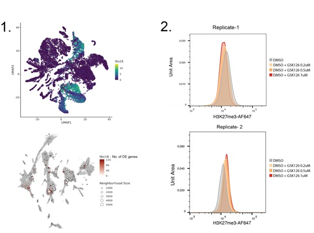
      I have some concerns and comments below: 1. The new algorithm described in the study selected omics variables by assigning response variable to decision tree nodes. How the response variables relate to biological responses/outcomes? From the authors' description, it seems that the selected omics variables using the IMD are almighty, i.e., they can predict anything needed, such as prognosis, cancer types, and et al. Actually, the usual logic to select omics variables to predict prognosis is to evaluate the association between omics variables and survival time. 2. Following the discussion in 1, what is the biological meaning to extract shared biomarkers from multiple data layers? While it is straightforward to think that the shared biomarkers between multiple data layers or data types may induce the same biological responses, the unique biomarkers also matter depending on what biological responses we care. 3. The Introduction section is not sufficient. The biological significance and technical details of "extract shared biomarkers from multiple data layers" need to be explained in more details. 4. It is advised to provide some examples of the statement in the Introduction: "may fail to capture nonlinear interactions" of the current methods (sPLS, CCA). 5. It is also advised to explain and illustrate how the new method proposed in this study addressed the challenge of traditional methods for capturing nonlinear relationships. Ablation study could be one of the choices. 6. The authors showed that their new approach "uncovered known cancer biological relevant pathways". How about the functional enrichment of genes selected from traditional methods, such as sPLS, CCA? 7. The authors showed that the selected RNA-seq and ATAC-seq features using the new approach are able to capture the distinction between different cancer types (Figure 8). It is suggested to quantitatively evaluate this capability using metrics of recall, precision, and et al. to calculate how many samples are corrected classified and how many are mis-classified in comparison with other methods. 8. It is advised to re-find the Discussion. In what scenario their new method can be applied? What biological insights can be obtained and what can be missed by the new method? 9. The authors did not provide sufficient details about the datasets they used in the section Method. How many samples in TCGA? How many features did they use? How many features left after filtering? 10. Although the performance of the new approach showed some kind of superior in comparison with other methods, the authors only used the currently known databases. It is advised to apply their approach to additional testing datasets or real-world datasets to increase the confidence of the conclusion of this study. It is also observed that the performance of sPLS is better than others in some cases (Figure 4). 11. It is suggested to re-fine the figures. The labels and legends are too tiny to be seen. 12. There is no sub-figure labels a,b,c,d,e,f in Figure 8. The positions of sub-figure labels in Figure 3, Figure 4, Figure 5, Figure 7 are not correct.
    1. AbstractThe processing and analysis of magnetic resonance images is highly dependent on the quality of the input data, and systematic differences in quality can consequently lead to loss of sensitivity or biased results. However, varying image properties due to different scanners and acquisition protocols, as well as subject-specific image interferences, such as motion artifacts, can be incorporated in the analysis. A reliable assessment of image quality is therefore essential to identify critical outliers that may bias results. Here we present a quality assessment for structural (T1-weighted) images using tissue classification. We introduce multiple useful image quality measures, standardize them into quality scales and combine them into an integrated structural image quality rating to facilitate the interpretation and fast identification of outliers with (motion) artifacts. The reliability and robustness of the measures are evaluated using synthetic and real datasets. Our study results demonstrate that the proposed measures are robust to simulated segmentation problems and variables of interest such as cortical atrophy, age, sex, brain size and severe disease-related changes, and might facilitate the separation of motion artifacts based on within-protocol deviations. The quality control framework presents a simple but powerful tool for the use in research and clinical settings.Competing Interest StatementThe authors have declared no competing interest.

      This work has been peer reviewed in GigaScience (see https://doi.org/10.1093/gigascience/giaf146), which carries out open, named peer-review. These reviews are published under a CC-BY 4.0 license and were as follows:

      Reviewer 1: Chris Foulon

      The article presents a valuable effort towards standardising quality control methods and their evaluation. However, too many choices seem arbitrary without sufficient justification, and too many sections are unclear. Overall, the quality of the work cannot be fully assessed in the current state of the manuscript, and major revisions are needed to correct that. There is also not enough comparison (one) with other methods and no way of evaluating whether these measures are relevant to actual downstream imaging uses. Additionally, the article's goal is highly unclear and led me to think the segmentation measures were part of the QC pipeline until I read the discussion ... Nothing until the discussion explains that the segmentation measures are used to evaluate the single SIQR score output of the QC pipeline.

      Comments: "All measures and tools are part of the Computational Anatomy Toolbox (CAT; https://neuro-jena.github.io//cat, Gaser et al., 2024) of the Statistical Parametric Mapping (SPM; http://www.fil.ion.ucl.ac.uk/spm, Ashburner et al. 2002) software and also available as a standalone version (https://neuro-jena.github.io/enigma-cat12/#standalone)." I cannot really expect everyone to avoid Matlab tools. Still, Matlab is a drag to the development of scalable tools nowadays (every system admin's nightmare is to have to try to make Matlab tools run on high-performance computing servers).

      "such as noise, inhomogeneities, and resolution (Figure 1B)." At this point in the article, it's a bit unclear how that works in Figure 1B.

      "It is assessed within optimized cerebrospinal fluid (CSF) and white matter (WM) regions." Then, the NCR relies on the segmentation, right? What if the segmentation fails?

      Oh, most of the measures actually rely on the segmentation. Are segmentation errors accounted for in the tool? I am thinking specifically about "abnormal" brains that can be difficult for segmentation algorithms. At least at this point of the article, it's not clear.

      "To accommodate various international rating systems, we have adopted a linear percentage and a corresponding (alpha-)numeric scaling." this doesn't match the complexity of the following explanation about the rather arbitrary range. I think a much more international and understandable rating would have been a 0 to 1 range. A 0.5 to 10.5 range is not helping users at all. As the rating is linear, I am struggling to see the added value of this choice.

      "Although the BWP does not include the simulation of motion artifacts, these are in general comparable to an increase of noise in the BWP dataset by 2 percentage points." Maybe that should be justified with a reference? "in general" might be a bit light to justify not having a direct measure for something presented as important (motion artefacts) in the introduction and goal of the tool. I think the absence of a noise estimation in the QC ratings should be more thoroughly justified.

      "To balance the sensitivity to different quality measures while ensuring that the necessary quality conditions are met, we apply an exponentially weighted averaging approach — similar to the root mean square (RMS) but using the fourth power and fourth root." Why is there no justification or references for these arbitrary choices? Why not the fifth root or tenth root? Why the square root and not an exponential or any other function?

      "Sample Normalization for Outlier Detection" It is unclear whether this is systematically applied or not. Is it a separate measure, or is it aggregated into another score? That measure could be relevant in many cases but could also be really bad in some specific cases (for example, historical data where the "ideal" quality would probably be well below standards.

      "raw (co-registered)" Well, it is not raw if it's co-registered. I suggest reformulation to avoid confusion with actual raw images.

      The "Evaluation Concept and Data" section is very unclear. The need for a training-testing scheme is not explained, and the scheme itself is very arbitrary (choosing odd and even numbered files ordered by filenames). How does that splitting strategy help with generalisation? Why that specific split? Why not another? How do we know that split is not biased? Finally, the selection of 6 scans also seems completely arbitrary. Overall, this section does not provide enough information to justify the seemingly arbitrary choices.

      "Of note, obvious subject/scan-specific motion artifacts generally increase the scans' rating for about 1 grade, which corresponds to a decrease of 10 rps (and +0.5 grade / -5 rps for light artifacts), in comparison to the typical rating achieved by the majority of scans of the same protocol." This is incredibly vague! How are readers supposed to evaluate the quality control measures with this information?

      Discussion: "as this is more relevant for segmentation and surface reconstruction (Ashburner et al., 2005)." A lot of work has been done in these domains in 20 years; this reference, however solid, is not enough to justify that choice. This might not be relevant with the methods developed in the last 20 years.

      "with a power of 4 rather than 2, to place greater emphasis on the more problematic aspects of image quality." Still not enough to justify that choice. The authors failed to convince me that one single score is better than reporting all the measures significantly, as different quality measures will influence different tasks. A very practical example is the fact that the vast majority of acquisitions in clinical settings, the resolution is anisotropic (though less with T1 images nowadays, historical datasets will still have it). This anisotropy is not necessarily an issue for human diagnosis, for example; however, aggregating all the scores in one might hide that a low-quality measurement might not affect the specific downstream task. Coupled with the lack of justification for the factor scalings, this choice of a single score is a significant negative point for the tool.

      Data availability: Where can the sources of these specific tools be accessed?

    1. R0:

      Review Comments to the Author

      Please use the space provided to explain your answers to the questions above. You may also include additional comments for the author, including concerns about dual publication, research ethics, or publication ethics. (Please upload your review as an attachment if it exceeds 20,000 characters)

      Reviewer #1: 1. The manuscript primarily shows that adding a visual inspection step increased the proportion of prosthetic feet deemed usable (83% to 94%). This outcome is predictable and does not constitute meaningful scientific innovation. The work reads as an operational description rather than rigorous research; novelty and contribution are therefore limited. 2. The proposed checklist is not validated. There is no mechanical or structural testing, no clinical functional outcomes, no prospective field evaluation, no inter-rater reliability assessment, and no sensitivity or specificity analysis. Accordingly, the checklist cannot be considered a standard, and the conclusions overstate the evidence. A formal validation phase is required. 3. Safety, mechanical integrity, and lifespan have not been evaluated. Visual inspection alone is inadequate for medical devices. No ISO-aligned static or cyclic loading tests are presented, nor are durability or time-in-service data available. This is a critical omission given the manuscript’s intent to inform international practice. 4. No patient-level outcomes are included (for example, fit success, comfort, skin issues, mobility, abandonment, repair frequency, or time-to-failure). Without these data, the practical value of the intervention remains uncertain. 5. Brand-level comparisons are underpowered, and model-level or material-level analyses are not presented. Despite acknowledging this limitation, the manuscript still interprets brand-related effects. 6. The Introduction and narrative sections are disproportionately long and repetitive; substantial condensation is recommended. In contrast, the Methods and Results require greater depth and clarity. 7. The statistical analysis is limited. Logistic models do not account for key confounders such as service age, storage duration, materials, or model type. Model diagnostics, effect sizes with confidence intervals, and multiple-comparison considerations are not reported. 8. Economic evaluation is absent. Donation and reuse programs in low and middle income settings are cost sensitive, and without cost modeling, the recommendations have limited actionable value. 9. Several claims are overstated, including suggestions related to circular economy effects, international standard development, and safety assurance. These assertions are not supported by the presented data and should be moderated.

      Reviewer #2: It is suggested to review the Nippon Foundation/Exceed Cambodia in proposing the standards of P&O. The case study that has been done in Cambodia, Myanmar, Laos, Vietnam and Sri Lanka in will guide the current P&O Standard in low and middle income countries.

      It is best to review the minimum standards of P&O in these countries as a underlying theory to govern the foundation of foot reuse and donation used.

      A robust systematic reviews are vital in proposing standards for foot reuse and donations used in low and middle income countries. An updated literature are needed.

      It is suggested to explore the preliminary findings in these low and middle income countries.

      Reviewer #3: GENERAL This reviewer welcomes the ambition of the authors to start developing standards for donated prosthetic componentry to LMICs. Such standards are indeed much needed as one important factor to improve the quality of the prosthetic devices provided within LMICs.

      The authors’ work has carefully been imbedded into a wealth of information and reasons for why the need is urgent for developing standards of donated prosthetic components. This information has been mindfully drafted including viewpoints and situation of many LMICs as well as HICs. Well done!

      What left this reviewer wondering is why the development of the checklist has not been carried out with locals at the two centers, where MB and PM were able to collect the data of the stored feet. The rationale for not doing so should be included into the Limitations section.

      Further, why has no testing of the developed checklist been carried out with the two centers? For example, dividing the available feet into two equal sized groups would have raised the opportunity to develop the checklist with one group of feet including the regression model and then test it on the remaining feet in the second group. Why was this not considered? One could classify all available feet as indicated in Table 1, but then consider only these feet who were mostly used in the field or were mostly available. Lowering the numbers of independent variables to the those variables that would represent the essence of the checklist best would have given the option for a regression model, or is this reviewer mistaken? These points should be discussed in the paper. In case the paper gets too long (word count), it is recommended to concise the actual discussion section as it provides similar points stated in the introduction.

      And lastly, this reviewer does not think that retesting used feet similar to the stated ISO standards would be feasible. Instead, it might be worthwhile checking in other industries (aviation, deep-sea shipping) what type of non-mechanical controls for checking of wear and tear on materials/motors are available without dismantling motors or testing of used structures. Perhaps some light and/or sonar evaluation would be a way to check the mechanical structure of used prosthetic feet and other componentry without putting any more strain on the used materials. That might be some thoughts for the Future Work section. Also probable collaboration with universities in LMICs should be considered as a close source of additional brain power for the development of standards within a given country.

      DETAILED The reviewer finds the word ‘prosthetics’ difficult and prefers the (correct) term ‘prosthetic componentry or prosthetic components’ instead. In her experience using the nomenclature of the P/O profession adds clarity in an interdisciplinary context. It is often unclear to people outside of or adjacent to the P/O profession that a ‘prosthetics’ is composed of different products, i.e. some industrial produced prosthetic components and – in most cases – a bespoken locally fabricated prosthetic socket. By using prosthetic components or prosthesis/prostheses when referring to the final product – the authors will signal directly that there are ‘pieces’ needed to compose an entire prosthesis. Further, using the correct term assists in distinguishing prostheses fabricated with componentry from those being fabricated by 3D printing, also a field needing standards for C2C design. Therefore, please change the wording accordingly within the entire paper – thank you!

      Lines 165-168. This sentence seems to be incomplete – please check.

      Line 229. This statement is incorrect. In Switzerland (and the reviewer is sure this is the case in France, Netherlands and the UK), prosthetic componentry has different life/warranty cycles depending on the type of prosthetic component and its model. Please rephrase this sentence pointing out that different prosthetic components and their models have different life/warranty cycles set by the industrial manufacturers.

      Lines 284-286.This sentence is unclear: Are the authors checking prosthetic feet shipped to Africa prior to the study or as part of the study when these feet arrive in Africa? If they are analyzed prior to the study how do the authors make sure that the damage seen is indeed due to shipping and not due to storage, for example? If the authors controlled feet within the study time period, would the sentence not needed to be stated “… we review prosthetic feet ALSO in Africa.”? Or did the authors not review the feet at the study place, but only in Africa? Please clarify and rephrase – thank you. These clarifications/details seem to be better placed within the Materials and Methods Chapter.

      Lines 287-311, in particular lines 311-317. Because the authors use an experimental setup, variables are usually considered as ‘independent’ or ‘dependent’. Please clarify what variables (independent, dependent) were considered. All variables the authors used to classify the different feet need be listed together with the rationale for the decision to include them into the regression model, including their order.

      Ok – are the variables listed on line 314 the once considered as independent variables to classify a prosthetic foot as ‘reusable’ or ‘not reusable’? If so, why? In other words, why do the authors consider the ‘brand’ to be more important than the condition of the foot itself? Or is it the case because only those feet that passed the visual test of being 'usable' were included into the regression model? Up to this point, this reviewer understood the aim of the study as being to develop a set of criteria to classify a prosthetic foot as reusable or not. If a visual pre-selection needs to be carried out first, how good/robust is the regression model that follows? Please clarify and add this clarification to the text – thank you.

      Lines 296-298. What variables (the authors call them ‘flaws’, if understood correctly) did the authors consider during the usability tests? How were these tests carried out? What happened with the feet the authors did consider as ‘not usable’: where they removed from the total sample of 366 feet (see below remarks to line 319)? For illustration: assuming the authors used for their visual check a variable called ‘cracks within the cosmetic’: did the authors classify a foot as still usable when only surface cracks were available, or did they exclude any foot with a crack in its shell? What were the criteria to classify a SACH foot as ‘usable’? More detailed information about the entire method for the visual checks and the resulting classification needs to be stated.

      When did the authors add any of this variable into the regression model and they give some of the variables a weighting, i.e. were some of the variables considered more important than others, and if so, why? Please add this information and make a reference to Table 2 or better, create a new Table or flowchart showing the authors thoughts and decision process including the variables used upon which they based their decision to classify a foot as ‘usable’ or ‘not usable’. Clarification on this matter will strengthen the work as it helps the reader to better understand the authors’ rationale – thank you!

      Line 319. Please start the results section with “A total of 366 feet where analyzed, 196 left and 170 right feet…”

      Line 320. Please add “… and A brand could be identified for… ” – thank you.

      Lines 320-322. Based on the information given in Table 1, there were 12 brands identified as categories plus one category with feet unknown to the authors. Because ‘unknown’ is not a brand, the sentence needs to be rephrased – thank you.

      Lines 353-357. These sentences seem to be missing some text, at least, they do not make sense to this reviewer. In lines 353-355 the authors state that the feet of Trulife and Ossur performed worst. Then in the following lines the authors state that they are (nevertheless??) considered as appropriate for donation. Please clarify – thank you.

      Table 4. Please explain/add, either in the corresponding text (lines 350 and subsequently) how the negative signs have to be read. Why has the measurement made against ‘BioQuest’ and not ‘Janton’ and how do the authors explain the difference in the coefficient between these two feet? Both feet were represented with n=1, why is there a difference? Please explain and add the clarification into the text within the Discussion section – thank you.

      Figure 2. Please add to Fig. 2, a, b, and c, as done in Fig. 1. This assists in clarifying matters. Please add this clarification into the text: line 364 = Figure 2a; line 378: delete (Figure 2) and add after ‘NCRPPD’ (Figure 2b); line 379: add (Figure 2c) after ‘K4C’.

      Line 388. Add at the end of the sentence ‘(Figure 3)’.

      Line 395. Please expand this sentence like or similar as proposed “…can be a burden to the recipient LMIC [31, 39,40], as indicated by Marks et al (2019 – Please check PLOS rules!!):” and then have the quotation followed. This will connect the quotation with the text and makes it easier to read.

      Line 469. Please check this sentence – the word ‘design’ seems to be twice stated. If this is correct, consider rephrasing as the sentence reads strange, thank you.

      Checklist questions: • Question (1): Please add example of ‘completeness’ of a prosthetic foot, as you did for Question 2. • Question (3): Add examples of what the authors consider ‘compliant’: forefoot, heel, middle section? All of these, only one? Usable for light persons, like children if only one part of the foot is too compliant? If so, which one do the authors consider as the most important variable for a foot to be still considered ‘usable’?

      Line 529. Word missing: “..cost of what” was the biggest barrier? Please complete.

      Line 533. Please consider replacing ‘in this way’ with ‘Therefore’ or similar that would connect clearer the content of the previous paragraph with this new one.

      Line 544. Typos: ‘reduce’ instead of ‘reduces’, ‘limit’ instead of ‘limits’.

      Line 567. Stop the sentence after ‘repair of equipment’ and continue with a new sentence starting, for example with “Hamner et al (please check PLOS rules!!) point out that … and than add the quotation.

      Line 570. Please delete ‘etc.’ This should not be used in a text as it lefts the reader wonder what else – in this case – could have had an influence. Instead write ‘for example’ and list the three most missing points that were not considered.

      Line 620. Keep the number correct: the authors tested 306 feet. The number speaks for itself, no need to bolster it. To this reviewer bolstering looks bad, stay with the figures.

      Line 622. Replace ‘are’ with ‘were’, as this was the case for the authors' sample. Samples of other authors might vary.

    1. Pew Research Center has been studying online harassment for several years now. A new report on Americans’ experiences with and attitudes toward online harassment finds that 41% of U.S. adults have personally experienced some form of online harassment – and the severity of the harassment has increased since we last studied it in 2017. We spoke with Emily Vogels, a research associate at the Center focusing on internet and technology research, about the new findings. The interview has been edited for clarity and condensed. One of the big takeaways from this report – and, to me, the biggest surprise – is that, while the overall number of people facing online harassment seems to be more or less stable, the nature of the harassment has changed over time. What are some of the most significant ways in which online harassment has worsened since we first started studying it? Emily Vogels, research associate at Pew Research Center While the overall number of those facing at least one of the six problems we ask about hasn’t changed, this survey finds that the level of harassment is increasing in two key ways: People are more likely to have encountered multiple forms of harassment online, and severe encounters have become more common. When the Center began studying online harassment in 2014, we found that 35% of American adults had experienced it. That grew to 41% in 2017 and remains the same in the new survey. But the shares who have ever experienced more severe forms of harassment – such as physical threats, stalking, sexual harassment or sustained harassment – or multiple forms of harassing behaviors online have both risen substantially in the past three years. This is not the pattern we saw in prior surveys. There has been a markedly steeper rise in these measures since 2017, compared with the change between our 2014 and 2017 studies. The shares who have ever experienced more severe forms of harassment or multiple forms of harassing behaviors online have both risen substantially in the past three years. Also, when we ask people about their most recent harassment experience, they’re more likely than in the past to include these more severe behaviors and involve multiple forms of harassment. And as of 2020, 41% of online harassment targets say their most recent experience spanned multiple locations online – for example, a person being harassed on social media and by text message. Does this suggest that online harassment is, to some extent, becoming “normalized”? It is commonplace. Roughly four-in-ten American adults say they’ve personally experienced harassment online. These numbers are more staggering when we look at adults under 30 – 64% of them say they’ve faced such issues online and 48% say they’ve experienced at least one of the more severe types of harassment. In addition, previous work by the Center found that a majority of adults overall have witnessed others being harassed online. Even when online harassment hasn’t been the focus of our research, we have seen this online incivility play a role in people’s perceptions and experiences of other online phenomena, such as online dating, political discussions on social media and social media in general. The Center’s past research on harassment has shown there are some demographic differences in the kinds of problems people face online. What did this survey show in particular about men, women and harassment? Men are slightly more likely than women to encounter at least one of the six types of online harassment we asked about, but there are notable differences in the types of harassment they encounter. Men are more likely than women to be called an offensive name or be physically threatened. Women are about three times as likely as men to face sexual harassment online, and younger women are even more likely to experience this type of abuse. Another difference in the new survey is that sexual harassment of women has doubled in the past three years, while the rate of sexual harassment among men is largely the same as in 2017. Women who have been the target of online harassment also report finding their most recent harassment experiences to be more upsetting than their male counterparts. There are also differences in where men and women encountered harassment online in their most recent experience. Social media sites are the most common location regardless of gender, but a larger share of women who have been harassed say their most recent incident was on social media, compared with men who have been targeted. Men targeted in online harassment are more likely than women to have been harassed while online gaming or while using an online forum or discussion site. Beyond personal experiences, men and women express different attitudes about online harassment, with women more likely to say it’s a major problem. And prior Center work finds that a greater share of women than men value people feeling safe online over people being able to speak their minds freely. When it comes to how to address online harassment, women are more optimistic than men about a variety of potential solutions, including criminal charges for social media users who harass others online, temporary or permanent bans for users who harass others, and social media companies proactively deleting bullying or harassing posts. Interesting. To what extent do those gender differences in harassment experiences reflect differences in men’s and women’s online activities? Men are more likely to report they had these types of experiences in online forums or gaming platforms. Is that because more men than women use such platforms? It’s a bit complicated. Prior work from the Center suggests there are modest gender differences in gaming, with men being more likely than women to at least sometimes play video games. But this study didn’t ask if people played games online, so we can’t say whether the gender differences in harassment incidents tied to gaming hold when looking at just online gamers. It’s worth keeping in mind that the data on where people were harassed online is for people’s most recent incident, not every incident these folks may have encountered in the past. Prior Center findings show people may stop engaging in an activity – for example, withdrawing from a platform or deleting a social media account – if they encounter harassment. Similarly, do the age differences in those who say they have experienced harassment reflect how many, and how frequently, people of different ages are online? In other words, does the fact that far more adults under 30 report experiencing online harassment reflect younger people spending much more of their lives online than older folks? We don’t quite have enough evidence to make this causal connection, but the broad patterns are pretty clear. This survey found that adults under 30 consistently experience each of the six forms of harassment we asked about at higher rates than any other age group. The Center’s previous work does show that younger adults are more likely to use the internet and to use it almost constantly. Our research on teens in 2018 found that greater exposure to the internet puts people at a higher likelihood of encountering harassment at some point online. It’s worth noting, though, that non-internet users were not asked about their possible experiences with online harassment. So, if people stopped using the internet sometime after they were harassed online, our data wouldn’t capture their earlier harassment experience. The survey finds that 75% of targets of online harassment say their most recent experience was on social media. Has this been true since the Center began researching online harassment? Do people feel social media companies have done enough to discourage this behavior? Fully 79% of Americans think social media companies are doing an only fair to poor job when it comes to addressing online harassment or bullying. The share of online harassment targets who say their most recent harassing encounter took place on social media is growing – up 17 percentage points since 2017. The Center’s prior work reveals a variety of negative opinions Americans hold about social media companies, and when it comes to Americans’ views of how these companies handle online harassment, the pattern of criticism continues. Fully 79% of Americans think social media companies are doing an only fair to poor job when it comes to addressing online harassment or bullying on their platforms. Based on previous Center findings, American teens hold similarly negative views of social media companies’ ability to address these issues. Many Americans suggest that permanent bans for users who harass others and required identity disclosure to use these platforms would be very effective ways to combat harassment on social media. To what extent do you think that the fact 2020 was an election year accounts for the increase in the number of people who say they were harassed because of their political views? Politics was already a heated issue long before this election. According to other research from the Center, partisan antipathy has been growing for years. Americans increasingly say they find they have less in common politically with people with whom they disagree, and they see political discussions online as less respectful, less civil and angrier than political discussions in other places. There are also some striking demographic differences among those who say they’ve been harassed for their politics. Online harassment targets who are White or male – 56% and 57% of each – are particularly likely to think their harassment was a result of their political views. This is especially true for White men who say they’ve been targeted, at 61%. Other groups commonly point to other aspects of their identity as the reason they faced harassment online. For example, roughly half or more Black or Hispanic online harassment targets – 54% and 47% respectively – identify their race or ethnicity as a reason they were harassed, while only 17% of their White counterparts say the same. Bear in mind that politics isn’t the only perceived reason for harassment being on the rise. Over the past several years, rising shares of online harassment targets have said they think they were harassed because of their gender, race, ethnicity, religion or sexual orientation.

      The government reports highlight that cyberbullying is widespread and often chronic, affecting many youth for long periods.

  4. Dec 2025
    1. Author response:

      The following is the authors’ response to the original reviews

      Reviewer #1 (Public review):

      The manuscript by Shan et al seeks to define the role of the CHI3L1 protein in macrophages during the progression of MASH. The authors argue that the Chil1 gene is expressed highly in hepatic macrophages. Subsequently, they use Chil1 flx mice crossed to Clec4F-Cre or LysM-Cre to assess the role of this factor in the progression of MASH using a high-fat, high-cholesterol diet (HFHC). They found that loss of Chil1 in KCs (Clec4F Cre) leads to enhanced KC death and worsened hepatic steatosis. Using scRNA seq, they also provide evidence that loss of this factor promotes gene programs related to cell death. From a mechanistic perspective, they provide evidence that CHI3L serves as a glucose sink and thus loss of this molecule enhances macrophage glucose uptake and susceptibility to cell death. Using a bone marrow macrophage system and KCs they demonstrate that cell death induced by palmitic acid is attenuated by the addition of rCHI3L1. While the article is well written and potentially highlights a new mechanism of macrophage dysfunction in MASH, there are some concerns about the current data that limit my enthusiasm for the study in its current form. Please see my specific comments below.

      (1) The authors' interpretation of the results from the KC (Clec4F) and MdM KO (LysM-Cre) experiments is flawed. For example, in Figure 2 the authors present data that knockout of Chil1 in KCs using Clec4f Cre produces worse liver steatosis and insulin resistance. However, in supplemental Figure 4, they perform the same experiment in LysM-Cre mice and find a somewhat different phenotype. The authors appear to be under the impression that LysM-Cre does not cause recombination in KCs and therefore interpret this data to mean that Chil1 is relevant in KCs and not MdMs. However, LysM-Cre DOES lead to efficient recombination in KCs and therefore Chil1 expression will be decreased in both KCs and MdM (along with PMNs) in this line.

      Therefore, a phenotype observed with KC-KO should also be present in this model unless the authors argue that loss of Chil1 from the MdMs has the opposite phenotype of KCs and therefore attenuates the phenotype. The Cx3Cr1 CreER tamoxifen inducible system is currently the only macrophage Cre strategy that will avoid KC recombination. The authors need to rethink their results with the understanding that Chil1 is deleted from KCs in the LysM-Cre experiment. In addition, it appears that only one experiment was performed, with only 5 mice in each group for both the Clec4f and LysM-Cre data. This is generally not enough to make a firm conclusion for MASH diet experiments.

      We thank the reviewer for raising this important point regarding our data interpretation. We have carefully examined the deletion efficiency of Chi3l1 in primary Kupffer cells (KCs) from Lyz2<sup>∆Chil1</sup> (LysM-Cre) mice. Our results show roughly a 40% reduction in Chi3l1 expression at both the mRNA and protein levels (Revised Manuscript, Figure S7B and C). Given this modest decrease, Chi3l1 deletion in KCs of Lyz2<sup>∆Chil1</sup> mice was incomplete, which likely accounts for the phenotypic differences observed between Clec4f<sup>∆Chil1</sup> and Lyz2<sup>∆Chil1</sup> mice in the MASLD model.

      Furthermore, we have increased the sample size in both the Clec4f- and LysM-Cre experiments to 9–12 mice per group following the HFHC diet, thereby strengthening the statistical power and reliability of our findings (Revised Figures 2 and S8).

      (2) The mouse weight gain is missing from Figure 2 and Supplementary Figure 4. This data is critical to interpret the changes in liver pathology, especially since they have worse insulin resistance.

      We thank the reviewer for this valuable comment. We have now included the mouse body weight data in the revised manuscript (Figure 2A, B and Figures S8A, B). Compared with mice on a normal chow diet (NCD), all groups exhibited progressive weight gain during HFHC diet feeding. Notably, Clec4f<sup>∆Chil1</sup> mice gained significantly more body weight than Chil1<sup>fl/fl</sup> controls, whereas Lyz2<sup>∆Chil1</sup> mice showed a similar weight gain trajectory to Chil1<sup>fl/fl</sup> mice under the same conditions.

      (3) Figure 4 suggests that KC death is increased with KO of Chil1. However, this data cannot be concluded from the plots shown. In Supplementary Figure 6 the authors provide a more appropriate gating scheme to quantify resident KCs that includes TIM4. The TIM4 data needs to be shown and quantified in Figure 4. As shown in Supplementary Figure 6, the F4/80 hi population is predominantly KCs at baseline; however, this is not true with MASH diets. Most of the recruited MoMFs also reside in the F4/80 hi gate where they can be identified by their lower expression of TIM4. The MoMF gate shown in this figure is incorrect. The CD11b hi population is predominantly PMNs, monocytes, and cDC,2 not MoMFs (PMID:33997821). In addition, the authors should stain the tissue for TIM4, which would also be expected to reveal a decrease in the number of resident KCs.

      We thank the reviewer for raising this critical point regarding the gating strategy and interpretation of KC death. We have now refined our flow cytometry gating based on the reviewer’s suggestion. Specifically, we analyzed TIM4 expression and attempted to identify TIM4<sup>low</sup> MoMFs populations in our model. However, we did not detect a distinct TIM4<sup>low</sup> population, likely because our mice were fed the HFHC diet for only 16 weeks and had not yet developed liver fibrosis. We therefore reason that MoMFs have not fully acquired TIM4 expression at this stage.

      To improve our analysis, we referred to published strategies (PMID: 41131393; PMID: 32562600) and gated KCs as CD45<sup>+</sup>CD11b<sup>+</sup>F4/80<sup>hi</sup> TIM4<sup>hi</sup> and MoMFs as CD45<sup>+</sup>Ly6G<sup>-</sup>CD11b<sup>+</sup>F4/80<sup>low</sup> TIM4<sup>low/-</sup>. Using this approach, we observed a gradual reduction of KCs and a corresponding increase in MoMFs in WT mice, with a significantly faster loss of KCs in Chil1<sup>-/-</sup> mice (Revised Figure 4C, D; Figure S10A).

      Furthermore, immunofluorescence staining for TIM4 combined with TUNEL or cleaved caspase-3 confirmed an increased number of dying KCs in Chil1<sup>-/-</sup> mice compared to WT following HFHC diet feeding (Revised Figure 4E; Figure S10B).

      (4) While the Clec4F Cre is specific to KCs, there is also less data about the impact of the Cre system on KC biology. Therefore, when looking at cell death, the authors need to include some mice that express Clec4F cre without the floxed allele to rule out any effects of the Cre itself. In addition, if the cell death phenotype is real, it should also be present in LysM Cre system for the reasons described above. Therefore, the authors should quantify the KC number and dying KCs in this mouse line as well.

      We thank the reviewer for raising this important point. During our study, we indeed observed an increased number of KCs in Clec4f-Cre mice compared to WT controls, suggesting that the Clec4f-Cre system itself may modestly affect KC homeostasis. To address this, we compared KCs numbers between Clec4f<sup>∆Chil1</sup> and Clec4f-Cre mice and found that Clec4f<sup>∆Chil1</sup> mice displayed a significant reduction in KCs numbers following HFHC diet feeding. Moreover, co-staining for TIM4 and TUNEL revealed a marked increase in KCs death in Clec4f<sup>∆Chil1</sup> mice relative to Clec4f-Cre mice, indicating that the observed phenotype is attributable to Chil1 deletion rather than Cre expression alone. These data have been reported in our related manuscript (He et al., bioRxiv, 2025.09.26.678483; doi: 10.1101/2025.09.26.678483).

      In addition, we quantified KCs numbers and KCs death in the Lyz2-Cre line. TIM4/TUNEL co-staining showed comparable levels of KCs death between Chil1<sup>fl/fl</sup> and Lyz2<sup>∆Chil1</sup> mice (Revised Figure S11B). Consistently, flow cytometry analyses revealed no significant differences in KCs numbers between these two groups before (0 weeks) or after (20 weeks) HFHC diet feeding (Revised Figures S11C, D). As discussed in our response to Comment 1, this may be due to the incomplete deletion of Chi3l1 in KCs (<50%) in the Lyz2-Cre line, which likely attenuates the phenotype.

      (5) I am somewhat concerned about the conclusion that Chil1 is highly expressed in liver macrophages. Looking at our own data and those from the Liver Atlas it appears that this gene is primarily expressed in neutrophils. At a minimum, the authors should address the expression of Chil1 in macrophage populations from other publicly available datasets in mouse MASH to validate their findings (several options include - PMID: 33440159, 32888418, 32362324). If expression of Chil1 is not present in these other data sets, perhaps an environmental/microbiome difference may account for the distinct expression pattern observed. Either way, it is important to address this issue.

      We thank the reviewer for this insightful comment and agree that analysis of scRNA-seq data, including our own and those reported in the Liver Atlas as well as in the referenced studies (PMID: 33440159, 32888418, 32362324), indicates that Chil1 is predominantly expressed in neutrophils.

      However, our immunofluorescence staining under normal physiological conditions revealed that Chi3l1 protein is primarily localized in Kupffer cells (KCs), as demonstrated by strong co-staining with TIM4 (Revised Figure 1E). In MASLD mouse models induced by HFHC or MCD diets, we observed that both KCs and monocyte-derived macrophages (MoMFs) express Chi3l1, with particularly high levels in MoMFs.

      We speculate that the apparent discrepancy between scRNA-seq datasets and our in situ findings may reflect differences in cellular proportions and detection sensitivity. Since hepatic macrophages (particularly KCs and MoMFs) constitute a larger proportion of total liver immune cells compared with neutrophils, their contribution to total Chi3l1 protein levels in tissue staining may appear dominant, despite lower transcript abundance per cell in sequencing datasets. We have included a discussion of this point in the revised manuscript to clarify this distinction (Revised manuscript, page 8,line 341-350 ).

      Minor points:

      (1) Were there any changes in liver fibrosis or liver fibrosis markers present in these experiments?

      We assessed liver fibrosis using Sirius Red staining and α-SMA Western blot analysis.

      We found no induction of liver fibrosis in our HFHC-induced MASLD model (Revised Figure S1A, B), but a clear elevation of fibrosis markers in the MCD-induced MASH model (Revised Figure S6A, B).

      (2) In Supplementary Figure 3, the authors do a western blot for CHI3L1 in BMDMs. This should also be done for KCs isolated from these mice. Does this antibody work for immunofluorescence? Staining liver tissue would provide valuable information on the expression patterns.

      We have included qPCR and western blot for Chi3l1 in isolated primary KCs from Lyz2<sup>∆Chil1</sup> mice. The data show a slight, non-significant reduction in both mRNA and protein levels in KCs (Revised Figure S7B, C). The immunofluorescence staining on liver tissue showed that Chi3l1 is more likely expressed in the plasma membranes of TIM4<sup>+</sup> F4/80<sup>+</sup> KCs both under NCD and HFHC diet (Revised Figure 1E).

      (3) What is the impact of MASH diet feeding on Chil1 expression in KCs or in the liver in general?

      In both our MASLD and MASH models, diet feeding consistently upregulates Chi3l1 in KCs or in the liver in general (Revised Figure 1F, G, S6C,D).

      (4) In Figure S1 the authors show tSNE plots of various monocyte and macrophage genes in the liver. Are these plots both diets together? How do things look when comparing these markers between the STD and HFHC diet? The population of recruited LAMs seems very small for 16 weeks of diet. Moreover, Chil1 should also be shown on these tSNE plots as well.

      Yes, these plots are both diets together. When compared separately, the core marker expression is consistent between NCD and HFHC diets. However, the HFHC diet induces a relative increase in KC marker expression within the MoMF cluster, suggesting phenotypic adaptation (Author response image 1A, below). Moreover, Chil1 expression on the t-SNE plot was shown (Author response image 1B, below). However, compared to lineage-specific marker genes, Chi3l1 expression is rather low.

      Author response image 1.

      Gene expression levels of lineage-specific marker genes in monocytes/macrophages clusters between NCD and HFHC diets. (A) UMAP plots show the scaled expression changes of lineage-specific markers in KCs/monocyte/macrophage clusters from mice under NCD and HFHC diets. Color represents the level of gene expression. (B) UMAP plots show the scaled expression changes of Chil1 in KCs/monocyte/macrophage clusters from mice under NCD and HFHC diets. Color represents the level of gene expression.

      (5) In Figure 5, the authors demonstrate that CHI3L1 binds to glucose. However, given that all chitin molecules bind to carbohydrates, is this a new finding? The data showing that CHI3L is elevated in the serum after diet is interesting. What happens to serum levels of this molecule in KC KO or total macrophage KO mice? Do the authors think it primarily acts as a secreted molecule or in a cell-intrinsic manner?

      We thank the reviewer for these insightful comments, which helped us clarify the novelty of our findings.

      (1) Novelty of CHI3L1-Glucose Binding:

      While chitin-binding domains are known to interact with carbohydrate polymers, our key discovery is that CHI3L1 (YKL-40)—a mammalian chitinase-like protein lacking enzymatic activity—specifically binds to glucose, a simple monosaccharide. This differs fundamentally from canonical binding to insoluble polysaccharides such as chitin and reveals a potential role for CHI3L1 in monosaccharide recognition, linking it to glucose metabolism and energy sensing. We clarified this point in the revised manuscript (page 9, line374-379).

      (2) Serum CHI3L1 in Knockout Models:

      Consistent with the reviewer’s suggestion, serum Chi3l1 levels are altered in our knockout models:

      KC-specific KO (Clec4f<sup>ΔChil1</sup>): Under normal chow, serum CHI3L1 is markedly reduced compared to controls and remains lower following HFHC feeding (Author response image 2A, below), indicating that Kupffer cells are the main source of circulating CHI3L1 under basal and disease conditions.

      Macrophage KO (Lyz2<sup>ΔChil1</sup>): No significant changes were observed between Chil1<sup>fl/fl</sup> and Lyz2<sup>ΔChil1</sup> mice under either diet (Author response image 2B, below), likely due to minimal monocyte-derived macrophage recruitment in this HFHC model (see Revised Figure 4C,D).

      (3) Secreted vs. Cell-Intrinsic Role:

      CHI3L1 predominantly localizes to the KC plasma membrane, consistent with a secreted role, and its serum reduction in KC-specific knockouts supports the physiological relevance of its secreted role. While cell-intrinsic effects have been reported elsewhere, our current data do not address this in KCs and warrant future investigation.

      Author response image 2.

      Chi3l1 expression in serum before and after HFHC in CKO mice. (A) Western blot to detect Chi3l1 expression in serum of Chil1<sup>fl/fl</sup> and Clec4f<sup>ΔChil1</sup> mice before and after 16 weeks’ HFHC diet. n=3 mice/group. (B) Western blot to detect Chi3l1 expression in serum of Chil1<sup>fl/fl</sup> and Lyz2ΔChil1 before and after 16 weeks’ HFHC diet. n=3 mice/group.

      Reviewer #2 (Public review):

      The manuscript from Shan et al., sets out to investigate the role of Chi3l1 in different hepatic macrophage subsets (KCs and moMFs) in MASLD following their identification that KCs highly express this gene. To this end, they utilise Chi3l1KO, Clec4f-CrexChi3l1fl, and Lyz2-CrexChi3l1fl mice and WT controls fed a HFHC for different periods of time.

      Major:

      Firstly, the authors perform scRNA-seq, which led to the identification of Chi3l1 (encoded by Chil1) in macrophages. However, this is on a limited number of cells (especially in the HFHC context), and hence it would also be important to validate this finding in other publicly available MASLD/Fibrosis scRNA-seq datasets. Similarly, it would be important to examine if cells other than monocytes/macrophages also express this gene, given the use of the full KO in the manuscript. Along these lines, utilisation of publicly available human MASLD scRNA-seq datasets would also be important to understand where the increased expression observed in patients comes from and the overall relevance of macrophages in this finding.

      We thank the reviewer for this valuable suggestion and acknowledge the limited number of cells analyzed under the HFHC condition in our original dataset. To strengthen our findings, we have now examined four additional publicly available scRNA-seq datasets— two from mouse models and two from human MASLD patients (Revised Figure S3, manuscript page 4, line 164-172). Across these datasets, the specific cell type showing the highest Chil1 expression varied somewhat between studies, likely reflecting model differences and disease stages. Nevertheless, Chil1 expression was consistently enriched in hepatic macrophage populations, including both Kupffer cells and infiltrating macrophages, in mouse and human livers. Notably, Chil1 expression was higher in infiltrating macrophages compared to resident Kupffer cells, supporting its upregulation during MASLD progression. These additional analyses confirm the robustness and crossspecies relevance of our finding that macrophages are the primary Chil1-expressing cell type in the liver.

      Next, the authors use two different Cre lines (Clec4f-Cre and Lyz2-Cre) to target KCs and moMFs respectively. However, no evidence is provided to demonstrate that Chil1 is only deleted from the respective cells in the two CRE lines. Thus, KCs and moMFs should be sorted from both lines, and a qPCR performed to check the deletion of Chil1. This is especially important for the Lyz2-Cre, which has been routinely used in the literature to target KCs (as well as moMFs) and has (at least partial) penetrance in KCs (depending on the gene to be floxed). Also, while the Clec4f-Cre mice show an exacerbated MASLD phenotype, there is currently no baseline phenotype of these animals (or the Lyz2Cre) in steady state in relation to the same readouts provided in MASLD and the macrophage compartment. This is critical to understand if the phenotype is MASLD-specific or if loss of Chi3l1 already affects the macrophages under homeostatic conditions.

      We thank the reviewer for raising this important point.

      (1) Chil1 deletion efficiency in Clec4f-Cre and Lyz2-Cre lines:

      We have assessed the efficiency of Chil1 deletion in both Lyz2<sup>∆Chil1</sup> and Clec4f<sup>∆Chil1</sup> mice by evaluating mRNA and protein levels of Chi3l1. For the Lyz2<sup>∆Chil1</sup> mice, we measured Chi3l1 expression in bone marrow-derived macrophages (BMDMs) and primary Kupffer cells (KCs). Both qPCR (for mRNA) and Western blotting (for protein) reveal that Chi3l1 is almost undetectable in BMDMs from Lyz2<sup>∆Chil1</sup> mice when compared to Chil1<sup>fl/fl</sup> controls. In contrast, we observe no significant reduction in Chi3l1 expression in KCs from these animals (Revised Figure S7B, C), suggesting Chil1 is deleted in BMDMs but not in KCs in Lyz2-Cre line.

      For the Clec4f<sup>∆Chil1</sup> mice, both mRNA and protein levels of Chi3l1 are barely detectable in BMDMs and primary KCs when compared to Chil1<sup>fl/fl</sup> controls (Revised Figure S4B, C). However, we did observe a faint Chi3l1 band in KCs of Clec4f<sup>∆Chil1</sup> mice, which we suspect is due to contamination from LSECs during the KC isolation process, given that the TIM4 staining for KCs was approximately 90%. Overall, Chil1 is deleted in both KCs and BMDMs in Clec4f-Cre line.

      Notably, since we observed a pronounced MASLD phenotype in Clec4f-Cre mice but not in Lyz2-Cre mice, these findings further underscore the critical role of Kupffer cells in the progression of MASLD.

      (2) Whether the phenotype is MASLD-specific or whether loss of Chi3l1 already affects the macrophages under homeostatic conditions: We now included phenotypic data of Clec4f<sup>ΔChil1</sup> mice (KC-specific KO) and Lyz2<sup>∆Chil1</sup> mice (MoMFs-specific KO) fed with NCD 16w (Revised Figure 2A-F, S8A-F). Shortly speaking, there is no baseline difference between Chil1<sup>fl/fl</sup> and Clec4f<sup>ΔChil1</sup> or Lyz2<sup>∆Chil1</sup> mice in steady state in relation to the same readouts provided in MASLD.

      Next, the authors suggest that loss of Chi3l1 promotes KC death. However, to examine this, they use Chi3l1 full KO mice instead of the Clec4f-Cre line. The reason for this is not clear, because in this regard, it is now not clear whether the effects are regulated by loss of Chi3l1 from KCs or from other hepatic cells (see point above). The authors mention that Chi3l1 is a secreted protein, so does this mean other cells are also secreting it, and are these needed for KC death? In that case, this would not explain the phenotype in the CLEC4F-Cre mice. Here, the authors do perform a basic immunophenotyping of the macrophage populations; however, the markers used are outdated, making it difficult to interpret the findings. Instead of F4/80 and CD11b, which do not allow a perfect discrimination of KCs and moMFs, especially in HFHC diet-fed mice, more robust and specific markers of KCs should be used, including CLEC4F, VSIG4, and TIM4.

      We thank the reviewer for raising this important point. We performed experiments in Clec4f<sup>∆Chil1</sup> (KC-specific KO) model. The phenotype in these mice closely mirrors that of the full KO: we observed a significant reduction in KC numbers and a concurrent increase in KC cell death following an HFHC diet in Clec4f<sup>∆Chil1</sup> mice post HFHC diet compared to Clec4f-cre mice. We have reported these data in the following related manuscript (Figure 6 D-G). This confirms that the loss of CHI3L1 specifically from KCs is sufficient to drive this effect.

      Hyperactivated Glycolysis Drives Spatially-Patterned Kupffer Cell Depletion in MASLD Jia He, Ran Li, Cheng Xie, Xiane Zhu, Keqin Wang, Zhao Shan bioRxiv 2025.09.26.678483; doi: https://doi.org/10.1101/2025.09.26.678483

      While other hepatic cells (e.g., neutrophils and liver sinusoidal endothelial cells) also express Chi3l1, our data indicate that KC-secreted Chi3l1 plays a dominant and cellautonomous role in maintaining KCs viability. The potential contribution of other cellular sources to this phenotype remains an interesting direction for future study.

      We apologize for the lack of clarity in our initial immunophenotyping. We have revised the flow cytometry data to clearly show that KCs are rigorously defined as TIM4+ cells (Revised Figure 4C, D).

      Additionally, while the authors report a reduction of KCs in terms of absolute numbers, there are no differences in proportions. Thus, coupled with a decrease also in moMF numbers at 16 weeks (when one would expect an increase if KCs are decreased, based on previous literature) suggests that the differences in KC numbers may be due to differences in total cell counts obtained from the obese livers compared with controls. To rule this out, total cell counts and total live CD45+ cell counts should be provided. Here, the authors also provide tunnel staining in situ to demonstrate increased KC death, but as it is typically notoriously difficult to visualise dying KCs in MASLD models, here it would be important to provide more images. Similarly, there appear to be many more Tunel+ cells in the KO that are not KCs; thus, it would be important to examine this in the CLEC4F-Cre line to ascertain direct versus indirect effects on cell survival.

      We thank the reviewer for raising this important point. We have now included the total cell counts and total live CD45<sup>+</sup> cell counts, which showed similar numbers between WT and Chil1<sup>-/-</sup> mice post HFHC diet (Figure 3A, below).

      Moreover, we included cleavaged caspase 3 and TIM4 co-staining in WT and Chil1<sup>-/-</sup> mice before and after HFHC diets, which confirmed increased KCs death in Chil1<sup>-/-</sup> mice (Revised Figure S10B). We have compared KCs number and KCs death between Clec4fcre and Clec4f<sup>∆Chil1</sup> mice under NCD and HFHC diet in the following manuscript (Figure 6 D-G). The data showed similar KCs number under NCD and reduced KCs number in Clec4f<sup>∆Chil1</sup> mice compared to Clec4f-cre mice, which confirms direct effects of Chi3l1 on cell survival but not because of cre insertion.

      Hyperactivated Glycolysis Drives Spatially-Patterned Kupffer Cell Depletion in MASLD Jia He, Ran Li, Cheng Xie, Xiane Zhu, Keqin Wang, Zhao Shan bioRxiv 2025.09.26.678483; doi: https://doi.org/10.1101/2025.09.26.678483

      Author response image 3.

      Number of total cells and total live CD45+ cells in liver of WT and Chil1<sup>-/-</sup> mice. (A) Number of total cells and total live CD45+ cells/liver were statistically analyzed. n= 3-4 mice per group.

      Finally, the authors suggest that Chi3l1 exerts its effects through binding glucose and preventing its uptake. They use ex vivo/in vitro models to assess this with rChi3l1; however, here I miss the key in vivo experiment using the CLEC4F-Cre mice to prove that this in KCs is sufficient for the phenotype. This is critical to confirm the take-home message of the manuscript.

      We agree that it is essential to confirm the in vivo relevance of Chi3l1-mediated glucose regulation in Kupffer cells (KCs). Our data suggest that KCs undergo cell death not because they express Chi3l1 per se, but because they exhibit a glucose-hungry metabolic phenotype that makes them uniquely dependent on Chi3l1-mediated regulation of glucose uptake. To directly assess this mechanism in vivo, we injected 2-NBDG, a fluorescent glucose analog, into overnight-fasted and refed mice and quantified its uptake in hepatic KCs. Notably, Chi3l1-deficient KCs exhibited significantly increased 2-NBDG uptake compared with controls, and this effect was markedly suppressed by co-treatment with recombinant Chi3l1 (rChi3l1) (Revised Figure 6G, H). These findings demonstrate that Chi3l1 regulates glucose uptake by KCs in vivo, supporting our proposed mechanism that Chi3l1 controls KC metabolic homeostasis through modulation of glucose availability.

      Minor points:

      (1) Some key references of macrophage heterogeneity in MASLD are not cited: PMID: 32362324 and PMID: 32888418.

      We thank the reviewer for highlighting these critical references and have included them in the introduction (Revised manuscript, page 2, line 64-73).

      (2) In the discussion, Figure 3H is referenced (Serum data), but there is no Figure 3H. If the authors have this data (increased Chi3l1 in serum of mice fed HFHC diet), what happens in CLEC4F-Cre mice fed the diet? Is this lost completely? This comes back to the point regarding the specificity of expression.

      We apologize for the mistake. It should be Figure 5F now in the revised version, in which serum Chi3l1 was significantly upregulated after HFHC diet. Moreover, under a normal chow diet (NCD), serum CHI3L1 is significantly lower in Clec4f<sup>ΔChil1</sup> mice compared to controls (Chil1<sup>fl/fl</sup>). Following an HFHC diet, levels increase in both genotypes but remain relatively lower in the KC-KO mice (please see Figure 2A above). This data strongly suggests that Kupffer Cells (KCs) are the primary source of serum CHI3L1 under basal conditions and a major contributor during MASLD progression.

      Reviewer #3 (Public review):

      This paper investigates the role of Chi3l1 in regulating the fate of liver macrophages in the context of metabolic dysfunction leading to the development of MASLD. I do see value in this work, but some issues exist that should be addressed as well as possible.

      (1) Chi3l1 has been linked to macrophage functions in MASLD/MASH, acute liver injury, and fibrosis models before (e.g., PMID: 37166517), which limits the novelty of the current work. It has even been linked to macrophage cell death/survival (PMID: 31250532) in the context of fibrosis, which is a main observation from the current study.

      We thank the reviewer for this insightful comment regarding the novelty of our findings. We agree that Chi3l1 has previously been linked to macrophage survival and function in models of liver injury and fibrosis (e.g., PMID: 37166517, 31250532). However, our study focuses specifically on the early stage of MASLD, prior to the onset of fibrosis, revealing a distinct mechanistic role for CHI3L1 in this context.

      We demonstrate that CHI3L1 directly interacts with extracellular glucose to regulate its cellular uptake—a previously unrecognized biochemical function. Furthermore, we show that CHI3L1’s protective role is metabolically dependent, safeguarding glucose-dependent Kupffer cells (KCs) but not monocyte-derived macrophages (MoMFs). This metabolic dichotomy and the direct link between CHI3L1 and glucose sensing represent conceptual advances beyond previous studies of CHI3L1 in fibrotic or injury models.

      (2) The LysCre-experiments differ from experiments conducted by Ariel Feldstein's team (PMID: 37166517). What is the explanation for this difference? - The LysCre system is neither specific to macrophages (it also depletes in neutrophils, etc), nor is this system necessarily efficient in all myeloid cells (e.g., Kupffer cells vs other macrophages). The authors need to show the efficacy and specificity of the conditional KO regarding Chi3l1 in the different myeloid populations in the liver and the circulation.

      We thank the reviewer for this important comment and the opportunity to clarify both the efficiency and specificity of our conditional knockouts, as well as the differences from the study by Feldstein’s group (PMID: 37166517).

      (1) Chil1 deletion efficiency in Clec4f-Cre and Lyz2-Cre lines:

      We have assessed the efficiency of Chil1 deletion in both Lyz2<sup>∆Chil1</sup> and Clec4f<sup>∆Chil1</sup> mice by evaluating mRNA and protein levels of Chi3l1. For the Lyz2<sup>∆Chil1</sup> mice, we measured Chi3l1 expression in bone marrow-derived macrophages (BMDMs) and primary Kupffer cells (KCs). Both qPCR (for mRNA) and Western blotting (for protein) reveal that Chi3l1 is almost undetectable in BMDMs from Lyz2<sup>∆Chil1</sup> mice when compared to Chil1<sup>fl/fl</sup> controls. In contrast, we observe no significant reduction in Chi3l1 expression in KCs from these animals (Revised Figure S7B, C), suggesting that Chil1 is deleted in BMDMs but not in KCs in Lyz2-Cre line.

      For the Clec4f<sup>∆Chil1</sup> mice, both mRNA and protein levels of Chi3l1 are barely detectable in BMDMs and primary KCs when compared to Chil1<sup>fl/fl</sup> controls (Revised Figure S4B, C). However, we did observe a faint Chi3l1 band in KCs of Clec4f<sup>∆Chil1</sup> mice, which we suspect is due to contamination from LSECs during the KC isolation process, given that the TIM4 staining for KCs was approximately 90%. Overall, Chil1 is deleted in both KCs and BMDMs in Clec4f-Cre line.

      Notably, since we observed a pronounced MASLD phenotype in Clec4f-Cre mice but not in Lyz2-Cre mice, these findings further underscore the critical role of Kupffer cells in the progression of MASLD.

      (2) Explanation for Differences from Feldstein et al. (PMID: 37166517):

      Our findings differ from those reported by Feldstein’s group primarily due to differences in disease stage and model. We used a high-fat, high-cholesterol (HFHC) diet to model earlystage MASLD characterized by steatosis and inflammation without fibrosis (Revised Figure S1A,B). In this context, we observed KC death but minimal MoMF infiltration (Revised Figure 4D). Accordingly, deletion of Chi3l1 in MoMFs (Lyz2<sup>∆Chil1</sup>) had no measurable effect on insulin resistance or steatosis, consistent with limited MoMF involvement at this stage. In contrast, the Feldstein study employed a CDAA-HFAT diet that models later-stage MASH with fibrosis. In that setting, Lyz2<sup>∆Chil1</sup> mice showed reduced recruitment of neutrophils and MoMFs, which likely underlies the attenuation of fibrosis and disease severity reported. Together, these data support a model in which KCs and MoMFs play temporally distinct roles during MASLD progression: KCs primarily drive early lipid accumulation and metabolic dysfunction, whereas MoMFs contribute more substantially to inflammation and fibrosis at later stages.

      (3) The conclusions are exclusively based on one MASLD model. I recommend confirming the key findings in a second, ideally a more fibrotic, MASH model.

      We thank the reviewer for this valuable suggestion to validate our findings in an additional MASH model. We have now included data from a methionine- and choline-deficient (MCD) diet–induced MASH model, which exhibits pronounced hepatic lipid accumulation and fibrosis (Revised Figure S6A,B). Consistent with our HFHC results, Clec4f<sup>∆Chil1</sup> mice displayed exacerbated MASH progression in this model, including increased lipid deposition, inflammation, and fibrosis (Revised Figure S6E-G).These findings confirm that CHI3L1 deficiency in Kupffer cells promotes hepatic lipid accumulation and disease progression across distinct MASLD/MASH models.

      (4) Very few human data are being provided (e.g., no work with own human liver samples, work with primary human cells). Thus, the translational relevance of the observations remains unclear.

      We thank the reviewer for this important comment regarding translational relevance. We fully agree that validation in human liver samples would further strengthen our study. However, obtaining tissue from early-stage steatotic livers is challenging due to the asymptomatic nature of this disease stage. Nonetheless, multiple studies have consistently reported Chi3l1 upregulation in human fibrotic and steatotic liver disease (PMID: 31250532, 40352927, 35360517), supporting the clinical significance of our mechanistic findings. We have now expanded the Discussion to highlight these human data and better contextualize our results within the spectrum of human MASLD/MASH progression (Revised manuscript, page 9, line390-394).

      Minor points:

      The authors need to follow the new nomenclature (e.g., MASLD instead of MAFLD, e.g., in Figure 1).

      "MASLD" used throughout.

      We thank the reviewers for their rigorous critique again. We thank eLife for fostering an environment of fairness and transparency that enables authors to communicate openly and present their data honestly.

      Reference

      (1) Tran, S. Baba I, Poupel L, et al(2020) Impaired Kupffer Cell Self-Renewal Alters the Liver Response to Lipid Overload during Non-alcoholic Steatohepatitis. Immunity 53, 627-640.

    1. Author response:

      The following is the authors’ response to the original reviews

      Public Reviews:

      Reviewer #1 (Public review):

      Summary:

      In this manuscript, Chengjian Zhao et al. focused on the interactions between vascular, biliary, and neural networks in the liver microenvironment, addressing the critical bottleneck that the lack of high-resolution 3D visualization has hindered understanding of these interactions in liver disease.

      Strengths:

      This study developed a high-resolution multiplex 3D imaging method that integrates multicolor metallic compound nanoparticle (MCNP) perfusion with optimized CUBIC tissue clearing. This method enables the simultaneous 3D visualization of spatial networks of the portal vein, hepatic artery, bile ducts, and central vein in the mouse liver. The authors reported a perivascular structure termed the Periportal Lamellar Complex (PLC), which is identified along the portal vein axis. This study clarifies that the PLC comprises CD34⁺Sca-1⁺ dual-positive endothelial cells with a distinct gene expression profile, and reveals its colocalization with terminal bile duct branches and sympathetic nerve fibers under physiological conditions.<br />

      Weaknesses:

      This manuscript is well-written, organized, and informative. However, there are some points that need to be clarified.

      (1) After MCNP-dye injection, does it remain in the blood vessels, adsorb onto the cell surface, or permeate into the cells? Does the MCNP-dye have cell selectivity?

      The experimental results showed that after injection, the MCNP series nanoparticles predominantly remained within the lumens of blood vessels and bile ducts, with their tissue distribution determined by physical perfusion. No diffusion of the dye signal into the surrounding parenchymal tissue was observed, nor was there any evidence of adsorption onto the cell surface or entry into cells. The newly added Supplementary Figure S2A–H further confirmed this feature, demonstrating that the dye signals were strictly confined to the luminal space, clearly delineating the continuous course of blood vessels and the branching morphology of bile ducts. These findings strongly support the conclusion that “MCNP dyes are distributed exclusively within the luminal compartments.”

      Therefore, the MCNP dyes primarily serve as intraluminal tracers within the tissue rather than as labels for specific cell types.

      (2) All MCNP-dyes were injected after the mice were sacrificed, and the mice's livers were fixed with PFA. After the blood flow had ceased, how did the authors ensure that the MCNP-dyes were fully and uniformly perfused into the microcirculation of the liver?

      Thank you for the reviewer’s valuable comments. Indeed, since all MCNP dyes were perfused after the mice were euthanized and blood circulation had ceased, we cannot fully ensure a homogeneous distribution of the dye within the hepatic microcirculation. The vascular labeling technique based on metallic nanoparticle dyes used in this study offers clear imaging, stable fluorescence intensity, and multiplexing advantages; however, it also has certain limitations. The main issue is that the dye distribution within the hepatic parenchyma can be affected by factors such as lobular overlap, local tissue compression, and variations in vascular pathways, resulting in regional inhomogeneity of dye perfusion. This is particularly evident in areas where multiple lobes converge or where anatomical structures are complex, leading to local dye accumulation or over-perfusion.

      In our experiments, we attempted to minimize local blockage or over-perfusion by performing PBS pre-flushing and low-pressure, constant-speed perfusion. Nevertheless, localized dye accumulation or uneven distribution may still occur in lobe junctions or structurally complex regions. Such variation represents one of the methodological limitations. Overall, the dye signals in most samples remained confined to the vascular and biliary lumens, and the distribution pattern was highly reproducible.

      We have addressed this issue in the Discussion section but would like to emphasize here that, although this system has clear advantages, it remains sensitive to anatomical variability in the liver—such as lobular overlap and vascular heterogeneity. At vascular junctions, local perfusion inhomogeneity or dye accumulation may occur; therefore, injection strategies and perfusion parameters should be adjusted according to liver size and vascular condition to improve reproducibility and imaging quality. It should also be noted that the results obtained using this method primarily aim to visualize the overall and fine anatomical structures of the hepatic vascular system rather than to quantitatively reflect hemodynamic processes. In the future, we plan to combine in vivo perfusion or dynamic fluid modeling to further validate the diffusion characteristics of the dyes within the hepatic microcirculation.

      (3) It is advisable to present additional 3D perspective views in the article, as the current images exhibit very weak 3D effects. Furthermore, it would be better to supplement with some videos to demonstrate the 3D effects of the stained blood vessels.

      Thank you for the reviewer’s valuable comments. In response to the suggestion, we have added perspective-rendered images generated from the 3D staining datasets to provide a more intuitive visualization of the spatial morphology of the hepatic vasculature. These images have been included in Figure S2A–J. In addition, we have prepared supplementary videos (available upon request) that dynamically display the three-dimensional distribution of the stained vessels, further enhancing the spatial perception and visualization of the results.

      (4) In Figure 1-I, the authors used MCNP-Black to stain the central veins; however, in addition to black, there are also yellow and red stains in the image. The authors need to explain what these stains are in the legend.

      Thank you for the reviewer’s constructive comment. In Figure 1I, MCNP-Black labels the central vein (black), MCNP-Yellow labels the portal vein (yellow), MCNP-Pink labels the hepatic artery (pink), and MCNP-Green labels the bile duct (green). We have revised the Figure 1 legend to include detailed descriptions of the color signals and their corresponding structures to avoid any potential confusion.

      (5) There is a typo in the title of Figure 4F; it should be "stem cell".

      Thank you for the reviewer’s careful correction. We have corrected the spelling error in the title of Figure 4F to “stem cell” and updated it in the revised manuscript.

      (6) Nuclear staining is necessary in immunofluorescence staining, especially for Figure 5e. This will help readers distinguish whether the green color in the image corresponds to cells or dye deposits.

      We thank the reviewer for the valuable suggestion. We understand that nuclear staining can help determine the origin of fluorescence signals. However, in our three-dimensional imaging system, the deep signal acquisition range after tissue clearing often causes nuclear dyes such as DAPI to generate highly dense and widespread fluorescence, especially in regions rich in vascular structures, which can obscure the fine vascular and perivascular details of interest. Therefore, this study primarily focuses on high-resolution visualization of the spatial architecture of the vascular and biliary systems. We have added an explanation regarding this point in Figures S2I–J.

      Reviewer #2 (Public review):

      Summary:

      The present manuscript of Xu et al. reports a novel clearing and imaging method focusing on the liver. The authors simultaneously visualized the portal vein, hepatic artery, central vein, and bile duct systems by injecting metal compound nanoparticles (MCNPs) with different colors into the portal vein, heart left ventricle, inferior vena cava, and the extrahepatic bile duct, respectively. The method involves: trans-cardiac perfusion with 4% PFA, the injection of MCNPs with different colors, clearing with the modified CUBIC method, cutting 200 micrometer thick slices by vibratome, and then microscopic imaging. The authors also perform various immunostaining (DAB or TSA signal amplification methods) on the tissue slices from MCNP-perfused tissue blocks. With the application of this methodical approach, the authors report dense and very fine vascular branches along the portal vein. The authors name them as 'periportal lamellar complex (PLC)' and report that PLC fine branches are directly connected to the sinusoids. The authors also claim that these structures co-localize with terminal bile duct branches and sympathetic nerve fibers, and contain endothelial cells with a distinct gene expression profile. Finally, the authors claim that PLC-s proliferate in liver fibrosis (CCl4 model) and act as a scaffold for proliferating bile ducts in ductular reaction and for ectopic parenchymal sympathetic nerve sprouting.

      Strengths:

      The simultaneous visualization of different hepatic vascular compartments and their combination with immunostaining is a potentially interesting novel methodological approach.

      Weaknesses:

      This reviewer has several concerns about the validity of the microscopic/morphological findings as well as the transcriptomics results. In this reviewer's opinion, the introduction contains overstatements regarding the potential of the method, there are severe caveats in the method descriptions, and several parts of the Results are not fully supported by the documentation. Thus, the conclusions of the paper may be critically viewed in their present form and may need reconsideration by the authors.

      We sincerely thank the reviewer for the thorough evaluation and constructive comments on our study. We fully understand and appreciate the reviewer’s concerns regarding the methodological validity and interpretation of the results. In response, we have made comprehensive revisions and additions to the manuscript as follows:

      First, we have carefully revised the Introduction and Discussion sections to provide a more balanced description of the methodological potential, removing statements that might be considered overstated, and clarifying the applicable scope and limitations of our approach (see the revised Introduction and Discussion).

      Second, we have substantially expanded the Methods section with detailed information on model construction, imaging parameters, data processing workflow, and technical aspects of the single-cell transcriptomic reanalysis, to enhance the transparency and reproducibility of the study.

      Third, we have added additional references and explanatory notes in the Results section to better support the main conclusions (see Section 6 of the Results).

      Finally, we have rechecked and validated all experimental data, and conducted a verification analysis using an independent single-cell RNA-seq dataset (Figure S6). The results confirm that the morphological observations and transcriptomic findings are consistent and reproducible across independent experiments.

      We believe these revisions have greatly strengthened the reliability of our conclusions and the overall scientific rigor of the manuscript. Once again, we sincerely appreciate the reviewer’s valuable comments, which have been very helpful in improving the logic and clarity of our work.

      Reviewer #3 (Public review):

      Summary:

      In the reviewed manuscript, researchers aimed to overcome the obstacles of high-resolution imaging of intact liver tissue. They report successful modification of the existing CUBIC protocol into Liver-CUBIC, a high-resolution multiplex 3D imaging method that integrates multicolor metallic compound nanoparticle (MCNP) perfusion with optimized liver tissue clearing, significantly reducing clearing time and enabling simultaneous 3D visualization of the portal vein, hepatic artery, bile ducts, and central vein spatial networks in the mouse liver. Using this novel platform, the researchers describe a previously unrecognized perivascular structure they termed Periportal Lamellar Complex (PLC), regularly distributed along the portal vein axis. The PLC originates from the portal vein and is characterized by a unique population of CD34⁺Sca-1⁺ dual-positive endothelial cells. Using available scRNAseq data, the authors assessed the CD34⁺Sca-1⁺ cells' expression profile, highlighting the mRNA presence of genes linked to neurodevelopment, biliary function, and hematopoietic niche potential. Different aspects of this analysis were then addressed by protein staining of selected marker proteins in the mouse liver tissue. Next, the authors addressed how the PLC and biliary system react to CCL4-induced liver fibrosis, implying PLC dynamically extends, acting as a scaffold that guides the migration and expansion of terminal bile ducts and sympathetic nerve fibers into the hepatic parenchyma upon injury.

      The work clearly demonstrates the usefulness of the Liver-CUBIC technique and the improvement of both resolution and complexity of the information, gained by simultaneous visualization of multiple vascular and biliary systems of the liver at the same time. The identification of PLC and the interpretation of its function represent an intriguing set of observations that will surely attract the attention of liver biologists as well as hepatologists; however, some claims need more thorough assessment by functional experimental approaches to decipher the functional molecules and the sequence of events before establishing the PLC as the key hub governing the activity of biliary, arterial, and neuronal liver systems. Similarly, the level of detail of the methods section does not appear to be sufficient to exactly recapitulate the performed experiments, which is of concern, given that the new technique is a cornerstone of the manuscript.

      Nevertheless, the work does bring a clear new insight into the liver structure and functional units and greatly improves the methodological toolbox to study it even further, and thus fully deserves the attention of readers.

      Strengths:

      The authors clearly demonstrate an improved technique tailored to the visualization of the liver vasulo-biliary architecture in unprecedented resolution.

      This work proposes a new biological framework between the portal vein, hepatic arteries, biliary tree, and intrahepatic innervation, centered at previously underappreciated protrusions of the portal veins - the Periportal Lamellar Complexes (PLCs).

      Weaknesses:

      Possible overinterpretation of the CD34+Sca1+ findings was built on re-analysis of one scRNAseq dataset.

      Lack of detail in the materials and methods section greatly limits the usefulness of the new technique to other researchers.

      We thank the reviewer for this important comment. We agree that when conclusions are mainly based on a single dataset, overinterpretation should be avoided. In response to this concern, we have carefully re-evaluated and clearly limited the scope of our interpretation of the scRNA-seq analysis. In addition, we performed a validation analysis using an independent single-cell RNA-seq dataset (see new Figure S6), which consistently confirmed the presence and characteristic transcriptional profile of the periportal CD34⁺Sca1⁺ endothelial cell population. These supplementary analyses strengthen the robustness of our findings and address the reviewer’s concern regarding potential overinterpretation.

      In the revised manuscript, we have also greatly expanded the Materials and Methods section by providing detailed information on sample preparation, imaging parameters, data processing workflow, and single-cell reanalysis procedures. These revisions substantially improve the transparency and reproducibility of our methodology, thereby enhancing the usability and reference value of this technique for other researchers.

      Recommendations for the authors:

      Reviewer #2 (Recommendations for the authors):

      Introduction

      (1) In general, the Introduction is very lengthy and repetitive. It needs extensive shortening to a maximum of 2 A4 pages.

      We thank the reviewer for the valuable suggestions. We have thoroughly condensed and restructured the Introduction, removing redundant content and merging related paragraphs to make the theme more focused and the logic clearer. The revised Introduction has been shortened to within two A4 pages, emphasizing the scientific question, innovation, and technical approach of the study.

      (2) Please correct this erroneous sentence:

      '...the liver has evolved the most complex and densely n organized vascular network in the body, consisting primarily of the portal vein system, central vein system, hepatic artery system, biliary system, and intrahepatic autonomic nerve network [6, 7].'

      We thank the reviewer for pointing out this spelling error. The revised sentence is as follows:

      “…the liver has evolved the most complex and densely organized ductal-vascular network in the body, consisting primarily of the portal vein system, central vein system, hepatic artery system, biliary system, and intrahepatic autonomic nerve network [6, 7].”

      (3) '...we achieved a 63.89% improvement in clearing efficiency and a 20.12% increase in tissue transparency'

      Please clarify what you exactly mean by 'clearing efficiency' and 'increased tissue transparency'.

      We thank the reviewer for the valuable comments and have clarified the relevant terminology in the revised manuscript.

      “Clearing efficiency” refers to the improvement in the time required for the liver tissue to become completely transparent when treated with the optimized Liver-CUBIC protocol (40% urea + H₂O₂), compared with the conventional CUBIC method. In this study, the clearing time was reduced from 9 days to 3.25 days, representing a 63.89% increase in time efficiency.

      “Tissue transparency” refers to the ability of the cleared tissue to transmit visible light. We quantified the optical transparency by measuring light transmittance across the 400–900 nm wavelength range using a microplate reader. The results showed that the average transmittance increased by 20.12%, indicating that Liver-CUBIC treatment markedly enhanced the optical clarity of the liver tissue.

      (4) I am concerned about claiming this imaging method as real '3D imaging'. Namely, while the authors clear full lobes, they actually cut the cleared lobes into 200-micrometer-thick slices and perform further microscopy imaging on these slices. Considering that they focus on ductular structures of the liver (such as vasculature, bile duct system, and innervations), 200 micrometer allows a very limited 3D overview, particularly in comparison with the whole-mount immuno-imaging methods combined with light sheet microscopy (such as Adori 2021, Liu 2021, etc). In this context, I feel several parts of the Introduction to be an overstatement: besides of emphasizing the advantages of the technique (such as simultaneous visualization of different hepatic vascular compartments and the bile duct system by MCNPs, the combination with immunostainings), the authors must honestly discuss the limitations (such as limited tissue overview, potential dye perfusion problems - uneven distribution of the dye etc).

      We appreciate the reviewer’s insightful comments. It is true that most of the imaging depth in this study was limited to approximately 200 μm, and thus it could not achieve whole-liver three-dimensional imaging comparable to light-sheet microscopy. However, the primary focus of our study was to resolve the microscopic intrahepatic architecture, particularly the spatial relationships among blood vessels, bile ducts, and nerve fibers. Through high-resolution imaging of thick tissue sections, combined with MCNP-based multichannel labeling and immunofluorescence co-staining, we were able to accurately delineate the three-dimensional distribution of these microstructures within localized regions.

      In addition to thick-section imaging, we also obtained whole-lobe dye perfusion data (as shown in Figure S1F), which comprehensively depict the three-dimensional branching patterns and distribution of the vascular systems within the liver lobe. These images were acquired from intact liver lobes perfused with MCNP dyes, revealing a continuous vascular network extending from major trunks to peripheral branches, thereby demonstrating that our approach is also capable of achieving organ-level visualization.

      We have added this image and a corresponding description in the revised manuscript to more comprehensively present the coverage of our imaging system, and we have incorporated this clarification into the Discussion section.

      Method

      (5) More information may be needed about MCNPs:

      a) As reported, there are nanoparticles with different colors in brightfield microscopy, but the particles are also excitable in fluorescence microscopy. Would you please provide a summary about excitation/emission wavelengths of the different MCNPs? This is crucial to understand to what extent the method is compatible with fluorescence immunohistochemistry.

      We thank the reviewer for the careful attention and professional suggestion. We fully agree that this issue is critical for evaluating the compatibility of our method with fluorescent immunohistochemistry. Different types of metal compound nanoparticles (MCNPs) have clearly distinguishable spectral properties:

      - MCNP-Green and MCNP-Yellow: AF488-matched spectra, with excitation/emission wavelengths of 495/519 nm.

      - MCNP-Pink: Designed for far-red spectra, with excitation/emission wavelengths of 561/640 nm.

      - MCNP-Black: Non-fluorescent, appearing black under bright-field microscopy only.

      The above information has been added to the Materials and Methods section.

      b) Also, is there more systematic information available concerning the advantage of these particles compared to 'traditional' fluorescence dyes, such as Alexa fluor or Cy-dyes, in fluorescence microscopy and concerning their compatibility with various tissue clearing methods (e.g., with the frequently used organic-solvent-based methods)?

      We thank the reviewer for the detailed question. Compared with conventional organic fluorescent dyes, MCNP offers the following advantages:

      - Enhanced photostability: Its inorganic core-shell structure resists fading even after hydrogen peroxide bleaching.

      - High signal stability: Fluorescence is maintained during aqueous-based clearing (e.g., CUBIC) and multiple rounds of staining without quenching.

      We appreciate the reviewer’s suggestion. In our Liver-CUBIC system, MCNP nanoparticles exhibited excellent multi-channel labeling stability and fluorescence signal retention. Regarding compatibility with other clearing methods (e.g., SCAFE, SeeDB, CUBIC), since these methods have limited effectiveness for whole-liver clearing (see Figure 2 of Tainaka, et al. 2014) and cannot meet the requirements for high-resolution microstructural imaging in this study, we consider further testing of their compatibility unnecessary.

      In summary, MCNP dye demonstrates superior signal stability and spectral separation compared with conventional organic fluorescent dyes in multi-channel, long-term, high-transparency three-dimensional tissue imaging.

      c) When you perfuse these particles, to which structures do they bind inside the ducts (vessels, bile ducts)? Is the 48h post-fixation enough to keep them inside the tubes/bind them to the vessel walls? Is there any 'wash-out' during the complex cutting/staining procedure? E.g., in Figure 2D: the 'classical' hepatic artery in the portal triad is not visible - but the MCNP apparently penetrated to the adjacent sinusoids at the edge of the lobulus. Also, in Figure 3B, there is a significant mismatch between the MNCP-green (bile duct) signal and the CD19 (epithelium marker) immunostaining. Please discuss these.

      The experimental results showed that following injection, MCNP nanoparticles primarily remained within the vascular and biliary lumens, and their tissue distribution depended on physical perfusion. No dye signal was observed to diffuse into the surrounding parenchyma, nor did the particles adhere to cell surfaces or enter cells. The newly added Supplementary Figures S2A–H further confirm this feature: the dye signal is strictly confined within the lumens, clearly delineating continuous vascular paths and biliary branching patterns, strongly supporting the conclusion that “MCNP dye is distributed only within luminal spaces.”

      Thus, MCNP dye mainly serves as an intraluminal tracer rather than a label for specific cell types.

      We provide the following explanations and analyses regarding MCNP distribution in the hepatic vascular and biliary systems and its post-fixation stability:

      - Potential signal displacement during sectioning/immunostaining: During slicing and immunostaining, a small number of particles may be washed away due to mechanical cutting or washing steps; however, the overall three-dimensional structure retains high spatial fidelity.

      - Observation in Figure 2D: MCNP was seen entering the sinusoidal spaces at the lobule periphery, but hepatic arteries were not visible, likely due to limitations in section thickness. Although arteries were not apparent in this slice, arterial distribution around the portal vein is visible in Figure 2C. It should be noted that Figures 2C, D, and E do not represent whole-liver imaging, so not all regions necessarily contain visible hepatic arteries. For easier identification, the main hepatic artery trunk is highlighted in cyan in Figure 2E.

      - Incomplete biliary signal in Figure 3B: This may be because CK19 labeling only covers biliary epithelial cells, whereas MCNP-green distributes throughout the biliary lumen. In Figure 3B, the terminal MCNP-green signal exhibits irregular polygonal structures, which we interpret as the canalicular regions.

      (6) Which fixative was used for 48h of postfixation (step 6) after MCNP injections?

      After MCNP injection, mouse livers were post-fixed in 4% paraformaldehyde (PFA) for 48 hours. This fixation condition effectively “locks” the MCNP particles within the vascular and biliary lumens, maintaining their spatial positions, while also being compatible with subsequent sectioning and multi-channel immunostaining analyses.

      The above information has been added to the Materials and Methods section

      (7) What is the 'desired thickness' in step 7? In the case of immunostained tissue, a 200-micrometer slice thickness is mentioned. However, based on the Methods, it is not completely clear what the actual thickness of the tissue was that was examined ultimately in the microscopes, and whether or not the clearing preceded the cutting or vice versa.

      We appreciate the reviewer’s question. The “desired thickness” referred to in step 7 of the manuscript corresponds to the thickness of tissue sections used for immunostaining and high-resolution microscopic imaging, which is typically around 200 µm. We selected 200 µm because this thickness is sufficient to observe the PLC structure in its entirety, allows efficient staining, and preserves tissue architecture well. Other researchers may choose different section thicknesses according to their experimental needs.

      In this study, the processing order for immunostained tissue samples was sectioning followed by clearing, as detailed below:

      Section Thickness

      To ensure antibody penetration and preservation of three-dimensional structure, tissue sections were typically cut to ~200 µm. Thicker sections can be used if more complete three-dimensional structures are required, but adjustments may be needed based on antibody penetration and fluorescence detection conditions.

      Clearing Sequence

      After sectioning, slices were processed using the Liver-CUBIC aqueous-based clearing system.

      (8) More information is needed concerning the 'deep-focus microscopy' (Keyence), the applied confocal system, and the THUNDER 'high resolution imaging system': basic technical information, resolutions, objectives (N.A., working distance), lasers/illumination, filters, etc.

      In this study, all liver lobes (left, right, caudate, and quadrate lobes) were subjected to Liver-CUBIC aqueous-based clearing to ensure uniform visualization of MCNP fluorescence and immunolabeling throughout the three-dimensional imaging of the entire liver.

      The above information has been added to the Materials and Methods section.

      Imaging Systems and Settings

      VHX-6000 Extended Depth-of-Field Microscope: Objective: VH-Z100R, 100×–1000×; resolution: 1 µm (typical); illumination: coaxial reflected; transmitted illumination on platform: ON.

      Zeiss Confocal Microscope (980): Objectives: 20× or 40×; image size: 1024 × 1024. Fluorescence detection was set up in three channels:

      - Channel 1: 639 nm laser, excitation 650 nm, emission 673 nm, detection range 673–758 nm, corresponding to Cy5-T1 (red).

      - Channel 2: 561 nm laser, excitation 548 nm, emission 561 nm, detection range 547–637 nm, corresponding to Cy3-T2 (orange).

      - Channel 3: 488 nm laser, excitation 493 nm, emission 517 nm, detection range 490–529 nm, corresponding to AF488-T3 (green).

      Leica THUNDER Imager 3D Tissue: Fluorescence detection in two channels:

      - Channel 1: FITC channel (excitation 488 nm, emission ~520 nm).

      - Channel 2: Orange-red channel (excitation/emission 561/640 nm).<br /> Equipped with matching filter sets to ensure signal separation.

      The above information has been added to the Materials and Methods section.

      (9) Liver-CUBIC, step 2: which lobe(s) did you clear (...whole liver lobes...).

      In this study, all liver lobes (left, right, caudate, and quadrate lobes) were subjected to Liver-CUBIC aqueous-based clearing to ensure uniform visualization of MCNP fluorescence and immunolabeling throughout the three-dimensional imaging of the entire liver.

      The above information has been added to the Materials and Methods section.

      (10) For the DAB and TSA IHC stainings, did you use free-floating slices, or did you mount the vibratome sections and do the staining on mounted sections?

      In this study, fixed livers were first sectioned into thick slices (~200 µm) using a vibratome. Subsequently, DAB and TSA immunohistochemical (IHC) staining were performed on free-floating sections. During the entire staining process, the slices were kept floating in the solutions, ensuring thorough antibody penetration in the thick sections while preserving the three-dimensional tissue architecture, thereby facilitating multiple rounds of staining and three-dimensional imaging.

      (11) Regarding the 'transmission quantification': this was measured on 1 mm thick slices. While it is interesting to make a comparison between different clearing methods in general, one must note that it is relatively easy to clear 1mm thick tissue slices with almost any kind of clearing technique and in any tissues. The 'real' differences come with thicker blocks, such as >5mm in the thinnest dimension. Do you have such experiences (e.g., comparison in whole 'left lateral liver lobes')?

      In this study, we performed three-dimensional visualization of entire liver lobes to depict the distribution of MCNPs and the overall spatial architecture of the vascular and biliary systems (Figure S1F). However, due to the limitations of the plate reader and fluorescence imaging systems in terms of spatial resolution and light penetration depth, quantitative analyses were conducted only on tissue sections approximately 1 mm thick.

      Regarding the comparative quantification of different clearing methods, as the reviewer noted, nearly all aqueous- or organic solvent–based clearing techniques can achieve relatively uniform transparency in 1 mm-thick tissue sections, so differences at this thickness are limited. We have not yet conducted systematic comparisons on whole-lobe sections thicker than 5 mm and therefore cannot provide “true” difference data for thicker tissues.

      (12) There is no method description for the ELMI studies in the Methods.

      Transmission Electron Microscopy (TEM) Analysis of MCNPs

      Before imaging, the MCNP dye solution was centrifuged at 14,000 × g for 10 minutes at 4 °C to remove aggregates and impurities. The supernatant was collected, diluted 50-fold, and 3–4 μL of the sample was applied onto freshly glow-discharged Quantifoil R1.2/1.3 copper grids (Electron Microscopy Sciences, 300 mesh). The sample was allowed to sit for 30 seconds to enable particle adsorption, after which excess liquid was gently wicked away with filter paper and the grid was air-dried at room temperature. The sample was then negatively stained with 1% uranyl acetate for 30 seconds and air-dried again before imaging.

      Negative-stain TEM images were acquired using a JEOL JEM-1400 transmission electron microscope operating at 120 kV and equipped with a CCD camera. Data acquisition followed standard imaging conditions.

      The above information has been added to the Materials and Methods section.

      (13) Please, provide a method description for the applied CCl4 cirrhosis model. This is completely missing.

      (1) Under a fume hood, carbon tetrachloride (CCl₄) was dissolved in corn oil at a 1:3 volume ratio to prepare a working solution, which was filtered through a 0.2 μm filter into a 30 mL glass vial. In our laboratory, to mimic chronic injury, mice in the experimental group were intraperitoneally injected at a dose of 1 mL/kg body weight per administration.

      (2) Mice were carefully removed from the cage and placed on a scale to record body weight for calculation of the injection volume.

      (3) The needle cap was carefully removed, and the required volume of the pre-prepared CCl₄ solution was drawn into the syringe. The syringe was gently flicked to remove any air bubbles.

      (4) Mice were placed on a textured surface (e.g., wire cage) and restrained. When the mouse was properly positioned, ideally with the head lowered about 30°, the left lower or right lower abdominal quadrant was identified.

      (5) Holding the syringe at a 45° angle, with the bevel facing up, the needle was inserted approximately 4–5 mm into the abdominal wall, and the calculated volume of CCl₄ was injected.

      (6) Mice were returned to their cage and observed for any signs of discomfort.

      (7) Needles and syringes were disposed of in a sharps container without recapping. A new syringe or needle was used for each mouse.

      (8) To establish a progressive liver fibrosis model, injections were administered twice per week (e.g., Monday and Thursday) for 3 or 6 consecutive weeks (n=3 per group). Control mice were injected with an equal volume of corn oil for 3 or 6 weeks (n=3 per group).

      (9) Forty-eight hours after the last injection, mice were euthanized by cervical dislocation, and livers were rapidly harvested. Portions of the liver were processed for paraffin embedding and histological sectioning, while the remaining tissue was either immediately frozen or used for subsequent molecular biology analyses.

      The above information has been added to the Materials and Methods section.

      (14) Please provide a method description for the quantifications reported in Figures 5D, 5F, and 6E.

      ImageJ software was used to analyze 3D stained images (Figs. 5F, 6E), and the ultra-depth-of-field 3D analysis module was used to analyze 3D DAB images (Fig. 5D). The specific steps are as follows:

      Figure 5D: DAB-stained 3D images from the control group and the CCl<sub>4</sub> 6-week (CCl<sub>4</sub>-6W) group were analyzed. For each group, 20 terminal bile duct branch nodes were randomly selected, and the actual path distance along the branch to the nearest portal vein surface was measured. All measurements were plotted as scatter plots to reflect the spatial extension of bile ducts relative to the portal vein under different conditions.

      Figure 5F: TSA 3D multiplex-stained images from the control group, CCl<sub>4</sub> 3-week (CCl<sub>4</sub>-3W), and CCl<sub>4</sub> 6-week (CCl<sub>4</sub>-6W) groups were analyzed. For each group, 5 terminal bile duct branch nodes were randomly selected, and the actual path distance along the branch to the nearest portal vein surface was measured. Measurements were plotted as scatter plots to illustrate bile duct spatial extension.

      Figure 6E: TSA 3D multiplex-stained images from the control, CCl<sub>4</sub>-3W, and CCl<sub>4</sub>-6W groups were analyzed. For each group, 5 terminal nerve branch nodes were randomly selected, and the actual path distance along the branch to the nearest portal vein surface was measured. Scatter plots were generated to depict the spatial distribution of nerves under different treatment conditions.

      (15) Please provide a method description for the human liver samples you used in Figure S6. Patient data, fixation, etc...

      The human liver tissue samples shown in Figure S6 were obtained from adjacent non-tumor liver tissues resected during surgical operations at West China Hospital, Sichuan University. All samples used were anonymized archived tissues, which were applied for scientific research in accordance with institutional ethical guidelines and did not involve any identifiable patient information. After being fixed in 10% neutral formalin for 24 hours, the tissues were routinely processed for paraffin embedding (FFPE), and sectioned into 4 μm-thick slices for immunostaining and fluorescence imaging.

      Results

      (16) While it is stated in the Methods that certain color MCNPs were used for labelling different structures (i.e., yellow: hepatic artery; green: bile duct; portal vein: pink; central veins: black), in some figures, apparently different color MCNPs are used for the respective structures. E.g., in Figure 1J, the artery is pink and the portal vein is green. Please clarify this.

      The color assignment of MCNP dyes is not fixed across different experiments or schematic illustrations. MCNP dyes of different colors are fundamentally identical in their physical and chemical properties and do not exhibit specific binding or affinity for particular vascular structures. We select different colors based on experimental design and imaging presentation needs to facilitate distinction and visualization, thereby enhancing recognition in 3D reconstruction and image display. Therefore, the color labeling in Figure 1F is primarily intended to illustrate the distribution of different vascular systems, rather than indicating a fixed correspondence to a specific dye or injection color.

      (17) In Figure 1J, the hepatic artery is extremely shrunk, while the portal vein is extremely dilated - compared to the physiological situation. Does it relate to the perfusion conditions?

      We appreciate the reviewer’s attention. In fact, under normal physiological conditions, the hepatic arteries labeled by CD31 are naturally narrow. Therefore, the relatively thin hepatic arteries and thicker portal veins shown in Figure 1J are normal and unrelated to the perfusion conditions. See figure 1E of Adori et al., 2021.

      (18) Re: MCNP-black labelled 'oval fenestrae': the Results state 50-100 nm, while they are apparently 5-10-micron diameter in Figure 1I. Accordingly, the comparison with the ELMI studies in the subsequent paragraph is inappropriate.

      We thank the reviewer for the correction. The previous statement was a typographical error. In fact, the diameter of the “elliptical windows” marked by MCNP-black is 5–10 μm, so the diameter of 5–10 μm shown in Figure 1I is correct.

      (19) Please, correct this erroneous sentence: 'Pink marked the hepatic arterial system by injection extrahepatic duct (Figure 2B).'

      Original sentence: “The hepatic arterial system was labeled in pink by injection through the extrahepatic duct (Figure 2B).”

      Revised sentence: “The hepatic arterial system was labeled in pink by injection through the left ventricle (Figure 2B).”

      (20) How do you define the 'primary portal vein tract'?

      We thank the reviewer for the question. The term “primary portal vein tract” refers to the first-order branches of the portal vein that enter the liver from the hepatic hilum. These are the major branches arising directly from the main portal vein trunk and are responsible for supplying blood to the respective hepatic lobes. This definition corresponds to the concept of the first-order portal vein in hepatic anatomy.

      (21) I am concerned that the 'periportal lamellar complex (PLC)' that the Authors describe really exists as a distinct anatomical or functional unit. I also see these in 3D scans - in my opinion, these are fine, lower-order portal vein branches that connect the portal veins to the adjacent sinusoid. The strong MCNP-labelling of these structures may be caused by the 'sticking' of the perfused MCNP solutions in these 'pockets' during the perfusion process. What do these structures look like with SMA or CD31 immunostaining? Also, one may consider that the anatomical evaluation of these structures may have limitations in tissue slices. Have you ever checked MCNP-perfused, cleared full live lobes in light sheet microscope scans? I think this would be very useful to have a comprehensive morphological overview. Unfortunately, based on the presented documentation, I am also not convinced that PLCs are 'co-localize' with fine terminal bile duct branches (Figure 3E, S3C), or with TH+ 'neuronal bead chain networks' (Fig 6C). More detailed and more convincing documentation is needed here.

      We thank the reviewer for the detailed comments. Regarding the existence and function of the periportal lamellar complex (PLC), our observations are based on MCNP-Pink labeling of the portal vein, through which we were able to identify the PLC structure surrounding the portal branches. It should be noted that the PLC represents a very small anatomical structure. Although we have not yet performed light-sheet microscopy scanning, we anticipate that such imaging would primarily visualize larger portal vein branches. Nevertheless, this does not affect our overall conclusions.

      We also appreciate the reviewer’s suggestion that the observed structures might result from MCNP adherence during perfusion. To verify the structural characteristics of the PLC, we performed immunostaining for SMA and CD31, which revealed a specific arrangement pattern of smooth muscle and endothelial markers rather than simple perfusion-induced deposition (Figures 4F and S6B).

      Regarding the apparent colocalization of the PLC with terminal bile duct branches (Figures 3E and S3C) and TH⁺ neuronal bead-like networks (Figure 6C), we acknowledge that current literature evidence remains limited. Therefore, we have carefully described these observations as possible spatial associations rather than definitive conclusions. Future studies integrating high-resolution three-dimensional imaging with functional analyses will help to further clarify the anatomical and physiological significance of the PLC.

      (22) 'Extended depth-of-field three-dimensional bright-field imaging revealed a strict 1:1 anatomical association between the primary portal vein trunk (diameter 280 {plus minus} 32 μm) and the first-order bile duct (diameter 69 {plus minus} 8 μm) (Figures 3A and S3A)'.

      How do you define '1:1 anatomical association'? How do you define and identify the 'order' (primary, secondary) of vessel and bile duct branches in 200-micrometer slices?

      We thank the reviewer for the question. In this study, the term “1:1 anatomical correlation” refers to the stable paired spatial relationship between the main portal vein trunk and its corresponding primary bile duct within the same portal territory. In other words, each main portal vein branch is accompanied by a primary bile duct of matching branching order and trajectory, together forming a “vascular–biliary bundle.”

      The definitions of “primary” and “secondary” branches were based on extended-depth 3D bright-field reconstructions, considering both branching hierarchy and vessel/duct diameters: primary branches arise directly from the main trunk at the hepatic hilum and exhibit the largest diameters (averaging 280 ± 32 μm for the portal vein and 69 ± 8 μm for the bile duct), whereas secondary branches extend from the primary branches toward the lobular interior with smaller calibers.

      (23) In my opinion, the applied methodical approach in the single cell transcriptomics part (data mining in the existing liver single cell database and performing Venn diagram intersection analysis in hepatic endothelial subpopulations) is largely inappropriate and thus, all the statements here are purely speculative. In my opinion, to identify the molecular characteristics of such small and spatially highly organized structures like those fine radial portal branches, the only way is to perform high-resolution spatial transcriptomic.

      We thank the reviewer for the comment. We fully acknowledge the importance of high-resolution spatial transcriptomics in identifying the fine structural characteristics of portal vein branches. Due to current funding and technical limitations, we were unable to perform such high-resolution spatial transcriptomic analyses. However, we validated the molecular features of the PLC using another publicly available liver single-cell RNA-sequencing dataset, which provided preliminary supporting evidence (Figures S6B and S6C). In the manuscript, we have carefully stated that this analysis is exploratory in nature and have avoided overinterpretation. In future studies, high-resolution spatial omics approaches will be invaluable for more precisely delineating the molecular characteristics of these fine structures.

      (24) 'How the autonomic nervous system regulates liver function in mice despite the apparent absence of substantive nerve fiber invasion into the parenchyma remains unclear.'

      Please consider the role of gap junctions between hepatocytes (e.g., Miyashita, 1991; Seseke, 1992).

      In this study, we analyzed the spatial distribution of hepatic nerves in mice using immunofluorescence staining and found that nerve fibers were almost exclusively confined to the portal vein region (Figure S6A). Notably, this distribution pattern differs markedly from that in humans. Previous studies have shown that, in human livers, nerves are not only located around the portal veins but also present along the central veins, interlobular septa, and within the parenchymal connective tissue (Miller et al., 2021; Yi, la Fleur, Fliers & Kalsbeek, 2010).

      Further research has provided a physiological explanation for this interspecies difference: even among species with distinct sympathetic innervation patterns in the parenchyma—i.e., with or without direct sympathetic input—the sympathetic efferent regulatory functions may remain comparable (Beckh, Fuchs, Ballé & Jungermann, 1990). This is because signals released from aminergic and peptidergic nerve terminals can be transmitted to hepatocytes through gap junctions as electrical signals (Hertzberg & Gilula, 1979; Jensen, Alpini & Glaser, 2013; Seseke, Gardemann & Jungermann, 1992; Taher, Farr & Adeli, 2017).

      However, the scarcity of nerve fibers within the mouse hepatic parenchyma suggests that the mechanisms by which the autonomic nervous system regulates liver function in mice may differ from those in humans. This observation prompted us to further investigate the potential role of PLC endothelial cells in this process.

      (25) Please, correct typos throughout the text.

      We thank the reviewer for this comment. We have carefully proofread the entire manuscript and corrected all typographical errors and minor language issues throughout the text.

      Reviewer #3 (Recommendations for the authors):

      (1) A strong recommendation - the authors ought to challenge their scRNAsq- re-analysis with another scRNAseq dataset, namely a recently published atlas of adult liver endothelial, but also mesenchymal, immune, and parenchymal cell populations https://pubmed.ncbi.nlm.nih.gov/40954217/, performed with Smart-seq2 approach, which is perfectly suitable as it brings higher resolution data, and extensive cluster identity validation with stainings. Pietilä et al. indicate a clear distinction of portal vein endothelial cells into two populations that express Adgrg6, Jag1 (e2c), from Vegfc double-positive populations (e5c and e2c). Moreover, the dataset also includes the arterial endothelial cells that were shown to be part of the PLC, but were not followed up with the scRNAseq analysis. This distinction could help the authors to further validate their results, better controlling for cross-contaminations that may occur during scRNAseq preparation.

      We thank the reviewer for the valuable suggestion. As noted, we have further validated the molecular characteristics of the PLC using a recently published atlas of adult liver endothelial cells (Pietilä et al., 2023, PMID: 40954217). This dataset, generated using the Smart-seq2 technique, provides high-resolution transcriptomic profiles. By analyzing this dataset, we identified a CD34⁺LY6A⁺ portal vein endothelial cell population within the e2 cluster, which is localized around the portal vein. We then examined pathways and gene expression patterns related to hematopoiesis, bile duct formation, and neural signaling within these cells. The results revealed gene enrichment patterns consistent with those observed in our primary dataset, further supporting the robustness of our analysis of the PLC’s molecular characteristics.

      (2) Improving the methods section is highly recommended, this includes more detailed information for material and protocols used - catalog numbers; protocol details of the usage - rocking platforms, timing, and tubes used for incubations; GitHub or similar page with code used for the scRNA seq re-analysis.

      We thank the reviewer for the valuable suggestion. We have added more detailed information regarding the materials and experimental procedures in the Methods section, including catalog numbers, incubation conditions (such as the type of shaker, incubation time, and tube specifications), and other relevant parameters.

      (3) In Figure 2A, the authors claim the size of the nanoparticle is 100nm, while based on the image, the size is ~150-180nm. A more thorough quantification of the particle size would help users estimate the usability of their method for further applications.

      We thank the reviewer for the comment. In the TEM image shown in Figure 2A, the nanoparticles indeed appear to be approximately 150–200 nm in size. We have re-verified the particle dimensions and will update the corresponding description in the Methods section to allow readers to more accurately assess the applicability of this approach.

      (4) In Figure 3E, it is not clear what is labeled by the pink signal. Please consider labeling the structures in the figure.

      We thank the reviewer for the valuable comment. The pink signal in Figure 3E was originally intended to label the hepatic artery. However, a slight spatial misalignment occurred during the labeling process, making its position appear closer to the central vein rather than the portal vein in the image. To avoid misunderstanding, we will add clear annotations to the image and clarify this deviation in the figure legend in the revised version. It should also be noted that this figure primarily aims to illustrate the spatial relationship between the bile duct and the portal vein, and this minor deviation does not affect the reliability of our experimental conclusions.

      (5) The following statement is not backed by quantification as it ought to be „Dual-channel three-dimensional confocal imaging combined with CK19 immunostaining revealed that the sites of dye leakage did not coincide with the CK19-positive terminal bile duct epithelium, but instead were predominantly localized within regions adjacent to the PLC structures".

      We thank the reviewer for the valuable comment. We have added the corresponding quantitative analysis to support this conclusion. Quantitative assessment of the extended-depth imaging data revealed that dye leakage predominantly occurred in regions adjacent to the PLC structure, rather than in the perivenous sinusoidal areas. The corresponding results have been presented in the revised Figure 3G.

      (6) Similarly, Figure 4F is central to the Sca1CD34 cell type identification but lacks any quantification, providing it would strengthen the key statement of the article. A possible way to approach this is also by FACS sorting the double-positive cells and bluk/qRT validation.

      We thank the reviewer for raising this point. We agree that quantitative validation of the Sca1⁺CD34⁺ population by FACS sorting could further support our conclusions. However, the primary focus of this study is on the spatial localization and transcriptional features of PLC endothelial cells. The identification of the Sca1⁺CD34⁺ subset is robustly supported by multiple complementary approaches, including three-dimensional imaging, co-staining with pan-endothelial markers, and projection mapping analyses. Collectively, these lines of evidence provide a solid basis for characterizing this unique endothelial population.

      (7) The images in Figure S4D are not comparable, as the Sca1-stained image shows a longitudinal section of the PV, but the other stainings are cross-sections of PVs.

      We thank the reviewer for the careful comment. We agree that the original Sca1-stained image, being a longitudinal section of the portal vein, was not optimal for direct comparison with other cross-sectional images. We have replaced it with a cross-sectional image of the portal vein to ensure comparability across all images. The updated image has been included in the revised Supplementary Figure S4D.

      (8) I might be wrong, but Figure 4J is entirely missing, and only a cartoon is provided. Either remove the results part or provide the data.

      We appreciate the reviewer’s careful observation. Figure 4J was intentionally designed as a schematic illustration to summarize the structural relationships and spatial organization of the portal vein, hepatic artery, and PLC identified in the previous panels (Figures 4A–4I). It does not represent newly acquired experimental data, but rather serves to provide a conceptual overview of the findings.

      To avoid misunderstanding, we have clarified this point in the figure legend and the main text, stating that Figure 4J is a schematic summary rather than an experimental image. Therefore, we respectfully prefer to retain the schematic figure to aid readers’ interpretation of the preceding results.

      (9) The methods section lacks information about the CCL4concentration, and it is thus hard to estimate the dosage of CCL4 received (ml/kg). This is important for the interpretation of the severity of the fibrosis and presence of cirrhosis, as different doses may or may not lead to cirrhosis within the short regimen performed by the authors [PMID: 16015684 DOI: 10.3748/wjg.v11.i27.4167]. Validation of the fibrosis/cirrhosis severity is, in this case, crucial for the correct interpretation of the results. If the level of cirrhosis is not confirmed, only progressive fibrosis should be mentioned in the manuscript, as these two terms cannot be used interchangeably.

      Thank you for the reviewer’s comment. We indeed omitted the information on the concentration of carbon tetrachloride (CCl<sub>4</sub>) in the Methods section. In our experiments, mice received intraperitoneal injections of CCl<sub>4</sub> at a dose of 1 mL/kg body weight, twice per week, for a total of six weeks. We have revised the manuscript accordingly, using the term “progressive fibrosis” to avoid confusion between fibrosis and cirrhosis.

      (10) The following statement is not backed by any correlation analysis: "Particularly during liver fibrosis progression, the PLC exhibits dynamic structural extension correlating with fibrosis severity,.. ".

      We thank the reviewer for the comment. The original statement that the “PLC correlates with fibrosis severity” lacked support from quantitative analysis. To ensure a precise description, we have revised the sentence as follows: “During liver fibrosis progression, the PLC exhibits dynamic structural extension.”

      (11) Similarly, the following statement is not followed by data that would address the impact of innervation on liver function: "How the autonomic nervous system regulates liver function in mice despite the apparent absence of substantive nerve fiber invasion into the parenchyma remains unclear.".

      This section has been revised. In this study, we analyzed the spatial distribution of nerves in the mouse liver using immunofluorescence staining. The results showed that nerve fibers were almost entirely confined to the portal vein region (Figure S6A). Notably, this distribution pattern differs significantly from that in humans. Previous studies have demonstrated that in the human liver, nerves are not only distributed around the portal vein but also present in the central vein, interlobular septa, and connective tissue of the hepatic parenchyma (Miller et al., 2021; Yi, la Fleur, Fliers & Kalsbeek, 2010).

      Previous studies have further explained the physiological basis for this difference: even among species with differences in parenchymal sympathetic innervation (i.e., species with or without direct sympathetic input), their sympathetic efferent regulatory functions may still be similar (Beckh, Fuchs, Ballé & Jungermann, 1990). This is because signals released by adrenergic and peptidergic nerve terminals can be transmitted to hepatocytes as electrical signals through intercellular gap junctions (Hertzberg & Gilula, 1979; Jensen, Alpini & Glaser, 2013; Seseke, Gardemann & Jungermann, 1992; Taher, Farr & Adeli, 2017). However, the scarcity of nerve fibers in the mouse hepatic parenchyma suggests that the mechanism by which the autonomic nervous system regulates liver function in mice may differ from that in humans. This finding also prompts us to further explore the potential role of PLC endothelial cells in this process.

      (12) Could the authors discuss their interpretation of the results in light of the fact that the innervation is lower in cirrhotic patients? https://pmc.ncbi.nlm.nih.gov/articles/PMC2871629/. Also, while ADGRG6 (Gpr126) may play important roles in liver Schwann cells, it is likely not through affecting myelination of the nerves, as the liver nerves are not myelinated https://pubmed.ncbi.nlm.nih.gov/2407769/ and https://www.pnas.org/doi/10.1073/pnas.93.23.13280.

      We have revised the text to state that although most hepatic nerves are unmyelinated, GPR126 (ADGRG6) may regulate hepatic nerve distribution via non-myelination-dependent mechanisms. Studies have shown that GPR126 exerts both Schwann cell–dependent and –independent functions during peripheral nerve repair, influencing axon guidance, mechanosensation, and ECM remodeling (Mogha et al., 2016; Monk et al., 2011; Paavola et al., 2014).

      (13) The manuscript would benefit from text curation that would:

      a) Unify the language describing the PLC, so it is clear that (if) it represents protrusions of the portal veins.

      We have standardized the description of the PLC throughout the manuscript, clearly specifying its anatomical relationship with the portal vein. Wherever appropriate, we indicate that the PLC represents protrusions associated with the portal vein, avoiding ambiguous or inconsistent statements.

      b) Increase the accuracy of the statements.

      Examples: "bile ducts, and the central vein in adult mouse livers."

      We have refined all statements for accuracy.

      c) Reduce the space given to discussion and results in the introduction, moving them to the respective parts. The same applies to the results section, where discussion occurs at more places than in the Discussion part itself.

      We have edited the Introduction, removing detailed results and functional explanations, and retaining only a concise overview.

      Examples: "The formation of PLC structures in the adventitial layer may participate in local blood flow regulation, maintenance of microenvironmental homeostasis, and vascular-stem cell interactions."

      "This finding suggests that PLC endothelial cells not only regulate the periportal microcirculatory blood flow, but also establish a specialized microenvironment that supports periportal hematopoietic regulation, contributing to stem cell recruitment, vascular homeostasis, and tissue repair. "

      "Together, these findings suggest the PLC endothelium may act as a key regulator of bile duct branching and fibrotic microenvironment remodeling in liver cirrhosis. " This one in particular would require further validation with protein stainings and similar, directly in your model.

      d) Provide a clear reference for the used scRNA seq so it's clear that the data were re-analyzed.

      Example: "single-cell transcriptomic analysis revealed significant upregulation of bile duct-related genes in the CD34<sup>+</sup>Sca-1<sup>+</sup> endothelium of PLC in cirrhotic liver, with notably high expression of Lgals1 (Galectin-1) and HGF(Figure 5G) "

      When describing the transcriptional analysis of PLC endothelial cells, we explicitly cited the original scRNA-seq dataset (Su et al., 2021), clarifying that these data were reanalyzed rather than newly generated.

      e) Introducing references for claims that, in places, are crucial for further interpretation of experiments.

      Examples: "It not only guides bile duct branching during development but also"; the authors show no data from liver development.

      Thank you for pointing this out. We have revised the relevant statement to ensure that the claim is accurate and well-supported.

      f) Results sentence "Instead, bile duct epithelial cells at the terminal ducts extended partially along the canalicular network without directly participating in the formation of the bile duct lumen." Lacks a callout to the respective Figure.

      We would like to thank the reviewers for pointing out this issue. In the revised manuscript, the relevant image (Figure 3D) has been clearly annotated with white arrows to indicate the phenomenon of terminal cholangiocytes extending along the bile canaliculi network. Additionally, the schematic diagram on the right side clearly shows the bile canaliculi, cholangiocytes, and bile flow direction using arrows and color coding, thus intuitively corresponding to the textual description.

      (14) Formal text suggestions: The manuscript text contains a lot of missed or excessive spaces and several typos that ought to be fixed. A few examples follow:

      a) "densely n organized vascular network "

      b) "analysis, while offering high spatial "

      c) "specific differences, In the human liver, "

      d) Figure 4F has a typo in the description.

      e) "generation of high signal-to-noise ratio, multi-target " SNR abbreviation was introduced earlier.

      f) Canals of Hering, CoH abbreviation comes much later than the first mention of the Canals of Hering.

      We thank the reviewer for the helpful comment regarding textual consistency. We have carefully reviewed and revised the entire manuscript to improve the accuracy, clarity, and consistency of the text.

    1. Author response:

      The following is the authors’ response to the original reviews

      Public Reviews:

      Reviewer #1 (Public review):

      Domínguez-Rodrigo and colleagues make a moderately convincing case for habitual elephant butchery by Early Pleistocene hominins at Olduvai Gorge (Tanzania), ca. 1.8-1.7 million years ago. They present this at the site scale (the EAK locality, which they excavated), as well as across the penecontemporaneous landscape, analyzing a series of findspots that contain stone tools and large-mammal bones. The latter are primarily elephants, but giraffids and bovids were also butchered in a few localities. The authors claim that this is the earliest well-documented evidence for elephant butchery; doing so requires debunking other purported cases of elephant butchery in the literature, or in one case, reinterpreting elephant bone manipulation as being nutritional (fracturing to obtain marrow) rather than technological (to make bone tools). The authors' critical discussion of these cases may not be consensual, but it surely advances the scientific discourse. The authors conclude by suggesting that an evolutionary threshold was achieved at ca. 1.8 ma, whereby regular elephant consumption rich in fats and perhaps food surplus, more advanced extractive technology (the Acheulian toolkit), and larger human group size had coincided.

      The fieldwork and spatial statistics methods are presented in detail and are solid and helpful, especially the excellent description (all too rare in zooarchaeology papers) of bone conservation and preservation procedures. However, the methods of the zooarchaeological and taphonomic analysis - the core of the study - are peculiarly missing. Some of these are explained along the manuscript, but not in a standard Methods paragraph with suitable references and an explicit account of how the authors recorded bone-surface modifications and the mode of bone fragmentation. This seems more of a technical omission that can be easily fixed than a true shortcoming of the study. The results are detailed and clearly presented.

      By and large, the authors achieved their aims, showcasing recurring elephant butchery in 1.8-1.7 million-year-old archaeological contexts. Nevertheless, some ambiguity surrounds the evolutionary significance part. The authors emphasize the temporal and spatial correlation of (1) elephant butchery, (2) Acheulian toolkits, and (3) larger sites, but do not actually discuss how these elements may be causally related. Is it not possible that larger group size or the adoption of Acheulian technology have nothing to do with megafaunal exploitation? Alternative hypotheses exist, and at least, the authors should try to defend the causation, not just put forward the correlation. The only exception is briefly mentioning food surplus as a "significant advantage", but how exactly, in the absence of food-preservation technologies? Moreover, in a landscape full of aggressive scavengers, such excess carcass parts may become a death trap for hominins, not an advantage. I do think that demonstrating habitual butchery bears very significant implications for human evolution, but more effort should be invested in explaining how this might have worked.

      Overall, this is an interesting manuscript of broad interest that presents original data and interpretations from the Early Pleistocene archaeology of Olduvai Gorge. These observations and the authors' critical review of previously published evidence are an important contribution that will form the basis for building models of Early Pleistocene hominin adaptation.

      This is a good example of the advantages of the eLife reviewing process. It has become much too common, among traditional peer-reviewing journals, to reject articles when there is no coincident agreement in the reviews, regardless of the heuristics (i.e., empirically-supported weight) of the arguments on both reviewers. Reviewers 1 and 2 provide contrasting evaluations, and the eLife dialogue between authors and reviewers enable us to address their comments differentially. Reviewer 1 (R1), whose evaluation is overall positive, remarks that the methods of the zooarchaeological and taphonomic analysis are missing. We have added them now in the revised version of our manuscript. R1 also remarks that our work highlights correlation of events, but not necessarily causation. We did not establish causation because such interpretations bear a considerable amount of speculation (and they might have fostered further criticism by R2); however, in the revised version, we expanded our discussion of these issues substantially. Establishing causation among the events described is impossible, but we certainly provide arguments to link them.

      Reviewer #2 (Public review):

      The authors argue that the Emiliano Aguirre Korongo (EAK) assemblage from the base of Bed II at Olduvai Gorge shows systematic exploitation of elephants by hominins about 1.78 million years ago. They describe it as the earliest clear case of proboscidean butchery at Olduvai and link it to a larger behavioral shift from the Oldowan to the Acheulean.

      The paper includes detailed faunal and spatial data. The excavation and mapping methods appear to be careful, and the figures and tables effectively document the assemblage. The data presentation is strong, but the behavioral interpretation is not supported by the evidence.

      The claim for butchery is based mainly on the presence of green-bone fractures and the proximity of bones and stone artifacts. These observations do not prove human activity. Fractures of this kind can form naturally when bones break while still fresh, and spatial overlap can result from post-depositional processes. The studies cited to support these points, including work by Haynes and colleagues, explain that such traces alone are not diagnostic of butchery, but this paper presents them as if they were.

      The spatial analyses are technically correct, but their interpretation extends beyond what they can demonstrate. Clustering indicates proximity, not behavior. The claim that statistical results demonstrate a functional link between bones and artifacts is not justified. Other studies that use these methods combine them with direct modification evidence, which is lacking in this case.

      The discussion treats different bodies of evidence unevenly. Well-documented cut-marked specimens from Nyayanga and other sites are described as uncertain, while less direct evidence at EAK is treated as decisive. This selective approach weakens the argument and creates inconsistency in how evidence is judged.

      The broader evolutionary conclusions are not supported by the data. The paper presents EAK as marking the start of systematic megafaunal exploitation, but the evidence does not show this. The assemblage is described well, but the behavioral and evolutionary interpretations extend far beyond what can be demonstrated.

      We disagree with the arguments provided by Reviewer 2 (R2). The arguments are based on two issues: bone breakage and spatial association. We will treat both separately here.

      Bone breakage

      R2 argues that:

      “The claim for butchery is based mainly on the presence of green-bone fractures and the proximity of bones and stone artifacts. These observations do not prove human activity. Fractures of this kind can form naturally when bones break while still fresh, and spatial overlap can result from post-depositional processes. The studies cited to support these points, including work by Haynes and colleagues, explain that such traces alone are not diagnostic of butchery, but this paper presents them as if they were.”

      In our manuscript, we argued that green-breakage provides an equally good (or even  better) taphonomic evidence of butchery if documented following clear taphonomic indicators. Not all green breaks are equal and not all “cut marks” are unambiguously identifiable as such. First, “natural” elephant long limb breaks have been documented only in pre/peri-mortem stages when an elephant breaks a leg. As a matter of fact, they have only been reported in publication on femora, the thinnest long bone (Haynes et al., 2021). Unfortunately, they have been studied many months after the death of the individuals, and the published diagnosis is made under the assumption that no other process intervened in the modification of those bones during this vast time span. Most of the breaks resulting from pre-mortem fractures produce long smooth, oblique/helical outlines. Occasionally, some flake scarring may occur on the cortical surface. This has been documented as uneven, small-sized, spaced, and we are not sure if it resulted from rubbing of broken fragments while the animal was alive and attempting to walk or some may have resulted from dessication of the bone after one year. When looking at them in detail, such breaks contain sometimes step-microfractures and angular (butterfly-like) outlines. Sometimes, they may be accompanied by pseudo-notches, which are distinct and not comparable to the deep notches that hammerstone breaking generates on the same types of bones. Commonly, the edges of the breaks show some polishing, probably from separate break planes rubbing against each other. It should be emphasized that the experimental work on hammerstone breaking documented by Haynes et al. (2021) is based on bone fracture properties of bones that are no longer completely green. The cracking documented in their hammerstone experimentation, with very irregular outlines differs from the cracking that we are documented in butchery of recently dead elephants.

      All this contrasts with the overlapping notches and flake scars (mostly occurring on the medullary side of the bone), both of them bigger in size, with clear smooth, spiral and longitudinal trajectories, with a more intensive modification on the medullary surface, and with sharp break edges resulting from hammerstone breaking of the green bone. No “natural” break has been documented replicating the same morphologies displayed in the Supplementary File to our paper. We display specimens with inflection points, hackle marks on the breaks, overlapping scarring on the medullary surface, with several specimens displaying percussion marks and pitting (also most likely percussion marks). Most importantly, we document this patterned modification on elements other than femora, for which no example has been documented of purported morphological equifinality caused by pre-mortem “natural” breaking. In contrast, such morphologies are documented in hammerstone-broken completely green bones (work in progress). We cited the works of Haynes to support this, because they do not show otherwise. As a matter of fact, Haynes himself had the courtesy of making a thorough reading of our manuscript and did not encounter any contradiction with his work. 

      Spatial association

      R2 argues in this regard:

      “The spatial analyses are technically correct, but their interpretation extends beyond what they can demonstrate. Clustering indicates proximity, not behavior. The claim that statistical results demonstrate a functional link between bones and artifacts is not justified. Other studies that use these methods combine them with direct modification evidence, which is lacking in this case.”

      We should emphasize that there is some confusion in the use and interpretation of clustering by R2 when applied to EAK. R2 appears to interpret clustering as the typical naked-eye perception of the spatial association of different items. In contrast, we rely on the statistical concept of clustering, more specifically on spatial interdependence or covariance, which is different. Items may appear visually clustered but still be statistically independent. This could, for example, result from two independent depositional episodes that happen to overlap spatially. In such cases, the item-to-item relationship does not necessarily show any spatial interdependence between classes other than simple clustering (i.e., spatial coincidence in intensity).

      Spatial statistical interdependence, on the other hand, reflects a spatial relationship or co-dependence between different items. This goes beyond the mere fact that classes appear clustered: items between classes may show specific spatial relationships — they may avoid each other or occupy distinct positions in space (regular co-dependence), or they may interact within the same spatial area (clustering co-dependence). Our tests indicate the latter for EAK.

      Such patterns are difficult to explain when depositional events are unrelated, since the probability that two independent events would generate identical spatial patterns in the same loci is very low. They are also difficult to reconcile when post-depositional processes intervene and resediment part of the assemblage (Domínguez-Rodrigo et al. 2018).

      Finally, R2 concludes:

      “The discussion treats different bodies of evidence unevenly. Well-documented cut-marked specimens from Nyayanga and other sites are described as uncertain, while less direct evidence at EAK is treated as decisive. This selective approach weakens the argument and creates inconsistency in how evidence is judged.”

      The Nyayanga hippo remains bearing modifications have not been well-documented cut marks. Neither R2 nor we can differentiate those marks from those inflicted by natural abrasive processes in coarse-grained sedimentary contexts, where the carcasses are found. The fact that the observable microscopic features (through low-quality photographs as appear in the original publication) differ between the cut marks documented on smaller animals and those inferred for the hippo remains makes them even more ambiguous. Nowhere in our manuscript do we treat the EAK evidence (or any other evidence) as decisive, but as the most likely given the methods used and the results reported.

      References

      Haynes G, Krasinski K, Wojtal P. 2021. A Study of Fractured Proboscidean Bones in Recent and Fossil Assemblages. Journal of Archaeological Method and Theory 28:956–1025.

      Domínguez-Rodrigo, M., Cobo-Sánchez, L., yravedra, J., Uribelarrea, D., Arriaza, C., Organista, E., Baquedano, E. 2018. Fluvial spatial taphonomy: a new method for the study of post-depositional processes. Archaeological and Anthropological Sciences 10: 1769-1789.

      Recommendations for authors:

      Reviewer #1 (Recommendations for the authors):

      I have several recommendations that, in my opinion, could enhance the communication of this study to the readers. The first point is the only crucial one.

      (1) A detailed zooarchaeological methods section must be added, with explanations (or references to them) of precisely how the authors defined and recorded bone-surface modifications and mode of bone fragmentation.

      This appears in the revised version of the manuscript in the form of a new sub-section within the Methods section.

      (2) The title could be improved to better represent the contents of the paper. It contains two parts: the earliest evidence for elephant butchery (that's ok), and revealing the evolutionary impact of megafaunal exploitation. The latter point is not actually revealed in the manuscript, just alluded to here and there (see also below).

      We have elaborated on this in the revised version, linking megafaunal exploitation and anatomical changes (which appear discussed in much more detail in the references indicated).

      (3) The abstract does not make it clear whether the authors think that the megafaunal adaptation strongly correlates with the Acheulian technocomplex. It seems that they do, so please make this point apparent in the abstract.

      From a functional point of view, we document the correlation, but do not believe in the causation, since most butchering tools around these megafaunal carcasses are typologically non Acheulian. We have indicated so in the abstract.

      (4) Please define what you mean by "megafauna". How large should an animal be to be considered as megafauna in this particular context?

      We have added this definition: we identify as “megafauna” those animals heavier than 800 kg.

      (5) In the literature survey, consider also this Middle Pleistocene case-study of elephant butchery, including a probable bone tool: Rabinovich, R., Ackermann, O., Aladjem, E., Barkai, R., Biton, R., Milevski, I., Solodenko, N., and Marder, O., 2012. Elephants at the middle Pleistocene Acheulian open-air site of Revadim Quarry, Israel. Quaternary International, 276, pp.183-197.

      Added to the revised version

      (6) The paragraph in lines 123-160 is unclear. Do the authors argue that the lack of evidence for processing elephant carcasses for marrow and grease is universal? They bring forth a single example of a much later (MIS 5) site in Germany. Then, the authors state the huge importance of fats for foragers (when? Where? Surely not in all latitudes and ecosystems). This left me confused - what exactly are you trying to claim here?

      We have explained this a little more in the revised text. What we pointed out was that most prehistoric (and modern) elephant butchery sites leave grease-containing long bones intact. Evidence of anthropogenic breakage of these elements is rather limited. The most probably reason is the overabundance of meat and fat from the rest of the carcass and the time-consuming effort needed to access the medullary cavity of elephant long bones.

      (7) The paragraph in lines 174-187 disrupts the flow of the text, contains previously mentioned information, ends with an unclear sentence, and could be cut.

      (8) Results: please provide the MNI for the EAK site (presumably 1, but this is never mentioned).

      Done in the revised version.

      (9) Lines 292 - 295: The authors found no traces of carnivoran activity (carnivoran remains, coprolites, or gnawing marks on the elephant bones), yet they attribute the absence of some non-dense skeletal elements to carnivore ravaging. I cannot understand this rationale, given that other density-mediated processes could have deleted the missing bones and epiphysis.

      This interpretation stems from our observations of several elephant carcasses in the Okavango delta in Botswana. Those that were monitored showed deletion of remains (i.e., disappearance of certain bones, like feet) without necessarily imprinting damage on the rest of the carcass. Carnivore intervention in an elephant death site can result in deletion of a few remains without much damage (if any), or if hyena clans access the carcass, much more conspicuous damage can be documented. There is a whole range of carnivore signatures in between. We are currently working on our study of several elephant carcasses subjected to these highly variable degrees of carnivore impact.

      (10) Lines 412 - 422: "The clustering of the elephant (and hippopotamus) carcasses in the areas containing the highest densities of landscape surface artifacts is suggestive of a hominin agency in at least part of their consumption and modification." - how so? It could equally suggest that both hominins and elephants were drawn to the same lush environments.

      We agree. Both hominins and megafauna must have been drawn to the same ecological loci for interaction to emerge. However, the fact that the highest density clusters of artifacts coincide with the highest density of carcasses “showing evidence of having been broken”, is suggestive of hominin use and consumption.

      (11) Discussion: I suggest starting the Discussion with a concise appraisal of the lines of evidence detailed in the Results and their interpretation, and only then, the critical reassessment of other studies. Similarly, a new topic starts in line 508, but without any subheading or an introductory sentence that could assist the readers.

      We added the introductory lines of the former Conclusion section to the revised Discussion section, as suggested by R1.

      (12) Line 607: Neumark-Nord are Late Pleistocene sites (MIS 5), not Middle Pleistocene.

      Corrected.

      (13) Regarding the ambiguity in how megafaunal exploitation may be causally related to the other features of the early Acheulian, the authors can develop the discussion. Alternatively, they should explicitly state that correlation is not causation, and that the present study adds the megafaunal exploitation element to be considered in future discussion of the shifts in lifestyles 1.8 million years ago.

      We have done so.

      Reviewer #2 (Recommendations for the authors):

      The following detailed comments are provided to help clarify arguments, ensure accurate representation of cited literature, and strengthen the logical and methodological framing of the paper. Line numbers refer to the version provided for review.

      (1) Line 55: Such concurrency (sometimes in conjunction with other variables)

      The term "other variables" is very vague. I would suggest expanding on this or taking it out altogether.

      (2) Line 146: Megafaunal long bone green breakage (linked to continuous spiral fractures on thick cortical bone) is probably a less ambiguous trace of butchery than "cut marks", since many of the latter could be equifinal and harder to identify, especially in contexts of high abrasion and trampling (Haynes et al., 2021, 2020).

      This reasoning is not supported by the evidence or the cited sources. Green-bone spiral fractures only show that a bone broke while it was fresh and do not reveal who or what caused it. Carnivore feeding, trampling, and natural sediment pressure can all create the same patterns, so these fractures are not clearer evidence of butchery than cut marks. Cut marks, when they are preserved and morphologically clear, remain the most reliable indicator of human activity. The Haynes papers actually show the opposite of what is claimed here. They warn that spiral fractures and surface marks can form naturally and that fracture patterns alone cannot be used to infer butchery. This section should be revised to reflect what those studies actually demonstrate.

      The reasoning referred to in line 146 is further explained below in the original text as follows:

      “Despite the occurrence of green fractures on naturally-broken bones, such as those trampled by elephants (Haynes et al., 2020), those occurring through traumatic fracturing or gnawed by carnivores (Haynes and Hutson, 2020), these fail to reproduce the elongated, extensive, or helicoidal spiral fractures (uninterrupted by stepped sections), accompanied by the overlapping conchoidal scars (both cortical and medullary), the reflected scarring, the inflection points, or the impact hackled break surfaces and flakes typical of dynamic percussive breakage. Evidence of this type of green breakage had not been documented earlier for the Early Pleistocene proboscidean or hippopotamid carcasses, beyond the documentation of flaked bone with the purpose of elaboration of bone tools (Backwell and d’Errico, 2004; Pante et al., 2020; Sano et al., 2020).”

      The problem in the way that R2 uses Haynes et al.´s works is that R2 uses features separately. Natural breaks occurring while the bone is green can generate spiral smooth breaks, for example, but it is not the presence of a single feature that invalidates the diagnosis of agency or that is taphonomically relevant, but the concurrence of several of them. The best example of a naturally (pre-mortem) broken bone was published by Haynes et al.

      The natural break shows helical fractures, subjugated to linear (angular) fracture outlines. Notice how the crack displays a zig-zag. The break is smooth but most damage occurs on the cortical surface, with flaking adjacent to the break and step micro-fracturing on the edges. The cortical scarring is discontinuous (almost marginal) and very small, almost limited to the very edge of the break. No modification occurs on the medullary surface. No extensive conchoidal fractures are documented, and certainly none inside the medullary surface of the break.

      Compare with Figure S8, S10, S17 and S34 (all specimens are shown in their medullary surface):

      In these examples, we see clearly modified medullary surfaces with multiple green breaks and large-sized step fractures, accompanied in some examples by hackle marks. Some show large overlapping scars (of substantially bigger size than those documented in the natural break image). Not a single example of naturally-broken bones has been documented displaying these morphologies simultaneously. It is the comprehensive analysis of the co-occurrence of these features and not their marginal and isolated occurrence in naturally-broken bones that make a difference in the attribution of agency. Likewise, no example of naturally-broken bone has been published that could mimic any of the two green-broken bones documented at EAK. In contrast, we do have bones from our on-going experimentation with green elephant carcasses that jointly reproduce these features. See also Figure 6 of the article to find another example without any modern referent in the naturally-broken bones documented.

      We should emphasize that R2 is inaccurately portraying what Haynes et al.´s results really document. Contrary to R2´s assertion, trampling does not reproduce any of the examples shown above. Neither do carnivores. It should be stressed that Haynes & Harrod only document similar overlapping scarring on the medullary surface of bones, when using much smaller animals. In all the carnivore damage repertoire that they document for elephants, durophagous spotted hyenas can only inflict furrowing on the ends of the biggest long bones, especially if they are adults. Long bone midshafts remain inaccessible to them. The mid-shaft portions of bones that we document in our Supplementary File and at EAK cannot be the result of hyena (or carnivore damage) for this reason, and also because their intense gnawing on elephant bones leaves tooth marking on most of the elements that they modify, being absent in our sample.

      (3) Line 176: other than hominins accessed them in different taphonomically-defined stages- stages - the "Stages" is repeated twice

      Defined in the revised version

      (4) Line 174: Regardless of the type of butchery evidence - and with the taphonomic caveat that no unambiguous evidence exists to confirm that megafaunal carcasses were hunted or scavenged other than hominins accessed them in different taphonomically-defined stages- stages - the principal reasons for exploring megafaunal consumption in early human evolution is its origin, its episodic or temporally-patterned occurrence, its impact on hominin adaptation to certain landscapes, and its reflection on hominin group size and site functionality.

      This sentence is confusing and needs to be rewritten for clarity. It tries to combine too many ideas at once, and the phrasing makes it hard to tell what the main point is. The taphonomic caveat in the middle interrupts the sentence and obscures the argument. It should be broken into separate, clearer statements that distinguish what evidence exists, what remains uncertain, and what the broader goals of the discussion are.

      We believe the ideas are displayed clearly

      (5) Line 179: landscapes, and its reflection on hominin group size and site functionality. If hominins actively sought the exploitation of megafauna, especially if targeting early stages of carcass consumption, the recovery of an apparent surplus of resources reflects a substantially different behavior from the small-group/small-site pattern documented at several earlier Oldowan anthropogenic sites (Domínguez-Rodrigo et al., 2019) -or some modern foragers, like the Hadza, who only exploit megafaunal carcasses very sporadically, mostly upon opportunistic encounters (Marlowe, 2010; O'Connell et al., 1992; Wood, 2010; Wood and Marlowe, 2013).

      This sentence makes a reasonable point, but is written in a confusing way. The idea that early, deliberate access to megafauna would represent a different behavioral pattern from smaller Oldowan or modern foraging contexts is valid, but the sentence is awkward and hard to follow. It should be rephrased to make the logic clearer and more direct.

      We believe the ideas are displayed clearly

      (6) Line 186: When the process started of becoming megafaunal commensal started has major implications for human evolution.

      This sentence is awkward and needs to be rewritten for clarity. The phrasing "when the process started of becoming megafaunal commensal started" is confusing and grammatically incorrect. It could be revised to something like "Determining when hominins first began to interact regularly with megafauna has major implications for human evolution," or another version that clearly identifies the process being discussed.

      Modified in the revised version

      (7) Line189: The multiple taphonomic biases intervening in the palimpsestic nature of most of these butchery sites often prevent the detection of the causal traces linking megafaunal carcasses and hominins. Functional links have commonly been assumed through the spatial concurrence of tools and carcass remains; however, this perception may be utterly unjustified as we argued above. Functional association of both archaeological elements can more securely be detected through objective spatial statistical methods. This has been argued to be foundational for heuristic interpretations of proboscidean butchery sites (Giusti, 2021). Such an approach removes ambiguity and solidifies spatial functional association, as demonstrated at sites like Marathousa 1 (Konidaris et al., 2018) or TK Sivatherium (Panera et al., 2019). This method will play a major role in the present study.

      This section overstates what spatial analysis can demonstrate and misrepresents the cited studies. The works by Giusti (2021), Konidaris et al. (2018), and Panera et al. (2019) do use spatial statistics to examine relationships between artifacts and faunal remains, but they explicitly caution that spatial overlap alone does not prove functional or behavioral association. These studies argue that clustering can support such interpretations only when combined with detailed taphonomic and stratigraphic evidence. None of them claims that spatial analysis "removes ambiguity" or "solidifies" functional links. The text should be revised to reflect the more qualified conclusions of those papers and to avoid implying that spatial statistics can establish behavioral causation on their own.

      We disagree. Both works (Giusti and Panera) use spatial statistical tools to create an inferential basis reinforcing a functional association of lithics and bones. In both cases, the anthropogenic agency inferred is based on that. We should stress that this only provides a basis for argumentation, not a definitive causation. Again, those analyses show much more than just apparent visual clustering.

      (8) Line 200: Here, we present the discovery of a new elephant butchery site (Emiliano Aguirre Korongo, EAK), dated to 1.78 Ma, from the base of Bed II at Olduvai Gorge. It is the oldest unambiguous proboscidean butchery site at Olduvai.

      It is fine to state the main finding in the introduction, but the phrasing here is too strong. Calling EAK "the oldest unambiguous proboscidean butchery site" asserts certainty before the evidence is presented. The claim should be stated more cautiously, for example, "a new site that provides early evidence for proboscidean butchery," so that the language reflects the strength of the data rather than pre-judging it.

      We understand the caution by R2, but in this case, EAK is the oldest taphonomically-supported evidence of elephant butchery at Olduvai (see discussion about FLK North in the text). Whether this is declared at the beginning or the end of the text is irrelevant.

      (9) Line 224: The drying that characterizes Bed II had not yet taken place during this moment.

      This sentence reads like a literal translation. It should be rewritten for clarity.

      Modified in the revised version

      (10) Line 233: During the recent Holocene, the EAK site was affected by a small landslide which displaced the...

      This section contains far more geological detail than is needed for the argument. The reader only needs to know that the site block was displaced by a small Holocene landslide but retains its stratigraphic integrity. The extended discussion of regional faults, seismicity, and slope processes goes well beyond what is necessary for context and distracts from the main focus of the paper.

      We disagree. The geological information is what is most commonly missing from most archaeological reports. Here, it is relevant because of the atypical process and because it has been documented only twice with elephant butchery sites. Explaining the dynamic geological process that shaped the site helps to understand its spatial properties.

      (11) Line 264: In June 2022, a partial elephant carcass was found at EAK on a fragmented stratigraphic block...

      This section reads like field notes rather than a formal site description. Most of the details about the discovery sequence, trench setup, and excavation process are unnecessary for the main text. Only the basic contextual information about the find location, stratigraphic position, and anatomical composition is needed. The rest could be condensed or moved to the methods or supplementary material.

      We disagree. See reply above.

      (12) Line 291: hominins or other carnivores. Ongoing restoration work will provide an accurate estimate of well-preserved and modified fractions of the assemblage.

      This sentence is unclear and needs to specify what kind of restoration work is being done and what is meant by well-preserved and modified fractions. It is not clear whether modified refers to surface marks, diagenetic alteration, or something else. If the bones are still being cleaned or prepared, the analysis is incomplete, and the counts cannot be considered final. If restoration only means conservation or stabilization, that should be stated clearly so the reader understands that it does not affect the results. As written, it is not clear whether the data presented here are preliminary or complete.

      We added: For this reason, until restoration is concluded, we cannot produce any asssertion about the presence or absence of bone surface modifications.

      (13) Line 294: The tibiae were well preserved, but the epiphyseal portions of the femora were missing, probably removed by carnivores, which would also explain why a large portion of the rib cage and almost all vertebrae are missing.

      This explanation is not well supported. The missing elements could be the result of other forms of density-mediated destruction, such as sediment compaction or post-depositional fragmentation, especially since no tooth marks were found. Given the low density of ribs, vertebrae, and femoral epiphyses, these processes are more likely explanations than carnivore removal. The text should acknowledge these alternatives rather than attributing the pattern to carnivore activity without direct evidence.

      Sediment compaction and post-depositional can break bones but cannot make them disappear. Our excavation process was careful enough to detect bone if present. Their absence indicates two possibilities: erosion through the years at the front of the excavation or carnivore intervention. Carnivores can take elephant bones without impacting the remaining assemblage (see our reply above to a similar comment).

      (14) Line 304: The fact that the carcass was moved while encased in its sedimentary context, along with the close association of stone tools with the elephant bones, is in agreement with the inference that the animal was butchered by hominins. A more objective way to assess this association is through spatial statistical analysis.

      The authors state that "the carcass was moved while encased in its sedimentary context, along with the close association of stone tools with the elephant bones, is in agreement with the inference that the animal was butchered by hominins." This does not logically follow. Movement of the block explains why the bones and tools remain together, not how that association was created. The preserved association alone does not demonstrate butchery, especially in the absence of cut marks or other direct evidence of hominin activity.

      Again, we are sorry that R2 is completely overlooking the strong signal detected by the spatial statistical analysis. The way that the block moved, it preserved the original association of bones and tools. This statement is meant to clarify that despite the allochthonous nature of the block, the original autochthonous depositional process of both types of archaeological materials has been preserved. The spatial association, as statistically demonstrated, indicates that the functional link is more likely than any other alternative process. The additional fact that nowhere else in that portion of the outcrop do we identify scatters of tools (all appear clustered at a landscape scale with the elephant) adds more support to this interpretation. This would have been further supported by the presence of cut marks, no doubt, but their absence does not indicate lack of functional association, since as Haynes´ works have clearly shown, most bulk defleshing of modern elephant leaves no traces on most bones.

      (15) Line 370: This also shows that the functional connection between the elephant bones and the tools has been maintained despite the block post-sedimentary movement.

      The spatial analyses appear to have been carried out appropriately, and the interpretations of clustering and segregation are consistent with the reported results. However, the conclusion that the "functional connection" between bones and tools has been maintained goes beyond what spatial correlation alone can demonstrate. These analyses show spatial proximity and scale-dependent clustering but cannot, by themselves, confirm a behavioral or functional link.

      R2 is making this comment repeatedly and we have addressed it more than once above. We disagree and we refer to our replies above to sustain it.

      (16) Line 412: The clustering of the elephant (and hippopotamus) carcasses in the areas containing the highest densities of landscape surface artifacts is suggestive of a hominin agency in at least part of their consumption and modification. The presence of green broken elephant long bone elements in the area surveyed is only documented within such clusters, both for lower and upper Bed II. This constitutes inverse negative evidence for natural breaks occurring on those carcasses through natural (i.e., non-hominin) pre- and peri-mortem limb breaking (Haynes et al., 2021, 2020; Haynes and Hutson, 2020). In this latter case, it would be expected for green-broken bones to show a more random landscape distribution, and occur in similar frequencies in areas with intense hominin landscape use (as documented in high density artifact deposition) and those with marginal or non-hominin intervention (mostly devoid of anthropogenic lithic remains).

      The clustering of green-bone fractures with stone tools is intriguing but should be interpreted cautiously. The Haynes references are misrepresented here. Those studies address both cut marks and green-bone (spiral) fractures, emphasizing that each can arise through non-hominin processes such as trampling, carcass collapse, and sediment loading. They do not treat green fractures as clearer evidence of butchery; in fact, they caution that such breakage patterns can occur naturally and even form clustered distributions in areas of repeated animal activity. The claim that these studies support spiral fractures as unambiguous indicators of hominin activity, or that natural breaks would be randomly distributed, is not accurate.

      We would like to emphasize again that the Haynes´references are not misrepresented here. See our extensive reply above. If R2 can provide evidence of natural breakage patterns resulting from pre-mortem limb breaking or post-mortem trampling resulting in all limb bones being affected by these processes and resulting in smooth spiral breaks, accompanied with extensive and overlapping scarring on the medullary surface, in conjunction with the other features described in our replies above, then we would be willing to reconsider. With the evidence reported until now, that does not occur simultaneously on specimens resulting from studies on modern elephant bones.

      R2 seems to contradict him(her)self here by saying that Haynes studies show that cut marks are not reliable because they can also be reproduced via trampling. Until this point, R2 had been saying that only cut marks could demonstrate a functional link and support butchery. Haynes´ studies do not deal experimentally with sediment loading.

      (17) Line 424: This indicates that from lower Bed II (1.78 Ma) onwards, there is ample documented evidence of anthropogenic agency in the modification of proboscidean bones across the Olduvai paleolandscapes. The discovery of EAK constitutes, in this respect, the oldest evidence thereof at the gorge. The taphonomic evidence of dynamic proboscidean bone breaking across time and space supports, therefore, the inferences made by the spatial statistical analyses of bones and lithics at the site.

      This conclusion is overstated. The claim of "ample documented evidence of anthropogenic agency" is too strong, given that the main support comes from indirect indicators like green-bone fractures and spatial clustering rather than clear butchery marks. It would be more accurate to say that the evidence suggests or is consistent with possible hominin involvement. The final sentence also conflates association with causation; spatial and taphonomic data can indicate a relationship, but do not confirm that the carcasses were butchered by hominins.

      The evidence is based on spatially clustering (at a landscape scale) of tools and elephant (and other megafaunal taxa) bones, in conjunction with a large amount of green-broken elements. This interpretation, if we compare it against modern referents is supported even stronger. In the past few years, we have been conducting work on modern naturally dead elephant carcasses in Botswana and Zambia, and of the several carcasses that we have seen, we have not identified a single case of long bone shaft breaks like those described by Haynes as natural or like those we describe here as anthropogenic. This probably means that they are highly unlikely or marginal occurrences at a landscape scale. This seems to be supported by Haynes´ work too. Out of the hundreds of elephant carcasses that he has monitored and studied over the years for different works, we have managed to identify only two instances where he described natural pre-mortem breaks. This certainly qualifies as extremely marginal. 

      Most of the Results section is clearly descriptive, but beginning with "The clustering of the elephant (and hippopotamus) carcasses..." the text shifts from reporting observations to drawing behavioral conclusions. From this point on, it interprets the data as evidence of hominin activity rather than simply describing the patterns. This part would be more appropriate for the Discussion, or should be rewritten in a neutral, descriptive way if it is meant to stay in the Results.

      This appears extensively discussed in the Discussion section, but the data presented in the results is also interpreted in that section, following a clear argumental chain.

      (18) Line 433: A recent discovery of a couple of hippopotamus partial carcasses at the 3.0-2.6 Ma site of Nyayanga (Kenya), spatially concurrent with stone artifacts, has been argued to be causally linked by the presence of cut marks on some bones (Plummer et al., 2023). The only evidence published thereof is a series of bone surface modifications on a hippo rib and a tibial crest, which we suggest may be the result of byproduct of abiotic abrasive processes; the marks contrast noticeably with the well-defined cut marks found on smaller mammal bones (Plummer et al. ́s 2023: Figure 3C, D) associated with the hippo remains (Plummer et al., 2023).

      The authors suggest that the Nyayanga marks could result from abiotic abrasion, but this claim does not engage with the detailed evidence presented by Plummer et al. (2023). Plummer and colleagues documented well-defined, morphologically consistent cut marks and considered the sedimentary context in their interpretation. Raising abrasion as a general possibility without addressing that analysis gives the impression of selective skepticism rather than an evaluation grounded in the published data.

      We disagree again on this matter. R2 does not clarify what he/she means by well-defined or morphologically consistent. We provide an alternative interpretation of those marks that fit their morphology and features and that Plummer at al did not successfully exclude. We also emphasize that the interpretation of the Nyayanga marks was made descriptively, without any analytical approach and with a high degree of subjectivity by the researcher. All of this disqualifies the approach as well defined and keeps casting an old look at modern taphonomy. Descriptive taphonomy is a thing of the 1980´s. Today there are a plethora of analytical methods, from multivariate statistics, to geometric morphometrics to AI computer vision (so far the most reliable) which represent how taphonomy (and more specifically, analysis of bone surface modifications) should be conducted in the XXI century. This approaches would reinforce interpretations as preliminarily published by Plummer et al, provided they reject alternative explanations like those that we have provided.

      (19) Line 459: It would have been essential to document that the FLK N6 tools associated with the elephant were either on the same depositional surface as the elephant bones and/or on the same vertical position. The ambiguity about the FLK N6 elephant renders EAK the oldest secure proboscidean butchery evidence at Olduvai, and also probably one of the oldest in the early Pleistocene elsewhere in Africa.

      The concern about vertical mixing is fair, but the tone makes it sound like the association is definitely not real. It would be more accurate to say that the evidence is ambiguous, not that it should be dismissed altogether.

      We have precisely done so. We do not dismiss it, but we cannot take it for anything solid since we excavated the site and show how easily one could make functional associations if forgetting about the third dimension. It is not a secure butchery site. This is what we said and we stick to this statement.

      (20) Line 479: In all cases, these wet environments must have been preferred places for water-dependent megafauna, like elephants and hippos, and their overlapping ecological niches are reflected in the spatial co-occurrence of their carcasses. Both types of megafauna show traces of hominin use through either cutmarked or percussed bones, green-broken bones, or both (Supplementary Information).

      The environmental part is good, but the behavioral interpretation is too strong. Saying elephants and hippos "must have been" drawn to these areas is too certain, and claiming that both "show traces of hominin use" makes it sound like every carcass was modified. It should be clearer that only some have possible evidence of this.

      The sentence only refers to both types of fauna taxonomically. No inference can be drawn therefor that all carcasses are modified.

      (21) Line 496: In most green-broken limb bones, we document the presence of a medullary cavity, despite the continuous presence of trabecular bone tissue on its walls.

      This sentence is confusing and doesn't seem to add anything meaningful. All limb bones naturally have a medullary cavity lined with trabecular bone, so it's unclear why this is noted as significant. The authors should clarify what they mean here or remove it if it's simply describing normal bone structure.

      No. Modern elephant long bones do not have a hollow medullary cavity. All the medullary volume is composed of trabecular tissue. Some elephants in the past had hollow medullary cavities, which probably contained larger amounts of marrow and fat. 

      (22) Line 518: We are not confident that the artefacts reported by de la Torre et al are indeed tools.

      While I generally agree with this statement, the paragraph reads as defensive rather than comparative. It would help if they briefly summarized what de la Torre et al. actually argued before explaining why they disagree.

      We devote two full pages of the Discussion section to do so precisely.

      (23) Lines 518-574: They are similar to the green-broken specimens that we have reported here...

      This part is very detailed but inconsistent. They argue that the T69 marks could come from natural processes, but they use similar evidence (green fractures, overlapping scars) to argue for human activity at EAK. If equifinality applies to one, it applies to both.

      We are confused by this misinterpretation. Features like green fractures and overlapping scars (among others) can be used to detect anthropogenic agency in elephant bone breaking; that is, any given specimen can be determined to have been an “artifact” (in the sense of human-created item), but going from there to interpreting an artifact as a tool, there is a large distance. Whereas an artifact (something made by a human) can be created indirectly through several processes (for example, demarrowing a bone resulting in long bone fragments), a tool suggest either intentional manufacture and use or both. That is the difference between de la Torre et al.´s interpretation and ours. We believe that they are showing anthropogenically-made items, but they have provided no proof that they were tools.

      (24) Line 576: A final argument used by the authors to justify the intentional artifactual nature of their bone implements is that the bone tools were found in situ within a single stratigraphic horizon securely dated to 1.5 million years ago, indicating systematic production rather than episodic use. This is taphonomically unjustified.

      The reasoning here feels uneven in how clustering evidence is used. At EAK, clustering of bones and artifacts is taken as meaningful evidence of hominin activity, but here the same pattern at T69 is treated as a natural by-product of butchery or carnivore activity. If clustering alone cannot distinguish between intentional and incidental association, the authors should clarify why it is interpreted as diagnostic in one case but not in the other.

      Again, we are confused by this misinterpretation. It applies to two different scenarios/questions:

      a) is there a functional link between tools and bones at EAK and T69? We have statistically demonstrated that at EAK and we think de la Torre et al. is trying to do the same for T69, although using a different method. 

      b) Are the purported tools at T69 tools? Are those that we report here tools? In this regard there is no evidence for either case and given that several bones from T69 come from animals smaller than elephants, we do not discard that carnivores might have been responsible for those, whereas hominin butchery might have been responsible for the intense long limb breaking at that site. It remains to be seen how many (if any) of those specimens were tools.

      (25) Line 600: If such a bone implement was a tool, it would be the oldest bone tool documented to date (>1.7 Ma).

      The comparison to prior studies is useful, and the point about missing use-wear traces is well taken. However, the last lines feel speculative. If no clear use evidence has been found, it's premature to suggest that one specimen "would be the oldest bone tool." That claim should be either removed or clearly stated as hypothetical.

      It clearly reads as hypothetical.

      (26) Line 606: Evidence documents that the oldest systematic anthropogenic exploitation of proboscidean carcasses are documented (at several paleolandscape scales) in the Middle Pleistocene sites of Neumark-Nord (Germany)(Gaudzinski-Windheuser et al., 2023a, 2023b).

      This is the first and only mention of Neumark-Nord in the paper, and it appears without any prior discussion or connection to the rest of the study. If this site is being used for comparison or as part of a broader temporal framework, it needs to be introduced and contextualized earlier. As written, it feels out of place and disconnected from the rest of the argument.

      This is a Late Pleistocene site and we do not see the need to present it earlier, given that the scope of this work is Early Pleistocene.

      (27) Line 608: Evidence of at least episodic access to proboscidean remains goes back in time (see review in Agam and Barkai, 2018; Ben-Dor et al., 2011; Haynes, 2022).

      The distinction between "systematic" and "episodic" exploitation is useful, but the authors should clarify what criteria define each. The phrase "episodic access...goes back in time" is vague and could be replaced with a clearer statement summarizing the nature of the earlier evidence.

      It is self-explanatory

      (28) Line 610: Redundant megafaunal exploitation is well documented at some early Pleistocene sites from Olduvai Gorge (Domínguez-Rodrigo et al., 2014a, 2014b; Organista et al., 2019, 2017, 2016).

      The phrase "redundant megafaunal exploitation" needs clarification. "Redundant" is not standard terminology in this context. Does this mean repeated, consistent, or overlapping behaviors? Also, while these same Olduvai sites are mentioned earlier, this phrasing also introduces new interpretive language not used before and implies a broader behavioral generalization than what the data actually show.

      Webster: Redundant means repetitive, occurring multiple times.

      (29) Line 612: At the very same sites, the stone artifactual assemblages, as well as the site dimensions, are substantially larger than those documented in the Bed I Oldowan sites (Diez-Martín et al., 2024, 2017, 2014, 2009).

      The placement and logic of this comparison are unclear. The discussion moves from Middle Pleistocene Neumark-Nord to early Pleistocene Olduvai sites, then to Bed I Oldowan contexts without clearly signaling the temporal or geographic transitions. If the intent is to contrast Acheulean vs. Oldowan site scale or organization, that connection needs to be made explicit. As written, it reads as a disjointed shift rather than a continuation of the argument.

      We disagree. Here, we finalize by bringing in some more recent assemblages where hominin agency is not in question.

      (30) Line 616: Here, we have reported a significant change in hominin foraging behaviors during Bed I and Bed II times, roughly coinciding with the replacement of Oldowan industries by Acheulian tool kits -although during Bed II, both industries co-existed for a substantial amount of time (Domínguez-Rodrigo et al., 2023; Uribelarrea et al., 2019, 2017).

      This section should be restructured for flow. The reference to behavioral change during Bed I-II and the overlap of Oldowan and Acheulean industries is important, but feels buried after a long detour. Consider moving this earlier or rephrasing so the main conclusion (behavioral change across Beds I-II) is clearly stated first, followed by supporting examples.

      It is not within the scope of this work and is properly described in the references mentioned.

      (31) Line 620: The evidence presented here, together with that documented by de la Torre et al. (2025), represents the most geographically extensive documentation of repeated access to proboscidean and other megafaunal remains at a single fossil locality.

      The phrase "most geographically extensive documentation of repeated access" overstates what has been demonstrated. The evidence presented is site-specific and does not justify such a broad superlative. This should be toned down or supported with comparative quantitative data.

      We disagree. There is no other example where such an abundant record of green-broken elements from megafauna is documented. Neumark-Nord is more similar because it shows extensive evidence of butchery, but not so much about degreasing.

      (32) Line 623: The transition from Oldowan sites, where lithic and archaeofaunal assemblages are typically concentrated within 30-40 m2 clusters, to Acheulean sites that span hundreds or even over 1000 m2 (as in BK), with distinct internal spatial organization and redundancy in space use across multiple archaeological layers spanning meters of stratigraphic sequence (Domínguez-Rodrigo et al., 2014a, 2009b; Organista et al., 2017), reflects significant behavioral and technological shifts.

      This sentence about site size and spatial organization repeats earlier claims without adding new insight. If it's meant as a synthesis, it should explicitly say how the spatial expansion relates to changes in behavior or mobility, not just describe the difference.

      In the Conclusion section these correlations have been explained in more detail to add some causation.

      (33) Line 628: This pattern likely signifies critical innovations in human evolution, coinciding with major anatomical and physiological transformations in early hominins (Dembitzer et al., 2022; Domínguez-Rodrigo et al., 2021, 2012).

      The conclusion that this "signifies critical innovations in human evolution" is too sweeping, given the data presented. It introduces physiological and anatomical transformation without connecting it to any evidence in this paper. Either cite the relevant findings or limit the claim to behavioral implications.

      The references cited elaboration in extension this. The revised version of the Conclusion section also elaborates on this.

      Overall, the conclusions section reads as a loosely connected set of assertions rather than a focused synthesis. It introduces new interpretations and terminology not supported or developed earlier in the paper, and the argument jumps across temporal and geographic scales without clear transitions. The discussion should be restructured to summarize key results, clarify the scope of interpretation, and avoid speculative or overstated claims about evolutionary significance.

      We have done so, supported by the references used in addition to extending some of the arguments

      (34) Line 639: The systematic excavation of the stratigraphic layers involved a small crew.

      This sentence is not necessary.

      No comment

      (35) Line 643: The orientation and inclination of the artifacts were recorded using a compass and an inclinometer, respectively.

      What were these measurements used for (e.g., post-depositional movement analysis, spatial patterning)? A short note on the purpose would make this more meaningful.

      Fabric analysis has been added to the revised version.

      (36) Line 659: Restoration of the EAK elephant bones

      This section could be streamlined and clarified. It includes procedural detail that doesn't contribute to scientific replicability (e.g., the texture of gauze, number of consolidant applications), while omitting some key information (such as how restoration may have affected analytical results). It also contains interpretive comments ("most of the assemblage has been successfully studied") that don't belong in Methods.

      No comment

      (37) Line 689: In the field laboratory, cleaning of the bone remains was carried out, along with adhesion of fragments and their consolidation when necessary.

      Clarify whether cleaning or adhesion treatments might obscure or alter bone surface modifications, as this has analytical implications.

      These protocols do not impact bone like that anymore.

      (38) Line 711: (b) Percussion Tools - Includes hammerstones or cobbles exhibiting diagnostic battering, pitting, and/or impact scars consistent with percussive activities.

      Define how diagnostic features (battering, pitting) were identified - visual inspection, magnification, or quantitative criteria?

      Both macro and microscopically

      (39) Line 734: We conducted the analysis in three different ways after selecting the spatial window, i.e., the analysed excavated area (52.56 m2).

      Clarify why the 52.56 m<sup>2</sup> spatial window was chosen. Was this the total excavated area or a selected portion?

      It was what was left of the elephant accumulation after erosion.

      (40) Line 728: The spatial statistical analyses of EAK.

      Adding one or two sentences at the start explaining the analytical objective, such as testing spatial association between faunal and lithic materials, would help readers understand how each analysis relates to the broader research questions.

      This is well explained in the main text

      (41) Line 782: An intensive survey seeking stratigraphically-associated megafaunal bones was carried out in the months of June 2023 and 2024.

      It would help to specify whether the same areas were resurveyed in both field seasons or if different zones were covered each year. This information is important for understanding sampling consistency and potential spatial bias.

      Both areas were surveyed in both field seasons. We were very consistent.

      (42) Line 787: We focused on proboscidean bones and used hippopotamus bones, some of the most abundant in the megafaunal fossils, as a spatial control.

      Clarify how the hippopotamus remains functional as a "spatial control." Are they used as a proxy for water-associated taxa to test habitat patterning, or as a baseline for comparing carcass distribution? The meaning of "control" in this context is ambiguous.

      As a proxy for megafaunal distribution given their greater abundance over any other megafaunal taxa.

      (43) Line 789: Stratigraphic association was carried out by direct observation of the geological context and with the presence of a Quaternary geologist during the whole survey.

      This is good methodological practice, but it would be helpful to describe how stratigraphic boundaries were identified in the field (for example, by reference to tuffs or marker beds). That information would make the geological framework more replicable.

      This is basic geological work. Of course, both tuffs and marker beds were followed.

      (44) Line 791: When fossils found were ambiguously associated with specific strata, these were excluded from the present analysis.

      You might specify what proportion of the total finds were excluded due to uncertain stratigraphic association. Reporting this would indicate the strength of the stratigraphic control.

      This was not quantified but it was a very small amount compared to those whose stratigraphic provenience was certain.

      (45) Line 799: The goals of this survey were: a) collect a spatial sample of proboscidean and megafaunal bones enabling us to understand if carcasses on the Olduvai paleolandscapes were randomly deposited or associated to specific habitats.

      You might clarify how randomness or habitat association was tested.

      Randomness was tested spatially and comparing density according to ecotone. Same for habitat association.

      (46) The Methods section provides detailed information about excavation, restoration, and spatial analyses but omits critical details about the zooarchaeological and taphonomic procedures. There is no explanation of how faunal remains were analyzed once recovered, including how cut marks, percussion marks, or green bone fractures were identified or what magnification or diagnostic criteria were used. The authors also do not specify the analytical unit used for faunal quantification (e.g., NISP, MNI, MNE, or other), making it unclear how specimen counts were generated for spatial or taphonomic analyses. Even if these details are provided in the Supplementary Information, the main text should include at least a concise summary describing the analytical framework, the criteria for identifying surface modifications and fracture morphology, and the quantification system employed. This information is essential for transparency, replicability, and proper evaluation of the behavioral interpretations.

      See reply above. There is a new subsection on taphonomic methods now.

      Supplementary information:

      (47) The Supplementary Information includes a large number of green-broken proboscidean specimens from other Olduvai localities (BK, LAS, SC, FLK West), but it is never explained why these are shown or how they relate to the EAK study. The main analysis focuses entirely on the EAK elephant, including so much unrelated material without any stated purpose, which makes the supplement confusing. If these examples are meant only to illustrate the appearance of green fractures, that should be stated. Otherwise, the extensive inclusion of non-EAK material gives the impression that they were part of the analyzed assemblage when they were not.

      This is stated in the opening paragraph to the section.

      (48) Line 96: A small collection of green-broken elephant bones was retrieved from the lower and upper Bed II units.

      It would help to clarify whether these specimens are part of the EAK assemblage or derive from other Bed II localities. As written, it is not clear whether this description refers to material analyzed in the main text or to comparative examples shown only in the Supplementary Information.

      No, EAK only occupies the lower Bed II section. They belong in the Bed II paleolandscape units.

      (49) Line 97: One of them, a proximal femoral shaft found within the LAS unit, has all the traces of having been used as a tool (Figure 6).

      This says the bone tool in Figure 6 is from LAS, but the main text caption identifies it as from EAK. If I am not mistaken, EAK is a site at the base of Bed II, and LAS is a separate stratigraphic unit higher in the sequence, so the authors should clarify which is correct.

      Our mistake. It provenience is from LAS in the vicinity of EAK.

      (50) Line 186: Figure S20. Example of other megafaunal long bone shafts showing green breaks.

      Not cited in text or SI narrative. No indication where these bones come from or why they are relevant.

      It appears justified in the revised version.

      (51) Line 474: Figure S28-S30. Hyena-ravaged giraffe bones from Chobe (Botswana).

      These figures are not discussed in the text or SI, and their relevance to the study is unclear. The authors should explain why these modern comparative examples were included and how they inform interpretations of the Olduvai assemblages.

      It appears justified in the revised version.

      (52) Line 498: Figure S31. Bos/Bison bone from Bois Roche (France).

      This figure is not mentioned in the text or Supplementary Information. The authors should specify why this specimen is shown and how it contributes to the study's taphonomic or behavioral comparisons.

      It appears justified in the revised version.

      (53) Line 504: Figure S32. Miocene Gomphotherium femur from Spain.

      This figure is never referenced in the paper. The authors should clarify the purpose of including a Miocene specimen from outside Africa and explain what it adds to the interpretation of Bed II material.

      It appears justified in the revised version.

      (54) Line 508: Figure S33. Elephant femoral shaft from BK (Olduvai).

      This figure appears to show comparative material but is not cited or discussed in the text. The authors should explain why the BK material is presented here and how it relates to EAK or the broader analysis.

      There are two figures labeled S33.

      It appears justified in the revised version.

      (55) Line 515: Figure S33. Tibia fragment from a large medium-sized bovid displaying multiple overlapping scars on both breakage planes inflicted by carnivore damage.

      Because this figure repeats the S33 label and is not cited or explained in the text, it is unclear why this specimen is included or how it contributes to the study. The authors should correct the duplicate numbering and clarify the purpose of this figure.

      It appears justified in the revised version.

      (56) Line 522: Same specimen as shown in Figure S30, viewed on its medial side.

      This is not the same bone as S30. This figure is not discussed in the text or Supplementary Information. The authors should clarify why it is included and how it relates to the rest of the analysis.

      It appears justified in the revised version.

    1. Author response:

      The following is the authors’ response to the original reviews.

      Public Reviews: 

      Reviewer #1 (Public review): 

      Summary: 

      This paper focuses on understanding how covalent inhibitors of peroxisome proliferator-activated receptor-gamma (PPARg) show improved inverse agonist activities. This work is important because PPARg plays essential roles in metabolic regulation, insulin sensitization, and adipogenesis. Like other nuclear receptors, PPARg, is a ligand-responsive transcriptional regulator. Its important role, coupled with its ligand-sensitive transcriptional activities, makes it an attractive therapeutic target for diabetes, inflammation, fibrosis, and cancer. Traditional non-covalent ligands like thiazolininediones (TZDs) show clinical benefit in metabolic diseases, but utility is limited by off-target effects and transient receptor engagement. In previous studies, the authors characterized and developed covalent PPARg inhibitors with improved inverse agonist activities. They also showed that these molecules engage unique PPARg ligand binding domain (LBD) conformations whereby the c-terminal helix 12 penetrates into the orthosteric binding pocket to stabilize a repressive state. In the nuclear receptor superclass of proteins, helix 12 is an allosteric switch that governs pharmacologic responses, and this new conformation was highly novel. In this study, the authors did a more thorough analysis of how two covalent inhibitors, SR33065 and SR36708 influence the structural dynamics of PPARg LBD. 

      Strengths: 

      (1) The authors employed a compelling integrated biochemical and biophysical approach.  

      (2) The cobinding studies are unique for the field of nuclear receptor structural biology, and I'm not aware of any similar structural mechanism described for this class of proteins.  

      (3) Overall, the results support their conclusions.  

      (4) The results open up exciting possibilities for the development of new ligands that exploit the potential bidirectional relationship between the covalent versus non-covalent ligands studied here. 

      Weaknesses: 

      (1) The major weakness in this work is that it is hard to appreciate what these shifting allosteric ensembles actually look like on the protein structure. Additional graphical representations would really help convey the exciting results of this study. 

      We thank the review for the comments. In response to the specific recommendations below, we added two new figures—Figure 1 and Figure 8 in this resubmission—that hopefully address the weakness identified by the reviewer.

      Reviewer #2 (Public review): 

      Summary: 

      The authors use ligands (inverse agonists, partial agonists) for PPAR, and coactivators and corepressors, to investigate how ligands and cofactors interact in a complex manner to achieve functional outcomes (repressive vs. activating). 

      Strengths: 

      The data (mostly biophysical data) are compelling from well-designed experiments. Figures are clearly illustrated. The conclusions are supported by these compelling data. These results contribute to our fundamental understanding of the complex ligand-cofactor-receptor interactions. 

      Weaknesses: 

      This is not the weakness of this particular paper, but the general limitation in using simplified models to study a complex system. 

      We appreciate the reviewer’s comments. Breaking down a complex system into a simpler model system, when possible, provides a unique lens with which to probe systems with mechanistic insight. While simplified models may not always explain the complexity of systems in cells, for example, our recently published work showed that a simplified model system — biochemical assays using reconstituted PPARγ ligand-binding domain (LBD) protein and peptides derived from coregulator proteins (similar to the assays in this current work) and protein NMR structural biology studies using PPARγ LBD — can explain the activity of ligand-induced PPARγ activation and repression to a high degree (pearson/spearman correlation coefficients ~0.7-0.9):

      MacTavish BS, Zhu D, Shang J, Shao Q, He Y, Yang ZJ, Kamenecka TM, Kojetin DJ. Ligand efficacy shifts a nuclear receptor conformational ensemble between transcriptionally active and repressive states. Nat Commun. 2025 Feb 28;16(1):2065. doi: 10.1038/s41467-025-57325-4. PMID: 40021712; PMCID: PMC11871303.

      Recommendations for the authors

      Reviewer #1 (Recommendations for the authors): 

      (1) More set-up is needed in the results section. The first paragraph is unclear on what is new to this study versus what was done previously. Likewise, a brief description of the assays used and the meaning behind differences in signals would help the general reader along. 

      We modified the last paragraph of the introduction and first results section to hopefully better set the stage for what was done previously vs. what is new/recollected in this study. In our results section, we also include more description about what the assays measure.

      (2) Since this paper is building on previous work, additional figures are needed in the introduction and discussion. Graphical depictions of what was found in the first study on how these ligands uniquely influence PPARg LBD conformation. A new model/depiction in the discussion for what was learned and its context with the rest of the field. 

      Our revised manuscript includes a new Figure 1 describing the possible allosteric mechanism by which a covalent ligand inhibits binding of other non-covalent ligands that was inferred from our previous study; and a new Figure 8 with a model for what has been learned.

      (3) It is stated that the results shown are representative data for at least two biological replicates. However, I do not see the other replicates shown in the supplementary information. 

      We appreciate the Reviewer’s emphasis on data reproducibility and rigor. We confirm that the biochemical and cellular assay data presented are indeed representative of consistent findings observed across two or more biological replicates—and we show representative data in our figures but not the extensive replicate data in supplementary information consistent with standard practices.

      (4) Figure 1a could benefit from labels of antagonists, inverse agonist, etc., next to each chemical structure. Likewise, if any co-crystal or other models are available it would be helpful to include those for comparison. 

      We added the pharmacological labels to Figure 2a (old Figure 1a).

      (5) The figure legends don't seem to match up completely with the figures. For example, Figure 2b states that fitted Ki values +/- standard deviation. are stated in the legend, but it's shown as the log Ki. 

      We revised the figure legends to ensure they display the appropriate errors as reported from the data fitting.

      (6) EC50, IC50, Ki, and Kd values alongside reported errors and R2 values for the fits should be reported in a table. 

      Our revised manuscript now includes a Source Data file (Figure 5—source data 1.xlsx) of the data (n=2) plotted in Figure 5 (old Figure 4) so that readers can regenerate the plots and calculate the errors and R2 values if desired. Otherwise, fitted values and errors are reported in figures when fitting in Prism permitted and reported errors; when Prism was unable to fit data or fit the error, n.d. (not determined) is specified.

      (7) Statistical analysis is missing in some places, for example, Figure 1b. 

      We revised Figure 2b (old Figure 1b) to include statistical testing.

      Reviewer #2 (Recommendations for the authors): 

      I suggest that the authors discuss the following points to broaden the significance of the results: 

      (1) The two partial agonists MRL24 and nTZDpa) are "partial" in the coactivator and corepressor recruitment assays, but are "complete" in the TR-FRET ligand displacement assay (Figure 2). Please explain that a partial agonist is defined based on the functional outcome (cofactor recruitment in this study) but not binding affinity/efficacy. 

      We added the following sentence to describe the partial agonist activity of these compounds: “These high affinity ligands are partial agonists as defined on their functional outcome in coregulator recruitment and cellular transcription; i.e., they are less efficacious than full agonists at recruiting peptides derived from coactivator proteins in biochemical assays (Chrisman et al., 2018; Shang et al., 2019; Shang and Kojetin, 2024) and increasing PPARγ-mediated transcription (Acton et al., 2005; Berger et al., 2003).“

      (2) Will the discovery reported here be broadly applicable? 

      (a) Applicable if other partial agonists and inhibitors are used? 

      (b) Applicable if different coactivators/corepressors, or different segments of the same cofactor, are used?

      (c) Applicable to other NRs (their AF-2 are similar but with sequence variation)?

      (d) The term "allosteric" might mean different things to different people - many readers might think that it means a "distal and unrelated" binding pocket. It might be helpful to point out that in this study, the allosteric site is actually "proximal and related". 

      We expanded our introduction and/or discussion sections to expand upon these concepts; specific answers as follows:

      (a) Orthosteric partial agonists?—yes, because helix 12 would clash with an orthosteiric ligand; other covalent inhibitors?—it depends on whether the covalent inhibitor stabilizes helix 12 in the orthosteric pocket.

      (b) yes with some nuanced exceptions where certain segments of the same coregulator protein bind with high affinity and others apparently do not bind or bind with low affinity

      (c) it is not clear yet if other NRs share a similar ligand-induced conformational ensemble to PPARγ

      (d) we addressed this point in the 4th paragraph of the introduction “...the non-covalent ligand binding event we previously described at the alternate/allosteric site, which is proximal to the orthosteric ligand-binding pocket, …”

    1. Reviewer #1 (Public review):

      Summary:

      Matsen et al. describe an approach for training an antibody language model that explicitly tries to remove effects of "neutral mutation" from the language model training task, e.g. learning the codon table, which they claim results in biased functional predictions. They do so by modeling empirical sequence-derived likelihoods through a combination of a "mutation" model and a "selection" model; the mutation model is a non-neural Thrifty model previously developed by the authors, and the selection model is a small Transformer that is trained via gradient descent. The sequence likelihoods themselves are obtained from analyzing parent-child relationships in natural SHM datasets. The authors validate their method on several standard benchmark datasets and demonstrate its favorable computational cost. They discuss how deep learning models explicitly designed to capture selection and not mutation, trained on parent-child pairs, could potentially apply to other domains such as viral evolution or protein evolution at large.

      Strengths:

      Overall, we think the idea behind this manuscript is really clever and shows promising empirical results. Two aspects of the study are conceptually interesting: the first is factorizing the training likelihood objective to learn properties that are not explained by simple neutral mutation rules, and the second is training not on self-supervised sequence statistics but on the differences between sequences along an antibody evolutionary trajectory. If this approach generalizes to other domains of life, it could offer a new paradigm for training sequence-to-fitness models that is less biased by phylogeny or other aspects of the underlying mutation process.

      Weaknesses:

      Some claims made in the paper are weakly or indirectly supported by the data. In particular, the claim that learning the codon table contributes to biased functional effect predictions may be true, but requires more justification. Additionally, the paper could benefit from additional benchmarking and comparison to enhanced versions of existing methods, such as AbLang plus a multi-hit correction. Further descriptions of model components and validation metrics could help make the manuscript more readable.

    1. Author response:

      The following is the authors’ response to the original reviews.

      Reviewer #1:

      In this well-written and timely manuscript, Rieger et al. introduce Squidly, a new deep learning framework for catalytic residue prediction. The novelty of the work lies in the aspect of integrating per-residue embeddings from large protein language models (ESM2) with a biology-informed contrastive learning scheme that leverages enzyme class information to rationally mine hard positive/negative pairs. Importantly, the method avoids reliance on the use of predicted 3D structures, enabling scalability, speed, and broad applicability. The authors show that Squidly outperforms existing ML-based tools and even BLAST in certain settings, while an ensemble with BLAST achieves state-of-the-art performance across multiple benchmarks. Additionally, the introduction of the CataloDB benchmark, designed to test generalization at low sequence and structural identity, represents another important contribution of this work.

      We thank the reviewer for their constructive and encouraging assessment of the manuscript. We appreciate the recognition of Squidly’s biology-informed contrastive learning framework with ESM2 embeddings, its scalability through the avoidance of predicted 3D structures, and the contribution of the CataloDB benchmark. We are pleased that the reviewer finds these aspects to be of value, and their comments will help us in further clarifying the strengths and scope of the work.

      The manuscript acknowledges biases in EC class representation, particularly the enrichment for hydrolases. While CataloDB addresses some of these issues, the strong imbalance across enzyme classes may still limit conclusions about generalization. Could the authors provide per-class performance metrics, especially for underrepresented EC classes?

      We thank the reviewer for raising this point. We agree that per-class performance metrics provide important insight into generalizability across underrepresented EC classes. In response, we have updated Figure 3 to include two additional panels: (i) per-EC F1, precision and recall scores, and (ii) a relative display of true positives against the total number of predictable catalytic residues. These additions allow the class imbalance to be more directly interpretable. We have also revised the text between lines 316-321 to better contextualize our generalizability claims in light of these results.

      An ablation analysis would be valuable to demonstrate how specific design choices in the algorithm contribute to capturing catalytic residue patterns in enzymes.

      We agree an ablation analysis is beneficial to show the benefits of a specific approach. We consider the main design choice in Squidly to be how we select the training pairs, hence we chose a standard design choice for the contrastive learning model. We tested the effect of different pair schemes on performance and report the results in Figure 2A and lines 244258. These results are a targeted ablation in which we evaluate Squidly against AEGAN using the AEGAN training and test datasets, while systematically varying the ESM2 model size and pair-mining scheme. As a baseline, we included the LSTM trained directly on ESM2 embeddings and random pair selection.  We showed that indeed the choice of pairs has a large impact on performance, which is significantly improved when compared to naïve pairing. This comparison suggests that performance gains are attributable to reactioninformed pair-mining strategies. We recognize that the way these results were originally presented made this ablation less clear. We have revised the wording in the Results section (lines 244-247) and updated the caption to Figure 2A to emphasize the purpose of this section of the paper.

      The statement that users can optionally use uncertainty to filter predictions is promising but underdeveloped. How should predictive entropy values be interpreted in practice? Is there an empirical threshold that separates high- from low-confidence predictions? A demonstration of how uncertainty filtering shifts the trade-off between false positives and false negatives would clarify the practical utility of this feature.

      Thank you for the suggestion. Your comment prompted us to consider what is the best way to represent the uncertainty and, additionally, what is the best metric to return to users and how to visualize the results. Based on this, we included several new figures (Figure 3H and Supplementary Figures S3-5). We used these figures to select the cutoffs (mean prediction of 0.6, and variance < 0.225) which were then set as the defaults in Squidly, and used in all subsequent analyses. The effect of these cutoffs is most evident in the tradeoff of precision and recall. Hence users may opt to select their own filters based on the mean prediction and variance across the predictions, and these cutoffs can be passed as command line parameters to Squidly. The choice to use a consistent default cutoff selected using the Uni3175 benchmark has slightly improved the reported performance for the benchmarks seen in table 1, and figure 3C. However, our interpretation remains the same.

      The excerpt highlights computational efficiency, reporting substantial runtime improvements (e.g., 108 s vs. 5757 s). However, the comparison lacks details on dataset size, hardware/software environment, and reproducibility conditions. Without these details, the speedup claim is difficult to evaluate. Furthermore, it remains unclear whether the reported efficiency gains come at the expense of predictive performance

      Thank you for pointing out this limitation in how we presented the runtime results. We have rerun the tests and updated the table. An additional comment is added underneath, which details the hardware/software environment used to run both tools, as well as that the Squidly model is the ensemble version. As per the relationship between efficiency gains and predictive performance, both 3B and 15B models are benchmarked side by side across the paper.

      Compared to the tools we were able to comprehensively benchmark, it does not come at a cost. However, we note that the increased benefits in runtime assume that a structure must be folded, which is not the case for enzymes already present in the PDB. If that is the case, then it is likely already annotated and, in those cases, we recommend using BLAST which is superior in terms of run time than either Squidly or a structure-based tool and highly accurate for homologous or annotated sequences.

      Given the well-known biases in public enzyme databases, the dataset is likely enriched for model organisms (e.g., E. coli, yeast, human enzymes) and underrepresents enzymes from archaea, extremophiles, and diverse microbial taxa. Would this limit conclusions about Squidly's generalizability to less-studied lineages?

      The enrichment for model organisms in public enzyme databases may indeed affect both ESM2 and Squidly when applied to underrepresented lineages such as archaea, extremophiles, and diverse microbial taxa. We agree that this limitation is significant and have adjusted and expanded the previous discussion of benchmarking limitations accordingly (lines 358, 369). We thank the reviewer for highlighting this issue, which has helped us to improve the transparency and balance of the manuscript.

      Reviewer #2:

      The authors aim to develop Squidly, a sequence-only catalytic residue prediction method. By combining protein language model (ESM2) embedding with a biologically inspired contrastive learning pairing strategy, they achieve efficient and scalable predictions without relying on three-dimensional structure. Overall, the authors largely achieved their stated objectives, and the results generally support their conclusions. This research has the potential to advance the fields of enzyme functional annotation and protein design, particularly in the context of screening large-scale sequence databases and unstructured data. However, the data and methods are still limited by the biases of current public databases, so the interpretation of predictions requires specific biological context and experimental validation.

      Strengths:

      The strengths of this work include the innovative methodological incorporation of EC classification information for "reaction-informed" sample pairing, thereby enhancing the discriminative power of contrastive learning. Results demonstrate that Squidly outperforms existing machine learning methods on multiple benchmarks and is significantly faster than structure prediction tools, demonstrating its practicality.

      Weaknesses:

      Disadvantages include the lack of a systematic evaluation of the impact of each strategy on model performance. Furthermore, some analyses, such as PCA visualization, exhibit low explained variance, which undermines the strength of the conclusions.

      We thank the reviewer for their comments and feedback. 

      The authors state that "Notably, the multiclass classification objective and benchmarks used to evaluate EasIFA made it infeasible to compare performance for the binary catalytic residue prediction task." However, EasIFA has also released a model specifically for binary catalytic site classification. The authors should include EasIFA in their comparisons in order to provide a more comprehensive evaluation of Squidly's performance.

      We thank the reviewer for raising this point. EasIFA’s binary classification task includes catalytic, binding, and “other” residues, which differs from Squidly’s strict catalytic residue prediction. This makes direct comparison non-trivial, which is why we originally had opted to not benchmark against EasIFA and instead highlight it in our discussion.

      Given your comment, we did our best to include a benchmark that could give an indication of a comparison between the two tools. To do this, we filtered EasIFA’s multiclass classification test dataset for a non-overlapping subset with Squidly and AEGAN training data and <40% sequence identity to all training sets. This left only 66 catalytic residue– containing sequences that we could use as a held-out test set from both tools. We note it is not directly equal as Squidly and AEGAN had lower average identity to this subset (8.2%) than EasIFA (23.8%), placing them at a relative disadvantage.

      We also identified a potential limitation in EasIFA’s original recall calculation, where sequences lacking catalytic residues were assigned a recall of 0. We adapted this to instead consider only the sequences which do have catalytic residues, which increased recall across all models. With the updated evaluation, EasIFA continues to show strong performance, consistent with it being SOTA if structural inputs are available. Squidly remains competitive given it operates solely from sequence and has a lower sequence identity to this specific test set.

      Due to the small and imbalanced benchmark size, differences in training data overlap, and differences in our analysis compared with the original EasIFA analysis, we present this comparison in a new section (A.4) of the supplementary information rather than in the main text. References to this section have been added in the manuscript at lines 265-268. Additionally, we do update the discussion and emphasize the potential benefits of using EasIFA at lines (353-356).

      The manuscript proposes three schemes for constructing positive and negative sample pairs to reduce dataset size and accelerate training, with Schemes 2 and 3 guided by reaction information (EC numbers) and residue identity. However, two issues remain:

      (a) The authors do not systematically evaluate the impact of each scheme on model performance.

      (b) In the benchmarking results, it is not explicitly stated which scheme was used for comparison with other models (e.g., Table 1, Figure 6, Figure 8). This lack of clarity makes it difficult to interpret the results and assess reproducibility.

      (c) Regarding the negative samples in Scheme 3 in Figure 1, no sampling patterns are shown for residue pairs with the same amino acid, different EC numbers, and both being catalytic residues.

      We thank the reviewer for these suggestions, which enabled us to improve the clarity and presentation of the manuscript. Please find our point by point response:

      (a) We thank the reviewer for highlighting the lack of clarity in the way we have presented our evaluation in the section describing the Uni3175 benchmark. We aimed to systematically evaluate the impact of each scheme using the Uni3175 benchmark and refer to these results at lines 244-258, Additionally, we have adjusted the presentation of this section at lines 244-247 also in line with related comments from reviewer 1 in order to make the intention of this section and benchmark results to allow a comparison of each scheme to baseline models and AEGAN. These results led us to use Scheme 3 in both models for the other benchmarks in Figures 2 and 3. Please let us know if there is anything we can do to further improve the interpretability of Squidly’s performance.

      (b) We thank the reviewer for highlighting this issue and improving the clarity of our manuscript. We agree that after the Uni3175 benchmark was used to evaluate the schemes, we did not clearly state in the other benchmarks that scheme 3 was chosen for both the 3B and 15B models. We have made changes in table 1 and the Figure legends of Figures 2 and 3 to state that scheme 3 was used. In addition, we integrated related results into panel figures (e.g. Figures 2 and 3 now show models trained and tested on consistent benchmark datasets) and standardized figure colors and legend formatting throughout. Furthermore, we suspect that the previous switch from using the individual vs ensembled Squidly models during the paper was not well indicated, and likely to confuse the reader. Therefore, we decided to consistently report the ensembled Squidly models for all benchmarks except in the ablation study (Figure 2A). In line with this, we altered the overview Figure 1A, so that it is clearer that the default and intended version of Squidly is the ensemble.

      (c) We appreciate the reviewer pointing this out. You’re correct, we explicitly did not sample the negatives described by the reviewer in scheme 3 as our focus was on the hard negatives that relate most to the binary objective.  We do think this is a great idea and would be worth exploring further in future versions of Squidly, where we will be expanding the label space used for hard-negative sampling and including binding sites in our prediction. We have updated the discussion at lines 395-396 to highlight this potential direction.

      The PCA visualization (Figure 3) explains very little variance (~5% + 1.8%), but its use to illustrate the separability of embedding and catalytic residues may overinterpret the meaning of the low-dimensional projection. We question whether this figure is appropriate for inclusion in the main text and suggest that it be moved to the Supporting Information.

      We thank the reviewer for this suggestion. We had discussed this as well, and in the end decided to include it in the main manuscript. We agree that the explained variance is low. However, when we first saw the PCA we were surprised that there was any separation at all. This then prompted us to investigate further, so we kept it in the manuscript to be true to the scientific story. However, we do agree that our interpretation could be interpreted as overly conclusive given the minimal variance explained by the top 2 PCs. Therefore, we agree with the assessment that the figure, alongside the accompanying results section, is more appropriately placed in the supplementary information. We moved this section (A.1) to the appendix to still explain the exploratory data analysis process that we used to tackle this problem, so that the general thought process behind Squidly is available for further reading.  

      Minor Comments:

      (1) Figure Quality and Legends a) In Figure 4, the legend is confusing: "Schemes 2 and 3 (S1 and S2) ..." appears inconsistent, and the reference to Scheme 3 (S3) is not clearly indicated.

      (b) In Figure 6, the legend overlaps with the y-axis labels, reducing readability. The authors should revise the figures to improve clarity and ensure consistent notation.

      The reviewer correctly notes inconsistencies in figure presentation. We have revised the legend of Figure 4 (now 2A) to ensure schemes are referred to consistently and Scheme 3 (S3) is clearly indicated. We also adjusted Figure 6 (now 2c) to remove the overlap between the legend and y-axis labels.  

      Conclusion

      We thank the reviewers and editor again for their constructive input. We believe the revisions and clarifications substantially strengthened the manuscript and the resource

    1. Author response:

      The following is the authors’ response to the original reviews.

      Public Reviews:

      Reviewer #1 (Public review):

      Summary:

      This study used explicit-solvent simulations and coarse-grained models to identify the mechanistic features that allow for the unidirectional motion of SMC on DNA. Shorter explicit-solvent models describe relevant hydrogen bond energetics, which were then encoded in a coarse-grained structure-based model. In the structure-based model, the authors mimic chemical reactions as signaling changes in the energy landscape of the assembly. By cycling through the chemical cycle repeatedly, the authors show how these time-dependent energetic shifts naturally lead SMC to undergo translocation steps along DNA that are on a length scale that has been identified.

      Strengths:

      Simulating large-scale conformational changes in complex assemblies is extremely challenging. This study utilizes highly-detailed models to parameterize a coarse-grained model, thereby allowing the simulations to connect the dynamics of precise atomistic-level interactions with a large-scale conformational rearrangement. This study serves as an excellent example for this overall methodology, where future studies may further extend this approach to investigated any number of complex molecular assemblies.

      We thank the reviewer for careful reading of our manuscript and highlighting the value of our bottom-up multiscale simulation approach.

      Weaknesses:

      The only relative weakness is that the text does not always clearly communicate which aspects of the dynamics are expected to be robust. That is, which aspects of the dynamics/energetics are less precisely described by this model? Where are the limits of the models, and why should the results be considered within the range of applicability of the models?

      We appreciate this insightful comment and agree that it is important to more explicitly describe the robustness and limitations of the simulation model used in this study. In response to this comment, we have revised the Discussion section of our manuscript.

      First, to clarify the robust aspects of our model, we have added a new subsection titled “Parametric choices and robustness of simulation model” to the Discussion, which is as follows:

      “The switching Gō approach adopted in this study is a powerful tool for providing the relationship between known large-scale conformational changes and the resulting functional and mechanical dynamics of the molecular machine (Brandani and Takada, 2018b; Koga and Takada, 2006b; Nagae et al., 2025). In this study, we mimic conformational change induced by ATP binding and hydrolysis events by instantaneously switching the potential energy function from one that stabilized a given conformation to another that stabilized a different conformation. This drives the protein to undergo a conformational transition toward the minimum of the new energy landscape.

      This approach is particularly well suited to investigate whether a given conformational change in a subunit of a molecular machine can produce the overall motion observed, and whether this process is mechanically feasible. Therefore, the fundamental mechanisms identified in this study, i.e., DNA segment capture mechanism, the correlation between step size and loop length, and the unidirectional translocation mechanism originating from the asymmetric kleisin path, can be considered as robust, as they emerge directly from the structural and topological constraints of the SMC-kleisin architecture rather than from tuned parameters.”

      Additionally, to more clearly define the limits of our model, we have expanded the "Limitations in current simulations" subsection. Specifically, we have added a detailed discussion regarding the energetics and transition pathways inherent to the switching Gō approach, which is as follows:

      “First, use of switching potentials to trigger conformational changes impose a limitation on predictive power for energetics and transition pathways. The switching of potentials is akin to a “vertical excitation” from one energy landscape to another, rather than a thermally activated crossing of an energy barrier. Consequently, the model cannot provide quantitative predictions of the transition rates or the free energy barriers associated with these changes. Furthermore, while the subsequent relaxation follows the new potential landscape, it is not guaranteed to reproduce the unique, physically correct transition pathway. Nevertheless, this simplification is justified because conformational changes within the protein are expected to occur on a much faster timescale than the large-scale motion of the DNA. Thus, this simplification has a limited impact on our main conclusions regarding the functional DNA dynamics driven by these large-scale conformational changes.”

      We have not made any additions regarding the timescale and dwell times for each ATP state, as these were already discussed in the original manuscript.

      Reviewer #2 (Public review):

      Summary:

      The authors perform coarse grained and all atom simulations to provide a mechanism for loop extrusion that is involved in genome compaction.

      Strengths:

      The simulations are very thoughtful. They provide insights into the translocation process, which is only one of the mechanisms. Much of the analyses is very good. Over all the study advances the use of simulations in this complicated systems.

      We sincerely thank the reviewer for their thoughtful and encouraging comments.

      Weaknesses:

      Even the authors point out several limitations, which cannot be easily overcome in the paper because of the paucity of experimental data. Nevertheless, the authors could have done so to illustrate the main assertion that loop extrusion occurs by the motor translocating on DNA. They should mention more clearly that there are alternative theories that have accounted for a number of experimental data.

      We thank the reviewer for these constructive suggestions. As the reviewer pointed out, it is important to state more explicitly how the unidirectional DNA translocation revealed in this study relates to the widely recognized loop-extrusion hypothesis of genome organization and situate our findings with the context of major alternative theories.

      To address this, we first clarify the relationship between the translocation mechanism we observed and the phenomenon of loop extrusion. We emphasize that our simulations were designed to elucidate the core motor activity of the SMC complex, and we explicitly state our view that loop extrusion is a functional consequence of this motor activity when the complex is anchored to DNA.

      Second, as the reviewer also suggested, we addressed alternative models of loop extrusion that also have experimental support in more details. We have revised the Discussion accordingly to provide a more balanced and comprehensive context. Further details are provided in our separate response to the comment below.

      Reviewer #3 (Public review):

      Summary:

      In this manuscript, Yamauchi and colleagues combine all-atom and coarse-grained MD simulations to investigate the mechanism of DNA translocation by prokaryotic SMC complexes. Their multiscale approach is well-justified and supports a segment-capture model in which ATP-dependent conformational changes lead to the unidirectional translocation of DNA. A key insight from the study is that asymmetry in the kleisin path enforces directionality. The work introduces an innovative computational framework that captures key features of SMC motor action, including DNA binding, conformational switching, and translocation.

      This work is well executed and timely, and the methodology offers a promising route for probing other large molecular machines where ATP activity is essential.

      Strengths:

      This manuscript introduces an innovative yet simple method that merges all-atom and coarse-grained, purely equilibrium, MD simulations to investigate DNA translocation by SMC complexes, which is triggered by activated ATP processes. Investigating the impact of ATP on large molecular motors like SMC complexes is extremely challenging, as ATP catalyses a series of chemical reactions that take and keep the system out of equilibrium. The authors simulate the ATP cycle by cycling through distinct equilibrium simulations where the force field changes according to whether the system is assumed to be in the disengaged, engaged, and V-shaped states; this is very clever as it avoids attempting to model the non-equilibrium process of ATP hydrolysis explicitly. This equilibrium switching approach is shown to be an effective way to probe the mechanistic consequences of ATP binding and hydrolysis in the SMC complex system.

      The simulations reveal several important features of the translocation mechanism. These include identifying that a DNA segment of ~200 bp is captured in the engaged state and pumped forward via coordinated conformational transitions, yielding a translocation step size in good agreement with experimental estimates. Hydrogen bonding between DNA and the top of the ATPase heads is shown to be critical for segment capturtrans, as without it, translocation is shown to fail. Finally, asymmetry in the kleisin subunit path is shown to be responsible for unidirectionally.

      This work highlights how molecular simulations are an excellent complement to experiments, as they can exploit experimental findings to provide high-resolution mechanistic views currently inaccessible to experiments. The findings of these simulations are plausible and expand our understanding of how ATP hydrolysis induces directional motion of the SMC complex.

      We thank the reviewer for the thoughtful and encouraging assessment of our work. We appreciate the reviewer’s summary of our key contributions, especially our switching Gō strategy, the segment-capture mechanism of SMC translocation, and the role of kleisin-path asymmetry in ensuring unidirectionality.

      Weaknesses:

      There are aspects of the methodology and modelling assumptions that are not clear and could be better justified. The major ones are listed below:

      (1) The all-atom MD simulations involve a 47-bp DNA duplex interacting with the ATPase heads, from which key residues involved in hydrogen bonding are identified. However, DNA mechanics-including flexibility and hydrogen bond formation-are known to be sequence-dependent. The manuscript uses a single arbitrary sequence but does not discuss potential biases. Could the authors comment on how sequence variability might affect binding geometry or the number of hydrogen bonds observed?

      We thank the reviewer for this insightful comment regarding the potential effects of DNA sequence.

      The primary biological role of the SMC complex is to organize genome architecture on a global scale; as such, its fundamental interaction with DNA is considered not to be sequence-specific. Our all-atom MD simulations and analysis pipeline were designed to probe the nature of this general interaction. Our approach confirms this rationale: the analysis exclusively identified hydrogen bonds formed between amino acid residues and the phosphate groups of the DNA's sugar-phosphate backbone. As shown in Figs. 1B and 1C, the results confirm that the key stabilizing interactions occur between basic residues on the SMC head surface and the DNA backbone. Since the backbone is chemically uniform, the stable binding mode we characterized is inherently sequence-independent.

      While the final bound state is likely sequence-independent, we agree that sequence-dependent properties such as local DNA flexibility or intrinsic curvature could influence the kinetics of the binding process. For example, the rate of initial recognition or the ease of DNA bending on the head surface might vary between AT-rich and GC-rich regions. However, once the DNA is bound, we expect the stable binding geometry and the identity of the key interacting residues to be conserved across different sequences.

      Therefore, we are confident that using a single, representative DNA sequence is a valid approach for elucidating the fundamental, non-sequence-specific aspects of SMC-DNA interaction and does not alter the general validity of the translocation mechanism proposed in this work.

      (2) A key feature of the coarse-grained model is the inclusion of a specific hydrogen-bonding potential between DNA and residues on the ATPase heads. The authors select the top 15 hydrogen-bond-forming residues from the all-atom simulations (with contact probability > 0.05), but the rationale for this cutoff is not explained. Also, the strength of hydrogen bonds in coarse-grained models can be sensitive to context. How did the authors calibrate the strength of this interaction relative to electrostatics, and did they test its robustness (e.g., by varying epsilon or residue set)? Could this interaction be too strong or too weak under certain ionic conditions? What happens when salt is changed?

      Thank you for these comments. We provide our rationale for the parameter choices below.

      The contact probability cutoff of 0.05 was chosen to create a comprehensive set of residues that form physically robust interactions with DNA. To establish this robustness, we performed a parallel set of all-atom simulations using a different force field (see Fig. S2). This cross-validation revealed two key points. First, the top six residues (Arg120, Arg123, Ile63, Arg111, Arg62, and Lys56), which include experimentally confirmed DNA-binding sites, consistently exhibited the highest contact probabilities in both force fields, confirming the reliability of our identification. Second, and just as importantly, many residues with lower contact probabilities (e.g., Trp115, Tyr107, Arg105, Ser124, and Ser54) were also consistently detected across both simulations. This reproducibility suggests that these interactions are physically robust and not artifacts of a specific force field. We therefore concluded that a 0.05 cutoff is a well-balanced threshold that ensures the inclusion of not only the primary anchor residues but also the secondary, moderately interacting residues that are crucial for cooperatively stabilizing the DNA. We discussed this point in Method in the revised manuscript, which is as follows:

      “The rationale for this cutoff is the physical robustness of the identified interactions; all-atom simulations using a different force field confirmed that the same set of key interacting residues, including both strong and moderate binders, was consistently identified (Fig. S2).”

      The strength of the hydrogen bond potential was set to ϵ = 4.0 k​T (≈2.4 kcal/mol), a physically plausible value corresponding to an ideal hydrogen bond. To test the robustness of this parameterization, we performed preliminary simulations where we varied these parameters by (i) reducing the value of ϵ and (ii) restricting the interaction to only the top six anchor residues. In both test cases, while a short DNA duplex (47 bp) could still bind to the ATPase heads, simulations with a long DNA (800 bp) failed to form a stable DNA loop after initial docking. These tests demonstrated that a larger set of cooperative interactions with a physically realistic strength was necessary for the full segment capture mechanism. Our final parameter set (15 residues at ϵ = 4.0 k​T) was thus chosen as the parameter set required to capture both the initial anchoring of DNA and the subsequent cooperative stabilization of the captured loop.

      As correctly pointed out, ionic conditions are a critical factor. Our simulations revealed that the salt concentration had a more pronounced effect on the kinetics of the DNA finding its correct binding site rather than on the thermodynamic stability of the final bound state. During our parameter tuning, we found that at physiological salt conditions (150 mM), long-range electrostatic interactions become dominant. This caused the DNA to be non-specifically captured by positively charged patches on the sides of the heads, which are not the functional binding sites. This off-pathway trapping kinetically prevented the DNA from reaching its proper location within the simulation timeframe. In contrast, the high-salt conditions (300 mM) used in this study screen these long-range interactions, suppressing non-specific trapping and allowing the DNA to efficiently explore the protein surface. This enables the correct binding to be established via the specific, short-range hydrogen bonds. Therefore, the ion concentration in our model is more as a crucial kinetic control factor to reproduce correct binding pathway within a realistic simulation timeframe. This point is discussed in the new subsection entitled “Parametric choices and robustness of simulation model”.

      (3) To enhance sampling, the translocation simulations are run at 300 mM monovalent salt. While this is argued to be physiological for Pyrococcus yayanosii, such a concentration also significantly screens electrostatics, possibly altering the interaction landscape between DNA and protein or among protein domains. This may significantly impact the results of the simulations. Why did the authors not use enhanced sampling methods to sample rare events instead of relying on a high-salt regime to accelerate dynamics?

      We agree that enhanced sampling methods are powerful for exploring rare events. However, many of these techniques require the pre-definition of a suitable, low-dimensional reaction coordinate (RC) to guide the simulation. The primary goal of our study was to discover the DNA translocation mechanism as it emerges naturally from fundamental physical interactions, without imposing a priori assumptions about the specific pathway.

      The DNA segment capture process is complex, involving the coordinated motion of a long DNA polymer and multiple protein domains. Defining a simple RC in advance was not feasible and would have carried a significant risk of biasing the system toward an artificial pathway. Therefore, to avoid such bias, we chose to perform direct, unbiased molecular dynamics simulations. Using a physiologically relevant high-salt concentration (300 mM) for Pyrococcus yayanosii was a strategy to accelerate the system's natural dynamics, allowing us to observe these unbiased trajectories within a feasible computational timescale.

      Because our current work has elucidated the fundamental steps of this mechanism, we agree that this work provides a foundation for more quantitative analyses. As suggested, future studies using methods like Markov State Model analysis or enhanced sampling techniques, guided by more sophisticated RCs defined from the insights of this work, would be a valuable next step for characterizing the free-energy landscape of the process or longer time scale dynamics.

      (4) Only a small fraction of the simulated trajectories complete successful translocation (e.g., 45 of 770 in one set), and this is attributed to insufficient simulation time. While the authors are transparent about this, it raises questions about the reliability of inferred success rates and about possible artefacts (e.g., DNA trapping in coiled-coil arms). Could the authors explore or at least discuss whether alternative sampling strategies (e.g., Markov State Models, transition path sampling) might address this limitation more systematically?

      We thank the reviewer for raising this point that is crucial for considering limitations and future directions of our study.

      As we noted in a previous response, the primary reason we did not employ such enhanced sampling methods was the limited prior knowledge available to define previously uncharacterized DNA translocation process. Therefore, we first try to define the key conformational states and transitions without the potential bias of a predefined model or reaction coordinate. This approach was successful, as it allowed us to identify critical on-pathway states like “DNA segment capture” and significant off-pathway or kinetically trapped states such as 'DNA trapping' between the coiled-coil arms.

      We fully agree that the low success rate observed is a key finding that points to significant kinetic bottlenecks, and that a more systematic analysis is required. Having identified the essential states, applying techniques such as Markov State Models (MSMs) or transition path sampling represents a powerful and logical next step. These methods, using a state-space definition based on our findings, will enable a quantitative characterization of the free-energy landscape and the transition rates between states. This will provide a rigorous understanding of the kinetic factors, such as the depth of the trapped-state energy well, that underlie the low translocation efficiency.

      In the revised manuscript, we discuss the application of these advanced sampling methods as a feasible and promising future direction, which is as follows:

      “Future studies can leverage the insights from this work to overcome the current timescale limitations. Techniques such as Markov state modeling (Husic and Pande, 2018; Prinz et al., 2011) or enhanced sampling methods (Hénin et al., 2022) may be employed to quantitatively characterize the free-energy landscape and transition rates. Such an approach would provide a rigorous understanding of the kinetic barriers, such as the stability of the trapped state, that govern the efficiency of SMC translocation.”

      Reviewer #1 (Recommendations for the authors):

      As noted in the public review, there could be a more systematic description of the limits of the model. The model appears to be carefully crafted, though every model has limits. It could be helpful for the general readership to give some idea of which parametric choices are more critical, and which mechanistic features should be robust to minor changes in parameters.

      We sincerely thank the reviewer for this constructive comment. We agree that clarifying which aspects of our model is robust and sensitive to specific parameter choices is crucial for the reader's understanding.

      We have expanded the Discussion to clarify how specific simulation parameters affect the efficiency and success rate of DNA translocation in our coarse-grained simulations. In particular, we have added a description of the parametric choices for (i) selection and strength of hydrogen bonds, (ii) ionic strength, and (iii) interaction strength between the coiled-coil arms. The discussion can be found in subsection entitled “Parametric choice and robustness of simulation model” in the Discussion, which is as follows:

      “On the other hand, the efficiency and success rate of DNA translocation in our simulations are more sensitive to certain parametric choices. For instance, the selection and strength of hydrogen bond-like interactions are a key factor. Our model incorporates specific hydrogen bonds between the upper surface of the ATPase heads and DNA, based on all-atom simulations. These interactions are essential for initiating segment capture; without them, DNA fails to migrate to the correct binding surface. While the identification of these key residues is a robust finding—persisting across different all-atom force fields (Fig. S2)—their strength and number in the coarse-grained potential are critical parameters that directly influence the probability and kinetics of DNA capture. Another critical parameter is the ionic strength. We performed translocation simulations at an ionic strength of 300 mM to accelerate DNA dynamics. At lower concentrations, non-specific electrostatic interactions between DNA and positively charged patches on the sides of the ATPase heads or coiled-coil arm became dominant, hindering the efficient migration of DNA to its functional binding site. Using a higher-than-physiological ionic strength is a justified practice in coarse-grained simulations employing the Debye-Hückel approximation, as it serves as a first-order correction to mimic the strong local charge screening by condensed counterions that is not explicitly captured by the mean-field model (Brandani et al., 2021; Niina et al., 2017b). Finaly, the interaction strength between the coiled-coil arms is also important. In our model, once the arms closed during the transition from the V-shaped to the disengaged state, they remained closed on the simulated timescale, frequently trapping DNA pushed from the hinge and thereby leading to failed translocation. This behavior suggests that the arm–arm interactions may be overestimated. A parameterization that allows for more frequent, transient opening of the arms could increase the success rate of DNA pumping.”

      Reviewer #2 (Recommendations for the authors):

      This paper reports simulations (all atom and coarse grained) to provide molecular details of loop extrusion. In general, it is a well done paper. There are a few issues that the authors should address.

      (1) The study supposes that loop extrusion occurs by translocation. Although they point out alternate models like scrunching (C Dekker; the theory by Takaki is also based on the scrunching model that the authors should mention), they should discuss this further. After all, the Takaki theory does predict several experimental outcomes very accurately. The precise mechanism has not been nailed down - The paper by Terakawa in Science suggests the extrusion is by translocation, but the evidence is not clear.

      We thank the reviewer for this insightful comment. We agree that our discussion should briefly acknowledge alternative models such as scrunching. We have therefore revised the manuscript to mention the theory by Takaki et al. (Nat. Commun., 2021), which reproduces several experimental outcomes.

      Because our present work specifically addresses the translocation mechanism based on DNA segment capture, we now state that scrunching and related models represent alternative proposals for loop extrusion.

      In this revision, we have added discussion to the end of the subsection titled "DNA segment capture as the mechanism of the DNA translocation by SMC complexes." in the Discussion section, which is as follows:

      “Turning to loop extrusion mechanisms, alternative mechanisms have been proposed in addition to the DNA-segment capture model. For example, Takaki et al. developed a scrunching-based theory that quantitatively accounts for several experimental observations, including force-velocity relationships and step-size distributions. While our present study focuses on the DNA translocation mechanism via segment capture, it is important to note that scrunching and other models remain plausible alternatives for loop extrusion. The precise mechanism may depends on the specific SMC complex and their subunits and remains to be fully resolved.”

      (2) It is unclear how one can say from Figure 4I and J that translocation has taken place. These panels show that the base pair length increases. This should be explained more clearly. They should also simultaneously plot the location of the heads (2D plot).

      Thank you for this valuable suggestion. In response to the comment on how translocation is presented in Fig. 4I and J, we have revised the text to make it clear that the SMC complex moves along DNA in subsection entitled “DNA translocation via DNA-segment capture”, as follows:

      “Fig. 4I represents the one-dimensional contour coordinate of the DNA molecule, indexed by base pairs (1-800). In this plot, translocation is visualized as a discontinuous shift in the range of base-pair indices that the SMC complex contacts over one complete ATP cycle”

      “This translocation is recorded in Fig. 4I as the average coordinate of the kleisin contact region (red dots) jumps from ~400 bp before the cycle to ~600bp after, which corresponds to a translocation event of ~200 bp”

      We believe that adding this explanation makes it clearer to readers that Fig. 4I and 4J provide direct evidence for unidirectional translocation of the SMC complex.

      (3) The transitions between the states are very abrupt (see Figure 2). Please explain. Also, in which state does extrusion take place? What is the role of the V-shape - is it part of the ATPase cycle?

      We thank the reviewer for raising these questions.

      In our simulation, we implemented ATP-binding state change by instantaneously switching the structure-based (Gō-type) potential between reference conformations for the disengaged (apo), engaged (ATP-bound), and V-shaped (ADP-bound) states at predetermined times. The system rapidly relaxes along the new funnel-shaped potential energy surface toward its minimum. This rapid relaxation is why the transition appears abrupt in metrics such as the Q-score in Fig.2.

      The V-shaped state corresponds to a key ADP-bound intermediate within the ATP hydrolysis cycle. Its primary role in our model is preparatory; it establishes the necessary open geometry that allows for the subsequent "zipping" of the coiled-coil arms. Crucially, unidirectional pumping motion is generated during the transition from the V-shaped state to the disengaged state. That is, the zipping motion of the coiled-coil arm pushes the captured DNA segment forward, resulting in a net translocation along the DNA.

      (4) It appears the heads do not move between the disengaged to engaged states. Why not in their model?

      Thank you for pointing out the lack of clarity in explanation of the SMC head movement in our simulations.

      In our model, the transition from the disengaged to the engaged state involves a dynamic rearrangement of the SMC heads. Specifically, one ATPase head slides (~10 Å) and rotates (~85°) relative to the other ATPase head to re-associate at a new dimer interface. This movement drives the global conformational change of the complex from a rod-like shape to an open ring, a mechanism proposed in a previous structural study (Diebold-Durand et al., Mol. Cell, 2017).

      As reviewer 2 noted, this crucial motion, which is reflected in the changing head-head distance and hinge angle in Fig. 2A, was not sufficiently highlighted in the text. We have therefore revised the manuscript to explicitly describe this head rearrangement to improve clarity, which is as follows:

      “Upon transition to the engaged state, the two ATPase heads were quickly rearranged to form the new inter-subunit contacts. Specifically, this rearrangement involves one ATPase head sliding by approximately 10 Å and rotating by 85° relative to the other, allowing it to associate through a different interface (Diebold-Durand et al., 2017b). The fractions of formed contacts, Q-scores, that exist at the disengaged (engaged) states quickly decreased (increased) (Fig. 2A, top two plots).”

      (5) What is pumping - it has been used in Marko NAR in the DNA capture model. How is that illustrated in the simulations?

      We thank the reviewer for raising this point. In the context of the DNA segment-capture model by Marko et al. (NAR, 2019), "pumping" refers to the conceptual process where a DNA loop, captured in an upper compartment of the SMC ring, is transferred to a lower compartment, resulting in net translocation.

      Our simulations provide a direct, molecular-resolution visualization of the physical mechanism underlying this concept. We illustrate that the "pumping" action is not a passive transfer but an active, mechanical process driven by a specific conformational change. This occurs during the transition from the V-shaped (ADP-bound) to the disengaged state. As shown in our trajectories, the two coiled-coil arms close in a zipper-like manner, beginning from the hinge and progressing toward the ATPase heads. This zipping motion physically pushes the captured DNA segment from the hinge region toward the kleisin ring.

      This process is visualized in our simulations as a clear, unidirectional translocation step (see Figs. 4B–D, 4I, and S6). The result is a net forward movement of the DNA by a distance that corresponds to the length of the initially captured loop, a key prediction of the Marko’s model that we quantify in our step-size analysis (Figs. 4K–L and S8).

      To make this point clearer for the reader, we have revised the manuscript. We have explicitly defined this "zipping and pushing" action as the physical basis for the "pumping" mechanism in the subsection titled "Zipping motion of coiled-coil arms pushes the DNA from hinge domain toward kleisin ring", which is as follows:.

      “This active, mechanical pushing of the DNA loop, driven by the sequential closing of the coiled-coil arm, constitutes the physical basis of the “pumping” mechanism that drives unidirectional translocation. Our simulations thus provide a concrete, molecular-level visualization for this key step in the DNA segment-capture model.”

      (6) The length of DNA simulated is small for understandable reasons. Both experiments and theory show that loop extrusion sizes can be very large, far exceeding the sizes of the SMA complex. Could the small size of DNA be affecting the results?

      We thank the reviewer for this important comment. The relationship between our simulated system size and the large-scale phenomena observed experimentally is a key point.

      Our study was specifically designed to elucidate the fundamental mechanism of the elementary, single-cycle translocation step at near-atomic resolution. For this purpose, the 800 bp DNA length was sufficient. The observed translocation step size per cycle was 216 ± 71 bp, which is substantially smaller than the total length of the simulated DNA. This confirms that the boundaries of our system did not artificially constrain the core translocation process we aimed to investigate. Therefore, we think that the DNA length used in this study did not systematically bias our main findings regarding the motor mechanism itself.

      As the reviewer pointed out, on the other hand, our current setup cannot reproduce the formation of kilobase-scale loops. We hypothesize that these large-scale events are intrinsically linked to the stochastic nature of the ATP hydrolysis cycle, which was simplified in our simulation model. We used fixed durations for each state for computational feasibility. In a more realistic scenario, a stochastically prolonged engaged state would provide a larger duration time for a captured DNA loop to grow via thermal diffusion. This could lead to occasional, much larger translocation steps upon ATP hydrolysis, contributing to the large loop sizes seen experimentally.

      (7) Minor point: The first CG model using three sites was introduced in PNAS vol 102, 6789 2005. The authors should consider citing it.

      Thank you for this suggestion. We have now cited the paper the reviewer recommended. Please find subsection entitled Coarse-grained simulations in Materials and Methods.

    1. Author response:

      The following is the authors’ response to the original reviews.

      Public reviews:

      Reviewer #1 (Public review):

      Summary:

      Wu and colleagues aimed to explain previous findings that adolescents, compared to adults, show reduced cooperation following cooperative behaviour from a partner in several social scenarios. The authors analysed behavioural data from adolescents and adults performing a zero-sum Prisoner's Dilemma task and compared a range of social and non-social reinforcement learning models to identify potential algorithmic differences. Their findings suggest that adolescents' lower cooperation is best explained by a reduced learning rate for cooperative outcomes, rather than differences in prior expectations about the cooperativeness of a partner. The authors situate their results within the broader literature, proposing that adolescents' behaviour reflects a stronger preference for self-interest rather than a deficit in mentalising.

      Strengths:

      The work as a whole suggests that, in line with past work, adolescents prioritise value accumulation, and this can be, in part, explained by algorithmic differences in weighted value learning. The authors situate their work very clearly in past literature, and make it obvious the gap they are testing and trying to explain. The work also includes social contexts that move the field beyond non-social value accumulation in adolescents. The authors compare a series of formal approaches that might explain the results and establish generative and modelcomparison procedures to demonstrate the validity of their winning model and individual parameters. The writing was clear, and the presentation of the results was logical and well-structured.

      We thank the reviewer for recognizing the strengths of our work.

      Weaknesses:

      (1) I also have some concerns about the methods used to fit and approximate parameters of interest. Namely, the use of maximum likelihood versus hierarchical methods to fit models on an individual level, which may reduce some of the outliers noted in the supplement, and also may improve model identifiability.

      We thank the reviewer for this suggestion. Following the comment, we added a hierarchical Bayesian estimation. We built a hierarchical model with both group-level (adolescent group and adult group) and individual-level structures for the best-fitting model. Four Markov chains with 4,000 samples each were run, and the model converged well (see Figure supplement 7).

      We then analyzed the posterior parameters for adolescents and adults separately. The results were consistent with those from the MLE analysis. These additional results have been included in the Appendix Analysis section (also see Figure supplement 5 and 7). In addition, we have updated the code and provided the link for reference. We appreciate the reviewer’s suggestion, which improved our analysis.

      (2) There was also little discussion given the structure of the Prisoner's Dilemma, and the strategy of the game (that defection is always dominant), meaning that the preferences of the adolescents cannot necessarily be distinguished from the incentives of the game, i.e. they may seem less cooperative simply because they want to play the dominant strategy, rather than a lower preferences for cooperation if all else was the same.

      We thank the reviewer for this comment and agree that adolescents’ lower cooperation may partly reflect a rational response to the incentive structure of the Prisoner’s Dilemma. 

      However, our computational modeling explicitly addressed this possibility. Model 4 (inequality aversion) captures decisions that are driven purely by self-interest or aversion to unequal outcomes, including a parameter reflecting disutility from advantageous inequality, which represents self-oriented motives. If participants’ behavior were solely guided by the payoff-dominant strategy, this model should have provided the best fit. However, our model comparison showed that Model 5 (social reward) performed better in both adolescents and adults, suggesting that cooperative behavior is better explained by valuing social outcomes beyond payoff structures.

      Besides, if adolescents’ lower cooperation is that they strategically respond to the payoff structure by adopting defection as the more rewarding option. Then, adolescents should show reduced cooperation across all rounds. Instead, adolescents and adults behaved similarly when partners defected, but adolescents cooperated less when partners cooperated and showed little increase in cooperation even after consecutive cooperative responses. This pattern suggests that adolescents’ lower cooperation cannot be explained solely by strategic responses to payoff structures but rather reflects a reduced sensitivity to others’ cooperative behavior or weaker social reciprocity motives. We have expanded our Discussion to acknowledge this important point and to clarify how the behavioral and modeling results address the reviewer’s concern.

      “Overall, these findings indicate that adolescents’ lower cooperation is unlikely to be driven solely by strategic considerations, but may instead reflect differences in the valuation of others’ cooperation or reduced motivation to reciprocate. Although defection is the payoff-dominant strategy in the Prisoner’s Dilemma, the selective pattern of adolescents’ cooperation and the model comparison results indicate that their reduced cooperation cannot be fully explained by strategic incentives, but rather reflects weaker valuation of social reciprocity.”

      Appraisal & Discussion:

      (3) The authors have partially achieved their aims, but I believe the manuscript would benefit from additional methodological clarification, specifically regarding the use of hierarchical model fitting and the inclusion of Bayes Factors, to more robustly support their conclusions. It would also be important to investigate the source of the model confusion observed in two of their models.

      We thank the reviewer for this comment. In the revised manuscript, we have clarified the hierarchical Bayesian modeling procedure for the best-fitting model, including the group- and individual-level structure and convergence diagnostics. The hierarchical approach produced results that fully replicated those obtained from the original maximumlikelihood estimation, confirming the robustness of our findings. Please also see the response to (1).

      Regarding the model confusion between the inequality aversion (Model 4) and social reward (Model 5) models in the model recovery analysis, both models’ simulated behaviors were best captured by the baseline model. This pattern arises because neither model includes learning or updating processes. Given that our task involves dynamic, multi-round interactions, models lacking a learning mechanism cannot adequately capture participants’ trial-by-trial adjustments, resulting in similar behavioral patterns that are better explained by the baseline model during model recovery. We have added a clarification of this point to the Results:

      “The overlap between Models 4 and 5 likely arises because neither model incorporates a learning mechanism, making them less able to account for trial-by-trial adjustments in this dynamic task.”

      (4) I am unconvinced by the claim that failures in mentalising have been empirically ruled out, even though I am theoretically inclined to believe that adolescents can mentalise using the same procedures as adults. While reinforcement learning models are useful for identifying biases in learning weights, they do not directly capture formal representations of others' mental states. Greater clarity on this point is needed in the discussion, or a toning down of this language.

      We sincerely thank the reviewer for this professional comment. We agree that our prior wording regarding adolescents’ capacity to mentalise was somewhat overgeneralized. Accordingly, we have toned down the language in both the Abstract and the Discussion to better align our statements with what the present study directly tests. Specifically, our revisions focus on adolescents’ and adults’ ability to predict others’ cooperation in social learning. This is consistent with the evidence from our analyses examining adolescents’ and adults’ model-based expectations and self-reported scores on partner cooperativeness (see Figure 4). In the revised Discussion, we state:

      “Our results suggest that the lower levels of cooperation observed in adolescents stem from a stronger motive to prioritize self-interest rather than a deficiency in predicting others’ cooperation in social learning”.

      (5) Additionally, a more detailed discussion of the incentives embedded in the Prisoner's Dilemma task would be valuable. In particular, the authors' interpretation of reduced adolescent cooperativeness might be reconsidered in light of the zero-sum nature of the game, which differs from broader conceptualisations of cooperation in contexts where defection is not structurally incentivised.

      We thank the reviewer for this comment and agree that adolescents’ lower cooperation may partly reflect a rational response to the incentive structure of the Prisoner’s Dilemma. However, our behavioral and computational evidence suggests that this pattern cannot be explained solely by strategic responses to payoff structures, but rather reflects a reduced sensitivity to others’ cooperative behavior or weaker social reciprocity motives. We have expanded the Discussion to acknowledge this point and to clarify how both behavioral and modeling results address the reviewer’s concern (see also our response to 2).

      (6) Overall, I believe this work has the potential to make a meaningful contribution to the field. Its impact would be strengthened by more rigorous modelling checks and fitting procedures, as well as by framing the findings in terms of the specific game-theoretic context, rather than general cooperation.

      We thank the reviewer for the professional comments, which have helped us improve our work.

      Reviewer #2 (Public review):

      Summary:

      This manuscript investigates age-related differences in cooperative behavior by comparing adolescents and adults in a repeated Prisoner's Dilemma Game (rPDG). The authors find that adolescents exhibit lower levels of cooperation than adults. Specifically, adolescents reciprocate partners' cooperation to a lesser degree than adults do. Through computational modeling, they show that this relatively low cooperation rate is not due to impaired expectations or mentalizing deficits, but rather a diminished intrinsic reward for reciprocity. A social reinforcement learning model with asymmetric learning rate best captured these dynamics, revealing age-related differences in how positive and negative outcomes drive behavioral updates. These findings contribute to understanding the developmental trajectory of cooperation and highlight adolescence as a period marked by heightened sensitivity to immediate rewards at the expense of long-term prosocial gains.

      Strengths:

      (1) Rigid model comparison and parameter recovery procedure.

      (2) Conceptually comprehensive model space.

      (3) Well-powered samples.

      We thank the reviewer for highlighting the strengths of our work.

      Weaknesses:

      A key conceptual distinction between learning from non-human agents (e.g., bandit machines) and human partners is that the latter are typically assumed to possess stable behavioral dispositions or moral traits. When a non-human source abruptly shifts behavior (e.g., from 80% to 20% reward), learners may simply update their expectations. In contrast, a sudden behavioral shift by a previously cooperative human partner can prompt higher-order inferences about the partner's trustworthiness or the integrity of the experimental setup (e.g., whether the partner is truly interactive or human). The authors may consider whether their modeling framework captures such higher-order social inferences. Specifically, trait-based models-such as those explored in Hackel et al. (2015, Nature Neuroscience)-suggest that learners form enduring beliefs about others' moral dispositions, which then modulate trial-bytrial learning. A learner who believes their partner is inherently cooperative may update less in response to a surprising defection, effectively showing a trait-based dampening of learning rate.

      We thank the reviewer for this thoughtful comment. We agree that social learning from human partners may involve higher-order inferences beyond simple reinforcement learning from non-human sources. To address this, we had previously included such mechanisms in our behavioral modeling. In Model 7 (Social Reward Model with Influence), we tested a higher-order belief-updating process in which participants’ expectations about their partner’s cooperation were shaped not only by the partner’s previous choices but also by the inferred influence of their own past actions on the partner’s subsequent behavior. In other words, participants could adjust their belief about the partner’s cooperation by considering how their partner’s belief about them might change. Model comparison showed that Model 7 did not outperform the best-fitting model, suggesting that incorporating higher-order influence updates added limited explanatory value in this context. As suggested by the reviewer, we have further clarified this point in the revised manuscript.

      Regarding trait-based frameworks, we appreciate the reviewer’s reference to Hackel et al. (2015). That study elegantly demonstrated that learners form relatively stable beliefs about others’ social dispositions, such as generosity, especially when the task structure provides explicit cues for trait inference (e.g., resource allocations and giving proportions). By contrast, our study was not designed to isolate trait learning, but rather to capture how participants update their expectations about a partner’s cooperation over repeated interactions. In this sense, cooperativeness in our framework can be viewed as a trait-like latent belief that evolves as evidence accumulates. Thus, while our model does not include a dedicated trait module that directly modulates learning rates, the belief-updating component of our best-fitting model effectively tracks a dynamic, partner-specific cooperativeness, potentially reflecting a prosocial tendency.

      This asymmetry in belief updating has been observed in prior work (e.g., Siegel et al., 2018, Nature Human Behaviour) and could be captured using a dynamic or belief-weighted learning rate. Models incorporating such mechanisms (e.g., dynamic learning rate models as in Jian Li et al., 2011, Nature Neuroscience) could better account for flexible adjustments in response to surprising behavior, particularly in the social domain.

      We thank the reviewer for the suggestion. Following the comment, we implemented an additional model incorporating a dynamic learning rate based on the magnitude of prediction errors. Specifically, we developed Model 9:  Social reward model with Pearce–Hall learning algorithm (dynamic learning rate), in which participants’ beliefs about their partner’s cooperation probability are updated using a Rescorla–Wagner rule with a learning rate dynamically modulated by the Pearce–Hall (PH) Error Learning mechanism. In this framework, the learning rate increases following surprising outcomes (larger prediction errors) and decreases as expectations become more stable (see Appendix Analysis section for details).

      The results showed that this dynamic learning rate model did not outperform our bestfitting model in either adolescents or adults (see Figure supplement 6). We greatly appreciate the reviewer’s suggestion, which has strengthened the scope of our analysis. We now have added these analyses to the Appendix Analysis section (see Figure Supplement 6) and expanded the Discussion to acknowledge this modeling extension and further discuss its implications.

      Second, the developmental interpretation of the observed effects would be strengthened by considering possible non-linear relationships between age and model parameters. For instance, certain cognitive or affective traits relevant to social learning-such as sensitivity to reciprocity or reward updating-may follow non-monotonic trajectories, peaking in late adolescence or early adulthood. Fitting age as a continuous variable, possibly with quadratic or spline terms, may yield more nuanced developmental insights.

      We thank the reviewer for this professional comment. In addition to the linear analyses, we further conducted exploratory analyses to examine potential non-linear relationships between age and the model parameters. Specifically, we fit LMMs for each of the four parameters as outcomes (α+, α-, β, and ω). The fixed effects included age, a quadratic age term, and gender, and the random effects included subject-specific random intercepts and random slopes for age and gender. Model comparison using BIC did not indicate improvement for the quadratic models over the linear models for α<sup>+</sup> (ΔBIC<sub>quadratic-linear</sub> = 5.09), α− (ΔBICquadratic-linear = 3.04), β (ΔBICquadratic-linear = 3.9), or ω (ΔBICquadratic-linear = 0). Moreover, the quadratic age term was not significant for α<sup>+</sup>, α<sup>−</sup>, or β (all ps > 0.10). For ω, we observed a significant linear age effect (b = 1.41, t = 2.65, p = 0.009) and a significant quadratic age effect (b = −0.03, t = −2.39, p = 0.018; see Author response image 1). This pattern is broadly consistent with the group effect reported in the main text. The shaded area in the figure represents the 95% confidence interval. As shown, the interval widens at older ages (≥ 26 years) due to fewer participants in that range, which limits the robustness of the inferred quadratic effect. In consideration of the limited precision at older ages and the lack of BIC improvement, we did not emphasize the quadratic effect in the revised manuscript and present these results here as exploratory.

      Author response image 1.

      Linear and quadratic model fits showing the relationship between age and the ω parameter, with 95% confidence intervals.<br />

      Finally, the two age groups compared - adolescents (high school students) and adults (university students) - differ not only in age but also in sociocultural and economic backgrounds. High school students are likely more homogenous in regional background (e.g., Beijing locals), while university students may be drawn from a broader geographic and socioeconomic pool. Additionally, differences in financial independence, family structure (e.g., single-child status), and social network complexity may systematically affect cooperative behavior and valuation of rewards. Although these factors are difficult to control fully, the authors should more explicitly address the extent to which their findings reflect biological development versus social and contextual influences.

      We appreciate this comment. Indeed, adolescents (high school students) and adults (university students) differ not only in age but also in sociocultural and socioeconomic backgrounds. In our study, all participants were recruited from Beijing and surrounding regions, which helps minimize large regional and cultural variability. Moreover, we accounted for individual-level random effects and included participants’ social value orientation (SVO) as an individual difference measure. 

      Nonetheless, we acknowledge that other contextual factors, such as differences in financial independence, socioeconomic status, and social experience—may also contribute to group differences in cooperative behavior and reward valuation. Although our results are broadly consistent with developmental theories of reward sensitivity and social decisionmaking, sociocultural influences cannot be entirely ruled out. Future work with more demographically matched samples or with socioeconomic and regional variables explicitly controlled will help clarify the relative contributions of biological and contextual factors. Accordingly, we have revised the Discussion to include the following statement:  “Third, although both age groups were recruited from Beijing and nearby regions, minimizing major regional and cultural variation, adolescents and adults may still differ in socioeconomic status, financial independence, and social experience. Such contextual differences could interact with developmental processes in shaping cooperative behavior and reward valuation. Future research with demographically matched samples or explicit measures of socioeconomic background will help disentangle biological from sociocultural influences.”

      Reviewer #3 (Public review):

      Summary:

      Wu and colleagues find that in a repeated Prisoner's Dilemma, adolescents, compared to adults, are less likely to increase their cooperation behavior in response to repeated cooperation from a simulated partner. In contrast, after repeated defection by the partner, both age groups show comparable behavior.

      To uncover the mechanisms underlying these patterns, the authors compare eight different models. They report that a social reward learning model, which includes separate learning rates for positive and negative prediction errors, best fits the behavior of both groups. Key parameters in this winning model vary with age: notably, the intrinsic value of cooperating is lower in adolescents. Adults and adolescents also differ in learning rates for positive and negative prediction errors, as well as in the inverse temperature parameter.

      Strengths: 

      The modeling results are compelling in their ability to distinguish between learned expectations and the intrinsic value of cooperation. The authors skillfully compare relevant models to demonstrate which mechanisms drive cooperation behavior in the two age groups.

      We thank the reviewer’s recognition of our work’s strengths.

      Weaknesses:

      Some of the claims made are not fully supported by the data:

      The central parameter reflecting preference for cooperation is positive in both groups. Thus, framing the results as self-interest versus other-interest may be misleading.

      We thank the reviewer for this insightful comment. In the social reward model, the cooperation preference parameter is positive by definition, as defection in the repeated rPDG always yields a +2 monetary advantage regardless of the partner’s action. This positive value represents the additional subjective reward assigned to mutual cooperation (e.g., reciprocity value) that counterbalances the monetary gain from defection. Although the estimated social reward parameter ω was positive, the effective advantage of cooperation is Δ=p×ω−2. Given participants’ inferred beliefs p, Δ was negative for most trials (p×ω<2), indicating that the social reward was insufficient to offset the +2 advantage of defection. Thus, both adolescents and adults valued cooperation positively, but adolescents’ smaller ω and weaker responsiveness to sustained partner cooperation suggest a stronger weighting on immediate monetary payoffs. 

      In this light, our framing of adolescents as more self-interested derives from their behavioral pattern: even when they recognized sustained partner cooperation and held high expectations of partner cooperation, adolescents showed lower cooperative behavior and reciprocity rewards compared with adults. Whereas adults increased cooperation after two or three consecutive partner cooperations, this pattern was absent among adolescents. We therefore interpret their behavior as relatively more self-interested, reflecting reduced sensitivity to the social reward from mutual cooperation rather than a categorical shift from self-interest to other-interest, as elaborated in the Discussion.

      It is unclear why the authors assume adolescents and adults have the same expectations about the partner's cooperation, yet simultaneously demonstrate age-related differences in learning about the partner. To support their claim mechanistically, simulations showing that differences in cooperation preference (i.e., the w parameter), rather than differences in learning, drive behavioral differences would be helpful.

      We thank the reviewer for raising this important point. In our model, both adolescents and adults updated their beliefs about partner cooperation using an asymmetric reinforcement learning (RL) rule. Although adolescents exhibited a higher positive and a lower negative learning rate than adults, the two groups did not differ significantly in their overall updating of partner cooperation probability (Fig. 4a-b). We then examined the social reward parameter ω, which was significantly smaller in adolescents and determined the intrinsic value of mutual cooperation (i.e., p×ω). This variable differed significantly between groups and closely matched the behavioral pattern.

      Following the reviewer’s suggestion, we conducted additional simulations varying one model parameter at a time while holding the others constant. The difference in mean cooperation probability between adults and adolescents served as the index (positive = higher cooperation in adults). As shown in the Author response image 2, decreases in ω most effectively reproduced the observed group difference (shaded area), indicating that age-related differences in cooperation are primarily driven by variation in the social reward parameter ω rather than by others.

      Author response image 2.

      Simulation results showing how variations in each model parameter affect the group difference in mean cooperation probability (Adults – Adolescents). Based on the best-fitting Model 8 and parameters estimated from all participants, each line represents one parameter (i.e., α+, α-, ω, β) systematically varied within the tested range (α±:0.1–0.9; ω, β:1–9) while other parameters were held constant. Positive values indicate higher cooperation in adults. Smaller ω values most strongly reproduced the observed group difference, suggesting that reduced social reward weighting primarily drives adolescents’ lower cooperation.

      Two different schedules of 120 trials were used: one with stable partner behavior and one with behavior changing after 20 trials. While results for order effects are reported, the results for the stable vs. changing phases within each schedule are not. Since learning is influenced by reward structure, it is important to test whether key findings hold across both phases.

      We thank the reviewer for this thoughtful and professional comment. In our GLMM and LMM analyses, we focused on trial order rather than explicitly including the stable vs. changing phase factor, due to concerns about multicollinearity. In our design, phases occur in specific temporal segments, which introduces strong collinearity with trial order. In multi-round interactions, order effects also capture variance related to phase transitions. 

      Nonetheless, to directly address this concern, we conducted additional robustness analyses by adding a phase variable (stable vs. changing) to GLMM1, LMM1, and LMM3 alongside the original covariates. Across these specifications, the key findings were replicated (see GLMM<sub>sup</sub>2 and LMM<sub>sup</sub>4–5; Tables 9-11), and the direction and significance of main effects remained unchanged, indicating that our conclusions are robust to phase differences.

      The division of participants at the legal threshold of 18 years should be more explicitly justified. The age distribution appears continuous rather than clearly split. Providing rationale and including continuous analyses would clarify how groupings were determined.

      We thank the reviewer for this thoughtful comment. We divided participants at the legal threshold of 18 years for both conceptual and practical reasons grounded in prior literature and policy. In many countries and regions, 18 marks the age of legal majority and is widely used as the boundary between adolescence and adulthood in behavioral and clinical research. Empirically, prior studies indicate that psychosocial maturity and executive functions approach adult levels around this age, with key cognitive capacities stabilizing in late adolescence (Icenogle et al., 2019; Tervo-Clemmens et al., 2023). We have clarified this rationale in the Introduction section of the revised manuscript.

      “Based on legal criteria for majority and prior empirical work, we adopt 18 years as the boundary between adolescence and adulthood (Icenogle et al., 2019; Tervo-Clemmens et al., 2023).”

      We fully agree that the underlying age distribution is continuous rather than sharply divided. To address this, we conducted additional analyses treating age as a continuous predictor (see GLMM<sub>sup</sub>1 and LMM<sub>sup</sub>1–3; Tables S1-S4), which generally replicated the patterns observed with the categorical grouping. Nevertheless, given the limited age range of our sample, the generalizability of these findings to fine-grained developmental differences remains constrained. Therefore, our primary analyses continue to focus on the contrast between adolescents and adults, rather than attempting to model a full developmental trajectory.

      Claims of null effects (e.g., in the abstract: "adults increased their intrinsic reward for reciprocating... a pattern absent in adolescents") should be supported with appropriate statistics, such as Bayesian regression.

      We thank the reviewer for highlighting the importance of rigor when interpreting potential null effects. To address this concern, we conducted Bayes factor analyses of the intrinsic reward for reciprocity and reported the corresponding BF10 for all relevant post hoc comparisons. This approach quantifies the relative evidence for the alternative versus the null hypothesis, thereby providing a more direct assessment of null effects. The analysis procedure is now described in the Methods and Materials section: 

      “Post hoc comparisons were conducted using Bayes factor analyses with MATLAB’s bayesFactor Toolbox (version v3.0, Krekelberg, 2024), with a Cauchy prior scale σ = 0.707.”

      Once claims are more closely aligned with the data, the study will offer a valuable contribution to the field, given its use of relevant models and a well-established paradigm.

      We are grateful for the reviewer’s generous appraisal and insightful comments.

      Recommendations for the authors

      Reviewer #1 (Recommendations for the authors):

      I commend the authors on a well-structured, clear, and interesting piece of work. I have several questions and recommendations that, if addressed, I believe will strengthen the manuscript.

      We thank the reviewer for commending the organization of our paper.

      Introduction: - Why use a zero-sum (Prisoner's Dilemma; PD) versus a mixed-motive game (e.g. Trust Task) to study cooperation? In a finite set of rounds, the dominant strategy can be to defect in a PD.

      We thank the reviewer for this helpful comment. We agree that both the rationale for using the repeated Prisoner’s Dilemma (rPDG) and the limitations of this framework should be clarified. We chose the rPDG to isolate the core motivational conflict between selfinterest and joint welfare, as its symmetric and simultaneous structure avoids the sequential trust and reputation dependencies/accumulation inherent to asymmetric tasks such as the Trust Game (King-Casas et al., 2005; Rilling et al., 2002).

      Although a finitely repeated rPDG theoretically favors defection, extensive prior research shows that cooperation can still emerge in long repeated interactions when players rely on learning and reciprocity rather than backward induction (Rilling et al., 2002; Fareri et al., 2015). Our design employed 120 consecutive rounds, allowing participants to update expectations about partner behavior and to establish stable reciprocity patterns over time. We have added the following clarification to the Introduction:

      “The rPDG provides a symmetric and simultaneous framework that isolates the motivational conflict between self-interest and joint welfare, avoiding the sequential trust and reputation dynamics characteristic of asymmetric tasks such as the Trust Game (Rilling et al., 2002; King-Casas et al., 2005)”

      Methods:

      Did the participants know how long the PD would go on for?

      Were the participants informed that the partner was real/simulated?

      Were the participants informed that the partner was going to be the same for all rounds?

      We thank the reviewer for the meticulous review work, which helped us present the experimental design and reporting details more clearly. the following clarifications: I. Participants were not informed of the total number of rounds in the rPDG. This prevented endgame expectations and avoided distraction from counting rounds, which could introduce additional effects. II. Participants were told that their partner was another human participant in the laboratory. However, the partner’s behavior was predetermined by a computer program. This design enabled tighter experimental control and ensured consistent conditions across age groups, supporting valid comparisons. III. Participants were informed that they would interact with the same partner across all rounds, aligning with the essence of a multiround interaction paradigm and stabilizing partner-related expectations. For transparency, we have clarified these points in the Methods and Materials section:

      “Participants were told that their partner was another human participant in the laboratory and that they would interact with the same partner across all rounds. However, in reality, the actions of the partner were predetermined by a computer program. This setup allowed for a clear comparison of the behavioral responses between adolescents and adults. Participants were not informed of the total number of rounds in the rPDG.”

      The authors mention that an SVO was also recorded to indicate participant prosociality. Where are the results of this? Did this track game play at all? Could cooperativeness be explained broadly as an SVO preference that penetrated into game-play behaviour?

      We thank the reviewer for pointing this out. We agree that individual differences in prosociality may shape cooperative behavior, so we conducted additional analyses incorporating SVO. Specifically, we extended GLMM1 and LMM3 by adding the measured SVO as a fixed effect with random slopes, yielding GLMM<sub>sup</sub>3 and LMM<sub>sup</sub>6 (Tables 12–13). The results showed that higher SVO was associated with greater cooperation, whereas its effect on the reward for reciprocity was not significant. Importantly, the primary findings remained unchanged after controlling for SVO. These results indicate that cooperativeness in our task cannot be explained solely by a broad SVO preference, although a more prosocial orientation was associated with greater cooperation. We have reported these analyses and results in the Appendix Analysis section.

      Why was AIC chosen rather an BIC to compare model dominance?

      Sorry for the lack of clarification. Both the Akaike Information Criterion (AIC, Akaike, 1974) and Bayesian Information Criterion (BIC, Schwarz, 1978) are informationtheoretic criterions for model comparison, neither of which depends on whether the models to be compared are nested to each other or not (Burnham et al., 2002). We have added the following clarification into the Methods.

      “We chose to use the AICc as the metric of goodness-of-fit for model comparison for the following statistical reasons. First, BIC is derived based on the assumption that the “true model” must be one of the models in the limited model set one compares (Burnham et al., 2002; Gelman & Shalizi, 2013), which is unrealistic in our case. In contrast, AIC does not rely on this unrealistic “true model” assumption and instead selects out the model that has the highest predictive power in the model set (Gelman et al., 2014). Second, AIC is also more robust than BIC for finite sample size (Vrieze, 2012).”

      I believe the model fitting procedure might benefit from hierarchical estimation, rather than maximum likelihood methods. Adolescents in particular seem to show multiple outliers in a^+ and w^+ at the lower end of the distributions in Figure S2. There are several packages to allow hierarchical estimation and model comparison in MATLAB (which I believe is the language used for this analysis; see https://journals.plos.org/ploscompbiol/article?id=10.1371/journal.pcbi.1007043).

      We thank the reviewer for this helpful comment and for referring us to relevant methodological work (Piray et al., 2019). We have addressed this point by incorporating hierarchical Bayesian estimation, which effectively mitigates outlier effects and improves model identifiability. The results replicated those obtained with MLE fitting and further revealed group-level differences in key parameters. Please see our detailed response to Reviewer#1 Q1 for the full description of this analysis and results.

      Results: Model confusion seems to show that the inequality aversion and social reward models were consistently confused with the baseline model. Is this explained or investigated? I could not find an explanation for this.

      The apparent overlap between the inequality aversion (Model 4) and social reward (Model 5) models in the recovery analysis likely arises because neither model includes a learning mechanism, making them unable to capture trial-by-trial adjustments in this dynamic task. Consequently, both were best fit by the baseline model. Please see Response to Reviewer #1 Q3 for related discussion.

      Figures 3e and 3f show the correlation between asymmetric learning rates and age. It seems that both a^+ and a^- are around 0.35-0.40 for young adolescents, and this becomes more polarised with age. Could it be that with age comes an increasing discernment of positive and negative outcomes on beliefs, and younger ages compress both positive and negative values together? Given the higher stochasticity in younger ages (\beta), it may also be that these values simply represent higher uncertainty over how to act in any given situation within a social context (assuming the differences in groups are true).

      We appreciate this insightful interpretation. Indeed, both α+ and α- cluster around 0.35–0.40 in younger adolescents and become increasingly polarized with age, suggesting that sensitivity to positive versus negative feedback is less differentiated early in development and becomes more distinct over time. This interpretation remains tentative and warrants further validation. Based on this comment, we have revised the Discussion to include this developmental interpretation.

      We also clarify that in our model β denotes the inverse temperature parameter; higher β reflects greater choice precision and value sensitivity, not higher stochasticity. Accordingly, adolescents showed higher β values, indicating more value-based and less exploratory choices, whereas adults displayed relatively greater exploratory cooperation. These group differences were also replicated using hierarchical Bayesian estimation (see Response to Reviewer #1 Q1). In response to this comment, we have added a statement in the Discussion highlighting this developmental interpretation.

      “Together, these findings suggest that the differentiation between positive and negative learning rates changes with age, reflecting more selective feedback sensitivity in development, while higher β values in adolescents indicate greater value sensitivity. This interpretation remains tentative and requires further validation in future research.”

      A parameter partial correlation matrix (off-diagonal) would be helpful to understand the relationship between parameters in both adolescents and adults separately. This may provide a good overview of how the model properties may change with age (e.g. a^+'s relation to \beta).

      We thank the reviewer for this helpful comment. We fully agree that a parameter partial correlation matrix can further elucidate the relationships among parameters. Accordingly, we conducted a partial correlation analysis and added the visually presented results to the revised manuscript as Figure 2-figure supplement 4.

      It would be helpful to have Bayes Factors reported with each statistical tests given that several p-values fall within the 0.01 and 0.10.

      We thank the reviewer for this important recommendation. We have conducted Bayes factor analyses and reported BF10 for all relevant post hoc comparisons. We also clarified our analysis in the Methods and Materials section: 

      “Post hoc comparisons were conducted using Bayes factor analyses with MATLAB’s bayesFactor Toolbox (version v3.0, Krekelberg, 2024), with a Cauchy prior scale σ = 0.707.”

      Discussion: I believe the language around ruling out failures in mentalising needs to be toned down. RL models do not enable formal representational differences required to assess mentalising, but they can distinguish biases in value learning, which in itself is interesting. If the authors were to show that more complex 'ToM-like' Bayesian models were beaten by RL models across the board, and this did not differ across adults and adolescents, there would be a stronger case to make this claim. I think the authors either need to include Bayesian models in their comparison, or tone down their language on this point, and/or suggest ways in which this point might be more thoroughly investigated (e.g., using structured models on the same task and running comparisons: https://journals.plos.org/plosone/article?id=10.1371/journal.pone.0087619).

      We thank the reviewer for the comments. Please see our response to Reviewer 1 (Appraisal & Discussion section) for details.

      Reviewer #2 (Recommendations for the authors):

      The authors may want to show the winning model earlier (perhaps near the beginning of the Results section, when model parameters are first mentioned).

      We thank the reviewer for this suggestion. We agree that highlighting the winning model early improves clarity. Currently, we have mentioned the winning model before the beginning of the Results section. Specifically, in the penultimate paragraph of the Introduction we state:

      “We identified the asymmetric RL learning model as the winning model that best explained the cooperative decisions of both adolescents and adults.”

      Reviewer #3 (Recommendations for the authors):

      In addition to the points mentioned above, I suggest the following:

      (1) Clarify plots by clearly explaining each variable. In particular, the indices 1 vs. 1,2 vs. 1,2,3 were not immediately understandable.

      We thank the reviewer for this suggestion. We agree that the indices were not immediately clear. We have revised the figure captions (Figure 1 and 4) to explicitly define these terms more clearly: 

      “The x-axis represents the consistency of the partner’s actions in previous trials (t<sub>−1</sub>: last trial; t<sub>−1,2</sub>: last two trials; t<sub>−1,2,3</sub>: last three trials).”

      It's unclear why the index stops at 3. If this isn't the maximum possible number of consecutive cooperation trials, please consider including all relevant data, as adolescents might show a trend similar to adults over more trials.

      We thank the reviewer for raising this point. In our exploratory analyses, we also examined longer streaks of consecutive partner cooperation or defection (up to four or five trials). Two empirical considerations led us to set the cutoff at three in the final analyses. First, the influence of partner behavior diminished sharply with temporal distance. In both GLMMs and LMMs, coefficients for earlier partner choices were small and unstable, and their inclusion substantially increased model complexity and multicollinearity. This recency pattern is consistent with learning and decision models emphasizing stronger weighting of recent evidence (Fudenberg & Levine, 2014; Fudenberg & Peysakhovich, 2016). Second, streaks longer than three were rare, especially among some participants, leading to data sparsity and inflated uncertainty. Including these sparse conditions risked biasing group estimates rather than clarifying them. Balancing informativeness and stability, we therefore restricted the index to three consecutive partner choices in the main analyses, which we believe sufficiently capture individuals’ general tendencies in reciprocal cooperation.

      The term "reciprocity" may not be necessary. Since it appears to reflect a general preference for cooperation, it may be clearer to refer to the specific behavior or parameter being measured. This would also avoid confusion, especially since adolescents do show negative reciprocity in response to repeated defection.

      We thank you for this comment. In our work, we compute the intrinsic reward for reciprocity as p × ω, where p is the partner cooperation expectation and ω is the cooperation preference. In the rPDG, this value framework manifests as a reciprocity-derived reward: sustained mutual cooperation maximizes joint benefits, and the resulting choice pattern reflects a value for reciprocity, contingent on the expected cooperation of the partner. This quantity enters the trade-off between U<sub>cooperation</sub> and U<sub>defection</sub>and captures the participant’s intrinsic reward for reciprocity versus the additional monetary reward payoff of defection. Therefore, we consider the term “reciprocity” an acceptable statement for this construct.

      Interpretation of parameters should closely reflect what they specifically measure.

      We thank the reviewer for pointing this out. We have refined the relevant interpretations of parameters in the current Results and Discussion sections.

      Prior research has shown links between Theory of Mind (ToM) and cooperation (e.g., Martínez-Velázquez et al., 2024). It would be valuable to test whether this also holds in your dataset.

      We thank the reviewer for this thoughtful comment. Although we did not directly measure participants’ ToM, our design allowed us to estimate participants’ trial-by-trial inferences (i.e., expectations) about their partner’s cooperation probability. We therefore treat these cooperation expectations as an indirect representation for belief inference, which is related to ToM processes. To test whether this belief-inference component relates to cooperation in our dataset, we further conducted an exploratory analysis (GLMM<sub>sup</sub>4) in which participants’ choices were regressed on their cooperation expectations, group, and the group × cooperation-expectation interaction, controlling for trial number and gender, with random effects. Consistent with the ToM–cooperation link in prior research (MartínezVelázquez et al., 2024), participants’ expectations about their partner’s cooperation significantly predicted their cooperative behavior (Table 14), suggesting that decisions were shaped by social learning about others’ inferred actions. Moreover, the interaction between group and cooperation expectation was not significant, indicating that this inference-driven social learning process likely operates similarly in adolescents and adults. This aligns with our primary modeling results showing that both age groups update beliefs via an asymmetric learning process. We have reported these analyses in the Appendix Analysis section.

      More informative table captions would help the reader. Please clarify how variables are coded (e.g., is female = 0 or 1? Is adolescent = 0 or 1?), to avoid the need to search across the manuscript for this information.

      We thank the reviewer for raising this point. We have added clear and standardized variable coding in the table notes of all tables to make them more informative and avoid the need to search the paper. We have ensured consistent wording and formatting across all tables.

      I hope these comments are helpful and support the authors in further strengthening their manuscript.

      We thank the three reviewers for their comments, which have been helpful in strengthening this work.

      Reference

      (1) Fudenberg, D., & Levine, D. K. (2014). Recency, consistent learning, and Nash equilibrium. Proceedings of the National Academy of Sciences of the United States of America, 111(Suppl. 3), 10826–10829. https://doi.org/10.1073/pnas.1400987111

      (2) Fudenberg, D., & Peysakhovich, A. (2016). Recency, records, and recaps: Learning and nonequilibrium behavior in a simple decision problem. ACM Transactions on Economics and Computation, 4(4), Article 23, 1–18. https://doi.org/10.1145/2956581

      (3) Hackel, L., Doll, B., & Amodio, D. (2015). Instrumental learning of traits versus rewards: Dissociable neural correlates and effects on choice. Nature Neuroscience, 18, 1233– 1235. https://doi.org/10.1038/nn.4080

      (4) Icenogle, G., Steinberg, L., Duell, N., Chein, J., Chang, L., Chaudhary, N., Di Giunta, L.,Dodge, K. A., Fanti, K. A., Lansford, J. E., Oburu, P., Pastorelli, C., Skinner, A. T.,Sorbring, E., Tapanya, S., Uribe Tirado, L. M., Alampay, L. P., Al-Hassan, S. M.,Takash, H. M. S., & Bacchini, D. (2019). Adolescents’ cognitive capacity reaches adult levels prior to their psychosocial maturity: Evidence for a “maturity gap” in a multinational, cross-sectional sample. Law and Human Behavior, 43(1), 69–85. https://doi.org/10.1037/lhb0000315

      (5) Krekelberg, B. (2024). Matlab Toolbox for Bayes Factor Analysis (v3.0) [Computer software]. Zenodo. https://doi.org/10.5281/zenodo.13744717

      (6) Martínez-Velázquez, E. S., Ponce-Juárez, S. P., Díaz Furlong, A., & Sequeira, H. (2024). Cooperative behavior in adolescents: A contribution of empathy and emotional regulation? Frontiers in Psychology, 15, 1342458. https://doi.org/10.3389/fpsyg.2024.1342458

      (7) Tervo-Clemmens, B., Calabro, F. J., Parr, A. C., et al. (2023). A canonical trajectory of executive function maturation from adolescence to adulthood. NatureCommunications, 14, 6922. https://doi.org/10.1038/s41467-023-42540-8

      (8) King-Casas, B., Tomlin, D., Anen, C., Camerer, C. F., Quartz, S. R., & Montague, P. R. (2005). Getting to know you: reputation and trust in a two-person economic exchange. Science, 308(5718), 78-83. https://doi.org/10.1126/science.1108062

      (9) Rilling, J. K., Gutman, D. A., Zeh, T. R., Pagnoni, G., Berns, G. S., & Kilts, C. D. (2002). A neural basis for social cooperation. Neuron, 35(2), 395-405. https://doi.org/10.1016/s0896-6273(02)00755-9

      (10) Fareri, D. S., Chang, L. J., & Delgado, M. R. (2015). Computational substrates of social value in interpersonal collaboration. Journal of Neuroscience, 35(21), 8170-8180. https://doi.org/10.1523/JNEUROSCI.4775-14.2015

      (11) Akaike, H. (2003). A new look at the statistical model identification. IEEE transactions on automatic control, 19(6), 716-723. https://doi.org/10.1109/TAC.1974.1100705

      (12) Schwarz, G. (1978). Estimating the dimension of a model. The annals of statistics, 461464. https://doi.org/10.1214/aos/1176344136

      (13) Burnham, K. P., & Anderson, D. R. (2002). Model selection and multimodel inference: A practical information-theoretic approach (2nd ed.). Springer.https://doi.org/10.1007/b97636

      (14) Gelman, A., & Shalizi, C. R. (2013). Philosophy and the practice of Bayesian statistics. British Journal of Mathematical and Statistical Psychology, 66(1), 8–38. https://doi.org/10.1111/j.2044-8317.2011.02037.x

      (15) Gelman, A., Carlin, J. B., Stern, H. S., Dunson, D. B., Vehtari, A., & Rubin, D. B. (2014). Bayesian data analysis (3rd ed.). Chapman and Hall/CRC. https://doi.org/10.1201/b16018

      (16) Vrieze, S. I. (2012). Model selection and psychological theory: A discussion of the differences between the Akaike Information Criterion (AIC) and the Bayesian Information Criterion (BIC). Psychological Methods, 17(2), 228–243. https://doi.org/10.1037/a0027127.

    1. Author response:

      The following is the authors’ response to the original reviews.

      Public Reviews:

      Reviewer #1 (Public review):

      Summary: 

      Zhang and colleagues examine neural representations underlying abstract navigation in the entorhinal cortex (EC) and hippocampus (HC) using fMRI. This paper replicates a previously identified hexagonal modulation of abstract navigation vectors in abstract space in EC in a novel task involving navigating in a conceptual Greeble space. In HC, the authors claim to identify a three-fold signal of the navigation angle. They also use a novel analysis technique (spectral analysis) to look at spatial patterns in these two areas and identify phase coupling between HC and EC. Finally, the authors propose an EC-HPC PhaseSync Model to understand how the EC and HC construct cognitive maps. While the wide array of techniques used is impressive and their creativity in analysis is admirable, overall, I found the paper a bit confusing and unconvincing. I recommend a significant rewrite of their paper to motivate their methods and clarify what they actually did and why. The claim of three-fold modulation in HC, while potentially highly interesting to the community, needs more background to motivate why they did the analysis in the first place, more interpretation as to why this would emerge in biology, and more care taken to consider alternative hypotheses seeped in existing models of HC function. I think this paper does have potential to be interesting and impactful, but I would like to see these issues improved first.

      General comments:

      (1) Some of the terminology used does not match the terminology used in previous relevant literature (e.g., sinusoidal analysis, 1D directional domain).

      We thank the reviewer for this valuable suggestion, which helps to improve the consistency of our terminology with previous literature and to reduce potential ambiguity. Accordingly, we have replaced “sinusoidal analysis” with “sinusoidal modulation” (Doeller et al., 2010; Bao et al., 2019; Raithel et al., 2023) and “1D directional domain” with “angular domain of path directions” throughout the manuscript.

      (2) Throughout the paper, novel methods and ideas are introduced without adequate explanation (e.g., the spectral analysis and three-fold periodicity of HC).

      We thank the reviewer for raising this important point. In the revised manuscript, we have substantially extended the Introduction (paragraphs 2–4) to clarify our hypothesis, explicitly explaining why the three primary axes of the hexagonal grid cell code may manifest as vector fields. We have also revised the first paragraph of the “3-fold periodicity in the HPC” section in the Results to clarify the rationale for using spectral analysis. Please refer to our responses to comment 2 and 3 below for details.

      Reviewer #2 (Public review):

      The authors report results from behavioral data, fMRI recordings, and computer simulations during a conceptual navigation task. They report 3-fold symmetry in behavioral and simulated model performance, 3-fold symmetry in hippocampal activity, and 6-fold symmetry in entorhinal activity (all as a function of movement directions in conceptual space). The analyses are thoroughly done, and the results and simulations are very interesting.

      We sincerely thank the reviewer for the positive and encouraging comments on our study.

      Recommendations for the authors:

      Reviewer #1 (Recommendations for the authors):

      (1) This paper has quite a few spelling and grammatical mistakes, making it difficult to understand at times.

      We apologize for the wordings and grammatical errors. We have thoroughly re-read and carefully edited the entire manuscript to correct typographical and grammatical errors, ensuring improved clarity and readability.

      (2) Introduction - It's not clear why the three primary axes of hexagonal grid cell code would manifest as vector fields.

      We thank the reviewer for raising this important point. In the revised Introduction (paragraphs 2, 3, and 4), we now explicitly explain the rationale behind our hypothesis that the three primary axes of the hexagonal grid cell code manifest as vector fields.

      In paragraph 2, we present empirical evidence from rodent, bat, and human studies demonstrating that mental simulation of prospective paths relies on vectorial representations in the hippocampus (Sarel et al., 2017; Ormond and O’Keefe, 2022; Muhle-Karbe et al., 2023).

      In paragraphs 3 and 4, we introduce our central hypothesis: vectorial representations may originate from population-level projections of entorhinal grid cell activity, based on three key considerations:

      (1) The EC serves as the major source of hippocampal input (Witter and Amaral, 1991; van Groen et al., 2003; Garcia and Buffalo, 2020).

      (2) Grid codes exhibit nearly invariant spatial orientations (Hafting et al., 2005; Gardner et al., 2022), which makes it plausible that their spatially periodic activity can be detected using fMRI.

      (3) A model-based inference: for example, in the simplest case, when one mentally simulates a straight pathway aligned with the grid orientation, a subpopulation of grid cells would be activated. The resulting population activity would form a near-perfect vectorial representation, with constant activation strength along the path. In contrast, if the simulated path is misaligned with the grid orientation, the population response becomes a distorted vectorial code. Consequently, simulating all possible straight paths spanning 0°–360° results in 3-fold periodicity in the activity patterns—due to the 180° rotational symmetry of the hexagonal grid, orientations separated by 180° are indistinguishable.

      We therefore speculate that vectorial representations embedded in grid cell activity exhibit 3-fold periodicity across spatial orientations and serve as a periodic structure to represent spatial direction. Supporting this view, reorientation paradigms in both rodents and young children have shown that subjects search equally in two opposite directions, reflecting successful orientation encoding but a failure to integrate absolute spatial direction (Hermer and Spelke, 1994; Julian et al., 2015; Gallistel, 2017; Julian et al., 2018).

      (3) It took me a few reads to understand what the spectral analysis was. After understanding, I do think this is quite clever. However, this paper needs more motivation to understand why you are performing this analysis. E.g., why not just take the average regressor at the 10º, 70º, etc. bins and compare it to the average regressor at 40º, 100º bins? What does the Fourier transform buy you?

      We are sorry for the confusion. we outline the rationale for employing Fast Fourier Transform (FFT) analysis to identify neural periodicity. In the revised manuscript, we have added these clarifications into the first paragraph of the “3-fold periodicity in the HPC” subsection in the Results.

      First, FFT serves as an independent approach to cross-validate the sinusoidal modulation results, providing complementary evidence for the 6-fold periodicity in EC and the 3-fold periodicity in HPC.

      Second, FFT enables unbiased detection of multiple candidate periodicities (e.g., 3–7-fold) simultaneously without requiring prior assumptions about spatial phase (orientation). By contrast, directly comparing “aligned” versus “misaligned” angular bins (e.g., 10°/70° vs. 40°/100°) would implicitly assume knowledge of the phase offset, which was not known a priori.

      Finally, FFT uniquely allows periodicity analysis of behavioral performance, which is not feasible with standard sinusoidal GLM approaches. This methodological consistency makes it possible to directly compare periodicities across neural and behavioral domains.

      (4) A more minor point: at one point, you say it’s a spectral analysis of the BOLD signals, but the methods description makes it sound like you estimated regressors at each of the bins before performing FFT. Please clarify. 

      We apologize for the confusion. In our manuscript, we use the term spectral analysis to distinguish this approach from sinusoidal modulation analysis. Conceptually, our spectral analysis involves a three-level procedure:

      (1) First level: We estimated direction-dependent activity maps using a general linear model (GLM), which included 36 regressors corresponding to path directions, down-sampled in 10° increments.

      (2) Second level: We applied a Fast Fourier Transform (FFT) to the direction-dependent activity maps derived from the GLM to examine the spectral magnitude of potential spatial periodicities.

      (3) Third level: We conducted group-level statistical analyses across participants to assess the consistency of the observed periodicities.

      We have revised the “Spectral analysis of MRI BOLD signals” subsection in the Methods to clarify this multi-level procedure.

      (5) Figure 4a:

      Why do the phases go all the way to 2*pi if periodicity is either three-fold or six-fold? 

      When performing correlation between phases, you should perform a circular-circular correlation instead of a Pearson's correlation.

      We thank the reviewer for raising this important point. In the original Figure 4a, both EC and HPC phases spanned 0–2π because their sinusoidal phase estimates were projected into a common angular space by scaling them according to their symmetry factors (i.e., multiplying the 3-fold phase by 3 and the 6-fold phase by 6), followed by taking the modulo 2π. However, this projection forced signals with distinct intrinsic periodicities (120° vs. 60° cycles) into a shared 360° space, thereby distorting their relative angular distances and disrupting the one-to-one correspondence between physical directions and phase values. Consequently, this transformation could bias the estimation of their phase relationship.

      In the revised analysis and Figure 4a, we retained the original phase estimates derived from the sinusoidal modulation within their native periodic ranges (0–120° for 3-fold and 0–60° for 6-fold) by applying modulo operations directly. Following your suggestion, the relationship between EC and HPC phases was then quantified using circular–circular correlation (Jammalamadaka & Sengupta, 2001), as implemented in the CircStat MATLAB toolbox. This updated analysis avoids the rescaling artifact and provides a statistically stronger and conceptually clearer characterization of the phase correspondence between EC and HPC.

      (6) Figure 4d needs additional clarification:

      Phase-locking is typically used to describe data with a high temporal precision. I understand you adopted an EEG analysis technique to this reconstructed fMRI time-series data, but it should be described differently to avoid confusion. This needs additional control analyses (especially given that 3 is a multiple of 6) to confirm that this result is specific to the periodicities found in the paper.

      We thank the reviewer for this insightful comment. We have extensively revised the description of the Figure 4 to avoid confusion with EEG-based phase-locking techniques. The revised text now explicitly clarifies that our approach quantifies spatial-domain periodic coupling across path directions, rather than temporal synchronization of neural signals.

      To further address the reviewer’s concern about potential effects of the integer multiple relationship between the 3-fold HPC and 6-fold EC periodicities, we additionally performed two control analyses using the 9-fold and 12-fold EC components, both of which are also integer multiples of the 3-fold HPC periodicity. Neither control analysis showed significant coupling (p > 0.05), confirming that the observed 3-fold–6-fold coupling was specific and not driven by their harmonic relationship.

      The description of the revised Figure 4 has been updated in the “Phase Synchronization Between HPC and EC Activity” subsection of the Results.

      (7) Figure 5a is misleading. In the text, you say you test for propagation to egocentric cortical areas, but I don’t see any analyses done that test this. This feels more like a possible extension/future direction of your work that may be better placed in the discussion.

      We are sorry for the confusion. Figure 5a was intended as a hypothesis-driven illustration to motivate our analysis of behavioral periodicity based on participants’ task performance. However, we agree with the reviewer that, on its own, Figure 5a could be misleading, as it does not directly present supporting analyses.

      To provide empirical support for the interpretation depicted in Figure 5a, we conducted a whole-brain analysis (Figure S8), which revealed significant 3-fold periodic signals in egocentric cortical regions, including the parietal cortex (PC), precuneus (PCU), and motor regions.

      To avoid potential misinterpretation, we have revised the main text to include these results and explicitly referenced Figure S8 in connection with Figure 5a.

      The updated description in the “3-fold periodicity in human behavior” subsection in the Results is as follows:

      “Considering the reciprocal connectivity between the medial temporal lobe (MTL), where the EC and HPC reside, and the parietal cortex implicated in visuospatial perception and action, together with the observed 3-fold periodicity within the DMN (including the PC and PCu; Fig. S8), we hypothesized that the 3-fold periodic representations of path directions extend beyond the MTL to the egocentric cortical areas, such as the PC, thereby influencing participants' visuospatial task performance (Fig. 5a)”.

      Additionally, Figure 5a has been modified to more clearly highlight the hypothesized link between activity periodicity and behavioral periodicity, rather than suggesting a direct anatomical pathway.

      (8) PhaseSync model: I am not an expert in this type of modeling, so please put a lower weight on this comment (especially compared to some of the other reviewers). While the PhaseSync model seems interesting, it’s not clear from the discussion how this compares to current models. E.g., Does it support them by adding the three-fold HC periodicity? Does it demonstrate that some of them can't be correct because they don't include this three-fold periodicity?

      We thank the reviewer for the insightful comment regarding the PhaseSync model. We agree that further clarifying its relationship to existing computational frameworks is important.

      The EC–HPC PhaseSync model is not intended to replace or contradict existing grid–place cell models of navigation (e.g., Bicanski and Burgess, 2019; Whittington et al., 2020; Edvardsen et al., 2020). Instead, it offers a hierarchical extension by proposing that vectorial representations in the hippocampus emerge from the projections of periodic grid codes in the entorhinal cortex. Specifically, the model suggests that grid cell populations encode integrated path information, forming a vectorial gradient toward goal locations.

      To simplify the theoretical account, our model was implemented in an idealized square layout. In more complex real-world environments, hippocampal 3-fold periodicity may interact with additional spatial variables, such as distance, movement speed, and environmental boundaries.

      We have revised the final two paragraphs of the Discussion to clarify this conceptual framework and emphasize the importance of future studies in exploring how periodic activity in the EC–HPC circuit interacts with environmental features to support navigation.

      Reviewer #2 (Recommendations for the authors):

      (1) Please show a histogram of movement direction sampling for each participant.

      We thank the reviewer for this helpful suggestion. We have added a new supplementary figure (Figure S2) showing histograms of path direction sampling for each participant (36 bins of 10°). The figure is also included. Rayleigh tests for circular uniformity revealed no significant deviations from uniformity (all ps > 0.05, Bonferroni-corrected across participants), confirming that path directions were sampled evenly across 0°–360°.

      (2) Why didn’t you use participants’ original trajectories (instead of the trajectories inferred from the movement start and end points) for the hexadirectional analyses? 

      In our paradigm, participants used two MRI-compatible 2-button response boxes (one for each hand) to adjust the two features of the greebles. As a result, the raw adjustment path contained only four cardinal directions (up, down, left, right). If we were to use the raw stepwise trajectories, the analysis would be restricted to these four directions, which would severely limit the angular resolution. By instead defining direction as the vector from the start to the end position in feature space, we can expand the effective range of directions to the full 0–360°. This approach follows previous literature on abstract grid-like coding in humans (e.g., Constantinescu et al., 2016), where direction was similarly defined by the relative change between two feature dimensions rather than the literal stepwise path. We have added this clarification in the “Sinusoidal modulation” subsection of the revised method.

      (3) Legend of Figure 2: the statement "localizing grid cell activity" seems too strong because it is still not clear whether hexadirectional signals indeed result from grid-cell activity (e.g., Bin Khalid et al., eLife, 2024). I would suggest rephrasing this statement (here and elsewhere). 

      Thank you for this helpful suggestion. We have removed the statement “localizing grid cell activity” to avoid ambiguity and revised the legend of Figure 2a to more explicitly highlight its main purpose—defining how path directions and the aligned/misaligned conditions were constructed in the 6-fold modulation. We have also modified similar expressions throughout the manuscript to ensure consistency and clarity.

      (4) Legend of Figure 2: “cluster-based SVC correction for multiple comparisons” - what is the small volume you are using for the correction? Bilateral EC?

      For both Figure 2 and Figure 3, the anatomical mask of the bilateral medial temporal lobe (MTL), as defined by the AAL atlas, was used as the small volume for correction. This has been clarified in the revised Statistical Analysis section of the Methods as “… with small-volume correction (SVC) applied within the bilateral MTL”.

      (5) Legend of Figure 2: "ROI-based analysis" - what kind of ROI are you using? "corrected for multiple comparisons" - which comparisons are you referring to? Different symmetries and also the right/left hemisphere?

      In Figure 2b, the ROI was defined as a functional mask derived from the significant activation cluster in the right entorhinal cortex (EC). Since no robust clusters were observed in the left EC, the functional ROI was restricted to the right hemisphere. We indeed included Figure 2c to illustrate this point; however, we recognize that our description in the text was not sufficiently clear.

      Regarding the correction for multiple comparisons, this refers specifically to the comparisons across different rotational symmetries (3-, 4-, 5-, 6-, and 7-fold). Only the 6-fold symmetry survived correction, whereas no significant effects were detected for the other symmetries.

      We have clarified these points in the “6-fold periodicity in the EC” subsection of the result as “… The ROI was defined as a functional mask of the right EC identified in the voxel-based analysis and further restricted within the anatomical EC. These analyses revealed significant periodic modulation only at 6-fold (Figure  2c; t(32) = 3.56, p = 0.006, two-tailed, corrected for multiple comparisons across rotational symmetries; Cohen’s d = 0.62) …”.

      We have also revised the “3-fold periodicity in the HPC” subsection of the result as “… ROI analysis, using a functional mask of the HPC identified in the spectral analysis and further restricted within the anatomical HPC, indicated that HPC activity selectively fluctuated at 3-fold periodicity (Figure 3e; t(32) = 3.94, p = 0.002, corrected for multiple comparisons across rotational symmetries; Cohen’s d = 0.70) …”.

      (6) Figure 2d: Did you rotationally align 0{degree sign} across participants? Please state explicitly whether (or not) 0{degree sign} aligns with the x-axis in Greeble space.

      We thank the reviewer for this helpful question. Yes, before reconstructing the directional tuning curve in Figure 2d, path directions were rotationally aligned for each participant by subtracting the participant-specific grid orientation (ϕ) estimated from the independent dataset (odd sessions). We have now made this description explicit in the revised manuscript in the “6-fold periodicity in the EC” subsection of the Results, stating “… To account for individual difference in spatial phase, path directions were calibrated by subtracting the participant-specific grid orientation estimated from the odd sessions ...”.

      (7) Clustering of grid orientations in 30 participants: What does “Bonferroni corrected” refer to? Also, the Rayleigh test is sensitive to the number of voxels - do you obtain the same results when using pair-wise phase consistency? 

      “Bonferroni corrected” here refers to correction across participants. We have clarified this in the first paragraph of the “6-fold periodicity in the EC” subsection of the Result and in the legend of Supplementary Figure S5 as “Bonferroni-corrected across participants.”

      To examine whether our findings were sensitive to the number of voxels, we followed the reviewer’s guidance to compute pairwise phase consistency (PPC; Vinck et al., 2010) for each participant. The PPC results replicated those obtained with the Rayleigh test. We have updated the new results into the Supplementary Figure S5. We also updated the “Statistical Analysis” subsection of the Methods to describe PPC as “For the PPC (Vinck et al., 2010), significance was tested using 5,000 permutations of uniformly distributed random phases (0–2π) to generate a null distribution for comparison with the observed PPC”.

      (8) 6-fold periodicity in the EC: Do you compute an average grid orientation across all EC voxels, or do you compute voxel-specific grid orientations?

      Following the protocol originally described by Doeller et al. (2010), we estimated voxel-wise grid orientations within the EC and then obtained a participant-specific orientation by averaging across voxels within a hand-drawn bilateral EC mask. The procedure is described in detail in the “Sinusoidal modulation” subsection of the Methods.

      (9) Hand-drawn bilateral EC mask: What was your procedure for drawing this mask? What results do you get with a standard mask, for example, from Freesurfer or SPM? Why do you perform this analysis bilaterally, given that the earlier analysis identified 6-fold symmetry only in the right EC? What do you mean by "permutation corrected for multiple comparisons"?

      We thank the reviewer for raising these important methodological points. To our knowledge, no standard volumetric atlas provides an anatomically defined entorhinal cortex (EC) mask. For example, the built-in Harvard–Oxford cortical structural atlas in FSL contains only a parahippocampal region that encompasses, but does not isolate, the EC. The AAL atlas likewise does not contain an EC region. In FreeSurfer, an EC label is available, but only in the fsaverage surface space, which is not directly compatible with MNI-based volumetric group-level analyses.

      Therefore, we constructed a bilateral EC mask by manually delineating the EC according to the detailed anatomical landmarks described by Insausti et al. (1998). Masks were created using ITK-SNAP (Version 3.8, www.itksnap.org). For transparency and reproducibility, the mask has been made publicly available at the Science Data Bank (link: https://www.scidb.cn/s/NBriAn), as indicated in the revised Data and Code availability section.

      Regarding the use of a bilateral EC mask despite voxel-wise effects being strongest in the right EC. First, we did not have any a priori hypothesis regarding laterality of EC involvement before performing analyses. Second, previous studies estimated grid orientation using a bilateral EC mask in their sinusoidal analyses (Doeller et al., 2010; Constantinescu et al., 2016; Bao et al., 2019; Wagner et al., 2023; Raithel et al., 2023). We therefore followed this established approach to estimate grid orientation.

      By “permutation corrected for multiple comparisons” we refer to the family-wise error correction applied to the reconstructed directional tuning curves (Figure 2d for the EC, Figure 3f for the HPC). Specifically, directional labels were randomly shuffled 5,000 times, and an FFT was applied to each shuffled dataset to compute spectral power at each fold. This procedure generated null distributions of spectral power for each symmetry. For each fold, the 95th percentile of the maximal power across permutations was used as the uncorrected threshold. To correct across folds, the 95th percentile of the maximal suprathreshold power across all symmetries was taken as the family-wise error–corrected threshold. We have clarified this procedure in the revised “Statistical Analysis” subsection of the Methods.

      (10) Figures 3b and 3d: Why do different hippocampal voxels show significance for the sinusoidal versus spectral analysis? Shouldn’t the analyses be redundant and, thus, identify the same significant voxels? 

      We thank the reviewer for this insightful question. Although both sinusoidal modulation and spectral analysis aim to detect periodic neural activity, the two approaches are methodologically distinct and are therefore not expected to identify exactly the same significant voxels.

      Sinusoidal modulation relies on a GLM with sine and cosine regressors to test for phase-aligned periodicity (e.g., 3-fold or 6-fold), calibrated according to the estimated grid orientation. This approach is highly specific but critically depends on accurate orientation estimation. In contrast, spectral analysis applies Fourier decomposition to the directional tuning profile, enabling the detection of periodic components without requiring orientation calibration.

      Accordingly, the two analyses are not redundant but complementary. The FFT approach allows for an unbiased exploration of multiple candidate periodicities (e.g., 3–7-fold) without predefined assumptions, thereby providing a critical cross-validation of the sinusoidal GLM results. This strengthens the evidence for 6-fold periodicity in EC and 3-fold periodicity in HPC. Furthermore, FFT uniquely facilitates the analysis of periodicities in behavioral performance data, which is not feasible with standard sinusoidal GLM approaches. This methodological consistency enables direct comparison of periodicities across neural and behavioral domains.

      Additionally, the anatomical distributions of the HPC clusters appear more similar between Figure 3b and Figure 3d after re-plotting Figure 3d using the peak voxel coordinates (x = –24, y = –18), which are closer to those used for Figure 3b (x = –24, y = –20), as shown in the revised Figure 3.

      Taken together, the two analyses serve distinct but complementary purposes.

      (11) 3-fold sinusoidal analysis in hippocampus: What kind of small volume are you using to correct for multiple comparisons?

      We thank the reviewer for this comment. The same small volume correction procedure was applied as described in R4. Specifically, the anatomical mask of the bilateral medial temporal lobe (MTL), as defined by the AAL atlas, was used as the small volume for correction. This procedure has been clarified in the revised Statistical Analysis section of the Methods as following: “… with small-volume correction (SVC) applied within the bilateral MTL.”

      (12) Figure S5: “right HPC” – isn’t the cluster in the left hippocampus? 

      We are sorry for the confusion. The brain image was present in radiological orientation (i.e., the left and right orientations are flipped). We also checked the figure and confirmed that the cluster shown in the original Figure S5 (i.e., Figure S6 in the revised manuscript) is correctly labeled as the right hippocampus, as indicated by the MNI coordinate (x = 22), where positive x values denote the right hemisphere. To avoid potential confusion, we have explicitly added the statement “Volumetric results are displayed in radiological orientation” to the figure legends of all volume-based results.

      (13) Figure S5: Why are the significant voxels different from the 3-fold symmetry analysis using 10{degree sign} bins?

      As shown in R10, the apparent differences largely reflect variation in MNI coordinates. After adjusting for display coordinates, the anatomical locations of the significant clusters are in fact highly similar between the 10°-binned (Figure 3d, shown above) and the 20°-binned results (Figure S6).

      Although both analyses rely on sinusoidal modulation, they differ in the resolution of the input angular bins (10° vs. 20°). Combined with the inherent noise in fMRI data, this makes it unlikely that the two approaches would yield exactly the same set of significant voxels. Importantly, both analyses consistently reveal robust 3-fold periodicity in the hippocampus, indicating that the observed effect is not dependent on angular bin size.

      (14) Figure 4a and corresponding text: What is the unit? Phase at which frequency? Are you using a circular-circular correlation to test for the relationship?

      We thank the reviewer for raising this important point. In the revised manuscript, we have clarified that the unit of the phase values is radians, corresponding to the 6-fold periodic component in the EC and the 3-fold periodic component in the HPC. In the original Figure 4a, both EC and HPC phases—estimated from sinusoidal modulation—were analyzed using Pearson correlation. We have since realized issues with this approach, as also noted R5 to Reviewer #1.

      In the revised analysis and Figure 4a (as shown above), we re-evaluated the relationship between EC and HPC phases using a circular–circular correlation (Jammalamadaka & Sengupta, 2001), implemented in the CircStat MATLAB toolbox. The “Phase synchronization between the HPC and EC activity” subsection of the Result has been accordingly updated as following:

      “To examine whether the spatial phase structure in one region could predict that in another, we tested whether the orientations of the 6-fold EC and 3-fold HPC periodic activities, estimated from odd-numbered sessions using sinusoidal modulation with rotationally symmetric parameters (in radians), were correlated across participants. A cross-participant circular–circular correlation was conducted between the spatial phases of the two areas to quantify the spatial correspondence of their activity patterns (EC: purple dots; HPC: green dots) (Jammalamadaka & Sengupta, 2001). The analysis revealed a significant circular correlation (Figure 4a; r = 0.42, p < 0.001) …”.

      In the “Statistical analysis” subsection of the method:

      “… The relationship between EC and HPC phases was evaluated using the circular–circular correlation (Jammalamadaka & Sengupta, 2001) implemented in the CircStat MATLAB toolbox …”.

      (15) Paragraph following “We further examined amplitude-phase coupling...” - please clarify what data goes into this analysis.

      We thank the reviewer for this helpful comment. In this analysis, the input data consisted of hippocampal (HPC) phase and entorhinal (EC) amplitude, both extracted using the Hilbert transform from the reconstructed BOLD signals of the EC and HPC derived through sinusoidal modulation. We have substantially revised the description of the amplitude–phase coupling analysis in the third paragraph of the “Phase Synchronization Between HPC and EC Activity” subsection of the Results to clarify this procedure.

      (16) Alignment between EC 6-fold phases and HC 3-fold phases: Why don't you simply test whether the preferred 6-fold orientations in EC are similar to the preferred 3-fold phases in HC? The phase-amplitude coupling analyses seem sophisticated but are complex, so it is somewhat difficult to judge to what extent they are correct. 

      We thank the reviewer for this thoughtful comment. We employed two complementary analyses to examine the relationship between EC and HPC activity. In the revised Figure 4 (as shown in Figure 4 for Reviewer #1), Figure 4a provides a direct and intuitive measure of the phase relationship between the two regions using circular–circular correlation. Figure 4b–c examines whether the activity peaks of the two regions are aligned across path directions using cross-frequency amplitude–phase coupling, given our hypothesis that the spatial phase of the HPC depends on EC projections. These two analyses are complementary: a phase correlation does not necessarily imply peak-to-peak alignment, and conversely, peak alignment does not always yield a statistically significant phase correlation. We therefore combined multiple analytical approaches as a cross-validation across methods, providing convergent evidence for robust EC–HPC coupling.

      (17) Figure 5: Do these results hold when you estimate performance just based on “deviation from the goal to ending locations” (without taking path length into account)? 

      We thank the reviewer for this thoughtful suggestion. Following the reviewer’s advice, we re-estimated behavioral performance using the deviation between the goal and ending locations (i.e., error size) and path length independently. As shown in the new Figure S9, no significant periodicity was observed in error size (p > 0.05), whereas a robust 3-fold periodicity was found for path length (p < 0.05, corrected for multiple comparisons).

      We employed two behavioral metrics,(1) path length and (2) error size, for complementary reasons. In our task, participants navigated using four discrete keys corresponding to the cardinal directions (north, south, east, and west). This design inherently induces a 4-fold bias in path directions, as described in the “Behavioral performance” subsection of the Methods. To minimize this artifact, we computed the objectively optimal path length and used it to calibrate participants’ path lengths. However, error size could not be corrected in the same manner and retained a residual 4-fold tendency (see Figure S9d).

      Given that both path length and error size are behaviorally relevant and capture distinct aspects of task performance, we decided to retain both measures when quantifying behavioral periodicity. This clarification has been incorporated into the “Behavioral performance” subsection of the Methods, and the 2<sup>nd</sup> paragraph of the “3-fold periodicity in human behavior” subsection of the Results.

      (18) Phase locking between behavioral performance and hippocampal activity: What is your way of creating surrogates here?

      We thank the reviewer for this helpful question. Surrogate datasets were generated by circularly shifting the signal series along the direction axis across all possible offsets (following Canolty et al., 2006). This procedure preserves the internal phase structure within each domain while disrupting consistent phase alignment, thereby removing any systematic coupling between the two signals. Each surrogate dataset underwent identical filtering and coherence computation to generate a null distribution, and the observed coherence strength was compared with this distribution using paired t-tests across participants. The statistical analysis section has been systematically revised to incorporate these methodological details.

      (19) I could not follow why the authors equate 3-fold symmetry with vectorial representations. This includes statements such as “these empirical findings provide a potential explanation for the formation of vectorial representation observed in the HPC.” Please clarify.

      We thank the reviewer for raising this point. Please refer to our response to R2 for Reviewer #1 and the revised Introduction (paragraphs 2–4), where we explicitly explain why the three primary axes of the hexagonal grid cell code can manifest as vector fields.

      (20) It was unclear whether the sentence “The EC provides a foundation for the formation of periodic representations in the HPC” is based on the authors’ observations or on other findings. If based on the authors’ findings, this statement seems too strong, given that no other studies have reported periodic representations in the hippocampus to date (to the best of my knowledge).

      We thank the reviewer for this comment. We agree that the original wording lacked sufficient rigor. We have extensively revised the 3rd paragraph of the Discussion section with more cautious language by reducing overinterpretation and emphasizing the consistency of our findings with prior empirical evidence, as follows: “The EC–HPC PhaseSync model demonstrates how a vectorial representation may emerge in the HPC from the projections of populations of periodic grid codes in the EC. The model was motivated by two observations. First, the EC intrinsically serves as the major source of hippocampal input (Witter and Amaral, 1991; van Groen et al., 2003; Garcia and Buffalo, 2020), and grid codes exhibit nearly invariant spatial orientations (Hafting et al., 2005; Gardner et al., 2022). Second, mental planning, characterized by “forward replay” (Dragoi and Tonegawa, 2011; Pfeiffer, 2020), has the capacity to activate populations of grid cells that represent sequential experiences in the absence of actual physical movement (Nyberg et al., 2022). We hypothesize that an integrated path code of sequential experiences may eventually be generated in the HPC, providing a vectorial gradient toward the goal location. The path code exhibits regular, vector-like representations when the path direction aligns with the orientations of grid axes, and becomes irregular when they misalign. This explanation is consistent with the band-like representations observed in the dorsomedial EC (Krupic et al., 2012) and the irregular activity fields of trace cells in the HPC (Poulter et al., 2021). ”

    1. Author response:

      The following is the authors’ response to the original reviews

      A point by point response included below. Before we turn to that we want to note one change that we decided to introduce, related to generalization on unseen tissues/cell types (Figure 3a in the original submission and related question by Reviewer #2 below). This analysis was based on adding a latent “RBP state” representation during learning of condition/tissue specific splicing. The “RBP state” per condition is captured by a dedicated encoder. Our original plan was to have a paper describing a new RBP-AE model we developed in parallel, which also served as the base to capture this “RBP State”. However, we got delayed in getting this second paper finalized (it was led by other lab members, some of whom have already left the lab). This delay affected the TrASPr manuscript as TrASPr’s code should be available and analysis reproducible upon publication. After much deliberation, we decided that in order to comply with reproducibility standards while not self scooping the RBP-AE paper, we eventually decided to take out the RBP-AE and replace it with a vanilla PCA based embedding for the “RBP-State”. The PCA approach is simpler and reproducible, based on linear transformation of the RBPs expression vector into a lower dimension. The qualitative results included in Figure 3a still hold, and we also produced the new results suggested by Reviewer #2 in other GTEX tissues with this PCA based embedding (below). 

      We don’t believe the switch to PCA based embedding should have any bearing on the current manuscript evaluation but wanted to take this opportunity to explain the reasoning behind this additional change.

      Public Reviews:

      Reviewer #1 (Public review):

      Summary:

      The authors propose a transformer-based model for the prediction of condition - or tissue-specific alternative splicing and demonstrate its utility in the design of RNAs with desired splicing outcomes, which is a novel application. The model is compared to relevant existing approaches (Pangolin and SpliceAI) and the authors clearly demonstrate its advantage. Overall, a compelling method that is well thought out and evaluated.

      Strengths:

      (1) The model is well thought out: rather than modeling a cassette exon using a single generic deep learning model as has been done e.g. in SpliceAI and related work, the authors propose a modular architecture that focuses on different regions around a potential exon skipping event, which enables the model to learn representations that are specific to those regions. Because each component in the model focuses on a fixed length short sequence segment, the model can learn position-specific features. Another difference compared to Pangolin and SpliceAI which are focused on modeling individual splice junctions is the focus on modeling a complete alternative splicing event.

      (2) The model is evaluated in a rigorous way - it is compared to the most relevant state-of-the-art models, uses machine learning best practices, and an ablation study demonstrates the contribution of each component of the architecture.

      (3) Experimental work supports the computational predictions.     

      (4) The authors use their model for sequence design to optimize splicing outcomes, which is a novel application.

      We wholeheartedly thank Reviewer #1 for these positive comments regarding the modeling approach we took to this task and the evaluations we performed. We have put a lot of work and thought into this and it is gratifying to see the results of that work acknowledged like this.

      Weaknesses:

      No weaknesses were identified by this reviewer, but I have the following comments:

      (1) I would be curious to see evidence that the model is learning position-specific representations.

      This is an excellent suggestion to further assess what the model is learning. To get a better sense of the position-specific representation we performed the following analyses:

      (1) Switching the transformers relative order: All transformers are pretrained on 3’ and 5’ splice site regions before fine-tunning for the PSI and dPSI prediction task. We hypothesized that if relative position is important, switching the order of the transformers would make a large difference on prediction accuracy. Indeed if we switch the 3’ and 5’ we see as expected a severe drop in performance, with Pearson correlation on test data dropping from 0.82 to 0.11. Next, we switched the two 5’ and 3’ transformers, observing a drop to 0.65 and 0.78 respectively. When focusing only on changing events the drop was from 0.66 to 0.54 (for 3’ SS transformers), 0.48 (for 5’ SS transformers), and 0.13 (when the 3’ and 5’ transformers flanking the alternative exon were switched). 

      (2) Position specific effect of RBPs: We wanted to test whether the model is able to learn position specific effects for RBPs. For this we focused on two RBPs, FOX (a family of three highly related RBPs), and QKI, both have a relatively well defined motif, known condition and position specific effect identified via RBP KD experiments combined with CLIP experiments (e.g. PMID: 23525800, PMID: 24637117, PMID: 32728246). For each, we randomly selected 40 highly and 40 lowly included cassette exons sequences. We then ran in-silico mutagenesis experiments where we replaced small windows of sequences with the RBP motifs (80 for RBFOX and 80 for QKI), then compared TrASPR’s predictions for the average predictions for 5 random sequences inserted in the same location. The results of this are now shown in Figure 4 Supp 3, where the y-axis represents the dPSI effect per position (x-axis), and the color represents the percentile of observed effects over inserting motifs in that position across all 80 sequences tested. We see that both RBPs have strong positional preferences for exerting a strong effect on the alternative exon. We also see differences between binding upstream and downstream of the alternative exon. These results, learned by the model from natural tissue-specific variations, recapitulate nicely the results derived from high-throughput experimental assays. However, we also note that effects were highly sequence specific. For example, RBFOX is generally expected to increase inclusion when binding downstream of the alternative exon and decrease inclusion when binding upstream. While we do observe such a trend we also see cases where the opposite effects are observed. These sequence specific effects have been reported in the literature but may also represent cases where the model errs in the effect’s direction. We discuss these new results in the revised text.

      (3) Assessing BOS sequence edits to achieve tissue-specific splicing: Here we decided to test whether BOS edits in intronic regions (at least 8b away from the nearest splice site) are important for the tissue-specific effect. The results are now included in Figure 6 Supp 1, clearly demonstrating that most of the neuronal specific changes achieved by BOS were based on changing the introns, with a strong effect observed for both up and downstream intron edits.

      (2) The transformer encoders in TrASPr model sequences with a rather limited sequence size of 200 bp; therefore, for long introns, the model will not have good coverage of the intronic sequence. This is not expected to be an issue for exons.

      The reviewer is raising a good question here. On one hand, one may hypothesize that, as the reviewer seems to suggest, TrASPr may not do well on long introns as it lacks the full intronic sequence.

      Conversely, one may also hypothesize that for long introns, where the flanking exons are outside the window of SpliceAI/Pangolin, TrASPr may have an advantage.

      Given this good question and a related one by Reviewer #2, we divided prediction accuracy by intron length and the alternative exon length.

      For short exons  (<100bp) we find TrASPr and Pangolin perform similarly, but for longer exons, especially those > 200, TrASPr results are better. When dividing samples by the total length of the upstream and downstream intron, we find TrASPr outperform all other models for introns of combined length up to 6K, but Pangolin gets better results when the combined intron length is over 10K. This latter result is interesting as it means that contrary to the second hypothesis laid out above, Pangolin’s performance did not degrade for events where the flanking exons were outside its field of view. We note that all of the above holds whether we assess all events or just cases of tissue specific changes. It is interesting to think about the mechanistic causes for this. For example, it is possible that cassette exons involving very long introns evoke a different splicing mechanism where the flanking exons are not as critical and/or there is more signal in the introns which is missed by TrASPr. We include these new results now as Figure 2 - Supp 1,2 and discuss these in the main text.

      (3) In the context of sequence design, creating a desired tissue- or condition-specific effect would likely require disrupting or creating motifs for splicing regulatory proteins. In your experiments for neuronal-specific Daam1 exon 16, have you seen evidence for that? Most of the edits are close to splice junctions, but a few are further away.

      That is another good question. Regarding Daam1 exon 16, in the original paper describing the mutation locations some motif similarities were noted to PTB (CU) and CUG/Mbnl-like elements (Barash et al Nature 2010). In order to explore this question beyond this specific case we assessed the importance of intronic edits by BOS to achieve a tissue specific splicing profile - see above.

      (4) For sequence design, of tissue- or condition-specific effect in neuronal-specific Daam1 exon 16 the upstream exonic splice junction had the most sequence edits. Is that a general observation? How about the relative importance of the four transformer regions in TrASPr prediction performance?

      This is another excellent question. Please see new experiments described above for RBP positional effect and BOS edits in intronic regions which attempt to give at least partial answers to these questions. We believe a much more systematic analysis can be done to explore these questions but such evaluation is beyond the scope of this work.

      (5) The idea of lightweight transformer models is compelling, and is widely applicable. It has been used elsewhere. One paper that came to mind in the protein realm:

      Singh, Rohit, et al. "Learning the language of antibody hypervariability." Proceedings of the National Academy of Sciences 122.1 (2025): e2418918121.

      We definitely do not make any claim this approach of using lighter, dedicated models instead of a large ‘foundation’ model has not been taken before. We believe Rohit et al mentioned above represents a somewhat different approach, where their model (AbMAP) fine-tunes large general protein foundational models (PLM) for antibody-sequence inputs by supervising on antibody structure and binding specificity examples. We added a description of this modeling approach citing the above work and another one which specifically handles RNA splicing (intron retention, PMID: 39792954).

      Reviewer #2 (Public review):

      Summary:

      The authors present a transformer-based model, TrASPr, for the task of tissue-specific splicing prediction (with experiments primarily focused on the case of cassette exon inclusion) as well as an optimization framework (BOS) for the task of designing RNA sequences for desired splicing outcomes.

      For the first task, the main methodological contribution is to train four transformer-based models on the 400bp regions surrounding each splice site, the rationale being that this is where most splicing regulatory information is. In contrast, previous work trained one model on a long genomic region. This new design should help the model capture more easily interactions between splice sites. It should also help in cases of very long introns, which are relatively common in the human genome.

      TrASPr's performance is evaluated in comparison to previous models (SpliceAI, Pangolin, and SpliceTransformer) on numerous tasks including splicing predictions on GTEx tissues, ENCODE cell lines, RBP KD data, and mutagenesis data. The scope of these evaluations is ambitious; however, significant details on most of the analyses are missing, making it difficult to evaluate the strength of the evidence. Additionally, state-of-the-art models (SpliceAI and Pangolin) are reported to perform extremely poorly in some tasks, which is surprising in light of previous reports of their overall good prediction accuracy; the reasoning for this lack of performance compared to TrASPr is not explored.

      In the second task, the authors combine Latent Space Bayesian Optimization (LSBO) with a Transformer-based variational autoencoder to optimize RNA sequences for a given splicing-related objective function. This method (BOS) appears to be a novel application of LSBO, with promising results on several computational evaluations and the potential to be impactful on sequence design for both splicing-related objectives and other tasks.

      We thank Reviewer #2 for this detailed summary and positive view of our work. It seems the main issue raised in this summary regards the evaluations: The reviewer finds details of the evaluations missing and the fact that SpliceAI and Pangolin perform poorly on some of the tasks to be surprising. We made a concise effort to include the required details, including code and data tables. In short, some of the concerns were addressed by adding additional evaluations, some by clarifying missing details, and some by better explaining where Pangolin and SpliceAI may excel vs. settings where these may not do as well. More details are given below. 

      Strengths:

      (1) A novel machine learning model for an important problem in RNA biology with excellent prediction accuracy.

      (2) Instead of being based on a generic design as in previous work, the proposed model incorporates biological domain knowledge (that regulatory information is concentrated around splice sites). This way of using inductive bias can be important to future work on other sequence-based prediction tasks.

      Weaknesses:

      (1) Most of the analyses presented in the manuscript are described in broad strokes and are often confusing. As a result, it is difficult to assess the significance of the contribution.

      We made an effort to make the tasks be specific and detailed,  including making the code and data of those available. We believe this helped improve clarity in the revised version.

      (2) As more and more models are being proposed for splicing prediction (SpliceAI, Pangolin, SpliceTransformer, TrASPr), there is a need for establishing standard benchmarks, similar to those in computer vision (ImageNet). Without such benchmarks, it is exceedingly difficult to compare models. For instance, Pangolin was apparently trained on a different dataset (Cardoso-Moreira et al. 2019), and using a different processing pipeline (based on SpliSER) than the ones used in this submission. As a result, the inferior performance of Pangolin reported here could potentially be due to subtle distribution shifts. The authors should add a discussion of the differences in the training set, and whether they affect your comparisons (e.g., in Figure 2). They should also consider adding a table summarizing the various datasets used in their previous work for training and testing. Publishing their training and testing datasets in an easy-to-use format would be a fantastic contribution to the community, establishing a common benchmark to be used by others.

      There are several good points to unpack here. Starting from the last one, we very much agree that a standard benchmark will be useful to include. For tissue specific splicing quantification we used the GTEx dataset from which we select six representative human tissues (heart, cerebellum, lung, liver, spleen, and EBV-transformed lymphocytes). In total, we collected 38394 cassette exon events quantified across 15 samples (here a ‘sample’ is a cassette exon quantified in two tissues) from the GTEx dataset with high-confidence quantification for their PSIs based on MAJIQ. A detailed description of how this data was derived is now included in the Methods section, and the data itself is made available via the bitbucket repository with the code.

      Next, regarding the usage of different data and distribution shifts for Pangolin: The reviewer is right to note there are many differences between how Pangolin and TrASPr were trained. This makes it hard to determine whether the improvements we saw are not just a result of different training data/labels. To address this issue, we first tried to finetune the pre-trained Pangolin with MAJIQ’s PSI dataset: we use the subset of the GTEx dataset described above, focusing on the three tissues analyzed in Pangolin’s paper—heart, cerebellum, and liver—for a fair comparison. In total, we obtained 17,218 events, and we followed the same training and test split as reported in the Pangolin paper. We got Pearson: 0.78 Spearman: 0.68 which are values similar to what we got without this extra fine tuning. Next, we retrained Pangolin from scratch, with the full tissues and training set used for TrASPr, which was derived from MAJIQ’s quantifications. Since our model only trained on human data with 6 tissues at the same time, we modified Pangolin from original 4 splice site usage outputs to 6 PSI outputs. We tried to take the sequence centered with the first or the second splice site of the mid exon. This test resulted in low performance (3’ SS: pearson 0.21 5’ SS: 0.26.). 

      The above tests are obviously not exhaustive but their results suggest that the differences we observe are unlikely to be driven by distribution shifts. Notably, the original Pangolin was trained on much more data (four species, four tissues each, and sliding windows across the entire genome). This training seems to be important for performance while the fact we switched from Pangolin’s splice site usage to MAJIQ’s PSI was not a major contributor. Other potential reasons for the improvements we observed include the architecture, target function, and side information (see below) but a complete delineation of those is beyond the scope of this work. 

      (3) Related to the previous point, as discussed in the manuscript, SpliceAI, and Pangolin are not designed to predict PSI of cassette exons. Instead, they assign a "splice site probability" to each nucleotide. Converting this to a PSI prediction is not obvious, and the method chosen by the authors (averaging the two probabilities (?)) is likely not optimal. It would be interesting to see what happens if an MLP is used on top of the four predictions (or the outputs of the top layers) from SpliceAI/Pangolin. This could also indicate where the improvement in TrASPr comes from: is it because TrASPr combines information from all four splice sites? Also, consider fine-tuning Pangolin on cassette exons only (as you do for your model).

      Please see the above response. We did not investigate more sophisticated models that adjust Pangolin’s architecture further as such modifications constitute new models which are beyond the scope of this work.

      (4) L141, "TrASPr can handle cassette exons spanning a wide range of window sizes from 181 to 329,227 bases - thanks to its multi-transformer architecture." This is reported to be one of the primary advantages compared to existing models. Additional analysis should be included on how TrASPr performs across varying exon and intron sizes, with comparison to SpliceAI, etc.

      This was a good suggestion, related to another comment made by Reviewer #1. Please see above our response to them with a breakdown by exon/intron length.

      (5) L171, "training it on cassette exons". This seems like an important point: previous models were trained mostly on constitutive exons, whereas here the model is trained specifically on cassette exons. This should be discussed in more detail.

      Previous models were not trained exclusively on constitutive exons and Pangolin specifically was trained with their version of junction usage across tissues. That said, the reviewer’s point is valid (and similar to ones made above) about a need to have a matched training/testing and potential distribution shifts. Please see response and evaluations described above. 

      (6) L214, ablations of individual features are missing.

      These were now added to the table which we moved to the main text (see table also below).

      (7) L230, "ENCODE cell lines", it is not clear why other tissues from GTEx were not included.

      Good question. The task here was to assess predictions in unseen conditions, hence we opted to test on completely different data of human cell lines rather than additional tissue samples. Following the reviewers suggestion we also evaluated predictions on two additional GTEx tissues, Cortex and Adrenal Gland. These new results, as well as the previous ones for ENCODE, were updated to use the PCA based embedding of “RBP-State” as described above. We also compared the predictions using the PCA based embedding of the “RBP-State” to training directly on data (not the test data of course) from these tissues. See updated Figure 3a,b. Figure 3 Supp 1,2.

      (8) L239, it is surprising that SpliceAI performs so badly, and might suggest a mistake in the analysis. Additional analysis and possible explanations should be provided to support these claims. Similarly, the complete failure of SpliceAI and Pangolin is shown in Figure 4d.

      Line 239 refers to predicting relative inclusion levels between competing 3’ and 5’ splice sites. We admit we too expected this to be better for SpliceAI and Pangolin but we were not able to find bugs in our analysis (which is all made available for readers and reviewers alike). Regarding this expectation to perform better, first we note that we are not aware of a similar assessment being done for either of those algorithms (i.e. relative inclusion for 3’ and 5’ alternative splice site events). Instead, our initial expectation, and likely the reviewer’s as well, was based on their detection of splice site strengthening/weakening due to mutations, including cryptic splice site activation. More generally though, it is worth noting in this context that given how SpliceAI, Pangolin and other algorithms have been presented in papers/media/scientific discussions, we believe there is a potential misperception regarding tasks that SpliceAI and Pangolin excel at vs other tasks where they should not necessarily be expected to excel. Both algorithms focus on cryptic splice site creation/disruption. This has been the focus of those papers and subsequent applications.  While Pangolin added tissue specificity to SpliceAI training, the authors themselves admit “...predicting differential splicing across tissues from sequence alone is possible but remains a considerable challenge and requires further investigation”. The actual performance on this task is not included in Pangolin’s main text, but we refer Reviewer #2 to supplementary figure S4 in the Pangolin manuscript to get a sense of Pangolin’s reported performance on this task. Similar to that, Figure 4d in our manuscript is for predicting ‘tissue specific’ regulators. We do not think it is surprising that SpliceAI (tissue agnostic) and Pangolin (slight improvement compared to SpliceAI in tissue specific predictions) do not perform well on this task. Similarly, we do not find the results in Figure 4C surprising either. These are for mutations that slightly alter inclusion level of an exon, not something SpliceAI was trained on - SpiceAI was trained on genomic splice sites with yes/no labels across the genome. As noted elsewhere in our response, re-training Pangolin on this mutagenesis dataset results in performance much closer to that of TrASPr. That is to be expected as well - Pangolin is constructed to capture changes in PSI (or splice site usage as defined by the authors), those changes are not even tissue specific for the CD19 data and the model has no problem/lack of capacity to generalize from the training set just like TrASPr does. In fact, if you only use combinations of known mutations seen during training a simple regression model gives correlation of ~92-95% (Cortés-López et al 2022). In summary, we believe that better understanding of what one can realistically expect from models such as SpliceAI, Pangolin, and TrASPr will go a long way to have them better understood and used effectively. We have tried to make this more clear in the revision.

      (9) BOS seems like a separate contribution that belongs in a separate publication. Instead, consider providing more details on TrASPr.

      We thank the reviewer for the suggestion. We agree those are two distinct contributions/algorithms and we indeed considered having them as two separate papers. However, there is strong coupling between the design algorithm (BOS) and the predictor that enables it (TrASPr). This coupling is both conceptual (TrASPr as a “teacher”) and practical in terms of evaluations. While we use experimental data (experiments done involving Daam1 exon 16, CD19 exon 2) we still rely heavily on evaluations by TrASPr itself. A completely independent evaluation would have required a high-throughput experimental system to assess designs, which is beyond the scope of the current paper. For those reasons we eventually decided to make it into what we hope is a more compelling combined story about generative models for prediction and design of RNA splicing.

      (10) The authors should consider evaluating BOS using Pangolin or SpliceTransformer as the oracle, in order to measure the contribution to the sequence generation task provided by BOS vs TrASPr.

      We can definitely see the logic behind trying BOS with different predictors. That said, as we note above most of BOS evaluations are based on the “teacher”. As such, it is unclear what value replacing the teacher would bring. We also note that given this limitation we focus mostly on evaluations in comparison to existing approaches (genetic algorithm or random mutations as a strawman). 

      Recommendations for the authors: 

      Reviewer #1 (Recommendations for the authors):

      Additional comments:

      (1) Is your model picking up transcription factor binding sites in addition to RBPs? TFs have been recently shown to have a role in splicing regulation:

      Daoud, Ahmed, and Asa Ben-Hur. "The role of chromatin state in intron retention: A case study in leveraging large scale deep learning models." PLOS Computational Biology 21.1 (2025): e1012755.

      We agree this is an interesting point to explore, especially given the series of works from the Ben-Hur’s group. We note though that these works focus on intron retention (IR) which we haven’t focused on here, and we only cover short intronic regions flanking the exons. We leave this as a future direction as we believe the scope of this paper is already quite extensive.

      (2) SpliceNouveau is a recently published algorithm for the splicing design problem:

      Wilkins, Oscar G., et al. "Creation of de novo cryptic splicing for ALS and FTD precision medicine." Science 386.6717 (2024): 61-69.

      Thank you for pointing out Wilkins et al recent publication, we now refer to it as well. 

      (3) Please discuss the relationship between your model and this deep learning model. You will also need to change the following sentence: "Since the splicing sequence design task is novel, there are no prior implementations to reference."

      We revised this statement and now refer to several recent publications that propose similar design tasks.  

      (4) I would suggest adding a histogram of PSI values - they appear to be mostly close to 1 or 0.

      PSI values are indeed typically close to either 0 or 1. This is a known phenomenon illustrated in previous studies of splicing (e.g. Shen et al NAR 2012 ). We are not sure what is meant by the comment to add a histogram but we made sure to point this out in the main text: 

      “...Still, those statistics are dominated by extreme values, such that 33.2\% are smaller than 0.15 and 56.0\% are higher than 0.85. Furthermore, most cassette exons do not change between a given tissue pair (only 14.0\% of the samples in the dataset, \ie a cassette exon measured across two tissues, exhibit ΔΨ| ≥ 0.15).”

      (5) Part of the improvement of TrASPr over Pangolin could be the result of a more extensive dataset.

      Please see above responses and new analysis.

      (6) In the discussion of the roles of alternative splicing, protein diversity is mentioned, but I suggest you also mention the importance of alternative splicing as a regulatory mechanism:

      Lewis, Benjamin P., Richard E. Green, and Steven E. Brenner. "Evidence for the widespread coupling of alternative splicing and nonsense-mediated mRNA decay in humans." Proceedings of the National Academy of Sciences 100.1 (2003): 189-192.

      Thank you for the suggestion. We added that point and citation. 

      (7) Line 96: You use dPSI without defining it (although quite clear that it should be Delta PSI).

      Fixed.

      (8) Pretrained transformers: Have you trained separate transformers on acceptor and donor sites, or a single splice junction transformer?

      Single splice junction pre-training.

      (9) "TrASPr measures the probability that the splice site in the center of Se is included in some tissue" - that's not my understanding of what TrASPr is designed to do.

      We revised the above sentence to make it more precise: “Given a genomic sequence context S<sub>e</sub> = (s<sub>e</sub>,...,s<sub>e</sub>), made of  a cassette exon e and flanking intronic/exonic regions, TrASPr predicts for tissue c the fraction of transcripts where exon e is included or skipped over, ΔΨ-<sub>e,c,c’</sub>.”

      (10) Please include the version of the human genome annotations that you used. 

      We used GENCODE v40 human genome hg38- this is now included in the Data section. 

      (11) I did not see a description of the RBP-AE component in the methods section. A bit more detail on the model would be useful as well.

      Please see above details about replacing RBP-AE with a simpler linear PCA “RBP-State” encoding. We added details about how the PCA was performed to the Methods section.

      (12) Typos, grammar:

      -   Fix the following sentence: ATP13A2, a lysosomal transmembrane cation transporter, linked to an early-onset form of Parkinson's Disease (PD) when 306 loss-of-function mutations disrupt its function.

      Sentence was fixed to now read: “The first example is of a brain cerebellum-specific cassette exon skipping event predicted by TrASPr in the ATP13A2 gene (aka PARK9). ATP13A2 is a lysosomal transmembrane cation transporter, for which loss of function mutation has been linked to early-onset of Parkinson’s Disease (PD)”.

      -   Line 501: "was set to 4e−4"(the - is a superscript). 

      Fixed

      -   A couple of citations are missing in lines 580 and 581.

      Thank you for catching this error. Citations in line 580, 581 were fixed.

      (13) Paper title: Generative modeling for RNA splicing predictions and design - it would read better as "Generative modeling for RNA splicing prediction and design", as you are solving the problems of splicing prediction and splicing design.  

      Thank you for the suggestion. We updated the title and removed the plural form.

      Reviewer #2 (Recommendations for the authors):

      (1) Appendices are not very common in biology journals. It is also not clear what purpose the appendix serves exactly - it seems to repeat some of the things said earlier. Consider merging it into the methods or the main text. 

      We merged the appendices into the Methods section and removed redundancy.

      (2) L112, "For instance, the model could be tasked with designing a new version of the cassette exon, restricted to no more than N edit locations and M total base changes." How are N and M different? Is there a difference between an edit location and a base change? 

      Yes, N is the number of locations (one can think of it as a start position) of various lengths (e.g. a SNP is of length 1) and the total number of positions edited is M. The text now reads “For instance, the model could be tasked with designing a new version of the cassette exon, restricted to no more than  $N$ edit locations (\ie start position of one or more consecutive bases) and $M$ total base changes.”

      (3) L122: "DEN was developed for a distinct problem". What prevents one from adapting DEN to your sequence design task? The method should be generic. I do not see what "differs substantially" means here. (Finally, wasn't DEN developed for the task you later refer to as "alternative splice site" (as opposed to "splice site selection")? Use consistent terminology. And in L236 you use "splice site variation" - is that also the same?).

      Indeed, our original description was not clear/precise enough. DEN was designed and trained for two tasks: APA, and 5’ alternative splice site usage. The terms “selection”, “usage”, and “variation” were indeed used interchangeably in different locations and the reviewer was right, noting the lack of precision. We have now revised the text to make sure the term “relative usage” is used. 

      Nonetheless, we hold DEN was indeed defined for different tasks. See figures from Figure 2A, 6A of Linder et al 2020 (the reference was also incorrect as we cited the preprint and not the final paper):

      In both cases DEN is trying to optimize a short region for selecting an alternative PA site (left) or a 5’ splice site (right). This work focused on an MPRA dataset of short synthetic sequences inserted in the designated region for train/test. We hold this is indeed a different type of data and task then the one we focus on here. Yes, one can potentially adopt DEN for our task, but this is beyond the scope of this paper. Finally, we note that a more closely related algorithm recently proposed is Ledidi (Schreiber et al 2025) which was posted as a pre-print. Similar to BOS, Ledidi tries to optimize a given sequence and adopt it with a few edits for a given task. Regardless, we updated the main text to make the differences between DEN and the task we defined here for BOS more clear, and we also added a reference to Ledidi and other recent works in the discussion section.

      (4) L203, exons with DeltaPSI very close to 0.15 are going to be nearly impossible to classify (or even impossible, considering that the DeltaPSI measurements are not perfect). Consider removing such exons to make the task more feasible.

      Yes, this is how it was done. As described in more details below, we defined changing samples as ones where the change was >= 0.15 and non-changing as ones where the change in PSI was < 0.05 to avoid ambiguous cases affecting the classification task.  

      (5) L230, RBP-AE is not explained in sufficient detail (and does not appear in the methods, apparently). It is not clear how exactly it is trained on each new cellular condition.

      Please see response in the opening of this document and Q11 from

      Reviewer 1 

      (6) L230, "significantly improving": the r value actually got worse; it is therefore not clear you can claim any significant improvement. Please mention that fact in the text.

      This is a fair point. We note that we view the “a” statistic as potentially more interesting/relevant here as the Pearson “r” is dominated by points being generally close to 0/1.  Regardless, revisiting this we realized one can also make a point that the term “significant” is imprecise/misplaced since there is no statistical test done here (side note: given the amount of points, a simple null of same distribution yes/no would pass significance but we don’t think this is an interesting/relevant test here). Also, we note that with the transition to PCA instead of RBP-AE we actually get improvements in both a and r values, both for the ENCODE samples shown in Figure 3a and the two new GTEX tissues we tested (see above). We now changed the text to simply state: 

      “...As shown in Figure 3a, this latent space representation allows TrSAPr to generalize from the six GTEX tissues to unseen conditions, including unseen GTEX tissues (top row), and ENCODE cell lines (bottom row). It improves prediction accuracy compared to TrASPr lacking PCA (eg a=88.5% vs a=82.3% for ENCODE cell lines), though naturally training on the additional GTEX and ENCODE conditions can lead to better performance  (eg a=91.7%, for ENCODE, Figure 3a left column).”

      (7) L233, "Notably, previous splicing codes focused solely on cassette exons", Rosenberg et al. focused solely on alternative splice site choice.

      Right - we removed that sentence.. 

      (8) L236, "trained TrASPr on datasets for 3' and 5' splice site variations". Please provide more details on this task. What is the input to TrASPr and what is the prediction target (splice site usage, PSI of alternative isoforms)? What datasets are used for this task?

      The data for this data was the same GTEx tissue data processed, just for alternative 3’ and 5’ splice sites events. We revised the description of this task in the main task and added information in the Methods section. The data is also included in the repo.

      (9) L243, "directly from genomic sequences", and conservation?

      Yes, we changed the sentence to read “...directly from genomic sequences combined with related features” 

      (10) L262, what is the threshold for significant splicing changes?

      The threshold is 0.15 We updated the main text to read the following:

      The total number of mutations hitting each of the 1198 genomic positions across the 6106 sequences is shown in \FIG{mut_effect}b (left), while the distribution of effects ($|\Delta \Psi|$) observed across those 6106 samples is shown in \FIG{mut_effect}b (right). To this data we applied three testing schemes. The first is a standard 5-fold CV where 20\% of combinations of point mutations were hidden in every fold while the second test involved 'unseen mutation' (UM) where we hide any sample that includes mutations in specific positions for a total of 1480 test samples. As illustrated by the CDF in \FIG{mut_effect}b, most samples (each sample may involve multiple positions mutated) do not involve significant splicing changes. Thus, we also performed a third test using only  the 883 samples were mutations cause significant changes ($|\Delta \Psi|\geq 0.15 $). 

      (11) L266, Pangolin performance is only provided for one of the settings (and it is not clear which). Please provide details of its performance in all settings.

      The description was indeed not clear. Pangolin’s performance was similar to SpliceAI as mentioned above but retraining it on the CD19 data yielded much closer performance to TrASPr. We include all the matching tests for Pangolin after retraining in Figure 4 Supp Figure 1. 

      (12) Please specify "n=" in all relevant plots. 

      Fixed.

      (13) Figure 3a, "The tissues were first represented as tokens, and new cell line results were predicted based on the average over conditions during training." Please explain this procedure in more detail. What are these tokens and how are they provided to the model? Are the cell line predictions the average of the predictions for the training tissues?

      Yes, we compared to simply the average over the predictions for the training tissues for that specific event as baseline to assess improvements (see related work pointing for the need to have similar baselines in DL for genomics in https://pubmed.ncbi.nlm.nih.gov/33213499/). Regarding the tokens - we encode each tissue type as a possible value and feed the two tissues as two tokens to the transformer.

      (14) Figure 4b, the total count in the histogram is much greater than 6106. Please explain the dataset you're using in more detail, and what exactly is shown here.

      We updated the text to read: 

      “...we used 6106 sequence samples where each sample may have multiple positions mutated (\ie mutation combinations) in exon 2 of CD19 and its flanking introns and exons (Cortes et al 2022). The total number of mutations hitting each of the 1198 genomic positions across the 6106 sequences is shown in Figure 4b (left).”

      (15) Figure 5a, how are the prediction thresholds (TrASPr passed, TrASPr stringent, and TrASPr very stringent) defined?

      Passed: dpsi>0.1, Stringent: dpsi>0.15, Very stringent: dpsi>0.2 This is now included in the main text.

      (16) L417, please include more detail on the relative size of TrASPr compared to other models (e.g. number of parameters, required compute, etc.).

      SpliceAI is a general-purpose splicing predictor with 32-layer deep residual neural network to capture long-range dependencies in genomic sequences. Pangolin is a deep learning model specifically designed for predicting tissue-specific splicing with similar architecture as SpliceAI. The implementation of SpliceAI that can be found here https://huggingface.co/multimolecule/spliceai involves an ensemble of 5 such models for a total of ~3.5M parameters. TrASPr, has 4 BERT transformers (each 6 layers and 12 heads) and MLP a top of those for a total of ~189M parameters. Evo 2, a genomic ‘foundation’ model has 40B parameters, DNABERT has ~86M (a single BERT with 12 layers and 12 heads), and Borzoi has 186M parameters (as stated in https://www.biorxiv.org/content/10.1101/2025.05.26.656171v2).  We note that the difference here is not just in model size but also the amount of data used to train the model. We edited the original L417 to reflect that.

      (17) L546, please provide more detail on the VAE. What is the dimension of the latent representation?

      We added more details in the Methods section like the missing dimension (256) and definitions for P(Z) and P(S). 

      (18) Consider citing (and possibly comparing BOS to) Ghari et al., NeurIPS 2024 ("GFlowNet Assisted Biological Sequence Editing").

      Added.

      (19) Appendix Figure 2, and corresponding main text: it is not clear what is shown here. What is dPSI+ and dPSI-? What pairs of tissues are you comparing? Spearman correlation is reported instead of Pearson, which is the primary metric used throughout the text.

      The dPSI+ and dPSI- sets were indeed not well defined in the original submission. Moreover, we found our own code lacked consistency due to different tests executed at different times/by different people. We apologize for this lack of consistency and clarity which we worked to remedy in the revised version. To answer the reviewer’s question, given two tissues ($c,c'$), dPSI+ and dPSI- is for correctly classifying the exons that are significantly differentially included or excluded. Specifically, differential included exons are those for which  $\Delta \Psi_{e,c1,c2} = \Psi_\Psi_{e,c1} - \Psi_{e,c2}  \geq 0.15$, compared to those that are not  ($\Delta \Psi_{e,c1,c2} < 0.05). Similarly, dPSI- is for correctly classifying the exons that are significantly differentially excluded in the first tissue or included in the second tissue ($\Delta \Psi_{e,c1,c2} = \Psi_\Psi_{e,c1} - \Psi_{e,c2}  \leq -0.15$) compared to those that are not  ($\Delta \Psi_{e,c1,c2} > -0.05). This means dPSI+ and dPSI- are dependent on the order of c1, c2. In addition, we also define a direction/order agnostic test for changing vs non changing events i.e. $|\Delta \Psi_{e,c1,c2}| \geq 0.15$ vs $|\Delta \Psi_{e,c1,c2}| < 0.05$. These test definitions are consistent with previous publications (e.g. Barash et al Nature 2010, Jha et al 2017) and also answer different biological questions: For example “Exons that go up in brain” and “Exons that go up in Liver” can reflect distinct mechanisms, while changing exons capture a model’s ability to identify regulated exons even if the direction of prediction may be wrong. The updated Appendix Figure 2 is now in the main text as Figure 2d and uses Pearson, while AUPRC and AUROC refer to the changing vs no-changing classification task described above such that we avoid dPSI+ and dPSI- when summarizing in this table over 3 pairs of tissues . Finally, we note that making sure all tests comply with the above definition also resulted in an update to Figure 2b/c labels and values, where TrASPr’s improvements over Pangolin reaches up to 1.8fold in AUPRC compared to 2.4fold in the earlier version. We again apologize for having a lack of clarity and consistent evaluations in the original submission.

      (20) Minor typographical comments:

      -   Some plots could use more polishing (e.g., thicker stroke, bigger font size, consistent style (compare 4a to the other plots)...).

      Agreed. While not critical for the science itself we worked to improve figure polishing in the revision to make those more readable and pleasant. 

      -   Consider using 2-dimensional histograms instead of the current kernel density plots, which tend to over-smooth the data and hide potentially important details. 

      We were not sure what the exact suggestion is here and opted to leave the plots as is.

      -   L53: dPSI_{e, c, c'} is never formally defined. Is it PSI_{e, c} - PSI_{e, c'} or vice versa?  

      Definition now included (see above).

      -   L91: Define/explain "transformer" and provide reference. 

      We added the explanation and related reference of the transformer in the introduction section and BERT in the method section.  

      -   L94: exons are short. Are you referring here to the flanking introns? Please explain. 

      We apologize for the lack of clarity. We are referring to a cassette exon alternative splicing event as is commonly defined by the splice junctions involved that is from the 5’ SS of the upstream exon to the 3’ SS of the downstream exon. The text now reads:

      “...In contrast, 24% of the cassette exons analyzed in this study span a region between the flanking exons' upstream 3' and downstream 5' splice sites that are larger than 10 kb.”

      -   L132: It's unclear whether a single, shared transformer or four different transformers (one for each splice site) are being pre-trained. One would at least expect 5' and 3' splice sites to have a different transformer. In Methods, L506, it seems that each transformer is pre-trained separately. 

      We updated the text to read:

      “We then center a dedicated transformer around each of the splice sites of the cassette exon and its upstream and downstream (competing) exons (four separate transformers for four splice sites in total).”

      -   L471: You explain here that it is unclear what tasks 'foundation' models are good for. Also in L128, you explain that you are not using a 'foundation' model. But then in L492, you describe the BERT model you're using as a foundation model! 

      Line 492 was simply a poor choice of wording as “foundation” is meant here simply as the “base component”. We changed it accordingly.

      -   L169, "pre-training ... BERT", explain what exactly this means. Is it using masking? Is it self-supervised learning? How many splice sites do you provide? Also explain more about the BERT architecture and provide references. 

      We added more details about the BERT architecture and training in the Methods section.

      -   L186 and later, the values for a and r provided here and in the below do not correspond to what is shown in Figure 2. 

      Fixed, thank you for noticing this.

      -   L187,188: What exactly do you mean by "events" and "samples"? Are they the same thing? If so, are they (exon, tissue) pairs? Please use consistent terminology. Moreover, when you say "changing between two conditions": do you take all six tissues whenever there is a 0.15 spread in PSI among them? Or do you take just the smallest PSI tissue and the largest PSI tissue when there is a 0.15 spread between them? Or something else altogether?

      Reviewer #2 is yet again correct that the definitions were not precise. A “sample” involves a specific exon skipping “event” measured in two tissues.  The text now reads: 

      “....most cassette exons do not change between a given tissue pair (only 14.0% of the samples in the dataset, i.e., a cassette exon measured across two tissues, exhibit |∆Ψ| ≥ 0.15). Thus, when we repeat this analysis only for samples involving exons that exhibited a change in inclusion (|∆Ψ| ≥ 0.15) between at least two tissues, performance degrades for all three models, but the differences between them become more striking (Figure 2a, right column).”

      -   Figure 1a, explain the colors in the figure legend. The 3D effect is not needed and is confusing (ditto in panel C).

      Color explanation is now added: “exons and introns are shown as blue rectangles and black lines. The blue dashed line indicates the inclusive pattern and the red junction indicates an alternative splicing pattern.” 

      These are not 3D effects but stacks to indicate multiple events/cases. We agree these are not needed in Fig1a to illustrate types of AS and removed those. However, in Fig1c and matching caption we use the stacks to  indicate HT data captures many such LSVs over which ML algorithms can be trained. 

      -   Figure 1b, this cartoon seems unnecessary and gives the wrong impression that this paper explores mechanistic aspects of splicing. The only relevant fact (RBPs serving as splicing factors) can be explained in the text (and is anyway not really shown in this figure).

      We removed Figure 1b cartoon.

      -   Figure 1c, what is being shown by the exon label "8"? 

      This was meant to convey exon ID, now removed to simplify the figure. 

      -   Figure 1e, left, write "Intron Len" in one line. What features are included under "..."? Based on the text, I did not expect more features.

      Also, the arrows emanating from the features do not make sense. Is "Embedding" a layer? I don't think so. Do not show it as a thin stripe. Finally, what are dPSI'+ and dPSI'-? are those separate outputs? are those logits of a classification task?

      We agree this description was not good and have updated it in the revised version. 

      -   Figure 1e, the right-hand side should go to a separate figure much later, when you introduce BOS.

      We appreciate the suggestion. However, we feel that Figure 1e serves as a visual representation of the entire framework. Just like we opted to not turn this work into two separate papers (though we fully agree it is a valid option that would also increase our publication count), we also prefer to leave this unified visual representation as is.

      -   Figure 2, does the n=2456 refer to the number of (exons, tissues) pairs? So each exon contributes potentially six times to this plot? Typo "approximately". 

      The “n” refers to the number of samples which is a cassette event measured in two tissues. The same cassette event may appear in multiple samples if it was confidently quantified in more than two tissues. We updated the caption to reflect this and corrected the typo.

      -   Figure 2b, typo "differentially included (dPSI+) or excluded" .

      Fixed.

      -   L221, "the DNABERT" => "DNABERT".

      Fixed.

      -   L232, missing percent sign.

      -    

      Fixed.

      -   L246, "see Appendix Section 2 for details" seems to instead refer to the third section of the appendix.

      We do not have this as an Appendix, the reference has been updated.

      -   Figure 3, bottom panels, PSI should be "splice site usage"? 

      PSI is correct here - we hope the revised text/definitions make it more clear now.

      -   Figure 3b: typo: "when applied to alternative alternative 3'".

      Fixed.

      -   p252, "polypyrimidine" (no capitalization).

      Fixed.

      -   Strange capitalization of tissue names (e.g., "Brain-Cerebellum"). The tissue is called "cerebellum" without capitalization.

      We used EBV (capital) for the abbreviation and lower case for the rest.

      -   Figure 4c: "predicted usage" on the left but "predicted PSI" on the right. 

      Right. We opted to leave it as is since Pangolin and SpliceAI do predict their definition of “usage” and not directly PSI, we just measure correlations to observed PSI as many works have done in the past. 

      -   Figure 4 legend typo: "two three".

      Fixed.

      -   L351, typo: "an (unsupervised)" (and no need to capitalize Transformer).

      Fixed.

      -   L384, "compared to other tissues at least" => "compared to other tissues of at least".

      Fixed.

      -   L549, P(Z) and P(S) are not defined in the text.

      Fixed.

      -   L572, remove "Subsequently". Add missing citations at the end of the paragraph.

      Fixed.

      -   L580-581, citations missing.

      Fixed.

      -   L584-585, typo: "high confidince predictions"

      Fixed.

      -   L659-660, BW-M and B-WM are both used. Typo?

      Fixed.

      -   L895, "calculating the average of these two", not clear; please rewrite.

      Fixed.

      -   L897, "Transformer" and "BERT", do these refer to the same thing? Be consistent.  

      BOS is a transformer and not a BERT but TrASPr uses the BERT architecture. BERT is a type of transformer as the reviewer is surely well aware so the sentence is correct. Still, to follow the reviewer’s recommendation for consistency/clarity we changed it here to state BERT.

      -   Appendix Figure 5: The term dPSI appears to be overloaded to also represent the difference between predicted PSI and measured PSI, which is inconsistent with previous definitions. 

      Indeed! We thank the reviewer again for their sharp eye and attention to details that we missed. We changed Supp Figure 5, now Figure 4 Supplementary Figure 2, to |PSI’-PSI| and defined those as the difference between TrASPr’s predictions (PSI’) and MAJIQ based PSI quantifications.

    1. Author response:

      The following is the authors’ response to the original reviews.

      Public Reviews:

      We thank the reviewers and editors for this peer review. Following the editorial assessment and specific review comments, in this revision we have included new analysis to support the validity of the behavioral task (Reviewer #2). We have improved data presentation by including 1) data points from individual animals (Reviewer #1, #3), 2) updated histology showing the expression of hM4Di in LC neurons as well as LC terminals in the mPFC (Reviewer #3), and 3) more detailed descriptions of methodology and data analysis (Reviewer #1, #2, #3).

      Recommendations for the authors:

      Reviewer #2 (Recommendations for the authors):

      (1) Planned t-tests should be performed in both control and experimental animals to determine if the number of trials needed to reach criterion on the ID is lower than on the ED. Based on the data analyses showing no difference among the control group, the data could be pooled to demonstrate that the task is valid. Reporting all p-values using 2 decimal points and standard language e.g., p < 0.001 would greatly improve the readability of the data. 

      Thank you for this suggestion. As pointed out by this reviewer, more trials to reach performance criterion in EDS than IDS is indicative of successful acquisition and switching of the attentional sets. Upon closer examination of the behavioral data, we exclude several sessions where more trials were taken in IDS than in EDS, and our conclusions that DREADD inhibition of the LC or LC input to the mPFC impaired rule switching in EDS remain robust (e.g., new Fig. 1e, 1h). We also pool control and test data (Fig. 1e, 1h, new Supp. Fig. 1a, 1b) to demonstrate the validity of this task (new Supp. Fig. 1c, IDS vs. EDS in the control group, 10 ± 1 trials vs. 16 ± 1 trials, P < 1e-3). The validity of set shifting is also supported by the new Fig. 1c.  

      We report p values using 2 decimal points and standard language as suggested by this reviewer.

      Relevant to the comments from Reviewer #1 in the public review, we now show individual data points on the bar charts (new Fig. 1e, 1h).  

      (2) It may also be helpful to provide the average time between CNO infusion and onset of the ED as well as information about when maximal effects are expected after these treatments.

      Systemic CNO injections were administered immediately after IDS, and we waited approximately one hour before proceeding to EDS. Maximal effects of systemic CNO activation were reported to occur after 30 minutes and last for at least 4-6 hours. Both control and test groups received the CNO injections in the same manner. This is now better described in Methods.  

      Reviewer #3 (Recommendations for the authors):

      (1) Add better histology images showing colocalization of TH and HM4Di. Quantification of colocalization would be optimal.

      We now include better histology images (new Fig. 1d) and have quantified the colocalization of TH and HM4Di in the main text (line 115-116).  

      (2) If possible, images showing HM4Di expression in mPFC axon terminals would be useful. If these are colocalized with TH immunostaining, that would increase confidence in their identity. This would be much more useful than the images provided in Figure 1C.

      We now include new image to show hM4Di expression (mCherry) in LC terminals in the mPFC (new Fig. 1f). However, due to technical limitations (species of the primary antibody), we did not co-stain with TH.

      (3) Include behavior of mice from the miniscope experiment in Figure 2 to show they are similar to those from Figure 1.

      This is now included in Supp. Fig. 1b.

      (4) More details about the processing and segmentation of miniscope data would be helpful (e.g., how many neurons were identified from each animal?). 

      We use standard preprocessing and segmentation pipelines in Inscopix data processing software (version 1.6), which includes modules for motion correction and signal extraction. Briefly, raw imaging videos underwent preprocessing, including a x4 spatial down sampling to reduce file size and processing time. No temporal down sampling was performed. The images were then cropped to eliminate post-registration borders and areas where cells were not visible. Prior to the calculation of the dF/F0 traces, lateral movement was corrected. For ROI identification, we used a constrained non-negative matrix factorization algorithm optimized for endoscopic data (CNMF-E) to extract fluorescence traces from ROIs. We identified 128 ± 31 neurons after manual selection, depending on recording quality and field of view. Number of neurons acquired from each animal are now included in Methods. This is now further elaborated in Methods (line 405415).  

      (5) Add more methodological detail for how cell tuning was analyzed, including how z-scoring was performed (across the entire session?), and how neurons in each category were classified. 

      We have expanded the Methods section to clarify how cell tuning was analyzed (line 419430). Calcium traces were z-scored on a per-neuron basis across the entire session. For each neuron, we computed trial-averaged activity aligned to specific task events (e.g., digging in one of the two ramekins available). A neuron was classified as responsive if its activity showed a significant difference (p < 0.05) between two conditions within the defined time window in the ROC analysis.

      (6) For data from Figure 2F it would be very useful to plot data from individual mice in addition to this aggregated representation.

      We now include data from individual mice in Supp. Table 1.

      (7) I think it would be helpful to move some parts of Figure S1 to the main Figure 1, in particular the table from S1A. 

      Fig. S1 is now part of the new Fig. 1.

      (8) Clarify whether Figure S2 is an independent replication, as implied, or whether the same test data is shown twice in two separate figures (In Figure 1b and Supplementary Figure 2).

      The test group in Fig. S2 (new Fig. S1) is the same as the test group in Fig. 1b (new Fig. 1e), but the control group is a separate cohort. This is now clarified in the figure legends.  

      (9) The authors should add a limitations section to the discussion where they specifically discuss the caveats involved in relating their results specifically to NE. This should include the possible involvement of co-transmitters and off-target expression of Cre in other populations.

      Thank you for this comment. Previous pharmacology and lesion studies showed that LC input or NE content in the mPFC was specifically required for EDS-type switching processes (Lapiz, M.D. et al., 2006; Tait, D.S. et al. 2007; McGaughy, J. et al. 2008), in light of which we interpret our mPFC neurophysiological effects with LC inhibition as at least partially mediated by the direct LC-NE input.  When discussing the limitations of our study, we now explicitly acknowledge the potential involvement of co-transmitters released by LC neurons (line 253-256).  

      (10) The authors should provide details about the TH antibody uses for IHC

      We now include more details in immunohistochemistry (line 384-388).

      (11) Throughout, it would be helpful to include datapoints from individual animals - these are included in some supplementary figures, but are missing in a number of the main plots.

      Reviewer #1 made a similar comment, and we now include individual data points in the figures (e.g., Fig. 1e, 1h).

    1. Author response:

      The following is the authors’ response to the original reviews.

      eLife Assessment

      This study introduces a novel method for estimating spatial spectra from irregularly sampled intracranial EEG data, revealing cortical activity across all spatial frequencies, which supports the global and integrated nature of cortical dynamics. The study showcases important technical innovations and rigorous analyses, including tests to rule out potential confounds; however, the lack of comprehensive theoretical justification and assumptions about phase consistency across time points renders the strength of evidence incomplete. The dominance of low spatial frequencies in cortical phase dynamics continues to be of importance, and further elaboration on the interpretation and justification of the results would strengthen the link between evidence and conclusions.

      Public Reviews:

      Reviewer #1 (Public review):

      Summary:

      The paper uses rigorous methods to determine phase dynamics from human cortical stereotactic EEGs. It finds that the power of the phase is higher at the lowest spatial phase.

      Strengths:

      Rigorous and advanced analysis methods.

      Weaknesses:

      The novelty and significance of the results are difficult to appreciate from the current version of the paper.

      (1) It is very difficult to understand which experiments were analysed, and from where they were taken, reading the abstract. This is a problem both for clarity with regard to the reader and for attribution of merit to the people who collected the data.

      We now explicitly state the experiments that were used, lines 715-716.

      (2) The finding that the power is higher at the lowest spatial phase seems in tune with a lot of previous studies. The novelty here is unclear and it should be elaborated better.

      It is not generally accepted in neuroscience that power is higher at lowest spatial frequencies, and recent research concludes that traveling waves at this scale may be the result of artefactual measurement (Orczyk et al., 2022; Hindriks et al., 2014; Zhigalov & Jensen,2023). The question we answer is therefore timely and a source of controversy to researchers analysing TWs in cortex. While, in our view, the previous literature points in the direction of our conclusions (notably the work of Freeman et. al. 2003; 2000; Barrie et al. 1996), it is not conclusive at the scale we are interested in, specifically >8cm, and certainly not convincing to the proponents of ‘artefactual measurement’.

      We have added to a sentence to make this explicit in the abstract, lines 20-22. Please also note previous text at the end of the introduction, lines 140-148 and in the first paragraph of the discussion, lines 563-569.

      I could not understand reading the paper the advantage I would have if I used such a technique on my data. I think that this should be clear to every reader.

      We have made the core part of the code available on github (line 1154), which should simplify adoption of the technique. We have urged, in the Discussion (lines 653-663), why habitual measurement of SF spectra is desirable, since the same task measured with EEG, sEEG or ECoG does not encompass the same spatial scales, and researchers may be comparing signals with different functional properties. Until reliable methods for estimating SF are available, not dependent on the layout of the recording array, data cannot be analysed to resolve this question. Publication of our results and methods will help this process along.

      (3) It seems problematic to trust in a strong conclusion that they show low spatial frequency dynamics of up to 15-20 cm given the sparsity of the arrays. The authors seem to agree with this concern in the last paragraph of page 12. 

      The new surrogate testing supports our conclusions. The sEEG arrays would not normally be a first choice to estimate SF spectra, for reasons of their sparsity, which may be why such estimates have not been done before. Yet, this is the research challenge that we sought to solve, and a problem for which there was no ready method to hand. Nevertheless, it is a problem that urgently needed to be solved given the current debate on the origin of large-scale TWs. We have now included detailed surrogate testing of real data plus varying strength model waves (Figure 6A and Supplementary Figure 4). We believe this should convince the reader that we are measuring the spatial frequency spectrum with sufficient accuracy to answer the central research question.

      They also say that it would be informative to repeat the analyses presented here after the selection of more participants from all available datasets. It begs the question of why this was not done. It should be done if possible.

      We have now doubled the number of participants in the main analyses. Since each participant comprises a test of the central hypothesis, now the hypothesis test now has 23 replications (Supplementary Figures 2 and 3). There were four failures to reach significance due to under-powered tests, i.e., not enough contacts. This is sufficient test of the hypothesis and, in our opinion, not the primary obstacle to scientific acceptance of our results. The main obstacle is providing convincing tests that the method is accurate, and this is what we have focussed on. Publication of python code and the detailed methods described here enable any interested researcher to extend our method to other datasets.

      (4) Some of the analyses seem not to exploit in full the power of the dataset. Usually, a figure starts with an example participant but then the analysis of the entire dataset is not as exhaustive. For example, in Figure 6 we have a first row with the single participants and then an average over participants. One would expect quantifications of results from each participant (i.e. from the top rows of GFg 6) extracting some relevant features of results from each participant and then showing the distribution of these features across participants. This would complement the subject average analysis.

      The results are now clearly split into sections, where we first deal with all the single participant analyses, then the surrogate testing to confirm the basic results, then the participant aggregate results (Figure 7 and Supplementary Figure 7). The participant aggregate results reiterate the basic findings for the single participants. The key finding is straightforward (SF power decreases with SF) and required only one statistical analysis per subject.

      (5) The function of brain phase dynamics at different frequencies and scales has been examined in previous papers at frequencies and scales relevant to what the authors treat. The authors may want to be more extensive with citing relevant studies and elaborating on the implications for them. Some examples below:

      Womelsdorf T, et alScience. 2007

      Besserve M et al. PloS Biology 2015

      Nauhaus I et al Nat Neurosci 2009

      We have added two paragraphs to the discussion, in response to the reviewer suggestion (lines 606-623). These paragraphs place our high TF findings in the context of previous research.

      Reviewer #2 (Public review):

      Summary:

      In this paper, the authors analyze the organization of phases across different spatial scales. The authors analyze intracranial, stereo-electroencephalogram (sEEG) recordings from human clinical patients. The authors estimate the phase at each sEEG electrode at discrete temporal frequencies. They then use higher-order SVD (HOSVD) to estimate the spatial frequency spectrum of the organization of phase in a data-driven manner. Based on this analysis, the authors conclude that most of the variance explained is due to spatially extended organizations of phase, suggesting that the best description of brain activity in space and time is in fact a globally organized process. The authors' analysis is also able to rule out several important potential confounds for the analysis of spatiotemporal dynamics in EEG.

      Strengths:

      There are many strengths in the manuscript, including the authors' use of SVD to address the limitation of irregular sampling and their analyses ruling out potential confounds for these signals in the EEG.

      Weaknesses:

      Some important weaknesses are not properly acknowledged, and some conclusions are overinterpreted given the evidence presented.

      The central weakness is that the analyses estimate phase from all signal time points using wavelets with a narrow frequency band (see Methods - "Numerical methods"). This step makes the assumption that phase at a particular frequency band is meaningful at all times; however, this is not necessarily the case. Take, for example, the analysis in Figure 3, which focuses on a temporal frequency of 9.2 Hz. If we compare the corresponding wavelet to the raw sEEG signal across multiple points in time, this will look like an amplitude-modulated 9.2 Hz sinusoid to which the raw sEEG signal will not correspond at all. While the authors may argue that analyzing the spatial organization of phase across many temporal frequencies will provide insight into the system, there is no guarantee that the spatial organization of phase at many individual temporal frequencies converges to the correct description of the full sEEG signal. This is a critical point for the analysis because while this analysis of the spatial organization of phase could provide some interesting results, this analysis also requires a very strong assumption about oscillations, specifically that the phase at a particular frequency (e.g. 9.2 Hz in Figure 3, or 8.0 Hz in Figure 5) is meaningful at all points in time. If this is not true, then the foundation of the analysis may not be precisely clear. This has an impact on the results presented here, specifically where the authors assert that "phase measured at a single contact in the grey matter is more strongly a function of global phase organization than local". Finally, the phase examples given in Supplementary Figure 5 are not strongly convincing to support this point.

      “using wavelets with a narrow frequency band … this analysis also requires a very strong assumption about oscillations, specifically that the phase at a particular frequency (e.g. 9.2 Hz in Figure 3, or 8.0 Hz in Figure 5) is meaningful at all points in time”

      Our method uses very short time-window Morlet wavelets to avoid the assumptions of oscillations, i.e., long-lasting sinusoids in the signal, in the sense of sinusoidal waveforms, or limit cycles extending in time. Cortical TWs can only last one or two cycles (Alexander et al., 2006), requiring methods that are compact in the time domain to avoid underreporting the desired phenomena. Additionally, the short time-window Morlet wavelets have low frequency resolution, so they are robust with respect to shifts in frequency between sites. We now discuss this issue explicitly in the Methods (lines 658-674). This means the phase estimation methods used in the manuscript precisely do not have the problem of assuming narrow-band oscillations in the signal. The methods are also robust to the exact shape of the waveforms; the signal needs be only approximately sinusoidal; to rise and fall. This means the Fourier variant we use does not introduce ringing artefact that can be introduced using longer timeseries methods, such as FFT.

      “This step makes the assumption that phase at a particular frequency band is meaningful at all times”

      This important consideration is entrenched in our choice of methods. By way of explanatory background, we point out that this step is not the final step. Aggregation methods can be used to distinguish between signal and noise. In the simple case, event-locked time-series of phase can be averaged. This would allow consistent (non-noise) phase relations to be preserved, while the inconsistent (including noise) phase relations would be washed out. This is part of the logic behind all such aggregation procedures, e.g., phase-locking, coherence. SVD has the advantage of capturing consistent relations in this sense, but without loss of information as occurs in averaging (up to the choice of number of singular vectors in the final model). Specifically, maps of the spatial covariances in phase are captured in the order of the variance explained. Noise (in the sense conveyed by the reviewer) in the phase measurements will not contribute to highest rank singular vectors. SVD is commonly used to remove noise, and that is one of its purposes here. This point can be seen by considering the very smooth singular vectors derived from MEG (Figure 3F) in this new version of the manuscript. These maps of phase gradients pull out only the non-noisy relations, even as their weighted sums reproduce any individual sample to any desired accuracy.

      To summarize, the next step (of incorporating the phase measure into the SVD) neatly bypasses the issue of non-meaningful phase quantification. This is one of the reasons why we do not undertake the spatial frequency estimates on the raw matrices of estimated phase.

      We now include a new sub-paragraph on this topic in the methods, lines 831-838.

      In addition, we have reworded the first description of the methods with a new paragraph at the end of the introduction, which better balances the description of the steps involved. The two sentences (lines 162-166 highlight the issue of concern to the reviewer.

      “there is no guarantee that the spatial organization of phase at many individual temporal frequencies converges to the correct description of the full sEEG signal.”

      The correct description of the full sEEG signal is beyond the scope of the present research. Our main goal, as stated, is to show that the hypothesis that ‘extra-cranial measurements of TWs is the result of projection from localized activity’ is not supported by the evidence of spatial patterns of activity in the cortex. Since this activity can be accessed as single frequency band (especially if localized sources create the large-scale patterns), analysis of SF on a TF-by-TF basis is sufficient.

      “This has an impact on the results presented here, specifically where the authors assert that "phase measured at a single contact in the grey matter is more strongly a function of global phase organization than local".

      We agree with the reviewer, even though we expect that the strongest influences on local phase are due to other cortical signals in the same band. The implicit assumption of the focus on bands of the same temporal frequency is now made explicit in the abstract (lines 31-34).

      A sentence addressing this issue had been added to the first paragraph of the discussion (lines 579-582).

      Inclusion of cross-frequency interactions would likely require a highly regular measurement array over the scales of interest here, i.e., the noise levels inherent in the spatial organization of sEEG contacts would not support such analyses.

      “Finally, the phase examples given in Supplementary Figure 5 are not strongly convincing to support this point.”

      We have removed the phase examples that were previously in Supplementary Figure 5 (and Figure 5 in the previous version of the main text), since further surrogate testing and modelling (Supplementary Figure 11) shows the LSVs from irregular arrays will inevitably capture mixtures of low and high SF signals. The final section of the Methods explains this effect in some detail. Instead, the new version of the manuscript relies on new surrogate testing to validate our methods.

      Another weakness is in the discussion on spatial scale. In the analyses, the authors separate contributions at (approximately) > 15 cm as macroscopic and < 15 cm as mesoscopic. The problem with the "macroscopic" here is that 15 cm is essentially on the scale of the whole brain, without accounting for the fact that organization in sub-systems may occur. For example, if a specific set of cortical regions, spanning over a 10 cm range, were to exhibit a consistent organization of phase at a particular temporal frequency (required by the analysis technique, as noted above), it is not clear why that would not be considered a "macroscopic" organization of phase, since it comprises multiple areas of the brain acting in coordination. Further, while this point could be considered as mostly semantic in nature, there is also an important technical consideration here: would spatial phase organizations occurring in varying subsets of electrodes and with somewhat variable temporal frequency reliably be detected? If this is not the case, then could it be possible that the lowest spatial frequencies are detected more often simply because it would be difficult to detect variable organizations in subsets of electrodes?

      The motivation for our study was to show that large-scale TWs measured outside the cortex cannot be the result of more localized activity being ‘projected up’. In this case, the temporal frequency of the artefactual waves would be the same as the localized sources, so the criticism does not apply.

      “while this point could be considered as mostly semantic in nature”

      We have changed the terminology in the paper to better coincide with standard usage. Macroscopic now refers to >1cm, while we refer to >8cm as large-scale.

      “15 cm is essentially on the scale of the whole brain, without accounting for the fact that organization in sub-systems may occur.”

      We can assume that subtle frequency variation (e.g., within an alpha phase binding) is greatest at the largest scales of cortex, or at least not less varying than measurements within regions. This means that not considering frequency-drift effects will not inflate low spatial frequency power over high spatial frequency power. Even so, the power spectrum we estimated is approximately 1/SF, so that unmeasured cross-frequency effects in binding (causal influences on local phase) would have to overcome the strength of this relation for this criticism to apply, which seems unlikely.

      “would spatial phase organizations occurring in varying subsets of electrodes and with somewhat variable temporal frequency reliably be detected?”

      See our previous comments about the low temporal frequency resolution of two cycle Morlet wavelets. The answer is yes, up to the range approximated by half-power bandwidth, which is large in the case of this method (see lines 760-764).

      Another weakness is disregarding the potential spike waveform artifact in the sEEG signal in the context of these analyses. Specifically, Zanos et al. (J Neurophysiol, 2011) showed that spike waveform artifacts can contaminate electrode recordings down to approximately 60 Hz. This point is important to consider in the context of the manuscript's results on spatial organization at temporal frequencies up to 100 Hz. Because the spike waveform artifact might affect signal phase at frequencies above 60 Hz, caution may be important in interpreting this point as evidence that there is significant phase organization across the cortex at these temporal frequencies.

      We have now added a sentence on this issue to the discussion (lines 600-602).

      However, our reading of the Zanos et al. paper is that the low temporal frequency (60-100Hz) contribution of spikes and spike patterns is negligible compared to genuine post-synaptic membrane fluctuations (see their Figure 3). These considerations come more strongly into play when correlations between LFP and spikes are calculated or spike triggered averaging is undertaken, since then a signal is being partly correlated with itself, or, partly averaged over the supposedly distinct signal with which it was detected.

      A last point is that, even though the present results provide some insight into the organization of phase across the human brain, the analyses do not directly link this to spiking activity. The predictive power that these spatial organizations of phase could provide for spiking activity - even if the analyses were not affected by the distortion due to the narrow-frequency assumption - remains unknown. This is important because relating back to spiking activity is the key factor in assessing whether these specific analyses of phase can provide insight into neural circuit dynamics. This type of analysis may be possible to do with the sEEG recordings, as well, by analyzing high-gamma power (Ray and Maunsell, PLoS Biology, 2011), which can provide an index of multi-unit spiking activity around the electrodes.

      “even if the analyses were not affected by the distortion due to the narrow-frequency assumption”

      See our earlier comment about narrow TFs; this is not the case in the present work.

      The spiking activity analysis would be an interesting avenue for future research. It appears the 1000Hz sampling frequency in the present data is not sufficient for method described in Ray & Maunsell (2011). On a related topic, we have shown that large-scale traveling waves in the MEG and 8cm waves in ECoG can both be used to predict future localized phase at a single sensor/contact, two cycles into the future (Alexander et al., 2019). This approach could be used to predict spiking activity, by combining it with the reviewer’s suggestion. However, the current manuscript is motivated by the argument that measured large-scale extra-cranial TWs are merely projections of localized cortical activity. Since spikes do not arise in this argument, we feel it is outside the scope of the present research. We have added this suggestion to the discussion as a potential line of future research (lines 686-688).

      Reviewer #3 (Public review):

      Summary:

      The authors propose a method for estimation of the spatial spectra of cortical activity from irregularly sampled data and apply it to publicly available intracranial EEG data from human patients during a delayed free recall task. The authors' main findings are that the spatial spectra of cortical activity peak at low spatial frequencies and decrease with increasing spatial frequency. This is observed over a broad range of temporal frequencies (2-100 Hz).

      Strengths:

      A strength of the study is the type of data that is used. As pointed out by the authors, spatial spectra of cortical activity are difficult to estimate from non-invasive measurements (EEG and MEG) due to signal mixing and from commonly used intracranial measurements (i.e. electrocorticography or Utah arrays) due to their limited spatial extent. In contrast, iEEG measurements are easier to interpret than EEG/MEG measurements and typically have larger spatial coverage than Utah arrays. However, iEEG is irregularly sampled within the threedimensional brain volume and this poses a methodological problem that the proposed method aims to address.

      Weaknesses:

      The used method for estimating spatial spectra from irregularly sampled data is weak in several respects.

      First, the proposed method is ad hoc, whereas there exist well-developed (Fourier-based) methods for this. The authors don't clarify why no standard methods are used, nor do they carry out a comparative evaluation.

      We disagree that the method is ad hoc, though the specific combination of SVD and multiscale differencing is novel in its application to sEEG. The SVD method has been used to isolate both ~30cm TWs in MEG and EEG (Alexander et al., 2013; 2016), as well as 8cm waves in ECoG (Alexander et al., 2013; 2019). In our opening examples in the results now reiterate these previous related findings, by way of example analysis of MEG data (Figure 3). This will better inform the reader on the extent of continuity of the method from previous research.

      Standard FFT has been used after interpolating between EEG electrodes to produce a uniform array (Alamia et al., 2023). There exist well-developed Fourier methods for nonuniform grids, such as simple interpolation, the butterfly algorithm, wavefield extrapolation and multi-scale vector field techniques. However, the problems for which these methods are designed require non-sparse sampling or less irregular arrays. The sEEG contacts (reduced in number to grey matter contacts) are well outside the spatial irregularity range of any Fourierrelated methods that we are aware of, particularly at the broad range of spatial scales of interest here (2cm up to 24cm). This would make direct comparison of these specialized Fourier method to our novel methods, in the sEEG, something of a straw-man comparison.

      We now include a summary paragraph in the introduction, which is a brief review of Fourier methods designed to deal with non-uniform sampling (lines 159-162).

      Second, the proposed method lacks a theoretical foundation and hinges on a qualitative resemblance between Fourier analysis and singular value decomposition.

      We have improved our description of the theoretical relation between Fourier analysis and SVD (additional material at lines 839-861 and 910-922). In fact, there are very strong links between the two methods, and now it should be clearer that our method does not rely on a mere qualitative resemblance.

      Third, the proposed method is not thoroughly tested using simulated data. Hence it remains unclear how accurate the estimated power spectra actually are.

      We now include a new surrogate testing procedure, which takes as inputs the empirical data and a model signal (of known spatial frequency) in various proportions. Thus, we test both the impact of small amount of surrogate signal on the empirical signal, and the impact of ‘noise’ (in the form of a small amount of empirical signal) added to the well-defined surrogate signal.

      In addition, there are a number of technical issues and limitations that need to be addressed or clarified (see recommendations to the authors).

      My assessment is that the conclusions are not completely supported by the analyses. What would convince me, is if the method is tested on simulated cortical activity in a more realistic set-up. I do believe, however, that if the authors can convincingly show that the estimated spatial spectra are accurate, the study will have an impact on the field. Regarding the methodology, I don't think that it will become a standard method in the field due to its ad hoc nature and well-developed alternatives.

      Simulations of cortical activity do not seem the most direct way to achieve this goal. The first author has published in this area (Liley et. al., 1999; Wright et al., 2001), and such simulations, for both bulk and neuronally based simulations, readily display traveling wave activity at low spatial frequencies (indeed, this was the origin of the present scientific journey). The manuscript outlines these results in the introduction, as well as theoretical treatments proposing the same. Several other recent studies have highlighted the appearance of largescale travelling waves using connectome-based models (https://www.biorxiv.org/content/10.1101/2025.07.05.663278v1; https://www.nature.com/articles/s41467-024-47860-x), which we do not include in the manuscript for reasons of brevity. In short, the emergence of TW phenomenon in models is partly a function of the assumptions put into them (i.e., spatial damping, boundary conditions, parameterization of connection fields) and would therefore be inconclusive in our view.

      Instead, we rely on the advantages provided by the way our central research question has been posed: that the spatial frequency distribution of grey matter signal can determine whether extra-cranial TWs are artefactual. The newly introduced surrogate methods reflect this advantage by directly adding ground truth spatial frequency components to individual sample measurements. This is a less expensive option than making cortical simulations to achieve the same goal.

      For the same reasons, we include testing of the methods using real cortical signals with MEG arrays (for which we could test the effects of increasing sparseness of contacts, test the effects of average referencing, and also construct surrogate time-series with alternative spectra).

      Recommendations for the authors:

      Reviewer #2 (Recommendations for the authors):

      Major points

      Methods, Page 18: "... using notch filters to remove the 50Hz line signal and its harmonics ...": The sEEG data appear to have been recorded in North America, where the line frequency is 60 Hz. Is this perhaps a typo, or was a 50 Hz notch filter in fact applied here (which would be a mistake)?

      This has now been fixed in the text to read 60Hz. This is the notch filter that was applied.

      Minor points

      (1) While the authors do state that they are analyzing the "spatial frequency spectrum of phase dynamics" in the abstract, this could be more clearly emphasized. Specifically, the difference between signal power at different spatial frequencies (as analyzed by a standard Fourier analysis) and the organization of phase in space (as done here) could be more clearly distinguished.

      We now address this point explicitly on lines 167-172. We now include at the end of the results additional analyses where the TF power is included. This means that the effects of including signal power at different temporal frequencies can be directly compared to our main analysis of the SF spectrum of the phase dynamics.

      (2) Figure 1A-C: It was not immediately clear what the lengths provided in these panels (e.g."> 40 cm cortex", "< 10 cm", "< 30 cm") were meant to indicate. This could be made clearer.

      Now fixed in the caption.

      (3) Figure 2A: If this is surrogate data to explain the analysis technique, it would be helpful to note explicitly at this point.

      This Figure has been completely reworked, and now the status of the examples (from illustrative toy models to actual MEG data) should be clearer.

      (4) Figure 4A: Why change from "% explained variance" for the example data in Figure 2C to arbitrary units at this point?

      This has now been explicitly stated in the methods (lines 1033-1036).

      (5) Page 15: "This means either the results were biased by a low pass filter, or had a maximum measurable...": If the authors mean that the low-pass filter is due to spatial blurring of neural activity in the EEG signal, it would be helpful to state that more directly at this point.

      Now stated directly, lines 567-568.

      (6) Page 23: "...where |X| is the complex magnitude of X...": The modulus operation is defined on a complex number, yet here is applied to a vector of complex numbers. If the operation is elementwise, it should be defined explicitly.

      ‘Elementwise’ is now stated explicitly (line 1020).

      Reviewer #3 (Recommendations for the authors):

      In the submitted manuscript, the authors propose a method to estimate spatial (phase) spectra from irregularly sampled oscillatory cortical activity. They apply the method to intracranial (iEEG) data and argue that cortical activity is organized into global waves up to the size of the entire cortex. If true, this finding is certainly of interest, and I can imagine that it has profound implications for how we think about the functional organization of cortical activity.

      We have added a section to the discussion outlining the most radical of these implications: what does it mean to do source localization when non-local signals dominate? Lines 670-681.

      The manuscript is well-written, with comprehensive introduction and discussion sections, detailed descriptions of the results, and clear figures. However, the proposed method comprised several ad hoc elements and is not well-founded mathematically, its performance is not adequately assessed, and its limitations are not sufficiently discussed. As such, the study failed to convince (me) of the correctness of the main conclusions.

      We now have a direct surrogate testing of the method. We have also improved the mathematical explanation to show that the link between Fourier analysis and SVD is not ad hoc, but well understood in both literatures. We had addressed explicitly in the text all of the limitations raised by the reviewers.

      Major comments

      (1) The main methodological contribution of the study is summarized in the introduction section:

      "The irregular sampling of cortical spatial coordinates via stereotactic EEG was partly overcome by the resampling of the phase data into triplets corresponding to the vertices of approximately equilateral triangles within the cortical sheet."

      There exist well-established Fourier methods for handling irregularly sampled data so it is unclear why the authors did not resort to these and instead proposed a rather ad hoc method without theoretical justification (see next comment).

      We have re-reviewed the literature on non-uniform Fourier analysis. We now briefly review the Fourier methods for handling irregularly sampled data (lines 155-162) and conclude that none of the existing methods can deal with the degree of irregularity, and especially sparsity, found for the grey-matter sEEG contacts.

      (2) In the Appendix, the authors write:

      "For appropriate signals, i.e., those with power that decreases monotonically with frequency, each of the first few singular vectors, v_k, is an approximate complex sinusoid with wavenumber equal to k."

      I don't think this is true in general and if it is, there must be a formal argument that proves it. Furthermore, is it also true for irregularly sampled data? And in more than one spatial dimension? Moreover, it is also unclear exactly how the spatial Fourier spectrum is estimated from the SVD.

      In response to these reviewer queries, we now spend considerably more time in the conceptual set-up of the manuscript, giving examples of where SVD can be used to estimate the Fourier spectrum. We have now unpacked the word ‘appropriate’ and we are now more exact in our phrasing. This is laid out in lines 843-850 of the manuscript. In addition, the methods now describe the mathematical links between Fourier analysis and SVD (lines 851861 and 910-922).

      The authors write:

      "The spatial frequency spectrum can therefore be estimated using SVD by summing over the singular values assigned to each set of singular vectors with unique (or by binning over a limited range of) spatial frequencies. This procedure is illustrated in Figure 1A-C."

      First, the singular vectors are ordered to decreasing values of the corresponding singular values. Hence, if the singular values are used to estimate spectral power, the estimated spectrum will necessarily decrease with increasing spatial frequency (as can be seen in Figure 2C). Then how can traveling waves be detected by looking for local maxima of the estimated power spectra?

      TWs are not detected by looking for local maxima in the spectra. Our work has focussed on the global wave maps derived from the SVD of phase (i.e., k=1-3), which also explain most of the variance in phase. This is now mentioned in the caption to Figure 3 (lines 291-294).

      Second, how are spatial frequencies assigned to the different singular vectors? The proposed method for estimating spatial power spectra from irregularly sampled data seems rather ad hoc and it is not at all clear if, and under what conditions, it works and how accurate it is.

      The new version of the manuscript uses a combination of the method previously presented (the multi-scale differencing) and the method previously outlined in the supplementary materials (doing complex-valued SVD on the spatial vectors of phase). We hope that along with the additional expository material in the methods the new version is clearer and seems less ad hoc to the reviewer. Certainly, there are deep and well-understood links between Fourier analysis and SVD, and we hope we have brought these into focus now.

      (3) The authors define spatial power spectra in three-dimensional Euclidean space, whereas the actual cortical activity occurs on a two-dimensional sheet (the union of two topological 2spheres). As such, it is not at all clear how the estimated wavelengths in three-dimensional space relate to the actual wavelengths of the cortical activity.

      We define spatial power spectra on the folded cortical sheet, rather than Cartesian coordinates. We use geodesic distances in all cases where a distance measurement is required. We have included two new figures (Figure 5 and Supplementary Figure1) showing the mapping of the triangles onto the cortical sheet, which should bring this point home.

      (4) The authors' analysis of the iEEG data is subject to a caveat that is not mentioned in the manuscript: As a reference for the local field potentials, the average white-matter signal was used and this can lead to artifactual power at low spatial frequencies. This is because fluctuations in the reference signal are visible as standing waves in the recording array. This might also explain the observation that

      "A surprising finding was that the shape of the spatial frequency spectrum did not vary much with temporal frequency."

      because fluctuations in the reference signal are expected to have power at all temporal frequencies (1/f spectrum). When superposed with local activity at the recording electrodes, this leads to spurious power at low spatial frequencies. Can the authors exclude this interpretation of the results?

      The new version of the manuscript deals explicitly with this potential confound (lines 454467). First, the artefactual global synchrony due to the reference signal (the DC component in our spatial frequency spectra of phase) is at a distinct frequency from the lowest SF of interest here. The lowest spatial frequency is a function of the maximum spatial range of the recording array and not overlapping in our method with the DC component, despite the loss of SF resolution due to the noise of the spatial irregularity of the recording array. This can be seen from consideration of the SF tuning (Figure 4) for the MEG wave maps shown in Figure 3, and the spectra generated for sparse MEG arrays in Supplementary Figure 5. Additionally, this question led us to a series of surrogate tests which are now included in the manuscript. We used MEG to test for the effects of average reference, since in this modality the reference free case is available. The results show that even after imposing a strong and artefactual global synchrony, the method is highly robust to inflation of the DC component, which either way does not strongly influence the SF estimates in the range of interest (4c/m to 12c/m for the case of MEG).

      (5) Related to the previous comment: Contrary to the authors' claims, local field potentials are susceptible to volume conduction, particularly when average references are used (see e.g. https://www.cell.com/neuron/fulltext/S0896-6273(11)00883-X)

      Methods exist to mitigate these effects (e.g. taking first- or second-order spatial differences of the signals). I think this issue deserves to be discussed.

      We have reviewed this research and do not find it to be a problem. The authors cited by the reviewer were concerned with unacknowledged volume conduction up to 1 cm for LFP. The maximum spatial frequency we report here is 50c/m, or equivalent to 2cm. While the intercontact distance on the sEEG electrodes was 0.5cm, in practice the smallest equilateral triangles (i.e., between two electrodes) to be found in the grey matter was around 2cm linear size. We make no statements about SF in the 1cm range. We do now cite this paper and mention this short-range volume conduction (lines 602-605). The method of taking derivatives has the same problems as source localization methods. They remove both artefactual correlations (volume conduction) and real correlations (the low SF interactions of interest here). We mention this now at lines 667-669. In addition, our method to remove negative SF components from the LSVs ameliorates the effects of average referencing. There are now more details in the Methods about this step (lines 924-947), as well as a new supplementary figure illustrating its effects on signal with a known SF spectrum (MEG, supplementary Figure 6).

      (6) Could the authors add an analysis that excludes the possibility that the observed local maxima in the spectra are a necessary consequence of the analysis method, rather than reflecting true maxima in the spectra? A (possibly) similar effect can be observed in ordinary Fourier spectra that are estimated from zero-mean signals: Because the signals have zero mean, the power spectrum at frequency zero is close to zero and this leads to an artificial local maximum at low frequencies.

      We acknowledge the reviewer’s mathematical point. We do not agree that it could be an issue, though it is important to rule it out definitively. First, removing the DC component will only produce an artefactual low SF peak if the power at low SF is high. This may occur in the reviewer’s example only because temporal frequency has a ~1/f spectrum. If the true spectrum is flat, or increasing in power with f, no such artificial low SF will be produced (see Supplementary Figure 5G). Additionally,

      (1) The DC component is well separated from the low SF components in our method;

      (2) We now include several surrogate methods which show that our method finds the correct spectral distribution and is not just finding a maximum at low SFs due to the suggested effect (subtraction of the DC component). Analysis of separated wave maps in MEG (Figures 3 & 4) shows the expected peaks in SF, increasing in peak SF for each family of maps when wavenumber increases (roughly three k=1 maps, three k=2 etc.). A specific surrogate test for this query was also undertaken by creating a reverse SF spectrum in MEG phase data, in which the spectrum goes linearly with f over the SF range of interest, rather than the usual 1/f. Our method correctly finds the former spectrum (Supplementary Figure 5). Additionally, we tested for the effects of introducing the average reference and the effects of our method to remove the DC component of the phase SF spectrum (Supplementary Figure 6). We can definitively rule out the reviewer’s concern.

      A related issue (perhaps) is the observation that the location of the maximum (i.e. the peak spatial frequency of cortical activity) depends on array size: If cortical activity indeed has a characteristic wavelength (in the sense of its spectrum having a local maximum) would one not expect it to be independent of array size?

      This is only true when making estimates for relatively clean sinusoidal signals, and not from broad-band signals. Fourier analysis and our related SVD methods are very much dependent on maximum array size used to measure cortical signals. This is why the first frequency band (after the DC component) in Fourier analysis is always at a frequency equivalent to 1/array_size, even if the signal is known to contain lower frequency components. We now include a further illustration of this in Figure 3, a more detailed exposition of this point in the methods, and in Supplementary Figure 11 we provide a more detailed example of the relation between Fourier analysis and SVD when grids with two distinct scales are used.

      In short, it is not possible, mathematically, to measure wavelengths greater than the array size in broad-band data. This is now stated explicitly in the manuscript (lines 143-144). A common approach in Neuroscience research is to first do narrowband filtering, then use a method that can accurately estimate ‘instantaneous’ phase change, such as the Hilbert transform. This is not possible for highly irregular sEEG arrays.

      (7) The proposed method of estimating wavelength from irregularly sampled threedimensional iEEG data involves several steps (phase-extraction, singular value decomposition, triangle definition, dimension reduction, etc.) and it is not at all clear that the concatenation of all these steps actually yields accurate estimates.

      Did the authors use more realistic simulations of cortical activity (i.e. on the convoluted cortical sheet) to verify that the method indeed yields accurate estimates of phase spectra?

      We now included detailed surrogate testing, in which varying combinations of sEEG phase data and veridical surrogate wavelengths are added together.

      See our reply from the public reviewer comments. We assess that real neurophysiological data (here, sEEG plus surrogate and MEG manipulated in various ways) is a more accurate way to address these issues. In our experience, large scale TWs appear spontaneously in realistic cortical simulations, and we now cite the relevant papers in the manuscript (line 53).

      Minor comments

      (1) Perhaps move the first paragraph of the results section to the Introduction (it does not describe any results).

      So moved.

      (2) The authors write:

      "The stereotactic EEG contacts in the grey matter were re-referenced using the average of low-amplitude white matter contacts"

      Does this mean that the average is taken over a subset of white-matter contacts (namely those with low amplitude)? Or do the authors refer to all white-matter contacts as "low-amplitude"? And had contacts at different needles different references? Or where the contacts from all needles pooled?

      A subset of white-matter contacts was used for re-referencing, namely those 50% with lowest amplitude signals. This subset was used to construct a pooled, single, average reference. We have rephrased the sentences referring to this procedure to improve clarity (line 202 and 743745).

    1. Reviewer #2 (Public review):

      I have completed a thorough review of this paper, which seeks to use the large datasets of species occurrences available through GBIF to estimate variation in how large numbers of plant and animal species are associated with urbanization throughout the world, describing what they call the "species urbanness distribution" or SUD. They explore how these SUDs differ between regions and different taxonomic levels. They then calculate a measure of urban tolerance and seek to explore whether organism size predicts variation in tolerance among species and across regions.

      The study is impressive in many respects. Over the course of several papers, Callaghan and coauthors have been leaders in using "big [biodiversity] data" to create metrics of how species' occurrence data are associated with urban environments, and in describing variation in urban tolerance among taxa and regions. This work has been creative, novel, and it has pushed the boundaries of understanding how urbanization affects a wide diversity of taxa. The current paper takes this to a new level by performing analyses on over 94000 observations from >30,000 species of plants and animals, across more than 370 plant and animal taxonomic families. All of these analyses were focused on answering two main questions:

      (1) What is the shape of species' urban tolerance distributions within regional communities?

      (2) Does body size consistently correlate with species' urban tolerance across taxonomic groups and biogeographic contexts?

      Overall, I think the questions are interesting and important, the size and scope of the data and analyses are impressive, and this paper has a potentially large contribution to make in pushing forward urban macroecology specifically and urban ecology and evolution more generally.

      Despite my enthusiasm for this paper and its potential impact, there are aspects that could be improved, and I believe the paper requires major revision.

      Some of these revisions ideally involve being clearer about the methodology or arguments being made. In other cases, I think their metrics of urban tolerance are flawed and need to be rethought and recalculated, and some of the conclusions are inaccurate. I hope the authors will address these comments carefully and thoroughly. I recognize that there is no obligation for authors to make revisions. However, revising the paper along the lines of the comments made below would increase the impact of the paper and its clarity to a broad readership.

      Major Comments:

      (1) Subrealms

      Where does the concept of "subrealms" come from? No citation is given, and it could be said that this sounds like an idea straight out of Middle Earth. How do subrealms relate to known bioclimatic designations like Koppen Climate classifications, which would arguably be more appropriate? Or are subrealms more socio-ecologically oriented? From what I can tell, each subrealm lumps together climatically diverse areas. It might be better and more tractable to break things in terms of continents, as the rationale for subrealms is unclear, and it makes the analyses and results more confusing. The authors rationalized the use of subrealms to account for potential intraspecific differences in species' response to urbanization, but that is never a core part of the questions or interpretation in the paper, and averaging across subrealms also accounts for intraspecific variation. Another issue with using the subrealm approach is that the authors only included a species if it had 100 observations in a given subrealm, leading to a focus on only the most common species, which may be biased in their SUD distribution. How many more species would be included if they did their analysis at the continental or global scale, and would this change the shape of SUDs?

      (2) Methods - urban score

      The authors describe their "urban score" as being calculated as "the mean of the distribution of VIIRS values as a relative species specific measure of a response to urban land cover."

      I don't understand how this is a "relative species-specific measure". What is it relative to? Figures S4 and S5 show the mean distribution of VIIRS for various taxa, and this mean looks to be an absolute measure. Mean VIIRS for a given species would be fine and appropriate as an "urban score", but the authors then state in the next sentence: "this urban score represents the relative ranking of that species to other species in response to urban land cover".

      That doesn't follow from the description of how this is calculated. Something is missing here. Please clarify and add an explicit equation for how the urban score is calculated because the text is unclear and confusing.

      (3) Methods - urban tolerance

      How the authors are defining and calculating tolerance is unclear, confusing, and flawed in my opinion.

      Tolerance is a common concept in ecology, evolution, and physiology, typically defined as the ability for an organism to maintain some measure of performance (e.g., fitness, growth, physiological homeostasis) in the presence versus absence of some stressor. As one example, in the herbivory literature, tolerance is often measured as the absolute or relative difference in fitness of plants that are damaged versus undamaged (e.g., https://academic.oup.com/evolut/article/62/9/2429/6853425?login=true).

      On line 309, after describing the calculation of urban scores across subrealms, they write: "Therefore, a species could be represented across multiple subrealms with differing measures of urban tolerance (Fig. S4). Importantly, this continuous metric of urban tolerance is a relative measure of a species' preference, or affinity, to urban areas: it should be interpreted only within each subrealm".

      This is problematic on several fronts. First, the authors never define what they mean by the term "tolerance". Second, they refer to urban tolerance throughout the paper, but don't describe the calculation until lines 315-319, where they write (text in [ ] is from the reviewer):

      "Within each subrealm, we further accounted for the potential of different levels of urbanization by scaling each species' urban score by subtracting the mean VIIRS of all observations in the subrealm (this value is hereafter referred to as urban tolerance). This 'urban tolerance' (Fig. S5) value can be negative - when species under-occupy urban areas [relative to the average across all species] suggesting they actively avoid them-or positive-when species over-occupy urban areas [relative to the average across all species] suggesting they prefer them (i.e., ranging from urban avoiders to urban exploiters, respectively).<br /> They are taking a relativized urban score and then subtracting the mean VIIRS of all observations across species in a subrealm. How exactly one interprets the magnitude isn't clear and they admit this metric is "not interpretative across subrealms".

      This is not a true measure of tolerance, at least not in the conventional sense of how tolerance is typically defined. The problem is that a species distribution isn't being compared to some metric of urbanness, but instead it is relative to other species' urban scores, where species may, on average, be highly urban or highly nonurban in their distribution, and this may vary from subrealm to subrealm. A measure of urban tolerance should be independent of how other species are responding, and should be interpretable across subrealms, continents, and the globe.

      I propose the authors use one of two metrics of urban tolerance:

      (i) Absolute Urban Tolerance = Mean VIIRS of species_i - Mean VIIRS of city centers<br /> Here, the mean VIIRS of city centers could be taken from the center of multiple cities throughout a subrealm, across a continent, or across the world. Here, the units are in the original VIIRS units where 0 would correspond to species being centered on the most extreme urban habitats, and the most extreme negative values would correspond to species that occupy the most non-urban habitats (i.e., no artificial light at night). In essence, this measure of tolerance would quantify how far a species' distribution is shifted relative to the most highly urbanized habitat available.

      (ii) % Urban Tolerance = (Mean VIIRS of species_i - Mean VIIRS of city centers)/MeanVIIRS of city centers * 100%<br /> This metric provides a % change in species mean VIIRS distribution relative to the most urban habitats. This value could theoretically be negative or positive, but will typically be negative, with -100% being completely non-urban, and 0% being completely urban tolerant.

      Both of these metrics can be compared across the world, as it would provide either absolute (equation 1) or relative (equation 2) metrics of urban tolerance that are comparable and easily interpretable in any region.

      In summary, the definition of tolerance should be clear, the metric should be a true measure of tolerance that is comparable across regions, and an equation should be given.

      (4) Figure 1: The figure does not stand alone. For example, what is the hypothesis for thermophily or the temperature-size rule? The authors should expand the legend slightly to make the hypotheses being illustrated clearer.

      (5) SUDs: I don't agree with the conclusion given on line 83 ("pattern was consistent across subrealms and several taxonomic levels") or in the legend of Figure 2 ("there were consistent patterns for kingdoms, classes, and orders, as shown by generally similar density histograms shapes for each of these").

      The shapes of the curves are quite different, especially for the two Kingdoms and the different classes. I agree they are relatively consistent for the different taxonomic Orders of insects.

    1. Author response:

      The following is the authors’ response to the original reviews.

      Public Reviews:

      Reviewer #1 (Public Review):

      Summary:

      Zhou and colleagues developed a computational model of replay that heavily builds on cognitive models of memory in context (e.g., the context-maintenance and retrieval model), which have been successfully used to explain memory phenomena in the past. Their model produces results that mirror previous empirical findings in rodents and offers a new computational framework for thinking about replay.

      Strengths:

      The model is compelling and seems to explain a number of findings from the rodent literature. It is commendable that the authors implement commonly used algorithms from wakefulness to model sleep/rest, thereby linking wake and sleep phenomena in a parsimonious way. Additionally, the manuscript's comprehensive perspective on replay, bridging humans and non-human animals, enhanced its theoretical contribution.

      Weaknesses:

      This reviewer is not a computational neuroscientist by training, so some comments may stem from misunderstandings. I hope the authors would see those instances as opportunities to clarify their findings for broader audiences.

      (1) The model predicts that temporally close items will be co-reactivated, yet evidence from humans suggests that temporal context doesn't guide sleep benefits (instead, semantic connections seem to be of more importance; Liu and Ranganath 2021, Schechtman et al 2023). Could these findings be reconciled with the model or is this a limitation of the current framework?

      We appreciate the encouragement to discuss this connection. Our framework can accommodate semantic associations as determinants of sleep-dependent consolidation, which can in principle outweigh temporal associations. Indeed, prior models in this lineage have extensively simulated how semantic associations support encoding and retrieval alongside temporal associations. It would therefore be straightforward to extend our model to simulate how semantic associations guide sleep benefits, and to compare their contribution against that conferred by temporal associations across different experimental paradigms. In the revised manuscript, we have added a discussion of how our framework may simulate the role of semantic associations in sleep-dependent consolidation.

      “Several recent studies have argued for dominance of semantic associations over temporal associations in the process of human sleep-dependent consolidation (Schechtman et al., 2023; Liu and Ranganath 2021; Sherman et al., 2025), with one study observing no role at all for temporal associations (Schechtman et al., 2023). At first glance, these findings appear in tension with our model, where temporal associations drive offline consolidation. Indeed, prior models have accounted for these findings by suppressing temporal context during sleep (Liu and Ranganath 2024; Sherman et al., 2025). However, earlier models in the CMR lineage have successfully captured the joint contributions of semantic and temporal associations to encoding and retrieval (Polyn et al., 2009), and these processes could extend naturally to offline replay. In a paradigm where semantic associations are especially salient during awake learning, the model could weight these associations more and account for greater co-reactivation and sleep-dependent memory benefits for semantically related than temporally related items. Consistent with this idea, Schechtman et al. (2023) speculated that their null temporal effects likely reflected the task’s emphasis on semantic associations. When temporal associations are more salient and task-relevant, sleep-related benefits for temporally contiguous items are more likely to emerge (e.g., Drosopoulos et al., 2007; King et al., 2017).”

      The reviewer’s comment points to fruitful directions for future work that could employ our framework to dissect the relative contributions of semantic and temporal associations to memory consolidation.

      (2) During replay, the model is set so that the next reactivated item is sampled without replacement (i.e., the model cannot get "stuck" on a single item). I'm not sure what the biological backing behind this is and why the brain can't reactivate the same item consistently.

      Furthermore, I'm afraid that such a rule may artificially generate sequential reactivation of items regardless of wake training. Could the authors explain this better or show that this isn't the case?

      We appreciate the opportunity to clarify this aspect of the model. We first note that this mechanism has long been a fundamental component of this class of models (Howard & Kahana 2002). Many classic memory models (Brown et al., 2000; Burgess & Hitch, 1991; Lewandowsky & Murdock 1989) incorporate response suppression, in which activated items are temporarily inhibited. The simplest implementation, which we use here, removes activated items from the pool of candidate items. Alternative implementations achieve this through transient inhibition, often conceptualized as neuronal fatigue (Burgess & Hitch, 1991; Grossberg 1978). Our model adopts a similar perspective, interpreting this mechanism as mimicking a brief refractory period that renders reactivated neurons unlikely to fire again within a short physiological event such as a sharp-wave ripple. Importantly, this approach does not generate spurious sequences. Instead, the model’s ability to preserve the structure of wake experience during replay depends entirely on the learned associations between items (without these associations, item order would be random). Similar assumptions are also common in models of replay. For example, reinforcement learning models of replay incorporate mechanisms such as inhibition to prevent repeated reactivations (e.g., Diekmann & Cheng, 2023) or prioritize reactivation based on ranking to limit items to a single replay (e.g., Mattar & Daw, 2018). We now discuss these points in the section titled “A context model of memory replay”

      “This mechanism of sampling without replacement, akin to response suppression in established context memory models (Howard & Kahana 2002), could be implemented by neuronal fatigue or refractory dynamics (Burgess & Hitch, 1991; Grossberg 1978). Non-repetition during reactivation is also a common assumption in replay models that regulate reactivation through inhibition or prioritization (Diekmann & Cheng 2023; Mattar & Daw 2018; Singh et al., 2022).”

      (3) If I understand correctly, there are two ways in which novelty (i.e., less exposure) is accounted for in the model. The first and more talked about is the suppression mechanism (lines 639-646). The second is a change in learning rates (lines 593-595). It's unclear to me why both procedures are needed, how they differ, and whether these are two different mechanisms that the model implements. Also, since the authors controlled the extent to which each item was experienced during wakefulness, it's not entirely clear to me which of the simulations manipulated novelty on an individual item level, as described in lines 593-595 (if any).

      We agree that these mechanisms and their relationships would benefit from clarification. As noted, novelty influences learning through two distinct mechanisms. First, the suppression mechanism is essential for capturing the inverse relationship between the amount of wake experience and the frequency of replay, as observed in several studies. This mechanism ensures that items with high wake activity are less likely to dominate replay. Second, the decrease in learning rates with repetition is crucial for preserving the stochasticity of replay. Without this mechanism, the model would increase weights linearly, leading to an exponential increase in the probability of successive wake items being reactivated back-to-back due to the use of a softmax choice rule. This would result in deterministic replay patterns, which are inconsistent with experimental observations.

      We have revised the Methods section to explicitly distinguish these two mechanisms:

      “This experience-dependent suppression mechanism is distinct from the reduction of learning rates through repetition; it does not modulate the update of memory associations but exclusively governs which items are most likely to initiate replay.”

      We have also clarified our rationale for including a learning rate reduction mechanism:

      “The reduction in learning rates with repetition is important for maintaining a degree of stochasticity in the model’s replay during task repetition, since linearly increasing weights would, through the softmax choice rule, exponentially amplify differences in item reactivation probabilities, sharply reducing variability in replay.”

      Finally, we now specify exactly where the learning-rate reduction applied, namely in simulations where sequences are repeated across multiple sessions:

      “In this simulation, the learning rates progressively decrease across sessions, as described above.“

      As to the first mechanism - experience-based suppression - I find it challenging to think of a biological mechanism that would achieve this and is selectively activated immediately before sleep (somehow anticipating its onset). In fact, the prominent synaptic homeostasis hypothesis suggests that such suppression, at least on a synaptic level, is exactly what sleep itself does (i.e., prune or weaken synapses that were enhanced due to learning during the day). This begs the question of whether certain sleep stages (or ultradian cycles) may be involved in pruning, whereas others leverage its results for reactivation (e.g., a sequential hypothesis; Rasch & Born, 2013). That could be a compelling synthesis of this literature. Regardless of whether the authors agree, I believe that this point is a major caveat to the current model. It is addressed in the discussion, but perhaps it would be beneficial to explicitly state to what extent the results rely on the assumption of a pre-sleep suppression mechanism.

      We appreciate the reviewer raising this important point. Unlike the mechanism proposed by the synaptic homeostasis hypothesis, the suppression mechanism in our model does not suppress items based on synapse strength, nor does it modify synaptic weights. Instead, it determines the level of suppression for each item based on activity during awake experience. The brain could implement such a mechanism by tagging each item according to its activity level during wakefulness. During subsequent consolidation, the initial reactivation of an item during replay would reflect this tag, influencing how easily it can be reactivated.

      A related hypothesis has been proposed in recent work, suggesting that replay avoids recently active trajectories due to spike frequency adaptation in neurons (Mallory et al., 2024). Similarly, the suppression mechanism in our model is critical for explaining the observed negative relationship between the amount of recent wake experience and the degree of replay.

      We discuss the biological plausibility of this mechanism and its relationship with existing models in the Introduction. In the section titled “The influence of experience”, we have added the following:

      “Our model implements an activity‑dependent suppression mechanism that, at the onset of each offline replay event, assigns each item a selection probability inversely proportional to its activation during preceding wakefulness. The brain could implement this by tagging each memory trace in proportion to its recent activation; during consolidation, that tag would then regulate starting replay probability, making highly active items less likely to be reactivated. A recent paper found that replay avoids recently traversed trajectories through awake spike‑frequency adaptation (Mallory et al., 2025), which could implement this kind of mechanism. In our simulations, this suppression is essential for capturing the inverse relationship between replay frequency and prior experience. Note that, unlike the synaptic homeostasis hypothesis (Tononi & Cirelli 2006), which proposes that the brain globally downscales synaptic weights during sleep, this mechanism leaves synaptic weights unchanged and instead biases the selection process during replay.”

      (4) As the manuscript mentions, the only difference between sleep and wake in the model is the initial conditions (a0). This is an obvious simplification, especially given the last author's recent models discussing the very different roles of REM vs NREM. Could the authors suggest how different sleep stages may relate to the model or how it could be developed to interact with other successful models such as the ones the last author has developed (e.g., C-HORSE)? 

      We appreciate the encouragement to comment on the roles of different sleep stages in the manuscript, especially since, as noted, the lab is very interested in this and has explored it in other work. We chose to focus on NREM in this work because the vast majority of electrophysiological studies of sleep replay have identified these events during NREM. In addition, our lab’s theory of the role of REM (Singh et al., 2022, PNAS) is that it is a time for the neocortex to replay remote memories, in complement to the more recent memories replayed during NREM. The experiments we simulate all involve recent memories. Indeed, our view is that part of the reason that there is so little data on REM replay may be that experimenters are almost always looking for traces of recent memories (for good practical and technical reasons).

      Regarding the simplicity of the distinction between simulated wake and sleep replay, we view it as an asset of the model that it can account for many of the different characteristics of awake and NREM replay with very simple assumptions about differences in the initial conditions. There are of course many other differences between the states that could be relevant to the impact of replay, but the current target empirical data did not necessitate us taking those into account. This allows us to argue that differences in initial conditions should play a substantial role in an account of the differences between wake and sleep replay.

      We have added discussion of these ideas and how they might be incorporated into future versions of the model in the Discussion section:

      “Our current simulations have focused on NREM, since the vast majority of electrophysiological studies of sleep replay have identified replay events in this stage. We have proposed in other work that replay during REM sleep may provide a complementary role to NREM sleep, allowing neocortical areas to reinstate remote, already-consolidated memories that need to be integrated with the memories that were recently encoded in the hippocampus and replayed during NREM (Singh et al., 2022). An extension of our model could undertake this kind of continual learning setup, where the student but not teacher network retains remote memories, and the driver of replay alternates between hippocampus (NREM) and cortex (REM) over the course of a night of simulated sleep. Other differences between stages of sleep and between sleep and wake states are likely to become important for a full account of how replay impacts memory. Our current model parsimoniously explains a range of differences between awake and sleep replay by assuming simple differences in initial conditions, but we expect many more characteristics of these states (e.g., neural activity levels, oscillatory profiles, neurotransmitter levels, etc.) will be useful to incorporate in the future.”

      Finally, I wonder how the model would explain findings (including the authors') showing a preference for reactivation of weaker memories. The literature seems to suggest that it isn't just a matter of novelty or exposure, but encoding strength. Can the model explain this? Or would it require additional assumptions or some mechanism for selective endogenous reactivation during sleep and rest?

      We appreciate the encouragement to discuss this, as we do think the model could explain findings showing a preference for reactivation of weaker memories, as in Schapiro et al. (2018). In our framework, memory strength is reflected in the magnitude of each memory’s associated synaptic weights, so that stronger memories yield higher retrieved‑context activity during wake encoding than weaker ones. Because the model’s suppression mechanism reduces an item’s replay probability in proportion to its retrieved‑context activity, items with larger weights (strong memories) are more heavily suppressed at the onset of replay, while those with smaller weights (weaker memories) receive less suppression. When items have matched reward exposure, this dynamic would bias offline replay toward weaker memories, therefore preferentially reactivating weak memories. 

      In the section titled “The influence of experience”, we updated a sentence to discuss this idea more explicitly: 

      “Such a suppression mechanism may be adaptive, allowing replay to benefit not only the most recently or strongly encoded items but also to provide opportunities for the consolidation of weaker or older memories, consistent with empirical evidence (e.g., Schapiro et al. 2018; Yu et al., 2024).”

      (5) Lines 186-200 - Perhaps I'm misunderstanding, but wouldn't it be trivial that an external cue at the end-item of Figure 7a would result in backward replay, simply because there is no potential for forward replay for sequences starting at the last item (there simply aren't any subsequent items)? The opposite is true, of course, for the first-item replay, which can't go backward. More generally, my understanding of the literature on forward vs backward replay is that neither is linked to the rodent's location. Both commonly happen at a resting station that is further away from the track. It seems as though the model's result may not hold if replay occurs away from the track (i.e. if a0 would be equal for both pre- and post-run).

      In studies where animals run back and forth on a linear track, replay events are decoded separately for left and right runs, identifying both forward and reverse sequences for each direction, for example using direction-specific place cell sequence templates. Accordingly, in our simulation of, e.g., Ambrose et al. (2016), we use two independent sequences, one for left runs and one for right runs (an approach that has been taken in prior replay modeling work). Crucially, our model assumes a context reset between running episodes, preventing the final item of one traversal from acquiring contextual associations with the first item of the next. As a result, learning in the two sequences remains independent, and when an external cue is presented at the track’s end, replay predominantly unfolds in the backward direction, only occasionally producing forward segments when the cue briefly reactivates an earlier sequence item before proceeding forward.

      We added a note to the section titled “The context-dependency of memory replay” to clarify this:

      “In our model, these patterns are identical to those in our simulation of Ambrose et al. (2016), which uses two independent sequences to mimic the two run directions. This is because the drifting context resets before each run sequence is encoded, with the pause between runs acting as an event boundary that prevents the final item of one traversal from associating with the first item of the next, thereby keeping learning in each direction independent.”

      To our knowledge, no study has observed a similar asymmetry when animals are fully removed from the track, although both types of replay can be observed when animals are away from the track. For example, Gupta et al. (2010) demonstrated that when animals replay trajectories far from their current location, the ratio of forward vs. backward replay appears more balanced. We now highlight this result in the manuscript and explain how it aligns with the predictions of our model:

      “For example, in tasks where the goal is positioned in the middle of an arm rather than at its end, CMR-replay predicts a more balanced ratio of forward and reverse replay, whereas the EVB model still predicts a dominance of reverse replay due to backward gain propagation from the reward. This contrast aligns with empirical findings showing that when the goal is located in the middle of an arm, replay events are more evenly split between forward and reverse directions (Gupta et al., 2010), whereas placing the goal at the end of a track produces a stronger bias toward reverse replay (Diba & Buzsaki 2007).” 

      Although no studies, to our knowledge, have observed a context-dependent asymmetry between forward and backward replay when the animal is away from the track, our model does posit conditions under which it could. Specifically, it predicts that deliberation on a specific memory, such as during planning, could generate an internal context input that biases replay: actively recalling the first item of a sequence may favor forward replay, while thinking about the last item may promote backward replay, even when the individual is physically distant from the track.

      We now discuss this prediction in the section titled “The context-dependency of memory replay”:

      “Our model also predicts that deliberation on a specific memory, such as during planning, could serve to elicit an internal context cue that biases replay: actively recalling the first item of a sequence may favor forward replay, while thinking about the last item may promote backward replay, even when the individual is physically distant from the track. While not explored here, this mechanism presents a potential avenue for future modeling and empirical work.”

      (6) The manuscript describes a study by Bendor & Wilson (2012) and tightly mimics their results. However, notably, that study did not find triggered replay immediately following sound presentation, but rather a general bias toward reactivation of the cued sequence over longer stretches of time. In other words, it seems that the model's results don't fully mirror the empirical results. One idea that came to mind is that perhaps it is the R/L context - not the first R/L item - that is cued in this study. This is in line with other TMR studies showing what may be seen as contextual reactivation. If the authors think that such a simulation may better mirror the empirical results, I encourage them to try. If not, however, this limitation should be discussed.

      Although our model predicts that replay is triggered immediately by the sound cue, it also predicts a sustained bias toward the cued sequence. Replay in our model unfolds across the rest phase as multiple successive events, so the bias observed in our sleep simulations indeed reflects a prolonged preference for the cued sequence.

      We now discuss this issue, acknowledging the discrepancy:

      “Bendor and Wilson (2012) found that sound cues during sleep did not trigger immediate replay, but instead biased reactivation toward the cued sequence over an extended period of time. While the model does exhibit some replay triggered immediately by the cue, it also captures the sustained bias toward the cued sequence over an extended period.”

      Second, within this framework, context is modeled as a weighted average of the features associated with items. As a result, cueing the model with the first R/L item produces qualitatively similar outcomes as cueing it with a more extended R/L cue that incorporates features of additional items. This is because both approaches ultimately use context features unique to the two sides.

      (7) There is some discussion about replay's benefit to memory. One point of interest could be whether this benefit changes between wake and sleep. Relatedly, it would be interesting to see whether the proportion of forward replay, backward replay, or both correlated with memory benefits. I encourage the authors to extend the section on the function of replay and explore these questions.

      We thank the reviewer for this suggestion. Regarding differences in the contribution of wake and sleep to memory, our current simulations predict that compared to rest in the task environment, sleep is less biased toward initiating replay at specific items, leading to a more uniform benefit across all memories. Regarding the contributions of forward and backward replay, our model predicts that both strengthen bidirectional associations between items and contexts, benefiting memory in qualitatively similar ways. Furthermore, we suggest that the offline learning captured  by our teacher-student simulations reflects consolidation processes that are specific to sleep.

      We have expanded the section titled The influence of experience to discuss these predictions of the model: 

      “The results outlined above arise from the model's assumption that replay strengthens bidirectional associations between items and contexts to benefit memory. This assumption leads to several predictions about differences across replay types. First, the model predicts that sleep yields different memory benefits compared to rest in the task environment: Sleep is less biased toward initiating replay at specific items, resulting in a more uniform benefit across all memories. Second, the model predicts that forward and backward replay contribute to memory in qualitatively similar ways but tend to benefit different memories. This divergence arises because forward and backward replay exhibit distinct item preferences, with backward replay being more likely to include rewarded items, thereby preferentially benefiting those memories.”

      We also updated the “The function of replay” section to include our teacher-student speculation:

      “We speculate that the offline learning observed in these simulations corresponds to consolidation processes that operate specifically during sleep, when hippocampal-neocortical dynamics are especially tightly coupled (Klinzing et al., 2019).”

      (8) Replay has been mostly studied in rodents, with few exceptions, whereas CMR and similar models have mostly been used in humans. Although replay is considered a good model of episodic memory, it is still limited due to limited findings of sequential replay in humans and its reliance on very structured and inherently autocorrelated items (i.e., place fields). I'm wondering if the authors could speak to the implications of those limitations on the generalizability of their model. Relatedly, I wonder if the model could or does lead to generalization to some extent in a way that would align with the complementary learning systems framework.

      We appreciate these insightful comments. Traditionally, replay studies have focused on spatial tasks with autocorrelated item representations (e.g., place fields). However, an increasing number of human studies have demonstrated sequential replay using stimuli with distinct, unrelated representations. Our model is designed to accommodate both scenarios. In our current simulations, we employ orthogonal item representations while leveraging a shared, temporally autocorrelated context to link successive items. We anticipate that incorporating autocorrelated item representations would further enhance sequence memory by increasing the similarity between successive contexts. Overall, we believe that the model generalizes across a broad range of experimental settings, regardless of the degree of autocorrelation between items. Moreover, the underlying framework has been successfully applied to explain sequential memory in both spatial domains, explaining place cell firing properties (e.g., Howard et al., 2004), and in non-spatial domains, such as free recall experiments where items are arbitrarily related. 

      In the section titled “A context model of memory replay”, we added this comment to address this point:

      “Its contiguity bias stems from its use of shared, temporally autocorrelated context to link successive items, despite the orthogonal nature of individual item representations. This bias would be even stronger if items had overlapping representations, as observed in place fields.”

      Since CMR-replay learns distributed context representations where overlap across context vectors captures associative structure, and replay helps strengthen that overlap, this could indeed be viewed as consonant with complementary learning systems integration processes. 

      Reviewer #2 (Public Review):

      This manuscript proposes a model of replay that focuses on the relation between an item and its context, without considering the value of the item. The model simulates awake learning, awake replay, and sleep replay, and demonstrates parallels between memory phenomenon driven by encoding strength, replay of sequence learning, and activation of nearest neighbor to infer causality. There is some discussion of the importance of suppression/inhibition to reduce activation of only dominant memories to be replayed, potentially boosting memories that are weakly encoded. Very nice replications of several key replay findings including the effect of reward and remote replay, demonstrating the equally salient cue of context for offline memory consolidation.

      I have no suggestions for the main body of the study, including methods and simulations, as the work is comprehensive, transparent, and well-described. However, I would like to understand how the CMRreplay model fits with the current understanding of the importance of excitation vs inhibition, remembering vs forgetting, activation vs deactivation, strengthening vs elimination of synapses, and even NREM vs REM as Schapiro has modeled. There seems to be a strong association with the efforts of the model to instantiate a memory as well as how that reinstantiation changes across time. But that is not all this is to consolidation. The specific roles of different brain states and how they might change replay is also an important consideration.

      We are gratified that the reviewer appreciated the work, and we agree that the paper would benefit from comment on the connections to these other features of consolidation.

      Excitation vs. inhibition: CMR-replay does not model variations in the excitation-inhibition balance across brain states (as in other models, e.g., Chenkov et al., 2017), since it does not include inhibitory connections. However, we posit that the experience-dependent suppression mechanism in the model might, in the brain, involve inhibitory processes. Supporting this idea, studies have observed increased inhibition with task repetition (Berners-Lee et al., 2022). We hypothesize that such mechanisms may underlie the observed inverse relationship between task experience and replay frequency in many studies. We discuss this in the section titled “A context model of memory replay”:

      “The proposal that a suppression mechanism plays a role in replay aligns with models that regulate place cell reactivation via inhibition (Malerba et al., 2016) and with empirical observations of increased hippocampal inhibitory interneuron activity with experience (Berners-Lee et al., 2022). Our model assumes the presence of such inhibitory mechanisms but does not explicitly model them.”

      Remembering/forgetting, activation/deactivation, and strengthening/elimination of synapses: The model does not simulate synaptic weight reduction or pruning, so it does not forget memories through the weakening of associated weights. However, forgetting can occur when a memory is replayed less frequently than others, leading to reduced activation of that memory compared to its competitors during context-driven retrieval. In the Discussion section, we acknowledge that a biologically implausible aspect of our model is that it implements only synaptic strengthening: 

      “Aspects of the model, such as its lack of regulation of the cumulative positive weight changes that can accrue through repeated replay, are biologically implausible (as biological learning results in both increases and decreases in synaptic weights) and limit the ability to engage with certain forms of low level neural data (e.g., changes in spine density over sleep periods; de Vivo et al., 2017; Maret et al., 2011). It will be useful for future work to explore model variants with more elements of biological plausibility.” Different brain states and NREM vs REM: Reviewer 1 also raised this important issue (see above). We have added the following thoughts on differences between these states and the relationship to our prior work to the Discussion section:

      “Our current simulations have focused on NREM, since the vast majority of electrophysiological studies of sleep replay have identified replay events in this stage. We have proposed in other work that replay during REM sleep may provide a complementary role to NREM sleep, allowing neocortical areas to reinstate remote, already-consolidated memories that need to be integrated with the memories that were recently encoded in the hippocampus and replayed during NREM (Singh et al., 2022). An extension of our model could undertake this kind of continual learning setup, where the student but not teacher network retains remote memories, and the driver of replay alternates between hippocampus (NREM) and cortex (REM) over the course of a night of simulated sleep. Other differences between stages of sleep and between sleep and wake states are likely to become important for a full account of how replay impacts memory. Our current model parsimoniously explains a range of differences between awake and sleep replay by assuming simple differences in initial conditions, but we expect many more characteristics of these states (e.g., neural activity levels, oscillatory profiles, neurotransmitter levels, etc.) will be useful to incorporate in the future.”

      We hope these points clarify the model’s scope and its potential for future extensions.

      Do the authors suggest that these replay systems are more universal to offline processes beyond episodic memory? What about procedural memories and working memory?

      We thank the reviewer for raising this important question. We have clarified in the manuscript:

      “We focus on the model as a formulation of hippocampal replay, capturing how the hippocampus may replay past experiences through simple and interpretable mechanisms.”

      With respect to other forms of memory, we now note that:

      “This motor memory simulation using a model of hippocampal replay is consistent with evidence that hippocampal replay can contribute to consolidating memories that are not hippocampally dependent at encoding (Schapiro et al., 2019; Sawangjit et al., 2018). It is possible that replay in other, more domain-specific areas could also contribute (Eichenlaub et al., 2020).”

      Though this is not a biophysical model per se, can the authors speak to the neuromodulatory milieus that give rise to the different types of replay?

      Our work aligns with the perspective proposed by Hasselmo (1999), which suggests that waking and sleep states differ in the degree to which hippocampal activity is driven by external inputs. Specifically, high acetylcholine levels during waking bias activity to flow into the hippocampus, while low acetylcholine levels during sleep allow hippocampal activity to influence other brain regions. Consistent with this view, our model posits that wake replay is more biased toward items associated with the current resting location due to the presence of external input during waking states. In the Discussion section, we have added a comment on this point:

      “Our view aligns with the theory proposed by Hasselmo (1999), which suggests that the degree of hippocampal activity driven by external inputs differs between waking and sleep states: High acetylcholine levels during wakefulness bias activity into the hippocampus, while low acetylcholine levels during slow-wave sleep allow hippocampal activity to influence other brain regions.”

      Reviewer #3 (Public Review):

      In this manuscript, Zhou et al. present a computational model of memory replay. Their model (CMR-replay) draws from temporal context models of human memory (e.g., TCM, CMR) and claims replay may be another instance of a context-guided memory process. During awake learning, CMR replay (like its predecessors) encodes items alongside a drifting mental context that maintains a recency-weighted history of recently encoded contexts/items. In this way, the presently encoded item becomes associated with other recently learned items via their shared context representation - giving rise to typical effects in recall such as primacy, recency, and contiguity. Unlike its predecessors, CMR-replay has built-in replay periods. These replay periods are designed to approximate sleep or wakeful quiescence, in which an item is spontaneously reactivated, causing a subsequent cascade of item-context reactivations that further update the model's item-context associations.

      Using this model of replay, Zhou et al. were able to reproduce a variety of empirical findings in the replay literature: e.g., greater forward replay at the beginning of a track and more backward replay at the end; more replay for rewarded events; the occurrence of remote replay; reduced replay for repeated items, etc. Furthermore, the model diverges considerably (in implementation and predictions) from other prominent models of replay that, instead, emphasize replay as a way of predicting value from a reinforcement learning framing (i.e., EVB, expected value backup).

      Overall, I found the manuscript clear and easy to follow, despite not being a computational modeller myself. (Which is pretty commendable, I'd say). The model also was effective at capturing several important empirical results from the replay literature while relying on a concise set of mechanisms - which will have implications for subsequent theory-building in the field.

      With respect to weaknesses, additional details for some of the methods and results would help the readers better evaluate the data presented here (e.g., explicitly defining how the various 'proportion of replay' DVs were calculated).

      For example, for many of the simulations, the y-axis scale differs from the empirical data despite using comparable units, like the proportion of replay events (e.g., Figures 1B and C). Presumably, this was done to emphasize the similarity between the empirical and model data. But, as a reader, I often found myself doing the mental manipulation myself anyway to better evaluate how the model compared to the empirical data. Please consider using comparable y-axis ranges across empirical and simulated data wherever possible.

      We appreciate this point. As in many replay modeling studies, our primary goal is to provide a qualitative fit that demonstrates the general direction of differences between our model and empirical data, without engaging in detailed parameter fitting for a precise quantitative fit. Still, we agree that where possible, it is useful to better match the axes. We have updated figures 2B and 2C so that the y-axis scales are more directly comparable between the empirical and simulated data. 

      In a similar vein to the above point, while the DVs in the simulations/empirical data made intuitive sense, I wasn't always sure precisely how they were calculated. Consider the "proportion of replay" in Figure 1A. In the Methods (perhaps under Task Simulations), it should specify exactly how this proportion was calculated (e.g., proportions of all replay events, both forwards and backwards, combining across all simulations from Pre- and Post-run rest periods). In many of the examples, the proportions seem to possibly sum to 1 (e.g., Figure 1A), but in other cases, this doesn't seem to be true (e.g., Figure 3A). More clarity here is critical to help readers evaluate these data. Furthermore, sometimes the labels themselves are not the most informative. For example, in Figure 1A, the y-axis is "Proportion of replay" and in 1C it is the "Proportion of events". I presumed those were the same thing - the proportion of replay events - but it would be best if the axis labels were consistent across figures in this manuscript when they reflect the same DV.

      We appreciate these useful suggestions. We have revised the Methods section to explain in detail how DVs are calculated for each simulation. The revisions clarify the differences between related measures, such as those shown in Figures 1A and 1C, so that readers can more easily see how the DVs are defined and interpreted in each case. 

      Reviewer #4/Reviewing Editor (Public Review):

      Summary:

      With their 'CMR-replay' model, Zhou et al. demonstrate that the use of spontaneous neural cascades in a context-maintenance and retrieval (CMR) model significantly expands the range of captured memory phenomena.

      Strengths:

      The proposed model compellingly outperforms its CMR predecessor and, thus, makes important strides towards understanding the empirical memory literature, as well as highlighting a cognitive function of replay.

      Weaknesses:

      Competing accounts of replay are acknowledged but there are no formal comparisons and only CMR-replay predictions are visualized. Indeed, other than the CMR model, only one alternative account is given serious consideration: A variant of the 'Dyna-replay' architecture, originally developed in the machine learning literature (Sutton, 1990; Moore & Atkeson, 1993) and modified by Mattar et al (2018) such that previously experienced event-sequences get replayed based on their relevance to future gain. Mattar et al acknowledged that a realistic Dyna-replay mechanism would require a learned representation of transitions between perceptual and motor events, i.e., a 'cognitive map'. While Zhou et al. note that the CMR-replay model might provide such a complementary mechanism, they emphasize that their account captures replay characteristics that Dyna-replay does not (though it is unclear to what extent the reverse is also true).

      We thank the reviewer for these thoughtful comments and appreciate the opportunity to clarify our approach. Our goal in this work is to contrast two dominant perspectives in replay research: replay as a mechanism for learning reward predictions and replay as a process for memory consolidation. These models were chosen as representatives of their classes of models because they use simple and interpretable mechanisms that can simulate a wide range of replay phenomena, making them ideal for contrasting these two perspectives.

      Although we implemented CMR-replay as a straightforward example of the memory-focused view, we believe the proposed mechanisms could be extended to other architectures, such as recurrent neural networks, to produce similar results. We now discuss this possibility in the revised manuscript (see below). However, given our primary goal of providing a broad and qualitative contrast of these two broad perspectives, we decided not to undertake simulations with additional individual models for this paper.

      Regarding the Mattar & Daw model, it is true that a mechanistic implementation would require a mechanism that avoids precomputing priorities before replay. However, the "need" component of their model already incorporates learned expectations of transitions between actions and events. Thus, the model's limitations are not due to the absence of a cognitive map.

      In contrast, while CMR-replay also accumulates memory associations that reflect experienced transitions among events, it generates several qualitatively distinct predictions compared to the Mattar & Daw model. As we note in the manuscript, these distinctions make CMR-replay a contrasting rather than complementary perspective.

      Another important consideration, however, is how CMR replay compares to alternative mechanistic accounts of cognitive maps. For example, Recurrent Neural Networks are adept at detecting spatial and temporal dependencies in sequential input; these networks are being increasingly used to capture psychological and neuroscientific data (e.g., Zhang et al, 2020; Spoerer et al, 2020), including hippocampal replay specifically (Haga & Fukai, 2018). Another relevant framework is provided by Associative Learning Theory, in which bidirectional associations between static and transient stimulus elements are commonly used to explain contextual and cue-based phenomena, including associative retrieval of absent events (McLaren et al, 1989; Harris, 2006; Kokkola et al, 2019). Without proper integration with these modeling approaches, it is difficult to gauge the innovation and significance of CMR-replay, particularly since the model is applied post hoc to the relatively narrow domain of rodent maze navigation.

      First, we would like to clarify our principal aim in this work is to characterize the nature of replay, rather than to model cognitive maps per se. Accordingly, CMR‑replay is not designed to simulate head‐direction signals, perform path integration, or explain the spatial firing properties of neurons during navigation. Instead, it focuses squarely on sequential replay phenomena, simulating classic rodent maze reactivation studies and human sequence‐learning tasks. These simulations span a broad array of replay experimental paradigms to ensure extensive coverage of the replay findings reported across the literature. As such, the contribution of this work is in explaining the mechanisms and functional roles of replay, and demonstrating that a model that employs simple and interpretable memory mechanisms not only explains replay phenomena traditionally interpreted through a value-based lens but also accounts for findings not addressed by other memory-focused models.

      As the reviewer notes, CMR-replay shares features with other memory-focused models. However, to our knowledge, none of these related approaches have yet captured the full suite of empirical replay phenomena, suggesting the combination of mechanisms employed in CMR-replay is essential for explaining these phenomena. In the Discussion section, we now discuss the similarities between CMR-replay and related memory models and the possibility of integrating these approaches:

      “Our theory builds on a lineage of memory-focused models, demonstrating the power of this perspective in explaining phenomena that have often been attributed to the optimization of value-based predictions. In this work, we focus on CMR-replay, which exemplifies the memory-centric approach through a set of simple and interpretable mechanisms that we believe are broadly applicable across memory domains. Elements of CMR-replay share similarities with other models that adopt a memory-focused perspective. The model learns distributed context representations whose overlaps encodes associations among items, echoing associative learning theories in which overlapping patterns capture stimulus similarity and learned associations (McLaren & Mackintosh 2002). Context evolves through bidirectional interactions between items and their contextual representations, mirroring the dynamics found in recurrent neural networks (Haga & Futai 2018; Levenstein et al., 2024). However, these related approaches have not been shown to account for the present set of replay findings and lack mechanisms—such as reward-modulated encoding and experience-dependent suppression—that our simulations suggest are essential for capturing these phenomena. While not explored here, we believe these mechanisms could be integrated into architectures like recurrent neural networks (Levenstein et al., 2024) to support a broader range of replay dynamics.”

      Recommendations For The Authors

      Reviewer #1 (Recommendations For The Authors):

      (1) Lines 94-96: These lines may be better positioned earlier in the paragraph.

      We now introduce these lines earlier in the paragraph.

      (2) Line 103 - It's unclear to me what is meant by the statement that "the current context contains contexts associated with previous items". I understand why a slowly drifting context will coincide and therefore link with multiple items that progress rapidly in time, so multiple items will be linked to the same context and each item will be linked to multiple contexts. Is that the idea conveyed here or am I missing something? I'm similarly confused by line 129, which mentions that a context is updated by incorporating other items' contexts. How could a context contain other contexts?

      In the model, each item has an associated context that can be retrieved via Mfc. This is true even before learning, since Mfc is initialized as an identity matrix. During learning and replay, we have a drifting context c that is updated each time an item is presented. At each timestep, the model first retrieves the current item’s associated context cf by Mfc, and incorporates it into c. Equation #2 in the Methods section illustrates this procedure in detail. Because of this procedure, the drifting context c is a weighted sum of past items’ associated contexts. 

      We recognize that these descriptions can be confusing. We have updated the Results section to better distinguish the drifting context from items’ associated context. For example, we note that:

      “We represent the drifting context during learning and replay with c and an item's associated context with cf.”

      We have also updated our description of the context drift procedure to distinguish these two quantities: 

      “During awake encoding of a sequence of items, for each item f, the model retrieves its associated context cf via Mfc. The drifting context c incorporates the item's associated context cf and downweights its representation of previous items' associated contexts (Figure 1c). Thus, the context layer maintains a recency weighted sum of past and present items' associated contexts.”

      (3) Figure 1b and 1d - please clarify which axis in the association matrices represents the item and the context.

      We have added labels to show what the axes represent in Figure 1.

      (4) The terms "experience" and "item" are used interchangeably and it may be best to stick to one term.

      We now use the term “item” wherever we describe the model results. 

      (5) The manuscript describes Figure 6 ahead of earlier figures - the authors may want to reorder their figures to improve readability.

      We appreciate this suggestion. We decided to keep the current figure organization since it allows us to group results into different themes and avoid redundancy. 

      (6) Lines 662-664 are repeated with a different ending, this is likely an error.

      We have fixed this error.

      Reviewer #3 (Recommendations For The Authors):

      Below, I have outlined some additional points that came to mind in reviewing the manuscript - in no particular order.

      (1) Figure 1: I found the ordering of panels a bit confusing in this figure, as the reading direction changes a couple of times in going from A to F. Would perhaps putting panel C in the bottom left corner and then D at the top right, with E and F below (also on the right) work?

      We agree that this improves the figure. We have restructured the ordering of panels in this figure. 

      (2) Simulation 1: When reading the intro/results for the first simulation (Figure 2a; Diba & Buszaki, 2007; "When animals traverse a linear track...", page 6, line 186). It wasn't clear to me why pre-run rest would have any forward replay, particularly if pre-run implied that the animal had no experience with the track yet. But in the Methods this becomes clearer, as the model encodes the track eight times prior to the rest periods. Making this explicit in the text would make it easier to follow. Also, was there any reason why specifically eight sessions of awake learning, in particular, were used?

      We now make more explicit that the animals have experience with the track before pre-run rest recording:

      “Animals first acquire experience with a linear track by traversing it to collect a reward. Then, during the pre-run rest recording, forward replay predominates.”

      We included eight sessions of awake learning to match with the number of sessions in Shin et al. (2017), since this simulation attempts to explain data from that study. After each repetition, the model engages in rest. We have revised the Methods section to indicate the motivation for this choice: 

      “In the simulation that examines context-dependent forward and backward replay through experience (Figs. 2a and 5a), CMR-replay encodes an input sequence shown in Fig. 7a, which simulates a linear track run with no ambiguity in the direction of inputs, over eight awake learning sessions (as in Shin et al. 2019)”

      (3) Frequency of remote replay events: In the simulation based on Gupta et al, how frequently overall does remote replay occur? In the main text, the authors mention the mean frequency with which shortcut replay occurs (i.e., the mean proportion of replay events that contain a shortcut sequence = 0.0046), which was helpful. But, it also made me wonder about the likelihood of remote replay events. I would imagine that remote replay events are infrequent as well - given that it is considerably more likely to replay sequences from the local track, given the recency-weighted mental context. Reporting the above mean proportion for remote and local replay events would be helpful context for the reader.

      In Figure 4c, we report the proportion of remote replay in the two experimental conditions of Gupta et al. that we simulate. 

      (4) Point of clarification re: backwards replay: Is backwards replay less likely to occur than forward replay overall because of the forward asymmetry associated with these models? For example, for a backwards replay event to occur, the context would need to drift backwards at least five times in a row, in spite of a higher probability of moving one step forward at each of those steps. Am I getting that right?

      The reviewer’s interpretation is correct: CMR-replay is more likely to produce forward than backward replay in sleep because of its forward asymmetry. We note that this forward asymmetry leads to high likelihood of forward replay in the section titled “The context-dependency of memory replay”: 

      “As with prior retrieved context models (Howard & Kahana 2002; Polyn et al., 2009), CMR-replay encodes stronger forward than backward associations. This asymmetry exists because, during the first encoding of a sequence, an item's associated context contributes only to its ensuing items' encoding contexts. Therefore, after encoding, bringing back an item's associated context is more likely to reactivate its ensuing than preceding items, leading to forward asymmetric replay (Fig. 6d left).”

      (5) On terminating a replay period: "At any t, the replay period ends with a probability of 0.1 or if a task-irrelevant item is reactivated." (Figure 1 caption; see also pg 18, line 635). How was the 0.1 decided upon? Also, could you please add some detail as to what a 'task-irrelevant item' would be? From what I understood, the model only learns sequences that represent the points in a track - wouldn't all the points in the track be task-relevant?

      This value was arbitrarily chosen as a small value that allows probabilistic stopping. It was not motivated by prior modeling or a systematic search. We have added: “At each timestep, the replay period ends either with a stop probability of 0.1 or if a task-irrelevant item becomes reactivated. (The choice of the value 0.1 was arbitrary; future work could explore the implications of varying this parameter).” 

      In addition, we now explain in the paper that task irrelevant items “do not appear as inputs during awake encoding, but compete with task-relevant items for reactivation during replay, simulating the idea that other experiences likely compete with current experiences during periods of retrieval and reactivation.”

      (6) Minor typos:

      Turn all instances of "nonlocal" into "non-local", or vice versa

      "For rest at the end of a run, cexternal is the context associated with the final item in the sequence. For rest at the end of a run, cexternal is the context associated with the start item." (pg 20, line 663) - I believe this is a typo and that the second sentence should begin with "For rest at the START of a run".

      We have updated the manuscript to correct these typos. 

      (7) Code availability: I may have missed it, but it doesn't seem like the code is currently available for these simulations. Including the commented code in a public repository (Github, OSF) would be very useful in this case.

      We now include a Github link to our simulation code: https://github.com/schapirolab/CMR-replay.

    1. early detection

      Regarding the decline in age-standardized incidence rates, we expect that as diagnostic tools improve and early detection advances, more cases will be identified, which may lead to an increase in this indicator. I think it might be better to relate this factor to the improvement of preventive strategies.

    1. Reviewer #2 (Public review):

      Okabe and colleagues build on a super-resolution-based technique that they have previously developed in cultured hippocampal neurons, improving the pipeline and using it to analyze spine nanostructure differences across 8 different mouse lines with mutations in autism or schizophrenia (Sz) risk genes/pathways. It is a worthy goal to try to use multiple models to examine potential convergent (or not) phenotypes, and the authors have made a good selection of models. They identify some key differences between the autism versus the Sz risk gene models, primarily that dendritic spines are smaller in Sz models and (mostly) larger in autism risk gene models. They then focus on three models (2 Sz - 22q11.2 deletion, Setd1a; 1 ASD - Nlgn3) for time-lapse imaging of spine dynamics, and together with computational modelling provide a mechanistic rationale for the smaller spines in Sz risk models. Bulk RNA sequencing of all 8 model cultures identifies several differentially expressed genes, which they go on to test in cultures, finding that ecgr4 is upregulated in several Sz models and its misexpression recapitulates spine dynamics changes seen in the Sz mutants, while knockdown rescues spine dynamics changes in the Sz mutants. Overall, these have the potential to be very interesting findings and useful for the field. However, I do have a number of major concerns.

      (1) The main finding of spine nanostructure changes is done by carrying out a PCA on various structural parameters, creating spine density plots across PC1 and PC2, and then subtracting the WT density plot from the mutant. Then, spines in the areas with obvious differences only are analyzed, from which they derive the finding that, for example, spine sizes are smaller. However, this seems a circular approach. It is like first identifying where there might be a difference in the data, then only analyzing that part of the data. I welcome input from a statistician, but to me, this is at best unconventional and potentially misleading. I assume the overall means are not different (although this should be included), but could they look at the distribution of sizes and see if these are shifted?

      (2) Despite extracting 64 parameters describing spine structure, only 5 of these seemed to be used for the PCA. It should be possible to use all parameters and show the same results. More information on PC1 and PC2 would be helpful, given that the rest of the paper is based on these - what features are they related to? These specific features could then be analyzed in the full dataset, without doing the cherry picking above. It would also be helpful to demonstrate whether PC1 and 2 differ across groups - for example, the authors could break their WT data into 2 subsets and repeat the analysis.

      (3) Throughout the paper, the 'n' used for statistical analysis is often spine, which is not appropriate. At a minimum, cell should be used, but ideally a nested mixed model, which would take into account factors like cell, culture, and animal, would be preferable. Also, all of these factors should be listed, with sufficient independent cultures.

      (4) The authors should confirm that all mutants are also on the C57BL/6J background, and clarify whether control cultures are from littermates (this would be important). Also, are control versus mutant cultures done simultaneously? There can be significant batch effects with cultures.

      (5) The spine analysis uses cultures from 18-22 DIV - this is quite a large range. It would be worth checking whether age is a confounder or correlated with any parameters / principal components.

      (6) The computational modelling is interesting, but again, I am concerned about some circularity. Parameter optimization was used to identify the best fit model that replicated the spine turnover rates, so it is somewhat circular to say that this matched the observations when one of these is the turnover rate. It is more convincing for spine density and size, but why not go back and test whether parameter differences are actually seen - for example, it would be possible to extract the probability of nascent spine loss, etc. More compelling would be to repeat the experiments and see if the model still fits the data. In the interpretation (line 314-318) it is stated that '... reduced spine maturation rate can account for the three key properties of schizophrenia-related spines...', which is interesting if true, but it has just been stated that the probability of spine destabilization is also higher in mutants (line 303) - the authors should test whether if the latter is set to be the same as controls whether all the findings are replicated.

      (7) No validation for overexpression or knockdown is shown, although it is mentioned in the methods - please include. Also, for the knockdown, a scrambled shRNA control would be preferable.

      (8) The finding regarding ecgr4 is interesting, but showing that some ecgr4 is expressed at boutons and spines and some in DCVs is not enough evidence to suggest that actively involved in the regulation of synapse formation and maturation (line 356).

      (9) The same caveats that apply to the analysis also apply to the ecgr4 rescue. In addition, while for 22q the control shRNA mutant vs WT looks vaguely like Figure 2, setd1a looks completely different. And if rescued, surely shRNA in the mutant should now resemble control in WT, so there shouldn't be big differences, but in fact, there are just as many differences as comparing mutant vs wildtype? Plus, for spine features, they only compare mutant rescue with mutant control, but this is not ideal - something more like a 2-way ANOVA is really needed. Maybe input from a statistician might be useful here?

      (10) Although this is a study entirely focused on spine changes in mouse models for Sz, there is no discussion (or citation) of the various studies that have examined this in the literature. For example, for Setd1a, smaller spines or reduced spine densities have been described in various papers (Mukai et al, Neuron 2019; Chen et al, Sci Adv 2022; Nagahama et al, Cell Rep 2020).

      (11) There is a conceptual problem with the models if being used to differentiate autism risk from Sz risk genes. It is difficult to find good mouse models for Sz, so the choice of 22q11.2del and Setd1a haploinsufficiency is completely reasonable. However, these are both syndromic. 22qdel syndrome involves multiple issues, including hearing loss, delayed development, and learning disabilities, and is associated with autism (20% have autism, as compared to 25% with Sz). Similarly, Setd1a is also strongly associated with autism as well as Sz (and also involves global developmental delay and intellectual disability). While I think this is still the best we can do, and it is reasonable to say that these models show biased risk for these developmental disorders, it definitely can't be used as an explanation for the higher variability seen in the autism risk models.

      (12) I am not convinced that using dissociated cultures is 'more likely to reflect the direct impact of schizophrenia-related gene mutations on synaptic properties' - first, cultures do have non-neuronal cells, although here glial proliferation was arrested at 2 days, glia will be present with the protocol used (or if not, this needs demonstrating). Second, activity levels will affect spine size, and activity patterns are very abnormal in dissociated cultures, so it is very possible that spine changes may not translate into in vivo scenarios. Overall, it is a weakness that the dissociated culture system has been used, which is not to say that it is not useful, and from a technical and practical perspective, there are good justifications.

      (13) As a minor comment, the spine time-lapse imaging is a strength of the paper. I wonder about the interpretation of Figure 5. For example, the results in Figure 5G and J look as if they may be more that the spines grow to a smaller size and start from a smaller size, rather than necessarily the rate of growth.

    1. Note: This response was posted by the corresponding author to Review Commons. The content has not been altered except for formatting.

      Learn more at Review Commons


      Reply to the reviewers

      Reviewer #1 (Evidence, reproducibility and clarity (Required)):

      *The authors have a longstanding focus and reputation on single cell sequencing technology development and application. In this current study, the authors developed a novel single-cell multi-omic assay termed "T-ChIC" so that to jointly profile the histone modifications along with the full-length transcriptome from the same single cells, analyzed the dynamic relationship between chromatin state and gene expression during zebrafish development and cell fate determination. In general, the assay works well, the data look convincing and conclusions are beneficial to the community. *

      Thank you for your positive feedback.

      *There are several single-cell methodologies all claim to co-profile chromatin modifications and gene expression from the same individual cell, such as CoTECH, Paired-tag and others. Although T-ChIC employs pA-Mnase and IVT to obtain these modalities from single cells which are different, could the author provide some direct comparisons among all these technologies to see whether T-ChIC outperforms? *

      In a separate technical manuscript describing the application of T-ChIC in mouse cells (Zeller, Blotenburg et al 2024, bioRxiv, 2024.05. 09.593364), we have provided a direct comparison of data quality between T-ChIC and other single-cell methods for chromatin-RNA co-profiling (Please refer to Fig. 1C,D and Fig. S1D, E, of the preprint). We show that compared to other methods, T-ChIC is able to better preserve the expected biological relationship between the histone modifications and gene expression in single cells.

      *In current study, T-ChIC profiled H3K27me3 and H3K4me1 modifications, these data look great. How about other histone modifications (eg H3K9me3 and H3K36me3) and transcription factors? *

      While we haven't profiled these other modifications using T-ChIC in Zebrafish, we have previously published high quality data on these histone modifications using the sortChIC method, on which T-ChIC is based (Zeller, Yeung et al 2023). In our comparison, we find that histone modification profiles between T-ChIC and sortChIC are very similar (Fig. S1C in Zeller, Blotenburg et al 2024). Therefore the method is expected to work as well for the other histone marks.

      *T-ChIC can detect full length transcription from the same single cells, but in FigS3, the authors still used other published single cell transcriptomics to annotate the cell types, this seems unnecessary? *

      We used the published scRNA-seq dataset with a larger number of cells to homogenize our cell type labels with these datasets, but we also cross-referenced our cluster-specific marker genes with ZFIN and homogenized the cell type labels with ZFIN ontology. This way our annotation is in line with previous datasets but not biased by it. Due the relatively smaller size of our data, we didn't expect to identify unique, rare cell types, but our full-length total RNA assay helps us identify non-coding RNAs such as miRNA previously undetected in scRNA assays, which we have now highlighted in new figure S1c .

      *Throughout the manuscript, the authors found some interesting dynamics between chromatin state and gene expression during embryogenesis, independent approaches should be used to validate these findings, such as IHC staining or RNA ISH? *

      We appreciate that the ISH staining could be useful to validate the expression pattern of genes identified in this study. But to validate the relationships between the histone marks and gene expression, we need to combine these stainings with functional genomics experiments, such as PRC2-related knockouts. Due to their complexity, such experiments are beyond the scope of this manuscript (see also reply to reviewer #3, comment #4 for details).

      *In Fig2 and FigS4, the authors showed H3K27me3 cis spreading during development, this looks really interesting. Is this zebrafish specific? H3K27me3 ChIP-seq or CutTag data from mouse and/or human embryos should be reanalyzed and used to compare. The authors could speculate some possible mechanisms to explain this spreading pattern? *

      Thanks for the suggestion. In this revision, we have reanalysed a dataset of mouse ChIP-seq of H3K27me3 during mouse embryonic development by Xiang et al (Nature Genetics 2019) and find similar evidence of spreading of H3K27me3 signal from their pre-marked promoter regions at E5.5 epiblast upon differentiation (new Figure S4i). This observation, combined with the fact that the mechanism of pre-marking of promoters by PRC1-PRC2 interaction seems to be conserved between the two species (see (Hickey et al., 2022), (Mei et al., 2021) & (Chen et al., 2021)), suggests that the dynamics of H3K27me3 pattern establishment is conserved across vertebrates. But we think a high-resolution profiling via a method like T-ChIC would be more useful to demonstrate the dynamics of signal spreading during mouse embryonic development in the future. We have discussed this further in our revised manuscript.

      Reviewer #1 (Significance (Required)):

      *The authors have a longstanding focus and reputation on single cell sequencing technology development and application. In this current study, the authors developed a novel single-cell multi-omic assay termed "T-ChIC" so that to jointly profile the histone modifications along with the full-length transcriptome from the same single cells, analyzed the dynamic relationship between chromatin state and gene expression during zebrafish development and cell fate determination. In general, the assay works well, the data look convincing and conclusions are beneficial to the community. *

      Thank you very much for your supportive remarks.

      Reviewer #2 (Evidence, reproducibility and clarity (Required)):

      *Joint analysis of multiple modalities in single cells will provide a comprehensive view of cell fate states. In this manuscript, Bhardwaj et al developed a single-cell multi-omics assay, T-ChIC, to simultaneously capture histone modifications and full-length transcriptome and applied the method on early embryos of zebrafish. The authors observed a decoupled relationship between the chromatin modifications and gene expression at early developmental stages. The correlation becomes stronger as development proceeds, as genes are silenced by the cis-spreading of the repressive marker H3k27me3. Overall, the work is well performed, and the results are meaningful and interesting to readers in the epigenomic and embryonic development fields. There are some concerns before the manuscript is considered for publication. *

      We thank the reviewer for appreciating the quality of our study.

      *Major concerns: *

        • A major point of this study is to understand embryo development, especially gastrulation, with the power of scMulti-Omics assay. However, the current analysis didn't focus on deciphering the biology of gastrulation, i.e., lineage-specific pioneer factors that help to reform the chromatin landscape. The majority of the data analysis is based on the temporal dimension, but not the cell-type-specific dimension, which reduces the value of the single-cell assay. *

      We focused on the lineage-specific transcription factor activity during gastrulation in Figure 4 and S8 of the manuscript and discovered several interesting regulators active at this stage. During our analysis of the temporal dimension for the rest of the manuscript, we also classified the cells by their germ layer and "latent" developmental time by taking the full advantage of the single-cell nature of our data. Additionally, we have now added the cell-type-specific H3K27-demethylation results for 24hpf in response to your comment below. We hope that these results, together with our openly available dataset would demonstrate the advantage of the single-cell aspect of our dataset.

      1. *The cis-spreading of H3K27me3 with developmental time is interesting. Considering H3k27me3 could mark bivalent regions, especially in pluripotent cells, there must be some regions that have lost H3k27me3 signals during development. Therefore, it's confusing that the authors didn't find these regions (30% spreading, 70% stable). The authors should explain and discuss this issue. *

      Indeed we see that ~30% of the bins enriched in the pluripotent stage spread, while 70% do not seem to spread. In line with earlier observations(Hickey et al., 2022; Vastenhouw et al., 2010), we find that H3K27me3 is almost absent in the zygote and is still being accumulated until 24hpf and beyond. Therefore the majority of the sites in the genome still seem to be in the process of gaining H3K27me3 until 24hpf, explaining why we see mostly "spreading" and "stable" states. Considering most of these sites are at promoters and show signs of bivalency, we think that these sites are marked for activation or silencing at later stages. We have discussed this in the manuscript ("discussion"). However, in response to this and earlier comment, we went back and searched for genes that show H3K27-demethylation in the most mature cell types (at 24 hpf) in our data, and found a subset of genes that show K27 demethylation after acquiring them earlier. Interestingly, most of the top genes in this list are well-known as developmentally important for their corresponding cell types. We have added this new result and discussed it further in the manuscript (Fig. 2d,e, , Supplementary table 3).

      *Minors: *

        • The authors cited two scMulti-omics studies in the introduction, but there have been lots of single-cell multi-omics studies published recently. The authors should cite and consider them. *

      We have cited more single-cell chromatin and multiome studies focussed on early embryogenesis in the introduction now.

      *2. T-ChIC seems to have been presented in a previous paper (ref 15). Therefore, Fig. 1a is unnecessary to show. *

      Figure 1a. shows a summary of our Zebrafish TChIC workflow, which contains the unique sample multiplexing and sorting strategy to reduce batch effects, which was not applied in the original TChIC workflow. We have now clarified this in "Results".

      1. *It's better to show the percentage of cell numbers (30% vs 70%) for each heatmap in Figure 2C. *

      We have added the numbers to the corresponding legends.

      1. *Please double-check the citation of Fig. S4C, which may not relate to the conclusion of signal differences between lineages. *

      The citation seems to be correct (Fig. S4C supplements Fig. 2C, but shows mesodermal lineage cells) but the description of the legend was a bit misleading. We have clarified this now.

      *5. Figure 4C has not been cited or mentioned in the main text. Please check. *

      Thanks for pointing it out. We have cited it in Results now.

      Reviewer #2 (Significance (Required)):

      *Strengths: This work utilized a new single-cell multi-omics method and generated abundant epigenomics and transcriptomics datasets for cells covering multiple key developmental stages of zebrafish. *

      *Limitations: The data analysis was superficial and mainly focused on the correspondence between the two modalities. The discussion of developmental biology was limited. *

      *Advance: The zebrafish single-cell datasets are valuable. The T-ChIC method is new and interesting. *

      *The audience will be specialized and from basic research fields, such as developmental biology, epigenomics, bioinformatics, etc. *

      *I'm more specialized in the direction of single-cell epigenomics, gene regulation, 3D genomics, etc. *

      Thank you for your remarks.

      Reviewer #3 (Evidence, reproducibility and clarity (Required)):

      *This manuscript introduces T‑ChIC, a single‑cell multi‑omics workflow that jointly profiles full‑length transcripts and histone modifications (H3K27me3 and H3K4me1) and applies it to early zebrafish embryos (4-24 hpf). The study convincingly demonstrates that chromatin-transcription coupling strengthens during gastrulation and somitogenesis, that promoter‑anchored H3K27me3 spreads in cis to enforce developmental gene silencing, and that integrating TF chromatin status with expression can predict lineage‑specific activators and repressors. *

      *Major concerns *

      1. *Independent biological replicates are absent, so the authors should process at least one additional clutch of embryos for key stages (e.g., 6 hpf and 12 hpf) with T‑ChIC and demonstrate that the resulting data match the current dataset. *

      Thanks for pointing this out. We had, in fact, performed T-ChIC experiments in four rounds of biological replicates (independent clutch of embryos) and merged the data to create our resource. Although not all timepoints were profiled in each replicate, two timepoints (10 and 24hpf) are present in all four, and the celltype composition of these replicates from these 2 timepoints are very similar. We have added new plots in figure S2f and added (new) supplementary table (#1) to highlight the presence of biological replicates.

      2. *The TF‑activity regression model uses an arbitrary R² {greater than or equal to} 0.6 threshold; cross‑validated R² distributions, permutation‑based FDR control, and effect‑size confidence intervals are needed to justify this cut‑off. *

      Thank you for this suggestion. We did use 10-fold cross validation during training and obtained the R2 values of TF motifs from the independent test set as an unbiased estimate. However, the cutoff of R2 > 0.6 to select the TFs for classification was indeed arbitrary. In the revised version, we now report the FDR-adjusted p-values for these R2 estimates based on permutation tests, and select TFs with a cutoff of padj supplementary table #4 to include the p-values for all tested TFs. However, we see that our arbitrary cutoff of 0.6 was in fact, too stringent, and we can classify many more TFs based on the FDR cutoffs. We also updated our reported numbers in Fig. 4c to reflect this. Moreover, supplementary table #4 contains the complete list of TFs used in the analysis to allow others to choose their own cutoff.

      3. *Predicted TF functions lack empirical support, making it essential to test representative activators (e.g., Tbx16) and repressors (e.g., Zbtb16a) via CRISPRi or morpholino knock‑down and to measure target‑gene expression and H3K4me1 changes. *

      We agree that independent validation of the functions of our predicted TFs on target gene activity would be important. During this revision, we analysed recently published scRNA-seq data of Saunders et al. (2023) (Saunders et al., 2023), which includes CRISPR-mediated F0 knockouts of a couple of our predicted TFs, but the scRNAseq was performed at later stages (24hpf onward) compared to our H3K4me1 analysis (which was 4-12 hpf). Therefore, we saw off-target genes being affected in lineages where these TFs are clearly not expressed (attached Fig 1). We therefore didn't include these results in the manuscript. In future, we aim to systematically test the TFs predicted in our study with CRISPRi or similar experiments.

      4. *The study does not prove that H3K27me3 spreading causes silencing; embryos treated with an Ezh2 inhibitor or prc2 mutants should be re‑profiled by T‑ChIC to show loss of spreading along with gene re‑expression. *

      We appreciate the suggestion that indeed PRC2-disruption followed by T-ChIC or other forms of validation would be needed to confirm whether the H3K27me3 spreading is indeed causally linked to the silencing of the identified target genes. But performing this validation is complicated because of multiple reasons: 1) due to the EZH2 contribution from maternal RNA and the contradicting effects of various EZH2 zygotic mutations (depending on where the mutation occurs), the only properly validated PRC2-related mutant seems to be the maternal-zygotic mutant MZezh2, which requires germ cell transplantation (see Rougeot et al. 2019 (Rougeot et al., 2019)) , and San et al. 2019 (San et al., 2019) for details). The use of inhibitors have been described in other studies (den Broeder et al., 2020; Huang et al., 2021), but they do not show a validation of the H3K27me3 loss or a similar phenotype as the MZezh2 mutants, and can present unwanted side effects and toxicity at a high dose, affecting gene expression results. Moreover, in an attempt to validate, we performed our own trials with the EZH2 inhibitor (GSK123) and saw that this time window might be too short to see the effect within 24hpf (attached Fig. 2). Therefore, this validation is a more complex endeavor beyond the scope of this study. Nevertheless, our further analysis of H3K27me3 de-methylation on developmentally important genes (new Fig. 2e-f, Sup. table 3) adds more confidence that the polycomb repression plays an important role, and provides enough ground for future follow up studies.

      *Minor concerns *

      1. *Repressive chromatin coverage is limited, so profiling an additional silencing mark such as H3K9me3 or DNA methylation would clarify cooperation with H3K27me3 during development. *

      We agree that H3K27me3 alone would not be sufficient to fully understand the repressive chromatin state. Extension to other chromatin marks and DNA methylation would be the focus of our follow up works.

      *2. Computational transparency is incomplete; a supplementary table listing all trimming, mapping, and peak‑calling parameters (cutadapt, STAR/hisat2, MACS2, histoneHMM, etc.) should be provided. *

      As mentioned in the manuscript, we provide an open-source pre-processing pipeline "scChICflow" to perform all these steps (github.com/bhardwaj-lab/scChICflow). We have now also provided the configuration files on our zenodo repository (see below), which can simply be plugged into this pipeline together with the fastq files from GEO to obtain the processed dataset that we describe in the manuscript. Additionally, we have also clarified the peak calling and post-processing steps in the manuscript now.

      *3. Data‑ and code‑availability statements lack detail; the exact GEO accession release date, loom‑file contents, and a DOI‑tagged Zenodo archive of analysis scripts should be added. *

      We have now publicly released the .h5ad files with raw counts, normalized counts, and complete gene and cell-level metadata, along with signal tracks (bigwigs) and peaks on GEO. Additionally, we now also released the source datasets and notebooks (.Rmarkdown format) on Zenodo that can be used to replicate the figures in the manuscript, and updated our statements on "Data and code availability".

      *4. Minor editorial issues remain, such as replacing "critical" with "crucial" in the Abstract, adding software version numbers to figure legends, and correcting the SAMtools reference. *

      Thank you for spotting them. We have fixed these issues.

      Reviewer #3 (Significance (Required)):

      The method is technically innovative and the biological insights are valuable; however, several issues-mainly concerning experimental design, statistical rigor, and functional validation-must be addressed to solidify the conclusions.

      Thank you for your comments. We hope to have addressed your concerns in this revised version of our manuscript.

    1. Author response:

      The following is the authors’ response to the original reviews.

      Public Reviews:

      Reviewer #1 (Public review):

      Summary

      This is a strong paper that presents a clear advance in multi-animal tracking. The authors introduce an updated version of idtracker.ai that reframes identity assignment as a contrastive learning problem rather than a classification task requiring global fragments. This change leads to gains in speed and accuracy. The method eliminates a known bottleneck in the original system, and the benchmarking across species is comprehensive and well executed. I think the results are convincing and the work is significant.

      Strengths

      The main strengths are the conceptual shift from classification to representation learning, the clear performance gains, and the fact that the new version is more robust. Removing the need for global fragments makes the software more flexible in practice, and the accuracy and speed improvements are well demonstrated. The software appears thoughtfully implemented, with GUI updates and integration with pose estimators.

      Weaknesses

      I don't have any major criticisms, but I have identified a few points that should be addressed to improve the clarity and accuracy of the claims made in the paper.

      (1) The title begins with "New idtracker.ai," which may not age well and sounds more promotional than scientific. The strength of the work is the conceptual shift to contrastive representation learning, and it might be more helpful to emphasize that in the title rather than branding it as "new."

      We considered using “Contrastive idtracker.ai”. However, we thought that readers could then think that we believe they could use both the old idtracker.ai or this contrastive version. But we want to say that the new version is the one to use as it is better in both accuracy and tracking times. We think “New idtracker.ai” communicates better that this version is the version we recommend.

      (2) Several technical points regarding the comparison between TRex (a system evaluated in the paper) and idtracker.ai should be addressed to ensure the evaluation is fair and readers are fully informed.

      (2.1) Lines 158-160: The description of TRex as based on "Protocol 2 of idtracker.ai" overlooks several key additions in TRex, such as posture image normalization, tracklet subsampling, and the use of uniqueness feedback during training. These features are not acknowledged, and it's unclear whether TRex was properly configured - particularly regarding posture estimation, which appears to have been omitted but isn't discussed. Without knowing the actual parameters used to make comparisons, it's difficult to dassess how the method was evaluated.

      We added the information about the key additions of TRex in the section “The new idtracker.ai uses representation learning”, lines 153-157. Posture estimation in TRex was not explicitly used but neither disabled during the benchmark; we clarified this in the last paragraph of “Benchmark of accuracy and tracking time”, lines 492-495.

      (2.2) Lines 162-163: The paper implies that TRex gains speed by avoiding Protocol 3, but in practice, idtracker.ai also typically avoids using Protocol 3 due to its extremely long runtime. This part of the framing feels more like a rhetorical contrast than an informative one.

      We removed this, see new lines 153-157.

      (2.3) Lines 277-280: The contrastive loss function is written using the label l, but since it refers to a pair of images, it would be clearer and more precise to write it as l_{I,J}. This would help readers unfamiliar with contrastive learning understand the formulation more easily.

      We added this change in lines 613-620.

      (2.4) Lines 333-334: The manuscript states that TRex can fail to track certain videos, but this may be inaccurate depending on how the authors classify failures. TRex may return low uniqueness scores if training does not converge well, but this isn't equivalent to tracking failure. Moreover, the metric reported by TRex is uniqueness, not accuracy. Equating the two could mislead readers. If the authors did compare outputs to human-validated data, that should be stated more explicitly.

      We observed TRex crashing without outputting any trajectories on some occasions (Appendix 1—figure 1), and this is what we labeled as “failure”. These failures happened in the most difficult videos of our benchmark, that’s why we treated them the same way as idtracker.ai going to P3. We clarified this in new lines 464-469.

      The accuracy measured in our benchmark is not estimated but it is human-validated (see section Computation of tracking accuracy in Appendix 1). Both softwares report some quality estimators at the end of a tracking (“estimated accuracy” for idtracker.ai and "uniqueness” for TRex) but these were not used in the benchmark.

      (2.5) Lines 339-341: The evaluation approach defines a "successful run" and then sums the runtime across all attempts up to that point. If success is defined as simply producing any output, this may not reflect how experienced users actually interact with the software, where parameters are iteratively refined to improve quality.

      Yes, our benchmark was designed to be agnostic to the different experiences of the user. Also, our benchmark was designed for users that do not inspect the trajectories to choose parameters again not to leave room for potential subjectivity.

      (2.6) Lines 344-346: The simulation process involves sampling tracking parameters 10,000 times and selecting the first "successful" run. If parameter tuning is randomized rather than informed by expert knowledge, this could skew the results in favor of tools that require fewer or simpler adjustments. TRex relies on more tunable behavior, such as longer fragments improving training time, which this approach may not capture.

      We precisely used the TRex parameter track_max_speed to elongate fragments for optimal tracking. Rather than randomized parameter tuning, we defined the “valid range” for this parameter so that all values in it would produce a decent fragment structure. We used this procedure to avoid worsening those methods that use more parameters.

      (2.7) Line 354 onward: TRex was evaluated using two varying parameters (threshold and track_max_speed), while idtracker.ai used only one (intensity_threshold). With a fixed number of samples, this asymmetry could bias results against TRex. In addition, users typically set these parameters based on domain knowledge rather than random exploration.

      idtracker.ai and TRex have several parameters. Some of them have a single correct value (e.g. number of animals) or the default value that the system computes is already good (e.g. minimum blob size). For a second type of parameters, the system finds a value that is in general not as good, so users need to modify them. In general, users find that for this second type of parameter there is a valid interval of possible values, from which they need to choose a single value to run the system. idtracker.ai has intensity_threshold as the only parameter of this second type and TRex has two: threshold and track_max_speed. For these parameters, choosing one value or another within the valid interval can give different tracking results. Therefore, when we model a user that wants to run the system once except if it goes to P3 (idtracker.ai) or except if it crashes (TRex), it is these parameters we sample from within the valid interval to get a different value for each run of the system. We clarify this in lines 452-469 of the section “Benchmark of accuracy and tracking time”.

      Note that if we chose to simply run old idtracker.ai (v4 or v5) or TRex a single time, this would benefit the new idtracker.ai (v6). This is because old idtracker.ai can enter the very slow protocol 3 and TRex can fail to track. So running old idtracker.ai or TRex up to 5 times until old idtracker.ai does not use Protocol 3 and TRex does not fail is to make them as good as they can be with respect to the new idtracker.ai

      (2.8) Figure 2-figure supplement 3: The memory usage comparison lacks detail. It's unclear whether RAM or VRAM was measured, whether shared or compressed memory was included, or how memory was sampled. Since both tools dynamically adjust to system resources, the relevance of this comparison is questionable without more technical detail.

      We modified the text in the caption (new Figure 1-figure supplement 2) adding the kind of memory we measured (RAM) and how we measured it. We already have a disclaimer for this plot saying that memory management depends on the machine's available resources. We agree that this is a simple analysis of the usage of computer resources.

      (3) While the authors cite several key papers on contrastive learning, they do not use the introduction or discussion to effectively situate their approach within related fields where similar strategies have been widely adopted. For example, contrastive embedding methods form the backbone of modern facial recognition and other image similarity systems, where the goal is to map images into a latent space that separates identities or classes through clustering. This connection would help emphasize the conceptual strength of the approach and align the work with well-established applications. Similarly, there is a growing literature on animal re-identification (ReID), which often involves learning identity-preserving representations across time or appearance changes. Referencing these bodies of work would help readers connect the proposed method with adjacent areas using similar ideas, and show that the authors are aware of and building on this wider context.

      We have now added a new section in Appendix 3, “Differences with previous work in contrastive/metric learning” (lines 792-841) to include references to previous work and a description of what we do differently.

      (4) Some sections of the Results text (e.g., lines 48-74) read more like extended figure captions than part of the main narrative. They include detailed explanations of figure elements, sorting procedures, and video naming conventions that may be better placed in the actual figure captions or moved to supplementary notes. Streamlining this section in the main text would improve readability and help the central ideas stand out more clear

      Thank you for pointing this out. We have rewritten the Results, for example streamlining the old lines 48-74 (new lines 42-48)  by moving the comments about names, files and order of videos to the caption of Figure 1.

      Overall, though, this is a high-quality paper. The improvements to idtracker.ai are well justified and practically significant. Addressing the above comments will strengthen the work, particularly by clarifying the evaluation and comparisons.

      We thank the reviewer for the detailed suggestions. We believe we have taken all of them into consideration to improve the ms.

      Reviewer #2 (Public review):

      Summary:

      This work introduces a new version of the state-of-the-art idtracker.ai software for tracking multiple unmarked animals. The authors aimed to solve a critical limitation of their previous software, which relied on the existence of "global fragments" (video segments where all animals are simultaneously visible) to train an identification classifier network, in addition to addressing concerns with runtime speed. To do this, the authors have both re-implemented the backend of their software in PyTorch (in addition to numerous other performance optimizations) as well as moving from a supervised classification framework to a self-supervised, contrastive representation learning approach that no longer requires global fragments to function. By defining positive training pairs as different images from the same fragment and negative pairs as images from any two co-existing fragments, the system cleverly takes advantage of partial (but high-confidence) tracklets to learn a powerful representation of animal identity without direct human supervision. Their formulation of contrastive learning is carefully thought out and comprises a series of empirically validated design choices that are both creative and technically sound. This methodological advance is significant and directly leads to the software's major strengths, including exceptional performance improvements in speed and accuracy and a newfound robustness to occlusion (even in severe cases where no global fragments can be detected). Benchmark comparisons show the new software is, on average, 44 times faster (up to 440 times faster on difficult videos) while also achieving higher accuracy across a range of species and group sizes. This new version of idtracker.ai is shown to consistently outperform the closely related TRex software (Walter & Couzin, 2021\), which, together with the engineering innovations and usability enhancements (e.g., outputs convenient for downstream pose estimation), positions this tool as an advancement on the state-of-the-art for multi-animal tracking, especially for collective behavior studies.

      Despite these advances, we note a number of weaknesses and limitations that are not well addressed in the present version of this paper:

      Weaknesses

      (1) The contrastive representation learning formulation. Contrastive representation learning using deep neural networks has long been used for problems in the multi-object tracking domain, popularized through ReID approaches like DML (Yi et al., 2014\) and DeepReID (Li et al., 2014). More recently, contrastive learning has become more popular as an approach for scalable self-supervised representation learning for open-ended vision tasks, as exemplified by approaches like SimCLR (Chen et al., 2020), SimSiam (Chen et al., 2020\), and MAE (He et al., 2021\) and instantiated in foundation models for image embedding like DINOv2 (Oquab et al., 2023). Given their prevalence, it is useful to contrast the formulation of contrastive learning described here relative to these widely adopted approaches (and why this reviewer feels it is appropriate):

      (1.1) No rotations or other image augmentations are performed to generate positive examples. These are not necessary with this approach since the pairs are sampled from heuristically tracked fragments (which produces sufficient training data, though see weaknesses discussed below) and the crops are pre-aligned egocentrically (mitigating the need for rotational invariance).

      (1.2) There is no projection head in the architecture, like in SimCLR. Since classification/clustering is the only task that the system is intended to solve, the more general "nuisance" image features that this architectural detail normally affords are not necessary here.

      (1.3) There is no stop gradient operator like in BYOL (Grill et al., 2020\) or SimSiam. Since the heuristic tracking implicitly produces plenty of negative pairs from the fragments, there is no need to prevent representational collapse due to class asymmetry. Some care is still needed, but the authors address this well through a pair sampling strategy (discussed below).

      (1.4) Euclidean distance is used as the distance metric in the loss rather than cosine similarity as in most contrastive learning works. While cosine similarity coupled with L2-normalized unit hypersphere embeddings has proven to be a successful recipe to deal with the curse of dimensionality (with the added benefit of bounded distance limits), the authors address this through a cleverly constructed loss function that essentially allows direct control over the intra- and inter-cluster distance (D\_pos and D\_neg). This is a clever formulation that aligns well with the use of K-means for the downstream assignment step.

      No concerns here, just clarifications for readers who dig into the review. Referencing the above literature would enhance the presentation of the paper to align with the broader computer vision literature.

      Thank you for this detailed comparison. We have now added a new section in Appendix 3, “Differences with previous work in contrastive/metric learning” (lines 792-841) to include references to previous work and a description of what we do differently, including the points raised by the reviewer.

      (2) Network architecture for image feature extraction backbone. As most of the computations that drive up processing time happen in the network backbone, the authors explored a variety of architectures to assess speed, accuracy, and memory requirements. They land on ResNet18 due to its empirically determined performance. While the experiments that support this choice are solid, the rationale behind the architecture selection is somewhat weak. The authors state that: "We tested 23 networks from 8 different families of state-of-the-art convolutional neural network architectures, selected for their compatibility with consumer-grade GPUs and ability to handle small input images (20 × 20 to 100 × 100 pixels) typical in collective animal behavior videos."

      (2.1) Most modern architectures have variants that are compatible with consumer-grade GPUs. This is true of, for example, HRNet (Wang et al., 2019), ViT (Dosovitskiy et al., 2020), SwinT (Liu et al., 2021), or ConvNeXt (Liu et al., 2022), all of which report single GPU training and fast runtime speeds through lightweight configuration or subsequent variants, e.g., MobileViT (Mehta et al., 2021). The authors may consider revising that statement or providing additional support for that claim (e.g., empirical experiments) given that these have been reported to outperform ResNet18 across tasks.

      Following the recommendation of the reviewer, we tested the architectures SwinT, ConvNeXt and ViT. We found out that none of them outperformed ResNet18 since they all showed a slower learning curve. This would result in higher tracking times. These tests are now included in the section “Network architecture” (lines 550-611).

      (2.2) The compatibility of different architectures with small image sizes is configurable. Most convolutional architectures can be readily adapted to work with smaller image sizes, including 20x20 crops. With their default configuration, they lose feature map resolution through repeated pooling and downsampling steps, but this can be readily mitigated by swapping out standard convolutions with dilated convolutions and/or by setting the stride of pooling layers to 1, preserving feature map resolution across blocks. While these are fairly straightforward modifications (and are even compatible with using pretrained weights), an even more trivial approach is to pad and/or resize the crops to the default image size, which is likely to improve accuracy at a possibly minimal memory and runtime cost. These techniques may even improve the performance with the architectures that the authors did test out.

      The only two tested architectures that require a minimum image size are AlexNet and DenseNet. DenseNet proved to underperform ResNet18 in the videos where the images are sufficiently large. We have tested AlexNet with padded images to see that it also performs worse than ResNet18 (see Appendix 3—figure 1).

      We also tested the initialization of ResNet18 with pre-trained weights from ImageNet (in Appendix 3—figure 2) and it proved to bring no benefit to the training speed (added in lines 591-592).

      (2.3) The authors do not report whether the architecture experiments were done with pretrained or randomly initialized weights.

      We adapted the text to make it clear that the networks are always randomly initialized (lines 591-592, lines 608-609 and the captions of Appendix 3—figure 1 and 2).

      (2.4) The authors do not report some details about their ResNet18 design, specifically whether a global pooling layer is used and whether the output fully connected layer has any activation function. Additionally, they do not report the version of ResNet18 employed here, namely, whether the BatchNorm and ReLU are applied after (v1) or before (v2) the conv layers in the residual path.

      We use ResNet18 v1 with no activation function nor bias in its last layer (this has been clarified in the lines 606-608). Also, by design, ResNet has a global average pool right before the last fully connected layer which we did not remove. In response to the reviewer, Resnet18 v2 was tested and its performance is the same as that of v1 (see Appendix 3—figure 1 and lines 590-591).

      (3) Pair sampling strategy. The authors devised a clever approach for sampling positive and negative pairs that is tailored to the nature of the formulation. First, since the positive and negative labels are derived from the co-existence of pretracked fragments, selection has to be done at the level of fragments rather than individual images. This would not be the case if one of the newer approaches for contrastive learning were employed, but it serves as a strength here (assuming that fragment generation/first pass heuristic tracking is achievable and reliable in the dataset). Second, a clever weighted sampling scheme assigns sampling weights to the fragments that are designed to balance "exploration and exploitation". They weigh samples both by fragment length and by the loss associated with that fragment to bias towards different and more difficult examples.

      (3.1) The formulation described here resembles and uses elements of online hard example mining (Shrivastava et al., 2016), hard negative sampling (Robinson et al., 2020\), and curriculum learning more broadly. The authors may consider referencing this literature (particularly Robinson et al., 2020\) for inspiration and to inform the interpretation of the current empirical results on positive/negative balancing.

      Following this recommendation, we added references of hard negative mining in the new section “Differences with previous work in contrastive/metric learning”, lines 792-841. Regarding curriculum learning, even though in spirit it might have parallels with our sampling method in the sense that there is a guided training of the network, we believe the approach is more similar to an exploration-exploitation paradigm.

      (4) Speed and accuracy improvements. The authors report considerable improvements in speed and accuracy of the new idTracker (v6) over the original idTracker (v4?) and TRex. It's a bit unclear, however, which of these are attributable to the engineering optimizations (v5?) versus the representation learning formulation.

      (4.1) Why is there an improvement in accuracy in idTracker v5 (L77-81)? This is described as a port to PyTorch and improvements largely related to the memory and data loading efficiency. This is particularly notable given that the progression went from 97.52% (v4; original) to 99.58% (v5; engineering enhancements) to 99.92% (v6; representation learning), i.e., most of the new improvement in accuracy owes to the "optimizations" which are not the central emphasis of the systematic evaluations reported in this paper.

      V5 was a two year-effort designed to improve time efficiency of v4. It was also a surprise to us that accuracy was higher, but that likely comes from the fact that the substituted code from v4 contained some small bug/s. The improvements in v5 are retained in v6 (contrastive learning) and v6 has higher accuracy and shorter tracking times. The difference in v6 for this extra accuracy and shorter tracking times is contrastive learning.

      (4.2) What about the speed improvements? Relative to the original (v4), the authors report average speed-ups of 13.6x in v5 and 44x in v6. Presumably, the drastic speed-up in v6 comes from a lower Protocol 2 failure rate, but v6 is not evaluated in Figure 2 - figure supplement 2.

      Idtracker.ai v5 runs an optimized Protocol 2 and, sometimes, the Protocol 3. But v6 doesn’t run either of them. While P2 is still present in v6 as a fallback protocol when contrastive fails, in our v6 benchmark P2 was never needed. So the v6 speedup comes from replacing both P2 and P3 with the contrastive algorithm.

      (5) Robustness to occlusion. A major innovation enabled by the contrastive representation learning approach is the ability to tolerate the absence of a global fragment (contiguous frames where all animals are visible) by requiring only co-existing pairs of fragments owing to the paired sampling formulation. While this removes a major limitation of the previous versions of idtracker.ai, its evaluation could be strengthened. The authors describe an ablation experiment where an arc of the arena is masked out to assess the accuracy under artificially difficult conditions. They find that the v6 works robustly up to significant proportions of occlusions, even when doing so eliminates global fragments.

      (5.1) The experiment setup needs to be more carefully described.

      (5.1.1) What does the masking procedure entail? Are the pixels masked out in the original video or are detections removed after segmentation and first pass tracking is done?

      The mask is defined as a region of interest in the software. This means that it is applied at the segmentation step where the video frame is converted to a foreground-background binary image. The region of interest is applied here, converting to background all pixels not inside of it. We clarified this in the newly added section Occlusion tests, lines 240-244.

      (5.1.2) What happens at the boundary of the mask? (Partial segmentation masks would throw off the centroids, and doing it after original segmentation does not realistically model the conditions of entering an occlusion area.)

      Animals at the boundaries of the mask are partially detected. This can change the location of their detected centroid. That’s why, when computing the ground-truth accuracy for these videos, only the groundtruth centroids that were at minimum 15 pixels further from the mask were considered. We clarified this in the newly added section Occlusion tests, lines 248-251.

      (5.1.3) Are fragments still linked for animals that enter and then exit the mask area?

      No artificial fragment linking was added in these videos. Detected fragments are linked the usual way. If one animal hides into the mask, the animal disappears so the fragment breaks.  We clarified this in the newly added section Occlusion tests, lines 245-247.

      (5.1.4) How is the evaluation done? Is it computed with or without the masked region detections?

      The groundtruth used to validate these videos contains the positions of all animals at all times. But only the positions outside the mask at each frame were considered to compute the tracking accuracy. We clarified this in the newly added section Occlusion tests, lines 248-251.

      (5.2) The circular masking is perhaps not the most appropriate for the mouse data, which is collected in a rectangular arena.

      We wanted to show the same proof of concept in different videos. For that reason, we used to cover the arena parametrized by an angle. In the rectangular arena the circular masking uses an external circle, so it is covering the rectangle parametrized by an angle.

      (5.3) The number of co-existing fragments, which seems to be the main determinant of performance that the authors derive from this experiment, should be reported for these experiments. In particular, a "number of co-existing fragments" vs accuracy plot would support the use of the 0.25(N-1) heuristic and would be especially informative for users seeking to optimize experimental and cage design. Additionally, the number of co-existing fragments can be artificially reduced in other ways other than a fixed occlusion, including random dropout, which would disambiguate it from potential allocentric positional confounds (particularly relevant in arenas where egocentric pose is correlated with allocentric position).

      We included the requested analysis about the fragment connectivity in Figure 3-figure supplement 1. We agree that there can be additional ways of reducing co-existing fragments, but we think the occlusion tests have the additional value that there are many real experiments similar to this test.

      (6) Robustness to imaging conditions. The authors state that "the new idtracker.ai can work well with lower resolutions, blur and video compression, and with inhomogeneous light (Figure 2 - figure supplement 4)." (L156). Despite this claim, there are no speed or accuracy results reported for the artificially corrupted data, only examples of these image manipulations in the supplementary figure.

      We added this information in the same image, new Figure 1 - figure supplement 3.

      (7) Robustness across longitudinal or multi-session experiments. The authors reference idmatcher.ai as a compatible tool for this use case (matching identities across sessions or long-term monitoring across chunked videos), however, no performance data is presented to support its usage. This is relevant as the innovations described here may interact with this setting. While deep metric learning and contrastive learning for ReID were originally motivated by these types of problems (especially individuals leaving and entering the FOV), it is not clear that the current formulation is ideally suited for this use case. Namely, the design decisions described in point 1 of this review are at times at odds with the idea of learning generalizable representations owing to the feature extractor backbone (less scalable), low-dimensional embedding size (less representational capacity), and Euclidean distance metric without hypersphere embedding (possible sensitivity to drift). It's possible that data to support point 6 can mitigate these concerns through empirical results on variations in illumination, but a stronger experiment would be to artificially split up a longer video into shorter segments and evaluate how generalizable and stable the representations learned in one segment are across contiguous ("longitudinal") or discontiguous ("multi-session") segments.

      We have now added a test to prove the reliability of idmatcher.ai in v6. In this test, 14 videos are taken from the benchmark and split in two non-overlapping parts (with a 200 frames gap in between). idmatcher.ai is run between the two parts presenting a 100% accuracy identity matching across all of them (see section “Validity of idmatcher.ai in the new idtracker.ai”, lines 969-1008).

      We thank the reviewer for the detailed suggestions. We believe we have taken all of them into consideration to improve the ms.

      Reviewer #3 (Public review):

      Summary

      The authors propose a new version of idTracker.ai for animal tracking. Specifically, they apply contrastive learning to embed cropped images of animals into a feature space where clusters correspond to individual animal identities.

      Strengths

      By doing this, the new software alleviates the requirement for so-called global fragments - segments of the video, in which all entities are visible/detected at the same time - which was necessary in the previous version of the method. In general, the new method reduces the tracking time compared to the previous versions, while also increasing the average accuracy of assigning the identity labels.

      Weaknesses

      The general impression of the paper is that, in its current form, it is difficult to disentangle the old from the new method and understand the method in detail. The manuscript would benefit from a major reorganization and rewriting of its parts. There are also certain concerns about the accuracy metric and reducing the computational time.

      We have made the following modifications in the presentation:

      (1) We have added section tiles to the main text so it is clearer what tracking system we are referring to. For example, we now have sections “Limitation of the original idtracker.ai”, “Optimizing idtracker.ai without changes in the learning method” and “The new idtracker.ai uses representation learning”.

      (2) We have completely rewritten all the text of the ms until we start with contrastive learning. Old L20-89 is now L20-L66, much shorter and easier to read.

      (3) We have rewritten the first 3 paragraphs in the section “The new idtracker.ai uses representation learning” (lines 68-92).

      (4) We now expanded Appendix 3 to discuss the details of our approach  (lines 539-897).  It discusses in detail the steps of the algorithm, the network architecture, the loss function, the sampling strategy, the clustering and identity assignment, and the stopping criteria in training

      (5) To cite previous work in detail and explain what we do differently, we have now added in Appendix 3 the new section “Differences with previous work in contrastive/metric learning” (lines 792-841).

      Regarding accuracy metrics, we have replaced our accuracy metric with the standard metric IDF1. IDF1 is the standard metric that is applied to systems in which the goal is to maintain consistent identities across time. See also the section in Appendix 1 "Computation of tracking accuracy” (lines 414-436) explaining IDF1 and why this is an appropriate metric for our goal.

      Using IDF1 we obtain slightly higher accuracies for the idtracker.ai systems. This is the comparison of mean accuracy over all our benchmark for our previous accuracy score and the new one for the full trajectories:

      v4:   97.42% -> 98.24%

      v5:   99.41% -> 99.49%

      v6:   99.74% -> 99.82%

      trex: 97.89% -> 97.89%

      We thank the reviewer for the suggestions about presentation and about the use of more standard metrics.

      Recommendations for the authors:

      Reviewer #2 (Recommendations for the authors):

      (1) Figure 1a: A graphical legend inset would make it more readable since there are multiple colors, line styles, and connecting lines to parse out.

      Following this recommendation, we added a graphical legend in the old Figure 1 (new Figure 2).

      (2) L46: "have images" → "has images".

      We applied this correction. Line 35.

      (3) L52: "videos start with a letter for the species (z,**f**,m)", but "d" is used for fly videos.

      We applied this correction in the caption of Figure 1.

      (4) L62: "with Protocol 3 a two-step process" → "with Protocol 3 being a two-step process".

      We rewrote this paragraph without mentioning Protocol 3, lines 37-41.

      (5) L82-89: This is the main statement of the problems that are being addressed here (speed and relaxing the need for global fragments). This could be moved up, emphasized, and made clearer without the long preamble and results on the engineering optimizations in v5. This lack of linearity in the narrative is also evident in the fact that after Figure 1a is cited, inline citations skip to Figure 2 before returning to Figure 1 once the contrastive learning is introduced.

      We have rewritten all the text until the contrastive learning, (old lines 20-89 are now lines 20-66). The text is shorter, more linear and easier to read.

      (6) L114: "pairs until the distance D_{pos}" → "pairs until the distance approximates D_{pos}".

      We rewrote as “ pairs until the distance 𝐷pos (or 𝐷neg) is reached” in line 107.

      (7) L570: Missing a right parenthesis in the equation.

      We no longer have this equation in the ms.

      (8) L705: "In order to identify fragments we, not only need" → "In order to identify fragments, we not only need".

      We applied this correction, Line 775.

      (9) L819: "probably distribution" → "probability distribution".

      We applied this correction, Line 776.

      (10) L833: "produced the best decrease the time required" → "produced the best decrease of the time required".

      We applied this correction, Line 746.

      Reviewer #3 (Recommendations for the authors):

      (1) We recommend rewriting and restructuring the manuscript. The paper includes a detailed explanation of the previous approaches (idTracker and idTracker.ai) and their limitations. In contrast, the description of the proposed method is short and unstructured, which makes it difficult to distinguish between the old and new methods as well as to understand the proposed method in general. Here are a few examples illustrating the problem. 

      (1.1) Only in line 90 do the authors start to describe the work done in this manuscript. The previous 3 pages list limitations of the original method.

      We have now divided the main text into sections, so it is clearer what is the previous method (“Limitation of the original idtracker.ai”, lines 28-51), the new optimization we did of this method (“Optimizing idtracker.ai without changes in the learning method”, lines 52-66) and the new contrastive approach that also includes the optimizations (“The new idtracker.ai uses representation learning”, lines 66-164). Also, the new text has now been streamlined until the contrastive section, following your suggestion. You can see that in the new writing the three sections are 25 , 15 and 99 lines. The more detailed section is the new system, the other two are needed as reference, to describe which problem we are solving and the extra new optimizations.  

      (1.2) The new method does not have a distinct name, and it is hard to follow which idtracker.ai is a specific part of the text referring to. Not naming the new method makes it difficult to understand.

      We use the name new idtracker.ai (v6) so it becomes the current default version. v5 is now obsolete, as well as v4. And from the point of view of the end user, no new name is needed since v6 is just an evolution of the same software they have been using. Also, we added sections in the main text to clarify the ideas in there and indicate the version of idtracker.ai we are referring to.

      (1.3) There are "Protocol 2" and "Protocol 3" mixed with various versions of the software scattered throughout the text, which makes it hard to follow. There should be some systematic naming of approaches and a listing of results introduced.

      Following this recommendation we no longer talk about the specific protocols of the old version of idtracker.ai in the main text. We rewritten the explanation of these versions in a more clear and straightforward way, lines 29-36.

      (2) To this end, the authors leave some important concepts either underexplained or only referenced indirectly via prior work. For example, the explanation of how the fragments are created (line 15) is only explained by the "video structure" and the algorithm that is responsible for resolving the identities during crossings is not detailed (see lines 46-47, 149-150). Including summaries of these elements would improve the paper's clarity and accessibility.

      We listed the specific sections from our previous publication where the reader can find information about the entire tracking pipeline (lines 539-549). This way, we keep the ms clear and focused on the new identification algorithm while indicating where to find such information.

      (3) Accuracy metrics are not clear. In line 319, the authors define it as based on "proportion of errors in the trajectory". This proportion is not explained. How is the error calculated if a trajectory is lost or there are identity swaps? Multi-object tracking has a range of accuracy metrics that account for such events but none of those are used by the authors. Estimating metrics that are common for MOT literature, for example, IDF1, MOTA, and MOTP, would allow for better method performance understanding and comparison.

      In the new ms, we replaced our accuracy metric with the standard metric IDF1. IDF1 is the standard metric that is applied to systems in which the goal is to maintain consistent identities across time. See also the section in Appendix 1 "Computation of tracking accuracy” explaining why IDF1 and not MOTA or MOTP is the adequate metric for a system that wants to give correct tracking by identification in time. See lines 416-436.

      Using IDF1 we obtain slightly higher accuracies for the idtracker.ai systems. This is the comparison of mean accuracy four our previous accuracy and the new one for the full trajectories:

      v4:   97.42% -> 98.24%

      v5:   99.41% -> 99.49%

      v6:   99.74% -> 99.82%

      trex: 97.89% -> 97.89%

      (4) Additionally, the authors distinguish between tracking with and without crossings, but do not provide statistics on the frequency of crossings per video. It is also unclear how the crossings are considered for the final output. Including information such as the frame rate of the videos would help to better understand the temporal resolution and the differences between consecutive frames of the videos.

      We added this information in the Appendix 1 “Benchmark of accuracy and tracking time”, lines 445-451. The framerate in our benchmark videos goes from 25 to 60 fps (average of 37 fps). On average 2.6% of the blobs are crossings (1.1% for zebrafish 0.7% for drosophila 9.4% for mice).

      (5) In the description of the dataset used for evaluation (lines 349-365), the authors describe the random sampling of parameter values for each tracking run. However, it is unclear whether the same values were used across methods. Without this clarification, comparisons between the proposed method, older versions, and TRex might be biased due to lucky parameter combinations. In addition, the ranges from which the values were randomly sampled were also not described.

      Only one parameter is shared between idtracker.ai and TRex: intensity_threshold (in idtracker.ai) and threshold (in TRex). Both are conceptually equivalent but differ in their numerical values since they affect different algorithms. V4, v5, and TRex each required the same process of independent expert visual inspection of the segmentation to select the valid value range. Since versions 5 and 6 use exactly the same segmentation algorithm, they share the same parameter ranges.

      All the ranges of valid values used in our benchmark are public here https://drive.google.com/drive/folders/1tFxdtFUudl02ICS99vYKrZLeF28TiYpZ as stated in the section “Data availability”, lines 227-228.

      (6) Lines 122-123, Figure 1c. "batches" - is an imprecise metric of training time as there is no information about the batch size.

      We clarified the Figure caption, new Figure 2c.

      (7) Line 145 - "we run some steps... For example..." leaves the method description somewhat unclear. It would help if you could provide more details about how the assignments are carried out and which metrics are being used.

      Following this recommendation, we listed the specific sections from our previous publication where the reader can find information about the entire tracking pipeline (lines 539-549). This way, we keep the ms clear and focused on the new identification algorithm while indicating where to find such information.

      (8) Figure 3. How is tracking accuracy assessed with occlusions? Are the individuals correctly recognized when they reappear from the occluded area?

      The groundtruth for this video contains the positions of all animals at all times. Only the groundtruth points inside the region of interest are taken into account when computing the accuracy. When the tracking reaches high accuracy, it means that animals are successfully relabeled every time they enter the non-masked region. Note that this software works all the time by identification of animals, so crossings and occlusion are treated the same way. What is new here is that the occlusions are so large that there are no global fragments. We clarified this in the new section “Occlusion tests” in Methods, lines 239-251.

      (9) Lines 185-187 this part of the sentence is not clear.

      We rewrote this part in a clearer way, lines 180-182.

      (10) The authors also highlight the improved runtime performance. However, they do not provide a detailed breakdown of the time spent on each component of the tracking/training pipeline. A timing breakdown would help to compare the training duration with the other components. For example, the calculation of the Silhouette Score alone can be time-consuming and could be a bottleneck in the training process. Including this information would provide a clearer picture of the overall efficiency of the method.

      We measured that the training of ResNet takes on average in our benchmark 47% of the tracking time (we added this information line 551 section “Network Architecture”). In this training stage the bottleneck becomes the network forward and backward pass, limited by the GPU performance. All other processes happening during training have been deeply optimized and parallelized when needed so their contribution to the training time is minimal. Apart from the training, we also measured 24.4% of the total tracking time spent in reading and segmenting the video files and 11.1% in processing the identification images and detecting crossings.

      (11) An important part of the computational cost is related to model training. It would be interesting to test whether a model trained on one video of a specific animal type (e.g., zebrafish_5) generalizes to another video of the same type (e.g., zebrafish_7). This would assess the model's generalizability across different videos of the same species and spare a lot of compute. Alternatively, instead of training a model from scratch for each video, the authors could also consider training a base model on a superset of images from different videos and then fine-tuning it with a lower learning rate for each specific video. This could potentially save time and resources while still achieving good performance.

      Already before v6, there was the possibility for the user to start training the identification network by copying the final weights from another tracking session. This knowledge transfer feature is still present in v6 and it still decreases the training times significatively. This information has been added in Appendix 4, lines 906-909.

      We have already begun working on the interesting idea of a general base model but it brings some complex challenges. It could be a very useful new feature for future idtracker.ai releases.

      We thank the reviewer for the many suggestions. We have implemented all of them.

    1. Author response:

      The following is the authors’ response to the original reviews.

      Public Reviews:

      Reviewer #2 (Public review):

      (1) Vglut2 isn't a very selective promoter for the STN. Did the authors verify every injection across brain slices to ensure the para-subthalamic nucleus, thalamus, lateral hypothalamus, and other Vglut2-positive structures were never infected?

      The STN is anatomically well-confined, with its borders and the overlying zona incerta (composed of GABAergic neurons) providing protection against off-target expression in most neighboring forebrain regions. All viral injections were histologically verified and did not into extend into thalamic or hypothalamic areas. As described in the Methods, we employed an app we developed (Brain Atlas Analyzer, available on OriginLab) that aligns serial histological sections with the Allen Brain Atlas to precisely assess viral spread and confirm targeting accuracy. The experiments included in the revised manuscript now focus on optogenetic inhibition and irreversible lesion approaches—three complementary methods that consistently targeted the STN and yielded similar behavioral effects.

      (2) The authors say in the methods that the high vs low power laser activation for optogenetic experiments was defined by the behavioral output. This is misleading, and the high vs low power should be objectively stated and the behavioral results divided according to the power used, not according to the behavioral outcome.

      Optogenetic excitation is no longer part of the study.

      (3) In the fiber photometry experiments exposing mice to the range of tones, it is impossible to separate the STN response to the tone from the STN response to the movement evoked by the tone. The authors should expose the mouse to the tones in a condition that prevents movement, such as anesthetized or restrained, to separate out the two components.

      The new mixed-effects modeling approach clearly differentiates sensory (auditory) from motor contributions during tone-evoked STN activation. In prior work (see Hormigo et al, 2023, eLife), we explored experimental methods such as head restraint or anesthesia to reduce movement, but we concluded that these approaches are unsuitable for addressing this question. Mice exhibit substantial residual movement even when head-fixed, and anesthesia profoundly alters neural excitability and behavioral state, introducing major confounds. To fully eliminate movement would require paralysis and artificial ventilation, which would again disrupt physiological network dynamics and raise ethical concerns. Therefore, the current modeling approach—incorporating window-specific covariates for movement—is the most appropriate and rigorous way to dissociate tone-evoked sensory activity from motor activity in behaving animals.

      (4) The claim 'STN activation is ideally suited to drive active avoids' needs more explanation. This claim comes after the fiber photometry experiments during active avoidance tasks, so there has been no causality established yet.

      Text adjusted. 

      (5) The statistical comparisons in Figure 7E need some justification and/or clarification. The 9 neuron types are originally categorized based on their response during avoids, then statistics are run showing that they respond differently during avoids. It is no surprise that they would have significantly different responses, since that is how they were classified in the first place. The authors must explain this further and show that this is not a case of circular reasoning.

      Statistically verifying the clustering is useful to ensure that the selected number of clusters reflects distinct classes. It is also necessary when different measurements are used to classify (movement time series classified the avoids) and to compare neuronal types within each avoid mode/class (know called “mode”). Moreover, the new modeling approach goes beyond the prior statistical limitations related to considering movement and neuronal variables separately. 

      (6) The authors show that neurons that have strong responses to orientation show reduced activity during avoidance. What are the implications of this? The author should explain why this is interesting and important.

      The new modeling approach goes beyond the prior analysis limitations. For instance, it shows that most of the prior orienting related activations closely reflect the orienting movement, and only in a few cases (noted and discussed in the results) orienting activations are related to the behavioral contingencies or behavioral outcomes in the task. 

      (8) The experiments in Figure 10 are used to say that STN stimulation is not aversive, but they only show that STN stimulation cannot be used as punishment in place of a shock. This doesn't mean that it is not aversive; it just means it is not as aversive as a shock. The authors should do a simpler aversion test, such as conditioned or real-time place preference, to claim that STN stimulation is not aversive. This is particularly surprising as previous work (Serra et al., 2023) does show that STN stimulation is aversive.

      Optogenetic excitation is no longer part of the study. 

      (7) It is not clear which conditions each mouse experienced in which order. This is critical to the interpretation of Figure 9 and the reduction of passive avoids during STN stimulation. Did these mice have the CS1+STN stimulation pairing or the STN+US pairing prior to this experiment? If they did, the stimulation of the STN could be strongly associated with either punishment or with the CS1 that predicts punishment. If that is the case, stimulating the STN during CS2 could be like presenting CS1+CS2 at the same time and could be confusing.

      Optogenetic excitation is no longer part of the study. 

      (8) The experiments in Figure 10 are used to say that STN stimulation is not aversive, but they only show that STN stimulation cannot be used as punishment in place of a shock. This doesn't mean that it is not aversive; it just means it is not as aversive as a shock. The authors should do a simpler aversion test, such as conditioned or real-time place preference, to claim that STN stimulation is not aversive. This is particularly surprising as previous work (Serra et al., 2023) does show that STN stimulation is aversive.

      Optogenetic excitation is no longer part of the study.

      (9) In the discussion, the idea that the STN encodes 'moving away' from contralateral space is pretty vague and unsupported. It is puzzling that the STN activates more strongly to contraversive turns, but when stimulated, it evokes ipsiversive turns; however, it seems a stretch to speculate that this is related to avoidance. In the last experiments of the paper, the axons from the STN to the GPe and to the midbrain are selectively stimulated. Do these evoke ipsiversive turns similarly?

      Optogenetic excitation is no longer part of the study. 

      (10) In the discussion, the authors claim that the STN is essential for modulating action timing in response to demands, but their data really only show this in one direction. The STN stimulation reliably increases the speed of response in all conditions (except maximum speed conditions such as escapes). It seems to be over-interpreting the data to say this is an inability to modulate the speed of the task, especially as clear learning and speed modulation do occur under STN lesion conditions, as shown in Figure 12B. The mice learn to avoid and increase their latency in AA2 vs AA1, though the overall avoids and latency are different from controls. The more parsimonious conclusion would be that STN stimulation biases movement speed (increasing it) and that this is true in many different conditions.

      Optogenetic excitation is no longer part of the study.

      (11)  In the discussion, the authors claim that the STN projections to the midbrain tegmentum directly affect the active avoidance behavior, while the STN projections to the SNr do not affect it. This seems counter to their results, which show STN projections to either area can alter active avoidance behavior. What is the laser power used in these terminal experiments? If it is high (3mW), the authors may be causing antidromic action potentials in the STN somas, resulting in glutamate release in many brain areas, even when terminals are only stimulated in one area. The authors could use low (0.25mW) laser power in the terminals to reduce the chance of antidromic activation and spatially restrict the optical stimulation.

      Optogenetic excitation is no longer part of the study. 

      (12) Was normality tested for data prior to statistical testing?

      Yes, although now we use mixed models

      (13) Why are there no error bars on Figure 5B, black circles and orange triangles?

      When error bars are not visible, they are smaller than the trace thickness or bar line—for example, in Figure 5B, the black circles and orange triangles include error bars, but they are smaller than the symbol size.

      Reviewer #3 (Public review):

      (1) I really don't understand or accept this idea that delayed movement is necessarily indicative of cautious movements. Is the distribution of responses multi-modal in a way that might support this idea, or do the authors simply take a normal distribution and assert that the slower responses represent 'caution'? Even if responses are multi-modal and clearly distinguished by 'type', why should readers think this that delayed responses imply cautious responding instead of say: habituation or sensitization to cue/shock, variability in attention, motivation, or stress; or merely uncertainty which seems plausible given what I understand of the task design where the same mice are repeatedly tested in changing conditions. This relates to a major claim (i.e., in the work's title).

      In our study, “caution” is defined operationally as the tendency to delay initiation of an avoidance response in demanding situations (e.g., taking more time or care before crossing a busy street). The increase in avoidance latency with task difficulty is highly robust, as we have shown previously through detailed analyses of timing distributions and direct comparisons with appetitive behaviors (e.g., Zhou et al., 2022 JNeurosci). Moreover, we used the tracked movement time series to statistically classify responses into cautious modes, which is likely novel. This definition can dissociate cautious responding from broader constructs listed by a reviewer, such as attention, motivation, or stress, which must be explicitly defined to be rigorously considered in this context, including the likelihood that they covary with caution without being equivalent to it. 

      Cue-evoked orienting responses at CS onset are directly measured, and their habituation and sensitization have been characterized in our prior work (e.g., Zhou et al., 2023 JNeurosci). US-evoked escapes are also measured in the present study and directly compared with avoidance responses. Together, these analyses provide a rigorous and consistent framework for defining and quantifying caution within our behavioral procedures.

      Importantly, mice exhibit cautious responding as defined here across different tasks, making it more informative to classify avoidance responses by behavioral mode rather than by task alone. Accordingly, in the miniscope, single-neuron, and mixed-effects model analyses, we classified active avoids into distinct modes reflecting varying levels of caution. Although these modes covary with task contingencies, their explicit classification improves model predictability and interpretability with respect to cautious responding.

      (2) Related to the last, I'm struggling to understand the rationale for dividing cells into 'types' based the their physiological responses in some experiments (e.g., Figure 7).

      This section has now been expanded into 3 figures (Fig. 7-9) with new modeling approaches that should make the rationale more straight forward.

      By emphasizing the mixed-effects modeling results and integrating these analyses directly into the figures, the revised manuscript now more clearly delineates what is encoded at the population and single-neuron levels. Including movement and baseline covariates allowed us to dissociate motor-related modulation from other neural signals, substantially clarifying the distinction between movement encoding and other task-related variables, which we focus on in the paper. These analyses confirm the strong role of the STN in representing movement while revealing additional signals related to aversive stimulation and cautious responding that persist after accounting for motor effects. These signals arise from distinct neuronal populations that can be differentiated by their movement sensitivity and activation patterns across avoidance modes, reflecting varying levels of caution. At the same time, several effects that initially reflected orienting-related activity at CS-onset (note that our movement tracking captures both head position and orientation as a directional vector) dissipated once movement and baseline covariates were included in the models, emphasizing the utility of the analytical improvements in the revision.

      (3)The description and discussion of orienting head movements were not well supported, but were much discussed in the avoidance datasets. The initial speed peaks to cue seem to be the supporting data upon which these claims rest, but nothing here suggests head movement or orientation responses.

      As described in the methods (and noted above), we track the head and decompose the movement into rotational and translational components. With the new approach, several effects that initially reflected orienting-related activity at CS-onset (note that our movement tracking captures both head position and orientation as a directional vector) dissipated once movement and baseline covariates were included in the models, emphasizing the utility of the analytical improvements in the revision.

      (4) Similar to the last, the authors note in several places, including abstract, the importance of STN in response timing, i.e., particularly when there must be careful or precise timing, but I don't think their data or task design provides a strong basis for this claim.

      The avoidance modes and the measured latencies directly support the relation to action timing, but now the portion of the previous paper about optogenetic excitation and apparently the main source of criticism is no longer in the present study. 

      (5) I think that other reports show that STN calcium activity is recruited by inescapable foot shock as well. What do these authors see? Is shock, independent of movement, contributing to sharp signals during escapes?

      The question, “Is shock, independent of movement, contributing to sharp signals during escapes?” is now directly addressed in the revised analyses. By incorporating movement and baseline covariates into the mixed-effects models, we dissociate STN activity related to aversive stimulation from that associated with motor output. The results show that shock-evoked STN activation persists even after controlling for movement within defined neuronal populations, supporting a specific nociceptive contribution independent of motor dynamics—a dissociation that appears to be new in this field.

      (6) In particular, and related to the last point, the following work is very relevant and should be cited:  Note that the focus of this other paper is on a subset of VGLUT2+ Tac1 neurons in paraSTN, but using VGLUT2-Cre to target STN will target both STN and paraSTN.

      We appreciate the reviewer’s reference to the recent preprint highlighting the role of the para-subthalamic nucleus in avoidance learning. However, our study focused specifically on performance in well-trained mice rather than on learning processes. Behavioral learning is inherently more variable and can be disrupted by less specific manipulations, whereas our experiments targeted the stable execution of learned avoidance behaviors. Future work will extend these findings to the learning phase and examine potential contributions of subthalamic subdivisions, which our current Vglut2-based manipulations do not dissociate. We will consider this and related work more closely in those studies.

      (7) In multiple other instances, claims that were more tangential to the main claims were made without clearly supporting data or statistics. E.g., claim that STN activation is related to translational more than rotational movement; claim that GCaMP and movement responses to auditory cues were small; claims that 'some animals' responded differently without showing individual data.

      We have adjusted the text accordingly.

      (8) In several figures, the number of subjects used was not described. This is necessary. Also necessary is some assessment of the variability across subjects. The only measure of error shown in many figures relates to trial-to-trial or event variability, which is minimal because, in many cases, it appears that hundreds of trials may have been averaged per animal, but this doesn't provide a strong view of biological variability. When bar/line plots are used to display data, I recommend showing individual animals where feasible.

      All experiments report number of mice and sessions. Wherever feasible, we display individual data points (e.g., Figures 1 and 2) to convey variability directly. However, in cases where figures depict hundreds of paired (repeated-measures) data points, showing all points without connecting them would not be appropriate, while linking them would make the figures visually cluttered and uninterpretable. All plots and traces include measures of variability (SEM), and the raw data will be shared on Dryad. When error bars are not visible, they are smaller than the trace thickness or bar line—for example, in Figure 5B, the black circles and orange triangles include error bars, but they are smaller than the symbol size.

      Also, to minimize visual clutter, only a subset of relevant comparisons is highlighted with asterisks, whereas all relevant statistical results, comparisons, and mouse/session numbers are fully reported in the Results section, with statistical analyses accounting for the clustering of data within subjects and sessions.

      (9) Can the authors consider the extent to which calcium imaging may be better suited to identify increases compared to decreases and how this may affect the results, particularly related to the GRIN data when similar numbers of cells show responses in both directions (e.g., Figure 3)?

      This is an interesting issue related to a widely used technique beyond the scope of our study.

      (10) Raw example traces are not provided.

      We do not think raw traces are useful here. All figures contain average traces to reflect the activity of the estimated population.

      (11) The timeline of the spontaneous movement and avoidance sessions was not clear, nor was the number of events or sessions per animal nor how this was set. It is not clear if there was pre-training or habituation, if many or variable sessions were combined per animal, or what the time gaps between sessions were, or if or how any of these parameters might influence interpretation of the results.

      We have enhanced the description of the sessions, including the number of animals and sessions, which are daily and always equal per animals in each group of experiments. As noted, the sessions are part of the random effects in the model.

      (12) It is not clear if or how the spread of expression outside of the target STN was evaluated, and if or how many mice were excluded due to spread or fiber placements.

      The STN is anatomically well-confined, with its borders and the overlying zona incerta (composed of GABAergic neurons) providing protection against off-target expression in most neighboring forebrain regions. All viral injections were histologically verified and did not into extend into thalamic or hypothalamic areas. As described in the Methods, we employed an app we developed (Brain Atlas Analyzer, available on OriginLab) that aligns serial histological sections with the Allen Brain Atlas to precisely assess viral spread and confirm targeting accuracy. The experiments included in the revised manuscript now focus on optogenetic inhibition and irreversible lesion approaches—three complementary methods that consistently targeted the STN and yielded similar behavioral effects.

      Recommendations for the authors:

      Reviewing Editor Comments:

      The primary feedback agreed upon by all the reviewers was that the manuscript requires significant streamlining as it is currently overly long and convoluted.

      We thank the reviewers and editors for their thoughtful and constructive feedback. In response to the primary comment that “the manuscript requires significant streamlining as it is currently overly long and convoluted,” we have substantially revised and refocused the paper. Specifically, we streamlined the included data and enhanced the analyses to emphasize the central findings: the encoding of movement, cautious responding, and punishment in the STN during avoidance behavior. We also focused the causal component of the study by including only the loss-of-function experiments—both optogenetic inhibition and irreversible viral/electrolytic lesions—that establish the critical role of STN circuits in generating active avoidance. Together, these revisions enhance clarity, tighten the narrative focus, and align the manuscript more closely with the reviewers’ recommendations.

      Major revisions include the addition of mixed-effects modeling to dissociate the contributions of movement from other STN-encoded signals related to caution and punishment. This modeling approach allowed us to reveal that these components are statistically separable, demonstrating that movement, cautious responding, and aversive input are encoded by neuronal subsets. To streamline the manuscript and address reviewer concerns, we removed the optogenetic excitation experiments. As revised, the paper presents a more concise and cohesive narrative showing that STN neurons differentially encode movement, caution, and aversive stimuli, and that this circuitry is essential for generating active avoidance behavior.

      Many of the specific points raised by reviewers now fall outside the scope of the revised manuscript. This is primarily because the revised version omits data and analyses related to optogenetic excitation and associated control experiments. By removing these components, the paper now presents a streamlined and internally consistent dataset focused on how the STN encodes movement, cautious responding, and aversive outcomes during avoidance behavior, as well as on loss-of-function experiments demonstrating its necessity for generating active avoidance. Below, we address the points that remain relevant across reviews.

      Following extensive revisions, the current manuscript differs in several important ways from what the assessment describes:

      The description that the study “uses fiber photometry, implantable lenses, and optogenetics” is more accurately represented as using both fiber photometry and singleneuron calcium imaging with miniscopes, combined with optogenetic and irreversible lesion approaches.

      The phrase stating that “active but not passive avoidance depends in part on STN projections to substantia nigra” is better characterized as “STN projections to the midbrain,” since our data show that optogenetic inhibition of STN terminals in both the mesencephalic reticular tegmentum (MRT) and substantia nigra pars reticulata (SNr) produce equivalent effects, and thus these sites are combined in the study. 

      Finally, the original concern that evidence for STN involvement in cautious responding or avoidance speed was incomplete no longer applies. The revised focus on encoding, through the inclusion of mixed-effects modeling, now dissociates movement-related, cautious, and aversive components of STN activity. By removing the optogenetic excitation data, we no longer claim that the STN controls caution but rather that it encodes cautious responding, alongside movement and punishment signals. Furthermore, loss-of-function experiments demonstrate that silencing STN output abolishes active avoidance entirely, supporting an essential role for the STN in generating goal-directed avoidance behavior—a behavioral domain that, unlike appetitive responding, is fundamentally defined by caution and the need to balance action timing under threat.

      Reviewer #2 (Recommendations for the authors):

      (1) Show individual data points on bar plots.

      Wherever feasible, we display individual data points (e.g., Figures 1 and 2) to convey variability directly. However, in cases where figures depict hundreds of paired (repeatedmeasures) data points, showing all points without connecting them would not be appropriate, while linking them would make the figures visually cluttered and uninterpretable. All plots and traces include measures of variability (SEM), and the raw data will be shared on Dryad. When error bars are not visible, they are smaller than the trace thickness or bar line—for example, in Figure 5B, the black circles and orange triangles include error bars, but they are smaller than the symbol size.

      Also, to minimize visual clutter, only a subset of relevant comparisons is highlighted with asterisks, whereas all relevant statistical results, comparisons, and mouse/session numbers are fully reported in the Results section, with statistical analyses accounting for the clustering of data within subjects and sessions.

      (2) The active avoidance experiments are confusing when they are introduced in the results section. More explanation of what paradigms were used and what each CS means at the time these are introduced would add clarity. For example, AA1, AA2, etc, are explained only with references to other papers, but a brief description of each protocol and a schematic figure would really help.

      The avoidance protocols (AA1–4) are now described briefly but clearly in the Results section (second paragraph of “STN neurons activate during goal-directed avoidance contingencies”) and in greater detail in the Methods section. As stated, these tasks were conducted sequentially, and mice underwent the same number of sessions per procedure, which are indicated. All relevant procedural information has been included in these sections. Mice underwent daily sessions and learnt these tasks within 1-2 sessions, progressing sequentially across tasks with an equal number of sessions per task (7 per task), and the resulting data were combined and clustered by mouse/session in the statistical models.

      (3) How do the Class 1, 2, 3 avoids relate to Class 1, 2, 3 neural types established in Figure 3? It seems like they are not related, and if that is the case, they should be named something different from each other to avoid confusion. (4) Similarly, having 3 different cell types (a,b,c) in the active avoidance seems unrelated to the original classification of cell types (1,2,3), and these are different for each class of avoid. This is very confusing, and it is unclear how any of these types relate to each other. Presumably, the same mouse has all three classes of avoids, so there are recordings from each cell during each type of avoid.

      The terms class, mode, and type are now clearly distinguished throughout the manuscript. Modes refer to distinct patterns of avoidance behavior that differ in the level of cautious responding (Mode 3 is most cautious). Within each mode, types denote subgroups of neurons identified based on their ΔF/F activity profiles. In contrast, classes categorize neurons according to their relationship to movement, determined by cross-correlation analyses between ΔF/F and head speed (Class1-4; Fig. 7 is a new analysis) or head turns (ClassA-C, renamed from 1-3). This updated terminology clarifies the analytic structure, highlighting distinct neuronal populations within each analysis. For example, during avoidance behaviors, these classifications distinguish neurons encoding movement-, caution-, and outcome-related signals. Comparisons are conducted within each analytical set, within classes (A-C or 1-4 separately), within avoidance modes, or within modespecific neuronal types.

      …So the authors could compare one cell during each avoid and determine whether it relates to movement or sound, or something else. It is interesting that types a,b, and c have the exact same proportions in each class of avoid, and makes it important to investigate if these are the exact same cells or not.

      That previous table with the a,b,c % in the three figure panels was a placeholder, which was not updated in the included figure. It has now been correctly updated. They do not have the same proportions as shown in Fig. 9, although they are similar.

      Also, these mice could be recorded during the open field, so the original neural classification (class 1, 2,3) could be applied to these same cells, and then the authors can see whether each cell type defined in the open field has a different response to the different avoid types. As it stands, the paper simply finds that during movement and during avoidance behaviors, different cells in the STN do different things.

      We included a new analysis in Fig. 7 that classifies neurons based on the cross-correlation with movement. The inclusion of the models now clearly assigns variance to movement versus the other factors, and this analysis leads to the classification based on avoid modes. 

      (5) The use of the same colors to mean two different things in Figure 9 is confusing. AA1 vs AA2 shouldn't be the same colors as light-naïve vs light signaling CS.

      Optogenetic excitation is no longer part of the study.

      (6) The exact timeline of the optogenetics experiments should be presented as a schematic for understanding. It is not clear which conditions each mouse experienced in which order. This is critical to the interpretation of Figure 9 and the reduction of passive avoids during STN stimulation. Did these mice have the CS1+STN stimulation pairing or the STN+US pairing prior to this experiment? If they did, the stimulation of the STN could be strongly associated with either punishment or with the CS1that predicts punishment. If that is the case, stimulating the STN during CS2 could be like presentingCS1+CS2 at the same time and could be confusing. The authors should make it clear whether the mice were naïve during this passive avoid experiment or whether they had experienced STN stimulation paired with anything prior to this experiment.

      Optogenetic excitation is no longer part of the study.

      (20) Similarly, the duration of the STN stimulation should be made clear on the plots that show behavior over time (e.g., Figure 9E).

      Optogenetic excitation is no longer part of the study.

      (21) There is just so much data and so many conditions for each experiment here. The paper is dense and difficult to read. It would really benefit readability if the authors put only the key experiments and key figure panels in the main text and moved much of the repetitive figure panels to supplemental figures. The addition of schematic drawings for behavioral experiment timing and for the different AA1, AA2, and AA3 conditions would also really improve clarity.

      By focusing the study, we believe it has substantially improved clarity and readability. 

      Reviewer #3 (Recommendations for the authors):

      (1) Minor error in results 'Cre-AAV in the STN of Vglut2-Cre' Fixed.

      (2) In some Figure 2 panels, the peaks appear to be cut off, and blue traces are obscured by red.

      In Fig. 2, the peaks of movement (speed) traces are intentionally truncated to emphasize the rising phase of the turn, which would otherwise be obscured if the full y-axis range were displayed (peaks and other measures are statistically compared). This adjustment enhances clarity without omitting essential detail and is now noted in the legend.

    1. Author response:

      The following is the authors’ response to the original reviews.

      Public Reviews:

      Reviewer #1 (Public review):

      Summary:

      Artiushin et al. establish a comprehensive 3D atlas of the brain of the orb-web building spider Uloborus diversus. First, they use immunohistochemistry detection of synapsin to mark and reconstruct the neuropils of the brain of six specimens and they generate a standard brain by averaging these brains. Onto this standard 3D brain, they plot immunohistochemical stainings of major transmitters to detect cholinergic, serotonergic, octopaminergic/taryminergic and GABAergic neurons, respectively. Further, they add information on the expression of a number of neuropeptides (Proctolin, AllatostatinA, CCAP, and FMRFamide). Based on this data and 3D reconstructions, they extensively describe the morphology of the entire synganglion, the discernible neuropils, and their neurotransmitter/neuromodulator content.

      Strengths:

      While 3D reconstruction of spider brains and the detection of some neuroactive substances have been published before, this seems to be the most comprehensive analysis so far, both in terms of the number of substances tested and the ambition to analyze the entire synganglion. Interestingly, besides the previously described neuropils, they detect a novel brain structure, which they call the tonsillar neuropil.<br /> Immunohistochemistry, imaging, and 3D reconstruction are convincingly done, and the data are extensively visualized in figures, schemes, and very useful films, which allow the reader to work with the data. Due to its comprehensiveness, this dataset will be a valuable reference for researchers working on spider brains or on the evolution of arthropod brains.

      Weaknesses:

      As expected for such a descriptive groundwork, new insights or hypotheses are limited, apart from the first description of the tonsillar neuropil. A more comprehensive labeling in the panels of the mentioned structures would help to follow the descriptions. The reconstruction of the main tracts of the brain would be a very valuable complementary piece of data.

      Reviewer #2 (Public review):

      Summary

      Artiushin et al. created the first three-dimensional atlas of a synganglion in the hackled orb-weaver spider, which is becoming a popular model for web-building behavior. Immunohistochemical analysis with an impressive array of antisera reveals subcompartments of neuroanatomical structures described in other spider species as well as two previously undescribed arachnid structures, the protocerebral bridge, hagstone, and paired tonsillar neuropils. The authors describe the spider's neuroanatomy in detail and discuss similarities and differences from other spider species. The final section of the discussion examines the homology between onychophoran and chelicerate arcuate bodies and mandibulate central bodies.

      Strengths

      The authors set out to create a detailed 3D atlas and accomplished this goal.

      Exceptional tissue clearing and imaging of the nervous system reveal the three-dimensional relationships between neuropils and some connectivity that would not be apparent in sectioned brains.

      A detailed anatomical description makes it easy to reference structures described between the text and figures.

      The authors used a large palette of antisera which may be investigated in future studies for function in the spider nervous system and may be compared across species.

      Weaknesses

      It would be useful for non-specialists if the authors would introduce each neuropil with some orientation about its function or what kind of input/output it receives, if this is known for other species. Especially those structures that are not described in other arthropods, like the opisthosomal neuropil. Are there implications for neuroanatomical findings in this paper on the understanding of how web-building behaviors are mediated by the brain?

      Likewise, where possible, it would be helpful to have some discussion of the implications of certain neurotransmitters/neuropeptides being enriched in different areas. For example, GABA would signal areas of inhibitory connections, such as inhibitory input to mushroom bodies, as described in other arthropods. In the discussion section on relationships between spider and insect midline neuropils, are there similarities in expression patterns between those described here and in insects?

      Reviewer #3 (Public review):

      Summary:

      This is an impressive paper that offers a much-needed 3D standardized brain atlas for the hackled-orb weaving spider Uloborus diversus, an emerging organism of study in neuroethology. The authors used a detailed immunohistological whole-mount staining method that allowed them to localize a wide range of common neurotransmitters and neuropeptides and map them on a common brain atlas. Through this approach, they discovered groups of cells that may form parts of neuropils that had not previously been described, such as the 'tonsillar neuropil', which might be part of a larger insect-like central complex. Further, this work provides unique insights into the previously underappreciated complexity of higher-order neuropils in spiders, particularly the arcuate body, and hints at a potentially important role for the mushroom bodies in vibratory processing for web-building spiders.

      Strengths:

      To understand brain function, data from many experiments on brain structure must be compiled to serve as a reference and foundation for future work. As demonstrated by the overwhelming success in genetically tractable laboratory animals, 3D standardized brain atlases are invaluable tools - especially as increasing amounts of data are obtained at the gross morphological, synaptic, and genetic levels, and as functional data from electrophysiology and imaging are integrated. Among 'non-model' organisms, such approaches have included global silver staining and confocal microscopy, MRI, and, more recently, micro-computed tomography (X-ray) scans used to image multiple brains and average them into a composite reference. In this study, the authors used synapsin immunoreactivity to generate an averaged spider brain as a scaffold for mapping immunoreactivity to other neuromodulators. Using this framework, they describe many previously known spider brain structures and also identify some previously undescribed regions. They argue that the arcuate body - a midline neuropil thought to have diverged evolutionarily from the insect central complex - shows structural similarities that may support its role in path integration and navigation.

      Having diverged from insects such as the fruit fly Drosophila melanogaster over 400 million years ago, spiders are an important group for study - particularly due to their elegant web-building behavior, which is thought to have contributed to their remarkable evolutionary success. How such exquisitely complex behavior is supported by a relatively small brain remains unclear. A rich tradition of spider neuroanatomy emerged in the previous century through the work of comparative zoologists, who used reduced silver and Golgi stains to reveal remarkable detail about gross neuroanatomy. Yet, these techniques cannot uncover the brain's neurochemical landscape, highlighting the need for more modern approaches-such as those employed in the present study.

      A key insight from this study involves two prominent higher-order neuropils of the protocerebrum: the arcuate body and the mushroom bodies. The authors show that the arcuate body has a more complex structure and lamination than previously recognized, suggesting it is insect central complex-like and may support functions such as path integration and navigation, which are critical during web building. They also report strong synapsin immunoreactivity in the mushroom bodies and speculate that these structures contribute to vibratory processing during sensory feedback, particularly in the context of web building and prey localization. These findings align with prior work that noted the complex architecture of both neuropils in spiders and their resemblance (and in some cases greater complexity) compared to their insect counterparts. Additionally, the authors describe previously unrecognized neuropils, such as the 'tonsillar neuropil,' whose function remains unknown but may belong to a larger central complex. The diverse patterns of neuromodulator immunoreactivity further suggest that plasticity plays a substantial role in central circuits.

      Weaknesses:

      My major concern, however, is that some of the authors' neuroanatomical descriptions rely too heavily on inference rather than what is currently resolvable from their immunohistochemistry stains alone.

      We would like to thank the reviewers for their time and effort in carefully reading our manuscript and providing helpful feedback, and particularly for their appreciation and realistic understanding of the scope of this study and its context within the existing spider neuroanatomical literature.

      Regarding the limitations and potential additions to this study, we believe these to be well-reasoned and are in agreement. We plan to address some of these shortcomings in future publications.

      As multiple reviewers remarked, a mapping of the major tracts of the brain would be a welcome addition to understanding the neuroanatomy of U. diversus. This is something which we are actively working on and hope to provide in a forthcoming publication. Given the length of this paper as is, we considered that a treatment of the tracts would be better served as an additional paper. Likewise, mapping of the immunoreactive somata of the currently investigated targets is a component which we would like to describe as part of a separate paper, keeping the focus of the current one on neuropils, in order to leverage our aligned volumes to describe co-expression patterns, which is not as useful for the more widely dispersed somata. Furthermore, while we often see somata through immunostaining, the presence and intensity of the signal is variable among immunoreactive populations. We are finding that these populations are more consistently and comprehensively revealed thru fluorescent in situ hybridization.

      We appreciate the desire of the reviewers for further information regarding the connectivity and function of the described neuropils, and where possible we have added additional statements and references. That being said, where this context remains sparse is largely a reflection of the lack of information in the literature. This is particularly the case for functional roles for spider neuropils, especially higher order ones of the protocerebrum, which are essentially unexamined. As summarized in the quite recent update to Foelix’s Spider Neuroanatomy, a functional understanding for protocerebral neuropil is really only available for the visual pathway. Consequently, it is therefore also difficult to speak of the implications for presence or absence of particular signaling elements in these neuropils, if no further information about the circuitry or behavioral correlates are available. Finally, multiple reviewers suggested that it might be worthwhile to explore a comparison of the arcuate body layer innervation to that of the central bodies of insects, of which there is a richer literature. This is an idea which we were also initially attracted to, and have now added some lines to the discussion section. Our position on this is a cautious one, as a series of more recent comparative studies spanning many insect species using the same antibody, reveals a considerable amount of variation in central body layering even within this clade, which has given us pause in interpreting how substantive similarities and differences to the far more distant spiders would be. Still, this is an interesting avenue which merits an eventual comprehensive analysis, one which would certainly benefit from having additional examples from more spider species, in order to not overstate conclusions based on the currently limited neuroanatomical representation.

      Given our framing for the impetus to advance neuroanatomical knowledge in orb-web builders, the question of whether the present findings inform the circuitry controlling web-building is one that naturally follows. While we are unable with this dataset alone to define which brain areas mediate web-building - something which would likely be beyond any anatomical dataset lacking complementary functional data – the process of assembling the atlas has revealed structures and defined innervation patterns in previously ambiguous sectors of the spider brain, particularly in the protocerebrum. A simplistic proposal is that such regions, which are more conspicuous by our techniques and in this model species, would be good candidates for further inquiries into web-building circuitry, as their absence or oversight in past work could be attributable to the different behavioral styles of those model species. Regardless, granted that such a hypothesis cannot be readily refuted by the existing neuroanatomical literature, underscores the need to have more finely refined models of the spider brain, to which we hope that we have positively contributed to and are gratified by the reviewer’s enthusiasm for the strengths of this study.

      Recommendations for the authors:

      Reviewer #1 (Recommendations for the authors):

      (1) Brenneis 2022 has done a very nice and comprehensive study focused on the visual system - this might be worth including.

      Thank you, we have included this reference on Line 34.

      (2) L 29: When talking about "connectivity maps", the emerging connectomes based on EM data could be mentioned.

      Additional references have been added, thank you. Line 35.

      (3) L 99: Please mention that you are going to describe the brain from ventral to dorsal.

      Thank you, we have added a comment to Line 99.

      (4) L 13: is found at the posterior.

      Thank you, revised.

      (5) L 168: How did you pick those two proctolin+ somata, given that there is a lot of additional punctate signal?

      Although not visible in this image, if you scroll through the stack there is a neurite which extends from these neurons directly to this area of pronounced immunoreactivity.

      (6) Figure 1: Please add the names of the neuropils you go through afterwards.

      We have added labels for neuropils which are recognizable externally.

      (7) Figure 1 and Figure 5: Please mark the esophagus.

      Label has now been added to Figure 1. In Figure 5, the esophagus should not really be visible because these planes are just ventral to its closure.

      (8) Figure 5A: I did not see any CCAP signal where the arrow points to; same for 5B (ChAT).

      In hindsight, the CCAP point is probably too minor to be worth mentioning, so we have removed it.

      The ChAT signal pattern in 5B has been reinforced by adding a dashed circle to show its location as well.

      (9) L 249: Could the circular spot also be a tract (many tracts lack synapsin - at least in insects)?

      Yes, thank you for pointing this out – the sentence is revised (L274). We are currently further analyzing anti-tubulin volumes and it seem that indeed there are tracts which occupy these synapsin-negative spaces, although interestingly they do not tend to account for the entire space.

      (10) L 302: Help me see the "conspicuous" thing.

      Brace added to Fig. 8B, note in caption.

      (11) L 315: Please first introduce the number of the eyes and how these relate to 1{degree sign} and 2{degree sign} pathway. Are these separate pathways from separate eyes or two relay stations of one visual pathway?

      We have expanded the introduction to this section (L336). Yes, these are considered as two separate visual pathways, with a typical segregation of which eyes contribute to which pathway – although there is evidence for species-specific differences in these contributions. In the context of this atlas, we are not currently able to follow which eyes are innervating which pathway.

      (12) L 343: It seems that the tonsillar neuropil could be midline spanning (at least this is how I interpret the signal across the midline). Would it make sense to re-formulate from a paired structure to midline-spanning? Would that make it another option for being a central complex homolog?

      In the spectrum from totally midline spanning and unpaired (e.g., arcuate body (at least in adults)) to almost fully distinct and paired (e.g., mushroom bodies (although even here there is a midline spanning ‘bridge’)), we view the tonsillar to be more paired due to the oval components, although it does have a midline spanning section, particularly unambiguous just posterior to the oval sections.

      Regarding central complex homology, if the suggestion is that the tonsillar with its midline spanning component could represent the entire central complex, then this is a possibility, but it would neglect the highly innervated and layered arcuate body, which we think represent a stronger contender – at least as a component of the central complex. For this reason, we would still be partial to the possibility that the tonsillar is a part of the central complex, but not the entire complex.

      (13) L 407: ...and dorsal (..) lobe...

      Added the word ‘lobe’ to this sentence (L429).

      (14) L 620ff: Maybe mention the role of MBs in learning and memory.

      A reference has been added at L661.

      (15) L 644: In the context of arcuate body homology with the central body, I was missing a discussion of the neurotransmitters expressed in the respective parts in insects. Would that provide additional arguments?

      This is an interesting comparison to explore, and is one that we initially considered making as well. There are certainly commonalities that one could point to, particularly in trying to build the case of whether particular lobes of the arcuate body are similar to the fan-shaped or ellipsoid bodies in insects. Nevertheless, something which has given us pause is studying the more recent comparative works between insect species (Timm et al., 2021, J Comp Neuro, Homberg et al., 2023, J Comp Neuro), which also reveal a fair degree of heterogeneity in expression patterns between species – and this is despite the fact that the neuropils are unambiguously homologous. When comparing to a much more evolutionarily distant organism such as the spider, it becomes less clear which extant species should serve as the best point of comparison, and therefore we fear making specious arguments by focusing on similarities when there are also many differences. We have added some of these comments to the discussion (L699-725).

      Throughout the text, I frequently had difficulties in finding the panels right away in the structures mentioned in the text. It would help to number the panels (e.g., 6Ai, Aii, Aii,i etc) and refer to those in the text. Further, all structures mentioned in the text should be labelled with arrows/arrowheads unless they are unequivocally identified in the panel

      Thank you for the suggestion. We have adopted the additional numbering scheme for panels, and added additional markers where suggested.

      Reviewer #2 (Recommendations for the authors):

      (1) L 18: "neurotransmitter" should be pluralized.

      Thank you, revised (L18).

      (2) L 55: Missing the word "the" before "U. diversus".

      Thank you, revised (L57).

      (3) L 179: Change synaptic dense to "synapse-dense".

      Thank you, revised (L189).

      (4) L 570: "present in" would be clearer than "presented on in".

      Our intention here was to say that Loesel et al did not show slices from the subesophageal mass for CCAP, so it was ambiguous as to whether it had immunoreactivity there but they simply did not present it, or if it indeed doesn’t show signal in the subesophageal. But agreed, this is awkward phrasing which has been revised (L606-608), thank you.

      (5) L 641: It would be worth noting that the upper and lower central bodies are referred to as the fan-shaped and ellipsoid bodies in many insects.

      Thank you, this has been added in L694.

      (6) L 642: Although cited here regarding insect central body layers, Strausfeld et al. 2006 mainly describe the onychophoran brain and the evolutionary relationship between the onychophoran and chelicerate arcuate bodies. The phylogenetic relationships described here would strengthen the discussion in the section titled "A spider central complex?"

      The phylogenetic relationship of onychophorans and chelicerates remains controversial and therefore we find it tricky to use this point to advance the argument in that discussion section, as one could make opposing arguments. The homology of the arcuate body (between chelicerates, onychophorans, and mandibulates) has likewise been argued over, with this Strausfeld et al paper offering one perspective, while others are more permissive (good summary at end of Doeffinger et al., 2010). Our thought was simply to draw attention to grossly similar protocerebral neuropils in examples from distantly related arthropods, without taking a stance, as our data doesn’t really deeply advance one view over the other.

      (7) L 701- Noduli have been described in stomatopods (Thoen et al., Front. Behav. Neurosci., 2017).

      This is an important addition, thank you – it has been incorporated and cited (L766).

      (8) Antisera against DC0 (PKA-C alpha) may distinguish globuli cells from other soma surrounding the mushroom bodies, but this may be accomplished in future studies.

      Agreed, this is something we have been interested in, but have not yet acquired the antibody.

      Reviewer #3 (Recommendations for the authors):

      Overall, this paper is both timely and important. However, it may face some resistance from classically trained arthropod neuroanatomists due to the authors' reliance on immunohistochemistry alone. A method to visualize fiber tracts and neuropil morphology would have been a valuable and grounding complement to the dataset and can be added in future publications. Tract-tracing methods (e.g., dextran injections) would strengthen certain claims about connectivity - particularly those concerning the mushroom bodies. For delineating putative cell populations across regions, fluorescence in situ hybridization for key transcripts would offer convincing evidence, especially in the context of the arcuate body, the tonsillar neuropil, and proposed homologies to the insect central complex.

      That said, the dataset remains rich and valuable. Outlined below are a number of issues the authors may wish to address. Most are relatively minor, but a few require further clarification.

      (1) Abstract

      (a) L 12-14: The authors should frame their work as a novel contribution to our understanding of the spider brain, rather than solely as a tool or stepping stone for future studies. The opening sentences currently undersell the significance of the study.

      Thank you for your encourament! We have revised the abstract.

      (b) Rather than touting "first of its kind" in the abstract, state what was learned from this.

      Thank you, we have revised the abstract.

      (c) The abstract does not mention the major results of the study. It should state which brain regions were found. It should list all of the peptides and transmitters that were tested so that they can be discoverable in searches.

      Thank you, revised.

      (2) Introduction

      (a) L 38: There's a more updated reference for Long (2016): Long, S. M. (2021). Variations on a theme: Morphological variation in the secondary eye visual pathway across the order of Araneae. Journal of Comparative Neurology, 529(2), 259-280.

      Thank you, this has been updated (L41 and elsewhere).

      (b) L 47: While whole-mount imaging offers some benefits, a downside is the need for complete brain dissection from the cuticle, which in spiders likely damages superficial structures (such as the secondary eye pathways).

      True – we have added this caveat to the section (L48-51).

      (c) L 49-52: If making this claim, more explicit comparisons with non-web building C. saeli in terms of neuropil presence, volume, or density later in the paper would be useful.

      We do not have the data on hand to make measured comparisons of C. salei structures, and the neuropils identified in this study are not clearly identifiable in the slices provided in the literature, so would likely require new sample preparations. We’ve removed the reference to proportionality and softened this sentence slightly – we are not trying to make a strong claim, but simply state that this is a possibility.

      (3) Results

      (a) The authors should state how they accounted for autofluorescence.

      While we did not explicitly test for autofluorescence, the long process of establishing a working whole-mount immuno protocol and testing antibodies produced many examples of treated brains which did not show any substantial signal.  We have added a note to the methods section (L866).

      (b) L 69: There is some controversy in delineating the subesophageal and supraesophageal mass as the two major divisions despite its ubiquity in the literature. It might be safer to delineate the protocerebrum, deutocerebrum, and fused postoral ganglia (including the pedipalp ganglion) instead.

      Thank you for this insight, we have modified the section, section headings and Figure 1 to account for this delineation as well. We have chosen to include both ways of describing the synganglion, in order to maintain a parallel with the past literature, and to be further accessible to non-specialist readers. L73-77

      (c) L 90: It might be useful to include a justification for the use of these particular neuropeptides.

      Thank you, revised. L97-99.

      (d) L 106 - 108: It is stated that the innervation pattern of the leg neuropils is generally consistent, but from Figure 2, it seems that there are differences. The density of 5HT, Proctolin, ChAT, and FMRFamide seems to be higher in the posterior legs. AstA seems to have a broader distribution in L1 and is absent in L4.

      We would still stand by the generalization that the innervation pattern is fairly similar for each leg. The L1 neuropils tend to be bigger than the posterior legs, which might explain the difference in density. Another important aspect to keep in mind is that not all of the leg neuropils appear at the exact same imaging plane as we move from ventral to dorsal. If you scroll through the synapsin stack (ventral to dorsal), you will see that L2 and L3 appear first, followed shortly by L1, and then L4, and at the dorsal end of the subesophageal they disappear in the opposite order. The observations listed here are true for the single z-plane in Figure 2, but the fact that they don’t appear at the same time seems to mainly account for these differences. For example, if you scroll further ventrally in the AstA volume, you will see a very similar innervation appear in L4 as well, even though it is absent in the Fig. 2 plane. We plan to have these individual volumes available from a repository so that they can be individually examined to better see the signal at all levels. At the moment, the entire repository can be accessed here: https://doi.org/10.35077/ace-moo-far.

      (e) Figure 1 and elsewhere: The axes for the posterior and lateral views show Lateral and Medial. It would be more accurate to label them Left and Right. because it does not define the medial-to-lateral axis. The medial direction is correct for only one hemiganglion, and it's the opposite for the contralateral side.

      Thank you, revised.

      (f) In Figures that show particular sections, it might be helpful to include a plane in the standard brain to illustrate where that section is.

      Yes, we agree and it was our original intention. It is something we can attempt to do, but there is not much room in the corners of many of the synapsin panels, making it harder to make the 3D representation big enough to be clear.

      (g) Figure 2, 3: Presenting the z-section stack separately in B and C is awkward because it makes it seem that they are unrelated. I think it would be better to display the z160-190 directly above its corresponding z230-260 for each of the exemplars in B and C. Since there's no left-right asymmetry, a hemibrain could be shown for all examples as was done for TH in D. It's not clear why TH was presented differently.

      Thank you for this suggestion. We rearranged the figure as described, but ultimately still found the original layout to be preferrable, in part because the labelling becomes too cramped. We hope that the potential confusion of the continuity of the B and C sections will be mitigated by focusing on the z plane labels and overall shape – which should suggest that the planes are not far from each other. We trust that the form of the leg neuropils is recognizable in both B and C synapsin images, and so readers will make the connection.

      Regarding TH, this panel is apart from the rest because we were unable to register the TH volume to the standard brain because the variant of the protocol which produced good anti-TH staining conflicted with synapsin, and we could not simultaneously have adequate penetration of the synapsin signal. We did not want to align the TH panel with the others to avoid potential confusion that this was a view from the same z-plane of a registered volume, as the others are. We have added a note to the figure caption.

      (h) The locations of the labels should be consistent. The antisera are below the images in Figure 2, above in Figure 3, and to the bottom left in Figure 5. The slices are shown above in Figure 2 and below in Figure 3.

      Thank you, this has been revised for better consistency.

      (i) It is surprising to me that there is no mention of the neuronal somata visible in Figure 2 and Figure 3. A typical mapping of the brain would map the locations of the neurons, not just the neuropils.

      Our first arrangement of this paper described each immunostain individually from ventral to dorsal, including locations of the immunoreactive somata which could be observed. To aid the flow of the paper and leverage the aligned volumes to emphasize co-expression in the function divisions of the brain, we re-formulated to this current layout which is organized around neuropils. Somata locations are tricky to incorporate in this format of the paper which focuses on key z-planes or tight max projections, because the relevant immunoreactive somata are more dispersed throughout the synganglion, not always overlapping in neighboring z-planes. Further, since only a minority of the antisera we used can reveal traceable projections from the supplying somata in the whole-mount preparation, we would be quite limited in the degree to which we could integrate the specific somata mapping with expression patterns in the neuropil.  Finally, compared to immuno, which can be variable in staining intensity between somata for the same target, we find that FISH reveals these locations more clearly and comprehensively – so while we agree that this mapping would also be useful for the atlas, we would like to better provide this information in a future publication using whole-mount FISH.

      (j) L 139: There is a reference to a "brace" in Figure 3B, which does not seem to exist. There's one in Figure 3C.

      There is a smaller brace near the bottom of the TDC2 panel in Fig. 3B.

      (k) L 151 should be "3D".

      Thank you, revised (L160).

      (l) Figure 4C: It is not mentioned in the legend that the bottom inset is Proctolin without synapsin.

      Thank you, revised (L1213).

      (m) L 199: Are the authors sure this subdivision is solely on the anterior-posterior axis? Could it also be dorsal ventral? (i.e., could this be an artifact of the protocerebrum and deutocerebrum?)

      Yes, this division can be appreciated to extend somewhat in the dorsal-ventral axis and it is possible that this is the protocerebrum emerging after the deutocerebrum, although this area is largely dorsal to the obvious part of the deutocerebrum. In the horizontal planes there appears to be a boundary line which we use for this subdivision in order to assist in better describing features within this generally ventral part of the protocerebrum – referred to as “stalk” because it is thinner before the protocerebrum expands in size, dorsally. Our intention was more organizational, and as stated in the text, this area is likely heterogenous and we are not suggesting that it has a unified function, so being a visual artifact would not be excluded.

      (n) L 249: Could it also indicate large tracts projecting elsewhere?

      Yes, definitely, we have evidence that part of the space is occupied by tracts. Revised, thank you (L262).

      (o) L 281: Several investigators, including Long (2021,) noted very large and robust mushroom bodies of Nephila.

      Thank you – the point is well taken that there are examples of orb-web builders that do have appreciable mushroom bodies. We have added a note in this section (L295), giving the examples of Deinopis spinosa and Argiope trifasciata (Figure 4.20 and 4.22 in Long, 2016).

      It looks like these species make the point better than Nephila, as Long lists the mushroom body percentage of total protocerebral volume for D. spinosa as 4.18%, for A. trifasciata as 2.38%, but doesn’t give a percentage for Nephila clavipes (Figure 4.24) and only labels the mushroom bodies structures as “possible” in the figure.

      In Long (2021), Nephilidae is described as follows: “In Nephilidae, I found what could be greatly reduced medullae at the caudal end of the laminae, as well as a structure that has many physical hallmarks of reduced mushroom bodies”

      (p) L 324: If the authors were able to stain for histamine or supplement this work with a different dissection technique for the dorsal structures, the visual pathways might have been apparent, which seems like a very important set of neuropils to include in a complete brain atlas.

      Yes, for this reason histamine has been an interesting target which we have attempted to visualize, but unfortunately have not yet been able to successfully stain for in U. diversus. An additional complication is that the antibodies we have seen call for glutaraldehyde fixation, which may make them incompatible with our approach to producing robust synapsin staining throughout the brain. 

      We agree that the lack of the complete visual pathway is a substantial weakness of our preparation, and should be amended in future work, but this will likely require developing a modified approach in order to preserve these delicate structures in U. diversus.

      (q) L 331: Is this bulbous shape neuropil, or just the remains of neuropil that were not fully torn away during dissection?

      This certainly is a severed part of the primary pathway, although it seems more likely that the bulbous shape is indicative of a neuropil form, rather than just being a happenstance shape that occurred during the breakage. We have examples where the same bulbous shape appears on both sides, and in different brains. It is possible that this may be the principal eye lamina – although we did not see co-staining with expected markers in examples where it did appear, so cannot be sure.

      (r) L 354: Is tyraminergic co-staining with the protocerebral bridge enough evidence to speculate that inputs are being supplied?

      We agree that this is not compelling, and have removed the statement.

      (s) L 372: This whole structure appears to be a previously described structure in spiders, the 'protocerebral commissure'.

      We are reasonably sure that what we are calling the PCB is a distinct structure from the protocerebral bridge (PCC). In Babu and Barth’s (1984) horizontal slice (Fig. 11b), you can see the protocerebral commissure immediately adjacent to the mushroom body bridge. It is found similarly located in other species, as can be seen in the supplementary 3D files provided by Steinhoff et al., (2024).

      While not visible with synapsin in U. diversus, we likewise can make out a commissure in this area in close proximity to the mushroom body bridge using tubulin staining. What we are calling the protocerebral bridge is a structure which is much more dorsal to the protocerebral commissure, not appearing in the same planes as the MB bridge.

      (t) L 377: Do you have an intuition why the tonsillar neuropil and the protocerebral bridge would show limited immunoreactivity, while the arcuate body's is quite extensive?

      This is an interesting question. Given the degree of interconnection and the fact that multiple classes of neurons in insects will innervate both central body as well as PCB or noduli, perhaps it would be expected that expression in tonsillar and protocerebral bridge should be commensurate to the innervation by that particular neurotransmitter expressing population in the arcuate body. Apart from the fact that the arcuate body is just bigger, perhaps this points to a great role of the arcuate body for integration, whereas the tonsillar and PCB may engage in more particular processing, or be limited to certain sensory modalities.

      Interestingly, it seems that this pattern of more limited immunoreactivity in the PCB and noduli compared with the central bodies (fan-shaped/ellipsoid) also appears in insects (Kahsai et al., 2010, J Comp Neuro, Timm et al., 2021, J Comp Neuro, Homberg et al., 2023, J Comp Neuro) – particularly, with almost every target having at least some layering in the fan-shaped body (Kahsai et al., 2010, J Comp Neuro).  For example, serotoninergic innervation is fairly consistently seen in the upper and lower central bodies across insects, but its presence in the PCB or noduli is more variable – appearing in one or the other in a species-dependent manner (Homberg et al., 2023, J Comp Neuro).

      (4) Discussion

      (a) L 556: But if confocal images from slices are aligned, is the 3D shape not preserved?

      Yes, fair enough – the point we wanted to make was that there is still a limitation in z resolution depending on the thickness of the slices used, which could obscure structures, but perhaps this is too minor of a comment.

      (b) L 597: This is a very interesting result. I agree it's likely to do with the processing of mechanosensory information relevant to web activities, and the mushroom body seems like the perfect candidate for this.

      (c) L 638: Worth noting that neuropil volume vs density of synapses might play a role in this, as the literature is currently a bit ambiguous with regards to the former.

      Thank you, noted (L689).

      (d) L 651: The latter seems far more plausible.

      Agreed, though the presence of mushroom bodies appears to be variable in spiders, so we didn’t want to take a strong stance, here.

    1. Author response:

      The following is the authors’ response to the current reviews.

      Public Reviews: 

      Reviewer #2 (Public review): 

      Summary: 

      This is an interesting study exploring methods for reconstructing visual stimuli from neural activity in the mouse visual cortex. Specifically, it uses a competition dataset (published in the Dynamic Sensorium benchmark study) and a recent winning model architecture (DNEM, dynamic neural encoding model) to recover visual information stored in ensembles of mouse visual cortex. 

      Strengths: 

      This is a great start for a project addressing visual reconstruction. It is based on physiological data obtained at a single-cell resolution, the stimulus movies were reasonably naturalistic and representative of the real world, the study did not ignore important correlates such as eye position and pupil diameter, and of course, the reconstruction quality exceeded anything achieved by previous studies. There appear to be no major technical flaws in the study, and some potential confounds were addressed upon revision. The study is an enjoyable read. 

      Weaknesses: 

      The study is technically competent and benchmark-focused, but without significant conceptual or theoretical advances. The inclusion of neuronal data broadens the study's appeal, but the work does not explore potential principles of neural coding, which limits its relevance for neuroscience and may create some disappointment to some neuroscientists. The authors are transparent that their goal was methodological rather than explanatory, but this raises the question of why neuronal data were necessary at all, as more significant reconstruction improvements might be achievable using noise-less artificial video encoders alone (network-to-network decoding approaches have been done well by teams such as Han, Poggio, and Cheung, 2023, ICML). Yet, even within the methodological domain, the study does not articulate clear principles or heuristics that could guide future progress. The finding that more neurons improve reconstruction aligns with well-established results in the literature that show that higher neuronal numbers improve decoding in general (for example, Hung, Kreiman, Poggio, and DiCarlo, 2005) and thus may not constitute a novel insight. 

      We thank the reviewer for this second round of comments and hope we were able to address the remaining points below. 

      Indeed, using surrogate noiseless data is interesting and useful when developing such methods, or to demonstrate that they work in principle. But in order to evaluate if they really work in practice, we need to use real neuronal data. While we did not try movie reconstruction from layers within artificial neural networks as surrogate data, in Supplementary Figure 3C we provide the performance of our method using simulated/predicted neuronal responses from the dynamic neural encoding model alongside real neuronal responses.

      Specific issues: 

      (1)The study showed that it could achieve high-quality video reconstructions from mouse visual cortex activity using a neural encoding model (DNEM), recovering 10-second video sequences and approaching a two-fold improvement in pixel-by-pixel correlation over attempts. As a reader, I was left with the question: okay, does this mean that we should all switch to DNEM for our investigations of mouse visual cortex? What makes this encoding model special? It is introduced as "a winning model of the Sensorium 2023 competition which achieved a score of 0.301...single trial correlation between predicted and ground truth neuronal activity," but as someone who does not follow this competition (most eLife readers are not likely to do so, either), I do not know how to gauge my response. Is this impressive? What is the best theoretical score, given noise and other limitations? Is the model inspired by the mouse brain in terms of mechanisms or architecture, or was it optimized to win the competition by overfitting it to the nuances of the data set? Of course, I know that as a reader, I am invited to read the references, but the study would stand better on its own, if it clarified how its findings depended on this model. 

      The revision helpfully added context to the Methods about the range of scores achieved by other models, but this information remains absent from the Abstract and other important sections. For instance, the Abstract states, "We achieve a pixel-level correlation of 0.57 between the ground truth movie and the reconstructions from single-trial neural responses," yet this point estimate (presented without confidence intervals or comparisons to controls) lacks meaning for readers who are not told how it compares to prior work or what level of performance would be considered strong. Without such context, the manuscript undercuts potentially meaningful achievements. 

      We appreciate that the additional information about the performance of the SOTA DNEM to predict neural responses could be made more visible in the paper and will therefore move it from the methods to the results section instead: 

      Line 348 “This model achieved an average single-trial correlation between predicted and ground truth neural activity of 0.291 during the competition, this was later improved to 0.301. The competition benchmark models achieved 0.106, 0.164 and 0.197 single-trial correlation, while the third and second place models achieved 0.243 and 0.265. Across the models, a variety of architectural components were used, including 2D and 3D convolutional layers, recurrent layers, and transformers, to name just a few.” will be moved to the results.

      With regard to the lack of context for the performance of our reconstruction in the abstract, we may have overcorrected in the previous revision round and have tried to find a compromise which gives more context to the pixel-level correlation value: 

      Abstract: “We achieve a pixel-level correlation of 0.57 (95% CI [0.54, 0.60]) between ground-truth movies and single-trial reconstructions. Previous reconstructions based on awake mouse V1 neuronal responses to static images achieved a pixel-level correlation of 0.238 over a similar retinotopic area.”

      (2) Along those lines, the authors conclude that "the number of neurons in the dataset and the use of model ensembling are critical for high-quality reconstructions." If true, these principles should generalize across network architectures. I wondered whether the same dependencies would hold for other network types, as this could reveal more general insights. The authors replied that such extensions are expected (since prior work has shown similar effects for static images) but argued that testing this explicitly would require "substantial additional work," be "impractical," and likely not produce "surprising results." While practical difficulty alone is not a sufficient reason to leave an idea untested, I agree that the idea that "more neurons would help" would be unsurprising. The question then becomes: given that this is a conclusion already in the field, what new principle or understanding has been gained in this study? 

      As mentioned in our previous round of revisions, we chose not to pursue the comparison of reconstructions using different model architectures in this manuscript because we did not think it would add significant insights to the paper given the amount of work it would require, and we are glad the reviewer agrees. 

      While the fact that more neurons result in better reconstructions is unsurprising, how quickly performance drops off will depend on the robustness of the method, and on the dimensionality of the decoding/reconstruction task (decoding grating orientation likely requires fewer neurons than gray scale image reconstruction, which in turn likely requires fewer neurons than full color movie reconstruction). How dependent input optimization based image/movie reconstruction is on population size has not been shown, so we felt it was useful for readers to know how well movie reconstruction works with our method when recording from smaller numbers of neurons. 

      (3) One major claim was that the quality of the reconstructions depended on the number of neurons in the dataset. There were approximately 8000 neurons recorded per mouse. The correlation difference between the reconstruction achieved by 1000 neurons and 8000 neurons was ~0.2. Is that a lot or a little? One might hypothesize that 7000 additional neurons could contribute more information, but perhaps, those neurons were redundant if their receptive fields are too close together or if they had the same orientation or spatiotemporal tuning. How correlated were these neurons in response to a given movie? Why did so many neurons offer such a limited increase in correlation? Originally, this question was meant to prompt deeper analysis of the neural data, but the authors did not engage with it, suggesting a limited understanding of the neuronal aspects of the dataset. 

      We apologize that we did not engage with this comment enough in the previous round. We assumed that the question arose because there was a misunderstanding about figure 5: 1000 not 1 neuron is sufficient to reconstruct the movies to a pixel-level correlation of 0.344. Of course, the fact that increasing the number of neurons from 1000 to 8000 only increased the reconstruction performance from 0.344 to 0.569 (65% increase in correlation) is still worth discussing. To illustrate this drop in performance qualitatively, we show 3 example frames from movie reconstructions using 1000-8000 neurons in Author response image 1.

      Author response image 1.

      3 example frames from reconstructions using different numbers of neurons. 

      As the reviewer points out, the diminishing returns of additional neurons to reconstruction performance is at least partly because there is redundancy in how a population of neurons represents visual stimuli. In supplementary figure S2, we inferred the on-off receptive fields of the neurons and show that visual space is oversampled in terms of the receptive field positions in panel C. However, the exact slope/shape of the performance vs population size curve we show in Figure 5 will also depend on the maximum performance of our reconstruction method, which is limited in spatial resolution (Figure 4 & Supplementary Figure S5). It is possible that future reconstruction approaches will require fewer neurons than ours, so we interpret this curve rather as a description of the reconstruction method itself than a feature of the underlying neuronal code. For that reason, we chose caution and refrained from making any claims about neuronal coding principles based on this plot. 

      (4) We appreciated the experiments testing the capacity of the reconstruction process, by using synthetic stimuli created under a Gaussian process in a noise-free way. But this originally further raised questions: what is the theoretical capability for reconstruction of this processing pipeline, as a whole? Is 0.563 the best that one could achieve given the noisiness and/or neuron count of the Sensorium project? What if the team applied the pipeline to reconstruct the activity of a given artificial neural network's layer (e.g., some ResNet convolutional layer), using hidden units as proxies for neuronal calcium activity? In the revision, this concern was addressed nicely in the review in Supplementary Figure 3C. Also, one appreciates that as a follow up, the team produced error maps (New Figure 6) that highlight where in the frames the reconstruction are likely to fail. But the maps went unanalyzed further, and I am not sure if there was a systematic trend in the errors. 

      We are happy to hear that we were able to answer the reviewers’ question of what the maximum theoretical performance of our reconstruction process is in figure 3C. Regarding systematic trends in the error maps, we also did not observe any clear systematic trends. If anything, we noticed that some moving edges were shifted, but we do not think we can quantify this effect with this particular dataset. 

      (5) I was encouraged by Figure 4, which shows how the reconstructions succeeded or failed across different spatial frequencies. The authors note that "the reconstruction process failed at high spatial frequencies," yet it also appears to struggle with low spatial frequencies, as the reconstructed images did not produce smooth surfaces (e.g., see the top rows of Figures 4A and 4B). In regions where one would expect a single continuous gradient, the reconstructions instead display specular, high-frequency noise. This issue is difficult to overlook and might deserve further discussion. 

      Thank you for pointing this out, this is indeed true. The reconstructions do have high frequency noise. We mention this briefly in line 102 “Finally, we applied a 3D Gaussian filter with sigma 0.5 pixels to remove the remaining static noise (Figure S3) and applied the evaluation mask.” In revisiting this sentence, we think it is more appropriate to replace “remove” with “reduce”. This noise is more visible in the Gaussian noise stimuli (Figure 4) because we did not apply the 3D Gaussian filter to these reconstructions, in case it interfered with the estimates of the reconstruction resolution limits. 

      Given that the Gaussian noise and drifting grating stimuli reconstructions were from predicted activity (“noise-free”), this high-frequency noise is not biological in origin and must therefore come from errors in our reconstruction process. This kind of high-frequency noise has previously been observed in feature visualization (optimizing input to maximize the activity of a specific node within a neural network to visualize what that node encodes; Olah, et al., "Feature Visualization", https://distill.pub/2017/feature-visualization/, 2017). It is caused by a kind of overfitting, whereby a solution to the optimization is found that is not “realistic”. Ways of combating this kind of noise include gradient smoothing, image smoothing, and image transformations during optimization, but these methods can restrict the resolution of the features that are recovered. Since we were more interested in determining the maximum resolution of stimuli that can be reconstructed in Figure 4 and Supplementary Figures 5-6, we chose not to apply these methods.

      Reviewer #3 (Public review): 

      Summary: 

      This paper presents a method for reconstructing input videos shown to a mouse from the simultaneously recorded visual cortex activity (two-photon calcium imaging data). The publicly available experimental dataset is taken from a recent brain-encoding challenge, and the (publicly available) neural network model that serves to reconstruct the videos is the winning model from that challenge (by distinct authors). The present study applies gradient-based input optimization by backpropagating the brain-encoding error through this selected model (a method that has been proposed in the past, with other datasets). The main contribution of the paper is, therefore, the choice of applying this existing method to this specific dataset with this specific neural network model. The quantitative results appear to go beyond previous attempts at video input reconstruction (although measured with distinct datasets). The conclusions have potential practical interest for the field of brain decoding, and theoretical interest for possible future uses in functional brain exploration. 

      Strengths: 

      The authors use a validated optimization method on a recent large-scale dataset, with a state-of-the-art brain encoding model. The use of an ensemble of 7 distinct model instances (trained on distinct subsets of the dataset, with distinct random initializations) significantly improves the reconstructions. The exploration of the relation between reconstruction quality and number of recorded neurons will be useful to those planning future experiments. 

      Weaknesses: 

      The main contribution is methodological, and the methodology combines pre-existing components without any new original component. 

      We thank the reviewer for their balanced assessment of our manuscript.


      The following is the authors’ response to the original reviews.

      Public Reviews:

      Reviewer #1 (Public review): 

      Summary: 

      This paper presents a method for reconstructing videos from mouse visual cortex neuronal activity using a state-of-the-art dynamic neural encoding model. The authors achieve high-quality reconstructions of 10-second movies at 30 Hz from two-photon calcium imaging data, reporting a 2-fold increase in pixel-by-pixel correlation compared to previous methods. They identify key factors for successful reconstruction including the number of recorded neurons and model ensembling techniques. 

      Strengths: 

      (1) A comprehensive technical approach combining state-of-the-art neural encoding models with gradient-based optimization for video reconstruction. 

      (2) Thorough evaluation of reconstruction quality across different spatial and temporal frequencies using both natural videos and synthetic stimuli. 

      (3) Detailed analysis of factors affecting reconstruction quality, including population size and model ensembling effects. 

      (4) Clear methodology presentation with well-documented algorithms and reproducible code. 

      (5) Potential applications for investigating visual processing phenomena like predictive coding and perceptual learning. 

      We thank the reviewer for taking the time to provide this valuable feedback. We would like to add that in our eyes one additional main contribution is the step of going from reconstruction of static images to dynamic videos. We trust that in the revised manuscript, we have now made the point more explicit that static image reconstruction relies on temporally averaged responses, which negates the necessity of having to account for temporal dynamics altogether. 

      Weaknesses: 

      The main metric of success (pixel correlation) may not be the most meaningful measure of reconstruction quality: 

      High correlation may not capture perceptually relevant features.

      Different stimuli producing similar neural responses could have low pixel correlations The paper doesn't fully justify why high pixel correlation is a valuable goal 

      This is a very relevant point. In retrospect, perhaps we did not justify this enough. Sensory reconstruction typically aims to reconstruct sensory input based on brain activity as faithfully as possible. A brain-to-image decoder might therefore be trained to produce images as close to the original input as possible. The loss function to train the decoder would therefore be image similarity on the pixel level. In that case, evaluating reconstruction performance based on pixel correlation is somewhat circular. 

      However, when reconstructing videos, we optimize the input video in terms of its perceptual similarity to the original video and only then evaluate pixel-level similarity. The perceptual similarity metric we optimize for is the estimate of how the neurons in mouse V1 respond to that video. We then evaluate the similarity of this perceptually optimized video to the original input video with pixel-level correlation. In other words, we optimize for perceptual similarity and then evaluate pixel similarity. If our method optimized pixel-level similarity, then we would agree that perceptual similarity is a more relevant evaluation metric. We do not think it was clear in our original submission that our optimization loss function is a perceptual loss function, and have now made this clearer in Figure 1C-D and have clarified this in the results section, line 70:

      “In effect, we optimized the input video to be perceptually similar with respect to the recorded neurons.”

      And in line 110: 

      “Because our optimization of the movies was based on a perceptual loss function, we were interested in how closely these movies matched the originals on the pixel level.”

      We chose to use pixel correlation to measure pixel-level similarity for several reasons. 1) It has been used in the past to evaluate reconstruction performance (Yoshida et al., 2020), 2) It is contrast and luminance insensitive, 3) correlation is a common metric so most readers will have an intuitive understanding of how it relates to the data. 

      To further highlight why pixel similarity might be interesting to visualize, we have included additional analysis in Figure 6 illustrating pixel-level differences between reconstructions from experimentally recorded activity and predicted activity. 

      We expect that the type of perceptual similarity the reviewer is alluding to is pretrained neural network image embedding similarity (Zhang et al., 2018: https://doi.org/10.48550/arXiv.1801.03924). While these metrics seem to match human perceptual similarity, it is unclear if they reflect mouse vision. We did try to compare the embedding similarity from pretrained networks such as VGG16, but got results suggesting the reconstructed frames were no more similar to the ground truth than random frames, which is obviously not true. This might be because the ground truth videos were too different in resolution from the training data of these networks and because these metrics are typically very sensitive to decreases in resolution. 

      The best alternative approach to evaluate mouse perceptual similarity would be to show the reconstructed videos to the same animals while recording the same neurons and to compare these neural activation patterns to those evoked by the original ground truth videos. This has been done for static images in the past: Cobos et al., bioRxiv 2022, found that static image reconstructions generated using gradient descent evoked more similar trial-averaged (40 trials) responses to those evoked by ground truth images compared to other reconstruction methods. Unfortunately, we are currently not able to perform these in vivo experiments, which is why we used publicly available data for the current paper. We plan to use this method in the future. But this method is also not flawless as it assumes that the average response to an image is the best reflection of how that image is represented, which may not be the case for an individual trial.

      As far as we are aware, there is currently no method that, given a particular activity pattern in response to an image/video, can produce an image/video that induces a neural activity pattern that is closer to the original neural response than simply showing the same image/video again. Hypothetically, such a stimulus exists because of various visual processing phenomena we mention in our discussion (e.g., predictive coding and selective attention), which suggest that the image that is represented by a population of neurons likely differs from the original sensory input. In other words, what the brain represents is an interpretation of reality not a pure reflection. Experimentally verifying this is difficult, as these variations might be present on a single trial level. The first step towards establishing a method that captures the visual representation of a population of neurons is sensory reconstruction, where the aim is to get as close as possible to the original sensory input. We think pixel-level correlation is a stringent and interpretable metric for this purpose, particularly when optimizing for perceptual similarity rather than image similarity directly.

      Comparison to previous work (Yoshida et al.) has methodological concerns: Direct comparison of correlation values across different datasets may be misleading; Large differences in the number of recorded neurons (10x more in the current study); Different stimulus types (dynamic vs static) make comparison difficult; No implementation of previous methods on the current dataset or vice versa. 

      Yes, we absolutely agree that direct comparison to previous static image reconstruction methods is problematic. We primarily do so because we think it is standard practice to give related baselines. We agree that direct comparison of the performance of video reconstruction methods to image reconstruction methods is not really possible. It does not make sense to train and apply a dynamic model on a static image data set where neural activity is time-averaged, as the temporal kernels could not be learned. Conversely, for a static model, which expects a single image as input and predicts time averaged responses, it does not make sense to feed it a series of temporally correlated movie frames and to simply concatenate the resulting activity perdition. The static model would need to be substantially augmented to incorporate temporal dynamics, which in turn would make it a new method. This puts us in the awkward position of being expected to compare our video reconstruction performance to previous image reconstruction methods without a fair way of doing so. We have now added these caveats in line 119:

      “However, we would like to stress that directly comparing static image reconstruction methods with movie reconstruction approaches is fundamentally problematic, as they rely on different data types both during training and evaluation (temporally averaged vs continuous neural activity, images flashed at fixed intervals vs continuous movies).”

      We have also toned down the language, emphasising the comparison to previous image reconstruction performance in the abstract, results, and conclusion. 

      Abstract: We removed “We achieve a ~2-fold increase in pixel-by-pixel correlation compared to previous state-of-the-art reconstructions of static images from mouse V1, while also capturing temporal dynamics.” and replaced with “We achieve a pixel-level correction of 0.57 between the ground truth movie and the reconstructions from single-trial neural responses.”

      Discussion: we removed “In conclusion, we reconstruct videos presented to mice based on the activity of neurons in the mouse visual cortex, with a ~2-fold improvement in pixel-by-pixel correlation compared to previous static image reconstruction methods.” and replaced with “In conclusion, we reconstruct videos presented to mice based on single-trial activity of neurons in the mouse visual cortex.”

      We have also removed the performance table and have instead added supplementary figure 3 with in-depth comparison across different versions of our reconstruction method (variations of masking, ensembling, contrast & luminance matching, and Gaussian blurring). 

      Limited exploration of how the reconstruction method could provide insights into neural coding principles beyond demonstrating technical capability. 

      The aim of this paper was not to reveal principles of neural coding. Instead, we aimed to achieve the best possible performance of video reconstructions and to quantify the limitations. But to highlight its potential we have added two examples of how sensory reconstruction has been applied in human vision research in line 321: 

      “Although fMRI-based reconstruction techniques are starting to be used to investigate visual phenomena in humans (such as illusions [Cheng et al., 2023] and mental imagery [Shen et al., 2019; Koide-Majima et al., 2024; Kalantari et al., 2025]), visual processing phenomena are likely difficult to investigate using existing fMRI-based reconstruction approaches, due to the low spatial and temporal resolution of the data.”

      We have also added a demonstration of how this method could be used to investigate which parts of a reconstruction from a single trial response differs from the model's prediction (Figure  6). We do this by calculating pixel-level differences between reconstructions from the recorded neural activity and reconstructions from the expected neural activity (predicted activity by the neural encoding model). Although difficult to interpret, this pixel-by-pixel error map could represent trial-by-trial deviations of the neural code from pure sensory representation. But at this point we cannot know whether these errors are nothing more than errors in the reconstruction process. To derive meaningful interpretations of these maps would require a substantial amount of additional work and in vivo experiments and so is outside the scope of this paper, but we include this additional analysis now to highlight a) why pixel-level similarity might be interesting to quantify and visualize and b) to demonstrate how video reconstruction could be used to provide insights into neural coding, namely as a tool to identify how sensory representations differ from a pure reflection of the visual input.  

      The claim that "stimulus reconstruction promises a more generalizable approach" (line 180) is not well supported with concrete examples or evidence. 

      What we mean by generalizable is the ability to apply reconstruction to novel stimuli, which is not possible for stimulus classification. We now explain this better in the paragraph in line 211: 

      “Stimulus identification, i.e. identifying the most likely stimulus from a constrained set, has been a popular approach for quantifying whether a population of neurons encodes the identity of a particular stimulus [Földiák, 1993, Kay et al., 2008]. This approach has, for instance, been used to decode frame identity within a movie [Deitch et al., 2021, Xia et al., 2021, Schneider et al., 2023, Chen et al.,2024]. Some of these approaches have also been used to reorder the frames of the ground truth movie [Schneider et al., 2023] based on the decoded frame identity. Importantly, stimulus identification methods are distinct from stimulus reconstruction where the aim is to recreate what the sensory content of a neuronal code is in a way that generalizes to new sensory stimuli [Rakhimberdina et al., 2021]. This is inherently a more demanding task because the range of possible solutions is much larger. Although stimulus identification is a valuable tool for understanding the information content of a population code, stimulus reconstruction could provide a more generalizable approach, because it can be applied to novel stimuli.”

      All the stimuli we reconstructed were not in the training set of the model, i.e., novel. We have also downed down the claim: we have replaced “promises” with “could provide”. 

      The paper would benefit from addressing how the method handles cases where different stimuli produce similar neural responses, particularly for high-speed moving stimuli where phase differences might be lost in calcium imaging temporal resolution. 

      Thank you for this suggestion, we think this is a great question. Calcium dynamics are slow and some of the high temporal frequency information could indeed be lost, particularly phase information. In other words, when the stimulus has high temporal frequency information, it is harder to decode spatial information because of the slow calcium dynamics. Ideally, we would look at this effect using the drifting grating stimuli; however, this is problematic because we rely on predicted activity from the SOTA DNEM, and due to the dilation of the first convolution, the periodic grating stimulus causes aliasing. At 15Hz, when the temporal frequency of the stimulus is half the movie frame rate, the model is actually being given two static images, and so the predicted activity is the interleaved activity evoked by two static images. We therefore do not think using the grating stimuli is a good idea. But we have used the Gaussian stimuli as it is not periodic, and is therefore less of a problem. 

      We have now also reconstructed phase-inverted Gaussian noise stimuli and plotted the video correlation between the reconstructions from activity evoked by phase-inverted stimuli. On the one hand, we find that even for the fastest changing stimuli, the correlation between the reconstructions from phase inverted stimuli are negative, meaning phase information is not lost at high temporal frequencies. On the other hand, for the highest spatial frequency stimuli, the correlation is negative. So, the predicted neural activity (and therefore the reconstructions) are phase-insensitive when the spatial frequency is higher than the reconstruction resolution limit we identified (spatial length constant of 1 pixel, or 3.38 degrees). Beyond this limit, the DNEM predicts activity in response to phase-inverted stimuli, which, when used for reconstruction, results in movies which are more similar to each other than the stimulus that actually evokes them. 

      However, not all information is lost at these high spatial frequencies. If we plot the Shannon entropy in the spatial domain or the motion energy in the temporal domain, we find that even when the reconstructions fail to capture the stimulus at a pixel-specific level (spatial length constant of 1 pixel, or 3.38 degrees), they do capture the general spatial and temporal qualities of the videos. 

      We have added these additional analyses to Figure 4 and Supplementary Figure 5.

      Reviewer #2 (Public review): 

      This is an interesting study exploring methods for reconstructing visual stimuli from neural activity in the mouse visual cortex. Specifically, it uses a competition dataset (published in the Dynamic Sensorium benchmark study) and a recent winning model architecture (DNEM, dynamic neural encoding model) to recover visual information stored in ensembles of the mouse visual cortex. 

      This is a great project - the physiological data were measured at a single-cell resolution, the movies were reasonably naturalistic and representative of the real world, the study did not ignore important correlates such as eye position and pupil diameter, and of course, the reconstruction quality exceeded anything achieved by previous studies. Overall, it is great that teams are working towards exploring image reconstruction. Arguably, reconstruction may serve as an endgame method for examining the information content within neuronal ensembles - an alternative to training interminable numbers of supervised classifiers, as has been done in other studies. Put differently, if a reconstruction recovers a lot of visual features (maybe most of them), then it tells us a lot about what the visual brain is trying to do: to keep as much information as possible about the natural world in which its internal motor circuits may act consequently. 

      While we enjoyed reading the manuscript, we admit that the overall advance was in the range of those that one finds in a great machine learning conference proceedings paper. More specifically, we found no major technical flaws in the study, only a few potential major confounds (which should be addressable with new analyses), and the manuscript did not make claims that were not supported by its findings, yet the specific conceptual advance and significance seemed modest. Below, we will go through some of the claims, and ask about their potential significance. 

      We thank the reviewer for the positive feedback on our paper.

      (1) The study showed that it could achieve high-quality video reconstructions from mouse visual cortex activity using a neural encoding model (DNEM), recovering 10-second video sequences and approaching a two-fold improvement in pixel-by-pixel correlation over attempts. As a reader, I am left with the question: okay, does this mean that we should all switch to DNEM for our investigations of the mouse visual cortex? What makes this encoding model special? It is introduced as "a winning model of the Sensorium 2023 competition which achieved a score of 0.301... single-trial correlation between predicted and ground truth neuronal activity," but as someone who does not follow this competition (most eLife readers are not likely to do so, either), I do not know how to gauge my response. Is this impressive? What is the best achievable score, in theory, given data noise? Is the model inspired by the mouse brain in terms of mechanisms or architecture, or was it optimized to win the competition by overfitting it to the nuances of the data set? Of course, I know that as a reader, I am invited to read the references, but the study would stand better on its own if clarified how its findings depended on this model. 

      This is a very good point. We do not think that everyone should switch to using this particular DNEM to investigate the mouse visual cortex, but we think DNEMs and stimulus reconstruction in general has a lot of potential. We think static neural encoding models have already been demonstrated to be an extremely valuable tool to investigate visual coding (Walker et al., 2019; Yoshida et al., 2021; Willeke et al., bioRxiv 2023). DNEMs are less common, largely because they are very large and are technically more demanding to train and use. That makes static encoding models more practical for some applications, but they do not have temporal kernels and are therefore only used for static stimuli. They cannot, for instance, encode direction tuning, only orientation tuning. But both static and dynamic encoding models have advantages over stimulus classification methods which we outline in our discussion. Here we provide the first demonstration that previous achievements in static image reconstruction are transferable to movies.

      It has been shown in the past for static neural encoding models that choosing a better-performing model produces reconstructed static images that are closer to the original image (Pierzchlewicz et al., 2023). The factors in choosing this particular DNEM were its capacity to predict neural activity (benchmarked against other models), it was open source, and the data it was designed for was also available. 

      To give more context to the model used in the paper, we have included the following, line 348:

      “This model achieved an average single-trial correlation between predicted and ground truth neural activity of 0.291 during the competition, this was later improved to 0.301. The competition benchmark models achieved 0.106, 0.164 and 0.197 single-trial correlation, while the third and second place models achieved 0.243 and 0.265. Across the models, a variety of architectural components were used, including 2D and 3D convolutional layers, recurrent layers, and transformers, to name just a few.” 

      Concerning biologically inspired model design. The winning model contained 3 fully connected layers comprising the “Cortex” just before the final readout of neural activity, but we would consider this level of biological inspiration as minor. We do not think that the exact architecture of the model is particularly important, as the crucial aspect of such neural encoders is their ability to predict neural activity irrespective of how they achieve it. There has been a move towards creating foundation models of the brain (Wang et al., 2025) and the priority so far has been on predictive performance over mechanistic interpretability or similarity to biological structures and processes. 

      Finally, we would like to note that we do not know what the maximum theoretical score for single-trial responses might be, and don't think there is a good way of estimating it in this context. 

      (2) Along those lines, two major conclusions were that "critical for high-quality reconstructions are the number of neurons in the dataset and the use of model ensembling." If true, then these principles should be applicable to networks with different architectures. How well can they do with other network types? 

      This is a good question. Our method critically relies on the accurate prediction of neural activity in response to new videos. It is therefore expected that a model that better predicts neural responses to stimuli will also be better at reconstructing those stimuli given population activity. This was previously shown for static images (Pierzchlewicz et al., 2023). It is also expected that whenever the neural activity is accurately predicted, the corresponding reconstructed frames will also be more similar to the ground truth frames. We have now demonstrated this relationship between prediction accuracy and reconstruction accuracy in supplementary figure 4.

      Although it would be interesting to compare the movie reconstruction performance of many different models with different architectures and activity prediction performances, this would involve quite substantial additional work because movie reconstruction is very resource- and time-intensive. Finding optimal hyperparameters to make such a comparison fair and informative would therefore be impractical and likely not yield surprising results. 

      We also think it is unlikely that ensembling would not improve reconstruction performance in other models because ensembling across model predictions is a common way of improving single-model performance in machine learning. Likewise, we think it is unlikely that the relationship between neural population size and reconstruction performance would differ substantially when using different models, because using more neurons means that a larger population of noisy neurons is “voting” on what the stimulus is. However, we would expect that if the model were worse at predicting neural activity, then more neurons are needed for an equivalent reconstruction performance. In general, we would recommend choosing the best possible DNEM available, in terms of neural activity prediction performance, when reconstructing movies using input optimization through gradient descent. 

      (3) One major claim was that the quality of the reconstructions depended on the number of neurons in the dataset. There were approximately 8000 neurons recorded per mouse. The correlation difference between the reconstruction achieved by 1 neuron and 8000 neurons was ~0.2. Is that a lot or a little? One might hypothesize that ~7,999 additional neurons could contribute more information, but perhaps, those neurons were redundant if their receptive fields were too close together or if they had the same orientation or spatiotemporal tuning. How correlated were these neurons in response to a given movie? Why did so many neurons offer such a limited increase in correlation? 

      In the population ablation experiments, we compared the performance using ~1000, ~2000, ~4000, ~8000 neurons, and found an attenuation of 39.5% in video correlation when dropping 87.5% of the neurons (~1000 neurons remaining), we did not try reconstruction using just 1 neuron. 

      (4) On a related note, the authors address the confound of RF location and extent. The study resorted to the use of a mask on the image during reconstruction, applied during training and evaluation (Line 87). The mask depends on pixels that contribute to the accurate prediction of neuronal activity. The problem for me is that it reads as if the RF/mask estimate was obtained during the very same process of reconstruction optimization, which could be considered a form of double-dipping (see the "Dead salmon" article, https://doi.org/10.1016/S1053-8119(09)71202-9). This could inflate the reconstruction estimate. My concern would be ameliorated if the mask was obtained using a held-out set of movies or image presentations; further, the mask should shift with eye position, if it indeed corresponded to the "collective receptive field of the neural population." Ideally, the team would also provide the characteristics of these putative RFs, such as their weight and spatial distribution, and whether they matched the biological receptive fields of the neurons (if measured independently). 

      We can reassure the reviewer that there is no double-dipping. We would like to clarify that the mask was trained only on videos from the training set of the DNEM and not the videos which were reconstructed. We have added the sentence, line 91: 

      “None of the reconstructed movies were used in the optimization of this transparency mask.”

      Making the mask dependent on eye position would be difficult to implement with the current DNEM, where eye position is fed to the model as an additional channel. When using a model where the image is first transformed into retinotopic coordinates in an eye position-dependent manner (such as in Wang et al., 2025) the mask could be applied in retinotopic coordinates and therefore be dependent on eye position. 

      Effectively, the alpha mask defines the relative level of influence each pixel contributes to neural activity prediction. We agree it is useful to compare the shape of the alpha mask with the location of traditional on-off receptive fields (RFs) to clarify what the alpha mask represents and characterise the neural population available for our reconstructions. We therefore presented the DNEM with on-off patches to map the receptive fields of single neurons in an in silico experiment (the experimentally derived RF are not available). As expected, there is a rough overlap between the alpha mask (Supplementary Figure 2D), the average population receptive field (Supplementary Figure 2B), and the location of receptive field peaks (Supplementary Figure 2C). In principle, all three could be used during training or evaluation for masking, but we think that defining a mask based on the general influence of images on neural activity, rather than just on off patch responses, is a more elegant solution.

      One idea of how to go a step further would be to first set the alpha mask threshold during training based on the % loss of neural activity prediction performance that threshold induces (in our case alpha=0.5 corresponds to ~3% loss in correlation between predicted vs recorded neural responses, see Supplementary Figure 3D), and second base the evaluation mask on a pixel correlation threshold (see example pixel correlation map in Supplementary Figure 2E) instead to avoid evaluating areas of the image with low image reconstruction confidence. 

      We referred to this figure in the result section, line 83:

      “The transparency masks are aligned with but not identical to the On-Off receptive field distribution maps using sparse-noise (Figure S2).” 

      We have also done additional analysis on the effect of masking during training and evaluation with different thresholds in Supplementary Figure 3.

      (5) We appreciated the experiments testing the capacity of the reconstruction process, by using synthetic stimuli created under a Gaussian process in a noise-free way. But this further raised questions: what is the theoretical capability for the reconstruction of this processing pipeline, as a whole? Is 0.563 the best that one could achieve given the noisiness and/or neuron count of the Sensorium project? What if the team applied the pipeline to reconstruct the activity of a given artificial neural network's layer (e.g., some ResNet convolutional layer), using hidden units as proxies for neuronal calcium activity? 

      That’s a very interesting point. It is very hard to know what the theoretical best reconstruction performance of the model would be. Reconstruction performance could be decreased due to neural variability, experimental noise, the temporal kernel of the calcium indicator and the imaging frame rate, information compression along the visual hierarchy, visual processing phenomena (such as predictive coding and selective attention), failure of the model to predict neural activity correctly, or failure of the reconstruction process to find the best possible image which explains the neural activity. We don't think we can disentangle the contribution of all these sources, but we can provide a theoretical maximum assuming that the model and the reconstruction process are optimal. To that end, we performed additional simulations and reconstructed the natural videos using the predicted activity of the neurons in response to the natural videos as the target (similar to the synthetic stimuli) and got a correlation of 0.766. So, the single trial performance of 0.569 is ~75% of this theoretical maximum. This difference can be interpreted as a combination of the losses due to neuronal variability, measurement noise, and actual deviations in the images represented by the brain compared to reality. 

      We thank the reviewer for this suggestion, as it gave us the idea of looking at error maps (Figure 6), where the pixel-level deviation of the reconstructions from recorded vs predicted activity is overlaid on the ground truth movie.

      (6) As the authors mentioned, this reconstruction method provided a more accurate way to investigate how neurons process visual information. However, this method consisted of two parts: one was the state-of-the-art (SOTA) dynamic neural encoding model (DNEM), which predicts neuronal activity from the input video, and the other part reconstructed the video to produce a response similar to the predicted neuronal activity. Therefore, the reconstructed video was related to neuronal activity through an intermediate model (i.e., SOTA DNEM). If one observes a failure in reconstructing certain visual features of the video (for example, high-spatial frequency details), the reader does not know whether this failure was due to a lack of information in the neural code itself or a failure of the neuronal model to capture this information from the neural code (assuming a perfect reconstruction process). Could the authors address this by outlining the limitations of the SOTA DNEM encoding model and disentangling failures in the reconstruction from failures in the encoding model? 

      To test if a better neural prediction by the DNEM would result in better reconstructions, we ran additional simulations and now show that neural activity prediction performance correlates with reconstruction performance (Supplementary Figure 4B). This is consistent with Pierzchlewicz et al., (2023) who showed that static image reconstructions using better encoding models leads to better reconstruction performance. As also mentioned in the answer to the previous comment, untangling the relative contributions of reconstruction losses is hard, but we think that improvements to the DNEM performance are key. Two suggestions to improving the DNEM we used would be to translate the input image into retinotopic coordinates and shift this image relative to eye position before passing it to the first convolutional layer (as is done in Wang et al. 2025), to use movies which are not spatially down sampled as heavily, to not use a dilation of 2 in the temporal convolution of the first layer and to train on a larger dataset. 

      (7) The authors mentioned that a key factor in achieving high-quality reconstructions was model assembling. However, this averaging acts as a form of smoothing, which reduces the reconstruction's acuity and may limit the high-frequency content of the videos (as mentioned in the manuscript). This averaging constrains the tool's capacity to assess how visual neurons process the low-frequency content of visual input. Perhaps the authors could elaborate on potential approaches to address this limitation, given the critical importance of high-frequency visual features for our visual perception. 

      This is exactly what we also thought. To answer this point more specifically, we ran additional simulations where we also reconstruct the movies using gradient ensembling instead of reconstruction ensembling. Here, the gradients of the loss with respect to each pixel of the movie is calculated for each of the model instances and are averaged at every iteration of the reconstruction optimization. In essence, this means that one reconstruction solution is found, and the averaging across reconstructions, which could degrade high-frequency content, is skipped. The reconstructions from both methods look very similar, and the video correlation is, if anything, slightly worse (Supplemental Figure 3A&C). This indicates that our original ensembling approach did not limit reconstruction performance, but that both approaches can be used, depending on what is more convenient given hardware restrictions. 

      Reviewer #3 (Public review): 

      Summary: 

      This paper presents a method for reconstructing input videos shown to a mouse from the simultaneously recorded visual cortex activity (two-photon calcium imaging data). The publicly available experimental dataset is taken from a recent brain-encoding challenge, and the (publicly available) neural network model that serves to reconstruct the videos is the winning model from that challenge (by distinct authors). The present study applies gradient-based input optimization by backpropagating the brain-encoding error through this selected model (a method that has been proposed in the past, with other datasets). The main contribution of the paper is, therefore, the choice of applying this existing method to this specific dataset with this specific neural network model. The quantitative results appear to go beyond previous attempts at video input reconstruction (although measured with distinct datasets). The conclusions have potential practical interest for the field of brain decoding, and theoretical interest for possible future uses in functional brain exploration. 

      Strengths: 

      The authors use a validated optimization method on a recent large-scale dataset, with a state-of-the-art brain encoding model. The use of an ensemble of 7 distinct model instances (trained on distinct subsets of the dataset, with distinct random initializations) significantly improves the reconstructions. The exploration of the relation between reconstruction quality and the number of recorded neurons will be useful to those planning future experiments. 

      Weaknesses: 

      The main contribution is methodological, and the methodology combines pre-existing components without any new original components. 

      We thank the reviewer for taking the time to review our paper and for their overall positive assessment. We would like to emphasise that combining pre-existing machine learning techniques to achieve top results in a new modality does require iteration and innovation. While gradient-based input optimization by backpropagating the brain-encoding error through a neural encoding model has been used in 2D static image optimization to generate maximally exciting images and reconstruct static images, we are the first to have applied it to movies which required accounting for the time domain. Previous methods used time averaged responses and were limited to the reconstruction of static images presented with fixed image intervals.

      The movie reconstructions include a learned "transparency mask" to concentrate on the most informative area of the frame; it is not clear how this choice impacts the comparison with prior experiments. Did they all employ this same strategy? If not, shouldn't the quantitative results also be reported without masking, for a fair comparison? 

      Yes, absolutely. All reconstruction approaches limit the field of view in some way, whether this is due to the size of the screen, the size of the image on the screen, or cropping of the presented/reconstructed images during analysis due to the retinotopic coverage of the recorded neurons. Note that we reconstruct a larger field of view than Yoshida et al. In Yoshida et al., the reconstructed field of view was 43 by 43 retinal degrees. we show the size of an example evaluation mask in comparison. 

      To address the reviewer’s concern more specifically, we performed additional simulations and now also show the performance using a variety of different training and evaluation masks, including different alpha thresholds for training and evaluation masks as well as the effective retinotopic coverage at different alpha thresholds. Despite these comparisons, we would also like to highlight that the comparison to the benchmark is problematic itself. This is because image and movie reconstruction are not directly comparable. It does not make sense to train and apply a dynamic model on a static image dataset where neural activity is time averaged. Conversely, it does not make sense to train or apply a static model that expects time-averaged neural responses on continuous neural activity unless it is substantially augmented to incorporate temporal dynamics, which in turn would make it a new method. This puts us in the awkward position of being expected to compare our video reconstruction performance to previous image reconstruction methods without a fair way of doing so. We have therefore de-emphasised the phrasing comparing our method to previous publications in the abstract, results, and discussion. 

      Abstract: “We achieve a ~2-fold increase in pixel-by-pixel correlation compared to previous state-of-the-art reconstructions of static images from mouse V1, while also capturing temporal dynamics.” with “We achieve a pixel-level correction of 0.57 between the ground truth movie and the reconstructions from single-trial neural responses.”

      Results: “This represents a ~2x higher pixel-level correlation over previous single-trial static image reconstructions from V1 in awake mice (image correlation 0.238 +/- 0.054 s.e.m for awake mice) [Yoshida et al., 2020] over a similar retinotopic area (~43° x 43°) while also capturing temporal dynamics. However, we would like to stress that directly comparing static image reconstruction methods with movie reconstruction approaches is fundamentally problematic, as they rely on different data types both during training and evaluation (temporally averaged vs continuous neural activity, images flashed at fixed intervals vs continuous movies).”

      Discussion: “In conclusion, we reconstruct videos presented to mice based on the activity of neurons in the mouse visual cortex, with a ~2-fold improvement in pixel-by-pixel correlation compared to previous static image reconstruction methods.” with “In conclusion, we reconstruct videos presented to mice based on single-trial activity of neurons in the mouse visual cortex.”

      We have also removed the performance table and have instead added supplementary figure 3 with in-depth comparison across different versions of our reconstruction method (variations of masking, ensembling, contrast & luminance matching, and Gaussian blurring). 

      We believe that we have given enough information in our paper now so that readers can make an informed decision whether our movie reconstruction method is appropriate for the questions they are interested in.

      Recommendations for the authors:

      Reviewer #2 (Recommendations for the authors): 

      (1) "Reconstructions have been luminance (mean pixel value across video) and contrast (standard deviation of pixel values across video) matched to ground truth." This was not clear: was it done by the investigating team? I imagine that one of the most easily captured visual features is luminance and contrast, why wouldn't the optimization titrate these well? 

      The contrast and luminance matching of the reconstructions to the ground truth videos was done by us, but this was only done to help readers assess the quality of the reconstructions by eye. Our performance metrics (frame and video correlation) are contrast and luminance insensitive. To clarify this, we have also added examples of non-adjusted frames in Supplementary Figure 3A, and added a sentence in the results, line 103: 

      “When presenting videos in this paper we normalize the mean and standard deviation of the reconstructions to the average and standard deviation of the corresponding ground truth movie before applying the evaluation masks, but this is not done for quantification except in Supplementary Figure 3D.”

      We were also initially surprised that contrast and luminance are not captured well by our reconstruction method, but this makes sense as V1 is largely luminance invariant (O’Shea et al., 2025 https://doi.org/10.1016/j.celrep.2024.115217 ) and contrast only has a gain effect on V1 activity (Tring et al., 2024 https://journals.physiology.org/doi/full/10.1152/jn.00336.2024). Decoding absolute contrast is likely unreliable because it is probably not the only factor modulating the overall gain of the neural population.

      To address the reviewer’s comment more fully, we ran additional experiments. More specifically, to test why contrast and luminance are not recovered in the reconstructions, we checked how the predicted activity between the reconstruction and the contrast/luminance corrected reconstructions differs. Contrast and luminance adjustment had little impact on predicted response similarity on average. This makes the reconstruction optimization loss function insensitive to overall contrast and luminance so it cannot be decoded. There is a small effect on activity correlation, however, so we cannot completely rule out that contrast and luminance could be reconstructed with a different loss function. 

      (2) The authors attempted to investigate the variability in reconstruction quality across different movies and 10-second snippets of a movie by correlating various visual features, such as video motion energy, contrast, luminance, and behavioral factors like running speed, pupil diameter, and eye movement, with reconstruction success. However, it would also be beneficial if the authors correlated the response loss (Poisson loss between neural responses) with reconstruction quality (video correlation) for individual videos, as these metrics are expected to be correlated if the reconstruction captures neural variance. 

      We thank the reviewer for this suggestion. We have now included this analysis and find that if the neural activity was better predicted by the DNEM then the reconstruction of the video was also more similar to the ground truth video. We further found that this effect is shift-dependent (in time), meaning the prediction of activity based on proximal video frames is more influential on reconstruction performance. 

      Reviewer #3 (Recommendations for the authors): 

      (1) I was confused about the choice of applying a transparency mask thresholded with alpha>0.5 during training and alpha>1 during evaluation. Why treat the two situations differently? Also, shouldn't we expect alpha to be in the [0,1] range, in which case, what is the meaning of alpha>1? (And finally, as already described in "Weaknesses", how does this choice impact the comparison with prior experiments? Did they also employ a similar masking strategy?) 

      We found that applying a mask during training increased performance regardless of the size of the evaluation mask. Using a less stringent mask during training than during evaluation increases performance slightly, but also allows inspection of the reconstruction in areas where the model will be less confident without sacrificing performance, if this is desired. The thresholds of 0.5 and 1 were chosen through trial and error, but the exact values do not hold intrinsic meaning. The alpha mask values can go above 1 during their optimization. We could have clipped alpha during the training procedure (algorithm 1), but we decided this was not worth redoing at this stage, as the alphas used for testing were not above 1. All reconstruction approaches in previous publications limit the field of view in some form, whether this is due to the size of the screen, the size of the image on the screen, or the cropping of the presented/reconstructed images during analysis. 

      To address the reviewer’s comment in detail, we have added extensive additional analysis to evaluate the coverage of the reconstruction achieved in this paper and how different masking strategies affect performance, as well as how the mask relates to more traditional receptive field mapping.  

      (2) I would not use the word "imagery" in the first sentence of the abstract, because this might be interpreted by some readers as reconstruction of mental imagery, a very distinct question. 

      We changed imagery to images in the abstract.

      (3) Line 145-146: "<1 frame, or <30Hz" should be "<1 frame, or >30Hz". 

      We have corrected the error.

      (4) Algorithm 1, Line 5, a subscript variable 'g' should be changed to 'h'

      We have corrected the error.

      Additional Changes

      (1) Minor grammatical errors

      (2) Addition of citations: We were previously not aware of a bioRxiv preprint from 2022 (Cobos et al., 2022), which used gradient descent-based input optimization to reconstruct static images but without the addition of a diffusion model. Instead, we had cited for this method Pierzchlewicz et al., 2023 bioRxiv/NeurIPS. In Cobos et al., 2022, they compare static image reconstruction similarity to ground truth images and the similarity of the in vivo evoked activity across multiple reconstruction methods. Performance values are only given for reconstructions from trial-averaged responses across ~40 trials (in the absence of original data or code we are also not able to retrospectively calculate single-trial performance). The authors find that optimizing for evoked activity rather than image similarity produces image reconstructions that evoke more similar in vivo responses compared to reconstructions optimized for image similarity itself. We have now added and discussed the citation in the main text. 

      (3) Workaround for error in the open-source code from https://github.com/lRomul/sensorium for video hashing function in the SOTA DNEM: By checking the most correlated first frame for each reconstructed movie, we discovered there was a bug in the open-source code and 9/50 movies we originally used for reconstruction were not properly excluded from the training data between DNEM instances. The reason for this error was that some of the movies are different by only a few pixels, and the video hashing function used to split training and test set folds in the original DNEM code classified these movies as different and split them across folds. We have replaced these 9 movies and provide a figure below showing the next closest first frame for every movie clip we reconstruct. This does not affect our claims. Excluding these 9 movie clips, did not affect the reconstruction performance (video correlation went from 0.563 to 0.568), so there was no overestimation of performance due to test set contamination. However, they should still be removed so some of the values in the paper have changed slightly. The only statistical test that was affected was the correlation between video correlation and mean motion energy (Supplementary Figure 4A), which went from p = 0.043 to 0.071. 

      Author response image 2.

      exclusion of movie clips with duplicates in the DNEM training data. A) example frame of a reconstructed movie (ground truth) and the most correlated first frame from the training data. b) all movie clips and their corresponding most correlated clip from the training data. Red boxes indicate excluded duplicates. 

    1. Note: This response was posted by the corresponding author to Review Commons. The content has not been altered except for formatting.

      Learn more at Review Commons


      Reply to the reviewers

      1. General Statements

      We thank the reviewers for their overall support, thorough review, and thoughtful comments. The points raised were all warranted and we feel that addressing them has improved the quality of our manuscript. Below we respond to each of the points raised.

      2. Point-by-point description of the revisions

      Reviewer #1

      Minor comments:

      Are the lgl-1; pac-1 M-Z- double mutants dead? Only the phenotype of pac-1(M-Z-); lgl-1 (M+Z-) is shown. In figures and text throughout, it should be clear whether mutants are referring to zygotic loss or both maternal and zygotic loss, as this distinction could have major implications on the interpretation of experiments.

      Almost all experiments we performed used a combination of RNAi of lgl-1 in a homozygous pac-1 null mutant background, or the other way around. RNAi should eliminate maternal product, but we hesitate to use the terminology M/Z since it has previously been used for protein degradation strategies.

      We have updated the text and figure 1 to address the potential of maternal product masking earlier phenotypes, and performed additional RNAi experiments to demonstrate that the phenotypes obtained by RNAi for either pac-1 or lgl-1 in a homozygous mutant background for the other are the same as for the genetic double mutant. The results are shown as additional images and quantifications in figure 1B,C. We also updated the legend to figure 1 to make it clear that double genetic mutants are obtained from heterozygous lgl-1/+ parents.

      Regarding the phenotype of lgl-1; pac-1 M-Z- double mutants: assuming the reviewer refers to M-Z- double genetic mutants, we cannot make such embryos as the pac-1(M-Z-); lgl-1(M+Z-) animals are already lethal.

      In Figure 1C, it would be more appropriate to show a fully elongated WT embryo to contrast with arrested elongation in mutant embryos.

      We agree with the reviewer and have replaced the 2-fold WT embryo with a 3-fold embryo.

      Is the lateral spread of DLG-1 in double mutant embryos a result of failure to polarize DLG-1, or failure to maintain polarity? This should be straightforward to address in higher time resolution movies.

      We have analyzed additional embryos at early stages of development. In lgl-1; pac-1 embryos we never see the appearance of complete junctions: defects are apparent already at dorsal intercalation. We interpret these results as a failure to properly polarize DLG-1. We have added additional images to Figure S2 and added this sentence to the text: Imaging of embryos from early stages of development on showed that normal continuous junctional DLG-1 bands are never established in pac-1(RNAi); lgl-1(mib201) embryos (Fig. S2B).

      The lack of enhancement of hmp-1(fe4) by lgl-1(RNAi) is quite interesting, given that pac-1 does enhance hmp-1(fe4). To rule out the possibility that this result stems from incomplete lgl-1 RNAi, this experiment should be repeated using the lgl-1 null mutant.

      We have done this experiment by recreating the fe4 S823F mutation in the lgl-1(null) mutant background as well as in the wild-type CGC1 background using CRISPR/Cas9. The phenotype of both was similar, but differs from that of the original PE97 strain. In the original strain, there is ~50% embryonic lethality but worms that complete embryogenesis grow up to be fertile adults. In our new "fe4" strains, nearly all animals are severely malformed with little to no elongation taking place. We are able to maintain both strains (with and without lgl-1) homozygous but with difficulty as only ~5% of animals grow up and give progeny. Apparently, there are genetic differences between PE97 and our CGC1 background that cause phenotypic differences despite having the same amino acid change in HMP-1.

      Nevertheless, using our original embryonic viability criterium of 'hatching', loss of lgl-1 does not enhance the S823F mutation. We have included the following text in the manuscript:

      To rule out that the lack of enhancement by lgl-1(RNAi) is due to incomplete inactivation of lgl-1, we also re-created the hmp-1(fe4) mutation (S823F) by CRISPR in lgl-1(mib201) mutant animals and wild-type controls. The phenotype of the S823F mutant we created is more severe than that of the original PE97 hmp-1(fe4) strain, with only ~5% of animals becoming fertile adults (Fig. S2F). This likely represents the presence of compensatory changes that have accumulated over time in PE97. Nevertheless, consistent with our RNAi results, the presence of lgl-1(mib201) did not further exacerbate the phenotype of HMP-1(S823F) (Fig. S2E, F). Taken together, the lack of enhancement of hmp-1(S823F) mutants by inactivation of loss of lgl-1 This observation argues against a primary role for lgl-1 in regulating cell junctions.

      • Related to point 4, do pac-1 or lgl-1 null mutants enhance partial knockdown of junction protein DLG-1, or is this effect (of pac-1) specific to HMP-1/AJs?*

      We have attempted to address this point using feeding RNAi against dlg-1. However, we were not able to obtain partial depletion of DLG-1. On RNAi feeding plates, control, pac-1, and lgl-1 animals did not show significant embryonic lethality. We checked RNAi effectiveness with a DLG-1::mCherry strain and found RNAi by feeding to be very ineffective. Since we could not deplete DLG-1 to a level that results in partial embryonic lethality, we were not able to address this question properly.

      Does lgl-1 loss affect PAC-1 protein localization and vice versa?

      It does not. We have added the following text and a figure panel: Loss-of-function mutants that strongly enhance a phenotype are often interpreted as acting in parallel pathways. We therefore examined whether loss of lgl-1 or pac-1 alters the localization of endogenously GFP-tagged LGL-1 or PAC-1. In neither null background did we detect changes in the subcellular localization of the other protein, consistent with LGL-1 and PAC-1 functioning in parallel pathways (Fig. S1D).

      Reviewer #2

      Very little of the imaging data are analyzed quantitatively, and in many cases it is not clear how many embryos were analyzed. While the images that are presented show clear defects, readers cannot determine how reproducible, strong or significant the phenotypes are.

      We completely agree with the reviewer that interpretation of our data requires this information and apologize for the omission in the first manuscript version. The phenotypes are highly penetrant and consistent (timing of arrest, % lethality, junctional defects), and we have now added quantifications throughout the manuscript.

      In particular, the data below should be quantified and, where possible, analyzed statistically:

      • The frequency of the various junctional phenotypes shown in 2C

      We have now quantified the junctional phenotypes. The junctional defects are highly penetrant: >90% of lgl-1; pac-1 embryos have junctional defects (new Fig. 2B). We used airy-scan confocal imaging to analyze the distribution of the different phenotypes (unaffected, spread laterally, and ring-like pattern). The results are shown in Fig. 2G.

      • The expansion of DLG-1::mCherry in pac-1 lgl-1 embryos should be quantified (related to Figure 2B). For example, the percentage of membrane (marked by PH::GFP) occupied by DLG-1 could be quantified.

      We have performed this quantification, shown in Fig. 2D.

      - Similarly, the expansion of the aPKC domain should be quantified (Figure 3A).

      An objective quantification of aPKC signal is difficult due to the relatively weak expression of aPKC::GFP and the lack of a clear demarcating boundary. This is part of the reason we measured tortuosity as a more quantifyable indicator of apical domain expansion. We have now added a qualitative observation table as Figure 3B. In addition, we have expanded the quantification of cell geometry by measuring lateral and basal surfaces. Lateral surfaces were decreased. We added the following text:

      To better understand the reason for the change in geometry, we also measured the lengths of the lateral and basal surfaces (Fig. 3F). We found that the absolute lengths of the apical surfaces were not significantly different between pac-1(RNAi); lgl-1(mib201) and control animals. Instead, the lengths of the lateral domain were reduced (Fig. 3F). Hence, the more dome-shaped appearance of epidermal cells in pac-1; lgl-1 double mutant animals is due to a decrease in lateral domain size, which is consistent with the observed lateral spreading of aPKC.

      • How many embryos were analyzed for each marker shown in Figure 2A, and what proportion showed the described phenotypes? This could be given in the text or in a panel.

      We have added these numbers to panel 2B, and indicated the percentage in the text.

      • The frequency of the various junctional phenotypes shown in 4F.

      To address this, we have changed figure 4F to show three types of phenotype (strong, mild, no phenotype) and added how frequently we observed each to the panels. In rescue experiments, 18/24 embryos showed no junctional defects, while 6/24 showed a mild defect (compared to 100% severe in non-rescued embryos). To make room for this and other quantifications in Figure 4, we moved the demonstration that PAC-1 is depleted by RNAi to supplemental figure S4.

      Because the genetic perturbations used are global (either deletions or RNAi), it is not established whether PAC-1/LGL-1 act in epidermal epithelial cells per se (versus an earlier requirement that manifests in epidermal epithelial cells). While I agree that this is the most likely scenario, other mechanisms are possible.

      Our experiments indeed use global depletion/deletion of lgl-1 and pac-1. We cannot exclude therefore that other tissues do not contribute to the epithelial phenotypes. We assume that other tissues would be affected as well, and in fact have observed abnormal looking pharynx tissue (see our response to reviewer 3 below for examples). As the epidermis is one of the first tissue to develop it is likely the first in which phenotypes become apparent.

      In particular, the overall GFP::aPKC levels appear notably higher in pac-1 lgl-1 embryos in Figure 3A. aPKC levels should be quantified to determine if this is true of pac-1 lgl-1 embryos. If so, couldn't that explain (or at least contribute to) the observed phenotypes?

      Overall higher levels could indeed contribute to the phenotype. However, we have now quantified total aPKC levels in control and pac-1; lgl-1 embryos found no difference between them. We have added the following text to the manuscript: To determine if increased expression of aPKC might explain the broadened apical localization, we measured total intensity levels of aPKC::GFP. However, we detected no differences in fluorescence levels between control and pac-1(RNAi); lgl-1(mib201) animals (Fig. S3B, C).

      Minor

      Figure 4: For completeness, please include the embryonic viability of pac-1 lgl-1 +/- embryos treated with EV and cdc-42(RNAi), as was done for pac-1 lgl-1 pkc-3(ts) in Figure 4E. Presumably the increased proportion of viable embryos with the lgl-1 deletion allele is reflected in an overall increase in embryonic viability.

      The embryonic viability indeed increases, but not as much as one might think because 15% of embryos die from the cdc-42 RNAi itself. The most important rescue argument is that we can obtain adult pac-1; lgl-1 animals with cdc-42 RNAi.

      We have now included the overall rescue and the following text: Overall, cdc-42 RNAi caused a mild increase in embryonic viability (Fig. 4A). However, total embryonic viability may underestimate rescue of pac-1; lgl-1 embryonic lethality, because it also includes the ~15% lethality caused by cdc-42 inactivation itself, even among animals wild type for lgl-1.

      The orientation of the inset images in Figures 2C, 3A and 3D is confusing. An illustration showing how these images are oriented relative to each other would be helpful.

      We have added a figure showing how the junctions are oriented in the figures (Fig. 2E). We have also added supplemental videos S3 and S4 that should illustrate the phenotype more clearly as well.

      For completeness, it would be good to test whether lgl-1(delta) is also synthetically lethal with picc-1(RNAi) (Zilberman 2017).

      We like this idea and had already looked into this. Lgl-1 and picc-1 are not synthetic lethal (see graph in word file submitted). However, PICC-1 is not the only junctional localization signal for PAC-1, as demonstrated by the Nance lab. We find the data interesting but feel that it deserves a more thorough structure/function investigation of PAC-1 than we can provide here. Therefore we would prefer not to include this data.

      Reviewer #3

      We thank the reviewer for their support of our manuscript.

      A few small areas to improve this manuscript:

      p. 6 like 139: "remain" should be "remaining"

      We have fixed this typo.

      Could the authors mention what is the phenotype of the 10% of pac-1 animals that die?

      Yes. They die with pleotropic phenotypes not resembling those of our pac-1; lgl-1 double mutant embryos. We have added examples of these to Figure S1.

      Based on the Supplemental figures, it made me curious to ask: Did the authors notice changes in dorsal epidermal fusions? Cadherin normally disappears in the dorsal hyp7 cells at this time. Did the timing of the fusions change at all?

      We haven't analyzed this in detail but our time-lapse videos show that dorsal fusions still take place and do not seem to be particularly delayed (overall development is slightly delayed but the delay in fusion is consistent with overall delay).

      Again, curiosity driven by the Supplemental figures: did the authors notice defects in apical regions of internal organs, like the pharynx or intestine? The CDC-42 biosensor is asymmetrical in the developing intestine. See: DOI: 10.1242/bio.056911

      We did not pay much attention to the intestine as PAC-1 is barely detectable in this tissue. The pharynx is formed, which we can easily detect in arrested embryos as we use GFP or BFP expressed under the myo-2 promoter to mark the deletion of pac-1. While we did not look closely, we do observe defects in pharynx development.

    1. Author response:

      The following is the authors’ response to the original reviews.

      Public Reviews:

      Reviewer #1 (Public review)

      Major:

      (1) In line 76, the authors make a very powerful statement: 'σRNN simulation achieves higher similarity with unseen recorded trials before perturbation, but lower than the bioRNN on perturbed trials.' I couldn't find a figure showing this. This might be buried somewhere and, in my opinion, deserves some spotlight - maybe a figure or even inclusion in the abstract.

      We agree with the reviewer that these results are important. The failure of σRNN on perturbed data could be inferred from the former Figures 1E, 2C-E, and 3D. Following the reviewers' comments, we have tried to make this the most prominent message of Figure 1, in particular with the addition of the new panel E. We also moved Table 1 from the  Supplementary to the main text to highlight this quantitatively. 

      (2) It's mentioned in the introduction (line 84) and elsewhere (e.g., line 259) that spiking has some advantage, but I don't see any figure supporting this claim. In fact, spiking seems not to matter (Figure 2C, E). Please clarify how spiking improves performance, and if it does not, acknowledge that. Relatedly, in line 246, the authors state that 'spiking is a better metric but not significant' when discussing simulations. Either remove this statement and assume spiking is not relevant, or increase the number of simulations.

      We could not find the exact quote from the reviewer, and we believe that he intended to quote “spiking is better on all metrics, but without significant margins”. Indeed, spiking did not improve the fit significantly on perturbed trials, this is particularly true in comparison with the benefits of Dale’s law and local inhibition. As suggested by the reviewer, we rephrased the sentence from this quote and more generally the corresponding paragraphs in the intro (lines 83-87) and in the results (lines 245-271). Our corrections in the results sections are also intended to address the minor point (4) raised by the same reviewer.

      (3) The authors prefer the metric of predicting hits over MSE, especially when looking at real data (Figure 3). I would bring the supplementary results into the main figures, as both metrics are very nicely complementary. Relatedly, why not add Pearson correlation or R2, and not just focus on MSE Loss?

      In Figure 3 for the in-vivo data, we do not have simultaneous electrophysiological recordings and optogenetic stimulation in this dataset.  The two are performed on different recording sessions. Therefore, we can only compare the effect of optogenetics on the behavior, and we cannot compute Pearson correlation or R2 of the perturbed network activity. To avoid ambiguity, we wrote “For the sessions of the in vivo dataset with optogenetic perturbation that we considered, only the behavior of an animal is recorded” on line 294. 

      (4) I really like the 'forward-looking' experiment in closed loop! But I felt that the relevance of micro perturbations is very unclear in the intro and results. This could be better motivated: why should an experimentalist care about this forward-looking experiment? Why exactly do we care about micro perturbation (e.g., in contrast to non-micro perturbation)? Relatedly, I would try to explain this in the intro without resorting to technical jargon like 'gradients'.

      As suggested, we updated the last paragraph of the introduction (lines 88 - 95) to give better motivation for why algorithmically targeted acute spatio-temporal perturbations can be important to dissect the function of neural circuits. We also added citations to recent studies with targeted in vivo optogenetic stimulation. As far as we know the existing previous work targeted network stimulation mostly using linear models, while we used non-linear RNNs and their gradients.

      Minor:

      (1) In the intro, the authors refer to 'the field' twice. Personally, I find this term odd. I would opt for something like 'in neuroscience'.

      We implemented the suggested change: l.27 and l.30

      (2) Line 45: When referring to previous work using data-constrained RNN models, Valente et al. is missing (though it is well cited later when discussing regularization through low-rank constraints)

      We added the citation: l.45

      (3) Line 11: Method should be methods (missing an 's').

      We fixed the typo.

      (4) In line 250, starting with 'So far', is a strange choice of presentation order. After interpreting the results for other biological ingredients, the authors introduce a new one. I would first introduce all ingredients and then interpret. It's telling that the authors jump back to 2B after discussing 2C.

      We restructured the last two paragraphs of section 2.1, and we hope that the presentation order is now more logical.

      (5) The black dots in Figure 3E are not explained, or at least I couldn't find an explanation.

      We added an explanation in the caption of Figure 3E.

      Reviewer #2 (Public review):

      (1) Some aspects of the methods are unclear. For comparisons between recurrent networks trained from randomly initialized weights, I would expect that many initializations were made for each model variant to be compared, and that the performance characteristics are constructed by aggregating over networks trained from multiple random initializations. I could not tell from the methods whether this was done or how many models were aggregated.

      The expectation of the reviewer is correct, we trained multiple models with different random seeds (affecting both the weight initialization and the noise of our model) for each variant and aggregated the results. We have now clarified this in Methods 4.6. lines 658-662.

      (2) It is possible that including perturbation trials in the training sets would improve model performance across conditions, including held-out (untrained) perturbations (for instance, to units that had not been perturbed during training). It could be noted that if perturbations are available, their use may alleviate some of the design decisions that are evaluated here.

      In general, we agree with the reviewer that including perturbation trials in the training set would likely improve model performance across conditions. One practical limitation explaining partially why we did not do it with our dataset is the small quantity of perturbed trials for each targeted cortical area: the number of trials with light perturbations is too scarce to robustly train and test our models.

      More profoundly, to test hard generalizations to perturbations (aka perturbation testing), it will always be necessary that the perturbations are not trivially represented in the training data. Including perturbation trials during training would compromise our main finding: some biological model constraints improve the generalization to perturbation. To test this claim, it was necessary to keep the perturbations out of the training data.

      We agree that including all available data of perturbed and non-perturbed recordings would be useful to build the best generalist predictive system. It could help, for instance, for closed-loop circuit control as we studied in Figure 5. Yet, there too, it will be important for the scientific validation process to always keep some causal perturbations of interest out of the training set. This is necessary to fairly measure the real generalization capability of any model. Importantly, this is why we think out-of-distribution “perturbation testing” is likely to have a recurring impact in the years to come, even beyond the case of optogenetic inactivation studied in detail in our paper.

      Recommendation for the authors:

      Reviewer #1 (Recommendation for the authors):

      The code is not very easy to follow. I know this is a lot to ask, but maybe make clear where the code is to train the different models, which I think is a great contribution of this work? I predict that many readers will want to use the code and so this will improve the impact of this work.

      We updated the code to make it easier to train a model from scratch.

      Reviewer #2 (Recommendation for the authors):

      The figures are really tough to read. Some of that small font should be sized up, and it's tough to tell in the posted paper what's happening in Figure 2B.

      We updated Figures 1 and 2 significantly, in part to increase their readability. We also implemented the "Superficialities" suggestions.

    1. Author response:

      The following is the authors’ response to the original reviews.

      eLife Assessment

      This Review Article explores the intricate relationship between humans and Mycobacterium tuberculosis (Mtb), providing an additional perspective on TB disease. Specifically, this review focuses on the utilization of systems-level approaches to study TB, while highlighting challenges in the frameworks used to identify the relevant immunologic signals that may explain the clinical spectrum of disease. The work could be further enhanced by better defining key terms that anchor the review, such as "unified mechanism" and "immunological route." This review will be of interest to immunologists as well as those interested in evolution and host-pathogen interactions.

      We thank the editors for reviewing our article and for the primarily positive comments. We accept that better definition and terminology will improve the clarity of the message, and so have changed the wording as suggested above in the revised manuscript.

      Public Reviews:

      Reviewer #1 (Public review):

      Summary:

      This is an interesting and useful review highlighting the complex pathways through which pulmonary colonisation or infection with Mycobacterium tuberculosis (Mtb) may progress to develop symptomatic disease and transmit the pathogen. I found the section on immune correlates associated with individuals who have clearly been exposed to and reacted to Mtb but did not develop latent infections particularly valuable. However, several aspects would benefit from clarification.

      Strengths:

      The main strengths lie in the arguments presented for a multiplicity of immune pathways to TB disease.

      Weaknesses:

      The main weaknesses lie in clarity, particularly in the precise meanings of the three figures.

      We accept this point, and have completely changed figure 2, and have expanded the legends for figure 1 and 3 to maximise clarity.

      I accept that there is a 'goldilocks zone' that underpins the majority of TB cases we see and predominantly reflects different patterns of immune response, but the analogies used need to be more clearly thought through.

      We are glad the reviewer agrees with the fundamental argument of different patterns of immunity, and have revised the manuscript throughout where we feel the analogies could be clarified.

      Reviewer #2 (Public review):

      Summary:

      This is a thought-provoking perspective by Reichmann et al, outlining supportive evidence that Mycobacterium tuberculosis co-evolved with its host Homo Sapiens to both increase susceptibility to infection and reduce rates of fatal disease through decreased virulence. TB is an ancient disease where two modes of virulence are likely to have evolved through different stages of human evolution: one before the Neolithic Demographic Transition, where humans lived in sparse hunter-gatherer communities, which likely selected for prolonged Mtb infection with reduced virulence to allow for transmission across sparse populations. Conversely, following the agricultural and industrial revolutions, Mtb virulence is likely to have evolved to attack a higher number of susceptible individuals. These different disease modalities highlight the central idea that there are different immunological routes to TB disease, which converge on a disease phenotype characterized by high bacterial load and destruction of the extracellular matrix. The writing is very clear and provides a lot of supportive evidence from population studies and the recent clinical trials of novel TB vaccines, like M72 and H56. However, there are areas to support the thesis that have been described only in broad strokes, including the impact of host and Mtb genetic heterogeneity on this selection, and the alternative model that there are likely different TB diseases (as opposed to different routes to the same disease), as described by several groups advancing the concept of heterogeneous TB endotypes. I expand on specific points below.

      Strengths:

      The idea that Mtb evolved to both increase transmission (and possible commensalism with humans) with low rates of reactivation is intriguing. The heterogeneous TB phenotypes in the collaborative cross model (PMID: 35112666) support this idea, where some genetic backgrounds can tolerate a high bacterial load with minimal pathology, while others show signs of pathogenesis with low bacterial loads. This supports the idea that the underlying host state, driven by a number of factors like genetics and nutrition, is likely to explain whether someone will co-exist with Mtb without pathology, or progress to disease. I particularly enjoyed the discussion of the protective advantages provided by Mtb infection, which may have rewired the human immune system to provide protection against heterologous pathogens- this is supported by recent studies showing that Mtb infection provides moderate protection against SARS-CoV-2 (PMID: 35325013, and 37720210), and may have applied to other viruses that are likely to have played a more significant role in the past in the natural selection of Homo Sapiens.

      We thank the reviewer for their positive comments, and also for pointing out work that we have overlooked citing previously. We now discuss and cite the work above as suggested

      Modeling from Marcel Behr and colleagues (PMID: 31649096) indeed suggests that there are at least TB clinical phenotypes that likely mirror the two distinct phases of Mtb co-evolution with humans. Most of the TB disease progression occurs rapidly (within 1-2 years of exposure), and the rest are slow cases of reactivation over time. I enjoyed the discussion of the difference between the types of immune hits needed to progress to disease in the two scenarios, where you may need severe immune hits for rapid progression, a phenotype that likely evolved after the Neolithic transition to larger human populations. On the other hand, a series of milder immune events leading to reactivation after a long period of asymptomatic infection likely mirrors slow progression in the hunter-gatherer communities, to allow for prolonged transmission in scarce populations. Perhaps a clearer analysis of these models would be helpful for the reader.

      We agree that we did not present these concepts in as much detail as we should, and so we now discuss this more on lines 81 – 83 and 184 - 187)

      Weaknesses:

      The discussion of genetic heterogeneity is limited and only discusses evidence from MSMD studies. Genetics is an important angle to consider in the co-evolution of Mtb and humans. There is a large body of literature on both host and Mtb genetic associations with TB disease. The very fact that host variants in one population do not necessarily cross-validate across populations is evidence in support of population-specific adaptations. Specific Mtb lineages are likely to have co-evolved with distinct human populations. A key reference is missing (PMID: 23995134), which shows that different lineages co-evolved with human migrations. Also, meta-analyses of human GWAS studies to define variants associated with TB are very relevant to the topic of co-evolution (e.g., PMID: 38224499). eQTL studies can also highlight genetic variants associated with regulating key immune genes involved in the response to TB. The authors do mention that Mtb itself is relatively clonal with ~2K SNPs marking Mtb variation, much of which has likely evolved under the selection pressure of modern antibiotics. However, some of this limited universe of variants can still explain co-adaptations between distinct Mtb lineages and different human populations, as shown recently in the co-evolution of lineage 2 with a variant common in Peruvians (PMID: 39613754).

      We thank the reviewer for these comments and agree we failed to cite and discuss the work from Sebastian Gagneux’s group on co-migration, which we now discuss. We include a new paragraph discussing co-evolution as suggested on lines 145 – 155 and 218 -220 , citing the work proposed, which we agree enhances the arguments about co-evolution.

      Although the examples of anti-TNF and anti-PD1 treatments are relevant as drivers of TB in limited clinical contexts, the bigger picture is that they highlight major distinct disease endotypes. These restricted examples show that TB can be driven by immune deficiency (as in the case of anti-TNF, HIV, and malnutrition) or hyperactivation (as in the case of anti-PD1 treatment), but there are still certainly many other routes leading to immune suppression or hyperactivation. Considering the idea of hyper-activation as a TB driver, the apparent higher rate of recurrence in the H56 trial referenced in the review is likely due to immune hyperactivation, especially in the context of residual bacteria in the lung. These different TB manifestations (immune suppression vs immune hyperactivation) mirror TB endotypes described by DiNardo et al (PMID: 35169026) from analysis of extensive transcriptomic data, which indicate that it's not merely different routes leading to the same final endpoint of clinical disease, but rather multiple different disease endpoints. A similar scenario is shown in the transcriptomic signatures underlying disease progression in BCG-vaccinated infants, where two distinct clusters mirrored the hyperactivation and immune suppression phenotypes (PMID: 27183822). A discussion of how to think about translating the extensive information from system biology into treatment stratification approaches, or adjunct host-directed therapies, would be helpful.

      We agree with the points made and that the two publications above further enhance the paper. We have added discussion of the different disease endpoints on line 65 - 67, the evidence regarding immune herpeactivation versus suppression in the vaccination study on lines 162 - 164, and expanded on the translational implications on lines 349 – 352.

      Reviewer #3 (Public review):

      Summary:

      This perspective article by Reichmann et al. highlights the importance of moving beyond the search for a single, unified immune mechanism to explain host-Mtb interactions. Drawing from studies in immune profiling, host and bacterial genetics, the authors emphasize inconsistencies in the literature and argue for broader, more integrative models. Overall, the article is thought-provoking and well-articulated, raising a concept that is worth further exploration in the TB field.

      Strengths:

      Timely and relevant in the context of the rapidly expanding multi-omics datasets that provide unprecedented insights into host-Mtb interactions.

      Weaknesses (Minor):

      Clarity on the notion of a "unified mechanism". It remains unclear whether prior studies explicitly proposed a single unifying immunological model. While inconsistencies in findings exist, they do not necessarily demonstrate that earlier work was uniformly "single-minded". Moreover, heterogeneity in TB has been recognized previously (PMIDs: 19855401, 28736436), which the authors could acknowledge.

      We accept this point and have toned down the language, acknowledging that we are expanding on an argument that others have made, whilst focusing on the implications for the systems immunology era, and cite the previous work as suggested.

      Evolutionary timeline and industrial-era framing. The evolutionary model is outdated. Ancient DNA studies place the Mtb's most recent common ancestor at ~6,000 years BP (PMIDs: 25141181; 25848958). The Industrial Revolution is cited as a driver of TB expansion, but this remains speculative without bacterial-genomics evidence and should be framed as a hypothesis. Additionally, the claim that Mtb genomes have been conserved only since the Industrial Revolution (lines 165-167) is inaccurate; conservation extends back to the MRCA (PMID: 31448322).

      Our understanding is that the evolutionary timeline is not fully resolved, with conflicting evidence proposing different dates. The ancient DNA studies giving a timeline of 6,000 years seem to oppose the evidence of evidence of Mtb infection of humans in the middle east 10,000 years ago, and other estimates suggesting 70,000 years. Therefore, we have cited the work above and added a sentence highlighting that different studies propose different timelines. We would propose the industrial revolution created the ideal societal conditions for the expansion of TB, and this would seem widely accepted in the field, but have added a proviso as suggested. We did not intent to claim that Mtb genomes have been conserved since the industrial revolution, the point we were making is that despite rapid expansion within human populations, it has still remained conserved. We therefore have revised our discussion of the conservation of the Mtb genomes on lines and 72 – 74, 81 – 83 and 185 – 190.

      Trained immunity and TB infection. The treatment of trained immunity is incomplete. While BCG vaccination is known to induce trained immunity (ref 59), revaccination does not provide sustained protection (ref 8), and importantly, Mtb infection itself can also impart trained immunity (PMID: 33125891). Including these nuances would strengthen the discussion.

      We have refined this section. We did cite PMID: 33125891 in the original submission but have changed the wording to emphasise the point on line …

      Recommendations for the authors:

      Reviewer #1 (Recommendations for the authors):

      Abstract

      Line 30: What is an immunological route? Suggest

      ”...host-pathogen interaction, with diverse immunological processes leading to TB disease (10%) or stable lifelong association or elimination. We suggest these alternate relationships result from the prolonged co-evolution of the pathogen with humans and may even confer a survival advantage in the 90% of exposures that do not progress to disease.”

      Thank you, we have reworded the abstract along the lines suggested above, but not identically to allow for other reviewer comments.

      Introduction

      Ln 43: It is misleading to suggest that the study of TB was the leading influence in establishing the Koch's postulates framework. Many other infections were involved, and Jacob Henle, one of Koch's teachers, is credited with the first clear formulation (see Evans AS. 1976 THE YALE JOURNAL OF BIOLOGY AND MEDICIN PMID: 782050).

      We have downplayed the language, stating that TB “contributed” to the formulation if Koch’s postulated.

      Ln 46: While the review rightly emphasises intracellular infection in macrophages, the importance and abundance of extracellular bacilli should not be ignored, particularly in transmission and in cavities.

      We agree, and have added text on the importance of extracellular bacteria and transmission.

      Ln: 56: This is misleading as primary disease prevention is implied, whereas the vaccine was given to individuals presumed to be already infected (TST or IGRA positive). Suggest ..."reduces by 50% progression to overt TB disease when given to those with immunological evidence of latent infection.

      Thank you, edit made as suggested

      Ln 62: Not sure why it is urgent. Suggest "high priority".

      Wording changed as suggested.

      Figure 1 needs clarification. The colour scale appears to signify the strength or vigour of the immune response so that disease is associated with high (orange/red) or low (green/blue) activity. The arrows seem to imply either a sequence or a route map when all we really have is an association with a plausible mechanistic link. They might also be taken to imply a hierarchy that is not appropriate. I'm not sure that the X-rays and arrows add anything, and the rectangle provides the key information on its own. Clarify please.

      We have clarified the figure legend. We feel the X-rays give the clinical context, and so have kept them, and now state in the legend that this is highlighting that there are diverse pathways leading to active disease to try to emphasise the point the figure is illustrating.

      Ln 149-157: I agree that the current dogma is that overt pulmonary disease is required to spread Mtb and fuel disease prevalence. It is vitally important to distinguish the spread of the organism from the occurrence of disease (which does not, of itself, spread). However, both epidemiological (e.g. Ryckman TS, et al. 2022Proc Natl Acad Sci U S A:10.1073/pnas.2211045119) and recent mechanistic (Dinkele R, et al. 2024iScience:10.1016/j.isci.2024.110731, Patterson B, et al. 2024Proc Natl Acad Sci U S A:10. E1073/pnas.2314813121, Warner DF, et al. 2025Nat Rev Microbiol:10.1038/s41579-025-01201-x) studies indicate the importance of asymptomatic infections, and those associated with sputum positivity have recently been recognised by WHO. I think it will be important to acknowledge the importance of this aspect and consider how immune responses may or may not contribute. I regard the view that Mtb is an obligate pathogen, dependent on overt pTB for transmission, as needing to be reviewed.

      We agree that we did not give sufficient emphasis to the emerging evidence on asymptomatic infections, and that this may play an important part in transmission in high incidence settings. We now include a discussion on this, and citation of the papers above, on lines 168 – 170.

      Ln 159: The terms colonise and colonisation are used, without a clear definition, several times. My view is that both refer to the establishment and replication of an organism on or within a host without associated damage. Where there is associated damage, this is often mediated by immune responses. In this header, I think "establishment in humanity" would be appropriate.

      We agree with this point and have changed the header as suggested, and clarified our meaning when we use the term colonisation, which the reviewer correctly interprets.

      Ln 181-: I strongly support the view that Mtb has contributed to human selection, even to the suggestion that humanity is adapted to maintain a long-term relationship with Mtb

      Thank you, and we have expanded on this evidence as suggested by other reviewers.

      Ln 189: improved.

      Apologies, typo corrected.

      Figure 2: I was also confused by this. The x-axis does not make sense, as a single property should increase. Moreover, does incidence refer to incidence in individuals with that specific balance of resistance and susceptibility, or contribution to overall global incidence - I suspect the latter (also, prevalence would make more sense). At the same time, the legend implies that those with high resistance to colonisation will be infrequent in the population, suggesting that the Y axis should be labelled "frequency in human population". Finally, I can't see what single label could apply to the X axis. While the implication that the majority of global infections reflect a balance between the resistance and susceptibilities is indicated, a frequency distribution does not seem an appropriate representation.

      The reviewer is correct that the X axis is aiming to represent two variables, which is not logical, and so we have completely changed this figure to a simple one that we hope makes the point clearly and have amended the legend appropriately. We are aiming to highlight the selective pressures of Mtb on the human population over millennia.

      Ln 244: Immunological failure - I agree with the statement but again find the figure (3) unhelpful. Do we start or end in the middle? Is the disease the outside - if so, why are different locations implied? The notion of a maze has some value, but the bacteria should start and finish in the same place by different routes.

      We are attempting to illustrate the concept that escape from host immunological control can occur through different mechanisms. As this comment was just from one reviewer, we have left the figure unchanged but have expanded the legend to try to make the point that this is just a conceptual illustration of multiple routes to disease.

      Ln 262 onward: I broadly agree with the points made about omic technologies, but would wish to see major emphasis on clear phenotyping of cases. There is something of a contradiction in the review between the emphasis on the multiplicity of immunological processes leading ultimately to disease and the recommendation to analyse via omics, which, in their most widely applied format, bundle these complexities into analyses of the humoral and cellular samples available in blood. Admittedly, the authors point out opportunities for 3-dimensional and single-cell analyses, but it is difficult to see where these end without extrapolation ad infinitum.

      We totally agree that clear phenotyping of infection is critical, and expand on this further on lines 307 - 309.

      Reviewer #2 (Recommendations for the authors):

      I suggest expanding on the genetic determinants of Mtb/host co-evolution.

      Thank you, we have now expanded on these sections as suggested.

      Reviewer #3 (Recommendations for the authors):

      We are in an era of exploding large-scale datasets from multi-omics profiling of Mtb and host interactions, offering an unprecedented lens to understand the complexity of the host immune response to Mtb-a pathogen that has infected human populations for thousands of years. The guiding philosophy for how to interpret this tremendous volume of data and what models can be built from it will be critical. In this context, the perspective article by Reichmann et al. raises an interesting concept: to "avoid unified immune mechanisms" when attempting to understand the immunology underpinning host-Mtb interactions. To support their arguments, the authors review studies and provide evidence from immune profiling, host and bacterial genetics, and showcase several inconsistencies. Overall, this perspective article is well articulated, and the concept is worthwhile for further exploration. A few comments for consideration:

      Clarity on the notion of a "unified mechanism". Was there ever a single, clearly proposed unified immunological mechanism? For example, in lines 64-65, the authors criticize that almost all investigations into immune responses to Mtb are based on the premise that a unifying disease mechanism exists. However, after reading the article, it was not clear to me how previous studies attempted to unify the model or what that unifying mechanism was. While inconsistencies in findings certainly exist, they do not necessarily indicate that prior work was guided by a unified framework. I agree that interpreting and exploring data from a broader perspective is valuable, but I am not fully convinced that previous studies were uniformly "single-minded". In fact, the concept of heterogeneity in TB has been previously discussed (e.g., PMIDs: 19855401, 28736436).

      We accept this point, and that we have overstated the argument and not acknowledged previous work sufficiently. We now downplay the language and cite the work as proposed.

      However, we would propose that essentially all published studies imply that single mechanisms underly development of disease. The authors are not aware of any manuscript that concludes “Therefore, xxxx pathway is one of several that can lead to TB disease”, instead they state “Therefore, xxxx pathway leads to TB disease”. The implication of this language is that the mechanism described occurs in all patients, whilst in fact it likely only is involved in a subset. We have toned down the language and expand on this concept on line 268 – 270.

      Evolutionary timeline and industrial-era framing. The evolutionary model needs updating. The manuscript cites a "70,000-year" origin for Mtb, but ancient-DNA studies place the most recent common ancestor at ~6,000 years BP (PMIDs: 25141181; 25848958). The Industrial Revolution is invoked multiple times as a driver of TB expansion, yet the magnitude of its contribution remains debated and, to my knowledge, lacks direct bacterial-genomics evidence for causal attribution; this should be framed as a hypothesis rather than a conclusion. In addition, the statement in lines 165-167 is inaccurate: at the genome level, Mtb has remained highly conserved since its most recent common ancestor-not specifically since the Industrial Revolution (PMID: 31448322).

      We accept these points and have made the suggested amendments, as outlined in the public responses. Our understanding is that the evidence about the most common ancestor is controversial; if the divergence of human populations occurred concurrently with Mtb, then this must have been significantly earlier than 6,000 years ago, and so there are conflicting arguments in this domain.

      Trained immunity and TB infection. The discussion of trained immunity could be expanded. Reference 59 suggests the induction of innate immune training, but reference 8 reports that revaccination does not confer protection against sustained TB infection, indicating that at least "re"-vaccination may not enhance protection. Furthermore, while BCG is often highlighted as a prototypical inducer of trained immunity, real-world infection occurs through Mtb itself. Importantly, a later study demonstrated that Mtb infection can also impart trained immunity (PMID: 33125891). Integrating these findings would provide a more nuanced view of how both vaccination and infection shape innate immune training in the TB context.

      We thank the reviewer for these suggestions and have edited the relevant section to include these studies.

    1. Author response:

      The following is the authors’ response to the original reviews.

      Public reviews:

      Reviewer #1 (Public review):

      In this important study, the authors characterized the transformation of neural representations of olfactory stimuli from the primary sensory cortex to multisensory regions in the medial temporal lobe and investigated how they were affected by non-associative learning. The authors used high-density silicon probe recordings from five different cortical regions while familiar vs. novel odors were presented to a head-restrained mouse. This is a timely study because unlike other sensory systems (e.g., vision), the progressive transformation of olfactory information is still poorly understood. The authors report that both odor identity and experience are encoded by all of these five cortical areas but nonetheless some themes emerge. Single neuron tuning of odor identity is broad in the sensory cortices but becomes narrowly tuned in hippocampal regions. Furthermore, while experience affects neuronal response magnitudes in early sensory cortices, it changes the proportion of active neurons in hippocampal regions. Thus, this study is an important step forward in the ongoing quest to understand how olfactory information is progressively transformed along the olfactory pathway.

      The study is well-executed. The direct comparison of neuronal representations from five different brain regions is impressive. Conclusions are based on single neuronal level as well as population level decoding analyses. Among all the reported results, one stands out for being remarkably robust. The authors show that the anterior olfactory nucleus (AON), which receives direct input from the olfactory bulb output neurons, was far superior at decoding odor identity as well as novelty compared to all the other brain regions. This is perhaps surprising because the other primary sensory region - the piriform cortex - has been thought to be the canonical site for representing odor identity. A vast majority of studies have focused on aPCx, but direct comparisons between odor coding in the AON and aPCx are rare. The experimental design of this current study allowed the authors to do so and the AON was found to convincingly outperform aPCx. Although this result goes against the canonical model, it is consistent with a few recent studies including one that predicted this outcome based on anatomical and functional comparisons between the AON-projecting tufted cells vs. the aPCx-projecting mitral cells in the olfactory bulb (Chae, Banerjee et. al. 2022). Future experiments are needed to probe the circuit mechanisms that generate this important difference between the two primary olfactory cortices as well as their potential causal roles in odor identification.

      The authors were also interested in how familiarity vs. novelty affects neuronal representation across all these brain regions. One weakness of this study is that neuronal responses were not measured during the process of habituation. Neuronal responses were measured after four days of daily exposure to a few odors (familiar) and then some other novel odors were introduced. This creates a confound because the novel vs. familiar stimuli are different odorants and that itself can lead to drastic differences in evoked neural responses. Although the authors try to rule out this confound by doing a clever decoding and Euclidian distance analysis, an alternate more straightforward strategy would have been to measure neuronal activity for each odorant during the process of habituation.

      Reviewer #2 (Public review):

      This manuscript investigates how olfactory representations are transformed along the cortico-hippocampal pathway in mice during a non-associative learning paradigm involving novel and familiar odors. By recording single-unit activity in several key brain regions (AON, aPCx, LEC, CA1, and SUB), the authors aim to elucidate how stimulus identity and experience are encoded and how these representations change across the pathway.

      The study addresses an important question in sensory neuroscience regarding the interplay between sensory processing and signaling novelty/familiarity. It provides insights into how the brain processes and retains sensory experiences, suggesting that the earlier stations in the olfactory pathway, the AON aPCx, play a central role in detecting novelty and encoding odor, while areas deeper into the pathway (LEC, CA1 & Sub) are more sparse and encodes odor identity but not novelty/familiarity. However, there are several concerns related to methodology, data interpretation, and the strength of the conclusions drawn.

      Strengths:

      The authors combine the use of modern tools to obtain high-density recordings from large populations of neurons at different stages of the olfactory system (although mostly one region at a time) with elegant data analyses to study an important and interesting question.

      Weaknesses:

      (1) The first and biggest problem I have with this paper is that it is very confusing, and the results seem to be all over the place. In some parts, it seems like the AON and aPCx are more sensitive to novelty; in others, it seems the other way around. I find their metrics confusing and unconvincing. For example, the example cells in Figure 1C show an AON neuron with a very low spontaneous firing rate and a CA1 with a much higher firing rate, but the opposite is true in Figure 2A. So, what are we to make of Figure 2C that shows the difference in firing rates between novel vs. familiar odors measured as a difference in spikes/sec. This seems nearly meaningless. The authors could have used a difference in Z-scored responses to normalize different baseline activity levels. (This is just one example of a problem with the methodology.)

      We appreciate the reviewer’s concerns regarding clarity and methodology. It is less clear why all neurons in a given brain area should have similar firing rates. Anatomically defined brain areas typically comprise of multiple cell types, which can have diverse baseline firing rates. Since we computed absolute firing rate differences per neuron (i.e., novel vs. familiar odor responses within the same neuron), baseline differences across neurons do not have a major impact.

      The suggestion to use Z-scores instead of absolute firing rate differences is well taken. However, Z-scoring assumes that the underlying data are normally distributed, which is not the case in our dataset. Specifically, when analyzing odor-evoked firing rates on a per-neuron basis, only 4% of neurons exhibit a normal distribution. In cases of skewed distributions, Z-scoring can distort the data by exaggerating small variations, leading to misleading conclusions. We acknowledge that different analysis methods exist, we believe that our chosen approach best reflects the properties of the dataset and avoids potential misinterpretations introduced by inappropriate normalization techniques.

      (2) There are a lot of high-level data analyses (e.g., decoding, analyzing decoding errors, calculating mutual information, calculating distances in state space, etc.) but very little neural data (except for Figure 2C, and see my comment above about how this is flawed). So, if responses to novel vs. familiar odors are different in the AON and aPCx, how are they different? Why is decoding accuracy better for novel odors in CA1 but better for familiar odors in SUB (Figure 3A)? The authors identify a small subset of neurons that have unusually high weights in the SVM analyses that contribute to decoding novelty, but they don't tell us which neurons these are and how they are responding differently to novel vs. familiar odors.

      We performed additional analyses to address the reviewer’s feedback (Figures 2C-E and lines 118-132) and added more single-neuron data (Figures 1, S3 and S4).

      (3) The authors call AON and aPCx "primary sensory cortices" and LEC, CA1, and Sub "multisensory areas". This is a straw man argument. For example, we now know that PCx encodes multimodal signals (Poo et al. 2021, Federman et al., 2024; Kehl et al., 2024), and LEC receives direct OB inputs, which has traditionally been the criterion for being considered a "primary olfactory cortical area". So, this terminology is outdated and wrong, and although it suits the authors' needs here in drawing distinctions, it is simplistic and not helpful moving forward.

      We appreciate the reviewer’s concern regarding the classification of brain regions as “primary sensory” versus “multisensory.” Of note, the cited studies (Poo et al., 2021; Federman et al., 2024; Kehl et al., 2024) focus on posterior PCx (pPCx), while our recordings were conducted in very anterior section of anterior PCx. The aPCx and pPCx have distinct patterns of connectivity, both anatomically and functionally. To the best of our knowledge, there is no evidence for multimodal responses in aPCx, whereas there is for LEC, CA1 and SUB. Furthermore, our distinction is not based on a connectivity argument, as the reviewer suggests, but on differences in the α-Poisson ratio (Figure 1E and F).

      To avoid confusion due to definitions of what constitutes a “primary sensory” region, we adopted a more neutral description throughout the manuscript.

      (4) Why not simply report z-scored firing rates for all neurons as a function of trial number? (e.g., Jacobson & Friedrich, 2018). Figure 2C is not sufficient.

      Regarding z-scores, please see response to 1). We further added a figure showing responses of all neurons to novel stimuli (using ROC instead of z-scoring, as described previously (e.g. Cohen et al. Nature 2012). We added the following figure to the supplementary for the completeness of the analysis (S2E).

      For example, in the Discussion, they say, "novel stimuli caused larger increases in firing rates than familiar stimuli" (L. 270), but what does this mean?

      This means that on average, the population of neurons exhibit higher firing rates in response to novel odors compared to familiar ones.

      Odors typically increase the firing in some neurons and suppress firing in others. Where does the delta come from? Is this because novel odors more strongly activate neurons that increase their firing or because familiar odors more strongly suppress neurons?

      We thank the reviewer for this valuable feedback and extended the characterization of firing rate properties, including a separate analysis of neurons i) significantly excited by odorants, ii) significantly inhibited by odorants and iii) not responsive to odorants. We added the analysis and corresponding discussion to the main manuscript (Figures 2C-E and lines 118-132)

      (5) Lines 122-124 - If cells in AON and aPCx responded the same way to novel and familiar odors, then we would say that they only encode for odor and not at all for experience. So, I don't understand why the authors say these areas code for a "mixed representation of chemical identity and experience." "On the other hand," if LEC, CA1, and SUB are odor selective and only encode novel odors, then these areas, not AON and aPCx, are the jointly encoding chemical identity and experience. Also, I do not understand why, here, they say that AON and PCx respond to both while LEC, CA1, and SUB were selective for novel stimuli, but the authors then go on to argue that novelty is encoded in the AON and PCx, but not in the LEC, CA1, and SUB.

      We appreciate the reviewer’s request for clarification. Throughout the brain areas we studied, odorant identity and experience can be decoded. However, the way information is represented is different between regions. We acknowledge that that “mixed” representation is a misleading term and removed it from the manuscript.

      In AON and aPCx, neurons significantly respond to both novel and familiar odors. However, the magnitude of their responses to novel and familiar odors is sufficiently distinct to allow for decoding of odor experience (i.e., whether an odor is novel or familiar). Moreover, novelty engages more neurons in encoding the stimulus (Figure 2D). In neural space, the position of an odor’s representation in AON and aPCx shifts depending on whether it is novel or familiar, meaning that experience modifies the neural representation of odor identity. This suggests that in these regions the two representations are intertwined.

      In contrast, some neurons in LEC, CA1, and SUB exhibit responses to novel odors, but few neurons respond to familiar odors at all. This suggests a more selective encoding of novelty.

      (6) Lines 132-140 - As presented in the text and the figure, this section is poorly written and confusing. Their use of the word "shuffled" is a major source of this confusion, because this typically is the control that produces outcomes at the chance level. More importantly, they did the wrong analysis here. The better and, I think, the only way to do this analysis correctly is to train on some of the odors and test on an untrained odor (i.e., what Bernardi et al., 2021 called "cross-condition generalization performance"; CCGP).

      We appreciate the feedback and thank the reviewer for the recommendation to implement cross-condition generalization performance (CCGP) as used in Bernardi et al., 2020. We acknowledge that the term "shuffled" may have caused confusion, as it typically refers to control analyses producing chance-level outcomes. In our case, by "shuffling" we shuffled the identity of novel and familiar odors to assess how much the decoder relies on odor identity when distinguishing novelty. This test provided insight into how novelty-based structure exists within neural activity beyond random grouping but does not directly assess generalization.

      As suggested, we used CCGP to measure how well novelty-related representations generalize across different odors. Our findings show that in AON and aPCx, novelty-related information is indeed highly generalizable, supporting the idea that these regions encode novelty in a less odor-selective manner (Figure 2K).

      Reviewer #3 (Public review):

      In this manuscript, the authors investigate how odor-evoked neural activity is modulated by experience within the olfactory-hippocampal network. The authors perform extracellular recordings in the anterior olfactory nucleus (AON), the anterior piriform (aPCx) and lateral entorhinal cortex (LEC), the hippocampus (CA1), and the subiculum (SUB), in naïve mice and in mice repeatedly exposed to the same odorants. They determine the response properties of individual neurons and use population decoding analyses to assess the effect of experience on odor information coding across these regions.

      The authors' findings show that odor identity is represented in all recorded areas, but that the response magnitude and selectivity of neurons are differentially modulated by experience across the olfactory-hippocampal pathway.

      Overall, this work represents a valuable multi-region data set of odor-evoked neural activity. However, limitations in the interpretability of odor experience of the behavioral paradigm, and limitations in experimental design and analysis, restrict the conclusions that can be drawn from this study.

      Recommendations for the authors:

      Reviewer #1 (Recommendations for the authors):

      Some suggestions, in no particular order, to further improve the manuscript:

      (1) The example neuronal responses for CA1 and SUB in Figure 1 are not very inspiring. To my eyes, the odor period response is not that different from the baseline period. In general, a thorough characterization of firing rate properties during the odor period between the different brain regions would be informative.

      We thank the reviewer for this valuable feedback. We have replaced the example neurons from CA1 and SUB in Figure 1C. We further extended the characterization of firing rate properties, including a separate analysis of neurons i) significantly excited by odorants, ii) significantly inhibited by odorants and iii) not responsive to odorants. We added the analysis and corresponding discussion to the main manuscript (Figures 2C-E and lines 118-132)

      (2) For the summary in Figure 1, why not show neuronal responses as z-scored firing rates as opposed to auROC?

      We chose to use auROC instead of z-scored firing rates due to the non-normality of the dataset, which can distort results when using z-scores. Specifically, z-scoring can exaggerate small deviations in neurons with low responsiveness, potentially leading to misleading conclusions. auROC provides a more robust measure of response change that is less sensitive to these distortions because it does not assume any specific distribution. This approach has been used previously (e.g. Cohen et al. 2012, Nature).

      (3) To study novelty, the authors presented odorants that were not used during four days of habituation. But this design makes it hard to dissociate odor identity from novelty. Why not track the response of the same odorants during the habituation process itself?

      We respectfully disagree with the argument that using different stimuli as novel and familiar constitutes a confound in our analysis. In our study, we used multiple different, structurally dissimilar single molecule chemicals which were randomly assigned to novel and familiar categories in each animal. If individual stimuli did cause “drastic differences in evoked neural responses”, these would be evenly distributed between novel and familiar stimuli. It is therefore extremely unlikely that the clear differences we observed between novel and familiar conditions and between brain areas can be attributed to the contribution of individual stimuli, in particular given our analyses was performed at the population level. In fact, we observed that responses between novel and familiar conditions were qualitatively very similar in the short time window after odor onset (Figure 1G and H).

      Importantly, the goal of this study was to investigate the impact of long-term habituation over more than 4 days, rather than short term habituation during one behavioral session. However, tracking the activity of large numbers of neurons across multiple days presents a significant technical challenge, due to the difficulty of identifying stable single-unit recordings over extended periods of time with sufficient certainty. Tools that facilitate tracking have recently been developed (e.g. Yuan AX et al., Elife. 2024) and it will be interesting to apply them to our dataset in the future.

      (4) Since novel odors lead to greater sniffing and sniffing strongly influences firing rates in the olfactory system, the authors decided to focus on a 400 ms window with similar sniffing rates for both novel vs. familiar odors. Although I understand the rationale for this choice, I worry that this is too restrictive, and it may not capture the full extent of the phenomenology.

      Could the authors model the effect of sniffing on firing rates of individual neurons from the data, and then check whether the odor response for novel context can be fully explained just by increased sniffing or not?

      It is an interesting suggestion to extend the window of analysis and observe how responses evolve with sniffing (and other behavioral reactions). To address this, we added an additional figure to the supplementary material, showing the mean responses of all neurons to novel stimuli during the entire odor presentation window (Fig. S1B).

      As suggested, we further created a Generalized Linear Model (GLM) for the entire 2s odor stimulation period, incorporating sniffing and novelty as independent variables. As expected, sniffing had a dominant impact on firing rate in all brain areas. A smaller proportion of neurons was modulated by novelty or by the interaction between novelty x breathing, suggesting the entrainment of neural activity by sniffing during the response to novel odors. These results support our decision to focus the analysis on the early 400ms window in order to dissociate the effects of novelty and behavioral responses. Taken together, our results suggest that odorant responses are modulated by novelty early during odorant processing, whereas at later stages sniffing becomes the predominant factor driving firing (Figure S2C-D).

      (5) The authors conclude that aPCx has a subset of neurons dedicated to familiar odors based on the distribution of SVM weights in Figure 3D. To me, this is the weakest conclusion of the paper because although significant, the effect size is paltry; the central tendencies are hardly different for the two conditions in aPCx. Could the authors show the PSTHs of some of these neurons to make this point more convincing?

      We appreciate the reviewer’s concern regarding the effect size. To strengthen our conclusion, we now include PSTHs of representative neurons in the least 10% and best 10% of neuronal population based on the SVM analysis (Figures S3 and S4). We hope this provides more clarity and support for the interpretation that there is a subset of neurons in aPCx that show greater sensitivity to familiar odors, despite the relatively modest central tendency differences.

      In the revised manuscript, we discuss the effect size more explicitly in the text to provide context for its significance (lines 193 - 195).

      Reviewer #2 (Recommendations for the authors):

      (1) The authors only talk about "responsive" neurons. Does this include neurons whose activity increases significantly (activated) and neurons whose activity decreases (suppressed)?

      Yes, the term "responsive" refers to neurons whose activity either increases significantly (excited) or decreases (inhibited) in response to the odor stimuli. We performed additional analyses to characterize responses separately for the different groups (Figure 2C-E and lines 118-132).

      (2) Line 54 - The Schoonover paper doesn't show that cells lose their responses to odors, but rather that the population of cells that respond to odors changes with time. That is, population responses don't become more sparse

      The fact that “the population of cells that respond to odors changes with time”, implies that some neurons lose their responsiveness (e.g. unit 2 in Figure 1 of Schoonover et al., 2021), while others become responsive (e.g. unit 1 in Figure 1 of Schoonover et al., 2021). Frequent responses reduce drift rate (Figure 4 of Schoonover et al., 2021), thus fewer neurons loose or gain responsiveness. We have revised the manuscript to clarify this.

      (3) Line 104 - "Recurrent" is incorrectly used here. I think the authors mean "repeated" or something more like that.

      Thank you for pointing this out. We replaced "recurrent" with "repeated".

      (4) Figure 3D - What is the scale bar here?

      We apologize for the accidental omission. The scale bar was be added to Figure 3D in the revised version of the manuscript.

      (5) Line 377 - They say they lowered their electrodes to "200 um/s per second." This must be incorrect. Is this just a typo, or is it really 200 um/s, because that's really fast?

      Thank you for pointing this out. It was 20 to 60 um/s, the change has been made in the manuscript.

      (6) Line 431: The authors say they used auROC to calculate changes in firing rates (which I think is only shown in Figure 1D). Note that auROC measures the discriminability of two distributions, not the strength or change in the strength of response.

      Indeed we used auROC to measure the discriminability of firing between baseline and during stimulus response. We have corrected the wording in the methods.

      (7) Figure 1B: The anatomical locations of the five areas they recorded from are straightforward, and this figure is not hugely helpful. However, the reader would benefit tremendously by including an experimental schematic. As is, we needed to scour the text and methods sections to understand exactly what they did when.

      We thank the reviewer for this suggestion. We included an experimental schematic in the supplementary material.

      (8) Figure 1F(left): This plot is much less useful without showing a pre-odor window, even if only times after the odor onset were used for calculation alpha

      We appreciate this concern, however the goal of Figure 1F is to illustrate the meaning of the alpha value itself. We chose not to include a pre-odor window comparison to avoid confusing the reader.

      (9) Figure 2A: What are the bar plots above the raster plots? Are these firing rates? Are the bars overlaid or stacked? Where is the y-axis scale bar?

      The bar plots above the raster plots represent a histogram of the spike count/trials over time, with a bin width of 50 ms. These bars are overlaid on the raster plot. We will include a y-axis scale bar in the revised figure to clarify the presentation.

      (10) Figure 4G: This makes no sense. First, the Y axis is supposed to measure standard deviation, but the axis label is spikes/s. Second, if responses in the AON are much less reliable than responses in "deeper" areas, why is odor decoding in AON so much better than in the other areas?

      We acknowledge the error in the axis label, and we will correct it to indicate the correct units. AON has a larger response variability but also larger responses magnitudes, which can explain the higher decoding accuracy.

      (11) From the model and text, one predicts that the lifetime sparseness increases along the pathway. The authors should use this metric as well/instead of "odor selectivity" because of problems with arbitrary thresholding.

      We acknowledge that lifetime sparseness, often computed using lifetime kurtosis, can be an informative measure of selectivity. However, we believe it has limitations that make it less suitable for our analysis. One key issue is that lifetime sparseness does not account for the stability of responses across multiple presentations of the same stimulus. In contrast, our odor selectivity measure incorporates trial-to-trial variability by considering responses over 10 trials and assessing significance using a Wilcoxon test compared to baseline. While the choice of a p-value threshold (e.g., 0.05) is somewhat arbitrary, it is a widely accepted statistical convention. Additionally, lifetime sparseness does not account for excitatory and inhibitory responses. For example, if a neuron X is strongly inhibited by odor A, strongly excited by odor B, and unresponsive to odors C and D, lifetime sparseness would classify it as highly selective for odor B, without capturing its inhibitory selectivity for odor A. The lifetime sparseness will be higher than if X was simply unresponsive for A.

      Our odor selectivity measure addresses this by considering both excitation and inhibition as potential responses. Thus, while lifetime sparseness could provide a useful complementary perspective in another type of dataset, it does not fully capture the dynamics of odor selectivity here.

      Author response 1.

      Lifetime Kurtosis distribution per region.

      Reviewer #3 (Recommendations for the authors):

      Main points:

      (1) The authors use a non-associative learning paradigm - repeated odor exposure - to test how experience modulates odor responses along the olfactory-hippocampal pathway. While repeated odor exposure clearly modulates odor-evoked neural activity, the relevance of this modulation and its differential effect across different brain areas are difficult to assess in the absence of any behavioral read-outs.

      Our experimental paradigm involves a robust, reliable behavioral readout of non-associative learning. Novel olfactory stimuli evoke a well-characterized orienting reaction, which includes a multitude of physiological reactions, including exploratory sniffing, facial movements and pupil dilation (Modirshanechi et al., Trends Neuroscience 2023). In our study, we focused on exploration sniffing.

      Compared to associative learning, non-associative learning might have received less attention. However, it is critically important because it forms the foundation for how organisms adapt to their environment through experience without forming associations. This is highlighted by the fact that non-instrumental stimuli can be remembered in large number (Standing, 1973) and with remarkable detail (Brady et al., 2008). While non-associative learning can thus create vast, implicit memory of stimuli in the environment, it is unclear how stimulus representations reflect this memory. Our study contributes to answering this question. We describe the impact of experience on olfactory sensory representations and reveal a transformation of representations from olfactory cortical to hippocampal structures. Our findings also indicate that sensory responses to familiar stimuli persist within sensory cortical and hippocampal regions, even after spontaneous orienting behaviors habituated. Further studies involving experimental manipulation techniques are needed to elucidate the causal mechanisms underlying the formation of stimulus memory during non-associative learning.

      (2) The authors discuss the olfactory-hippocampal pathway as a transition from primary sensory (AON, aPCx) to associative areas (LEC, CA1, SUB). While this is reasonable, given the known circuit connectivity, other interpretations are possible. For example, AON, aPCx, and LEC receive direct inputs from the olfactory bulb ('primary cortex'), while CA1 and SUB do not; AON receives direct top-down inputs from CA1 ('associative cortex'), while aPCx does not. In fact, the data presented in this manuscript does not appear to support a consistent, smooth transformation from sensory to associative, as implied by the authors (e.g. Figure 4A, F, and G).

      Thank you for this insightful comment. Indeed, there are complexities in the circuitry, and the relationships between different areas are not linear. We believe that AON and aPCx are distinctly different from LEC, CA1 and SUB, as the latter areas have been shown to integrate multimodal sensory information. To avoid confusion due to definitions of what constitutes a “primary sensory” region, we adopted a more neutral description throughout the manuscript. We also removed the term “gradual” to describe the transition of neural representations from olfactory cortical to hippocampal areas.

      (3) The analysis of odor-evoked responses is focused on a 400 ms window to exclude differences in sniffing behavior. This window spans 200 ms before and after the first inhalation after odor onset. Inhalation onset initiates neural odor responses - why do the authors include neural data before inhalation onset?

      The reason to include a brief time window prior to odor onset is to account for what is often called “partical” sniffs. In our experimental setup, odor delivery is not triggered by the animal’s inhalation. Therefore, it can happen that an animal has just begun to inhale when the stimulus is delivered. In this case, the animal is exposed to odorant molecules prior to the first complete inhalation after odor onset. We acknowledge that this limits the temporal resolution of our measurements, but it does not affect the comparison of sensory representations between different brain areas.

      It would also be interesting to explore the effect of sniffing behavior (see point 2) on odor-evoked neural activity.

      Thank you for your comment, we performed additional analysis including a GLM to address this question (Figure S2C-D).

      Minor points:

      (4) Figure 2A represents raster plots for 2 neurons per area - it is unclear how to distinguish between the 2 neurons in the plots.

      Figure 2A shows one example neuron per brain area. Each neurons has two raster plot which indicate responses to either a novel (orange) or a familiar stimulus (blue). We have revised the figure caption for clarity.

      (5) Overall, axes should be kept consistent and labeled in more detail. For example, Figure 2H and I are difficult to compare, given that the y-axis changes and that decoding accuracies are difficult to estimate without additional marks on the y-axis.

      Axes are indeed different, because chance level decoding accuracy is different between those two figures. The decoding between novel and familiar odors has a chance level of 0.5, while chance level decoding odors is 0.1 (there are 10 odors to decode the identity from).

      (6) Some parts of the discussion seem only loosely related to the data presented in this manuscript. For example, the statement that 'AON rather than aPCx should be considered as the primary sensory cortex in olfaction' seems out of context. Similarly, it would be helpful to provide data on the stability of subpopulations of neurons tuned to familiar odors, rather than simply speculate that they could be stable. The authors could summarize more speculative statements in an 'Ideas and Speculation' subsection.

      Thank you for your comment. We appreciate your perspective on our hypotheses. We have revised the discussion accordingly. Specifically, we removed the discussion of stable subpopulations, since we have not performed longitudinal tracking in this study.

      (7) The authors should try to reference relevant published work more comprehensively.

      Thank you for your comment. We attempted to include relevant published work without exceeding the limit for references but might have overseen important contributions. We apologize to our colleagues, whose relevant work might not have been cited.

    1. Author response:

      The following is the authors’ response to the original reviews.

      Public Reviews:

      Reviewer #1 (Public review):

      Summary:

      The main contributions of this paper are: (1) a replication of the surprising prior finding that information about peripherally-presented stimuli can be decoded from foveal V1 (Williams et al 2008), (2) a new demonstration of cross-decoding between stimuli presented in the periphery and stimuli presented at the fovea, (3) a demonstration that the information present in the fovea is based on shape not semantic category, and (4) a demonstration that the strength of foveal information about peripheral targets is correlated with the univariate response in the same block in IPS.

      Strengths:

      The design and methods appear sound, and finding (2) above is new, and importantly constrains our understanding of this surprising phenomenon. The basic effect investigated here is so surprising that even though it has been replicated several times since it was first reported in 2008, it is useful to replicate it again.

      We thank the reviewer for their summary. While we agree with many points, we would like to respectfully push back on the notion that this work is a replication of Williams et al. (2008). What our findings share with those of Williams is a report of surprising decoding at the fovea without foveal stimulation. Beyond this similarity, we treat these as related but clearly separate findings, for the following reasons:

      (1) Foveal feedback, as shown by Williams et al. (2008) and others during fixation, was only observed during a shape discrimination task, specific to the presented stimulus. Control experiments without such a task (or a color-related task) did not show effects of foveal feedback. In contrast, in the present study, the participants’ task was merely to perform saccades towards stimuli, independently of target features. We thus show that foveal feedback can occur independently of a task related to stimulus features. This dissociation demonstrates that our study must be tapping into something different than reported by Williams.

      (2) In a related study, Kroell and Rolfs (2022, 2025) demonstrated a connection between foveal feedback and saccade preparation, including the temporal details of the onset of this effect before saccade execution, highlighting the close link of this effect to saccade preparation. Here we used a very similar behavioral task to capture this saccade-related effect in neural recordings and investigate how early it occurs and what its nature is. Thus, there is a clear motivation for this study in the context of eye movement preparation that is separate from the previous work by Williams.

      (3) Lastly, decoding in the experimental task was positively associated with activity in FEF and IPS, areas that have been reliably linked to saccade preparation. We have now also performed an additional analysis (see our response to Specific point 2 of Reviewer 2) showing that decoding in the control condition did not show the same association, further supporting the link of foveal feedback to saccade preparation. 

      Despite our emphasis on these critical differences in studies, covert peripheral attention, as required by the task in Williams et al., and saccade preparation in natural vision, as in our study, are tightly coupled processes. Indeed, the task in Williams et al. would, during natural vision, likely involve an eye movement to the peripheral target. While speculative, a parsimonious and ecologically valid explanation is that both ours and earlier studies involve eye movement preparation, for which execution is suppressed, however, in studies enforcing fixation (e.g., Williams et al., 2008). We now discuss this idea of a shared underlying mechanism more extensively in the revised manuscript (pg 8 ln 228-240). 

      Weaknesses:

      (1) The paper, including in the title ("Feedback of peripheral saccade targets to early foveal cortex") seems to assume that the feedback to foveal cortex occurs in conjunction with saccade preparation. However, participants in the original Williams et al (2008) paper never made saccades to the peripheral stimuli. So, saccade preparation is not necessary for this effect to occur. Some acknowledgement and discussion of this prior evidence against the interpretation of the effect as due to saccade preparation would be useful. (e.g., one might argue that saccade preparation is automatic when attending to peripheral stimuli.)

      We agree that the effects Williams et al. showed were not sufficiently discussed in the first version of this manuscript. To more clearly engage with these findings we now introduce saccade related foveal feedback (foveal prediction) and foveal feedback during fixation separately in the introduction (pg 2 ln 46-59).

      We further added another section in the discussion called “Foveal feedback during saccade preparation” in which we discuss how our findings are related to Williams et al. and how they differ (pg 8 ln 211-240). 

      As described in our previous response, we believe that our findings go beyond those described by Williams et al. (2008) and others in significant ways. However, during natural vision, the paradigm used by Williams et al. (2008) would likely be solved using an eye movement. Thus, while participants in Williams et al. (2008) did not execute saccades, it appears plausible that they have prepared saccades. Given the fact that covert peripheral attention and saccade preparation are tightly coupled processes (Kowler et al., 1995, Vis Res; Deubel & Schneider, 1996, Vis Res; Montagnini & Castet, 2007, J Vis; Rolfs & Carrasco, 2012, J Neurosci; Rolfs et al., 2011, Nat Neurosci), their results are parsimoniously explained by saccade preparation (but not execution) to a behaviorally relevant target.

      (2) The most important new finding from this paper is the cross-decodability between stimuli presented in the fovea and stimuli presented in the periphery. This finding should be related to the prior behavioral finding (Yu & Shim, 2016) that when a foveal foil stimulus identical to a peripheral target is presented 150 ms after the onset of the peripheral target, visual discrimination of the peripheral target is improved, and this congruency effect occurred even though participants did not consciously perceive the foveal stimulus (Yu, Q., & Shim, W. M., 2016). Modulating foveal representation can influence visual discrimination in the periphery (Journal of Vision, 16(3), 15-15).

      We thank the reviewer for highlighting this highly relevant reference. In the revised version of the manuscript, we now put more emphasis on the finding of cross-decodability (pg 2 ln 60-61). We now also discuss Yu et al.’s finding, which support our conclusion that foveal feedback and direct stimulus presentation share representational formats in early visual areas (pg 9 ln 277-279).

      (3) The prior literature should be laid out more clearly. For example, most readers will not realize that the basic effect of decodability of peripherally-presented stimuli in the fovea was first reported in 2008, and that that original paper already showed that the effect cannot arise from spillover effects from peripheral retinotopic cortex because it was not present in a retinotopic location between the cortical locus corresponding to the peripheral target and the fovea. (For example, this claim on lines 56-57 is not correct: "it remains unknown 1) whether information is fed back all the way to early visual areas".) What is needed is a clear presentation of the prior findings in one place in the introduction to the paper, followed by an articulation and motivation of the new questions addressed in this paper. If I were writing the paper, I would focus on the cross-decodability between foveal and peripheral stimuli, as I think that is the most revealing finding.

      We agree that the structure of the introduction did not sufficiently place our work in the context of prior literature. We have now expanded upon our Introduction section to discuss past studies of saccade- and fixation-related foveal feedback (pg 2 ln 49-59), laying out how this effect has been studied previously. We also removed the claim that "it remains unknown 1) whether information is fed back all the way to early visual areas", where our intention was to specifically focus on foveal prediction. We realize that this was not clear and hence removed this section. Instead, we now place a stronger focus on the cross-decodability finding (pg 2 ln 60-61).

      Reviewer #2 (Public review):

      Summary:

      This study investigated whether the identity of a peripheral saccade target object is predictively fed back to the foveal retinotopic cortex during saccade preparation, a critical prediction of the foveal prediction hypothesis proposed by Kroell & Rolfs (2022). To achieve this, the authors leveraged a gaze-contingent fMRI paradigm, where the peripheral saccade target was removed before the eyes landed near it, and used multivariate decoding analysis to quantify identity information in the foveal cortex. The results showed that the identity of the saccade target object can be decoded based on foveal cortex activity, despite the fovea never directly viewing the object, and that the foveal feedback representation was similar to passive viewing and not explained by spillover effects. Additionally, exploratory analysis suggested IPS as a candidate region mediating such foveal decodability. Overall, these findings provide neural evidence for the foveal cortex processing the features of the saccade target object, potentially supporting the maintenance of perceptual stability across saccadic eye movements.

      Strengths:

      This study is well-motivated by previous theoretical findings (Kroell & Rolfs, 2022), aiming to provide neural evidence for a potential neural mechanism of trans-saccadic perceptual stability. The question is important, and the gaze-contingent fMRI paradigm is a solid methodological choice for the research goal. The use of stimuli allowing orthogonal decoding of stimulus category vs stimulus shape is a nice strength, and the resulting distinctions in decoded information by brain region are clean. The results will be of interest to readers in the field, and they fill in some untested questions regarding pre-saccadic remapping and foveal feedback.

      We thank the reviewer for the positive assessment of our study.

      Weaknesses:

      The conclusions feel a bit over-reaching; some strong theoretical claims are not fully supported, and the framing of prior literature is currently too narrow. A critical weakness lies in the inability to test a distinction between these findings (claiming to demonstrate that "feedback during saccade preparation must underlie this effect") and foveal feedback previously found during passive fixation (Williams et al., 2008). Discussions (and perhaps control analysis/experiments) about how these findings are specific to the saccade target and the temporal constraints on these effects are lacking. The relationship between the concepts of foveal prediction, foveal feedback, and predictive remapping needs more thorough treatment. The choice to use only 4 stimuli is justified in the manuscript, but remains an important limitation. The IPS results are intriguing but could be strengthened by additional control analysis. Finally, the manuscript claims the study was pre-registered ("detailing the hypotheses, methodology, and planned analyses prior to data collection"), but on the OSF link provided, there is just a brief summary paragraph, and the website says "there have been no completed registrations of this project".

      We thank the reviewer for these helpful considerations. We agree that some of the claims were not sufficiently supported by the evidence, and in the revised manuscript, we added nuance to those claims (pg 8 ln 211-240). Furthermore, we now address more directly the distinction between foveal feedback during fixation and foveal feedback (foveal prediction) during saccade preparation. In particular, we now describe the literature about these two effects separately in the introduction (pg 2 ln 46-59), and we have added a new section in the discussion (“Foveal feedback during saccade preparation”) that more thoroughly explains why a passive fixation condition would have been unlikely to produce the same results we find (pg 8 ln 211-227). We also adapted the section about “Saccadic remapping or foveal prediction”, clearly delineating foveal prediction from feature remapping and predictive updating of attention pointers. As recommended by the reviewer, we conducted the parametric modulation analyses on the control condition, strengthening the claim that our findings are saccade-related. These results were added as Supplementary Figure 2 and are discussed in (pg 7 ln 190-191) and (pg 8 ln 224-227). 

      Lastly, we would like to apologize about a mistake we made with the pre-registration. We realized that the pre-registration had indeed not been submitted. We have now done so without changing the pre-registration itself, which can be seen from the recent activity of the preregistration (screenshot attached in the end). After consulting an open science expert at the University of Leipzig, we added a note of this mistake to the methods section of the revised manuscript (pg 10 ln 326-332). We could remove reference to this preregistration altogether, but would keep it at the discretion of the editor. 

      Specifics:

      (1) In the eccentricity-dependent decoding results (Figure 2B), are there any statistical tests to support the results being a U-shaped curve? The dip isn't especially pronounced. Is 4 degrees lower than the further ones? Are there alternative methods of quantifying this (e.g., fitting it to a linear and quadratic function)?

      We statistically tested the U-shaped relationship using a weighted quadratic regression, which showed significant positive curvature for decoding between fovea and periphery in all early visual areas (V1: t(27) = 3.98, p = 0.008, V2: t(27) = 3.03, p = 0.02, V3: t(27)= 2.776, p = 0.025, one-sided). We now report these results in the revised manuscript (pg 5 ln 137-138).

      (2) In the parametric modulation analysis, the evidence for IPS being the only region showing stronger fovea vs peripheral beta values was weak, especially given the exploratory nature of this analysis. The raw beta value can reflect other things, such as global brain fluctuations or signal-to-noise ratio. I would also want to see the results of the same analysis performed on the control condition decoding results.

      We appreciate the reviewer’s suggestion and repeated the same parametric modulation analysis on the control condition to assess the influence of potential confounds on the overall beta values (Supplementary Figure 2). The results show a negative association between foveal decoding and FEF and IPS (likely because eye movements in the control condition lead to less foveal presentation of the stimulus) and a positive association with LO. Peripheral decoding was not associated with significant changes in any of the ROIs, indicating that global brain fluctuations alone are not responsible for the effects reported in the experimental condition. The results of this analysis thus show a specific positive association of IPS activity with the experimental condition, not the control condition, which is in line with the idea that the foveal feedback effect reported in this study may be related to saccade preparation.

      (3) Many of the claims feel overstated. There is an emphasis throughout the manuscript (including claims in the abstract) that these findings demonstrate foveal prediction, specifically that "image-specific feedback during saccade preparation must underlie this effect." To my understanding, one of the key aspects of the foveal prediction phenomenon that ties it closely to trans-saccadic stability is its specificity to the saccade target but not to other objects in the environment. However, it is not clear to what degree the observed findings are specific to saccade preparation and the peripheral saccade target. Should the observers be asked to make a saccade to another fixation location, or simply maintain passive fixation, will foveal retinotopic cortex similarly contain the object's identity information? Without these control conditions, the results are consistent with foveal prediction, but do not definitively demonstrate that as the cause, so claims need to be toned down.

      We fully agree with the reviewer and toned down claims about foveal prediction. We engage with the questions raised by the reviewer more thoroughly in the new discussion section “Foveal feedback during saccade preparation”.

      In addition, we agree that another condition in which subjects make a saccade towards a different location would have been a great addition that we also considered, but due to concerns with statistical power did not add. While including such a condition exceeds the scope of the current study, we included this limitation in the Discussion section (pg 10 ln 316) and hope that future studies will address this question.

      (4) Another critical aspect is the temporal locus of the feedback signal. In the paradigm, the authors ensured that the saccade target object was never foveated via the gaze-contingent procedure and a conservative data exclusion criterion, thus enabling the test of feedback signals to foveal retinotopic cortex. However, due to the temporal sluggishness of fMRI BOLD signals, it is unclear when the feedback signal arrives at the foveal retinotopic cortex. In other words, it is possible that the feedback signal arrives after the eyes land at the saccade target location. This possibility is also bolstered by Chambers et al. (2013)'s TMS study, where they found that TMS to the foveal cortex at 350-400 ms SOA interrupts the peripheral discrimination task. The authors should qualify their claims of the results occurring "during saccade preparation" (e.g., pg 1 ln 22) throughout the manuscript, and discuss the importance of temporal dynamics of the effect in supporting stability across saccades.

      We fully agree that the sluggishness of the fMRI signal presents an important challenge in investigating foveal feedback. We have now included this limitation in the discussion (pg 10 ln 306-318). We also clarify that our argument connects to previous studies investigating the temporal dynamics of foveal feedback using similar tasks (pg 10 ln 313-316). Specifically, in their psychophysical work, Kroell and Rolfs (2022) and (2025) showed that foveal feedback occurs before saccade execution with a peak around 80 ms before the eye movement. 

      (5) Relatedly, the claims that result in this paradigm reflect "activity exclusively related to predictive feedback" and "must originate from predictive rather than direct visual processes" (e.g., lines 60-65 and throughout) need to be toned down. The experimental design nicely rules out direct visual foveal stimulation, but predictive feedback is not the only alternative to that. The activation could also reflect mental imagery, visual working memory, attention, etc. Importantly, the experiment uses a block design, where the same exact image is presented multiple times over the block, and the activation is taken for the block as a whole. Thus, while at no point was the image presented at the fovea, there could still be more going on than temporally-specific and saccade-specific predictive feedback.

      We agree that those claims could have misled the reader. Our intention was to state that the activation originates from feedback rather than direct foveal stimulation because of the nature of the design. We have now clarified these statements (pg 2 ln 65) and also included a discussion of other effects including imagery and working memory in the limitations section (pg 10 ln 306-313).

      (6) The authors should avoid using the terms foveal feedback and foveal prediction interchangeably. To me, foveal feedback refers to the findings of Williams et al. (2008), where participants maintained passive fixation and discriminated objects in the periphery (see also Fan et al., 2016), whereas foveal prediction refers to the neural mechanism hypothesized by Kroell & Rolfs (2022), occurring before a saccade to the target object and contains task irrelevant feature information.

      We agree, and we have now adopted a clearer distinction between these terms, referring to foveal prediction only when discussing the distinct predictive nature of the effect discovered by Kroell and Rolfs (2022). Otherwise we referred to this effect as foveal feedback.

      (7) More broadly, the treatment of how foveal prediction relates to saccadic remapping is overly simplistic. The authors seem to be taking the perspective that remapping is an attentional phenomenon marked by remapping of only attentional/spatial pointers, but this is not the classic or widely accepted definition of remapping. Within the field of saccadic remapping, it is an ongoing debate whether (/how/where/when) information about stimulus content is remapped alongside spatial location (and also whether the attentional pointer concept is even neurophysiologically viable). This relationship between saccadic remapping and foveal prediction needs clarification and deeper treatment, in both the introduction and discussion.

      We thank the reviewer for their remarks. We reformulated the discussion section on “Saccadic remapping or foveal prediction” to include the nuances about spatial and feature remapping laid out in the reviewer’s comment (pg 8-9 ln 241-269). We also put a stronger focus on the special role the fovea seems to be playing regarding the feedback of visual features (pg 8-9 ln 265-269).

      (8) As part of this enhanced discussion, the findings should be better integrated with prior studies. E.g., there is some evidence for predictive remapping inducing integration of non-spatial features (some by the authors themselves; Harrison et al., 2013; Szinte et al., 2015). How do these findings relate to the observed results? Can the results simply be a special case of non-spatial feature integration between the currently attended and remapped location (fovea)? How are the results different from neurophysiological evidence for facilitation of the saccade target object's feature across the visual field (Burrow et al., 2014)? How might the results be reconciled with a prior fMRI study that failed to find decoding of stimulus content in remapped responses (Lescroart et al, 2016)? Might this reflect a difference between peripheral-to-peripheral vs peripheral-to-foveal remapping? A recent study by Chiu & Golomb (2025) provided supporting evidence for peripheral-to-fovea remapping (but not peripheral-to-peripheral remapping) of object-location binding (though in the post-saccadic time window), and suggested foveal prediction as the underlying mechanism.

      We thank the reviewer for raising these intriguing questions. We now address them in the revised discussion. We argue that the findings by Harrison et al., 2013 and Szinte et al., 2015 of presaccadic integration of features across two peripheral locations can be explained by presaccadic updating of spatial attention pointers rather than remapping of feature information (pg 8 ln 248-253). The lack of evidence for periphery-to-periphery remapping (Lescroart et al, 2016) and the recent study by Chiu & Golomb (2025) showing object-location binding from periphery to fovea nicely align with our characterization of foveal processing as unique in predicting feature information of upcoming stimuli (pg 8-9 ln 265-269). Finally, we argue that the global (i.e., space-invariant) selection task-irrelevant saccadic target features (Burrows et al., 2014) is well-established at the neural level, but does not suffice to explain the spatially specific nature of foveal prediction (pg 8 ln 220-224). We now include these studies in the revised discussion section.

      Reviewer #3 (Public review):

      Summary:

      In this paper, the authors used fMRI to determine whether peripherally viewed objects could be decoded from the foveal cortex, even when the objects themselves were never viewed foveally. Specifically, they investigated whether pre-saccadic target attributes (shape, semantic category) could be decoded from the foveal cortex. They found that object shape, but not semantic category, could be decoded, providing evidence that foveal feedback relies on low-mid-level information. The authors claim that this provides evidence for a mechanism underlying visual stability and object recognition across saccades.

      Strengths:

      I think this is another nice demonstration that peripheral information can be decoded from / is processed in the foveal cortex - the methods seem appropriate, and the experiments and analyses are carefully conducted, and the main results seem convincing. The paper itself was very clear and well-written.

      We thank the reviewer for this positive evaluation of our work. As discussed in our response to Reviewer 1, we now elaborate on the differences between previous work showing decoding of peripheral information from foveal cortex from the effect shown here. While there are important similarities between these findings, foveal prediction in our study occurs in a saccade condition and in the absence of a task that is specific to stimulus features. 

      Weaknesses:

      There are a couple of reasons why I think the main theoretical conclusions drawn from the study might not be supported, and why a more thorough investigation might be needed to draw these conclusions.

      (1) The authors used a blocked design, with each object being shown repeatedly in the same block. This meant that the stimulus was entirely predictable on each block, which weakens the authors' claims about this being a predictive mechanism that facilitates object recognition - if the stimulus is 100% predictable, there is no aspect of recognition or discrimination actually being tested. I think to strengthen these claims, an experiment would need to have unpredictable stimuli, and potentially combine behavioural reports with decoding to see whether this mechanism can be linked to facilitating object recognition across saccades.

      We appreciate the reviewer’s point and would like to highlight that it was not our intention to claim a behavioral effect on object recognition. We believe that an ambiguous formulation in the original abstract may have been interpreted this way, and we thus removed this reference. We also speculated in our Discussion that a potential reason for foveal prediction could be a headstart in peripheral object recognition and in the revised manuscript more clearly highlight that this is a  potential future direction only.

      (2)  Given that foveal feedback has been found in previous studies that don't incorporate saccades, how is this a mechanism that might specifically contribute to stability across saccades, rather than just being a general mechanism that aids the processing/discrimination of peripherally-viewed stimuli? I don't think this paper addresses this point, which would seem to be crucial to differentiate the results from those of previous studies.

      We fully agree that this point had not been sufficiently addressed in the previous version of the manuscript. As described in our responses to similar comments from reviewers 1 and 2, we included an additional section in the Discussion (“Foveal feedback during saccade preparation”) to more clearly delineate the present study from previous findings of foveal feedback. Previous studies (Williams et al., 2008) only found foveal feedback during narrow discrimination tasks related to spatial features of the target stimulus, not during color-discrimination or fixation-only tasks, concluding that the observed effect must be related to the discrimination behavior. In contrast, we found foveal feedback (as evidenced by decoding of target features) during a saccade condition that was independent of the target features, suggesting a different role of foveal feedback than hypothesized by Williams et al. (2008).

      Recommendations for the authors:  

      Reviewer #2 (Recommendations for the authors):

      (A) Minor comments:

      (1)  The task should be clarified earlier in the manuscript.

      We now characterise the task in the abstract and clarified its description in the third paragraph, right after introducing the main literature.

      (2) Is there actually only 0.5 seconds between saccades? This feels very short/rushed.

      The inter-trial-interval was 0.5 seconds, though effectively it varied because the target only appeared once participants fixated on the fixation dot. Note that this pacing is slower than the rate of saccades in natural vision (about 3 to 4 saccades per second).Participants did not report this paradigm as rushed.

      (3) Typo on pg2 ln64 (whooe).

      Fixed.

      (4)  Can the authors also show individual data points for Figures 3 and 4?

      We added individual data points for Figures 4 and S2

      (5) The MNI coordinates on Figure 4A seem to be incorrect.

      We took out those coordinates.

      (6) Pg4 ln126 and pg6 ln194, why cite Williams et al. (2008)?

      We included this reference here to acknowledge that Williams et al. raised the same issues. We added a “cf.” before this reference to clarify this.

      (7) Pg7 ln207 Fabius et al. (2020) showed slow post-saccadic feature remapping, rather than predictive remapping of spatial attention.

      We have corrected this mistake.

      (8) The OSF link is valid, but I couldn't find a pre-registration.

      The issue with the OSF link has been resolved. The pre-registration had been set up but not published. We now published it without changing the original pre-registration (see the screenshot attached).

      (9) I couldn't access the OpenNeuro repository.

      The issue with the OpenNeuro link has been resolved.

      (B) Additional references you may wish to include:

      (1) Burrows, B. E., Zirnsak, M., Akhlaghpour, H., Wang, M., & Moore, T.  (2014). Global selection of saccadic target features by neurons in area v4. Journal of Neuroscience.

      (2) Chambers, C. D., Allen, C. P., Maizey, L., & Williams, M. A. (2013). Is delayed foveal feedback critical for extra-foveal perception?. Cortex.

      (3) Chiu, T. Y., & Golomb, J. D. (2025). The influence of saccade target status on the reference frame of object-location binding. Journal of Experimental Psychology. General.

      (4) Harrison, W. J., Retell, J. D., Remington, R. W., & Mattingley, J. B. (2013). Visual crowding at a distance during predictive remapping. Current Biology.

      (5) Lescroart, M. D., Kanwisher, N., & Golomb, J. D. (2016). No evidence for automatic remapping of stimulus features or location found with fMRI. Frontiers in Systems Neuroscience.

      (6) Moran, C., Johnson, P. A., Hogendoorn, H., & Landau, A. N. (2025). The representation of stimulus features during stable fixation and active vision. Journal of Neuroscience.

      (7) Szinte, M., Jonikaitis, D., Rolfs, M., Cavanagh, P., & Deubel, H. (2016). Presaccadic motion integration between current and future retinotopic locations of attended objects. Journal of Neurophysiology.

      We thank the reviewer for pointing out these references. We have included them in the revised version of the manuscript.

      Reviewer #3 (Recommendations for the authors):

      I just have a few minor points where I think some clarifications could be made.

      (1) Line 64 - "whooe" should be "whoose" I think.

      Fixed.

      (2) Around line 53 - you might consider citing this review on foveal feedback - https://doi.org/10.1167/jov.20.12.2

      We included the reference (pg 2 ln 55).

      (3) Line 129 - you mention a u-shaped relationship for decoding - I wasn't quite sure of the significance/relevance of this relationship - it would be helpful to expand on this / clarify what this means.

      We have expanded this section and added statistical tests of the u-shaped relationship in decoding using a weighted quadratic regression. We found significant positive curvature in all early visual areas between fovea and periphery (V1: t(27) = 3.98, p = 0.008, V2: t(27) = 3.03, p = 0.02, V3: t(27)= 2.776, p = 0.025). These findings support a u-shaped relationship. We now report these results in the revised manuscript (pg 5 ln 137-138).

      (4) Figure 1 - it would be helpful to indicate how long the target was viewed in the "stim on" panels - I assume it was for the saccade latency, but it would be good to include those values in the main text.

      We included that detail in the text (pg 3 ln 96-97).