Author response:

The following is the authors’ response to the original reviews.

Public Reviews:

Reviewer #1 (Public review):

Summary:

Ducrocq et al. present research exploring the genetic link between simple multicellular group formation (ace2Δ/ace2Δ) and its interaction with cell-cycle progression mutants (e.g., cln3Δ/cln3Δ), demonstrating that this combination can provide fitness benefits during fluctuating resource conditions, resulting in a rapid increase in the fraction of multicellular cell-cycle mutants over unicellular yeast without selection for multicellular size. Because both the multicellular phenotype and the regulatory link enabling faster escape from the stationary phase are controlled by the Ace2 transcription factor, this work demonstrates that multicellularity can arise as a side-effect of a completely independent fitness advantage unrelated to the benefits of group formation itself. As a "passenger phenotype," multicellularity could thus emerge for other selective reasons, potentially facilitating a later transition to more entrenched multicellularity if novel conditions arise where group formation becomes directly beneficial.

Strengths:

This work is novel and exciting for research exploring the very first steps of the transition from unicellularity to simple multicellularity. This is particularly significant because the formation of multicellular groups is almost always assumed to come at a cell-level fitness cost due to reduced reproductive fitness compared to remaining unicellular. This cell-level fitness cost generally needs to be outweighed by the benefits of multicellular group formation (e.g., large size escaping predation) for the multicellular phenotype to be stable, which is true for a large number of cases studied in the literature, where the multicellular phenotype can only evolve over unicellular competitors under strong selection for multicellular groups. However, this study presents an interesting case of a genetic and environmental condition under which individual cells (forming simple multicellular clusters) can actually have higher reproductive fitness than unicellular yeast. This demonstrates that the assumed cost at the single-cell level does not always apply. In summary, this work represents a unique example contrary to common assumptions regarding the costs of multicellular phenotypes, showing that simple multicellular phenotypes can evolve and remain stable without requiring strong selection for multicellular size or other benefits of group formation.

The claims and interpretation of the results align well with the data presented. This is due to the careful and straightforward experimental design testing predictions with a clear, stepwise methodology, ruling out alternative explanations and providing support for the proposed link between the mutations (ace2, cln3, and others), their impact on faster exit from quiescence, and thus earlier entry into reproduction in fresh media, resulting in higher fitness in the snowflake yeast phenotype compared to unicellular yeast.

Weaknesses:

The authors show that the same multicellular phenotype with higher cell-level fitness due to faster exit from the stationary phase can also be observed with alleles found at other loci in non-laboratory yeast strains, implying that the results are likely not specific to a peculiar case genetically engineered in laboratory strains, but that similar phenotypes may be present in nature. However, this remains to be explored further by examining the natural ecology of commercially available or wild yeast isolates and their genomes. This is by no means a weakness of this study and, therefore, not necessarily something the current work can improve. It does mean, however, that the relevance of these findings for early multicellularity in yeast, and even more so for nascent multicellularity in distinct taxa, remains to be explored in the future. Until then, it is difficult to make strong claims about how applicable these results would be for non-laboratory yeast and other taxa. Regardless, this work does its part by representing a very exciting finding.

Reviewer #2 (Public review):

Summary:

Here, the authors attempt to demonstrate that a simple model of multicellularity - snowflake yeast - exhibits key ecologically relevant changes in the regulation of the cell cycle. By examining the effects of the ace2 mutation in environments where multicellularity is not directly selected for or against, and combining it with mutations in key cell cycle regulators, they hope to show that mutations driving simple multicellularity can be selectively favored due to their effects on the release from quiescence rather than their effects on multicellularity itself.

Strengths:

The experiments performed are extensive and thorough. The yeast genotypes examined are judiciously chosen, so as to map out a functional model of the relationship between alterations to cell cycle control and changes to multicellularity phenotypes. Multiple possible interactions are examined, with the causal link and model of the relationship between the multicellular passenger phenotype and the selectable quiescence-release phenotype being well-supported. There are extensive controls demonstrating the separation between the 'passenger' multicellular phenotype and the cell cycle regulation phenotypes examined, including haploid/diploid strains with different multicellular phenotypes but similar cell cycle regulation phenotypes, and phenocopy strains in which downstream enzymes are deleted rather than key central regulators.

Weaknesses:

My only concerns about these results relate to the focus on selection on cell cycle control being examined in a model of multicellularity with key core cell cycle mutations rather than in a wild-type background, as this is a somewhat artificial system.

I believe, however, that the authors convincingly make their case that this work on the multicellular phenotypes of yeast represents a potent proof-of-concept that simple multicellularity can be driven into existence or selected for as a passenger phenotype due to pleiotropic effects of mutations under selection from real-world ecological pressures. They are able to connect this phenotype back to known mutations of particular cell cycle regulators (RB) in other multicellular lineages and demonstrate that ecologically relevant changes to the cell cycle are connected to multicellular phenotypes. As a proof of concept of the connection between these phenotypes, rather than a study of a particular event in the past of a living lineage, it makes a strong case.

A longstanding question in the field of multicellularity is the selective pressures that can drive simple multicellularity into existence and then act on simple multicells to drive their increased size and complexity. This work brings to the table tangible evidence of the possibility that, instead of being selected for on its own, simple multicellularity can be a side-effect of selection on other key phenotypes.

This separates the question of the origins of multicellularity and the forces that drive its further evolution. This separation can reframe how the field is studied, especially in the context of the apparent dichotomy between dozens of origins of 'simple' multicellularity across the tree of life and a few origins of 'complex' multicellularity in the history of Earth. Especially in light of other evidence that multicellularity is connected to changes in cell cycle regulation, I believe that this is an important insight that will alter the way we think about the origins of this key evolutionary transition.

We thank the reviewers for their insightful comments on our work.

We agree with reviewer #1 that further experiments would be needed to figure out how the observations done on lab strains can apply to yeast in various ecological conditions and particularly in the wild. We here provide a proof of principle that multicellularity selection can arise as a side-effect. It obviously does not prove that it took place during yeast evolution, but we would like to emphasize that resource fluctuations are very common in ecological conditions, making it highly likely that the environmental conditions necessary for the selection of the side effects described have arisen.

We agree with reviewer #2 that our work on yeast strains is “somewhat artificial” as often the case with model organisms under laboratory conditions. Importantly though, we showed that the effect found with the cln3 knock-out mutation can be phenocopied by overexpression of WHI5 (encoding the yeast equivalent of Rb). We propose that variations in the levels of cell cycle regulators during evolution may have played a role in multicellularity selection as a side effect. We agree that this is merely a hypothesis to explain the selection of multicellularity (just like predator escape) and that there is no direct evidence that this occurred in the history of the lineage. Nevertheless, our work provides a first evidence that such a selection of multicellularity as a side effect could be possible, and gives a framework to understand how multicellularity can persist in the wild, even when it is not the primary target of selection.

Recommendations for the authors:

Reviewer #1 (Recommendations for the authors):

As mentioned in my public review, I very much appreciate this work, its interpretation for early multicellularity as an example opposite to the assumed cost of multicellular phenotypes, and the robust design behind the premise and claims. Therefore, my suggestions below are mostly aimed at improving the readability and data presentation.

(1) In the abstract, Lines 24-27 (the last sentence): This statement is worded too generally and therefore reads as too strong. I think the authors' work provides an example that multicellularity itself does not need to be beneficial all the time - this is really exciting and makes sense! However, there is a substantial body of work showing the origin and maintenance of multicellularity for its direct benefits. Relative to that body of work, this represents a special case, and therefore, while we should definitely reconsider the view that "multicellularity always comes at a cell-level fitness cost," we cannot overgeneralize these findings. Please consider reframing this statement.

Done, now line 25 (addition of “in some cases”)

(2) Line 48 (Introduction): "This mostly concerns two major regulators, RB and Cyclin D." Which organisms are you referring to? Please specify.

Done.

(3) In the Introduction, there are at least three sentences that need citations: L57-58, L59-60, and L65. For instance, I do not know what makes CLN3 the yeast functional equivalent of RB, and I wanted to verify this claim, but no references are cited. Please ensure citations are provided throughout the manuscript.

Done: ref 11,12 and 13 were added

(4) This is my main request regarding data collection and presentation. The authors share some microscopy images of mutant strains in Figure 2 for different purposes (e.g., Figure 2B compares the fraction of budded cells between two genotypes). However, I would appreciate seeing a collected microscopy figure showcasing the phenotypes of all genotypes that went into competition experiments, including the planktonic (WT lab strain) yeast, either where they appear or in a supplementary figure, all presented with the same magnification and scale to make them comparable. Because cell size, shape, and multicellular phenotype are all key aspects of the competition experiments, being able to see all those genotypes/phenotypes would prepare the reader to make predictions about the fitness assays and other experiments.

Done Supplementary Figure 1 B-E were added

(5) Related to my previous point, I would appreciate seeing cell size measurements for the different genotypes (both single cells of planktonic genotypes and single cells forming multicellular clusters). Cell size is a key trait that directly impacts the results shown in the paper, and summary statistics comparing them would be helpful for interpreting the results.

Done Supplementary Figure 1 F was added

(6) In competition experiments, the authors mix unicellular and multicellular yeast clusters at 50/50 and measure the fraction of a phenotype of interest (usually the % of snowflake). It took me a while to understand what is being counted under the "% snowflake yeast" category. This is because, while each cell in unicellular yeast should be counted as one unit, one can count a snowflake yeast composed of 50 cells as 50 units or as 1 unit. Please clearly state what is being counted for the Y-axis labeled "% of snowflake yeast" (or relabel those Y-axes in plots to make this clear).

Done: Added in figure legend 1A and Y-axes of competition figures

(7) I recommend editing the genotype labels in figures (see, for instance, Figure 1B, C, D). In Figure 1B, the bars are labeled as "CLN3/CLN3 co-culture" or "cln3Δ/cln3Δ co-culture," etc. These are actually co-cultures of SF vs. PK (with or without a CLN3 copy). Please consider using more representative labels that will be easier for readers to understand.

Done: this has been changed in all concerned figures

(8) In the Results, L225, you begin referring to AMN1368D as AMN1. I suggest using the full allelic form throughout the text so it will be clear each time that you are referring to that specific allele, as I was confused about whether you were discussing the allele or the gene AMN1 itself.

This has been changed throughout the text.

(9) Discussion, Lines 250-252, states that this is a "situation that is likely to happen very often under ecological conditions." Are there any examples you can cite?

Done, as also requested by reviewer #2 (now line 256-7)

(10) Lines 272-275 contain a strong, general statement suggesting that co-evolution of cell cycle regulation and multicellularity could be more general (which is acceptable as speculation). However, the suggestion that this co-evolution could have "started very early in the evolution of eukaryotic cells" is too speculative. I would recommend sticking with the alternative, suggesting that the link between the two phenotypes may be a case of convergent evolution.

Done

(11) Lines 278-279 are both vague and too bold. The text mentions a link between cancer and multicellularity and then extends this link through cell cycle regulators. Without explaining the connection between cancer and multicellularity and then trying to link it to cell cycle regulators, all in a few words without background, this sentence is too vague. Please consider deleting this or spending more time clearly explaining the link, which would at best still be speculative.

These speculative sentences were removed.

(12) First, I wanted to note that I highlighted Lines 284-287, as this passage is clearly written and provides a nice argument. I also wonder if you could mention that your work shows simple multicellular cluster formation should not always come at a cost, contrary to the general assumption in the literature, and add a few citations to support that claim. This would highlight how significant this work is within the broader multicellularity literature.

Changed in discussion (now line 242-4 with additional references 30 and 31)

(13) I recommend labeling the genotype of your "quintuple mutant" in Figure 3. You can refer to it as the quintuple mutant in the text, but I had to go back and forth to see what those mutations were when trying to think about potential genetic interactions. Even the legend of Figure 3 does not specify the genotype and refers to it only as the "quintuple mutant."

Now explicitly stated in the title of the figure

Reviewer #2 (Recommendations for the authors):

I find the presented research to be of high quality, with very important implications. I have suggestions for improvement of the manuscript, but they are largely stylistic, with one paper that I believe deserves citation regarding the proteins involved. I see little need for additional experiments or analysis, just a clearer description of the results and their significance.

(1) Line 62: Yeast CLN3 definitely performs the same role as cyclin D in the cell cycle, but has an unclear phylogenetic relationship with the rest of the cyclins. See Cross, Buchler, & Skotheim 2011 ("Evolution of networks and sequences in eukaryotic cell cycle control"). This reference also covers the functional relationship between RB and Whi5, referred to in nearby sentences, as does Medina, Walsh, and Buchler 2019 ("Evolutionary innovation, fungal cell biology, and the lateral gene transfer of a viral KilA-N domain").

The reference has been added

(2) Line 69: Is the question whether the evolution of G1/S regulation favoring multicellularity the question, or the two of them being connected such that the evolution of one can affect the other?

It is clearly the first of the two questions.

(3) Line 73: Comma after Ace2.

Done

(4) Line 76: It would be clearer to specify that snowflake and ACE2 yeast were co-cultured without settling selection or other selection that explicitly favors multicellularity, unlike in experiments where multicellular evolution is observed, as in Ratcliff publications.

This is now specified.

(5) Line 80: Specify which phenotypes observed for ace2 mutants are observed, specifically, both the multicellularity and the release from quiescence.

Done

(6) Line 146: This observation should be noted as another indication that the multicellular phenotype is not behind the selective pressure, because it is so different between unicells and multicells.

Overall, you have very strong evidence that this is the case, and emphasizing this would benefit the paper!

Done.

(7) Line 151: specify that you are maintaining yeast in proliferation in coculture.

Done.

(8) Line 181: This is another key experiment showing that the multicellular phenotype is not the causal reason for the change in quiescence. It might make things clearer to bring all these confirmatory experiments together, particularly the haploids and the sonicated single cells.

This is now clearly stated line 195.

(9) Line 225: The choice of referring to the non-laboratory strain as the 'AMN1' wild type default may be confusing to readers, who may treat the genetic background you are using as the ground truth wild type. I recommend throughout the paper always specifying the allele's amino acid to avoid any confusion.

The genotype is now clearly presented throughout the text.

(10) Line 238: I would continue to specify that the multicellular phenotype has no selective advantage, specifically when no selection for size is applied.

See added sentence Line 242-4 (revised version)

(11) Line 243: I would say that the evolution of cell cycle regulation may interact with the multicellular phenotype.

This was changed (now line 248)

(12) Line 244: Strike 'indeed' and the 'the' before AMN1 and ACE2.

Done

(13) Line 252: Suggest some ecological conditions under which quiescence exit is likely, such as boom and bust or moving from rotting fruit to rotting fruit.

Done

(14) Line 267: Are you suggesting that the specific genes AMN1 and ACE2 had particular effects on actual organisms in the past, or that it represents a broad pattern of evolution in which multicellularity could be more broadly related to exit from quiescence? I believe it is the latter, and I think that should be clearer.

Modified as suggested

(15) Line 280: In this paragraph, I think that the point being made could be slightly clearer - if I am not mistaken, you are making the distinction between the appearance of multicellularity and its refinement under selection, and that the former may be more common than previously believed, given this proof of concept. I think this can be made clearer. Furthermore, it is worth noting that all experiments that show effects of the multicellular phenotype are in mutant backgrounds, and explaining why this is still relevant to wild organisms. It might be taken by some as indicating that the multicellular phenotypes are not relevant to a wild population, but the connection to known RB mutations in known multicellular lineages and the fact that it is connected to a very key aspect of cell cycle regulation, I think, overcomes this issue, and this should be made clear.

Our study reveals a genetic link between multicellularity and Whi5 and Cln3, two important G1/S cell cycle regulators. Similar genetic interactions have been observed in phylogenetically distant species, reinforcing the idea that the interplay between cell cycle regulation and multicellularity is a general feature and not a mere artifact of mutant background.

The neutral fitness effect of multicellularity in wild-type backgrounds is particularly of interest. By being maintained as a side effect of selection on fundamental cellular processes, the neutral effect of multicellularity may have provided “an evolutionary scheme” for its repeated emergence throughout the tree of life. As such, the "passenger selection" hypothesis fits well with the observations of phenotypic reversibility and facultative multicellularity, despite varying and specific selective pressures. Our work thus gives a framework to understand how multicellularity can persist in the wild, even when it is not the primary target of selection.

(16) Line 314: What promoters are they driven by?

Specified

(17) Line 336: What was the culture volume, and the volume transferred?

Specified

(18) Line 362: How was the proportion of blue-stained cells scored? Manually, or with an imaging software cutoff?

Specified

(19) Figure 1: I think that the full genotypes of each strain should be specified, either in the legend or the key of the figure, rather than always specifying the ACE2 genotype and other mutations separately.

Done as requested by reviewer #1

(20) Figure 2E, 2F: Same as Figure 1, regarding genotypes.

Done

Author response:

Public Reviews:

Reviewer #1 (Public review):

Summary:

The manuscript has several strengths, including a technically comprehensive approach that combines mouse genetics, electrophysiology, live imaging in assembloids, and human organoid models, providing a rich and multifaceted dataset. Cross-species validation through the parallel use of mouse and human systems strengthens the generality of the observed phenotypes and increases relevance to human neurodevelopment.

Consistent phenotypic observations across systems show that ARHGEF6 loss affects migration, neurite morphology, growth cone structure, and neuronal survival, supporting a coherent role in cytoskeletal regulation.

There is clear evidence for developmental defects, including reduced interneuron numbers, increased apoptosis in the ganglionic eminences, and migration deficits, all well supported by quantitative analyses. Also, there is a high-quality electrophysiological characterization that demonstrates reduced firing in interneurons, providing a well-controlled functional phenotype.

Strengths:

The manuscript has several strengths, including a technically comprehensive approach that combines mouse genetics, electrophysiology, live imaging in assembloids, and human organoid models, providing a rich and multifaceted dataset. Cross-species validation through the parallel use of mouse and human systems strengthens the generality of the observed phenotypes and increases relevance to human neurodevelopment.

Consistent phenotypic observations across systems show that ARHGEF6 loss affects migration, neurite morphology, growth cone structure, and neuronal survival, supporting a coherent role in cytoskeletal regulation.

There is clear evidence for developmental defects, including reduced interneuron numbers, increased apoptosis in the ganglionic eminences, and migration deficits, all well supported by quantitative analyses. Also, there is a high-quality electrophysiological characterization that demonstrates reduced firing in interneurons, providing a well-controlled functional phenotype.

We thank the reviewer for their positive and thoughtful assessment of our manuscript. We appreciate their recognition of the technical breadth of the study, including the integration of mouse genetics, electrophysiology, live imaging in assembloids, and human organoid models. We are also grateful that the reviewer highlights the value of our cross-species approach, as a major goal of the study was to determine whether ARHGEF6 loss produces convergent developmental and cellular phenotypes in both mouse and human systems.

Weaknesses:

Despite the strengths mentioned above, the study has some conceptual and experimental weaknesses that reduce its impact. The mechanistic insight is limited, as the research does not directly establish how ARHGEF6 regulates downstream signaling pathways.

We appreciate the reviewer’s constructive comment. We agree that, although our data establish a phenotypic link between ARHGEF6 loss and interneuron development, they do not directly dissect the molecular mechanisms underlying the observed defects. Our interpretation that the mutant phenotype involves dysregulation of cytoskeletal dynamics is based on the directly observed defects in actin polymerization and organization in neural progenitor cells and neuronal growth cones respectively, and is consistent with the abnormalities observed in neurite morphology and neuronal migration. This interpretation is further supported by the established role of Arhgef6 as a regulator of the small Rho GTPases Rac1 and Cdc42. Previous evidence shows that Arhgef6 loss reduces the activity of both GTPases and deregulates the expression of the cytoskeletal regulators Pak1–3, Limk1, and Cofilin in the mouse brain (Ramakers et al., 2012). Moreover, spine abnormalities in Arhgef6-knockdown ex vivo slice cultures can be rescued by expressing the active form of Pak3, a downstream effector of Rac1 and Cdc42 (Node-Langlois et al., 2006). Together, these findings support a model in which the loss of the protein affects development through cytoskeletal dysregulation, likely involving altered Rho GTPase signalling. We nevertheless agree that further experiments would be required to establish a direct causal relationship between ARHGEF6 loss, Rho GTPase activity, cytoskeletal dysregulation, and the interneuron phenotypes described here. We will therefore revise the manuscript to clarify that this mechanistic link remains an interpretation supported by our data and the literature, rather than a direct demonstration within the present study.

Also, there is insufficient evidence for interneuron specificity; although the central claim is that ARHGEF6 plays a selective role in interneurons, the data do not adequately exclude the possibility that the observed effects reflect broader neuronal defects. The study lacks critical controls across cell types, as several phenotypes observed in organoids and progenitors, including apoptosis, reduced neuronal output, and altered morphology, could also affect multiple neuronal populations without being directly tested.

We agree that the current data do not exclude the possibility of alterations in other neuronal lineages, specifically the excitatory lineage. With regard to this, we would like to emphasize that the investigation of excitatory cell phenotypes was beyond the scope of the present study, as this aspect has previously been examined by Ramakers et al., 2012 and Node-Langlois et al., 2006, particularly in the context of hippocampal pyramidal cells, which are among the few cell types showing consistent expression of the gene in the adult mouse brain (Allen Brain Atlas; Yao et al., 2021). In this context, it is interesting to note that, in Ramakers et al., 2012 (Figure S1), MAP2 immunostaining of hippocampal formations revealed comparable distribution and intensity of neuronal cell bodies and dendrites throughout the hippocampus of both wild-type and Arhgef6-KO animals. With regard to morphological maturation of excitatory cells, whereas we observe a simplification of interneuron morphology in both mouse and human models, Ramakers et al., 2012 reported increased dendritic arborization complexity in hippocampal pyramidal cells. With regard to migration, a direct comparison with excitatory neurons would be intrinsically difficult, as excitatory and inhibitory neurons undergo highly distinct migratory processes and are therefore not directly comparable. We greatly appreciate the reviewer’s comment, as it gives us the opportunity to better discuss the relationship between our findings and previous studies in the Discussion. We will revise the manuscript and avoid implying that the phenotype observed is exclusive to interneurons.

Furthermore, the data are predominantly descriptive, with many results remaining correlative and failing to establish causal relationships.

We agree that our study primarily establishes a phenotypic framework and does not fully resolve the causal hierarchy among altered survival, migration, cytoskeletal morphology, and intrinsic excitability. We will revise the manuscript to make this limitation explicit, avoiding statements that imply direct causality beyond the data presented.

Some more comments:

(1) Given that ARHGEF6 is a guanine nucleotide exchange factor for Rac1 and Cdc42, the absence of direct measurements of GTPase activity or downstream signaling represents a significant gap. The interpretation that the observed phenotypes are mediated through specific cytoskeletal pathways, therefore, remains inferential.

We appreciate the comment. The interpretation that our phenotype involves dysregulated cytoskeletal dynamics is based on the observed defects in actin polymerization and F-actin organization in neuronal growth cones and is consistent with the abnormalities in neurite morphology and neuronal migration. We will explicitly state in the Discussion that, since we did not directly measure Rac1 and Cdc42 activity levels in our models, our hypothesis regarding the involvement of this molecular pathway in the establishment of the observed phenotype therefore remains inferential, despite being supported by the current literature.

(2) The manuscript repeatedly interprets the findings as interneuron-specific. However, several key observations are not demonstrated to be restricted to IN. Without direct comparison to excitatory neurons or other cell types, it is difficult to conclude that ARHGEF6 plays a selective role in interneurons rather than a more general role in neuronal development. The well-done analysis of the transcriptomic dataset is not sufficient to claim IN specificity. This issue is particularly important for the interpretation of the human organoid experiments, where reductions in SOX2⁺ progenitors and NEUN⁺ neurons, as well as increased apoptosis, could reflect global developmental defects. Similarly, in the mouse experiments, the reduction in GAD67⁺ cells is compelling, but it is not shown whether other neuronal populations are also affected.

As previously mentioned, we understand the reviewer’s concern regarding the specificity of the observed phenotypes in interneurons and agree that the claims should be tempered. However, it is important to note that the interpretation of the human organoid experiments should be reconsidered. The use of specifically ventralized MGE-like organoids allowed us to assess the cell-autonomous nature of defects such as the reduction in inhibitory progenitors’ neuronal output, the increased apoptosis, and the morphological abnormalities of inhibitory neurons. We will acknowledge in the Discussion the limitations of the study with regard to assessing the cell-autonomous nature of the observed migration defects.

(3) The study provides a strong phenotypic description but limited causal resolution. For example, migration defects, altered growth cone morphology, and reduced branching are all consistent with impaired cytoskeletal regulation, but the links between these phenotypes are not directly established. Likewise, while the electrophysiological data convincingly show reduced firing in interneurons, the connection between altered cytoskeletal dynamics and intrinsic excitability is not explored.

The observed migration defects, altered growth-cone morphology, and reduced branching are consistent with impaired cytoskeletal regulation. However, we acknowledge that the mechanistic links among these phenotypes remain to be directly demonstrated. Similarly, although our electrophysiological data show reduced firing in ARHGEF6-KO interneurons, the present study does not provide direct evidence linking impaired excitability to altered cytoskeletal dynamics. In the latter case, we think that the underlying mechanisms should be further investigated at the subcellular level, particularly with respect to cytoskeleton-mediated intracellular trafficking and localization and distribution of ion channels. One limitation of the present study, which may have masked electrophysiological alterations associated with differences in membrane composition (current Figure S1D–H), is that different interneuron subtypes with distinct intrinsic properties were pooled together in the analysis. We will expand the Discussion to address these limitations.

(4) Several aspects of data presentation could be improved. In multiple figures (e.g., Figure 1A, D; Figure 4 and Video S1, 2), the images are difficult to interpret due to high cellular density, limited magnification, or lack of clear annotation. In some cases, it is not fully clear how quantifications were performed or which regions were analyzed. Improving the visual clarity with arrows, boxes, and high-magnification inserts of the data would strengthen confidence in the conclusions.

We would like to thank the reviewer for pointing this out. We agree that some images and videos would benefit from clearer annotation. In the revised manuscript, we will add high-magnification insets, arrows or boxes highlighting the relevant regions/cells, and clearer descriptions of the quantified regions. We will also improve legends and video labels to indicate genotype, region, and tracked cells.

Reviewer #2 (Public review):

The authors investigate the impact of the deletion of the small GTPase regulator ARHGEF6 on the development and physiology of interneurons. Using public databases, they first show that ARHGEF6 is enriched in interneurons or in areas that give rise to them, both in development and adulthood, in humans and mice. Using a complete KO mouse previously reported, and using a GAD67-GFP reporter mice line, they show that in the adult mouse cortex and hippocampus, there is a notorious reduction GFP+ cells. These mice show increased apoptotic cells at different timepoints and areas of the brain during development. In the developing cortex of ARHGEF6-KO mice, there are fewer IN in all layers of the developing cortex, and cells present processes not correctly oriented. IN from the hippocampus in culture show reduced excitability and impaired neurite branching. The authors then established isogenic hiPSCs lines to study ARHGEF6 deletion in human cells and differentiated ventral forebrain neurons, to find interneuron-related and non-related phenotypes. Most importantly, human interneurons grown in organoids show reduced branching and altered growth cone morphology. The authors claim that the novel interneuron phenotypes found in these models can explain, in part, the human intellectual disabilities associated with mutations in this protein. The study is well conducted and opens new avenues of research not only for the role of small GTPases regulation in early nervous system development, but also for how interneuron deficiencies impact a wider range of intellectual disability syndromes found in humans.

We appreciate the reviewer’s positive evaluation of our manuscript and their recognition of this work’s potential to expand the focus of intellectual disability research on the development and function of the inhibitory system. We are particularly encouraged that the reviewer highlights the strength of our combined mouse and human cellular models, as well as the relevance of the interneuron-related phenotypes we identify across systems.

However, most conclusions of the present version would be strengthened after considering the following comments:

Major comments:

(1) The reported biological processes evaluated at different developmental stages may be directly or indirectly related to ARHGEF6 function itself. As a model of a hereditary disease, full organism gene deletion is valid, since the human patients suffer from that condition as well. However, to investigate the roles of a protein, complete deletions may not be very accurate since they can give rise to phenotypes that are only indirectly related to the protein function itself. Most conclusions of the present manuscript should either be discussed in this regard or add evidence for a direct role of the protein. One such evidence is typically performed with acute knockdowns in culture, or in developing brains by in utero electroporation. For example, Figure 1C shows that the principal excitatory neurons in the hippocampus do not express ARHGEF6. However, most electrophysiological and behavioral evidence of defects in ARHGEF6-KO mice arises from evaluating these cells (Ramakers et al., 2012). I am not suggesting that either previous or actual evidence is wrong. But I believe readers would benefit from a clear distinction (or add caution notes) between a functional consequence of the deletion (that can be months away and in other cells than the actual molecular defect) and a true cell biological function of the protein under study. In favor of the authors, this is a concern with most conclusions derived from KO organisms.

We agree with the reviewer that phenotypes observed in constitutive knockout models may, in some contexts, reflect indirect or compensatory consequences of long-term gene loss. Conditional and/or inducible knockout or knockdown approaches can certainly help dissect the nature of the observed defects and better define the effects of gene ablation at different developmental stages or in specific cell types. However, in the context of our study, it is important to note that the experiments performed in ventralized MGE-like organoids allowed us to assess the cell-autonomous nature of very early developmental defects in the inhibitory lineage, in isolation from other cell types. These defects include reduced neuronal output from inhibitory progenitors, increased apoptosis, and morphological abnormalities in inhibitory neurons. Therefore, the phenotypes reported here are less likely to reflect effects originating in, or indirectly caused by, cell types that do not express Arhgef6.

With regard to Figure 1C, we state in the Results that “among excitatory populations, only CA3 pyramidal neurons and mossy cells exhibited expression levels comparable to those observed in inhibitory clusters (Figure 1D, Table S2),” thereby not neglecting the potential effect of the lack of a functional protein in these populations.

(2) Figure 1E-G H I. All conclusions are made with a GAD67-GFP reporter, which is a very powerful and reliable tool for large-scale screening. All the conclusions of the paper would be strengthened if some immunohistochemical staining in the same areas of specific markers for interneurons would be added as supporting complementary evidence.

We appreciate the insightful comment of the reviewer. Additional validation using established interneuronal markers will further strengthen the GAD67-eGFP analysis. We will perform complementary stainings (e.g., PVALB and CCK) and quantifications and include these data as a Supplementary Figure.

(3) Cell death in development: It is surprising that the high amount of TUNEL staining during development does not translate into gross histological changes in the adult brain (studied elsewhere). Can authors discuss possible explanations?

We appreciate the thoughtful consideration of our findings. We think that possible explanations include partial compensatory mechanisms during development, which may mitigate the long-term anatomical consequences of increased cell death. In addition, the phenotype may be restricted to specific neuronal populations or developmental windows, thereby producing functional alterations without necessarily resulting in overt macroanatomical defects. Thus, although increased developmental cell death may contribute to altered circuit assembly and neuronal output, it may not be sufficient to produce gross histological changes detectable at the adult brain level.

(4) Section 4 (Figures 2F-J) - The authors present this staining as an analysis of migration. Normally, migration studies are performed with a "pulse-chase" paradigm, where a single cohort is labeled and then followed over time (normally by in utero electroporation of a fluorescent protein). Tissue is then fixed at different time points, and migration can be followed. On the contrary, the evidence is from a single point, in an experimental setting in which all Gad67 IN are stained, and hence, one cannot imply a defect in migration. The differences between WT and ARHGEF6-KO are obvious and interesting; it is just that they cannot be solely attributed to a problem in migration.

Also, a true phenotype of migration in the current setting should have found that the cells that failed to migrate are accumulated in deeper layers. My impression is that the changes in IN per layer are easier explained by total cell number, rather than migration. Perhaps evaluating earlier timepoints could clarify this.

We appreciate the reviewer’s suggestion to implement an additional time point in the in vivo migration analysis. Since an earlier in vivo time point would most likely not reveal migration-related defects, as most cells would still be confined to the ganglionic eminence (Liaci et al., 2022), we will include analyses performed at a later developmental time point as supplementary evidence. We will also revise the wording to clarify that the fixed-tissue data show altered distribution and orientation of GAD67-eGFP-positive interneurons, which are consistent with impaired migratory behavior when considered together with the in vitro live-imaging data. At the same time, we will acknowledge that reduced interneuron survival and/or neuronal output may also contribute to the observed phenotype.

(5) It is known that ARHGEF6 deletion produces severe F-actin phenotypes in neurons. Have the authors confirmed in their hippocampal cultures GAD67 cells ALSO have these phenotypes? Stress fibers in somas, growth cones, and actin patches along neurites.

We did not directly assess F-actin organization in GAD67-eGFP murine primary cultures. Direct analyses of F-actin organization, growth-cone morphology, and cytoskeletal organization were performed only in the human system. To further assess this phenotype, we will perform phalloidin staining on GAD67-eGFP brain sections to evaluate F-actin organization in interneurons in vivo.

(6) Section 4. The authors present data for deficient migration of the GFP-labeled interneurons. Is it possible to assess, in the same sections, whether other cell types are also affected? Although the hypothesis that ARHGEF6 deletion will have an impact in IN is well rooted in expression data, by assessing other cell types, one can even include a positive control or evidence for a cell-autonomous phenotype.

We thank the reviewer for their thoughtful suggestions. We agree that extending the analysis to additional cell types would provide further insight into the specificity of the phenotype; however, a comprehensive evaluation of all neuronal populations falls beyond the scope of this research. The use of ventralized MGE-like organoids enabled us to examine whether key defects were cell-autonomous, including the reduced neuronal output of inhibitory progenitors, increased apoptosis, and abnormal inhibitory-neuron morphology.

(7) ARHGEDF6 deletion has an important impact on organoid development (size, shape, etc). Have the authors analysed whether these organoids produced fewer interneurons?

We would like to clarify that the organoids analyzed in the study are ventral MGE-like organoids and therefore the reduction in neuronal output (current Figure 4K) primarily reflects the ventral/interneuron lineage in this model.

(8) In assembloids, the differences in migration parameters are very small between WT and ARHGEF6-KO, which reinforces that perhaps what is observed in the different layers of cortex during mouse development is likely not entirely due to migration, as concluded.

We agree that the migration parameters in assembloids should not be interpreted in isolation. We will revise the text to emphasize that the reduction in the number of interneurons observed in the adult brains is part of a broader pattern that also includes altered neuronal output and reduced viability.

(9) To properly weigh the present evidence -interneuron deficits- using the ARHGEF6-KO model, authors should include a deeper discussion in light of much work that has been done using these mice. How does the finding of a diminished IN population in the brain of these mice explain the large amount of electrophysiological and behavioral evidence produced before with these animals? Perhaps the most important work to discuss these aspects is the initial ARHGEF6-KO report by Ramakers and colleagues (2012), but there are others.

We appreciate the reviewer’s emphasis on the importance of framing our findings within the broader context of the existing literature. We will expand the Discussion to better integrate previous work on ARHGEF6-KO mice. Specifically, we will discuss how reduced interneuron number and altered interneuronal function may contribute to previously reported electrophysiological and behavioral phenotypes, acting in concert with previously described alterations in excitatory neurons and synaptic plasticity (Ramakers et al., 2012).

Minor comments:

(1) Figure 1A. It looks clear that the GE shows the highest expression of ARHGEF6; however, the reader needs the reference levels where the log2 expression is calculated. What are the reference levels?

We would like to thank the reviewer for pointing this out. We will clarify in the caption that the log2(RPKM+1) expression values are shown as absolute values and are not relative to a reference condition.

(2) Have the authors compared the number of GAD67-eGFP cells in the hippocampal cultures between WT and ARHGEF6-KO mice?

We did not rely on total GAD67-eGFP counts in dissociated hippocampal cultures because differences could reflect initial plating composition, survival, and maturation. In our experience, the MGE-like organoid system provides a more controlled in vitro context to assess neuronal output in the ventral lineage.

(3) Section 3, as a caution note, authors should mention that it is not possible to know from the evidence provided which cells are dying.

We agree with the reviewer and will add a cautionary statement noting that TUNEL staining alone does not identify the precise dying cell type. We will clarify that increased cell death in the ganglionic eminence and MGE-like organoids is consistent with a prominent involvement of the ventral/inhibitory lineage, while acknowledging the limits of the assay.

(4) In the dorsal-ventral assembloids, it is expected that the ventral organoid would contain lots of GFP expression compared to the dorsal, but in the image shown (Figure 5A) both parts of the assembloid seem to have the same amount and distribution of GFP. How is that possible?

We appreciate the thoughtful comment of the reviewer. After two weeks of fusion, a considerable number of interneurons are expected to have migrated from the ventral to the dorsal compartment of the assembloid (Birey et al., 2017; Sloan et al., 2018). In terms of distribution, we think that current Figure 5A shows a gradient of eGFP-positive cells within the dorsal compartment, with the number of labeled cells decreasing as the distance from the fusion interface between the two organoids increases. By contrast, a comparable gradient is not evident in the ventral compartment, where several labeled neurons remain present even in regions distal to the fusion site.

Reviewer #3 (Public review):

Summary:

ARHGEF6 is a RAC1/CDC42 guanine nucleotide exchange factor that has been proposed to be associated with X-linked intellectual disability, but its relevance to the pathology is not well established. ARHGEF6 has been assigned a role in spine density and plasticity of hippocampal pyramidal neurons, but nothing is known about its role in interneuron development. Here, the authors show that ARHGEF6 is expressed early in development in the inhibitory lineage during the peak of interneuron generation and migration. The aim of the study is therefore to investigate whether, in addition to its role in pyramidal neurons, ARHGEF6 could play a role in inhibitory neuron development. Using both ARHGEF6-KO mice and organoids from ARHGEF6-KO hiPSCs, the authors show that ARHGEF6 plays a critical role in interneuron development and function

Strengths:

The major strength of the paper is the very detailed analysis of the role of ARHGEF6 using two different systems: ARHGEF6-KO mice and deletion of ARHGEF6 in human iPSC-derived organoids. Strikingly, deletion of ARHGEF6 in both systems induces similar defects such as an increase in apoptosis, reduced neuronal output, impaired neuronal morphology, and disrupted migratory dynamics. This compelling evidence demonstrates that ARHGEF6, in addition to its already well-described role in spine formation and plasticity, is playing a crucial role during embryonic development through its function in interneurons.

We thank the reviewer for this positive assessment of our work and for highlighting the strength of our combined in vivo and human iPSC-derived organoid approaches. We are pleased that the reviewer recognizes the consistency of the phenotypes observed across both systems and acknowledges that our findings support a crucial role, during early stages of embryonic development, for a protein previously thought to be relevant primarily in the synaptic context.

Weaknesses:

(1) In Figure 1, the authors show that ARHGEF6 is expressed in different regions of the brain, including the interneuron lineage, and that depletion of ARHGEF6 reduces the number of GABAergic neurons in the adult cortex and hippocampus. To try to better characterize this defect, the authors in Figure 2 investigate whether deletion of ARHGEF6 affects interneuron migration and survival during embryonic development. To do so, ARHGEF6 ko mice were crossed with the GAD67-eGFP reporter line to follow the inhibitory lineage. The authors analyse apoptosis using TUNEL staining, and show that it is significantly increased in the ganglion eminence of ARHGEF6-KO E14.5 embryos. The authors claim that this is not the case in the cortex. However, the image shown in Figure 2A really suggests that staining is increased. Which part of the neocortex is analysed for quantification? This should be clarified.

We would like to thank the reviewer for pointing this out. The region analyzed was the same as that used to assess GAD67-eGFP-positive cells in Figure 2F. We will clarify the exact neocortical region used for TUNEL quantification and revise the figure and legend to make the analyzed area explicit. We will also analyze additional animals to improve the accuracy of the analysis.

(2) In Figure 2F-J, the authors investigate the migration of interneurons by analysing the GAD67-eGFP staining, and clearly show that the migratory abilities of the depleted neurons are reduced. However, the authors do not discuss the fact that, because depletion of ARHGEF6 increases apoptosis, there are fewer neurons available for migration. This is important for the interpretation of the data. This point should be clarified.

We appreciate this comment and believe that it is particularly relevant to the interpretation of the data shown in Figure 2F–G. We will clarify the limited interpretation of this specific analysis in the Results section. The altered directionality observed in vivo, together with evidence of impaired migratory behavior obtained through in vitro live imaging, supports the possibility that altered migratory dynamics contribute to the phenotype, although increased apoptosis and reduced neuronal output may also contribute.

(3) In Supplementary Figure S2, the authors describe the establishment of the ARHGEF6-KO human iPSC line and test the ability of these cells to undergo correct development, especially for the generation of neural progenitor cells. I was wondering why the authors do not present the data of both control and ARHGEF6-KO cells.

We thank the reviewer for pointing this out. All staining reported in the organoids and assembloids in this paper shows that the WT ATCC-DYS0100 cell line, as well as the mutant, efficiently differentiates into neuronal tissue. The Supplementary Figure was intended to validate the impact of the mutation on the ability of the iPSC line to retain its differentiation capacity as a preliminary step before proceeding with organoid differentiation. We will integrate stainings for NPC markers on the WT line in the Supplementary Figure.

(4) At the molecular level, how ARHGEF6 depletion could affect neuronal survival is missing. In addition, as ARHGEF6 is a GEF for RAC1 and Cdc42 amongst other GEFs, I would have expected that the authors test how RAC1 activity (and Cdc42) is affected in ARHGEF6-depleted brains and in ARHGEF6-KO organoids. The measure of phalloidin staining and the anisotropy index are not really meaningful.

We appreciate the thoughtful comment of the reviewer. Previous evidence already shows that Arhgef6 loss reduces the activity of both GTPases and deregulates the expression of the cytoskeletal regulators Pak1–3, Limk1, and Cofilin in the mouse brain (Ramakers et al., 2012). Regarding organoids, we agree that direct RAC1/CDC42 activity measurements would have strengthened the molecular mechanism. We will revise the manuscript to avoid implying that our phalloidin-based measurements alone establish the underlying dysregulated molecular pathway.

(5) The authors show that ARHGEF6-KO forebrain organoids were markedly smaller compared to their isogenic controls, and their study suggests that ARHGEF6 expression impacts progenitor maintenance and neurogenesis. Despite representing only a minority of the total neuronal population, I was wondering whether ARHGEF6-KO mice present brain morphology defects such as microcephaly.

We appreciate the comment. We did not perform a morphometric analysis for microcephaly in the present study. We will add this limitation to the Discussion and note that gross brain morphology changes were not reported in the previously published ARHGEF6-KO mouse characterization (Ramakers et al., 2012). We will also clarify that the smaller organoid phenotype may reflect developmental defects that may reflect developmental defects that are not fully compensated in a reductionist in vitro model and therefore do not necessarily imply overt microcephaly in vivo.

References

Allen Institute for Brain Science. Allen Mouse Brain Atlas: Arhgef6 ISH data. Available from: Allen Brain Map.

Birey, F., Andersen, J., Makinson, C. D., Islam, S., Wei, W., Huber, N., Fan, H. C., Metzler, K. R. C., Panagiotakos, G., Thom, N., O’Rourke, N. A., Steinmetz, L. M., Bernstein, J. A., Hallmayer, J., Huguenard, J. R., & Pașca, S. P. (2017). Assembly of functionally integrated human forebrain spheroids. Nature, 545(7652), 54–59. https://doi.org/10.1038/nature22330

Liaci, C., Camera, M., Zamboni, V., Sarò, G., Ammoni, A., Parmigiani, E., Ponzoni, L., Hidisoglu, E., Chiantia, G., Marcantoni, A., Giustetto, M., Tomagra, G., Carabelli, V., Torelli, F., Sala, M., Yanagawa, Y., Obata, K., Hirsch, E., & Merlo, G. R. (2022). Loss of ARHGAP15 affects the directional control of migrating interneurons in the embryonic cortex and increases susceptibility to epilepsy. Frontiers in Cell and Developmental Biology, 10, 875468. https://doi.org/10.3389/fcell.2022.875468

Nodé-Langlois, R., Muller, D., & Boda, B. (2006). Sequential implication of the mental retardation proteins ARHGEF6 and PAK3 in spine morphogenesis. Journal of Cell Science, 119(23), 4986–4993. https://doi.org/10.1242/jcs.03273

Pelkey, K. A., Chittajallu, R., Craig, M. T., Tricoire, L., Wester, J. C., & McBain, C. J. (2017). Hippocampal GABAergic inhibitory interneurons. Physiological Reviews, 97(4), 1619–1747. https://doi.org/10.1152/physrev.00007.2017

Ramakers, G. J. A., Wolfer, D., Rosenberger, G., Kuchenbecker, K., Kreienkamp, H.-J., Prange-Kiel, J., Rune, G., Richter, K., Langnaese, K., Masneuf, S., Bösl, M. R., Fischer, K.-D., Krugers, H. J., Lipp, H.-P., van Galen, E., & Kutsche, K. (2012). Dysregulation of Rho GTPases in the αPix/Arhgef6 mouse model of X-linked intellectual disability is paralleled by impaired structural and synaptic plasticity and cognitive deficits. Human Molecular Genetics, 21(2), 268–286. https://doi.org/10.1093/hmg/ddr457

Sloan, S. A., Andersen, J., Pașca, A. M., Birey, F., & Pașca, S. P. (2018). Generation and assembly of human brain region-specific three-dimensional cultures. Nature Protocols, 13(9), 2062–2085. https://doi.org/10.1038/s41596-018-0032-7

Yao, Z., Nguyen, T. N., van Velthoven, C. T. J., Goldy, J., Sedeno-Cortes, A. E., Baftizadeh, F., Bertagnolli, D., Casper, T., Chiang, M., Crichton, K., Ding, S.-L., Fong, O., Garren, E., Glandon, A., Gouwens, N. W., Gray, J., Graybuck, L. T., Hawrylycz, M. J., Hirschstein, D., … Zeng, H. (2021). A taxonomy of transcriptomic cell types across the isocortex and hippocampal formation. Cell, 184(12), 3222–3241.e26. https://doi.org/10.1016/j.cell.2021.04.021

Author response:

The following is the authors’ response to the original reviews

Reviewer #1 (Evidence, reproducibility and clarity):

Summary

Sheidaei and colleagues report a novel and potentially important role for an early mitotic actomyosinbased mechanism, PANEM contraction, in promoting timely congression of chromosomes located at the nuclear periphery, particularly those in polar positions. The manuscript will interest researchers studying cell division, cytoskeletal dynamics, and motor proteins. Although some data overlap with the group's prior work, the authors extend those findings by optimizing key perturbations and performing more detailed analyses of chromosome movements, which together provide a clearer mechanistic explanation. The study also builds naturally on recent ideas from other groups about how chromosome positioning influences both early and later mitotic movements.

In its current form, however, the manuscript is not acceptable for publication. It suffers from major organizational problems, an overcrowded and confusing Results section and figures, and a lack of essential experimental controls and contextual discussion. These deficiencies make it difficult to evaluate the data and the authors' conclusions. A substantial structural revision is required to improve clarity and persuasiveness. In addition, several key control experiments and more conceptual context are needed to establish the specificity and relevance of PANEM relative to other microtubule- and actin-based mitotic mechanisms. Testing PANEM in additional cell lines or contexts would also strengthen the claim. I therefore recommend Major Revision, addressing the structural, conceptual, and experimental issues detailed below.

Major Comments

A. Structural overhaul and figure reorganization

The Results section is overly dense, lacks clear structure, and includes descriptive content that belongs in the Methods. Many figure panels should be moved to Supplementary Materials. A substantial reorganization is required to transform the manuscript into a focused, "Reports"-type article.

Move methodological and descriptive details (e.g., especially from the second Results subheading and Figure 2) to the Methods or Supplementary Materials.

In these parts, we define four phases of kinetochore motion in early mitosis. Without such a description in the main text, readers would be confused about subsequent analyses. Figure 2 is also important to show examples of how the four phases develop. Although we respect this suggestion from the reviewer, we would like to keep these parts in the main text and main figure.

Remove repetitive statements that simply restate that later phenotypes arise as consequences of delayed Phase 1 (applicable to subheadings 3 onward).

As suggested, we have removed the statement for the delayed start of Phase 2 for peripheral kinetochores in azBB-treated cells (Page 9, second paragraph). We have also simplified the statement for the delayed start of Phase 3 and Phase 4 to avoid repetition (Page 9, third paragraph; Page 10, second paragraph).

Figure 4I: This panel is currently unclear and should be drastically simplified.

Following this suggestion, we simplified Figure 4I by removing the column of ‘Start’, which is easily deduced from the ‘Duration’ results and therefore does not provide much new information.

I recommend to reorganize figures as follows:

Figure I: Keep as single figure but simplify. Figure 1D and 1E could be combined, move unnormalized SCV to supplementary materials. Same goes for 1F.

We have reorganized Figure 1, as suggested, and moved unnormalized data to supplemental materials.

New Figure 2: Combine current Figures 2A, 3A, 3C, 3D, 4C, 4F, and 4H to illustrate how PANEM contraction facilitates initial interactions of peripheral chromosomes with spindle microtubules which increases speed of congression initiation.

If we were to follow this suggestion, we would lose Figure 2B, D, Figure 3B and Figure 4A, where examples of kinetochore motions are shown in images and 3D diagrams. The new Figure would mostly consist of only graphs. Without examples of images and 3D diagrams, readers would have difficulty understanding the study. Although we respect this suggestion from the reviewer, we would like to keep Figures 2, 3 and 4, as they are (except for making Figure 4I simpler; see above).

New Figure 3: Combine current Figures 5A, 5C, 5D, 5F, 6B, 6C, and lower panels of 4H to show how

PANEM contraction repositions polar chromosomes and reduces chromosome volume in early mitosis to enable rapid initiation of congression.

If we were to follow this suggestion, we would lose Figure 5B and Figure 6A, where examples of kinetochore/chromosome dynamics are shown in images and 3D diagrams. For the same reason as above, we would like to keep Figure 5 and 6 as they are, although we respect this suggestion from the reviewer.

New Figure 4: Combine Figures 7A, 7B, 7D, 7E, 7F, expanded Supplementary Figure S7, and new data to demonstrate that PANEM actively pushes peripheral chromosomes inward which is important for efficient chromosome congression in diverse cellular contexts.

We have conducted new experiments to demonstrate the role of PANEM in diverse cellular contexts, as detailed below. We have combined the new results with the original Figure S7 to create Figure 8 in line with this suggestion.

On the other hand, in our view, combining Figure 7A-E and the extended Figure S7 would be confusing because the two parts address different topics. Although we respect this suggestion from the reviewer, we would like to keep Figure 7 and the extended Figure S7 (i.e. Figure 8) separate.

B. Specificity and redundancy of actin perturbation

To establish the specificity and relevance of PANEM, the authors should include or discuss appropriate controls:

Apply global actin inhibitors (e.g., cytochalasin D, latrunculin A) to disrupt the entire actin cytoskeleton. These perturbations strongly affect mitotic rounding and cytokinesis but only modestly influence early chromosome movements, as reported previously (Lancaster et al., 2013; Dewey et al., 2017; Koprivec et al., 2025). The minimal effect of global inhibition must be addressed when proposing a localized actomyosin mechanism. Comment if the apparent differences in this approach and one that the authors were using arises due to different cell types.

We did experiments along this line, using a dominant-negative LINC construct, in our previous study (Booth et al eLife 2019). LINC-DN should more specifically remove/reduce PANEM than the global actin inhibitors mentioned above. LINC-DN attenuated the reduction of CSV soon after NEBD and increased the number of polar chromosomes (Booth et al eLife 2019); i.e. in this regard, the outcome was similar to azBB treatment in the current study. One can expect that global actin inhibitors would also inhibit the PANEM formation and show effects similar to LINC-DN. By contrast, the indicated references reported that global actin inhibitors strongly affect mitotic rounding and cytokinesis but only modestly influence early chromosome movements, as the reviewer noted. One possibility is that such differences may have arisen from different cell types – this could be important, especially given that some cells form the PANEM and others do not (Figure 8A). A second possibility is that cytokinesis, mitotic rounding and PANEM formation may rely on actin polymerization to different extents. For example, the same concentration of global actin polymerization inhibitors may affect cytokinesis, but may still allow PANEM formation to proceed without observable effects on early chromosome movements. As suggested, we discussed this topic in the Discussion (page 16, third paragraph).

Clarify why spindle-associated actin, especially near centrosomes, as reported in prior studies using human cultured cells (Kita et al., 2019; Plessner et al., 2019; Aquino-Perez et al., 2024), was not observed in this study. The Myosin-10 and actin were also observed close to centrosomes during mitosis in X.laevis mitotic spindles (Woolner et al., 2008). Possible explanations include differences in fixation, probe selection, imaging methods, or cell type. Note that some actin probes (e.g., phalloidin) poorly penetrate internal actin, and certain antibodies require harsh extraction protocols. Comment on possibility that interference with a pool of Myo10 at the centrosomes is important for effects on congression.

As the reviewer implies, we cannot rule out that we could not detect actin associated with the spindle or centrosomes because of the difference in methods or cell lines between the current study and the literature mentioned by the reviewer. We have therefore moderated our claim in the Discussion that ‘we did not detect any actin network inside the nucleus, on the spindle or between chromosomes’ by adding ‘at least, using the method and the cell line in the current study’ to this statement (Page 14, second paragraph). We have also cited the three references mentioned by the reviewer in the Discussion (Page 14, second paragraph). Regarding Myosin10, azBB (blebbistatin variant) should have negligible effects on class-X myosin, including Myosin-10 (Limouze et al 2004 [PMID 15548862]). It is therefore unlikely that the effects of azBB that we observed in the current study are due to the inhibition of Myosin-10. We have cited Woolner et al 2008 and another paper and discussed this topic in the Discussion (Page 14, second paragraph).

C. Expansion of PANEM functional analysis

To strengthen the conclusions and broaden the study beyond the group's previous work, PANEM function should be tested in additional contexts (some may be considered optional but important for broader impact): [underlined by authors]

Test PANEM function in at least one additional cell line that displays PANEM to rule out cell-line-specific effects.

As suggested, we have studied the effect of PANEM contraction in cell lines other than U2OS. We have found that when PANEM contraction was inhibited, the reduction in chromosome scattering was diminished in RPE1 cells (new Figure 8B, C). Moreover, we have found that inhibition of PANEM contraction increased polar chromosomes during prometaphase/ metaphase in RPE1 and HCT116 cells (which form PANEM), but not in HeLa cells (which do not form PANEM) (new Figure 8D, E). These results suggest that the effects of PANEM contraction, originally observed in U2OS cells, are also present in other cell lines (RPE1 and HCT116) that form PANEM.

Examine higher-ploidy or binucleated cells to determine whether multiple PANEM contractions are coordinated and if PANEM contraction contributes more in cells of higher ploidies or specific nuclear morphologies.

This is an interesting suggestion, but it takes lots of time to conduct such a study, and it goes beyond the scope of this paper.

Investigate dependency on nuclear shape or lamina stiffness; test whether PANEM force transmission requires a rigid nuclear remnant.

This is an interesting suggestion, but it takes lots of time to conduct such a study, and it goes beyond the scope of this paper.

Analyze PANEM's contribution under mild microtubule perturbations that are known to induce congression problems (e.g., low-dose nocodazole).

In the current study, we found that PANEM contraction affects chromosome motions in Phase 1 and Phase 3 but not Phase 2 or Phase 4. Mild microtubule perturbation itself could affect chromosome motions in all four Phases. We do not think it would be so informative to study what additional effects the reduced PANEM contraction shows when combined with mild microtubule perturbation.

Evaluate PANEM contraction role in unsynchronized U2OS cells, where centrosome separation can occur before NEBD in a subset of cells (Koprivec et al., 2025), and in other cell types with variable spindle elongation timing.

Following this suggestion, we first investigated the timing of spindle elongation, relative to NEBD, in asynchronous U2OS cells (Figure 8 – figure supplement 3). We imaged cells every 5 min (it was difficult to reasonably observe enough mitotic cells using a shorter interval). Most of the cells showed no significant change in the spindle length (distance between two spindle poles) after (or around) NEBD [e.g. Cell 1 in A] or a mild reduction in it [e.g. Cell 2 in A]. Only a small number of cells (2-3 out of 26) showed a mild increase in the spindle length after (or around) NEBD [e.g. Cell 3 in A]. Because the spindle elongation after NEBD was rare and mild, it was difficult to address how the timing of spindle elongation affects the effect of PANEM on reducing chromosome scattering and on chromosome relocation from polar regions. We explained this result and discussed this topic in the Discussion section.

Quantify not only the percentage of affected cells after azBB but also the number of chromosomes per cell with congression defects in the current and future experiments.

It is tricky to count the number of chromosomes because they frequently overlap. Counting kinetochores is more feasible, but kinetochore signals show some non-specific background (e.g. those outside of the nucleus in prophase). We therefore quantified the chromosome volume at polar regions in azBB-treated cells (Figure 6C).

D. Conceptual integration in Introduction and Discussion

The manuscript should better situate its findings within the context of early mitotic chromosome movements:

Clearly state in the Introduction and elaborate in the Discussion that initiation of congression is coupled to biorientation (Vukušić & Tolić, 2025). This provides essential context for how PANEM-mediated nuclear volume reduction supports efficient congression of polar chromosomes.

It has been a widely accepted view in the field that chromosome congression precedes biorientation, since the publication in 2006 (Kapoor et al Science 2006). Very recently, this view has been challenged by the new publication (Vukušić & Tolić, Nat comm 2025), as indicated by this reviewer. We have mentioned this new model and discussed the new interpretation of our results based on this new model, in the Discussion (page 15; ‘It has been a widely accepted view…’).

To explain the new interpretation of our results more clearly, we have a new diagram as a supplemental figure (Figure 9 – figure supplement 1) in the revised manuscript.

Explain that PANEM is most critical for polar chromosomes because their peripheral positions are unfavorable for rapid biorientation (Barišić et al., 2014; Vukušić & Tolić, 2025).

We have included such a statement in the Discussion, as a part of the new interpretation of our results based on the new model that chromosome biorientation precedes congression (see above). We have also cited the indicated two papers.

Discuss how cell lines lacking PANEM (e.g., HeLa and others) nonetheless achieve efficient congression, and what alternative mechanisms compensate in the absence of PANEM. For example, it is well established that cells congress chromosomes after monastrol or nocodazole washout, which essentially bypasses the contribution of PANEM contraction.

Following this suggestion, we discussed three possible mechanisms that could compensate for a lack of PANEM and facilitate kinetochore-MT interaction and chromosome congression, based on previous literature (Page 17): 1) the enhanced assembly rate of spindle MTs may facilitate kinetochore-MT interactions in N-CIN+ cancer cells, 2) chromosome biorientation may precede congression more frequently to promote the congression towards the spindle midplane, and 3) the balance between CENP-E, Dynein and chromokinesin’s activities may incline to greater chromosome-arm ejection forces towards the spindle midplane.

Minor Comments

These issues are more easily addressable but will significantly improve clarity and presentation.

Introduction

Remove the reference to Figure 1A in the Introduction. The portion of Figure 1 and related text that recapitulates the authors' previous work should be incorporated into the Introduction, not the Results.

As suggested in the second sentence of this comment, we have moved most of the second paragraph of the first section of Results to Introduction (Page 4) and cited Figure 1A and 1B in Introduction. We would like to keep the reference to Figure 1A in the Introduction, because showing the PANEM images at the beginning of the manuscript would help readers’ understanding of our study. In addition, citing Figure 1A in the Introduction is more consistent with the suggestion in the second sentence of this comment.

Results (by subheading)

First subheading: When introducing the ~8-minute early mitotic interval, cite additional studies that have characterized this period: Magidson et al., 2011 (Cell); Renda et al., 2022 (Cell Reports); Koprivec et al., 2025 (bioRxiv); Vukušić & Tolić, 2025 (Nat Commun); Barišić et al., 2013 (Nat Cell Biol).

As suggested, we cited these references at the indicated part of the first section of the Results (page 5).

Second subheading: Cite key reviews and foundational research on kinetochore architecture and sequential chromosome movement during early mitosis: Mussachio & Desai, 2017 (Biology); Itoh et al., 2018 (Sci Rep); Magidson et al., 2011 (Cell); Vukušić & Tolić, 2025 (Nat Commun); Koprivec et al., 2025 (bioRxiv); Rieder & Alexander, 1990 (J Cell Biol); Skibbens et al., 1993 (J Cell Biol); Kapoor et al., 2006 (Science); Armond et al., 2015 (PLoS Comput Biol); Jaqaman et al., 2010 (J Cell Biol).

Rieder & Alexander, 1990 (J Cell Biol) and Kapoor et al., 2006 (Science) have already been cited in the second section of the Results in the original manuscript. We agree that all other references should be cited in this manuscript, and they are now cited in the Introduction and/or Discussion where they fit best (e.g. Mussachio & Desai 2017 reviews the kinetochore in general and is therefore best cited in the Introduction).

Third subheading: Clarify why some kinetochores on Figure 3A appear outside the white boundaries if these boundaries are intended to represent the nuclear envelope.

We interpret that these are background signals in the cytoplasm, which do not come from kinetochores, because 1) before NEBD, they were outside of the nucleus, and 2) after NEBD, they did not show any characteristic kinetochore motions such as those towards a spindle pole (Phase 2) and the spindle mid-plane (Phase 4). We have commented on these background signals in the legend for Figure 3A.

Fourth subheading: Note that congression speed is lower for centrally located kinetochores because they achieve biorientation more rapidly (Barišić et al., 2013, Nat Cell Biol; Vukušić & Tolić, 2025, Nat Commun).

Relevant to this comment, there was an error regarding the congression speed of central kinetochores (original Figure 4H). The congression speed of peripheral kinetochores was shown correctly, but for central kinetochores it was shown incorrectly with µm per time interval (30s) shown, rather than µm per minute. We amended this error in the revised manuscript (new Figure 4H). Based on the corrected data, the speed of congression is similar between peripheral and central kinetochores. The original Figure 3G (the speed of poleward motion for central kinetochores) had a similar error, which we have also corrected in the revised manuscript. We apologize for these errors and the confusion it may have caused.

Regarding this comment, if biorientation is achieved more rapidly for central kinetochores, Phase 3 (rather than congression speed) would be shorter for central kinetochores. Indeed, Phase 3 is slightly shorter for central kinetochores (control) than for peripheral kinetochores (control) (Figure 4C), but the difference is not statistically significant (t test; p\=0.21).

Fifth subheading: Cite studies on polar chromosome movements: Klaasen et al., 2022 (Nature); Koprivec et al., 2025 (bioRxiv). Clarify that Figure 5F displays only those kinetochores that initiated directed congression movements.

These two references have already been cited and discussed in this Result section of our original manuscript. However, considering this suggestion, we have discussed more about polar chromosome movements reported by Koprivec et al (page 11). Meanwhile, the reviewer is correct about Figure 5F, and we have clarified this point in the Figure 5F legend.

Sixth subheading (currently in Discussion): Move the final paragraph of the Discussion into the Results and expand it with preliminary analyses linking PANEM contraction to congression efficiency across untreated cell types or under mild nocodazole treatment.

As suggested, we have moved the final paragraph of the Discussion in the original manuscript to make a new final section in the Results in the revised manuscript. Moreover, as suggested, we have studied the outcome of inhibiting PANEM contraction in cell lines other than U2OS (Figure 8 B–E), and have described the new results to the new final section in the Results.

Discussion

1. When discussing cortical actin, cite key reviews on its presence and function during mitosis: Kunda & Baum, 2009 (Trends Cell Biol); Pollard & O'Shaughnessy, 2019 (Annu Rev Biochem); Di Pietro et al., 2016 (EMBO Rep).

As suggested, we have cited all these review papers in the Discussion (page 17), and mentioned the role of the cortical actin on the spindle orientation and positioning (Kunda & Baum, 2009; Di Pietro et al., 2016), as well as the function of the actomyosin ring on cytokinesis (Pollard & O'Shaughnessy, 2019).

Significance

Advance

This study's main strength is its novel and potentially important demonstration that contraction of PANEM, a peripheral actomyosin network that operates contracts early mitosis, contributes to the timely initiation of chromosome congression, especially for polar chromosomes. While PANEM itself was previously described by this group, this manuscript provides new mechanistic evidence, improved perturbations, and detailed chromosome tracking. To my knowledge, no prior studies have mechanistically connected this contraction to polar chromosome congression in this level of detail. The work complements dominant microtubule-centric models of chromosome congression and introduces actomyosin-based forces as a cooperating system during very early mitosis. However, the impact of the study is currently limited by major organizational issues, insufficient controls, and incomplete contextualization within existing literature. Addressing these issues will substantially improve clarity and credibility. [underlined by authors]

We have addressed the underlined criticisms as detailed above.

Audience

Primary audience of this study will be researchers working in cell division, mitosis, cytoskeleton dynamics, and motor proteins. The findings may interest also the wider cell biology community, particularly those studying chromosome segregation fidelity, spindle mechanics, and cytoskeletal crosstalk. If validated and clarified, the concept of PANEM could be integrated into textbooks and models of chromosome congression and could inform studies on mitotic errors and cancer cell mechanics.

Expertise

My expertise lies in kinetochore-microtubule interactions, spindle mechanics, chromosome congression, and mitotic signaling pathways.

Reviewer #2 (Evidence, reproducibility and clarity):

In this manuscript, Sheidaei et al. reported on their study of chromosome congression during the early stages of mitotic spindle assembly. Building on their previous study (ref. #15, Booth et al., Elife, 2019), they focused on the exact role of the actin-myosin-based contraction of the nuclear envelope. First, they addressed a technical issue from their previous study, finding a way to specifically impair the actomyosin contraction of the nuclear membrane without affecting the contraction of the plasma membrane. This allowed them to study the former more specifically. They then tracked individual kinetochores to reveal which were affected by nuclear membrane contraction and at what stage of displacement towards the metaphase plate. The investigation is rigorous, with all the necessary controls performed. The images are of high quality. The analyses are accurate and supported by convincing quantifications. In summary, they found that peripheral chromosomes, which are close to the nuclear membrane, are more influenced by nuclear membrane contraction than internal chromosomes. They discovered that nuclear membrane contraction primarily contributes to the initial displacement of peripheral chromosomes by moving them towards the microtubules. The microtubules then become the sole contributors to their motion towards the pole and subsequently the midplane. This step is particularly critical for the outermost chromosomes, which are located behind the spindle pole and are most likely to be missegregated.

Significance

While the conclusions are somewhat intuitive and could be considered incremental with regard to previous works, they are solid and improve our understanding of mitotic fidelity. The authors had already reported the overall role of nuclear membrane contraction in reducing chromosome missegregation in their previous study, as mentioned fairly and transparently in the text. However, the reason for this is now described in more detail with solid quantification. Overall, this is good-quality work which does not drastically change our understanding of chromosome congression, but contributes to improving it. Personally, I am surprised by the impact of such a small contraction (of around one micron) on the proper capture of chromosomes and wonder whether the signalling associated with the contraction has a local impact on microtubule dynamics. However, investigating this point is clearly beyond the scope of this study, which can be published as it is. [underlined by authors]

The suggested topic (underlined) is intriguing. However, we agree with the reviewer that it is beyond the scope of this paper. The reviewer recommends publication of our manuscript as it is.

Reviewer #3:

Sheidaei et al., report how chromosomes are brought to positions that facilitate kinetochore-microtubule interactions during mitosis. The study focusses on an important early step of the highly orchestrated chromosome segregation process. Studying kinetochore capture during early prophase is extremely difficult due to kinetochore crowding but the team has taken up the challenge by classifying the types of kinetochore movements, carefully marking kinetochore positions in early mitosis and linking these to map their fate/next-positions over time. The work is an excellent addition to the field as most of the literature has thus far focussed on tracking kinetochore in slightly later stages of mitosis. The authors show that the PANEM facilitates chromosome positioning towards the interior of the newly forming spindle, which in turn facilitates chromosome congression - in the absence of PANEM chromosomes end up in unfavourable locations, and they fail to form proper kinetochore-microtubule interactions. The work highlights the perinuclear actomyosin network in early mitosis (PANEM) as a key spatial and temporal element of chromosome congression which precedes the segregation process.

Major points

(1) The complexity of tracking has been managed by classifying kinetochore movements into 4 categories, considering motions towards or away from the spindle mid-plane. While this is a very creative solution in most cases, there may be some difficult phases that involve movement in both directions or no dominant direction (eg Phase3-like). It is unclear if all kinetochores go through phase1, 2, 3 and 4 in a sequential or a few deviate from this pattern. A comment on this would be helpful. Also, it may be interesting to compare those that deviate from the sequence, and ask how they recover in the presence and absence of azBB.

To respond to this comment, we would like to first clarify how we selected kinetochores for our analysis. We selected kinetochores that can be individually tracked. If kinetochore tracking was difficult (before the start of Phase 4 in control and azBB-treated cells or before observing the extended Phase 3 in azBB-treated cells) because of kinetochore crowding, we did not choose such kinetochores. For example, related to the next comment of this Reviewer, we did not include kinetochores close to spindle poles (within 4 µm) at NEBD in our analysis for the following two reasons: First, these kinetochores often did not show clear and rapid movements towards a spindle pole, which we used to define Phase 2. Second, although we referred to kinetochore co-localization with a microtubule signal for the start of Phase 2, this was difficult for kinetochores close to spindle poles because of a high density of microtubules. As requested, we have added this comment to the Method section (page 25).

With the above selection, all selected kinetochores without azBB treatment (control) showed the poleward motion (Phase 2) and congression (Phase 4) in this order, though their extents were varied among kinetochores. All selected kinetochores with azBB treatment also showed the poleward motion (Phase 2), and some of them showed congression (Phase 4) after Phase 2. Then, Phase 1 and Phase 3 were defined as intervals between NEBD and Phase 2 and between Phase 2 and Phase 4, respectively. If no Phase 4 was observed with azBB, we judged that Phase 3 continued till the end of tracking. We have added this comment to the Method section (page 25-26).

(2) Would peripheral kinetochore close to poles behave differently compared to peripheral kinetochore close to the midplane (figure S4)? In figure 3D, are they separated? If not, would it look different?

Since we did not include kinetochores close to spindle poles (at NEBD), for which it was difficult to define Phase 2 (see our response to the above major point 1), in our analysis, the suggested comparison is not feasible.

(3) Uncongressed polar chromosomes (eg., CENPE inhibited cells) are known to promote tumbling of the spindle. In figure 5B with polar chromosomes, it will be helpful to indicate how the authors decouple spindle pole movements from individual kinetochore movements.

In contrast to CENPE-inhibited cells, azBB-treated cells did not show much tumbling of the spindle, though both cells showed uncongressed polar chromosomes. The reason for this difference may be fewer uncongressed polar chromosomes in azBB-treated cells. There were still modest spindle motions in azBB-treated cells. However, because kinetochore motions were assessed relative to a spindle pole (and other reference points on the spindle) in our study (Figure 2A, C), the modest spindle motions were offset in our analyses of kinetochore motions. We have clarified the underlined part in the Method section (page 24).

(4) The work has high quality manual tracking of objects in early mitosis- if this would be made available to the field, it can help build AI models for tracking. The authors could consider depositing the tracking data and increasing the impact of their work.

As suggested, we have included kinetochore tracking data as supplemental data in the revised manuscript (Figure 3 – source data 1–4; Figure 5 – source data 1, 2).

Minor points

(1) It will be helpful for readers to see how many kinetochores/cell were considered in the tracking studies. Figure legends show kinetochore numbers but not cell numbers.

As suggested, we have now mentioned the number of cells, where the kinetochore motions were analyzed, in the legends for Figures 3, 4, 5, and supplemental figures.

(2) Discussion point: If cells had not separated their centrosomes before NEBD, would PANEM still be effective? Perhaps the cancer cell lines or examples as shown in Figure 6A have some clues here.

Following this suggestion, we first investigated the timing of spindle elongation, relative to NEBD, in asynchronous U2OS cells (Figure 8 – figure supplement 3). We imaged cells every 5 min (it was difficult to reasonably observe enough mitotic cells using a shorter interval). Most of the cells showed no significant change in the spindle length (distance between two spindle poles) after (or around) NEBD [e.g. Cell 1 in A] or a mild reduction in it [e.g. Cell 2 in A]. Only a small number of cells (2-3 out of 26) showed a mild increase in the spindle length after (or around) NEBD [e.g. Cell 3 in A]. Because the spindle elongation after NEBD was rare and mild, it was difficult to address how the timing of spindle elongation affects the effect of PANEM on reducing chromosome scattering and on chromosome relocation from polar regions. We explained this result and discussed this topic in the Discussion section.

(3) Figure 7 cartoon shows misalignment leading to missegregation. It may be useful to consider this in the context of the centrosome directed kinetochore movements via pivoting microtubules. Is this process blocked in azBB-treated cells?

We understand that the Reviewer refers to the kinetochore pivoting mechanism around a spindle pole, which was recently reported by the Tolic group (Koprivec et al., 2026). Such a pivoting mechanism would work only when the spindle elongates (i.e. the distance between spindle poles is enlarged) after NEBD. Therefore, to address this Reviewer’s question, we tried to assess how PANEM contraction contributes to relocating polar chromosomes when the spindle elongates before or after NEBD in asynchronous U2OS cells (i.e. in the situation where the kinetochore pivoting mechanism is applied or not), as we noted above in response to Point 2. However, spindle elongation after NEBD was rare and mild, and we were unable to address this issue (see our response to Point 2). We discussed this matter in the Discussion section.

(4) Are all the N-CIN- lines with PANEM highly sensitive to azBB? In other words, is PANEM essential for normal congression in some of these lines.

Because blebbistatin could kill cells by inhibiting cytokinesis, the blebbistatin sensitivity of cell growth may not necessarily reflect how essential the PANEM contraction is for chromosome congression.

Instead, we addressed more directly how essential the PANEM contraction is for chromosome congression. We analyzed chromosome congression in RPE1 and HCT116 cells (both are NCIN-) in the presence and absence of pnBB, the inhibitor of PANEM contraction (new Figure 8D, E). With pnBB, these cells showed congression defects, suggesting that the PANEM contraction is essential for chromosome congression in these N-CIN- cells.

(5) Are congression times delayed in lines that naturally lack PANEM?

For example, it takes 10-20 min for HeLa cells (lacking PANEM) to complete chromosome congression after the NEBD (Bancroft et al 2025: https://doi.org/10.1242/jcs.163659). This is not significantly different from the time (8-18 min) for chromosome congression we observed in U2OS cells (which form PANEM). We assume that cells lacking PANEM have developed a compensatory mechanism for efficient chromosome congression – we have discussed possible compensatory mechanisms in the last paragraph of the Discussion (page 17).

(6) Page 23 "we first identified the end of congression" how does this relate to kinetochore oscillations that move kinetochores away from the metaphase plate?

The start of kinetochore oscillation was defined as the end of Phase 4 if we could track the kinetochore until that point. In some cases where the kinetochore became close to the midplane (< 2.5 µm), it was not possible to track it further due to kinetochore crowding around the spindle mid-plane – in such cases, the end of Phase 4 was assigned as the end of tracking. These definitions were not necessarily clear in the original manuscript. Moreover, in the original manuscript, it was not clearly stated that the end of Phase 4 was defined in the same way for both non-polar and polar kinetochores. We have now clarified these points in the Method section (page 25).

(7) Are spindle pole distances (spindle sizes) different in early and late mitotic cells (4min vs 6min after NEBD) in control vs azBB-treated cells? Please comment on Figure S2E (mean distance) in the context of when phase 4 is completed. Does spindle size return to normal after congression?

In Figure S2E (Figure 1 – figure supplement 6 in the revised manuscript), we did not observe a significant difference in the spindle-pole distance (the spindle size) between control and azBBtreated cells at any individual time points. The smallest p-value was 0.094 at 6.0 min. As suggested, we have explained this in the legend for this supplementary figure. Completion of Phase 4 is highly variable across different kinetochores within the same cell; thus, a general comment on its completion timing in cells is not feasible.

Significance:

The current work builds upon their previous work, in which the authors demonstrated that an actomyosin network forms on the cytoplasmic side of the nuclear envelope during prophase. This work explains how the network facilitates chromosome capture and congression by tracking motions of individual kinetochores during early mitosis. The findings can be broadly useful for cell division and the cytoskeletal fields.

Author response:

The following is the authors’ response to the original reviews.

Public Reviews:

Reviewer #1 (Public review):

Summary:

Renard, Ukrow et al. applied their recently published computational pipeline (CHROMAS) to the skin of Euprymna berryi and Sepia officinalis to track the dynamics of cephalopod chromatophore expansion. By segmenting each chromatophore into radial slices and analyzing the co-expansion of slices across regions of the skin, they inferred the motor control underlying chromatophore groups.

Strengths:

The authors demonstrate that most motor units of cephalopod skin include a subregion of multiple chromatophores, creating "virtual chromatophores" in between the fixed chromatophores. This is an interesting concept that challenges prevailing models of chromatophore organization, and raises interesting possibilities for how chromatophore arrays may be patterned during development.

This study introduces new analyses of cephalopod skin that will be valuable for the quantitative study of cephalopod behavior.

Weaknesses:

The authors chose to image spontaneous skin changes in sedated animals, rather than visually-evoked skin changes in awake, freely-moving animals. Spontaneous chromatophore changes tend to be small shimmers of expansion and contraction, rather than obvious, sizable expansions. This may make it more challenging to distinguish truly co-occurring expansions from background activity. The authors don't provide any raw data (videos) of the skin, so it is difficult to independently assess the robustness of the inferred chromatophore groupings.

The patch-clamp experiments in E. berryi are used to test the validity of their approach for inferring motor units. The stimulations evoke expansions of sub-regions of each chromatophore, creating "virtual chromatophores" as predicted from the behavioral analysis. However, the authors were not able to predict these specific motor units from behavioral analysis before confirming them with patch-clamp, limiting the strength of the validation. It would be informative to quantify the results of the patch-clamp experiments - are the inferred motor units of similar sizes to those predicted from behavior?

The authors report testing multiple experimental conditions (e.g., age, size, behavioral stimuli, sedation, head-fixation, and lighting), but only a small subset of these data are presented. It is difficult to determine which conditions were used for which experiments, and the manuscript would benefit from pooling data from multiple experiments to draw general conclusions about the motor control of cephalopod skin.

The authors use a different clustering algorithm for E. berryi and S. officinalis, but do not discuss why different clustering approaches were required for the two species.

Impact:

The authors use their computational pipeline to generate a number of interesting predictions about chromatophore control, including motor unit size, their spatial distribution within the skin, and the independent control of subregions within individual chromatophores by putatively distinct motor neurons. While these observations are interesting, the current data do not yet fully support them.

The CHROMAS tool is likely to be valuable to the field, given the need for quantitative frameworks in cephalopod biology. The predictions outlined here provide a useful foundation for future experimental investigation.

We thank the reviewer for the thoughtful and detailed evaluation of our work and for recognizing the potential of the CHROMAS pipeline for studying chromatophore control.

We agree that some aspects of the manuscript required clarification and additional explanation, and we have revised the text accordingly. We also now provide access to representative raw video recordings in the Data Availability section. In the E. berryi patch-clamp experiments, single motor neurons evoked expansions of sub-regions of chromatophores, consistent with the “virtual chromatophore” concept. We have now quantified the size of motor units across patch-clamp sessions, and the results show that the inferred motor-unit sizes broadly match those predicted from behavioral recordings, supporting the validity of our approach.

We agree that pooling data across individuals would provide valuable insight into variability across animals. In practice, we recorded chromatophore activity from several animals (14 Euprymna berryi and 12 Sepia officinalis) under different experimental conditions during development of the experimental pipeline. However, acquiring long, stable, artifact-free recordings suitable for motor unit analysis is technically challenging. We now clarify this point in the manuscript. Specifically, we explain that multiple animals were recorded during pipeline development, while the analyses presented focus on recordings with the highest signal quality. We anticipate that the framework introduced here will enable future studies to collect larger datasets and compare motor unit organization across individuals, developmental stages, and species.

HDBSCAN was used for E. berryi during initial exploratory analyses, and Affinity Propagation was adopted for S. officinalis because it better captured the correlation structure of those recordings. We did not re-analyze the E. berryi data with Affinity Propagation, and the implications of algorithm choice are now discussed in the Discussion.

Reviewer #2 (Public review):

Summary:

Overall, this is an excellent paper, making use of a newly developed system for monitoring the behaviour of chromatophores in the skin of (mostly) free-swimming bobtail squid and European cuttlefish. The manuscript is very well-written, clearly presented and very well-structured. The central finding, that individual chromatophores are connected to multiple motor neurones, is not new. Novelty instead comes from the ability to measure the actuation of chromatophore sections across wide areas of skin in free-swimming animals, showing the diversity of local motor units and reinforcing the notion that individual chromatophores are not necessarily the individual units of colour change, but rather local motor units that cover multiple neighbour and near-neighbour chromatophore muscles. This is an excellent finding and one that will shape our understanding of the neural control of cephalopod skin colour.

Strengths:

The methodological approach to collecting large amounts of data about local variations in the expansion of sections of chromatophores is exciting, and the analysis pipeline for clustering sections of chromatophores whose spontaneous activity correlated over time is powerful and exciting.

Weaknesses:

Some minor edits and typographical errors need correcting. I also had some concerns that the preparation for the electrophysiological section of the manuscript complies with the journal's ethical requirements, so I would urge that this be carefully checked.

We thank the reviewer for the positive evaluation of our work and for recognizing the value of the methodological approach and the clarity of the manuscript.

We have carefully reviewed the manuscript and corrected minor typographical errors.

Regarding the ethical considerations raised for the electrophysiological experiments, we have carefully verified that the experimental procedures comply with the journal's ethical requirements and relevant institutional guidelines.

Reviewer #3 (Public review):

Summary:

This study uses high-resolution videography and a custom computer-vision pipeline to dissect the motor control of cephalopod chromatophores in Euprymna berryi and Sepia officinalis. By quantifying anisotropic chromatophore deformations and applying dimensionality reduction methods, the authors infer that individual chromatophores can be a part of multiple motor units. Clustering analyses reveal putative motor units that often span multiple chromatophores, with diverse and overlapping geometries. Chromatophore expansion dynamics are faster and more stereotyped than relaxation, consistent with active neural contraction followed by passive recoil. Together, the results show that chromatophores function not as uniform pixels but as fractionated, coordinately controlled elements that enable flexible pattern generation

Strengths:

The authors present compelling, direct evidence that a). chromatophore deformations are anisotropic, and indirect evidence that b) individual chromatophores can be split across multiple putative motor units. This evidence is provided through data collected over large spatial scales, but also at a sub-chromatophore resolution. This combination of scale and resolution is not possible using traditional neuroanatomical and physiological approaches alone.

The authors also develop a new non-invasive, image analysis approach to extract information about chromatophore deformation across large spatial scales on the organism's body. In principle, this approach is applicable across species and may allow for further comparative characterization of chromatophore motor control. It is therefore a promising new tool and useful resource for the community.

Weaknesses:

An important weakness of the work is that the methods the authors develop can only be applied during resting, spontaneous 'flickering' activity of chromatophores. The inability to reliably apply their technique during any kind of realistic camouflage is a large limitation, as it means this method cannot be used to study the dynamics of motor control during realistic camouflage behaviors.

Another weakness of this paper is the rather limited electrophysiological validation of the computational findings. The authors present only one electrophysiology experiment in E. berryi, the species that they used only for 'methodological development' and not for detailed characterization. A complementary electrophysiological experiment in S. officinalis, or some visualization of neuron morphology confirming that motor neurons do indeed project to multiple chromatophores, would strengthen the generalizability of their computational analysis. This would be particularly pertinent to validate the author's claim that some motor units contain chromatophores that are quite distant from one another on the animal.

Overall, the authors' technical contributions and method development are an important advance. This work serves as an excellent proof of concept that their method can extract useful information about chromatophore motor control. Further validation of their method is needed to fully trust the fine-scale conclusions drawn about the distribution and composition of multi-innervated chromatophores. Furthermore, the authors raise many interesting ideas about developmental constraints on circuit wiring and potential adaptive significance of multi-innervated chromatophores for certain features of camouflage patterning. Their method may be able to help resolve some of these questions in the future if it is refined and applied across developmental stages, regions of the animal, and across species

We thank the reviewer for their thoughtful evaluation and for recognizing the potential of the computational approach introduced in this study.

Regarding the focus on spontaneous chromatophore activity, we have clarified earlier in the Results section why these events are necessary to isolate individual muscle activations. While large camouflage patterns are visually striking, they involve the coordinated activation of many groups of chromatophores by premotor circuits simultaneously, making the identification of individual motor units, our goal here, impossible. Our approach can, however, also be applied during active behavior, including camouflage; the questions addressed there would be different, focusing on how multiple motor units are coordinated to generate the resulting skin patterns, rather than resolving the structure of single motor units. This could be challenging if the patterns of premotor control are highly variable, thus making the detection of meaningful or interpretable motion correlations difficult. This remains to be tested.

We also acknowledge that electrophysiological validation remains limited. Patch-clamp experiments were performed in Euprymna berryi to test predictions generated by the computational analysis, and these experiments confirmed that activation of single motor neurons can produce anisotropic expansion of chromatophore subregions. We now provide the associated datasets in the Data Availability section. We agree that complementary electrophysiological or anatomical experiments in Sepia officinalis would further strengthen the conclusions. Such experiments represent an important direction for future work.

Recommendations for the authors:

Reviewer #1 (Recommendations for the authors):

General points:

(1) Given all the experimental conditions and animals tested, the manuscript would be much stronger if the figures represented pooled data from many animals and experiments (e.g. Figure 1C).

We agree that pooling data from multiple animals would strengthen the manuscript. In practice, we tested these experimental conditions across several animals (14 Euprymna berryi and 12 Sepia officinalis), but we selected the segments shown in the figures for their minimal artifacts and errors. Acquiring high-quality, stable recordings of this type is extremely challenging, and the presented data represents the clearest examples suitable for analysis and visualization. We hope that in the future these methods will enable not only the collection of a larger, high-quality dataset, but also comparisons across individuals, ages, species, and different regions of the mantle.

(2) It's very unclear what animals were used for each experiment:

(a) E. berryi: L677 states that 14 animals were filmed, and L684 implies that non-sedated individuals were used in addition to sedated animals, but it appears all the data is from a single E. berryi with sedation?

The original wording was unclear, so we modified the sentence for clarity. The Methods now specify that 14 animals were filmed to refine the experimental pipeline and explore different conditions, while the data presented in the Results are from a single lightly sedated individual chosen for quality and stability of chromatophore activity.

(b) S. officinalis: L692 onwards states that lots of different conditions and animals were explored, but only minimal data from a couple of animals is described in the figures. L156 states that all (?) the data comes from one head-fixed animal and one sedated and head-fixed animal. L549: The conclusion states that the pipeline was used in freely moving animals, but it appears that all of the S. officinalis were head-fixed? This is very confusing. Rather than describing the conditions of every experiment ever performed, the manuscript would benefit from explicitly stating the experimental conditions used for each figure.

The original text was unclear. We have clarified in the manuscript which animals and experimental conditions were used for the analyses in each figure. To clarify, E. berryi was recorded without head fixation, whereas S. officinalis data were obtained under head-fixed conditions. We did film 11 S. officinalis without head fixation, and data can in principle be extracted from these recordings. Head fixation was used both to minimize visual artifacts and to enable longer, stable recordings, which was important for capturing the highest level of apparent noise in motor unit activation—information that is critical for our analyses of motor-unit organization, though not necessary for studies of broader camouflage patterns. Our computational pipeline enables large-scale analyses that would be very difficult or impossible with traditional electrophysiology, not that all data were acquired from freely behaving animals. While fully unconstrained recordings remain technically challenging due to optical and logistical constraints, we maintain that our approach provides a valid framework for analyzing freely behaving animals.

(c) Additionally, there is a claim that the sedated condition represents the unsedated one (e.g. L151 and L643), but no data is shown to support this. L173 references Figure 6d as evidence, but 6d doesn't exist. Only L210 provides sedation/no sedation statistics for the number of components per motor unit. However, in L643 it says "and motor unit organization remained unchanged". This data needs to be shown to include that statement.

Reference to the inexistant 6d figure was removed. L170 provides statistics for the number of principal components per chromatophore, and L210 provides statistics for the number of components per MU. We do not think a sub-figure is necessary. We, however, agree that L643 “motor unit organisation” is potentially misleading as we only compared the number of chromatophores belonging to a single MU and not the MU shape or distribution. Changed “organization” to “size (in chromatophores)”.

(3) The text needs considerable revision. There are many typos (including multiple instances of "refs" instead of the actual references being inserted). These issues make the manuscript much more difficult to evaluate.

Our apologies. We have now added the missing refs.

(4) It is not clear how convincing the chromatophore groups are. For instance, Figure 4h could alternatively be interpreted as a group of 5 chromatophores in a motor group that happen to co-vary with a sixth one at a great distance. Without seeing some of the raw data (videos), it's difficult to assess how convincing it is that these chromatophores belong to the same group. I recommend analyzing: when multiple chromatophores expand together, what is the likelihood that other chromatophores also happen to expand at the same time (given the frequency that they're all changing shape spontaneously)?

We appreciate the reviewer’s concern. Chromatophores are assigned to the same cluster because their activity, or that of their slices, covaries consistently over time. It is, of course, possible that what appears as a single motor unit may reflect two or more motor neurons acting simultaneously during the recording. Longer video segments increase confidence in the integrity of inferred motor units, but in the absence of a ground truth for motor unit spatial organization in this species at this age, it is difficult to quantify the likelihood that two motor units are being conflated. Raw video data is provided in the Data Availability section. We note, however, that most of the time motor units cannot be readily discerned by eye, because individual chromatophores and their constituent slices fluctuate continuously, and motor-unit correlations are subtle and distributed across multiple chromatophores.

(5) The rationale for focusing on spontaneous activity is introduced relatively late in the manuscript and would benefit from being stated earlier. Examples should be provided of what this looks like (as opposed to regular chromatophore expansion). It would be valuable to see measurements across many experiments of how expanded the chromatophores are - what is the change in surface area? And what is the frequency of expansion for each chromatophore?

Thank you for the remark. This is true. We have added a paragraph at the beginning of the Results section to clarify the rationale for focusing on spontaneous activity.

This section now reads:

“Because our primary aim was to describe the composition and coordination of chromatophore motor units, it was important to examine animals in the absence of the descending commands that occur during active behavior. Spontaneous activity, typically mild and “noisy” was thus ideal to enable measurements of the motion correlations between chromatophores that reflected shared motor neuron drive, rather than shared correlations due to upstream motor neuron groupings by premotor circuits.”

We added an example of video recording of spontaneous activity in our Data Availability section.

While quantifying expansion magnitude and frequency across experiments would indeed be valuable, these questions fall outside the primary focus of the present study, which centers on resolving motor unit organization. In the section “Dynamics of chromatophore expansion and contraction,” we analyze the speed of expansion and contraction to demonstrate that such kinetic features can be reliably detected with the temporal resolution of our video imaging approach. By isolating single muscle activations, we establish a methodological framework that can be used in future work to quantify expansion amplitude, rate of change and frequency across preparations.

(6) Chromatophore expansion was only measured in anesthetized E. berryi, and L679 states that chromatophore expansion was triggered by shining light on the skin. However, light-mediated chromatophore expansion may be mediated by a different mechanism, so chromatophore correlations do not necessarily reflect the underlying motor control.

We agree that there is, in principle, a theoretical risk of direct light-mediated activation of chromatophores. Yet, the kinetics of this light mediated activation are very different, and are the object of a separate, on-going investigation by our groups. In our experiments, the illumination was applied to the whole animal rather than locally to the skin, ensuring that all chromatophores and the eyes were exposed to the same light source. By transitioning from darkness to light, we created a window in which chromatophores were partially expanded—both fully contracted and fully expanded states would show little to no decorrelation. Within this window, we observed spontaneous fluctuations in chromatophore activity, which formed the basis for our correlation analyses. To our knowledge, direct light-mediated expansion of chromatophores has not been reported in E. berryi although it may exist there. Finally, the size, shape, and orientation of the inferred motor units align with electrophysiological evidence, supporting the validity of our motor unit inferences.

(7) Some figures might be better suited for the supplement. For instance, it's not clear what the significance of Figure 5 is (it's not currently sufficiently justified in the text).

We have clarified the purpose of Fig. 5 in both the Results and Discussion sections. In the Results, we now explain that events are separated by amplitude to show that expansion–contraction kinetics can be reliably measured across a full range of chromatophore events, validating the precision of our videographic approach. In the Discussion, we highlight that this precision allows measurement of radial muscle speeds and opens avenues to study chromatophore biomechanics, including the contributions of intertwined forces such as radial muscles, elastic pigment sacs, and intercellular coupling.

(8) Multiple chromatophores can belong to multiple clusters - this study reveals that this is because subsections of a chromatophore are controlled separately. But do the same sections (slices) of chromatophores ever belong to multiple clusters?

Yes, it is possible. Dubas (1985) used videographic recordings to show that the same chromatophore muscle fibers could be activated by stimulation of different nerve bundles, supporting Florey’s (1969) electrophysiological evidence for polyneuronal excitatory innervation. From Dubas: "Usually, different muscle fibres were recruited by each nerve but sometimes a single muscle fibre responded to stimulation of each nerve. Variations of the stimulus voltage also produced gradation of the amplitude of shortening of individual muscle fibres. This supports the evidence above for multiple innervation of single muscle fibres."

The petal-like distribution of motor-neuron influence shows overlapping territories, suggesting that some chromatophore sections may be influenced by multiple neurons. However, this overlap could arise from polyinnervation of individual muscles, the presence of gap junctions between muscles, or passive mechanical coupling due to the elastic properties of the pigment sac.

The petal-like distribution of motor-neuron influence shows overlapping territories, suggesting that some chromatophore sections may be influenced by multiple neurons. However, this overlap could arise from polyinnervation of individual muscles, the presence of gap junctions between muscles, or passive mechanical coupling due to the elastic properties of the pigment sac.

With the present approach, it is not possible to disentangle the relative contributions of these mechanisms, which will require targeted physiological or anatomical experiments. For this reason, we adopted a hard clustering approach for individual chromatophore slices.

(9) All time should be labeled in seconds, not in frames, and all distances should be measured in um or mm, not in pixels.

We chose to present figures in pixels and frames to reflect the native units of our recordings and analyses, which preserves fidelity and reproducibility of the computational pipeline. For biological interpretation, corresponding values are converted to µm in the main text, providing the relevant real-world scale. A scale for conversion is provided in the figure legend.

Specific comments:

(1) L36: I'm not sure the description of virtual chromatophores here is clear enough to make sense to a more general audience.

Addressed. We retained the concept of ‘virtual chromatophores’ in the abstract and added a brief clarifying phrase to indicate that these are functional groupings of adjacent chromatophore territories that act as single units.

(2) L50: "Rimmed by" - consider rephrasing.

Addressed. Replaced with “surrounded”.

(3) L64: "refs" - actual references aren't inserted. There are multiple other examples of this.

Addressed. Added missing references.

(4) L100: This section could use rewriting. Some of the text reads more like a figure legend.

Addressed. We have streamlined the main text to reduce redundancy with the figure legend.

(5) L101: Consider the opening sentence/s providing a more general introduction to the question and approach.

Addressed.

(6) L104: This implies that the data presented are from 14 animals of many ages. This is only relevant if the pooled data is analyzed and presented.

We agree that the original phrasing was ambiguous. We have modified the sentence for clarity, and explain in the Methods that 14 animals were filmed to refine the pipeline and explore experimental conditions, while the analyses shown are from a single animal.

(7) L111: HDBSCAN should be defined.

Addressed. The acronym has been expanded.

(8) L173: Figure 6D doesn't exist.

Addressed. Reference to the inexistent 6d figure was removed.

(9) L193: "excluding negative (contraction) phases" This phrase requires clarification.

Addressed. Added “see Methods” in the legend and added clarification on the reasoning in Methods.

(10) L204: Should explain why the switch to affinity-propagation clustering was made when a different method was used for E. berryi.

Addressed in discussion.

(11) Figure 3: I recommend including a diagram or image of a whole cuttlefish and showing what the corresponding imaging area was in relation to the animal so the reader gets an intuitive sense of scale.

Thank you. We have added a supplementary figure to give the reader a sense of scale.

(12) L221/Fig 3b: These colors are supposed to represent clusters of 3 to 5 chromatophores? The clusters look much bigger.

The figure shows clusters of 3 to 5 chromatophores, but many adjacent clusters were assigned the same color. We have changed the colors to remove this ambiguity.

(13) Figure 3c: This would be more powerful if it represented the combined data of many experiments to draw a general conclusion. Also, shouldn't these cluster sizes match those in 2e, e.g. they get as big as 40?

We assume the reviewer is referring to a comparison between Figures 3c and 2e. For visualization purposes, the graph in 3c was truncated to display over 90% of the data, which explains why the largest clusters appear smaller than in 2e. We modified the legend accordingly. We agree that the results would be strengthened by pooling data from additional experiments; however, acquiring high-quality, artifact-free recordings suitable for motor unit analysis is extremely challenging. We hope that our framework will enable future studies to extend this analysis.

(14) Figure 4: I would show some of these examples earlier, to give the reader an intuitive sense of the data and claims (though it doesn't need its own figure - provide a couple of examples, and the diagram of how much of the mantle you're sampling) then put the rest in the supplement, and include some videos too.

We agree that providing spatial context is important for readers to develop an intuitive understanding of the dataset. However, introducing examples of motor units earlier in the manuscript would, in our view, interrupt the logical progression of the Results, where motor unit identification builds on prior analyses. To address the reviewer’s concern, we have added a new supplementary figure (Fig. S1) illustrating the size and location of the sampled mantle region. In addition, we now provide representative videos in the Data Availability section to give readers direct visual access to the underlying dynamics.

(15) Figure 4f: Is the location of the split color in each dot accurate? It's surprising that each one is split down the middle, and the pink side is always on the right - this is unintuitive given where the motor neuron is likely to be located.

The dots and half dots represent the membership of a chromatophore to a particular cluster.

(16) Figure 5: I didn't find this figure sufficiently justified in the text. I would move this to the supplement.

Addressed in General point #7.

(17) L350: States that 12 animals were patched, but the data isn't shown. It's important to show all of this data (some of which can be in the supplement).

Addressed. We provided the data in the Data Availability Section.

(18) Figure 5: I would quantify how many chromatophores were in each motor group across all the recording sessions, and compare this to the equivalent behavioral analysis.

We assume the reviewer means Fig. 6. We calculated and stated the size of motor units across patching sessions.

(19) Figure 5c: I recommend labeling each panel with a different number so you can refer to specific data.

We assume the reviewer means Fig. 6c. We consider the figure layout clear enough to allow readers to follow the data without additional panel numbers.

(20) L379: Typo: repeat of "quantitative"

Addressed.

(21) L576: Salinity should be 33-36 ppt, not %

Addressed.

(22) L877: The salinity units are sg? That should be stated. Though I would use the same units for salinity throughout.

Addressed.

Overall, this work introduces a potentially valuable quantitative framework for studying chromatophore dynamics. Addressing the points above would substantially strengthen the manuscript and clarify the scope and support for its conclusions.

We thank the reviewer for these many helpful comments.

Reviewer #2 (Recommendations for the authors):

(1) Line 64 - missing references for chromatophore colour with age.

Addressed. Added missing refs.

(2) Line 64-65 - would be good to have a little more detail about what is meant by 'migrating through the skin'. Is this a lateral process, or depth in the skin?

Addressed. Changed “migrating in the thickness..” with “through the thickness..” to emphasize verticality.

(3) Line 72 - typo, should read '...individual and groups...'

Addressed.

(4) Remove 'In Fig 1, ...' from line 104.

Addressed.

(5) Figure 1 - It's unclear why some chromatophores are uncoloured with a red dot in the centre. Are these chromatophores that do not share a cluster with neighbours? If so, wouldn't it make more sense to colour the chromatophore with a unique colour of its own? Or, at the very least, make a note in the caption to indicate that all white chromatophores are not clustered with neighbours.

Segmented chromatophores are shown in white, with coloured slices highlighting cluster membership. Uncoloured slices represent outliers. Addressed in the figure legend.

(6) Line 119 - the concept of a 'closed virtual chromatophore' needs a few more words of explanation. The way I interpret the text as it is, is that the motor units driving colour change are not necessarily the individual chromatophores, but a motor region containing a mixture of whole and partial chromatophores innervated by the same motor neuron. If this is the case, a few extra words of description would help here to remove any ambiguity as I think this is an important concept for the paper.

Addressed. We added a sentence clarifying the concept.

(7) Line 173 - Figure 6d doesn't exist in the paper. Was a different panel intended? If so, please make sure to number the figures in order of appearance in the manuscript.

Reference to the inexistent figure 6d was removed.

(8) Figure 3b is very difficult to see. Perhaps consider lightening the background image. Please also indicate whether the individual colours refer to individual clusters. If this is the case, then some of these clusters look much larger than the 3-5 suggested in the caption.

This issue has been corrected.

(9) Line 210 - remove the bold type.

Addressed.

(10) Line 211 - please specify which 'two groups' you are referring to here. Presumably, this is anaesthetised and non-anaesthetised.

Addressed.

(11) I think that the text is missing any indication of the pixel sizes involved in extracting slice metrics, particularly from the S. officinalis data. It would be great to include some data on how many pixels span the radius of an expanded chromatophore. There is some small indication of this in Figure 2a, but a panel or two with details about the pixel size of S. officinalis chromatophores and their slices would be welcome. This would help with the judgment of the robustness of the resolution of the analysis. Looking at the y-axis in Figure 5a, there is some indication that the chromatophore radius is only 1 to 8 pixels. Is this the case?

Figure 5a doesn’t show chromatophore radius but instead the relative change in peak amplitude during an expansion event. At that point the chromatophore has likely a larger radius as you sum the baseline radius of the chromatophore + the size of the peak.

(12) Line 246-7 - reword this sentence to avoid referring to Figure 3d in the narrative. Include it in parentheses instead.

Addressed.

(13) Lines 408 and 409 - missing references.

Addressed.

(14) Line 576 - salinity should be reported in parts per thousand, not per cent.

Addressed.

(15) Line 593 - how were animals <50mm fed?

Animals smaller than 50 mm were fed Neomysis spp. or small Palaemonetes spp., as noted a few lines above the description for animals larger than 50 mm.

(16) Line 847 - typo - '...putative motor units' ramifications...'

Addressed.

(17) Line 854 - better to write out the [chrom_id, label] info as narrative text rather than using the variable names.

Addressed.

(18) Line 876 - two typos '...were reared in an artificial...'

Addressed.

(19) Line 877 - please use the same salinity metric as used in the earlier part of the methods.

Addressed.

(20) Section 898-910 - equipment details would ideally include the location of the company. E.g. (BX51W1, Olympus, Tokyo, Japan).

Addressed.

Reviewer #3 (Recommendations for the authors):

I am left with a number of questions that arise from the authors' work, some of which the authors themselves briefly mention in the technical limitations section.

(1) In relation to the first weakness, do the authors know if the recruitment patterns they identify are likely to be the same when octopi perform visually-mediated camouflage to their environment?

Thank you for this comment. We assume the reviewer is referring to S. officinalis. There seems to be a misunderstanding: our approach is designed to reveal the smallest independent functional units—motor units—that together generate skin patterns. The technique is fully applicable to an animal displaying camouflage, but the results would necessarily differ. Camouflage patterns are composed of relatively large shapes compared to individual motor units and arise from the coordinated activation of multiple units. Disentangling motor units requires decorrelated activity, whereas visually-evoked camouflage inherently drives correlated motor-unit activation by premotor control. To use an analogy, if our goal were to map the distribution and wiring of pixels on a screen, it would be more informative to broadcast a noise signal rather than display coherent images, as the noise produces decorrelated activity that allows the underlying structure to be resolved. We have clarified this important point in the early results section.

(2) The authors provide indirect evidence that motor neurons innervate multiple chromatophores. Can sets of radial muscles within a chromatophore be innervated by multiple motor neurons? Is there neuroanatomical evidence or experiments that could perhaps shed light on this?

Addressed above. Same question as #1(8).

(3) Are multi-innervated chromatophores evenly distributed across the octopus's body? For instance, could the authors compare chromatophore recruitment over multiple patches on the animal from multiple regions?

At present, we do not have sufficient data to quantitatively compare motor-unit structure or the distribution of multi-innervated chromatophores across different body regions of cuttlefish. However, we would not necessarily expect uniformity across the skin, as distinct body regions are associated with characteristic pattern elements (e.g., the white square on the central mantle or the thicker zebra stripes along the sides). It is therefore plausible that different motor-unit geometries and densities are differentially represented across regions to support these region-specific patterns. Future recordings spanning multiple patches and body locations will be required to test this question directly.

(4) Relatedly, is there any idea of whether chromatophore size or age corresponds with the number of motor units within a single chromatophore?

At present, our analyses are limited to single developmental time points, and we therefore cannot directly assess whether chromatophore size or age correlates with the number of motor neurons innervating an individual chromatophore. However, this is a question that our analysis framework is explicitly designed to address. Our custom pipeline, CHROMAS, (Ukrow, Renard et al., 2025) includes tools for longitudinal image alignment that allow chromatophores to be tracked within the same animal across development. Applying these scripts to developmental datasets enables future analyses linking chromatophore growth or age to changes in the motor innervation of single chromatophores.

I understand that a full resolution to the issues raised above may require substantial additional experiments. At a minimum, further discussion of these points with integration of existing literature would elevate the paper.

Author response:

The following is the authors’ response to the original reviews.

Reviewer #1 (Public review):

(1) The rationale behind averaging sentence embeddings across multiple transformer models (with different architectures and training objectives) is unclear. These transformer-based models have different training paradigms and model architectures, which may result in misaligned semantic spaces. The averaging operation may dilute the distinct sentence representations learned by each model, potentially weakening the overall semantic encoding for sentences. Please clarify this choice or cite supporting methodology.

The reviewer questions the rationale for averaging sentence embeddings across different models. However, our method involves computing correlations separately for each model, then averaging the correlations. We apologize for the confusion. We have clarified this on page 3:

“Results for the ‘Transformers’ model are computed by computing correlations separately for five different transformer models and then taking a simple average of these correlations. Results for each individual transformer are presented in Supplementary Information Figure S2.”

(2) All structure-sensitive models discussed incorporate semantics to some extent. Including a purely syntactic baseline, such as a model based on context-free grammar, would help confirm the importance of syntactic structures.

Following the suggestion, we have implemented two syntactic models and discuss the results on page 10:

“We also found that purely syntactic models based on constituency parses (see Benepar and CFG) show poor correlations with brain activity (see Supplementary Information Figure S2). Examining the corresponding RSA matrices (see Figure S1), this seems to be due to such models being overly sensitive to syntactic form, and relatively insensitive to which words are assigned to different nodes within the syntactic tree. This is most evident for the edit-distance similarity metric, and to a lesser extent also for the subtree similarity metric. This finding highlights the value of hybrid approaches designed to appropriately balance sensitivity to lexical, syntactic, and compositional information in representing semantic information at the sentence level.”

(3) In Figure 2, human behavioral judgments show weak correlations with neural data, and even fall below those of computational models, suggesting the behavioral judgments may not reflect the sentence structures in a brain-like way. This discrepancy between behavioral and neural data should be clarified, as it affects the interpretation of the results.

While the behavioural judgements are made by different participants and involve a different task than the neuroimaging results, nonetheless we agree the difference is surprising and warrants more detailed consideration. We have included a more detailed discussion of this issue on page 11:

“Our study has several limitations. First, we found a surprisingly low correlation between behavioural ratings and brain activations (see Figure 2). This may be partly explained by differences in task structure. In the behavioural experiment, participants viewed many pairs of related sentences, and were explicitly asked to pay attention to differences in the words of each sentence. In contrast, in the fMRI task, participants read one sentence at a time without an explicit comparison. In addition, we suspect that presentation of so many sentence pairs with highly similar structures may have biased the way in which participants rated sentence similarity. Modifications to the behavioural task to mitigate these aspects may reduce the divergence between behavioural and brain findings.”

(4) To better contextualize model and neural performance, sentence similarity should be anchored to a notion of semantic "ground truth", such as the matrix shown in Figure 1a. Comparing this reference with human judgments, brain responses, and model similarities would help establish an upper bound.

While our design matrix served as the basis for constructing a set of stimuli with systematic modifications, we respectfully suggest that it should not be regarded as a ‘semantic ground truth’. Sentence pairs within each category will not have the same degrees of semantic similarity since the words and context differ across sentences in a graded manner. Furthermore, while we anticipated ‘different’ sentence pairs would be less similar than ‘swapped’ sentence pairs, and that within each of the six block diagonals the ‘modified’ or ‘substituted’ sentence pairs would be the most similar, we did not have any prediction about the magnitude of these differences. Our goal was to construct a set of sentence pairs which spanned a range of semantic similarities, and allowed for dissociation between lexical similarity and overall similarity in meaning. The design matrix is not intended to represent a ‘ground truth’ that human judgements or brain representations would be expected to conform with.

(5) The structure of this paper is confusing. For instance, Figure 5 is cited early but appears much later. Reordering sections and figures would enhance readability.

We agree that placement of figures was not ideal in the previous draft. We have reworked the manuscript so that all figures appear closer to their mention in the text, and the figure (now Figure 3) appears in the correct order. We have also substantially revised the discussion, and included subheadings to help guide the reader through the various different issues we include.

(6) While the analysis is broad and comprehensive, it lacks depth in some respects. For instance, it remains unclear what specific insights are gained from comparing across brain regions (e.g., whole brain, language network, and other subregions). Similarly, the results of simple-average and group-average RSA appear quite similar and may not advance the interpretation.

We included both analyses in line with our preregistration, and also because we believe the fact that two distinct approaches to analyzing the data yield similar results strengthens our conclusions.

(7) While explaining the grid-like pattern due to sentence length is important, this part feels somewhat disconnected from the central question of this paper (word order). It might be better placed in supplementary material.

We believe that the grid-like pattern in the RSA results is an important unexpected finding that warrants discussion in the main manuscript.

Reviewer #1 (Recommendations for the authors):

(1) Consider including a purely syntactic baseline model. For instance, parse each sentence into a constituency tree and compute tree edit distances between pairs of trees. This would allow you to construct a sentence similarity matrix based solely on syntactic structure, and may clarify the role of syntax in sentence representations.

See our response to Public Review comment 2.

(2) Instead of averaging embeddings across different transformer-based models, I recommend reporting RSA results for each model individually. For instance, compare one sentence-level model (e.g., SentBERT or SimCSE) and one general-purpose language model (e.g., GPT-2 or Llama).

See our response to Public Review comment 1.

(3) I suggest revisiting the structure of the Results section to improve the clarity and impact of your key findings. Consider which results are most central to the paper's claims and ensure they are presented in the main text. Less central analyses (e.g., the analysis on the grid-like pattern) might be better suited for the supplementary information. Presenting behavioral results prior to neuroimaging results could also improve logical flow by first validating model similarity estimates behaviorally.

As mentioned in our response to Public Review comment 5, we have revised the ordering of the figures to improve the flow of the main manuscript. We believe that the grid-like pattern in the RSA results is an important unexpected finding that warrants discussion in the main manuscript. In addition, we believe that presenting the neuroimaging results first is appropriate as this is the primary and most important contribution of our study.

Reviewer #2 (Public review):

(1) The stimuli are not fully controlled for lexical content across conditions. Residual lexical differences between sentences could still influence both brain and model similarity patterns. To more cleanly isolate syntactic effects, it would be useful to systematically vary only a single structural element while keeping all other lexical content constant (e.g., the boy kicked the ball / the ball kicked the boy). It would be better to engage more with the minimal pair paradigm, which is widely used in large language model probing research.

The reviewer rightly argues that our stimuli do not fully control for lexical content across conditions, and that a more appropriate paradigm may be to utilise minimal pairs in which only a single variable of interest (such as sentence structure) is modified. We agree that most of our sentence pairs do not constitute minimal pairs; however, this was not our objective. Our study design aimed to synthesise traditional minimal pair approaches with more recent research paradigms using naturalistic stimuli. As such, we selected stimuli which are more complex and contain more variable features than traditional minimal pair studies, but which also are tailored to highlight differences which are of particular theoretical interest.

Because we are interested in comparing the effects of multiple sentence elements and semantic roles, a systematic pairwise comparison of minimal pairs is not necessarily optimal. Instead, we designed our stimuli to leverage the advantage of fMRI in that we can measure the brain representations corresponding to each sentence, and hence can conduct a full series of pairwise comparisons of sentence representations. We do not claim this approach to be universally superior to a minimal pair approach, but we do believe our novel approach provides additional insights and a new perspective on semantic representation relative to minimal pair studies.

We have added the following paragraph on pages 9-10 contrasting our approach to previous minimal-pair studies:

“Another approach that has seen widespread use is the presentation of minimal sentence pairs that differ only in one specified aspect, for example, interchanging subject and object in a sentence (Frankland 2015, Wang 2016, Frankland 2020, Giglio 2024), or altering adjective-noun phrases to influence composition (Graves 2010, Schell 2017, Fyshe 2019, Ciapparelli 2025). Our approach is an extension of these approaches utilising more naturalistic and complex sentences, designed to facilitate comparison of a wider range of structural manipulations (see Table 1). In more completely characterising the representational structure of various computational models in response to different structural contrasts, we can more comprehensively evaluate their adequacy as models of semantic processing in the brain.”

(2) The comparisons are done across fundamentally different model types, including static embeddings, graph-based parsers, and transformers. The inherent differences in dimensionality and training objectives might make the conclusion drawn from RSA inconclusive. Transformer embeddings typically occupy much higher-dimensional, anisotropic representational spaces, and their similarity structure may reflect richer, more heterogeneous information than models explicitly encoding semantic roles. A lower RSA correlation in this study does not necessarily imply that transformers fail to encode syntactic information; rather, they may represent additional aspects of meaning or context that diverge from the narrow structural contrasts probed here.

The reviewer notes that low RSA correlations do not necessarily imply that transformers fail to encode syntactic information. We acknowledge this in our discussion (page 10), where we also highlight that our focus is not on whether transformers encode such information, but rather what transformer representations can tell us about how sentence structure is represented in the brain. Our results indicate that transformer embeddings do not have the same geometric properties as brain representations of sentence meaning, at least for certain types of sentences where lexical information is insufficient to determine overall meaning.

The reviewer also notes that transformer embeddings are highly anisotropic; however, we adjust for this by normalising each feature as discussed on page 14. Finally, the reviewer notes that the transformers we examine differ in architecture and training objectives. This is not critical for our study because we are not seeking to determine which architecture or training objectives are best. Our goal is simply to compare a range of approaches and see which, if any, have similar sentence representations to those formed by the brain. In fact, our results indicate that architecture and training regime make relatively little difference for our stimuli, as shown by the pattern of results for all models in Figure S2.

(3) The interpretation of the RSA correlation largely depends on the understanding of models. The authors suggest that because hybrid models correlate better than transformers, this implies that transformers are inferior at representing syntax. However, this is not a direct test of syntactic ability. Transformers may encode syntactic information, but it may not be expressed in a way that aligns with the RSA paradigm or the chosen stimuli. RSA does not reveal what the model encodes, and the models might achieve a good correlation for non-syntactic reasons (e.g., length of sentence, orthographic similarity, lexical features).

The reviewer argues that RSA correlations do not measure the extent to which a model encodes syntactic information. This is very similar to the previous point. We do not claim that our results show that transformers do not encode syntactic information. Rather, our claim is that sentence embeddings derived from transformers have different geometric properties to brain representations, and that brain representations are better described by models explicitly representing key semantic roles. From this we conclude that, at least for the sentences we present, the brain is highly sensitive to semantic roles in a way that transformer representations are not (at least to the same extent). We have clarified this in a modified paragraph on page 11:

“We emphasise that our results do not show that transformers fail to represent syntactic or semantic role information. Indeed, large language models show clear capabilities of correctly interpreting sentence structure (Chang 2024), and probing studies have found that transformers represent information about syntax and word order (Clark 2019, Manning 2020). This is consistent with our finding that directly prompting GPT-4 to rate sentence similarity yields very high correlations with human judgements (see Supplementary Information Figure S3). Nonetheless, the fact that transformers can encode and utilise structural information to perform linguistic tasks does not mean that they effectively utilise this information to construct a brain-like representation of sentence meaning.”

We also respectfully disagree with the reviewer’s suggestions that sentence length and orthographic or lexical similarities may drive model correlations with brain activity. As we discuss on page 19, we explicitly control for differences in sentence length when computing correlations. Our process for constructing our sentence set also controls for lexical similarity by generating pairs of sentences with all or mostly the same words but different orderings. We did not explicitly address orthographic similarity, but this will be strongly correlated with lexical similarity.

Reviewer #2 (Recommendations for the authors):

(1) Model dimensionality: the interpretability of cosine similarity diminishes as the dimensionality increases, and there are some math tricks to work around it. To make a fair comparison among models with different dimensionalities, it would be better to apply some dimensionality-insensitive distance metrics.

We thank the reviewer for this suggestion. We repeated all vector-based similarity calculations using the Dimension Insensitive Euclidean Metric (DIEM). As shown in Figure S9, the results are broadly similar, though with overall somewhat lower brain correlations for most transformers compared to cosine similarity.

(2) Depending on the scope of the current study, if the authors would like to establish whether transformers are inferior to graph-based models in representing syntax, a linear classifier using the model embeddings would be sufficient. I think this would be a more direct assessment of model syntax ability than correlation with brain data.

As we discuss in our previous responses, our objective in this study was not to assess how well transformers can represent syntax. Rather, the goal was to assess whether internal transformer representations have similar geometric properties to patterns of brain activation. Our results indicate that transformers do represent sentence structure, but in a different manner to the human brain.

Reviewer #3 (Public review):

(1) The interpretation of findings is nuanced. Although Transformers underperform as brain models on the critical subsets of controlled sentences, a Transformer outperforms all other models when evaluated on the union of all sentences when both word-level content and structure vary. Transformers also yield equivalent or better models of human behavioral data. Thus, although Transformers have demonstrable flaws as human models, which are pinpointed here, in the general case, (some) Transformers are more human-like than the other models considered.

The reviewer argues that we overstate some of our conclusions, as several transformers achieve higher brain correlations than the hybrid model when computed over all sentence pairs, as well as on the behavioural data. In response, we first note that our primary interest in this paper is on the block diagonal sentence pairs, as these were specifically designed to interrogate how different models represent sentence structure. The comparison with all sentence pairs is presented for comparison but is not our primary focus on this paper, as also reflected in the pre-registered prediction that our VerbNet-CN hybrid model would show higher brain correlations than transformers over this block diagonal subset.

Second, we have included a new analysis in the revised manuscript (Figure S9) where we compute brain correlations controlling for the pattern of similarities observed in the primary visual cortex (averaged over participants), as a way to control for visual similarity. This added control substantially reduces the brain correlations of the transformers, such that they all have lower correlations than VerbNet-CN and AMR-smatch even over the set of all sentence pairs. We provide interpretation of this result in the discussion.

Third, we would like to note one of the disadvantages of transformers as a model of mind or brain representations is that they are largely a ‘black box’ whose workings are poorly understood. One advantage of hybrid models like our simple semantic role model is that they can be much easier to interpret, thereby enabling them to be used to determine which features are most important for brain representations of sentence meaning, and what mechanisms are used to combine individual words into a full sentence. Given their relative simplicity and interpretability, we believe hybrid models have considerable value as scientific tools, even in cases where they achieve comparable correlations to transformers. We have added a short discussion of this issue in the revised manuscript (page 10).

(2) There may be confounds between the critical sentence structure manipulations and visual representations of sentence stimuli. This is inconvenient because activation in brain regions that process semantics tends to partially correlate with visual cortex representations, and computational models tend to reflect the number of words/tokens/elements in sentences. Although the study commendably controls for confounds associated with sentence length, there could still be residual effects that remain. For instance, the Graph model correlates most strongly with the visual cortex despite these sentence length controls.

We agree with the reviewer that this is a potential confound. As noted in the previous response, we have implemented a new control analysis in which we directly control for visual similarities as reflected in participant-averaged similarities of primary visual cortex activations in response to all stimuli. These results are shown in Figures S8-S11 in the SI. We show that transformer correlations are reduced much more than graph and hybrid models with this control. Also, we note that the AMR-smatch graph model shows high correlations with other brain regions even after removing correlations with the visual cortex (Figure S10). This indicates that the model represents a range of sentence features, including both superficial visual or length-related features, as well as semantic features that are represented in common with language and other cortical regions.

(3) Sentence similarity computations are emphasized as the basis for unifying comparative analyses of graph structures and vector data. A strength of this approach is that correlation is not always the ideal similarity metric. However, a weakness is that similarity computations are not unified across models. This has practical consequences here because different similarity metrics applied to the same model produce positive or negative correlations with brain data.

The reviewer notes that the method for computing similarities differs between the vector-based (mean and transformer) models, and the hybrid and syntax-based models, thereby potentially adding an additional confound to our results. We agree that this is a potential limitation, and our correlations should always be understood as applying to a model paired with a similarity metric. However, we believe that this is mostly unavoidable when comparing different formalisms. In the revised manuscript we have incorporated an entirely new similarity metric for vector-based models (DIEM similarity), as well as an extended discussion of the effect of different similarity metrics for graph and hybrid models.

Reviewer #3 (Recommendations for the authors):

(1) Compute separate RSAs on each sentence pair type (especially Swapped), to quantify how each sentence type manipulation contributed to the divergence between model and brain. Although the manuscript is already brimming with analyses, I think squeezing this in would be helpful because the results currently rely on qualitative inspection of group-average scatter plots to interpret how sentence pair manipulations contributed to the divergence between Transformers and humans. The Swapped condition would appear to be the centrepiece of the title and manuscript, and potentially the only condition for which confounds associated with the surface form of sentence are controlled for (because sentences should be the same words in different orders). Thus, this analysis might see to the inconvenient visual cortex correlations in Figures 3d/e.

We respectfully disagree that computing separate RSA for each sentence pair type would be a useful additional analysis. The motivation for the construction of our stimulus set was to provide a range of variants of a given base sentence that alter the semantic meaning and lexical content (somewhat) independently. The purpose of the ‘modified’ sentences, for instance, is to construct sentences with a similar overall meaning but lower lexical similarity due to the inclusion of many modifier words. It is precisely the comparisons across the different pair types that provide information about how each model represents sentence semantics, so restricting an analysis to only a single subset would not be very informative. Another problem with this approach is that it would dramatically reduce the number of sentence pairs analysed, thereby decreasing statistical power. In the revised manuscript we have provided additional details regarding the motivation and rationale for how our stimulus set of 108 sentences was constructed, which should help to elucidate this point more clearly. The following excerpt is from page 3:

“Within each of the six subsets, we begin with a base sentence such as `the cameraman brought the equipment to the director', which we then systematically modified in various ways to create different combinations of lexical and compositional similarity, in order to dissociate these two aspects of meaning (see Table 1 for further details).”

(2) Explaining the motivation for the sentence stimulus types. I appreciated the careful design of the dataset, but I couldn't immediately work out the motivation for all the different sentence types, and why this selection was ideal to identify divergences with Transformers. For instance, given the goal of (approximately) controlling for lexical similarity whilst varying sentence meaning, I couldn't immediately see why stimulus blocks weren't all built from rearranging the same content words (as in the Swapped condition). The negative RSA correlation with the Mean model also made me stop and think - it seems like the more similar the words in a sentence, the more different their structure, and vice versa, but I wasn't clear that this was a design feature. Thus, a few extra words motivating the conditions could be helpful for the reader, and these might helpfully lead them to anticipate the negative RSA correlation.

As noted in the previous response, in the revised manuscript we have expanded our explanation of the rationale for the construction of our 108 sentences. In particular, Table 1 in the methods section now includes two additional columns which summarise the intended combinations of lexical and overall sentence similarity which our sentence pairs are intended to satisfy.

(3) Explanation for why different implementations and similarity computations between variants of ostensibly equivalent Graph / Hybrid models yielded widely divergent positive vs negative brain correlations, despite both positively capturing behavioural ratings. This might incorporate a brief intuitive explanation of how Graph model similarities were computed (e.g., what SMATCH and WWLK do). In light of the above, why do different similarity algorithms applied to the Graph model yield positive and negative correlations on the same brain (e.g., Figure S2 - Graph / Graph-WL a,b, diag-pairs). Same goes for why Hybrid and Hybrid-AMR yielded positive vs negative correlations (e.g., Figure S2 - Graph / Graph-WL a,b, diag-pairs). Acknowledge that the brain results are sensitive to similarity computations in the Discussion.

We appreciate this suggestion. We have added an extended consideration of these issues to the discussion (pages 10-11), as well as some additional details regarding the differences between the Smatch and WWLK metrics in the methods section (page 17).

(4) Acknowledgement and explanation of why the human similarity ratings were poor at explaining brain data in Figure 2a,b (right column diag-pairs). The poor behaviour vs brain match is indirectly implied in the Discussion as "the comparison between behavioural and fMRI data is somewhat difficult owing to the difference in task structure." However, I would suggest being upfront and explicitly mentioning and explaining the poor brain match in Figures 2a and b, because the reader will notice and wonder - especially because the models correlate strongly with the behavioural data without the models doing the human behavioral task (though this could be a possibility, see later).’

As suggested, we have included a passing reference to this in the presentation of our main results in page 5, and a lengthier discussion on page 11:

“Our study has several limitations. First, we found a surprisingly low correlation between behavioural ratings and brain activations (see Figure 2). This may be partly explained by differences in task structure. In the behavioural experiment, participants viewed many pairs of related sentences, and were explicitly asked to pay attention to differences in the words of each sentence. In contrast, in the fMRI task participants (who were not the same as the behavioural task participants) read one sentence at a time without an explicit comparison. In addition, we suspect that presentation of so many sentence pairs with highly similar structures may have biased the way in which participants rated sentence similarity. Modifications to the behavioural task to mitigate these aspects may reduce the divergence between behavioural and brain findings.”

(5) Brief explanation of why model vs brain correlations tended to be strongest in the visual cortex (Figure 3d,e). Currently, this issue is only mentioned in passing, however, it seems worthy of further comment.

We appreciate the reviewer for highlighting this issue. We have added discussion of the potential for visual confounds to several points in the revised manuscript, including the ‘Neuroscience of semantics’ subsection on page 11. As noted, we have also added a new analysis in which we compute correlations controlling for the average RSA similarities of the primary visual cortex. We find that this additional control significantly reduces correlations for most transformer models, but only has a more modest reduction on the correlations for most of the graph and hybrid models, particularly VerbNet-CN (see Figures S8-S11).

(6) Softening/clarifying some statements that could be misconstrued as suggesting Transformers were universally inferior models. Statements made in the Abstract/Discussion initially came over to me as implying that Transformers were universally inferior models when compared to the Graph/Hybrid models - but this appears only to be true when one looks at analyses conducted within block diagonal sentence subsets. Otherwise, when analyses are conducted on all sentences (between and within blocks, Figure 5) Llama 3 L2 provides by far the strongest brain model. Transformers also appear to yield the strongest accounts of the behavioural data, whether tested on block diagonal or all sentence pairs (Figure S3). To remedy this, I would suggest softening some statements in the Abstract/Discussion that could be misconstrued as suggesting that Transformers were universally inferior. I would also suggest explicitly acknowledging that when the entire dataset was analyzed, Transformers were most accurate, and that (some) Transformers best accounted for the behavioural data.

We agree that there was some lack of precision in certain sections of the previous draft regarding the conclusions to be drawn regarding the representational capacities of transformers. We have revised the abstract and conclusion to better reflect our intended message, which is that transformers certainly can represent sentence structure and semantic roles, but that the way in which they do this (through vector representations in their hidden layers) is significantly different to how such features are represented in the human brain. In particular, we have included this new text on page 10:

“We emphasise that our results do not show that transformers fail to represent syntactic or semantic role information. Indeed, large language models show clear capabilities of correctly interpreting sentence structure, and probing studies have found that transformers represent information about syntax and word order. This is consistent with our finding that directly prompting GPT-4 to rate sentence similarity yields very high correlations with human judgements (see Figure S3). Nonetheless, the fact that transformers can encode and utilise structural information to perform linguistic tasks does not mean that they effectively utilise this information to construct a brain-like representation of sentence meaning.

(7) Given that GPT-4 was already deployed to parse semantic roles for the hybrid model, and GPT-4 should be able to generate reasonable similarity ratings between sentence pairs, it struck me that an interesting addendum could be to use GPT-4 similarities derived from the human behavioral task to interpret both brain and human behavioral data. This might also help support the case for conducting analyses within a similarity-based framework.

We appreciate this suggestion. We have added this model (GPT-4 ratings of sentence similarity) to the revised manuscript (see Figures S1-S3).

Other changes

As noted by reviewer 3, the full set of sentence pairs was missing from the previous draft. They have been added to the SI of the revised manuscript.

We have renamed the Graph and Hybrid models in the manuscript to AMR-Smatch and Verbnet-CN respectively, for greater clarity as to which models these terms refer to, and also to better differentiate from the newly added constituency parse graph models.

We have thoroughly revised the discussion section, incorporating feedback from all reviewers regarding areas needing additional depth.

We have added subsections to the discussion to aid the reader navigating the now lengthier section.

Author response:

The following is the authors’ response to the original reviews.

Joint Public Review

This manuscript puts forward the provocative idea that a posttranslational feedback loop regulates daily and ultradian rhythms in neuronal excitability. The authors used in vivo long-term tip recordings of the long trichoid sensilla of male hawkmoths to analyze spontaneous spiking activity indicative of the ORNs' endogenous membrane potential oscillations. This firing pattern was disrupted by pharmacological blockade of the Orco receptor. They then use these recordings together with computational modeling to predict that Orco receptor neuron (ORN) activity is required for circadian, not ultradian, firing patterns. Orco did not show a circadian expression pattern in a qPCR experiment, and its conductance was proposed to be regulated by cyclic nucleotide levels. This evidence led the authors to conclude that a post-translational feedback loop (PTFL) clockwork, associated with the ORN plasma membrane, allows for temporal control of pheromone detection via the generation of multi-scale endogenous membrane potential oscillations. The findings will interest researchers in neurophysiology, circadian rhythms, and sensory biology. However, the manuscript has limited experimental evidence to support its central hypothesis and is undermined by several questionable assumptions that underlie their data analysis and model builds, as well as insufficient biological data, including critical controls to validate and/or fully justify the model the authors are proposing.

We thank the reviewers for their thorough and thoughtful comments and believe that the manuscript is much stronger now after the revision which incorporates the requested changes. We added results of new experiments and additional analyses. Although these new insights did not change the previous conclusions, we significantly reworked the Discussion and added further references to clarify the conclusions we want to make.

Please note that we used ORN as acronym for “olfactory receptor neuron” throughout the manuscript. ORNs contain odorant receptors (ORs), and in insects these ORs associate with the olfactory receptor co-receptor (Orco) to be trafficked to the membrane of the cilium of the ORN, where they can be contacted by pheromones and odorants. In Manduca sexta, evidence is accumulating for G-protein coupled metabotropic pheromone transduction and not for OR-Orco dependent ionotropic transduction, as shown for Drosophila melanogaster. In both insect species, besides its chaperone function, Orco can form leaky cation channels, which can regulate the spontaneous spiking activity of ORNs. In this study, we explored this role of Orco.

Strengths:

The study is notable for its combination of long-term in vivo tip recordings with computational modeling, which is technically challenging and adds weight to the authors' claims. The link between Orco, cyclic nucleotides, and circadian regulation is potentially important for sensory neuroscience, and the modeling framework itself - a stochastic Hodgkin-Huxley formulation that explicitly incorporates channel noise - is a solid and forward-looking contribution. Together, these elements make the study conceptually bold and of clear interest to circadian and olfactory biologists.

Major weaknesses:

At the same time, several limitations temper the conclusions. The pharmacological evidence relies on a single antagonist and concentration, without key controls. The circadian analysis is based on relatively small numbers of neurons, with rhythms detected only in subsets, and the alignment procedure used in constant darkness raises concerns of bias. The molecular evidence is sparse, with only three qPCR timepoints, and the model, while creative, rests on assumptions that are not yet fully supported by in vivo data.

Please see our responses to the detailed comments.

Detailed comments are provided below:

(1) The role for Orco proposed in the authors' model largely stems from the effects seen following the administration of (a single dose) of the Orco antagonist, OLC15. However, this hypothesis is undercut by the lack of adequate pharmacological controls, including a basic multipoint OLC15 dose-response series in addition to the administration of blockers for the other channels that are embedded in their model, but which were ruled out as being involved in the modulation of biological rhythms. In addition, these studies would (ideally) also benefit from the inclusion of the same concentration (series) of an inactive OLC15 analog to better control for off-target effects.

The Orco agonist VUAA1 (Jones et al., 2011) binds directly to Orco and increases the channel open time probability. In M. sexta hawkmoths, we have already published that VUAA 1 increases the low spontaneous activity of ORNs in a dose-dependent fashion (Nolte et al., 2013). Chen and Luetje (2012) systematically varied the chemical structure of VUAA1 to identify new Orco ligands and discovered 22 Orco ligand candidates (OLCs) that either activated or inhibited Orco. In their heterologous expression system, Orco was most sensitive to inhibition by OLC15. Based on these results, we published a dose-response curve of OLC15 inhibition (1-100 µM) using in vivo tip recordings of pheromone-sensitive long trichoid sensilla of M. sexta (Nolte et al., 2016). There, we also demonstrated that OLC15 dose-dependently antagonizes the VUAA1-dependent activation of Orco.

Furthermore, we tested other published Orco antagonists, which were characterized in heterologous assays, in primary cell cultures of hawkmoth ORNs, as well as in in vivo assays in intact hawkmoths. We focused on amiloride-derived antagonists, because we previously identified an amiloride-sensitive cation channel in hawkmoth ORNs. We found that, in contrast to OLC15, the amilorides HMA and MIA were not Orco-specific antagonists but instead affected different ion channel targets depending on the time of day (Nolte et al., 2016). Based on those experiments and the dose-response curves we determined that the Orco agonist VUAA1 (Jones et al., 2011) and the Orco antagonist OLC15 (Chen and Luetje, 2012) worked best in hawkmoth ORNs to target Orco pharmacologically. Due to those results and other comparative tests with other published Orco antagonists we settled since then in all further experiments on a dose of 50 µM OLC15 as most adequate to antagonize Orco functions in Manudca. In the current study, we focus on Orco without excluding the possibility that other ion channels in the ORNs contribute to the control of membrane potential rhythms.

We have clarified the Methods section accordingly.

(2) The expression pattern of Orco was assessed using qPCR at only three timepoints. Rhythmic transcripts can easily be missed with such sparse sampling (Hughes et al., 2017). A minimum of six evenly spaced timepoints across a 24-hour cycle would be required to confidently rule out circadian transcriptional regulation. In addition, the use of the timeless mRNA control from another study is not acceptable. Furthermore, qPCR analysis measures transcript abundance, not transcription, as the authors repeatedly state. Transcriptional studies would require nuclear run-off or, more recently, can be done with snRNAseq analysis. Taken together, these concerns undermine the authors' desire to rule out TTFL-based control that directly led them to implicate a PTTF-based model.

We agree with the referees that more time points and a direct comparison between timeless and Orco mRNA levels should be included in this manuscript. We included these additional qPCR experiments and edited the manuscript to make clear that we measure transcript abundance, but we will not perform snRNAseq analysis due to time- and financial constraints.

(3) The modelling presented is based on Orco as a ZT-dependent conductance tied to the cAMP oscillations that were reported by this group in the cockroach and from the presence and functionality in Manduca of homomeric Orco complexes that are devoid of tuning ORs. While these complexes have been generated in cell culture and other heterologous expression systems, as well as presumably exist in vivo in the Drosophila empty neuron and other tuning OR mutants, there is no evidence that these complexes exist in wild-type Manduca ORNs. While this doesn't necessarily undermine every aspect of their models, the authors should note the presence of Orco/OR complexes rather than Orco homomeric complexes.

Our ELISAs found circadian oscillations in cAMP levels not only in antennae of the Madeira cockroach (Schendzielorz et al., 2014, 2012), but also in hawkmoth antennae (Schendzielorz et al., 2015). For clarification, we added the 2015 citation to the Modeling chapter in the Methods section.

We agree with the referees that we cannot distinguish between Orco homo- and heteromers in the different compartments of our hawkmoth ORNs but we know that both are expressed in the pheromone-sensitive ORNs. Thus, as the referee suggests, we added text regarding the presence and localization of OR-Orco heteromers. Consistent data collected across different experiments (heterologous expression systems, primary cell cultures of hawkmoth ORNs, in vivo/in situ studies) support that Orco homomers are present in hawkmoth ORNs. In addition to co-expression of MsexOrco and MsexSNMP-1 with either MsexOr-1 or MsexOr-4 in a heterologous expression system, MsexOrco expression alone was already sufficient to increase intracellular Ca²⁺ levels spontaneously as a result of its property as leaky, non-specific cation channel, and in response to VUAA1 application (Nolte et al., 2013). Both in developing hawkmoth pupae and differentiating primary cell cultures of hawkmoth ORNs, Orco expression started during a developmental time window where ORNs did not yet express pheromone receptors but where Orco affected spontaneous activity and intracellular Ca²⁺ levels dependent on VUAA1 (Nolte et al., 2016). In vitro patch clamp studies of differentiating cultured hawkmoth ORNs during this time window of pupal development characterized ion channels/currents with properties of Orco as a leaky, non-specific cation channel/current that depends on protein kinase C and cyclic nucleotides (Dolzer et al., 2021, 2008; Krannich and Stengl, 2008; Stengl, 1993). Thus, Orco homomers are present in developing hawkmoth ORNs during a time window where ORNs already express spontaneous activity but they do not heteromerize with pheromone receptors. However, we do not know whether and in what ratio homo- and heteromers of Orco and ORs are present in the respective sensillum compartments of adult hawkmoths because all OR-specific antibodies tested did not work in immunocytochemical studies of hawkmoth antennae (Nolte et al., 2013; Stengl, 1994; Stengl and Hildebrand, 1990). Our hypothesis of differential distribution of Orco homomers in the some and dendrite compartment, and OR-Orco heteromers in the cilia is based on differential immunocytochemical localization of Drosophila ORs mainly in the cilia compartment (Benton et al., 2006).

We clarified our manuscript accordingly.

(4) Some aspects of the authors' models, most notably the decision to phase align/optimize their DD and OLC15 recordings, are likely to bias their interpretations.

It is consensus that insects display daily and circadian rhythms in pheromone-dependent mating, odor-gated feeding, and egg-laying behavior that phase-locks to environmental rhythms, corresponding with daily/circadian rhythms of sensory neuron physiology (e.g., Merlin et al., 2007; Rymer et al., 2007; Schendzielorz et al., 2015, 2012). However, circadian rhythms can be easily masked by stress, like the disturbances during an experimentally very challenging long-term recording experiment over several days. In addition, we observed over the years in our animal raising facility that in 17:7 light-dark cycles the originally nocturnal hawkmoths M. sexta distribute their activity patterns over the course of the day, finding nocturnal as well as diurnal hawkmoths. Thus, light-dark cycles were not enough to ensure phase-synchronized behavioral rhythms, and it is very likely that the nocturnal hawkmoths, next to stress signals, rely heavily on pheromone/odor dependent synchronization as also found in other moth species (Ghosh et al., 2024). Because we focus on spontaneous activity and not on pheromone-dependent physiology in this study, we used isolated males that were never exposed to the female pheromones, taking phase dispersal into account. Therefore, it became necessary in free-running conditions to first determine the respective behavioral rhythm for each animal, and then to phase-align their activity patterns to allow for statistical analysis. Otherwise, circadian differences would average out in a phase-dispersed free-running population. As requested by the referees in point (7), we added RAIN to test for rhythmicity in each of our recordings and revised the manuscript accordingly.

Furthermore, in preliminary experiments we briefly exposed hawkmoths to pheromone the night before the start of the experiment. However, we failed to obtain phase-synchronized spiking rhythms. Most likely, a circadian pattern of pheromone exposure would have been necessary as zeitgeber, which could not be used here due to long-term pheromone-dependent effects in spiking activity. These results are added as supplementary figure to Fig 3.

(5) The tip recordings from long trichoid sensilla are critical aspects of this study. These recordings were carried out on upper sensillar tips located on the distal-most second annulus. Since there are approximately 80 annuli on the Manduca antennae, it is unclear whether the recordings are representative of the antennal response.

We think the reviewers might have misinterpreted our description of the recording site. In the Methods, we state that we clip off the 20 most distal annuli (leaving a stump of about 60 annuli) and insert the reference electrode into the flagellum up to the second annulus from the cut end, i.e., the recording sites are located at 2/3 – 3/4 of the antenna length as seen from the head of the animal. We clarified this in the Methods section.

In addition, our lab did show with antibody stainings against Orco that apparently all ORNs that innervate long and short trichoid sensilla along the whole flagellum express the same staining pattern (Nolte et al., 2016). Lee and Strausfeld (1990) mapped all types of antennal sensilla, and together with pheromone-dependent tip-recordings of Kaissling et al. (1989) it was shown that most of the male antennal sensilla are pheromone-sensitive long trichoid sensilla, with one of the two innervating ORNs always responding to bombykal, ensuring high sensitivity to pheromone detection. Furthermore, our patch clamp recordings of primary cell cultures of whole male antennae found largely overlapping ion channel populations across ORNs (review: (Stengl, 2010)). This would indicate that all ORNs, whether they express ORs sensitive to pheromone or general odorants, could potentially share the same Orco-dependent spontaneous activity rhythms. Furthermore, in our lab, different experimenters from different years that recorded from long trichoid sensilla on different annuli did not detect obvious differences in neither the spontaneous activity nor the pheromone responses (c.f., Dolzer et al., 2003; Gawalek and Stengl, 2018; Schneider et al., 2025). Thus, it is very likely that we are reporting a general encoding mechanism that is not locally restricted along the antennal flagellum and is very likely shared by all types of OR-Orco expressing ORNs.

(6.1) The authors do not provide any data in support of their cAMP/cGMP-based Orco gating…

There are publications supporting cyclic nucleotide gating of Orco in Drosophila, but only after previous phosphorylation via protein kinase C (PKC; review: (Wicher and Miazzi, 2021)). Since Orco is very conserved among insect species, it is likely that PKC- and cGMP/cAMP-dependent regulations are present for Orco in other insect species. To test this, we are currently characterizing second messenger-dependence of spontaneous spiking activity, which is the focus of a follow-up manuscript. Nevertheless, to provide more evidence for our hypothesis of the current manuscript, we added a new set of tip-recording experiments that demonstrate cAMP-dependent gating of Orco. Because of the addition of this figure, we merged figures 8-10 into Figure 8 and added the cAMP data as Figure 9.

(6.2) … and the PTTF model proposed is somewhat disappointing.

For a detailed introduction of our PTFL membrane clock hypothesis please see our opinion paper that we refer to in the manuscript (Stengl and Schneider, 2024). We added clarification of how Orco activation can influence cAMP levels. A more elaborate PTFL clock model including many more of the identified ion channels in hawkmoth ORNs is the focus of another manuscript to come.

(6.3) The model seems to be influenced by their long-held proposal that insect olfactory signaling has a critical metabotropic component involving cyclic nucleotides, PKC, etc, a view that may be influenced by the use of Orco homomeric complexes generated in HEK cells.

Indeed, we propose a metabotropic pheromone-transduction cascade, which in moths and cockroaches is based on G-protein-mediated activation of phospholipase C but not on adenylyl cyclase activation. Our hypothesis is not influenced by HEK cell heterologous expression studies of Orco but is supported by our own work comparing in vivo tip recordings of intact hawkmoths with patch clamp experiments on hawkmoth primary cell cultures of olfactory receptor neurons, which are able to respond to their species-specific pheromones in vitro (Schneider et al., 2025; Stengl, 2010; Stengl and Funk, 2013; Wicher and Miazzi, 2021). In addition, a multitude of publications by other laboratories with in vivo and in vitro studies using physiological, genetic, and immunocytochemical assays all support a metabotropic signal transduction cascade in insect olfaction (Stengl, 2010; Stengl and Funk, 2013; Takagi et al., 2025; Wicher and Miazzi, 2021). In contrast, the hypothesis suggesting a solely ionotropic pheromone- and general odor-dependent transduction cascade for all insect species is based on very sparse experimental evidence, based primarily on heterologous expression studies such as HEK cells that lack the insect’s WT molecular surroundings, and thus, cannot predict OR-Orco function in vivo. Furthermore, the ionotropic hypothesis is heavily based upon the argument that an inverse 7TM receptor cannot couple to G-proteins, which lacks careful backup via biochemical and structural studies. In addition, the ionotropic hypothesis lacks support via carefully performed physiological in vivo studies in different insect species that paid attention to analysis of the distinct kinetic components of ORN´s odor/pheromone responses and that employ physiological concentrations and durations of odor/pheromone stimuli (please see our most recent publication by Schneider et al. (2025)). We added references to the possible odor transduction mechanisms to the introduction.

(6.4) Nevertheless, structural studies on Orco do not support a cyclic nucleotide binding site, although PKC-based phosphorylation has been implicated in the fine-tuning/adaptation of olfactory signaling.

While structural studies did not find evidence for conserved known cyclic nucleotide binding sites on Orco, this does not exclude the presence of indirect cAMP effects via e.g., Orco subunits complexing with other molecules under direct cAMP control, such as other ion channel subunits. Furthermore, it does not exclude so far unknown binding sites, or via sites that fold out only after a specific sequence of previous phosphorylations of the many phosphorylation sites on Orco. Indeed, physiological studies in Drosophila presented evidence for cyclic nucleotide dependence of Orco after previous PKC-dependent phosphorylation (Getahun et al., 2013). Our ongoing in vivo experiments in hawkmoths further corroborate a zeitgeber time-dependent PKC- and cyclic nucleotide-dependent modulation of Orco. These detailed studies will be published in a follow-up publication. In the revised version of this manuscript, we added tip-recording experiments that indicate cAMP involvement in Orco gating (new Figure 9).

(7) Because only 5/11 LD and 7/10 DD animals showed daily rhythms, with averages lacking clear daily modulation, the methods are not sufficiently reliable enough to reveal novel underlying mechanisms of circadian rhythm generation. The reported results are therefore not yet reliable or quantifiable. To quantify their results, the authors should apply tests for circadian rhythmicity using methods such as RAIN, JTK CYCLE, MetaCycle, or Echo. The use of FFT and Wavelet is applauded, but these methods do not have tests of significance for rhythms and can be biased when analyzing data in which there could only be 1-3 circadian cycles. Because the conclusions appear to be based on 11-12 neurons that were recorded for 2-4 days, the reader is concerned that the methods are not yet perfected to provide strong evidence for circadian regulation of spontaneous firing of ORNs. The average data (e.g., Figure 3Bii and 3Cii) highlight the apparent lack of daily rhythms. In summary, the results would be more compelling if more than 50% of the recordings had significant circadian amplitudes and with similar periods and phases.

The long-term tip-recordings of intact hawkmoths are very challenging and take a very long time to accomplish, thus, we are very happy that we succeeded in obtaining so many of them (N=40). We are thankful to the reviewers’ suggestion to use RAIN since this analysis revealed circadian rhythms in 7 of 11 LD recordings, 8 of 12 DD recordings, and 2 of 12 OLC15 recordings. Please see also our response to (4) above, commenting the phase-dispersal of activity rhythms observed in our experiments, as well as in the behavior of hawkmoth males in the mating cage.

(8) The statement that circadian patterns of ORN firing are lost with the Orco antagonist (OLC15) is not strongly supported. The manuscript should be revised to quantify how Orco changed circadian amplitude in the 12 recorded neurons. Measures of circadian amplitude can avoid confusing/vague statements like Line 394 “low and high frequency bands appeared to merge during the activity phase around ZT 0 in the animals that showed clear circadian rhythms (N = 5 of 11 in LD)”. The conclusion that Orco blocks circadian firing appears to be contradicted by Figure 6, which indicates that ~6 of these neurons had circadian periods detected by wavelet. The manuscript would be strengthened with details about the specificity and reproducibility of the Orco antagonist. The authors quantify the gradual decrease in firing with the slope of a linear fit to estimate how the “effectiveness [of OLC15] increased over time.” They conclude that the drug “obliterated circadian rhythms and attenuated the spontaneous activity in several, but not all experiments (N = 8 of 12).” The report would be greatly strengthened with corroborating data from additional Orco antagonists and additional doses of OLC15 (the authors use only 50 uM OLC15).

According to the valuable suggestions of the referees, we used RAIN to detect circadian rhythms in the spiking attributes in each individual animal. Since only 2 of 12 animals displayed a circadian rhythm in OLC15, statistical comparison of circadian amplitudes is not possible. We revised the results section accordingly and added to the figure legend to make it clearer that the heat maps in Fig 5 are representative from one animal each and not averages across animals.

As the reviewer states correctly in (7), wavelet results of circadian rhythmicity must be interpreted carefully because of the low number of circadian cycles in ~3-4 day recordings. Since the heatmaps in Figure 5 visually revealed the presence of ultradian rhythms, the main focus of the wavelet analysis in Figure 6 is in the detection and quantification of ultradian periods up to 20 h.

We revised the Methods section to include references to previous experiments that characterized the effect of different doses of OLC15 and other Orco antagonists and agonists in M. sexta antennae (Nolte et al., 2016). Please see also our response to (1).

(9) The manuscript includes several statements that are more speculation than conclusion. For example, there is no evidence for tuning or plasticity in this report. Statements like the following should be removed or addressed with experiments that show changes in odor response specificity or sensitivity: "ORN signalosomes are highly plastic endogenous PTFL clocks comprising receptors for circadian and ultradian Zeitgebers that allow to tune into internal physiological and external environmental rhythms as basis for active sensing." (Discussion Line 622). The paper concludes that (line 380) "mean frequency of spontaneous spiking and the frequency of bursting expressed daily modulation, and are both most likely controlled via a circadian clock that targets the leak channel Orco." This is too bold given the available results.

We revised the manuscript accordingly and clarified which statements are supported via published evidence and which are predictions based upon our novel hypothesis published in our opinion paper (Stengl and Schneider, 2024).

(10.1) Because Orco conductance is modulated by cyclic nucleotides, it remains highly plausible that circadian regulation occurs upstream at the level of signaling pathways (e.g., calcium, calcium-binding proteins, GPCRs, cyclases, phosphodiesterases).

We agree with the referees that it is very likely that there are multiple layers of interconnected feedback cycles that control Orco localization and activity. Our novel hypothesis suggests interlocked TTFL and PTFL control of physiological circadian rhythms, not strictly hierarchical TTFL control, which would require a daily turnover of membrane proteins and transcriptional control via the established TTFL clock in insect ORNs. We are currently searching for TTFL control at all levels of odor/pheromone transduction using ZT-dependent transcriptomics in combination with qPCR and single-nucleus transcriptomics, involving also all the molecules suggested by the referees. These studies are ongoing, are very time- and money-consuming, and are beyond the scope of this manuscript. However, we added a set of experiments to this manuscript in which we demonstrate that the effect of increased cAMP on the spontaneous spiking activity is mediated by Orco (new Figure 9).

(10.2) The possibility that circadian oscillations of cyclic nucleotides are generated by the canonical TTFL mechanism has not been excluded. In fact, extensive work in Drosophila has demonstrated that the TTFL-based molecular clock proteins are required for circadian rhythms in olfaction.

Our experiments that test circadian TTFL control at different levels of the cAMP transduction cascade in hawkmoth antennae are on the way and are part of another publication. In section 6.2 we already stated that our experiments do not exclude that Orco is under indirect control of the TTFL. We revised our discussion accordingly.

The experiments published for TTFL dependent control of Drosophila olfaction that we are aware of (Krishnan et al., 1999; Tanoue et al., 2004) do not exclude interlinked PTFL and TTFL clocks. Krishnan et al. (1999) demonstrated that the TTFL clock in antennal olfactory receptor neurons correlates with circadian rhythms in odor responses measured in electroantennogram (EAG) recordings, not in single sensillum recordings as in our experiments. EAG recordings comprise not only voltage responses of the olfactory sensory neurons but also voltage changes generated in non-neuronal antennal cells such as trichogen and tormogen cells that built the transepithelial potential gradient via vATPases that generates the high K⁺ concentration in the sensillum lymph (Jain et al., 2024; Klein, 1992; Thurm and Küppers, 1980). In addition, EAG recordings most likely contain responses of afferent neurons originating from somata in the brain that maintain central control of the antennae. Thus, EAG recordings are difficult to interpret.

(11) A defining feature of circadian oscillators is the feedback mechanism that generates a time delay (e.g., PERIOD/TIMELESS repressing their own transcription). While the authors describe how cyclic nucleotides can regulate Orco conductance, they do not provide a convincing explanation of how Orco activity could, in turn, feed back into the proposed PTFL to sustain oscillations. For these reasons, the authors should consider:

(a) Providing a broader discussion of non-TTFL models of circadian rhythms (e.g., redox cycles, post-translational modifications).

We revised the discussion accordingly.

(b) Reassessing Orco expression using a higher-resolution temporal sampling ({greater than or equal to}6 timepoints per 24 h).

We added those experiments to the revised version of the manuscript (see our response to (2)).

(c) Clarifying or revising the PTFL model to explicitly address how feedback would be achieved. Alternatively, the data may be more consistent with Orco conductance rhythms being regulated by post-translational mechanisms downstream of the canonical TTFL oscillator, as suggested by the Drosophila olfactory system literature.

We added possible negative feedback elements to the Discussion to explain how our proposed PTFL could in principle work independent of TTFL clock.

Minor weaknesses:

(1) The authors should compare the firing patterns of ORN neurons to the bursts, clusters, and packets of retinal efferent spikes reported in Liu JS and Passaglia CL (2011; JBR). By comparing measures in moths to measures in Limulus, the authors might be able to address the question: Is the daily firing pattern of ORN neurons likely a conserved feature of circadian control of sensory sensitivity?

We have revised the discussion accordingly.

(2) The methods need further details. For example, it is unclear if or how single neuron activity was discriminated and whether the results were compromised by the relatively large environmental fluctuations in temperature (21-27oC), humidity (35-60%), or other cues known to modulate spontaneous firing.

These large fluctuations stem from doing experiments at different seasons (higher temperature and humidity in the summer months, lower temperature and humidity in winter). Throughout each individual experiment, conditions were stable. We clarified the Methods section accordingly.

Recommendations for the authors:

The authors should post the code for their computational model to a repository like GitHub.

The code for the computational model is now available at https://github.com/a-c-schneider/VijayanForlinoEtAl2025_Model.git

References

Benton R, Sachse S, Michnick SW, Vosshall LB. 2006. Atypical Membrane Topology and Heteromeric Function of Drosophila Odorant Receptors In Vivo. PLOS Biology 4:e20. DOI: https://doi.org/10.1371/journal.pbio.0040020

Chen S, Luetje CW. 2012. Identification of New Agonists and Antagonists of the Insect Odorant Receptor Co-Receptor Subunit. PLOS ONE 7:e36784. DOI: https://doi.org/10.1371/journal.pone.0036784

Dolzer J, Fischer K, Stengl M. 2003. Adaptation in pheromone-sensitive trichoid sensilla of the hawkmoth Manduca sexta. Journal of Experimental Biology 206:1575–1588. DOI: https://doi.org/10.1242/jeb.00302

Dolzer J, Krannich S, Stengl M. 2008. Pharmacological Investigation of Protein Kinase C- and cGMP-Dependent Ion Channels in Cultured Olfactory Receptor Neurons of the Hawkmoth Manduca sexta. Chemical Senses 33:803–813. DOI: https://doi.org/10.1093/chemse/bjn043

Dolzer J, Schröder K, Stengl M. 2021. Cyclic nucleotide-dependent ionic currents in olfactory receptor neurons of the hawkmoth Manduca sexta suggest pull–push sensitivity modulation. European Journal of Neuroscience 54:4804–4826. DOI: https://doi.org/10.1111/ejn.15346

Gawalek P, Stengl M. 2018. The Diacylglycerol Analogs OAG and DOG Differentially Affect Primary Events of Pheromone Transduction in the Hawkmoth Manduca sexta in a Zeitgebertime-Dependent Manner Apparently Targeting TRP Channels. Frontiers in Cellular Neuroscience 12:218. DOI: https://doi.org/10.3389/fncel.2018.00218

Getahun MN, Olsson SB, Lavista-Llanos S, Hansson BS, Wicher D. 2013. Insect Odorant Response Sensitivity Is Tuned by Metabotropically Autoregulated Olfactory Receptors. PLOS ONE 8:e58889. DOI: https://doi.org/10.1371/journal.pone.0058889

Ghosh S, Suray C, Bozzolan F, Palazzo A, Monsempès C, Lecouvreur F, Chatterjee A. 2024. Pheromone-mediated command from the female to male clock induces and synchronizes circadian rhythms of the moth Spodoptera littoralis. Current biology 34:1414-1425.e5. DOI: https://doi.org/10.1016/j.cub.2024.02.042, PMID: 38479388

Jain K, Prelic S, Hansson BS, Wicher D. 2024. Expression of Drosophila melanogaster V-ATPases in Olfactory Sensillum Support Cells. Insects 15:1016. DOI: https://doi.org/10.3390/insects15121016

Jones PL, Pask GM, Rinker DC, Zwiebel LJ. 2011. Functional agonism of insect odorant receptor ion channels. Proceedings of the National Academy of Sciences 108:8821–8825. DOI: https://doi.org/10.1073/pnas.1102425108

Kaissling KE, Hildebrand JG, Tumlinson JH. 1989. Pheromone receptor cells in the male moth Manduca sexta. Archives of Insect Biochemistry and Physiology 10:273–279. DOI: https://doi.org/10.1002/arch.940100403

Klein U. 1992. The insect V-ATPase, a plasma membrane proton pump energizing secondary active transport: immunological evidence for the occurrence of a V-ATPase in insect ion-transporting epithelia. Journal of Experimental Biology 172:345–354. DOI: https://doi.org/10.1242/jeb.172.1.345

Krannich S, Stengl M. 2008. Cyclic Nucleotide-Activated Currents in Cultured Olfactory Receptor Neurons of the Hawkmoth Manduca sexta. Journal of Neurophysiology 100:2866–2877. DOI: https://doi.org/10.1152/jn.01400.2007

Krishnan B, Dryer SE, Hardin PE. 1999. Circadian rhythms in olfactory responses of Drosophila melanogaster. Nature 400:375–378. DOI: https://doi.org/10.1038/22566

Lee JK, Strausfeld NJ. 1990. Structure, distribution and number of surface sensilla and their receptor cells on the olfactory appendage of the male mothManduca sexta. Journal of Neurocytology 19:519–538. DOI: https://doi.org/10.1007/BF01257241

Merlin C, Lucas P, Rochat D, François M-C, Maïbèche-Coisne M, Jacquin-Joly E. 2007. An Antennal Circadian Clock and Circadian Rhythms in Peripheral Pheromone Reception in the Moth Spodoptera littoralis. Journal of Biological Rhythms 22:502–514. DOI: https://doi.org/10.1177/0748730407307737

Nolte A, Funk NW, Mukunda L, Gawalek P, Werckenthin A, Hansson BS, Wicher D, Stengl M. 2013. In situ Tip-Recordings Found No Evidence for an Orco-Based Ionotropic Mechanism of Pheromone-Transduction in Manduca sexta. PLOS ONE 8:e62648. DOI: https://doi.org/10.1371/journal.pone.0062648

Nolte A, Gawalek P, Koerte S, Wei H, Schumann R, Werckenthin A, Krieger J, Stengl M. 2016. No Evidence for Ionotropic Pheromone Transduction in the Hawkmoth Manduca sexta. PLOS ONE 11:e0166060. DOI: https://doi.org/10.1371/journal.pone.0166060

Rymer J, Bauernfeind AL, Brown S, Page TL. 2007. Circadian rhythms in the mating behavior of the cockroach, Leucophaea maderae. Journal of Biological Rhythms 22:43–57. DOI: https://doi.org/10.1177/0748730406295462, PMID: 17229924

Schendzielorz J, Schendzielorz T, Arendt A, Stengl M. 2014. Bimodal Oscillations of Cyclic Nucleotide Concentrations in the Circadian System of the Madeira Cockroach Rhyparobia maderae. Journal of Biological Rhythms 29:318–331. DOI: https://doi.org/10.1177/0748730414546133

Schendzielorz T, Peters W, Boekhoff I, Stengl M. 2012. Time of Day Changes in Cyclic Nucleotides Are Modified via Octopamine and Pheromone in Antennae of the Madeira Cockroach. Journal of Biological Rhythms 27:388–397. DOI: https://doi.org/10.1177/0748730412456265

Schendzielorz T, Schirmer K, Stolte P, Stengl M. 2015. Octopamine Regulates Antennal Sensory Neurons via Daytime-Dependent Changes in cAMP and IP3 Levels in the Hawkmoth Manduca sexta. PLOS ONE 10:e0121230. DOI: https://doi.org/10.1371/journal.pone.0121230

Schneider AC, Schröder K, Chang Y, Nolte A, Gawalek P, Stengl M. 2025. Hawkmoth Pheromone Transduction Involves G-Protein–Dependent Phospholipase Cβ Signaling. eNeuro 12:ENEURO.0376-24.2024. DOI: https://doi.org/10.1523/ENEURO.0376-24.2024, PMID: 39880675

Stengl M. 2010. Pheromone Transduction in Moths. Frontiers in Cellular Neuroscience 4:133. DOI: https://doi.org/10.3389/fncel.2010.00133

Stengl M. 1994. Inositol-trisphosphate-dependent calcium currents precede cation currents in insect olfactory receptor neurons in vitro. Journal of Comparative Physiology A 174:187–194. DOI: https://doi.org/10.1007/BF00193785

Stengl M. 1993. Intracellular-Messenger-Mediated Cation Channels in Cultured Olfactory Receptor Neurons. Journal of Experimental Biology 178:125–147. DOI: https://doi.org/10.1242/jeb.178.1.125

Stengl M, Funk NW. 2013. The role of the coreceptor Orco in insect olfactory transduction. Journal of Comparative Physiology A 199:897–909. DOI: https://doi.org/10.1007/s00359-013-0837-3

Stengl M, Hildebrand JG. 1990. Insect olfactory neurons in vitro: morphological and immunocytochemical characterization of male-specific antennal receptor cells from developing antennae of male Manduca sexta. Journal of Neuroscience 10:837–847. DOI: https://doi.org/10.1523/JNEUROSCI.10-03-00837.1990, PMID: 2319305

Stengl M, Schneider AC. 2024. Contribution of membrane-associated oscillators to biological timing at different timescales. Frontiers in Physiology 14:1243455. DOI: https://doi.org/10.3389/fphys.2023.1243455

Takagi S, Abuin L, Mermet J, Lee D, Benton R. 2025. A GPCR signaling pathway in insect odor detection. DOI: https://doi.org/10.1101/2025.10.03.680299

Tanoue S, Krishnan P, Krishnan B, Dryer SE, Hardin PE. 2004. Circadian Clocks in Antennal Neurons Are Necessary and Sufficient for Olfaction Rhythms in Drosophila. Current Biology 14:638–649. DOI: https://doi.org/10.1016/j.cub.2004.04.009, PMID: 15084278

Thurm U, Küppers J. 1980. Epithelial physiology of insect sensilla. In: Locke M, Smith DS (Eds). Insect Biology in the Future. Academic Press. p. 735–763. DOI: https://doi.org/10.1016/B978-0-12-454340-9.50039-2

Wicher D, Miazzi F. 2021. Functional properties of insect olfactory receptors: ionotropic receptors and odorant receptors. Cell and Tissue Research 383:7–19. DOI: https://doi.org/10.1007/s00441-020-03363-x

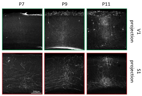
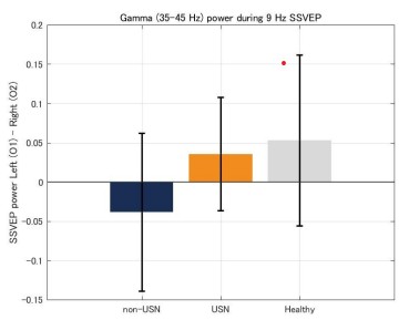
Author response:

Public Reviews:

Reviewer #1 (Public review):

This rigorous and creative study uses an elegant combination of metabolomics, transcriptomics, and budding yeast molecular genetics to discover that (i) activating AMPK to maintain mitochondrial respiration fueled by cytosolic Acetyl CoA and (ii) increasing fatty acid synthesis independent of respiration drive independent pathways that increase the fitness of replicatively-aged budding yeast cells, albeit without increasing their lifespan. This work will be of interest to scientists in the field of aging and metabolism. Some clarifications in the text would address the following concerns, which would increase the impact of the study:

(1) What does activation of AMPK (via PGDP-Sak1 expression) do to the replicative lifespan? How many bud scars, in general, do the subpopulations that are older - yet have less Tom70 (increased mitochondrial fitness) - have, after the 48 hrs time point that they are examining? How many divisions occurred in this 48hr time period - i.e. is it long enough to have all cells reach the end of their replicative lifespan? This information is important to rule out that a subset of the mutant cells just divided faster and hence had more divisions within 48 hrs (growing faster and living longer are different things). Having identical growth curves doesn't indicate per se that they all divide at the same rate, as there may be a subpopulation that divides faster and a subpopulation that doesn't grow so well.

Increasing AMPK activity increases replicative lifespan [PMID: 25869125], but given our finding that AMPK activation splits the population, such replicative lifespan assays are hard to interpret. Bud scar counts have a similar issue. Hence we restricted the lifespan and bud scar analyses to wt and A2A which are more homogenous (Figures S2 B and E). A2A cells at 48h have ~25% more bud scars than wt cells. Yes, by 48h most of the cells have lost viability (Figure 2E). The reviewer is correct that you can't properly compare the lifespan curves if the cells divide at different rates, hence our follow-up test of wt at 48h vs A2A at 40h viability after we had confirmed that these timepoints captured cells at equivalent replicative ages (Figure 2D,E). This shows that viability of A2A is slightly lower than wt at matched age, indicating a slightly shorter lifespan.

(2) A2A cells do not have an extended replicative lifespan (RLS) but show an increase in the "low senescence" population (Figure 2). If the cells are not becoming senescent, why don't they have longer RLS? Not having a longer lifespan seems inconsistent with the statement that "bud scar counting confirmed that A2A cells reach a higher age than wild type", which comes back to how many times the cells can divide in the 48hr timepoint studied and their rate of cell division? Also, the lifespan curve shown is plotted against time, not cell division number, which does not take into account different division times of cells within the population (described above). It would be much more useful to show standard lifespan curves showing cell division numbers per lifespan per cell.

Our observation that cells can reach the end of life without senescing is consistent with other studies that have studied the life course of individual cells by microscopy [PMID: 31291577, 32675375]. These studies always highlight some proportion of the cells that reach the end of life with no or minimal senescence, though this fraction varies with the experimental system. The question of why cells lose viability without senescing is a complete unknown in the field, but reflects a wider lack of consensus as to why yeast lose viability with replicative age.

We are wary about making strong statements on lifespan for exactly the reason the reviewer picks out. In liquid culture we can only assess viability over time, and it is clear from the comparison of liquid and solid media lifespans performed by the Gottschling lab [PMID: 19652178] that culture system has a huge effect on lifespan, with cells in classical microdissection-based lifespan assays living far longer than they do in liquid. This of course means that classical microdissection assays are not very useful for A2A so we are left with an unsatisfactory approximation. We have therefore restricted our conclusion on lifespan to simply say that lifespan of A2A cells is not extended which our data in Figures 2D,E,S2B does support (see also answer to Q1), and therefore with the majority of A2A cells showing low senescence marks and high fitness at 48h we can conclude that lifespan and fitness loss must be separable.

We will note these limitations of lifespan measurements in the manuscript.

(3) Increased "fitness" of the old cells is implied from the increased size of the colonies that the old cells can make. However, this is a measure of the fitness of the daughters per se, not the old mother cells. Are the old mothers just passing on healthier mitochondria and more lipids to the daughters, such that they can divide more times? If the aged cells have an "increased fitness", why don't they divide more times themselves (i.e. live longer?).

Yes, colony growth speed is defined by daughter cell replication, and as long as the daughters and subsequent generations divide at the same rate irrespective of whether they come from a young or old mothers then the size of the colony after 24 hours varies based on the time it took the initial mother to produce a daughter. This is what the assay really measures. We note that aged wildtype mothers often do not divide at all in the first 24 hours after being put on an agar plate (hence the tiny reported colony size), even though they do eventually produce a daughter which then forms a colony, whereas A2A cells tend to produce the first daughter rapidly whether young or old. It is known that daughters of aged wildtype mothers also divide slower, which will also contribute to differences in colony size, and this may well result from a lipid and/or mitochondrial contribution, but the primary driver of colony size in 24 hours is the time the mother took to initially divide. We will add this detail to the manuscript.

As noted above, the mechanistic basis of lifespan is unknown, but although senescence can shorten lifespan, our work and that of others shows that lifespan is still limited in the absence of senescence.

(4) The statement is made that "these experiments define two classes of aging cells with distinct metabolic needs, coherent with the model of two aging trajectories previously proposed (referencing Nan Hao's work)". However, the big difference here is that in Nan Hao's work, their two aging trajectories influenced the length of lifespan, but that does not appear to be the case here. That distinction should be made clear. Perhaps the authors could also speculate as to why the A2A yeast stops dividing after presumably the same number of cell divisions, even though they have an activated AMPK and activated fatty acid synthesis pathway.

We will add this distinction. As noted above, we are wary of making strong statements regarding lifespan as the assays we can do in liquid culture are limited. We are therefore similarly wary about speculating about causes for the lack of lifespan difference because in reality all we can do is rule out a big effect. We would love to speculate on why the A2A cells don't have an extended lifespan, but at this point we don't have any good ideas on this point!

(5) I am a bit confused by the use of the word "senescence" by this lab here and in their previous growth on galactose studies. If yeast don't senesce, which is usually defined as an irreversible arrest of the cell cycle where cells stop dividing, shouldn't the yeast that do not senesce still be dividing and hence have a longer lifespan? Should a different term be used rather than senescence? Such as "fitness late in life". The authors giving their definition of senescence may help reduce this apparent contradiction.

We completely agree, this is confusing and noted this distinction in the Introduction. Use of the term senescence to mean a loss of fitness late in life in yeast stems from the classical definition of senescence as applied to whole organisms. However, the term senescence as applied to cells has a more specific meaning in terms of the cell cycle as the reviewer notes. As an individual S. cerevisiae is both a cell and an organism, the terminology clashes. However, the marker we largely employ (Tom70-GFP) which in our hands is a very good proxy for fitness was originally defined as marking the senescence entry point (SEP), so overall we feel we can't avoid the term.

Reviewer #2 (Public review):

Summary:

In this study, the authors investigate how cytosolic acetyl-CoA metabolism influences replicative aging in budding yeast. They propose that acetyl-CoA regulates aging through three major pathways: (1) mitochondrial transport to support mitochondrial function, (2) fatty acid synthesis, and (3) global protein acetylation. The data show that AMPK activation promotes mitochondrial import of acetyl-CoA and partially mitigates mitochondrial decline in a subset of aging cells.

Furthermore, the engineered A2A strain, which enhances mitochondrial acetyl-CoA utilization while relieving inhibition of fatty acid synthesis, increases the proportion of cells exhibiting a "low senescence" phenotype.

Overall, this is a thoughtful and potentially impactful study that advances our understanding of metab to olic control of aging. Addressing the points below, particularly by refining interpretations and, where feasible, incorporating additional analyses, will further strengthen the manuscript and its conclusions.

Strengths:

The study has several notable strengths. It addresses an important question by shifting the focus from lifespan to preservation of late-life fitness, which is highly relevant to aging biology. The work integrates metabolic, genetic, and functional analyses to link cytosolic acetyl-CoA flux with distinct aging outcomes, and the engineering of the A2A strain provides a clear and elegant demonstration of how coordinated pathway modulation can improve cellular fitness.

Weaknesses:

(1) While the manuscript focuses on mitochondrial transport and fatty acid synthesis, cytosolic acetyl-CoA is also a key regulator of histone acetylation and chromatin silencing. It would strengthen the study to consider whether acetyl-CoA depletion contributes to improved fitness through enhanced rDNA silencing. Given the well-established role of rDNA instability in yeast aging, additional experiments examining rDNA silencing and stability would be valuable. For example, monitoring rDNA copy number changes (not necessarily ERCs) under AMPK activation, oleic acid supplementation, and in the A2A strain, similar to approaches used in the authors' prior work, would help clarify whether chromatin regulation contributes to the observed phenotypes.

We have data addressing this point that we will add to the manuscript. In short, we see no difference in gene expression from Sir2-repressed sub-telomeric regions or MAT loci, but the genome-wide gene expression dysregulation associated with age is partially suppressed in PGPD-SAK1. However, A2A does not suppress this further, so it is not critical for the suppression of senescence in A2A though we are following this up. ERC accumulation is higher in A2A at 48h, consistent with the cells being older, meaning that ERCs are unlinked to senescence onset as we have previously reported. There is a strong upregulation of transcripts from Sir2-repressed rDNA intergenic spacers with age in all genotypes, but we attribute this simply to the copy number increase of these regions on ERCs rather than a defect in silencing. We have previously looked for heritable changes in rDNA copy number arising during ageing and found (to our surprise) absolutely nothing, so we don't expect any changes under these conditions.

(2) The current data do not fully distinguish whether AMPK activation and oleic acid supplementation act on distinct subpopulations of aging cells. An alternative explanation is that oleic acid supplementation enhances mitochondrial function and acts additively with AMPK activation, thereby increasing the fraction of cells in the "low senescence" state. Since this distinction is not central to the main conclusions, I suggest softening the language around subpopulation specificity. Emphasizing instead that the A2A strain coordinately modulates multiple branches of acetyl-CoA metabolism to improve late-life fitness would maintain the strength of the central message without overinterpretation.

We agree that oleic acid and the lipids produced downstream of Acc1 in A2A may improve late life fitness via enhanced mitochondrial function, and in support of this Oxygen Consumption Rate is marginally (though significantly) higher in A2A than PGPD-SAK1. We will add this data to the manuscript. However, we disagree with the interpretation of an additive effect as we report throughout the study that AMPK activation and lipid biosynthesis/supplementation affect different sub-populations of cells. We do not observe populations of intermediate senescence cells, rather by flow cytometry and fitness assays we observe individual cells in binary low senescence or high senescence states.

(3) The manuscript proposes that lipid starvation and excess acetyl-CoA are major drivers of senescence in distinct subpopulations of wild-type aging cells. This conclusion is not yet fully supported by the presented data. Direct measurements of age-dependent divergence in acetyl-CoA and fatty acid levels at the single-cell level would be needed to substantiate this model. Based on the current evidence, a more conservative interpretation would be that aging cells exhibit differential sensitivity to perturbations in acetyl-CoA and lipid metabolism. Accordingly, I recommend revising the statement in the Abstract ("We further implicate lipid starvation and excess acetyl coenzyme A availability as major drivers of senescence...") and the corresponding discussion text to better align with the data.

We agree and will adjust the abstract to make it clearer that the lipid starvation / excess acetyl coA interpretation is a model.

Reviewer #3 (Public review):

Summary:

These findings suggest that PGPD-SAK1 yeast show a subpopulation with lowered TOM70-GFP expression in high bud scar staining aged cells. Deletion of CAT2 or MLS1 reduces this effect. A PGPD-SAK1 acc1S1157A double mutant (called "A2A" here) shows an even larger effect of lowered tom70 expression in high bud scar staining aged cells. Utilization of various additional mutants involved in acetyl-CoA transport, carnitine shuttle, respiration, etc., leads the authors to conclude that these shifts in TOM70-GFP in aged cells are linked to the AMPK-fatty acid metabolic regulatory system.

Strengths:

These extensive and clearly described experiments reveal interesting changes in TOM70-GFP intensity in subsets of aged yeast in several mutants eventually identified as linked to the AMPK-fatty acid metabolic regulatory system.

Weaknesses:

(1) 3 biological replicates for mRNASeq is low.

Thank you for pointing this out. We performed another replicate after posting the initial preprint but didn’t update the figure in the eLIFe-reviewed version. We will add this to the scatter plots and analysis in Figure 1, the findings have not changed.

(2) While "Traditional conceptions of ageing implicate a progressive accumulation of damage leading to systemic degradation in performance until death, with evolutionary pressures acting to maximise early life fitness and fecundity at the expense of ageing health." is tangential perhaps to the data and conclusions of the study, both claims of this sentence are at best controversial, and the manuscript is no weaker for their omission.

We actually feel that this sentence is very important to the message of the manuscript, which is that ageing does not necessarily have to involve a loss of fitness before death. Ageing is often described as the progressive wearing out of components leading to decline and death (with an old car often used as an analogy); in the ageing field this is certainly controversial, but outside the field this remains the normal understanding. We think it is important to state this widely held viewpoint with which our findings are hard to reconcile.

Our interpretation that yeast are bet-hedging as a population growth strategy and this drives ageing in the long term is a classic antagonistic pleiotropy - we will add this term (from the citation that is already in the manuscript) and clarify in the discussion to make it obvious why we are introducing this concept in the introduction.

(3) The statement that "Here, we determine the basis of senescence and fitness loss in replicatively ageing yeast" is a bit strong as a summary of the present careful work presented here. If the authors had created yeast mutants that retained fitness indefinitely, this would be a more appropriate strength of claim to summarize the work.

Indeed - we will refine this sentence.

Author response:

The following is the authors’ response to the original reviews.

Reviewer #1 (Public review):

Summary:

This study investigated how visuospatial attention influences the way people build simplified mental representations to support planning and decision-making. Using computational modeling and virtual maze navigation, the authors examined whether spatial proximity and the spatial arrangement of obstacles determine which elements are included in participants' internal models of a task. The study developed and tested an extension of the value-guided construal (VGC) model that incorporates features of spatial attention for selecting simpler task mental representation.

Strengths:

(1) Original Perspective:

The study introduces an explicit attentional component to established models of planning, offering an approach that bridges perception, attention, and decisionmaking.

(2) Methodological Approach:

The combination of computational modeling, behavioral data, and eye-tracking provides converging measures to assess the relationship between attention and planning representations.

(3) Cross-validated data:

The study relies on the analysis of three separate datasets, two already published and an additional novel one. This allows for cross-validation of the findings and enhances the robustness of the evidence.

(4) Focus on Individual Differences:

Reports of how individual variability in attentional "spillover" correlates with the sparsity of task representations and spatial proximity add depth to the analysis.

We thank the Reviewer for their overall positive assessment of our work and their helpful comments. We have addressed each point below.

Weaknesses:

(1) Clarity of the VGC model and behavioral task:

The exposition of the VGC model lacks sufficient detail for non-expert readers. It is not clear how this model infers which maze obstacles are relevant or irrelevant for planning, nor how the maze tasks specifically operationalize "planning" versus other cognitive processes.

The method for classifying obstacles as relevant or irrelevant to the task and connecting metacognitive awareness (i.e., participants' reports of noticing obstacles) to attentional capture is not well justified. The rationale for why awareness serves as a valid attention proxy, as opposed to behavioral or neurophysiological markers, should be clearer.

We thank the reviewer for urging further clarity here. Our work builds closely on the previous maze navigation paradigm and VGC model developed and reported by Ho et al. Nature (2022). We directly adopted variants of their maze stimuli, computational model and obstacle awareness measures, and married these with an investigation of the role of visuospatial attention. We agree that it would be useful for the reader to have a more in-depth description of the paradigm and model, and how it operationalises planning, without needing to refer back to the original Ho et al. paper. We have now added additional explanatory sections to the Introduction and Methods as follows:

On page 4:

“One elegant approach to forming such a simplified representation is to adaptively select the granularity of information required to complete the task (Ho et al., 2022), known as value-guided construal (VGC). Unlike previous accounts, which model human planning as a search over all items (e.g.., tube lines), the VGC model predicts that a cognitively limited decision-maker selects a manageable subset of information over which to plan— i.e., a task representation—balancing utility and complexity (Ho et al., 2022). In our example, the VGC algorithm would plan over a few relevant tube lines rather than planning over all possible stations. To select the representation that achieves the best balance between utility and complexity, the model searches across all possible combinations of tube lines, computing the value (i.e., the plan’s utility minus its cost) of each representation for planning a specific journey. The algorithm then selects the representation with the highest value, which ensures that an ideal observer selects a representation which only includes the items (i.e., tube lines) that lead to successful planning while excluding as many items as possible to keep the plan as simple as possible. For our purposes, items included in the representation are considered taskrelevant, while items that are not represented are considered task-irrelevant. This algorithm, therefore, provides a normative standard of an efficient plan to which we can compare people’s actual plans.”

On page 6:

“We operationalized planning using a maze navigation paradigm, akin to our tube-related example, where participants were required to plan a route through the maze, avoiding obstacles that blocked their path. Obstacles predicted by the sVGC model to be included in the representation were considered task-relevant.”

“At the end of every trial, participants reported their awareness of specific obstacles (see Methods for details). The level of awareness reported for different obstacles provides a read-out of what features of the environment individuals were subjectively representing while solving a particular maze. While other markers of attention and awareness (for instance, behavioural or neurophysiological variables) could also be used, here we focused on direct awareness reports in order to relate our findings both to those of Ho and colleagues and to the subjective awareness reports used in consciousness science (e.g. the Perceptual Awareness Scale (Barnett et al., 2024; Overgaard & Sandberg, 2021; Ramsøy & Overgaard, 2004; Samaha et al., 2015)). Participants were instructed to maintain central fixation while planning (see dataset dSC 1), in line with previous empirical work using this task (Ho et al., 2022).”

To visualize our effects, we binarized the predictions of the sVGC model such that obstacles with a marginalized probability greater than 0.5 were considered taskrelevant, while other obstacles were considered task-irrelevant (e.g., Figure 2b). We now clarify this point in the caption of Figure 2.

(2) Attention framework:

The account of attention is largely limited to the "spotlight" model. When solving a maze, participants trace the correct trail, following it mentally with their overt or covert attention. In this perspective, relevant concepts are also rooted in attention literature pertaining to object-based attention using tasks like curve tracing (e.g., Pooresmaeili & Roelfsema, 2014) and to mental maze solving (e.g., Wong & Scholl, 2024), which may be highly relevant and add nuance to the current work. This view of attention may be more pertinent to the task than models of simultaneously tracking multiple objects cited here. Prior work (notably from the Roelfsema group) indicates that attentional engagement in curve-tracing tasks may be a continuous, bottom-up process that progressively spreads along a trajectory, in time and space, rather than a "spotlight" that simply travels along the path. The spread of attention depends on the spatial proximity to distractors - a point that could also be pertinent to the findings here.

Moreover, the tracing of a "solution" trail in a maze may be spontaneous and not only a top-down voluntary operation (Wong & Scholl, 2024), a finding that requires a more careful framing of the link to conscious perception discussed in the manuscript.

Conceptualizing attention as a spatial spotlight may therefore oversimplify its role in navigation and planning. Perhaps the observed attentional modulation reflects a perceptual stage of building the trail in the maze rather than a filter for a later representation for more efficient decision making and planning. A fuller discussion of whether the current model and data can distinguish between these frameworks would benefit readers.

We thank the reviewer for highlighting relevant findings in the attention literature that were missing from our discussion. We fully agree that a complete account of the interplay of planning, navigation, and attention is likely to recruit the kind of curvetracing processes highlighted by the reviewer. However, we emphasise that our current focus is not on the process of navigation through a maze, but on the process of construing the maze itself. In other words, we are focused not on how people represent their path from A to B, but how they represent the maze itself, which they then use as a basis for planning between A and B. The VGC model predicts that a subset of obstacles will be included in this construal. We think that a spotlight model is a good starting point for this work, because attention is being deployed across the whole maze stimulus, and then becomes attached to particular objects located in particular positions. This is a distinct process from that involved in navigating the path itself. Accordingly, our stimuli were designed such that task-relevant obstacles could be presented either proximally or distally to the optimal path (e.g., Figure 1a and Supplemental Figures S1-6). An obstacle that blocks any possible path on one side of the maze is task-relevant but located a long way from the optimal path. The results of Ho and colleagues’ (2022) third experiment demonstrate how task-relevant yet distal obstacles are better remembered than task-irrelevant proximal obstacles (see Figure 4 of Ho et al., 2022). We also observed that obstacles further away from the navigation path were often represented by participants (see Figures S1-6), which cannot be explained by curve tracing alone.

While these results cannot definitively rule out the possibility that participants automatically trace the path while also construing the maze, they suggest that the value-guided construal process is an independent predictor of participants’ representations beyond proximity to the navigated path. To make this distinction clearer, we now cite the papers alluded to by the reviewer, in the Discussion on pages 28-29, while also acknowledging the potential for investigating attention during the navigation process itself:

“Future work may also wish to examine the relevance of visuospatial attention for the navigation process itself in this task. While our present findings speak to how individuals perceive the maze while planning, it remains unclear how attention is deployed during navigation along a path, such as how object-based attention progressively spreads along trajectories in time and space(Pooresmaeili & Roelfsema, 2014; Wong & Scholl, 2024).”

There is also one additional nuance to the current spotlight model that we were inspired to consider by the reviewer’s comment. This is the idea that attentional effects may spread within or along the obstacles themselves. We cannot explore this in the current data because we asked for awareness of the entire obstacles, not parts of obstacles, but it may be possible to explore this in future work, for instance, with eye tracking measures.

More generally, the growth-cone (i.e., zoom lens) model of attention for curve tracing proposed by Roelfsema and colleagues shares considerable similarities with the spotlight of attention model. Both models argue for the grouping of spatially proximal items based on attention. While the growth-cone model argues for varying sizes of zoom lenses (i.e., receptive fields of neurons) that facilitate the tracing of proximal items, both models predict that spatially proximal items are preferentially processed together because of attention. Indeed, the spotlight model could model these varying zoom lenses by altering the width of the attentional spotlight dynamically across the visual scene based on the spatial proximity of obstacles. Following related comments by Reviewer 2, we now investigate inter-individual differences in the attentional spotlight of participants and observed that these differences significantly predict participants’ mental representations (see Attentional spotlight model of task representations). We have now updated the Discussion to include consideration of these alternative model frameworks:

On page 27:

“Second, in the current work we were unable to distinguish whether these attentional effects are driven by a fixed spotlight of attention, or whether attention operates akin to a zoom lens, shifting the ‘width’ of the focus of attention according to the task demands (Eriksen & St. James, 1986; Müller et al., 2003; Schad & Engbert, 2012). The latter view would be consistent with growth-cone models of attention in which the focus of attention expands and contracts in accordance with task demands, mirroring the various receptive field sizes in the visual hierarchy (Pooresmaeili et al., 2014; Pooresmaeili & Roelfsema, 2014). In partial support of this idea, we found significant inter-individual differences in the width of participants’ attentional spotlight (Figure S11). It is also possible that attention is deployed within or along parts of obstacles, rather than on entire obstacles. Future work using naturalistic measures of eye movements may be able to address these questions.”

(3) Lateralization of attention:

The analysis considers whether relevant information is distributed bilaterally or unilaterally across the visual display, but does not sufficiently address evidence for attentional asymmetries across the left and right visual fields due to hemispheric specialization (e.g., Bartolomeo & Seidel Malkinson, 2019). Whether effects differ for left versus right hemifield arrangements is not made explicit in the presented findings.

We thank the reviewer for this suggestion. To address this point, we fitted a three-way interaction model between VGC model prediction, lateralization index, and side (left vs right hemifield). We did not find evidence for the three-way effect (β= 0.01, SE= 0.02, 95% CI [-0.03, 0.04], p = 0.738; ΔBIC = 58.30 in favour of the null effect; see table below), suggesting that the side to which participants lateralized their attention did not influence their task representations. This result is now reported on page 12:

“This effect did not vary significantly as a function of the specific hemifield (i.e., left vs right) in which task-relevant information was presented (β= 0.01, SE= 0.02, 95% CI [-0.03, 0.04], p = 0.738; ΔBIC = 58.30 in favour of the null effect; see table S14).”

We also explored inter-individual differences in participants’ tendency to lateralize their attention (see also the next point). We observed that participants tended to lateralize their attention slightly more to the right-hand side for non-lateralized maze stimuli, despite the normative sVGC model predicting that participants should not lateralize their attention for these stimuli (Figure 3c). These results may speak to potential asymmetries in lateralization, but given the exploratory nature of these analyses, they should be verified and replicated in future work.

(4) Individual differences:

Individual differences in attentional modulation are a strength of the work, but similar analyses exploring individual variation in lateralization effects could provide further insight, and the lack of such analyses may mask important effects.

Thank you for this suggestion. In new analyses, we explored whether i) participants exhibited differences in their tendency to lateralize their awareness reports, and ii) whether the degree to which they tended to lateralize their awareness predicted their performance on a separate set of maze stimuli. In short, we observed substantial variation in participants’ tendency to lateralize their awareness (Figure S11) and found that this tendency reflected an inter-individual difference which was stable across maze types. We report these new findings on pages 14-16.

“Inter-individual variation in lateralization of attention

Next, we investigated participants’ tendency to pay attention to obstacles within a single hemifield (left vs right) regardless of the sVGC model predictions. To do so, we computed an awareness lateralization index (ALI) based on participants’ self-reported awareness reports of obstacles on each trial (Figure 3a). Large positive values indicate that participants were preferentially aware of the right hemifield, whereas negative values indicate preferential awareness of the left hemifield. Values close to zero indicate that participants paid attention to both hemifields equally (see Methods for details). We observed that participants’ tendency to lateralize their awareness varied greatly across the Ho datasets 1 and 2 (Figure 3b); some participants preferentially paid attention to a single hemifield, regardless of whether the sVGC model predictions were lateralized. For the dSC1 dataset, we observed that on some trials, participants significantly lateralized their awareness (|ALI| > 0.5; Figure 3c) even though the sVGC model predictions were non-lateralized. These findings suggest that participants’ tendency to pay attention to a single hemifield may represent an observable inter-individual difference in how they allocate their awareness to form task construals.”

“To further explore these inter-individual differences, we tested whether participants’ tendencies to lateralize their attention to a single hemifield was consistent across trials and maze stimuli. We observed that participants’ tendency to lateralize their attention to a single hemifield was similar for left and right lateralized maze stimuli (Spearman ⍴= 0.72, Figure 3d). This suggests that participants who preferentially attended to a single hemifield did so regardless of which hemifield they should attend to. More consequentially, the tendency for participants to lateralize their awareness on maze stimuli whose model predictions were also lateralized linearly correlated with participants’ tendency to lateralize their attention on non-lateralized maze stimuli (Spearman ⍴= 0.88, Figure 3d). Taken together, these findings emphasize that some individuals tend to preferentially attend to a single hemifield when planning. This tendency, importantly, represents an inter-individual difference in how participants allocate their attention across various maze types.”

(5) Distinction between overt and covert attention:

The current report at times equates eye movement patterns with the locus of attention. However, attention can be covertly shifted without corresponding gaze changes (see, for example, Pooresmaeili & Roelfsema, 2014).

We fully agree, and thank the reviewer for prompting further reflection on this distinction. In the online experiments run by Ho and colleagues (i.e., datasets Ho1 and Ho2), participants’ eye movements were not tracked, and therefore, they could not disambiguate whether participants were engaging in covert or overt attention to sample maze obstacles. In our third experiment (i.e., dataset dSC1), we both recorded eye movements and explicitly instructed participants to fixate centrally while viewing the maze. This ensured that participants oriented their attention only covertly during planning (see Figure S13-14).

We now elaborate on this important distinction in the Results section of the manuscript, page 12:

“In addition, we monitored participants’ eye movements in dataset dSC 1 to ensure that attention shifts would be covert as opposed to overt—a distinction which could not be determined in the online samples of datasets Ho 1 and 2.”

On page 28:

“Importantly, while the visuospatial attention effects observed in the Ho 1 and 2 datasets are likely driven by both covert and overt shifts in attention, the findings presented in experiment 3 (i.e., dSC1 dataset) rule out the contribution of overt shifts in attention through the use of eye tracking (see Figure S13-14)(Carrasco, 2011; Pooresmaeili & Roelfsema, 2014).”

The implications for interpreting the relationship between eye movement, memory, and attention in this setting are not fully addressed. The potential dynamics of attention along a maze trajectory and their impact on lateralization analysis would benefit from further clarification.

We thank the reviewer for urging more clarity here. The attentional dynamics we document in our study concern how people perceive / construe the maze itself, rather than how they deploy their attention to guide active navigation. We have now sought to make this distinction clear at a number of points in the paper. The core idea is that attention acts as an early filter to select which obstacles are part of a task construal, which then affects both awareness and memory.

We have now clarified the focus of our study in the introduction on pages 5-7:

“Our focus in this study was to examine how participants perceive and represent their environment (the maze stimulus). This is a distinct process to how participants orient their attention during navigation itself, which is not part of our current study. To do so, we harness classical signatures of attentional selection to characterise how visuospatial attention shapes awareness of maze obstacles during planning.” … “Our focus in the present study was to examine attentional effects on participants’ perception of the maze stimulus. We did not quantify how individuals deploy their attention in the phase in which they were navigating through the maze.”

We did not explicitly test for memory effects in our new experiments, but Ho and colleagues demonstrated that the sVGC model predicted not only awareness reports, but also participants’ memory of obstacles (see Ho et al., 2022). Indeed, task representations computed from memory or awareness reports were strikingly similar in their experiments (Spearman ⍴ = 0.86 between memory accuracy and awareness; ⍴ = 0.86 between confidence in memory and awareness). In relation to eye movements, we refer the reviewer back to our previous response, which details how eye movements were measured and controlled during maze construal.

Figure 1 legend (b) --> (c)

We have corrected this typo in the figure caption.

Reviewer #2 (Public review):

Summary:

Castanheira et al. investigate the role of spatial attention for planning during three maze navigation experiments (one new experiment and two existing datasets). Effective planning in complex situations requires the construction of simplified representations of the task at hand. The authors find that these mental representations (as assessed by conscious awareness) of a given stimulus are influenced by (spatially) surrounding stimuli. Individual participants varied in the degree to which attention influenced their task representations, and this attentional effect correlated with the sparsity of representations (as measured by the range of awareness reports across all stimuli). Spatially grouping taskrelevant information on either the left or right side of the maze led to mental representations more similar to optimal representations predicted by the valueguided construal (VGC) model - a normative model describing a theoretical approach to simplifying complex task information. Finally, the authors propose an update to this model, incorporating an attentional spotlight component; the revised descriptive model predicts empirical task representations better than the original (normative) VGC model.

Strengths:

The novelty of this study lies in the proposal and investigation of a cognitive mechanism through which a normative model like value-guided construal can enable human planning. After proposing attention as this mechanism, the authors make concrete hypotheses about mismatches between the VGC predictions and real human behavior, which are experimentally validated. Thus, not only does this study describe a possible mechanism for simplification of task information for planning, but the authors also propose a descriptive model, revising VGC to incorporate this attentional component.

A strength of this paper is the variety of investigative approaches: analysis of existing data, novel experiment, and a computational approach to predict experimental findings from a theoretical model. Analyzing pre-existing datasets increases the size of the participant cohort and strengthens the authors' conclusions. Meanwhile, comparing the predictions of the existing normative model and the authors' own refined model is a clever approach to substantiate their claims. In addition, the authors describe several crucial controls, which are key to the interpretability of their results. In particular, the eye tracking results were critical.

In summary, this paper constitutes an important step toward a more complete understanding of the human ability to plan.

We thank the Reviewer for their thoughtful and positive assessment of our findings. We also appreciate the constructive feedback on our methodology, which we believe has substantially improved our manuscript.

Weaknesses:

(1) There is a critical conceptual gap in the study and its interpretation, mainly due to the reliance on a self-report metric of awareness (rather than an objective measure of behavioral performance).

a. Awareness is tested by a 9-point self-report scale. It is currently unclear why awareness of task-irrelevant obstacles in this task would necessarily compromise optimal planning. There is no indication of whether self-reported awareness affects performance (e.g., navigation path distance, time to complete the maze, number of errors). Such behavioral evidence of planning would be more compelling.

We thank the reviewer for prompting further reflection on the connection between construal and navigation performance. We wish to emphasise that the primary focus of our study was on measuring and modeling participants’ task construals using perceptual awareness judgments, building on the methods developed by Ho and colleagues, rather than on navigation performance itself. However, as the reviewer points out, there is a natural relationship between construal and performance – if you represent the wrong obstacles, plans may be disrupted.

To explore the relationship between task construals and performance on the navigation task we first regressed out the effects of the sVGC model on participants’ awareness reports and computed the mean squared residuals for each trial. We then used these values to predict participants’ navigation response times on each trial. We observed a significant negative relationship, suggesting that on trials where participants’ representations showed greater deviations from the normative model, they were in fact faster at navigating the mazes. This relationship was surprising, and at odds with the initial idea that adhering to normative VGC aids in task performance. However, we think that this direction of effect may make sense if one considers that a large part of the actual construal (rather than the normative prediction) in our data was in fact driven by effects such as lateralisation which are not accounted for by the sVGC model. If one is faster at harnessing inductive biases such as lateralisation, then one may be faster to complete the maze but also show a greater deviation from the predictions of the original model.

To further explore these effects, we next focused on the distinction between lateralised and non-lateralised mazes. Here, we reasoned that the initial phase of lateralised attentional selection would lead to lateralised mazes being easier to navigate than nonlateralised ones. We conducted new analyses to determine whether participants navigated lateralized maze stimuli faster and with fewer moves than maze stimuli with non-lateralized model predictions. As detailed in Methods, we excluded trials in which participants significantly deviated from the optimal number of moves (9 or more moves) and took longer than 20 seconds to solve the maze. In line with our interpretation that attention operates as an inductive bias, participants were faster and deviated less from the optimal path on lateralized compared to non-lateralized mazes.

We now report these new results on navigation performance on pages 20-21:

“Maze navigation performance

The previous analyses focused on participants’ task representations during planning. We next sought to explore links between participants’ task representations and maze navigation performance. Participants performed the maze navigation task near-ceiling: they solved 95% of maze stimuli in under 20 seconds, with minimal deviation from the optimal path (i.e., 9 moves or fewer). Notwithstanding this limited variance in task performance, we explored whether participants’ task construals may have impacted their navigation speed. To do so, we first regressed out the effects of the sVGC model from participants’ awareness reports and used the mean squared residuals for each trial to predict response times (see Methods for details). Surprisingly, we observed a negative relationship between mean squared residual variance and response times (β = -0.31, SE = 0.05, 95% CI [-0.41, -0.21], p < 0.001), indicating that participants were faster on trials where the sVGC model explained less variance in their awareness reports. In other words, trials in which participants deviated more from the sVGC model predictions were solved faster. We note that one reason for this may be the strong influence of the lateralisation effect on navigation performance (see paragraph below), which itself is not part of the sVGC model prediction.”

“We then explored whether participant performance differed between lateralised and nonlateralised mazes. Here, we reasoned that the initial phase of lateralised attentional selection would lead to lateralised mazes being easier to navigate than non-lateralised ones. Consistent with this hypothesis, participants were faster (β = -0.04, SE = 5.91*10³, 95% CI [-0.06, -0.03], p< 0.001) and followed the optimal path more closely (β = -0.59, SE = 0.09, 95% CI [-0.78, -0.40], p< 0.001) when maze stimuli were more lateralized.”

And in the Discussion section, on page 23:

“Mental representations and task performance

We observed that participants were faster and deviated less from the optimal path on maze stimuli that were lateralized. This effect is not predicted by the original sVGC model but dovetails with the interpretation that early visuospatial attention operates as an inductive bias to guide the formation of simplified task representations. Surprisingly, we also observed that participants were faster to navigate mazes on trials where their simplified task representation deviated from the sVGC model prediction. We interpret this seemingly contradictory finding in the following way: there are several factors beyond the sVGC model – including, for instance, maze lateralisation – that predict both construal and performance on the maze navigation task. Further work is needed to understand how inductive biases such as lateralisation shape both construal and performance, and the real-world benefits that such strategies might afford for naturalistic stimuli.”

b. Relatedly, it would have been more convincing to have an objective measure of awareness, for instance, how the presence or absence of a "task-irrelevant" obstacle affects performance (e.g., change navigation path distance or time to complete the maze), or whether participants can accurately recall the location of obstacles.

We thank the reviewer for prompting further reflection on the validity and robustness of our awareness measures. We emphasise however that our focus is not (primarily) on maze navigation performance, but on task construal, which as noted in our previous response may come apart from navigation performance for a variety of reasons. Our primary goal is to measure participants’ subjective awareness of the maze as a marker of their idiosyncratic (conscious) mental representation on each trial. In doing so, we build on a rich tradition of measuring subjective awareness in consciousness and perception science (for instance, work using the Perceptual Awareness Scale, or detection judgments). In this sense, we think our awareness scale (following Ho et al.) represents a valid and straightforward way of assessing our target psychological construct. However, we also agree with the Reviewer that convergent evidence from other measures is always valuable. In Ho and colleagues’ original paper, they developed a variant of the maze task where participants had to recall the location of obstacles, as well as rate their awareness (Exp 3) and a variant in which participants could hover their mouse over hidden obstacles in the maze to reveal their location – an online metric of attentional deployment (Exp 4). These data afforded us the opportunity to validate the awareness reports against an objective measure of recall, as suggested by the Reviewer. In reanalysing these data, we observed that the obstacle awareness and memory/hover measures were strikingly correlated within two independent samples of participants (Spearman ⍴ = 0.86 between memory accuracy and awareness; ⍴ = 0.86 between confidence in memory and awareness; ⍴ = 0.76 between the probability of hovering over the obstacle and awareness; ⍴ = 0.65 between the duration of the mouse hovering and awareness). These re-analyses are now reported on page 22 of our manuscript, to highlight the convergent validity of the awareness metric:

“Finally, we examined the convergent validity of participants’ awareness reports by reanalyzing the memory recall data reported in Ho and colleagues’ experiment(Ho et al., 2022). We reasoned that participants should demonstrate similar task representations regardless of the measure used to probe the construal. In line with this prediction, we observed that the obstacle awareness reports and memory/hover measures were strikingly correlated within three independent samples of participants (Spearman ⍴ = 0.86 between memory accuracy and awareness; ⍴ = 0.86 between confidence in memory and awareness; ⍴ = 0.76 between the probability of hovering over the obstacle and awareness; ⍴ = 0.65 between the duration of the mouse hovering and awareness; see Tables S18 and S19).”

c. Consequently, I'm not sure that we can conclude that the spatial context does impact participants' ability to plan spatial navigation or to "incorporate taskrelevant information into their construal". We know that the spatial context affects subjective (self-reported) awareness, but the authors do not present evidence that spatial context affects behavioral performance.

Following the line of argument above, we think it’s important to separate out task construal (the simplified representation of the maze, measured by awareness reports), and the impact of this on navigation and other aspects of behaviour. The awareness reports (and other convergent measures) show that task-relevant information (as predicted by the VGC) is incorporated into the construal, a process which is modulated by spatial context. These are the key targets of our modeling. Whether this impacts performance is a distinct question, and one that we now address in our response to point a above.

d. Another concern that may complicate interpretation is the following: Figure 3c shows improved VGC model predictions (steeper slope) for mazes with greater lateralization. However, there are notable outliers in these plots, where a high lateralization index does not correspond to good model performance. There is currently no discussion/explanation of these cases.

The Reviewer astutely points out some outliers in our analysis. While on average lateralized maze stimuli are represented more closely to the sVGC model, there are indeed some noticeable outlier mazes. These mazes represent stimuli in which participants tended to lateralize their attention to the ‘wrong hemifield’—e.g., participants were more aware of obstacles in the right hemifield despite sVGC model predicting that obstacles on the left hemifield were task-relevant. We believe this explains the poor sVGC model fits on these trials. We note, however, that on average participants were capable of attending to the correct hemifield without explicit instructions (i.e., 9 out of 12 mazes).

We have now included a discussion of these outliers in the results section of the paper on page 12:

“We note that for three maze stimuli whose model predictions were lateralized there was nevertheless a poor fit to the sVGC model (see Figure 2c, right panel). These outliers correspond to maze stimuli where participants, on average, lateralized their attention to the incorrect hemifield (i.e., the opposite hemifield to that predicted by the sVGC model).”

(2) I noticed an issue with clarity regarding task-relevance. It is currently not fully clear which obstacles are "task irrelevant". Also, the term is used inconsistently, sometimes conflating with "awareness". For example, in the "Attentional spotlight model of task representations" section, the authors state that "taskrelevant information becomes less relevant when surrounded by task-irrelevant information". But they really mean that participants become less aware of those task-relevant obstacles. I assume task-relevance is an objective characteristic related to maze organization, not to a participant's construal. Indeed, the following paragraph provides evidence of model predictions of awareness.

We apologize for any confusion regarding the terminology of our manuscript. We indeed use the terms task-relevant and task-irrelevant to refer to obstacles that are objectively predicted by the normative sVGC model or the attentional spotlight model to be included in (>0.5) or excluded from (<0.5) task construals, respectively. This designation reflects the predictions from the computational model and does not reflect participants’ reported awareness. We then ran linear hierarchical models to predict participants’ awareness reports from these model predictions. The Reviewer is correct that the task-relevance of obstacles is indeed related to the maze’s organization, and not related to participants’ subjective reports of awareness. We have now clarified this point throughout the manuscript to better emphasize the difference between the model predictions of taskrelevance and participants’ subjective reports.

On page 17:

“To achieve this, we computed the predictions of the existing VGC model for each obstacle’s task relevance in a given maze, and averaged these predictions within an attentional spotlight of 3 squares (Figure 4a & S8, see Methods for details). This process yielded novel model predictions, whereby some obstacles which were once predicted as task-irrelevant by the normative sVGC are now predicted as task-relevant by the attentional spotlight model. We depict the effects of this spatial spotlight in Figure 4a: task-irrelevant stimuli (plotted in grey; see middle left obstacle) neighbouring taskrelevant obstacles (plotted in orange) become more task-relevant, whereas taskrelevant information becomes less relevant when surrounded by task-irrelevant information (see bottom right orange obstacle). This deviation in model predictions from the normative sVGC model was used to predict participants’ awareness reports. We hypothesized that this spotlight-VGC model would predict participants’ reports better than the original VGC model, which does not account for spatial attention.”

(3) The behavioral paradigm has some distinct disadvantages, and the validity of the task is not backed up by behavioral data.

a. I understand the need for central fixation, but it also makes the task less naturalistic.

The fixation cross was required on every trial such that participants could maintain central fixation for our eye tracking experiment. While this design is less naturalistic, it allows us to examine the eye movements of participants. Requiring participants to fixate during the ‘planning’ phase of the experiment allowed us to isolate the effects of covert attention from changes in awareness due to overt shifts in attention. In other words, differences in participants’ awareness reports in the 3rd experiment cannot be explained by longer fixation times to specific obstacles.

b. The task with its top-down grid view does not seem to mimic real human navigation. Though this grid may be similar to mental maps we form for navigation, the sensory stimuli corresponding to possible paths and to spatial context during real-life navigation are very different.

We agree with the reviewer that while our task is engaging for participants and simple to follow, it does not mimic naturalistic navigation in humans. There is a natural tension in computational / experimental work in cognitive science in wanting to build closely on previous results and paradigms, while ensuring that results can generalise to real-world contexts. Here, our choice of paradigm and measures was closely built on previous papers using this task from Ho and colleagues (2022, 2023). While preparing this response, we learnt that the MIT group had also harnessed this same task to develop a novel dynamic variant of the VGC model (Chen et al., 2026) called the Just in Time model (JIT). The advantage of building on this prior work is that we are able to iteratively refine and expand the VGC approach, and (in our case) bring it into closer contact with work on modeling the deployment of spatial attention in human vision. The top-down aspect of the maze notably facilitated the study of the spatial deployment of attention. We now discuss the novel dynamic variant of the VGC model in our paper on page 27:

“We close by reflecting on opportunities for further work in this area. First, an important next step is to explore the process by which task representations are formed, and how inductive biases might affect the process of task construal. The sVGC model is a normative model of the optimal task representation. Since it’s construction involves an exhaustive calculation over possible paths, it is not a plausible basis for a model of the psychological process by which participants actually construct task representations. More recently a process model of task construal has been proposed, the Just in Time model (JIT). The hypothesis of the JIT model is that participants’ task representations are built up over time by iteratively simulating possible paths through the maze, affording insight into the construal process (Chen et al., 2026). In future work, it would be of interest to ask whether the attentional effects we observe in our experiments could be meshed with a dynamic JIT account of construal. We speculate that visuospatial attention may operate as an early filter, limiting the space of potential construals based on coarse spatial features of the environment, constraining a dynamic selection of obstacles. Brain imaging techniques with high time resolution, such as M/EEG, may be able to shed further light on how task representations are formed as participants plan.”

c. Behavioral performance is not reported, so it is unknown whether participants are able to properly complete the task. The task seems pretty difficult to navigate, especially when the obstacles disappear, and in combination with the central fixation.

Behavioural performance is now reported in response to point 1a above.

d. There is no discussion of whether/how this navigation task generalizes to other forms of planning.

We fully agree that an important next step would be to generalise our results on construal to naturalistic forms of planning – for instance, using immersive VR mazes, and or investigating cognitive rather than perceptual construals. We have now added a line to this effect to the Discussion on page 28.

“An important next step to further our understanding of task representations would be to extend the current paradigm to other forms of planning and more naturalistic tasks, such as navigating immersive virtual reality (VR) environments, planning over cognitive rather than perceptual representations (e.g. planning over an abstract space), or internallyguided planning based on working memory.”

Reviewer #2 (Recommendations for the authors):

(1) There are, of course, benefits to simple tasks like the ones described, but it would be interesting to compare the results to a possible experiment in which a top-down grid/map is used for planning, but then task execution is carried out in a simulated environment corresponding to the map. Also, perhaps beyond the scope of the questions addressed in this paper, but I am curious how unexpected obstacles affect representations. For instance, if participants plan based on a topdown map and then begin "real" navigation but encounter an unexpected obstacle that was not indicated on the map, does this modulate representations/awareness of future obstacles (near vs. far)?

We fully agree that all of these lines of investigation would be super interesting to pursue in future studies, and we have added a line to the discussion to that effect on page 28:

“An important next step to further our understanding of task representations would be to extend the current paradigm to other forms of planning and more naturalistic tasks, such as navigating immersive virtual reality (VR) environments, planning over cognitive rather than perceptual representations (e.g.. planning over an abstract space), or internallyguided planning based on working memory.”

(2) Regarding self-reported awareness as a metric, an additional experiment could ask participants to recreate the maze (identify locations of obstacles after they disappear). This would be a more objective measure of awareness.

Yes indeed, and as described above, this was a metric used by Ho and colleagues in their previous experiment. As we describe in more detail above, the task representations obtained via memory or awareness reports demonstrated striking similarity (⍴ = 0.86).

(3) What is meant by "all possible orientations of the maze" in this Methods sentence: "For dataset dSC 1, participants solved each of these 24 mazes four times (i.e., all possible orientations of the maze)"?

We thank the Reviewer for prompting more clarity here. We vertically and horizontally reversed mazes (i.e., left-right flipped) such that participants could not predict the location of the goal or start location. In this way, each maze stimulus had four potential orientations. This resulted in 96 trials of 24 unique mazes. We have clarified this point in the Methods section on page 30:

Maze stimuli were vertically and horizontally reversed (i.e., left-right flipped) such that participants could not predict the location of the start or goal location. This resulted in four potential orientations of each maze across all 24 mazes, 96 trials in total.

(4) For lateralization, it was unclear until reading the Methods that the lateralization index was calculated using the VGC-predicted level of taskrelevance. From the main text and Figure 2, I assumed you were just counting the number of task-relevant obstacles on each side, rather than also quantifying relevance. I understood after reading the Methods, but this could be clarified further.

We agree with the Reviewer that this was not evident from the text. We have now updated the Results section of the manuscript to clarify this point on page 11:

“To test this hypothesis, we derived a measure of task-relevant lateralization inspired by the attention literature (Ghafari et al., 2024; Keefe & Störmer, 2021; Vollebregt et al., 2015) (Figure 2a). Specifically, we separated maze stimuli across the vertical meridian and computed the ratio of task-relevant information presented on the left versus right side derived from the sVGC model. For example, the maze shown in Figure 2a has twice the amount of task-relevant information presented in the left hemifield than in the right (lat. Index= 1/3). A lateralization index of 0.0 indicates that both hemifields contain equal amounts of task-relevant information (i.e., non-lateralized). The lateralization index was computed using the continuous VGC predictions for each obstacle (see Methods).”

(5) The explanation in the Methods of how the width of the attentional spotlight was chosen references Figure 1b and Supplementary Figure S2, but it seems that Supplementary Figure S8 explains this more in the caption. Also, I don't see how Figure S2 supports this.

We apologize for this typo. The explanation of how we selected the width of the attentional spotlight should indeed reference supplemental Figure 15 (previously Figure S8). We have now corrected this and elaborated on this choice in the Methods section on page 35:

“We fixed the ‘width’ of the attentional spotlight to a distance of 3 squares based on the observation that the two neighbouring obstacles positively predicted the awareness of a probe. We observed that the mean and median distance between neighbouring obstacles of the 2nd rank (i.e., second closest) was 3 squares away for all mazes (Figure S15). We therefore opted to fix the value of the attention spotlight to 3 squares based on these observations. Future work utilizing this model should consider the statistics of their maze stimuli when deciding on the ‘width’ of the attentional spotlight.”

(6) The attentional spotlight width was assumed to be 3 squares, based on the linear regression predictions of the effect of neighboring obstacles on stimulus awareness. Given the individual differences across participants, it would be interesting to choose a different attentional spotlight size for each participant. Would a participant-specific attentional spotlight width improve the predictions of the spotlight-VGC model?

The Reviewer highlights a very interesting question: do individuals vary in terms of their attentional spotlight? To test this hypothesis, we first estimated the size of the attentional spotlight for each individual based on lateralized maze stimuli, and then used this to generate personalized attentional spotlight model predictions for each subject based on these values (Figure S11). We restricted this analysis to the dSC1 dataset, where we had substantially more trials (96 in total).

In brief, we observed that indeed the personalized spotlight model fit participants’ awareness reports better than both a normative sVGC model and a group-level attentional spotlight model. We interpret these findings with some caution as i) a subset of individuals had flat attentional slopes and therefore were excluded from these analyses, and ii) we believe we require additional trials to ensure a robust model fit at the individual level. While our results are encouraging, we hope future investigations into inter-individual differences will extend these findings.

We have included these additional analyses in the main text.

On page 18:

“To further explore inter-individual differences in task construal, we tested whether adjusting the attentional spotlight width to each participant’s awareness reports improved the predictions of the attentional spotlight model. To do so, we first determined the width attentional spotlight of each individual in the dSC1 dataset based on lateralized maze stimuli. We then generated person-specific attentional spotlight model predictions for the non-lateralized maze stimuli to avoid overfitting the data (Figure S11). We note that 7 participants had either flat attentional slopes or negative beta coefficients, which prevented the selection of an appropriate attentional spotlight width (see Methods for details). We observed a significant improvement in model fit for the person-specific attentional spotlight model relative to both the group-level attentional spotlight model (ΔBIC= -1487.39) and the normative sVGC model (ΔBIC= -1655.29). While the limited trial numbers per participant in our current dataset warrants caution in interpreting these findings, these findings do encourage further research on inter-individual differences in attentional deployment during planning.”

On pages 23-24:

“Inter-individual differences in attention

We also observed considerable inter-individual differences in attentional effects across participants (Figure 1c). While some participants were strongly influenced by the spatial context of neighbouring stimuli, others showed more limited evidence for an attentional effect (Figure 1b). Inter-individual differences in attention predicted the sparsity of participants’ simplified representations: participants with larger attention effects exhibited sparser representations. Moreover, these inter-individual differences in effects of spatial proximity could be incorporated into the attentional spotlight model by varying the width of the spotlight, resulting in better model predictions.”

“Beyond these spatial proximity effects, we also observed that participants varied in their tendency to lateralize their attention to a single hemifield (Figure 3). This tendency was observed across all three datasets, including on maze stimuli whose value-guided model predictions were not lateralized. This suggests that although a strategy of allocating attention is sub-optimal for these maze stimuli, some individuals preferentially attend to a single hemifield in a heuristic-like fashion. This tendency to attend to a single hemifield was a robust inter-individual difference across maze stimuli (Figure 3d), and dovetails with individual-level variation in spatial proximity effects. Taken together, these findings offer novel insights into how people vary in the ways they allocate spatial attention to solve complex problems. Future research could explore how these individual differences constrain performance on other tasks that require planning and search in highdimensional spaces.”

On page 17 of the Supplemental Materials:

(7) The supplementary text about lateralization effects, above Supplementary Table S8, references Table S6, but it is Table S6 does not seem to display lateralization results.

We thank the Reviewer for pointing out this typo: we now refer to the correct supplementary table (S9).

(8) Why does it matter that "the maze stimuli were not designed to test horizontalmeridian lateralization effects"? What is the effect on power? Is it because there is not a good enough range in lateralization indices? It would be good to clarify, or just remove that explanation, since the cortical retinotopy explanation seems more convincing.

We did not specifically design the maze stimuli such that there is an equal number of obstacles above and below the horizontal meridian. As such, the lateralization index derived along the horizontal meridian does not control for the number of obstacles in each hemifield, which may influence participants’ awareness reports. In contrast, we designed maze stimuli such that this would not be a concern for the vertical meridian. We have clarified this point in the discussion on page 27.

“Third, while we observed clear lateralization effects along the vertical meridian (i.e., left vs right hemifield), effects along the horizontal meridian were less clear (i.e., above vs below; see Table S15-16). One potential explanation of this asymmetry is the retinotopic organization of the cortex, in which spatially adjacent stimuli can be retinotopically distant if presented on the opposite side of the vertical (but not horizontal) meridian, facilitating distractor inhibition. Importantly, while the visuospatial attention effects observed in the Ho 1 and 2 datasets are likely driven by both covert and overt shifts in attention, the findings presented in experiment 3 (i.e., dSC1 dataset) rule out the contribution of overt shifts in attention through the use of eye tracking (see Figure S13-14)(Carrasco, 2011; Pooresmaeili & Roelfsema, 2014).”

(9) For Figure 2c, it would be helpful to directly state what each dot and line mean.

We updated the caption of Figure 2c to clarify what we are plotting: each point represents an obstacle, and each line the linear fit for a maze stimulus.

“Each point represents an obstacle in a maze, and each line represents the model fit for that specific maze stimulus.”

(10) Figures and wording imply there is only a single probe obstacle per trial, but methods and model imply that participants are asked to report awareness for every obstacle. This should be clarified.

We apologize for any confusion regarding the methodology of our study. The Reviewer is correct that participants reported their awareness of every obstacle presented on a given trial. We have clarified this in the Results section of the manuscript on page 7:

“Note, participants reported their awareness of every obstacle presented on a given trial.”

We have also updated the caption of Figure 1 to clarify this point:

“Once participants finished navigating the maze, they were asked to report their awareness of every obstacle presented on a given trial in a random order.”

(11) What is the reason for the exclusion of participants (33 for experiment 1 and 26 for experiment 2)?

Participants were excluded from the Ho et al. datasets 1 and 2 based on their preregistered exclusion criteria, as detailed in the Methods section of their paper. In short, trials were excluded if participants took longer than 20 seconds to complete the trial, or if they spent longer than 5 seconds in the initial state. Participants were excluded if less than 80% of trials remained after reaction time exclusions or if they failed 2 out of 3 comprehension checks. We have elaborated on this point in the Methods section on page 31.

“Participants were excluded from analyses based on pre-registered exclusion criteria as detailed in (Ho et al., 2022). In short, participants were excluded if 20% or more of their trials were removed based on reaction times, or if they failed 2 out of 3 comprehension checks.”

(12) The supplemental figures are not referenced in order, and some are not referenced at all; this should be fixed.

We thank the Reviewer for pointing this out and have reorganized our Supplementary materials accordingly.

Reviewer #3 (Public review):

Summary:

The authors build on a recent computational model of planning, the "value-guided construal" framework by Ho et al. (2022), which proposes that people plan by constructing simple models of a task, such as by attending to a subset of obstacles in a maze. They analyze both published experimental data and new experimental data from a task in which participants report attention to objects in mazes. The authors find that attention to objects is affected by spatial proximity to other objects (i.e., attentional overspill) as well as whether relevant objects are lateralized to the same hemifield. To account for these results, the authors propose a "spotlight-VGC" model, in which, after calculating attention scores based on the original VGC model, attention to objects is enhanced based on distance. They find that this model better explains participant responses when objects are lateralized to different hemifields. These results demonstrate complex interactions between filtering of task-relevant information and more classical signatures of attentional selection.

Strengths:

(1) The paper builds on existing modeling work in a novel manner and integrates classic results on attention into the computational framework.

(2) The authors report new and extensive analyses of existing data that shed light on additional sources of systematic variability in responses related to attentional spillover effects

(3) They collect new data using new stimuli in the original paradigm that directly test predictions related to the lateralization of task-relevant information, including eye tracking data that allows them to control for possible confounds.

(4) The extended model (spotlight-VGC) provides a formal account of these new results.

We thank the Reviewer for their positive assessment of our manuscript and their insightful comments, which has improved the clarity of our findings.

Weaknesses:

(1) The spotlight-VGC model has a free parameter - the "width" of the attentional spotlight. This seems to have been fixed to be 3 squares. It would be good if the authors could describe a more principled procedure for selecting the width so that others can use the model in other contexts.

Our choice for this parameter was informed by the spatial effects reported in Figure 1b. We observed that the two closest neighbouring obstacles to a probe had similar awareness (i.e., positive beta weights). We therefore compute the mean and median distances between obstacle pairs that were the second closest obstacle to a probe. This distance was 3 squares away, as depicted in Figure S15. We fixed the width of the attentional spotlight across all studies based on this observation. We agree that future research utilizing this model may need to tune this hyperparameter depending on the mean distance between a probe and its neighbours.

We have clarified this point in the methods section on page 35:

“We fixed the ‘width’ of the attentional spotlight to a distance of 3 squares based on the observation that the two neighbouring obstacles positively predicted the awareness of a probe. We observed that the mean and median distance between neighbouring obstacles of the 2nd rank (i.e., second closest) was 3 squares away for all mazes (Figure S15). We therefore opted to fix the value of the attention spotlight to 3 squares based on these observations. Future work utilizing this model should consider the statistics of their maze stimuli when deciding on the ‘width’ of the attentional spotlight.”

Following the suggestion of Reviewer 2 point 6, we now also explored inter-individual differences in this parameter. To do so, we first used the lateralized mazes in the dSC1 dataset to determine the optimal width of the attentional spotlight for each individual.

Then, we used this spotlight to derive model predictions for each person. We observed that these personalized attentional spotlight model predictions fit participants’ awareness reports on non-lateralized mazes better than the fixed-width spotlight model. We believe this preliminary result suggests the importance of modelling inter-individual differences in attentional deployment during planning. We report these effects on page 17.

(2) Have the authors considered other ways in which factors such as attentional spillover and lateralization could be incorporated into the model? The spotlightVGC model, as presented, involves first computing VGC predictions and only afterwards computing spillover. This seems psychologically implausible, since it supposes that the "optimal" representation is first formed and then it gets corrupted. Is there a way to integrate these biases directly into the VGC framework, perhaps as a prior on construals? The authors gesture towards this when they talk about "inductive biases", but this is not formalized.

We thank the reviewer for bringing up this very important point. We think that a full computational treatment of the inductive bias would be a distinct project, but now seek to expand our discussion on the mechanisms by which representations could be formed. In this context, we specifically highlight novel computational work from the MIT group that was published as a preprint in the time since we submitted our paper, and which proposes a new process account of construal, the “Just in Time” (JIT) model. We also elaborate on a possible mechanism by which visuospatial attention may aid the dynamics of the construal process. In short, we agree with the reviewer that spatial attention may bias individuals to search over a subset of potential representations based on low-level spatial characteristics of the obstacles (e.g., their spatial spread in the visual field), prior to (or in concert with) a dynamic JIT-like selection process. We now elaborate on these possibilities on pages 27-28:

“We close by reflecting on opportunities for further work in this area. First, an important next step is to explore the process by which task representations are formed, and how inductive biases might affect the process of task construal. The sVGC model is a normative model of the optimal task representation. Since it’s construction involves an exhaustive calculation over possible paths, it is not a plausible basis for a model of the psychological process by which participants actually construct task representations. More recently a process model of task construal has been proposed, the Just in Time model (JIT). The hypothesis of the JIT model is that participants’ task representations are built up over time by iteratively simulating possible paths through the maze, affording insight into the construal process (Chen et al., 2026). In future work, it would be of interest to ask whether the attentional effects we observe in our experiments could be meshed with a dynamic JIT account of construal. We speculate that visuospatial attention may operate as an early filter, limiting the space of potential construals based on coarse spatial features of the environment, constraining a dynamic selection of obstacles. Brain imaging techniques with high time resolution, such as M/EEG, may be able to shed further light on how task representations are formed as participants plan.”

[…]

“Fourth, it will also be necessary to elaborate on how bottom-up and top-down aspects of attentional selection are combined to guide complex task representations and plans. Foundational questions remain unanswered, for instance: can multiple spatial locations be preferentially selected at once, i.e. are there multiple spotlights (Awh & Pashler, 2000; McMains & Somers, 2004; Pylyshyn & Storm, 1988; Shaw & Shaw, 1977)? There is also discourse on how spatial attention may move from one location to another: are the intervening visual regions between attended locations similarly selected (Dubois et al., 2009; Kr & Np, 1999; McMains & Somers, 2004, 2005)? Our findings tentatively suggest that individuals are able to attend to disparate spatial regions to form sparse task representations, yet there is substantial variability in how individuals orient their attention during the task. The present paradigm and computational modelling, in conjunction with carefully designed stimuli, may help resolve these outstanding questions.”

(3) Can the authors rule out that the lateralization effects are the result of memory biases since the main measure used is a self-report of attention?

We thank the reviewer for bringing up this important point. In our experiments, we sought to measure participants’ subjective awareness of the maze stimuli as a readout of their conscious task representation on each trial. This approach marries an extensive literature on measures of perceptual awareness in consciousness science (e.g., using the Perceptual Awareness Scale) with computational models of planning. Participants’ memory of (their awareness of) the obstacles is inherent to this approach, but just as with similar approaches in consciousness science (e.g. measures of iconic memory in the Sperling paradigm), we think it provides a reasonably “online” measure of awareness. It’s important of course to ensure that results obtained with awareness reports are not idiosyncratic, and generalise to other approaches to quantifying task representations.

To further bolster the convergent validity of our awareness measure, we reanalyzed the data from Ho and colleagues. In their original paper, they developed a variant of the maze-navigation task where participants were asked to recall the location of obstacles as well as report their awareness (Exp 3) and a third variant of the task where participants could hover their cursors over hidden obstacles to reveal their locations (Exp 4). These data allowed us to validate the awareness reports against objective measures of recall and mouse-tracking data. We observed that the subjective awareness reports of participants were strikingly correlated with recall/hover measures across two independent samples of participants (Spearman ⍴ = 0.86 between memory accuracy and awareness; ⍴ = 0.86 between confidence in memory and awareness; ⍴ = 0.76 between the probability of hovering over the obstacle and awareness; ⍴ = 0.65 between the duration of the mouse hovering and awareness). We believe these findings validate participants’ awareness reports. These findings are now reported on page 22 of the manuscript.

“Finally, we examined the convergent validity of participants’ awareness reports by reanalyzing the memory recall data reported in Ho and colleagues’ experiment (Ho et al., 2022). We reasoned that participants should demonstrate similar task representations regardless of the measure used to probe the construal. In line with this prediction, we observed that the obstacle awareness reports and memory/hover measures were strikingly correlated within three independent samples of participants (Spearman ⍴ = 0.86 between memory accuracy and awareness; ⍴ = 0.86 between confidence in memory and awareness; ⍴ = 0.76 between the probability of hovering over the obstacle and awareness; ⍴ = 0.65 between the duration of the mouse hovering and awareness; see Tables S18 and S19).”

Author response:

The following is the authors’ response to the current reviews.

Reviewer #1 (Public review)

Summary:

In this manuscript the authors derive a mean-field model for a network of Hodgkin-Huxley neurons retaining the equations for ion exchange between the intracellular and extracellular space.

The mean-field model derived in this work relies on approximations and heuristic arguments that, on the one hand, allow a closed-form derivation of the mean-field equations, and on the other hand restrict its validity to a limited regime of activity corresponding to quasi-synchronous neuronal populations. Therefore, rather than an exact mean-field representation, the model provides a description of a mesoscopic population of connected neurons driven by ion exchange dynamics.

Strengths:

The idea of deriving a mean-field model which relates the slow-timescale biophysical mechanism of ion exchange and transportation in the brain to the fast-timescale electrical activities of large neuronal ensembles.

Weaknesses:

The idea underlying this work is not completely implemented in practice.

The derived mean field model do not show a one-to-one correspondence with the neural network simulations, except in strongly synchronous regimes. The agreement with the in vitro experiment is hardly evident, both for the mean-field model and for the network model. The assumptions made to derive the closed-form equations of the mean field model have not been justified by any biological reason, they just allow for the mathematical derivation. The final form of the mean-field equations do not clarify whether or not microscopic variables are used together with macroscopic variables in an inconsistent mixture.

Comments on revisions:

The main weaknesses I listed in the first report are still present, since the authors did not answer my questions on a solid basis. I report the list for completeness:

(1) It seems that the reduction methodology that is employed is not the most suitable one for the single-neuron model they are considering.

(2) The formulation of the mean-field derivation is unnecessarily complicated. It could be heavily simplified by following previously published approaches to derive biologically realistic neural masses.

(3) The model seems to work only for highly synchronized situations and not for the standard asynchronous evolution usually observed in neural circuits.

Therefore, my statement remains unchanged.

Reviewer #2 (Public review)

Summary:

The authors aiming in developing a neural mass model characterized by few collective variables mimicking the dynamics of a network of Hodgkin - Huxley neurons encompassing ion-exchange mechanisms. They describe in details the derivation of the mean-field model , then they compare experimental results obtained for the hippocampus of a mice with the neural network simulations and the mean-field results. Furthermore, they report a bifurcation analysis of the developed model and simulation of a small network containing various coupled neural masses, somehow moving towards the simulation of an entire connectome.

Strengths:

The author attempts to develop a mean-field model for a globally coupled network of heterogeneous Hodgkin-Huxley neurons with explicit ion exchange mechanism between the cell interior and exterior.

Weaknesses:

(1) They do not employ the reduction methodology more suited for the single neuron model they consider.

(2) Their derivation of the neural mass model is based on several assumptions, and not all well justified.

(3) Their formulation of the mean-field derivation is unnecessary complicated, it can be strongly simplified by following previously published approaches to derive biologically realistic neural masses.

(4) Their model seems to work only for highly synchronized situations and not for the standard asynchronous evolution usually observed in neural circuits.

General Statements:

The authors honestly declared the many limitations of their approach, once assumed this the results of the mean-field are somehow inconsistent with the neural network simulations as expected.

The authors suggest to employ this model for the simulations on the whole connectome to follow seizure propagation, however I believe that a simpler model, as the Epileptor, remains superior in this respect to this model. That indeed includes biophysical parameters but their correspondence with the ones employed in the network dynamics remain elusive, due to the many assumptions required to derive this mean field model. Furthermore it is more complicated than the Epileptor, I do not think that the present model will be largely employed by the community.

Comments on revisions:

The authors have corrected mistakes present in the manuscript and put a correct list of references.

However, they refuse

(1) To simplify the formulation of the model, the model contains unnecessary complications, as I have clearly written in my report, the authors agree, but they do not want to change the formulation;

(2) To derive the mean field model in a simpler way, as possible, and as I asked many times in my Referee report, this would help the readers to understand the important aspect of the derivation, without not needed and confusing complicated formulations;

(3) To compare direct simulations of the network with neural mass results in sub-section "Bifurcation analysis: emergent network states and multistability" to show bistability, as I asked.

As a matter of fact the performed modifications do not solve my previous doubts on the validity of the results reported in the manuscript.

Therefore, my previous assessments remain valid.

We thank the editors and the two reviewers for their continued engagement with our manuscript. The three weaknesses retained from the first round are essentially identical between the two public reviews:

(i) The reduction methodology is not the most suitable for the single-neuron model we consider;

(ii) The mean-field derivation is unnecessarily complicated;

(iii) The model works only in highly synchronous regimes and does not reproduce the asynchronous evolution typical of neural circuits.

Both reviewers explicitly note that their assessments remain unchanged and we have decided not to alter the formulation of the model. We use this response to state—on the public record—exactly where we agree with the reviewers, where we disagree, and why.

On point (i): the reduction methodology.

We fully agree with the reviewers' technical observation: the Ott–Antonsen / Lorentzian-ansatz reduction in the form introduced by Montbrió, Pazó and Roxin (2015) is exact for canonical Type I neurons (QIF), whose membrane-potential equation is quadratic, and is not directly applicable to a Type II / Hodgkin–Huxley-type neuron whose voltage dynamics is cubic-like. On this point there is no disagreement.

Where we differ is in the conclusion the reviewers draw from this observation. The reviewers read our work as applying an inappropriate reduction methodology to an inappropriate neuron model. We instead positioned our work, from the outset, as an extension of that methodology: we keep the biophysically detailed Hodgkin–Huxley substrate (because it is the only level at which extracellular ion concentrations, depolarization block, bursting and seizure-like events are biophysically grounded), and we adapt the reduction by approximating the cubic voltage nullcline as a piece-wise quadratic with two parabolas of opposite curvature. This is explicitly an approximate, not exact, mean-field. The Lorentzian ansatz is then applied on each branch of the piece-wise quadratic, with the limitations of this construction analyzed in the manuscript.

The reviewers' alternative—starting from a Type I canonical model and grafting on biophysical features—would indeed yield an exact mean-field, but it would forfeit precisely what motivates our work: a tractable mesoscopic description in which the slow variables are physiologically interpretable ion concentrations rather than phenomenological parameters. The trade-off is that we give up exact rigour in order to construct a bridge between the Montbrió-style next-generation neural mass models on one side and the Epileptor on the other, with the additional benefit that the parameters of the resulting neural mass retain a biophysical correspondence (e.g., [K⁺]_bath, Δ[K⁺]_int, [K⁺]_g, the gating variable n) that the Epileptor does not afford.

We therefore respectfully maintain our position: the methodology is not "the wrong reduction for a Type II neuron"; it is an extended reduction designed to be applicable beyond the Type I case, with explicitly characterized validity.

On point (ii): the formulation is unnecessarily complicated.

We agree with the reviewers that, given the assumptions we ultimately adopt, namely that the gating variable n and the potassium concentrations Δ[K⁺]_int and [K⁺]_g are treated as collective (mesoscopic) variables shared by the population, with n a function of the average membrane potential, the closed neural mass equations could be reached by the more direct path used by Guerreiro et al. (2022) and the related literature (R1–R7). In the revised manuscript we now state this explicitly, and we note that the same five-dimensional system arises under either derivation.

Our choice to follow Chen and Campbell (2022) is motivated by the fact that it makes each approximation visible at the point where it is invoked. In particular, it exposes the moment-closure step (Eq. 19), the vanishing-flux boundary condition (Eq. 28), and the locations where microscopic and mesoscopic variables enter the description. We believe that for a reader trying to extend our framework, for instance to a setting with partial heterogeneity in the slow variables, or with stochastic gating, this is the more useful presentation. We have added a remark stating that the simpler Guerreiro-type derivation reaches the same equations under our assumptions, so that readers can take whichever route they find clearer.

On point (iii): the model only works in highly synchronous regimes.

Here we partially agree and partially disagree, and we would like the partial disagreement to appear on the public record.

We agree that the Lorentzian ansatz is, strictly, valid in regimes where the population's membrane potential distribution is unimodal, that is, when essentially all neurons sit on the same side of the threshold V*. Where we disagree is with the implication that the mean-field model fails outside the strongly synchronous regime. The supplementary analysis in Fig. S2, added in the previous round, quantifies the error introduced by the first-moment approximation of n as a collective variable across the full range of [K⁺]_bath values, spanning quiescent, bursting, seizure-like, sustained ictal and depolarization-block dynamics. The fraction of neurons whose gating variable deviates from the population mean is below 2% for the parameters used throughout the manuscript, and the error becomes appreciable only during the brief transitions between sub- and supra-threshold states. These are precisely the moments at which the population is genuinely bimodal and the single-Lorentzian assumption is theoretically expected to leak. In other words, the error peaks coincide with the moments where our derivation tells us in advance that the assumption is locally invalid; the model "knows where it fails." Away from these transitions, the mean-field tracks the population average across all dynamical regimes shown in Fig. 3, not only in the most strongly synchronized ones.

This is, in our view, the strongest argument we can make: we are not claiming exactness, and we are not unaware of the limitations. We have characterized them analytically (the construction of the piece-wise Lorentzian, and the theoretical reason a closed solution exists only when the two branches collapse onto one), and we have characterized them numerically (Fig. S2). The deviations are bounded, their location in parameter space is well identified, and they coincide with transitions where the underlying assumption is locally violated. We believe this constitutes a controlled approximation rather than an uncontrolled one, and we would like this distinction to be visible to readers of the Reviewed Preprint.

We note, in this connection, that the reviewers' preferred reference point, the next-generation neural mass model of Montbrió et al. (2015), which is exact and one-to-one with its underlying network, is exact precisely because the underlying network is a network of QIF neurons. The corresponding statement for a network of Hodgkin–Huxley-type neurons with explicit ion exchange does not, to our knowledge, exist in closed form, and may not exist at all. The relevant question is therefore not whether our model matches the exactness of the QIF case, but whether the controlled approximation we provide is useful. Given the qualitative agreement with neural-network simulations across the full range of [K⁺]_bath, the qualitative agreement with the in vitro recordings, and the recovery of the expected bifurcation structure with new emergent regimes, we believe the answer is yes.

Other outstanding points in the review.

Reviewer 2 reiterates the view that the Epileptor remains superior for whole-connectome seizure-propagation simulations because it is simpler and better characterized. We do not dispute that the Epileptor is more thoroughly analyzed and more parsimonious. The complementarity we propose is not a replacement but a parameter-grounding, as the Epileptor's phenomenological parameters (excitability, slow permittivity) acquire, in the present framework, an interpretation in terms of measurable biophysical quantities (extracellular potassium, intracellular potassium variation, glial buffering).

We thank the reviewers and editors once again for their careful reading, and we are grateful that the points of disagreement have been sharpened to a state where readers can judge them transparently.

The following is the authors’ response to the original reviews.

Public Reviews:

Reviewer #1 (Public review):

Summary:

In this manuscript, the authors derive a mean-field model for a network of Hodgkin-Huxley neurons retaining the equations for ion exchange between the intracellular and extracellular space.

The mean-field model derived in this work relies on approximations and heuristic arguments that, on the one hand, allow a closed-form derivation of the mean-field equations, and on the other hand restrict its validity to a limited regime of activity corresponding to quasi-synchronous neuronal populations. Therefore, rather than an exact mean-field representation, the model provides a description of a mesoscopic population of connected neurons driven by ion exchange dynamics.

We agree with the reviewer's characterization. Our manuscript describes the derivation as relying on "approximations and heuristic arguments" and states that "the derivation is not exact"; what we provide is a controlled, approximate mesoscopic description in which the slow variables are physiologically interpretable ion concentrations rather than phenomenological parameters. An exact closed-form thermodynamic limit is, to our knowledge, available only for canonical Type I (QIF) networks (Montbrió, Pazó and Roxin, 2015) and a few of their extensions; it is not currently known for a Hodgkin–Huxley-type network with explicit ion-exchange dynamics. We acknowledge that the original description of the regime of validity may have caused confusion on this point, and in the revised manuscript we have therefore replaced the looser formulation "strongly synchronous regimes" by the more accurate "regimes where the membrane-potential distribution is unimodal and can be reasonably approximated by a Lorentzian" throughout the manuscript.

Strengths:

The idea of deriving a mean-field model that relates the slow-timescale biophysical mechanism of ion exchange and transportation in the brain to the fast-timescale electrical activities of large neuronal ensembles.

We thank the reviewer for recognizing the motivation behind our work. This explicit coupling between slow biophysical ion dynamics and fast electrical activity is precisely the feature we tried to preserve in the reduction, even at the cost of giving up exactness.

Weaknesses:

The idea underlying this work is not completely implemented in practice.

We address this general statement through the four specific sub-points the reviewer raises in the paragraph that follows.

The derived mean field model does not show a one-to-one correspondence with the neural network simulations, except in strongly synchronous regimes.

We partially agree and partially disagree. We agree that the Lorentzian ansatz is strictly valid where the membrane-potential distribution is unimodal, i.e. when essentially all neurons sit on the same side of the threshold V*. We disagree with the implication that the mean-field fails outside this regime. To make this claim quantitative, we added a new supplementary figure (Fig. S2) that quantifies the deviation of individual neurons' gating variables from the population mean across the full range of [K⁺]_bath values—quiescent, bursting, seizure-like, sustained ictal and depolarization-block dynamics. The fraction of deviating neurons is below 2% for the parameters used in the manuscript, with localized peaks only during the brief, genuinely bimodal transitions between sub- and supra-threshold states—precisely the moments at which the theory predicts the assumption to be locally invalid. Away from these transitions, the mean-field tracks the population average across all dynamical regimes shown in Fig. 3, not only in the strongly synchronized ones.

The agreement with the in vitro experiment is hardly evident, both for the mean-field model and for the network model.

We acknowledge that the experimental and simulated traces in the original Fig. 4 did not match quantitatively; this was never our intention. The figure and its caption have been reorganized in the revised manuscript to frame the comparison as qualitative: we aim to demonstrate the shared structure i.e., the slow modulation of fast population activity by extracellular potassium fluctuations, rather than to claim a quantitative fit.

We also added two clarifications that account for the residual differences: (i) the network simulations were intentionally run with rescaled biophysical parameters (membrane capacitance, gating time constants) to keep the computational cost feasible, a standard practice when the goal is to validate dynamical mechanisms rather than absolute timescales; (ii) the in vitro LFP recordings were AC-coupled, so the slow DC components visible in the mean-field traces are filtered out at acquisition.

The assumptions made to derive the closed-form equations of the mean-field model have not been justified by any biological reason, they just allow for the mathematical derivation.

We agree that the modelling assumptions were scattered through the original derivation. In the revised manuscript, the three core assumptions are stated explicitly at the point of derivation: (i) the gating variable n is treated as a collective, population-averaged variable; (ii) the potassium concentrations Δ[K⁺]_int and [K⁺]_g are homogeneous across the population, biophysically justified by the rapid redistribution of ions through diffusion and electrochemical gradients, which enforces near-instantaneous equilibration at the mesoscopic scale; (iii) no heterogeneity is assumed at the level of ion dynamics. The meaning of "locally homogeneous" is now defined explicitly.

On the biophysical motivation of the in vitro perturbation used in the experiment, we have added a new Methods subsection that explains how low extracellular Mg²⁺ unblocks NMDARs and abolishes the divalent-cation stabilisation of the resting membrane potential, depolarising hippocampal neurons and increasing the driving force for outward K⁺ currents. This provides a biophysical link between the experimental perturbation and the model's main control parameter, the extracellular potassium concentration. We also added a reference to the well-established model of epileptic discharges that underpins the experiment.

The final form of the mean-field equations does not clarify whether or not microscopic variables are used together with macroscopic variables in an inconsistent mixture.

We now explicitly acknowledge that in the spiking-network simulations the gating variable n is microscopic (each neuron has its own n_i), whereas in the mean-field derivation it is treated as mesoscopic and shared by the population. This asymmetry between modalities is discussed both in the Results and in the Limitations sections, and is identified as a likely source of some of the discrepancy between the two modalities.

We have also made the notation in Eqs. (36)–(37) consistent (firing rate r used throughout, full current-based dV/dt̄ restored) and fixed the typos and broken equation/reference labels that contributed to the impression of inconsistency (Eqs. 18, 28, 29; the Fig. 2(c) [K⁺] bath label; the lost reference at line 696).

Reviewer #2 (Public review):

Summary:

The authors aim to develop a neural mass model characterized by a few collective variables mimicking the dynamics of a network of Hodgkin – Huxley neurons encompassing ion-exchange mechanisms. They describe in detail the derivation of the mean-field model, then they compare experimental results obtained for the hippocampus of a mouse with the neural network simulations and the mean-field results. Furthermore, they report a bifurcation analysis of the developed model and simulation of a small network containing various coupled neural masses, somehow moving towards the simulation of an entire connectome.

We thank the reviewer for the accurate summary of the manuscript's structure and aims.

Strengths:

The author attempts to develop a mean-field model for a globally coupled network of heterogeneous Hodgkin-Huxley neurons with an explicit ion exchange mechanism between the cell interior and exterior.

We thank the reviewer for recognizing this objective. The retention of Hodgkin–Huxley dynamics with explicit ion exchange is precisely the feature that distinguishes our framework from QIF-based reductions, and it is what enables the slow variables of the resulting mean-field to retain a direct biophysical interpretation.

Weaknesses:

(1) It seems that the reduction methodology that is employed is not the most suitable one for the single-neuron model they are considering.

We agree, on technical grounds, with the observation: the Ott–Antonsen / Lorentzian-ansatz reduction is exact for canonical Type I neurons (QIF) and is not directly applicable to a Type II Hodgkin–Huxley-type neuron with a cubic-like voltage nullcline. Where we differ is in the conclusion. We did not apply an inappropriate reduction to an inappropriate neuron; we deliberately extended the methodology by approximating the cubic nullcline as a piece-wise quadratic with two parabolas of opposite curvature, and then applying the Lorentzian ansatz on each branch. The result is an explicitly approximate, biophysically grounded mean-field, with its regime of validity stated and quantified (Fig. S2).

To make this positioning explicit, we have added a paragraph to the Introduction that situates our work within the next-generation neural mass literature (Byrne et al. 2020; Montbrió, Pazó & Roxin 2015; Guerreiro et al. 2022; Forrester et al. 2024; Perl et al. 2023; Gerster et al. 2021; and works on short-term plasticity, adaptation, conductance-based reductions,

spike-timing-dependent plasticity, random connectivity and noise) and clarifies that we see our contribution as complementary to these approaches, not as a competitor to the exact QIF reductions.

(2) The authors' derivation of the neural mass model is based on several assumptions, and not all well justified.

We agree that, in the original submission, the modelling assumptions were scattered through the derivation. In the revised manuscript, the three core assumptions are stated explicitly at the point of derivation: (i) the gating variable n is treated as a collective population-averaged variable; (ii) the potassium concentrations Δ[K⁺]_int and [K⁺]_g are homogeneous across the population, biophysically justified by the rapid redistribution of ions through diffusion and electrochemical gradients, which enforces near-instantaneous equilibration at the mesoscopic scale; (iii) no heterogeneity at the level of ion dynamics is assumed. The meaning of "locally homogeneous" is now defined explicitly. In addition, we have added Fig. S2, which quantifies numerically the error introduced by the moment-closure assumption (deviation below 2% for the parameters used in the manuscript).

(3) The formulation of the mean-field derivation is unnecessarily complicated. It could be heavily simplified by following previously published approaches to derive biologically realistic neural masses.

We agree that, under the assumptions ultimately adopted in our model—namely that n, Δ[K⁺]_int and [K⁺]_g are mesoscopic—the final five-dimensional system can be reached by the more direct path used by Guerreiro et al. (2022) and the related literature. We now state this explicitly in the revised manuscript and note that the same system arises under either derivation, so that the reader can take whichever route they find clearer. Our choice to retain the Chen and Campbell (2022) formalism is pedagogical: it exposes the moment-closure step (Eq. 19), the vanishing-flux boundary condition (Eq. 28), and the locations where microscopic versus mesoscopic variables enter the description, which is the more useful presentation for a reader wishing to extend the framework (e.g. to partial heterogeneity in the slow variables or to stochastic gating). We also made the notation in Eqs. (36)–(37) consistent (firing rate r used throughout, full current-based dV/dt̄ restored) and fixed a number of typos and broken equation/reference labels.

(4) The model seems to work only for highly synchronized situations and not for the standard asynchronous evolution usually observed in neural circuits.

We partially agree and partially disagree. We agree that the Lorentzian ansatz is strictly valid where the membrane-potential distribution is unimodal; we have replaced "strongly synchronous regimes" by this more accurate formulation throughout the manuscript. We disagree, however, with the implication that the mean-field is useful only in those regimes. Fig. S2, added in this revision, explicitly quantifies the deviation across all dynamical regimes (quiescent, bursting, seizure-like, sustained ictal and depolarization-block dynamics): it remains below 2% for the parameters used in the manuscript, with localized peaks only during the brief sub-to-supra-threshold transitions where the population is genuinely bimodal. Away from these transitions, the mean-field tracks the population average across all dynamical regimes shown in Fig. 3.

General Statements:

The authors honestly declared the many limitations of their approach. It is assumed that the results of the mean-field are somehow inconsistent with the neural network simulations as expected.

We thank the reviewer for acknowledging that the limitations are honestly declared. As detailed above and quantified in Fig. S2, the deviation from the network simulations is bounded and well characterized; it is not assumed but measured.

The authors suggest employing this model for the simulations on the whole connectome to follow seizure propagation, however, I believe that the Epileptor remains superior in this respect to this model. That indeed includes biophysical parameters but their correspondence with the ones employed in the network dynamics remains elusive, due to the many assumptions required to derive this mean-field model. Furthermore, it is more complicated than the Epileptor, I do not think that the present model will be largely employed by the community.

We do not propose our model as a direct replacement for the Epileptor and we do not dispute that the Epileptor is more thoroughly analyzed and more parsimonious. The complementarity we propose is not a replacement but a parameter-grounding: the Epileptor's phenomenological parameters (excitability, slow permittivity) acquire, in our framework, a concrete interpretation in terms of measurable biophysical variables (extracellular potassium, intracellular potassium variation, glial buffering). Retaining the Hodgkin–Huxley substrate is essential to ground these variables biophysically.

To make this complementarity more visible, the Limitations and Discussion section has been expanded to discuss the choice of a purely excitatory network as a first step (with excitatory–inhibitory generalizations available via the synaptic reversal potential) and to point to additional biological ingredients (calcium and other ions, plastic synapses, random connectivity and noise, adaptation, spike-timing-dependent plasticity) that the framework can accommodate, with reference to the next-generation neural mass literature.

We thank the reviewers and editors for their careful reading. We hope this public response makes our reasoning, the limits of our approach, and the concrete revisions made in this round transparent.

Recommendations for the authors:

Reviewer #1 (Recommendations for the authors):

(1) In general, the writing is scattered. Every time a model is introduced, one starts from the general formulation only to find that a very simplified case is used with respect to that formulation, which is very confusing. Authors need to reduce unnecessary formulations that confuse the reader and make it clear which formulations are actually used.

We thank the reviewer for this comment and understand the concern regarding the balance between general formulations and specific approximations. Our intention in including the more general equations and derivations (e.g., Eq. 7 and others) was pedagogical — to ensure completeness and transparency in the modeling steps, especially for readers less familiar with mean-field reductions of biophysically detailed models. These general forms also serve to clarify the assumptions underlying the simplifications we employ. In the latest version, we improved the clarity of core equations (e.g., Eq. 37), which form the basis of all simulations presented (see details below, in the answer to question 14).

(2) The Introduction would benefit from a wider view of the literature. The literature on exact mean field models (i.e. derived from the Lorentzian Ansatz) has flourished in the last years. In particular, it would be worth considering the following papers, where exact neural mass models are applied to perform whole-brain and large-scale brain simulations:

Forrester, M., Petros, S., Cattell, O., Lai, Y. M., O'Dea, R. D., Sotiropoulos, S., & Coombes, S. (2024). Whole brain functional connectivity: Insights from next generation neural mass modelling incorporating electrical synapses. PLOS Computational Biology, 20(12), e1012647.

Perl, Y. S., Zamora-Lopez, G., Montbrio, E., Monge-Asensio, M., Vohryzek, J., Fittipaldi, S.,

Campo, C. G., Moguilner, S., Ibanez, A., Tagliazucchi, E., Yeo, B. T. T., Kringelbach, M. L., & Deco, G. (2023). The impact of regional heterogeneity in whole-brain dynamics in the presence of oscillations. Network Neuroscience, 7(2), 632-660.

Byrne, Aine, James Ross, Rachel Nicks, and Stephen Coombes. "Mean-field models for EEG/MEG: from oscillations to waves." Brain topography 35, no. 1 (2022): 36-53.

Gerster, M., Taher, H., Skoch, A., Hlinka, J., Guye, M., Bartolomei, F.,... & Olmi, S. (2021). Patient-specific network connectivity combined with a next generation neural mass model to test clinical hypothesis of seizure propagation. Frontiers in Systems Neuroscience, 15, 675272.

Byrne, Aine, Reuben D. O'Dea, Michael Forrester, James Ross, and Stephen Coombes. "Next-generation neural mass and field modeling." Journal of neurophysiology 123, no. 2 (2020): 726-742.

Benitez-Stulz, Sophie, Samy Castro, Gregory Dumont, Boris Gutkin, and Demian Battaglia. "Compensating functional connectivity changes due to structural connectivity damage via modifications of local dynamics." bioRxiv (2024): 2024-05.

We have added the following paragraph:

“Recently, a class of these models, called next-generation neural mass models [42], has been developed based on an analytical approach introduced by [25] that allowed for the exact derivation of mean field parameters for a population of quadratic integrate-and-fire (QIF) neurons. These can be linked to EEG/MEG oscillations [43], including epipeltic seizures [43], and have been used to study various aspects of the whole-brain dynamics such as the low-dimensional manifold of the resting state [45,46], aging [47] and neural signatures of consciousness [48].”

We have also modified the preceding paragraph of the introduction that now reads:

“At the mesoscopic level, the observable properties of a neuronal ensemble are generally explained by statistical physics formalism of mean-field theory [19-22]. Mean-field models demonstrated a predictive value for studying the mesoscopic dynamics of neuronal populations [23], providing statistical descriptions of neuronal networks [2, 19, 24-29], which can be used to address questions related to network-level mechanisms [12, 24, 30].

In general, neural mass models have a low enough number of parameters to be tractable and provide general intuitions regarding mechanisms underlying complex neuronal activity [31-36]. For example, statistical population measures, such as the firing rate, can be used to assess mesoscopic dynamics [1, 7, 31, 36-41].”

(3) Moreover, conductance-based models have been already implemented in neural mass models not only in references [69, 71, 95], but also in:

Guerreiro, I. C., Di Volo, M., & Gutkin, B. (2023). A new generation of reduction methods for networks of neurons with complex dynamic phenotypes.

Capone, C., Di Volo, M., Romagnoni, A., Mattia, M., & Destexhe, A. (2019). State-dependent mean-field formalism to model different activity states in conductance-based networks of spiking neurons. Physical Review E, 100(6), 062413.

We have added the following sentence:

“Moreover, conductance-based couplings between the spiking neurons have been already implemented in neural mass models [58, 59, 91, 93, 121], but without an extracellular exchange mechanism.”

(4) Sec. 1.1 As previously established in the literature, a system of all-to-all coupled neuronal equations can be solved exactly in the thermodynamic limit (i.e., infinite neurons limit) if the single neuron membrane potential equation is a quadratic function and if the instantaneous distribution of membrane potentials of neurons in a population is described by a Lorentzian [Montbrió, E., Pazó, D. & Roxin, A. Physical Review X 5 (2), 021028 (2015)]. This means that the thermodynamic limit can be performed for a Canonical Type I model like the quadratic integrate-and-fire.

What is the biological justification and the reason to approximate a different neuron type (a type II neuron model), whose membrane potential equation resembles a cubic function, with a quadratic function? The fact that it can be solved in the quadratic approximation is not, in my opinion, a sufficient justification. It would be more correct to start from a type I neuron at the microscopic level with a quadratic function and then provide additional biological features.

We thank the reviewer for raising this important point. We respectfully disagree with the notion that starting from a canonical Type I model (such as the quadratic integrate-and-fire neuron) would be a more biologically grounded approach. While the quadratic form is analytically convenient, it does not capture certain key features of neuronal excitability particularly those related to bursting, seizure-like events, and depolarization block which are closely tied to the cubic-like nullcline geometry arising in Hodgkin–Huxley-type models, especially in the presence of slow ion dynamics.

Our work seeks to bridge biophysical realism with analytical tractability. The step-wise quadratic approximation we employ is specifically designed to mimic the cubic membrane potential profile that emerges from the full ion-exchange dynamics. While the Lorentzian Ansatz is not strictly justified in this case from first principles, we show that it yields a workable and biologically interpretable mean-field description, which aligns with single-neuron dynamics, population simulations, and even in vitro observations. To our knowledge, this is a novel contribution that extends mean-field modeling beyond currently available approaches, which are often restricted to simplified or phenomenological neuron models.

In this context, using a quadratic approximation is not merely a mathematical convenience — it is a means to retain key dynamical features of more realistic (non-Type I) neurons within a tractable framework, enabling insights into complex behaviors like multistability and pathological bursting.

(5) Sec. 1.2 As shown in Figure 3, the mean-field equations do not show a one-to-one correspondence with the neural network simulations, except in strongly synchronous regimes. This represents a strong limitation in the model, especially because exact neural mass models (as shown in Reference [23]) perfectly fit the dynamics of the underlying network model both in the asynchronous and in the synchronized regime.

We appreciate the reviewer’s observation and acknowledge that our original description may have caused confusion. The model's validity is not strictly limited to strongly synchronous regimes, but rather to regimes where the distribution of membrane potentials across the neuronal population remains unimodal and can be reasonably approximated by a Lorentzian. This includes but is not restricted to—highly synchronized states.

We agree that this distinction is important and have clarified it in the revised manuscript (e.g., “in strongly synchronous regimes” —> “in regimes where the membrane potentials' distribution is unimodal and can be reasonably approximated by a Lorentzian”).

In contrast to exact mean-field reductions based on quadratic integrate-and-fire neurons (e.g., [23]), our model originates from a biophysically grounded HH-type neuron with ion exchange dynamics, and necessarily involves heuristic approximations to achieve a closed-form mean-field description. While this results in a less exact correspondence with network simulations in more heterogeneous or bimodal states, our goal was to retain biological interpretability and account for phenomena such as ion-driven bursting and seizure-like transitions, which are not captured by standard QIF-based neural masses.

We see our contribution as complementary to existing exact reductions — offering a biophysically grounded alternative that remains tractable and informative in a relevant class of unimodal, mesoscopic dynamical regimes.

(6) Sec. 1.3 In this section the authors show the comparison between in vitro experiments and simulations with both the network model and the neural mass model (Figure 4, panels a,b,c). The qualitative agreement that is supposed to be shown is hardly evident. The shape of the signals is different as is the type of bursting. The only agreement results in the fact that there are repeated spiking events at successive times in a periodic manner. However, the time scale of the simulations is different for neural network simulation and mean-field experiment, making it difficult to compare them. While the period of the bursting event is around 2 min for mean field simulation (in according with experiments), the time scale of the network simulation is 60 times smaller, thus meaning that we are considering completely different mechanisms and phenomena. The justification given by the authors, that "the parameters were modified to simulate shorter fluctuations (in the network of Hodgkin-Huxley neurons) for computational efficiency" is inappropriate.

The poor agreement turns out to be even worse in the comparison between experiments and mean-field simulations shown in panels d and e of Figure 4. While the mean field simulation is characterized by a periodic behaviour both in the mean membrane potential and in the external potassium concentration, the in-vitro traces are not periodic and show an increasing irregular activity of the extracellular LFP in correspondence with increasing external potassium concentration.

How it is possible to justify the implementation of this model if the working hypotheses are not supported by the results? The worst agreement of the network simulations with the experiments reinforces the doubt raised in the previous point: what is the reasoning underlying the choice of Hodgkin-Huxley as a single neuron model?

We thank the reviewer for this detailed critique. We acknowledge that the comparisons in Figure 4 involve limitations and we now provide a clearer rationale and context in the revised manuscript. First, we emphasize that our intention is not to claim a quantitative match between the experimental and simulated traces, but rather to demonstrate that our model grounded in biophysical mechanisms such as ion exchange is capable of qualitatively reproducing a key feature observed experimentally: the slow modulation of neuronal activity by extracellular potassium concentration. For example, both in vitro (Fig. 4a, 4d) and in our simulations (Fig. 4b, 4e), bursts of activity ride on slower oscillations of potassium, and the interplay of fast and slow dynamics is central to both.

Regarding the discrepancy in timescales between the neural network and mean-field simulations: the network simulations were intentionally run with accelerated dynamics by rescaling biophysical parameters (e.g., membrane capacitance and gating time constants) to keep the computational cost feasible. We now clarify in the manuscript that this choice is standard practice in computational modeling when the primary goal is to validate dynamical mechanisms rather than replicate absolute timescales.

On the shape of LFP signals: the experimental recordings were AC-coupled, and the DC components associated with slower shifts in membrane potential such as those modeled in the mean-field simulations are not captured in those recordings. This limits the visibility of key features like the underlying potential jumps. Additionally, no claim is made regarding a specific bursting classification in either data or simulation.

We agree that the experimental trace in Fig. 4d shows more complex, non-periodic dynamics (e.g., slowing burst frequency and irregularity), which are not captured by our current deterministic model. These differences could plausibly arise from additional physiological processes (e.g., stochastic transitions between metastable regimes or variability in ion regulation) that are not modeled here. In future work, such phenomena may be captured by introducing noise or parameter variability (see, e.g., Saggio et al., A taxonomy of seizure dynamotypes , elife 2020), or by allowing the parabola coefficients in the nullcline approximation to vary dynamically.

Finally, regarding the choice of a Hodgkin–Huxley-type neuron: this model allows us to incorporate a biophysical description of ion exchange, which is central to the phenomena we study. While modeling the spiking mechanisms explicitly precludes certain mathematical simplifications available to very simplified neuron models with reset, it enables direct links between mesoscopic dynamics and measurable quantities such as extracellular potassium an essential objective of our work. To summarize, we rearranged Fig4:

Potassium can have periodic behavior with V bursting riding on top (Fig.4 a). The model also shows this behavior at different timescales (Fig. b,c,e).

AC LFP recording is filtered so we might not see the V jump during the bursts (because we do not have DC recordings). No claim about bursting class here.

Potassium can also have more complex behavior (e.g., slowing down of burst frequency Fig.4.d), that the deterministic model do not show, but maybe exploring dynamical parameters (e.g., from parabolas or K_bath) or with added noise allowing to jump between regimes (reference Saggio et al. eLife 2020).

(7) Sec. 1.5 Here six neural masses are coupled via long-range structural connections with random weights. Simulations of the system are shown for two different values of the global coupling parameter (G = 0 and G = 100). How many realisations of the network have been considered?

We thank the reviewer for pointing this out. The presented simulation was intended as a proof-of-concept demonstration to illustrate the model’s capacity to support network-level propagation of pathological activity. For this purpose, we considered a single representative realization of the structural connectivity with random weights. Given the deterministic nature of the model and the qualitative focus of the demonstration, additional realizations do not qualitatively change the observed behavior — namely, the transition from localized to network-wide bursting as coupling strength increases. We have now clarified this in the revised manuscript.

“This simulation serves as a proof of concept to illustrate how local pathological activity can propagate through a network depending on the strength of coupling. We used a single representative realization of randomly weighted structural connectivity. While we did not perform a systematic exploration of different realizations or coupling strengths, we observed that the qualitative behavior namely, the emergence of network-wide bursting beyond a critical coupling threshold remains robust across similar setups. The model is compatible with empirical connectome data and can be readily extended to simulations using realistic brain network architectures.”

In future applications involving data-driven network architectures or variability analyses, we agree that exploring multiple realizations or empirical connectomes will be valuable.

How do the results depend on the different choices of the random weights? What is the dependence of the emergent dynamics on G? What kind of dynamics can be observed varying smoothly the parameter G (e.g. from 0 to 100)?

This section serves as a proof of concept to show that pathological activity in one node can propagate through the network when coupling is strong. We used a single random weight configuration and did not systematically explore variations in G or connectivity. While richer dynamics likely emerge across intermediate values of G, a full parameter sweep is beyond the scope of this study. We clarify this in the revised text (see answer above).

(8) Sec. 2.1 In the description of the experiment it is mentioned that only Mg^{2+} is varied. What is the role played by Mg^{2+} variation in influencing the external potassium concentration variation? How the experiment can be linked to the model? How the hypothesis of introducing an equation for the potassium concentration current in the microscopic model is supported by the experiment and vice-versa?

We thank the reviewer for this question. We have added a new subsection in the Methods explaining the.agnesium removal as a mean to influence the external potassium dynamics:

“The membrane of hippocampal neurons is equipped with N-methyl-D-aspartate type glutamate receptors (NMDARs). These receptors have a very high affinity for glutamate and can, in principle, be activated by ambient glutamate present at low concentrations in the brain extracellular fluid (ECF). Under normal physiological conditions, this activation does not occur because extracellular magnesium ions (Mg²⁺) block the NMDAR channel at membrane potentials more negative than about –50 mV; this voltage-dependent block prevents receptor activation at rest. When extracellular magnesium is removed, the block is relieved, allowing NMDARs to be activated, leading to neuronal depolarization toward the action potential threshold [117].”

“In addition, as a divalent cation, Mg²⁺ interacts with the negatively charged neuronal membrane, contributing to the stabilization of the resting membrane potential. Lowering extracellular magnesium concentration disrupts this effect, resulting in membrane depolarization [118].”

“Consequently, magnesium removal not only facilitates NMDAR-dependent depolarization, but also directly depolarizes neurons. This depolarization increases the driving force for outward potassium currents through K⁺ channels, meaning that variations in Mg²⁺ can indirectly influence external potassium dynamics during neuronal activity.”

(9) Sec. 2.6 The modified version of the continuity equation has been derived following Reference [95], where the authors consider a network of Izhikevich neurons, and each neuron is modelled by a two-dimensional system consisting of a quadratic integrate and fire equation plus an equation that implements spike frequency adaptation. In particular, in [95] the authors achieve a closed set of mean-field equations with the inclusion of the mean-field dynamics of the adaptation variable by using a Lorentzian ansatz combined with the moment closure approach. The moment closure condition is also assumed in the present manuscript (Eq. 19). Under which assumptions is the implementation of the moment closure condition justified?

We are thankful to the reviewer (and also to the R2) for pointing out to the validity of the justification of the assumptions that we have used in our formalism. We hence agree that the moment closure is not a sufficient justification for assuming that V depends on the mean n, which is neccessary for the derivation of Eq. 20, but in addition we need the assumption that n can be treated as a collective variable as it is done in the works mentioned by the reviewer 2. In addition we have performed numerical simulations of the full system to calculate the error term introduced by this approximation, and the results in the new Fig. S2 show that this is below 2% for each of the different dynamical regimes.

We have hence modified the justification for Eq. (19) reading:

“Next we assume a first-order moment closure condition for the variable n [59], justified by the numerical simulations of the full network (see Fig. S2) which show that for most of the neurons (close to 99 \% for the value of ∆ same as in the other simulations) the mean of the population is well capturing the behavior of the single neurons [122]. Finally, putting together these factors and assuming that n can be treated as a collective variable for each neuron (see Limitations of the model} section) we arrive to ” and also

“The validity of the first moment closure, Eqs. (19), as in [59], is supported by the numerical simulations, which show that, both, during the silent regime and when seizure-like events occur, n_i for most neurons track the network averaged ⟨n | V, η⟩. In particular, it is less than 2% of the neurons that fire while the mean is low, and vice-versa, Fig. S2. In less synchronized scenarios (larger ∆ or smaller J), however, this value would increase, but the mean would always capture the qualitative behaviour of the population.”

This is also now explicitly mentioned in the following paragraph:

“Unlike the mean membrane potential ⟨V⟩ and the firing rate (r), which can be explicitly derived from the continuity equation under the Lorentzian assumption, the expression for ⟨n(t)⟩ in Eq. (26) is formal. In our mean-field model, the gating variable (n) is treated as a global population variable, evolving deterministically as a function of the average membrane potential. Therefore, ⟨n(t)⟩ corresponds to the collective gating variable assumed to be shared by all neurons, and is not computed by averaging distinct microscopic (n_i) values.”

(10) Considering also the comments reported above, I think that it would make more sense to start from an Izhikevich neuron model as microscopic model and add the equations for the ionic currents as mesoscopic variables (i.e. written as population average variables), instead of starting from the Hodgkin-Huxley single neuron model and trying to make hardly justifiable approximations and simplifications.

We respectfully disagree. While the Izhikevich model is computationally efficient, it lacks the biophysical detail required to capture key ion-driven mechanisms such as depolarization block, slow ion accumulation, and specific burst-initiation dynamics all of which are central to our study. The Hodgkin–Huxley framework, despite requiring approximation, provides the necessary physiological grounding to link microscopic ion exchange with emergent population behavior.

(11) Sec. 2.7 What is the advantage of using six more parameters to fit, like R-,R+,c-,c+,I-,I+?

This is in contradiction with the spirit of deriving a mean-field model, where the number of parameters should be reduced. What is the advantage of this mean-field derivation with respect to other mean-field derivations of Hodgkin-Huxley neurons, like the one in Reference [9]?

The additional parameters (R±, c±, I±) are not arbitrary they compactly parametrize the cubic-like nonlinearity of the membrane potential dynamics in our stepwise-quadratic approximation. This trade-off allows us to preserve essential biophysical features of HH neurons (e.g., bursting regimes, depolarization block) within a tractable analytic framework. Compared to alternative approaches like in ref. [9], which focus on phenomenological reductions and do not yield an ODE system, our model offers more direct interpretability in terms of ion dynamics, providing a closer link between microscopic mechanisms and mesoscopic activity patterns.

(12) Sec. 2.11 The derivation of the mean-field dynamics for the gating variable is rather heavy and difficult to follow. This section could be simplified, whilst also better explaining the underlying approximations and the validity of these approximations, which is currently missing.

We agree that the derivation is technical, but we chose to retain it for transparency, as it follows the Chen and Campbell approach and makes key approximations such as moment closure explicit. We have now added a clarification that n is treated as a collective variable We hope that the current level of detail helps readers understand the assumptions underlying the gating variable dynamics.

(13) Sec. 2.12 The derivation of Eqs. (36) is quite confusing and needs to be re-written in a clearer form. Why are both the variables x and r present in these equations, since they are proportional according to Eq. (25)?

We thank the reviewer for pointing this out. We have adjusted the equations to improve clarity and now consistently express the firing rate in terms of a single variable. This removes the redundancy and simplifies the presentation.

(14) Sec. 2.13 The derivation of Eqs. (37) is quite confusing and needs to be rewritten in a clearer form.

Both the auxiliary variable x and the firing rate r are present in this equation, the same as in Eq. (36). Therefore it is presented as a set of equations for the auxiliary variable x and for the physical variable V. Moreover in the equation for dV/dt, the quadratic term in V has disappeared and it is not clear to me which are the variables corresponding to I- and I+. In particular, in Eqs. (36) there are two different current terms I-,I+ for the two equations related to dy/dt. In Eqs. (37) there is a single term (I_{cl} +I_{Na}+I_K+I_{pump})/C_m which is identical for both equations related to dV/dt. I was expecting two different terms also in Eqs. (37).

We appreciate the reviewer’s close reading. To improve clarity, we now express the dynamics in terms of the firing rate r, replacing \dot{x} with \dot{r} in both Eq. (36) and Eq. (37) to avoid confusion.

As for the current terms: in Eq. (37), we reverse the stepwise quadratic approximation and reintroduce the original ionic currents from Eq. (16). This is why the expressions involving I_{\text{cl}}, I_{\text{Na}}, I_K, and I_{\text{pump}} appear as a single summed term in \dot{V}, rather than the split I_-,I_+ terms used in the stepwise approximation. We now clarify this in the text.

We also write V as \bar{V} to clarify that it refers to the average membrane potential for the neuronal population. Finally, we wrote the final equation in a more compact form to improve clarity (new Eq.38).

(15) Moreover, while the equation for the gating variable n can be considered as a differential equation for a mesoscopic variable since n depends on average values only, it is not clear to me if the remaining variables 𝛥[K+]_{int}, [K+]_g can be considered mesoscopic or not. Since Eqs. (37) represent a mean-field model, I expect every variable to be a mean-field variable. This could be easily achievable for the extracellular potassium concentration, but I do not understand how a site-specific microscopic variable like the intracellular potassium concentration variation can be automatically inserted in a set of mean-field equations without any averaging or intermediate steps. This is a crucial point to be clarified for the validity of the neural mass equations.

We thank the reviewer for raising this important point. In our model, we assume spatial homogeneity at the mesoscopic scale, meaning that ion concentrations — both intra- and extracellular — are uniformly distributed across the population. As a result, variables such as \Delta[K^+]_{\text{int}}, Δ[K+]int and [K+]g are treated as population-level averages, consistent with the mean-field framework.

Moreover, the rate of change of intracellular potassium is tightly coupled to extracellular dynamics via ion exchange mechanisms, justifying its inclusion as a slow, mesoscopic variable. We now clarify this modeling assumption explicitly in the text.

“By locally homogeneous, we mean that all neurons in the population are assumed to share the same extracellular and intracellular ionic environment and are connected with identical coupling rules, allowing us to treat the population as uniform with respect to ion dynamics and connectivity.”

“These slow variables are in addition considered to be mesoscopic, meaning they are identical for every neuron in the population.”

Minor points:

(1) Figure 2, panel d. Please detail the variable on the y-axis, which is not reported in the figure.

Done

(2) Eq. (15) is cited in many parts of the manuscript, while it seems to me it would be more appropriate to reference Eq. (2). Is this a mistake or is there a reason to cite Eq. (15)?

The reviewer is correct, we have had a wrong equation label, which we have now corrected.

(3) Figure 4 Would it be possible to show enlargements of the mean membrane potential traces to directly compare the different bursting types shown by the simulation of the different models?

The panel d already contains enlarged part of the membrane potential traces. For the rest, going back to the Q6, we want to stress again that our intention is not to claim a quantitative match between the experimental and simulated traces.

(4) Figure 5 In the caption the author refers to "the generic model, single neuron model, and epileptor model". Could you please better explain the models referred to and why they are mentioned? Are the generic model and the single neuron model those that are presented in the Materials and Methods section? Or do you refer to completely different models, as for the epileptor?

We have removed the reference to the generic model (we had in mind the canonical model for seizures by Saggio et al. 2017), since it is not mentioned in the paper, and we have clarified that the single neuron model and epileptor model, which were used to simulate seizure like events.

(5) Sec 2.5 As already stated above, the authors need to reduce unnecessary formulations that confuse the reader. Here, for example, Eqs. (6) and (7) are unnecessary, in view of the fact that delta spikes are used (Eq. 8).

We thank the reviewer for the suggestion, but we disagree, and we think it is better to start the derivations from the more general case, as done with Eqs. 6-7.

(6) Sec. 2.6 Could you please better explain why in Eqs. (15) and (16), the variable V0 is introduced, while before and after this, the variable V is used?

We thank the reviewer for the comment. In Eqs. (15) and (16), \dot{V}_0 denotes the free term of the membrane potential equation, i.e., the component driven solely by the intrinsic ionic currents and excluding the synaptic input I_syn. Only this \dot{V}_0 term (a function rather than an independent variable) is approximated by the piece-wise quadratic expression in Eq.(21). In contrast, the variable V represents the membrane–potential variable, which dynamics is obtained by combining \dot{V}_0 with the synaptic current contribution I_syn. In summary, there is no independent variable V_0; only the function \dot{V}_0 is introduced to represent the intrinsic (non-synaptic) component of the membrane–potential dynamics. We have now clarified this in the text.

(7) In the square brackets of the r.h.s. of Eq. (18), for all the intermediate steps, it appears G^n(V,n) ϱ^V, while there should be G^n(V,n) ϱ^n.

We thank the reviewer for catching this typo. We have corrected this in the revised manuscript.

(8) Sec. 2.8 Here the authors affirm that "a double-Lorentzian (or a piece-wise Lorentzian) could be a suitable form for ρ^V (t, V | η). However, it is not clear under which conditions such an assumption would allow a solution to the continuity equation". What are the problems underlying the implementation of the double Lorentzian? It seems to be a more correct form than the single Lorentzian actually implemented.

We thank the reviewer for this thoughtful question. In principle, a double-Lorentzian ansatz for \rho^V can indeed be implemented in several reasonable ways–for example, by enforcing that the combined area of the two Lorentzian components is normalized to one (to preserve the probabilistic interpretation) and by imposing smoothness constraints at their boundaries. However, despite exploring these implementations, we were unable to obtain non-trivial solutions of the continuity equation under this parametrization. The only solvable case we found is the degenerate one in which the two Lorentzians collapse onto each other (i.e., (x_- = x_+) and (y_- = y_+)), which reduces the ansatz to the single-Lorentzian form used in the manuscript. For this reason, although the double-Lorentzian is conceptually appealing, it did not yield practically useful solutions within our framework.

(9) Eq. (28). The symbols used for the flux (especially those used in the second-to-last step once the inner integration is performed) are confusing and it is difficult to understand what they mean.

We thank the reviewer for noting this issue. The problem was due to a LaTeX typo that prevented the vertical lines—indicating that the flux is evaluated at specific points—from rendering correctly. We have now corrected this.

(10) Eq. (29) In the third step there are some misprints that impair comprehension.

We thank the reviewer for noting this. We have corrected these misprints in the revised version.

(11) Line 696. The reference is not displayed.

Fixed.

Reviewer #2 (Recommendations for the authors):

As a really general remark, this manuscript is written in a confusing manner, the authors present their model in a general formulation and their analysis in a complicated way that in the end is not needed, as I will explain in detail in the following.

Another general question is why the authors want to employ the neural mass reduction methodology developed in [23] to obtain exact mean-field evolution for quadratic neurons (like the quadratic integrate and fire (QIF)) for a model that reveals a cubic dependence on the membrane potential, as the FizhHugh-Nagumo neuron (that indeed is a 2d reduction of the Hodkgin-Huxley model), to obtain an approximate neural mass model that somehow works qualitatively only for synchronized dynamics? Why not use another approach more suited to derive the neural mass model for cubic nonlinearity, as the one suggested in [33] and [69] by Di Volo and co-authors? What is the rationale behind the choice of the authors?

We appreciate the reviewer’s critical feedback and the opportunity to clarify our methodological choices. Our decision to base the mean-field model on Hodgkin–Huxley-type neurons stems from the need to retain ion channel dynamics, which are essential to capture the coupling between membrane activity and extracellular ionic concentrations. This biophysical link is central to our study and cannot be achieved using more abstract neuron models such as QIF or FitzHugh-Nagumo alone.

Regarding the mean-field reduction method: while the Ott-Antonsen/Lorentzian framework is indeed exact for QIF neurons, we adopted a stepwise quadratic approximation to apply a similar formalism to the cubic-like dynamics of the HH model. This choice enables us to analytically capture a rich set of behaviors, including bursting, depolarization block, and seizure-like dynamics, in a tractable mean-field system.

We considered the approach of Di Volo and colleagues [33, 69], but their methodology is tailored to asynchronous irregular regimes, whereas our model is specifically designed to capture dynamics in quasi-synchronous or bursting regimes — including epileptiform activity — which are not covered by the assumptions of the Di Volo framework.

We now clarify these modeling choices more explicitly in the revised manuscript.

"Unlike phenomenological or reduced models, the Hodgkin–Huxley framework allows us to retain explicit ion exchange dynamics, which are essential for linking membrane behavior to extracellular potassium fluctuations. This level of biophysical detail is crucial for modeling pathological regimes such as seizure onset and propagation."

Furthermore, the derivation of the neural mass equations is unnecessarily complicated, as a matter of fact, they approximate all the variables (except the membrane potentials of the single neurons) as collective variables (i.e. the gating variable and the potassium concentration) common to all the neurons. The neural network model for which they derive the neural mass model presents microscopic evolutions of the membrane potential cubic-like plus other global variables equal for all neurons, that depend on collective variables such as the mean membrane potential or the mean firing rate. Once clarified, the derivation of the neural mass model is much simpler, and it is not necessary to follow the approach reported in Reference [95] [Chen, L. & Campbell, S. A. Exact mean-field models for spiking neural networks with adaptation. Journal of Computational Neuroscience 50 (4), 445-469 (2022)] which is unnecessarily complicated. The authors can follow a much simpler methodology as explained by Guerriero et al in Reference [R6] (cited below) where the authors consider the same model studied in [95]. Such a methodology has been applied in many cases already, to introduce realistic aspects in the neural mass model [23] (see References [R1-R7] below). I strongly encourage the authors to reformulate their approach in a simpler and clearer manner, by following the approach reported in [R1-R7]. The manuscript will become more readable and it will gain in comprehension.

We thank the reviewer for this helpful suggestion. We agree that, given the assumptions made in our derivation (i.e., shared gating and ion concentration variables across neurons), the mean-field equations could alternatively be obtained using the simpler methodology proposed by Guerriero et al. [R6] and related works [R1–R7]. However, we chose to follow the derivation presented by Chen and Campbell [95] because it makes the approximations (e.g., moment closure, flux boundary assumptions) explicit and generalizable to future extensions. However, we also acknowledge that the assumption of n to be treated as a collective variable is needed, and for clarity, we have now added a remark in the manuscript indicating that the same result could be recovered more directly using the approach of Guerriero et al.

“We note that, under the assumption of globally shared gating and ion concentration variables across the neuronal population, the resulting mean-field equations can also be derived using simpler methods as proposed by Guerriero et al [58]. In this work, we follow the more general formalism of Chen and Campbell [59], which makes the role of key approximations (e.g., moment closure, vanishing flux at boundaries) explicit. This also facilitates potential generalizations to settings with partial heterogeneity or dynamic gating distributions.”

“Finally, putting together these factors and assuming that n can be treated as a collective variable for each neuron”

“Unlike the mean membrane potential ⟨V⟩ and the firing rate (r), which can be explicitly derived from the continuity equation under the Lorentzian assumption, the expression for ⟨n(t)⟩ in Eq. (26) is formal. In our mean-field model, the gating variable (n) is treated as a global population variable, evolving deterministically as a function of the average membrane potential. Therefore, ⟨n(t)⟩ corresponds to the collective gating variable assumed to be shared by all neurons, and is not computed by averaging distinct microscopic (n_i) values.”

Now I will examine in detail all the manuscript and report comments/remarks/suggestions numbered as (Q#) on how to improve the present manuscript to render it easier to read and more comprehensible, these are not minor remarks, just detailed ones.

Introduction

(Q1) The Introduction section needs a part devoted to the reduction methodology developed in [23] for QIF neurons and a presentation of previous works dealing with the introduction of biologically realistic aspects in the neural mass model derived in [23]. Here is a non exhaustive list of such papers concerning the introduction of the following realistic aspects in the neural mass developed in [23]:

(I) short-term synaptic plasticity :

[R1] Exact neural mass model for synaptic-based working memory H Taher, A Torcini, S Olmi, PLOS Computational Biology 16 (12), e1008533 (2020)

[R2] Bursting in a next generation neural mass model with synaptic dynamics: a slow-fast approach H Taher, D Avitabile, M Desroches, Nonlinear Dynamics 108 (4), 4261-4285 (2022)

[R3] Mean-field approximations of networks of spiking neurons with short-term synaptic plasticity R Gast, K Thomas R, H Schmidt, Physical Review E 104 (4), 044310 (2021)

(II) spike frequency adaptation:

[R4] Gast, Richard, Helmut Schmidt, Thomas R. Knösche. "A mean-field description of bursting dynamics in spiking neural networks with short-term adaptation." Neural computation 32.9 (2020): 1615-1634.

[R5] Population spiking and bursting in next-generation neural masses with spike-frequency adaptation, A Ferrara, D Angulo-Garcia, A Torcini, S Olmi, Physical Review E 107 (2), 024311 (2023).

(III) conductance-based neuron with a slow current (Izekievic model):

[R6] A new generation of reduction methods for networks of neurons with complex dynamic phenotypes,IC Guerreiro, M Di Volo, B Gutkin, preprint arxiv: 2206.10370 (2022)

(IV) spike timing-dependent plasticity:

[R7] Mean-field approximations with adaptive coupling for networks with spike-timing-dependent plasticity, B Duchet, C Bick, Á Byrne, Neural computation 35 (9), 1481-1528 (2023).

(V) random connectivity and noise:

[R8] Mean-field models of populations of quadratic integrate-and-fire neurons with noise on the basis of the circular cumulant approach

DS Goldobin Chaos: An Interdisciplinary Journal of Nonlinear Science 31 (8) (2021)

[R9] A reduction methodology for fluctuation-driven population dynamics DS Goldobin, M Di Volo, A Torcini, Phys. Rev. Lett. 127, 038301 (2021)

[R10] Shot noise in next-generation neural mass models for finite-size networks VV Klinshov, SY Kirillov Physical Review E 106 (6), L062302 (2022)

I think the authors should refer in the introduction to these previous papers, where realistic biological aspects have been already introduced in the neural mass model developed in [23].

We have added a whole pragaraph devoted to the next-generation neural mass models and in particular to the other works introducing biological realism in this class of models:

“Recently, a class of these models, called next-generation neural mass models [42], has been developed based on an analytical approach introduced by [25] that allowed for the exact derivation of mean field parameters for a population of quadratic integrate-and-fire (QIF) neurons. These can be linked to EEG/MEG oscillations [43], including epipeltic seizures [44], and have been used to study various aspects of the whole-brain dynamics such as the low-dimensional manifold of the resting state [45, 46], aging [47] and neural sig natures of consciousness [48]. Number of works dealt with the introduction of biologically realistic aspects in the mostly phenomenological neural mass model derived in [25]. These included short-term synaptic plasticity [49–51], spike frequency adaptation [52, 53], spike timing-dependent plasticity [54], synaptic delay [29], random connectivity and noise [55–57], as well as an extension of the conductance-based neurons with a recovery variable [58–60].”

(Q2) Line 117 - Please specify what you mean by locally homogeneous, here.

Thank you for allowing us the opportunity to clarify this. We now report:

"By locally homogeneous, we mean that all neurons in the population are assumed to share the same extracellular and intracellular ionic environment and are connected with identical coupling rules, allowing us to treat the population as uniform with respect to ion dynamics and connectivity."

(Q3) In this sub-section the authors should clarify all the hypotheses they employ to derive the neural mass models, not only the Lorentzian approximation they did for a cubic model, but also the fact that they assume that the gating variable n is a global variable as well as that the potassium concentration are assumed to be the same for all neurons, that they assume no heterogeneity at this level. This is a fundamental aspect that should be clarified at this stage already.

We thank the reviewer for this important observation. We agree and have revised the text in the derivation section to explicitly state all key assumptions. Specifically, we now clarify that:

(1) The gating variable n is treated as a population-average (global) variable;

(2) The potassium concentrations Δ[K+]int and [K+]g are assumed to be homogeneous across the neuronal population; and (3) No heterogeneity is assumed at the level of the ion dynamics.

This assumption is biophysically motivated: ion concentrations — particularly extracellular potassium — tend to redistribute rapidly due to diffusion and electrochemical forces, leading to an effectively well-mixed environment at the mesoscopic scale. As such, assigning separate compartments to individual neurons is not justified in this modeling context. We now explicitly note this in the manuscript to avoid ambiguity.

“3) We assume that the potassium concentrations, both intracellular(\( \Delta[K^+]_{\text{int}} \)) and extracellular (through the buffering variable \( [K^+]_g \)), are homogeneous across the neuronal population. This is justified physiologically by the rapid redistribution of ions through diffusion and electrochemical gradients, which enforce near-instantaneous equilibration at the mesoscopic scale. As such, assigning separate compartments to each neuron is neither practical nor biologically meaningful in this context. We assume that the potassium concentrations, both intracellular (\( \Delta[K^+]_{\text{int}} \)) and extracellular (through the buffering variable \( [K^+]_g \)), are homogeneous across the neuronal population. This is justified physiologically by the rapid redistribution of ions through diffusion and electrochemical gradients, which enforce near-instantaneous equilibration at the mesoscopic scale. As such, assigning separate compartments to each neuron is neither practical nor biologically meaningful in this context; 4) We assume that the gating variable n, which governs potassium conductance, can be treated as a population-averaged variable. This allows us to describe the neuronal ensemble using a reduced set of collective (mean-field) variables.”

Comparison with neural network simulations

(Q4) The comparison the authors perform between the microscopic model and the neural mass is misleading, From what the authors wrote it seems that you are considering 4 variables for each neuron in the network model (this is unclear from how the model is written in Eq (9)), I guess one for the membrane potential, one for the gating variable and two for the potassium concentration. However, this is not the network model for which the neural mass has been developed, the neural mass has been obtained for a network made of N + 3 variables (N membrane potentials and 3 collective variables for gate, and potassium concentrations) this is a sort of mesoscopic network models, analogously to what done previously in references [R1,R3,R4] above and others. If the authors would compare their neural mass with this mesoscopic model the agreement among the two would be improved.

We agree with reviewer’s observation and we now acknowledge this issue in the Results and in the Limitations. We have already modified the text to explicitly state that for the mean filed derivations n is treated as a collective variable and we have added the following statements:

“Also note that the gating variable n is treated as microscopic in the neural network, while in the derivations for the mean-field it is considered as a mesoscopic and identical for the whole population. This is likely responsible for some of the discrepancies between the two modalities.”

“Moreover, the discrepancy between the two modalities would have likely been smaller if for the neural network we also adopted a gating variable that is mesoscopic and identical across the spiking neurons, as in similar works [49–51]. However, here we demonstrate the validity of the mean-field approximation even for the more natural, microscopic representation of the gating variable in the neural network.”

Comparison with in vitro experiments

(Q5) Experiment -- The experiment is performed in vitro on the intact Hippocampus of mice between postnatal days P5-P7. It is known [R1] that neuronal activity at an early developmental stage is provided in the Hippocampus by a network primarily driven by synchronized GABA_A that provides an excitatory action and generates giant depolarizing potentials (GDPs) [R11]. However, GDPs have frequencies in the range of 1 Hz - 0.1 Hz, not matching the oscillation frequencies reported by the authors. I have several questions here:

(E1) At this stage P5-P7 are the interactions among neurons essentially excitatory? Or not, please explain why, Are the oscillations reported by the authors somehow related to GDPs? The depolarizing action of GABAergic transmission and the presence of GDPs during early rodent brain development, as described by Ben-Ari and some others researchers, are characteristics commonly observed in ex vivo brain preparations, but are not evident under physiological in vivo conditions (see doi: 10.3389/fphar.2012.00065).

In our preparation—intact mouse hippocampus—GABAergic synaptic transmission is not depolarizing. This is evidenced by the fact that inhibition of ionotropic GABA_A receptors with bicuculline triggers interictal-like discharges, which are routinely used as a model of epileptiform activity (see doi: 10.1016/j.nbd.2014.12.013). Therefore, in our experiments at P5–P7, neuronal interactions are not purely excitatory, and the observed low Mg2+ induced oscillations are not related to GDP.

(E2) What is the nature of the oscillations reported by the authors in Figure 4 ? Which is their origin, please explain in the text of the paper clearly.

The model of epileptic discharges presented in our study was first introduced over 20 years ago and has since become a well-established paradigm for screening potential antiepileptic drugs and research on the mechanism of epileptic seizure. A detailed description of this model can be found in doi: 10.1046/j.1460-9568.2002.02143.x, and its pharmacological properties are reviewed in doi: 10.1046/j.1528-1157.2003.19503.x. These references have now been added to the manuscript for clarity.

We have added the following:

“The model of epileptic discharges presented in our study was first introduced over 20 years ago [115] and has since become a well-established paradigm for screening potential antiepileptic drugs and research on the mechanism of epileptic seizure [116].”

(E3) How exactly does the concentration of extracellular potassium ions change, this is not clear even in Methods, please clarify.

[R11] Excitatory actions of GABA during development: the nature of the nurture Y Ben-Ari, Nature Reviews Neuroscience 3 (9), 728-739 (2002).

We have now added a new Subsection in the methods explaining how we use Mg2+ variation to influence the external potasium variation.

“The membrane of hippocampal neurons is equipped with N-methyl-D aspartate type glutamate receptors (NMDARs). These receptors have a very high affinity for glutamate and can, in principle, be activated by ambient glutamate present at low concentrations in the brain extracellular fluid (ECF).Under normal physiological conditions, this activation does not occur because extracellular magnesium ions (Mg²⁺) block the NMDAR channel at membrane potentials more negative than about –50 mV; this voltage-dependent block prevents receptor activation at rest. When extracellular magnesium is removed, the block is relieved, allowing NMDARs to be activated, leading to neuronal depolarization toward the action potential threshold [117]. In addition, as a divalent cation, Mg²⁺ interacts with the negatively charged neuronal membrane, contributing to the stabilization of the resting membrane potential. Lowering extracellular magnesium concentration disrupts this effect, resulting in membrane depolarization [118]”

“Consequently, magnesium removal not only facilitates NMDAR-dependent depolarization, but also directly depolarizes neurons. This depolarization increases the driving force for outward potassium currents through K⁺ channels, meaning that variations in Mg²⁺ can indirectly influence external potassium dynamics during neuronal activity.”

(Q6) Lines 187-191 and Figure 4 -- The authors wrote : "In Figure 4.c we show the membrane potential and external potassium for a simulation of N = 3000 coupled HH-like neurons showing a similar behavior, although the parameters were modified to simulate shorter fluctuations for computational efficiency." This sentence is unclear. What is clear from Figure 4 is that the network simulations gave rise to collective oscillations on a completely different scale seconds with respect to minutes and also the profile of the potassium concentration has a clearly different evolution. From Figure 4 one can conclude that network simulations have nothing to do with the neural mass evolution and the experiment. I think the authors should better clarify and describe the results reported in Figure 4.

We thank the reviewer for the observation. We have revised the relevant section of the manuscript to clarify the interpretation of Figure 4 and avoid any implication of quantitative matching. As stated in our response to Reviewer 1 (comment 6), the comparison is intended to highlight the shared qualitative structure across experimental data, the neural mass model, and the network simulation — specifically, the modulation of fast bursting by slow extracellular potassium fluctuations. The difference in timescale in the network simulation arises from rescaled parameters used for computational efficiency. We now explicitly state this and have updated the figure caption and accompanying text accordingly to reflect these points.

(Q7) Why do the authors consider a purely excitatory network to describe the experimental results? What is the reason for this choice? Why they do not consider as usual balanced excitatory- inhibitory networks? Please clarify this point.

We thank the reviewer for raising this point. We chose to model a purely excitatory network as a first step in isolating the role of extracellular potassium dynamics in generating population-level bursting. This allows us to focus on the ion-driven modulation mechanisms without introducing additional complexity from inhibitory feedback. Similar modeling choices have been made in previous studies of bursting and seizure-like dynamics (e.g., Gutkin et al.,), where inhibition is omitted to emphasize intrinsic or modulatory mechanisms. We acknowledge that incorporating inhibitory populations is an important next step for capturing a broader range of dynamics, but for the current study, the excitatory-only network provides a minimal and interpretable framework aligned with our focus.

(Q8) By comparing Figures 4 (a) and (b) it seems that the bursting activity observed in the experiment and in the mean-field simulations seem quite different, originating from different mechanisms and bifurcations, Can the authors comment on this?

We thank the reviewer for this important observation. We have reorganized the presentation of Figure 4 and revised the accompanying text to better clarify the nature of the comparison (see also our response to Reviewer 1, point 6). Our aim is not to claim that the experimental and simulated bursts arise from identical bifurcation mechanisms, but rather to highlight shared qualitative features — in particular, slow modulation of population activity by extracellular potassium. We now also comment on the potential role of more complex or noise-driven bifurcations (see Saggio et al. 2020) in shaping experimental bursting dynamics, which are not fully captured by the current deterministic model.

Bifurcation analysis: emergent network states and multistability

(Q9) This sub-section will gain interest by reporting simulations of the network and of the neural mass model presenting bistable dynamics.

We agree with the reviewer that this would be an important addition, but we believe that it goes beyond the scope of this work (for the computational reasons among others) and it remains for future work. We have however updated the bifurcation analysis section.

Limitations of the model

(Q10) Lines 276- 280 -- I think that the parameters c+,c_,R+,R_ depend not only on the slow variables, potassium concentrations but also on the actual value of the gate variable n. This should be stressed.

We thank the reviewer for this helpful observation. We agree and have clarified in the revised manuscript. This reflects the mean-field assumption that n is treated as a collective variable, and we now make this dependency explicit in the text.

“Furthermore, the parabola coefficients c_-,c_+, R_-, R_+ were fixed as constants, however, these coefficients could be made functions of the slow variables and the gating variable, which might unveil new dynamical regimes and extend the validity of the thermodynamic limit beyond the regimes described in this work. Also, in the case of constant values, an in-depth exploration of the parameter space is required to fully characterize the model and its bifurcation structure.”

(Q11) The authors wrote: " Other limiting assumptions are the moment closure condition (19) and the assumptions that the functions (3) averaged across the neuronal population can be expressed as functions of the average membrane potential V and gating variable n (which is only true in the cases where the functions (3) can be reasonably approximated as linear functions in a range of V and n." Apart from that a parenthesis is lacking, I think that this last aspect has been already taken into account when performing the fit with 2 parabolas to the sum of the currents, or not? In case, please specify.

We thank the reviewer for catching the missing parenthesis — this has been corrected in the revised manuscript. Regarding the modeling point: the two-parabola fit applies specifically to the membrane potential dynamics and captures the nonlinear dependence of the total current on V (eq.16). In contrast, the moment closure assumption involves approximating averages of nonlinear functions of both V and n, such as those appearing in the gating dynamics (e.g., n∞(V)). This is not directly accounted for by the parabola approximation, but is handled separately via the mean-field approximation of G^n as a function of the average variables (eq.15).

(Q12) A limitation that should be stressed is that the authors in the neural mass model consider the gate variable and the potassium concentrations, as global variable equal for all neurons, and where n depends on the mena membrane potential, to write that the moment closure (19) is a limiting assumption is honestly too clear, please be explicit here.

We have now the following two statements:

“These slow variables are in addition considered to be mesoscopic, meaning they are identical for every neuron in the population.”

“In our mean-field model, the gating variable (n) is treated as a global population variable, evolving deterministically as a function of the average membrane potential. Therefore, ⟨n(t)⟩ corresponds to the collective gating variable assumed to be shared by all neurons, and is not computed by averaging distinct microscopic (n_i) values.”

Discussion

(Q13) The authors could discuss in this section the further biological ingredients they can introduce in their neural mass based on the previous works [R1-R9] that have already shown how to include plastic synapses, random connectivity, noise, adaptation, spike-timing-dependent plasticity, etc and which of these ingredients they consider more relevant for the whole brain dynamics.

In order not to repeat the same statements from the Introduction, we have now addded the following sentence:

“This approach, taking into account key biophysical details, offers a first step in considering the role of the glia in neural tissue excitability. Following this direction, other ions, such as calcium should be taken into consideration, as well as other effects such as plastic synapses, random connectivity, noise, adaptation, spike-timing-dependent plasticity, as already discussed in the Introduction.”

(Q14) The authors should also discuss why they limited their analysis to purely excitatory networks, and what would change by including excitatory-inhibitory interactions in each single mass and across neural masses, if this makes sense or not.

As stated in our response to Q7, we chose to focus on purely excitatory networks as a first step to isolate and study the core role of extracellular potassium dynamics in driving bursting behavior. This modeling choice allows for a minimal system where the interaction between intrinsic ionic mechanisms and network coupling is most transparent.

We also note that excitatory and inhibitory effects can be modeled within the same formalism by adjusting the synaptic reversal potential — for example, $E_{syn}=0$mV for excitatory, and $E_{syn}=-80$mV for inhibitory interactions. Including inhibitory populations would introduce additional complexity and richer dynamical regimes (e.g., oscillatory instabilities, balance states), which are certainly of interest but beyond the scope of this study.

Materials and Methods

(Q15) Fig.2 - I think a plus is lost in panel (c) where it should be [K+bath];

Thank you. We corrected the figure.

(Q16) Caption of Figure 2- the authors wrote: "In the case where the derivative of the membrane potential is zero for V > V ⋆ (e.g., if the cubic function is shifted up by adding a constant current to the membrane potential derivative), the population is described by the red distribution in the steady state, and the continuity equation is governed by the negative parabola equation." This sentence is unclear, the authors mean in the case where the derivative of the membrane potential crosses zero at V > V*? Please clarify.

We thank the reviewer for pointing this out. Yes, we refer to the case where the membrane potential derivative crosses zero at a point V>V∗. We have clarified this in the revised figure caption.

(Q17) Lines 558-562 -- Eqs (6) and (7) are examples of unnecessary complications of which this manuscript is full of. Since the authors do not consider any synaptic dynamics and homogenous (equal) couplings, these equations are not needed, I strongly recommend removing Eqs (6) and (7) and limiting to the expression reported in Eq (8), which indeed should also be corrected see next remark.

We appreciate the reviewer’s concern regarding clarity. As mentioned in our response to Reviewer 1, the inclusion of Eqs. (6) and (7) was intentional and serves a pedagogical purpose — to present the general structure of the network interactions before introducing simplifying assumptions. While we agree that Eq. (8) suffices for the simulations considered in this manuscript, we believe that showing the more general form helps clarify the model’s extensibility, for instance to cases with heterogeneous coupling or synaptic dynamics.

(Q18) Eq (8) - line 562 - Since the authors assume no synaptic evolution, i.e. instantaneous post-synaptic potentials, they can clarify that Eq (8) represents the population firing rate that later will be one of the fundamental variables of the neural mass model and call it r, as in the following. Furthermore, $s_i$ does not depend on the neuron index $i$ in a fully coupled network with homogenous coupling, as in the present case, this quantity is the same for all neurons. Please drop the index and call it r since it is the population firing rate.

We thank the reviewer for this useful suggestion. We now clarify in the text that under the assumptions of all-to-all homogeneous coupling and no synaptic dynamics, s_i is identical for all neurons and can be interpreted as the population firing rate r. This connection is made explicit in the revised manuscript.

“Under the assumption of instantaneous synaptic transmission and homogeneous all-to-all coupling, the synaptic activation variable (s_i) is the same for all neurons and corresponds to the population firing rate, which we denote by (r)”

(Q19) Line 564-567 - Here the network model is incomplete, it is not sufficient that the authors report the evolution equation for the membrane potential Eq (9). They should report the evolution equation for the gate variable n and for the potassium concentration as done in Eq (1). This request is fundamental because it is unclear from the present formulation which are the variables that are microscopic (associated with the single neuron evolution) and which are global (common to all the neurons). This is a fundamental aspect and it should be clarified. I guess that n will depend on the neuron index $i$, while the potassium concentration it is unclear how the authors will consider them, global or local. I guess that the internal density should depend on the neuron index $i$ or not ? Anyway, I would like to know exactly which network model has been simulated e.g. to obtain the results reported in Figure 3.

We thank the reviewer for this essential clarification request. In the revised manuscript, we now explicitly state the full network model, including the evolution equations for the gating variable n_i and potassium variables. While in some simulations we consider the full microscopic model involving 4N variables (where each neuron has its own V_i ,n_i ,Δ[K+]int_i ,[K+]g_i), for the mean-field reduction and mesoscopic comparisons we assume that the gating and potassium variables are shared across neurons. This assumption is consistent with prior work (e.g., Chen & Campbell) and is biophysically justified in the case of potassium due to its fast spatial equilibration in extracellular space. We also now mention this explicitly in the Limitations.

(Q20) Continuity equation - Lines 568 - 597 - This part can be largely simplified and rewritten, as a matter of fact, the authors consider the gate variable n, the potassium concentrations as global (collective variables) depending on mean field values of <V> they can directly start from eq 20, by stating that they assume that the other variables (n, $\Delta[K^+]_{int}$, $[K^+]_g$) are collective variables, common to all the neurons, and that depends only on mean field variables as <V> or r. This has been done in many previous cases since the Ott-Antonsen Ansatz can be applied whenever the potential evolution is driven by quadratic terms and in the presence of mean field variables, the first indication of this was reported in 1993 by Watanabe and Strogatz for phase oscillators :

[R12] Watanabe, Shinya, and Steven H. Strogatz. "Integrability of a globally coupled oscillator array." Physical review letters 70.16 (1993): 2391.

Anyway, this approach has been previously employed to derive a neural mass model for networks of QIF neurons in the presence of various further neuronal variables (ranging from slow currents to plastic evolution of the couplings) describing more biologically realistic situations, see references [R1-R7] above. I strongly encourage the authors to reformulate their approach in a simpler and clearer manner, particularly interesting is for them the article [R6] by Guerriero et al, the authors examine exactly the same model as in Ref [95] [Chen, L. & Campbell, S. A. Exact mean-field models for spiking neural networks with adaptation. Journal of Computational Neuroscience 50 (4), 445-469 (2022)]. However, they solve the problem in a much more simple way, I encourage the authors to follow this approach.

We thank the reviewer for the constructive suggestion. We acknowledge that, under the assumption that n, Δ[K+]int , and [K+]g are collective variables shared across the neuronal population, one could directly begin from Eq. (20) and proceed using the simpler approaches found in Guerriero et al. [R6] or related works [R1–R7]. However, we chose to retain the Chen & Campbell formalism, with additional clarification regarding the mesoscopic nature of the gatin variable, as it explicitly highlights the key approximations used in the derivation, which may be beneficial for readers seeking to extend the method. See also general response to reviewer 2 at the beginning.

(Q21) Eq (26) -- I do not think the authors can estimate explicitly <n(t)> from the equation (26), as they do for the mean membrane potential and the firing rate. This is just a formal expression representing a collective variable, I do not think that <n> will coincide with the average of the values of n_i for each neuron. Please discuss this point, and in this case show that <n> indeed coincides with the average of all of the values of the single neuron gate variable n_i.

We thank the reviewer for raising this important point. We agree that Eq. (26) is more formal than operational, as ⟨n(t)⟩ is not directly derived from the continuity equation in the same way as ⟨V⟩ or the firing rate r. Rather, it reflects our mean-field assumption that the gating variable evolves as a collective population-averaged quantity, governed by the dynamics of the average membrane potential. In our formulation, n is treated as a global variable shared across neurons, and thus ⟨n(t)⟩ effectively is the gating variable in the neural mass model — rather than the result of averaging heterogeneous n_i. We have clarified this distinction in the text to avoid suggesting that Eq. (26) provides an explicit estimate of microscopic gating dynamics.

“Unlike the mean membrane potential ⟨V⟩ and the firing rate (r)>, which can be explicitly derived from the continuity equation under the Lorentzian assumption, the expression for ⟨n(t)⟩ in Eq. (26) is formal. In our mean-field model, the gating variable (n) is treated as a global population variable, evolving deterministically as a function of the average membrane potential. Therefore ⟨n(t)⟩ corresponds to the collective gating variable assumed to be shared by all neurons, and is not computed by averaging distinct microscopic (n_i) values.”

(Q22) Mean-field dynamics for the gating variable - All this sub-section is in my opinion not useful, if the authors assume from the beginning that <n(t)> is a global variable. Indeed in the end they write for <n(t)> the evolution equation Eq (30) which is the same equation as for the single neuron gate variable (1) but for the mean values of n and <V>. I suggest removing this sub-section.

We thank the reviewer for this suggestion. We agree that, under the assumption that n is a global collective variable, the resulting equation for ⟨n(t)⟩\langle n(t) \rangle⟨n(t)⟩ is equivalent in form to the single-neuron gating equation, driven by the average membrane potential. However, we chose to retain this subsection to explicitly demonstrate how the gating dynamics enter into the mean-field formulation, especially for readers less familiar with this type of reduction. This step also mirrors the structure of the derivation used for other state variables in the model and maintains clarity for potential extensions where n may not be strictly global.

(Q23) Line 696 - here an equation reference is lost.

Thank you for pointing this out. We have corrected the text and restored the missing equation reference in the revised manuscript.

(Q24) Eqs (36) -(37) -- Since the variables r and x entered in Eq (36) are essentially the same as Eq (25), apart from a constant R/pi, the use of two different names complicated in a useless manner an already complicated expression, Please decide to use everywhere r or x and then proceed consequently this applies also to Eq (37). This will also allow us to rewrite the equation in x or r in a more compact form.

As noted in our response to Reviewer 1, point 14, we have revised Eq. (37) to ensure consistency in notation by replacing x with r throughout.

(Q25) Eq (37) - This equation is written in a manner that is not careful enough, apart from that the authors are passed now from (x,y) to (pi*r/R,V) , therefore they should substitute everywhere x with r. Furthermore, the equation for the derivative of V is confusing, the authors should use the same approximate expression employed in eq (36) that makes explicit the quadratic dependence on V itself, otherwise, I believe that the equation is incorrect.

In the same response to Reviewer 1, point 14, we also clarified the expression for \dot{V} in Eq. (37), we reintroduced the full current-based formulation (as in Eq. 16), reversing the quadratic approximation used earlier. This is now explicitly stated in the text, and we have improved the equation presentation to avoid confusion.

(Q26) Eq (37) below line 708 - From this expression, it is clear that the gate variable n and the potassium variables are ruled exactly by the same equations as for the single neuron Eq (1) and that the Lorentzian Ansatz enter only in the rewriting of the evolution of the membrane potentials of the neurons in the network. In the end, the authors are doing exactly the same approximation made by many other authors [R1-R7], that these variables are collective, i.e. they are the same for all neurons, and in particular n=n(V) is a function of the mean membrane potential V. The mean field model that the authors derive corresponds to a microscopic model where the single neurons are heterogenous only in the intrinsic currents $\eta_i$, but they are all driven by collective variables, like n(V) and the potassium variables that are identical for all neurons. This should be clarified.

We agree with the conclusion by the reviewer, and as seen through the previous responses, we now explicitly acknowledge the fact that n and the two slow variables are considered as a mesoscopic variables for the mean-field derivation, while for the spiking network, n remains microscopic.

Author response:

The following is the authors’ response to the original reviews.

Public Reviews:

Reviewer #1 (Public review):

The authors conducted a comprehensive benchmarking and evaluation of co-folding platforms, including AlphaFold3, Boltz-2, Chai-1, and the docking algorithm Dock3.7, which employs a physics-based scoring function that incorporates van der Waals interactions, electrostatics, and ligand desolvation energies. The system of interest was the SARS-CoV-2 NSP3 macrodomain (Mac1), an increasingly popular antiviral target, and the ligand sets comprised 557 unseen ligand poses (keeping the training for these co-folding platforms in mind). Additionally, the authors investigated whether the co-folding models could distinguish true ligands from non-binding small molecules. The study is thorough, with extensive statistical support and consensus across multiple metrics (chemoinformatics for quantifying ligand similarity and efficacy). The questions that the authors aim to address are whether the co-folding models struggle with memorization, whether they can distinguish between a true and a false binder, whether they replicate experimental binding affinities and efficacy, and how they compare to the physics-based docking algorithm (Dock3.7).

We thank Reviewer 1 for this thoughtful summary of our work.

Strengths:

Overall, this is a scientifically solid paper. The work is highly detailed and well executed, featuring thorough data analysis and statistical assessment.

Weaknesses:

My main concern is that the study's aim is a bit unclear. Modern benchmarking studies comparing physics-based docking with deep learning-based co-folding approaches (e.g., AF3, Boltz-2, Chai-1, and others) are increasingly expected to go beyond aggregate performance metrics.

Indeed, we have gone into several examples of failures and successes for each of these methods. As we are not developing these methods ourselves, we also think this dataset will be a valuable contribution for improving them further.

In addition to rigorous dataset construction, transparent methodology, and appropriate statistical evaluation, high-impact benchmarks typically provide actionable guidance on when each method class is most appropriate, reflecting their distinct inductive biases and practical constraints. Failure-mode analyses that link performance differences to protein flexibility, ligand chemistry, or binding-site characteristics are particularly valuable, as they move comparisons beyond "scoreboard" assessments toward mechanistic understanding.

Right now, we do not observe meaningful trends that separate the failure modes for any individual method. This is covered in Supplementary Figures 6 and 7.

While full biological validation is not expected, qualitative interpretation grounded in physical and biological principles strengthens conclusions. Providing reproducible workflows or reference pipelines is not mandatory, but it is increasingly viewed as a best practice because it facilitates adoption and helps contextualize results for practitioners.

We note that our code is available (https://github.com/jongbin99/Cofolding/) and all structural data will be publicly accessible in the PDB alongside publication (we only held it back only for “blinding” during peer review to avoid contamination with any new deep learning methods).

Reviewer #2 (Public review):

Summary:

The manuscript by Kim et al. evaluates the performance of three modern AI-based methods in predicting complex structures and binding affinities between proteins and chemical compounds. An honest 'prospective' evaluation is achieved by studying benchmark structures and chemical compounds that did not exist in the PDB at the time the AI structure prediction models (AlphaFold3, Chai-1, Boltz-2) were trained.

Strengths:

(1) The study addresses an important question in modern computational biology and drug discovery, and establishes the strengths and limitations of the three tools in solving various computational chemistry tasks, including compound pose prediction, active-inactive discrimination, and potency ranking.

(2) The conclusions are based on examination of four separate targets and respective compound datasets, where for one of the targets, the authors also obtained numerous X-ray structures to serve as experimental answers for the binding pose prediction task.

(3) The study reports relationships between structure prediction confidence, predicted energies (DOCK3.7), and affinity predictions (Boltz-2) with the geometric accuracy of compound pose prediction as well as the experimentally measured potency.

(4) One of the key findings is the limited ability of co-folding methods to predict conformational rearrangements, which does not correlate with their ability to predict binding poses of the compounds inducing these rearrangements.

(5) The findings could serve as useful guidelines for computational chemists in selecting appropriate software and scoring schemes for each task.

We appreciate Reviewer 2’s summary of the novelty of the dataset and analysis.

Weaknesses:

While I consider this a solid study, several aspects would need to be addressed to make it really strong:

(1) DOCK3.7 docking and scoring experiments were performed using one experimental structure of Mac1, selected from dozens of structures based on a criterion that is not sufficiently well justified. For sigma2 receptor, dopamine D4 receptor, and AmpC β-lactamase, it is not clear which structures or models were selected for docking at all. It is well known that geometry predictions, scoring, and active-inactive ROC AUCs are all strongly influenced by the selected structure. It would be important to attempt Mac1 docking using all available experimental Mac1 structures, or at least against representative structures in various conformations; it would also be quite insightful to compare results to docking of the same compound sets to AF3, Boltz-2 and Chai-1 predicted structures of Mac1. Same goes for the docking studies of sigma2, D4, and AmpC β-lactamase.

In any program, a decision has to be made as to which template will be used for docking, we justified the choice in the methods:

“We used this structure because the inhibitor (Z5014193706) was the most potent molecule with a structure determined around the same time as the ligands in this dataset were tested.”

We stand by this as a reasonable assumption. Similarly, for sigma2, D4, and AmpC β-lactamase, the template was chosen in the respective papers:

a) The σ2 receptor bound to cholesterol (PDB ID: 7MFI) was used in the docking calculations.

- This structure was determined in the paper, the first structure of sigma2 and therefore a worthy template

b) The D4 receptor campaign used PDB 5WIU

- This was one of two D4 structures available and chosen because it was not bound to sodium

c) For AmpC, the campaign used the structure in the Protein Data Bank (PDB) 1L2S

- This maximizes comparisons to other docking studies that used the same receptor template.

The major goal of this study is to compare different methods under reasonable (but perhaps as the reviewer points out, not optimal) conditions, not to optimize docking score.

(2) For binding affinity predictions, as a control, authors should consider compound co-folding with an unrelated protein, or even with a pseudo-peptide that consists of a few random single amino acids - this would provide an honest baseline for such predictions.

This suggestion would be valuable for understanding the performance for these methods from the perspective of ligand specificity (a valuable, but separate, goal). Surely this will generate some number or some prediction - but what would this baseline mean and how would it be relevant for drug discovery? Therefore, we do not think this suggestion is relevant for the issues being investigated in this manuscript.

(3) ROC curves Figure 3 and elsewhere should be shown, and AUCs quantified/reported on a log or square-root scaled x-axis, to emphasize early enrichment, which is the area of practical significance for these predictions. For example, Figure 3A currently suggests that the pose prediction performance of AF3 exceeds that of Boltz-2 whereas the early enrichment is clearly better for Boltz-2.

We agree with this, and added a semi-logAUC plot for Figure 3A. For Figure 5, we also generated a semi-logAUC plot to see early ligand enrichment clearly, added as Supplementary Figure 11. We added the text:

“Considering its early enrichment performance, Boltz-2 Ligand ipTM was the strongest predictor of pose accuracy based on normalized logAUC (20.5% above random, Fig. 3a). In contrast, although Boltz-2 pIC50 showed poor overall discrimination, it overestimated its ability to enrich true positive poses at low false positive rates, despite having a weak early enrichment behavior”

(4) 'Trained set' in figures and text should probably be 'training set'? Or otherwise explain this new term the first time it is introduced.

Thank you for pointing out this for clarification. ‘Training set’ is the correct word, and we made changes appropriately across all figures and texts.

(5) Figure 1 illustrates a projection onto the first two principal components of a space that apparently had only one (scalar) metric for each compound pair (% maximum common substructure or Tanimoto coefficient); the authors need to better explain the principle behind this analysis and visualization.

This suggestion is valuable, since we often use PCA to reduce dimensionality for more complex features. For clarification, we actually have a full pairwise similarity matrix for all tested Mac1 compounds based on each of Tc and MCS%. PCA for each MCS% and Tc is a representation of each pairwise similarity matrix. We also made a change in Figure 1 caption to make this point clearer:

“projection of compounds represented by their full pairwise similarity vectors (by ECFP-4 Tc and MCS%)”

Reviewer #3 (Public review):

Summary:

This study's core conclusions are well-supported by data. It is shown that co-folding outperforms docking in known ligand pose/affinity prediction (validated by RMSD and IC₅₀ correlation), struggles with false-positive discrimination in virtual screens (lower AUC values), and is complementary to docking (non-correlated errors, distinct strengths in drug discovery stages).

Strengths:

(1) Unprecedented prospective design with 557 novel Mac1-ligand complexes ensures rigorous, independent evaluation of co-folding methods.

(2) Comprehensive comparison of 3 co-folding tools (AlphaFold3, Chai-1, Boltz-2) with DOCK3.7 across diverse targets and metrics enables nuanced performance assessment.

(3) The study clearly demonstrates complementary roles of co-folding (superior pose/affinity prediction for known ligands) and docking (better hit prioritization), and addresses deep learning memorization concerns via ligand similarity analysis.

We thank Reviewer 3 for pointing out the unprecedented and comprehensive nature of our study

Weaknesses:

(1) Limited generalization to diverse protein families (e.g., no ion channels/transporters).

We agree - we have not explored the entire proteome and these are important target classes that will surely be investigated by future studies. We focused on targets here where we had large number of X-ray crystal structures (Mac1) and affinity/inhibition measurements from docking (the other three targets).

(2) Ambiguity in the mechanism underlying co-folding's failure to predict rare conformational changes.

Again, we agree. We are not the developers of these methods. We observe that these methods do not predict conformational changes with high fidelity and this weakness is an area that co-folding methods will surely prioritize in the future.

(3) Virtual screen comparison is unbalanced (docking-prioritized hit lists bias results).

We acknowledge this in the results: “An important caveat is that the hit-lists were composed of molecules prioritized by docking in the first place, giving it an advantage on these particular sets.” and discussion: “Finally, comparing co-folding to docking based on hit-lists themselves selected by docking is arguably unfair to co-folding. Counter-balancing this is the inclusion, in each of the three hit lists, of molecules that had mediocre and poor docking scores intentionally selected to test the correlation between docking score and hit-rate. Here too, the correlation between co-folding score and likelihood to bind, what we sometimes call a “dock-response-curve” was no better than docking’s, often worse (SFig.11).”

Recommendations for the authors:

Reviewer #1 (Recommendations for the authors):

Here are suggestions for revisions:

(1) The writing is at times obtuse and hard to follow.

This happens sometimes when multiple authors are writing together. We apologize and are happy to respond to specific areas that can be streamlined to be easier to follow.

(2) In the Results section, "A set of 557 previously unreported Mac1 ligand complexes", the authors have compared the ligand poses across different metrics such as Tc - a standard, highly effective method in chemo-informatics and MCS (maximum common substructures); these are standard metrics for quantifying the structural similarity between pairs of small molecules. This part of the analysis checks whether this is memorization; it is critical to compare the two metrics, but it is not sufficient to draw a conclusion.

Thank you for pointing out about the structural similarity of molecules co-folded to those present in the training set (resolved as Mac1 complexes and deposited in PDB before training dates). We have conducted an analysis where we do a pairwise similarity comparison for all ligands present in the PDB (regardless of the target), by both Tc and MCS, and overlay the cluster of ligands we tested (Mac1, AmpC, sigma2, D4). This should show where our tested benchmark datasets lie in the chemical space covered in the entire PDB. Each cluster (around 500 to 1300 compounds per target system) is overlaid on the cluster of all ligands deposited in PDB (over 50,000 compounds), and each cluster was relatively diverse by both Tc and MCS.

(3) In the "Co folding can accurately reproduce poses of ligands dissimilar to those trained." Subsection under Results, the authors' conclusions are hard to follow; they state that the co-folding models often mispredict or miss the alternative conformation, but they also predict poses that are distinct from the training set. What does that imply?

Our interpretation is actually a somewhat unsettling one: co-folding gets the ligand pose right even when it gets the protein wrong, and even when the ligand is novel. This suggests the models may be anchoring on conserved pharmacophoric interactions (like the adenosine-mimicking purine scaffold) rather than truly modeling the physics of the full complex. We added to the results section:

This result suggests that co-folding reliably recapitulates dominant ligand-binding interactions even in the absence of accurate protein conformational modeling, providing further support to the idea that they are learning specific interaction patterns rather than a deeper physics-based representation (Masters et al. 2025).

(4) The Discussion section connects the results and conclusions, but it can be challenging to grasp the study's overall message.

We think the final paragraph hits on three major points:

- Co-folding accurately predicts ligand poses for known binders, but fails to capture conformational changes

- Co-folding does not reliably distinguish true binders from false positives in virtual screening hit lists

- Docking and co-folding are complementary rather than competing tools

(5) The work is highly detailed and well executed, featuring thorough data analysis and statistical assessment. The value of the paper would be further enhanced by explaining how it differs from seemingly similar results reported in other studies, including the one cited in this manuscript (see https://www.biorxiv.org/content/10.64898/2025.12.04.692352v1).

The Mac1 results are completely unique. However, the docking datasets are exactly the same as those analyzed in the Menon et al manuscript. We don’t think our results differs from conclusions of the Menon et al manuscript as we wrote: These observations are supported by a fascinating study on some of the same ligand sets as investigated here, using AlphaFold3, reaching similar conclusions (Menon et al. 2025).

Reviewer #3 (Recommendations for the authors):

(1) Expand target diversity to include ion channels, transporters, etc., beyond enzymes and GPCRs.

(2) Investigate the cause of co-folding's failure in predicting rare conformational changes (e.g., adjust sampling, MSA inputs, or add experimental constraints).

(3) Mitigate docking bias in virtual screens (e.g., re-analyze unbiased compound libraries).

We addressed these three points in the public review above

(4) Test Boltz-2's affinity predictions without linear calibration and compare with FEP.

The data without linear calibration are included in the manuscript. Comparing such a large number of compounds with FEP is currently beyond our capabilities.

(5) Conduct proof-of-concept to test co-folding-docking integration for better hit rates.

We think this is well beyond the scope of this manuscript - but look forward to testing this idea in the future.

We also got one community review that we respond to below:

Summary

This manuscript evaluates the performance of co-folding models when tasked with 1) the recapitulation of a large number of experimentally determined co-crystal structures of Mac1 with a series of Mac1 ligands and 2) the rescoring of hits to identify false positives originally derived from a set of large docking-based virtual screens. The evaluation leverages a dataset of crystal structures and affinity data from high-throughput crystallographic and biophysical screens, respectively. These data uniquely enable this report to focus on the ability of co-folding models to handle ligands, resulting in an analysis that is particularly timely given the wide adoption of co-folding models and the relative scarcity of such ligand-focused benchmarks among existing evaluations, which have primarily focused on protein structure prediction or binder design.

Thank you for this thoughtful summary of our work

Feedback

The experiments and analyses in the manuscript are well thought-out and do not have any significant issues. There are a few high-level points that may improve the clarity and completeness of the results. Importantly, none of the suggested additional experiments will affect the conclusions of the paper, but rather help provide additional context for the results:

The first section presents an exciting opportunity to frame the Mac1 ligands against ligands in the PDB more broadly. It would be informative to assess whether chemotypes that are easier or harder to predict accurately and confidently are over- or under-represented in the PDB as a whole. Note that this is not a recommendation that new scaffold similarity metrics be incorporated into the analysis, but rather that analyses similar to those already performed in the manuscript are performed using all ligands in the PDB. For example, PCA-based analyses similar to those in Fig. 1c could be used to examine Mac1 ligands in the context of all PDB ligands enabling questions such as whether similarity to a nearest PDB neighbor, cluster size in a Tc/MCS PCA space, or other frequency-based measures show any relationship with prediction vs. crystal structure RMSD. Such analyses could provide additional insight into how effectively models leverage ligand information present in the PDB overall, as opposed to biases arising specifically from scaffolds represented in Mac1 structures in the PDB, which are already well covered in the manuscript. The conclusion that Tc/MCS do not correlate with the ligand RMSDs for the ligands already associated with the Mac1 is well supported, and presumably suggests that a correlation would not exist against the backdrop of the PDB, but it would be interesting to see the data using analyses similar to those already done in the manuscript nonetheless.

We are adding new figures in SFig.1 that consider how different clusters of ligands tested for our co-folding analysis are distributed across the chemical space in PDB. This is done by making a similarity comparison between every ligand in PDB and those tested in our analysis by Tc and MCS%, then plotting in PCA space for each metric. We are excited to see that each dataset covers a wide scope in PCA space, but at the same time, there are unexplored areas in the chemical space of PDB by co-folding.

Similarly, even though the four proteins used in this manuscript are not themselves the primary focus of the analysis, it would be valuable to perform a high-level assessment of the precedent for each protein in the PDB (beyond the count of liganded structures in Table S6), either in protein sequence space (e.g., MSAs) or structural space (e.g., FoldSeek). An analysis like this would provide important context about whether any of the proteins in the study have close homologs with liganded structures in the PDB, or are generally overrepresented in the PDB. The fact that the AUC for L-pLDDT for AmpC is higher than σ2 and D4, for example, is notable given the relative abundance of liganded AmpC structures in the PDB (this raises potentially interesting questions related to where DOCK3.7 and AF3 actually place the ligands, given the orthosteric β-lactam binding pocket in AmpC, although this is outside of the scope of this manuscript).

High-level assessment of the precedent for each protein in the PDB will definitely help to understand if proteins we used have close homologs with liganded structures in the PDB. Our Supplementary Table 6 covers the extent to which these liganded structures were available by cutoff dates for AF3, Chai-1 and Boltz-2. AmpC had more homologs than sigma2 and D4, and this may explain a better AUC for AF3 L-pLDDT specifically for this target.

A discussion of the affinity probability results (`affinity_probability_binary`) from Boltz-2 is likely warranted in the second section in addition to the pIC50s that are already reported (`affinity_pred_value`). The former seems like it would be more applicable for section 2 of the manuscript, but both warrant inclusion—they should both be calculated by default when the affinity pipeline in Boltz-2 is turned on, so it wouldn't involve any more inference.

As boltz-2 affinity module outputs both affinity probability binary output and affinity predicted value, we kept track of both metrics. So we tried re-ranking hit lists using both metrics. Where boltz-2 performed better (Sigma2, D4), binary probability values were more representative as a metric to differentiate true actives from non-binders. This was more clear in semi-logarithmic ROC plots. However, in AmpC, both Boltz-2 scoring metrics performed similarly. Such inconsistency in trend made it difficult to draw conclusions.

Minor points

A more detailed description of the experimental methods used to generate the ground-truth data in the introduction (even though these have been explained in prior works) would help orient the reader early on, and ground the benchmarking aspect of the story. In general, the abstract and introduction would benefit from a more cohesive through-line to tie the two complementary but orthogonal sections of the paper together.

We will include a more thorough description alongside the PDB depositions. As for the two sections, we have tried to tie them together from the perspective of drug discovery workflows…

The cutoffs in the "Co-folding can accurately reproduce..." section shift between 2.5 Å (from the ligand center of mass) and 2.0 Å. Is there a reason for this? Along similar lines, mentioning cutoffs for true positives/negatives when introducing the ROC analyses later on in the Mac1 section seems unnecessary since no cutoff should be necessary here.

We used 2.5A distance to COM to just get at “broadly the correct binding site” for fast filtering and 2.0A RMSD because that is the broadly accepted standard in the field for “relatively correct binding pose”.

Note: This response was posted by the corresponding author to Review Commons. The content has not been altered except for formatting.

Learn more at Review Commons

Reply to the reviewers

Manuscript number: RC-2026-03407

Corresponding author(s): Laura Cantini, Julio Saez-Rodriguez

[The "revision plan" should delineate the revisions that authors intend to carry out in response to the points raised by the referees. It also provides the authors with the opportunity to explain their view of the paper and of the referee reports.

• *

The document is important for the editors of affiliate journals when they make a first decision on the transferred manuscript. It will also be useful to readers of the reprint and help them to obtain a balanced view of the paper.

• *

If you wish to submit a full revision, please use our "Full Revision" template. It is important to use the appropriate template to clearly inform the editors of your intentions.]

1. General Statements [optional]

This section is optional. Insert here any general statements you wish to make about the goal of the study or about the reviews.

We thank both reviewers for their thorough and constructive evaluation of our manuscript.

Reviewer 1 highlighted that the manuscript would benefit from 1) a stronger positioning of ReCoN within the existing literature on multicellular modelling and network exploration, 2) a justification of our methodological choices, including the use of Random Walk with Restart (RWR), 3) the choice of input datasets for GRN inference and an assessment of the robustness of ReCoN's predictions to noise in these networks, 4) a more systematic exploration of ReCoN's parameter space (restart probability, layer transition probabilities, filtering thresholds).

Reviewer 2 raised concerns about 1) the generalisability of the α parameter value (by default, 0.8) across independent datasets, 2) the expected contribution of the indirect effect in prediction performances, 3) the robustness of GRN across datasets and systems, and 4) the need for more quantitative validation in the spatial/microenvironment showcase. They also pointed out an unsupported claim regarding gene knockout prediction in the abstract.

Several clarifications on figures, methods, and writing were also requested by both reviewers.

As the main addition to the manuscript, we propose a new showcase based on the recently published Human Cytokine Dictionary (Oesinghaus et al., 2025). This showcase will simultaneously address several reviewer concerns by allowing us to 1) test the robustness and performance of α = 0.8 in an independent dataset, 2) evaluate the impact of different GRN inference methods (HuMMuS, SCENIC+, CellOracle, GRNBoost2) and noise on ReCoN's predictions..

We will conduct a systematic parameter exploration on the Heart Atlas showcase, covering restart probability and inter-layer transition probabilities. We will additionally strengthen the validation of the microenvironment showcase by providing additional comparison to matched single-cell fibroblast data.

Regarding the manuscript, we will substantially expand the discussion to better contextualise ReCoN within existing multicellular modelling approaches and the methods to justify our methodological choices (RWR/MultiXrank, dataset selection). We will remove the unsupported gene knockout claim from the abstract and reframe it as a future direction. In addition, we will clarify the distinction between ReCoN variants and rename them for clarity in the results section 1.2., improve figure legends. Finally, we will also work on the tool's documentation, including new tutorials on using spatial data and on running ReCoN with scRNA-seq-only GRN inference.

We believe these revisions will substantially strengthen the manuscript and address the reviewers' concerns regarding method's robustness, generalisation, and contextualisation.

2. Description of the planned revisions

Reviewers' comments are in blue

Authors' answers are in black

Proposed text modifications are in green

Reviewer #1

R1.1. This is a very well-written paper; the methods used are adequate, and the use cases are relevant and broad, exploiting state-of-the-art datasets and tools.

The author's claims are mostly justified. The authors could make an effort to more explicitly cite other efforts in similar directions. The claim 'We envision ReCoN as an extension to prior multicellular modelling, offering an interesting compromise between prediction of cell type responses and understanding of their molecular coordination.' is very general and could be better substantiated. In fact, the authors do not really give examples of alternative approaches to study systems of interacting cells, other than mechanistic agent-based models, which are clearly very different.

Response:

We thank the reviewer for pointing out the lack of contextualisation for ReCoN in this closing discussion.

We wanted to remind that ReCoN builds notably on multicellular factor decomposition methods. We also want to emphasise the interest in completing cell communication methods that describe the big picture in multicellular interactions.

• *

We proposed to *explicitly state these two points with such rephrasing: *

• *

Network-based representations of multicellular systems have been an active field for many years, from early conceptual cytokine networks (Frankenstein, Alon, and Cohen 2006) to curated ligand-receptor cascades of hematopoietic tissue (Kirouac et al. 2010, Qiao et al. 2014). In parallel, and from bulk RNA-seq, the consideration of tissue specificities in GRN inference has been another way to consider the importance of the context in molecular mechanisms reconstruction (Sonawane et al. 2017). Single-cell analysis allowed decomposing tissue composition and quantifying gene expression, opening the possibility of scaling the inference of these networks and the inference of multicellular mechanisms in general, to large sets of molecules. Several methods have been developed to recover multicellularity. A first direction extends ligand-receptor interaction inference into the receiver cell response through curated signalling cascades, yielding ligand to target cascades (Browaeys, Saelens, and Saeys 2020, Jin et al. 2021, Zhang et al. 2021, Yan et al. 2025). A second direction leverages spatial context through explainable multi-view models that decompose marker variation in both intra- and intercellular contributions (Arnol et al. 2019, Tanevski et al. 2022), without considering the mediating cascades. Finally, the more recent family of multicellular factor decomposition methods focuses on the coordinated aspect of cellular programs rather than on the mechanisms. ReCoN's methodology proposes a network-based approach based on single-cell data and the philosophy of this last group of methods. Indeed, ReCoN aims to retrieve links between molecular drivers and such coordinated multicellular programs by bridging and exploring CCC inference and GRN modelling (Badia-i-Mompel et al. 2023) within large and coherent heterogeneous multilayer network.

Arnol D, Schapiro D, Bodenmiller B et al. Modeling Cell-Cell Interactions from Spatial Molecular Data with Spatial Variance Component Analysis. Cell Rep 2019;29(1):202-211.e6. https://doi.org/10.1016/j.celrep.2019.08.077.

Badia-i-Mompel P, Casals-Franch R, Wessels L et al. Comparison and evaluation of methods to infer gene regulatory networks from multimodal single-cell data. Preprint, bioRxiv, 21 Dec. 2024, 2024.12.20.629764. https://doi.org/10.1101/2024.12.20.629764.

Badia-i-Mompel P, Wessels L, Müller-Dott S et al. Gene regulatory network inference in the era of single-cell multi-omics. Nat Rev Genet 2023;24(11):739-54. https://doi.org/10.1038/s41576-023-00618-5.

Browaeys R, Saelens W, Saeys Y. NicheNet: modeling intercellular communication by linking ligands to target genes. Nat Methods 2020;17(2):159-62. https://doi.org/10.1038/s41592-019-0667-5.

Frankenstein Z, Alon U, Cohen IR. The immune-body cytokine network defines a social architecture of cell interactions. Biol Direct 2006;1(1):32. https://doi.org/10.1186/1745-6150-1-32.

Jin S, Guerrero-Juarez CF, Zhang L et al. Inference and analysis of cell-cell communication using CellChat. Nat Commun 2021;12(1):1088. https://doi.org/10.1038/s41467-021-21246-9.

Kirouac DC, Ito C, Csaszar E et al. Dynamic interaction networks in a hierarchically organized tissue. Mol Syst Biol 2010;6(1):MSB201071. https://doi.org/10.1038/msb.2010.71.

Oesinghaus L, Becker S, Vornholz L et al. A single-cell cytokine dictionary of human peripheral blood. Preprint, bioRxiv, 15 Dec. 2025, 2025.12.12.693897. https://doi.org/10.64898/2025.12.12.693897.

Qiao W, Wang W, Laurenti E et al. Intercellular network structure and regulatory motifs in the human hematopoietic system. Mol Syst Biol 2014;10(7):MSB145141. https://doi.org/10.15252/msb.20145141.

Radig J, Droit R, Doncevic D et al. Tracking biological hallucinations in single-cell perturbation predictions using scArchon, a comprehensive benchmarking platform. Preprint, bioRxiv, 27 June 2025, 2025.06.23.661046. https://doi.org/10.1101/2025.06.23.661046.

Sonawane AR, Platig J, Fagny M et al. Understanding Tissue-Specific Gene Regulation. Cell Rep 2017;21(4):1077-88. https://doi.org/10.1016/j.celrep.2017.10.001.

Tanevski J, Flores ROR, Gabor A et al. Explainable multiview framework for dissecting spatial relationships from highly multiplexed data. Genome Biol 2022;23(1):97. https://doi.org/10.1186/s13059-022-02663-5.

Yan L, Cheng J, Nie Q et al. Dissecting multilayer cell-cell communications with signaling feedback loops from spatial transcriptomics data. Genome Res published online 12 May 2025. https://doi.org/10.1101/gr.279857.124.

Zhang Y, Liu T, Hu X et al. CellCall: integrating paired ligand-receptor and transcription factor activities for cell-cell communication. Nucleic Acids Res 2021;49(15):8520-34. https://doi.org/10.1093/nar/gkab638.

R1.2. Moreover, the exploration of the multilayer networks with RWR is a very reasonable choice but could there be other approaches? I think the authors could discuss this issue to briefly support their choice of this method.

Response:

It is a very relevant comment, as this choice has not been discussed in the paper; we propose extending the method section about ReCoN's networks exploration with a justification about this choice.

• *

There is currently a limited set of network exploration methods that have been implemented for multilayer networks. It includes notably pymnet (Nurmi et al., 2024), natively adapted to heterogenous multilayer networks, and multinet (Bagavathi et al., 2019) and muxviz (De Domenico et al., 2015), initially developed for multiplexed networks (e.g. social network where the same set of nodes is present in each layer) but adaptable to more complex multilayer networks. However, to our knowledge, only MultiXrank proposes a robust measurement of proximity between each pair of nodes.

Indeed, pymnet does not propose implementation for pairwise distance, similarly for muxViz, which focuses on community and motif detection. Multi-net does propose pairwise distance based on shortest paths, but implements it only for nodes of the same multiplex (e.g. in our network, it would only be two genes, or two receptors, respectively). https://www.rdocumentation.org/packages/multinet/versions/4.3.2/topics/multinet.distance

• *

We provide the additional justification for choosing RWR and MultiXrank over a reimplementation of another method or an extension of another method.

• *

• The total complexity of the RWR is O(δm) - when the number of nodes is negligible compared to the number of edges, with m the number of edges and δ the number of iterations in the walk (Baptista et al., 2022 - Supp Notes 2.A; Jin W. et al, 2019). This linear increase with the number of edges is particularly interesting for large networks, such as ReCoN ones that can contain several million* edges. The number of iteration δ and the computational time increases inversely to the restart probability, which is an important factor to keep this probability high. *

• *

• *MultiXrank is particularly interesting for its flexibility as it allows to easily attribute different weights to the different layers and to precise the direction of the exploration easily. *

• *

• It also produces deterministic results by prolonging exploration until convergence.

• *

• Additionally, in the context of ReCoN, the indirect effect of each cell is run independently. We previously extended the implementation of multiXrank for running RWR in parallel in a previous work (Trimbour et al., 2024), making it already adapted for optimising ReCoN's explorations.

• *

For all these reasons MultiXRank implementation seemed to be the best choice for robust and efficient exploration of ReCoN's HMLN.

• *

Bagavathi, A., Krishnan, S. (2019). Multi-Net: A Scalable Multiplex Network Embedding Framework. In: Aiello, L., Cherifi, C., Cherifi, H., Lambiotte, R., Lió, P., Rocha, L. (eds) Complex Networks and Their Applications VII. COMPLEX NETWORKS 2018. Studies in Computational Intelligence, vol 813. Springer, Cham. https://doi.org/10.1007/978-3-030-05414-4_10

Manlio De Domenico, Mason A. Porter, Alex Arenas, MuxViz: a tool for multilayer analysis and visualization of networks, Journal of Complex Networks, Volume 3, Issue 2, June 2015, Pages 159-176, https://doi.org/10.1093/comnet/cnu038

Nurmi et al., (2024). pymnet: A Python Library for Multilayer Networks. Journal of Open Source Software, 9(99), 6930, https://doi.org/10.21105/joss.06930

Jin, Woojeong, Jinhong Jung, and U. Kang. "Supervised and extended restart in random walks for ranking and link prediction in networks." PloS one 14.3 (2019): e0213857

R1.3. Generally the discussion should provide the reader the context in the existing literature in which the work can be set, detailing its impact. I think this could be improved.

Response:

• *

We hope that the correction on the context proposed for comment R1.1 offers a first clarification on the context in the literature.

• *

We also propose to extend the description of ReCoN's impact with the following sentences in the discussion: "Unlike purely data-driven approaches, ReCoN contextualizes prior knowledge balancing both robustness through literature data, and specificity through new measurements. This mechanistic approach opens new possibilities for understanding how cellular coordination shapes tissue-level responses and for designing targeted molecular interventions."

• *

R1.4. Regarding the choice of datasets, it is clear that the method is quite demanding, requiring single cell and different omics to build the model, in addition to the expression dataset that is used as a use case. This inevitably leads to using a mix of datasets.

For example in the mouse experiments the gene regulatory network was inferred from both a lymph node scRNA-seq dataset and a splenic scATAC-seq dataset, presumably due to the lack of multiome data in this setting. However the cell-cell communication network was inferred from the control case of the Immune Dictionary. Why can't the authors use the control data also for inferring GRNs?

Is atac-seq really necessary in the inference of the GRN? What is the impact of the fact that lymph node and spleen samples might be different?

:

• *

Is it a very *interesting comment, and we propose to add both 1) an explanation about our dataset choice to generate the GRN as a Supplementary text, and 2) a new experiment about the effect of GRNs built from multi-omics and scRNA-seq alone. *

• *

• Dataset choice

• *

We decided to infer a GRN using multiomics data, as these methods seem to perform better and are becoming the state of the art (Badia-i-Mompel et al. 2023, Trimbour, Deutschmann, and Cantini 2024, Yuan and Duren 2025).

As scATAC-seq data was not produced for the Mouse Immune dictionary, we tried to find an external dataset, used HuMMuS, the method we previously developed, as it is also based on RWR and performs well on unpaired data.

• *

scATAC-seq

Our first criteria was to match the mouse model used in the immune dictionary dataset, which reduced importantly the number of multicellular immune cell datasets available. We extended our research to a splenic dataset, as spleen is itself classified as a high specialised lymphatic structure, (check) and contains notably the same cell types than classical lymph nodes.

• *

scRNA-seq

While we could technically use the control mice of the Immune Dictionary single-cel RNA-seq data with the spleen scATAC-seq data, the Immune Dictionary only provides 100 or less cells for each cell types per stimulation, which would results in a low number of cells. As GRN quality seems to depend a lot on the number of cell used, we favoured choosing a larger dataset.

• *

Our choice to use single-cell multiomics methods was driven by the novelty of these methods over scRNA-seq based ones, the performance improvement that they seemed to offer in several benchmarkings, and the will of developing a pipeline integrating the most complete data available for contextualization (Badia-i-Mompel et al. 2024).

• *

• GRN impact over the Human Immune Dictionary

• *

While it does not relate directly to this showcase, we will also add a new dataset analysis, detailed in the the comment R1.12. In the Human Cytokine Dictionary showcase,, we propose exploring the effect of choosing different GRNs, built from external multi-omics data or from the control scRNA-seq data of the dataset itself. We hope it can partially help users to decide in general wether to use external datasets of higher quality or sample-specific datasets.

• *

Finally, we propose to add in the documentation of the tool, a section showing how to use ReCoN with only scRNA-seq for the GRN inference, and the performance of different GRNs for the Human Cytokine Dictionary dataset directly in the paper.

• *

R1.5. The code is very clear, we were able to install and run it and it is quite well-documented. However, a few more details should be given in the text regarding how the evaluation of the performance is carried out.

For example: If I understand correctly, when predicting the impact of cytokine perturbations the ReCoN predictions of genes impacted are compared to differentially expressed genes identified through traditional DEG analysis. What is compared is the ranking of these genes from ReCoN with the ranking provided by DEseq2. There is no description of how this comparison of ranking gives rise to AUROC values. Also, is it just the ranking that is predicted or can they also estimate how well they can predict the effect size?

Response:

• *

We are thankful for pointing out the unclear technical details. DEG results were binarised, to obtain the list of differentially genes using the thresholds indicated in the section 4.4.4. We considered a gene as perturbed in each cytokine treatment if the comparison of control and treated cells had a t-test p-value below 0.1 and if the log-fold change was above 1.

• *

The second, and more general point of the reviewers, ReCoN scores should be considered to provide ranking on the possible regulations, but cannot be considered proportional to the effect size. As they are represent a likelihood more than a score, the binarisation should be the most appropriate transformation for the validation

• *

*Moreover, as the scores can be seen as the probability to end up the exploration on each node, they are always summing to one. This also prevents interpreting the scores as the amplitude of change. As an illustration example: if a receptor regulates three genes identically, they would (hopefully) all be having a score of (1 - R)/3, R being the restart probability in ReCoN, whether their expression doubles or is multiplied by 10. *

• *

While it can legitimately be seen as a downside, we believe it is similar in practice to most methods inferring GRN methods in practice, where trying to predict the true amplitude of gene perturbations usually results in very low performances (Badia-i-Mompel et al. 2024).

• *

We propose changes related to this comment.

• *

• We would modify the section 4.4.4. of the method with the following paragraph to explicit that it consists in a binary selection: "For each cytokine-cell type pair, differentially expressed genes were binarised: genes passing the significance thresholds (FDR P-val 1) were labelled as positives, and all remaining genes as negatives. ReCoN scores were then used to rank all genes, and AUROC values were computed from this ranking against the binary labels."

• *

• We will also include a section "ReCoN scores interpretation" on the documentation website, as score interpretation precisions will be particularly useful for users.

  R1.6. When describing the use cases, I think a bit more detail would help.

For example 'To identify the cell-type-specific genes associated with HF, we used the MOFAcell scores of the multicellular factor 1 (MCP1) reported in ReHeat236' I supposed the explanation is on the dataset but for the sake of clarity it would be good to expand this sentence to give at least an idea of the approach.

Response:

• *

We completely agree that more explanations should be provided, to avoid for the reader having to switching between articles to understand the concepts behind this showcase. As suggested by the reviewer, we propose a general description of the approach with the short paragraph, and to remove the term "loading":

• *

"In the ReHeat2 study, the first multicellular factor (MCP1) was associated with heart failure. We used the gene loadings of MCP1 as a proxy for the cell-type-specific transcriptomic changes associated with heart failure, ranking genes by their absolute loading values."

• *

We also propose to complete the method section: "MOFAcell is a multicellular factor analysis method that decomposes multi-sample single-cell data into latent factors representing coordinated gene expression patterns across cell types. Each factor is characterised by cell-type-specific gene scores, reflecting their individual contribution to the coordinated program. In this showcase, we use the first multicellular program (MCP1), as it was associated with heart failure"

R1.7. Regarding the calculation of the R matrix from the NichNet matrices L and G, I gather that the R matrix is calculated once and is thus fully data-independent and available just like the L and G matrices from NichNet. This was not very clear in the tutorials.

Response:

• *

We are very thankful for the reviewers' involvement in testing the tools itself and its documentation. First, we propose a new website page explaining the pre-computed resources available for receptor - gene links, and added a descriptive paragraph in the tutorial themselves.

*Second, we notice a typo in the equation, where it should actually be L = R * G with the current definition. We corrected it in the next version, and precised that R is fully data independent and solely inferred from prior knowledge. *

R1.8. Also, this might just be a typo in the tutorial: 'The default α = 0.8 gives more weight to direct effects, which has been empirically validated. You can adjust this based on your biological question." I believe the manuscript says alpha>0.5 refers to indirect effects dominating.

Response:

• *

We corrected the saying in the tutorials. Indeed, a high alpha represents a stronger indirect effect. Additionally, a similar typo was in the first equation of the paper, we are correcting it too.

R1.9. Same for the pre-processing of the spatial data for the third use case, a little more details on how this was done would help the users and readers.

Response:

• *

We propose adding a specific section about the spatial pre-processing and analysis in the methods.

We are also adding a tutorial on spatial data. Since spatial data processing is computationally intensive without GPUs, we will also provide the data already processed, in order to allow anyone to test this tutorial too.

• *

R1.10. I don't see issues with the statistical power of the analysis.

Rather, I think the authors should provide some examination of the parameter space for their model. Whereas ana analysis of the impact of the Alpha parameter is provided, I believe there are several more parameters that have a crucial impact and choices for their values should be discussed.

For example 'In the GRN reconstruction only the links with a score above 1.5e-7 were retained in ReCoN's gene regulatory layer. How was this chosen?

We have identified the following parameters that are somehow justified but could be explored to have a better feel for how they impact the results

Restart probability: How often the walker goes back to the starting seed/molecule

Layer transition probability: How often the walker stays in the same layer - different cell? - different layers? Gamma

Node transition within a layer: How often one jumps to a different layer

Response:

This is a very valid point raised by the reviewer about parameters explorations.

• *

We focused on exploring the alpha (direct/indirect effect) parameter, as its value was the incertitude when designing the model.

• *

We would like to address this comment by adding new explorations for the restart probability and the transition probability between layers. The probability to transition between specific nodes inside a layer directly depends itself on 1) the restart probability, 2) the transition probabilities, and 3) the weights of the edges, that are determined before and independently to ReCoN's exploration.

• *

The Heart Atlas showcase allows to evaluate each set of parameters in around 10 min instead of 10h for the Immune Dictionary. We thus propose to evaluate restart probability and layer transition probabilities on the data of this showcase.

• *

• We would explore the restart probability of 0.1 * N, with N between 1 and 9.

• *

• For transitions probabilities we propose varying GRN, receptor, and cell communication importance with the following configurations: - Staying in CCC probabilities (- not jumping to receptor layer) among (0.1, 0.3, 0.5, 0.7, 0.9), staying in receptor layer (- not jumping to GRN) of (0.25, 0.5, 0.75), staying in GRN layer (- not jumping to CCC) of (0.25, 0.5, 0.75). It would result in 9 intracellular variations combined with 5 intercellular variations.

• *

We envision an evaluation by measuring the correlation between the results of the different configurations, and the time before convergence of the results, as it could potentially increase drastically when decreasing the restart probability. If correlations below 0.9 are observed between some results, we will compare their absolute performances.

• *

We would include the figures related to these explorations in the supplementary data. We would highlight the main findings in the method section dedicated to the random walk with restart. Finally, we would briefly describe the parameter exploration design in the first section of the results, for curious readers who would like to verify parameter choice before reading the showcases.

• *

R1.11. Weighting parameters: How much weight for direct or indirect effect to account for the combined effect - alpha - this is the only one that is explicitly explored.

Response:

We are very thankful for this comment, and we decided to modify our tutorial guidelines to make this choice more intuitive and general.

• *

Indeed, 1.5e-7 would hardly make sense for most methods, which would not produce such low scores. We now propose to select the first 2 million connections of GRNs, in order to keep a complete or a large portion of the network if other methods than HuMMuS are applied.

• *

In our case, 1.5e-7 was empirically determined from the distribution of HuMMuS scores, to keep the 2 million top connections as HuMMuS networks are generally almost fully connected, which is a particularity for classical GRN inference methods, and keeping it entirely would make exploration time much longer.

• *

R1.12. Finally, this might be considered OPTIONAL but would greatly improve the work in our opinion:

The method crucially depends on the networks that are used in the different layers and to connect layers and cell types. As we know, biological data is noisy and incomplete (FP and FN) at each level and in each datatype. It would be really useful to estimate what is the robustness of the results to this noise. Particularly, from personal experience, we think the GRNs reconstructed from data are often almost fully connected and it is exceedingly difficult to validate them in specific contexts. This means that some 'errors' are likely to be present.

Since several methods exist for inferring GRNs one could simply compare the results using different methods for this part of the network.

A related point involves the characteristics of the RWR algorithm, that will be quite impacted by the presence of hubs in these networks (either in single layers or across several) that is likely to impact the exploration. If proteins that are hub are effectively important, that is not a problem, but in some layers, for example, the receptor-receptor layer that presumably will contain PPIs, there might be biases in hubs being just better studied proteins, and these hubs might have an 'unjustified' weight in the walks.

One potential approach to assess the robustness of the method to these issues could be an empirical one that just randomly perturbs the networks in ReCoN to see to what extent similar predictions are achieved.

*Response: *

• *

We are thankful for this relevant comment on GRN and prediction stability, and would like to take it as an opportunity to support the hypothesis that different GRN methods can be used in ReCoN.

• *

When developing our previous HMLN-based tool, HuMMuS (Trimbour et al. 2024 - Supp Figure 6), we observed that its multilayer structure provided more robust results than individual layers. We would like to reproduce such an analysis, verifying that ReCoN results have less variability than the GRN layers individually.

We propose to integrate a new showcase on the Human Cytokine Dictionary (Oesinghaus et al. 2025), trying to predict cytokine downstream effects similarly to the Mouse Immune Dictionary showcase.

This showcase would be useful to confirm the contribution of the indirect effect and test the impact of different GRN on the results.

We would generate different GRN with several other GRNs methods: SCENIC+, CellOracle, and GRNBoost2 - the latest using only the scRNA-seq of the control samples in the Human Cytokine Dictionary.

• *

The GRN methods produce generally output with very low overlap (Badia-i-Mompel et al. 2024)*. *

*If we observe high correlations between the ReCoN predictions associated with the different GRNS, it would provide already a validation of ReCoN's robustness to GRN noise. *

If lower correlations between ReCoN's predictions are obtained, we will add a specific permutation experience over the HuMMuS GRN, creating different level of artificial noise and assessing more precisely the robustness of ReCoN to GRN stochasticity.

• *

Regarding PPI hub justification, our *applications did not use receptor PPI and are not affected by bias at this level in the showcases. This bias could specifically be present in the receptor-gene links, as we derive it from the ligand-gene connections of Nichenet which was itself partially based on prior knowledge. It is thus possible that some receptor are reached more often due to this bias and not a stronger effect. It seems however, hard to control in this context, as ReCoN currently relies on this prior knowledge. Currently, we hope that the combination of personalised, literature-agnostic GRN with literature-based receptor - gene can provide an interesting trade-off. In future development, we could imagine a receptor-gene network based solely on perturbations, but it would require controlling also the bias of ligand - receptor binding couples, which limits even the use of ligand-based experience. *

We propose adding a short point in the discussion about hub effects from RWR-based methods.

• *

R1.13. Please add page numbers.

*Response: *

• *

We will add the page numbers.

• *

R1.14. Figures are nice and clear.

Some specific minor points are listed here below.

Define hMLN on first appearance fig1 caption (no page numbers..

2nd appearance heterogeneous multilayer structure (HMLN) ...

Response:

• *

We updated the legend of the figure to include the definition of the acronym, as it arrives before first text occurrence. (Or define at both positions ?)

R1.15. Bi_j not so clear to what it refers when first mentioned

Response:

• *

*Bi_j represents a weight that can be attributed to favour some cell-to-cell transitions. It is usually not necessary to use them.

*

*It is of interest notably to model 1) known spatial patterns in situ and hypothesis/design where cell types favour some connections. *

• *

E.g.: for modelling the skin, a user might notably want to increase connections between epidermic and dermic cells, and between dermic and hypodermic cells.

• *

We propose a new explanation of Bi_j to both explain it's meaning in the modelling, and illustrates situations for using it: "The coefficient B_{i,j} modulates the influence of cell type i on cell type j in the indirect effect computation. By default, all B_{i,j} are set to one, weighting each cell type's contribution equally per cell. However, it can be adjusted to encode additional biological knowledge, such as spatial proximity between cell types or known cooperation patterns. For instance, when modelling the skin, a user might increase B_{i,j} between epidermal and dermal cells, and between dermal and hypodermal cells, to reflect their spatial organisation."

R1.16. personalized interaction specificity. - maybe better word than personalised (contextualised?)

Response:

• *

We agree that contextualised explicits better the meaning behind this model. Personalised might notably lead to expect patient-specific data, which is not the case here.

• *

We propose to rephrase all the model names to : Receptor-matrix, ReCoN-no-CCC, ReCoN-no-context, ReCoN-complete.

R1.17. ReCoN-genetic and ReCoN, ( generic?)

Response:

• *

We will correct this typo.

R1.18. responses. It is expected to observe common behaviors in-between cell-type, that the GRN

and the generic CCC network already contribute captures.

• not very clear

Response:

• *

We aimed here to provide an explanation to the already good performance of the "ReCoN-no-context" (or its name updated according to comment R1.16), which could be surprising as no cell-type specific information is used. The explanation proposed is the good prediction of several properties shared by all immune cell types, such as similar metabolic pathways, despite their specific roles. If we adopt a quantitative view on their transcriptome like in this showcase, it can be expected that the cell type responses are relatively well predicted through the common properties only.

• *

As this is a very relevant comment, and that several comments pre-submission we received were also related to this result, we would like to keep an explanatory sentence.

• *

R1.19. Figure 2b the icon of cells with double arrows might suggest phenotype shift when instead this is just communication

Response:

(left side) We are very thankful for paying attention to the details of the paper and fully agree with this analysis. We propose to represent ligand emission instead of arrows, reusing the convention of the Figure 1.

R1.20. eTACs explain acronym and what they are

Response:

• *

We update the first occurrence of eTACS to extrathymic Aire-expressing cells (eTACS).

R1.21. Due to very few genes being differentially

expressed, only cDC1 was conserved and evaluated for IL22,

Not so clear

Response:

• *

As we are commenting on IL22 stimulation results, we reorganised the sentence to make it less convoluted: "For IL22 stimulation, only cDC1 presented enough genes being differentially expressed."

R1.22. In this showcase (not very clear, use case?)

Response:

• *

We perceive "use case" as describing a type of use for the method, while a show case is a specific example of a use case. We thus find showcase more appropriate here. We will however go over all use of the word, to be sure it is only used for the precise examples we provided, and not to describe "use cases".

R1.23. different fibroblast specializations - maybe phenotypes?

Response:

• *

• • It is a very good suggestion, as specialisation would involve functional aspects (that we can't really be sure of), and a chronological evolution*
• Phenotype generally includes numerous properties, such as morphology, that we cannot validate here. We think the use of phenotype might be stronger than specialisation here. To simplify, phenotype can work, to be more precise: transcriptomic specialisation? I am honestly not sure of the best change here.

R1.24. Figure 4b

1. b) Schematic view of the deconvolution process and cell type-specific count inference from the spatial niches.

Not so clear what the heatmap shows, rows and columns

Spots heatmap : label niche on rectangles in cols

And each col is a spot

Rows are cell types or cells?

In the cell types x spot

Response:

This figure can indeed benefit strongly from legend modifications. On both matrix, lines represent the genes, while columns represent the spot / individual cells deconvoluted per spots

• *

• We would annotate the niche legend (here the colour surroundings) by a symbolic drawing instead of writing it on the matrix

• *

Legend "genes" on the first matrix

• *

Write deconvolution ON the figure directly

R1.25. Cell2location. Add reference, maybe explain basic functionality?

Response:

• *

Cell2location was not referenced in the results section, and was only referenced in the section 4.6.2 of the methods, as the 72th citation. We corrected this oversight, and propose 1) a brief explanation of deconvolution right before, 2) a brief explanation of Cell2location particularity in inferring individual cell profiles - which is not common in spatial deconvolution.

R1.26. reconstructing different patients, tissues, and microenvironments to predict

context-specific molecular treatments.

Unclear

fibrosis in different - at

molecular levels

Response:

• *

We will modify this section title according to the reviewer's citation and the different reformulation.

R1.27. Figure 5d myeloid and endothelial colour code inversed from 5 BC

Response:

• *

The legends are individually correct, but there is no reason to not make them coherent across panels. We will update the legend of the panel 5.d..

• *

R1.28. 5d indicate important pathways in organe should not change the colour of the nodes (purple=common, blue or green specific). Use border colour maybe?

Response:

• *

We had forgotten to precise the colour code of this panel, where the choice of orange highlighted here the gene set related to molecular pathways instead of functional annotations. As the name already explicits pathway, we now think that the orange background is redundant informations and may create some confusion. We thus would like to update Wnt and TNFA pathways backgrounds to ___ (more enriched in cell type), and purple (significantly enriched in all cell types).

R1.29. 5e is not a venn diagram

1. e) Venn diagram showing the overlap between transcription factors (TFs) predicted by ReCoN (green) and those previously

implicated in fibrosis (orange) or cardiac diseases (violet). Only the top 10 TFs were annotated from literature

sources; full sizes of fibrosis- and cardiac disease-related receptor sets can therefore not be represented.

1. f) also not a venn diagram e/f now in supp

the "NABA ECM collagens" gene set. Nodes are

grouped by molecular type (e.g., transcription factors, receptors, ligands), and links represent the weighted,

direct regulatory interactions present in the ReCoN-constructed

Response:

• *

As the diagrams do not indicate the total number of receptor/TF that are in the literature, it cannot be Venn diagrams. We updated the legend to :Venn diagram showing the Overlapp between [...]

• *

As we reorganised the paper, these plots are now only in supplementary; we removed the duplicate occurrence in the figure 5 legend.

R1.30. Why Sankey plot? Normally sankey plot represents flow (of regions changing from 1 state to another) but here this is just a weighted network?

No communication from firbos back to other cell types? No communication between ventricular/myeloid/lymphoid?

Response:

• *

We are thankful for this useful feedback which helped us realising interesting details were missing from the paragraph.

• *

*This is only intended for visualising regulatory cascade, so users have to decide on one receiving cell, a set of target genes, and sending cells. It includes a specific subset of regulatory cells, and only their interactions with the target cells. Here, we illustrated the regulation of some ECM genes produced by fibroblast. *

• *

Sankey Diagram might indeed not be the clearest representation, as we are not modelling the all diffusion, and not a flow per se. We propose to replace by another representation that we hope will be more intuitive for biologists (and more aesthetic), such as illustrated below:

R1.31. as a extension to - an

underrepresented in the current. - current framework?

Response:

• *

framework works perfectly to fill the missing word in the sentence

• *

R1.32. However, it can't represent more - cannot

Borrowing representation from hypergraphs, which introduces

The network exploration implementation of ReCoN also present some limitations.

limitations. While random walks

with restarts offer a stable and fast exploration workflow for multilayer networks, it

currently only considers positive weights to predict regulation strengths. It involves that the

nature of the regulation, as activation or inhibition, has to be identified a posteriori.

• check concordance/grammar

Response:

• *

We will update the raised grammatical errors

• *

R1.33. Only the nodes that are included in one of the layers are present in the

final results, ignoring the ones present only in bipartites.

Unclear

Response:

• *

Layers and bipartites are treated differently by the algorithm, and layer presence is necessary to appear in the results.

• *

In practice, it just means that receptors/ligands not paired in the CCC, or genes not regulated by any TF in the GRN, won't appear.

• *

We propose clarifying with this second explanation

• *

"In practice, a node must have at least one connection in its layer to appear in the final results. It thus means that receptors or ligands absent from the CCC network and genes not targeted by any transcription factor in the GRN will not receive a score from the random walk exploration."

• *

R1.34. a scATAC - an

• *

Barsi et al is published https://journals.plos.org/ploscompbiol/article?id=10.1371/journal.pcbi.1013188

Response:

• *

We updated the reference with the published article.

R1.35. effects, allowing for modulating in a second

time their contribution. - word order

Response:

• *

We propose to formulate "allowing in a second time to modulate their contribution"

R1.36. others. However, it is possible to adjust the Beta coefficient to

represent it based on the available information for each dataset.

Represent- adjust?

Response:

• *

We agree with the reviewer's suggestion to use adjust.

R1.37. We use the latter to compare the different models. - what is the latter?

Response:

• *

The latter referred to the 25 cytokines of the Immune Dictionary which had at least one connection in the inferred cell communication network with CellPhoneDB. We propose clarifying this formulation to "..."

R1.38. It resulted in the scRNA-seq in 1,789 cells with 13,167

genes, and for the scATAC-seq in 3,759 cells with 254,545 regions.

Check english

Response:

• *

We propose replacing this sentence by the following: "It resulted in a scRNAseq dataset of 1,789 cells with 13,167 genes, and a scATACseq dataset of 3,759 cells with 254,545 regions."

R1.39. GRETA pipeline.- reference

Response:

• *

We added the citation to the paper of the GRETA pipeline in the section 4.5 of the methods: "Badia-i-Mompel et al., 2026"

R1.40. We kept all the cells whose annotations through unsupervised clustering,

followed by marker gene annotations, through scANVI were coherent.

Word order

Response:

• *

We propose the following reformulation to correct the sentence: "We kept all cells whose annotations were coherent between unsupervised clustering with marker-gene labelling and scANVI-based label transfer"

R1.41. In parallel, pairs of ligands and receptors with both associated with scores above

an absolute gene loading of 0.1 were considered potential driver interactions in HF.

Unclear

Response:

• *

In the MOFAcell results, factors correspond to linear combination of genes that explain a large part of the data variance; the contribution of each gene is called loading. We chose the factor that classified the best patient with and without fibrosis, and kept all the top genes, all of those with a score above 0.1.

• *

We propose reformulating this sentence as the word "loading" could overcomplicate here for most readers: "To identify the ligand and receptors driving heart failure, we considered all of those with an absolute contribution to the multicellular factor of 0.1."

R1.42. gseapy Python - reference?

Response:

• *

The gseapy package was indeed not cited, we now include the citation : "Zhuoqing Fang, Xinyuan Liu, Gary Peltz, GSEApy: a comprehensive package for performing gene set enrichment analysis in Python, Bioinformatics, 2022;, btac757, https://doi.org/10.1093/bioinformatics/btac757"

R1.43. and to calculate average for each spatial context the average cell type expression.

Unclear

Response:

• *

we propose to reformulate the sentence to: "These cell-type-spot profiles were used later for each spatial context to create a specific cell-cell communication networks and to calculate cell type average expressions."

R1.44. We only used the loadings of all cell

types but the fibroblasts to consider the effect of the sole environment.

Unclear

Response:

• *

we propose to use "APART from the fibroblast" to clarify the sentence and "to ONLY consider the environment effect".

R1.45. We realised a downstream - performed

Response:

• *

We fully agree with the reviewer's suggestion.

R1.46. The profiles inferred by ReCoN were first very correlated in all three contexts. - unclear

Response:

• *

The sentence was missing clarity and deserved being rephrased. We propose: "When looking at the absolute scores of ReCoN in all three contexts, results were initially highly correlated. To focus on context-specific differences, enrichments were performed using the log-ratio of each context profile over the mean of the other profiles."

• *

R1.47. Potentially the closest results are models that can predict the effect of perturbations on cell line cultures. Several approaches in the literature employ either transformers or optimal transport to predict the effect of perturbations in single cell datasets. One of the main issues is an underlying necessary assumption that the perturbation effect will be larger than the heterogeneity (in cell lines for example), which becomes increasingly difficult when considering in-vivo experiments. ReCoN obviously goes beyond this by considering explicitly the presence of different cell types but distinctions of cell types are sometimes quite arbitrary and potentially application of ReCoN to some of the in-vitro culture datasets, even on cell lines, could be a way to test its performance and benchmark it against other methods.

The main bottleneck in the application of this framework to 'personalisation' of therapies, mentioned even in the abstract as a potential future goal for such an approach, will be the lack of data. This approach requires single cell level descriptions of the system at hand, plus additional datasets to build the model structure. To a certain extent, public data of related tissues/contexts can be used, but it will be necessary to test the dependence of performance on coherence of the input data to develop sufficient trust to use it for new predictions, especially in a medical field.

• *

We thank the reviewer for these reflections, which raise several distinct points that we would like to add in the discussion.

Cell line perturbation is indeed a close and active field of research, with notably numerous models based on optimal transport and VAE and relevant benchmarks(Radig et al. 2025)*. In our view, ReCoN tries to take a complementary angle, by both focusing on the environment effect and using a network-driven approach providing explainability. *

These perturbation methods are typically benchmarked on single cell line screenings, where cell-cell communication is highly limited or absent by design, while ReCoN is specifically designed to exploit multiple cell types interactions. Furthermore, ReCoN relies on a network that aims to provide only explainable hypotheses and molecular cascades. They also typically learn from different data, as ReCoN only uses single-cell data and best perturbation prediction methods learn from a subset of perturbation experiments.

Exploring the performance of ReCoN in perturbation predictions would require designing extensive comparisons with the state-of-the-art taking into account all these nuances which we believe goes outside of the scope of the present study. It however still raises a fundamental question for the development of the next methods and the need to assess whether the perturbation effect is actually larger than the heterogeneity, and we propose to extend the discussion to cover these aspects.

Secondly, this comment raised a point about cell type definition, which can be a hard task and sometimes a wrong description of cells heterogeneity. We note that even if ReCoN relies on grouping cells in some way, it does not impose any particular cell type ontology: users can define their own cell types or cell states, since the CCC layer is typically inferred from single-cell RNA-seq alone and does not require canonical cell-type annotations. This flexibility allows ReCoN to accommodate finer or coarser groupings depending on the biological question. We do not propose a framework to take into account diversity in other ways than homogeneous clusters of cells, but we think that it constitutes an interesting future development of ReCoN or new multicellular modelling methods.

Lastly, we fully agree that an important limitation for ReCoN's use is data availability and generation, which was also a limitation when identifying datasets for the manuscript's applications. We hope that the development of open source atlases will make it easier to leverage tissue-specific prior knowledge and increase potential application, prediction performances, and trust in ReCoN results.

In conclusion, we propose to state in the discussion two new points:

*1) extending multicellular perturbations (including gene knock-out) to conditions where cell types cannot be defined prior to the analysis, or are more to consider across a spectrum, will be an interesting future direction. *

2) there is new a need for broad benchmarks covering both multicellular and single-cell line tasks to evaluate the trade-off between accounting for cell heterogeneity and overall prediction accuracy.

Radig, J., Droit, R., Doncevic, D. et al. scArchon: a scalable benchmarking framework for assessing single-cell perturbation models. Genome Biol 27, 162 (2026). https://doi.org/10.1186/s13059-026-04104-z

R1.48. The authors could comment on how their method compares to others that do not require single cell level information. Despite clear differences, it might be important to show the advantage of using this more complex approach that requires data that is less available. Given the ease with which bulk profiles can be constructed from single cell data, it might be possible to compare the approaches directly. For example, see

1. Wang, S. Patkar, J.S. Lee, E.M. Gertz, W. Robinson, F. Schischlik, D.R. Crawford, A.A. Schäffer, E. Ruppin Deconvolving Clinically Relevant Cellular Immune Cross-talk from Bulk Gene Expression Using CODEFACS and LIRICS Stratifies Patients with Melanoma to Anti-PD-1 Therapy

Mike van Santvoort, Óscar Lapuente-Santana, Maria Zopoglou, Constantin Zackl, Francesca Finotello, Pim van der Hoorn, Federica Eduati,

Mathematically mapping the network of cells in the tumor microenvironment,

Cell Reports Methods 2025

We propose to extend the discussion with additional methods, notably from before single-cell technology developments. We did not plan to include this two specific methods, as to our knowledge, they don't provide output directly comparable to ReCoN's purpose.

• The first work proposes to deconvolute the bulk RNA-seq profile into cell-type-specific expression profiles. It is an interesting reference, as it could allow applying ReCoN even to bulk RNA-seq, but they do not provide comparable results, as their final task corresponds to inferring the ligand-receptor interactions, without providing downstream molecular mechanisms.
• The second method proposed in this paper, RaCInG builds cell-to-cell networks for individual patients. They do not explore the molecular interactions inside the cells themselves, which could be used to build personalised ReCoN's model but seem to be more a prior to recent CCC than ReCoN itself.

• *

• *

Reviewer #2

R2.1. It is not clear how well it performs in independent validations. Authors showed that it can predict the effect of cytokine perturbations in the immune dictionary by selecting an optimal alpha. Authors should validate that using the same alpha value of 0.8, it is possible to accurately predict the effect of cytokine perturbations in independent datasets. This is particularly concerning for cytokine-cell type pairs where the optimal alpha is not known. Therefore, the potential utility of Recon to estimate the effect of multicellular perturbations is not well established.

• *

Response:

• *

*The reviewers raised a very relevant point by pointing out that the alpha coefficient might vary between datasets. *

• *

The value of 0.8 was chosen because it produced the best results in two independent datasets, the immune dictionary and the heart failure showcases. We could here observe some cross-dictionary reproducibility. To complete these findings, we will also verify that 0.8 provides the best performance in a new showcase: the Human Cytokine Dictionary (Oesinghaus et al. 2025)

• *

We tried to contrast this choice by opening on the need to confirm the importance of the indirect effect. We propose to add a sentence explicitly commenting on the impact of these new findings on the alpha coefficient and its robustness value.

• *

It is also accurate to say that ReCoN cannot currently estimate the alpha parameter autonomously. We proposed this default value as it worked on both datasets, but it is possible that no default value could fit them all. The value of alpha is currently a default value, but users are completely free in the current implementation of ReCoN to modify its value depending on their needs

If it was not the case, one option could be to fit its value using similar prior perturbations, when such data is available. For example, perturbing one or a few cytokines, a user could choose the value that explained the best the gene expression responses.

• *

R2.2. Authors claimed that optimal alpha value of 0.8 implies the dominance of indirect effect. But in contrast to this claim, the performance across cytokine-celltype pair only increased from 0.72 to 0.76, which seem to imply that indirect effects do not add much.

*Response: *

• *

The range of performance improvement is an interesting point to discuss for us, as it roughly doubles the computational time and consequently a trade-off between resource usage and this improvement.

• *

While the average improvement from combining the direct and indirect effects observed on the first showcase was around 5%, it reached more than 10% in some cell types. We consider that it still corresponds to an interesting improvement for the current task. Indeed, it here "only" incorporates the coordination of immune cells to a cytokine stimulation, which should not necessarily change their profile drastically compared to isolated exposition.

R2.3. How does the cell-type specific effects prediction perform by just considering the intracellular layers? The authors constructed multiple variants of ReCoN to estimate unicellular and multicellular effects. How is the variant ReCoN-grn different from full ReCoN where gamma is set to zero.

*Response: *

• *

We are thankful for this comment, which will help to restructure the section 2.2.

• *

As the ReCoN-GRN differs from the full ReCoN model, even with a gamma value of 0, as the latest include ligand-to-receptor weights. However, the ReCoN-GRN would correspond to the ReCoN-generic with an alpha of 0, which does not weight ligand-to-receptor links.

• *

We propose to clarify this detail in the section 2.2.2 by adding after the introduction of the ReCoN-generic model the sentence: "Note that ReCoN-grn corresponds to the ReCoN-generic model with alpha set to zero, where no indirect effects are considered. It differs from the full ReCoN model with alpha set to zero, which still includes ligand-to-receptor weights through the receptor-gene bipartite network."

R2.4. In section 2.2, authors assert that if matching datasets are not available, GRN layer can be extracted from other datasets. How well does the GRN layer from one system generalizes to the other system in terms of perturbation prediction?

*Response: *

• *

It is, of course, a complex question, as it probably strongly depends on the studied system. However, we believe while it is important to consider similar systems, using the same samples for the cell-communication and the GRN layer is not necessary.

• *

The first showcase that we propose explores exactly this case. We built the GRN from two unpaired datasets, and the cell communication from a third one. It provided convincing performances, justifying our earlier claim. It is additionally something done in most methods contextualising prior knowledge, which usually comes from other samples and sometimes even other organs (Browaeys, Saelens, and Saeys 2020, Jin et al. 2021, Badia-i-Mompel et al. 2023).

• *

To provide additional insights, we will run the new Human Cytokine Dictionary showcase using both 1) multiomics methods on external PBMC datasets, and 2) a single-cell RNA-seq only method on the Human Dictionary directly. We will then be able to show performances using both data and corresponding methods.

• *

To justify more clearly our claim according to reviewer's comment, we propose highlighting in the showcase itself this justification: ".... this showcase highlights the possibility to combine networks obtained from distinct datasets...".

Related to combining datasets, we propose to clarify the reasons behind our choices for the Immune Dictionary showcase with the additional supplementary text proposed in response to the comment R1.4.

• *

Badia-i-Mompel P, Wessels L, Müller-Dott S et al. Gene regulatory network inference in the era of single-cell multi-omics. Nat Rev Genet 2023;24(11):739-54. https://doi.org/10.1038/s41576-023-00618-5.

Browaeys R, Saelens W, Saeys Y. NicheNet: modeling intercellular communication by linking ligands to target genes. Nat Methods 2020;17(2):159-62. https://doi.org/10.1038/s41592-019-0667-5.

Jin S, Guerrero-Juarez CF, Zhang L et al. Inference and analysis of cell-cell communication using CellChat. Nat Commun 2021;12(1):1088. https://doi.org/10.1038/s41467-021-21246-9.

R2.5. In the abstract, authors claimed that ReCoN can predict the effect of gene knockouts. But authors did not show any application or validation to support this claim.

Response:

• *

We indeed had no showcase that could explicitly measure the performance of ReCoN directly for gene knockout, while the possible application was introduced in the abstract.

* We believe that ReCoN could be used in the future to infer such perturbations, but we fully agree that this claim cannot be presented without justification.

We propose to remove the introduction of gene-knockout there, and to introduce it in the discussion opening instead, specifying that it will require specific experience and constitutes a possible future extension of the work.*

R2.6. The communication between cells might be dependent on their spatial proximity. Is it possible to construct the CCC layer by incorporating the context-matched spatial data? How would that affect the performance of multicellular response prediction?

Response:

• *

*This is a very interesting comment as numerous methods using spatial transcriptomic data have been published recently. *

• *

In the current formulation, the beta coefficient Bi_j modulates the impact of the cell type i on the cell type j. If the spatial transcriptomic data can inform on the proximity between cell types, and its overall impact on their communication, users could enforce more communication between some.

• *

However, as ReCoN is a cell-type centric model, adding spatial information can only be done at a general scale, or by modelling independently spatial regions such as presented in the Microenvironments heart infarction showcase. It means that ReCoN cannot beneficiate from the potential of spatial transcriptomic as much as models representing the tissue structure.

R2.7. In the fibroblast application in Fig 4d, based on the cardiac cell types expression in region type, they are predicting fibroblast gene expression. Wouldn't the most direct benchmarking be comparison with observed fibroblast expression from the ST (after deconvolution perhaps)?

Response:

• *

This was a helpful comment to guide the restructuration of the microenvironment heart infarction showcase, as we believe the whole showcase objective was not formulated clearly enough.

• *

We aim at modelling the impact of the environment on the transcriptome. As the complete transcriptome of a cell results from numerous interacting variables, we believe that comparing the correlation between ReCoN's scores and the transcriptome would not evaluate the prediction of the environment impact.

• *

For this reason, we wanted to compare the results to the specific differences from the microenvironment. We focused on gene set enrichment that seemed less noisy for such a comparative experiment, in particular from Visium10X data that has a particularly high dropout rate.

• *

We propose to strengthen the validation by providing molecular insights into the three groups of cells studied.

The spatial data themselves are bulk, adding a layer of noise over the small number of genes captured by Visium. Instead of a correlation with the deconvoluted spots, we have equivalent single-cell RNA-seq fibroblast data annotated in the same study, which matches the three modelled niches. We propose to conduct a differential expression here and try to compute a correlation between these groups and ReCoN scores, providing a quantitative analysis.

If the correlation was low because of the noise in the data (notably leading to the permutation of individual gene orders even if overall biological signals and gene set orders are conserved), we will additionally do a pathway enrichment over this data, enriching also the qualitative validation.

R2.8. Section 2.6 Besides the cytokine section, it is difficult to assess the added value of this approach. Likely there is a lot of valuable findings here but difficult to say because the assessment is very qualitative.

Response:

• *

One of the challenges around this work was to find relevant dataset to evaluate ReCoN. We tried to complete the direct quantitative evaluation from the Immune Dictionary with another quantitive evaluation from the heart atlas multicellular programs, despite a much less direct validation.

• *

We hope that the production of new perturbation experiments over multicellular datasets, especially cell-type targeted perturbations, will provide more opportunities to validate the different findings and claim from our current manuscript.

• *

On a similar note, no method seemed proposing similar predictions to be compared to. It led to the use of Nichenet score and the current decomposition of the ReCoN model in the section 2.2.1 to evaluate the contribution of the model.

R2.9. The article is dense and writing should be reorganized for better readability.

Minor issues -

No p-values in figures.

*Response: *

• *

We agree that integrating values directly in the panels would make the reading of the figure easier. We would like to introduce the p-values in the panels 2d, 2e, 2f, 2g. We had forgot to indicate in the legend of the panel 4.d that all bold scores were associated with a p-value *

R2.10. Typo - ReCoN-genetic should be - ReCoN-generic.

• *

Response:

• *

We are thankful for noticing the typo and corrected it in the new version.

• *

R2.11. Authors may consider adding figures to describe their results on balance between direct and indirect effects in section 2.2.2.

• *

Response:

• *

Depending on the new findings on the indirect effect iterations, we propose adding an additional panel on their combination or a supplementary figure.

• *

R2.12. Redundancy in the following two lines -

o While these approaches effectively describe what tissue-wide programs are coordinated, they generally offer limited insight into the molecular mechanisms that establish or regulate these programs.

o Despite their ability to identify coordinated tissue-wide programs, multicellular program analyses typically offer limited insight into the underlying molecular mechanisms that orchestrate these programs.

• *

Response:

• *

We propose in the version of the manuscript to remove the first sentence. In our opinion, starting the next paragraph by this clarification seems more helpful to guide the reader than having it at the end of the previous one.

3. Description of the revisions that have already been incorporated in the transferred manuscript

Please insert a point-by-point reply describing the revisions that were already carried out and included in the transferred manuscript. If no revisions have been carried out yet, please leave this section empty.

• *

4. Description of analyses that authors prefer not to carry out

Please include a point-by-point response explaining why some of the requested data or additional analyses might not be necessary or cannot be provided within the scope of a revision. This can be due to time or resource limitations or in case of disagreement about the necessity of such additional data given the scope of the study. Please leave empty if not applicable.

R2.13. The direct and indirect effects are treated in two separate steps. In reality of course these effects are operating simultaneously. I wonder if this could be better modelled by iterating through the two steps. It might be worthwhile

trying to see if that improves the performance.

We thank the reviewer for this interesting idea, and propose to add a supplementary text to present the result of this discussion to the readers.

• *

The direct effect is supposed to be measurable from the first iteration only, as we try to represent the effect of direct receptor binding. Regarding the indirect effect, iterations could be done to model the indirect effect, which could represent more distant effect in time.

• *

On an algorithmic note, the indirect effect already allow several "iterations" of this effect, as each random walk can loop between all cell types until restart. However, it does not allow to control the weight of the different successive transition. In practice, with a high restart probability, an extreme weight is given to the first "iteration" over the second, as there is three layers to cross to explore the next cell.

• *

First, we propose clarifying this section of the manuscript, to explain the depth of the indirect effect explorations.

• *

Biologically, it is highly possible that these iterations have an important role to explain the complete reaction of the cells. However, we believe that it hits a major limitation of our modelling, and RWR based exploration in general, as it goes against the enforcement of restarts.

• *

We aim to represent pairwise measurements, representing the impact of one node on another. But random walks without restart are not naturally well fitted to this problem, as they naturally converge to a stationary distribution ((László, Lov, and Erdos 1996)). In the case of ReCoN, it means that each gene and receptor, if we pushed the exploration indefinitely, would have the same probability to end up on each node of the system.

• *

The restart mitigates this impact and enforces the impacts of the seeds by ensuring that the walkers stay close to the seed. (Tong, Faloutsos, and Pan 2006). By iterating successively from the new distribution obtained from the RWR, we would go against this important probability and progressively converge toward the stationary distribution from classical random walks.

• *

So we completely share the opinion of the reviewer that the iterative nature of the indirect effect should be explored too, but we don't believe that ReCoN can model them accurately. We hope that new exploration methods will be able to decipher the importance of these iterations, once additional arguments have been gathered to justify the global interest of considering the indirect effect.

• *

Bibliography:

• *

László L, Lov L, Erdos O. Random Walks on Graphs: A Survey. 1 Jan. 1996:1-46.

• *

Tong H, Faloutsos C, Pan J yu. Fast Random Walk with Restart and Its Applications. Sixth Int Conf Data Min ICDM06 Dec. 2006:613-22. https://doi.org/10.1109/ICDM.2006.70.

Delete this entire section it is a repeat from begining of 1.4.

Author response:

The following is the authors’ response to the original reviews.

eLife Assessment

The nematode C. elegans is an ideal model in which to achieve the ambitious goal of a genome-wide atlas of protein expression and localization. In this paper, the authors explore the utility of a new and efficient method for labeling proteins with fluorescent tags, evaluating its potential to be the basis for a larger, genome-wide effort that is likely to be very useful for the community. While the evidence for the method itself is solid, carrying out this project at a large scale will require significant additional feasibility studies.

We appreciate the editor’s recognition that the evidence for our method is solid and that a genome-wide protein atlas in C. elegans would be highly valuable to the community. However, we respectfully disagree that “significant additional feasibility studies” are required. Take the yeast proteome-wide GFP tagging project (Huh et al., Nature 2003). It achieved ~75% coverage of ~6,000 proteins directly from an established protocol without any prior significant feasibility studies, at least to our knowledge. While the C. elegans genome is 3 times in size, we would argue that our tagging protocol may even be less labor intensive as it does not involve any cloning and the screening is visual, requiring no molecular biology skills. Reviewer 3 notes: ‘They also provide convincing evidence that labelling the whole proteome is an achievable goal with relatively limited resources and time.’

Our pilot study validates all key parameters for genome-wide scaling: editing efficiency at novel loci with untested reagents, viability of tagged worms, and detectability of multiple spectrally separated fluorophores across expression ranges. These address the core technical, biological, and practical challenges of large-scale endogenous tagging in a multicellular organism, leaving no fundamental barriers in our view.

The proposed cost and timeline align quite favorably with established large-scale consortium projects: e.g., ENCODE pilot analyzed 1% of the human genome at ~$55 million over 4 years; Mouse Knockout Consortium scaled to ~20,000 genes over 20 years (ongoing) with ~$100 million; Human Protein Atlas mapped ~87% of proteins with antibodies in fixed cells (through much more labor intensive methods) over 20+ years at >$100 million. With ~8% of C. elegans genes already tagged (WormTagDB) and labs already tagging entire gene classes (PMID: 40463100), scaling our protocol to the proteome is feasible, potentially covering the genome in 5-6 years by a single lab or faster with distributed effort at a reagent cost of merely $2.2 million. The main barriers now are funding commitment and assembling collaborators, not further feasibility testing.

Public Reviews:

Reviewer #1 (Public review):

Summary:

Eroglu and Hobert demonstrate that injecting CRISPR guides and repair constructs to target three genes at a time, tagging each with a different fluorescent protein, and selecting which gene to tag with which fluorophore based on genes' expression levels, can improve the efficiency of gene tagging.

Strengths:

This manuscript demonstrates that three genes can be targeted efficiently with three different fluorophores. It also presents some practical considerations, like using the fluorophore least complicated by agar/worm autofluorescence for genes with low expression levels, and cost calculations if the same methods were used on all genes.

Weaknesses:

Eroglu has demonstrated in a previous publication that single-stranded DNA injection can increase the efficiency of CRISPR in C. elegans while inserting two fluorescent proteins and a co-CRISPR marker into three loci. The current work is, therefore, an incremental advance. In general, I applaud the authors' willingness to think ahead to how whole proteome tagging might be accomplished, but I predict that the advance here will be one of many small advances that will get the field to that goal.

Our manuscript indeed builds on prior multiplex editing (including our own co-CRISPR work), but the manuscript's primary contribution is not a novel technical breakthrough per se. Instead, our main goal was to pilot and strategize a feasible path to whole-proteome tagging in C. elegans and, most critically, test the following key parameters: (1) success rate of triple pools with prior untested reagents at novel targets; (2) utility of fluorophores across expression levels; (3) major effects on tagged protein function. In prior multiplexing, we used two targets which we already knew could be edited quite efficiently, with the 3rd target a point mutation with nearly 100% efficiency. Thus, it was not at all clear that picking 3 random genes and replacing the 3rd highly efficient locus with another less efficient large insertion would work or be sufficiently scalable for thousands of novel genes with unvalidated reagents at first pass.

The title vastly oversells the advance in my view, and the first sentence of the Discussion seems a more apt summary of the key advance here.

Some injections target genes on the same chromosome together, which will create unnecessary issues when doing necessary backcrossing, especially if the mutation rate is increased by CRISPR.

We disagree with the reviewer’s assessment of the need for backcrossing, for two reasons: (1) Prior studies have shown that off-target mutations are not a serious concern in C. elegans (reviewed in PMID: 26336798). For instance, WGS of strains after CRISPR/Cas9 found negligible off-target effects (PMID: 25249454, PMID: 30420468 – using similar RNP/ssDNA method and multiple guides; PMID: 23979577, PMID: 27650892 using other methods). Targeted sequencing studies have reported similar findings, using various CRISPR/Cas9 methods, with essentially no mutations at sites other than the intended target (PMID: 23995389; PMID: 23817069). (2) If the goal is to tag the entire genome, the introduction of backcrossing should not reasonably be a routine part of the initial tagging.

Lastly, if one really does want to backcross, the existence of tags on the same chromosome is actually an advantage because it permits selection for recombinants with wild-type chromosomes.

Also, the need for backcrossing and perhaps sequencing made me wonder if injecting 3 together really is helpful vs targeting each gene separately, since only 5 worms need to be injected.

Apart from our disagreement regarding backcrossing, we are puzzled by the reviewer’s comment. Why would one do single tagging at a time, rather than triple tagging if the whole point is to scale up tagging? It is important to keep in mind that the rate limiting step for tagging the whole genome is the number of injections that can be done per day. Since there is no cloning to generate the repair templates/guides and all other reagents are commercially available and not sample specific, these can be prepared quite rapidly. Being able to isolate multiple lines (together or independently) from the same injection increases throughput 3-fold and in our view does not provide any disadvantages as individual tags can be isolated independently if desired.

Beyond the numerous technical advantages pooling provides (also lower cost and throughput for making injection mixes as well as imaging), our results show that it yields epistemic benefits as well: we would never have noted the subcellular pattern in Fig. 6B, C with different sets of mitochondria being marked by different mitochondrial proteins had we imaged them separately or even aligned to a pan-mitochondrial landmark. As we mentioned in the discussion, grouping proteins predicted to localize to the same compartment together can simultaneously test how uniform or differentiated such compartments are during the screen.

The limited utility of current blue fluorescent proteins makes me wonder if it's worth using at all at this stage, before there are better blue (or far red) fluorescent proteins.

We do not think that the utility of current BFPs is that limiting. At least the theoretical brightness of mTagBFP2 is comparable to that of EGFP (PMID: 30886412), which was useful for the bulk of currently tagged proteins. Due to modestly higher autofluorescence in the blue spectrum, the practical brightness is somewhat less ideal, but we have shown that many proteins are expressed high enough to be detected quite well with mTagBFP2 by eye at low magnification. We also note that many tags that are not visible by eye under a dissection scope become visible with long exposure cameras of widefield microscopes or modern confocal (GaAsP) detectors, so the list of genes detectable with mTagBFP2 is likely to be much higher. We routinely use mTagBFP2 to super-resolve subnuclear structures with endogenous tags (e.g., in the nucleolus), with some tags having lower annotated FPKMs than the genes tested here.

Some literature reviews, particularly in the Introduction and Abstract, rely too much on recent examples from the authors' laboratory instead of presenting the state of the field. I'd like to have known what exactly has been done with simultaneous injection targeting multiple loci more thoroughly, comparing what has been accomplished to date by various laboratories' advances to date.

We are not sure what the reviewer is referring to. In the Abstract, we do not refer to any literature. In the Introduction, we cite 28 papers, 6 of those from our lab (4 of which providing examples of protein tags). We do not believe that this can be fairly called an unbalanced presentation of the state of the field.

This being said, we have gladly expanded our Introduction to provide more background on co-CRISPRing. Labs have routinely used co-conversion (“coCRISPR”) markers for picking out their intended edits (e.g., point mutations or insertions), as it has been shown by multiple groups that a CRISPR/Cas9 edit at one locus correlates with efficiency at other simultaneous targets (PMID: 25161212). Generally, making point mutations with the Cas9/RNP protocol is highly efficient, especially at specific loci such as dpy-10. However, multiple FP-sized insertions have not been routinely attempted. We and only one other group have successfully attempted it using previously working targets and reagents (e.g., 28% in PMID: 26187122). Importantly, the efficiency of such multiple insertions has never been assessed at scale and using entirely untested reagents at novel sites – critical parameters to determine for a whole genome approach. So, we test here (1) the efficiency of triple insertions and (2) the chance of getting them with new and untested guides and reagents.

In our view, since we have to use some injection/coCRISPR marker anyway for those genes which are not expressed at dissecting-scope visible levels (likely most genes), using highly expressed intended targets as improvised markers in a pooled approach makes our approach much more efficient. It allows us to find the worms with the highest chance of yielding CRISPR insertions, which we can screen with higher power methods for the dimmer targets, while enabling us to co-isolate other intended targets. Insertions, being often heterozygous in F1, can be segregated independently if desired, or homozygosed together to facilitate maintenance then outcrossed individually by those interested in studying specific genes in more detail.

In the revised version of this manuscript, we now discuss some of these points in the introduction section:

“Currently, around 1554 proteins representing 8% of the proteome are estimated to have been endogenously tagged (Leyhr et al., 2025). However, at current rates, tagging the proteome is projected to take around 100 years and likely involve numerous duplicate attempts on a small number of commonly studied proteins (Leyhr et al., 2025). It will thus be crucial for the field to coordinate tagging efforts and scale up tagging protocols to enable coverage of the entire genome at a reasonable timescale and cost. Given the number of injections is a major time-limiting factor, pooling multiple injections into one would at minimum cut tagging time by a factor of 3. In C. elegans, screening for novel CRISPR/Cas9-induced genomic edits is already facilitated either by use of co-injection markers (i.e., plasmids that form extrachromosomal arrays) that yield phenotypes or fluorescence in progeny of successfully injected worms, or co-editing well characterized loci using established and highly efficient reagents which likewise yield visible phenotypes. In the latter approach, termed “co-CRISPR”, worms edited at the marker locus are most likely to also carry the intended edit (Arribere et al., 2014). Recent methods for CRISPR/Cas9 mediated genomic insertions have pushed efficiencies to sufficient levels to simultaneously insert multiple fluorophores (e.g., mNeonGreen and mScarlet) as well as a co-CRISPR marker (dpy-10) at three independent loci in a single injection (Eroglu et al., 2023; Paix et al., 2015). These attempts pooled reagents previously established to work efficiently and targeted genes that were known to yield functional fusion proteins when tagged. Thus, while in principle current methods could allow tagging of at least 3 independent loci in one injection if a co-CRISPR marker is omitted, it is not known to what extent such an approach could be generalized across the genome with previously unvalidated reagents (i.e., guides and repair template homology arms) at novel loci to yield functional tags”

Reviewer #2 (Public review):

The manuscript by Eroglu and Hobert presents a set of strains each harboring up to three fluorescently tagged endogenous proteins. While there is technically nothing wrong with the method and the images are beautiful, we struggled to appreciate the advance of this work - who is this paper for?

We consider this paper to have two purposes: (1) motivate the community to come together to consider such genome-wide tagging approach; (2) provide a reference point for funding agencies that such an aim is not unreasonable and will provide novel interesting insights.

As a technical method, the advance is minimal since the first author had already demonstrated that three mutations (fluorophore insertion and co-CRISPR marker) could be introduced simultaneously.

We agree that the basic principle is similar. However, it was not clear that triple pooling three novel large edits would work, given the numbers in our original paper or that it would be scalable.

The dpy-10 coCRISPR marker previously used is a highly efficient single site, with close to 100% hit rate. We also knew in the earlier study that the two pooled insertions already worked quite efficiently and did not disrupt the function of targeted proteins. Exchanging these plus dpy-10 for three novel tags was not guaranteed to succeed for many potential reasons, including both biological and technical. For instance, such a “marker free” approach necessitates that a significant number of targets in the genome should be expressed highly enough to be visible by fluorescence stereomicroscopy when tagged with current best fluorophores. The chance of disrupting gene function by tagging was also not explored in detail in C. elegans, nor whether one untested guide is generally sufficient. We think that establishing these parameters was meaningful and necessary for the goal of whole genome tagging. We have clarified some of these points in the text.

As a pilot for creating genome-scale resources, it is not clear whether three different fluorophores in one animal, while elegantly designed and implemented, will be desired by the broader community. 

The usage of three different fluorophores is largely driven by the ability to co-inject and therefore cut injection effort by a factor of three. Moreover, having all three fluorophores together facilitates imaging and maintenance. Lastly, co-labeling has the potential to reveal unexpected patterns of co-localization or lack thereof (example: two mitochondrial proteins that we found to not have overlapping distribution). We clarified this point in the revised text in both the results and discussion.

Finally, the interpretation of the patterns observed in the created lines is somewhat lacking. A Table with all the observations must be included. This can replace the descriptions of the observations with the different lines, which could be somewhat laborious for the reader, and are often wrong. There are numerous mistaken expectations of protein expression here, but two examples include:

We are not convinced that our expectations are mistaken. Below we respond to the reviewer’s specific examples, and we are open to hear from the reviewer about additional cases.

(1) The expectation that ACDH-10 is enriched in the intestine and epidermal tissues (hypodermis).

There are multiple paralogs of this protein (see WormPaths or WormFlux) that may share functions in different tissues. There is also no reason to assume that fatty acid metabolism does not occur in other tissues (including the germline). Finally, there are no published studies about this enzyme, so we really don't know for sure what it's doing.

The expression of acdh-10 is annotated in multiple scRNA datasets as intestine and epidermal enriched (CeNGEN/Taylor et al. 2021, highest in epidermis; Ghaddar et al 2023 highest in intestine). We did not mean to imply that fatty acid metabolism does not occur in the gonad, nor that a paralog of acdh-10 could not be performing the same function in tissues where acdh-10 is not expressed.

However, this raises an important question: why have different paralogs doing the same thing? Duplicate genes with the same function are generally not evolutionarily stable (PMID: 11073452, PMID: 24659815). That there are such striking tissue specific expression patterns of an essential or widely expressed protein class suggests that paralogs of the gene likely differ in some meaningful parameter that might align with tissue-specific functional needs or regulation. The reviewer’s statement that ‘there are no published studies about this enzyme, so we really don't know for sure what it's doing’ is in fact an excellent demonstration of our point; finding out where the duplicates are expressed can provide a starting point to uncover potential differences between the paralogs. At the very least it can delineate to what degree paralogs diverge in their expression across the proteome and identify which such cases merit further study. In a more ideal scenario, prior information of protein function could indicate that the involved pathway requires tissue specific regulation.

(2) The expectation that HXK-1 is ubiquitously expressed.

Three paralogous enzymes are all associated with the same reaction, and we have shown that these three function redundantly in vivo, perhaps in different tissues (PMID: 40011787).

The cited paper (PMID: 40011787) does not show where they are expressed. We discussed redundancy/paralogs above in point 1, and in our view the same applies here. They may perform the same reaction but are likely to differ in some meaningful way, be it regulation or rate of activity, for them to be stably maintained as functional genes over evolution.

Moreover, single-cell RNA-seq data (PMID: 38816550) also show enrichment of hxk-1 in gonadal sheath cells.

The Ghaddar et al. and CeNGEN/Taylor et al. datasets do not show this. The scRNA paper cited (PMID: 38816550) also shows enrichment in neurons, pharynx, coelomocyte and germ cells which we did not note. In our view, these in fact further support our goals: often, transcript datasets alone (frequently used to infer tissue function) do not sufficiently predict protein expression. One can post hoc find an scRNA-seq dataset that aligns somewhat with our protein observations, but how does one know which to trust a priori? Disagreements between transcript datasets will ultimately require resolution at the protein level, in our view.

To clarify these points, we added the following to the discussion section:

“We also noted unexpected cell type dependent distributions of proteins involved in broadly important metabolic processes such as ACDH-10, which was depleted from the germline compared to other tissues, and HXK-1, which was highly enriched in the gonadal sheath. Notably, for these as well as other cases, scRNA-seq datasets were not sufficient to deduce a priori the observed cell type specific differences at the protein level. Importantly, many genes encoding metabolic enzymes including acdh-10 and hxk-1 have paralogs that likely perform similar catalytic functions. Yet, duplicate genes with identical functions are generally not evolutionarily stable (Adler et al., 2014; Lynch and Conery, 2000); thus such genes are likely to differ in some meaningful parameter (e.g., regulation or activity) that might align with tissue-specific functional needs. Fully annotating the expression patterns of paralogs at the protein level could indicate which tissues require unique metabolic needs and indicate which paralogous genes have undergone sub- versus neo-functionalization. For those proteins that are less functionally understood, unexpected distributions might indicate which merit further study.”

The table should have at least the following information: gene/protein name - Wormbase ID - TPM levels of single cell data assigned to tissues for L2, L4, and adult (all published) - tissues in which expression is observed in the lines presented by the authors.

We added some of this information such as annotated expression levels in young adults from various scRNA datasets (but not larval datasets as we did not image these). We note that each of these studies use different pipelines and report different metrics (scaled TPM/Z-score versus Seurat average expression versus TPM), so comparisons between them are not informative unless they are integrated and analyzed together.

Reviewer #3 (Public review):

Summary:

The authors argue that establishing the expression pattern and subcellular localisation of an animal's proteome will highlight many hypotheses for further study. To make this point and show feasibility, they developed a pipeline to knock in DNA encoding fluorescent tags into C. elegans genes.

Strengths:

The authors effectively make the points above. For example, they provide evidence of two populations of mitochondria in the C. elegans germline that differ qualitatively in the proteins they express. They also provide convincing evidence that labelling the whole proteome is an achievable goal with relatively limited resources and time.

We appreciate the referee’s recognition that whole proteome tagging is feasible.

Weaknesses:

Cell biology in C. elegans is challenging because of the small size of many of its cells, notably neurons. This can make establishing the sub-cellular localisation of a fluorescently tagged protein, or co-localizing it with another protein, tricky. The authors point out in their introduction that advances in light microscopy, such as diSPIM, STED, and ISM (a close relative of SIM), have increased the resolution of light microscopy. They also point out that recent advances in expansion microscopy can similarly help overcome the resolution limit.

(1) Have the authors investigated if the three fluorescent tags they use are appropriate for super-resolution microscopy of C. elegans, e.g., STED or SIM? Would Elektra be better than mTAGBFP2? How does mScarlet3-S2 compare to mScarlet 3?

All three tags work for ISM (i.e., Airyscan). We previously tried Electra (not for the genes tested here) but could not isolate positive tags. Given Electra is not that much brighter on paper than mTagBFP2 we did not pursue it further, though we recognize that these may simply have been unlucky injections. mScarlet3-S2 is quite a bit dimmer than mScarlet3 on paper – the advantage is that it has higher photostability. In our view, the limiting factor will be having FPs that are bright enough to screen, image and scale to the whole genome, so brightness will likely provide an advantage over photostability at this stage.

(2) Have the authors investigated what tags could be used in expansion microscopy - that is, which retain antigenicity or even fluorescence after the protocol is applied? It may be useful to add different epitope tags to the knock-in cassettes for this purpose.

mSG and mSc3 retain fluorescence after fixing with formaldehyde. We have not tested mTagBFP2 fluorescence in fixed worms. We agree that adding different epitope tags would be useful.

The paper is fine as it stands. The experiments above could add value to it and future-proof it, but are not essential. If the experiments are not attempted, the authors could refer to the points above in the discussion.

Recommendations for the authors:

Reviewer #1 (Recommendations for the authors):

(1) Merged figures appear saturated, and use colors that won't work for red-green colorblind viewers. 

For all figures, we also show individual channels separately, which is common practice for making fluorescence images accessible to colorblind readers (PMID: 33788834). Figures highlighting non-overlap like 6B and C are already in accessible colors when merged (blue/green) and include a numerical quantification. 3-color RGB images preserve the greatest information for the highest number of individuals.

(2) Targeting ubiquitously expressed genes as a proof of concept gives me some concern that this might underestimate the challenges that may be experienced with less widely expressed genes.

While the genes were predicted to be ubiquitously expressed, many were not in practice, like HXK-1 and F54C8.1, which were also among the lower expressed genes on our list and highly cell type restricted. As discussed, the more tissue restricted a gene, the likelier that bulk RNA levels underestimate expression. Such genes are therefore more likely to be detected in a specific tissue. We routinely isolate tissue restricted endogenous tags, including those expressed in only a few neurons, with bulk FPKMs lower than the ranges tested in this manuscript.

(3) Some results are not shown or referenced (autofluorescence, for example, is shown using a schematic in Figure 1C).

We now provide representative images alongside what would be expected to be observed by eye during screening.

(4) It would be useful to describe how to recover worms from what is shown in Figure 1A. 

In the revised version, we added the following in the caption for Fig. 1A:

“Selected worms expressing the brighter tag can be screened for dimmer tags by higher magnification and long exposure imaging. Worms can be recovered directly from slides if immobilized by levamisole as described (Ghanta et al., 2021). Alternatively, single hermaphrodite worms can be isolated, allowed to lay eggs, then screened.”

(5) A blue bar of data must be missing from Figure 3B injection pool 5.

As stated in the text, “All but one tag (cox-6B::mTagBFP2) was visible in the F1 generation of injected P0 animals, and these were subsequently isolated among F2 worms positive for the other tags in the pool.”

To clarify that data points are not unintentionally omitted, we added the following text to the caption of Fig. 3B:

“For group 5 including cox-6B::mTagBFP2, worms with detectable levels of mTagBFP2 fluorescence were not recovered in the F1 generation but were isolated among progeny of F1s positive for mStayGold and mScarlet3; we were thus unable to quantify efficiency for this locus at F1.”

(6) Some expression or localization patterns were unexpected, but complications like germline silencing and protein mislocalization, with a small fraction localizing normally and rescuing function, were not presented as possibilities. Viability is used to confirm function, but without presenting whether this means 100% viability, less, or just the ability to maintain a strain.

We already do discuss mislocalization and functionality issues in the Discussion, as well as tradeoffs of alternate methods. Any existing method to observe biological molecules, be it protein, RNA or DNA, has multiple drawbacks and sources of artifacts, which are unlikely to be fully eliminated in the foreseeable future.

In regard to germline silencing of endogenously tagged genes in C. elegans, there is actually very little evidence for this. Collectively, various labs have now generated over 200 reporter alleles of germline-expressed genes (WormTagDB), with robust expression throughout the germline and retention of function. Likewise, numerous of our tags across fluorophores showed robust germline expressions including EEF-1A.1::mTagBFP2, Y22D7AL.10::mStayGold, and HAT-1::mScarlet3. In fact, overall transcript levels generally tended to underestimate germline enrichment at the protein level. We note that single-copy transgenes driven by eef-1A.1/eft-3 promoter by itself are frequently not expressed in the germline (PMID: 31064766); that we could detect EEF-1A.1 robustly in the germline when tagged endogenously is evidence that silencing is unlikely to be a widespread concern, and at the least less of a concern than single copy transgenes. We appreciate that for a transgene, presence/absence of specific sequence elements and genomic loci play a role in expression, but an endogenous tag captures all such information at a given locus.

Indeed, we found only two reports of endogenous tags being silenced in the germline, the first being a novel tag (not fluorophore) which initially prevented expression at the tagged locus (PMID: 30109984), but after making changes to the sequence to avoid silencing signals the authors could rescue expression and thereafter saw robust expression in various novel contexts with this tag. The second example (PMID: 34547227) leaves open the possibility that germline repression of that particular gene might be a part of its endogenous regulation.

Nevertheless, given it is probably rare if occurs at all, it will likely take a large scale tagging effort to uncover such cases at sufficient numbers to study. In our view, this further justifies tagging at large, ideally genomic, scales. If we do discover that there are numerous annotated germline proteins which we don’t observe by tagging, that would be interesting to study on its own.

(7) Halotag is presented in the Discussion as a small tag, but it is bigger than GFP.

Thank you for catching this. We have removed the discussion of Halotag. Given the comparable size to FPs, it would be unlikely to alleviate issues of tag functionality.

(8) It would be useful to include FPKMs and viability percentages in Table 1.

FPKM is included in column 6, but the title for this column is cut off. In the revised table FPKM values are now shown more clearly across stages.

We did not quantify viability percentage. In our view it does not yield an informative metric when there is little information about the protein’s required dosage for function, which was the case for most proteins here. A haplosufficient gene might yield a full brood size even if 50% of protein function is lost; conversely, a highly dose sensitive protein could yield penetrant and severe inviability with mild perturbation of function. It also is not actionable information at this stage if there is no alternate tagging strategy as a baseline of comparison. The worms we picked to image all have viable embryos as adults, so in those individuals the genes were likely to be sufficiently expressed and functional.

(9) Because establishing that a guide works well is a limiting step for many CRISPR experiments (once a guide works well, it's easy to inject 5 worms and get lines), I wondered if testing that for many genes is what is really needed in the field at this stage. 

Guide quality is rarely an issue in C. elegans, as for all the genes here we tried only one guide, all of which were previously untested. We now clarified this in the discussion section:

“Notably, we find that previously untested guide RNAs and homology arms perform exceptionally well at novel loci, as we only tested one set of reagents for each locus which yielded satisfactory tagging rates.”

(10) For a manuscript where the injection is so central to what was done, I was surprised to read in the Acknowledgments that all of the injections were done by someone who is not included as an author.

We are likewise surprised by such a comment but gladly clarify: Chi Chen has been with us as an expert microinjection specialist for more than 25 years and her very important technical contributions have been acknowledged in many dozen papers. Multiple authorship guidelines, including COPE’s and ICMJE’s, state that technical contributions alone do not qualify for authorship.

Reviewer #2 (Recommendations for the authors):

(1) We would encourage the authors to provide systematic validation of the reported insertions. The manuscript reports that 24 of 30 tags were isolated and visible, but does not clearly state whether each isolated line was confirmed by sequence‑level validation to be correctly in‑frame and free of unintended mutations at the target locus.

We appreciate the reviewer’s concerns on fidelity. These parameters have been assessed in prior published work (e.g., PMID: 30504364, PMID: 34748534) and in our hands are in the range of 80% whenever we sequence non-fluorescent tags of similar sizes. The efficiencies we observed are high enough that one can expect to recover numerous worms with the exact intended sequence for each target, though we would argue mutations within the FP reporter are less likely to matter if it retains high fluorescence.

(2) The manuscript presents aggregated success counts (e.g., 8/10 mTagBFP2 tags, 9/10 mStayGold, 7/10 mScarlet3) and useful narrative descriptions of injection outcomes. We also suggest including per‑locus success rates.

Figure 3B shows per locus success rate and source data is provided for this figure. Each dot is an individual injection and the Y axis is per locus rate. We now worded this more clearly in the figure’s caption.

“Total insertion efficiencies per locus for the indicated targets across injection pools.”

(3) For pools that required re‑injection after initial failures, we would like to see a description of the specific changes that were made to the injection mixes or procedures (e.g., new repair template prep, different Cas9 reagent lot, guide redesign). This will be useful troubleshooting information for others.

We re-made the exact same injection mix but with nanodrop to ensure the purity of the repair templates as assessed by absorbance ratios (A260/230 and A260/280) were sufficient after each purification step. No other changes were made. This is now specified in the methods section in the following way:

“For re-runs of pools 4, 6 and 10 which failed initially, we regenerated the repair templates and ensured that after each column purification, the A260/230 ratio of the purified DNA was ≥2.2 and A260/280 was 1.8 ± 0.05 when measured with a Nanodrop spectrophotometer.”

(4) The authors state that the fluorophore sequences are codon-optimized for C. elegans. We suggest they provide the exact donor/tag sequences, specifically state whether the fluorophore sequences contain any synthetic/artificial introns, or whether other sequence modifications (e.g., silent PAM‑disrupting mutations) were included in the donor templates. 

This information is provided in Supplementary Table 1.

(5) Page 3: Include a reference for "The C. elegans genome encodes around 20,000 genes" 

We added a reference to the most recent release of the genome (WS237, May 2013). Spieth et al., 2014.

Author response:

The following is the authors’ response to the original reviews.

Public Reviews:

Reviewer #1 (Public review):

Summary:

The authors aimed to uncover novel therapeutic vulnerabilities in APC-mutant colorectal cancer (CRC), which constitutes the majority of CRC cases. They hypothesized that modulating oxygen-sensing pathways (via PHD inhibition) could disrupt adaptive stress responses in these tumours.

Strengths:

The study employs a powerful, two-pronged approach to identify Molidustat's targets. By using both Thermal Proteome Profiling (TPP) and an orthogonal chemical proteomic competition assay, the authors provide compelling evidence that GSTP1 is a genuine, direct off-target, effectively addressing the common limitation of indirect effects in proteomic screens.

Weaknesses:

(1) In Figure 1, the current data rely on a single guide RNA (sgRNA). To make the data solid, at least two independent sgRNAs targeting different regions of PHD2 should be used.

We thank the reviewer for raising this. Clarity on the CRISPR strategy was missing from the original submission and we have now added the following to the Methods (Page 4). We did not use a single sgRNA. PHD2 was targeted with a pool of three chemically modified crRNAs:

(IDT Alt-R; target sequences: 5'-TACAACCAGCATATGCTACA, 5'GTGGCTGCCGAAGCCGAGCC, 5'-GATAAGATCACCTGGATCGA)

Delivered as in vitro assembled ribonucleoprotein complexes with high-fidelity Cas9. This format has been reported to achieve high on-target efficiency while minimising off-target cutting [1,2] such that any residual stochastic off-target events are distributed across the population and are not expected to manifest as a coherent phenotype at the population level. Working with pooled, unselected knockouts rather than single-cell clones also avoids the confounds of clonal heterogeneity that normally motivate the use of multiple independent guides and rescue experiments in single-clone workflows. We have previously validated this approach for GSTP1 knockout in a separate single-cell proteomics study [3], where loss of GSTP1 protein was observed in over 90% of single cells and GSTP1 was the most significantly altered protein between sgControl and sgGSTP1 populations.

(2) Figure 3E: Asn205 site should be mutated to prove that whether Molidustat inhibits GSTP1 activity via Asn205 or not.

This is a good suggestion, and we explored it in silico before concluding it was not tractable. We used PyMol mutagenesis to model Molidustat binding to GSTP1 variants at the predicted contact residues: Asn205 was mutated to Ala, Gly and Ser; Trp39 (predicted to hydrogen-bond Molidustat) was mutated to Ala, Phe and Thr; and a Tyr8Phe/Asn205Ser double mutant was also modelled. In every case, Molidustat reoriented within the active site and adopted an alternative hydrogen-bonding configuration (most commonly with Tyr8), yielding a docking score equal to or better than binding to native GSTP1 (Author response image 1– Author response image 4). The model therefore does not predict any single or double point mutant that would ablate Molidustat binding in a clean, interpretable way, and we could not design a rational loss-of-interaction mutant on this basis. Given this limitation, and that definitive mapping of the binding interface would require co-crystallography, which is beyond the scope of the present study, we have moved the docking model to the supplement and flagged it as predictive rather than definitive.

Author response image 1.

Molidustat in native GSTP1

Author response image 2.

Molidustat docking with mutated GSTP1, Asn205 mutated to Gln205

Author response image 3.

Molidustat docking with mutated GSTP1, Tyr39 mutated to Phe39

Author response image 4.

Molidustat docking with mutated GSTP1, Asn205 mutated to Ser205 and Tyr8 mutated to Phe8

(3) Figure 5B and 5C: The metabolic imbalance phenotype observed upon dual knockout of PHD2 and GSTP1 requires rescue experiments to confirm on-target specificity.

We thank the reviewer for this important point and agree that rescue experiments could represent the most direct demonstration of on-target specificity for the metabolic phenotype observed in Figures 5B and 5C. These rescue experiments are necessary when working with single clones, as they allow for comparing a knock-out clone with a reconstituted pool and sidestep the issue of clonal heterogeneity.

In our case, we think that there is no advantage to doing so, as we work with pooled knockouts, so any clonal heterogeneity is diluted in the pool.

One could even make the case that such a rescue experiment would introduce additional artefacts. Combined loss of PHD2 and GSTP1 leads to reduced cellular viability, with decreased proliferation and increased apoptosis, consistent with a synthetic lethal interaction. To devise a rescue experiment, we would have to isolate a single-cell clone (the pool is not a complete 100% knock out, WT cells would outgrow the knock out cells). The isolation of such a clone that has overcome the anti-proliferative insult of the double knockout is likely to have a phenotype distinct from the original, pooled population, as would the rescued have from the WT cells. For these reasons, we have not performed rescue experiments in the current study. We have added the absence of a rescue as a limitation to the study in the discussion

“While genetic rescue experiments would provide definitive confirmation of on-target specificity, the pronounced loss-of-fitness and apoptotic phenotype observed upon combined PHD2 and GSTP1 loss limited the feasibility of establishing stable rescued double-knockout populations, and therefore represents a limitation of the current study.”

Reviewer #2 (Public review):

Summary:

The authors aimed to determine Molidustat targets and the potential utility of these findings. They clearly demonstrate that Molidustat interferes with GSTP1 and some other proteins on top of PHD2. They also demonstrate that PHD2 deletion is not sufficient to recapitulate Molidustat effects in cells and proteomes. Finally, they demonstrate synthetic lethality in organoids for Molidustat and APC deletion.

Strengths:

The data on Molidustat proteomes, GSTP1 binding, inhibition and metabolic health of organoids is really clear. All biochemical, docking and omic data are really strong. The potential impact of these findings could be the use of Molidustat in APC null tumours and awareness of potential off-target effects.

Weaknesses:

A main but minor weakness is that Molidustat also inhibits other PHDs, although these are less expressed. PHD1 has been shown to control the cell cycle and be expressed in the colon, where it is needed for viability. Although this does not explain the lack of effect of other PHD inhibitors, it does warrant some discussion. The use of MTT is not very good to detect viability when it measures metabolism; this also needs to be discussed and perhaps supplemented with colony or cell number measurements.

Great point, for this reason, we have assayed apoptosis throughout. In addition, we have added a clonogenicity assay with APC organoids. Organoid cells were treated with an acute dose of Molidustat. We subsequently measured the level of Lgr5 (a stem cell marker) and of the ability of the cells to generate organoids (these data have been added as Figure 5 F-G.)

Reviewer #3 (Public review):

In this paper, the authors revealed that Molidustat can induce a dose-dependent increase in Caspase-3/7 activity in the HT29 cell line, which is an APC-mutant colorectal cancer cell line. More importantly, they found that targeting PHD2 alone cannot cause cell death. By using thermal proteome profiling (TPP) and orthogonal chemical proteomic competition assays, they determined GTSP1 as a previously undiscovered off-target of Molidustat. They also revealed that combined PHD2 and GSTP1 loss leads to an increase in intracellular ROS and apoptosis. Moreover, they evaluated the effects of Molidustat in colonic organoids and showed that

Molidustat has a high selectivity for colonic organoids with activated WNT signaling and/or KRAS pathway alterations, and this effect is not reproduced by hydroxylase inhibition alone, providing a new potential approach to targeting both PHD2 and GTSP1 for the treatment of APC-mutant CRC.

Specific comments:

(1) What is the possible molecular mechanism of dual GSTP1/PHD2 loss, inducing cell death?

This is an important question. Our data support a model in which combined loss of GSTP1 and PHD2 disrupts cellular redox homeostasis, leading to accumulation of reactive oxygen species, increased GSSG/GSH ratios, and depletion of antioxidant buffering capacity. This redox imbalance is accompanied by downregulation of pro-survival pathways. In this context, activation of apoptotic signalling, as evidenced by increased caspase-3/7 activity and proteomic enrichment of apoptosis-associated pathways, contributes to the observed cell death phenotype.

While apoptosis is supported by our data, the magnitude of oxidative stress suggests that additional oxidative stress-associated cell death mechanisms may also contribute. We have clarified this point in the Discussion (Page 11).

(2) Can the authors mutate the binding site of Molidustat on GTSP1 to verify the in silico docking results?

This is a very important question. Currently, the model is of limited value. Reviewer 1 had a similar question. Can we refer you to Reviewer 1, question 2.

(3) Evidence for Molidustat inhibiting PHD2 activity or stabilising HIF-1α should be provided.

We thank the reviewer for this suggestion. Data showing HIF-1α stabilisation and evidence of downstream signalling is now added to Supplementary Figure 1.

Recommendations for the authors:

Reviewer #2 (Recommendations for the authors):

I only have minor suggestions:

Molidustat also inhibits other PHDs, although these are less expressed. PHD1 has been shown to control the cell cycle and be expressed in the colon, where it is needed for viability. Although this does not explain the lack of effect of other PHD inhibitors, it does warrant some discussion. The use of MTT is not very good to detect viability when it measures metabolism; this also needs to be discussed and perhaps supplemented with colony or cell number measurements.

This is correct, PHD1 is of particular interest, given the effects inhibition/knock-out has on the inflamed colon. We have added a new paragraph to the Discussion (Page 13) that addresses the isoform selectivity of Molidustat. We note that, although developed as a PHD2 inhibitor, Molidustat retains appreciable activity against PHD1 and PHD3 [4], and we discuss the non-redundant and in some contexts opposing roles of PHD1 and PHD2 in the colon, PHD1 loss is protective in DSS colitis [5] and restrains colitis-associated tumour growth, whereas PHD2 loss in the tumour and stroma is reported to inhibit metastasis and treatment response [6]. We further note that this pattern of isoform engagement is shared with other pan-PHD inhibitors that did not phenocopy Molidustat in our screens, indicating that PHD isoform profile alone is insufficient to explain Molidustat’s distinctive activity and pointing to GSTP1 off-target engagement as the key distinguishing feature. We argue that localised colonic delivery (as discussed earlier in the Discussion) would concentrate drug at the APC-mutant epithelium while limiting systemic exposure.

We fully agree with the reviewer, MTT measures metabolic activity/NADH levels rather than viability in the strict sense, and that this is particularly relevant for a compound that perturbs redox metabolism. We have added a clonogenicity assay in APC organoids (Fig. 5 F-G) to supplement the MTT and Cleaved Caspase 3 assays already present in the manuscript.

(1) Lee, J. K. et al. Directed evolution of CRISPR-Cas9 to increase its specificity. Nat. Commun. 9, (2018).

(2) Sakovina, L., Vokhtantsev, I., Vorobyeva, M., Vorobyev, P. & Novopashina, D. Improving Stability and Specificity of CRISPR/Cas9 System by Selective Modification of Guide RNAs with 2′-fluoro and Locked Nucleic Acid Nucleotides. Int. J. Mol. Sci. 23, (2022).

(3) Makar, A. N., Holkham, J., Lilla, S., Wilkinson, S. & von Kriegsheim, A. Overcoming preservation challenges to enable single-cell proteomics of fixed cell and tissue samples with retained proteome integrity. Preprint at https://doi.org/10.1101/2025.03.10.642380 (2025).

(4) Flamme, I. et al. Mimicking hypoxia to treat anemia: HIF-stabilizer BAY 85-3934 (molidustat) stimulates erythropoietin production without hypertensive effects. PLoS One 9, (2014).

(5) Tambuwala, M. M. et al. Loss of prolyl hydroxylase-1 protects against colitis through reduced epithelial cell apoptosis and increased barrier function. Gastroenterology 139, (2010).

(6) Leite de Oliveira, R. et al. Gene-Targeting of Phd2 Improves Tumor Response to Chemotherapy and Prevents Side-Toxicity. Cancer Cell 22, (2012).

Author response:

The following is the authors’ response to the original reviews.

eLife Assessment

This study used pupillometry to provide an objective assessment of a form of synesthesia in which people see additional color when reading numbers. It provides convincing evidence that subjective color ratings are matched by changes in pupil size that recapitulate brightnessmediated changes when exposed to the real color. The work provides a valuable contribution to the literature on both synesthetic perception and the use of pupillometry to probe perception and related psychological processes.

We were pleased to learn that our manuscript was of interest to the reviewers and the editor. We thank the reviewers for their useful feedback and have addressed all their comments in the revised version. We here give the most prominent changes as quotes.

We thank all reviewers and for their very helpful input.

Public Reviews:

Reviewer #1 (Public review):

Summary:

Knowing that small pupil-size variations accompany brightness variations (even when these are illusory), the authors asked whether pupil constrictions would accompany the synesthetic perception of a brighter color (compared with a darker one), induced by the presentation of a blackwhite character. This grapheme-colour synesthesia is only experienced by a few participants, sixteen of whom were enrolled in this study. The results reliably showed that a relative pupil constriction would "betray" the perception of a brighter color in these participants, while no such effect would be observed in control participants who were asked to report a color in association with each grapheme, even though they did not perceive any.

Strengths:

The main strength of the study lies in its combination of psychophysics (brightness ratings) and pupillometry, which allowed for showing clear-cut results.

Weaknesses:

Some relatively minor weaknesses concern the ancillary analyses, which tackle secondary questions and are not entirely convincing.

(1) The linear mixed model approach is a powerful way to identify important variables, but it does not clarify whether the key factors are between-subject or between-trial variations. Some variables are inherently defined at a subject level (e.g., PA scores), others are not. I would strongly recommend an alternative visualisation of the results to examine inter-individual variability.

Visualizing the highly idiosyncratic effects is indeed challenging. Addressing R1’s point 4 and a point brought up by R2, we updated all figures to now visualize pupil size in millimeters instead of arbitrary units. Furthermore, we added a supplementary figure (supplementary figure 4) that visualizes pupil size change without demeaning (please see reply to point 4).

To get a better grasp of the interaction between lightness and coupling strength, we further included the supplementary figure 5 that splits by lightness and coupling strength in synesthetes.

Furthermore, as this review and response will be publicly available, Author response image 1 provides participant-mean traces per lightness bin in addition to the overall means and hopefully makes the stability/variability of effects visually clearer (in addition to the strip plots that attempt this for the average response).

Author response image 1.

We hope that these additional visualizations make the effects of interest more transparent. Ultimately, however, the LME figure likely provides the information best, albeit at the cost of complexity.

(2) It is not clear why taking the first derivative of pupil size in Figure 5 would isolate the effect of arousal, eliminating those of luminance and contrast changes (in fact, one could argue for the opposite, since arousal effects are generally constant for extended periods of time while contrast effects are typically more local and transient).

First, please note that the results in 2.3.1 cannot be explained by task or context effects such as luminance and contrast: the exact same active color reporting task (same task and context) was presented to synesthetes and non-synesthetes.

Indeed, the reviewer is correct that the first derivative does not eliminate other concurrent pupil-driving effects, that was expressed wrongly in our original text. Indeed, any stimulus-locked effect, such as the luminance and contrast effects, but also the effort effect will reflect similarly in the derivative measure.

We did take the derivative because pupil responses driven by other non-trial related activity, such as increasing tiredness or excitement over the course of trials differ almost by necessity between participants, thus creating variability. However, these effects are most likely happening at a slower timescale and thus show less in the derivative measure. Accordingly in past research, we previously found clearer response-locked effects in the past when using a derivative measure (Douze et al., 2025; Ten Brink et al., 2024). This way, we also hoped to get rid of such variability that happens between participants for this between participant analysis.

Even if we were to use the same baseline corrected analysis, we would arrive at the same conclusion: we here directly compared baseline-corrected pupil sizes by taking individual differences into account (using a LME). In other words, we tested for the same question, but not relying on the derivative. We thus compared baseline-corrected pupil sizes using over-time LMEs. Group (active control vs. synesthete) gained significance between ~1.7s and 3s, aligning with the derivative-based result.

Author response image 2.

t-values of a per-time point LME predicting pupil response from group (synesthete/active control) Group reached significance.

In sum, we deem the derivative more powerful/more appropriate in this context, but the interpretation of findings does not hinge on that analysis choice (as can be seen in the Author response image 2).

We corrected the claims on the derivative as a measure cleaning out other effects that indeed was oversimplified as it stood. We now write:

“Mental effort presents in task-evoked pupil dilations, yet other factors simultaneously affect the pupil, such as luminance and contrast changes at trial onset, as well as slower trends across the session (e.g., fatigue). To reduce the influence of these slower, non-trial-locked fluctuations while retaining the trial-evoked dynamics, we calculated the first derivative of the pupil time course to assess the velocity of pupillary changes (Butterworth filter, 18 Hz, order 3, 2.5 Hz lowpass, following our previous works [60, 61]).”

Douze, B. T., Ten Brink, A. F., Dijkerman, H. C., & Strauch, C. (2025). Pupil responses objectively index pharmacologically altered tactile sensitivity. Cortex, 193, 90-104.

Ten Brink, A. F., Heiner, I., Dijkerman, H. C., & Strauch, C. (2024). Pupil dilation reveals the intensity of touch. Psychophysiology, 61(6), e14538.

(3) It is a pity that responses to physical brightness modulations were only measured in the synesthete group, not in controls, as this would have allowed for ruling out differences in pupil reactivity across the two populations.

The reviewer is correct that this would allow additional comparisons, but argue that light responses in healthy control samples are very well documented and stereotypical. For instance, Bergamin & Kardon (2003) provide very systematic latency estimations, for low-luminance change stimuli in the realm of about 320ms that can accelerate to about 250ms for very strong luminance changes. Our relatively small luminance increments should thus be expected in this range. Indeed, this also well describes the response latencies we observed in synesthetes when exposed to the colored disks. While there is no detailed information about participants in Bergamin & Kardon (2003), data from previous studies shows very similar pupil light response profiles in a healthy student control population that matches our synesthetes well demographically (Strauch, Romein et al., 2022 Figure 2a, exact same lab as for the present study; Koevoet et al., 2025 Figure 3a). See also the further responses, baseline pupil size in millimeters across groups did not differ.

Together, we can safely conclude that pupil light responses in synesthetes are not different from pupil light responses in controls. We agree with the reviewer that this is a sensible point to also make in the manuscript:

“Specifically, pupil size first responded significantly to physical luminance after 330 ms (see Supplementary Figure 7 for per-timepoint LME; in line with response latencies of similar control populations, see Bergamin & Kardon [52], Koevoet et al. [40], and Strauch et al. [53]), but only responded significantly to synesthetic lightness at about 870 ms (see also Figure 3c vs e and Figure 4 for per-timepoint LME)”.

Bergamin, O., & Kardon, R. H. (2003). Latency of the pupil light reflex: sample rate, stimulus intensity, and variation in normal subjects. Investigative Ophthalmology & Visual Science, 44(4), 1546-1554.

Koevoet, D., Naber, M., Strauch, C. & Van der Stigchel, S. Presaccadic Attention Shifts Up-and Downwards: Evidence From the Pupil Light Response. Psychophysiology 62, e70047 (2025).

Strauch, C., Romein, C., Naber, M., Van der Stigchel, S., & Ten Brink, A. F. (2022). The orienting response drives pseudoneglect—Evidence from an objective pupillometric method. Cortex, 151, 259-271.

(4) Another concern is with the visualisation of the pupil traces in Figure 3 (main results); these were heavily pre-processed (per-participant demeaned), losing any feature besides the effect of interest and generating the unrealistic expectation that perception of dark/bright colors generate a net dilation/constriction of the pupil - whereas perception-related modulations of pupil size are always relative and generally small compared to the numerous other effects registered in pupil size. It would be far better to see the actual profiles, preserving the unfolding of dilations and constrictions over time, especially since these are further analysed in Figures 4 and 5.

Indeed, the expectation that any dark synesthetic experience would lead to pupil dilation whereas any bright synesthetic experience would lead to constriction is not warranted – it would only do that relative to the counterfactual of not having that experience.

Many factors affect the pupillary signal at the same time, and often differently across individuals (think of tiredness etc.), making merely baseline corrected traces seemingly noisy. Our visualization highlights that there is a systematic part to that variation that lies in the synesthetic brightness experience.

Visualizing the effects of idiosyncratic experiences, varying within and between participants is challenging. For the theoretical insight brought about through our paper in Figure 4 (synesthesia being sensory in nature), demeaning is favorable in our opinion as it isolates the effect of interest in visualization. However, for methodological reasons and to better show effect sizes etc., there is certainly use in additional transparency. We now thus provide non-demeaned traces in the supplementary material as the reviewer suggested and also refer to these in the main manuscript. Furthermore, all figures are now provided in millimeters, with all pupil related analysis being rerun and updated to this end (without qualitative changes to the results). This should further rectify possibly inflated expectations about the absolute size of effects and allows to put effects into perspective across studies. We now added:

“Pupillary data were transformed from arbitrary eyelink units to millimeters using a conversion factor obtained with an artificial eye (see Hayes & Petrov, 2016).”

Hayes, T. R., & Petrov, A. A. (2016). Mapping and correcting the influence of gaze position on pupil size measurements. Behavior research methods, 48(2), 510-527.

Impact:

Despite these weaknesses, and especially if they are adequately addressed in the review, this work is likely to improve our understanding of synesthesia, providing a new tool to quantify the subjective sensations; an interesting potential extension would be using pupillometry for tracking changes over time of the synesthetic experiences, opening up the possibility to evaluate the importance of learning for this peculiar experience.

We were happy to read our manuscript was evaluated this positively and hope that our replies can address the remaining smaller concerns and make findings more transparent to the readers.

Reviewer #2 (Public review):

Synesthesia is a neurological condition where stimulation of one sensory channel leads to involuntary, automatic, and consistent experience of another, unrelated percept. For example, Sir Francis Galton (1880, Nature) famously described the robust tendency of some individuals (synesthetes) to associate numerals with a distinct color. Ever since, synesthesia has continued to attract a broad interest in the cognitive neurosciences in light of its implications for the study of domains such as perception, consciousness, and brain connectivity, among others.

Strauch, Leenaars, and Rouw measured pupil size in a group of 16 grapheme-color synesthetes and two matched control groups. The participants were presented with gray digits - that is, visual stimuli having identical physical properties in terms of brightness. Each participant subsequently rated the corresponding evoked color and brightness: unlike controls, synesthetes did so in a very consistent and reliable fashion. Accordingly, this was also shown in their pupils: despite the same objective luminance, digits associated with brighter percepts caused their pupils to constrict, and digits associated with darker percepts caused their pupils to dilate more than controls. These results highlight how crossmodal correspondences are deeply rooted in synesthetes, and put forward pupillometry as a particularly appealing biomarker for some phenomenological experience (at least those grounded in "brightness").

Further strengths of the technique are its temporal resolution and its responsiveness to several constructs. Across several tasks, the authors show, for example, that responses to synesthetic light are somewhat slower than responses to real light (i.e., they are likely mediated), but at the same time faster than responses to mental imagery. The role of mental imagery can also be reasonably dismissed when considering the second feature of pupil size: its responsiveness to mental effort and cognitive load. The pupils tend to dilate with demanding, challenging tasks, and this was the case when control participants were asked to report the color of a digit for which they did not consistently experience a synesthetic association. The same task was, instead, seemingly effortless for synesthetes, again speaking in favor of the automaticity of number-color correspondences in their case.

Overall, the findings by Strauch, Leenaars, and Rouw are highly significant for the field and likely to be impactful. The strength of their evidence, when accounting for the relatively small sample size and the inherent variability of both phenomenology (color perception and subjective reporting) and physiology (pupil size), is adequate and sufficiently convincing.

We were glad to read this overall very positive assessment of our work and thank the reviewer for the additional non-public suggestions for improvements.

Reviewer #3 (Public review):

Summary:

In the present study, the authors examined pupillary responses to uncolored stimuli (number graphemes) among number-color synesthetes and non-synesthetes. After seeing a digit, the synesthetes and active control participants were asked to indicate which color they perceived using three dimensions of hue, saturation, and lightness. The lightness values were the primary independent variable for follow-up analyses. To see how the pupil responded to psychologically "bright" and "dark" digits, the authors split the reported lightness values at the median and plotted them. The synesthetes showed a pupillary constriction to digits they perceived as bright and dilation to digits they perceived as dark. Active control participants did not show that effect. In a subsequent block, only the synesthetes were shown the colors they reported perceiving as colored discs. Their pupillary responses were similar. The authors also found that the differences in pupillary responses between light and dark perceptions (with digits) were only slightly delayed in their onset to the perception of a colored disc, and therefore, the color perception accompanying a digit is unlikely to be effortful or a retrieved association, but occurs rather automatically.

Strengths:

The authors employed a well-controlled and designed quasi-experiment comparing colorgrapheme synesthetes to non-synesthetes and showed convincingly that the color perceptions accompanying graphemes alter the physical perception of brightness. They also made a reasoned attempt to rule out the possibility that color associations are occurring effortfully via retrieved associations.

We appreciate the positive assessment and useful suggestions for revision.

Weaknesses:

There are some areas in which the implications of these findings could be elaborated upon. I had the following questions:

(1) Are the pupillary responses among synesthetes, which objectively do not seem to match the degree of physical stimulation entering the retina, in any way maladaptive for eye functioning? I understand the constriction/dilation of the pupil to not only benefit visual acuity but also to protect the retina from damage. Are synesthetes at any risk of retinal damage due to over-dilation of the pupil to brighter stimuli? Or are these effects of a magnitude that is too small to matter? As reported in arbitrary units, it was hard to know how large these effects were in terms of measurable changes in dilation (e.g., millimeters).

This is an interesting point. Some argue that pupil size changes in a mid-range mildly affect optics thus affecting detection performance, contrast perception, and depth of field (Eberhardt et al., 2022, Mathôt & Ivanov 2019, Ruuskanen, Boehler, & Mathôt, 2025), rather than serving a protective role for the retina (Mathôt, 2018). Indeed, any effects reported here were quite small. We agree with the reviewer that this can be made more accessible by reporting effects in millimeters. We thus now adjusted all figures accordingly and write in the methods section:

“Pupillary data were transformed from arbitrary eyelink units to millimeters using a conversion factor obtained with an artificial eye (see Hayes & Petrov, 2016).”

Note that even the largest effects here (those elicited by physical luminance change in block 2 for the synesthetes) only caused differences in pupil size of about 0.3mm. This lies below the maximal pupil dilations observable in response maximal effort (about 0.5mm), for instance, and substantially below the full range of pupil size changes elicited through strong luminance stimulation (several millimeters). We therefore deem the changes in pupil size as obtained in our study too minor to be practically maladaptive for optics/perception.

Eberhardt, L. V., Strauch, C., Hartmann, T. S., & Huckauf, A. (2022). Increasing pupil size is associated with improved detection performance in the periphery. Attention, perception, & psychophysics, 84(1), 138-149.

Hayes, T. R., & Petrov, A. A. (2016). Mapping and correcting the influence of gaze position on pupil size measurements. Behavior research methods, 48(2), 510-527.

Mathôt, S., & Ivanov, Y. (2019). The effect of pupil size and peripheral brightness on detection and discrimination performance. PeerJ, 7, e8220.

Mathôt, S. (2018). Pupillometry: Psychology, physiology, and function. Journal of cognition, 1(1), 16.

Ruuskanen, V., Boehler, C. N., & Mathôt, S. (2025). The Interplay of Spontaneous Pupil-Size Fluctuations and EEG Power in Near-Threshold Detection. Psychophysiology, 62(3), e70035.

(2) Likewise, is the automatic synesthetic merging of two percepts something that could be learned such that natural synesthetes and "artificial" synesthetes would look similar? For example, if a group of non-synesthetic participants were to learn a color-grapheme association to automaticity, would you expect their pupillary responses to the graphemes look similar to the synesthetes'? If so (or if not), what would this tell us anything about the phenomenology of synesthesia?

We find this question most interesting. Likely, different synesthesia researchers wouldn’t even fully agree on the most plausible answers to these questions. Training studies have shown that nonsynesthetes can be trained to associate particular colors to particular graphemes, as revealed in the synesthetic Stroop effect: interference effects of the learned color onto reporting the typeface color of the grapheme. The degree to which non-synesthetes can be trained to become similar to synesthetes is however still topic of debate.

We now discuss as follows:

“Future studies could examine to what degree training a non-synesthete to associate specific colors to particular inducers (e.g., digits), can provide similar patterns of results as genuine synesthesia (Bor et al., 2014, Colizoli et al., 2012, Rothen & Meier, 2014). Could learning produce similar brightness-related pupil effects in non-synesthetes? Similarly, would effort-linked responses diminish with increased training duration? The perhaps most interesting question relates to response latencies: Would a trained participant ever be able to produce brightnessrelated pupil effects as fast as a synesthete?”

Bor, D., Rothen, N., Schwartzman, D. J., Clayton, S., & Seth, A. K. (2014). Adults can be trained to acquire synesthetic experiences. Scientific reports, 4(1), 7089.

Colizoli, O., Murre, J. M., & Rouw, R. (2012). Pseudo-synesthesia through reading books with colored letters. PloS one, 7(6), e39799.

Rothen, N., & Meier, B. (2014). Acquiring synaesthesia: insights from training studies. Frontiers in human neuroscience, 8, 109.

(3) Do the synesthetic perceptions of digit graphemes merge in a sensible way? For example, if a synesthete sees a particular color with the digit 1, and a different color with the digit 9, what do they perceive when they see 19? or 1-9, or 1 9? Is there color blending, or an altogether different color perception?

This is a very interesting question indeed. While each synesthete will have their own specific expression of synesthesia, there are regularities in how a combination of digits evokes synesthetic color. First, if asked about the color of a specific digit, each digit keeps its own color, as the color of a digit is linked to the identity of the digit (Dixon et al., 2006). Context effects are however possible, in particular when context alters the interpretation of the digit (Myles et al., 2003). A particularly common context in a multi-digit number is a dominant first digit, spreading its color to the subsequent digits in the number. However, as the digit color is linked to digit identity, what does ‘not’ happen is a mixing of colors into a qualitatively new color; for example, a yellow "1" and blue "9" do not merge into a green "19".

Dixon, M. J., Smilek, D., Duffy, P. L., Zanna, M. P., & Merikle, P. M. (2006). The role of meaning in grapheme-colour synaesthesia. Cortex, 42(2), 243-252.

Myles, K. M., Dixon, M. J., Smilek, D., & Merikle, P. M. (2003). Seeing double: The role of meaning in alphanumeric-colour synaesthesia. Brain and Cognition, 53(2), 342-345.

Many thanks for the constructive assessment of our work.

Recommendations for the authors:

Reviewer #1 (Recommendations for the authors):

(1) I am not sure I'd use the term 'cross-modal' given that the case considered here (graphemecolor) is purely visual.

The reviewer is absolutely right: the term 'cross-modal' has a historical background rather than reflecting an exact factual accuracy. The term is still commonly used however, as it readily reflects how the induced additional experience is always of a different (sub)type than the inducing experience. There is a cross-over between experiences that might occur within the same sensory modality, or even induce awareness of a particular concept. But key to synesthesia is the crossover experience as the inducer and concurrent are different (sub)types of experiences. For example, seeing a letter can evoke a synesthetic experience of seeing a color, or evoke awareness of a particular gender or personality of that letter, but does not evoke another letter. To remain consistent with literature, we refer to 'cross-modality' when explaining the link to previous literature, but generally switched to using 'cross-over experience':

“Therefore, synesthesia might provide a unique window into how the brain’s constructive processes can generate additional, conscious content, in cross-over experiences, often across modalities, going all the way down to the level of sensory phenomenology.”

We adjusted throughout the manuscript accordingly.

(2) I would not recommend focusing the introduction on the problem of qualia; this is a much more general and complex question than the one addressed in the study; the space of the introduction may be better used to present the actual object of study, giving a better picture of the synesthetic phenomenon and of previous work aimed at characterising it (behavioural, including PA scores and consistency measures, and neuroimaging). It is important to discuss how the pupillometric approach differs from the previously adopted neuroimaging techniques and what it can add to those.

We agree that qualia is a very general and complex question. However, we respectfully disagree that this complex question is not the object of the study. What is remarkable about synesthesia is not the presence of an additional perceptual association per se, but the presence of a specific perceptual experience. As illustration, think of a test where an unconscious color association to the word 'banana' was tested. While a generic 'yellow' could semantically be linked and would likely be obtained in the (e.g. priming) experimental results, a follow-up question of picking on a color wheel the exact shade of yellow to this association, or describing the perceptual sensation of the color, would be non-sensical to the participants.

This sharply contrasts with the current study: synesthetes, but not non-synesthetes, indicate a perceptual sensation of additional colors, and subsequently indeed the sensory properties of this percept (experienced brightness) affects the objective reflection of this sensation (pupil size) in synesthetes but not in non-synesthetes. In our view, the presence of additional qualia is key in understanding what sets synesthetic apart from non-synesthete associations, including so-called cross-modal correspondences (unconscious consistent associations across modalities, common to us all). We even believe that the reported qualia is what makes synesthesia so interesting in the first place. We now more clearly explain this link to qualia better in the introduction.

"The most remarkable aspect of synesthesia is the subjective perceptual phenomenology of the induced colors, setting these sensations apart from color memory, thought, or amodal association. The contrast between synesthetes and non-synesthetes can thus offer an interesting doorway into examining qualia, the subjective perceptual phenomenology or first person (what's-it-like) perspective."

We also improved the explanation of the synesthetic phenomenon, including a more detailed characterisation of behavioural measures (including consistency scores) and added neuroimaging studies. These changes have been incorporated into the text in response to previous comments (point 1- reviewer 1).

Please note that we have chosen not to include more detailed discussion of PA scores. Our results show a trend but do not allow for a conclusive interpretation on PA scores, and we feel that placing greater emphasis on this topic might therefore be confusing or even misleading. Still, it would be a very interesting topic for follow-up research to examine how alterations in characteristics of the synesthetic experience influence pupil responses.

The different synesthesia types all share the defining characteristics of an additional conscious and consistent experience. Synesthetes can verbally report their additional experience, and synesthetic sensations can be measured in behavioral paradigms such as the ’synesthetic Stroop’ effect, or brain activation patterns in sensory cortex [15]. Furthermore, test-retest paradigms show how synesthetic, but not non-synesthetic associations are highly specific and consistent [16-18]. Thus, over the past decades, research has established synesthesia as a ’real’ condition that can reliably be identified using behavior, neurophysiology, and neuroimaging [11, 13, 15–21]. The most remarkable aspect of synesthesia is the subjective perceptual phenomenology of the induced additional sensation, i.e., color in grapheme-color synesthesia. This sets synesthetic sensations apart from (color) memory, thought, or amodal association. Synesthesia can thus offer an interesting doorway into examining qualia, the subjective perceptual phenomenology or first person (what’s-it-like) perspective.

We now discuss the pupillometric approach as it differs from the previously adopted neuroimaging techniques as follows:

“Compared to neuroimaging studies [12,15,51], pupillometry may offer a more direct window into synesthetic phenomenology, as the directionality between pupil light reflex and perceived brightness is straightforward. Finally, improved understanding of the underlying processes can be obtained by contrasting responses to perceived versus actual (physical) brightness, given that the pupil light reflex is a well-characterised reflex arc involving few inferential steps.

This adds to the explanation that was already present on how the current approach differs from previous techniques, and what it can add to those techniques:

"Instead, current paradigms capturing synesthesia employ objective measures, but fail to capture its phenomenology [16, 17, 21, 23]."

(3) There are a few typos and word repetitions.

Many thanks – we identified typos and repetitions after another set of careful reads and hope to have eradicated them completely now.

Reviewer #2 (Recommendations for the authors):

I am overall very supportive of this work, but addressing the following points may enrich it further:

(1) Paragraph 2.2.1. Here, models do not seem to compare synesthetes versus controls but rather assess the effects of interest separately in the two groups. The fact that experimental effects are significant in synesthetes, but not in controls, does not tell us much about differences between groups. Controls (e.g., Figure 3) do show a similar trend, albeit clearly smaller. There is one passage in which this issue appears to be tackled (page 10): "Critically, in an LME ran on synesthetes and controls and using only graphemes and the interaction of group and lightness as predictors, we found lightness to predict pupil size in synesthetes (t = -2.754, p = 0.006), but not controls (t = -1.134, p = 0.257)." But I am not sure that the reported statistics belong to the interaction - they seem to refer to the lightness effect within each group, not the difference.

This is an important point, power for between-group comparisons is inherently limited for n = 16 per group (while still feasible for overall responses, things become trickier when less trials remain). A simple model of pupil ~ grapheme + group * lightness_scaled + (1 | participant) shows no significant interaction (despite one group showing the effect and the other not showing the effect significantly). The additional negative effect for group is in line with the effort-related effect reported later in the manuscript. Where does this leave us? Based on the lightness responses alone, the group difference can be characterized as a quantitative distinction, but the degree in which it is also a qualitative distinction cannot clearly be determined from current data. We revised the manuscript to make sure that such an interaction is not implied/ point to the absence of the significance of that interaction.

The sensory nature of synesthetic color is supported by within-synesthete analyses, where coupling strength parametrically modulates the lightness-pupil relationship in a theoretically predicted manner. Importantly, the effort-related findings provide a complementary and statistically robust group comparison: synesthetes and controls performing the identical colorreporting task showed significantly different pupil dilation rates, directly demonstrating that the two groups differ in how they access color information. Together, these two independent pupillometric signatures, one tracking perceptual quality, one tracking effort, converge on the same conclusion and mutually reinforce the interpretation that synesthetic color constitutes genuine sensory phenomenology.

Author response image 3.

We now make this more explicit in the manuscript as follows:

“We found significant modulations of pupil size by the lightness of the grapheme's synesthetic color - sustained and in the to-be-expected time window. Specifically, the pupil constricted more for brighter reported colors, and dilated more for darker reported colors, as predicted (Average pupil size 800-4000ms, t = -3.601, p < 0.001). In an LME ran for synesthetes and controls and using only graphemes and lightness as predictors, we found lightness to predict pupil size in synesthetes (t = 2.844, p = 0.004), but not controls (t = 0.606, p = 0.544). However, when taking group as interacting factor in a joint LME, there was no interaction of lightness and group (t = -0.949 p = 0.342).”

and

“For controls a separate model was run, now without the PA score as predictor (not assessed for controls). Neither lightness (t = -0.815, p = 0.415), coupling strength (t = 0.438, p = 0.661), nor their interaction gained significance (t = -1.058, p = 0.290; all for average pupil size between 800 ms and 4000 ms). Critically, we also ran a LME with the three-way interaction of coupling strength, group, and lightness (Wilkinson notation: pupil = grapheme + group + lightness * group + coupling strength * lightness * group + (1 | participant)). This analysis revealed a significant three-way interaction between lightness, coupling strength, and group (F = 3.86, p = .021), indicating that the lightness × coupling strength effect on pupil size was not equivalent across groups. Decomposing this interaction by group, the lightness × coupling strength slope was significant in synesthetes (t = 2.59, p = .010) but not in controls (t=-1.01, p=.311), suggesting that reported lightness and its coupling strength were more consistently related to pupil size in synesthetes than in controls. Note however, that this decomposition does not directly test whether the two slopes significantly differ from each other, however. Lastly, pupil size was marginally larger in controls than in synesthetes (t = 1.94, p = .062; see later sections for more in-depth analyses)”

(2) The authors choose to analyze pupil size in arbitrary eye tracker units. This is fine, although I would recommend assessing and reporting whether the average pupil size (e.g., during the baseline) is roughly comparable between groups. The size of the effects may be difficult to compare between groups in the presence of very different baseline pupil size.

Please see Author response image 4 for Baseline pupil sizes per group in millimeters. There were no differences between groups.

Author response image 4.

F2, 45) = 0.707, p = 0.499 (One-way Anova).

We now write:

“Baseline pupil sizes did not differ between groups (F(2, 45) = 0.707, p = 0.499).”

We agree with the reviewer that millimeters are a more intuitive measure and updated all figures throughout manuscript and supplementary materials accordingly. We also briefly added to signal processing that this conversion was applied.

“Pupillary data were transformed from arbitrary eyelink units to millimeters using a conversion factor obtained with an artificial eye (see Hayes & Petrov, 2016).”

Hayes, T. R., & Petrov, A. A. (2016). Mapping and correcting the influence of gaze position on pupil size measurements. Behavior research methods, 48(2), 510-527.

(3) If I understand correctly, the main task counted 120 trials overall (12 per digit). It seems, however, that only 3 and 4 participants remained with at least 50 trials (or 25 per median split by lightness) after preprocessing. This appears to be quite a massive data loss: is there a reason behind it? Please also clarify: the overall percentage of discarded trials; whether the median split by lightness was computed on all responses or only on those of the remaining, valid trials.

This is an important point for clarification indeed. The exclusion of participants in Figure 3 applies only to that particular visualization, not to the statistical analyses. The linear mixed effects models (LMEs) used all available valid trials from all participants, with no participant-level exclusions. The figure-specific threshold (≥25 trials per median-split bin) was applied purely for display clarity, as plotting participants with very few trials per bin would produce unreliable/noisy and thus visually misleading traces (as we note in the figure caption and point readers to Supplementary Figure 1, which shows the same visualization without any exclusions).

Since the paradigm required participants to repeat discarded trials until 120 valid trials were collected, all participants thus contributed exactly 120 valid trials to the analyses. There was therefore no data loss at the analysis level for the LME that is central to the claims of the manuscript (albeit more complex to grasp than the t-tests between bins).

Why were there sometimes so little trials per brightness bin?

First, participants differed in how dark or bright (synesthetic or forced-report) colors were overall, meaning that differing proportions thereof would fall above or below the 0.5 cutoff that overall, well represented the sample (but not necessarily every single participant). Note that this median split was not performed per individual but across all color reports to allow an apples-to-apples comparison.

Second, participants often reported colors that differed in Hue and Saturation, but not Lightness. This is in line with synesthetes picking certain colors more often than others, as compared with non-synesthetes (Rouw & Root, 2019; Ward et al., 2025).

We now include a new Supplementary Figure that visualizes responses on the Hue and Saturation dimensions of HSL space for both synesthetes and controls; fully saturated reports appear on the outer edge. We refer to the supplementary figure in the caption of Figure 2 as follows:

"See Supplementary Figure 1 for color reports on the hue and saturation axes.”

Rouw, R., & Root, N. B. (2019). Distinct colours in the ‘synaesthetic colour palette’. Philosophical Transactions of the Royal Society B: Biological Sciences, 374(1787).

Ward, J., Maciel, S., Rouw, R., Simner, J., & Root, N. (2025). Synaesthesia is linked to differences in music preference and musical sophistication and a distinctive pattern of sound-color associations. Psychology of Music, 53(3), 453-473.

Minor points:

(1) "Building on this evidence, we hypothesized that the cross modal color phenomenology in synesthesia can, if truly sensory in nature, could likewise be (...)" -> may need rephrasing (can/could).

Many thanks, fixed.

(2) Caption of Figure 1: "Block 2 (synesthetes only): a colored disk and gray central patch, matching the average indicated color per digit, and the number and luminance of pixels of said digit were presented to assess externally triggered light responses." -> I find this sentence a bit hard to follow; perhaps consider rephrasing it.

Agreed, we rephrased to:

Block 2 (synesthetes only): a colored disk was presented, colored according to the synesthete's average indicated color for that digit. At its center sat a gray patch matching the luminance and pixel area of the original digit from Block 1, together allowing assessment of externally triggered light responses.

(3) Figure 2 b: Consider truncating the y-axis to 1 if that improves the visualization.

We adjusted the axis accordingly and added a bit more detail in the caption for the interpretation of the measure.

(4) Caption of Figure 3 points to "see Supplementary Figure 1", but it should probably be SF2.

Many thanks for spotting, all references to supplementary figures have been checked and are corrected now.

Elvio Blini

Reviewer #3 (Recommendations for the authors):

(1) As a minor comment, there are some terms that felt overused in the manuscript. For example, the words "extraordinary" and "exceptional" were used multiple times throughout. I believe I understand the authors to mean them in their descriptive sense (i.e., outside the realm of typical experience), but in context, those words make it seem like they are touting their own experiment as "exceptional" or "extraordinary," which I don't believe was their intention.

We agree. We removed words such as exceptional and extraordinary when they do not directly refer to the sensation throughout the manuscript (which is indeed how we intended to use it). We hope that this removes unnecessary and convoluting hyperbole.

(2) It seemed counterintuitive to me that the color consistency score would be reverse-coded. In this case, the scores actually seem to indicate inconsistency, rather than consistency. Perhaps the raw scores can be inverted for a more intuitive interpretation that aligns with the terminology. I understand that they were following a previous publication in their method (Rothen et al., 2013).

This manner of coding is counter-intuitive indeed. However, there are both logical and practical reasons to this approach. Importantly, this is indeed the standard way of reporting color consistency in synesthesia research (Carmichael et al., 2015; Eagleman et al., 2007; Root et al., 2025; Rothen et al., 2013). The calculation is based on a simple logic; a higher number reflects a larger distance in color space. An additional advantage is the clear and intuitive zero- reference: a score of zero implies choosing the exact same color. Finally, it intuitively reflects the distinction between synesthetes and non-synesthetes; there is by definition little variation across synesthetes (visualized at the bottom of the graph), then a 'cut-off line' (if consistency is used as diagnostic tool), and then the height of the range shows how large the range in consistency is, in that particular sample of non-synesthetes. In a way we therefore inherit a confusing definition/standard, but changing it would lead to new confusion instead. We now specifically clarify this in the caption as follows:

“Note that higher consistency is reflected in lower color distance, hence lower values [17].”

Carmichael, D.A., Down, M.P., Shillcock, R.C., Eagleman, D.M., Simner, J., 2015. Validating a standardised test battery for synesthesia: does the synesthesia battery reliably detect synesthesia? Conscious. Cogn. 33, 375–385

Eagleman, D.M., Kagan, A.D., Nelson, S.S., Sagaram, D., Sarma, A.K., 2007. A standardized test battery for the study of synesthesia. J. Neurosci. Methods 159 (1), 139–145.

Root, N., Chkhaidze, A., Melero, H., Sidoro -Dorso, A., Volberg, G., Zhang, Y., & Rouw, R. (2025). How “diagnostic” criteria interact to shape synesthetic behavior: The role of self-report and test–retest consistency in synesthesia research. Consciousness and Cognition, 129, 103819.

Rothen, N., Seth, A.K., Witzel, C., Ward, J., 2013. Diagnosing synaesthesia with online colour pickers: maximising sensitivity and specificity. J. Neurosci. Methods 215 (1), 156–160.

Author response:

The following is the authors’ response to the original reviews.

Public Reviews:

Reviewer #1 (Public review):

(1) All outcomes are attributed specifically to L6b neurons, but the genetic manipulation is not specific to L6b neurons. The authors acknowledge this as a limitation, but in my view, this global manipulation is more than a limitation - it affects the overall interpretations of the data. The Hoerder-Suabedissen et al., 2018 paper shows sparse, but also dense, expression of Drd1a+ neurons in brain regions outside of the L6b. Given this issue, the results are largely overstated throughout the paper.

We appreciate the reviewer’s careful reading and concern that some of our statements may have overstated the implications of our data. The Drd1a Cre mouse model used (FK164) has a relatively selective expression of Drd1a Cre in cortex, but indeed some expression is seen subcortically. This is an acknowledged limitation which is now explicitly addressed in the revised manuscript.

(2) It is not clear to me that the "silencing" of Drd1a+ neurons was verified.

In our previous publications, we showed confirmation of the loss of regulated synaptic vesicle release from the Cre-positive neuronal population (Marques-Smith et al., 2016; Hoerder-Suabedissen et al., 2018; Messore et al., 2024). This has now been described in the revised manuscript.

(3) There were various discrepancies (and potentially misattributions) between the stated significant differences in Supplementary Table T1 data and Figure 3a & S2 spectral plots. This issue makes it difficult to effectively evaluate the main text and stated outcomes.

We thank the reviewer for their careful attention to the statistical analyses and for noting the inconsistencies in how the results of the spectral analysis were presented: in the text we described two-way ANOVAs with according posthoc tests but in the figures significance markers were positioned based on multiple t tests. We have now carefully revised the spectral results and implemented a consistent approach in statistical reporting and spectral plots. We have updated Supplementary Table T1, Figure 3a and S2 to ensure that all statistics are presented consistently throughout the manuscript, i.e. with two-way ANOVAs and accompanying posthoc tests. Please note that we performed all spectral analyses in the range between 0.5 and 128 Hz (excluding the range between 49-51.5 Hz due to electrical noise from the power grid) but only plot the range between 0.5-30 Hz as the spectral bands most relevant for sleep neurophysiology are contained in this range.

Related, the authors stated that post hoc comparisons of EEG spectral frequency bins were not corrected for multiple testing. Instead, significance was only denoted if changes in at least two consecutive frequency bins were significant. However, there are multiple plots in which a single significance marker is placed over an isolated bin (i.e., 4c, 6, S5, S6). Unless each marker is equivalent to 2 consecutive frequency bins, these markers should be removed from the plots. Otherwise, please define the frequency and size of these markers in the main text.

In line with the previous comment, we have adjusted markers to reflect the results from posthoc tests after two-way ANOVAs.Please note that Figure 6 and the related supplementary figures S5 and S6 have now been removed from the manuscript, as careful re-analysis indicated that the sample size was too low to support a strong conclusion regarding the comparison of orexin effects between genotypes. We stated in the text that we would only include posthoc significance when at least two consecutive bins were significant, but this was indeed not supported in our figure, where each marker reflects one 0.25 Hz bin. We have now adjusted our code to ensure that only markers are plotted when at least two consecutive bins are significant in bin-wise posthoc comparisons.

(4) A rainbow color scale, as in Figure 3, we've now learned, can be misleading and difficult to interpret. The viridis color scale or a different diverging color scale are good alternatives.

Thank you for pointing this out, we have adjusted the colour scale.

(5) How much time elapsed between vehicle/orexin A & B infusions?

There were 2-4 non-infusions days between infusions. We have added this information to methods.

(6) For Figure 6, there are statistical discrepancies between the main text and the plots (pg. 10):

(a) The text claims post hoc differences for relative ORXA frontal EEG, but there are no significance markers on the plot.

(b) The text states that there were no post hoc differences for the relative ORXA occipital EEG, but significance markers are on the plot.

(c) The main test for the relative ORXB frontal EEG was not significant, but there are post hoc significance markers on the plot.

(d) For relative ORXB occipital EEG, there are significant markers on the plot outside of the stated range in the text.

We agree with the reviewer, and we decided to exclude this figure from the manuscript as the sample size for some key comparisons was too low to support any strong conclusions and therefore presenting this analysis is potentially misleading. We explain the rationale for excluding this analyses in the revised manuscript.

(7) Some important details are only available in figure captions, making it difficult to understand the main text. For example, when describing Figure 3c in the main text on page 7, it is not clear what type of transitions are being discussed without reading the figure caption. Likewise, a "decrease," "shift," and "change" are mentioned, but relative to what? Similar comment for the EEG theta activity description on pages 7 - 8. Please add relevant details to the main text.

We have adjusted the wording in the main text to reflect more precisely which comparisons are shown in the figures.

(8) Statistical comparisons for data in Figure 3e, post hoc analyses for data in Figure S7a-b REM data, and post hoc analyses for Figure S7c (not b) occipital EEG should be included to support differences claims. Please denote these differences on the respective plots.

Please note that the previously named Supplementary Figures S5 and S6 have been removed from the manuscript, and that the Supplementary Figure S7 in this comment refers to the figure currently named Supplementary Figure S5.

We have added the statistical comparisons for Figure 3e, Supplementary Figure S5A and Figure S5b to the results section. In Figure S5c, there was an overall genotype difference, but there was no significant time x genotype interaction, so we have not performed posthoc tests and did not plot posthoc significance markers for this figure. We have adjusted the wording in the results section to make this clearer. We have adjusted the reference to the figure S5c which was incorrect, thank you for your careful attention.

(9) In the subsection titled "Layer 6b mediates effects of orexin on vigilance states (pg. 8)," there does not seem to be any stated differences between control and L6b silenced mice. A more accurate subtitle is needed.

We agree with the reviewer and the title of this sub-section has now been changed accordingly.

Reviewer #2 (Public review):

Weaknesses:

(1) Although the authors used a highly selective approach to silence layer 6b neurons, the observed changes in EEG oscillations cannot be solely attributed to layer 6b neurons because of the ICV route for orexin administration.

We thank the reviewer for this important comment. The ICV route of orexin administration cannot guarantee that only cortical Drd1a-Cre–expressing neurons are reached by orexin, and the Drd1a-Cre driver line is highly selective but not entirely specific for layer 6b neurons (see also response to reviewer #1, comment 1). We have therefore changed the wording of the stated effects and addressed this consideration in the Limitations section of the manuscript. Please note that, as mentioned above, Figure 6 has now been excluded from the manuscript.

(2) The rationale for using only male rats is not provided.

We thank the reviewer for highlighting this omission. We now provide the rationale for using only male mice in the methods section as follows: “In the current study, only male mice were used, because our experimental protocol precluded the possibility of accurately monitoring the oestrous cycle, which has marked effects on brain activity, arousal and vigilance states. We therefore decided to use male mice only for the current study but are planning to use both sexes in future work.”

Recommendations for the authors:

Reviewer #1 (Recommendations for the authors):

(1) Better descriptions of L6b connectivity will improve clarity in the second paragraph of the Introduction (pg. 3). For example, it is not explicitly stated that L6b projects to L5 before the authors describe L5. Therefore, the L5 description seems irrelevant.

We thank the reviewer for this request for clarification. We mention the connectivity between L6b and L5 because L5 pyramidal neurons have recently been found to play a key role in sleep-wake regulation (Krone et al., Nat. Neurosci. 2021; Honjo et al., 2025; Wasilczuk et al, 2025; Krone et al., 2025). We have now amended the corresponding section of the introduction to emphasise the potential functional relevance of this connection as follows:

“L5, the major output layer of the cortex, is also bidirectionally communicative with higher order thalamic nuclei (Hoerder-Suabedissen et al., 2018) as well as layer 5 pyramidal neurons (Zolnik et al., 2024). Since several subtypes of L5 pyramidal neurons have recently been shown to play important roles in distinct aspects of sleep-wake regulation (Krone et al., 2021, 2025; Hong et al. 2023; Wasilczuk et al. 2025; Honjo et al., 2025; Chouafeev et al., 2025); depth of anaesthesia (Wasilczuk et al. 2025), and the influence of stress on sleep (Chouafeev et al. 2025) the projections of orexin-sensitive L6b to L5 pyramidal neurons may be a key circuitry in the top-down regulation of brain states.”

(2) There are plots where the y-axis tick label appears to be offset from the tick mark (4a, S5b, S6a).

Thank you for spotting this graphical issue. We have removed the y-axis tick labels from Figure 4a to avoid confusion. Please note that we decided to remove Figure S5 and Figure S6, because after careful re-analysis we concluded that the group size was too small to draw conclusions on orexin spectra and that any results could be potentially misleading.

(3) The 2-h time constant, I believe, is depicted in Figure 4H (not 4G).

Thank you for spotting this. We have corrected the figure legends accordingly and double-checked that Figure 4G depicts the 2-h time constant and Figure 4H the 6-h time constant.

(4) "...although there was an indication of a higher absolute theta-peak power in layer 6b silenced mice (Figure S6)," pg. 10. It is not clear to me how the data lead to this conclusion.

Thank you for identifying this inconsistency, which resulted from a preliminary statistical analysis subsequently corrected. We have now improved the statistical analysis of spectral data (for more details see comments to both reviewers in public response) and removed this statement, which in fact is no longer supported by the data.

(5) Exclusion of female mice is not listed as a limitation.

We now discuss this limitation as follows:

“In the current study, only male mice were used, because our experimental protocol precluded the possibility of accurately monitoring the oestrous cycle, which has marked effects on brain activity, arousal and vigilance states. We therefore decided to use male mice only for the current study but are planning to use both sexes in future work.”

(6) A brief description of why Cplx3 and Tbr1 antibodies are being used will be helpful to include in the Methods (pg. 21) in addition to what is in the figure caption.

We have added the following information to the methods section to clarify why we used these two antibodies: “rabbit α-Cplx3 to distinguish between L6a and L6b” “mouse α-Tbr1 to identify the L5-6 boundary”

(7) Including a label/title for the Figure 2c spectral plots will be helpful. It is not immediately clear if these are light period & dark period data or frontal & occipital data.

Thank you for pointing this out, we have updated the figure legend to clarify what is shown on this Figure

Similar comments for S2 and S3a plots. Including a state label on the plots will be helpful in addition to the caption description.

We have now added the state labels for Figure panels S2 and S3a for improved clarity.

Reviewer #2 (Recommendations for the authors):

This is a soundly conducted and well-written study that enhances our understanding of the cortical control of states of consciousness. I do not have any major concerns, but would like the authors to consider some alternate possibilities as suggested in my comments below:

We thank the reviewer for this positive assessment of our manuscript and the helpful suggestions.

(1) Given that the inactivation of layer6b neurons did not affect the time spent in sleep-wake states, to me it appears that these neurons likely have a role in creating the background neural conditions/oscillations supportive of an activated state rather than a direct role in behavioral state control.

We completely agree with the reviewer and have made the wording more consistent throughout the manuscript, now using “brain state control” rather than “behavioural state control” to clarify that the main effect observed in the L6b-silenced mouse model is a change in spectral characteristics reflecting brain oscillations, rather than effects on vigilance states, which were modest.

(2) Does the observed shift in REM sleep-related theta-peak frequency in the occipital derivation suggest changes in local neural processes, or could it be just a matter of better signal detection because theta is most prominent at or around the hippocampal region, which is approximately the location of occipital electrodes in this study.

The source of the shift in REM sleep–related theta peak frequency in the occipital derivation cannot be established with EEG recordings alone. Additional intracortical or intrahippocampal recordings would be necessary to distinguish between the two possible explanations proposed by the reviewer. We have discussed this further in the revised manuscript.

(3) Orexinergic system innervates multiple subcortical sites and widely covers the cortex too, because of which the effect of ICV orexins cannot be attributed to just layer6b neurons as described in the manuscript ("Layer 6b mediates effects of orexin on brain activity.").

We agree with the reviewer that this is a limitation. We have now adjusted the subtitle of the paragraph describing the results from the ICV administration of orexin and further mention this important consideration in the ‘limitations’ section of the discussion.

(4) While the current study is focused on sleep-wake mechanisms, the findings reported here have much broader implications for behavioral and/or brain state arousal and provide a mechanistic bridge between different states of consciousness, including general anesthesia. Therefore, the authors may consider tying these findings with the recent work on the role of the prefrontal cortex in arousal from general anesthesia and slow-wave sleep (PMID: 35436248, PMID: 29937348, PMID: 33328847).

We thank the reviewer for this excellent recommendation. We are now citing these papers in the revised manuscript.

(5) It's up to the authors, but I do not see the need for the section on Clinical Implications. It's very speculative, and it makes the entire discussion section heavy.<br />

We have considerably shortened the discussion of potential clinical implications to make the manuscript more concise.

(6) Figure 1: It's difficult to compare the EEG power the way figures are set up right now. I think it would enhance clarity if the authors separate the plots based on state and show power from the control and silenced neuronal group in the same plot. Also, the colors are too similar (essentially a shade of green/blue) to provide effective visual resolution. This is especially true in panel d. Please consider changing the color scheme.

This comment seems to refer to Figure 2 and subsequent figures with analysis of vigilance states and EEG spectra (Figure 1 contains histological images). We have selected the colour scheme for colour-blind individuals. Therefore, the main difference is in the saturation, not the colour of the plots. We have tested the visibility of the colour scheme on a high-resolution screen with the original image files and can reassure the reviewer that the genotype differences, which are slightly blurred in the reduced-resolution figures provided within the combined text file for the review process, are easily distinguishable in the final figure quality.

(7) I don't understand the y-axis scale in Figure 1. How can this be 500% and if it is, then 500% of what?

This comment also seems to refer to the analysis of slow wave activity (SWA) in Figure 2 rather than to Figure 1 (histology figure). The percentage of SWA is normalised to the average SWA across the recording. Since NREM sleep is characterised by considerably higher SWA than wakefulness and REM sleep, the level of SWA during NREM sleep is in the range of 200-300%, and can be even higher after long wake episodes which are followed by a rebound of NREM sleep SWA. Hence, the upper limit of the y-axis in these (and subsequent) plots of SWA is 500% (of the average SWA). We have amended the figure legend to clarify that SWA is presented here as percentage of average SWA across the recording.

Author Response:

Reviewer #1 (Public review):

Summary:

The authors present a novel approach to subcellular spatial proteomics by combining laser microdissection with expansion microscopy and LC-MS/MS analysis (SPEx). They implement two different workflows for LMD and LC-MS/MS quantification:

(1)The standard approach, where an area of interest is cut out by LMD, subjected to proteomics analysis, and compared to the rest of the cell without the dissected ROI.

(2) The subtraction approach, where ROIs are removed, and the remaining cellular material is compared to samples containing both the surrounding material and the ROI.

The authors assess the technique by applying it to subcellular targets of various sizes, volumes, and protein compositions such as the nucleus, nucleoli, and Golgi. They demonstrate that SPEx can identify proteins enriched or reduced in ROIs.

Strengths:

The broad, relatively easy, and inexpensive applicability of this approach to potentially many cell types and subcellular areas of interest provides an exciting alternative to subcellular fractionation, native immunoprecipitation, or genetically encoded proximity labeling constructs. Moreover, by visually selecting ROIs for subsequent analysis, subcellular context or organelle morphology can be taken into account, as discussed by the authors in the discussion section.

Weaknesses:

While strongly supporting the sharing of this approach, we have a number of comments and questions that will improve the impact of the manuscript:

We thank the reviewer for the careful evaluation of our manuscript and the generally positive assessment. We plan on improving our manuscript based on the reviewers’ comments.

(1) General:

a) The manuscript would benefit from restructuring and language revision. In its current form, the writing is sometimes dense and verbose (in particular, the Results section). This makes it difficult to follow the authors' arguments.

We will improve readability and clarity of the results section in the revised manuscript.

b) The authors mention the possibility of selecting organelles based on morphology. This is left for the discussion, but it seems like a missed opportunity - the authors could compare individual organelles in different morphological states, e.g., connected vs. fragmented mitochondria.

The authors agree with the reviewers’ assessment that investigating proteome of organelles based on morphology or cellular state is an exciting application of SPEx. While we plan experiments along this line in the future, we think that these experiments are beyond the scope of this manuscript, which is meant to describe the method and its general usefulness.

(2) Technical:

a) Why do the authors strive and optimize for a 10x expansion factor? Is SPEx compatible with a more standard 4x expansion, as e.g., used in the classic U-ExM approach (https://www.nature.com/articles/s41592-018-0238-1)? This could be added to the discussion.

We aimed for 10x expansion solely because our ultimate goal is to cut out very small structures. Isolating structures as small as nucleoli would not be as reliable with a lower expansion factor (i.e. 4x) expansion. We did not assess the compatibility with U-ExM. We would assume that SPEx would also work with U-ExM as expansion method; omitting protease treatment, however. Still, we performed pilots with just 4x expansion (using TREx) in the early stages of optimization. We were able to isolate single cells and obtain similar protein coverage as with 10x expansion. We will further clarify our motivation to use 10x expansion in the discussion.

We would also like to point out whether to U-ExM the standard method or not is rather subjective. Even though TREx was published three years later, it is also very widely used. The original expansion microscopy method was published three years prior to U-ExM.

b) The U-ExM approach shows improved ultrastructural preservation when using 3%FA with 0.1% glutaraldehyde fixation (GA). Is SPEx compatible with the use of low amounts of GA for fixation?

We tried different fixation methods in the early stages of this study (where expansion was not yet close to 10x). We saw a mild negative effect of GA on the expansion factor, so we avoided it in the later experiments since it also did not seem necessary to preserve the structure of our organelles of interest. However, the use of GA would generally be compatible with SPEx, potentially at the cost of a mild negative effect on expansion factor (see Author response image 1) and proteome coverage. We can add this information to the discussion.

Author response image 1.

Fixation methods mini-screen. Cells were fixed with the indicated reagents for 10 minutes at 37°C. After TREx expansion, the diameter of the nucleus was measured (A) and the resulting expansion factor compared to the non-expanded control was determined (B).

Related to the above, was the anchoring efficiency reduced only to achieve a 10x expansion factor or does this additionally affect the proteome coverage?

We solely lowered the anchoring in order to allow for higher expansion factors. In earlier pilots we performed proteomic analysis on samples that were just expanded 4x using standard TREx expansion (also using the original anchoring strategy from the TREx publication, consisting of 0.2 mg/ml AcX for overnight at RT). We presented the results of this pilot in Fig S1A. We still detected over 2,000 proteins from 10 cells, a coverage, which is highly similar to what we found in the final experiments (Figure 2F), in which the anchoring was lower yielding 10x expansion. Based on these data, we hypothesize that anchoring (and expansion factor!) has a negligible impact on protein coverage. We will clarify this in the manuscript.

d) Have the authors considered using alternative anchoring approaches, such as GMA (https://journals.plos.org/plosone/article?id=10.1371/journal.pone.0291506#pone.0291506.s001), which potentially increase the amount of sample retained in the hydrogel, thus allowing for better proteome coverage? This could be added to the discussion.

We did not use alternative anchoring approaches. We modified the TREx protocol to fit our purposes and since this was sufficient, we did not explore alternatives. However, using anchoring approaches, in which higher amounts of sample could be retained in the gel might be beneficial for the proteomics coverage. We will keep this suggestion in mind for future experiments. Thank you for the suggestion!

e) The limitation of the approach to near-2D samples should be mentioned, and alternative approaches for more 3D samples could be discussed.

The authors agree that SPEx is limited to near-2D samples at this point. We suggest that SPEx is applicable for 3D samples (e.g. in tissues) by performing cryosectioning. TREx has been shown to be compatible with sectioned tissue (Damstra et al., 2022). We will elaborate this in the discussion.

f) How are peptides that are directly anchored to the hydrogel dealt with during LC-MS/MS analysis? Are they excluded, or can they be identified during the spectral search? The latter would allow us to get a deeper structural understanding of how proteins are actually anchored into hydrogels, which so far has not been assessed.

The reviewer raises an interesting point. In general, peptides carrying the anchoring modification are analysed by LC-MS, but we did not include these specific modifications in the database search. Overall, we assumed that the labeling would be low and stochastic and hence should, if at all, only minimally affect the detection of peptides. Nevertheless, in response to the reviewers’ comment, we searched the MS data again for the crosslinking reagent linked to lysine residues. However, we could not get any confident hit for any peptide containing this modification. Since we cannot exclude that the modification precludes the identification of the corresponding peptides, we compared the number peptides generated by trypsin cleavage after arginine and lysine. As the human genome contains similar proportions of both amino acids, one would expect similar numbers of both peptide types being identified. Any modifications of lysine by the anchoring reagent used, would prevent tryptic cleavage and thus reduce the number of lysine peptides. As shown in Author response image 2, the number of lysine terminating is only slightly lower compared to arginine terminating peptides. Notably, the proteomics results of a different fixed human tissue sample directly extracted by laser capture micro dissection without expansion showed a very similar lysine to arginine peptide ratio. This indicates that the large majority of lysine residues is not modified and affected by the hydrogel anchoring.

Author response image 2.

Number of peptides identified either terminating with lysine (K) or arginine (R) across all samples shown in Figure 5F.

An alternative approach to address this question would be to investigate if the peptide coverage of proteins detected by SPEx is enriched for peptides representing the folded core of proteins as opposed to the surface-exposed regions, which likely get more anchored into the hydrogel.

Because of the negligible amounts of modified peptides, we did not investigate this potential bias of surface-exposed versus folded-core peptides.

g) Same question regarding peptides with NHS labeling. Can they be identified, or do they just compete for ionization and thus negatively affect coverage and dynamic range of the LC-MS/MS approach?

The reviewer raises a similar point as above for another lysine labeling used during the SPEx protocol. Again, we specifically looked for this modification by re-searching the raw MS data, but still could not identify any peptides, carrying this modification on a lysine residue. Even though we cannot exclude that this rather large modification prevents detection, considering the high number of lysine terminating peptides in our dataset (see Figure 2), we would expect that also this labeling step is stochastic and affects only a minor proportion of the proteins.

h) How are the primary and secondary antibodies affecting the proteomics analysis identified as contaminants?

We thank the reviewer for this comment. Since antibodies bind to proteins in a non-covalent manner, they will be released during the denaturing steps of the protocol. Of course, the antibodies will stay in the sample, be digested and analyzed and could, if very abundant, affect the analysis of the proteins from the samples. To check this possibility, we re-searched the MS data including the sequences of the antibodies used. To our surprise, we could not detect any peptides of these antibodies. This suggests that the concentrations of the antibodies used are much lower than those of the sample proteins and thus should not have any impact on the proteomics results.  We interpret this result also as a benefit of our method compared to organellar-IP.

i) Have the authors observed differences in proteomics coverage of only antibody vs NHS-labeling? Depending on the questions above, could pure antibody-based labeling increase proteomic coverage?

We did not perform this comparative analysis, since we always used NHS dyes. In the experiments presented in this manuscript, NHS dyes allowed easy visualization of the whole cell without the use of antibodies. This NHS staining was essential for this particular setup for sample acquisition. We cut out entire cells, cells lacking the nucleus and cells lacking the Golgi apparatus, which served as critical controls. However, other ways of detecting cell boundaries could be used to avoid NHS staining. As shown above, both, the anchor and NHS labeling are likewise sparse and stochastic. Moreover, we could not detect any impact of the antibody labeling to our results. Thus, we assume that both labeling procedures could be used.

Reviewer #2 (Public review):

Summary:

This study introduces a method that combines physical expansion of cells, imaging-guided isolation of defined regions, and protein identification to enable compartment-resolved analysis of protein composition at the subcellular scale. The authors aim to address a central limitation in existing approaches, namely the loss of spatial information during sample preparation or the indirect nature of proximity-based labeling methods. Using several cellular compartments as examples, they demonstrate that their approach can recover compartment-enriched protein sets and identify candidate proteins with previously unassigned localization.

Strengths:

A major strength of this work is the conceptual simplicity and accessibility of the approach. By combining established techniques in a modular way, the method avoids the need for genetic manipulation or specialized labeling strategies, making it broadly adaptable across experimental systems. The ability to directly select regions of interest based on imaging represents a clear advantage over indirect enrichment strategies and allows flexible targeting of both membrane-bound and non-membrane-bound compartments.

The experimental design is also a strong aspect of the study. The use of complementary comparison strategies-analyzing isolated compartments alongside matched "subtracted" controls-provides an internal framework for assessing enrichment and depletion, increasing confidence in spatial assignment. The application of the method across multiple organelles of different sizes and properties demonstrates versatility, and the reported specificity for several compartments is encouraging. In particular, the ability to profile small and biochemically challenging structures highlights a potentially important niche for the approach.

Weaknesses:

Despite these strengths, several methodological limitations constrain the interpretation of the results. The most important relates to spatial accuracy in three dimensions. While lateral resolution is improved through physical expansion, the lack of depth resolution introduces uncertainty regarding contributions from structures above and below the selected region. Although the authors argue that this does not substantially affect specificity, the current evidence is largely indirect, and a more rigorous quantification of potential contamination would strengthen this conclusion.

Quantitative interpretation also remains challenging. Because the measurements reflect total protein abundance rather than local concentration, differences in compartment size and protein density can influence enrichment values, particularly for small structures embedded within larger volumes. This issue is evident in the analysis of smaller compartments and complicates direct comparison across conditions. Additional normalization or modeling would help clarify how to interpret these measurements.

Another limitation concerns variability in the expansion process and its downstream consequences. Differences in expansion factor across samples may affect the definition of regions of interest and introduce variability in sampling, yet the impact of this variability is not fully explored. Similarly, the use of a modified chemical treatment to preserve proteins for downstream analysis is central to the workflow but is not extensively validated with respect to preservation of spatial organization.

While the identification of previously unannotated proteins is an appealing aspect of the study, validation is limited to a small number of examples, and broader support from independent datasets or literature context is lacking. In addition, the study primarily focuses on steady-state measurements in a single cell type, and therefore does not yet demonstrate the ability of the method to capture dynamic or condition-dependent changes in protein localization.

Finally, the positioning of the method relative to existing approaches could be more clearly articulated. Although qualitative comparisons are provided, a more systematic and quantitative benchmarking against alternative strategies would help readers better understand the specific advantages and trade-offs.

We thank the reviewer for the careful evaluation of the manuscript and for the constructive feedback. We think the reviewer raises valid points and will address them in the revised manuscript.

Reviewer #3 (Public review):

Franziscus et al. describe an elegant approach for spatially specific proteome analysis. To achieve this, they expand fixed cells and subsequently use a laser to micro-dissect a region of interest, which is then analyzed by mass spectrometry.

They demonstrate the effectiveness of their approach by analyzing the nucleus, nucleolus, and the Golgi, and benchmark their hits against previous datasets for these organelles.

The manuscript is very well written and nicely guides the reader through the applied methods. The presented data is convincing, and I do not see the need for additional experimental verification of the protocol. The only minor concern is the novelty of the method and the presentation. A combination of expansion, laser microdissection, and proteomics has been applied in the past (PMID: 36450705, PMID: 39477916). In the manuscript, one of these studies is cited, though it does not become clear that this approach is already described. However, Franziscus et al. describe the approach better and make it more accessible to the reader, especially since the other studies described this methodology in combination with tissue expansion and not in combination with single cell expansion as it is done here. I would ask the authors to be clearer in the introduction about what others have already done and what their contribution is here. In general, I am convinced that the community will benefit from the presented protocol to analyze organelle proteomics in detail.

We thank the reviewer for the careful evaluation of our manuscript and overwhelmingly positive assessment. We apologize for the omission of the mentioned citations, and will adjust the introduction to make it clearer what has already been done and what the advance our method provides.

References

Damstra HG, Mohar B, Eddison M, Akhmanova A, Kapitein LC, Tillberg PW. 2022. Visualizing cellular and tissue ultrastructure using Ten-fold Robust Expansion Microscopy (TREx). eLife 11:e73775. DOI: https://doi.org/10.7554/eLife.73775

Gambarotto D, Hamel V, Guichard P. 2021. Ultrastructure expansion microscopy (U-ExM). Methods in Cell Biology 161:57–81. DOI: https://doi.org/10.1016/bs.mcb.2020.05.006, PMID: 33478697

Liffner B, Silva TLA e., Vega-Rodriguez J, Absalon S. 2024. Mosquito Tissue Ultrastructure-Expansion Microscopy (MoTissU-ExM) enables ultrastructural and anatomical analysis of malaria parasites and their mosquito. BMC Methods 1:13. DOI: https://doi.org/10.1186/s44330-024-00013-4

Author response:

The following is the authors’ response to the original reviews.

We thank the editor and reviewers for their constructive questions, valuable feedback, and for approving our manuscript. We truly appreciate the opportunity to improve our work based on their insightful comments. Before addressing the editor’s and each referee’s remarks individually, we provide below a point-by-point response summarizing the revisions made.

Duplication of control groups across experiments

We appreciate the reviewers’ concern regarding the potential duplication of control groups. In the revised manuscript, we have explicitly clarified that independent groups of control mice were used for each experiment. These details are now clearly indicated in the Materials and Methods section to avoid any ambiguity and to reinforce the rigor of our experimental design (Page 15, Line 453-455): “Furthermore, knockout animals and those treated with pharmacological inhibitors or neutralizing antibodies shared the same control groups (chow and HFCD), as required by the animal ethics committee.”

Validation of the MASLD model

To strengthen the metabolic characterization of our MASLD model, we have now included additional parameters, including liver weight, Picrosirius staining and blood glucose measurements. These data are presented as new graphs in the revised manuscript and support the metabolic relevance of the HFCD diet model (Figure Suplementary S1). The corresponding description has been added to the Results section (Page 5, Lines 116-117) as follows: “Mice fed HFCD showed no increase in liver weight and collagen deposition as evidenced by Picrosirius staining (Fig. S1A and Fig. S1C)”

Assessment of liver injury in RagKO and anti-NK1.1 mice

We fully agree that assessment of liver injury is essential for these models. For mice treated with antiNK1.1, ALT levels are shown in Figure 4G, confirming increased liver injury after treatment. Regarding Rag⁻/⁻ mice, the animals exhibit exacerbation of liver injury when fed a HFCD diet and challenged with LPS (Page 7, Lines 183–184). The corresponding description has been added to the Results section (Page 7, Lines 175-176) as follows: “Interestingly, Rag1-deficient animals under the HFCD remained susceptible to the LPS challenge (Fig. 4C) with exacerbation of liver injury (Fig. 4D) ”

Discussion of limitations

We have expanded the Discussion section to provide a more comprehensive and balanced perspective on the limitations of our model and experimental approach (Page 13-14, Lines 401–414) “Our study presents several limitations that should be acknowledged and discussed. First, we cannot entirely rule out the possibility that our mice deficient in pro-inflammatory components exhibit reduced responsiveness to LPS. However, our ex vivo analyses using splenocytes from these animals revealed a preserved cytokine production following LPS stimulation. These results suggest that the in vivo differences observed are primarily driven by the MAFLD condition rather than by intrinsic defects in LPS sensitivity. Second, the absence of publicly available single-cell RNA-seq datasets from MAFLD subjects under endotoxemic or septic conditions limited our ability to perform direct translational comparisons. To overcome this, we analyzed existing MAFLD patients and experimental MAFLD datasets, which consistently demonstrated upregulation of IFN-y and TNF-α inflammatory pathways in MALFD. In line with these findings, our murine model revealed TNF-α⁺ myeloid and IFN-y⁺ NK cell populations, thereby reinforcing the validity and translational relevance of our results.”. This revision highlights the constraints of the MASLD model, the inherent variability among in vivo experiments, and the interpretative limitations related to immunodeficient mouse strains.

Recommendations for the authors:

Reviewer #1 (Recommendations for the authors):

(1) In Figure 4 the authors are showing the number of IFN+ positive CD4, CD8, and NK 1.1+ cells. Could they show from total IFNg production, how much it goes specifically on NK cells and how much on other cell populations since NK1.1 is NK but also NKT and gamma delta T cell marker? Also, in Figure 2E the authors see a substantial increase in IFNg signal in T cells.

While we did not specifically assess IFNγ production in NKT cells or other minor populations, our data indicate that the NK1.1+CD3+ cells (NKT cells) cited in Page 7, Lines  188-192 were essentially absent in the liver tissue of LPS-challenged animals, as shown in Supplementary Figures 3C and S10. The corresponding description has been added to the Results section (Page 7, Lines 188-192) as follows: “We observed that the number of NK cells increased in the liver tissue of PBS-treated MAFLD mice compared with mice fed a control diet (Fig. 4E). LPS challenge increased the accumulation of NK1.1+CD3− NK cells in the liver tissue of MAFLD mice and the absence of NK1.1+CD3+ NKT cells (Fig. S3C and 4E)”.

This absence was consistent across all experimental conditions, corroborating our focus on NK1.1+CD3− cells as the primary source of NK1.1-associated IFNγ production. Furthermore, data demonstrated in Figure 2E illustrate the presence of IFNγ primarily in NK cells. Therefore, the observed IFNγ signal, attributed to NK1.1+ cells, predominantly reflects conventional NK cells, with minimal contribution from NKT or γδ T cells.

(2) In Figure 4C, the authors state that the results suggest that T and B cells do not contribute to susceptibility to LPS challenge. However, they observe a drop in survival compared to chow+LPS. Are the authors certain there is no statistical significance there?

The observed decrease in survival is consistent with our expectations, as T and B cells are not the primary source of interferon-gamma (IFNγ) in this context. Even in their absence, animals remain susceptible to LPS challenge due to the presence of other IFNγ-producing cells that drive the observed lethality. We have carefully re-examined the statistical analysis and confirm that it was correctly performed.  

(3) Since the survival curve and rate are exactly the same (60%) in Figures 3F, 3G, 4C, 4F, 5G, and 5H I would just like to double-check that the authors used different controls for each experiment.

The number of mice used in each experiment was carefully determined to ensure sufficient statistical power while fully complying with the limits established by our institutional Animal Ethics Committee. To minimize animal use, the same control group was shared across multiple survival experiments. Despite using shared controls, the total number of animals per experimental group was adequate to produce robust and reproducible survival outcomes. All groups were properly randomized, and the shared control data were rigorously incorporated into statistical analyses. This strategy allowed us to maintain both ethical standards and the scientific rigor of our findings.

(4) In Figure 5 the authors are saying that it is neutrophils but not monocytes mediate susceptibility of animals with NAFLD to endotoxemia. However, CXCR2i depletion and CCR2 knock out mice affect both monocytes/macrophages and neutrophils. And in Figures 5E, 5G, and 5H they see that a) LPS+CXCR2i decreases liver damage more than LPS+anti Ly6G, b) HFCD mice challenged with LPS and treated with anti-LY6G do not rescue survival to levels of CHOW LPS and c) anti Ly6G treatment helps less than CXCR2i. Therefore, from both knock out mice and depletion experiments the authors can conclude that most likely monocytes (but potentially also other cells) together with neutrophils are substantial for the development of endotoxemic shock in choline-deficient high-fat diet model.

While neutrophils express CCR2, our data clearly show that CCR2 deficiency does not impair neutrophil migration, as demonstrated in Supplemental Figures 5A and 5B (added to the manuscript, page 8, lines 213–217). The corresponding description has been added to the Results section (Page 8, Lines 213217) as follows: ``Interestingly, animals deficient in monocyte migration (CCR2-/-) showed a high mortality rate compared to wild type after LPS challenge and neutrophil migration is not altered (Fig. 5SA and Fig. 5SB)``, In contrast, CCR2 deficiency primarily affects monocyte recruitment, yet in our experimental conditions, monocyte depletion or CCR2 knockout did not significantly alter the severity of endotoxemic shock, indicating that monocytes play a minimal role in mediating susceptibility in HFCD-fed mice.

To specifically investigate neutrophils, we used pharmacological blockade of CXCR2 to inhibit migration and antibody-mediated neutrophil depletion. Both approaches have consistently demonstrated that neutrophils are critical factors in endotoxemic shock.

These findings support our conclusion that neutrophils are the primary cellular contributors to susceptibility in HFCD-fed mice during endotoxemia, with monocytes making a negligible contribution under the tested conditions.

(6) In Figure 6A (but also others with PD-L1) did the authors do isotype control? And can they show how much of PD1+ population goes on neutrophils, and how much on all the other populations?

To address this issue, we performed additional analyses to assess the distribution of PD-L1 expression on CD45+CD11B+ leukocytes. These new results, detailed on Page 9, lines 245-250, and now presented in Supplemental Figure 6, demonstrate that PD-L1 expression is predominantly enriched in neutrophils compared to other immune subsets. This observation further reinforces our conclusion that neutrophils represent a major source of PD-L1 in our experimental model.

To ensure the robustness of these findings, we also included FMO controls for PD-L1 staining in the newly added Supplemental Figure S6. These controls validate the specificity of our gating strategy and confirm the reliability of the detected PD-L1 signal. The corresponding description has been added to the Results section (Page 9, Lines 245-250) as follows: ``First, we observed that only the MAFLD diet caused a significant increase in PD-L1 expression in CD45+CD11b+ leukocytes after LPS challenge (Fig. S6C). We observed that within this population, neutrophils predominate in their expression when compared to monocytes (Fig. 6SA, Fig. 6SB, and Fig. 6SD). Furthermore, PD-L+1 neutrophils showed an exacerbated migration of PD-L1+ neutrophils towards the liver (Fig. 6A and 6B)”

(7) In Figure 6D it is interesting that there is not an increase in PD-L1+ neutrophils in LPS HFCD IFNg+/+ mice in comparison to LPS chow IFNg+/+ mice, since those should be like WT mice (Figure 6A going from 50% to 97%) and so an increase should be seen?

The apparent difference between Figures 6A and 6D likely reflects inter-experimental variability rather than a biological discrepancy. Although the absolute percentages of PD-L1⁺ neutrophils varied slightly among independent experiments, the overall phenotype and trend were consistently maintained namely, that PD-L1 expression on neutrophils is enhanced in response to LPS stimulation and modulated by IFNγ signaling. Thus, the data shown in Figure 6D are representative of this consistent phenotype despite minor quantitative variation.

(8) In Figure 7 do the authors have isotype control for TNFa because gating seems a bit random so an isotype control graph would help a lot as supplementary information, in order to make the figure more persuasive

To address the concern regarding gating in Figure 7, we have included the FMO showing TNFα as a histogram Supplementary Figure 8gG. These control reaffirm the accuracy and reliability of our gating strategy for TNFα, further supporting the robustness of our data. The corresponding description has been added to the Results section (Page 9, Lines 272-274) as follows:`` We observed an exacerbated TNF-α expression by PD-L1+ neutrophils from MAFLD when compared to control chow animals (Fig. 7A, Fig. 7B, Fig. 7D, and Fig8SG).

(9) Figure 6C IFNg+/+ mice on CHOW +LPS is same as Figure 8E mice chow +LPS but just with different numbers. Can the authors explain this?

Although the data points in Figures 6C and 8E may appear similar, we confirm that they originate from entirely independent experiments and represent distinct datasets. To enhance clarity and avoid any potential confusion, we have adjusted the figure presentation and sizing in the revised manuscript. These changes make it clear that the datasets, while comparable, are derived from separate experimental replicates.

(10) Figure 1E chow B6+LPS is the same as Figure 5D B6+LPS but should they be different since those should be two different experiments?

We confirm that Figures 1E and 5D correspond to data obtained from independent experiments. Although the experimental conditions were similar, each dataset was generated and analyzed separately to ensure the reproducibility and robustness of our results.

Reviewer #2 (Recommendations for the authors):

(1) Why did you look at kidney injury in Figure 1D? I think this should be explained a little.

We assessed kidney injury alongside ALT, a marker of liver damage, because both the liver and kidneys are among the primary organs affected during sepsis and endotoxemia. This rationale has been added to the manuscript (page 5, lines 129–131): “Remarkably, compared to the Chow group, HFCD mice exposed to LPS did not show greater changes in other organs commonly affected by endotoxemia, such as the kidneys (Figure 1D).” By evaluating markers of injury in both organs, we aimed to determine whether our physiopathological condition was liver-specific or indicative of broader systemic injury.

(2) I know Figure 2C isn't your data, but why are there so few NK cells, considering NK cells are a resident liver cell type? Doesn't that also bring into question some of your data if there are so few NK cells? And the IFNG expression (2E) looks to mostly come from T-cells (CD8?).

The data shown in Figure 2C were reanalyzed from a separate NAFLD model based on a 60% high-fat diet. Although this model differs from ours, the observed low number of NK cells is consistent with expectations for animals subjected solely to a hyperlipidic diet, which primarily provides an inflammatory stimulus that promotes recruitment rather than maintaining high baseline NK cell numbers.

In our experimental model, these observations align with published data. Specifically, liver tissue from NAFLD animals typically exhibits low baseline NK cell numbers, but upon LPS challenge, there is a marked increase in NK cell recruitment to the liver. This dynamic illustrates the interplay between dietinduced inflammation and immune cell recruitment in our experimental context and supports the interpretation of our IFNγ data.

(3) In your methods, I think you didn't explain something. You said LPS was administered to 56 week old mice, but that HFCD diet was started in 5-6 week old mice and lasted 2 weeks, then LPS was administered. So LPS administration happened when the mice were 7-8 weeks old, right?

We thank the reviewer for pointing out this inconsistency in our Methods section. The reviewer is correct: the HFCD diet was initiated in 5–6-week-old mice, and LPS was administered after 2 weeks on the diet, such that LPS challenge occurred when the mice were 7–8 weeks old.

We have revised the Methods section (add page 15-16, lines 474–480).  to clarify this timeline and ensure it is accurately described in the manuscript. The corresponding description has been added to the Materials and Methods section (Page 14, Lines 436-442) as follows: “Lipopolysaccharide (LPS; Escherichia coli (O111:B4), L2630, Sigma-Aldrich, St. Louis, MO, USA) was administered intraperitoneally (i.p.; 10 mg/kg) in C57BL/6, CCR2 -/-, IFN-/-, and TNFR1R2 -/- mice. The HFCD was initiated in 5–6 week-old mice, and LPS was administered after 2 weeks on the diet, meaning that LPS administration occurred when the mice were 7–8 weeks old, with body weights ranging from 22 to 26 g. LPS was previously solubilized in sterile saline and frozen at -70°C. The animals were euthanized 6 hours after LPS administration”.

(4) Throughout the manuscript, I would consider changing the term NAFLD to something else. I think HFCD diet is a closer model to NASH, so there needs to be some discussion on that. And the field is changing these terms, so NAFLD is now MASLD and NASH is now MASH.

We appreciate the reviewer’s comment regarding the terminology and disease classification. In our experimental conditions, the animals were subjected to a high-fat, choline-deficient (HFCD) diet for only two weeks, a period considered very early in the progression of diet-induced liver disease. At this stage, histological analysis revealed lipid accumulation in hepatocytes without evidence of hepatocellular injury, inflammation, or fibrosis. Therefore, our model more closely resembles the metabolic-associated fatty liver disease (MAFLD, formerly NAFLD) stage rather than the more advanced metabolic-associated steatohepatitis (MASH, formerly NASH).

Indeed, prolonged exposure to HFCD diets, typically 8 to 16 weeks, is required to induce the inflammatory and fibrotic features characteristic of MASH. Since our objective was to study the initial metabolic and immune alterations preceding overt liver injury, we believe that using the term MAFLD more accurately reflects the pathological stage represented in our model. Accordingly, we have revised the text to align with the updated nomenclature and disease context.

(6) I am concerned about over interpretation of the publicly available RNA-seq data in Figure 2. This data comes from human NAFLD patients with unknown endotoxemia and mouse models using a traditional high-fat diet model. So it is hard to compare these very disparate datasets to yours. Also, if these datasets have elevated IFNG, why does your model require LPS injection?

We thank the reviewer for their thoughtful comments regarding the interpretation of the RNA-seq data presented in Figure 2. We would like to clarify that the human NAFLD datasets referenced in our study do not specifically include patients with endotoxemia; rather, they focus on individuals with NAFLD alone.

Comparing data from human and murine MAFLD models, we observed that NK cells, T cells, and neutrophils are present and contribute to the hepatic inflammatory environment. Our reanalysis indicates that the elevations of IFNγ and TNF in NAFLD are primarily derived from NK cells, T cells, and myeloid cells, respectively.

In our experimental model, LPS administration was used to evaluate whether these immune populations particularly NK cells are further potentiated under a hyperinflammatory state, leading to exacerbated IFNγ production. This approach allows us to determine whether increased IFNγ contributes to worsening outcomes in NAFLD, providing mechanistic insights that cannot be obtained from static human or traditional mouse datasets alone.

(7) The zoom-ins for the histology (for example, Figure 1E) don't look right compared to the dotted square. The shape and area expanded don't match. And the cells in the zoom-in don't look exactly the same either.

We have thoroughly re-examined the histological sections and the corresponding zoom-ins, including the example in Figure 1E. Upon verification, we confirm that the zoom-ins accurately represent the highlighted areas indicated by the dotted squares. The apparent discrepancies in shape or cellular appearance are likely due to minor differences in orientation or cropping during figure preparation. Nevertheless, the content and regions depicted are consistent with the original sections.  

(8) Did the authors measure myeloid infiltration in the CCR2-/- mice? Did you measure Neutrophil infiltration in the TNF-Receptor KO mice?

Analysis of CD45+ cell migration in CCR2 knockout mice, as shown in Supplemental Figure 5C and 5D, demonstrates that the absence of CCR2 does not impair overall leukocyte migration. Similarly, assessment of neutrophil migration in TNF receptor (TNFR1/2) knockout mice, presented in Supplemental Figure 8A, shows that neutrophil trafficking is not affected in these animals. These results indicate that the respective knockouts do not compromise the migration of the analyzed immune populations, supporting the interpretations presented in our study.

(9) Regarding Methods for RNA-seq Analysis. Was the Mitochondrial percentage cutoff 0.8%, because that seems low. And was there not a Padj or FDR cutoff for the differential expression?

The mitochondrial percentage in our scRNA-seq analysis reflects the proportion of mitochondrial gene expression per cell, which serves as a quality control metric. A low mitochondrial gene expression percentage, such as the 0.8% cutoff used here, is indicative of highly viable cells.

For differential gene expression analysis, we employed the FindMarkers function in Seurat with standard parameters: adjusted p-value (Padj) < 0.05 and log2 fold change > 0.25 for upregulated genes, and adjusted p-value < 0.05 with log2 fold change < -0.25 for downregulated genes. These thresholds ensure robust identification of differentially expressed genes while balancing sensitivity and specificity.

(10) Regarding Methods for Flow Cytometry. How were IFNG and TNF staining performed? Was this an intracellular stain? Did you need to block secretion? TNF and IFNG antibodies have the same fluorophore (PE), so were these stainings and analyses performed separately?

Six hours after LPS challenge, non-parenchymal liver cells were isolated using Percoll gradient centrifugation. Because the animals were in a hyperinflammatory state induced by LPS, no in vitro stimulation was performed; all staining was carried out immediately after cell isolation. Detection of IFNγ and TNF was performed via intracellular staining using the Foxp3 staining kit (eBioscience). Due to both antibodies being conjugated to PE, IFN-γ and TNF-α staining and analyses were conducted in separate experiments. These distinct staining protocols and analyses are detailed in Supplemental Figures 10 and 11. The corresponding description has been added to the Materials and Methods section (Page 16, Lines 490-493) as follows: ``As animals were already in a hyperinflammatory state, no additional in vitro stimulation was required. Intracellular detection of IFN-γ and TNF-α was conducted using the Foxp3 staining kit (eBioscience). Since both antibodies were conjugated to PE, staining and analyses were performed in separate experiments``

Reviewer #3 (Recommendations for the authors):

(1) Achieving an NAFLD model/disease is the starting point of this study. I understand that a two-week HFCD diet period was applied due to the decrease in lymphocyte numbers. Was it enough to initiate NAFLD then? Or is it a milder metabolic disease? Which parameters have been evaluated to accept this model as a NAFLD model?

Indeed, the two-week HFCD diet induces an early-stage form of NAFLD, characterized by initial fat accumulation in the liver without significant hepatic injury. While this represents a milder metabolic phenotype, it is sufficient to study the inflammatory and immune responses associated with NAFLD. To validate this model, we assessed multiple parameters: liver weight, blood glucose levels, and collagen deposition. These measurements confirmed the presence of early-stage NAFLD features in the animals, providing a relevant and reliable context for investigating susceptibility to endotoxemia and immune cell dynamics. They are shown in Figure Suplementary 1 and the text was included in the manuscript (Page 5, Lines 116-117): “Mice fed HFCD showed no increase in liver weight and collagen deposition as evidenced by Picrosirius staining (Fig. S1A and Fig. S1C) ”.

(2) It is true that the CD274 gene (encoding PD-L1) and the IFNGR2 gene, corresponding to the IFNγ receptor, are among the upregulated genes when authors analyzed the publicly available RNAseq data but they are not the most significantly elevated genes. What is the reasoning behind this cherrypicking? Why are other high DEGs not analyzed but these two are analyzed?

We highlighted the expression of the IFN-γ receptor (IFNGR2) and CD274 (encoding PD-L1) in the publicly available RNA-seq data to align and corroborate these findings with the key results observed later in our study. To avoid redundancy, we chose to present these genes in the initial figures as they are directly relevant to the subsequent analyses. Regarding the broader analysis of human RNA-seq data, our primary objective was to identify enriched biological processes and pathways, which served as a foundation for the focus and direction of this study.

(3) Figures 3C-3G: I understand that IFNg-/- and NFR1R2a-/- mice are not showing elevated liver damage but it may simply be because of the non-responsiveness to the LPS challenge. I suggest using a different challenge or recovery experiments with the cytokines to show that the challenge is successful and results are caused by NAFLD, truly. The same goes for Figure 6: Looking at Figure 6D one may think that IFNg deficiency alters the LPS response independent of the diet condition (or NAFLD condition).

We appreciate the reviewer’s insightful comment and fully understand the concern regarding the potential non-responsiveness of IFN-γ⁻/⁻ and TNFR1R2a⁻/⁻ mice to the LPS challenge. To address this point and confirm that these knockout animals are indeed responsive to LPS stimulation, we conducted an additional set of ex vivo experiments.

Specifically, WT and cytokine-deficient (IFN-γ⁻/⁻) mice were fed either Chow or HFCD for two weeks, after which spleens were collected, and splenocytes were challenged in vitro with LPS. We then quantified TNF, IFN, and IL-6 production to confirm that these mice are capable of mounting cytokine responses upon LPS stimulation.

Due to current breeding limitations and a temporary issue in colony maintenance of TNF-deficient mice, we were unable to include TNFR1R2a⁻/⁻ animals in this additional experiment. Nevertheless, we prioritized performing the analysis with the available knockout line to avoid leaving this important point unaddressed.

These additional data demonstrate that IFN-γ-deficient mice remain responsive to LPS, reinforcing that the differences observed in vivo are related to the NAFLD condition rather than a lack of LPS responsiveness.

(4) Figure 1 vs Figure 4: Rag-/- mice seem more susceptible to LPS-derived death even after normal conditions. But If I compare the survival data between Figure 1 and Figure 4, Rag-/- HFCD diet mice seem to be doing better than wt mice after LPS treatment. (1 day survival vs 2 days survival). How do you explain these different outcomes?

We thank the reviewer for this insightful question regarding the survival data in Figures 1 and 4. Although there is a one-day difference in survival outcomes, Rag-/- mice consistently exhibit increased susceptibility to LPS-induced mortality can influence the exact survival timing. Nonetheless, across all experiments, Rag-/- mice display a reproducible phenotype of heightened sensitivity to LPS challenge, which is supported by multiple independent observations in our study.

(5) How do you explain Figure 4J in connection to the observation presented with Figure 7: TNFa tissue levels, even though significant, seem very similar between the conditions?

We would like to clarify that the animals in this study are in a metabolic syndrome state, with early-stage NAFLD characterized by hepatic fat accumulation without significant tissue injury, as shown in Figure 1C.

Under these conditions, the LPS challenge triggers an exacerbated inflammatory response, leading to increased secretion of IFN-γ and TNF-α, primarily from NK cells and neutrophils. While TNFα levels may appear visually similar across conditions, the HFCD mice exhibit a heightened predisposition for an amplified immune response compared to chow-fed mice. This difference is consistent with the functional outcomes observed in our study and highlights the diet-specific sensitization of the immune system.

Author response:

The following is the authors’ response to the current reviews.

We thank the editors and reviewers for their assessment of this manuscript, and for the positive words highlighting the value of undertaking evaluation of small molecule drugs for snakebite in the neotropics, inclusive of the quality of this work and the value of the validated screening pipeline. We completely agree that the next steps for this work will be to evaluate the preclinical efficacy of the identified drugs in mouse models, though this considerable undertaking will form the basis of future work. Critically, the pipeline that we describe herein facilitates the selection of the most appropriate candidates to progress into such mouse studies, aligning with the 3Rs principles for minimising the need for animal research. The comment around insufficient venom characterisation seems somewhat misplaced – the objective of this project was not to characterise the venoms used, but to evaluate the in vitro inhibition of venom toxin family activities and identify the potential utility of specific repurposed drugs as therapeutics for snakebite in the neotropics. Venom characterisation of the diverse samples used in this project would represent an entire project and manuscript in its own right. We are pleased that the reviewers highlight the gap in research on serine protease inhibitors and the value this paper has in highlighting that more research is required in this area to identify a candidate that is more suitable for future clinical use than nafamostat.

The following is the authors’ response to the original reviews.

Public Reviews:

Reviewer #1 (Public review):

Summary:

Small molecule therapeutics for snakebite have received a lot of attention for their potential to close the gap between bite and treatment, where antivenom is not immediately available.

Strengths:

There has been a lot of focus on Africa, Asia, and India, but very little work related to neotropical regions. The authors seek to begin filling this gap in the preclinical literature. The authors use well-developed methods for preclinical assessment.

Weaknesses:

A clearer and more focused discussion of the limitations of the overall present work would be desirable (e.g. protection vs. rescue, why marimastat over prinomastat for in vivo assays when both have been through clinical trials for other indications; real-world feasibility of nafamostat, which has a half-life of 1-2 minutes compared to camostat, which has a half-life of hours). All of this could be improved in a revision.

We thank the reviewer for their shared opinion of the potential value of small molecules as snakebite envenoming therapeutics and their insight on the gap in focus in the neotropics, which this manuscript aims to address.

Our work in this manuscript included standard practice of pre-incubation between drug and venom for all in vitro studies, and sequential (i.e. not co-incubation) administration in the egg model. In our revised manuscript we will make these distinctions clearer. Use of a ‘rescue’ approach in the in vitro assays is not feasible due to the rapid destruction of the substrates used for assay readouts. The clearest rationale for the use of rescue models relates to their power within in vivo preclinical models (i.e. murine envenoming models) which, following the in vitro characterisations presented in this paper, are the logical next step for evaluating small molecule drugs for inhibiting neotropical snake venoms.

Although both marimastat and prinomastat are repurposed drugs that have undergone clinical evaluation for other indications, marimastat has been more extensively characterised preclinically than prinomastat for snakebite, and will soon enter Phase II clinical trial evaluation for this indication (https://www.ddw-online.com/ophirex-to-produce-snake-venom-inhibitor-for-lstm-study-40669-202602/). Marimastat also has a longer half-life in humans of 8-10 hours (Millar et al. 1998), compared to prinomastat (2-5h, Hande et al. 2004). We will more clearly highlight the rationale for selecting marimastat in the revised manuscript.

Although we appreciate the reviewer’s point regarding the short half-life of nafamostat (which is typically given by continuous iv infusion due to its short half-life), in the manuscript we have already stated that we do not recommend the progression of nafamostat as a snake venom serine protease (SVSP) inhibitor candidate due its low efficacy and off target effects. We highlight the need for the community to identify other serine protease inhibitors that might have utility for snakebite.

Reviewer #2 (Public review):

Summary:

The authors set out to test whether a defined set of small molecules can lessen damaging effects caused by venoms from several Bothrops species, and whether these effects are consistent enough to suggest a broadly applicable approach. They present a cross-venom dataset spanning in-vitro activity readouts and blood-based functional outcomes, and include a chicken embryo model to explore whether venom inhibition can translate into improved survival. The central message is that certain small molecules can reduce specific venom-driven effects across multiple samples, providing a comparative resource for the field and a basis for prioritizing future validation.

Strengths:

The main value of this work is the breadth and structure of the dataset, which places multiple venoms and multiple readouts into a single, comparable framework that should be useful for readers evaluating patterns across samples. The experimental flow is generally coherent, moving from activity measurements to functional outcomes and then to an in-vivo test, which helps the reader understand how the authors link mechanism-oriented assays to more integrated endpoints. The manuscript also provides practical information for the community by highlighting which readouts appear most consistently affected across venoms, which can help guide hypothesis generation and study design in follow-up work.

Weaknesses:

Several aspects of the study design and framing reduce the confidence with which readers can translate the findings beyond the specific experimental context presented. The evidence base is strongest in controlled in-vitro settings, while the bridge to real-world effectiveness remains limited, particularly for understanding performance under conditions that better reflect delayed treatment and systemic exposure. As a result, the manuscript is best interpreted as a well-organized comparative screening study with promising signals, rather than a definitive demonstration of a broadly effective, deployable intervention.

We appreciate the reviewer’s opinion on the thorough and logical workflow we present in this manuscript and the value this pipeline providers the field for future and parallel work. We agree with the reviewer that this provides a well-organized comparative screening study applicable to different snake species or therapeutics. In relation to the comment on this manuscript being a definitive demonstration of a broadly effective, deployable intervention we agree with their opinion and are happy to clarify that while the evidence presented in this manuscript is promising, there is much work still to do before such molecules are ready for deployment for treating snakebite. Ultimately, this manuscript supports the growing evidence of the promising utility of marimastat and varespladib, and extends this evidence to neotropical snake venoms in a comparative manner. The next step will be to evaluate the efficacy of these molecules within in vivo murine preclinical models, which will be crucial for further supporting the evidence base for onward translation.

Reviewer #3 (Public review):

In this work, the authors wanted to evaluate repurposed small molecule inhibitors for the treatment of envenomation by snakes of the Bothrops genus; one of the most medically relevant in the Americas. I believe the objectives of the research were clearly achieved, and compelling evidence for the ability of these molecules to neutralize enzymatic and toxic activities of metalloproteinases and phospholipases in all the tested venoms is provided. Furthermore, the work highlights the limited efficacy of the tested serine protease inhibitor, suggesting a need for drug discovery campaigns to address toxicity caused by this protein family. The methods are well designed and performed, and the use of both in vitro and in vivo methodologies makes this a thorough and robust work.

These results are extremely relevant, since they take us one step further to a potential orally administered snakebite treatment. The existence of such a treatment could improve the outcomes for thousands of snakebite victims worldwide. I have a few comments and questions that I hope will be useful to the authors:

We thank the author for their high regard for the purpose and execution of this work. Their insight in relation to questions are supportive for an improved manuscript and discussion points for the field.

During the introduction, the authors mention that small-molecule inhibitors can neutralize the localized tissue damage via cytotoxicity of some venoms, and cite PLA2s, SVMPs and/or cytotoxic 3FTxs as the main causing agents of this pathology. I am not aware of any direct effect described by small molecule inhibitors on cytotoxic 3FTxs alone. Has this been observed at all? Or is it more likely that the small molecule inhibitors act on the enzymatic toxins only, preventing synergistic effects with 3FTxs?

We apologise for this error on our behalf. While inhibitory molecules have been described for cytotoxic 3FTxs, these are not small molecules as alluded to in the previous version of the manuscript. We have amended this text in our revised manuscript.

I think it would be relevant to address the effects of non-enzymatic PLA2s, such as myotoxin II, which have been described in detail within Bothrops venoms. I believe there is some evidence of Varespladib also having a neutralizing effect on the myotoxicity caused by these non-enzymatic PLA2s. I suggest adding a comment about the contribution of these toxins in the discussion or in the section where PLA2 activity of the venoms is compared. In my opinion, right now it seems like these were overlooked.

We thank the reviewer for highlighting this point. We agree that this is highly relevant and would benefit from discussion in the revised manuscript given the nature of our assays and the non-enzymatic mechanism of action of certain Bothrops PLA₂s. We have added this to the discussion.

Regarding Marimastat and the other MP inhibitors, are there any studies showing that they don't have an effect on endogenous MPs? I understand they have been approved for human use before, but is there any indication that they would not have an effect at the doses that would be required to treat envenomation?

Most matrix metalloproteinases inhibitors will act on endogenous MPs to at least some extent (variable potency on different MMPs). Marimastat has demonstrated activity against endogenous metalloproteinases, including MMP1, which was hypothesised to cause severe joint pain when used chronically (i.e. frequent dosing over many weeks) for indications such as cancer, though this effect was reversible within 8 weeks of cessation of drug administration (Wojtowicz-Praga, 1998). Thus long-term use of matrix metalloproteinases inhibitors can cause safety concerns. However, the anticipated duration of dosing for snakebite, which is an acute life-threatening condition, is a few days. It is therefore unlikely that prior safety concerns observed following chronic dosing in cancer studies would apply to its potential use as a snakebite field therapy.

Regarding the quenched fluorescence substrate used for enzymatic activity. Is there a possibility that some of the SVMPs would not act on this substrate, and therefore their activity or neutralization is not observed? Would it be relevant to test other substrates, such as gelatin, collagen, or even specific clotting factors?

It has been observed that certain SVMPs (specifically several PI SVMPs) are not active against this ES010 substrate in vitro. The substrate used in the in vitro SVMP assay is reported by the manufacturer as a substrate for a wide range of MMPs which target the extracellular matrix components mentioned by the reviewer, i.e. collagenases and gelatinases as well as matrilysins, stromelysins and elastate. This in vitro assay combined with the coagulation assays are complementary in covering the main targets of SVMPs (ECM and clotting cascade), prior to haemorrhagic assessment in the egg model. Thus, we are confident that activity for the broad range of SVMP isoforms will be captured through the screening pipeline we have developed.

Finally, could the authors comment or provide some bibliography regarding the translatability of the chicken embryo model in the context of envenomation?

Our current model is based on an earlier egg embryo model (Sells et al. 1997, Sells et al. 1998 and Sells et al. 2000) which described good correlations (p<0.01) with the standard WHO murine preclinical envenoming model. These studies have assessed correlations for minimal haemorrhagic doses (MHDs), LD50s and ED50s in both models for a selection of viper venoms. As chicken embryos at day 6 of development have incomplete neural arcs, the model is not well suited for assessing neurotoxic effects, but can be effectively used for addressing venom-induced haemorrhage and lethality and for testing therapeutics. In addition, a more recent study (Yusuf et al. 2023) reported almost identical LD50s for the venom of Bitis arietans between the two in vivo approaches. The model is also being pursued as a preclinical testing model by an antivenom manufacturer with the focus of reducing the use of rodents in batch release testing (Verity et al. 2021). We will provide further clarification on the rationale for using the egg model, including the supportive references outlined above, in the revised manuscript.

Recommendations for the authors:

Reviewer #2 (Recommendations for the authors):

The manuscript provides a useful comparative dataset across multiple Bothrops venoms and supports SVMP inhibition as a broadly effective lever in the authors in-vitro work. However, the strength of the 'pan-Bothrops' and translational claims is currently limited by insufficient characterization of the exact venom samples tested and by experimental designs that fall in clinically realistic rescue.

Major comments:

(1) The venoms used in this study are historical batches and are not formally characterized beyond SDS-PAGE and literature summaries, despite well-known intra- and inter-population venom variability; this weakens the generalization of the conclusions.

To address this comment, we have increased clarity on our venom sources being historic, Due to the historic source locality is not available beyond country of origin, with the exception of B. lanceolatus which is endemic to Martinique. Figure 1 also makes clear that we agree with the reviewer that the variation is high within Bothrops species. We discuss this variation on the limitations in our sampling for making broad conclusions throughout the first paragraph of the discussion, with the final sentence stating Future proteomic characterisations of the specific venom samples used in this study, which were all sourced from a historical collection (except for B. lanceolatus), would be informative in this regard. Although venom composition of our samples has not been characterised, the focus of the manuscript is the characterisation of the whole venom functional activity through a wide ranging screening pipeline, and the generalisation of our findings is supported by the diversity of the venom samples (i.e. several species) despite them not being characterised (which is not critical for the focus of the study).

(2) On a technical comment, the venom inhibition assays appear to rely on drug-first or preincubation conditions, which can easily overestimate efficacy compared with real snakebite envenomation, where toxins distribute and engage targets rapidly. Here, a translational gap is the clinical feasibility of the 'repurposed' inhibitors, as it is unclear whether the drugs central to the conclusions (especially marimastat, prinomastat and varespladib) are realistically available or stocked in hospitals or could be deployed in regions where Bothrops envenoming occurs. I think that the manuscript should clearly distinguish this from candidates with a plausible access and delivery pathway.

Our work in this manuscript includes standard practice of pre-incubation between drug and venom for all in vitro studies, and sequential (i.e. not co-incubation) administration in the egg model. None of our methods administer drug-first. Throughout the methods and figure legends we have made these distinctions clearer. Use of a ‘rescue’ approach in the in vitro assays is not feasible due to the rapid destruction of the substrates used for assay readouts. The clearest rationale for the use of rescue models relates to their power within in vivo preclinical models (i.e. murine envenoming models), which would be the next step for this research programme.

While the evidence presented in this manuscript is promising, there is much work still to do before such molecules are ready for deployment for treating snakebite, inclusive of the requirement to complete clinical trials, cost-benefit analysis and policy change and manufacturing/distribution feasibility assessments. Ultimately, this manuscript supports the growing evidence of the promising utility of marimastat and varespladib, and extends this evidence to neotropical snake venoms in a comparative manner. The next step will be to evaluate the efficacy of these molecules within rescue in vivo murine preclinical models, which will be crucial for further supporting the evidence base for onward translation. To further support this point we have included an additional section to the manuscript discussing the current preclinical and clinical progression of prinomastat and marimastat, which also incorporates the public comment on selection of marimastat over prinomastat.

(3) In my opinion, the Nafamostat results and discussion need reframing, given weak SVSP inhibition and intrinsic anticoagulant behavior at 5 µM. Excluding it from certain analyses undermines interpretability, and it may be more appropriate to include it throughout as an explicit negative control condition (showing its baseline anticoagulant effect) rather than omitting it.

Although we understand the reviewers opinion here, we disagree and believe that including nafomastat as a ‘negative control’ may present a negative reflection on the benefit that an efficacious serine protease inhibitor could provide. Furthermore, as the intrinsic anticoagulant effect of nafamostat cannot be de-coupled from direct SVSP toxin inhibition we were unable to interpret the activity which undermines the results. This can be seen in Figure 3b, which demonstrates that a false positive result would occur. For the serine protease assay, we do clearly discuss the lack of efficacy and justification of why EC₅₀ testing wasn’t appropriate within the guidance of our screening protocols.

In the manuscript we have now further justified our approach in relation to the limitations of nafamostat as a snake venom serine protease (SVSP) inhibitor candidate due its low efficacy and off target effects. We highlight the need for the community to identify other serine protease inhibitors that might have utility for snakebite.

(4) The data presentation needs consistent statistical analyses (currently absent for multiple key figures, including Figures 2, 3, 4, 6 and 7) and a clearer explanation for the dose of venom and drugs you choose. For example, Figure 3 relies on a fixed 5 µM drug concentration and very different venom amounts (50-100-250 ng), but it is not discussed whether such exposures are achievable in vivo, or how these concentrations map onto expected pharmacokinetics in patients. Likewise, Bothrops venoms can contain both pro- and anticoagulant activities, so the authors should justify how their framework accounts for anticoagulant components and why the observed plasma phenotypes are interpreted as they are

In relation to the reviewers comment on the need for consistent analysis we thank the reviewer for flagging this and have now included these in figures 3, 4, 6 and 7. However, Figure 2 is presented to display the variation between all the venoms and ultimately used to select the most relevant doses for the latter inhibition experiments, therefore statistical analysis is not relevant for this figure. The updated statistical analysis now includes the following, which has been included in the relevant figure legends and results sections;

Figure 3 - Bars indicate significant results (p = <0.05) identified through one-way ANOVA with Dunnett’s multiple comparisons test to the DMSO control

Figure 4 - two-way ANOVA with Šídák's multiple comparisons test of each venom control compared to the matched venom treated with inhibitor

Figure 6 – the CT and MCF data were analysed independently using one-way ANOVA with Tukey’s multiple comparisons test

Figure 7 - Log-rank test (Mantel-Cox) with Holm- Šídák's multiple comparisons test against treatment vs venom-only control

We have ensured that all figure legends clearly indicate the venom and drug dose to aid the clarity which the reviewer requested.

The comment Figure 3 relies on a fixed 5 µM drug concentration and very different venom amounts (50-100-250 ng), but it is not discussed whether such exposures are achievable in vivo, or how these concentrations map onto expected pharmacokinetics in patients. is an understandable query however, in vitro assessment such as those carried out in this manuscript are not designed to directly inform pharmacokinetic/pharmacodynmanic interpretations, largely because they do not replicate real world envenoming (i.e. preincubation would not occur between a venom and treatment). This is why, as stated, follow on preclinical and clinical assessments are needed for onward progression of these inhibitors to inform dosing regimens that might achieve the necessary exposures required for in vivo venom neutralisation. That being said, PK/PD work has been initiated within Phase I trials, for example with DMPS Abouyannis et al. 2025 demonstrated a plasma exposure of >10 µg/mL for single doses of 1,200 mg and higher. This is equivalent to 80 µM, which although is lower than the EC₅₀ for some venoms in the clotting assay (Figure 3J), the venom dose (50 to 250 ng/ 50 µL, i.e. 1,000 to 5,000 ng/µL) is estimated to be >1000 times higher than a natural envenoming by Bothrops atrox at less than 1 ng/mL in serum (https://doi.org/10.1016/j.toxicon.2022.09.010). These extrapolations therefore indicate that the doses selected in our studies would have human clinical relevance.

Finally, in terms of anticoagulant venom effects - these would be observed in our experimental approach either as reduced kinetic responses in the plasma clotting assay (as observed with nafamostat in Figure 3B) or as a prolonged clotting time in the thromboelastography assay (Figure 6). As stated in the results section Comparison of coagulation profiles, all of the venoms tested presented with a procoagulant effect. If underlying anticoagulant activity from PLA₂ toxins was to arise after inhibition of the procoagulant toxins (i.e. SVMPs by marimastat), as has been seen for certain other snake venoms previously, this would result in a percentage inhibition far greater than 100% in the plasma assay (Figure 3C to I) or as a prolonged clotting time in the thromboelastography assay. These described anticoagulant profiles were not observed with any venom tested in this study.

(5) Finally, the in vivo evidence is limited to a chicken embryo model. To support your hypothesis, a conventional mouse model with delayed post-envenomation dosing (24-36 h monitoring) is needed to address both safety/toxicity and post-exposure efficacy, and to define a realistic therapeutic window, especially because venom toxins act very quickly and the timing of administration is central to the clinical utility of any small-molecule approach.

We agree with the reviewer that the next important step for this research activity is utilising murine preclinical models to validate the in vitro and preliminary in vivo findings described in this manuscript. However, as stated above, this study provides the initial evidence base that the promising utility of marimastat, DMPS and varespladib as repurposed snakebite drugs extends to a range of neotropical viper venoms. Evaluating the safety, efficacy (both precincubation and rescue approaches) and PK/PD relationships to inform optimal dosing strategies of these molecules will be crucial next steps for the field. However, these activities are far from trivial and will take several years of additional research, and therefore fall outside the scope of this initial manuscript.

To address the concern related to the evidence is limited to a chicken embryo model, we have included additional sentences to discuss the wider use of the egg model within snakebite research and related translation to murine studies.

Minor comments:

(1) Figure 2D: How do you discuss the fact that "no venom" has SVSP activity?

The data for all in vitro assays in Figure 2 is presented as AUC from the raw data (absorbance or fluorescence), for consistency across assay. Therefore, all assays (B to D) have background signal in the absence of venom. The SVSP assay has a greater background signal.

(2) For better understanding, I would suggest adding a dedicated column in Figure 4A with Nafamostat SVSP data reported as "N/D" where applicable.

As stated in the results, due to the weak inhibitory activity EC₅₀ assessment was not justified, therefore adding this column would be redundant.

(3) The introduction is too long relative to the experimental content and would benefit from tightening to sharpen the motivation and unmet need.

We thank the reviewer for their opinion and we have reviewed the introductory section again. While we made minor edits throughout, we decided not to make substantial modifications to it.

Reviewer #3 (Recommendations for the authors):

I only have some minor comments:

(1) In line 100, the word "that" is repeated.

We thank the reviewer for spotting this error, which we have corrected.

(2) Line 433. I believe the word "compromising" should be substituted by "comprising" here.

We thank the reviewer for spotting this.

(3) Figure 1 and supplementary: Bothrops asper venom has been very thoroughly studied, and using only one study from Costa Rica might underestimate the venom variation within the species. I suggest looking at the following study: https://doi.org/10.1016/j.toxicon.2022.106983. Maybe it is not necessary to change anything, but worth looking into.

We appreciate the reviewer flagging this paper, it has been added to the manuscript (reference 48) and has provided additional data for Figure 1 and Supplementary table 1.

(4) Methods: Given the intraspecies variation described for some of these species, I believe it is relevant to add the locality of origin of the venoms, and not only the country. I, of course, understand this is often unknown for historical samples.

We have included the following sentence in the methods. Due to the historic nature of the venom samples, the source locality is not available beyond country of origin, with the exception of B. lanceolatus which is endemic to Martinique.

(5) Figure 3: It is not very accurate to show an SD when the sample number is 2. I suggest, when possible, showing the mean and the two data points in the plots. This also applies to other figures where n=2. Also, in Figure 3D, does Marimastat seem to have an anticoagulant effect, or is this just within normal variation?

We have removed the statement in the statistics paragraph of the methods Standard deviation (SD) for all kinetic reads and standard error for AUC is reported based on Prism v10 but kept the sentence. The sample sizes for HTS assays including the SVMP, PLA₂ and coagulation experiment are the average of the means from independent assays (n >2 within each independent assay). We understand the reviewer’s opinion on limited meaning of SD as well as SE for Fig 3 A to I, therefore we have changed the error bars to range, as we think that displaying the individual points would result in a lack of visual and analytic clarity.

In relation to the query about marimastat anticoagulant effect in Fig 4D, as shown in 4B marimastat has no direct anticoagulant effect. The >100% inhibition for marimastat is likely to be normal variation as this is a biological assay which has high variability. However, it could also be that the strong inhibition of the SVMPs in B. asper along with limited SVSP activity has unmasked an anticoagulant effect of the remaining PLA₂ toxin which has high activity in this venom. That being said, as B. asper has a similar profile, we would have expected to see a similar profile in B. atrox in both the plasma and TEG assays. Therefore, assay variation seems the most likely reason for this observation.

Author response:

The following is the authors’ response to the original reviews

Public Reviews:

Reviewer #1 (Public review):

Summary

In this review paper, the authors describe the concept of neural correlates of consciousness (NCC) and explain how noninvasive neuroimaging methods fall short of being able to properly characterise an unconfounded NCC. They argue that intracranial research is a means to address this gap and provide a review of many intracranial neuroimaging studies that have sought to answer questions regarding the neural basis of perceptual consciousness.

Strengths

The authors have provided an in-depth, timely, and scholarly contribution to the study of NCCs. First and foremost, the review surveys a vast array of literature. The authors synthesise findings such that a coherent narrative of what invasive electrophysiology studies have revealed about the neural basis of consciousness can be easily grasped by the reader. The review is also, to the best of my knowledge, the first review to specifically target intracranial approaches to consciousness and to describe their results in a single article. This is a credit to the authors, as it becomes ever harder to apply strict tests to theories of consciousness using methods such as fMRI and M/EEG it is important to have informative resources describing the results of human intracranial research so that theorists will have to constrain their theories further in accordance with such data. As far as the authors were aiming to provide a complete and coherent overview of intracranial approaches to the study of NCCs, I believe they have achieved their aim.

We appreciate the reviewer's positive feedback on our work.

Weaknesses

Overall, I feel positive about this paper. However, there are a couple of aspects to the manuscript that I think could be improved.

(1) Distinguishing NCCs from their prerequisites or consequences

This section in the introduction was particularly confusing to me. Namely, in this section, the authors' aim is to explain how intracranial recordings can help distinguish 'pure' NCCs from their antecedents and consequences. However, the authors almost exclusively describe different tasks (e.g., no-report tasks) that have been used to help solve this problem, rather than elaborating on how intracranial recordings may resolve this issue. The authors claim that no-report designs rely on null findings, and invasive recordings can be more sensitive to smaller effects, which can help in such cases. However, this motivation pertains to the previous sub-section (limits of noninvasive methods), since it is primarily concerned with the lack of temporal and spatial resolution of fMRI and M/EEG. It is not, in and of itself, a means to distinguish NCCs from their confounds.

As such, in its current formulation, I do not find the argument that intracranial recordings are better suited to identifying pure NCCs (i.e. separating them from pre- or post-processing) convincing. To me, this is a problem solved through novel paradigms and better-developed theories. As it stands, the paper justifies my position by highlighting task developments that help to distinguish NCCs from prerequisites and consequences, rather than giving a novel argument as to why intracranial recordings outperform noninvasive methods beyond the reasons they explained in the previous section. Again, this position is justified when, from lines 505-506, the authors describe how none of the reported single-cell studies were able to dissociate NCCs from post-perceptual processing. As such, it seems as if, even with intracranial recording, NCCs and their confounds cannot be disentangled without appropriate tasks.

The section 'Towards Better Behavioural Paradigms' is a clear attempt to address these issues and, as such, I am sure the authors share the same concerns as I am raising. Still, I remain unconvinced that the distinguishing of NCCs from pre-/post- processing is a fair motivation for using intracranial over noninvasive measures.

We agree that distinguishing proper NCCs from their prerequisites or consequences is primarily a matter of experimental design and theoretical framework, not merely of recording modality. We did not mean to imply that intracranial recordings inherently solve this dissociation.This is now explicitly stated that at the beginning of this section. Instead, we argued that the high signal-to-noise ratio and spatiotemporal accuracy of sEEG offer a stronger "testing ground" for the null findings often relied on by no-report paradigms. This is now also further clarified in the revised section “Limits of noninvasive measures”.

We also explicitly acknowledge, as the reviewer noted, that even the most precise recordings require careful task dissociations to distinguish NCCs from their prerequisites and consequences.

(2) Drawing misleading conclusions from certain studies

There are passages of the manuscript where the authors draw conclusions from studies that are not necessarily warranted by the studies they cite. For instance:

Lines 265 - 271: "The results of these two studies revealed a complex pattern: on the one hand, HGA in the lateral occipitotemporal cortex and the ventral visual cortex correlated with stimulus strength. On the other hand, it also correlated with another factor that does not appear to play a role in visibility (repetition suppression), and did not correlate with a non-sensory factor that affects visibility reports (prior exposure). These results suggest that activity in occipitotemporal cortex regions reflecting higher-order visual processing may be a precursor to the NCC but not an NCC proper."

It's possible to imagine a theory that would predict HGA could correlate with stimulus strength and repetition suppression, or that it would not correlate with prior exposure (e.g. prior exposure could impact response bias without affecting subjective visibility itself). The authors describe this exact ambiguity in interpretation later in the article (line 664), but in its current form, at least in line 270 (when the study is most extensively discussed), the manuscript heavily implies that HGA is not an NCC proper. This generates a false impression that intracranial recordings have conclusively determined that occipitotemporal HGA is not a pure NCC, which is certainly a premature conclusion.

We agree that our interpretation of these studies (lines 265–271 of the previous version of the manuscript) was presented too definitively. We have modified the text (now lines 314-317) to soften this conclusion and align it with the more nuanced discussion later in the manuscript. Specifically, we now frame this as a "suggested dissociation" rather than a conclusive finding (line 730), and we explicitly acknowledge that alternative interpretations remain viable.

Line 243: "Altogether, these early human intracranial studies indicate that early-latency visual processing steps, reflected in broadband and low gamma activity, occur irrespective of whether a stimulus is consciously perceived or not. They also identified a candidate NCC: later (>200 ms) activity in the occipitotemporal region responsible for higher-order visual processing."

The authors claim in this section that later (>200ms) activity in occipitotemporal regions may be a candidate for an NCC. However, the Fisch et al. (2009) study they describe in support of this conclusion found that early (~150ms) activity could dissociate conscious and unconscious processing. This would suggest that it is early processing that lays claim to perceptual consciousness. The authors explicitly describe the Fisch et al results as showing evidence for early markers of consciousness (line 240: '...exhibited an early...response following recognized vs unrecognised stimuli.) Yet only a few lines later they use this to support the conclusion that a candidate NCC is 'later (>200ms) activity in the occipitotemporal region' (line 245). As such, I am not sure what conclusion the authors want me to make from these studies.

This problem is repeated in lines 386-387: "Altogether, studies that investigated the cortical correlates of visual consciousness point to a role of neural responses starting ~250 ms after stimulus onset in the non-primary visual cortex and prefrontal cortex."

This seems to be directly in conflict with the Fisch et al results, which show that correlates of consciousness can begin ~100ms earlier than the authors state in this passage.

We thank the reviewer for pointing out this inconsistency. We agree that stating ">200 ms" conflicts with the findings of Fisch et al. (2009), who observed dissociations as early as ~150 ms. Our goal was to contrast the very early, stimulus-driven responses with the later responses that reflect consciousness. However, as the reviewer correctly notes, the exact "onset" of these signals varies across studies and paradigms. To address this, we have removed the specific ">200 ms" mentioned in line 245 of the previous version of the manuscript and updated the timing in line 284 to "starting 150 ms" to better reflect the results of Fisch et al. We also clarify that while the exact latency depends on the paradigm, a consistent finding is that activity representing conscious contents in higher-order visual cortex follows an initial wave of unconscious processes (lines 809-810).

(3) Justifying single-neuron cortical correlates of consciousness

The purpose of the present manuscript is to highlight why and how intracortical measures of neural activity can help reveal the neural correlates of perceptual consciousness. As such, in the section 'Single-neuron cortical correlates of perceptual consciousness', I think the paper is lacking an argument as to why single-neuron research is useful when searching for the NCC. Most theories of consciousness are based around circuit or system-level analyses (e.g., global ignition, recurrent feedback, prefrontal indexing, etc.) and usually do not make predictions about single cells. Without any elaboration or argument as to why single-cell research is necessary for a science of consciousness, the research described in this section, although excellent and valuable in its own right, seems out of place in the broader discussion of NCCs. A particularly strong interpretation here could be that intracranial recordings mislead researchers into studying single cells simply because it is the finest level of analysis, rather than because it offers helpful insight into the NCCs.

It is true that many prominent theories of consciousness were developed based on macroscopic observations, largely due to the prevalence of non-invasive recordings in humans. However, we argue that recording single-unit activity is important for several reasons, and we made this clearer in the revised version. First, signals like fMRI, EEG (or even LFP) often conflate multiple distinct neural populations. SUA allows us to dissociate neurons representing the percept from neighboring neurons involved in task-related confounds (e.g., motor preparation or arousal) that would otherwise be blurred together. Therefore, some percepts might be represented by sparse coding involving a small, specific population of "concept" or "percept" cells. Electrophysiological studies in animal models reveal that various cognitive processes are encoded within neuronal subspaces that only emerge when single-unit activity is analyzed as lower-dimensional projections of the broader neural activity manifold (Mante et al., 2013; Ebitz & Hayden, 2021; Jayazeri & Afraz, 2017). Importantly, many neural computations are only discernible through the lens of population dynamics (i.e. with single neuron activity) (Vyas et al., 2021). We believe that providing high granularity through SUA recordings prevents over-aggregation of data, ensuring that even system-level theories can build on biologically accurate foundations.

Moreover, some theories are defined at the cellular level. For instance, the Dendritic Integration Theory (Bachmann et al., 2020) posits that the integration of feedforward and feedback signals occurs at the level of individual pyramidal neurons. Without SUA, these cellular mechanisms remain untestable. Beyond spatial granularity, SUA also provides excellent temporal granularity, which is crucial for testing theories that rely on the precise timing of spikes (e.g., neural synchrony). As LFPs reflect average activity across populations, only SUA can confirm whether individual neurons lock their spikes to a specific phase, a mechanism hypothesized to bind features into a conscious whole.

We added these points to a new section in the revised manuscript. References:

Bachmann, T., Suzuki, M., & Aru, J. (2020). Dendritic integration theory: A thalamo-cortical theory of state and content of consciousness. Philosophy and the Mind Sciences, 1(II).

Ebitz, R. B., & Hayden, B. Y. (2021). The population doctrine in cognitive neuroscience. Neuron, 109(19), 3055-3068.

Jazayeri, M., & Afraz, A. (2017). Navigating the neural space in search of the neural code. Neuron, 93(5), 1003-1014.

Mante, V., Sussillo, D., Shenoy, K. V., & Newsome, W. T. (2013). Context-dependent computation by recurrent dynamics in prefrontal cortex. nature, 503(7474), 78-84.

Vyas, S., Golub, M. D., Sussillo, D., & Shenoy, K. V. (2020). Computation Through Neural Population Dynamics. Annual Review of Neuroscience, 43(1), 249-275.

(4) No mention of combined fMRI-EEG research

A minor point, but I was surprised that the authors did not mention any combined fMRI-EEG research when they were discussing the limits of noninvasive recordings. Intracortical recordings are one way to surpass the spatial and temporal resolution limits of M/EEG and fMRI respectively, but studies that combine fMRI and EEG are also an alternative means to solve this problem: by combining the spatial resolution of fMRI with the temporal resolution of EEG, researchers can - in theory - compare when and where certain activity patterns (be they univariate ERPs or multivariate patterns) arise. The authors do cite one paper (Dellert et al., 2021 JNeuro) that used this kind of setup, but they discuss it only with respect to the task and ignore the recording method. The argument for using intracranial recordings is weaker for not mentioning a viable, noninvasive alternative that resolves the same issues.

We thank the reviewer for this point. We have added a discussion of fMRI-EEG to the "Limits of noninvasive measures" section (lines 167-171). While we acknowledge that fMRI-EEG is a powerful non-invasive tool for bridging spatial and temporal scales, we note that it relies on merging an indirect metabolic signal with a weak electrophysiological one filtered by the skull, which is computationally complex and often noisy. In contrast, intracranial recordings provide direct measures of both local field potentials and spiking activity within the same neural population, offering interpretability and signal-to-noise ratio that non-invasive combinations cannot match. In our view, this is not just an alternative to these methods, but a unique means of accessing the underlying neuronal ground truth.

Reviewer #2 (Public review):

Summary:

In this work, the authors review the study of the neural correlates of consciousness (NCCs). They discuss several of the difficulties that researchers must face when studying NCCs, and argue that several of these difficulties can be alleviated by using intracranial recordings in humans.

They describe what constitutes an NCC, and the difficulties to distinguish between an NCC proper from the prerequisites and consequences of conscious processing.

They also describe the two main types of experimental designs used to study NCCs. These are the contrastive approach (with its report and non-report variants), and the supraliminal approach, each with its own merits and pitfalls.

They discuss the limitations of non-invasive methods, such as fMRI, EEG and MEG, as well as the limitations of the use of invasive recordings in non-human animals.

After setting the stage in this way, the authors provide an extensive review of the knowledge acquired by using invasive recordings in humans. This included population-level measurements in vision and in other sensory modalities, as well as single-neuron level studies. The authors also discuss studies of subcortical NCCs.

The second half of this work discusses the theoretical insights gained through the use of intracranial recordings, as well as their limitations, and a perspective for future work.

Strengths:

This work offers an impressive review, which will serve as a useful reference document, both for newcomers to the study of NCC and for experienced researchers. The inclusion of non-visual and subcortical NCCs is of particular merit, as these have been understudied.

Besides serving as a review, this work includes a perspective, exploring several directions to pursue for the progress of the field.

We thank the reviewer for acknowledging the strength of our work.

Weaknesses:

The intention of the authors is to argue how some of the problems faced when studying NCCs are alleviated by the use of intracranial recordings in humans. But in some cases, the link between the problems related to the study of NCCs and the advantages of intracranial recordings over non-invasive methods is not clear.

For example, the authors explain the difficulties in distinguishing between true NCCs from their prerequisites and consequences. This constitutes a difficult conceptual problems that plague all recording techniques. The authors don't provide a convincing explanation of how intracranial recordings offer advantages over EEG or MEG when dealing with these problems.

We agree that the distinction between proper NCCs and their prerequisites or consequences is a fundamental challenge that affects all recording modalities. We did not intend to imply that intracranial recordings are a "silver bullet" for solving this conceptual problem in isolation, and we now explicitly state that at the beginning of this section (line 101).

We have revised the section on "Distinguishing NCCs from their prerequisites or consequences" to clarify that intracranial recordings are a powerful tool when used in conjunction with appropriate experimental designs, rather than a standalone solution to these conceptual difficulties.

For example, the authors explain how the use of non-report designs to rule out post-perceptual processing relies on null results, which, according to them, are harder to interpret given the low resolution of non-invasive methods. But the interpretation of null results is actually more complicated in the case of intracranial recordings. As the coverage achieved by the electrodes is sparse, if a null result is attested, it remains possible that a true effect was present in a nearby patch of cortex out of coverage.

It is true that a null result in an intracranial study may simply reflect that the relevant neural population was not sampled by the specific electrode implantation scheme. However, we argue that interpreting null results is equally, if not more, complicated in non-invasive methods, albeit for different reasons. While M/EEG offers broader coverage, it is blind to many cortical sources because of their orientation (radial sources in MEG) or their location in deep sulci and subcortical structures. The signal-to-noise ratio of M/EEG is also much lower than that of intracranial EEG, making it more likely that null results obscure the existence of subtle effects (Parvizi & Kastner, 2018).

To address this, we revised the manuscript to clarify that intracranial recordings provide high local certainty within the sampled regions (lines 224-227), whereas non-invasive methods provide broader coverage (lines 247-249). We now explicitly emphasize that drawing conclusions from null results based on intracranial recordings requires caution regarding electrode placement. We also point out that these approaches are complementary: M/EEG can identify large regions of interest, while sEEG can then provide high-resolution "ground truth" to confirm whether those regions are part of the NCC.

Reference: Parvizi, J., & Kastner, S. (2018). Promises and limitations of human intracranial electroencephalography. Nature Neuroscience, 21(4), 474-483. https://doi.org/10.1038/s41593-018-0108-2

The authors argue that the spatial resolution of intracranial recordings is better than that of EEG and MEG. While this is technically true (especially compared to EEG), the true spatial scale of the NCCs is unknown. If NCCs' span is in the mm range, then the additional spatial resolution of intracranial recordings might not be an advantage.

We agree with the reviewer that the exact spatial scale of the NCC remains a topic of ongoing debate. However, we believe that the advantage of intracranial recordings holds true whether the NCC spans millimeters or centimeters. The main spatial limitation of non-invasive electrophysiology (M/EEG) is not just its spatial resolution but also the inverse problem. Since scalp sensors detect a mixture of signals from across the brain, different cortical configurations can produce identical scalp patterns. This makes it challenging to precisely locate the NCC or distinguish it from nearby activity (e.g., motor or attentional signals). When recording intracortically, a widespread NCC could be captured across multiple adjacent channels with high accuracy. Conversely, if the NCC is focal, it can be isolated with high spatial resolution. In either case, intracranial recordings eliminate the spatial ambiguity inherent in scalp recordings. We have revised the Introduction (lines 158-164) to clarify that the "spatial advantage" of intracranial recordings also pertains to the inverse problem, not merely to the ability to record from smaller cortical areas.

Another factor that should be taken into consideration when assessing the spatial resolution of intracranial recordings is that while the listening zone of individual intracranial contacts is small, coverage is sparse and defined by clinical criteria (something that the authors discuss). In practice, the activity recorded by contacts is usually attributed to anatomically defined ROIs with a scale in the cm range. Given the sparse and uneven (across regions and patients) coverage afforded by intracranial recordings, the advantage of intracranial recordings in terms of spatial resolution is overstated.

We thank the reviewer for raising this point regarding how intracranial data is often aggregated into regions of interest. We agree that if researchers generalize findings to large anatomical regions without accounting for single-channel recordings, some of the spatial benefits of intracranial recordings are indeed mitigated. We toned down some of the original claims accordingly, and acknowledged more clearly that clinical constraints of sEEG lead to sparse coverage (245-249).

However, we maintain that even when using an ROI-based approach, intracranial recordings offer a clear advantage over non-invasive methods, in that they represent a direct measure from a specific patch of tissue, rather than a statistical estimate that may be contaminated by "leakage" from distant sources. To address the reviewer’s concern, we have updated the manuscript (lines 244-245) to emphasize the importance of relying on MNI coordinates and individual anatomy rather than solely on broad ROI labels.

Appraisal of whether the authors achieved their aims:

In this work, the authors have gathered an impressive review and have discussed several important problems in the field of study of NCCs, as well as provided a perspective on how the field could move forward.

What is less clear is how the use of intracranial recordings per se holds potential to overcome problems such as the distinction between true NCCs and the prerequisites and consequences of conscious processing.

Discussion of the likely impact of the work on the field:

This work has the potential of becoming a must-read for anyone working in the field of consciousness research.

Reviewer #3 (Public review):

Summary:

This narrative review provides a clear, well-structured, and comprehensive synthesis of intracerebral recording work on the neural correlates of consciousness. It is written in an accessible manner that will be useful to a broad community of researchers, from those new to iEEG to specialists in the field.

Strengths:

The manuscript successfully integrates methodological and theoretical perspectives and offers a balanced overview of current, sometimes contradicting evidence. As such, the manuscript is important as it calls for a concerted and better exploration of NCCs using iEEG in the future.

We thank the reviewer for stating the importance of our work and its potential contribution to the field.

Weaknesses:

The manuscript extensively discusses the use of "report" as a criterion for identifying conscious perception and its limitations for separating between correlates of consciousness and post-consciousness processes, yet the term is not defined at the outset. The authors should specify what they mean by "report" (e.g., verbal report, nonverbal self-report, or any meta-cognitive indication of experience). Importantly, this definition should be explicitly linked to the theoretical landscape: whether the authors adopt an access-consciousness perspective in which (self) reportability is central, or whether the review also aims to address phenomenal consciousness. Making this conceptual grounding explicit at the beginning will help readers interpret the empirical work surveyed throughout the review.

We agree that a clear definition of report is essential for the reader to interpret the empirical findings presented. We have added a definition to the Introduction (lines 108-111), specifying that we use "report" to refer to any explicit behavioral response (whether verbal, manual, or otherwise) that communicates a subject’s subjective state.

Regarding the conceptual distinction between Phenomenal and Access consciousness, we refer to recent work from some of the co-authors (Mudrik et al., 2025), which suggests that P and A should not be seen as two types of consciousness, but rather as two necessary conditions for conscious experience. While a full discussion of this distinction is beyond the scope of this review, we now clearly state that our focus is on identifying neural activity that reflects the subjective experience itself, regardless of the downstream requirements of report.

Reference: Mudrik, L., Faivre, N., Pitts, M., & Schurger, A. (2025). On a confusion about there being two types of consciousness. Trends in Cognitive Sciences. https://doi.org/10.1016/j.tics.2025.11.012

In addition, the review would benefit from an earlier introduction of the distinction between states and contents of consciousness. This distinction becomes important in the later section on anaesthesia, sleep, and epileptic seizures, where the focus shifts from content-specific NCCs to alterations in global states. Presenting these definitions upfront and briefly explaining how states and contents interact would strengthen the coherence of the manuscript.

We agree that clarifying the distinction between contents and levels of consciousness early on provides a stronger framework for the paper.

We have added a brief clarification in the Introduction (lines 63-76): "It is also helpful to distinguish between levels of consciousness, defined as a global level of arousal or wakefulness (e.g., being awake vs. under anesthesia), and the contents of consciousness, defined as the specific subjective experiences one has while conscious (e.g., perceiving a visual stimulus; Bayne et al., 2016; Laureys, 2005). While the majority of this review focuses on 'content-specific' NCCs, the two dimensions are intrinsically linked, as global states typically set the conditions for the occurrence of specific conscious contents."

Overall, this is an excellent and timely review. With clearer initial theoretical definitions of consciousness, the manuscript will offer an even stronger conceptual framework for interpreting intracerebral studies of consciousness.

We thank the reviewer again for this highly positive assessment of the manuscript.

Recommendations for the authors:

Reviewer #1 (Recommendations for the authors):

I would like to reiterate that I believe this is a very scholarly piece of writing, and I congratulate the authors on producing such a useful and timely manuscript. Below, I suggest just a few ways the authors may resolve some of the issues I raised in the public review. However, I would like to emphasise that these are merely suggestions - the authors may think of different and better ways to address these comments that are more in line with either their thinking or writing style, and I would certainly encourage the authors to follow their own preferences if they feel they are at odds with my suggestions.

For the longer comment questioning whether intracranial recordings are really a way to isolate NCCs from their pre- and post-processing, there are two ways the authors could resolve this. One is that they collapse the section distinguishing NCCs from their prerequisites and consequences into the previous section regarding limits of noninvasive measures. For instance, they could make the point that null results are easier to interpret with intracranial recordings in this previous section. Then they could discuss how specific intracranial studies have been able to resolve questions of pre-/post- processing confounds when they introduce studies later in the manuscript. At the moment, the Distinguishing NCCs from their prerequisites and consequences section, at least to me, undermines the argument of why intracranial recordings are important because it spends too much time describing how tasks are the core component of isolating pure NCCs, and not the recording method.

Alternatively, the authors could keep the structure as it is. In this case, I would urge the authors to emphasise the role of intracortical recordings here and to make the argument that this is a problem that intracortical recordings (rather than novel tasks) can solve more convincingly. Citing specific studies that combined intracortical recordings with no-report paradigms and emphasising how the invasive recording allowed the researchers to reach a conclusion that would not have been possible with noninvasive measures would also be helpful.

We thank the reviewer for these useful suggestions and agree that we would not want readers to take from this paper that design issues can be fixed by using invasive recordings. Because confounding issues are crucial in research on the NCC, we believe it is important to include a section on this topic in the Introduction. However, as we explained in our response to the public review, we revised the section introducing Human intracranial electrophysiology to reflect that intracranial recordings are a complementary tool that improves the interpretability of no-report paradigms, rather than a “silver bullet” solution for confound issues. We also explicitly say now that this problem is relevant to all techniques in the study of consciousness, including intracranial recordings (line 101). Additionally, based on the reviewer’s suggestion, we have added a more detailed explanation of how studies that pair intracranial recordings with no-report paradigms provide a unique insight in the Temporal Insights section (lines 822-823).

For my comment: Drawing misleading conclusions from certain studies, I think the public review speaks for itself. I would recommend that the authors make sure they are drawing correct conclusions from the studies they cite, and make clear from the outset where there is ambiguity in interpretation.

We thank the reviewer for bringing these ambiguities to our attention. As explained in the response to the public review, we have modified the text accordingly.

Finally, with regard to the single-cell analyses, I would imagine that most readers will share at least some scepticism around single neurons being the appropriate level of analysis for revealing the basis of perceptual experience. As such, I think it would strengthen the manuscript greatly if the authors could provide a brief argument as to how such work can either inform theories of consciousness or contribute more generally to the study of NCCs, given that the field and its theories are mostly biased towards studying system-level neural processes. I think single-cell analyses are extremely valuable to NCC research, and the authors have a good opportunity to frame these studies accordingly.

We agree. As detailed in the response to the public review, we now specify (1) how a higher level of granularity in electrophysiological measurements can distinguish between awareness-related signals and confounds, (2) that these measurements provide an opportunity to study neuronal population dynamics where various cognitive processes have been shown to emerge in animals and (3) that single-neuron measurements are necessary to test predictions of theories that are defined at the cellular level

Reviewer #2 (Recommendations for the authors):

Recommendations for improving the writing and presentation:

My compliments for having written an impressive review. Overall, I think that this is a beautiful piece of work that will be of great use to the community. My only concern is that the advantages of intracranial recordings over non-invasive methods in solving the difficulties faced in the study of NCCs are overstated.

Here I provide more precise comments for your consideration.

(1) On page 5, lines 100 to 102, you argue that "Scalp EEG and MEG have limitedanatomical resolution due to the overlap of deep and superficial brain signals at the scalp level and, in the case of EEG, the scattering of the adjacent electrical signals through the scalp". It would be good to provide precise estimates of the spatial resolutions of EEG, MEG and intracranial recordings, with accompanying references. Consider also that MEG is relatively insensitive to deep sources. I recommend this paper: Piastra et al. 2020 https://onlinelibrary.wiley.com/doi/10.1002/hbm.25272

We thank the reviewer once again for their positive evaluation of our work. As detailed in the response to the public reviews, we now clarify that intracranial recordings provide high local certainty within the sampled regions (lines 224-227), whereas non-invasive methods provide broader coverage (lines 247-249). We thank the reviewer for their additional suggestions and have clarified our concern about the anatomical conclusions that can be drawn from scalp EEG and MEG data (lines 158-164).

(2) On page 11, you describe work showing that activity in the occipitotemporal cortex mightreflect a precursor to consciousness, but not an NCC proper, except for the case of faces, in which the fusiform seems to behave like a true NCC. Could you discuss how these seemingly contradictory results could be reconciled?

One possibility is that activity in some parts of the occipitotemporal cortex instantiates content-specific NCCs, i.e., correlates that are only specific to certain stimulus types (in this case: faces), while activity in other parts instantiates precursors of the NCCs. Because faces have been extensively studied, we might have uncovered the content-specific NCCs for these stimuli but not for others. This is now discussed in the text on lines 342-344. Based on reviewer 1’s suggestion, we have also toned down our claim about occipitotemporal activity being a precursor to the NCC.

(3) From line 322, you start to discuss connectivity analyses. Adding a subheading mightimprove readability.

We appreciate the suggestion; however, adding a subheading to a single paragraph would require restructuring the entire section, which could disrupt the flow. We believe the current format maintains clarity and cohesion.

(4) In line 329, you write "It remains unclear to what extent these connectivity patterns reflectpost-perceptual processing and how the signals associated with perceptual consciousness in the occipitotemporal cortex interact with frontoparietal regions." But it's not clear why this is the case.

We meant to make two separate points: (1) these studies did not control for report-related activity using no-report paradigms and (2) there has been no investigation so far of the interaction between occipitotemporal and frontoparietal signals associated with perceptual consciousness. These two points have been clarified in the text (lines 378-381).

(5) In line 692, it would be good to clarify that Pereira 2021 is a single-neuron study.

This has been clarified in the text.

(6) The phrase "more research/work is needed" is repeated several times.

Thank you for pointing this out. To avoid redundancy, we have deleted the second mention of this phrase.

Think about this more and state in a a more reasoned logical way. Note that we're largely thinking about price here (as well as taste, nutrition and availability). We're largely focused on the the impact of cost and price on consumption and substitution. In fact, skeptics were saying that "we don't care too much about substitution and price impacts because 1. it has such a low market share and 2. it's not taste or nutrition comparable."

Note: This response was posted by the corresponding author to Review Commons. The content has not been altered except for formatting.

Learn more at Review Commons

Reply to the reviewers

1. General Statements

We thank the reviewers for their constructive evaluation of our manuscript. We are pleased by the overwhelmingly positive consensus regarding the quality and significance of our data. In particular, the reviewers highlighted that this is a "nice, clean study with interesting data" and noted that our in vivo functional genetic findings in the Drosophila wing are "clearly a strength" that "moves the paper beyond cell-culture correlations" to provide a "simple, straightforward take-home message".

The principal critique across the reports concerns the extent of direct mechanistic evidence linking Groucho (Gro) to regulation of the early elongation checkpoint. Several reviewers suggested additional genomic experiments, including RNA-seq, PRO-seq, or Pol II ChIP approaches, to further examine transcription and pausing behaviour. However, we would like to flag up that genomic datasets addressing these questions across multiple Drosophila cell lines have already been published previously, including work from our own group and others.

The primary objective of the current study is therefore not to replicate these existing genomic analyses, but rather to build directly upon them. We identify a consistent genomic association between Gro and pausing/elongation factors across cell types. Importantly, we extend these findings beyond genomic correlations through in vivo genetic analysis in the developing Drosophila wing.

1. Description of the planned revisions

• *

• *

Reviewer 1

The figures and text could lay out the logic of the genetic interactions for non-Drosophila readers. For example, the comparison of single and double copies of Gro-RNAi to combinatorial knockdowns, when it is additive, and when it is interpreted as synergistic.

The statistical analyses presented in Figure 5C, including Fisher’s exact tests comparing phenotype distributions between genotypes, were intended to address the distinction between additive and synergistic genetic interactions. However, we agree that the presentation of these comparisons could potentially be made clearer for readers less familiar with Drosophila genetic interaction assays. We would therefore be open to revising the presentation of Figure 5 and the accompanying explanatory text following editorial guidance and with consideration of the intended readership of the eventual journal.

The statistical analysis of the phenotype distributions should be shown more clearly (Fig. 5B).

Figure 5B is intended to present the distribution of observed phenotypic classes and does not include statistical comparisons. A similar analysis has been published for experiments looking at the phenotypes of moderate Groucho overexpression in the wing in the presence of HDAC inhibitors (Winkler et al., 2010 doi.10.1371/journal.pone.0010166). Statistical analyses of the genetic interaction experiments are presented separately in 5C. We therefore believe the current presentation of Figure 5B is appropriate for illustrating phenotype frequencies rather than statistical inference, but we will consider moving this panel to the Supplementary material.

Minor comments

-Figure 5 would gain clarity if the phenotype classes/panel letters were shown more clearly on the images. -The legends of the wing figures should be expanded, especially for readers outside the Drosophila field. -"in vivo" should be italicised consistently.

We agree that clearer labelling of phenotype classes, panel annotations and expanded figure legends could improve the accessibility of Figure 5, particularly for readers less familiar with Drosophila wing phenotypes and genetic interaction assays. We would therefore be open to revising the presentation of this figure and its accompanying legends in a future revised version.

We thank the reviewer for noting the typographical inconsistency of italics for in vivo. This will be corrected during manuscript revision and proofing.

__Reviewer #2 __

Reviewer #2 (Significance (Required)):

I think this is nice little paper providing a simple, straightforward take-home message. It does not conceptually shake the world, and the evidence consists of (nice) correlations, with no direct proof put forward for the conclusions. I am not a Drosophila geneticist but probably rather an 'expert' on basic transcription mechanisms. I think the data in the paper are of high quality, if limited in scope, and that the conclusions are supported by the results, but I do not think the results or conclusions will have a big audience. Having said that, I found it interesting to learn about this group of repressors and their likely mode of action.

On the other hand, it is worth emphasizing that proteins such as NELF and CDK9 would arguably be expected to be found at very many genes, as promoter-proximal pausing does exist at a plethora of genes, also genes that are house-keeping genes, ie not regulated by cell type or stimuli. So, lots of genes with pausing are not regulated by modulation of pausing. So, basically, the fact that knockdown of the repressor Groucho and loss of pausing is additive does not in my opinion necessarily mean that Groucho works by stabilizing pausing. Although it is admittedly a reasonably assumption, Groucho could also work by repressing transcription initiation; the genetic outcomes of 'double relief' would be the same, ie higher transcription levels. I think a brief comment to this effect might be appropriate, especially in the absence of (difficult to obtain) direct evidence that the transcription initiation step is not affected by Groucho.

While we agree that the current study does not directly exclude possible effects of Groucho on transcription initiation, previously published work has already provided evidence arguing against repression by Groucho occurring primarily through inhibition of transcription initiation or prevention of pre-initiation complex assembly. Groucho-bound transcriptional start sites were previously shown to retain RNAP II occupancy, active chromatin features, and detectable basal transcriptional activity despite repression (Kaul et al., 2014).

To acknowledge this possibility and explain why it is unlikely, we will add the sentence “While effects on transcription initiation cannot be completely excluded, previous work argues against Gro repressing transcription primarily through inhibition of transcription initiation. Gro-bound promoters remain accessible, overlap RNAP II occupancy, and retain active chromatin features and basal transcriptional activity” to the start of the third paragraph of the Discussion.

Reviewer #3

The methods section is lacking details on how ChIP-seq was performed in the BG3 cell line. The methods section does a good job of indicating how the data were processed. Information on the antibodies and conditions used is critical, as is whether spike-in controls were used.

The generation of the ChIP-seq data from BG3 cells has already been published. __We will add the line “The production of ChIP-seq datasets for Gro binding in Kc167, S2R+ and BG3 cells has been described elsewhere (Kaul, Schuster and Jennings, 2014; Bar-Cohen et al., 2023)” in the Analysis of ChIP-seq data subsection of the Methods. __

1. Description of analyses that authors prefer not to carry out

• *

__Reviewer #1 __ Major comments 1. The main weakness is the lack of a mechanistic link between Gro and the early elongation checkpoint. This is really the main point for this reviewer. The manuscript builds an interesting model, and the data support a functional connection between Gro and pausing-related factors, but the mechanistic link is absent. At present, the paper relies on co-localisation of ChIP peaks and genetic interaction in vivo. This is interesting and supportive, but with several possible interpretations. The title and some parts of the text are thus a bit stronger than what is directly demonstrated. Two possibilities could be proposed: either tone down the mechanistic claim or strengthen it experimentally. A more direct assay of pause release or productive elongation after Gro depletion at endogenous targets would be highly valuable. For example, Gro-KD followed by Pol II Ser2-P ChIP, or promoter vs. gene body analysis on Gro-bound genes, ideally comparing genes with Gro at TSS vs. not-TSS, would greatly support the proposed model. If the assay is established, this seems feasible in about 4 months.

We thank the reviewer for this thoughtful comment. We agree that the current study does not directly measure genome-wide RNAP II pause release following Gro depletion. However, several key observations linking Gro with promoter-proximal pausing have already been published and are summarised in the Introduction. Previous work demonstrated that Gro occupancy correlates with paused genes and that depletion of Gro reduces RNAP II pausing and increases elongating RNAP II at the endogenous E(spl)mbeta-HLH locus, an established target gene of Groucho-mediated repression (Kaul et al., 2014; doi.10.1371/journal.pgen.1004595). We also note that several of the experiments proposed by the reviewer have already been addressed in previous work. Specifically, Kaul et al. (2014) demonstrated that Gro depletion increases elongating RNAP II (Ser2-P) at the endogenous E(spl)mbeta-HLH locus while total promoter-associated RNAP II occupancy remains largely unchanged. Promoter versus gene body analyses in that study further supported a role for Gro in regulating progression through the early elongation checkpoint rather than transcription initiation.

The aim of the current manuscript was therefore to build upon these earlier mechanistic and genomic observations by asking whether the relationship between Gro and pausing-associated factors extends across multiple cell types and whether it has functional significance in vivo. By integrating comparative genomic analyses with sensitised developmental genetic assays in the wing, we provide evidence that Gro functionally interacts with multiple regulators of the early elongation checkpoint during development.

The bioinformatic part could be strengthened on "distinct TF repertoires" between cell types.The authors interpret the cell type-specific Gro recruitment as reflecting distinct transcription factor repertoires in BG3, Kc167 and S2R+ cells. This is interesting, but not really shown. To make this point more strongly, the author could provide a map of TF expression across different cell types, especially for the TFs corresponding to the enriched motifs they discuss. Otherwise, this remains speculative.In line, the manuscript discusses enriched motifs in BG3 and compares them to Kc167 and S2R+ cells, but this remains a bit descriptive. A clearer side-by-side comparison would strengthen the paper. This is particularly relevant to the motifs used in interpreting cell type-specific recruitment.

The interpretation that cell type-specific Gro recruitment reflects differences in transcription factor repertoires is based on several previously established observations already described in the manuscript. BG3 cells are derived from the larval CNS, whereas Kc167 and S2R+ cells are embryonic haemocyte-like lines (Cherbas et al., 2011; doi.10.1101/gr.112961.110). Transcriptomic analyses have further shown that these Drosophila cell lines maintain stable and distinct lineage-associated transcriptional identities, including differences in transcription factor expression (Cherbas et al., 2011). Given the diversity of transcription factors known to recruit Gro, the observed cell-type-specific binding patterns and motif enrichments are consistent with the distinct lineage-associated transcriptional programmes previously described for these cell lines.

1. Several overlap analyses could be discussed more in depth. A few statements feel too strong for the actual percentages. For example, the GAF overlap in BG3 is around 51% genome-wide and 56% at TSS, which is meaningful, but not especially high. The text already states that it is not universal, and this point could be discussed more clearly.

We note that the manuscript already explicitly states that overlap between Gro and GAF is not universal. Given the diversity of factors known to recruit Gro and the broad genomic distribution of GAF, we consider overlap frequencies of approximately 50% to represent a substantial association, particularly at transcription start sites. Importantly, the interpretation does not rely on complete co-occupancy between these factors, but rather on the observation that Gro-bound regions show significant enrichment for multiple factors associated with promoter-proximal pausing across different cell types.

Similarly, for the UpSet plot, the wording around the "most frequent" combination could be toned down, because this is not a dominant pattern.

The statement that the overlap between Gro, Nelf-E, GAF, Cdk9 and RNAP II represents the “most frequent” combination refers specifically to the relative frequency of the intersection categories within the UpSet analysis. In this context, the overlap between all five factors represents the largest intersection category identified (306 of 649 Gro peaks), with the next most frequent category containing substantially fewer peaks (90 of 649). We therefore feel that the current wording accurately describes the distribution observed in the analysis.

More generally, I think the manuscript needs a clearer quantitative breakdown of TSS versus non-TSS peaks for the overlap analyses with NELF, GAF, Cdk9 and CycT. Several interpretations depend on this distinction, and right now, this is not always clear enough.

The overlap analyses presented in Figure 3 explicitly distinguish between TSS and non-TSS peaks, and the corresponding quantitative overlap frequencies are described in the Results section. We do not consider that additional breakdowns are required for interpretation of the current data as this distinction is already incorporated into both the analyses and figure presentation.

The "enhancer chromatin" interpretation is interesting, but not fully integrated with the genomic distribution. The observation that Gro is enriched in open enhancer-type chromatin is interesting and supports the idea that Gro does not act mainly through classical repressed chromatin. However, Gro peaks are also enriched at promoters and introns, and this reviewer feels that the manuscript does not fully connect these observations. Where are these enhancer-type peaks located exactly? Are they often intronic? Can this be correlated with the distribution of Gro peaks? This would help the reader and also strengthen the discussion because intronic Gro peaks are present in the data, but are not well integrated into the model.

In the current manuscript, “enhancer chromatin” refers to chromatin states defined by combinations of enhancer-associated histone modifications, including H3K4me1, H3K27ac and H3K56ac as defined by Skalska et al.,2015 (doi.10.15252/embj.201489923), rather than exclusively to distal intergenic regulatory regions. As described in the chromatin-state analysis, these enhancer-associated chromatin signatures do occur at intronic regulatory regions, including regions classified as active intron chromatin. We therefore do not consider the enrichment of Gro peaks at promoters, enhancers and intronic regions to be mutually exclusive observations within this framework.

Intronic enhancer localisation is common in Drosophila, where the compact organisation of the genome results in many developmental regulatory elements residing within introns (Arnold et al., 2013; doi.10.1126/science.1232542). We therefore consider the presence of Gro peaks within intronic regions to be fully consistent with the observed enrichment of Gro binding within enhancer-associated chromatin states.

The in vivo part is a strength, but some important points need clarification.The in vivo section is a clear highlight of the manuscript. It gives functional relevance to the model and moves the paper beyond cell-culture correlations. That said, a few points need to be clearer:-RNAi efficiency is not clear for the tested genes, especially the pausing factors. This is important because the differential effects between NELF subunits could simply reflect differences in knockdown efficiency.

While differences in RNAi efficiency could potentially contribute to variation in phenotype strength between individual knockdowns, multiple biological explanations could also account for the differing effects observed between NELF subunits, including differences in protein stability, residual complex activity, or subunit-specific functions. Importantly, the central conclusion of the manuscript does not depend on quantitative comparison of phenotype strength between individual NELF components, but rather on the observation that perturbation of multiple pausing-associated factors genetically interacts with Gro in vivo.

If RNAi validation is possible with existing reagents, this seems realistic within 3 months.

The manuscript focuses on the genetic interactions observed between Gro and pausing-associated factors in vivo rather than on quantitative comparison between individual RNAi lines. As no specific validation experiments were proposed, we are not currently planning additional RNAi validation analyses for the present study.

The discussion could be expanded, especially because the mechanism is not fully shown.Since the direct mechanism is still missing, the discussion could compensate. Right now, the proposed model is interesting, but it still leaves many open questions. For example:-Is Gro affecting the recruitment or activity of elongation factors?-Could looping or enhancer-promoter communication contribute?-How should the intronic Gro peaks be interpreted in the model?-In the wing, could the phenotype be discussed more mechanistically, in light of what is already known about Gro and derepression of vein-promoting genes?For example, a model figure could help here.

We thank the reviewer for these thoughtful suggestions.

Several of the points raised by the reviewer are discussed in the manuscript already. For example, we discuss the possibility that Gro influences the activity or recruitment of elongation-associated factors. We agree that enhancer-promoter communication and chromatin looping are a plausible component of this mechanism. As the Drosophila genome is compact and intronic enhancers are highly prevalent, topological looping provides a clear physical framework for how Gro molecules distributed at non-TSS sites regulate promoter-proximal machinery. Indeed, we have previously published this model (Kaul, Schuster, and Jennings, 2015; see Figure 1C; doi.10.1080/21541264.2014.1000709). Our current in vivo and genomic findings build directly upon this model, suggesting that within these established looped configurations, Gro acts locally to interface with and stabilize the pausing machinery.

With respect to the wing phenotypes, the Discussion focuses primarily on the interpretation of the observed genetic interactions between Gro and pausing-associated factors rather than on defining the precise downstream target genes contributing to vein phenotypes. We agree that additional mechanistic dissection of these developmental phenotypes would be interesting. However, this would require a substantial expansion of the study into the detailed developmental and signalling mechanisms underlying vein specification, which lies beyond the primary focus of the current manuscript.

OPTIONAL: It would be interesting to know whether the same peak distribution / functional logic is observed in mammalian TLE orthologs. This is not essential for the current conclusions, but it would broaden the impact.

Determining whether similar genomic distributions and functional relationships are conserved for mammalian TLE orthologues will be an important future project. However, relatively little comparable genome-wide TLE occupancy data are currently available, meaning that such analyses would require a substantial independent undertaking beyond the scope of the present study.

Minor comments -Please explain why promoters were defined as {plus minus}250 bp from the TSS. This seems rather narrow.

Promoters were defined as ±250 bp from annotated transcription start sites. This window size is commonly used in Drosophila genomic studies, where the compact organisation of the genome means that broader windows frequently overlap adjacent genes.

-Please clarify why S2R+ cells are included in the comparative part but are not followed in the same way in some downstream analyses.

S2R+ cells were included in the comparative analyses to determine which aspects of Gro recruitment were shared across multiple cell types and which were cell-type specific. Some downstream analyses focused on BG3 and Kc167 cells because these lines had the most extensive corresponding datasets available for the chromatin and pausing-factor analyses performed in the current study.

__Reviewer #3 __ Here Martínez Quiles and Jennings investigate the role of the Groucho repressor in BG3 cells. This extends a previous study that used S2R+ cells, published previously by one of the authors, as well as Kc167 cells. They find that Gro is recruited to gene promoters in a cell-type-specific manner. Gro associates with open chromatin, is mostly associated with enhancer regions, and is primarily excluded from regions of the genome that are repressed by Polycomb. After studying its function in cell culture, the authors investigate the role of Gro in a wing-specific background. The findings here are mostly correlative, showing that loss of Gro results in stronger phenotypic defects when combined with loss of factors including NELF-B or NELF-D, LARP7, and bin3. They propose that Gro acts to attenuate gene expression during early gene expression. This claim would be greatly strengthened if the authors provided RNA-seq data in addition to the ChIP-seq data shown in this manuscript, especially to examine gene expression patterns among the different cell lines studied here. At present, this is a correlative study that does not illuminate the mechanism of Gro in directly regulating promoter-proximal pausing or RNA polymerase behavior.

We thank the reviewer for this suggestion. However, extensive transcriptomic analyses of Drosophila cell lines, including Kc167, S2R+ and BG3-derived lines, have already been published (Cherbas et al., 2011), together with RNA-seq analyses following Gro depletion (Kaul et al., 2014). In addition, the association between Gro occupancy and paused genes has also been reported previously (Kaul et al., 2014; Chambers et al., 2017; doi. 10.1186/s12864-017-3589-6).

While additional RNA-seq analyses could further characterise transcriptional differences between cell lines, RNA-seq alone would not directly determine whether altered transcript levels arise specifically through changes in promoter-proximal pausing, as opposed to effects on transcription initiation, transcript stability, or indirect downstream regulatory effects. We therefore do not consider additional RNA-seq analyses necessary to support the central conclusions of the present study.

Figure 2-3: For the ChIP-seq data, scale the y-axis in the same manner to better understand enrichment between the samples.

These ChIP-seq datasets were generated independently using different antibodies and experimental conditions, direct comparison of enrichment magnitudes across datasets would not be biologically meaningful. Accordingly, our analyses focus on significant peak calls and overlap relationships rather than relative signal intensity. Applying identical y-axis scaling across all tracks would obscure significant enrichment in several datasets and could therefore be misleading.

RNA-seq data between different cell lines would greatly enhance the authors findings or Pro-Seq to really show a relationship with Gro binding and promoter proximal pausing.

We note that RNA-seq datasets for Gro depletion in Kc167 and S2R+ cells have already been published previously (Kaul et al., 2014), together with evidence linking Gro occupancy to paused genes (Kaul et al., 2014; Chambers et al., 2017). We therefore do not consider that additional RNA-seq analysis would substantially strengthen the central conclusions of the current manuscript.

Moreover, RNA-seq alone cannot distinguish if altered transcript abundance reflects changes in promoter-proximal pausing from other mechanisms influencing transcript abundance. While PRO-seq approaches could provide further mechanistic information regarding RNAPII dynamics, such experiments are beyond the scope of the present study.

This study helps to further clarify how Gro binds DNA in different cell types and indicates that may intersect with factors involved in promoter proximal pausing. The study is highly correlative and would require additional work to show a mechanistic link between Gro and transcription attenuation due to promoter proximal pausing.

While we agree that PRO-seq approaches could provide additional mechanistic information regarding RNAPII dynamics, establishing an appropriate experimental and analytical framework for these analyses would require a substantial extension beyond the scope of the present study. In addition, several aspects of the relationship between Gro occupancy, transcriptional repression, and promoter-proximal pausing that underpin these suggestions have already been addressed in previously published work, including RNA-seq analyses following Gro depletion (Kaul et al., 2014), evidence linking Gro occupancy with paused genes (Kaul et al., 2014; Chambers et al., 2017), and studies demonstrating that Gro-mediated repression does not occur through inhibition of pre-initiation complex assembly. The current manuscript is therefore intended to build upon these existing findings by integrating comparative genomic analyses with new in vivo genetic interaction data.

• *

Author response:

The following is the authors’ response to the original reviews.

eLife Assessment

This important study sought to investigate the role that early childhood malaria exposure plays in the development of antibody responses to unrelated pathogens and vaccine-derived antigens in Kenyan children. In this natural experiment, the authors compare antibody levels among children who have been exposed to different levels of malaria transmission by using protein microarray technology. Although the findings are of importance, the evidence remains incomplete, and the analysis would benefit from a more in-depth evaluation of potential confounders. With the appropriate analysis, the findings will be of great interest for global health, immunology, and vaccine development.

We thank the editors for highlighting the need for a more comprehensive evaluation of potential confounding. We agree that this is a critical aspect of the study and have now undertaken additional analyses to address this directly.

The original longitudinal cohort was designed to investigate the acquisition of naturally acquired immunity to malaria and did not include systematic collection of anthropometric/nutritional, environmental or socioeconomic data, precluding direct adjustment for these factors within the primary dataset. However, to assess whether there were population-level differences in these factors, we leveraged contemporaneous hospital-based surveillance data from the same geographic regions, which includes measurements of anthropometry and nutritional status (muac, weight-for-age, and height-for-age) and detailed infection diagnostics.

Using this independent dataset, we fitted mixed-effects regression models adjusting for age, calendar year, and concurrent infections (RSV, parainfluenza, influenza A, human metapneumovirus, OC43). For all three anthropometric indices, we found no evidence of systematic differences between children from Junju and Ngerenya. Adjusted differences were small and centred around zero (muac: −0.12, 95% CI −0.38 to 0.15, weight-for-age: −0.05, −0.28 to 0.19, height-for-age: 0.08, −0.17 to 0.33), with no consistent directional effect.

As the longitudinal cohort was randomly selected from these underlying populations, these findings suggest that the groups were broadly comparable with respect to nutritional status and there were no differences in their exposure to the infections that were included in the analysis. We have incorporated these analyses into the revised manuscript, added a new figure focussed on this analysis -fig. 6, updated the statistical analysis and discussion sections), and believe they substantially strengthen the evidence by addressing a key source of potential confounding.

Public Reviews:

Reviewer #1 (Public review):

Summary:

The study shows that childhood malaria can weaken the antibody response to other vaccines and infections. This suggests that early exposure to P. falciparum may have a long-lasting effect on immunity, with implications for vaccine efficacy in endemic areas.

Strengths:

This study stands out for its longitudinal design, the use of robust immunological techniques, and the comparison between areas with different levels of malaria exposure. Its findings reveal that early malaria can weaken the response to childhood vaccines, with important implications for public health in endemic regions.

We thank the reviewer for this comment

Weaknesses:

One of the study's main limitations is the lack of functional data confirming the clinical impact of the low antibody levels. Furthermore, although multiple immune responses were measured, other important components, such as cellular immunity, were not assessed. Furthermore, the results may not be generalizable to other regions.

We thank the reviewer for this important comment and agree that the absence of functional immunological assays is a limitation of the current study. Our analysis was designed to determine whether early-life malaria exposure is associated with durable alterations in antibody responses to unrelated pathogens and vaccine antigens, rather than to establish the downstream functional consequences of these differences. As such, the study is able to demonstrate a broad and persistent attenuation of humoral responses but cannot directly determine whether the lower antibody levels observed translate into reduced neutralising capacity or diminished protection at the individual level.

We have revised the manuscript to make this distinction more explicit. In the revised discussion, we now state that although reduced antibody titres to vaccine-preventable pathogens may have implications for long-term protection, the clinical significance of these differences remains to be established in future studies incorporating functional assays and clinical outcome data.

Reviewer #2 (Public review):

Summary:

The authors investigated whether early-life malaria exposure has long-term effects on immune responses to unrelated antigens. They leveraged a natural experiment in coastal Kenya where two adjacent communities (Junju and Ngerenya) experienced divergent malaria transmission patterns after 2004. Using 15 years of longitudinal data from 123 children with weekly malaria surveillance and annual serological sampling, they measured antibody responses to multiple pathogens using a protein microarray technology and ELISA.

Strengths:

(1) Extensive longitudinal data collection with weekly malaria surveillance, enabling precise exposure classification.

(2) Use of a natural experiment design that allows for causal inference about malaria's immunological effects.

(3) Broad panel of antigens tested, demonstrating generalized rather than antigen-specific effects.

(4) Within-cohort analysis in Ngerenya controls for geographic and environmental factors.

(5) Validation of key findings using both serologic microarray and ELISA.

(6) Important public health implications for vaccine strategies in malaria-endemic regions.

We thank the reviewer for these comments

Weaknesses:

(1) Lack of participants' characteristics (socio-economic, nutritional, physical).

We thank the reviewer for this important comment. We have now included a detailed summary of participant characteristics in Table 1to provide context for the study population. This includes key demographic and longitudinal variables stratified by cohort (Junju and Ngerenya), including sex distribution, age at study entry and exit, duration of follow-up, number of visits per participant, and total serum samples analysed. Detailed data on socio-economic status, nutritional status, and other environmental or physical characteristics were not consistently available across all participants and time points, and therefore could not be included. This has now been explicitly stated as a limitation in the discussion.

(2) Somewhat limited sample size (longitudinal analysis of 123 children total), with further subdivision reducing statistical power for some analyses.

We thank the reviewer for this important observation. The study is based on an intensively followed cohort with weekly malaria surveillance and repeated serological measurements throughout childhood, allowing detailed characterisation of early-life exposure and subsequent immune trajectories. This depth of longitudinal sampling provides resolution that is not achievable in larger cross-sectional studies. We acknowledge that subdivision of the cohort reduces statistical power for some analyses. Nevertheless, the key findings were consistent in several independent comparisons, including a reduction in antibody levels for broad panel of antigens in the malaria endemic setting, within-cohort analyses in Ngerenya that replicated this observation, and the confirmation of results generated on the protein microarray on the ELISA platform. The consistency of these findings across analytical approaches and measurement platforms reduces the likelihood that the observed effects are driven by small-sample variability. We have clarified this point in the revised discussion to emphasise that the strength of the study lies in the depth and longitudinal resolution of the data rather than the absolute sample size.

(3) Potential confounding by unmeasured socioeconomic, nutritional, or environmental factors between communities.

We thank the reviewer for this important point and agree that residual confounding between communities must be considered. As outlined in reponse to the editorial assesment, we have undertaken additional analyses using contemporaneous population-level data from the same regions and found no evidence of systematic differences in anthropometric indices between children from Junju and Ngerenya after accounting for age, calendar year, and concurrent infections, with effect estimates small and crossing zer. In addition, the within-Ngerenya analysis provides an internal comparison within a shared geographic and environmental setting, reducing the likelihood that unmeasured socioeconomic or environmental differences between communities account for the observed associations. The new analyses suggest that major population-level differences in nutritional status or infection burden are unlikely to explain the observed patterns. We have clarified this point in the revised discussion and explicitly acknowledge the possibility of residual confounding.

(4) Lack of ability to determine the direction of the associations found between malaria exposure and other IgG levels to unrelated pathogens.

We agree that, as an observational study, our analysis cannot definitively establish the direction of the association between malaria exposure and antibody responses to unrelated antigens. However, several features of the study design strengthen the inference that early-life malaria exposure contributes to the observed differences. First, malaria exposure was characterised prospectively through intensive weekly surveillance, allowing precise temporal definition of exposure in early childhood. Second, within the Ngerenya cohort, where children were exposed to different levels of malaria due to a rapid decline in transmission, those with even limited early-life exposure exhibited lower antibody responses at 10 years of age than malaria-naïve peers, despite residing in the same geographic and environmental context. In addition, we now show that these differences are not confined to a single timepoint but are evident across the full longitudinal follow-up after adjustment for age and repeated measurements. While we cannot exclude the possibility of residual confounding or bidirectional relationships, the convergence of evidence from the natural experiment design, within-cohort contrasts, and age-adjusted longitudinal analyses supports early-life malaria exposure as a key contributor to long-term differences in antibody responses. We have clarified this in the discussion.

(5) Despite good longitudinal data, the main analysis was conducted as a cross-sectional analysis at age 10 for many comparisons, which limits the understanding of temporal dynamics.

We thank the reviewer for highlighting this point. While age 10 was initially used as a standardised reference point for cross-sectional comparisons, the underlying dataset is longitudinal, with repeated antibody measurements across childhood. To address this more directly, we have now complemented these analyses with antigen-specific mixed-effects regression models incorporating all available longitudinal data, with adjustment for age and a random intercept for repeated measurements within individuals. These models demonstrate that the differences between cohorts are not confined to the age-10 cross-section but are evident in an age-adjusted longitudinal framework for multiple antigens. We have retained the age-10 comparisons for reference, but the primary inference is now based on the longitudinal mixed-effects analyses. These changes are reflected in the revised results and statistical analysis sections. We thank the reviewer for this astute point, which we think has substantially improved the manuscript.

(6) Statistical analysis is limited to univariable comparisons without consideration for confounders or adjusting for multiple comparisons.

We agree that the original analyses relied primarily on univariable comparisons. In the revised manuscript, we have extended the analytical framework to include mixed-effects regression models that account for age effects and repeated measurements within individuals. These models estimate the average age-adjusted difference in antibody responses between cohorts across the full follow-up period. We have also applied false discovery rate (FDR) correction to account for multiple antigen testing. For multiple antigens, the direction and magnitude of cohort differences remain consistent under this approach, strengthening the robustness of the findings beyond the original univariable comparisons. These analyses have been incorporated into the revised results and statistical analysis sections.

(7) No mechanistic understanding of how early malaria exposure creates lasting immunosuppression.

We agree that this study does not directly resolve the mechanistic basis underlying the observed long-term differences in antibody responses. The primary aim of this work was to identify and characterise durable alterations in humoral immune profiles associated with early-life malaria exposure, rather than to define the cellular or molecular pathways involved. However, our findings are consistent with a growing body of experimental and clinical literature suggesting that malaria infection can induce sustained perturbations in B cell and T cell compartments, including the expansion of atypical memory B cells, altered germinal centre responses, and increased regulatory immune activity. These mechanisms have been proposed to impair the generation and maintenance of effective humoral immunity. In the revised discussion, we have clarified that the mechanistic basis of this phenomenon remains to be fully defined and have expanded the discussion of plausible pathways in light of existing literature. We now explicitly position our findings as providing population-level evidence of a durable immunological phenotype that warrants further mechanistic investigation.

(8) No understanding of the clinical Implications of the reduced IgG levels observed in the area with high malaria exposure.

We agree that this study does not directly establish the clinical consequences of the reduced antibody levels observed in malaria-exposed children. The primary objective of this study was to characterise long-term differences in humoral immune profiles associated with early-life malaria exposure, rather than to assess downstream clinical outcomes or functional antibody activity. We have clarified this limitation in the revised discussion. Nevertheless, the breadth and consistency of the observed differences for multiple vaccine-preventable and infectious antigens raise the possibility that early-life malaria exposure may have implications for long-term immune protection. We now emphasise in the revised discussion that future studies incorporating functional assays and clinical outcome data will be required to determine whether these serological differences translate into altered susceptibility to infection or reduced vaccine effectiveness.

Assessment of Claims:

The data appear to support the authors' primary claims, but the strength of the evidence is limited, and the results should be interpreted with caution. Together with the currently available evidence of P. falciparum's impact on the host's immune function, this natural experiment design provides further evidence for a relationship between early malaria exposure and reduced antibody responses. The within-Ngerenya analysis controls for geographic factors and thus enhances the quality of the evidence, however, it still fails to account for the physical, nutritional, and socio-economic factors that may have driven the observed changes. Additionally, the mechanism underlying this effect remains unclear, and the clinical significance of reduced antibody levels is not established.

We thank the reviewer for this assessment and for recognising the strengths of the natural experiment design and within-cohort analyses. We agree that, as an observational study, our findings should be interpreted appropriately. In the revised manuscript, we have undertaken additional analyses and clarifications to strengthen the evidential basis of our conclusions and to address the points raised. To address potential confounding by nutritional and related factors, we analysed contemporaneous hospital-based surveillance data from the same geographic populations since nutritional and socioeconomic variables were not consistently collected during the course of longitudinal follow up. For three independent anthropometric indices of nutrition status (muac, weight-for-age, and height-for-age), we found no evidence of systematic differences between children from Junju and Ngerenya after adjustment for age, calendar year, and concurrent infections. As the longitudinal cohort subjects were randomly drawn from these populations, these findings suggest that the two groups were broadly comparable with respect to early-life growth and nutritional status.

We agree that the mechanistic basis of the observed differences is not resolved in this observational study. We have clarified this point in the revised discussion and expanded our consideration of plausible biological pathways based on existing literature, including perturbations in B cell and T cell compartments. Similarly, we now explicitly state that the clinical implications of reduced antibody levels remain to be determined and will require studies incorporating functional assays and clinical outcomes. We believe these revisions strengthen the manuscript by providing a more comprehensive interpretation of the data.

Impact and Utility:

This work has fundamental implications for understanding vaccine effectiveness in malaria-endemic regions and may contribute to informing vaccination strategies. The findings, if strengthened, would suggest that children in areas of high malaria transmission may require modified immunization approaches. The dataset provides a valuable resource for future studies of malaria's immunological legacy.

We thank the reviewer for this comment

Context:

This study builds on prior work showing acute immunosuppressive effects of malaria but uniquely attempts to demonstrate the durability of these effects years after exposure. The natural experiment design addresses limitations of previous observational studies by providing a more controlled comparison.

We thank the reviewer for this comment

Recommendations for the authors:

Reviewing Editor Comments:

We suggest that further analyses of potential confounders such as anthropometric indices, socioeconomic status, and comorbidities would render the evidence more robust.

We thank the Reviewing Editor for this important suggestion. We agree that careful consideration of potential confounding factors is critical to the interpretation of these findings, and have undertaken additional analyses to address this.

Because anthropometric and related socioeconomic measurements were not collected systematically within the original longitudinal malaria cohort, we assessed potential population-level differences using hospital-based surveillance data from the same geographic regions. This dataset includes measurements of anthropometry (mid-upper arm circumference, weight-for-age, and height-for-age) as well as detailed infection diagnostics in childhood. Using these data, we fitted regression models adjusting for age, calendar year, and concurrent, clinically diagnosed infections. For all three anthropometric indices, we found no evidence of systematic differences between children from Junju and Ngerenya, with effect estimates small and crossing zero (fig. 6). As the longitudinal cohorts were randomly selected from these populations, these findings suggest that the groups were broadly comparable with respect to nutritional status and infection exposure. With respect to socioeconomic status and comorbidities, detailed individual-level data were not available within the longitudinal cohort. However, the within-Ngerenya analysis, where children with differing early-life malaria exposure were compared within the same geographic and environmental setting, provides a complementary control for these factors. We have incorporated these additional analyses and clarifications into the revised manuscript statistical analysis, discussion lines and believe they strengthen the robustness of the findings by addressing key sources of potential confounding.

Reviewer #1 (Recommendations for the authors):

The manuscript is well written, with clear and informative figures that effectively support the findings.

We thank the reviewer for this comment

Suggestions:

(1) Although the study well controlled for malaria exposure, other environmental or infectious factors that influence immunity could be considered:

Nutritional status in childhood (malnutrition impacts immune response), co-infections (helminths, respiratory viruses), socioeconomic differences, or differences in access to health services, even minimal, between Junju and Ngerenya.

We thank the reviewer for highlighting the potential influence of environmental, infectious, and socioeconomic factors on immune responses. We agree that these are important considerations in the interpretation of observational data. To address nutritional status and concurrent infectious exposures, we analysed contemporaneous hospital-based surveillance data from the same geographic populations. This dataset includes measurements of anthropometric indices (mid-upper arm circumference, weight-for-age, and height-for-age) alongside detailed clinical diagnostics for common childhood infections. Using regression models adjusting for age, calendar year, and concurrent infections, we found no evidence of systematic differences in anthropometric profiles between children from Junju and Ngerenya (fig. 6). These findings suggest that the populations from which the longitudinal cohorts were randomly selected were comparable with regard to early-life growth and nutritional status. We agree that we cannot fully exclude the influence of unmeasured factors such as helminth infections, socioeconomic variation, or subtle differences in healthcare access. However, the within-Ngerenya analysis, where children with differing early-life malaria exposure were compared within the same geographic, environmental, and healthcare setting, provides an internal control for many of these factors. The persistence of similar patterns within this setting supports malaria exposure as a key contributor of the observed differences. We have clarified these considerations in the revised discussion and believe that, the additional analyses and within-cohort comparisons strengthen the robustness of our conclusions while acknowledging the limitations inherent to observational studies.

(2) Measurement of other immunological markers:

In addition to IgG, include: B cell subpopulations (naive, memory, atypical), cytokine levels (IL-10, IFN-γ) to characterize the immunological microenvironment.

You could include these recommendations in the text for future studies.

We thank the reviewer for this thoughtful suggestion. We agree that detailed immunophenotyping, including characterisation of B cell subpopulations and cytokine profiles, would provide important insight into the mechanisms underlying the observed differences in antibody responses. In the revised manuscript, we have expanded the discussion to highlight these important avenues for future work, including the potential role of altered B cell subsets (and regulatory or inflammatory cytokine environments in shaping long-term humoral responses).

Reviewer #2 (Recommendations for the authors):

The manuscript is well-written.

We thank the reviewer for this comment

(1) Methodological Clarifications:

Do the authors have any information regarding the characteristics of these children that could be of use in understanding their immune responses better? (e.g., weight, height, BMI, socioeconomic status, HB level, access to health care, etc.).

We thank the reviewer for highlighting the importance of participant characteristics in interpreting immune responses. Anthropometric and related clinical measures were not collected systematically within the original longitudinal malaria cohort, as the study was designed to investigate the acquisition of naturally acquired immunity to malaria.

To address this, we analysed contemporaneous hospital-based surveillance data from the same geographic populations, which include measurements of anthropometric indices (mid-upper arm circumference, weight-for-age, and height-for-age) alongside detailed infection diagnostics. Using regression models adjusting for age, calendar year, and concurrent infections, we found no evidence of systematic differences in anthropometric profiles between children from Junju and Ngerenya (fig. 6) Detailed individual-level data on socioeconomic status, haemoglobin levels, and healthcare access were not available within the longitudinal cohort impeding direct adjustment in the longitudinal cohorts. However, the within-Ngerenya analysis, where children with differing early-life malaria exposure were compared within the same geographic and healthcare setting, provides an internal control for many of these factors. These considerations are now clarified in the revised discussion.

Could the authors provide more detailed statistical analysis, including power calculations and multiple comparison corrections?

In the revised manuscript, we have extended the statistical analysis and now include antigen-specific mixed-effects regression models incorporating all available longitudinal measurements, which is comprehensively described in the statistical analysis section. We have also applied false discovery rate (FDR) correction to account for multiple testing across antigens, and report both unadjusted and FDR-adjusted significance in the revised results. With respect to power, the sample size was determined by the number of children meeting inclusion criteria within the long-term surveillance cohorts in terms of availability of a sufficient number of longitudinal samples. We have clarified this in the revised manuscript.

Clarify the criteria for selecting the 123-child subset from the larger surveillance cohorts.

We thank the reviewer for this comment. The 123 children included in this analysis were selected from the larger surveillance cohorts based on the availability of sufficiently dense longitudinal serum sampling as described above. Specifically, children were required to have at least eight longitudinal samples available in the archive, enabling robust assessment of within-individual antibody trends over time. This criterion was applied to ensure adequate temporal resolution to examine the long-term stability of malaria-associated effects on antibody responses. Children with fewer available samples were therefore excluded, as limited sampling would not allow reliable characterisation of longitudinal patterns. We have clarified these inclusion criteria in the revised manuscript.

(2) Additional Analyses and Data Presentation:

The authors could consider dose-response analyses relating malaria episode frequency/timing to degree of immunosuppression or even AMA-1 IgG levels and degree of immunosuppression. How do they associate over time?

We thank the reviewer for this suggestion. To address this, we examined the relationship between malaria exposure (using cumulative febrile malaria episode count derived from longitudinal surveillance data) and the magnitude of heterologous antibody responses. In mixed-effects models adjusting for age and repeated antibody measurements, higher malaria episode burden was associated with lower antibody responses against multiple antigens (fig 7).

Analyze whether the effects vary by specific age at malaria exposure.

We agree that age at exposure is an important consideration. We have now assessed how the relationship between malaria burden and antibody responses varies with age by including age as a non-linear term and modelling interactions between malaria exposure and age as described above. These analyses did not suggest substantial heterogeneity in the association over age, and therefore we have retained the simpler presentation for clarity.

Provide correlation analyses between different antibody responses to assess whether suppression is generalized.

We have addressed this by modelling responses jointly across a panel of heterologous antigens and by examining antigen-specific associations. The direction of effect was consistent for the majority of antigens, with no evidence of opposing trends, supporting a broad rather than antigen-specific effect.

The authors could consider moving Figures 2a and b to the supplementary material.

We thank the reviewer for this suggestion. We carefully considered whether panels 2a and 2b could be moved to the supplementary material. However, we have retained them in the main text because they provide a simple, intuitive illustration of how AMA1 antibody responses track with malaria exposure at the individual level, complementing the population-level analysis shown in fig. 2c. We feel that this helps establish the biological validity of the microarray platform in a way that is immediately interpretable to the reader, and therefore supports the interpretation of subsequent analyses.

The authors could consider replacing Figures 3a and b with IgG levels from ALL vaccinated children and ALL non-vaccinated children.

We thank the reviewer for this suggestion. We would like to retain these figures for the same reasons that have been articulated above for figures 2a and b.

(3) Discussion Enhancements:

The authors should consider expanding the discussion to address the limitations of the data more thoroughly, particularly regarding the potential differences between cohorts that could have contributed to the results.

We have expanded the discussion to more explicitly address potential differences between cohorts that could contribute to the observed findings, including nutritional, socioeconomic, and environmental factors.

The discussion needs to acknowledge the lack of directionality for the associations observed. As stated above, although I agree in general terms with the observations that the authors have made, it is not possible to distinguish between a suppressive effect of malaria on immune responses to infection-derived pathogens or a protective effect of malaria that leads to less exposure to infection-derived pathogens (and consequently lower IgG levels). The mechanisms behind these could include things like different health-seeking behaviors or social interactions from kids who have malaria versus those who don't, for example.

We agree that, as an observational study, we cannot definitively establish the direction of the association between malaria exposure and antibody responses to unrelated antigens. We have now clarified this limitation explicitly in the discussion. We acknowledge the alternative interpretations raised by the reviewer, including the possibility that differences in exposure to other pathogens, potentially driven by behavioural, environmental or healthcare-related factors, could contribute to the observed patterns. At the same time, we note that the natural experiment design, prospective malaria exposure classification, and within-Ngerenya comparisons support early-life malaria exposure as a key contributing factor. We have revised the discussion to reflect this balance.

Extend the discussion of potential biological mechanisms underlying durable immunosuppression.

We thank the reviewer for this suggestion. We have expanded the discussion to more fully consider potential biological mechanisms that could underlie the observed long-term differences in antibody responses. Specifically, we now discuss evidence from prior studies indicating that malaria infection can induce sustained alterations in B cell and T cell compartments, including expansion of atypical memory B cells, disruption of germinal centre responses, and increased regulatory immune activity. We position our findings as providing population-level evidence of a durable immunological phenotype, while noting that targeted mechanistic studies will be required to define the underlying pathways.

Extend the discussion around the clinical implications of the observed antibody level differences.

In the revised discussion, we highlight that studies incorporating functional assays and clinical outcome data will be required to determine whether these serological differences translate into altered susceptibility to infection or reduced vaccine effectiveness.

(4) Technical Issues:

Could the authors please:

(1) Clarify microarray data processing and quality control procedures.

We thank the reviewer for this request. We have expanded the methods section to provide additional detail on microarray data processing and quality control procedures.

(2) Provide information on inter-assay variability and batch effects.

We have expanded the methods section to clarify how these were evaluated and addressed. Inter-assay variability was monitored using pooled adult serum included on every slide as a consistent positive control. This allowed us to assess slide-to-slide consistency in signal detection across the full antigen panel. In addition, fluorophore-conjugated IgG and IgA controls were printed directly onto each miniarray to confirm scanner performance independently of antigen–antibody interactions. At the sample level, each specimen was assayed on two independent miniarrays per slide, generating four spatially separated replicate measurements per antigen. Technical variability was quantified using the coefficient of variation (CV), and measurements with CV >20% were excluded from downstream analyses.

(3) Include details on how missing data were handled in longitudinal analyses.

We thank the reviewer for highlighting this point. We have added clarification in the statistical analysis section describing how missing data were handled. Specifically, mixed-effects models were used, which accommodate unbalanced longitudinal data without requiring imputation, allowing all available observations to contribute to the analysis.

(4) Include details of the parameters of the LOWESS analysis shown in Figure 1.

We have expanded the figure 1 legend to include the parameters used for the loess smoothing shown, including the smoothing span.

(5) Include details of the samples used for Figure 3d (Negative and Pooled Adult Serum).

We have clarified in the methods the nature and purpose of the samples used in Figure 3d. The negative control consisted of phosphate-buffered saline applied to a full miniarray in place of serum, allowing assessment of background and non-specific signal in the absence of antibody binding. The pooled adult serum comprised a composite of sera from multiple healthy adults from the same setting and was included as a positive reference sample, expected to contain a broad repertoire of antigen-specific antibodies. These controls were included on each slide to enable interpretation of assay performance, with the negative control defining baseline signal and the pooled adult serum providing a consistent reference for antigen recognition across the microarray.

Author response:

The following is the authors’ response to the original reviews.

Public Reviews:

Reviewer #1 (Public review):

Strengths:

This work sets a benchmark for integrative 3D genomics in oncology. Its methodological sophistication and conceptual advances establish a new paradigm for studying nuclear architecture in disease.

We appreciate the very kind words.

Weaknesses:

Major Issues

(1) Functional tests would strengthen the observed links between structure and gene changes. For example, the COL12A1 gene loop formation correlates with its increased expression. Disrupting this loop using CRISPR-dCas9 at chr6 position 75280 kb could prove whether the loop causes COL12A1 activation. Such experiments would turn strong correlations into clear mechanisms.

We agree that targeted disruption of specific loops such as COL12A1 will be important for functional validation of the causal relationships between enhancer-promoter loop formation/dissipation and changes in gene expression. However, the intent of our current study was to profile changes in genome organization at a global scale to deduce general features of cancer progression-associated changes in genome organization, rather than to explore specific loop interactions. The current findings are a foundation for more targeted functional follow-up studies.

(2) The H3K27ac looping idea needs deeper validation. Data suggests H3K27ac loss weakens loops without affecting CTCF. Testing how cohesin proteins interact with H3K27acmodified sites would clarify this process. Degron systems could rapidly remove H3K27ac to observe real-time effects. Also, the AP-1 motifs found at dynamic loop sites deserve functional tests. Knocking down AP-1 factors might show if they control loop formation.

We agree that modulating histone modifications or transcription factors would provide insights into the underlying mechanisms driving the changes we observed. However, such studies utilizing degrons or small molecule inhibitors that globally knock down either H3K27ac or specific transcription factors are often difficult to interpret. For example, assessing the role of AP-1 factors, as suggested, would be complicated by the variety of AP-1 proteins. In addition, H3K27ac reduction could inhibit loop strength either directly (i.e. by reducing cohesin recruitment) or indirectly (i.e. by reducing gene expression which could in turn affect loop strength). Parsing out the exact relationships between these features will require extensive follow-up work and falls outside of the scope of the current study.

(3) Connecting findings to patient data would boost clinical relevance. The MCF10 model is excellent for controlled studies. Checking if TAD boundary weakening occurs in actual patient metastases would show real-world importance. Comparing primary and metastatic tumor samples from the same patients could reveal new structural biomarkers. If tissue is scarce, testing cancer cells with added stroma cells might mimic tumor environment effects.

We have leveraged publicly available datasets to link the observations from the progression model to clinical samples. Specifically, we have compared our datasets to chromatin organization data in non-cancerous mammary epithelial cells (HMEC), five cell lines representing distinct cancer subtypes ranging from less (luminal) to more aggressive (triple negative, TNBC), as well as tissue samples from TNBC patients with contralateral normal controls. We explored the conservation of both loops and TADs identified in the MCF10 progression system in each of these maps, paying particular attention to how features that are differential between MCF10 cells differ across other cancer cell types. We observe a high degree of conservation of static loops and TAD boundaries among the cancer samples, as well as some degree of cell-specific changes among loops and boundaries that change during MCF10 progression. These findings are included in Supplemental Figures 3 and 4 and are discussed on page 7.

Minor Issues

(1) Adding a clear definition for static loops would help readers. For example, state that static loops show less than 10 percent contact change across replicates.

Static loops are defined as loops with a fold-change of 1.5 or more between any two MCF10 cell lines and an adjusted p-value of less than 0.025 considering change across biological and technical replicates. This definition is stated on page 6).

(2) In the ABC model analysis, removing promoter regions from the enhancer list would focus results on true long-range interactions.

The ABC model already excludes the promoter of each gene. Only self-promoters are excluded, whereas the model allows promoters of other genes to act as potential long-range enhancers of the target gene. We have added text to make this clear (see page 11).

(3) Briefly noting why this study sees TAD weakening while other cancer types show different patterns would provide useful context.

The biological reason for TAD weakening in the MCF10 model is not known, but neither the mechanism for boundary weakening nor the reason for apparently different behavior amongst cancers is known. We expanded the text on this discussion slightly, but we refrain from making any definitive claims. We do note that differences in the types of cancer studied or the methods used for detecting changes in TADs (i.e. different sensitivities and thresholds for detecting change) could be responsible (see page 15). We also mention that the loss of insulation at many TAD boundaries detected in our study are subtle changes in intensity that could be potentially missed if using methods tailored to find more drastic changes in TAD architecture.

Reviewer #2 (Public review):

While the conclusions are broadly supported, methodological and analytical refinements are required.

We appreciate these comments.

(1) Model representativeness. The long-term culture-adapted MCF10 genome harbours extensive aneuploidies and translocations. Validation of key COL12A1/WNT5A loop dynamics in an independent breast-cancer line (e.g., MDA-MB-231, T47D) or in patientderived organoids/PDX models would strengthen generalizability.

Although the generation of Micro-C datasets in additional cell lines is outside of the scope of this study, we used publicly available Hi-C data from triple negative breast cancer (TNBC) progression and patient samples (Kim, Han & Chun et al. 2022) to assess generalizability of the MCF10 model findings. While these maps are lower resolution than the Micro-C maps used in our study, they are of sufficient depth to detect loops at a similar resolution (10 kb). We report these findings in Supplemental Figures 3 and 4 and discuss them on page 7.

We find that chromatin loops and TAD boundaries detected across the MCF10 system are highly conserved across all other mammary epithelial lines studied. Chromatin loops that were more prominent in MCF10AT1 and MCF10CA1a lines were also significantly stronger in TNBC cells. Insulation score boundaries that were weakened in MCF10CA1a showed strong insulation across all cell lines in TNBC. These findings highlight that different model systems indeed have distinct profiles of structural change, just as they have distinct gene expression profiles.

It is worth noting that direct comparison at individual loci is complicated by variations in gene expression profiles between the MCF10 model and the TNBC progression model; for example, COL12A1 is not significantly upregulated between normal and TNBC tissues in this study (unlike in the TCGA-BRCA data) and is downregulated between HMEC and TNBC cell lines. Regardless, our analysis provides some indication of conserved and divergent features in the various model systems.

(2) The study remains purely correlative; no perturbation experiments are conducted to demonstrate causal roles of chromatin loops on gene expression. CRISPR interference (CRISPR-Cas9-KRAB/HDAC) or enhancer deletion/inversion should be applied to 3-5 pivotal loops (e.g., COL12A1, WNT5A) to test their impact on target-gene expression and cellular phenotypes (e.g., proliferation, migration).

We agree that targeted disruption of specific loops such as COL12A1 will be important for understanding the causal relationships between enhancer-promoter loop formation/dissipation and changes in gene expression. However, the intent of our current study was to profile changes in genome organization at a global scale to deduce general features of cancer progression-associated changes in genome organization, rather than exploring specific loop interactions. The current findings are a foundation for more targeted follow-up functional studies.

(3) The manuscript lacks integration with clinical datasets. Integrate TCGA-BRCA data to assess whether elevated COL12A1/WNT5A expression associates with overall survival (OS) or distant metastasis-free survival (DMFS)

To assess clinical significance of specific loci, we have queried expression of all differentially expressed genes in the MCF10 progression system among TCGA-BRCA expression data. We summarize our findings in Supp. Fig. 5E and discuss them on page 8.

We found that roughly 25% of genes that change in our model also change significantly in breast cancer, but only roughly half of those genes change in the same direction (i.e. up-regulated in MCF10CA1a vs MCF10A, and up-regulated in tumor vs normal samples). Interestingly, there was a higher degree of directional agreement between latechanging genes (i.e. genes that change in MCF10CA1a compared to MCF10A and MCF10AT1) than early-changing genes (i.e. genes that change in MCF10AT1 and MCF10CA1a compared to MCF10A).

We have also explored the impact of select highlighted genes on overall survival (OS). We present these data in Supp. Fig. 6 and discuss it on page 8. While not all genes showcased in this study have a significant impact on overall survival, most trend in the same direction as their differential expression would suggest (i.e. genes more highly expressed in cancer vs tumor also have a hazard ratio above 1).

Reviewer #3 (Public review):

The differential topology analysis and its integration with transcription is very well done- one of the best versions of this I have read in the 3D genome field!

We appreciate the reviewers’ endorsement.

However, the paper is framed largely as a cancer biology study, and it teaches us much less about this. I am worried that some of the trends for each topologic feature are not going to be consistent across the pre-malignant-malignant-metastatic spectrum and would like the authors to soften some of their claims a bit regarding how this clarifies our understanding of cancer evolution.

We agree that the strength of the study lies in its deep mapping of chromatin architecture and the landscape of enhancers and differentially expressed genes, which we hope to use to better understand the relationship between chromatin structure and gene expression, regardless of their cancer relevance. To better relate the findings in the progression system to cancer, we have added new data from direct comparisons of the MCF10 progression system with multiple patient-derived cancer cell lines and cancer tissues. These data are shown in Supp. Fig. 3 and 4 and discussed on p. 7. Regardless, we have softened the claims regarding cancer progression throughout the manuscript.

Weaknesses:

Major Concerns:

(1) The integration of gene expression and chromatin loops is intriguing. The authors' differential analysis, however, omits consideration of genes that are on and simply further upregulated versus genes that transition on/off or off/on. It would be nice to see the authors break out looping patterns for these two different patterns of regulation, as it may be instructive regarding the rules for how EP loops govern transcription.

To address different types of gene expression patterns, we analyzed 108 genes that went from an unexpressed or “off” state (2 or fewer read counts) in one cell line to an expressed “on” state (100 or more read counts) in another, and 111 genes that go from “on” to “high” (1000 or more read counts). We present these data in Supp. Fig. 8 and discuss the findings on page 9. While neither of these genes were enriched for differential loops, a large number overlap with loop anchors. We found a relationship between loop strength and gene expression levels; genes that are more strongly expressed are more likely to overlap with the anchor of a chromatin loop. All gene sets show similar strong trends at distal regulatory regions.

(2) Given the paucity of differential loops at the majority of genes whose expression changes, the authors should examine chromatin subcompartments, as these may associate more with differential transcription.

We present subcompartment analysis in Supp. Fig. 9. Our CALDER compartment calls are qualitative rather than quantitative, so to explore this we examined how compartments change genome-wide and at specific promoters. We show these data in Supp. Fig. 9 and discuss the findings on page 10-11. We see that between any two cell types, a majority of changes occur between closely related subcompartments, i.e. from A.2.2 to A.2.1 (1 step more A-like) or B.1.1 (1 step more B-like). The promoters of differentially expressed genes have minimal subcompartment changes, but genes that shift from on to off have larger changes. Differentially expressed genes with promoters that shift by multiple subcompartments have significant impacts on fold-change, but smaller shifts have minimal impacts on gene expression. In summary, small changes in subcompartments are very common and have little impact on gene expression, while larger changes are infrequent and correlate more strongly with changes in gene expression.

(3) The authors could push their TAD analysis further by integrating it with transcription. Can they look at genes and their enhancers that span these altered boundaries to see if these shifts impact transcription?

We provide this analysis in Supp. Fig. 9. We started, as suggested, by looking at genes with distal enhancers (as determined by the ABC model) that span a single TAD boundary. However, the number of genes that fit this definition was relatively small, so we expanded to look at any genes with promoters in the proximity (50kb) of differential insulation score boundaries, for which we saw the same trends with more robust signal. Our findings are shown in Supp. Fig. 9 and discussed on page 10. We found that genes near weakened boundaries are not enriched for differentially expressed genes, while those near strengthened boundaries are. Comparing the fold-change of genes near strengthened, weakened, and static boundaries showed a significant inverse correlation between boundary strength and gene expression, although effect sizes were small. These results show that changes in TAD boundary insulation have small but noticeable impacts on gene expression.

(4) The progression of cancer critically goes from a benign -> pre-malignant -> malignant -> metastatic series of steps. The AT1 line is described as 'premalignant' and thus the authors' series omits a malignant line. While I think adding such a sample is an unreasonable request at this point (as it would have had to have been studied in 'batch' with these other samples), the authors should acknowledge that they omit this step and spend some time discussing the genetic, morphologic, and phenotypic features for their 3 conditions. The images in Figure 1S aren't particularly useful- they don't tell the reader that these cells are malignant/benign. The karyotypic data are intriguing but not fully analyzed, so it is hard to know what true phenotype these cells represent. For example, malignant means DCIS/invasive carcinoma - so then what does this pre-malignant cell model represent? The described alteration in the AT1 line is a Ras oncogene, so in some sense, the transition to this line really is just +/- Ras. The authors could spend some time thinking about the effects of Ras specifically on the 3D genome.

We have expanded our discussion of the relevance of the MCF10 model on page 4, and the limitations of the model on page 17. The MCF10 progression model has been extensively used by many laboratories, and its properties have been discussed in detail (i.e. Polizzotti et al. 2012). Critically, the MCF10AT1 cell line is the product not only of Ras oncogene expression but then derived from a 100-day-old precancerous lesion that formed a squamous carcinoma in a mouse, and over this time it accumulated additional changes. The MCF10AT1 line is considered pre-malignant as it has accrued critical changes that prepare it for the metastatic transition, but it does not immediately form tumors when injected back into mice. Unlike the MCF10DCIS cell line which is malignant but not metastatic, the more aggressive MCF10CA1a is classified as both malignant and highly metastatic, forming tumors that quickly metastasize to the lungs in mouse xenografts. While both MCF10AT1 and MCF10CA1a are tumorigenic, we acknowledge the lack of a nonmetastatic malignant cell line in the discussion on page 17. We have also provided updated karyotype characterization of the cell lines used in this study in Supp. Fig. 1B and now include full composite karyotypes in the Methods section (page 18).

Recommendations for the authors:

Reviewer #1 (Recommendations for the authors):

The reviewer’s recommendations are the same as their public review comments. See our response to the review comments above.

Reviewer #2 (Recommendations for the authors):

(1) If conditions permit, it is recommended that inclusion of primary human mammary epithelial cells (HMECs) to distinguish immortalisation-specific from malignancy-specific 3D changes.

Micro-C data of equal resolution is not available for HMECs. We have, however, incorporated analysis of publicly available deeply sequenced Hi-C data of HMECs into several figures that explore the conservation of loops and TADs in these cells (Supp. Fig. 3 and 4).

We find that chromatin loops and TAD boundaries detected across the MCF10 system are highly conserved across all other mammary epithelial lines studied. Chromatin loops that were more prominent in MCF10AT1 and MCF10CA1a lines were also significantly stronger in TNBC cells. Insulation score boundaries that were weakened in MCF10CA1a showed strong insulation across all cell lines in the TNBC system. These findings highlight that different model systems indeed have distinct profiles of structural change, just as they have distinct gene expression profiles.

(2) The relationship between loop alterations and copy-number variations (CNVs) is not explored. If conditions permit, it is recommended that overlay differential loops with SNP/Indel/CNV data to exclude spurious differences arising from structural alterations.

While we have not conducted an in-depth SNP analysis, we have clarified our discussion of the karyotype analysis on pages 21 and 23 and how we mitigated these effects when identifying differential loops between cell lines.

(3) The horizontal and vertical coordinates of the diagram are difficult to view; it is recommended that the size of the text on the picture be adjusted to ensure that it is clear to read. Some of the text coordinates of the figure are labeled in gray; it is recommended that they be in black.

The clarity of the figures has been improved.

Reviewer #3 (Recommendations for the authors):

I really like this paper. I think if the cancer focus can be down-emphasized (because I'm not fully clear what we've really learned about cancer), then it represents a nice dataset and a thoughtful, comprehensive analysis.

We greatly appreciate the kind words and helpful feedback. The cancer focus has been toned down throughout the manuscript, as suggested.

Minor Concerns:

(1) The authors present a nice summary of the topological changes across samples. However, summary statistics can mask noise/bias and also don't fully convey the effect size of the reported changes. Highlighting individual loci and visualizing these would strengthen the paper and participate in maintaining a high standard for our genomic studies of topology, in which we summarize, but also provide representative examples. I would appreciate seeing more example plots at distinct loci (even if in the supplemental information).

We have included several more example regions in Supp. Fig. 7 and 12, including four looped genes that change similarly between the MCF10 series and TCGA-BRCA data (2 stably looped genes and 2 differentially looped genes, 2 up-regulated and 2 downregulated), and six differentially looped and differentially expressed genes (3 which change in the same direction as the loops, and 3 which change in the opposite direction).

(2) "To identify loops that changed significantly during cancer progression, we assessed changes in contact frequency among every loop in each cell type, correcting for karyotypic differences that result in differences in coverage between cell lines (see Methods)." The Methods section is not adequately explained. Also, could you go a bit deeper to define if these large-scale changes shift the 3D genome specifically? This is hard, but there may be some low-hanging fruit given the otherwise fairly isogenic features in your model.

We have added more detail to the Methods section on pages 21 and 23 on how karyotypic abnormalities were included in our analysis and differential loop calling. A deeper analysis of how large-scale karyotypic changes affect chromatin organization (i.e. through the formation of neoloops and TADs through translocations) is indeed an attractive subject, but due to its complexity requires a separate dedicated study.

(3) "Approximately half of chromatin loops featured some combination of active gene promoters and enhancers within 10kb of loop anchors". The authors have high-resolution topology data and should be more stringent; these features should have to overlap loop anchors or at least use a distance less than 10kb, which, in some sense, forfeits the advantages of high-resolution topology data.

The threshold of 10kb was chosen for several specific reasons: First, the loop sizes detected here are large enough that this relatively large region still represents a small fraction of the loop span, and these regions are reasonably considered anchor-proximal. Second, the loops we detect are non-punctate, both in aggregate analysis (Figure 1H, bottom) and at individual loci (see example regions), showing increased contact frequency among several 5kb or 10kb bins. Therefore, adding 10kb to either side (2 pixels on 5kb maps and 1 pixel on 10kb maps) ensures that the full region of increased contact frequency is included. Finally, ultra-resolution Hi-C data has also shown that loops remain diffuse even with 1kb resolution maps (albeit they do get smaller than the 30kb used here) (Harris & Gu 2023). We have added a brief justification of this overlap size to the text on page 24.

(4) "These results show that not only changes in either contact frequency and enhancer activity correlate with increased gene expression, but they also correlate with each other, suggesting a potentially linked functional role during enhancer-promoter communication." The authors could use this opportunity to disentangle the contributions of loops and chromatin modifications a bit more. The exceptions are of interest - e.g., loop is stable, gene expression changes or loop changes, gene expression does not. Highlighting exemplar cases for these exceptions (rather than just a genomics summary) would be nice to see.

The additional example regions we have included in Supp. Fig. 7 and 12 now showcase a wider variety of scenarios; in addition to more examples of static loops with gene expression changes (Fig. 2, Supp. Fig. 7E-F) and differential loops with matching gene expression changes (Fig. 4, Supp. Fig. 7C-D, Supp. Fig. 12A-C), we now also feature examples of differential loops where gene expression changes in the opposite direction (i.e. a strengthened loop at a down-regulated gene, Supp. Fig. 12D-F).

No plan is unilateral, we are a conduit of past relationships, of people who have influenced us, and we acknowledge this so much that we allow the transference of autonomy through "differently abled" people guardians, stewards of nature, animal caretakers, and political representatives.

What Volpi is looking for without stating is a sustainable equalised economy where there are no power monopolies and notable hierarchies that may lead to oppression. But to say that "inefficiency" is a "strength" unkowingly perpetuates those oppressive structures, because this "inefficiency" is almost exclusive of wealthy people. Volpi's language is colonised, as they probably don't realise this.

Say they get involved in an actually slow process, one where they don't propose, but wait for others to ask, one, like an ethnography, where they learn and listen and don't try to impose themselves and their ideas because that is the productivist system that academia perpetuates... then the group they end up in will either be a marginally small group of outcast people, or privileged (or both), with minimal potential impact for change; or they will end up in a bigger already existing association where they in a way "inflitrate" and only over multiple years start to achieve trust capital to push their ideas (having also taken some others' in order to claim epistemic humility and a certain representativeness).

Let's see... how do I spell this? We must not condone infinite growth, but when it comes to things like ending poverty, I think our stance should be unambiguously clear that this is progress, that this is positive.

Author response:

The following is the authors’ response to the previous reviews

Public Reviews:

Reviewer #1 (Public review):

Summary:

This manuscript addresses an important methodological issue-the fragility of meta-analytic findings-by extending fragility concepts beyond trial-level analysis. The proposed EOIMETA framework provides a generalizable and analytically tractable approach that complements existing methods such as the traditional Fragility Index and Atal et al.'s algorithm. The findings are significant in showing that even large meta-analyses can be highly fragile, with results overturned by very small numbers of event recodings or additions. The evidence is clearly presented, supported by applications to vitamin D supplementation trials, and contributes meaningfully to ongoing debates about the robustness of meta-analytic evidence. Overall, the strength of evidence is moderate to strong.

Strengths:

(1) The manuscript tackles a highly relevant methodological question on the robustness of meta-analytic evidence.

(2) EOIMETA represents an innovative extension of fragility concepts from single trials to meta-analyses.

(3) The applications are clearly presented and highlight the potential importance of fragility considerations for evidence synthesis.

Reviewer #3 (Public review):

(1) The manuscript would benefit from a clearer explanation of in what sense EOIMETA is generalizable. The author mentions this several times, but without a clear explanation of what they mean here.

This is a point I was remiss not to better elucidate. With regards to generalisation, the text has been modified to explicitly state that generalisability in this context means no specific study dependence, just a net number of subjects required to flip a result. The text reads:

“Atal's method is highly useful, but one possible objection is that it has the downside of non-generalisability, as it finds very specific combinations of trials and patients that would have to be re-coded (events classified as non-events and vice-versa) for results to become insignificant. For example, an Atal meta-analytic fragility of 4 pertains to a specific and often unique circumstance when 4 patients could be recoded from a specific study or combinations thereof to change outputs, but this does not generalise to any 4 patients in that meta-analysis. This makes this definition of meta-analytic fragility useful but not general, and perhaps less intuitive to interpret than a typical RCT fragility metric. In this work, we establish a generalizable meta-analytic fragility metric, based upon Ellipse of Insignificance (EOI) analysis for dichotomous outcome trials. This method creates a pool of events and non-events in both arms, adjusted for weighing, and answers the general question of how many patients would have to be effectively recoded in a meta-analysis for results to flip, without requiring specific study identification.”

(2) The authors mentioned the proposed tools assume low between-study heterogeneity. Could the author illustrate mathematically in the paper how the between-study heterogeneity would influence the proposed measures? Moreover, the between-study heterogeneity is high in Zhang et al's 2022 study. It would be a good place to comment on the influence of such high heterogeneity on the results, and specifying a practical heterogeneity cutoff would better guide future users.

This is a very fair observation, and I need to better explain myself here! So there are effectively two measures of heterogeneity considered in this work; the typical value from a meta-analysis and the measure of divergence between the crude and the inverse-variance weighed adjusted – when these differ my small amounts, one could conceivably use either measure. I’ve changed the text to better reflect this, including:

“This modification in akin to pooled in a meta-analysis, and adjusts for study level heterogeneity. After this modification, a standard EOI analysis can then be applied to the vector . In addition, we can also employ ROAR analysis to the same vector, yielding the raw number of patients in either or both arm who could be added a given direction to change the result, and exact combination of control and experimental group redactions required to change the result from a significant finding to a null one. Caveats for implementation and interpretation are outlined in the discussion section.”

(3) I think clarifying the concepts of "small effect", "fragile result", and "unreliable result" would be helpful for preventing misinterpretation by future users. I am concerned that the audience may be confusing these concepts. A small effect may be related to a fragile meta-analysis result. A fragile meta-analysis doesn't necessarily mean wrong/untrustworthy results. A fragile but precise estimate can still reflect a true effect, but whether that size of true effect is clinically meaningful is another question. Clarifying the effect magnitude, fragility, and reliability in the discussion would be helpful.

This is an excellent suggestion – I’ve tried to do it with percentages, as in table 2, but these are minute in the case of the vitamin D trials, partially I suspect because they are extraordinarily weak. The Cohen’s H for these meta-analyses yields tiny values, which I think might be tied to the virtually negligible percentages we obtain for number needed to flip. With stronger data, it might be worth expanding this into a useful heuristic measure for robustness, though I don’t think vitamin D data as in this work is going to help us much. In light of the reviewer’s excellent comment, I added the following:

In light of the reviewer’s excellent comment, I added lines 230-240 in the revised manuscript.

(4) Comments on revisions:

I am unable to find the author's responses to my previous round comments (Reviewer #3) in the revision package, though replies to the other reviewers are present. I will provide my updated feedback once these responses are available for review.

My sincere apologies, I neglected the specific comments in error – this document should address them now, thank you again for giving this your time and consideration!

Author response:

The following is the authors’ response to the original reviews.

Public Reviews:

Reviewer #1 (Public review):

Summary:

Fogel & Ujfalussy report an extension of a visualization tool that was originally designed to enable an understanding of detailed biophysical neuron models. Named "extended currentscape", this new iteration enables visual assessment of individual currents across a neuron's spatially extended dendritic arbor with simultaneous readout of somatic currents and voltage. The overall aim was to permit a visually intuitive understanding for how a model neuron's inputs determine its output. This goal was worthwhile and the authors achieved it. Their manuscript makes two additional contributions of note: (1) a clever algorithmic approach to model the axial propagation of ionic currents (recursively traversing acyclic graph subsections) and (2) interesting, albeit not easily testable, insights into important neurophysiological phenomena such as complex spike generation and place field dynamics. Overall, this study provides a valuable and well-characterized biophysical modeling resource to the neuroscience community.

Strengths:

The authors significantly extended a previously published open-source biophysical modeling tool. Beyond providing important new capabilities, the potential impact of "extended currentscape" is boosted by its integration with preexisting resources in the field.

The code is well-documented and freely available via GitHub.

The author's clever portioning algorithm to relate dendritic/synaptic currents to somatic yielded multiple intriguing observations regarding when and why CA1 pyramidal neurons fire complex spikes versus single action potentials. This topic carries major implications for how the hippocampus represents and stores information about an animal's environment.

Weaknesses:

While extended currentscape is clearly a valuable contribution to the neuroscience community, this reviewer would argue that it is framed in a way that oversells its capabilities. The Abstract, Introduction, Results, and Methods all contain phrases implying that extended currentscape infers dendritic/synaptic currents contributing to somatic output., i.e. backwards inference of unknown inputs from a known output. This is not the case; inputs are simulated and then propagated through the model neuron using a clever partitioning algorithm that essentially traverses a biologically undirected graph structure by treating it like a time series of tiny directed graphs. This is an impressive solution, but it does not infer a neuron's input structure.

We are sorry if our text could be interpreted as if we were inferring unobserved inputs from the known outputs. This was not intentional and we were unaware of the possibility of such interpretation.

In fact, at the beginning of the Results, we started the description of the extended currentscape method by explicitly stating that we need to measure the input currents: “Our method … requires measuring the membrane and axial currents throughout the dendritic tree of a neuron (in every node of the circuit)”.

To further clarify that our method starts with measuring the input currents, we made this information explicit already in the abstract (“Our approach relies on the iterative decomposition of the axial current flowing between neighbouring compartments in proportion to the underlying membrane currents measured in the model.”), and in the Introduction (“Even if the membrane currents are known, studying the impact of particular ion channels on the neuronal response in such a dynamical system under in vivo conditions is hindered by two major obstacles”). We also rewrote several parts of the text to remove any phrases that could imply the inference of the inputs (line 568). We believe that after clarifying this at the beginning of the paper, the readers will not misinterpret our descriptions later in the text.

Because a directed acyclic graph architecture is shown in Figure 2, it is unintuitive that the authors can infer bidirectional current flow, e.g. Figure 3 showing current flowing from basal dendrites and axon to soma, and further towards the apical dendrites. This is explained in Methods, but difficult to parse from Results amidst lots of rather abstract jargon (target, reference, collision, compartment). Figure 2 would have presented an opportunity to clearly illustrate the author's portioning algorithm by (1) rooting it in the exact morphology of one of their multicompartmental model neurons and (2) illustrating that "target" and "reference" have arbitrary morphological meanings; they describe the direction of current flow which is reevaluated at each time step.

We thank for this comment. We agree that the concepts introduced here to explain our method are rather abstract and could be difficult to understand. To help the reader we followed the instructions of Reviewer and redesigned Fig. 2 to provide a step by step explanation of the extended currentscape method. In particular,

We used a simpler model where the structure of the graph can be directly related to the morphology of the model.

We show that the target node can connect multiple subtrees with axial currents flowing in different directions. We explain that in this case the inward and the outward subtrees are pruned and partitioned separately.

We provide a glossary in Table 1 to ensure that the readers can follow our description and do not get lost amidst lots of rather abstract jargon.

We also clarified that although the target compartment is chosen arbitrarily by the user, it remains the same for all time points throughout the analysis.

Analyses in Figure 7, C and D, are insightfully devised and illuminating. However, they could use some reconciliation with Figure 5 regarding initiation of individual APs versus CSBs within place fields.

We thank the reviewer for the positive comments and also for pointing out the potential source of misunderstanding. We slightly changed the text at Fig 5 to emphasize that this is a single example trial, and we added the following sentence to the paragraph describing Fig 7CD: “Consequently, the somatic current dynamics before the iAP and the CSB presented in Fig 5Cc-Dd can be regarded as illustrative samples from a broad distribution, but the differences observed between them are not representative.}”

The intriguing observations generated by extended currentscape also point to its main weakness, which the authors openly acknowledge: as of now, no experimental methods exist to conclusively tests its predictions.

We agree with the Reviewer that not being able to apply our extended currentscape method to reveal the current types driving real neurons recorded in vivo is currently a weakness of our approach. However, we would like to emphasize that it may be feasible to use it to estimate the spatial distribution of the membrane currents driving the cell based on in vivo voltage imaging data, as we briefly outline in the discussion.

Reviewer #2 (Public review):

Summary

The electrical activity of neurons and neuronal circuits is dictated by the concerted activity of multiple ionic currents. Because directly investigating these currents experimentally isn't possible with current methods, researchers rely on biophysical models to develop hypotheses and intuitions about their dynamics. Models of neural activity produce large amounts of data that is hard to visualize and interpret. The currentscape technique helps visualize the contributions of currents to membrane potential activity, but it's limited to model neurons without spatial properties. The extended currentscape technique overcomes this limitation by tracking the contributions of the different currents from distant locations. This extension allows tracking not only the types of currents that contribute to the activity in a given location, but also visualizing the spatial region where the currents originate. The method is applied to study the initiation of complex spike bursts in a model hippocampal place cell.

Strengths.
>

The visualization method introduced in this work represents a significant improvement over the original currentscape technique. The extended currentscape method enables investigation of the contributions of currents in spatially extended models of neurons and circuits. 
>

Weaknesses.

The case study is interesting and highlights the usefulness of the visualization method. A simpler case study may have been sufficient to exemplify the method, while also allowing readers to compare the visualizations against their own intuitions of how currents should flow in a simpler setting. 
>

We thank the reviewer for this comment. In fact we had been also considering to include a simpler case study to illustrate the extended currentscape method in the original submission. In accordance with the comments from Reviewer 1, we now use a simple model to introduce the concepts in Figure 2 and provide a few examples where the reader can compare the results with their own intuition in simpler cases.

Recommendations for the authors:

Reviewing Editor Comments:

(1) Model complexity vs. intuition/validation. The case study relies on a very complex CA1 model, making it difficult to build intuition about current flow and to validate the visualization. Inclusion of a simpler benchmark (e.g., soma plus a dendrite with two branches, fewer compartments) is recommended to demonstrate how the extended currentscape behaves in a more tractable setting.

Inspired by the suggestions of the Reviewers, we modified Figure 2 and now first use a simple model with a soma and a dendrite with two branches to introduce the concepts of our analysis. We start with a few examples where the reader can compare the results with their own intuition in simpler cases.

(2) Rationale and citations for input structure. The in vivo-like input design (untuned inhibition; 12 co-tuned excitatory clusters with large conductances; the goal of generating place fields) would benefit from a more explicit rationale and substantially more literature support. Alternative plausible scenarios (e.g., distributed co-tuned inputs and homosynaptic plasticity) should be articulated, and choices situated within the experimental literature on CA1 excitation/inhibition, including tuning and anti-tuning results.

We extended the paragraph in the Results describing the input structure and added the most important references there. We added further references to the Methods section where we argue that “Reliable place cell tuning can be achieved by functional synaptic clustering without increased excitatory drive in the place field (Ujfalussy and Makara 2020) or via strong excitatory drive without input clustering (Grienberger et al., 2017, Ujfalussy and Makara, 2020). However, experimental data indicates that both of these mechanisms are present and contribute to the activity of place cells (Adoff et al., 2021,Tasciotti et al., 2025)” and “although interneurons can display spatial tuning, they typically have a broad tuning with low selectivity (Ego-Stengel et al., 2007, Dupret et al., 2013, Geiller et al., 2020). A weak disinhibition within the place field can also contribute to the selective firing of place cells (Geiller et al., 2022, Valero et al., 2022), this was not necessary for place cell activity in novel environments (Geiller et al., 2022) and the overall inhibitory input to place cells is largely untuned (Grienberger et al., 2017).”

(3) Scope of PCA-based claims. The interpretations derived from the PCA analysis appear broader than warranted, given subcellular heterogeneity and the dominance of somatic action potential variance. These claims should be tempered with more explicit statements about what PCA can and cannot resolve in this context.

We thank the Reviewer for the opportunity and encouragement to clarify this part of the text. We agree with the Editor and the Reviewers that the results of the PCA analysis can not be used to support claims regarding the presence or the absence of independent dendritic events. In fact, we aimed to use it as an illustration that global activity tends to dominate PCA analysis even when the “neuron is mainly driven by strong, functionally clustered synaptic inputs to a few dendritic branches”. We acknowledge that we did not formulate this point clearly in the original submission. Therefore we substantially rewrote this part of the Results and performed additional analysis to clarify that there is a substantial amount of soma-independent dendritic activity in our model that remains invisible for a PCA based analysis.

Reviewer #1 (Recommendations for the authors):

Major concerns:

(1) Depolarization-inactivated K+ may be an important consideration to model burst-firing.

Our current model includes 2 kinds of transient K+ channels that show inactivation after depolarization: a proximal and a distal type, as the original model in Jarsky et al., 2005. We now made this explicit in the main text (line 178).

(2) Description of the in vivo-like model's excitatory and inhibitory input structure needs many more citations of biological studies to communicate rationale for the author's decisions, e.g. untuned inhibitory neurons, organization of a subset of excitatory inputs into 12 function synaptic clusters with co-tuned presynaptic neurons and outsized synaptic conductances. The goal is clearly to create CA1 pyramidal neurons with place fields, which would be helpful to state upfront. But additionally, (a) place fields could arise from homosynaptic potentiation of distributed co-tuned excitatory inputs (e.g., Bittner, et al. 2017 study describing BTSP made no assumptions) and (b) CA1 inhibitory interneurons can be spatially tuned (Ego-Stengel & Wilson, 2006; Wilent & Nitz, 2007; Geiller, et al. 2020) and even anti-tuned (Geiller, et al. 2021).

We thank the Reviewer for pointing out the lack of appropriate references in this section. We made the following changes in the manuscript:

(1) Stated explicitly that the goal was to create place cell activity.

(2) Added references to the main text to justify our choices of the inputs (lines 234-241).

(3) We included a longer rationale for the choice of synaptic clusters and the lack of inhibitory (anti-)tuning in the Methods section, describing the neuron model. In brief, Adoff et al., 2021 reported more clustering of excitatory inputs within the place field. In our model, the degree of clustering is somewhat larger than the clusters reported. Although inhibitory neurons can be tuned, their tuning is much weaker than that of place cells and seems to play only a minor role in the generation of place fields (Grienberger et al., 2017). The presence of inhibitory anti-tuning is controversial: although Geiller et al., 2021 reported weak (~10%) anti-tuning, they did not find it in novel environments, indicating that it is not needed for spatially selective activity (lines 628-646).

(3) Interpretation of principal component-based analyses shown in Figure 4 could be toned down. As written in section "CSBs in the CA1 pyramidal neuron", it sounds like CA1 pyramidal neuron dendrites display minimal autonomous activity. However, PCA does not seem well-suited to address the heterogeneity of subcellular voltage dynamics over physiologically relevant timescales. Somatic action potentials, and their backpropagation/modulation of dendritic voltage, would of course explain a very large fraction of variance. However, if local dendritic events summate over fine timescales to initiate somatic firing, it is hard to imagine this important nuance being detected. On the other hand, it is hard to imagine single dendritic branches driving robust somatic firing except in the relatively extreme situation in which large numbers of synapses synchronously drive the same branch to initiate a local Ca2+ spike (Figure 3, A-C).

We agree with the reviewer that PCA can not reveal the potential dendritic origin of somatic APs, and thus is not suitable to assess the role of local dendritic spikes in shaping the output of the cell. We wanted to highlight here that even in cells with excitable dendrites driven by strong, local input clusters, exhibiting frequent local dendritic spikes, the dendritic membrane potential dynamics will be dominated by global fluctuations with surprisingly little sign of local dynamics in the PCA components. As the reviewer also pointed out, this may not be surprising as local events either remain spatially restricted and thus contribute little to the overall variability of the dendritic Vm or they initiate somatic APs and will thus be counted as global events.

To demonstrate the high propensity of local dendritic events, we analysed local Vm peaks in dendritic branches and found that ~7.6% of the peaks were not coupled to somatic APs.

Although this number could seem low, we emphasize that most of the 92.4% of the dendritic peaks coupled to APs potentially reflect the backpropagation of the same somatic events to multiple dendritic sites. To confirm this, we performed an additional analysis measuring the spatial extent (number of branches involved) of the individual dendritic events. We found that 90% of the events remained local, restricted to a few dendritic branches, while 10% of the events were global, associated with BAPs and involving the majority of the dendritic tree. Interestingly, these global events dominate the PCA analysis and are responsible for >90% of the dendritic Vm peaks. These results are included in a new panel in Figure 4H.

We conclude that, “this way, although only 10% of the dendritic Vm events were associated with bAPs, they were ~60-times larger than local events and they dominated the PCA analysis even in the presence of local regenerative dendritic events driven by strong, functionally clustered synaptic inputs.” We believe that this model and analysis could serve as an important benchmark for future experimental studies investigating the structure of membrane potential correlations in in vivo voltage imaging data (Lee et al., 2026).

(4) One suggestion would be to display more data as shown in Figure 4F, with a longer X axis to clarify the temporal relationship between local dendritic spikes and the first somatic action potential.

We added a few more examples including the CSBs presented in Fig8G-I as a new supplementary Figure S4. We also slightly extended the x-axis on this supplementary figure as the reviewer requested.

If the models indicate that passively filtered EPSPs drive most somatic action potentials, as seems to be the case in Figure 5, then this would also be helpful to show as in Figure 4F.

In Fig 5 we showed two examples of isolated APs. The first AP was indeed driven by passively filtered EPSPs. The second one was preceded and possibly caused by a dendritic spike, as highlighted by the black arrowhead labelled c in Fig. 5Cc. We further analysed the currents driving iAPs in Fig 7B and C, and found that there is considerable heterogeneity in the magnitude of the dendritic Na currents driving the soma before action potentials. Figure 8 and Figure S3 (now Fig. S5) show further examples for iAPs driven either by passively filtered EPSPs or dendritic spikes. We also included these examples in the new supplementary Figure S4.

(5) Another suggestion would be to use one-hot vectors containing onset times of different event types, since this would divorce the amplitude/duration of events from their influence over total variance.

In this paper our goal was to illustrate the ability of the extended currentscape method to reveal the origin of the axial currents driving neuronal activity. In Fig. 4, our primary intention was to characterize the membrane potential response of the model in a way that is easily comparable with experimental data. To further quantify the frequency of local events, we added a new panel showing the spatial extent of dendritic events (Fig. 4H). To make our model more comparable with recent publications, we also calculated two additional metrics used to evaluate the relationship between somatic and dendritic activity (Fig 4I-J). We hope that these additional analyses help the reader to characterize the prevalence and impact of local dendritic events on somatic activity.

(6) From section "Input conditions for complex spike burst generation", paragraph 2: "Note that synapse density, the ion channel mechanisms and the input statistics are identical for tuft and oblique branches,...". The authors should justify this parameterization given the numerous known differences between tuft and oblique branches in both of these regards and acknowledge accompanying interpretational caveats.

We agree with the reviewer that experimental data demonstrated several significant differences between the tuft and oblique branches regarding both the inputs they receive and the way they process it. However, in the present paper we chose not to include these differences for several reasons:

Here we aimed to focus on the abilities of the dendritic currentscape methods and use CSBs as a case study to illustrate how dendritic currentscape can reveal the membrane currents underlying complex neuronal responses.

Currently there is no CA1PN model that would be able to reproduce all data regarding tuft and oblique integration and would be able to fire calcium spikes. We only wanted to make minimal modifications to the existing CA1PN model to make it capable of generating Ca-spikes and CSBs. We are currently working towards developing and extensively testing a new model, examining the role of these regional differences in CSB generation.

Although there is information regarding input statistics and dendritic physiology in the literature, many of the relevant parameters are underconstrained. We wanted to avoid overfitting by keeping the model simple.

By maintaining identical inputs and ion channel distribution we can distinctly highlight the special role of tuft morphology in CSB generation. Altering the inputs or the ion channel density for the tuft would make the interpretation more ambiguous, and elucidating the specific role of the different factors in CSB generation is the subject of future investigations.

In sum, although we acknowledge that our model does not reflect the full complexity of CA1 PNs and its inputs, we regard this simplicity as a useful feature of the model. We added a section discussing potential future extensions of the model and highlighting interpretational caveats in the discussion (lines 482-490).

(7) Given the debate in the field regarding the level of functional autonomy present in dendrites, the authors' finding that dendritic voltage largely tracks that of the soma (though see concern above re: PCA), and their access to specific currents, the authors have an important opportunity investigate the divergence between Ca2+ and voltage sensors as reporters of dendritic activity.

For instance, why have some studies reported relatively common isolated dendritic Ca2+ transients in CA1 pyramidal neurons while other studies, including voltage imaging studies, have reported the opposite?

We thank the Reviewer for the opportunity to highlight a few important points regarding functional autonomy of dendrites based on the analysis of our model. We would like to first note that only parallel calcium and voltage imaging studies will be able to ultimately resolve this debate. Nevertheless, below we briefly summarize our take on this issue.

(1) In general, most Ca2+ imaging studies found that soma-independent dendritic events are rare. "Isolated dendritic transients (no coincident somatic event; see fig. S6, C and D, for example) were overall rare. Isolated apical dendritic Ca2+ transients, which have not previously been reported in CA1PNs, were larger and more frequent than those observed in basal dendrites." (O’Hare et al., 2022). "Activity in the ... basal dendrites ... along the track but outside of the place field was rarely observed” (Sheffield and Dombeck, 2014) and “overall, isolated dendritic transients were similar in size but occurred far less frequently than coincident dendrite-soma transients”, or “data indicate that spatially reliable dendritic firing was almost exclusively yoked to somatic tuning, likely reflecting strong backpropagation of burst firing during traversals of the somatic PF” (Rolotti et al., 2022). Consistent with this observation, a dendritic Vm peak chosen randomly from any branch has ~93% probability to be related to a bAP in our model. However, it is also true that ~90% of events in the model are local events, simply because isolated events involve ~60-times fewer branches (1.8 on average) than events associated with bAPs (114 branches) in the model. If the spatial extent of typical local events are also similarly small in real neurons as in the model, then even rare occurrences of dendritic events may reveal substantial dendritic independence. We added a section quantifying the functional autonomy of dendrites in the model in the main text, around Fig 4H.

(2) Ca2+ indicators are slower and nonlinear and thus they are somewhat unreliable reporters of dendritic voltage events, especially in distal dendrites (Wu et al., 2026; Gonzalez et al., 2026). To illustrate this, we calculated three metrics in our model that were also reported in recent dendritic Ca2+ imaging studies (Rolotti et al., 2022, Sheffield et al., 2014, 2017). First, we calculated the fraction of bAPs detected in a branch (called dendrite-soma coupling in Rolotti et al., 2022, see their Fig. 2C) as a function of the distance of the branch from the soma (our new Fig. 4I). In the Ca2+ imaging data, this was essentially constant ~30% between distances 5-100 µm from the soma. In contrast, the fraction of bAPs detected in the model was 100% in this range as bAPs propagation failures did not occur before µ100 µm. This is also consistent with a recent voltage imaging study showing that even low-transmission bAPs reliably propagate to the proximal dendrites (Lee et al., 2026, Fig 3G). The low and distance independent dendrite-soma coupling reported by Rolotti et al. can only be reconciled with the known biophysics of neurons if the recorded calcium signal is unreliable reporter of the underlying voltage. Indeed, it has been reported that Ca signals associated with bAPs can be absent in some dendritic branches (Landau et al., 2022) or that local, nonlinear Ca signals can appear in the absence of local regenerative voltage response (Weber et al., 2016, Tran-Van-Minh et al., 2016) and that the Ca signals are highly variable across cells (Eltes et al., 2019).

Second, we calculated the fraction of local events as a function of the distance from the soma (our Fig 4J; see also Fig. 2F in Rolotti et al.). When averaged across all branches, this was somewhat lower in the model (18%) than in the data (38%) which, again, could be explained by the low reliability of detecting global voltage events in all compartments based on the calcium signal.

Third, the range of branch-spike-prevalence (BSP) values in our model (0.5-0.9; Fig. 4H) seem consistent with that reported (0.4-0.8) at first (Fig 4C of Sheffield et al., 2014; Fig 2 of Sheffield et al., 2017). However, we note that there are several important differences: for technical reasons, Sheffield et al. reported BSP for place field traversals and not for individual events, and they measured Ca2+ dynamics in the basal dendrites. Since bAPs are almost always present in all basal dendrites in the model (basal BSP > 0.9 for all events with somatic spikes) and place field traversals were always accompanied by somatic APs, BSP for basal dendrites would be nearly 1 in the model. Thus, the lower BSP values reported by Sheffield et al. could be explained by the limited reliability of the Ca2+ indicators in reporting regenerative voltage events in neuronal processes.

We briefly discussed these differences in the Discussion (lines 474-478).

(3) Finally, to our knowledge, there are 3 relevant in vivo voltage imaging studies in CA1 PNs. Liao et al., 2024 found that in induced place cells the tuning of dendritic events (presumably local or back-propagating Na-spike) was similar to the somatic tuning, which is consistent with our model where dendritic activity and tuning is dominated by bAPs. However, they did not acquire simultaneous signals from the dendrites and the soma so they could not study the independence of the dendritic events. Lee et al. (2026) found that only 10% of the dendritic events are not associated with a somatic spike, which is lower than the number of independent events in the model. However, the events they found were generated in the distal apical trunk (their Fig 3D) and they could not record from the most distal branches where most of the isolated events were generated in our model. Gonzalez et al., 2026 measured voltage and calcium in selected locations within the dendritic tree, and could not reliably estimate the fraction of isolated events throughout the cell. (Gonzalez et al, 2024 measured voltage only in single spines and soma, but did not quantify independent dendritic events; Wong-Campos et al., 2023 measured dendritic integration and bAPs in L23 branches; Wu et al. 2026 recorded in CA2 neurons.)

We added a paragraph in the discussion comparing the level of functional autonomy present in the model dendrites to recent Ca- and voltage-imaging studies (lines 467-474).

Minor concerns:

(1) Abstract:

There is a need to explain what currentscape is - even at the cost of not invoking its name. To a reader not familiar with currentscape, the abstract is extremely difficult to understand.

We reworded the title and the abstract to make them more accessible to readers not familiar with the term currentscape.

(2) "Currentscape analysis of place field dynamics" section:

It would be helpful to emphasize upfront that dendritic determinants of individual somatic APs versus CSBs will be discussed separately. Since somatic action potentials are discussed before CSBs, I found this section initially confusing as I attributed those findings to CSBs until reading the next paragraph.

We added a sentence to clarify that we analysed subthreshold responses, APs and CSBs separately.

(3) Bottom of p2 discussing mixed literature on what drives CSBs in CA1 PCs:

Overall accurate and useful point, but an important nuance is glossed over which misportrays state of field. References ex vivo studies that fail to drive CSBs with somatic current injection and in vivo study successfully doing so. These aren't really conflicting results. In vivo current injection co-occurs with spontaneous synaptic input, which is high in CA1 and results in PCs that are significantly depolarized at rest relative to those in acute slices. Bittner 2017 ex vivo results are consistent with this: CSBs driven by Cs+-based internal solution to block K+ channels (partially, using strategy of purposefully high series resistance). Similar situation in vivo given that A-type K+ channels are inactivated by depol. Resulting increase in input resistance lowers input threshold to CSB. This is clarified in Results, p.5: "Under in vivo-like synaptic input conditions (see below and Methods), dendritic Ca2+-spikes could also be evoked by somatic current injection (Fig. S1E), as in Bittner et al. (2015).", which makes p. 2 feel especially awkward.

We agree with the Reviewer that these are not necessarily conflicting results. We rephrased this section, emphasizing that the role of the different input pathways in the initiation of CSBs are not clear.

(4) Abbreviating "pyramidal neuron" with PC is confusing:

PC often means place cell. The authors could change this, such that PC refers to "pyramidal cell", or else use PN as an abbreviation. It is important to avoid confusion, especially because place cell dynamics feature prominently in the manuscript.

Thanks for the suggestion. We replaced PC with PN throughout the manuscript.

(5) Only apical dendritic parameters are described in section 2 of Results, but the full morphology is shown in Figure 3B with basal currents shown in panels C and F. Some clarification is needed - either what currents were considered for basal dendrites and why, or else why basal dendritic current parameters were not considered for this simulation using apical dendritic current injection but nonetheless examining basal dendritic currents.

We clarified in the text that the original model contained a standard set of Na and K channels (line 178).

(6) Clarify "i" and "s" in the Figure 3C legend - "intrinsic" and "synaptic" white letterings are small/hard to see in the bottom subpanels.

We now spell out intrinsic and synaptic in the Figure and increased the contrast of the letterings.

(7) Regarding the computational benefit of recursively decomposing axial currents along an adaptively truncated acyclic graph, it would be useful to (a) include a supplemental figure benchmarking this approach to standard approaches to quantify the described gain in computational efficiency and (b) describe computing hardware in the Methods.

We included an estimated benefit of the pruning process (line 758) as well as the utilised computing hardware and the simulation times in the Methods (line 776).

Reviewer #2 (Recommendations for the authors):

The manuscript is in great shape, it is well organized, and the figures are gorgeous. I believe that the extended currentscape is a great extension of the original currentscape method. In particular, the possibility of partitioning currents by the spatial location of their sources is a great addition. 
>

Recommendations:

(1) The method is applied in the context of an interesting case study that highlights its usefulness. However, the model in the study is so complex that it is difficult to develop an intuition of how currents should be flowing, and this makes it hard to intuitively validate the visualization method. I think that applying the extended currentscape in a simpler model - maybe a soma with a dendrite with two branches, fewer compartments - would be instrumental in developing this intuition. 
>

We now first use a simple model with a soma and a dendrite with two branches to introduce the concepts in Figure 2 and provide a few examples where the reader can compare the results with their own intuition in simpler cases. We also added the currentscape analysis of a standard, two-compartmental model from Pinsky and Rinzel, 1994 as Supplementary Figure 1.

(2) I found a number of typos and minor stylistic details you may want to fix in a revised version of the manuscript.

(a) Abstractine, line 12. I believe the word "recursive" is a bit technical at this point. It's meaning in this context becomes clear after ones goes through the details of the algorithm (Figure 2). 
>

We replaced the word “recursive” with “iterative”. We hope that this will make the abstract clearer for the readers. In fact, we realized that the word iterative is a better description of the algorithm, so we replaced the “recursive” with “iterative” consistently throughout the manuscript.

(b) Figure 1, caption."Since we included the capacitive current, the magnitude of the inward and the outward currents is identical (Kirchhoff's law)."This sentence can be confusing. If the inward and outward currents are the same, the membrane potential doesn't change. I believe that you are including the capacitive current in the inward (or outward) currents.

Indeed, we included the capacitive current in the inward or outward currents. We changed the text to clarify this.

(c) Lines 92-93. I do not fully understand this sentence. Are you making an assumption? What does 'continuos flow of axial current' mean?
>

By ‘continuous flow of axial current’ we meant a spatially continuous stream of axial currents flowing from the reference to the target. To clarify this, we added the explanatory sentence: “i.e., if the axial current is not blocked or reversed between the reference and the target.”

(d) Equation (1.) Why summing axial currents over j? Is this for the case of a branching point?

The compartment could be 1) part of a continuous segment of dendritic branch, where axial currents can flow from the distal and the proximal direction (sum over 2); 2) It can be a branch point with 3 axial currents; 3) or it can be a leaf compartment with only one axial current, in which case the summation is not relevant. We clarified this in the text.

(e) Figure 2, caption. Typo. "When the axial currents flows…" Should it be 'current'? - Figure 3, caption. Typo in (C) "Extended currentscape" 
>

Corrected.

(f) Figure 4. I cannot see the grey lines or the dotted lines mentioned in the caption. 
>

We added an arrow highlighting the gray and the dotted lines in the figure.

(g) Figure 5, caption. "Red boxes highlight regions analyzed in panels B-D."Because this is a spatially extended model, region may be confused with spatial location, but you are highlighting a temporal interval.
>

We rephrased the caption referring to temporal intervals now.

(h) Line 341. This is a numerical experiment, correct? 
>

We clarified in the text and added that it was indeed a simulation experiment.

(i) Line 349. Should it be 'distributions'? 
>

Corrected

(j) Line 422. Typo. Missing space 'in vivousing'
>

Corrected

(k) Line 537. "Preprocessing membrane…" I found this entire subsection a bit confusing and hard to read.

We rephrased this subsection to clarify it and facilitate reading.

Author response:

eLife Assessment

This study provides fundamental insights by demonstrating that the Nanog mRNA coding sequence (CDS) and 3′UTR domains are spatially segregated and functionally distinct in pluripotent stem cells and blastocysts, with 3′UTR-enriched border cells primarily influencing morphogenesis and CDS-enriched inner cells largely regulating transcription and epigenetic programs. The work opens a novel conceptual avenue for understanding how separable mRNA domains can differentially control cell behavior and differentiation. However, the evidence is incomplete, as key aspects of the molecular nature, biogenesis, and precise characterization of the separated 3′UTR and CDS RNA species, as well as causal links between their perturbation and the observed phenotypes (e.g., via rescue and deeper characterization of 3′UTR elements), remain to be fully established.

We thank the editors and the three reviewers for their careful and constructive engagement with our manuscript. We greatly appreciate the reviewers’ recognition of the conceptual significance of the study and their thoughtful suggestions for strengthening the mechanistic and molecular characterization of the work. We have carefully considered all points raised and outline below the revisions planned for the revised manuscript.

The phenomenon of differential CDS and 3’UTR expression is not unique to Nanog. Independent 3’UTR and CDS expression and differential CDS/3’UTR usage has been observed across multiple genes, tissues, and developmental contexts, including genome-wide (Mercer et al., 2011) and transcriptome scale studies (Kocabas et al., 2025, Ji et al., 2021). Prior studies have proposed that isolated 3’UTRs may arise through regulated RNA processing pathways coupled to exonucleolytic degradation and, in some cases, recapping mechanisms (Malka et al, 2017, Haberman et al., 2024). While the precise molecular mechanisms underlying isolated Nanog CDS and 3’UTR generation remain unresolved, our observations (contained here) support regulated RNA processing models. Our original submission included a brief discussion of this topic; however the revised manuscript will include substantially expanded analyses and discussion of the generation of isolated Nanog CDS and 3’UTR species.

The revised manuscript will address the major concerns regarding:

(1) The molecular nature, biogenesis, and precise characterization of the separated 3′UTR and CDS mRNA species

(2) The causal relationship between perturbation of these RNA species and the observed phenotypes, including additional rescue experiments and deeper computational characterization of putative, functional 3′UTR elements.

Specifically:

(A) New supplementary analyses and schematics designed to further clarify the conceptual and mechanistic framework of the study, including:

(i) Computational examination of the Nanog 3’UTR across all reading frames for open reading frames (ORFs).

(ii) As suggested by Reviewers 1 and 3, single cell traces of Nanog mRNA expression from the full-length mESC dataset used in this study, illustrating distinct transcript isoforms and CDS/3’UTR expression patterns across individual cells, complementing the color-coded tSNE analyses currently presented in Fig. 2.

(iii) Expanded schematic model and analyses addressing possible mechanisms underlying the generation of isolated Nanog CDS and 3’UTR enriched RNA species, including transcript architecture, predicted RNA structural barriers, and exonucleolytic processing models.

(iv) Expanded discussion of the predominantly nuclear localization of the Nanog 3’UTR signal and its implications for transcript biogenesis, processing, and potential noncoding functions.

(B) Correction of all minor labeling errors.

(C) Additional experimental analyses, including:

- Expansion of Nanog 3’UTR overexpression and rescue experiments to include cell spreading assays.

- Expanded analysis of the effects of ROCK pathway inhibitors on colony morphology and cytoskeletal organization.

- Examination of the ability of ROCK inhibition to restore normal embryoid body formation.

Collectively, these planned revisions are intended to strengthen the mechanistic framing, molecular characterization, and broader significance of the study while clarifying the interpretation and scope of the conclusions.

Public Reviews:

Reviewer #1 (Public review):

Summary:

There is evidence that some genes encode mRNAs from which separate processed transcripts may arise, separating the coding sequence (CDS) from the 3'-UTR, and with both mRNA elements remaining stable in the cell. However, the functional consequences of these mRNA fragments have not been firmly established. In the manuscript by Yang et al., the authors probe the mRNA domain architecture of Nanog in the context of embryonic stem cell colonies and blastocysts. The authors detect spatial separation of Nanog CDS-containing mRNA from abundant Nanog 3'-UTR RNAs depending on the cell position in 2D embryonic stem cell colonies or in blastocysts.

Strengths:

The phenotypic analyses of the Nanog mRNA hold promise for revealing distinct roles for the Nanog encoded protein and a separate RNA encompassing the Nanog 3'-UTR.

Weaknesses:

There are a number of questions about the molecular nature of the mRNA species that the authors should address in order for the results to be firmly established, as noted below.

(1) It is not clear how the authors verified that their probes are specific for Nanog CDS or 3'-UTR regions. Especially for the 3'-UTR probe, it is confusing why colonies show green only regions, suggesting only the CDS is present. I would expect the CDS and 3'-UTR probes to colocalize in the interior cells. Is it possible that the 3'-UTR probe is targeting another RNA?

We thank the reviewer for raising the important question of probe specificity. We realize that the data that underlying this concern is the absence of colocalizing between CDS and 3’UTR probes in colony border cells.

The absence of CDS/3’UTR colocalization in colony border cells is not due to probe failure but instead reflects the principal observation underlying the study. If Nanog CDS and 3’UTR sequences were present exclusively as intact full-length transcripts in a strict stoichiometric ratio, Nanog positive cells would be expected to be positive for both probes (appearing yellow). Instead, border cells exhibit strong 3’UTR signal with minimal or absent CDS signal, while adjacent interior cells show the opposite pattern.

The fact that both probes robustly detect signal within the same sample but in spatially distinct cell populations, argues that both probes are functional and that the observed differential localization reflects genuine biological differences in levels of transcript components.

The CDS probe targets ~300 bp within the coding region, while the 3’UTR probe targets ~300 bp within the proximal region of the Nanog 3’UTR. Hybridization specificity was validated as described in the Methods and in our previous studies (Kocabas et al 2015; Ji et al 2021), including negative controls. We additionally now provide a supplemental figure (New Figure 1-figure supplement 2A), highlighting that the Nanog 3’UTR and CDS probes label cell populations distinct from each other, further indicating their specificity.

In addition, full-length scRNA seq datasets from both mouse and human ESCs demonstrate differential CDS/3’UTR expression patterns for Nanog and many other genes. To further clarify this point, the revised manuscript will include single cell transcript traces from mESCs illustrating the distinct Nanog isoforms detected across individual cells (New Figure 2-figure supplement 1A)

(2) It would help for the authors to include a graphic similar to Figure 3, Figure Supplement 1A, that diagrams the location of the CDS and 3'-UTR probes (this should also be done for Oct4 and Sox2). This graphic could also show all potential polyadenylation signals.

We agree that additional schematic clarification would improve readability. The revised manuscript will include schematics showing the locations of the CDS and 3’UTR probes for Nanog, Sox2 and Oct4 (New Fig. 1- figure supplement 1A).

(3) I think, based on the fluorescence patterns, there is evidence that the signal for the Nanog 3'-UTR probe is nuclear (images with DAPI staining), but this is not commented on that I could find. This should be discussed, as nuclear retention has implications for the noncoding function of the 3'-UTR fragment.

The reviewer is correct that the Nanog 3’UTR signal mostly nuclear. Whie this was noted in (the original) Figure 1-figure supplement 2A, we agree that it is possible that mechanistic and functional implications were not sufficiently discussed in the original manuscript. The revised manuscript will include expanded discussion of the relationship between nuclear localization transcript processing, and potential noncoding functions of isolated Nanog 3’UTR species

(4) Figure 2, Figure Supplement 1A needs a better explanation. It's not clear how the reads map to the different regions of the Nanog mature mRNA. The authors should show examples at different ratios of CDS to 3'-UTR. Do the reads have a sharp boundary at the junction of where the isolated 3'-UTR is thought to occur?

We thank the reviewer for this suggestion. The revised manuscript will include new single cell read maps across the Nanog locus from full length mESC scRNA-seq datasets (New Figure 2-figure supplement 1A), illustrating distinct CDS enriched and 3’UTR enriched transcript isoforms across individual cells.

These analyses indicate that some CDS dominant transcripts contain 3’UTR sequence, while many appear to contain little or no detectable 3’UTR sequence. Conversely, many 3’UTR enriched transcripts contain only minimal or truncated CDS sequence. Importantly full CDS and 3’UTR mRNA components are frequently not present in a strict 1:1 ratio, either within individual cells, or across cell populations.

The revised manuscript will also include expanded supplementary analyses integrating transcript architecture, predicted RNA structural barriers, polyadenylation analysis, and single cell coverage patterns to further examine possible mechanisms underlying the generation of isolated Nanog CDS and 3’UTR species (New Figure 2-figure supplement 1B,C).

(5) I looked in the Zenbu browser at human NANOG CAGE mapping in the FANTOM5 dataset. I could not see evidence for substantial capping of a 3'-UTR fragment when filtering for embryonic cell types. Given the strong signal for the 3'-UTR in border cells, I would expect to see evidence for capping if the RNA were indeed capped. This suggests that if it exists, it is likely uncapped and (as noted in point 3) is likely nuclear retained.

Prior studies have reported isolated uncapped and recapped 3’UTR species in multiple systems (Malka et al, 2017; Haberman et al, 2024). We agree that the predominantly nuclear localization and lack of a strong CAGE signal for Nanog are important observations and will expand discussion of these points in the revised manuscript.

(6) Are there predicted polyadenylation signals near the end of the CDS that would generate a short 3'-UTR, and are these signals conserved across mammals?

Computational analysis of the mouse Nanog 3'UTR identifies a single canonical PAS (AATAAA) at position 1074, located at the 3’ end of the annotated 3’UTR and this terminal PAS is conserved across mammals. These analyses will be included as a supplementary figure and discussed further in the revised manuscript section addressing Nanog transcript biogenesis.

(7) It would help to see a zoomed-in view of the region targeted by one of the guide RNAs in the 3'-UTR, and where that site is relative to the polyadenylation signal. Is the polyadenylation signal upstream, i.e., CDS proximal?

This will be provided in the revised manuscript (New Figure 2-figure supplement 1C,i) Two guide RNAs were used to generate the Nanog 3’UTR deletions. The downstream guide is upstream of the terminal polyadenylation signal at nt 1074 to preserve polyadenylation of the remaining Nanog CDS containing transcript.

Consistent with this, all Nanog 3’UTR knockout lines retain normal Nanog protein levels. The revised manuscript will include supplementary schematics showing guide RNA positions relative to the CDS, 3’UTR probes, and terminal PAS.

(8) A final note, the use of green and red together will be challenging for those who are colorblind. Providing a different false color palette would be helpful. 

We appreciate this attention to accessibly. The red/green color combination was chosen to provide the highest contrast between CDS and 3’UTR signals in the in situ hybridization experiments, which is important for visualizing their differential spatial localization. We will ensure that figure legends clearly indicate channel assignments throughout the manuscript.

I am refraining from comments on the cell biology and morphological insights, as they are remote from my core expertise.

Reviewer #2 (Public review):

Summary:

This manuscript shows that the coding sequence (CDS) and 3' untranslated region (3'UTR) of mRNA transcripts from the Nanog gene have distinct expression patterns and functions. In both human and mouse embryonic stem cells colonies and blastocysts, these domains are spatially segregated, with 3'UTR-enriched cells occupying the borders and CDS-enriched cells residing in the interior. CDS mRNA expression is correlated with the expected regulation of transcription and epigenetics associated with the Nanog protein. Interestingly, expression of the 3'UTR appears to play an independent role in cell behavior and colony morphogenesis. Indeed, deletion of the 3'UTR causes specific defects in cell spreading and protrusive activity, with alteration in the localization of adhesion and cytoskeleton-associated proteins. Remarkably, a large proportion of those defects are rescued upon ROCK inhibition. Deletion of either Nanog CDS or 3'UTR leads to distinct modifications in the differentiation competence.

Strengths:

The independent role of 3'UTR mRNA domains, although identified in neurosciences a couple of years ago, is a novel and exciting field relatively unexplored in early development.

The manuscript offers a multilayer series of experiments, in ES cells colony, blastocysts, and embryoid bodies, including imaging, -omics, genetic and pharmacological challenges, and differentiation experiments, thereby unveiling very convincingly the role of Nanog 3'UTR in morphogenesis.

Weaknesses:

The pathways leading to the generation of those distinct transcript domains are unknown. Although the functional differential roles are well demonstrated whether the expression patterns are a cause or a consequence of the cells' localization in the embryo remains to be explored.

We thank the reviewer for these thoughtful comments and for recognizing the potential significance of independent 3’UTR functions in early developmental systems.

Regarding the mechanisms underlying generation of distinct CDS and 3’UTR transcript domains, the revised manuscript will include new supplementary analyses and schematic models addressing possible Nanog transcript processing pathways, as outlined above.

We agree that the relation between spatial location and Nanog 3’UTR expression is an important question. Specifically, it remains unclear whether cells first acquire high Nanog 3’UTR expression and subsequently localize to the colony border or whether border position itself promotes high Nanog 3’UTR expression.

Our current data suggest that both processes may contribute. Deletion of the Nanog 3’UTR does not prevent colonies from establishing border/interior pattern, indicating that high Nanog 3’UTR is not strictly required for border pattern itself. At the same time, Nanog 3’UTR overexpression and rescue experiments increased the likelihood of border localization, suggesting that elevated Nanog 3’UTR expression promotes behaviors associated with border occupancy.

Reviewer #3 (Public review):

Summary:

In this manuscript, Yang et al reported distinct functions of the protein-coding sequence (CDS) and the 3' untranslated region (UTR) in the Nanog mRNA in pluripotent stem cells. They first observed different localization patterns for the CDS and 3' UTR in embryonic stem cells and in blastocyst embryos, and this pattern correlates with cell populations in different pluripotent states based on single-cell sequencing data. To characterize the potentially distinct functions of these regions, the authors generated knockout (KO) cell lines in which either the CDS or the 3' UTR was genetically ablated. These deletions led to different phenotypes in multiple assays. These results provided evidence that the CDS and 3' UTR of an mRNA could have distinct functions. Although these results are potentially interesting, several questions need to be addressed before the validity of their conclusion can be confirmed.

Strengths:

This study provides evidence for distinct functions of the protein-coding sequence and 3' untranslated region of an mRNA in pluripotent stem cells. The concept could be more broadly applied.

Weaknesses:

The initial observation (distinct localization of CDS and 3' UTRs) and the causal relationship between the KO and phenotype need further validation.

Major points:

(1) The authors showed distinct localization patterns of the CDS and 3' UTRs in human and mouse ESCs and blastocysts, and the overlap between their signals was minimal (Figure 1). Does this mean that the CDS and 3' UTR RNAs exist separately? For example, in cells that only showed signals for 3' UTRs, do these RNAs only contain 3' UTRs and lack CDS? Was this confirmed by RNA-seq experiments? If so, how are they generated (i.e., by transcription from a novel promoter or partial degradation of the full-length mRNAs)? This is a key question. Without a clear characterization of these RNAs, the rest of the study cannot be substantiated.

We thank the reviewer for raising this important question, which overlaps substantially with several key points raised by Reviewer #1 concerning the molecular nature and characterization of the Nanog CDS and 3’UTR species.

Colony border cells exhibit strong Nanog 3’UTR signal with minimal detectable CDS signal, while adjacent interior cells show the reciprocal pattern. These observations strongly suggest the existence of distinct Nanog transcript species rather than exclusively full-length transcripts containing stoichiometric amounts of both CDS and 3’UTR sequence.

This conclusion is independently supported by full-length Smart-seq2 scRNA seq datasets from both mouse and human ESCs, which provide transcript coverage across both CDS and 3’UTR regions.

(2) To confirm that the phenotypes of CDS or 3' UTR KO cells were caused by the deleted regions instead of other artifacts, rescue experiments should be performed.

Rescue experiments were included in the original submission (Fig. 4). The revised manuscript will expand these analyses to include cell spreading. We will also include additional ROCK pathway modulation experiments.

(3) As over-expression of the 3' UTR showed a phenotype, important regions within it should be identified, and also the possibility that the 3' UTR contains open reading frame(s) and is translated should be tested.

The revised manuscript will also include supplementary computational analyses of the Nanog 3’UTR, including open reading frame prediction, Kozak scoring, and evolutionary conservation analysis. (New Figure 2-figure supplement 1B). These analyses identify no evidence for strongly supported coding potential within the 3’UTR. Further, isolated Nanog 3’UTR transcripts are largely confined to the nucleus, making active translation unlikely.

The revised manuscript will include new supplementary analyses addressing Nanog transcript structure and possible biogenesis mechanisms (New Figure 2-figure supplement 1C).

References:

ViennaRNA/RNA fold – Lorenz et al 2011 Algorithms Mol Biol 6:26- RNA Secondary Structure stem loop, minimum free energy (MFE) prediction

NCBI BLASTP- Altschul et al (1990) J Mol Biol 215:403- ORF conservation, protein sequence similarity search

NCBI Entrez/Biohthon- Cock et al (2009) Bioinformatics 25:1422- sequence retrieval

PhastCons/UCSC multiz alignments- Siepel et al (2005) Genome Res 15:1034- evolutionary conservation scoring

UCSC Genome Browser- Kent et al. (2002) Genome Res 12:996-1006- conservation track access

Eaton et al (2020) Mol Cell 78:439- Stall model

Brannan et al (2012) Genes Dev 26:2621-Stall model

Addition to Methods.

ORFs (≥10 amino acids) were identified in all three forward frames according to Kozak (1987). Evolutionary conservation was assessed by BLASTP (Altschul et al., 1990) against RefSeq proteins. Poly(A) signals were identified by pattern matching for canonical and non-canonical hexamers. Conserved sequence blocks were obtained from UCSC PhastCons tracks (Siepel et al., 2005). RNA secondary structures were predicted using ViennaRNA RNAfold (Lorenz et al., 2011) with a sliding 80-nt window. The stall model for isolated transcript generation follows Eaton et al. (2020).

Note: This response was posted by the corresponding author to Review Commons. The content has not been altered except for formatting.

Learn more at Review Commons

Reply to the reviewers

We thank the reviewers and we are glad that they acknowledge this work to be a timely contribution to a quickly moving field and a valuable tool to generate testable hypothesis. We are pleased that reviewer #2 highlights that “a major strength is the combination of orthogonal evidence types” and that the tool serves to generate novel hypothesis. The revised manuscript will sharpen the positioning of the study within this context. Additional experimental evidence will be provided to address the points raised by reviewers #1 and #3.

Reviewer #1* 1.The authors do not co-IP ARF1. This does not surprise me as small GTPases often hydrolyse their GTP during lysis. *

We agree that this is likely due to transient association and GTP hydrolysis during lysis and will add a section to the manuscript.

There have been a number of ARF1 bioID screens done- have the authors checked if their complex has turned up here?

We will include this in the revised manuscript.

1. I am a bit confused by some of the interpretation about KO and loss of JTB staining. They interpret: "The SYS1 acts as a Golgi recruitment factor for both ARFRP1 and JTB". The ARFRP1 has been published and is a cytosolic protein, so that makes sense. However, the JTB is not cytosolic by a membrane protein, so cannot be "recruited". Now maybe it is retained in the Golgi by this interaction, but if that is the case you would still expect signal on another organelle or the plasma membrane (and we see it isnt degraded in the lysosome due to the western blot). I am confused by the authors model here.

We will clarify the phrasing and will provide a clearer interpretation, also considering the other improved imaging experiments that will be included in the revised manuscript.

4.The authors validate their JTB antibody and confirm the fact that there are not reduced SYS1 levels in the JTBKO- this is very clear (albeit unquantified). What I do not see validated is the SYS1KO. I think this is quite important.

We will validate SYS1 KO using TIDE and/or western blotting.

5.The colocalisation in panel 3D is weak and unclear to me. It is not quantified. It is not clear if there have been 3 repeats.

The revised manuscript will include improved imaging data. We will repeat relevant experiments, include appropriate controls and quantify where necessary.

6.The imaging in figure 3 is not clear in places, and it stands out in a very clear manuscript. I cannot see the JTB in panel F. There are no scale bars. The dynamic range of the image is not utalised. I do not see the stain in the JTB in either of the sys1 KO, i do not see the SYS1-FLAG staining in the complement, and it is not quantified at all. It may all seem trivial, but (to me) this is an absolutely critical bit of biology data to support the informatics.

The revised manuscript will include improved imaging data. We will repeat relevant experiments, include appropriate controls and quantify where necessary.

7.I am a bit unconvinced by the interpretation of it being a retrograde trafficking complex. This is for 2 key reasons- 1) the VSV-G is antrograde (despite unusually they interpret a "severe defect in retrograde transport"). 2) Even if it was only having an effect in the retrograde direction I would still remain a little open minded about it as you can easily mistake trafficking of a protein in one direction for another if an unknown protein (SNARE for example) has defective trafficking.

We used VSVG-KDEL in this assay. This setup specifically measures retrograde trafficking. We will clarify this in the revised manuscript. We will clarify in the Discussion that we confirmed a role in retrograde trafficking but cannot exclude a role in anterograde trafficking

Reviewer #2

Major comment: scope and interpretation of DepMap-derived functional evidence The manuscript could benefit from more clearly defining the scope of the functional evidence used to nominate complexes. The central co-dependency signal is derived from DepMap 24Q2 CRISPR gene-effect profiles, which are primarily cancer cell-line fitness/proliferation data. This is an important limitation because the resulting correlations may preferentially capture complexes or pathways that influence viability in proliferating cancer cells, while missing complexes active in differentiated, tissue-specific, stimulus-dependent, or non-proliferative contexts. Conversely, some correlations may reflect shared cancer-lineage or fitness dependencies rather than direct participation in a stable complex. The authors are appropriately cautious in stating that DepCom is not a complete inventory of human protein complexes, but the title, framing, and resource description could still be read as implying a more general catalogue of functional protein complexes. The authors might consider adding a clearer introduction to DepMap and explicitly discuss how the cancer-cell-line origin of the data affects interpretation of the 518 predicted complexes. This could be addressed without new experiments, for example by adding text early in the Results section explaining what the CRISPR gene-effect scores measure, and by expanding the Discussion to clarify that DepCom represents structurally plausible complexes prioritized by co-dependency across cancer cell lines, rather than an unbiased or context-independent map of human protein complexes. The selection of highlighted examples would also benefit from clearer justification. The peroxisome, actin, WNK/TSC22D2, and Golgi/JASS examples are biologically interesting, but the rationale for choosing them is not always explicit. Were they selected because they were novel, high-confidence, disease-associated, experimentally tractable, or representative of different resource categories? Briefly stating the selection criteria would help readers understand whether these examples are illustrative case studies or representative outcomes of the pipeline.

We agree with the reviewers' assessment that this resource should be viewed as hypothesis-generating and that the overall framing should be improved. We will revise the manuscript at the appropriate sections, according to the more detailed comments of all reviewers.

Minor comments

1. Clarify post-clustering removal of large/problematic protein families and complexes. In the Methods, the authors state that "clusters of histones and keratin clusters, as well as the mito-ribosome, complexes of the electron transport chain and the mediator complex" were removed because of their large sizes. This filtering step would benefit from additional detail. Please specify the criteria used to define these removed clusters, how many clusters/proteins were removed at this stage, and whether removal was based only on size or also on biological/manual curation. It would also be helpful to explain why these proteins or clusters were removed after clustering rather than excluded before graph construction and clustering, since highly connected or compositionally biased protein families could potentially influence neighboring cluster assignments. If available, a brief robustness check showing that pre-removal of these proteins gives similar candidate complexes would strengthen confidence in the clustering procedure.

We will add the requested information to the relevant section. Alongside the manuscript we will also provide lists of the complexes before and after every filtering step

1. Clarify the rationale for excluding complexes larger than 5000 residues. The 5000-residue cutoff is understandable for AF3 computational cost, but the manuscript should briefly state how many candidate complexes were excluded by this cutoff and whether this preferentially removes known large assemblies. This would help readers understand the scope of complexes that DepCom is expected to miss.

Alongside the manuscript we will now also provide lists of the complexes before and after every filtering step.

1. Improve wording in the CAP1/CFL1/WDR1/ACTB example. The sentence "Additionally, CAP1 works in concert with CFL1 to accelerate depolymerisation, though if a four-protein complex consisting of actin, WDR1, CAP1 and CFL1 is relevant is not clear" is difficult to parse. Possible revision might be something like: "Additionally, CAP1 works in concert with CFL1 to accelerate depolymerisation, although it remains unclear whether actin, WDR1, CAP1 and CFL1 form a stable four-protein complex in cells." This more clearly separates known biology from the speculative interpretation of the DepCom prediction.

Wording will be improved.

1. Improve reproducibility details for AF3 predictions. The Methods state that predictions were run using a local AF3 installation, but reproducibility would be improved by reporting relevant AF3 settings, number of seeds/models per complex, whether templates were used, how disordered regions were handled, and whether predictions were repeated for all complexes or only selected examples. This is especially important because the manuscript notes that multiple predictions can yield different subunit arrangements.

We will provide detailed settings in the methods section. Regarding disordered parts: All predictions used full length sequences (canonical UNIPROT ID) for each protein, so disordered residues are included. If disordered regions have low PLDDT and poor PAE, these regions will simply not score as interfaces in AlphaBridge. The one exception where we did crop structures is Figure 2D, but purely for visualization purposes, the full length complex did score in the pipeline (uncropped).

Reviewer #3

Co-essentiality is not the same as physical complex membership. This is the biggest conceptual concern. Genes in the same pathway are co-essential whether or not their products bind. The authors lean on the structural prediction step to filter this out, but that means the entire pipeline rests on AF3+AlphaBridge being correct about who interacts with whom. There is no independent benchmarking shown of how often AlphaBridge calls a true positive vs a false positive at the chosen 0.5 cutoff. Why 0.5? Where does that number come from? A short benchmarking section using known complexes (CORUM 5.0, hu.MAP 2.0, the PDB) would make the choice defensible. Right now it reads as arbitrary.

We thank the reviewer for bringing up the need for such an important clarification. We fully agree that co-essentiality does not equal physical interaction and structure predictions are imperfect. This is precisely the logic underlying our pipeline design, not a limitation we overlooked. The two data sources are used sequentially and serve distinct roles: first, we construct protein sets that are connected through networks of predicted binary physical interactions; then we cluster these based on DepMap correlations, selecting likely physical complexes that display co-essentiality between their components.

In other words, clustering on DepMap data alone would certainly return many spurious correlations: as the referee points out “Co-essentiality is not the same as physical complex membership”. Anchoring the search space with structural predictions substantially reduces this noise. Neither data source alone is sufficient, nor do we claim either is definitively "correct": the value lies in their combination. We hope improved phrasing in the revised manuscript will highlight this better.

Regarding benchmarking AlphaBridge score: we have benchmarked AlphaBridge, in response to reviewer feedback on the original AlphaBridge paper (Structure, Cell Press). In the figure here it is clear that in our benchmark of PDB structures (with

Comparison to existing resources is incomplete. I can't help but wonder what was found here that would not have been possible by analysing existing resources. CORUM 5.0 (7,193 mammalian complexes, ~71% human-derived; Tsitsiridis et al. 2024 NAR), hu.MAP 2.0 (Drew et al. 2021, ~6,965 complexes from >15,000 MS experiments), BioPlex 3.0 (Huttlin et al. 2021, 118,162 interactions in HEK293T), ad the Complex Portal already cover a large fraction of the human complexome. The authors compare to PDB, the original interactome paper, and Complex Portal, but they explicitly skip CORUM and hu.MAP, both of which are central reference resources in this space. Without including these, the "60 complexes unique to DepCom" number is not really meaningful. This needs to be redone properly.

We will add the comparison with Corum and hu-MAP in the revision.

Validation rate is one out of 518. The JASS work is solid, but a single experimentally validated complex out of 518 gives the reader essentially no estimate of how often the rest of the predictions are correct. Even a smaller systematic effort, say IP-MS on five to ten predicted novel complexes in the same cell line, would do an enormous amount to establish how trustworthy the resource is. The authors already have the V5/IP-MS pipeline running. Right now the manuscript implicitly asks the reader to trust 517 predictions on the strength of one validation.

In this paper we validated one out of the 60 complexes we claim are new. Notably we provide new biological data and demonstrate how consulting our resource, or following the same logic of combining functional and structural information, can lead to new exciting discoveries. We note that out of the 518 complexes we list, 69 complexes are exactly mirrored in the PDB and/or Complex Portal, while for another 389 there is partial evidence. Thus, our dataset is amply validated, and at the same time contains data to enable new discoveries. We also note, that following the release of our resource eight months ago, a new high-impact publication “validated” a complex we have independently picked in DepMap (Oosterheert et al, Choreography of rapid actin filament by coronin, cofilin and AIP1, Cell, 2025). We will rephrase relevant sections (also in response to reviewer 2) to increase clarity about validation.

The functional and disease clustering is potentially circular. GO terms and STRING associations are themselves derived in large part from the published literature on protein function, including text mining channels in STRING, much of which is downstream of complex membership. Of course complexes cluster into "DNA repair" and "vesicle trafficking" if you cluster on GO and STRING. The same applies to Open Targets, which integrates GWAS Catalog, ClinVar, literature mining, and other sources. The clustering is fine as a navigation aid for the website, but it is not, as currently presented, an independent validation of anything. I would tone the discussion down accordingly.

We did not mean to present the clustering as an independent validation. We will tone down the discussion accordingly.

AF3 limitations on this class of problem. AF3 itself acknowledges limitations (Abramson et al. 2024, including the December 2024 addendum), and subsequent benchmarking has flagged disordered regions, dynamic/large assemblies, and certain transmembrane systems as known weak points. The JASS complex is largely transmembrane, the WNK1-TSC22D2 example involves disorder-to-order transitions, and several flagship examples involve large multi-domain proteins. The authors acknowledge some of this in passing but should state explicitly which complexes were trimmed, how the trimming choices were made, and whether predictions were repeated with different seeds to check stability. Figure S4 is a good start, but for a resource paper a more systematic seed-stability analysis is warranted.

No complexes were trimmed for the initial AF3 predictions. The WNK1-TSC22D2 example was trimmed and re-predicted only for visualization purposes. We apologize for the misunderstanding and will state this more clearly.

AF3 certainly has limitations. Regarding disordered regions, these will almost always be assigned a poor pLDDT (also if AF3 wrongly folds them into helices). AlphaBridge will not pickup these low pLDDT regions as interfaces. Regarding dynamic assemblies, these might again lead to poor confidence scores and consequently these will not be picked up as interfaces by AlphaBridge. If AF3 confidence metrics are analyzed properly, the main concern for both disordered regions and dynamic assemblies is to miss true positive interactions, rather than finding false positive. As we did not aim to identify all possible human complexes, we consider focusing on the most confidently predicted interactions to be a fair trade off.

While the JASS complex is indeed a membrane protein complex, the predictions are exceptionally confident across multiple seeds (we can provide predictions from multiple seeds for revision), and validates experimentally. Of course, structure predictions are no substitute for experimental structures, as cautioned multiple times throughout the manuscript.

Figure S4 shows that despite the complex overall geometry being flexible, the interaction sites are predicted with high confidence across different poses. Since the aim of this study was to identify proteins interacting with each other, not accurate structures (which need to be solved experimentally), we argue that recomputing all structures with multiple seeds is disproportionately expensive computationally and would delay publication of a timely study while adding little.

Statistics are thin in several places. On the Fisher exact test for Golgi/ER enrichment in V5-JTB IP-MS (Supplemental Table 1), an odds ratio of 2.77 is modest, and there is no comparison to a matched control IP. Is this more than expected by chance against an appropriate background? The IP-MS volcano plots show many significant proteins, but how was the background controlled? On the LLM section, no quantitative evaluation is presented at all and the assessment is admitted to be subjective.

We will qualify the conclusions drawn from the IP-MS experiments. We maintain that together with the additional cell biology data, we build a compelling and convincing picture for this JASS complex.

Experimentally, the background is controlled by measuring enrichment over WT cell lines that have undergone the same IP procedure as the V5-SYS1/JTB expressing cells (lysis, incubation with the anti-V5 conjugated beads, same wash procedure and sample processing), as is the standard in the field. We will clarify in the Methods section. Regarding identification, FDR rate was set to 1% at protein and peptide level and peptide spectrum matches (PSMs) were additionally filtered for SequestHT Xcorr score >1.

We agree with the referee that the LLM interpretation is subjective and cannot be benchmarked. We suggest revising the resource and the paper, only providing structured LLM prompts to facilitate users asking the right questions, but we will not provide the LLM answers as part of the resource.

The 4�ACTB speculation. The authors themselves note the AlphaBridge score declines from 0.9 (1�ACTB) to 0.78 (4�ACTB), yet they speculate about functional implications. This is exactly the kind of post-hoc rationalisation around weak evidence that should either be supported with experiment or removed. Either remove or qualify as speculative.

We will qualify this as speculative

The LLM-assisted analysis. I am genuinely uncomfortable with releasing 76 LLM-generated complex annotations as part of a published resource when the authors openly state these have "not been systematically validated". Putting these summaries on a website with the imprimatur of a peer-reviewed paper will lead to them being cited and reused. At minimum, the website needs prominent warnings on every page where an LLM summary appears, the prompts must be fully reproducible (not just downloadable as JSON), and a small validation table, say 10 complexes scored by a domain expert for accuracy of each claim, should be included as a supplemental figure. As it stands this section reads like an enthusiastic add-on that has not been thought through with the same care as the rest of the work.

We thank the referee for bringing forward this consideration. We agree to remove the LLM answers for the 78 complexes from the manuscript and from the website, to ensure that the outputs cannot be cited. We will provide two different objective structure prompts for download to encourage variety in responses for curious users who want to explore. We will add a prominent disclaimer noting that responses resulting from these prompts cannot be interpreted as facts without validation.

We cannot guarantee reproducibility with modern LLM inference architecture. Even if seeds are kept the same and temperature=0, floating-point non-determinism in GPU operations, distributed inference, and batch effects may lead to different results. Furthermore, models go through many different iterations rapidly. As a consequence, it is impossible for us to guarantee reproducibility

Cutoffs and cluster numbers need stability analysis. The cutoff for the 75th-percentile DepMap correlation (mean of random + 3 SD = 0.147) is reasonable but should be accompanied by an FDR or precision/recall estimate against a labelled reference set. The choice of 20 final clusters in functional clustering (because that gave a peak in silhouette score) and 14 for disease clustering should also be supported by stability analysis, e.g. resampling.

The 75th percentile cutoff is, in our opinion, well justified and sufficient for our purposes. FDR and precision recall need a set of true and false positives. The DepMap correlation clusters are an intermediate step in our pipeline and do not necessarily hold the final complexes. How can intermediate reference DepMap clusters be constructed and defined as true or false positives? Even if we would score clusters that contain a known complex as true positives, how to define false positives? If clusters do not contain a known complex, that does not necessarily mean that these proteins don’t interact, just that they have not been shown to interact yet.

We will run resampling to improve confidence in the choice of cluster number.

Internal numerical consistency. The bioRxiv preprint abstract refers to 354 high-confidence multi-protein complexes, while the body of the manuscript discusses 518 (224 dimers + 294 multimers). The relationship between these numbers should be stated explicitly. Likewise, the breakdown of "60 unique to DepCom" into 41 heterodimers + 19 multimeric should be reconcilable in the figures and tables. The number "9,764 unique seed proteins" should also be clarified to confirm it is the DepCom-internal seed set and not inherited from the Zhang et al. coverage or hu.MAP 2.0 (9,963 proteins). These are easy fixes but matter for a resource paper.

BioRxiv preprint: The preprint that the reviewer read is an older version, which will be updated. .

The 9,764 unique seed proteins is from the Zhang et al paper, and are the human proteins identified to confidently interact with at least one other human protein. We will make this more clear.

Mander's overlap coefficient. The VSV-G(ts045)-KDELR retrograde-transport assay is well established and the experiment is clean, but MOC has been increasingly criticised in the colocalisation literature (Adler & Parmryd 2010, 2021). Best practice is to also report Manders' M1/M2 coefficients or Pearson's correlation alongside MOC. Adding these would be straightforward and would strengthen Fig 4B.

We will improve co-localization measures where appropriate.

Minor comments 1. Page 4: "candidate sets of potential multi-protein complex members". Pick one, they are either candidates or potential, not both.

Will be addressed.

Page 7: "Complex 294... mechanistic basis for CFL1 and WDR1 cooperation has only recently been described". Please update the reference list and language given how recent this is.

Will be addressed.

Page 7: JTB is described as "poorly characterised". This is a bit too strong. JTB has been studied in the context of TGF-β-induced mitochondrial regulation (Kanome et al. 2007), cytokinesis and chromosomal passenger complex association (Platica et al. 2011), the structural characterisation of its extracellular domain (Rousseau et al. 2012), and breast cancer biomarker work (Jayathirtha et al. 2022). A more accurate framing would be "incompletely characterised, with previously reported but functionally unresolved roles". The novelty here is the Golgi connection, which is genuine.

We will rephrase.

Page 8: the citation of Blomen et al. 2015 Science for "Golgi-related synthetic lethality" should be checked against the actual supplementary data of that paper to confirm the JTB attribution is correct.

Will be check.

Figure 1: as in many omics papers, please think of us colourblind readers. The pink-green DepMap correlation scale will be hard for some of us.

The color scheme in use, alongside others, was tested with two colleagues that have different variants of colour blindness and was judged to be the best compromise.

Figure 5A and 5B: 21 and 14 colour-coded clusters respectively in a single UMAP is too much. Consider splitting into separate panels by broad theme or providing an interactive version only.

We will focus on a subsection, and provide the full interactive version on the homepage

Page 11: "manually evaluated the quality of outputs". By whom, blinded to which model produced which output? Methods are silent on this.

As stated above, we will remove the LLM part

Some figures show "hairballs" with very limited informative content. Fig. 1B left panel and the AlphaBridge wheel plots in particular convey relatively little at the size shown.

We will try and find a way to draw the AlphaBridge circular plots in better resolution; we do not however that the reviewer’s observation might be an artefact of the PDF file distributed to reviewers.

The reference list looks a bit thin on prior systematic complexome efforts. BioPlex 3.0 (Huttlin et al. 2021 Cell), hu.MAP 2.0 (Drew et al. 2021 MSB) and CORUM 5.0 (Tsitsiridis et al. 2024 NAR) should all be cited and discussed.

We will include the additional references where appropriate

The discussion section drifts into general comments about AI in science that don't add much. I would cut about a third of it and use the space for a more careful framing of the actual contribution.

We will shorten the discussion section and phrase more carefully.

General assessment Reviewer #3: The strongest aspect of this study is the JASS complex story. The IP-MS, the SYS1-KO rescue experiment, the VSV-G(ts045)-KDELR transport assay, and the orthogonal CRISPR screens with diphtheria and Pseudomonas exotoxins together build a convincing case for JTB as a regulator of Golgi-to-ER retrograde trafficking. This part of the paper is genuinely nice work and would stand on its own. The pipeline itself, combining structural predictions with functional dependency data and filtering with AlphaBridge, is sensible and timely. It is a reasonable demonstration of how confidence filtering should be done at this kind of scale. The main limitations concern the resource framing. After reading the manuscript several times I am still trying to identify the central novel contribution beyond the JASS validation. The interactome predictions are taken from Zhang et al., DepMap is public, AF3 is public, AlphaBridge is the authors' own previously published tool, and GO/STRING/Open Targets/dbPTM are all public. The manuscript is essentially an integrative pipeline plus a website plus one experimentally followed-up complex. The framing oversells what is genuinely new. The authors' own comparison (Fig. S3) shows 60 complexes "unique to DepCom" out of 518, of which 41 are heterodimers and only 19 are multimeric. Nineteen genuinely novel multi-protein complexes is still a contribution but it is a long way from the 354/518 that the abstract and discussion implicitly emphasise. The validation rate (one of 518) and the missing comparisons to CORUM 5.0 and hu.MAP 2.0 are the two issues that most need addressing.

We will rephrase these issue to adjust the framing. We would put forward that the main contribution of this manuscript is to present an integrative framework that combines data from orthogonal sources to highlight the possibility of structure prediction models to serve as a discovery tool. The reviewer identifies correctly (albeit derogatorily) that this is “essentially” an integrative pipeline. But it is an integrative pipeline that combines genetics and computational structure predictions in a novel (to the best of our knowledge) way and surfaces interesting new biology. The biology of the JASS complex goes well-beyond simple validation experiments, and we believe its discovery (based on our data) carries more value that the reviewer attributes to it.

Note: This preprint has been reviewed by subject experts for Review Commons. Content has not been altered except for formatting.

Learn more at Review Commons

Referee #1

Evidence, reproducibility and clarity

Characterising protein complexes is a fundamental goal in modern molecular cell biology. Here, Uckelmann and colleagues have presented a solution to part of this problem. By combining functional clustering with alphafold modelling, they present a high throughput bioinformatic solution. The paper and figures are exceptionally clear and well presented. The conclusions are reasonable, and the data interesting. I am a cell biologist with expertise in molecular machinery of trafficking, so the focus of my review will be on the identification of a new complex, that is proposed to have a role in retrograde trafficking. On the whole I find this a interesting and convincing finding. However I have some comments and questions that I hope may help the authors. I will naturally focus my comments on the cell biology.

1.The authors do not co-IP ARF1. This does not surprise me as small GTPases often hydrolyse their GTP during lysis. 2.There have been a number of ARF1 bioID screens done- have the authors checked if their complex has turned up here? 3.I am a bit confused by some of the interpretation about KO and loss of JTB staining. They interpret: "The SYS1 acts as a Golgi recruitment factor for both ARFRP1 and JTB". The ARFRP1 has been published and is a cytosolic protein, so that makes sense. However, the JTB is not cytosolic by a membrane protein, so cannot be "recruited". Now maybe it is retained in the Golgi by this interaction, but if that is the case you would still expect signal on another organelle or the plasma membrane (and we see it isnt degraded in the lysosome due to the western blot). I am confused by the authors model here. 4.The authors validate their JTB antibody and confirm the fact that there are not reduced SYS1 levels in the JTBKO- this is very clear (albeit unquantified). What I do not see validated is the SYS1KO. I think this is quite important. 5.The colocalisation in panel 3D is weak and unclear to me. It is not quantified. It is not clear if there have been 3 repeats. 6.The imaging in figure 3 is not clear in places, and it stands out in a very clear manuscript. I cannot see the JTB in panel F. There are no scale bars. The dynamic range of the image is not utalised. I do not see the stain in the JTB in either of the sys1 KO, i do not see the SYS1-FLAG staining in the complement, and it is not quantified at all. It may all seem trivial, but (to me) this is an absolutely critical bit of biology data to support the informatics. 7.I am a bit unconvinced by the interpretation of it being a retrograde trafficking complex. This is for 2 key reasons- 1) the VSV-G is antrograde (despite unusually they interpret a "severe defect in retrograde transport"). 2) Even if it was only having an effect in the retrograde direction I would still remain a little open minded about it as you can easily mistake trafficking of a protein in one direction for another if an unknown protein (SNARE for example) has defective trafficking.

Significance

Characterising protein complexes is a fundamental goal in modern molecular cell biology. Here, Uckelmann and colleagues have presented a solution to part of this problem. By combining functional clustering with alphafold modelling, they present a high throughput bioinformatic solution. The paper and figures are exceptionally clear and well presented. The conclusions are reasonable, and the data interesting. I am a cell biologist with expertise in molecular machinery of trafficking, so the focus of my review will be on the identification of a new complex, that is proposed to have a role in retrograde trafficking. On the whole I find this a interesting and convincing finding.

Author response:

The following is the authors’ response to the original reviews.

Public Reviews:

Reviewer #1 (Public review):

Summary

The strength of this manuscript lies in the behavior: mice use a continuous auditory background (pink vs brown noise) to set a rule for interpreting an identical single-whisker deflection (lick in W+ and withhold in W− contexts) while always licking to a brief 10 kHz tone. Behaviorally, animals acquire the rule and switch rapidly at block transitions and take a few trials to fully integrate the context cue. What's nice about this behavior is the separate auditory cue, which shows the animals remain engaged in the task, so it's not just that the mice check out (i.e., become disengaged in the W- context). The authors then use optical tools, combining cortexwide optogenetic inactivation (using localized inhibition in a grid-like fashion) with widefield calcium imaging to map what regions are necessary for the task and what the local and global dynamics are. Classic whisker sensorimotor nodes (wS1/wS2/wM/ALM) behave as expected with silencing reducing whisker-evoked licking. Retrosplenial cortex (RSC) emerges as a somewhat unexpected, context-specific node: silencing RSC (and tjS1) increases licking selectively in W−, arguing that these regions contribute to applying the "don't lick" policy in that context. I say somewhat because work from the Delamater group points to this possibility, albeit in a Pavlovian conditioning task and without neural data. I would still recommend the authors of the current manuscript review that work to see whether there is a relevant framework or concept (Castiello, Zhang, Delamater, 'The retrosplenial cortex as a possible 'sensory integration' area: a neural network modeling approach of the differential outcomes effect of negative patterning', 2021, Neurobiology of Learning and Memory).

The widefield imaging shows that RSC is the earliest dorsal cortical area to show W+ vs W− divergence after the whisker stimulus, preceding whisker motor cortex, consistent with RSC injecting context into the sensorimotor flow. A "Context Off" control (continuous white noise; same block structure) impairs context discrimination, indicating the continuous background is actually used to set the rule (an important addition!) Pre-stimulus functional-connectivity analyses suggest that there is some activity correlation that maps to the context presumably due to the continuous background auditory context. Simultaneous opto+imaging projects perturbations into a low-dimensional subspace that separates lick vs no-lick trajectories in an interpretable way.

In my view, this is a clear, rigorous systems-level study that identifies an important role for RSC in context-dependent sensorimotor transformation, thereby expanding RSC's involvement beyond navigation/memory into active sensing and action selection. The behavioral paradigm is thoughtfully designed, the claims related to the imaging are well defended, and the causal mapping is strong. I have a few suggestions for clarity that may require a bit of data analysis. I also outline one key limitation that should be discussed, but is likely beyond the scope of this manuscript.

Major strengths

(1) The task is a major strength. It asks the animal to generate differential motor output to the same sensory stimulus, does so in a block-based manner, and the Context-Off condition convincingly shows that the continuous contextual cue is necessary. The auditory tone control ensures this is more than a 'motivational' context but is decision-related. In fact, the slightly higher bias to lick on the catch trials in the W+ context is further evidence for this.

(2) The dorsal-cortex optogenetic grid avoids a 'look-where-we-expect' approach and lets RSC fall out as a key node. The authors then follow this up with pharmacology and latency analyses to rule out simple motor confounds. Overall, this is rigorous and thoughtfully done.

(3) While the mesoscale imaging doesn't allow for cellular resolution, it allows for mapping of the flow of information. It places RSC early in the context-specific divergence after whisker onset, a valuable piece that complements prior work.

(4) The baseline (pre-stim) functional connectivity and the opto-perturbation projections into a task subspace increase the significance of the work by moving beyond local correlates.

Key limitation

The current optogenetic window begins ~10 ms before the sensory cue and extends 1s after, which is ideal for perturbing within-trial dynamics but cannot isolate whether RSC is required to maintain the context-specific rule during the baseline. Because context is continuously available, it makes me wonder whether RSC is the locus maintaining or, instead, gating the context signal. The paper's results are fully consistent with that possibility, but causality in the pre-stimulus window remains an open question. (As a pointer for future work, pre-stimulusonly inactivation, silencing around block switches, or context-omission probe trials (e.g., removing the background noise unexpectedly within a W+ or W- context block), could help separate 'holding' from 'gating' of the rule. But I'm not suggesting these are needed for this manuscript, but would be interesting for future studies.)

We thank the reviewer for the comprehensive summary of our work.

We also thank the reviewer for highlighting the work from the Delamater group (Castiello et al., 2021), and we now briefly discuss this paper on P. 14 Lines 434-437 writing: “RSC was shown to contribute to negative patterning in behavioral tasks requiring rats to learn that the simultaneous presentation of two stimuli lead to an opposite outcome than each individual stimulus (Castiello et al., 2021).”

We also agree with the reviewer’s noted ‘Key limitation’ regarding the role of RSC as either maintaining context representation or serving a gating function. The reviewer proposes an exciting set of further experiments inactivating RSC at different time points to investigate when RSC activity is needed. We hope to carry out such experiments in the future. We now include a brief discussion of this interesting point on P. 14-15 Lines 455-459 writing: “First, further inactivation experiments would shed light on the timing at which RSC activity is necessary for the integration of contextual information. Specifically, it would be of great interest to inactivate RSC at different time points such as during the intertrial interval or at the transition between contexts.”

We have of course also addressed each of the more detailed comments from the “Recommendations for the authors” section, please see below.

Reviewer #2 (Public review):

Summary:

The authors aim to understand the neural basis of context-dependent sensory processing and decision-making.

Strengths:

They used an innovative behavioral paradigm where the action-outcome association changes independent of the sensory stimulus. This theoretically allows the authors to disentangle the effect of behavioral context on sensory processing. Using this approach combined with optogenetic silencing, they discover that RSC activity is necessary for suppressing a lick response when the stimulus switches to the unrewarded context.

Weaknesses:

Sensory processing appears to be entangled with jaw/tongue movement initiation. Activity in M1 and RSC during auditory-evoked lick responses appears to be identical to activity during whisker-evoked lick responses, indicating that movement initiation is the main driver of M1/RSC activity, rather than changes in the flow of sensory information. If sensory information were the main driver of the initial M1/RSC response, then auditory evoked responses should have a longer latency. Perhaps this is beyond the resolution of the calcium indicator or imaging frame rate. It is not clear from the data shown if differences in S1 activity when comparing W+ and W- stimulation are caused by context-sensitive sensory processing or whisker movement following whisker deflection.

We thank the reviewer for the comments on our work and we agree that separating sensory processing and movement initiation is very important. In the revised manuscript, we have carried out several new analyses to specifically address the points of the reviewer. The most important point is that context-dependent activity in RSC emerges at ~50 ms after the whisker stimulus, which precedes any differences in movements of the jaw or whisker. Although sensory and motor representations become increasingly entangled after stimulus delivery, we think that the first ~100 ms after the whisker stimulus is a relatively safe period for analysing sensory processing and decision making before overt context-dependent differences in movements.

Addressing the specific point “Activity in M1 and RSC during auditory-evoked lick responses appears to be identical to activity during whisker-evoked lick responses, indicating that movement initiation is the main driver of M1/RSC activity, rather than changes in the flow of sensory information.” - We have now directly compared the pattern of cortical activity evoked by whisker and auditory stimuli in correct trials in the W+ context (new Figure 3 – figure supplement 2). As expected, activity in wS1/wS2 and A1 is stronger in whisker and auditory trials respectively, following their sensory modalities. However, we also evidence a stronger response of wM1/wM2 in whisker trials as early as 40 to 60 ms following the stimulus, showing the specificity to the whisker system. We also observe a stronger response of RSC to whisker than to auditory stimulus. The auditory and whisker evoked responses are therefore different.

Addressing the specific point “If sensory information were the main driver of the initial M1/RSC response, then auditory evoked responses should have a longer latency. Perhaps this is beyond the resolution of the calcium indicator or imaging frame rate.” – As stated above, the responses to auditory and whisker stimuli are different.

Addressing the specific point “It is not clear from the data shown if differences in S1 activity when comparing W+ and W- stimulation are caused by context-sensitive sensory processing or whisker movement following whisker deflection.” - We think that the data shown in Figure 3F-H indicate that differences in S1 activity when comparing W+ and W- stimulation are not directly caused by context-sensitive sensory processing. On P. 9 Lines 270273 we write: “Early after stimulus onset, whisker deflection evoked similar activation of primary and secondary whisker somatosensory cortices (wS1 and wS2) in both W+ and W− contexts.” Indeed, context separation in wS1/wS2 only emerged later than 100 ms, which is indeed confounded by the difference in movement evoked by the sensory stimulus (now quantified in new Figure 3 – figure supplement 4). On the contrary RSC and wM1/2 responses to the whisker stimulus were different in W+ and W- at early time points (~50 ms for RSC and ~80 ms for wM1/2) which is consistent with context dependent sensory processing. At least 2 hypotheses could explain the absence of early difference in whisker evoked activity in wS1/wS2 between W+ and W-. The first one is that sensory activity in wS1/wS2 is not modulated by contextual information at all, while the alternative option would imply that sensory activity is mediated by different neuronal populations depending on context with an overall similar average response. We think this is an interesting question which we hope to address in future experiments using Neuropixels recordings and multiphoton cellular imaging to address the single neuron representation of whisker stimulus in wS1/wS2 according to context in the task presented here.

We have of course also addressed each of the more detailed comments from the“Recommendations for the authors” section, please see below.

Recommendations for the authors:

Reviewer #1 (Recommendations for the authors):

Suggestions to strengthen the manuscript (no new data collection)

(1) The block-switch dynamics were clearly demonstrated behaviorally. It would be very powerful to mirror this with an analysis of neural data around the block-switch: how do the various areas adjust immediately after a shift in the continuous contextual sound? Does the RSC show any evidence of changing activity patterns? How does the within-trial activity dynamic look as a function of the number of trials from the context switch? This could be done with the data collected for Figure 3 (for within-trial dynamics), but also for the pre-stimulus baseline activity data (Figure 4A-B).

We thank the reviewer for raising this interesting point. We have now investigated the change of cortical activity at the transition between contexts (new Figure 3 – figure supplement 5). At the context transition, both to W+ and to W- contexts, we observed a rapid activation of the auditory cortex (new Figure 3 – figure supplement 5A). In addition, there appeared to be a slightly higher activation of RSC when transitioning to W- rather than to W+ (new Figure 3 – figure supplement 5A). In the future, it will be of great interest to further investigate this phenomenon.

We also evaluated the whisker deflection-evoked responses of the different cortical regions according to the number of whisker trials from context switch (new Figure 3 – figure supplement 5B&C). This analysis revealed that while the sensory response in wS1 and wS2 were constant over the time course of a context block, the response of wM1/2 and especially RSC became progressively lower in the W- context, consistent with the behavioral results in Figure 1 supporting time-dependent contextual integration.

Overall, these results strengthen the role of RSC and wM1/2 in integrating contextual information to guide the response to the whisker stimulus, and we thank the reviewer for raising this important point.

(2) It might be useful to state 'earliest among the imaged dorsal cortical areas,' and briefly acknowledge potential subcortical contributors (since those were not explored and could be earlier than cortical areas).

We agree with the reviewer. In the Summary, on P. 2 Line 39-40 we now write: “Widefield calcium imaging revealed that retrosplenial cortex was the first dorsal cortical area to show context discrimination in response to whisker stimulation”. On P. 8 Lines 257-258, we now write: “To investigate the spatiotemporal neural dynamics underlying task execution, we recorded calcium activity across the dorsal cortex in transgenic mice”. On P. 13 Lines 416-420 we now write: “Functional imaging of cortical activity with two different genetically-encoded calcium indicators each showed similar spatiotemporal dynamics of whisker sensory processing with the earliest contextdependent divergence in signalling being detected in RSC, out of the imaged dorsal cortical areas (Figure 3).” On P. 15 Lines 470-473, we now write: “Finally, it is of course important to note that many subcortical regions (as well as non-dorsal cortical regions, which were not imaged) are likely to contribute importantly to context-dependent task performance.”

(3) Fit a simple exponential/logistic to lick probability vs time-since-switch (your Figure 1Hstyle analysis) to report a time constant with CIs; it will help quantify the integration of the continuous cue.

We thank the reviewer for this suggestion. We have fitted an exponential to the grand average data to quantify the time constants for integration of contextual information before the presentation of the first whisker stimulus of the block (see new Figure 1H). On P. 6 Lines 170-173 we now write: “To assess whether this temporal integration would differ between contexts we fitted an exponential to the time evolution of the lick probability. This suggested a faster transition to the W+ context than to the W- context (W+ time constant: 9.4 s, W- time constant: 15.5 s) (Figure 1H).”

(4) Because catch-trial false alarms are higher in W+ than W−, report per-context d′ and criterion for whisker trials (using signal detection theory); this separates sensitivity from bias and makes the behavioral shift more interpretable. It is also further proof that the behavior is contextual (versus a compound stimulus, for example).

We have computed the d’ and criterion for the whisker trials in the W- and W+ contexts. (see new Figure 1 - figure supplementary 1D). As suggested by the reviewer, this further supports that the behavior is driven by contextual information.

(5) For the pre-stimulus seed-correlation analysis, can you regress out the pupil/jaw/whisker activity to confirm whether the context modulation is (or is not) movement-driven? It would be helpful to better understand whether the baseline correlation is driven by differences in lowlevel factors between the contexts, versus the higher-level decision rule/context.

The reviewer raises an interesting point. However, we did not find a straightforward way to regress out movements, and thus we leave this point for future in-depth analysis. On P. 11 Lines 354-357 we now write: “It is important to note that these context-dependent changes in resting-state functional connectivity could relate to the overt context-dependent movements in the prestimulus baseline (Figure 1I&J) and/or a manifestation of higher-level internal rule representations.”

(6) For the earliest divergence analysis, is this consistent across animals and across sessions within animals? Can you show per-mouse distributions of first-crossing times (d′>2) for RSC vs wM1/2/wS2? This would help provide confidence in this key finding.

The d’ presented in Figure 3H is computed as the discriminability between contexts at the population level, meaning that at each timepoint (from Figure 3F) we compared the 2 distributions built on N=6 mice. As such if the divergence between context was not consistent across animals this d’ would be low. That said, as suggested by the reviewer, we further investigated this context divergence at single mouse level and single session level. Our analysis supporting the main finding (Figure 3F-H) is shown in new Figure 3 – figure supplement 3.

First, we show the results for a single mouse across sessions in Figure 3 – figure supplement 3A. We show the stimulus aligned activity in correct whisker trials in both contexts for the 3 recording sessions. For each session we quantified the main effect size defined as the difference of the trial average between contexts. Plotting the difference of mean response, we consistently observed that RSC ramps-up before wM1/2 for the 3 sessions.

Second, across all individual mice: we further aggregated the session average responses to show discriminability between context for each region at the single mouse level (Figure 3 – figure supplement 3B). We show that RSC is the first region to exhibit context separation in 4 out of the 6 mice that we recorded. In 2 other mice all regions seemed to show context separation but without clear temporal ordering.

Finally, when averaging across mice, we observed a clear separation and first discrimination in RSC (Figure 3F-H and Figure 3 – figure supplement 3C).

Overall, these further analyses suggest that the early divergence of RSC activity appears to be robust with a consistent mean difference in single sessions and single mice, as well as across the population of mice. We think this analysis has strengthened our manuscript and we thank the reviewer for the valuable suggestion.

(7) For the opto mapping data, could you provide P(lick) effect sizes with CIs per grid site? It would also be nice to summarize the qualitative dichotomy: RSC/tjS1 increases licking in W−; canonical wS1/wS2/wM/ALM decreases licking across contexts (to my understanding).

We now provide the P(lick) effect sizes for the main cortical areas studied in the paper in Figure 2 – figure supplement 1C. This shows the relative change in lick probability in optogenetic trials compare to control trials for each mouse.

Reviewer #2 (Recommendations for the authors):

(1) Do mice move their whiskers after stimulus onset? If so, are these movements dependent on behavioral context? What causes the increase in S1 activity during auditory-evoked response trials?

To answer the reviewer’s questions we have further investigated whisker movements following the sensory stimuli (whisker and auditory correct trials) in both contexts. The results of this analysis are presented in new Figure 3 – figure supplement 4.

We find that mice move their whiskers shortly after the whisker stimulus in both contexts. The time course of whisker angle in correct whisker trials is similar in both contexts with a discriminability index (d’) consistently below 1. The whisker speed in response to stimulus is slightly higher in the W+ context compared to W- with a d’ slightly above 1 after ~100 ms. We also observed evoked whisker movements in auditory trials independent of context. Thus, whisker movements are indeed evoked by the sensory stimuli, but the overall context-dependent modulation of whisker movements is weak. The early differences in whisker-evoked cortical activity in W+ compared to W- contexts are therefore more likely related to the integration of contextual information than to differences in evoked movements.

The reviewer is correct to point out that wS1 activity increases in auditory trials (Figure 3E). The response is initially very weak, but becomes more prominent after ~100 ms following the auditory tone. We do not know the underlying mechanisms, but there are several likely explanations. First, as discussed above, there are indeed some whisker movements evoked in response to the auditory stimulus (Figure 3 – figure supplement 4), which could result in sensory input to wS1. Equally, the increase could relate to licking, given the broad representation of movements in cortex and an appropriate reaction time in auditory trials (Figure 3C). Alternatively, wS1 activity in auditory trials could also be related to input connectivity from auditory cortex, top-down input from frontal cortex or subcortical regions such as high-order POm.

(2) What do the authors think is causing the W+ vs W- difference in S1/S2 activity approximately 100ms after whisker deflection?

The late W+ vs W- difference in wS1/wS2 activity could be explained by several factors. First this could be due to the difference in whisker movements after ~100 ms as shown in Figure 3 – figure supplement 4. Second this could be driven by the lick vs no lick activity (see reaction time in Figure 3C for whisker trials ~110 ms). Finally, this could be partly due to some movement independent top-down contextual information reaching wS1/wS2 at late time points. Overall, our claim in the paper is that there was no contextual difference in whisker primary and secondary cortices at early time points (before movement). On P. 9 Lines 270-273 we explicitly write: “Early after stimulus onset, whisker deflection evoked similar activation of primary and secondary whisker somatosensory cortices (wS1 and wS2) in both W+ and W− contexts.” In contrast, our main findings are grounded in the divergence of cortical activity in RSC and wM1/2 at early time points (<100 ms).

(3) The choice of PC3 seems arbitrary. Is there no task-relevant information in PC1 and PC2?

We appreciate the point raised by the reviewer and have clarified the reasoning leading to PC3 selection in the main text, where on P. 12-13 Lines 384-391 we now write: “The loadings of the first principal components were uniformly distributed and could reflect a late movement driven activation distributed across all cortical areas (Figure 4 – figure supplement 2C&D). PC2 loadings show variation along the anteroposterior axis that could reflect differences between sensory and motor regions but its time course does not separate between lick and no lick in control conditions (Figure 4 – figure supplement 2C&D). The loadings of PC3 highlighted task-related cortical regions and its time course exhibited clear differences comparing lick and no-lick trials.” In addition, we now also show the time courses for PC1 and PC2 in Figure 4 – figure supplementary 2D.

Overall, the reasoning is the following:

PC1 has spatially-homogeneous positive loadings (Figure 4 – figure supplementary 2C) and activity along PC1 gradually ramps up following sensory stimulation (Figure 4 – figure supplementary 2D). It is likely driven by widespread activation of the cortex following the whisker stimulus and the lick response. As such we believe that the taskrelated information captured by PC1 is movement related and not necessarily informative about processing of whisker and context.

PC 2 has loadings varying along the antero-posterior axis (Figure 4 – figure supplementary 2C), which could be relevant for the task, but its time-course does not discriminate between lick and no lick neither in W+ nor W- (Figure 4 – figure supplementary 2D).

PC3 has both loadings that vary between several cortical regions involved in the task (Figure 4 – figure supplementary 2C) and a time course that separates between lick and no lick in both contexts (Figure 4 – figure supplementary 2D). We thus focus on PC3 to investigate the effect of optogenetic inactivation on whisker stimulus evoked activity.

The remaining components beyond PC3 contain a very small fraction of variance and were thus not considered.

(4) Figure 3 - Supplement 1: What explains the change in fluorescence in GFP/tdT mice during W+ stimulation? Is it brain movement on the z-dimension? Could this explain differences in calcium imaging results?

We thank the reviewer for this question. The nature of intrinsic signals is a complex topic, but brain movement is unlikely to contribute importantly, because under similar behavioral conditions we (and others) typically find brain movements to be on the scale of a few microns. The three most widely-reported contributions to intrinsic optical changes in cortex relate to:

(i) Light scattering – as neurons integrate synaptic inputs and fire action potentials, the neuronal elements swell slightly due to the ionic and water fluxes (see for example Vincis et al. Cell Reports 2015, doi: 10.1016/j.celrep.2015.06.016). This reduces the refractive index mismatch between the intracellular and extracellular space. This in turn reduces light scattering, which could result in fluorescence increases.

(ii) Hemodynamics – changes in blood volume and changes in oxygenation/deoxygenation will change the absorption of light at different wavelengths, in an activity-dependent manner (also forming the basis of BOLD fMRI signals).

(iii) Flavoproteins – endogenous fluorescent proteins, such as flavoproteins present at high levels in mitochondria, have been reported to change their fluorescence depending upon neuronal activity, presumably in relationship to increased mitochondrial activity.

We therefore think it is very important to image GFP/tdTomato-expressing mice as controls, and we would suggest that this should be carried out more commonly in the field. Indeed, similar to our results, another study (Yogesh et al., eLife 2025, doi: 10.7554/eLife.104914) recently reported upon the importance of carefully examining intrinsic fluorescence changes, which were found to be present in both wide-field and two-photon imaging of GFP expressing mice.

Our results reported in Figure 3 – figure supplement 1, show that GFP/tdTomato signals over the first ~120 ms following whisker stimulation were much smaller that the equivalent changes in GCaMP6f/jRGECO1a-expressing mice, and therefore would only have a minor contribution to our analyses. However, we refrained from analysing fluorescence changes at later post-stimulus times, because the intrinsic signals indeed become increasingly prominent as the mice initiate licking.

Author response:

The following is the authors’ response to the original reviews

General note

We have issued a new release of the general Peekbank database, 2026.1, which includes more data integrity checks and several more datasets. As a result of this release, the underlying dataset we use in our paper has shifted slightly. The shifts represent a relatively small proportion of the total data and thus these changes have caused only relatively minor changes to our numerical results. We also highlight that we now include a small amount of data regarding children younger than 12 months, increasing the developmental range of our analysis (see Figure 1).

Reviewer 1 (Public review):

The limitations of the study are acknowledged to some extent, but need to be improved and ensured that they run throughout the manuscript. Thus, in the discussion, the authors note that the approach is observational and exploratory, and highlight for me a key alternative explanation of the findings, namely that faster children could be faster due to their larger vocabulary, rather than faster children learning more words. Indeed, the latter explanation for the relationship is called into question, given that growth in speed was not related to growth in vocabulary. Here, the authors note that the null result may be related to the fact that they do not sufficiently precise estimates of growth slopes, rather than taking the alternative explanation seriously that there may not be as causal a link between being a faster word learner and a better word learner (learn more words).

Thank you very much for your challenging and thoughtful comments. In hindsight we did not realize that the way we were writing about our results was ambiguous between several interpretations (one of which we endorse and one of which we do not).

We respond below to the specific suggestions about causal directionality in the longitudinal analysis, but we certainly believe that we cannot draw strong conclusions about causality from our dataset and have attempted throughout the paper to remove causal language that might have crept into our interpretation.

In response to your comments, we have made a number of key revisions aimed at qualifying and clarifying our points:

• The abstract now prominently notes that our design is observational: “In an observational study…”

• The abstract notes a positive and a negative result in the relationship between word recognition and vocabulary: “Further, across a range of longitudinal models, speed, accuracy, and vocabulary were coupled. Children with overall faster word recognition tended to show faster vocabulary growth, though developmental growth in word recognition skill was not specifically associated with growth in vocabulary.”

• The abstract removes potential casual language in the final sentence: “... these findings support the view that word recognition is a skill that develops gradually across early childhood and that this skill is deeply intertwined with early language learning.”

• A new paragraph in the Results introduces the potential hypotheses investigated via the longitudinal models.

• The final paragraph of the Results section sharpens the contrast between two possible growth hypotheses: “However, we did not find evidence for the stronger version of this claim: in neither the non-linear growth model nor the linear SEM did we find evidence that increases in speed were related to increases in vocabulary size. Thus, our findings do not support a ‘virtuous cycle’ model in which increases in recognition specifically lead to increases in vocabulary size.”

We hope these changes lead to a manuscript that better aligns with the limitations of the study.

This is especially since, but correct me if I’m wrong here, the current vocabulary size is not taken into consideration in the model examining vocabulary growth. Given the increasing number of studies showing that current vocabulary knowledge predicts vocabulary growth (Laing, Kalinowski et al, Siew & Vitevitch), one simple alternative explanation is that current vocabulary knowledge predicts both current word recognition skill and later vocabulary knowledge. Is there anything in the data speaking against this hypothesis?

We think the reviewer’s overall point is generally correct, as we described above, but we want to clarify a specific statistical point. The non-linear longitudinal model of vocabulary growth does in fact take into account a child’s average vocabulary size. (This point feels tricky in a non-linear model but it’s actually quite similar to a linear model for the purposes of this discussion). Basically, vocabulary (at all timepoints) is modeled as a function of age, with both main effects and interactions with age. Critically, each participant is also modeled as having a random intercept capturing their deviation from the average growth pattern across ages (as expressed by the fixed effects). In this model, the “main effect” (here captured by the intercept for the logistic curve in the model) that we observe for speed indicates that vocabulary growth for individuals is predicted to be faster (their curve is shifted left) if their RTs are fast. The presence of the random effects in this model thus “controls” for the fact that some participants have overall higher vocabularies (and are shifted up relative to the average growth curve).

But, we note that this model does not show an “interaction effect” (here captured by the null effect of RT on the slope parameter in the logistic model). That’s one of the null effects that we now call out much more prominently in the abstract and end of the results (per our response above).

Equally, while the SEM examines vocabulary growth controlling for age, I wonder about the other way around. What would happen to the effect of age on word recognition skill (in the LME model, S8) if one were to add concurrent vocabulary size? So does chronological age explain word recognition skill or vocabulary knowledge? Right now, the manuscript describes this effect purely related to chronological age, but is it age per se or other cognitive abilities, including a key change across development, namely, vocabulary size? Thus, the presentation of the skill learning hypothesis suggests that age is a proxy for experience, while you actually have here a very nice proxy for experience in terms of children’s vocabulary size.

Again, thank you for engaging with this tricky set of issues. Overall, our goal is to adjust the manuscript to reflect points of agreement; in particular, we agree that age is a proxy for language experience, vocabulary, and other cognitive changes, and we have stated this explicitly now in the intro to the factor analyses: “In our prior analyses, chronological age acts as a proxy for greater language experience and larger vocabulary as well as a host of other correlated developmental changes in cognition. Now we explicitly explore relations to vocabulary growth and the triadic relationship between age, word recognition, and vocabulary.”

On the statistical side, we do think that the NLME (non-linear mixed effects; the logistic growth mode) effectively controls for average vocabulary size, as described above. The longitudinal SEM also relates vocabulary growth to growth in word recognition skill. In both models, we find no evidence for coupled growth; instead the evidence points to children with higher baseline word recognition skill showing faster growth in vocabulary (speed intercept significantly related to vocabulary slope, -.14, p < .01) but not the reverse (vocabulary intercept not strongly related to speed slope; -.01, ns).

More generally, we hope our edits to the paper, detailed above, both clarify this tricky set of issues and also remove inappropriate casual language throughout.

Critically, while the discussion is more nuanced, the way the abstract is concluded and the way the Introduction is phrased suggest that the study is able to answer a causal question, which, as the authors themselves note, is not possible. The abstract, for instance, states that word recognition becomes faster, more accurate and less variable...consistent with a process of skill learning. And also that this skill plays a role in supporting early language learning, which is very causal language. I don’t think you can really claim that you are testing the two hypotheses you suggest here. The work is definitely embedded in the context of these hypotheses, but are you really able to test them? My worry is that while the discussion is more nuanced, the extent to which this study will then be cited down the line as showing that children learn more words down the line because they are faster at recognizing words, and anything that you can do to tamper with such interpretations would be good for the literature. For me, this should not just be relegated to the discussion but should be touched upon in the abstract and Introduction.

Thanks for pushing us to be more precise with how we frame and describe our findings. We agree with the reviewer that our findings do not warrant strong conclusions about the causal role of word recognition skill in vocabulary growth. Per our response above, we have now tried to carefully revise our language throughout the paper (in particular, in the abstract and introduction, as noted by the reviewer).

Finally, it would help to talk more about the mechanisms at work in any relationship between word recognition and language learning. It seems to me that this would rely on some predictive processing framework, given the description on page 4, and it would be good to make this clear (faster and more accurately you can recognize a ball, better use this evidence to infer the speaker’s intended meaning).

Thanks, this is a great point. We’ve revised this text and added references to predictive processing, unpacking a problematic paragraph into two:

“Familiar word recognition -- as measured by LWL -- is hypothesized to play a key role in language learning (19). The idea, in a nutshell, is that the faster and more accurately a child can process incoming words, the more opportunities they have for learning. Consider a child hearing the utterance "Can you put the ball in the crate?" The better the child can recognize the word "ball", the better they can use this evidence to help infer the speaker's intended meaning, allowing possible inferences about the meaning of the less familiar word, "crate" (20).

“Real time language processing, including word recognition, relies heavily on predictive processing, in which comprehenders integrate expectations from prior linguistic context with noisy and ephemeral incoming signals (21, 22). The more input a child receives, the better their predictions are likely to be, and hence the more they can learn (19, 23). Indeed, measurements of children's language input at home are consistently associated with their vocabulary size (24, 25). And, in line with this predictive processing framework, one important study found that children's word recognition speed mediated the longitudinal relationship between home language input and vocabulary growth (26). Thus, word recognition is thought to be a key support for ongoing word learning.”

Equally, when referring to word recognition, it would be good to clarify what this refers to - how well a child knows what a word refers to (and in the context of LWL, what it does not refer to) or how quickly it directs attention to what is referred to.

Thanks, we’ve added a capsule definition in the second paragraph, and added the sentence “This procedure [LWL] measures the general construct of word recognition by operationalizing knowledge of a meaning as visual attention to a specific named referent.” We hope this clarifies the relationship between LWL and word recognition.

With regards to the data, I wonder if there is a clustering of kids past 24 months that is happening here, looking at Figures 1 and 2, where it seems like there is less change past the 24-month point. Is there any way to look at whether the effect of age or vocabulary on word recognition is not linear but asymptotic?

Thanks for pointing this out; we do see what you are talking about but think it’s being handled appropriately in the analysis. In Figure 1 it clearly looks like changes to RT are asymptotic – this is why we analyze the logarithm of RT throughout the paper. In Supplement S6 we show that reaction time is indeed best fit by a log-log function. Your question about Figure 2 asks whether there is further structure beyond the log-log fit; in Supplement S7 we show some analyses that suggest a polynomial fit is not better than the log-log fit; there is some small additional linear effect of age over and above the log-log fit, but it’s minor and pretty hard to interpret in our view.

Recommendations for the authors:

Reviewer #1 (Recommendations for the authors):

Page 3. Word production may manifest in overt behaviour but need not reflect complete knowledge. A child can say the word dog and use it to refer to a cat.

This is a good point. Since we are not able to speak to the precision of meaning representations (an important issue in its own right), we have omitted the phrase “with incomplete knowledge.”

Page 4. The first two sentences of the paragraph beginning with word recognition ability... don’t go together. The second sentence does not support the claim that word recognition plays a role in language learning.

Thanks, we’ve tried to smooth out this transition as part of unpacking the role of predictive processes.

Page 4. “predicts children’s standardized test scores years later” - make clear what test scores are here.

We added some additional details. The specific tests were the CELF (expressive language) and the KABC (IQ), but we thought too much detail might be distracting.

Page 5. I love Table 1, but would like for the data to be weighted somehow. So, given that some studies had a lot more trials and more children, what percentage of the data did this study contribute? That allows a clearer view of how biased the sample is in certain studies. The x in CDIS and longitudinal could be aligned to the right. I kept wondering why there was an x near some trials.

Thanks, we’ve adjusted the table to add the percentage of the total dataset (in trials) due to each study and fixed the alignment issue.

Page 6. 12 million individual samples: what samples are these? Individual data points per trial per time point. Making this clear would be great.

Clarified, thanks.

Page 9. Your accuracy measures only seem to consider the target. From what I remember of my preferential looking days, this measure usually also includes the distractor. Why do you not do this? This is especially since you have such a wide age range, so if a 12-month-old only looks for about 50 per cent of the trial and spends that time looking at the target, that is very different from a child who looks at the screen all of the trial and spends less time looking at the target here.

Sorry for any lack of clarity: we do in fact compute accuracy as the ratio of looking to target over looking to target plus looking to distractor. We have added this information to the parenthetical referenced above: “... accuracy (more target looking; computed as the ratio of target to target plus distractor looking)”.

Page 12. I only found out that age was in this model by looking at S9.

Thanks for mentioning this omission, we’ve clarified in the text: “We initially add age as an additional variable to our models to explore whether this factor structure relates to age; later we treat age as a predictor of latent factors.”

Page 12. Isn’t it trivial that speed and accuracy show negative covariance, especially given how you measure accuracy? Thus, if I take longer to fixate the target, I have less time to look at the target during the trial. If, however, I included the distractor in my accuracy measure, then I could still take longer to look at the target, but still look more at the target than the distractor.

Thanks for mentioning that this covariance is not the key result of interest; that observation didn’t come out in the text. Now we note that this covariation is “... as expected since they [speed and accuracy] are derived from the same data.” Note per above that accuracy is computed as target / target + distractor looking; even so, your observation is correct: slower looking at the target means lower accuracy at least to some degree.

Page 19. If you excluded data from trials with less than 50% of timepoints, how did this vary across age? Arguably, your study has to worry less about this, given your sample size, but it would be nice to know, which you could include in the percentage of data that each study contributed to the final sample.

Thanks, we’ve added this information to a new table in S1.

Reviewer #2 (Public review):

First, I wasn’t entirely clear about what the authors meant by “word recognition ability”. For much of the manuscript (including the use of the term “word recognition ability” itself), this comes across as an intrinsic ability or skill that improves with development. Alternatively, the speed and accuracy metrics taken from studies in Peekbank might capture children’s increasing knowledge of the common, concrete words typically used in these studies. To me, this is a somewhat different construct from a general skill at recognizing words. It would be helpful if the authors could clarify which construct they intend to capture, or if it is not possible to distinguish between these constructs from the Peekbank data.

In response to this comment and related comments above, we’ve added text to the first two paragraphs trying to clarify the general construct that we’re talking about – recognizing the meaning of a word in real-time language comprehension. We’ve also clarified several times throughout the introduction that we’re talking about familiar word recognition, that is, the ability to recognize specific known words. Further, we directly acknowledge the issue above in the introduction:

“Critically, most word recognition paradigms use words that children at the target age are reported to understand and produce. They are thus not indices of vocabulary size but rather measures of how quickly and accurately the child can recognize a familiar spoken word and use it to guide their visual attention to a referent. However, it is unknown the extent to which specific responses reflect an individual child's general speed of language processing versus their familiarity of specific words.”

Second, and relatedly, if the source of the age-related improvements is increasing experience with the common concrete words used in the Peekbank studies, then one might expect word recognition and improvements with age to be related to word frequency, given that more frequent words are experienced more often. Word frequency predicts word knowledge when assessed using CDI data. Can effects of frequency be detected in Peekbank word recognition metrics? If not, why? Similarly, is the speed and accuracy of word recognition in Peekbank data related to CDI-derived word age of acquisition, and again, if not, why?

This is a fascinating set of ideas, and one that we’ve pursued extensively using the Peekbank data. Unfortunately, we think it is out of scope for the current paper, which focuses on child-level metrics (including vocabulary and processing measures). Right now the current paper doesn’t include any analysis of individual words.

Just to expand a bit on the problem here: unfortunately, modeling word recognition as a simple linear function of (log) word frequency is only possible in the case that distractors are held constant (e.g., “ball” always has “book” as its distractor), because distractor frequency plays an important role in the recognition process. However, in our dataset, words are paired with many different distractors across studies. This property means a fairly complex model of the LWL decision process would be necessary for a model to successfully predict effects for individual words. While such a model is an exciting research goal, it’s not something we can include in the current manuscript.

Finally, there is a bit of a risk of the main findings of this paper coming across as a foregone conclusion. I.e., how could it be otherwise that word recognition improves with development?

Reviewer #2 (Recommendations for the authors):

Regarding the feedback about the risk of the findings coming across as a foregone conclusion - perhaps a primary place in the paper where it would be useful to clarify this point is on page 6, in the paragraph beginning, “We investigate two specific hypotheses here. First, one influential theory...”. Here, it might be worth clarifying whether there are alternative ideas about the emergence of word recognition in childhood that predict different patterns, so that the findings of the current paper can be framed as shedding new light on word recognition in development, rather than a confirmation of the common-sense idea that word recognition must improve over development.

Thanks, we appreciate this feedback and it’s something we’ve struggled with in this project. Our conclusion is that this paper does not constitute a binary hypothesis test of e.g., whether word recognition is linked to vocabulary development. Instead, we lean into the idea that there are empirical issues (rather than hypotheses) that have not been quantified sufficiently. Thus, we end the revised introduction with the following paragraph:

“Across both of these issues, the contribution of our work here lies in the detailed quantitative description of development. Nearly every theory of language learning assumes some role for continuous developmental change in word recognition, but these assumptions have not previously been anchored to specific measurements. Hence neither the functional form of the assumed changes nor their concurrent and predictive relationships to vocabulary have been quantified. We leverage the Peekbank dataset to accomplish these goals.”

Author response:

The following is the authors’ response to the original reviews.

We would like to express our deep appreciation to the editor and reviewers for their constructive comments and suggestions, which have significantly improved the quality of our manuscript. In response, we have carefully revised the manuscript, addressed all comments, and performed additional experiments and analyses to strengthen our findings.

(1) We repeated retrograde tracing using CTB-647 to verify precise targeting of SPN and DGC neurons, as shown in the new Figure 7.

(2) We performed dual retrograde tracing combined with fiber photometry or optogenetic activation to investigate the role of PMC dual-projecting neurons in the control of urination, as shown in Figure supplements 11 and 12.

(3) We conducted new experiments activating PMC^ESR1+ neurons after PDNx to assess their role in urination, as shown in new Figure 6.

(4) We added a more detailed analysis of the dynamics of neural responses in PMC^ESR1+ neurons in Figure supplements 3F-3G.

(5) We analyzed peak Ca²⁺ signals in the PMC during and after the onset of EMG bursting, as shown in Figure supplement 4F.

(6) We added a comparison of spontaneous and light-induced spikes in PMC^ESR1+ neurons, as shown in Figure supplements 3B–3C.

(7) We expanded the Discussion to address how PMC^ESR1+ neurons coordinate bladder contraction and sphincter relaxation to control both the initiation and suspension of urination.

We hope these revisions meet the reviewers' expectations and contribute to the improvement of our manuscript.

Reviewer #1 (Public review):

Summary:

Urination requires precise coordination between the bladder and external urethral sphincter (EUS), while the neural substrates controlling this coordination remain poorly understood. In this study, Li et al. identify estrogen receptor 1-expressing neurons (ESR1+) in Barrington's nucleus as key regulators that faithfully initiate or suspend urination. Results from peripheral nerve lesions suggest that BarEsr1 neurons play independent roles in controlling bladder contraction and relaxation of the EUS. Finally, the authors performed region-specific retrograde tracing, claiming that distinct populations of BarEsr1 neurons target specific spinal nuclei involved in regulating the bladder and EUS, respectively.

Strengths:

Overall, the work is of high quality. The authors integrate several cutting-edge technologies and sophisticated, thorough analyses, including opto-tagged single unit recordings, combined optogenetics, and urodynamics, particularly those following distinct peripheral nerve lesions.

We are grateful for your insightful and constructive comments, which affirmed the importance and technical depth of our work. Thank you for dedicating your expertise and time to reviewing our manuscript. Guided by your suggestions, we have revised the paper as detailed below.

Weaknesses:

(1) My major concern is the novelty of this study. Keller et al. 2018 have shown that BarEsr1 neurons are active during urination and play an essential role in relaxing the external urethral sphincter (EUS). Minimally, substantial content that merely confirms previous findings (e.g. Figures 1A-E; Figures 3A-E) should be move to the supplementary datasets.

Thank you for this valuable and constructive comment. We fully agree that the novelty of our study relative to Keller et al., 2018 must be made explicit. Keller et al. established that PMC^ESR1+ neurons are active during socially evoked urine-marking behavior (voluntary urination) and demonstrated their essential role in relaxing the EUS. Their study mainly focused on behavioral context and EUS relaxation. In contrast, our work addresses a distinct, mechanistic question: how these same neurons participate in reflexive, physiological urination and coordinate both bladder detrusor contraction and EUS relaxation.

Novel aspects of the present study:

(1) Temporal dynamics of PMC^ESR1+ neurons during reflexive micturition.

Using opto-tagging and single-unit recordings, we reveal the precise firing pattern of PMC^ESR1+ neurons during reflexive voiding. Simultaneous fiber photometry, cystometry, and EUS-EMG recordings demonstrate that population-level activity of PMC^ESR1+ neurons precedes and tightly correlates with both bladder contraction and EUS relaxation a coordination not previously demonstrated.

(2) Causal role in reflexive urination.

Manual closed-loop optogenetic inhibition at the onset of reflexive voiding acutely terminates EUS bursting and bladder contraction, immediately halting urine release.

(3) Dual control of bladder and EUS.

Optogenetic activation combined with selective pelvic or pudendal nerve transection shows that PMC^ESR1+ neurons drive both bladder contraction and EUS relaxation, revealing a coordinating role beyond EUS relaxation alone.

(4) Anatomical substrate for coordinated control of bladder contraction and EUS relaxation in reflexive urination.

Retrograde tracing identifies three spinal-projecting sub-populations: SPN-only, DGC-only, and dual-targeting neurons, providing a circuit-level explanation for the simultaneous control of bladder and EUS.

Following your suggestion, panels that merely replicate Keller et al. (former Figures 1A–1E and Figures 3A–3E) have been moved to new Figure Supplements 1 and 7, respectively, so that the main figures now emphasize the new mechanistic findings.

(2) I also have concerns regarding the results showing that the inactivation of BarEsr1 neurons led to the cessation of EUS muscle firing (Figures 2G and S5C). As shown in the cartoon illustration of Figure 8, spinal projections of BarEsr1 neurons contact interneurons (presumably inhibitory) that innervate motor neurons, which in turn excite the EUS. I would therefore expect that the inactivation of BarEsr1 should shift the EUS firing pattern from phasic (as relaxation) to tonic (removal of relaxation), rather than stopping their firing entirely. Could the authors comment on this and provide potential reasons or mechanisms for this finding?

Thank you for this crucial comment. We apologize that the representative EUS-EMG traces in Figures 2G and S5C were too small to be clearly seen and that the corresponding results description was not sufficiently accurate. We have now replaced these EMG traces with enlarged versions (revised Figures 2G and S5C) and revised the corresponding Results section (lines 184, 197, 340-341). Based on the enlarged traces, we found that acute photoinhibition of PMC^ESR1+ neurons at the onset of phasic EUS-EMG bursting shifted the EUS firing pattern from large-amplitude phasic bursts to low-amplitude tonic firing. This suggests that ongoing activity of PMC^ESR1+ neurons is required to maintain phasic EUS bursting. A similar shift from phasic to tonic EUS-EMG activity during optogenetic silencing of PMC^ESR1+ neurons was reported by Keller et al., 2018 (Figure supplement 8C), confirming the reproducibility of the phenotype. We propose that the potential mechanism of this low-amplitude tonic activity may be mediated in part by a spinal reflex pathway (the guarding reflex) for preventing urination, whereby the loss of PMC^ESR1+ neurons-mediated supraspinal facilitation reduces inhibition of spinal interneurons, leading to enhanced baseline excitability of EUS motor neurons in response to bladder afferent input during bladder distension (William C. de Groat et al., Comprehensive Physiology. 2015, PMID: 25589273).

(3) Current evidence is insufficient to support the claim that the majority of BarEsr1 neurons innervate the SPN but not DGC. The current spinal images are uninformative, as the fluorescence reflects the distribution of Esr1- or Crh-expressing neurons in the spinal cord, along with descending BarEsr1 or BarCrh axons. Given the close anatomical proximity of these two nuclei, a more thorough histological analysis is required to demonstrate that the spinal injections were accurately confined to either the SPN or the DGC.

Thank you for raising this important concern. To rigorously verify that our spinal injections were confined to either the SPN or the DGC, we performed new retrograde-tracing experiments in ESR1-Cre and CRH-Cre mice. We injected a mixture of AAV-Retro-DIO-mCherry or AAV-Retro-DIO-EGFP with the retrograde tracer CTB-647 specifically into the SPN or DGC (Methods, lines 465-466). Only animals in which CTB-647 fluorescence was strictly limited to the target nucleus, without detectable spread to the adjacent region, were included in the analysis (new Figures 7A and 7E). These results confirm our original observation that PMC^ESR1+ neurons comprise three distinct spinal-projection subpopulations: one (19.0%) targeting the SPN, one (52.2%) innervating the DGC, and a third (28.8%) projecting to both regions (Results, lines 304–306; new Figures 7F–7H). In addition, the majority of PMC^CRH+ neurons project to the SPN but not the DGC (new Figures 7B–7D; Results, lines 297–301). We have assembled new Figure 7 using the newly acquired spinal images and the validated data.

Reviewer #1 (Recommendations for the authors):

From the abstract: "Anatomically, PMCESR1+ cells possess two subpopulations projecting to either the pelvic or pudendal nerve". I don't think these neurons directly project to either nerve.

Thank you for this precise comment. We apologize for incorrectly stating that PMC^ESR1+ cells project directly to the pelvic or pudendal nerves. In the revised Abstract (lines 32–36) we have rephrased the sentence to clarify the actual anatomy: “Anatomically, PMC^ESR1+ neurons consist of three distinct spinal-projection-based subpopulations: one targeting the sacral parasympathetic nucleus (SPN), one innervating the dorsal gray commissure (DGC), and a third that projects to both regions, thereby enforcing the coordination of bladder contraction and sphincter relaxation in a rigid temporal sequence.”. We trust this revision now accurately reflects the anatomical findings.

Reviewer #2 (Public review):

Summary:

The authors have performed a rigorous study to assess the role of ESR1+ neurons in the PMC to control the coordination of bladder and sphincter muscles during urination. This is an important extension of previous work defining the role of these brainstem neurons, and convincingly adds to the understanding of their role as master regulators of urination. This is a thorough, well-done study that clarifies how the Pontine micturition center coordinates different muscle groups for efficient urination, but there are some questions and considerations that remain.

Strengths:

These data are thorough and convincing in showing that ESR1+PMC neurons exert coordinated control over both the bladder and sphincter activity, which is essential for efficient urination. The anatomical distinctions in pelvic versus pudendal control are clear, and it's an advance to understand how this coordination occurs. This work offers a clearer picture of how micturition is driven.

We sincerely thank you for highlighting the rigor of our study and for recognizing the advance in understanding how PMC^ESR1+ neurons exert coordinated, anatomically segregated control over bladder and sphincter. We also appreciate the constructive suggestions that helped us further improve clarity, which we address point-by-point below.

Weaknesses:

The dynamics of how this population of ESR1+ neurons is engaged in natural urination events remains unclear. Not all ESR1+ neurons are always engaged, and it is not measured whether this is simply variation in population activity, or if more neurons are engaged during more intense starting bladder pressures, for instance. In particular, the response dynamics of single and doubly-projecting neurons are not defined. Additionally, the model for how these neurons coordinate with CRH+ neuron activity in the PMC is not addressed, although these cell types seem to be engaged at the same time. Lastly, it would be interesting to know how sensory input can likely modulate the activity of these neurons, but this is perhaps a future direction.

Thank you for this insightful comment. First, we agree that not all ESR1+ neurons are consistently engaged during urination (Figure 1B). Because bladder pressure was not measured during the opto-tagging experiments, we cannot determine whether this reflects trial-to-trial variability in population activity or pressure-dependent recruitment of additional neurons. We speculate that stronger starting bladder pressures may recruit a larger subset of ESR1+ neurons, analogous to graded, pressure-dependent recruitment observed in peripheral sensory neurons (Bruns et al., J Neural Eng. 2011, PMID: 21878706; Marshall et al., Nature. 2020, PMID: 33057202).

Second, using fiber photometry recording and optogenetic activation, we examined the dynamics of dual-projecting neurons in the PMC that were retrogradely labeled from the SPN and DGC. Their activity correlated with bladder contraction and sphincter relaxation, and optogenetic activation sequentially induced these events to trigger urination (see Recommendation #8). Although retrograde labeling captured only a subset of dual-projecting neurons, the results indicate that they coordinate bladder and sphincter activity.

Third, previous studies suggest that PMC^CRH+ cells are associated with bladder contraction and likely serve as an integration center for context-dependent micturition behavior (Hou et al., Cell. 2016, PMID: 27662084; Ito et al., Elife. 2020, PMID: 32347794). We therefore propose that PMC^CRH+ cells establish the baseline conditions and contextual readiness for voiding, whereas PMC^ESR1+ cells act as the executive command to reliably initiate and execute the event.

Finally, we agree that sensory inputs likely modulate PMC^ESR1+ neuron activity. Although this falls beyond the scope of the present study, it represents an important avenue for future investigation.

Reviewer #2 (Recommendations for the authors):

(1) In the introduction, the authors write that Keller 2018 only showed this ESR1 population to induce EUS relaxation, but those results also do show bladder contraction with photostimulation of this population. While the authors' work extends this finding in important ways, this should be acknowledged (line 60).

Thank you for this important correction. We have now revised the Introduction to explicitly acknowledge that stimulation of neurons expressing estrogen receptor 1 (ESR1) in the PMC (PMC^ESR1+) contributes to sphincter relaxation and increased bladder pressure (Introduction, lines 60-62), as originally reported by Keller et al., 2018.

(2) I think a more detailed analysis of the dynamics of neural responses in the PMC ESR1 neurons would be valuable. For example: are the same cells always engaged before micturition, or do different populations activate on different trials? Can the authors comment on the half of the opto-tagged ESR1 population that is not firing during urination? Do they ever fire? A cell-by-cell analysis of which neurons are engaged over multiple trials would be very valuable to understand the dynamics of population activity. Figure 1H shows cumulative sessions, but what do single sessions look like?

Thank you for these valuable comments. In response, we have performed refined single-trial analyses of neuronal activity, as detailed in the point-by-point replies below.

For example: are the same cells always engaged before micturition, or do different populations activate on different trials?

Among 11 PMC^ESR1+ units that showed urination-related excitation, 8 units exhibited a consistent firing increase in every voiding trial, whereas the remaining 3 increased their discharge in >78 % of trials (Figure 1B; new Figure supplement 3F). Thus, the same PMC^ESR1+ cells are recruited repeatedly, rather than distinct populations being activated on different trials. We have added this clarification to Results (lines 106–108).

Can the authors comment on the half of the opto-tagged ESR1 population that is not firing during urination? Do they ever fire? A cell-by-cell analysis of which neurons are engaged over multiple trials would be very valuable to understand the dynamics of population activity.

Approximately half of the opto-tagged PMC^ESR1+ cells showed no increase in firing rate during urination, yet exhibited spontaneous spikes at other times (new Figure supplement 3G), confirming their electrical competence. Because the PMC also participates in defecation, uterine activity, and other pelvic functions (Rouzade-Dominguez et al., Eur J Neurosci. 2003, PMID: 14686905; Schellino et al., Frontiers in Neuroanatomy. 2020, PMID: 33013330; Quaghebeur et al., Auton Neurosci. 2021, PMID: 34391125), these ESR1+ neurons may serve functions other than urination. We have now added this cell-by-cell analysis and discussion to the manuscript (Results, lines 108-112).

Figure 1 H shows cumulative sessions, but what do single sessions look like?

As shown in new Figure supplements 3F–3G, single-session raster plots reveal that PMC^ESR1+ neurons display consistent firing patterns across individual trials. Neurons whose firing rate increased during urination did so in most trials (Figure supplement 3F), whereas neurons unrelated to voiding remained silent or showed no discernible rate change during voiding across trials (Figure supplement 3G). These single-session observations are consistent with the cumulative population analysis shown in Figure 1H (new Figure 1B).

(3) Supplemental Figure 4: It seems clear from this figure that NVCs are only occurring when the sphincter fails to engage. Can the authors quantify how often this is the case?

Thank you for this important point. We have now quantified the occurrence of non-voiding contractions (NVCs) across all 229 bladder contraction events from 3 mice shown in Supplemental Figure 4. NVCs were observed exclusively when the external urethral sphincter failed to relax, accounting for 62/229 events (27.1 %), whereas coordinated voiding contractions (VCs) occurred in the remaining 167 events (72.9 %). These new data are presented in Figure supplement 4C.

(4) Continuing from the above point: the authors say that the insufficient top-down drive or strength of activity from PMC ESR1 neurons is why NVCs occur. In looking closely, it also seems there is a small hump and subsequent increase in the calcium signal when the EUS bursting begins (particularly clear in Supplementary Figure 4). Could this instead mean that the bursting/urethral activity itself is feeding back onto the PMC to continue/enhance its activity, and it is instead the lack of sphincter bursting that results in the NVC? Could the authors analyze the signal during and after bursting starts? This model is consistent with one of the classic reflexes defined by Barrington, in which urethral fluid flow/activation enhances bladder contraction. The Figure 4 transection experiments do not fully answer this, as the authors are driving activity in the PMC at this time, but they could test this using PDN transection with fiber photometry recording.

Thank you for this important point. We fully agree that EUS bursting may provide excitatory feedback to the PMC that sustains or even amplifies its activity, and that the absence of such feedback could underlie NVCs. To test this possibility, we re-analyzed the fiber-photometry traces aligned to the onset and offset of each EUS bursting (new Figure supplement 4). A small but consistent hump in the Ca²⁺ signal appeared before bursting onset and the Ca²⁺ signal continued to rise throughout the bursting (Figure supplement 4B, yellow arrow). The amplitude at bursting offset was significantly higher than both the NVC peak and the level recorded at bursting onset. These observations support the interpretation that urethral fluid flow/activation supplies excitatory feedback that reinforces PMC activity and bladder contraction, consistent with Barrington’s classic reflex. We have incorporated these new analyses into the revised manuscript (lines 145–155 and Figure supplement 4F).

We agree that the positive-feedback loop described by Barrington’s classic urethra-to-bladder reflex is an intriguing mechanism. However, the PDN-transection experiment in Figure 4 was designed to determine if bladder contractions triggered by PMC^ESR1+ cells can proceed in the absence of sphincter bursting, not to evaluate this reflex. Incorporating simultaneous fiber-photometry recording into the PDN-transection experiment would therefore go beyond the scope of the present study. In future work we are keen to combine PDN transection with fiber photometry to further determine whether the urethra-to-bladder reflex contributes to the sustained PMC activity observed in our paradigm.

(5) In Figure 4, is the timing of sphincter engagement different with ChR2 stimulation from what normally occurs? It appears that the bursting happens immediately upon activation whereas bladder contraction is a bit delayed.

Thank you for this important observation. We have carefully re-examined the EMG traces from all animals shown in Figure 4. We confirm that the onset of sphincter bursting activity during ChR2 stimulation is indeed more rapid than during natural reflex voiding; nevertheless, the onset of phasic sphincter bursting during ChR2 stimulation remained delayed relative to the intravesical pressure rise (see Figure 8B).

The immediate sphincter discharge visible in some trials was tonic EUS discharge or rare irregular bursting, not the typical EUS bursting. This tonic pattern corresponds to the spinal guarding reflex that suppresses urine leakage (Fowler et al., Nature Reviews Neuroscience. 2008, PMID: 18490916; Keller et al., Nature Neuroscience. 2018, PMID: 30104734). These segments were identified by their amplitude and spectral content and excluded from burst-onset analysis. Our analysis protocol therefore distinguishes tonic guarding activity from true phasic bursting, ensuring that only the latter was used to determine burst timing.

(6) The explanation on line 299 about how spinal reflexes are impinging on this circuit is confusing. I agree that the bladder contraction stopping later than the EUS signal likely has something to do with spinal reflexes, but it seems this could instead be feedback from the urethral fluid flow, which continues bladder contractions (urethra-destrusor facilitative reflex). Could the authors clarify their thoughts here?

Thank you for highlighting this ambiguity. We agree that the delayed cessation of bladder contraction could equally reflect either (1) the urethra-to-bladder facilitative reflex driven by ongoing urethral fluid flow or (2) spinal reflexes that we described. In the revised manuscript (Results, lines 343–349), we have re-worded the paragraph to make this dual possibility explicit, thereby avoiding an overly strong emphasis on spinal mechanisms alone.

(7) A note on phrasing: the authors frequently say PMCESR1 cells drive sphincter relaxation, but then show an effect on sphincter bursting. Experienced readers might realize that relaxation and bursting are connected, but this might be confusing for readers and should be clarified in the text.

Thank you for highlighting the potential ambiguity. We agree that the sentence “PMC^ESR1 cells drive sphincter relaxation” can seem paradoxical when our data show increased EUS bursting. In adult mice, the EUS does not remain continuously relaxed during voiding; instead, it generates rhythmic bursting composed of high-frequency spike clusters (active periods) alternating with low tonic activity (silent periods), resulting in rhythmic contractions and relaxations of EUS. This phasic activity acts as a pump that facilitates urine flow through the narrow rodent urethra (Kadekawa et al., Am J Physiol Regul Integr Comp Physiol, 2016, PMID: 26818058). The EUS bursting activity we recorded is consistent with the results reported in previous studies (Keller et al., Nat Neurosci, 2018, PMID:30104734; Ito et al., Elife, 2020, PMID:32347794).

Consequently, when PMC^ESR1 neurons initiate bursting, they simultaneously generate the relaxation phases that separate the spikes. To make this explicit we have replaced the phrase “PMC^ESR1+ cells drive sphincter relaxation” with “PMC^ESR1 neurons trigger EUS bursting, which generates rhythmic sphincter contractions and relaxations.” (Results, page 7, lines 219-221). We have applied similar clarifications throughout the revised manuscript (Results, lines 125-129). We hope this revision eliminates any apparent contradiction.

(8) The question remains as to which neurons (dual projecting, single projecting, or all?) are active in natural urination. This is possible to do through dual injection of retrograde virus in SPN and DGC that could coordinately turn on Gcamp, but this challenging experiment is perhaps beyond the scope of this paper. Even still, the authors could discuss their model for whether the dual- and single-projecting neurons are all engaged at once in a natural urination event. Do the authors have any data that could provide insight as to when these sub-populations are active? Results from the opto-tagging in Figure 1 (and comment #2 about single neuron firing properties) might provide a foundation for hypotheses or insights.

Thank you for this valuable suggestion. We have now performed the experiment you proposed: dual injection of retrograde virus (AAV-Retro-Cre and AAV-Retro-DIO-GCaMP6s) in SPN and DGC were used to selectively label PMC dual-projecting neurons, and a 200-µm optic fiber was implanted above the PMC to record their Ca²⁺ dynamics during natural urination (Figure supplement 11A and Methods, lines 470–474, 652-655). Dual-projecting neurons exhibited robust activation throughout the entire voiding phase that was tightly correlated with intravesical pressure rise and EUS bursting (Figure supplements 11A–11H). However, technical limits of current retrograde tools preclude selective isolation of single-projecting (SPN-only or DGC-only) subsets for independent fiber-photometry recordings and injection restricted to one target unavoidably labels both single- and dual-projecting cells. We now state this technical limitation explicitly (Discussion, lines 426-430).

Accordingly, in the revised Discussion (lines 389-406), we integrate fiber-photometry Ca²⁺ signals with single-unit data from opto-tagged recordings to propose several testable, non-mutually-exclusive models for how dual- and single-projecting PMC^ESR1+ neurons are engaged during natural urination: “Based on population dynamics obtained by fiber photometry (Figures 1D-1H, Figure supplements 1A-1F, and Figure supplements 11A-11H) and single-neuron firing properties recorded via optrode (Figures 1A-1C), we propose several mechanistic models for the engagement of dual- and single-projecting PMC^ESR1+ neurons during natural micturition. One possibility is that all three populations (dual-projecting, SPN-projecting and DGC-projecting neurons) are co-activated, with the dual-projecting subset acting as a “bridging amplifier” that sustains rising bladder pressure while coordinating EUS relaxation. Alternatively, SPN-projecting neurons may be recruited first to initiate bladder contraction, followed by DGC-projecting neurons that evoke EUS bursting and facilitate urine entry into the urethra; once flow begins, the urethro-detrusor facilitative reflex could recruit dual-projecting neurons to further enhance voiding efficiency. In addition, contextual or state-dependent urination—such as scent-marking behavior characterized by multiple voiding events with smaller volumes than reflexive urination—may predominantly rely on sequential and cooperative activation of single-projecting neurons. Other recruitment sequences remain conceivable. Future studies combining diverse urination-related behavioral paradigms with simultaneous recordings from projection-specifically labeled PMC neurons will be required to validate and refine these models.”

Reviewer #3 (Public review):

Summary:

The paper by Li et al explored the role of Estrogen receptor 1 (Esr1) expressing neurons in the pontine micturition center (PMC), a brainstem region also known as Barrington's nucleus (Hou et al 2016, Keller et al 2018). First, the author conducted bulk Ca2+ imaging/unit recording from PMCESR1 to investigate the correlations of PMCESR1 neural activity to voiding behavior in conscious mice and bladder pressure/external urethral muscle activity in urethane anesthetized mice. Next, the authors conducted optogenetics inactivation/activation of PMCESR1 to confirm the contribution to the voiding behavior also conducted peripheral nerve transection together with optogenetics activation to confirm the independent control of bladder pressure and urethral sphincter muscle.

We sincerely thank you for providing a thoughtful summary and insightful comments on our study.

Weaknesses:

(1) The study demonstrates that pelvic nerve transection reduces urinary volume triggered by PMC ESR1+ cell photoactivation in freely moving mice. Could the role of pudendal nerve transection also be examined in awake mice to provide a more comprehensive understanding of neural involvement?

Thank you for this valuable suggestion. We conducted an additional experiment to determine the contribution of the pudendal nerve to PMC^ESR1+ neuron-driven voiding in awake mice. Bilateral pudendal nerve transection (PDNx) reduced the optogenetically evoked urine volume compared with sham-operated controls, yet photoactivation of PMC^ESR1+ neurons still reliably induced urination after PDNx (new Figure 6). Thus, bilateral integrity of the pudendal nerve is required for efficient PMC^ESR1+ neuron-driven voiding, most likely by transmitting the signals that entrain rhythmic EUS bursting. These data and experimental details have been incorporated into Figure 6, Results (lines 272–276), and Methods (lines 542–545).

(2) While the paper primarily focuses on PMCESR1+ cells in bladder-sphincter coordination, the analysis of PMCESR1+-DGC/SPN neural circuits - given their distinct anatomical projections in the sacral spinal cord - feels underexplored. How do these circuits influence bladder and sphincter function when activated or inhibited? Also, do you have any tracing data to confirm whether bladder-sphincter innervation comes from distinct spinal nuclei?

Thank you for this critical comment. To determine how PMC^ESR1+ neurons that target distinct sacral nuclei influence bladder–sphincter coordination, we first focused on the dual-projecting subset in a new experiment (Figures supplement 11 and Methods, lines 470–477, 652-655, 669-673). Dual retrograde virus injections into SPN and DGC selectively labelled PMC dual-projecting neurons, a subset of which are ESR1+. Fiber-photometry recordings showed that these cells were active during bladder contraction and sphincter relaxation (Figure supplements 11E-11H), whereas optogenetic activation reliably initiated urination: bladder pressure rose immediately and was followed by rhythmic EUS bursting (Figure supplements 11I-11N and 12B; Results, lines 309-313, 332-335). Thus, the dual-projecting sub-population is sufficient to coordinate bladder contraction with sphincter relaxation. Current retrograde tools do not allow selective isolation of single-projecting (SPN-only or DGC-only) subsets; injecting only one target unavoidably labels both single- and dual-projecting cells. Consequently, we cannot yet compare the functional impact of pure SPN-only versus DGC-only PMC populations. This limitation is now stated explicitly in the revised Discussion (lines 426–430).

In our 2025 paper (Yan et al., Commun Biol, 2025, PMID: 40259086), we used PRV-based retrograde tracing to show that SPN and DGC constitute two separate spinal nuclei controlling the bladder and the EUS, respectively. Classic studies have reached the same conclusion (Yao et al., Nat Neurosci, 2018, PMID: 30361547; Karnup & De Groat, IBRO Reports, 2020, PMID: 32775758; Karnup, Auton Neurosci, 2021, PMID: 34391124). These citations and a concise summary have been added to the Results (lines 289–294).

(3) Although the paper successfully identifies the physiological role of PMCESR1+ cells in bladder-sphincter coordination, the study falls short in examining the electrophysiological properties of PMC ESR1+-DGC/SPN cells. A deeper investigation here would strengthen the findings.

Thank you for this thoughtful suggestion. While a detailed electrophysiological characterization of PMC^{ESR1+-DGC/SPN} neurons would provide complementary information, the primary goal of the present study was to define the in vivo functional dynamics and behavioral role of these neurons during natural urination. As you suggested, further electrophysiological analysis of PMC^{ESR1+-DGC/SPN} neurons will be an important direction for our future work.

(4) The parameters for photoactivation (blue light pulses delivered at 25 Hz for 15 ms, every 30 s) and photoinhibition (pulses at 50 Hz for 20 ms) vary. What drove the selection of these specific parameters? Moreover, for photoactivation experiments, the change in pressure (ΔP = P5 sec - P0 sec) is calculated differently from photoinhibition (Δpressure = Ppeak - Pmin). Can you clarify the reasoning behind these differing approaches?

Thank you for this opportunity to clarify our experimental design. The photoactivation protocol (25 Hz, 15 ms pulses) was chosen because PMC^ESR1+ neurons faithfully follow this frequency without depolarisation block and it reliably triggers voiding (Keller et al., Nat Neurosci, 2018, PMID:30104734). For photoinhibition we originally stated “50 Hz, 20 ms pulses”, but this was an error. Consistent with the same study (Keller et al., Nat Neurosci, 2018, PMID:30104734), we used continuous light (constant illumination) to maintain sustained suppression. The Methods section has been corrected (lines 659-661, 690-691).

The ΔP formula was tailored to the temporal profile of each manipulation. For activation, ΔP (P_{5 sec} - P_{0 sec}) captures the rapid pressure rise after light onset; the same window was used in (Hou et al., Cell. 2016, PMID: 27662084). For inhibition, because saline infusion produces rhythmic reflex voiding, we delivered light at the onset of EUS bursting (i.e. when pressure was already at ~peak). Inhibition abruptly stops the bladder contraction, so the bladder cannot return to its pre-void baseline. The Δpressure (P_peak – P_min) was therefore used to quantify the extent to which the ongoing pressure wave was aborted by photoinhibition. P_min is the lowest value reached before the next infusion-driven upswing, making the metric insensitive to the slow baseline drift produced by continuous infusion. These clarifications have been added to the Methods (Methods, lines 676-677, 679-680, 692-693).

(5) The discussion could further emphasize how PMCESR1+ cells coordinate bladder contraction and sphincter relaxation to control urination, highlighting their central role in the initiation and suspension of this process.

Thank you for this valuable comment. We have revised the Discussion to emphasize that PMC^ESR1+ neurons coordinate urination by sequentially driving bladder contraction followed by sphincter relaxation through their dual projections to the SPN and DGC. We also emphasized that this coordination is essential for the initiation and effective execution of voiding (Discussion, lines 369-388). In addition, in the revised Discussion (Discussion, lines 389-406), we integrate fiber-photometry Ca²⁺ signals with single-unit data from opto-tagged recordings to propose several testable, non-mutually-exclusive models for how PMC^ESR1+ cells are engaged during natural urination.

(6) In Figure 8, The authors analyze the temporal sequence of bladder pressure and EUS bursting during natural voiding and PMC activation-induced voiding. It would be acceptable to consider the existence of a lower spinal reflex circuit, however, the interpretation of the data contains speculation. Bladder pressure measurement is hard to say reflecting efferent pelvic nerve activity in real time. (As a biological system, bladder contraction is mediated by smooth muscle, and does not reflect real-time efferent pelvic nerve activity. As an experimental set-up, bladder pressure measurement has some delays to reflect bladder pressure because of tubing, but EUS bursting has no delay.) Especially for the inactivation experiment, these factors would contribute to the interpretation of data. This reviewer recommends a rewrite of the section considering these limitations. Most of the section is suitable for the results.

We agree with the reviewer that bladder pressure, mediated by smooth muscle contraction, provides an indirect measure of efferent pelvic nerve activity and is subject to both physiological and experimental delays. Regarding potential delay from the tubing system, pressure propagates in fluid at approximately 1000 m/s (Kela & Pekka, Proceedings of World Academy of Science Engineering & Technology, 2009, DOI: 10.5281/zenodo.1080526). Given that the total tubing length in our setup is 0.5-1 meter, this gives an estimated transmission delay of only 0.5-1 ms. However, this delay is negligible compared with the observed time difference (~700 ms) between the cessation of EUS bursting and the termination of bladder contraction. Theoretically, pressure transmission is not expected to introduce a temporal delay. However, we cannot exclude the possibility that the pressure measurement itself may impose such a delay, because bladder pressure does not necessarily reflect efferent pelvic nerve activity in real time. Future studies using simultaneous recordings of bladder pressure and pelvic nerve discharges will help clarify whether a true temporal delay exists. Nevertheless, we agree that additional physiological or peripheral factors may also contribute to this difference in timing. As suggested by the reviewer, we have revised the discussion to consider the potential influence of other factors, such as urethra-detrusor facilitative reflex (Results, lines 343-349).

Reviewer #3 (Recommendations for the authors):

(1) In opto-tag experiments, a comparison of average AP waveform during behavior and during light stimulation should be included as criteria. It should be mostly the same waveform.

Thank you for bringing this to our attention. We have now added this comparison as an inclusion criterion in the revised manuscript. Figure supplement 3B shows representative examples of the average waveforms, and Figure supplement 3C displays the distribution of correlation coefficients between spontaneous and light-evoked spikes for all recorded PMC^ESR1+ units, all of which exhibited r > 0.8.

(2) Optical fiber implantation seems to be done in two different methods. In Figure 1 and Figure 2, the fiber tip is positioned just above PMC but in Figure 3 it seems to be angled. The information should be included in the Methods section.

Thank you for this important comment. We have now clarified in the Methods that for Figures 1 and 2, the optical fibers were implanted vertically above the PMC, whereas for Figure 3, the left optical fiber was implanted at a 33° lateral angle targeting the PMC (Methods, lines 499-503).

(3) In the closed-loop inhibition experiments of Figure 2, the parameters to start closed-loop photo-inactivation were not described in the method. If it is a manual closed loop, it should be described clearly.

Thank you for raising this important point. We apologize for omitting these details in the original Methods. We have now added a complete description of the manual closed-loop photo-inhibition protocol, including the triggering criteria and operator-controlled timing, in the revised Methods section (lines 602–605).

(4) In Figure 7A/E the authors provide a spinal cord image to show the injection site, but the image is misleading. The figure only shows AAV-infected CRH/ESR1 neurons in the spinal cord section. It does not indicate the AAV injection site or the terminal distribution.

Thank you for your important comment. We apologize for providing a spinal cord image that did not accurately depict the injection site. To rigorously verify that our spinal injections were confined to SPN or DGC, we performed new retrograde-tracing experiments in ESR1-Cre and CRH-Cre mice. A mixture of AAV-Retro-DIO-mCherry or AAV-Retro-DIO-EGFP with the retrograde tracer CTB-647 was injected specifically into SPN or DGC. Only animals in which CTB-647 fluorescence was strictly limited to the target nucleus, without spread to the adjacent region, were included (new Figures 7A and 7E). These data confirmed our original observations and have been pooled in Figure 7. The manuscript and figure have been updated accordingly (Results, lines 297-301, 304-306; Methods, lines 465–466).

Author response:

The following is the authors’ response to the original reviews.

We thank both editors and the three reviewers for their constructive criticism of our work. As a result of these comments, we have made several significant revisions to the paper that we believe strengthen and clarify our major results:

(1) Following suggestions from Reviewers #1 and #3, we have have improved our introduction to the different fitness concepts (lines 105–148) and streamlined the discussion of the logit encoding (lines 175–190). In particular, we have moved the most technical points to the SI (Sec. S3).

(2) Based on criticisms of our usage of the population dynamics model from Reviewers #1 and #3, we significantly revised our explanation of the motivation and interpretation of this model (lines 284–310 and 323–336) and our discussion of the generalizability of these results (lines 678–728), including the possible effects of interactions besides resource competition.

(3) Following a request from Reviewer #3, we have expanded our analysis of epistasis to systematically test all possible double mutants between qualitative types of trait perturbations in the model. We have added a new main text figure (Fig. 3), new SI figures (Figs. S9–S15), a new subsection in the Results (lines 344–395), and corresponding new sections in the Methods (lines 864–892) and SI (Sec. S8).

(4) Following concerns from Reviewers #2 and #3 about the limited empirical data, we have expanded our analysis of the LTEE data (new main text Fig. 4, revised text on lines 416–439, and revised SI Figs. S16–S18) and have analyzed two new benchmarking datasets for bulk fitness to test our predictions (new main text Fig. 6, new Results subsection on lines 561–590, and new SI Figs. S24 and S25).

(5) Following the criticism of Reviewer #3 about the lack of a clear recommendation on fitness quantification that provides the greatest value for a given scientific question, we have better explained what we think the scientific consequences of fitness are as a motivation for our analysis (lines 82–88, 319–322, and 615–630) and replaced the final flowchart figure with a step-by-step guide in the Methods to implement our recommendations in practice (lines 964–982).

Reviewer #1 (Public review):

The authors point out that the fitness estimates obtained from different experimental assays (monoculture, pairwise competition, or bulk competition) are not generally equivalent, not even with regard to the fitness ranking of different genotypes. Using a computational model based on experimentally measured growth phenotypes for knockout strains in yeast, as well as data from Lenski’s Long Term Evolution Experiment (LTEE), they derive a set of best practice rules aimed at extracting the optimal amount of information from such experiments.

The study is very complete on a technical level and I have no suggestions for further analyses. However, I feel the readability and the conceptual focus of the manuscript could be significantly improved by rearranging the material with regard to the contents of the main text vs. the Methods and the Supplement. Detailed recommendations:

(1) Regarding readability, the large number of references to material in the Methods and Supplement fragment the main text and make it difficult to follow.

We understand the challenges these references pose to the flow of the main text; we have attempted to keep those references to a minimum, while ensuring that technical details of the work are fully documented and referenced for completeness.

(2) Conceptually, it seems to me that the current presentation obscures the reasons why we should care about fitness in the first place. In the first paragraph of Results, the authors define fitness “as any number that is sufficient to predict the genotype’s relative abundance x(t) over a short-time horizon”. To me, this seems like an extremely narrow and not very interesting definition. Instead, I view fitness as an intrinsic property of a genotype that allows us to predict its performance under a range of conditions, including in particular conditions that are different from the experimental setup that was used to obtain the fitness estimates. The latter viewpoint is well expressed in Supplementary Section S1, where the authors discuss the notion of fitness potential. I would recommend to move at least part of this discussion to the main text.

We appreciate the reviewer’s viewpoint and have moved that conceptual discussion from the SI to the beginning of the Results section to give readers a broader perspective on fitness (lines 105–148). We use “potential” in analogy with potential energy in physics and have clarified this on lines 126–135.

What we call fitness potential, like the other notions of fitness we discuss in this paper (relative and absolute fitness), is still specific to an environmental condition. Fitness as a property intrinsic to a genotype and independent of any environment, as the reviewer mentions, is an interesting concept but beyond the scope of this paper, which is focused on analyzing fitness measurements that are inevitably environment-specific and we have clarified this on lines 142–148. While it is true that this definition of fitness is narrow, it is what can be empirically measured directly, and thus we believe it is crucial to understand how to best interpret that data.

By comparison, the arguments in favor of the logit encoding that currently opens the Results session are rather straightforward and could be shortened significantly.

We agree and have condensed this section (lines 175–192).

(3) Similarly, the modeling strategy used in this work is quite subtle and needs to be explained more fully in the main text. The authors use growth traits (lag time, growth rate, and yield) extracted from monoculture experiments on a yeast knockout collection and feed them into a specific mathematical model to simulate pairwise and bulk competition scenarios. Since a key claim of the work is that monoculture experiments are generally poor predictors of competitive fitness, the basis for this conclusion and the assumptions on which it is based need to be described clearly in the main text. In the current version of the manuscript, this information has been largely relegated to the Methods section.

We agree that our motivation for the population dynamics model and growth curve data was not clearly explained. We have significantly revised this section of the Results in the main text (lines 284–310).

In particular, we recognize the potential for misunderstanding this material we do not intend the relative fitness values calculated from this model to be interpreted as predictions of the true relative fitness between yeast deletion strains. Rather, we use the population dynamics model for our proof of principle: that the most basic features of microbial population dynamics in laboratory experiments, as captured by this model (resource competition, lag phase, growth phase, saturation), are sufficient to create discrepancies between common fitness statistics used in these experiments (different encodings, time scales, choices of reference subpopulations). We have added a statement to highlight existing work on monoculture predictors for competition outcomes [32, 34, 36, 37] on lines 453–459.

Reviewer #1 (Recommendations for the authors):

In the discussion of the LTEE in Section S8, the authors write on page 8 that “we couldn’t fit the fitted values a,b in ref. 29 so we were unable to check it”. I don’t understand this sentence - is the claim that the fit in ref. 29 was incorrect?

We have clarified this point in the SI (now Sec. S9). Our point was not that the fit in Wiser et al. 2013 is incorrect, but merely that we could not find the exact values of the fitted parameters they obtained documented in their paper, so we could not compare our own fitted parameters directly to theirs.

Also, at the end of the section, the authors refer to theory work on the long-term fitness trend in the LTEE. Here, two early references arguing for a logarithmic increase in fitness could be mentioned as well:

International Journal of Modern Physics B 12,:361-391 (1998) Evolution and Extinction Dynamics in Rugged Fitness Landscapes Paolo Sibani, Michael Brandt, and Preben Alstrøm

J. Stat. Mech. (2008) P04014 Evolution in random fitness landscapes: the infinite sites model Su-Chan Park and Joachim Krug

We thank the reviewer for providing these two references and have added them to the list of previous works on long-term fitness trends at the end of the section (now Sec. S9).

Reviewer #2 (Public review):

Summary:

The manuscript “Quantifying microbial fitness in high-throughput experiments” provides a comprehensive analysis of the various approaches to quantifying fitness in microbial evolution, focusing on three primary factors: encoding of relative abundance, time scale of measurement, and the choice of reference subpopulation. The authors systematically explore how these choices impact fitness statistics and provide recommendations aimed at standardizing practices in the field. This manuscript aims to highlight the impact of differing fitness definitions and the methodologies utilized for analysis and how that can significantly alter interpretations of mutant fitness, affecting evolutionary predictions and the overall understanding of genetic interactions in the experiments. Although this manuscript focuses on a critical issue in the quantification of fitness in high throughput experiments, it heavily relies on only one experimental dataset (Warringer et al 2003) and one organism i.e, Yeast (Saccharomyces cerevisiae) grown in a defined medium, the environmental influence is not completely captured. While the theoretical framework is strong, more experimental examples with more organisms (i.e., more datasets) in their analysis and comparison would enhance the manuscript, especially its conclusion.

We have expanded our analysis of competition data from the Long-Term Evolution Experiment in E. coli (lines 416– 439), including adding a main text figure (Fig. 4) along with the three SI figures (Figs. S16–S18). We have also added two completely different data sets that directly test our predicted discrepancies in fitness estimates from bulk competition experiments. From this data we have added a new main text figure (Fig. 6), two new SI figures (Figs. S24 and S25), and a new section at the end of the Results (lines 563–590).

We wish to clarify, though, that the aim of this study is to develop theory on fitness quantification choices and minimal examples to demonstrate the potential for discrepancies between these choices. While we appreciate the reviewer’s interest in understanding how discrepancies in fitness statistics vary across organisms and environments, that is an empirical question beyond the scope of this paper.

Strengths:

The choices for quantifying fitness in evolution experiments are critical and highly relevant given the increasing prevalence of high-throughput experiments in evolutionary biology. The authors methodically categorize fitness statistics and their implications, providing clarity on a complex subject. This structured approach aids in understanding the nuances of fitness measurement. The manuscript effectively highlights how different choices in fitness measurement can influence fitness rankings and the understanding of epistasis, which is important for modeling evolutionary dynamics.

Weaknesses:

The theoretical framework is robust, but the manuscript could benefit from more empirical examples to illustrate how different fitness quantification methods lead to varied conclusions in experiments.

Please see our response to the previous comment on this point.

The discussion on the choice of reference subpopulation could be expanded with the influence of the environment or the condition. Different types of reference groups might yield different implications for fitness calculations, and further elaboration would enhance this section.

While we agree that studying how environmental conditions affect fitness is an important and interesting problem, it goes beyond the scope of this paper, which focuses on the basic theory of quantifying microbial fitness from highthroughput experiments. Applications of this theory to empirical questions about environmental variation would be best served by their own studies. We have added a statement clarifying this goal (lines 144–148).

We are unsure how the choice of reference subpopulation is related to this issue. In our view, if the goal of a mutant fitness measurement is to predict how that mutant would behave when arising spontaneously and competing against its immediate ancestor, the gold-standard reference subpopulation must always be the mutant’s immmediate ancestor, or another mutant that is known to be phenotypically equivalent to the ancestor (e.g., neutral mutants in the case of a large mutant library). Other choices of reference subpopulations would not provide directly meaningful information in this regard.

The authors overgeneralize some findings; for instance, the implications of fitness measurement choices could vary significantly across different microbes or experimental conditions. A more detailed discussion would strengthen the conclusion.

We certainly agree that the consequences of fitness quantification choices could vary significantly across organisms and environments; our goal for this paper is to demonstrate what discrepancies are possible in principle and in particular how they depend on basic features of microbial population dynamics (e.g., variation in yield). We have added two separate paragraphs in the Discussion section to address the generalizability of our results in the context of pairwise (lines 678–710) and bulk fitness measurements (lines 711–728).

Overall, this manuscript is a significant contribution to the field of evolutionary biology, addressing a critical issue in the quantification of fitness but lacks more experimental support to make it a wider claim. By systematically exploring the factors that influence fitness measurements, the authors provide valuable insights that can guide future research - the framework is computationally thorough but needs a more detailed explanation of concepts instead of generalizing.

We have improved our explanation of several of the important concepts. In particular, we have significantly revised our explanation of the population dynamics model (lines 284–310) to emphasize its role as a null model to demonstrate how fundamental aspects of microbial growth are sufficient to cause discrepancies between fitness statistics. We have also revised two paragraphs on the generalizability of our results in the Discussion section (lines 678–728).

Further work is needed, particularly to incorporate empirical examples and expand certain discussions to include environmental variation and their impact, which would improve clarity and applicability.

We have added a sentence at the beginning of the Results section to acknowledge the environmental dependence of fitness (lines 142–148). We believe further discussion of that issue is beyond the scope of this paper, as it would require a significant amount of additional data and/or environmental modeling.

Reviewer #2 (Recommendations for the authors):

In addition to the comments from the previous sections, other specific comments:

(1) Figure 5 needs to be populated with additional parameter details. For example, include brief descriptions of each parameter involved in the encoding, time scale, and reference choices. This will help users understand the implications of each choice. Adding these details will make the flow diagram more comprehensive, aiding researchers in implementing these steps more clearly.

Following this comment and another comment about this figure from Reviewer #3, we decided to replace this figure with a new Methods section with step-by-step instructions (lines 964–982).

(2) Duplication in Line 620: “Nevertheless, the fact that we see the fact that we see...” This redundancy needs to be corrected.

We thank the reviewer for pointing this out; we have rewritten this paragraph.

(3) More experimental data comparisons and their assessment concerning various microbial systems and multiple environmental conditions are recommended to support the claim.

Please see our responses to the related public comments.

Reviewer #3 (Public review):

Summary:

The authors present analyses of different fitness measures derived from empirical data from yeast knockout mutants and the long-term evolution experiment (LTEE) with Escherichia coli to explore discrepancies and identify preferred methods to estimate relative fitness in high-throughput experiments. Their work has three components. They first discuss the different “encodings” of relative abundance data and conclude that logit transformations are preferred because they transform nonlinear abundance trajectories into linear trajectories with greater predictive power. Next, they compare per-generation with per-growth cycle relative fitness estimates inferred from simulations of pairwise competitions based on published growth traits for the yeast strains and on published pairwise competition measurements for the LTEE data. Both data sets show quantitative and qualitative (i.e. rank order) discrepancies of estimates across different time scales, which are highlighted by considering possible underlying causes (i.e. trade-offs between growth traits) and consequences (i.e. epistasis among mutations affecting different growth traits). Finally, the authors compare simulated pairwise and bulk (i.e. where many mutants compete during a growth cycle in a single environment) competition assays based on the yeast knock-out mutants and demonstrate an optimal ratio of collective mutants to wild-type strains that minimizes both sampling error and overestimation of fitness estimates when compared with pairwise competitions.

Strengths:

The study deals with a highly relevant topic. Fitness is central to general evolutionary theory, but also poorly defined and implies different traits for different organisms and conditions. For microbes, which are often used in evolution experiments, high-throughput experiments may yield different measures to quantify abundance over time, from individual growth traits to bulk competition experiments. Hence, it is relevant to consider discrepancies among those measures and identify preferred measures with respect to predicting population dynamics and evolutionary processes. The present study contributes to this aim by (i) making readers aware of differences among commonly used fitness estimates, (ii) showing that simulated (yeast) and calculated (E. coli) competitive fitness may differ across time scales, and (iii) showing that bulk competitions may yield relative fitness estimates that are systematically higher than pairwise competitions. The study is rather thorough on the theory side, with extensive derivations and analyses of various fitness measures using their resource competition model in the Supplementary Information. The study ends with a few practical recommendations for preferred methods to infer relative fitness estimates, that may be useful for experimentalists and stimulate further investigations.

Weaknesses:

The study has several limitations. Perhaps the most apparent limitation is the lack of a clear answer to the question of which fitness measure is best “in the light of first principles”. The authors show clear discrepancies between fitness estimates across different time scales or using different reference genotypes in bulk competition and provide useful recommendations based on practical considerations (e.g. using pairwise competitions as the “golden standard”), but it remains unclear whether these measures provide the greatest value for the questions researchers may want to answer with them (e.g. predict shifts in genotype frequencies).

We agree on the importance of considering the scientific questions researchers want to answer in determining the best way to quantify fitness. We have revised both the Introduction (lines 82–88) and the Discussion (lines 615–630) to more clearly explain possible downstream questions researchers may wish to answer with fitness data, and thus why discrepancies in that data based on analysis choices may be important.

We believe that the text does provide a specific recommendation (second subsection of the Discussion, lines 635– 658) for how to quantify relative fitness: using the logit encoding (rather than other encodings), measuring fitness per-cycle (rather than per-generation), and using the wild-type or a phenotypically-equivalent proxy as reference subpopulation to calculate pairwise fitness in a bulk competition (rather than using the mutant library as a whole). This recommendation is based on first principles: the logit encoding is based on the principle of the logistic equation as the null model of relative abundance dynamics (lines 635–637), the choice of the per-cycle timescale is based on the principle that in non-steady state environments the time scale for measuring selection should not depend on the wild-type growth (lines 640–645), and the choice of reference population is based on the principle that a mutant’s fitness should serve as a predictor of its dynamics when arising de novo at low frequency and competing against its wild-type (lines 648–653).

A second limitation is that the authors analyse fitness differences arising solely from resource competition, whereas microbes often interact via other mechanisms, e.g. the production of anticompetitor toxins, cross-feeding of metabolites, or lack of growth to enhance their persistence in stress conditions. Without simulations of these processes, understanding discrepancies among fitness measures is necessarily limited.

We agree that other interactions are important in many microbial ecosystems and could affect measurements of fitness. We discuss the possibility of these other interactions and their potential consequences for fitness on lines 697– 710.

We focus on resource competition in this paper, however, for two reasons. One is that we are using it as a null model: resource competition is always present, and thus it provides an important baseline for discrepancies in fitness statistics in the absence of any other assumptions. Indeed, our results are that this minimal assumption alone is sufficient to produce a wide range of significant discrepancies, which provides the proof of principle that choices of fitness quantification matter. We have clarified this in a revised explanation of the population dynamics model on lines 294–304.

The second reason is that fitness measurements of the type discussed in this paper are typically performed on mutants that have only small genetic differences with their ancestor (e.g., a point mutation or gene deletion). While more complex interactions between such similar genotypes are not impossible, we expect them to be rare, in which case resource competition is the only interaction. Explicit modeling of other interactions is an important question for future work, but would require more detailed models and data of those phenomena, and thus would go beyond the scope of the present study. We have added a sentence to explain our emphasis on resource competition on lines 298–301 and 690–697.

In addition, the analysis of trade-offs between growth traits causing these discrepancies during resource competition seems confounded by biases in measurement error or parameter estimation, at least for growth rate and lag time (Figure 2B), where the replicate estimates for the wildtype show a similar negative correlation.

The tradeoff between growth traits was only an incidental observation and is not necessary for the fitness statistic discrepancies we analyze in this paper; the only important pattern in the growth traits is the existence of mutants with reduced yields (so as to reduce the wild-type log fold-change in a competition) as well as variation in one other trait under selection (lag time or growth rate in this model). We have clarified this mechanism on lines 328–336, which is demonstrated by Fig. S7. Since these tradeoffs are not relevant to the results and we agree that their significance may be unreliable due to the noisiness of the data, we have removed mention of them.

Third, the study does not validate relative fitness predictions from growth traits (as is done for the yeast mutants) with measured relative fitness estimates using competition assays, while such data are available, e.g. for the LTEE. This would strengthen their inferences about preferred fitness measures.

The goal of our modeling with the yeast growth trait data is not to test the ability to predict competition experiments from monoculture data; that has been the focus of previous studies [32, 34, 36, 37]. Rather, we use the population dynamics model for a proof of principle: that the most basic features of microbial population dynamics in laboratory experiments, as captured by this model (resource competition, lag phase, growth phase, saturation), are sufficient to create discrepancies between common fitness statistics used in these experiments (different encodings, time scales, choices of reference subpopulations). The yeast growth curve data merely provides realistic parameters for this model, to ensure we are studying a biologically relevant regime of the dynamics. To avoid this misconception, we have revised our explanation of this model and the data on lines 284–310.

Fourth, the analysis of epistasis between mutations affecting different growth traits (shown in Figure 3) based on the LTEE data could be better introduced and analysed more comprehensively. Now, the examples given in panels C-F seem rather idiosyncratic and readers may wonder how general these consequences of using fitness estimates based on different time scales are.

We agree that this analysis was incomplete and missed an opportunity to emphasize this important consequence of fitness quantification. We have thus expanded this analysis into a systematic test of all possible double mutants between qualitative types of trait perturbations in the model. We have added a new main text figure (Fig. 3), new SI figures (Figs. S9–S15), a new subsection in the Results (lines 346–395), and corresponding new sections in the Methods (lines 864–892) and SI (Sec. S8).

Finally, the study is generally less accessible to experimentalists due to the extensive and principled treatment of specific population dynamic models and fitness inferences. This may distract from the overarching aim to identify fitness measures that are most accurate and useful for predictions of population dynamics and evolutionary processes.

We appreciate this concern as we do hope to make the paper as broadly accessible as possible, especially to experimentalists who measure microbial fitness. To this end, we have reduced the technical discussion of encodings in the first section of the Results (lines 164–187); revised explanations of the population dynamics model (lines 284–310), importance of growth trait variation (lines 328–336), and epistasis (lines 346–395) to better emphasize the conceptual intuition of these parts; and added a step-by-step guide for our recommended best practices of quantifying fitness in bulk competition experiments (lines 964–982).

In this light, the motivation for the initial discussion of the importance of how to best encode relative abundance (Figure 1) is unclear. Also, the conclusion, that logit encoding is preferred, because it linearizes logistic growth dynamics and “improves the quality of predictions”, is not further motivated. Experimentalists using non-linear models to infer fitness from growth curves or competition assays may miss the relevance of this discussion.

The motivation for the discussion of encodings is that it is one of the choices made differently by researchers, mainly using either the logit (more common in experimental evolution and population genetics studies) or log encoding (more common in TnSeq analyses). As such we believe it is important to explain where this choice comes from (a transformation of relative abundance data to make it approximately linear in time, and thus amenable to characterization by a single slope parameter) and why we believe the logit encoding is more logical in most cases. We have streamlined and revised this subsection to make it clearer (lines 164–187).

Our argument for favoring the logit encoding in most cases is based on the logistic model being a null model for relative abundance dynamics (Sec. S3). In light of the reviewer’s comments, we have realized this may be confusing because there are two common usages of logistic dynamics that are biologically distinct. What we mean by logistic model is the dynamics of relative abundance x of a mutant in competition with other genotypes:

Here s turns out to be the relative fitness under the logit encoding. On the other hand, researchers also use a logistic ODE to describe the dynamics of absolute abundance N of a single strain in monoculture (e.g., as in a growth curve):

We believe the reviewer’s last point refers to Eq. (2), whereas our argument about the logit encoding is based on Eq. (1). We have added a note to clarify this distinction for the reader (lines 192–196).

Reviewer #3 (Recommendations for the authors):

In addition to my general comments in the public review, I have several more specific recommendations:

(1) Line 183-189: unclear why logit-based relative fitness is preferred. Abundance data are not typically binomial.

We agree this claim about abundance data was incorrect and have removed it. We have revised the section to focus on motivating the logit encoding from logistic dynamics of relative abundance as a null model for most systems (main text lines 175–187 and Sec. S3).

(2) Line 205: it may be mentioned that s(logit) is the same as the “selection rate constant” often used in microbial studies.

We have added a sentence clarifying the equivalence of the logit-encoded relative fitness to the selection coefficient in population genetics (lines 188–190).

(3) Line 368: why do mutations that increase biomass yield also increase WT LFC? Is this, because they grow slower and hence allow the WT more time to grow?

Mutants with higher yield allow the wild-type to achieve higher log fold-change because those mutants consume fewer resources per cell, which frees up more resources for the wild-type to consume and increase its overall growth. It’s not about growth rate or time, as this would occur even for mutants whose growth rates are identical to the wild-type’s. We have revised our explanation of how variation in growth traits differentially affects fitness statistics (lines 323–340) and epistasis (lines 361–378).

(4) Line 382-386: you may want to cite Ram et al. (2019, 10.1073/pnas.1902217116), who also did such analyses for experimental data from E. coli.

We have cited this work as Ref. [34].

(5) Line 415: perhaps use “bulk relative fitness” instead of “total relative fitness”, to contrast with “pairwise relative fitness”.

We acknowledge the language in this section can be subtle. However, “bulk” is not a sufficient identifier for the concept of total relative fitness as bulk competition experiments (with many genotypes competing simultaneously) can be used to measure either total relative fitness or pairwise relative fitness. (In pairwise competition experiments with only two genotypes, these two types of fitness are identical.) As such we adhere to our original language but have added words to clarify which type of experiment (bulk or pairwise) we are talking about in a given context (e.g., on lines 495–504).

(6) Line 451-453: why does a population in bulk competition consume resources more slowly than in pairwise competitions?

Mutant libraries used in bulk competition experiments usually include a large number of deleterious mutants, which grow more slowly than the wild-type. Thus these populations typically consume resources more slowly than a population in a pairwise competition would, where a large part of the population is the wild-type.

(7) Line 565: I don’t understand how one can compare relative fitness to other timescales.

Relative fitness, as we’ve defined it, has units of rate, since it describes the rate of change of relative abundance (or an encoding of it) over some time scale (e.g., a batch growth cycle or a generation). Therefore it can be compared to other times scales of the system, such the rate of new mutations arising or the rate of genetic drift fluctuations, as long as they are measured in the same units. This comparison is important to population genetics analyses, such as determining whether the population is in the strong selection-weak mutation limit or the clonal interference regime.

(8) Line 620 repeats text.

Thank you, we have revised this paragraph and removed the typo.

(9) Figure 1C+D: the link between the scenarios on the left and the graphs on the right may be better explained. For example, it may help to make explicit that the 4 scenarios in panel C show the same relative fitness per cycle and that mutant and wildtype have the same growth rate, but different growth periods in both scenarios in panel D. It is also unclear whether the grey dot links to the upper scenario in D.

We have clarified this issue in the caption and changed the colors to avoid this confusion.

(10) Figure 2E: it is unclear why “mutants with equal fitness are assigned the lowest rank”.

This was a technical comment about how to handle ties in our analysis of mutant rankings, but it is moot since no exact ties actually occur in our simulations. We have removed this remark to avoid confusion.

(11) Figure 2F: the axis labels are confusing, as for the WT estimates no LFC mutant exists. It would also help to make explicit in the legend against which WT replicate/reference strain each strain has competed.

We agree the inclusion of wild-type replicates in this plot was confusing and unnecessary, so we have removed them. The mutants compete against a wild-type with traits defined by their median values across all wild-type replicates; this is noted in Fig. 2A and the Methods section on our analysis of this data (lines 809–813).

(12) Figure 5: I am not sure this is needed, as its information is rather limited.

We agree and have removed this figure.

Note: This response was posted by the corresponding author to Review Commons. The content has not been altered except for formatting.

Learn more at Review Commons

Reply to the reviewers

Reviewer #1

Summary: This manuscript has presented a high-throughput fluorescence recovery after photobleaching (HiT-FRAP) platform to screen genes affecting the dynamics of the nucleolar scaffold nucleophosmin (NPM1). The platform included the siRNA-based screening of 65 RNA helicases, 9 phylogenetically related helicase pairs, and 290 ribosomal proteins along with selected assembly factors. These factors were classified as those accelerating or decelerating NPM1 dynamics based on the t1/2 measurements. Combined with nucleolar morphological changes, the authors identified that depletion of early-stage (A-F) and later-stage (G-H) LSU assembly factors resulted in different nucleolar phenotypes, suggesting the pre-ribosome assembly can impact nucleolar morphology. Further exploring the potential mechanis m suggested that the NPM1's intrinsically disordered region (IDR) contributed to the nucleolar organization and dynamics.

Together, this well-designed study uncovered that the ribosome assembly, both the early and late ribosomal precursors can influence biophysical properties of the nucleolus. Below please find our concerns for the authors to consider to strengthen the major conclusions.

Major comments:

The main conclusion that NPM1's biophysical states directly impact its interaction strength with ribosome intermediates (and thereby nucleolar dynamics) should be further strengthened as listed below:

1). Given the nucleolus's complexity, an additional GC factor, or/and one more marker of other nucleolar regions, should be examined to substantiate the proposed impact of LSU-associated factors on nucleolar morphology (Figures 3, 4).

We thank the reviewer for this very important point. We have now included representative images for representative hits in major phenotypic clusters co-stained for SURF6, another GC marker, which shows similar localization patterns as NPM1 (Fig. S4B). For other nucleolar subcompartments, we have included images obtained from a cell line harboring endogenously tagged FBL-mNeonGreen (a marker for the DFC) for representative hits (Fig. S4A). We see a similar overall distribution of the DFC within the GC (i.e. DFCs distribute to fill the area of the disrupted GC), confirming our screen results. We look forward to further examining the changes in nucleolar subcompartment architecture in future work.

As additional support, we note that we probed NOG2, NOP53, and NOP2 in our IF results, all of which are GC-localized factors. We see a very similar distribution for these factors in our hits as for NPM1 (see Fig. S8D). In addition, FISH data for pre-rRNA precursors show similar morphological patterns as NPM1, further confirming our results (Fig. S7). We have noted this in text and have also included representative images in supplement.

2). Additional experiments are needed to support the proposed model that ribosomal intermediates, especially the pre-LSU complexes could determine nucleolar biophysical properties through the interaction with NPM1. Their direct interaction by biochemical assays should be provided. Also, when analyzing the interaction with other nucleolar factors, the authors should provide data that show NPM1 mutant expression levels were comparable to endogenous levels (Figures 4, 6).

We agree that directly probing NPM1's interactions with LSU precursors is critical to supporting our model, and we have addressed this through several complementary biochemical approaches. First, we performed immunoprecipitation of tagged NPM1 (NPM1-mScarlet, IP-ed using RFP-trap agarose) and assessed interaction with pre-LSU rRNA transcripts via Northern blot (Fig. 5D). We find that NPM1 interacts strongly with the 32S pre-rRNA. Second, we performed sucrose gradient sedimentation and find that NPM1 preferentially co-migrates with pre-60S complexes (Fig. 5B). Together with previous reports of NPM1-pre-LSU interactions, these data provide direct biochemical support for the proposed interaction.

To test whether interaction strength with pre-LSUs could regulate NPM1 dynamics, we next asked whether our NPM1 mutants that differ in their dynamics in turn interact differentially with pre-LSU complexes. Using co-IP Northern blot for ITS2 and sucrose co-sedimentation, we find that NPM1 mA3 pulls down more 32S and co-sediments more robustly with pre-60S complexes, while NPM1 mB2 shows reduced association (Fig. 5D, E; Fig. S10F, G). These data support that the strength of the NPM1-pre-LSU interaction is a determinant of NPM1 exchange dynamics, and, by extension, of nucleolar biophysical properties.

Exogenous mutant NPM1 is expressed at approximately 10% of endogenous levels (Fig. S10A). We address this in two ways. First, all interaction comparisons are made between WT and mutant exogenous constructs, not against endogenous NPM1, controlling for expression level differences. Second, we observe similar effects on interactions both in the presence of endogenous NPM1 and in null backgrounds, indicating that the differences we detect reflect NPM1 mutation, not expression level.

3). Northern Blotting should be done to dissect which pre-rRNA intermediates interact with NPM1 and contribute to the nucleolar dynamics (Figures 4B, D, F). These additional experiments should be feasible within a reasonable timeframe.

We agree with the reviewer and have performed northern blots for major hits in our different nucleolar phenotypes, and results reinforce what we see by FISH and qPCR (Fig. S6B). Briefly, depletion of the “RNA Exosome” hit SKIV2L2 results in smearing of pre-rRNA precursors that harbor both ITS1 and ITS2 and an accumulation of the 12S, in keeping with its role in end-processing of these transcripts. For “Other” hit PHF5A, we see an enrichment for 47S/45S/41S species, consistent with an early precursor stall. Notably, we do not see this phenotype for depletion of “Other” hit CNOT1, which suggests multiple processing defects may lead to a similar nucleolar phenotype. Treatment with PolI inhibitor CX5461 shows a depletion in ITS1 containing transcripts, and minimal impact on ITS2-containing transcripts, similar to FISH results. Lastly, depletion of “LSU” hits NOP53 and RPF2 leads to accumulation of the 32S and 12S species, in keeping with accumulation of abortive pre-LSUs.

In addition, the authors should provide the code and the hardware control procedures for HiT-FRAP to ensure reproducibility.

We thank the reviewer for this thoughtful suggestion. We have made our software available on GitHub (https://github.com/jess-sheu/colony_blob_bleacher) and archived on Zenodo

(https://doi.org/10.5281/zenodo.20275447).

According to the authors' statement, all the experiments are adequately replicated, and the statistical analysis is adequate.

Minor comments:

To enhance clarity and focus, consider the following:

1). Simplifying the HiT-FRAP screening section (Fig. 1-3) would emphasize the significant findings.

We have simplified text throughout to better highlight significant findings.

2). Expanding analysis and experimental validation could help to solidify the interdependency between rRNA / ribosome precursors and the NPM1- driven nucleolar dynamics (Fig. 4-5). Indeed, additional experiments suggested above in the major concerns should be supplemented here.

We have performed additional experiments to demonstrate the interdependency between ribosomal precursors and their interaction with NPM1 in shaping nucleolar dynamics, as described above.

Reviewer #1 (Significance (Required)):

This work has established a powerful toolkit, named HiT-FRAP, to identify factors involved in the organization and regulation of the membrane-less nucleolus, which will be useful for understanding the complexity not only the nucleolus, but likely other condensates in cells in the future. Using this platform and with the Granular Component (GC)-localized NPM1 as an indicator of nucleolar morphology, the authors found that the biophysical properties of the nucleolus are sensitive to the ordered assembly of ribosomes, in particular the LSU maturation steps at the GC. This finding is important as it suggests the interdependency between the dynamic rRNA processing and the functional assembly and morphology of the nucleolus. Further studies are warranted to analyze the dynamics of other nucleolar constituents, particularly those localized at other sub-nucleolar regions, to fully depict how exactly the nucleolar function is coordinated with its biophysical properties.

Reviewer #2

Reviewer #2 (Evidence, reproducibility and clarity (Required)):

Summary: The nucleolus is a multiphase biomolecular condensate whose primary function is ribosome biogenesis. There are mounting evidences that the material state of condensates is important for their function. Here the authors have probed how the material property of the nucleolus responds to inhibitions of ribosome biogenesis.

They have assessed nucleolar dynamics (molecular diffusivity) of a nucleolar protein, NPM1, by fluorescence recovery after photobleaching (FRAP). NPM1 is a protein that labels the periphery of the nucleolus (the so-called granular component, GC). (The nucleolus has 3 main subcompartments: the internal fibrillar centers, the middle dense fibrillar components, and the GC).

One of the main findings of the work is that inhibition of late steps of ribosome biogenesis increases fluidity (faster recovery of NPM1), while inhibition of earlier (and inhibition of mRNA processing -but see below) rather increases rigidification (slower recovery). They then attempt to correlate what is interpreted as biophysical changes to pre-ribosomal intermediates and interaction with NPM1.

Practically, the authors have produced reporter cell lines (HeLa) expressing stably (CRISPR engineering) mono or bi-allelic fluorescent version of NPM1; they have developed a powerful platform to conduct high throughout FRAP (this is really good); they have calibrated their system, initially with basic perturbations (ATP depletion, proteasome inhibition, etc), and then they focused on a family of trans-acting factors: the helicases, investigating systematically their effect on NPM1 recovery. They then extended their initial candidate-based screen to additional factors (using STRING interactions). This is nice and useful. Later in the work, they include in their analysis additional (morphological) features of nucleoli to cluster functionally their hits, as was done earlier by others in similar works. Finally, using recently published structural data (CryoEM), they attempt to correlate groups in the cluster with particular pre-ribosomal species. This part is less advanced and weaker than the initial part of the paper (screens and FRAP measurements).

Major comments:

-A major comment is with the compositional analysis of precursor intermediates that should be better defined. The stage assignment of particles is not quite as good as the screening part of the paper. At the RNA level, the authors provided FISH, as histograms of quantifications (see e.g. Fig 4D, and Fig SS6E). It would be necessary to show images, and to perform biochemistry. At the protein level, the authors provide immunostaining, but it does not really prove the detected protein is part of a particle,..

We thank the reviewer for this important critique. We have taken several steps to address both the stage assignment and biochemical characterization concerns.

Regarding stage assignment: We have consolidated our LSU phenotypic clusters (previously LSU1 and LSU2) into a single "late pre-LSU" group based on their shared features and proximity in PCA space. We want to be clear that this consolidation is intended to more accurately represent what our data can support: the screen reliably identifies factors whose perturbation produces a coherent late LSU assembly phenotype, and we do not wish to overstate the resolution of state assignment from imaging data alone. Sub-cluster distinctions are retained in supplementary materials for transparency. We have revised language throughout to reflect this framing.

Regarding biochemical characterization of intermediates: We have now performed Northern blots on strong hits within our phenotypic groups (Fig. S6B). For LSU cluster hits, we observe accumulation of the 32S and 12S species, indicating a stall in ITS2 processing, which is directly consistent with our ITS2 FISH results and confirms that the RNA-level phenotypes reflect genuine pre-rRNA processing defects rather than indirect effects. For "Other" group factor PHF5A, we observe 47/45/41S accumulation consistent with an early processing stall. We have also added representative FISH images to Fig. S7 to allow direct visual assessment of RNA-level phenotypes.

Regarding protein-level particle assignment: We agree that IF alone cannot establish that assembly factors are incorporated into discrete pre-ribosomal particles rather than existing as free factors. To more directly test whether the LSU cluster phenotypes reflect accumulation of genuine pre-ribosomal particles rather than mislocalized free factors we used NOP53 knockdown as a representative LSU cluster perturbation and, similar to RPF2 knockdown, see an accumulation of ITS2 and NOG2 in the nucleolus by FISH and IF (Fig. 4E). We then performed nuclear sucrose gradient fractionation and found that NOG2 co-migrates with the LSU peak and does not enrich in soluble fractions (Fig. 4F-H), supporting the interpretation that late pre-LSU particles accumulate in the nucleolus upon disruption of LSU cluster genes. Importantly, we also observe a strong decrease in co-sedimentation of NPM1 with the LSU peak upon depletion of NOP53 (Fig. 4G,H). This result, together with the Northern blot and FISH data, provides biochemical and cell biological evidence that the nucleolar phenotypes we identified by HiT-FRAP are associated with accumulation of late LSU assembly intermediates.

-Another concern is to know if NPM: a GC component located periphery of the condensate and a late assembly factor is an appropriate marker for assessing the effects on nucleolar material state of all (including early and late) inhibitions.

Would factors involved in earlier ribosomal assembly steps, and localized more internally would not be better tools to evaluate change in material states caused by alterations in early steps?

We appreciate this important point and agree that NPM1 reports primarily on GC dynamics. However, we would argue this is a feature rather than a limitation for two reasons.

First, the GC is the terminal assembly compartment through which pre-ribosomal particles must transit before nuclear export. Perturbations to earlier assembly steps, including FC/DFC-localized processes, likely propagate into GC dynamics, because stalled or aberrant particles accumulate in or are excluded from the GC. NPM1 FRAP thus functions as a downstream integrator of upstream assembly status, not only a reporter of GC-proximal events. This interpretation is consistent with our observation that depletion of early factors (and, therefore, depletion of downstream intermediates) do produce detectable NPM1 phenotypes in our screen. Second, the pattern of our screen results supports rather than undermines this logic: the striking enrichment of late LSU factors and near-complete absence of SSU hits is precisely what one would predict if NPM1 reports selectively on pre-LSU flux through the GC. A sensor that reported indiscriminately on all condensate perturbations would not produce this specificity.

We do acknowledge, however, that NPM1 cannot report on material state changes that are compartmentally confined to the FC or DFC and do not propagate outward. Extending this approach to internal markers remains an important future direction. To clarify the scope of our readout, we have revised the text to specify that we are monitoring GC dynamics, and we have added representative images of fibrillarin localization in Supplemental Figure S4A to illustrate the relationship between DFC and GC compartments in our experimental system.

-About the engineered cell lines used for screening by FRAP (Fig 1S): NPM1-mNeonGreen (biallelic with reduced expression of NPM1) and mScarlet (heterozygous): There is a need to characterize pre-rRNA processing in both cell lines to show they are not affected for ribosome biogenesis. This is important information since the entire work is based on these cells.

We have performed a Northern blot across the cell lines used in this paper as compared to their parent cell line and see no substantial difference in rRNA processing. We have included this data as Supplemental Figure 1D.

The screening cells are HeLa cells implying they are not physiologically regulated for p53. Nucleolar surveillance is a key regulatory surveillance loop triggered by ribosome biogenesis inhibitions leading to p53 stabilisation. How could this affect this work? Should key findings be confirmed in diploid p53 positive cells?

We acknowledge that our choice of HeLa cells limits our ability to distinguish cell-type-specific responses from more universal mechanisms and have added an explicit discussion of cell choice in the main text. To begin exploring the impact of p53, we performed gene depletions for representative hits across phenotypic clusters in untransformed, diploid hTERT-RPE cells that were lentivirally-transduced with NPM1-mScarlet and assessed nucleolar morphological phenotypes at smaller scale (Figure S6C, Supplementary Text). At baseline, RPE cells show more and smaller nucleoli than HeLa cells, which may reflect a difference in basal nucleolar assembly and, potentially, ribosome biogenesis, in keeping with previous observations that transformed cells rely more heavily on ribosome biogenesis than non-transformed.

Upon gene depletion, we found that hits from the "RNA exosome" cluster shows a different phenotype than seen in HeLa cells, where we observe less size difference and a marked decrease in eccentricity, which may reflect a p53 or cell type specific response. Depletion of the “Other” cluster gene PHF5A results in a milder though qualitatively similar phenotype as seen in HeLa cells, with nucleolar rounding and an increase in NPM1 intensity. Depletion of “LSU”-associated hits in RPE cells very robustly replicated most of the nucleolar features we observed in HeLa, which suggest that these are likely generalizable responses to LSU disruption. We have included this data in Supplementary Figure 5C. We note that we did not directly test whether p53 is stabilized upon depletion of our hits in RPE cells, and whether p53 activation feeds back on condensate dynamics remains an open area for future work. However, the concordance of LSU-associated phenotypes across HeLa and RPE cells, which differ substantially in p53 status, transformation state, and baseline nucleolar architecture, supports the generalizability of our core findings.

-About factor depletion, e.g. helicases, it's important to consider direct versus indirect effects on ribosome biogenesis, the timeline of depletion should be well described in the paper. Apparently, most factors, including the helicases were depleted for 72 hours, this is very long considering most of them play important roles in essential processes for cell homeostasis implying severely reduced growth at the time of capture (and the possibility of indirect effects).

We thank the reviewer for this important point. To directly address depletion timeline, we performed time courses for strong hits and monitored nucleolar morphology at 24 and 48 hour intervals (now included in Fig. S3D). Morphological changes begin to emerge by 48 hours across phenotypic classes; for the RPF2 LSU phenotype specifically, nucleolar expansion and decreased NPM1 intensity are detectable as early as 24 hours, inconsistent with a general stress response and more consistent with a direct downstream consequence of LSU assembly disruption. Moreover, despite all targeted genes being essential for homeostasis, phenotypic profiles are cluster-specific and associated with multiple genes of coherent function, which suggests that observed impacts are downstream of specific pathway inhibition rather than a general cellular stress response.

-Another cause of concern is that some perturbations (factor depletion) affect very deeply nucleolar structure/morphology (eg uL2 depletion shown in Fig 2C); how easy/difficult was it to control/make sure that a correct area was obliterated in the FRAP experiment using the (remarkable) data-adaptive approach. For cases where the nucleolus was deeply affected how did you check that a significant nucleolar area had been selected for analysis? It would be good to describe this in the text.

We manually ensured our segmentation protocol accurately captured nucleoli, defined by higher intensity regions of NPM1, for all depletion cases during screen development. As this is the key factor in ensuring where the bleach point is, most bleaches, even in disrupted cases, bleached the nucleolar interior. To address this point, we have included figures in the supplement (Fig. S4D) that show bleaching time courses for select highly disrupted hits uL2 and eL39.

• Fig 6C, interaction of NPM1 constructs with pre-ribosomes: the authors have tested interaction with select nucleolar proteins (NOP53, NOP2, NOG2, and uL2), which is not the same as preribosomes.

It would be important to see the interactions with precursors (Fig S9C, now histograms) please show the actual data, this was tested by qPCR, please show classical northern blots as RTqPCR have shown their limits in such applications.

Indeed, we cannot distinguish between assembly factors/ribosomal proteins that are associated with NPM1 in their latent, non-pre-LSU bound state versus those that are part of a developing ribosome. We have addressed this gap in several ways. Firstly, we have performed IP-northern blots for tagged NPM1-mutants, as suggested, and find that the mA3 mutant co-IPs more 32S than WT, while the mB2 binds less (Fig. 5D). We also performed sucrose gradient analysis of pre-ribosomal complexes and find that the mA3 mutant co-sediments more with the pre-60S peak, while mB2 co-sediments less (Fig. 5E). These findings are consistent with in vitro findings in the field that B2 mediates interactions with rRNA, while A3 occludes B2 through intramolecular interactions. Collectively with our co-IP western data, we believe the evidence strongly suggests that NPM1 mutants interact differentially with pre-LSU complexes.

-Minor comments:

-The effects of mRNA processing disruption on nucleolar dynamics could be (is most likely) very indirect (the so-called "slow hits"). The respective time course of inhibitions is important to describe.

We direct the reviewer to our response above for other phenotypes. For our "slow hit" / "Other" cluster, we also used the splicing inhibitor PladB as an orthogonal approach. Strikingly, nucleolar rounding was detectable within less than one hour of treatment, well before any general cell health effects would be expected, while dynamics changes required approximately 24 hours — suggesting that morphological and biophysical responses are kinetically separable and that the early morphological response is directly downstream of splicing inhibition. We have included a representative rounding timecourse in Fig. S8E.

Reviewer #2 (Significance (Required)):

-General assessment: strengths and limitations

Strengths: -The automated platform for high throughput FRAP\

-The authors develop a potentially interesting model where they attempt to connect rigidification/fluidity of a condensate to its function in assembly of large ribonucleoprotein complexes. -The manuscript reads very well; it has been prepared with great care (figures). Some complicated concepts are explained very well (Introduction/Discussion). Limitations: -particle stage assignment based on FISH and immunostaining only. The authors have not demonstrated that the LSU1 cluster = state F and LSU2 cluster = states G/H

-Advance: -Technological advance, high throughput FRAP, a powerful platform to interrogate macromolecular diffusivity.

-Several nucleolar screens have been conducted in the past (but at steady-state, not using FRAP), in these works textural and morphological features were used together with dimensionality reduction techniques to define functional clusters of genes that impact the homeostasis of the nucleolus. Often these references are cited but it could be useful to expand a bit on some of the earlier findings to bring the new ones in perspective. Some clusters (typically, the transcriptional cluster that disrupts the nucleolus; and the late binder ribosomal proteins) have been well identified before.

-Audience: Cell biologists, scientists involved in ribosome biogenesis research, scientists with an interest in helicases. The growing condensate community.

-Describe your expertise: ribosome biogenesis, structure-function relationships in the nucleolus, technological development in microscopy.

Reviewer #3 (Evidence, reproducibility and clarity (Required)):

Summary: The authors use high throughput FRAP (HiT-FRAP) in arrayed genetic screens of HeLa cells expressing nucleophosmin (NPM1)-fluorescent protein variants to monitor the biophysical properties of the nucleolus in response to genetic perturbations. HiT-FRAP uses a data adaptive imaging strategy to automatically identify and photobleach fluorescently labeled organelles in living cells and acquire movies for FRAP. Quantitative analysis of FRAP curves include t1/2 and mobile fraction. NPM1 was monitored since it is an important nucleolar scaffolding protein that is thought to interact with many pre-ribosome intermediates.

The authors depleted 65 RNA helicases (+ 9 pairs) with siRNA and found that 15 of them either increased or decreased t1/2. Knockdowns were confirmed with western blotting. RNA helicase knockdowns with faster NPM1 diffusion were associated with large subunit (LSU) assembly. Most RNA helicase knockdowns with slower NPM1 diffusion were associated with early rRNA processing via the small subunit (SSU) intermediate. The authors screened an additional 290 gene depletions of many ribosomal proteins and assembly factors. With this expanded set of perturbations, they categorized nucleoli based on four morphological features in addition to t1/2 and mobile fraction. Using principal component analysis (PCA), the authors identified clusters of genes with similar effects on NPM1 dynamics and nucleolar morphology. From this secondary screen, the majority exhibited slower NPM1 dynamics. The knockdowns associated with faster NPM1 dynamics were associated with LSU assembly, similar to the helicase experiments. The authors further analyzed several mutants of NPM1 to elucidate the likely interactions between the scaffolding protein and ribosome biogenesis factors. The accumulation of early ribosomal intermediates were associated with decreases in NPM1 dynamics, and accumulation of late intermediates led to increased NPM1 dynamics. The findings established a link between the biophysical properties of the nucleolus and the stages of ribosome biogenesis.

Major comments:

• The claims are supported by experimentation.
• No additional experiments requested.
• The experiments are adequately replicated, and statistical analysis is sufficient. • Methods are very detailed, which should facilitate reproducibility. Minor comments:

• Prior studies are referenced appropriately.

• A bit more coverage of background on the nucleolar scaffolding protein, nucleophosmin (NPM1) would be helpful in the introduction, perhaps in favor of the details on ribosome biogenesis o Paragraph 2 could be shorter or placed elsewhere

We thank the reviewer for this suggestion and have now included some background on NPM1 in the introduction and have shortened paragraph 2.

• Figures

o In Figures 2 - 5: explicitly state in the figure caption what dotted lines are encircling (entire cell?)

We have now included this in the figure captions (they encircle the nucleus).

o In Figures 2 - 5: explicitly state what the mp-inferno LUT intensity in the images is quantitating (amount of NPM1?)

We have now included this in the figure captions (NPM1/mScarlet intensity).

o Figure 7: more detail in the figure caption

We have now expanded our model figure caption.

• The paper is quite dense with a lot of nice work, discussing many different genetic perturbations. It feels a bit overwhelming, and I think the biological significance gets somewhat lost in the presentation of all the data. Perhaps some of the presentation of results can be moved to the supplement in favor of a "leaner" main text. Currently, there are only figures in the supplement, but I feel that some of the text that is not central to the key conclusions can be moved to the supplement. I found myself getting a bit bogged down and having to re-read several times to catch the takeaway messages. Some of the clarifying statements that are found in the discussion section can be moved to the results section. In short, some reorganization would help with readability. One suggestion is to move the Inhibition of rRNA transcription or the RNA exosome leads to nucleolar fragmentation and/or the Perturbation of mRNA processing pathways results in slowed NPM1 dynamics and accumulation of rRNA precursors in the nucleolus to the supplement.

We thank the reviewer for this helpful suggestion. Due to this and other reviewers, we have now simplified discussion of phenotypic groups, including combining the “LSU” phenotypes into a single group and discussing LSU1/2 in the supplementary text. In addition, while we have chosen to keep the “rRNA transcription/exosome” and “Other” descriptions in the main text, they have been condensed and included in one main section with the other ribosome biogenesis phenotypes to highlight this key takeaway. Remaining discussion of phenotypes is now in supplemental text, as suggested.

Reviewer #3 (Significance (Required)):

• General Assessment: The main claim of the paper is that nucleolar phenotype (measured by morphology and NPM1 diffusivity) is correlated with stages in ribosome assembly - i.e. the stage of ribosome assembly determines the biophysical properties of the nucleolus. A strength of the study is the wide range of genetic perturbations tested enabled by the high throughput FRAP. With FRAP, I do worry a bit about using t1/2 as the sole dynamic measurement, but it is not a deal breaker. The authors introduce morphology as another way to characterize the nucleoli. • The claims are well supported by extensive experiments and data. The experiments are well designed, and proper controls were conducted. To validate the method, the authors used perturbations of NPM1 dynamics from the literature including ATP depletion, blocking glycolysis and oxidative phosphorylation, inhibition with MG132, and treatment with sodium arsenite. They observed slower NPM1 diffusivity under all validation conditions. • Advance: The authors have introduced a high-throughput technique for extracting diffusivity with FRAP, yielding a lot of data, but I think the paper suffers a bit in trying to present so much data in the main text. The mechanistic biological insights are compelling but get a bit overshadowed. Improved organization can help the messages come across more clearly. • To my knowledge, there is not a similar study in the literature as the detailed mechanisms of ribosome biogenesis are not well studied. • Audience: The audience for this manuscript seems to be biophysical researchers, thought there may be broader interest due to the wide screening of genetic perturbations. • Expertise: I have evaluated this manuscript from the perspective of a single-molecule biophysicist that studies protein-protein interactions between ribosome biogenesis factors. I am not an expert in FRAP, but I use FCS.

References:

(1) Winther, Å. M. E. et al. An Endocytic Scaffolding Protein together with Synapsin Regulates Synaptic Vesicle Clustering in the Drosophila Neuromuscular Junction. J Neurosci 35, 14756–14770 (2015).
(2) Winther, Å. M. E. et al. The dynamin-binding domains of Dap160/intersectin affect bulk membrane retrieval in synapses. J Cell Sci 126, 1021–1031 (2013).
(3) Bai, J., Hu, Z., Dittman, J. S., Pym, E. C. G. & Kaplan, J. M. Endophilin functions as a membrane-bending molecule and is delivered to endocytic zones by exocytosis. Cell 143, 430–441 (2010).
(4) Wong, M. Y. et al. Liprin-alpha3 controls vesicle docking and exocytosis at the active zone of hippocampal synapses. Proc Natl Acad Sci U S A 115, 2234–2239 (2018).
(5) Emperador-Melero, J., de Nola, G. & Kaeser, P. S. Intact synapse structure and function after combined knockout of PTPδ, PTPσ, and LAR. Elife 10, (2021).
(6) Emperador-Melero, J. et al. PKC-phosphorylation of Liprin-α3 triggers phase separation and controls presynaptic active zone structure. Nat Commun 12, 3057 (2021).
(7) Emperador-Melero, J. et al. Distinct active zone protein machineries mediate Ca2+ channel clustering and vesicle priming at hippocampal synapses. Nature Neuroscience 2024 1–15 (2024) doi:10.1038/s41593-024-01720-5.
(8) Tan, C., Wang, S. S. H., de Nola, G. & Kaeser, P. S. Rebuilding essential active zone functions within a synapse. Neuron 110, 1498-1515.e8 (2022).
(9) Wang, S. S. H. et al. Fusion Competent Synaptic Vesicles Persist upon Active Zone Disruption and Loss of Vesicle Docking. Neuron 91, 777–791 (2016).
(10) Held, R. G. et al. Synapse and Active Zone Assembly in the Absence of Presynaptic Ca(2+) Channels and Ca(2+) Entry. Neuron 107, 667-683.e9 (2020).
(11) Chin, M. & Kaeser, P. S. The intracellular C-terminus confers compartment-specific targeting of voltage-gated calcium channels. Cell Rep 43, 114428 (2024).
(12) Nyitrai, H., Wang, S. S. H. & Kaeser, P. S. ELKS1 Captures Rab6-Marked Vesicular Cargo in Presynaptic Nerve Terminals. Cell Rep 31, 107712 (2020).
(13) Del Signore, S. J., Mitzner, M. G., Silveira, A. M., Fai, T. G. & Rodal, A. A. An approach for quantitative mapping of synaptic periactive zone architecture and organization. Mol Biol Cell 34, (2023).
(14) Sweeney, S. T., Broadie, K., Keane, J., Niemann, H. & O’Kane, C. J. Targeted expression of tetanus toxin light chain in Drosophila specifically eliminates synaptic transmission and causes behavioral defects. Neuron 14, 341–351 (1995).
(15) Kaeser, P. S. & Regehr, W. G. Molecular mechanisms for synchronous, asynchronous, and spontaneous neurotransmitter release. Annu Rev Physiol 76, 333–363 (2014).
(16) Santos, T. C., Wierda, K., Broeke, J. H., Toonen, R. F. & Verhage, M. Early Golgi Abnormalities and Neurodegeneration upon Loss of Presynaptic Proteins Munc18-1, Syntaxin-1, or SNAP-25. Journal of Neuroscience 37, 4525–4539 (2017).
(17) de Jong, A. P. H. et al. RIM C2B Domains Target Presynaptic Active Zone Functions to PIP2-Containing Membranes. Neuron 98, 335-349.e7 (2018).
(18) Del Signore, S. J. et al. An autoinhibitory clamp of actin assembly constrains and directs synaptic endocytosis. Elife 10, (2021).
(19) Imoto, Y. et al. Dynamin 1xA interacts with Endophilin A1 via its spliced long C-terminus for ultrafast endocytosis. EMBO Journal https://doi.org/10.1038/S44318-024-00145-X
(20) Imoto, Y. et al. Dynamin is primed at endocytic sites for ultrafast endocytosis. Neuron 110, 2815-2835.e13 (2022).
References

(1) Kim, A., Bellar, A., McMullen, M. R., Li, X. & Nagy, L. E. Functionally Diverse Inflammatory Responses in Peripheral and Liver Monocytes in Alcohol-Associated Hepatitis. Hepatol Commun 4, 1459-1476 (2020). https://doi.org:10.1002/hep4.1563
(2) Stansfield, J. C., Cresswell, K. G. & Dozmorov, M. G. multiHiCcompare: joint normalization and comparative analysis of complex Hi-C experiments. Bioinformatics 35, 2916-2923 (2019). https://doi.org:10.1093/bioinformatics/btz048
Chen, Xinlei et al. (2021). “Exploring simple siamese representation learning”. In: Proceedings of the IEEE/CVF Conference on Computer Vision and Pattern Recognition, pp. 15750–15758.
Srinath Halvagal, Manu et al. (2023). “Implicit variance regularization in non-contrastive SSL”. In: Advances in Neural Information Processing Systems 36, pp. 63409–63436.
Mikulasch, Fabian A et al. (2026). Understanding Self-Supervised Learning via Latent Distribution Matching. arXiv: 2605.03517[cs.LG].
Furutachi, Shohei, Alexis D. Franklin, et al. (Sept. 2024). “Cooperative thalamocortical circuit mechanism for sensory prediction errors”. en. In: Nature 633.8029. Publisher: Nature Publishing Group, pp. 398–406. issn: 1476-4687. doi: 10.1038/s41586-024-07851-w.
Furutachi, Shohei and Sonja B Hofer (2026). “Rethinking Predictive Processing”. In: Annual Review of Neuroscience 49.
Vasilevskaya, Anna et al. (2026). “A functional influence based circuit motif that constrains the set of plausible algorithms of cortical function”. In: bioRxiv. doi: 10.64898/2026.01.29.702557. eprint: https://www.biorxiv.org/content/early/2026/01/29/2026.01.29.702557.full. pdf.
Nejad, Kevin Kermani et al. (July 2025). “Self-supervised predictive learning accounts for cortical layer-specificity”. en. In: Nat Commun 16.1, p. 6178. issn: 2041-1723. doi: 10.1038/s41467-025-61399-5.
Ekman, Matthias et al. (Feb. 2023). “Successor-like representation guides the prediction of future events in human visual cortex and hippocampus”. In: eLife 12. Ed. by Morgan Barense et al., e78904. issn: 2050-084X. doi: 10.7554/eLife.78904.
Dayan, Peter (1993). “Improving generalization for temporal difference learning: The successor representation”. In: Neural computation 5.4, pp. 613–624.
Nøkland, Arild (2016). “Direct feedback alignment provides learning in deep neural networks”. In: Advances in neural information processing systems 29.
Lillicrap, Timothy P et al. (2016). “Random synaptic feedback weights support error backpropagation for deep learning”. In: Nature communications 7.1, p. 13276.
Zenke, Friedemann et al. (2018). “Superspike: Supervised learning in multilayer spiking neural networks”. In: Neural computation 30.6, pp. 1514–1541.
Bellec, Guillaume et al. (2020). “A solution to the learning dilemma for recurrent networks of spiking neurons”. In: Nature communications 11.1, p. 3625.
Illing, Bernd et al. (2021). “Local plasticity rules can learn deep representations using self-supervised contrastive predictions”. In: Advances in Neural Information Processing Systems 34.
Zihan, Wu S et al. (2026). “Can Local Learning Match Self-Supervised Backpropagation?” In: arXiv preprint arXiv:2601.21683.
Srivastava, Nitish et al. (2015). “Unsupervised learning of video representations using lstms”. In: International conference on machine learning. PMLR, pp. 843–852.
Ghaemi, Hafez et al. (2024). “Seq-JEPA: Autoregressive Predictive Learning of Invariant-Equivariant World Models”. In: NeurIPS 2024 Workshop: Self-Supervised Learning - Theory and Practice.
Garrido, Quentin et al. (2023). “Self-supervised learning of split invariant equivariant representations”. In: arXiv preprint arXiv:2302.10283.
Hauri, Michael et al. (2026). “Dreamer-CDP: Improving Reconstruction-free World Models Via Continuous Deterministic Representation Prediction”. In: arXiv preprint arXiv:2603.07083.
Oord, Aaron van den et al. (July 2018). “Representation Learning with Contrastive Predictive Coding”. In: arXiv:1807.03748 [cs, stat]. arXiv: 1807.03748.
Bardes, Adrien et al. (2024). V-JEPA: Latent Video Prediction for Visual Representation Learning.
Assran, Mido et al. (2025). “V-jepa 2: Self-supervised video models enable understanding, prediction and planning”. In: arXiv preprint arXiv:2506.09985.
Drozdov, Katrina et al. (2024). “Video representation learning with joint-embedding predictive architectures”. In: arXiv preprint arXiv:2412.10925.
LeCun, Yann (2022). “A Path Towards Autonomous Machine Intelligence Version 0.9.2, 2022-0627”. en. In.
Asabuki, Toshitake et al. (2025). “Learning predictive signals within a local recurrent circuit”. In: Proceedings of the National Academy of Sciences 122.27, e2414674122. doi: 10.1073/pnas. 2414674122. eprint: https://www.pnas.org/doi/pdf/10.1073/pnas.2414674122.
Yerxa, Thomas et al. (2024). “Contrastive-equivariant self-supervised learning improves alignment with primate visual area it”. In: Advances in neural information processing systems 37, pp. 96045–96070.
Margalit, Eshed et al. (2024). “A unifying framework for functional organization in early and higher ventral visual cortex”. In: Neuron 112.14, pp. 2435–2451.
Bakhtiari, Shahab et al. (2021). “The functional specialization of visual cortex emerges from training parallel pathways with self-supervised predictive learning”. In: Advances in Neural Information Processing Systems. Ed. by M. Ranzato et al. Vol. 34. Curran Associates, Inc., pp. 25164–25178.
Niu, Julie Xueyan et al. (2024). “Learning predictable and robust neural representations by straightening image sequences”. In: Advances in Neural Information Processing Systems 37, pp. 40316– 40335.
H´enaff, Olivier J et al. (2019). “Perceptual straightening of natural videos”. In: Nature neuroscience 22.6, pp. 984–991.
Rossbroich, Julian et al. (2025). “Breaking Balance: Encoding local error signals in perturbations of excitation-inhibition balance”. In: bioRxiv, pp. 2025–05.
Liu, Peng et al. (2025). “Layer-specific changes in sensory cortex across the lifespan in mice and humans”. In: Nature neuroscience 28.9, pp. 1978–1989.
Carandini, Matteo et al. (2012). “Normalization as a canonical neural computation”. In: Nature reviews neuroscience 13.1, pp. 51–62.
Myerson, J., Green, L., & Warusawitharana, M. (2001). Area under the curve as a measure of discounting. Journal of the experimental analysis of behavior, 76(2), 235–243. https://doi.org/10.1901/jeab.2001.76-235
Xu, T., Zhang, S., Zhou, F., & Feng, T. (2023). Stimulation of left dorsolateral prefrontal cortex enhances willingness for task completion by amplifying task outcome value. Journal of experimental psychology. General, 152(4), 1122–1133. https://doi.org/10.1037/xge0001312
Zhang, S., Verguts, T., Zhang, C., Feng, P., Chen, Q., & Feng, T. (2021). Outcome Value and Task Aversiveness Impact Task Procrastination through Separate Neural Pathways. Cerebral cortex (New York, N.Y. : 1991), 31(8), 3846–3855. https://doi.org/10.1093/cercor/bhab053
Zhang, S., Liu, P., & Feng, T. (2019). To do it now or later: The cognitive mechanisms and neural substrates underlying procrastination. Wiley interdisciplinary reviews. Cognitive science, 10(4), e1492. https://doi.org/10.1002/wcs.1492
Zhang, S., & Feng, T. (2020). Modeling procrastination: Asymmetric decisions to act between the present and the future. Journal of experimental psychology. General, 149(2), 311–322. https://doi.org/10.1037/xge0000643
(7) Coming back to the point about the statistical analyses not being described in enough detail: One important example of this is the inclusion of random slopes in their mixed-effects model which is unclear. This is highly relevant as omission of random slopes has been repeatedly shown that it can lead to extremely inflated Type 1 errors (e.g., inflating Type 1 errors by a factor of then, e.g., a significant p value of .05 might be obtained when the true p value is .5). Thus, if indeed random slopes have been omitted, then it is possible that significant effects are significant only due to inflated Type 1 error. Without more information about the models, this cannot be ruled out.
Thank you for sharing this very timely and crucial comment. After careful scrutiny, we identified this statistical flaw you pointed out - each participant was not yet modeled as random slopes but as random intercepts merely. As you kindly suggested, we have reanalyzed all the statistics by adding random slopes (i.e., (1 + day|SubjectID)). Results showed a statistically significant interaction effect for both procrastination willingness (β = -7.8, SE = 1.8, DF = 45.6, p < .001) and actual procrastination rates (β = -7.4, SE = 2.4, DF = 46.6, p = .004), indicating the effectiveness of multi-session neuromodulation in mitigating procrastination. In the post-hoc simple effect analyses, participants who engaged in active neuromodulation (NM) showed a significant increase in task-execution willingness (i.e., decreased procrastination willingness; NM-before: 35.65 ± 30.20, NM-after: 80.43 ± 19.92, t.ratio = 5.4, p < .0001, Tukey correction) and a decrease in actual procrastination rates (NM-before: 43.26 ± 39.09, NM-after: 0.00 ± 0.00, t.ratio = 5.1, p < .0001, Tukey correction), while no such effects were identified for participants in the sham control group (for willingness, SC-before: 37.57 ± 26.46, SC-after: 47.35 ± 30.49, t.ratio =0.3, p = .77, Tukey correction; for actual procrastination, SC-before: 46.47 ± 40.75, SC-after: 33.34 ± 37.82, t.ratio = 0.7, p = .48, Tukey correction). Taken together, we do appreciate your pointing out this definitely crucial statistical weakness, and have confirmed that our findings remain reliable after adjusting for Type 1 error by adding random slopes. Moreover, as you kindly suggested, we have incorporated these statistical details, particularly those concerning the GLMM, into the main text to facilitate your evaluation. Please see specific revisions below:
Methods Section (Page 8, Line 381-401)
“To clarify whether multiple-session HD-tDCS neuromodulation can reduce procrastination, the generalized mixed-effects linear model (GLMM) was constructed with full factorial design for subjective procrastination willingness (i.e., self-reported visual analog scores) and actual procrastination behavior (i.e., real-world task-completion rate before deadline). Here, sex, age and socioeconomic status (SES) were modeled as covariates of no interest. As the National Bureau of Statistics (China) issued (https://www.stats.gov.cn/sj/tjbz/gjtjbz/), on the basis of per capita annual household income, the SES was divided into seven hierarchical tiers from 1 (poor) to 7 (rich). To obviate subjective rating bias stemming from individual daily mood, we separately measured participants’ daily emotional fluctuation at 10:00 and 16:00 using a self-rating visual analog item (i.e., “How do feel for your mood today?”, 0 for “completely uncomfortable” and 100 for “definitely happy”). By doing so, the averaged score of those self-rating emotions at the two time points was modeled into the GLMM as covariate of no interests, yielding the final expression of “outcome ~ Group*Treatment_Day + Age + Gender + SES + Emotions + (1 + Treatment_Day | SubjectID)” in the statistical model”. This analysis was implemented using the “lme4” and “lmerTest” packages. Employing “emmeans” package, simple effects were also tested at baseline and post-last-intervention using Tukey-adjusted pairwise comparisons of estimated marginal means from the full GLMM, controlling for covariates and random-effects structure. To validate statistical robustness, instead of continuous outcomes for parametric tests, we also conducted a between-group comparison for the number of tasks that procrastination emerges by using the nonparametric x<sup>2</sup> test with φ correction or Fisher exact test....”
Results Section (Page 9, Line 428-449)
“To identify whether ms-tDCS targeting the left DLPFC can alleviate subjective procrastination willingness and actual procrastination behavior, a generalized linear mixed-effects model with Scatterthwaite algorithm was built, with task-execution willingness and actual procrastination rates (PR) as primary outcomes, respectively. For procrastination willingness, results showed a statistically significant interaction effect between multi-session neuromodulations and groups (β = -7.8, SE = 1.8, DF = 45.6, p < .001; Fig. 3A). In the post-hoc simple effect analysis, it demonstrated a significantly increased task-execution willingness (i.e., decreased procrastination willingness) after neuromodulation in the active neuromodulation group (NM-before: 35.65 ± 30.20, NM-after: 80.43 ± 19.92, t.ratio = 5.4, p < .0001, Tukey correction), but no such effects were identified in the sham control group (SC-before: 37.57 ± 26.46, SC-after: 47.35 ± 30.49, t.ratio =0.3, p = .77, Tukey correction) (Fig. 3B-C). A linear uptrend for task-execution willingness was further observed across multiple sessions in the active NM group, indicating gradually increasing neuromodulation effects (Fig. 3D; p < .01, Mann-Kendall test). For actual procrastination behavior, changes to actual procrastination rates across all the sessions have been detailed in the Fig. 3E. Similarly, a statistically significant interaction effect was identified here (β = -7.4, SE = 2.4, DF = 46.6, p = .004), and the simple effect analysis further revealed decreased actual procrastination rates after ms-tDCS in the active neuromodulation group (NM-before: 43.26 ± 39.09, NM-after: 0.00 ± 0.00, t.ratio = 5.1, p < .0001, Tukey correction), but no such prominent changes found in the sham control group (SC-before: 46.47 ± 40.75, SC-after: 33.34 ± 37.82, t.ratio = 0.7, p = .48, Tukey correction) (Fig. 3F-G). Also, a significant downtrend for procrastination rates across all the sessions was identified in the active NM group (Fig. 3H; p < .01, Mann-Kendall test).”
(8) Related to the previous point: The authors report, for example, on the first results page, line 420, an F-test as F(1, 269). This means the test has 269 residual degrees of freedom despite a sample size of about 50 participants. This likely suggests that relevant random slopes for this test were omitted, meaning that this statistical test likely suffers from inflated Type 1 error, and the reported p-value < .001 might be severely inflated. If that is the case, each observation was treated as independent instead of accounting for the nestedness of data within participants. The authors should check this carefully for this and all other statistical tests using mixed-effects models.
Thank you for underlining this very timely and helpful comment. As you correctly pointed out above, we did not include random slopes in the original GLMM, highly risking the inflation of the false-positive rate (i.e., Type-I error). By adding the random slopes, we reanalyzed all the statistics from the GLMM, and confirmed that all the findings are still reliable from those new GLMMs with random slopes. Again, thank you for this crucial statistical advice, and please see the above response for full details regarding what we have revised to address this comment you kindly raised.
(9) Many of the statistical procedures seem quite complex and hard to follow. If the results are indeed so robust as they are presented to be, would it make sense to use simpler analysis approaches (perhaps in addition to the complex ones) that are easier for the average reader to understand and comprehend?
We do thank you for this practical and helpful comment. In the original manuscript, we incorporated a joint model of longitudinal and survival data (JM-LSD), in conjunction with machine learning algorithms, to strengthen the robustness of our statistical findings. Nevertheless, we all agree with you on this point: there is no need to complicate the analyses by repeatedly probing the same research question to increase methodological robustness, at the expense of compromising readability and intelligibility for a broader audience. As you suggested, we have removed these complicated statistical methods, and merely maintained the primary ones - GLMM and X<sup>2</sup> cross-tab test, as well as a complementary one - Mann-Kendall linear trend test. Thus, we have almost rewritten the whole Results section. Please see the specific instances below:
Results Section (Page 9, Line 468-485)
“Ms-tDCS changes task aversiveness and task-outcome value
Both task aversiveness and task outcome value serve as key pathways determining whether one would procrastinate. To this end, we further utilized a generalized linear mixed-effects model to examine the effects of ms-tDCS on changes in task aversiveness and task outcome value. Task aversiveness changes across all the sessions are shown in the Fig. 4A and 4C. We demonstrated a statistically significant decrease in task aversiveness and an increase in task outcome value via ms-tDCS in the neuromodulation group (Task aversiveness: interaction effect, β = -0.12, SE = 0.04, DF = 46.7, p = .002; simple effect, NM-before <sub>(AUC)</sub>: 1.13 ± 0.53, NM-after <sub>(AUC)</sub>: 1.95 ± 0.85, t.ratio = 4.5, p < .001, Tukey correction; Outcome value: β = -6.8, SE = 1.74, DF = 46.2, p < .001; simple effect, NM-before: 35.86 ± 27.82, NM-after: 73.08 ± 23.33, t.ratio = 5.0, p < .001, Tukey correction; see Fig. 4B), but not in the sham control group (Task aversiveness: SC-before <sub>(AUC)</sub>: 1.07 ± 0.51, SC-after <sub>(AUC)</sub>: 1.28 ± 0.46, t.ratio = 1.3, p = .20, Tukey correction; Outcome value: SC-before: 34.00 ± 25.17, SC-after: 40.13 ± 28.94, t.ratio = 0.8, p = .41, Tukey correction; see Fig. 4D). In the neuromodulation (NM) group, task aversiveness steadily decreased with the cumulative number of stimulation sessions, while perceived task outcome value increased significantly (see Fig. 4E-F, p < .05, Mann-Kendall test). Thus, it provides causal evidence clarifying that neuromodulation to left DLPFC reduces task aversiveness and enhances task-outcome value meanwhile.”
Results Section (Page 10, Line 525-542)
“Long-term effects of ms-tDCS
We have also attempted to conduct a follow-up investigation to test the long-term retention of ms-tDCS in reducing actual procrastination. Almost all the participants had undergone follow-up except one in the neuromodulation group after last neuromodulation for 6 months (N<sub>NM</sub> = 22, N<sub>SC</sub> = 23). Thus, the GLMM was constructed, with the PR before first neuromodulation vs. PR after last neuromodulation for 6 months as covariates of interest. Results showed the statistically significant group*time interaction effects (β = 16.5, SE = 9.9, p = .049). Simple-effect model demonstrated a decrease in actual procrastination rates in the active neuromodulation group after last stimulation for 6 months compared to baseline (β = -22.05, SE = 10.0, p = .038, Tukey correction; NM-before: 40.68 ± 37.96, NM-after<sub>6-months</sub>: 18.63 ± 29.80), and revealed null effects in the SC group (β = 1.26, SE = 9.78, p = .99, Tukey correction; SC-before: 46.47 ± 40.75, SC-after<sub>6-months</sub>: 47.73 ± 39.18) (see Fig. 6).. Furthermore, using a nonparametric x<sup>2</sup> test to compare differences in the number of procrastinated tasks, we still found a statistically significant reduction in procrastination frequency in NM group after neuromodulation for 6 months compared to baseline (x<sup>2</sup> = 3.30, p = .035, NM-before: 68.19% (15/22), NM-after<sub>6-months</sub>: 40.91% (9/22)), while no significant changes were observed in the SC group (x<sup>2</sup> = 0.11, p = .74, SC-before: 69.56% (16/23), SC-after<sub>6-months</sub>: 73.91% (17/23)). Therefore, beyond to short-term effects, the benefits of ms-tDCS neuromodulation to reduce procrastination pose the long-term retention.”
(10) As was noted by an earlier reviewer, the paper reports nearly exclusively about the role of the left DLPFC, while there is also work that demonstrates the role of the right DLPFC in self-control. A more balanced presentation of the relevant scientific literature would be desirable.
We are grateful to you for noticing the unbalanced presentation of the literature on left DLPFC. As you kindly suggested, we have added literature to support the association between self-control and the right lateralization of the DLPFC. Please see below for what we have revised:
Introduction Section (Page 4, Line 137-143)
“...In addition to the left lateralization, there is solid evidence indicating significant associations between self-control and the right DLPFC indeed, particularly given that this region specifically functions in top-down regulation, future self-continuity representation and social decisions (Huang et al., 2025; Lin and Feng, 2024; Knoch & Fehr, 2007). Despite this case, Xu and colleagues demonstrated null effects of anodally stimulating the right DPFC to modulate either value evaluation or emotional regulation for changing procrastination willingness (Xu et al., 2023).”
(11) Active stimulation reduced procrastination, reduced task aversiveness, and increased the outcome value. If I am not mistaken, the authors claim based on these results that the brain stimulation effect operates via self-control, but - unless I missed it - the authors do not have any direct evidence (such as measures or specific task measures) that actually capture self-control. Thus, that self-control is involved seems speculation, but there is no empirical evidence for this; or am I mistaken about this? If that is indeed correct, I think it needs to be made explicit that it is an untested assumption (which might be very plausible, but it is still in the current study not empirically tested) that self-control plays any role in the reported results.
We truly appreciate your pointing out this weakness with regard to conceptualization. Yes, you are correct in understanding this causal chain: we conceptually speculate that the HD-tDCS stimulation over the left DLPFC operates self-control to change procrastination, rather than empirically validating this component in the chain: brain stimulation→increased self-control→increased task outcome value→decreased procrastination. In this causal chain, we did not collect data to directly measure self-control at either baseline or post-neuromodulation times. Therefore, we all agree with your suggestion to explicitly claim this case in the main text. Following this advice, we have redrawn a portion of the Conclusion by clearly pointing out the hypothesis-generating role of self-control in mitigating procrastination, and have further claimed this case in the Limitation section:
Abstract Section (Page 2, Line 55-57)
“... This establishes a precise, value-driven neurocognitive pathway to account the conceptualized roles of self-control on procrastination, and offers a validated, theory-driven strategy for interventions.”
Results Section (Page 10, Line 489-492 and 520-522)
“Given the dual neurocognitive pathways identified above—reduced task aversiveness and increased task-outcome value—we proposed that these changes, conceptually driven by enhanced self-control via ms-tDCS over left DLPFC, account for how neuromodulation reduces procrastination. ...”
“In summary, these findings demonstrated a mechanistic pathway underlying procrastination: the self-control that was conceptualized to be governed by left DLPFC mitigate procrastination by plausibly increasing task-outcome value.”
Discussion Section (Page 13, Line 642-645)
“Moreover, this study did not collect data for assessing participants’ self-control at either baseline or post-neuromodulation, thereby limiting our ability to determine whether the effects on procrastination were uniquely attributable to neuromodulation-induced changes in self-control. ...”
(12) Figures 3F and 3H show that procrastination rates in the active modulation group go to 0 in all participants by sessions 6 and 7. This seems surprising and, to be honest, rather unlikely that there is absolutely no individual variation in this group anymore. In any case, this is quite extraordinary and should be explicitly discussed, if this is indeed correct: What might be the reasons that this is such an extreme pattern? Just a random fluctuation? Are the results robust if these extreme cells are ignored? The authors remove other cells in their design due to unusual patterns, so perhaps the same should be done here, at least as a robustness check.
Thank you for raising this highly important and helpful comment. Indeed, we fully understand that this result is somewhat extraordinary, a fact that was equally striking to us when unblinding the data. After carefully scrutinizing the data and statistics, we are thrilled to confirm that this pattern is true. In support of this observation, we were gratified to receive numerous thank-you letters from participants who engaged in active neuromodulation. They expressed gratitude to us, and reported that they have substantially ameliorated procrastination behavior in real-life activities after completing the trial. While this does not constitute formal scientific evidence, we are also glad to see the benefits of this neuromodulation for those procrastinators.
Two reasons could account for this pattern herein. One interpretation is to attribute this pattern to “scalar inflation”. In the present study, the procrastination rate was calculated as 1 minus the task-completion rate (e.g., 80%, 60%, 40%) by the deadline. At sessions # 6 and #7, all the participants completed their real-life tasks before the deadline, yielding a 0% (1 minus 100% completion rate) procrastination rate, without any between-individual variation. Thus, rather than there being no individual variation in procrastination, this scalar – the procrastination rate - is too insensitive to capture subtle differences per se. For instance, although participants #1 and #2 both showed a 0% procrastination rate - meaning that both completed their tasks before the deadline - Participant #1 might have completed it 3 hours before the deadline, whereas Participant #2 might have completed it only 10 minutes before. In this case, the “scalar inflation” emerges to let us perceive that both participants have equivalent procrastination rates, although participant #2 may have a higher procrastination level than #1. As conceptually defined in the field, procrastination is contextualized as “not completing a task before the deadline”. Thus, if this task is completed before the deadline, regardless of whether it was finished close to or far in advance of the deadline, this case is defined as “no procrastination”. In the present study, the primary outcome is whether a participant procrastinated on a real-life task before the deadline in real-world settings, irrespective of when she/he completed this task. Thus, this scalar - procrastination rate - fits our conceptualization of procrastination.
Another reason is the potential accumulative effects from sequential multi-session tDCS stimulation. As shown in Mann-Kendall trend tests, the procrastination rates show a significant linear downtrend in the active neuromodulation group across sessions, even after removing sessions #6 and #7. This indicates that the improvements of going against procrastination may be sequentially accumulative along with the increase in sessions, implying a potential “dose-dependent effect”. Despite a speculative interpretation, this “dose-dependent effect” in neuromodulation has been well-documented in previous studies, showing the robustly linear association between the number of sessions and effectiveness (c.f., Cole et al., 2020; Hutton et al., 2023; Sabé et al., 2024; Schulze et al., 2018). Therefore, although this extreme pattern is somewhat extraordinary compared to previous observations, it makes sense.
Yes, this is a definitely great idea to carry out a robustness check by removing sessions #6, #7, or both. We do believe that this analysis could support statistical robustness to go against potential biases from extreme cells. By doing so, we found that all the group*treatment_day interaction effects remained significant when removing either session #6 or session #7 (or even both, all p-values < .05), indicating high statistical robustness. Please see Supplementary table S3 and S4
Taken together, in spite of their being extraordinary, we confirm that those findings are statistically robust to extreme outliers. As you kindly suggested, we have added those findings of the robustness check into the revised Supplemental Materials section.
Cole, E. J., Stimpson, K. H., Bentzley, B. S., Gulser, M., Cherian, K., Tischler, C., Nejad, R., Pankow, H., Choi, E., Aaron, H., Espil, F. M., Pannu, J., Xiao, X., Duvio, D., Solvason, H. B., Hawkins, J., Guerra, A., Jo, B., Raj, K. S., Phillips, A. L., … Williams, N. R. (2020). Stanford Accelerated Intelligent Neuromodulation Therapy for Treatment-Resistant Depression. The American journal of psychiatry, 177(8), 716–726. https://doi.org/10.1176/appi.ajp.2019.19070720
Hutton, T. M., Aaronson, S. T., Carpenter, L. L., Pages, K., Krantz, D., Lucas, L., Chen, B., & Sackeim, H. A. (2023). Dosing transcranial magnetic stimulation in major depressive disorder: Relations between number of treatment sessions and effectiveness in a large patient registry. Brain stimulation, 16(5), 1510–1521. https://doi.org/10.1016/j.brs.2023.10.001
Sabé, M., Hyde, J., Cramer, C., Eberhard, A., Crippa, A., Brunoni, A. R., Aleman, A., Kaiser, S., Baldwin, D. S., Garner, M., Sentissi, O., Fiedorowicz, J. G., Brandt, V., Cortese, S., & Solmi, M. (2024). Transcranial Magnetic Stimulation and Transcranial Direct Current Stimulation Across Mental Disorders: A Systematic Review and Dose-Response Meta-Analysis. JAMA network open, 7(5), e2412616. https://doi.org/10.1001/jamanetworkopen.2024.12616
Schulze, L., Feffer, K., Lozano, C., Giacobbe, P., Daskalakis, Z. J., Blumberger, D. M., & Downar, J. (2018). Number of pulses or number of sessions? An open-label study of trajectories of improvement for once-vs. twice-daily dorsomedial prefrontal rTMS in major depression. Brain stimulation, 11(2), 327–336. https://doi.org/10.1016/j.brs.2017.11.002
(13) The supplemental materials, unfortunately, do not give more information, which would be needed to understand the analyses the authors actually conducted. I had hoped I would find the missing information there, but it's not there.
Sorry to offer uninformative supplemental materials (SM) in the original submission. As you suggested, we have added a substantial number of details to clarify how we conducted data analyses in the main text, and also tightened the whole SM section to improve readability and comprehensibility. We do hope that this revised manuscript could offer clear and adequate information in understanding methods and statistics for broader readers.
In sum, the reported/cited/discussed literature gives the impression of being incomplete/selectively reported; the analyses are not reported sufficiently transparently/fully to evaluate whether they are appropriate and thus whether the results are trustworthy or not. At least some of the patterns in the results seem highly unlikely (0 procrastination in the verum group in the last 2 observation periods), and the sample size seems very small for a between-subjects design.
Thank you for this very helpful summary. As you kindly suggested above, we have overhauled this manuscript to address those points that you listed here, particularly where we added relevant literature to balance our claims, added a huge amount of details to sufficiently/transparently report statistics, and conducted a robustness check to confirm the statistical robustness of our findings to those plausible extreme patterns (sessions #6 and #7), as well as justified how we determined this sample size fulfilling medium statistical power in a priori. Please see above for full details regarding how we addressed those comments, point-by-point.
(2) Additionally, it is unclear whether the reported effects could be due to differential reporting of tasks (e.g., it could be that participants learned across sessions to report more achievable or less aversive task goals, rather than stimulation of DLPFC reducing procrastination per se). It would be helpful to demonstrate whether these self-reported tasks are consistent across sessions and similar in difficulty within each participant, which would strengthen the claims regarding the intervention.
Thank you for raising this very crucial comment. We indeed agree with you on this point that the reported effects may vary with task difficulties and task-execution proficiency, which potentially confound the effects of stimulation on mitigating procrastination. As you correctly comment, given no data collection on difficulties or other relevant characteristics of tasks, we cannot completely rule out this confounder in interpreting our findings on the one hand. As a result, we have explicitly claimed this limitation in the Discussion section.
On the other hand, despite no quantitative evidence, this risk of confounding main effects with disparities in task characteristics was controlled experimentally. As we reported above, all the reported tasks were mandated to meet three criteria: (a) they were already assigned in the real-world settings; (b) the deadline was constrained to 18:00-24:00; (3) they were likely to lead to procrastinate. To do so, each participant was clearly instructed to report a real-life task that was more likely to be procrastinated in real-world settings, and was not allowed to report easy, achievable and cost-less tasks. Supporting this case, those reported tasks were found spanning academic (e.g., submitting an assignment), occupational (e.g., preparing a presentation), administrative (e.g., applying for a license), self-improvement (e.g., practicing guitar for ≥30 min), domestic (e.g., laundry), and health-related domains (e.g., running ≥ 2,000m for exercise), indicating a plausible task diversity and difficulty. This was resonated by observing the high within-subject task homogeneity. For instance, for Participant #5, she/he reported the tasks that were almost all around academic activities across all the sessions. Therefore, as the task list reported (please see Appendix 1), these self-reported tasks were plausibly consistent across sessions and similar in difficulty within each participant.
In addition, as we tested, almost all the participants reported they were receiving treatment, with 91.30% (21/23) for the active neuromodulation group (NM) and with 86.95% (20/23) for the sham control group (SC) (x<sup>2</sup> = 0.224, p = .636), indicating the effectiveness of the double-blinding methods. If participants learned across sessions to report more achievable or less aversive task goals, their procrastination willingness and procrastination rates for their reported tasks would all increasingly decrease, irrespective of whether they were in the active neuromodulation-effect group or the sham group. However, no such effects - procrastination willingness and procrastination rates for their reported tasks increasingly decreasing across sessions - existed in the sham control group (Mann-Kendall test, for procrastination willingness, tau = 0.60, p = .13; for procrastination rate, tau = 0.61, p = .13), indicating no statistically significant learning effect or strategic effect on task performance. Again, thank you for this very crucial comment, and we do hope these clarifications could address it.
Limitations Section (Page 12, Line 637-640)
“In addition, despite instructing to report valid real-life tasks with high probabilities to procrastinate, we had not yet measured the task difficulty and consistency across sessions for each participant. Consequently, interpreting the effects of neuromodulation to mitigate procrastination as “unique contributions” should warrant cautions. ...”
(3) It would be helpful to show evidence that the procrastination measures are valid and consistent, and detail how each of these measures was quantified and differed across sessions and by intervention. For instance, while the AUC metric is an innovative way to quantify the temporal dynamics of task-aversiveness, it was unclear how the timepoints were collected relative to the task deadline. It would be helpful to include greater detail on how these self-reported tasks and deadlines were determined and collected, which would clarify how these procrastination measures were quantified and varied across time.
We do appreciate your highlighting the importance of clarifying how to measure procrastination, substantially helping readers to interpret these findings. As reported above, the primary outcomes of this experiment included subjective procrastination willingness and objective actual procrastination rate. For the subjective procrastination willingness, using the purpose-built mobile app, participants were required to report subjective task-execution willingness score (i.e., one-item 100-point visual analog scale, “How willing are you to do this task?”, 0 for “I will definitely procrastinate this task” and 100 for “I will take action to complete this task immediately”). Thus, the procrastination willingness was computed as “100 – the task-execution willingness score”. For the objective procrastination rate, rather than self-reported scores from those one-item visual analog scales, we asked participants to report the real “task completion rate from 1% to 99%” for the objective quantification of the “real-world procrastination behavior”. Full details can be found in Response #1.
For determining sampling time points for the quantification of AUC, we capitalized on both the conceptual Temporal Decision Model and the statistical Myerson algorithm. Specifically, the Temporal Decision Model (TDM) was originally proposed by our team (Xu et al., 2023; Zhang et al., 2019, 2020, 2021), which theoretically conceptualizes procrastination as the failure of the trade-off between task outcome value (i.e., motivation to take actions now for pursuing task reward) and task aversiveness (i.e., motivations for avoiding taking action now for avoiding negative experiences). Once task aversiveness overrides the pursuits of task outcome values, the procrastination emerges. One overarching hypothesis in this theoretical model is that the task aversiveness is hyperbolically discounted when approaching the deadline: it would be discounted sharply when being far from the deadline but discounted slowly when nearing the deadline (Zhang et al., 2019). To maximize statistical power to fit dynamic motivational curves, we employed a log-spaced temporal sampling scheme (Myerson et al., 2001). By this fitting algorithm (Myerson et al., 2001), five time points were selected to fulfill the statistical prerequisites for hyperbolic model fitting, with increasing sampling density toward the deadline (e.g., for a task due at 20:00: sampled at 10:00, 16:00, 18:00, 19:30, 20:00).
Once the task-specific five sampling time points were determined per participant, this mobile app sent a digital message to ask her/him to immediately report the task aversiveness and the task outcome value then. After capturing the task aversiveness from those five time points, the task aversiveness discounting was calculated as 1- (A(t) / A(earliest)), where t(earliest) was the earliest sampling point (e.g., 10:00), serving as the reference for immediate execution. Subsequently, using the GraphPad Prisma software (v9, 525), we estimated the AUC from those five data points based on the Myerson algorithm (Myerson et al., 2001), which was computed via the trapezoidal integration between task aversiveness discounting and time. By this modelling method, a higher AUC reflects stronger temporal discounting of task aversiveness, which means that participants experience a faster decline in subjective aversiveness as execution is delayed, yielding lower effective aversiveness and reduced avoidance behavior. That is to say, if a participant showcases a greater discounting of task aversiveness as reflected by a higher AUC, she/he experiences a more pronounced reduction in subjective aversiveness upon postponement, plausibly yielding less procrastination.
Taken together, following your suggestion, we have added a substantial number of details to clarify how to measure procrastination, when to sample the data and how to estimate the AUC into the revised manuscript. Please see them in Response #1.
(4) There are strong claims about the multi-session neuromodulation alleviating chronic procrastination, which should be moderated, given the concerns regarding how procrastination was quantified. It would also be helpful to clarify whether DLPFC stimulation modulates subjective measures of procrastination, or alternatively, whether these effects could be driven by improved working memory or attention to the reported tasks. In general, more work is needed to clarify whether the targeted mechanisms are specific to procrastination and/or to rule out alternative explanations.
Yes, we fully agree with you on this consideration: we should tone down the conclusions currently claimed in the main text, given the inherent shortcomings mentioned above. As you helpfully suggested, we have moderated our overall claims regarding the effects of multi-session neuromodulation in alleviating chronic procrastination. Please see specific instances below:
“... This establishes a precise, value-driven neurocognitive pathway to account the conceptualized roles of self-control on procrastination, and potentially offers a validated, theory-driven strategy for interventions.”
Conclusion Section (Page 13, Line 657-664)
“In conclusion, this study potentially provides an effective way to reduce both procrastination willingness and actual procrastination behavior by using neuromodulation on the left DLPFC. Furthermore, such effects have been observed for 2-day-interval long-term after-effects, and were also found for 6-month long-term retention in part. More importantly, this study identified that the ms-tDCS neuromodulation could decrease task aversiveness and increase task outcome value while, and further demonstrated that the increased task outcome value could predict decreased procrastination, a relationship conceptually driven by enhancing self-control. In this vein, the current study enriches our understanding of neurocognitive mechanism of procrastination by showing the prominent role of increased task outcome value in reducing procrastination. Also, it may provide an effective method for intervening in human procrastination.”
Moreover, yes, as we clarified above, in addition to the objective measure of procrastination behavior, we also leveraged a one-item visual analog scale (i.e. one-item 100-point visual analog scale, “How willing are you to do this task?”, 0 for “I will definitely procrastinate this task” and 100 for “I will take action to complete this task immediately”) to measure subjective procrastination willingness. Results demonstrated that the subjective procrastination willingness significantly decreased across neuromodulation sessions in the active group, but not in the sham control group, consistent with the observed reduction in the objective procrastination measure. In addition, we all perceive it as helpful and crucial to note that we cannot draw the conclusion that the effects of neuromodulation on mitigating procrastination are contributed by increasing task outcome value uniquely. Given no measures or evidence of other factors, such as working memory and attention, we cannot rule out other neurocognitive pathways. To address this point, we have removed or rephrased such statements throughout the whole revised manuscript, and explicitly constrained to interpret this neurocognitive mechanism (i.e., increased task outcome value) within the theory-driven framework of the temporal decision model.
Alexander, A.K., Rice, E.J., Lujic, J., Simon, L.E., Tanis, S., Barshad, G., Zhu, L., Lama, J., Cohen, P.E., and Danko, C.G. (2023). A-MYB and BRDT-dependent RNA Polymerase II pause release orchestrates transcriptional regulation in mammalian meiosis. Nature communications 14.
Cole, L., Kurscheid, S., Nekrasov, M., Domaschenz, R., Vera, D.L., Dennis, J.H., and Tremethick, D.J. (2021). Multiple roles of H2A.Z in regulating promoter chromatin architecture in human cells. Nature communications 12, 2524.
Ernst, C., Eling, N., Martinez-Jimenez, C.P., Marioni, J.C., and Odom, D.T. (2019). Staged developmental mapping and X chromosome transcriptional dynamics during mouse spermatogenesis. Nature communications 10, 1251.
Kim, T.K., Hemberg, M., Gray, J.M., Costa, A.M., Bear, D.M., Wu, J., Harmin, D.A., Laptewicz, M., Barbara-Haley, K., Kuersten, S., et al. (2010). Widespread transcription at neuronal activity-regulated enhancers. Nature 465, 182-187.
Sporrij, A., Choudhuri, A., Prasad, M., Muhire, B., Fast, E.M., Manning, M.E., Weiss, J.D., Koh, M., Yang, S., Kingston, R.E., et al. (2023). PGE(2) alters chromatin through H2A.Z-variant enhancer nucleosome modification to promote hematopoietic stem cell fate. Proceedings of the National Academy of Sciences of the United States of America 120, e2220613120.
Turner, J.M. (2015). Meiotic Silencing in Mammals. Annu Rev Genet 49, 395-412. Wu, T., Lyu, R., You, Q., and He, C. (2020). Kethoxal-assisted single-stranded DNA sequencing captures global transcription dynamics and enhancer activity in situ.
Nature methods 17, 515-523.
Berg, R. W. (2017). Neuronal Population Activity in Spinal Motor Circuits: Greater Than the Sum of Its Parts. Frontiers in Neural Circuits, 11. https://doi.org/10.3389/fncir.2017.00103
Biewener, A. A., Blickhan, R., Perry, A. K., Heglund, N. C., & Taylor, C. R. (1988). Muscle Forces During Locomotion in Kangaroo Rats: Force Platform and Tendon Buckle Measurements Compared. Journal of Experimental Biology, 137(1), 191–205. https://doi.org/10.1242/jeb.137.1.191
Chung, B., Zia, M., Thomas, K. A., Michaels, J. A., Jacob, A., Pack, A., Williams, M. J., Nagapudi, K., Teng, L. H., Arrambide, E., Ouellette, L., Oey, N., Gibbs, R., Anschutz, P., Lu, J., Wu, Y., Kashefi, M., Oya, T., Kersten, R., … Sober, S. J. (2023). Myomatrix arrays for high-definition muscle recording. eLife, 12, RP88551. https://doi.org/10.7554/eLife.88551
De Luca, C. J. (1985). Control properties of motor units. Journal of Experimental Biology, 115(1), 125–136. https://doi.org/10.1242/jeb.115.1.125
De Luca, C. J., & Erim, Z. (1994). Common drive of motor units in regulation of muscle force. Trends in Neurosciences, 17(7), 299–305. https://doi.org/10.1016/0166-2236(94)90064-7
Farina, D., Negro, F., & Dideriksen, J. L. (2014). The effective neural drive to muscles is the common synaptic input to motor neurons. The Journal of Physiology, 592(16), 3427–3441. https://doi.org/10.1113/jphysiol.2014.273581
Hartigan, P. M. (1985). Algorithm AS 217: Computation of the Dip Statistic to Test for Unimodality. Applied Statistics, 34(3), 320. https://doi.org/10.2307/2347485
Henneman, E., Somjen, G., & Carpenter, D. O. (1965). FUNCTIONAL SIGNIFICANCE OF CELL SIZE IN SPINAL MOTONEURONS. Journal of Neurophysiology, 28(3), 560–580. https://doi.org/10.1152/jn.1965.28.3.560
Karabulut, D., Dogru, S. C., Lin, Y.-C., Pandy, M. G., Herzog, W., & Arslan, Y. Z. (2020). Direct Validation of Model-Predicted Muscle Forces in the Cat Hindlimb During Locomotion. Journal of Biomechanical Engineering, 142(5), 051014. https://doi.org/10.1115/1.4045660
Kim, J. J., Wyche, I. S., Olson, W., Lu, J., Bakir, M. S., Sober, S. J., & O’Connor, D. H. (2024). Myo-optogenetics: Optogenetic stimulation and electrical recording in skeletal muscles. https://doi.org/10.1101/2024.06.21.600113
Lu, J., Zia, M., Baig, D. A., Yan, G., Kim, J. J., Nagapudi, K., Anschutz, P., Oh, S., O’Connor, D., Sober, S. J., & Bakir, M. S. (2024). Opto-Myomatrix: μLED integrated microelectrode arrays for optogenetic activation and electrical recording in muscle tissue. https://doi.org/10.1101/2024.07.01.601601
Manuel, M., & Heckman, C. J. (2011). Adult mouse motor units develop almost all of their force in the subprimary range: A new all-or-none strategy for force recruitment? Journal of Neuroscience, 31(42), 15188–15194. https://doi.org/10.1523/JNEUROSCI.2893-11.2011
Marshall, N. J., Glaser, J. I., Trautmann, E. M., Amematsro, E. A., Perkins, S. M., Shadlen, M. N., Abbott, L. F., Cunningham, J. P., & Churchland, M. M. (2022). Flexible neural control of motor units. Nature Neuroscience, 25(11), 1492–1504. https://doi.org/10.1038/s41593-022-01165-8
Martínez-Silva, M. de L., Imhoff-Manuel, R. D., Sharma, A., Heckman, C. J., Shneider, N. A., Roselli, F., Zytnicki, D., & Manuel, M. (2018). Hypoexcitability precedes denervation in the large fast-contracting motor units in two unrelated mouse models of ALS. eLife, 7(2007), 1–26. https://doi.org/10.7554/eLife.30955
Miles, G. B., & Sillar, K. T. (2011). Neuromodulation of Vertebrate Locomotor Control Networks. Physiology, 26(6), 393–411. https://doi.org/10.1152/physiol.00013.2011
Petersen, P. C., & Berg, R. W. (2016). Lognormal firing rate distribution reveals prominent fluctuation–driven regime in spinal motor networks. eLife, 5. https://doi.org/10.7554/elife.18805
Srivastava, K. H., Elemans, C. P. H., & Sober, S. J. (2015). Multifunctional and Context-Dependent Control of Vocal Acoustics by Individual Muscles. The Journal of Neuroscience, 35(42), 14183–14194. https://doi.org/10.1523/JNEUROSCI.3610-14.2015
Srivastava, K. H., Holmes, C. M., Vellema, M., Pack, A. R., Elemans, C. P. H., Nemenman, I., & Sober, S. J. (2017). Motor control by precisely timed spike patterns. Proceedings of the National Academy of Sciences of the United States of America, 114(5), 1171–1176. https://doi.org/10.1073/pnas.1611734114
Chen, L., Zhang, Z., Han, Q., Maity, B. K., Rodrigues, L., Zboril, E., Adhikari, R., Ko, S.-H., Li, X., Yoshida, S. R., Xue, P., Smith, E., Xu, K., Wang, Q., Huang, T. H.-M., Chong, S., & Liu, Z. (2023). Hormone-induced enhancer assembly requires an optimal level of hormone receptor multivalent interactions. Molecular Cell, 83(19), 3438-3456.e12. https://doi.org/10.1016/j.molcel.2023.08.027
Coté, A., O’Farrell, A., Dardani, I., Dunagin, M., Coté, C., Wan, Y., Bayatpour, S., Drexler, H. L., Alexander, K. A., Chen, F., Wassie, A. T., Patel, R., Pham, K., Boyden, E. S., Berger, S., Phillips-Cremins, J., Churchman, L. S., & Raj, A. (2023). Post-transcriptional splicing can occur in a slow-moving zone around the gene. eLife, 12. https://doi.org/10.7554/eLife.91357.2
Coulon, A., Ferguson, M. L., de Turris, V., Palangat, M., Chow, C. C., & Larson, D. R. (2014). Kinetic competition during the transcription cycle results in stochastic RNA processing. eLife, 3, e03939. https://doi.org/10.7554/eLife.03939
Drexler, H. L., Choquet, K., & Churchman, L. S. (2020). Splicing Kinetics and Coordination Revealed by Direct Nascent RNA Sequencing through Nanopores. Molecular Cell, 77(5), 985-998.e8. https://doi.org/10.1016/j.molcel.2019.11.017
Gamliel, A., Meluzzi, D., Oh, S., Jiang, N., Destici, E., Rosenfeld, M. G., & Nair, S. J. (2022). Long-distance association of topological boundaries through nuclear condensates. Proceedings of the National Academy of Sciences of the United States of America, 119(32), e2206216119. https://doi.org/10.1073/pnas.2206216119
Honkela, A., Peltonen, J., Topa, H., Charapitsa, I., Matarese, F., Grote, K., Stunnenberg, H. G., Reid, G., Lawrence, N. D., & Rattray, M. (2015). Genome-wide modeling of transcription kinetics reveals patterns of RNA production delays. Proceedings of the National Academy of Sciences of the United States of America, 112(42), 13115. https://doi.org/10.1073/pnas.1420404112
Oh, S., Shao, J., Mitra, J., Xiong, F., D’Antonio, M., Wang, R., Garcia-Bassets, I., Ma, Q., Zhu, X., Lee, J.-H., Nair, S. J., Yang, F., Ohgi, K., Frazer, K. A., Zhang, Z. D., Li, W., & Rosenfeld, M. G. (2021). Enhancer release and retargeting activates disease-susceptibility genes. Nature, 595(7869), Article 7869. https://doi.org/10.1038/s41586-021-03577-1
Patange, S., Ball, D. A., Wan, Y., Karpova, T. S., Girvan, M., Levens, D., & Larson, D. R. (2022). MYC amplifies gene expression through global changes in transcription factor dynamics. Cell Reports, 38(4). https://doi.org/10.1016/j.celrep.2021.110292
Raj, A., van den Bogaard, P., Rifkin, S. A., van Oudenaarden, A., & Tyagi, S. (2008). Imaging individual mRNA molecules using multiple singly labeled probes. Nature Methods, 5(10), Article 10. https://doi.org/10.1038/nmeth.1253
Rodriguez, J., Ren, G., Day, C. R., Zhao, K., Chow, C. C., & Larson, D. R. (2019). Intrinsic Dynamics of a Human Gene Reveal the Basis of Expression Heterogeneity. Cell, 176(1–2), 213-226.e18. https://doi.org/10.1016/j.cell.2018.11.026
Saravanan, B., Soota, D., Islam, Z., Majumdar, S., Mann, R., Meel, S., Farooq, U., Walavalkar, K., Gayen, S., Singh, A. K., Hannenhalli, S., & Notani, D. (2020). Ligand dependent gene regulation by transient ERα clustered enhancers. PLOS Genetics, 16(1), e1008516. https://doi.org/10.1371/journal.pgen.1008516
Stossi, F., Dandekar, R. D., Mancini, M. G., Gu, G., Fuqua, S. A. W., Nardone, A., De Angelis, C., Fu, X., Schiff, R., Bedford, M. T., Xu, W., Johansson, H. E., Stephan, C. C., & Mancini, M. A. (2020). Estrogeninduced transcription at individual alleles is independent of receptor level and active conformation but can be modulated by coactivators activity. Nucleic Acids Research, 48(4), 1800. https://doi.org/10.1093/nar/gkz1172
Vargas, D. Y., Shah, K., Batish, M., Levandoski, M., Sinha, S., Marras, S. A. E., Schedl, P., & Tyagi, S. (2011). Single-Molecule Imaging of Transcriptionally Coupled and Uncoupled Splicing. Cell, 147(5), 1054–1065. https://doi.org/10.1016/j.cell.2011.10.024
Waks, Z., Klein, A. M., & Silver, P. A. (2011). Cell-to-cell variability of alternative RNA splicing. Molecular Systems Biology, 7(1), 506. https://doi.org/10.1038/msb.2011.32
Zambrano, S., Loffreda, A., Carelli, E., Stefanelli, G., Colombo, F., Bertrand, E., Tacchetti, C., Agresti, A., Bianchi, M. E., Molina, N., & Mazza, D. (2020). First Responders Shape a Prompt and Sharp NF-κB-Mediated Transcriptional Response to TNF-α. iScience, 23(9), 101529. https://doi.org/10.1016/j.isci.2020.101529
REFERENCES

Ekroth AKE, Gerth M, Stevens EJ, Ford SA, King KC. 2021. Host genotype and genetic diversity shape the evolution of a novel bacterial infection. ISME Journal 15:2146–2157. DOI: https://doi.org/10.1038/s41396-021-00911-3, PMID: 33603148
Kramer A, Lexow F, Bludau A, Köster AM, Misailovski M, Seifert U, Eggers M, Rutala W, Dancer SJ, Scheithauer S. 2024. How long do bacteria, fungi, protozoa, and viruses retain their replication capacity on inanimate surfaces? A systematic review examining environmental resilience versus healthcare-associated infection risk by “fomite-borne risk assessment.” Clinical Microbiology Reviews. PMID: 39388143
Sifri CD, Begun J, Ausubel FM, Calderwood SB. 2003. Caenorhabditis elegans as a model host for Staphylococcus aureus pathogenesis. Infection and Immunity 71:2208–2217. DOI: https://doi.org/10.1128/IAI.71.4.2208-2217.2003, PMID: 12654843
Tran NN, Morrisette T, Jorgensen SCJ, Orench-Benvenutti JM, Kebriaei R. 2023. Current therapies and challenges for the treatment of Staphylococcus aureus biofilm-related infections. Pharmacotherapy 43:816–832. DOI: https://doi.org/10.1002/phar.2806, PMID: 37133439
Cao, J. and Schnittler, H. (2019). Putting VE-cadherin into JAIL for junction remodeling. J. Cell Sci. 132.
Cao, J., Ehling, M., März, S., Seebach, J., Tarbashevich, K., Sixta, T., Pitulescu, M. E., Werner, A. C., Flach, B., Montanez, E., et al. (2017). Polarized actin and VE-cadherin dynamics regulate junctional remodelling and cell migration during sprouting angiogenesis. Nat. Commun. 8, 1–20.
Chou, S. Z., Chatterjee, M. and Pollard, T. D. (2022). Mechanism of actin filament branch formation by Arp2/3 complex revealed by a high-resolution cryo-EM structure of the branch junction. Proc. Natl. Acad. Sci. U. S. A. 119, e2206722119.
Fernandez-Gonzalez, R., Simoes, S. de M., Röper, J. C., Eaton, S. and Zallen, J. A. (2009). Myosin II Dynamics Are Regulated by Tension in Intercalating Cells. Dev. Cell 17, 736–743.
Hetrick, B., Han, M. S., Helgeson, L. A. and Nolen, B. J. (2013). Small molecules CK-666 and CK-869 inhibit actin-related protein 2/3 complex by blocking an activating conformational change. Chem. Biol. 20, 701–712.
Kipcke, J. P., Odenthal-Schnittler, M., Aldirawi, M., Franz, J., Bojovic, V., Seebach, J. and Schnittler, H. (2025). TNF-α induces VE-cadherin-dependent gap/JAIL cycling through an intermediate state essential for neutrophil transmigration. Front. Immunol. 16,.
Law, A. L., Jalal, S., Pallett, T., Mosis, F., Guni, A., Brayford, S., Yolland, L., Marcotti, S., Levitt, J. A., Poland, S. P., et al. (2021). Nance-Horan Syndrome-like 1 protein negatively regulates Scar/WAVE-Arp2/3 activity and inhibits lamellipodia stability and cell migration. Nature Communications 2021 12:1 12, 5687-.
Malchow, J., Eberlein, J., Li, W., Hogan, B. M., Okuda, K. S. and Helker, C. S. M. (2024). Neural progenitor-derived Apelin controls tip cell behavior and vascular patterning. Sci. Adv. 10, 1174.
Munjal, A., Philippe, J. M., Munro, E. and Lecuit, T. (2015). A self-organized biomechanical network drives shape changes during tissue morphogenesis. Nature 524, 351–355.
Paatero, I., Sauteur, L., Lee, M., Lagendijk, A. K., Heutschi, D., Wiesner, C., Guzmán, C., Bieli, D., Hogan, B. M., Affolter, M., et al. (2018). Junction-based lamellipodia drive endothelial cell rearrangements in vivo via a VE-cadherin-F-actin based oscillatory cell-cell interaction. Nat. Commun. 9,.
Padrick, S. B., Doolittle, L. K., Brautigam, C. A., King, D. S. and Rosen, M. K. (2011). Arp2/3 complex is bound and activated by two WASP proteins. Proc. Natl. Acad. Sci. U. S. A. 108, E472–E479.
Sauteur, L., Krudewig, A., Herwig, L., Ehrenfeuchter, N., Lenard, A., Affolter, M. and Belting, H. G. (2014). Cdh5/VE-cadherin promotes endothelial cell interface elongation via cortical actin polymerization during angiogenic sprouting. Cell Rep. 9, 504–513.
Seebach, J., Klusmeier, N. and Schnittler, H. (2021). Autoregulatory “Multitasking” at Endothelial Cell Junctions by Junction-Associated Intermittent Lamellipodia Controls Barrier Properties. Front. Physiol. 11,.
Taha, A. A., Taha, M., Seebach, J. and Schnittler, H. J. (2014). ARP2/3-mediated junction-associated lamellipodia control VE-cadherin-based cell junction dynamics and maintain monolayer integrity. Mol. Biol. Cell 25, 245–256.
Chau, J., Kulnane, L.S., and Salz, H.K. (2009). Sex-lethal facilitates the transition from germline stem cell to committed daughter cell in the Drosophila ovary. Genetics 182, 121-132.
Li, X., Yang, F., Chen, H., Deng, B., Li, X., and Xi, R. (2016). Control of germline stem cell differentiation by Polycomb and Trithorax group genes in the niche microenvironment. Development 143, 3449-3458.
Li, Y., Minor, N.T., Park, J.K., McKearin, D.M., and Maines, J.Z. (2009). Bam and Bgcn antagonize Nanos-dependent germ-line stem cell maintenance. Proc Natl Acad Sci U S A 106, 9304-9309.
Adamson B, Smogorzewska A, Sigoillot FD, King RW & Elledge SJ (2012) A genome-wide homologous recombination screen identifies the RNA-binding protein RBMX as a component of the DNA-damage response. Nat Cell Biol 14: 318-328
Badie S, Liao C, Thanasoula M, Barber P, Hill MA & Tarsounas M (2009) RAD51C facilitates checkpoint signaling by promoting CHK2 phosphorylation. J Cell Biol 185: 587-600
Bergen DJM, Stevenson NL, Skinner REH, Stephens DJ & Hammond CL (2017) The Golgi matrix protein giantin is required for normal cilia function in zebrafish. Biol Open 6: 1180-1189
Berti M, Teloni F, Mijic S, Ursich S, Fuchs J, Palumbieri MD, Krietsch J, Schmid JA, Garcin EB, Gon S, et al (2020) Sequential role of RAD51 paralog complexes in replication fork remodeling and restart. Nat Commun 11: 3531
Boutros M, Kiger AA, Armknecht S, Kerr K, Hild M, Koch B, Haas SA, Paro R, Perrimon N & Heidelberg Fly Array Consortium (2004) Genome-wide RNAi analysis of growth and viability in Drosophila cells. Science 303: 832-835
Brinkmann K, Schell M, Hoppe T & Kashkar H (2015) Regulation of the DNA damage response by ubiquitin conjugation. Front Genet 6: 98
Garvey CM, Spiller E, Lindsay D, Chiang C-T, Choi NC, Agus DB, Mallick P, Foo J & Mumenthaler SM (2016) A high-content image-based method for quantitatively studying context-dependent cell population dynamics. Sci Rep 6: 29752
Ghannoum S, Fantini D, Zahoor M, Reiterer V, Phuyal S, Leoncio Netto W, Sørensen Ø, Iyer A, Sengupta D, Prasmickaite L, et al (2023) A combined experimental-computational approach uncovers a role for the Golgi matrix protein Giantin in breast cancer progression. PLoS Comput Biol 19: e1010995
Greenhough LA, Liang C-C, Belan O, Kunzelmann S, Maslen S, Rodrigo-Brenni MC, Anand R, Skehel M, Boulton SJ & West SC (2023) Structure and function of the RAD51B-RAD51C-RAD51D-XRCC2 tumour suppressor. Nature619: 650-657
Halim VA, García-Santisteban I, Warmerdam DO, van den Broek B, Heck AJR, Mohammed S & Medema RH (2018) Doxorubicin-induced DNA damage causes extensive ubiquitination of ribosomal proteins associated with a decrease in protein translation. Mol Cell Proteomics 17: 2297-2308
Koreishi M, Gniadek TJ, Yu S, Masuda J, Honjo Y & Satoh A (2013) The golgin tether giantin regulates the secretory pathway by controlling stack organization within Golgi apparatus. PLoS One 8: e59821
Martin HL, Adams M, Higgins J, Bond J, Morrison EE, Bell SM, Warriner S, Nelson A & Tomlinson DC (2014) High-content, high-throughput screening for the identification of cytotoxic compounds based on cell morphology and cell proliferation markers. PLoS One 9: e88338
Meindl A, Hellebrand H, Wiek C, Erven V, Wappenschmidt B, Niederacher D, Freund M, Lichtner P, Hartmann L, Schaal H, et al (2010) Germline mutations in breast and ovarian cancer pedigrees establish RAD51C as a human cancer susceptibility gene. Nat Genet 42: 410-414
Mikheeva AM, Bogomolov MA, Gasca VA, Sementsov MV, Spirin PV, Prassolov VS & Lebedev TD (2024) Improving the power of drug toxicity measurements by quantitative nuclei imaging. Cell Death Discov 10: 181
Ovejero S, Kumanski S, Soulet C, Azarli J, Pardo B, Santt O, Constantinou A, Pasero P & Moriel-Carretero M (2023) A sterol-PI(4)P exchanger modulates the Tel1/ATM axis of the DNA damage response. EMBO J 42: e112684
Prakash R, Rawal Y, Sullivan MR, Grundy MK, Bret H, Mihalevic MJ, Rein HL, Baird JM, Darrah K, Zhang F, et al(2022) Homologous recombination-deficient mutation cluster in tumor suppressor RAD51C identified by comprehensive analysis of cancer variants. Proc Natl Acad Sci U S A 119: e2202727119
Prakash R, Zhang Y, Feng W & Jasin M (2015) Homologous recombination and human health: the roles of BRCA1, BRCA2, and associated proteins. Cold Spring Harb Perspect Biol 7: a016600
Presley JF, Cole NB, Schroer TA, Hirschberg K, Zaal KJM & Lippincott-Schwartz J (1997) ER-to-Golgi transport visualized in living cells. Nature 389: 81-85
Rawal Y, Jia L, Meir A, Zhou S, Kaur H, Ruben EA, Kwon Y, Bernstein KA, Jasin M, Taylor AB, et al (2023) Structural insights into BCDX2 complex function in homologous recombination. Nature 619: 640-649
Somyajit K, Saxena S, Babu S, Mishra A & Nagaraju G (2015) Mammalian RAD51 paralogs protect nascent DNA at stalled forks and mediate replication restart. Nucleic Acids Res 43: 9835-9855
Soulet C, Catalan J & Moriel-Carretero M (2026) The DNA Damage Response kinase ATM restricts Golgi extension. bioRxiv
Stadler C, Hjelmare M, Neumann B, Jonasson K, Pepperkok R, Uhlén M & Lundberg E (2012) Systematic validation of antibody binding and protein subcellular localization using siRNA and confocal microscopy. J Proteomics 75: 2236-2251
Stevenson NL, Bergen DJM, Lu Y, Prada-Sanchez ME, Kadler KE, Hammond CL & Stephens DJ (2021) Correction: Giantin is required for intracellular N-terminal processing of type I procollagen. J Cell Biol 220
Tang Z, Kang B, Li C, Chen T & Zhang Z (2019) GEPIA2: an enhanced web server for large-scale expression profiling and interactive analysis. Nucleic Acids Res 47: W556-W560
Thorn CF, Oshiro C, Marsh S, Hernandez-Boussard T, McLeod H, Klein TE & Altman RB (2011) Doxorubicin pathways: pharmacodynamics and adverse effects. Pharmacogenet Genomics 21: 440-446
van der Zanden SY, Qiao X & Neefjes J (2021) New insights into the activities and toxicities of the old anticancer drug doxorubicin. FEBS J 288: 6095-6111
Zhang Y-W, Otterness DM, Chiang GG, Xie W, Liu Y-C, Mercurio F & Abraham RT (2005) Genotoxic stress targets human Chk1 for degradation by the ubiquitin-proteasome pathway. Mol Cell 19: 607-618
1. I deal with two kinds of writingblocks. One occurs when we cannot write in fluent, timely fashion. Thisfirst sort of block is a familiar pressure for many of us (and for our stu-dents). The second kind of writing block refers to the paradoxical reluc-tance evidenced by academicians who could but do not offer help tostymied colleagues or students as writers.
This is interesting and makes me think of other instances outside of writing where I may experience that paradoxical reluctance.
Baltar, F. et al. (2012) Prokaryotic community structure and respiration during long-term incubations. Microbiology open, 1, 214–224.
Bizic-Ionescu, M. et al. (2018) Organic Particles: heterogeneous hubs for microbial interactions in aquatic ecosystems. Front. Microbiol., 9.
Fogg, G. E. and Calvario-Martinez, O. (1989) Effects of bottle size in determinations of primary productivity by phytoplankton. Hydrobiologia, 173, 89–94.
Hammes, F. et al. (2010) Critical evaluation of the volumetric “bottle effect” on microbial batch growth. Appl. Environ. Microbiol., 76, 1278–1281.
Herlemann, D. P. R. et al. (2019) Individual physiological adaptations enable selected bacterial taxa to prevail during long-term incubations. Appl. Environ. Microbiol., 85.
Ionescu, D. et al. (2015) A new tool for long-term studies of POM-bacteria interactions: Overcoming the century-old Bottle Effect. Sci. Rep., 5.
Ploug, H. and Jørgensen, B. B. (1999) A net-jet flow system for mass transfer and microsensor studies of sinking aggregates. Mar. Ecol. Prog. Ser., 176, 279–290.
2. On 2021-12-30 15:35:00, user Jacob Cram wrote:
This is a public comment on Szabo et al. “Ecological stochasticity and phage induction diversify bacterioplankton communities at the microscale”, submitted to BioArxiv on Sep 21, 2021.
Understanding the dynamics by which microorganisms attach to and grow on particles is an important and contemporary field in microbial ecology, and in the understanding of the factors that influence the role of particle flux in the global carbon cycle. Szabo et al focus on the randomness of this process. By taking ~1000 identical chiton beads and incubating them in the sea-water from the same sample, and looking at the community structure 100 beads at a time, over the course of seven days, the authors aim to quantify how much variability there is in the microbial take-over of these particles.
The authors applied shotgun metagenomics to each and every particle, focusing on assembling genomes into metagenome assembled genomes (MAGs).
Several key findings stand out to me:
1) There is substantial variability over time in the microbial community structure, and on the number of microorganisms present per particle. <br /> 1a) The authors suggest that random variation in which bacteria attach to the particles and when they attach drives much of this variability.
2) There do not appear to be statistical associations between which microorganisms are on a given particle. That is if a given species “A” is common on particle A and not particle B, that has no bearing whatsoever on the abundance of any other microbe on either particle.<br /> 2a) Such a finding suggests that there are essentially no meaningful interactions between the microbes on the particles. Cross feeding, predation, symbiosis, chemical warfare, all believed to be important for microbial communities (Fuhrman and Steele 2008; Steele et al. 2011) would each be expected to lead to some sort of statistical association between organisms, but in this scenario at least such patterns are essentially absent.
3) The authors looked for contigs (partial phage genomes) and identified which appeared to “bin into the MAGs of their bacterial hosts”, suggesting that they were lysogenic with and therefore part of the genome of at least some members of that host. The more copies of this contig were present, the more active this phage was said to be. They found associations between the activity of these phages and the apparent growth of their hosts and negative associations between bacterial abundance and the presence of these phages.<br /> 3a) The authors suggest that stochastic absence of particular phages can lead to the situations where their hosts can rapidly take over a particle.
I found this to be a very thought provoking manuscript and it raises a number of interesting and testable questions for future research. The sequencing and assembly of so many metagenomes, especially on very low biomass samples is an impressive technological feat (and clearly required diligent work on the part of the authors) which will be of value to the community at large. While some of my comments below are critical, I want to be clear that I was quite impressed with this paper and share these comments because I think the research is important and merits reflection.
I have comments about each of the three main points listed above that I would like to share. I have not, as of yet, been asked to review this manuscript for any journal, but would be happy for any editor to use my comments. After preparing this review, I discussed it with Dr. Mina Bizic and she indicated that she shares my opinions. Dr. Bizic had several additional comments which she plans to make separately.
Comment 1: On Stochasticity
The authors make the case that there is randomness in the attachment and growth dynamics of microbial communities on particles. The authors suggest that because the variability between the communities on the particles is much higher than that of the surrounding water samples. However, I suspect that random variability in which rare taxa end up in each incubation could drive many of the patterns that they see.
As context, in this experiment, chitinous beads (~80 micron diameter) are enclosed, one per well, in 96 well plates and incubated in, 175 ul of sea water. The microbes and particles have been concentrated in this small volume up to ten times by centrifugation. That is, volumes of whole sea-water were filtered, and then centrifuged and the bottom 1/10, presumably containing intact cells and small particles from the environment was retained. This means that each bead is incubated with essentially 1.75 ml of sea-water worth of microbes and microaggregates.
I suspect that microbes that are adapted to degrading chitinous beads are scarce in the water, perhaps near or slightly below a concentration of 1 per 1.75ml. In this case, there could be random variability in whether chitin degrading microbes end up in any given well. Furthermore, a big driver in the randomness between which bacteria are in a well could be the presence of chitinous particles (smaller than the 60 micron filtration cutoff) in the background water. Ambient chitinous particles likely contain communities that would be adapted to break down chitinous beads. If one well happens to have one of these particles that particle is likely to come in contact with the bead near the beginning of the experiment in which case the microbes on the microaggregate can take over the bead. If such particles are absent, then perhaps the takeover of the bead doesn’t happen, or happens more slowly. Thus the stochastic process that drives the variability that the authors see may be in the starting community of the water in which the particle is incubated. If these organisms are rare, they would be likely to be missed by the sequencing, which can only sample the most abundant organisms. As they sequenced the seawater samples to a depth of ~500,000 reads per sample, and maintained about 25% of the samples (Table S5), this means that they essentially considered ~125,000 sequences per sample. Assuming the water had on the order of 1 million bacteria per ml, we might expect that any organism present at lower than ~10 copies per ml would likely be missed by their process. As there is an amplification step in their sequencing (supplementary methods) their method may even be less sensitive to rare organisms.
Indeed, it is clear that the sequencing of the seawater didn’t catch every organism that could colonize the particles because per Table S7, some of the jackpot taxa (taxa that take over some particles) are either never seen or rarely seen in the seawater samples. Since they must have come from the seawater, it is clear that some species are missed by sequencing.
Thus I contend that some of the particle to particle variability is likely from well to well variability in which microbes were stochastically placed in wells with each particle.
On the other hand, it is possible that this stochasticity is environmentally relevant. For instance, an 80 micron bead that sinks through 100 m of the water column only clears a total volume of ~500 μl {π(80 μm / 2) ^2 * 100 m = 503 μl} and so it is possible that microbes beyond this abundance in water would actually be unlikely to encounter a particle as it sinks out of the photic zone, for instance.
Comment 2: On interactions
I’m surprised that there don’t seem to be interactions between organisms, but their graphical lasso based statistics seem reasonable to me.
I’m furthermore surprised the authors did not seem to consider Bižić-Ionescu et al. (2018)’s paper, which has a very complementary design to this paper, but seemed to find the opposite pattern with respect to microbial interactions.
Bižić-Ionescu et al. (2018) presented a very similar project, in which the authors also had replicate particles, though fewer than in the paper by Szabo et al. Key differences were that the authors used a flow-through rolling tank which exposed the particles to more water, and that those authors used (larger) aggregates of algae rather than chitinous beads as their particles. Bižić-Ionescu et al. did not quantify the variability in microbial abundance and so would not have seen the abundance dynamics that Szabo et al. saw, if they had occurred. Like Szabo et al. (this manuscript), they suggested that differences in the timing of microbial colonization of particles drive a lot of the particle-to-particle variability. Bižić-Ionescu et al. also saw statistical patterns that suggested interactions, as well as expression of genes for microbial interactions, including antagonistic processes. I hope the authors will consider the possible differences between the two systems and why those might lead to different dynamics, and what that says about the robustness and environmental realism of the patterns seen in both experiments.
Comment 3: On viral contigs and non-assembled microbes
The authors consider viruses that bin into MAGs which I presume means that they are often or always part of the microbial genome of a particular organism. I am not an expert on this process, but it seems to me a reasonable way of assigning viruses to hosts. I note that other validated tools for metagenomic host assignment are also available (Zielezinski et al. 2021). I presume there are many viral contigs that did not bin to a specific MAG. Why did the authors choose to ignore these?
Similarly the authors focus only on those species that assemble into MAGs, I presume there is a bunch of microbial diversity that doesn’t assemble (since my impression is that in most communities not all sequenced contigs end up as part of a MAG). Could the authors expand on why they chose to ignore this diversity, and what impacts on their analysis only looking at assembled bacteria and not the rest of the microbial diversity might have on the analysis.
I thank the authors for sharing this pre-print in a public forum and encourage them to consider these comments.
Sincerely,<br /> Jacob Cram
Bižić-Ionescu M, Ionescu D, Grossart H-P. Organic Particles: Heterogeneous Hubs for Microbial Interactions in Aquatic Ecosystems. Front Microbiol [Internet]. 2018 [cited 2019 Dec 18];9. Available from: https://www.frontiersin.org...
Fuhrman J, Steele J. Community structure of marine bacterioplankton: patterns, networks, and relationships to function. Aquat Microb Ecol. 2008 Sep 18;53:69–81.
Steele JA, Countway PD, Xia L, Vigil PD, Beman JM, Kim DY, et al. Marine bacterial, archaeal and protistan association networks reveal ecological linkages. ISME J. 2011;5(9):1414–25.
Zielezinski A, Deorowicz S, Gudyś A. PHIST: fast and accurate prediction of prokaryotic hosts from metagenomic viral sequences. Bioinformatics. 2021 Dec 14;btab837.
1. On 2022-01-07 09:57:20, user David Bhella wrote:
To help readers understand the process of peer-review, I am adding the peer-reviewer comments and article submission history for all of my preprints. For this article, although I was senior author - I was not corresponding author as the work was largely led by Dr Swetha Vijayakrishnan.
The article was rejected without review at two journals prior to being sent for review at the journal of record. It underwent two rounds of review before acceptance.
Reviewer Comments (Round 1):
Reviewer 1
In their manuscript Vijayakrishnan use Tokuyashi sections for electron microscopic imaging in the frozen hydrated state (‘cryo’). Tokuyashi sections are commonly used for immuno EM imaging in cell biology and then combined with dehydration. Direct imaging in the frozen-hydrated state results in higher molecular preservation compared to dehydration and resin embedding. The method is broadly applicable and relatively straightforward compared to cryo-FIB milling but does not allow comparable resolution levels.
It was interesting to see that this manuscript again highlights the possible usefulness of cryo imaging of Tokoyashu sections. However, on the experimental side the reviewer does not see the novelty. In particular, Bos et al (ref. 13) seems to cover all novelty claims of the manuscript (application to cell culture, correlation with light microscopy). The remaining possibly novel aspect is the analysis of viruses by subtomogram averaging, which may shed some light on the quality of sample preparation. Nevertheless, the description of methods and analysis is somewhat superficial at this point. The conclusions on the association of pUL36 remain somewhat vague and do not appear statistically significant. Given the low resolution (~6 nm) indeed not too much can be concluded. Overall, the manuscript appears to touch on many things, but there is little novelty and conclusive results.
Major points:
• Page 5: “To our knowledge however, use of this method has thus far been confined to 3D imaging of tissue specimens 10-13.” This claim appears to be incorrect as Bos et al (ref. 13) applied the approach to cell culture – just as in this manuscript. Thus, it should be specifically stated which new contribution this manuscript makes to the field.
• Page 5: “Here we present a modified strategy that combines correlative light microscopy and cryo-ET to locate regions of interest (ROI) in re-vitrified cell sections”. Again: what specifically is the novelty compared to ref. 13?
• Page 14: “We successfully implemented this method …”. How do the authors validate their success? There are no quantifications provided. Is the method available?
• Page 14: “To our knowledge this is the first attempt to implement this method on sub tomograms.” Previous implementations have already been reported in Schmid et al, PLOS Pathogens, possibly also later.
• Probably the major problem in cryo-sectioning is the resulting compression. Thus, the reviewer would have expected an analysis of the effect of compression on subtomogram averages. Such analysis should be relatively straightforward given the available high-resolution structures of capsids.
• The resolution of subtomogram averages appears overly low. Have the authors focused alignment and/or resolution measurement on specific parts of the capsids to compensate for compression and/or variable density in the core?
• In the discussion the authors only compare cryo imaging of Tokuyashi sections to cryo-FIB milling / cryo-ET. A comparison to high-pressure freezing with freeze substitution and resin embedding should also be included.
Reviewer 2
In this manuscript, Vijayakrishnan et al. present an approach that allows the visualization of cells that have previously been fixed (cross-linking) prior to imaging using electron cryo-microsocpy. In this case the sample is subsequently vitrified in a state where the macromolecules have been chemically altered but in a way that allows direct imaging as opposed to imaging a counterstain, such as osmium or uranyl compounds. The fixation of material is normally avoided due to the significant chemical alteration of macromolecules within sample, and makes the analysis of additional densities associated with any such macromolecule a potential minefield to study. The reviewer appreciates the need to make the analysis of cellular material using cryoEM easier, but is unconvinced that performing structural biology in a background of chemical fixation is an appropriate route to go and will inevitably lead to structural information that is wrong.
The attempt to visualize viral capsids is an interesting application and is one that is sensible. The capsids in the nucleus look to have retained much of their native architecture. The argument put forward that the C-capsids in the nucleus have extra densities present seen in mature capsids is strong, but is beset by a lack of control experiments, a lack of analysis in terms of other material found in their preparations, and a lack of appropriate interpretation of secondary analyses.
1. The use of fixation using this approach results in the material not being in a “native” state as is the case with regular cryoEM methods. This is significant as this alteration to the macromolecular structure means that any subsequent structural analysis will be potentially affected by artefacts of this approach. This reviewer believes therefore that one must be very careful when analyzing the results of any potential structural analysis in this manuscript.
2. The authors have not presented the proper controls for some of the interpretation of their results.
A control is needed here to structurally analyse the herpesvirus capsid with the CVSC (positive control) after fixation – this should be relatively easy if you fix the mature virions and do sub-volume averaging on these virions to assess whether deformities in the CVSC structure are introduced. It is a gross misrepresentation to compare this structure in a fixed/unnatural/dead state to one from the EMDB determined in a frozen-hydrated state as has been done in Figure 5.
These controls also apply to the subsequent analysis to determine the architecture of the capsid pore vertex.
The capsids found in the cytosol exhibit significant breakage and are distorted when compared to those in found inside the nucleus (see figure 3) and is not commented in the manuscript. This is a significant concern as it would suggest that there is some damage to the structural integrity of potential targets. It also a shame, as the cytosolic capsids would appear to me to be a great target to compare structurally with the nuclear capsids.
This would also be a concern were anyone wanting to use this approach to target processes occurring in the cytosol, as it seems there is a greater effect on macromolecules in this subcellular compartment.
1. The cells are initially grown to confluency as a monolayer and then infected with the virus for 12hr. At this time point the cells are fixed which completely kills the cells. The cells are then scraped and pelleted. One assumes that after fixation of cells there is significant disruption to the structural integrity of the cells – a picture or demonstration of the state of the cells after this treatment would help to understand what exactly goes into the subsequent steps. Figure S1 shows widespread DAPI staining illustrating the point that there is significant mixing of compartments making knowing exactly what is being imaged difficult. My concern is that an additional step is needed to ascertain where is being imaged as the DAPI is almost everywhere.
2. The attempt to classify the capsid 5-fold vertices makes the analysis of the CVSC confusing and brings up further questions about what is really going on as the analysis done here restores the CVSC to the B-capsids.
The techniques outlined aim to address a curious debate in the herpesvirus field – namely whether the capsid vertex specific component (CVSC) is present on C-capsids on the nucleus, and it is important to frame the conclusions of the paper in this context. The protein component has multiple names that reflects the belief among different members in the herpesvirus community as to its true role or when/where/how it functions in relation to the capsid. The CVSC is made up primarily of pUL17 and pUL25 with a significant contribution of two helices from the C-terminal tail of pUL36. pUL36 is a very large protein, and its presence in the nucleus is unlikely in is full-length state. Debate continues in the field as to whether splice isoforms of pUL36 contribute to binding at the CVSC in the nucleus.
In the present study, extra density is visible on C-capsids that is not visible on other capsids types (A and B), though in the case of B-capsids this density is visible after classification. These discrepancies need to be cleared up as the resolution limitation on the capsids makes it impossible to say what components are visible on the CVSC at this point – UL17 and UL25? UL17, Ul25 and extra density (UL36?)?
1. Washing the sections a few times in PBS after infiltration would seem to this reviewer not wholly effective at removing73 the sucrose. Fig3 – halo around the multimembrane.
2. The sentence “The pentaskelion density in B-capsids is more prominent than C-capsids; likely owing to far greater numbers of B-capsids (526) used during processing than of C-capsids (125). These data support our suggestion that low occupancy of CATC on B-capsids led to weaker density in icosahedrally averaged density maps. They are clearly visible upon asymmetric reconstruction (Figure 6), but not during symmetric reconstruction (Figure 4).” The significance of this analysis is not clearly explained.
3. Introduction is far too long – I suggest the authors rewrite in order to make it more concise and streamlined i.e. significance of SPA, the play-off between cryoET and classical methods and the need to find more approachable methods. This introduction could be written with the same effect in half the space.
4. It would really help the reader to have a correlative figure in the supplement (for example in S1) that goes from light microscopy
Figure 1.<br /> The DAPI stain is present in the field of view of both cytosolic and nuclear regions – why is this?
It is very hard to discern in this figure how the determination of what is nucleus and what is cytoplasm is made.
Figure 2.<br /> Why have the authors excluded fluorescence data from this figure? One would assume this would be the most effective use of their correlative approach as it is possible to actually discern cellular features directly through EM here.
The segmentation in Figure 2b is something of an eyesore. I would redraw or redesign a mean of highlighting the membranes.
It is not easy to see the different types of capsid with this annotation- an A-capsid is not highlighted (left of field of view) for example, and the box is not immediately obvious. Why box and arrow? Why not all box or all arrow?
Panel d is completely unannotated. Why is there a halo around the multilamellar vesicle (that is not a CTF effect)?
Figure 3.<br /> The authors should comment on why the capsids in panels A and B look undamaged, while those in C and D exhibit significant damage/deformation.
Figure 4.<br /> Why do the densities interface between the capsid coat and the inner regions blur as you move from A to B and C? A myriad of cryoEM structures of viral capsids have been determined and do not exhibit such an artefact.
Figure 5.<br /> The comparison in this figure is not appropriate at all for a number of reasons: the structures are determined via different means (fixed vs non-fixed), the structures are at completely different resolutions which I consider to be a cynical attempt to improve how the authors’ own data appear - the figure on the right should at least be presented at the same resolution as the authors. The colour scheme is inadequate to show the CVSV, which should be the only thing visible here to help the reader to see what the authors are referring to in its entirety.
Figure 6. <br /> The data in this figure are in conflict with those shown in Figure 5, and leads to some confusion. Symmetrically-determined 5-fold vertices are classified in an asymmetric manner. Therefore, the number of icosahedrally-related positions for the C-capsids remains the same. The data suggest that if you relax the symmetry then the CVSC density on the C-capsids smears due to low numbers – but this seems completely illogical to me. Why would an ordered density smear? Remember that this structure can be refined to ~3.5Å in cryoEM. If the occupancy in B-capsids is too low to get an effective CVSC in an icohedral reconstruction why would it be better in an asymmetric classification unless the structure of the CVSC is different to that of A-capsids? What happens if you reduce the number of particles from each each virus type to be the same number? Does the B-capsid density also smear?
Once again, using the EMDB structure as shown in C is inappropriate.
Figure S1.
It is almost impossible to know how the authors came to the determination that these are different regions of the cell from this figure. This figure makes it clear that it is hard to determine what parts of the cell belong to where.
Reviewer Comments (Round 2):
It is a shame that the current pandemic has resulted in the shutdown of the Authors’ Institute, and the reviewer would like to express their sympathy for this situation. Hopefully, things will change in the coming months.
The lack of experiments validating either of the method or the major results (putative CVSC density on the capsid surface in the nucleus) is still a major concern, and without such experiments it is not possible for the reviewer to recommend publication.
1. Publishing a single structural result at low resolution and without further validation either from comparison to other subcellular structures (e.g. ribosome or cytosolic capsids) or using biochemical means (e.g. immunolabelling with nanogold of CVSC components) adds to the confusion in the literature as to whether the CVSC is present, in part, whole or not at all, in the nucleus or not and such a publication would not be beneficial. Should analyses on other components also lead to structures that exhibit no difference to results previously published one can be more confident in novel results – though still not 100%.
2. It is still unclear to this reviewer how exactly capsids are determined to be nuclear from the analysis of Figures 1, 2, and S1. While it is possible to see regions of membranes, the fact that the cells are disrupted using their methodology combined with the presence of DAPI in multiple regions adds to the confusion as to whether the nuclear capsids are indeed nuclear capsids. In Figure 1, it is possible to make out blue dots and red dots separate from one another and together. Capsids also containing DNA and would likely be stained by DAPI. This is not followed on in Figure 2, which is annotated manually. Is it assumed all capsids away from membranous regions are nuclear?
3. In Figure S1, the caption says nuclei are stained with DAPI. Everything seems to be stained with DAPI.
4. Figure 4 separates A-, B- and C-capsids. C-capsids would be more prevalent in the cytosol as this is a sign of maturity. Through following Figure 1 and Figure 2 it is not clear how the isolation of populations from subcellular components is achieved. The authors should think about how to make this process clearer.
5. In terms of the method itself, the Authors propose this as a relatively easy method for routine examination of macromolecules in situ. This should mean that subcellular structures should not be difficult to determine and well know samples should be examined.
This reviewer would like to re-assert the point that chemical fixation in a background macromolecular milieu is prone to artifacts. As such, fixation in cellulo vs in vitro is different. This is reflected in a statement that remains in the text of the manuscript:
“The use of chemical fixative may cause some structural artefacts, possibly contributing to the low resolution of capsid structures in our study (5-6 nm), in comparison to resolutions obtained from subtomogram averaging of proteins from unfixed cryo-ET of for example purified virions (0.8-2 nm).”
In the Authors’ rebuttal, they make the point that gradient fixation methods have been previously employed to determine structures of macromolecular complexes. However, the objective of these methods is to stabilise complexes of recombinantly expressed and isolated macromolecules that are prone to falling apart under buffer conditions. Furthermore, the complexes are known as they are biochemically characterised. The original grafix paper (Kastner et al., 2008) argues that the potential for the technique to improve structure determination is due to homogeneity, and this is borne out by the citations of that article.
There is also a contradiction in logic; if chemical fixation is one stated factor potentially limiting the resolution of the capsids in this manuscript, why then are grafix methods elsewhere able to be used to determine high-resolution structures. Is It due to the presence of cross-linked entities or due to lack of particles? Such questions are why I feel the need for more work is required to validate the major finding.
Finally, a 40-60Å structure is not equivalent to a 3-4Å structure and should not be presented as such.
Reviewer 3
In this manuscript, Vijayakrishnan et al describe the in-situ structures of HSV-1 capsids within the nuclei of host cells determined by subtomogram averaging, coupled with correlative light and electron microscopy (CLEM) and cryo-electron tomography (cryo-ET) of re-vitrified cell sections. Although at low resolutions, the reconstructions of the three types of capsids show the major components of penton, hexon and triplex. In addition, the C-capsids within the nucleus have extra densities, contributed by the capsid-vertex specific component (CVSC), are readily observed. The structural work is interesting in that the authors demonstrates an economic, easier and high-throughput approach to determine the in-situ structures of viruses using re-vitrified sections. However, a number of overstatements or concerns have to be corrected or be addressed before the publication.
1. In the abstract on page 2: “Our reconstructions reveal that the capsid associated tegument complex is present on capsids prior to nuclear egress.” This is an overstatement. Previous single particle cryo-EM works have demonstrated that the CVSC binds to capsid prior to nuclear egress. (Conway at al., JMB 2010; Homa et al., JMB 2013; Dai et al., Science 2018 and Ref 29)
2. In the introduction on page 6: “Our data reveal the presence of the CVSC pentaskelion on HSV nucleocapsids in the nucleus, suggesting that capsids may bind the tegument protein pUL36 (VP1/2) prior to nuclear egress.” This is again an overstatement. Previous single particle cryo-EM works have already revealed the presence of the CVSC on HSV C capsids purified from the nucleus.
3. On page 10: “There has been uncertainty in the HSV field of how pUL36 and pUL37 are recruited to the capsid, if this happens within the nucleus or after nuclear egress. To shed light on this question, we carried out cryo-ET on the mutant lacking pUL37 (FRΔUL37).” Given the low resolution of the HSV capsid reconstruction determined by the authors, this work has no help to solve the uncertainty of how pUL36 is recruited to the capsid.
4. Page 14: “Moreover, our analysis revealed pronounced star-like CVSC density at the penton vertex in the C-capsids, comparable to previously reported high-resolution structures of capsids within purified HSV-1 virions.” The CVSC density of nucleocapsid from virion are obviously better than the counterpart from the C-capsid. While the nucleocapsid shows strong CVSC densities extending from the penton to the triplex Ta, the C-capsid shows a much weaker and smaller tegument densities that only bind to the penton of C-capsid (Fig. 5).
5. Page 15: “Our method opens the possibility of determining and characterising specific complexes and their interactions at high-resolution within the functional context of the cell or tissue, providing snapshots of important and dynamic events in biology.” Given the poor resolution of the HSV capsid determined in this work, this statement is hard to be justified.
6. Page 20: “The subvolumes were subjected to 3D classification with a T value of 5, to reconstruct a single 5-fold vertex, without refining orientations and origins. A total of 10 classes were calculated with one of them identified to have apparent pentaskelion density over the 5-fold axis, corresponding to CVSC, in both B-capsids and C-capsids. " It is well established that all the vertices of HSV C-capsid and virion nuelcocapsid are fully occupied by CVSC, why only one of the ten classes has apparent pentaskelion density over the 5-fold axis in the C-capsid?
7. Legend for Figure 5 on page 22: “high-resolution structure of purified capsids from within the nucleus at an equivalent resolution. " This sentence should be corrected. At first, the structure is from virion nucleocapsid not from nuclear capsid; Second, the structure has already been filtered to low resolution and could not be stated as high-resolution.
1. On 2022-01-06 08:28:03, user David Bhella wrote:
To help readers understand the process of peer-review, I am adding the peer-reviewer comments and article submission history for all of my preprints. This article presents the work of a number of students and post-docs that passed through my lab over many years, we attacked the problem from a number of different directions before we achieved an interpretable structure, through the application of Cryo-electron tomography and sub-tomogram averaging.
The paper was rejected without review by two journals. We made it out to review at the next journal we submitted to, but unfortunately the article was rejected following one negative review. I found the quality of that review rather disappointing, but the journal refused our appeal (see below).
Fortunately we had a far better experience at the journal of record where the paper was handled by a very supportive editor and peer-reviewers were positive about our work. The review process there is transparent, the critique is available on the publisher site.
Here is the peer-review report that led to the paper being rejected.<br /> Thanks to reviewer 2 for their constructive report. Reviewer 1 - not so much.
Reviewer: 1
This is a paper that might have been submitted 10 (or even 20) years ago, but is so far from current standards in cryo-EM that I have no enthusiasm for seeing it published, even in a more specialized journal. The authors talk about how the problems frustrated attempts at a Fourier-Bessel 3D reconstruction, but it has been many years since people used such approaches. Modern software, such as Relion or cryoSPARC, all use iterative realspace methods for helical reconstruction. The analysis of the lattice is based upon one horribly noisy power spectrum from one tube. Many other large diameter tubes have been studied at high resolution, and almost all of these involve variability in diameters. The authors should look at Kalia et al., Nature, 2018 on Drp1 tubes, or Junglas et al., Cell, 2021 on PspA tubes to see how such problems are routinely treated. The paper is filled with statements such as how the features they see are "morphologically very similar to previously described decameric and undecameric rings produced by recombinant expression of RSV N" or how "making accurate measurements of the lattice was challenging" or "leading to these densities appearing to be more closely packed in the sub-tomogram average than they actually are". Given all of this, I found all of the modeling highly questionable.
Reviewer: 2
General comments
RSV is an important human pathogen and the main cause of bronchiolitis in newborn children. There is no vaccine nor efficient antiviral compounds against this virus and the exact architecture of virions remains to be deciphered. In this work, the authors have used cryogenic electron microscopy (cryoEM) and cryogenic electron tomography (cryoET) to study the architecture of real RSV particles. They also used a particular technique to obtain these impressive data, the growing of RSV particles directly on transmission electron microscopy grids before flash freezing. This important detail was critical to obtain original filamentous viral particles instead of heterogenous and anarchic shaped virions as seen in previous publications. The use of a 300 keV electron microscope allowed images of unprecedented high quality, revealing a couple of quite unexpected results: (1) viral particles are much more organized than expected; (2) the matrix layer is formed by M-dimers geometrically organized as a curved lattice; (3) the presence of ring-shaped assemblies, likely formed of the nucleocapsid protein N and RNA and packaged within RSV particles in addition to the helical, long and filamentous viral genome encapsidated by the N protein; (4) there is a helical ordering of the glycoproteins on the virus surface (5) … that tend to cluster in pairs.
The structural data presented in this manuscript are novel, convincing and make a significant contribution to the field. The data show for the first time that RSV particles exhibit helical symmetry at two levels, the matrix protein and the surface glycoproteins.
Using the previously resolved atomic structure of M dimers, they modeled the lattice of M dimers that coordinate virions assembly and helical ordering of the glycoproteins at the surface of virions.
The viral genomic RNA, 15 kb in length, is encapsidated by the viral nucleocapsid protein (N) to form a left-handed helical ribonucleoprotein complex. However, when N was previously expressed as a recombinant protein, N-RNA rings were obtained in bacteria or using the baculovirus system; but their presence, their role in infected cells and their possible presence in viral particles was totally unknown. The presence of RNA-N rings in viral particles was unexpected and intriguing result, raising new questions, in particular do these N-RNA rings packaged in virions play a role in the viral cycle or are they packaged incidentally? Do they contain some specific RNAs? The images indicate that they are located around the central nucleocapsid containing the viral genome.
1. Al-Shayeb et al. 2021. Borgs are giant extrachromosomal elements with the potential to augment methane oxidation. bioRxiv: https://www.biorxiv.org/con... doi: https://doi.org/10.1101/202....
2. Al-Shayeb et al. 2020. Clades of huge phage from across Earth’s ecosystems. bioRxiv: https://www.biorxiv.org/con... doi: https://doi.org/10.1101/572362.
3. L.R. Comolli, J.F. Banfield, 2014. Inter-species interconnections in acid mine drainage microbial communities. Front Microbiol. 5:367.
4. Bandea CI. 1983. A new theory on the origin and the nature of viruses. Journal of Theoretical Biology 105(4), 591-602.
5. Bandea CI. 2009. The origin and evolution of viruses as molecular organisms. Nature Precedings: https://www.nature.com/arti...
6. Bandea CI. 2019. Are Antarctic Nanohaloarchaeota Emerging Viral Lineages? PrePrints: https://www.preprints.org/m...
7. Forterre P. 2010. Giant viruses: conflicts in revisiting the virus concept. Intervirology. 53:362-78.
8. Claverie JM. 2006. Viruses take center stage in cellular evolution. Genome Biol. 7, 110.
9. V. Racaniello, The virus and the virion. 2010. Virology Blog. http://www.virology.ws/2010...
10. Definition of “Eclipse phase.” 2021. Biologyonline. https://www.biologyonline.c...
11. Husnik et al. 2021. Bacterial and archaeal symbioses with protists. Current Biology. doi: 10.1016/j.cub.2021.05.049
12. Luria SE and Darnell JE. 1967. General Virology. Wiley. New-York.
13. Koonin et al. 2006. The ancient Virus World and evolution of cells. Biol Direct. 1-27
14. Krupovic et al. 2019. Origin of viruses: primordial replicators recruiting capsids from hosts. Nat Rev Microbiol. 17(7):449-458.
15. Temin HM. 1976. The DNA provirus hypothesis. Science. 192(4244):1075-80.
16. Banfield J. 2021. Comments on the discovery of Borgs. https://twitter.com/banfiel... ; https://twitter.com/hashtag...
1. On 2021-06-28 02:48:27, user Stephen Goldstein wrote:
1. I think including an unrelated email to the SRA was unwise. It’s a reasonable inference from this that Chinese scientists somewhat broadly are involved in unscrupulous data handling and sharing practices. My understanding from others with respect to that specific email is that the data in question is back on the SRA, and the pangolin CoV sequences associated with that paper are available on GISAID. Implicating researchers unrelated to the Wang et. al. paper in this matter seems unfair. I don't think it serves a positive purpose but can have a negative connotation for Chinese researchers.
2. It's of course true you recovered the raw data files and you do reference Wang et al preprint and paper. However, I think you need to acknowledge that Wang et. al. specifically describes the mutations assigning these sequences to lineages A and B and even reference the lineage split (called L and S at the time). So while the raw sequences are newly recovered, the key information gleaned from them was not concealed. Your response on twitter that the data are less useful for analysis purposes in a paper table is something you can bring up to still support your argument that this was underhanded (though I disagree about the strength of evidence for this). But I think currently the reader comes away thinking not only the raw data but the genetic diversity information associated with it was concealed and as you know, this is not the case.
3. In general, it doesn't surprise me at all that the earliest sequences recovered might not actually represent the first infections. Since the outbreak didn't really catch attention until super-spreading at the Huanan market, almost all viruses preceding that went un-sampled. Uf the first human infections were in November as calculated (maybe at Huanan, maybe not, maybe there and somewhere else) then these viruses could not be the first sequenced examples and in fact none of the first sequences likely exist. So I don't think the discordance between the first reported sequences being more distant from the bat viruses is unusual, even if Lineage B is derived. I would argue it's actually expected. It may be particularly difficult to identify the first cases of a respiratory disease, often with unremarkable symptoms, then infections with a more unusual presentation.
4. I agree A may be a better root than B, though the proper route may also be between them. However, the details of this particular rooting issue is somewhat beyond my phylogenetic expertise.
5. It does not necessarily follow, however, that B is descended from A in humans. I think it's just as likely (or more for the below reasons) this split occurred in an intermediate host and represent independent spillovers. These sequences are from January, WA-1 is from January, there's one A virus from Dec (maybe?) in the WHO report. The existing evidence is therefore consistent with contemporaneous introduction of these lineages, rather than lineage A entering the human population first and B diverging from within lineage A diversity. Apparent intermediate sequences may result from early Illumina pipelines calling low coverage bases as Wuhan-1 (the reference) making it appear that some LinA sequences were LinA+a B mutation, though this requires additional study. There is precedent for diversity of SARSr-CoVs arising in an intermediate animal reservoir. Among four animal sequences of SARS-CoV sampled in spring 2003, they differed by 0 to 8 nucleotides in the spike gene, following several months of transmission among animals in wildlife markets, which were not shut down until the following winter.
6. Given the above, the Huanan market, if it was a spillover site, is certainly not the only spillover site. The Lineage A virus in the WHO report was linked to an unnamed market and one beneficial outcome of your work highlighting these sequences would be if epidemiological data can be linked to these sequences. I believe Huanan is a plausible spillover site with subsequent human-to-human transmission for Lineage B. The limited infections in early December (and molecular clock analyses) point to perhaps a mid-late Nov introduction there with limited onward transmission for some time before super-spreading commenced.
7. In terms of tone, I suggest sticking to the findings and staying away from assigning motive, in particular to individual researchers in undoubtedly difficult circumstances. The Chinese government has obviously been obfuscatory throughout this pandemic as with most things. Notably, the most well-documented obfuscation related to early stages of the epidemic was the denial to the WHO team that live mammals were sold at Huanan, which we now know to be untrue. Criticism of the Chinese government is therefore firmly within bounds. Based on the limited information available, I believe extreme caution with respect to criticizing the Wang et. al. authors is warranted.
8. You obviously need to add something in response to the NIH statement about the data removal, and the revelation that eight other data sets were also removed from the SRA.
-Stephen Goldstein, PhD
1. On 2021-06-14 19:49:00, user Fraser Lab wrote:
EDITORIAL COMMENTS
Reviewers agree that this is an excellent showcase of state of the art native MS as applied to membrane proteins. The detection of a small drug bound in the complex with the membrane is an impressive technical achievement. There is some concern that these experiments may teach us more about the limitations of native MS than about AM2 function specifically; even in face of that concern, this manuscript is valuable. The key technical considerations that merit further caveats/discussion in the manuscript are:
1) contrasting how insertion into detergent/nanodisc vs. translation and incorporation into “real” membranes might affect the results
2) given differences in native mass spec and biases about certain oligomers flying, etc better - is there any orthogonal metric to use to calibrate how each oligomer might be biased or to calibrate the reproducibility<br /> - See especially this comment by Reviewer #3: The authors offer two interpretations of their data in the discussion: 1) that it is very challenging to capture the pure tetramer 2) that the oligomeric states of AM2 are more complex than previously thought. The former is unlikely to have any physiological relevance while the latter could have important implications for development of novel therapeutics. A third interpretation could also be that the oligomeric profile observed is a byproduct of the native MS technique utilized. This manuscript would be much more impactful if this study included experiments to differentiate between these possibilities.
3) the concentration dependence (of AM2 and of detergents) of the results
James Fraser (UCSF)
Note: I solicited some reviews and am acting as an “editor” and authenticator of their expertise to preserve their anonymity. Happy to facilitate any interactions between authors, reviewers, or any other interested party.
REVIEWER #1
In this study, Townsend and colleagues utilize native-state mass spectrometry to characterize the oligomeric state distribution of matrix protein 2 from influenza A (AM2) in response to varying environmental conditions and pharmacologic agents. AM2 is a well characterized viroporin, which are small transmembrane proteins which oligomerize into ion-conducting channels during viral infection. Viroporins are clinically validated drug targets, and investigating the structural and mechanistic properties of viroporins is important for understanding their roles in the viral replication cycle and could aid future drug discovery.
Most prior structural insights into AM2 have been obtained by X-ray crystallography or NMR. This manuscript adds to this structural investigation of AM2 by using native-state MS to investigate AM2 oligomeric states in the solution state and in nanodiscs, which could better reflect the physiologic membrane context. Their key findings are that 1) AM2 adopts a range of oligomeric states (monomers to hexamers) and 2) the distribution of these oligomers vary depending on environmental conditions (lipid composition, pH), small-molecule inhibitors, and mutations. The relative quantification of AM2 oligomer polydispersity is uniquely enabled by the authors’ use of native-state MS. This contrasts with the predominantly tetrameric state that has been appreciated from prior structural studies of AM2. The authors’ findings present a compelling case for investigators to employ careful experimental design and data interpretation when working on AM2/viroporins and other dynamic and oligomeric proteins. The implications of this polydispersity on AM2 function and viral replication remain unknown. Insights into the energetics and dynamics of interconversion of these oligomers, and application to other viroporin homologs are also areas for future investigation.
The manuscript is written clearly and the researcher’s rationale and methods are described in detail. Specific comments are listed below:
How were the equilibration time and temperature of the samples for native-state MS analysis chosen? These two parameters (among others) can have significant effects on the population distribution of oligomers observed.
Page 5, first paragraph. “The precise oligomeric state distribution varied substantially between replicate measurements, indicating variable and relatively nonspecific oligomerization.”.
Could the authors provide some context/examples on this variation between replicates? For most figures, a representative spectra or an average with error bars (with no individual data points noted) are presented.
Could the authors comment what implications the observed replicate variability would have on their interpretations of AM2 polydispersity?
Could the authors explain why they conclude that the oligomerization is driven by relatively non-specific interactions? Prior structures of AM2, at least of the tetramer, show a symmetric oligomer with specific contacts being made at the interface between the monomers to form a conducting pore. Would the authors expect the interactions in the non-tetrameric states to be similar to or different from those observed in the tetramer?
Were oligomers/aggregates larger than hexamers observed?
In Figure 4, the distribution with 0 uM AMT of WT AM2 solubilized in C8E4 appears quite different than in Figure S1 and in the Figure S9 QToF data. Could the authors comment on the reproducibility of these distributions?
Monomeric AM2 appears to be very low or non-existent in detergent, but is present in nanodiscs. Could the authors comment on how the detergent vs nanodisc environment could be responsible for the observed differences?
Did the authors investigate the dependence on the AM2 to nanodisc ratio on the oligomeric distribution of AM2?
The authors suggest that the S31N mutant is unable to bind amantadine because it is locked in a predominantly non-binding pentameric state (based on Figure 4 data). However, in nanodiscs, the S31N mutant forms monomers/dimers/trimers but no larger oligomers. Could the authors comment on this observed difference in their data, and how the authors’ proposed mechanism of resistance relates to previous studies on the mechanism of the S31N mutant?
Page 9: “Importantly, AM2 S31N nanodiscs did not show any mass defect shifts upon addition of amantadine, confirming specificity of drug binding.” Could the authors include this data, potentially in the supplementary file?
REVIEWER #2
The paper by the Marty group investigates by native MS of nanodiscs the oligomerization state and drug binding properties of the viral Matrix protein 2 from influenza A (AM2) at different chemical environments. Interestingly, AM2, which is thought to exist primarily as a tetramer, is shown in this study to be highly sensitive to the chemical environment and displays a distribution of assembly states, depending on pH and lipid composition. The findings that illuminate the polydispersity of Am2 provide new potential mechanisms of influenza physiology and pathology. The data is high quality and reproducible and the manuscript is well-written. I recommend addressing the points raised below.
1) According to the materials and methods section, the protein was analyzed at a concentration of 50 μM (of the monomer?), which is quite high. Understandably, if a tetramer is expected, then higher amounts of the monomer are needed. However, since the protein appears in a range of assembly states, non-specific oligomerization should be ruled out.
2) In the few cases in which dilution experiments were performed the extent of dilution is not indicated, i.e. what are the starting and end concentrations.
3) The data in Figs. 4, S1-S6 and S9 is processed, can the authors provide representative raw spectra, so the quality of data can be estimated.
4) The discussion section should be extended, with emphasis on the biological relevance of the results. Like what is the composition of the natural host membrane? How can polydispersity in assembly states benefit the influenza virus? and their similarity to the membranes tested. Does any of the tested conditions mimic the natural environment of the host membranes? Can any conclusions be drawn as to the endogenous assembly state of AM2 in the host cells? In a structural and chemical point of view what is the mechanism in which pH or lipid content affect assembly?
5) AM2 is post-translationally modified. Can the author comment on this aspect and how do they think it affects the assembly state distribution?
6) In Figs 4, S1, S2 and S3 the concentration of Am2 is not indicated.
7) The mass defect analysis should be explained.
8) Raw data of the IM-MS results shown in Fig. S6 should be provided.
9) Theoretical and measured masses, including mass measurement errors should be added (also of drug binding). Perhaps in a table.<br /> 10) Figure 2, in panels E and F the y axis in the inset is distorted.
11) What does the cartoon in figure 5 demonstrate?
REVIEWER #3
In Townsend et al. the authors utilized native mass spectrometry to characterize the oligomerization state of the influenza A M2 channel in different environments and found that in contrast to what has been previously reported, AM2 exists in multiple oligomeric states depending on pH, lipid composition, and presence of drug. Of note, this study utilizes native MS to measure drug binding to a membrane protein in an intact lipid bilayer, which is technically challenging. Although this is a novel application of native mass spectrometry, additional experiments are needed to provide convincing data that would support the main conclusion, namely that the oligomeric state of AM2 is actually more polydisperse than previously reported. This manuscript would be greatly improved by addressing the following questions:
1.The authors offer two interpretations of their data in the discussion: 1) that it is very challenging to capture the pure tetramer 2) that the oligomeric states of AM2 are more complex than previously thought. The former is unlikely to have any physiological relevance while the latter could have important implications for development of novel therapeutics. A third interpretation could also be that the oligomeric profile observed is a byproduct of the native MS technique utilized. This manuscript would be much more impactful if this study included experiments to differentiate between these possibilities.
1. The author's note that "There are several dozen X-ray or NMR structures of the AM2 TM domain in a variety of membrane mimetics, all depicting monodisperse homotetramers" yet most of their conditions do not replicate this finding. Could the authors please comment in more detail on how their conditions differ from the previously reported structural studies which indicate AM2 is present as a homotetramer? The authors mention that most studies used high concentrations of drug - are there other explanations as to why they observed high variability and complex instability where others did not? Do all the previous studies use drug to stabilize the complex? In cases where they did not use drug, what was different?
2. The fact that the replicate measurements showed significant variation suggests that these results may be due to technical complications rather than truly reflecting distinct complex formation. Did the authors consider using a positive control - perhaps something else known to form a tetrameric complex of similar molecular weight for comparison? This would help build confidence that utilizing native MS for this application can provide reliable data.
3. In figure 2 and S1, please provide intensity values associated with each condition. Larger complexes are harder to ionize and more likely to inadvertently dissociate in the gas phase. It is impossible to understand how well AM2 ionized in each of these conditions when it is presented as a percent of total. Have the authors considered creating covalently bonded versions of dimer, trimer, and tetramer AM2 to use as standards to accurately quantify the amount of each complex in each condition?
4. In figure S2, as protein concentration increases, a shift towards higher molecular weight complexes is observed. Is it possible this is due to protein aggregation and unlikely to be observed in physiological conditions?
5. The "orthogonal measurements confirm oligomeric sensitivity" section is confusing. What do the authors mean by oligomeric sensitivity? It is also unclear how the SEC data supports the authors' claims about the oligomeric state of AM2.
6. Please explain the statement "very small signals for bound drug were observed". Does this refer to the signal from AM2 or from the drug itself or for drug bound to AM2?
Minor:
1. Could the authors please comment on why the select conditions were chosen for figure 2? Supplemental figure 1 is more informative and is worth including in the main figures. Similar question for the other figures where parital datasets are shown in the main text.
2. Please clarify the concentration of AM2 used in Figures 1, 2, 3, 4 and S1 and S3.
3. Clarify which detergent was used in figure S9.
REVIEWER #4
The authors of this manuscript explore the effects of detergents, drugs, pH, and lipids on the oligomerization state of a well-studied viroporin from the influenza A virus, the M2 channel. Using native mass spectrometry as their main approach, the authors show that pH and the chemical nature of the membrane or membrane mimetic influence the observed polydispersity of M2. While native mass spectrometry captures a distribution of oligomeric states that was not seen in previous analytical studies, the question, ultimately, is whether this polydispersity is physiologically relevant or whether it highlights the need for rigorous testing and vetting of membrane mimetics for structural and functional studies.<br /> In the initial detergent study, the authors investigate how various detergents affect oligomerization of the channel at different pH. They show that certain detergents favor different oligomeric states over others and capture an array of states in the detergents tested. They then show that the binding of drug to the WT shifts the observed population distribution to favor the tetramer. They repeat these experiments with the S31N mutant, which forms pentameric assemblies in the given conditions.<br /> To see the effects of lipid bilayers on the oligomerization state of M2, they assembled M2-incorporated nanodiscs. They show that choice of lipid composition of the nanodiscs is crucial to the observed distribution of states with DPPC being the lipid that favors the homotetramer. Moreover, they show that they are able to detect mass defect shifts from drug binding, corroborating earlier work in the field. The authors repeat the nanodisc studies with the S31N mutant. From their lipid studies with and without drug, they again rationalize that the drug-resistance of the mutant to amantadine and rimantidine may arise from the formation of small oligomers that preclude binding.<br /> The big question is whether these newly observed states are physiologically relevant or whether they’re an artifact of the physicochemical nature of the local environment. Overall, the authors clearly show that the assembly of M2 is sensitive to its chemical environment, and from their data, seem to suggest that the observed polydispersity reflects the true distribution of states in the physiological context. The data showing the polydispersity is very convincing and serve as a reminder that the choice in membrane mimetics plays a critical role in determining which oligomeric state, whether functional or otherwise, is favored. However, if the point is that these non-tetrameric states have some biological or channel function, then the authors bear the burden of proof.
Bibliography

1. Khoo S., Back D., Winstanley P. The potential for interactions between antimalarial and<br /> antiretroviral drugs. In AIDS 2005, 19: 995-1005.
2. Back D., Gatti G., Fletcher C., Garaffo R., Haubrich R., Hoetelmans R., et al. Therapeutic drug monitoring in HIV infection: current status and future directions. AIDS 2002; 16 (Suppl 1): S5-S37.
Q. A reader writes: Viral load: Reason advanced: it was not our database (missing data). This reason is not valid: Because the real reason is that, at the time, no laboratory in Kinshasa still had equipment for measuring of this viral load.
A. In agreement.
Q. A reader writes: Do different ART regimens have any effect?
A. In agreement. They have effects, but in our sample, all patients were under the same ART regimen in first-line treatment with triomune-40.
Q.A reader writes: We know that some ART train more easily resistances than others.
A.15. In agreement.
Q. A reader writes: Opportunistic diseases and comorbidities: not take into account, is this a valid hypothesis?
A. According to our collect of routinely data, the model that does not exclude another model that can hold account of this valid hypothesis. The important thing for a model is its interpretation:<br /> - Our model is limited to weight on admission and 12 months under ART.<br /> - However, its interpretation takes into account opportunistic diseases and co-morbidities.<br /> And it is obvious that co-infection with severe malaria-HIV / AIDS should be cited first<br /> in a tropical area.<br /> It is this explanation that our model has brought. With the exception of severe malaria<br /> causing weight loss, there are:<br /> - HIV itself which is supposed to be inactive under ART<br /> - other opportunistic diseases that are eliminated as and when e of the recovery of<br /> CD4 lymphocytes with ART.<br /> - other comorbidities such as cirrhosis or diabetes that can be controlled,<br /> But malaria that is often severe in immunocompromised patients is overlooked, no lines<br /> guidelines for the treatment of HIV-Malaria co-infection on a global scale according to<br /> Flateau's review of the literature which states that because of the lack of criteria<br /> rigorous diagnostics to prove malaria, the precise assessment of the effect of<br /> Malaria in HIV-infected patients is limited (Flateau CG: 2011).
Q. A reader writes: Civil status: he was not mentioned on the health data consulted?
A. In agreement. Yes, it was missing on some medical records consulted.
Q. A reader writes: Absence of control with HIV (-).
A. In agreement. The study focused on the medical records of HIV + patients under ART.
Q. A reader writes: Some limitations could have been overcome.
Q. A reader writes: Targets of insulin: hepatocyte, adipocyte, myocyte,... there is also the neuron!
Q. A reader writes: p.44 (6th line): ... .TNFα increases what catabolism:<br /> hat of proteins, carbohydrates or lipids?
A. The proteins.
Q.A reader writes: It can be understood that the excess of the production of SOD which releases H2O2 precursor hydroxyl radical HO ° according to the reaction it<br /> catalysis: 2 O2 + 2H + H2O2 + O2 May exacerbate oxidative stress. But how to integrate in this exacerbation the opposite phenomenon of insufficient production of SOD.
A. In agreement. It is the excessive production of SOD that demands the organism to use another non-enzymatic pathway with NADPH oxidase which involves the Selenium in its composition. This is the key to the thesis: fever (malaria or HIV) activates NADPH oxidase. HIV is blocked by ARVs. So if there is fever in an HIV subject on ARV, the HIV factor is eliminated, while the severe malaria factor due to the endemic area is always present. Which makes us say that this fever is mostly of malaria origin. NADPH oxidase fights oxidative stress (SOD). Selenium intake goes into the sense to increase the role of antioxidant played by NADPH oxidase.
Q.A reader writes: As non-enzymatic antioxidants, there is no that selenium, we must also mention Vit C and Vit E.
A. In agreement, but selenium is powerful non-enzymatic antioxidant, more powerful<br /> that Vit C and Vit E together.
Q.A reader writes: introduction of a parameter different from previous ones: 200 CD4 / μl whereas everywhere else in the work it is 50 CD4 / μl you speak. How to reconcile this change of cell count?
A. In agreement. I remember that the cut-off for ARV is less than 200 CD4 / μl whereas in the cards consulted, the patients had a quarter of this number less than 50 CD4 / μl so on admission, patients had very compromised immunity so naive to make a serious malaria.
Q. A reader writes: The title of table 4 is not precise: it is actually about<br /> analysis of variance for the four moments of weight: 0, 3, 6 and 12 months.
Q.A reader writes: You write: HIV infection increases the repetition of episodes of severe malaria.
Q.A reader writes: Will weight loss be associated with HIV or repeat episodes of severe malaria?
A. In agreement. HIV is inactive on ARVs, so weight loss would be associated with<br /> repetition of severe malaria episodes that activate the enzyme NADPH oxidase.
Q. A reader writes: We know that HIV is already associated with a loss weight. So?
A. In agreement. HIV is inactive on ART, so weight loss would be associated with<br /> repetition of severe malaria episodes that activate the enzyme NADPH oxidase.
Q. A reader writes: the variance analysis table shows the test of non-significance of the weights on admission, after 3, 6 and 12 months?
A. I agree
Q. A reader writes: Apparently from your statistical results, you only have 2 variables: response variable (Y) ; Predictive variable 1 (X1). Finally, the equation used would be: Y = a + b1X1.
A. In agreement. Weight loss can be adequately modeled at 12 months on ART<br /> (y), the diagnosis of severe malaria on admission (x) as y = ax + b; where "a" is<br /> a constant and "b" is the slope of the linear regression.
Q. A reader writes: The binary logistic regression. We read ... Using Minitab software, we calculate the binary logistic regressi we have follows: Severe malaria = Number of CD4 <50 cells / μl (no separation) Weight (in) on admission(no separation) Weight (in) 12 months later ...It would have been clearer to systematize your model: Y = severe malaria; X1 = CD4; X2 = initial weight; X3 = Weight after 12 months. What would have given as equation:<br /> Y = a + b1x1 + b2X2 + b3X3.
Q. A reader writes: it is necessary to begin by exposing the complete model with Y = Initial weight, X1 = CD4 / μl, X2 = Weight after 12 months, X3 = severe Malaria, X4 = severe HIV / malaria coinfection, X i + j = diabetes, cirrhosis, etc ...
Q. A reader writes: This raises the question of how many predictive variables (2, 3, 4, 5, etc ...) have been incorporated into your initial model of logistic regression: (1) CD4 / μl, (2) Weight after 12 months, (3) severe malaria, (4) HIV / severe malaria coinfection, (5) diabetes, (6) cirrhosis, (7) tuberculosis, (8) ) cancer, (9) age ... etc. .. This is not explicit in your text. Because from 9, 10, 11 variables predictives poses the conceptual problem of the utility of each of these variables for include in the model. This problem needs to be explained clearly. Because we would have to show the table drawn for the Khi-Carré of each variable predictive so that we realize its meaning.
A. In agreement: 3 predictor variables were incorporated in the initial model of<br /> Logistic regression: (1) CD4 / μl <50 cells, (2) Initial weight, (3) Weight after 12 months.<br /> The logistic regression was not significant however, she had shown<br /> in the cards consulted a link between the diagnosis of severe malaria and<br /> admission (y) and a number of CD4 / μl <50 cells (x1).<br /> So, I switched to linear regression to adequately model weight loss<br /> at 12 months on ARV (y), diagnosis of severe malaria on admission (x)<br /> y = ax + b; where "a" is a constant and "b" is the slope of the linear regression.<br /> y = Weight after 12 months, x1 = Diagnosis of severe malaria at admission, x2 = co-infection<br /> HIV / severe malaria, x i + j = diabetes, cirrhosis.
Q. A reader writes: No evaluation of the accuracy or the reproducibility and the reliability of counting CD4 in the laboratory of AMOCONGO. For good reason: retrospective study!
A. At variance. Good reason: AMOCONGO is a social structure, not for the scientific purpose. The laboratory is living with limited time subsidies.
Q. A reader writes: Your Conceptual Model is not well explained: in the box beginning with ... 72 medical ... all the text included in this box should be reduced to a bare minimum, returning the rest in the text.
A. In agreement. Here is the conceptual model well explained ; Evolution of the weight of HIV-positive subjects on antiretroviral treatment in an area of malaria endemic
Q.A reader writes: BMI or IMC (Body Mass Index in French).<br /> This index is calculated by the formula: BMI = Weight (kg) / [Size (m)] 2. Your work is titled: "Evolution of BMI ..." in addition, your sample is limited to adults (age≥18 years). Under these conditions, within 12 months, can the size of a subject undergo significant variation to the point of affecting BMI?
A. No. In agreement.
Q. A reader writes: Of course, BMI is a report that changes when one terms: numerator or denominator changes. The analysis of the medical records of your sample suggest this change in subject size ??
Q. A reader writes: If this is not the case, then replace Evolution of BMI by Evolution of weight ...
Q. A reader writes: You evoke Eastern DRC as an unstable malaria and Kinshasa as a stable malaria area. Have you determined the workforce patients from that area who were eventually included in your sample of 72 patients?
A. No. In agreement. However, this work draws our attention to the vulnerability of a<br /> HIV + who leaves an unstable malaria area and comes for treatment in an area stable malaria: it runs the risk of making more severe forms of malaria. And we know that the war would have increased the number of HIV-positive women in Eastern DRC with the rapes suffered by girls and sons in this part of the country during atrocities, this is no longer to be demonstrated with all the African forces who had elected home during the war of liberation.
Q. A reader writes: MATERIEL. You're saying: Toshiba Computer,<br /> medical fislands, sheets of paper, pens. Is it really worth aligning sheets of paper<br /> and bics among the material used? Why not add chairs and tables too! In<br /> finally, your material consisted only of patients' medical files!
R. In agreement.
Q. A reader writes: Admit it's simple!
A. In disagreement. The medical forms were used for the finalization of the thesis to be included in the whole of the global theme which is POVERTY with 5 PREPRINT<br /> published articles and 2 in peer-review submission. And talking about POVERTY is not lean. Regarding weight loss, there are 10 key messages:<br /> - 1. HIV-AIDS and malnutrition are interdependent.<br /> - 2. HIV affects nutrition through multiple mechanisms. Its impact starts early<br /> during asymptomatic infection and continues throughout the life cycle.<br /> -3. HIV exposure and HIV infection worsen malnutrition issues<br /> infantile<br /> -4. Infants who are not breastfed because of maternal choice, illness or<br /> mortality are particularly vulnerable to malnutrition.<br /> -5. Nutritional interventions benefit HIV patients<br /> -6. Nutritional education can improve adherence or adherence to ARVs and<br /> other drugs to treat opportunistic infections.<br /> -7. The objectives for nutrition education vary at different stages of infection<br /> Asymptomatic HIV HIV and AIDS and post-mortem HIV<br /> surviving members of the family.<br /> -8. Priority actions include nutrition for a positive life, management of<br /> disease nutrition, management of interactions between ARVs and foods,<br /> Therapeutic feeding for HIV seropositive moderately and severely malnourished,<br /> children and adults, infants and young children, and the elderly in<br /> accommodation or palliative care.<br /> -9. Nutrition interventions for people living with HIV / AIDS<br /> include the food supply and the assessment of nutritional status,<br /> support tips, targeted nutritional supplements, and links to programs<br /> supply and food security.<br /> -10. Nutrition education, care and support are important elements of<br /> in charge of HIV and should be considered initially when planning<br /> programs.
Q. A reader writes: In a real environment, can we observe a phenomenon<br /> with p = 0.00? No.
Q.A reader writes: The probability that you score 0.000 is indeed a very low probability that it should be indicated 0.0003 .... 0.00005 ... At least indicate that it is inferior to such value and not to affirm that it is 0.000!
Q. A reader writes: Where do you plan to present the research question?
A. In agreement. The research question is presented in the introduction.
Q. A reader writes: A summary should summarize the essence of the work: a<br /> brief introduction with objective of the subject: methods used in a few words, results<br /> essentials and conclusion and not to exceed a certain number of words: 250 words! That's not what we find in your summary.
Q. A reader writes: The title of the project is too long for nothing. We can<br /> shorten by replacing it with: PROSPECTIVE STUDY ON BMI EVOLUTION OF<br /> HIV / AIDS SUBJECTS UNDER ART IN MALARIA ENDEMIC AREA.
Q. A reader writes: The whole page and the ¾ of the page are devoted to the mechanisms of oxidative stress in the progression of HIV and malaria. Is it in the acknowledgments the appropriate place to talk about these mechanisms?
A. In agreement. No, it's in the generalities.
Q. A reader writes: Can it be understood that these are febrile patients with diagnosis of severe malaria with a CD4 count <50 cells / μl ... is not better, so expressed?
Q. A reader writes: ... confounding factors as opportunistic infections (OI), helminths, poverty, diabetic, cirrhosis, ... In this line, what is the grammatical role diabetic : adjective or noun? If adjectiof, how do you list it with nouns: infections, poverty, etc ...? Replace diabetic by diabetes.
1. On 2019-02-07 15:55:21, user UMass microbial ecology jclub wrote:
Thank you for this paper. It does a nice job of demonstrating that priming effect is in the eye of the beholder. We read it for journal club today, and I am summarizing some comments and suggestions we came up with, primarily related to the display of the data. This is because the objective set out for the paper (see if bacteria can grow on NOM) is not in line with much of the introduction, experimental design, or interpretation of the results. We suggest 1. see if bacteria grow on NOM, and 2. how the presence of LOM affects this. Figure 1 should then be just NOM minus C-free controls, and a separate figure for just the composite and mix samples were plotted (as figure 2). Even better, just plot the priming effect through time by subtracting the composite from the mix. At present, figure 1 is complete information overload, and making everything divided by or subtracted from some control will go a long way to remedying this. And hopefully also getting rid of the ANOVA tables. We would also suggest plotting the respiration data as a rate rather than cumulative respiration to enable figure 1 and 2 to be viewed more comparably could also be useful.
A strength of your paper is that it shows that whether priming effect exists depends on whether you look at respiration or growth. However, what we are usually interested in when we think of priming is how much of the native organic matter will be lost. If you have any measures of the remaining LOM or NOM to indicate whether more was lost overall under priming, this would be a great addition. Including in particular LOM data from the different components to show if the crash and burn growth was a response to depleting the LOM or whether LOM became limiting would also be very useful in interpreting the priming results.
Finally, a strong theoretical basis for why time matters for priming effect is much needed; is a priming effect real if it is not consistent? What does it mean? How does growing the cells on acetate and then switching them to NOM affect results compared to another source? Do bacteria undergo batch culture in estuaries, or is it more like chemostats? Physiology is very different during different growth phases and this may ultimately change the conclusions made in the paper.
1. On 2019-01-26 14:53:59, user Jingjing Liang wrote:
Response to Dormann et al.
Thank you for your comments on Liang et al. 2016. It is always stimulating when someone is discussing our findings. There are many interesting questions you raise, and others neither you nor we have yet wrestled with fully. Please find, below, our response to your comments as numbered on Page 1.
(1) The authors computed “relative tree species richness” in such a way that it represents a gradient from boreal to tropical plots, rather than in local species richness. When instead computing species richness relative to the maximum value in the region the effect of species richness on productivity is dramatically reduced.
Response: Thank you for your suggestion in your first sentence. However, confining our analysis strictly at the ecoregion level would render us unable to derive a true global biodiversity-productivity relationship (BPR) which should account for both intra- and inter-ecoregion variability. There are likely a variety of different ways of assessing this; ours and yours are just two. Considering mounting concerns on the delineation of ecoregion boundaries (e.g. Jepson and Whittaker 2002), an ecoregion-level study would create substantial problems of its own. Thus we believe both options (yours and ours) have strengths and weaknesses, and address the same overall question but from different angles. There are many other issues that could be, and should be addressed, in grappling with how best to do this. This includes whether productivity should be standardized (i.e. the issues raised for richness might also apply in some way for productivity); and how best to standardize either richness or productivity (as there a number of ways of doing this). We are working on delving further into these issues.
Regarding the point in the second sentence, we disagree that the BPR relationship is dramatically reduced when examined at eco-regional scales. We will demonstrate below that even when we use relative tree species richness at an ecoregion-level, the trendline and standard error bands are similar to the global trend as reported by Liang et al. 2016.
For this demonstration, we selected the three grassland biomes (i.e. Montane Grasslands and Shrublands, Flooded Grasslands and Savannas, and Temperate Grasslands, Savannas and Shrublands), because your graphs in Page 32 suggest that these biomes do not conform to the global trend of Liang et al. 2016. For this analysis, we combined the three biomes together, because there are less than 2000 plots for Montane Grasslands and Shrublands and Flooded Grasslands and Savannas together, and almost a half of the plots within these two ecoregions are monocultures
The combined grassland biomes have a total of 23,133 plots (including ~3000 monoculture plots). For simplicity, we ignored the spatial autocorrelation, and the result from a robust bootstrapping estimation (Efron and Tibshirani, 1993) is quite consistent with the global trend of Liang et al. 2016 (Fig. B1) (see the Appendix for the R script for estimating BPR for the grassland biomes). This is also generally true for most of the other ecoregions (not shown), as long as there are a sufficient number of plots and a sufficient number of mixed-species plots. In fact, the theta values we have produced to date across regions don’t systematically differ from the global one, although we are still working on making sure we are doing these appropriately. So we are unclear how you arrived at the values you did. Additionally, we also think that perhaps we (and you or anyone else working with these data) should eventually re-run everything eliminating data from the desert ecoregion. Looking at the total lack of productivity there it is hard to justify calling anything that went into that group a forest.
We acknowledge that performing an ecoregion-level study would be a good supplement to Liang et al. 2016. We would be glad to collaborate with you or anyone else on this idea. Additionally we believe that examining alternative approaches, including non-parametric models, and different ways of standardizing either or both productivity and richness, to the global relationship would be worth doing.
We also note that we have some residual questions about your approach. We are unable to understand how a global line like yours (your left panel, Figure 1) could average and max out around 2.5 for productivity when so many of the Ecoregions with most of the data have means so much higher than that? Additionally, you call the x-axis of your first panel in Figure 1 ”relative local species richness” which confuses us. If your draws were across all data, then the ‘relative’ value is not ‘local’ even if you used the maximum values of each draw rather than the global max as we did (but we am not entirely sure what you did). If the maximum richness was from each draw, should your x-axis be “sample max” not “local max”. Are we misinterpreting what you did or is this just unclearly labeled?
https://uploads.disquscdn.c... <br /> Figure B1. Estimated BPR curve (with 95% confidence interval bands), using an ordinary least squares (OLS) model, based on the three grassland biomes (i.e. Montane Grasslands and Shrublands, Flooded Grasslands and Savannas, and Temperate Grasslands, Savannas and Shrublands). We converted species richness (S) to relative species richness (S_hat): S_hat = S *100 / 271.
(2) Plots are overwhelmingly from temperate forest; indeed only some 2500 plots are from the tropics (equivalent to 0.4%), despite these forests representing around 30% of the world’s forest. Stratifying the plots accordingly weakens the TSR-P-relationship.
Response: Thanks for the concern raised in your first sentence. We are well aware of that problem, and have even discussed it in our paper. Of course this is just one more case of a general trend of under-documentation of all species (not just trees) from developing countries. This is problem all researchers from developed countries should at least be aware of and try to mend as best we can; we at the GFBi are doing our part and currently trying to collect more samples from the tropics for future research studies.
Regarding your second point, we recognize that stratifying the plots may make the results more robust, but its effect would be limited and will not alter the overall global trend, because you already stated in your comments (Page 20) that “the (stratification) effect is moderate, with slightly lower values than the original non-stratified approach. This result suggests that also with non-stratified sampling always some tropical plots with high species richness are drawn, making the original Š robust to unrepresentative sampling.”
Additionally, because the data are overwhelmingly temperate, roughly 3% boreal, and <1% tropical, and draws in Liang et al 2016 were random across the globe, most of the 500-stand draws in our original 2016 paper were likely to have most data from non-tropical sites, so the influence of tropical high diversity, high productivity sites were likely modest, unless they had extremely high influence per datum on the overall fitted function because of their position in data space (which is possible). This is relevant to your concern (above) about our global result being influenced by the sharp gradient in boreal to tropical forests in both productivity and richness. Similarly, boreal stands would have shown up not very often; maybe 15 or times on average in each 500 stand draw, with tropical stands drawn twice or so on average out of each 500 draw. In contrast, if our data had hypothetically been roughly representative equally of boreal, temperate and tropical forests, the global relationship might have been much more influenced by the gradient from low diversity, low productivity boreal to high-high tropical. In other words, our original data and fits were likely strongly temperate in flavor, despite our concerns about the undue influence of the boreal-tropical gradient. It may be in fact that we should have a different concern; not that boreal-tropical gradient exerted too much influence on our published global fitted relationship of productivity-richness, but that our global analysis ‘undercounted’ the impact of tropical and boreal forests on the global relationship, given that the vast majority of stands in each 500-lot draw were temperate. We are not yet sure how best to check these issues.
(3) In the spatial regression model, distances between plots were computed without taking the spherical nature of earth into account. This had little effect on the slope estimate of the TSRP-relationship.
Response: Thank you for sharing your insight into and findings about this. We appreciate it. We recognize that calculating distances between plots by taking the spherical nature of earth into account may slightly improve the accuracy of our estimated BPR. The magnitude of such improvement is yet to be determined by future research.
(4) The computational burden of the spatial model required subsampling the data to 500 data points. The authors did not correctly compute confidence intervals for this approach, wrongly interpreting subsampling as bootstrapping and additionally incorrectly computing bootstrap standard errors. A correct subsampling-based estimation led to approximate trippling of the reported confidence interval.
Response:
Thank you for raising this concern. Bootstrapping is only efficient at depicting a global trend if the re-sampling size is close to the global sampling size (Efron and Tibshirani 1993). However, for our study, the 500-plot subsample is far from our global sampling size (>700,000). Considering that you used a minimalism approach, in which “while Liang et al. (2016) run 10000 bootstraps, we only do 50,” (p.8) your suggested global results only represent, in fact, ~ 50*500=25000 plots or approximately 3 percent of the global sample. In other words, there is a 97% information loss in your approach.
In the textbook description of the bootstrapping by Efron and Tibshirani (1993), echoed by many (e.g. Hesterberg 2015), it is outlined that the bootstrap sample should be equal in size as the original sample, and that any smaller re-sampling sizes would lead to a biased estimate of standard error. This is also the main reason why you did not find a significant global BPR as it should have been.
Allow us to demonstrate, with R-code (in blue) and outputs, how we have derived our results. While there is well-established literature regarding the validity of the subsampling method we have taken, less is known about an appropriate choice of the size of a subsample and the number of subsamples. With a global sample size over 600,000, we have chosen the subsample size to be 500 and a total of 10,000 subsamples out of consideration for computational feasibility and adequate representation of the global sample. Our approach leading to these choices is indeed ad-hoc and the standard errors are at best approximations. We welcome ideas and possible collaboration to establish more rigorous approaches. On the other hand, with a large amount of data and thus information, statistical significance is not tenuous to attain.
1. For each random subset of 500 plots, we consider this subset a separate study unit (one can regard this as equivalent to a subregion). In the Geospatial Random Forests model, we calibrate one biodiversity-productivity relationship (BPR) curve based on this subset. With a global sampling size of >700,000, we find that it takes more than 2,000 subsets of 500 samples in our global BPR analysis, so that any single plot would have been accounted for at least once in the analysis. To be safe, we used 10,000 subsets (i.e. iterations) (Fig. 1);
https://uploads.disquscdn.c... <br /> Figure 1. A graphic demonstration of the Geospatial random forests model. We randomly select 500 plots from across the world as one study unit or “subregion” (yellow), calibrate one biodiversity-productivity relationship (BPR) using the model, and draw a ceteris paribus BPR curve. Repeating this 10,000 times provide a sufficient global coverage as each plot has on average been covered for ~7 times (500*10000/720000≈7). Note that actual subregions can be spatially discontinuous depending on the randomization. <br /> A major strength of this approach is that it does not require any a priori assumption on the population distribution or any a priori delineation of forest type units across the world, within which forests have similar conditions. This is especially useful because there is no universally accepted forest type delineation across the world (FAO 2015).
1. Load the global data set, note that we did remove plots with extreme species richness or productivity values (i.e. those beyond 99.996th percentile), and plots with zero species richness or productivity.
Load packages
library(nlme)
Load plot-level data
Download GFB1_data_figshare.xlxs from Figshare and convert to a csv file
data<- read.csv("GFB1_data_figshare.csv")<br /> data <- subset(data, P>0)<br /> data <- subset(data, S>0)
quantile(data$S,0.99996)<br /> quantile(data$P,0.99996)
data1 <- subset(data,data$S<=270 & data$P<=533 & data$S >0 & data$P>0) # removed 894 plots with 0 or extreme S and P values
1. For each subset of 500 plots (without replacement), we consider this subset a separate study unit (one can regard this as equivalent to a subregion). We draw one BPR curve based on this subset, using our geospatial random forests, by keeping other variables constant at their sample mean, only increasing species richness from 1 to 271 (the global maximum).
#############################################################
############# Derive Global GeoRF Estimation #####################
logP <- log(data1$P)
jig coordinates to avoid duplicated values
Lon1 <- data1$Lon+ runif(length(data1$Lon),-0.0001,0.0001)<br /> Lat1 <- data1$Lat+ runif(length(data1$Lat),-0.0001,0.0001)<br /> data1 <- cbind.data.frame(data1, logP, Lat1, Lon1)
###### Loop ##################
coef <- matrix(0, nrow=10000, ncol=20) # Coef Matrix
for(i in 1: 10000) {<br /> tryCatch({<br /> training <- data1[sample(1:nrow(data1), 500, replace=FALSE),] # turn 'replace' off to maximize inclusion of new plots<br /> logS <- log(training$S)<br /> training <- cbind.data.frame(training, logS)<br /> gls1 <- gls(logP~ logS + G + T3 + C1 + C3 + PET + IAA + E, data=training, method="ML", corr= corSpher(form = ~ Lon1 + Lat1, nugget = TRUE), control=glsControl(singular.ok=TRUE))<br /> coef[i,3] <- i<br /> coef[i,4] <- logLik (gls1)<br /> coef[i,5] <- AIC (gls1)<br /> coef[i,6]<- BIC (gls1)<br /> #Generalized coefficient of determination<br /> gls0 <- gls(logP~ 1, data=training, method="ML") <br /> R2 <- 1-exp(logLik(gls0)-logLik(gls1))^(2/500)<br /> coef[i,7]<- R2<br /> coef[i,8] <- coef(gls1)[1] <br /> coef[i,9] <- coef(gls1)[2]<br /> coef[i,10] <- coef(gls1)[3]<br /> coef[i,11] <- coef(gls1)[4]<br /> coef[i,12] <- coef(gls1)[5]<br /> coef[i,13] <- coef(gls1)[6]<br /> coef[i,14] <- coef(gls1)[7]<br /> coef[i,15] <- coef(gls1)[8]<br /> coef[i,16] <- coef(gls1)[9]<br /> coef[i,17] <- 0<br /> # Baseline (S=1) productivity<br /> # logS + B1 + T3 + C1 + C3 + PET + IAA + E<br /> newdata <- data.frame(logS=0, G=mean(training$G), T3=mean(training$T3), C1=mean(training$C1), C3=mean(training$C3),PET=mean(training$PET), IAA=mean(training$IAA), E=mean(training$E))<br /> coef[i,20] <- exp(predict(gls1,newdata))<br /> #counter<br /> cat(i, " of ", 1000, date(),"Theta=",coef(gls1)[2], "R2=", R2, "\n" )<br /> #remove files<br /> rm(training, newdata, gls1, R2)<br /> }, error=function(e){})<br /> }<br /> coef_df <- as.data.frame(coef)
names(coef_df) <- c("0", "0", "i", "Loglik", "AIC", "BIC", "R2","const","theta", "B", "T3", "C1", "C3", "PET", "IAA", "E", "0", "0", "0", "P_1")
write.csv(coef_df, "global_estimates.csv")
1. Repeating the foregoing step 10,000 times, we get a combined subregions that cover the entire global forest range. Meanwhile, we have 10,000 curves (green in the following Fig. 2) that represent possible BPR’s across the world. Treating each region as an independent study unit, instead of a bootstrapping re-sample, we can calculate and plot the mean and standard error (SE) of the predicted BPR curves across the world as shown in the figure below (mean: black line, with red curves representing 95% C.I.)
##############################################################
Draw estimated Biodiversity-Productivity Relationship (BPR) curves #########
data<- read.csv("global_estimates.csv")
theta <- data$theta<br /> mean(theta)<br /> P_base <- mean(data$P_1)
Predict P over an increased S from 1 to global max (271), which corresponds to S_hat from 100/271 to 100
S <- seq(1,271,1)<br /> S_hat <- S*100/271
P_est <- data.frame(matrix(0, 10000, ncol =273))<br /> P_est[,1] <- P_base<br /> P_est[,2] <- theta
for (i in 1:10000){<br /> P_est[i,3:273] <- P_est[i,1] * S ^ P_est[i,2]<br /> }
demosntration plot only shows the first 18 iterations
plot(S_hat,colMeans(P_est[,3:273]), ylim=c(0,20), type="l",col = "blue", ylab="P")<br /> for (i in 1:18){<br /> P_est[i,3:273] <- P_est[i,1] * S ^ P_est[i,2]<br /> lines(S_hat,P_est[i,3:273],col = "green")<br /> }
Confidence intervals
lines(S_hat,colMeans(P_est[,3:273])+1.96*apply(P_est[,3:273], 2, sd)/sqrt(10000), ylim=c(0,20), type="l",col = "red")<br /> lines(S_hat,colMeans(P_est[,3:273])-1.96*apply(P_est[,3:273], 2, sd)/sqrt(10000), ylim=c(0,20), type="l",col = "red")
https://uploads.disquscdn.c... <br /> Figure 2. Sample BPR curves from the 10,000 estimated curves from across the world. The figure is nearly identical to Fig. 3A of Liang et al. 2016, with some minor differences due to the random process. For easy comparison across the world, we set the base value of P as 2.5m3ha-1yr-1, and convert species richness (S) to relative species richness (S_hat): S_hat = S *100 / 271.
1. To demonstrate that this estimated global mean and confidence interval from our Geospatial random forests model (Fig. 2) is a good proxy of the true global BPR trend, we compare this result with an outcome from an ordinary least squares model (OLS), of which the estimates are based on the entire sample (with >700,000 plots).
A comparison with OLS model ##
data <- read.csv("GFB1_data_figshare.csv")<br /> data1 <- subset(data,data$S<=270 & data$P<=533 & data$S >0 & data$P>0) # removed 894
logS <- log(data1$S)<br /> ols1 <- lm(logP~ logS + G + T3 + C1 + C3 + PET + IAA + E, data=data1)
theta <- coef(ols1)[2]<br /> summary(ols1)<br /> se_theta <- 2.100e-03
S <- seq(1,271,1)<br /> S_hat <- S*100/271<br /> P_base <- 2.5
P_est_ols <- P_base * S ^ theta # mean predicted BPR<br /> P_est_ols_ub <- P_base * S ^ (theta+1.96* se_theta) # upper bound of 95% CI<br /> P_est_ols_lb <- P_base * S ^ (theta-1.96* se_theta) # lower bound of 95% CI
plot(S_hat, P_est_ols, ylim=c(0,20), type="l",col = "blue", ylab="P")
lines(S_hat,P_est_ols_ub, ylim=c(0,20), type="l",col = "red")<br /> lines(S_hat,P_est_ols_lb , ylim=c(0,20), type="l",col = "red")
The corresponding line plot is printed below. According to this graph, the BPR has the same curvature, but estimated productivity (P) is in general 10-20% lower than the estimated values from the Geospatial random forests, presumably due to the fact that spatial autocorrelation is not accounted for in the OLS model. Nevertheless, the confidence interval from the OLS model generally matches the confidence interval from the Geospatial random forests (Fig. 2).
https://uploads.disquscdn.c... <br /> Figure 3 Estimated BPR curve (with 95% confidence interval bands), using an ordinary least squares (OLS) model, based on the entire GFB sample with >700,000 plots. For easy comparison across the world, we set the base value of P as 2.5m3ha-1yr-1, and convert species richness (S) to relative species richness (S_hat): S_hat = S *100 / 271. <br /> <br /> (5) As noted earlier (Schulze et al., 2018), some 4% of the plots had productivity values (far)<br /> beyond what is biologically plausible (Stape et al., 2010). The likely reason is that small plots with large inventory errors in the productivity may lead to erratically high values. Not taking this into account in the analysis, e.g. by down-weighting plots with productivities above 30 m2ha????1y????1 at least indicates an unre ected use of data.
Response: <br /> Thank you for your concern. As shown in the R-code above, we have removed extremely high productivity values, above the top 0.004 percent quantile (P<=533). It is admittedly a difficult task to filter out the potentially biased values from such a large sample, but we are working with data scientists and data contributors to further improve the accuracy of our data.
Efron, B., and R. J. Tibshirani. 1993. An introduction to the bootstrap. Chapman & Hall, New York.<br /> FAO. 2015. Global Forest Resources Assessment 2015 - How are the world’s forests changing? , Food and Agriculture Organization of the United Nations, Rome, Italy.<br /> Hesterberg, T. C. 2015. What teachers should know about the bootstrap: Resampling in the undergraduate statistics curriculum. The American Statistician 69:371-386.<br /> Jepson, P., and R. J. Whittaker. 2002. Ecoregions in Context: A Critique with Special Reference to Indonesia. Conservation Biology 16:42-57.
Appendix: R script for estimating BPR for the grassland biomes
Estimate BPR curves by ecoregion
(C) Jingjing Liang 2018
data<- read.csv("GFB1_data_figshare.csv")<br /> data <- subset(data, P>0)<br /> data <- subset(data, S>0)<br /> attach(data)
Montane Grass and shrubs
data1 <- subset(data, data$Ecoregion==10 | data$ Ecoregion ==9 | data$Ecoregion ==8)<br /> data1 <- subset(data1,data1$P<=quantile(data1$P,0.999))
######## BPR Estimation
###### Bootstrapping ##################
coef <- matrix(0, nrow=50, ncol=101) # Coef Matrix
for(i in 1: 50) {<br /> tryCatch({
training <- data1[sample(1:nrow(data1), 23133, replace=TRUE),]<br /> logP <- log(training$P)
Lat1 <- training$Lat + rnorm(length(training$Lat))<br /> Lon1 <- training$Lon + rnorm(length(training$Lon))<br /> training <- cbind(training, logP, Lat1, Lon1)
S_max <- max(training$S)<br /> SR <- training$S/S_max*100
logS <- log(SR)<br /> training <- cbind(training, logS)
lm1 <- lm(logP~ logS + G + T3 + C1 + C3 + PET + IAA + E, data=training)
Derive ceteris paribus BPR curve
newdata <- data.frame(logS=log(seq(1,100,1)), G=mean(training$G),T3=mean(training$T3), C1=mean(training$C1), C3=mean(training$C3),PET=mean(training$PET), IAA=mean(training$IAA), E=mean(training$E))<br /> coef[i,1] <-coef(lm1)[2] #theta<br /> coef[i,2:101] <- exp(predict(lm1,newdata))<br /> plot(coef[i,])<br /> #counter<br /> cat(i, " of ", 50, date(), "\n" )
remove files
rm(training, newdata, gls1)
}, error=function(e){})<br /> }
coef_df <- as.data.frame(coef)
write.csv(coef_df, "Ecoregion_Grasslands_BPR.csv")
Plot mean and 95% CI of bootstrapping
plot(seq(1,100,1),colMeans(coef_df[,2:101]), ylim=c(0,6), type="l",col = "blue", ylab="P",xlab="S_relative")
Confidence interval
lines(seq(1,100,1),colMeans(coef_df[,2:101])+1.96*apply(coef_df[,2:101], 2, sd), ylim=c(5,8), type="l",col = "red")<br /> lines(seq(1,100,1),colMeans(coef_df[,2:101])-1.96*apply(coef_df[,2:101], 2, sd), ylim=c(5,8), type="l",col = "red")
End of the code
1. On 2018-11-29 09:06:32, user Conrad Mullineaux wrote:
Speculative hypothesis papers can be fun and good for stimulating debate. But, to be useful, I think they need to present a plausible and coherent scenario (something that at least has a chance of being true) and they need to pay reasonable attention to the facts. I’m not sure that’s the case here. My main concerns are:<br /> 1. Fig. 3. The feedback loop looks neat, but it ignores the fact that the local [O2] around the nitrogenase need not correlate to any significant extent with the global atmospheric [O2]. Huge discrepancies could occur, due to local environmental conditions, and also due to the metabolic activity of the cell itself. Considering only the latter factor, the intracellular [O2] could be much higher than ambient (due to PSII activity) or much lower than ambient (due to respiration). If the nitrogenase doesn’t actually see the global atmospheric [O2], such a feedback loop could not clamp global [O2] at any particular level as proposed.<br /> 2. P.5 “If diazotrophic cyanobacteria are grown under conditions where they have sufficient CO2 and light, and with N2 as the sole N source, then they grow and accumulate no more than 2% oxygen in their culture atmosphere (16). The 2% O2 remains constant during prolonged culture growth because this is the O2 partial pressure beyond which nitrogenase activity becomes inhibited. With greater O2, nitrogenase is inactivated and there is no fixed N to support further biomass accumulation. With less O2, nitrogenase outpaces CO2 fixation until the latter catches up, returning O2 to 2% in the culture.” The outcome of this experiment will come as a surprise to anyone who has observed diazotrophic cyanobacteria happily growing without a combined nitrogen source at 21% ambient O2 (it depends on the cyanobacterium, of course). The result is a key plank of the authors’ argument, but it’s not clear if, when or how the experiment has been carried out. It’s not as straightforward as it seems, and nothing like that is described in the cited reference (16: Berman-Frank et al 2003). The nearest thing in that paper is a statement that a specific cyanobacterium, Plectonema boryanum, is unable to fix nitrogen above certain ambient [O2] levels. The limits are actually rather lower that the 2% quoted: 0.5% in the light and 1.5% in the dark (16). Plectonema is a specialist for microaerobic environments, and most other diazotrophic cyanobacteria are not so susceptible to O2 inhibition. <br /> 3. P.5 “Cyanobacteria have evolved mechanisms to avoid nitrogenase inhibition by oxygen, including N2 fixation in the dark, heterocysts or filament bundles as in Trichodesmium. Critics might counter that any one of those mechanisms could have bypassed O2 feedback inhibition.” Indeed they might. The authors go on to brush aside their imaginary critic on 3 grounds, none of which seem valid. “First, evolution operates without foresight”. Foresight isn’t needed: there would have been an immediate selective advantage to acquiring an O2 protection mechanism. “Second, the mechanisms that cyanobacteria use to deal with modern O2 levels appear to have arisen independently in diverse phylogenetic lineages, not at the base of cyanobacterial evolution when water oxidation had just been discovered”. Very likely so, but what about the next 2 billion years? “Third, the oldest uncontroversial fossil heterocysts trace to land ecosystems of the Rhynie chert”. It may or may not be the case that heterocysts evolved late, but, in any case, heterocysts are not significant contributors to marine nitrogen fixation: in extant cyanobacteria it’s the other protection mechanisms that allow cyanobacteria to make a huge contribution to oceanic nitrogen fixation even in the presence of 21% atmospheric O2. What about those other mechanisms? The fact that different lineages of cyanobacteria have independently come up with at least 3 different ways to protect their nitrogenase from O2 indicates that evolving such mechanisms is not really such a big deal. The authors’ scenario suggests that for a period approaching 2 billion years there was a nitrogen-limited biosphere with cyanobacterial nitrogenase operating right up against an inhibitory concentration of O2. There would have been intensive selective pressure for adaptations to protect the nitrogenase from oxygen. The scenario depends on the assumption that no cyanobacterium was able to develop a protection mechanism that would allow nitrogen fixation at >2% O2, despite selective pressure operating over a period of about 2 billion years and the availability of multiple solutions to the problem, as seen in extant cyanobacteria. I’m afraid that’s implausible, and I suggest that we need to look elsewhere for an explanation of the low O2 level through the Proterozoic.