Author Response:
Reviewer #1 (Public Review):
In this article, Bollmann and colleagues demonstrated both theoretically and experimentally that blood vessels could be targeted at the mesoscopic scale with time-of-flight magnetic resonance imaging (TOF-MRI). With a mathematical model that includes partial voluming effects explicitly, they outline how small voxels reduce the dependency of blood dwell time, a key parameter of the TOF sequence, on blood velocity. Through several experiments on three human subjects, they show that increasing resolution improves contrast and evaluate additional issues such as vessel displacement artifacts and the separation of veins and arteries.
The overall presentation of the main finding, that small voxels are beneficial for mesoscopic pial vessels, is clear and well discussed, although difficult to grasp fully without a good prior understanding of the underlying TOF-MRI sequence principles. Results are convincing, and some of the data both raw and processed have been provided publicly. Visual inspection and comparisons of different scans are provided, although no quantification or statistical comparison of the results are included.
Potential applications of the study are varied, from modeling more precisely functional MRI signals to assessing the health of small vessels. Overall, this article reopens a window on studying the vasculature of the human brain in great detail, for which studies have been surprisingly limited until recently.
In summary, this article provides a clear demonstration that small pial vessels can indeed be imaged successfully with extremely high voxel resolution. There are however several concerns with the current manuscript, hopefully addressable within the study.
Thank you very much for this encouraging review. While smaller voxel sizes theoretically benefit all blood vessels, we are specifically targeting the (small) pial arteries here, as the inflow-effect in veins is unreliable and susceptibility-based contrasts are much more suited for this part of the vasculature. (We have clarified this in the revised manuscript by substituting ‘vessel’ with ‘artery’ wherever appropriate.) Using a partial-volume model and a relative contrast formulation, we find that the blood delivery time is not the limiting factor when imaging pial arteries, but the voxel size is. Taking into account the comparatively fast blood velocities even in pial arteries with diameters ≤ 200 µm (using t_delivery=l_voxel/v_blood), we find that blood dwell times are sufficiently long for the small voxel sizes considered here to employ the simpler formulation of the flow-related enhancement effect. In other words, small voxels eliminate blood dwell time as a consideration for the blood velocities expected for pial arteries.
We have extended the description of the TOF-MRA sequence in the revised manuscript, and all data and simulations/analyses presented in this manuscript are now publicly available at https://osf.io/nr6gc/ and https://gitlab.com/SaskiaB/pialvesseltof.git, respectively. This includes additional quantifications of the FRE effect for large vessels (adding to the assessment for small vessels already included), and the effect of voxel size on vessel segmentations.
Main points:
1) The manuscript needs clarifying through some additional background information for a readership wider than expert MR physicists. The TOF-MRA sequence and its underlying principles should be introduced first thing, even before discussing vascular anatomy, as it is the key to understanding what aspects of blood physiology and MRI parameters matter here. MR physics shorthand terms should be avoided or defined, as 'spins' or 'relaxation' are not obvious to everybody. The relationship between delivery time and slab thickness should be made clear as well.
Thank you for this valuable comment that the Theory section is perhaps not accessible for all readers. We have adapted the manuscript in several locations to provide more background information and details on time-of-flight contrast. We found, however, that there is no concise way to first present the MR physics part and then introduce the pial arterial vasculature, as the optimization presented therein is targeted towards this structure. To address this comment, we have therefore opted to provide a brief introduction to TOF-MRA first in the Introduction, and then a more in-depth description in the Theory section.
Introduction section:
"Recent studies have shown the potential of time-of-flight (TOF) based magnetic resonance angiography (MRA) at 7 Tesla (T) in subcortical areas (Bouvy et al., 2016, 2014; Ladd, 2007; Mattern et al., 2018; Schulz et al., 2016; von Morze et al., 2007). In brief, TOF-MRA uses the high signal intensity caused by inflowing water protons in the blood to generate contrast, rather than an exogenous contrast agent. By adjusting the imaging parameters of a gradient-recalled echo (GRE) sequence, namely the repetition time (T_R) and flip angle, the signal from static tissue in the background can be suppressed, and high image intensities are only present in blood vessels freshly filled with non-saturated inflowing blood. As the blood flows through the vasculature within the imaging volume, its signal intensity slowly decreases. (For a comprehensive introduction to the principles of MRA, see for example Carr and Carroll (2012)). At ultra-high field, the increased signal-to-noise ratio (SNR), the longer T_1 relaxation times of blood and grey matter, and the potential for higher resolution are key benefits (von Morze et al., 2007)."
Theory section:
"Flow-related enhancement
Before discussing the effects of vessel size, we briefly revisit the fundamental theory of the flow-related enhancement effect used in TOF-MRA. Taking into account the specific properties of pial arteries, we will then extend the classical description to this new regime. In general, TOF-MRA creates high signal intensities in arteries using inflowing blood as an endogenous contrast agent. The object magnetization—created through the interaction between the quantum mechanical spins of water protons and the magnetic field—provides the signal source (or magnetization) accessed via excitation with radiofrequency (RF) waves (called RF pulses) and the reception of ‘echo’ signals emitted by the sample around the same frequency. The T1-contrast in TOF-MRA is based on the difference in the steady-state magnetization of static tissue, which is continuously saturated by RF pulses during the imaging, and the increased or enhanced longitudinal magnetization of inflowing blood water spins, which have experienced no or few RF pulses. In other words, in TOF-MRA we see enhancement for blood that flows into the imaging volume."
"Since the coverage or slab thickness in TOF-MRA is usually kept small to minimize blood delivery time by shortening the path-length of the vessel contained within the slab (Parker et al., 1991), and because we are focused here on the pial vasculature, we have limited our considerations to a maximum blood delivery time of 1000 ms, with values of few hundreds of milliseconds being more likely."
2) The main discussion of higher resolution leading to improvements rather than loss presented here seems a bit one-sided: for a more objective understanding of the differences it would be worth to explicitly derive the 'classical' treatment and show how it leads to different conclusions than the present one. In particular, the link made in the discussion between using relative magnetization and modeling partial voluming seems unclear, as both are unrelated. One could also argue that in theory higher resolution imaging is always better, but of course there are practical considerations in play: SNR, dynamics of the measured effect vs speed of acquisition, motion, etc. These issues are not really integrated into the model, even though they provide strong constraints on what can be done. It would be good to at least discuss the constraints that 140 or 160 microns resolution imposes on what is achievable at present.
Thank you for this excellent suggestion. We found it instructive to illustrate the different effects separately, i.e. relative vs. absolute FRE, and then partial volume vs. no-partial volume effects. In response to comment R2.8 of Reviewer 2, we also clarified the derivation of the relative FRE vs the ‘classical’ absolute FRE (please see R2.8). Accordingly, the manuscript now includes the theoretical derivation in the Theory section and an explicit demonstration of how the classical treatment leads to different conclusions in the Supplementary Material. The important insight gained in our work is that only when considering relative FRE and partial-volume effects together, can we conclude that smaller voxels are advantageous. We have added the following section in the Supplementary Material:
"Effect of FRE Definition and Interaction with Partial-Volume Model
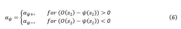
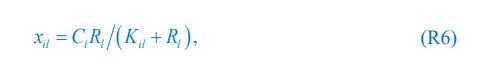
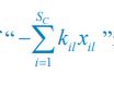
For the definition of the FRE effect employed in this study, we used a measure of relative FRE (Al-Kwifi et al., 2002) in combination with a partial-volume model (Eq. 6). To illustrate the implications of these two effects, as well as their interaction, we have estimated the relative and absolute FRE for an artery with a diameter of 200 µm or 2 000 µm (i.e. no partial-volume effects at the centre of the vessel). The absolute FRE expression explicitly takes the voxel volume into account, and so instead of Eq. (6) for the relative FRE we used"
Eq. (1)

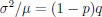
"Note that the division by M_zS^tissue⋅l_voxel^3 to obtain the relative FRE from this expression removes the contribution of the total voxel volume (l_voxel^3).
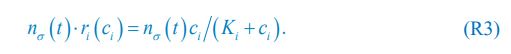
Supplementary Figure 2 shows that, when partial volume effects are present, the highest relative FRE arises in voxels with the same size as or smaller than the vessel diameter (Supplementary Figure 2A), whereas the absolute FRE increases with voxel size (Supplementary Figure 2C). If no partial-volume effects are present, the relative FRE becomes independent of voxel size (Supplementary Figure 2B), whereas the absolute FRE increases with voxel size (Supplementary Figure 2D). While the partial-volume effects for the relative FRE are substantial, they are much more subtle when using the absolute FRE and do not alter the overall characteristics."

Supplementary Figure 2: Effect of voxel size and blood delivery time on the relative flow-related enhancement (FRE) using either a relative (A,B) (Eq. (3)) or an absolute (C,D) (Eq. (12)) FRE definition assuming a pial artery diameter of 200 μm (A,C) or 2 000 µm, i.e. no partial-volume effects at the central voxel of this artery considered here.
In addition, we have also clarified the contribution of the two definitions and their interaction in the Discussion section. Following the suggestion of Reviewer 2, we have extended our interpretation of relative FRE. In brief, absolute FRE is closely related to the physical origin of the contrast, whereas relative FRE is much more concerned with the “segmentability” of a vessel (please see R2.8 for more details):
"Extending classical FRE treatments to the pial vasculature
There are several major modifications in our approach to this topic that might explain why, in contrast to predictions from classical FRE treatments, it is indeed possible to image pial arteries. For instance, the definition of vessel contrast or flow-related enhancement is often stated as an absolute difference between blood and tissue signal (Brown et al., 2014a; Carr and Carroll, 2012; Du et al., 1993, 1996; Haacke et al., 1990; Venkatesan and Haacke, 1997). Here, however, we follow the approach of Al-Kwifi et al. (2002) and consider relative contrast. While this distinction may seem to be semantic, the effect of voxel volume on FRE for these two definitions is exactly opposite: Du et al. (1996) concluded that larger voxel size increases the (absolute) vessel-background contrast, whereas here we predict an increase in relative FRE for small arteries with decreasing voxel size. Therefore, predictions of the depiction of small arteries with decreasing voxel size differ depending on whether one is considering absolute contrast, i.e. difference in longitudinal magnetization, or relative contrast, i.e. contrast differences independent of total voxel size. Importantly, this prediction changes for large arteries where the voxel contains only vessel lumen, in which case the relative FRE remains constant across voxel sizes, but the absolute FRE increases with voxel size (Supplementary Figure 2). Overall, the interpretations of relative and absolute FRE differ, and one measure may be more appropriate for certain applications than the other. Absolute FRE describes the difference in magnetization and is thus tightly linked to the underlying physical mechanism. Relative FRE, however, describes the image contrast and segmentability. If blood and tissue magnetization are equal, both contrast measures would equal zero and indicate that no contrast difference is present. However, when there is signal in the vessel and as the tissue magnetization approaches zero, the absolute FRE approaches the blood magnetization (assuming no partial-volume effects), whereas the relative FRE approaches infinity. While this infinite relative FRE does not directly relate to the underlying physical process of ‘infinite’ signal enhancement through inflowing blood, it instead characterizes the segmentability of the image in that an image with zero intensity in the background and non-zero values in the structures of interest can be segmented perfectly and trivially. Accordingly, numerous empirical observations (Al-Kwifi et al., 2002; Bouvy et al., 2014; Haacke et al., 1990; Ladd, 2007; Mattern et al., 2018; von Morze et al., 2007) and the data provided here (Figure 5, 6 and 7) have shown the benefit of smaller voxel sizes if the aim is to visualize and segment small arteries."
Note that our formulation of the FRE—even without considering SNR—does not suggest that higher resolution is always better, but instead should be matched to the size of the target arteries:
"Importantly, note that our treatment of the FRE does not suggest that an arbitrarily small voxel size is needed, but instead that voxel sizes appropriate for the arterial diameter of interest are beneficial (in line with the classic “matched-filter” rationale (North, 1963)). Voxels smaller than the arterial diameter would not yield substantial benefits (Figure 5) and may result in SNR reductions that would hinder segmentation performance."
Further, we have also extended the concluding paragraph of the Imaging limitation section to also include a practical perspective:
"In summary, numerous theoretical and practical considerations remain for optimal imaging of pial arteries using time-of-flight contrast. Depending on the application, advanced displacement artefact compensation strategies may be required, and zero-filling could provide better vessel depiction. Further, an optimal trade-off between SNR, voxel size and acquisition time needs to be found. Currently, the partial-volume FRE model only considers voxel size, and—as we reduced the voxel size in the experiments—we (partially) compensated the reduction in SNR through longer scan times. This, ultimately, also required the use of prospective motion correction to enable the very long acquisition times necessary for 140 µm isotropic voxel size. Often, anisotropic voxels are used to reduce acquisition time and increase SNR while maintaining in-plane resolution. This may indeed prove advantageous when the (also highly anisotropic) arteries align with the anisotropic acquisition, e.g. when imaging the large supplying arteries oriented mostly in the head-foot direction. In the case of pial arteries, however, there is not preferred orientation because of the convoluted nature of the pial arterial vasculature encapsulating the complex folding of the cortex (see section Anatomical architecture of the pial arterial vasculature). A further reduction in voxel size may be possible in dedicated research settings utilizing even longer acquisition times and/or larger acquisition volumes to maintain SNR. However, if acquisition time is limited, voxel size and SNR need to be carefully balanced against each other."
3) The article seems to imply that TOF-MRA is the only adequate technique to image brain vasculature, while T2 mapping, UHF T1 mapping (see e.g. Choi et al., https://doi.org/10.1016/j.neuroimage.2020.117259) phase (e.g. Fan et al., doi:10.1038/jcbfm.2014.187), QSM (see e.g. Huck et al., https://doi.org/10.1007/s00429-019-01919-4), or a combination (Bernier et al., https://doi.org/10.1002/hbm.24337, Ward et al., https://doi.org/10.1016/j.neuroimage.2017.10.049) all depict some level of vascular detail. It would be worth quickly reviewing the different effects of blood on MRI contrast and how those have been used in different approaches to measure vasculature. This would in particular help clarify the experiment combining TOF with T2 mapping used to separate arteries from veins (more on this question below).
We apologize if we inadvertently created the impression that TOF-MRA is a suitable technique to image the complete brain vasculature, and we agree that susceptibility-based methods are much more suitable for venous structures. As outlined above, we have revised the manuscript in various sections to indicate that it is the pial arterial vasculature we are targeting. We have added a statement on imaging the venous vasculature in the Discussion section. Please see our response below regarding the use of T2* to separate arteries and veins.
"The advantages of imaging the pial arterial vasculature using TOF-MRA without an exogenous contrast agent lie in its non-invasiveness and the potential to combine these data with various other structural and functional image contrasts provided by MRI. One common application is to acquire a velocity-encoded contrast such as phase-contrast MRA (Arts et al., 2021; Bouvy et al., 2016). Another interesting approach utilises the inherent time-of-flight contrast in magnetization-prepared two rapid acquisition gradient echo (MP2RAGE) images acquired at ultra-high field that simultaneously acquires vasculature and structural data, albeit at lower achievable resolution and lower FRE compared to the TOF-MRA data in our study (Choi et al., 2020). In summary, we expect high-resolution TOF-MRA to be applicable also for group studies to address numerous questions regarding the relationship of arterial topology and morphometry to the anatomical and functional organization of the brain, and the influence of arterial topology and morphometry on brain hemodynamics in humans. In addition, imaging of the pial venous vasculature—using susceptibility-based contrasts such as T2-weighted magnitude (Gulban et al., 2021) or phase imaging (Fan et al., 2015), susceptibility-weighted imaging (SWI) (Eckstein et al., 2021; Reichenbach et al., 1997) or quantitative susceptibility mapping (QSM) (Bernier et al., 2018; Huck et al., 2019; Mattern et al., 2019; Ward et al., 2018)—would enable a comprehensive assessment of the complete cortical vasculature and how both arteries and veins shape brain hemodynamics.*"
4) The results, while very impressive, are mostly qualitative. This seems a missed opportunity to strengthen the points of the paper: given the segmentations already made, the amount/density of detected vessels could be compared across scans for the data of Fig. 5 and 7. The minimum distance between vessels could be measured in Fig. 8 to show a 2D distribution and/or a spatial map of the displacement. The number of vessels labeled as veins instead of arteries in Fig. 9 could be given.
We fully agree that estimating these quantitative measures would be very interesting; however, this would require the development of a comprehensive analysis framework, which would considerably shift the focus of this paper from data acquisition and flow-related enhancement to data analysis. As noted in the discussion section Challenges for vessel segmentation algorithms, ‘The vessel segmentations presented here were performed to illustrate the sensitivity of the image acquisition to small pial arteries’, because the smallest arteries tend to be concealed in the maximum intensity projections. Further, the interpretation of these measures is not straightforward. For example, the number of detected vessels for the artery depicted in Figure 5 does not change across resolutions, but their length does. We have therefore estimated the relative increase in skeleton length across resolutions for Figures 5 and 7. However, these estimates are not only a function of the voxel size but also of the underlying vasculature, i.e. the number of arteries with a certain diameter present, and may thus not generalise well to enable quantitative predictions of the improvement expected from increased resolutions. We have added an illustration of these analyses in the Supplementary Material, and the following additions in the Methods, Results and Discussion sections.
"For vessel segmentation, a semi-automatic segmentation pipeline was implemented in Matlab R2020a (The MathWorks, Natick, MA) using the UniQC toolbox (Frässle et al., 2021): First, a brain mask was created through thresholding which was then manually corrected in ITK-SNAP (http://www.itksnap.org/) (Yushkevich et al., 2006) such that pial vessels were included. For the high-resolution TOF data (Figures 6 and 7, Supplementary Figure 4), denoising to remove high frequency noise was performed using the implementation of an adaptive non-local means denoising algorithm (Manjón et al., 2010) provided in DenoiseImage within the ANTs toolbox, with the search radius for the denoising set to 5 voxels and noise type set to Rician. Next, the brain mask was applied to the bias corrected and denoised data (if applicable). Then, a vessel mask was created based on a manually defined threshold, and clusters with less than 10 or 5 voxels for the high- and low-resolution acquisitions, respectively, were removed from the vessel mask. Finally, an iterative region-growing procedure starting at each voxel of the initial vessel mask was applied that successively included additional voxels into the vessel mask if they were connected to a voxel which was already included and above a manually defined threshold (which was slightly lower than the previous threshold). Both thresholds were applied globally but manually adjusted for each slab. No correction for motion between slabs was applied. The Matlab code describing the segmentation algorithm as well as the analysis of the two-echo TOF acquisition outlined in the following paragraph are also included in our github repository (https://gitlab.com/SaskiaB/pialvesseltof.git). To assess the data quality, maximum intensity projections (MIPs) were created and the outline of the segmentation MIPs were added as an overlay. To estimate the increased detection of vessels with higher resolutions, we computed the relative increase in the length of the segmented vessels for the data presented in Figure 5 (0.8 mm, 0.5 mm, 0.4 mm and 0.3 mm isotropic voxel size) and Figure 7 (0.16 mm and 0.14 mm isotropic voxel size) by computing the skeleton using the bwskel Matlab function and then calculating the skeleton length as the number of voxels in the skeleton multiplied by the voxel size."
"To investigate the effect of voxel size on vessel FRE, we acquired data at four different voxel sizes ranging from 0.8 mm to 0.3 mm isotropic resolution, adjusting only the encoding matrix, with imaging parameters being otherwise identical (FOV, TR, TE, flip angle, R, slab thickness, see section Data acquisition). The total acquisition time increases from less than 2 minutes for the lowest resolution scan to over 6 minutes for the highest resolution scan as a result. Figure 5 shows thin maximum intensity projections of a small vessel. While the vessel is not detectable at the largest voxel size, it slowly emerges as the voxel size decreases and approaches the vessel size. Presumably, this is driven by the considerable increase in FRE as seen in the single slice view (Figure 5, small inserts). Accordingly, the FRE computed from the vessel mask for the smallest part of the vessel (Figure 5, red mask) increases substantially with decreasing voxel size. More precisely, reducing the voxel size from 0.8 mm, 0.5 mm or 0.4 mm to 0.3 mm increases the FRE by 2900 %, 165 % and 85 %, respectively. Assuming a vessel diameter of 300 μm, the partial-volume FRE model (section Introducing a partial-volume model) would predict similar ratios of 611%, 178% and 78%. However, as long as the vessel is larger than the voxel (Figure 5, blue mask), the relative FRE does not change with resolution (see also Effect of FRE Definition and Interaction with Partial-Volume Model in the Supplementary Material). To illustrate the gain in sensitivity to detect smaller arteries, we have estimated the relative increase of the total length of the segmented vasculature (Supplementary Figure 9): reducing the voxel size from 0.8 mm to 0.5 mm isotropic increases the skeleton length by 44 %, reducing the voxel size from 0.5 mm to 0.4 mm isotropic increases the skeleton length by 28 %, and reducing the voxel size from 0.4 mm to 0.3 mm isotropic increases the skeleton length by 31 %. In summary, when imaging small pial arteries, these data support the hypothesis that it is primarily the voxel size, not the blood delivery time, which determines whether vessels can be resolved."
"Indeed, the reduction in voxel volume by 33 % revealed additional small branches connected to larger arteries (see also Supplementary Figure 8). For this example, we found an overall increase in skeleton length of 14 % (see also Supplementary Figure 9)."
"We therefore expect this strategy to enable an efficient image acquisition without the need for additional venous suppression RF pulses.
Once these challenges for vessel segmentation algorithms are addressed, a thorough quantification of the arterial vasculature can be performed. For example, the skeletonization procedure used to estimate the increase of the total length of the segmented vasculature (Supplementary Figure 9) exhibits errors particularly in the unwanted sinuses and large veins. While they are consistently present across voxel sizes, and thus may have less impact on relative change in skeleton length, they need to be addressed when estimating the absolute length of the vasculature, or other higher-order features such as number of new branches. (Note that we have also performed the skeletonization procedure on the maximum intensity projections to reduce the number of artefacts and obtained comparable results: reducing the voxel size from 0.8 mm to 0.5 mm isotropic increases the skeleton length by 44 % (3D) vs 37 % (2D), reducing the voxel size from 0.5 mm to 0.4 mm isotropic increases the skeleton length by 28 % (3D) vs 26 % (2D), reducing the voxel size from 0.4 mm to 0.3 mm isotropic increases the skeleton length by 31 % (3D) vs 16 % (2D), and reducing the voxel size from 0.16 mm to 0.14 mm isotropic increases the skeleton length by 14 % (3D) vs 24 % (2D).)"
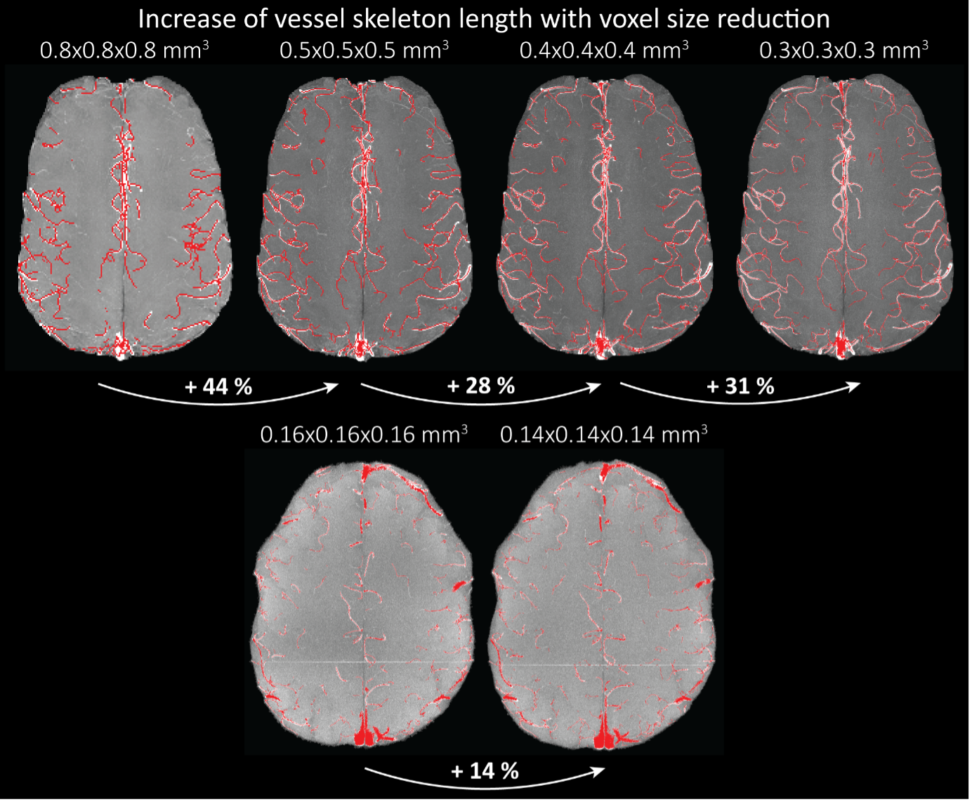
Supplementary Figure 9: Increase of vessel skeleton length with voxel size reduction. Axial maximum intensity projections for data acquired with different voxel sizes ranging from 0.8 mm to 0.3 mm (TOP) (corresponding to Figure 5) and 0.16 mm to 0.14 mm isotropic (corresponding to Figure 7) are shown. Vessel skeletons derived from segmentations performed for each resolution are overlaid in red. A reduction in voxel size is accompanied by a corresponding increase in vessel skeleton length.
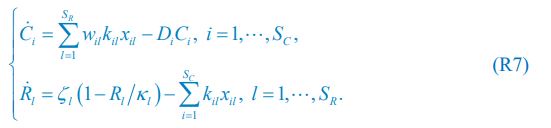
Regarding further quantification of the vessel displacement presented in Figure 8, we have estimated the displacement using the Horn-Schunck optical flow estimator (Horn and Schunck, 1981; Mustafa, 2016) (https://github.com/Mustafa3946/Horn-Schunck-3D-Optical-Flow). However, the results are dominated by the larger arteries, whereas we are mostly interested in the displacement of the smallest arteries, therefore this quantification may not be helpful.
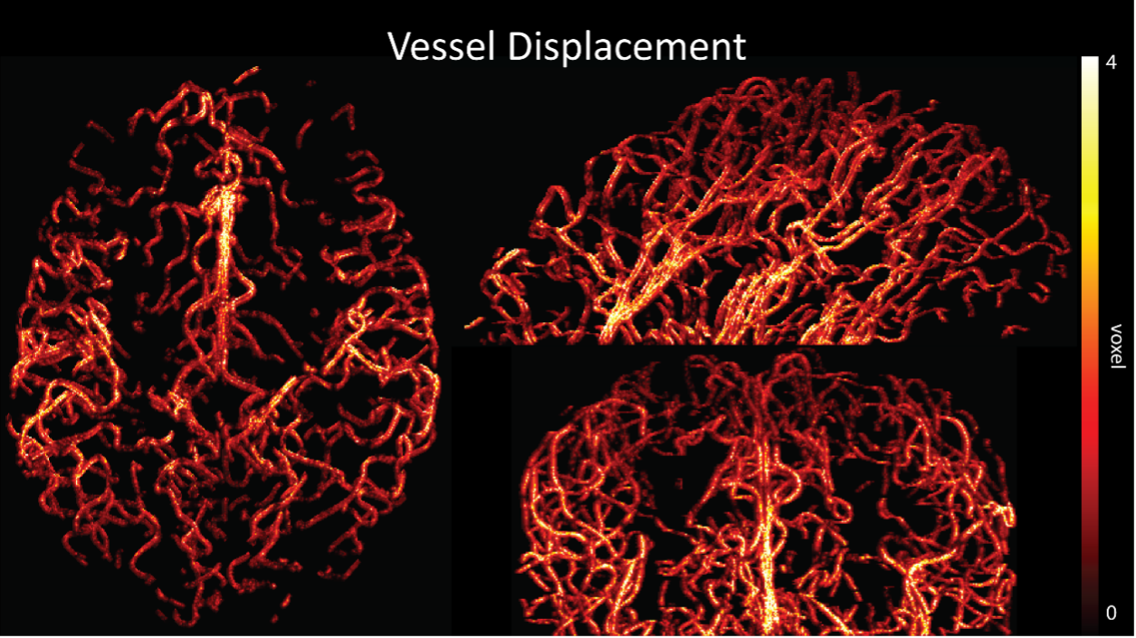
Because the theoretical relationship between vessel displacement and blood velocity is well known (Eq. 7), and we have also outlined the expected blood velocity as a function of arterial diameter in Figure 2, which provided estimates of displacements that matched what was found in our data (as reported in our original submission), we believe that the new quantification in this form does not add value to the manuscript. What would be interesting would be to explore the use of this displacement artefact as a measure of blood velocities. This, however, would require more substantial analyses in particular for estimation of the arterial diameter and additional validation data (e.g. phase-contrast MRA). We have outlined this avenue in the Discussion section. What is relevant to the main aim of this study, namely imaging of small pial arteries, is the insight that blood velocities are indeed sufficiently fast to cause displacement artefacts even in smaller arteries. We have clarified this in the Results section:
"Note that correction techniques exist to remove displaced vessels from the image (Gulban et al., 2021), but they cannot revert the vessels to their original location. Alternatively, this artefact could also potentially be utilised as a rough measure of blood velocity."
"At a delay time of 10 ms between phase encoding and echo time, the observed displacement of approximately 2 mm in some of the larger vessels would correspond to a blood velocity of 200 mm/s, which is well within the expected range (Figure 2). For the smallest arteries, a displacement of one voxel (0.4 mm) can be observed, indicative of blood velocities of 40 mm/s. Note that the vessel displacement can be observed in all vessels visible at this resolution, indicating high blood velocities throughout much of the pial arterial vasculature. Thus, assuming a blood velocity of 40 mm/s (Figure 2) and a delay time of 5 ms for the high-resolution acquisitions (Figure 6), vessel displacements of 0.2 mm are possible, representing a shift of 1–2 voxels."
Regarding the number of vessels labelled as veins, please see our response below to R1.5.
In the main quantification given, the estimation of FRE increase with resolution, it would make more sense to perform the segmentation independently for each scan and estimate the corresponding FRE: using the mask from the highest resolution scan only biases the results. It is unclear also if the background tissue measurement one voxel outside took partial voluming into account (by leaving a one voxel free interface between vessel and background). In this analysis, it would also be interesting to estimate SNR, so you can compare SNR and FRE across resolutions, also helpful for the discussion on SNR.
The FRE serves as an indicator of the potential performance of any segmentation algorithm (including manual segmentation) (also see our discussion on the interpretation of FRE in our response to R1.2). If we were to segment each scan individually, we would, in the ideal case, always obtain the same FRE estimate, as FRE influences the performance of the segmentation algorithm. In practice, this simply means that it is not possible to segment the vessel in the low-resolution image to its full extent that is visible in the high-resolution image, because the FRE is too low for small vessels. However, we agree with the core point that the reviewer is making, and so to help address this, a valuable addition would be to compare the FRE for the section of a vessel that is visible at all resolutions, where we found—within the accuracy of the transformations and resampling across such vastly different resolutions—that the FRE does not increase any further with higher resolution if the vessel is larger than the voxel size (page 18 and Figure 5). As stated in the Methods section, and as noted by the reviewer, we used the voxels immediately next to the vessel mask to define the background tissue signal level. Any resulting potential partial-volume effects in these background voxels would affect all voxel sizes, introducing a consistent bias that would not impact our comparison. However, inspection of the image data in Figure 5 showed partial-volume effects predominantly within those voxels intersecting the vessel, rather than voxels surrounding the vessel, in agreement with our model of FRE.
"All imaging data were slab-wise bias-field corrected using the N4BiasFieldCorrection (Tustison et al., 2010) tool in ANTs (Avants et al., 2009) with the default parameters. To compare the empirical FRE across the four different resolutions (Figure 5), manual masks were first created for the smallest part of the vessel in the image with the highest resolution and for the largest part of the vessel in the image with the lowest resolution. Then, rigid-body transformation parameters from the low-resolution to the high-resolution (and the high-resolution to the low-resolution) images were estimated using coregister in SPM (https://www.fil.ion.ucl.ac.uk/spm/), and their inverse was applied to the vessel mask using SPM’s reslice. To calculate the empirical FRE (Eq. (3)), the mean of the intensity values within the vessel mask was used to approximate the blood magnetization, and the mean of the intensity values one voxel outside of the vessel mask was used as the tissue magnetization."
"To investigate the effect of voxel size on vessel FRE, we acquired data at four different voxel sizes ranging from 0.8 mm to 0.3 mm isotropic resolution, adjusting only the encoding matrix, with imaging parameters being otherwise identical (FOV, TR, TE, flip angle, R, slab thickness, see section Data acquisition). The total acquisition time increases from less than 2 minutes for the lowest resolution scan to over 6 minutes for the highest resolution scan as a result. Figure 5 shows thin maximum intensity projections of a small vessel. While the vessel is not detectable at the largest voxel size, it slowly emerges as the voxel size decreases and approaches the vessel size. Presumably, this is driven by the considerable increase in FRE as seen in the single slice view (Figure 5, small inserts). Accordingly, the FRE computed from the vessel mask for the smallest part of the vessel (Figure 5, red mask) increases substantially with decreasing voxel size. More precisely, reducing the voxel size from 0.8 mm, 0.5 mm or 0.4 mm to 0.3 mm increases the FRE by 2900 %, 165 % and 85 %, respectively. Assuming a vessel diameter of 300 μm, the partial-volume FRE model (section Introducing a partial-volume model) would predict similar ratios of 611%, 178% and 78%. However, if the vessel is larger than the voxel (Figure 5, blue mask), the relative FRE remains constant across resolutions (see also Effect of FRE Definition and Interaction with Partial-Volume Model in the Supplementary Material). To illustrate the gain in sensitivity to smaller arteries, we have estimated the relative increase of the total length of the segmented vasculature (Supplementary Figure 9): reducing the voxel size from 0.8 mm to 0.5 mm isotropic increases the skeleton length by 44 %, reducing the voxel size from 0.5 mm to 0.4 mm isotropic increases the skeleton length by 28 %, and reducing the voxel size from 0.4 mm to 0.3 mm isotropic increases the skeleton length by 31 %. In summary, when imaging small pial arteries, these data support the hypothesis that it is primarily the voxel size, not blood delivery time, which determines whether vessels can be resolved."
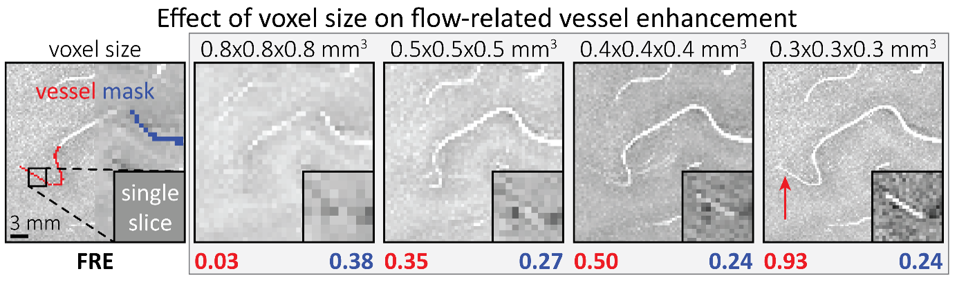
Figure 5: Effect of voxel size on flow-related vessel enhancement. Thin axial maximum intensity projections containing a small artery acquired with different voxel sizes ranging from 0.8 mm to 0.3 mm isotropic are shown. The FRE is estimated using the mean intensity value within the vessel masks depicted on the left, and the mean intensity values of the surrounding tissue. The small insert shows a section of the artery as it lies within a single slice. A reduction in voxel size is accompanied by a corresponding increase in FRE (red mask), whereas no further increase is obtained once the voxel size is equal or smaller than the vessel size (blue mask).
After many internal discussions, we had to conclude that deducing a meaningful SNR analysis that would benefit the reader was not possible given the available data due to the complex relationship between voxel size and other imaging parameters in practice. In detail, we have reduced the voxel size but at the same time increased the acquisition time by increasing the number of encoding steps—which we have now also highlighted in the manuscript. We have, however, added additional considerations about balancing SNR and segmentation performance. Note that these considerations are not specific to imaging the pial arteries but apply to all MRA acquisitions, and have thus been discussed previously in the literature. Here, we wanted to focus on the novel insights gained in our study. Importantly, while we previously noted that reducing voxel size improves contrast in vessels whose diameters are smaller than the voxel size, we now explicitly acknowledge that, for vessels whose diameters are larger than the voxel size reducing the voxel size is not helpful---since it only reduces SNR without any gain in contrast---and may hinder segmentation performance, and thus become counterproductive.
"In general, we have not considered SNR, but only FRE, i.e. the (relative) image contrast, assuming that segmentation algorithms would benefit from higher contrast for smaller arteries. Importantly, the acquisition parameters available to maximize FRE are limited, namely repetition time, flip angle and voxel size. SNR, however, can be improved via numerous avenues independent of these parameters (Brown et al., 2014b; Du et al., 1996; Heverhagen et al., 2008; Parker et al., 1991; Triantafyllou et al., 2011; Venkatesan and Haacke, 1997), the simplest being longer acquisition times. If the aim is to optimize a segmentation outcome for a given acquisition time, the trade-off between contrast and SNR for the specific segmentation algorithm needs to be determined (Klepaczko et al., 2016; Lesage et al., 2009; Moccia et al., 2018; Phellan and Forkert, 2017). Our own—albeit limited—experience has shown that segmentation algorithms (including manual segmentation) can accommodate a perhaps surprising amount of noise using prior knowledge and neighborhood information, making these high-resolution acquisitions possible. Importantly, note that our treatment of the FRE does not suggest that an arbitrarily small voxel size is needed, but instead that voxel sizes appropriate for the arterial diameter of interest are beneficial (in line with the classic “matched-filter” rationale (North, 1963)). Voxels smaller than the arterial diameter would not yield substantial benefits (Figure 5) and may result in SNR reductions that would hinder segmentation performance."
5) The separation of arterial and venous components is a bit puzzling, partly because the methodology used is not fully explained, but also partly because the reasons invoked (flow artefact in large pial veins) do not match the results (many small vessels are included as veins). This question of separating both types of vessels is quite important for applications, so the whole procedure should be explained in detail. The use of short T2 seemed also sub-optimal, as both arteries and veins result in shorter T2 compared to most brain tissues: wouldn't a susceptibility-based measure (SWI or better QSM) provide a better separation? Finally, since the T2* map and the regular TOF map are at different resolutions, masking out the vessels labeled as veins will likely result in the smaller veins being left out.
We agree that while the technical details of this approach were provided in the Data analysis section, the rationale behind it was only briefly mentioned. We have therefore included an additional section Inflow-artefacts in sinuses and pial veins in the Theory section of the manuscript. We have also extended the discussion of the advantages and disadvantages of the different susceptibility-based contrasts, namely T2, SWI and QSM. While in theory both T2 and QSM should allow the reliable differentiation of arterial and venous blood, we found T2* to perform more robustly, as QSM can fail in many places, e.g., due to the strong susceptibility sources within superior sagittal and transversal sinuses and pial veins and their proximity to the brain surface, dedicated processing is required (Stewart et al., 2022). Further, we have also elaborated in the Discussion section why the interpretation of Figure 9 regarding the absence or presence of small veins is challenging. Namely, the intensity-based segmentation used here provides only an incomplete segmentation even of the larger sinuses, because the overall lower intensity found in veins combined with the heterogeneity of the intensities in veins violates the assumptions made by most vascular segmentation approaches of homogenous, high image intensities within vessels, which are satisfied in arteries (page 29f) (see also the illustration below). Accordingly, quantifying the number of vessels labelled as veins (R1.4a) would provide misleading results, as often only small subsets of the same sinus or vein are segmented.
"Inflow-artefacts in sinuses and pial veins
Inflow in large pial veins and the sagittal and transverse sinuses can cause flow-related enhancement in these non-arterial vessels. One common strategy to remove this unwanted signal enhancement is to apply venous suppression pulses during the data acquisition, which saturate bloods spins outside the imaging slab. Disadvantages of this technique are the technical challenges of applying these pulses at ultra-high field due to constraints of the specific absorption rate (SAR) and the necessary increase in acquisition time (Conolly et al., 1988; Heverhagen et al., 2008; Johst et al., 2012; Maderwald et al., 2008; Schmitter et al., 2012; Zhang et al., 2015). In addition, optimal positioning of the saturation slab in the case of pial arteries requires further investigation, and in particular supressing signal from the superior sagittal sinus without interfering in the imaging of the pial arteries vasculature at the top of the cortex might prove challenging. Furthermore, this venous saturation strategy is based on the assumption that arterial blood is traveling head-wards while venous blood is drained foot-wards. For the complex and convoluted trajectory of pial vessels this directionality-based saturation might be oversimplified, particularly when considering the higher-order branches of the pial arteries and veins on the cortical surface. Inspired by techniques to simultaneously acquire a TOF image for angiography and a susceptibility-weighted image for venography (Bae et al., 2010; Deistung et al., 2009; Du et al., 1994; Du and Jin, 2008), we set out to explore the possibility of removing unwanted venous structures from the segmentation of the pial arterial vasculature during data postprocessing. Because arteries filled with oxygenated blood have T2-values similar to tissue, while veins have much shorter T2-values due to the presence of deoxygenated blood (Pauling and Coryell, 1936; Peters et al., 2007; Uludağ et al., 2009; Zhao et al., 2007), we used this criterion to remove vessels with short T2* values from the segmentation (see Data Analysis for details). In addition, we also explored whether unwanted venous structures in the high-resolution TOF images—where a two-echo acquisition is not feasible due to the longer readout—can be removed based on detecting them in a lower-resolution image."
"Removal of pial veins
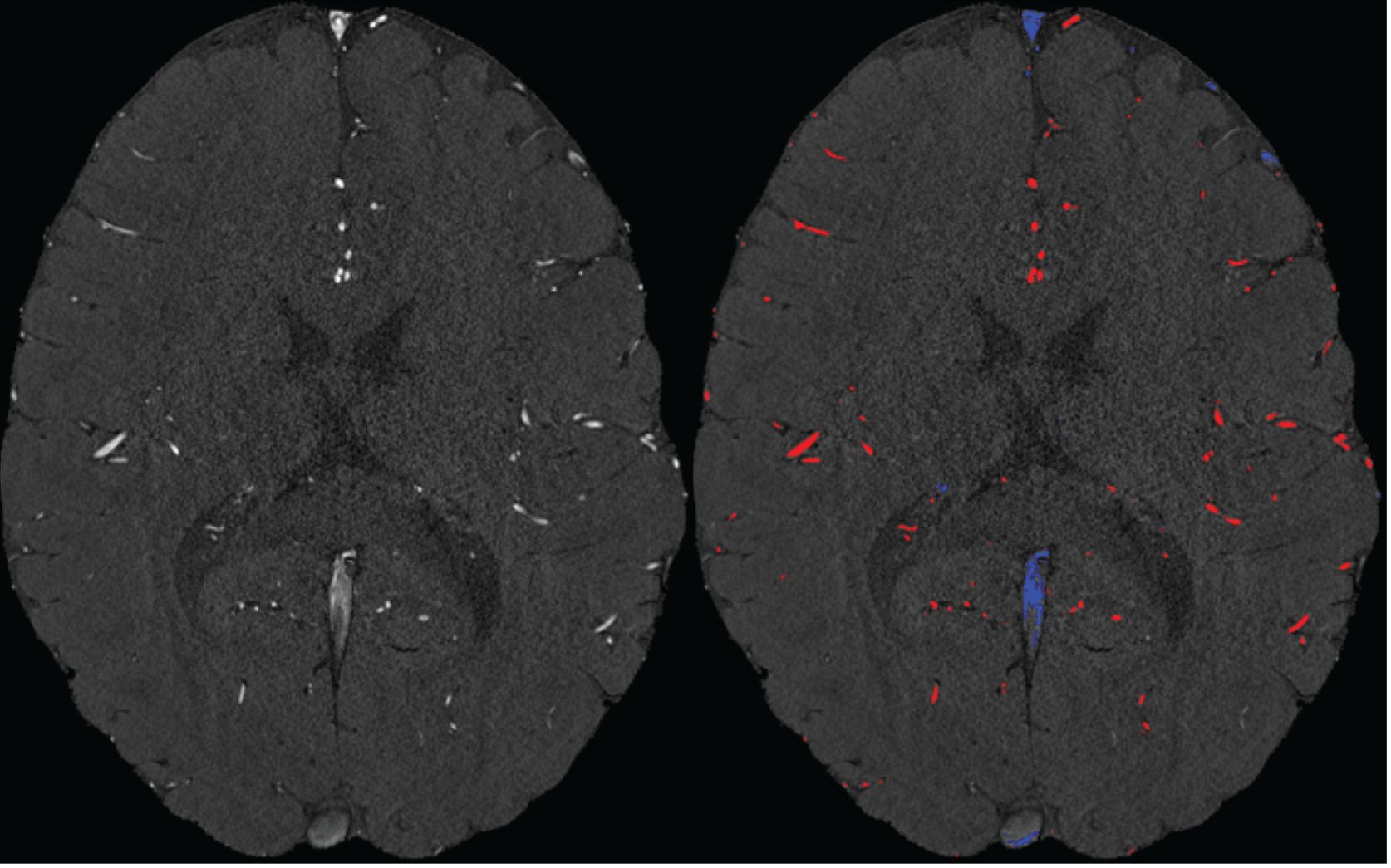
Inflow in large pial veins and the superior sagittal and transverse sinuses can cause a flow-related enhancement in these non-arterial vessels (Figure 9, left). The higher concentration of deoxygenated haemoglobin in these vessels leads to shorter T2 values (Pauling and Coryell, 1936), which can be estimated using a two-echo TOF acquisition (see also Inflow-artefacts in sinuses and pial veins). These vessels can be identified in the segmentation based on their T2 values (Figure 9, left), and removed from the angiogram (Figure 9, right) (Bae et al., 2010; Deistung et al., 2009; Du et al., 1994; Du and Jin, 2008). In particular, the superior and inferior sagittal and the transversal sinuses and large veins which exhibited an inhomogeneous intensity profile and a steep loss of intensity at the slab boundary were identified as non-arterial (Figure 9, left). Further, we also explored the option of removing unwanted venous vessels from the high-resolution TOF image (Figure 7) using a low-resolution two-echo TOF (not shown). This indeed allowed us to remove the strong signal enhancement in the sagittal sinuses and numerous larger veins, although some small veins, which are characterised by inhomogeneous intensity profiles and can be detected visually by experienced raters, remain."
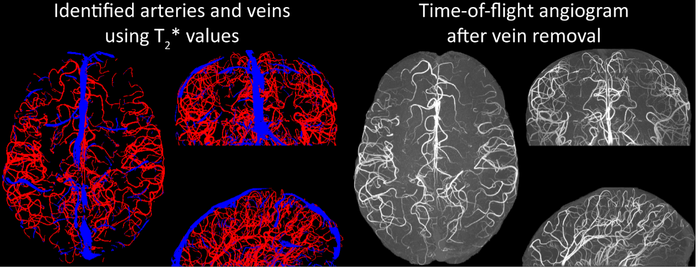
Figure 9: Removal of non-arterial vessels in time-of-flight imaging. LEFT: Segmentation of arteries (red) and veins (blue) using T_2^ estimates. RIGHT: Time-of-flight angiogram after vein removal.*
Our approach also assumes that the unwanted veins are large enough that they are also resolved in the low-resolution image. If we consider the source of the FRE effect, it might indeed be exclusively large veins that are present in TOF-MRA data, which would suggest that our assumption is valid. Fundamentally, the FRE depends on the inflow of un-saturated spins into the imaging slab. However, small veins drain capillary beds in the local tissue, i.e. the tissue within the slab. (Note that due to the slice oversampling implemented in our acquisition, spins just above or below the slab will also be excited.) Thus, small veins only contain blood water spins that have experienced a large number of RF pulses due to the long transit time through the pial arterial vasculature, the capillaries and the intracortical venules. Hence, their longitudinal magnetization would be similar to that of stationary tissue. To generate an FRE effect in veins, “pass-through” venous blood from outside the imaging slab is required. This is only available in veins that are passing through the imaging slab, which have much larger diameters. These theoretical considerations are corroborated by the findings in Figure 9, where large disconnected vessels with varying intensity profiles were identified as non-arterial. Due to the heterogenous intensity profiles in large veins and the sagittal and transversal sinuses, the intensity-based segmentation applied here may only label a subset of the vessel lumen, creating the impression of many small veins. This is particularly the case for the straight and inferior sagittal sinus in the bottom slab of Figure 9. Nevertheless, future studies potentially combing anatomical prior knowledge, advanced segmentation algorithms and susceptibility measures would be capable of removing these unwanted veins in post-processing to enable an efficient TOF-MRA image acquisition dedicated to optimally detecting small arteries without the need for additional venous suppression RF pulses.
6) A more general question also is why this imaging method is limited to pial vessels: at 140 microns, the larger intra-cortical vessels should be appearing (group 6 in Duvernoy, 1981: diameters between 50 and 240 microns). Are there other reasons these vessels are not detected? Similarly, it seems there is no arterial vasculature detected in the white matter here: it is due to the rather superior location of the imaging slab, or a limitation of the method? Likewise, all three results focus on a rather homogeneous region of cerebral cortex, in terms of vascularisation. It would be interesting for applications to demonstrate the capabilities of the method in more complex regions, e.g. the densely vascularised cerebellum, or more heterogeneous regions like the midbrain. Finally, it is notable that all three subjects appear to have rather different densities of vessels, from sparse (participant II) to dense (participant I), with some inhomogeneities in density (frontal region in participant III) and inconsistencies in detection (sinuses absent in participant II). All these points should be discussed.
While we are aware that the diameter of intracortical arteries has been suggested to be up to 240 µm (Duvernoy et al., 1981), it remains unclear how prevalent intracortical arteries of this size are. For example, note that in a different context in the Duvernoy study (in teh revised manuscript), the following values are mentioned (which we followed in Figure 1):
“Central arteries of the Iobule always have a large diameter of 260 µ to 280 µ, at their origin. Peripheral arteries have an average diameter of 150 µ to 180 µ. At the cortex surface, all arterioles of 50 µ or less, penetrate the cortex or form anastomoses. The diameter of most of these penetrating arteries is approximately 40 µ.”
Further, the examinations by Hirsch et al. (2012) (albeit in the macaque brain), showed one (exemplary) intracortical artery belonging to group 6 (Figure 1B), whose diameter appears to be below 100 µm. Given these discrepancies and the fact that intracortical arteries in group 5 only reach 75 µm, we suspect that intracortical arteries with diameters > 140 µm are a very rare occurrence, which we might not have encountered in this data set.
Similarly, arteries in white matter (Nonaka et al., 2003) and the cerebellum (Duvernoy et al., 1983) are beyond our resolution at the moment. The midbrain is an interesting suggesting, although we believe that the cortical areas chosen here with their gradual reduction in diameter along the vascular tree, provide a better illustration of the effect of voxel size than the rather abrupt reduction in vascular diameter found in the midbrain. We have added the even higher resolution requirements in the discussion section:
"In summary, we expect high-resolution TOF-MRA to be applicable also for group studies, to address numerous questions regarding the relationship of arterial topology and morphometry to the anatomical and functional organization of the brain, and the influence of arterial topology and morphometry on brain hemodynamics in humans. Notably, we have focused on imaging pial arteries of the human cerebrum; however, other brain structures such as the cerebellum, subcortex and white matter are of course also of interest. While the same theoretical considerations apply, imaging the arterial vasculature in these structures will require even smaller voxel sizes due to their smaller arterial diameters (Duvernoy et al., 1983, 1981; Nonaka et al., 2003)."
Regarding the apparent sparsity of results from participant II, this is mostly driven by the much smaller coverage in this subject (19.6 mm in Participant II vs. 50 mm and 58 mm in Participant I and III, respectively). The reduction in density in the frontal regions might indeed constitute difference in anatomy or might be driven by the presence or more false-positive veins in Participant I than Participant III in these areas. Following the depiction in Duvernoy et al. (1981), one would not expect large arteries in frontal areas, but large veins are common. Thus, the additional vessels in Participant I in the frontal areas might well be false-positive veins, and their removal would result in similar densities for both participants. Indeed, as pointed out in section Future directions, we would expect a lower arterial density in frontal and posterior areas than in middle areas. The sinuses (and other large false-positive veins) in Participant II have been removed as outlined and discussed in sections Removal of pial veins and Challenges for vessel segmentation algorithms, respectively.
7) One of the main practical limitations of the proposed method is the use of a very small imaging slab. It is mentioned in the discussion that thicker slabs are not only possible, but beneficial both in terms of SNR and acceleration possibilities. What are the limitations that prevented their use in the present study? With the current approach, what would be the estimated time needed to acquire the vascular map of an entire brain? It would also be good to indicate whether specific processing was needed to stitch together the multiple slab images in Fig. 6-9, S2.
Time-of-flight acquisitions are commonly performed with thin acquisition slabs, following initial investigations by Parker et al. (1991) to maximise vessel sensitivity and minimize noise. We therefore followed this practice for our initial investigations but wanted to point out in the discussion that thicker slabs might provide several advantages that need to be evaluated in future studies. This would include theoretical and empirical evaluations balancing SNR gains from larger excitation volumes and SNR losses due to more acceleration. For this study, we have chosen the slab thickness such as to keep the acquisition time at a reasonable amount to minimize motion artefacts (as outlined in the Discussion). In addition, due to the extreme matrix sizes in particular for the 0.14 mm acquisition, we were also limited in the number of data points per image that can be indexed. This would require even more substantial changes to the sequence than what we have already performed. With 16 slabs, assuming optimal FOV orientation, full-brain coverage including the cerebellum of 95 % of the population (Mennes et al., 2014) could be achieved with an acquisition time of (16 11 min 42 s = 3 h 7 min 12 s) at 0.16 mm isotropic voxel size. No stitching of the individual slabs was performed, as subject motion was minimal. We have added a corresponding comment in the Data Analysis.
"Both thresholds were applied globally but manually adjusted for each slab. No correction for motion between slabs was applied as subject motion was minimal. The Matlab code describing the segmentation algorithm as well es the analysis of the two-echo TOF acquisition outlined in the following paragraph are also included in the github repository (https://gitlab.com/SaskiaB/pialvesseltof.git)."
8) Some researchers and clinicians will argue that you can attain best results with anisotropic voxels, combining higher SNR and higher resolution. It would be good to briefly mention why isotropic voxels are preferred here, and whether anisotropic voxels would make sense at all in this context.
Anisotropic voxels can be advantageous if the underlying object is anisotropic, e.g. an artery running straight through the slab, which would have a certain diameter (imaged using the high-resolution plane) and an ‘infinite’ elongation (in the low-resolution direction). However, the vessels targeted here can have any orientation and curvature; an anisotropic acquisition could therefore introduce a bias favouring vessels with a particular orientation relative to the voxel grid. Note that the same argument applies when answering the question why a further reduction slab thickness would eventually result in less increase in FRE (section Introducing a partial-volume model). We have added a corresponding comment in our discussion on practical imaging considerations:
"In summary, numerous theoretical and practical considerations remain for optimal imaging of pial arteries using time-of-flight contrast. Depending on the application, advanced displacement artefact compensation strategies may be required, and zero-filling could provide better vessel depiction. Further, an optimal trade-off between SNR, voxel size and acquisition time needs to be found. Currently, the partial-volume FRE model only considers voxel size, and—as we reduced the voxel size in the experiments—we (partially) compensated the reduction in SNR through longer scan times. This, ultimately, also required the use of prospective motion correction to enable the very long acquisition times necessary for 140 µm isotropic voxel size. Often, anisotropic voxels are used to reduce acquisition time and increase SNR while maintaining in-plane resolution. This may indeed prove advantageous when the (also highly anisotropic) arteries align with the anisotropic acquisition, e.g. when imaging the large supplying arteries oriented mostly in the head-foot direction. In the case of pial arteries, however, there is not preferred orientation because of the convoluted nature of the pial arterial vasculature encapsulating the complex folding of the cortex (see section Anatomical architecture of the pial arterial vasculature). A further reduction in voxel size may be possible in dedicated research settings utilizing even longer acquisition times and a larger field-of-view to maintain SNR. However, if acquisition time is limited, voxel size and SNR need to be carefully balanced against each other."
Reviewer #2 (Public Review):
Overview
This paper explores the use of inflow contrast MRI for imaging the pial arteries. The paper begins by providing a thorough background description of pial arteries, including past studies investigating the velocity and diameter. Following this, the authors consider this information to optimize the contrast between pial arteries and background tissue. This analysis reveals spatial resolution to be a strong factor influencing the contrast of the pial arteries. Finally, experiments are performed on a 7T MRI to investigate: the effect of spatial resolution by acquiring images at multiple resolutions, demonstrate the feasibility of acquiring ultrahigh resolution 3D TOF, the effect of displacement artifacts, and the prospect of using T2* to remove venous voxels.
Impression
There is certainly interest in tools to improve our understanding of the architecture of the small vessels of the brain and this work does address this. The background description of the pial arteries is very complete and the manuscript is very well prepared. The images are also extremely impressive, likely benefiting from motion correction, 7T, and a very long scan time. The authors also commit to open science and provide the data in an open platform. Given this, I do feel the manuscript to be of value to the community; however, there are concerns with the methods for optimization, the qualitative nature of the experiments, and conclusions drawn from some of the experiments.
Specific Comments :
1) Figure 3 and Theory surrounding. The optimization shown in Figure 3 is based fixing the flip angle or the TR. As is well described in the literature, there is a strong interdependency of flip angle and TR. This is all well described in literature dating back to the early 90s. While I think it reasonable to consider these effects in optimization, the language needs to include this interdependency or simply reference past work and specify how the flip angle was chosen. The human experiments do not include any investigation of flip angle or TR optimization.
We thank the reviewer for raising this valuable point, and we fully agree that there is an interdependency between these two parameters. To simplify our optimization, we did fix one parameter value at a time, but in the revised manuscript we clarified that both parameters can be optimized simultaneously. Importantly, a large range of parameter values will result in a similar FRE in the small artery regime, which is illustrated in the optimization provided in the main text. We have therefore chosen the repetition time based on encoding efficiency and then set a corresponding excitation flip angle. In addition, we have also provided additional simulations in the supplementary material outlining the interdependency for the case of pial arteries.
"Optimization of repetition time and excitation flip angle
As the main goal of the optimisation here was to start within an already established parameter range for TOF imaging at ultra-high field (Kang et al., 2010; Stamm et al., 2013; von Morze et al., 2007), we only needed to then further tailor these for small arteries by considering a third parameter, namely the blood delivery time. From a practical perspective, a TR of 20 ms as a reference point was favourable, as it offered a time-efficient readout minimizing wait times between excitations but allowing low encoding bandwidths to maximize SNR. Due to the interdependency of flip angle and repetition time, for any one blood delivery time any FRE could (in theory) be achieved. For example, a similar FRE curve at 18 ° flip angle and 5 ms TR can also be achieved at 28 ° flip angle and 20 ms TR; or the FRE curve at 18 ° flip angle and 30 ms TR is comparable to the FRE curve at 8 ° flip angle and 5 ms TR (Supplementary Figure 3 TOP). In addition, the difference between optimal parameter settings diminishes for long blood delivery times, such that at a blood delivery time of 500 ms (Supplementary Figure 3 BOTTOM), the optimal flip angle at a TR of 15 ms, 20 ms or 25 ms would be 14 °, 16 ° and 18 °, respectively. This is in contrast to a blood delivery time of 100 ms, where the optimal flip angles would be 32 °, 37 ° and 41 °. In conclusion, in the regime of small arteries, long TR values in combination with low flip angles ensure flow-related enhancement at blood delivery times of 200 ms and above, and within this regime there are marginal gains by further optimizing parameter values and the optimal values are all similar."
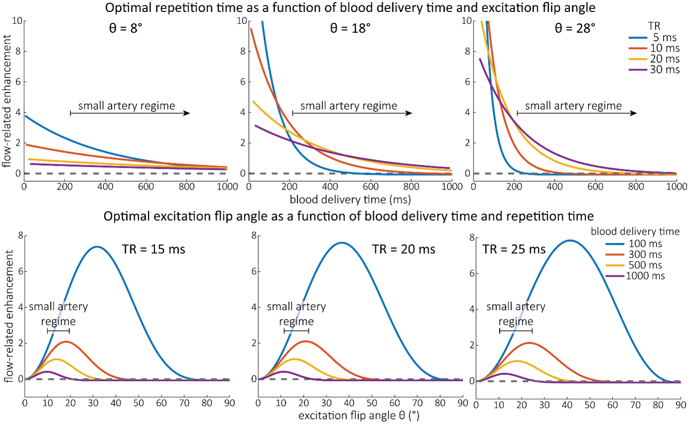
Supplementary Figure 3: Optimal imaging parameters for small arteries. This assessment follows the simulations presented in Figure 3, but in addition shows the interdependency for the corresponding third parameter (either flip angle or repetition time). TOP: Flip angles close to the Ernst angle show only a marginal flow-related enhancement; however, the influence of the blood delivery time decreases further (LEFT). As the flip angle increases well above the values used in this study, the flow-related enhancement in the small artery regime remains low even for the longer repetition times considered here (RIGHT). BOTTOM: The optimal excitation flip angle shows reduced variability across repetition times in the small artery regime compared to shorter blood delivery times.
"Based on these equations, optimal T_R and excitation flip angle values (θ) can be calculated for the blood delivery times under consideration (Figure 3). To better illustrate the regime of small arteries, we have illustrated the effect of either flip angle or T_R while keeping the other parameter values fixed to the value that was ultimately used in the experiments; although both parameters can also be optimized simultaneously (Haacke et al., 1990). Supplementary Figure 3 further delineates the interdependency between flip angle and T_R within a parameter range commonly used for TOF imaging at ultra-high field (Kang et al., 2010; Stamm et al., 2013; von Morze et al., 2007). Note how longer T_R values still provide an FRE effect even at very long blood delivery times, whereas using shorter T_R values can suppress the FRE effect (Figure 3, left). Similarly, at lower flip angles the FRE effect is still present for long blood delivery times, but it is not available anymore at larger flip angles, which, however, would give maximum FRE for shorter blood delivery times (Figure 3, right). Due to the non-linear relationships of both blood delivery time and flip angle with FRE, the optimal imaging parameters deviate considerably when comparing blood delivery times of 100 ms and 300 ms, but the differences between 300 ms and 1000 ms are less pronounced. In the following simulations and measurements, we have thus used a T_R value of 20 ms, i.e. a value only slightly longer than the readout of the high-resolution TOF acquisitions, which allowed time-efficient data acquisition, and a nominal excitation flip angle of 18°. From a practical standpoint, these values are also favorable as the low flip angle reduces the specific absorption rate (Fiedler et al., 2018) and the long T_R value decreases the potential for peripheral nerve stimulation (Mansfield and Harvey, 1993)."
2) Figure 4 and Theory surrounding. A major limitation of this analysis is the lack of inclusion of noise in the analysis. I believe the results to be obvious that the FRE will be modulated by partial volume effects, here described quadratically by assuming the vessel to pass through the voxel. This would substantially modify the analysis, with a shift towards higher voxel volumes (scan time being equal). The authors suggest the FRE to be the dominant factor effecting segmentation; however, segmentation is limited by noise as much as contrast.
We of course agree with the reviewer that contrast-to-noise ratio is a key factor that determines the detection of vessels and the quality of the segmentation, however there are subtleties regarding the exact inter-relationship between CNR, resolution, and segmentation performance.
The main purpose of Figure 4 is not to provide a trade-off between flow-related enhancement and signal-to-noise ratio—in particular as SNR is modulated by many more factors than voxel size alone, e.g. acquisition time, coil geometry and instrumentation—but to decide whether the limiting factor for imaging pial arteries is the reduction in flow-related enhancement due to long blood delivery times (which is the explanation often found in the literature (Chen et al., 2018; Haacke et al., 1990; Masaryk et al., 1989; Mut et al., 2014; Park et al., 2020; Parker et al., 1991; Wilms et al., 2001; Wright et al., 2013)) or due to partial volume effects. Furthermore, when reducing voxel size one will also likely increase the number of encoding steps to maintain the imaging coverage (i.e., the field-of-view) and so the relationship between voxel size and SNR in practice is not straightforward. Therefore, we had to conclude that deducing a meaningful SNR analysis that would benefit the reader was not possible given the available data due to the complex relationship between voxel size and other imaging parameters. Note that these considerations are not specific to imaging the pial arteries but apply to all MRA acquisitions, and have thus been discussed previously in the literature. Here, we wanted to focus on the novel insights gained in our study, namely that it provides an expression for how relative FRE contrast changes with voxel size with some assumptions that apply for imaging pial arteries.
Further, depending on the definition of FRE and whether partial-volume effects are included (see also our response to R2.8), larger voxel volumes have been found to be theoretically advantageous even when only considering contrast (Du et al., 1996; Venkatesan and Haacke, 1997), which is not in line with empirical observations (Al-Kwifi et al., 2002; Bouvy et al., 2014; Haacke et al., 1990; Ladd, 2007; Mattern et al., 2018; von Morze et al., 2007).
The notion that vessel segmentation algorithms perform well on noisy data but poorly on low-contrast data was mainly driven by our own experiences. However, we still believe that the assumption that (all) segmentation algorithms are linearly dependent on contrast and noise (which the formulation of a contrast-to-noise ratio presumes) is similarly not warranted. Indeed, the necessary trade-off between FRE and SNR might be specific to the particular segmentation algorithm being used than a general property of the acquisition. Please also note that our analysis of the FRE does not suggest that an arbitrarily high resolution is needed. Importantly, while we previously noted that reducing voxel size improves contrast in vessels whose diameters are smaller than the voxel size, we now explicitly acknowledge that, for vessels whose diameters are larger than the voxel size reducing the voxel size is not helpful---since it only reduces SNR without any gain in contrast---and may hinder segmentation performance, and thus become counterproductive. But we take the reviewer’s point and also acknowledge that these intricacies need to be mentioned, and therefore we have rephrased the statement in the discussion in the following way:
"In general, we have not considered SNR, but only FRE, i.e. the (relative) image contrast, assuming that segmentation algorithms would benefit from higher contrast for smaller arteries. Importantly, the acquisition parameters available to maximize FRE are limited, namely repetition time, flip angle and voxel size. SNR, however, can be improved via numerous avenues independent of these parameters (Brown et al., 2014b; Du et al., 1996; Heverhagen et al., 2008; Parker et al., 1991; Triantafyllou et al., 2011; Venkatesan and Haacke, 1997), the simplest being longer acquisition times. If the aim is to optimize a segmentation outcome for a given acquisition time, the trade-off between contrast and SNR for the specific segmentation algorithm needs to be determined (Klepaczko et al., 2016; Lesage et al., 2009; Moccia et al., 2018; Phellan and Forkert, 2017). Our own—albeit limited—experience has shown that segmentation algorithms (including manual segmentation) can accommodate a perhaps surprising amount of noise using prior knowledge and neighborhood information, making these high-resolution acquisitions possible. Importantly, note that our treatment of the FRE does not suggest that an arbitrarily small voxel size is needed, but instead that voxel sizes appropriate for the arterial diameter of interest are beneficial (in line with the classic “matched-filter” rationale (North, 1963)). Voxels smaller than the arterial diameter would not yield substantial benefits (Figure 5) and may result in SNR reductions that would hinder segmentation performance."
3) Page 11, Line 225. "only a fraction of the blood is replaced" I think the language should be reworded. There are certainly water molecules in blood which have experience more excitation B1 pulses due to the parabolic flow upstream and the temporal variation in flow. There is magnetization diffusion which reduces the discrepancy; however, it seems pertinent to just say the authors assume the signal is represented by the average arrival time. This analysis is never verified and is only approximate anyways. The "blood dwell time" is also an average since voxels near the wall will travel more slowly. Overall, I recommend reducing the conjecture in this section.
We fully agree that our treatment of the blood dwell time does not account for the much more complex flow patterns found in cortical arteries. However, our aim was not do comment on these complex patterns, but to help establish if, in the simplest scenario assuming plug flow, the often-mentioned slow blood flow requires multiple velocity compartments to describe the FRE (as is commonly done for 2D MRA (Brown et al., 2014a; Carr and Carroll, 2012)). We did not intend to comment on the effects of laminar flow or even more complex flow patterns, which would require a more in-depth treatment. However, as the small arteries targeted here are often just one voxel thick, all signals are indeed integrated within that voxel (i.e. there is no voxel near the wall that travels more slowly), which may average out more complex effects. We have clarified the purpose and scope of this section in the following way:
"In classical descriptions of the FRE effect (Brown et al., 2014a; Carr and Carroll, 2012), significant emphasis is placed on the effect of multiple “velocity segments” within a slice in the 2D imaging case. Using the simplified plug-flow model, where the cross-sectional profile of blood velocity within the vessel is constant and effects such as drag along the vessel wall are not considered, these segments can be described as ‘disks’ of blood that do not completely traverse through the full slice within one T_R, and, thus, only a fraction of the blood in the slice is replaced. Consequently, estimation of the FRE effect would then need to accommodate contribution from multiple ‘disks’ that have experienced 1 to k RF pulses. In the case of 3D imaging as employed here, multiple velocity segments within one voxel are generally not considered, as the voxel sizes in 3D are often smaller than the slice thickness in 2D imaging and it is assumed that the blood completely traverses through a voxel each T_R. However, the question arises whether this assumption holds for pial arteries, where blood velocity is considerably lower than in intracranial vessels (Figure 2). To answer this question, we have computed the blood dwell time , i.e. the average time it takes the blood to traverse a voxel, as a function of blood velocity and voxel size (Figure 2). For reference, the blood velocity estimates from the three studies mentioned above (Bouvy et al., 2016; Kobari et al., 1984; Nagaoka and Yoshida, 2006) have been added in this plot as horizontal white lines. For the voxel sizes of interest here, i.e. 50–300 μm, blood dwell times are, for all but the slowest flows, well below commonly used repetition times (Brown et al., 2014a; Carr and Carroll, 2012; Ladd, 2007; von Morze et al., 2007). Thus, in a first approximation using the plug-flow model, it is not necessary to include several velocity segments for the voxel sizes of interest when considering pial arteries, as one might expect from classical treatments, and the FRE effect can be described by equations (1) – (3), simplifying our characterization of FRE for these vessels. When considering the effect of more complex flow patterns, it is important to bear in mind that the arteries targeted here are only one-voxel thick, and signals are integrated across the whole artery."
4) Page 13, Line 260. "two-compartment modelling" I think this section is better labeled "Extension to consider partial volume effects" The compartments are not interacting in any sense in this work.
Thank you for this suggestion. We have replaced the heading with Introducing a partial-volume model (page 14) and replaced all instances of ‘two-compartment model’ with ‘partial-volume model’.
5) Page 14, Line 284. "In practice, a reduction in slab …." "reducing the voxel size is a much more promising avenue" There is a fair amount on conjecture here which is not supported by experiments. While this may be true, the authors also use a classical approach with quite thin slabs.
The slab thickness used in our experiments was mainly limited by the acquisition time and the participants ability to lie still. We indeed performed one measurement with a very experienced participant with a thicker slab, but found that with over 20 minutes acquisition time, motion artefacts were unavoidable. The data presented in Figure 5 were acquired with similar slab thickness, supporting the statement that reducing the voxel size is a promising avenue for imaging small pial arteries. However, we indeed have not provided an empirical comparison of the effect of slab thickness. Nevertheless, we believe it remains useful to make the theoretical argument that due to the convoluted nature of the pial arterial vascular geometry, a reduction in slab thickness may not reduce the acquisition time if no reduction in intra-slab vessel length can be achieved, i.e. if the majority of the artery is still contained in the smaller slab. We have clarified the statement and removed the direct comparison (‘much more’ promising) in the following way:
"In theory, a reduction in blood delivery time increases the FRE in both regimes, and—if the vessel is smaller than the voxel—so would a reduction in voxel size. In practice, a reduction in slab thickness―which is the default strategy in classical TOF-MRA to reduce blood delivery time―might not provide substantial FRE increases for pial arteries. This is due to their convoluted geometry (see section Anatomical architecture of the pial arterial vasculature), where a reduction in slab thickness may not necessarily reduce the vessel segment length if the majority of the artery is still contained within the smaller slab. Thus, given the small arterial diameter, reducing the voxel size is a promising avenue when imaging the pial arterial vasculature."
6) Figure 5. These image differences are highly exaggerated by the lack of zero filling (or any interpolation) and the fact that the wildly different. The interpolation should be addressed, and the scan time discrepancy listed as a limitation.
We have extended the discussion around zero-filling by including additional considerations based on the imaging parameters in Figure 5 and highlighted the substantial differences in voxel volume. Our choice not to perform zero-filling was driven by the open question of what an ‘optimal’ zero-filling factor would be. We have also highlighted the substantial differences in acquisition time when describing the results.
Changes made to the results section:
"To investigate the effect of voxel size on vessel FRE, we acquired data at four different voxel sizes ranging from 0.8 mm to 0.3 mm isotropic resolution, adjusting only the encoding matrix, with imaging parameters being otherwise identical (FOV, TR, TE, flip angle, R, slab thickness, see section Data acquisition). The total acquisition time increases from less than 2 minutes for the lowest resolution scan to over 6 minutes for the highest resolution scan as a result."
Changes made to the discussion section:
"Nevertheless, slight qualitative improvements in image appearance have been reported for higher zero-filling factors (Du et al., 1994), presumably owing to a smoother representation of the vessels (Bartholdi and Ernst, 1973). In contrast, Mattern et al. (2018) reported no improvement in vessel contrast for their high-resolution data. Ultimately, for each application, e.g. visual evaluation vs. automatic segmentation, the optimal zero-filling factor needs to be determined, balancing image appearance (Du et al., 1994; Zhu et al., 2013) with loss in statistical independence of the image noise across voxels. For example, in Figure 5, when comparing across different voxel sizes, the visual impression might improve with zero-filling. However, it remains unclear whether the same zero-filling factor should be applied for each voxel size, which means that the overall difference in resolution remains, namely a nearly 20-fold reduction in voxel volume when moving from 0.8-mm isotropic to 0.3-mm isotropic voxel size. Alternatively, the same ’zero-filled’ voxel sizes could be used for evaluation, although then nearly 94 % of the samples used to reconstruct the image with 0.8-mm voxel size would be zero-valued for a 0.3-mm isotropic resolution. Consequently, all data presented in this study were reconstructed without zero-filling."
7) Figure 7. Given the limited nature of experiment may it not also be possible the subject moved more, had differing brain blood flow, etc. Were these lengthy scans acquired in the same session? Many of these differences could be attributed to other differences than the small difference in spatial resolution.
The scans were acquired in the same session using the same prospective motion correction procedure. Note that the acquisition time of the images with 0.16 mm isotropic voxel size was comparatively short, taking just under 12 minutes. Although the difference in spatial resolution may seem small, it still amounts to a 33% reduction in voxel volume. For comparison, reducing the voxel size from 0.4 mm to 0.3 mm also ‘only’ reduces the voxel volume by 58 %—not even twice as much. Overall, we fully agree that additional validation and optimisation of the imaging parameters for pial arteries are beneficial and have added a corresponding statement to the Discussion section.
Changes made to the results section (also in response to Reviewer 1 (R1.22))
"We have also acquired one single slab with an isotropic voxel size of 0.16 mm with prospective motion correction for this participant in the same session to compare to the acquisition with 0.14 mm isotropic voxel size and to test whether any gains in FRE are still possible at this level of the vascular tree."
Changes made to the discussion section:
"Acquiring these data at even higher field strengths would boost SNR (Edelstein et al., 1986; Pohmann et al., 2016) to partially compensate for SNR losses due to acceleration and may enable faster imaging and/or smaller voxel sizes. This could facilitate the identification of the ultimate limit of the flow-related enhancement effect and identify at which stage of the vascular tree does the blood delivery time become the limiting factor. While Figure 7 indicates the potential for voxel sizes below 0.16 mm, the singular nature of this comparison warrants further investigations."
8) Page 22, Line 395. Would the analysis be any different with an absolute difference? The FRE (Eq 6) divides by a constant value. Clearly there is value in the difference as other subtractive inflow imaging would have infinite FRE (not considering noise as the authors do).
Absolutely; using an absolute FRE would result in the highest FRE for the largest voxel size, whereas in our data small vessels are more easily detected with the smallest voxel size. We also note that relative FRE would indeed become infinite if the value in the denominator representing the tissue signal was zero, but this special case highlights how relative FRE can help characterize “segmentability”: a vessel with any intensity surrounded by tissue with an intensity of zero is trivially/infinitely segmentatble. We have added this point to the revised manuscript as indicated below.
Following the suggestion of Reviewer 1 (R1.2), we have included additional simulations to clarify the effects of relative FRE definition and partial-volume model, in which we show that only when considering both together are smaller voxel sizes advantageous (Supplementary Material).
"Effect of FRE Definition and Interaction with Partial-Volume Model
For the definition of the FRE effect in this study, we used a measure of relative FRE (Al-Kwifi et al., 2002) in combination with a partial-volume model (Eq. 6). To illustrate the effect of these two definitions, as well as their interaction, we have estimated the relative and absolute FRE for an artery with a diameter of 200 µm and 2 000 µm (i.e. no partial-volume effects). The absolute FRE explicitly takes the voxel volume into account, i.e. instead of Eq. (6) for the relative FRE we used"
Eq. (1)

Note that the division by
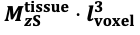
to obtain the relative FRE removes the contribution of the total voxel volume

"Supplementary Figure 2 shows that, when partial volume effects are present, the highest relative FRE arises in voxels with the same size as or smaller than the vessel diameter (Supplementary Figure 2A), whereas the absolute FRE increases with voxel size (Supplementary Figure 2C). If no partial-volume effects are present, the relative FRE becomes independent of voxel size (Supplementary Figure 2B), whereas the absolute FRE increases with voxel size (Supplementary Figure 2D). While the partial-volume effects for the relative FRE are substantial, they are much more subtle when using the absolute FRE and do not alter the overall characteristics."
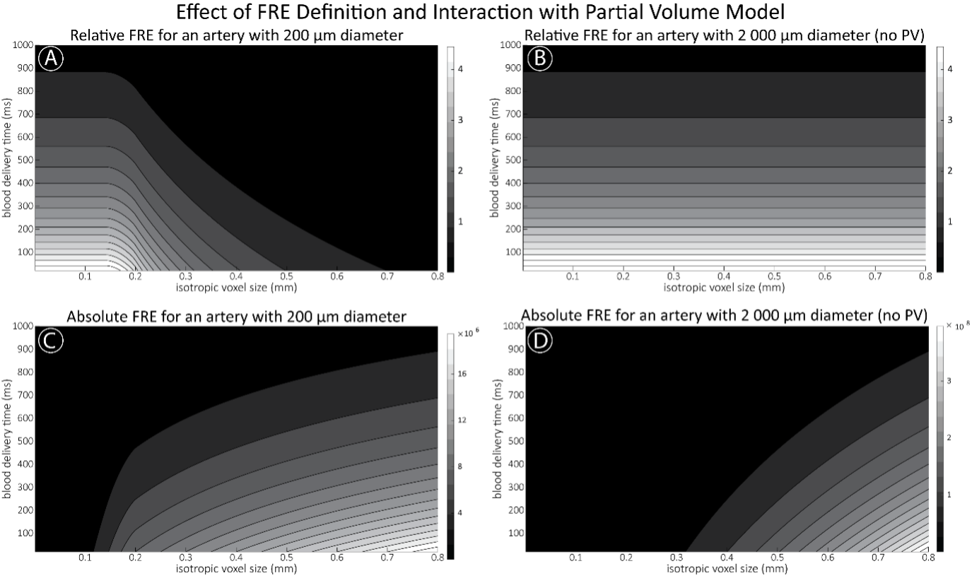
Supplementary Figure 2: Effect of voxel size and blood delivery time on the relative flow-related enhancement (FRE) using either a relative (A,B) (Eq. (3)) or an absolute (C,D) (Eq. (12)) FRE definition assuming a pial artery diameter of 200 μm (A,C) or 2 000 µm, i.e. no partial-volume effects at the central voxel of this artery considered here.
Following the established literature (Brown et al., 2014a; Carr and Carroll, 2012; Haacke et al., 1990) and because we would ultimately derive a relative measure, we have omitted the effect of voxel volume on the longitudinal magnetization in our derivations, which make it appear as if we are dividing by a constant in Eq. 6, as the effect of total voxel volume cancels out for the relative FRE. We have now made this more explicit in our derivation of the partial volume model.
"Introducing a partial-volume model
To account for the effect of voxel volume on the FRE, the total longitudinal magnetization M_z needs to also consider the number of spins contained within in a voxel (Du et al., 1996; Venkatesan and Haacke, 1997). A simple approximation can be obtained by scaling the longitudinal magnetization with the voxel volume (Venkatesan and Haacke, 1997) . To then include partial volume effects, the total longitudinal magnetization in a voxel M_z^total becomes the sum of the contributions from the stationary tissue M_zS^tissue and the inflowing blood M_z^blood, weighted by their respective volume fractions V_rel:"

A simple approximation can be obtained by scaling the longitudinal magnetization with the voxel volume (Venkatesan and Haacke, 1997) . To then include partial volume effects, the total longitudinal magnetization in a voxel M_z^total becomes the sum of the contributions from the stationary tissue M_zS^tissue and the inflowing blood M_z^blood, weighted by their respective volume fractions V_rel:
Eq. (4)

For simplicity, we assume a single vessel is located at the center of the voxel and approximate it to be a cylinder with diameter d_vessel and length l_voxel of an assumed isotropic voxel along one side. The relative volume fraction of blood V_rel^blood is the ratio of vessel volume within the voxel to total voxel volume (see section Estimation of vessel-volume fraction in the Supplementary Material), and the tissue volume fraction V_rel^tissue is the remainder that is not filled with blood, or
Eq. (5)
We can now replace the blood magnetization in equation Eq. (3) with the total longitudinal magnetization of the voxel to compute the FRE as a function of vessel-volume fraction:
Eq. (6)

Based on your suggestion, we have also extended our interpretation of relative and absolute FRE. Indeed, a subtractive flow technique where no signal in the background remains and only intensities in the object are present would have infinite relative FRE, as this basically constitutes a perfect segmentation (bar a simple thresholding step).
"Extending classical FRE treatments to the pial vasculature
There are several major modifications in our approach to this topic that might explain why, in contrast to predictions from classical FRE treatments, it is indeed possible to image pial arteries. For instance, the definition of vessel contrast or flow-related enhancement is often stated as an absolute difference between blood and tissue signal (Brown et al., 2014a; Carr and Carroll, 2012; Du et al., 1993, 1996; Haacke et al., 1990; Venkatesan and Haacke, 1997). Here, however, we follow the approach of Al-Kwifi et al. (2002) and consider relative contrast. While this distinction may seem to be semantic, the effect of voxel volume on FRE for these two definitions is exactly opposite: Du et al. (1996) concluded that larger voxel size increases the (absolute) vessel-background contrast, whereas here we predict an increase in relative FRE for small arteries with decreasing voxel size. Therefore, predictions of the depiction of small arteries with decreasing voxel size differ depending on whether one is considering absolute contrast, i.e. difference in longitudinal magnetization, or relative contrast, i.e. contrast differences independent of total voxel size. Importantly, this prediction changes for large arteries where the voxel contains only vessel lumen, in which case the relative FRE remains constant across voxel sizes, but the absolute FRE increases with voxel size (Supplementary Figure 9). Overall, the interpretations of relative and absolute FRE differ, and one measure may be more appropriate for certain applications than the other. Absolute FRE describes the difference in magnetization and is thus tightly linked to the underlying physical mechanism. Relative FRE, however, describes the image contrast and segmentability. If blood and tissue magnetization are equal, both contrast measures would equal zero and indicate that no contrast difference is present. However, when there is signal in the vessel and as the tissue magnetization approaches zero, the absolute FRE approaches the blood magnetization (assuming no partial-volume effects), whereas the relative FRE approaches infinity. While this infinite relative FRE does not directly relate to the underlying physical process of ‘infinite’ signal enhancement through inflowing blood, it instead characterizes the segmentability of the image in that an image with zero intensity in the background and non-zero values in the structures of interest can be segmented perfectly and trivially. Accordingly, numerous empirical observations (Al-Kwifi et al., 2002; Bouvy et al., 2014; Haacke et al., 1990; Ladd, 2007; Mattern et al., 2018; von Morze et al., 2007) and the data provided here (Figure 5, 6 and 7) have shown the benefit of smaller voxel sizes if the aim is to visualize and segment small arteries."
9) Page 22, Line 400. "The appropriateness of " This also ignores noise. The absolute enhancement is the inherent magnetization available. The results in Figure 5, 6, 7 don't readily support a ratio over and absolute difference accounting for partial volume effects.
We hope that with the additional explanations on the effects of relative FRE definition in combination with a partial-volume model and the interpretation of relative FRE provided in the previous response (R2.8) and that Figures 5, 6 and 7 show smaller arteries for smaller voxels, we were able to clarify our argument why only relative FRE in combination with a partial volume model can explain why smaller voxel sizes are advantageous for depicting small arteries.
While we appreciate that there exists a fundamental relationship between SNR and voxel volume in MR (Brown et al., 2014b), this relationship is also modulated by many more factors (as we have argued in our responses to R2.2 and R1.4b).
We hope that the additional derivations and simulations provided in the previous response have clarified why a relative FRE model in combination with a partial-volume model helps to explain the enhanced detectability of small vessels with small voxels.
10) Page 24, Line 453. "strategies, such as radial and spiral acquisitions, experience no vessel displacement artefact" These do observe flow related distortions as well, just not typically called displacement.
Yes, this is a helpful point, as these methods will also experience a degradation of spatial accuracy due to flow effects, which will propagate into errors in the segmentation.
As the reviewer suggests, flow-related artefacts in radial and spiral acquisitions usually manifest as a slight blur, and less as the prominent displacement found in Cartesian sampling schemes. We have added a corresponding clarification to the Discussion section:
"Other encoding strategies, such as radial and spiral acquisitions, experience no vessel displacement artefact because phase and frequency encoding take place in the same instant; although a slight blur might be observed instead (Nishimura et al., 1995, 1991). However, both trajectories pose engineering challenges and much higher demands on hardware and reconstruction algorithms than the Cartesian readouts employed here (Kasper et al., 2018; Shu et al., 2016); particularly to achieve 3D acquisitions with 160 µm isotropic resolution."
11) Page 24, Line 272. "although even with this nearly ideal subject behaviour approximately 1 in 4 scans still had to be discarded and repeated" This is certainly a potential source of bias in the comparisons.
We apologize if this section was written in a misleading way. For the comparison presented in Figure 7, we acquired one additional slab in the same session at 0.16 mm voxel size using the same prospective motion correction procedure as for the 0.14 mm data. For the images shown in Figure 6 and Supplementary Figure 4 at 0.16 mm voxel size, we did not use a motion correction system and, thus, had to discard a portion of the data. We have clarified that for the comparison of the high-resolution data, prospective motion correction was used for both resolutions. We have clarified this in the Discussion section:
"This allowed for the successful correction of head motion of approximately 1 mm over the 60-minute scan session, showing the utility of prospective motion correction at these very high resolutions. Note that for the comparison in Figure 7, one slab with 0.16 mm voxel size was acquired in the same session also using the prospective motion correction system. However, for the data shown in Figure 6 and Supplementary Figure 4, no prospective motion correction was used, and we instead relied on the experienced participants who contributed to this study. We found that the acquisition of TOF data with 0.16 mm isotropic voxel size in under 12 minutes acquisition time per slab is possible without discernible motion artifacts, although even with this nearly ideal subject behaviour approximately 1 in 4 scans still had to be discarded and repeated."
12) Page 25, Line 489. "then need to include the effects of various analog and digital filters" While the analysis may benefit from some of this, most is not at all required for analysis based on optimization of the imaging parameters.
We have included all four correction factors for completeness, given the unique acquisition parameter and contrast space our time-of-flight acquisition occupies, e.g. very low bandwidth of only 100 Hz, very large matrix sizes > 1024 samples, ideally zero SNR in the background (fully supressed tissue signal). However, we agree that probably the most important factor is the non-central chi distribution of the noise in magnitude images from multiple-channel coil arrays, and have added this qualification in the text:
"Accordingly, SNR predictions then need to include the effects of various analog and digital filters, the number of acquired samples, the noise covariance correction factor, and—most importantly—the non-central chi distribution of the noise statistics of the final magnitude image (Triantafyllou et al., 2011)."
Al-Kwifi, O., Emery, D.J., Wilman, A.H., 2002. Vessel contrast at three Tesla in time-of-flight magnetic resonance angiography of the intracranial and carotid arteries. Magnetic Resonance Imaging 20, 181–187. https://doi.org/10.1016/S0730-725X(02)00486-1
Arts, T., Meijs, T.A., Grotenhuis, H., Voskuil, M., Siero, J., Biessels, G.J., Zwanenburg, J., 2021. Velocity and Pulsatility Measures in the Perforating Arteries of the Basal Ganglia at 3T MRI in Reference to 7T MRI. Frontiers in Neuroscience 15.
Avants, B.B., Tustison, N., Song, G., 2009. Advanced normalization tools (ANTS). Insight j 2, 1–35.
Bae, K.T., Park, S.-H., Moon, C.-H., Kim, J.-H., Kaya, D., Zhao, T., 2010. Dual-echo arteriovenography imaging with 7T MRI: CODEA with 7T. J. Magn. Reson. Imaging 31, 255–261. https://doi.org/10.1002/jmri.22019
Bartholdi, E., Ernst, R.R., 1973. Fourier spectroscopy and the causality principle. Journal of Magnetic Resonance (1969) 11, 9–19. https://doi.org/10.1016/0022-2364(73)90076-0
Bernier, M., Cunnane, S.C., Whittingstall, K., 2018. The morphology of the human cerebrovascular system. Human Brain Mapping 39, 4962–4975. https://doi.org/10.1002/hbm.24337
Bouvy, W.H., Biessels, G.J., Kuijf, H.J., Kappelle, L.J., Luijten, P.R., Zwanenburg, J.J.M., 2014. Visualization of Perivascular Spaces and Perforating Arteries With 7 T Magnetic Resonance Imaging: Investigative Radiology 49, 307–313. https://doi.org/10.1097/RLI.0000000000000027
Bouvy, W.H., Geurts, L.J., Kuijf, H.J., Luijten, P.R., Kappelle, L.J., Biessels, G.J., Zwanenburg, J.J.M., 2016. Assessment of blood flow velocity and pulsatility in cerebral perforating arteries with 7-T quantitative flow MRI: Blood Flow Velocity And Pulsatility In Cerebral Perforating Arteries. NMR Biomed. 29, 1295–1304. https://doi.org/10.1002/nbm.3306
Brown, R.W., Cheng, Y.-C.N., Haacke, E.M., Thompson, M.R., Venkatesan, R., 2014a. Chapter 24 - MR Angiography and Flow Quantification, in: Magnetic Resonance Imaging. John Wiley & Sons, Ltd, pp. 701–737. https://doi.org/10.1002/9781118633953.ch24
Brown, R.W., Cheng, Y.-C.N., Haacke, E.M., Thompson, M.R., Venkatesan, R., 2014b. Chapter 15 - Signal, Contrast, and Noise, in: Magnetic Resonance Imaging. John Wiley & Sons, Ltd, pp. 325–373. https://doi.org/10.1002/9781118633953.ch15
Carr, J.C., Carroll, T.J., 2012. Magnetic resonance angiography: principles and applications. Springer, New York.
Cassot, F., Lauwers, F., Fouard, C., Prohaska, S., Lauwers-Cances, V., 2006. A Novel Three-Dimensional Computer-Assisted Method for a Quantitative Study of Microvascular Networks of the Human Cerebral Cortex. Microcirculation 13, 1–18. https://doi.org/10.1080/10739680500383407
Chen, L., Mossa-Basha, M., Balu, N., Canton, G., Sun, J., Pimentel, K., Hatsukami, T.S., Hwang, J.-N., Yuan, C., 2018. Development of a quantitative intracranial vascular features extraction tool on 3DMRA using semiautomated open-curve active contour vessel tracing: Comprehensive Artery Features Extraction From 3D MRA. Magn. Reson. Med 79, 3229–3238. https://doi.org/10.1002/mrm.26961
Choi, U.-S., Kawaguchi, H., Kida, I., 2020. Cerebral artery segmentation based on magnetization-prepared two rapid acquisition gradient echo multi-contrast images in 7 Tesla magnetic resonance imaging. NeuroImage 222, 117259. https://doi.org/10.1016/j.neuroimage.2020.117259
Conolly, S., Nishimura, D., Macovski, A., Glover, G., 1988. Variable-rate selective excitation. Journal of Magnetic Resonance (1969) 78, 440–458. https://doi.org/10.1016/0022-2364(88)90131-X
Deistung, A., Dittrich, E., Sedlacik, J., Rauscher, A., Reichenbach, J.R., 2009. ToF-SWI: Simultaneous time of flight and fully flow compensated susceptibility weighted imaging. J. Magn. Reson. Imaging 29, 1478–1484. https://doi.org/10.1002/jmri.21673
Detre, J.A., Leigh, J.S., Williams, D.S., Koretsky, A.P., 1992. Perfusion imaging. Magnetic Resonance in Medicine 23, 37–45. https://doi.org/10.1002/mrm.1910230106
Du, Y., Parker, D.L., Davis, W.L., Blatter, D.D., 1993. Contrast-to-Noise-Ratio Measurements in Three-Dimensional Magnetic Resonance Angiography. Investigative Radiology 28, 1004–1009.
Du, Y.P., Jin, Z., 2008. Simultaneous acquisition of MR angiography and venography (MRAV). Magn. Reson. Med. 59, 954–958. https://doi.org/10.1002/mrm.21581
Du, Y.P., Parker, D.L., Davis, W.L., Cao, G., 1994. Reduction of partial-volume artifacts with zero-filled interpolation in three-dimensional MR angiography. J. Magn. Reson. Imaging 4, 733–741. https://doi.org/10.1002/jmri.1880040517
Du, Y.P., Parker, D.L., Davis, W.L., Cao, G., Buswell, H.R., Goodrich, K.C., 1996. Experimental and theoretical studies of vessel contrast-to-noise ratio in intracranial time-of-flight MR angiography. Journal of Magnetic Resonance Imaging 6, 99–108. https://doi.org/10.1002/jmri.1880060120
Duvernoy, H., Delon, S., Vannson, J.L., 1983. The Vascularization of The Human Cerebellar Cortex. Brain Research Bulletin 11, 419–480.
Duvernoy, H.M., Delon, S., Vannson, J.L., 1981. Cortical blood vessels of the human brain. Brain Research Bulletin 7, 519–579. https://doi.org/10.1016/0361-9230(81)90007-1
Eckstein, K., Bachrata, B., Hangel, G., Widhalm, G., Enzinger, C., Barth, M., Trattnig, S., Robinson, S.D., 2021. Improved susceptibility weighted imaging at ultra-high field using bipolar multi-echo acquisition and optimized image processing: CLEAR-SWI. NeuroImage 237, 118175. https://doi.org/10.1016/j.neuroimage.2021.118175
Edelstein, W.A., Glover, G.H., Hardy, C.J., Redington, R.W., 1986. The intrinsic signal-to-noise ratio in NMR imaging. Magn. Reson. Med. 3, 604–618.
https://doi.org/10.1002/mrm.1910030413
Fan, A.P., Govindarajan, S.T., Kinkel, R.P., Madigan, N.K., Nielsen, A.S., Benner, T., Tinelli, E., Rosen, B.R., Adalsteinsson, E., Mainero, C., 2015. Quantitative oxygen extraction fraction from 7-Tesla MRI phase: reproducibility and application in multiple sclerosis. J Cereb Blood Flow Metab 35, 131–139. https://doi.org/10.1038/jcbfm.2014.187
Fiedler, T.M., Ladd, M.E., Bitz, A.K., 2018. SAR Simulations & Safety. NeuroImage 168, 33–58. https://doi.org/10.1016/j.neuroimage.2017.03.035
Frässle, S., Aponte, E.A., Bollmann, S., Brodersen, K.H., Do, C.T., Harrison, O.K., Harrison, S.J., Heinzle, J., Iglesias, S., Kasper, L., Lomakina, E.I., Mathys, C., Müller-Schrader, M., Pereira, I., Petzschner, F.H., Raman, S., Schöbi, D., Toussaint, B., Weber, L.A., Yao, Y., Stephan, K.E., 2021. TAPAS: An Open-Source Software Package for Translational Neuromodeling and Computational Psychiatry. Front. Psychiatry 12. https://doi.org/10.3389/fpsyt.2021.680811
Gulban, O.F., Bollmann, S., Huber, R., Wagstyl, K., Goebel, R., Poser, B.A., Kay, K., Ivanov, D., 2021. Mesoscopic Quantification of Cortical Architecture in the Living Human Brain. https://doi.org/10.1101/2021.11.25.470023
Haacke, E.M., Masaryk, T.J., Wielopolski, P.A., Zypman, F.R., Tkach, J.A., Amartur, S., Mitchell, J., Clampitt, M., Paschal, C., 1990. Optimizing blood vessel contrast in fast three-dimensional MRI. Magn. Reson. Med. 14, 202–221. https://doi.org/10.1002/mrm.1910140207
Helthuis, J.H.G., van Doormaal, T.P.C., Hillen, B., Bleys, R.L.A.W., Harteveld, A.A., Hendrikse, J., van der Toorn, A., Brozici, M., Zwanenburg, J.J.M., van der Zwan, A., 2019. Branching Pattern of the Cerebral Arterial Tree. Anat Rec 302, 1434–1446. https://doi.org/10.1002/ar.23994
Heverhagen, J.T., Bourekas, E., Sammet, S., Knopp, M.V., Schmalbrock, P., 2008. Time-of-Flight Magnetic Resonance Angiography at 7 Tesla. Investigative Radiology 43, 568–573. https://doi.org/10.1097/RLI.0b013e31817e9b2c
Hirsch, S., Reichold, J., Schneider, M., Székely, G., Weber, B., 2012. Topology and Hemodynamics of the Cortical Cerebrovascular System. J Cereb Blood Flow Metab 32, 952–967. https://doi.org/10.1038/jcbfm.2012.39
Horn, B.K.P., Schunck, B.G., 1981. Determining optical flow. Artificial Intelligence 17, 185–203. https://doi.org/10.1016/0004-3702(81)90024-2
Huck, J., Wanner, Y., Fan, A.P., Jäger, A.-T., Grahl, S., Schneider, U., Villringer, A., Steele, C.J., Tardif, C.L., Bazin, P.-L., Gauthier, C.J., 2019. High resolution atlas of the venous brain vasculature from 7 T quantitative susceptibility maps. Brain Struct Funct 224, 2467–2485. https://doi.org/10.1007/s00429-019-01919-4
Johst, S., Wrede, K.H., Ladd, M.E., Maderwald, S., 2012. Time-of-Flight Magnetic Resonance Angiography at 7 T Using Venous Saturation Pulses With Reduced Flip Angles. Investigative Radiology 47, 445–450. https://doi.org/10.1097/RLI.0b013e31824ef21f
Kang, C.-K., Park, C.-A., Kim, K.-N., Hong, S.-M., Park, C.-W., Kim, Y.-B., Cho, Z.-H., 2010. Non-invasive visualization of basilar artery perforators with 7T MR angiography. Journal of Magnetic Resonance Imaging 32, 544–550. https://doi.org/10.1002/jmri.22250
Kasper, L., Engel, M., Barmet, C., Haeberlin, M., Wilm, B.J., Dietrich, B.E., Schmid, T., Gross, S., Brunner, D.O., Stephan, K.E., Pruessmann, K.P., 2018. Rapid anatomical brain imaging using spiral acquisition and an expanded signal model. NeuroImage 168, 88–100. https://doi.org/10.1016/j.neuroimage.2017.07.062
Klepaczko, A., Szczypiński, P., Deistung, A., Reichenbach, J.R., Materka, A., 2016. Simulation of MR angiography imaging for validation of cerebral arteries segmentation algorithms. Computer Methods and Programs in Biomedicine 137, 293–309. https://doi.org/10.1016/j.cmpb.2016.09.020
Kobari, M., Gotoh, F., Fukuuchi, Y., Tanaka, K., Suzuki, N., Uematsu, D., 1984. Blood Flow Velocity in the Pial Arteries of Cats, with Particular Reference to the Vessel Diameter. J Cereb Blood Flow Metab 4, 110–114. https://doi.org/10.1038/jcbfm.1984.15
Ladd, M.E., 2007. High-Field-Strength Magnetic Resonance: Potential and Limits. Top Magn Reson Imaging 18, 139–152.
Lesage, D., Angelini, E.D., Bloch, I., Funka-Lea, G., 2009. A review of 3D vessel lumen segmentation techniques: Models, features and extraction schemes. Medical Image Analysis 13, 819–845. https://doi.org/10.1016/j.media.2009.07.011
Maderwald, S., Ladd, S.C., Gizewski, E.R., Kraff, O., Theysohn, J.M., Wicklow, K., Moenninghoff, C., Wanke, I., Ladd, M.E., Quick, H.H., 2008. To TOF or not to TOF: strategies for non-contrast-enhanced intracranial MRA at 7 T. Magn Reson Mater Phy 21, 159. https://doi.org/10.1007/s10334-007-0096-9
Manjón, J.V., Coupé, P., Martí‐Bonmatí, L., Collins, D.L., Robles, M., 2010. Adaptive non-local means denoising of MR images with spatially varying noise levels. Journal of Magnetic Resonance Imaging 31, 192–203. https://doi.org/10.1002/jmri.22003
Mansfield, P., Harvey, P.R., 1993. Limits to neural stimulation in echo-planar imaging. Magn. Reson. Med. 29, 746–758. https://doi.org/10.1002/mrm.1910290606
Masaryk, T.J., Modic, M.T., Ross, J.S., Ruggieri, P.M., Laub, G.A., Lenz, G.W., Haacke, E.M., Selman, W.R., Wiznitzer, M., Harik, S.I., 1989. Intracranial circulation: preliminary clinical results with three-dimensional (volume) MR angiography. Radiology 171, 793–799. https://doi.org/10.1148/radiology.171.3.2717754
Mattern, H., Sciarra, A., Godenschweger, F., Stucht, D., Lüsebrink, F., Rose, G., Speck, O., 2018. Prospective motion correction enables highest resolution time-of-flight angiography at 7T: Prospectively Motion-Corrected TOF Angiography at 7T. Magn. Reson. Med 80, 248–258. https://doi.org/10.1002/mrm.27033
Mattern, H., Sciarra, A., Lüsebrink, F., Acosta‐Cabronero, J., Speck, O., 2019. Prospective motion correction improves high‐resolution quantitative susceptibility mapping at 7T. Magn. Reson. Med 81, 1605–1619. https://doi.org/10.1002/mrm.27509
Mennes, M., Jenkinson, M., Valabregue, R., Buitelaar, J.K., Beckmann, C., Smith, S., 2014. Optimizing full-brain coverage in human brain MRI through population distributions of brain size. NeuroImage 98, 513–520. https://doi.org/10.1016/j.neuroimage.2014.04.030
Moccia, S., De Momi, E., El Hadji, S., Mattos, L.S., 2018. Blood vessel segmentation algorithms — Review of methods, datasets and evaluation metrics. Computer Methods and Programs in Biomedicine 158, 71–91. https://doi.org/10.1016/j.cmpb.2018.02.001
Mustafa, M.A.R., 2016. A data-driven learning approach to image registration.
Mut, F., Wright, S., Ascoli, G.A., Cebral, J.R., 2014. Morphometric, geographic, and territorial characterization of brain arterial trees. International Journal for Numerical Methods in Biomedical Engineering 30, 755–766. https://doi.org/10.1002/cnm.2627
Nagaoka, T., Yoshida, A., 2006. Noninvasive Evaluation of Wall Shear Stress on Retinal Microcirculation in Humans. Invest. Ophthalmol. Vis. Sci. 47, 1113. https://doi.org/10.1167/iovs.05-0218
Nishimura, D.G., Irarrazabal, P., Meyer, C.H., 1995. A Velocity k-Space Analysis of Flow Effects in Echo-Planar and Spiral Imaging. Magnetic Resonance in Medicine 33, 549–556. https://doi.org/10.1002/mrm.1910330414
Nishimura, D.G., Jackson, J.I., Pauly, J.M., 1991. On the nature and reduction of the displacement artifact in flow images. Magnetic Resonance in Medicine 22, 481–492. https://doi.org/10.1002/mrm.1910220255
Nonaka, H., Akima, M., Hatori, T., Nagayama, T., Zhang, Z., Ihara, F., 2003. Microvasculature of the human cerebral white matter: Arteries of the deep white matter. Neuropathology 23, 111–118.
https://doi.org/10.1046/j.1440-1789.2003.00486.x
North, D.O., 1963. An Analysis of the factors which determine signal/noise discrimination in pulsed-carrier systems. Proceedings of the IEEE 51, 1016–1027. https://doi.org/10.1109/PROC.1963.2383
Park, C.S., Hartung, G., Alaraj, A., Du, X., Charbel, F.T., Linninger, A.A., 2020. Quantification of blood flow patterns in the cerebral arterial circulation of individual (human) subjects. Int J Numer Meth Biomed Engng 36. https://doi.org/10.1002/cnm.3288
Parker, D.L., Goodrich, K.C., Roberts, J.A., Chapman, B.E., Jeong, E.-K., Kim, S.-E., Tsuruda, J.S., Katzman, G.L., 2003. The need for phase-encoding flow compensation in high-resolution intracranial magnetic resonance angiography. J. Magn. Reson. Imaging 18, 121–127. https://doi.org/10.1002/jmri.10322
Parker, D.L., Yuan, C., Blatter, D.D., 1991. MR angiography by multiple thin slab 3D acquisition. Magn. Reson. Med. 17, 434–451. https://doi.org/10.1002/mrm.1910170215
Pauling, L., Coryell, C.D., 1936. The magnetic properties and structure of hemoglobin, oxyhemoglobin and carbonmonoxyhemoglobin. Proceedings of the National Academy of Sciences 22, 210–216. https://doi.org/10.1073/pnas.22.4.210
Payne, S.J., 2017. Cerebral Blood Flow And Metabolism: A Quantitative Approach. World Scientific.
Peters, A.M., Brookes, M.J., Hoogenraad, F.G., Gowland, P.A., Francis, S.T., Morris, P.G., Bowtell, R., 2007. T2* measurements in human brain at 1.5, 3 and 7 T. Magnetic Resonance Imaging 25, 748–753. https://doi.org/10.1016/j.mri.2007.02.014
Pfeifer, R.A., 1930. Grundlegende Untersuchungen für die Angioarchitektonik des menschlichen Gehirns. Berlin: Julius Springer.
Phellan, R., Forkert, N.D., 2017. Comparison of vessel enhancement algorithms applied to time-of-flight MRA images for cerebrovascular segmentation. Medical Physics 44, 5901–5915. https://doi.org/10.1002/mp.12560
Pohmann, R., Speck, O., Scheffler, K., 2016. Signal-to-Noise Ratio and MR Tissue Parameters in Human Brain Imaging at 3, 7, and 9.4 Tesla Using Current Receive Coil Arrays. Magn. Reson. Med. 75, 801–809. https://doi.org/10.1002/mrm.25677
Reichenbach, J.R., Venkatesan, R., Schillinger, D.J., Kido, D.K., Haacke, E.M., 1997. Small vessels in the human brain: MR venography with deoxyhemoglobin as an intrinsic contrast agent. Radiology 204, 272–277. https://doi.org/10.1148/radiology.204.1.9205259
Schmid, F., Barrett, M.J.P., Jenny, P., Weber, B., 2019. Vascular density and distribution in neocortex. NeuroImage 197, 792–805. https://doi.org/10.1016/j.neuroimage.2017.06.046
Schmitter, S., Bock, M., Johst, S., Auerbach, E.J., Uğurbil, K., Moortele, P.-F.V. de, 2012. Contrast enhancement in TOF cerebral angiography at 7 T using saturation and MT pulses under SAR constraints: Impact of VERSE and sparse pulses. Magnetic Resonance in Medicine 68, 188–197. https://doi.org/10.1002/mrm.23226
Schulz, J., Boyacioglu, R., Norris, D.G., 2016. Multiband multislab 3D time-of-flight magnetic resonance angiography for reduced acquisition time and improved sensitivity. Magn Reson Med 75, 1662–8. https://doi.org/10.1002/mrm.25774
Shu, C.Y., Sanganahalli, B.G., Coman, D., Herman, P., Hyder, F., 2016. New horizons in neurometabolic and neurovascular coupling from calibrated fMRI, in: Progress in Brain Research. Elsevier, pp. 99–122. https://doi.org/10.1016/bs.pbr.2016.02.003
Stamm, A.C., Wright, C.L., Knopp, M.V., Schmalbrock, P., Heverhagen, J.T., 2013. Phase contrast and time-of-flight magnetic resonance angiography of the intracerebral arteries at 1.5, 3 and 7 T. Magnetic Resonance Imaging 31, 545–549. https://doi.org/10.1016/j.mri.2012.10.023
Stewart, A.W., Robinson, S.D., O’Brien, K., Jin, J., Widhalm, G., Hangel, G., Walls, A., Goodwin, J., Eckstein, K., Tourell, M., Morgan, C., Narayanan, A., Barth, M., Bollmann, S., 2022. QSMxT: Robust masking and artifact reduction for quantitative susceptibility mapping. Magnetic Resonance in Medicine 87, 1289–1300. https://doi.org/10.1002/mrm.29048
Stucht, D., Danishad, K.A., Schulze, P., Godenschweger, F., Zaitsev, M., Speck, O., 2015. Highest Resolution In Vivo Human Brain MRI Using Prospective Motion Correction. PLoS ONE 10, e0133921. https://doi.org/10.1371/journal.pone.0133921
Szikla, G., Bouvier, G., Hori, T., Petrov, V., 1977. Angiography of the Human Brain Cortex. Springer Berlin Heidelberg, Berlin, Heidelberg. https://doi.org/10.1007/978-3-642-81145-6
Triantafyllou, C., Polimeni, J.R., Wald, L.L., 2011. Physiological noise and signal-to-noise ratio in fMRI with multi-channel array coils. NeuroImage 55, 597–606. https://doi.org/10.1016/j.neuroimage.2010.11.084
Tustison, N.J., Avants, B.B., Cook, P.A., Zheng, Y., Egan, A., Yushkevich, P.A., Gee, J.C., 2010. N4ITK: Improved N3 Bias Correction. IEEE Transactions on Medical Imaging 29, 1310–1320. https://doi.org/10.1109/TMI.2010.2046908
Uludağ, K., Müller-Bierl, B., Uğurbil, K., 2009. An integrative model for neuronal activity-induced signal changes for gradient and spin echo functional imaging. NeuroImage 48, 150–165. https://doi.org/10.1016/j.neuroimage.2009.05.051
Venkatesan, R., Haacke, E.M., 1997. Role of high resolution in magnetic resonance (MR) imaging: Applications to MR angiography, intracranial T1-weighted imaging, and image interpolation. International Journal of Imaging Systems and Technology 8, 529–543. https://doi.org/10.1002/(SICI)1098-1098(1997)8:6<529::AID-IMA5>3.0.CO;2-C
von Morze, C., Xu, D., Purcell, D.D., Hess, C.P., Mukherjee, P., Saloner, D., Kelley, D.A.C., Vigneron, D.B., 2007. Intracranial time-of-flight MR angiography at 7T with comparison to 3T. J. Magn. Reson. Imaging 26, 900–904. https://doi.org/10.1002/jmri.21097
Ward, P.G.D., Ferris, N.J., Raniga, P., Dowe, D.L., Ng, A.C.L., Barnes, D.G., Egan, G.F., 2018. Combining images and anatomical knowledge to improve automated vein segmentation in MRI. NeuroImage 165, 294–305. https://doi.org/10.1016/j.neuroimage.2017.10.049
Wilms, G., Bosmans, H., Demaerel, Ph., Marchal, G., 2001. Magnetic resonance angiography of the intracranial vessels. European Journal of Radiology 38, 10–18. https://doi.org/10.1016/S0720-048X(01)00285-6
Wright, S.N., Kochunov, P., Mut, F., Bergamino, M., Brown, K.M., Mazziotta, J.C., Toga, A.W., Cebral, J.R., Ascoli, G.A., 2013. Digital reconstruction and morphometric analysis of human brain arterial vasculature from magnetic resonance angiography. NeuroImage 82, 170–181. https://doi.org/10.1016/j.neuroimage.2013.05.089
Yushkevich, P.A., Piven, J., Hazlett, H.C., Smith, R.G., Ho, S., Gee, J.C., Gerig, G., 2006. User-guided 3D active contour segmentation of anatomical structures: Significantly improved efficiency and reliability. NeuroImage 31, 1116–1128. https://doi.org/10.1016/j.neuroimage.2006.01.015
Zhang, Z., Deng, X., Weng, D., An, J., Zuo, Z., Wang, B., Wei, N., Zhao, J., Xue, R., 2015. Segmented TOF at 7T MRI: Technique and clinical applications. Magnetic Resonance Imaging 33, 1043–1050. https://doi.org/10.1016/j.mri.2015.07.002
Zhao, J.M., Clingman, C.S., Närväinen, M.J., Kauppinen, R.A., van Zijl, P.C.M., 2007. Oxygenation and hematocrit dependence of transverse relaxation rates of blood at 3T. Magn. Reson. Med. 58, 592–597. https://doi.org/10.1002/mrm.21342
Zhu, X., Tomanek, B., Sharp, J., 2013. A pixel is an artifact: On the necessity of zero-filling in fourier imaging. Concepts Magn. Reson. 42A, 32–44. https://doi.org/10.1002/cmr.a.21256
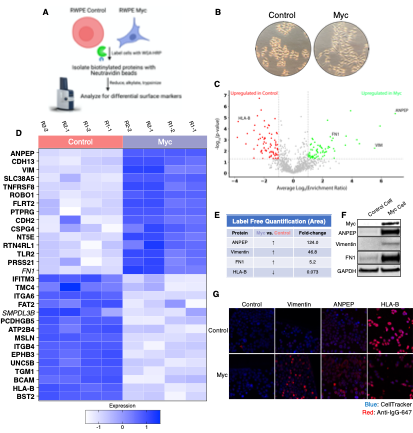
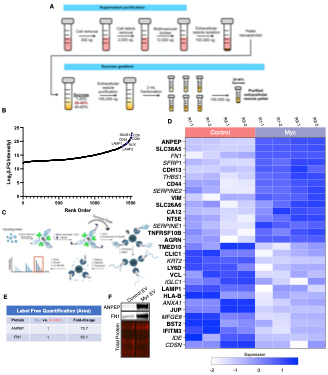
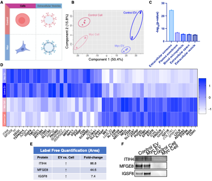
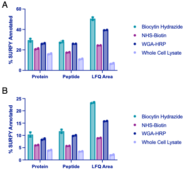
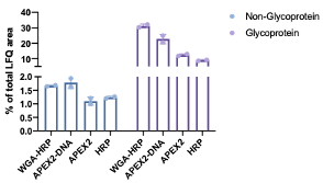
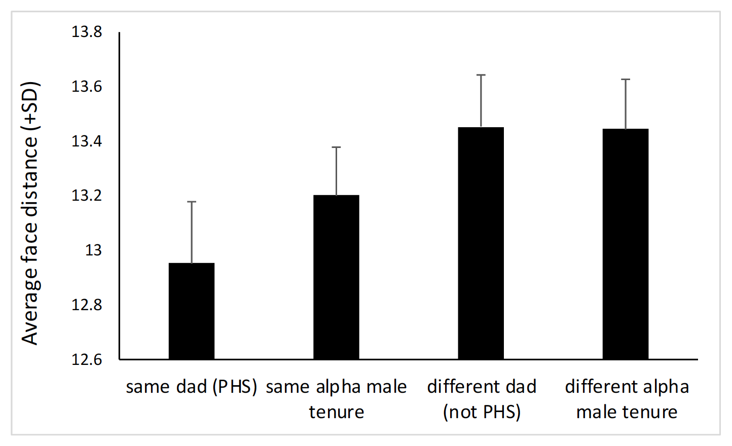
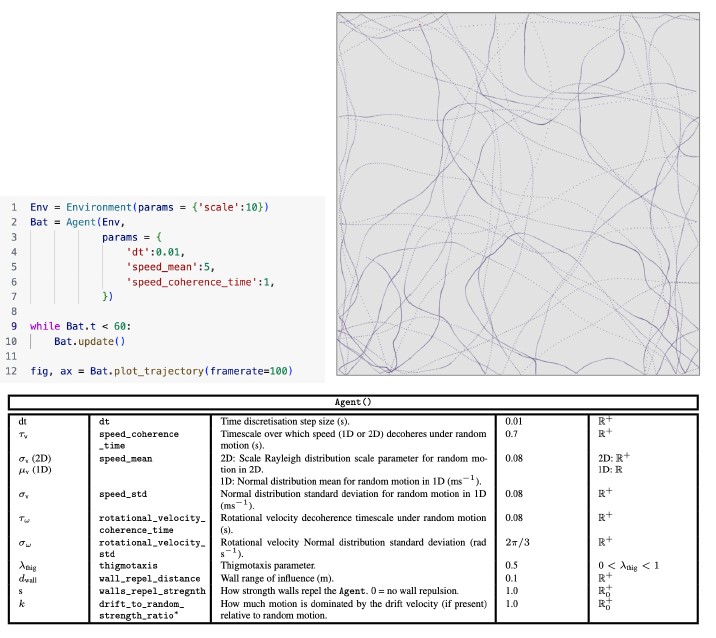
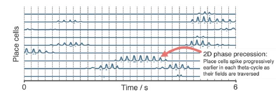
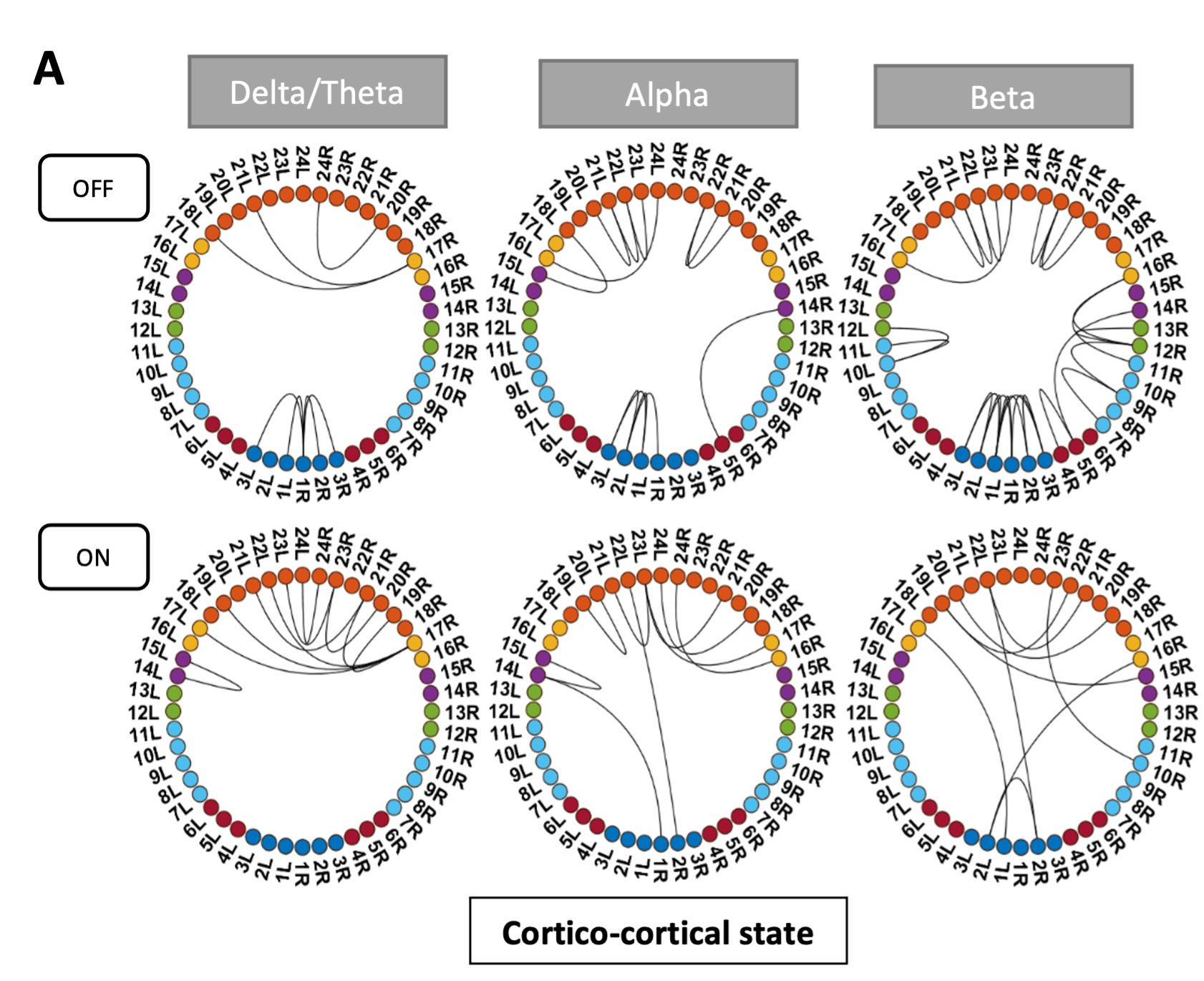
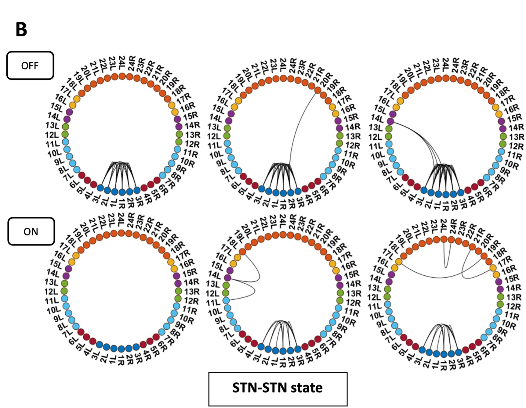
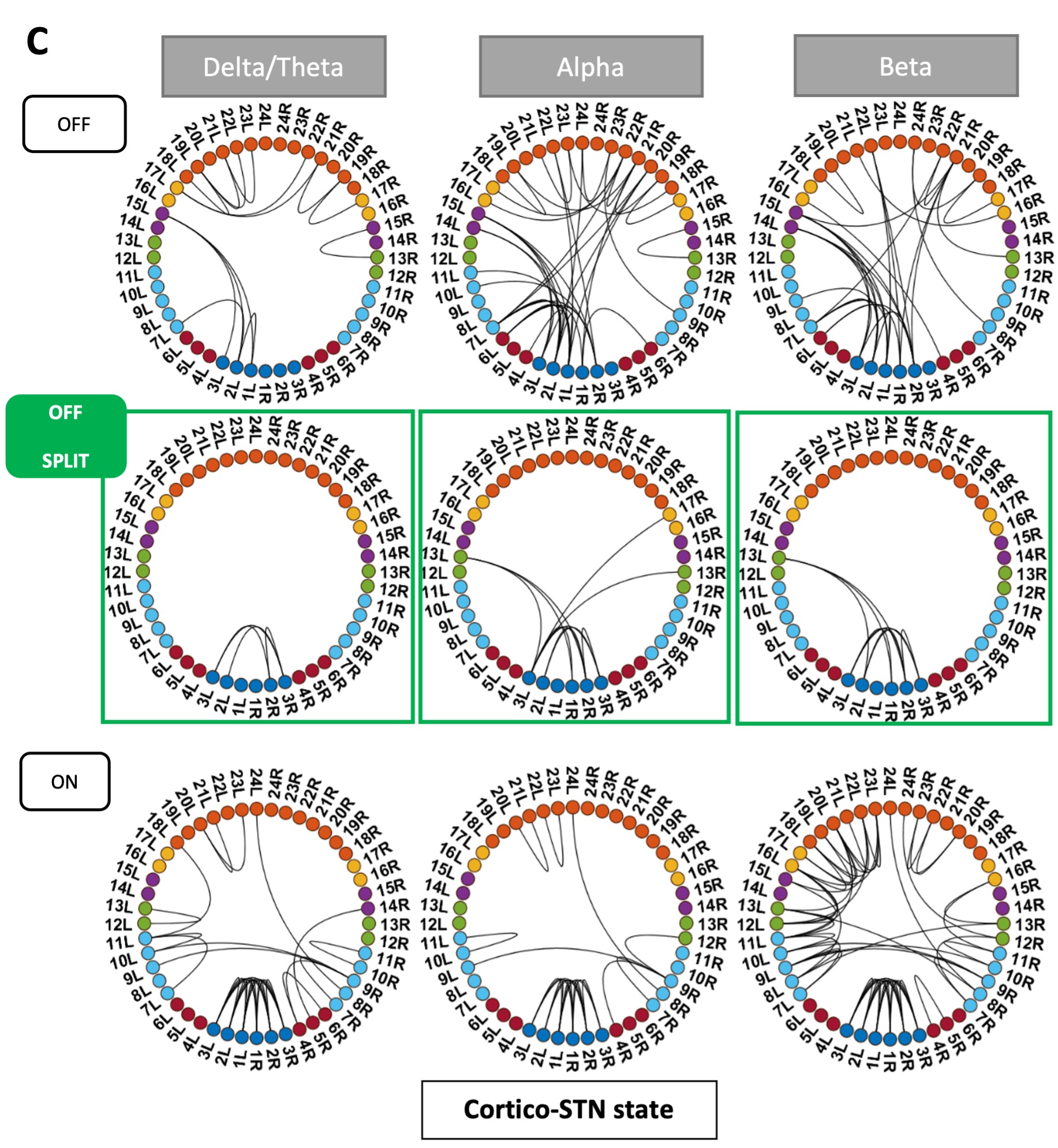
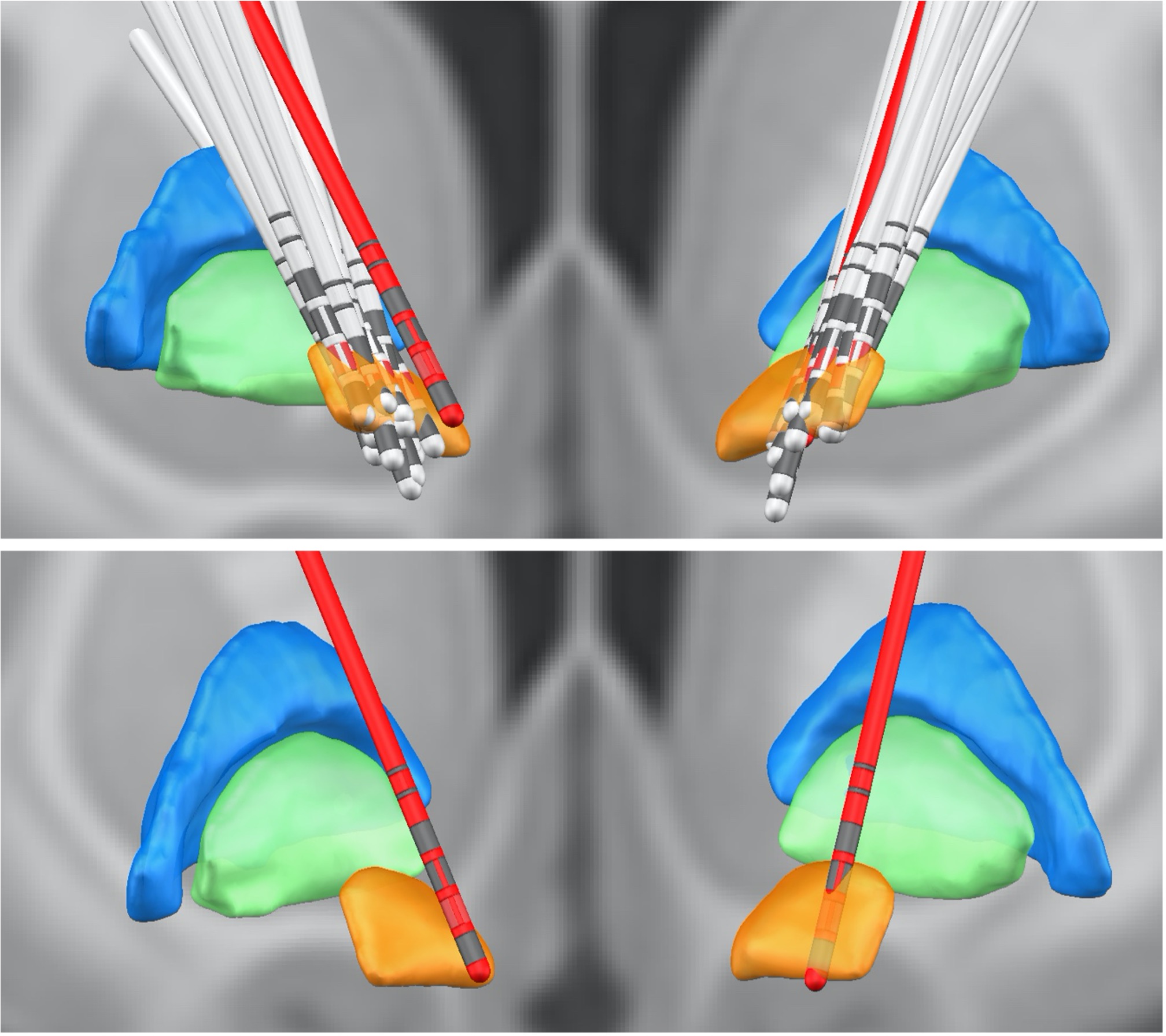
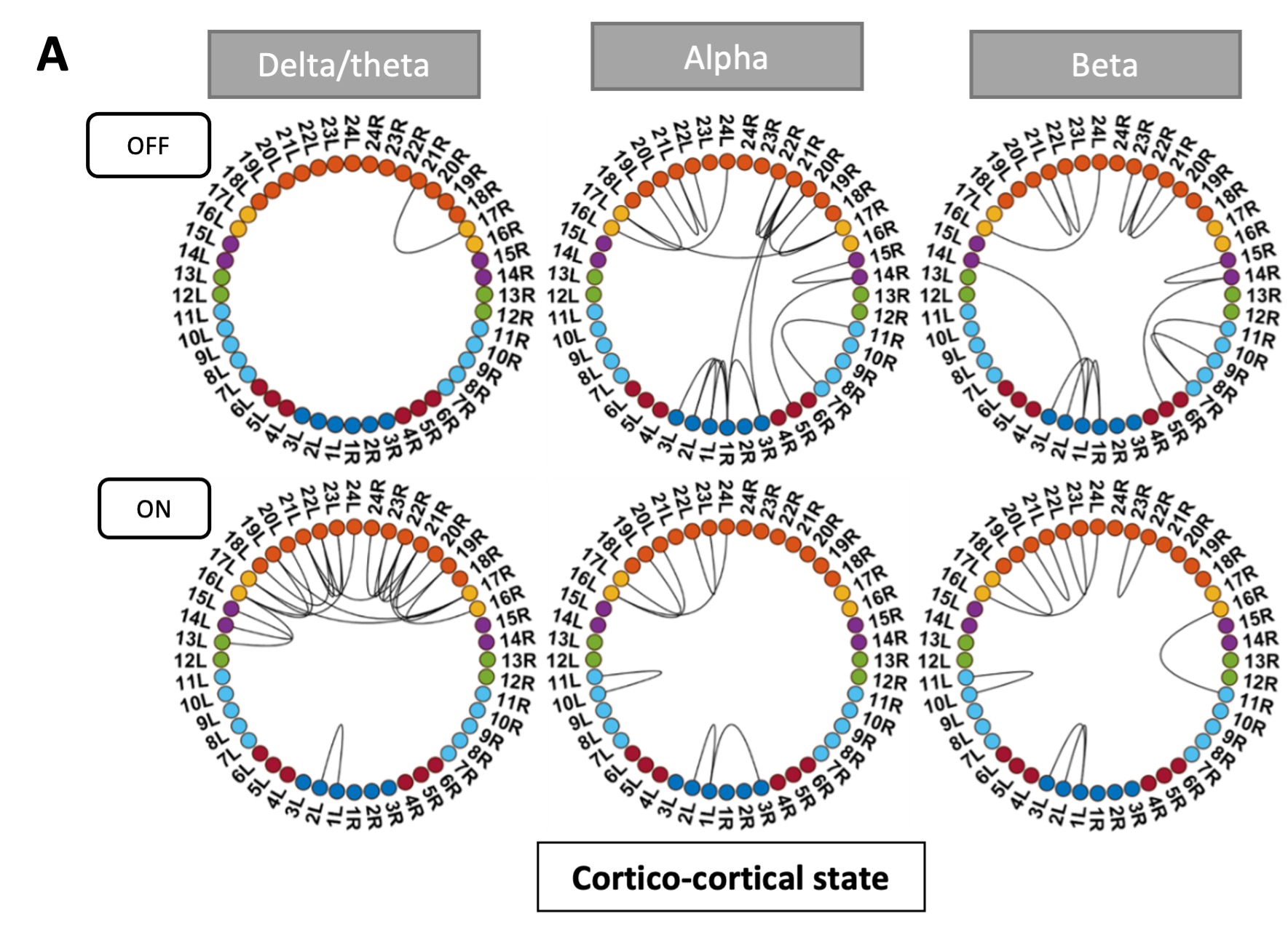
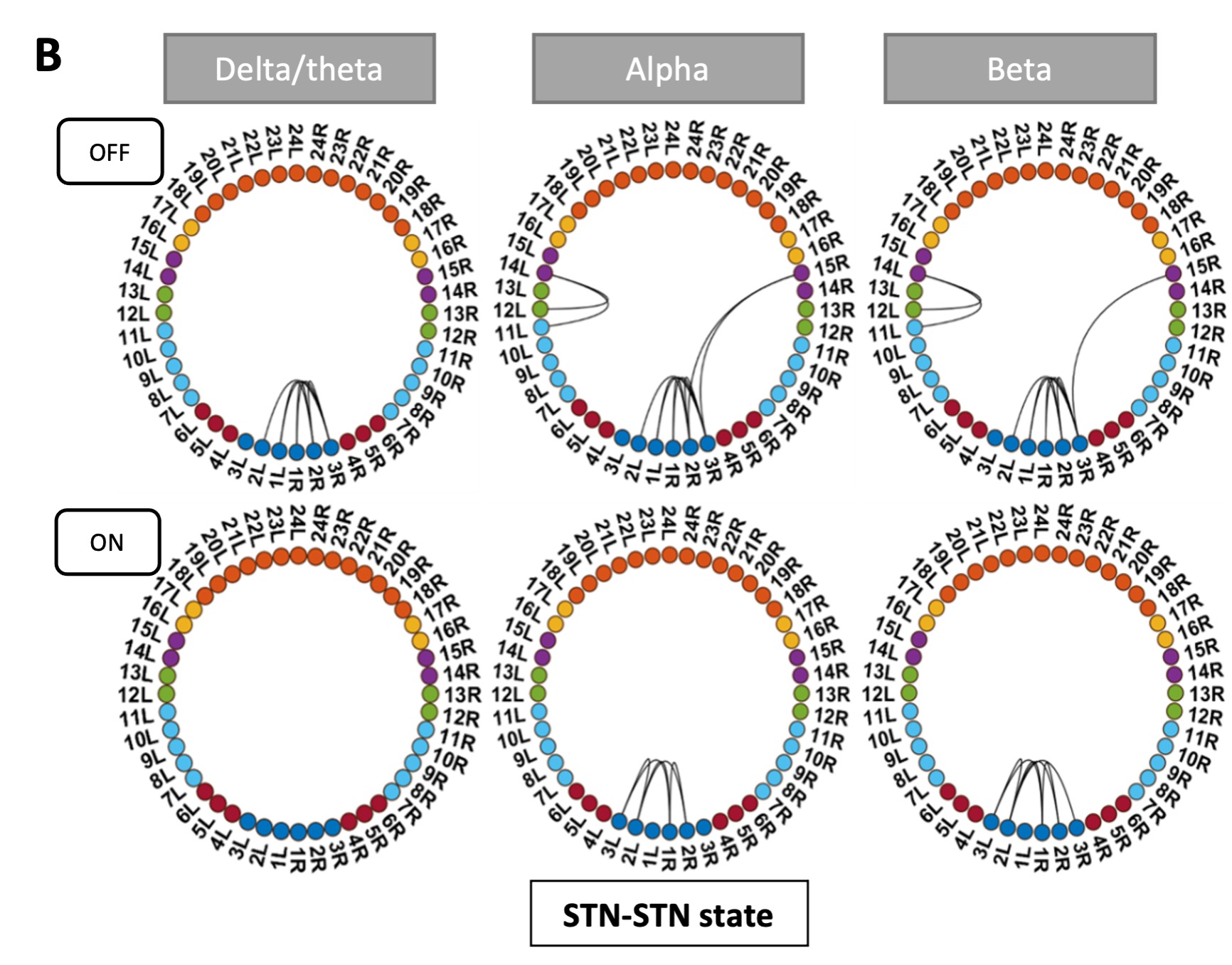
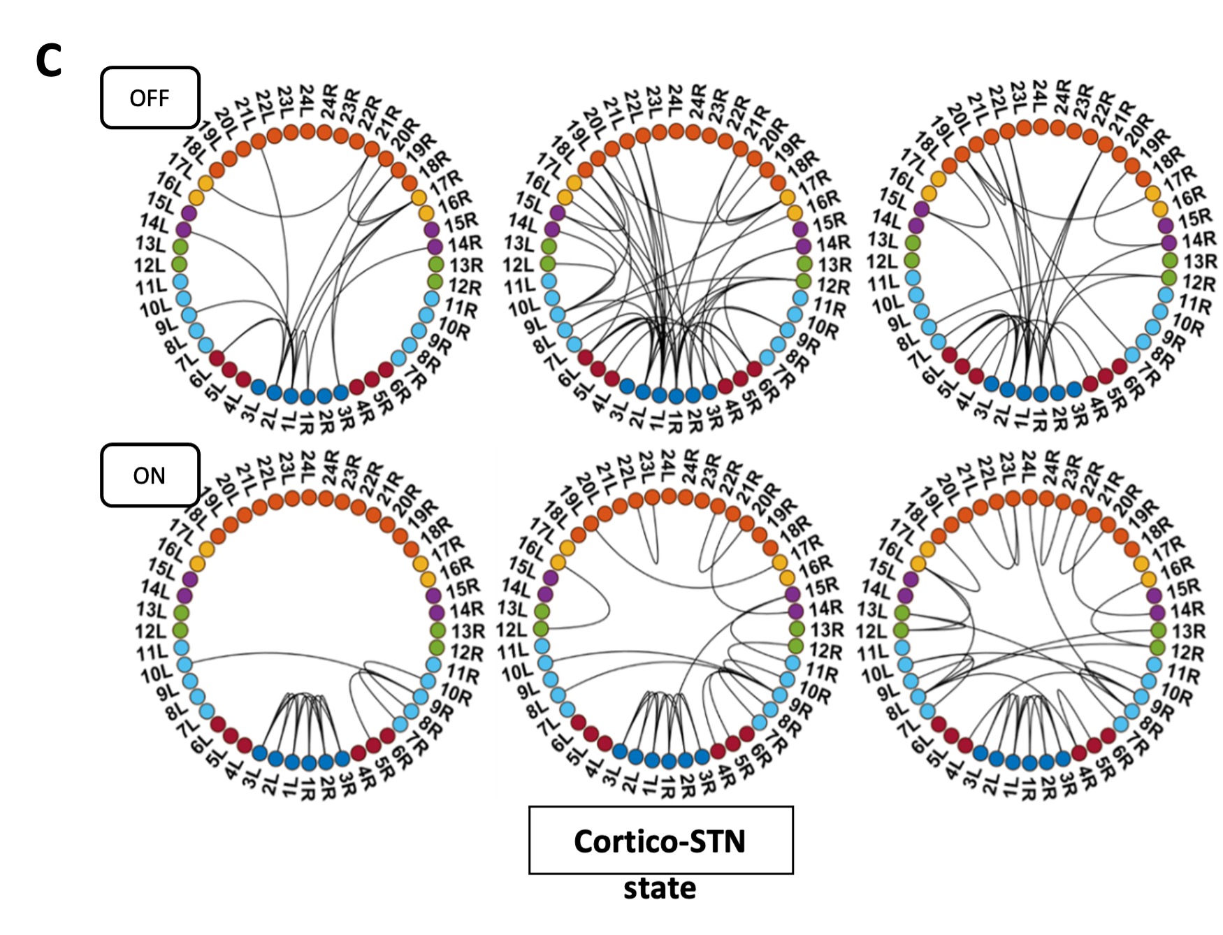
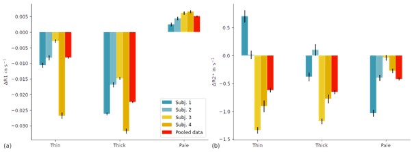
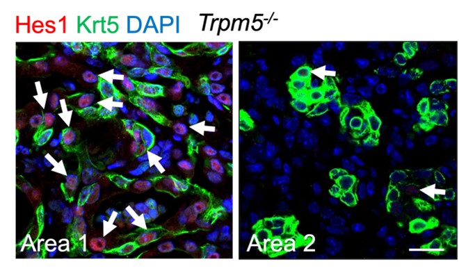
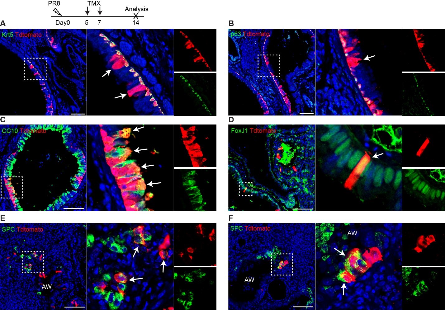
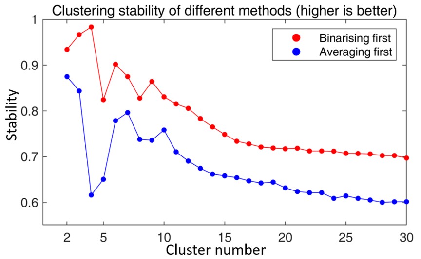
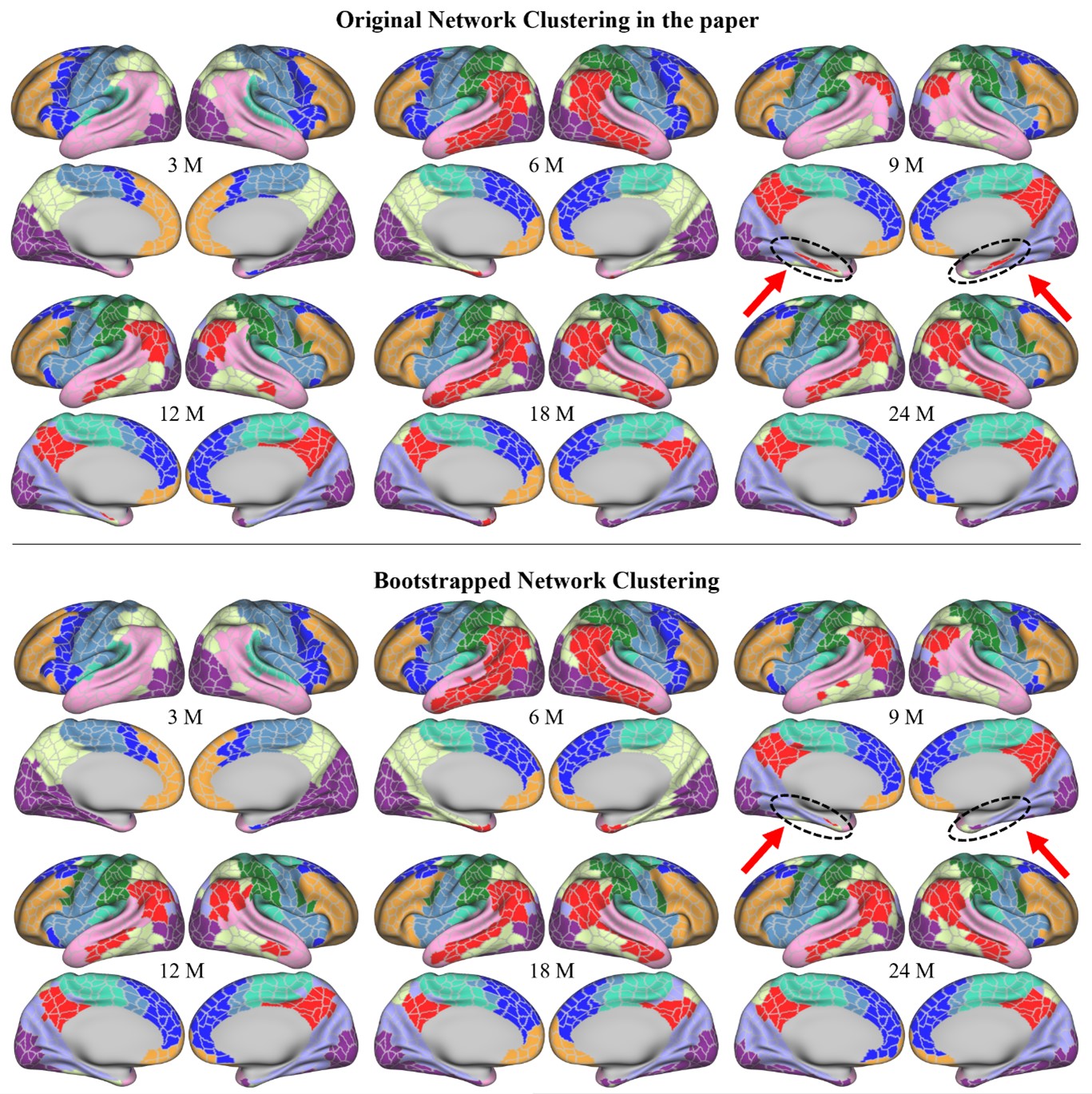
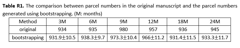
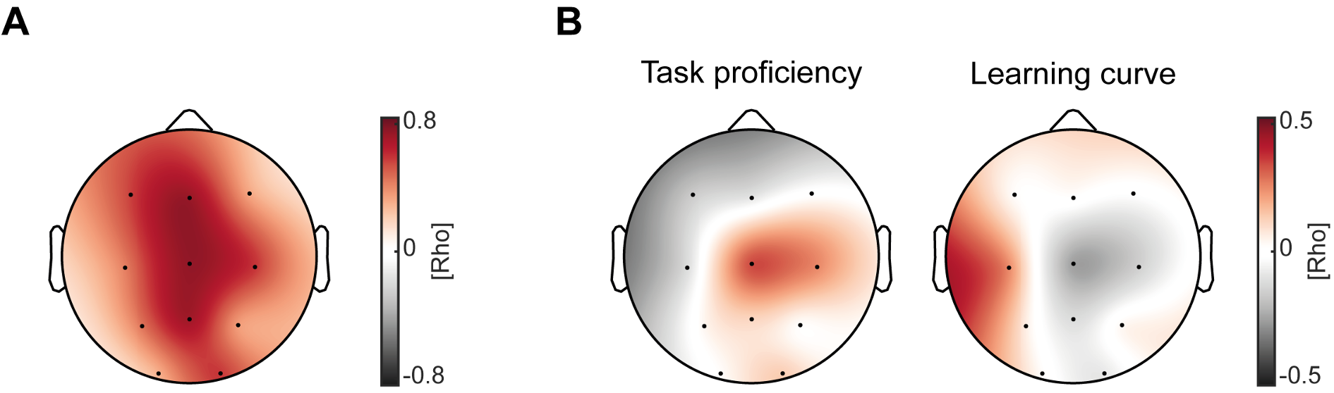
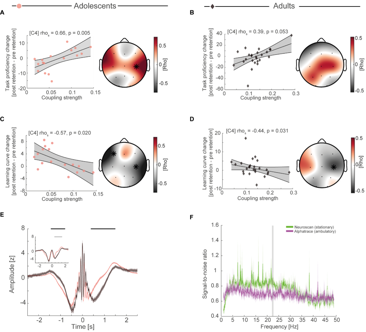

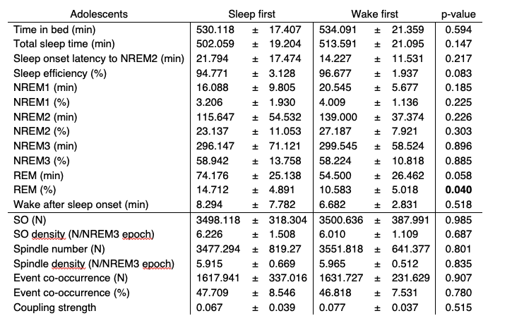
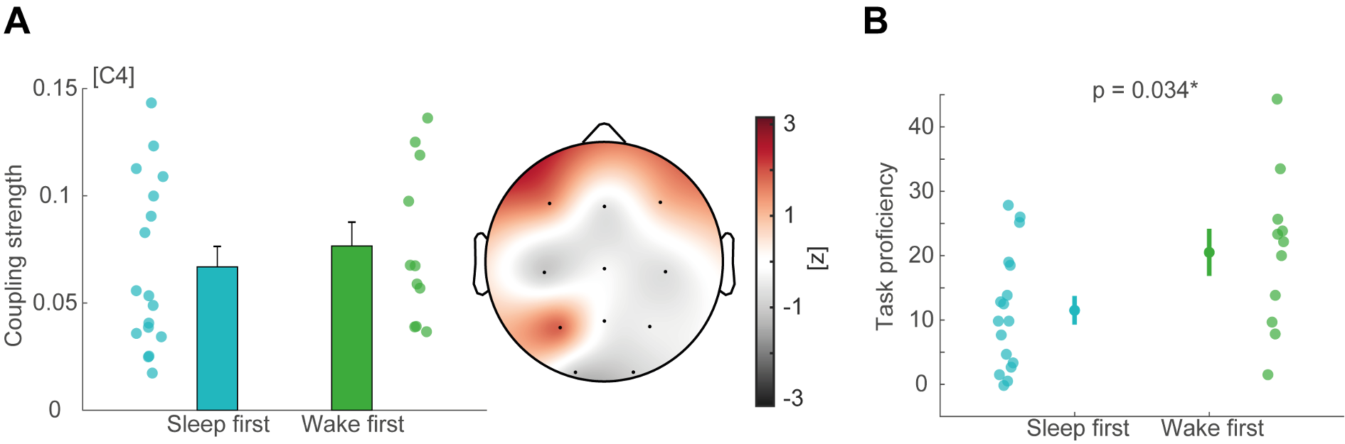
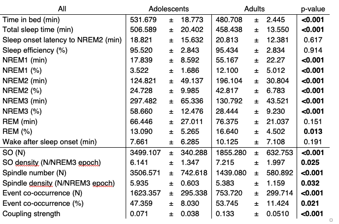
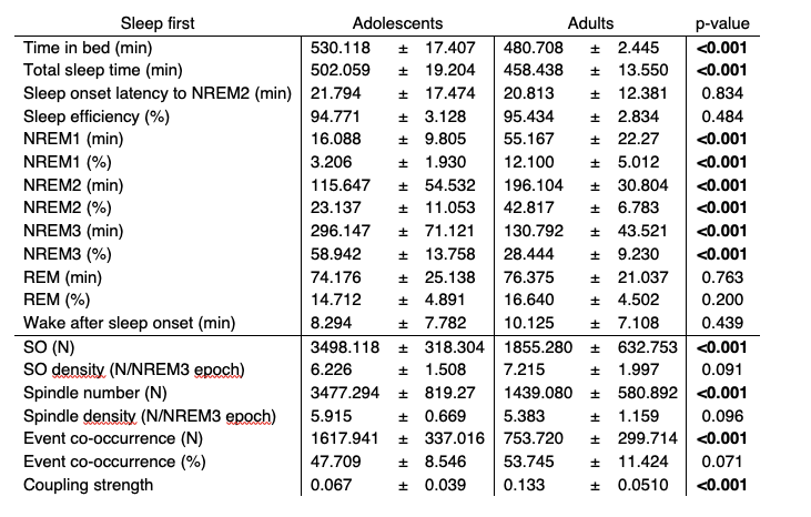
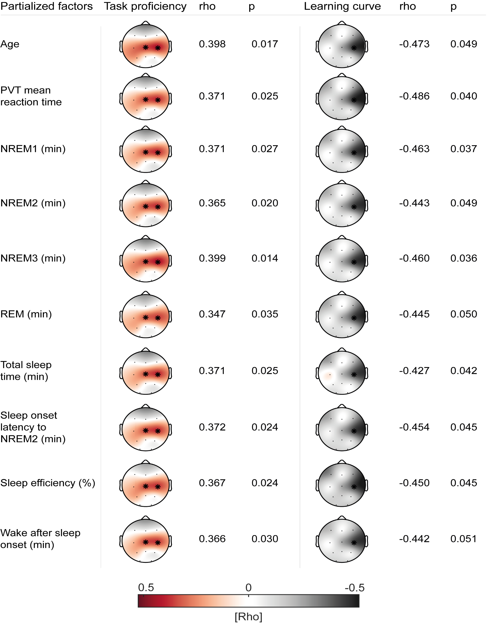
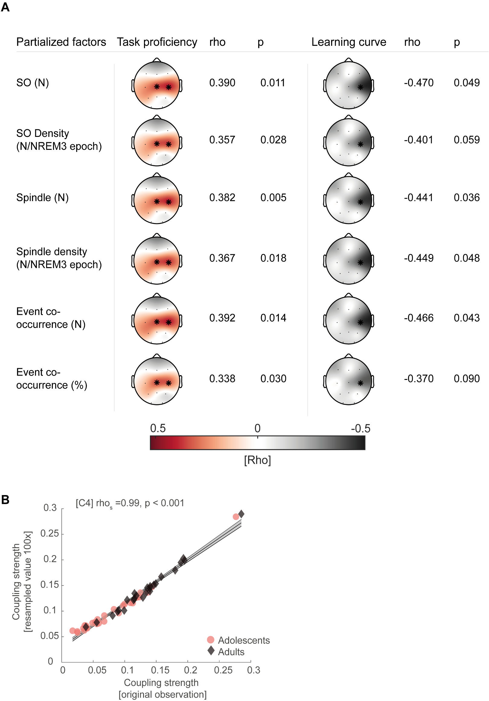
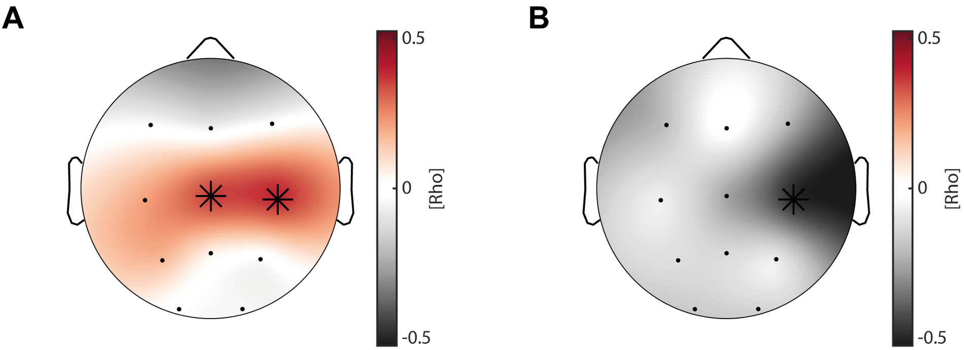
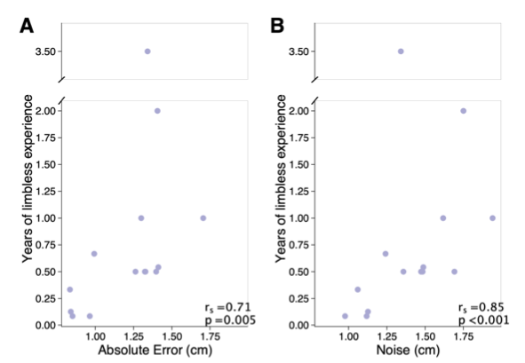
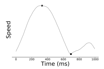
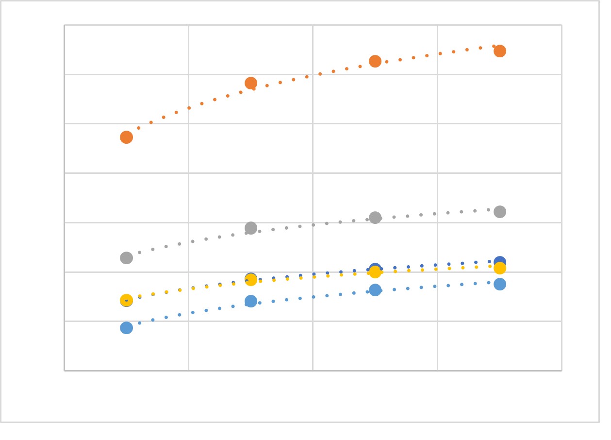
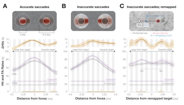
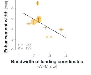
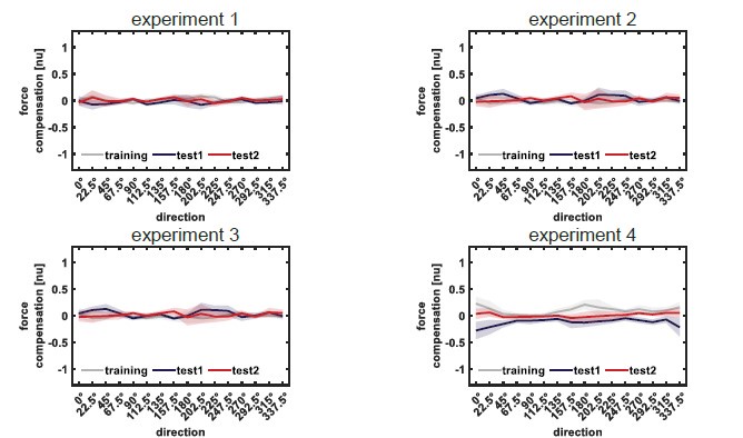
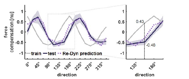

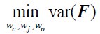


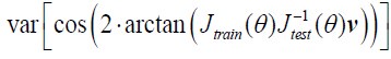
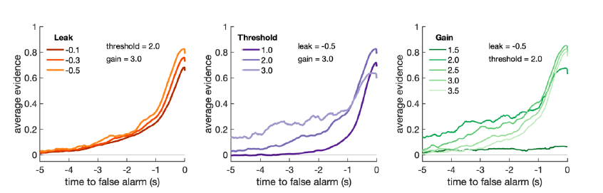
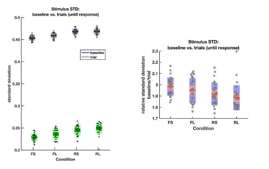
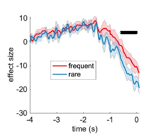
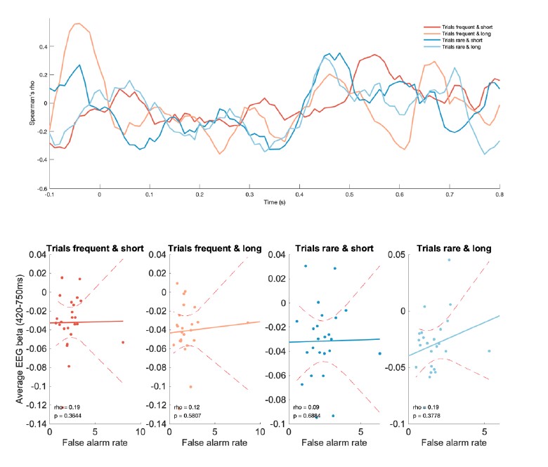
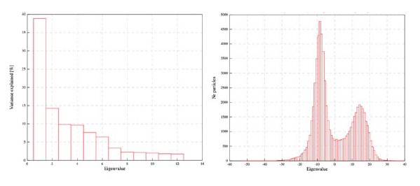
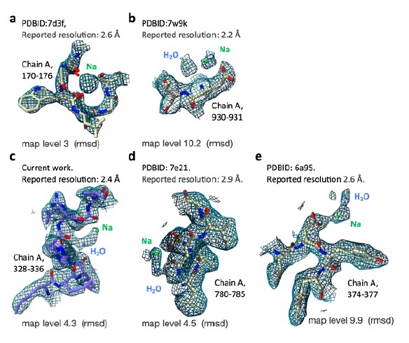
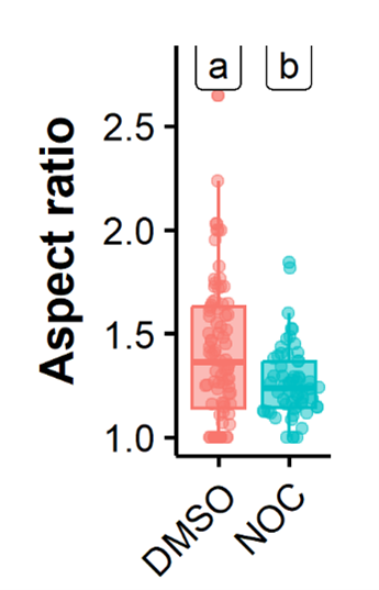
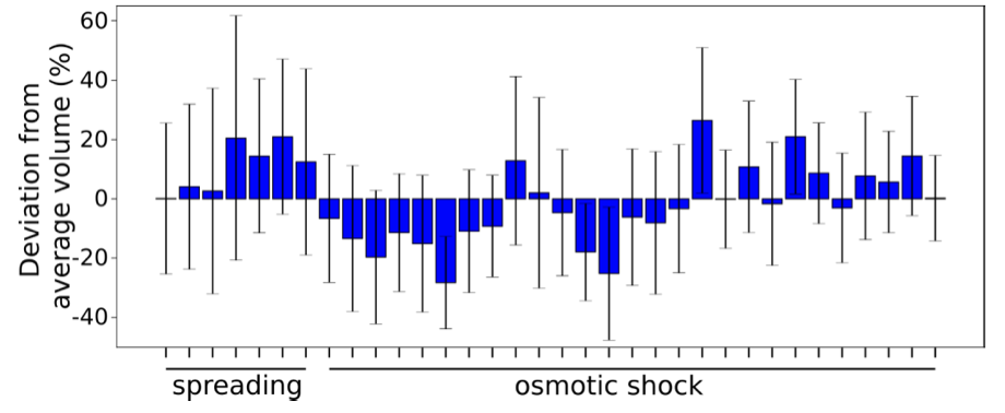
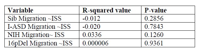
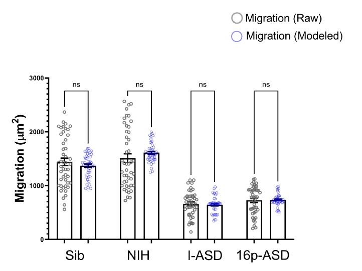
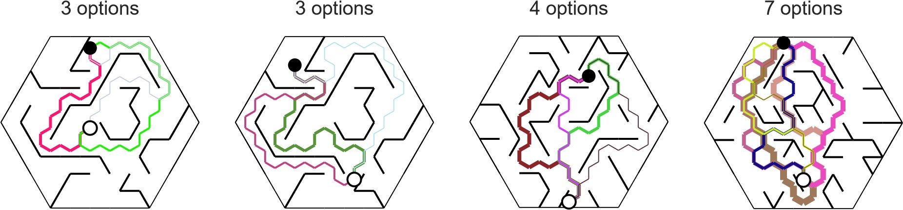
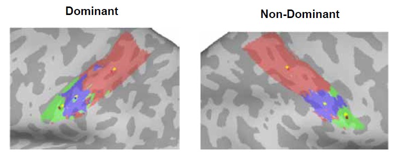
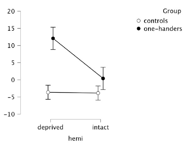
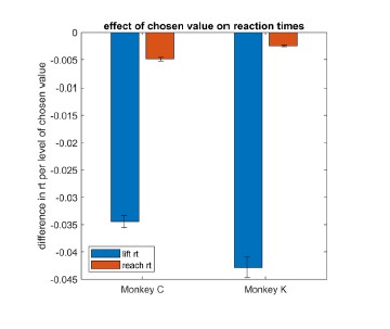
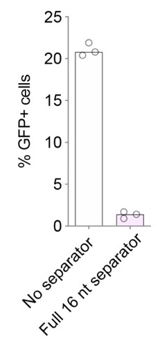


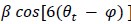
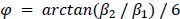

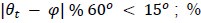
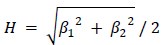
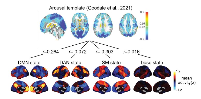
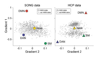
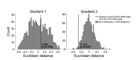
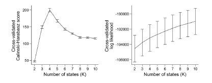
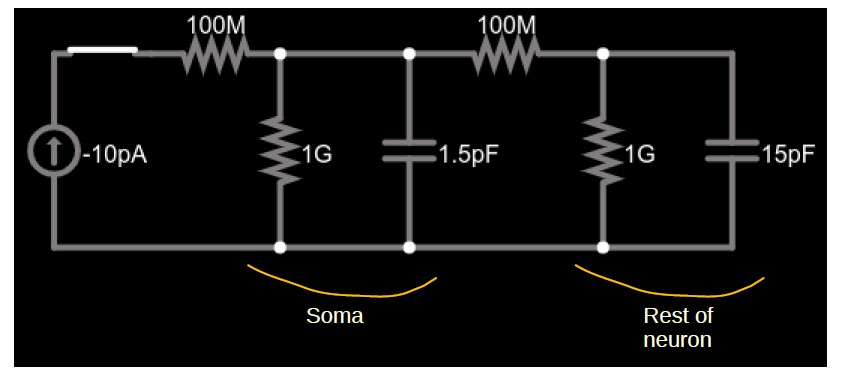
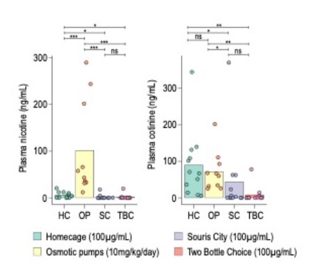
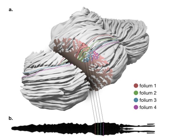
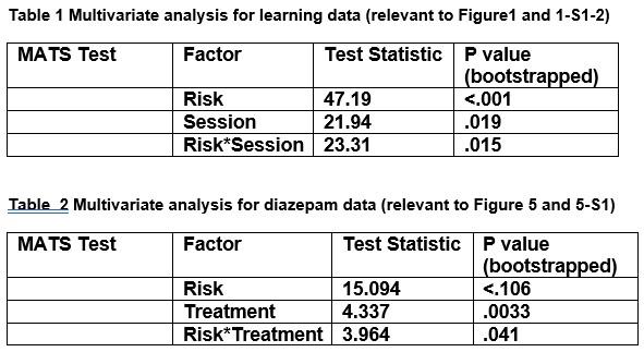
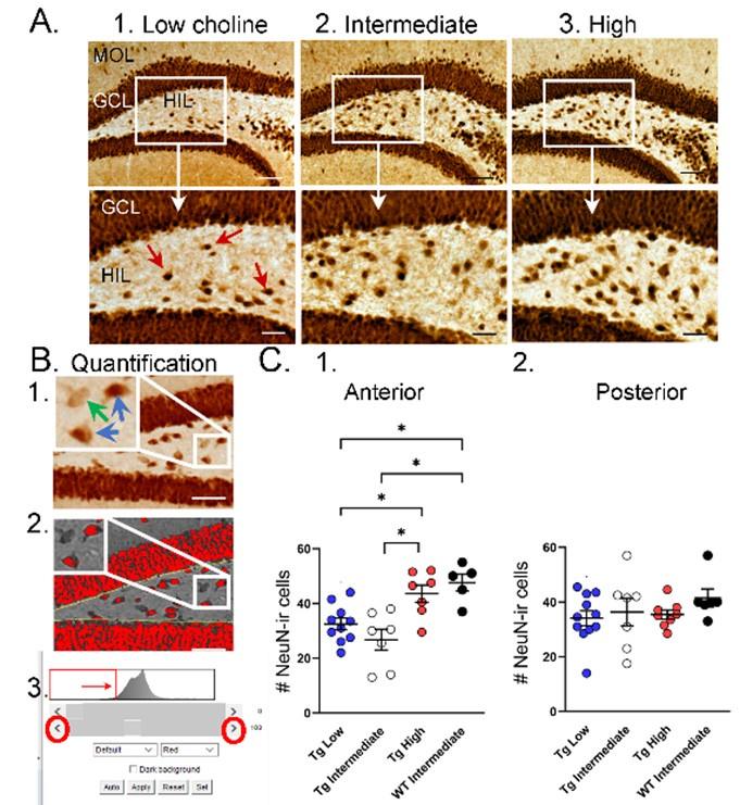
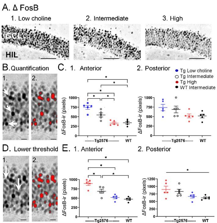
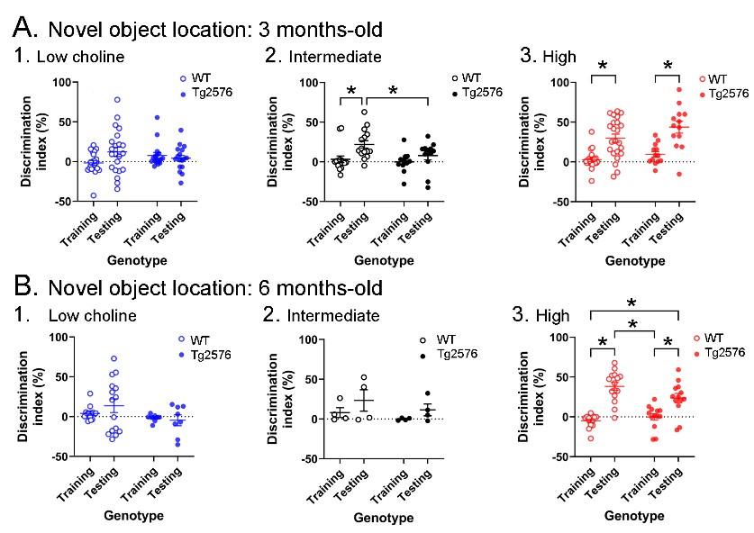
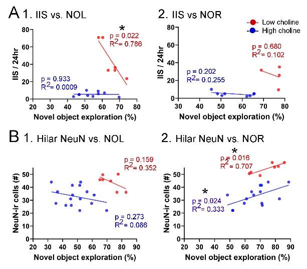
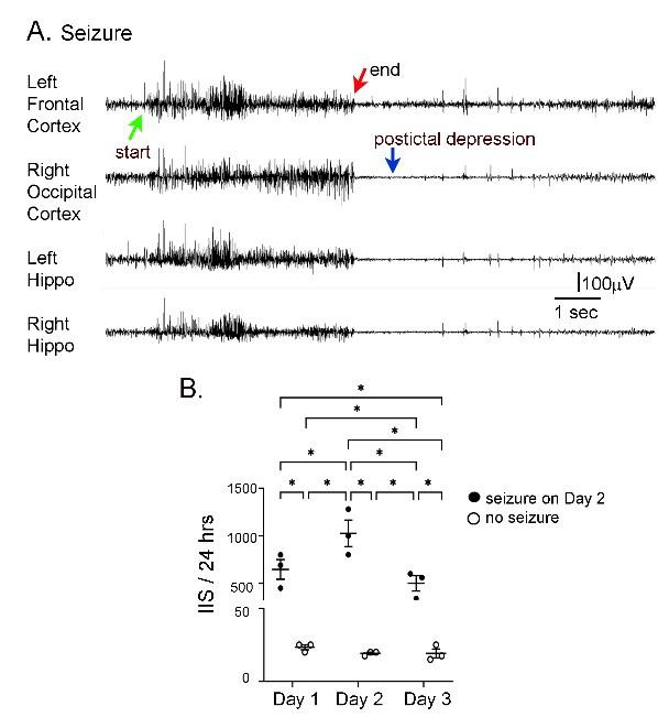
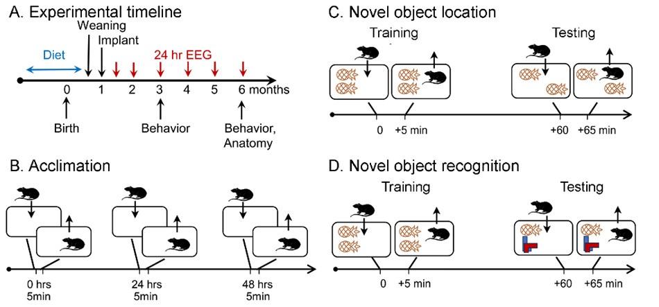
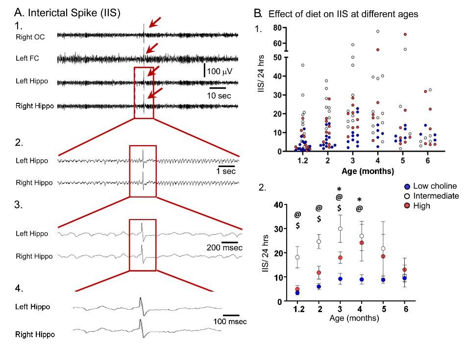
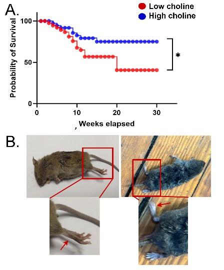
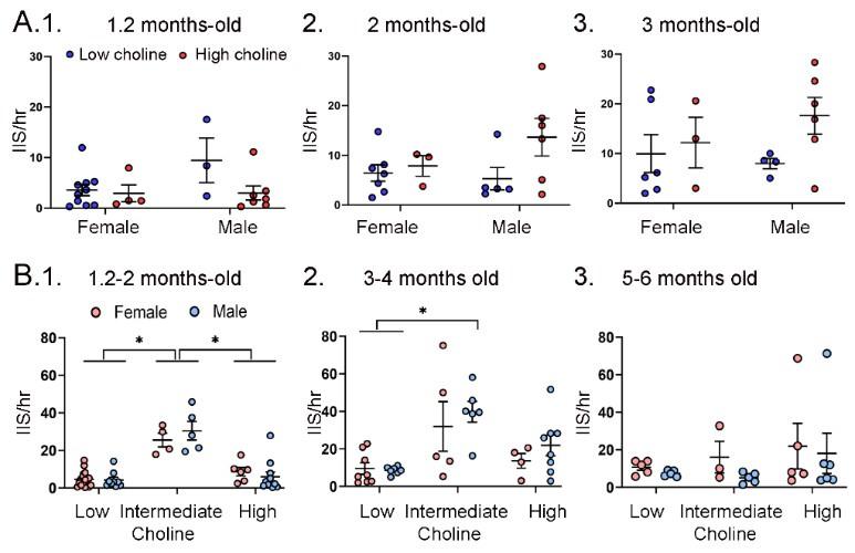
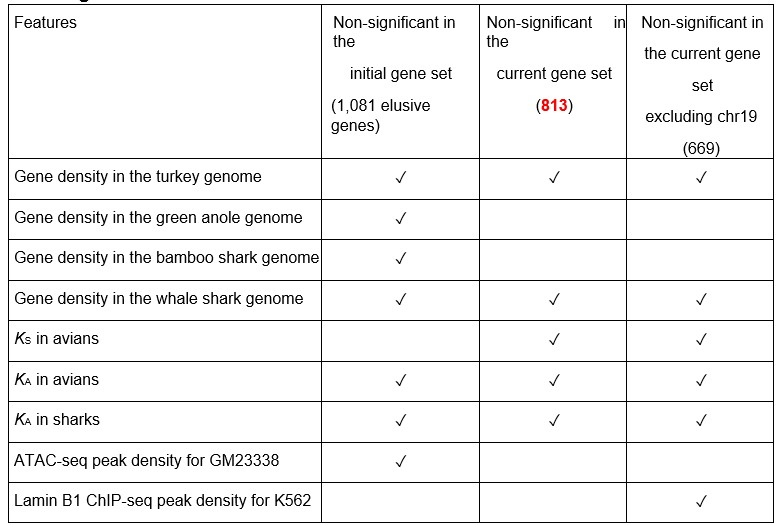
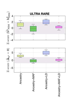
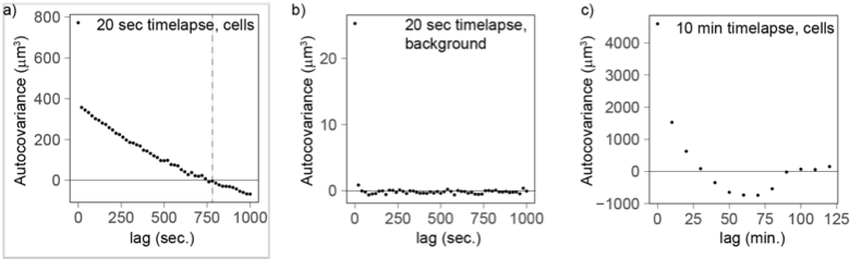
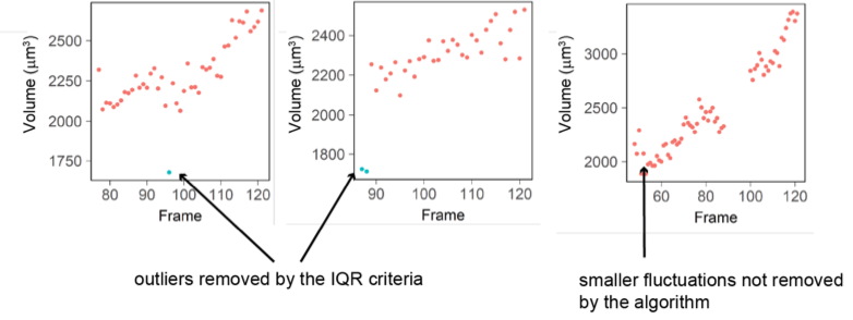
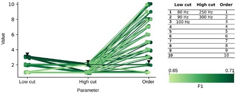
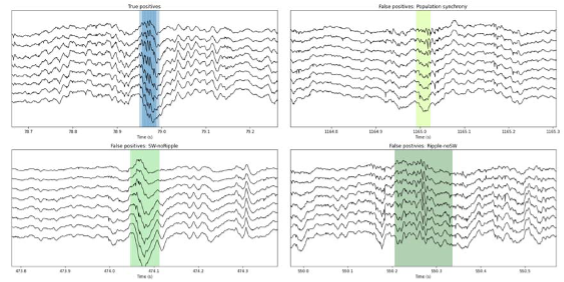
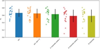
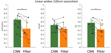
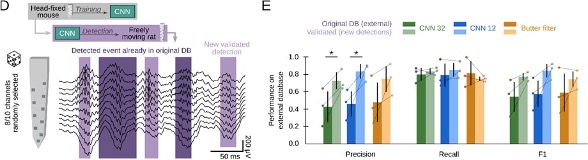
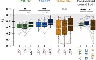
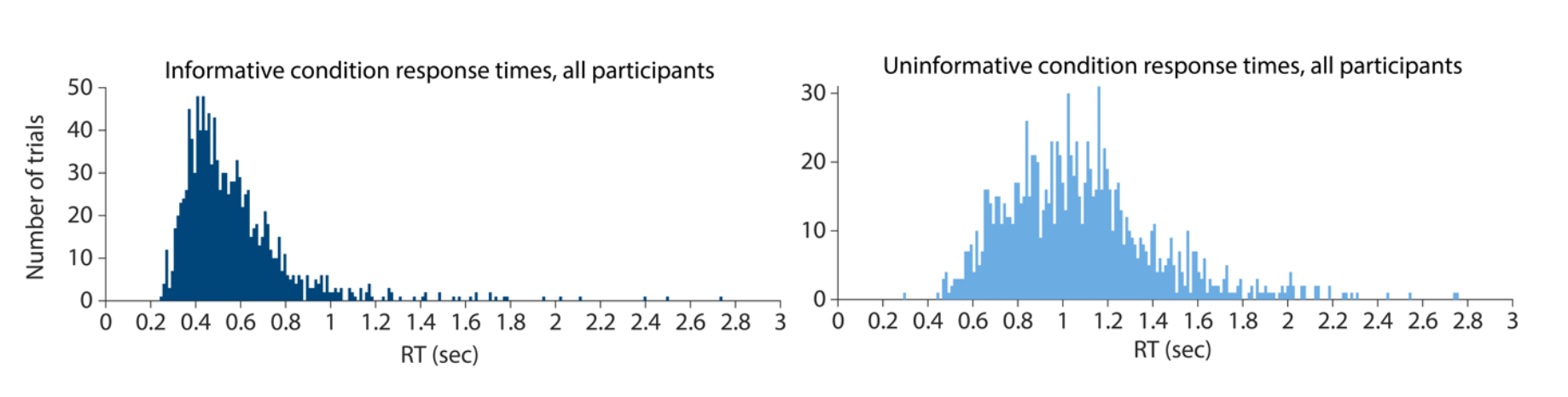
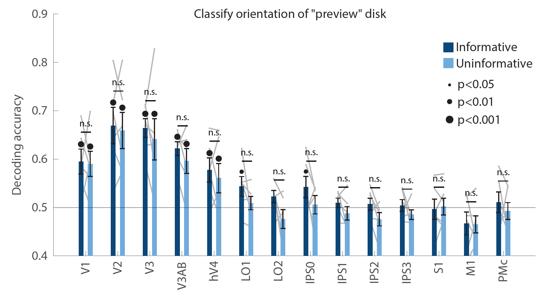
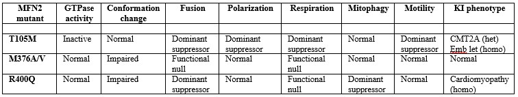
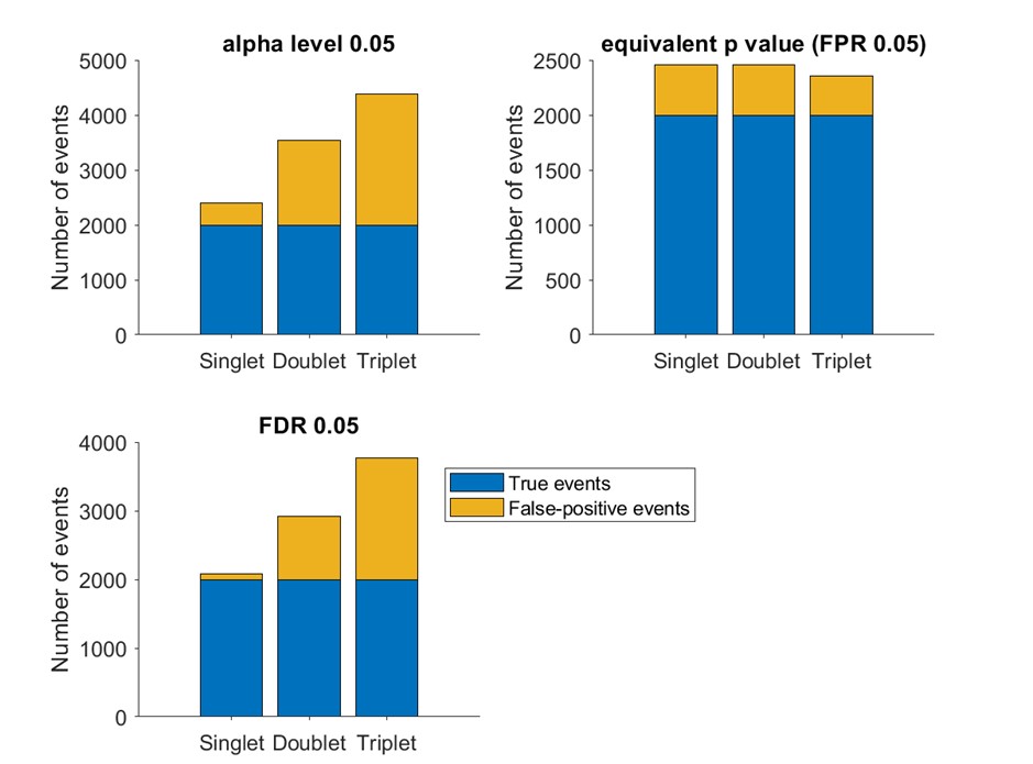
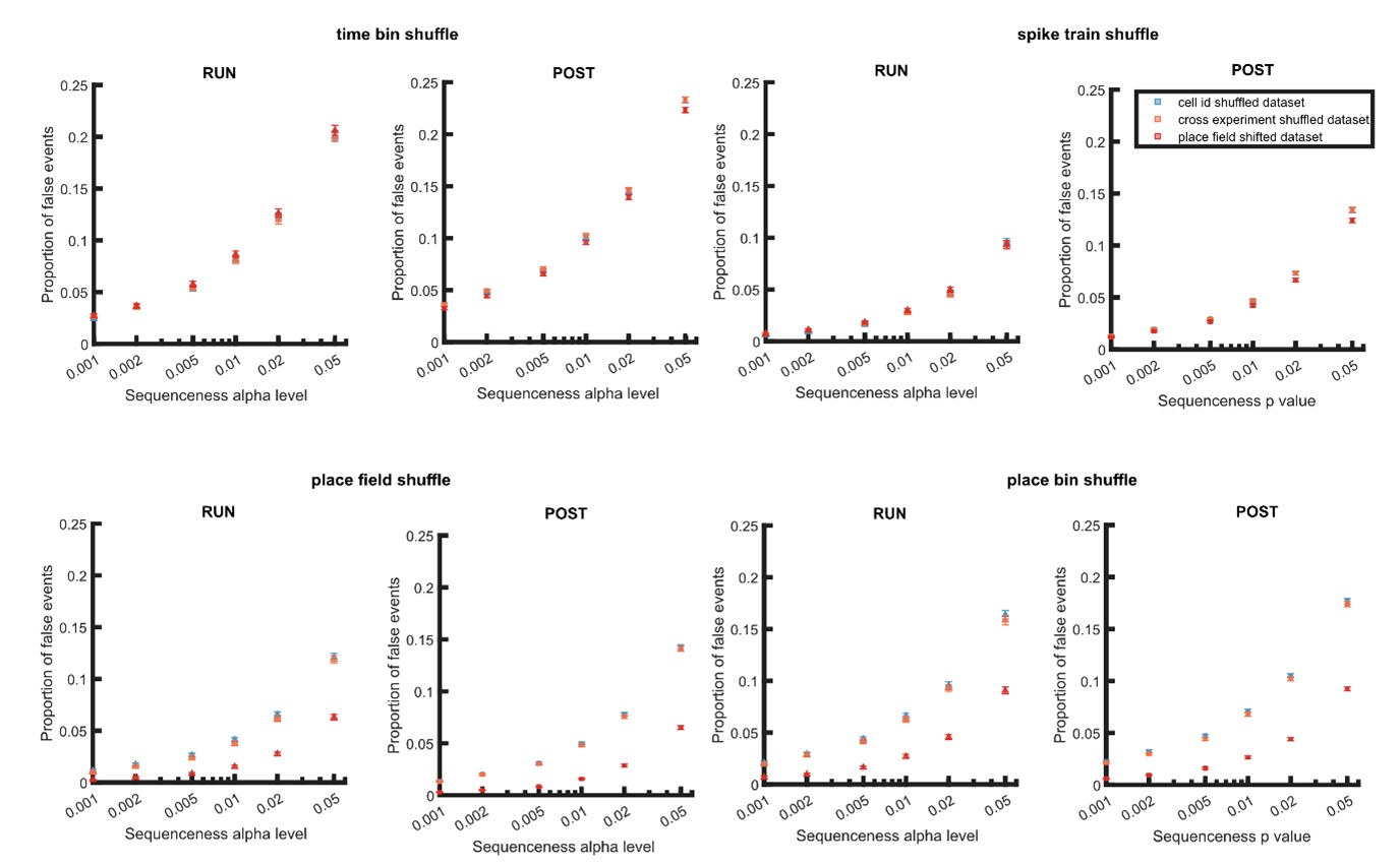
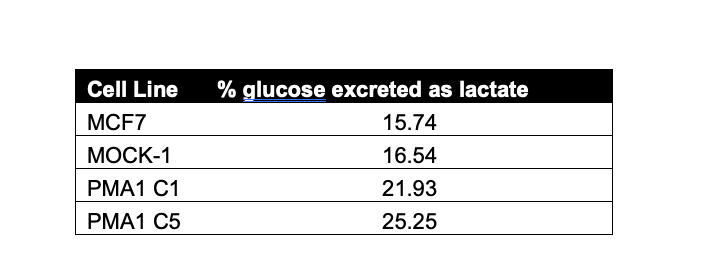
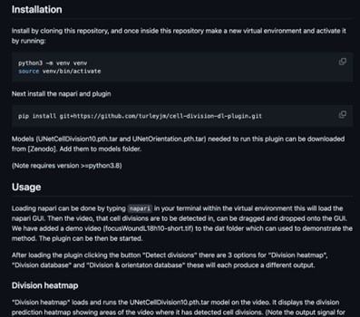
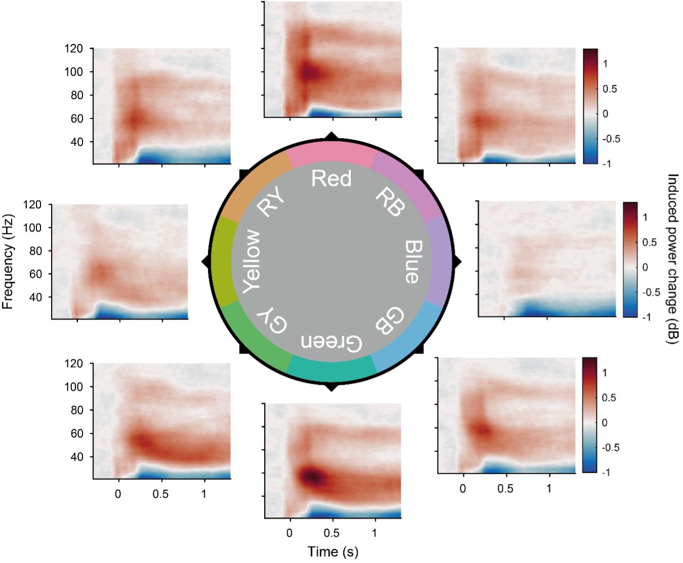
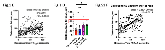
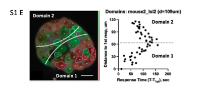
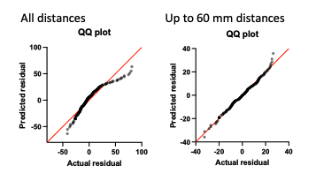
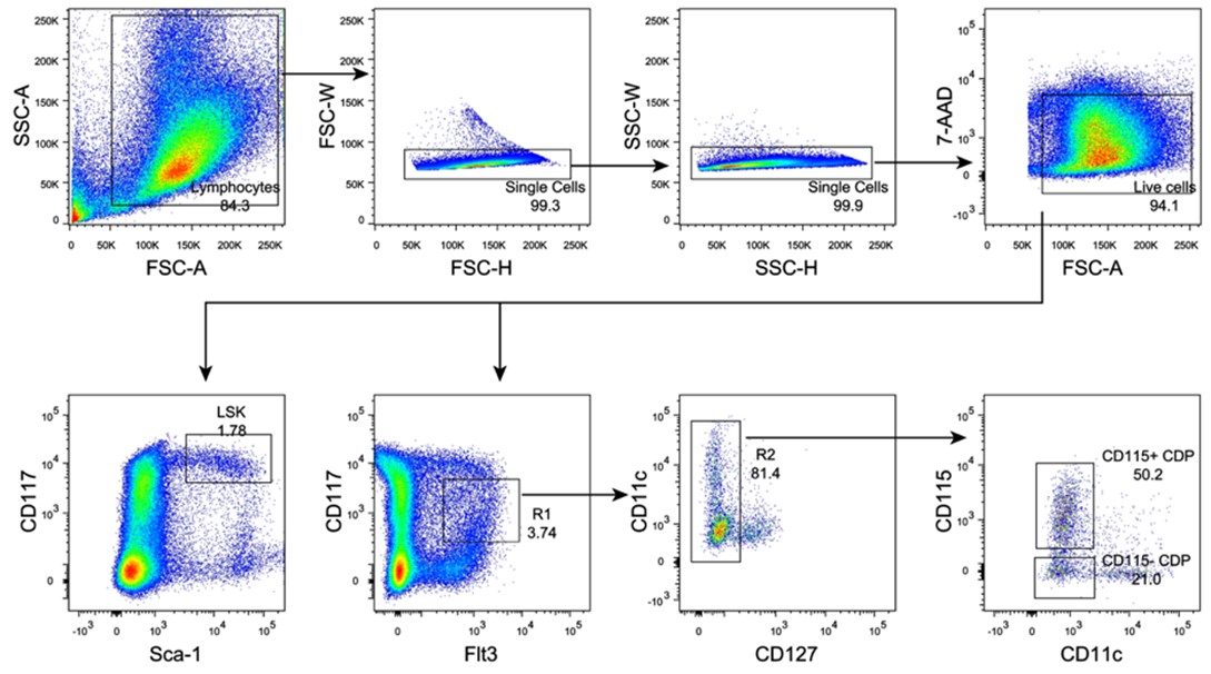
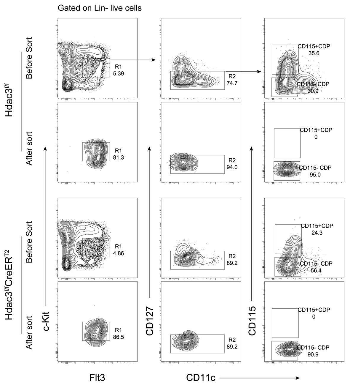
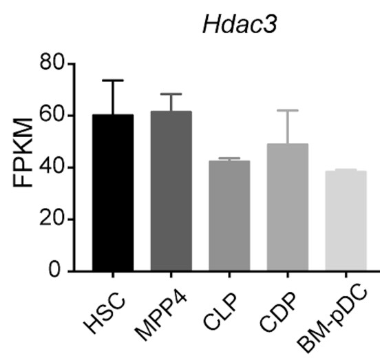
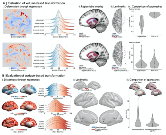
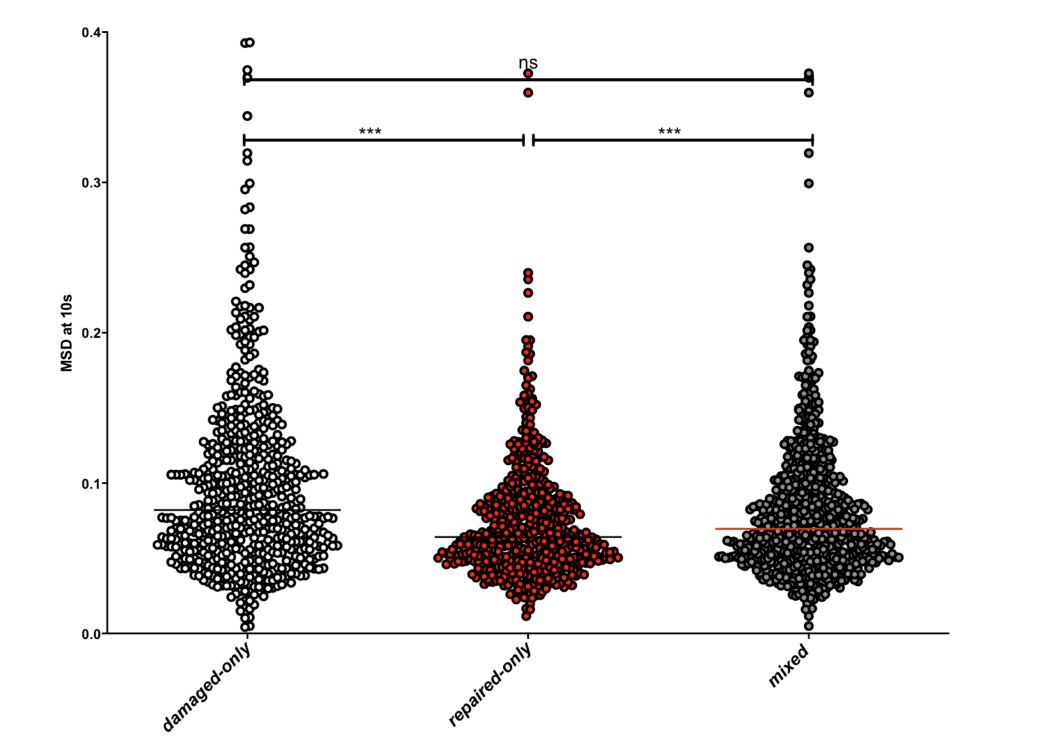
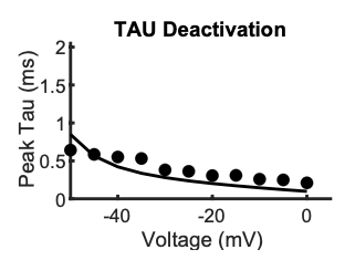
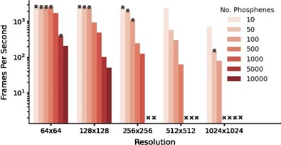
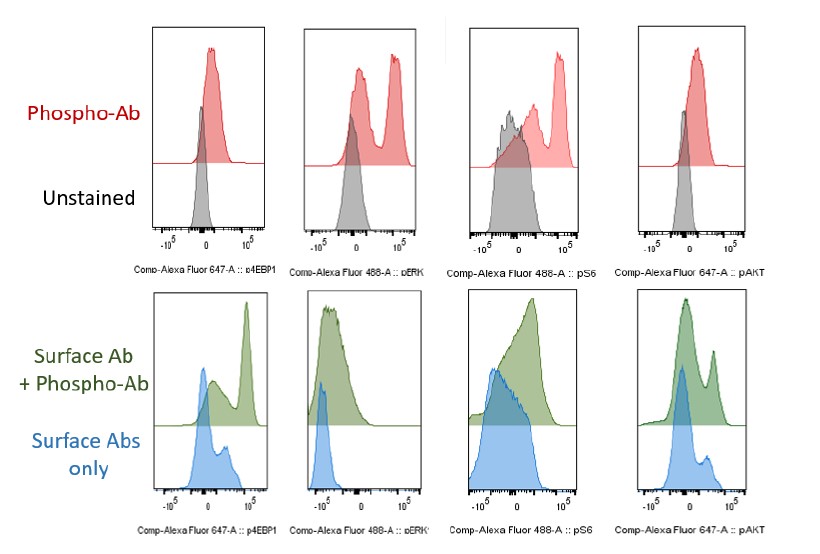
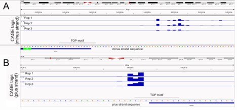
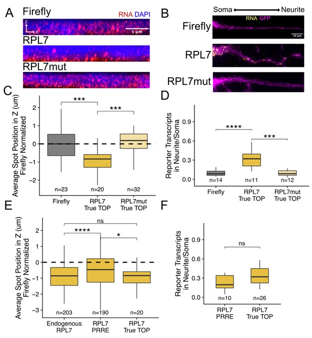
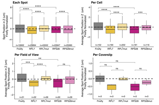
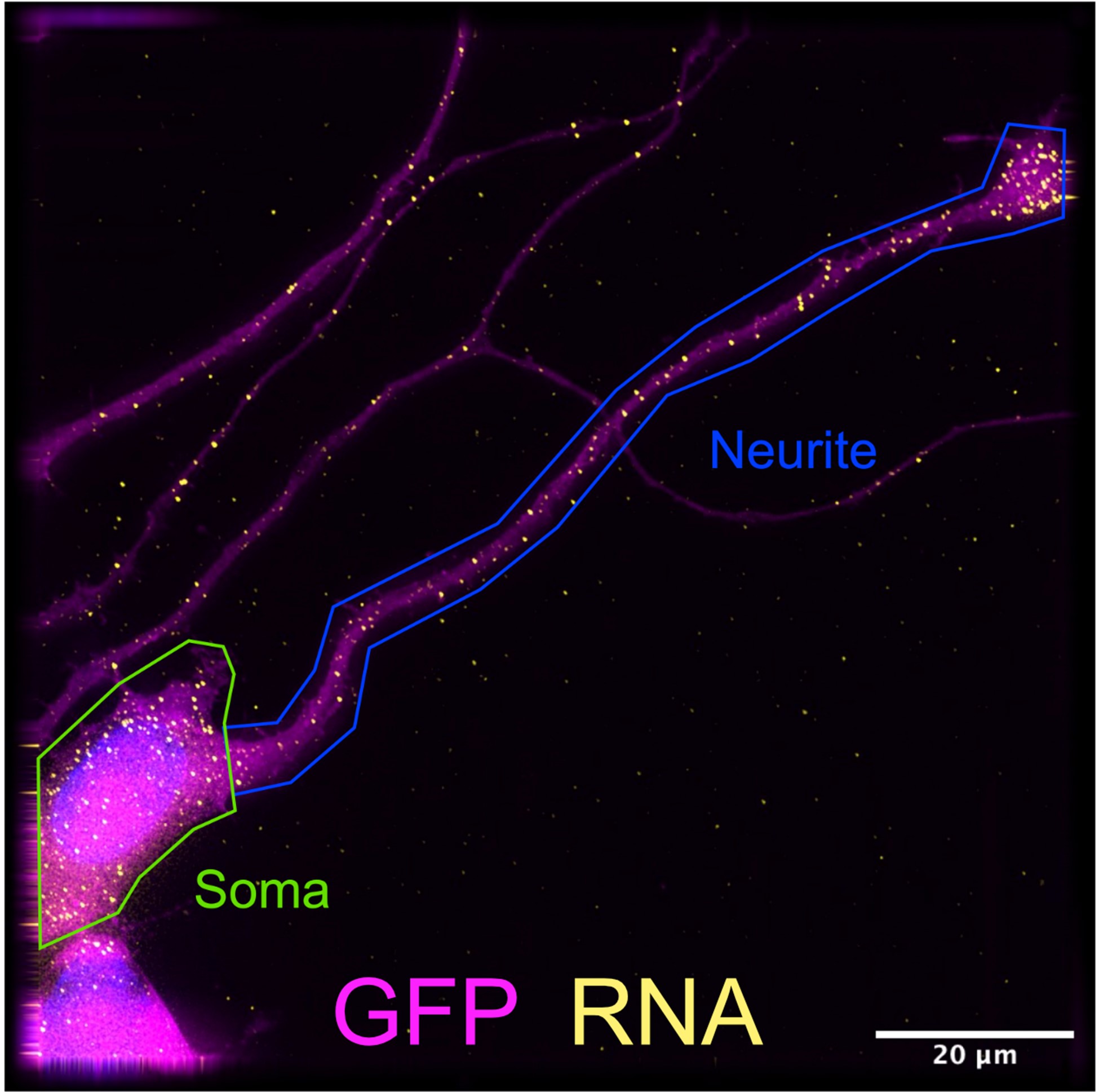
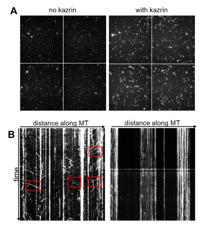
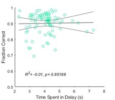
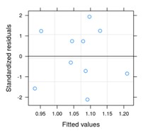
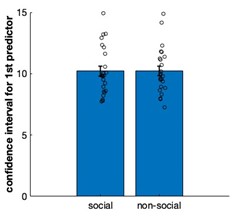
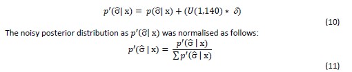
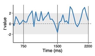
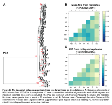
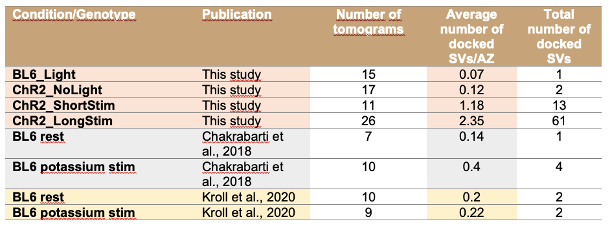
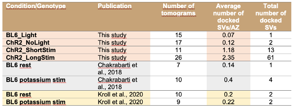
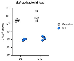
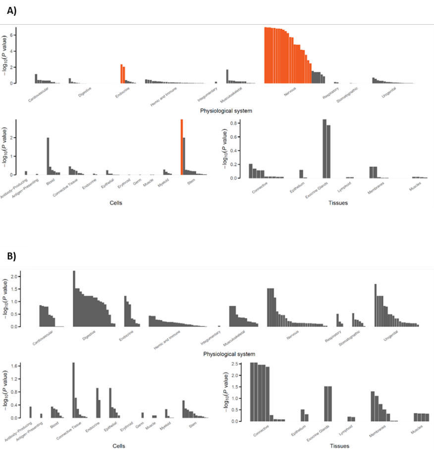
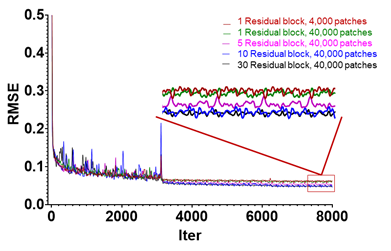
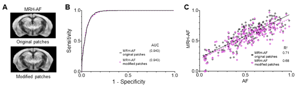
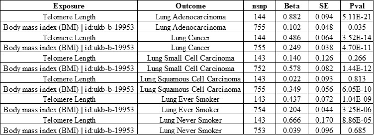
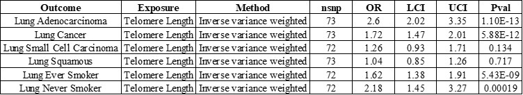
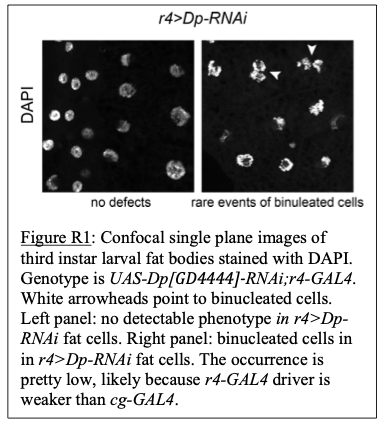
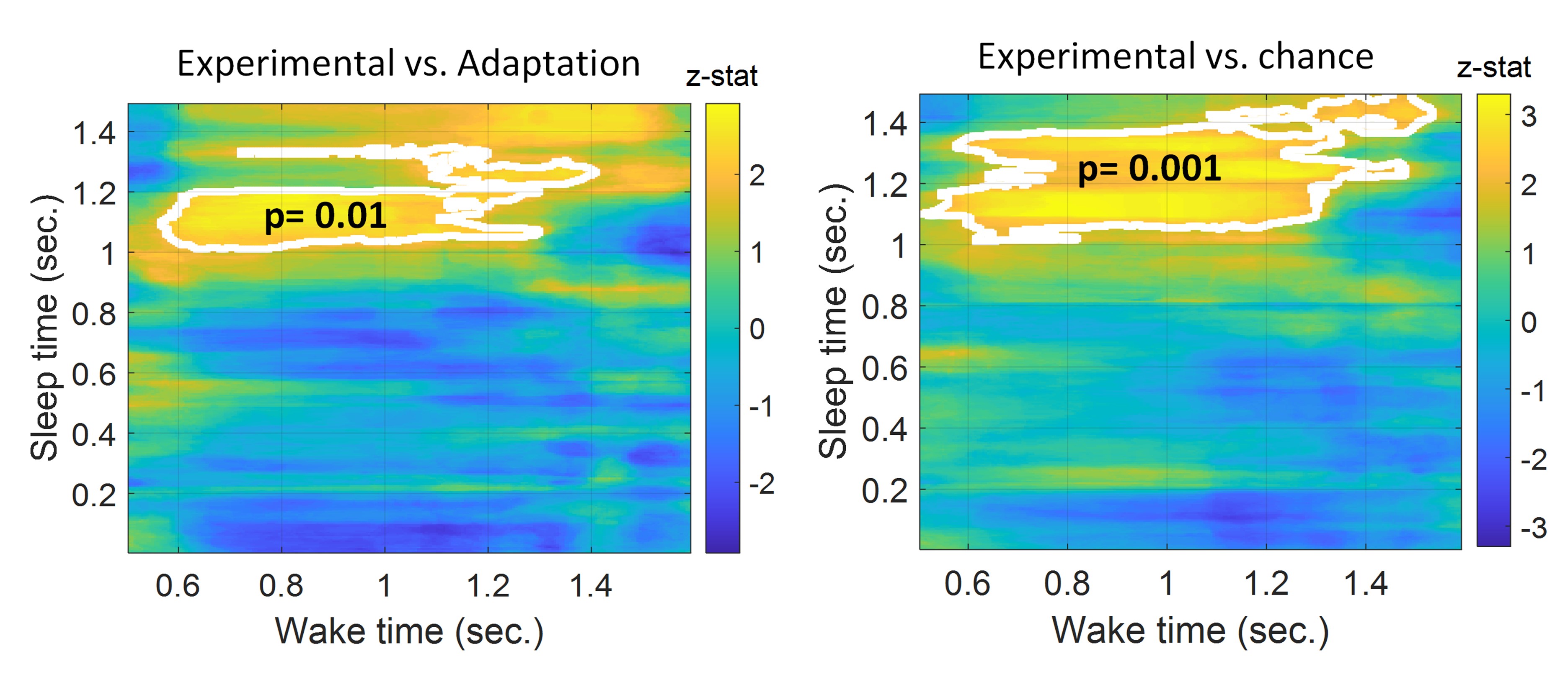
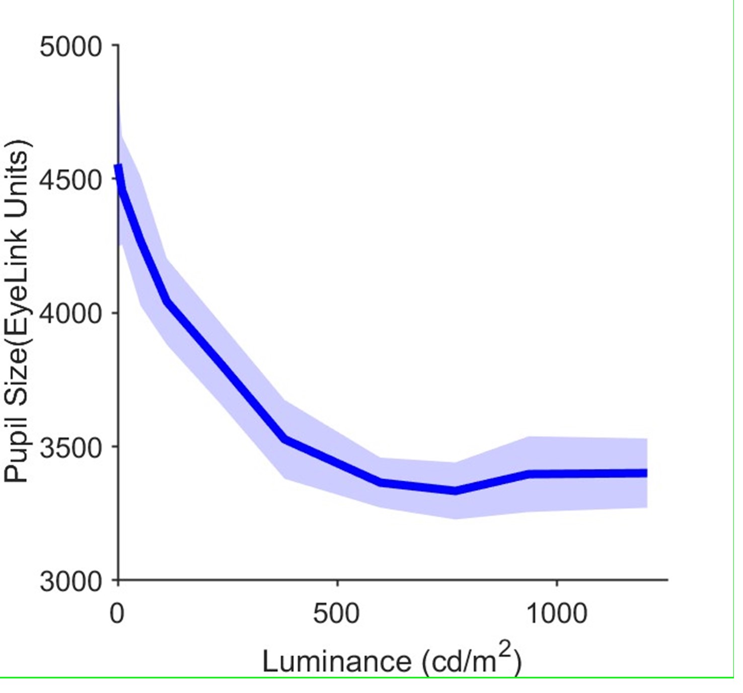


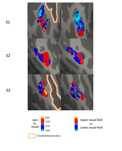
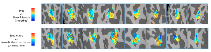
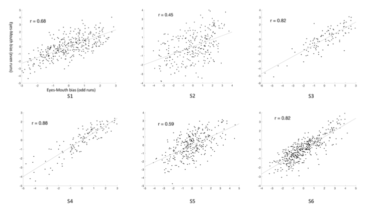
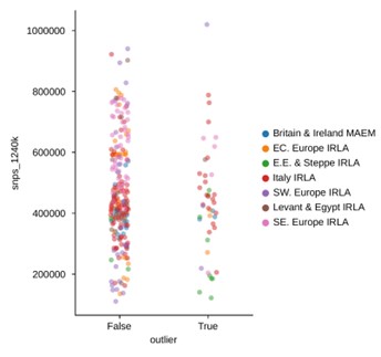
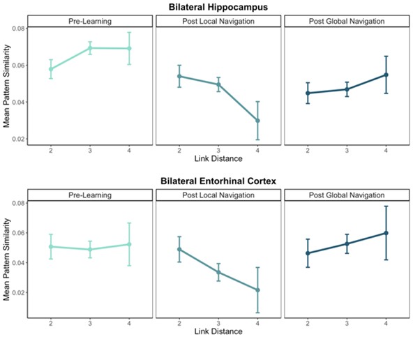
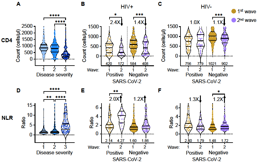
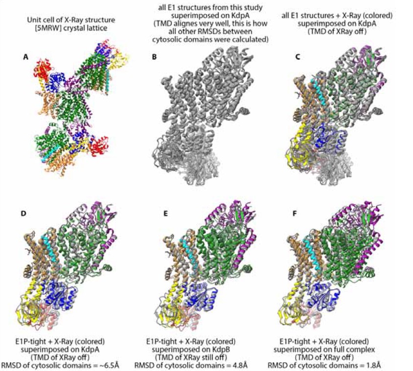
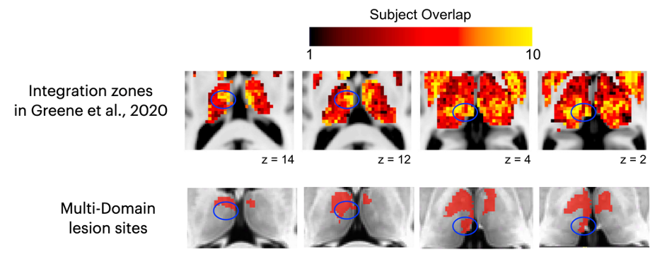
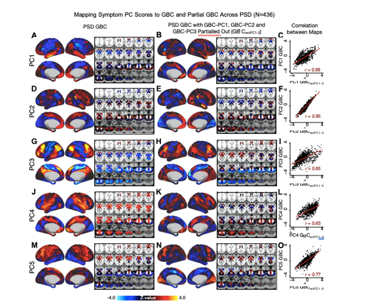
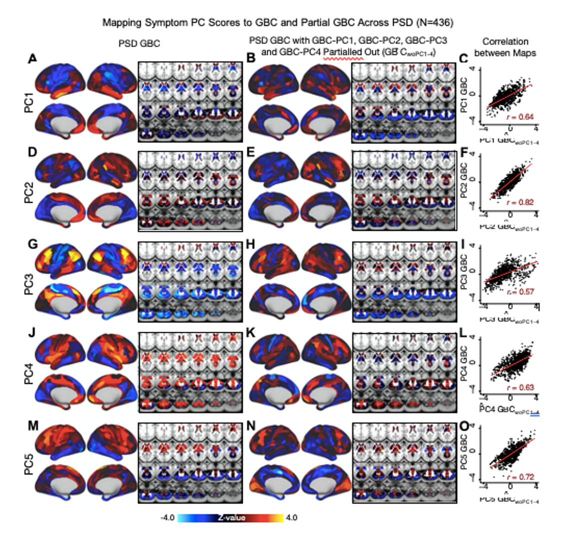
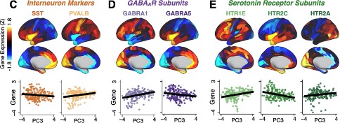
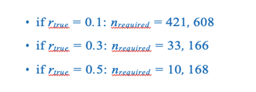
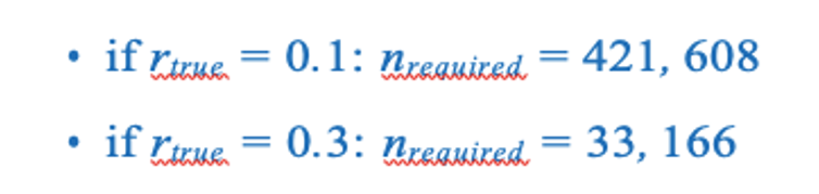

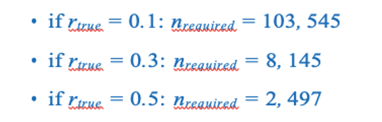
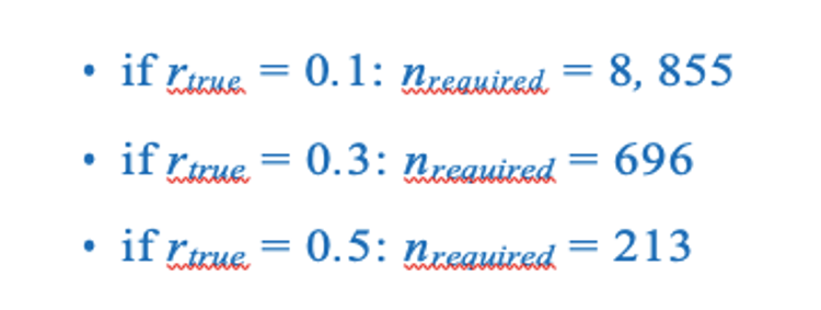
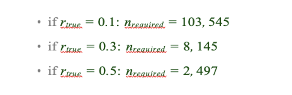
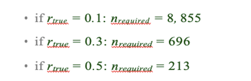
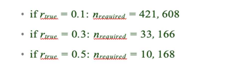
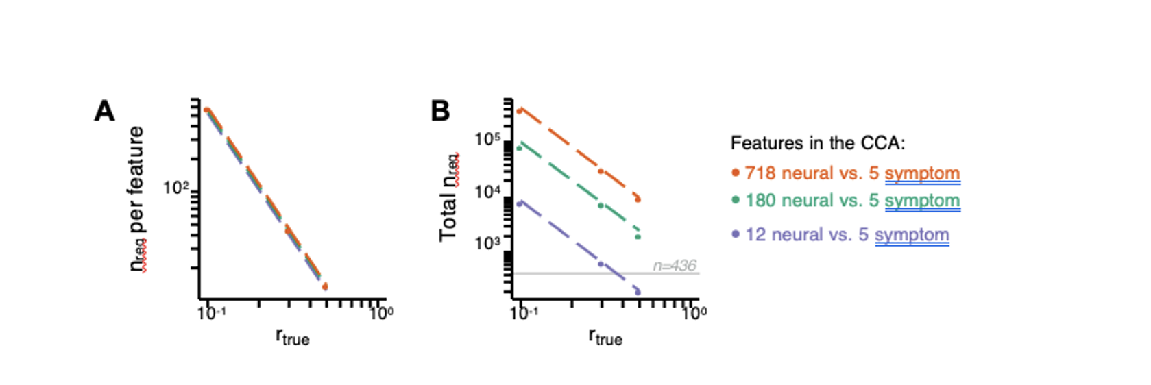
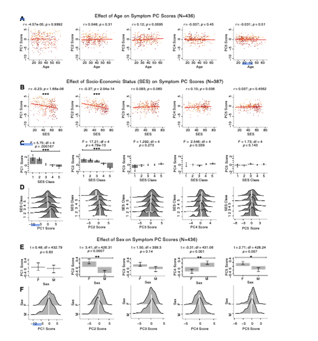

 Supplementary Experiment Figure 1. EEG results of Supplementary Experiment 1. (a) Mean rating scores of happy intensity related to happy and neutral expressions of faces with awardee or actor/actress identities. (b) ERPs to faces with awardee or actor/actress identities at the frontal electrodes. The voltage topography shows the scalp distribution of the P570 amplitude with the maximum over the central/parietal region. (c) Mean differential P570 amplitudes to happy versus neutral expressions of faces with awardee or actor/actress identities. The voltage topographies illustrate the scalp distribution of the P570 difference waves to happy (vs. neutral) expressions of faces with awardee or actor/actress identities, respectively. Shown are group means (large dots), standard deviation (bars), measures of each individual participant (small dots), and distribution (violin shape) in (a) and (c).
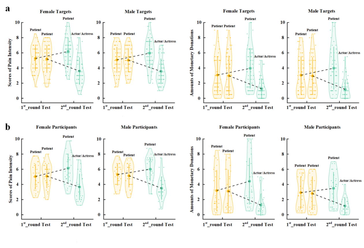 Figure legend: (a) Scores of pain intensity and amount of monetary donations are reported separately for male and female target faces. (b) Scores of pain intensity and amount of monetary donations are reported separately for male and female participants.