layout of what one dont want to happen

změnit slovosled, aby nebyly 2 čísla za sebou

všechna čísla s % a p.b., m2 apod. pevně spojit

mělo by být pevně spojeno s následujícím slovem, aby nebylo na konci řádku

Nová Ivana: Graf velké subjektivní zatížení, Rakousko začíná dřív než ostatní apod.

Nová Ivana: Zajímavé subjektivní zatížení výdaji na bydlení a Pardubický kraj…?

Nová Ivana: V důstojné reziduální příjmy nejsou důchodci (ověřit i u ostatních grafů)

Nová Ivana: V grafu podíl lidí pod hranicí chudoby nadměrného zatížení výdaji…Německo začíná až o 2010

Nová Ivana: Ve srovnání se státy Evropy se Česko řadí dlouhodobě k průměru EU.

Nová Ivana: Karogram zatížení výdaji na bydlení v EU a je tam Velká Británie (týká se to i ostatních kartogramů ve zprávě)

Chybí mezery mezi odstavci / odrážkami

.

.

.

.

.

vocab term?

This entire page seems very high level for Chapter 1. Is there a way to decrease the readability level and simplify the content?

humans lack off on taking care of the environment heavily now days as well.

timeline?

Résumé de la vidéo [00:00:07][^1^][1] - [00:21:31][^2^][2]:

Cette vidéo présente une journée dédiée à la santé mentale des enfants et des adolescents, organisée par des chercheurs et des cliniciens. Elle met en avant l'importance de la collaboration entre enseignants, chercheurs et cliniciens pour améliorer les pratiques et la formation des enseignants sur ce sujet crucial.

Temps forts: + [00:00:07][^3^][3] Introduction et objectifs de la journée * Réflexion sur la santé mentale des enfants * Collaboration entre enseignants et chercheurs * Amélioration des pratiques éducatives + [00:02:02][^4^][4] Définition de la santé mentale * Bien-être selon l'OMS * Importance de la résilience et de l'adaptation * Interaction sociale et compétences émotionnelles + [00:06:23][^5^][5] Facteurs influençant la santé mentale * Poids des facteurs environnementaux et biologiques * Importance de l'estime de soi * Régulation émotionnelle et autocontrôle + [00:10:00][^6^][6] Développement des compétences chez les enfants * Langage oral et fonctions exécutives * Contrôle cognitif et maturation * Différences de développement entre garçons et filles + [00:15:08][^7^][7] Études et données sur la santé mentale * Enquête en classe et résultats * Prévalence des troubles anxiodépressifs * Impact du COVID-19 sur la santé mentale des jeunes

Résumé de la vidéo [00:21:34][^1^][1] - [00:28:48][^2^][2]:

Cette vidéo présente une étude épidémiologique sur la santé mentale des enfants, coconstruite avec des enseignants, des parents et des experts. Elle met en lumière les différences de perception entre les enfants, leurs enseignants et leurs parents, et souligne l'importance de corréler ces perceptions pour une meilleure compréhension.

Temps forts: + [00:21:34][^3^][3] Conception de l'étude * Manque d'indicateurs récents * Étude coconstruite avec divers acteurs * Croisement des perceptions + [00:22:12][^4^][4] Méthodologie de l'étude * Échantillon significatif de 706 écoles * Acceptation positive par les participants * Reproductibilité de l'étude + [00:22:40][^5^][5] Résultats principaux * 13 % des enfants ont des troubles émotionnels * Différences entre filles et garçons * Bien-être augmente en primaire, se dégrade au collège + [00:24:00][^6^][6] Facteurs de risque et de protection * Importance de l'estime de soi * Compétences psychosociales et environnement familial * Interactions précoces et développement cérébral + [00:26:01][^7^][7] Modélisation des troubles des conduites * Interaction entre facteurs biologiques et environnementaux * Importance des relations d'attachement * Trajectoires développementales et prévention

Encourage breaking up or bulleting this content.

Note d'Information : Santé Mentale, Bien-être et Apprentissage à l'École

Synthèse Exécutive

Ce document de synthèse analyse l'intervention de Stanislas Dehaene, président du Conseil scientifique de l'Éducation nationale (CSEN), consacrée à la santé mentale et au bien-être des élèves comme conditions fondamentales de la réussite scolaire.

Les constats majeurs et orientations scientifiques présentés s'articulent autour des points suivants :

• Redéfinition des « fondamentaux » : Aux deux piliers traditionnels (le langage et les mathématiques) s'ajoute un troisième pilier indispensable : la santé mentale et le bien-être.

Ce dernier est présenté comme le plus fondamental, car sans confiance en soi, sentiment de sécurité et capacités d'engagement, aucun apprentissage disciplinaire ne peut s'effectuer efficacement.

• Données épidémiologiques et classements alarmants :

  • 13 % des enfants de 6 à 11 ans (1 sur 7 ou 8) présentent un trouble probable de la santé mentale.

• 24 % des lycéens (1 sur 4) rapportent des pensées suicidaires au cours des 12 derniers mois.

• 13 % des lycéens ont fait une tentative de suicide, et près d'un élève par classe (1 sur 30) a été hospitalisé pour ce motif.

• La France figurait au 62ᵉ rang sur 65 pays de l'OCDE dans le classement PISA 2018 concernant la confiance en soi des élèves.

• Rôle et méthode du CSEN : Créé en janvier 2018 et officialisé par décret en juin 2024, le CSEN regroupe 30 spécialistes pro bono.

Son objectif est de promouvoir une culture de l'expérimentation scientifique (tester des dispositifs sur des sous-groupes avant généralisation) et de diffuser des recommandations fondées sur la recherche.

• Facteurs clés d'action : La science du sommeil (maintien de la sieste en maternelle), l'adoption d'un « état d'esprit de développement », le travail collaboratif et le rôle déterminant des enseignants pour restaurer la confiance des élèves en difficulté (illustré par l'initiative « Les Z'Héros ont du talent »).

Analyse Détaillée des Thèmes Principaux

1. La Structure des Trois Piliers de l'Éducation

L'institution scolaire met traditionnellement l'accent sur la maîtrise de savoirs disciplinaires.

L'analyse du CSEN propose un modèle à trois piliers interconnectés formant un cercle vertueux.

   ```
   [ Troisième Pilier (Socle) : Santé Mentale & Bien-être ]
                             │
     ┌───────────────────────┴───────────────────────┐
     ▼                                               ▼

[ Premier Pilier : Langage ] [ Deuxième Pilier : Mathématiques ] ```

Premier Pilier : Le Langage

La maîtrise du langage dans toutes ses dimensions constitue le premier pilier traditionnellement identifié :

• Développement du vocabulaire dès la classe de maternelle.

• Maîtrise de la première langue, de la lecture, de l'orthographe, et de l'expression orale et écrite.

• Ouverture vers la maîtrise d'une seconde langue, l'accès à la littérature et à la culture.

Deuxième Pilier : Les Mathématiques

Les mathématiques sont réaffirmées comme un élément fondamental de la culture générale pour l'ensemble des élèves :

• Apprentissage du nombre et de l'arithmétique.

• Développement de la vision dans l'espace, de la géométrie, de la résolution de problèmes et de la démarche scientifique.

Troisième Pilier : La Santé Mentale et le Bien-être

Ce troisième pilier est présenté comme la condition sine qua non des deux premiers.

Il englobe la stabilité de l'esprit nécessaire à l'engagement scolaire et repose sur des compétences psychosociales précises :

• La confiance en soi : La certitude que l'effort personnel produit le succès.

Sans cette conviction, l'élève ne s'engage pas dans l'apprentissage.

• L'envie d'apprendre : Le fait de se rendre à l'école avec un sentiment de sécurité, sans crainte d'être harcelé ou puni.

• La persévérance et le statut de l'effort : La déconstruction de la croyance erronée selon laquelle devoir faire des efforts est le signe d'un manque de talent.

• La confiance dans les autres : La capacité à collaborer et à travailler en groupe.

2. État des Lieux Statistiques : Santé Mentale et Comparaisons Internationales

Les données présentées soulignent la sévérité des enjeux de santé mentale chez la jeunesse scolarisée en France ainsi que la faiblesse du niveau de confiance généré par le système éducatif.

Chiffres clés de la santé mentale infantile et juvénile en France

| Population | Indicateur de santé mentale | Proportion / Statistique | | --- | --- | --- | | Enfants (6 à 11 ans) | Troubles probables de la santé mentale | 13 % (1 enfant sur 7 ou 8) | | Lycéens | Pensées suicidaires (au cours des 12 derniers mois) | 24 % (1 élève sur 4) | | Lycéens | Tentatives de suicide | 13 % (1 élève sur 7 ou 8) | | Lycéens | Hospitalisation suite à une tentative de suicide | ~1 élève par classe (environ 1 sur 30) |

Positionnement International (PISA 2018)

• Classement PISA 2018 : La France se situait à la 62ᵉ place sur 65 pays de l'OCDE évalués en matière de confiance en soi des élèves.

• Modèle comparatif (Danemark) : Dès l'entrée à l'école, le premier objectif institutionnel au Danemark est le bien-être de l'élève et sa capacité à être heureux dans le contexte collectif, parallèlement aux apprentissages scolaires.

3. Rôle, Fonctionnement et Recommandations du CSEN

Le Conseil scientifique de l'Éducation nationale (CSEN) intervient pour éclairer la décision publique et les pratiques pédagogiques par les apports de la recherche.

Institution et Mode de Fonctionnement

• Historique : Existant depuis janvier 2018, le CSEN a été institué par décret en juin 2024.

• Composition : Il rassemble 30 spécialistes issus de toutes les disciplines scientifiques pertinentes pour l'éducation, œuvrant à titre pro bono.

• Mode de saisine : Le conseil peut s'autosaisir ou être saisi par le ministre de l'Éducation nationale, ainsi que par les acteurs du terrain.

• Missions :

  • Faciliter l'intégration des travaux scientifiques, des expérimentations et des comparaisons internationales dans le domaine éducatif.

• Promouvoir une « culture de l'expérimentation » au sein du ministère (tester les innovations sur des sous-groupes témoins avant toute généralisation).

• Formuler des recommandations concrètes pour les acteurs de l'éducation.

Publications et Outils de Diffusion

Le CSEN produit différents supports de synthèse et d'accompagnement (17 synthèses publiées à ce jour) :

• Ouvrages de synthèse : 3 volumes thématiques publiés en librairie pour alimenter les bibliothèques d'établissements et les instituts de formation des enseignants.

• La lettre d'information « Le Passeur » : Publication électronique proposant des résumés accessibles, accompagnée de contenus vidéo réalisés avec le vulgarisateur Fred Courant (L'Esprit Sorcier).

• Thématiques transversales traitées :

  • L'état d'esprit de développement (développer l'idée que l'effort fait progresser).

• Les méthodes de travail en groupe.

• L'évaluation au service des besoins spécifiques des élèves.

• L'enseignement explicite.

La Science du Sommeil et de la Sieste

Le CSEN met en avant la synthèse de la recherche intitulée « Mieux dormir pour mieux apprendre », pilotée par Stéphanie Maza :

• Le sommeil est un pilier biologique fondamental de la plasticité cérébrale, de l'apprentissage et de la stabilité émotionnelle.

• Le manque de sommeil génère des troubles de l'attention et accroît les risques de vulnérabilité en santé mentale.

• Recommandation pratique : Légitimer scientifiquement le maintien de la sieste en école maternelle tout au long de la scolarité pour les enfants dont les besoins individuels le nécessitent, conformément aux préconisations de l'Académie de pédiatrie.

4. L'Initiative « Les Z'Héros ont du talent » et les Leçons Pédagogiques

Pour illustrer la plasticité des trajectoires individuelles et l'impact de l'environnement scolaire, le CSEN a mené une série d'entretiens intitulée « Les Z'Héros ont du talent ».

Parcours de Personnalités Présentées

• Thierry Marx : En décrochage scolaire précoce, qualifié à tort d'élève sans avenir, il a été remobilisé et inséré grâce au compagnonnage.

• Zhang Zhang : Violoniste ayant connu une scolarité fortement hachée et sporadique en raison de migrations successives, confrontée au harcèlement scolaire en tant qu'étrangère.

• Seddik Quider : Enfant de parents analphabètes vivant en banlieue sans logement stable, s'estimant condamné à l'échec à l'âge de 15 ans.

Il est devenu directeur de recherche au CNRS, fondateur d'entreprise innovante et enseignant à l'université d'Harvard.

• Note : La figure du navigateur Jean Le Cam est également citée parmi les profils illustrant ces parcours de résilience.

Deux Principes Pédagogiques Majeurs

• Interdiction de la Stigmatisation Définitive : Aucun éducateur ne doit signifier à un enfant qu'il est « nul » ou qu'il « ne fera jamais rien de sa vie ».

Ce message est qualifié de factuellement faux et scientifiquement infondé.

• Le Rôle Déterminant des Rencontres : Les réussites ultérieures d'élèves en situation de décrochage reposent quasi systématiquement sur la rencontre avec un tiers (un enseignant passionné, un groupe structurant comme les Compagnons du Devoir) capable de restaurer la confiance et de réorienter la trajectoire personnelle.

Citations Clés

« [Le bien-être] est mis en 3ᵉ ici mais qui est peut-être le plus fondamental de tous parce que comment voulez-vous apprendre si vous n'avez pas d'abord confiance en vous... »

« Le classement PISA de 2018 a classé la France tout en bas de l'échelle, c'est-à-dire 62ᵉ sur 65 pour les pays de l'OCDE [...] pour la confiance en soi des élèves. Notre école ne fait pas assez attention à ce pilier absolument fondamental... »

« Cessons de traiter ce sujet [le sommeil] avec un petit sourire, traitons-le avec le sérieux qu'il mérite. Le sommeil est un aspect fondamental de la biologie du cerveau, c'est un aspect fondamental de la biologie de l'apprentissage... »

« Personne jamais ne devrait dire à un enfant "tu es nul, tu ne feras jamais rien dans la vie", parce que c'est toujours faux. »

Conclusions et Recommandations Institutionnelles

L'intervention se conclut sur la nécessité d'un changement d'attitude collective au sein de l'Éducation nationale, articulé autour des axes suivants :

• Refus d'opposer la rigueur académique et le bien-être : Les acquisitions disciplinaires (mathématiques, langage) et la santé mentale se renforcent mutuellement.

L'élève gagne en confiance lorsqu'il prend conscience de ses progrès scolaires.

• Changement de posture institutionnelle : Développer une plus grande bienveillance au sein de l'institution scolaire afin de corriger les faiblesses structurelles révélées par les enquêtes internationales (PISA).

• Mobilisation des acteurs : Utiliser la science pour transformer l'environnement éducatif et donner à chaque enseignant les moyens de devenir l'intervenant clé capable de modifier positivement la trajectoire d'un élève.

This course is heavily taken by medical assistants. It would be important to briefly describe that field.

May want to indicate PA and NP roles and responsibilities may vary by state

Encourage a revision on the definition of provider: Healthcare provider: A licensed person or organization that provides health care services. Examples include medical doctor, therapist, dentist, nurse practitioner, and physician assistant.

Should be "emergency department"

Nová Ivana: Ještě do toho mohou možná potencionálně vstoupit změny v daních pronajímatelů, marže, to že roste tržní cena bytů apod.?

Nová Ivana: NEJSOU ZEMĚ OECD…? (týká se to i ostatních karogramů ve zprávě..

nebo spíš právě proto

Dala bych pryč slova "tak" a "dokonce" - působí to, jako by to bylo více než v předchozí větě...

to to by chtělo trochu přeformulovat pro lepší čitelnost

ta pomlčka je nějaká dlouhá, ne?

přeházet slovosled tak, aby nebyly 2 čísla za sebou - tedy rok a pak hned hodnota

Bylo by možné, aby všechny tooltipy měly jedno desetinné místo? Např. U Olomouce je jen 7, což vypadá trochu divně. Zároveň je potřeba změnit na desetinnou čárku namísto tečky

Zvýšil?

můžeme vyměnit např. za slovo "nárůst" nebo jiné, aby nebylo dvakrát za sebou "zhoršení"?

Nová Ivana: V TOM JE TAKÉ ANGAŽOVÁNO MPO..?

Nová Ivana: …v ostatních grafech členění na nájmníci, vlastníci, družstevníci a celkem…tady nejsou družstevníci

Nová Ivana: …to je z nějakého průzkumu?

Nová Ivana: …to jsou také cihla v existující zástavbě?

Nová Ivana: … ta skupinka trochu nesourodá (nájemníci) , ale asi v pohodě….

Nová Ivana: Vliv vysokých nabídkových cen u nájmů nemůže být ovlivněn tím, že to je aktuální tržní cena, že ceny díky situaci na trhu takto vzrostly? Nebo to skutečně odráží jen stabilitu dlouhodobých nájemních vztahů a nevyužívání tržní inzerce?

Nová Ivana: Cihla v existující zástavbě se týká i celého textu o nájemním bydlení?

Nová Ivana: Graf není ozdrojován

inference

More Question

difference between Study 2A and 2B

use this sale for our study?

difference between 1A and 1B

our study is 12-18

majority white participants

more question

Question

These divergences can be limited by traditional institutions

Increasing divergence followed by the breakdown of traditional cleavages and the rise of particularization

The particularization of issue provided opportunity both negatively and positively for older parties

New associations needed to keep former parties relevant cut the bonds of former cleavages

The new problems arising cut across the old cleavages especially from the left

Expression of group based interests and conflicts

Expression of interests is the key

Declining cleavage politics rely on the dissipation of previous conflicts which traditional cleavages had relied on

Certain characteristics which used to define cleavages will have less relevance

The growing diversification within society makes their linkage far weaker

The degradation of older cleavages lead to a loosening of their power over the individual

The necessary bounds of particularization

Institutional restrictions may also prevent particularization

Model of political coherence to counter the particularization of the electorate

Particularization process is eroding political loyalties

Materialism vs Postmaterialism

Increasing diversification of political issues and of individuals categorization

Social identity was more homogenous in the past in terms of political preference

People derive many identities from social position and this leads them in many different political directions

The individuals growing desire for specialization is breaking down the appeal of larger social groups

The public are becoming far more specialized in their opinions

Homogenized society is disintegrating

The specifics of political concern are becoming far more domesticized

Development thus began with parties based on social cleavages but has evolved to see lesser impact

Disintegration of the linkage between political parties and the social cleavages they previously represented

Political emancipation

Cleavages based on class and religion

Divisions between parties were deeply linked to cleavages and social distinctions within society

Document de Briefing : Des Facteurs de Risque Environnementaux à la Psychiatrie de Précision

Synthèse Exécutive

La psychiatrie traverse un changement de paradigme majeur, évoluant d'un modèle centré sur la génétique pure vers une approche axée sur la psychiatrie de précision et les interactions gène-environnement.

Présentée par la Pr Marion Leboyer (professeure de psychiatrie à l'UPEC, directrice de la Fondation FondaMental et lauréate du Grand Prix INSERM 2021), cette discipline cherche à déconstruire les catégories cliniques traditionnelles (dépression, schizophrénie, troubles bipolaires) pour identifier des sous-groupes homogènes de patients selon leurs mécanismes biologiques et leurs facteurs d'exposition.

Principaux enseignements :

• Enjeu de santé publique mondial et économique : Les maladies mentales constituent la première cause mondiale de handicap et représentent un coût direct et indirect de 163 milliards d'euros en France, dépassant largement les maladies cardiovasculaires et les cancers.

Environ 20 % de la population générale est touchée.

• Le lien biologique de l'inflammation chronique : L'interaction entre un terrain de vulnérabilité génétique complexe et des facteurs environnementaux (infections périnatales, alimentation ultra-transformée, pollution, stress) déclenche une inflammation chronique de bas niveau.

Celle-ci affecte le cerveau, les cellules (dysfonction mitochondriale), le sang et l'axe cerveau-intestin.

• Facteurs environnementaux majeurs :

• Infections : Un tiers des cas de schizophrénie pourrait être évité par la prévention des infections pendant la grossesse.

• Nutrition : Le syndrome métabolique touche jusqu'à 38 % des patients souffrant de dépression résistante.- Urbanicité : Le risque de schizophrénie et de troubles bipolaires est deux fois plus élevé en milieu urbain qu'en milieu rural.

• Projets de recherche et outils digitaux : Le Programme Français de Psychiatrie de Précision (PEPR France 2030, 2022-2031) déploie la cohorte French Minds (3 000 patients) pour analyser l'exposome et la biologie.

Parallèlement, des applications ciblées (MyMood, MiaMental, LENA, BAE, Food for Mood) sont développées pour le diagnostic précoce et la prévention.

• Urgence de la prévention et du décloisonnement : Le retard diagnostique reste dramatique en France (10 à 13 ans pour les troubles bipolaires).

Il est critique de briser les stéréotypes, de décloisonner la médecine somatique de la psychiatrie et d'inciter les décideurs publics à agir sur l'environnement.

1. Enjeux Majeurs de Santé Publique et Impact Économique

Les pathologies mentales représentent un défi socio-économique d'une ampleur inédite, encore sous-estimé en raison du tabou et des préjugés sociaux qui freinent l'accès aux soins.

• Prévalence : On estime que 20 % de la population générale sera directement touchée par une maladie mentale au cours de sa vie.

La majorité de ces pathologies débutent chez les jeunes adultes (entre 15 et 25 ans).

• Première cause de handicap : Les maladies mentales constituent la première cause mondiale de handicap invisible et silencieux.

Elles regroupent des affections variées : dépressions, troubles bipolaires, psychoses (schizophrénies), troubles anxieux et troubles du neurodéveloppement (autisme, TDAH).

• Impact financier : En France, les coûts directs et indirects associés aux maladies mentales atteignent 163 milliards d'euros, plaçant cette catégorie de pathologies largement devant les maladies cardiovasculaires, les cancers et les démences.

2. Évolution du Modèle : L'Interaction Gène-Environnement

Au cours des vingt dernières années, la recherche est passée d'un modèle axé sur la « psychiatrie génétique » à la compréhension de maladies dites complexes, résultant d'interactions dynamiques entre le terrain génétique d'un individu et son exposition environnementale tout au long de la vie.

+------------------------+ +-------------------------------+ | Terrain Génétique | + | Facteurs Environnementaux | | Complexité/Mutations | | (Infections, Stress, Poll.) | +-----------+------------+ +---------------+---------------+ | | +-----------------+-----------------+ | v +-------------------------------+ | Inflammation Chronique | | de Bas Niveau | +---------------+---------------+ | v +-------------------------------+ | Pathologies Psychiatriques | | et Syndrome Métabolique | +-------------------------------+

• Terrain génétique complexe : Il n'existe pas un seul gène majeur, mais une multitude de variants génétiques de vulnérabilité touchant la réponse immunitaire.

• Poids de l'environnement : Les expositions environnementales comprennent les complications obstétricales, la saison de naissance, les traumatismes infantiles, la consommation de cannabis (facteur déclenchant et aggravant majeur), ainsi que les facteurs d'urbanicité (pauvreté, isolement social, migration, pollution de l'air et de l'eau).

3. Le Mécanisme Biologique Central : L'Inflammation Chronique

Les découvertes en immunopsychiatrie ont permis de démontrer le rôle régulateur du système immunitaire dans le déclenchement des maladies mentales.

• De l'inflammation aiguë à l'inflammation chronique : Normalement, une réaction inflammatoire est un mécanisme de protection temporaire contre une agression.

Chez les personnes vulnérables, le corps ne parvient pas à « appuyer sur le bouton stop », conduisant à une inflammation chronique de bas niveau.

• Conséquences multisystémiques :

  • Cerveau & Sang : L'inflammation est mesurable au niveau périphérique (prise de sang) et cérébral.

• Dysfonction Mitochondriale : Les mitochondries (usines énergétiques cellulaires) fonctionnent mal.

Comme le cerveau consomme à lui seul 20 % de l'énergie de l'organisme, ce défaut de production explique directement l'épuisement profond en phase dépressive ou les accès d'hyperénergie en phase maniaque.

• Axe Cerveau-Intestin : Des altérations significatives sont observées au niveau de la perméabilité et de la dynamique intestinale.

• Formes cliniques spécifiques : Ces mécanismes donnent lieu à de nouvelles entités cliniques telles que les psychoses auto-immunes ou la réactivation de rétrovirus humains endogènes (HERV).

4. Analyse Détaillée des Facteurs de Risque Environnementaux

A. Infections Périnatales et Précoce

Le lien entre les infections virales ou parasitaires et la survenue de troubles psychiatriques est historiquement documenté et confirmé par des données épidémiologiques rigoureuses :

• Pandémie de grippe espagnole (1918) : 30 % des survivants infectés ont développé une schizophrénie.

• Epidémie de rubéole (États-Unis, 1964) : L'incidence de l'autisme a été multipliée par 200 chez les enfants de mères infectées.

• Pandémie de COVID-19 (2020) : Augmentation de 25 % des troubles anxio-dépressifs, essor du COVID long et hausse observée des troubles du spectre de l'autisme.

• Impact de la prévention périnatale : Un tiers des cas de schizophrénie pourrait être évité en prévenant les infections durant la grossesse :

  • Grippe pendant la grossesse : risque de troubles bipolaires multiplié par 4 à 5 ; risque de schizophrénie multiplié par 3.

• Toxoplasmose & Virus de l'Herpès : augmentation significative du risque de schizophrénie et de troubles bipolaires.

B. Alimentation et Syndrome Métabolique

L'alimentation exerce un impact direct sur l'inflammation et le fonctionnement cérébral.

La première cause de mortalité des patients psychiatriques n'est pas le suicide, mais les maladies cardiovasculaires, induites par le métabolisme et la qualité de la nutrition.

• Définition du syndrome métabolique : Association de l'hypertension artérielle, du surpoids, d'anomalies de la glycémie et des lipides.

• Prévalence du syndrome métabolique :

| Population / Pathologie | Taux de prévalence du syndrome métabolique | | --- | --- | | Population générale (France) | 10 % | | Troubles bipolaires | 20 % | | Schizophrénie | 24 % | | Dépression résistante | 38 % |

Note : 80 à 90 % de ces cas métaboliques chez les patients psychiatriques ne sont actuellement pas diagnostiqués par les médecins.

• Effet protecteur du régime méditerranéen : Un régime riche en huile d'olive, légumes, poissons, céréales, et pauvre en produits ultra-transformés, viandes rouges et sucres raffinés est directement associé à une réduction de l'inflammation et de la sévérité des dépressions, en particulier chez les jeunes adultes.

C. Urbanicité et Pollution Atmosphérique

Les études comparatives européennes (comme les analyses réalisées entre Créteil et le Puy-de-Dôme) mettent en évidence des variations géographiques et spatiales majeures :

• Rapport Ville/Campagne : Il y a deux fois plus de cas de schizophrénie et de troubles bipolaires en milieu urbain qu'en milieu rural.

• Impact des polluants atmosphériques : Une hausse des pics de pollution de l'air est corrélée de façon synchrone à une augmentation des rechutes de schizophrénie, mesurable par le taux de passage aux urgences.

• Facteurs cumulatifs de l'urbanicité :

  • Psychosociaux : pauvreté, précarité, insécurité, isolement social, traumatismes, conduisant au stress chronique.

• Physiques : pollution de l'air, bruit, manque d'accès aux espaces verts.

5. La Psychiatrie de Précision et les Projets Majeurs à l'UPEC

La psychiatrie de précision vise à sortir des grandes catégories hétérogènes pour proposer des traitements ciblés et personnalisés (hygiène de vie, réduction de la pollution, immunothérapies, traitements métaboliques).

A. Programme PEPR France 2030 (2022–2031)

Dirigé par la Pr Marion Leboyer, ce programme doté de financements majeurs ambitionne de transformer la recherche et la prise en charge :

• Cohorte French Minds : Évaluation approfondie de 3 000 patients atteints de maladies mentales sévères.

• Étude de l'Exposome : Reconstruction cartographique de l'historique résidentiel des patients (exposition aux polluants in utero, durant l'enfance et à l'âge adulte), suivi prospectif de la pollution par capteurs, mesure des traumatismes et accès aux espaces verts (projets IMRB, LISA, INERIS, Phonix).

B. Écosystème d'Applications et Plateformes Digitales

La Fondation FondaMental et l'UPEC ont développé une suite d'outils numériques validés scientifiquement pour le grand public et les usagers :

+-------------------------------------------------------------------+ | ÉCOSYSTÈME D'OUTILS DIGITAUX | +-------------------+-----------------------------------------------+ | Food for Mood | Alliance nutrition-dépression, conseils d'achat| | | et recettes adaptées. | +-------------------+-----------------------------------------------+ | MyMood | « Thermomètre » de santé mentale, auto- | | | questionnaires, ressources et orientation. | +-------------------+-----------------------------------------------+ | MiaMental | Plateforme dédiée à la santé mentale des | | | femmes (vulnérabilités hormonales/sociales). | +-------------------+-----------------------------------------------+ | LENA | Plateforme et application axées sur la santé | | | mentale périnatale (dépression du postpartum).| +-------------------+-----------------------------------------------+ | BAE | Suivi mobile destiné à contrôler et prévenir | | | les idées suicidaires chez les jeunes. | +-------------------------------------------------------------------+

6. PRÉVENTION, ENJEUX SOCIAUX ET OPPORTUNITÉS D'ACTION

A. Les Trois Niveaux de Prévention et le Retard Diagnostique

La psychiatrie française accuse un retard critique dans la détection précoce des pathologies :

• Prévention Primaire : Information du public sur les facteurs de risque environnementaux (cannabis, nutrition, sommeil, espaces verts).

• Prévention Secondaire (Le défi du délai diagnostique) :

  • En France, il s'écoule actuellement 10 à 13 ans entre le premier épisode dépressif et le diagnostic formiel d'un trouble bipolaire.

• Ce retard provoque des ruptures académiques, professionnelles et familiales majeures chez les jeunes de 15 à 25 ans.

• Prévention Tertiaire : Prise en charge personnalisée une fois la maladie installée (combinaison de traitements médicamenteux, thérapies psychologiques et modifications du style de vie).

B. Décloisonnement de la Médecine Somatique et Psychiatrique

Historiquement, les services de psychiatrie ont été isolés des centres hospitaliers universitaires (CHU) généraux. Cette barrière institutionnelle et mentale est préjudiciable :

• Durant la pandémie de COVID-19, le premier facteur de risque de mortalité à l'arrivée aux urgences était le fait d'être atteint de schizophrénie.

• Il est impératif de former les praticiens (médecins généralistes, cardiologues) à la santé somatique des patients psychiatriques pour réduire leur surmortalité cardiovasculaire.

C. Propositions d'Actions pour les Étudiants et Décideurs

Pour surmonter le frein des préjugés et des fausses représentations, plusieurs initiatives clés sont ouvertes aux contributions des étudiants et acteurs politiques :

• Événement au Parlement Européen (14 octobre à Bruxelles) : Initiative visant à bâtir une « Europe unie de la recherche en psychiatrie », décloisonner les efforts nationaux, intégrer l'intelligence artificielle et traiter des questions de désinformation.

• Rédaction de 10 Propositions Présidentielles : Élaboration d'un manifeste pour refondre la prise en charge psychiatrique en France à destination des futurs candidats.

• Lutte contre la Désinformation Médiale : Mise en place d'équipes académiques et étudiantes chargées d'identifier et de contrer les fausses informations scientifiques dans les médias, à l'instar des modèles britannique (Wellcome Trust) et espagnol.

• Politiques Municipales et d'Urbanisme : Sensibilisation des décideurs locaux pour adapter l'espace urbain (création d'espaces verts, réduction du bruit et de la pollution, accès facilité aux produits frais pour les étudiants) afin d'en faire un levier de protection de la santé mentale.

having this only on the rhs is weird -- probably give it full horizontal space

Add box and adjust the interface a bit -- encourage people to provide feedback along with their rating of the crux, not just whether it was described incorrectly.

What does "reviewed" mean here? Who reviewed it?

Explain the "rate the croaks" bit - and make that a bit more prominent, including the "quick rate" part.

Put the table below. Make it clearer that you can click on each column to sort by that column. make this general across pages like this.

"Date" is this the date the paper/object was last made public, or updated?

If possible, use tooltips to explain what each column means and how it was generated. For example Op/.Clarity it's probably something about the clarity of operationalization, but most people won't understand this.

The yellow color of some of these boxes takes a bit too much attention, and it also overlaps with the color used by the hypothesis tool. Use a more muted color or just gray.

Use the column space a bit better in this table. In particular, the second column seems to be a bit too wide given the size of the content. Also, I know that the label "targeted: AI governance blah blah blah" is very long, but that could be split across two lines.

Mettre à la place de Nouvel agent

faire remonter au dessus de Petites annonces

à déplacer sur la colonne de gauche

Une fois que la période est terminé, le contenu est figé

le remonter juste en dessus des filtres

Supprimer

Supprimer

A garder ?

supprimer

supprimer

Lien vers l'organigramme

Texte enrichi ? Illustration ?

eLife Assessment

The identification of a pleiotropic EPAS1 enhancer that influences adipocyte responses to hypoxia and thermogenic stimulation provides a valuable contribution to our understanding of high-altitude adaptation in Tibetans. The data are solid, although additional experiments would strengthen the link between ENH5 activity and the mechanisms underlying high-altitude adaptation.

Reviewer #1 (Public review):

In the article, the authors set out to characterize in adipocytes an enhancer, ENH5, of the gene EPAS1, a gene that was found to show strong selection in Tibetan populations. They investigate whether this enhancer contributes to adipocyte response to environmental stress. The authors show that ENH5 is active in preadipocytes and that the Tibetan high-altitude allele confers reduced activity. They then use a mouse ENH5 knockout model to show a hypoxia/thermogenesis responsive phenotype of stronger transcriptional downregulation of aerobic respiration, electron transport chain, and adipogenesis pathways. The authors interpret these findings as evidence that ENH5 conditionally regulates adipocyte energetics and thermogenic response, potentially favoring energy conservation in Tibetans exposed to the demands of high-altitude hypoxia and cold. Overall, the paper presents an interesting potential connection between EPAS1-mediated high-altitude tolerance and energy metabolism; however, more work needs to be done to establish this connection.

Major comments:

(1) The authors use mouse ENH5 enhancer knockout (ENH5-KO) as the model of the Tibetan EPAS1 locus because the high-altitude allele of human ENH5 has lower transcriptional activity than the low-altitude allele (Figure 1A) and mouse ENH5 (musENH5) has enhancer activity (Figure 1D) in mouse preadipocytes. However, it is an overstatement to claim the functional role of Tibetan ENH5 haplotype only based on these data because musENH5 is neither identical to human ENH5 nor the murine high-altitude haplotype. The title should also be revised to better reflect the function of ENH5, like "An EPAS1 enhancer mediates hypoxic and cold response in mouse adipocytes". The authors should consider in some way to actually show that the Tibetan haplotype in ENH5-KO leads to expression changes. This could be done by inserting the haplotype into preadipocytes via CRISPR (realize this is a tough one) or if they have available cells from Tibetans or some eQTL or other similar datasets. The more closely they can connect this haplotype to EPAS1 expression, the more beneficial it would be for the article. As it stands, they currently have episomal luciferase assays showing reduction of enhancer activity in mouse preadipocytes of a human allele and a complete knockout of the mouse enhancer that doesn't recapitulate the Tibetan haplotype. A bit more work is needed to connect all of these to the Tibetan adaptation. As it stands now, this is all very circumstantial.

(2) In Figure 2A, the body weight of ENH5-KO normal diet is significantly lower until four weeks in male, and until 11 weeks and 18 and 19 weeks in female than that of WT. These are slight but significant differences between ENH5-KO and WT; therefore, the authors should describe and discuss this and how it could affect their results.

(3) For the mouse work, it is not clear why the authors did not do cold-exposure or some type of hypoxia experiment for the mice themselves. This will be helpful to support their claim, and if not done, or done without significant differences in the results, the authors should add and mention this. The RNA-seq work, while substantial, again provides circumstantial support.

(4) The authors used CL316243 as a β3-AR selective agonist to mimic thermogenesis in vitro. In humans, it is not β3-AR but β2-AR that mainly drives thermogenesis (Blondin et al., Cell Metabolism, 32, 287-300. e7). Therefore, the authors should describe the limitation due to the difference in mechanisms of action of thermogenesis between humans and mice, as they use the mouse cells as a human model.

(5) The authors note in the discussion that Figure 3's CL316243 stimulation intended to simulate a thermogenic reaction to cold temperatures also generated a change in OXPHOS pathways associated with hypoxia, thus making it difficult to separate the contribution of β3-adrenergic/thermogenic effect from an indirect local hypoxia response. The authors could further interrogate this effect by measuring canonical hypoxia-responsive genes, oxygen consumption, or performing an in vivo cold challenge.

(6) Figure 4: The authors mention that reduced aerobic respiration pathways are evidence for reduced thermogenesis, but it does not directly demonstrate altered thermogenesis correlates. They do not measure heat synthesis, oxygen consumption/respiration, uncoupled respiration, UCP1 protein levels or activity, mitochondrial changes, etc. Their evidence for changed thermogenesis stems from transcriptional changes in energy consumption pathways shared with hypoxia changes. They should tone down their findings.

(7) In the Discussion, the authors should interpret and discuss their data carefully. For example, in the GSEA analysis, the authors identified enriched gene sets in ENH5-KO. Therefore, the authors should discuss which genes might contribute to each pathway, since some genes show large logFC changes. In the current discussion, there is little mention of their results, and it mostly focuses on prospects.

Reviewer #2 (Public review):

Summary:

This study extends previous work on the adaptive EPAS1 locus by examining the pleiotropic activity of the ENH5 enhancer in adipocytes and its potential role in metabolic and thermogenic responses. The authors progress from demonstrating enhancer activity and evolutionary conservation to in vivo phenotyping and environmentally dependent transcriptional responses in primary adipocytes. The work provides an interesting example of how pleiotropic regulatory effects can contribute to the complexity of adaptation, with a single adaptive regulatory locus influencing multiple biological processes in an environmentally dependent manner.

Strengths:

The study is well executed and is clearly presented, with a logical experimental progression. A particular strength is the genotype-by-treatment interaction analysis demonstrating that ENH5 loss alters metabolic and adipocyte-associated transcriptional programs following both hypoxia and beta-3-adrenergic stimulation. The convergence of these responses is particularly interesting in the context of regulatory pleiotropy and suggests that selection at the EPAS1 locus may have consequences extending beyond the canonical hypoxia response. The inclusion of negative findings, including the absence of an overt baseline metabolic phenotype and the lack of an additive response to combined stimulation, also provides a balanced presentation of the results.

Weaknesses:

The principal conclusions are generally supported by the data, and the weaknesses are relatively minor and primarily relate to the scope of interpretation. The study assesses transcriptional programs associated with thermogenic signaling using CL316243 rather than directly measuring physiological thermogenesis. Nonetheless, CL316243 is a rational and well-established approach for experimentally inducting beta-3-adrenergic thermogenic signaling. In addition, the murine ENH5 knockout is a useful model of reduced enhancer activity that phenocopies the Tibetan ENH5 haplotype, but it is not genetically equivalent to the naturally occurring Tibetan ENH5 haplotype. The authors generally recognize these limitations, and they do not substantially detract from the central findings.

signal phrase

Ce qui donne cette impression que l'IA est plus "forte", plus "intelligente" que l'humain et engendre de la perte de confiance en ses capacités à analyser chez les utilisateurs.

Ah bon c'était comme ça

deniz :)

Test test

This passage really stood out to me because it reminded me of a time in my life when I was trying to find more meaning in myself and understand what my purpose in the world was. I like how this definition describes spirituality as something personal and based on a person's own experience instead of only following a set of doctrines or beliefs. It made me think about how someone's spiritual journey can change as they learn more about themselves and what gives their life meaning. I also found the difference between “feeling good” and “being good” interesting. Can someone focus on their own spiritual growth while still having a strong sense of responsibility toward other people?

What really stood out to me in this passage was the part about how having parents who divorced can make someone more likely to divorce themselves. I have an older sister who has gone through a divorce, and my younger sister almost got to that point, so this made me think about how different people's experiences with relationships can affect how they view marriage. I also thought it was interesting that the textbook says people who are financially independent have more options when it comes to leaving a marriage. Does having more financial independence actually make divorce more likely, or does it just make it easier for someone to leave an unhealthy relationship? I think that would be interesting to look at because being able to leave and actually wanting a divorce are two different things.

Othello ends by playing his soldier role one last time. But in his own story he is both the Venetian who punishes and the Turk who is killed: by stabbing himself he becomes the enemy, the outsider. He executes himself in the name of Venice.

Othello tries to take back control of his story before dying. He finds again the eloquence he lost, and asks them to report him exactly as he is — but his version is already generous with himself. The last fight of the play is about who tells the story.

Iago refuses to explain himself, so nobody ever learns his real motive, not even the audience. The man who destroyed everything with words chooses silence. By saying nothing he keeps control until the end: it's his last victory.

Emilia finally breaks her silence even though her husband may kill her for it. She gave him the handkerchief to please him, and now she destroys him by speaking. The most obedient woman of the play is the one who disobeys — and words finally beat Iago.

With her last breath Desdemona lies to protect the man who killed her, taking the blame herself and calling him her kind lord. It's the same thing she sang in the willow song: nobody should blame him. Her love goes further than her own death.

Desdemona begs for less and less: a night, then half an hour, then one prayer. Each request is smaller and Othello refuses them all. He said he didn't want to kill her soul, but he doesn't even let her pray.

Othello convinces himself he isn't acting out of hate but out of duty: he kills to protect other men from her. He even calls it a sacrifice, not a murder. He needs to believe it's justice to be able to do it.

The first "light" is the candle, the second is Desdemona's life. Othello explains the difference himself: he can relight a candle, but he can't bring her back. The whole play moves from light to darkness, and here he finishes it.

eLife Assessment

This study provides important insights into the regulation of neuroblast lifespan and proliferation in the Drosophila mushroom body, identifying Krüppel (Kr) as a key transcription factor promoting timely termination of these neuroblasts by regulating Imp/Syp transition and E93 expression. This study proposes that Kr acts antagonistic to Krüppel homolog 1 (Kr-h1), whose overexpression leads to prolonged mushroom body neuroblast proliferation and tumor-like expansion. The findings are impactful for researchers interested in temporal patterning and neural development. The methods and data analysis are solid.

Reviewer #1 (Public review):

Summary:

In this manuscript, the authors investigated factors required for neural progenitors to exit cell cycle before the adult stage. They first show that Kr is expressed in pupal stage MBNBs, and depletion of Kr from pupal stage NBs leads to retention of MBNBs into the adult stage. Then they demonstrate that these retained NBs maintain the expression of Imp, and co-depletion of Imp abolishes the extended neurogenesis. Further, they show that co-depletion of kr-h1 significantly reduces the retained MBNBs caused by loss of kr, suggesting antagonistic genetic interactions between these two. In addition, they demonstrate that over-expressing Kr-h1 leads to the striking phenotype of tumor-like neuroblast overgrowth in adult brains. In the revised manuscript, they provide evidence suggesting that Kr does not regulate Kr-h1 expression, but rather Kr and Kr-h1 may regulate the late temporal gene E93 expression in parallel.

Strengths:

(1) The authors leveraged well-controlled powerful genetic tools (including temporal control of RNAi knock down using the Gal80ts system), and provided strong evidence that Kr is required for the Imp to Syp transition and to promote the end of neurogenesis through E93 in mushroom body neuroblasts. Similarly, the experimental result of co-depleting Kr-h1 and Kr, and the striking phenotype upon Kr-h1 mis-expression, support the antagonistic roles played by Kr-h1 and Kr in this process.

(2) The sample sizes, quantification methods and p-values are well documented for all experiments. In most parts, the data presented strongly support their conclusions.

(3) Identification of two transcription factors with opposite roles in controlling cell cycle exit, and their possible interactions with the Imp/Syp axis, is highly significant for the study on how the proliferation of neural progenitors is regulated and limited before the adult stage.

Weaknesses:

(1) In the revised manuscript, Kr immunostaining was done in KrIf-1 mutant brains using tyramide signal amplification (TSA) to enhance the weak endogenous Kr signal, and they conclude that Kr is ectopically detected in MBNBs and their progeny. However, a wildtype control with TSA amplified Kr immunostaining was not provided, so it is not known whether the elevated signal comes from TSA amplification or the mutant condition. If Kr is indeed mis-expressed in MBNBs in the KrIf-1 mutant, the authors should provide a hypothesis to explain why both loss of Kr and mis-expression of Kr in MBNBs lead to the same NB retention phenotype.

Reviewer #2 (Public review):

In this paper, the authors study the role of Krüppel in regulating the termination and survival of mushroom body neuroblasts. They first confirm that adult wild-type brains have no proliferation and report that Kr mutants and Kr RNAi specifically in neuroblasts prolong MBNB lifespan, enabling continued neurogenesis in the adult brain. They further show that Kr acts during pupal stages to regulate the elimination to the mushroom body neuroblasts, as its depletion leads to neuroblast retention, revealing a previously unrecognised postembryonic function of Kr distinct from its established role in embryonic neurogenesis. Mechanistically, this is achieved by the regulation of the Imp/Syp transition and E93 expression. Finally, they show that Kr acts antagonistically to Kr-h1, which is expressed predominantly in larval stages. Together, these results identify Kr as a mushroom body neuroblast regulator coordinating intrinsic and extrinsic signal to regulate neuroblast termination.

Strengths:

The main strength of this paper is that it identified a novel regulator of Imp expression in the mushroom body neuroblasts. Imp is a conserved RNA binding protein that has been shown to regulate neural stem cell proliferation and survival in different animals.

Moreover, the authors provide a series of evidence that this regulator, Kruppel, acts by integrating extrinsic signals (ecdysone) with intrinsic timers (Imp-Syp transition) to regulate neuroblast termination.

Weaknesses:

No significant weaknesses were identified.

Reviewer #3 (Public review):

Summary:

Drosophila neuroblasts (NBs) serve as a well-established model for studying neural stem cell biology. The intrinsic genetic programs that control their mitotic potential throughout development have been described in remarkable detail, highlighting a series of sequentially expressed transcription factors and RNA-binding proteins that together constitute the temporal patterning system.

However, the mechanisms that limit the number of NB divisions remain largely unknown in a specific subset of NBs known as mushroom body neuroblasts (MB NBs). Unlike other NBs, which terminate proliferation before or shortly after the onset of metamorphosis, MB NBs continue dividing until the end of metamorphosis, ceasing only just before adulthood.<br /> In this study, the authors identify the transcription factor Krüppel (Kr), a member of the conserved Krüppel-like family, as temporally regulated in MB NBs. They demonstrate that Kr knockdown during pupal stages maintains expression of the RNA-binding protein Imp and results in prolonged MB NB proliferation into adulthood. Their data suggest that Kr contributes to the timely silencing of Imp during metamorphosis. The authors further identify Kr-h1, a related transcription factor, as a potential antagonist. While Kr-h1 appears dispensable for the timely termination of MB NBs under normal conditions, its overexpression leads to their continued proliferation and tumor-like expansion in adults.

This work provides the first evidence for a transcription factor-driven temporal regulation mechanism in MB NBs, offering new insight into the control of neural stem cell self-renewal. Given the evolutionary conservation of Krüppel-like factors, this study may have broader implications for the neural stem cell field.

Strengths:

(1)The study possibly identifies a new series of temporal transcription factors that are specific for mushroom body neuroblasts.

(2) The mechanism could be conserved in vertebrates.

Comment on revised version.

The authors have clarified the expression status of Kr in the KrIf-1 mutant, as well as the regulatory interactions among Kr, Kr-h1, and E93. My other concerns have also been satisfactorily addressed. I congratulate the authors on this excellent work and on discovering a novel mechanism that regulates temporal progression and the termination of division in mushroom body neuroblasts.

Author response:

The following is the authors’ response to the original reviews.

Public Reviews:

Reviewer #1 (Public review):

Summary:

In this manuscript, the authors investigated factors required for neural progenitors to exit the cell cycle before the adult stage. They first show that Kr is turned on in pupal stage MBNBs, and depletion of Kr from pupal stage NBs leads to retention of MBNBs into the adult stage. Then they demonstrate that these retained NBs maintain the expression of Imp, and co-depletion of Imp abolishes the extended neurogenesis. Further, they show that co-depletion of kr-h1 significantly reduces the retained MBNBs caused by loss of kr, suggesting antagonistic genetic interactions between these two. In addition, they demonstrate that over-expressing Kr-h1 leads to the striking phenotype of tumor-like neuroblast overgrowth in adult brains.

Strengths:

(1) The authors leveraged well-controlled, powerful genetic tools (including temporal control of RNAi knockdown using the Gal80ts system), and provided strong evidence that Kr expression in pupal stage MBNBs is required to repress Imp and promote the end of neurogenesis. Similarly, the experimental result of co-depleting Kr-h1 and Kr, and the striking phenotype upon Kr-h1 mis-expression, support the antagonistic roles played by Kr-h1 and Kr in this process.

(2) The sample sizes, quantification methods, and p-values are well documented for all experiments. In most parts, the data presented strongly support their conclusions.

(3) Identification of two transcription factors with opposite roles in controlling cell cycle exit, and their possible interactions with the Imp/Syp axis, is highly significant for the study on how the proliferation of neural progenitors is regulated and limited before the adult stage.

We thank Reviewer #1 for their thoughtful and constructive assessment of our manuscript. We are grateful that the reviewer recognised the strength of our genetic approaches, the significance of identifying Kr and Kr-h1 as opposing regulators of MBNB termination, and the value of linking these factors to the Imp/Syp axis. We have revised the manuscript substantially in response to the reviewer’s comments. In particular, we have further characterised Kr expression in the KrIf-1 mutant background, examined the relationship between Kr, Kr-h1 and E93, analysed Kr-h1 expression in MBNBs using a Kr-h1::GFP BAC reporter, revised the proposed model, improved figure presentation and corrected typographical errors throughout the manuscript.

Weaknesses:

(1) The nature of the KrIf-1 allele is not clear. It is mentioned that this allele leads to misexpression of Kr in various tissues. However, it is not clear if Kr is mis-expressed or lost in MBNBs in the KrIf-1 mutant. If Kr is mis-expressed in MBNBs in the KrIf-1 mutant, then it would be difficult to explain why both loss of Kr and mis-expression of Kr in MBNBs lead to the same NB retention phenotype. The authors should examine Kr expression in MBNBs in the KrIf-1 mutant.

We agree that clarifying the nature of Kr expression in the KrIf-1 mutant background is important. We have therefore performed additional Kr immunostaining in KrIf-1 mutant brains using tyramide signal amplification (TSA) to enhance the weak endogenous Kr signal. These new data show that Kr is ectopically detected in MBNBs and their progeny in KrIf-1 mutant late pupal and adult brains (Fig. S3G, H), and quantification of TSA-enhanced Kr signals further supports Kr misexpression in MBNBs during late pupal stages (Fig. S3I). We have added these data to the revised manuscript. These results indicate that the KrIf-1 phenotype is associated with aberrant Kr expression in MBNBs rather than a simple loss of Kr expression. We agree with the reviewer that it may appear counterintuitive that both Kr depletion and Kr misexpression can lead to MBNB retention. We now discuss this point more explicitly. Our interpretation is that MBNB termination requires tight control of Kr activity during a narrow developmental window. Loss of Kr prevents the normal progression of the Imp-to-Syp transition and E93 activation, whereas ectopic or mistimed Kr expression in KrIf-1 mutants may also interfere with the same termination programme. Thus, both reduced Kr activity and inappropriate Kr expression can disrupt the precisely regulated Kr-dependent transition required for timely MBNB cell-cycle exit and elimination.

We have revised the Results and Discussion to make this interpretation clearer and to avoid describing KrIf-1 simply as equivalent to Kr loss of function.

(2) Some parts of the regulations and interactions between Kr, Kr-h1, Imp, Syp, and E93 are not well-defined. For example, the data suggest that Kr is turned on in the pupal stage MBNBs, and is required to end neurogenesis through repressing Imp and Kr-h1. To further support this conclusion, the authors can examine if Kr-h1 expression is up-regulated in kr-RNAi.

The authors suggested that Kr-h1 may act upstream or in parallel to Imp/Syp, but also suggested that Kr-h1 may repress E93. The expression of Imp, Syp, and E93 can be examined in brains with Kr-h1 mis-expression to determine where Kr-h1 acts. If Imp expression is elevated when Kr-h1 is mis-expressed, then Kr-h1 may act upstream of Imp. If Imp/Syp expression does not change, then Kr-h1 may act on the E93 level.

We thank the reviewer for this helpful suggestion. We agree that the regulatory relationships between Kr, Kr-h1, Imp/Syp and E93 were not sufficiently defined in the original manuscript. In the revised manuscript, we have therefore clarified which relationships are supported by our data and which remain unresolved.

During revision, we placed particular emphasis on the relationship between Kr, Kr-h1 and E93, because our genetic interaction data showed that co-depletion of Kr-h1 partially suppresses MBNB retention caused by Kr depletion (Fig. 5A). This indicated that Kr and Kr-h1 functionally oppose each other during MBNB termination. We therefore asked whether this functional antagonism could be explained by a simple linear pathway in which Kr promotes termination by suppressing Kr-h1, which in turn antagonises E93.

We first tested whether Kr-h1 regulates E93 in the MBNB lineage. Kr-h1 depletion increased E93 expression in the MBNB lineage, whereas Kr-h1 overexpression strongly reduced E93 expression (Fig. S5B). These data support the conclusion that Kr-h1 antagonises E93 expression in this lineage, consistent with the established antagonistic relationship between Kr-h1 and E93 in other developmental contexts.

We next examined whether Kr regulates this Kr-h1–E93 axis by suppressing Kr-h1 expression. To address this, we used a functional Kr-h1::GFP BAC reporter. Kr-h1::GFP was readily detected in larval MBNBs but was strongly downregulated during pupal development, consistent with the MBNB-lineage-specific RNA-seq dataset of Liu et al. (2015). However, Kr depletion did not significantly increase Kr-h1::GFP levels in late pupal MBNBs (Fig. 5B and Fig. S5C). Moreover, despite the absence of detectable Kr-h1::GFP upregulation, Kr depletion strongly reduced E93 expression in the progeny region of the MBNB lineage, while the weak E93 signal detectable in MBNBs themselves was not substantially altered (Fig. 5B).

These results argue against a simple linear pathway in which Kr promotes MBNB termination by directly repressing Kr-h1 expression. Instead, they suggest that Kr supports E93 expression within the MBNB lineage through a mechanism that does not require detectable upregulation of Kr-h1. Thus, Kr and Kr-h1 functionally oppose each other during MBNB termination, but they are unlikely to act through a simple linear Kr–Kr-h1–E93 pathway. We have revised the model accordingly, proposing that Kr and Kr-h1 act through convergent or parallel mechanisms to regulate the MBNB termination programme.

Regarding the Imp/Syp axis, the original manuscript had already shown that Kr depletion causes persistent Imp expression in adult MBNB lineages and that co-depletion of Imp suppresses MBNB retention caused by Kr depletion. These data supported the conclusion that persistent Imp expression is required for MBNB retention following Kr depletion. In the revised manuscript, we strengthened this conclusion by analysing Imp and Syp expression during late pupal development, when MBNBs normally undergo cell-cycle exit and elimination. We found that Kr-depleted MBNBs maintain higher Imp expression and show reduced Syp expression compared with controls (Fig. 4A, B), supporting the idea that Kr promotes MBNB termination by facilitating the normal Imp-to-Syp transition.

We also considered whether Kr-h1 acts upstream of the Imp/Syp transition. Kr-h1 overexpression caused persistent Imp expression in proliferating adult NBs (Fig. 5E). However, this manipulation produced a severe tumour-like overgrowth phenotype and likely represents a strongly non-physiological state. We therefore do not conclude that Kr-h1 normally acts upstream of Imp/Syp during MBNB termination. Rather, our revised interpretation is that Kr promotes MBNB termination through the Imp-to-Syp transition and by supporting E93 expression, whereas Kr-h1 counteracts termination at least in part by repressing E93. How the Imp/Syp and E93-associated pathways converge during MBNB termination remains an important question for future work.

We have revised the Results, Discussion and Fig. 6D model accordingly, distinguishing experimentally supported relationships from more speculative connections.

Reviewer #2 (Public review):

Summary:

In this paper, the authors study the role of Kruppel in regulating the survival of mushroom body neuroblasts. They first confirm that adult wild-type brains have no proliferation and report that Kruppel mutants and Kruppel RNAi in neuroblasts show a few proliferative clones; they show that these proliferative clones are localized in the mushroom body. They then show that Kruppel is expressed mostly during pupal stages and acts by downregulating the expression of Imp, which has been shown to positively regulate neuroblast proliferation and survival. Expectedly, this also affects neuronal diversity in the mushroom body, which is enriched in gamma neurons that are born during the Imp-expression window. Finally, they show that Kr acts antagonistically to Kr-h1, which is expressed predominantly in larval stages.

Strengths:

The main strength of this paper is that it identified a novel regulator of Imp expression in the mushroom body neuroblasts. Imp is a conserved RNA-binding protein that has been shown to regulate neural stem cell proliferation and survival in different animals.

We thank Reviewer #2 for their critical assessment of our manuscript and for the specific suggestions regarding manuscript framing, figure clarity, public dataset analysis and textual accuracy. We have revised the manuscript extensively in response to these comments. In particular, we have clarified that our study does not aim to describe physiological adult neurogenesis in Drosophila, but rather investigates how normally terminating neural progenitors can retain or regain neurogenic potential when the developmental termination programme is disrupted. We have also revised the text to avoid overstatement about functional integration of adult-born neurons, improved figure presentation, removed the incomplete targeted-screen framing, added analysis of public MBNB-lineage transcriptomic data, and corrected multiple textual and citation issues.

Weaknesses:

(1) The main weakness of the paper is that the authors want to test adult neurogenesis in a system where no adult neurogenesis exists. To achieve this, they force neuroblasts to survive in adulthood by altering the genetic program that prevents them from terminating their proliferation. If this was reminiscing about "adult neurogenesis", the authors should at least show how adult neurons incorporate into the mushroom body even if they are born much later. On the contrary, this more likely resembles a tumorigenic phenotype, when stem cells divide way past their appropriate timing.

We appreciate this important point and agree that Drosophila does not normally show substantial physiological neurogenesis in the adult central brain under standard conditions. We have therefore revised the manuscript to clarify the framing of our study. Our aim is not to claim that Kr depletion reveals a normal physiological adult neurogenesis programme, but rather to identify developmental mechanisms that normally terminate MBNB proliferation and restrict latent neurogenic potential in the adult brain.

We note, however, that the original manuscript already provided evidence that the persistent proliferative cells induced by Kr depletion or the KrIf-1 mutation are associated with the MB lineage and generate neuronal progeny in young adult brains. EdU-positive clones were detected predominantly in the dorsoposterior MB cell body region (Fig. 2A, B). These clones generally contained a single Mira- and insc>GFP-positive NB-like cell, including mitotic cells with cortical Mira localisation (Fig. 2C, D), together with surrounding Elav-positive neuronal progeny (Fig. 2E). In addition, persistent mitotic cells in KrIf-1 mutant brains were found in the MB cell body region marked by mb247>GFP and OK107>GFP, and showed Mira localisation consistent with dividing MBNBs (Fig. 2F-H). Thus, although we have not directly demonstrated mature circuit integration, the original data support the conclusion that Kr depletion and the KrIf-1 mutation allow MBNBs to persist beyond their normal termination window and generate neuronal progeny within the MB region.

At the same time, our data do not establish the precise neuronal identity, connectivity or functional incorporation of the newly generated progeny into mature MB circuits, nor do they determine the long-term behaviour of these progeny in older adult brains. We have therefore revised the text and Discussion to avoid overinterpreting these cells as fully integrated adult-born MB neurons, and now state that these issues remain important questions for future work.

We also agree that prolonged progenitor proliferation can become pathological in some contexts. However, we do not think that the Kr-depletion and KrIf-1 phenotypes are equivalent to tumour-like overgrowth, at least under the conditions analysed here. In young adult brains, retained MBNBs remained spatially restricted to the MB cell body region, and each EdU-positive clone generally contained only a single NB-like cell with asymmetric Mira localisation, surrounded by Elav-positive neuronal progeny (Fig. 2C-E, G, H). This pattern is more consistent with persistent asymmetric MBNB divisions than with tumour-like expansion. This contrasts with Kr-h1 overexpression, which caused extensive tumour-like NB overproliferation with impaired neuronal differentiation; we now describe this latter phenotype as tumour-like NB overgrowth (Fig. 5C-E). We have revised the manuscript to distinguish these phenotypes more clearly.

(2) Moreover, the figures are, in many cases, hard to understand, and the interpretation of the figures doesn't always match what one sees. The manuscript would benefit from better figures; for example, in Figure 2C, Miranda expression in insc>GFP in Kr-IF-1 is not visible.

We thank the reviewer for pointing out the need to improve figure clarity. We have revised the figure presentation throughout the manuscript to improve readability, including increasing label size, improving panel labelling and ensuring that the interpretation in the Results is consistent with the corresponding figure panels and legends.

Regarding the specific concern about Fig. 2C, we agree that the Mira signal was not sufficiently clear in the merged image. We have therefore added a Mira-only single-channel panel to Fig. 2C to allow the relevant signal to be evaluated more directly. We have also revised the text to clarify that retained MBNBs were identified based on combined positional, morphological and marker criteria, rather than by Mira signal alone.

(3) The authors describe a targeted genetic screen, but they don't describe which genes were tested, how they were chosen, and why Kruppel was finally selected.

We agree that the original description of a targeted genetic screen was insufficient. Because the screen was preliminary and incomplete, we concluded that presenting partial screening information would not be sufficiently informative and could overstate the scope of the present study. We have therefore removed the screen-based framing from the revised manuscript. Instead, the revised manuscript presents Kr as a candidate selected for focused functional analysis based on its known role in neuroblast temporal regulation and the strong MBNB retention phenotype observed upon Kr depletion and in the KrIf-1 mutant background.

(4) The authors argue that Kr does not behave as a typical tTF in MBNBs. However, they show no expression in the embryo, limited expression in the larva and early pupa, and a peak around P24-P48. This sounds like a temporally regulated expression of a transcription factor. Importantly, they mentioned that they tested their observations against different datasets (FlyAtlas2, modENCODE, and MBNB-lineage-specific RNA-seq data), but they don't provide the data.

We thank the reviewer for this helpful comment. We agree that our original wording could have been clearer. Our intention was not to argue that Kr cannot have a temporally restricted function in MBNBs, but rather that Kr does not behave like a canonical temporal transcription factor whose expression undergoes a strong stage-specific switch in this lineage.

We have revised both the text and the corresponding quantification. In the original version, Kr signal levels in pupal MBNBs appeared to vary modestly across pupal stages. However, after reanalysing cytoplasmic and nuclear Kr signals separately using Welch’s ANOVA followed by Dunnett T3 multiple-comparison correction, no pairwise comparisons reached statistical significance (Fig. 3E, F). Thus, the revised quantification does not support a significant temporal change in Kr protein levels during the pupal stages analysed, and we have avoided describing Kr as showing a clear pupal expression peak.

As requested, we have also included the public MBNB-lineage RNA-seq analysis in the revised manuscript as Fig. S5A. This analysis shows that Kr transcript levels remain low across the analysed developmental stages, in contrast to the stronger temporal changes observed for other regulators, including larval Kr-h1 expression followed by pupal downregulation, reciprocal induction of E93, and marked increases in Syp expression. Because FlyAtlas2 and modENCODE have limited spatial resolution for MBNB-specific expression, we now focus this comparison on the MBNB-lineage-specific RNA-seq dataset.

We have therefore revised the manuscript to describe Kr as a postembryonic regulator required for pupal MBNB termination, rather than as a conventional temporally induced tTF in this lineage. In our revised interpretation, Kr expression is low and not detectably strongly temporally induced in MBNBs, whereas Kr function is temporally required during pupal MBNB termination, as supported by the Gal80ts knockdown experiments.

(5) Finally, the contribution of Kr to the neuronal composition of the mushroom body is expected (since Imp is known to regulate neuronal diversity in the MB), but the presentation in the paper is very incomplete.

We agree that, given the known role of Imp/Syp in MB neuronal temporal identity, altered MB neuronal composition is a plausible consequence of disrupted Kr function. However, we also agree that our study does not directly determine the precise neuronal identities, connectivity or functional properties of the progeny produced by persistent MBNBs. We have therefore revised the manuscript to present this aspect more cautiously.

In the original manuscript, we had shown that Kr depletion and the KrIf-1 mutation affect MB morphology. In the revised manuscript, we have clarified the presentation of these data and added new analysis of the severe MB defects caused by Kr-h1 overexpression (Fig. 6C). We now describe these phenotypes as changes in MB morphology and lineage progression, rather than as direct evidence for altered neuronal composition.

In the Discussion, we state that persistent Imp expression in Kr-depleted MBNBs could bias neuronal progeny toward earlier identities or delay their transition to later identities, but we explicitly note that neuronal identity and connectivity were not directly analysed. We also state that future studies will be required to determine whether prolonged MB neurogenesis alters MB circuit function, learning, plasticity or ageing. Thus, we have revised the manuscript to avoid overstating the contribution of Kr to MB neuronal composition.

Unfortunately, based on the above, I am not convinced that the authors can use this framework to infer anything about adult neurogenesis. Therefore, the impact of this work is limited to the role of Kruppel in regulating Imp, which has already been shown to regulate the extent of neuroblast division, as well as the neuronal types that are born at different temporal windows.

We understand the reviewer’s concern and have revised the manuscript to avoid implying that our data establish physiological adult neurogenesis in Drosophila. Instead, we now frame the study as identifying mechanisms that normally terminate MBNB proliferation and restrict latent neurogenic potential in the adult brain.

We respectfully note, however, that the impact of this study is not limited to showing that Kr regulates Imp. First, we identify Kr as a postembryonic regulator required for timely MBNB termination during pupal development. Second, we show that both Kr depletion and the KrIf-1 mutation allow MBNBs to persist beyond their normal termination window and generate neuronal progeny in the adult MB region. Third, we show that Kr promotes not only the Imp-to-Syp transition but also proper E93 expression within the MBNB lineage. Finally, we identify Kr-h1 as a functionally opposing KLF-family factor that represses E93 and can drive tumour-like NB overgrowth when misexpressed. We have revised the manuscript to present these conclusions more clearly and cautiously.

Reviewer #3 (Public review):

Summary:

Drosophila neuroblasts (NBs) serve as a well-established model for studying neural stem cell biology. The intrinsic genetic programs that control their mitotic potential throughout development have been described in remarkable detail, highlighting a series of sequentially expressed transcription factors and RNA-binding proteins that together constitute the temporal patterning system.

However, the mechanisms that limit the number of NB divisions remain largely unknown in a specific subset of NBs known as mushroom body neuroblasts (MB NBs). Unlike other NBs, which terminate proliferation before or shortly after the onset of metamorphosis, MB NBs continue dividing until the end of metamorphosis, ceasing only just before adulthood.

In this study, the authors identify the transcription factor Krüppel (Kr), a member of the conserved Krüppel-like family, as temporally regulated in MB NBs. They demonstrate that Kr knockdown during pupal stages maintains expression of the RNA-binding protein Imp and results in prolonged MB NB proliferation into adulthood. Their data suggest that Kr contributes to the timely silencing of Imp during metamorphosis. The authors further identify Kr-h1, a related transcription factor, as a potential antagonist. While Kr-h1 appears dispensable for the timely termination of MBNBs under normal conditions, its overexpression leads to their continued proliferation and tumor-like expansion in adults.

This work provides the first evidence for a transcription factor-driven temporal regulation mechanism in MB NBs, offering new insight into the control of neural stem cell self-renewal. Given the evolutionary conservation of Krüppel-like factors, this study may have broader implications for the neural stem cell field.

Strengths:

(1) The study possibly identifies a new series of temporal transcription factors that are specific for mushroom body neuroblasts.

(2) The mechanism could be conserved in vertebrates.

We thank Reviewer #3 for their positive and constructive assessment of our study. We are grateful that the reviewer recognised the significance of identifying Kr as a regulator of mushroom body neuroblast termination, and the potential broader relevance of KLF-family transcription factors to neural stem cell regulation.

In response to the reviewer’s comments, we have substantially revised the manuscript. In particular, we have added new data on Kr expression in the KrIf-1 mutant background, Kr-h1 expression in MBNBs, and the regulation of E93 by Kr and Kr-h1. We have also incorporated public MBNB-lineage transcriptomic data to place Kr, Kr-h1, E93, Imp and Syp within the known temporal progression of the MB lineage. Finally, we have revised the proposed model to distinguish experimentally supported interactions from open mechanistic questions.

Weaknesses:

Some proposed regulatory interactions, particularly between Kr, Kr-h1, and other temporal factors like Imp, Chinmo, and E93, have not been thoroughly investigated, which weakens the support for the proposed model. Additional experimental validation is needed to confirm these relationships and strengthen the mechanistic framework.

We agree with the reviewer that some regulatory relationships in the original model required further experimental support. In response, we have added new data and revised the model substantially to distinguish experimentally supported interactions from unresolved mechanistic links.

In the revised manuscript, we provide additional analysis of the Imp/Syp axis after Kr depletion, direct evidence for Kr-h1 expression in MBNBs, and new data showing that Kr-h1 antagonises E93 expression in the MBNB lineage. We also found that Kr depletion reduces E93 expression in the progeny region of the MBNB lineage without significantly increasing Kr-h1::GFP levels in MBNBs, arguing against a simple linear pathway in which Kr promotes termination by directly repressing Kr-h1. Together, these results support a revised model in which Kr promotes MBNB termination by facilitating the Imp-to-Syp transition and supporting E93 expression, whereas Kr-h1 functionally opposes termination at least in part through E93 repression.

Recommendations for the authors:

Reviewing Editor Comments:

The majority of the reviewers agreed that a few major important points should be addressed, in particular:

(1) Better characterization of the nature of the KrIf-1 allele.

(2) Better define the regulations and interactions between Kr, Kr-h1, Imp, Syp, chinmo, and E93.

(3) More information about the genetic screen performed.

(4) The timings of expression of Kr in pupal MBNBs and of KrIf-1.

The reviewers also found that a general proofreading of the manuscript would greatly benefit its readability and comprehension and suggested several small corrections and more detailed explanations.

We thank the Reviewing Editor and Senior Editor for their careful assessment of our manuscript and for summarising the major points that required revision. We have addressed these points as follows.

(1) Better characterisation of the nature of the KrIf-1 allele

We agree that clarifying the nature of the KrIf-1 allele was important. We have now examined Kr expression in KrIf-1 mutant brains using TSA-enhanced Kr immunostaining. These new data show ectopic Kr signal in MBNBs and their progeny in KrIf-1 mutant late pupal and adult brains (Fig. S3G–I), supporting the conclusion that the KrIf-1 phenotype is associated with Kr misexpression rather than simple loss of Kr expression. We have revised the Results and Discussion to explain that MBNB termination requires precise control of Kr activity, and that both Kr depletion and inappropriate Kr expression can disrupt this termination programme.

(2) Better definition of the regulatory relationships between Kr, Kr-h1, Imp, Syp, Chinmo and E93

We have strengthened this part of the manuscript by combining the genetic evidence already present in the original manuscript with new expression analyses of temporal and hormone-responsive regulators. The original manuscript already showed that co-depletion of Imp suppresses MBNB retention caused by Kr depletion, supporting Imp as a key downstream effector of Kr. In the revised manuscript, we further show that Kr depletion causes persistent Imp expression and reduced Syp expression in late pupal MBNBs (Fig. 4), supporting the conclusion that Kr promotes MBNB termination by facilitating the Imp-to-Syp transition.

We have also added new data on Kr-h1 and E93. Kr-h1 depletion increases E93 expression in the MBNB lineage, whereas Kr-h1 overexpression reduces E93 expression (Fig. S5B), supporting an antagonistic relationship between Kr-h1 and E93 in this lineage. In addition, Kr depletion reduces E93 expression in the surrounding progeny of the MBNB lineage without detectably increasing Kr-h1::GFP levels in late pupal MBNBs (Fig. 5B). These data argue against a simple linear Kr-Kr-h1-E93 pathway and instead support a model in which Kr and Kr-h1 function through convergent or parallel mechanisms to regulate MBNB termination.

Regarding Chinmo, we agree that it is an important temporal factor. However, Chinmo is best characterised in this context as an early temporal fate regulator acting downstream of the Imp/Syp programme in MB lineages, where Imp and Syp regulate Chinmo translation post-transcriptionally (Liu et al., 2015). Because our study focuses primarily on late pupal MBNB termination, and because we were unable to obtain reliable Chinmo antibodies or reporter lines within the timeframe of this revision, we did not directly analyse Chinmo expression. We have therefore removed Chinmo from the main model and revised the Discussion to focus on the experimentally supported Imp/Syp and Kr-h1/E93 axes.

(3) More information about the genetic screen

We agree that the original screen-based description was not sufficiently informative. Because the targeted screen was preliminary and incomplete, we have removed the screen-based framing from the revised manuscript. Instead, we now present Kr as a candidate selected for focused functional analysis based on its known role in neuroblast temporal regulation and the strong MBNB retention phenotype observed upon Kr depletion and in the KrIf-1 mutant background.

(4) Timing of Kr expression in pupal MBNBs and in KrIf-1

We have clarified the timing of Kr expression in MBNBs. In wild-type brains, weak Kr signals were detected in MBNBs during pupal development using two Kr antibodies and a Kr::GFP BAC reporter, and these signals were reduced by Kr RNAi (Fig. 3E, F and Fig. S3F). We also analysed MBNB-lineage RNA-seq data, which show relatively low but persistent Kr transcript levels during postembryonic development (Fig. S5A). In the KrIf-1 background, TSA-enhanced Kr staining revealed ectopic Kr expression in MBNBs and their progeny during late pupal and adult stages (Fig. S3G–I). We have revised the manuscript to describe these expression patterns more clearly and to avoid overinterpreting weak embryonic or larval Kr signals.

We have also proofread the manuscript, corrected typographical errors, standardised figure references and nomenclature, improved figure legends and revised several figures for clarity.

Reviewer #1 (Recommendations for the authors):

(1) The authors identified Kr from a targeted genetic screen. Information about how many factors and what factors they have screened will also be very helpful to readers.

We thank the reviewer for this suggestion. In the original manuscript, we briefly referred to a targeted genetic screen that led us to focus on Kr. However, because this screen was preliminary and incomplete, we agree that including partial screening information would not be sufficiently informative and might overstate the scope of the present study. We have therefore revised the manuscript to remove the screen-based framing and instead present Kr as a candidate selected for focused functional analysis based on its known role in neuroblast temporal regulation and the strong MBNB retention phenotype observed upon Kr depletion and in the KrIf-1 mutant background.

(2) In Figure 2C wild type brains, what are the Mira+ cells and insc>GFP+ cells? There seems to be one cell that expresses both. Could it be a dormant NB?

We thank the reviewer for pointing this out. We agree that a small number of weakly Mira-positive and insc>GFP-positive cells can occasionally be observed in adult control brains, as well as in KrIf-1 mutant brains. These cells were few in number, were generally located outside the stereotyped MBNB region, and showed much weaker marker signals than the retained MBNBs observed after Kr depletion or in KrIf-1 mutants. Because they did not appear to express other NB markers examined in this study, such as wor>GFP, we did not investigate them further. Their identity therefore remains unclear, and we cannot exclude the possibility that they represent rare dormant or NB-like cells in the adult brain.

We have revised the text and figure legend to clarify that the retained MBNBs analysed in this study were identified based on their stereotyped MB-region position and strong NB-marker expression.

(3) Kr is normally expressed in stage 10 embryonic NBs. Have stage 10 embryos been examined to make sure that there is no Kr expression in MBNBs?

We thank the reviewer for this important point. We agree that Kr expression in early embryonic neuroblasts is well established. Early embryonic MBNBs can in principle be identified using a detailed positional and combinatorial marker map, as shown by Kunz et al. (2012), who traced individual MBNBs from late embryonic stages back to stage 9 using combinations of Dac, Ey, Svp-lacZ and Rx, together with morphological and positional criteria. However, reliable identification of MBNBs at such early stages is technically challenging in our assay, because our analysis depended on simultaneous detection of OK107>GFP, Mira and Kr, and OK107>GFP/Mira-based identification of the MB lineage was more robust at later embryonic stages. We therefore focused our embryonic Kr analysis on stages at which MBNBs could be confidently identified by their position and marker expression.

In these embryos, Kr was broadly detected in surrounding embryonic CNS cells, including thoracic NBs, but was not robustly detected in OK107>GFP- and Mira-positive MBNBs (Fig. S3A, B). We cannot fully exclude the possibility that MBNBs transiently express very low levels of Kr at earlier embryonic stages before they can be reliably identified in our assay. However, our temporally controlled Gal80ts experiments show that Kr depletion during the pupal stage, but not during earlier embryonic or larval stages, is sufficient to cause MBNB retention in adult brains (Fig. 3C, D). Thus, any transient embryonic Kr expression, if present, is unlikely to be the main cause of the adult MBNB retention phenotype described here.

We have revised the text to avoid overinterpreting the absence of embryonic Kr expression and to emphasise that the critical requirement for Kr in this study occurs during pupal MBNB termination.

(4) In Figure S3C, Kr expression seems to be cytoplasmic. Also in S3D, the expression of KrGFP in NBs is not obvious. Overall, Kr expression in pupal MBNBs is much more convincing than the larval expression.

We agree with the reviewer. Kr expression in larval MBNBs is weak and less convincing than the pupal signal. We have therefore revised the manuscript to describe larval Kr expression more cautiously. In the revised text, we state that Kr was weakly detected in larval MBNBs by antibody staining and that the Kr::GFP BAC reporter showed stronger signals in cells adjacent to MBNBs, likely corresponding to GMCs or immature neurons that may have inherited Kr::GFP from MBNBs.

We now base our main conclusion primarily on the pupal-stage data. At this stage, weak Kr signals were detected in MBNBs using two independent Kr antibodies and the Kr::GFP BAC reporter, and Kr depletion reduced the antibody signal (Fig. 3E, F and Fig. S3F). Importantly, this expression pattern is consistent with our functional data showing that pupal-stage-specific Kr depletion is sufficient to induce MBNB retention in adult brains, whereas earlier embryonic or larval depletion did not produce the same phenotype (Fig. 3C, D). Thus, both the expression and temporal knockdown data support a critical role for Kr during pupal MBNB termination.

We also discuss the observation that Kr signals in pupal MBNBs appear partly cytoplasmic, raising the possibility that Kr may not act solely as a canonical nuclear transcription factor in this context, or that its localisation may be dynamically regulated during MBNB termination. Thus, we agree that the pupal expression data provide the strongest support for Kr expression in MBNBs, and we have revised the text accordingly.

(5) A thorough proofreading is needed to correct the typos.

We apologise for the typographical and formatting errors in the original manuscript. We have thoroughly proofread the revised manuscript, corrected typographical errors, standardised figure references and gene/protein nomenclature, and revised multiple sections for clarity and readability. We have also revised the figure legends and improved figure presentation where possible.

Reviewer #2 (Recommendations for the authors):

(1) The authors should proofread for typos; there are quite a few ("survivial", "fount", "mitoic", "persistenc").

We apologise for these typographical errors. We have thoroughly proofread the revised manuscript, corrected typographical errors and formatting problems, and revised multiple sections for clarity and readability.

(2) In line 59, "adult eclosion" is incorrect. MBNBs also cease dividing before adult eclosion.

We thank the reviewer for pointing this out. We have revised the wording to avoid the incorrect phrase “adult eclosion” and now state that MBNBs normally terminate during late pupal development, before adulthood.

(3) In line 70, this progression of transcription factors is seen in the mammalian retina, not the brain.

We thank the reviewer for this correction. We have revised the relevant sentence to more accurately describe temporal patterning in mammalian neural progenitors, including the well-characterised example of retinal progenitor temporal progression and broader examples of temporal competence changes in cortical development.

(4) In lines 73-75, I don't think that any of the cited papers show that Cas triggers cell cycle exit. Ref 11 shows that, in UAS-Cas, NBs persist (as the authors also say in lines 79-81).

We agree that the original wording was too strong and potentially misleading. We have revised this section to state more generally that temporal transcription factors can influence NB proliferation and NB lifespan, rather than claiming that Cas directly triggers cell-cycle exit. We have also adjusted the discussion of Cas and Svp to better reflect the cited literature.

(5) In lines 133-134, it should be Figure 2A, B instead of Figure 3A, B.

We thank the reviewer for identifying this error. We have corrected the figure reference.

(6) Figures 1B and 1C are impossible to read. The x-axis should be reorganized and grouped into positive and negative CCRs to make a better argument. Moreover, the purpose of this figure is unclear. We already knew that neurons are postmitotic and all adult clusters are neurons. IF there were any NBs in the adult, they would be so few that they would be invisible with this resolution.

We thank the reviewer for this comment. We agree that the dot plots are dense, because they summarise the expression of 112 selected cell-cycle regulator (CCR) genes across multiple adult and larval brain cell clusters. In preparing the revised manuscript, we have ensured that the figure legends explain the meaning of colour intensity and dot size, and that the submitted PDF preserves sufficient resolution for the gene and cluster labels to be read upon enlargement.

In the original figures, CCR genes were arranged according to broad functional categories. We have not forced all CCR genes into a simple positive-versus-negative classification, because the function of many CCRs is context-dependent. For example, APC/C components can contribute to either mitotic progression or G1 maintenance depending on co-activator context, and mitotic regulators such as Polo and Aurora kinases regulate multiple aspects of mitosis rather than acting simply as positive cell-cycle drivers. We therefore present the genes according to broad functional categories and discuss representative examples of positive and inhibitory regulators in the Results and figure legends, rather than implying that every CCR can be assigned unambiguously to one of two categories.

Regarding the purpose of these analyses, our aim was not simply to restate that adult neurons are postmitotic, nor to claim that scRNA-seq can definitively exclude extremely rare adult progenitors. Rather, we used published scRNA-seq datasets to compare CCR expression programmes across adult and larval brain cell populations in an unbiased manner. The analysis shows that no adult brain cluster displays a coordinated larval NB-like positive CCR expression programme, whereas such a programme is readily observed in larval NB clusters. We have clarified this point in the text and acknowledge the limitation that very rare or non-canonical progenitor-like cells may not be detected by this approach.

(7) The survival assays are confusing. Do the authors believe that the presence or absence of 2-3 clones in the adult brain of a few cells would lead to such a limited survival?

We thank the reviewer for raising this point. We agree that the survival assay required clearer explanation and should be interpreted cautiously. In this experiment, E2F1-Dp and Cdk2-CycE were expressed using TH-Gal4 to test whether forced activation of positive cell-cycle regulators can drive postmitotic neurons into aberrant cell-cycle re-entry. Although only a small number of pH3-positive cells may be detected at any single time point, this represents only a snapshot of an ongoing process and may underestimate the cumulative number of affected cells over time.

TH-Gal4-positive dopaminergic neurons are relatively limited in number, but they include functionally important neuronal populations involved in motor behaviour, arousal, sleep/wake regulation and ageing-associated behavioural decline. Therefore, broad induction of aberrant cell-cycle re-entry and apoptosis within these neurons could plausibly affect organismal survival. However, we agree that the survival phenotype should not be overinterpreted. We cannot exclude the possibility that TH-Gal4 expression outside dopaminergic neurons, developmental effects of the manipulation, or other indirect consequences contribute to the reduced survival. Moreover, the precise cause of death was not determined in this study. We have therefore revised the manuscript to present the survival assay as supporting evidence that inappropriate activation of positive cell-cycle regulators is deleterious in postmitotic neurons, rather than as a direct mechanistic explanation for organismal lethality.

(8) In Figure 2, how many of the proliferative clones are found in the mushroom body. Is it all of them?

We thank the reviewer for this question. In Fig. 2, EdU-positive proliferative clones were scored based on their stereotyped position in the dorsoposterior MB cell body region. Under the conditions analysed, the scored clones were consistently detected within this MB region, and their number did not exceed four per brain hemisphere, consistent with the expected number of MBNBs (Fig. 2A, B). In addition, the identity of these clones as retained MBNB lineages was supported by NB marker expression, Mira localisation, insc>GFP expression where applicable, and their association with MB lineage markers such as mb247>GFP and OK107>GFP in KrIf-1 mutant brains (Fig. 2C-H). We have clarified this point in the revised text and figure legend.

(9) In Figure 2C, why are there so many Miranda-positive cells?

We thank the reviewer for this question. We agree that several Mira-positive cells can be observed in Fig. 2C, including in control brains. The identity of these additional Mira-positive cells remains unclear. They did not consistently co-express the canonical NB markers examined in this study, such as insc>GFP or wor>GFP, and therefore do not appear to represent canonical proliferative NBs. However, we cannot exclude the possibility that some weak Mira-positive cells represent rare dormant or NB-like cells in the adult brain. We have revised the text and figure legend to clarify this point.

(10) In Figure 3C, the authors argue that Kr has an opposing function in NB regulation during larval stages, however, the Kr mutant (which is in both larval and pupal stages) has the highest number of EdU-positive clones. Moreover, conditions 2 and 9 have a comparable (low) number of EdU positive clones, although condition 2 has Kruppel downregulated in all stages.

We thank the reviewer for this comment. We agree that this part of the temporal knockdown experiment required more careful interpretation, and we have revised the manuscript to avoid overinterpreting small quantitative differences among individual temperature-shift conditions.

First, Fig. 3C does not include a Kr mutant condition. We assume that the reviewer is referring to the constitutive insc>KrIR condition grown at 29°C throughout development (condition 1). This condition does not contain tub-Gal80ts and may therefore produce stronger and more continuous Kr RNAi induction than the Gal80ts-based temporal knockdown conditions. In addition, for practical reasons, flies in all conditions were initially kept at 25°C during egg laying to obtain sufficient embryos before being shifted to the indicated temperature regime, including condition 2. These differences may explain why condition 1 produced the highest number of EdU-positive clones. For this reason, we do not interpret condition 1 as a temporal-control condition and do not use it for direct quantitative comparison with the Gal80ts-based conditions.

Second, regarding the comparison between conditions 2 and 9, we agree that these conditions should not be used to infer a simple relationship between the total duration of Kr knockdown and the number of retained MBNBs. We therefore avoid using these differences to infer an additional larval function of Kr. Instead, we now interpret this temporal knockdown experiment more conservatively: Kr depletion during the pupal period is sufficient to induce MBNB retention in adult brains, whereas depletion restricted to earlier embryonic/larval stages or later adult stages has little or no effect.

Thus, the key conclusion supported by these data is the pupal-stage requirement for Kr in MBNB termination, rather than detailed comparisons among all temperature-shift conditions. We have revised the text accordingly.

Overall, we have revised the manuscript to address the reviewer’s concerns by narrowing the framing of adult neurogenesis, clarifying the distinction between persistent MBNBs and tumour-like overgrowth, improving figure presentation, removing the incomplete screen description, adding public dataset analysis, and correcting textual and citation errors. We believe these revisions make the scope and conclusions of the study more precise.

Reviewer #3 (Recommendations for the authors):

Major Points

(1) Targeted screen: The authors mention performing a targeted genetic screen. Please specify which transcription factors were tested.

We thank the reviewer for this suggestion. In the original manuscript, we briefly referred to a targeted genetic screen. However, this screen was preliminary, incomplete, and included a broader set of candidate regulators rather than a systematically completed transcription-factor collection. We therefore agree that listing a partial set of tested factors would not be sufficiently informative and could overstate the scope of the present study.

We have therefore removed the screen-based framing from the revised manuscript. Instead, the revised manuscript presents Kr as a candidate selected for focused functional analysis based on its established role in neuroblast temporal patterning and the strong MBNB retention phenotype observed upon Kr depletion and in the KrIf-1 mutant background. We also no longer use the preliminary screen as part of the evidence supporting our conclusions.

(2) KrIf-1 allele : The authors report that KrIf-1 mutants retain MB NBs in adults, a phenotype resembling Kr loss of function. They propose that this results from Kr deregulation. However, KrIf-1 is a neomorphic allele known to cause ectopic expression in imaginal discs, raising the possibility that Kr is upregulated, not downregulated, in MB NBs. The authors should present experimental data on Kr expression in MB NBs in the KrIf-1 background to clarify this point.

We agree that clarification of Kr expression in the KrIf-1 background is important. We have therefore performed additional Kr immunostaining in KrIf-1 mutant brains using tyramide signal amplification (TSA) to enhance the weak endogenous Kr signal. These new data show that Kr is ectopically detected in MBNBs and their progeny in KrIf-1 mutant late pupal and adult brains (Fig. S3G, H), and quantification of TSA-enhanced Kr signals further supports Kr misexpression in MBNBs during late pupal stages (Fig. S3I).

These results indicate that KrIf-1 is associated with ectopic or aberrant Kr expression in MBNBs, rather than simple loss or downregulation of Kr expression. We have revised the manuscript to clarify this point and no longer interpret KrIf-1 as a simple Kr loss-of-function condition. Although both Kr depletion and KrIf-1 lead to MBNB retention, our revised interpretation is that MBNB termination requires precise temporal and spatial control of Kr activity. Kr depletion disrupts the normal Imp-to-Syp transition and reduces E93 expression in the MBNB lineage, whereas ectopic or mistimed Kr expression in KrIf-1 mutants may also interfere with the termination programme. Thus, both reduced Kr activity and inappropriate Kr expression can perturb the tightly regulated transition required for timely MBNB cell-cycle exit and elimination.

(3) Line 258 - OK107>GFP subset (Fig. 2G): Please clarify why only a subset of EdU-positive clones co-express OK107>GFP. Is this due to EdU labeling other NB lineages not related to the mushroom body?

We thank the reviewer for raising this point. We do not think that the OK107-negative EdU-positive clones represent unrelated NB lineages. The EdU-positive clones analysed in Fig. 2G were located in the dorsoposterior MB cell body region and were associated with Mira-positive NB-like cells, supporting their identification as persistent MBNB-lineage clones.

The reason that only a subset of EdU-positive clones clearly co-express OK107>GFP is likely that, while OK107-Gal4 strongly labels MB neurons and lineage cells, its activity in MBNBs and very young progeny appears to be weaker or more variable at the stages analysed. Thus, the absence of strong OK107>GFP signal in some EdU-positive cells does not necessarily indicate that these clones belong to non-MB lineages.

We have revised the text and figure legend to clarify this point.

(4) Line 261 - Early adulthood mitotic activity: The statement that NBs retain mitotic activity during early adulthood (citing Technau, 2007; Li and Hidalgo, 2020) is misleading. To my knowledge, this mitotic activity has only been reported in glial cells, not NBs. Please revise accordingly.

We thank the reviewer for pointing this out. We agree that the original wording was misleading, because it could be read as implying that normal NBs retain mitotic activity during early adulthood. We have revised the text accordingly. The revised manuscript now refers more cautiously to the previously described early-adult period during which rare residual cell-cycle or proliferative activity has been reported in the adult Drosophila brain, without attributing this activity to normal persistent NBs.

(5) Line 313 - Public dataset analysis: The manuscript mentions analysis of publicly available data, but no results are presented. Please include these findings.

We agree and have now included the public dataset analysis in the revised manuscript. We analysed a published MBNB-lineage-specific RNA-seq dataset and present the expression profiles of selected temporal regulators in Fig. S5A.

This analysis shows that Imp and chinmo transcripts are high during larval stages and decrease during pupal development, whereas Syp is strongly upregulated during the same period. Kr transcript levels remain relatively low throughout the analysed larval and pupal stages and do not show strong temporal induction. In contrast, Kr-h1 is highly expressed during larval stages and sharply downregulated after the larval-to-pupal transition, whereas E93 is strongly induced during pupal development.

These expression profiles support the idea that MBNBs undergo a major temporal transition during pupal development, including the Imp/Syp transition and reciprocal changes in Kr-h1 and E93 expression. They are also consistent with our experimental finding that Kr-h1 antagonises E93 expression in the MBNB lineage. We have added this analysis to the Results and incorporated it into the revised model.

(6) Figure 3A - Kr localization: Kr is detected predominantly in the cytoplasm, which contrasts with its function as a transcription factor. Is cytoplasmic localization typical for Kr? Please discuss.

We thank the reviewer for this important observation. We agree that the weak Kr signal in pupal MBNBs appears partly enriched in the cytoplasm, which is unexpected for a canonical nuclear transcription factor. We have revised the Discussion to address this point.

Because this signal was reduced upon Kr RNAi, we think that it is likely to represent a Kr-dependent signal rather than nonspecific background. However, we do not yet know whether the apparent cytoplasmic enrichment reflects dynamic regulation of Kr localisation, a non-canonical aspect of Kr function in postembryonic MBNBs, or technical limitations associated with detecting very low endogenous Kr levels. We therefore avoid overinterpreting the cytoplasmic signal, but note that Kr localisation and activity in pupal MBNBs may be more complex than expected for a canonical nuclear transcription factor. Future studies will be required to determine how Kr activity and localisation are regulated in pupal MBNBs.

(7) Temporal Kr knockdown experiment: The result that Kr knockdown during pupal stages - but not earlier - leads to MB NB persistence is interesting but counterintuitive. Given the limitations of RNAi (e.g., leaky expression, incomplete knockdown), MARCM clones for Kr mutants would provide stronger evidence and improve confidence in this conclusion.

We agree that MARCM analysis of Kr mutant MBNB clones would provide a valuable independent test of the temporal RNAi results. We attempted to establish this approach during revision, but it proved technically difficult within the available timeframe.

A major practical limitation is that MBNBs are very few in number, with only four per brain hemisphere. Conventional MARCM or flip-out approaches therefore generate stochastic clones that are inefficient for reliably recovering and analysing MBNB clones. We also explored the possibility of using MB-lineage MARCM reagents reported in a previous study (Rossi & Desplan, 2020), but the available stocks were not directly compatible with the FRT chromosome required for our Kr mutant analysis. Generating the necessary compatible stocks and recovering sufficient MBNB clones would require substantial additional crossing and screening.

For this reason, we were not able to include Kr mutant MARCM data in the revised manuscript. Instead, we base our conclusion on several complementary lines of evidence, including temporal Gal80ts-based Kr RNAi, two independent Kr RNAi lines, the reduction of Kr signal upon Kr RNAi newly added in this revision, and the independent KrIf-1 phenotype, which supports the idea that precise regulation of Kr activity is required for MBNB termination.

(8) OK107-GAL4 activity: Please indicate early in the manuscript that OK107-GAL4 is not active in MB NBs but is active in their progeny. This would clarify the rationale for using the pan-NB driver insc-GAL4 for manipulating MB NBs.

We thank the reviewer for this suggestion. We have revised the manuscript to clarify the use of OK107-Gal4 and insc-Gal4 earlier in the Results and in the relevant figure legends.

Although OK107-Gal4 activity is not completely absent from MBNBs, its activity in MBNBs is stage-dependent and weaker or more variable than in MB neurons and their progeny. We therefore used OK107-Gal4 mainly to visualise MB structures and MB lineage regions, whereas insc-Gal4 was used for robust NB-specific manipulation. This clarification should help explain why insc-Gal4, rather than OK107-Gal4, was used for MBNB-targeted knockdown experiments.

(9) Figure 5A - Mira+ cell numbers: There appears to be an excess of Mira+ cells compared to the expected number of MB NBs. Please explain this observation.

We thank the reviewer for pointing this out. In Fig. 5A, we quantified the number of EdU-positive clones, not the total number of Mira-positive cells. As shown in Fig. 2, proliferative cells retained in Kr-depleted or KrIf-1 mutant adult brains were identified as persistent MBNBs based on combined criteria, including EdU incorporation, NB marker expression such as Mira and insc>GFP, NB-like morphology, and stereotyped location in the dorsoposterior MB region.

We agree that additional Mira-positive cells can be observed in adult brains, including in control and Kr-depleted brains. However, these cells were not associated with EdU-positive proliferative clones and did not consistently express canonical NB markers examined in this study. Their identity therefore remains unclear, and they were not scored as retained MBNBs.

(10) Line 430 - Kr-h1 over-expression phenotype: The amplification phenotype caused by Kr-h1 overexpression is reminiscent of that caused by chinmo overexpression (Narbonne-Reveau et al., 2016), suggesting that Kr-h1 may promote chinmo and Imp expression. Also, what is the expression pattern of Kr in the supernumerary adult MB NBs following Kr-h1 overexpression? Is Kr silenced? Investigating this would help clarify the regulatory links between Kr, Kr-h1, and Imp/chinmo.

We agree that the Kr-h1 overexpression phenotype is reminiscent of NB amplification phenotypes associated with forced or aberrant activation of early temporal growth programmes, including those linked to Chinmo. Narbonne-Reveau et al. showed that Chinmo can promote NB amplification and tumour growth, and that Chinmo, Imp and Lin-28 form a growth-promoting module in neural tumours. Consistent with this idea, our revised manuscript shows that Kr-h1 overexpression causes extensive tumour-like NB overgrowth, impaired neuronal differentiation and persistent Imp expression (Fig. 5C–E).

Although we did not analyse Chinmo expression in this revision, we did examine Imp expression following Kr-h1 overexpression and found persistent Imp expression in tumour-like NB cells (Fig. 5E). These data are consistent with the idea that excessive Kr-h1 activity can reinforce a progenitor-like state. However, we have interpreted this result cautiously, because Kr-h1 overexpression produces a severe tumour-like phenotype with impaired asymmetric division and neuronal differentiation. Thus, persistent Imp expression in this context could reflect either a more direct effect of Kr-h1 on early temporal programmes or an indirect consequence of the strongly perturbed progenitor-like state.

We also did not directly analyse Kr expression in supernumerary NB-like cells following Kr-h1 overexpression. This is an interesting question, but the severe tissue disruption caused by Kr-h1 overexpression would make it difficult to distinguish a physiological regulatory effect on Kr from an indirect consequence of tumour-like overgrowth. In addition, endogenous Kr signals in MBNBs are weak, making it technically challenging to reliably quantify changes in Kr expression in this strongly perturbed condition.

We have therefore revised the Discussion to clarify that the Kr-h1 overexpression phenotype should be interpreted mainly as evidence that excessive Kr-h1 activity can oppose MBNB termination and maintain Imp-positive progenitor-like cells, rather than as evidence for a defined normal regulatory pathway from Kr-h1 to Chinmo, Imp or Kr. In parallel, our revised loss-of-function and expression analyses show that Kr depletion causes persistent Imp and reduced Syp expression, that Kr supports E93 expression in the MBNB lineage (Fig. 5B), and that Kr-h1 antagonises E93 expression (Fig. S5B). Because Kr depletion did not significantly increase Kr-h1::GFP expression (Fig. 5B), we no longer present a simple linear model in which Kr promotes MBNB termination by repressing Kr-h1 expression.

(11) Kr-h1 expression in MB NBs: Please provide direct evidence that Kr-h1 is expressed in MB NBs during development.

We agree that direct evidence for Kr-h1 expression in MBNBs is important. We have therefore analysed Kr-h1 expression using a functional Kr-h1::GFP BAC reporter. Kr-h1::GFP was clearly detected in MBNBs during third-instar larval stages, with nuclear enrichment, but became barely detectable in late pupal MBNBs (Fig. 5B and Fig. S5C).

This developmental downregulation is consistent with the published MBNB-lineage RNA-seq dataset, which shows high Kr-h1 transcript levels during larval stages and strong reduction after the larval-to-pupal transition (Fig. S5A). Together, these data provide direct evidence that Kr-h1 is expressed in MBNBs during development and is downregulated before MBNB termination.

(12) Figure 6D - Model validation: The model in Figure 6D is appealing, but many of the proposed interactions remain untested. For example:

- It is not established that Kr-h1 antagonizes E93 or vice versa in MB NBs.

- The antagonistic relationship between Kr and Kr-h1 has not been experimentally confirmed.

- The temporal expression of Kr-h1 in MB NBs is unknown.

- The repression of E93 by Kr-h1 is unlikely to fully explain the MB NB amplification phenotype.

We thank the reviewer for this helpful critique. We have substantially revised Fig. 6D and the accompanying text to distinguish experimentally supported interactions from unresolved regulatory links.

First, we have now tested the relationship between Kr-h1 and E93 in the MBNB lineage. Kr-h1 depletion increased E93 expression, whereas Kr-h1 overexpression reduced E93 expression (Fig. S5B), supporting the conclusion that Kr-h1 antagonises E93 expression in this lineage. Reciprocal antagonism between Kr-h1 and E93 has been reported in other insect developmental contexts. However, because we did not directly test whether E93 represses Kr-h1 in MBNBs, we now present this possible E93-to-Kr-h1 regulation as an unresolved or putative interaction rather than as an experimentally established relationship in our system.

Second, we have clarified the relationship between Kr and Kr-h1. Our genetic data show that Kr-h1 knockdown partially suppresses MBNB retention caused by Kr depletion (Fig. 5A), indicating that Kr and Kr-h1 have opposing functions during MBNB termination. However, although Kr depletion reduced E93 expression in the MBNB lineage, it did not detectably increase Kr-h1::GFP levels in late pupal MBNBs (Fig. 5B). We therefore no longer present Kr as a direct upstream repressor of Kr-h1. Instead, the revised model proposes that Kr promotes MBNB termination by supporting the Imp-to-Syp transition and E93 expression, whereas Kr-h1 opposes termination at least in part by repressing E93.

Third, we now provide direct evidence for Kr-h1 expression in MBNBs using a functional Kr-h1::GFP BAC reporter. Kr-h1::GFP was detected in larval MBNBs and became strongly reduced during pupal development (Fig. 5B and Fig. S5C). This temporal pattern is also consistent with the published MBNB-lineage RNA-seq dataset, which shows high Kr-h1 transcript levels during larval stages and downregulation after the larval-to-pupal transition (Fig. S5A).

Finally, we agree that repression of E93 by Kr-h1 is unlikely to fully explain the strong tumour-like NB overgrowth caused by Kr-h1 overexpression. In the revised manuscript, we show that supernumerary tumour-like NB cells induced by Kr-h1 overexpression retain high Imp expression (Fig. 5E). This suggests that excessive Kr-h1 activity can oppose MBNB termination and maintain an Imp-positive progenitor-like state.

However, we interpret the Kr-h1 overexpression phenotype cautiously, because this strong gain-of-function condition causes severe tumour-like overgrowth and may not accurately reflect the physiological regulatory relationship between Kr-h1 and the normal MBNB termination programme. We have therefore revised the Discussion to state that Chinmo, an early temporal factor linked to the Imp/Syp programme, may be relevant to the persistent progenitor-like state observed after Kr depletion or Kr-h1 overexpression. However, because we did not directly analyse Chinmo expression in this study, we do not include Chinmo in the main model and leave this question for future work.

Minor Points

(1) OK107-GAL4 activity: Please check and indicate early on in the manuscript that OK107-GAL4 is not active in MB NBs (although being active in their progeny). It would clarify why the authors keep using the pan NB insc-GAL4 to manipulate MB NBs.

As described in our response to Major Point 8, we have clarified earlier in the Results that OK107-Gal4 strongly labels MB neurons and the MB lineage, but is not a robust or consistent driver in MBNBs at the stages relevant to our functional assays. We therefore used OK107-Gal4 primarily for visualising MB structures and MB lineage regions, whereas insc-Gal4 was used for robust NB-specific manipulation.

(2) CCR list: Please clarify how the list of candidate cell cycle regulators (CCRs) was compiled.

We have revised the Materials and Methods to clarify how the list of candidate cell-cycle regulators was compiled. Briefly, the CCR list was manually curated to include core cell-cycle regulators, cyclins and CDKs, DNA replication factors, checkpoint regulators, mitotic regulators, APC/C and ubiquitin-proteasome components, and non-canonical CDKs with known roles in transcriptional regulation.

(3) Line 77-78 - Cas and Svp: The statement that Cas and Svp regulate neurogenesis termination by directly regulating cell cycle regulators needs references. As far as I know, the direct targets of Cas and Svp remain unidentified.

We agree that the original wording was too strong. We have revised the text to state more generally that temporal transcription factors, including Cas and Svp, influence NB proliferation and lifespan, without implying that they directly regulate known cell-cycle target genes.

(4) Line 410: Please add references to support this statement.

We have added the appropriate reference to the original genetic modifier screen by Abrell et al., 2000, in which Kr-h1 mutations were identified as enhancers of the KrIf-1 eye phenotype. We have also revised the wording to state that this finding suggests a functional interaction between Kr and Kr-h1, rather than using it alone as evidence for a direct regulatory relationship.

(5) Typos and minor edits:

- Line 38: "capable" (spelling)

- Line 102: Replace "unexplored" with "explored"

- Line 106: "potential" (spelling)

- Line 243: "mitotic" (spelling)

- Line 260: "KrIf-1" (correct gene formatting)

We have corrected the typographical errors and formatting issues indicated by the reviewer, including spelling errors and KrIf-1 gene formatting. We have also proofread the manuscript throughout.

eLife Assessment

This paper provides a valuable observation that imiquimod, a compound often used to induce a psoriasis-like skin inflammation in mice, has a TLR7-independent effect acting through the unfolded protein response and binding to Gelsolin. These solid findings expand our understanding of imiquimod-mediated inflammation and are of interest to the field of skin immunology.

Reviewer #2 (Public review):

Summary:

This paper shows that imiquimod, a compound often used to induce a psoriasis-like skin inflammation in mice, has a TLR7-independent effects that induce the unfolded protein response and amplify cytokine expression in dendritic cells. Although these effects of imiquimod have been described in the literature before, this study provides more detailed evidence and different contexts to this observation. These findings add to existing literature that imiquimod has a pleotropic mechanism of action involving changes in mitochondrial functions and cellular stress responses. Specifically, the authors show that imiquimod can induce calcium signaling in immune cells and potentiate two branches of the unfolded protein response in a TLR7-independent and MyD88-independent manner. They also show that some of these effects might be partially mediated by direct binding of imiquimod to Gelsolin. These findings expand our understanding of imiquimod-mediated inflammation and are useful for the field of experimental skin immunology and mouse models of psoriasis. However, molecular and cellular mechanisms connecting Gelsolin to the unfolded protein response and skin inflammation presented in this paper requires further investigation in the context of TLR-mediated inflammation.

Strengths:

(1) TLR7-independent effects of imiquimod to the expression of genes and proteins involved into the unfolded protein response are well demonstrated.

(2) Gelsolin is identified as a new imiquimod-binding protein in mouse cells.

Weaknesses:

(1) Effects of imiquimod on mitochondrial Ca signaling are not clear form the presented data.

(2) The mechanism of action connecting imiquimod to Gelsolin on the unfolded protein response and cytokine production remains not fully explained.

(3) It remains unclear if Gelsolin contributes to regulating TLR7 (or other types of TLR-mediated) inflammation in vivo.

Author response:

The following is the authors’ response to the original reviews.

Public Reviews:

Reviewer #1 (Public review):

Summary:

The study is technically extensive and employs a wide range of experimental approaches, including in vivo analyses, cell-based assays, and transcriptomic data integration. The authors provide a detailed characterization of inflammatory and stress-related pathways activated following IMQ exposure in mouse skin. These datasets may be informative for researchers specifically interested in IMQ-induced dermatitis or in stress responses triggered by chemical skin irritants.

We sincerely thank the reviewer for this positive assessment of our study. We appreciate the recognition of the breadth of our experimental approaches, including the integration of in vivo analyses, cell-based experiments, and transcriptomic analyses, as well as the acknowledgement that our findings provide useful insights into IMQ-induced dermatitis and stress responses triggered by chemical skin irritants. We have carefully considered the reviewer's comments and have substantially revised the manuscript to address the concerns regarding the interpretation and disease relevance of our findings. Detailed responses to the specific points raised are provided below.

Strengths:

The study is technically extensive and employs a wide range of experimental approaches, including in vivo analyses, cell-based assays, and transcriptomic data integration. The authors provide a detailed characterization of inflammatory and stress-related pathways activated following IMQ exposure in mouse skin. These datasets may be informative for researchers specifically interested in IMQ-induced dermatitis or in stress responses triggered by chemical skin irritants.

We sincerely thank the reviewer for this positive assessment and for recognizing the breadth of our experimental approaches and the potential value of our findings for researchers studying IMQ-induced dermatitis and stress responses.

Weaknesses:

A major limitation of the manuscript is its exclusive reliance on the IMQ model, which does not adequately represent the immunological drivers, cellular interactions, or therapeutic responsiveness of human psoriasis, despite the manuscript's framing. IMQ-induced inflammation is dominated by innate immune activation and mouse-specific pathways, whereas human psoriasis is driven primarily by IL-23/IL-17-mediated interactions between keratinocytes and Th17/Tc17 cells. As a result, conclusions drawn entirely from IMQ-based experiments have limited relevance to human disease biology.

Consistent with this issue, the manuscript places strong emphasis on pathways such as TLR signaling, inflammasome activation, and IL-1-associated responses, none of which are established as central drivers of plaque psoriasis in patients. Therapeutic strategies targeting these pathways have failed to achieve clinical efficacy comparable to IL-23 or IL-17 blockade, yet this translational gap is not adequately addressed.

The in vitro keratinocyte experiments further limit interpretability. Stimulation of keratinocytes with IMQ is not an accepted model of psoriasis-relevant keratinocyte activation, and the study does not demonstrate induction of well-established psoriasis signature gene programs. Without this validation, it is difficult to assess the relevance of the observed cellular stress responses to human disease.

The RNA-sequencing analyses raise additional concerns regarding rationale and interpretation. The basis for selecting specific mouse and human datasets is unclear, including the use of unpublished or non-psoriasis inflammatory datasets. Key methodological details related to data processing, normalization, cross-species comparison, and statistical analysis are insufficiently described. In addition, the limited number of differentially expressed genes identified does not align with the extensive psoriasis transcriptomic literature, raising concerns about analytical rigor.

Finally, the manuscript emphasizes a small number of genes described as "psoriasis-associated" while failing to demonstrate regulation of widely accepted psoriasis signature genes known to correlate with disease activity and therapeutic response in patients.

We thank the reviewer for this thoughtful and comprehensive assessment of our study. We carefully considered each of the concerns raised regarding the interpretation and translational relevance of our findings and have substantially revised the manuscript accordingly.

Specifically, we have tempered our interpretation throughout the manuscript to clearly distinguish IMQ-induced dermatitis from human plaque psoriasis and to emphasize that our conclusions should be interpreted primarily within the context of the IMQ-induced inflammation model. To improve the relevance of our findings to psoriasis biology, we performed additional experiments using IL-17A- and TNF-α-stimulated primary keratinocytes and incorporated these data into the revised manuscript. We also expanded the description of our RNA-seq analyses, including dataset selection, analytical procedures, and cross-species comparison, and clarified the rationale for selecting representative UPR-responsive genes for validation. In addition, we revised the Introduction and Discussion to more appropriately position the roles of inflammasome signaling, IL-1-associated pathways, and Gelsolin in the context of IMQ-induced inflammation and human psoriasis.

We believe that these revisions substantially strengthen the manuscript and address the reviewer's major concerns. Detailed responses to each specific point are provided below.

Reviewer #2 (Public review):

Summary:

This paper shows that imiquimod, a compound often used to induce a psoriasis-like skin inflammation in mice, has a TLR7-independent effects that induce the unfolded protein response and amplify cytokine expression in dendritic cells. Although these effects of imiquimod have been described in the literature before, this study provides more detailed evidence and different contexts to this observation. These findings add to existing literature that imiquimod has a pleotropic mechanism of action involving changes in mitochondrial functions and cellular stress responses. Specifically, the authors show that imiquimod can induce calcium signaling in immune cells and potentiate two branches of the unfolded protein response in a TLR7-independent and MyD88-independent manner. They also show that some of these effects might be partially mediated by direct binding of imiquimod to Gelsolin. These findings expand our understanding of imiquimod-mediated inflammation and are useful for the field of experimental skin immunology and mouse models of psoriasis. However, the molecular and cellular mechanisms connecting Gelsolin to the unfolded protein response and skin inflammation presented in this paper require further investigation in the context of TLR-mediated inflammation.

We sincerely thank the reviewer for this thoughtful and balanced assessment of our study. We greatly appreciate the recognition that our work provides additional mechanistic insight into the TLR7-independent actions of IMQ and expands current understanding of IMQ-induced inflammation, mitochondrial dysfunction, and unfolded protein response signaling. We also appreciate the recognition that our findings may be valuable for the fields of experimental skin immunology and mouse models of psoriasis. In response to the reviewer's comments, we have further revised the manuscript to clarify the rationale for investigating Gelsolin, to better distinguish IMQ-induced inflammation from human psoriasis, and to more appropriately discuss the limitations of our mechanistic interpretation. Detailed responses to the specific points raised are provided below.

Strengths:

(1) TLR7-independent effects of imiquimod on the expression of genes and proteins involved in the unfolded protein response are well demonstrated.

(2) Gelsolin is identified as a new imiquimod-binding protein in mouse cells.

We sincerely thank the reviewer for these positive comments. We greatly appreciate the recognition that our study provides clear evidence for the TLR7-independent effects of IMQ on unfolded protein response signaling and identifies Gelsolin as a novel IMQ-binding protein. We are grateful for the reviewer's positive assessment of these findings.

Weaknesses:

(1) Effects of imiquimod on mitochondrial Ca signaling are not clear from the presented data.

(2) The mechanism of action connecting imiquimod to Gelsolin on the unfolded protein response and cytokine production remains not fully explained.

(3) It remains unclear if Gelsolin contributes to regulating TLR7 (or other types of TLR-mediated) inflammation in vivo.

We thank the reviewer for these thoughtful comments. We have carefully considered each of the concerns raised regarding the interpretation of mitochondrial Ca²⁺ signaling, the mechanistic link between Gelsolin and UPR signaling, and the role of Gelsolin in TLR-mediated inflammatory responses. In the revised manuscript, we have clarified the interpretation of our mitochondrial Ca²⁺ data, strengthened the discussion regarding the mechanistic role of Gelsolin based on the additional experiments performed in this revision, and more clearly defined the scope of our conclusions regarding Gelsolin in IMQ-induced inflammation. We believe these revisions substantially strengthen the manuscript while avoiding conclusions that extend beyond the experimental evidence. Detailed responses to each point are provided below.

Recommendations for the authors:

Reviewer #1 (Recommendations for the authors):

The following points outline specific issues that would need to be addressed to substantially strengthen the manuscript. Several of these represent fundamental limitations of the current study design and interpretation.

We thank the reviewer for this overall assessment. We have carefully addressed each of the points raised and have revised the manuscript accordingly. Detailed point-by-point responses are provided below.

(1) Model limitations

- The manuscript relies exclusively on imiquimod (IMQ), which does not model the core immune drivers or treatment responsiveness of human psoriasis.

- Claims regarding relevance to human psoriasis should therefore be substantially tempered, or alternative models more reflective of human disease biology should be incorporated.

We thank the reviewer for this important comment. We agree that the IMQ-induced dermatitis model does not fully recapitulate the immunopathology, chronicity, or therapeutic responsiveness of human plaque psoriasis. Accordingly, we have substantially tempered our interpretation throughout the manuscript. In the revised Introduction and Discussion, we explicitly state that our findings should be interpreted primarily in the context of IMQ-induced skin inflammation rather than human psoriasis, and that further validation in human psoriasis-relevant systems will be required. We have also revised statements throughout the manuscript to avoid overgeneralization regarding human psoriasis. In addition, to improve the disease relevance of our mechanistic findings, we have performed additional keratinocyte experiments using IL-17A and TNF-α stimulation, which better reflect the canonical inflammatory pathways implicated in human psoriasis. Together with the revised interpretation throughout the manuscript, we believe these changes appropriately position our findings within the context of the IMQ-induced dermatitis model while improving their relevance to human psoriasis.

Changes made in the manuscript: See Figure S6

- The Introduction and Discussion were revised to clarify the limitations of the IMQ-induced dermatitis model and to distinguish IMQ-driven inflammation from human plaque psoriasis.

- Statements implying direct relevance to human psoriasis were revised to more appropriately reflect the scope of the study.

- Additional experiments using IL-17A and TNF-α-stimulated keratinocytes were incorporated to strengthen the relevance of the findings to established psoriasis biology.

(2) Immune context

- gdT cells should be removed from the Introduction as contributors to IL-17A production in human psoriasis, as this is a feature of mouse models rather than human disease (PMID: 28945199).

- The roles of Th17 and Tc17 cells should be emphasized, with appropriate acknowledgment that IMQ-driven inflammation differs substantially from human psoriasis immunopathology.

We thank the reviewer for this valuable comment. We agree that gdT cells are major IL-17A-producing cells in the IMQ-induced mouse model but are not considered the principal source of IL-17A in human plaque psoriasis. Accordingly, we have revised the Introduction to remove statements implying that gdT cells are major contributors to IL-17A production in human psoriasis and have instead emphasized the established roles of Th17 and Tc17 cells. In addition, we have revised the Discussion to explicitly acknowledge that the immunopathology of the IMQ-induced dermatitis model differs substantially from that of human psoriasis and that our findings should therefore be interpreted within the context of IMQ-induced skin inflammation.

Changes made in the manuscript:

- Statements describing gdT cells as major IL-17A-producing cells in human psoriasis were removed from the Introduction.

- The roles of Th17 and Tc17 cells in human psoriasis were emphasized.

- Additional text was added to the Discussion clarifying the immunological differences between the IMQ-induced dermatitis model and human plaque psoriasis.

(3) Keratinocyte stimulation

- IMQ stimulation of keratinocytes is not an accepted model of psoriasis-relevant keratinocyte activation.

- To support disease relevance, experiments should incorporate stimulation with IL-17A (100 ng/ml) {plus minus} TNF-a (10 ng/ml) and appropriate time points consistent with established psoriasis biology.

We thank the reviewer for this constructive suggestion. We agree that stimulation of keratinocytes with IL-17A and TNF-α more closely reflects cytokine-mediated keratinocyte activation in human psoriasis than stimulation with IMQ alone.

We would like to clarify that our IMQ stimulation experiments were not intended to serve as a model of psoriasis-associated keratinocyte activation. Rather, these experiments were designed to investigate the molecular mechanisms by which IMQ directly induces UPR signaling in keratinocytes, as IMQ is the primary experimental stimulus used throughout this study.

To address the reviewer's concern regarding disease relevance, we performed additional experiments using primary keratinocytes stimulated with IL-17A and TNF-α. As expected, IL-17A and TNF-α robustly induced canonical psoriasis-associated genes, including S100a8, S100a9, and Defb14, thereby providing complementary evidence supporting the relevance of our findings to psoriasis-associated inflammatory signaling. These new data have been incorporated as Figure S6.

We believe that these additional experiments appropriately complement our mechanistic studies by linking the identified pathways to established psoriasis-associated inflammatory signaling while preserving the original objective of the IMQ stimulation experiments.

Changes made in the manuscript: See Figure S6

- New experiments using IL-17A and TNF-a-stimulated primary keratinocytes were performed.

- A time-course analysis was conducted to evaluate cytokine-induced gene expression.

- The new data have been included as Figure S6.

(4) Inflammasome and IL-1-related claims

- The manuscript should acknowledge that IL-1 and inflammasome targeting have failed to demonstrate clinical efficacy in plaque psoriasis.

- Observations in inflammasome-, MyD88-, or TLR-deficient mice should not be interpreted as evidence of underexplored human psoriasis pathways, but rather as reflecting IMQ-specific biology.

We thank the reviewer for this important comment. We agree that the contribution of IL-1 signaling and inflammasome activation to IMQ-induced skin inflammation should not be directly extrapolated to human plaque psoriasis. Accordingly, we have revised the Discussion to acknowledge that clinical studies targeting IL-1 signaling have not demonstrated consistent therapeutic efficacy in plaque psoriasis. We have also tempered our interpretation of findings obtained from inflammasome-, MyD88-, and TLR-deficient mouse models, emphasizing that these observations likely reflect mechanisms specific to the IMQ-induced dermatitis model rather than underexplored pathways in human psoriasis. Throughout the revised manuscript, statements implying direct relevance to human psoriasis have been modified accordingly.

Changes made in the manuscript:

- The Introduction and Discussion now acknowledge the limited clinical efficacy of IL-1-targeted therapies in plaque psoriasis.

- Statements regarding inflammasome-, MyD88-, and TLR-dependent mechanisms have been revised to clarify that they primarily reflect IMQ-specific biology.

- Interpretations linking these pathways directly to human psoriasis have been moderated throughout the manuscript.

(5) Cathelicidin and defensin biology

- Statements suggesting that LL37 or b-defensins "exacerbate psoriasis" should be revised to reflect their contributory roles in disease pathogenesis rather than disease worsening.

- It should be acknowledged that CRAMP- or defensin-deficient mice do not show improvement in IMQ-induced dermatitis, consistent with IMQ bypassing these pathways.

We thank the reviewer for this valuable comment. We agree that LL37 and b-defensins should not be described as factors that directly exacerbate psoriasis, but rather as multifunctional mediators that contribute to disease pathogenesis in a context-dependent manner. Accordingly, we have revised the relevant statements throughout the manuscript to more accurately reflect their proposed roles.

In addition, we have expanded the Discussion to acknowledge previous studies demonstrating that CRAMP- or b-defensin-deficient mice do not exhibit substantial improvement in IMQ-induced dermatitis. We now explicitly state that IMQ-driven inflammation can proceed independently of these pathways, highlighting the distinction between mechanisms contributing to human psoriasis pathogenesis and those operating in the IMQ-induced dermatitis model.

Changes made in the manuscript:

- Statements describing LL37 or b-defensins as exacerbating psoriasis were revised to indicate that they contribute to disease pathogenesis.

- The Discussion was expanded to acknowledge that CRAMP- or b-defensin deficiency does not substantially attenuate IMQ-induced dermatitis, consistent with the IMQ model bypassing these pathways.

- The limitations of extrapolating these observations to human psoriasis were clarified.

(6) Gelsolin and IMQ-binding experiments

- Experiments focused on proteins that bind IMQ have limited translational relevance.

- If gelsolin is to be emphasized, the rationale should be grounded in human psoriasis data demonstrating altered gelsolin levels rather than IMQ binding (PMIDs: 36902587, 32002760).

We thank the reviewer for this important comment. We agree that the translational relevance of proteins identified solely through their ability to bind IMQ is limited. Accordingly, we have revised the manuscript to clarify that our rationale for focusing on Gelsolin is supported not only by its interaction with IMQ but also by independent evidence demonstrating altered Gelsolin expression in patients with psoriasis and psoriatic arthritis. We have incorporated these human studies into the Introduction and Discussion and have revised the relevant text to emphasize the potential clinical relevance of Gelsolin beyond its interaction with IMQ.

Changes made in the manuscript:

- Statements emphasizing IMQ binding as the primary rationale for studying Gelsolin were revised.

- Additional references reporting altered Gelsolin expression in patients with psoriasis and psoriatic arthritis were incorporated.

- The Discussion now clarifies that the rationale for investigating Gelsolin is supported by both its interaction with IMQ and independent observations from human disease.

(7) Vehicle controls

- Appropriate vehicle controls for IMQ treatment (Aldara alone) should be included and clearly described, particularly given the known inflammasome-activating properties of isostearic acid (PMID: 23463003).

- The use of DMSO or ethanol as vehicle controls is not justified in this context.

We thank the reviewer for this important comment. We agree that inclusion of an appropriate vehicle control for Aldara cream would have strengthened the interpretation of the in vivo experiments. Unfortunately, the vehicle formulation of Aldara was not commercially available to us and therefore could not be included in the present study.

Because the in vivo experiment assessing mtDNA accumulation in ear tissue following topical IMQ cream application could not be appropriately controlled, we have removed these data from the revised manuscript. We believe this is the most appropriate approach to avoid overinterpretation of results that may potentially be influenced by the cream formulation.

Importantly, our in vitro experiments were performed using purified IMQ rather than IMQ cream. Thus, our conclusion that IMQ induces mtDNA release is supported by experiments performed with purified IMQ, independent of the topical cream formulation.

Changes made in the manuscript: See Figure 4

- The in vivo experiment assessing mtDNA accumulation in ear tissue following topical IMQ cream application has been removed from the revised manuscript.

- The Results and corresponding figure have been revised accordingly.

- The Discussion has been updated to acknowledge the limitation associated with the absence of an Aldara vehicle control.

(8) RNA-sequencing and bioinformatics

- The rationale for selecting specific mouse and human RNA-sequencing datasets should be clearly articulated.

- All datasets analyzed should be explicitly identified, with clarification of their relevance and publication status.

- Methods describing normalization, differential expression analysis, false-discovery correction, and cross-species gene mapping should be expanded to ensure transparency and reproducibility.

We thank the reviewer for this constructive comment. We have substantially expanded the description of the RNA-sequencing and bioinformatics analyses to improve transparency and reproducibility.

First, we now explicitly describe the rationale for selecting the public RNA-seq datasets. GSE289485 was selected because it contains transcriptomic profiles from an IMQ-induced mouse model of psoriasis-like dermatitis, whereas GSE117405 contains transcriptomic data from human psoriasis lesions and healthy control skin, enabling comparison between the mouse model and human disease. We also clarify that both datasets were publicly available at the time of analysis.

Second, detailed information regarding all GEO datasets analyzed, including accession numbers, sample descriptions, publication status, and the specific samples included in the present study, has been provided in Supplementary Table 14.

Finally, the bioinformatics workflow has been described in substantially greater detail. The revised Methods now include descriptions of raw data retrieval from the SRA, quality trimming, sequence alignment, rRNA read removal, read counting, normalization, differential expression analysis, multiple-testing correction, and the orthology-based cross-species comparison used to identify conserved transcriptional responses between mouse and human datasets.

Changes made in the manuscript: See Table S14

- The rationale for selecting GSE289485 and GSE117405 was added.

- Detailed information for all analyzed datasets was summarized in Supplementary Table 14.

- The RNA-seq Methods were expanded to describe quality control, alignment, read counting, normalization, differential expression analysis, false-discovery correction, and orthology-based cross-species comparison.

(9) Gene selection and validation

- Validation should include canonical psoriasis signature genes known to correlate with disease activity and therapeutic response (e.g., S100A8/A9, IL-17C, IL-36g, IL-23, TNF; see PMID: 21085185).

- The current emphasis on Ccl20, Nr4a3, and Defb14 does not adequately capture established psoriasis biology and should be better justified.

We thank the reviewer for this valuable suggestion. We agree that validation using canonical psoriasis-associated genes strengthens the disease relevance of our findings. Accordingly, we performed additional experiments using primary keratinocytes stimulated with IL-17A and TNF-α and evaluated the expression of established psoriasis signature genes, including S100a8 and S100a9. As expected, both genes were robustly induced by IL-17A and TNF- a stimulation. In addition, Defb14, which was also induced by IMQ stimulation, was similarly upregulated by IL-17A and TNF-α. These results further support the relevance of our findings to psoriasis-associated inflammatory signaling.

We have also clarified the rationale for selecting Ccl20, Nr4a3, and Defb14 for further validation. These genes were not intended to represent canonical psoriasis biomarkers but were selected because our transcriptomic analyses identified them as representative UPR-responsive genes that were strongly induced by IMQ stimulation. Accordingly, they were used to investigate the mechanistic contribution of UPR signaling rather than to represent the overall psoriasis transcriptional signature. This rationale has now been clarified in the revised Results section.

Changes made in the manuscript: See Figure S6, and S7

- Additional validation experiments were performed using IL-17A/TNF-a-stimulated keratinocytes.

- The rationale for selecting Ccl20, Nr4a3, and Defb14 was clarified in the Results section.

(10) Histology and data presentation

- Ear skin sampling procedures should be standardized and clearly described.

- All relevant control groups should be shown histologically.

- Figures require clearer labeling, consistent terminology (e.g., ear skin vs. ear lobe), appropriate white balancing, and improved quantitative presentation (e.g., dot plots where appropriate).

- qRT-PCR data should be presented using clearly defined raw or normalized values rather than scaled or ambiguous controls.

We thank the reviewer for these helpful suggestions. We have revised the manuscript to improve the description of histological procedures and the presentation of histological and quantitative data.

First, the Methods section has been expanded to clearly describe the ear skin sampling procedure. We now specify that approximately the distal 2 mm of the ear was collected and processed for histological analysis, thereby ensuring consistent sampling among all animals.

Second, we carefully reviewed the histological figures and confirmed that the relevant control groups are included in the revised manuscript.

Third, figure labeling and terminology have been standardized throughout the manuscript. In addition, quantitative histological data are now presented with individual data points overlaid on the graphs where appropriate, thereby improving data visualization and transparency. The representative histological images are intended to illustrate epidermal thickening, whereas the conclusions are based on quantitative measurements rather than qualitative assessment of image appearance.

Finally, the presentation of the RT-qPCR data has been clarified. The Y-axis labels now explicitly indicate the reference condition used for normalization, and the Methods section has been expanded to describe the DDCt method, including the reference genes used for normalization.

Changes made in the manuscript: See Figure 4D, and 5C

- The ear skin sampling procedure was described in greater detail in the Methods.

- Histological figures and figure labels were reviewed and terminology was standardized throughout the manuscript.

- Individual data points were added to quantitative graphs where appropriate.

- The RT-qPCR y-axis labels were revised to clearly indicate the normalization reference, and the DDCt analysis was described in the Methods.

Reviewer #2 (Recommendations for the authors):

(1) The effects of IMQ in Figure 1B are very small. I recommend adding an orthogonal approach to support that mitochondrial Ca is involved.

We sincerely thank the reviewer for this thoughtful and constructive comment. We agree that the increase in the Rhod-2 signal observed following IMQ stimulation is quantitatively modest. However, we respectfully believe that the biological significance of this observation should not be judged solely by the magnitude of the fluorescence change. Rather, the increase in mitochondrial Ca²⁺ should be interpreted in the context of the multiple independent functional assays presented throughout Figure 1, all of which consistently support a role for mitochondrial Ca²⁺ in IMQ-induced inflammatory responses.

First, we demonstrated that IMQ stimulation significantly increased intracellular ROS production, as assessed by CellROX staining (Figure 1C), and that this increase was significantly suppressed by pretreatment with 2-APB, suggesting that Ca²⁺ dysregulation functionally contributes to ROS generation. In addition, 2-APB markedly reduced IL-1b secretion (Figure 1D), further supporting a functional link between Ca²⁺ signaling and inflammasome activation.

Second, IMQ stimulation induced mitochondrial dysfunction, as demonstrated by JC-1 staining (Figure 1G), and significantly increased mitochondrial ROS production, as measured by MitoSOX (Figure 1H). These findings indicate that IMQ triggers a cascade of mitochondrial events extending beyond the modest increase in mitochondrial Ca²⁺, ultimately resulting in oxidative stress and mitochondrial damage.

Furthermore, treatment with the mitochondria-targeted antioxidant MitoQ, as well as the antioxidants GSHEE, NAC, and PDTC, significantly suppressed IMQ-induced IL-1b secretion (Figures 1I and 1K), supporting the conclusion that mitochondrial ROS is a critical downstream mediator of IMQ-induced inflammatory signaling.

Taken together, these complementary findings provide multiple independent lines of evidence supporting a role for mitochondrial Ca²⁺-associated signaling in IMQ-induced inflammation. Although the increase in Rhod-2 fluorescence was relatively modest, it was consistently accompanied by mitochondrial ROS generation, mitochondrial dysfunction, and inflammasome activation. We therefore believe that the biological significance of mitochondrial Ca²⁺ is best evaluated in the context of these convergent functional outcomes rather than by the magnitude of the Rhod-2 signal alone.

We agree that an independent approach for measuring mitochondrial Ca²⁺ would further strengthen this conclusion. However, because several complementary functional assays consistently support the involvement of mitochondrial Ca²⁺-associated mitochondrial dysfunction in IMQ-induced inflammatory responses, we believe that the current data collectively provide strong evidence for the proposed mechanism.

(2) Figure 7E-G would benefit from testing effects of IMQ versus RSQ on observed phenotypes to confirm that they are mediated by Gelsolin-IMQ interaction but not an effect of Gelsolin on TLR7-mediated inflammation.

We sincerely thank the reviewer for this valuable suggestion. We agree that it is important to determine whether the observed phenotypes reflect a specific interaction between Gelsolin and IMQ rather than a general role of Gelsolin in TLR7-mediated signaling.

In response to this comment, we performed additional experiments using resiquimod (RSQ), a TLR7/8 agonist. Gelsolin-deficient MEFs were stimulated with RSQ, and the same parameters analyzed in the IMQ experiments were evaluated.

Unlike the phenotypes observed following IMQ stimulation, RSQ stimulation did not reveal significant differences between wild-type and Gelsolin-deficient MEFs. Specifically, the Xbp1s/Xbp1 ratio was comparable between the two genotypes following RSQ stimulation. Similarly, mitochondrial ROS production, assessed by MitoSOX staining, and MAM formation, evaluated by proximity ligation assay (PLA), were not significantly altered by Gelsolin deficiency under RSQ stimulation.

Although the IMQ and RSQ experiments were performed independently and were not intended as a direct side-by-side quantitative comparison, the absence of genotype-dependent effects in the RSQ experiments indicates that Gelsolin deficiency alone does not generally enhance TLR7-mediated responses. Instead, these findings support the interpretation that the enhanced UPR activation, mitochondrial ROS production, and MAM formation observed in Gelsolin-deficient cells are specific to IMQ stimulation, consistent with the interaction between Gelsolin and IMQ.

Accordingly, the Results section has been revised to include these additional experiments, and the corresponding data have been incorporated into the revised Figure S11.

Changes made in the manuscript: See Figure S12

- Additional experiments using RSQ-stimulated wild-type and Gelsolin-deficient MEFs were performed.

- The Xbp1s/Xbp1 ratio, mitochondrial ROS production, and MAM formation were evaluated following RSQ stimulation.

- No significant genotype-dependent differences were observed under RSQ stimulation, supporting the specificity of the phenotypes observed following IMQ stimulation.

meta annotation - Target - TYPE: class - FIELD: class's member variables - METHOD - PARAMETER

JDK automatic proxy

1. JDBC Driver
2. Spring IOC load bean from configuration files .xml

our objects are reachable or not. searching from GC Roots.

1. new
2. Clazz object's newInstance()
3. clone
4. serialization
5. factory (e.g. ThreadExecutors)

if we know the clazz object, we can know what we define in code in reflection mechanism. but if we only have one of the object, we can not know what is exact parameter when creating because of type erasure mechanism.

2 main reasons: - code reuse, developers don't need to prepare different version of code for different types. - compile-time checking instead of runtime checking, e,g, if we want put “123” and 123 in a list, but if this list can only store Integer? if we use generic, such as List<Integer> we can discover it on compile-time.

generic

1. Cloneable interface, and implement the clone method.
2. Serializable interface, using streaming to realize clone
3. mutual implementation

eLife Assessment

This important study addresses a discrepancy between population-level growth laws and single-cell correlations. It shows, for flagellar and synthetic genes in E. coli, that while gene expression of certain genes reduces population-average growth, expression levels positively correlate with growth at the single-cell level. The measurements are convincing, and the proposed mechanism - inheritance of growth factors such as ribosomes during asymmetric division - can explain this observation.

Reviewer #1 (Public review):

Summary:

Garcia-Alcala, Kratz and Cluzel investigate to what extent our understanding of bacterial physiology in bulk experiments can be applied to single-cell observations. They find that intrinsic noise may be powerful enough to even inverse the trends found in the bulk. The authors hypothesize that asymmetric distribution of ribosomes to daughter cells during the cell division plays the dominant role in the intrinsic noise and is able to generate the observed phenomenon. They do not show it directly, but the data and its agreement with the model suffice to support this claim.

Strengths:

The experimental part is convincing: the positive correlation between the elongation rate and promoter activity of unnecessary protein is clear, as well as the negative correlation between the mean values while changing the promoter strength. This was demonstrated in both rich and poor media. The causality between the growth rate and the promoter activity was shown using the negative lag time of the cross-correlation function. A simple, reasonable model accounts well for the data. This paper demonstrates an interesting phenomenon and provides a plausible theory for it, advancing our understanding of bacterial physiology on the single-cell level.

Weaknesses:

(1) Mean-reversion timescales were assumed to be longer than the simulation time and much longer than the cell cycle time. It is not clear whether the results robust in case mean-reversion timescales become of the order of cell cycle or smaller. If not, is there an argument for such practically infinite reversion timescales?

(2) It is not easy to understand the simulation part unless one reads Ref. [14]. Is k(t) assumed to follow Eq. (1) from ref. [14]? Is this crucial that the ribosome noise appears only at the division? The ribosome noise strength \sigma_R=0.06 - is it lower or higher than the naively expected binomial division?<br /> Also, more intuitive explanation of the Simpson paradox would help the reader.

(3) It would be useful for the reader to see the raw data and not only the filtered one to appreciate the measurement noise level.

(4) Negative lag time of the cross-correlation function is visible, but consider adding statistical test for it.

(5) Can you make similar cross-correlation plots using the model? Can you infer using it whether the data agrees better with the assumption that ribosomes noise appear only at division or continuous fluctuations during the cell cycle?

Comments on revised version:

The authors addressed the five comments listed above.

Reviewer #2 (Public review):

Summary:

The manuscript by Garcia-Alcala et al. reports an interesting paradox: the cost of gene expression slows the population-average growth rate, whereas at the single-cell level, expression levels from these genes positively correlate with the growth rate. The effect is observed in the expression of flagellar genes and a gene under a synthetic promoter in E. coli. The findings are explained by the inheritance of growth factors, including ribosomes, during asymmetric division.

Strengths:

(1) The manuscript adds strength to an emerging body of literature showing that the population-level bacterial growth laws do not match correlations based on single-cell data. The evidence presented here is more striking than in previous works (such as Pavlou et al., Nat. Commun. 2025), as the trends in population-level data and single-cell data are reversed.

(2) A relatively simple model correctly explains the trends in the data.

The findings raise an interesting question of whether similar effects occur in other bacterial species and, more broadly, in other organisms.

Comment on latest version:

The additional analysis has strengthened the conclusions.

Author response:

The following is the authors’ response to the previous reviews.

Public Reviews:

Reviewer #2 (Public review):

(1) The differing behavior of the MG1655 and MC4100 strains remains a lingering question concerning the generality of the conclusions. It appears unlikely that ribosomes or other growth factors partition significantly differently in the MC4100 strain than in the MG1655 strain. Furthermore, based on Fig. S15, it is still unclear to what extent MC4100 exhibits growth-rate fluctuations, as stated in the text, rather than primarily size fluctuations, as shown in the figure. It is also unclear why such very slow fluctuations would lead to qualitatively different behavior, given that the proposed mechanism appears to be rather fundamental. It would be helpful for the authors to discuss these two points.

We thank the reviewer for revisiting this point. Here, we re-examined the MC4100 data in more detail and found that our original analysis was inaccurate; we now clarify this below along with new supporting analyses.

We agree that there is no a priori reason for ribosome or growth-factor partitioning to differ between MC4100 and MG1655, and our expanded analysis now supports this directly in Fig.S15.

Using the Class-1 promoter of the flagellar cascade in MC4100, which behaves under our conditions as a quasi-constitutive promoter, we find a positive correlation between instantaneous elongation rate and promoter activity that is comparable in magnitude to MG1655 (Fig.15C). We further analyzed publicly available data from two independent studies of strains expressing a constitutive fluorescent protein (new Fig.S18): Tanouchi et al. [44, 48], who tracked MC4100 at 25°C and 37°C, and Wang et al. [33], who tracked MG1655 and B/r strains. In these datasets, we found the same positive coupling between instantaneous elongation rate and expression, consistent with what we observe in MG1655. Together, these results indicate that the short-timescale coupling between growth-factor availability and gene expression that underlies our proposed mechanism is not strain-specific and is present in MC4100 for constitutively expressed and Class-1 activity.

On the nature of MC4100's slow fluctuations: We thank the reviewer for pointing out that Fig. S15 did not distinguish growth-rate from size fluctuations. We have now computed the autocorrelation function of elongation rate for both strains and added it to Fig. S15. This analysis shows that MC4100's characteristic oscillation is present in cell size but is absent from the elongation-rate autocorrelation. We have revised the text accordingly to state that MC4100 displays long-timescale oscillations in cell size, rather than describing this as a growth-rate phenomenon.

On why MC4100 does not show coupling between elongation rate and flagellar Class-2 activity despite this coupling being present at Class-1: In MC4100, the positive correlation between elongation rate and promoter activity, comparable to MG1655 at Class-1, is markedly attenuated at Class-2. Since both promoters are measured from the same cells and time series, this rules out our first assumption, a generic masking effect, and instead localizes the discrepancy to the Class-1-to-Class-2 step of the flagellar cascade, the pulse-generating switch we and others have described previously (Sassi et al., 2020, [24]). We do not have data to determine the molecular basis of this attenuation and present it as an open question.

(2) It is unclear what fraction of the total proteome mVenus represents in different measurements. Adding this information would strengthen the conclusions.

We agree that a direct proteomic quantification (e.g., Coomassie staining or mass spectrometry) would be the most direct way to determine the fraction of the proteome occupied by mVenus. However, we are no longer in a position to carry out such experiments.

As in our original response, our elongation-rate reductions (1.3-9.3% across our promoter series; see Table S3) remain far smaller than the 67% reduction associated with ~27% proteome occupancy reported by Scott et al. [6], making it unlikely that mVenus approaches such an extreme fraction in our system.

Now we used a validated quantitative model relating relative growth-rate reduction to unnecessary-protein fraction, built on the same ribosome-allocation theory as Scott et al. and empirically calibrated specifically for a GFP-family fluorescent protein (Bienick et al., 2014, PLoS ONE [59]). This model predicts μ/μ_max = 1 - b·ɸ_U, with b = 2.33 µg dry cell weight (DCW) per µg protein determined for eGFP across multiple growth media. Applying this relationship to our own elongation-rate data, using the growth rate of our non-expressing WT strain as μ_max, we estimate that mVenus constitutes approximately 0.6-4.0% of dry cell weight across our promoter series, reaching ~4.0% in our strongest-expressing strain, P5.

While this remains a model-based estimate rather than a direct proteomic measurement and involves some extrapolation across growth media and strain background relative to the original Bienick et al. study, both independent approaches converge on the same conclusion: mVenus occupies a modest fraction of the proteome in our experiments, well below the f_U = 14.4% upper value explored in our simulations. This supports our original framing of f_U = 14.4% as a conservative exploratory upper bound rather than an underestimate of experimental burden, and we have added this quantitative estimate (Table S3) to the revised manuscript to strengthen this point, as suggested.

The Aeneid gives another example of love becoming very closely intertwined with death. Dido’s love for Aeneas starts as beautiful and overwhelming, but it is created through divine manipulation when Cupid causes her to fall in love with him. Once Aeneas leaves, that very same love becomes destructive enough that Dido kills herself using his sword and is surrounded by objects that remind her of him. Eliot creates a parallel contradiction in the hyacinth garden scene. The memory seems romantic, with flowers, wet hair, and the two characters returning to the garden together, yet the speaker responds by growing lifeless. In both works, love does not simply make someone feel more alive; an overwhelming experience of love actually brings them much closer to death. The parallel is that life and beauty are brought painfully close to death and loss.

Dante’s Inferno describes an enormous crowd of dead souls, and Eliot brings almost the same image into an ordinary moving morning in London. What makes the comparison particularly fascinating is that Eliot's crowd is technically alive; they are commuters walking through the city, yet he describes them using language meant originally for the dead. The people also seem to move together rather than as individuals, making London feel less like a living city and more like Dante's grim afterlife. I think that Eliot uses the reference to suggest a certain kind of spiritual death rather than literal physical death. After the general destruction that happened in WWI, people may have survived physically while still moving through a world that feels empty, repetitive, and disconnected. In Dante, death brings people into hell. In Eliot, modern life already begins to resemble it.

The story of Hyacinthus in Lempriere makes the flower a connection to both love and death. After Hyacinth dies, Apollo transforms his memory into the hyacinth, allowing something living to emerge from his death. This makes Eliot's later description of being neither living nor dead particularly fascinating. The hyacinth seems to exist between the two states: it grows due to the fact that Hyacinthus died, but it also allows his memory to continue living. Eliot might be drawing on this contradiction to make the hyacinth girl represent a cocktail of love, memory, life, loss, and grief,

Eliot's use of “son of man: connects this passage to Ezekiel, where God repeatedly addresses the prophet ezekie; as “son of man.” However, Eliot changes the situation with his “son of man”, who says that “you cannot say or guess” because all he knows is a heap of broken images. In Ezekiel, the prophet is able to understand a world ruined through divine revelation, while Eliot presents someone surrounded by fragments without the ability to make sense of them. I think that the heap of broken images could therefore be read as the condition of Europe after WWI. The old culture, religion, and societies still exist in pieces, but those pieces no longer clearly connect to one image.

The lines read, “I am not a russian woman at all; I come from Lithuania, absolutely German.” Rather than simply establishing where Marie comes from, the line shows how unstable national identity was in Europe around WWI. Lithuania had been part of the Russian Empire, but Germany’s culture had spread out to far beyond its political boundaries. Marie, therefore, is forced to explain herself through different national categories and identities, demonstrating how political borders fail to neatly align with personal identity.

The poem also contributes to the known modernist desire of impersonal poetry while all the same time, still telling a meaningful story. Eliot does not explain Marie’s historical circumstances, and instead forces the readers to create a story from the fraction that is given. Her insistence that she is “absolutely German” becomes especially meaningful in a postwar Europe obsessed with defining nationality.

In the Golden Borough, the article discusses the changing seasons and the death of vegetation. That is to say, the article speaks about how different cultures and religions have related concepts and ideas about their gods dying; when the god dies, the fertility and successful harvest go with them, meaning that the land that is left behind is barren and desolate; in other words, a wasteland.

Elliot ends this section with this quote, almost directly repeating Ophealis words in Hamlet. Ophelia says this after the death of her father has driven her into madness, forcing her speech to reflect her fragmented and disconnected state of mind. Eliot places the same words at the end of a section filled with broken conversations and troubled relationships. By connecting these women to Ophelia, Eliot is suggesting that their fragmented speech reflects a deeper emotional distress rather than simply meaningless and confused conversation.

The story of Parsifal presents sexual temptation as something that is an obstacle to be conquered in order to achieve or reach something sacred. Parsifal is specifically able to succeed because he resists the flower maidens and Kundry, while other knights are defeated by their own desires. This connects to Eliot’s description of the Thames as having lost the nymphs and theur lovers. In place of sexuality leading toward a greater spiritual significance, the relationships Eliot describes seem temporary and leave very little behind. By placing this kind of empty modern sexuality against stories like that of Parsifal, Eliot makes the modern world comparatively hollow spiritually. Desire still exists, but there is no sacred goal or achievement awaiting on the other side of it.

In this round of readings I was struck by Psalm 63, which says, “[1] O God, thou art my God; early will I seek thee: my soul thirsteth for thee, my flesh longeth for thee in a dry and thirsty land, where no water is;” We are brought back to this idea of thirst in a waterless land, but here his thirst seems to be a longing for a higher power. Although he does refer to the environment as “dry and thirsty,” his use of “my soul thirsteth for thee” signifies that the drought is more metaphorical than physical.

Yes, water can represent the human life cycle, but also the human thirst for a higher power, as represented in these readings. The rock thus symbolizes the specific figure of Christ, pairing the human need for general deities and Christ in his role as the “savior of man”.

John Donne's writing also described a man sexually “exploring” a woman’s body, even asking permission to let his hands move across her. Eliot takes this idea and makes it much colder and more cynical. The young man’s “exploring hands” meet “no defence”, but the woman's lack of resistance is described as indifference as opposed to desire. Unlike Donne’s speaker, who sees and treats sex as an enthralling discovery, Eliot removes almost all of the intimacy from the encounter. The similarity between the two men's actions, nakedness, and the lack of emotion in Eliot’s scene makes all the more noticeable.

The repeated burning directly connects Eliot’s ending to the Buddha’s Fire Sermon, which described the senses and mind as burning with passion, hatred, delusion, and suffering. This is especially significant after Eliot has spent the section describing a series of sexual encounters. Desire has not brought the characters fulfilment; instead, it has repeatedly left them disconnected or hurt. The sudden plea, “o lord, thou pluckest me out,” therefore sounds like a desire to escape this cycle. Eliot takes Buddha’s idea that freedom comes from detaching oneself from certain passions that may cause suffering and seeks it after examples of people who are unable to achieve that dream.

Connects to the resurrection imagery in John. In John, death can be overcome and even becomes necessary in order to grow new life, like the grain of the wheat that has to die before it can grow. Here, Eliot gives us a landscape that seems ready for that same movement from death into life, but it cannot happen due to the lack of water. The possibility of resurrection exists, but the waste land is still stuck before it.

I really like Jami's idea of "dry sterile thunder without rain" as Eliot's way of creating expectation and subsequent denial of renewal. This ties into a larger pattern throughout The Waste Land, where Eliot repeatedly uses symbols of regeneration such as water, fertility, and Grail logic to emphasize the instability and sterility in the cycle. Thunder also becomes a sign that Eliot uses to show that there is a hope for water but not the expected results: thunder can be heard, but the rain that would give the thunder any meaning never arrives. I also think Jami's point about thunder as divine communication is interesting, because she is implying that a society and its people can perceive a divine presence without necessarily experiencing the effects that come with it (sanctuary, an answer to their prayers, etc.). It's fascinating to interpret the passage as a sort of suspension where humans can hear their salvation approaching but cannot access it.

All play long Iago was weaving his web slowly like a spider, saying that patience was his method. Tonight he risks everything on a single night. He has lost control of his own plan, and that's exactly what will destroy him.

Emilia just made a speech about equality between men and women, and now she calls Bianca a "strumpet" without questioning Iago. She uses the same insult Othello threw at Desdemona. The woman who defended wives attacks the most vulnerable one, just because her husband said so.

Iago now puts the doubt on Bianca with a new lie. He uses the same method as with Othello: he doesn't accuse her, he just points at her pale face and lets the others conclude. He also picks the easiest victim, a prostitute nobody will defend.

Iago kills Roderigo in front of everyone while pretending to stop a murder. He removes the only man who could expose him, and his reputation protects him even in public. Roderigo finally sees who he really is — and dies one second later.

Othello praises Iago's loyalty while the man is committing a crime at that exact moment. Once again he hears without seeing and believes immediately. He even says Iago teaches him: he takes a murderer as a moral example and leaves to kill his wife.

Iago sets up a win-win plan: if Roderigo dies he keeps the money and jewels, if Cassio dies he removes a witness and a man whose virtue makes him look ugly. Both have become dangerous for him, so he lets them kill each other.

risk of etnocentrism

I personally wouldn't intervene at this stage. If something big happens, maybe I would consider it but in general I respect their wishes. If something big did happen and their safety is proven to be jeopardized, I would put them in a home.

**Myofilaments ** Thread like protein strands that make the muscle contract and relax.

In death by water, this tale of Phlebas shows that people who seem to be on top of the world can have a quick, tragic downfall. Phlebas drowned, and the ocean did whatever it wanted with him. Also, while Phlebas died by ater, it was interesting to look at and read corinthians and see the messages about the water of like, from Jesus Christ, that the narrator preaches about. It is life by water rather than death.

Another framework that could be added is epistemological nihilism, which doubts that we could ever have knowledge that is completely certain. Our beliefs are based on things like perception, memory, reasoning, but all of these can be wrong. The problem with taking this too far, however, is that “nothing can be known” sounds like a knowledge claim in itself. I think a more useful version is that we can know things, but we should always be open to the possibility that we are wrong, or could be wrong.

3 different animal care industries (farms, laboratories, and zoos/aquariums) all have a focus on animal welfare; though each industry has different reasons/trajectories for this focus, there are some overlaps across each industry, as animal welfare research/advocacy in one industry influences the others.

eLife Assessment

This valuable study examines how the rodent prelimbic cortex represents learned and generalized threat over time and identifies distinct stable and dynamic neuronal populations that contribute to these representations. The evidence is convincing, supported by longitudinal calcium imaging, appropriate control groups, and sophisticated analyses showing that the relevant neural signals cannot be explained simply by freezing behavior. The work provides a conceptual framework for understanding how stable threat-related representations supporting memory generalization and discrimination can be maintained despite ongoing changes in neuronal ensemble composition.

Reviewer #1 (Public review):

[Editors' note: this version has been assessed by the Reviewing Editor without further input from the original reviewers. We appreciate the care with which the authors have addressed the remaining concerns. The additional analyses and the revisions to the framing and interpretation have strengthened the manuscript and clarified several of the issues raised during the previous round of review. In particular, the added analyses in Figure 4 and the more precise treatment of repeated retrieval, learned threat value, and the relationship between neural activity and freezing have improved the paper substantially.]

Summary:

The authors combine discriminative auditory fear conditioning with longitudinal in vivo calcium imaging to ask how prelimbic (PL) representations of learned and generalized threat evolve across recent and remote memory time points. Using two different CS+ frequencies and a no-shock control group, they report that PL population activity tracks graded behavioral generalization, that population similarity is highest for tones eliciting strong threat responding, and that distinct subnetworks can be identified that appear to encode tone-specific sensory features versus learned threat-related response structure.

To my knowledge, this may be the first study to comprehensively examine neural encoding of fear generalization in prelimbic cortex (PL). The manuscript is ambitious and technically interesting, and several aspects are potentially important. In particular, the suggestion that neurons showing graded, learning-related response patterns become selectively stabilized over time is intriguing. The inclusion of two CS+ training conditions and a no-shock control also strengthens the case that at least some of the reported effects are related to associative learning rather than simple sensory differences.

Reviewer #3 (Public review):

Summary:

Normandin et al. explore the coding of stimuli predicting an aversive event in the prelimbic cortex. Stimuli could either be explicitly paired, explicitly unpaired, or novel but with an inferred association with the aversive event (generalization). Long-term tracking of GCaMP positive neurons allowed them to examine how coding evolves out to a month following training. In general, they found two types of ensemble codes. One was ensembles coding for each stimulus independently, but with enhanced responding to the one eliciting a freezing response. The other was ensembles that responded to all stimuli in proportion to their similarity to the stimulus paired with the aversive event, either increasing or decreasing their activation with the degree of freezing elicited by a stimulus. Importantly, this second set of ensembles was more stable across days, potentially providing a memory trace.

Strengths:

(1) The authors track ensembles in prelimbic cortex over long time scales, providing valuable information on the consolidation of neural codes.

(2) Neural coding of generalization is examined, which is under examined in the field.

Author response:

The following is the authors’ response to the previous reviews.

Public Reviews:

Reviewer #1 (Public review):

Summary:

The authors combine discriminative auditory fear conditioning with longitudinal in vivo calcium imaging to ask how prelimbic (PL) representations of learned and generalized threat evolve across recent and remote memory time points. Using two different CS+ frequencies and a noshock control group, they report that PL population activity tracks graded behavioral generalization, that population similarity is highest for tones eliciting strong threat responding, and that distinct subnetworks can be identified that appear to encode tone-specific sensory features versus learned threat-related response structure.

To my knowledge, this may be the first study to comprehensively examine neural encoding of fear generalization in prelimbic cortex (PL). The manuscript is ambitious and technically interesting, and several aspects are potentially important. In particular, the suggestion that neurons showing graded, learning-related response patterns become selectively stabilized over time is intriguing. The inclusion of two CS+ training conditions and a no-shock control also strengthens the case that at least some of the reported effects are related to associative learning rather than simple sensory differences. However, in its current form, the manuscript does not yet fully support the strength of the conceptual claims. Several issues limit confidence in the interpretation, including the possibility that repeated testing itself contributes to changes across days, uncertainty about the relationship between neural activity and freezing behavior, limited quantitative documentation of longitudinal cell registration, and a number of problems in figure clarity and statistical framing. Overall, the study contains promising observations, but the claims should be narrowed, and several analyses or controls would be needed to fully support the proposed framework.

Comments on revised version.

The authors have addressed my previous concerns well, and the revised manuscript is substantially improved. In particular, the additional analyses strengthen the conclusion that prelimbic cortical activity reflects learned threat value rather than simply freezing behavior, while the revised framing and additional controls clarify the interpretation of the longitudinal neural dynamics. This paper represents an important contribution to our understanding of the neural mechanisms supporting aversive learning, memory, and generalization.

We thank Reviewer 1 for his/her constructive comments, which significantly contributed to strengthen our conclusions.

In response to the reviewer’s recommendations, we added two new analyses to Fig. 4, presented in Fig. 4c–g.

Reviewer #2 (Public review):

The authors have substantially revised the paper in response to the original review, which is greatly appreciated. It is clear that it will eventually make a nice contribution to the literature. This being said, the following points are somewhere between major and minor in term of their implications for interpretation of the study results. If they were to be addressed, the paper would be again improved.

We thank Reviewer 2 for the careful second review, which helped us sharpen our arguments and improve the manuscript. The reviewer’s additional comments prompted us to refine the scope and precision of several interpretations. Accordingly, we have removed or clarified potentially confusing language, reframed the longitudinal findings in terms of repeated retrieval rather than the passage of time, and explicitly acknowledged the limitations of relying exclusively on freezing as a behavioral measure. We now also recognize repeated nonreinforced testing as the most direct explanation for the sharpening of the generalization gradients and the responses of newly recruited neurons, while clarifying below how we view this additional learning as contributing to memory updating. We believe these revisions have substantially improved the manuscript, and we are grateful for the reviewer’s thoughtful and detailed feedback.

There are a few remnants of the past language that are not helpful for the interpretation of the study results: 1) "Specifically, the observed population gradients could emerge either from the pooled activity of frequency-selective neurons that respond to individual tones or from neuronal subpopulations that integrate information across tones to encode their learned threat-value."; and 2) "Together, these findings suggest that the PL integrates sensory similarity with learned threat value to generate stable representations that support adaptive generalization and discrimination." Neither of these statement follows what has been shown in the study, even with inclusion of the results from the GLM analysis (see point 4 below).

We directly address this point in response to the reviewer’s point 4

(1) This paragraph in the Discussion is difficult to follow: "Generalization has traditionally been explained by perceptual similarity (Shepard, 1987), whereby stimuli resembling a conditioned cue recruit overlapping sensory representations and evoke similar behavioral responses (Corches et al., 2019; Grosso et al., 2018). Although perceptual similarity clearly influences the extent of generalization, accumulating evidence indicates that it cannot fully account for generalized responding (Verra et al., 2026). More recent frameworks propose that associative learning assigns learned value to novel stimuli by integrating their sensory similarity with previous experience, allowing behavior to scale according to predicted biological significance (Verra et al., 2026; Zaman et al., 2023). Our findings provide a neural framework consistent with these ideas. Sensory similarity promoted consistent neuronal population responses across tones, whereas associative learning organized these responses into graded representations that tracked learned threat value across the stimulus continuum. Thus, sensory similarity appears to define the neuronal substrate upon which associative learning constructs value-based representations that support graded behavioral generalization."

While the revisions have removed the many unnecessary references to inference and integration, this paragraph seems like it is adhering to the original idea of how the authors wished to present their work. If the authors wished to talk about something more than perceptual similarity in the context of generalization, they should have used a task that lends itself to a more-than-perceptual-similarity explanation. Again, the inclusion of the GLM analysis is suggestive for some of what the authors wish to say, but doesn't justify the statements that: "Sensory similarity promoted consistent neuronal population responses across tones, whereas associative learning organized these responses into graded representations that tracked learned threat value across the stimulus continuum." In short, the analysis does not substitute for the design that could have and should have been used to assess learned threat value independently of sensory similarity.

We thank the reviewer for this comment, which helped us identify ambiguity in our terminology. By “learned threat value,” we did not intend to imply that the PL independently infers or computes the value of each novel tone, separate from perceptual similarity. Rather, we used this term to denote the associative significance acquired by the CS+ and CS− during conditioning. Novel cues may then be evaluated according to their perceptual similarity to these learned associations. We have now defined “learned threat value” when it first appears in the manuscript.

Furthermore, we agree that perceptual similarity can account for the graded generalization of responses from the CS+ to neighboring frequencies. We therefore do not consider learned associations and perceptual similarity to be competing explanations. Instead, conditioning determines which stimulus anchors the gradient and its direction according to their acquired “threat value”, whereas perceptual similarity governs how the response extends across intermediate frequencies. This interpretation is supported by our reversed conditioning design: the same frequency continuum produced opposite neural gradients depending on whether 3 or 15 kHz served as the CS+, and no gradients emerged in control animals exposed to the same tones without conditioning. Thus, the physical relationships among the tones shape the graded response, but mnemonic experience determines its organization along the frequency continuum.

The GLM analysis was not intended to demonstrate threat value independently of sensory similarity. Rather, it showed that the learning-dependent gradient remained after accounting for freezing and therefore could not be explained solely by this behavioral response (we address the point of other potential fear responses below).

“Generalization has traditionally been explained in terms of perceptual similarity (Shepard, 1987): stimuli resembling a conditioned cue recruit overlapping sensory representations and therefore evoke similar behavioral responses (Corches et al., 2019; Grosso et al., 2018). More recent frameworks propose that responses to novel stimuli depend not only on sensory similarity but also on mnemonic representations of learned threat value, allowing behavior to scale with the predicted significance of each stimulus (Verra et al., 2026; Zaman et al., 2023). This mnemonic contribution should be especially important when generalization is assessed long after conditioning because responding to a novel cue requires retrieval of the associations formed during learning. Our design did not manipulate sensory similarity and learned threat value independently. However, the reversed conditioning procedure dissociated them in one respect: depending on whether 3 or 15 kHz served as the CS+, the neural gradients ran in opposite directions along the same frequency continuum, with each anchored to the threat-associated tone. A gradient determined by spectral features alone would have run in the same direction in both groups. Thus, the learned associations and their mnemonic representations must have determined the anchor and direction of the neural gradient. By contrast, the contribution of sensory similarity is inferred rather than directly demonstrated: intermediate tones were represented in an order that followed their spectral distance from the CS+. Because discriminative conditioning tends to narrow generalization gradients (Dunsmoor & LaBar, 2013; Herzog et al., 2021; Jenkins & Harrison, 1960; Lommen et al., 2017), tracking neural representations over 30 days allowed us to examine how PL populations evolved as behavioral discrimination became progressively more precise during repeated retrieval. Whereas stable neuronal populations retained consistent response profiles across retrieval sessions, neurons recruited after conditioning exhibited changes that paralleled the behavioral sharpening. These results suggest that memory, new learning, and sensory similarity interact to shape generalization gradients.”

(2) The next paragraph in the Discussion is also confusing. "Such reorganization has been proposed to provide flexibility by allowing new information to be incorporated into existing cortical representations while preserving stable behavioral performance (Mau et al., 2020; Zaki & Cai, 2024). Several mechanisms could contribute to this turnover, including systems consolidation, retrieval-induced reconsolidation or memory updating, and repeated nonreinforced stimulus exposure (Lacagnina et al., 2019; Mau et al., 2020; Sangha, 2015; Zaki & Cai, 2024). Although our experiments cannot distinguish between the first two possibilities, the behavioral data argue against extinction as the primary explanation. Extinction is generally associated with the formation of new CS+-safety associations (Bouton et al., 2021), whereas discrimination ratios increased across retrieval sessions, indicating that animals progressively improved their discrimination between threat-associated and safe stimuli rather than acquiring generalized safety responses. This pattern is consistent with previous work showing that discrimination learning sharpens stimulus representations and narrows behavioral generalization gradients (Dunsmoor & LaBar, 2013; Herzog et al., 2021; Jenkins & Harrison, 1960; Lommen et al., 2017). Importantly, turnover was not uniform across the population. Graded neurons retained remarkably consistent response profiles across retrieval sessions, and their activity remained more strongly associated with learned threat value than with freezing behavior. These observations indicate that stable components of the population code can coexist with extensive reorganization of surrounding neuronal ensembles."

The issue with repeated testing is not caused by extinction per se. The issue is that nonreinforcement across the repeated testing should differentially affect the CS+ and CS-. Specifically, it should extinguish responding to the CS- stimulus at a rate that matches its distance from the CS+, thereby sharpening the CS+ versus CS- discrimination in precisely the ways that have been observed. Ergo, the repeated testing is a problem for inferences that might be drawn about the way that generalization gradients change with; and is a problem for statements regarding "dynamic reorganization of cortical activity patterns over time." There is nothing in the study that allows one to comment on the reorganization of cortical activity patterns over time. The reorganization can and should be attributed to the repeated testing, which is confounded with time. Nonetheless, the reorganization must be due to the repeated testing and NOT time as the present findings are inconsistent with the well-documented broadening of generalization gradients with time.

We agree with the reviewer that discrimination between the CS− and CS+ sharpened across retrieval sessions and that repeated testing may have contributed to this effect. Our discussion of extinction was included specifically to address a concern previously raised by Reviewer 1 and to clarify that the observed sharpening did not reflect a uniform reduction in conditioned responding. We now only left this explanation in the results section.

We also agree that later retrieval sessions are not passive readouts of the original memory. Repeated presentation can provide new opportunities for learning, update reactivated memory traces, and initiate reconsolidation. The intermediate tones illustrate this point particularly well: they are novel during the first retrieval session but become familiar through subsequent exposure, and their representations may therefore change across sessions. Thus, new learning, memory updating, and reconsolidation are not mutually exclusive explanations but interacting processes engaged by repeated retrieval. We have revised the Discussion to acknowledge these contributions more explicitly.

We also agree that our use of phrases such as “over time” was imprecise. We have replaced this language with “across retrieval sessions” to avoid implying that the passage of time alone produced ensemble turnover.

However, we respectfully disagree that cortical reorganization cannot be evaluated across repeated retrieval sessions or that repeated testing alone necessarily accounts for all the observed changes. Multiple studies have documented turnover within cortical ensembles following learning (Lacagnina et al., 2019; Mau et al., 2020; Sangha, 2015; Zaki & Cai, 2024). Importantly, we observed ensemble turnover by test day 1, before repeated testing could have exerted a cumulative effect, and similar early turnover has been reported by other laboratories (Kitamura et al., 2017; DeNardo et al., 2019). These previous studies have also interpreted changes in ensemble composition between conditioning and subsequent retrieval sessions, including remote retrieval, as evidence of cortical reorganization. Our paradigm differs from these studies because we introduced novel tones to examine how representations of the original CS+/CS− associations interact with representations of perceptually similar cues.

In summary, we agree with the reviewer that repeated testing may generate additional learning that contributes to the sharpening of behavioral generalization gradients and the responses of newly recruited neurons. However, we view this learning as inseparable from memory updating and reconsolidation, because information acquired during retrieval must be incorporated into existing memory representations to persist across sessions.

“The ensemble turnover observed here is consistent with previous studies demonstrating dynamic reorganization of cortical activity patterns across temporally separated retrieval sessions (DeNardo et al., 2019; Gallego et al., 2020; Kitamura et al., 2017; Tome et al., 2024). Such reorganization has been proposed to provide flexibility by allowing new information to be incorporated into existing cortical representations while preserving stable behavioral performance (Mau et al., 2020; Zaki & Cai, 2024). Several processes could contribute to this turnover, including additional learning during repeated nonreinforced testing, memory updating, and reconsolidation (Lacagnina et al., 2019; Mau et al., 2020; Sangha, 2015; Zaki & Cai, 2024). In our experiments, turnover was already evident at the first retrieval session, before repeated testing could have exerted a cumulative effect, indicating that this reorganization emerges early after learning. Nevertheless, repeated testing provides a plausible explanation for changes during subsequent sessions. Each retrieval session reactivated the original CS+/CS− associations while presenting the conditioned and intermediate tones without reinforcement, thereby creating opportunities for additional discrimination learning. These experiences may have progressively sharpened differentiation between the CS+ and CS-, modifying the retrieved memory representations and changing which neurons participated in representing the refined associations. Although our data do not establish a mechanistic link between neuronal turnover and additional learning, they raise the possibility that dynamic ensemble membership provides the flexibility needed to incorporate new information.”

(3) In the next paragraph, the authors state: "At the same time, narrower generalization gradients and improved discrimination across retrieval sessions suggests ongoing memory updating. These observations are consistent with contemporary theories proposing that systems consolidation and retrieval-dependent updating are complementary processes through which memories continue to evolve after learning (Mau et al., 2020; Tome et al., 2024; Zaki & Cai, 2024)."

In general, I'm not sure why one would invoke systems consolidation or retrieval-induced reconsolidation as an explanation for any of the present findings: they are not explanations of much at all. In this specific text, the authors seem to be implying an updating process that occurs independently of what is learned across the repeated sessions of testing. Why? The changes that occur in the behaviour and neuronal representations are perfectly explicable in terms of additional learning that occurs - of the sort that I hope to have made clear in my previous comment. Why invoke more than what is needed to explain the observed pattern of results?

We appreciate the reviewer’s clarification. As discussed in our response to the preceding comment, we agree that repeated nonreinforced testing provided additional learning opportunities and offers the most direct explanation for the progressive sharpening of behavioral discrimination and neuronal responses. We recognize that our original wording could have been interpreted as proposing memory updating as a process occurring independently of learning during the test sessions. This was not our intention. By “memory updating,” we meant that new information acquired during repeated retrieval modified the existing representations of the CS+ and CS−, allowing these stimuli to become more clearly differentiated. Thus, the additional learning that occurs through repeated testing provides the experience through which the original associations are refined.

We agree that systems consolidation and retrieval-induced reconsolidation are not required as direct explanations for the observed sharpening and that our design cannot isolate their contributions. However, ensemble turnover was evident by day 1, before repeated testing could have exerted cumulative effects, indicating that repeated testing cannot fully explain the turnover. We view the additional learning acquired during subsequent retrieval sessions as refining the represented values of the CS+ and CS− and, if these changes persist, as requiring incorporation into existing memory representations through updating and reconsolidation. These processes therefore complement, rather than compete with, additional learning. The revised Discussion distinguishes repeated testing as the most direct explanation for the sharpening of discrimination from the broader memory processes that may accompany this learning and contribute to cortical ensemble reorganization.

“In summary, PL population responses formed generalization gradients that paralleled behavioral generalization and were primarily organized according to tone-learned threat value. The overlap among responses to conditioned and novel tones was consistent with their perceptual similarity, whereas repeated nonreinforced testing was accompanied by progressive sharpening of both behavioral discrimination and the response gradients expressed by neurons recruited after conditioning. Together, these findings provide a potential neural framework through which stored threat associations may guide the evaluation of perceptually similar cues.”

“The coexistence of these stable neurons with dynamic ensembles may allow repeated retrieval to refine a memory while preserving core features of its original representation (Mau et al., 2020; Tome et al., 2024; Zaki & Cai, 2024). Determining whether these stable graded neurons are causally required for memory storage or retrieval—and whether they constitute a persistent cortical memory trace—will require longitudinal imaging combined with selective manipulation of this population.”

(4) Re the GLM analysis - The authors write that: "the fact that the GLM analysis indicates that these neurons reflect learned threat value more than freezing behavior, suggests that they encode an abstract property of the learned stimulus rather than simply mirroring behavioral output."

This is fine if freezing fully indexes the state of conditioned fear and there are no other behaviours in which animals express their fear. If, however, fear is expressed in a range of other behaviours that are likely coordinated by the PL (e.g., startle, vigilance, scanning, orienting to source of danger), this interpretation of the GLM analysis is unwarranted. This is an important point and would be worth noting somewhere in the paragraph where the statement appears.

We agree with the reviewer. Our GLM demonstrates that the graded neuronal responses cannot be explained by freezing behavior alone, but it does not exclude contributions from other unmeasured manifestations of conditioned fear, including vigilance, scanning, orienting, startle, or physiological responses. We have therefore removed the claim that these neurons primarily encode threat value and revised the Discussion to acknowledge this limitation explicitly.

“Freezing, however, does not exhaust the conditioned defensive state, and we cannot rule out contributions from unmeasured behavioral or physiological correlates of fear, including vigilance, scanning, orienting, startle, and changes in autonomic state. Our findings are therefore consistent with PL neurons representing the learned significance of the stimuli, but they do not establish that this representation is independent of all fear-related behavioral and physiological states.”

Reviewer #3 (Public review):

Summary:

Normandin et al. explore the coding of stimuli predicting an aversive event in the prelimbic cortex. Stimuli could either be explicitly paired, explicitly unpaired, or novel but with an inferred association with the aversive event (generalization). Long-term tracking of GCaMP positive neurons allowed them to examine how coding evolves out to a month following training. In general, they found two types of ensemble codes. One was ensembles coding for each stimulus independently, but with enhanced responding to the one eliciting a freezing response. The other was ensembles that responded to all stimuli in proportion to their similarity to the stimulus paired with the aversive event, either increasing or decreasing their activation with the degree of freezing elicited by a stimulus. Importantly, this second set of ensembles was more stable across days, potentially providing a memory trace.

Strengths:

(1) The authors track ensembles in prelimbic cortex over long time scales, providing valuable information on the consolidation of neural codes.

(2) Neural coding of generalization is examined, which is under examined in the field.

Comments on revised version.

The authors have convincingly and thoroughly addressed my concerns. I have no further issues regarding this study.

We thank reviewer 3 for his thoughtful and constructive comments and the suggestion to use the GLM which greatly improved the interpretation of our data.

Recommendations for the authors:

Reviewer #1 (Recommendations for the authors):

One small point is that the authors could report the beta coefficients for the tone and freezing predictors from the GLM analysis shown in Figure 4. Providing these values would make it easier to directly compare the relative contributions of tone-related and freezing-related activity to the model.

We now include this analysis in Figure 4c and 4g

Menagerie closed 1835. Majority of collection moved to ZSL collection. Major turning point in role of Zoos (from status/human entertainment to conservation/education focus).

beginning of menagerie marked in early 13th century when King Henry III was gifted 3 leopards by Holy Roman Emperor Frederick II.

eLife Assessment

This study presents a valuable human organoid platform for investigating neuron-immune interactions in Alzheimer's disease and modeling the interplay between innate and adaptive immunity in the context of amyloid pathology. The system has the potential to advance the field by enabling the study of human-specific neuroimmune interactions that is difficult to recapitulate in rodent models. The evidence on the microglia-T cell crosstalk are convincing. The study will interest researchers in neuroimmunology and Alzheimer's disease.

Reviewer #2 (Public review):

Summary:

In this study, the authors developed a human forebrain organoid model that incorporates both iPSC-derived microglia and CD8⁺ T cells, allowing them to recreate and investigate multicellular aspects of AD pathology in a human-relevant system.

Their findings show that microglia help clear amyloid-β deposits, but they also promote inflammatory responses. Activated microglia recruit CD8⁺ T cells by releasing the chemokines CCL4, CCL5, and CXCL10, which signal through the receptors CCR1/CCR5 and CXCR3. Pharmacological inhibition of CCR5 or CXCR3 prevents T-cell recruitment and alters autophagy pathways in a microglia-dependent manner.

Strengths:

The manuscript has several strengths, including its innovative multicellular organoid model, the combination of complementary experimental approaches, and the identification of potentially relevant immune signaling pathways.

Comment on the revised version.

Overall, the revised manuscript is considerably improved, and the major conceptual concerns raised in the initial review have been adequately addressed.

Author response:

The following is the authors’ response to the original reviews.

Public Reviews:

Reviewer #1 (Public review):

Summary:

A growing body of evidence indicates that Alzheimer's disease is not simply a disease of neurons accumulating toxic protein aggregates, but one in which the immune system, both its resident brain component and its circulating peripheral arm, plays an active and sustained role. Understanding how these two immune compartments interact with one another and with diseased neural tissue has been hampered by the fact that the mouse immune system differs fundamentally from the human one in ways likely to matter for disease progression. The authors set out to address this gap by building a modular laboratory model that brings together three human cell types in a three-dimensional setting: brain organoids derived from human stem cells to provide a neural substrate, stem cell-derived brain immune cells (microglia) to represent the resident immune compartment, and circulating immune cells (CD8-positive T cells) harvested from human blood to represent the peripheral adaptive immune response. By exposing this tri-cellular system to a toxic form of amyloid protein, the hallmark aggregating molecule of Alzheimer's disease, the authors aimed to dissect, step by step, how microglia respond to amyloid stress, what inflammatory signals they release as a consequence, and whether those signals are sufficient to attract T cells into the neural environment. They further aimed to test whether blocking the molecular receptors that guide T cell movement could interrupt this process, with the broader goal of positioning the platform as a tool for human-relevant drug screening.

Strengths

The conceptual architecture of the platform is one of its clearest strengths. The decision to add immune components in a stepwise, modular fashion, first characterising the neural response to amyloid, then adding microglia, then adding T cells, makes it possible to attribute observed changes to specific cellular contributions in a way that a more complex all-at-once model would not allow. This staged design is well thought-through, and its logic is clearly communicated. The combination of single-cell transcriptional profiling, calcium imaging for real-time functional readouts, transwell migration assays, and protein secretion measurements gives the study a genuinely multi-modal character that goes beyond what purely transcriptomic or purely imaging-based approaches can offer. The observation that T cells failed to migrate toward amyloid-treated organoids in the absence of microglia is a clean and conceptually important result, clearly supporting the idea that the resident immune response acts as an intermediary between amyloid pathology and the recruitment of peripheral immune cells. The identification of specific chemokine receptor pathways mediating T cell movement and the demonstration that pharmacological blockade of those receptors reduces migration and provide a degree of mechanistic resolution useful for thinking about future therapeutic strategies.

Weaknesses

Despite these strengths, several aspects of the work as presented substantially limit the confidence one can place in its conclusions.

The most consequential issue concerns the origin of the cells used in the model. The three cellular components: the brain organoids, the microglia, and the T cells are derived from genetically unrelated individuals. The T cells, in particular, come from healthy blood donors unrelated to the stem cell lines used to generate the neural tissue. This means the immune cells and the tissue they are interacting with carry different molecular identity markers (the proteins that the immune system uses to distinguish self from non-self). In this setting, any T cell activation or directed movement could reflect a generic rejection-like response to foreign tissue rather than a disease-relevant, chemokine-directed recruitment process. This is not a subtle concern: it represents a fundamental ambiguity at the heart of the model's central finding, and it is not acknowledged anywhere in the manuscript. For the transwell migration data to be interpretable as a model of Alzheimer's disease rather than of immune incompatibility, the authors would need to demonstrate that migration is driven by the specific chemokine environment and not by the genetic mismatch between cells, for example, using cells from the same donor or from matched donors, or by showing that blocking identity-marker recognition does not alter migration.

A related concern is that the T cells used are from healthy individuals, whereas T cells from people with Alzheimer's disease are known to differ in their activation state, surface receptor expression, and functional behaviour. The platform cannot yet claim to model the specific T cell biology of Alzheimer's disease until disease-relevant T cells are incorporated.

Beyond this foundational issue, the study frequently describes findings in causal terms that the experimental design does not support. The resident immune cells are said to "drive" T cell recruitment and "establish" a feedback loop. These are strong mechanistic claims. The evidence presented indicates that when microglia are present, more T cells migrate, and that blocking T cells receptors reduces migration. What is missing is direct evidence that the specific molecules measured, particularly the chemokines CCL4 and CCL5, are the agents responsible, as opposed to other signals also present in the conditioned environment. No experiment directly neutralises these chemokines to test whether their removal is sufficient to abolish T cell recruitment. Without such an experiment, the receptor-blocking data show only that the receptors matter, not that the measured ligands are the ones activating those receptors.

The abstract describes one particular molecule, CXCL10, as a contributor to T cell recruitment, but the data in the paper itself show no significant change in CXCL10 levels between conditions. This discrepancy between the abstract and the results is misleading to readers who may not read the figures in detail.

The single-cell sequencing data, which form the basis for claims about changes in cell populations following amyloid treatment or microglia addition, are presented without validation of the cell type labels against established reference datasets from human brain tissue. The proportional shifts in cell populations between conditions (Figures 1H and 3E) are described as significant findings but are shown without any statistical test appropriate for this type of compositional data. Comparisons of cell-type proportions derived from single-cell sequencing require specialised statistical approaches that account for the interdependence of proportions and the variability between samples; standard tests are not appropriate here, and none are applied.

There is also an unresolved inconsistency in the age at which the organoids were analysed by single-cell sequencing: the text states day 90, while the figure legend states day 60, and the methods section contains a passage describing experimental conditions (including a cholesterol treatment and a drug called semaglutide) that are entirely unrelated to this study and appear to have been copied from a different manuscript. These issues raise concerns about the rigour of the manuscript preparation and should be corrected.

Finally, the sample sizes underpinning several key conclusions are small (typically three to four organoids per group), particularly for the protein-secretion measurements used to identify the inflammatory signals responsible for T cell recruitment. While organoid studies are inherently limited in scale, the strength of the mechanistic claims made here would benefit from larger sample size or independent experimental replication.

Conclusion:

The authors have built a platform that is conceptually well-conceived and generates data consistent with a role for microglia in bridging amyloid pathology and T cell recruitment. In that sense, they have made meaningful progress toward their stated aims. However, the platform, as described, cannot yet deliver the human-specific mechanistic insight it claims to provide, primarily because the non-autologous configuration of the model introduces an uncontrolled variable that confounds the interpretation of the immune interaction data. The claim to have provided "the first human-specific mechanistic demonstration" of microglial activation as a bridge between amyloid pathology and adaptive immune recruitment is not supported by the evidence presented. The data are consistent with this interpretation but do not establish it.

The general approach, building increasingly complex human neural-immune models by adding components in a controlled, stepwise manner, is a valuable direction for the field and one that other groups working on neuroinflammation will find useful to consider. The combination of live calcium imaging and transcriptional profiling in the same experimental system is a practical contribution that demonstrates the kind of multi-modal readout this class of model can support. If the autologous confound is resolved in future iterations and if the mechanistic claims are grounded in more direct experimental evidence, this type of platform could become a genuinely useful tool for investigating human neuroimmune biology and for screening candidate therapeutic compounds in a human-relevant context. As currently presented, however, readers and researchers considering adopting this approach should be aware that the immune interaction data may reflect genetic mismatches between cell sources rather than disease-specific biology, and that the causal conclusions drawn from the chemokine and migration data go beyond what the experiments can support.

Reviewer #2 (Public review):

Summary:

In this study, the authors developed a human forebrain organoid model incorporating both iPSC-derived microglia and CD8⁺ T cells, enabling them to recreate and investigate multicellular aspects of AD pathology in a human-relevant system.

Their findings show that microglia help clear amyloid-β deposits, but they also promote inflammatory responses. Activated microglia recruit CD8⁺ T cells by releasing the chemokines CCL4, CCL5, and CXCL10, which signal through the receptors CCR1/CCR5 and CXCR3. Pharmacological inhibition of CCR5 or CXCR3 prevents T-cell recruitment and alters autophagy pathways in a microglia-dependent manner.

Strengths:

The study presents a versatile human organoid platform for investigating neuron-immune interactions in Alzheimer's disease. It highlights the critical role of microglia-driven recruitment of CD8⁺ T cells in sustaining neuroinflammation and identifies CCR5 and CXCR3 signaling pathways as promising therapeutic targets for neuroinflammatory conditions.

This study is interesting and presents novel findings supported by state-of-the-art approaches, including single-cell RNA sequencing, a three-dimensional cerebral organoid model, and co-culture systems involving two distinct immune cell populations.

Weaknesses:

Several aspects of the study require clarification and further improvement. For example:

(1) Figure 1H is missing statistical analyses.

(2) The scRNA-seq analysis shows a reduction in the proportion of cells occupying transcriptional states associated with later pseudotime values, which the authors interpret as evidence that Aβ treatment inhibits neuronal maturation. However, the data presented do not appear sufficient to support this conclusion. An alternative explanation is that Aβ preferentially affects the survival of more mature neuronal populations, leading to their depletion, consequently, an apparent enrichment of cells at earlier pseudotime states. Therefore, the observed pseudotime shift does not necessarily demonstrate impaired maturation per se. The authors should revise the interpretation of these results in the first paragraph and either provide additional evidence supporting a maturation defect or discuss alternative explanations such as selective loss of mature neurons.

(3) A similar concern applies to the scRNA-seq data presented in Figure 3. The authors interpret the shift toward later pseudotime states in the presence of microglia as evidence of enhanced neuronal maturation. However, the data do not exclude alternative explanations. For instance, microglia may preferentially promote the survival of more mature neuronal populations or protect them from cell death, thereby increasing their relative abundance in the dataset. Consequently, the observed pseudotime distribution cannot be taken as direct evidence of enhanced maturation. The authors should revise their interpretation accordingly and discuss the possibility that the observed effect reflects differential survival rather than accelerated neuronal maturation.

(4) In Figures 4A-E, the authors should report the levels of the secreted proteins in pg/mL instead of relative values, as this would better reflect the actual amounts produced. In Figure 4H, the inhibitor-treated control T-cell samples should be included. Furthermore, it should be explicitly stated that the inhibitor-treated data points currently shown refer to T cells cultured in the presence of myeloid Aβ.

Recommendations for the authors:

Reviewer #1 (Recommendations for the authors):

(1) Addressing the allogeneic confound

To determine whether observed T cell migration reflects chemokine-driven recruitment rather than allogeneic recognition, the authors should perform one or more of the following: (a) repeat transwell migration assays using HLA-matched donors for T cells and iPSC lines; (b) include a blocking condition using anti-HLA class I antibody to suppress allogeneic recognition and test whether migration is reduced; (c) compare migration toward conditioned media alone (without cells) versus co-culture conditions to establish whether secreted factors are sufficient to drive migration independently of direct cell contact. If HLA-matched material is not currently available, the authors could, at a minimum, use conditioned media transfer experiments to dissociate chemokine-mediated from contact-mediated effects.

We agree this is an important limitation. We have not performed HLA-matched migration assays, anti-HLA class I blockade, or conditioned-media-only migration experiments. We note that in our transwell assay design (Fig. 4G–H), T cells are seeded in the upper chamber and organoids in the lower chamber, separated by a porous membrane; while this precludes direct T cell–organoid cell contact, live organoid/microglial cells are present throughout the assay rather than their conditioned medium alone, so we have not directly tested part (c) as the reviewer describes it.

We would also note that the CD8⁺ T cells used in this assay were derived from a single healthy donor, while the organoids and iMGLs were derived from a separate iPSC line (DYR0100); the same T cell donor and the same organoid/microglial line were used across all conditions (CTR, Aβ42, Aβ42+iMGL). The T cell–organoid pairing is therefore allogeneic, but identical in every condition. Any contribution of allogeneic recognition to baseline migration should, in principle, be present equally across conditions and would not by itself account for the increased migration specifically toward the Aβ42 and Aβ42+iMGL conditions relative to CTR.

(2) Direct validation of CCL5 as the responsible ligand

To substantiate the claim that microglia-derived CCL5 is responsible for T cell recruitment, a CCL5-neutralising antibody should be added to the transwell assay. Similarly, a CCL4-neutralising antibody should be tested independently. This would allow the authors to attribute the migration effect to specific molecules rather than to the overall conditioned environment and would substantially strengthen the mechanistic interpretation.

We appreciate this comment and agree that ligand-neutralization experiments would substantially strengthen the mechanistic interpretation. We have not performed these experiments in the current study but will consider including CCL5- and CCL4-neutralizing antibody conditions in future follow-up work. We have revised the Results/Discussion to make clear that our receptor-blockade data (Fig. 4H) establish that CCR5/CXCR3/CCR1 signaling on T cells is necessary for recruitment, but do not by themselves attribute this effect to CCL4 or CCL5 specifically, as opposed to other chemokines present in the conditioned environment.

(3) Cell-type annotation validation for single-cell data

The authors should add a supplementary figure showing a dot plot or heatmap of canonical marker gene expression across all annotated clusters, cross-referenced to at least one published human brain atlas or human organoid single-cell reference dataset. Module score analysis using published cell-type gene signatures (e.g., Velmeshev et al. 2019, for neuronal subtypes or established microglial signature sets) would further validate the annotations. The specific software tool and reference dataset used for annotation should be explicitly named in the Methods section.

We thank the reviewer for this suggestion. Canonical marker gene expression supporting our cluster annotations is provided in Supplementary Figure S1 (violin plots of marker genes across annotated clusters.

(4) Statistical testing for cell-type proportion comparisons

Figures 1H and 3E should be reanalysed using a compositional statistical framework. The authors are encouraged to use the propeller method (Phipson et al., Bioinformatics, 2022) or scCODA (Büttner et al., Nature Communications, 2021), both of which are designed for this type of comparison in single-cell data. Individual organoid-level proportion values should be shown as overlaid data points to make biological variability is visible.

We agree and have reanalysed both comparisons with scCODA (Büttner et al., 2021), using cell-type counts aggregated per library (n = 2 per condition). Because scCODA estimates are conditional on a reference population, we specified migrating neurons as reference — the only population with a near-unity fold change (1.19×) and no credible change under any alternative reference. The results are shown in Supplementary Table 1.

We note that scCODA reports posterior inclusion probabilities rather than P values, and have removed P-value notation from all proportion comparisons. Figures 1H and 3E now display composition for each individual library as separate stacked bars, so that between-replicate variability is directly visible.

(5) Functional validation of microglial-promoted neuronal maturation

To support the claim that microglia promote neuronal maturation, at least one functional or morphological measurement attributable specifically to the microglia co-culture condition should be provided. Suggested approaches include: quantification of neurite length or branching complexity by automated image analysis comparing organoid slices with and without microglia; or synaptic puncta density measurements (already used elsewhere in the manuscript) comparing Aβ42 and Aβ42+iMGL conditions.

Thanks a lot for pointing this out. We agree that trajectory inference alone cannot support a claim that microglia promote neuronal maturation, and we regret that we are unable to provide the requested measurement: synaptic puncta quantification in this study was performed only for the CTR and Aβ42 conditions, and the material required to extend it to Aβ42+iMGL is no longer available. We have therefore revised the interpretation rather than defend the original claim.

We now describe the effect as a shift in organoid cell-type composition and transcriptional state toward more differentiated populations, rather than as microglia-driven neuronal maturation. The Results text has been changed from "…indicating that microglia promote neuronal maturation and partially reverse the Aβ42-induced immature state" to:

" Pseudotime analysis showed that microglial co-culture shifted cells toward higher pseudotime values compared with Aβ42 alone (Fig. 3F–G), consistent with a shift in organoid cell-type composition toward more differentiated populations (Fig. 3E) and a partial reversal of the Aβ42-associated skew toward progenitor states.”

(6) Chemokine secretion follow-up after T cell addition

To begin closing the proposed feedback loop, the authors should measure CCL4 and CCL5 levels (and ideally a broader cytokine panel) in conditioned media from the Aβ42+iMGL+T condition and compare them with those from Aβ42+iMGL. If T cells amplify microglial activation (as shown by calcium imaging), one would predict increased chemokine output. Including this measurement would substantially strengthen the feedback loop claim.

We would first clarify the scope of our claim. The feedback loop described in the manuscript operates at the level of cellular activation state: microglia-derived chemokines recruit CD8⁺ T cells (Fig. 4A–E, 4G–H), and recruited CD8⁺ T cells in turn amplify microglial activation (Fig. 4L). Each step is supported by direct measurement, and we do not claim that T cells increase microglial chemokine output or drive a further round of recruitment.

We agree that measuring chemokine secretion after T cell addition would test an important extension of this model — whether T cell-driven amplification of microglial activity translates into increased chemokine output and thus a self-sustaining recruitment cycle. We are unable to perform this experiment within the revision period, as the tri-culture conditioned media were not retained.

We would also note that this measurement is not straightforward in bulk conditioned media. CD8⁺ T cells are themselves major producers of CCL4 and CCL5, releasing preformed CCL5 from cytotoxic granules within hours of activation, so an increase in the Aβ42+iMGL+T condition could not be attributed to microglia. A rigorous test would require cell-type-resolved output — intracellular cytokine staining, single-cell profiling of the tri-culture, or physical separation of the two populations — and we now identify this explicitly as the next step.

(7) Time-course data for the protective-to-pathological transition

The dual functionality narrative requires temporal data to be credible. The authors should consider measuring Aβ clearance, pseudotime distribution, and chemokine secretion at multiple time points after microglial addition (e.g., 6, 24, and 48 hours) to determine whether the protective and inflammatory outputs are sequential or whether they co-occur from the outset.

We agree that a single 48-hour timepoint cannot determine whether protective and inflammatory microglial outputs are sequential or concurrent, and we are unable to add a time course within the revision period.

We have therefore moderated our interpretation. The Discussion previously stated that "microglial activation is not a binary state but a spectrum, where sustained Aβ stress drives the transition from a protective to a pathological, T-cell-recruiting state." This has been revised to: "This duality indicates that microglial activation is not a binary state: within the Aβ42 environment, clearance and neuroprotective functions are detectable alongside inflammatory, T-cell-recruiting outputs at the same timepoint." The temporal claim implied by "transition" has been removed, as our data establish co-occurrence at 48 hours rather than a sequence.

Recommendations for writing and presentation

(8) Abstract correction

CXCL10 must be removed from the mechanistic description of T cell recruitment in the abstract, as Figure 4E shows no significant change in CXCL10. The abstract should also moderate the language around "establishing a feedback loop" to reflect that the loop was observed and partially characterised rather than mechanistically closed.

CXCL10 has been removed from the mechanistic description in the Abstract, as Fig. 4E shows no significant change in its secretion. CXCR3 has been retained, as pharmacological blockade reduced T cell migration (Fig. 4H), but is now presented as a receptor-level finding without an identified ligand. We have also moderated the concluding clause, which now describes a neuroimmune circuit in which recruited T cells amplify microglial activation, rather than stating that a feedback loop is established. The Abstract sentence now reads: Using this platform, we demonstrate that microglia mediate amyloid-β clearance and shift organoid cell composition toward more differentiated states, but also become inflammatory and recruit CD8⁺ T cells through CCL4/CCL5 signaling via CCR1, CCR5, and CXCR3, forming a neuroimmune circuit in which recruited T cells further amplify microglial activation.

(9) Resolve the day 90 / day 60 inconsistency

The discrepancy between "day 90" in the Results text (line 88) and "day 60" in the Figure 1G legend must be corrected throughout the manuscript.

"Day 90" in the Results text (line 88) has been corrected with “day 60”.

(10) Rewrite the scRNA-seq library preparation methods

The methods section (lines 357-360) must be rewritten to describe the actual experimental conditions used in this study. The passage referring to cholesterol-treated and semaglutide-treated organoids on day 30 must be removed entirely.

The methods section has been now revised as: For isolation of iPSC-derived forebrain cells, cells were collected from CTR and Aβ42-treated organoids at day 60, and from Aβ42-treated organoids with and without a 48-hour iMGL co-culture (Aβ42 and Aβ42+iMGL). Two biological replicates were included in each group. Three organoids were pooled within each replicate and washed three times with pre-chilled PBS. Single-cell suspensions were prepared by incubating with 0.5 mg/mL papain for 30 min at 37 °C in a water bath. Suspensions were filtered through a 70 µm cell strainer (BD Falcon, 352350). After centrifugation at 500 g for 5 min, the cell pellet was resuspended in PBS + 0.01% BSA.

(11) Report the number of organoids per scRNA-seq replicate

The Methods section should explicitly state how many organoids were pooled per biological replicate for each single-cell sequencing experiment and how many replicates were included per condition.

The Methods section has been revised to state explicitly the number of organoids pooled per biological replicate and the number of replicates per condition for each single-cell experiment, as described in our response to comment (10). Two biological replicates were included per condition, each prepared from 3 pooled organoids.

(12) Attribute iPSC lines to specific experiments

A table or supplementary note should specify which cell line (H9, DYR0100, or DXR0109B) was used for each experiment and figure. If different lines were used interchangeably within the same figure, this should be stated and any resulting variability discussed.

All organoid data presented in this manuscript were generated from a single line, DYR0100; the H9 and DXR0109B lines were not used for any experiment reported here. We have removed them from the Methods to avoid ambiguity, and the Methods now state that DYR0100 was used for all organoid experiments. No experiment or figure combines material from different lines.

(13) Moderate the use of "human-specific"

Throughout the manuscript, claims of human specificity should be restricted to contexts where a direct comparison with rodent data has been performed or cited. When the platform uses only human cells, the appropriate phrasing is "human-derived" or "in a human cellular context" rather than "human-specific mechanisms."

We have replaced "human-specific" throughout with "human-derived" or "in a human cellular context," at four locations: the Abstract, the final paragraph of the Introduction, the second paragraph of the Discussion, and the legend of Fig. 4O.

(14) Revise the "first demonstration" claim

The claim to provide the "first human-specific mechanistic demonstration" (line 218) is not substantiated and should be removed or substantially qualified.

This claim has been revised.

(15) Immunofluorescence panel legibility

Protein label text in Figures 1B-E and 3B should be rendered in a contrasting colour (e.g., white with a black outline, or placed on a coloured background tab) so that they are readable against the fluorescence image background. Scale bars should be present and consistent across all panels within a figure.

Protein label text in Figures 1B–E and 3B has been re-rendered in a contrasting colour so that it is legible against the fluorescence background. Scale bars are present in all panels, and their dimensions are stated in the corresponding figure legends.

(16) Remove or justify the Animals section in Methods

If no mouse data are presented in the paper, the Animals section should be removed. If mouse experiments were performed and the data are available, a corresponding figure or supplementary figure should be included.

Animals section description has been removed from Methods.

Corrections & Clarifications

(17) The following must be corrected before resubmission:

(a) Replace "(ref)" placeholders on lines 46 and 63 with full citations.

(b) Replace "(cell reports 2023)" on line 48 with a properly formatted citation. This appears to refer to Feng et al., Cell Reports 42, 113313 (2023), which is already reference 9 in the list - it should simply be cited as such.

(c) Reference 14 (Feng et al., STAR Protoc, glioma organoid protocol) does not support the CCL5-CCR5 claim for which it is cited and should be replaced with an appropriate reference.

(d) Reference 20, cited in the text (line 56), does not exist in the reference list. The intended citation must be identified and added.

(e) Reference 3 (Michell-Robinson et al.) is listed but not cited in the text. It should either be cited where appropriate or removed from the list.

We have carefully reviewed the manuscript and corrected the incomplete and incorrect references.

(18) GEO accession numbers

The manuscript states that bulk RNA-seq data have been deposited at GEO but does not provide an accession number. The accession number must be included in the Data Availability section.

Accession numbers have been added to the Data Availability section: bulk RNA-seq data are deposited under GSE339404 and single-cell RNA-seq data under GSE339602. Both datasets are publicly accessible.

(19) Single-cell RNA-seq data availability

The single-cell RNA-seq data are not mentioned in the Data Availability statement. These data should also be deposited in a public repository (GEO or a single-cell-specific repository such as the Human Cell Atlas data portal), and the accession number should be provided.

Mentioned in comment (18).

(20) Zenodo DOI

The Code Availability section states that code has been deposited at Zenodo, but no DOI is provided. The Zenodo DOI must be included.

Zenodo DOI has been added in the Methods: Single-cell RNA-seq data have been deposited at GEO under accession GSE339602 and bulk RNA-seq data under accession GSE339404; both are publicly accessible as of the date of publication. Microscopy data are available at Zenodo (DOI: 10.5281/zenodo.21686712). All other raw data, including cytokine array images, and all original code are available at https://github.com/FengYilinElaine/2-3D-AD-oranoids.

(21) Ethical approval for human blood collection

The manuscript states that blood was collected from healthy donors at Zhangzhou People's Hospital but does not mention institutional ethical approval for this collection or informed consent procedures. A statement confirming ethical approval (with approval number) and donor-informed consent must be added to the Methods section in accordance with eLife's policies on human subjects research.

Ethical approval for this study was granted by the First Affiliated Hospital of Zhengzhou University (2021-KY-0875-003) and Tsinghua Shenzhen International Graduate School (2024-F125). It has been added to the Methods.

(22) Microscopy data availability

The manuscript states that microscopy data will be shared upon request. eLife's data policy requires that primary data supporting the figures be made publicly available at the time of publication. The authors should deposit representative raw imaging data (or processed calcium imaging traces) in an appropriate repository such as Figshare, Zenodo, or the Image Data Resource and provide the link in the Data Availability section.

Mentioned in comment (20)

Reviewer #2 (Recommendations for the authors):

This study is interesting and presents novel findings supported by state-of-the-art approaches, including single-cell RNA sequencing, a three-dimensional cerebral organoid model, and co-culture systems involving two distinct immune cell populations.

These innovative methodologies provide valuable insights into the mechanisms under investigation. Nevertheless, several aspects of the study require clarification and further improvement.

The authors should address the points in the public review and the following additional points:

(1) Throughout the manuscript, the figure legends contain conclusions and interpretations of the data. These statements should be removed from the figure legends and incorporated into the Results section, while the legends should be restricted to describing the experimental conditions and the data displayed.

Revised manuscript and legends fixed the problem.

(2) The reference list and in-text citations appear to be incomplete. In several instances, the manuscript contains placeholder citations (e.g., "Ref") instead of full references. The authors should carefully review and complete all citations.

We have carefully reviewed the manuscript and corrected the incomplete and incorrect references. All placeholder citations have been replaced with the appropriate references, and the reference list and in-text citations have been checked for completeness.

eLife Assessment

This study presents an important examination of the role of cis-acting versus trans-acting genetic variation on DNA methylation divergence between humans and chimpanzees, including its consequences for gene expression. By differentiating fused interspecies tetraploid cell lines into multiple cell types, the study provides compelling evidence for the importance of cis-acting changes and solid evidence for the relevance of these changes to adaptive evolution in humans. This work will be of interest to biologists and evolutionary anthropologists studying the evolution and genetics of gene regulation, particularly in primates.

Reviewer #1 (Public review):

Ma et al. use human-chimpanzee tetraploid cells, across different cell types, to identify the genetic causes and then transcriptomic consequences of divergence in DNA methylation. They conclude that the evolution of DNA methylation is driven primarily by cis-regulatory changes, and that the evolution of CpG sites contributes to cis-regulation while transcription factor expression underlies some trans changes. They then argue that divergence in DNA methylation is associated with changes in gene expression and may contribute to human phenotypes.

The tetraploid model is able to provide compelling evidence that most regulatory evolution occurs due to cis-regulatory changes, and that sites that have diverged in DNA methylation level cluster together into DMRs which share similar divergence patterns and genetic architecture. This stands in intriguing contrast to trans-mechanisms which explain most variation within modern human populations. The authors proceed to show that trans-effects can be explained, in part, by nearby TF binding motifs and many cis-regulatory changes are explained by CpG-disrupting variants. While these mechanisms clearly contribution to divergence in DNA methylation, the degree to which they explain cis- and trans-regulatory divergence would be valuable.

Next, the authors seek to show that differences in DNA methylation are functionally relevant. Consistent with previous results, they show that differences in DNA methylation are (weakly) associated with changes in gene expression. They hypothesize that genes with concordant regulatory should exhibit great methylation-expression coupling than other genes and show that cis-expression/cis-methylation pairs are more strongly correlated than trans/trans pairs. I think that looking at cis/trans or trans/cis changes would also be useful. Another limitation is that this analysis is limited to promoter regions. It is not clear how many divergent DMRs that includes and how many of those genes have differences in expression. The key question is whether differences in DNA methylation are functionally important, and the answer provided by these analyses is "sometimes".

Finally, the authors make a case for lineage-specific selection on DNA methylation that is connected to human traits. Using a sign-test, they identify sets of genes which have likely experienced selection in humans and may underlie human phenotypes.

In conclusion, I think this study provides a valuable resource for differences in DNA methylation between humans and chimpanzees across tissues and provides important insight into the relative abundance of cis and trans regulatory divergence. Additional research is necessary to investigate the underlying regulatory mechanisms and more care needs to be taken in exploring the functional consequences.

Reviewer #3 (Public review):

Summary:

Ma et al. use human-chimpanzee tetraploid cells to examine species differences in DNA methylation. They identify differentially methylated regions under cis or trans regulation. Cis-DMRs are enriched near SNVs that disrupt or create CpGs, providing a plausible mechanism for cis changes in methylation. They also seek to identify transcription factors that might affect methylation in trans, as well as gene sets with evidence for consistent changes in methylation and expression between humans and chimpanzees, suggesting that they may underlie lineage-specific traits.

Strengths:

The authors have generated a new dataset across multiple different cell types examining differences in DNA methylation between humans and chimpanzees using human diploid cells, chimpanzee diploid cells, and human-chimpanzee tetraploid cells. Using this dataset, they identify that cis-DMRs are enriched near SNVs that disrupt or create CpGs compared to trans-DMRs and identify transcription factors as candidate trans-acting factors. Both identified SNVs and transcription factors are good candidates for future experimentation. The authors also find that cis-DMRs are more highly correlated with cis-expressed genes than trans-DMRs with trans-expressed genes, providing evidence that methylation and expression are linked genome-wide. Further, they apply a clever sign test approach to identify gene pathways with evidence for lineage-specific selection.

Comments on revised version.

They authors have addressed my concerns from their initial manuscript. In particular, the authors have noted the limitations of their study as appropriate, including the use of permissive FDR cut-offs.

Author response:

Summary of changes:

(1) Framing of the sign test results. Throughout the manuscript we have clarified that the sign test provides direct evidence that the implicated gene sets are under lineage-specific selection, while the connection of this selective signal to any specific human phenotype is inferential and would require experimental validation. We also now emphasize that some sign test results are expected to be false positives, as indicated by the FDR.

(2) FDR and cis:trans quantification. We have added explicit statements that (i) the cis dominance is consistent across a range of FDR thresholds (FDR < 0.25, 0.20, 0.10, 0.05, 0.01), (ii) the mean proportion of divergent sites explained by cis-regulation is 91%, and (iii) using the changepoint detection method, we identified 9159 cis-DMRs and 2046 trans-DMRs in total for downstream TF motif and SNV analysis. A power analysis comparing sensitivity to detect cis vs. trans effects is provided as author response image 1.

(3) Clarification of regulation groups, including pure cis, pure trans, conserved, cis × trans and cis + trans. We have added explicit definitions of these categories in the Results.

(4) Cis-gene direction-of-effect definition. We have clarified in the text that cis-regulated genes are defined as those where the direction of allelic difference is consistent between hybrid and parental samples. We note that the scatter plots in Figure 2B as well as Figure 2 supplemental figures plots the per-sample average percent difference in methylation. Cis genes appearing to have opposite direction-of-effect along the y=x diagonal on the scatter plot were due to a difference between this average, used only for visualization, and the values used for analysis in our statistical model. For values close to zero, average log2FC or per cent difference can flip sign even when the model correctly identifies the site as cis-regulated. The regulation classification is based on a statistical model and not the direction of average difference, so there will naturally be some small deviation around the axes when visualizing the results as a scatter plot.

(5) New limitations. We have added four new limitations to the Discussion: (i) absence of an outgroup species; (ii) TFBS-disrupting mutations as an alternative cis mechanism; (iii) the need for experimental validation of SNV-methylation and TF-methylation links; and (iv) the scope of cell types examined.

(6) Quantitative reporting. We have replaced "substantial" with specific numbers throughout.

(7) Additional supplemental resource. A list of cis–cis regulated promoters and their associated genes has been added as Supplemental File 8.

(8) Minor corrections. Missing citation for Hallgrímsdóttir et al. (2024) added; "Preprint at" removed from published paper citations; sequencing coverage reported in Methods.

eLife Assessment:

This study presents an important examination of the role of cis-acting versus trans-acting genetic variation on DNA methylation divergence between humans and chimpanzees, including its consequences for gene expression. By differentiating fused interspecies tetraploid cell lines into multiple cell types, the study provides compelling evidence for the importance of cis-acting changes, but incomplete evidence that these changes are of importance for adaptive trait evolution in humans. This work will be of interest to biologists and evolutionary anthropologists studying the evolution and genetics of gene regulation, particularly in primates.

We appreciate the assessment and agree that the evidence for adaptive trait evolution is indirect. We would like to clarify what the sign test does and doesn’t establish. By rejecting a rigorous neutral null model, the sign test provides strong evidence for lineage-specific selection on DNA methylation divergence. Since the coordinated directional divergence we observe is not expected under neutral evolution, we are confident that the data are evidence of selection. However, the sign test does not identify the specific traits that selection acted upon; the connection between the signal of selection and any phenotype is speculative. Accordingly, we have now revised the manuscript to describe the sign test results as evidence of selection while keeping the interpretation of specific traits explicitly speculative. We also added discussion of the limitations on the trait-level inference (such as the absence of an outgroup, reliance on clinical HPO ontologies, etc.).

Reviewer #1 (Public review):

Ma et al. use human-chimpanzee tetraploid cells across different cell types to identify the genetic causes and then transcriptomic consequences of divergence in DNA methylation. They conclude that the evolution of DNA methylation is driven primarily by cis-regulatory changes, and that the evolution of CpG sites contributes to cis-regulation, while transcription factor expression underlies some trans changes. They then argue that divergence in DNA methylation is associated with changes in gene expression and may contribute to human phenotypes.

We thank Reviewer 1 for a detailed summary of our work.

The tetraploid model is able to provide compelling evidence that most regulatory evolution occurs due to cis-regulatory changes. My only concern is that the extent of trans-changes may be overstated, as almost all are eliminated by changing from a nominal p-value criterion to even a 25% false discovery rate.

We agree that trans-effects are more sensitive to FDR thresholds than cis-effects, and we have addressed this directly. This is a well-recognised limitation of existing cis/trans classification frameworks, and we acknowledge this limitation in the discussion and have added suggestions in experimental set-up to mitigate it. To address the reviewer's concern directly, we have added a formal power analysis quantifying the relative power to detect cis and trans effects as a function of read depth as well as biological noise (dispersion). We now explicitly state in the Results that the cis dominance over trans is consistent across a range of FDR cutoffs (FDR < 0.25, 0.20, 0.10, 0.05, 0.01; Figure 2—figure supplement 1–2), and we note that the greater FDR-sensitivity of trans-DMRs likely reflects systematically smaller effect sizes rather than false positives. We have added a power analysis in Author response image 1 that formally compares our sensitivity to detect cis vs. trans effects. We also note that DMR-level analyses recover both cis and trans effects at meaningful FDRs, consistent with the idea that trans effects are real but requires more replicates as well as a higher sequencing depth to make significant calls at the same level as cis changes at the individual CpG level.

Author response image 1.

Power analysis of cis and trans effects detected by the beta-binomial GLM framework. For each combination of effect size, per-unit read depth, and overdispersion (φ), we simulated a genome of 10,000 units — either individual CpG sites or regions/DMRs — comprising 2,000 true-effect units and 8,000 null units. The simulation is unit-agnostic: a "unit" represents a single CpG when modeling the per-CpG analysis and an aggregated region when modeling the regional (DMR-level) analysis, with read depth interpreted as the per-CpG coverage or the region-level (aggregate) coverage, respectively, and effect size as the corresponding per-CpG or region-level H–C methylation difference.

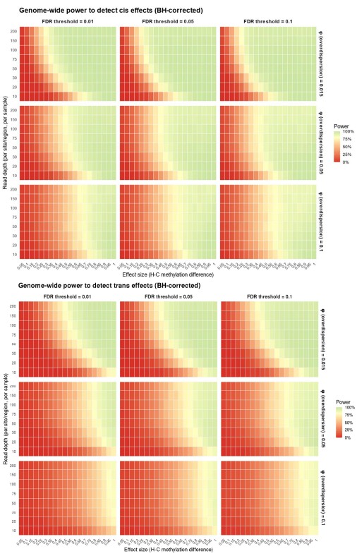
Effects were classified using the same two-model scheme as the main analysis. A unit was called cis if the hybrid allelic (H–C) test was significant and the allele-by-generation interaction was not significant, and trans if the interaction was significant and the hybrid allelic test was not significant; all tests were Benjamini–Hochberg–corrected across the genome at the stated FDR threshold. Each unit was simulated with the full six-measurement design (two parental samples and four hybrid alleles from two hybrids), both models were fit, each set of p-values was BH-corrected across the genome, and "power" is the fraction of true units that land in the correct class.

Cis-effect units were simulated with an equal H–C difference in both parents and hybrid (zero true interaction); trans-effect units with a parental H–C difference and no hybrid allelic difference (full-magnitude interaction); null units with no difference in either parents or hybrid. Sequencing depth was treated as a fixed design parameter: every sample at every simulated unit was assigned the same total read depth (the value on the y-axis of the heatmaps), corresponding to per-CpG coverage for the site-level analysis or aggregate per-region coverage for the regional analysis.

We estimated the beta-binomial overdispersion (φ) directly from the data for each cell type used in this study: DA = 0.024, CNCC = 0.016, IPSC = 0.013, SKM = 0.014, and HEP = 0.011 (median = 0.014). To span this empirical range and to assess robustness to higher-than-observed dispersion, we evaluated power at φ = 0.015 (approximating the empirically observed median), 0.05, and 0.10; the latter two represent substantially more conservative (higher-noise) scenarios than any cell type in our data. Because power declines monotonically with φ, the φ = 0.015 row reflects the sensitivity expected under realistic conditions, while the higher rows bound the worst case. For each unit, a methylation probability was drawn from a beta distribution whose mean equals the unit's true methylation level and whose dispersion is set by the overdispersion parameter φ, and the number of methylated reads was then drawn from a binomial with that probability and the specified total depth. Consequently, the reported power describes the sensitivity expected at a given uniform per-unit (per-CpG or per-region) depth, spanning 10× to 200×, and is interpreted as the proportion of true-effect units assigned to the correct class.

The follow-up analyses are incomplete with major gaps. The authors focus on single potential mechanisms for cis- and trans-changes, but it is not clear to what degree these mechanisms explain the extent of cis and trans changes. There are also other mechanisms which are not investigated, such as the importance of TF binding sites for cis-regulatory evolution.

We agree that CpG-disrupting SNVs and TF binding motifs are just two out of many possible mechanisms, and we have added explicit acknowledgements of this in the text. Our goal was not to investigate all possible mechanisms, but rather to focus on two that showed promising results. For cis-regulation, we now state that TFBS mutations and other sequence variants could also contribute. We agree that further mechanistic investigation is an important direction for future work, and we have noted this explicitly in the Discussion.

Next, the authors seek to show that differences in DNA methylation are functionally relevant... I worry that this result could be confounded by larger effect sizes for cis-changes than trans effects.

We agree that larger cis-regulatory effect sizes could contribute to this result, and have now mentioned this in the Discussion: “This finding suggests that the repressive effects of species-specific methylation are strongest when both layers of regulation are driven in cis, perhaps because cis-regulated methylation changes tend to have larger effect sizes than trans-regulated changes.”

Finally, the authors make a case for lineage-specific selection on DNA methylation that is connected to human traits. This evidence was not convincing. In fact, it is even said that these tests cannot be interpreted as evidence of lineage-specific selection (lines 399-401), so I am confused why these results are framed as testing for selection.

We appreciate this comment but want to clarify. Lines 399–401 in the original manuscript state that the dental pulp stem cell (DPSC) sign test results specifically should not be interpreted as evidence of lineage-specific selection, because DPSCs use parental rather than hybrid cell lines. This caveat applies only to DPSCs. For all other cell types (iPSC, DA, CNCC, SKM, HEP), which use hybrid cell lines that control for trans-acting confounders, the sign test does indeed provide evidence of non-random directional bias inconsistent with neutral evolution, thereby constituting evidence of lineage-specific selection. We have added a clarifying sentence to make this distinction explicit: "For all other cell types (iPSC, DA, SKM, HEP, CNCC), which use hybrid cell lines, the sign test results provide direct evidence of lineage-specific selection on the implicated gene sets, as the hybrid system controls for trans-acting confounders."

To be clear about the scope of the claim: the sign test directly demonstrates that the implicated gene sets are under lineage-specific selection. What remains inferential is the connection between this selective signal and any specific human phenotype, which would require experiments or further validation to establish; we have revised the framing throughout to keep this distinction explicit.

Reviewer #1 (Recommendations for the authors):

(1) Line 96: How many iPSC lines were used for each species? When a replicate is mentioned (e.g., Figure 1B), are those technical or biological replicates?

We have added the iPSC line counts to both the Results and Methods sections: two human and two chimpanzee iPSC lines were used. Replicates shown in Figure 1B are biological replicates (independent differentiation experiments from the same iPSC lines).

(2) Line 98: How many donors for the DPSCs?

We have added DPSC donor counts to the Methods: two human and two chimpanzee donors.

(3) Line 103: PCA and other analyses combined data from WGBS and RRBS cell types. Some clarification about how this was done (e.g. restricting to RRBS sites?) would be useful in the main text as well as an acknowledgement of potential biases. And

(4) Line 103: Related, what is the number of CpG sites considered?

We have added a clarifying sentence to the Results: cross-cell-type analyses including Figure 1B heatmap and Figure 1C PCA analysis were restricted to CpG sites covered in all samples (i.e., the intersection of all covered sites, after phasing the hybrid samples), totaling 561,762 shared CpG sites. Within-cell-type PCA analysis in Figure 1—supplemental figure 1 was restricted to CpG sites shared across samples of the same cell type, which contains 31,802,196 sites for CNCC samples, 26,163,237 sites for DA, 29,787,850 sites for DPSC, and 1,006,674, 935,636 and 952,835 sites for IPSC, SKM and HEP, respectively. We acknowledge that this restriction to the intersected CpG sites result in PCA performed on sites covered by both WGBS and RRBS, which are most frequent in CpG-dense regions.

(5) Line 103: For Figure 1B, it would be useful to first mention how human/chimp reads were parsed and for how many CpG sites this was possible.

We have added a brief description of the allele-parsing approach (SNPsplit using species-specific SNV positions). For hybrid WGBS samples (DA and CNCC), on average, 48.2% ± 0.2% of all aligned reads are unassignable using SNPs between human and chimpanzee genome, 25.9% ± 0.2% of the reads are specific to human, and 25.1% ± 0.2% of reads are specific to chimpanzee. For hybrid RRBS samples (IPSC, SKM and HEP), on average, 88.4% ± 0.3% of all aligned reads are unassignable using SNPs between human and chimpanzee genome, 5.3%±0.1% of the reads are specific to human; 5.3%±0.1% of reads are specific to chimpanzee. We have added information above to the main text. Per sample splitting reports containing the exact number of reads assignable to each of human and chimpanzee are provided as a comprehensive table at Supplemental File 1. The lower assignment rate in RRBS is expected, and we have performed two additional analyses to demonstrate why. First, the reduced representation strategy concentrates coverage in CpG-dense promoters that are highly conserved between human and chimpanzee and therefore SNV-poor, while the short MspI fragments that dominate these libraries frequently fail to reach an informative SNV even when one is nearby. Quantifying this directly: among the 16,845,376 CpG positions covered by the union of all unphased hybrid RRBS libraries, 65.1% contain a human–chimpanzee SNV within ±50 bp (the reach of a typical RRBS read), compared with 90.8% within ±150 bp (the reach of a typical WGBS read pair) — a 1.40-fold difference in SNV accessibility at the very same CpGs. Second, we compared the aligned-length distributions of allele-resolved and unassigned reads across all ten hybrid libraries (Author response image 2). In the four WGBS libraries the two distributions are indistinguishable, confirming that read length is not driving mappability. In contrast, for all six RRBS libraries, allele-resolved reads are consistently longer than unassigned reads, with the effect reproducible across every cell type and replicate.

Author response image 2.

Aligned read length determines allele-assignment success in RRBS but not in WGBS. Aligned read lengths were extracted from the Bismark-aligned BAM files produced by phasing all ten hybrid bisulfite libraries: four WGBS libraries (CNCC and DA, two replicates each; left) and six RRBS libraries (HEP, iPSC and SKM, two replicates each; right). For each library, reads assigned to either the human (genome1) or chimpanzee (genome2) alleles were pooled into a single phased set (blue) and compared with the reads that could not be phased (grey); distributions were computed from subsampled reads and are shown as boxplots (box, interquartile range; line, median; whiskers, 5th–95th percentiles). In the WGBS libraries, phased and unassigned reads have effectively identical length distributions (median 150 bp for both; means 147.4–147.8 vs 142.1–143.1 bp), indicating that read length does not drive mappability in WGBS. In the RRBS libraries, which are dominated by short MspI fragments, phased reads are consistently longer than unassigned reads across every cell type and replicate (medians 70–75 vs 49–50 bp; means 80.5–85.7 vs 58.6–60.6 bp, ~1.4-fold). Because a read can be assigned to a parental allele only if it spans an informative human–chimpanzee SNV, these results show that the short fragment length characteristic of RRBS — together with its enrichment for SNV-poor, evolutionarily conserved CpG-dense promoters — accounts for its lower allele-resolution rate relative to WGBS.

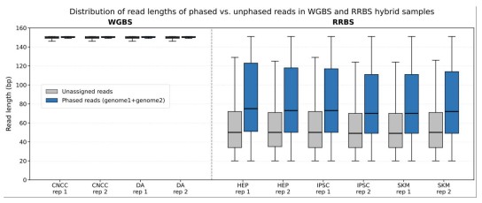
(6) Line 103: Hybrid/parental line isn't noted in the PCA. Is this just the parental samples?

We clarify that Figure 1C shows both parental and hybrid samples, and we have updated the figure caption for Figure 1C to note that both hybrid and parental samples are plotted in the PCA. The parent/hybrid stratifications are shown in Figure 1—figure supplement 1 and referred to in the main text.

(7) Line 149: No citation # is given for the Hallgrimsdottir paper.

Corrected. Citation number 50 (Hallgrímsdóttir et al., 2024) has been added.

(8) Line 167-169: Some explicit test here would be useful. Is this more than we'd expect just because the majority of CpG sites have conserved methylation levels? How much more do divergent CpG sites cluster than expected by chance?

We agree that an explicit test of clustering would be informative, and we want to be clear about what our analysis does and does not establish. The changepoint algorithm is not a test of non-random clustering: it detects shifts in the local composition of regulatory classifications along the genome and segments each chromosome into locally homogeneous stretches. Its purpose here is enrichment rather than inference, because it selects regions in which neighboring CpG sites share both a regulatory classification and a consistent direction of species bias, so that the downstream motif-enrichment and CpG-SNV proximity analyses operate on interpretable units rather than on mixtures of mechanisms. Because the segmentation is not compared against a null model, it cannot by itself establish that divergent sites co-localize more than expected given that 83–93% of all sites are conserved. We have therefore revised the text so that Figure 2D reads as a descriptive summary of the neighbourhood composition of each regulation group, and removed any implication that the co-localization has been tested against a chance expectation. Asking whether divergent sites cluster more than expected is a genuinely different question from the one our DMR-calling addresses and answering it well would require a dedicated null model. We think this is a worthwhile analysis and a natural extension of this framework, but it is separate from the claims we make here, and we have not attempted it in this revision.

(9) Line 186-187: It should be made clear that you looked to cis, trans, and cis + trans DMRs independently.

We have revised this sentence to make explicit that cis-DMRs, trans-DMRs, and cis+trans DMRs were identified independently using the changepoint detection method applied separately to each regulatory class.

(10) Line 190-192: Some quantification of the degree to which cis effects exceed trans effects would be useful. What proportion of total divergence (e.g. mean and s.d.) is explained by cis factors?

We have added this quantification: “At FDR < 0.05, cis-regulation accounted for a mean of 91% of divergent sites and trans-regulation a mean of 4.5% across cell types, and cis remained the dominant category at every FDR cutoff tested (FDR < 0.25–0.01; Figure 2C, Figure 2—figure supplement 1–2, Supplemental Files 1–2).”

(11) Line 194-196: It should be made clear that motif enrichment was done in the human genome, right? Are the results consistent if motif enrichment was done in the chimpanzee genome?

We have clarified in the Methods that HOMER motif enrichment was performed using the human genome (hg38) as background. Repeating the analysis using the chimpanzee genome as background is a valuable future direction; we acknowledge this has not been formally tested.

(12) Line 208: For TFs other than FOXM1 and FOXA2, is TF expression generally associated (positively or negatively) with trans DMRs favoring the chimpanzee or human lineage? An idea of the distribution would be useful.

We plotted the distribution of differential TF expression for those with predicted binding sites enriched in Hu>Ch trans-DMRs versus Hu<Ch trans-DMRs in DA and CNCC. In neither cell type do the two distributions show a clear separation of directional shift. TF expression differences are broadly overlapping regardless of whether the associated trans-DMR favors the human or chimpanzee lineage. We speculate the lack of separation reflects multiple trans-acting inputs shaping methylation divergence such that single TF expression does not predict it. Aggregating across TFs with potentially opposing effects could further contribute to this observation as well (Figure 3—figure supplement 1). FOXM1 and FOXA2 are individual cases where a suggestive relationship was visible rather than evidence of genome-wide pattern.

Author response image 3.

Distribution of differential expression of TFs with predicted binding sites enriched in trans-DMRs. Density distribution of TF expression difference in human versus chimpanzee parental samples. There is a lack of separation between expression of TFs with predicted binding sites enriched in Hu>Ch trans-DMRs versus Hu<Ch trans-DMRs, in both DA and CNCC.

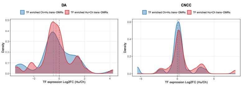
(13) Line 211-212: Stats are needed.

This statement is intended as a qualitative description rather than a quantitative statement. With only 4 cell types per comparison (Figure 3B), we do not have enough statistical power to establish a significant correlation, therefore we present this result as an exploratory observation rather than a statistically significant finding. We have therefore removed "consistent with this expectation," reframed the FOXM1 and FOXA2 results as descriptive observations from individual factors, and added an explicit statement that they are exploratory and hypothesis-generating rather than evidence of a genome-wide pattern.

(14) Figure 3C: Direction is not given. It should be made clear that this is a gain/loss in humans.

We have updated the Figure 3C caption to explicitly label the three SNV categories as: CpG gains in humans (human allele creates a CpG), CpG losses in humans (human allele disrupts a CpG), and no CpG change.

(15) Figure 3C: Most cell types have a bias towards increased DNA methylation when there are no nearby CpG sites (gray bars). Why? Is this a consequence of a reference bias?

We thank the reviewer for raising this. The grey bars correspond to methylation levels of conserved CpG sites near SNVs with no CpG-altering substitution and serve as the genome-wide background/control category, against which the substitution-containing categories are compared. Their modest skew toward higher methylation reflects a global offset shared by all categories rather than a substitution-specific effect. We suggest two non-exclusive explanations for this baseline offset: a genuine genome-wide difference in the distribution of human- versus chimpanzee-biased methylation, and/or a possible contribution of reference genome mapping bias arising from alignment to the human genome. Importantly, this does not affect the conclusions drawn from Figure 3C. Because the genome-wide offset is shared across all categories, the substitution-attributable signal is reflected in the difference between the CpG-gain/loss categories and the no-change (grey) baseline, and any genome-wide baseline shift — biological or technical — cancels in that comparison. We therefore interpret the grey-category asymmetry as a background property and explicitly do not attribute it to the substitutions themselves. Future work such as analyzing with reads mapped to the chimpanzee or a masked consensus genome or restricting to mappability- and coverage-matched regions could directly quantify any reference-bias contribution, and we note these as promising directions.

(16) Line 258-269: Figure 3D is not referenced in the text.

We have added a reference to Figure 3D in the relevant paragraph of the Results: “To test this, we compared the genomic distance between each DMR and its nearest CpG SNV. Consistent with our model, we found consistently shorter distances for cis-DMRs than trans-DMRs across all cell types examined: Median distances to the nearest CpG SNV were 24 ± 6 bp for trans-DMRs vs. 11 ± 2 bp for cis-DMRs (Figure 3D; Mann-Whitney p < 0.001 for all comparisons) [65].”

(17) It is unclear why Figure 4A-C focus exclusively on cis-regulated promoters. Is this for biological or technical reasons?

Both. Biologically, cis-regulated promoters are the most interpretable for assessing cell type-specificity, because cis effects are allele-intrinsic and not confounded by differences in trans-acting environments across cell types. Technically, trans-regulated promoters show methylation differences that depend on the trans-environment, making cross-cell-type comparisons less straightforward.

(18) Line 371: How many DMRs are being considered?

We have added the total number of DMRs (promoters) considered in the sign test analysis: 6,283.

(19) Line 371-372: What is the ASM/ASE concordance test? I thought you were restricting the analysis to genes with a negative association between ASM and ASE (lines 366-367), so this needs to be clarified.

We have clarified this in the text. The two-step procedure works as follows: (1) a binomial sign test is applied to all genes with promoter ASM to identify gene sets with directional bias in methylation; (2) separately, a binomial sign test is applied to the subset of genes where ASM and ASE show a negative (repressive) relationship. Gene sets that pass both steps are reported as candidates. The "ASM/ASE concordance test" refers to step 2. We have revised the text to make this two-step logic clearer.

(20) Line 379: It may be worth mentioning that these are the DMRs which are most likely to be functionally relevant in shaping expression levels.

We have added this sentence: " This subset represents cases where methylation changes are most likely to have a simple and direct repressive effect on transcription, filtering out more complex regulatory scenarios where methylation and expression changes may be uncoupled or subject to competing regulatory influences."

(21) Line 387: The test here needs to be clearer. Does a significant result mean an enrichment of differences in that gene set, or a bias in the ratio of Hu/Ch differences?

We have clarified: a significant result from the binomial sign test indicates a statistically significant bias in the ratio of human-biased to chimpanzee-biased changes within a gene set, relative to the genome-wide background ratio. It does not test for enrichment of the number of differences, only for non-random directionality.

(22) Line 403: Why the focus on expression, when the rest of the paper is focused on the methylation patterns?

Gene expression is the most direct functional readout of promoter methylation changes. The two-step sign test uses expression data in the second step precisely because it allows us to identify cases where methylation divergence has a demonstrable downstream consequence on transcription, which is the canonical mechanism by which promoter methylation affects phenotype. We have added a brief justification of this rationale to the text.

(23) Line 456: Not clear where there is actually evidence of lineage-specific selection.

We have added an explicit sentence in the Discussion describing what the evidence consists of: "Specifically, the evidence rejecting a neutral null model of cis-regulatory evolution consists of statistically significant directional bias in both promoter methylation and gene expression within functionally coherent gene sets, assessed using a two-step binomial sign test with permutation-based FDR correction." This constitutes direct evidence that the implicated gene sets are under lineage-specific selection; the separate question of which specific human phenotypes that selection shaped remains inferential and is framed as such throughout.

(24) Line 457-459: I think this line needs to be further explained: "Our use of hybrid cell lines was critical to this discovery, as it allowed us to isolate cis-acting regulatory changes from confounding trans-acting and environmental effects." Specifically, it's not apparent why cis-regulation is important for demonstrating evidence of selection.

We have added an explanation: "Isolating cis-acting changes is critical because the sign test requires that each promoter represents an independent observation; in hybrid cells, each allele's methylation is determined by its own cis-regulatory sequence, making observations across promoters genuinely independent and thus satisfying the assumptions of the binomial test."

(25) Line 460-465: The concluding claims throughout this paragraph appear to be overstated.

We have revised the concluding paragraph of the Results and the Discussion conclusion to soften the language.

(26) Line 487: Provide the actual numbers instead of saying "substantial".

We have replaced "substantial numbers of allele-specifically methylated promoters" with the actual count: 6,283 allele-specifically methylated promoters across all cell types.

(27) Line 502: I question this interpretation. While it could be that there is a shared mechanistic basis, it could also be that the cis effects tend to be larger than the trans effects, providing additional power to identify strong correlations.

We agree and have added this alternative explanation explicitly to the Discussion (see response to public review comment above).

(28) Line 510: But the results section states that it's not possible to interpret these as lineage-specific selection.

The caveat at lines 399–401 applies specifically to DPSCs, not to hybrid cell types. We have revised the text to make this distinction unambiguous.

(29) Line 601: What coverage was the methylation data?

We have added sequencing coverage and the number of CpG sites assayed below “Bisulfite-seq library preparation, sequencing and mapping” section in Methods. WGBS libraries achieved a mean coverage of 9.68× per CpG site, covering 43.6M unique CpG positions in CNCC (hybrid) and 43.4M in CNCC (parental), 41.9M in DA (hybrid) and 38.8M in DA (parental). RRBS libraries achieved a mean coverage of 5.02× per CpG site, covering 5.0M, 4.8M, and 4.5M unique CpG positions in the hybrid HEP, IPSC, and SKM libraries respectively, and 3.3M, 3.4M, and 3.2M in the corresponding parental libraries. The total number of CpG sites (union) of all WGBS samples is 48,994,320 sites, and the union of all CpG sites of RRBS samples is 7,289,251. The union of all samples (including WGBS and RRBS) is 49,049,052. We have also included coverage information per sample as a table in Supplemental File 1.

(30) Line 820: citation shouldn't include "preprint at".

Corrected. "Preprint at" has been removed from all published paper citations in the reference list.

Reviewer #2 (Public review):

This manuscript investigates the causes and consequences of human-specific DNA methylation divergence relative to chimpanzees... This study provides a valuable dataset and a compelling framework for understanding how local sequence variation contributes to epigenetic and transcriptional divergence, with likely broad impact in comparative and evolutionary genomics.

We thank Reviewer 2 for this positive assessment and for the constructive suggestions.

Although the authors identify transcription factors associated with differential methylation, it is unclear what proportion of differentially methylated CpGs or DMRs can be attributed to these factors. Providing a quantitative estimate would help assess the relative contribution of trans-acting regulation.

We agree that a quantitative estimate of the proportion of differentially methylated CpGs or DMRs attributable to these transcription factors would be informative in principle. In practice, however, such an estimate is challenging to produce reliably: predicted binding sites are not all occupied or functional, individual DMRs are typically influenced by multiple trans-factors, and we lack the per-site functional data needed to assign methylation differences to specific TFs with confidence. More importantly, even if we could generate such a number, an association-based estimate would not establish that these factors causally drive the observed methylation differences. We have added a note to the main text clarifying that our analysis identifies candidate trans-acting factors associated with differential methylation rather than quantifying their causal contribution.

The analysis of CpG-disrupting mutations is interesting but raises two concerns. First, other classes of variants—such as transcription factor binding site-disrupting mutations—could also influence local methylation patterns and are not considered here. Second, the causal direction remains ambiguous: CpG-disrupting mutations may result from methylation-associated mutational processes (e.g., C->T transitions at methylated CpGs) rather than being the primary drivers of methylation divergence.

We have addressed both concerns in the revised manuscript. On the first point, our goal was not to suggest that CpG-disrupting variants are the only causes of local methylation divergence. We now explicitly acknowledge in the Results that TFBS mutations and other variant classes could also contribute to cis-methylation divergence and represent an important avenue for future investigation. On the second point: while CpG-disrupting mutations are indeed expected to be enriched in highly methylated regions, they would be expected to associate with methylation level rather than methylation divergence, and thus cannot explain the patterns we observe.

Regarding the discussion comparing the distance between CpG-disrupting SNVs and trans-DMRs, without information on the absolute or relative distance distributions, it was difficult to assess the magnitude of the observed differences. Moreover, trans-DMRs, by definition, are not driven by local (cis) variation, and the lack of proximity to CpG-disrupting SNVs is expected. Clarifying what additional insight this analysis provides beyond this expectation may improve this section.

We agree that the lack of proximity of trans-DMRs to CpG-disrupting SNVs is expected. We have revised the text to clarify that this analysis serves as an affirming result: it is consistent with the fact that cis-DMR are under local sequence-driven regulation, and that the CpG-disrupting SNV mechanism is more closely associated to cis-DMRs than trans-DMRs. The quantifications for distance distributions are shown in Figure 3D, and we have added a sentence noting the median distances for trans-DMRs vs. cis-DMRs: 24 ± 6 bp vs. 11 ± 2 bp.

One potential extension would be to examine whether the same cis-acting SNVs are consistently associated with methylation differences across multiple cell types.

We thank the reviewer for this suggestion and have performed this analysis below. For each of the three regulatory region classes (promoters, enhancers, CTCF binding sites), we intersected CpG SNVs (±100 bp window) with cis-classified DMRs (pure_cis or cis_plus_trans at BH-corrected FDR < 0.05) across the five cell types (CNCC, DA, HEP, IPSC, SKM), and counted the number of cell types in which each SNV overlapped a cis-DMR. To assess significance, we compared this distribution to a permutation null in which, for each cell type, we randomly sampled the same number of regions from that cell type's pool of tested-but-conserved regions of the same class (1,000 permutations); SNVs were restricted to those falling within the tested universe across cell types.

Local methylation effects of CpG SNVs were shared across cell types substantially more than expected by chance in all three region classes. The observed mean number of cell types sharing per SNV-in-cis-DMR was 1.244 vs. 1.077 ± 0.006 in the null for promoters, 1.133 vs. 1.042 ± 0.001 for enhancers, and 1.171 vs. 1.061 ± 0.002 for CTCF binding sites (all p < 0.001). Fold-enrichment scaled sharply with the degree of sharing: at the highest sharing level (cis-DMR in all five cell types), observed counts exceeded the permutation null by ~3,500-fold for promoters, ~800-fold for CTCF, and ~700-fold for enhancers. The slightly stronger consistency signal at promoters relative to enhancers is consistent with the more constitutive activity of promoter elements across cell types. These results indicate that the same cis-acting variants tend to drive methylation divergence across multiple cell types, supporting a shared mechanistic basis for cis-methylation divergence. We have added the figure in the main text as Figure 3—figure supplement 2.

Regarding their two-step sign test analysis, because enrichment-based approaches can sometimes overemphasize statistical significance without reflecting effect size, I wonder if incorporating the magnitude of methylation change would provide additional information.

We agree. The magnitude of methylation change (effect size) for each gene and gene set is now provided in Supplemental File 7 alongside the directional bias statistics. We have added a sentence to the Results pointing readers to this resource.

Strength:

I recommend that the authors provide a list of cis-cis-regulated promoters and their associated genes, which would be a valuable resource for the field.

We have added this list as Supplemental File 8.

Reviewer #3 (Public review):

Ma et al. use human-chimpanzee tetraploid cells to examine species differences in DNA methylation... Both identified SNVs and transcription factors are good candidates for future experimentation. Further, they find that cis-DMRs are more highly correlated with cis-expressed genes than trans-DMRs with trans-expressed genes, providing evidence that methylation and expression are linked genome-wide.

We thank Reviewer 3 for this summary and for the detailed recommendations.

Weakness

(1) Strengthening their cis/trans analysis, including: (a) only showing or analyzing genomic regions that pass FDR correction; (b) clarifying how cis genes are defined (Figure 2B shows some genes labeled as cis where the direction-of-effect differs between hybrid and parent cells); (c) assessing how well powered they are to perform each analysis.

(a) Figure 2B has been updated to show regulatory classifications of promoter regions in cranial neural crest cells (CNCCs) at FDR < 0.05. Scatter plots and bar plots for all cell types at the level of individual CpG sites have been moved to Figure 2—figure supplement 1, and the corresponding promoter-level plots for all cell types other than CNCCs to Figure 2—figure supplement 2. We have clarified in the Figure 2—figure supplement 1 caption that nominal p-values are used to preserve the full dynamic range of the data, whereas FDR-corrected thresholds are applied for visualization of promoter scatter plots as well as all formal inference and for reporting significant candidate loci. FDR-corrected results are presented in Figure 2—figure supplements 1–2, and we have added explicit statements in the Results confirming that the cis: trans ratio is stable across FDR thresholds.

(b) We have clarified the definition of cis-regulated genes in the text: cis-regulated genes are defined as those where the direction of allelic difference is consistent between hybrid and parental samples for both methylation and expression. We have verified that this definition is applied consistently throughout the manuscript and downstream analyses.

(c) We have clarified the FDR correction approach for the sign test in the Methods: FDRs are estimated by permutation (10,000 permutations), and we report results at FDR < 0.25 for the two-step test with supporting evidence from the methylation-only sign test (nominal p < 0.05). We acknowledge that this is a relatively liberal threshold. The sign test itself provides direct evidence that the implicated gene sets are under lineage-specific selection; what we have toned down is the downstream interpretation, framing the link between these gene sets and specific human phenotypes as inferential and requiring experimental validation rather than as confirmed.

(d) We agree that experimental validation would strengthen the mechanistic claims. We have added this explicitly to the Limitations section: "definitive demonstration of causality requires targeted experimental perturbations such as base editing (for CpG-disrupting SNVs) or TF knockdown/overexpression experiments (for trans-acting TFs)."

(2) Softening claims about human evolution or human specificity for several reasons: (a) Their comparison lacks tetraploid controls (e.g. human-human tetraploids and chimp-chimp tetraploids) or experimental follow-up in diploid cells, making it hard to be certain that observed effects are not due to ploidy. (b) There are no outgroup species included in the analysis. (c) The use of no or very loose FDR corrections with the sign test makes it difficult to draw conclusions. (d) Experimental data to link SNVs to changes in cis methylation or identified transcription factors to changes in trans methylation would be needed to validate the authors' predictions.

(a) The concern about ploidy effects is noted. We note, however, that the primary evidence for cis-regulation comes from allele-specific methylation within the same tetraploid nucleus, where both alleles experience identical ploidy and trans-environments. Ploidy effects would be expected to affect both alleles equally and would therefore not produce the allele-specific differences we observe. We acknowledge that single-species tetraploid controls would provide additional confidence and represent a valuable future experiment.

(b) We have added the absence of an outgroup species as an explicit limitation in the Discussion.

(c) We have clarified the FDR correction approach for the sign test in the Methods: FDRs are estimated by permutation (10,000 permutations), and we report results at FDR < 0.25 for the two-step test with supporting evidence from the methylation-only sign test (nominal p < 0.05). We acknowledge that this is a relatively liberal threshold and have emphasized this by adding a new sentence: “However, as indicated by the FDR, we do expect some fraction of these candidate gene sets to be false positives.”

(d) We agree that experimental validation would strengthen the mechanistic claims. We have added this explicitly to the Limitations section: "definitive demonstration of causality requires targeted experimental perturbations such as base editing (for CpG-disrupting SNVs) or TF knockdown/overexpression experiments (for trans-acting TFs)."

Reviewer #3 (Recommendations for the authors):

(1) Why are dental pulp stem cells so different from the other cell types transcriptionally (e.g. Figure 1C)? Is this due to being primary cells vs. stem-cell-derived cells?

The transcriptional distinctiveness of DPSCs is most likely attributable to their status as primary cells rather than iPSC-derived cells. Primary cells retain the epigenetic and transcriptional signatures of their tissue of origin and have not undergone reprogramming, whereas iPSC-derived cell types share a common pluripotent origin that may reduce inter-cell-type transcriptional distance. Additionally, DPSCs are mesenchymal stem cells with a distinct developmental lineage and were obtained from adult donors rather than differentiated in vitro, which may further contribute to their distinct profile. We have added a brief note to the Results acknowledging this.

(2) I am concerned about how cis genes are defined. In Figure 2B, there are genes labeled as cis, where the direction-of-effect differs between hybrid and parent cells. I believe cis should only include genes with the same direction-of-effect between hybrid and parent cells, as illustrated in Figure 2A. This fix should propagate through the ensuing figures and results.

We have clarified the definition of cis-regulated genes in the text (see response to Weakness 1b above). The classification framework assigns a site to "cis" when the allele effect test is significant in hybrids and the System × Allele interaction term is not significant, meaning there is no detectable change in the allelic difference between the hybrid and parental systems. Sites where the allelic difference genuinely differs between systems — that is, where the interaction term is significant — are classified as cis × trans (interactive) or cis + trans (additive) rather than pure cis, depending on whether the two systems disagree in direction or only in magnitude.

We note that Figure 2B plots parental and hybrid methylation differences as the per-sample average difference in fractional methylation, which is used for visualization only. Points labeled cis that fall on the opposite side of the y = x diagonal are an artifact of this averaging: where the underlying difference is close to zero, the coverage-weighted per-sample average can flip sign even though the beta-binomial model, which fits the read counts directly and accounts for coverage and overdispersion, finds no significant interaction. The regulatory classification is based on the model, not on the sign of the averaged difference, so a small amount of scatter around the diagonal is expected. We have verified that this definition is applied consistently throughout the manuscript and downstream analyses and have clarified the caption of Figure 2B to make this explicit.

(3) Are you equally powered to detect cis and trans effects?

At the single-CpG level, the two hypotheses do differ in statistical power, but at the regional level this difference is mitigated by the higher effective read depth, and we now state this explicitly in the revised manuscript.

The first hypothesis in our classification framework tests allele-specific methylation directly, whereas the second hypothesis includes an interaction term that evaluates whether allelic differences shift between the parental and hybrid systems. Because the interaction test is inherently less powerful, it requires greater sequencing depth and, ideally, additional replicates to yield comparably confident estimates and to assign sites to certain classification categories with significance. As a consequence, at the single-CpG level, trans effects are more sensitive to FDR thresholds than cis effects of equivalent nominal significance, which reduces our power to detect them. At the regional level, however, as well as in CpG-level analyses with high-coverage samples, this disparity in power between cis and trans largely disappears.

This is the technical component of the issue. From a biological standpoint, cis effects are also intrinsically easier to detect than trans effects: estimates of trans effects necessarily incorporate not only trans-acting molecular mechanisms but also environmental and technical noise, so cis estimates will always be cleaner. This is a well-recognized limitation of existing cis/trans classification frameworks, and we acknowledge this limitation in the discussion and have added suggestions in experimental set-up to mitigate it. To address the reviewer's concern directly, we have performed a formal power analysis quantifying the relative power to detect cis and trans effects as a function of read depth (See Author response image 1).

(4) Are the results shown for SNVs in CpGs in Figure 3C only for cis-DMRs or for all DMRs? If the latter, please show cis-DMRs and trans-DMRs separately and explain why trans-DMRs show the same pattern as cis-DMRs. In addition, I would expect that the CpG that contains an SNV leading to CpG loss or gain would be the most affected in terms of methylation status, rather than CpGs within 25bp vs. 50bp vs. 100bp. It would be helpful to see that plot as well.

We thank the reviewer for the opportunity to clarify. Figure 3C is not an analysis stratified by cis-DMRs or trans-DMRs. Rather, it examines local methylation changes at conserved CpG sites located within 25 bp, 50 bp, and 100 bp of a CpG-disrupting SNV. The purpose of this analysis is to test a specific mechanistic hypothesis: that a CpG-disrupting mutation may influence the methylation status of nearby, intact CpG sites in cis. The analysis is therefore agnostic to cis/trans-DMR classification, as it asks a different question, namely whether sequence disruption at one CpG propagates locally to neighboring CpGs.

We note that Figure 3D addresses a related but distinct question, showing that cis-acting sequence changes more broadly (not restricted to CpG-disrupting mutations) are more strongly associated with cis-DMRs than with trans-DMRs. Together, Figures 3C and 3D support complementary aspects of the cis mechanism: the local propagation of methylation changes around disrupted CpGs (3C) and the broader association of sequence variation with cis-DMRs (3D).

Regarding the reviewer's second point: we agree that the CpG site directly disrupted by the SNV would itself be the most affected, by definition, since the CpG dinucleotide is destroyed (in the case of CpG loss) or newly created (in the case of CpG gain). Because methylation cannot be measured at a CpG that no longer exists (or has only just been created on one allele), this site cannot be included in a comparative methylation analysis across alleles or species. The 25/50/100 bp windows were therefore chosen specifically to test the local effect on conserved, measurable CpGs surrounding the disruption. We have clarified this rationale in the revised text/figure legend.

(5) The finding that cis-DMRs and cis-expressed genes are more correlated than trans-DMRs with trans-expressed genes is nice to see. What is a potential explanation for why the patterns across the genomic interval surrounding the TSS are so different across cell types, and even positively correlated near the TSS in dopaminergic neurons? Why do you not see a difference between cis and trans in CNCCs? In addition, it would be nice to see the correlation between cis-DMRs and trans-expressed genes, and vice versa, as a control for these plots.

We have added the suggested control analysis. For the cis-DMR/trans-expressed-gene and trans-DMR/cis-expressed-gene sets in both DA neurons and CNCCs, the correlations around the TSS are less consistently negative than for the cis-DMR/cis-expressed-gene set. In both cell types, cis-methylation and cis-expressed genes show the strongest opposing (negative) relationship to one another, which supports the specificity of the cis–cis coupling reported in Figure 4G. Regarding why the correlation profiles across the TSS-flanking interval differ so markedly across cell types—including the positive correlation near the TSS in dopaminergic neurons—and why the cis–trans distinction is less pronounced in CNCCs, we are not able to offer a confident explanation. The variation may reflect cell-type-specific regulatory architecture, but a great deal remains unknown about how methylation and transcription are coupled in a cell-type-specific manner, and our four cell types do not allow us to distinguish among the possible explanations. We think this is an open and interesting question, and that analyzing additional cell types with matched WGBS and gene expression data would be the most informative way to establish how general these patterns are and what drives the between-cell-type variation. We have noted this explicitly in the main text.

Author response image 4.

Spearman correlation of expression and methylation for CNCC and DA for subsets of genes with cis-regulated methylation and trans-regulated expression (orange), as well as genes with trans-regulated methylation and cis-regulated expression (blue). Two kb surrounding each transcription start site (TSS) is shown, split into 10 bins of 200 bp where individual CpG sites are pooled and averaged as fractional methylation values and correlated with expression values of the neighboring genes (in TPM).

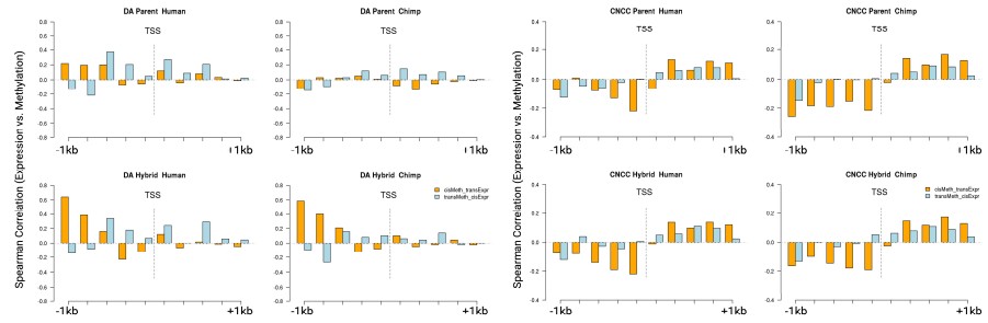
(6) The use of the sign test to identify pathways with the same direction of effect is a great approach. However, I am concerned with the use of no or very loose FDR corrections (e.g. FDR < 0.25 in line 372 and no FDR correction in line 374). Combined with Figure 6, where many of the signals appear to be weak or driven by a few genes (e.g. highly arched eyebrow and poor speech), it makes it difficult to draw robust conclusions. It is notable that the strongest signal is seen in DPSCs, which the authors note contains experimental confounds. We also think that the authors should tone down their biological interpretations, particularly for stem cells. For instance, COLEC11 is involved in neural crest cell migration but is identified from the iPSC analysis and not the CNCC analysis. Why not?

We have added a sentence to emphasize the possibility of some false positive sign test results (“However, as indicated by the FDR, we do expect some fraction of these candidate gene sets to be false positives”), and we have toned down the biological interpretations accordingly.

We want to clarify that the sign test directly demonstrates that these gene sets are under lineage-specific selection. We have clarified that the test does not establish a definitive link between these gene sets and specific human phenotypes; that link is inferential and would require experiments or further validation, and we have toned down the biological interpretations accordingly.

Regarding COLEC11: in response to this comment, we directly examined COLEC11 expression and methylation in CNCCs and found that it is in fact significant in this cell type. In CNCC hybrid cells, COLEC11 shows significant chimpanzee-biased allele-specific expression (log2 fold change [human/chimpanzee allele] = –2.45; DESeq adjusted p = 0.005), together with significant human-biased methylation (fractional methylation [human – chimpanzee] = 14%; adjusted p < 0.001). The direction of this divergence is therefore consistent with IPSC. The reason COLEC11 did not surface at the pathway level in CNCCs is that other genes in the same pathway contribute to the directional signal for that cell type; we would not expect every individual gene to emerge in the cell type where its pathway is most relevant. We have added a note making this point and cautioning against over-interpreting any single gene example.

(7) We appreciate that the authors provide a careful list of limitations of their study. In addition to the limitations listed, the authors should also include that experiments would be needed to validate that SNVs disrupting or creating CpGs affect methylation.

We have added this to the Limitations section: “definitive demonstration of causality requires targeted experimental perturbations such as base editing (for CpG-disrupting SNVs) or TF knockdown/overexpression experiments (for trans-acting TFs).”

(8) We also caution the authors in describing their findings as "human-specific" because there is no outgroup in this study.

We agree and have added the absence of an outgroup as an explicit limitation in the Discussion.

We thank all three reviewers again for their thorough and constructive engagement with our work. We believe the revised manuscript is improved as suggested.

eLife Assessment

This computational study constitutes an extension to prior work on biophysical calcium-based synaptic plasticity rules, investigating how the regulation thresholds for strengthening and weakening connection help solve learning tasks. This important work presents a significantly simpler solution to the studied problem with potentially broad applicability, the evidence to support the core conclusions is solid.

Reviewer #1 (Public review):

Summary

This computational modelling study investigates the functional role of metaplasticity in a calcium-dependent synaptic plasticity rule, using a biophysically detailed model of a striatal projection neuron. The learning rule is deliberately simple: local calcium signals derived from different sources regulate LTP and LTD through separate plasticity thresholds, while dopamine provides a reward-related signal that determines the direction of synaptic updates. The author uses linear and nonlinear feature-binding problems (FBP and NFBP) as learning tasks to illustrate the mechanics of competing LTP and LTD processes in this rule. The central aim is thus to use these classification tasks to understand what metaplasticity in the two calcium thresholds contributes to learning.

The study identifies complementary roles for metaplasticity in the LTP and LTD thresholds, enabling synapses exposed to competing plasticity processes to converge toward a stable outcome. In reversal-learning tasks, relaxing the conditions for metaplasticity allows previously stabilized synaptic states to become flexible again and permits relearning. Finally, the manuscript investigates whether two separate calcium thresholds are themselves necessary. While a modified rule with a single adaptive calcium threshold can solve the same tasks comparably well, two thresholds allow separate control over synaptic strengthening and weakening.

Strengths

A major strength of the study is the simplicity of the learning rule, which makes it possible to dissect the roles of individual components while retaining a connection to experimentally motivated mechanisms of cortico-striatal plasticity. The use of shared features in the FBP and NFBP is useful for exposing the interaction between competing LTP and LTD processes and for showing how adaptation of one plasticity threshold can indirectly permit expression of the opposite form of plasticity.

The manuscript also provides a much more systematic analysis of the rule than the original version. In particular, the expanded parameter analyses explore both successful and failing regimes for the learning and metaplasticity rates, while the scan over the maximum synaptic weight provides a clear mechanistic motivation for the additional upper LTP threshold.

Importantly, the single-threshold simulations directly address whether two calcium thresholds are computationally necessary. These additional simulations clarify that the principal advantage of two thresholds is not that they uniquely enable nonlinear learning, but that they permit independent regulation of strengthening and weakening. This considerably strengthens the conceptual conclusions of the study.

Weaknesses

The main limitations concern the scope and biological generalizability of the results. The simulations in this paper are based on a particular detailed SPN model and depend on several specific biological and modelling assumptions. Most notably, solving the nonlinear task requires appropriately clustered excitatory inputs, but the learning rule itself does not provide a mechanism for generating these clusters. The manuscript now discusses this limitation explicitly and appropriately identifies structural plasticity as an important direction for future work.

A second important assumption is the upper calcium threshold that prevents LTP once sufficiently strong supralinear responses are reached. This mechanism plays an important functional role in the model but has not been experimentally established for cortico-striatal synapses. The manuscript appropriately identifies this as a major assumption and discusses potential molecular mechanisms that could implement such an effect.

Overall assessment

The revised manuscript is substantially stronger. The conclusions are carefully matched to what is demonstrated by the simulations, and several important alternative explanations and model configurations are tested directly. In particular, the revised framing provides a more specific mechanistic account of what metaplasticity in two separate thresholds contributes within the proposed rule. The work therefore provides a valuable contribution to computational studies of synaptic plasticity and metaplasticity, with convincing evidence supporting its principal conclusions.

Reviewer #2 (Public review):

Summary:

The manuscript proposes interesting synaptic plasticity rules grounded in experimental data. Its main features are: (1) plasticity depends on local calcium concentration driven by presynaptic activity and is independent of somatic action potentials, (2) the rules incorporate metaplasticity, and (3) they demonstrate how a single neuron could address the feature-binding problem at the dendritic level.<br /> The work extends a previous study (https://doi.org/10.7554/eLife.97274.2), to which the author also contributed.

The author models two calcium thresholds (LTP/LTD) from two different calcium sources (NMDA/VGCC) and these thresholds are flexible (metaplasticity rule, similar to BCM) which is claimed to be necessary for successful learning of both FBP and NFBP (linear and nonlinear feature binding problem with 1 or 2 patterns). The role of each threshold seems to be is opposite and complementary. One extra condition has been added : an upper threshold for LTP. This threshold serves to stop synaptic strengthening once synapses are strong enough to evoke a plateau. With that, synapses are not strengthened to the maximal value, avoiding strong supralinear integration for irrelevant patterns.

Strengths:

The current model implements not only local synaptic plasticity but also metaplasticity and solves the FBP at the dendrite level. Another strong aspect of the model is that metaplasticity in the LTD threshold protects strengthened synapses from weakening. In this way, as the author mentioned, metaplasticity is able to protect learned patterns from being forgotten or weakened and prevent irrelevant patterns from being stored. This is a nice modelling example of metaplasticity being helpful in preventing the catastrophic interference or forgetting (as has been explicitly discussed in a recent article https://doi.org/10.1016/j.tins.2022.06.002). The author might want to briefly mention or emphasize this aspect of the model, which might be interesting also for the AI community.

Comments on revised version:

The author improved the paper significantly. He conducted new simulations on relearning. He addressed the problems and limitations, added new simulation results and reasoned better in the discussion and the introduction. Also, the figures are improved.

Author response:

The following is the authors’ response to the original reviews.

The goal of the study was to demonstrate the role of the two thresholds in learning, i.e. the role of metaplasticity with a learning rule that is both as simple as possible, but also biologically-based (hence the use of the detailed SPN model, as well). The goal was not to solve the FBP and NFBP with a different rule. However, the text likely gives that impression. Therefore, in addition to addressing the reviewers’ comments, the text has been substantially revised to reflect the following:

Main results

(1) Metaplasticity enables synapses that undergo both LTP and LTD to ultimately express just one plasticity outcome (either LTP or LTD).

(2) Metaplasticity in the LTP threshold allows LTD to be expressed, and vice versa. (That is, the threshold regulating one plasticity process allows the expression of the opposite plasticity process.)

Reason for using the FBP and NFBP

The reason why the FBP and NFBP are particularly useful to demonstrate the thresholds’ roles is that the patterns in the tasks share features. (For example, in the FBP, the feature ‘strawberry’ is shared between both ‘red strawberry’ and ‘yellow strawberry’.) The synapses for these shared features experience precisely such competing LTP and LTD processes where the role of metaplasticity becomes evident. Specifically, the role of the LTD threshold is visible in shared synapses that need to be strengthened during learning (such as the shared ‘strawberry’ synapses in the FBP), while the LTP threshold’s role is visible in shared synapses that need to be weakened (there are no such synapses in the FBP, but there are in the NFBP, which is why it is needed in this article). In addition, feature binding is relevant for the striatum (now described in the introduction).

In the first version of the article there are sentences that are likely confusing and misleading regarding the goal of the study, and these have been removed (lines 98-100 in the tracked changes file).

The revised article now contains 4 new main figures and 15 new figure supplements prompted by the reviewers’ comments, thus expanding the scope of the study and hopefully clarifying its content, the mechanisms, and the conclusions.

Finally, the question whether this rule can solve the NFBP with excitatory synapses alone is being addressed in a new, ongoing study, as written at the end of the Discussion section in the first version of this article. The new study tests 100+ SPN models (71 dSPN and 34 iSPN models differing in ion channel composition, with two different morphologies), different locations of the synaptic clusters along the dendrites (from proximal to distal), and two different learning regimes (suprathreshold – where the neuron initially spikes for all patterns, and subthreshold – where the neuron is initially silent for all patterns, as in this study) containing both clustered and distributed synapses in the same setup. Where necessary, preliminary results from this study are attached in the responses.

Public Reviews:

Reviewer #1 (Public review):

Summary:

This computational modelling study addresses the important question of how neurons can learn non-linear functions using biologically realistic plasticity mechanisms. The study extends the previous related work on metaplasticity by Khodadadi et al. (2025), using the same detailed biophysical model and basic study design, while significantly simplifying the synaptic plasticity rule by removing non-linearities, reducing the number of free parameters, and limiting plasticity to only excitatory synapses. The rule itself is supervised by the presence or absence of a binary dopamine reward signal, and gated by separate calcium-sensitive thresholds for potentiation and depression. The author shows that, when paired with a strong form of dendritic non-linearity called a "plateau potential" and appropriate pre-existing dendritic clustering of features, this simpler learning mechanism can solve a non-linear classification task similar to the classic XOR logic operator, with equal or better performance than the previous publication. The primary claims of this publication are that metaplasticity is required for learning non-linear feature classification, and that simultaneous dynamics in two separate thresholds (for potentiation and depression) are critical in this process. By systematically studying the properties of a biophysically plausible supervised learning rule, this paper adds interesting insights into the mechanics of learning complex computations in single neurons.

As mentioned in the introductory response above, the goal of the article was not to solve the NFBP, but to study the role of metaplasticity. The text has now been substantially revised to reflect that. One of the primary claims that “metaplasticity is required for learning non-linear feature classification, and that simultaneous dynamics in two separate thresholds (for potentiation and depression) are critical in this process” is now removed from the abstract. Instead, the abstract now focuses on the main results regarding the role of metaplasticity, as well as the results which arose from addressing the reviewers’ comments. However, I guess I should note that to be able to study the role of metaplasticity using the FBP and the NFBP, it was first necessary to have a rule that solves these tasks – that allows to later observe the effects of systematically fixing or modifying parameters in the rule. Another aspect which may have added to the confusion about the study’s goal may be due to the NFBP being a complex task requiring supralinear dendritic integration. Because of this, plateaus have received significant attention in the article, possibly diverting from the main focus. This is also now clarified in the article.

Strengths:

The simplified form of the learning rule makes it easier to understand and study than previous metaplasticity rules, and makes the conclusions more generalizable, while preserving biological realism. Since similar biophysical mechanisms and dynamics exist in many different cell types across the whole brain, the proposed rule could easily be integrated into a wide range of computational models specializing in brain regions beyond the striatum (which is the focus of this study), making it of broad interest to computational neuroscientists. The general approach of systematically fixing or modifying each variable while observing the effects and interactions with other variables is sound and brings great clarity to understanding the dynamic properties and mechanics of the proposed learning rule.

It would indeed be great if this rule facilitates similar studies in other neuron types. The rule requires at least qualitatively accurate calcium dynamics, which at the moment are not widely available for other neuron types (but will likely appear in the future).

Weaknesses:

General notes

(1) The credibility of the main claims is mainly limited by the very narrow range of model parameters that was explored, including several seemingly arbitrary choices that were not adequately justified or explored.

The parameter range has now been expanded to address all comments below.

(2) The choice to use a morphologically detailed biophysical model, rather than a simpler multicompartment model, adds a great deal of complexity that further increases uncertainty as to whether the conclusions can generalize beyond the specific choices of model and morphology studied in this paper.

Regarding the plasticity rule and the role of metaplasticity, the conclusions should hold if the calcium dynamics of other (simpler or detailed) neuron models is qualitatively similar (i.e. shows the same monotonicity of “stronger synaptic input – stronger calcium”, and not something like Figs. 12A, B for which the rule was not tested).

As to whether the NFBP can be solved, that is being addressed in the new study with 100+ neuron models (71 dSPN models and 34 iSPN models, and two morphologies: one for the dSPNs and another for the iSPNs). So far, the results show that the important ingredient is the threshold nonlinearity provided by the plateau potential (both dSPNs and iSPNs exhibit this nonlinearity, irrespectively of where the synaptic cluster is located, see Author response image 1).

Also, plateaus can be evoked in passive SPN dendrites (as stated in the methods in lines 916-919, by “turning off” ion channels in the computational model as in Fig. S7 of Du et al. (2017) (see list of references provided)). Although plateaus are somewhat modified by active conductances, the main behavior important for the NFBP is given by NMDARs. The most striking contributions of the other ion channels in SPNs are the low resting potential around -85 mV, delayed first spike under current injection and strong inward rectification. Basically, SPNs require more input to be stimulated compared to other neurons that lack these properties. So, other neurons with NMDAR-dependent nonlinearities should in principle be able to solve the same task, but perhaps needing less inputs (provided dendritic integration is sufficiently supralinear – see response to comment (2) under Reviewer #2 (Recommendations for the authors)).

(3) The requirement for pre-existing synaptic clustering, while not implausible, greatly limits the flexibility of this rule to solve non-linear problems more generally.

In my view, the limitation of this rule is that there is no mechanism for structural plasticity with which clusters could be “grown”. For example, Hedrick et al. 2022 demonstrate that during learning in the motor cortex, existing functional clusters are “enlarged” by growing new spines. Devising a biologically realistic rule for structural plasticity is a separate research project, which would be very interesting to do.

In any case, to solve the NFBP with excitatory synapses alone, supralinear voltage elevations are necesssary (Tran-van-Minh et al. 2015). When it comes to NMDAR-dependent supralinear integration, clustering is basically necessary, within a smaller, e.g. 20 micron dendritic stretch, or more loosely, within a single dendritic branch (Losonczy and Magee, 2006; Branco et al. 2010). Also, synaptic clustering is quite present across different brain regions (such as the sensory and motor cortices, pallium, striatum, hippocampus, brainstem, the developing cortex, and across species, e. g. see the introduction of Kirchner and Gjorgjieva, 2021), so I suppose it is not that implausible. Inputs from motor cortex to striatum are also clustered (Hwang et al. 2022).

(4) In order to claim that two thresholds are truly necessary, the author would have to show that other well-known rules with a single threshold (e.g., BCM) cannot solve this problem. No such direct head-to-head comparisons are made, raising the question of whether the same task could be achieved without having two separate plasticity thresholds.

Although the goal of the study was not to solve the NFBP, this is a very interesting question related to the question “what is the use of having two separate thresholds for plasticity”? I have added simulations in which the rule is modified to use a single calcium threshold instead, showing that the FBP, NFBP, and reversal learning are solved just as well (Fig. 12 and Figure 12 – figure supplements 1 – 4). The results show that two calcium thresholds allow for separate control over the LTP and LTD processes (lines 687-706).

Specific notes

(1) Regarding the limited hyperparameter search:

(a) On page 5, the author introduces the upper LTP threshold Theta_LTP. It is not clear why this upper threshold is necessary when the weights are already bounded by w_max. Since w_max is just another hyperparameter, why not set it to a lower value if the goal is to avoid excessively strong synapses? The values of w_max and Theta_LTP appear to have been chosen arbitrarily, but this question could be resolved by doing a proper hyperparameter search over w_max in the absence of an upper Theta_LTP.

Thank you for raising this question – it is closely related to the very important question of when to stop updating the weights. Before providing the response, I should clear up any confusion made due to an error in notation. In this study, , and , meaning that during learning the weights can increase up to twice (up to 100% of) the initial value, and can decrease down to 1% of the initial value. Currently, it says w_max = 2, and w_min = 0.01, which is a mistake, and possibly a reason why the chosen values seem arbitrary.

The reason for introducing the upper threshold θ_LTP is most easily seen in the parameter scan for w_max done in the absence of θ_LTP (Figure 4 – figure supplement 4) – it is very difficult to choose a value for w_max with which all three tasks will be solved (FBP with linear integration, i.e. distributed synapses, the FBP with supralinear integration, i.e. clustered synapses, and the NFBP). Put differently, if there is a range of w_max values which solves all three tasks, it is very narrow. So, θ_LTP is introduced to solve all three cases without specially tuning w_max.

The following is a description of the results in Figure 4 – figure supplement 4, which is also present in the article in lines 383-396. The reason why a single preset value for w_max does not work is that distributed synapses sum only linearly at the soma, while clustered synapses sum supralinearly. This means that to trigger somatic spiking, the distributed synapses need to be strengthened more compared to clustered synapses. Concretely, this means that a is needed to solve the FBP with linear integration (distributed synapses), but it is already too strong to solve the NFBP (Figure 4 – figure supplement 4, column four: top panel shows that FBP with linear integration is solved, while the bottom panel shows the average performance for the NFBP is right at the border – pink line aligns with the dashed line). On the other hand, is enough in the FBP with clustered synapses and the NFBP to trigger glutamate spillover and a plateau potential, which drives somatic spiking (Figure 4 – figure supplement 4, column two). However, it is not enough to solve the FBP with linear integration. Larger values for w_max increase the performance on the FBP with linear integration, but lower the performance on the NFBP due to spiking for the irrelevant patterns (especially visible once ). As said, in this parameter scan, only the value solves all three tasks, with borderline performance on the NFBP (it is arguable whether the borderline performance means the NFBP is solved). This suggests that if a range of values for w_max exists which solves all three tasks, it is very narrow.

With the settings used in the study, the w _max threshold for triggering glutamate spillover is a number between 1.2 and 1.3 with many decimals – 1.230769231. A possibility could be to program spillover to always occur at , but this is also not a general solution. For example, other dSPN models from the model library in Lindroos et al. (2021) have different excitability, and that would mean a different, specific value of w_max would be needed for each neuron model.

θ_LTP is thus a solution that prevents “over-excitation” in a dendrite. The logic is that synapses in a cluster do not need to be as strong as distributed synapses to be effective in exciting the neuron. θ_LTP ensures that once plateaus appear, synapses are not strengthened further. This allows using the same value across all scenarios, i.e. avoiding tuning of w_max or tuning the number of synapses representing the features. (Also, preliminary results show this works well in the new study which tests all dSPN and iSPN models in the model library.) As for the value of θ_LTP, it can be set anywhere in the “blank” region in Fig. 2C₃ where the supralinear jump in [Ca]_NMDA occurs. What is important is that [Ca]_NMDA evoked by a plateau should be above θ_LTP – then no more strengthening will occur once plateaus can be evoked.

(b) The author does not explore the effect of having separate learning rates for theta_LTP and theta_LTD, which could also improve learning performance in the NFBP. A more comprehensive exploration of these parameters would make the inclusion of theta_max (and the specific value chosen) a lot less arbitrary.

I am not sure I have understood this comment properly, but hopefully this response addresses it adequately. In fact, the computer code does use separate variables for the learning rates for θ_LTP and θ_LTP, but for simplicity, they are set to the same value. In this response I have included some simulations in which they are set to different values (Author response image 2), but to understand their effect it is better to read the response to the comment under c) first. The metaplasticity rates determine how fast the synaptic weights are stabilized, i.e. how long the time window is where the synapses are “flexible”. When the thresholds reach the calcium amplitudes, the weights are “locked”.

If the metaplasticity rates are too low, the weights take a longer time to stabilize and solving the tasks takes a long time (Figure 4 – figure supplement 10 from the response to c). If they are too high, weights are quickly stabilized and, in the case of weakened synapses, prematurely so, leading to worse performance on the NFBP due to spiking for the irrelevant patterns. (Figure 4 – figure supplement 11).

One can use different values for the metaplasticity rates, as in the examples in Fig. 2 , and this affects the speed of learning. A large η_θLTD = 20 quickly prevents the LTD process (Figs. 2D₁, D₂), causing faster synaptic strengthening, but also quickly limiting weakening (Figs. 2B₁, B₂) – as a result, after learning, the neuron spiked for an irrelevant pattern (Fig. 2A₁). Conversely, a large η_θLTD = 20 quickly prevents the LTP process (Figs. 2C₃, C₄), prolonging synaptic strengthening and allowing faster weakening (Figs. 2B₃, B₄) – as a result, the NFBP is solved, but takes a longer time. However, this does not remove the need for using an upper threshold θ_LTP. If I have not understood the comment properly, please let me know so I can address it further.

(c) Figure 4 Supplements 3-4: The author shows results for a hyperparameter search of the learning rule parameters, which is important to see. However, the parameter search is very limited: only 3 parameter values were tried, and there is no explanation or rationale for choosing these specific parameters. In particular, the metaplasticity learning rates do not even span one order of magnitude. If the author wants to claim that the learning rule is insensitive to this parameter, it should be explored over a much broader range of values (e.g., something like the range [0.1-10]).

Thank you for bringing this up! I have expanded the parameter scan for both the learning rate η (Figure 4 – figure supplements 7 and 8) and the metaplasticity rate η_θ (Figure 4 – figure supplements 10 and 11) to cover three orders of magnitude (when taken together with the results already present in the article in Figure 4 – figure supplements 6 and 9).

Figure 4 – figure supplements 7 and 8: The learning rate η was was tested with the values 0.1 and 20. This shows a known result in other plasticity rules, which is that if the learning rate is too fast or too slow, learning is not successful or is too slow. For η = 0.1, learning takes very long (around 2000 patterns for FBP with linear integration), and for the NFBP is at the borderline score (Figure 4 – figure supplement 7E). As the LTD thresholds rise, they will prevent the slowly decreasing synaptic weights from decreasing sufficiently. For η = 20, the weight updates are too large and no pattern is stored because calcium quickly falls below the thresholds as a result of such large weight updates (Figure 4 – figure supplement 8E). This leaves some intermediate range of learning rates that “works”. (The three values {0.4, 0.85, 1.7} that were tested in Figure 4 – figure supplement 6 are roughly a factor of 2 apart.) Results are described in more detail in lines 409-414 of the revised article.

Figure 4 – figure supplements 10 and 11: The metaplasticity rate η_θ was tested with the values 0.2 and 20. This further demonstrates the role of metaplasticity as a “lock” on the learning process. η_θ determines how fast the weights stabilize (i.e. how long they remain flexible for learning). With the value η_θ = 0.2 the weights take a longer time to stabilize, because it takes a long time for the thresholds to reach the calcium amplitudes (Figure 4 – figure supplement 10). This affects the learning time on the NFBP only. In contrast, with the value η_θ = 20, the thresholds quickly reach the calcium amplitudes, and quickly stabilize the weights. While the neuron does learn to evoke plateaus, the weakened synapses are stabilized too early, resulting in spikes for the irrelevant patterns and lowering the performance on the NFBP. (Figure 4 – figure supplement 11). Results are described in more detail in lines 415-429 of the revised article.

(2) Regarding the similarity to BCM, the author would ideally directly implement the BCM learning rule in their model, but at the least the author could have shown whether a slight variant of their rule presented here can be effective: for example having a single (plastic, not fixed) Cadependent threshold that applies to both LTP and LTD, with a single learning rate parameter.

- As mentioned above, this is also a very interesting question, related to the important question of “what is the use of having two separate calcium thresholds?”. I have added simulations according to your second suggestion – using a single calcium threshold that applies to both LTP and LTD. A single threshold can solve the FBP, NFBP, and reversal learning equally well (Fig. 12 and Figure 12

- Figure Supplements 1, 2). This indeed raises the question what are two separate thresholds useful for? Figure 12 – figure supplement 3 shows that when keeping the single calcium threshold fixed, none of the shared synapses stabilize. Comparing this to Figs. 5 and 6, where the LTP and LTD threshold are kept fixed one at a time, it shows that having two separate thresholds allows separate control over the LTP and LTD processes.

I also tried an implementation of the BCM rule using a nonlinear (quadratic) function in the metaplasticity rule for updating the threshold:

where c_norm is a normalization constant set to 80 μM for [Ca]_NMDA and 20 μM for [Ca]_L-type (close to the maximal concentrations achieved throughout the article). In the BCM rule, a nonlinear function is necessary to prevent runaway growth (or collapse) of the weights. So, in principle, w_max and θ_LTP should be unnecessary with this quadratic metaplasticity rule. However, even though the weights seem to stabilize (around a high value), they are too strong and plateaus are triggered for all patterns (see Author response image 3). It is possible that only a narrow range of parameters in the quadratic function will allow weights to stabilize at appropriate values, similarly to the narrow range in w_max in the absence of θ_LTP (as described for comment 1a) above).

Below are some questions about how to “correctly translate” the BCM rule from its formulation for rate-coded inputs to a formulation for sparsely-coded inputs which are used in this article. I did not address these questions in detail. The following is meant for readers who might be interested in pursuing these questions.

Questions when translating the BCM rule for rate-coded inputs to a rule for sparsely-coded inputs:

The similarity of this study’s rule to BCM is only qualitative – a sliding threshold was added that follows an indicator of synaptic activity (in this study it is the amplitude of the calcium concentration). The original BCM rule is defined for rate-based synapses, and its threshold θ is a nonlinear function of the average (synaptic) activity:

where p and c₀ are positive constants, and c) is the average activity. The threshold θ is updated as the average activity c) changes (the averaging being done over a time interval) [1]. Changes in the rate-coded inputs drive changes in c) continuously, thus changing θ over time.

(1) What should be chosen as the average activity c̅ ?

In the BCM model, the average activity, and consequently the threshold θ, are global for the whole neuron (which is represented just by its firing rate), meaning that θ is the same for all synapses. In a morphologically realistic neuron model, what should be the average activity? Especially in the case of supralinear integration occuring in a dendrite, one could also consider average activities in dendrites. In the dSPN model, the calcium concentration decays by the time the next pattern arrives, so one probably needs another, low-pass filtered variable of the calcium concentration (or voltage), with a much longer time constant than that of the calcium decay. (I have chosen to slide the thresholds towards the amplitude of the calcium evoked by a pattern, which could be viewed as an approximation of such a long-lived variable. This is one possible “translation” of this aspect of the BCM rule.)

(2) How to update the chosen indicator of activity c̅?

Assuming an adequate indicator is chosen (different from the calcium amplitude that I have chosen), how should it be updated when using sparsely-coded inputs? Should it evolve continuously, or only when the sparsely-coded inputs are active? If updated continuously, it should not decay very fast when synapses are inactive (not activated by a pattern), while still change fast enough to detect changes in synaptic weight occuring due to learning. (I have chosen to slide the thresholds towards the evoked calcium amplitude only when synapses have been activated, so this is also one way of “translating” this second aspect.)

(1) which in the BCM article is replaced with the average over the input’s probability distribution

(3) What nonlinear function to use to update the threshold?

The BCM rule allows any function with p > 1, but how fast the synapses stabilize will likely depend on c₀, the normalization constant in the nonlinear function, and the power p. The role of the nonlinear function is to ensure stability of the synaptic weights (prevent runaway growth), meaning no θ_LTP nor w_max should be needed. However, achieving high performance on all three tasks might still require a specific tuning of these parameters, as w_max does if no θ_LTP is used. That is, these parameters will need to be chosen such that the threshold quickly goes up once a plateau appears, so weights are not allowed to strengthen further. Having in mind that there is a very narrow range in w_max where all three tasks are solved, there might similarly be only a narrow range in c₀ and p.

Since the goal of the article was to study the role of the two thresholds (not to optimize the rule’s parameters on the three tasks), I have only tried a quadratic function for the metaplasticity rule, and did not search for a region of parameters that could work.

(3) This paper is extremely similar (and essentially an extension) to the work of Khodadadi et al. (2025). Yet this paper is not mentioned at all in the introduction, and the relation between these papers is not made clear until the discussion, leaving me initially puzzled as to what problems this paper addresses that have not already been extensively solved. The introduction could be reworked to make this connection clearer while pointing out the main differences in approach (e.g., the important distinction between "boosting" nonlinearities and plateau potentials).

The last paragraph in the introduction now makes this comparison, highlighting the differences in approach, and mainly emphasizing that the goal of the two studies is different. The open question that this study addresses is to pinpoint the roles of the two calcium thresholds (present in dSPNs) in learning. Also see the response to the similar comment (1) from Reviewer #2 (Public review): Weaknesses.

(4) The introduction is missing some citations of other recent work that has addressed single-neuron non-linear computation and learning, such as Gidon et al (2020); Jones & Kording (2021).

Thank you for mentioning this. Since the first version of the article caused confusion regarding the goal of the study (which is to study metaplasticity), I avoided focusing on nonlinear computation in the introduction, and instead added these references to the Discussion (in line 850 the section regarding nonlinear computation).

(5) Figure 1: The figure prominently features mGluR next to the CaV channel, but there is no mention of mGluR in the introduction. The introduction should be updated to include this.

Thank you for noticing this. It is now included in the introduction in lines 50-53.

(6) Could the author explain why there is a non-monotonic increase/decrease in the [Ca]_L in Figure 2B_4? Perhaps my confusion comes from not understanding what a single line represents. Does each line represent the [Ca] in a single spine (and if so, which spine), or is each line an average of all the spines in a given stim condition?

Thank you for noticing this, that information was missing from the figure caption. The line is from a single spine which is placed at a random location on a randomly chosen dendrite. Because each line comes from a different trial with a different number of synapses, the spine it corresponds to is in a different location, resulting in different voltage and different calcium signals when using distributed synapses. (Clustered synapses are placed at approximately the same somatic distance, despite being on a randomly chosen dendrite, so this effect does not appear in Figs. 2C₃, C₄). The figure caption has been updated accordingly.

(7) Row 124 (page 4): L-type Ca microdomains (in which ions don't diffuse and therefore don't interact with Ca_NMDA) is a critical assumption of this model. The references for this appear only in the discussion, so when reading this paper, I found myself a bit confused about why the same ion is treated as two completely independent variables with separate dynamics. Highlighting the assumption (with citations) a bit more clearly in the results section when describing the rule would help with understanding.

Thank you for pointing this out! This assumption is now clearly stated with citations in lines 174176 when characterizing the plateaus in SPNs, and lines 205-207 when describing the rule (in addition to the existing description in the Methods).

(8) Row 149 (page 5): The current formulation of the update rule is not actually multiplicative. The fact that the update is weight-dependent alone does not make it a multiplicative rule, and judging by equation (1) it appears to simply be an additive rule with a weight regularization term that guarantees weight bounds. For example, a similar weight-dependent update is also a core component of BTSP (Milstein et al. 2021; Galloni et al. 2025), which is another well-known *additive* rule. An actual multiplicative rule implies that the update itself is applied via a multiplication, i.e. w_new = w_old * delta_w

For an example of a genuinely multiplicative rule, see: Cornford et al. 2024, "Brain-like learning with exponentiated gradients"). Multiplicative rules have very different properties to additive rules, since larger weights tend to grow quickly while small weights shrink towards 0.

Thank you for explaining the difference between “additive” and “multiplicative”. I have removed the word “multiplicative” from the description of the rule, as it is not necessary. (In the first version of the manuscript I followed the nomenclature by Gütig et al. (2003), which refers to the weight-dependent update as a multiplicative rule, while an additive rule has no weight dependence in the equation for Δw, which is Eq. 2 in Gütig et al. (2003).)

(9) Equation 1 (page 5): Shouldn't the depression term be written as: (w_min - w)? This term would be negative if w is larger than w_min, leading to LTD. As it is written now, a large w and small w_min would just cause further potentiation instead of depression.

Yes, a minus sign is missing in front of the depression term. Thank you for noticing this! It is now corrected.

(10) In the introduction, the teaching signal is described in binary terms (DA peak, or DA pause), but in Equation 1, it actually appears to take on 3 different values. Could the author clarify what the difference is between a "DA pause" and the "no DA" condition? The way I read it, pause = absence of DA = no DA

Yes, the “no DA” condition should say “baseline DA”. The DA signal does indeed take three different values. In the striatum, there is a baseline tone of dopamine. The DA peaks are transient increases from this tone, and the DA pauses are transient decreases. The basal dopamine level is now introduced in line 113 of the introduction, so that Eq. 1 should be clearer. In the computer code, DA is in effect a ternary signal, with three values, +1 for DA peak, -1 for DA pause, and 0 for baseline DA.

(11) Figure 3: In these experimental simulations, DA feedback comes in 400ms after the stimulus. The author could motivate this choice a bit better and explain the significance of this delay. Clearly, the equations have a delta_t term, but as far as the learning algorithm is concerned, it seems like learning would be more effective at delta_t=0. Is the choice of 400ms mainly motivated by experimental observations? On a related note, is it meaningful that the 200ms delta_t before the next stimulus is shorter than the 400ms pause from the first stimulus? Wouldn't the DA that arrives shortly before a stimulus also have an effect on the learning rule?

These time windows were chosen purely to keep the simulations as short as possible (since a computing cluster was used to run many trials). In reality, two patterns would probably arrive after a longer time window, as an animal should reach for the pattern (and in the case of these fruit patterns, eat it) which would last on the order of seconds. However, the calcium signals that trigger plasticity in these simulations are shorter than that (Figs. 2B_3,4, 2C_3,4), and only the amplitude of the signal is used to trigger plasticity. This gives an opportinity to not have to wait for several seconds between two patterns arrive (as might occur in reality), but shorten that interval and so shorten the simulation time. (This is now stated in lines 245-247 in the Results section where the rule is described, pointing to the Methods for more detials.)

Hence, the dopamine feedback is given at 400 ms after a pattern appears because the calcium amplitudes would have surely occurred by then (even if a plateau were evoked, see Figs. 2B_3,4, 2C_3,4). Similarly, the next pattern is given at 600 ms because the calcium signals would have decreased to baseline by then. (This is already explained in the Methods section in lines 1101-1117). The key implicit assumption here is that the calcium amplitude is somehow remembered by the synaptic circuitry. In experiments, dopamine feedback up to 2 seconds after synaptic stimulation can cause LTP, so it is OK to assume this (Yagishita et al., 2014). However, dopamine signaling before synaptic stimulation has no effect (Yagishita et al., 2014). (This assumption is now clearly stated in the Methods in lines 902-906.)

Lastly, in this rule, if the dopamine feedback coincides with the pattern, then whatever calcium levels were reached at that time would be used to check whether the thresholds are crossed, and these will most likely not be the maximal calcium levels (these are reached some time later, as seen in Figs. 2B_3,4, 2C_3,4).

One last note is that from your comment I got the impression that you may have understood Δt to be the time until dopamine feedback is provided. It is not, it is simply the time step in the simulation (already stated in line 211; now an additional explanation is added in lines 211-214, just in case).

(12) Figure 4C: How is it possible that the theta_LTP value goes higher than the upper threshold (dashed line)? Equation 3 implies that it should always be lower.

This is also just a choice of implementation: θ_LTP evolves independently of θ_LTP, reflecting an implicit assumption that different molecular machinery implements θ_LTP and θ_LTP. This assumption is similar to the findings in Figs. 4, 5 in Ngezahayo et al. 2000, where in weakened synapses the voltage threshold for LTD can increase (to -20 mV) above the voltage threshold for LTP (at -30 mV). (This assumption is now explicitly written out in lines 316-322.)

(13) Row 429 (page 11): The statement that "without metaplasticity the NFBP cannot be solved" is overly general and not supported by the evidence presented. There exist many papers in which people solve similar non-linear feature learning problems with Hebbian or other bio-plausible rules that don't have metaplasticity. A more accurate statement that can be made here is that the specific rule presented in this paper requires metaplasticity.

Yes, that is what is meant with that statement – that this specific rule requires metaplasticity. The text has been corrected. Thank you for noticing this.

(14) The methods section does not make any mention of publicly available code or a GitHub repository. The author should add a link to the code and put some effort into improving the documentation so that others can more easily assess the code and reproduce the simulations.

The link to the code is given in the Data availability statement. However, this statement might not appear in the manuscript files that you are receiving (it is available online and in the article PDF downloadable from eLife), so I am providing the link here, as well. The Readme.md file now describes the code, and how to reproduce figures in the article.

https://github.com/danieltrpevski/Plasticity/tree/metaplasticity

Reviewer #2 (Public review):

Summary:

The manuscript proposes interesting synaptic plasticity rules grounded in experimental data. Its main features are:

(1) plasticity depends on local calcium concentration driven by presynaptic activity and is independent of somatic action potentials,

(2) the rules incorporate metaplasticity, and

(3) they demonstrate how a single neuron could address the feature-binding problem at the dendritic level.

The work extends a previous study (https://doi.org/10.7554/), to which the author also contributed.

The author models two calcium thresholds (LTP/LTD) from two different calcium sources (NMDA/VGCC), and these thresholds are flexible (metaplasticity rule, similar to BCM), which is claimed to be necessary for successful learning of both FBP and NFBP (linear and nonlinear feature binding problem with 1 or 2 patterns). The role of each threshold seems to be opposite and complementary. One extra condition has been added: an upper threshold for LTP. This threshold serves to stop synaptic strengthening once synapses are strong enough to evoke a plateau. With that, synapses are not strengthened to the maximal value, avoiding strong supralinear integration for irrelevant patterns.

This is summarizes the learning rule well. What I should probably add is that, as mentioned in the introductory response, the article’s first version may cause some confusion about the study’s goal. The goal was to study the role of metaplasticity in the two thresholds, not to solve feature binding in particular. Nevertheless, feature binding is a very useful task to demonstrate the roles of each threshold because the patterns share features: the synapses for the shared features experience both LTP and LTD, and metaplasticity is necessary to express (or to converge to) just one plasticity state (either LTP or LTD). More specifically, the threshold for one plasticity process (e.g. LTD) is necessary to express the opposite process (e.g. LTP). However, to be able to study metaplasticity using feature binding, a prerequisite is to have a rule that can solve it. (So, in that sense, it was first necessary to show that the rule solves the tasks before exploring the roles of metaplasticity. The article has been revised to clearly state this.)

Strengths:

The current model implements not only local synaptic plasticity but also metaplasticity and solves the FBP at the dendrite level. Another strong aspect of the model is that metaplasticity in the LTD threshold protects strengthened synapses from weakening. In this way, as the author mentioned, metaplasticity is able to protect learned patterns from being forgotten or weakened and prevent irrelevant patterns from being stored. This is a nice modelling example of metaplasticity being helpful in preventing the catastrophic interference or forgetting (as has been explicitly discussed in a recent article https://doi.org/10.1016/j.). The author might want to briefly mention or emphasize this aspect of the model, which might be interesting also for the AI community.

This is a great suggestion, thank you! I have instead emphasized a related aspect of the model: that it can solve the plasticity-stability dilemma (when taking away the closed-loop implementation of metaplasticity). I did not focus on catastrophic forgetting, because in machine learning it has a slightly more specific meaning: forgetting that occurs in sequential learning of different tasks. Instead, I exemplified the plasticity-stability dilemma using reversal learning (the reward policy is switched in the middle of the simulation), which can be viewed as a special case of sequential learning of opposite tasks. So, strictly speaking, there is no demonstration that metaplasticity prevents catastrophic forgetting (in the more general sense), but there is a demonstration that it retains (stabilizes) what has been learned (within the same task). The latter does suggest that metaplasticity could help prevent catastrophic forgetting, as well.

Weaknesses:

(1) What is novel in the current paper as compared to Khodadadi et al. eLife 2025? That is not completely clear and should be made clearer. Is it only a minor difference related to the fact that the new learning rule has metaplasticity in both calcium thresholds and is simpler? This seems to be just an incremental increase in knowledge/methods. Can the author defend his paper against this point from the „devil's advocate"? How is the conclusion of the author in the abstract that „metaplasticity in both thresholds is necessary" reconcilable with his previous publication (Khodadadi et al. eLife 2025), in which only metaplasticity in one threshold was successful in solving the nonlinear feature binding problem?

Thank you for raising this question, since the answer was not clear in the first version. The study may be an incremental increase in methods, but is (in my view) a solid increase in knowledge, giving concrete new insights into metaplasticity (an area that is still comparatively little understood). The two main conclusions are:

(1) In synapses that are exposed to both the LTP and the LTD process, metaplasticity is necessary to ultimately express just one of them (converge to either LTP or LTD).

(2) Metaplasticity in the threshold regulating one plasticity process is necessary for expressing the opposite process (metaplasticity in the LTD threshold is necessary for expressing LTP, and vice versa).

The article has been substantially revised to clearly state these main conclusions (as well as the study’s goal), while a full list of all conclusions is given in points 1-7 the Discussion.

The conclusion in the abstract that „metaplasticity in both thresholds is necessary" is stated too generally, and it was meant to refer to this rule only. I have now removed it from the abstract, since the study’s goal was not to solve feature binding. Instead, the focus is on the two conclusions above as well as other conclusions obtained from expanding the study with reversal learning and using a single threshold (prompted by the comments from yourself and reviewer #1).

Lastly, the differences compared to Khodadadi et al. 2025 (eLife) are:

(1) Yes, the rule is simpler and has metaplasticity in both calcium thresholds, instead of just one in Khodadadi et al. 2025 that operates according to a different mechanism (where the threshold, along with the entire LTP plasticity kernel, moves in a direction opposite of the calcium signal).

(2) Plateau potentials are used here, versus the “boosting” nonlinearities in Khodadadi et al. 2025.

(3) The most detailed calcium diffusion model to date for SPNs is implemented in this study (by Dorman et al. (2018)). This was a necessary addition to avoid non-monotonous increases in calcium (shown in Fig. 13A, B). No calcium diffusion between neuronal compartments is implemented in Khodadadi et al., 2025. This is indeed a small methodological difference, but not trivial to implement.

The relation to Khodadadi et al., 2025 is now stated both in the introduction in lines 137-144, and at greater length in the discussion in lines 856-870.

Perhaps I should note that the two learning rules (this one and that in Khodadadi et al. 2025) developed in parallel, this one being based on formulations similar to Gütig et al. 2003 by adding metaplasticity, while the rule in Khodadadi et al. 2025 was inspired from the ideas in Schiess et al. (2016) and Urbanczik and Senn (2014) (see list of references provided). The two studies have different goals (and in that sense one was not meant to be an extension of the other):

- Khodadadi et al. (2025) studies whether the NFBP can be solved by SPNs,

- this article studies the role of metaplasticity in the two calcium thresholds that exist in dSPNs; it uses feature binding as a task because the role of metaplasticity is exposed precisely by the shared features in the task (they cause shared synapses to undergo competing LTP and LTD, and metaplasticity is necessary to direct synapses into just one outcome); importantly, feature binding is also relevant for the striatum (now described in the introduction in lines 126-136)

Finally, to obtain the conclusions in this study about the roles of the two thresholds, it was necessary to devise a suitable rule. They cannot be obtained neither with the rule in Khodadadi et al. 2025, nor with any other rule, because none have a formulation with two separate thresholds for LTP and LTD. Phrased more generally, one needs a new/different rule (new/different assumptions) to obtain new/different conclusions, even if the new rule may be related to existing ones. That said, a rule with a single threshold would have reached conclusion 1. above, as is now shown in the article in Fig. 12 and Figure 12 – figure supplements 1 – 4, but SPNs have two thresholds, prompting the use of a rule with two thresholds. Also, although not demonstrated with the cascade model (by Fusi et al. (2005) and its extensions), conclusion 1. should be obtainable with it, and is implied by the dynamics of the cascade model (which uses one threshold to control transitions between strong and weak synapses). More on the cascade model is given below and in the revised article.

Hopefully that provided a clearer answer. If you have more questions, please let me know so I can try to clarify further.

(2) As far as I can judge without testing the model, metaplasticity causes thresholds to monotonically increase during systematic pattern presentation, which stabilizes weights and allows pattern separation. Due to the closed-loop nature of the current implementation, where metaplasticity only happens if plasticity happens, this also effectively locks patterns in place. However, flexible learning is an essential mechanism for survival. Imagine a mutation event takes place and bananas suddenly become red and/or strawberries turn yellow. It seems that the current model would be unable to adapt to these new patterns even if rewards were to be shifted. While out of the scope of the study, due to its importance, I feel that pattern shifting/relearning should at least be briefly discussed. How could the model be improved to allow relearning?

This is a very important question, and I think it is in fact within the scope of the study, so it is now addressed using reversal learning as a task (the reward policy is switched in the middle of the simulation, after the FBP and NFBP are learned). As you pointed out, the closed-loop formulation of metaplasticity effectively locks the patterns in the dendrites, and reversal learning cannot be solved (Fig. 9). On the other hand, if the conditions for metaplasticity are relaxed by allowing any calcium levels to trigger metaplasticity (i.e. no longer have a closed-loop formulation requiring that [Ca]_NMDA or [Ca]_L-type be above their thresholds), reversal learning in both the FBP and NFBP is solved (Fig. 10 and Figure 10 – figure supplements 1 – 3). (Note that [Ca]_NMDA or [Ca]_L-type still need to be above their thresholds for plasticity to occur.)

Recommendations for the authors:

Reviewing Editor Comments:

While the reviewers were very positive, they highlighted limitations on the strength of evidence. Addressing these points could help revise this assessment.

Reviewer #1 (Recommendations for the authors):

(1) Framing the problem as "feature binding" is easy to understand, but it's a slightly narrow view of learning in general. Some mention of how NFBP relates to the XOR problem in the introduction would help you relate your solution to the much broader class of computational problems, since XOR is a more fundamental computational primitive. Non-linear feature learning is very general and relates to all machine learning problems and to computations that occur across every brain region.

Since the goal of the study was not to solve the NFBP or feature binding (but to study metaplasticity), the relation of the NFBP to the XOR is put in the Discussion instead (to avoid further confusion about the study’s goal). Nevertheless, this connection is clearly made in the introduction of the new study that uses 100+ SPN models.

(2) Since the requirement for clustered synapses is one of the main limitations of this learning rule, it would help if there were some discussion of how clustering might occur (e.g., whether there are any other related learning rules or mechanisms that might promote clustering, or if you are assuming that this has to occur entirely through developmental wiring).

This is now discussed in lines 817-827 and related to developing a learning rule that would incorporate structural plasticity.

(3) Page 5, row 157: Another potentially relevant citation here is Bittner et al. 2017, showing that a dendritic plateau potential in silent CA1 neurons drives place field formation without any prior spiking activity.

Thank you, that is indeed a very relevant citation here! It is now added in line 222.

(4) Figure 4C: It would be helpful to add a sentence in the figure legend explaining what the dashed lines represent (even though you also mention it in the main text).

Added, thank you!

(5) Across all figures, the author should consider using color combinations that are more colorblindfriendly (e.g., cyan/red). As a R/G colorblind person, I find it slightly difficult to see which line is which in the panels that compare scores in the NFBP.

The panels showing the NFBP scores have been changed throughout the article, and all other figures have been checked. If there are any more difficult color combinations, please let me know.

(6) The conventional, widely used abbreviation for dopamine is "DA", not "Da".

Now changed.

(7) A few typos I spotted in the paper:

(a) Row 117 (page 3): missing parenthesis around citation

(b) Row 173 (page 5): "uner" --> under

(c) Row 248 (page 7): repeated sentence "...are first seen above..."

(d) Row 255 (page 7): "NBFP" --> NFBP

These are now fixed, thank you for reporting them!

Reviewer #2 (Recommendations for the authors):

(1) How are synapses distributed in the nonlinear integration case? Are pattern combinations branch-specific, or are features distributed randomly across the whole dendritic tree? Does this matter in any way? In any case, it should be clarified.

Yes, they are branch-specific. In the NFBP, the feature combinations from Figure 3 – figure supplement 1 (and later from Figure 10 – figure supplement 1) are placed on two dendrites, chosen at random from 8 dendrites, in a 20-micrometre dendritic stretch starting around 120 micrometers away from the soma. 12 different trials are run for each feature combination, meaning that 12 randomly chosen pairs of dendrites were tested for each feature combination. In the FBP, the clusters are placed in one dendrite chosen at random from 8 dendrites, at the same distance from the soma as in the NFBP. This information is now added in the caption of Fig. 3.

The idea behind placing clusters on the same dendrite is that, after learning, two strong clusters will produce a plateau (e.g. ‘red’ and ‘strawberry’), while one strong and one weak cluster will not (e.g. ‘yellow’ and ‘strawberry’), as in Figs. 3C₂, 3C₃ (with the weights shown in Figs. 4B₂, 4B₃). For this the clusters need to be in the same branch, so that two features are “bound” together “into” a larger, plateau-evoking cluster. Also, a strong and a weak cluster should evoke a sufficiently lower somatic amplitude so that any additional noise will not cause somatic spiking. This is assured by the large voltage jump in the plateau (the all-or-none quality of the plateaus, Fig. 2D₁).

If the clusters are distributed randomly on different dendrites, it might or it might not work. Fig. 10 of Oikonomou et al. (2012) shows that dendritic spikes (that individually do not evoke somatic spiking) summate sublinearly at the soma in pyramidal neurons: weak + weak cluster = no spiking (Fig. 10A); strong + strong = no spiking (Fig. 10B); but also strong + strong = spiking (Fig. 10C). To reliably solve the NFBP, a large enough supralinearity is necessary instead, so one should test how the soma integrates dendritic spikes/plateaus in SPNs. As the goal of this study was not to solve the NFBP, this is left for the future (perhaps within the new ongoing study focusing on the NFBP).

(2) To produce dendritic plateau potentials, the model (as in the previously published model - Trpevski et al. 2023) implements glutamate spillover activating extrasynaptic NMDARs. This is an interesting mechanism, but is there empirical evidence supporting this way of generating plateau potentials? Are synaptic NMDARs not sufficient? If not, which experiments support the role of nonsynaptic ones?

This is still an ongoing area of research, indicating that glutamate spillover is regulated by reuptake from glial cells, which could even reverse function and excrete glutamate (Rusakov and Stewart, 2021; Malarkey and Parpura, 2014).

Except for the experiments from Szapiro and Barbour, 2007 showing that climbing fibers in the cerebellum signal to molecular-layer interneurons exclusively through glutamate spillover, there are no other “in-vivo-like” experimental conditions which show that spillover activates extrasynaptic NMDARs (eNMDARs). The strongest other in vitro data come from the following experiments:

(1) Chalifoux and Carter (2011), where glutamate reuptake by transporters was blocked with TBOA, which promoted NMDA spikes evoked by synaptic stimulation, suggesting that glutamate spillover activates eNMDARs. A similar experiment was done in Suzuki et al. (2008), where, in addition, synaptic NMDARs were blocked, leaving only eNMDARs available to trigger plateaus.

(2) Glutamate iontophoresis, which ejects glutamate directly into the extrasynaptic space, activates plateaus once the iontophoretic current is strong enough (Oikonomou et al., 2012), with or without blocking glutamate reuptake (Suzuki et al. 2008).

(3) Repetitive synaptic stimulation is thought to produce glutamate spillover (Suzuki et al. 2008; Oikonomou et al., 2012). For example, two synaptic shocks trigger NMDA spikes, while 5 synaptic shocks trigger plateaus in pyramidal neurons (Oikonomou et al., 2012).

On the other hand, studies that employ glutamate uncaging at spines, which should activate eNMDARs much less, evoke NMDA spikes instead (Losonczy and Magee, 2006; Branco et al. 2010). Compared to plateaus, these have much smaller amplitudes, and the size of the supralinearity (the voltage jump) is much smaller than in the plateaus obtained with glutamate iontophoresis (compare Fig. 3 in Losonczy and Magee, (2006), Fig. 3B in Branco et al. (2010) to Fig. 4C in Oikonomou et al. (2012), Fig. 6 in Oikonomou et al. (2014)).

The reason why glutamate spillover was implemented is precisely this robust all-or-none quality of the plateaus, i.e. the large jump in somatic voltage (Fig. 2D₁) after a threshold level of stimulation (when the stimulus intensity increases in equal amounts). Without spillover, plateaus are graded in amplitude (and duration, Fig. 2B₁ in Trpevski et al. (2023)), and the NFBP cannot be solved (Fig. 6 in Trpevski et al. (2023)).

(3) The check for dependence on initial conditions of theta_LTP/LTD is missing. Especially for the conditions of the thresholds being fixed. How do you decide what fixed value to use? How about having a corresponding limit for weights and not for thresholds? Why is there still an increase in threshold going on even when weights reach the maximum?

The initial conditions for θ_LTP and θ_LTD are also an important question. The idea behind starting with low values of the thresholds (or fixing them to low values) is to make the synapses flexible for learning. One can view metaplasticity’s role as a “lock” on the weights, locking them once learning is done, and unlocking them (making them flexible) when something needs to be learned. Which signals determine when to lock or unlock the weights is what the metaplasticity rule implements, and is insufficiently understood experimentally. In any case, it makes sense to start with flexible synapses (low thresholds) at the beginning of learning; otherwise, no/little learning will take place (Figure 9 – figure supplement 2, the panels for “thresholded” metaplasticity). Throughout the article I choose the initial values of the thresholds to be lower than the calcium evoked by weakened synapses, ensuring that any calcium signal will trigger plasticity (but higher values also work).

Instead of doing a scan over the initial conditions of θ_LTP and θ_LTD, I chose to show the following:

(1) An example with initial threshold values higher than the calcium amplitudes: these “lock” the weights (Figure 9 – figure supplement 2, panels for “thresholded” metaplasticity) from the start and no learning can occur.

(2) An example initialized with high values for the thresholds, but where metaplasticity can be triggered by any calcium amplitudes (no closed-loop in the metaplasticity rule, Figure 9 – figure supplement 2, panels for “relaxed” metaplasticity): here the thresholds adapt and learning can take place afterwards.

This is supposed to illustrate a mechanism that can “unlock” weights. A scan over the initial conditions of θ_LTP and θ_LTD will give the lowest calcium level that the thresholds can be initialized to so that “thresholded” metaplasticity will work. But it is not important to know these precise values to obtain the conclusions in the article, which is why I did not do such a scan. (The above is treated in the article in the section on reversal learning, lines 569-577 and 628-633.)

Also, when the rule is used for learning, it is not meant to have fixed thresholds, as synapses cannot stabilize and nothing will be stored (Figs. 5, 6, and 8). Fixing the thresholds to a low value was meant to show what happens without any metaplasticity (or if metaplasticity were “dysfunctional”). If in reality a mechanism exists to fix the thresholds to a low value or a high value, fixing would be temporary (until necessary to keep the weights flexible or locked, respectively). 

I am probably not understanding this part of the comment: “How about having a corresponding limit for weights and not for thresholds?” There are two limits, the maximal and minimal weights in the rule w_max and w_min, and are initialized to random values within the interval [0.3, 0.35], but this is probably not what you mean.

When the weights reach their maximum, the thresholds still increase because they have not reached the calcium amplitudes evoked by the maximal weights. (This is most visible with supralinear integration, where strengthened weights evoke plateaus Fig. 4C₂-C₄.) The thresholds move towards the calcium amplitudes with a rate η_θ, which if made very high (as in Figure 4 – figure supplement 11), will make the thresholds rise as fast as the weights. But this is not good, as it will “lock” the learning processes in the synapses too soon (i.e. shorten the window where they are flexible). Neither is a too low η_θ good, as then the synapses are flexible for a very long time and learning of the NFBP is prolonged (Figure 4 – figure supplements 10B₃, 10B₄, 10E₃, learning simulations last longer than in Fig. 4).

(4) Calcium modelling: The author writes that the largest voltage plateaus do not correspond to the largest calcium amplitude because of the plateau's voltage approaching the NMDAR reversal potentials, which might be a problem for the plasticity rule. To solve this, the author tried to implement a monotonic increase of calcium with increasing plateau by implementing axial calcium diffusion and buffering. My question is, is the monotonic increase realistic? Is not the NMDAR reversal effect, described above, a realistic scenario in dendrites?

It seems to be realistic. The closest experiment that I know of is in Fig. 2C₂, D₂ in Oikonomou et al. (2012), where 2 synaptic shocks produce an NMDA spike, and 5 shocks produce a plateau. The calcium dye shows a higher response from the plateau, suggesting a higher calcium amplitude (with a monotonic increase). Moreover, in the detailed calcium model for SPNs by Dorman et al. (2018), larger synaptic clusters produce monotonically higher calcium amplitudes. These two pieces of evidence suggest the calcium amplitudes are not affected by the membrane voltage approaching to the reversal potential. Most likely, this happens because of strong intracellular calcium buffering.

Similarly, the experiments in Figs. 5 and 8 in Losonczy and Magee (2006) with glutamate uncaging at spine heads show a monotonic increase in calcium dye flourescence as the cluster size is increased. However, these experiments evoke NMDA spikes, which might not have approached the NMDAR reversal potential as closely as plateaus do (so, it is theoretically possible that monotonicity does not hold if a plateau were evoked, although it seems unlikely). This is now added to the Methods in lines 957-961.

(5) Function: What is the actual function of the SPN, and how does it relate to FBP/NFBP learning? SPNs are involved in motor control/decision making and generally in sensorimotor tasks. Rather, use an example for that than a visual stimulus, though I understand it is more easily illustrated. Is feature binding what SPNs do and have to solve?

It is not known yet what SPNs do precisely. The initial action selection role of the basal ganglia is currently being challenged or replaced by a role in movement initiation and/or invigoration (with action selection being done by the cortex, see e.g. Thura and Cisek (2017)). In any case, SPNs receive convergent input from sensory, motor, limbic and associative areas, as well as thalamic and neuromodulatory inputs (with topographical projections indicating functional specialization). In that sense, feature binding is particularly relevant for the striatum, as diverse features from different areas would arrive there. The basal ganglia participate in non-motor loops as well, so the striatum may have a role in initiation and termination of cognitive processes such as planning and attention, and in regulating emotional and motivated behavior (Purves et al. 2018).

The role of the striatum and the relevance of feature binding is now stated in the introduction in lines 126-136, and a task with features more suited for the striatum is given in Figure 1 – figure supplement 1 (inspired from similar tasks in Bernklau et al. (2024)). I have kept the example from the visual system in the main text simply because it is widely used throughout the literature and easily recognizable, while clearly stating that other features would be involved in the striatum and pointing to the example in Figure 1 – figure supplement 1. Hopefully this will make a good compromise between ease of reading and relevance to the striatum.

(6) The population of striatal projection neurons can express dopamine D2 receptors and not only D1 receptors. SPNs with different receptors thus undergo synaptic plasticity according to different rules. Would that lead to similar results? A combination of both populations?

This is also being tested in the new study, and preliminary results indicate the answer is “yes” (see Author response image 4). Contrary to the dSPNs, the indirect-pathway SPNs (iSPNs), which predominantly express D₂ receptors, are thought to be involved in suppressing competing or related movements. The learning rule is almost the opposite to dSPNs: to trigger LTP, a dopamine pause is needed, and to trigger LTD a dopamine peak is needed (Fig. 4B and Shen et al. (2008)). So, with such a rule, iSPNs will store the irrelevant patterns and spike to them, and be silent to the relevant patterns (which indeed happens after learning in Author response image 4F₂, F₃). This aligns well with their role to suppress movements – reaching for the irrelevant patterns will be suppressed, while reaching for the relevant patterns will be disinhibited (the indirect pathway inhibits movement initiation). 

(7) Other synaptic plasticity & metaplasticity models (possible comparison or discussion): https://pubmed.ncbi.nlm.nih./ https://linkinghub.elsevier.(https://link.springer.com/ For example, in the last model, there is only one modification LTP/LTD threshold, but it is different from the voltage threshold (which would be comparable to calcium thresholds in the current paper - see the voltage threshold different from the modification threshold here: https://doi.org/10.1371/). The modification threshold favors LTP or LTD - depending on the previous spiking activity of the cell and effectively works as an anti-Hebbian firing rate „homeostasis" mechanism. How is the firing rate homeostasis maintained in the current paper/model? Can you explain how this model is related to the previous models of Benuskova and Abraham, and also Clopath (there was also a metaplasticity version of the Clopath model), in terms of firing rate stability? The current model implements not only local synaptic plasticity but also metaplasticity, which is a nice feature, and seems to not only solve the FBP but also maintain firing stability. Is the stability of firing a consequence of the hard bounds for synaptic weights, or is it also a consequence of plasticity and metaplasticity? I like that each synaptic weight is changed independently based on local calcium concentration, with its own LTP and LTD thresholds.

I will first describe what happens to the firing rate in this model, and then compare with the references you mentioned. In the FBP with linear integration, yes, the firing rate stability is only maintained because of the hard bounds for synaptic weights (Figure 4 – figure supplement 5A₁, the neuron goes into depolarization block without w_max). Without w_max, the weights would grow until [Ca]_NMDA saturates in the spine (which does not happen for most spines within the simulation time in Figure 4 – figure supplement 5B₁).

In the FBP with supralinear integration and the NFBP, the weights are prevented from increasing by the upper threshold for LTP, θ_LTP. If θ_LTP and w_max are gone, synapses also grow without bound (Figure 4 – figure supplement 5B₂). Regardless of how high the synaptic weight becomes, firing rate stability is ensured by the plateau potential, as the maximally achievable voltage is limited by the NMDAR reversal potential (Figure 4 – figure supplement 5A₂, a somatic depolarization block does not happen as in Figure 4 – figure supplement 5A₁). This is part of the plateaus’ function to provide dynamic range compression, as shown experimentally in Figs. 3E, 4D and 12 in Oikonomou et al. (2012). (Of course, such high weights are unrealistic, but they happen in the model without w_max and without θ_LTP). This is now described in the text in lines 397-407.

Regarding the other studies, the second link did not work, so I will refer to Jedlicka et al. (2015), Clopath et al. (2010) and Zenke et al. (2013). (The rule in Jedlicka et al. (2015) is the same as in Benuskova and Abraham, (2007) but with a more detailed neuron model.) In these studies, there is a threshold representing a (weighted) average of the postsynaptic activity (postsynaptic voltage or spiking). In Clopath et al. (2010) and Zenke et al. (2013) it modulates only the amount of LTD, while in Jedlicka et al. (2015) it modulates the amounts of both LTP and LTD that occur due to plasticity. The threshold is global for a neuron (i.e. all synapses use the same threshold), and allows for heterosynaptic effects that compensate increased excitation from synaptic strengthening with stronger weakening in depressed synapses (thus maintaining stable firing rates). (However, the rule in Jedlicka et al. (2015) and Benuskova and Abraham, (2007) has only one threshold, there is no separate voltage threshold. Indeed, the threshold is a low-pass filtered variable of the input spike train, so is similar to calcium concentration.)

There are no such effects in the current learning rule. Some compensatory effects are visible when comparing supralinear integration with and without an upper threshold θ_LTP, as e.g. in Fig. 4B₂ and Figure 4—figure supplement 3B₁. With θ_LTP, synapses do not increase to w_max, and without it, they do. As a consequence, the weakened synaptic cluster is weakened less when using θ_LTP (‘yellow’ synapses in Fig. 4B₂), and more without θ_LTP (‘yellow’ synapses in Figure 4—figure supplement 2B₁). The increased weakening in the latter case is because the strengthened ‘strawberry’ synapses have reached w_max, and contribute to spiking for the irrelevant pattern (‘yellow strawberry’). As a result, the weakened ‘yellow’ synapses have to decrease more so no spiking for the irrelevant pattern occurs. In effect, the increased strengthening in the ‘strawberry’ synapses drives increased weakening in the ‘yellow’ synapses. However, this is a result of the task structure, i. e. that the patterns share features, and not from the learning rule.

The above is briefly explained in the Discussion in lines 778-786.

(8) The last sentence in the discussion is a bold claim: SPN can completely solve NFBP alone. Is that statement too strong, or is it a sign of multiple different mechanisms implementing the same function (i.e., degeneracy)?

The sentence was not meant to be a bold claim. It currently says:

“This indicates that ... SPNs might completely solve the task ... Whether this is true will be explored in another study …”

I have now toned this claim down, as the purpose was only to point to the new study that explores this question (using with 100+ SPN models, in two learning regimes and varying cluster location). Nevertheless, the preliminary results in the new study suggest that SPNs can indeed solve the NFBP (if the plateaus are all-or-none), so I agree that it is a sign of multiple mechanisms implementing the same function.

Figures/Table:

(1) Figure 2: The layout of the figure is confusing. B shows distributed input as in upper A, and C shows clustered input as in lower A. This should be illustrated better (e.g., as in Figure 3 or 4). The term cluster size is confusing as well because it also refers to the distributed inputs; better use the number of synapses here. The color choice is difficult, as similar colors are chosen for cluster size and for differentiating linear and nonlinear integration in D.

Thank you for the detailed comments! The figure has been reworked accordingly.

(2) Figure 4: C What are dashed lines?

They indicate the upper threshold for LTP, θ_LTP.Thank you for noticing this, it is now added in the figure caption, and in other figures where it was missing.

(3) Figure 5 and Figure 6: B is missing.

These figures have been reworked to match the revision of the text describing the role of metaplasticity in the shared synapses. Now, the FBP is described first, followed by the NFBP, so the figures have been merged with their figure supplements (where the FBP results used to be in the first version).

(4) Figure 4 Supplement 1: What do the colors and regions mean in B3? Why show here and not for others?

The main text in lines 311-312, 331-333, and 358-359 refers to these regions when explaining the dynamics of the calcium, the thresholds and the weights (e.g. the pink region shows that [Ca]_L-type in the ‘strawberry’ synapses evoked by ‘yellow strawberry’ is much lower than the calcium threshold for ‘strawberry’, protecting these synapses from weakening). They are simply highlighted with different colors, so readers know precisely where to look when reading the main text. The figure caption has been updated to state this.

Also, the figure caption says that the same regions exist in all panels, although they have not been highlighted. I could have chosen any panel to mark these regions, and I chose B₃ because it looked like it had the least visual clutter.

(5) Table 1: Typo for LTD

Now fixed.

(6) Line 21: „thehsold"

Now fixed.

(7) Line 50: Closing parentheses missing.

Now fixed.

(5) Line 55: "All metaplasticity models so far have only one modifiable threshold". This is not true as it stands. Multiple sliding thresholds have been proposed before:

- experimentally by Ngezahayo et al. (2000)

- multiple pathways reviewed by Abraham (2008)

- multiple structural LTP thresholds observed experimentally by Ueda et al. (2022)

- models of synaptic states and cascade models can be considered to employ multiple thresholds (depending on state); e.g., Fusi et al. (2005)

Thank you for providing these references! The sentence has been changed (it was supposed to refer only to computational models), and the studies have been added in the text where appropriate.

Importantly, Fusi et al. (2005) is now being discussed throughout the text, as it contains important results and conclusions about metaplasticity which are used as comparison. (In the first version of the article I did not include it because I was not sure about the interpretation of the thresholds – strictly speaking there is only one plasticity threshold (q, determining whether a synapse will switch sign), while the other is a metaplasticity threshold (p, determining whether the synapse will change its metaplastic state). However, the precise number of thresholds is not as important, as the study’s results are relevant to compare with.)

(9) Lines 117/118: Missing parentheses around reference.

Fixed.

(10) Line 140: "a small difference". I feel like "small" is a bit of an understatement here, as from what I can see, the differences are almost a magnitude -- see blue/black traces in Figure 2B4 vs. 2C4.

Thank you for noticing this. It was meant to refer only to the amplitude of the somatic voltage when the cluster size is small (in Fig 2D₁). The text has been clarified now.

(11) I think it's unnecessary to rewrite Eq. 1 in Eq. 3.

I decided to keep this.

(12) Lines 181-183: It would probably still be useful to show that NFBP can't be solved by distributed inputs.

It is now shown in Figure 4 – figure supplement 1, and briefly described in the text in lines 298300.

(13) Line 210: Typo, double "(the"

Fixed, thank you.

(14) Lines 248-249: Typo, double partial sentence.

Now fixed.

(15) Line 760: The year in the „STDP rule endowed with the BCM sliding threshold accounts for hippocampal heterosynaptic plasticity" should be corrected to 2007. Also, all other references should be checked for mistakes and missing pages, etc. (see e.g., also line 882).

Thank you for noticing this! The references have been checked.

References

Benuskova, L., Abraham, W.C. STDP rule endowed with the BCM sliding threshold accounts for hippocampal heterosynaptic plasticity. J Comput Neurosci 22, 129–133 (2007). https://doi.org/10.1007/s10827-006-0002-x

Bernklau TW, Righetti B, Mehrke LS, Jacob SN. (2024) Striatal dopamine signals reflect perceived cue–action–outcome associations in mice. Nature Neuroscience 27(4):747–757. doi: 10.1038/

Branco, T., Clark, B. A., & Häusser, M. (2010). Dendritic Discrimination of Temporal Input Sequences in Cortical Neurons. Science, 329(5999), 1671–1675. http://www.jstor.org.focus.lib.kth.se/stable/40803162

Chalifoux JR, Carter AG (2011) Glutamate Spillover Promotes the Generation of NMDA Spikes. J. Neurosci. 31(45):16435–16446. doi:10.1523/JNEUROSCI.2777-11.2011

Clopath, C., Büsing, L., Vasilaki, E. et al. Connectivity reflects coding: a model of voltage-based STDP with homeostasis. Nat Neurosci 13, 344–352 (2010). https://doi.org/10.1038/nn.2479

Dorman, D. B., Jędrzejewska-Szmek, J., Blackwell, K. T. (2018) Inhibition enhances spatiallyspecific calcium encoding of synaptic input patterns in a biologically constrained model. elife 7:e38588 https://doi.org/10.7554/eLife.38588

Du K., Wu Y., Lindroos R., Liu Y., Rózsa B., Katona G., Ding J.B., & Kotaleski J.H. (2017) Celltype–specific inhibition of the dendritic plateau potential in striatal spiny projection neurons, Proc. Natl. Acad. Sci. U.S.A. 114 (36) E7612-E7621, https://doi.org/10.1073/pnas.1704893114.

Gjorgjieva J., Clopath C., Audet J., & Pfister J. (2011) A triplet spike-timing–dependent plasticity model generalizes the Bienenstock–Cooper–Munro rule to higher-order spatiotemporal correlations, Proc. Natl. Acad. Sci. U.S.A. 108 (48) 19383-19388, https://doi.org/10.1073/pnas.1105933108

Gütig R., Aharonov R., Rotter S., Sompolinsky H (2003) Learning Input Correlations through Nonlinear Temporally Asymmetric Hebbian Plasticity. J. Neurosci. 23 (9) 3697-3714; DOI: 10.1523/JNEUROSCI.23-09-03697.2003

Hedrick, N.G., Lu, Z., Bushong, E. et al. (2022) Learning binds new inputs into functional synaptic clusters via spinogenesis. Nat Neurosci 25, 726–737 . https://doi.org/10.1038/s41593-022-01086-6

Hwang F, Roth R, Wu Y et al. (2022) Motor learning selectively strengthens cortical and striatal synapses of motor engram neurons Neuron 110, 2790-2801.e5

Jedlicka P, Benuskova L, Abraham WC. (2015) A Voltage-Based STDP Rule Combined with Fast BCM-Like Metaplasticity Accounts for LTP and Concurrent “Heterosynaptic” LTD in the Dentate Gyrus In Vivo. PLOS Comput Biol 11(11):1–24. https://doi.org/10.1371/journal.pcbi.1004588

Kirchner, J.H., Gjorgjieva, J. (2021) Emergence of local and global synaptic organization on cortical dendrites. Nat Commun 12, 4005. https://doi.org/10.1038/s41467-021-23557-3

Lindroos R, Hellgren Kotaleski J (2021) Predicting complex spikes in striatal projection neurons of the direct pathway following neuromodulation by acetylcholine and dopamine. Eur J Neurosci. 53:2117–2134. https://doi.org/10.1111/ejn.14891

Losonczy A, Magee J (2006) Integrative Properties of Radial Oblique Dendrites in Hippocampal CA1 Pyramidal Neurons. Neuron 50: 291-307

Malarkey EB, Parpura V (2008) Mechanisms of glutamate release from astrocytes, Neurochemistry International 52(1–2): 142-154, doi: 10.1016/j.neuint.2007.06.005.

Oikonomou KD, Short SM, Rich MT and Antic SD (2012) Extrasynaptic Glutamate Receptor Activation as Cellular Bases for Dynamic Range Compression in Pyramidal Neurons. Front. Physio. 3:334. doi: 10.3389/fphys.2012.00334

Oikonomou KD, Singh MB, Sterjanaj EV and Antic SD (2014) Spiny neurons of amygdala, striatum, and cortex use dendritic plateau potentials to detect network UP states. Front. Cell. Neurosci. 8:292. doi: 10.3389/fncel.2014.00292

Purves D, Augustine GJ, Fitzpatrick D, Hall WC, LaMantia AS, White LE, et al. (2018) Neuroscience. 6 ed. New York:Oxford University Press

Rusakov DA, Stewart MG (2021) Synaptic environment and extrasynaptic glutamate signals: The quest continues, Neuropharmacology 195: 108688, https://doi.org/10.1016/j.neuropharm.2021.108688

Schiess M, Urbanczik R, Senn W (2016) Somato-dendritic Synaptic Plasticity and Errorbackpropagation in Active Dendrites. PLoS Comput Biol 12(2): e1004638. https://doi.org/10.1371/journal.pcbi.1004638

Suzuki, T., Kodama, S., Hoshino, C., Izumi, T. and Miyakawa, H. (2008), A plateau potential mediated by the activation of extrasynaptic NMDA receptors in rat hippocampal CA1 pyramidal neurons. European Journal of Neuroscience, 28: 521-534. https://doi.org/10.1111/j.14609568.2008.06324.x

Thura D, Cisek P. (2017) The Basal Ganglia Do Not Select Reach Targets but Control the Urgency of Commitment. Neuron 95(5):1160–1170.e5. doi: 10.1016/j.neuron.2017.07.039)

Tran-Van-Minh A, Cazé RD, Abrahamsson T, Cathala L, Gutkin BS and DiGregorio DA (2015) Contribution of sublinear and supralinear dendritic integration to neuronal computations. Front. Cell. Neurosci. 9:67. doi: 10.3389/fncel.2015.00067

Trpevski D, Khodadadi Z, Carannante I and Hellgren Kotaleski J (2023) Glutamate spillover drives robust all-or-none dendritic plateau potentials—an in silico investigation using models of striatal projection neurons. Front. Cell. Neurosci. 17:1196182. doi: 10.3389/fncel.2023.1196182

Urbanczik R, Senn W (2014) Learning by the Dendritic Prediction of Somatic Spiking. Neuron 81: 521-528

Author response image 1.

Plateau potentials (A1, B1) and their somatic amplitudes in dSPNs (A) and iSPNs (B) when the location of the synaptic cluster is varied. Distally evoked plateaus have a smaller somatic amplitude in both dSPNs and iSPNs, bust still exhibit a nonlinear jump in the somatic voltage. In (A2, B2) all 71 dSPN and 34 iSPN models were tested, color coded with respect to their excitability to a synaptic cluster of 10 synapses.

Author response image 2.

Two learning simulations on the NFBP where different metaplasticity rates for LTP and LTD were used. (Top) The metaplasticity rate for LTD is higher, stopping the LTD process prematurely (D1, D2), resulting in less weakening of the synapses (B1, B2) and spiking for one irrelevant pattern (A1). (Bottom) The metaplasticity rate for LTP is higher, preventing frequent synaptic strengthening(C1, C2). As a result, it takes a longer time for synapses to strengthen and trigger plateaus (B3, B4).

Author response image 3.

Learning on the NFBP with a nonlinear (quadratic) metaplasticity rule, which implements the BCM rule. (A) Somatic and dendritic voltage before and after learning. (B-D) Evolution of synaptic weights (B), LTP (C) nad LTD thresholds (D). Weights in (B) seem to stabilize around a high value once the LTP threshold reaches the maximal [Ca]NMDA; however, the value is too high and triggers plateau potentials for all patterns.

Author response image 4.

Learning to solve the NFBP in one dSPN and one iSPN model. (A, B) Schemes describing the requirements for cortico-striatal synaptic plasticity in dSPNs (A) and iSPNs (B). (C) Dopamine peaks are emitted from the midbrain after the relevant patterns, and dopamine pauses after the irrelevant patterns. (D) Stimulation protocol. (E, F) A single learning simulation in a dSPN (E) and an iSPN (F) model. Before learning the neurons spike to all patterns (due to additional feature-unspecific distributed inputs, shown with the third panels in E3, F3). After learning, the dSPN spikes only for the relevant patterns (E2) and the iSPN only for the irrelevant ones (F2). (E3, F3) The evolution of clustered and distributed synptic weights (In dendrite 1 of the iSPN, the synapses for 'red' experienced some strengtheneing after being weakened, but this does not seem to affect learning in this example.) The neurons in th enew study receive less background synaptic input than in the current article, and additional distributed synapses are needed along with a plateau for somatic spiking, making for a more challenging learning scenario.

不同类别的使用场景： （1）manual： 几乎不使用 （2）pytorch: 日常开发、模型训练和推理的默认首选。常用的有优化就直接写 (3) CUDA： 需要极致性能，且 PyTorch 没有对应优化算子，或者需要极特殊的硬件控制（如 FlashAttention v1 的早期实现） （4）triton time: 需要自定义融合算子（Custom Fused Kernel），但不想写复杂的 CUDA C++ 时 (5) torch.compile: 自动捕获计算图进行算子融合。如果你不想手写 Triton，直接在你的 PyTorch 模型外面套一层 torch.compile(model)，往往就能获得接近 Triton 手写的性能。

x= t1.load加载数据-》store， 一次加载一次写回。

数据写回HBM “内存融合体现在 Triton 内核中 tl.load 到 tl.store 之间的所有计算代码（手动档）。在这段区间内，数据被加载到寄存器后，连续完成 x^3、加法、乘法、exp、除法、tanh 等所有数学运算，中间没有发生任何 HBM 读写，最后只通过一次 tl.store 写回最终结果。

如果对比纯 PyTorch 的实现，差异极其明显。PyTorch 的逐元素操作会为每一个数学运算符启动一个独立的 CUDA 内核。例如 x**3 是一个内核，x + term 是另一个内核。这导致数据在 HBM 和 SM 之间被反复搬运了十几次，受限于内存墙，性能极差。

而 Triton 的这段代码，通过内核融合，把十几次 HBM 读写压缩成了 1次读和1次写。数据一次性加载到 SM，在寄存器中算完再写回。这彻底消除了中间结果的显存开销和内核启动开销，这就是它比手写 PyTorch 快几倍甚至十倍的根本原因。”

Python 封装函数（triton_gelu）负责检查 is_cuda 和 is_contiguous、分配输出张量、计算网格大小并启动内核；Triton 内核(triton_gelu_kernel)则负责实际的 GPU 计算。

每个pid分配一段block，只计算block内的数据就好

同一个块内的线程间通信（开销很小），而手写CUDA可能需要全局同步。必须手写 __shfl_xor_sync、__syncthreads()，极易出错，需要跨线程块通信。

手动实现：一次实现就一次启动内核+DRAM读写，有几个基础操作就几次。而CUDA实现将基础计算融合，总共只需实现一次DRAM。

supprimer les renvois

Retirer le carrousel sur la page de liste

ajouter bouton retour

eLife Assessment

This valuable study provides a practical computational framework for inferring latent neural states directly from calcium fluorescence recordings, bypassing the traditional need for a separate spike deconvolution step. The evidence supporting the method is convincing, featuring rigorous validation across multiple latent variable model families (including HMM, GPFA, and LFADS) using both simulated and experimental data. To further strengthen method's generality, it would require further application to a broader range of experimental datasets, such as recordings from different brain regions or using different calcium indicators.

Reviewer #1 (Public review):

Summary:

In this study, the authors elegantly combined latent variable models (i.e., HMM, GPFA and dynamical system models) with a calcium imaging observation model (i.e., latent Poisson spiking and autoregressive calcium dynamics (AR)).

Strengths:

Integrating a calcium observation model into existing latent variable models improves significantly the inference of latent neural states compared to existing approaches such as spike deconvolution or Gaussian assumptions.

The authors also provide an open-source access to their method for direct application to calcium imaging data analysis.

Weaknesses:

As acknowledged by the authors, their method is dependent on the quality of calcium traces extraction from fluorescence videos. It should be noted that this limitation applies to alternative strategies.

While the contribution of this study should prove useful for researchers using calcium imaging, the novelty is limited, as it consists of an integration of the calcium imaging model from Ganmor et al. 2016 with existing LVM frameworks.

Comments on revised version.

The authors addressed my comments and I have no further concerns.

Reviewer #2 (Public review):

Summary:

This compelling study proposes a framework to implement latent variable models using population level calcium imaging data. The study incorporates autoregressive dynamics and latent Poisson spiking to improve inference of latent states across different model classes including HMMs, Gaussian Process Factor Analysis and nonlinear dynamical systems models. This approach allows for a more seamless integration of existing methods typically used with spiking data to apply on calcium imaging data. The authors test the model on piriform cortex recordings as well as a biophysical simulator to validate their methods. This approach promises to have wide usability for neuroscientists using large population level calcium imaging.

Strengths:

The strength of this study is the flexibility in the choice of models and relatively easy adaptation to user-specific use cases.

Weaknesses:

The weakness of the study lies in its limited validation of biological calcium imaging data. Calcium dynamics in a task-specific context in a sensory brain region might be very different from slower dynamics in a region of integration.

Reviewer #3 (Public review):

Summary:

S. Keeley & collaborators propose a computational approach to infer time-varying latent variables directly from calcium traces (e.g., obtained with 2p imaging) without the need for deconvolving the traces into spike trains in a preliminary, independent step. Their approach rests on 1 of 3 families of latent models: GPFA, HMM and dynamical systems - which they augment with an observation model that maps latent variables to fluorescence traces. They validate their approach on simulated data as well as a single real dataset, showing that the approach improves latent variable inference and model fitting, compared to more traditional approaches (although not directly compared with the 2-step one; see below). They provide a GitHub repository with code to fit their models (which I have not tested).

Strengths:

The approach is sound and well-motivated. The authors are specialists of latent variable models. The manuscript is succinct, well-written and the figures are clear. I particularly liked the diversity of latent models considered, in particular latent models with continuous (GPFA) vs. discrete (HMM) dynamics, which are useful for characterizing different types of neural computations. The validation on both simulated and real data is convincing.

Weaknesses:

The main weakness point that I see is that the approach is tested only on a single real dataset (odor response dataset). The other model fits are obtained from simulated data. While the results are convincing, it would be useful to see the approach tested on other datasets, for instance datasets with different brain areas, different behavioral conditions, or different calcium indicators. This would help assess the generality of the approach and its robustness to different experimental conditions.

Author response:

The following is the authors’ response to the original reviews.

Public Reviews:

Reviewer #1 (Public review):

Summary:

In this study, the authors elegantly combined latent variable models (i.e., HMM, GPFA and dynamical system models) with a calcium imaging observation model (i.e., latent Poisson spiking and autoregressive calcium dynamics (AR)).

Strengths:

Integrating a calcium observation model into existing latent variable models improves significantly the inference of latent neural states compared to existing approaches such as spike deconvolution or Gaussian assumptions.

The authors also provide an open-source access to their method for direct application to calcium imaging data analysis.

Weaknesses:

As acknowledged by the authors, their method is dependent on the quality of calcium trace extraction from fluorescence videos. It should be noted that this limitation applies to alternative strategies.

While the contribution of this study should prove useful for researchers using calcium imaging, the novelty is limited, as it consists of an integration of the calcium imaging model from Ganmor et al. 2016 with existing LVM frameworks.

Reviewer #2 (Public review):

Summary:

This compelling study proposes a framework to implement latent variable models using population level calcium imaging data. The study incorporates autoregressive dynamics and latent Poisson spiking to improve inference of latent states across different model classes including HMMs, Gaussian Process Factor Analysis and nonlinear dynamical systems models. This approach allows for a more seamless integration of existing methods typically used with spiking data to apply on calcium imaging data. The authors test the model on piriform cortex recordings as well as a biophysical simulator to validate their methods. This approach promises to have wide usability for neuroscientists using large population level calcium imaging.

Strengths:

The strengths of this study are the flexibility in the choice of models and relatively easy adaptation to user-specific use cases.

Weaknesses:

The weakness of the study lies in its limited validation of biological calcium imaging data. Calcium dynamics in a task-specific context in a sensory brain region might be very different from slower dynamics in a region of integration. The biophysical properties of the data would also be dependent on the SNR of the imaging platform and the generation of calcium indicator being used.

Reviewers 1 and 2 correctly point out that our method depends on the quality of the upstream calcium trace extraction. As they noted, these traces can vary based on the specific indicator used, the signal-to-noise ratio (SNR) of the recording, and the region of the brain being imaged (such as sensory vs. integrative areas). As Reviewer 1 rightly mentions, this is a universal challenge that applies to alternative strategies as well, rather than a limitation unique to our framework. To address these points, we have added a paragraph to our Discussion section.

Reviewer #3 (Public review):

Summary:

S. Keeley & collaborators propose a computational approach to infer time-varying latent variables directly from calcium traces (for instance, obtained with 2p imaging) without the need for deconvolving the traces into spike trains in a preliminary, independent step. Their approach rests on 1 of 3 families of latent models: GPFA, HMM and dynamical systems - which they augment with an observation model that maps latent variables to fluorescence traces. They validate their approach on simulated and real data, showing that the approach improves latent variable inference and model fitting, compared to more traditional approaches (although not directly compared with the 2-step one; see below). They provide a GitHub repository with code to fit their models (which I have not tested).

Strengths:

The approach is sound and well-motivated. The authors are specialists in latent variable models. The manuscript is succinct, well-written, and the figures are clear. I particularly liked the diversity of latent models considered, in particular latent models with continuous (GPFA) vs.

discrete (HMM) dynamics, which are useful for characterizing different types of neural computations. The validation on both simulated and real data is convincing.

Weaknesses:

One advantage … is that one can inspect the quality of the deconvolution step independently from the latent variable inference step. For instance, if the inferred latent variables are not interpretable, how can one determine whether this is due to a poor choice of latent model (e.g., HMM with too few states), or a poor fit of the observation model (e.g., wrong parameters for the calcium dynamics)?

We agree with the reviewer that integrating the calcium likelihood introduces additional parameters that require careful diagnostics. However, for the vast majority of imaging datasets, there is no simultaneous electrophysiology to verify the deconvolution step. If the final latent states are not interpretable, it remains impossible to determine whether the error originated in the initial spike inference from deconvolution or the subsequent model fitting.

Our framework addresses this by maintaining the raw fluorescence as the fixed observation. We suggest for those using this model to employ cross-validation using this data to select model parameters. We outline how to do this below, but because the data itself does not change with each model fit, you can compare P(data | λ) across any model configuration. In contrast, different deconvolution methods change the data itself (the spiketimes) making comparison across models impossible.

Could the authors comment on whether their approach allows for instance to compare different forms of latent models (e.g., HMM vs. GPFA) in terms of model evidence, cross-validated log-likelihood or other model comparison metrics?

We thank the reviewer for highlighting this. In short: yes. Because our framework integrates the calcium observation likelihood with various latent variable models, we can assess held-out prediction P(data | λ) irrespective of the specific latent structure.

However, because fitting the LVM requires inferring the latent state z to determine the firing rate λ, proper cross-validation across models involves holding out both neurons and timepoints. A principled approach—which our framework supports—is as follows:

(1) Train both the latent states z and the model parameters (e.g., the mapping from latent space to observations) on a training portion of the recording.

(2) On a held-out test segment, withhold a subset of "test" neurons and infer the latent states using only the "held-in" neurons.

(3) Calculate the likelihood of the observed fluorescence for the test neurons given the inferred rates.

We clarify this procedure in the revised manuscript. While a comprehensive benchmarking across all possible LVM architectures is beyond the scope of this study, we provide the statistical infrastructure for users to perform such comparisons. Furthermore, we would like to emphasize that while predictive likelihood is a rigorous metric for model selection, the primary utility of these LVMs often lies in the interpretability of the latent states themselves, which can remain biologically informative even if cross-validated performance is not the sole optimization target.

While it certainly makes sense that models accounting for the full transformation of latent => spikes => fluorescence data should outperform the two-step (1) deconvolution => (2) latent variance inference approach, the amount of improvement is not clear. A direct comparison … would be useful

We thank the reviewer for this point. Figure 4 was designed to address this comparison directly. By using a biophysical simulator, we generated a pseudo-realistic spiking network with ground-truth latent trajectories governed by a Gaussian Process. This allowed us to explicitly compare our unified approach against the traditional deconvolution-then-Poisson-GPFA pipeline. While a first-order (AR1) calcium likelihood did not show improvement over the two-step deconvolution method in recovering the ground-truth latents, the second-order (AR2) process demonstrated an improvement. Because there are no ground-truth parameters in the model, we use the reconstruction error of the latent values as our primary metric for recovery. These results suggest that when the observation model sufficiently captures the underlying calcium kinetics, the unified approach offers a more accurate estimation of the neural state.

It would be useful to discuss the possible extension of the approach to other types of data that … have different observation models.

We thank the reviewer for this helpful comment. We agree that the general framing of the likelihood has potential use in a wider range of data modalities.

Specifically, all sensors (aside from some voltage sensors) have a rise and decay time in line with our model. Thus the autoregressive (AR) nature of the calcium likelihood we utilize makes the current implementation particularly well-suited for a broad range of fluorescence-based sensors with similar temporal profiles. The specific use and extension would depend heavily on the biological target of the sensor. For example Glutamate, dopamine, and similar indicators can be thought of as having a similar underlying Poisson firing model, as the release of these products is tied to neural firing. Other sensors that might relate to other biological processes, such as hemodynamics (via imaging or ultrasound) or broader neuromodulation (Norepinephrine imaging with nLight) might be more continually varying and therefore would require changing the Poisson with an appropriate alternative, for example a Gaussian Process or similar.

Voltage imaging is the one exception that may require more complex observation models. However, the challenge in voltage imaging is not the ability to identify individual spikes, but more that the speed and scope of imaging is inherently limited by the speed of the voltage process and signal-to-noise ratios induced by the low quantum efficiency and membrane-bound nature of these indicators. If imaged well, single spikes would be clearly visible and the two-stage likelihood would not be necessary—one could simply use the spike times in a Poisson model just as with electrophysiology. We have added a paragraph in the discussion highlighting these points.

i think this is good. for example, i often use tiktok to chat and socialize, and share videos that i watch every day.

i think this word is actually more like a platform that can be used to communicate with people. It's not just computes or smartphones or the Internet.

le lien n'est plus bon