en la comesa de llur ofici
quan fan la seva feina
en la comesa de llur ofici
quan fan la seva feina
un rau-rau
un pensament constant a la consciència
Vós rai!
expressió per treure la importància (Això rai!, tu rai!)
Ex: - Estic cansat... - Tu rai, que demà pots dormir fins tard! Jo, en canvi, entro a treballar a les 7!
us en sortíeu
solucionàveu la situació
em vaig ben lluir...!
la vaig cagar
a par
separat de la resta de persones
Deixeu-la estar
no feu cas, no escolteu
la trampa
la Providència
el destí
mateix
vostè mateix! - en aquest cas es refereix que ell ha de ser qui prengui la decisió i qui en rebrà la conseqüència
esverada,
nerviosa (esverat/da)
no hi havia pas qui m’empatés la basa
ningú ni res podia molestar-me o fer-me menys feliç
elmentó
la barbeta
Ja hi torna
expressió equivalent a "un altre cop", per indicar que algú repeteix el mateix tema, és pesat i insistent
amatent
disposat/da, a punt
la beneiteria
la ximpleria
tirar-hi
en aquest context es referiex a pagar els deu cèntims per rebre la bonaventura de l'ocell
bonaventura
la sort, el destí
l’esguard
la mirada
abatiment.
sensació de perdre la força física o anímica
cobriment de cor
despatx
oficina, habitació dedicada a la feina
rebuts
factures dels serveis que paguem (com la llum, l'aigua)
mobles
la disposició
la distribució, la localització
l’assumpte
la situació
donant a entendre
amb la implicació
dir-hi la seva
dir la seva opinió
li costava pas seguir una plasenteria de joventut
entenia la situació dels joves
posat a fe
arribada la circumstància
menjador
part de la casa on dinem, mirem la tele, llegim
foraste
algú que no forma part de la comunitat, de fora
de l’empaperat
de la paret
rebedor
l'entrada de la casa
cuitós
que fa quelcom amb pressa, ràpidament
La
dèbil
la tebio
ni fred ni calent, tebi
fa capgirell
tombarelles, girs
en la comesa de llur ofici
quan fan la seva feina
un rau-rau
un pensament constant a la consciència
us en sortíeu
solucionàveu la situació
Vós rai!
expressió per treure la importància (Això rai!, tu rai!)
Ex: - Estic cansat... - Tu rai, que demà pots dormir fins tard! Jo, en canvi, entro a treballar a les 7!
Deixeu-la estar
no feu cas, no escolteu
em vaig ben lluir...!
la vaig cagar
a par
separat de la resta de persones
la trampa
la Providència
el destí
mateix
vostè mateix! - en aquest cas es refereix que ell ha de ser qui prengui la decisió i qui en rebrà la conseqüència
esverada,
nerviosa (esverat/da)
no hi havia pas qui m’empatés la basa
ningú ni res podia molestar-me o fer-me menys feliç
elmentó
la barbeta
Ja hi torna
expressió equivalent a "un altre cop", per indicar que algú repeteix el mateix tema, és pesat i insistent
tirar-hi
en aquest context es referiex a pagar els deu cèntims per rebre la bonaventura de l'ocell
amatent
disposat/da, a punt
la beneiteria
la ximpleria
bonaventura
la sort, el destí
abatiment.
sensació de perdre la força física o anímica
l’esguard
la mirada
cobriment de cor
despatx
oficina, habitació dedicada a la feina
rebuts
factures dels serveis que paguem (com la llum, l'aigua)
mobles
la disposició
la distribució, la localització
l’assumpte
la situació
donant a entendre
amb la implicació
dir-hi la seva
dir la seva opinió
posat a fe
arribada la circumstància
li costava pas seguir una plasenteria de joventut
entenia la situació dels joves
menjador
part de la casa on dinem, mirem la tele, llegim
un rau-rau
un pensament constant a la consciència
us en sortíeu
solucionàveu la situació
Vós rai!
expressió per treure la importància (Això rai!, tu rai!)
Ex: - Estic cansat... - Tu rai, que demà pots dormir fins tard! Jo, en canvi, entro a treballar a les 7!
em vaig ben lluir...!
la vaig cagar
Deixeu-la estar
no feu cas, no escolteu
a par
separat de la resta de persones
la trampa
la Providència
el destí
mateix
vostè mateix! - en aquest cas es refereix que ell ha de ser qui prengui la decisió i qui en rebrà la conseqüència
esverada,
nerviosa (esverat/da)
no hi havia pas qui m’empatés la basa
ningú ni res podia molestar-me o fer-me menys feliç
elmentó
la barbeta
Ja hi torna
expressió equivalent a "un altre cop", per indicar que algú repeteix el mateix tema, és pesat i insistent
amatent
disposat/da, a punt
tirar-hi
en aquest context es referiex a pagar els deu cèntims per rebre la bonaventura de l'ocell
la beneiteria
la ximpleria
bonaventura
la sort, el destí
abatiment.
sensació de perdre la força física o anímica
l’esguard
la mirada
cobriment de cor
rebuts
factures dels serveis que paguem (com la llum, l'aigua)
despatx
oficina, habitació dedicada a la feina
mobles
la disposició
la distribució, la localització
l’assumpte
la situació
donant a entendre
amb la implicació
dir-hi la seva
dir la seva opinió
li costava pas seguir una plasenteria de joventut
entenia la situació dels joves
posat a fe
arribada la circumstància
menjador
part de la casa on dinem, mirem la tele, llegim
foraste
algú que no forma part de la comunitat, de fora
rebedor
l'entrada de la casa
de l’empaperat
de la paret
cuitós
que fa quelcom amb pressa, ràpidament
La
dèbil
la tebio
ni fred ni calent, tebi
fa capgirell
tombarelles, girs
en la comesa de llur ofici
quan fan la seva feina
Ku ktorým morálnym sústavám vedie sme opísali vyššie.
Které části textu výše vysvětlují, ke kterým morálním soustavám vede kapitalismus? Měl autor na mysli tuto pasáž?
Kapitalizmus stavia samého seba do kontrastu s agresívnymi totalitami, aby skryl vlastnú plíživú totalitárnosť a mohol sa tváriť ako nie dokonalý, no najlepší možný systém. V kombinácii s demokratickými ideálmi sa odieva do plášťa garanta dodržiavania univerzálnych ľudských práv, ktoré sú pre neho však iba nadstavbou. Je kompatibilný s akoukoľvek sústavou morálnych hodnôt a preto sa nevylučuje ani s fašizmom. Práve naopak. Mechanizmy, ktoré zavádza, rozsievajú semienka fašistických tendencií. Tie klíčia na ním zoranej pôde a napokon vyrastú do podoby, v ktorej sa začnú kriticky veľkej časti spoločnosti javiť ako prijateľná alternatíva k nedôstojným pomerom, do ktorých ju paradoxne uvrhla sama kapitalistická mašinéria.
Asian Visual Culture. La cultura visual ha sido producida y moldeada por las comunidades asiáticas a lo largo de la historia. La investigación reunida en esta colección discute la creación, representación y exhibición de formas de arte asiático, tanto dentro de culturas específicas como en el extranjero. Los artículos plantean una variedad de preguntas para los investigadores: ¿Cómo los eventos sociales y culturales han moldeado los estilos artísticos? ¿Cómo se adapta el cine asiático para el público transcultural? ¿Y pueden las exposiciones internacionales de arte actuar como una forma de diplomacia cultural? Explore los artículos de nuestras principales revistas de cultura visual, navegando por un amplio espectro de formas artísticas en y desde Asia, incluso en pantalla, en pinturas, colecciones de museos y diseño estético.
super interesante un acercamiento a la cultura asiatica vía las humanidades digitales
No hay mayor oportunidad, responsabilidad u obligación que pueda tocarle a un ser humano que convertirse en médico. En la atención del sufrimiento, el médico necesita habilidades técnicas, conocimientos científicos y comprensión de los aspectos humanos. Del médico se espera tacto, empatía y comprensión, ya que el paciente es algo más que un cúmulo de síntomas, signos, trastornos funcionales, daño de órganos y emociones alteradas. El enfermo es un ser humano que tiene temores, alberga esperanzas y por ello busca alivio, ayuda y consuelo.
Importante
Art. 158
Pertence ao Município, aos Estados e ao Distrito Federal a titularidade das receitas arrecadadas a título de imposto de renda retido na fonte incidente sobre valores pagos por eles, suas autarquias e fundações a pessoas físicas ou jurídicas contratadas para a prestação de bens ou serviços, conforme disposto nos arts. 158, I, e 157, I, da Constituição Federal. Nesse sentido:
RECURSO EXTRAORDINÁRIO. REPERCUSSÃO GERAL. INCIDENTE DE RESOLUÇÃO DE DEMANDAS REPETITIVAS (IRDR). DIREITO TRIBUTÁRIO. DIREITO FINANCEIRO. REPARTIÇÃO DE RECEITAS ENTRE OS ENTES DA FEDERAÇÃO. TITULARIDADE DO IMPOSTO DE RENDA INCIDENTE NA FONTE SOBRE RENDIMENTOS PAGOS, A QUALQUER TÍTULO, PELOS MUNICÍPIOS, A PESSOAS FÍSICAS OU JURÍDICAS CONTRATADAS PARA PRESTAÇÃO DE BENS OU SERVIÇOS. ART. 158, INCISO I, DA CONSTITUIÇÃO FEDERAL. RECURSO EXTRAORDINÁRIO DESPROVIDO. TESE FIXADA.
1. A Constituição Federal de 1988 rompeu com o paradigma anterior - no qual verificávamos a tendência de concentração do poder econômico no ente central (União)-, implementando a descentralização de competências e receitas aos entes subnacionais, a fim de garantir-lhes a autonomia necessária para cumprir suas atribuições.
2. A análise dos dispositivos constitucionais que versam sobre a repartição de receitas entre os Entes Federados, considerando o contexto histórico em que elaborados, deve ter em vista a tendência de descentralização dos recursos e os valores do federalismo de cooperação, com vistas ao fortalecimento e autonomia dos entes subnacionais.
3. A Constituição Federal, ao dispor no art. 158, I, que pertencem aos Municípios “ o produto da arrecadação do imposto da União sobre renda e proventos de qualquer natureza, incidente na fonte, sobre rendimentos pagos, a qualquer título, por eles, suas autarquias e pelas fundações que instituírem e mantiverem.”, optou por não restringir expressamente o termo ‘rendimentos pagos’, por sua vez, a expressão ‘a qualquer título’ demonstra nitidamente a intenção de ampliar as hipóteses de abrangência do referido termo. Desse modo, o conceito de rendimentos constante do referido dispositivo constitucional não deve ser interpretado de forma restritiva.
4. A previsão constitucional de repartição das receitas tributárias não altera a distribuição de competências, pois não influi na privatividade do ente federativo em instituir e cobrar seus próprios impostos, influindo, tão somente, na distribuição da receita arrecadada, inexistindo, na presente hipótese, qualquer ofensa ao art. 153, III, da Constituição Federal.
5. O direito subjetivo do ente federativo beneficiado com a participação no produto da arrecadação do Imposto de Renda Retido na Fonte - IRRF, nos termos dos arts. 157, I, e 158, I, da Constituição Federal, somente existirá a partir do momento em que o ente federativo competente criar o tributo e ocorrer seu fato imponível. No entanto, uma vez devidamente instituído o tributo, não pode a União - que possui a competência legislativa - inibir ou restringir o acesso dos entes constitucionalmente agraciados com a repartição de receitas aos valores que lhes correspondem.
6. O acórdão recorrido, ao fixar a tese no sentido de que “O artigo 158, I, da Constituição Federal de 1988 define a titularidade municipal das receitas arrecadadas a título de imposto de renda retido na fonte, incidente sobre valores pagos pelos Municípios, a pessoas físicas ou jurídicas contratadas para a prestação de bens ou serviços”, atentou-se à literalidade e à finalidade (descentralização de receitas) do disposto no art. 158, I, da Lei Maior.
7. Ainda que em dado momento alguns entes federados, incluindo a União, tenham adotado entendimento restritivo relativamente ao disposto no art. 158, I, da Constituição Federal, tal entendimento vai de encontro à literalidade do referido dispositivo constitucional, devendo ser extirpado do ordenamento jurídico pátrio.
8. A delimitação imposta pelo art. 64 da Lei 9.430/1996 - que permite a retenção do imposto de renda somente pela Administração federal - é claramente inconstitucional, na medida em que cria uma verdadeira discriminação injustificada entre os entes federativos, com nítida vantagem para a União Federal e exclusão dos entes subnacionais.
9. Recurso Extraordinário a que se nega provimento. Fixação da seguinte tese para o TEMA 1130: “Pertence ao Município, aos Estados e ao Distrito Federal a titularidade das receitas arrecadadas a título de imposto de renda retido na fonte incidente sobre valores pagos por eles, suas autarquias e fundações a pessoas físicas ou jurídicas contratadas para a prestação de bens ou serviços, conforme disposto nos arts. 158, I, e 157, I, da Constituição Federal.”
Tema 1130 - Titularidade das receitas arrecadadas a título de imposto de renda retido na fonte incidente sobre valores pagos pelos Municípios, suas autarquias e fundações a pessoas físicas ou jurídicas contratadas para a prestação de bens ou serviços.
Tese - Pertence ao Município, aos Estados e ao Distrito Federal a titularidade das receitas arrecadadas a título de imposto de renda retido na fonte incidente sobre valores pagos por eles, suas autarquias e fundações a pessoas físicas ou jurídicas contratadas para a prestação de bens ou serviços, conforme disposto nos arts. 158, I, e 157, I, da Constituição Federal.
Outras ocorrências Decisão (1)
Author response:
The following is the authors’ response to the original reviews
Reviewer #1:
Summary
The authors develop a set of biophysical models to investigate whether a constant area hypothesis or a constant curvature hypothesis explains the mechanics of membrane vesiculation during clathrin-mediated endocytosis.
Strengths
The models that the authors choose are fairly well-described in the field and the manuscript is wellwritten.
Thank you for your positive comments on our work.
Weaknesses
One thing that is unclear is what is new with this work. If the main finding is that the differences are in the early stages of endocytosis, then one wonders if that should be tested experimentally. Also, the role of clathrin assembly and adhesion are treated as mechanical equilibrium but perhaps the process should not be described as equilibria but rather a time-dependent process. Ultimately, there are so many models that address this question that without direct experimental comparison, it's hard to place value on the model prediction.
Thank you for your insightful questions. We fully agree that distinguishing between the two models should ultimately be guided by experimental tests. This is precisely the motivation for including Fig. 5 in our manuscript, where we compare our theoretical predictions with experimental data. In the middle panel of Fig. 5, we observe that the predicted tip radius as a function of 𝜓<sub>𝑚𝑎𝑥</sub> from the constant curvature model (magenta curve) deviates significantly from both the experimental data points and the rolling median, highlighting the inconsistency of this model with the data.
Regarding our treatment of clathrin assembly and membrane adhesion as mechanical equilibrium processes, our reasoning is based on a timescale separation argument. Clathrin assembly typically occurs over approximately 1 minute. In contrast, the characteristic relaxation time for a lipid membrane to reach mechanical equilibrium is given by  , where 𝜇∼5 × 10<sup>-9</sup> 𝑁𝑠𝑚<sup>-1</sup> is the membrane viscosity, 𝑅<sub>0</sub> =50𝑛𝑚 is the vesicle size, 𝜅=20 𝑘<sub>𝐵</sub>𝑇 is the bending rigidity. This yields a relaxation time of 𝜏≈1.5 × 10<sup>−4</sup>𝑠, which is several orders of magnitude shorter than the timescale of clathrin assembly. Therefore, it is reasonable to treat the membrane shape as being in mechanical equilibrium throughout the assembly process.
We believe the value of our model lies in the following key novelties:
(1) Model novelty: We introduce an energy term associated with curvature generation, a contribution that is typically neglected in previous models.
(2) Methodological novelty: We perform a quantitative comparison between theoretical predictions and experimental data, whereas most earlier studies rely on qualitative comparisons.
(3) Results novelty: Our quantitative analysis enables us to unambiguously exclude the constant curvature hypothesis based on time-independent electron microscopy data.
In the revised manuscript (line 141), we have added a statement about why we treat the clathrin assembly as in mechanical equilibrium.
While an attempt is made to do so with prior published EM images, there is excessive uncertainty in both the data itself as is usually the case but also in the methods that are used to symmetrize the data. This reviewer wonders about any goodness of fit when such uncertainty is taken into account.
Author response: We thank the reviewer for raising this important point. We agree that there is uncertainty in the experimental data. Our decision to symmetrize the data is based on the following considerations:
(1) The experimental data provide a one-dimensional membrane profile corresponding to a cross-sectional view. To reconstruct the full two-dimensional membrane surface, we must assume rotational symmetry.
(2)In addition to symmetrization, we also average membrane profiles within a certain range of 𝜓<sub>𝑚𝑎𝑥</sub> values (see Fig. 5d). This averaging helps reduce the uncertainty (due to biological and experimental variability) inherent to individual measurements.
(3)To further address the noise in the experimental data, we compare our theoretical predictions not only with individual data points but also with a rolling median, which provides a smoothed representation of the experimental trends.
These steps are taken to ensure a more robust and meaningful comparison between theory and experiments.
In the revised manuscript (line 338), we have explained why we have to symmetrize the data:
“To facilitate comparison between the axisymmetric membrane shapes predicted by the model and the non-axisymmetric profiles obtained from electron microscopy, we apply a symmetrization procedure to the experimental data, which consist of one-dimensional membrane profiles extracted from cross-sectional views, as detailed in Appendix 3 (see also Appendix 3--Fig. 1).”
Reviewer #2:
Summary
In this manuscript, the authors employ theoretical analysis of an elastic membrane model to explore membrane vesiculation pathways in clathrin-mediated endocytosis. A complete understanding of clathrin-mediated endocytosis requires detailed insight into the process of membrane remodeling, as the underlying mechanisms of membrane shape transformation remain controversial, particularly regarding membrane curvature generation. The authors compare constant area and constant membrane curvature as key scenarios by which clathrins induce membrane wrapping around the cargo to accomplish endocytosis. First, they characterize the geometrical aspects of the two scenarios and highlight their differences by imposing coating area and membrane spontaneous curvature. They then examine the energetics of the process to understand the driving mechanisms behind membrane shape transformations in each model. In the latter part, they introduce two energy terms: clathrin assembly or binding energy, and curvature generation energy, with two distinct approaches for the latter. Finally, they identify the energetically favorable pathway in the combined scenario and compare their results with experiments, showing that the constant-area pathway better fits the experimental data.
Thank you for your clear and comprehensive summary of our work.
Strengths
The manuscript is well-written, well-organized, and presents the details of the theoretical analysis with sufficient clarity. The calculations are valid, and the elastic membrane model is an appropriate choice for addressing the differences between the constant curvature and constant area models.
The authors' approach of distinguishing two distinct free energy terms-clathrin assembly and curvature generation-and then combining them to identify the favorable pathway is both innovative and effective in addressing the problem.
Notably, their identification of the energetically favorable pathways, and how these pathways either lead to full endocytosis or fail to proceed due to insufficient energetic drives, is particularly insightful.
Thank you for your positive remarks regarding the innovative aspects of our work.
Weaknesses and Recommendations
Weakness: Membrane remodeling in cellular processes is typically studied in either a constant area or constant tension ensemble. While total membrane area is preserved in the constant area ensemble, membrane area varies in the constant tension ensemble. In this manuscript, the authors use the constant tension ensemble with a fixed membrane tension, σe. However, they also use a constant area scenario, where 'area' refers to the surface area of the clathrin-coated membrane segment. This distinction between the constant membrane area ensemble and the constant area of the coated membrane segment may cause confusion.
Recommendation: I suggest the authors clarify this by clearly distinguishing between the two concepts by discussing the constant tension ensemble employed in their theoretical analysis.
Thank you for raising this question.
In the revised manuscript (line 136), we have added a sentence, emphasizing the implication of the term “constant area model”:
“We emphasize that the constant area model refers to the assumption that the clathrin-coated area 𝑎<sub>0</sub> remains fixed. Meanwhile, the membrane tension 𝜎<sub>𝑒</sub> at the base is held constant, allowing the total membrane area 𝐴𝐴 to vary in response to deformations induced by the clathrin coat.”
Weakness: As mentioned earlier, the theoretical analysis is performed in the constant membrane tension ensemble at a fixed membrane tension. The total free energy E_tot of the system consists of membrane bending energy E_b and tensile energy E_t, which depends on membrane tension, σe. Although the authors mention the importance of both E_b and E_t, they do not present their individual contributions to the total energy changes. Comparing these contributions would enable readers to cross-check the results with existing literature, which primarily focuses on the role of membrane bending rigidity and membrane tension.
Recommendation: While a detailed discussion of how membrane tension affects their results may fall outside the scope of this manuscript, I suggest the authors at least discuss the total membrane area variation and the contribution of tensile energy E_t for the singular value of membrane tension used in their analysis.
Thank you for the insightful suggestion. In the revised manuscript (line 916), we have added Appendix 6 and a supplementary figure to compare the bending energy 𝐸<sub>𝑏</sub> and the tension energy 𝐸<sub>𝑡</sub>. Our analysis shows that both energy components exhibit an energy barrier between the flat and vesiculated membrane states, with the tension energy contributing more significantly than the bending energy.
In the revised manuscript (line 151), we have also added one paragraph explaining why we set the dimensionless tension  . This choice is motivated by our use of the characteristic length
  as the length scale, and
  as the energy scale. In this way, the dimensionless tension energy is written as
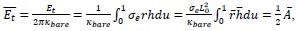
Where  is the dimensionless area.
Weakness: The authors introduce two different models, (1,1) and (1,2), for generating membrane curvature. Model 1 assumes a constant curvature growth, corresponding to linear curvature growth, while Model 2 relates curvature growth to its current value, resembling exponential curvature growth. Although both models make physical sense in general, I am concerned that Model 2 may lead to artificial membrane bending at high curvatures. Normally, for intermediate bending, ψ > 90, the bending process is energetically downhill and thus proceeds rapidly. The bending process is energetically downhill and thus proceeds rapidly. However, Model 2's assumption would accelerate curvature growth even further. This is reflected in the endocytic pathways represented by the green curves in the two rightmost panels of Fig. 4a, where the energy steeply increases at large ψ. I believe a more realistic version of Model 2 would require a saturation mechanism to limit curvature growth at high curvatures.
Recommendation 1: I suggest the authors discuss this point and highlight the pros and cons of Model 2. Specifically, addressing the potential issue of artificial membrane bending at high curvatures and considering the need for a saturation mechanism to limit excessive curvature growth. A discussion on how Model 2 compares to Model 1 in terms of physical relevance, especially in the context of high curvature scenarios, would provide valuable insights for the reader.
Thank you for raising the question of excessive curvature growth in our models and the constructive suggestion of introducing a saturation mechanism. In the revised manuscript (line 405), following your recommendation, we have added a subsection “Saturation effect at high membrane curvatures” in the discussion to clarify the excessive curvature issue and a possible way to introduce a saturation mechanism:
“Note that our model involves two distinct concepts of curvature growth. The first is the growth of imposed curvature — referred to here as intrinsic curvature and denoted by the parameter 𝑐<sub>0</sub> — which is driven by the reorganization of bonds between clathrin molecules within the coat. The second is the growth of the actual membrane curvature, reflected by the increasing value of 𝜓<sub>𝑚𝑎𝑥</sub>.
The latter process is driven by the former.
Models (1,1) and (1,2) incorporate energy terms (Equation 6) that promote the increase of intrinsic curvature 𝑐<sub>0</sub>, which in turn drives the membrane to adopt a more curved shape (increasing 𝜓<sub>𝑚𝑎𝑥</sub>). In the absence of these energy contributions, the system faces an energy barrier separating a weakly curved membrane state (low 𝜓<sub>𝑚𝑎𝑥</sub>) from a highly curved state (high 𝜓<sub>𝑚𝑎𝑥</sub>). This barrier can be observed, for example, in the red curves of Figure 3(a–c) and in Appendix 6—Figure 1. As a result, membrane bending cannot proceed spontaneously and requires additional energy input from clathrin assembly.
The energy terms described in Equation 6 serve to eliminate this energy barrier by lowering the energy difference between the uphill and downhill regions of the energy landscape. However, these same terms also steepen the downhill slope, which may lead to overly aggressive curvature growth.
To mitigate this effect, one could introduce a saturation-like energy term of the form:
where 𝑐<sub>𝑠</sub> represents a saturation curvature. Importantly, adding such a term would not alter the conclusions of our study, since the energy landscape already favors high membrane curvature (i.e., it is downward sloping) even without the additional energy terms. “
Recommendation 2: Referring to the previous point, the green curves in the two rightmost panels of Fig. 4a seem to reflect a comparison between slow and fast bending regimes. The initial slow vesiculation (with small curvature growth) in the left half of the green curves is followed by much more rapid curvature growth beyond a certain threshold. A similar behavior is observed in Model 1, as shown by the green curves in the two rightmost panels of Fig. 4b. I believe this transition between slow and fast bending warrants a brief discussion in the manuscript, as it could provide further insight into the dynamic nature of vesiculation.
Thank you for your constructive suggestion regarding the transition between slow and fast membrane bending. As you pointed out, in both Fig. 4a (model (1,2)) and Fig. 4b (model (1,1)), the green curves tend to extend vertically at the late stage. This suggests a significant increase in 𝑐<sub>0</sub> on the free energy landscape. However, we remain cautious about directly interpreting this vertical trend as indicative of fast endocytic dynamics, since our model is purely energetic and does not explicitly incorporate kinetic details. Meanwhile, we agree with your observation that the steep decrease in free energy along the green curve could correspond to an acceleration in dynamics. To address this point, we have added a paragraph in the revised manuscript (in Subsection “Cooperativity in the curvature generation process”) discussing this potential transition and its consistency with experimental observations (line 395):
“Furthermore, although our model is purely energetic and does not explicitly incorporate dynamics, we observe in Figure 3(a) that along the green curve—representing the trajectory predicted by model (1,2)—the total free energy (𝐸<sub>𝑡𝑜𝑡</sub>) exhibits a much sharper decrease at the late stage (near the vesiculation line) compared to the early stage (near the origin). This suggests a transition from slow to fast dynamics during endocytosis. Such a transition is consistent with experimental observations, where significantly fewer number of images with large 𝜓<sub>𝑚𝑎𝑥</sub> are captured compared to those with small 𝜓<sub>𝑚𝑎𝑥</sub> (Mund et al., 2023).”
The geometrical properties of both the constant-area and constant-curvature scenarios, as well depicted in Fig. 1, are somewhat straightforward. I wonder what additional value is presented in Fig. 2. Specifically, the authors solve differential shape equations to show how Rt and Rcoat vary with the angle ψ, but this behavior seems predictable from the simple schematics in Fig. 1. Using a more complex model for an intuitively understandable process may introduce counter-intuitive results and unnecessary complications, as seen with the constant-curvature model where Rt varies (the tip radius is not constant, as noted in the text) despite being assumed constant. One could easily assume a constant-curvature model and plot Rt versus ψ. I wonder What is the added value of solving shape equations to measure geometrical properties, compared to a simpler schematic approach (without solving shape equations) similar to what they do in App. 5 for the ratio of the Rt at ψ=30 and 150.
Thank you for raising this important question. While simple and intuitive theoretical models are indeed convenient to use, their validity must be carefully assessed. The approximate model becomes inaccurate when the clathrin shell significantly deviates from its intrinsic shape, namely a spherical cap characterized by intrinsic curvature 𝑐<sub>0</sub>. As shown in the insets of Fig. 2b and 2c (red line and black points), our comparison between the simplified model and the full model demonstrates that the simple model provides a good approximation under the constant-area constraint. However, it performs poorly under the constant-curvature constraint, and the deviation between the full model and the simplified model becomes more pronounced as 𝑐<sub>0</sub> increases.
In the revised manuscript, we have added a sentence emphasizing the discrepancy between the exact calculation with the idealized picture for the constant curvature model (line 181):
“For the constant-curvature model, the ratio remains close to 1 only at small values of 𝑐<sub>0</sub>, as expected from the schematic representation of the model in Figure 1. However, as 𝑐<sub>0</sub> increases, the deviation from this idealized picture becomes increasingly pronounced.”
Recommendation: The clathrin-mediated endocytosis aims at wrapping cellular cargos such as viruses which are typically spherical objects which perfectly match the constant-curvature scenario. In this context, wrapping nanoparticles by vesicles resembles constant-curvature membrane bending in endocytosis. In particular analogous shape transitions and energy barriers have been reported (similar to Fig.3 of the manuscript) using similar theoretical frameworks by varying membrane particle binding energy acting against membrane bending:
DOI: 10.1021/la063522m
DOI: 10.1039/C5SM01793A
I think a short comparison to particle wrapping by vesicles is warranted.
Thank you for your constructive suggestion to compare our model with particle wrapping. In the revised manuscript (line 475), we have added a subsection “Comparison with particle wrapping” in the discussion:
“The purpose of the clathrin-mediated endocytosis studied in our work is the recycling of membrane and membrane-protein, and the cellular uptake of small molecules from the environment — molecules that are sufficiently small to bind to the membrane or be encapsulated within a vesicle. In contrast, the uptake of larger particles typically involves membrane wrapping driven by adhesion between the membrane and the particle, a process that has also been studied previously (Góźdź, 2007; Bahrami et al., 2016). In our model, membrane bending is driven by clathrin assembly, which induces curvature. In particle wrapping, by comparison, the driving force is the adhesion between the membrane and a rigid particle. In the absence of adhesion, wrapping increases both bending and tension energies, creating an energy barrier that separates the flat membrane state from the fully wrapped state. This barrier can hinder complete wrapping, resulting in partial or no engulfment of the particle. Only when the adhesion energy is sufficiently strong can the process proceed to full wrapping. In this context, adhesion plays a role analogous to curvature generation in our model, as both serve to overcome the energy barrier. If the particle is spherical, it imposes a constant-curvature pathway during wrapping. However, the role of clathrin molecules in this process remains unclear and will be the subject of future investigation.”
Minor points:
Line 20, abstract, "....a continuum spectrum ..." reads better.
Line 46 "...clathrin results in the formation of pentagons ...." seems Ito be grammatically correct.
Line 106, proper citation of the relevant literature is warranted here.
Line 111, the authors compare features (plural) between experiments and calculations. I would write "....compare geometric features calculated by theory with those ....".
Line 124, "Here, we choose a ..." (with comma after Here).
Line 134, "The membrane tension \sigma_e and bending rigidity \kappa define a ...."
Line 295, "....tip radius, and invagination ...." (with comma before and).
Line 337, "abortive tips, and ..." (with comma before and).
We thank you for your thorough review of our manuscript and have corrected all the issues raised.
Dionysos and satyrs on a vase made by Brygos and painted by the Brygos Painter, ca. 480 BC (Cabinet des Médailles, Paris)
Perhaps comment on what this is, analyze it maybe
Últimos anos de Itamar Franco Depois da presidência, Itamar Franco não abandonou a política. Entre 1995 e 1996, ele assumiu o posto de embaixador do Brasil em Portugal. Em 1998, ele concorreu ao governo de Minas Gerais pelo PMDB, e venceu no segundo turno ao obter mais de 57% dos votos. Dessa vez, seguindo apenas um mandato. Em 2010, Itamar Franco concorreu novamente ao cargo de senador por Minas Gerais, e conseguiu eleger-se ao obter quase 27% dos votos. Ele ficou poucos meses na função, pois faleceu em 2 de julho de 2011, vítima de leucemia. A vaga deixada por ele foi ocupada por Zezé Perrella.
Últimas notícias de Itamar Franco
Author response:
The following is the authors’ response to the original reviews.
Recommendations for the Authors:
(1) Clarify Mechanistic Interpretations
(a) Provide stronger evidence or a more cautious interpretation regarding whether intracellular BK-CaV1.3 ensembles are precursors to plasma membrane complexes.
This is an important point. We adjusted the interpretation regarding intracellular BKCa<sub>V</sub>1.3 hetero-clusters as precursors to plasma membrane complexes to reflect a more cautious stance, acknowledging the limitations of available data. We added the following to the manuscript.
“Our findings suggest that BK and Ca<sub>V</sub>1.3 channels begin assembling intracellularly before reaching the plasma membrane, shaping their spatial organization and potentially facilitating functional coupling. While this suggests a coordinated process that may contribute to functional coupling, further investigation is needed to determine the extent to which these hetero-clusters persist upon membrane insertion.”
(b) Discuss the limitations of current data in establishing the proportion of intracellular complexes that persist on the cell surface.
We appreciate the suggestion. We expanded the discussion to address the limitations of current data in determining the proportion of intracellular complexes that persist on the cell surface. We added the following to the manuscript.
“Our findings highlight the intracellular assembly of BK-Ca<sub>V</sub>1.3 hetero-clusters, though limitations in resolution and organelle-specific analysis prevent precise quantification of the proportion of intracellular complexes that ultimately persist on the cell surface. While our data confirms that hetero-clusters form before reaching the plasma membrane, it remains unclear whether all intracellular hetero-clusters transition intact to the membrane or undergo rearrangement or disassembly upon insertion. Future studies utilizing live cell tracking and high resolution imaging will be valuable in elucidating the fate and stability of these complexes after membrane insertion.”
(2) Refine mRNA Co-localization Analysis
(a) Include appropriate controls using additional transmembrane mRNAs to better assess the specificity of BK and CaV1.3 mRNA co-localization.
We agree with the reviewers that these controls are essential. We explain better the controls used to address this concern. We added the following to the manuscript.
“To explore the origins of the initial association, we hypothesized that the two proteins are translated near each other, which could be detected as the colocalization of their mRNAs (Figure 5A and B). The experiment was designed to detect single mRNA molecules from INS-1 cells in culture. We performed multiplex in situ hybridization experiments using an RNAScope fluorescence detection kit to be able to image three mRNAs simultaneously in the same cell and acquired the images in a confocal microscope with high resolution. To rigorously assess the specificity of this potential mRNA-level organization, we used multiple internal controls. GAPDH mRNA, a highly expressed housekeeping gene with no known spatial coordination with channel mRNAs, served as a baseline control for nonspecific colocalization due to transcript abundance. To evaluate whether the spatial proximity between BK mRNA (KCNMA1) and Ca<sub>V</sub>1.3 mRNA (CACNA1D) was unique to functionally coupled channels, we also tested for Na<sup>V</sup>1.7 mRNA (SCN9A), a transmembrane sodium channel expressed in INS-1 cells but not functionally associated with BK. This allowed us to determine whether the observed colocalization reflected a specific biological relationship rather than shared expression context. Finally, to test whether this proximity might extend to other calcium sources relevant to BK activation, we probed the mRNA of ryanodine receptor 2 (RyR2), another Ca<sup>2+</sup> channel known to interact structurally with BK channels [32]. Together, these controls were chosen to distinguish specific mRNA colocalization patterns from random spatial proximity, shared subcellular distribution, or gene expression level artifacts.”
(b) Quantify mRNA co-localization in both directions (e.g., BK with CaV1.3 and vice versa) and account for differences in expression levels.
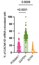
We thank the reviewer for this suggestion. We chose to quantify mRNA co-localization in the direction most relevant to the formation of functionally coupled hetero-clusters, namely, the proximity of BK (KCNMA1) mRNA to Ca<sub>V</sub>1.3 (CACNA1D) mRNA. Since BK channel activation depends on calcium influx provided by nearby Ca<sub>V</sub>1.3 channels, this directional analysis more directly informs the hypothesis of spatially coordinated translation and channel assembly. To address potential confounding effects of transcript abundance, we implemented a scrambled control approach in which the spatial coordinates of KCNMA1 mRNAs were randomized while preserving transcript count. This control resulted in significantly lower colocalization with CACNA1D mRNA, indicating that the observed proximity reflects a specific spatial association rather than expressiondriven overlap. We also assessed colocalization of CACNA1D with both KCNMA1, GAPDH mRNAs and SCN9 (NaV1.7); as you can see in the graph below these data support t the same conclusion but were not included in the manuscript.
Author response image 1.
(c) Consider using ER labeling as a spatial reference when analyzing mRNA localization
We thank the reviewers for this suggestion. Rather than using ER labeling as a spatial reference, we assess BK and CaV1.3 mRNA localization using fluorescence in situ hybridization (smFISH) alongside BK protein immunostaining. This approach directly identifies BK-associated translation sites, ensuring that observed mRNA localization corresponds to active BK synthesis rather than general ER association. By evaluating BK protein alongside its mRNA, we provide a more functionally relevant measure of spatial organization, allowing us to assess whether BK is synthesized in proximity to CaV1.3 mRNA within micro-translational complexes. The results added to the manuscript is as follows.
“To further investigate whether KCNMA1 and CACNA1D are localized in regions of active translation (Figure 7A), we performed RNAScope targeting KCNMA1 and CACNA1D alongside immunostaining for BK protein. This strategy enabled us to visualize transcript-protein colocalization in INS-1 cells with subcellular resolution. By directly evaluating sites of active BK translation, we aimed to determine whether newly synthesized BK protein colocalized with CACNA1D mRNA signals (Figure 7A). Confocal imaging revealed distinct micro-translational complex where KCNMA1 mRNA puncta overlapped with BK protein signals and were located adjacent to CACNA1D mRNA (Figure 7B). Quantitative analysis showed that 71 ± 3% of all KCNMA1 colocalized with BK protein signal which means that they are in active translation. Interestingly, 69 ± 3% of the KCNMA1 in active translation colocalized with CACNA1D (Figure 7C), supporting the existence of functional micro-translational complexes between BK and Ca<sub>V</sub>1.3 channels.”
(3) Improve Terminology and Definitions
(a) Clarify and consistently use terms like "ensemble," "cluster," and "complex," especially in quantitative analyses.
We agree with the reviewers, and we clarified terminology such as 'ensemble,' 'cluster,' and 'complex' and used them consistently throughout the manuscript, particularly in quantitative analyses, to enhance precision and avoid ambiguity.
(b) Consider adopting standard nomenclature (e.g., "hetero-clusters") to avoid ambiguity.
We agree with the reviewers, and we adapted standard nomenclature, such as 'heteroclusters,' in the manuscript to improve clarity and reduce ambiguity.
(4) Enhance Quantitative and Image Analysis
(a) Clearly describe how colocalization and clustering were measured in super-resolution data.
We thank the reviewers for this suggestion. We have modified the Methods section to provide a clearer description of how colocalization and clustering were measured in our super-resolution data. Specifically, we now detail the image processing steps, including binary conversion, channel multiplication for colocalization assessment, and density-based segmentation for clustering analysis. These updates ensure transparency in our approach and improve accessibility for readers, and we added the following to the manuscript.
“Super-resolution imaging:
Direct stochastic optical reconstruction microscopy (dSTORM) images of BK and 1.3 overexpressed in tsA-201 cells were acquired using an ONI Nanoimager microscope equipped with a 100X oil immersion objective (1.4 NA), an XYZ closed-loop piezo 736 stage, and triple emission channels split at 488, 555, and 640 nm. Samples were imaged at 35°C. For singlemolecule localization microscopy, fixed and stained cells were imaged in GLOX imaging buffer containing 10 mM β-mercaptoethylamine (MEA), 0.56 mg/ml glucose oxidase, 34 μg/ml catalase, and 10% w/v glucose in Tris-HCl buffer. Single-molecule localizations were filtered using NImOS software (v.1.18.3, ONI). Localization maps were exported as TIFF images with a pixel size of 5 nm. Maps were further processed in ImageJ (NIH) by thresholding and binarization to isolate labeled structures. To assess colocalization between the signal from two proteins, binary images were multiplied. Particles smaller than 400 nm<sup>2</sup> were excluded from the analysis to reflect the spatial resolution limit of STORM imaging (20 nm) and the average size of BK channels. To examine spatial localization preference, binary images of BK were progressively dilated to 20 nm, 40 nm, 60 nm, 80 nm, 100 nm, and 200 nm to expand their spatial representation. These modified images were then multiplied with the Ca<sub>V</sub>1.3 channel to quantify colocalization and determine BK occupancy at increasing distances from Ca<sub>V</sub>1.3. To ensure consistent comparisons across distance thresholds, data were normalized using the 200 nm measurement as the highest reference value, set to 1.”
(b) Where appropriate, quantify the proportion of total channels involved in ensembles within each compartment.
We thank the reviewers for this comment. However, our method does not allow for direct quantification of the total number of BK and Ca<sub>V</sub>1.3 channels expressed within the ER or ER exit sites, as we rely on proximity-based detection rather than absolute fluorescence intensity measurements of individual channels. Traditional methods for counting total channel populations, such as immunostaining or single-molecule tracking, are not applicable to our approach due to the hetero-clusters formation process. Instead, we focused on the relative proportion of BK and Ca<sub>V</sub>1.3 hetero-clusters within these compartments, as this provides meaningful insights into trafficking dynamics and spatial organization. By assessing where hetero-cluster preferentially localize rather than attempting to count total channel numbers, we can infer whether their assembly occurs before plasma membrane insertion. While this approach does not yield absolute quantification of ER-localized BK and Ca<sub>V</sub>1.3 channels, it remains a robust method for investigating hetero-cluster formation and intracellular trafficking pathways. To reflect this limitation, we added the following to the manuscript.
“Finally, a key limitation of this approach is that we cannot quantify the proportion of total BK or Ca<sub>V</sub>1.3 channels engaged in hetero-clusters within each compartment. The PLA method provides proximity-based detection, which reflects relative localization rather than absolute channel abundance within individual organelles”.
(5) Temper Overstated Claims
(a) Revise language that suggests the findings introduce a "new paradigm," instead emphasizing how this study extends existing models.
We agree with the reviewers, and we have revised the language to avoid implying a 'new paradigm.' The following is the significance statement.
“This work examines the proximity between BK and Ca<sub>V</sub>1.3 molecules at the level of their mRNAs and newly synthesized proteins to reveal that these channels interact early in their biogenesis. Two cell models were used: a heterologous expression system to investigate the steps of protein trafficking and a pancreatic beta cell line to study the localization of endogenous channel mRNAs. Our findings show that BK and Ca<sub>V</sub>1.3 channels begin assembling intracellularly before reaching the plasma membrane, revealing new aspects of their spatial organization. This intracellular assembly suggests a coordinated process that contributes to functional coupling.”
(b) Moderate conclusions where the supporting data are preliminary or correlative.
We agree with the reviewers, and we have moderated conclusions in instances where the supporting data are preliminary or correlative, ensuring a balanced interpretation. We added the following to the manuscript.
“This study provides novel insights into the organization of BK and Ca<sub>V</sub>1.3 channels in heteroclusters, emphasizing their assembly within the ER, at ER exit sites, and within the Golgi. Our findings suggest that BK and Ca<sub>V</sub>1.3 channels begin assembling intracellularly before reaching the plasma membrane, shaping their spatial organization, and potentially facilitating functional coupling. While this suggests a coordinated process that may contribute to functional coupling, further investigation is needed to determine the extent to which these hetero-clusters persist upon membrane insertion. While our study advances the understanding of BK and Ca<sub>V</sub>1.3 heterocluster assembly, several key questions remain unanswered. What molecular machinery drives this colocalization at the mRNA and protein level? How do disruptions to complex assembly contribute to channelopathies and related diseases? Additionally, a deeper investigation into the role of RNA binding proteins in facilitating transcript association and localized translation is warranted”.
(6) Address Additional Technical and Presentation Issues
(a) Include clearer figure annotations, especially for identifying PLA puncta localization (e.g., membrane vs. intracellular).
We agree with the reviewers, and we have updated the figures to include clearer annotations that distinguish PLA puncta localized at the membrane versus those within intracellular compartments.
(b) Reconsider the scale and arrangement of image panels to better showcase the data.
We agree with the reviewers, and we have adjusted the scale and layout of the image panels to enhance data visualization and readability. Enlarged key regions now provide better clarity of critical features.
(c) Provide precise clone/variant information for BK and CaV1.3 channels used.
We thank the reviewers for their suggestion, and we now provide precise information regarding the BK and Ca<sub>V</sub>1.3 channel constructs used in our experiments, including their Addgene plasmid numbers and relevant variant details. These have been incorporated into the Methods section to ensure reproducibility and transparency. We added the following to the manuscript.
“The Ca<sub>V</sub>1.3 α subunit construct used in our study corresponds to the rat Ca<sub>V</sub>1.3e splice variant containing exons 8a, 11, 31b, and 42a, with a deletion of exon 32. The BK channel construct used in this study corresponds to the VYR splice variant of the mouse BKα subunit (KCNMA1)”.
(d) Correct typographical errors and ensure proper figure/supplementary labeling throughout.
Typographical errors have been corrected, and figure/supplementary labeling has been reviewed for accuracy throughout the manuscript.
(7) Expand the Discussion
(a) Include a brief discussion of findings such as BK surface expression in the absence of CaV1.3.
We thank the reviewers for their suggestion. We expanded the Discussion to include a brief analysis of BK surface expression in the absence of Ca<sub>V</sub>1.3. We included the following in the manuscript.
“BK Surface Expression and Independent Trafficking Pathways
BK surface expression in the absence of Ca<sub>V</sub>1.3 indicates that its trafficking does not strictly rely on Ca<sub>V</sub>1.3-mediated interactions. Since BK channels can be activated by multiple calcium sources, their presence in intracellular compartments suggests that their surface expression is governed by intrinsic trafficking mechanisms rather than direct calcium-dependent regulation. While some BK and Ca<sub>V</sub>1.3 hetero-clusters assemble into signaling complexes intracellularly, other BK channels follow independent trafficking pathways, demonstrating that complex formation is not obligatory for all BK channels. Differences in their transport kinetics further reinforce the idea that their intracellular trafficking is regulated through distinct mechanisms. Studies have shown that BK channels can traffic independently of Ca<sub>V</sub>1.3, relying on alternative calcium sources for activation [13, 41]. Additionally, Ca<sub>V</sub>1.3 exhibits slower synthesis and trafficking kinetics than BK, emphasizing that their intracellular transport may not always be coordinated. These findings suggest that BK and Ca<sub>V</sub>1.3 exhibit both independent and coordinated trafficking behaviors, influencing their spatial organization and functional interactions”.
(b) Clarify why certain colocalization comparisons (e.g., ER vs. ER exit sites) are not directly interpretable.
We thank the reviewer for their suggestion. A clarification has been added to the result section and discussion of the manuscript explaining why colocalization comparisons, such as ER versus ER exit sites, are not directly interpretable. We included the following in the manuscript.
“Result:
ER was not simply due to the extensive spatial coverage of ER labeling, we labeled ER exit sites using Sec16-GFP and probed for hetero-clusters with PLA. This approach enabled us to test whether the hetero-clusters were preferentially localized to ER exit sites, which are specialized trafficking hubs that mediate cargo selection and direct proteins from the ER into the secretory pathway. In contrast to the more expansive ER network, which supports protein synthesis and folding, ER exit sites ensure efficient and selective export of proteins to their target destinations”.
“By quantifying the proportion of BK and Ca<sub>V</sub>1.3 hetero-clusters relative to total channel expression at ER exit sites, we found 28 ± 3% colocalization in tsA-201 cells and 11 ± 2% in INS-1 cells (Figure 3F). While the percentage of colocalization between hetero-clusters and the ER or ER exit sites alone cannot be directly compared to infer trafficking dynamics, these findings reinforce the conclusion that hetero-clusters reside within the ER and suggest that BK and Ca<sub>V</sub>1.3 channels traffic together through the ER and exit in coordination”.
“Colocalization and Trafficking Dynamics
The colocalization of BK and Ca<sub>V</sub>1.3 channels in the ER and at ER exit sites before reaching the Golgi suggests a coordinated trafficking mechanism that facilitates the formation of multi-channel complexes crucial for calcium signaling and membrane excitability [37, 38]. Given the distinct roles of these compartments, colocalization at the ER and ER exit sites may reflect transient proximity rather than stable interactions. Their presence in the Golgi further suggests that posttranslational modifications and additional assembly steps occur before plasma membrane transport, providing further insight into hetero-cluster maturation and sorting events. By examining BK-Ca<sub>V</sub>1.3 hetero-cluster distribution across these trafficking compartments, we ensure that observed colocalization patterns are considered within a broader framework of intracellular transport mechanisms [39]. Previous studies indicate that ER exit sites exhibit variability in cargo retention and sorting efficiency [40], emphasizing the need for careful evaluation of colocalization data. Accounting for these complexities allows for a robust assessment of signaling complexes formation and trafficking pathways”.
Reviewer #1 (Recommendations for the authors):
In addition to the general aspects described in the public review, I list below a few points with the hope that they will help to improve the manuscript:
(1) Page 3: "they bind calcium delimited to the point of entry at calcium channels", better use "sources"
We agree with the reviewer. The phrasing on Page 3 has been updated to use 'sources' instead of 'the point of entry at calcium channels' for clarity.
(2) Page 3 "localized supplies of intracellular calcium", I do not like this term, but maybe this is just silly.
We agree with the reviewer. The term 'localized supplies of intracellular calcium' on Page 3 has been revised to “Localized calcium sources”
(3) Regarding the definitions stated by the authors: How do you distinguish between "ensembles" corresponding to "coordinated collection of BK and Cav channels" and "assembly of BK clusters with Cav clusters"? I believe that hetero-clusters is more adequate. The nomenclature does not respond to any consensus in the protein biology field, and I find that it introduces bias more than it helps. I would stick to heteroclusters nomenclature that has been used previously in the field. Moreover, in some discussion sections, the term "ensemble" is used in ways that border on vague, especially when talking about "functional signaling complexes" or "ensembles forming early." It's still acceptable within context but could benefit from clearer language to distinguish ensemble (structural proximity) from complex (functional consequence).
We agree with the reviewer, and we recognize the importance of precise nomenclature and have adopted hetero-clusters instead of ensembles to align with established conventions in the field. This term specifically refers to the spatial organization of BK and Ca<sub>V</sub>1.3 channels, while functional complexes denote mechanistic interactions. We have revised sections where ensemble was used ambiguously to ensure clear distinction between structure and function.
The definition of "cluster" is clearly stated early but less emphasized in later quantitative analyses (e.g., particle size discussions in Figure 7). Figure 8 is equally confusing, graphs D and E referring to "BK ensembles" and "Cav ensembles", but "ensembles" should refer to combinations of both channels, whereas these seem to be "clusters". In fact, the Figure legend mentions "clusters".
We agree with the reviewer. Terminology has been revised throughout the manuscript to ensure consistency, with 'clusters' used appropriately in quantitative analyses and figure descriptions.
(4) Methods: how are clusters ("ensembles") analysed from the STORM data? What is the logarithm used for? More info about this is required. Equally, more information and discussion about how colocalization is measured and interpreted in superresolution microscopy are required.
We thank the reviewer for their suggestion, and additional details have been incorporated into the Methods section to clarify how clusters ('ensembles') are analyzed from STORM data, including the role of the logarithm in processing. Furthermore, we have expanded the discussion to provide more information on how colocalization is measured and interpreted in super resolution microscopy. We include the following in the manuscript.
“Direct stochastic optical reconstruction microscopy (dSTORM) images of BK and Ca<sub>V</sub>1.3 overexpressed in tsA-201 cells were acquired using an ONI Nanoimager microscope equipped with a 100X oil immersion objective (1.4 NA), an XYZ closed-loop piezo 736 stage, and triple emission channels split at 488, 555, and 640 nm. Samples were imaged at 35°C. For singlemolecule localization microscopy, fixed and stained cells were imaged in GLOX imaging buffer containing 10 mM β-mercaptoethylamine (MEA), 0.56 mg/ml glucose oxidase, 34 μg/ml catalase, and 10% w/v glucose in Tris-HCl buffer. Single-molecule localizations were filtered using NImOS software (v.1.18.3, ONI). Localization maps were exported as TIFF images with a pixel size of 5 nm. Maps were further processed in ImageJ (NIH) by thresholding and binarization to isolate labeled structures. To assess colocalization between the signal from two proteins, binary images were multiplied. Particles smaller than 400 nm<sup>2</sup> were excluded from the analysis to reflect the spatial resolution limit of STORM imaging (20 nm) and the average size of BK channels. To examine spatial localization preference, binary images of BK were progressively dilated to 20 nm, 40 nm, 60 nm, 80 nm, 100 nm, and 200 nm to expand their spatial representation. These modified images were then multiplied with the Ca<sub>V</sub>1.3 channel to quantify colocalization and determine BK occupancy at increasing distances from Ca<sub>V</sub>1.3. To ensure consistent comparisons across distance thresholds, data were normalized using the 200 nm measurement as the highest reference value, set to 1”.
(5) Related to Figure 2:
(a) Why use an antibody to label GFP when PH-PLCdelta should be a membrane marker? Where is the GFP in PH-PKC-delta (intracellular, extracellular? Images in Figure 2E are confusing, there is a green intracellular signal.
We thank the reviewer for their feedback. To clarify, GFP is fused to the N-terminus of PH-PLCδ and primarily localizes to the inner plasma membrane via PIP2 binding. Residual intracellular GFP signal may reflect non-membrane-bound fractions or background from anti-GFP immunostaining. We added a paragraph explaining the use of the antibody anti GFP in the Methods section Proximity ligation assay subsection.
(b) The images in Figure 2 do not help to understand how the authors select the PLA puncta located at the plasma membrane. How do the authors do this? A useful solution would be to indicate in Figure 2 an example of the PLA signals that are considered "membrane signals" compared to another example with "intracellular signals". Perhaps this was intended with the current Figure, but it is not clear.
We agree with the reviewer. We have added a sentence to explain how the number of PLA puncta at the plasma membrane was calculated.
“We visualized the plasma membrane with a biological sensor tagged with GFP (PHPLCδ-GFP) and then probed it with an antibody against GFP (Figure 2E). By analyzing the GFP signal, we created a mask that represented the plasma membrane. The mask served to distinguish between the PLA puncta located inside the cell and those at the plasma membrane, allowing us to calculate the number of PLA puncta at the plasma membrane”.
(c) Figure 2C: What is the negative control? Apologies if it is described somewhere, but I seem not to find it in the manuscript.
We thank the reviewer for their suggestion. For the negative control in Figure 2C, BK was probed using the primary antibody without co-staining for Ca<sub>V</sub>1.3 or other proteins, ensuring specificity and ruling out non-specific antibody binding or background fluorescence. A sentence clarifying the negative control for Figure 2C has been added to the Results section, specifying that BK was probed using the primary antibody without costaining for Ca<sub>V</sub>1.3 or other proteins to ensure specificity.
“To confirm specificity, a negative control was performed by probing only for BK using the primary antibody, ensuring that detected signals were not due to non-specific binding or background fluorescence”.
(d) What is the resolution in z of the images shown in Figure 2? This is relevant for the interpretation of signal localization.
The z-resolution of the images shown in Figure 2 was approximately 270–300 nm, based on the Zeiss Airyscan system’s axial resolution capabilities. Imaging was performed with a step size of 300 nm, ensuring adequate sampling for signal localization while maintaining optimal axial resolution.
“In a different experiment, we analyzed the puncta density for each focal plane of the cell (step size of 300 nm) and compared the puncta at the plasma membrane to the rest of the cell”.
(e) % of total puncta in PM vs inside cell are shown for transfected cells, what is this proportion in INS-1 cells?
This quantification was performed for transfected cells; however, we have not conducted the same analysis in INS-1 cells. Future experiments could address this to determine potential differences in puncta distribution between endogenous and overexpressed conditions.
(6) Related to Figure 3:
(a) Figure 3B: is this antibody labelling or GFP fluorescence? Why do they use GFP antibody labelling, if the marker already has its own fluorescence? This should at least be commented on in the manuscript.
We thank the reviewer for their concern. In Figure 3B, GFP was labeled using an antibody rather than relying on its intrinsic fluorescence. This approach was necessary because GFP fluorescence does not withstand the PLA protocol, resulting in significant fading. Antibody labeling provided stronger signal intensity and improved resolution, ensuring optimal signal-to-noise ratio for accurate analysis.
A clarification regarding the use of GFP antibody labeling in Figure 3B has been added to the Methods section, explaining that intrinsic GFP fluorescence does not endure the PLA protocol, necessitating antibody-based detection for improved signal and resolution.We added the following to the manuscript.
“For PLA combined with immunostaining, PLA was followed by a secondary antibody incubation with Alexa Fluor-488 at 2 μg/ml for 1 hour at 21˚C. Since GFP fluorescence fades significantly during the PLA protocol, resulting in reduced signal intensity and poor image resolution, GFP was labeled using an antibody rather than relying on its intrinsic fluorescence”.
(b) Why is it relevant to study the ER exit sites? Some explanation should be included in the main text (page 11) for clarification to non-specialized readers. Again, the quantification should be performed on the proportion of clusters/ensembles out of the total number of channels expressed at the ER (or ER exit sites).
We thank the reviewer for their feedback. We have modified this section to include a more detailed explanation of the relevance of ER exit sites to protein trafficking. ER exit sites serve as specialized sorting hubs that regulate the transition of proteins from the ER to the secretory pathway, distinguishing them from the broader ER network, which primarily facilitates protein synthesis and folding. This additional context clarifies why studying ER exit sites provides valuable insights into ensemble trafficking dynamics.
Regarding quantification, our method does not allow for direct measurement of the total number of BK and Ca<sub>V</sub>1.3 channels expressed at the ER or ER exit sites. Instead, we focused on the proportion of hetero-clusters localized within these compartments, which provides insight into trafficking pathways despite the limitation in absolute channel quantification. We included the following in the manuscript in the Results section.
“To determine whether the observed colocalization between BK–Ca<sub>V</sub>1.3 hetero-clusters and the ER was not simply due to the extensive spatial coverage of ER labeling, we labeled ER exit sites using Sec16-GFP and probed for hetero-clusters with PLA. This approach enabled us to test whether the hetero-clusters were preferentially localized to ER exit sites, which are specialized trafficking hubs that mediate cargo selection and direct proteins from the ER into the secretory pathway. In contrast to the more expansive ER network, which supports protein synthesis and folding, ER exit sites ensure efficient and selective export of proteins to their target destinations”.
“By quantifying the proportion of BK and Ca<sub>V</sub>1.3 hetero-clusters relative to total channel expression at ER exit sites, we found 28 ± 3% colocalization in tsA-201 cells and 11 ± 2% in INS-1 cells (Figure 3F). While the percentage of colocalization between hetero-clusters and the ER or ER exit sites alone cannot be directly compared to infer trafficking dynamics, these findings reinforce the conclusion that hetero-clusters reside within the ER and suggest that BK and Ca<sub>V</sub>1.3 channels traffic together through the ER and exit in coordination”.
(7) Related to Figure 4:
A control is included to confirm that the formation of BK-Cav1.3 ensembles is not unspecific. Association with a protein from the Golgi (58K) is tested. Why is this control only done for Golgi? No similar experiment has been performed in the ER. This aspect should be commented on.
We thank the reviewer for their suggestion. We selected the Golgi as a control because it represents the final stage of protein trafficking before proteins reach their functional destinations. If BK and Ca<sub>V</sub>1.3 hetero-cluster formation is specific at the Golgi, this suggests that their interaction is maintained throughout earlier trafficking steps, including within the ER. While we did not perform an equivalent control experiment in the ER, the Golgi serves as an effective checkpoint for evaluating specificity within the broader protein transport pathway. We included the following in the manuscript.
“We selected the Golgi as a control because it represents the final stage of protein trafficking, ensuring that hetero-cluster interactions observed at this point reflect specificity maintained throughout earlier trafficking steps, including within the ER”.
(8) How is colocalization measured, eg, in Figure 6? Are the images shown in Figure 6 representative? This aspect would benefit from a clearer description.
We thank the reviewer for their suggestion. A section clarifying colocalization measurement and the representativeness of Figure 6 images has been added to the Methods under Data Analysis. We included the following in the manuscript.
For PLA and RNAscope experiments, we used custom-made macros written in ImageJ. Processing of PLA data included background subtraction. To assess colocalization, fluorescent signals were converted into binary images, and channels were multiplied to identify spatial overlap.
(9) The text should be revised for typographical errors, for example:
(a) Summary "evidence of" (CHECK THIS ONE)
We agree with the reviewer, and we corrected the typographical errors
(b) Table 1, row 3: "enriches" should be "enrich"
We agree with the reviewer. The term 'enriches' in Table 1, row 3 has been corrected to 'enrich'.
(c) Figure 2B "priximity"
We agree with the reviewer. The typographical errors in Figure 2B has been corrected from 'priximity' to 'proximity'.
(d) Legend of Figure 7 (C) "size of BK and Cav1.3 channels". Does this correspond to individual channels or clusters?
We agree with the reviewer. The legend of Figure 7C has been clarified to indicate that 'size of BK and Cav1.3 channels' refers to clusters rather than individual channels.
(e) Methods: In the RNASCOPE section, "Fig.4-supp1" should be "Fig. 5-supp1"
(f) Page 15, Figure 5B is cited, should be Figure 6B
We agree with the reviewer. The reference in the RNASCOPE section has been updated from 'Fig.4-supp1' to 'Fig. 5-supp1,' and the citation on Page 15 has been corrected from Figure 5B to Figure 6B.
Reviewer #2 (Recommendations for the authors):
(1) The abstract could be more accessible for a wider readership with improved flow.
We thank the reviewer for their suggestion. We modified the summary as follows to provide a more coherent flow for a wider readership.
“Calcium binding to BK channels lowers BK activation threshold, substantiating functional coupling with calcium-permeable channels. This coupling requires close proximity between different channel types, and the formation of BK–Ca<sub>V</sub>1.3 hetero-clusters at nanometer distances exemplifies this unique organization. To investigate the structural basis of this interaction, we tested the hypothesis that BK and Ca<sub>V</sub>1.3 channels assemble before their insertion into the plasma membrane. Our approach incorporated four strategies: (1) detecting interactions between BK and Ca<sub>V</sub>1.3 proteins inside the cell, (2) identifying membrane compartments where intracellular hetero-clusters reside, (3) measuring the proximity of their mRNAs, and (4) assessing protein interactions at the plasma membrane during early translation. These analyses revealed that a subset of BK and Ca<sub>V</sub>1.3 transcripts are spatially close in micro-translational complexes, and their newly synthesized proteins associate within the endoplasmic reticulum (ER) and Golgi. Comparisons with other proteins, transcripts, and randomized localization models support the conclusion that BK and Ca<sub>V</sub>1.3 hetero-clusters form before their insertion at the plasma membrane”.
(2) Figure 2B - spelling of proximity.
We agree with the reviewer. The typographical errors in Figure 2B has been corrected from 'priximity' to 'proximity'.
Reviewer #3 (Recommendations for the authors):
Minor issues to improve the manuscript:
(1) For completeness, the authors should include a few sentences and appropriate references in the Introduction to mention that BK channels are regulated by auxiliary subunits.
We agree with the reviewer. We have revised the Introduction to include a brief discussion of how BK channel function is modulated by auxiliary subunits and provided appropriate references to ensure completeness. These additions highlight the broader regulatory mechanisms governing BK channel activity, complementing the focus of our study. We included the following in the manuscript.
“Additionally, BK channels are modulated by auxiliary subunits, which fine-tune BK channel gating properties to adapt to different physiological conditions. β and γ subunits regulate BK channel kinetics, altering voltage sensitivity and calcium responsiveness [18]. These interactions ensure precise control over channel activity, allowing BK channels to integrate voltage and calcium signals dynamically in various cell types. Here, we focus on the selective assembly of BK channels with Ca<sub>V</sub>1.3 and do not evaluate the contributions of auxiliary subunits to BK channel organization.”
(2) Insert a space between 'homeostasis' and the square bracket at the end of the Introduction's second paragraph.
We agree with the reviewer. A space has been inserted between 'homeostasis' and the square bracket in the second paragraph of the Introduction for clarity.
(3) The images presented in Figures 2-5 should be increased in size (if permitted by the Journal) to allow the reader to clearly see the puncta in the fluorescent images. This would necessitate reconfiguring the figures into perhaps a full A4 page per figure, but I think the quality of the images presented really do deserve to "be seen". For example, Panels A & B could be at the top of Figure 2, with C & D presented below them. However, I'll leave it up to the authors to decide on the most aesthetically pleasing way to show these.
We agree with the reviewer. We have increased the size of Figures 2–8 to enhance the visibility of fluorescent puncta, as suggested. To accommodate this, we reorganized the panel layout for each figure—for example, in Figure 2, Panels A and B are now placed above Panels C and D to support a more intuitive and aesthetically coherent presentation. We believe this revised configuration highlights the image quality and improves readability while conforming to journal layout constraints.
(4) I think that some of the sentences could be "toned down"
(a) eg, in the first paragraph below Figure 2, the authors state "that 46(plus minus)3% of the puncta were localised on intracellular membranes" when, at that stage, no data had been presented to confirm this. I think changing it to "that 46(plus minus)3% of the puncta were localised intracellularly" would be more precise.
(b) Similarly, please consider replacing the wording of "get together at membranes inside the cell" to "co-localise intracellularly".
(c) In the paragraph just before Figure 5, the authors mention that "the abundance of KCNMA1 correlated more with the abundance of CACNA1D than ... with GAPDH." Although this is technically correct, the R2 value was 0.22, which is exceptionally poor. I don't think that the paper is strengthened by sentences such as this, and perhaps the authors might tone this down to reflect this.
(d) The authors clearly demonstrate in Figure 8 that a significant number of BK channels can traffic to the membrane in the absence of Cav1.3. Irrespective of the differences in transcription/trafficking time between the two channel types, the authors should insert a few lines into their discussion to take this finding into account.
We appreciate the reviewer’s feedback regarding the clarity and precision of our phrasing.
Our responses for each point are below.
(a) We have modified the statement in the first paragraph below Figure 2, changing '46 ± 3% of the puncta were localized on intracellular membranes' to '46 ± 3% of the puncta were localized ‘intracellularly’ to ensure accuracy in the absence of explicit data confirming membrane association.
(b) Similarly, we have replaced 'get together at membranes inside the cell' with 'colocalize intracellularly' to maintain clarity and avoid unintended implications.
(c) Regarding the correlation between KCNMA1 and CACNA1D abundance, we recognize that the R² value of 0.22 is relatively low. To reflect this appropriately, we have revised the phrasing to indicate that while a correlation exists, it is modest. We added the following to the manuscript.
“Interestingly, the abundance of KCNMA1 transcripts correlated more with the abundance of CACNA1D transcripts than with the abundance of GAPDH, a standard housekeeping gene, though with a modest R² value.”
(d) To incorporate the findings from Figure 8, we have added discussion acknowledging that a substantial number of BK channels traffic to the membrane independently of Ca<sub>V</sub>1.3. This addition provides context for potential trafficking mechanisms that operate separately from ensemble formation.
(5) For clarity, please insert the word "total" in the paragraph after Figure 3 "..."63{plus minus}3% versus 50%{plus minus}6% of total PLA puncta were localised at the ER". I know this is explicitly stated later in the manuscript, but I think it needs to be clarified earlier.
We agree with the reviewer. The word 'total' has been inserted in the paragraph following Figure 3 to clarify the percentage of PLA puncta localized at the ER earlier in the manuscript
(6) In the discussion, I think an additional (short) paragraph needs to be included to clarify to the reader why the % "colocalization between ensembles and the ER or the ER exit sites can't be compared or used to understand the dynamics of the ensembles". This may permit the authors to remove the last sentence of the paragraph just before the results section, "BK and Cav1.3 ensembles go through the Golgi."
We thank the reviewer for their suggestion. We have added a short paragraph in the discussion to clarify why colocalization percentages between ensembles and the ER or ER exit sites cannot be compared to infer ensemble dynamics. This allowed us to remove the final sentence of the paragraph preceding the results section ('BK and Cav1.3 ensembles go through the Golgi).
(7) In the paragraph after Figure 6, Figure 5B is inadvertently referred to. Please correct this to Figure 6B.
We agree with the reviewer. The reference to Figure 5B in the paragraph after Figure 6 has been corrected to Figure 6B.
(8) In the discussion under "mRNA co-localisation and Protein Trafficking", please insert a relevant reference illustrating that "disruption in mRNA localization... can lead to ion channel mislocalization".
We agree with the reviewer. We have inserted a relevant reference under 'mRNA Colocalization and Protein Trafficking' to illustrate that disruption in mRNA localization can lead to ion channel mislocalization.
(9) The supplementary Figures appear to be incorrectly numbered. Please correct and also ensure that they are correctly referred to in the text.
We agree with the reviewer. The numbering of the supplementary figures has been corrected, and all references to them in the text have been updated accordingly.
(10) The final panels of the currently labelled Figure 5-Supplementary 2 need to have labels A-F included on the image.
We agree with the reviewer. Labels A-F have been added to the final panels of Figure 5-Supplementary 2.
References
(1) Shah, K.R., X. Guan, and J. Yan, Structural and Functional Coupling of Calcium-Activated BK Channels and Calcium-Permeable Channels Within Nanodomain Signaling Complexes. Frontiers in Physiology, 2022. Volume 12 - 2021.
(2) Chen, A.L., et al., Calcium-Activated Big-Conductance (BK) Potassium Channels Traffic through Nuclear Envelopes into Kinocilia in Ray Electrosensory Cells. Cells, 2023. 12(17): p. 2125.
(3) Berkefeld, H., B. Fakler, and U. Schulte, Ca2+-activated K+ channels: from protein complexes to function. Physiol Rev, 2010. 90(4): p. 1437-59.
(4) Loane, D.J., P.A. Lima, and N.V. Marrion, Co-assembly of N-type Ca2+ and BK channels underlies functional coupling in rat brain. J Cell Sci, 2007. 120(Pt 6): p. 98595.
(5) Boncompain, G. and F. Perez, The many routes of Golgi-dependent trafficking. Histochemistry and Cell Biology, 2013. 140(3): p. 251-260.
(6) Kurokawa, K. and A. Nakano, The ER exit sites are specialized ER zones for the transport of cargo proteins from the ER to the Golgi apparatus. The Journal of Biochemistry, 2019. 165(2): p. 109-114.
(7) Chen, G., et al., BK channel modulation by positively charged peptides and auxiliary γ subunits mediated by the Ca2+-bowl site. Journal of General Physiology, 2023. 155(6).
Author response:
The following is the authors’ response to the original reviews.
Reviewer #1 (Public review):
Summary
Lysine acetoacetylation (Kacac) is a recently discovered histone post-translational modification (PTM) connected to ketone body metabolism. This research outlines a chemo-immunological method for detecting Kacac, eliminating the requirement for creating new antibodies. The study demonstrates that acetoacetate acts as the precursor for Kacac, which is catalyzed by the acyltransferases GCN5, p300, and PCAF, and removed by the deacetylase HDAC3. AcetoacetylCoA synthetase (AACS) is identified as a central regulator of Kacac levels in cells. A proteomic analysis revealed 139 Kacac sites across 85 human proteins, showing the modification's extensive influence on various cellular functions. Additional bioinformatics and RNA sequencing data suggest a relationship between Kacac and other PTMs, such as lysine βhydroxybutyrylation (Kbhb), in regulating biological pathways. The findings underscore Kacac's role in histone and non-histone protein regulation, providing a foundation for future research into the roles of ketone bodies in metabolic regulation and disease processes.
Strengths
(1) The study developed an innovative method by using a novel chemo-immunological approach to the detection of lysine acetoacetylation. This provides a reliable method for the detection of specific Kacac using commercially available antibodies.
(2) The research has done a comprehensive proteome analysis to identify unique Kacac sites on 85 human proteins by using proteomic profiling. This detailed landscape of lysine acetoacetylation provides a possible role in cellular processes.
(3) The functional characterization of enzymes explores the activity of acetoacetyltransferase of key enzymes like GCN5, p300, and PCAF. This provides a deeper understanding of their function in cellular regulation and histone modifications.
(4) The impact of acetyl-CoA and acetoacetyl-CoA on histone acetylation provides the differential regulation of acylations in mammalian cells, which contributes to the understanding of metabolic-epigenetic crosstalk.
(5) The study examined acetoacetylation levels and patterns, which involve experiments using treatment with acetohydroxamic acid or lovastatin in combination with lithium acetoacetate, providing insights into the regulation of SCOT and HMGCR activities.
We thank all the reviewers for their positive, insightful comments which have helped us improve our manuscript. We have revised the manuscript as suggested by the reviewers.
Weakness
(1) There is a limitation to functional validation, related to the work on the biological relevance of identified acetoacetylation sites. Hence, the study requires certain functional validation experiments to provide robust conclusions regarding the functional implications of these modifications on cellular processes and protein function. For example, functional implications of the identified acetoacetylation sites on histone proteins would aid the interpretation of the results.
We agree with the reviewer that investigating the functional role of individual histone Kacac sites is essential for understanding the epigenetic impact of Kacac marks on gene expression, signaling pathways, and disease mechanisms. This topic is out of the scope of this paper which focuses on biochemical studies and proteomics. Functional elucidation in specific pathways will be a critical direction for future investigation, ideally with the development of site-specific anti-Kacac antibodies.
(2) The authors could have studied acetoacetylation patterns between healthy cells and disease models like cancer cells to investigate potential dysregulation of acetoacetylation in pathological conditions, which could provide insights into their PTM function in disease progression and pathogenesis.
We appreciate the reviewer’s valuable suggestion. In our study, we measured Kacac levels in several types of cancer cell lines, including HCT116 (Fig. 2B), HepG2 (Supplementary Fig. S2), and HeLa cells (data not shown in the manuscript), and found that acetoacetate-mediated Kacac is broadly present in all these cancer cell lines. Our proteomics analysis linked Kacac to critical cellular functions, e.g. DNA repair, RNA metabolism, cell cycle regulation, and apoptosis, and identified promising targets that are actively involved in cancer progression such as p53, HDAC1, HMGA2, MTA2, LDHA. These findings suggest that Kacac has significant, non-negligible effects on cancer pathogenesis. We concur that exploring the acetoacetylation patterns in cancer patient samples with comparison with normal cells represents a promising direction for next-step research. We plan to investigate these big issues in future studies.
(3) The time-course experiments could be performed following acetoacetate treatment to understand temporal dynamics, which can capture the acetoacetylation kinetic change, thereby providing a mechanistic understanding of the PTM changes and their regulatory mechanisms.
As suggested, time-course experiments were performed, and the data have been included in the revised manuscript (Supplementary Fig. S2A).
(4) Though the discussion section indeed provides critical analysis of the results in the context of existing literature, further providing insights into acetoacetylation's broader implications in histone modification. However, the study could provide a discussion on the impact of the overlap of other post-translational modifications with Kacac sites with their implications on protein functions.
We appreciate the reviewer’s helpful suggestion. We have added more discussions on the impact of the Kacac overlap with other post-translational modifications in the discussion section of the revised manuscript.
Impact
The authors successfully identified novel acetoacetylation sites on proteins, expanding the understanding of this post-translational modification. The authors conducted experiments to validate the functional significance of acetoacetylation by studying its impact on histone modifications and cellular functions.
We appreciate the reviewer’s comments.
Reviewer #2 (Public review):
In the manuscript by Fu et al., the authors developed a chemo-immunological method for the reliable detection of Kacac, a novel post-translational modification, and demonstrated that acetoacetate and AACS serve as key regulators of cellular Kacac levels. Furthermore, the authors identified the enzymatic addition of the Kacac mark by acyltransferases GCN5, p300, and PCAF, as well as its removal by deacetylase HDAC3. These findings indicate that AACS utilizes acetoacetate to generate acetoacetyl-CoA in the cytosol, which is subsequently transferred into the nucleus for histone Kacac modification. A comprehensive proteomic analysis has identified 139 Kacac sites on 85 human proteins. Bioinformatics analysis of Kacac substrates and RNA-seq data reveals the broad impacts of Kacac on diverse cellular processes and various pathophysiological conditions. This study provides valuable additional insights into the investigation of Kacac and would serve as a helpful resource for future physiological or pathological research.
The following concerns should be addressed:
(1) A detailed explanation is needed for selecting H2B (1-26) K15 sites over other acetylation sites when evaluating the feasibility of the chemo-immunological method.
The primary reason for selecting the H2B (1–26) K15acac peptide to evaluate the feasibility of our chemo-immunological method is that H2BK15acac was one of the early discovered modification sites in our preliminary proteomic screening data. The panKbhb antibody used herein is independent of peptide sequence so different modification sites on histones can all be recognized. We have added the explanation to the manuscript.
(2) In Figure 2(B), the addition of acetoacetate and NaBH4 resulted in an increase in Kbhb levels. Specifically, please investigate whether acetoacetylation is primarily mediated by acetoacetyl-CoA and whether acetoacetate can be converted into a precursor of β-hydroxybutyryl (bhb-CoA) within cells. Additional experiments should be included to support these conclusions.
We appreciate the reviewer’s valuable comments. In our paper, we had the data showing that acetoacetate treatment had very little effect on histone Kbhb levels in HEK293T cells, as observed in lanes 1–4 of Fig. 2A, demonstrating that acetoacetate minimally contributes to Kbhb generation. We drew the conclusion that histone Kacac is primarily mediated by acetoacetyl-CoA based on multiple pieces of evidence: first, we observed robust Kacac formation from acetoacetyl-CoA upon incubation with HATs and histone proteins or peptides, as confirmed by both western blotting (Figs. 3A, 3B; Supplementary Figs. S3C– S3F) and MALDI-MS analysis (Supplementary Fig. S4A). Second, treatment with hymeglusin—a specific inhibitor of hydroxymethylglutaryl-CoA synthase, which catalyzes the conversion of acetoacetyl-CoA to HMG-CoA—led to increased Kacac levels in HepG2 cells (PMID: 37382194). Third, we demonstrated that AACS whose function is to convert acetoacetate into acetoacetyl-CoA leads to marked histone Kacac upregulation (Fig. 2E). Collectively, these findings strongly support the conclusion that acetoacetate promotes Kacac formation primarily via acetoacetyl-CoA.
(3) In Figure 2(E), the amount of pan-Kbhb decreased upon acetoacetate treatment when SCOT or AACS was added, whereas this decrease was not observed with NaBH4 treatment. What could be the underlying reason for this phenomenon?
In the groups without NaBH₄ treatment (lanes 5–8, Figure 2E), the Kbhb signal decreased upon the transient overexpression of SCOT or AACS, owing to protein loading variation in these two groups (lanes 7 and 8). Both Ponceau staining and anti-H3 results showed a lower amount of histones in the AACS- or SCOT-treated samples. On the other hand, no decrease in the Kbhb signal was observed in the NaBH₄-treated groups (lanes 1–4), because NaBH₄ treatment elevated Kacac levels, thereby compensating for the reduced histone loading. The most important conclusion from this experiment is that AACS overexpression increased Kacac levels, whereas SCOT overexpression had no/little effect on histone Kacac levels in HEK293T cells.
(4) The paper demonstrates that p300, PCAF, and GCN5 exhibit significant acetoacetyltransferase activity and discusses the predicted binding modes of HATs (primarily PCAF and GCN5) with acetoacetyl-CoA. To validate the accuracy of these predicted binding models, it is recommended that the authors design experiments such as constructing and expressing protein mutants, to assess changes in enzymatic activity through western blot analysis.
We appreciate the reviewer’s valuable suggestion. Our computational modeling shows that acetoacetyl-CoA adopts a binding mode similar to that of acetyl-CoA in the tested HATs. This conclusion is supported by experimental results showing that the addition of acetyl-CoA significantly competed for the binding of acetoacetyl-CoA to HATs, leading to reduced enzymatic activity in mediating Kacac (Fig. 3C). Further structural biology studies to investigate the key amino acid residues involved in Kacac binding within the GCN5/PCAF binding pocket, in comparison to Kac binding—will be a key direction of future studies.
(5) HDAC3 shows strong de-acetoacetylation activity compared to its de-acetylation activity. Specific experiments should be added to verify the molecular docking results. The use of HPLC is recommended, in order to demonstrate that HDAC3 acts as an eraser of acetoacetylation and to support the above conclusions. If feasible, mutating critical amino acids on HDAC3 (e.g., His134, Cys145) and subsequently analyzing the HDAC3 mutants via HPLC and western blot can further substantiate the findings.
We appreciate the reviewer’s helpful suggestion. In-depth characterizations of HDAC3 and other HDACs is beyond this manuscript. We plan in the future to investigate the enzymatic activity of recombinant HDAC3, including the roles of key amino acid residues and the catalytic mechanism underlying Kacac removal, and to compare its activity with that involved in Kac removal.
(6) The resolution of the figures needs to be addressed in order to ensure clarity and readability.
Edits have been made to enhance figure resolutions in the revised manuscript.
Reviewer #3 (Public review):
Summary:
This paper presents a timely and significant contribution to the study of lysine acetoacetylation (Kacac). The authors successfully demonstrate a novel and practical chemo-immunological method using the reducing reagent NaBH4 to transform Kacac into lysine β-hydroxybutyrylation (Kbhb).
Strengths:
This innovative approach enables simultaneous investigation of Kacac and Kbhb, showcasing their potential in advancing our understanding of post-translational modifications and their roles in cellular metabolism and disease.
Weaknesses:
The paper's main weaknesses are the lack of SDS-PAGE analysis to confirm HATs purity and loading consistency, and the absence of cellular validation for the in vitro findings through knockdown experiments. These gaps weaken the evidence supporting the conclusions.
We appreciate the reviewer’s positive comments on the quality of this work and the importance to the field. The SDS-PAGE results of HAT proteins (Supplementary Fig. S3A) was added in the revised manuscript. The cellular roles of p300 and GCN5 as acetoacetyltransferases were confirmed in a recent study (PMID: 37382194). Their data are consistent with our studies herein and provide further support for our conclusion. We agree that knockdown experiments are essential to further validate the activities of these enzymes and plan to address this in future studies.
Reviewer #1 (Recommendations for the authors):
This study conducted the first comprehensive analysis of lysine acetoacetylation (Kacac) in human cells, identifying 139 acetoacetylated sites across 85 proteins in HEK293T cells. Kacac was primarily localized to the nucleus and associated with critical processes like chromatin organization, DNA repair, and gene regulation. Several previously unknown Kacac sites on histones were discovered, indicating its widespread regulatory role. Key enzymes responsible for adding and removing Kacac marks were identified: p300, GCN5, and PCAF act as acetoacetyltransferases, while HDAC3 serves as a remover. The modification depends on acetoacetate, with AACS playing a significant role in its regulation. Unlike Kbhb, Kacac showed unique cellular distribution and functional roles, particularly in gene expression pathways and metabolic regulation. Acetoacetate demonstrated distinct biological effects compared to βhydroxybutyrate, influencing lipid synthesis, metabolic pathways, and cancer cell signaling. The findings suggest that Kacac is an important post-translational modification with potential implications for disease, metabolism, and cellular regulation.
Major Concerns
(1) The authors could expand the study by including different cell lines and also provide a comparative study by using cell lines - such as normal vs disease (eg. Cancer cell like) - to compare and to increase the variability of acetoacetylation patterns across cell types. This could broaden the understanding of the regulation of PTMs in pathological conditions.
We sincerely appreciate the reviewer’s valuable suggestions. We concur that a
deeper investigation into Kacac patterns in cancer cell lines would significantly enhance understanding of Kacac in the human proteome. Nevertheless, due to constraints such as limited resource availability, we are currently unable to conduct very extensive explorations as proposed. Nonetheless, as shown in Fig. 2A, Fig. 2B, and Supplementary Fig. S2, our present data provide strong evidence for the widespread occurrence of acetoacetatemediated Kacac in both normal and cancer cell lines. Notably, our proteomic profiling identified several promising targets implicated in cancer progression, including p53, HDAC1, HMGA2, MTA2, and LDHA. We plan to conduct more comprehensive explorations of acetoacetylation patterns in cancer samples in future studies.
(2) The paper lacks inhibition studies silencing the enzyme genes or inhibiting the enzyme using available inhibitors involved in acetoacetylation or using aceto-acetate analogues to selectively modulate acetoacetylation levels. This can validate their impact on downstream cellular pathways in cellular regulation.
We appreciate the reviewer’s valuable suggestions. Our study, along with the previous research, has conducted initial investigations into the inhibition of key enzymes involved in the Kacac pathway. For example, inhibition of HMGCS, which catalyzes the conversion of acetoacetyl-CoA to HMG-CoA, was shown to enhance histone Kacac levels (PMID: 37382194). In our study, we examined the inhibitory effects of SCOT and HMGCR, both of which potentially influence cellular acetoacetyl-CoA levels. However, their respective inhibitors did not significantly affect histone Kacac levels. We also investigated the role of acetyl-CoA, which competes with acetoacetyl-CoA for binding to HAT enzymes and can function as a competitive inhibitor in histone Kacac generation. Furthermore, inhibition of HDAC activity by SAHA led to increased histone Kacac levels in HepG2 cells (PMID: 37382194), supporting our conclusion that HDAC3 functions as the eraser responsible for Kacac removal. These inhibition studies confirmed the functions of these enzymes and provided insights into their regulatory roles in modulating Kacac and its downstream pathways. Further in-depth investigations will explore the specific roles of these enzymes in regulating Kacac within cellular pathways.
(3) The authors could validate the functional impact of pathways using various markers through IHC/IFC or western blot to confirm their RNA-seq analysis, since pathways could be differentially regulated at the RNA vs protein level.
We agree that pathways can be differentially regulated at the RNA and protein levels. It is our future plan to select and fully characterize one or two gene targets to elaborate the presence and impact of Kacac marks on their functional regulation at both the gene expression and protein level.
(4) Utilize in vitro reconstitution assays to confirm the direct effect of acetoacetylation on histone modifications and nucleosome assembly, establishing a causal relationship between acetoacetylation and chromatin regulation.
We appreciate this suggestion, and this will be a very fine biophysics project for us and other researchers for the next step. We plan to do this and related work in a future paper to characterize the impact of lysine acetoacetylation on chromatin structure and gene expression. Technique of site-specific labelling will be required. Also, we hope to obtain monoclonal antibodies that directly recognize Kacac in histones to allow for ChIP-seq assays in cells.
(5) The authors could provide a site-directed mutagenesis experiment by mutating a particular site, which can validate and address concerns regarding the specificity of a particular site involved in the mechanism.
We agree that validating and characterizing the specificity of individual Kacac sites and understanding their functional implications are important for elucidating the mechanisms by which Kacac affects these substrate proteins. Such work will involve extensive biochemical and cellular studies. It is our future goal to select and fully characterize one or two gene targets in detail and in depth to elaborate the presence and impact of Kacac on their function regulation using comprehensive techniques (transfection, mutation, pulldown, and pathway analysis, etc.).
(6) If possible, the authors could use an in vivo model system, such as mice, to validate the physiological relevance of acetoacetylation in a more complex system.
We currently do not have access to resources of relevant animal models. We will conduct in vivo screening and characterization of protein acetoacetylation in animal models and clinical samples in collaboration with prospective collaborators.
Minor Concerns
(1) The authors could discuss the overlap of Kacac sites with other post-translational modifications and their implications on protein functions. They could provide comparative studies with other PTMs, which can improvise a comprehensive understanding of acetoacetylation function in epigenetic regulation.
We have expanded the discussion in the revised manuscript to address the overlap between Kacac and other post-translational modifications, along with their potential functional implications.
(2) The authors could provide detailed information on the implications of their data, which would enhance the impact of the research and its relevance to the scientific community. Specifically, they could clarify the acetoacetylation (Kacac) significance in nucleosome assembly and its correlation with RNA processing.
In the revised manuscript, we have added more elaborations on the implication and significance of Kacac in nucleosome assembly and RNA processing.
Reviewer #3 (Recommendations for the authors):
Major Comments:
(1) Figures 3A, 3B, Supplementary Figures S3A-D
I could not find the SDS-PAGE analysis results for the purified HATs used in the in vitro assay. It is imperative to display these results to confirm consistent loading amounts and sufficient purity of the HATs across experimental groups. Additionally, I did not observe any data on CBP, even though it was mentioned in the results section. If CBP-related experiments were not conducted, please remove the corresponding descriptions.
We appreciate the reviewer’s valuable suggestion. The SDS-PAGE results for the HAT proteins have been included, and the part in the results section discussing CBP has been updated according to the reviewer’s suggestion in the revised manuscript.
(2) Knockdown of Selected HATs and HDAC3 in cells
The authors should perform gene knockdown experiments in cells, targeting the identified HATs and HDAC3, followed by Western blot and mass spectrometry analysis of Kacac expression levels. This would validate whether the findings from the in vitro assays are biologically relevant in cellular contexts.
We appreciate the reviewer’s valuable suggestion. Our identified HATs, including p300 and GCN5, were reported as acetoacetyltransferases in cellular contexts by a recent study (PMID: 37382194). Their findings are precisely consistent with our biochemical results, providing additional evidence that p300 and GCN5 mediate Kacac both in vitro and in vivo. In addition, inhibition of HDAC activity by SAHA greatly increased histone Kacac levels in HepG2 cells (PMID: 37382194), supporting the role of HDAC3 as an eraser responsible for Kacac removal. We plan to further study these enzymes’ contributions to Kacac through gene knockdown experiments and investigate the specific functions of enzyme-mediated Kacac under some pathological contexts.
Minor Comments:
(1) Abstract accuracy
In the Abstract, the authors state, "However, regulatory elements, substrate proteins, and epigenetic functions of Kacac remain unknown." Please revise this statement to align with the findings in Reference 22 and describe these elements more appropriately. If similar issues exist in other parts of the manuscript, please address them as well.
The issues have been addressed in the revised manuscript based on the reviewer's comments.
(2) Terminology issue
GCN5 and PCAF are both members of the GNAT family. It is not accurate to describe "GCN5/PCAF/HAT1" as one family. Please refine the terminology to reflect the classification accurately.
The description has been refined in the revised manuscript to accurately reflect the classification, in accordance with the reviewer's suggestion.
(3) Discussion on HBO1
Reference 22 has already established HBO1 as an acetoacetyltransferase. This paper should include a discussion of HBO1 alongside the screened p300, PCAF, and GCN5 to provide a more comprehensive perspective.
More discussion on HBO1 alongside the other screened HATs has been added in the revised manuscript.
Author response:
The following is the authors’ response to the original reviews.
Reviewer #1 (Public Review):
Lu & Golomb combined EEG, artificial neural networks, and multivariate pattern analyses to examine how different visual variables are processed in the brain. The conclusions of the paper are mostly well supported, but some aspects of methods and data analysis would benefit from clarification and potential extensions.
The authors find that not only real-world size is represented in the brain (which was known), but both retinal size and real-world depth are represented, at different time points or latencies, which may reflect different stages of processing. Prior work has not been able to answer the question of real-world depth due to the stimuli used. The authors made this possible by assessing real-world depth and testing it with appropriate methodology, accounting for retinal and real-world size. The methodological approach combining behavior, RSA, and ANNs is creative and well thought out to appropriately assess the research questions, and the findings may be very compelling if backed up with some clarifications and further analyses.
The work will be of interest to experimental and computational vision scientists, as well as the broader computational cognitive neuroscience community as the methodology is of interest and the code is or will be made available. The work is important as it is currently not clear what the correspondence between many deep neural network models and the brain is, and this work pushes our knowledge forward on this front. Furthermore, the availability of methods and data will be useful for the scientific community.
Reviewer #2 (Public Review):
Summary:
This paper aims to test if neural representations of images of objects in the human brain contain a 'pure' dimension of real-world size that is independent of retinal size or perceived depth. To this end, they apply representational similarity analysis on EEG responses in 10 human subjects to a set of 200 images from a publicly available database (THINGS-EEG2), correlating pairwise distinctions in evoked activity between images with pairwise differences in human ratings of real-world size (from THINGS+). By partialling out correlations with metrics of retinal size and perceived depth from the resulting EEG correlation time courses, the paper claims to identify an independent representation of real-world size starting at 170 ms in the EEG signal. Further comparisons with artificial neural networks and language embeddings lead the authors to claim this correlation reflects a relatively 'high-level' and 'stable' neural representation.
Strengths:
The paper features insightful figures/illustrations and clear figures.
The limitations of prior work motivating the current study are clearly explained and seem reasonable (although the rationale for why using 'ecological' stimuli with backgrounds matters when studying real-world size could be made clearer; one could also argue the opposite, that to get a 'pure' representation of the real-world size of an 'object concept', one should actually show objects in isolation).
The partial correlation analysis convincingly demonstrates how correlations between feature spaces can affect their correlations with EEG responses (and how taking into account these correlations can disentangle them better).
The RSA analysis and associated statistical methods appear solid.
Weaknesses:
The claim of methodological novelty is overblown. Comparing image metrics, behavioral measurements, and ANN activations against EEG using RSA is a commonly used approach to study neural object representations. The dataset size (200 test images from THINGS) is not particularly large, and neither is comparing pre-trained DNNs and language models, or using partial correlations.
Thanks for your feedback. We agree that the methods used in our study – such as RSA, partial correlations, and the use of pretrained ANN and language models – are indeed well-established in the literature. We therefore revised the manuscript to more carefully frame our contribution: rather than emphasizing methodological novelty in isolation, we now highlight the combination of techniques, the application to human EEG data with naturalistic images, and the explicit dissociation of real-world size, retinal size, and depth representations as the primary strengths of our approach. Corresponding language in the Abstract, Introduction, and Discussion has been adjusted to reflect this more precise positioning:
(Abstract, line 34 to 37) “our study combines human EEG and representational similarity analysis to disentangle neural representations of object real-world size from retinal size and perceived depth, leveraging recent datasets and modeling approaches to address challenges not fully resolved in previous work.”
(Introduction, line 104 to 106) “we overcome these challenges by combining human EEG recordings, naturalistic stimulus images, artificial neural networks, and computational modeling approaches including representational similarity analysis (RSA) and partial correlation analysis …”
(Introduction, line 108) “We applied our integrated computational approach to an open EEG dataset…”
(Introduction, line 142 to 143) “The integrated computational approach by cross-modal representational comparisons we take with the current study…”
(Discussion, line 550 to 552) “our study goes beyond the contributions of prior studies in several key ways, offering both theoretical and methodological advances: …”
The claims also seem too broad given the fairly small set of RDMs that are used here (3 size metrics, 4 ANN layers, 1 Word2Vec RDM): there are many aspects of object processing not studied here, so it's not correct to say this study provides a 'detailed and clear characterization of the object processing process'.
Thanks for pointing this out. We softened language in our manuscript to reflect that our findings provide a temporally resolved characterization of selected object features, rather than a comprehensive account of object processing:
(line 34 to 37) “our study combines human EEG and representational similarity analysis to disentangle neural representations of object real-world size from retinal size and perceived depth, leveraging recent datasets and modeling approaches to address challenges not fully resolved in previous work.”
(line 46 to 48) “Our research provides a temporally resolved characterization of how certain key object properties – such as object real-world size, depth, and retinal size – are represented in the brain, …”
The paper lacks an analysis demonstrating the validity of the real-world depth measure, which is here computed from the other two metrics by simply dividing them. The rationale and logic of this metric is not clearly explained. Is it intended to reflect the hypothesized egocentric distance to the object in the image if the person had in fact been 'inside' the image? How do we know this is valid? It would be helpful if the authors provided a validation of this metric.
We appreciate the comment regarding the real-world depth metric. Specifically, this metric was computed as the ratio of real-world size (obtained via behavioral ratings) to measured retinal size. The rationale behind this computation is grounded in the basic principles of perspective projection: for two objects subtending the same retinal size, the physically larger object is presumed to be farther away. This ratio thus serves as a proxy for perceived egocentric depth under the simplifying assumption of consistent viewing geometry across images.
We acknowledge that this is a derived estimate and not a direct measurement of perceived depth. While it provides a useful approximation that allows us to analytically dissociate the contributions of real-world size and depth in our RSA framework, we agree that future work would benefit from independent perceptual depth ratings to validate or refine this metric. We added more discussions about this to our revised manuscript:
(line 652 to 657) “Additionally, we acknowledge that our metric for real-world depth was derived indirectly as the ratio of perceived real-world size to retinal size. While this formulation is grounded in geometric principles of perspective projection and served the purpose of analytically dissociating depth from size in our RSA framework, it remains a proxy rather than a direct measure of perceived egocentric distance. Future work incorporating behavioral or psychophysical depth ratings would be valuable for validating and refining this metric.”
Given that there is only 1 image/concept here, the factor of real-world size may be confounded with other things, such as semantic category (e.g. buildings vs. tools). While the comparison of the real-world size metric appears to be effectively disentangled from retinal size and (the author's metric of) depth here, there are still many other object properties that are likely correlated with real-world size and therefore will confound identifying a 'pure' representation of real-world size in EEG. This could be addressed by adding more hypothesis RDMs reflecting different aspects of the images that may correlate with real-world size.
We thank the reviewer for this thoughtful and important point. We agree that semantic category and real-world size may be correlated, and that semantic structure is one of the plausible sources of variance contributing to real-world size representations. However, we would like to clarify that our original goal was to isolate real-world size from two key physical image features — retinal size and inferred real-world depth — which have been major confounds in prior work on this topic. We acknowledge that although our analysis disentangled real-world size from depth and retinal size, this does not imply a fully “pure” representation; therefore, we now refer to the real-world size representations as “partially disentangled” throughout the manuscript to reflect this nuance.
Interestingly, after controlling for these physical features, we still found a robust and statistically isolated representation of real-world size in the EEG signal. This motivated the idea that realworld size may be more than a purely perceptual or image-based property — it may be at least partially semantic. Supporting this interpretation, both the late layers of ANN models and the non-visual semantic model (Word2Vec) also captured real-world size structure. Rather than treating semantic information as an unwanted confound, we propose that semantic structure may be an inherent component of how the brain encodes real-world size.
To directly address the your concern, we conducted an additional variance partitioning analysis, in which we decomposed the variance in EEG RDMs explained by four RDMs: real-world depth, retinal size, real-world size, and semantic information (from Word2Vec). Specifically, for each EEG timepoint, we quantified (1) the unique variance of real-world size, after controlling for semantic similarity, depth, and retinal size; (2) the unique variance of semantic information, after controlling for real-world size, depth, and retinal size; (3) the shared variance jointly explained by real-world size and semantic similarity, controlling for depth and retinal size. This analysis revealed that real-world size explained unique variance in EEG even after accounting for semantic similarity. And there was also a substantial shared variance, indicating partial overlap between semantic structure and size. Semantic information also contributed unique explanatory power, as expected. These results suggest that real-world size is indeed partially semantic in nature, but also has independent neural representation not fully explained by general semantic similarity. This strengthens our conclusion that real-world size functions as a meaningful, higher-level dimension in object representation space.
We now include this new analysis and a corresponding figure (Figure S8) in the revised manuscript:
(line 532 to 539) “Second, we conducted a variance partitioning analysis, in which we decomposed the variance in EEG RDMs explained by three hypothesis-based RDMs and the semantic RDM (Word2Vec RDM), and we still found that real-world size explained unique variance in EEG even after accounting for semantic similarity (Figure S9). And we also observed a substantial shared variance jointly explained by real-world size and semantic similarity and a unique variance of semantic information. These results suggest that real-world size is indeed partially semantic in nature, but also has independent neural representation not fully explained by general semantic similarity.”
The choice of ANNs lacks a clear motivation. Why these two particular networks? Why pick only 2 somewhat arbitrary layers? If the goal is to identify more semantic representations using CLIP, the comparison between CLIP and vision-only ResNet should be done with models trained on the same training datasets (to exclude the effect of training dataset size & quality; cf Wang et al., 2023). This is necessary to substantiate the claims on page 19 which attributed the differences between models in terms of their EEG correlations to one of them being a 'visual model' vs. 'visual-semantic model'.
We argee that the choice and comparison of models should be better contextualized.
First, our motivation for selecting ResNet-50 and CLIP ResNet-50 was not to make a definitive comparison between model classes, but rather to include two widely used representatives of their respective categories—one trained purely on visual information (ResNet-50 on ImageNet) and one trained with joint visual and linguistic supervision (CLIP ResNet-50 on image–text pairs). These models are both highly influential and commonly used in computational and cognitive neuroscience, allowing for relevant comparisons with existing work (line 181-187).
Second, we recognize that limiting the EEG × ANN correlation analyses to only early and late layers may be viewed as insufficiently comprehensive. To address this point, we have computed the EEG correlations with multiple layers in both ResNet and CLIP models (ResNet: ResNet.maxpool, ResNet.layer1, ResNet.layer2, ResNet.layer3, ResNet.layer4, ResNet.avgpool; CLIP: CLIP.visual.avgpool, CLIP.visual.layer1, CLIP.visual.layer2, CLIP.visual.layer3, CLIP.visual.layer4, CLIP.visual.attnpool). The results, now included in Figure S4, show a consistent trend: early layers exhibit higher similarity to early EEG time points, and deeper layers show increased similarity to later EEG stages. We chose to highlight early and late layers in the main text to simplify interpretation.
Third, we appreciate the reviewer’s point that differences in training datasets (ImageNet vs. CLIP's dataset) may confound any attribution of differences in brain alignment to the models' architectural or learning differences. We agree that the comparisons between models trained on matched datasets (e.g., vision-only vs. multimodal models trained on the same image–text corpus) would allow for more rigorous conclusions. Thus, we explicitly acknowledged this limitation in the text:
(line 443 to 445) “However, it is also possible that these differences between ResNet and CLIP reflect differences in training data scale and domain.”
The first part of the claim on page 22 based on Figure 4 'The above results reveal that realworld size emerges with later peak neural latencies and in the later layers of ANNs, regardless of image background information' is not valid since no EEG results for images without backgrounds are shown (only ANNs).
We revised the sentence to clarify that this is a hypothesis based on the ANN results, not an empirical EEG finding:
(line 491 to 495) “These results show that real-world size emerges in the later layers of ANNs regardless of image background information, and – based on our prior EEG results – although we could not test object-only images in the EEG data, we hypothesize that a similar temporal profile would be observed in the brain, even for object-only images.”
While we only had the EEG data of human subjects viewing naturalistic images, the ANN results suggest that real-world size representations may still emerge at later processing stages even in the absence of background, consistent with what we observed in EEG under with-background conditions.
The paper is likely to impact the field by showcasing how using partial correlations in RSA is useful, rather than providing conclusive evidence regarding neural representations of objects and their sizes.
Additional context important to consider when interpreting this work:
Page 20, the authors point out similarities of peak correlations between models ('Interestingly, the peaks of significant time windows for the EEG × HYP RSA also correspond with the peaks of the EEG × ANN RSA timecourse (Figure 3D,F)'. Although not explicitly stated, this seems to imply that they infer from this that the ANN-EEG correlation might be driven by their representation of the hypothesized feature spaces. However this does not follow: in EEG-image metric model comparisons it is very typical to see multiple peaks, for any type of model, this simply reflects specific time points in EEG at which visual inputs (images) yield distinctive EEG amplitudes (perhaps due to stereotypical waves of neural processing?), but one cannot infer the information being processed is the same. To investigate this, one could for example conduct variance partitioning or commonality analysis to see if there is variance at these specific timepoints that is shared by a specific combination of the hypothesis and ANN feature spaces.
Thanks for your thoughtful observation! Upon reflection, we agree that the sentence – "Interestingly, the peaks of significant time windows for the EEG × HYP RSA also correspond with the peaks of the EEG × ANN RSA timecourse" – was speculative and risked implying a causal link that our data do not warrant. As you rightly points out, observing coincident peak latencies across different models does not necessarily imply shared representational content, given the stereotypical dynamics of evoked EEG responses. And we think even variance partitioning analysis would still not suffice to infer that ANN-EEG correlations are driven specifically by hypothesized feature spaces. Accordingly, we have removed this sentence from the manuscript to avoid overinterpretation.
Page 22 mentions 'The significant time-window (90-300ms) of similarity between Word2Vec RDM and EEG RDMs (Figure 5B) contained the significant time-window of EEG x real-world size representational similarity (Figure 3B)'. This is not particularly meaningful given that the Word2Vec correlation is significant for the entire EEG epoch (from the time-point of the signal 'arriving' in visual cortex around ~90 ms) and is thus much less temporally specific than the realworld size EEG correlation. Again a stronger test of whether Word2Vec indeed captures neural representations of real-world size could be to identify EEG time-points at which there are unique Word2Vec correlations that are not explained by either ResNet or CLIP, and see if those timepoints share variance with the real-world size hypothesized RDM.
We appreciate your insightful comment. Upon reflection, we agree that the sentence – "'The significant time-window (90-300ms) of similarity between Word2Vec RDM and EEG RDMs (Figure 5B) contained the significant time-window of EEG x real-world size representational similarity (Figure 3B)" – was speculative. And we have removed this sentence from the manuscript to avoid overinterpretation.
Additionally, we conducted two analyses as you suggested in the supplement. First, we calculated the partial correlation between EEG RDMs and the Word2Vec RDM while controlling for four ANN RDMs (ResNet early/late and CLIP early/late) (Figure S8). Even after regressing out these ANN-derived features, we observed significant correlations between Word2Vec and EEG RDMs in the 100–190 ms and 250–300 ms time windows. This result suggests that
Word2Vec captures semantic structure in the neural signal that is not accounted for by ResNet or CLIP. Second, we conducted an additional variance partitioning analysis, in which we decomposed the variance in EEG RDMs explained by four RDMs: real-world depth, retinal size, real-world size, and semantic information (from Word2Vec) (Figure S9). And we found significant shared variance between Word2Vec and real-world size at 130–150 ms and 180–250 ms. These results indicate a partially overlapping representational structure between semantic content and real-world size in the brain.
We also added these in our revised manuscript:
(line 525 to 539) “To further probe the relationship between real-world size and semantic information, and to examine whether Word2Vec captures variances in EEG signals beyond that explained by visual models, we conducted two additional analyses. First, we performed a partial correlation between EEG RDMs and the Word2Vec RDM, while regressing out four ANN RDMs (early and late layers of both ResNet and CLIP) (Figure S8). We found that semantic similarity remained significantly correlated with EEG signals across sustained time windows (100-190ms and 250-300ms), indicating that Word2Vec captures neural variance not fully explained by visual or visual-language models. Second, we conducted a variance partitioning analysis, in which we decomposed the variance in EEG RDMs explained by three hypothesis-based RDMs and the semantic RDM (Word2Vec RDM), and we still found that real-world size explained unique variance in EEG even after accounting for semantic similarity (Figure S9). And we also observed a substantial shared variance jointly explained by realworld size and semantic similarity and a unique variance of semantic information. These results suggest that real-world size is indeed partially semantic in nature, but also has independent neural representation not fully explained by general semantic similarity.”
Reviewer #3 (Public Review):
The authors used an open EEG dataset of observers viewing real-world objects. Each object had a real-world size value (from human rankings), a retinal size value (measured from each image), and a scene depth value (inferred from the above). The authors combined the EEG and object measurements with extant, pre-trained models (a deep convolutional neural network, a multimodal ANN, and Word2vec) to assess the time course of processing object size (retinal and real-world) and depth. They found that depth was processed first, followed by retinal size, and then real-world size. The depth time course roughly corresponded to the visual ANNs, while the real-world size time course roughly corresponded to the more semantic models.
The time course result for the three object attributes is very clear and a novel contribution to the literature. However, the motivations for the ANNs could be better developed, the manuscript could better link to existing theories and literature, and the ANN analysis could be modernized. I have some suggestions for improving specific methods.
(1) Manuscript motivations
The authors motivate the paper in several places by asking " whether biological and artificial systems represent object real-world size". This seems odd for a couple of reasons. Firstly, the brain must represent real-world size somehow, given that we can reason about this question. Second, given the large behavioral and fMRI literature on the topic, combined with the growing ANN literature, this seems like a foregone conclusion and undermines the novelty of this contribution.
Thanks for your helpful comment. We agree that asking whether the brain represents real-world size is not a novel question, given the existing behavioral and neuroimaging evidence supporting this. Our intended focus was not on the existence of real-world size representations per se, but the nature of these representations, particularly the relationship between the temporal dynamics and potential mechanisms of representations of real-world size versus other related perceptual properties (e.g., retinal size and real-world depth). We revised the relevant sentence to better reflect our focue, shifting from a binary framing (“whether or not size is represented”) to a more mechanistic and time-resolved inquiry (“how and when such representations emerge”):
(line 144 to 149) “Unraveling the internal representations of object size and depth features in both human brains and ANNs enables us to investigate how distinct spatial properties—retinal size, realworld depth, and real-world size—are encoded across systems, and to uncover the representational mechanisms and temporal dynamics through which real-world size emerges as a potentially higherlevel, semantically grounded feature.”
While the introduction further promises to "also investigate possible mechanisms of object realworld size representations.", I was left wishing for more in this department. The authors report correlations between neural activity and object attributes, as well as between neural activity and ANNs. It would be nice to link the results to theories of object processing (e.g., a feedforward sweep, such as DiCarlo and colleagues have suggested, versus a reverse hierarchy, such as suggested by Hochstein, among others). What is semantic about real-world size, and where might this information come from? (Although you may have to expand beyond the posterior electrodes to do this analysis).
We thank the reviewer for this insightful comment. We agree that understanding the mechanisms underlying real-world size representations is a critical question. While our current study does not directly test specific theoretical frameworks such as the feedforward sweep model or the reverse hierarchy theory, our results do offer several relevant insights: The temporal dynamics revealed by EEG—where real-world size emerges later than retinal size and depth—suggest that such representations likely arise beyond early visual feedforward stages, potentially involving higherlevel semantic processing. This interpretation is further supported by the fact that real-world size is strongly captured by late layers of ANNs and by a purely semantic model (Word2Vec), suggesting its dependence on learned conceptual knowledge.
While we acknowledge that our analyses were limited to posterior electrodes and thus cannot directly localize the cortical sources of these effects, we view this work as a first step toward bridging low-level perceptual features and higher-level semantic representations. We hope future work combining broader spatial sampling (e.g., anterior EEG sensors or source localization) and multimodal recordings (e.g., MEG, fMRI) can build on these findings to directly test competing models of object processing and representation hierarchy.
We also added these to the Discussion section:
(line 619 to 638) “Although our study does not directly test specific models of visual object processing, the observed temporal dynamics provide important constraints for theoretical interpretations. In particular, we find that real-world size representations emerge significantly later than low-level visual features such as retinal size and depth. This temporal profile is difficult to reconcile with a purely feedforward account of visual processing (e.g., DiCarlo et al., 2012), which posits that object properties are rapidly computed in a sequential hierarchy of increasingly complex visual features. Instead, our results are more consistent with frameworks that emphasize recurrent or top-down processing, such as the reverse hierarchy theory (Hochstein & Ahissar, 2002), which suggests that high-level conceptual information may emerge later and involve feedback to earlier visual areas. This interpretation is further supported by representational similarities with late-stage artificial neural network layers and with a semantic word embedding model (Word2Vec), both of which reflect learned, abstract knowledge rather than low-level visual features. Taken together, these findings suggest that real-world size is not merely a perceptual attribute, but one that draws on conceptual or semantic-level representations acquired through experience. While our EEG analyses focused on posterior electrodes and thus cannot definitively localize cortical sources, we see this study as a step toward linking low-level visual input with higher-level semantic knowledge. Future work incorporating broader spatial coverage (e.g., anterior sensors), source localization, or complementary modalities such as MEG and fMRI will be critical to adjudicate between alternative models of object representation and to more precisely trace the origin and flow of real-world size information in the brain.”
Finally, several places in the manuscript tout the "novel computational approach". This seems odd because the computational framework and pipeline have been the most common approach in cognitive computational neuroscience in the past 5-10 years.
We have revised relevant statements throughout the manuscript to avoid overstating novelty and to better reflect the contribution of our study.
(2) Suggestion: modernize the approach
I was surprised that the computational models used in this manuscript were all 8-10 years old. Specifically, because there are now deep nets that more explicitly model the human brain (e.g., Cornet) as well as more sophisticated models of semantics (e.g., LLMs), I was left hoping that the authors had used more state-of-the-art models in the work. Moreover, the use of a single dCNN, a single multi-modal model, and a single word embedding model makes it difficult to generalize about visual, multimodal, and semantic features in general.
Thanks for your suggestion. Indeed, our choice of ResNet and CLIP was motivated by their widespread use in the cognitive and computational neuroscience area. These models have served as standard benchmarks in many studies exploring correspondence between ANNs and human brain activity. To address you concern, we have now added additional results from the more biologically inspired model, CORnet, in the supplementary (Figure S10). The results for CORnet show similar patterns to those observed for ResNet and CLIP, providing converging evidence across models.
Regarding semantic modeling, we intentionally chose Word2Vec rather than large language models (LLMs), because our goal was to examine concept-level, context-free semantic representations. Word2Vec remains the most widely adopted approach for obtaining noncontextualized embeddings that reflect core conceptual similarity, as opposed to the contextdependent embeddings produced by LLMs, which are less directly suited for capturing stable concept-level structure across stimuli.
(3) Methodological considerations
(a) Validity of the real-world size measurement
I was concerned about a few aspects of the real-world size rankings. First, I am trying to understand why the scale goes from 100-519. This seems very arbitrary; please clarify. Second, are we to assume that this scale is linear? Is this appropriate when real-world object size is best expressed on a log scale? Third, the authors provide "sand" as an example of the smallest realworld object. This is tricky because sand is more "stuff" than "thing", so I imagine it leaves observers wondering whether the experimenter intends a grain of sand or a sandy scene region. What is the variability in real-world size ratings? Might the variability also provide additional insights in this experiment?
We now clarify the origin, scaling, and interpretation of the real-world size values obtained from the THINGS+ dataset.
In their experiment, participants first rated the size of a single object concept (word shown on the screen) by clicking on a continuous slider of 520 units, which was anchored by nine familiar real-world reference objects (e.g., “grain of sand,” “microwave oven,” “aircraft carrier”) that spanned the full expected size range on a logarithmic scale. Importantly, participants were not shown any numerical values on the scale—they were guided purely by the semantic meaning and relative size of the anchor objects. After the initial response, the scale zoomed in around the selected region (covering 160 units of the 520-point scale) and presented finer anchor points between the previous reference objects. Participants then refined their rating by dragging from the lower to upper end of the typical size range for that object. If the object was standardized in size (e.g., “soccer ball”), a single click sufficed. These size judgments were collected across at least 50 participants per object, and final scores were derived from the central tendency of these responses. Although the final size values numerically range from 0 to 519 (after scaling), this range is not known to participants and is only applied post hoc to construct the size RDMs.
Regarding the term “sand”: the THINGS+ dataset distinguished between object meanings when ambiguity was present. For “sand,” participants were instructed to treat it as “a grain of sand”— consistent with the intended meaning of a discrete, minimal-size reference object.
Finally, we acknowledge that real-world size ratings may carry some degree of variability across individuals. However, the dataset includes ratings from 2010 participants across 1854 object concepts, with each object receiving at least 50 independent ratings. Given this large and diverse sample, the mean size estimates are expected to be stable and robust across subjects. While we did not include variability metrics in our main analysis, we believe the aggregated ratings provide a reliable estimate of perceived real-world size.
We added these details in the Materials and Method section:
(line 219 to 230) “In the THINGS+ dataset, 2010 participants (different from the subjects in THINGS EEG2) did an online size rating task and completed a total of 13024 trials corresponding to 1854 object concepts using a two-step procedure. In their experiment, first, each object was rated on a 520unit continuous slider anchored by familiar reference objects (e.g., “grain of sand,” “microwave oven,” “aircraft carrier”) representing a logarithmic size range. Participants were not shown numerical values but used semantic anchors as guides. In the second step, the scale zoomed in around the selected region to allow for finer-grained refinement of the size judgment. Final size values were derived from aggregated behavioral data and rescaled to a range of 0–519 for consistency across objects, with the actual mean ratings across subjects ranging from 100.03 (‘grain of sand’) to 423.09 (‘subway’).”
(b) This work has no noise ceiling to establish how strong the model fits are, relative to the intrinsic noise of the data. I strongly suggest that these are included.
We have now computed noise ceiling estimates for the EEG RDMs across time. The noise ceiling was calculated by correlating each participant’s EEG RDM with the average EEG RDM across the remaining participants (leave-one-subject-out), at each time point. This provides an upper-bound estimate of the explainable variance, reflecting the maximum similarity that any model—no matter how complex—could potentially achieve, given the intrinsic variability in the EEG data.
Importantly, the observed EEG–model similarity values are substantially below this upper bound. This outcome is fully expected: Each of our model RDMs (e.g., real-world size, ANN layers) captures only a specific aspect of the neural representational structure, rather than attempting to account for the totality of the EEG signal. Our goal is not to optimize model performance or maximize fit, but to probe which components of object information are reflected in the spatiotemporal dynamics of the brain’s responses.
For clarity and accessibility of the main findings, we present the noise ceiling time courses separately in the supplementary materials (Figure S7). Including them directly in the EEG × HYP or EEG × ANN plots would conflate distinct interpretive goals: the model RDMs are hypothesis-driven probes of specific representational content, whereas the noise ceiling offers a normative upper bound for total explainable variance. Keeping these separate ensures each visualization remains focused and interpretable.
Reviewer #1 (Recommendations For The Authors)::
Some analyses are incomplete, which would be improved if the authors showed analyses with other layers of the networks and various additional partial correlation analyses.
Clarity
(1) Partial correlations methods incomplete - it is not clear what is being partialled out in each analysis. It is possible to guess sometimes, but it is not entirely clear for each analysis. This is important as it is difficult to assess if the partial correlations are sensible/correct in each case. Also, the Figure 1 caption is short and unclear.
For example, ANN-EEG partial correlations - "Finally, we directly compared the timepoint-bytimepoint EEG neural RDMs and the ANN RDMs (Figure 3F). The early layer representations of both ResNet and CLIP were significantly correlated with early representations in the human brain" What is being partialled out? Figure 3F says partial correlation
We apologize for the confusion. We made several key clarifications and corrections in the revised version.
First, we identified and corrected a labeling error in both Figure 1 and Figure 3F. Specifically, our EEG × ANN analysis used Spearman correlation, not partial correlation as mistakenly indicated in the original figure label and text. We conducted parital correlations for EEG × HYP and ANN × HYP. But for EEG × ANN, we directly calculated the correlation between EEG RDMs and ANN RDM corresponding to different layers respectively. We corrected these errors: (1) In Figure 1, we removed the erroneous “partial” label from the EEG × ANN path and updated the caption to clearly outline which comparisons used partial correlation. (2) In Figure 3F, we corrected the Y-axis label to “(correlation)”.
Second, to improve clarity, we have now revised the Materials and Methods section to explicitly describe what is partialled out in each parital correlation analysis:
(line 284 to 286) “In EEG × HYP partial correlation (Figure 3D), we correlated EEG RDMs with one hypothesis-based RDM (e.g., real-world size), while controlling for the other two (retinal size and real-world depth).”
(line 303 to 305) “In ANN (or W2V) × HYP partial correlation (Figure 3E and Figure 5A), we correlated ANN (or W2V) RDMs with one hypothesis-based RDM (e.g., real-world size), while partialling out the other two.”
Finally, the caption of Figure 1 has been expanded to clarify the full analysis pipeline and explicitly specify the partial correlation or correlation in each comparison.
(line 327 to 332) “Figure 1 Overview of our analysis pipeline including constructing three types of RDMs and conducting comparisons between them. We computed RDMs from three sources: neural data (EEG), hypothesized object features (real-world size, retinal size, and real-world depth), and artificial models (ResNet, CLIP, and Word2Vec). Then we conducted cross-modal representational similarity analyses between: EEG × HYP (partial correlation, controlling for other two HYP features), ANN (or W2V) × HYP (partial correlation, controlling for other two HYP features), and EEG × ANN (correlation).”
We believe these revisions now make all analytic comparisons and correlation types full clear and interpretable.
Issues / open questions
(2) Semantic representations vs hypothesized (hyp) RDMs (real-world size, etc) - are the representations explained by variables in hyp RDMs or are there semantic representations over and above these? E.g., For ANN correlation with the brain, you could partial out hyp RDMs - and assess whether there is still semantic information left over, or is the variance explained by the hyp RDMs?
Thank for this suggestion. As you suggested, we conducted the partial correlation analysis between EEG RDMs and ANN RDMs, controlling for the three hypothesis-based RDMs. The results (Figure S6) revealed that the EEG×ANN representational similarity remained largely unchanged, indicating that ANN representations capture much more additional representational structure not accounted for by the current hypothesized features. This is also consistent with the observation that EEG×HYP partial correlations were themselves small, but EEG×ANN correlations were much greater.
We also added this statement to the main text:
(line 446 to 451) “To contextualize how much of the shared variance between EEG and ANN representations is driven by the specific visual object features we tested above, we conducted a partial correlation analysis between EEG RDMs and ANN RDMs controlling for the three hypothesis-based RDMs (Figure S6). The EEG×ANN similarity results remained largely unchanged, suggesting that ANN representations capture much more additional rich representational structure beyond these features. ”
(3) Why only early and late layers? I can see how it's clearer to present the EEG results. However, the many layers in these networks are an opportunity - we can see how simple/complex linear/non-linear the transformation is over layers in these models. It would be very interesting and informative to see if the correlations do in fact linearly increase from early to later layers, or if the story is a bit more complex. If not in the main text, then at least in the supplement.
Thank you for the thoughtful suggestion. To address this point, we have computed the EEG correlations with multiple layers in both ResNet and CLIP models (ResNet: ResNet.maxpool, ResNet.layer1, ResNet.layer2, ResNet.layer3, ResNet.layer4, ResNet.avgpool; CLIP:CLIP.visual.avgpool, CLIP.visual.layer1, CLIP.visual.layer2, CLIP.visual.layer3, CLIP.visual.layer4, CLIP.visual.attnpool). The results, now included in Figure S4 and S5, show a consistent trend: early layers exhibit higher similarity to early EEG time points, and deeper layers show increased similarity to later EEG stages. We chose to highlight early and late layers in the main text to simplify interpretation, but now provide the full layerwise profile for completeness.
(4) Peak latency analysis - Estimating peaks per ppt is presumably noisy, so it seems important to show how reliable this is. One option is to find the bootstrapped mean latencies per subject.
Thanks for your suggestion. To estimate the robustness of peak latency values, we implemented a bootstrap procedure by resampling the pairwise entries of the EEG RDM with replacement. For each bootstrap sample, we computed a new EEG RDM and recalculated the partial correlation time course with the hypothesis RDMs. We then extracted the peak latency within the predefined significant time window. Repeating this process 1000 times allowed us to get the bootstrapped mean latencies per subject as the more stable peak latency result. Notably, the bootstrapped results showed minimal deviation from the original latency estimates, confirming the robustness of our findings. Accordingly, we updated the Figure 3D and added these in the Materials and Methods section:
(line 289 to 298) “To assess the stability of peak latency estimates for each subject, we performed a bootstrap procedure across stimulus pairs. At each time point, the EEG RDM was vectorized by extracting the lower triangle (excluding the diagonal), resulting in 19,900 unique pairwise values. For each bootstrap sample, we resampled these 19,900 pairwise entries with replacement to generate a new pseudo-RDM of the same size. We then computed the partial correlation between the EEG pseudo-RDM and a given hypothesis RDM (e.g., real-world size), controlling for other feature RDMs, and obtained a time course of partial correlations. Repeating this procedure 1000 times and extracting the peak latency within the significant time window yielded a distribution of bootstrapped latencies, from which we got the bootstrapped mean latencies per subject.”
(5) "Due to our calculations being at the object level, if there were more than one of the same objects in an image, we cropped the most complete one to get a more accurate retinal size. " Did EEG experimenters make sure everyone sat the same distance from the screen? and remain the same distance? This would also affect real-world depth measures.
Yes, the EEG dataset we used (THINGS EEG2; Gifford et al., 2022) was collected under carefully controlled experimental conditions. We have confirmed that all participants were seated at a fixed distance of 0.6 meters from the screen throughout the experiment. We also added this information in the method (line 156 to 157).
Minor issues/questions - note that these are not raised in the Public Review
(6) Title - less about rigor/quality of the work but I feel like the title could be improved/extended. The work tells us not only about real object size, but also retinal size and depth. In fact, isn't the most novel part of this the real-world depth aspect? Furthermore, it feels like the current title restricts its relevance and impact... Also doesn't touch on the temporal aspect, or processing stages, which is also very interesting. There may be something better, but simply adding something like"...disentangled features of real-world size, depth, and retinal size over time OR processing stages".
Thanks for your suggestion! We changed our title – “Human EEG and artificial neural networks reveal disentangled representations and processing timelines of object real-world size and depth in natural images”.
(7) "Each subject viewed 16740 images of objects on a natural background for 1854 object concepts from the THINGS dataset (Hebart et al., 2019). For the current study, we used the 'test' dataset portion, which includes 16000 trials per subject corresponding to 200 images." Why test images? Worth explaining.
We chose to use the “test set” of the THINGS EEG2 dataset for the following two reasons:
(1) Higher trial count per condition: In the test set, each of the 200 object images was presented 80 times per subject, whereas in the training set, each image was shown only 4 times. This much higher trial count per condition in the test set allows for substantially higher signal-tonoise ratio in the EEG data.
(2) Improved decoding reliability: Our analysis relies on constructing EEG RDMs based on pairwise decoding accuracy using linear SVM classifiers. Reliable decoding estimates require a sufficient number of trials per condition. The test set design is thus better suited to support high-fidelity decoding and robust representational similarity analysis.
We also added these explainations to our revised manuscript (line 161 to 164).
(8) "For Real-World Size RDM, we obtained human behavioral real-world size ratings of each object concept from the THINGS+ dataset (Stoinski et al., 2022).... The range of possible size ratings was from 0 to 519 in their online size rating task..." How were the ratings made? What is this scale - do people know the numbers? Was it on a continuous slider?
We should clarify how the real-world size values were obtained from the THINGS+ dataset.
In their experiment, participants first rated the size of a single object concept (word shown on the screen) by clicking on a continuous slider of 520 units, which was anchored by nine familiar real-world reference objects (e.g., “grain of sand,” “microwave oven,” “aircraft carrier”) that spanned the full expected size range on a logarithmic scale. Importantly, participants were not shown any numerical values on the scale—they were guided purely by the semantic meaning and relative size of the anchor objects. After the initial response, the scale zoomed in around the selected region (covering 160 units of the 520-point scale) and presented finer anchor points between the previous reference objects. Participants then refined their rating by dragging from the lower to upper end of the typical size range for that object. If the object was standardized in size (e.g., “soccer ball”), a single click sufficed. These size judgments were collected across at least 50 participants per object, and final scores were derived from the central tendency of these responses. Although the final size values numerically range from 0 to 519 (after scaling), this range is not known to participants and is only applied post hoc to construct the size RDMs.
We added these details in the Materials and Method section:
(line 219 to 230) “In the THINGS+ dataset, 2010 participants (different from the subjects in THINGS EEG2) did an online size rating task and completed a total of 13024 trials corresponding to 1854 object concepts using a two-step procedure. In their experiment, first, each object was rated on a 520unit continuous slider anchored by familiar reference objects (e.g., “grain of sand,” “microwave oven,” “aircraft carrier”) representing a logarithmic size range. Participants were not shown numerical values but used semantic anchors as guides. In the second step, the scale zoomed in around the selected region to allow for finer-grained refinement of the size judgment. Final size values were derived from aggregated behavioral data and rescaled to a range of 0–519 for consistency across objects, with the actual mean ratings across subjects ranging from 100.03 (‘grain of sand’) to 423.09 (‘subway’).”
(9) "For Retinal Size RDM, we applied Adobe Photoshop (Adobe Inc., 2019) to crop objects corresponding to object labels from images manually... " Was this by one person? Worth noting, and worth sharing these values per image if not already for other researchers as it could be a valuable resource (and increase citations).
Yes, all object cropping were performed consistently by one of the authors to ensure uniformity across images. We agree that this dataset could be a useful resource to the community. We have now made the cropped object images publicly available https://github.com/ZitongLu1996/RWsize.
We also updated the manuscript accordingly to note this (line 236 to 239).
(10) "Neural RDMs. From the EEG signal, we constructed timepoint-by-timepoint neural RDMs for each subject with decoding accuracy as the dissimilarity index " Decoding accuracy is presumably a similarity index. Maybe 1-accuracy (proportion correct) for dissimilarity?
Decoding accuracy is a dissimilarity index instead of a similarity index, as higher decoding accuracy between two conditions indicates that they are more distinguishable – i.e., less similar – in the neural response space. This approach aligns with prior work using classification-based representational dissimilarity measures (Grootswagers et al., 2017; Xie et al., 2020), where better decoding implies greater dissimilarity between conditions. Therefore, there is no need to invert the decoding accuracy values (e.g., using 1 - accuracy).
Grootswagers, T., Wardle, S. G., & Carlson, T. A. (2017). Decoding dynamic brain patterns from evoked responses: A tutorial on multivariate pattern analysis applied to time series neuroimaging data. Journal of Cognitive Neuroscience, 29(4), 677-697.
Xie, S., Kaiser, D., & Cichy, R. M. (2020). Visual imagery and perception share neural representations in the alpha frequency band. Current Biology, 30(13), 2621-2627.
(11) Figure 1 caption is very short - Could do with a more complete caption. Unclear what the partial correlations are (what is being partialled out in each case), what are the comparisons "between them" - both in the figure and the caption. Details should at least be in the main text.
Related to your comment (1). We revised the caption and the corresponding text.
Reviewer #2 (Recommendations For The Authors):
(1) Intro:
Quek et al., (2023) is referred to as a behavioral study, but it has EEG analyses.
We corrected this – “…, one recent study (Quek et al., 2023) …”
The phrase 'high temporal resolution EEG' is a bit strange - isn't all EEG high temporal resolution? Especially when down-sampling to 100 Hz (40 time points/epoch) this does not qualify as particularly high-res.
We removed this phrasing in our manuscript.
(2) Methods:
It would be good to provide more details on the EEG preprocessing. Were the data low-pass filtered, for example?
We added more details to the manuscript:
(line 167 to 174) “The EEG data were originally sampled at 1000Hz and online-filtered between 0.1 Hz and 100 Hz during acquisition, with recordings referenced to the Fz electrode. For preprocessing, no additional filtering was applied. Baseline correction was performed by subtracting the mean signal during the 100 ms pre-stimulus interval from each trial and channel separately. We used already preprocessed data from 17 channels with labels beginning with “O” or “P” (O1, Oz, O2, PO7, PO3, POz, PO4, PO8, P7, P5, P3, P1, Pz, P2) ensuring full coverage of posterior regions typically involved in visual object processing. The epoched data were then down-sampled to 100 Hz.”
It is important to provide more motivation about the specific ANN layers chosen. Were these layers cherry-picked, or did they truly represent a gradual shift over the course of layers?
We appreciate the reviewer’s concern and fully agree that it is important to ensure transparency in how ANN layers were selected. The early and late layers reported in the main text were not cherry-picked to maximize effects, but rather intended to serve as illustrative examples representing the lower and higher ends of the network hierarchy. To address this point directly, we have computed the EEG correlations with multiple layers in both ResNet and CLIP models (ResNet: ResNet.maxpool, ResNet.layer1, ResNet.layer2, ResNet.layer3, ResNet.layer4, ResNet.avgpool; CLIP: CLIP.visual.avgpool, CLIP.visual.layer1, CLIP.visual.layer2, CLIP.visual.layer3, CLIP.visual.layer4, CLIP.visual.attnpool). The results, now included in Figure S4, show a consistent trend: early layers exhibit higher similarity to early EEG time points, and deeper layers show increased similarity to later EEG stages.
It is important to provide more specific information about the specific ANN layers chosen. 'Second convolutional layer': is this block 2, the ReLu layer, the maxpool layer? What is the 'last visual layer'?
Apologize for the confusing! We added more details about the layer chosen:
(line 255 to 257) “The early layer in ResNet refers to ResNet.maxpool layer, and the late layer in ResNet refers to ResNet.avgpool layer. The early layer in CLIP refers to CLIP.visual.avgpool layer, and the late layer in CLIP refers to CLIP.visual.attnpool layer.”
Again the claim 'novel' is a bit overblown here since the real-world size ratings were also already collected as part of THINGS+, so all data used here is available.
We removed this phrasing in our manuscript.
Real-world size ratings ranged 'from 0 - 519'; it seems unlikely this was the actual scale presented to subjects, I assume it was some sort of slider?
You are correct. We should clarify how the real-world size values were obtained from the THINGS+ dataset.
In their experiment, participants first rated the size of a single object concept (word shown on the screen) by clicking on a continuous slider of 520 units, which was anchored by nine familiar real-world reference objects (e.g., “grain of sand,” “microwave oven,” “aircraft carrier”) that spanned the full expected size range on a logarithmic scale. Importantly, participants were not shown any numerical values on the scale—they were guided purely by the semantic meaning and relative size of the anchor objects. After the initial response, the scale zoomed in around the selected region (covering 160 units of the 520-point scale) and presented finer anchor points between the previous reference objects. Participants then refined their rating by dragging from the lower to upper end of the typical size range for that object. If the object was standardized in size (e.g., “soccer ball”), a single click sufficed. These size judgments were collected across at least 50 participants per object, and final scores were derived from the central tendency of these responses. Although the final size values numerically range from 0 to 519 (after scaling), this range is not known to participants and is only applied post hoc to construct the size RDMs.
We added these details in the Materials and Method section:
(line 219 to 230) “In the THINGS+ dataset, 2010 participants (different from the subjects in THINGS EEG2) did an online size rating task and completed a total of 13024 trials corresponding to 1854 object concepts using a two-step procedure. In their experiment, first, each object was rated on a 520unit continuous slider anchored by familiar reference objects (e.g., “grain of sand,” “microwave oven,” “aircraft carrier”) representing a logarithmic size range. Participants were not shown numerical values but used semantic anchors as guides. In the second step, the scale zoomed in around the selected region to allow for finer-grained refinement of the size judgment. Final size values were derived from aggregated behavioral data and rescaled to a range of 0–519 for consistency across objects, with the actual mean ratings across subjects ranging from 100.03 (‘grain of sand’) to 423.09 (‘subway’).”
Why is conducting a one-tailed (p<0.05) test valid for EEG-ANN comparisons? Shouldn't this be two-tailed?
Our use of one-tailed tests was based on the directional hypothesis that representational similarity between EEG and ANN RDMs would be positive, as supported by prior literature showing correspondence between hierarchical neural networks and human brain representations (e.g., Cichy et al., 2016; Kuzovkin et al., 2014). This is consistent with a large number of RSA studies which conduct one-tailed tests (i.e., testing the hypothesis that coefficients were greater than zero: e.g., Kuzovkin et al., 2018; Nili et al., 2014; Hebart et al., 2018; Kaiser et al., 2019; Kaiser et al., 2020; Kaiser et al., 2022). Thus, we specifically tested whether the similarity was significantly greater than zero.
Cichy, R. M., Khosla, A., Pantazis, D., Torralba, A., & Oliva, A. (2016). Comparison of deep neural networks to spatio-temporal cortical dynamics of human visual object recognition reveals hierarchical correspondence. Scientific reports, 6(1), 27755.
Kuzovkin, I., Vicente, R., Petton, M., Lachaux, J. P., Baciu, M., Kahane, P., ... & Aru, J. (2018). Activations of deep convolutional neural networks are aligned with gamma band activity of human visual cortex. Communications biology, 1(1), 107.
Nili, H., Wingfield, C., Walther, A., Su, L., Marslen-Wilson, W., & Kriegeskorte, N. (2014). A toolbox for representational similarity analysis. PLoS computational biology, 10(4), e1003553.
Hebart, M. N., Bankson, B. B., Harel, A., Baker, C. I., & Cichy, R. M. (2018). The representational dynamics of task and object processing in humans. Elife, 7, e32816.
Kaiser, D., Turini, J., & Cichy, R. M. (2019). A neural mechanism for contextualizing fragmented inputs during naturalistic vision. elife, 8, e48182.
Kaiser, D., Inciuraite, G., & Cichy, R. M. (2020). Rapid contextualization of fragmented scene information in the human visual system. Neuroimage, 219, 117045.
Kaiser, D., Jacobs, A. M., & Cichy, R. M. (2022). Modelling brain representations of abstract concepts. PLoS Computational Biology, 18(2), e1009837.
Importantly, we note that using a two-tailed test instead would not change the significance of our results. However, we believe the one-tailed test remains more appropriate given our theoretical prediction of positive similarity between ANN and brain representations.
The sentence on the partial correlation description (page 11 'we calculated partial correlations with one-tailed test against the alternative hypothesis that the partial correlation was positive (greater than zero)') didn't make sense to me; are you referring to the null hypothesis here?
We revised this sentence to clarify that we tested against the null hypothesis that the partial correlation was less than or equal to zero, using a one-tailed test to assess whether the correlation was significantly greater than zero.
(line 281 to 284) “…, we calculated partial correlations and used a one-tailed test against the null hypothesis that the partial correlation was less than or equal to zero, testing whether the partial correlation was significantly greater than zero.”
(3) Results:
I would prevent the use of the word 'pure', your measurement is one specific operationalization of this concept of real-world size that is not guaranteed to result in unconfounded representations. This is in fact impossible whenever one is using a finite set of natural stimuli and calculating metrics on those - there can always be a factor or metric that was not considered that could explain some of the variance in your measurement. It is overconfident to claim to have achieved some form of Platonic ideal here and to have taken into account all confounds.
Your point is well taken. Our original use of the term “pure” was intended to reflect statistical control for known confounding factors, but we recognize that this wording may imply a stronger claim than warranted. In response, we revised all relevant language in the manuscript to instead describe the statistically isolated or relatively unconfounded representation of real-world size, clarifying that our findings pertain to the unique contribution of real-world size after accounting for retinal size and real-world depth.
Figure 2C: It's not clear why peak latencies are computed on the 'full' correlations rather than the partial ones.
No. The peak latency results in Figure 2C were computed on the partial correlation results – we mentioned this in the figure caption – “Temporal latencies for peak similarity (partial Spearman correlations) between EEG and the 3 types of object information.”
SEM = SEM across the 10 subjects?
Yes. We added this in the figure caption.
Figure 3F y-axis says it's partial correlations but not clear what is partialled out here.
We identified and corrected a labeling error in both Figure 1 and Figure 3F. Specifically, our EEG × ANN analysis used Spearman correlation, not partial correlation as mistakenly indicated in the original figure label and text. We conducted parital correlations for EEG × HYP and ANN × HYP. But for EEG × ANN, we directly calculated the correlation between EEG RDMs and ANN RDM corresponding to different layers respectively. We corrected these errors: (1) In Figure 1, we removed the erroneous “partial” label from the EEG × ANN path and updated the caption to clearly outline which comparisons used partial correlation. (2) In Figure 3F, we corrected the Y-axis label to “(correlation)”.
Reviewer #3 (Recommendations For The Authors):
(1) Several methodologies should be clarified:
(a) It's stated that EEG was sampled at 100 Hz. I assume this was downsampled? From what original frequency?
Yes. We added more detailed about EEG data:
(line 167 to 174) “The EEG data were originally sampled at 1000Hz and online-filtered between 0.1 Hz and 100 Hz during acquisition, with recordings referenced to the Fz electrode. For preprocessing, no additional filtering was applied. Baseline correction was performed by subtracting the mean signal during the 100 ms pre-stimulus interval from each trial and channel separately. We used already preprocessed data from 17 channels with labels beginning with “O” or “P” (O1, Oz, O2, PO7, PO3, POz, PO4, PO8, P7, P5, P3, P1, Pz, P2) ensuring full coverage of posterior regions typically involved in visual object processing. The epoched data were then down-sampled to 100 Hz.”
(b) Why was decoding accuracy used as the human RDM method rather than the EEG data themselves?
Thanks for your question! We would like to address why we used decoding accuracy for EEG RDMs rather than correlation. While fMRI RDMs are typically calculated using 1 minus correlation coefficient, decoding accuracy is more commonly used for EEG RDMs (Grootswager et al., 2017; Xie et al., 2020). The primary reason is that EEG signals are more susceptible to noise than fMRI data. Correlation-based methods are particularly sensitive to noise and may not reliably capture the functional differences between EEG patterns for different conditions. Decoding accuracy, by training classifiers to focus on task-relevant features, can effectively mitigate the impact of noisy signals and capture the representational difference between two conditions.
Grootswagers, T., Wardle, S. G., & Carlson, T. A. (2017). Decoding dynamic brain patterns from evoked responses: A tutorial on multivariate pattern analysis applied to time series neuroimaging data. Journal of Cognitive Neuroscience, 29(4), 677-697.
Xie, S., Kaiser, D., & Cichy, R. M. (2020). Visual imagery and perception share neural representations in the alpha frequency band. Current Biology, 30(13), 2621-2627.
We added this explanation to the manuscript:
(line 204 to 209) “Since EEG has a low SNR and includes rapid transient artifacts, Pearson correlations computed over very short time windows yield unstable dissimilarity estimates (Kappenman & Luck, 2010; Luck, 2014) and may thus fail to reliably detect differences between images. In contrast, decoding accuracy - by training classifiers to focus on task-relevant features - better mitigates noise and highlights representational differences.”
(c) How were the specific posterior electrodes selected?
The 17 posterior electrodes used in our analyses were pre-selected and provided in the THINGS EEG2 dataset, and corresponding to standard occipital and parietal sites based on the 10-10 EEG system. Specifically, we included all 17 electrodes with labels beginning with “O” or “P”, ensuring full coverage of posterior regions typically involved in visual object processing (Page 7).
(d) The specific layers should be named rather than the vague ("last visual")
Apologize for the confusing! We added more details about the layer information:
(line 255 to 257) “The early layer in ResNet refers to ResNet.maxpool layer, and the late layer in ResNet refers to ResNet.avgpool layer. The early layer in CLIP refers to CLIP.visual.avgpool layer, and the late layer in CLIP refers to CLIP.visual.attnpool layer.”
(line 420 to 434) “As shown in Figure 3F, the early layer representations of both ResNet and CLIP (ResNet.maxpool layer and CLIP.visual.avgpool) showed significant correlations with early EEG time windows (early layer of ResNet: 40-280ms, early layer of CLIP: 50-130ms and 160-260ms), while the late layers (ResNet.avgpool layer and CLIP.visual.attnpool layer) showed correlations extending into later time windows (late layer of ResNet: 80-300ms, late layer of CLIP: 70-300ms). Although there is substantial temporal overlap between early and late model layers, the overall pattern suggests a rough correspondence between model hierarchy and neural processing stages.
We further extended this analysis across intermediate layers of both ResNet and CLIP models (from early to late, ResNet: ResNet.maxpool, ResNet.layer1, ResNet.layer2, ResNet.layer3, ResNet.layer4, ResNet.avgpool; from early to late, CLIP: CLIP.visual.avgpool, CLIP.visual.layer1, CLIP.visual.layer2, CLIP.visual.layer3, CLIP.visual.layer4, CLIP.visual.attnpool).”
(e) p19: please change the reporting of t-statistics to standard APA format.
Thanks for the suggestion. We changed the reporting format accordingly:
(line 392 to 394) “The representation of real-word size had a significantly later peak latency than that of both retinal size, t(9)=4.30, p=.002, and real-world depth, t(9)=18.58, p<.001. And retinal size representation had a significantly later peak latency than real-world depth, t(9)=3.72, p=.005.”
(2) "early layer of CLIP: 50-130ms and 160-260ms), while the late layer representations of twoANNs were significantly correlated with later representations in the human brain (late layer of ResNet: 80-300ms, late layer of CLIP: 70-300ms)."
This seems a little strong, given the large amount of overlap between these models.
We agree that our original wording may have overstated the distinction between early and late layers, given the substantial temporal overlap in their EEG correlations. We revised this sentence to soften the language to reflect the graded nature of the correspondence, and now describe the pattern as a general trend rather than a strict dissociation:
(line 420 to 427) “As shown in Figure 3F, the early layer representations of both ResNet and CLIP (ResNet.maxpool layer and CLIP.visual.avgpool) showed significant correlations with early EEG time windows (early layer of ResNet: 40-280ms, early layer of CLIP: 50-130ms and 160-260ms), while the late layers (ResNet.avgpool layer and CLIP.visual.attnpool layer) showed correlations extending into later time windows (late layer of ResNet: 80-300ms, late layer of CLIP: 70-300ms). Although there is substantial temporal overlap between early and late model layers, the overall pattern suggests a rough correspondence between model hierarchy and neural processing stages.”
(3) "Also, human brain representations showed a higher similarity to the early layer representation of the visual model (ResNet) than to the visual-semantic model (CLIP) at an early stage. "
This has been previously reported by Greene & Hansen, 2020 J Neuro.
Thanks! We added this reference.
(4) "ANN (and Word2Vec) model RDMs"
Why not just "model RDMs"? Might provide more clarity.
We chose to use the phrasing “ANN (and Word2Vec) model RDMs” to maintain clarity and avoid ambiguity. In the literature, the term “model RDMs” is sometimes used more broadly to include hypothesis-based feature spaces or conceptual models, and we wanted to clearly distinguish our use of RDMs derived from artificial neural networks and language models. Additionally, explicitly referring to ANN or Word2Vec RDMs improves clarity by specifying the model source of each RDM. We hope this clarification justifies our choice to retain the original phrasing for clarity.
Ev88 là sân chơi cá cược trực tuyến hiện đang chiếm lĩnh thị trường hiện nay. Tự hào là nhà cái tốt nhất mang đến cho bet thủ những trải nghiệm chất lượng. Bài viết hôm nay sẽ giúp bạn khám phá tất tần tật thông tin về thương hiệu giải trí này.
Ev88 san choi ca cuoc chuyen nghiep ngay cang khang dinh vi the cua minh tren thi truong. Nen tang mang den cho anh em trai nghiem tot nhat.
Dia chi: 214 D. Le Duc Tho, Phuong 6, Go Vap, Ho Chi Minh, Viet Nam
Email: thriftdarianh50648@gmail.com
Website: https://ev88.miami/
Dien thoai: (+84) 886602928
Social Links:
https://ev88.miami/
https://www.youtube.com/channel/UCmc7c2XgimpDY6V6QFTzIEw
https://www.reddit.com/user/ev88miami/
https://www.pinterest.com/ev88miami/
https://rant.li/ev88miami/ev88miami
https://gravatar.com/ev88miami
https://www.blogger.com/profile/11156575866609057322
https://thriftdarianh50648.wixsite.com/ev88miami
https://www.tumblr.com/ev88miami
https://ev88miami.wordpress.com/
https://www.twitch.tv/ev88miami/about
https://sites.google.com/view/ev88miami/home
https://bookmarksclub.com/backlink/ev88miami/
https://ev88miami.mystrikingly.com/
https://ev88miami.amebaownd.com/
https://telegra.ph/ev88miami-07-04
https://mk.gta5-mods.com/users/ev88miami
https://686750e952e4f.site123.me/
https://scholar.google.com/citations?hl=vi&user=2EVhH7AAAAAJ
https://www.pearltrees.com/ev88miami/item724998896
https://ev88miami.localinfo.jp/
https://ev88miami.shopinfo.jp/
https://ev88miami.hashnode.space/default-guide/ev88miami
https://ev88miami.themedia.jp/
https://rapidapi.com/user/ev88miami
https://fliphtml5.com/homepage/tbhcq/ev88miami/
https://ev88miami.therestaurant.jp/
https://ask.mallaky.com/?qa=user/ev88miami
https://ev88miami.website3.me/
https://www.quora.com/profile/Ev88miami
https://ev88miami.pixieset.com/
https://ev88miami.gumroad.com/
https://flipboard.com/@ev88miami/ev88miami-5298g17jy
https://www.threadless.com/@ev88miami/activity
https://wakelet.com/@ev88miami
https://www.magcloud.com/user/ev88miami
https://hackmd.io/@ev88miami/ev88miami
https://ev88miami.blogspot.com/2025/07/ev88miami.html
https://ev88miami.doorkeeper.jp/
https://ev88miami.storeinfo.jp/
https://velog.io/@ev88miami/about
https://bato.to/u/2796582-ev88miami
https://zb3.org/ev88miami/ev88miami
https://community.fabric.microsoft.com/t5/user/viewprofilepage/user-id/1302474
https://www.question-ksa.com/user/ev88miami
https://bulkwp.com/support-forums/users/ev88miami/
https://orcid.org/0009-0001-5206-0502
https://community.cisco.com/t5/user/viewprofilepage/user-id/1894315
https://archive.org/details/@ev88miami/web-archive
https://wpfr.net/support/utilisateurs/ev88miami
https://youbiz.com/profile/ev88miami/
https://plaza.rakuten.co.jp/ev88miami/diary/202507040000/
https://pad.darmstadt.social/s/8SuC_5Ur-
https://pixabay.com/users/51169801/
https://disqus.com/by/ev88miami/about/
https://www.reverbnation.com/artist/ev88miami
https://es.gta5-mods.com/users/ev88miami
https://www.gamblingtherapy.org/forum/users/ev88miami/
https://forum.m5stack.com/user/ev88miami/
https://app.readthedocs.org/profiles/ev88miami/
https://public.tableau.com/app/profile/ev88.miami/viz/ev88miami/Sheet1#1
https://connect.garmin.com/modern/profile/8c107765-b180-48ad-8f3c-ff50448b4ce5
https://www.pixiv.net/en/users/117693818
https://community.amd.com/t5/user/viewprofilepage/user-id/511056
https://readtoto.com/u/2796582-ev88miami
https://qna.habr.com/user/ev88miami
https://linkr.bio/ev88miami
https://www.bark.com/en/gb/company/ev88miami/3Oj1Rg/
https://pastebin.com/u/ev88miami
https://www.storeboard.com/ev88miami
https://etextpad.com/phjlllk9dj
https://md.darmstadt.ccc.de/s/zosh_lgJ_
https://comicvine.gamespot.com/profile/ev88miami/
https://padlet.com/ev88miami/ev88miami
https://3dwarehouse.sketchup.com/by/ev88miami
https://muckrack.com/ev88-miami/bio
https://hedgedoc.k8s.eonerc.rwth-aachen.de/s/yQb4mFtzl
https://nl.gta5-mods.com/users/ev88miami
https://openlibrary.org/people/ev88miami
Author response:
The following is the authors’ response to the original reviews.
Reviewer #1 (Public review):
This study presents cryoEM-derived structures of the Trypanosome aquaporin AQP2, in complex with its natural ligand, glycerol, as well as two trypanocidal drugs, pentamidine and melarsoprol, which use AQP2 as an uptake route. The structures are high quality, and the density for the drug molecules is convincing, showing a binding site in the centre of the AQP2 pore.
The authors then continue to study this system using molecular dynamics simulations. Their simulations indicate that the drugs can pass through the pore and identify a weak binding site in the centre of the pore, which corresponds with that identified through cryoEM analysis. They also simulate the effect of drug resistance mutations, which suggests that the mutations reduce the affinity for drugs and therefore might reduce the likelihood that the drugs enter into the centre of the pore, reducing the likelihood that they progress through into the cell.
While the cryoEM and MD studies are well conducted, it is a shame that the drug transport hypothesis was not tested experimentally. For example, did they do cryoEM with AQP2 with drug resistance mutations and see if they could see the drugs in these maps? They might not bind, but another possibility is that the binding site shifts, as seen in Chen et al.
TbAQP2 from the drug-resistant mutants does not transport either melarsoprol or pentamidine and there was thus no evidence to suggest that the mutant TbAQP2 channels could bind either drug. Moreover, there is not a single mutation that is characteristic for drug resistance in TbAQP2: references 12–15 show a plethora of chimeric AQP2/3 constructs in addition to various point mutations in laboratory strains and field isolates. In reference 17 we describe a substantial number of SNPs that reduced pentamidine and melarsoprol efficacy to levels that would constitute clinical resistance to acceptable dosage regimen. It thus appears that there are many and diverse mutations that are able to modify the protein sufficiently to induce resistance, and likely in multiple different ways, including the narrowing of the pore, changes to interacting amino acids, access to the pore etc. We therefore did not attempt to determine the structures of the mutant channels because we did not think that in most cases we would see any density for the drugs in the channel, and we would be unable to define ‘the’ resistance mechanism if we did in the case of one individual mutant TbAQP2. Our MD data suggests that pentamidine binding affinity is in the range of 50-300 µM for the mutant TbAQP2s selected for that test (I110W and L258Y/L264R), i.e. >1000-fold higher than TbAQP2WT. Thus these structures will be exceedingly challenging to determine with pentamidine in the pore but, of course, until the experiment has been tried we will not know for sure.
Do they have an assay for measuring drug binding?
We tried many years ago to develop a <sup>3</sup>H-pentamidine binding assay to purified wild type TbAQP2 but we never got satisfactory results even though the binding should be in the doubledigit nanomolar range. This may be for any number of technical reasons and could also be partly because flexible di-benzamidines bind non-specifically to proteins at µM concentrations giving rise to high background. Measuring binding to the mutants was not tested given that they would be binding pentamidine in the µM range. If we were to pursue this further, then isothermal titration calorimetry (ITC) may be one way forward as this can measure µM affinity binding using unlabelled compounds, although it uses a lot of protein and background binding would need to be carefully assessed; see for example our work on measuring tetracycline binding to the tetracycline antiporter TetAB (https://doi.org/10.1016/j.bbamem.2015.06.026 ). Membrane proteins are also particularly tricky for this technique as the chemical activity of the protein solution must be identical to the chemical activity of the substrate solution which titrates in the molecule binding to the protein; this can be exceedingly problematic if any free detergent remains in the purified membrane protein. Another possibility may be fluorescence polarisation spectroscopy, although this would require fluorescently labelling the drugs which would very likely affect their affinity for TbAQP2 and how they interact with the wild type and mutant proteins – see the detailed SAR analysis in Alghamdi et al. 2020 (ref. 17). As you will appreciate, it would take considerable time and effort to set up an assay for measuring drug binding to mutants and is beyond the current scope of the current work.
I think that some experimental validation of the drug binding hypothesis would strengthen this paper. Without this, I would recommend the authors to soften the statement of their hypothesis (i.e, lines 65-68) as this has not been experimentally validated.
We agree with the referee that direct binding of drugs to the mutants would be very nice to have, but we have neither the time nor resources to do this. We have therefore softened the statement on lines 65-68 to read ‘Drug-resistant TbAQP2 mutants are still predicted to bind pentamidine, but the much weaker binding in the centre of the channel observed in the MD simulations would be insufficient to compensate for the high energy processes of ingress and egress, hence impairing transport at pharmacologically relevant concentrations.’
Reviewer #2 (Public review):
Summary:
The authors present 3.2-3.7 Å cryo-EM structures of Trypanosoma brucei aquaglyceroporin-2 (TbAQP2) bound to glycerol, pentamidine, or melarsoprol and combine them with extensive allatom MD simulations to explain drug recognition and resistance mutations. The work provides a persuasive structural rationale for (i) why positively selected pore substitutions enable diamidine uptake, and (ii) how clinical resistance mutations weaken the high-affinity energy minimum that drives permeation. These insights are valuable for chemotherapeutic re-engineering of diamidines and aquaglyceroporin-mediated drug delivery.
My comments are on the MD part.
Strengths:
The study
(1) Integrates complementary cryo-EM, equilibrium, applied voltage MD simulations, and umbrella-sampling PMFs, yielding a coherent molecular-level picture of drug permeation.
(2) Offers direct structural rationalisation of long-standing resistance mutations in trypanosomes, addressing an important medical problem.
Weaknesses:
Unphysiological membrane potential. A field of 0.1 V nm ¹ (~1 V across the bilayer) was applied to accelerate translocation. From the traces (Figure 1c), it can be seen that the translocation occurred really quickly through the channel, suggesting that the field might have introduced some large changes in the protein. The authors state that they checked visually for this, but some additional analysis, especially of the residues next to the drug, would be welcome.
This is a good point from the referee, and we thank them for raising it. It is common to use membrane potentials in simulations that are higher than the physiological value, although these are typically lower than used here. The reason we used the higher value was to speed sampling and it still took 1,400 ns for transport in the physiologically correct direction, and even then, only in 1/3 repeats. Hence this choice of voltage was probably necessary to see the effect. The exceedingly slow rate of pentamidine permeation seen in the MD simulation was consistent with the experimental observations, as discussed in Alghamdi et al (2020) [ref. 17] where we estimated that TbAQP2-mediated pentamidine uptake in T. brucei bloodstream forms proceeds at just 9.5×10<sup>5</sup> molecules/cell/h; the number of functional TbAQP2 units in the plasma membrane is not known but their location is limited to the small flagellar pocket (Quintana et al. PLoS Negl Trop Dis 14, e0008458 (2020)).
The referee is correct that it is important to make sure that the applied voltage is not causing issues for the protein, especially for residues in contact with the drug. We have carried out RMSF analysis to better test this. The data show that comparing our simulations with the voltage applied to the monomeric MD simulations + PNTM with no voltage reveals little difference in the dynamics of the drug-contacting residues.
We have added these new data as Supplementary Fig12b with a new legend (lines1134-1138)
‘b, RMSF calculations were run on monomeric TbAQP2 with either no membrane voltage or a 0.1V nm<sup>-1</sup> voltage applied (in the physiological direction). Shown are residues in contact with the pentamidine molecule, coloured by RMSF value. RMSF values are shown for residues Leu122, Phe226, Ile241, and Leu264. The data suggest the voltage has little impact on the flexibility or stability of the pore lining residues.’
We have also added the following text to the manuscript (lines 524-530):
‘Membrane potential simulations were run using the computational electrophysiology protocol. An electric field of 0.1 V/nm was applied in the z-axis dimension only, to create a membrane potential of about 1 V (see Fig. S10a). Note that this is higher than the physiological value of 87.1 ± 2.1 mV at pH 7.3 in bloodstream T. brucei, and was chosen to improve the sampling efficiency of the simulations. The protein and lipid molecules were visually confirmed to be unaffected by this voltage, which we quantify using RMSF analysis on pentamidine-contacting residues (Fig. S12b).’
Based on applied voltage simulations, the authors argue that the membrane potential would help get the drug into the cell, and that a high value of the potential was applied merely to speed up the simulation. At the same time, the barrier for translocation from PMF calculations is ~40 kJ/mol for WT. Is the physiological membrane voltage enough to overcome this barrier in a realistic time? In this context, I do not see how much value the applied voltage simulations have, as one can estimate the work needed to translocate the substrate on PMF profiles alone. The authors might want to tone down their conclusions about the role of membrane voltage in the drug translocation.
We agree that the PMF barriers are considerable, however we highlight that other studies have seen similar landscapes, e.g. PMID 38734677 which saw a barrier of ca. 10-15 kcal/mol (ca. 4060 kJ/mol) for PNTM transversing the channel. This was reduced by ca. 4 kcal/mol when a 0.4 V nm ¹ membrane potential was applied, so we expect a similar effect to be seen here.
We have updated the Results to more clearly highlight this point and added the following text (lines 274-275):
We note that previous studies using these approaches saw energy barriers of a similar size, and that these are reduced in the presence of a membrane voltage[17,31].’
Pentamidine charge state and protonation. The ligand was modeled as +2, yet pKa values might change with the micro-environment. Some justification of this choice would be welcome.
Pentamidine contains two diamidine groups and each are expected to have a pKa above 10 in solution (PMID: 20368397), suggesting that the molecule will carry a +2 charge. Using the +2 charge is also in line with previous MD studies (PMID: 32762841). We have added the following text to the Methods (lines 506-509):
‘The pentamidine molecule used existing parameters available in the CHARMM36 database under the name PNTM with a charge state of +2 to reflect the predicted pKas of >10 for these groups [73] and in line with previous MD studies[17].’
We note that accounting for the impact of the microenvironment is an excellent point – future studies might employ constant pH calculations to address this.
The authors state that this RMSD is small for the substrate and show plots in Figure S7a, with the bottom plot being presumably done for the substrate (the legends are misleading, though), levelling off at ~0.15 nm RMSD. However, in Figure S7a, we see one trace (light blue) deviating from the initial position by more than 0.2 nm - that would surely result in an RMSD larger than 0.15, but this is somewhat not reflected in the RMSD plots.
The bottom plot of Fig. S9a (previously Fig. S7a) is indeed the RMSD of the drug (in relation to the protein). We have clarified the legend with the following text (lines 1037-1038): ‘… or for the pentamidine molecule itself, i.e. in relation to the Cα of the channel (bottom).’
With regards the second comment, we assume the referee is referring to the light blue trace from Fig S9c. These data are actually for the monomeric channel rather than the tetramer. We apologise for not making this clearer in the legend. We have added the word ‘monomeric’ (line 1041).
Reviewer #3 (Public review):
Summary:
Recent studies have established that trypanocidal drugs, including pentamidine and melarsoprol, enter the trypanosomes via the glyceroaquaporin AQP2 (TbAQP2). Interestingly, drug resistance in trypanosomes is, at least in part, caused by recombination with the neighbouring gene, AQP3, which is unable to permeate pentamidine or melarsoprol. The effect of the drugs on cells expressing chimeric proteins is significantly reduced. In addition, controversy exists regarding whether TbAQP2 permeates drugs like an ion channel, or whether it serves as a receptor that triggers downstream processes upon drug binding. In this study the authors set out to achieve three objectives:
(1) to determine if TbAQP2 acts as a channel or a receptor,
We should clarify here that this was not an objective of the current manuscript as the transport activity has already been extensively characterised in the literature, as described in the introduction.
(2) to understand the molecular interactions between TbAQP2 and glycerol, pentamidine, and melarsoprol, and
(3) to determine the mechanism by which mutations that arise from recombination with TbAQP3 result in reduced drug permeation.
Indeed, all three objectives are achieved in this paper. Using MD simulations and cryo-EM, the authors determine that TbAQP2 likely permeates drugs like an ion channel. The cryo-EM structures provide details of glycerol and drug binding, and show that glycerol and the drugs occupy the same space within the pore. Finally, MD simulations and lysis assays are employed to determine how mutations in TbAQP2 result in reduced permeation of drugs by making entry and exit of the drug relatively more energy-expensive. Overall, the strength of evidence used to support the author's claims is solid.
Strengths:
The cryo-EM portion of the study is strong, and while the overall resolution of the structures is in the 3.5Å range, the local resolution within the core of the protein and the drug binding sites is considerably higher (~2.5Å).
I also appreciated the MD simulations on the TbAQP2 mutants and the mechanistic insights that resulted from this data.
Weaknesses:
(1) The authors do not provide any empirical validation of the drug binding sites in TbAQP2. While the discussion mentions that the binding site should not be thought of as a classical fixed site, the MD simulations show that there's an energetically preferred slot (i.e., high occupancy interactions) within the pore for the drugs. For example, mutagenesis and a lysis assay could provide us with some idea of the contribution/importance of the various residues identified in the structures to drug permeation. This data would also likely be very valuable in learning about selectivity for drugs in different AQP proteins.
On a philosophical level, we disagree with the requirement for ‘validation’ of a structure by mutagenesis. It is unclear what such mutagenesis would tell us beyond what was already shown experimentally through <sup>3</sup>H-pentamidine transport, drug sensitivity and lysis assays i.e. a given mutation will impact permeation to a certain extent. But on the structural level, what does mutagenesis tell us? If a bulky aromatic residue that makes many van der Waals interactions with the substrate is changed to an alanine residue and transport is reduced, what does this mean? It would confirm that the phenylalanine residue is very likely indeed making van der Waals contacts to the substrate, but we knew that already from the WT structure. And if it doesn’t have any effect? Well, it could mean that the van der Waals interactions with that particular residue are not that important or it could be that the substrate has changed its positions slightly in the channel and the new pose has similar energy of interactions to that observed in the wild type channel. Regardless of the result, any data from mutagenesis would be open to interpretation and therefore would not impact on the conclusions drawn in this manuscript. We might not learn anything new unless all residues interacting with the substrate are mutated, the structure of each mutant was determined and MD simulations were performed for all, which is beyond the scope of this work. Even then, the value for understanding clinical drug resistance would be limited, as this phenomenon has been linked to various chimeric rearrangements with adjacent TbAQP3 (references 12–15), each with a structure distinct from TbAQP2 with a single SNP. We also note that the recent paper by Chen et al. did not include any mutagenesis of the drug binding sites in TbAQP2 in their analysis of TbAQP2, presumably for similar reasons as discussed above.
(2) Given the importance of AQP3 in the shaping of AQP2-mediated drug resistance, I think a figure showing a comparison between the two protein structures/AlphaFold structures would be beneficial and appropriate
We agree that the comparison is of considerably interest and would contribute further to our understanding of the unique permeation capacities of TbAQP2. As such, we followed the reviewer’s suggestion and made an AlphaFold model of TbAQP3 and compared it to our structures of TbAQP2. The RMSD is 0.6 Å to the pentamidine-bound TbAQP2, suggesting that the fold of TbAQP3 has been predicted well, although the side chain rotamers cannot be assessed for their accuracy. Previous work has defined the selectivity filter of TbAQP3 to be formed by W102, R256, Y250. The superposition of the TbAQP3 model and the TbAQP2 pentamidine-bound structure shows that one of the amine groups is level with R256 and that there is a clash with Y250 and the backbone carbonyl of Y250, which deviates in position from the backbone of TbAQP2 in this region. There is also a clash with Ile252.
Although these observations are indeed interesting, on their own they are highly preliminary and extensive further work would be necessary to draw any convincing conclusions regarding these residues in preventing uptake of pentamidine and melarsoprol. The TbAQP3 AlphaFold model would need to be verified by MD simulations and then we would want to look at how pentamidine would interact with the channel under different experimental conditions like we have done with TbAQP2. We would then want to mutate to Ala each of the residues singly and in combination and assess them in uptake assays to verify data from the MD simulations. This is a whole new study and, given the uncertainties surrounding the observations of just superimposing TbAQP2 structure and the TbAQP3 model, we feel that, regrettably, this is just too speculative to add to our manuscript.
(3) A few additional figures showing cryo-EM density, from both full maps and half maps, would help validate the data.
Two new Supplementary Figures have been made, on showing the densities for each of the secondary structure elements (the new Figure S5) and one for the half maps showing the ligands (the new Figure S6). All the remaining supplementary figures have been renamed accordingly.
(4) Finally, this paper might benefit from including more comparisons with and analysis of data published in Chen et al (doi.org/10.1038/s41467-024-48445-4), which focus on similar objectives. Looking at all the data in aggregate might reveal insights that are not obvious from either paper on their own. For example, melarsoprol binds differently in structures reported in the two respective papers, and this may tell us something about the energy of drug-protein interactions within the pore.
We already made the comparisons that we felt were most pertinent and included a figure (Fig. 5) to show the difference in orientation of melarsoprol in the two structures. We do not feel that any additional comparison is sufficiently interesting to be included. As we point out, the structures are virtually identical (RMSD 0.6 Å) and therefore there are no further mechanistic insights we would like to make beyond the thorough discussion in the Chen et al paper.
Reviewer #1 (Recommendations for the authors):
(1) Line 65 - I don't think that the authors have tested binding experimentally, and so rather than 'still bind', I think that 'are still predicted to bind' is more appropriate.
Changed as suggested
(2) Line 69 - remove 'and'
Changed as suggested
(3) Line 111 - clarify that it is the protein chain which is 'identical'. Ligands not.
Changed to read ‘The cryo-EM structures of TbAQP2 (excluding the drugs/substrates) were virtually identical…
(4) Line 186 - make the heading of this section more descriptive of the conclusion than the technique?
We have changed the heading to read: ‘Molecular dynamics simulations show impaired pentamidine transport in mutants’
Reviewer #2 (Recommendations for the authors):
(1) Methods - a rate of 1 nm per ns is mentioned for pulling simulations, is that right?
Yes, for the generation of the initial frames for the umbrella sampling a pull rate of 1 nm/ns was used in either an upwards or downwards z-dimension
(2) Figure S9 and S10 have their captions swapped.
The captions have been swapped to their proper positions.
(3) Methods state "40 ns per window" yet also that "the first 50 ns of each window was discarded as equilibration".
Well spotted - this line should have read “the first 5 ns of each window was discarded as equilibration”. This has been corrected (line 541).
Reviewer #3 (Recommendations for the authors):
(1) Abstract, line 68-70: incomplete sentence.
The sentence has been re-written: ‘The structures of drug-bound TbAQP2 represent a novel paradigm for drug-transporter interactions and are a new mechanism for targeting drugs in pathogens and human cells.
(2) Line 312-313: The paper you mention here came out in May 2024 - a year ago. I appreciate that they reported similar structural data, but for the benefit of the readers and the field, I would recommend a more thorough account of the points by which the two pieces of work differ. Is there some knowledge that can be gleaned by looking at all the data in the two papers together? For example, you report a glycerol-bound structure while the other group provides an apo one. Are there any mechanistic insights that can be gained from a comparison?
We already made the comparisons that we felt were most pertinent and included a figure (Fig. 5) to show the difference in orientation of melarsoprol in the two structures. We do not feel that any additional comparison is sufficiently interesting to be included. As we point out, the structures are virtually identical (RMSD 0.6 Å) and therefore there are no further mechanistic insights we would like to make beyond the thorough discussion in the Chen et al paper.
(3) Similarly, you can highlight the findings from your MD simulations on the TbAQP2 drug resistance mutants, which are unique to your study. How can this data help with solving the drug resistance problem?
New drugs will need to be developed that can be transported by the mutant chimera AQP2s and the models from the MD simulations will provide a starting point for molecular docking studies. Further work will then be required in transport assays to optimise transport rather than merely binding. However, the fact that drug resistance can also arise through deletion of the AQP2 gene highlights the need for developing new drugs that target other proteins.
(4) A glaring question that one has as a reader is why you have not attempted to solve the structures of the drug resistance mutants, either in complex with the two compounds or in their apo/glycerol-bound form? To be clear, I am not requesting this data, but it might be a good idea to bring this up in the discussion.
TbAQP2 containing the drug-resistant mutants does not transport either melarsoprol or pentamidine (Munday et al., 2014; Alghamdi et al., 2020); there was thus no evidence to suggest that the mutant TbAQP2 channels could bind either drug. We therefore did not attempt to determine the structures of the mutant channels because we did not think that we would see any density for the drugs in the channel. Our MD data suggests that pentamidine binding affinity is in the range of 50-300 µM for the mutant TbAQP2, supporting the view that getting these structures would be highly challenging, but of course until the experiment is tried we will not know for sure.
We also do not think we would learn anything new about doing structures of the drug-free structures of the transport-negative mutants of TbAQP2. The MD simulations have given novel insights into why the drugs are not transported and we would rather expand effort in this direction and look at other mutants rather than expend further effort in determining new structures.
(5) Line 152-156: Is there a molecular explanation for why the TbAQP2 has 2 glycerol molecules captured in the selectivity filter while the PfAQP2 and the human AQP7 and AQP10 have 3?
The presence of glycerol molecules represents local energy minima for binding, which will depend on the local disposition of appropriate hydrogen bonding atoms and hydrophobic regions, in conjunction with the narrowness of the channel to effectively bind glycerol from all sides. It is noticeable that the extracellular region of the channel is wider in TbAQP2 than in AQP7 and AQP10, so this may be one reason why additional ordered glycerol molecules are absent, and only two are observed. Note also that the other structures were determined by X-ray crystallography, and the environment of the crystal lattice may have significantly decreased the rate of diffusion of glycerol, increasing the likelihood of observing their electron densities.
(6) I would also think about including the 8JY7 (TbAQP2 apo) structure in your analysis.
We included 8JY7 in our original analyses, but the results were identical to 8JY6 and 8JY8 in terms of the protein structure, and, in the absence of any modelled substrates in 8JY7 (the interesting part for our manuscript), we therefore have not included the comparison.
(7) I also think, given the importance of AQP3 in this context, it would be really useful to have a comparison with the AQP3 AlphaFold structure in order to examine why it does not permeate drugs.
We made an AlphaFold model of TbAQP3 and compared it to our structures of TbAQP2. The RMSD is 0.6 Å to the pentamidine-bound TbAQP2, suggesting that the fold of TbAQP3 has been predicted well, although the side chain rotamers cannot be assessed for their accuracy. Previous work has defined the selectivity filter of TbAQP3 to be formed by W102, R256, Y250. The superposition of the TbAQP3 model and the TbAQP2 pentamidine-bound structure shows that one of the amine groups is level with R256 and that there is a clash with Y250 and the backbone carbonyl of Y250, which deviates in position from the backbone of TbAQP2 in this region. There is also a clash with Ile252.
Although these observations are interesting, on their own they are preliminary in the extreme and extensive further work will be necessary to draw any convincing conclusions regarding these residues in preventing uptake of pentamidine and melarsoprol. The TbAQP3 AlphaFold model would need to be verified by MD simulations and then we would want to look at how pentamidine would interact with the channel under different experimental conditions like we have done with TbAQP2. We would then want to mutate to Ala each of the residues singly and in combination and assess them in uptake assays to verify data from the MD simulations. This is a whole new study and, given the uncertainties surrounding the observations of just superimposing TbAQP2 structure and the TbAQP3 model, we feel this is just too speculative to add to our manuscript.
(8) To validate the densities representing glycerol and the compounds, you should show halfmap densities for these.
A new figure, Fig S6 has been made to show the half-map densities for the glycerol and drugs.
(9) I would also like to see the density coverage of the individual helices/structural elements.
A new figure, Fig S5 has been made to show the densities for the structural elements.
(10) While the LigPlot figure is nice, I think showing the data (including the cryo-EM density) is necessary validation.
The LigPlot figure is a diagram (an interpretation of data) and does not need the densities as these have already been shown in Fig. 1c (the data).
(11) I would recommend including a figure that illustrates the points described in lines 123-134.
All of the points raised in this section are already shown in Fig. 2a, which was referred to twice in this section. We have added another reference to Fig.2a on lines 134-135 for completeness.
(12) Line 202: I would suggest using "membrane potential/voltage" to avoid confusion with mitochondrial membrane potential.
We have changed this to ‘plasma membrane potential’ to differentiate it from mitochondrial membrane potential.
(13) Figure 4: Label C.O.M. in the panels so that the figure corresponds to the legend.
We have altered the figure and added and explanation in the figure legend (lines 716-717):
‘Cyan mesh shows the density of the molecule across the MD simulation. and the asterisk shows the position of the centre of mass (COM).’
(14) Figure S2: Panels d and e appear too similar, and it is difficult to see the stick representation of the compound. I would recommend either using different colours or showing a close-up of the site.
We have clarified the figure by including two close-up views of the hot-spot region, one with melarsoprol overlaid and one with pentamidine overlaid
(15) Figure S2: Typo in legend: 8YJ7 should be 8JY7.
Changed as suggested
(16) Figure S3 and Figure S4: Please clarify which parts of the process were performed in cryoSPARC and which in Relion.
Figure S3 gives an overview of the processing and has been simplified to give the overall picture of the procedures. All of the details were included in the Methods section as other programmes are used, not just cryoSPARC and Relion. Given the complexities of the processing, we have referred the readers to the Methods section rather than giving confusing information in Fig. S3.
We have updated the figure legend to Fig. S4 as requested.
(17) Figure S9 and Figure S10: The legends are swapped in these two figures.
The captions have been swapped to their proper positions.
(18) For ease of orientation and viewing, I would recommend showing a vertical HOLE plot aligned with an image of the AQP2 pore.
The HOLE plot has been re-drawn as suggest (Fig. S2)
De bestiis et aliis rebus [Bestiary, France, ca. 1230]
Catálogo: https://archivesetmanuscrits.bnf.fr/ark:/12148/cc60312z Galería incompleto: https://mandragore.bnf.fr/recherche/avancee?searchData={%22formType%22:%22UD%22,%22formField%22:[{%22operator%22:null,%22value%22:%22Latin%202495B%22,%22exactValue%22:true,%22critere%22:%22UD_COTE%22}]}
Otra: https://portail.biblissima.fr/ark:/43093/mdatab86f068a79b2b088088f3f7ecf931feb5482e7c4
Reviewer #2: Evidentiary Rating: Strong
Written Review: This is an excellent manuscript. I have a few suggestions that may make the manuscript more useful for the reader. * Fig 2. Please indicate which Omicron lineages the different Nextclade lineages represent (eg, BA.1). * It would be useful if there were a similarly styled graphic below the current figure which shows when the various nextclade clades were in circulation. If I am not mistaken, some of the patient infections were not detected for the first time until a while after that clade had stopped circulating. This would help in illustrating it for the reader. * The authors don’t make it easy to look up what the different convergent changes are other than the ones that are 3 or more times. I would recommend adding all of the mutations to the main table that occurred at a position 2 or more times. Alternatively, they could just adjust the table to make it so that it can be more easily sorted based on position. Or they could add another column that lists how many times there were mutations at this position. Any would work. * The authors only focus on the mutation that occurred between the first and last times it was sequenced. I think it would be worthwhile to enumerate the consensus changes in the genome that differ from the closest ancestor on the phylogenetic tree. In other words, what mutations were acquired before the virus was sequenced the first time. There probably aren’t that many of these.
Según su visión, mientras que en la Antigüedad el cuerpo era la cárcel del alma, hoy día, en este azaroso mundo, es el alma —sobre todo, la urbana, la de las grandes ciudades— la que se erige como cárcel del cuerpo.
Interesante reflexion. @danicotillas mira esto
Reviewer #2 (Public review):
Summary
This work explores the relationship between body structure and behavior by studying self-righting in Drosophila larvae, a conserved behavior that restores proper orientation when turned upside-down. The authors first introduce a novel "water unlocking" approach to induce self-righting behavior in a controlled manner. Then, they develop a method for region-specific inhibition of sensory neurons, revealing that anterior, but not posterior, sensory neurons are essential for proper self-righting. Deep-learning-based behavioral analysis shows that anterior inhibition prolongs self-righting by shifting head movement patterns, indicating a behavioral switch rather than a mere delay. Additional genetic and molecular experiments demonstrate that specific Hox genes are necessary in sensory neurons, underscoring how developmental patterning genes shape region-specific sensory mechanisms that enable adaptive motor behaviors.
Strengths
The work of Roseby et al. does what it says on the tin. The experimental design is elegant, introducing innovative methods that will likely benefit the fly behavior community, and the results are robustly supported, without overstatement.
Weaknesses:
The manuscript is clearly written, flows smoothly, and features well-designed experiments. Nevertheless, there are areas that could be improved. Below is a list of suggestions and questions that, if addressed, would strengthen this work:
(1) Figure 1A illustrates the sequence of self-righting behavior in a first instar larva, while the experiments in the same figure are performed on third instar larvae. It would be helpful to clarify whether the sequence of self-righting movements differs between larval stages. Later on in the manuscript, experiments are conducted on first instar larvae without explanation for the choice of stage. Providing the rationale for using different larval stages would improve clarity.
(2) What was the genotype of the larvae used for the initial behavioral characterization (Figure 1)? It is assumed they were wild type or w1118, but this should be stated explicitly. This also raises the question of whether different wild-type strains exhibit this behavior consistently or if there is variability among them. Has this been tested?
(3) Could the observed slight leftward bias in movement angles of the tail (Figure 1I and S1) be related to the experimental setup, for example, the way water is added during the unlocking procedure? It would be helpful to include some speculation on whether the authors believe this preference to be endogenous or potentially a technical artifact.
(4) The genotype of the larvae used for Figure 2 experiments is missing.
(5) The experiment shown in Figure 2E-G reports the proportion of larvae exhibiting self-righting behavior. Is the self-righting speed comparable to that measured using the setup in Figure 1?
(6) Line 496 states: "However, the effect size was smaller than that for the entire multidendritic population, suggesting neurons other than the daIVs are important for self-righting". Although I agree that this is the more parsimonious hypothesis, an alternative interpretation of the observed phenomenon could be that the effect is not due to the involvement of other neuronal populations, but rather to stronger Gal4 expression in daIVs with the general driver compared to the specific one. Have the authors (or someone else) measured or compared the relative strengths of these two drivers?
(7) Is there a way to quantify or semi-quantify the expression of the Hox genes shown in Figure 6A? Also, was this experiment performed more than once (are there any technical replicates?), or was the amount of RNA material insufficient to allow replication?
(8) Since RNAi constructs can sometimes produce off-target effects, it is generally advisable to use more than one RNAi line per gene, targeting different regions. Given that Hox genes have been extensively studied, the RNAis used in Figure 6B are likely already characterized. If this were the case, it would strengthen the data to mention it explicitly and provide references documenting the specificity and knockdown efficiency of the Hox gene RNAis employed. For example, does Antp RNAi expression in the 109(2)80 domain decrease Antp protein levels in multidendritic anterior neurons in immunofluorescence assays?
(9) In addition to increasing self-righting time, does Antp downregulation also affect head casting behavior or head movement speed? A more detailed behavioral characterization of this genetic manipulation could help clarify how closely it relates to the behavioral phenotypes described in the previous experiments.
(10) Does down-regulation of Antp in the daIV domain also increase self-righting time?
Note: This preprint has been reviewed by subject experts for Review Commons. Content has not been altered except for formatting.
Learn more at Review Commons
Kok et al. report on the role of the chromatin remodelers Hrp1 and Hrp3 in maintaining nucleosome positioning and preventing antisense transcription in Schizosaccharomyces pombe. As commented below, the main criticism of the manuscript is that the first half describes results that are very similar to those already reported by several other laboratories. Therefore, the main novel aspect of the work is the interaction between Hrp3 and the Prf1 subunit of the PAF complex.
Specific points:
The articles of Hennig et al. (2012), Pointner et al. (2012) and Shim et al. (2012) are cited in the manuscript (line 119, Refs. 61-63) only as a confirmation of the minor effect of the absence of Hrp1 on nucleosome positioning and antisense expression. However, these three articles reached the same conclusion as Kok et al. that the absence of Hrp3 in S. pombe causes severe, genome-wide loss of nucleosome positioning and overexpression of antisense transcripts, whereas the absence of Hrp1 has a much weaker effect. These results were also discussed in a short review article (Touat-Todeschini et al. EMBO J. 2012. 31: 4371). Although Kok et al. analysed transcription at a higher resolution and mapped transcription initiation using Pro-Seq (Figures 1, 2 and 3), their results do not add much to what was already reported in these previous studies.
Several sites in the manuscript state that Hrp3 belongs to the SWI/SNF family of chromatin remodelers (for example, line 92). However, Hrp3 is a member of the CHD family, whose members have a very different structure and function (see, for example, Clapier et al. 2017. Nat Rev Mol Cell Biol 18: 407; Paliwal et al. 2024 TIGs 41:236).
The authors should indicate where the nucleosome remodelling activity of some of the proteins in Figure 1A like Irc20, Rrp1, Rrp2 and Mot1) has been reported.
The analysis of nucleosome positioning by aggregating thousands of genes, such as those shown in Figure 1B, has low resolution and can only detect gross alterations affecting many genes. Nevertheless, several mutants, such as swr1∆ and rrp1∆, also exhibit altered nucleosomal profiles in Figure 1B. In other cases, the occupancy of the first and second nucleosomes after the TSS is reduced relative to the wild type. Therefore, it cannot be concluded that "nucleosome arrays in wild type and most remodeller mutant cells were highly ordered and regular" (line 105).
Although it was previously reported that hrp3∆ mutants overexpress antisense transcripts (see point 1 above), it is unclear how this finding is represented in Figure 1D. Similarly, it not clear either why antisense transcription is undetectable in hrp1∆ relative to WT in Figure 1D, yet significantly higher than in WT in Figures 2B, 3A and 3B. Furthermore, sense transcription in the single and double mutants is comparable to WT in Figure 2A, yet much higher in Figure S3B.
Figure S3C claims that antisense transcription is higher in genes with greater nucleosome disruption in the double mutant hrp1∆hrp3∆. However, without a quantitative analysis, it is difficult to discern any significant differences in the degree of disruption across the four quartiles of antisense expression.
Figures 3D and S4C show that the TSS of antisense transcription colocalizes with a region resistant to MNase that is at least 300 bp wide. This size does not correspond to that occupied by a nucleosome and contrasts with the expected size of the four nucleosome peaks downstream from it.
In relation to the previous point, Figure S4C (bottom) shows that the centre of the region above the TSS is slightly displaced in the three mutants. This displacement corresponds to an increase in the G+C content of approximately 1.5% (Figure S4C top), equivalent to an increase of less than 2.5 Gs and Cs every 150 bp of nucleosomal DNA. Without some cause and effect experiments, it is difficult to attribute a functional significance to such a tiny difference. How repetitive is this difference in biological replicates?
The authors should also explain how the position of the dyads was estimated in the double mutant hrp1∆hrp3∆ in Figure S4B. The severe loss of nucleosomal positioning suggests that the dyads occupy different positions in different cells within the same population. While most of the remaining figures show data for the three mutants, this figure shows results for the double hrp1∆hrp3∆ mutant only.
Figures 3G and 3H show the analysis of the promoter activity of some regions upstream from antisense transcripts, achieved by replacing the endogenous ura4 gene promoter with these regions. This analysis lacks negative controls showing the level of transcription in the recipient strain following the removal of the endogenous ura4 promoter and its replacement for genomic regions not associated with the initiation of antisense transcription in the mutants. Furthermore, transcription should be measured by quantitative PCR of the ura4 mRNA rather than by the more indirect method of measuring OD600 in 384-well plates (line 708).
Figure F4 suggests that Hrp3 may regulate the expression of genes specific to meiosis by showing an anticorrelation between the expression levels of Hrp3 and a selection of genes that are upregulated during meiosis (MUGs) 5 hours after the onset of meiosis. While this is an interesting possibility, it will remain speculative until it is demonstrated that the level of Hrp3 protein is reduced at the same stage of meiosis, and that MUG overexpression is associated with reduced nucleosomal occupancy adjacent to their TSS at that stage.
The experiments in Figures 5 and 6, which describe the interaction between the Hpr3-specific CHCT domain and the Prf1 protein, are interesting and represent the main element of novelty of the manuscript. However, this interaction in figure 6D and 6E should be confirmed in vivo.
Kok et al. indicate that the triple prf1∆ hrp1∆ hrp3∆ mutant exhibits stronger growth defects than the single prf1∆ mutant. However, Figure S9F shows that no growth is detectable in the single prf1∆ mutant, a phenotype that cannot be exacerbated in the triple mutant. Perhaps the use of a prf1 mutant showing a less severe phenotype migh help.
As indicated in point 1, the first half of the manuscript describes results that are very similar to those already reported in the literature.
The interaction between Hrp3 and the Prf1 subunit is new and interesting, and could lead to further research and a new manuscript.
Author response:
Reviewer #1:
Indicated the paper provided a strong analysis of RNAseq databases to provide a biological context and resource for the massive amounts of data in the field on RNA editing. The reviewer noted that future studies will be important to define the functional consequences of the individual edits and why the RNA editing rules we identified exist. We address these comments below.
(1) The reviewer wondered about the role of noncanonical editing to neuronal protein expression.
Indeed, the role of noncanonical editing has been poorly studied compared to the more common A-to-I ADAR-dependent editing. Most non-canonical coding edits we found actually caused silent changes at the amino acid level, suggesting evolutionary selection against this mechanism as a pathway for generating protein diversity. As such, we suspect that most of these edits are not altering neuronal function in significant ways. Two potential exceptions to this were non-canonical edits that altered conserved residues in the synaptic proteins Arc1 and Frequenin 1. The C-to-T coding edit in the activity-regulated Arc1 mRNA that encodes a retroviral-like Gag protein involved in synaptic plasticity resulted in a P124L amino acid change (see Author response image 1 panel A below). ~50% of total Arc1 mRNA was edited at this site in both Ib and Is neurons, suggesting a potentially important role if the P124L change alters Arc1 structure or function. Given Arc1 assembles into higher order viral-like capsids, this change could alter capsid formation or structure. Indeed, P124 lies in the hinge region separating the N- and C-terminal capsid assembly regions (panel B) and we hypothesize this change will alter the ability of Arc1 capsids to assemble properly. We plan to experimentally test this by rescuing Arc1 null mutants with edited versus unedited transgenes to see how the previously reported synaptic phenotypes are modified. We also plan to examine the ability of the change to alter Arc1 capsid assembly in a collaboration using CyroEM.
Author response image 1.
A. AlphaFold predictions of Drosophila Arc1 and Frq1 with edit site noted. B. Structure of the Drosophila Arc1 capsid. Monomeric Arc1 conformation within the capsid is shown on the right with the location of the edit site indicated.
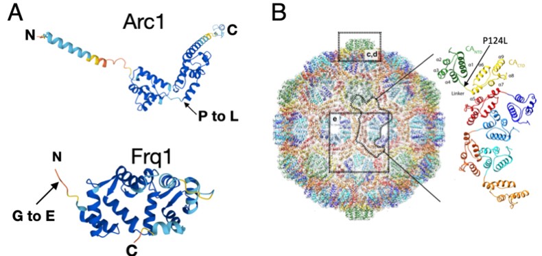
The other non-canonical edit (G-to-A) that stood out was in Frequenin 1 (Frq1), a multi-EF hand containing Ca<sup>2+</sup> binding protein that regulates synaptic transmission, that resulted in a G2E amino acid substitution (location within Frq1shown in panel A above). This glycine residue is conserved in all Frq homologs and is the site of N-myristoylation, a co-translational lipid modification to the glycine after removal of the initiator methionine by an aminopeptidase. Myristoylation tethers Frq proteins to the plasma membrane, with a Ca<sup>2+</sup>-myristoyl switch allowing some family members to cycle on and off membranes when the lipid domain is sequestered in the absence of Ca<sup>2+</sup>. Although the G2E edit is found at lower levels (20% in Ib MNs and 18% in Is MNs), it could create a pool of soluble Frq1 that alters it’s signaling. We plan to functionally assay the significance of this non-canonical edit as well. Compared to edits that alter amino acid sequence, determining how non canonical editing of UTRs might regulate mRNA dynamics is a harder question at this stage and will require more experimental follow-up.
(2) The reviewer noted the last section of the results might be better split into multiple parts as it reads as a long combination of two thoughts.
We agree with the reviewer that the last section is important, but it was disconnected a bit from the main story and was difficult for us to know exactly where to put it. All the data to that point in the paper was collected from our own PatchSeq analysis from individual larval motoneurons. We wanted to compare these results to other large RNAseq datasets obtained from pooled neuronal populations and felt it was best to include this at the end of the results section, as it no longer related to the rules of RNA editing within single neurons. We used these datasets to confirm many of our edits, as well as find evidence for some developmental and neuron-specific cell type edits. We also took advantage of RNAseq from neuronal datasets with altered activity to explore how activity might alter the editing machinery. We felt it better to include that data in this final section given it was not collected from our original PatchSeq approach.
Reviewer #2:
Noted the study provided a unique opportunity to identify RNA editing sites and rates specific to individual motoneuron subtypes, highlighting the RNAseq data was robustly analyzed and high-confidence hits were identified and compared to other RNAseq datasets. The reviewer provided some suggestions for future experiments and requested a few clarifications.
(1) The reviewer asked about Figure 1F and the average editing rate per site described later in the paper.
Indeed, Figure 1F shows the average editing rate for each individual gene for all the Ib and Is cells, so we primarily use that to highlight the variability we find in overall editing rate from around 20% for some sites to 100% for others. The actual editing rate for each site for individual neurons is shown in Figure 4D that plots the rate for every edit site and the overall sum rate for that neuron in particular.
(2) The reviewer also noted that it was unclear where in the VNC the individual motoneurons were located and how that might affect editing.
The precise segment of the larvae for every individual neuron that was sampled by Patch-seq was recorded and that data is accessible in the original Jetti et al 2023 paper if the reader wants to explore any potential anterior to posterior differences in RNA editing. Due to the technical difficulty of the Patch-seq approach, we pooled all the Ib and Is neurons from each segment together to get more statistical power to identify edit sites. We don’t believe segmental identify would be a major regulator of RNA editing, but cannot rule it out.
(3) The reviewer also wondered if including RNAs located both in the nucleus and cytoplasm would influence editing rate.
Given our Patch-seq approach requires us to extract both the cytoplasm and nucleus, we would be sampling both nuclear and cytoplasmic mRNAs. However, as shown in Figure 8 – figure supplement 3 D-F, the vast majority of our edits are found in both polyA mRNA samples and nascent nuclear mRNA samples from other datasets, indicating the editing is occurring co-transcriptionally and within the nucleus. As such, we don't think the inclusion of cytoplasmic mRNA is altering our measured editing rates for most sites. This may not be true for all non-canonical edits, as we did see some differences there, indicating some non-canonical editing may be happening in the cytoplasm as well.
Reviewer #3:
indicated the work provided a valuable resource to access RNA editing in single neurons. The reviewer suggested the value of future experiments to demonstrate the effects of editing events on neuronal function. This will be a major effort for us going forwards, as we indeed have already begun to test the role of editing in mRNAs encoding several presynaptic proteins that regulate synaptic transmission. The reviewer also had several other comments as discussed below.
(1) The reviewer noted that silent mutations could alter codon usage that would result in translational stalling and altered protein production.
This is an excellent point, as silent mutations in the coding region could have a more significant impact if they generate non-preferred rare codons. This is not something we have analyzed, but it certainly is worth considering in future experiments. Our initial efforts are on testing the edits that cause predictive changes in presynaptic proteins based on the amino acid change and their locale in important functional domains, but it is worth considering the silent edits as well as we think about the larger picture of how RNA editing is likely to impact not only protein function but also protein levels.
(2) The reviewer noted future studies could be done using tools like Alphafold to test if the amino acid changes are predicted to alter the structure of proteins with coding edits.
This is an interesting approach, though we don’t have much expertise in protein modeling at that level. We could consider adding this to future studies in collaboration with other modeling labs.
(3) The reviewer wondered if the negative correlation between edits and transcript abundance could indicate edits might be destabilizing the transcripts.
This is an interesting idea, but would need to be experimentally tested. For the few edits we have generated already to begin functionally testing, including our published work with editing in the C-terminus of Complexin, we haven’t seen a change in mRNA levels causes by these edits. However, it would not be surprising to see some edits reducing transcript levels. A set of 5’UTR edits we have generated in Syx1A seem to be reducing protein production and may be acting in such a manner.
(4) The reviewer wondered if the proportion of edits we report in many of the figures is normalized to the length of the transcript, as longer transcripts might have more edits by chance.
The figures referenced by the reviewer (1, 2 and 7) show the number of high-confidence editing sites that fall into the 5’ UTR, 3’ UTR, or CDS categories. Our intention here was to highlight that the majority of the high confidence edits that made it through the stringent filtering process were in the coding region. This would still be true if we normalized to the length of the given gene region. However, it would be interesting to know if these proportions match the expected proportions of edits in these gene regions given a random editing rate per gene region length across the Drosophila genome, although we did not do this analysis.
(5) The reviewer noted that future studies could expand on the work to examine miRNA or other known RBP binding sites that might be altered by the edits.
This is another avenue we could pursue in the future. We did do this analysis for a few of the important genes encoding presynaptic proteins (these are the most interesting to us given the lab’s interest in the synaptic vesicle fusion machinery), but did not find anything obvious for this smaller subset of targets.
(6) The reviewer suggested sequence context for Adar could also be investigated for the hits we identified.
We haven’t pursued this avenue yet, but it would be of interest to do in the future. In a similar vein, it would be informative to identify intron-exon base pairing that could generate the dsDNA template on which ADAR acts.
(7) The reviewer noted the disconnect between Adar mRNA levels and overall editing levels reported in Figure 4A/B.
Indeed, the lack of correlation between overall editing levels and Adar mRNA abundance has been noted previously in many studies. For the type of single cell Patch-seq approach we took to generate our RNAseq libraries, the absolute amount of less abundant transcripts obtained from a single neuron can be very noisy. As such, the few neurons with no detectable Adar mRNA are likely to represent that single neuron noise in the sampling. Per the reviewer’s question, these figure panels only show A-to-I edits, so they are specific to ADAR.
(8) The reviewer notes the scale in Figure 5D can make it hard to visualize the actual impact of the changes.
The intention of Figure 5D was to address the question of whether sites with high Ib/Is editing differences were simply due to higher Ib or Is mRNA expression levels. If this was the case, then we would expect to see highly edited sites have large Ib/Is TPM differences. Instead, as the figure shows, the vast majority of highly-edited sites were in mRNAs that were NOT significantly different between Ib and Is (red dots in graph) and are therefore clustered together near “0 Difference in TPMs”. TPMs and editing levels for all edit sites can be found in Table 1, and a visualization of these data for selected sites is shown in Figure 5E.
These restrictions persist today, in the form of practices.d-undefined, .lh-undefined { background-color: rgba(0, 0, 0, 0.2) !important; }2A they/them Pollicino, Jillian McCarten like dropping names from voter rolls, requiring photo IDs, and limits to early voting—the burdens of which are felt disproportionately by low-income people, people of color, and others who lack the time or resources to jump through these additional bureaucratic hoops.
These restrictions do persist today; between transportation barriers and computer literacy barriers alone. I have seen first hand several people unable to vote during the last town election because they were unable to get to the fire hall where voting was taking place. And for many, voting online requires one on one help with the technology; something not everyone has.
Author response:
The following is the authors’ response to the current reviews.
Reviewer #1 (Public review):
In this manuscript, Hoon Cho et al. present a novel investigation into the role of PexRAP, an intermediary in ether lipid biosynthesis, in B cell function, particularly during the Germinal Center (GC) reaction. The authors profile lipid composition in activated B cells both in vitro and in vivo, revealing the significance of PexRAP. Using a combination of animal models and imaging mass spectrometry, they demonstrate that PexRAP is specifically required in B cells. They further establish that its activity is critical upon antigen encounter, shaping B cell survival during the GC reaction. Mechanistically, they show that ether lipid synthesis is necessary to modulate reactive oxygen species (ROS) levels and prevent membrane peroxidation.
Highlights of the Manuscript:
The authors perform exhaustive imaging mass spectrometry (IMS) analyses of B cells, including GC B cells, to explore ether lipid metabolism during the humoral response. This approach is particularly noteworthy given the challenge of limited cell availability in GC reactions, which often hampers metabolomic studies. IMS proves to be a valuable tool in overcoming this limitation, allowing detailed exploration of GC metabolism.
The data presented is highly relevant, especially in light of recent studies suggesting a pivotal role for lipid metabolism in GC B cells. While these studies primarily focus on mitochondrial function, this manuscript uniquely investigates peroxisomes, which are linked to mitochondria and contribute to fatty acid oxidation (FAO). By extending the study of lipid metabolism beyond mitochondria to include peroxisomes, the authors add a critical dimension to our understanding of B cell biology.
Additionally, the metabolic plasticity of B cells poses challenges for studying metabolism, as genetic deletions from the beginning of B cell development often result in compensatory adaptations. To address this, the authors employ an acute loss-of-function approach using two conditional, cell-type-specific gene inactivation mouse models: one targeting B cells after the establishment of a pre-immune B cell population (Dhrs7b^f/f, huCD20-CreERT2) and the other during the GC reaction (Dhrs7b^f/f; S1pr2-CreERT2). This strategy is elegant and well-suited to studying the role of metabolism in B cell activation.
Overall, this manuscript is a significant contribution to the field, providing robust evidence for the fundamental role of lipid metabolism during the GC reaction and unveiling a novel function for peroxisomes in B cells.
Comments on revisions:
There are still some discrepancies in gating strategies. In Fig. 7B legend (lines 1082-1083), they show representative flow plots of GL7+ CD95+ GC B cells among viable B cells, so it is not clear if they are IgDneg, as the rest of the GC B cells aforementioned in the text.
We apologize for missing this item in need of correction in the revision and sincerely thank the reviewer for the stamina and care in picking this up. The data shown in Fig. 7B represented cells (events) in the IgD<sup>neg</sup> Dump<sup>neg</sup> viable lymphoid gate. We will correct this omission/blemish in the final revision that becomes the version of record.
Western blot confirmation: We understand the limitations the authors enumerate. Perhaps an RT-qPCR analysis of the Dhrs7b gene in sorted GC B cells from the S1PR2-CreERT2 model could be feasible, as it requires a smaller number of cells. In any case, we agree with the authors that the results obtained using the huCD20-CreERT2 model are consistent with those from the S1PR2-CreERT2 model, which adds credibility to the findings and supports the conclusion that GC B cells in the S1PR2-CreERT2 model are indeed deficient in PexRAP.
We will make efforts to go back through the manuscript and highlight this limitation to readers, i.e., that we were unable to get genetic evidence to assess what degree of "counter-selection" applied to GC B cells in our experiments.
We agree with the referee that optimally to support the Imaging Mass Spectrometry (IMS) data showing perturbations of various ether lipids within GC after depletion of PexRAP, it would have been best if we could have had a qRT2-PCR that allowed quantitation of the Dhrs7b-encoded mRNA in flow-purified GC B cells, or the extent to which the genomic DNA of these cells was in deleted rather than 'floxed' configuration.
While the short half-life of ether lipid species leads us to infer that the enzymatic function remains reduced/absent, it definitely is unsatisfying that the money for experiments ran out in June and the lab members had to move to new jobs.
Lines 222-226: We believe the correct figure is 4B, whereas the text refers to 4C.
As for the 1st item, we apologize and will correct this error.
Supplementary Figure 1 (line 1147): The figure title suggests that the data on T-cell numbers are from mice in a steady state. However, the legend indicates that the mice were immunized, which means the data are not from steady-state conditions.
We will change the wording both on line 1147 and 1152.
Reviewer #2 (Public review):
Summary:
In this study, Cho et al. investigate the role of ether lipid biosynthesis in B cell biology, particularly focusing on GC B cell, by inducible deletion of PexRAP, an enzyme responsible for the synthesis of ether lipids.
Strengths:
Overall, the data are well-presented, the paper is well-written and provides valuable mechanistic insights into the importance of PexRAP enzyme in GC B cell proliferation.
Weaknesses:
More detailed mechanisms of the impaired GC B cell proliferation by PexRAP deficiency remain to be further investigated. In minor part, there are issues for the interpretation of the data which might cause confusions by readers.
Comments on revisions:
The authors improved the manuscript appropriately according to my comments.
To re-summarize, we very much appreciate the diligence of the referees and Editors in re-reviewing this work at each cycle and helping via constructive peer review, along with their favorable comments and overall assessments. The final points will be addressed with minor edits since there no longer is any money for further work and the lab people have moved on.
The following is the authors’ response to the original reviews.
Reviewer #1 (Public review):
In this manuscript, Sung Hoon Cho et al. presents a novel investigation into the role of PexRAP, an intermediary in ether lipid biosynthesis, in B cell function, particularly during the Germinal Center (GC) reaction. The authors profile lipid composition in activated B cells both in vitro and in vivo, revealing the significance of PexRAP. Using a combination of animal models and imaging mass spectrometry, they demonstrate that PexRAP is specifically required in B cells. They further establish that its activity is critical upon antigen encounter, shaping B cell survival during the GC reaction.
Mechanistically, they show that ether lipid synthesis is necessary to modulate reactive oxygen species (ROS) levels and prevent membrane peroxidation.
Highlights of the Manuscript:
The authors perform exhaustive imaging mass spectrometry (IMS) analyses of B cells, including GC B cells, to explore ether lipid metabolism during the humoral response. This approach is particularly noteworthy given the challenge of limited cell availability in GC reactions, which often hampers metabolomic studies. IMS proves to be a valuable tool in overcoming this limitation, allowing detailed exploration of GC metabolism.
The data presented is highly relevant, especially in light of recent studies suggesting a pivotal role for lipid metabolism in GC B cells. While these studies primarily focus on mitochondrial function, this manuscript uniquely investigates peroxisomes, which are linked to mitochondria and contribute to fatty acid oxidation (FAO). By extending the study of lipid metabolism beyond mitochondria to include peroxisomes, the authors add a critical dimension to our understanding of B cell biology.
Additionally, the metabolic plasticity of B cells poses challenges for studying metabolism, as genetic deletions from the beginning of B cell development often result in compensatory adaptations. To address this, the authors employ an acute loss-of-function approach using two conditional, cell-type-specific gene inactivation mouse models: one targeting B cells after the establishment of a pre-immune B cell population (Dhrs7b^f/f, huCD20-CreERT2) and the other during the GC reaction (Dhrs7b^f/f; S1pr2-CreERT2). This strategy is elegant and well-suited to studying the role of metabolism in B cell activation.
Overall, this manuscript is a significant contribution to the field, providing robust evidence for the fundamental role of lipid metabolism during the GC reaction and unveiling a novel function for peroxisomes in B cells.
We appreciate these positive reactions and response, and agree with the overview and summary of the paper's approaches and strengths.
However, several major points need to be addressed:
Major Comments:
Figures 1 and 2
The authors conclude, based on the results from these two figures, that PexRAP promotes the homeostatic maintenance and proliferation of B cells. In this section, the authors first use a tamoxifen-inducible full Dhrs7b knockout (KO) and afterwards Dhrs7bΔ/Δ-B model to specifically characterize the role of this molecule in B cells. They characterize the B and T cell compartments using flow cytometry (FACS) and examine the establishment of the GC reaction using FACS and immunofluorescence. They conclude that B cell numbers are reduced, and the GC reaction is defective upon stimulation, showing a reduction in the total percentage of GC cells, particularly in the light zone (LZ).
The analysis of the steady-state B cell compartment should also be improved. This includes a more detailed characterization of MZ and B1 populations, given the role of lipid metabolism and lipid peroxidation in these subtypes.
Suggestions for Improvement:
B Cell compartment characterization: A deeper characterization of the B cell compartment in non-immunized mice is needed, including analysis of Marginal Zone (MZ) maturation and a more detailed examination of the B1 compartment. This is especially important given the role of specific lipid metabolism in these cell types. The phenotyping of the B cell compartment should also include an analysis of immunoglobulin levels on the membrane, considering the impact of lipids on membrane composition.
Although the manuscript is focused on post-ontogenic B cell regulation in Ab responses, we believe we will be able to polish a revised manuscript through addition of results of analyses suggested by this point in the review: measurement of surface IgM on and phenotyping of various B cell subsets, including MZB and B1 B cells, to extend the data in Supplemental Fig 1H and I. Depending on the level of support, new immunization experiments to score Tfh and analyze a few of their functional molecules as part of a B cell paper may be feasible.
Addendum / update of Sept 2025: We added new data with more on MZB and B1 B cells, surface IgM, and on Tfh populations.
GC Response Analysis Upon Immunization: The GC response characterization should include additional data on the T cell compartment, specifically the presence and function of Tfh cells. In Fig. 1H, the distribution of the LZ appears strikingly different. However, the authors have not addressed this in the text. A more thorough characterization of centroblasts and centrocytes using CXCR4 and CD86 markers is needed.
The gating strategy used to characterize GC cells (GL7+CD95+ in IgD− cells) is suboptimal. A more robust analysis of GC cells should be performed in total B220+CD138− cells.
We first want to apologize the mislabeling of LZ and DZ in Fig 1H. The greenish-yellow colored region (GL7<sup>+</sup> CD35<sup>+</sup>) indicate the DZ and the cyan-colored region (GL7<sup>+</sup> CD35<sup>+</sup>) indicates the LZ. Addendum / update of Sept 2025: We corrected the mistake, and added new experimental data using the CD138 marker to exclude preplasmablasts.
As a technical note, we experienced high background noise with GL7 staining uniquely with PexRAP deficient (Dhrs7b<sup>f/f</sup>; Rosa26-CreER<sup>T2</sup>) mice (i.e., not WT control mice). The high background noise of GL7 staining was not observed in B cell specific KO of PexRAP (Dhrs7b<sup>f/f</sup>; huCD20-CreER<sup>T2</sup>). Two formal possibilities to account for this staining issue would be if either the expression of the GL7 epitope were repressed by PexRAP or the proper positioning of GL7<sup>+</sup> cells in germinal center region were defective in PexRAPdeficient mice (e.g., due to an effect on positioning cues from cell types other than B cells). In a revised manuscript, we will fix the labeling error and further discuss the GL7 issue, while taking care not to be thought to conclude that there is a positioning problem or derepression of GL7 (an activation antigen on T cells as well as B cells).
While the gating strategy for an overall population of GC B cells is fairly standard even in the current literature, the question about using CD138 staining to exclude early plasmablasts (i.e., analyze B220<sup>+</sup> CD138<sup>neg</sup> vs B220<sup>+</sup> CD138<sup>+</sup>) is interesting. In addition, some papers like to use GL7<sup>+</sup> CD38<sup>neg</sup> for GC B cells instead of GL7<sup>+</sup> Fas (CD95)<sup>+</sup>, and we thank the reviewer for suggesting the analysis of centroblasts and centrocytes. For the revision, we will try to secure resources to revisit the immunizations and analyze them for these other facets of GC B cells (including CXCR4/CD86) and for their GL7<sup>+</sup> CD38<sup>neg</sup>. B220<sup>+</sup> CD138<sup>-</sup> and B220<sup>+</sup> CD138<sup>+</sup> cell populations.
We agree that comparison of the Rosa26-CreERT2 results to those with B cell-specific lossof-function raise a tantalizing possibility that Tfh cells also are influenced by PexRAP. Although the manuscript is focused on post-ontogenic B cell regulation in Ab responses, we hope to add a new immunization experiments that scores Tfh and analyzes a few of their functional molecules could be added to this B cell paper, depending on the ability to wheedle enough support / fiscal resources.
Addendum / update of Sept 2025: Within the tight time until lab closure, and limited $$, we were able to do experiments that further reinforced the GC B cell data - including stains for DZ vs LZ sub-subsetting - and analyzed Tfh cells. We were not able to explore changes in functional antigenic markers on the GC B or Tfh cells.
The authors claim that Dhrs7b supports the homeostatic maintenance of quiescent B cells in vivo and promotes effective proliferation. This conclusion is primarily based on experiments where CTV-labeled PexRAP-deficient B cells were adoptively transferred into μMT mice (Fig. 2D-F). However, we recommend reviewing the flow plots of CTV in Fig. 2E, as they appear out of scale. More importantly, the low recovery of PexRAP-deficient B cells post-adoptive transfer weakens the robustness of the results and is insufficient to conclusively support the role of PexRAP in B cell proliferation in vivo.
In the revision, we will edit the text and try to adjust the digitized cytometry data to allow more dynamic range to the right side of the upper panels in Fig. 2E, and otherwise to improve the presentation of the in vivo CTV result. However, we feel impelled to push back respectfully on some of the concern raised here. First, it seems to gloss over the presentation of multiple facets of evidence. The conclusion about maintenance derives primarily from Fig. 2C, which shows a rapid, statistically significant decrease in B cell numbers (extending the finding of Fig. 1D, a more substantial decrease after a bit longer a period). As noted in the text, the rate of de novo B cell production does not suffice to explain the magnitude of the decrease.
In terms of proliferation, we will improve presentation of the Methods but the bottom line is that the recovery efficiency is not bad (comparing to prior published work) inasmuch as transferred B cells do not uniformly home to spleen. In a setting where BAFF is in ample supply in vivo, we transferred equal numbers of cells that were equally labeled with CTV and counted B cells. The CTV result might be affected by lower recovered B cell with PexRAP deficiency, generally, the frequencies of CTV<sup>low</sup> divided population are not changed very much. However, it is precisely because of the pitfalls of in vivo analyses that we included complementary data with survival and proliferation in vitro. The proliferation was attenuated in PexRAP-deficient B cells in vitro; this evidence supports the conclusion that proliferation of PexRAP knockout B cells is reduced. It is likely that PexRAP deficient B cells also have defect in viability in vivo as we observed the reduced B cell number in PexRAP-deficient mice. As the reviewer noticed, the presence of a defect in cycling does, in the transfer experiments, limit the ability to interpret a lower yield of B cell population after adoptive transfer into µMT recipient mice as evidence pertaining to death rates. We will edit the text of the revision with these points in mind.
In vitro stimulation experiments: These experiments need improvement. The authors have used anti-CD40 and BAFF for B cell stimulation; however, it would be beneficial to also include antiIgM in the stimulation cocktail. In Fig. 2G, CTV plots do not show clear defects in proliferation, yet the authors quantify the percentage of cells with more than three divisions. These plots should clearly display the gating strategy. Additionally, details about histogram normalization and potential defects in cell numbers are missing. A more in-depth analysis of apoptosis is also required to determine whether the observed defects are due to impaired proliferation or reduced survival.
As suggested by reviewer, testing additional forms of B cell activation can help explore the generality (or lack thereof) of findings. We plan to test anti-IgM stimulation together with anti-CD40 + BAFF as well as anti-IgM + TLR7/8, and add the data to a revised and final manuscript.
Addendum / update of Sept 2025: The revision includes results of new experiments in which anti-IgM was included in the stimulation cocktail, as well as further data on apoptosis and distinguishing impaired cycling / divisions from reduced survival .
With regards to Fig. 2G (and 2H), in the revised manuscript we will refine the presentation (add a demonstration of the gating, and explicate histogram normalization of FlowJo).
It is an interesting issue in bioscience, but in our presentation 'representative data' really are pretty representative, so a senior author is reminded of a comment Tak Mak made about a reduction (of proliferation, if memory serves) to 0.7 x control. [His point in a comment to referees at a symposium related that to a salary reduction by 30% :) A mathematical alternative is to point out that across four rounds of division for WT cells, a reduction to 0.7x efficiency at each cycle means about 1/4 as many progeny.]
We will try to edit the revision (Methods, Legends, Results, Discussion] to address better the points of the last two sentences of the comment, and improve the details that could assist in replication or comparisons (e.g., if someone develops a PexRAP inhibitor as potential therapeutic).
For the present, please note that the cell numbers at the end of the cultures are currently shown in Fig 2, panel I. Analogous culture results are shown in Fig 8, panels I, J, albeit with harvesting at day 5 instead of day 4. So, a difference of ≥ 3x needs to be explained. As noted above, a division efficiency reduced to 0.7x normal might account for such a decrease, but in practice the data of Fig. 2I show that the number of PexRAP-deficient B cells at day 4 is similar to the number plated before activation, and yet there has been a reasonable amount of divisions. So cell numbers in the culture of mutant B cells are constant because cycling is active but decreased and insufficient to allow increased numbers ("proliferation" in the true sense) as programmed death is increased. In line with this evidence, Fig 8G-H document higher death rates [i.e., frequencies of cleaved caspase3<sup>+</sup> cell and Annexin V<sup>+</sup> cells] of PexRAP-deficient B cells compared to controls. Thus, the in vitro data lead to the conclusion that both decreased division rates and increased death operate after this form of stimulation.
An inference is that this is the case in vivo as well - note that recoveries differed by ~3x (Fig. 2D), and the decrease in divisions (presentation of which will be improved) was meaningful but of lesser magnitude (Fig. 2E, F).
Reviewer #2 (Public review):
Summary:
In this study, Cho et al. investigate the role of ether lipid biosynthesis in B cell biology, particularly focusing on GC B cell, by inducible deletion of PexRAP, an enzyme responsible for the synthesis of ether lipids.
Strengths:
Overall, the data are well-presented, the paper is well-written and provides valuable mechanistic insights into the importance of PexRAP enzyme in GC B cell proliferation.
We appreciate this positive response and agree with the overview and summary of the paper's approaches and strengths.
Weaknesses:
More detailed mechanisms of the impaired GC B cell proliferation by PexRAP deficiency remain to be further investigated. In the minor part, there are issues with the interpretation of the data which might cause confusion for the readers.
Issues about contributions of cell cycling and divisions on the one hand, and susceptibility to death on the other, were discussed above, amplifying on the current manuscript text. The aggregate data support a model in which both processes are impacted for mature B cells in general, and mechanistically the evidence and work focus on the increased ROS and modes of death. Although the data in Fig. 7 do provide evidence that GC B cells themselves are affected, we agree that resource limitations had militated against developing further evidence about cycling specifically for GC B cells. We will hope to be able to obtain sufficient data from some specific analysis of proliferation in vivo (e.g., Ki67 or BrdU) as well as ROS and death ex vivo when harvesting new samples from mice immunized to analyze GC B cells for CXCR4/CD86, CD38, CD138 as indicated by Reviewer 1. As suggested by Reviewer 2, we will further discuss the possible mechanism(s) by which proliferation of PexRAP-deficient B cells is impaired. We also will edit the text of a revision where to enhance clarity of data interpretation - at a minimum, to be very clear that caution is warranted in assuming that GC B cells will exhibit the same mechanisms as cultures in vitro-stimulated B cells.
Addendum / update of Sept 2025: We were able to obtain results of intravital BrdU incorporation into GC B cells to measure cell cycling rates. The revised manuscript includes these results as well as other new data on apoptosis / survival, while deleting the data about CD138 populations whose interpretation was reasonably questioned by the referees.
Reviewer #1 (Recommendations for the authors):
We believe the evidence presented to support the role of PexRAP in protecting B cells from cell death and promoting B cell proliferation is not sufficiently robust and requires further validation in vivo. While the study demonstrates an increase in ether lipid content within the GC compartment, it also highlights a reduction in mature B cells in PexRAP-deficient mice under steady-state conditions. However, the IMS results (Fig. 3A) indicate that there are no significant differences in ether lipid content in the naïve B cell population. This discrepancy raises an intriguing point for discussion: why is PexRAP critical for B cell survival under steady-state conditions?
We thank the referee for all their care and input, and we agree that further intravital analyses could strengthen the work by providing more direct evidence of impairment of GC B cells in vivo. To revise and improve this manuscript before creation of a contribution of record, we performed new experiments to the limit of available funds and have both (i) added these new data and (ii) sharpened the presentation to correct what we believe to be one inaccurate point raised in the review.
(A) Specifically, we immunized mice with a B cell-specific depletion of PexRAP (Dhrs7b<sup>D/D-B</sup> mice) and measured a variety of readouts of the GC B cells' physiology in vivo: proliferation by intravital incorporation of BrdU, ROS in the viable GC B cell gate, and their cell death by annexin V staining directly ex vivo. Consistent with the data with in vitro activated B cells, these analyses showed increased ROS (new - Fig. 7D) and higher frequencies of Annexin V<sup>+</sup> 7AAD<sup>+</sup> in GC B cells (GL7<sup>+</sup> CD38<sup>-</sup> B cell-gate) of immunized Dhrs7b<sup>D/D-B</sup> mice compared with WT controls (huCD20-CreERT2<sup>+/-</sup>, Dhrs7b<sup>+/+</sup>) (new - Fig. 7E). Collectively, these results indicate that PexRAP aids (directly or indirectly) in controlling ROS in GC B cells and reduces B cell death, likely contributing to the substantially decreased overall GC B cell population. These new data are added to the revised manuscript in Figure 7.
Moreover, in each of two independent experiments (each comprising 3 vs 3 immunized mice), BrdU<sup>+</sup> events among GL7<sup>+</sup> CD38<sup>-</sup> (GC B cell)-gated cells were reduced in the B cell-specific PexRAP knockouts compared with WT controls (new, Fig. 7F and Supplemental Fig 6E). This result on cell cycle rates in vivo is presented with caution in the revised manuscript text because the absolute labeling fractions were somewhat different in Expt 1 vs Expt 2. This situation affords a useful opportunity to comment on the culture of "P values" and statistical methods. It is intriguing to consider how many successful drugs are based on research published back when the standard was to interpret a result of this sort more definitively despite a merged "P value" that was not a full 2 SD different from the mean. In the optimistic spirit of the eLife model, it can be for the attentive reader to decide from the data (new, Fig. 7F and Supplemental Fig 6E) whether to interpret the BrdU results more strongly that what we state in the revised text.
(B) On the issue of whether or not the loss of PexRAP led to perturbations of the lipidome of B cells prior to activation, we have edited the manuscript to do a better job making this point more clear.
We point out to readers that in the resting, pre-activation state abnormalities were detected in naive B cells, not just in activated and GC B cells. In brief, the IMS analysis and LC-MS-MS analysis detected statistically significant differences in some, but not all, the ether phospholipids species in PexRAP deficient cells (some of which was in Supplemental Figure 2 of the original version).
With this appropriate and helpful concern having been raised, we realize that this important point merited inclusion in the main figures. We point specifically to a set of phosphatidyl choline ions shown in Fig. 3 (revised - panels A, B, D) of the revised manuscript (PC O-36:5; PC O-38:5; PC O-40:6 and -40:7).
For this ancillary record (because a discourse on the limitations of each analysis), we will note issues such as the presence of many non-B cells in each pixel of the IMS analyses (so that some or many "true positives" will fail to achieve a "significant difference") and for the naive B cells, differential rates of synthesis, turnover, and conversion (e.g., addition of another 2-carbon unit or saturation / desaturation of one side-chain). To the extent the concern reflects some surprise and perhaps skepticism that what seem relatively limited differences (many species appear unaffected, etc), we share in the sentiment. But the basic observation is that there are differences, and a reasonable connection between the altered lipid profile and evidence of effects on survival or proliferation (i.e., integration of survival and cell cycling / division).
Additionally, it would be valuable to evaluate the humoral response in a T-independent setting. This would clarify whether the role of PexRAP is restricted to GC B cells or extends to activated B cells in general.
We agree that this additional set of experiments would be nice and would extend work incrementally by testing the generality of the findings about Ab responses. The practical problem is that money and time ran out while testing important items that strengthen the evidence about GC B cells.
Finally, the manuscript would benefit from a thorough revision to improve its readability and clarity. Including more detailed descriptions of technical aspects, such as the specific stimuli and time points used in analyses, would greatly enhance the flow and comprehension of the study. Furthermore, the authors should review figure labeling to ensure consistency throughout the manuscript, and carefully cite the relevant references. For instance, S1PR2 CreERT2 mouse is established by Okada and Kurosaki (Shinnakasu et al ,Nat. Immunol, 2016)
We appreciate this feedback and comment, inasmuch as both the clarity and scholarship matter greatly to us for a final item of record. For the revision, we have given our best shot to editing the text in the hopes of improved clarity, reduction of discrepancies (helpfully noted in the Minor Comments), and further detail-rich descriptions of procedures. We also edited the figure labeling to give a better consistency. While we note that the appropriate citation of Shinnakasu et al (2016) was ref. #69 of the original and remains as a citation, we have rechecked other referencing and try to use citations with the best relevant references.
Minor Comments: The labeling of plots in Fig. 2 should be standardized. For example, in Fig. 2C, D, and G, the same mouse strain is used, yet the Cre+ mouse is labeled differently in each plot.
We agree and have tried to tighten up these features in the panels noted as well as more generally (e.g., Fig. 4, 5, 6, 7, 9; consistency of huCD20-CreERT2 / hCD20CreERT2).
According to the text, the results shown in Fig. 1G and H correspond to a full KO (Dhrs7b^f/f; Rosa26-CreERT2 mice). However, Fig. 1H indicates that the bottom image corresponds to Dhrs7b^f/f, huCD20-CreERT2 mice (Dhrs7bΔ/Δ -B).
We have corrected Fig. 1H to be labeled as Dhrs7b<sup>Δ/Δ</sup> (with the data on Dhrs7b<sup>Δ/Δ-B</sup> presented in Supplemental Figure 4A, which is correctly labeled). Thank you for picking up this error that crept in while using copy/paste in preparation of figure panels and failing to edit out the "-B"!
Similarly, the gating strategy for GC cells in the text mentions IgD− cells, while the figure legend refers to total viable B cells. These discrepancies need clarification.
We believe we located and have corrected this issue in the revised manuscript.
Figures 3 and 4. The authors claim that B cell expression of PexRAP is required to achieve normal concentrations of ether phospholipids.
Suggestions for Improvement:
Lipid Metabolism Analysis: The analysis in Fig. 3 is generally convincing but could be strengthened by including an additional stimulation condition such as anti-IgM plus antiCD40. In Fig. 4C, the authors display results from the full KO model. It would be helpful to include quantitative graphs summarizing the parameters displayed in the images.
We have performed new experiments (anti-IgM + anti-CD40) and added the data to the revised manuscript (new - Supplemental Fig. 2H and Supplemental Fig 6, D & F). Conclusions based on the effects are not changed from the original.
As a semantic comment and point of scientific process, any interpretation ("claim") can - by definition - only be taken to apply to the conditions of the experiment. Nonetheless, it is inescapable that at least for some ether P-lipids of naive, resting B cells, and for substantially more in B cells activated under the conditions that we outline, B cell expression of PexRAP is required.
With regards to the constructive suggestion about a new series of lipidomic analyses, we agree that for activated B cells it would be nice and increase insight into the spectrum of conditions under which the PexRAP-deficient B cells had altered content of ether phospholipids. However, in light of the costs of metabolomic analyses and the lack of funds to support further experiments, and the accuracy of the point as stated, we prioritized the experiments that could fit within the severely limited budget.
[One can add that our results provide a premise for later work to analyze a time course after activation, and to perform isotopomer (SIRM) analyses with [13] C-labeled acetate or glucose, so as to understand activation-induced increases in the overall To revise the manuscript, we did however extrapolate from the point about adding BCR cross-linking to anti-CD40 as a variant form of activating the B cells for measurements of ROS, population growth, and rates of division (CTV partitioning). The results of these analyses, which align with and thereby strengthen the conclusions about these functional features from experiments with anti-CD40 but no anti-IgM, are added to Supplemental Fig 2H and Supplemental Fig 6D, F.
Figures 5, 6, and 7
The authors claim that Dhrs7b in B cells shapes antibody affinity and quantity. They use two mouse models for this analysis: huCD20-CreERT2 and Dhrs7b f/f; S1pr2-CreERT2 mice.
Suggestions for Improvement:
Adaptive immune response characterization: A more comprehensive characterization of the adaptive immune response is needed, ideally using the Dhrs7b f/f; S1pr2-CreERT2 model. This should include: Analysis of the GC response in B220+CD138− cells. Class switch recombination analysis. A detailed characterization of centroblasts, centrocytes, and Tfh populations. Characterization of effector cells (plasma cells and memory cells).
Within the limits of time and money, we have performed new experiments prompted by this constructive set of suggestions.
Specifically, we analyzed the suggested read-outs in the huCD20-CreERT2, Dhrs7b<sup>f/f</sup> model after immunization, recognizing that it trades greater signal-noise for the fact that effects are due to a mix of the impact on B cells during clonal expansion before GC recruitment and activities within the GC. In brief, the results showed that
(a) the GC B cell population - defined as CD138<sup>neg</sup> GL7<sup>+</sup> CD38<sup>lo/neg</sup> IgD<sup>neg</sup> B cells - was about half as large for PexRAP-deficient B cells net of any early- or preplasmablasts (CD138<sup>+</sup> events) (new - Fig 5G);
(b) the frequencies of pre- / early plasmablasts (CD138<sup>+</sup> GL7<sup>+</sup> CD38<sup>neg</sup>) events (see new - Fig. 6H, I; also, new Supplemental Fig 5D) were so low as to make it unlikely that our data with the S1pr2-CreERT2 model (in Fig 7B, C) would be affected meaningfully by analysis of the CD138 levels;
(c) There was a modest decrease in centrocytes (LZ) but not centroblasts (DZ) (new - Fig 5H, I) - consistent with the immunohistochemical data of Supplemental Fig. 5A-C).
Because of time limitations (the "shelf life" of funds and the lab) and insufficient stock of the S1pr2-CreERT2, Dhrs7b<sup>f/f</sup> mice as well as those that would be needed as adoptive transfer recipients because of S1PR2 expression in (GC-)Tfh, the experiments were performed instead with the huCD20-CreERT2, Dhrs7b<sup>f/f</sup> model. We would also note that using this Cre transgene better harmonizes the centrocyte/centroblast and Tfh data with the existing data on these points in Supplemental Fig. 4.
(d) Of note, the analyses of Tfh and GC-Tfh phenotype cells using the huCD20-CreERT2 B cell type-specific inducible Cre system to inactivate Dhrs7b (new - Supplemental Fig 1G-I; which, along with new - Supplemental Fig 5E) provide evidence of an abnormality that must stem from a function or functions of PexRAP in B cells, most likely GC B cells. Specifically, it is known that the GC-Tfh population proliferates and is supported by the GC B cells, and the results of B cell-specific deletion show substantial reductions in Tfh cells (both the GC-Tfh gating and the wider gate for plots of CXCR5/PD-1/ fluorescence of CD4 T cells
Timepoint Consistency: The NP response (Fig. 5) is analyzed four weeks postimmunization, whereas SRBC (Supp. Fig. 4) and Fig. 7 are analyzed one week or nine days post-immunization. The NP system analysis should be repeated at shorter timepoints to match the peak GC reaction.
This comment may stem from a misunderstanding. As diagrammed in Fig. 5A, the experiments involving the NP system were in fact measured at 7 d after a secondary (booster) immunization. That timing is approximately the peak period and harmonizes with the 7 d used for harvesting SRBC-immunized mice. So in fact the data with each system were obtained at a similar time point. Of course the NP experiments involved a second immunization so that many plasma cell and Ab responses derived from memory B cells generated by the primary immunization. However, the field at present is dominated by the view that the vast majority of the GC B cells after this second immunization (which historically we perform with alum adjuvant) are recruited from the naive rather than the memory B cell pool. For the revised manuscript, we have taken care that the Methods, Legend, and Figure provide the information to readers, and expanded the statement of a rationale.
It may seem a technicality but under NIH regulations we are legally obligated to try to minimize mouse usage. It also behooves researchers to use funds wisely. In line with those imperatives, we used systems that would simultaneously allow analyses of GC B cells, identification of affinity maturation (which is minimal in our hands at a 7 d time point after primary NP-carrier immunization), and a switched repertoire (also minimal), and where with each immunogen the GC were scored at 7-9 d after immunization (9 d refers to the S1pr2-CreERT2 experiments). Apart from the end of funding, we feel that what little might be learned from performing a series of experiments that involve harvests 7 d after a primary immunization with NP-ovalbumin cannot well be justified.
In vitro plasma cell differentiation: Quantification is missing for plasma cell differentiation in vitro (Supp. Fig. 4). The stimulus used should also be specified in the figure legend. Given the use of anti-CD40, differentiation towards IgG1 plasma cells could provide additional insights.
As suggested by reviewer, we have added the results of quantifying the in vitro plasma cell differentiation in Supplemental Fig 6B. Also, we edited the Methods and Supplemental Figure Legend to give detailed information of in vitro stimulation.
Proliferation and apoptosis analysis: The observed defects in the humoral response should be correlated with proliferation and apoptosis analyses, including Ki67 and Caspase markers.
As suggested by the review, we have performed new experiment and analyzed the frequencies of cell death by annexin V staining, and elected to use intravital uptake of BrdU as a more direct measurement of S phase / cell cycling component of net proliferation. The new results are now displayed in Figure 5 and Supplemental Fig. 5.
Western blot confirmation: While the authors have demonstrated the absence of PexRAP protein in the huCD20-CreERT2 model, this has not been shown in GC B cells from the Dhrs7b f/f; S1pr2-CreERT2 model. This confirmation is necessary to validate the efficiency of Dhrs7b deletion.
We were unable to do this for technical reasons expanded on below. For the revision, we have edited in a bit of text more explicitly to alert readers to the potential impact of counter-selection on interpretation of the findings with GC B cells. Before entering the GC, B cells have undergone many divisions, so if there were major pre-GC counterselection, in all likelihood the GC B cells would PexRAP-sufficient. To recap from the original manuscript and the new data we have added, IMS shows altered lipid profiles in the GC B cells and the literature indicates that the lipids are short-lived, requiring de novo resynthesis. The BrdU, ROS, and annexin V data show that GC B cells are abnormal. Accordingly, abnormal GC B cells represent the parsimonious or straightforward interpretation of the new results with GC-Tfh cell prevalence.
While we take these findings together to suggest that counterselection (i.e., a Western result showing normal levels of PexRAP in the GC B cells) seems unlikely, it is formally possible and would mean that the in situ defects of GC B cells arose due to environmental influences of the PexRAP-deficient B cells during the developmental history of the WT B cells observed in the GC.
Having noted all that, we understand that concerns about counter-selection are an issue if a reader accepts the data showing that mutant (PexRAP-deficient) B cells tend to proliferate less and die more readily. Indeed, one can speculate that were we also to perform competition experiments in which the Ighb, Cd45.2 B cells (WT or Dhrs7b D/D) are mixed with equal numbers of Igha, Cd45.1 competitors, the differences would become much greater. With this in mind, Western blotting of flow-purified GC B cells might give a sense of how much counter-selection has occurred.
That said, the Westerns need at least 2.5 x 10<sup>6</sup> B cells (those in the manuscript used five million, 5 x 10<sup>6</sup>) and would need replication. Taken together with the observation that ~200,000 GC B cells (on average) were measured in each B cell-specific knockout mouse after immunization (Fig. 1, Fig 5) and taking into account yields from sorting, each Western would require some 20-25 tamoxifen-injected ___-CreERT2, Dhrs7b f/f mice, and about half again that number as controls. The expiry of funds prohibited the time and costs of generating that many mice (>70) and flow-purified GC B cells.
Figure 8
The authors claim that Dhrs7b contributes to the modulation of ROS, impacting B cell proliferation.
Suggestions for Improvement:
GC ROS Analysis: The in vitro ROS analysis should be complemented by characterizing ROS and lipid peroxidation in the GC response using the Dhrs7b f/f; S1pr2-CreERT2 model. Flow cytometry staining with H2DCFDA, MitoSOX, Caspase-3, and Annexin V would allow assessment of ROS levels and cell death in GC B cells.
While subject to some of the same practical limits noted above, we have performed new experiments in line with this helpful input of the reviewer, and added the helpful new data to the revised manuscript. Specifically, in addition to the BrdU and phenotyping analyses after immunization of huCD20-CreER<sup>T2</sup>, Dhrs7b<sup>f/f</sup> mice, DCFDA (ROS), MitoSox, and annexin V signals were measured for GC B cells. Although the mitoSox signals did not significantly differ for PexRAP-deficient GCB, the ROS and annexin V signals were substantially increased. We added the new data to Figure 5 and Supplemental Figure 5. Together with the decreased in vivo BrdU incorporation in GC B cells from Dhrs7b<sup>D/D-B</sup> mice, these results are consistent with and support our hypothesis that PexRAP regulates B cell population growth and GC physiology in part by regulating ROS detoxification, survival and proliferation of B cells.
Quantification is missing in Fig. 8E, and Fig. 8F should use clearer symbols for better readability.
We added quantification for Fig 8E in Supplemental Fig 6E, and edited the symbols in Fig 8F for better readability.
Figure 9
The authors claim that Dhrs7b in B cells affects oxidative metabolism and ER mass. The results in this section are well-performed and convincing.
Suggestion for Improvement:
Based on the results, the discussion should elaborate on the potential role of lipids in antigen presentation, considering their impact on mitochondria and ER function.
We very much appreciate the praise of the tantalizing findings about oxidative metabolism and ER mass, and will accept the encouragement that we add (prudently) to the Discussion section to make note of the points mentioned by the Reviewer, particularly now that (with their encouragement) we have the evidence that B cell-specific loss of PexRAP (with the huCD20-CreERT2 deletion prior to immunization) resulted in decreased (GC-)Tfh and somewhat lower GC B cell proliferation.
Reviewer #2 (Recommendations for the authors):
The authors should investigate whether PexRAP-deficient GC B cells exhibit increased mitochondrial ROS and cell death ex vivo, as observed in in vitro cultured B cells.
We very much appreciate the work of the referee and their input. We addressed this helpful recommendation, in essence aligned with points from Reviewer 1, via new experiments (until the money ran out) and addition of data to the manuscript. To recap briefly, we found increased ROS in GC B cells along with higher fractions of annexin V positive cells; intriguingly, increased mtROS (MitoSox signal) was not detected, which contrasts with the results in activated B cells in vitro in a small way. To keep the text focused and not stray too far outside the foundation supported by data, this point may align with papers that provide evidence of differences between pre-GC and GC B cells (for instance with lack of Tfam or LDHA in B cells).
It remains unclear whether the impaired proliferation of PexRAP-deficient B cells is primarily due to increased cell death. Although NAC treatment partially rescued the phenotype of reduced PexRAP-deficient B cell number, it did not restore them to control levels. Analysis of the proliferation capacity of PexRAP-deficient B cells following NAC treatment could provide more insight into the cause of impaired proliferation.
To add to the data permitting an assessment of this issue, we performed new experiments in which B cells were activated (BCR and CD40 cross-linking), cultured, and both the change in population and the CTV partitioning were measured in the presence or absence of NAC. The results, added to the revision as Supplemental Fig 6FH, show that although NAC improved cell numbers for PexRAP-deficient cells relative to controls, this compound did not increase divisions at all. We infer that the more powerful effect of this lipid synthesis enzyme is to promote survival rather than division capacity.
Primary antibody responses were assessed at only one time point (day 20). It would be valuable to examine the kinetics of antibody response at multiple time points (0, 1w, 2w, 3w, for example) to better understand the temporal impact of PexRAP on antibody production.
We thank the reviewer for this suggestion. While it may be that the kinetic measurement of Ag-specific antibody level across multiple time points would provide an additional mechanistic clue into the of impact PexRAP on antibody production, the end of sponsored funding and imminent lab closure precluded performing such experiments.
CD138+ cell population includes both GC-experienced and GC-independent plasma cells (Fig. 7). Enumeration of plasmablasts, which likely consists of both PexRAP-deleted and undeleted cells (Fig. 7D and E), may mislead the readers such that PexRAP is dispensable for plasmablast generation. I would suggest removing these data and instead examining the number of plasmablasts in the experimental setting of Fig. 4A (huCD20-CreERT2-mediated deletion) to address whether PexRAP-deficiency affects plasmablast generation.
We have eliminated the figure panels in question, since it is accurate that in the absence of a time-stamping or marking approach we have a limited ability to distinguish plasma cells that arose prior to inactivation of the Dhrs7b gene in B cells. In addition, we performed new experiments that were used to analyze the "early plasmablast" phenotype and added those data to the revision (Supplemental Fig 5D).
Author response:
The following is the authors’ response to the original reviews.
Reviewer #1 (Public review):
Summary:
The authors use the theory of planned behavior to understand whether or not intentions to use sex as a biological variable (SABV), as well as attitude (value), subjective norm (social pressure), and behavioral control (ability to conduct behavior), across scientists at a pharmacological conference. They also used an intervention (workshop) to determine the value of this workshop in changing perceptions and misconceptions. Attempts to understand the knowledge gaps were made.
Strengths:
The use of SABV is limited in terms of researchers using sex in the analysis as a variable of interest in the models (and not a variable to control). To understand how we can improve on the number of researchers examining the data with sex in the analyses, it is vital we understand the pressure points that researchers consider in their work. The authors identify likely culprits in their analyses. The authors also test an intervention (workshop) to address the main bias or impediments for researchers' use of sex in their analyses.
Weaknesses:
There are a number of assumptions the authors make that could be revisited:
(1) that all studies should contain across sex analyses or investigations. It is important to acknowledge that part of the impetus for SABV is to gain more scientific knowledge on females. This will require within sex analyses and dedicated research to uncover how unique characteristics for females can influence physiology and health outcomes. This will only be achieved with the use of female-only studies. The overemphasis on investigations of sex influences limits the work done for women's health, for example, as within-sex analyses are equally important.
The Sex and Gender Equity in Research (SAGER) guidelines (1) provide guidance that “Where the subjects of research comprise organisms capable of differentiation by sex, the research should be designed and conducted in a way that can reveal sex-related differences in the results, even if these were not initially expected.”. This is a default position of inclusion where the sex can be determined and analysis assessing for sex related variability in response. This position underpins many of the funding bodies new policies on inclusion.
However, we need to place this in the context of the driver of inclusion. The most common reason for including male and female samples is for those studies that are exploring the effect of a treatment and then the goal of inclusion is to assess the generalisability of the treatment effect (exploratory sex inclusion)(2). The second scenario is where sex is included because sex is one of the variables of interest and this situation will arise because there is a hypothesized sex difference of interest (confirmatory sex inclusion).
We would argue that the SABV concept was introduced to address the systematic bias of only studying one sex when assessing treatment effect to improve the generalisability of the research. Therefore, it isn’t directly to gain more scientific knowledge on females. However, this strategy will highlight when the effect is very different between male and female subjects which will potentially generate sex specific hypotheses.
Where research has a hypothesis that is specific to a sex (e.g. it is related to oestrogen levels) it would be appropriate to study only the sex of interest, in this case females. The recently published Sex Inclusive Research Framework gives some guidance here and allows an exemption for such a scenario classifying such proposals “Single sex study justified” (3).
We have added an additional paragraph to the introduction to clarify the objectives behind inclusion and how this assists the research process.
(2) It should be acknowledged that although the variability within each sex is not different on a number of characteristics (as indicated by meta-analyses in rats and mice), this was not done on all variables, and behavioral variables were not included. In addition, across-sex variability may very well be different, which, in turn, would result in statistical sex significance. In addition, on some measures, there are sex differences in variability, as human males have more variability in grey matter volume than females. PMID: 33044802.
The manuscript was highlighting the common argument used to exclude the use of females, which is that females are inherently more variable as an absolute truth. We agree there might be situations, where the variance is higher in one sex or another depending on the biology. We have extended the discussion here to reflect this, and we also linked to the Sex Inclusive Research Framework (3) which highlights that in these situations researchers can utlise this argument provided it is supported with data for the biology of interest.
(3) The authors need to acknowledge that it can be important that the sample size is increased when examining more than one sex. If the sample size is too low for biological research, it will not be possible to determine whether or not a difference exists. Using statistical modelling, researchers have found that depending on the effect size, the sample size does need to increase. It is important to bare this in mind as exploratory analyses with small sample size will be extremely limiting and may also discourage further study in this area (or indeed as seen the literature - an exploratory first study with the use of males and females with limited sample size, only to show there is no "significance" and to justify this as an reason to only use males for the further studies in the work.
The reviewer raises a common problem: where researchers have frequently argued that if they find no sex differences in a pilot then they can proceed to study only one sex. The SAGER guidelines (1), and now funder guidelines (4, 5), challenge that position. Instead, the expectation is for inclusion as the default in all experiments (exploratory inclusion strategy) to allow generalisable results to be obtained. When the results are very different between the male and female samples, then this can be determined. This perspective shift (2) requires a change in mindset and understanding that the driver behind inclusion is of generalisability not exploration of sex differences. This has been added to the introduction as an additional paragraph exploring the drivers behind inclusion.
We agree with the reviewer that if the researcher is interested in sex differences in an effect (confirmatory inclusion strategy, aka sex as a primary variable) then the N will need to be higher. However, in this situation, one, of course, must have male and female samples in the same experiment to allow the simultaneous exploration to assess the dependency on sex.
Reviewer #2 (Public review):
Summary:
The investigators tested a workshop intervention to improve knowledge and decrease misconceptions about sex inclusive research. There were important findings that demonstrate the difficulty in changing opinions and knowledge about the importance of studying both males and females. While interventions can improve knowledge and decrease perceived barriers, the impact was small.
Strengths:
The investigators included control groups and replicated the study in a second population of scientists. The results appear to be well substantiated. These are valuable findings that have practical implications for fields where sex is included as a biological variable to improve rigor and reproducibility.
Thank you for assessment and highlighting these strengths. We appreciate your recognition of the value and practical implications of this work.
Weaknesses:
I found the figures difficult to understand and would have appreciated more explanation of what is depicted, as well as greater space between the bars representing different categories.
We have improved the figures and figure legends to improve clarity.
Reviewer #3 (Public review):
Summary:
This manuscript aims to determine cultural biases and misconceptions in inclusive sex research and evaluate the efficacy of interventions to improve knowledge and shift perceptions to decrease perceived barriers for including both sexes in basic research.
Overall, this study demonstrates that despite the intention to include both sexes and a general belief in the importance of doing so, relatively few people routinely include both sexes. Further, the perceptions of barriers to doing so are high, including misconceptions surrounding sample size, disaggregation, and variability of females. There was also a substantial number of individuals without the statistical knowledge to appropriately analyze data in studies inclusive of sex. Interventions increased knowledge and decreased perception of barriers.
Strengths:
(1) This manuscript provides evidence for the efficacy of interventions for changing attitudes and perceptions of research.
(2) This manuscript also provides a training manual for expanding this intervention to broader groups of researchers.
Thank you for highlighting these strengths. We appreciate your recognition that the intervention was effect in changing attitudes and perception. We deliberately chose to share the material to provide the resources to allow a wider engagement.
Weaknesses:
The major weakness here is that the post-workshop assessment is a single time point, soon after the intervention. As this paper shows, intention for these individuals is already high, so does decreasing perception of barriers and increasing knowledge change behavior, and increase the number of studies that include both sexes? Similarly, does the intervention start to shift cultural factors? Do these contribute to a change in behavior?
Measuring change in behaviour following an intervention is challenging and hence we had implemented an intention score as a proxy for behaviour. We appreciate the benefit of a long-term analysis, but it was beyond the scope of this study and would need a larger dataset size to allow for attrition. We agree that the strategy implemented has weaknesses. We have extended the limitation section in the discussion to include these.
Reviewer #1 (Recommendations for the authors):
I would ask them to think about alternative explanations and ask for free-form responses, and to revise with the caveats written above - sample size does need to be increased depending on effect size, and that within sex studies are also important. Not all studies should focus on sex influences.
The inclusion of the additional paragraph in the introduction to clarify the objective of inclusion and the resulting impact on experimental design should address these recommendations.
We have also added the free-form responses as an additional supplementary file.
Reviewer #2 (Recommendations for the authors):
This is an important set of studies. My only recommendation to improve the data presentation so that it is clear what is depicted and how the analyses were conducted. I know it is in the methods, but reminding the reader would be helpful.
We have revisited the figures and included more information in the legends to explain the analysis and improve clarity.
Reviewer #3 (Recommendations for the authors):
There are parts in the introduction which read as contradictory and as such are confusing - for example, in the 3rd paragraph it states that little progress on sex inclusive research has been made, and in the following sentences it states that the proportion of published studies across sex has improved. The references in these two statements are from the same time range, so has this improved? Or not?
The introduction does include a summation statement on the position: “Whilst a positive step forward, this proportion still represents a minority of studies, and notably this inclusion was not associated with an increase in the proportion of studies that included data analysed by sex.” We have reworded the text to ensure it is internally consistent with this summary statement and this should increase clarity.
In discussing the results, it is sometimes confusing what the percentages mean. For example, "the researchers reported only conducting sex inclusive research in <=55% of their studies over the past 5 years (55% in study 1 general population and 35% study 2 pre-assessment)." Does that mean 55% of people are conducting sex inclusive research, or does this mean only half of their studies? These two options have very different implications.
We agree that the sentence is confusing and it has been reworded.
Addressing long-term assessments in attitude and action (ie, performing sex inclusive research) is a crucial addition, with data if possible, but at least substantive discussion.
We have add this to the limitation section in the discussion
One minor but confusing point is the analogy comparing sex inclusive studies with attending the gym. The point is well taken - knowledge is not enough for behavior change. However, the argument here is that to increase sex inclusive research requires cultural change. To go to the gym, requires motivation.This seems like an oranges-to-lemons comparison (same family, different outcome when you bite into it).
At the core, both scenarios involve the challenge of changing established habits and cultural norms in action based on knowledge (the right thing to do). The exercise scenario is a primary example provided by the original authors to describe how aspects of the theory of planned behaviour (perceived behavioural control, attitude, and social norms) may influence behavioural change. Understanding which of these aspects may drive or influence change is why we used this framework to understand our study population. We disagree that is an oranges-to-lemons comparison.
References
(1) Heidari S, Babor TF, De Castro P, Tort S, Curno M. Sex and Gender Equity in Research: rationale for the SAGER guidelines and recommended use. Res Integr Peer Rev. 2016;1:2.
(2) Karp NA. Navigating the paradigm shift of sex inclusive preclinical research and lessons learnt. Commun Biol. 2025;8(1):681.
(3) Karp NA, Berdoy M, Gray K, Hunt L, Jennings M, Kerton A, et al. The Sex Inclusive Research Framework to address sex bias in preclinical research proposals. Nat Commun. 2025;16(1):3763.
(4) MRC. Sex in experimental design - Guidance on new requirements https://www.ukri.org/councils/mrc/guidance-for-applicants/policies-and-guidance-forresearchers/sex-in-experimental-design/: UK Research and Innovation; 2022 [
(5) Clayton JA, Collins FS. Policy: NIH to balance sex in cell and animal studies. Nature. 2014;509(7500):282-3.
Me
tady máš nastavenou tu velikost textu os na 7 - otázkou, chceme to sjednotit na jednu velikost nebo to tam nebudeme psát?
o
U legendy by bylo dobré tedy taky předělat na velké začáteční písmeno, až to máme všude stejné: používám tyto kategorie: typ_bydl_mlada_dom <- typ_bydl_mlada_dom |> mutate( byt_upr = case_when( byt_upr == "vlastnické" ~ "Vlastnické", byt_upr == "nájemní" ~ "Nájemní", byt_upr == "družstevní" ~ "Družstevní", byt_upr == "bydleni u příbuzných,\nznámých apod." ~ "Bydleni u příbuzných,\nznámých apod.", TRUE ~ byt_upr # ostatní ponechá beze změny, pro jistotu ), byt_upr = factor(byt_upr, levels = c( "Vlastnické", "Nájemní", "Družstevní", "Bydleni u příbuzných,\nznámých apod." )) )
Author response:
The following is the authors’ response to the previous reviews
Reviewer #1 (Public review):
Summary:
Asthenospermia, characterized by reduced sperm motility, is one of the major causes of male infertility. The "9 + 2" arranged MTs and over 200 associated proteins constitute the axoneme, the molecular machine for flagellar and ciliary motility. Understanding the physiological functions of axonemal proteins, particularly their links to male infertility, could help uncover the genetic causes of asthenospermia and improve its clinical diagnosis and management. In this study, the authors generated Ankrd5 null mice and found that ANKRD5-/- males exhibited reduced sperm motility and infertility. Using FLAG-tagged ANKRD5 mice, mass spectrometry, and immunoprecipitation (IP) analyses, they confirmed that ANKRD5 is localized within the N-DRC, a critical protein complex for normal flagellar motility. However, transmission electron microscopy (TEM) and cryo-electron tomography (cryo-ET) of sperm from Ankrd5 null mice did not reveal significant structural abnormalities.
Strengths:
The phenotypes observed in ANKRD5-/- mice, including reduced sperm motility and male infertility, are conversing. The authors demonstrated that ANKRD5 is an N-DRC protein that interacts with TCTE1 and DRC4. Most of the experiments are well designed and executed.
Weaknesses:
The last section of cryo-ET analysis is not convincing. "ANKRD5 depletion may impair buffering effect between adjacent DMTs in the axoneme".
"In WT sperm, DMTs typically appeared circular, whereas ANKRD5-KO DMTs seemed to be extruded as polygonal. (Fig. S9B,D). ANKRD5-KO DMTs seemed partially open at the junction between the A- and B-tubes (Fig. S9B,D)." In the TEM images of 4E, ANKRD5-KO DMTs look the same as WT. The distortion could result from suboptimal sample preparation, imaging or data processing. Thus, the subsequent analyses and conclusions are not reliable.
Thank you for your valuable advice. To validate the results of cryo-ET, we carefully analyzed the TEM results (previously we only focused on the global "9+2" structure of the axial filament) and found that deletion of ANKRD5 resulted in both normal and deformed DMT morphologies, which was consistent with the results observed by cryo-ET. At the same time, we have added the corresponding text and picture descriptions in the article:
The text description we added is: “Upon re-examining the TEM data in light of the Cryo-ET findings, similar abnormalities were observed in the TEM images (Fig.4E, Fig. S10B). Notably, both intact and deformed DMT structures were consistently observed in both TEM and STA analyses, with the deformation of the B-tube being more obvious (Fig.4E, Fig. S10). ”
This paper still requires significant improvements in writing and language refinement. Here is an example: "While N-DRC is critical for sperm motility, but the existence of additional regulators that coordinate its function remains unclear" - ill-formed sentences.
We appreciate the reviewer’s valuable comment regarding the clarity of our writing. The sentence cited (“While N-DRC is critical for sperm motility, but the existence of additional regulators that coordinate its function remains unclear”) was indeed ill-formed. We have revised it to improve readability and precision. The corrected version now reads:“Although the N-DRC is critical for sperm motility, whether additional regulatory components coordinate its function remains unclear.” We have carefully re-examined the manuscript and refined the language throughout to ensure clarity and conciseness.
Reviewer #2 (Public review):
Summary:
The manuscript investigates the role of ANKRD5 (ANKEF1) as a component of the N-DRC complex in sperm motility and male fertility. Using Ankrd5 knockout mice, the study demonstrates that ANKRD5 is essential for sperm motility and identifies its interaction with N-DRC components through IP-mass spectrometry and cryo-ET. The results provide insights into ANKRD5's function, highlighting its potential involvement in axoneme stability and sperm energy metabolism.
Strengths:
The authors employ a wide range of techniques, including gene knockout models, proteomics, cryo-ET, and immunoprecipitation, to explore ANKRD5's role in sperm biology.
Weaknesses:
“Limited Citations in Introduction: Key references on the role of N-DRC components (e.g.,DRC2, DRC4) in male infertility are missing, which weakens the contextual background.”
We appreciate the reviewer’s valuable suggestion. To address this concern, we have added the following sentence in the Introduction:
“Recent mammalian knockout studies further confirmed that loss of DRC2 or DRC4 results in severe sperm flagellar assembly defects, multiple morphological abnormalities of the sperm flagella (MMAF), and complete male infertility, highlighting their indispensable roles in spermatogenesis and reproduction [31].”
This addition introduces up-to-date evidence on DRC2 and DRC4 functions in male infertility and strengthens the contextual background as recommended.
Reviewer #1 (Recommendations for the authors):
"Male infertility impacts 8%-12% of the global male population, with sperm motility defects contributing to 40%-50% of these cases [2,3]. " Is reference 3 proper? I don't see "sperm motility defects contributing to 40%-50%" of male infertility.
Thank you for identifying this issue. You are correct—reference 3 does not support the statement about sperm motility defects comprising 40–50% of male infertility cases; it actually states:
“Male factor infertility is when an issue with the man’s biology makes him unable to impregnate a woman. It accounts for between 40 to 50 percent of infertility cases and affects around 7 percent of men.”
This was a misunderstanding on my part, and I apologize for the oversight.
To correct this, we have replaced the statement with more accurate references:
PMID: 33968937 confirms:
“Asthenozoospermia accounts for over 80% of primary male infertility cases.”
PMID: 33191078 defines asthenozoospermia (AZS) as reduced or absent sperm motility and notes it as a major cause of male infertility.
We have updated the manuscript accordingly:
In the Significance Statement: “Male infertility affects approximately 8%-12% of men globally, with defects in sperm motility accounting for over 80% of these cases.”
In the Introduction: “Male infertility affects approximately 8% to 12% of the global male population, with defects in sperm motility accounting for over 80% of these cases[2,3].”
Thank you again for your careful review and for giving us the opportunity to improve the accuracy of our manuscript.
"Rather than bypassing the issue with ICSI, infertility from poor sperm motility could potentially be treated or even cured through stimulation of specific signaling pathways or gene therapy." Need references.
We appreciate the reviewer’s insightful comment. In response, we have added three supporting references to the relevant sentence.
The first reference (PMID: 39932044) demonstrates that cBiMPs and the PDE-10A inhibitor TAK-063 significantly and sustainably improve motility in human sperm with low activity, including cryopreserved samples, without inducing premature acrosome reaction or DNA damage. The second reference (PMID: 29581387) shows that activation of the PKA/PI3K/Ca²⁺ signaling pathways can reverse reduced sperm motility. The third reference (PMID: 33533741) reports that CRISPR-Cas9-mediated correction of a point mutation in Tex11<sup>PM/Y</sup> spermatogonial stem cells (SSCs) restores spermatogenesis in mice and results in the production of fertile offspring.
These references provide mechanistic support and demonstrate the feasibility of treating poor sperm motility through targeted pathway modulation or gene therapy, thus reinforcing the validity of our statement.
"Our findings indicate that ANKRD5 (Ankyrin repeat domain 5; also known as ANK5 or ANKEF1) interacts with N-DRC structure". The full name should be provided the first time ANKRD5 appears. Is ANKRD5 a component of N-DRC or does it interact with N-DRC?
We thank the reviewer for the valuable suggestion. In response, we have moved the full name “Ankyrin repeat domain 5; also known as ANK5 or ANKEF1” to the abstract where ANKRD5 first appears, and have removed the redundant mention from the main text.
Based on our experimental data, we consider ANKRD5 to be a novel component of the N-DRC (nexin-dynein regulatory complex), rather than merely an interacting partner. Therefore, we have revised the sentence in the main text to read:
“Here, we demonstrate that ANKRD5 is a novel N-DRC component essential for maintaining sperm motility.”
Fig 5E, numbers of TEM images should be added.
We thank the reviewer for the suggestion. We would like to clarify that Fig. 5E does not contain TEM images, and it is likely that the reviewer was referring to Fig. 4E instead.
In Fig. 4E, we conducted three independent experiments. In each experiment, 60 TEM cross-sectional images of sperm tails were analyzed for both Ankrd5 knockout and control mice.
The findings were consistent across all replicates.
We have updated the figure legend accordingly, which now reads:
“Transmission electron microscopy (TEM) of sperm tails from control and Ankrd5 KO mice. Cross-sections of the midpiece, principal piece, and end piece were examined. Red dashed boxes highlight regions of interest, and the magnified views of these boxed areas are shown in the upper right corner of each image. In three independent experiments, 20 sperm cross-sections per mouse were analyzed for each group, with consistent results observed.”
There are random "222" in the references. Please check and correct.
I sincerely apologize for the errors caused by the reference management software, which resulted in the insertion of random "222" and similar numbering issues in the reference list. I have carefully reviewed and corrected the following problems:
References 9, 11, 13, 26, 34, 63, and 64 had the number "222" mistakenly placed before the title; these have now been removed. References 15 and 18 had "111" incorrectly inserted before the title; this has also been corrected. Reference 36 had an erroneous "2" before the title and was found to be a duplicate of Reference 32; these have now been merged into a single citation. Additionally, References 22 and 26 were identified as duplicates of the same article and have been consolidated accordingly.
All these issues have been resolved to ensure the reference list is accurate and properly formatted.
Reviewer #2 (Recommendations for the authors):
The authors have already addressed most of the issues I am concerned about.
In addition, we have also corrected some errors in the revised manuscript:
(1) In Figure 3G, the y-axis label was previously marked as “Sperm count in the oviduct (10⁶)”, which has now been corrected to “Sperm count in the oviduct”.
(2) All p-values have been reformatted to italic lowercase letters to comply with the journal style guidelines.
Figure 6 Legend: A typographical error in the figure legend has been corrected. The text previously read “(A) The differentially expressed proteins of Ankrd5<sup>+/–</sup> and Ankrd5<sup>+/-</sup> were identified...”. This has now been amended to “(A) The differentially expressed proteins of Ankrd5<sup>+/–</sup> and Ankrd5<sup>+/–</sup> were identified...” to correctly represent the comparison between heterozygous and homozygous knockout groups.
In the original Figure 4E, we added a zoom-in panel to the image to show the deformed DMT.
Author response:
The following is the authors’ response to the previous reviews
Reviewer #2 (Public review):
Summary:
The paper describes the high-resolution structure of KdpFABC, a bacterial pump regulating intracellular potassium concentrations. The pump consists of a subunit with an overall structure similar to that of a canonical potassium channel and a subunit with a structure similar to a canonical ATP-driven ion pump. The ions enter through the channel subunit and then traverse the subunit interface via a long channel that lies parallel to the membrane to enter the pump, followed by their release into the cytoplasm.
The work builds on the previous structural and mechanistic studies from the authors' and other labs. While the overall architecture and mechanism have already been established, a detailed understanding was lacking. The study provides a 2.1 Å resolution structure of the E1-P state of the transport cycle, which precedes the transition to the E2 state, assumed to be the ratelimiting step. It clearly shows a single K+ ion in the selectivity filter of the channel and in the canonical ion binding site in the pump, resolving how ions bind to these key regions of the transporter. It also resolves the details of water molecules filling the tunnel that connects the subunits, suggesting that K+ ions move through the tunnel transiently without occupying welldefined binding sites. The authors further propose how the ions are released into the cytoplasm in the E2 state. The authors support the structural findings through mutagenesis and measurements of ATPase activity and ion transport by surface-supported membrane (SSM) electrophysiology.
Reviewer #3 (Public review):
Summary:
By expressing protein in a strain that is unable to phosphorylate KdpFABC, the authors achieve structures of the active wildtype protein, capturing a new intermediate state, in which the terminal phosphoryl group of ATP has been transferred to a nearby Asp, and ADP remains covalently bound. The manuscript examines the coupling of potassium transport and ATP hydrolysis by a comprehensive set of mutants. The most interesting proposal revolves around the proposed binding site for K+ as it exits the channel near T75. Nearby mutations to charged residues cause interesting phenotypes, such as constitutive uncoupled ATPase activity, leading to a model in which lysine residues can occupy/compete with K+ for binding sites along the transport pathway.
Strengths:
The high resolution (2.1 Å) of the current structure is impressive, and allows many new densities in the potassium transport pathway to be resolved. The authors are judicious about assigning these as potassium ions or water molecules, and explain their structural interpretations clearly. In addition to the nice structural work, the mechanistic work is thorough. A series of thoughtful experiments involving ATP hydrolysis/transport coupling under various pH and potassium concentrations bolsters the structural interpretations and lends convincing support to the mechanistic proposal. The SSME experiments are generally rigorous.
Weaknesses:
The present SSME experiments do not support quantitative comparisons of different mutants, as in Figures 4D and 5E. Only qualitative inferences can be drawn among different mutant constructs.
Thank you to both reviewers for your thorough review of our work. We acknowledge the limitations of SSME experiments in quantitative comparison of mutants and have revised the manuscript to address this point. In addition, we have included new ATPase data from reconstituted vesicles which we believe will help to strengthen our contention that both ATPase and transport are equally affected by Val496 mutations.
Reviewer #2 (Recommendations for the authors):
I have a minor editorial comment:
Perhaps I am confused. However, in reference to the text in the Results: "Our WT complex displayed high levels of K+-dependent ATPase activity and generated robust transport currents (Fig. 1 - figure suppl. 1).", I do not see either K+-dependency of ATPase activity nor transport currents in Fig. 1 - figure suppl. 1. Perhaps the text needs to be edited for clarity.
Thank you for pointing this out. This confusion was caused by our removal of a panel from the revised manuscript, which depicted K+-dependent transport currents. Although this panel is somewhat redundant, given inclusion of raw SSME traces from all the mutants, it has been replaced as Fig. 1 - figure supplement 1F, thus providing a thorough characterization of the preparation used for cryo-EM analysis and supporting the statement quoted by this reviewer.
Reviewer #3 (Recommendations for the authors):
The authors have provided a detailed description of the SSME data collection, and followed rigorous protocols to ensure that the currents measured on a particular sensor remained stable over time.
I still have reservations about the direct comparison of transport in the different mutants. Specifically, on page 6, the authors state that "The longer side chain of V496M reduces transport modestly with no effect on ATPase activity. V496R, which introduces positive charge, completely abolishes activity. V496W and V496H reduce both transport and ATPase activity by about half, perhaps due to steric hindrance for the former and partial protonation for the latter." And in figures 4D and 5B, by plotting all of the peak currents on the same graph, the authors are giving the data a quantitative veneer, when these different experiments really aren't directly comparable, especially in the absence of any controls for reconstitution efficiency.
In terms of overall conclusions, for the more drastic mutant phenotypes, I think it is completely reasonable to conclude that transport is not observed. But a 2-fold difference could easily result from differences in reconstitution or sensor preparation. My suggestion would be to show example traces rather than a numeric plot in 4D/5E, to convey the qualitative nature of the mutant-to-mutant comparisons, and to re-write the text to acknowledge the shortcomings of mutant-to-mutant comparisons with SSME, and avoid commenting on the more subtle phenotypes, such as modest decreases and reductions by about half.
Figure 4, supplement 1. What is S162D? I don't think it is mentioned in the main text.
We agree with the reviewer's point that quantitative comparison of different mutants by SSME is compromised by ambiguity in reconstitution. However, we do not think that display of raw SSME currents is an effective way to communicate qualitative effects to the general reader, given the complexity of these data (e.g., distinction between transient binding current seen in V496R and genuine, steady-state transport current seen in WT). So we have taken a compromise approach. To start, we have removed the transport data from the main figure (Fig. 4). Luckily, we had frozen and saved the batch of reconstituted proteoliposomes from Val496 mutants that had been used for transport assays. We therefore measured ATPase activities from these proteoliposomes - after adding a small amount of detergent to prevent buildup of electrochemical gradients (1 mg/ml decylmaltoside which is only slightly more than the critical micelle concentration of 0.87 mg/ml). Differences in ATPase activity from these proteoliposomes were very similar to those measured prior to reconstitution (i.e., data in Fig. 4d) indicating that reconstitution efficiencies were comparable for the various mutants. Furthermore, differences in SSME currents are very similar to these ATPase activities, suggesting that Val496 mutants did not affect energy coupling. These data are shown in the revised Fig. 4 - figure suppl. 1a, along with the SSME raw data and size-exclusion chromatography elution profiles (Fig. 4 - figure suppl. 1b-g). We also altered the text to point out the concern over comparing transport data from different mutants (see below). We hope that this revised presentation adequately supports the conclusion that Val496 mutations - and especially the V496R substitution - influence the passage of K+ through the tunnel without affecting mechanics of the ATP-dependent pump.
The paragraph in question now reads as follows (pg. 6-7, with additional changes to legends to Fig. 4 and Fig. 4 - figure suppl. 1):
"In order to provide experimental evidence for K+ transport through the tunnel, we made a series of substitutions to Val496 in KdpA. This residue resides near the widest part of the tunnel and is fully exposed to its interior (Fig. 4a). We made substitutions to increase its bulk (V496M and V496W) and to introduce charge (V496E, V496R and V496H). We used the AlphaFold-3 artificial intelligence structure prediction program (Jumper et al., 2021) to generate structures of these mutants and to evaluate their potential impact on tunnel dimensions. This analysis predicts that V496W and V496R reduce the radius to well below the 1.4 Å threshold required for passage of K+ or water (Fig. 4c); V496E and V496M also constrict the tunnel, but to a lesser extent. Measurements of ATPase and transport activity (Fig. 4d) show that negative charge (V496E) has no effect. The or a longer side chain of (V496M) reduces transport modestly with have no apparent effect on ATPase activity. V496R, which introduces positive charge, almost completely abolishes activity. V496W and V496H reduce both transport and ATPase activity by about half, perhaps due to steric hindrance for the former and partial protonation for the latter. Transport activity of these mutants was also measured, but quantitative comparisons are hampered by potential inconsistency in reconstitution of proteoliposomes and in preparation of sensors for SSME. To account for differences in reconstitution, we compared ATPase activity and transport currents taken from the same batch of vesicles (Fig. 4 - figure suppl. 1a). These data show that differences in ATPase activity of proteoliposomes was consistent with differences measured prior to reconstitution (Fig. 4d). Transport activity, which was derived from multiple sensors, mirrored ATPase activity, indicating that the Val496 mutants did not affect energy coupling, but simply modulated turnover rate of the pump."
S162D was included as a negative control, together with D307A. However, given the inactive mutants discussed in Fig. 5 (Asp582 and Lys586 substitutions), these seem an unnecessary distraction and have been removed from Fig. 4 - figure suppl. 1.
Note: This response was posted by the corresponding author to Review Commons. The content has not been altered except for formatting.
Learn more at Review Commons
We would like to thank the referees for their time and effort in giving feedback on our work, and their overall positive attitude towards the manuscript. Most of the referees' points were of clarifying and textual nature. We have identified three points which we think require more attention in the form of additional analyses, simulations or significant textual changes:
Within the manuscript we state that conserved non coding sequences (CNSs) are a proxy for cis regulatory elements (CREs). We proceed to use these terms interchangeably without explaining the underlying assumption, which is inaccurate. To improve on this point we ensured in the new text that we are explicit about when we mean CNS or CRE. Secondly, we added a section to the discussion (‘Limitations of CNSs as CREs’) dedicated to this topic. During stabilising selection (maintaining the target phenotype) DSD can occur fully neutrally, or through the evolution of either mutational or developmental robustness. We describe the evolutionary trajectories of our simulations as neutral once fitness mostly plateaued; however, as reviewer 3 points out, small gains in median fitness still occur, indicating that either development becomes more robust to noisy gene expression and tissue variation, and/or the GRNs become more robust to mutations. To discern between fully neutral evolution where the fitness distribution of the population does not change, and the higher-order emergence of robustness, we performed additional analysis of the given results. Preliminary results showed that many (near-)neutral mutations affect the mutational robustness and developmental robustness, both positively and negatively. To investigate this further we will run an additional set of simulations without developmental stochasticity, which will take about a week. These simulations should allow us to more closely examine the role of stabilising selection (of developmental robustness) in DSD by removing the need to evolve developmental robustness. Additionally, we will set up simulations in which we changed the total number of genes, and the number of genes under selection to investigate how this modelling choice influences DSD. In the section on rewiring (‘Network redundancy creates space for rewiring’) we will analyse the mechanism allowing for rewiring in more depth, especially in the light of gene duplications and redundancy. We will extend this section with an additional analysis aimed to highlight how and when rewiring is facilitated. We will describe the planned and incorporated revisions in detail below; we believe these have led to a greatly improved manuscript.
Kind regards,
Pjotr van der Jagt, Steven Oud and Renske Vroomans
Referee cross commenting (Reviewer 4)
Reviewer 3's concern about DSD resulting from stabilising selection for robustness is something I missed -- this is important and should be addressed.
We understand this concern, and agree that we should be more thorough in our analysis of DSD by assessing the higher-order effects of stabilising selection on mutational robustness and/or environmental (developmental) robustness (McColgan & DiFrisco 2024).
We will 1) extend our analysis of fitness under DSD by computing the mutational and developmental robustness (similar to Figure 2F) over time for a number of ancestral lineages. By comparing these two measures over evolutionary time we will gain a much more fine grained image of the evolutionary dynamics and should be able to find adaptive trends through gain of either type of robustness. Preliminary results suggest that during the plateaued fitness phase both mutational robustness and developmental robustness undergo weak gains and losses, likely due to the pleiotropic nature of our GPM. Collectively, these weak gains and losses result in the gain observed in Figure S3. So, rather than fully neutral we should discern (near-)neutral regimes in which clear adaptive steps are absent, but in which the sum of them is a net gain. These are interesting findings we initially missed, and give insights into how this high-dimensional fitness landscape is traversed, and will be included in a future revised version of the manuscript.
2) We will run extra simulations without stochasticity to investigate DSD in the absence of adaptation through developmental robustness, and include the comparison between these and our original simulations in a future revised version.
Finally 3) we will address stabilising selection more prominently in the introduction and discussion to accommodate these additional simulations.
Reviewer 3 suggests that the model construction may favor DSD because there are many genes (14) of which only two determine fitness. I agree that some discussion on this point is warranted, though I am not sure enough is known about "the possible difference in constraints between the model and real development" for such a discussion to be on firm biological footing. A genetic architecture commonly found in quantitative genetic studies is that a small number of genes have large effects on the phenotype/fitness, whereas a very large number of genes have effects that are individually small but collectively large (see, e.g. literature surrounding the "omnigenic model" of complex traits). Implementing such an architecture is probably beyond the scope of the study here. More generally, would be natural to assume that the larger the number of genes, and the smaller the number of fitness-determining genes, the more likely DSD / re-wiring is to occur. That being said, I think the authors' choice of a 14-gene network is biologically defensible. It could be argued that the restriction of many modeling studies to small networks (often including just 3 genes) on the ground of convenience artificially ensures that DSD will not occur in these networks.
The choice of 14 genes does indeed stem from a compromise between constraining the number of available genes, but at the same time allowing for sufficient degrees of freedom and redundancy. We have added a ‘modelling choices’ section in the discussion in which we address this point. Additionally, it is important to note that, while the fitness criterion only measures the pattern of 2 genes, throughout the evolutionary lineage additional genes become highly important for the fitness of an individual, because these genes evolved to help generate the target pattern (see for example Figure 4); the other genes indeed reflect reviewer 4’s point that most genes have a small effect. Crucially, we observe that even the genes and interactions that are important for fitness undergo DSD.
Nevertheless, we think it is interesting to investigate this point of the influence of this particular modelling choice on the potential for DSD, and have set up an extra set of simulations with fewer gene types, and one with additional fitness genes.
Furthermore, we discuss the choice of our network architecture more in depth in a discussion section on our modelling choices: ‘Modelling assumptions and choices’.
Reviewer 1
The observation of DSD in the computational models remains rather high-level in the sense that no motifs, mechanisms, subgraphs, mutations or specific dynamics are reported to be associated to it ---with the exception of gene expression domains overlapping. Perhaps the authors feel it is beyond this study, but a Results section with a more in-depth "mechanistic" analysis on what enables DSD would (a) make a better case for the extensive and expensive computational models and (b) would push this paper to a next level. As a starting point, it could be nice to check Ohno's intuition that gene duplications are a creative "force" in evolution. Are they drivers of DSD? Or are TFBS mutations responsible for the majority of cases?
We agree that some mechanistic analysis would strengthen the manuscript, and will therefore extend the section ‘Network redundancy creates space for rewiring’ to address how this redundancy is facilitated. For instance, in the rewiring examples given in Figure 4 we can highlight how this new interaction emerges, if this is through a gene mutation followed by rewiring and loss of a redundant gene, or if the gain, redundancy and loss are all on the level of TFBS mutations. Effectively we will investigate which route of the three in the following schematic is most prominent:
Additionally, we will do analysis on the different effects of the transcription dynamics for each of these routes. (note that this is not an exhaustive schematic, and combinations could be possible).
l171. You discuss an example here, would it be possible to generalize this analysis and quantify the amount of DSD amongst all cloned populations? And related question: of the many conserved interactions in Fig 4A, how many do the two clonal lineages share? None? All?
We agree that this is a good idea. In a new supplementary figure, we will show the number of times a conserved interaction gets lost, and a new interaction is gained as a metric for DSD in every cloned population.
The populations in Fig 4A are cloned at generation 50.000, any interaction starting before then and still present at a point in time is shared. Any interactions starting after 50.000 are unique (or independently gained at least).
- l269. What about phenotypic plasticity due to stochastic gene expression? Does it play a role in DSD in your model? I am thinking about https://pubmed.ncbi.nlm.nih.gov/24884746/ and https://pubmed.ncbi.nlm.nih.gov/21211007/
We agree that this is an interesting point which should be included into the discussion. Following the comments of reviewer 3 we have set up extra simulations to investigate this in more detail, we will make sure to include these citations in the revised discussion when we have the results of those simulations.
Reviewer 3
Issue One: Interpretation of fitness gains under stabilising selection
A central issue concerns how the manuscript defines and interprets developmental systems drift (DSD) in relation to evolution on the fitness landscape. The authors define DSD as the conservation of a trait despite changes in its underlying genetic basis, which is consistent with the literature. However, the manuscript would benefit from clarifying the relationship between DSD, genotype-to-phenotype maps, and fitness landscapes. Very simply, we can say that (i) DSD can operate along neutral paths in the fitness landscape, (ii) DSD can operate along adaptive paths in the fitness landscape. During DSD, these neutral or adaptive paths along the fitness landscape are traversed by mutations that change the gene regulatory network (GRN) and consequent gene expression patterns whilst preserving the developmental outcome, i.e., the phenotype. While this connection between DSD and fitness landscapes is referenced in the introduction, it is not fully elaborated upon. A complete elaboration is critical because, when I read the manuscript, I got the impression that the manuscript claims that DSD is prevalent along neutral paths in the fitness landscape, not just adaptive ones. If I am wrong and this is not what the authors claim, it should be explicitly stated in the results and discussed. Nevertheless, claiming DSD operates along neutral paths is a much more interesting statement than claiming it operates along adaptive paths. However, it requires sufficient evidence, which I have an issue with.
The issue I have is about adaptations under stabilising selection. Stabilising selection occurs when there is selection to preserve the developmental outcome. Stabilising selection is essential to the results because evolutionary change in the GRN under stabilising selection should be due to DSD, not adaptations that change the developmental outcome. To ensure that the populations are under stabilising selection, the authors perform clonal experiments for 100,000 generations for 8 already evolved populations, 5 clones for each population. They remove 10 out of 40 clones because the fitness increase is too large, indicating that the developmental outcome changes over the 100,000 generations. However, the remaining 30 clonal experiments exhibit small but continual fitness increases over 100,000 generations. The authors claim that the remaining 30 are predominantly evolving due to drift, not adaptations (in the main text, line 137: "indicating predominantly neutral evolution", and section M: "too shallow for selection to outweigh drift"). The author's evidence for this claim is a mathematical analysis showing that the fitness gains are too small to be caused by beneficial adaptations, so evolution must be dominated by drift. I found this explanation strange, given that every clone unequivocally increases in fitness throughout the 100,000 generations, which suggests populations are adapting. Upon closer inspection of the mathematical analysis (section M), I believe it will miss many kinds of adaptations possible in their model, as I now describe.
The mathematical analysis treats fitness as a constant, but it's a random variable in the computational model. Fitness is a random variable because gene transcription and protein translation are stochastic (Wiener terms in Eqs. (1)-(5)) and cell positions change for each individual (Methods C). So, for a genotype G, the realised fitness F is picked from a distribution with mean μ_G and higher order moments (e.g., variance) that determine the shape of the distribution. I think these assumptions lead to two problems.
The first problem with the mathematical analysis is that F is replaced by an absolute number f_q, with beneficial mutations occurring in small increments denoted "a", representing an additive fitness advantage. The authors then take a time series of the median population fitness from their simulations and treat its slope as the individual's additive fitness advantage "a". The authors claim that drift dominates evolution because this slope is lower than a drift-selection barrier, which they derive from the mathematical analysis. This analysis ignores that the advantage "a" is a distribution, not a constant, which means that it does not pick up adaptations that change the shape of the distribution. Adaptations that change the shape of the distribution can be adaptations that increase robustness to stochasticity. Since there are multiple sources of noise in this model, I think it is highly likely that robustness to noise is selected for during these 100,000 generations.
The second problem is that the mathematical analysis ignores traits that have higher-order effects on fitness. A trait has higher-order effects when it increases the fitness of the lineage (e.g., offspring) but not the parent. One possible trait that can evolve in this model with higher-order effects is mutational robustness, i.e., traits that lower the expected mutational load of descendants. Since many kinds of mutations occur in this model (Table 2), mutational robustness may be also evolving.
Taken together, the analysis in Section M is set up to detect only immediate, deterministic additive gains in a single draw of fitness. It therefore cannot rule out weak but persistent adaptive evolution of robustness (to developmental noise and/or to mutations), and is thus insufficient evidence that DSD is occurring along neutral paths instead of adaptive paths. The small but monotonic fitness increases observed in all 40 clones are consistent with such adaptation (Fig. S3). The authors also acknowledge the evolution of robustness in lines 129-130 and 290-291, but the possibility of these adaptations driving DSD instead of neutral evolution is not discussed.
To address the issue I have with adaptations during stabilising selection, the authors should, at a minimum, state clearly in their results that DSD is driven by both the evolution of robustness and drift. Moreover, a paragraph in the discussion should be dedicated to why this is the case, and why it is challenging to separate DSD through neutral evolution vs DSD through adaptations such as those that increase robustness.
[OPTIONAL] A more thorough approach would be to make significant changes to the manuscript by giving sufficient evidence that the experimental clones are evolving by drift, or changing the model construction. One possible way to provide sufficient evidence is to improve the mathematical analysis. Another way is to show that the fitness distributions (both without and with mutations, like in Fig. 2F) do not significantly change throughout the 100,000 generations in experimental clones. It seems more likely that the model construction makes it difficult to separate the evolution of robustness from evolution by drift in the stabilising selection regime. Thus, I think the model should be constructed differently so that robustness against mutations and noise is much less likely to evolve after a "fitness plateau" is reached. This could be done by removing sources of noise from the model or reducing the kinds of possible mutations (related to issue two). In fact, I could not find justification in the manuscript for why these noise terms are included in the model, so I assume they are included for biological realism. If this is why noise is included, or if there is a separate reason why it is necessary, please write that in the model overview and/or the methods.
We agree that we should be more precise about whether DSD operates along neutral vs adaptive paths in the fitness landscape, and have expanded our explanation of this distinction in the introduction. We also agree that it is worthwhile to distinguish between neutral evolution that does not change the fitness distribution of the population (either through changes in developmental or mutational robustness), higher-order evolutionary processes that increase developmental robustness, and drift along a neutral path in the fitness landscape towards regions of greater connectivity, resulting in mutational robustness (as described in Huynen et al., 1999). We have performed a preliminary analysis to identify changes in mutational robustness and developmental robustness over evolutionary time in the populations in which the maximum fitness has already plateaued. This analysis shows frequent weak gains and losses, in which clear adaptive steps are absent but a net gain can be seen in robustness, as consistent with higher-order fitness effects.
To investigate the role of stabilising selection more in depth we will run simulations without developmental noise in the form of gene expression noise and tissue connectivity variation, thus removing the effect of the evolution of developmental robustness. We will compare the evolutionary dynamics of the GRNs with our original set of simulations, and include both these types of analyses in a supplementary figure of the revised manuscript.
Furthermore, we now discuss the limitations of the mathematical analysis with regard to adaptation vs neutrality in our simulations, in the supplementary section.
Issue two: The model construction may favour DSD
In this manuscript, fitness is determined by the expression pattern of two types of genes (genes 12 and 13 in Table 1). There are 14 types of genes in total that can all undergo many kinds of mutations, including duplications (Table 2). Thus, gene regulatory networks (GRNs) encoded by genomes in this model tend to contain large numbers of interactions. The results show that most of these interactions have minimal effect on reaching the target pattern in high fitness individuals (e.g. Fig. 2F). A consequence of this is that only a minimal number of GRN interactions are conserved through evolution (e.g. Fig. 2D). From these model constructions and results from evolutionary simulations, we can deduce that there are very few constraints on the GRN. By having very few constraints on the GRN, I think it makes it easy for a new set of pattern-producing traits to evolve and subsequently for an old set of pattern-producing traits to be lost, i.e., DSD. Thus, I believe that the model construction may favour DSD.
I do not have an issue with the model favouring DSD because it reflects real multicellular GRNs, where it is thought that a minority fraction of interactions are critical for fitness and the majority are not. However, it is unknown whether the constraints GRNs face in the model are more or less constrained than real GRNs. Thus, it is not known whether the prevalence of DSD in this model applies generally to real development, where GRN constraints depend on so many factors. At a minimum, the possible difference in constraints between the model and real development should be discussed as a limitation of the model. A more thorough change to the manuscript would be to test the effect of changing the constraints on the GRN. I am sure there are many ways to devise such a test, but I will give my recommendation here.
[OPTIONAL] My recommendation is that the authors should run additional simulations with simplified mutational dynamics by constraining the model to N genes (no duplications and deletions), of which M out of these N genes contribute to fitness via the specific pattern (with M=2 in the current model). The authors should then test the effect of changing N and M independently, and how this affects the prevalence of DSD. If the prevalence of DSD is robust to changes in N and M, it supports the authors argument that DSD is highly prevalent in developmental evolution. If DSD prevalence is highly dependent on M and/or N, then the claims made in the manuscript about the prevalence of DSD must change accordingly. I acknowledge that these simulations may be computationally expensive, and I think it would be great if the authors knew (or devised) a more efficient way to test the effect of GRN constraints on DSD prevalence. Nevertheless, these additional simulations would make for a potentially very interesting manuscript.
We agree that these modelling choices likely influence the potential for DSD. We think that our model setup, where most transcription factors are not under direct selection for a particular pattern, more accurately reflects biological development, where the outcome of the total developmental process (a functional organism) is what is under selection, rather than each individual gene pattern. As also mentioned by the referee, in real multicellular development the majority of interactions is not crucial for fitness, similar to our model. We also observe that, as fitness increases, additional genes experience emergent selection for particular expression patterns or interaction structures in the GRN, resulting in their conservation. Nevertheless, we do agree that the effect of model construction on DSD is an unexplored avenue and this work lends itself to addressing this. We will run additional sets of simulations: one in which we reduce the size of the network (‘N’), and a second set where we double the number of fitness contributing genes (‘M’), and show the effect on the extent of DSD in a future supplementary figure.
Referee cross commenting (Reviewer 4)
Overall I agree with the comments of Reviewer 1, 2 and 3. I note that reviewers 1, 3, and 4 each pointed out the difficulties with assuming that CNSs = CREs, so this needs to be addressed. Two reviewers (3 and 4) also point out problems with equating bulk RNAseq with a conserved phenotype.
We agree that caution is warranted with the assumption of CNSs = CREs. We have added a section to the discussion in which we discuss this more thoroughly, see ‘Limitations of CNSs as CREs’ in the revised manuscript.
Additionally, we made textual changes to the statement of significance, abstract and results to better reflect when we talk about CNSs or CREs.
I agree with Reviewer 1's hesitancy about the rhetorical framing of the paper potentially generalising too far from a computational model of plant meristem patterning.
We agree that the title should reflect the scope of the manuscript, and our short title reflects that better than ubiquitous, which implies we investigated beyond plant (meristem) development. We have changed the title in the revised version, to ‘System drift in the evolution of plant meristem development’.
Reviewer 1
It is system drift, not systems drift (see True and Haag 2001). No 's' after system.
Thank you for catching this – we corrected this throughout.
- I am afraid I have a problem with the manuscript title. I think "Ubiquitoes" is misplaced, because it strongly suggests you have a long list of case studies across plants and animals, and some quantification of DSD in these two kingdoms. That would have been an interesting result, but it is not what you report. I suggest something along the lines of "System drift in the evolution of plant meristem development", similar to the short title used in the footer.
- Alternatively, the authors may aim to say that DSD happens all over the place in computational models of development? In that case the title should reflect that the claim refers to modeling. (But what then about the data analysis part?)
As remarked in the summary (point 2), we agree with this assessment and have changed the title to ‘System drift in the evolution of plant meristem development’’
Multiple times in the Abstract and Introduction the authors make statements on "cis-regulatory elements" that are actually "conserved non-coding sequences" (CNS). Even if it is not uncommon for CNSs to harbor enhancers etc., I would be very hesitant to use the two as synonyms. As the authors state themselves, sequences, even non-coding, can be conserved for many reasons other than CREs. I would ask the authors to support better their use of "CREs" or adjust language. As roughly stated in their Discussion (lines 310-319), one way forward could be to show for a few CNS that are important in the analysis (of Fig 5), that they have experimentally-verified enhancers. Is that do-able or a bridge too far?
We changed the text such that we use CNS instead of CRE when discussing the bioinformatic analysis. Additionally we added a section in the discussion to clarify the relationship between CNS and CRE.
line 7. evo-devo is jargon
We changed this to ‘…evolution of development (evo-devo) research…’
l9. I would think "using a computational model and data analysis"
Yes, corrected.
l13. Strictly speaking you did not look at CREs, but at conserved non-coding sequences.
Indeed, we changed this to CNS.
l14. "widespread" is exaggerated here, since you show for a single organ in a handful of plant species. You may extrapolate and argue that you do not see why it should not be widespread, but you did not show it. Or tie in all the known cases that can be found in literature.
We understand that ‘widespread’ seems to suggest that we have investigated a broader range of species and organs. To be more accurate we changed the wording to ‘prevalent’.
l16. "simpler" than what?
We added the example of RNA folding.
l27. Again the tension between CREs and non-coding sequence.
Changed to conserved non coding sequence.
l28. I don't understand the use of "necessarily" here.
This is indeed confusing and unnecessary, removed
l34-35. A very general biology statement is backed up by two modeling studies. I would have expected also a few based on comparative analyses (e.g., fossils, transcriptomics, etc).
We added extra citations and a discussion of more experimental work
l36. I was missing the work on "phenogenetic drift" by Weiss; and Pavlicev & Wagner 2012 on compensatory mutations.
Changed the text to:
This phenomenon is called developmental system drift (DSD) (True and Haag, 2001; McColgan and DiFrisco, 2024), or phenogenetic drift (Weiss and Fullerton, 2000), and can occur when multiple genotypes which are separated by few mutational steps encode the same phenotype, forming a neutral (Wagner, 2008a; Crombach et al., 2016); or adaptive path (Johnson and Porter, 2007; Pavlicev and Wagner, 2012) .
l38. Kimura and Wagner never had a developmental process in mind, which is much bigger than a single nucleotide or a single gene, respectively. First paper that I am aware of that explicitly connects DSD to evolution on genotype networks is my own work (Crombach 2016), since the editor of that article (True, of True and Haag 2001) highlighted that point in our communications.
Added citation and moved Kimura to the theoretical examples of protein folding DSD.
l40. While Hunynen and Hogeweg definitely studied the GP map in many of their works, the term goes back to Pere Alberch (1991).
Added citation.
l54-55. I'm missing some motivation here. If one wants to look at multicellular structures that display DSD, vulva development in C. elegans and related worms is an "old" and extremely well-studied example. Also, studies on early fly development by Yogi Jaeger and his co-workers are not multicellular, but at least multi-nuclear. Obviously these are animal-based results, so to me it would make sense to make a contrast animal-plant regarding DSD research and take it from there.
Indeed, DSD has been found in these species and we now reference some of this work; the principle is better known in animals. Nevertheless, within the theoretical literature there is a continuing debate on the importance/extent of DSD.
Changed text:
‘For other GPMs, such as those resulting from multicellular development, it has been suggested that complex phenotypes are sparsely distributed in genotype space, and have low potential for DSD because the number of neutral mutations anti-correlates with phenotypic complexity (Orr, 2000; Hagolani et al., 2021). On the other hand, theoretical and experimental studies in nematodes and fruit flies have shown that DSD is present in a phenotypically complex context (Verster et al., 2014; Crombach et al., 2016; Jaeger, 2018). It therefore remains debated how much DSD actually occurs in species undergoing multicellular development. DSD in plants has received little attention. One multicellular structure which …’
l66-86. It is a bit of a style-choice, but this is a looong summary of what is to come. I would not have done that. Instead, in the Introduction I would have expected a bit more digging into the concept of DSD, mention some of the old animal cases, perhaps summarize where in plants it should be expected. More context, basically.
We extended the paragraph on empirical examples of DSD by adding the animal cases and condensed our summary.
l108. Could you quantify the conserved interactions shared between the populations? Or is each simulation so different that they are pretty much unique?
Each simulation here is independent of the other simulations, so a per interaction comparison would be uninformative. After cloning they do share ancestry, but that is much later in the manuscript and here the quantification of the conserved interactions would be the inverse of the divergence as shown in, for instance Figure 3B.
l169. "DSD driving functional divergence" needs some context, since DSD is supposed to not affect function (of the final phenotype). Or am I misunderstanding?
This is indeed a confusing sentence. We mean to say that DSD allows for divergence to such an extent that the underlying functional pathway is changed. So instead of a mere substitution of the underlying network, in which the topology and relative functions stay conserved, a different network structure is found. We have modified the line to read “Taken together, we found that DSD can drive functional divergence in the underlying GRN resulting in novel spatial expression dynamics of the genes not directly under selection.”
l176. Say which interaction it is. Is it 0->8, as mentioned in the next paragraph?
It is indeed 0->8, we have clarified this in the text.
l197. Bulk RNAseq has the problem of averaging gene expression over the population of cells. How do you think that impacts your test for rewiring? If you would do a similar "bulk RNA" style test on your computational models, would you pick up DSD?
The rewiring is based on the CNSs, whereas the RNAseq is used as phenotype, so it does not impact the test for rewiring.
The averaging of bulk RNAseq does however, mean that we cannot show conservation/divergence of the phenotype within the tissues, only between the different tissues.
The most important implication of doing this in our model would be the definition of the ‘phenotype’ which undergoes DSD. Currently the phenotype is a gene expression pattern on a cellular level, for bulk RNA this phenotype would change to tissue-level gene expression.
This change in what we measure as phenotype implicates how we interpret our results, but would not hinder us in picking up DSD, it just has a different meaning than DSD on a cellular - and single tissue scale.
We added clarification of the roles of the datasets at the start of the paragraph.
‘The Conservatory Project collects conserved non-coding sequences (CNSs) across plant genomes, which we used to investigate the extent of GRN rewiring in flowering plants. Schuster et al. measured gene expression in different homologous tissues of several species via bulk RNAseq, which we used to test for gene expression (phenotype) conservation, and how this relates to the GRN rewiring inferred from the CNSs.’
l202. I do not understand the "within" of a non-coding sequence within an orthogroup. How are non-coding sequences inside an orthogroup of genes?
We clarify this sentence by saying ‘A CNS is defined as a non-coding sequence conserved within the upstream/downstream region of genes within an orthogroup’, to more clearly separate the CNS from the orthogroup of genes. We also updated Figure 5A to reflect this better.
l207-217. This paragraph is difficult to read and would benefit of a rephrasing. Plant-specific jargon, numbers do not add up (line 211), statements are rather implicit (9 deeply conserved CNS are the 3+6? Where do I see them in Fig 5B? And where do I see the lineage-specific losses?).
We added extra annotations to the figure to make the plant jargon (angiosperm, eudicot, Brassicaceae) clear, and show the loss more clearly in the figure. We also clarified the text by splitting up 9 to 3 and 6.
l223. Looking at the shared CNS between SEP1-2, can you find a TF binding site or another property that can be interpreted as regulatory importance?
Reliably showing an active TF binding site would require experimental data, which we don’t have. We do mention in the discussion the need for datasets which could help address this gap.
l225. My intuition says that the continuity of the phenotype may not be necessary if its loss can be compensated for somehow by another part of the organism. I.e., DSD within DSD. It is a poorly elaborated thought, I leave it here for your information. Perhaps a Discussion point?
Although very interesting we think this discussion might be outside of the scope of this work, and would benefit from a standalone discussion – especially since the capacity for such compensation might differ between animals and plants (which are more “modular” organisms). This is our interpretation:
First, let’s take a step back from ‘genotype’ and ‘phenotype’ and redefine DSD more generally: in a system with multiple organisational levels, where a hierarchical mapping between them exists, DSD is changes on one organisational level which do not alter the outcome of the ‘higher’ organisational level. In other words, DSD can exist any many-to-one mapping in which a set of many (which map to the same one) are within a certain distance in space, which we generally define as a single mutational step.
Within this (slightly) more general definition we can extend the definition of DSD to the level of phenotype and function, in which phenotype describes the ‘many’ layer, and multiple phenotypes can fulfill the same function. When we are freed from the constraint of ‘genotype’ and ‘phenotype’, and DSD is defined at the level of this mapping, than it becomes an easy exercise to have multiple mappings (genotype→phenotype→function) and thus ‘DSD within DSD’.
l233. "rarely"? I don't see any high Pearson distances.
True in the given example there are no high Pearson distances, however some of the supplementary figures do so rarely felt like the most honest description. We changed the text to refer to these supplementary figures.
Fig 4. Re-order of panels? I was expecting B at C and vice versa.
Agreed, we swapped the order of the panels
Fig 5B. Red boxes not explained. Mention that it is an UpSetplot?
We added clarification to the figure caption.
Fig 5D. It would be nice to quantify the minor and major diffs between orthologs and paralogs.
We quantify the similarities (and thus differences) in Figure F, but we do indeed not show orthologs vs paralogs explicitly. We have extended Figure F to distinguish which comparisons are between orthologs vs paralogs with different tick marks, which shows their different distributions quite clearly.
- l247. Over-generalization. In a specific organ of plants...
Changed to vascular plant meristem.
- l249. Where exactly is this link between diverse expression patterns and the Schuster dataset made? I suggest the authors to make it more explicit in the Results.
We are slightly overambitious in this sentence. The Schuster dataset confirms the preservation of expression where the CNS dataset shows rewiring. That this facilitates diversification of expression patterns in traits not under selection is solely an outcome of the computational model. We have changed the text to reflect this more clearly.
- l268. Final sentence of the paragraph left me puzzled. Why talk about opposite function?
The goal here was to highlight regulatory rewiring which, in the most extreme case, would achieve an opposite function for a given TF within development. We agree that this was formulated vaguely so we rewrote this to be more to the point.
These examples demonstrate that whilst the function of pathways is conserved, their regulatory wiring often is not.
- l269. What about time scales generated by the system? Looking at Fig 2C and 2D, the elbow pattern is pretty obvious. That means interactions sort themselves into either short-lived or long-lived. Worth mentioning?
Added a sentence to highlight this.
- l291. Evolution in a *constant* fitness landscape increases robustness.
Changed
- l296. My thoughts, for your info: I suspect morphogenesis as single parameters instead of as mechanisms makes for a brittle landscape, resulting in isolated parts of the same phenotype.
We agree, and now include citations to different models in which morphogenesis evolves which seem to display a more connected landscape.
Reviewer 2
Every computational model necessarily makes some simplifying assumptions. It would be nice if the authors could summarise in a paragraph in the Discussion the main assumptions made by their model, and which of those are most worth revisiting in future studies. In the current draft, some assumptions are described in different places in the manuscript, which makes it hard for a non-expert to evaluate the limitations of this model.
We added a section to the discussion: ‘Modelling assumptions and choices’
I did not find any mention of potential energetic constraints or limitations in this model. For example, I would expect high levels of gene expression to incur significant energy costs, resulting in evolutionary trade-offs. Could the authors comment on how taking energy limitations into account might influence their results?
This would put additional constraints on the evolution/fitness landscape. Some paths/regions of the fitness landscape which are currently accessible will not be traversable anymore. On the other hand, an energy constraint might reduce certain high fitness areas to a more even plane and thus make it more traversable. During analysis of our data there were no signs of extremely high gene expression levels.
Figure 3C lists Gene IDs 1, 2, 8, and 11, but the caption refers to genes 1, 2, 4, and 11.
Thank you for catching this.
Reviewer 3
The authors present an analysis correlating conserved non-coding sequence (CNS) composition with gene expression to investigate developmental systems drift. One flaw of this analysis is that it uses deeply conserved sequences as a proxy for the entire cis-regulatory landscape. The authors acknowledge this flaw in the discussion.
Another potential flaw is equating the bulk RNA-seq data with a conserved phenotype. In lines 226-227 of the manuscript, it is written that "In line with our computational model, we compared gene expression patterns to measure changes in phenotype." I am not sure if there is an equivalence between the two. In the computational model, the developmental outcome determining fitness is a spatial pattern, i.e., an emergent product of gene expression and cell interactions. In contrast, the RNA-seq data shows bulk measurements in gene expression for different organs. It is conceivable that, despite having very similar bulk measurements, the developmental outcome in response to gene expression (such as a spatial pattern or morphological shape) changes across species. I think this difference should be explicitly addressed in the discussion. The authors may have intended to discuss this in lines 320-326, although it is unclear to me.
It is correct that the CNS data and RNA-seq data has certain limitations, and the brief discussion of some of these limitations in lines 320-326 is not sufficient. We have been more explicit on this point in the discussion.
The gene expression data used in this study represents bulk expression at the organ level, such as the vegetative meristem (Schuster et al., 2024). This limits our analysis of the phenotypic effects of rewiring to comparisons between organs, which is different to our computational simulations where we look at within organ gene expression. Additionally, the bulk RNA-seq does not allow us to discern whether the developmental outcome of similar gene expression is the same in all these species. More fine-grained approaches, such as single-cell RNA sequencing or spatial transcriptomics, will provide a more detailed understanding of how gene expression is modulated spatially and temporally within complex tissues of different organisms, allowing for a closer alignment between computational predictions and experimental observations.
Can the authors justify using these six species in the discussion or the results? Are there any limitations with choosing four closely related and two distantly related species for this analysis, in contrast to, say, six distantly related species? If so, please elaborate in the discussion.
The use of these six species is mainly limited by the datasets we have available. Nevertheless, the combination of four closely related species, and two more distantly related species gives a better insight into the short vs long term divergence dynamics than six distantly related species would. We have noted this when introducing the datasets:
This set of species contains both closely (A. thaliana, A. lyrata, C. rubella, E. salsugineum) and more distantly related species (M. truncatula, B. distachyon), which should give insight in short and long term divergence.
In Figure S7, some profiles show no conservation across the six species. Can we be sure that a stabilising selection pressure conserves any CNSs? Is it possible that the deeply conserved CNSs mentioned in the main text are conserved by chance, given the large number of total CNSs? A brief comment on these points in the results or discussion would be helpful.
In our simulations, we find that even CREs that were under selection for a long time can disappear; however, in our neutral simulations, CREs were not conserved, suggesting that deep conservation is the result of selection. When it comes to CNSs, the assumption is that they often contain CREs that are under selection.We have added a more elaborate section on CNSs in the discussion. See ‘Limitations of CNSs as CREs’
Line 7-8: I thought this was a bit difficult to read. The connection between (i) evolvability of complex phenotypes, (ii) neutral/beneficial change hindered by deleterious mutations, and (iii) DSD might not be so simple for many readers, so I think it should be rewritten. The abstract was well written, though.
We made the connection to DSD and evolvability clearer and removed the specific mutational outcomes:
*A key open question in evolution of development (evo-devo) is the evolvability of complex phenotypes. Developmental system drift (DSD) may contribute to evolvability by exploring different genotypes with similar phenotypic outcome, but with mutational neighbourhoods that have different, potentially adaptive, phenotypes. We investigated the potential for DSD in plant development using a computational model and data analysis. *
Line 274 vs 276: Is there a difference between regulatory dynamics and regulatory mechanisms?
No, we should use the same terminology. We have changed this to be clearer.
Figure S4: Do you expect the green/blue lines to approach the orange line in the long term? In some clonal experiments, it seems like it will. In others, it seems like it has plateaued. Under continual DSD, I assume they should converge. It would be interesting to see simulations run sufficiently long to see if this occurs.
In principle yes, however this might take a considerable amount of time given that some conserved interactions take >75000 generations to be rewired.
Line 27: Evolutionarily instead of evolutionary?
Changed
Line 67-68: References in brackets?
Changed
Line 144: Capitalise "fig"
Changed
Fig. 3C caption: correct "1, 2, 4, 11" (should be 8)
Changed
Line 192: Reference repeated
Changed
Fig. 5 caption: Capitalise "Supplementary figure"
Changed
Line 277: Correct "A previous model Johnson.."
Changed
Line 290: Brackets around reference
Changed
Line 299: Correct "will be therefore be"
Changed
Line 394: Capitalise "table"
Changed
Line 449: Correct "was build using"
Changed
Fig. 5B: explain the red dashed boxes in the caption
Added explanation to the caption
Some of the Figure panels might benefit from further elaboration in their respective captions, such as 3C and 5F.
Improved the figure captions.
Reviewer 4
Statement of significance. The logical connection between the first two sentences is not clear. What does developmental system drift have to do with neutral/beneficial mutations?
This is indeed an unclear jump. Changed such that the connection between evolvability of complex phenotypes and DSD is more clear:
*A key open question in evolution of development (evo-devo) is the evolvability of complex phenotypes. Developmental system drift (DSD) contributes to evolvability by exploring different genotypes with similar phenotypic outcome, but with mutational neighbourhoods that have different, potentially adaptive, phenotypes..We investigated the potential for DSD in plant development using a computational model and data analysis. *
l 41 - "DSD is found to ... explain the developmental hourglass." Caution is warranted here. Wotton et al 2015 claim that "quantitative system drift" explains the hourglass pattern, but it would be more accurate to say that shifting expression domains and strengths allows compensatory regulatory change to occur with the same set of genes (gap genes). It is far from clear how DSD could explain the developmental hourglass pattern. What does DSD imply about the causes of differential conservation of different developmental stages? It's not clear there is any connection here.
We should indeed be more cautious here. DSD is indeed not in itself an explanation of the hourglass model, but only a mechanism by which the developmental divergence observed in the hourglass model could have emerged. As per Pavlicev and Wagner, 2012, compensatory changes resulting from other shifts would fall under DSD, and can explain how the patterning outcome of the gap gene network is conserved. However, this does not explain why some stages are under stronger selection than others. We changed the text to reflect this.
‘...be a possible evolutionary mechanism involved in the developmental hourglass model (Wotton et al., 2015; Crombach et al., 2016)...’
ll 51-53 - "Others have found that increased complexity introduces more degrees of freedom, allowing for a greater number of genotypes to produce the same phenotype and potentially allowing for more DSD (Schiffman and Ralph, 2022; Greenbury et al., 2022)." Does this refer to increased genomic complexity or increased phenotypic complexity? It is not clear that increased phenotypic complexity allows a greater number of genotypes to produce the same phenotype. Please explain further.
The paragraph discusses complexity in the GPM as a whole, where the first few examples in the paragraph regard phenotypic complexity, and the ones in l51-53 refer to genomic complexity. This is currently not clear so we clarified the text.
‘For other GPMs, such as those resulting from multicellular development, it has been suggested that complex phenotypes are sparsely distributed in genotype space, and have low potential for DSD because the number of neutral mutations anti-correlates with phenotypic complexity (Orr, 2000; Hagolani et al., 2021). Others have found that increased genomic complexity introduces more degrees of freedom, allowing for a greater number of genotypes to produce the same phenotype and potentially allowing for more DSD (Schiffman and Ralph, 2022; Greenbury et al., 2022).’
It was not clear why some gene products in the model have the ability to form dimers. What does this contribute to the simulation results? This feature is introduced early on, but is not revisited. Is it necessary?
*Fitness. The way in which fitness is determined in the model was not completely clear to me. *
Dimers are not necessary, but as they have been found to play a role in actual SAM development we added them to increase the realism of the developmental simulations. In some simulations the patterning mechanism involves the dimer, in others it does not, suggesting that dimerization is not essential for DSD.
We have made changes to the methods to clarify fitness.
Lines 103-104 say: "Each individual is assigned a fitness score based on the protein concentration of two target genes in specific regions of the SAM: one in the central zone (CZ), and one in the organizing center (OC)." How are these regions positionally defined in the simulation?
We have defined bounding boxes to define cells as either CZ, OC or both. We have added these bounds in the figure description and more clearly in the revised methods.
F, one reads (l. 385): "Fitness depends on the correct protein concentration of the two fitness genes in each cell, pcz and poc respectively." This sounds like fitness is determined by the state of all cells rather than the state of the two specific regions of the SAM. Please clarify.
A fitness penalty is given for incorrect expression so it is true that the fitness is determined by the state of all cells. We agree that it is phrased unclearly and have clarified this in the text.
The authors use conserved non-coding sequences as a proxy for cis-regulatory elements. More specification of how CNSs were assigned to an orthogroup seems necessary in this section. Is assignment based on proximity to the coding region? Of course the authors will appreciate that regulatory elements can be located far from the gene they regulate. This data showed extensive gains and losses of CNS. It might be interesting to consider how much of this is down to transposons, in which case rapid rearrangement is not unexpected. A potential problem with the claim that the data supports the simulation results follows from the fact that DSD is genetic divergence despite trait conservation, but conserved traits appear to have only been defined or identified in the case of the SEP genes. It can't be ruled out that divergence in CNSs and in gene expression captured by the datasets is driven by straightforward phenotypic adaptation, thus not by DSD. Further caution on this point is needed.
CNSs are indeed assigned based on proximity up to 50kb, the full methods are described in detail in Hendelman et al., (2021). CREs can be located further than 50kb, but evidence suggests that this is rare for species with smaller genomes.
In the cases where both gene expression and the CNSs diverged it can indeed not be ruled out that there has been phenotypic adaptation. We clarified in the text that the lower Pearson distances are informative for DSD as they highlight conserved phenotypes.
l. 290-291 - "However, evolution has been shown to increase mutational robustness over time, resulting in the possibility for more neutral change." It is doubtful that there is any such unrestricted trend. If mutational robustness only tended to increase, new mutations would not affect the phenotype, and phenotypes would be unable to adapt to novel environments. Consider rethinking this statement.
We have reformulated this statement, since it is indeed not expected that this trend is indefinite. Infinite robustness would indeed result in the absence of evolvability; however, it has been shown for other genotype-phenotype maps that mutational robustness, where a proportion of mutations is neutral, aids the evolution of novel traits. The evolution of mutational robustness also depends on population size and mutation rate. This trend will, most probably, also be stronger in modelling work where the fitness function is fixed, compared to a real life scenario where ‘fitness’ is much less defined and subject to continuous change. We added ‘constant’ to the fitness landscape to highlight this disparity.
ll. 316-317 "experimental work investigating the developmental role of CREs has shown extensive epistasis - where the effect of a mutation depends on the genetic background - supporting DSD." How does extensive epistasis support DSD? One can just as easily imagine scenarios where high interdependence between genes would prevent DSD from occurring. Please explain further.
We should be more clear. Experimental work has shown that the effect of mutating a particular CRE strongly depends on the genetic background, also known as epistasis. Counterintuitively, this indirectly supports the presence of DSD, since it means that different species or strains have slightly different developmental mechanisms, resulting in these different mutational effects. We have shown how epistatic effects shift over evolutionary time.
Overall I found the explanation of the Methods, especially the formal aspects, to be unclear at times and would recommend that the authors go back over the text to improve its clarity.
We rewrote parts of the methods and some of the equations to be more clear and cohesive throughout the text.
C. Tissue Generation. Following on the comment on fitness above, it would be advisable to provide further details on how cell positions are defined. How much do the cells move over the course of the simulation? What is the advantage of modelling the cells as "springs" rather than as a simple grid?
The tissue generation is purely a process to generate a database of tissue templates: the random positions, springs and voronoi method serve the purpose of having similar but different tissues to prevent unrealistic overfitting of our GRNs on a single topology. For each individual’s development however, only one, unchanging template is used. We clarified this in the methods.
E. Development of genotype into phenotype. The diffusion term in the SDE equations is hard to understand as no variable for spatial position (x) is included in the equation. It seems this equation should rather be an SPDE with a position variable and a specified boundary condition (i.e. the parabola shape). In eq. 5 it should be noted that the Wi are independent. Also please justify the choice of how much noise/variance is being stipulated here.
We have rewritten parts of this section for clarity and added citations.
F. Fitness function. I must say I found formula 7 to be unclear. It looks like fi is the fitness of cell(s) but, from Section G, fitness is a property of the individual. It seems formula 7 should define fi as a sum over the cell types or should capture the fitness contribution of the cell types.
Correct. We have rewritten this equation. We’ll define fi as the fitness contribution of a cell, F as the sum of fi, so the fitness of an individual, and use F in function 8.
What is the basis for the middle terms (fractions) in the equation? After plugging in the values for pcz and poc, this yields a number, but how does that number assign a cell to one of the types? If a reviewer closely scrutinizing this section cannot make sense of it, neither will readers. Please explain further.
The cell type is assigned based on the spatial location of the cell, and the correct fitness function for each of these cell types is described in this equation. We have clarified the text and functions.
A minor note: it would be best practice not to re-use variables to refer to different things within the same paper. For example p refers to protein concentration but also probability of mutation.
Corrected
Note: This preprint has been reviewed by subject experts for Review Commons. Content has not been altered except for formatting.
Learn more at Review Commons
# Summary
On the basis of computational modelling and bioinformatic data analysis, the authors report evidence for Developmental System Drift in the plant apical meristem (a plant stem cell tissue from which other tissues and organs grow, like shoots and roots). The modelling focuses on a general (shoot) apical meristem, the data analysis on the floral meristem. As a non-plant computational biologist, I was lacking some basic plant biology to immediately understand all the technical terms. It hindered a bit, but was not a show-stopper. That said, I interpret their study as follows.
In the computational modelling part, the authors take into account gene expression, protein complex formation, stochasticity (expression noise), tissue shape, etc. to do evolutionary simulations to obtain a "standard" gene expression pattern known from the shoot apical meristem. Next, they analyze the gene regulatory networks in terms of conserved regulatory interactions. They find two timescales, either interactions quickly turn-over or they are slowly replaced (because under selection). The slowly replaced interactions are important for the realization of the phenotype and their turnover (further explored in a separate set of "neutral evolution" simulations) is called DSD by the authors. The authors state that at the basis of DSD is overlap in gene expression domains, such that genes can take over from each other. Next, the authors analyze two public data sets to show that DSD-associated phenomena such as turn-over of (conserved) noncoding sequences and differences in gene expression patterns occur in plants.
Considering my limited amount of time and energy, I apologize in advance for stupidities and/or un-elegantly formulated sentences. I'll be happy to discuss with the authors about this work, it was a pleasant summer read!
Anton Crombach
Major comments
Minor comments
Statement of significance:
Abstract:
Introduction:
Results:
l233. "rarely"? I don't see any high Pearson distances.
Fig 4. Re-order of panels? I was expecting B at C and vice versa.
Discussion: - l247. Over-generalization. In a specific organ of plants...<br /> - l249. Where exactly is this link between diverse expression patterns and the Schuster dataset made? I suggest the authors to make it more explicit in the Results. - l268. Final sentence of the paragraph left me puzzled. Why talk about opposite function?<br /> - l269. What about phenotypic plasticity due to stochastic gene expression? Does it play a role in DSD in your model? I am thinking about https://pubmed.ncbi.nlm.nih.gov/24884746/ and https://pubmed.ncbi.nlm.nih.gov/21211007/ - l269. What about time scales generated by the system? Looking at Fig 2C and 2D, the elbow pattern is pretty obvious. That means interactions sort themselves into either short-lived or long-lived. Worth mentioning? - l291. Evolution in a constant fitness landscape increases robustness. - l296. My thoughts, for your info: I suspect morphogenesis as single parameters instead of as mechanisms makes for a brittle landscape, resulting in isolated parts of the same phenotype.
Methods: I have diagonally read through the Methods section, I did not have time to dig in. I hope another reviewer can compensate for me.
Nature and significance of advance
I find this study a strong contribution to the concept of DSD. It was good to see that colleagues have done the effort of making a convincing case for the presence of DSD in plants. This will be appreciated by the evo-devo community in general. On top of that, the computational modelling work is excellent and sets new standards that will be appreciated by computational colleagues. And I anticipate that the evolutionary biology community welcomes the extension of DSD to the plant kingdom; so far it has been dominated by animal studies.
I see two limitations: (1) almost no mechanistic explanation of what drives DSD in the simulations. (2) the Abstract, Introduction, etc. need some polishing to be better in line with the results reported.
Context of existing literature
Literature is very modeling focused, it could use some empirical support. Also, some literature on DSD is missing: Weiss 2005, Pavlicev 2012, "Older" C. elegans work by the group of Marie-Anne Felix. Probably some more recent empirical case studies have established DSD as well... I may not be aware, as I did not keep track of it.
What audience?
In no particular order: plant evolution, plant development, evo-devo, computational biology.
My field of expertise
My expertise: gene regulatory networks, evolution, development (in animals), computational modelling, bioinformatic data analysis (single cell omics).
Phylogenetic tree building is surely not my strength.
Author response:
The following is the authors’ response to the previous reviews
Reviewer #1 (Public review):
The study presents significant findings on the role of mitochondrial depletion in axons and its impact on neuronal proteostasis. It effectively demonstrates how the loss of axonal mitochondria and elevated levels of eIF2β contribute to autophagy collapse and neuronal dysfunction. The use of Drosophila as a model organism and comprehensive proteome analysis adds robustness to the findings.
In this revision, the authors have responded thoughtfully to previous concerns. In particular, they have addressed the need for a quantitative analysis of age-dependent changes in eIF2β and eIF2α. By adding western blot data from multiple time points (7 to 63 days), they show that eIF2β levels gradually increase until middle age, then decline. In milton knockdown flies, this pattern appears shifted, supporting the idea that mitochondrial defects may accelerate aging-related molecular changes. These additions clarify the temporal dynamics of eIF2β and improve the overall interpretation.
Other updates include appropriate corrections to figures and quantification methods. The authors have also revised some of their earlier mechanistic claims, presenting a more cautious interpretation of their findings.
Overall, this work provides new insights into how mitochondrial transport defects may influence aging-related proteostasis through eIF2β. The manuscript is now more convincing, and the revisions address the main points raised earlier. I find the updated version much improved.
Thank you so much for the review, insightful comments and encouragement. We appreciate it.
Reviewer #2 (Public review):
In the manuscript, the authors aimed to elucidate the molecular mechanism that explains neurodegeneration caused by the depletion of axonal mitochondria. In Drosophila, starting with siRNA depletion of milton and Miro, the authors attempted to demonstrate that the depletion of axonal mitochondria induces the defect in autophagy. From proteome analyses, the authors hypothesized that autophagy is impacted by the abundance of eIF2β and the phosphorylation of eIF2α. The authors followed up the proteome analyses by testing the effects of eIF2β overexpression and depletion on autophagy. With the results from those experiments, the authors proposed a novel role of eIF2β in proteostasis that underlies neurodegeneration derived from the depletion of axonal mitochondria, which they suggest accelerates age-dependent changes rather than increasing their magnitude.
Strong caution is necessary regarding the interpretation of translational regulation resulting from the milton KD. The effect of milton KD on translation appears subtle, if present at all, in the puromycin incorporation experiments in both the initial and revised versions. Additionally, the polysome profiling data in the revised manuscript lack the clear resolution for ribosomal subunits, monosomes, and polysomes that is typically expected in publications.
Thank you so much for the review and insightful comments. We appreciate it.
Reviewer #2 (Recommendations for the authors):
The revised manuscript demonstrates many improvements. The authors have provided a more comprehensive data set and a more detailed description of their results. Furthermore, their explanation of the Integrated Stress Response (ISR) has been corrected, and this correction is reflected in the data interpretation.
As in the public review, I maintained my emphasis on the weakness of the claim on suppressed global translation, since the data are the same in the initial and the revised versions.
Thank you for your review. We understand that further studies will be needed to elucidate the roles on mitochondrial distribution in global translation profile. We will keep working on it.
A few suggestions for minor corrections.
(1) The order of figures in the revised version is disorganized.
Thank you for pointing it out. We corrected the order.
(2) In Figure 1A, mitochondria is bound by milton, and kinesin is bound by Miro. Their roles should be opposite.
Thank you for pointing it out, and we are sorry for the oversight. We corrected it.
Reviewer #1 (Public review):
The aim of this study was a better understanding of the reproductive life history of acoels. The acoel Hofstenia miamia, an emerging model organism, is investigated; the authors nevertheless acknowledge and address the high variability in reproductive morphology and strategies within Acoela.
The morphology of male and female reproductive organs in these hermaphroditic worms is characterised through stereo microscopy, immunohistochemistry, histology, and fluorescent in situ hybridization. The findings confirm and better detail historical descriptions. A novelty in the field is the in situ hybridization experiments, which link already published single-cell sequencing data to the worms' morphology. An interesting finding, though not further discussed by the authors, is that the known germline markers cgnl1-2 and Piwi-1 are only localized in the ovaries and not in the testes.
The work also clarifies the timing and order of appearance of reproductive organs during development and regeneration, as well as the changes upon de-growth. It shows an association of reproductive organ growth to whole body size, which will be surely taken into account and further explored in future acoel studies. This is also the first instance of non-anecdotal degrowth upon starvation in H. miamia (and to my knowledge in acoels, except recorded weight upon starvation in Convolutriloba retrogemma [1]).
Egg laying through the mouth is described in H. miamia for the first time as well as the worms' behavior in egg laying, i.e. choosing the tanks' walls rather than its floor, laying eggs in clutches, and delaying egg-laying during food deprivation. Self-fertilization is also reported for the first time.
The main strength of this study is that it expands previous knowledge on the reproductive life history traits in H. miamia and it lays the foundation for future studies on how these traits are affected by various factors, as well as for comparative studies within acoels. As highlighted above, many phenomena are addressed in a rigorous and/or quantitative way for the first time. This can be considered the start of a novel approach to reproductive studies in acoels, as the authors suggest in the conclusion. It can be also interpreted as a testimony of how an established model system can benefit the study of an understudied animal group.
The main weakness of the work is the lack of convincing explanations on the dynamics of self-fertilization, sperm storage, and movement of oocytes from the ovaries to the central cavity and subsequently to the pharynx. These questions are also raised by the authors themselves in the discussion. Another weakness (or rather missing potential strength) is the limited focus on genes. Given the presence of the single-cell sequencing atlas and established methods for in situ hybridization and even transgenesis in H. miamia, this model provides a unique opportunity to investigate germline genes in acoels and their role in development, regeneration, and degrowth. It should also be noted that employing Transmission Electron Microscopy would have enabled a more detailed comparison with other acoels, since ultrastructural studies of reproductive organs have been published for other species (cfr e.g. [2],[3],[4]). This is especially true for a better understanding of the relation between sperm axoneme and flagellum (mentioned in the Results section), as well as of sexual conflict (mentioned in the Discussion).
(1) Shannon, Thomas. 2007. 'Photosmoregulation: Evidence of Host Behavioral Photoregulation of an Algal Endosymbiont by the Acoel Convolutriloba Retrogemma as a Means of Non-Metabolic Osmoregulation'. Athens, Georgia: University of Georgia [Dissertation].
(2) Zabotin, Ya. I., and A. I. Golubev. 2014. 'Ultrastructure of Oocytes and Female Copulatory Organs of Acoela'. Biology Bulletin 41 (9): 722-35.
(3) Achatz, Johannes Georg, Matthew Hooge, Andreas Wallberg, Ulf Jondelius, and Seth Tyler. 2010. 'Systematic Revision of Acoels with 9+0 Sperm Ultrastructure (Convolutida) and the Influence of Sexual Conflict on Morphology'.
(4) Petrov, Anatoly, Matthew Hooge, and Seth Tyler. 2006. 'Comparative Morphology of the Bursal Nozzles in Acoels (Acoela, Acoelomorpha)'. Journal of Morphology 267 (5): 634-48.
Author response:
The following is the authors’ response to the original reviews.
Reviewer #1:
Specifically, the authors need to define the DFG conformation using criteria accepted in the field, for example, see https://klifs.net/index.php.
We thank the reviewer for this suggestion. In the manuscript, we use pseudodihedral and bond angle-based DFG definitions that have been previously established by literature cited in the study (re-iterated below) to unambiguously define the side-chain conformational states of the DFG motif. As we are interested in the specific mechanics of DFG flips under different conditions, we’ve found that the descriptors defined below are sufficient to distinguish between DFG states and allow a more direct comparison with previously-reported results in the literature using different methods.
We amended the text to be more clear as to those definitions and their choice:
DFG angle definitions:
Phe382/Cg, Asp381/OD2, Lys378/O
Source: Structural Characterization of the Aurora Kinase B "DFG-flip" Using Metadynamics. Lakkaniga NR, Balasubramaniam M, Zhang S, Frett B, Li HY. AAPS J. 2019 Dec 18;22(1):14. doi: 10.1208/s12248-019-0399-6. PMID: 31853739; PMCID: PMC7905835.
“Finally, we chose the angle formed by Phe382's gamma carbon, Asp381's protonated side chain oxygen (OD2), and Lys378's backbone oxygen as PC3 based on observations from a study that used a similar PC to sample the DFG flip in Aurora Kinase B using metadynamics \cite{Lakkaniga2019}. This angular PC3 should increase or decrease (based on the pathway) during the DFG flip, with peak differences at intermediate DFG configurations, and then revert to its initial state when the flip concludes.”
DFG pseudodihedral definitions:
Ala380/Cb, Ala380/Ca, Asp381/Ca, Asp381/Cg
Ala380/Cb, Ala380/CA, Phe382/CA, Phe382Cg
Source: Computational Study of the “DFG-Flip” Conformational Transition in c-Abl and c-Src Tyrosine Kinases. Yilin Meng, Yen-lin Lin, and Benoît Roux The Journal of Physical Chemistry B 2015 119 (4), 1443-1456 DOI: 10.1021/jp511792a
“For downstream analysis, we used two pseudodihedrals previously defined in the existing Abl1 DFG flip simulation literature \cite{Meng2015} to identify and discriminate between DFG states. The first (dihedral 1) tracks the flip state of Asp381, and is formed by the beta carbon of Ala380, the alpha carbon of Ala380, the alpha carbon of Asp381, and the gamma carbon of Asp381. The second (dihedral 2) tracks the flip state of Phe382, and is formed by the beta carbon of Ala380, the alpha carbon of Ala380, the alpha carbon of Phe381, and the gamma carbon of Phe381. These pseudodihedrals, when plotted in relation to each other, clearly distinguish between the initial DFG-in state, the target DFG-out state, and potential intermediate states in which either Asp381 or Phe381 has flipped.”
Convergence needs to be demonstrated for estimating the population difference between different conformational states.
We agree that demonstrating convergence is important for accurate estimations of population differences between conformational states. However, as the DFG flip is a complex and concerted conformational change with an energy barrier of 30 kcal/mol [1], and considering the traditional limitations of methods like weighted ensemble molecular dynamics (WEMD), it would take an unrealistic amount of GPU time (months) to observe convergence in our simulations. As discussed in the text (see examples below), we caveat our energy estimations by explicitly mentioning that the state populations we report are not converged and are indicative of a much larger energy barrier in the mutant.
“These relative probabilities qualitatively agree with the large expected free energy barrier for the DFG-in to DFG-out transition (~32 kcal/mol), and with our observation of a putative metastable DFG-inter state that is missed by NMR experiments due to its low occupancy.”
“As an important caveat, it is unlikely that the DFG flip free energy barriers of over 70 kcal/mol estimated for the Abl1 drug-resistant variants quantitatively match the expected free energy barrier for their inactivation. Rather, our approximate free energy barriers are a symptom of the markedly increased simulation time required to sample the DFG flip in the variants relative to the wild-type, which is a strong indicator of the drastically reduced propensity of the variants to complete the DFG flip. Although longer WE simulations could allow us to access the timescales necessary for more accurately sampling the free energy barriers associated with the DFG flip in Abl1's drug-resistant compound mutants, the computational expense of running WE for 200 iterations is already large (three weeks with 8 NVIDIA RTX3900 GPUs for one replicate); this poses a logistical barrier to attempting to sample sufficient events to be able to fully characterize how the reaction path and free energy barrier change for the flip associated with the mutations. Regardless, the results of our WE simulations resoundingly show that the Glu255Lys/Val and Thr315Ile compound mutations drastically reduce the probability for DFG flip events in Abl1.”
(1) Conformational states dynamically populated by a kinase determine its function. Tao Xie et al., Science 370, eabc2754 (2020). DOI:10.1126/science.abc2754
The DFG flip needs to be sampled several times to establish free energy difference.
Our simulations have captured thousands of correlated and dozens of uncorrelated DFG flip events. The per-replicate free energy differences are computed based on the correlated transitions. Please consult the WEMD literature (referenced below and in the manuscript, references 34 and 36) for more information on how WEMD allows the sampling of multiple such events and subsequent estimation of probabilities:
Zuckermann et al (2017) 10.1146/annurev-biophys-070816-033834
Chong et al (2021) 10.1021/acs.jctc.1c01154
The free energy plots do not appear to show an intermediate state as claimed.
Both the free energy plots and the representative/anecdotal trajectories analyzed in the study show a saddle point when Asp381 has flipped but Phe382 has not (which defines the DFG-inter state), we observe a distinct change in probability when going to the pseudodihedral values associated with DFG-inter to DFG-up or DFG-out. We removed references to the putative state S1 as we we agree with the reviewer that its presence is unlikely given the data we show.
The trajectory length of 7 ns in both Figure 2 and Figure 4 needs to be verified, as it is extremely short for a DFG flip that has a high free energy barrier.
We appreciate this point. To clarify, the 7 ns segments corresponds to a collated trajectory extracted from the tens of thousands of walkers that compose the WEMD ensemble, and represent just the specific moment at which the dihedral flips occur rather than the entire flip process. On average, our WEMD simulations sample over 3 us of aggregate simulation time before the first DFG flip event is observed, in line with a high energy barrier. This is made clear in the manuscript excerpt below: “Over an aggregate simulation time of over 20 $\mu$s, we have collected dozens of uncorrelated and unbiased inactivation events, starting from the lowest energy conformation of the Abl1 kinase core (PDB 6XR6) \cite{Xie2020}.”
The free energy scale (100 kT) appears to be one order of magnitude too large.
As discussed in the text and quoted in response to comment 2, the exponential splitting nature of WEMD simulations (where the probability of individual walkers are split upon crossing each bin threshold) often leads to unrealistically high energy barriers for rare events. This is not unexpected, and as discussed in the text, we consider that value to be a qualitative measurement of the decreased probability of a DFG flip in Abl1 mutants, and not a direct measurement of energy barriers.
Setting the DFG-Asp to the protonated state is not justified, because in the DFG-in state, the DFG-Asp is clearly deprotonated.
According to previous publications, DFG-Asp is frequently protonated in the DFG-in state of Abl1 kinase. For instance, as quoted from Hanson, Chodera, et al., Cell Chem Bio (2019), “C onsistent with previous simulations on the DFG-Asp-out/in interconversion of Abl kinase we only observe the DFG flip with protonated Asp747 ( Shan et al., 2009 ). We showed previously that the pKa for the DFG-Asp in Abl is elevated at 6.5.”
Finally, the authors should discuss their work in the context of the enormous progress made in theoretical studies and mechanistic understanding of the conformational landscape of protein kinases in the last two decades, particularly with regard to the DFG flip. and The study is not very rigorous. The major conclusions do not appear to be supported. The claim that it is the first unbiased simulation to observe DFG flip is not true. For example, Hanson, Chodera et al (Cell Chem Biol 2019), Paul, Roux et al (JCTC 2020), and Tsai, Shen et al (JACS 2019) have also observed the DFG flip.
We thank the reviewer for pointing out these issues. We have revised the manuscript to better contextualize our claims within the limitations of the method and to acknowledge previous work by Hanson, Chodera et al., Paul, Roux et al., and Tsai, Shen et al.
The updated excerpt is described below
“Through our work, we have simulated an ensemble of DFG flip pathways in a wild-type kinase and its variants with atomistic resolution and without the use of biasing forces, also reporting the effects of inhibitor-resistant mutations in the broader context of kinase inactivation likelihood with such level of detail. “
Reviewer #2:
I appreciated the discussion of the strengths/weaknesses of weighted ensemble simulations. Am I correct that this method doesn't do anything to explicitly enhance sampling along orthogonal degrees of freedom? Maybe a point worth mentioning if so.
Yes, this is correct. We added a sentence to WEMD summary section of Results and Discussion discussing it.
“As a supervised enhanced sampling method, WE employs progress coordinates (PCs) to track the time-dependent evolution of a system from one or more basis states towards a target state. Although weighted ensemble simulations are unbiased in the sense that no biasing forces are added over the course of the simulations, the selection of progress coordinates and the bin definitions can potentially bias the results towards specific pathways \cite{Zuckerman2017}. Additionally, traditional WEMD simulations do not explicitly enhance sampling along orthogonal degrees of freedom (those not captured by the progress coordinates). In practice, this means that insufficient PC definitions can lead to poor sampling.”
I don't understand Figure 3C. Could the authors instead show structures corresponding to each of the states in 3B, and maybe also a representative structure for pathways 1 and 2?
We have remade Figure 3. We removed 3B and accompanying discussion as upon review we were not confident on the significance of the LPATH results where it pertains to the probability of intermediate states. We replaced 3B with a summary of the pathways 1 and 2 in regards to the Phe382 flip (which is the most contrasting difference).
Why introduce S1 and DFG-inter? And why suppose that DFG-inter is what corresponds to the excited state seen by NMR?
As a consequence of dropping the LPATH analysis, we also removed mentions to S1 as it further analysis made it hard to distinguish from DFG-in, For DFG-inter, we mention that conformation because (a) it is shared by both flipping mechanisms that we have found, and (b) it seems relevant for pharmacology, as it has been observed in other kinases such as Aurora B (PDB 2WTV), as Asp381 flipping before Phe382 creates space in the orthosteric kinase pocket which could be potentially targeted by an inhibitor.
It would be nice to have error bars on the populations reported in Figure 3.
Agreed, upon review we decided do drop the populations as we were not confident on the significance of the LPATH results where it pertains to the probability of intermediate states.
I'm confused by the attempt to relate the relative probabilities of states to the 32 kca/mol barrier previously reported between the states. The barrier height should be related to the probability of a transition. The DFG-out state could be equiprobable with the DFG-in state and still have a 32 kcal/mol barrier separating them.
Thanks for the correction, we agree with the reviewer and have amended the discussion to reflect this. Since we are starting our simulations in the DFG-in state, the probability of walkers arriving in DFG-out in our steady state WEMD simulations should (assuming proper sampling) represent the probability of the transition. We incorrectly associated the probability of the DFG-out state itself with the probability of the transition.
How do the relative probabilities of the DFG-in/out states compare to experiments, like NMR?
Previous NMR work has found the population of apo DFG in (PDB 6XR6) in solution to be around 88% for wild-type ABL1, and 6% for DFG out (PDB 6XR7). The remaining 6% represents post-DFG-out state (PDB 6XRG) where the activation loop has folded in near the hinge, which we did not simulate due to the computational cost associated with it. The same study reports the barrier height from DFG-in to DFG-out to be estimated at around 30 kcal/mol.
(1) Conformational states dynamically populated by a kinase determine its function. Tao Xie et al., Science 370, eabc2754 (2020). DOI:10.1126/science.abc2754
(we already have that in the text, just need to quote here)
“Do the staggered and concerted DFG flip pathways mentioned correspond to pathways 1 and 2 in Figure 3B, or is that a concept from previous literature?”
Yes, we have amended Figure 3B to be clearer. In previous literature both pathways have been observed [1], although not specifically defined.
Source: Computational Study of the “DFG-Flip” Conformational Transition in c-Abl and c-Src Tyrosine Kinases. Yilin Meng, Yen-lin Lin, and Benoît Roux The Journal of Physical Chemistry B 2015 119 (4), 1443-1456 DOI: 10.1021/jp511792a
Reviewer #1 (Public review):
Domínguez-Rodrigo and colleagues make a moderately convincing case for habitual elephant butchery by Early Pleistocene hominins at Olduvai Gorge (Tanzania), ca. 1.8-1.7 million years ago. They present this at the site scale (the EAK locality, which they excavated), as well as across the penecontemporaneous landscape, analyzing a series of findspots that contain stone tools and large-mammal bones. The latter are primarily elephants, but giraffids and bovids were also butchered in a few localities. The authors claim that this is the earliest well-documented evidence for elephant butchery; doing so requires debunking other purported cases of elephant butchery in the literature, or in one case, reinterpreting elephant bone manipulation as being nutritional (fracturing to obtain marrow) rather than technological (to make bone tools). The authors' critical discussion of these cases may not be consensual, but it surely advances the scientific discourse. The authors conclude by suggesting that an evolutionary threshold was achieved at ca. 1.8 ma, whereby regular elephant consumption rich in fats and perhaps food surplus, more advanced extractive technology (the Acheulian toolkit), and larger human group size had coincided.
The fieldwork and spatial statistics methods are presented in detail and are solid and helpful, especially the excellent description (all too rare in zooarchaeology papers) of bone conservation and preservation procedures. However, the methods of the zooarchaeological and taphonomic analysis - the core of the study - are peculiarly missing. Some of these are explained along the manuscript, but not in a standard Methods paragraph with suitable references and an explicit account of how the authors recorded bone-surface modifications and the mode of bone fragmentation. This seems more of a technical omission that can be easily fixed than a true shortcoming of the study. The results are detailed and clearly presented.
By and large, the authors achieved their aims, showcasing recurring elephant butchery in 1.8-1.7 million-year-old archaeological contexts. Nevertheless, some ambiguity surrounds the evolutionary significance part. The authors emphasize the temporal and spatial correlation of (1) elephant butchery, (2) Acheulian toolkits, and (3) larger sites, but do not actually discuss how these elements may be causally related. Is it not possible that larger group size or the adoption of Acheulian technology have nothing to do with megafaunal exploitation? Alternative hypotheses exist, and at least, the authors should try to defend the causation, not just put forward the correlation. The only exception is briefly mentioning food surplus as a "significant advantage", but how exactly, in the absence of food-preservation technologies? Moreover, in a landscape full of aggressive scavengers, such excess carcass parts may become a death trap for hominins, not an advantage. I do think that demonstrating habitual butchery bears very significant implications for human evolution, but more effort should be invested in explaining how this might have worked.
Overall, this is an interesting manuscript of broad interest that presents original data and interpretations from the Early Pleistocene archaeology of Olduvai Gorge. These observations and the authors' critical review of previously published evidence are an important contribution that will form the basis for building models of Early Pleistocene hominin adaptation.
eLife Assessment
This important study presents a thoughtful design and characterization of chimeric influenza hemagglutinin (HA) head domains combining elements of distinct receptor-binding sites. The results provide convincing evidence that polyclonal cross-group responses to influenza A virus can be elicited by a single immunization. While the mechanistic basis of heterotrimer formation and immunodominance differences remains unclear, the authors provide new insights for protein design, vaccinology, and computational vaccine design.
Reviewer #2 (Public review):
Summary:
The manuscript from Castro et al describes the engineering of influenza hemagglutinin H1-based head domains that display receptor-binding-site residues from H5 and H3 HAs. The initial head-only chimeras were able to bind to FluA20, which recognizes the trimer interface, but did not bind well to H5 or H3-specific antibodies. Furthermore, these constructs were not particularly stable in solution as assessed by low melting temperatures. Crystal structures of each chimeric head in complex with FluA20 were obtained, demonstrating that the constructs could adopt the intended conformation upon stabilization with FluA20. The authors next placed the chimeric heads onto an H1 stalk to create homotrimeric HA ectodomains, as well as a heterotrimeric HA ectodomain. The homotrimeric chimeric HAs were better behaved in solution, and H3- and H5-specific antibodies bound to these trimers with affinities that were only about 10-fold weaker compared to their respective wildtype HAs. The heterotrimeric chimeric HA showed transient stability in solution and could bind more weakly to the H3- and H5-specific antibodies. Mice immunized with these trimers elicited cross-reactive binding antibodies, although the cross-neutralizing titers were less robust. The most positive result was that the H1H3 trimer was able to elicit sera that neutralized both H1 and H3 viruses.
Strengths:
The manuscript is very well-written with clear figures. The biophysical and structural characterizations of the antigen were performed to a high standard. The engineering approach is novel, and the results should provide a basis for further iteration and improvement of RBS transplantation.
Weaknesses:
The main limitation of the study is that there are no statistical tests performed for the immunogenicity results shown in Figures 4 and 5. It is therefore unknown whether the differences observed are statistically significant. Additionally, fits of the BLI data in Figure 3 to the binding model used to determine the binding constants should be shown.
AbstractBackground Soil ecosystems have long been recognized as hotspots of microbial diversity, but most estimates of their complexity remain speculative, relying on limited data and extrapolation from shallow sequencing. Here, we revisit this question using one of the deepest metagenomic sequencing efforts to date, applying 148 Gbp of Nanopore long-read and 122 Gbp of Illumina short-read data to a single forest soil sample.Results Our hybrid assembly reconstructed 837 metagenome-assembled genomes (MAGs), including 466 high- and medium-quality genomes, nearly all lacking close relatives among cultivated taxa. Rarefaction and k-mer analyses reveal that, even at this depth, we capture only a fraction of the extant diversity: nonparametric models project that over 10 Tbp would be required to approach saturation. These findings offer a quantitative, technology-enabled update to long-standing diversity estimates and demonstrate that conventional metagenomic sequencing efforts likely miss the majority of microbial and biosynthetic potential in soil. We further identify over 11,000 biosynthetic gene clusters (BGCs), >99% of which have no match in current databases, underscoring the breadth of unexplored metabolic capacity.Conclusions Taken together, our results emphasize both the power and the present limitations of metagenomics in resolving natural microbial complexity, and they provide a new baseline for evaluating future advances in microbial genome recovery, taxonomic classification, and natural product discovery.
This work has been peer reviewed in GigaScience (see https://doi.org/10.1093/gigascience/giaf135), which carries out open, named peer-review. These reviews are published under a CC-BY 4.0 license and were as follows:
Reviewer 2: Ameet Pinto
The manuscript provides long-read mock community datasets from GridION and PromethION sequencing platforms along with draft genomes of mock community organisms sequenced on the Illumina Platform. The entire dataset is available for reuse by the research community and this is an extremely valuable resource that the authors have made available. While there are some analyses of the data included in the current manuscript, it is largely limited to summary statistics (which seems appropriate for a Data Note type manuscript) and some analyses of interest to the field (e.g., de novo metagenome assembly). It would have been helpful to have a more detailed evaluation of the de novo assembly and parameter optimization, but this may have been outside the scope of a Data Note type manuscript. I have some minor comments below to improve clarity of the manuscript.
Minor comments: 1. Line 28-29: Would suggest that the authors provide the citation (15) without the statement in parenthesis or revised version of statement in parenthesis.
"DNA extraction protocol" section 2. The last few lines were a little bit unclear. For instance: "45 ul (Even) and 225ul (Log) of the supernatant retained earlier…" It was a bit confusing. Possibly because the line "The standard was spun…before removing the supernatant and retaining." seems incomplete. I would suggest that the authors consider posting the entire protocol on protocols.io - as is quite possible that other groups may want to reproduce the sequencing step for these mock community standards. This would be particularly helpful as the authors suggest that the protocol was modified to increase fragment length.
"Illumina sequencing" section: 3. Suggest that the authors improve clarity in this section by re-structuring this paragraph. For instance, early in paragraph it is stated that the pooled library was sequenced on four lanes on Illumina HiSeq 1500, but later stated that the even community was sequenced on a MiSeq.
"Nanopore sequencing metrics" in results: 4. Table 2, Figure 3a. - please fix this to Figure 1a. 5. Figure 1B: The x-axis is "accuracy" while in this section Figure 1b is referred to as providing "quality scores". Please replace "quality scores" with "accuracy" for consistency. 6. Figure 1C: Please provide a legend mapping colors to "even" and "log". I realize this information is in Figure 1B, but would be helpful for the reader. Finally, there is no significant trend in sequencing speed over time. Considering this, would be easier to remove the Time component and just have a single panel with the GridION and PromethION sequencing speed for both even and log community in the same panel. It would make it easier to compare the different in sequencing speeds visually.
"Illumina sequencing metrics" in results: 7. Table 5 is mentioned before Tables 3 and 4. Please correct this.
"Nanopore mapping statistics" in results: 8. For Figure 2, consider also providing figure for the even community. 9. Further, it would be helpful to get clarity on where the data for Figure 2 is coming from. Is this from mapping of long-reads to mock community draft (I think so) or from the kraken analyses.
"Nanopore metagenome assemblies" in results: 1. It is unclear how the genome completeness was estimated. 2. The consensus accuracy data is provided for all assemblies combined. Would be helpful if there was some discussion on accuracy of assemblies as a function of wtdgb2 parameters tested. There is some discussion of this in the "Discussion section", but would be helpful if this was laid out clearly in the results, with an additional appropriate figure/table.
AbstractPredicting essential genes is important for understanding the minimal genetic requirements of organisms, identifying disease-associated genes, and discovering potential drug targets. Wet-lab experiments for identifying essential genes are time-consuming and labor-intensive. Although various machine learning methods have been developed for essential gene prediction, both systematic testing with large collections of gene knockout data and rigorous benchmarking for efficient methods are very limited to date. Furthermore, current graph-based approaches require learning the entire gene interaction networks, leading to high computational costs, especially for large-scale networks. To address these issues, we propose EssSubgraph, an inductive representation learning method that integrates graph-structured network data with omics features for training graph neural networks. We used comprehensive lists of human essential genes distilled from the latest collection of knockout datasets for benchmarking. When applied to essential gene prediction with multiple types of biological networks, EssSubgraph achieved superior performance compared to existing graph-based and other models. The performance is more stable than other methods with respect to network structure and gene feature perturbations. Because of its inductive nature, EssSubgraph also enables predicting gene functions using dynamical networks with unseen nodes and it is scalable with respect to network sizes. Finally, EssSubgraph has better performance in cross-species essential gene prediction compared to other methods. Our results show that EssSubgraph effectively combines networks and omics data for accurate essential gene identification while maintaining computational efficiency. The source code and datasets used in this study are freely available at https://github.com/wenmm/EssSubgraph.
This work has been peer reviewed in GigaScience (see https://doi.org/10.1093/gigascience/giaf136), which carries out open, named peer-review. These reviews are published under a CC-BY 4.0 license and were as follows:
Reviewer 2: Ju Xiang
This paper proposes an inductive graph neural network model EssSubgraph for prediction of mammalian essential genes by integrating protein-protein interaction (PPI) networks with multi-omics data. Experimental results demonstrate the performance of methods, with additional validation showing effective cross-species prediction and biological consistency of predicted essential genes through functional enrichment analysis. This work is interesting, but some questions need to be clarified before publication. (1)The literature review lacks discussion about inductive vs. transductive graph learning approaches. Expanding this background would better contextualize the model's technical contributions. (2)While PCA dimensions for expression features were optimized (Figure 2A-B), other key hyperparameters like sampling depth (K-hop) deserve similar systematic evaluation to ensure optimal configuration. (3)What is RuLu? How does the author handle the issue of sample imbalance? Does CONCAT mean that two vectors are connected end-to-end to become a vector? If yes, does it mean that the number of rows of W is set to 1 in order to generate the final prediction output? (4)How to perform the sampling of nodes in EssSubgraph? The explanation of 'Subgraph' in the method name is not sufficient. (5)What are 'Edge perturbation' and 'feature perturbations'? How to perform? What is the performance of the algorithm in this article when only the network structure is used or only gene expression data is used? Or say, on the basis of the network, does adding gene expression data bring performance improvements, and vice versa? (6)The computational efficiency analysis focuses on memory usage but omits critical metrics like training time and scalability with respect to batch size or sampling strategies. Is it appropriate to directly compare 'Memory efficiency and network scalability'? The same method may require different amounts of memory and computation time when using different encoding technologies. (7)Minor revisions: --"and can predict identities of genes which can then predict the identities of genes that were either included in the training network or are unseen nodes." --Lines 244-251, "We used the EssSubgraph model mentioned above." The logical relationship here needs to be optimized. --"The model is an inductive deep learning method that generates low-dimensional vector representations for nodes in graphs and can predict identities of genes which can then predict the identities of genes that were either included in the training network or are unseen nodes." It is not clear. --Suggest to supplement statistical data on 'high density'. In terms of existing networks, they generally may not be called high-density. --Placing the perturbation curves of different methods in the same figure is more convenient for comparing the stability of different methods.
Dharma-teaching monk
please make this link to the glossary entry for chos smra ba/ dharmabhāṇaka with these alternative entries:
chos smra ba'i dge slong/ dharmabhāṇakabhikṣu/ AD/ Dharma-teaching monk
Vanquishing the Darkness of All Sorrow
add glossary entry: མྱ་ངན་ཐམས་ཅད་ཀྱི་མུན་པ་ངེས་པར་འཇོམས་པ་ mya ngan thams cad kyi mun pa nges par 'joms pa/ [no Sanskrit]/Vanquishing the Darkness of All Sorrow/ A bodhisattva present in the audience for this discourse.
RRID:SCR_009550
DOI: 10.3390/brainsci15111139
Resource: Connectivity Toolbox (RRID:SCR_009550)
Curator: @scibot
SciCrunch record: RRID:SCR_009550
La palabra itacate proviene del náhuatl itacatl. El térmi-no refiere tanto a la provisión de alimentos que una personalleva a un viaje como al contenedor (caja, bolsa, mochila)en el que serán transportados
@LIBSAN deberías recibir un correo con este comentario.
Lin Zixü
I suppose this is the Lin that La Motte mentioned as having something of a Boston Tea Party.
Who it’s for (students, faculty, staff) What the task is (announcement, summary, email, syllabus)
Learning flow could benefit from switching these. To me it seems more natural to say who am I , what ma I building, who am I building it for and reading that in this section seems natural to read it that way to reinforce that order of operations.
I typically would say, I am < insert who I am here > building a < insert task here > for < insert audience here >
Ruha Benjamin: ‘We definitely can’t wait for Silicon Valley to become more diverse’
@lajulia ahor me da curiosidad saber si puedo citar a alguien en un comentario de Hypothesis. De paso si no conoces a Ruha Benjamin acabo de conocerla y me parece que tiene cosas muy interesantes!
Author response:
The following is the authors’ response to the original reviews
Public Reviews:
Reviewer #1 (Public review):
Summary
Query: In this manuscript, the authors introduce Gcoupler, a Python-based computational pipeline designed to identify endogenous intracellular metabolites that function as allosteric modulators at the G protein-coupled receptor (GPCR) - Gα protein interface. Gcoupler is comprised of four modules:
I. Synthesizer - identifies protein cavities and generates synthetic ligands using LigBuilder3
II. Authenticator - classifies ligands into high-affinity binders (HABs) and low-affinity binders (LABs) based on AutoDock Vina binding energies
III. Generator - trains graph neural network (GNN) models (GCM, GCN, AFP, GAT) to predict binding affinity using synthetic ligands
IV. BioRanker - prioritizes ligands based on statistical and bioactivity data
The authors apply Gcoupler to study the Ste2p-Gpa1p interface in yeast, identifying sterols such as zymosterol (ZST) and lanosterol (LST) as modulators of GPCR signaling. Our review will focus on the computational aspects of the work. Overall, we found the Gcoupler approach interesting and potentially valuable, but we have several concerns with the methods and validation that need to be addressed prior to publication/dissemination.
We express our gratitude to Reviewer #1 for their concise summary and commendation of our work. We sincerely apologize for the lack of sufficient detail in summarizing the underlying methods employed in Gcoupler, as well as its subsequent experimental validations using yeast, human cell lines, and primary rat cardiomyocyte-based assays.
We wish to state that substantial improvements have been made in the revised manuscript, every section has been elaborated upon to enhance clarity. Please refer to the point-by-point response below and the revised manuscript.
Query: (1) The exact algorithmic advancement of the Synthesizer beyond being some type of application wrapper around LigBuilder is unclear. Is the grow-link approach mentioned in the methods already a component of LigBuilder, or is it custom? If it is custom, what does it do? Is the API for custom optimization routines new with the Synthesizer, or is this a component of LigBuilder? Is the genetic algorithm novel or already an existing software implementation? Is the cavity detection tool a component of LigBuilder or novel in some way? Is the fragment library utilized in the Synthesizer the default fragment library in LigBuilder, or has it been customized? Are there rules that dictate how molecule growth can occur? The scientific contribution of the Synthesizer is unclear. If there has not been any new methodological development, then it may be more appropriate to just refer to this part of the algorithm as an application layer for LigBuilder.
We appreciate Reviewer #1's constructive suggestion. We wish to emphasize that
(1) The LigBuilder software comprises various modules designed for distinct functions. The Synthesizer in Gcoupler strategically utilizes two of these modules: "CAVITY" for binding site detection and "BUILD" for de novo ligand design.
(2) While both modules are integral to LigBuilder, the Synthesizer plays a crucial role in enabling their targeted, automated, and context-aware application for GPCR drug discovery.
(3) The CAVITY module is a structure-based protein binding site detection program, which the Synthesizer employs for identifying ligand binding sites on the protein surface.
(4) The Synthesizer also leverages the BUILD module for constructing molecules tailored to the target protein, implementing a fragment-based design strategy using its integrated fragment library.
(5) The GROW and LINK methods represent two independent approaches encompassed within the aforementioned BUILD module.
Author response image 1.
Schematic representation of the key strategy used in the Synthesizer module of Gcoupler.
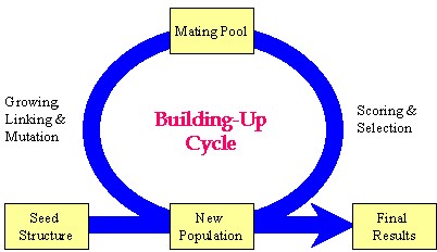
Our manuscript details the "grow-link" hybrid approach, which was implemented using a genetic algorithm through the following stages:
(1) Initial population generation based on a seed structure via the GROW method.
(2) Selection of "parent" molecules from the current population for inclusion in the mating pool using the LINK method.
(3) Transfer of "elite" molecules from the current population to the new population.
(4) Population expansion through structural manipulations (mutation, deletion, and crossover) applied to molecules within the mating pool.
Please note, the outcome of this process is not fixed, as it is highly dependent on the target cavity topology and the constraint parameters employed for population evaluation. Synthesizer customizes generational cycles and optimization parameters based on cavity-specific constraints, with the objective of either generating a specified number of compounds or comprehensively exploring chemical diversity against a given cavity topology.
While these components are integral to LigBuilder, Synthesizer's innovation lies
(1) in its programmatic integration and dynamic adjustment of these modules.
(2) Synthesizer distinguishes itself not by reinventing these algorithms, but by their automated coordination, fine-tuning, and integration within a cavity-specific framework.
(3) It dynamically modifies generation parameters according to cavity topology and druggability constraints, a capability not inherently supported by LigBuilder.
(4) This renders Synthesizer particularly valuable in practical scenarios where manual optimization is either inefficient or impractical.
In summary, Synthesizer offers researchers a streamlined interface, abstracting the technical complexities of LigBuilder and thereby enabling more accessible and reproducible ligand generation pipelines, especially for individuals with limited experience in structural or cheminformatics tools.
Query: (2) The use of AutoDock Vina binding energy scores to classify ligands into HABs and LABs is problematic. AutoDock Vina's energy function is primarily tuned for pose prediction and displays highly system-dependent affinity ranking capabilities. Moreover, the HAB/LAB thresholds of -7 kcal/mol or -8 kcal/mol lack justification. Were these arbitrarily selected cutoffs, or was benchmarking performed to identify appropriate cutoffs? It seems like these thresholds should be determined by calibrating the docking scores with experimental binding data (e.g., known binders with measured affinities) or through re-scoring molecules with a rigorous alchemical free energy approach.
We again express our gratitude to Reviewer #1 for these inquiries. We sincerely apologize for the lack of sufficient detail in the original version of the manuscript. In the revised manuscript, we have ensured the inclusion of a detailed rationale for every threshold utilized to prioritize high-affinity binders. Please refer to the comprehensive explanation below, as well as the revised manuscript, for further details.
We would like to clarify that:
(1) The Authenticator module is not solely reliant on absolute binding energy values for classification. Instead, it calculates binding energies for all generated compounds and applies a statistical decision-making layer to define HAB and LAB classes.
(2) Rather than using fixed thresholds, the module employs distribution-based methods, such as the Empirical Cumulative Distribution Function (ECDF), to assess the overall energy landscape of the compound set. We then applied multiple statistical tests to evaluate the HAB and LAB distributions and determine an optimal, data-specific cutoff that balances class sizes and minimizes overlap.
(3) This adaptive approach avoids rigid thresholds and instead ensures context-sensitive classification, with safeguards in place to maintain adequate representation of both classes for downstream model training, and in this way, the framework prioritizes robust statistical reasoning over arbitrary energy cutoffs and aims to reduce the risks associated with direct reliance on Vina scores alone.
(4) To assess the necessity and effectiveness of the Authenticator module, we conducted a benchmarking analysis where we deliberately omitted the HAB and LAB class labels, treating the compound pool as a heterogeneous, unlabeled dataset. We then performed random train-test splits using the Synthesizer-generated compounds and trained independent models.
(5) The results from this approach demonstrated notably poorer model performance, indicating that arbitrary or unstructured data partitioning does not effectively capture the underlying affinity patterns. These experiments highlight the importance of using the statistical framework within the Authenticator module to establish meaningful, data-driven thresholds for distinguishing High- and Low-Affinity Binders. The cutoff values are thus not arbitrary but emerge from a systematic benchmarking and validation process tailored to each dataset.
Please note: While calibrating docking scores with experimental binding affinities or using rigorous methods like alchemical free energy calculations can improve precision, these approaches are often computationally intensive and reliant on the availability of high-quality experimental data, a major limitation in many real-world screening scenarios.
In summary, the primary goal of Gcoupler is to enable fast, scalable, and broadly accessible screening, particularly for cases where experimental data is sparse or unavailable. Incorporating such resource-heavy methods would not only significantly increase computational overhead but also undermine the framework’s intended usability and efficiency for large-scale applications. Instead, our workflow relies on statistically robust, data-driven classification methods that balance speed, generalizability, and practical feasibility.
Query: (3) Neither the Results nor Methods sections provide information on how the GNNs were trained in this study. Details such as node features, edge attributes, standardization, pooling, activation functions, layers, dropout, etc., should all be described in detail. The training protocol should also be described, including loss functions, independent monitoring and early stopping criteria, learning rate adjustments, etc.
We again thank Reviewer #1 for this suggestion. We would like to mention that in the revised manuscript, we have added all the requested details. Please refer to the points below for more information.
(1) The Generator module of Gcoupler is designed as a flexible and automated framework that leverages multiple Graph Neural Network architectures, including Graph Convolutional Model (GCM), Graph Convolutional Network (GCN), Attentive FP, and Graph Attention Network (GAT), to build classification models based on the synthetic ligand datasets produced earlier in the pipeline.
(2) By default, Generator tests all four models using standard hyperparameters provided by the DeepChem framework (https://deepchem.io/), offering a baseline performance comparison across architectures. This includes pre-defined choices for node features, edge attributes, message-passing layers, pooling strategies, activation functions, and dropout values, ensuring reproducibility and consistency. All models are trained with binary cross-entropy loss and support default settings for early stopping, learning rate, and batch standardization where applicable.
(3) In addition, Generator supports model refinement through hyperparameter tuning and k-fold cross-validation (default: 3 folds). Users can either customize the hyperparameter grid or rely on Generator’s recommended parameter ranges to optimize model performance. This allows for robust model selection and stability assessment of tuned parameters.
(4) Finally, the trained models can be used to predict binding probabilities for user-supplied compounds, making it a comprehensive and user-adaptive tool for ligand screening.
Based on the reviewer #1 suggestion, we have now added a detailed description about the Generator module of Gcoupler, and also provided relevant citations regarding the DeepChem workflow.
Query: (4) GNN model training seems to occur on at most 500 molecules per training run? This is unclear from the manuscript. That is a very small number of training samples if true. Please clarify. How was upsampling performed? What were the HAB/LAB class distributions? In addition, it seems as though only synthetically generated molecules are used for training, and the task is to discriminate synthetic molecules based on their docking scores. Synthetic ligands generated by LigBuilder may occupy distinct chemical space, making classification trivial, particularly in the setting of a random split k-folds validation approach. In the absence of a leave-class-out validation, it is unclear if the model learns generalizable features or exploits clear chemical differences. Historically, it was inappropriate to evaluate ligand-based QSAR models on synthetic decoys such as the DUD-E sets - synthetic ligands can be much more easily distinguished by heavily parameterized ligand-based machine learning models than by physically constrained single-point docking score functions.
We thank reviewer #1 for these detailed technical queries. We would like to clarify that:
(1) The recommended minimum for the training set is 500 molecules, but users can add as many synthesized compounds as needed to thoroughly explore the chemical space related to the target cavity.
(2) Our systematic evaluation demonstrated that expanding the training set size consistently enhanced model performance, especially when compared to AutoDock docking scores. This observation underscores the framework's scalability and its ability to improve predictive accuracy with more training compounds.
(3) The Authenticator module initially categorizes all synthesized molecules into HAB and LAB classes. These labeled molecules are then utilized for training the Generator module. To tackle class imbalance, the class with fewer data points undergoes upsampling. This process aims to achieve an approximate 1:1 ratio between the two classes, thereby ensuring balanced learning during GNN model training.
(4) The Authenticator module's affinity scores are the primary determinant of the HAB/LAB class distribution, with a higher cutoff for HABs ensuring statistically significant class separation. This distribution is also indirectly shaped by the target cavity's topology and druggability, as the Synthesizer tends to produce more potent candidates for cavities with favorable binding characteristics.
(5) While it's true that synthetic ligands may occupy distinct chemical space, our benchmarking exploration for different sites on the same receptor still showed inter-cavity specificity along with intra-cavity diversity of the synthesized molecules.
(6) The utility of random k-fold validation shouldn't be dismissed outright; it provides a reasonable estimate of performance under practical settings where class boundaries are often unknown. Nonetheless, we agree that complementary validation strategies like leave-class-out could further strengthen the robustness assessment.
(7) We agree that using synthetic decoys like those from the DUD-E dataset can introduce bias in ligand-based QSAR model evaluations if not handled carefully. In our workflow, the inclusion of DUD-E compounds is entirely optional and only considered as a fallback, specifically in scenarios where the number of low-affinity binders (LABs) synthesized by the Synthesizer module is insufficient to proceed with model training.
(8) The primary approach relies on classifying generated compounds based on their derived affinity scores via the Authenticator module. However, in rare cases where this results in a heavily imbalanced dataset, DUD-E compounds are introduced not as part of the core benchmarking, but solely to maintain minimal class balance for initial model training. Even then, care is taken to interpret results with this limitation in mind. Ultimately, our framework is designed to prioritize data-driven generation of both HABs and LABs, minimizing reliance on synthetic decoys wherever possible.
Author response image 2.
Scatter plots depicting the segregation of High/Low-Affinity Metabolites (HAM/LAM) (indicated in green and red) identified using Gcoupler workflow with 100% training data. Notably, models trained on lesser training data size (25%, 50%, and 75% of HAB/LAB) severely failed to segregate HAM and LAM (along Y-axis). X-axis represents the binding affinity calculated using IC4-specific docking using AutoDock.
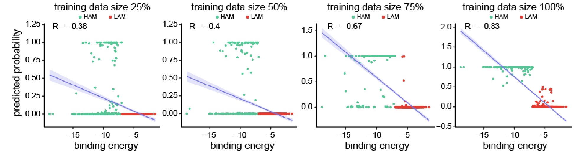
Based on the reviewer #1’s suggestion, we have now added all these technical details in the revised version of the manuscript.
Query: (5) Training QSAR models on docking scores to accelerate virtual screening is not in itself novel (see here for a nice recent example: https://www.nature.com/articles/s43588-025-00777-x), but can be highly useful to focus structure-based analysis on the most promising areas of ligand chemical space; however, we are perplexed by the motivation here. If only a few hundred or a few thousand molecules are being sampled, why not just use AutoDock Vina? The models are trained to try to discriminate molecules by AutoDock Vina score rather than experimental affinity, so it seems like we would ideally just run Vina? Perhaps we are misunderstanding the scale of the screening that was done here. Please clarify the manuscript methods to help justify the approach.
We acknowledge the effectiveness of training QSAR models on docking scores for prioritizing chemical space, as demonstrated by the referenced study (https://www.nature.com/articles/s43588-025-00777-x) on machine-learning-guided docking screen frameworks.
We would like to mention that:
(1) While such protocols often rely on extensive pre-docked datasets across numerous protein targets or utilize a highly skewed input distribution, training on as little as 1-10% of ligand-protein complexes and testing on the remainder in iterative cycles.
(2) While powerful for ultra-large libraries, this approach can introduce bias towards the limited training set and incur significant overhead in data curation, pre-computation, and infrastructure.
(3) In contrast, Gcoupler prioritizes flexibility and accessibility, especially when experimental data is scarce and large pre-docked libraries are unavailable. Instead of depending on fixed docking scores from external pipelines, Gcoupler integrates target-specific cavity detection, de novo compound generation, and model training into a self-contained, end-to-end framework. Its QSAR models are trained directly on contextually relevant compounds synthesized for a given binding site, employing a statistical classification strategy that avoids arbitrary thresholds or precomputed biases.
(4) Furthermore, Gcoupler is open-source, lightweight, and user-friendly, making it easily deployable without the need for extensive infrastructure or prior docking expertise. While not a complete replacement for full-scale docking in all use cases, Gcoupler aims to provide a streamlined and interpretable screening framework that supports both focused chemical design and broader chemical space exploration, without the computational burden associated with deep learning docking workflows.
(5) Practically, even with computational resources, manually running AutoDock Vina on millions of compounds presents challenges such as format conversion, binding site annotation, grid parameter tuning, and execution logistics, all typically requiring advanced structural bioinformatics expertise.
(6) Gcoupler's Authenticator module, however, streamlines this process. Users only need to input a list of SMILES and a receptor PDB structure, and the module automatically handles compound preparation, cavity mapping, parameter optimization, and high-throughput scoring. This automation reduces time and effort while democratizing access to structure-based screening workflows for users without specialized expertise.
Ultimately, Gcoupler's motivation is to make large-scale, structure-informed virtual screening both efficient and accessible. The model serves as a surrogate to filter and prioritize compounds before deeper docking or experimental validation, thereby accelerating targeted drug discovery.
Query: (6) The brevity of the MD simulations raises some concerns that the results may be over-interpreted. RMSD plots do not reliably compare the affinity behavior in this context because of the short timescales coupled with the dramatic topological differences between the ligands being compared; CoQ6 is long and highly flexible compared to ZST and LST. Convergence metrics, such as block averaging and time-dependent MM/GBSA energies, should be included over much longer timescales. For CoQ6, the authors may need to run multiple simulations of several microseconds, identify the longest-lived metastable states of CoQ6, and perform MM/GBSA energies for each state weighted by each state's probability.
We appreciate Reviewer #1's suggestion regarding simulation length, as it is indeed crucial for interpreting molecular dynamics (MD) outcomes. We would like to mention that:
(1) Our simulation strategy varied based on the analysis objective, ranging from short (~5 ns) runs for preliminary or receptor-only evaluations to intermediate (~100 ns) and extended (~550 ns) runs for receptor-ligand complex validation and stability assessment.
(2) Specifically, we conducted three independent 100 ns MD simulations for each receptor-metabolite complex in distinct cavities of interest. This allowed us to assess the reproducibility and persistence of binding interactions. To further support these observations, a longer 550 ns simulation was performed for the IC4 cavity, which reinforced the 100 ns findings by demonstrating sustained interaction stability over extended timescales.
(3) While we acknowledge that even longer simulations (e.g., in the microsecond range) could provide deeper insights into metastable state transitions, especially for highly flexible molecules like CoQ6, our current design balances computational feasibility with the goal of screening multiple cavities and ligands.
(4) In our current workflow, MM/GBSA binding free energies were calculated by extracting 1000 representative snapshots from the final 10 ns of each MD trajectory. These configurations were used to compute time-averaged binding energies, incorporating contributions from van der Waals, electrostatic, polar, and non-polar solvation terms. This approach offers a more reliable estimate of ligand binding affinity compared to single-point molecular docking, as it accounts for conformational flexibility and dynamic interactions within the binding cavity.
(5) Although we did not explicitly perform state-specific MM/GBSA calculations weighted by metastable state probabilities, our use of ensemble-averaged energy estimates from a thermally equilibrated segment of the trajectory captures many of the same benefits. We acknowledge, however, that a more rigorous decomposition based on metastable state analysis could offer finer resolution of binding behavior, particularly for highly flexible ligands like CoQ6, and we consider this a valuable direction for future refinement of the framework.
Reviewer #2 (Public review):
Summary:
Query: Mohanty et al. present a new deep learning method to identify intracellular allosteric modulators of GPCRs. This is an interesting field for e.g. the design of novel small molecule inhibitors of GPCR signalling. A key limitation, as mentioned by the authors, is the limited availability of data. The method presented, Gcoupler, aims to overcome these limitations, as shown by experimental validation of sterols in the inhibition of Ste2p, which has been shown to be relevant molecules in human and rat cardiac hypertrophy models. They have made their code available for download and installation, which can easily be followed to set up software on a local machine.
Strengths:
Clear GitHub repository
Extensive data on yeast systems
We sincerely thank Reviewer #2 for their thorough review, summary, and appreciation of our work. We highly value their comments and suggestions.
Weaknesses:
Query: No assay to directly determine the affinity of the compounds to the protein of interest.
We thank Reviewer #2 for raising these insightful questions. During the experimental design phase, we carefully accounted for validating the impact of metabolites in the rescue response by pheromone.
We would like to mention that we performed an array of methods to validate our hypothesis and observed similar rescue effects. These assays include:
a. Cell viability assay (FDA/PI Flourometry-based)
b. Cell growth assay
c. FUN1<sup>TM</sup>-based microscopy assessment
d. Shmoo formation assays
e. Mating assays
f. Site-directed mutagenesis-based loss of function
g. ransgenic reporter-based assay
h. MAPK signaling assessment using Western blot.
i. And via computational techniques.
Concerning the in vitro interaction studies of Ste2p and metabolites, we made significant efforts to purify Ste2p by incorporating a His tag at the N-terminal. Despite dedicated attempts over the past year, we were unsuccessful in purifying the protein, primarily due to our limited expertise in protein purification for this specific system. As a result, we opted for genetic-based interventions (e.g., point mutants), which provide a more physiological and comprehensive approach to demonstrating the interaction between Ste2p and the metabolites.
Author response image 3.
(a) Affinity purification of Ste2p from Saccharomyces cerevisiae. Western blot analysis using anti-His antibody showing the distribution of Ste2p in various fractions during the affinity purification process. The fractions include pellet, supernatant, wash buffer, and sequential elution fractions (1–4). Wild-type and ste2Δ strains served as positive and negative controls, respectively. (b) Optimization of Ste2p extraction protocol. Ponceau staining (left) and Western blot analysis using anti-His antibody (right) showing Ste2p extraction efficiency. The conditions tested include lysis buffers containing different concentrations of CHAPS detergent (0.5%, 1%) and glycerol (10%, 20%).
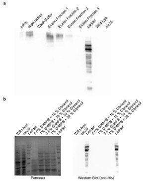
Furthermore, in addition to the clarification above, we have added the following statement in the discussion section to tone down our claims: “A critical limitation of our study is the absence of direct binding assays to validate the interaction between the metabolites and Ste2p. While our results from genetic interventions, molecular dynamics simulations, and docking studies strongly suggest that the metabolites interact with the Ste2p-Gpa1 interface, these findings remain indirect. Direct binding confirmation through techniques such as surface plasmon resonance, isothermal titration calorimetry, or co-crystallization would provide definitive evidence of this interaction. Addressing this limitation in future work would significantly strengthen our conclusions and provide deeper insights into the precise molecular mechanisms underlying the observed phenotypic effects.”
We request Reviewer #2 to kindly refer to the assays conducted on the point mutants created in this study, as these experiments offer robust evidence supporting our claims.
Query: In conclusion, the authors present an interesting new method to identify allosteric inhibitors of GPCRs, which can easily be employed by research labs. Whilst their efforts to characterize the compounds in yeast cells, in order to confirm their findings, it would be beneficial if the authors show their compounds are active in a simple binding assay.
We express our gratitude and sincere appreciation for the time and effort dedicated by Reviewer #2 in reviewing our manuscript. We are confident that our clarifications address the reviewer's concerns.
Reviewer #3 (Public review):
Summary:
Query: In this paper, the authors introduce the Gcoupler software, an open-source deep learning-based platform for structure-guided discovery of ligands targeting GPCR interfaces. Overall, this manuscript represents a field-advancing contribution at the intersection of AI-based ligand discovery and GPCR signaling regulation.
Strengths:
The paper presents a comprehensive and well-structured workflow combining cavity identification, de novo ligand generation, statistical validation, and graph neural network-based classification. Notably, the authors use Gcoupler to identify endogenous intracellular sterols as allosteric modulators of the GPCR-Gα interface in yeast, with experimental validations extending to mammalian systems. The ability to systematically explore intracellular metabolite modulation of GPCR signaling represents a novel and impactful contribution. This study significantly advances the field of GPCR biology and computational ligand discovery.
We thank and appreciate Reviewer #3 for vesting time and efforts in reviewing our manuscript and for appreciating our efforts.
Recommendations for the authors:
Reviewing Editor Comments:
We encourage the authors to address the points raised during revision to elevate the assessment from "incomplete" to "solid" or ideally "convincing." In particular, we ask the authors to improve the justification for their methodological choices and to provide greater detail and clarity regarding each computational layer of the pipeline.
We are grateful for the editors' suggestions. We have incorporated significant revisions into the manuscript, providing comprehensive technical details to prevent any misunderstandings. Furthermore, we meticulously explained every aspect of the computational workflow.
Reviewer #2 (Recommendations for the authors):
Query: Would it be possible to make the package itself pip installable?
Yes, it already exists under the testpip repository and we have now migrated it to the main pip. Please access the link from here: https://pypi.org/project/gcoupler/
Query: I am confused by the binding free energies reported in Supplementary Figure 8. Is the total DG reported that of the protein-ligand complex? If that is the case, the affinities of the ligands would be extremely high. They are also very far off from the reported -7 kcal/mol active/inactive cut-off.
We thank Reviewer #2 for this query. We would like to mention that we have provided a detailed explanation in the point-by-point response to Reviewer #2's original comment. Briefly, to clarify, the -7 kcal/mol active/inactive cutoff mentioned in the manuscript refers specifically to the docking-based binding free energies (ΔG) calculated using AutoDock or AutoDock Vina, which are used for compound classification or validation against the Gcoupler framework.
In contrast, the binding free energies reported in Supplementary Figure 8 are obtained through the MM-GBSA method, which provides a more detailed and physics-based estimate of binding affinity by incorporating solvation and enthalpic contributions. It is well-documented in the literature that MM-GBSA tends to systematically underestimate absolute binding free energies when compared to experimental values (10.2174/1568026616666161117112604; Table 1).
Author response image 4.
Scatter plot comparing the predicted binding affinity calculated by Docking and MM/GBSA methods, against experimental ΔG (10.1007/s10822-023-00499-0)
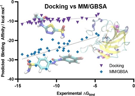
Our use of MM-GBSA is not to match experimental ΔG directly, but rather to assess relative binding preferences among ligands. Despite its limitations in predicting absolute affinities, MM-GBSA is known to perform better than docking for ranking compounds by their binding potential. In this context, an MM-GBSA energy value still reliably indicates stronger predicted binding, even if the numerical values appear extremely higher than typical experimental or docking-derived cutoffs.
Thus, the two energy values, docking-based and MM-GBSA, serve different purposes in our workflow. Docking scores are used for classification and thresholding, while MM-GBSA energies provide post hoc validation and a higher-resolution comparison of binding strength across compounds.
To corroborate their findings, can the authors include direct binding affinity assays for yeast and human Ste2p? This will help in establishing whether the observed phenotypic effects are indeed driven by binding of the metabolites.
We thank Reviewer #2 for raising these insightful questions. During the experimental design phase, we carefully accounted for validating the impact of metabolites in the rescue response by pheromone.
We would like to mention that we performed an array of methods to validate our hypothesis and observed similar rescue effects. These assays include:
a. Cell viability assay (FDA/PI Flourometry- based)
b. Cell growth assay
c. FUN1<sup>TM</sup>-based microscopy assessment
d. Shmoo formation assays
e. Mating assays
f. Site-directed mutagenesis-based loss of function
g. Transgenic reporter-based assay
h. MAPK signaling assessment using Western blot.
i. And via computational techniques.
Concerning the in vitro interaction studies of Ste2p and metabolites, we made significant efforts to purify Ste2p by incorporating a His tag at the N-terminal. Despite dedicated attempts over the past year, we were unsuccessful in purifying the protein, primarily due to our limited expertise in protein purification for this specific system. As a result, we opted for genetic-based interventions (e.g., point mutants), which provide a more physiological and comprehensive approach to demonstrating the interaction between Ste2p and the metabolites.
Furthermore, in addition to the clarification above, we have added the following statement in the discussion section to tone down our claims: “A critical limitation of our study is the absence of direct binding assays to validate the interaction between the metabolites and Ste2p. While our results from genetic interventions, molecular dynamics simulations, and docking studies strongly suggest that the metabolites interact with the Ste2p-Gpa1 interface, these findings remain indirect. Direct binding confirmation through techniques such as surface plasmon resonance, isothermal titration calorimetry, or co-crystallization would provide definitive evidence of this interaction. Addressing this limitation in future work would significantly strengthen our conclusions and provide deeper insights into the precise molecular mechanisms underlying the observed phenotypic effects.”
We request Reviewer #2 to kindly refer to the assays conducted on the point mutants created in this study, as these experiments offer robust evidence supporting our claims.
Did the authors perform expression assays to make sure the mutant proteins were similarly expressed to wt?
We thank reviewer #2 for this comment. We would like to mention that:
(1) In our mutants (S75A, T155D, L289K)-based assays, all mutants were generated using integration at the same chromosomal TRP1 locus under the GAL1 promoter and share the same C-terminal CYC1 terminator sequence used for the reconstituted wild-type (rtWT) construct, thus reducing the likelihood of strain-specific expression differences.
(2) Furthermore, all strains were grown under identical conditions using the same media, temperature, and shaking parameters. Each construct underwent the same GAL1 induction protocol in YPGR medium for identical durations, ensuring uniform transcriptional activation across all strains and minimizing culture-dependent variability in protein expression.
(3) Importantly, both the rtWT and two of the mutants (T155D, L289K) retained α-factor-induced cell death (PI and FUN1-based fluorometry and microscopy; Figure 4c-d) and MAPK activation (western blot; Figure 4e), demonstrating that the mutant proteins are expressed at levels sufficient to support signalling.
Reviewer #3 (Recommendations for the authors):
My comments that would enhance the impact of this method are:
(1) While the authors have compared the accuracy and efficiency of Gcoupler to AutoDock Vina, one of the main points of Gcoupler is the neural network module. It would be beneficial to have it evaluated against other available deep learning ligand generative modules, such as the following: 10.1186/s13321-024-00829-w, 10.1039/D1SC04444C.
Thank you for the observation. To clarify, our benchmarking of Gcoupler’s accuracy and efficiency was performed against AutoDock, not AutoDock Vina. This choice was intentional, as AutoDock is one of the most widely used classical techniques in computer-aided drug design (CADD) for obtaining high-resolution predictions of ligand binding energy, binding poses, and detailed atomic-level interactions with receptor residues. In contrast, AutoDock Vina is primarily optimized for large-scale virtual screening, offering faster results but typically with lower resolution and limited configurational detail.
Since Gcoupler is designed to balance accuracy with computational efficiency in structure-based screening, AutoDock served as a more appropriate reference point for evaluating its predictions.
We agree that benchmarking against other deep learning-based ligand generative tools is important for contextualizing Gcoupler’s capabilities. However, it's worth noting that only a few existing methods focus specifically on cavity- or pocket-driven de novo drug design using generative AI, and among them, most are either partially closed-source or limited in functionality.
While PocketCrafter (10.1186/s13321-024-00829-w) offers a structure-based generative framework, it differs from Gcoupler in several key respects. PocketCrafter requires proprietary preprocessing tools, such as the MOE QuickPrep module, to prepare protein pocket structures, limiting its accessibility and reproducibility. In addition, PocketCrafter’s pipeline stops at the generation of cavity-linked compounds and does not support any further learning from the generated data.
Similarly, DeepLigBuilder (10.1039/D1SC04444C) provides de novo ligand generation using deep learning, but the source code is not publicly available, preventing direct benchmarking or customization. Like PocketCrafter, it also lacks integrated learning modules, which limits its utility for screening large, user-defined libraries or compounds of interest.
Additionally, tools like AutoDesigner from Schrödinger, while powerful, are not publicly accessible and hence fall outside the scope of open benchmarking.
Author response table 1.
Comparison of de novo drug design tools. SBDD refers to Structure-Based Drug Design, and LBDD refers to Ligand-Based Drug Design.
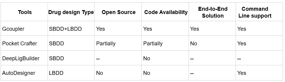
In contrast, Gcoupler is a fully open-source, end-to-end platform that integrates both Ligand-Based and Structure-Based Drug Design. It spans from cavity detection and molecule generation to automated model training using GNNs, allowing users to evaluate and prioritize candidate ligands across large chemical spaces without the need for commercial software or advanced coding expertise.
(2) In Figure 2, the authors mention that IC4 and IC5 potential binding sites are on the direct G protein coupling interface ("This led to the identification of 17 potential surface cavities on Ste2p, with two intracellular regions, IC4 and IC5, accounting for over 95% of the Ste2p-Gpa1p interface (Figure 2a-b, Supplementary Figure 4j-n)..."). Later, however, in Figure 4, when discussing which residues affect the binding of the metabolites the most, the authors didn't perform MD simulations of mutant STE2 and just Gpa1p (without metabolites present). It would be beneficial to compare the binding of G protein with and without metabolites present, as these interface mutations might be affecting the binding of G protein by itself.
Thank you for this insightful suggestion. While we did not perform in silico MD simulations of the mutant Ste2-Gpa1 complex in the absence of metabolites, we conducted experimental validation to functionally assess the impact of interface mutations. Specifically, we generated site-directed mutants (S75A, L289K, T155D) and expressed them in a ste2Δ background to isolate their effects.
As shown in the Supplementary Figure, these mutants failed to rescue cells from α-factor-induced programmed cell death (PCD) upon metabolite pre-treatment. This was confirmed through fluorometry-based viability assays, FUN1<sup>TM</sup> staining, and p-Fus3 signaling analysis, which collectively monitor MAPK pathway activation (Figure 4c–e).
Importantly, the induction of PCD in response to α-factor in these mutants demonstrates that G protein coupling is still functionally intact, indicating that the mutations do not interfere with Gpa1 binding itself. However, the absence of rescue by metabolites strongly suggests that the mutated residues play a direct role in metabolite binding at the Ste2p–Gpa1p interface, thus modulating downstream signaling.
While further MD simulations could provide structural insight into the isolated mutant receptor–G protein interaction, our experimental data supports the functional relevance of metabolite binding at the identified interface.
(3) While the experiments, performed by the authors, do support the hypothesis that metabolites regulate GPCR signaling, there are no experiments evaluating direct biophysical measurements (e.g., dissociation constants are measured only in silicon).
We thank Reviewer #3 for raising these insightful comments. We would like to mention that we performed an array of methods to validate our hypothesis and observed similar rescue effects. These assays include:
a. Cell viability assay (FDA/PI Flourometry- based)
b. Cell growth assay
c. FUN1<sup>TM</sup>-based microscopy assessment
d. Shmoo formation assays
e. Mating assays
f. Site-directed mutagenesis-based loss of function
g. Transgenic reporter-based assay
h. MAPK signaling assessment using Western blot.
i. And via computational techniques.
Concerning the direct biophysical measurements of Ste2p and metabolites, we made significant efforts to purify Ste2p by incorporating a His tag at the N-terminal, with the goal of performing Microscale Thermophoresis (MST) and Isothermal Titration Calorimetry (ITC) measurements. Despite dedicated attempts over the past year, we were unsuccessful in purifying the protein, primarily due to our limited expertise in protein purification for this specific system. As a result, we opted for genetic-based interventions (e.g., point mutants), which provide a more physiological and comprehensive approach to demonstrating the interaction between Ste2p and the metabolites.
Furthermore, in addition to the clarification above, we have added the following statement in the discussion section to tone down our claims: “A critical limitation of our study is the absence of direct binding assays to validate the interaction between the metabolites and Ste2p. While our results from genetic interventions, molecular dynamics simulations, and docking studies strongly suggest that the metabolites interact with the Ste2p-Gpa1 interface, these findings remain indirect. Direct binding confirmation through techniques such as surface plasmon resonance, isothermal titration calorimetry, or co-crystallization would provide definitive evidence of this interaction. Addressing this limitation in future work would significantly strengthen our conclusions and provide deeper insights into the precise molecular mechanisms underlying the observed phenotypic effects.”
(4) The authors do not discuss the effects of the metabolites at their physiological concentrations. Overall, this manuscript represents a field-advancing contribution at the intersection of AI-based ligand discovery and GPCR signaling regulation.
We thank reviewer #3 for this comment and for recognising the value of our work. Although direct quantification of intracellular free metabolite levels is challenging, several lines of evidence support the physiological relevance of our test concentrations.
- Genetic validation supports endogenous relevance: Our genetic screen of 53 metabolic knockout mutants showed that deletions in biosynthetic pathways for these metabolites consistently disrupted the α-factor-induced cell death, with the vast majority of strains (94.4%) resisting the α-factor-induced cell death, and notably, a subset even displayed accelerated growth in the presence of α‑factor. This suggests that endogenous levels of these metabolites normally provide some degree of protection, supporting their physiological role in GPCR regulation.
- Metabolomics confirms in vivo accumulation: Our untargeted metabolomics analysis revealed that α-factor-treated survivors consistently showed enrichment of CoQ6 and zymosterol compared to sensitive cells. This demonstrates that these metabolites naturally accumulate to protective levels during stress responses, validating their biological relevance.
Deux ou trois heures sans smartphone en état de fonctionnement leur étaient tout bonnement insupportable et pouvait déclencher une réelle crise de manque
Le smartphone devient un objet “toxicomaniaque” : il ne sert plus à communiquer, mais à pallier à une angoisse d’absence. Janssen fait ici le lien entre dépendance numérique et fragilité du moi — la connexion devient une drogue relationnelle.
Là où le doudou de l’enfant lui assure une continuité d’existence et du lien au monde par-delà la séparation, il semble que le smartphone et les applications qu’il renferme, les réseaux sociaux ou autres messageries instantanées soient davantage utilisés pour assurer l’absolue continuité du lien déniant la séparation.
Janssen applique la théorie de Winnicott au monde numérique : le smartphone, au lieu d’aider à supporter l’absence comme le ferait un objet transitionnel, ne permet pas de la vivre. Il garde la personne dans une impression de présence continue.
Le sociologue Zygmunt Bauman [6] évoque cette paradoxalité des liens virtuels en repérant les phénomènes de « proximité virtuelle » et de « distance virtuelle ».
En citant Bauman (L’amour liquide, 2004), Janssen montre que la technologie alimente des liens à la fois trop proches et trop éloignés : une illusion de connexion permanente qui masque une distance émotionnelle grandissante.
Chronique du Hérisson
Dans l'article mettre les liens vers RCF et RadioB https://www.rcf.fr/culture/dans-le-coain https://www.radio-b.fr/la-chronique-du-herisson-286
Dans le chapeau de l'article (en rouge) rajouter mercredi 19 novembre
Author response:
The following is the authors’ response to the original reviews
Reviewer #1 (Public review):
This study investigates the sex determination mechanism in the clonal ant Ooceraea biroi, focusing on a candidate complementary sex determination (CSD) locus-one of the key mechanisms supporting haplodiploid sex determination in hymenopteran insects. Using whole genome sequencing, the authors analyze diploid females and the rarely occurring diploid males of O. biroi, identifying a 46 kb candidate region that is consistently heterozygous in females and predominantly homozygous in diploid males. This region shows elevated genetic diversity, as expected under balancing selection. The study also reports the presence of an lncRNA near this heterozygous region, which, though only distantly related in sequence, resembles the ANTSR lncRNA involved in female development in the Argentine ant, Linepithema humile (Pan et al. 2024). Together, these findings suggest a potentially conserved sex determination mechanism across ant species. However, while the analyses are well conducted and the paper is clearly written, the insights are largely incremental. The central conclusion - that the sex determination locus is conserved in ants - was already proposed and experimentally supported by Pan et al. (2024), who included O. biroi among the studied species and validated the locus's functional role in the Argentine ant. The present study thus largely reiterates existing findings without providing novel conceptual or experimental advances.
Although it is true that Pan et al., 2024 demonstrated (in Figure 4 of their paper) that the synteny of the region flanking ANTSR is conserved across aculeate Hymenoptera (including O. biroi), Reviewer 1’s claim that that paper provides experimental support for the hypothesis that the sex determination locus is conserved in ants is inaccurate. Pan et al., 2024 only performed experimental work in a single ant species (Linepithema humile) and merely compared reference genomes of multiple species to show synteny of the region, rather than functionally mapping or characterizing these regions.
Other comments:
The mapping is based on a very small sample size: 19 females and 16 diploid males, and these all derive from a single clonal line. This implies a rather high probability for false-positive inference. In combination with the fact that only 11 out of the 16 genotyped males are actually homozygous at the candidate locus, I think a more careful interpretation regarding the role of the mapped region in sex determination would be appropriate. The main argument supporting the role of the candidate region in sex determination is based on the putative homology with the lncRNA involved in sex determination in the Argentine ant, but this argument was made in a previous study (as mentioned above).
Our main argument supporting the role of the candidate region in sex determination is not based on putative homology with the lncRNA in L. humile. Instead, our main argument comes from our genetic mapping (in Fig. 2), and the elevated nucleotide diversity within the identified region (Fig. 4). Additionally, we highlight that multiple genes within our mapped region are homologous to those in mapped sex determining regions in both L. humile and Vollenhovia emeryi, possibly including the lncRNA.
In response to the Reviewer’s assertion that the mapping is based on a small sample size from a single clonal line, we want to highlight that we used all diploid males available to us. Although the primary shortcoming of a small sample size is to increase the probability of a false negative, small sample sizes can also produce false positives. We used two approaches to explore the statistical robustness of our conclusions. First, we generated a null distribution by randomly shuffling sex labels within colonies and calculating the probability of observing our CSD index values by chance (shown in Fig. 2). Second, we directly tested the association between homozygosity and sex using Fisher’s Exact Test (shown in Supplementary Fig. S2). In both cases, the association of the candidate locus with sex was statistically significant after multiple-testing correction using the Benjamini-Hochberg False Discovery Rate. These approaches are clearly described in the “CSD Index Mapping” section of the Methods.
We also note that, because complementary sex determination loci are expected to evolve under balancing selection, our finding that the mapped region exhibits a peak of nucleotide diversity lends orthogonal support to the notion that the mapped locus is indeed a complementary sex determination locus.
The fourth paragraph of the results and the sixth paragraph of the discussion are devoted to explaining the possible reasons why only 11/16 genotyped males are homozygous in the mapped region. The revised manuscript will include an additional sentence (in what will be lines 384-388) in this paragraph that includes the possible explanation that this locus is, in fact, a false positive, while also emphasizing that we find this possibility to be unlikely given our multiple lines of evidence.
In response to Reviewer 1’s suggestion that we carefully interpret the role of the mapped region in sex determination, we highlight our careful wording choices, nearly always referring to the mapped locus as a “candidate sex determination locus” in the title and throughout the manuscript. For consistency, the revised manuscript version will change the second results subheading from “The O. biroi CSD locus is homologous to another ant sex determination locus but not to honeybee csd” to “O. biroi’s candidate CSD locus is homologous to another ant sex determination locus but not to honeybee csd,” and will add the word “candidate” in what will be line 320 at the beginning of the Discussion, and will change “putative” to “candidate” in what will be line 426 at the end of the Discussion.
In the abstract, it is stated that CSD loci have been mapped in honeybees and two ant species, but we know little about their evolutionary history. But CSD candidate loci were also mapped in a wasp with multi-locus CSD (study cited in the introduction). This wasp is also parthenogenetic via central fusion automixis and produces diploid males. This is a very similar situation to the present study and should be referenced and discussed accordingly, particularly since the authors make the interesting suggestion that their ant also has multi-locus CSD and neither the wasp nor the ant has tra homologs in the CSD candidate regions. Also, is there any homology to the CSD candidate regions in the wasp species and the studied ant?
In response to Reviewer 1’s suggestion that we reference the (Matthey-Doret et al. 2019) study in the context of diploid males being produced via losses of heterozygosity during asexual reproduction, the revised manuscript will include (in what will be lines 123-126) the highlighted portion of the following sentence: “Therefore, if O. biroi uses CSD, diploid males might result from losses of heterozygosity at sex determination loci (Fig. 1C), similar to what is thought to occur in other asexual Hymenoptera that produce diploid males (Rabeling and Kronauer 2012; Matthey-Doret et al. 2019).”
We note, however, that in their 2019 study, Matthey-Doret et al. did not directly test the hypothesis that diploid males result from losses of heterozygosity at CSD loci during asexual reproduction, because the diploid males they used for their mapping study came from inbred crosses in a sexual population of that species.
We address this further below, but we want to emphasize that we do not intend to argue that O. biroi has multiple CSD loci. Instead, we suggest that additional, undetected CSD loci is one possible explanation for the absence of diploid males from any clonal line other than clonal line A. In response to Reviewer 1’s suggestion that we reference the (Matthey-Doret et al. 2019) study in the context of multilocus CSD, the revised manuscript version will include the following additional sentence in the fifth paragraph of the discussion (in what will be lines 372-374): “Multi-locus CSD has been suggested to limit the extent of diploid male production in asexual species under some circumstances (Vorburger 2013; Matthey-Doret et al. 2019).”
Regarding Reviewer 2’s question about homology between the putative CSD loci from the (Matthey-Doret et al. 2019) study and O. biroi, we note that there is no homology. The revised manuscript version will have an additional Supplementary Table (which will be the new Supplementary Table S3) that will report the results of this homology search. The revised manuscript will also include the following additional sentence in the Results, in what will be lines 172-174: “We found no homology between the genes within the O. biroi CSD index peak and any of the genes within the putative L. fabarum CSD loci (Supplementary Table S3).”
The authors used different clonal lines of O. biroi to investigate whether heterozygosity at the mapped CSD locus is required for female development in all clonal lines of O. biroi (L187-196). However, given the described parthenogenesis mechanism in this species conserves heterozygosity, additional females that are heterozygous are not very informative here. Indeed, one would need diploid males in these other clonal lines as well (but such males have not yet been found) to make any inference regarding this locus in other lines.
We agree that a full mapping study including diploid males from all clonal lines would be preferable, but as stated earlier in that same paragraph, we have only found diploid males from clonal line A. We stand behind our modest claim that “Females from all six clonal lines were heterozygous at the CSD index peak, consistent with its putative role as a CSD locus in all O. biroi.” In the revised manuscript version, this sentence (in what will be lines 199-201) will be changed slightly in response to a reviewer comment below: “All females from all six clonal lines (including 26 diploid females from clonal line B) were heterozygous at the CSD index peak, consistent with its putative role as a CSD locus in all O. biroi.”
Reviewer #2 (Public review):
The manuscript by Lacy et al. is well written, with a clear and compelling introduction that effectively conveys the significance of the study. The methods are appropriate and well-executed, and the results, both in the main text and supplementary materials, are presented in a clear and detailed manner. The authors interpret their findings with appropriate caution.
This work makes a valuable contribution to our understanding of the evolution of complementary sex determination (CSD) in ants. In particular, it provides important evidence for the ancient origin of a non-coding locus implicated in sex determination, and shows that, remarkably, this sex locus is conserved even in an ant species with a non-canonical reproductive system that typically does not produce males. I found this to be an excellent and well-rounded study, carefully analyzed and well contextualized.
That said, I do have a few minor comments, primarily concerning the discussion of the potential 'ghost' CSD locus. While the authors acknowledge (line 367) that they currently have no data to distinguish among the alternative hypotheses, I found the evidence for an additional CSD locus presented in the results (lines 261-302) somewhat limited and at times a bit difficult to follow. I wonder whether further clarification or supporting evidence could already be extracted from the existing data. Specifically:
We agree with Reviewer 2 that the evidence for a second CSD locus is limited. In fact, we do not intend to advocate for there being a second locus, but we suggest that a second CSD locus is one possible explanation for the absence of diploid males outside of clonal line A. In our initial version, we intentionally conveyed this ambiguity by titling this section “O. biroi may have one or multiple sex determination loci.” However, we now see that this leads to undue emphasis on the possibility of a second locus. In the revised manuscript, we will split this into two separate sections: “Diploid male production differs across O. biroi clonal lines” and “O. biroi lacks a tra-containing CSD locus.”
(1) Line 268: I doubt the relevance of comparing the proportion of diploid males among all males between lines A and B to infer the presence of additional CSD loci. Since the mechanisms producing these two types of males differ, it might be more appropriate to compare the proportion of diploid males among all diploid offspring. This ratio has been used in previous studies on CSD in Hymenoptera to estimate the number of sex loci (see, for example, Cook 1993, de Boer et al. 2008, 2012, Ma et al. 2013, and Chen et al., 2021). The exact method might not be applicable to clonal raider ants, but I think comparing the percentage of diploid males among the total number of (diploid) offspring produced between the two lineages might be a better argument for a difference in CSD loci number.
We want to re-emphasize here that we do not wish to advocate for there being two CSD loci in O. biroi. Rather, we want to explain that this is one possible explanation for the apparent absence of diploid males outside of clonal line A. We hope that the modifications to the manuscript described in the previous response help to clarify this.
Reviewer 2 is correct that comparing the number of diploid males to diploid females does not apply to clonal raider ants. This is because males are vanishingly rare among the vast numbers of females produced. We do not count how many females are produced in laboratory stock colonies, and males are sampled opportunistically. Therefore, we cannot report exact numbers. However, we will add the highlighted portion of the following sentence (in what will be lines 268-270) to the revised manuscript: “Despite the fact that we maintain more colonies of clonal line B than of clonal line A in the lab, all the diploid males we detected came from clonal line A.”
(2) If line B indeed carries an additional CSD locus, one would expect that some females could be homozygous at the ANTSR locus but still viable, being heterozygous only at the other locus. Do the authors detect any females in line B that are homozygous at the ANTSR locus? If so, this would support the existence of an additional, functionally independent CSD locus.
We thank the reviewer for this suggestion, and again we emphasize that we do not want to argue in favor of multiple CSD loci. We just want to introduce it as one possible explanation for the absence of diploid males outside of clonal line A.
The 26 sequenced diploid females from clonal line B are all heterozygous at the mapped locus, and the revised manuscript will clarify this in what will be lines 199-201. Previously, only six of those diploid females were included in Supplementary Table S2, and that will be modified accordingly.
(3) Line 281: The description of the two tra-containing CSD loci as "conserved" between Vollenhovia and the honey bee may be misleading. It suggests shared ancestry, whereas the honey bee csd gene is known to have arisen via a relatively recent gene duplication from fem/tra (10.1038/nature07052). It would be more accurate to refer to this similarity as a case of convergent evolution rather than conservation.
In the sentence that Reviewer 2 refers to, we are representing the assertion made in the (Miyakawa and Mikheyev 2015) paper in which, regarding their mapping of a candidate CSD locus that contains two linked tra homologs, they write in the abstract: “these data support the prediction that the same CSD mechanism has indeed been conserved for over 100 million years.” In that same paper, Miyakawa and Mikheyev write in the discussion section: “As ants and bees diverged more than 100 million years ago, sex determination in honey bees and V. emeryi is probably homologous and has been conserved for at least this long.”
As noted by Reviewer 2, this appears to conflict with a previously advanced hypothesis: that because fem and csd were found in Apis mellifera, Apis cerana, and Apis dorsata, but only fem was found in Mellipona compressipes, Bombus terrestris, and Nasonia vitripennis, that the csd gene evolved after the honeybee (Apis) lineage diverged from other bees (Hasselmann et al. 2008). However, it remains possible that the csd gene evolved after ants and bees diverged from N. vitripennis, but before the divergence of ants and bees, and then was subsequently lost in B. terrestris and M. compressipes. This view was previously put forward based on bioinformatic identification of putative orthologs of csd and fem in bumblebees and in ants [(Schmieder et al. 2012), see also (Privman et al. 2013)]. However, subsequent work disagreed and argued that the duplications of tra found in ants and in bumblebees represented convergent evolution rather than homology (Koch et al. 2014). Distinguishing between these possibilities will be aided by additional sex determination locus mapping studies and functional dissection of the underlying molecular mechanisms in diverse Aculeata.
Distinguishing between these competing hypotheses is beyond the scope of our paper, but the revised manuscript will include additional text to incorporate some of this nuance. We will include these modified lines below (in what will be lines 287-295), with the additions highlighted:
“A second QTL region identified in V. emeryi (V.emeryiCsdQTL1) contains two closely linked tra homologs, similar to the closely linked honeybee tra homologs, csd and fem (Miyakawa and Mikheyev 2015). This, along with the discovery of duplicated tra homologs that undergo concerted evolution in bumblebees and ants (Schmieder et al. 2012; Privman et al. 2013) has led to the hypothesis that the function of tra homologs as CSD loci is conserved with the csd-containing region of honeybees (Schmieder et al. 2012; Miyakawa and Mikheyev 2015). However, other work has suggested that tra duplications occurred independently in honeybees, bumblebees, and ants (Hasselmann et al. 2008; Koch et al. 2014), and it remains to be demonstrated that either of these tra homologs acts as a primary CSD signal in V. emeryi.”
(4) Finally, since the authors successfully identified multiple alleles of the first CSD locus using previously sequenced haploid males, I wonder whether they also observed comparable allelic diversity at the candidate second CSD locus. This would provide useful supporting evidence for its functional relevance.
As is already addressed in the final paragraph of the results and in Supplementary Fig. S4, there is no peak of nucleotide diversity in any of the regions homologous to V.emeryiQTL1, which is the tra-containing candidate sex determination locus (Miyakawa and Mikheyev 2015). In the revised manuscript, the relevant lines will be 307-310. We want to restate that we do not propose that there is a second candidate CSD locus in O. biroi, but we simply raise the possibility that multi-locus CSD *might* explain the absence of diploid males from clonal lines other than clonal line A (as one of several alternative possibilities).
Overall, these are relatively minor points in the context of a strong manuscript, but I believe addressing them would improve the clarity and robustness of the authors' conclusions.
Reviewer #3 (Public review):
Summary:
The sex determination mechanism governed by the complementary sex determination (CSD) locus is one of the mechanisms that support the haplodiploid sex determination system evolved in hymenopteran insects. While many ant species are believed to possess a CSD locus, it has only been specifically identified in two species. The authors analyzed diploid females and the rarely occurring diploid males of the clonal ant Ooceraea biroi and identified a 46 kb CSD candidate region that is consistently heterozygous in females and predominantly homozygous in males. This region was found to be homologous to the CSD locus reported in distantly related ants. In the Argentine ant, Linepithema humile, the CSD locus overlaps with an lncRNA (ANTSR) that is essential for female development and is associated with the heterozygous region (Pan et al. 2024). Similarly, an lncRNA is encoded near the heterozygous region within the CSD candidate region of O. biroi. Although this lncRNA shares low sequence similarity with ANTSR, its potential functional involvement in sex determination is suggested. Based on these findings, the authors propose that the heterozygous region and the adjacent lncRNA in O. biroi may trigger female development via a mechanism similar to that of L. humile. They further suggest that the molecular mechanisms of sex determination involving the CSD locus in ants have been highly conserved for approximately 112 million years. This study is one of the few to identify a CSD candidate region in ants and is particularly noteworthy as the first to do so in a parthenogenetic species.
Strengths:
(1) The CSD candidate region was found to be homologous to the CSD locus reported in distantly related ant species, enhancing the significance of the findings.
(2) Identifying the CSD candidate region in a parthenogenetic species like O. biroi is a notable achievement and adds novelty to the research.
Weaknesses
(1) Functional validation of the lncRNA's role is lacking, and further investigation through knockout or knockdown experiments is necessary to confirm its involvement in sex determination.
See response below.
(2) The claim that the lncRNA is essential for female development appears to reiterate findings already proposed by Pan et al. (2024), which may reduce the novelty of the study.
We do not claim that the lncRNA is essential for female development in O. biroi, but simply mention the possibility that, as in L. humile, it is somehow involved in sex determination. We do not have any functional evidence for this, so this is purely based on its genomic position immediately adjacent to our mapped candidate region. We agree with the reviewer that the study by Pan et al. (2024) decreases the novelty of our findings. Another way of looking at this is that our study supports and bolsters previous findings by partially replicating the results in a different species.
Recommendations for the authors:
Reviewer #1 (Recommendations for the authors):
L307-308 should state homozygous for either allele in THE MAJORITY of diploid males.
This will be fixed in the revised manuscript, in what will be line 321.
Reviewer #3 (Recommendations for the authors):
The association between heterozygosity in the CSD candidate region and female development in O. biroi, along with the high sequence homology of this region to CSD loci identified in two distantly related ant species, is not sufficient to fully address the evolution of the CSD locus and the mechanisms of sex determination.
Given that functional genetic tools, such as genome editing, have already been established in O. biroi, I strongly recommend that the authors investigate the role of the lncRNA through knockout or knockdown experiments and assess its impact on the sex-specific splicing pattern of the downstream tra gene.
Although knockout experiments of the lncRNA would be illuminating, the primary signal of complementary sex determination is heterozygosity. As is clearly stated in our manuscript and that of (Pan et al. 2024), it does not appear to be heterozygosity within the lncRNA that induces female development, but rather heterozygosity in non-transcribed regions linked to the lncRNA. Therefore, future mechanistic studies of sex determination in O. biroi, L. humile, and other ants should explore how homozygosity or heterozygosity of this region impacts the sex determination cascade, rather than focusing (exclusively) on the lncRNA.
With this in mind, we developed three sets of guide RNAs that cut only one allele within the mapped CSD locus, with the goal of producing deletions within the highly variable region within the mapped locus. This would lead to functional hemizygosity or homozygosity within this region, depending on how the cuts were repaired. We also developed several sets of PCR primers to assess the heterozygosity of the resultant animals. After injecting 1,162 eggs over several weeks and genotyping the hundreds of resultant animals with PCR, we confirmed that we could induce hemizygosity or homozygosity within this region, at least in ~1/20 of the injected embryos. Although it is possible to assess the sex-specificity of the splice isoform of tra as a proxy for sex determination phenotypes (as done by (Pan et al. 2024)), the ideal experiment would assess male phenotypic development at the pupal stage. Therefore, over several more weeks, we injected hundreds more eggs with these reagents and reared the injected embryos to the pupal stage. However, substantial mortality was observed, with only 12 injected eggs developing to the pupal stage. All of these were female, and none of them had been successfully mutated.
In conclusion, we agree with the reviewer that functional experiments would be useful, and we made extensive attempts to conduct such experiments. However, these experiments turned out to be extremely challenging with the currently available protocols. Ultimately, we therefore decided to abandon these attempts.
We opted not to include these experiments in the paper itself because we cannot meaningfully interpret their results. However, we are pleased that, in this response letter, we can include a brief description for readers interested in attempting similar experiments.
Since O. biroi reproduces parthenogenetically and most offspring develop into females, observing a shift from female- to male-specific splicing of tra upon early embryonic knockout of the lncRNA would provide much stronger evidence that this lncRNA is essential for female development. Without such functional validation, the authors' claim (lines 36-38) seems to reiterate findings already proposed by Pan et al. (2024) and, as such, lacks sufficient novelty.
We have responded to the issue of “lack of novelty” above. But again, the actual CSD locus in both O. biroi and L. humile appears to be distinct from (but genetically linked to) the lncRNA, and we have no experimental evidence that the putative lncRNA in O. biroi is involved in sex determination at all. Because of this, and given the experimental challenges described above, we do not currently intend to pursue functional studies of the lncRNA.
References
Hasselmann M, Gempe T, Schiøtt M, Nunes-Silva CG, Otte M, Beye M. 2008. Evidence for the evolutionary nascence of a novel sex determination pathway in honeybees. Nature 454:519–522.
Koch V, Nissen I, Schmitt BD, Beye M. 2014. Independent Evolutionary Origin of fem Paralogous Genes and Complementary Sex Determination in Hymenopteran Insects. PLOS ONE 9:e91883.
Matthey-Doret C, van der Kooi CJ, Jeffries DL, Bast J, Dennis AB, Vorburger C, Schwander T. 2019. Mapping of multiple complementary sex determination loci in a parasitoid wasp. Genome Biology and Evolution 11:2954–2962.
Miyakawa MO, Mikheyev AS. 2015. QTL mapping of sex determination loci supports an ancient pathway in ants and honey bees. PLOS Genetics 11:e1005656.
Pan Q, Darras H, Keller L. 2024. LncRNA gene ANTSR coordinates complementary sex determination in the Argentine ant. Science Advances 10:eadp1532.
Privman E, Wurm Y, Keller L. 2013. Duplication and concerted evolution in a master sex determiner under balancing selection. Proceedings of the Royal Society B: Biological Sciences 280:20122968.
Rabeling C, Kronauer DJC. 2012. Thelytokous parthenogenesis in eusocial Hymenoptera. Annual Review of Entomology 58:273–292.
Schmieder S, Colinet D, Poirié M. 2012. Tracing back the nascence of a new sex-determination pathway to the ancestor of bees and ants. Nature Communications 3:1–7.
Vorburger C. 2013. Thelytoky and Sex Determination in the Hymenoptera: Mutual Constraints. Sexual Development 8:50–58.
Aportacion 2 en la parte de que te exijan títulos supe cortos está bien hasta que te das cuenta de que terminas diciendo cualquier cosa. Es como cuando resumes una película y solo dices trata de algun problema.. pues sí pero no se entiende nada Mejor que sobre una palabra a que falte claridad.
aportacion 1 Criticar un título por ser demasiado largo es como quejarse de un mapa por ser demasiado detallado. El verdadero problema no es la cantidad de palabras, sino si cada una de ellas es necesaria para no perder el rumbo. Prefiero un título de 25 palabras que me lleve exactamente al destino, que uno de 10 que me deje a mitad del camino.
Martínez-Pujalte, (2015)afirma que “los derechos fundamentales son propios de todo ser humano, que han sido constitucionalizados y están ligados con la misma dignidad, que según el aut
martinez
Reviewer #1 (Public review):
The paper reports some interesting patterns in epistasis in a recently published large fitness landscape dataset. The results may have implications for our understanding of fitness landscapes and protein evolution. However, this version of the paper remains fairly descriptive and has significant deficiencies in clarity and rigor.
The authors have addressed some of my criticisms (e.g., I appreciate the additional analysis of synonymous mutations, and a more rigorous approach to calling fitness peaks), but many of the issues raised in my first round of review remain in the current version. Frankly, I am quite disappointed that the authors did not address my comments point by point, which is the norm. The remaining (and some new) issues are below.
(1a) (Modified from first round) I previously suggested to dissect what appears to be three different patterns of epistasis: "strong" and "weak" global epistasis and what one can could "purely idiosyncratic", i.e., not dependent on background fitness. The authors attempted to address this, but I don't think what they have done is sufficient. They make a statement "The lethal mutations have a slope smaller than -0.7 and average slope of -0.98. The remaining mutations all have a slope greater than -0.56" (LL 274-276)", but there is no evidence provided to support this claim. This is a strong and I think interesting statement (btw, how is "lethal" defined?) and warrants a dedicated figure. This statement suggests that the mixed patterns shown in Figure 5 can actually be meaningfully separated. Why don't the authors show this? Instead, they still claim "overall, global epistasis is not very strong on the folA landscape" (LL. 273-274). I maintain that this claim does not quite capture the observations.
Later in the text there is a whole section called "Only a small fraction of mutations exhibit strong global epistasis", which also seems related to this issue. First, I don't follow the logic here. Why is this section separate from this initial discussion? Second, here the authors claim "only a small subset of mutations exhibits strong global epistasis (R^2 > 0.5)" and then "This sharp contrast suggests a binary behavior of mutations: they either exhibit strong global epistasis (R2 > 0.5), or not (R2 < 0.5)." But this R^2 threshold seems arbitrary, and I don't see any statistical support for this binary nature.
(1b) (Verbatim from first round) Another rather remarkable feature of this plot is that the slopes of the strong global epistasis patterns sem to be very similar across mutations. Is this the case? Is there anything special about this slope? For example, does this slope simply reflect the fact that a given mutation becomes essentially lethal (i.e., produces the same minimal fitness) in a certain set of background genotypes?
(1c) (Verbatim from first round) Finally, how consistent are these patterns with some null expectations? Specifically, would one expect the same distribution of global epistasis slopes on an uncorrelated landscape? Are the pivot points unusually clustered relative to an expectation on an uncorrelated landscape?
(1d) (Verbatim from first round) The shapes of the DFE shown in Figure 7 are also quite interesting, particularly the bimodal nature of the DFE in high-fitness (HF) backgrounds. I think this bimodalilty must be a reflection of clustering of mutation-background combinations mentioned above. I think the authors ought to draw this connection explicitly. Do all HF backgrounds have a bimodal DFE? What mutations occupy the "moving" peak?
(1e) (Modified from first round). I still don't understand why there are qualitative differences in the shape of the DFE between functional and non-functional backgrounds (Figure 8B,C). Why is the transition between bimodal DFE in Figure 8B and unimodal DFE in Figure 8C is so abrupt? Perhaps the authors can plot the DFEs for all backgrounds on the same plot and just draw a line that separates functional and non-functional backgrounds so that the reader can better see whether DFE shape changes gradually or abruptly.
(1f) (Modified from first round) I am now more convinced that synonymous mutations alter epistasis and behave differently than non-synonymous mutations, but I still have some questions. (i) I would have liked a side-by-side comparison of synonymous and non-synonymous mutations, both in terms of their effects on fitness and on epistasis.<br /> (ii) The authors claim (LL 278-286) that "synonymous substitutions tend to follow two recurring behaviors" but this is not shown. To demonstrate this, the authors ought to plot (for example) the distribution of slopes of regression lines. Is this distribution actually bimodal? (iii) Later in the same paragraph the authors say "synonymous changes do not exhibit very strong background fitness-dependence". I don't see how this follows from the previous discussion.
(2) The authors claim to have improved statistical rigor of their analysis, but the Methods section is really thin and inadequate for understanding how the statistical analyses were done.
(3) In general, I notice a regrettable lack of attention to detail in the text, which makes me worried about a similar problem in the actual data analysis. Here are a few examples. (i) Throughout the text, the authors now refer to functional and non-functional genotypes, but several figures and captions retained the old HF and LF designations. (ii) Figure 7 is called Figure 8. (iii) Figure 3B is not discussed, though it logically precedes Figure 3A and 3C. (iv) Many of my comments, especially minor, were not addressed at all.
Author response:
The following is the authors’ response to the original reviews.
Reviewer #1 (Public review):
This paper describes a number of patterns of epistasis in a large fitness landscape dataset recently published by Papkou et al. The paper is motivated by an important goal in the field of evolutionary biology to understand the statistical structure of epistasis in protein fitness landscapes, and it capitalizes on the unique opportunities presented by this new dataset to address this problem.
The paper reports some interesting previously unobserved patterns that may have implications for our understanding of fitness landscapes and protein evolution. In particular, Figure 5 is very intriguing. However, I have two major concerns detailed below. First, I found the paper rather descriptive (it makes little attempt to gain deeper insights into the origins of the observed patterns) and unfocused (it reports what appears to be a disjointed collection of various statistics without a clear narrative. Second, I have concerns with the statistical rigor of the work.
(1) I think Figures 5 and 7 are the main, most interesting, and novel results of the paper. However, I don't think that the statement "Only a small fraction of mutations exhibit global epistasis" accurately describes what we see in Figure 5. To me, the most striking feature of this figure is that the effects of most mutations at all sites appear to be a mixture of three patterns. The most interesting pattern noted by the authors is of course the "strong" global epistasis, i.e., when the effect of a mutation is highly negatively correlated with the fitness of the background genotype. The second pattern is a "weak" global epistasis, where the correlation with background fitness is much weaker or non-existent. The third pattern is the vertically spread-out cluster at low-fitness backgrounds, i.e., a mutation has a wide range of mostly positive effects that are clearly not correlated with fitness. What is very interesting to me is that all background genotypes fall into these three groups with respect to almost every mutation, but the proportions of the three groups are different for different mutations. In contrast to the authors' statement, it seems to me that almost all mutations display strong global epistasis in at least a subset of backgrounds. A clear example is C>A mutation at site 3.
(1a) I think the authors ought to try to dissect these patterns and investigate them separately rather than lumping them all together and declaring that global epistasis is rare. For example, I would like to know whether those backgrounds in which mutations exhibit strong global epistasis are the same for all mutations or whether they are mutation- or perhaps positionspecific. Both answers could be potentially very interesting, either pointing to some specific site-site interactions or, alternatively, suggesting that the statistical patterns are conserved despite variation in the underlying interactions.
(1b) Another rather remarkable feature of this plot is that the slopes of the strong global epistasis patterns seem to be very similar across mutations. Is this the case? Is there anything special about this slope? For example, does this slope simply reflect the fact that a given mutation becomes essentially lethal (i.e., produces the same minimal fitness) in a certain set of background genotypes?
(1c) Finally, how consistent are these patterns with some null expectations? Specifically, would one expect the same distribution of global epistasis slopes on an uncorrelated landscape? Are the pivot points unusually clustered relative to an expectation on an uncorrelated landscape?
(1d) The shapes of the DFE shown in Figure 7 are also quite interesting, particularly the bimodal nature of the DFE in high-fitness (HF) backgrounds. I think this bimodality must be a reflection of the clustering of mutation-background combinations mentioned above. I think the authors ought to draw this connection explicitly. Do all HF backgrounds have a bimodal DFE? What mutations occupy the "moving" peak?
(1e) In several figures, the authors compare the patterns for HF and low-fitness (LF) genotypes. In some cases, there are some stark differences between these two groups, most notably in the shape of the DFE (Figure 7B, C). But there is no discussion about what could underlie these differences. Why are the statistics of epistasis different for HF and LF genotypes? Can the authors at least speculate about possible reasons? Why do HF and LF genotypes have qualitatively different DFEs? I actually don't quite understand why the transition between bimodal DFE in Figure 7B and unimodal DFE in Figure 7C is so abrupt. Is there something biologically special about the threshold that separates LF and HF genotypes? My understanding was that this was just a statistical cutoff. Perhaps the authors can plot the DFEs for all backgrounds on the same plot and just draw a line that separates HF and LF backgrounds so that the reader can better see whether the DFE shape changes gradually or abruptly.
(1f) The analysis of the synonymous mutations is also interesting. However I think a few additional analyses are necessary to clarify what is happening here. I would like to know the extent to which synonymous mutations are more often neutral compared to non-synonymous ones. Then, synonymous pairs interact in the same way as non-synonymous pair (i.e., plot Figure 1 for synonymous pairs)? Do synonymous or non-synonymous mutations that are neutral exhibit less epistasis than non-neutral ones? Finally, do non-synonymous mutations alter epistasis among other mutations more often than synonymous mutations do? What about synonymous-neutral versus synonymous-non-neutral. Basically, I'd like to understand the extent to which a mutation that is neutral in a given background is more or less likely to alter epistasis between other mutations than a non-neutral mutation in the same background.
(2) I have two related methodological concerns. First, in several analyses, the authors employ thresholds that appear to be arbitrary. And second, I did not see any account of measurement errors. For example, the authors chose the 0.05 threshold to distinguish between epistasis and no epistasis, but why this particular threshold was chosen is not justified. Another example: is whether the product s12 × (s1 + s2) is greater or smaller than zero for any given mutation is uncertain due to measurement errors. Presumably, how to classify each pair of mutations should depend on the precision with which the fitness of mutants is measured. These thresholds could well be different across mutants. We know, for example, that low-fitness mutants typically have noisier fitness estimates than high-fitness mutants. I think the authors should use a statistically rigorous procedure to categorize mutations and their epistatic interactions. I think it is very important to address this issue. I got very concerned about it when I saw on LL 383-388 that synonymous stop codon mutations appear to modulate epistasis among other mutations. This seems very strange to me and makes me quite worried that this is a result of noise in LF genotypes.
Thank you for your review of the manuscript. In the revised version, we have addressed both major criticisms, as detailed below.
When carefully examining the plots in Figure 5 independently, we indeed observe that the fitness effect of a mutation on different genetic backgrounds can be classified into three characteristic patterns. Our reasoning for these patterns is as follows:
Strong correlation: Typically observed when the mutation is lethal across backgrounds. Linear regression of mutations exhibiting strong global epistasis shows slopes close to −1 and pivot points near −0.7 (Table S4). Since the reported fitness threshold is −0.508, these mutations push otherwise functional backgrounds into the non-functional range, consistent with lethal effects.
Weak correlation: Observed when a mutation has no significant effect on fitness across backgrounds, consistent with neutrality.
No correlation: Out of the 261,333 reported variants, 243,303 (93%) lie below the fitness threshold of −0.508, indicating that the low-fitness region is densely populated by nonfunctional variants. The “strong correlation” and “weak correlation” lines intersect in this zone. Most mutations in this region have little effect (neutral), but occasional abrupt fitness increases correspond to “resurrecting” mutations, the converse of lethal changes. For example, mutations such as X→G at locus 4 or X→A at locus 5 restore function, while the reverse changes (e.g. C→A at locus 3) are lethal.
Thus, the “no-correlation” pattern is largely explained by mutations that reverse the effect of lethal changes, effectively resurrecting non-functional variants. In the revised manuscript, we highlight these nuances within the broader classification of fitness effect versus background fitness (pp. 10–13).
Additional analyses included in the revision:
Synonymous vs. non-synonymous pairs: We repeated the Figure 1 analysis for synonymous–synonymous pairs. As expected, synonymous pairs exhibit lower overall frequencies of epistasis, consistent with their greater neutrality. However, the qualitative spectrum remains similar: positive and negative epistasis dominate, while sign epistasis is rare (Supplementary Figs. S6–S7, S9–S10).
Fitness effect vs. epistasis change: We tested whether the mean fitness effect of a mutation correlates with the percent of cases in which it changes the nature of epistasis. No correlation was found (R² ≈ 0.11), and this analysis is now included in the revised manuscript.
Epistasis-modulating ability: Non-synonymous mutations more frequently alter the interactions between other mutations than synonymous substitutions. Within synonymous substitutions, the subset with measurable fitness effects disproportionately contributes to epistasis modulation. Thus, the ability of synonymous substitutions to modulate epistasis arises primarily from the non-neutral subset.
These analyses clarify the role of synonymous mutations in reshaping epistasis on the folA landscape.
Revision of statistical treatment of epistasis:
In our original submission, we used an arbitrary threshold of 0.05 to classify the presence or absence of epistasis, following Papkou et al., who based conclusions on a single experimental replicate. However, as the reviewer correctly noted, this does not adequately account for measurement variability across different genotypes.
In the revised manuscript, we adopt a statistically rigorous framework that incorporates replicate-based error directly. Specifically, we now use the mean fitness across six independent replicates, together with the corresponding standard deviation, to classify fitness peaks and epistasis. This eliminates arbitrary thresholds and ensures that epistatic classifications reflect the precision of measurements for each genotype.
This revision led to both quantitative and qualitative changes:
For high-fitness genotypes, the core patterns of higher-order (“fluid”) epistasis remain robust (Figures 2–3).
For low-fitness genotypes, incorporating replicate-based error removed spurious fluidity effects, yielding a more accurate characterization of epistasis (Figures 2–3; Supplementary Figs. S6–S7, S9–S10).
We describe these methodological changes in detail in the revised Methods section and provide updated code.
Together, these revisions directly address the reviewer’s concerns. They improve the statistical rigor of our analysis, strengthen the robustness of our conclusions, and underscore the importance of accounting for measurement error in large-scale fitness landscape studies—a point we now emphasize in the manuscript.
Reviewer #2 (Public review):
Significance:
This paper reanalyzes an experimental fitness landscape generated by Papkou et al., who assayed the fitness of all possible combinations of 4 nucleotide states at 9 sites in the E. coli DHFR gene, which confers antibiotic resistance. The 9 nucleotide sites make up 3 amino acid sites in the protein, of which one was shown to be the primary determinant of fitness by Papkou et al. This paper sought to assess whether pairwise epistatic interactions differ among genetic backgrounds at other sites and whether there are major patterns in any such differences. They use a "double mutant cycle" approach to quantify pairwise epistasis, where the epistatic interaction between two mutations is the difference between the measured fitness of the double-mutant and its predicted fitness in the absence of epistasis (which equals the sum of individual effects of each mutation observed in the single mutants relative to the reference genotype). The paper claims that epistasis is "fluid," because pairwise epistatic effects often differs depending on the genetic state at the other site. It also claims that this fluidity is "binary," because pairwise effects depend strongly on the state at nucleotide positions 5 and 6 but weakly on those at other sites. Finally, they compare the distribution of fitness effects (DFE) of single mutations for starting genotypes with similar fitness and find that despite the apparent "fluidity" of interactions this distribution is well-predicted by the fitness of the starting genotype.
The paper addresses an important question for genetics and evolution: how complex and unpredictable are the effects and interactions among mutations in a protein? Epistasis can make the phenotype hard to predict from the genotype and also affect the evolutionary navigability of a genotype landscape. Whether pairwise epistatic interactions depend on genetic background - that is, whether there are important high-order interactions -- is important because interactions of order greater than pairwise would make phenotypes especially idiosyncratic and difficult to predict from the genotype (or by extrapolating from experimentally measured phenotypes of genotypes randomly sampled from the huge space of possible genotypes). Another interesting question is the sparsity of such high-order interactions: if they exist but mostly depend on a small number of identifiable sequence sites in the background, then this would drastically reduce the complexity and idiosyncrasy relative to a landscape on which "fluidity" involves interactions among groups of all sites in the protein. A number of papers in the recent literature have addressed the topics of high-order epistasis and sparsity and have come to conflicting conclusions. This paper contributes to that body of literature with a case study of one published experimental dataset of high quality. The findings are therefore potentially significant if convincingly supported.
Validity:
In my judgment, the major conclusions of this paper are not well supported by the data. There are three major problems with the analysis.
(1) Lack of statistical tests. The authors conclude that pairwise interactions differ among backgrounds, but no statistical analysis is provided to establish that the observed differences are statistically significant, rather than being attributable to error and noise in the assay measurements. It has been established previously that the methods the authors use to estimate high-order interactions can result in inflated inferences of epistasis because of the propagation of measurement noise (see PMID 31527666 and 39261454). Error propagation can be extreme because first-order mutation effects are calculated as the difference between the measured phenotype of a single-mutant variant and the reference genotype; pairwise effects are then calculated as the difference between the measured phenotype of a double mutant and the sum of the differences described above for the single mutants. This paper claims fluidity when this latter difference itself differs when assessed in two different backgrounds. At each step of these calculations, measurement noise propagates. Because no statistical analysis is provided to evaluate whether these observed differences are greater than expected because of propagated error, the paper has not convincingly established or quantified "fluidity" in epistatic effects.
(2) Arbitrary cutoffs. Many of the analyses involve assigning pairwise interactions into discrete categories, based on the magnitude and direction of the difference between the predicted and observed phenotypes for a pairwise mutant. For example, the authors categorize as a positive pairwise interaction if the apparent deviation of phenotype from prediction is >0.05, negative if the deviation is <-0.05, and no interaction if the deviation is between these cutoffs. Fluidity is diagnosed when the category for a pairwise interaction differs among backgrounds. These cutoffs are essentially arbitrary, and the effects are assigned to categories without assessing statistical significance. For example, an interaction of 0.06 in one background and 0.04 in another would be classified as fluid, but it is very plausible that such a difference would arise due to error alone. The frequency of epistatic interactions in each category as claimed in the paper, as well as the extent of fluidity across backgrounds, could therefore be systematically overestimated or underestimated, affecting the major conclusions of the study.
(3) Global nonlinearities. The analyses do not consider the fact that apparent fluidity could be attributable to the fact that fitness measurements are bounded by a minimum (the fitness of cells carrying proteins in which DHFR is essentially nonfunctional) and a maximum (the fitness of cells in which some biological factor other than DHFR function is limiting for fitness). The data are clearly bounded; the original Papkou et al. paper states that 93% of genotypes are at the low-fitness limit at which deleterious effects no longer influence fitness. Because of this bounding, mutations that are strongly deleterious to DHFR function will therefore have an apparently smaller effect when introduced in combination with other deleterious mutations, leading to apparent epistatic interactions; moreover, these apparent interactions will have different magnitudes if they are introduced into backgrounds that themselves differ in DHFR function/fitness, leading to apparent "fluidity" of these interactions. This is a well-established issue in the literature (see PMIDs 30037990, 28100592, 39261454). It is therefore important to adjust for these global nonlinearities before assessing interactions, but the authors have not done this.
This global nonlinearity could explain much of the fluidity claimed in this paper. It could explain the observation that epistasis does not seem to depend as much on genetic background for low-fitness backgrounds, and the latter is constant (Figure 2B and 2C): these patterns would arise simply because the effects of deleterious mutations are all epistatically masked in backgrounds that are already near the fitness minimum. It would also explain the observations in Figure 7. For background genotypes with relatively high fitness, there are two distinct peaks of fitness effects, which likely correspond to neutral mutations and deleterious mutations that bring fitness to the lower bound of measurement; as the fitness of the background declines, the deleterious mutations have a smaller effect, so the two peaks draw closer to each other, and in the lowest-fitness backgrounds, they collapse into a single unimodal distribution in which all mutations are approximately neutral (with the distribution reflecting only noise). Global nonlinearity could also explain the apparent "binary" nature of epistasis. Sites 4 and 5 change the second amino acid, and the Papkou paper shows that only 3 amino acid states (C, D, and E) are compatible with function; all others abolish function and yield lower-bound fitness, while mutations at other sites have much weaker effects. The apparent binary nature of epistasis in Figure 5 corresponds to these effects given the nonlinearity of the fitness assay. Most mutations are close to neutral irrespective of the fitness of the background into which they are introduced: these are the "non-epistatic" mutations in the binary scheme. For the mutations at sites 4 and 5 that abolish one of the beneficial mutations, however, these have a strong background-dependence: they are very deleterious when introduced into a high-fitness background but their impact shrinks as they are introduced into backgrounds with progressively lower fitness. The apparent "binary" nature of global epistasis is likely to be a simple artifact of bounding and the bimodal distribution of functional effects: neutral mutations are insensitive to background, while the magnitude of the fitness effect of deleterious mutations declines with background fitness because they are masked by the lower bound. The authors' statement is that "global epistasis often does not hold." This is not established. A more plausible conclusion is that global epistasis imposed by the phenotype limits affects all mutations, but it does so in a nonlinear fashion.
In conclusion, most of the major claims in the paper could be artifactual. Much of the claimed pairwise epistasis could be caused by measurement noise, the use of arbitrary cutoffs, and the lack of adjustment for global nonlinearity. Much of the fluidity or higher-order epistasis could be attributable to the same issues. And the apparently binary nature of global epistasis is also the expected result of this nonlinearity.
We thank the reviewer for raising this important concern. We fully agree that the use of arbitrary thresholds in the earlier version of the manuscript, together with the lack of an explicit treatment of measurement error, could compromise the rigor of our conclusions. To address this, we have undertaken a thorough re-analysis of the folA landscape.
(1) Incorporating measurement error and avoiding noise-driven artifacts
In the original version, we followed Papkou et al. in using a single experimental replicate and applying fixed thresholds to classify epistasis. As the reviewer correctly notes, this approach allows noise to propagate from single-mutant measurements to double-mutant effects, and ultimately to higher-order epistasis.
In the revised analysis, we now:
Use the mean fitness across all six independent replicates for each genotype.
Incorporate the corresponding standard deviation as a measure of experimental error.
Classify epistatic interactions only when differences between a genotype and its neighbors exceed combined error margins, rather than using a fixed cutoff.
This ensures that observed changes in epistasis are statistically distinguishable from noise. Details are provided in the revised Methods section and updated code.
(2) Replacing arbitrary thresholds with error-based criteria
Previously, we used an arbitrary ±0.05 cutoff to define the presence/absence of epistasis. As the reviewer notes, this could misclassify interactions (e.g. labeling an effect as “fluid” when the difference lies within error). In the revised framework, these thresholds have been eliminated. Instead, interactions are classified based on whether their distributions overlap within replicate variance.
This approach scales naturally with measurement precision, which differs between high-fitness and low-fitness genotypes, and removes the need for a universal cutoff.
(3) Consequences of re-analysis
Implementing this revised framework produced several important updates:
High-fitness backgrounds: The qualitative picture of higher-order (“fluid”) epistasis remains robust. The patterns reported originally are preserved.
Low-fitness backgrounds: Accounting for replicate variance revealed that part of the previously inferred “fluidity” arose from noise. These spurious effects are now removed, giving a more conservative but more accurate view of epistasis in non-functional regions.
Fitness peaks: Our replicate-aware analysis identifies 127 peaks, compared to 514 in Papkou et al. Importantly, all 127 peaks occur in functional regions of the landscape. This difference highlights the importance of replicate-based error treatment: relying on a single run without demonstrating repeatability can yield artifacts.
(4) Addressing bounding effects and terminology
We also agree with the reviewer that bounding effects, arising from the biological limits of fitness, can create apparent nonlinearities in the genotype–phenotype map. To clarify this, we made the following changes:
Terminology: We now use the term higher-order epistasis instead of fluid epistasis, emphasizing that the observed background-dependence involves more than two mutations and cannot be explained by global nonlinearities alone.
We also clarify the definitions of sign-epistasis used in this work.
By replacing arbitrary cutoffs with replicate-based error estimates and by explicitly considering bounding effects, we have substantially increased the rigor of our analysis. While this reanalysis led to both quantitative and qualitative changes in some regions, the central conclusion remains unchanged: higher-order epistasis is pervasive in the folA landscape, especially in functional backgrounds.
All analysis scripts and codes are provided as Supplementary Material.
Reviewer #3 (Public review):
Summary:
The authors have studied a previously published large dataset on the fitness landscape of a 9 base-pair region of the folA gene. The objective of the paper is to understand various aspects of epistasis in this system, which the authors have achieved through detailed and computationally expensive exploration of the landscape. The authors describe epistasis in this system as "fluid", meaning that it depends sensitively on the genetic background, thereby reducing the predictability of evolution at the genetic level. However, the study also finds two robust patterns. The first is the existence of a "pivot point" for a majority of mutations, which is a fixed growth rate at which the effect of mutations switches from beneficial to deleterious (consistent with a previous study on the topic). The second is the observation that the distribution of fitness effects (DFE) of mutations is predicted quite well by the fitness of the genotype, especially for high-fitness genotypes. While the work does not offer a synthesis of the multitude of reported results, the information provided here raises interesting questions for future studies in this field.
Strengths:
A major strength of the study is its detailed and multifaceted approach, which has helped the authors tease out a number of interesting epistatic properties. The study makes a timely contribution by focusing on topical issues like the prevalence of global epistasis, the existence of pivot points, and the dependence of DFE on the background genotype and its fitness. The methodology is presented in a largely transparent manner, which makes it easy to interpret and evaluate the results.
The authors have classified pairwise epistasis into six types and found that the type of epistasis changes depending on background mutations. Switches happen more frequently for mutations at functionally important sites. Interestingly, the authors find that even synonymous mutations in stop codons can alter the epistatic interaction between mutations in other codons. Consistent with these observations of "fluidity", the study reports limited instances of global epistasis (which predicts a simple linear relationship between the size of a mutational effect and the fitness of the genetic background in which it occurs). Overall, the work presents some evidence for the genetic context-dependent nature of epistasis in this system.
Weaknesses:
Despite the wealth of information provided by the study, there are some shortcomings of the paper which must be mentioned.
(1) In the Significance Statement, the authors say that the "fluid" nature of epistasis is a previously unknown property. This is not accurate. What the authors describe as "fluidity" is essentially the prevalence of certain forms of higher-order epistasis (i.e., epistasis beyond pairwise mutational interactions). The existence of higher-order epistasis is a well-known feature of many landscapes. For example, in an early work, (Szendro et. al., J. Stat. Mech., 2013), the presence of a significant degree of higher-order epistasis was reported for a number of empirical fitness landscapes. Likewise, (Weinreich et. al., Curr. Opin. Genet. Dev., 2013) analysed several fitness landscapes and found that higher-order epistatic terms were on average larger than the pairwise term in nearly all cases. They further showed that ignoring higher-order epistasis leads to a significant overestimate of accessible evolutionary paths. The literature on higher-order epistasis has grown substantially since these early works. Any future versions of the present preprint will benefit from a more thorough contextual discussion of the literature on higher-order epistasis.
(2) In the paper, the term 'sign epistasis' is used in a way that is different from its wellestablished meaning. (Pairwise) sign epistasis, in its standard usage, is said to occur when the effect of a mutation switches from beneficial to deleterious (or vice versa) when a mutation occurs at a different locus. The authors require a stronger condition, namely that the sum of the individual effects of two mutations should have the opposite sign from their joint effect. This is a sufficient condition for sign epistasis, but not a necessary one. The property studied by the authors is important in its own right, but it is not equivalent to sign epistasis.
(3) The authors have looked for global epistasis in all 108 (9x12) mutations, out of which only 16 showed a correlation of R^2 > 0.4. 14 out of these 16 mutations were in the functionally important nucleotide positions. Based on this, the authors conclude that global epistasis is rare in this landscape, and further, that mutations in this landscape can be classified into one of two binary states - those that exhibit global epistasis (a small minority) and those that do not (the majority). I suspect, however, that a biologically significant binary classification based on these data may be premature. Unsurprisingly, mutational effects are stronger at the functional sites as seen in Figure 5 and Figure 2, which means that even if global epistasis is present for all mutations, a statistical signal will be more easily detected for the functionally important sites. Indeed, the authors show that the means of DFEs decrease linearly with background fitness, which hints at the possibility that a weak global epistatic effect may be present (though hard to detect) in the individual mutations. Given the high importance of the phenomenon of global epistasis, it pays to be cautious in interpreting these results.
(4) The study reports that synonymous mutations frequently change the nature of epistasis between mutations in other codons. However, it is unclear whether this should be surprising, because, as the authors have already noted, synonymous mutations can have an impact on cellular functions. The reader may wonder if the synonymous mutations that cause changes in epistatic interactions in a certain background also tend to be non-neutral in that background. Unfortunately, the fitness effect of synonymous mutations has not been reported in the paper.
(5) The authors find that DFEs of high-fitness genotypes tend to depend only on fitness and not on genetic composition. This is an intriguing observation, but unfortunately, the authors do not provide any possible explanation or connect it to theoretical literature. I am reminded of work by (Agarwala and Fisher, Theor. Popul. Biol., 2019) as well as (Reddy and Desai, eLife, 2023) where conditions under which the DFE depends only on the fitness have been derived. Any discussion of possible connections to these works could be a useful addition.
We thank the reviewer for the summary of our work and for highlighting both its strengths and areas for improvement. We have carefully considered the points raised and revised the manuscript accordingly. The revised version:
(1) Clarifies the conceptual framework. We emphasize the distinction between background-dependent, higher-order epistasis and global nonlinearities. To avoid ambiguity, we have replaced the term “fluid” epistasis with higher-order epistasis throughout, in line with prior literature (e.g. Szendro et al., 2013; Weinreich et al., 2013). We now explicitly situate our results in the context of these studies and clarify our definitions of epistasis, correcting the earlier error where “strong sign epistasis” was used in place of “sign epistasis.”
(2) Improves statistical rigor. We now incorporate replicate variance and statistical error criteria in place of arbitrary thresholds. This ensures that classification of epistasis reflects experimental precision rather than fixed, arbitrary cutoffs.
(3) Expands treatment of synonymous mutations. We now explicitly analyze synonymous mutations, separating those that are neutral from those that are non-neutral. Our results show that non-neutral synonymous mutations are disproportionately responsible for altering epistatic interactions, while neutral synonymous mutations rarely do so. We also report the fitness effects of synonymous mutations directly and include new analyses showing that there is no correlation between the mean fitness effect of a synonymous mutation and the frequency with which it alters epistasis (Supplementary Fig. S11).
These revisions strengthen both the rigor and the clarity of the manuscript. We hope they address the reviewer’s concerns and make the significance of our findings, particularly the siteresolved quantification of higher-order epistasis in the folA landscape, including in synonymous mutations, more apparent.
Reviewing Editor Comments:
Key revision suggestions:
(1) Please quantify the impact of measurement noise on your conclusions, and perform statistical analysis to determine whether the observed differences of epistasis due to different backgrounds are statistically significant.
(2) Please investigate how your conclusions depend on the cutoffs, and consider choosing them based on statistical criteria.
(3) Please reconsider the possible role of global epistasis. In particular, the effect of bounds on fitness values. All reviewers are concerned that all claims, including about global epistasis, may be consistent with a simple null model where most low fitness genotypes are non-functional and variation in their fitness is simply driven by measurement noise. Please provide a convincing argument rejecting this model.
More generally, we recommend that you consider all suggestions by reviewers, including those about results, but also those about terminology and citing relevant works.
Thank you for your guidance. We have substantially revised the manuscript to incorporate the reviewers’ suggestions. In addition to addressing the three central issues raised, we have refined terminology, expanded the discussion of prior work, and clarified the presentation of our main results. We believe these changes significantly strengthen both the rigor and the impact of the study. We are grateful to the Reviewing Editor and reviewers for their constructive feedback.
In the revised manuscript, we address the three major points as follows:
(1) Quantifying measurement noise and statistical significance. We now use the average of six independent experimental runs for each genotype, together with the corresponding standard deviations, to explicitly quantify measurement uncertainty. Pairwise and higher-order epistasis are assessed relative to these error estimates, rather than against fixed thresholds. This ensures that differences across genetic backgrounds are statistically distinguishable from noise.
(2) Replacing arbitrary cutoffs with statistical criteria. We have eliminated the use of arbitrary thresholds. Instead, classification of interactions (positive, negative, or neutral epistasis) is based on whether fitness differences exceed replicate variance. This approach scales naturally with measurement precision. While some results change quantitatively for high-fitness backgrounds and qualitatively for low-fitness backgrounds, our central conclusions remain robust.
(3) Analysis of synonymous mutations. We now separately analyze synonymous mutations to test their role in altering epistasis. Our results show that there is no correlation between the average fitness effect of a synonymous mutation and the frequency with which it changes epistatic interactions.
We have revised terminology for clarity (replacing “fluid” with higher-order epistasis) and updated the Discussion to place our work in the broader context of the literature on higher-order epistasis.
Finally, we have rewritten the entire manuscript to improve clarity, refine the narrative flow, and ensure that the presentation more crisply reflects the subject of the study
Reviewer #1 (Recommendations for the authors):
MINOR COMMENTS
(1) Lines 102-107. Papkou's definition of non-functional genotypes makes sense since it is based on the fact that some genotypes are statistically indistinguishable in terms of fitness from mutants with premature stop codons in folA. It doesn't really matter whether to call them low fitness or non-functional, but it would be helpful to explain the basis for this distinction.
Thank you for raising this point. To maintain consistency with the original dataset and analysis, we retain Papkou et al.’s nomenclature and refer to these genotypes as “functional” or “non-functional.”
(2) Lines 111-112. I think the authors need to briefly explain here how they define the absence of epistasis. They do so in the Methods, but this information is essential and needs to be conveyed to the reader in the Results as well.
Thank you for the suggestion. We agree that this definition is essential for readers to follow the Results. In the revised manuscript, we have added a brief explanation at the start of the Results section clarifying how we define the absence of epistasis. Specifically, we now state that two mutations are considered non-epistatic when the observed fitness of the double mutant is statistically indistinguishable (within error of six replicates) from the additive expectation based on the single mutants. This ensures that the Results section is selfcontained, while full details remain in the Methods.
(3) Lines 142 and elsewhere. The authors introduce the qualifier "fluid" to describe the fact that the value or sign of pairwise epistasis changes across genetic backgrounds. I don't see a need for this new terminology, since it is already captured adequately by the term "higher-order epistasis". The epistasis field is already rife with jargon, and I would prefer if new terms were introduced only when absolutely necessary.
Thank you for this helpful suggestion. We agree that introducing new terminology is unnecessary here. In the revised manuscript, we have replaced the term “fluid” epistasis with “higher-order epistasis” throughout, to align with established usage and avoid adding jargon.
(4) Figure 6. I don't think this is the best way of showing that the pivot points are clustered. A histogram would be more appropriate and would take less space. However it would allow the authors to display a null distribution to demonstrate that this clustering is indeed surprising.
(5) Lines 320-321. Mann-Whitney U tests whether one distribution is systematically shifted up or down relative to the other. Please change the language here. It looks like the authors also performed the Kolmogorov-Smirnoff test, which is appropriate, but it doesn't look like the results are reported anywhere. Please report.
(6) Lines 330-334. The fact that HF genotypes seem to have more similar DFEs than LF genotypes is somewhat counterintuitive. Could this be an artifact of the fact that any two random HF genotypes are more similar to each other than any two randomly sampled LF genotypes?
(7) Lines 427. The sentence "The set of these selected variants are assigned their one hamming distance neighbours to construct a new 𝑛-base sequence space" is confusing. I think it is pretty clear how to construct a n-base sequence space, and this sentence adds more confusion than it removes.
Thank you for raising this point. To maintain consistency with the original dataset and analysis, we retain Papkou et al.’s nomenclature and refer to these genotypes as “functional” or “non-functional.”
We now start the results section of the manuscript with a brief description of how each type of epistasis is defined. Specifically, we now state that two mutations are considered non-epistatic when the observed fitness of the double mutant is statistically indistinguishable (within the error of six replicates) from the additive expectation based on the single mutants. This ensures that the Results section is self-contained, while full details remain in the Methods.
We also agree that introducing new terminology is unnecessary. In the revised manuscript, we have replaced the term “fluid” epistasis with “higher-order epistasis” throughout, to align with established usage and avoid adding jargon. Finally, we concur that the identified sentence was unnecessary and potentially confusing; it has been removed from the revised manuscript to improve clarity. In fact, we have rewritten the entire manuscript for better flow and readability.
Reviewer #2 (Recommendations for the authors):
(1) Supplementary Figure S2A and S3 seem to be the same.
(3) The classification scheme for reciprocal sign/single sign/other sign epistasis differs from convention and should be made more explicit or renamed.
(4) Re the claim that high and low fitness backgrounds have different frequencies of the various types of epistasis:
Are the frequency distributions of the different types of epistasis statistically different between high and low fitness backgrounds statistically significant? It seems that they follow similar general patterns, and the sample size is much smaller for high fitness backgrounds so more variance in their distributions is expected.
Do bounding of fitness measurements play a role in generating the differences in types of epistasis seen in high vs. low-fitness backgrounds? If many variants are at the lower bound of the fitness assay, then positive epistasis might simply be less detectable for these backgrounds (which seems to be the biggest difference between high/low fitness backgrounds).
(5) In Figure 4B, points are not independent, because the mutation effects are calculated for all mutations in all backgrounds, rather than with reference to a single background or fluorescence value. The same mutations are therefore counted many times.
(6) It is not clear how the "pivot growth rate" was calculated or what the importance of this metric is.
(7) In the introduction, the justification for reanalyzing the Papkou et al dataset in particular is not clear.
(8) Epistasis at the nucleotide level is expected because of the genetic code: fitness and function are primarily affected by amino acid changes, and nucleotide mutations will affect amino acids depending on the state at other nucleotide sites in the same codon. For the most part, this is not explicitly taken account of in the paper. I recommend separating apparent epistasis due to the genetic code from that attributable to dependence among codons.
Thank you for noting this. Figure S2A shows results for high-fitness peaks only, whereas Figure S3 shows results for all peaks across the landscape. We have now made this distinction explicit in the figure legends and main text of the revised manuscript.
In the revised analysis, peaks are defined using the average fitness across six experimental replicates along with the corresponding standard deviation. Each genotype is compared with all single-step neighbors, and it is classified as a peak only if its mean fitness is significantly higher than all neighbors (p < 0.05). This procedure explicitly accounts for measurement error and replaces the arbitrary thresholding used previously. Full details are now described in the Methods.
To avoid confusion, we now state our definitions explicitly at the start of the analysis. We have now corrected our definition in the text. We define sign epistasis as a one where at least one mutation switches from being beneficial to deleterious.
We have clarified our motivation in the Introduction. The Papkou et al. dataset is the most comprehensive experimental map of a complete 9-bp region of folA and provides six independent replicates, making it uniquely suited for testing hypotheses about backgrounddependent epistasis. Importantly, Papkou et al. based their conclusions on a single run, whereas our reanalysis incorporates replicate means and variances, leading to substantive differences—for example, a reduction in reported peaks from 514 to 127. By recalibrating the analysis, we provide a more rigorous account of this landscape and highlight how methodological choices affect conclusions.
We also agree that some nucleotide-level epistasis reflects the structure of the genetic code (i.e., codon degeneracy and context-dependence of amino acid substitutions). In the revised manuscript, we explicitly separate epistasis attributable to codon structure from epistasis arising among codons. For example, synonymous mutations that alter epistasis within codons are treated separately from those affecting interactions across codons, and this distinction is now clearly indicated in the Results.
Reviewer #3 (Recommendations for the authors):
(1) The analysis of peak density and accessibility in the paragraph starting on line 96 seems a bit out of context. Its connection with the various forms of epistasis treated in the rest of the paper is unclear.
(2) As mentioned in the Public Review, the term 'sign epistasis' has been used in a non-standard way. My suggestion would be to use a different term. Even a slightly modified term, such as "strong sign epistasis", should help to avoid any confusion.
(3) mentioned in the public review that it is not clear whether the synonymous mutations that change the type of epistasis also tend to be non-neutral. This issue could be addressed by computing, for example, the fitness effects of all synonymous mutations for backgrounds and mutation pairs where a switch in epistasis occurs, and comparing it with fitness effects where no such switch occurs.
(4) Do the authors have any proposal for why synonymous mutations seem to cause more frequent changes in epistasis in low-fitness backgrounds? Related to this, is there any systematic difference between the types of switch caused by synonymous mutations in the low- versus high-fitness backgrounds?
(5) It is unclear exactly how the pivot points were determined, especially since the data for many mutations is noisy. The protocol should be provided in the Methods section.
(6) Line 303: possible typo, "accurate" --> "inaccurate".
(7) The value of Delta used for the "phenotypic DFE" has not been mentioned in the main text (including Methods).
We agree that the connection needed to be clearer. In the revised manuscript, we (i) relocate and retitle this material as a brief “Landscape overview” preceding the epistasis analyses, (ii) explicitly link multi-peakedness and path accessibility to epistasis (e.g., multi-peak structure implies the presence of sign/reciprocal-sign epistasis; accessibility is shaped by background-dependent effects), and (iii) move derivations to the Supplement. We also recomputed peak density and accessibility using replicate-averaged fitness with replicate SDs, so the overview and downstream epistasis sections now use a single, error-aware landscape (updated in Figs. 1–3, with cross-references in the text).
We have aligned our terminology and now state definitions upfront.
After replacing fixed cutoffs with replicate-based error criteria, switches are more frequent in high-fitness backgrounds (Fig. 3). Mechanistically, near the lower fitness bound, deleterious effects are masked (global nonlinearity), reducing apparent switching. Functional/high-fitness backgrounds allow both beneficial and deleterious outcomes, so background-dependent (higher-order) interactions manifest more readily. Switch types also vary by background fitness: high-fitness backgrounds show more sign/strong-sign switches, whereas low-fitness backgrounds show mostly magnitude reclassifications (Fig. 3C; Supplement Fig. Sx).
Finally, we corrected a typo by replacing “accurate” with “inaccurate” and now define Δ (equal to 0.05) in the main text (in Results and Figure 8 caption).
Author response:
The following is the authors’ response to the original reviews.
Reviewer #1 (Public review):
Summary:
Dendrotweaks provides its users with a solid tool to implement, visualize, tune, validate, understand, and reduce single-neuron models that incorporate complex dendritic arbors with differential distribution of biophysical mechanisms. The visualization of dendritic segments and biophysical mechanisms therein provide users with an intuitive way to understand and appreciate dendritic physiology.
Strengths:
(1) The visualization tools are simplified, elegant, and intuitive.
(2) The ability to build single-neuron models using simple and intuitive interfaces.
(3) The ability to validate models with different measurements.
(4) The ability to systematically and progressively reduce morphologically-realistic neuronal models.
Weaknesses:
(1) Inability to account for neuron-to-neuron variability in structural, biophysical, and physiological properties in the model-building and validation processes.
We agree with the reviewer that it is important to account for neuron-to-neuron variability. The core approach of DendroTweaks, and its strongest aspect, is the interactive exploration of how morpho-electric parameters affect neuronal activity. In light of this, variability can be achieved through the interactive updating of the model parameters with widgets. In a sense, by adjusting a widget (e.g., channel distribution or kinetics), a user ends up with a new instance of a cell in the parameter space and receives almost real-time feedback on how this change affected neuronal activity. This approach is much simpler than implementing complex optimization protocols for different parameter sets, which would detract from the interactivity aspect of the GUI. In its revised version, DendroTweaks also accounts for neuron-to-neuron morphological variability, as channel distributions are now based on morphological domains (rather than the previous segment-specific approach). This makes it possible to apply the same biophysical configuration across various morphologies. Overall, both biophysical and morphological variability can be explored within DendroTweaks.
(2) Inability to account for the many-to-many mapping between ion channels and physiological outcomes. Reliance on hand-tuning provides a single biased model that does not respect pronounced neuron-to-neuron variability observed in electrophysiological measurements.
We acknowledge the challenge of accounting for degeneracy in the relation between ion channels and physiological outcomes and the importance of capturing neuron-to-neuron variability. One possible way to address this, as we mention in the Discussion, is to integrate automated parameter optimization algorithms alongside the existing interactive hand-tuning with widgets. In its revised version, DendroTweaks can integrate with Jaxley (Deistler et al., 2024) in addition to NEURON. The models created in DendroTweaks can now be run with Jaxley (although not all types of models, see the limitations in the Discussion), and their parameters can be optimized via automated and fast gradient-based parameter optimization, including optimization of heterogeneous channel distributions. In particular, a key advantage of integrating Jaxley with DendroTweaks was its NMODL-to-Python converter, which significantly reduced the need to manually re-implement existing ion channel models for Jaxley (see here: https://dendrotweaks.readthedocs.io/en/latest/tutorials/convert_to_jaxley.html).
(1) Michael Deistler, Kyra L. Kadhim, Matthijs Pals, Jonas Beck, Ziwei Huang, Manuel Gloeckler, Janne K. Lappalainen, Cornelius Schröder, Philipp Berens, Pedro J. Gonçalves, Jakob H. Macke Differentiable simulation enables large-scale training of detailed biophysical models of neural dynamics bioRxiv 2024.08.21.608979; doi:https://doi.org/10.1101/2024.08.21.608979
Lack of a demonstration on how to connect reduced models into a network within the toolbox.
Building a network of reduced models is an exciting direction, yet beyond the scope of this manuscript, whose primary goal is to introduce DendroTweaks and highlight its capabilities. DendroTweaks is designed for single-cell modeling, aiming to cover its various aspects in great detail. Of course, we expect refined single-cell models, both detailed and simplified, to be further integrated into networks. But this does not need to occur within DendroTweaks. We believe this network-building step is best handled by dedicated network simulation platforms. To facilitate the network-building process, we extended the exporting capabilities of DendroTweaks. To enable the export of reduced models in DendroTweaks’s modular format, as well as in plain simulator code, we implemented a method to fit the resulting parameter distributions to analytical functions (e.g., polynomials). This approach provided a compact representation, requiring a few coefficients to be stored in order to reproduce a distribution, independently of the original segmentation. The reduced morphologies can be exported as SWC files, standardized ion channel models as MOD files, and channel distributions as JSON files. Moreover, plain NEURON code (Python) to instantiate a cell class can be automatically generated for any model, including the reduced ones. Finally, to demonstrate how these exported models can be integrated into larger simulations, we implemented a "toy" network model in a Jupyter notebook included as an example in the GitHub repository. We believe that these changes greatly facilitate the integration of DendroTweaks-produced models into networks while also allowing users to run these networks on their favorite platforms.
(4) Lack of a set of tutorials, which is common across many "Tools and Resources" papers, that would be helpful in users getting acquainted with the toolbox.
This is an important point that we believe has been addressed fully in the revised version of the tool and manuscript. As previously mentioned, the lack of documentation was due to the software's early stage. We have now added comprehensive documentation, which is available at https://dendrotweaks.readthedocs.io. This extensive material includes API references, 12 tutorials, 4 interactive Jupyter notebooks, and a series of video tutorials, and it is regularly updated with new content. Moreover, the toolbox's GUI with example models is available through our online platform at https://dendrotweaks.dendrites.gr.
Reviewer #2 (Public review):
The paper by Makarov et al. describes the software tool called DendroTweaks, intended for the examination of multi-compartmental biophysically detailed neuron models. It offers extensive capabilities for working with very complex distributed biophysical neuronal models and should be a useful addition to the growing ecosystem of tools for neuronal modeling.
Strengths
(1) This Python-based tool allows for visualization of a neuronal model's compartments.
(2) The tool works with morphology reconstructions in the widely used .swc and .asc formats.
(3) It can support many neuronal models using the NMODL language, which is widely used for neuronal modeling.
(4) It permits one to plot the properties of linear and non-linear conductances in every compartment of a neuronal model, facilitating examination of the model's details.
(5) DendroTweaks supports manipulation of the model parameters and morphological details, which is important for the exploration of the relations of the model composition and parameters with its electrophysiological activity.
(6) The paper is very well written - everything is clear, and the capabilities of the tool are described and illustrated with great attention to detail.
Weaknesses
(1) Not a really big weakness, but it would be really helpful if the authors showed how the performance of their tool scales. This can be done for an increasing number of compartments - how long does it take to carry out typical procedures in DendroTweaks, on a given hardware, for a cell model with 100 compartments, 200, 300, and so on? This information will be quite useful to understand the applicability of the software.
DendroTweaks functions as a layer on top of a simulator. As a result, its performance scales in the same way as for a given simulator. The GUI currently displays the time taken to run a simulation (e.g., in NEURON) at the bottom of the Simulation tab in the left menu. While Bokeh-related processing and rendering also consume time, this is not as straightforward to measure. It is worth noting, however, that this time is short and approximately equivalent to rendering the corresponding plots elsewhere (e.g., in a Jupyter notebook), and thus adds negligible overhead to the total simulation time.
(2) Let me also add here a few suggestions (not weaknesses, but something that can be useful, and if the authors can easily add some of these for publication, that would strongly increase the value of the paper).
(3) It would be very helpful to add functionality to read major formats in the field, such as NeuroML and SONATA.
We agree with the reviewer that support for major formats will substantially improve the toolbox, ensuring the reproducibility and reusability of the models. While integration with these formats has not been fully implemented, we have taken several steps to ensure elegant and reproducible model representation. Specifically, we have increased the modularity of model components and developed a custom compact data format tailored to single-cell modeling needs. We used a JSON representation inspired by the Allen Cell Types Database schema, modified to account for non-constant distributions of the model parameters. We have transitioned from a representation of parameter distributions dependent on specific segmentation graphs and sections to a more generalized domain-based distribution approach. In this revised methodology, segment groups are no longer explicitly defined by segment identifiers, but rather by specification of anatomical domains and conditional expressions (e.g., “select all segments in the apical domain with the maximum diameter < 0.8 µm”). Additionally, we have implemented the export of experimental protocols into CSV and JSON files, where the JSON files contain information about the stimuli (e.g., synaptic conductance, time constants), and the CSV files store locations of recording sites and stimuli. These features contribute toward a higher-level, structured representation of models, which we view as an important step toward eventual compatibility with standard formats such as NeuroML and SONATA. We have also initiated a two-way integration between DendroTweaks and SONATA. We developed a converter from DendroTweaks to SONATA that automatically generates SONATA files to reproduce models created in DendroTweaks. Additionally, support for the DendroTweaks JSON representation of biophysical properties will be added to the SONATA data format ecosystem, enabling models with complex dendritic distributions of channels. This integration is still in progress and will be included in the next version of DendroTweaks. While full integration with these formats is a goal for future releases, we believe the current enhancements to modularity and exportability represent a significant step forward, providing immediate value to the community.
(4) Visualization is available as a static 2D projection of the cell's morphology. It would be nice to implement 3D interactive visualization.
We offer an option to rotate a cell around the Y axis using a slider under the plot. This is a workaround, as implementing a true 3D visualization in Bokeh would require custom Bokeh elements, along with external JavaScript libraries. It's worth noting that there are already specialized tools available for 3D morphology visualization. In light of this, while a 3D approach is technically feasible, we advocate for a different method. The core idea of DendroTweaks’ morphology exploration is that each section is “clickable”, allowing its geometric properties to be examined in a 2D "Section" view. Furthermore, we believe the "Graph" view presents the overall cell topology and distribution of channels and synapses more clearly.
(5) It is nice that DendroTweaks can modify the models, such as revising the radii of the morphological segments or ionic conductances. It would be really useful then to have the functionality for writing the resulting models into files for subsequent reuse.
This functionality is fully available in local installations. Users can export JSON files with channel distributions and SWC files after morphology reduction through the GUI. Please note that for resource management purposes, file import/export is disabled on the public online demo. However, it can be enabled upon local installation by modifying the configuration file (app/default_config.json). In addition, it is now possible to generate plain NEURON (Python) code to reproduce a given model outside the toolbox (e.g., for network simulations). Moreover, it is now possible to export the simulation protocols as CSV files for locations of stimuli and recordings and JSON files for stimuli parameters.
(6) If I didn't miss something, it seems that DendroTweaks supports the allocation of groups of synapses, where all synapses in a group receive the same type of Poisson spike train. It would be very useful to provide more flexibility. One option is to leverage the SONATA format, which has ample functionality for specifying such diverse inputs.
Currently, each population of “virtual” neurons that form synapses on the detailed cell shares the same set of parameters for both biophysical properties of synapses (e.g., reversal potential, time constants) and presynaptic "population" activity (e.g., rate, onset). The parameter that controls an incoming Poisson spike train is the rate, which is indeed shared across all synapses in a population. Unfortunately, the current implementation lacks the capability to simulate complex synaptic inputs with heterogeneous parameters across individual synapses or those following non-uniform statistical distributions (the present implementation is limited to random uniform distributions). We have added this information in the Discussion (3. Discussion - 3.2 Limitations and future directions - ¶.5) to make users aware of the limitations. As it requires a substantial amount of additional work, we plan to address such limitations in future versions of the toolbox.
(7) "Each session can be saved as a .json file and reuploaded when needed" - do these files contain the whole history of the session or the exact snapshot of what is visualized when the file is saved? If the latter, which variables are saved, and which are not? Please clarify.
In the previous implementation, these files captured the exact snapshot of the model's latest state. In the new version, we adopted a modular approach where the biophysical configuration (e.g., channel distributions) and stimulation protocols are exported to separate files. This allows the user to easily load and switch the stimulation protocols for a given model. In addition, the distribution of parameters (e.g., channel conductances) is now based on the morphological domains and is agnostic of the exact morphology (i.e., sections and segments), which allows the same JSON files with biophysical configurations to be reused across multiple similar morphologies. This also allows for easy file exchange between the GUI and the standalone version.
Joint recommendations to Authors:
The reviewers agreed that the paper is well written and that DendroTweaks offers a useful collection of tools to explore models of single-cell biophysics. However, the tooling as provided with this submission has critical limitations in the capabilities, accessibility, and documentation that significantly limit the utility of DendroTweaks. While we recognize that it is under active development and features may have changed already, we can only evaluate the code and documentation available to us here.
We thank the reviewers for their positive evaluation of the manuscript and express our sincere appreciation for their feedback. We acknowledge the limitations they have pointed out and have addressed most of these concerns in our revised version.
In particular, we would emphasize:
(1) While the features may be rich, the documentation for either a user of the graphical interface or the library is extremely sparse. A collection of specific tutorials walking a GUI user through simple and complex model examples would be vital for genuine uptake. As one category of the intended user is likely to be new to computational modeling, it would be particularly good if this documentation could also highlight known issues that can arise from the naive use of computational techniques. Similarly, the library aspect needs to be documented in a more standard manner, with docstrings, an API function list, and more didactic tutorials for standard use cases.
DendroTweaks now features comprehensive documentation. The standalone Python library code is well-documented with thorough docstrings. The overall code modularity and readability have improved. The documentation is created using the widely adopted Sphinx generator, making it accessible for external contributors, and it is available via ReadTheDocs https://dendrotweaks.readthedocs.io/en/latest/index.html. The documentation provides a comprehensive set of tutorials (6 basic, 6 advanced) covering all key concepts and workflows offered by the toolbox. Interactive Jupyter notebooks are included in the documentation, along with the quick start guide. All example models also have corresponding notebooks that allow users to build the model from scratch.
The toolbox has its own online platform, where a quick-start guide for the GUI is available https://dendrotweaks.dendrites.gr/guide.html. We have created video tutorials for the GUI covering the basic use cases. Additionally, we have added tips and instructions alongside widgets in the GUI, as well as a status panel that displays application status, warnings, and other information. Finally, we plan to familiarize the community with the toolbox by organizing online and in-person tutorials, as the one recently held at the CNS*2025 conference (https://cns2025florence.sched.com/event/25kVa/building-intuitive-and-efficient-biophysicalmodels-with-jaxley-and-dendrotweaks). Moreover, the toolbox was already successfully used for training young researchers during the Taiwan NeuroAI 2025 Summer School, founded by Ching-Lung Hsu. The feedback was very positive.
(2) The paper describes both a GUI web app and a Python library. However, the code currently mixes these two in a way that largely makes sense for the web app but makes it very difficult to use the library aspect. Refactoring the code to separate apps and libraries would be important for anyone to use the library as well as allowing others to host their own DendroTweak servers. Please see the notes from the reviewing editor below for more details.
The code in the previous `app/model` folder, responsible for the core functionality of the toolbox, has been extensively refactored and extended, and separated into a standalone library. The library is included in the Python package index (PyPI, https://pypi.org/project/dendrotweaks).
Notes from the Reviewing Editor Comments (Recommendations for the authors):
(1) While one could import morphologies and use a collection of ion channel models, details of synapse groups and stimulation approaches appeared to be only configurable manually in the GUI. The ability to save and load full neuron and simulation states would be extremely useful for reproducibility and sharing data with collaborators or as an interactive data product with a publication. There is a line in the text about saving states as json files (also mentioned by Reviewer #2), but I could see no such feature in the version currently online.
We decided to reserve the online version for demonstration and educational purposes, with more example models being added over time. However, this functionality is available upon local installation of the app (and after specifying it in the ‘default_config.json’ in the root directory of the app). We’ve adopted a modular model representation to store separately morphology, channel models, biophysical parameters, and stimulation protocols.
(2) Relatedly, GUI exploration of complex data is often a precursor to a more automated simulation run. An easy mechanism to go from a user configuration to scripting would be useful to allow the early strength of GUIs to feed into the power of large-scale scripting.
Any model could be easily exported to a modular DendroTweaks representation and later imported either in the GUI or in the standalone version programmatically. This ensures a seamless transition between the two use cases.
(3) While the paper discusses DendroTweaks as both a GUI and a python library, the zip file of code in the submission is not in good form as a library. Back-end library code is intermingled with front-end web app code, which limits the ability to install the library from a standard python interface like PyPI. API documentation is also lacking. Functions tend to not have docstrings, and the few that do, do not follow typical patterns describing parameters and types.
As stated above, all these issues have been resolved in the new version of the toolbox. The library code is now housed in a separate repository https://github.com/Poirazi-Lab/DendroTweaks and included in PyPI https://pypi.org/project/dendrotweaks. The classes and public methods follow Numpy-style docstrings, and the API reference is available in the documentation: https://dendrotweaks.readthedocs.io/en/latest/genindex.html.
(4) Library installation is very difficult. The requirements are currently a lockfile, fully specifying exact versions of all dependencies. This is exactly correct for web app deployment to maintain consistency, but is not feasible in the context of libraries where you want to have minimal impact on a user's environment. Refactoring the library from the web app is critical for making DendroTweaks usable in both forms described in the paper.
The lockfile makes installation more or less impossible on computer setups other than that of the author. Needless to say, this is not acceptable for a tool, and I would encourage the authors to ask other people to attempt to install their code as they describe in the text. For example, attempting to create a conda environment from the environment.yml file on an M1 MacBook Pro failed because it could not find several requirements. I was able to get it to install within a Linux docker image with the x86 platform specified, but this is not generally viable. To make this be the tool it is described as in text, this must be resolved. A common pattern that would work well here is to have a requirements lockfile and Docker image for the web app that imports a separate, more minimally restrictive library package with that could be hosted on PyPI or, less conveniently, through conda-forge.
The installation of the standalone library is now straightforward via pip install dendrotweaks.On the Windows platform, however, manual installation of NEURON is required as described in the official NEURON documentation https://nrn.readthedocs.io/en/8.2.6/install/install_instructions.html#windows.
(5) As an aside, to improve potential uptake, the authors might consider an MIT-style license rather than the GNU Public License unless they feel strongly about the GPL. Many organizations are hesitant to build on GPL software because of the wide-ranging demands it places on software derived from or using GPL code.
We thank the editor for this suggestion. We are considering changing the licence to MPL 2.0. It will maintain copyleft restrictions only on the package files while allowing end-users to freely choose their own license for any derived work, including the models, generated data files, and code that simply imports and uses our package.
Reviewer #1 (Recommendations for the authors):
(1) Abstract: Neurons rely on the interplay between dendritic morphology and ion channels to transform synaptic inputs into a sequence of somatic spikes. Technically, this would have to be morphology, ion channels, pumps, transporters, exchangers, buffers, calcium stores, and other molecules. For instance, if the calcium buffer concentration is large, then there would be less free calcium for activating the calcium-activated potassium channels. If there are different chloride co-transporters - NKCC vs. KCC - expressed in the neuron or different parts of the neuron, that would alter the chloride reversal for all the voltage- or ligand-gated chloride channels in the neuron. So, while morphology and ion channels are two important parts of the transformation, it would be incorrect to ignore the other components that contribute to the transformation. The statement might be revised to make these two components as two critical components.
The phrase “Two critical components” was added as it was suggested by the reviewer.
(2) Section 2.1 - The overall GUI looks intuitive and simple.
(3) Section 2.2
(a) The Graph view of morphology, especially accounting for the specific d_lambda is useful.
(b) "Note that while microgeometry might not significantly affect the simulation at a low spatial resolution (small number of segments) due to averaging, it can introduce unexpected cell behavior at a higher level of spatial discretization."
It might be good to warn the users that the compartmentalization and error analyses are with reference to the electrical lambda. If users have to account for calcium microdomains, these analyses wouldn't hold given the 2 orders of magnitude differences between the electrical and the calcium lambdas (e.g., Zador and Koch, J Neuroscience, 1994). Please sensitize users that the impact of active dendrites in regulating calcium microdomains and signaling is critical when it comes to plasticity models in morphologically realistic structures.
We thank the reviewer for this important point. We have clarified in the text that our spatial discretization specifically refers to the electrical length constant. We acknowledge that electrical and chemical processes operate on fundamentally different spatial and temporal scales, which requires special consideration when modeling phenomena like synaptic plasticity. We have sensitized users about this distinction. However, we do not address such examples in the manuscript, thus leaving the detailed discussion of non-electrical compartmentalization beyond the scope of this work.
(c) I am not very sure if the "smooth" tool for diameters that is illustrated is useful. Users shouldn't consider real variability in morphology as artifacts of reconstruction. As mentioned above, while this might not be an issue with electrical compartmentalization, calcium compartmentalization will severely be affected by small changes in morphology. Any model that incorporates calcium-gated channels should appropriately compartmentalize calcium. Without this, the spread of activation of calcium-dependent conductances would be an overestimate. Even small changes in cellular shape and curvature can have large impacts when it comes to signaling in terms of protein aggregation and clustering.
Although this functionality is still available in the toolbox, we have removed the emphasis from it in the manuscript. Nevertheless, for the purpose of addressing the reviewer’s comment, we provide an example when this “smoothening” might be needed:please see Figure S1 from Tasciotti et al. 2025.
(2) Simone Tasciotti, Daniel Maxim Iascone, Spyridon Chavlis, Luke Hammond, Yardena Katz, Attila Losonczy, Franck Polleux, Panayiota Poirazi. From Morphology to Computation: How Synaptic Organization Shapes Place Fields in CA1 Pyramidal Neurons bioRxiv 2025.05.30.657022; doi: https://doi.org/10.1101/2025.05.30.657022
(4) Section 2.3
(a) The graphical representation of channel gating kinetics is very useful.
(b) Please warn the users that experimental measurements of channel gating kinetics are extremely variable. Taking the average of the sigmoids or the activation/deactivation/inactivation kinetics provides an illusion that each channel subtype in a given cell type has fixed values of V_1/2, k, delta, and tau, but it is really a range obtained from several experiments. The heterogeneity is real and reflects cell-to-cell variability in channel gating kinetics, not experimental artifacts. Please sensitize the readers that there is not a single value for these channel parameters.
This is a fair comment, and it refers to a general problem in neuronal modeling. In DendroTweaks, we follow the approach widely used in the community that indeed doesn't account for heterogeneity. We added a paragraph in the revised manuscript's Discussion (3. Discussion - 3.3 Limitations and future directions - ¶.3) to address this issue.
(5) Section 2.4
(a) Same as above: Please sensitize users that the gradients in channel conductances are measured as an average of measurements from several different cells. This gradient need not be present in each neuron, as there could be variability in location-dependent measurements across cells. The average following a sigmoid doesn't necessarily mean that each neuron will have the channel distributed with that specific sigmoid (or even a sigmoid!) with the specific parametric values that the average reported. This is extremely important because there is an illusion that the gradient is fixed across cells and follows a fixed functional form.
We added this information to our Discussion in the same paragraph mentioned above.
(b) Please provide an example where the half-maximal voltage of a channel varies as a function of distance (such as Poolos et al., Nature Neuroscience, 2002 or Migliore et al., 1999; Colbert and Johnston, 1997). This might require a step-like function in some scenarios. An illustration would be appropriate because people tend to assume that channel gating kinetics are similar throughout the dendrite. Again, please mention that these shifts are gleaned from the average and don't really imply that each neuron must have that specific gradient, given neuron-to-neuron variability in these measurements.
We thank the reviewer for the provided literature, which we now cite when describing parameter distributions (2. Results - 2.4 Distributing ion channels - ¶.1). Please note that DendroTweaks' programming interface and data format natively support non-linear distribution of kinetic parameters alongside the channel conductances. As for the step-like function, users can either directly apply the built-in step-like distribution function or create it by combining two constant distributions.
(6) Section 2.5
(a) It might be useful to provide a mechanism for implementing the normalization of unitary conductances at the cell body, (as in Magee and Cook, 2000; Andrasfalvy et al., J Neuroscience, 2001). Specifically, users should be able to compute AMPAR conductance values at each segment which would provide a somatic EPSP value of 0.2 mV.
This functionality is indeed useful and will be added in future releases. Currently, it has been mentioned in the list of known limitations when working with synaptic inputs (3. Discussion - 3.3 Limitations and future directions - ¶.5).
(b) Users could be sensitized about differences in decay time constants of GABA_A receptors that are associated with parvalbamin vs. somatostatin neurons. As these have been linked to slow and fast gamma oscillations and different somatodendritic locations along different cell types, this might be useful (e.g., 10.1016/j.neuron.2017.11.033;10.1523/jneurosci.0261-20.2020; 10.7554/eLife.95562.1; 10.3389/fncel.2023.1146278).
We thank the reviewer for highlighting this important biological detail. DendroTweaks enables users to define model parameters specific to their cell type of interest. For practical reasons, we leave the selection of biologically relevant parameters to the users. However, we will consider adding an explicit example in our tutorials to showcase the toolbox's flexibility in this regard.
(7) Section 2.6
While reducing the morphological complexity has its advantages, users of this tool should be sensitized in this section about how the reduction does not capture all the complexity of the dendritic computation. For instance, the segregation/amplification properties of Polsky et al., 2004, Larkum et al., 2009 would not be captured by a fully reduced model. An example across different levels of reductions, implementing simulations in Figure 7F (but for synapses on the same vs. different branches), would be ideal. Demonstrate segregation/amplification in the full model for the same set of synapses - coming on the same branch/different branch (linear integration of synapses on different branches and nonlinear integration of synapses on the same branch). Then, show that with different levels of reduction, this segregation/amplification vanishes in the reduced model. In addition, while impedance-based approaches account for account for electrical computation, calcium-based computation is not something that is accountable with reduced models, given the small lambda_calcium values. Given the importance of calcium-activated conductances in electrical behaviour, this becomes extremely important to account for and sensitize users to. The lack of such sensitization results in presumptuous reductions that assume that all dendritic computation is accounted for by reduced models!
We agree with the reviewer that reduction leads to a loss in the complexity of dendritic computation. This has been stated in both the original algorithm paper (Amsalem et al., 2020) and in our manuscript (e.g., 3. Discussion - 3.2 Comparison to existing modeling software - ¶.6). In fact, to address this problem, we extended the functionality of neuron_reduce to allow for multiple levels of morphology reduction. Our motivation for integrating morphology reduction in the toolbox was to leverage the exploratory power of DendroTweaks to assess how different degrees of reduction alter cell integrative properties, determining which computations are preserved, which are lost, and at what specific reduction level these changes occur. Nevertheless, to address this comment, we've made it more explicit in the Discussion that reduction inevitably alters integrative properties and, at a certain level, leads to loss of dendritic computations.
(8) Section 2.7
(a) The validation process has two implicit assumptions:
(i) There is only one value of physiological measurements that neurons and dendrites are endowed with. The heterogeneity in these measurements even within the same cell type is ignored. The users should be allowed to validate each measurement over a range rather than a single value. Users should be sensitized about the heterogeneity of physiological measurements.
(ii) The validation process is largely akin to hand-tuning models where a one-to-one mapping of channels to measurements is assumed. For instance, input resistance can be altered by passive properties, by Ih, and by any channel that is active under resting conditions. Firing rate and patterns can be changed by pretty much every single ion channel that expresses along the somatodendritic axis.
An updated validation process that respects physiological heterogeneities in measurements and accounts for global dependencies would be more appropriate. Please update these to account for heterogeneities and many-to-many mappings between channels and measurements. An ideal implementation would be to incorporate randomized search procedures (across channel parameters spanning neuron-to-neuron variability in channel conductances/gating properties) to find a population of models that satisfy all physiological constraints (including neuron-to-neuron variability in each physiological measurement), rather than reliance on procedures that are akin to hand-tuning models. Such population-based approaches are now common across morphologically-realistic models for different cell types (e.g., Rathour and Narayanan, PNAS, 2014; Basak and Narayanan, J Physiology, 2018; Migliore et al., PLoS Computational Biology, 2018; Basak and Narayanan, Brain Structure and Function, 2020; Roy and Narayanan, Neural Networks, 2021; Roy and Narayanan, J Physiology, 2023; Arnaudon et al., iScience, 2023; Reva et al., Patterns, 2023; Kumari and Narayanan, J Neurophysiology, 2024) and do away with the biases introduced by hand-tuning as well as the assumption of one-to-one mapping between channels and measurements.
We appreciate the reviewer’s comment and the suggested alternatives to our validation process. We have extended the discussion on these alternative approaches (3. Discussion - 2. Comparison to existing modeling software - ¶.5). However, it is important to note that neither one-value nor one-to-one mapping assumption is imposed in our approach. It is true that validation is performed on a given model instance with fixed single-value parameters. However, users can discover heterogeneity and degeneracy in their models via interactive exploration. In the GUI, a given parameter can be changed, and the influence of this change on model output can be observed in real time. Validation can be run after each change to see whether the model output still falls within a biologically plausible regime or not. This is, of course, time-consuming and less efficient than any automated parameter optimization.
However, and importantly, this is the niche of DendroTweaks. The approach we provide here can indeed be referred to as model hand-tuning. This is intentional: we aim to complement black-box optimization by exposing the relationship between parameters and model outputs. DendroTweaks is not aimed at automated parameter optimization and is not meant to provide the user with parameter ranges automatically. The built-in validation in DendroTweaks is intended as a lightweight, fast feedback tool to guide manual tuning of dendritic model parameters so as to enhance intuitive understanding and assess the plausibility of outputs, not as a substitute for comprehensive model validation or optimization. The latter can be done using existing frameworks, designed for this purpose, as mentioned by the reviewer.
(b) Users could be asked to wait for RMP to reach steady state. For instance, in some of the traces in Figure 7, the current injection is provided before RMP reaches steady-state. In the presence of slow channels (HCN or calcium-activated channels), the RMP can take a while to settle down. Users might be sensitized about this. This would also bring to attention the ability of several resting channels in modulating RMP, and the need to wait for steady-state before measurements are made.
We agree with the observation and updated the validation process accordingly. We have added functionality for simulation stabilization, allowing users to pre-run a simulation before the main simulation time. For example, model.run(duration=1000, prerun_time=300) could be used to stabilize the model for a period of 300 ms before running the main simulation for 1 s.
(c) Strictly speaking, it is incorrect to obtain membrane time constant by fitting a single exponential to the initial part of the sag response (Figure 7A). This may be confirmed in the model by setting HCN to zero (strictly all active channel conductances to zero), obtaining the voltage-response to a pulse current, fitting a double exponential (as Rall showed, for a finite cable or for a real neuron, a single exponential would yield incorrect values for the tau) to the voltage response, and mapping membrane time constant to the slower of the two time-constants (in the double exponential fit). This value will be very different from what is obtained in Figure 7A. Please correct this, with references to Rall's original papers and to electrophysiological papers that use this process to assess membrane properties of neurons and their dendrites (e.g., Stuart and Spruston, J Neurosci, 1998; Golding and Spruston, J Physiology, 2005).
We updated the algorithm for calculating the membrane time constant based on the reviewer's suggestions and added the suggested references. The time constant is now obtained in a model with blocked HCN channels (setting maximal conductance to 0) via a double exponential fit, taking the slowest component.
(9) Section 3
(a) May be good to emphasize the many-to-many mapping between ion channels and neuronal functions here in detail, and on how to explore this within the Dendrotweaks framework.
We have added a paragraph in the Discussion that addresses both the problems of heterogeneity and degeneracy in biological neurons and neuronal models (3. Discussion - 3.3 Limitations and future directions - ¶.3)
(b) May be good to have a specific section either here or in results about how the different reduced models can actually be incorporated towards building a network.
As mentioned earlier, building a network of reduced models is a promising new direction. However, it is beyond the scope of this manuscript, whose primary goal is to introduce DendroTweaks and highlight its capabilities. DendroTweaks is designed for single-cell modeling and provides export capabilities that allow integrating it into broader workflows, including network modeling. We have added a paragraph in the manuscript (3. Discussion - 3.1 Conceptual and implementational accessibility - ¶.2) that addresses how DendroTweaks could be used alongside other software, in particular for scaling up single-cell models to the network level.
(10) Section 4
(a) Section 4.3: In the second sentence (line 568), the "first Kirchhoff's law" within parentheses immediately after Q=CV gives an illusion that Q=CV is the first Kirchhoff's law! Please state that this is with reference to the algebraic sum of currents at a node.
We have corrected the equations and apologize for this oversight.
(b) Table 1: In the presence of active ion channels, input resistance, membrane time constant, and voltage attenuation are not passive properties. Input resistance is affected by any active channel that is active at rest (HCN, Kir, A-type K+ through the window current, etc). The same holds for membrane time constant and voltage attenuation as well. This could be made clear by stating if these measurements are obtained in the presence or absence of active ion channels. In real neurons, all these measurements are affected by active ion channels; so, ideally, these are also active properties, not passive! Also, please mention that in the presence of resonating channels (e.g., HCN, M-type K+), a single exponential fit won't be appropriate to obtain tau, given the presence of sag.
We thank the reviewer for pointing out this ambiguity. What the term “Passive” means in Table 1 (e.g., for the input resistance, R_in) is that the minimal set of parameters needed to validate R_in are the passive ones (i.e., Cm, Ra, and Leak). We have changed the table listing to reflect this.
Reviewer #2 (Recommendations for the authors):
(1) Figure 2B and the caption to Figure 2F show and describe the diameter of the sections, whereas the image in Figure 2F shows the radius. Which is the correct one?
The reason for this is that Figure 2B shows the sections' geometry as it is represented in NEURON, i.e., with diameters, while Figure 2F shows the geometry as it is represented in an SWC file (as these changes are made based on the SWC file). Nevertheless, as mentioned earlier, we decided to remove panel F from the figure in the new version, to present a more important panel on tree graph representations.
(2) "Each segment can be viewed as an equivalent RC circuit representing a part of the membrane". The example in Figure 2B is perhaps a relatively simple case. For more complex cases where multiple nonlinear conductances are present in each section, would it be possible to show each of these conductances explicitly? If yes, it would be nice to illustrate that.
We would like to clarify that "can be viewed" here was intended to mean "can be considered," and we have updated the text accordingly. The schematic RC circuits were added to the corresponding figure for illustration purposes only and are not present in the GUI, as this would indeed be impractical for multiple conductances.
(3) Some extra citations could be added. For example, it is a little strange that BRIAN2 is mentioned, but NEST is not. It might be worth mentioning and citing it. Also, the Allen Cell Types Database is mentioned, but no citation for it is given. It could be useful to add such citations (https://doi.org/10.1038/s41593-019-0417-0, https://doi.org/10.1038/s41467-017-02718-3).
Brian 2 is extensively used in our lab on its own and as a foundation of the Dendrify library (Pagkalos et al., 2023). As stated in the discussion, we are considering bridging reduced Hodgkin-Huxley-type models to Dendrify leaky integrate-and-fire type models. For these reasons, Brian 2 is mentioned in the discussion. However, we acknowledge that our previous overview omitted references to some key software, which have now been added to the updated manuscript. We appreciate the reviewer providing references that we had overlooked.
(3) Pagkalos, M., Chavlis, S. & Poirazi, P. Introducing the Dendrify framework for incorporating dendrites to spiking neural networks. Nat Commun 14, 131 (2023). https://doi.org/10.1038/s41467-022-35747-8
Author response:
The following is the authors’ response to the original reviews.
Reviewing Editor Comments:
The study design used reversal learning (i.e. the CS+ becomes the CS- and vice versa), while the title mentions 'fear learning and extinction'. In my opinion, the paper does not provide insight into extinction and the title should be changed.
Thank you for this important point. We agree that our paradigm focuses more directly on reversal learning than on standard extinction, as the test phases represent extinction in the absence of a US but follow a reversal phase. To better reflect the core of our investigation, we have changed the title.
Proposed change in manuscript (Title): Original Title: Distinct representational properties of cues and contexts shape fear learning and extinction
New Title: Distinct representational properties of cues and contexts shape fear and reversal learning
Secondly, the design uses 'trace conditioning', whereas the neuroscientific research and synaptic/memory models are rather based on 'delay conditioning'. However, given the limitations of this design, it would still be possible to make the implications of this paper relevant to other areas, such as declarative memory research.
This is an excellent point, and we thank you for highlighting it. Our design, where a temporal gap exists between the CS offset and US onset, is indeed a form of trace conditioning. We also agree that this feature, particularly given the known role of the hippocampus in trace conditioning, strengthens the link between our findings and the broader field of episodic memory.
Proposed change in manuscript (Methods, Section "General procedure and stimuli"): We inserted the following text (lines 218-220): "It is important to note that the temporal gap between the CS offset and potential US delivery (see Figure 1A) indicates that our paradigm employs a trace conditioning design. This form of learning is known to be hippocampus-dependent and has been distinguished from delay conditioning.
Proposed change in manuscript (Discussion): We added the following to the discussion (lines 774-779): "Furthermore, our use of a trace conditioning paradigm, which is known to engage the hippocampus more than delay conditioning does, may have facilitated the detection of item-specific, episodiclike memory traces and their interaction with context. This strengthens the relevance of our findings for understanding the interplay between aversive learning and mechanisms of episodic memory."
The strength of the evidence at this point would be described as 'solid'. In order to increase the strength (to convincing), analyses including FWE correction would be necessary. I think exploratory (and perhaps some FDR-based) analyses have their valued place in papers, but I agree that these should be reported as such. The issue of testing multiple independent hypotheses also needs to be addressed to increase the strength of evidence (to convincing). Evaluating the design with 4 cues could lead to false positives if, for example, current valence, i.e. (CS++ and CS-+) > (CS+- and CS--), and past valence (CS++ > CS+-) > (CS-+ > CS--) are tested as independent tests within the same data set. Authors need to adjust their alpha threshold.
We fully agree. As summarized in our general response, we have implemented two major changes to our statistical approach to address these concerns comprehensively. These, are stated above, are the following:
(1) Correction for Multiple Hypotheses: We previously used FWER-corrected p-values that were obtained through permutation testing. We have now applied a Bonferroni adjustment to the FWER-corrected threshold (previously 0.05) used in our searchlight analyses. For instance, in the acquisition phase, since 2 independent tests (contrasts) were conducted, the significance threshold of each of these searchlight maps was set to p <0.025 (after FWE-correction estimated through non-parametric permutation testing); in reversal, 4 tests were conducted, hence the significance threshold was set to p<0.0125. This change is now clearly described in the Methods section (section “Searchlight approach” (lines 477484). This change had no impact on our searchlight results, given that all clusters that were previously as significant with the previous FWER alpha of 0.05 were also significant at the new, Bonferroni-adjusted thresholds; we also now report the cluster-specific corrected p-values in the cluster tables in Supplementary Material.
(2) ROI Analyses: Our ROI-based analyses used FDR-based correction for within each item reinstatement/generalized reinstatement pair of each ROI. We now explicitly state in the abstract, methods and results sections that these ROI-based analyses are exploratory and secondary to the primary whole-brain results, given that the correction method used is more liberal, in accordance with the exploratory character of these analyses.
We are confident that these changes ensure both the robustness and transparency of our reported findings.
Reviewer #1 (Public Review):
(1) I had a difficult time unpacking lines 419-420: "item stability represents the similarity of the neural representation of an item to other representations of this same item."
We thank the reviewer for pointing out this lack of clarity. We have revised the definition to be more intuitive and have ensured it is introduced earlier in the manuscript.
Proposed change in manuscript (Introduction, lines 144-150): We introduced the concept earlier and more clearly: "Furthermore, we can measure the consistency of a neural pattern for a given item across multiple presentations. This metric, which we refer to as “item stability”, quantifies how consistently a specific stimulus (e.g., the image of a kettle) is represented in the brain across multiple repetitions of the same item. Higher item stability has been linked to successful episodic memory encoding (Xue et al., 2010)."
Proposed change in manuscript (Methods, Section "Item stability and generalization of cues"): Original text: "Thus, item stability represents the similarity of the neural representation of an item to other representations of this same item (Xue, 2018), or the consistency of neural activity across repetitions (Sommer et al., 2022)."
Revised text (lines 434-436): "Item stability is defined as the average similarity of neural patterns elicited by multiple presentations of the same item (e.g., the kettle). It therefore measures the consistency of an item's neural representation across repeated encounters."
(2) The authors use the phrase "representational geometry" several times in the paper without clearly defining what they mean by this.
We apologize for this omission. We have now added a clear and concise definition of "representational geometry" in the Introduction, citing the foundational work by Kriegeskorte et al. (2008).
Proposed change in manuscript (Introduction): We inserted the following text (lines 117-125): " By contrast, multivariate pattern analyses (MVPA), such as representational similarity analysis (RSA; Kriegeskorte et al., 2008) has emerged as a powerful tool to investigate the content and structure of these representations (e.g., Hennings et al., 2022). This approach allows us to characterize the “representational geometry” of a set of items – that is, the structure of similarities and dissimilarities between their associated neural activity patterns. This geometry reveals how the brain organizes information, for instance, by clustering items that are conceptually similar while separating those that are distinct."
(3) The abstract is quite dense and will likely be challenging to decipher for those without a specialized knowledge of both the topic (fear conditioning) and the analytical approach. For instance, the goal of the study is clearly articulated in the first few sentences, but then suddenly jumps to a sentence stating "our data show that contingency changes during reversal induce memory traces with distinct representational geometries characterized by stable activity patterns across repetitions..." this would be challenging for a reader to grok without having a clear understanding of the complex analytical approach used in the paper.
We agree with your assessment. We have rewritten it to be more accessible to a general scientific audience, by focusing on the conceptual findings rather than methodological jargon.
Proposed change in manuscript (Abstract): We revised the abstract to be clearer. It now reads: " When we learn that something is dangerous, a fear memory is formed. However, this memory is not fixed and can be updated through new experiences, such as learning that the threat is no longer present. This process of updating, known as extinction or reversal learning, is highly dependent on the context in which it occurs. How the brain represents cues, contexts, and their changing threat value remains a major question. Here, we used functional magnetic resonance imaging and a novel fear learning paradigm to track the neural representations of stimuli across fear acquisition, reversal, and test phases. We found that initial fear learning creates generalized neural representations for all threatening cues in the brain’s fear network. During reversal learning, when threat contingencies switched for some of the cues, two distinct representational strategies were observed. On the one hand, we still identified generalized patterns for currently threatening cues, whereas on the other hand, we observed highly stable representations of individual cues (i.e., item-specific) that changed their valence, particularly in the precuneus and prefrontal cortex. Furthermore, we observed that the brain represents contexts more distinctly during reversal learning. Furthermore, additional exploratory analyses showed that the degree of this context specificity in the prefrontal cortex predicted the subsequent return of fear, providing a potential neural mechanism for fear renewal. Our findings reveal that the brain uses a flexible combination of generalized and specific representations to adapt to a changing world, shedding new light on the mechanisms that support cognitive flexibility and the treatment of anxiety disorders via exposure therapy."
(4) Minor: I believe it is STM200 not the STM2000.
Thank you for pointing this out. We have corrected it in the Methods section.
Proposed change in manuscript (Methods, Page 5, Line 211): Original: STM2000 -> Corrected: STM200
(5) Line 146: "...could be particularly fruitful as a means to study the influence of fear reversal or extinction on context representations, which have never been analyzed in previous fear and extinction learning studies." I direct the authors to Hennings et al., 2020, Contextual reinstatement promotes extinction generalization in healthy adults but not PTSD, as an example of using MVPA to decipher reinstatement of the extinction context during test.
Thank for pointing us towards this relevant work. We have revised the sentence to reflect the state of the literature more accurately.
Proposed change in manuscript (Introduction, Page 3): Original text: "...which have never been analyzed in previous fear and extinction learning studies."
Revised text (lines 154-157): "...which, despite some notable exceptions (e.g., Hennings et al., 2020), have been less systematically investigated than cue representations across different learning stages."
(6) This is a methodological/conceptual point, but it appears from Figure 1 that the shock occurs 2.5 seconds after the CS (and context) goes off the screen. This would seem to be more like a trace conditioning procedure than a standard delay fear conditioning procedure. This could be a trivial point, but there have been numerous studies over the last several decades comparing differences between these two forms of fear acquisition, both behaviorally and neurally, including differences in how trace vs delay conditioning is extinguished.
Thank you for this pertinent observation; this was also pointed out by the editor. As detailed in our response to the editor, we now explicitly acknowledge that our paradigm uses a trace conditioning design, and have added statements to this effect in the Methods and Discussion sections (lines 218-220, and 774-779).
(7) In Figure 4, it would help to see the individual data points derived from the model used to test significance between the different conditions (reinstatement between Acq, reversal, and test-new).
We agree that this would improve the transparency of our results. We have revised Figure 4 to include individual data points, which are now plotted over the bar graphs.
Reviewer #2 (Public Review & Recommendations)
Use a more stringent method of multiple comparison correction: voxel-wise FWE instead of FDR; Holm-Bonferroni across multiple hypothesis tests. If FDR is chosen then the exploratory character of the results should be transparently reported in the abstract.
Thank you for these critical comments regarding our statistical methods. As detailed in the general response and response to the editor (Comment 3), we have thoroughly revised our approach to ensure its rigor. We now clarify that our whole-brain analyses consistently use FWER-corrected pvalues. Additionally, the significance of these FWER-corrected p-values (obtained through permutation testing), which were previously considered significant against a default threshold of 0.05, are now compared with a Bonferroni-adjusted threshold equal to the number of tested contrasts in each experimental phase. We have modified the revised manuscript accordingly, in the methods section (lines 473-484) and in the supplementary material, where we added the p-values (FWER-corrected) of each cluster, evaluated against the new Bonferroni-adjusted thresholds. It is to be of note that this had no impact on our searchlight results, given that all clusters that were previously reported as significant with the alpha threshold of 0.05 were also significant at the new, corrected thresholds.
Proposed change in manuscript (Methods): We revised the relevant paragraphs (lines 473-484): "Significance corresponding to the contrast between conditions of the maps of interest was FWER-corrected using nonparametric permutation testing at the cluster level (10,000 permutations) to estimate significant cluster size. Additionally, we adjusted the alpha threshold against which we assessed the significance of the cluster-specific FWERcorrected p-values using Bonferroni correction. In this order, we divided the default alpha corrected threshold of 0.05 by the number of statistical comparisons that were conducted in each experimental phase. For example, for fear acquisition, we compared the CS+>CS- contrast for both item stability and cue generalization, resulting in 2 comparisons and hence a corrected alpha threshold of 0.025. Only clusters that had a FWER-corrected p-value below the Bonferroni-adjusted threshold were deemed significant. All searchlight analyses were restricted within a gray matter mask.”
The authors report fMRI results from line 96 onwards; all of these refer exclusively to mass-univariate fMRI which could be mentioned more transparently... The authors contrast "activation fMRI" with "RSA" (line 112). Again, I would suggest mentioning "mass-univariate fMRI", and contrasting this with "multivariate" fMRI, of which RSA is just one flavour. For example, there is some work that is clear and replicable, demonstrating human amygdala involvement in fear conditioning using SVM-based analysis of highresolution amygdala signals (one paper is currently cited in the discussion).
Thank you for this important clarification. We have revised the manuscript to incorporate your suggestions. We now introduce our initial analyses as "mass-univariate" and contrast them with the "multivariate pattern analysis" (MVPA) approach of RSA.
Proposed change in manuscript (Introduction): We revised the relevant paragraphs (lines 113-125): " While mass-univariate functional magnetic resonance imaging (fMRI) activation studies have been instrumental in identifying the brain regions involved in fear learning and extinction, they are insensitive to the patterns of neural activity that underlie the stimulus-specific representations of threat cues and contexts. Contrastingly, multivariate pattern analyses methods, such as representational similarity analysis (RSA; Kriegeskorte et al., 2008), have emerged as a powerful tool to investigate the content and structure of these representations (e.g., Hennings et al., 2022). This approach allows us to characterize the “representational geometry” of a set of items – i.e., the structure of similarities and dissimilarities between their associated neural activity patterns. This geometry reveals how the brain organizes information, for instance, by clustering items that are conceptually similar while separating those that are distinct.”
Line 177: unclear how incomplete data was dealt with. If there are 30 subjects and 9 incomplete data sets, then how do they end up with 24 in the final sample?
We apologize for the unclear wording in our original manuscript. We have clarified the participant exclusion pipeline in the Methods section.
Proposed change in manuscript (Methods, Section "Participants"): Original text: "The number of participants with usable fMRI data for each phase was as follows: N = 30 for the first phase of day one, N = 29 for the second phase of day one, N = 27 for the first phase of day two, and N = 26 for the second phase of day two. Of the 30 participants who completed the first session, four did not return for the second day and thus had incomplete data across the four experimental phases. An additional two participants were excluded from the analysis due to excessive head movement (>2.5 mm in any direction). This resulted in a final sample of 24 participants (8 males) between 18 and 32 years of age (mean: 24.69 years, standard deviation: 3.6) with complete, low-motion fMRI data for all analyses."
Revised text: "The number of participants with usable fMRI data for each phase was as follows: N = 30 for the first phase of day one, N = 29 for the second phase of day one, N = 27 for the first phase of day two, and N = 26 for the second phase of day two. An additional two participants were excluded from the analysis due to excessive head movement (>2.5 mm in any direction). This resulted in a final sample of 24 participants (8 males) between 18 and 32 years of age (mean: 24.69 years, standard deviation: 3.6) with complete, low-motion fMRI data for all analyses."
Typo in line 201.
Thank you for your comment. We have re-examined line 201 (“interval (Figure 1A). A total of eight CSs were presented during each phase and”) and the surrounding text but were unable to identify a clear typographical error in the provided quote. However, in the process of revising the manuscript for clarity, we have rephrased this section.
it would be good to see all details of the US calibration procedure, and the physical details of the electric shock (e.g. duration, ...).
Thank you for your comment. We have expanded the Methods section to include these important details.
Proposed change in manuscript (Methods, Section "General procedure and stimuli"): We inserted the following text (lines 225-230): "Electrical stimulation was delivered via two Ag/AgCl electrodes attached to the distal phalanx of the index and middle fingers of the non-dominant hand. he intensity of the electrical stimulation was calibrated individually for each participant prior to the experiment. Using a stepping procedure, the voltage was gradually increased until the participant rated the sensation as 'unpleasant but not painful'.
"beta series modelling" is a jargon term used in some neuroimaging software but not others. In essence, the authors use trial-by-trial BOLD response amplitude estimates in their model. Also, I don't think this requires justification - using the raw BOLD signal would seem outdated for at least 15 years.
Thank you for this helpful suggestion. We have simplified the relevant sentences for improved clarity.
Proposed change in manuscript (Methods, Section "RSA"): Original text: "...an approach known as beta-series modeling (Rissman et al., 2004; Turner et al., 2012)."
Revised text (lines 391-393): "...an approach that allows for the estimation of trial-by-trial BOLD response amplitudes, often referred to as beta-series modeling (Rissman et al., 2004). Specifically, we used a Least Square Separate (LSS) approach..."
I found the use of "Pavlovian trace" a bit confusing. The authors are coming from memory research where "memory trace" is often used; however, in associative learning the term "trace conditioning" means something else. Perhaps this can be explained upon first occurrence, and "memory trace" instead of "Pavlovian trace" might be more common.
We are grateful for this comment, as it highlights a critical point of potential confusion, especially given that we now acknowledge our paradigm uses a trace conditioning design. To eliminate this ambiguity, we have replaced all instances of "Pavlovian trace" with "lingering fear memory trace" throughout the manuscript (lines 542 and 599).
I would suggest removing evaluative statements from the results (repeated use of "interesting").
Thank you for this valuable suggestion. We have reviewed the Results section and removed subjective evaluative words to maintain a more objective tone.
Line 882: one of these references refers to a multivariate BOLD analysis using SVM, not explicitly using temporal information in the signal (although they do show session-by-session information).
Thank you for this correction. We have re-examined the cited paper (Bach et al., 2011) and removed its inclusion in the text accordingly.
five acts of immediate retribution
add glossary entry for mtshams med pa lnga - Standard Definition
it also occurs later in the text (1.69) as "five deeds of immediate retribution" and at 1.75 as "deeds of immediate retribution" (without "five") -- these should also be caught by the glossary entry.
Author response:
The following is the authors’ response to the original reviews.
Reviewer #1 (Public review):
Summary:
The study explores the use of Transport-based morphometry (TBM) to predict hematoma expansion and growth 24 hours post-event, leveraging Non-Contrast Computed Tomography (NCCT) scans combined with clinical and location-based information. The research holds significant clinical potential, as it could enable early intervention for patients at high risk of hematoma expansion, thereby improving outcomes. The study is well-structured, with detailed methodological descriptions and a clear presentation of results. However, the practical utility of the predictive tool requires further validation, as the current findings are based on retrospective data. Additionally, the impact of this tool on clinical decision-making and patient outcomes needs to be further investigated.
Strengths:
(1) Clinical Relevance: The study addresses a critical need in clinical practice by providing a tool that could enhance diagnostic accuracy and guide early interventions, potentially improving patient outcomes.
(2) Feature Visualization: The visualization and interpretation of features associated with hematoma expansion risk are highly valuable for clinicians, aiding in the understanding of model-derived insights and facilitating clinical application.
(3) Methodological Rigor: The study provides a thorough description of methods, results, and discussions, ensuring transparency and reproducibility.
Weaknesses:
(1) The limited sample size in this study raises concerns about potential model overfitting. While the reported AUCROC of 0.71 may be acceptable for clinical use, the robustness of the model could be further enhanced by employing techniques such as k-fold crossvalidation. This approach, which aggregates predictive results across multiple folds, mimics the consensus of diagnoses from multiple clinicians and could improve the model's reliability for clinical application. Additionally, in clinical practice, the utility of the model may depend on specific conditions, such as achieving high specificity to identify patients at risk of hematoma expansion, thereby enabling timely interventions. Consequently, while AUC is a commonly used metric, it may not fully capture the model's clinical applicability. The authors should consider discussing alternative performance metrics, such as specificity and sensitivity, which are more aligned with clinical needs. Furthermore, evaluating the model's performance in real-world clinical scenarios would provide valuable insights into its practical utility and potential impact on patient outcomes.
We thank the reviewer for these thoughtful comments. We agree that k-fold cross validation is a valid approach to reduce bias associated with overfitting and account for variability in the dataset composition. During the training and optimization process, this was employed within the VISTA dataset where data were shuffled at random and separated into independent training (60%) and internal validation (40%) datasets. This process was repeated 1000 times, to generate 1000 different training and internal validation splits. Statistical analyses and data visualization were performed independently on each of the 1000 cross-validation samples, and the mean results with corresponding 95% confidence intervals are presented. The p-values were averaged using the Fisher’s method. We have included this information in the methods section. [Page 22; Paragraph 1, Lines 8-10]. External validation was performed on the ERICH dataset and analyzed only once. We chose not to perform k-fold cross validation with the test dataset in attempt to assess the model’s generalizability to unseen data from a different patient cohort. However, we agree that taking advantage of the full 1,066 ERICH cases for model validation would improve the strength of our conclusions regarding the model’s robustness. This has been included in the discussion. [Page 15; Paragraph 1; Lines 11-14].
We agree that the AUC alone will not effectively describe the clinical applicability of the intended model. We have added the sensitivity and specificity metrics for the TBM’s performance in the external dataset to the discussion. The design of the present study was primarily a pre-clinical methodological study. However, we have suggested that future external validation studies should seek to identify ideal sensitivity and specificity thresholds when evaluating the model’s translatability to a clinical setting. [Page 11; Paragraph 2; Line 22 and Page 12; Paragraph 1; Lines 2-4]. We agree that future validation studies should also assess the model’s performance in a real-world clinical setting and have emphasized this point in the discussion. [Page 13; Paragraph 2; Lines 22-23 and Page 14; Paragraph 1; Lines 1-4].
(2) The authors compared the performance of TBM with clinical and location-based information, as well as other machine learning methods. While this comparison highlights the relative strengths of TBM, the study would benefit from providing concrete evidence on how this tool could enhance clinicians' ability to assess hematoma expansion in practice. For instance, it remains unclear whether integrating the model's output with a clinician's own assessment would lead to improved diagnostic accuracy or decisionmaking. Investigating this aspect-such as through studies evaluating the combined performance of clinician judgment and model predictions-could significantly enhance the tool's practical value.
We thank the reviewer for this suggestion. The present study intended to suggest potential advantages of the TBM method with comparison to alternate clinician-based and machine learning methods. While we agree that the TBM method warrants further evaluation in a realworld clinical setting to determine its practical utility, we propose that further optimization of TBM is first needed to improve its predictive accuracy.
In developing TBM, our eventual goal is to produce a prediction tool, which can identify patients at risk for hematoma expansion early in the disease course, who may benefit from intervention with surgical and/or medical therapies. Current clinician-based risk stratification methods are highly variable in accuracy, inefficient, and require subjective interpretation of the NCCT scan. Our eventual goal is to aid clinical decision making with an automated, accurate and efficient model. In follow up work, we will study how to combine information derived from imaging and TBM with other assessment tools and clinical data in order to best inform clinicians. This has been incorporated into the discussion. [Page 14; Paragraph 1; Lines 1-4].
Reviewer #2 (Public review):
Summary:
The author presents a transport-based morphometry (TBM) approach for the discovery of noncontrast computed tomography (NCCT) markers of hematoma expansion risk in spontaneous intracerebral hemorrhage (ICH) patients. The findings demonstrate that TBM can quantify hematoma morphological features and outperforms existing clinical scoring systems in predicting 24-hour hematoma expansion. In addition, the inversion model can visualize features, which makes it interpretable. In conclusion, this research has clinical potential for ICH risk stratification, improving the precision of early interventions.
Strengths:
TBM quantifies hematoma morphological changes using the Wasserstein distance, which has a well-defined physical meaning. It identifies features that are difficult to detect through conventional visual inspection (such as peripheral density distribution and density heterogeneity), which provides evidence supporting the "avalanche effect" hypothesis in hematoma expansion pathophysiology.
Weaknesses:
(1) As a methodology-focused study, the description of the methods section somewhat lacks depth and focus, which may make it challenging for readers to fully grasp the overall structure and workflow of the approach. For instance, the manuscript lacks a systematic overview of the entire process, from NCCT image input to the final prediction output. A potential improvement would be to include a workflow figure at the beginning of the manuscript, summarizing the proposed method and subsequent analytical procedures. This would help readers better understand the mechanism of the model.
We thank the reviewer for this suggestion. We have included a figure detailing the TBM workflow to improve reader understanding. [Figure 1, Page 5; Paragraph 2; Lines 19-20 and Page 30; Paragraph 1].
(2) The description of the comparison algorithms could be more detailed. Since TBM directly utilizes NCCT images as input for prediction, while SVM and K-means are not inherently designed to process raw imaging data, it would be beneficial to clarify which specific features or input data were used for these comparison models. This would better highlight the effectiveness and advantages of the TBM method.
We thank the reviewer for this suggestion. We have included additional details of the comparison with machine learning models in the methods section. While we used PCA on the extracted transport maps and raw image data for dimensionality reduction prior to classification, we agree that the machine learning methods described may not have been optimally tuned to examine the data in the format in which it was presented. Future studies should aim to compare TBM with optimized machine and deep learning methods to determine TBM’s potential as an automated clinical risk stratification tool. We have added this to the limitations section of the discussion. [Page 14; Paragraph 2; Lines 22-23 and Page 15; Paragraph 1; Lines 1-2].
(3) The relatively small training and testing dataset may limit the model's performance and generalizability. Notably, while the study mentions that 1,066 patients from the ERICH dataset met the inclusion criteria, only 170 were randomly selected for the test set. Leveraging the full 1,066 ERICH cases for model training and internal validation might potentially enhance the model's robustness and performance.
We thank the reviewer for this suggestion. As the reviewer highlights, the intention of the manuscript was to present a methodologically focused study which led to our small validation cohort of 170 patients from the ERICH dataset. It is our intention to further optimize and validate the TBM method in a future larger study which is underway, taking full advantage of the ERICH dataset. This has been incorporated into the discussion section. [Page 15; Paragraph 1; Lines 1114].
(4) Some minor textual issues need to be checked and corrected, such as line 16 in the abstract "Incorporating these traits into a v achieved an AUROC of 0.71 ...".
We thank the reviewer for this comment. The typographical error has been corrected.
(5) Some figures need to be reformatted (e.g., the x-axis in Figure 2 a is blocked).
We thank the reviewer for this comment. This was intentional to demonstrate that the X-axis in Figure 2a and 2b are identical and thereby highlight image features corresponding to the regression line on the graph.
Author response:
The following is the authors’ response to the original reviews
Reviewing Editor Comments:
Recommendations for improvement:
(1) Address data presentation, editing, and other issues of lack of clarity as pointed out by the reviewers.
We have now addressed all comments from reviewers that identify editing errors and lack of clarity issues. Regarding data presentation we have made some changes, for example including a combined heatmap to show consistency between row names (Figure 2 - figure supplement 2), but also kept some stylistic features such as the balance between main and supplemental figures that we think fits more naturally with the story of the paper.
(2) Inclusion of requested and critical details in the methodology section, an important component for broad applicability of a new methodology by other investigators.
We have added the requested details to the methods section, specifically the RCA protocol.
(3) More in-depth discussion of the limitations of the methodology and approach to capture important but more complex components of tissues of interest, for example, sexual dimorphism.
We have now edited the ‘pitfalls of study’ section in the discussion to include further detail of the limitations of the number of genes that can be used to deeply profile transcriptomic types, including sexual dimorphism. Regarding its use in other tissues of interest, we have now included a reference in the discussion (Bintu et al., 2025) where a similar strategy has been used to profile cells in the olfactory epithelium and olfactory bulb. We have also used hamFISH in other brain areas (as commented in our public reviews responses) but as this is unpublished work we will refrain from mentioning it in the main text.
Reviewer #1 (Recommendations for the authors):
The manuscript by Edwards et al. would benefit from minor revisions. Here, we outline several points that could / should be addressed:
(1) General balance of data presentation between main and supplementary figures
(a) quantifications were often missing from main figures and only presented in the supplements
Thank you for raising this point. We believe that the balance of panels between the main and supplemental figures matches our story and results section well with quantifications included in the main figures where appropriate.
(b) more informative figure legends in supplements (e.g.: Supplementary Figure I - Figure 3)
We have now revised the figure legends and added more description where appropriate.
(c) missing subpanel in Figure 3; figure legend describes 3H, which is missing in the figure
We thank the reviewer for pointing this out and have now amended the subpanel.
stand-alone figure on inhibitory neuron cluster i3 cells
We agree that this is an important characterisation of i3 cells but decided to place this figure in the supplement as it does not fall within the main storyline (defining transcriptomic characterisation of cell types in a multimodal fashion), but rather acts as accessory information for those specifically interested in these inhibitory cell types.
statistical tests used (e.g.: Figure 1 C -, Supplementary Figure 3 - Figure 2)/ graphs shown (Supplementary Figure 1 - 1 D)
The statistical tests used are described in the figure legends.
t-SNE dimensionality reduction of positional parameters
Explanations of the t-SNE dimensionality reduction of positional parameters can be found in the materials and methods.
(d) heatmaps similarly informative and more convincing
We have included an extra heatmap (Figure 2 - figure supplement 2) in response to Reviewer 3’s comment (see below) in order to more easily follow genes across all the different clusters. We hope this helps to make the heatmaps more convincing and informative.
code availability
Code availability is described in the methods section of the manuscript.
page 6, 3rd paragraph wrong description of PMCo abbreviation
We thank the reviewer for identifying the mistake and we have now amended it.
Reviewer #2 (Recommendations for the authors):
The pre-existing scRNA-seq dataset on which the manuscript is based is an older Drop-seq dataset for which minimal QC information is provided. The authors should include QC information (genes/cells and UMIs/cells) in the Methods. Moreover, the Seurat clustering of these cells and depiction of marker genes in feature plots are not shown.
It is therefore difficult to determine how the authors selected their 31 genes for their hamFISH panel, or how selective they are to the original Drop-seq clusters.
The QC information of this dataset can be found in the original publication (Chen et al., 2019) with our clustering methods described in the materials and methods section. We have not included individual gene names in our heatmap plots for presentation purposes (there are over 200 rows), but the data and cluster descriptions can be found in supplemental tables.
Reviewer #3 (Recommendations for the authors):
(1) The imaging modality is not entirely clear in the methods. The microscopy technique is referenced to prior work and involves taking z-stacks, but analysis appears to be done on maximum z-projections, which seems like it would introduce the risk of false attribution of gene expression to cells that are overlapping in "z".
Thank you for pointing out the technical limitation of the microscopy. For imaging we used epifluorescence microscopy with 14x 500 nm z-steps to collect our raw data and generate a maximum intensity projection for further analysis. Because of the thin sections (10 um) used for the imaging, the overlap between cells in z is expected to be minimal. However, we cannot completely rule out misattribution raised in the comment. The method section contains this information.
(2) Supplemental Figure 1 - Figure Supplement 2B: RCA looks significantly different when compared to v2 smFISH from the representative image, although it is written as comparable. Additionally, there is no information about RCA mentioned in the Materials and Methods section. Supplemental Figure 1 - Figure Supplement 2B: The figure label for RCA is missing.
By comparable we are referring to the intensity rather than pattern as mentioned in the results section. We did not analyze the number of spots. It is true that the pattern of RCA signal is much sparser due to its inherent insensitivity compared with hamFISH. We thank the reviewer for identifying the lack of a methodological RCA description and have amended the manuscript to include this. We have also now amended the missing RCA label in the figure.
(3) Figure 2C and associated supplement: The rows (each gene) are not consistent across the subpanels (i.e. they do not line up left-to-right), this makes it difficult for the reader to follow the patterns that distinguish the cell types in each subset.
We have done this as we believe it makes for an easier interpretation of inhibitory vs excitatory clusters for the reader. However, we agree with the reviewer that one may wish to look at the dataset as a whole with a consistent gene order, and we have now provided this in the corresponding supplemental figure.
(4) "Consistent with previous work, most inhibitory classes are localized in the dorsal and ventral subdivisions of the MeA, whereas excitatory neurons occupy primarily the ventral MeA (Figure 2D, Figure 2 - Figure Supplement 2C, Figure 1D)". - The reference to Figure 1D seems to be an error.
We thank the reviewer for identifying the mistake, and we have now amended it.
(5) Supplemental Figure 2 - Figure Supplement 1, "published by Chen et al." - should have a proper reference number to be compatible with the rest of the manuscript. Also, the lack of gene info makes it difficult to understand Panel A. Finally, the text on Panel B refers to "hamMERFISH" which seems an error.
We thank the reviewer for identifying the mistake on Panel B, it has now been amended. We have also changed the reference format. Regarding the lack of gene information in panel A, it is difficult to present all row names due to the large number of rows (>200), but this information can be found in supplemental table 2.
(6) Supplemental Figure 2 - Figure Supplement 1: there are thin dividing lines drawn on each section, but these are not described or defined, making it difficult to understand what is being delineated.
We thank the reviewer for identifying this omission and have now edited to figure legend to contain a description.
(7) Page 4, "...we found 26 clusters in cells that are positive for Slc32a1 (inhibitory) or Slc17a6 (encoding Vglut2 and therefore excitatory) positive (Figure 2 - figure supplement 1A, Table S2)."
This seems to be an error as Figure 2 - figure supplement 1A does not show this.
We double-checked that this description describes the panel accurately.
(8) "The clustering revealed that inhibitory and excitatory classes generally have different spatial properties (Figure 1E, left), although the salt-and-pepper, sparse nature of e10 (Nts+) cells is more similar to inhibitory cells than other excitatory classes".
The references to Figure 1E's should be to Figure 2E.
We thank the reviewer for identifying the mistake, and we have now amended it.
(9) "Comparison of the proportion of all cells that are cluster X vs projection neurons labelled by CTB that are cluster X". Please explain cluster X in this context.
We have now rephrased this sentence in the figure legend for clarity.
(10) Figure 3 - figure supplement 3: There appears to be quite a bit of heterogeneity in the patterns of activity across clusters even within behavioral contexts (e.g. the bottom 2 animals paired with females). It might be worth commenting on (or quantifying) whether there were any evident differences in the social behaviors observed (e.g. mating or not?) in individuals demonstrating these patterns.
We thank the reviewer for this observation. We unfortunately did not quantify the behaviors, but we agree that more work is needed to link the pattern of c-fos activity with incrementally measured behavioral variables. At least, we did not include animals that did not display the anticipated social behaviours (as described in the materials and methods) in the in situ transcriptomic profiling work.
Přes 30 % z nich je přetíženo náklady na bydlení
v krajských městech, ne všude, ne?
na s bydlení
na bydlení
Vývoj
nedat nadpisy nad text? když se odkáže z jiné části, tak se zaskroluje na graf a pod ním je text, který je ale až k dalšímu grafu
podílu osob
V grafech na ose y [jednotky] do hranatých závorek
Shrnutí
Bylo by možné do shrnutí provést přeci jen nějaké hodnocení? Např. nebylo by nějaké mezinárodní srovnání, že třeba ostatní státy vydávají na bydlení víc, nebo že více podporují tu nabídkovou stranu?
výdaje
Bylo by lepší dát sem nejdřív nějaký přehled, o jaké výdaje se jedná, jaký mají vztah k bydlení, jaký resort to má na starosti. Čtenář by se pak lépe zorientoval v tom grafu. (mj. tápu v tom propojení resort/typ výdaje: bylo by vhodné to více vysvětlit právě úvodním podrobnějším popisem).
výdajů
Na bydlení.
Author response:
The following is the authors’ response to the original reviews.
Reviewer #1 (Public Review):
In the current article, Octavia Soegyono and colleagues study "The influence of nucleus accumbens shell D1 and D2 neurons on outcome-specific Pavlovian instrumental transfer", building on extensive findings from the same lab. While there is a consensus about the specific involvement of the Shell part of the Nucleus Accumbens (NAc) in specific stimulus-based actions in choice settings (and not in General Pavlovian instrumental transfer - gPIT, as opposed to the Core part of the NAc), mechanisms at the cellular and circuitry levels remain to be explored. In the present work, using sophisticated methods (rat Cre-transgenic lines from both sexes, optogenetics, and the well-established behavioral paradigm outcome-specific PIT-sPIT), Octavia Soegyono and colleagues decipher the diNerential contribution of dopamine receptors D1 and D2 expressing spiny projection neurons (SPNs).
After validating the viral strategy and the specificity of the targeting (immunochemistry and electrophysiology), the authors demonstrate that while both NAc Shell D1- and D2SPNs participate in mediating sPIT, NAc Shell D1-SPNs projections to the Ventral Pallidum (VP, previously demonstrated as crucial for sPIT), but not D2-SPNs, mediates sPIT. They also show that these eNects were specific to stimulus-based actions, as valuebased choices were left intact in all manipulations.
This is a well-designed study, and the results are well supported by the experimental evidence. The paper is extremely pleasant to read and adds to the current literature.
We thank the Reviewer for their positive assessment.
Reviewer 2 (Public Review):
Summary:
This manuscript by Soegyono et al. describes a series of experiments designed to probe the involvement of dopamine D1 and D2 neurons within the nucleus accumbens shell in outcome-specific Pavlovian-instrumental transfer (osPIT), a well-controlled assay of cueguided action selection based on congruent outcome associations. They used an optogenetic approach to phasically silence NAc shell D1 (D1-Cre mice) or D2 (A2a-Cre mice) neurons during a subset of osPIT trials. Both manipulations disrupted cue-guided action selection but had no eNects on negative control measures/tasks (concomitant approach behavior, separate valued guided choice task), nor were any osPIT impairments found in reporter-only control groups. Separate experiments revealed that selective inhibition of NAc shell D1 but not D2 inputs to ventral pallidum was required for osPIT expression, thereby advancing understanding of the basal ganglia circuitry underpinning this important aspect of decision making.
Strengths:
The combinatorial viral and optogenetic approaches used here were convincingly validated through anatomical tract-tracing and ex vivo electrophysiology. The behavioral assays are sophisticated and well-controlled to parse cue and value-guided action selection. The inclusion of reporter-only control groups is rigorous and rules out nonspecific eNects of the light manipulation. The findings are novel and address a critical question in the literature. Prior work using less decisive methods had implicated NAc shell D1 neurons in osPIT but suggested that D2 neurons may not be involved. The optogenetic manipulations used in the current study provide a more direct test of their involvement and convincingly demonstrate that both populations play an important role. Prior work had also implicated NAc shell connections to ventral pallidum in osPIT, but the current study reveals the selective involvement of D1 but not D2 neurons in this circuit. The authors do a good job of discussing their findings, including their nuanced interpretation that NAc shell D2 neurons may contribute to osPIT through their local regulation of NAc shell microcircuitry.
We thank the Reviewer for their positive assessment.
Weaknesses:
The current study exclusively used an optogenetic approach to probe the function of D1 and D2 NAc shell neurons. Providing a complementary assessment with chemogenetics or other appropriate methods would strengthen conclusions, particularly the novel demonstration of D2 NAc shell involvement. Likewise, the null result of optically inhibiting D2 inputs to the ventral pallidum leaves open the possibility that a more complete or sustained disruption of this pathway may have impaired osPIT.
We acknowledge the reviewer's valuable suggestion that demonstrating NAc-S D1- and D2-SPNs engagement in outcome-specific PIT through another technique would strengthen our optogenetic findings. Several approaches could provide this validation. Chemogenetic manipulation, as the reviewer suggested, represents one compelling option. Alternatively, immunohistochemical assessment of phosphorylated histone H3 at serine 10 (P-H3) oMers another promising avenue, given its established utility in reporting striatal SPNs plasticity in the dorsal striatum (Matamales et al., 2020). We hope to complete such an assessment in future work since it would address the limitations of previous work that relied solely on ERK1/2 phosphorylation measures in NAc-S SPNs (Laurent et al., 2014). The manuscript was modified to report these future avenues of research (page 12).
Regarding the null result from optical silencing of D2 terminals in the ventral pallidum, we agree with the reviewer's assessment. While we acknowledge this limitation in the current manuscript (page 13), we aim to address this gap in future studies to provide a more complete mechanistic understanding of the circuit.
Reviewer 3 (Public Review):
Summary:
The authors present data demonstrating that optogenetic inhibition of either D1- or D2MSNs in the NAc Shell attenuates expression of sensory-specific PIT while largely sparing value-based decision on an instrumental task. They also provide evidence that SS-PIT depends on D1-MSN projections from the NAc-Shell to the VP, whereas projections from D2-MSNs to the VP do not contribute to SS-PIT.
Strengths:
This is clearly written. The evidence largely supports the authors' interpretations, and these eNects are somewhat novel, so they help advance our understanding of PIT and NAc-Shell function.
We thank the Reviewer for their positive assessment.
Weaknesses:
I think the interpretation of some of the eNects (specifically the claim that D1-MSNs do not contribute to value-based decision making) is not fully supported by the data presented.
We appreciate the reviewer's comment regarding the marginal attenuation of valuebased choice observed following NAc-S D1-SPN silencing. While this manipulation did produce a slight reduction in choice performance, the behavior remained largely intact. We are hesitant to interpret this marginal eMect as evidence for a direct role of NAc-S D1SPNs in value-based decision-making, particularly given the substantial literature demonstrating that NAc-S manipulations typically preserve such choice behavior (Corbit et al., 2001; Corbit & Balleine, 2011; Laurent et al., 2012). Furthermore, previous work has shown that NAc-S D1 receptor blockade impairs outcome-specific PIT while leaving value-based choice unaMected (Laurent et al., 2014). We favor an alternative explanation for our observed marginal reduction. As documented in Supplemental Figure 1, viral transduction extended slightly into the nucleus accumbens core (NAc-C), a region established as critical for value-based decision-making (Corbit et al., 2001; Corbit & Balleine, 2011; Laurent et al., 2012; Parkes et al., 2015). The marginal impairment may therefore reflect inadvertent silencing of a small number of NAc-C D1-SPNs rather than a functional contribution from NAc-S D1-SPNs. Future studies specifically targeting larger NAc-C D1-SPN populations would help clarify this possibility and provide definitive resolution of this question.
Reviewer 1 (Recommendations for the Author):
My main concerns and comments are listed below.
(1) Could the authors provide the "raw" data of the PIT tests, such as PreSame vs Same vs PreDiNerent vs DiNerent? Could the authors clarify how the Net responding was calculated? Was it Same minus PreSame & DiNerent minus PreDiNerent, or was the average of PreSame and PreDiNerent used in this calculation?
The raw data for PIT testing across all experiments are now included in the Supplemental Figures (Supplemental Figures S1E, S2E, S3E, and S4E). Baseline responding was quantified as the average number of lever presses per minute for both actions during the two-minute period (i.e., average of PreSame and PreDiMerent) preceding each stimulus presentation. This methodology has been clarified in the revised manuscript (page 7).
(2) While both sexes are utilized in the current study, no statistical analysis is provided. Can the authors please comment on this point and provide these analyses (for both training and tests)?
As noted in the original manuscript, the final sample sizes for female and male rats were insuMicient to provide adequate statistical power for sex-based analyses (page 15). To address this limitation, we have now cited a previous study from our laboratory (Burton et al., 2014) that conducted such analyses with suMicient power in identical behavioural tasks. That study identified only marginal sex diMerences in performance, with female rats exhibiting slightly higher magazine entry rates during Pavlovian conditioning. Importantly, no diMerences were observed in outcome-specific PIT or value-based choice performance between sexes.
(3) Regarding Figure 1 - Anterograde tracing in D1-Cre and A2a-Cre rats (from line 976), I have one major and one minor question:
(3.1) I do not understand the rationale of showing anterograde tracing from the Dorsal Striatum (DS) as this region is not studied in the current work. Moreover, sagittal micrographs of D1-Cre and A2a-Cre would be relevant here. Could the authors please provide these micrographs and explain the rationale for doing tracing in DS?
We included dorsal striatum (DS) tracing data as a reference because the projection patterns of D1 and D2 SPNs in this region are well-established and extensively characterized, in contrast to the more limited literature on these cell types in the NAc-S. Regarding the comment about sagittal micrographs, we are uncertain of the specific concern as these images are presented in Figure 1B.
If the reviewer is requesting sagittal micrographs for NAc-S anterograde tracing, we did not employ this approach because: (1) the NAc-S and ventral pallidum are anatomically adjacent regions and (2) the medial-lateral coordinates of the ventral pallidum and lateral hypothalamus do not align optimally with those of the NAc-S, limiting the utility of sagittal analysis for these projections.
(3.2) There is no description about how the quantifications were done: manually? Automatically? What script or plugin was used? If automated, what were the thresholding conditions? How many brain sections along the anteroposterior axis? What was the density of these subpopulations? Can the authors include a methodological section to address this point?
We apologize for the omission of quantification methods used to assess viral transduction specificity. This methodological description has now been added to the revised manuscript (page 22). Briefly, we employed a manual procedure in two sections per rat, and cell counts were completed in a defined region of interest located around the viral infusion site.
(4) Lex A & Hauber (2008) Dopamine D1 and D2 receptors in the nucleus accumbens core and shell mediate Pavlovian-instrumental transfer. Learning & memory 15:483- 491, should be cited and discussed. It also seems that the contribution of the main dopaminergic source of the brain, the ventral tegmental area, is not cited, while it has been investigated in PIT in at least 3 studies regarding sPIT only, notably the VP-VTA pathway (Leung & Balleine 2015, accurately cited already).
We did not include the Lex & Hauber (2008) study because its experimental design (single lever and single outcome) prevents diMerentiation between the eMects of Pavlovian stimuli on action performance (general PIT) versus action selection (outcome-specific PIT, as examined in the present study). Drawing connections between their findings and our results would require speculative interpretations regarding whether their observed eMects reflect general or outcome-specific PIT mechanisms, which could distract from the core findings reported in the article.
Several studies examining the role of the VTA in outcome-specific PIT were referenced in the manuscript's introduction. Following the reviewer's recommendation, these references have also been incorporated into the discussion section (page 13).
(5) While not directly the focus of this study, it would be interesting to highlight the accumbens dissociation between General vs Specific PIT, and how the dopaminergic system (diNerentially?) influences both forms of PIT.
We agree with the reviewer that the double dissociation between nucleus accumbens core/shell function and general/specific PIT is an interesting topic. However, the present manuscript does not examine this dissociation, the nucleus accumbens core, or general PIT. Similarly, our study does not directly investigate the dopaminergic system per se. We believe that discussing these topics would distract from our core findings and substantially increase manuscript length without contributing novel data directly relevant to these areas.
(6) While authors indicate that conditioned response to auditory stimuli (magazine visits) are persevered in all groups, suggesting intact sensitivity to the general motivational properties of reward-predictive stimuli (lines 344, 360), authors can't conclude about the specificity of this behavior i.e. does the subject use a mental representation of O1 when experiencing S1, leading to a magazine visits to retrieve O1 (and same for S2-O2), or not? Two food ports would be needed to address this question; also, authors should comment on the fact that competition between instrumental & pavlovian responses does not explain the deficits observed.
We agree with the Reviewer that magazine entry data cannot be used to draw conclusions about specificity, and we do not make such claims in our manuscript. We are therefore unclear about the specific concern being raised. Following the Reviewer’s recommendation, we have commented on the fact that response competition could not explain the results obtained (page 11, see also supplemental discussion).
The minor comments are listed below.
(7) A high number of rats were excluded (> 32 total), and the number of rats excluded for NAc-S D1-SPNs-VP is not indicated.
We apologize for omitting the number of rats excluded from the experiment examining NAc-S D1-SPN projections to the ventral pallidum. This information has been added to the revised manuscript (page 22).
(7.1) Can authors please comment on the elevated number of exclusions?
A total of 133 rats were used across the reported experiments, with 40 rats excluded based on post-mortem analyses. This represents an attrition rate of approximately 30%, which we consider reasonable given that most animals received two separate viral infusions and two separate fiber-optic cannula implantations, and that the inclusion of both female and male rats contributed to some variability in coordinates and so targeting.
(7.2) Can authors please present the performance of these animals during the tasks (OFF conditions, and for control ones, both ON & OFF conditions)?
Rats were excluded after assessing the spread of viral infusions, placement of fibre-optic cannulas and potential damage due to the surgical procedures (page 21). The requested data are presented below and plotted in the same manner as in Figures 3-6. The pattern of performance in excluded animals was highly variable.
Author response image 1.
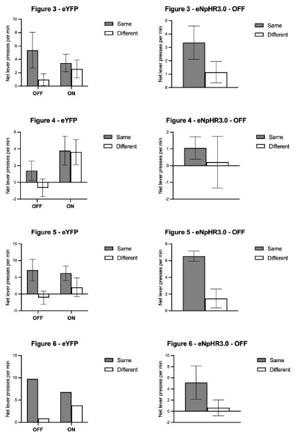
(8) For tracing, only males were used, and for electrophysiology, only females were used.
(8.1) Can authors please comment on not using both sexes in these experiments?
We agree that equal allocation of female and male rats in the experiments presented in Figures 1-2 would have been preferable. Animal availability was the sole factor determining these allocations. Importantly, both female and male D1-Cre and A2A-Cre rats were used for the NAc-S tracing studies, and no sex diMerences were observed in the projection patterns. The article describing the two transgenic lines of rats did not report any sex diMerence (Pettibone et al., 2019).
(8.2) Is there evidence in the literature that the electrophysiological properties of female versus male SPNs could diNer?
The literature indicates that there is no sex diMerence in the electrophysiological properties of NAc-S SPNs (Cao et al., 2018; Willett et al., 2016).
(8.3) It seems like there is a discrepancy between the number of animals used as presented in the Figure 2 legend versus what is described in the main text. In the Figure legend, I understand that 5 animals were used for D1-Cre/DIO-eNpHR3.0 validation, and 7 animals for A2a-Cre/DIO-eNpHR3.0; however, the main text indicates the use of a total of 8 animals instead of the 12 presented in the Figure legend. Can authors please address this mismatch or clarify?
The number of rats reported in the main text and Figure 2 legend was correct. However, recordings sometimes involved multiple cells from the same animal, and this aspect of the data was incorrectly reported and generated confusion. We have clarified the numbers in both the main text and Figure 2 legend to distinguish between animal counts and cell counts.
(9) Overall, in the study, have the authors checked for outliers?
Performance across all training and testing stages was inspected to identify potential behavioral outliers in each experiment. Abnormal performance during a single session within a multi-session stage was not considered suMicient grounds for outlier designation. Based on these criteria, no subjects remaining after post-mortem analyses exhibited performance patterns warranting exclusion through statistical outlier analysis. However, we have conducted the specific analyses requested by the Reviewer, as described below.
(9.1) In Figure 3, it seems that one female in the eYFP group, in the OFF situation, for the diNerent condition, has a higher level of responding than the others. Can authors please confirm or refute this visual observation with the appropriate statistical analysis?
Statistical analysis (z-score) confirmed the reviewer's observation regarding responding of the diMerent action in the OFF condition for this subject (|z| = 2.58). Similar extreme responding was observed in the ON condition (|z| = 2.03). Analyzing responding on the diMerent action in isolation is not informative in the context of outcome-specific PIT. Additional analyses revealed |z| < 2 when examining the magnitude of choice discrimination in outcome-specific PIT (i.e., net same versus net diMerent responding) in both ON and OFF conditions. Furthermore, this subject showed |z| < 2 across all other experimental stages. Based on these analyses, we conclude that the subject should be kept in all analyses.
(9.2) In Figure 5, it seems that one male, in the ON situation, in the diNerent condition, has a quite higher level of responding - is this subject an outlier? If so, how does it aNect the statistical analysis after being removed? And who is this subject in the OFF condition?
The reviewer has identified two diMerent male rats infused with the eNpHR3.0 virus and has asked closer examination of their performance.
The first rat showed outlier-level responding on the diMerent action in the ON condition (|z| = 2.89) but normal responding for all other measures across LED conditions (|z| < 2). Additional analyses revealed |z| = 2.55 when examining choice discrimination magnitude in outcome-specific PIT during the ON condition but not during the OFF condition (|z| = 0.62). This subject exhibited |z| < 2 across all other experimental stages.
The second rat showed outlier-level responding on the same action in the OFF condition (|z| = 2.02) but normal responding for all other measures across LED conditions (|z| < 2). Additional analyses revealed |z| = 2.12 when examining choice discrimination magnitude in outcome-specific PIT during the OFF condition but not during the ON condition (|z| = 0.67). This subject also exhibited |z| < 2 across all other experimental stages.
We excluded these two subjects and conducted the same analyses as described in the original manuscript. Baseline responding did not diMer between groups (p = 0.14), allowing to look at the net eMect of the stimuli. Overall lever presses were greater in the eYFP rats (Group: F(1,16) = 6.08, p < 0.05; η<sup>2</sup> = 0.28) and were reduced by LED activation (LED: F(1,16) = 9.52, p < 0.01; η<sup>2</sup> = 0.44) and this reduction depended on the group considered (Group x LED: F(1,16) = 12.125, p < 0.001; η<sup>2</sup> = 0.43). Lever press rates were higher on the action earning the same outcome as the stimuli compared to the action earning the diMerent outcome (Lever: F(1,16)= 49.32; η<sup>2</sup> = 0.76; p < 0.001), regardless of group (Group x Lever: p = 0.14). There was a Lever by LED light condition interaction (Lever x LED: F(1,16)= 5.25; η<sup>2</sup> = 0.24; p < 0.05) but no an interaction between group, LED light condition, and Lever during the presentation of the predictive stimuli (p = 0.10). Given the significant Group x LED and Lever x LED interactions, additional analyses were conducted to determine the source of these interactions. In eYFP rats, LED activation had no eMect (LED: p = 0.70) and lever presses were greater on the same action (Lever: (F(1,9) = 23.94, p < 0.001; η<sup>2</sup> = 0.79) regardless of LED condition (LED x Lever: p = 0.72). By contrast, in eNpHR3.0 rats, lever presses were reduced by LED activation (LED: F(1,9) = 23.97, p < 0.001; η<sup>2</sup> = 0.73), were greater on the same action (Lever: F(1,9) = 16.920, p < 0.001; η<sup>2</sup> = 0.65) and the two factors interacted (LED x Lever: F(1,9) = 9.12, p < 0.01; η<sup>2</sup> = 0.50). These rats demonstrated outcome-specific PIT in the OFF condition (F(1,9) = 27.26, p < 0.001; η<sup>2</sup> = 0.75) but not in the ON condition (p = 0.08).
Overall, excluding these two rats altered the statistical analyses, but both the original and revised analyses yielded the same outcome: silencing the NAc-S D1-SPN to VP pathway disrupted PIT. More importantly, we do not believe there are suMicient grounds to exclude the two rats identified by the reviewer. These animals did not display outlier-level responding across training stages or during the choice test. Their potential classification as outliers would be based on responding during only one LED condition and not the other, with notably opposite patterns between the two rats despite belonging to the same experimental group.
(10) I think it would be appreciable if in the cartoons from Figure 5.A and 6.A, the SPNs neurons were color-coded as in the results (test plots) and the supplementary figures (histological color-coding), such as D1- in blue & D2-SPNs in red.
Our current color-coding system uses blue for D1-SPNs transduced with eNpHR3.0 and red for D2-SPNs transduced with eNpHR3.0. The D1-SPNs and D2-SPNs shown in Figures 5A and 6A represent cells transduced with either eYFP (control) or eNpHR3.0 virus and therefore cannot be assigned the blue or red color, which is reserved for eNpHR3.0transduced cells specifically. The micrographs in the Supplemental Figures maintain consistency with the color-coding established in the main figures.
(11) As there are (relatively small) variations in the control performance in term of Net responding (from ~3 to ~7 responses per min), I wonder what would be the result of pooling eYFP groups from the two first experiments (Figures 3 & 4) and from the two last ones (Figures 5 & 6) - would the same statically results stand or vary (as eYFP vs D1-Cre vs A2a-Cre rats)? In particular for Figures 3 & 4, with and without the potential outlier, if it's indeed an outlier.
We considered the Reviewer’s recommendation but do not believe the requested analysis is appropriate. The Reviewer is requesting the pooling of data from subjects of distinct transgenic strains (D1-Cre and A2A-Cre rats) that underwent surgical and behavioral procedures at diMerent time points, sometimes months apart. Each experiment was designed with necessary controls to enable adequate statistical analyses for testing our specific hypotheses.
(12) Presence of cameras in operant cages is mentioned in methods, but no data is presented regarding recordings, though authors mention that they allow for real-time observations of behavior. I suggest removing "to record" or adding a statement about the fact that no videos were recorded or used in the present study.
We have removed “to record” from the manuscript (page 18).
(13) In all supplementary Figures, "F" is wrongly indicated as "E".
We thank the Reviewer for reporting these errors, which have been corrected.
(14) While the authors acknowledge that the eNicacy of optogenetic inhibition of terminals is questionable, I think that more details are required to address this point in the discussion (existing literature?). Maybe, the combination of an anterograde tracer from SPNs to VP, to label VP neurons (to facilitate patching these neurons), and the Credependent inhibitory opsin in the NAc Shell, with optogenetic illumination at the level of the VP, along with electrophysiological recordings of VP neurons, could help address this question but may, reasonably, seem challenging technically.
Our manuscript does not state that optogenetic inhibition of terminals is questionable. It acknowledges that we do not provide any evidence about the eMicacy of the approach. Regardless, we have provided additional details and suggestions to address this lack of evidence (page 13).
(15) A nice addition could be an illustration of the proposed model (from line 374), but it may be unnecessary.
We have carefully considered the reviewer's recommendation. The proposed model is detailed in three published articles, including one that is freely accessible, which we have cited when presenting the model in our manuscript (page 14). This reference should provide interested readers with easy access to a comprehensive illustration of the model.
Reviewer 2 (Recommendations for the Author):
As noted in my public comments, this is a truly excellent and compelling study. I have only a few minor comments.
(1) I could not find the coordinates/parameters for the dorsal striatal AAV injections for that component of the tract tracing experiment.
We apologize for this omission, which has now been corrected (page 16).
(2) Please add the final group sizes to the figure captions.
We followed the Reviewer’s recommendation and added group sizes in the main figure captions.
(3) The discussion of group exclusions (p 21 line 637) seems to accidentally omit (n = X) the number of NAc-S D1-SPNs-VP mice excluded.
We apologize for this omission, which has now been corrected (page 22).
(4) There were some labeling issues in the supplementary figures (perhaps elsewhere, too). Specifically, panel E was listed twice (once for F) in captions.
We apologize for this error, which has now been corrected.
(5) Inspection of the magazine entry data from PIT tests suggests that the optogenetic manipulations may have had some eNects on this behavior and would encourage the authors to probe further. There was a significant group diNerence for D1-SPN inhibition and a marginal group eNect for D2-SPNs. The fact that these eNects were in opposite directions is intriguing, although not easily interpreted based on the canonical D1/D2 model. Of course, the eNects are not specific to the light-on trials, but this could be due to carryover into light-oN trials. An analysis of trial-order eNects seems crucial for interpreting these eNects. One might also consider normalizing for pre-test baseline performance. Response rates during Pavlovian conditioning seem to suggest that D2eNpHR mice showed slightly higher conditioned responding during training, which contrasts with their low entry rates at test. I don't see any of this as problematic -- but more should be done to interpret these findings.
We thank the reviewer for raising this interesting point regarding magazine entry rates. Since these data are presented in the Supplemental Figures, we have added a section in the Supplemental Material file that elaborates on these findings. This section does not address trial order eMects, as trial order was fully counterbalanced in our experiments and the relevant statistical analyses would lack adequate power. Baseline normalization was not conducted because the reviewer's suggestion was based on their assumption that eNpHR3.0 rats in the D2-SPNs experiment showed slightly higher magazine entries during Pavlovian training. However, this was not the case. In fact, like the eNpHR3.0 rats in the D1-SPNs experiment, they tended to display lower magazine entries during training. The added section therefore focuses on the potential role of response competition during outcome-specific PIT tests. Although we concluded that response competition cannot explain our findings, we believe it may complicate interpretation of magazine entry behavior. Thus, we recommend that future studies examine the role of NAc-S SPNs using purely Pavlovian tasks. It is worth nothing that we have recently completed experiments (unpublished) examining NAc-S D1- and D2-SPN silencing during stimulus presentation in a Pavlovian task identical to the one used here. Silencing of either SPN population had no eMect on magazine entry behavior.
Reviewer 3 (Recommendations for the Author):
Broad comments:
Throughout the manuscript, the authors draw parallels between the eNect established via pharmacological manipulations and those shown here with optogenetic manipulation. I understand using the pharmacological data to launch this investigation, but these two procedures address very diNerent physiological questions. In the case of a pharmacological manipulation, the targets are receptors, wherever they are expressed, and in the case of D2 receptors, this means altering function in both pre-synaptically expressed autoreceptors and post-synaptically expressed D2 MSN receptors. In the case of an optogenetic approach, the target is a specific cell population with a high degree of temporal control. So I would just caution against comparing results from these types of studies too closely.
Related to this point is the consideration of the physiological relevance of the manipulation. Under normal conditions, dopamine acts at D1-like receptors to increase the probability of cell firing via Ga signaling. In contrast, dopamine binding of D2-like receptors decreases the cell's firing probability (signaling via Gi/o). Thus, shunting D1MSN activation provides a clear impression of the role of these cells and, putatively, the role of dopamine acting on these cells. However, inhibiting D2-MSNs more closely mimics these cells' response to dopamine (though optogenetic manipulations are likely far more impactful than Gi signaling). All this is to say that when we consider the results presented here in Experiment 2, it might suggest that during PIT testing, normal performance may require a halting of DA release onto D2-MSNs. This is highly speculative, of course, just a thought worth considering.
We agree with the comments made by the Reviewer, and the original manuscript included statements acknowledging that pharmacological approaches are limited in the capacity to inform about the function of NAc-S SPNs (pages 4 and 9). As noted by the Reviewer, these limitations are especially salient when considering NAc-S D2-SPNs. Based on the Reviewer’s comment, we have modified our discussion to further underscore these limitations (page 12). Finally, we agree with the suggestion that PIT may require a halting of DA release onto D2-SPNs. This is consistent with the model presented, whereby D2-SPNs function is required to trigger enkephalin release (page 13).
Section-Specific Comments and Questions:
Results:
Anterograde tracing and ex vivo cell recordings in D1 Cre and A2a Cre rats: Why are there no statistics reported for the e-phys data in this section? Was this merely a qualitative demonstration? I realize that the A2a-Cre condition only shows 3 recordings, so I appreciate the limitations in analyzing the data presented.
The reviewer is correct that we initially intended to provide a qualitative demonstration. However, we have now included statistical analyses for the ex vivo recordings. It is important to note that there were at least 5 recordings per condition, though overlapping data points may give the impression of fewer recordings in certain conditions. We have provided the exact number of recordings in both the main text (page 5) and figure legend.
What does trial by trial analysis look like, because in addition to the eNects of extinction, do you know if the responsiveness of the opsin to light stimulation is altered after repeated exposures, or whether the cells themselves become compromised in any way with repeated light-inhibition, particularly given the relatively long 2m duration of the trial.
The Reviewer raises an interesting point, and we provide complete trial-by-trial data for each experiment below. As identified by the Reviewer, there is some evidence for extinction, although it remained modest. Importantly, the data suggest that light stimulation did not aMect the physiology of the targeted cells. In eNpHR3.0 rats, performance across OFF trials remained stable (both for Same and DiMerent) even though they were preceded by ON trials, indicating no carryover eMects from optical stimulation.
Author response image 2.
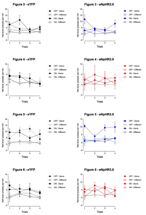
The statistics for the choice test are not reported for eNpHR-D1-Cre rats, but do show a weakening of the instrumental devaluation eNect "Group x Lever x LED: F1,18 = 10.04, p < 0.01, = 0.36". The post hoc comparisons showed that all groups showed devaluation, but it is evident that there is a weakening of this eNect when the LED was on (η<sup>2</sup> = 0.41) vs oN (η<sup>2</sup> = 0.78), so I think the authors should soften the claim that NAcS-D1s are not involved in value-based decision-making. (Also, there is a typo in the legend in Figure S1, where the caption for panel "F" is listed as "E".) I also think that this could be potentially interesting in light of the fact that with circuit manipulation, this same weakening of the instrumental devaluation eNect was not observed. To me, this suggests that D1-NAcS that project to a diNerent region (not VP) contribute to value-based decision making.
This comment overlaps with one made in the Public Review, for which we have already provided a response. Given its importance, we have added a section addressing this point in the supplemental discussion of the Supplementary Material file, which aligns with the location of the relevant data. The caption labelling error has been corrected.
Materials and Methods:
Subjects:
Were these heterozygous or homozygous rats? If hetero, what rats were used for crossbreeding (sex, strain, and vendor)? Was genotyping done by the lab or outsourced to commercial services? If genotyping was done within the lab, please provide a brief description of the protocol used. How was food restriction established and maintained (i.e., how many days to bring weights down, and was maintenance achieved by rationing or by limiting ad lib access to food for some period in the day)?
The information requested by the Reviewer have been added to the subjects section (pages 15-16).
Were rats pair/group housed after implantation of optic fibers?
We have clarified that rats were group houses throughout (see subjects section; pages 15-16).
Behavioral Procedures:
How long did each 0.2ml sucrose infusion take? For pellets, for each US delivery, was it a single pellet or two in quick succession?
We have modified the method section to indicate that the sucrose was delivered across 2 seconds and that a single pellet was provided (page 17).
The CS to ITI duration ratio is quite low. Is there a reason such a short ratio was used in training?
These parameters are those used in all our previous experiments on outcome-specific PIT. There is no specific reason for using such a ratio, except that it shortens the length of the training session.
Relative to the end of training, when were the optical implantation surgeries conducted, and how much recovery time was given before initiating reminder training and testing?
Fibre-optic implantation was conducted 3-4 days after training and another 3-4 days were given for recovery. This has been clarified in the Materials and methods section (pages 15-16).
I think a diagram or schematic showing the timeline for surgeries, training, and testing would be helpful to the audience.
We opted for a text-based experimental timeline rather than a diagram due to slight temporal variations across experiments (page 15).
On trials, when the LED was on, was light delivered continuously or pulsed? Do these opto-receptors 'bleach' within such a long window?
We apologize for the lack of clarity; the light was delivered continuously. We have modified the manuscript (pages 6 and 19) and figure legend accordingly. The postmortem analysis did not provide evidence for photobleaching (Supplemental Figures) and as noted above, the behavioural results do not indicate any negative physiological impact on cell function.
Immunofluorescence: The blocking solution used during IHC is described as "NHS"; is this normal horse serum?
The Reviewer is correct; NHS stands for normal horse serum. This has been added (page 21).
Microscopy and imaging:
For the description of rats excluded due to placement or viral spread problems, an n=X is listed for the NAc S D1 SPNs --> VP silencing group. Is this a typo, or was that meant to read as n=0? Also, was there a major sex diNerence in the attrition rate? If so, I think reporting the sex of the lost subjects might be beneficial to the scientific community, as it might reflect a need for better guidance on sex-specific coordinates for targeting small nuclei.
We apologize for the error regarding the number of excluded animals. This error has been corrected (page 23). There were no major sex diMerences in the attrition rate. The manuscript has been updated to provide information about the sex of excluded animals (page 23).
References
Cao, J., Willett, J. A., Dorris, D. M., & Meitzen, J. (2018). Sex DiMerences in Medium Spiny Neuron Excitability and Glutamatergic Synaptic Input: Heterogeneity Across Striatal Regions and Evidence for Estradiol-Dependent Sexual DiMerentiation. Front Endocrinol (Lausanne), 9, 173. https://doi.org/10.3389/fendo.2018.00173
Corbit, L. H., Muir, J. L., Balleine, B. W., & Balleine, B. W. (2001). The role of the nucleus accumbens in instrumental conditioning: Evidence of a functional dissociation between accumbens core and shell. J Neurosci, 21(9), 3251-3260. http://eutils.ncbi.nlm.nih.gov/entrez/eutils/elink.fcgi?dbfrom=pubmed&id=11312 310&retmode=ref&cmd=prlinks
Corbit, L. H., & Balleine, B. W. (2011). The general and outcome-specific forms of Pavlovian-instrumental transfer are diMerentially mediated by the nucleus accumbens core and shell. J Neurosci, 31(33), 11786-11794. https://doi.org/10.1523/JNEUROSCI.2711-11.2011
Laurent, V., Bertran-Gonzalez, J., Chieng, B. C., & Balleine, B. W. (2014). δ-Opioid and Dopaminergic Processes in Accumbens Shell Modulate the Cholinergic Control of Predictive Learning and Choice. J Neurosci, 34(4), 1358-1369. https://doi.org/10.1523/JNEUROSCI.4592-13.2014
Laurent, V., Leung, B., Maidment, N., & Balleine, B. W. (2012). μ- and δ-opioid-related processes in the accumbens core and shell diMerentially mediate the influence of reward-guided and stimulus-guided decisions on choice. J Neurosci, 32(5), 1875-1883. https://doi.org/10.1523/JNEUROSCI.4688-11.2012
Matamales, M., McGovern, A. E., Mi, J. D., Mazzone, S. B., Balleine, B. W., & BertranGonzalez, J. (2020). Local D2- to D1-neuron transmodulation updates goal-directed learning in the striatum. Science, 367(6477), 549-555. https://doi.org/10.1126/science.aaz5751
Parkes, S. L., Bradfield, L. A., & Balleine, B. W. (2015). Interaction of insular cortex and ventral striatum mediates the eMect of incentive memory on choice between goaldirected actions. J Neurosci, 35(16), 6464-6471. https://doi.org/10.1523/JNEUROSCI.4153-14.2015
Pettibone, J. R., Yu, J. Y., Derman, R. C., Faust, T. W., Hughes, E. D., Filipiak, W. E., Saunders, T. L., Ferrario, C. R., & Berke, J. D. (2019). Knock-In Rat Lines with Cre Recombinase at the Dopamine D1 and Adenosine 2a Receptor Loci. eNeuro, 6(5). https://doi.org/10.1523/ENEURO.0163-19.2019
Willett, J. A., Will, T., Hauser, C. A., Dorris, D. M., Cao, J., & Meitzen, J. (2016). No Evidence for Sex DiMerences in the Electrophysiological Properties and Excitatory Synaptic Input onto Nucleus Accumbens Shell Medium Spiny Neurons. eNeuro, 3(1), ENEURO.0147-15.2016. https://doi.org/10.1523/ENEURO.0147-15.2016
Reviewer #2 (Public review):
Summary:
This work by den Bakker and Kloosterman contributes to the vast body of research exploring the dynamics governing the communication between the hippocampus (HPC) and the medial prefrontal cortex (mPFC) during spatial learning and navigation. Previous research showed that population activity of mPFC neurons is replayed during HPC sharp-wave ripple events (SWRs), which may therefore correspond to privileged windows for the transfer of learned navigation information from the HPC, where initial learning occurs, to the mPFC, which is thought to store this information long term. Indeed, it was also previously shown that the activity of mPFC neurons contains task-related information that can inform about the location of an animal in a maze, which can predict the animals' navigational choices. Here, the authors aim to show that the mPFC neurons that are modulated by HPC activity (SWRs and theta rhythms) are distinct from those "encoding" spatial information. This result could suggest that the integration of spatial information originating from the HPC within the mPFC may require the cooperation of separate sets of neurons.
This observation may be useful to further extend our understanding of the dynamics regulating the exchange of information between the HPC and mPFC during learning. However, my understanding is that this finding is mainly based upon a negative result, which cannot be statistically proven by the failure to reject the null hypothesis. Moreover, in my reading, the rest of the paper mainly replicates phenomena that have already been described, with the original reports not correctly cited. My opinion is that the novel elements should be precisely identified and discussed, while the current phrasing in the manuscript, in most cases, leads readers to think that these results are new. Detailed comments are provided below.
Major concerns:
ORIGINAL COMMENT: (1) The main claim of the manuscript is that the neurons involved in predicting upcoming choices are not the neurons modulated by the HPC. This is based upon the evidence provided in Figure 5, which is a negative result that the authors employ to claim that predictive non-local representations in the mPFC are not linked to hippocampal SWRs and theta phase. However, it is important to remember that in a statistical test, the failure to reject the null hypothesis does not prove that the null hypothesis is true. Since this claim is so central in this work, the authors should use appropriate statistics to demonstrate that the null hypothesis is true. This can be accomplished by showing that there is no effect above some size that is so small that it would make the effect meaningless (see https://doi.org/10.1177/070674370304801108).
AUTHOR RESPONSE: We would like to highlight a few important points here. (1) We indeed do not intend to claim that the SWR-modulated neurons are not at all involved in predicting upcoming choice, just that the SWR-unmodulated neurons may play a larger role. We have rephrased the title and abstract to make this clearer.
REVIEWER COMMENT: The title has been rephrased but still conveys the same substantive claim. The abstract sentence also does not clearly state what was found. Using "independently" in the new title continues to imply that SWR modulation and prediction of upcoming choices are separate phenomena. By contrast, in your response here in the rebuttall you state only that "SWR-unmodulated neurons may play a larger role," which is a much more tempered claim than what the manuscript currently argues. Why is this clarification not adopted in the article? Moreover, the main text continues to use the same arguments as before; beyond the cosmetic changes of title and abstract, the claim itself has not materially changed.
AUTHOR RESPONSE: (2) The hypothesis that we put forward is based not only on a negative effect, but on the findings that: the SWR-unmodulated neurons show higher spatial tuning (Fig 3b), more directional selectivity (Fig 3d), more frequent encoding of the upcoming choice at the choice point (new analysis, added in Fig 4d), and higher spike rates during the representations of the upcoming choice (Fig 5b). This is further highlighted by the fact that the representations of upcoming choice in the PFC are not time locked to SWRs (whereas the hippocampal representations of upcoming choice are; see Fig 5a and Fig 6a), and not time-locked to hippocampal theta phase (whereas the hippocampal representations are; see Fig 5c and Fig 6c). Finally, the representations of upcoming and alternative choices in the PFC do not show a large overlap in time with the representations in the hippocampus (see updated Fig 4e were we added a statistical test to show the likelihood of the overlap of decoded timepoints). All these results together lead us to hypothesize that SWR-modulation is not the driving factor behind non-local decoding in the PFC.
REVIEWER COMMENT: I do not see how these precisions address my remark. The main claim in the title used to be "Neurons in the medial prefrontal cortex that are not modulated by hippocampal sharp-wave ripples are involved in spatial tuning and signaling upcoming choice." It is now "Neurons in the medial prefrontal cortex are involved in spatial tuning and signaling upcoming choice independently from hippocampal sharp-wave ripples." The substance has not changed. This specific claim is supported solely by Figure 5.
The other analyses cited describe functional characteristics of SWR-unmodulated neurons but, unless linked by explicit new analyses, do not substantiate independence/orthogonality between SWR modulation and non-local decoding in PFC. If there is an analysis that makes this link explicit, it should be clearly presented; as it stands, I cannot find an explanation in the manuscript for why "all these results together" justify the conclusion that "All these results together lead us to hypothesize that SWR-modulation is not the driving factor behind non-local decoding in the PFC". Also: is the main result of this work a "hypothesis"? If so, this should be clearly differentiated from a conclusion supported by results and analyses.
AUTHOR RESPONSE: (3) Based on the reviewers suggestion, we have added a statistical test to compare the phase-locking based of the non-local decoding to hippocampal SWRs and theta phase to shuffled posterior probabilities. Instead of looking at all SWRs in a -2 to 2 second window, we have now only selected the closest SWR in time within that window, and did the statistical comparison in the bin of 0-20 ms from SWR onset. With this new analysis we are looking more directly at the time-locking of the decoded segments to SWR onset (see updated Fig 5a and 6a).
REVIEWER COMMENT: I appreciate the added analysis focusing on the closest SWR and a 0-20 ms bin. My understanding is that you consider the revised analyses in Figures 5a and 6a sufficient to show that predictive non-local representations in mPFC are not linked to hippocampal SWRs and theta phase.
First, the manuscript should explicitly explain the rationale for this analysis and why it is sufficient to support the claim. From the main text it is not possible to understand what was done; the Methods are hard to follow, and the figure legends are not clearly described (e.g. the shuffle is not even defined there).
Specific points I could not reconcile:
i) The gray histograms in the revised Figures 5a and 6a now show a peak at zero lag, whereas in the previous version they were flat, although they are said to plot the same data. What changed?
ii) Why choose a 20 ms bin? A single narrow bin invites false negatives. Please justify this choice.
iii) Comparing to a shuffle is a useful control, but when the p-value is non-significant we only learn that no difference was detected under that shuffle-not that there is no difference or that the processes are independent.
ORIGINAL COMMENT: (2) The main claim of the work is also based on Figure 3, where the authors show that SWRs-unmodulated mPFC neurons have higher spatial tuning, and higher directional selectivity scores, and a higher percentage of these neurons show theta skipping. This is used to support the claim that SWRs-unmodulated cells encode spatial information. However, it must be noted that in this kind of task, it is not possible to disentangle space and specific task variables involving separate cognitive processes from processing spatial information such as decision-making, attention, motor control, etc., which always happen at specific locations of the maze. Therefore, the results shown in Figure 3 may relate to other specific processes rather than encoding of space and it cannot be unequivocally claimed that mPFC neurons "encode spatial information". This limitation is presented by Mashoori et al (2018), an article that appears to be a major inspiration for this work. Can the authors provide a control analysis/experiment that supports their claim? Otherwise, this claim should be tempered. Also, the authors say that Jadhav et al. (2016) showed that mPFC neurons unmodulated by SWRs are less tuned to space. How do they reconcile it with their results?
AUTHOR RESPONSE: The reviewer is right to assert caution when talking about claims such as spatial tuning where other factors may also be involved. Although we agree that there may be some other factors influencing what we are seeing as spatial tuning, it is very important to note that the behavioral task is executed on a symmetrical 4-armed maze, where two of the arms are always used for the start of the trajectory, and the other two arms (North and South) function as the goal (reward) arms. Therefore, if the PFC is encoding cognitive processes such as task phases related to decision-making and reward, we would not be able to differentiate between the two start arms and the two goal arms, as these represent the same task phases. Note also that the North and South arm are illuminated in a pseudo-random order between trials and during cue-based rule learning this is a direct indication of where the reward will be found. Even in this phase of the task, the PFC encodes where the animal will turn on a trial-to-trial basis (meaning the North and South arm are still differentiated correctly on each trial even though the illumination and associated reward are changing).
REVIEWER COMMENT: I appreciate that the departure location was pseudorandomized. However, this control does not rule out that PFC activity reflects motor preparation (left vs right turns) and associated perceptual decision-making/attentional processes that are inherently tied to a specific action. As such, it cannot by itself support the claim that PFC neurons "encode spatial information." Moreover, the authors acknowledge here that "other factors may also be involved," yet this caveat is not reflected in the manuscript. Why?
AUTHOR RESPONSE: Secondly, importantly, the reviewer mentions that we claimed that Jadhav et al. (2016) showed that mPFC neurons unmodulated by SWRs are less tuned to space, but this is incorrect. Jadhav et al. (2016) showed that SWR-unmodulated neurons had lower spatial coverage, meaning that they are more spatially selective (congruent with our results). We have rephrased this in the text to be clearer.
REVIEWER COMMENT: Thanks for clarifying this.
ORIGINAL COMMENT: (3) My reading is that the rest of the paper mainly consists of replications or incremental observations of already known phenomena with some not necessarily surprising new observations:<br /> a) Figure 2 shows that a subset of mPFC neurons is modulated by HPC SWRs and theta (already known), that vmPFC neurons are more strongly modulated by SWRs (not surprising given anatomy), and that theta phase preference is different between vmPFC and dmPFC (not surprising given the fact that theta is a travelling wave).
AUTHOR RESPONSE: The finding that vmPFC neurons are more strongly modulated by SWRs than dmPFC indeed matches what we know from anatomy, but that does not make it a trivial finding. A lot remains unknown about the mPFC subregions and their interactions with the hippocampus, and not every finding will be directly linked to the anatomy. Therefore, in our view this is a significant finding which has not been studied before due to the technical complexity of large-scale recordings along the dorsal-ventral axis of the mPFC.
REVIEWER COMMENT: This finding is indeed non-trivial; however, it seems completely irrelevant to the paper's main claim unless the Authors can argue otherwise.
AUTHOR RESPONSE: Similarly, theta being a traveling wave (which in itself is still under debate), does not mean we should assume that the dorsal and ventral mPFC should follow this signature and be modulated by different phases of the theta cycle. Again, in our view this is not at all trivial, but an important finding which brings us closer to understanding the intricate interactions between the hippocampus and PFC in spatial learning and decision-making.
REVIEWER COMMENT: Yes, but in what way does this support the manuscript's primary claim? This is unclear to me.
ORIGINAL COMMENT: b) Figure 4 shows that non-local representations in mPFC are predictive of the animal's choice. This is mostly an increment to the work of Mashoori et al (2018). My understanding is that in addition to what had already been shown by Mashoori et al here it is shown how the upcoming choice can be predicted. The author may want to emphasize this novel aspect.
AUTHOR RESPONSE: In our view our manuscript focuses on a completely different aspect of learning and memory than the paper the reviewer is referring to (Mashoori et al. 2018). Importantly, the Mashoori et al. paper looked at choice evaluation at reward sites and shows that disappointing reinforcements are associated with reactivations in the ACC of the unselected target. This points to the role of the ACC in error detection and evaluation. Although this is an interesting result, it is in essence unrelated to what we are focusing on here, which is decision making and prediction of upcoming choices. The fact that the turning direction of the animal can be predicted on a trial-to-trial basis, and even precedes the behavioral change over the course of learning, sheds light on the role of the PFC in these important predictive cognitive processes (as opposed to post-choice reflective processes).
REVIEWER COMMENT: Indeed, as I said, the new element here is that the upcoming choice can be predicted. This appears only incremental and could belong to another story; as the manuscript is currently written, it does not support the article's main claim. I would like to specify that, regarding this and the other points above, my inability to see how these minor results support the Authors' claim may reflect my misunderstanding; nevertheless, this suggests that the manuscript should be extensively rewritten and reorganized to make the Authors' meaning clear.
ORIGINAL COMMENT: c) Figure 6 shows that prospective activity in the HPC is linked to SWRs and theta oscillations. This has been described in various forms since at least the works of Johnson and Redish in 2007, Pastalkova et al 2008, and Dragoi and Tonegawa (2011 and 2013), as well as in earlier literature on splitter cells. These foundational papers on this topic are not even cited in the current manuscript.
AUTHOR RESPONSE: We have added these citations to the introduction (line 37).
REVIEWER COMMENT: This is an example of how the Authors fail to acknowledge the underlying problem with how the manuscript is written; the issue has not been addressed except with a cosmetic change like the one described above. The Results section contains a series of findings that are well-known phenomena described previously (see below). Prior results should be acknowledged at the beginning of each relevant paragraph, followed by an explicit statement of what is new, so that readers can distinguish replication from novelty. Here, I pointed specifically to the results of Figure 6, and the Authors deemed it sufficient simply to add the citations I indicated to an existing sentence in the Introduction, while keeping the Results description unchanged. As written, this reads as if these phenomena are being described for the first time. This is incorrect. It is hard to avoid the impression that the Authors did not take this concern seriously; the same issue appears elsewhere in the manuscript, and I fail to see how the Authors "have improved clarity of the text throughout to highlight the novelty of our results better."
Author response:
The following is the authors’ response to the original reviews.
Reviewer #1 (Public review):
Summary:
The authors used high-density probe recordings in the medial prefrontal cortex (PFC) and hippocampus during a rodent spatial memory task to examine functional sub-populations of PFC neurons that are modulated vs. unmodulated by hippocampal sharp-wave ripples (SWRs), an important physiological biomarker that is thought to have a role in mediating information transfer across hippocampal-cortical networks for memory processes. SWRs are associated with the reactivation of representations of previous experiences, and associated reactivation in hippocampal and cortical regions has been proposed to have a role in memory formation, retrieval, planning, and memory-guided behavior. This study focuses on awake SWRs that are prevalent during immobility periods during pauses in behavior. Previous studies have reported strong modulation of a subset of prefrontal neurons during hippocampal SWRs, with some studies reporting prefrontal reactivation during SWRs that have a role in spatial memory processes. The study seeks to extend these findings by examining the activity of SWR-modulated vs. unmodulated neurons across PFC sub-regions, and whether there is a functional distinction between these two kinds of neuronal populations with respect to representing spatial information and supporting memory-guided decision-making.
Strengths:
The major strength of the study is the use of Neuropixels 1.0 probes to monitor activity throughout the dorsal-ventral extent of the rodent medial prefrontal cortex, permitting an investigation of functional distinction in neuronal populations across PFC sub-regions. They are able to show that SWR-unmodulated neurons, in addition to having stronger spatial tuning than SWR-modulated neurons as previously reported, also show stronger directional selectivity and theta-cycle skipping properties.
Weaknesses:
(1) While the study is able to extend previous findings that SWR-modulated PFC neurons have significantly lower spatial tuning that SWR-unmodulated neurons, the evidence presented does not support the main conclusion of the paper that only the unmodulated neurons are involved in spatial tuning and signaling upcoming choice, implying that SWR-modulated neurons are not involved in predicting upcoming choice, as stated in the abstract. This conclusion makes a categorical distinction between two neuronal populations, that SWR-modulated neurons are involved and SWR-unmodulated are not involved in predicting upcoming choice, which requires evidence that clearly shows this absolute distinction. However, in the analyses showing non-local population decoding in PFC for predicting upcoming choice, the results show that SWR-unmodulated neurons have higher firing rates than SWR-modulated neurons, which is not a categorical distinction. Higher firing rates do not imply that only SWR-unmodulated neurons are contributing to the non-local decoding. They may contribute more than SWR-modulated neurons, but there are no follow-up analyses to assess the contribution of the two sub-populations to non-local decoding.
We agree with the reviewer that this is indeed not a categorical distinction, and do not wish to claim that the SWR-modulated neurons have absolutely no role in non-local decoding and signaling upcoming choice. We have adjusted this in the title, abstract and text to clarify this for the reader. Furthermore, we have performed additional analyses to elucidate the role of SWR-modulated neurons in non-local decoding by creating separate decoding models for SWR-modulated and unmodulated PFC neurons respectively. These analyses show that the SWR-unmodulated neurons are indeed encoding representations of the upcoming choice more often than the alternative choice, whereas the SWR-modulated neurons do not reliably differentiate the upcoming and alternative choices in non-local decoding at the choice point (see new Fig 4d).
(2) Further, the results show that during non-local representations of the hippocampus of the upcoming options, SWR-excited PFC neurons were more active during hippocampal representations of the upcoming choice, and SWR-inhibited PFC neurons were less active during hippocampal representations of the alternative choice. This clearly suggests that SWR-modulated neurons are involved in signaling upcoming choice, at least during hippocampal non-local representations, which contradicts the main conclusion of the paper.
This does not contradict the main conclusion of the paper, but in fact strengthens the hypothesis we are putting forward: that the SWR-modulated neurons are more linked to the hippocampal non-local representations, whereas the SWR-unmodulated neurons seem to have their own encoding of upcoming choice which is not linked to the signatures in the hippocampus (almost no time overlap with hippocampal representations, no phase locking to hippocampal theta, no time locking to hippocampal SWRs, no increased firing during hippocampal representations of upcoming choice).
(3) Similarly, one of the analyses shows that PFC nonlocal representations show no preference for hippocampal SWRs or hippocampal theta phase. However, the examples shown for non-local representations clearly show that these decodes occur prior to the start of the trajectory, or during running on the central zone or start arm. The time period of immobility prior to the start arm running will have a higher prevalence of SWRs and that during running will have a higher prevalence of theta oscillations and theta sequences, so non-local decoded representations have to sub-divided according to these known local-field potential phenomena for this analysis, which is not followed.
These analyses are in fact separated based on proximity to SWRs (only segments that occurred within 2 seconds of SWR onset were included, see Methods) and theta periods respectively (selected based on a running speed of more than 5 cm/s and the absence of SWRs in the hippocampus, see Methods). We have clarified this in the main text.
(4) The primary phenomenon that the manuscript relies on is the modulation of PFC neurons by hippocampal SWRs, so it is necessary to perform the PFC population decoding analyses during SWRs (or examine non-local decoding that occurs specifically during SWRs), as reported in previous studies of PFC reactivation during SWRs, to see if there is any distinction between modulated and unmodulated neurons in this reactivation. Even in the case of independent PFC reactivation as reported by one study, this PFC reactivation was still reported to occur during hippocampal SWRs, therefore decoding during SWRs has to be examined. Similarly, the phenomenon of theta cycle skipping is related to theta sequence representations, so decoding during PFC and hippocampal theta sequences has to be examined before coming to any conclusions.
The histograms shown in Figure 5a (see updated Fig 5a where we look at the closest SWR in time and compare the occurrence with shuffled data) show that there is no increased prevalence of decoding upcoming and alternative choices in the PFC during hippocampal SWRs. The lack of overlap of non-local decoding between the hippocampus and PFC further shows that these non-local representations occur at different timepoints in the PFC and hippocampus (see updated Fig 4e where we added a statistical test to show the likeliness of the overlap between the decoded segments in the PFC and hippocampus). Based on the reviewer's suggestion, we have additionally decoded the information in the PFC during hippocampal SWRs exclusively, and found that the direction on the maze could not be predicted based on the decoding of SWR time points in the PFC. See figure below. Similarly, we can see from the histograms in Figure 5c that there is no phase locking to the hippocampal theta phase for non-local representations in the PFC, and in contrast there is phase locking of the hippocampal encoding of upcoming choice to the rising phase of the theta cycle (Fig 6c), further highlighting the separation between these two regions in the non-local decoding.
Reviewer #2 (Public review):
Summary:
This work by den Bakker and Kloosterman contributes to the vast body of research exploring the dynamics governing the communication between the hippocampus (HPC) and the medial prefrontal cortex (mPFC) during spatial learning and navigation. Previous research showed that population activity of mPFC neurons is replayed during HPC sharp-wave ripple events (SWRs), which may therefore correspond to privileged windows for the transfer of learned navigation information from the HPC, where initial learning occurs, to the mPFC, which is thought to store this information long term. Indeed, it was also previously shown that the activity of mPFC neurons contains task-related information that can inform about the location of an animal in a maze, which can predict the animals' navigational choices. Here, the authors aim to show that the mPFC neurons that are modulated by HPC activity (SWRs and theta rhythms) are distinct from those "encoding" spatial information. This result could suggest that the integration of spatial information originating from the HPC within the mPFC may require the cooperation of separate sets of neurons.
This observation may be useful to further extend our understanding of the dynamics regulating the exchange of information between the HPC and mPFC during learning. However, my understanding is that this finding is mainly based upon a negative result, which cannot be statistically proven by the failure to reject the null hypothesis. Moreover, in my reading, the rest of the paper mainly replicates phenomena that have already been described, with the original reports not correctly cited. My opinion is that the novel elements should be precisely identified and discussed, while the current phrasing in the manuscript, in most cases, leads readers to think that these results are new. Detailed comments are provided below.
Major concerns:
(1) The main claim of the manuscript is that the neurons involved in predicting upcoming choices are not the neurons modulated by the HPC. This is based upon the evidence provided in Figure 5, which is a negative result that the authors employ to claim that predictive non-local representations in the mPFC are not linked to hippocampal SWRs and theta phase. However, it is important to remember that in a statistical test, the failure to reject the null hypothesis does not prove that the null hypothesis is true. Since this claim is so central in this work, the authors should use appropriate statistics to demonstrate that the null hypothesis is true. This can be accomplished by showing that there is no effect above some size that is so small that it would make the effect meaningless (see https://doi.org/10.1177/070674370304801108).
We would like to highlight a few important points here. (1) We indeed do not intend to claim that the SWR-modulated neurons are not at all involved in predicting upcoming choice, just that the SWR-unmodulated neurons may play a larger role. We have rephrased the title and abstract to make this clearer. (2) The hypothesis that we put forward is based not only on a negative effect, but on the findings that: the SWR-unmodulated neurons show higher spatial tuning (Fig 3b), more directional selectivity (Fig 3d), more frequent encoding of the upcoming choice at the choice point (new analysis, added in Fig 4d), and higher spike rates during the representations of the upcoming choice (Fig 5b). This is further highlighted by the fact that the representations of upcoming choice in the PFC are not time locked to SWRs (whereas the hippocampal representations of upcoming choice are; see Fig 5a and Fig 6a), and not time-locked to hippocampal theta phase (whereas the hippocampal representations are; see Fig 5c and Fig 6c). Finally, the representations of upcoming and alternative choices in the PFC do not show a large overlap in time with the representations in the hippocampus (see updated Fig 4e were we added a statistical test to show the likelihood of the overlap of decoded timepoints). All these results together lead us to hypothesize that SWR-modulation is not the driving factor behind non-local decoding in the PFC. (3) Based on the reviewers suggestion, we have added a statistical test to compare the phase-locking based of the non-local decoding to hippocampal SWRs and theta phase to shuffled posterior probabilities. Instead of looking at all SWRs in a -2 to 2 second window, we have now only selected the closest SWR in time within that window, and did the statistical comparison in the bin of 0-20 ms from SWR onset. With this new analysis we are looking more directly at the time-locking of the decoded segments to SWR onset (see updated Fig 5a and 6a).
(2) The main claim of the work is also based on Figure 3, where the authors show that SWRs-unmodulated mPFC neurons have higher spatial tuning, and higher directional selectivity scores, and a higher percentage of these neurons show theta skipping. This is used to support the claim that SWRs-unmodulated cells encode spatial information. However, it must be noted that in this kind of task, it is not possible to disentangle space and specific task variables involving separate cognitive processes from processing spatial information such as decision-making, attention, motor control, etc., which always happen at specific locations of the maze. Therefore, the results shown in Figure 3 may relate to other specific processes rather than encoding of space and it cannot be unequivocally claimed that mPFC neurons "encode spatial information". This limitation is presented by Mashoori et al (2018), an article that appears to be a major inspiration for this work. Can the authors provide a control analysis/experiment that supports their claim? Otherwise, this claim should be tempered. Also, the authors say that Jadhav et al. (2016) showed that mPFC neurons unmodulated by SWRs are less tuned to space. How do they reconcile it with their results?
The reviewer is right to assert caution when talking about claims such as spatial tuning where other factors may also be involved. Although we agree that there may be some other factors influencing what we are seeing as spatial tuning, it is very important to note that the behavioral task is executed on a symmetrical 4-armed maze, where two of the arms are always used for the start of the trajectory, and the other two arms (North and South) function as the goal (reward) arms. Therefore, if the PFC is encoding cognitive processes such as task phases related to decision-making and reward, we would not be able to differentiate between the two start arms and the two goal arms, as these represent the same task phases. Note also that the North and South arm are illuminated in a pseudo-random order between trials and during cue-based rule learning this is a direct indication of where the reward will be found. Even in this phase of the task, the PFC encodes where the animal will turn on a trial-to-trial basis (meaning the North and South arm are still differentiated correctly on each trial even though the illumination and associated reward are changing).
Secondly, importantly, the reviewer mentions that we claimed that Jadhav et al. (2016) showed that mPFC neurons unmodulated by SWRs are less tuned to space, but this is incorrect. Jadhav et al. (2016) showed that SWR-unmodulated neurons had lower spatial coverage, meaning that they are more spatially selective (congruent with our results). We have rephrased this in the text to be clearer.
(3) My reading is that the rest of the paper mainly consists of replications or incremental observations of already known phenomena with some not necessarily surprising new observations:
(a) Figure 2 shows that a subset of mPFC neurons is modulated by HPC SWRs and theta (already known), that vmPFC neurons are more strongly modulated by SWRs (not surprising given anatomy), and that theta phase preference is different between vmPFC and dmPFC (not surprising given the fact that theta is a travelling wave).
The finding that vmPFC neurons are more strongly modulated by SWRs than dmPFC indeed matches what we know from anatomy, but that does not make it a trivial finding. A lot remains unknown about the mPFC subregions and their interactions with the hippocampus, and not every finding will be directly linked to the anatomy. Therefore, in our view this is a significant finding which has not been studied before due to the technical complexity of large-scale recordings along the dorsal-ventral axis of the mPFC.
Similarly, theta being a traveling wave (which in itself is still under debate), does not mean we should assume that the dorsal and ventral mPFC should follow this signature and be modulated by different phases of the theta cycle. Again, in our view this is not at all trivial, but an important finding which brings us closer to understanding the intricate interactions between the hippocampus and PFC in spatial learning and decision-making.
(b) Figure 4 shows that non-local representations in mPFC are predictive of the animal's choice. This is mostly an increment to the work of Mashoori et al (2018). My understanding is that in addition to what had already been shown by Mashoori et al here it is shown how the upcoming choice can be predicted. The author may want to emphasize this novel aspect.
In our view our manuscript focuses on a completely different aspect of learning and memory than the paper the reviewer is referring to (Mashoori et al. 2018). Importantly, the Mashoori et al. paper looked at choice evaluation at reward sites and shows that disappointing reinforcements are associated with reactivations in the ACC of the unselected target. This points to the role of the ACC in error detection and evaluation. Although this is an interesting result, it is in essence unrelated to what we are focusing on here, which is decision making and prediction of upcoming choices. The fact that the turning direction of the animal can be predicted on a trial-to-trial basis, and even precedes the behavioral change over the course of learning, sheds light on the role of the PFC in these important predictive cognitive processes (as opposed to post-choice reflective processes).
(c) Figure 6 shows that prospective activity in the HPC is linked to SWRs and theta oscillations. This has been described in various forms since at least the works of Johnson and Redish in 2007, Pastalkova et al 2008, and Dragoi and Tonegawa (2011 and 2013), as well as in earlier literature on splitter cells. These foundational papers on this topic are not even cited in the current manuscript.
We have added these citations to the introduction (line 37).
Although some previous work is cited, the current narrative of the results section may lead the reader to think that these results are new, which I think is unfair. Previous evidence of the same phenomena should be cited all along the results and what is new and/or different from previous results should be clearly stated and discussed. Pure replications of previous works may actually just be supplementary figures. It is not fair that the titles of paragraphs and main figures correspond to notions that are well established in the literature (e.g., Figure 2, 2nd paragraph of results, etc.).
We have changed the title of paragraph 2 and Figure 2 to highlight more clearly the novel result (the difference between the dorsal and ventral mPFC), and have improved clarity of the text throughout to highlight the novelty of our results better.
(d) My opinion is that, overall, the paper gives the impression of being somewhat rushed and lacking attention to detail. Many figure panels are difficult to understand due to incomplete legends and visualizations with tiny, indistinguishable details. Moreover, some previous works are not correctly cited. I tried to make a list of everything I spotted below.
We have addressed all the comments in the Recommendations for Authors.
Reviewer #1 (Recommendations for the authors):
(1) Expanding on the points above, one of the strengths of the study is expanding the previous result that SWR-unmodulated neurons are more spatially selective (Jadhav et al., 2016), across prefrontal sub-regions, and showing that these neurons are more directionally selective and show more theta cycle skipping. Theta cycle skipping is related to theta sequence representations and previous studies have established PFC theta sequences in parallel to hippocampal theta sequences (Tang et al., 2021; Hasz and Redish, 2020; Wang et al., 2024), and the theta cycle skipping result suggests that SWR-unmodulated neurons should show stronger participation than SWR-modulated neurons in PFC theta sequences that decode to upcoming or alternative location, which can be tested in this high-density PFC physiology data. This is still unlikely to make a categorical distinction that only SWR-unmodulated neurons participate in theta sequence decoding, but will be useful to examine.
We thank the reviewer for their suggestion and have now included results based on separate decoding models that only use SWR-modulated or SWR-unmodulated mPFC neurons. From this analysis we see that indeed SWR-unmodulated neurons are not the only group contributing to theta sequence decoding, but they do distinguish more strongly between the upcoming and alternative arms at the choice point (see new Fig 4d).
(2) Non-local decoding in 50ms windows on a theta timescale is a valid analysis, but ignoring potential variability in the internal state during running vs. immobility, and as indicated by LFPs by the presence of SWRs or theta oscillations, is incorrect especially when conclusions are being made about decoding during SWRs and theta oscillation phase, and in light of previous evidence that these are distinct states during behavior. There are multiple papers on PFC theta sequences (Tang et al., 2021; Hasz and Redish, 2020; Wang et al., 2024), and on PFC reactivation during SWRs (Shin et al., 2019; Kaefer et al., 2020; Jarovi et al., 2023), and this dataset of high-density prefrontal recordings using Neuropixels 1.0 provides an opportunity to investigate these phenomena in detail. Here, it should be noted that although Kaefer et al. reported independent prefrontal reactivation from hippocampal reactivation, these PFC reactivation events still occurred during hippocampal SWRs in their data, and were linked to memory performance.
From our data we see that the time segments that represent upcoming or alternative choice in the prefrontal cortex are in fact not time-locked to hippocampal SWRs (updated Fig 5a where we look only at the closest SWR in time and compare this to shuffled data). In addition, these segments do not overlap much with the decoded segments in the hippocampus (see updated Fig 4e where we added a shuffling procedure to assess the likelihood of the overlap with hippocampal decoded segments). Importantly, we are not ignoring the variability during running and immobility, as theta segments were selected based on a running speed of more than 5 cm/s and the absence of SWRs in the hippocampus (see Methods), ensuring that the theta and SWR analyses were done on the two different behavioral states respectively. We have clarified this in the main text.
(3) The majority of rodent studies make the distinction between ACC, PrL, and IL, although as the authors noted, there are arguments that rodent mPFC is a continuum (Howland et al., 2022), or even that rodent mPFC is a unitary cingulate cortical region (van Heukelum et al., 2020). The authors choose to present the results as dorsal (ACC + dorsal PrL) vs. ventral mPFC (ventral PrL + IL), however, in my opinion, it will be more useful to the field to see results separately for ACC, PrL, and IL, given the vast literature on connectivity and functional differences in these regions.
We appreciate the reviewer’s suggestion. Initially, we did perform all analyses separately for the ACC, PLC and ILC subregions. However, we observed that the differences between subregions (strength of SWR-modulation and the phase locking to theta) varied uniformly along the dorsal-ventral axis, i.e., the PLC showed a profile of SWR-modulation and theta phase locking that fell in between that of the ACC and the ILC. This is also highlighted in paragraph 3 of the introduction (lines 52-56). For that reason, and for the sake of reducing the number of variables, increasing statistical power, and improving readability, we focused on the dorsal-ventral distinction instead, as this is where the main differences were seen.
(4) I suggest that the authors refrain from making categorical distinctions as in their title and abstract, such as "neurons that are involved in predicting upcoming choice are not the neurons that are modulated by hippocampal sharp-wave ripples" when the evidence presented can only support gradation of participation of the two neuronal sub-populations, not an absolute distinction. The division of SWR-modulated and SWR-unmodulated neurons itself is determined by the statistic chosen to divide the neurons into one or two sub-classes and will vary with the statistical threshold employed. Further, previous studies have suggested that SWR-excited and SWR-inhibited neurons comprise distinct functional sub-populations based on their activity properties (Jadhav et al., 2016; Tang et al., 2017), but it is not clear to what degree is SWR-modulated neurons a distinct and singular functional sub-population. In the absence of connectivity information and cross-correlation measures within and across sub-populations, it is prudent to be conservative about this interpretation of SWR-unmodulated neurons.
We agree with the reviewer that the distinction is not categorical and have changed the wording in the title and abstract. We also do not intend to claim that the SWR-modulated neurons are a distinct and singular functional sub-population, and for that reason the firing rates from the SWR-excited and SWR-inhibited groups are reported separately throughout the paper.
Reviewer #2 (Recommendations for the authors):
Minor detailed remarks:
(1) The authors should provide a statistical test, perhaps against shuffled data, for Figures 5a,c and 6a,c.
We thank the reviewer for their suggestion and have added statistical tests in Figures 5a, 5c, 6a and 6c.
(2) The behavioral task is explained only in the legend of Figure 1c, and the explanation is quite vague. In this type of article format, readers need to have a clear understanding of the task without having to refer to the methods section. A clear understanding of the task is crucial for interpreting all subsequent analyses. In my opinion, the word 'trial' in the figure is misleading, as these are sessions composed of many trials.
We have added a more thorough description of the behavioral task, both in the main text and the Figure legend.
(3) Figure 1d, legend of markers missing.
We have added a legend for the markers.
(4) When there are multiple bars and a single p-value is presented, it is unclear which group comparisons the p-value pertains to. For instance, Figures 2c-f and 3b, d, f (right parts), and 5b...
For all p-values we have added lines to the figures that indicate the groups that were compared and have added descriptions of the statistical test to the figure legends to indicate what each p-value represents.
(5) In Figure 3c, the legend does not explain what the colored lines represent, and the lines themselves are very small and almost indistinguishable.
We have changed the colored lines to quadrants on the maze to clarify what each direction represents.
(6) Figure 4a is too small, and the elements are so tiny that it is impossible to distinguish them and their respective colors. The term 'segment' has not been unequivocally explained in the text. All the different elements of the panel should be explicitly explained in the legend to make it easily understandable. What do the pictograms of the maze on the left represent? What does the dashed vertical line indicate?
We have added the definition of a segment in the text (lines 283-286) and have improved the clarity and readability of Figure 4a.
(7) In Figure 5, what do the red dots on the right part relate to? The legend should explicitly explain what is shown in the left and right parts, respectively. What comparisons do the p-values relate to?
We have adjusted the legend to explain the left and right parts of the figure and we have added the statistical test that was used to get to the p-value (in addition to the text which already explained this).
(8) Panels b of Figures 5 and 6 should have the same y-axis scale for comparison. The position of the p-values should also be consistent. With the current arrangement in Figure 6, it is unclear what the p-values relate to.
We have adjusted the y-scale to be the same for Figures 5 and 6, and we have added a description of the statistical test to the legend.
(9) Multiple studies have previously shown that mPFC activity contains spatial information (e.g., refs 24-27). It is important that, throughout the paper, the authors frame their results in relation to previous findings, highlighting what is novel in this work.
We thank the reviewer for this valuable suggestion. In the revised manuscript, we have indicated more clearly which results replicate previous findings and highlighted novel results.
(10) Please note that Peyrache et al. (2009) do not show trajectory replay, nor do they decode location. I am not familiar with all the cited literature, but this makes me think that the authors may want to double-check their citations to ensure they assign the correct claims to each past work.
We have adjusted the reference to the work to exclude the word ‘trajectory’ and doublechecked our other citations.
(11) The authors perform theta-skipping analysis, first described by Kay et al., but do not cite the original paper until the discussion.
Thank you pointing out this oversight. We have now included this citation earlier in the paper (line 231).
(12) Additionally, some parts of the text are difficult to grasp, and there are English vocabulary and syntax errors. I am happy to provide comments on the next version of the text, but please include page and line numbers in the PDF. The authors may also consider using AI to correct English mistakes and improve the fluency and readability of their text.
We have carefully gone through the text to correct any errors. We have now also included page and line numbers and we will be happy to address any specific issues the reviewer may spot in the revised manuscript.
Author response:
The following is the authors’ response to the original reviews
Public Reviews:
Reviewer #1 (Public review):
This study presents evidence that remote memory in the APP/PS1 mouse model of Alzheimer's disease (AD) is associated with PV interneuron hyperexcitability and increased inhibition of cortical engram cells. Its strength lies in the fact that it explores a neglected aspect of memory research - remote memory impairments related to AD (for which the primary research focus is usually on recent memory impairments) -which has received minimal attention to date. While the findings are intriguing, the weakness of the paper hovers around purely correlational types of evidence and superficial data analyses, which require substantial revisions as outlined below.
We thank the reviewer for their feedback, and we appreciate the recognition of the study’s novelty in addressing remote memory impairments in AD. We acknowledge the reviewer’s concerns and have implemented revisions to strengthen the manuscript.
Major concerns:
(1) In light of previous work, including that by the authors themselves, the data in Figure 1 should be implemented by measurements of recent memory recall in order to assess whether remote memories are exclusively impaired or whether remote memory recall merely represents a continuation of recent memory impairments.
We agree with the reviewer that is an important point. In line with their suggestion in minor comment 1, we now omitted the statement on recent memory in the results (previously on lines 109-111 and 117). Nonetheless, previous independent experiments from our group have repeatedly shown recent memory deficits in APP/PS1 mice at 12 weeks of age, including a recent article published in 2023. We refer the reviewer to figure 2c in Végh et al. (2014) and figure 2i in Kater et al. (2023). We have added a reference of the latter paper to our discussion section (line 458-459). Therefore, we are confident that the recent memory deficit at 12 weeks of age is a stable phenotype in our APP/PS1 mice.
With these data in mind, we argue that the remote memory recall impairment is not a continuation of recent memory impairments. Recent memory deficits emerge already at 12 weeks of age, and when remote memory is assessed at 16 weeks (4 weeks after training at 12 weeks of age), APP/PS1 mice are still capable of forming and retrieving a remote memory. This suggests that remote memory retrieval can occur even when recent memory is compromised, arguing against the idea that the remote memory deficit observed at 20 weeks is a continuation of earlier recent memory impairments. We have clarified this point in the revised manuscript by adding the following sentence to the discussion section (line 462-465):
‘This suggests that a remote memory can be formed even when recent memory expression is already compromised, indicating that the remote memory deficit in 20-week-old APP/PS1 mice is not a continuation of earlier recent memory impairments.’
(2) Figure 2 shows electrophysiological properties of PV cells in the mPFC that correlate with the behavior shown in Figure 1. However, the mice used in Figure 2 are different than the mice used in Figure 1. Thus, the data are correlative at best, and the authors need to confirm that behavioral impairments in the APP/PS1 mice crossed to PV-Cre (and SST-Cre mice) used in Figure 2 are similar to those of the APP/PS1 mice used in Figure 1. Without that, no conclusions between behavioral impairments and electrophysiological as well as engram reactivation properties can be made, and the central claims of the paper cannot be upheld.
We thank the reviewer for raising this concern. Indeed, the remote memory impairment and PV hyperexcitability are correlative data, and therefore we do not make causal claims based on these data. However, please note that most of our key findings, including behavioural impairments, characterization of the engram ensemble and reactivation thereof, as well as inhibitory input measurements, were acquired using the same mouse line (APP/PS1), strengthening the coherence of our conclusions. Also, our electrophysiological findings in APP/PS1 (enhanced sIPSC frequency) and APP/PS1-PV-Cre-tdTomato (enhanced PV cell excitability) mice align well. Direct comparisons between the transgenic mouse lines APP/PS1 and APP/PS1 Parv-Cre were performed in our previous studies, confirming that these lines are similar in terms of behaviour and pathology. Specifically, we demonstrated that APP/PS1 mice display spatial memory impairments at 16 weeks of age, Fig 4a-d, consistent with the deficits observed in APP/PS1 Parv-Cre mice at 16 weeks of age, Fig 5a-c (Hijazi et al., 2020a). Additionally, Hijazi et al. (2020a) showed that soluble and insoluble Aβ levels do not differ between APP/PS1 Parv-Cre and APP/PS1 mice (sFig. 1), indicating comparable levels of pathology between these lines. While we do not have a similar characterization of the APP/PS1 SST-Cre line, we should mention that we also did not observe excitability differences in SST cells. We now acknowledge the limitation in the revised discussion section (line 480-487), and stress that our electrophysiology and behavioural findings are correlative in nature:
‘Although the excitability measurements were performed in APP/PS1-PV-Cre-tdTomato mice, and not in the APP/PS1 parental line, we previously found that these transgenic mouse lines exhibit comparable amyloid pathology (both soluble and insoluble amyloid beta levels) as well as similar spatial memory deficits (Hijazi et al., 2020a; Kater et al., 2023). Thus, our observations indicate that the APP/PS1 PV-Cre-tdTomato and APP/PS1 lines are similar in terms of pathology and behaviour. Nonetheless, further work is needed to identify a causal link between PV cell hyperexcitability and remote memory impairment.’
(3) The reactivation data starting in Figure 3 should be analysed in much more depth:
a) The authors restrict their analysis to intra-animal comparisons, but additional ones should be performed, such as inter-animal (WT vs APP/PS1) as well as inter-age (12-16w vs 16-20w). In doing so, reactivation data should be normalized to chance levels per animal, to account for differences in labelling efficiency - this is standard in the field (see original Tonegawa papers and for a reference). This could highlight differences in total reactivation that are already apparent, such as for instance in WT vs APP/PS1 at 20w (Figure 3o) and highlight a decrease in reactivation in AD mice at this age, contrary to what is stated in lines 213-214.
We would like to thank the reviewer for the valuable input on the reactivation data in Figure 3.
We agree with the reviewer and now depict the data as normalized to chance levels (Figure 3). The original figures are now supplemental (sFig. 5). The reactivation data normalized to chance are similar to the original results, i.e. no difference was observed in the reactivation of the mPFC engram ensemble between genotypes. The reviewer may have overlooked that we did perform inter-animal (WT vs. APP/PS1) comparisons, however these were not significantly different. We have made this clearer in the main text, lines 277, 288-289, 294-295 and 303-304. Moreover, the reviewer recommended including inter-age group comparisons, which have now been added to the supplemental figures (sFig. 6). No genotype-dependent differences were observed. While a main effect of age group did emerge, indicating that there is a potential increased overlap between Fos+ and mCherry+ in animals aged 16-20 weeks, we caution against overinterpreting this finding. These experimental groups were processed in separate cohorts, with viral injection and 4TM-induced tagging performed at different moments in time, which may have contributed to the observed differences in overlap. We have addressed this point in the revised discussion (line 612-617):
‘Furthermore, we also observed an increase in the amount overlap between Fos+ and mCherry+ engram cells when comparing the 12-16w and 16-20w age groups. This finding should be interpreted with caution, as the experimental groups were processed in separate cohorts, with viral injections and 4TM-induced tagging performed at different moments in time. This may have contributed to the observed differences between ages.’
b) Comparing the proportion of mcherry+ cells in PV- and PV+ is problematic, considering that the PV- population is not "pure" like the PV+, but rather likely to represent a mix of different pyramidal neurons (probably from several layers), other inhibitory neurons like SST and maybe even glial cells. Considering this, the statement on line 218 is misleading in saying that PVs are overrepresented. If anything, the same populations should be compared across ages or groups.
We thank the reviewer for their insightful comment and agree that the PV- population of cells is likely more heterogenous than the PV+ population. However, we would like to clarify that all quantified cells were selected based on Nissl immunoreactivity, and to exclude non-neuronal cells, stringent thresholding was applied in the script that was used to identify Nissl+ cells. The threshold information has now been added to the methods section (line 758-760). Thus, although heterogenous, the analysed PV- population reflects a neuronal subset. In response to the reviewer’s suggestion, we have now included overlap measurements relative to chance levels (Figure 3). These analyses did not reveal differences with the original analyses, i.e., there are no genotype specific differences. We have also incorporated the suggested inter-age group comparisons (sFig. 6) and found no differences between age groups. In light of the raised concerns, we have removed the statement that PV cells were overrepresented in the engram ensemble.
c) A similar concern applies to the mcherry- population in Figure 4, which could represent different types of neurons that were never active, compared to the relatively homogeneous engram mcherry+ population. This could be elegantly fixed by restricting the comparison to mCherry+Fos+ vs mCherry+Fos- ensembles and could indicate engram reactivation-specific differences in perisomatic inhibition by PV cells.
The comparison the reviewer suggests, comparing mCherry+Fos+ to mCherry+Fos- is indeed conceptually interesting and could provide more insight into engram reactivation and PV input. However, there are practical limitations to performing this analysis, as neurons in close proximity need to be compared in a pairwise manner to account for local variability in staining intensity. As shown in Figure 3c+k and Figure 4a+b, d+e, PV immunostaining intensity varies to a certain extend within a given image. While pairwise comparisons of neighbouring neurons were feasible when analysing mCherry+ and mCherry- cells, they are unfortunately not feasible for the mCherry+Fos+ vs. mCherry+Fos- comparison. The occurrence of spatially adjacent mCherry+Fos+ and mCherry+Fos- neurons is too sparse for a pairwise comparison. This analysis would therefore result in substantial under-sampling and limit the reliability of the analysis. Nonetheless, we agree with the reviewer that the mCherry- population may be more heterogenous than the mCherry+ population, despite the fact that PV+ neurons and that non-neuronal cells were excluded from both populations in the analyses. We therefore added a statement to the discussion to acknowledge this limitation (line 536-539):
‘Although PV+ cells were not included in this analysis and we excluded non-neuronal cells based on the area of the Nissl stain, the mCherry- population was potentially more heterogenous than the mCherry+ population, which may have contributed to the differences we observed.’
(4) At several instances, there are some doubts about the statistical measures having been employed:
a) In Figure 4f, it is unclear why a repeated measurement ANOVA was used as opposed to a regular ANOVA.
b) In Supplementary Figure 2b, a Mann-Whitney test was used, supposedly because the data were not normally distributed. However, when looking at the individual data points, the data does seem to be normally distributed. Thus, the authors need to provide the test details as to how they measured the normalcy of distribution.
a) Based on the pairwise comparison of neighbouring neurons within animals, the data in Figure 4f was analysed with a repeated measure ANOVA.
b) We thank the author for their comment on Supplementary Figure 2b. The data is indeed normally distributed, and we have analysed it using a D’Agostino & Pearson test. We have corrected this in the supplemental figure.
Minor concerns:
(1) Line 117: The authors cite a recent memory impairment here, as shown by another paper. However, given the notorious difficulty in replicating behavioral findings, in particular in APP/PS1 mice (number of backcrossings, housing conditions, etc., might differ between laboratories), such a statement cannot be made. The authors should either show in their own hands that recent memory is indeed affected at 12 weeks of age, or they should omit this statement.
We thank the reviewer for this thoughtful comment. As noted in our response to major concern (1), we have addressed this concern by providing additional information and clarification in the discussion (line 462-465) regarding the possibility that remote memory impairments are a continuation of recent memory impairments. As mentioned in our response, we have added a reference to a more recent study from our lab (Kater et al. (2023). These findings are consistent with the earlier report from our lab (Végh et al. (2014), underscoring the reproducibility of this phenotype across independent cohorts and time. Notably, the experiments in the 2023 and present study were performed using the same housing and experimental conditions. Nevertheless, in light of the reviewer’s suggestion, and to avoid overstatement or speculation, we have now omitted the sentence referring to recent memory impairments at 12 weeks of age from the results section.
(2) Pertaining to Figure 3, low-resolution images of the mPFC should be provided to assess the spread of injection and the overall degree of double-positive cells.
We agree with the reviewer and have added images of the mPFC as a supplemental figure (sFig. 3) that show the spread of the injection. Unfortunately, it is not possible to visualize the overall degree of double-positive cells at a lower magnification (or low-resolution). Representative examples of colocalization are presented in Figure 3.
Reviewer #2 (Public review):
This study presents a comprehensive investigation of remote memory deficits in the APP/PS1 mouse model of Alzheimer's disease. The authors convincingly show that these deficits emerge progressively and are paralleled by selective hyperexcitability of PV interneurons in the mPFC. Using viral-TRAP labeling and patch-clamp electrophysiology, they demonstrate that inhibitory input onto labeled engram cells is selectively increased in APP/PS1 mice, despite unaltered engram size or reactivation. These findings support the idea that alterations in inhibitory microcircuits may contribute to cognitive decline in AD.
However, several aspects of the study merit further clarification. Most critically, the central paradox, i.e., increased inhibitory input without an apparent change in engram reactivation, remains unresolved. The authors propose possible mechanisms involving altered synchrony or impaired output of engram cells, but these hypotheses require further empirical support. Additionally, the study employs multiple crossed transgenic lines without reporting the progression of amyloid pathology in the mPFC, which is important for interpreting the relationship between circuit dysfunction and disease stage. Finally, the potential contribution of broader network dysfunction, such as spontaneous epileptiform activity reported in APP/PS1 mice, is also not addressed.
We thank the reviewer for their evaluation and appreciate the positive assessment of our study’s contributing to understanding remote memory deficits and the dysfunction of inhibitory microcircuits in AD. We also acknowledge the relevant points raised and have revised the manuscript to clarify our interpretations.
Recommendations for the authors:
Reviewer #1 (Recommendations for the authors):
(1) Line 68: What are "APP23xPS45" mice? This is most likely a typo.
This line is a previously reported double transgenic amyloid beta mouse model that was obtained by crossing APP23 (overexpressing human amyloid precursor protein with the Swedish double mutation at position 670/671) with PS45 (carrying a transgene for mutant Presenilin 1, G384A mutation) (Busche et al., 2008; Grienberger et al., 2012).
(2) Line 148: The authors should also briefly describe in the main text that APP/PS1 x SST-Cre mice were generated and used here.
We thank the reviewer for their comment and have added their suggestion to the main text (line 166-168):
‘To do this, APP/PS1 mice were crossed with SST-Cre mice to generate APP/PS1 SST-Cre mice. Following microinjection of AAV-hSyn::DIO-mCherry into the mPFC, recordings were obtained from SST neurons.’
(3) The discussion should be condensed because of redundancies on several occasions. For example, memory allocation is discussed starting on line 371, then again on line 392. This should be combined. Likewise, how the correlative nature of the findings about PV interneurons could be further functionally addressed is discussed on lines 413 and 454, and should be condensed into one paragraph.
We thank the reviewer for this suggestion and have revised the discussion to remove the redundancies as proposed.
Reviewer #2 (Recommendations for the authors):
To strengthen the manuscript, the following points should be addressed:
(1) Quantify amyloid pathology: It is essential to assess amyloid-β levels (soluble and insoluble) in the mPFC of APP/PS1-PV-Cre-tdTomato mice at the studied ages. This would help determine whether the observed circuitlevel changes track with disease progression as seen in canonical APP/PS1 models.
We thank the reviewer for this valuable suggestion and agree that assessing Aβ levels in the mPFC is important to determine whether the observed circuit level alterations in APP/PS1 mice coincide with the progression of amyloid pathology. Therefore, we assessed the amyloid plaque load in the mPFC of APP/PS1 mice at 16 and 20 weeks of age (new supplemental figure sFig. 1) and observed no difference in plaque load between these two time points. This suggests that the increased excitability in the mPFC cannot be attributed to differences in plaque load (insoluble amyloid beta).
In line with this, we previously studied both soluble and insoluble Aβ levels in the CA1 and reported that there are no differences between 12 and 16 weeks of age (Kater et al., 2023), while PV cell hyperexcitability is present at 16 weeks of age (Hijazi et al., 2020a). From 24 weeks onwards, the level of amyloid beta increases. Similarly, Végh et al. (2014) showed using immunoblotting that monomeric and low molecular weight oligomeric forms of soluble Aβ are already present as early as 6 weeks of age and become more prominent at 24 weeks of age. Although the soluble Aβ measurements were performed in the hippocampus, we think these findings can be extrapolated to cortical regions, as the APP and PS1 mutations in APP/PS1 mice are driven by a prion promotor, which should induce consistent expression across brain regions. Data from other research groups support this hypothesis (Kim et al., 2015; Zhang et al., 2011). Thus, large regional differences in soluble Aβ are not expected. The temporal progression suggests that increasing levels of soluble amyloid beta might contribute to the emergence of PV cell hyperexcitability. We have added this point to the manuscript (line 585-591):
‘Since amyloid beta plaque load in the mPFC remains comparable between 16- and 20-week-old APP/PS1 mice, the observed increased excitability is unlikely the result of changes in insoluble amyloid beta levels. Previous data from our lab show that soluble amyloid beta is already present as early as 6 weeks of age and becomes more prominent at 24 weeks of age (Kater et al., 2023; Végh et al., 2014). The progressive increase in soluble amyloid beta levels may contribute to the emergence of PV cell hyperexcitability.’
Finally, we previously compared soluble and insoluble amyloid beta levels in APP/PS1 and APP/PS1 Parv Cre mice and show that these are similar (Hijazi et al., 2020a). While our current study shows the progression of amyloid beta accumulation in APP/PS1 mice, these mice also exhibit altered microcircuitry (enhanced sIPSC frequency on engram cells) at 20 weeks of age, the same age at which we observed PV cell hyperexcitability in APP/PS1 Parv Cre tdTomato mice. This further supports the generalizability of our findings across genotypes, between APP/PS1 and APP/PS1 Parv Cre tdTomato mice.
(2) Examine later disease stages: Since the current effects are modest, assessing memory performance, PV cell excitability, and engram inhibition at more advanced stages could clarify whether these alterations become more pronounced with disease progression.
We thank the reviewer for this thoughtful suggestion. Investigating advanced disease stages could indeed provide valuable insights into whether the observed alterations in memory performance, PV cell hyperexcitability and engram inhibition become more pronounced over time. Our previous work has shown that changes in pyramidal cell excitability emerge at a later stage than in PV cells, supporting the idea of progressive circuit dysfunction (Hijazi et al., 2020a). However, at these more advanced stages, additional pathological processes, such as an increased gliosis (Janota, Brites, Lemere, & Brito, 2015; Kater et al., 2023) and synaptic loss (Alonso-Nanclares, MerinoSerrais, Gonzalez, & DeFelipe, 2013; Bittner et al., 2012), will likely contribute to both electrophysiological and behavioural measurements. Furthermore, we would like to point out that the current changes observed in memory performance, PV hyperexcitability and increased inhibitory input on engram cells at 16-20 weeks of age are not modest, but already quite substantial. Our focus on these early time points in APP/PS1 mice were intentional, as it helps us understand the initial changes in Alzheimer’s disease at a circuit level and to identify therapeutic targets early intervention. What happens at later stages is certainly of interest, but beyond the scope of this study and should therefore be addressed in future studies. We have incorporated a discussion related to this point into the revised manuscript (line 602-606):
‘Moreover, it is relevant to investigate whether changes in PV and PYR cell excitability, as well as input onto engram cells in the mPFC, become more pronounced at later disease stages. Nonetheless, by focussing on early disease timepoints in the present study, we aimed to understand the initial circuit-level changes in AD and identify targets for early therapeutic intervention.’
(3) Address network hyperexcitability: Spontaneous epileptiform activity has been reported in APP/PS1 mice from 4 months of age (Reyes-Marin & Nuñez, 2017). Including EEG data or discussing this point in relation to your findings would help contextualize the observed inhibitory remodeling within broader network dysfunction.
We thank the reviewer for this valuable input and for highlighting the study by Reyes-Marin and Nuñez (2017). In line with this, we recently reported longitudinal local field potential (LFP) recordings in freely behaving APP/PS1 Parv-Cre mice and wild type control animals between the ages of 3 to 12 months (van Heusden et al., 2023). Weekly recordings were performed in the home cage under awake mobile conditions. These data showed no indications of epileptiform activity during wakefulness, consistent with previous findings that epileptic discharges in APP/PS1 mice predominantly occur during sleep (Gureviciene et al., 2019). Recordings were obtained from the prefrontal cortex (PFC), parietal cortex and the hippocampus. In contrast, the study by Reyes-Marin and Nuñez (2017) recorded from the somatosensory cortex in anesthetized animals. Here, during spontaneous recordings, no differences were observed in delta, theta or alpha frequency bands between APP/PS1 and WT mice. Interestingly, we observed an early increase in absolute power, particularly in the hippocampus and parietal cortex from 12 to 24 weeks of age in APP/PS1 mice. In the PFC we found a shift in relative power from lower to higher frequencies and a reduction in theta power. Connectivity analyses revealed a progressive, age-dependent decline in theta/alpha coherence between the PFC and both the parietal cortex and hippocampus. Given the well-established role of PV interneurons network synchrony and coordinating theta and gamma oscillations critical for cognitive function (Sohal, Zhang, Yizhar, & Deisseroth, 2009; Xia et al., 2017), these findings support the idea of early circuit dysfunction in APP/PS1 mice. Our findings, i.e. hyperexcitability of PV cells, align with these LFP based networklevel observations. These data suggest an early shift in the E/I balance, contributing to altered oscillatory dynamics and impaired inter-regional connectivity, possibly leading to alterations in memory. However, whether the observed PV hyperexcitability in our study directly contributes to alterations in power and synchrony remains to be elucidated. Furthermore, it would be interesting to determine the individual contribution of PV cell hyperexcitability in the hippocampus versus the mPFC to network changes and concurrent memory deficits. We have added a statement on network hyperexcitability to the discussion (line 561-565).
‘Interestingly, we recently found a progressive disruption of oscillatory network synchrony between the mPFC and hippocampus in APP/PS1 Parv-Cre mice (van Heusden et al., 2023). However, whether the observed PV cell hyperexcitability directly contributes to changes in inter-regional synchrony, and whether this leads to alterations at a network level, i.e. increased inhibitory input on engram cells, and consequently to memory deficits, remains to be elucidated in future studies.’
(4) Mechanisms responsible for PV hyperexcitability: Related to the previous point, a discussion of the possible underlying mechanisms, e.g., direct effects of amyloid-β, inflammatory processes, or compensatory mechanisms, would strengthen the discussion.
We agree with the reviewer that this will strengthen the discussion. We have now added a comprehensive discussion in the revised manuscript to address potential mechanisms responsible for PV cell hyperexcitability (line 579-594).:
‘Prior studies have shown that neurons in the vicinity of amyloid beta plaques show increased excitability (Busche et al., 2008). We demonstrated that PV neurons in the CA1 are hyperexcitable and that treatment with a BACE1 inhibitors, i.e. reducing amyloid beta levels, rescues PV excitability (Hijazi et al., 2020a). In line with this, we also reported that addition of amyloid beta to hippocampal slices increases PV excitability, without altering pyramidal cell excitability (Hijazi et al., 2020a). Finally, applying amyloid beta to an induced mouse model of PV hyperexcitability further impairs PV function (Hijazi et al., 2020b). Since amyloid beta plaque load in the mPFC remains comparable between 16- and 20-week-old APP/PS1 mice, the observed increased excitability is unlikely the result of changes in insoluble amyloid beta levels. Previous data from our lab show that soluble amyloid beta is already present as early as 6 weeks of age and becomes more prominent at 24 weeks of age (Kater et al., 2023; Végh et al., 2014). The progressive increase in soluble amyloid beta levels may contribute to the emergence of PV cell hyperexcitability. We hypothesize that the hyperexcitability induced by amyloid beta may result from disrupted ion channel function, as PV neuron dysfunction can result from altered potassium (Olah et al., 2022) and sodium channel activity (Verret et al., 2012).’
(5) Excitatory-inhibitory balance: While the main focus is on increased inhibition onto engram cells, the reported increase in sEPSC frequency (Figure 5g) across genotypes suggests the presence of excitatory remodelling as well. A brief discussion of how this may interact with increased inhibition would be valuable.
We thank the reviewer for this comment regarding the interaction between excitatory and inhibitory remodelling. We have now incorporated this discussion point into the revised manuscript (line 528-534):
‘Interestingly, both WT and APP/PS1 mice showed an increase in sEPSC frequency onto engram cells, suggesting that increased excitatory input is a consequence of memory retrieval and not affected by genotype. However, only in APP/PS1 mice, the augmented excitatory input coincided with an elevation of inhibitory input onto engram cells. The resulting imbalance between excitation and inhibition could therefore potentially disrupt the precise control of engram reactivation and contribute to the observed remote memory impairment.’
References
Alonso-Nanclares, L., Merino-Serrais, P., Gonzalez, S., & DeFelipe, J. (2013). Synaptic changes in the dentate gyrus of APP/PS1 transgenic mice revealed by electron microscopy. J Neuropathol Exp Neurol, 72(5), 386-395. doi:10.1097/NEN.0b013e31828d41ec
Bittner, T., Burgold, S., Dorostkar, M. M., Fuhrmann, M., Wegenast-Braun, B. M., Schmidt, B., . . . Herms, J. (2012). Amyloid plaque formation precedes dendritic spine loss. Acta Neuropathologica, 124(6), 797807. doi:10.1007/s00401-012-1047-8
Busche, M. A., Eichhoff, G., Adelsberger, H., Abramowski, D., Wiederhold, K. H., Haass, C., . . . Garaschuk, O. (2008). Clusters of hyperactive neurons near amyloid plaques in a mouse model of Alzheimer's disease. Science, 321(5896), 1686-1689. doi:10.1126/science.1162844
Grienberger, C., Rochefort, N. L., Adelsberger, H., Henning, H. A., Hill, D. N., Reichwald, J., . . . Konnerth, A. (2012). Staged decline of neuronal function in vivo in an animal model of Alzheimer's disease. Nat Commun, 3, 774. doi:10.1038/ncomms1783
Gureviciene, I., Ishchenko, I., Ziyatdinova, S., Jin, N., Lipponen, A., Gurevicius, K., & Tanila, H. (2019). Characterization of Epileptic Spiking Associated With Brain Amyloidosis in APP/PS1 Mice. Front Neurol, 10, 1151. doi:10.3389/fneur.2019.01151
Hijazi, S., Heistek, T. S., Scheltens, P., Neumann, U., Shimshek, D. R., Mansvelder, H. D., . . . van Kesteren, R. E. (2020a). Early restoration of parvalbumin interneuron activity prevents memory loss and network hyperexcitability in a mouse model of Alzheimer's disease. Mol Psychiatry, 25(12), 3380-3398. doi:10.1038/s41380-019-0483-4
Hijazi, S., Heistek, T. S., van der Loo, R., Mansvelder, H. D., Smit, A. B., & van Kesteren, R. E. (2020b). Hyperexcitable Parvalbumin Interneurons Render Hippocampal Circuitry Vulnerable to Amyloid Beta. iScience, 23(7), 101271. doi:10.1016/j.isci.2020.101271
Janota, C. S., Brites, D., Lemere, C. A., & Brito, M. A. (2015). Glio-vascular changes during ageing in wild-type and Alzheimer's disease-like APP/PS1 mice. Brain Res, 1620, 153-168. doi:10.1016/j.brainres.2015.04.056
Kater, M. S. J., Huffels, C. F. M., Oshima, T., Renckens, N. S., Middeldorp, J., Boddeke, E., . . . Verheijen, M. H. G. (2023). Prevention of microgliosis halts early memory loss in a mouse model of Alzheimer's disease. Brain Behav Immun, 107, 225-241. doi:10.1016/j.bbi.2022.10.009
Kim, H. Y., Kim, H. V., Jo, S., Lee, C. J., Choi, S. Y., Kim, D. J., & Kim, Y. (2015). EPPS rescues hippocampus-dependent cognitive deficits in APP/PS1 mice by disaggregation of amyloid-β oligomers and plaques. ature Communications, 6(1), 8997. doi:10.1038/ncomms9997
Olah, V. J., Goettemoeller, A. M., Rayaprolu, S., Dammer, E. B., Seyfried, N. T., Rangaraju, S., . . . Rowan, M. J. M. (2022). Biophysical Kv3 channel alterations dampen excitability of cortical PV interneurons and contribute to network hyperexcitability in early Alzheimer’s. Elife, 11, e75316. doi:10.7554/eLife.75316
Reyes-Marin, K. E., & Nuñez, A. (2017). Seizure susceptibility in the APP/PS1 mouse model of Alzheimer's disease and relationship with amyloid β plaques. Brain Res, 1677, 93-100. doi:10.1016/j.brainres.2017.09.026
Sohal, V. S., Zhang, F., Yizhar, O., & Deisseroth, K. (2009). Parvalbumin neurons and gamma rhythms enhance cortical circuit performance. Nature, 459(7247), 698-702. doi:10.1038/nature07991
van Heusden, F. C., van Nifterick, A. M., Souza, B. C., França, A. S. C., Nauta, I. M., Stam, C. J., . . . van Kesteren, R. E. (2023). Neurophysiological alterations in mice and humans carrying mutations in APP and PSEN1 genes. Alzheimers Res Ther, 15(1), 142. doi:10.1186/s13195-023-01287-6
Végh, M. J., Heldring, C. M., Kamphuis, W., Hijazi, S., Timmerman, A. J., Li, K. W., . . . van Kesteren, R. E. (2014). Reducing hippocampal extracellular matrix reverses early memory deficits in a mouse model of Alzheimer's disease. Acta Neuropathol Commun, 2, 76. doi:10.1186/s40478-014-0076-z
Verret, L., Mann, E. O., Hang, G. B., Barth, A. M., Cobos, I., Ho, K., . . . Palop, J. J. (2012). Inhibitory interneuron deficit links altered network activity and cognitive dysfunction in Alzheimer model. Cell, 149(3), 708-721. doi:10.1016/j.cell.2012.02.046
Xia, F., Richards, B. A., Tran, M. M., Josselyn, S. A., Takehara-Nishiuchi, K., & Frankland, P. W. (2017). Parvalbumin-positive interneurons mediate neocortical-hippocampal interactions that are necessary for memory consolidation. Elife, 6. doi:10.7554/eLife.27868
Zhang, W., Hao, J., Liu, R., Zhang, Z., Lei, G., Su, C., . . . Li, Z. (2011). Soluble Aβ levels correlate with cognitive deficits in the 12-month-old APPswe/PS1dE9 mouse model of Alzheimer's disease. Behavioural Brain Research, 222(2), 342-350. doi:https://doi.org/10.1016/j.bbr.2011.03.072
RRID:AB_528100
DOI: 10.1101/2025.05.09.653141
Resource: (DSHB Cat# 40-1a, RRID:AB_528100)
Curator: @scibot
SciCrunch record: RRID:AB_528100
The Jackson Laboratory_007903
DOI: 10.1016/j.crmeth.2025.101212
Resource: None
Curator: @areedewitt04
SciCrunch record: RRID:IMSR_JAX:007903
Rolling in the Deep

@Haesbaert2013_MitoDesterritorializacion
url:: urn:x-pdf:b96f48ad8135c841b85965310cbc3cb8
accessed:: 2025-10-28
started:: 2025-10-28
Haesbaert, Rogério. 2013. “Del mito de la desterritorialización a la multiterritorialidad”. Cultura y representaciones sociales 8 (15): 9–42.
El texto critica la falta de perspectiva de género en las encuestas mexicanas sobre discriminación hacia migrantes, lo que genera una visión androcéntrica que invisibiliza a las mujeres. Destaca su valor al combinar una crítica metodológica con una reflexión feminista, mostrando que las encuestas también construyen realidad. No obstante, carece de evidencia empírica propia y no propone soluciones concretas para corregir el sesgo en el diseño de los cuestionarios.
El texto denuncia una omisión sistemática del género en las encuestas mexicanas que estudian la discriminación hacia las personas migrantes. La autora sostiene que esta falta de perspectiva genera una visión androcéntrica de la migración, donde los hombres aparecen como los únicos protagonistas visibles del fenómeno, invisibilizando las experiencias de las mujeres migrantes. Este enfoque es valioso porque combina una crítica metodológica con una reflexión epistemológica feminista, mostrando cómo los instrumentos de medición también producen realidad, no solo la registran. Sin embargo, ell texto depende del análisis de cuestionarios ya existentes, pero no ofrece evidencia empírica propia que demuestre cómo cambiaría la percepción si se incluyera la variable de género. Igualmente, aunque critica las deficiencias, no detalla cómo podría corregirse el sesgo en el diseño de encuestas.
La ceguera de género en las encuestas mexicanas sobre discriminación hacia a las personas inmigrantes
“al no incorporar una perspectiva de género en los cuestionarios, retratan una realidad equivocada.” pág. 181 Si bien la autora señala que la falta de incorporación de la perspectiva de género en los instrumentos de medición conduce a que los cuestionarios de las encuestas sobre migración y discriminación produzcan datos incompletos. Esto quiere decir, que, los resultados no reflejan diferencias sistemáticas entre hombres y mujeres migrantes, lo que a su vez limita la capacidad de conocer plenamente las dinámicas de discriminación basada en género dentro del fenómeno migratorio. En pocas palabras, si las encuestas no preguntan ¿Eres hombre o mujer migrante? o ¿Cómo afecta tu género tu experiencia migratoria?, entonces pasan por alto que las mujeres migrantes podrían estar viviendo discriminaciones distintas o adicionales. Es como si miráramos sólo la parte visible del iceberg y creyéramos que todo lo que importa está ahí arriba.
“no se considera la manera en que el género interseca con otras formas de desigualdad, como la nacionalidad o la clase social.” pág. 180 El texto resalta que la ceguera de género no sólo ignora las diferencias entre hombres y mujeres, sino que también desconoce la interseccionalidad. Es decir, el género se cruza con otros factores estructurales (como clase, etnicidad o estatus migratorio) que agravan las condiciones de vulnerabilidad. Su omisión impide comprender cómo las mujeres migrantes enfrentan formas múltiples y simultáneas de discriminación. Esto me parece clave, porque no todas las mujeres migrantes viven lo mismo, pues no es igual una mujer centroamericana pobre que una extranjera con más recursos. Ignorar esas diferencias es como decir que la discriminación afecta a todos igual, y eso borra las desigualdades que más pesan en la vida real.
“la de un país al que sólo llegan y por el que sólo transita una migración masculina.” pág. 180 Ahora bien, al describir el efecto de la “ceguera de género”, la autora observa que las encuestas reproducen un imaginario migratorio masculinizado, ya que, se asume implícitamente que la migración es mayoritariamente masculina. Esta visión sesgada impide reconocer la presencia, la situación y las necesidades específicas de las mujeres migrantes, reproduciendo una invisibilidad de género en los datos y, por ende, en las políticas públicas que podrían derivar de esos datos. Me hace pensar que muchas veces cuando escuchamos la palabra “los migrantes”, quizás pensamos automáticamente en hombres jóvenes. Pero, ¿Qué pasa con las mujeres que migran solas o en contexto familiar? Si los instrumentos no lo captan, es como si ni siquiera estuvieran consideradas. Y eso tiene consecuencias porque si no se mide, no se visibiliza, y si no se visibiliza, difícilmente se atiende.
Art. 735
REsp 1747637 / SP
DIREITO CIVIL. RECURSO ESPECIAL. AÇÃO DE INDENIZAÇÃO POR DANOS MORAIS. ATO LIBIDINOSO PRATICADO CONTRA PASSAGEIRA NO INTERIOR DE UMA COMPOSIÇÃO DE METRÔ NA CIDADE DE SÃO PAULO/SP ("ASSÉDIO SEXUAL"). RESPONSABILIDADE DA TRANSPORTADORA. NEXO CAUSAL. ROMPIMENTO. FATO EXCLUSIVO DE TERCEIRO. CONEXIDADE COM A ATIVIDADE DE TRANSPORTE. RESPONSABILIDADE DA CPTM. 1. Ação ajuizada em 02/07/2014. Recurso especial interposto em 28/10/2015 e distribuído ao Gabinete em 31/03/2017. 2. O propósito recursal consiste em definir se a concessionária do metrô da cidade de São Paulo/SP deve responder pelos danos morais sofridos por passageira que foi vítima de ato libidinoso ou assédio sexual praticado por outro usuário, no interior de um vagão. 3. A cláusula de incolumidade é ínsita ao contrato de transporte, implicando <u>obrigação de resultado</u> do transportador, consistente em levar o passageiro com conforto e segurança ao seu destino, salvo se demonstrada causa de exclusão do nexo de causalidade, notadamente o caso fortuito, a força maior ou a culpa exclusiva da vítima ou de terceiro. 4. O fato de terceiro, conforme se apresente, pode ou não romper o nexo de causalidade. Exclui-se a responsabilidade do transportador quando a conduta praticada por terceiro, sendo causa única do evento danoso, não guarda relação com a organização do negócio e os riscos da atividade de transporte, equiparando-se a fortuito externo. De outro turno, a culpa de terceiro não é apta a romper o nexo causal quando se mostra conexa à atividade econômica e aos riscos inerentes à sua exploração, caracterizando fortuito interno. 5. Na hipótese, conforme consta no acórdão recorrido, a recorrente foi vítima de ato libidinoso praticado por outro passageiro do trem durante a viagem, isto é, um conjunto de atos referidos como assédio sexual. 6. É evidente que ser exposta a assédio sexual viola a cláusula de incolumidade física e psíquica daquele que é passageiro de um serviço de transporte de pessoas. 7. Na hipótese em julgamento, a ocorrência do assédio sexual guarda conexidade com os serviços prestados pela recorrida CPTM e, por se tratar de fortuito interno, a transportadora de passageiros permanece objetivamente responsável pelos danos causados à recorrente. Precedente. 8. Recurso especial não provido.
AgInt no AgInt no AREsp 2152026 / CE
CIVIL. AGRAVO INTERNO NO AGRAVO INTERNO NO AGRAVO EM RECURSO ESPECIAL. AUSÊNCIA DE VIOLAÇÃO DOS ARTS. 489 E 1.022 DO CPC. OMISSÕES INEXISTENTES. INDENIZAÇÃO POR DANOS MORAIS E ESTÉTICOS. ACIDENTE DE TRÂNSITO. TRANSPORTE COLETIVO. RESPONSABILIDADE CONTRATUAL OBJETIVA. CLÁUSULA DE INCOLUMIDADE DOS PASSAGEIROS. EXCLUDENTE DE RESPONSABILIDADE INEXISTENTE NO CASO CONCRETO. CULPA DE TERCEIRO. FORTUITO INTERNO. RISCO DA ATIVIDADE. VALOR DA INDENIZAÇÃO. EXCESSO NÃO CARACTERIZADO. REEXAME DE FATOS E PROVAS. IMPOSSIBILIDADE. SÚMULA N. 7/STJ. 1. Não se reconhecem a omissão e negativa de prestação jurisdicional quando há o exame, de forma fundamentada, de todas as questões submetidas à apreciação judicial na medida necessária para o deslinde da controvérsia, ainda que em sentido contrário à pretensão da parte. Ausência de violação dos arts. 489 e 1.022 do CPC. 2. Nos termos da jurisprudência desta Corte, a responsabilidade do transportador em relação aos passageiros é contratual e objetiva, somente podendo ser elidida por fortuito externo, força maior, fato exclusivo da vítima ou por fato doloso e exclusivo de terceiro - quando este não guardar conexão com a atividade de transporte. Precedentes. 3. O ato culposo de terceiro, conexo com a atividade do transportador e relacionado com os riscos próprios do negócio, caracteriza o fortuito interno, inapto a excluir a responsabilidade do transportador. 4. Hipótese em que o acidente de trânsito é risco inerente à exploração da atividade econômica de modo que, mesmo que causados exclusivamente por ato culposo de terceiro, são considerados fortuitos internos, incapazes de excluir a responsabilidade civil do transportador quanto à incolumidade dos passageiros. 5. O valor arbitrado a título de reparação civil observou os critérios de proporcionalidade e de razoabilidade, além de estar compatível com as circunstâncias narradas no acórdão e sua eventual redução demandaria, por consequência, o reexame de fatos e provas, o que é vedado em recurso especial ante o óbice da Súmua n. 7/STJ. Agravo interno improvido.
Tato část zprávy si klade za cíl odpovědět na jednu z nejčastějších otázek v debatě o bydlení: Chybí v Česku byty? A pokud ano, kolik jich chybí?
S ohledem na to, k čemu zpráva nakonec došla, by bylo taktičtější trochu mírnit tyto cíle.
Het epigenoom
besturingssysteem DNA, bepaald of gen (stukje chromosoon die codeert voor psychische eigenschappen) acief is ja of nee
I
ADMINISTRATIVO. ENUNCIADO ADMINISTRATIVO N. 2/STJ. SERVIDOR PÚBLICO ESTADUAL. APOSENTADORIA POR INVALIDEZ. REVERSÃO. INSUBSISTÊNCIA DOS MOTIVOS GERADORES DA INCAPACIDADE LABORAL. POSSIBILIDADE. DECADÊNCIA. INOCORRÊNCIA. TEORIA DA ACTIO NATA. - 1. Não há óbices ao conhecimento dos recursos especiais submetidos a esta Corte Superior pelo Estado e pela Assembleia recorrente. - 2. A aposentadoria por invalidez é de ordem <u>temporária</u>. - 3. Verificada a insubsistência dos motivos geradores da incapacidade laboral, deve a Administração Pública proceder à reversão ao serviço público de servidor aposentado por invalidez. - 4. "O servidor aposentado por invalidez poderá ser convocado a qualquer momento para reavaliação das condições que ensejaram a aposentadoria, procedendo-se à reversão, com o seu retorno à atividade, quando a junta médica oficial declarar insubsistentes os motivos da aposentadoria (...)" (MS 15.141/DF, Rel. Ministro HAMILTON CARVALHIDO, CORTE ESPECIAL, DJe 24/05/2011), - 5. A pretensão somente se inicia com a <u>ciência da insubsistência dos motivos</u> que ensejaram a aposentadoria, uma vez que, aqui, não se está diante de anulação ou revogação do ato originário concessivo. - 6. "O curso do prazo prescricional do direito de reclamar inicia-se somente quando o titular do direito subjetivo violado passa a conhecer o fato e a extensão de suas conseqüências, conforme o princípio da 'actio nata'" (REsp 1257387/RS, Rel. Ministra ELIANA CALMON, SEGUNDA TURMA, DJe 17/09/2013). - 7. Embargos de declaração acolhidos como agravos regimentais, agravos regimentais não providos.
(EDcl no REsp n. 1.443.365/SC, relator Ministro Mauro Campbell Marques, Segunda Turma, julgado em 10/5/2016, DJe de 16/5/2016.)
Reviewer #3 (Public review):
Summary:
The manuscript by Chang and colleagues provides compelling evidence that glia-derived Shriveled (Shv) modulates activity-dependent synaptic plasticity at the Drosophila neuromuscular junction (NMJ). This mechanism differs from the previously reported function of neuronally released Shv, which activates integrin signaling. They further show that this requirement of Shv is acute and that glial Shv supports synaptic plasticity by modulating neuronal Shv release and the ambient glutamate levels. However, there are a number of conceptual and technical issues that need to be addressed.
Major comments
(1) From the images provided for Fig 2B +RU486, the bouton size appears to be bigger in shv RNAi + stimulation, especially judging from the outline of GluR clusters.
(2) The shv result needs to be replicated with a separate RNAi.
(3) The phenotype of shv mutant resembles that of neuronal shv RNAi - no increased GluR baseline. Any insights why that is the case?
(4) In Fig 3B, SPG shv RNAi has elevated GluR baseline, while PG shv RNAi has a lower baseline. In both cases, there is no activity induced GluR increase. What could explain the different phenotypes?
(5) In Fig 4C, the rescue of PTP is only partial. Does that suggest neuronal shv is also needed to fully rescue the deficit of PTP in shv mutants?
(6) The observation in Fig 5D is interesting. While there is a reduction in Shv release from glia after stimulation, it is unclear what the mechanism could be. Is there a change in glial shv transcription, translation or the releasing machinery? It will be helpful to look at the full shv pool vs the released ones.
(7) In Fig 5E, what will happen after stimulation? Will the elevated glial Shv after neuronal shv RNAi be retained in the glia?
(8) It would be interesting to see if the localization of shv differs based on if it is released by neuron or glia, which might be able to explain the difference in GluR baseline. For example, by using glia-Gal4>UAS-shv-HA and neuronal-QF>QUAS-shv-FLAG. It seems important to determine if they mix together after release? It is unclear if the two shv pools are processed differently.
(9) Alternatively, do neurons and glia express and release different Shv isoforms, which would bind different receptors?
(10) It is claimed that Sup Fig 2 shows no observable change in gross glial morphology, further bolstering support that glial Shv does not activate integrin. This seems quite an overinterpretation. There is only one image for each condition without quantification. It is hard to judge if glia, which is labeled by GFP (presumably by UAS-eGFP?), is altered or not.
(11) The hypothesis that glutamate regulates GluR level as a homeostatic mechanism makes sense. What is the explanation of the increased bouton size in the control after glutamate application in Fig 6?
(12) What could be a mechanism that prevents elevated glial released Shv to activate integrin signaling after neuronal shv RNAi, as seen in Fig 5E?
(13) Any speculation on how the released Shv pool is sensed?
Comments on revisions:
The authors have addressed most of my previous comments and questions in their revision.
Author response:
The following is the authors’ response to the original reviews.
Reviewer #1 (Public review):
In this manuscript, Chang et al. investigated the cell type-specific role of the integrin activator Shv in activity-dependent synaptic remodeling. Using the Drosophila larval neuromuscular junction as a model, they show that glial-secreted Shv modulates synaptic plasticity by maintaining the extracellular balance of neuronal Shv proteins and regulating ambient extracellular glutamate concentrations, which in turn affects postsynaptic glutamate receptor abundance. Furthermore, they report that genetic perturbation of glial morphogenesis phenocopies the defects observed with the loss of glial Shv. Altogether, their findings propose a role for glia in activity-induced synaptic remodeling through Shv secretion. While the conclusions are intriguing, several issues related to experimental design and data interpretation merit further discussion.
We appreciate the insightful and constructive comments. We have added new data and modified the text to address your concerns. In doing so, the manuscript has been substantially strengthened. Please see our detailed point-by-point response below.
Reviewer #2 (Public review):
In this paper Chang et al follow up on their lab's previous findings about the secreted protein Shv and its role in activity-induced synaptic remodeling at the fly NMJ. Previously they reported that shv mutants have impaired synaptic plasticity. Normally a high stimulation paradigm should increase bouton size and GluR expression at synapses but this does not happen in shv mutants. The phenotypes relating to activity dependent plasticity were completely recapitulated when Shv was knocked down only in neurons and could be completely rescued by incubation in exogenously applied Shv protein. The authors also showed that Shv activation of integrin signaling on both the pre- and post- synapse was the molecular mechanism underlying its function. Here they extend their study to consider the role of Shv derived from glia in modulating synaptic features at baseline and remodeling conditions. This study is important to understand if and how glia contribute to these processes. Using cell-type specific knockdown of Shv only in glia causes abnormally high baseline GluR expression and prevents activity-dependent increases in bouton size or GluR expression post-stimulation. This does not appear to be a developmental defect as the authors show that knocking down Shv in glia after basic development has the same effects as lifelong knockdown, so Shv is acting in real time. Restoring Shv in ONLY glia in mutant animals is sufficient to completely rescue the plasticity phenotypes and baseline GluR expression, but glial-Shv does not appear to activate integrin signaling which was shown to be the mechanism for neuronally derived Shv to control plasticity. This led the authors to hypothesize that glial Shv works by controlling the levels of neuronal Shv and extracellular glutamate. They provide evidence that in the absence of glial Shv, synaptic levels of Shv go up overall, presumably indicating that neurons secrete more Shv. In this context which could then work via integrin signaling as described to control plasticity. They use a glutamate sensor and observe decreased signal (extracellular glutamate) from the sensor in glial Shv KD animals, however, this background has extremely high GluR levels at the synapse which may account for some or all of the decreases in sensor signal in this background. Additional controls to test if increased GluR density alone affects sensor readouts and/or independently modulating GluR levels in the glial KD background would help strengthen this data. In fact, glialspecific shv KD animals have baseline levels of GluR that are potentially high enough to have hit a ceiling of expression or detection that accounts for the inability for these levels to modulate any higher after strong stimulation and such a ceiling effect should be considered when interpreting the data and conclusions of this paper. Several outstanding questions remain-why can't glial derived Shv activate integrin pathways but exogenously applied recombinant Shv protein can? The effects of neuronal specific rescue of shv in a shv mutant are not provided vis-à-vis GluR levels and bouton size to compare to the glial only rescue. Inclusion of this data might provide more insight to outstanding questions of how and why the source of Shv seems to matter for some aspects of the phenotypes but not others despite the fact that exogenous Shv can rescue and in some experimental paradigms but not others.
We appreciate your insightful comments. We have added new data and modified the text to address your concerns. In doing so, the manuscript has been substantially strengthened. Please also see the enclosed point-by-point response.
To address the question of whether altered GluR density alone affects sensor readouts, we expressed GluR using a mhc promoter-driven GluRIIA fusion line, which increases total GluRIIA expression in muscle independently of the Gal4/UAS system. As shown in Figure 6 – figure supplement 1, mhc-GluRIIA animals exhibited elevated levels of not only GluRIIA but also the obligatory GluRIIC subunit. Despite this increase in GluR expression, we did not observe any change in extracellular glutamate levels, as measured by live imaging using the neuronal iGluSnFR sensor (updated Figure 6A). These results suggest that elevated GluR density alone does not alter iGluSnFR sensors dynamics and further support our conclusions.
In regard to the question about ceiling effect, we do not think that the lack of GluR enhancement in repo>shv-RNAi is due to a saturated postsynaptic state. This is based on results in Figure 6, which shows that GluR levels can increase up to fourfold upon stimulation in the presence of glutamate, whereas repo>shv-RNAi results in only a ~2-fold increase in baseline GluR concentration. These results suggest that the synapse retains the capacity for further upregulation.
To address the question of why exogenously applied Shv activates integrin while glial derived Shv does not, we tested whether glia and neurons could differentially modify Shv. Based on Western blot analyses of adult heads and larval brains showing that Shv is present as a single band (Fig. 1A and Figure 2 – figure supplement 1B), the functional differences in neuronal or glial Shv is not likely due to the presence of different isoforms. Consistent with this, FlyBase also suggests that shv encodes a single isoform. However, while we did not detect obvious posttranslational modifications when Shv protein was expressed in neurons or glia (Figure 5 – figure supplement 1A), we cannot exclude the possibility that different cell types process Shv differently through post-transcriptional or post-translational mechanisms. Notably, shv is predicted to undergo A-to-I RNA editing, including an editing site in the coding region, which will result in a single amino acid change (St Laurent et al., 2013). Given that ADAR, the editing enzyme, is enriched in neurons and absent from glia (Jepson et al., 2011), such cell-specific editing could contribute to functional differences. It will be interesting to investigate this in the future. We have now included this in the Discussion section.
Additionally, we have now included new data on neuronal Shv rescue of shv<sup>1</sup> mutants as suggested in the updated Figure 4. Consistent with previous findings that neuronal Shv rescues integrin signaling and electrophysiological phenotypes (Lee et al., 2017), we found that it also restores bouton size, GluR levels, and activity-induced synaptic remodeling. These results support the functional contribution of neuronal Shv.
Reviewer #3 (Public review):
Summary:
The manuscript by Chang and colleagues provides compelling evidence that glia-derived Shriveled (Shv) modulates activity-dependent synaptic plasticity at the Drosophila neuromuscular junction (NMJ). This mechanism differs from the previously reported function of neuronally released Shv, which activates integrin signaling. They further show that this requirement of Shv is acute and that glial Shv supports synaptic plasticity by modulating neuronal Shv release and the ambient glutamate levels. However, there are a number of conceptual and technical issues that need to be addressed.
We appreciate the insightful and constructive comments. We have added new data and modified the text to address your concerns. In doing so, the manuscript has been substantially strengthened. Please see our detailed point-by-point response below.
Major comments:
(1) From the images provided for Fig 2B +RU486, the bouton size appears to be bigger in shv RNAi + stimulation, especially judging from the outline of GluR clusters.
Thank you for pointing this out. We have selected another image to better represent the data.
(2) The shv result needs to be replicated with a separate RNAi.
We have used another independent RNAi line targeting shv to confirm our findings (BDSC 37507). This shv-RNAi<sup>37507</sup> line also showed the same phenotype, including increased GluR levels and impaired activity-induced synaptic remodeling line (new Figure 2 – figure supplement 1A).
(3) The phenotype of shv mutant resembles that of neuronal shv RNAi - no increased GluR baseline. Any insights why that is the case?
This is an interesting question. We speculate that neuronal Shv normally has a dominant role in maintaining GluR levels during development, mainly through its ability to activate integrin signaling. Consistent with this, we have shown that mutations in integrin leads to a drastic reduction in GluR levels at the NMJ (Lee et al., 2017). While we have shown that neuronal knockdown of shv elevates Shv from glia (Fig. 5E), glial Shv cannot activate integrin signaling (Fig. 5B, 5C). Additionally, high levels of glial Shv will elevate ambient glutamate concentrations (Figure 6A), which will likely reduce GluR abundance and impair synaptic remodeling (Augustin et al. 2007, Chen et al., 2009, and Figure 6B). Therefore, neuronal knockdown of Shv resulted in the same phenotype as shv<sup>1</sup> mutant.
(4) In Fig 3B, SPG shv RNAi has elevated GluR baseline, while PG shv RNAi has a lower baseline. In both cases, there is no activity induced GluR increase. What could explain the different phenotypes?
SPG is the middle glial cell layer in the fly peripheral nervous system and may also influence the PG layer through signaling mechanisms (Lavery et al., 2007), therefore having a stronger effect. We have now mentioned this in the text.
(5) In Fig 4C, the rescue of PTP is only partial. Does that suggest neuronal shv is also needed to fully rescue the deficit of PTP in shv mutants?
This is indeed a possibility. We have shown that neuronal and glial Shv each contribute to activity-induced synaptic remodeling through different mechanisms. It will be interesting test this in the future.
(6) The observation in Fig 5D is interesting. While there is a reduction in Shv release from glia after stimulation, it is unclear what the mechanism could be. Is there a change in glial shv transcription, translation or the releasing machinery? It will be helpful to look at the full shv pool vs the released ones.
Thank you for the suggestion. To address this, we monitored the levels of intracellular Shv using a permeabilized preparation (we found that the addition of detergent to permeabilize the sample strips away extracellular Shv). Combined with the extracellular staining results, we can get an idea about the total amount of Shv. As shown in the updated Figure 5D, intracellular Shv levels (permeabilized) remained unchanged following stimulation, indicating that there is no intracellular accumulation and that the observed decrease in extracellular Shv is unlikely due to impaired release machinery.
(7) In Fig 5E, what will happen after stimulation? Will the elevated glial Shv after neuronal shv RNAi be retained in the glia?
Thank you for the interesting question. We agree that examining Shv distribution following neuronal activity would be highly informative. While we plan to perform time-lapse experiments in future studies to address this, we feel that such analyses are beyond the scope of the current manuscript.
(8) It would be interesting to see if the localization of shv differs based on if it is released by neuron or glia, which might be able to explain the difference in GluR baseline. For example, by using glia-Gal4>UAS-shv-HA and neuronal-QF>QUAS-shv-FLAG. It seems important to determine if they mix together after release? It is unclear if the two shv pools are processed differently.
We agree that investigating whether neuronal and glial shv pools colocalize or are differentially processed is an important future direction. We hope to examine how each pool responds to stimulation in the shv<sup>1</sup> mutant background using LexA and Gal4 systems in the future
(9) Alternatively, do neurons and glia express and release different Shv isoforms, which would bind different receptors?
Thank you for the questions. We have now addressed this in the discussion and also enclosed below:
Based on Western blot analyses of adult heads and larval brains showing that Shv is present as a single band (Fig. 1A and Figure 2 – figure supplement 1B), the functional differences in neuronal or glial Shv is not likely due to the presence of different isoforms. Consistent with this, FlyBase also suggests that shv encodes a single isoform (Ozturk-Colak et al., 2024). However, while we did not detect obvious post-translational modifications when Shv protein was expressed in neurons or glia (Figure 5 – figure supplement 1A), we cannot exclude the possibility that different cell types process Shv differently through posttranscriptional or post-translational mechanisms. Notably, shv is predicted to undergo A-to-I RNA editing, including an editing site in the coding region, which could result in a single amino acid change (St Laurent et al., 2013). Given that ADAR, the editing enzyme, is enriched in neurons and absent from glia (Jepson et al., 2011), such cell-specific editing could contribute to functional differences. It will be interesting to investigate this in the future.
(10) It is claimed that Sup Fig 2 shows no observable change in gross glial morphology, further bolstering support that glial Shv does not activate integrin. This seems quite an overinterpretation. There is only one image for each condition without quantification. It is hard to judge if glia, which is labeled by GFP (presumably by UAS-eGFP?), is altered or not.
Thank you for raising this concern. To strengthen our claim, we now include additional images (Figure 5, figure supplement 2). No obvious change in overall glial morphology was observed, with glia continuing to wrap the segmental nerves and extend processes that closely associate with proximal synaptic boutons (Figure 5, figure supplement 2). These observations suggest that glial Shv is not essential for maintaining normal glial structure or survival, and is consistent with the idea that glial Shv does not activate integrin, as integrin signaling is required to maintain the integrity of peripheral glial layers.
(11) The hypothesis that glutamate regulates GluR level as a homeostatic mechanism makes sense. What is the explanation of the increased bouton size in the control after glutamate application in Fig 6?
We speculate that it could be due to a retrograde signaling mechanism activated by elevated extracellular glutamate, allowing neurons to modulate bouton morphology in response to synaptic demand. It will be interesting to investigate this possibility in the future.
(12) What could be a mechanism that prevents elevated glial released Shv to activate integrin signaling after neuronal shv RNAi, as seen in Fig 5E?
One potential mechanism is post-translational or post-transcriptional processing of Shv. Although our Western blots did not reveal differences in the molecular weight of glial vs. neuronal Shv, we cannot exclude the possibility that modifications not readily detectable by this method are responsible. Additionally, as mentioned in the Discussion section, post-transcriptional processing such as A-to-I RNA editing could introduce changes in the Shv protein, potentially altering its ability to interact with or activate integrin.
(13) Any speculation on how the released Shv pool is sensed?
The same RNA editing modification mentioned earlier or post-translational modifications in Shv may also influence how it is sensed by target cells.
Reviewer #1 (Recommendations for the authors):
Issues Regarding Cell Type-Specific Secretion and the Role of Shv:
Extracellular Secretion of Shv:
(1) The data in Figure 1 suggest that Shv is not secreted under resting conditions, challenging the proposed extracellular role of Shv. It remains unclear whether Shv secretion can be confirmed using Shv-eGFP (knock-in) following high K+ stimulation.
We apologize for not being clear. In Figure 1, Shv signals we’ve shown are from permeabilized preparation, which preferentially labels intracellular Shv. We do observe secreted Shv-eGFP following stimulation (Figure 5E), consistent with our hypothesis. However, endogenous extracellular Shv-eGFP signal is very weak, and was therefore detected using the GFP antibody and amplified with a fluorescent secondary antibody. We have now also included additional controls in Figure 5E to demonstrate the specificity of the staining.
(2) In Figure 5D, total Shv staining should be included to evaluate potential presynaptic accumulation of intracellular Shv, which may lead to extracellular secretion upon stimulation. Additionally, the representative images of glial rescue do not seem to align with the quantification data; more extracellular Shv signals were observed after stimulation.
Thank you for the comments. We monitored the levels of intracellular Shv using a permeabilized preparation (detergent treatment stripped away extracellular Shv signal). When combined with non-permeabilized extracellular staining, this approach provides insights into total Shv levels. We found no intracellular accumulation of Shv and the intracellular levels remained unchanged following stimulation (updated Figure 5D), suggesting that reduced extracellular Shv is not likely due to impaired release. Additionally, we have selected another image for glial rescue by avoiding the trachea region, which better represent the quantification data.
(3) In Figure 5E, "extracellular" Shv staining in repo>shv-RNAi samples appears localized within synaptic boutons. This raises concerns about the staining protocol potentially labeling intracellular proteins. Control experiments using presynaptic cytosolic markers are needed to confirm staining specificity.
Thank you for the thoughtful suggestion. To validate that our staining protocol is selective for extracellular proteins, we also stained for cysteine string protein (CSP), an intracellular synaptic vesicle protein predominantly located in the presynaptic terminals (Zinsmaier et al., 1990; Umbach et al., 1994), under the same conditions. CSP was detected only in the permeabilized condition (updated Figure 5E), suggesting that the non-permeabilizing protocol is selective for extracellular proteins.
(4) The study does not clarify why Shv knockdown in either perineurial glia or subperineurial glia abolishes stimulus-dependent synaptic remodeling. Does Shv secretion occur from PG, SPG, or both toward the synaptic bouton?
Thank you for raising this point. SPG is the middle glial cell layer in the fly peripheral nervous system and may also influence the PG layer through signaling mechanisms (Lavery et al., 2007). Consistent with this, we observed a stronger effect on GluR levels when SPG was disrupted compared to PG. It will be interesting to distinguish whether Shv is released by PG or SPG in the future.
(5) The possibility of an inter-glial role for Shv via integrin signaling in regulating glial morphogenesis is underexplored. The rough morphological characterization in Supplemental Figure 2 requires more detailed quantification and the use of sub-glial typespecific GAL4 drivers.
We now include additional images (Figure 5, figure supplement 2) to examine the overall glial morphology. There was no obvious change in gross glial morphology, with glia continuing to wrap the segmental nerves and extend processes that closely associate with proximal synaptic boutons when shv is knocked down in glia (Figure 5, figure supplement 2). These observations suggest that glial Shv is not essential for maintaining normal glial structure or survival, and is consistent with the idea that glial Shv does not activate integrin, as integrin signaling is required to maintain the integrity of peripheral glial layers (Xie and Auld, 2011; Hunter et al., 2020).
(6) While repo>shv rescues stimulus-dependent bouton size and GluR increases in the shv mutant (Figure 5), the interaction between neuronal and glial Shv remains unclear. Does neuronal Shv influence the expression or distribution of glial Shv?
We agree that investigating whether neuronal and glial shv pools influence each other’s expression or distribution is an important future direction. We hope to investigate this in more detail in the future using LexA-LexOp and GAL4/UAS dual expression systems.
Issues Regarding the Regulation of GluR and Perisynaptic Glutamate by Glial Shv:
(7) The methodology for iGluSnFR measurement (Figure 6A) is inadequately described. If anti-HRP staining was used to normalize signals, it suggests the experiment may have involved fixed tissue. However, iGluSnFR typically measures glutamate levels in live cells, raising concerns about the validity of this approach in fixed samples.
We apologize for not being clear about the method used to measure iGluSnFR. The original figure was generated from imaging iGluSnFR signals immediately following fixation. To address the reviewer’s concern and validate these results, we have now performed live imaging experiments using a water dipping objective to measure iGluSnFR intensity in unfixed preparations (new Figure 6A). To label synaptic boutons, we co-expressed mtdTomato using the neuronal driver, nSybGAL4. The results from the live imaging experiments confirmed our original observations that glial Shv required to control ambient extracellular glutamate levels (see updated Fig. 6A and text). Additionally, to ascertain that the decrease in iGluSnFR signal reflects a decrease in ambient extracellular glutamate levels rather than glutamate depletion caused by high levels of GluR, we upregulated GluR levels using mhc-GluRIIA, which drives GluRIIA expression in muscles (Petersen et al., 1997). We found mhc-GluRIIA animals exhibited elevated levels of not only GluRIIA but also the obligatory GluRIIC subunit. However, iGluSnFR signals at the synapse remained unchanged (Figure 6A), suggesting that elevated GluR density alone does not reduce signals. Taken together, these results suggest that glial Shv plays a critical role in controlling ambient extracellular glutamate levels.
(8) As shown in Figure 2, repo>shv-RNAi increases GluR levels before high K+ stimulation, potentially saturating postsynaptic GluR expression and precluding further increases upon stimulation.
Our data in Figure 6 show that GluR levels can increase up to four-fold upon stimulation in the presence of glutamate, whereas repo>shv-RNAi results in only a ~2-fold increase in baseline GluR concentration. These results suggest that the synapse retains the capacity for further upregulation. Thus, we do not think that the lack of GluR enhancement in repo>shv-RNAi is due to a saturated postsynaptic state, but rather reflects a requirement for glial Shv in activity-dependent modulation.
(9) Despite glial shv knockdown lowering extracellular glutamate levels, GluR levels unexpectedly increase (Figure 6B). This contradicts the known requirement for high ambient glutamate concentrations to promote GluR clustering and membrane expression (Chen et al., 2009). Furthermore, adding 2 mM glutamate reverses these increases, suggesting additional complexity in the regulation of Shv synaptic remodeling.
Thank you for the comment and the opportunity to clarify this point. While it may seem counterintuitive at first glance, our observations are in line with previous reports that showed low ambient glutamate levels significantly elevated GluR intensity at the Drosophila NMJ (Chen et al., 2009), but such increase can be reversed by glutamate supplementation (Augustin et al., 2007; Chen et al., 2009). We have revised the text to more clearly reflect this connection.
(10) If glial Shv promotes GluR expression, why does the increased extracellular Shv from neuronal shv knockdown (elav>shv-RNAi, Figure 5E) fail to elicit stimulus-dependent GluR elevation?
We speculate that this is because glial Shv does not activate integrin signaling (Figure 5B, C), and elevated glial Shv increases ambient glutamate concentration (Figure 6A), thereby reducing GluR expression (Augustin et al., 2007; Chen et al., 2009). This is indeed what we observed when shv is knocked down in neurons.
Additional Issues:
(11) The type of bouton used for quantification (e.g., Ib or Is boutons) is not specified, which is critical for interpreting the results.
We apologize for not being clear. We analyzed type Ib boutons as done previously (Lee et al., 2017 and Chang et al., 2024), and have now included this information in the Methods section.
(12) The extent of Shv protein depletion in the repo-GeneSwitch system needs validation to confirm the efficacy of the knockdown.
Thank you for the suggestion. We confirmed the efficiency of acute shv knockdown by the repo-GeneSwitch system by performing Western blot analysis of dissected larval brains (Figure 2 – figure supplement 1B). Acute glial knockdown using the repo-GeneSwitch driver resulted in a 30% reduction in Shv levels, similar to the decrease observed with the repo-GAL4 driver, suggesting that the GeneSwitch driver is functional. Furthermore, knockdown of shv by the ubiquitous tubulin-GAL4 driver completely eliminated Shv protein, indicating that the RNAi construct is effective.
Reviewer #2 (Recommendations for the authors):
(1) General comment on statistics/data presentation: The authors employ an unusual method of using both one-way ANOVA and multiple t-test stats for the same data. Would a 2-way ANOVA be the more appropriate solution to this problem (to analyze across genotype and stimulation condition)? Also a chart in the supplementals showing all comparisons rather than just the fraction explicitly reported in the graphs would be helpful (it is not clear if no indication on significance indicates no difference or just not reported between some of the baseline levels, especially since everything is presented as ratios and in some cases this could help with data interpretation of which baseline levels are different and how they compare to other baselines and other post-stim levels). Further, there are no sample sizes given for any experiment, nor are any values of means, SD, etc ever explicitly given.
We appreciate the thoughtful suggestion. While a two-way ANOVA could be used to examine interaction effects between genotype and stimulation condition, our analysis was designed to address a specific biological question: whether each genotype, independent of baseline levels, is capable of undergoing activitydependent synaptic remodeling. To this end, we used t-tests to directly compare unstimulated vs. stimulated conditions within each genotype, allowing us to determine whether stimulation produces a significant effect in an all-or-none manner. In parallel, we applied one-way ANOVA with post hoc tests to analyze differences among baseline (unstimulated) conditions across genotypes. This approach is justified by the fact that stimulation was applied acutely and separately, and therefore the baseline values should not be influenced by the stimulated condition. Because we were not aiming to compare the extent of synaptic remodeling between genotypes, we did not use a two-way ANOVA to analyze interaction effects across all conditions.
In response to the reviewer’s suggestion, we have now added the sample number in the graphs. Additionally, in the Methods section, we include information that each sample represents biological repeats, and that data are presented as fold-change relative to unstimulated controls from the same experimental batch. This normalization is necessary, as absolute GluR intensities can vary depending on microscope settings and staining conditions.
(2) To clarify distinct roles of Shv coming from neurons vs glia it would help if the authors could include more data on the rescue of shv mutants with UAS-Shv in neurons alone. This data is never shown in the manuscript and data on what effect this rescue has on the pertinent phenotypes in this paper (bouton size and GluR staining) is not reported in the referred to 2017 paper. What this does and does not do for these phenotypes has important implications for how to interpret the glia-only rescue findings.
Thank you for the suggestion. We have now included new data on neuronal Shv rescue in shv<sup>1</sup> mutants as suggested (updated Figure 4A). Consistent with previous findings that neuronal Shv rescues integrin signaling and electrophysiological phenotypes (Lee et al., 2017), we found that it also restores bouton size, GluR levels, and activity-induced synaptic remodeling. These results support the functional contribution of neuronal Shv.
(3) Figure 1C: Where are the images in the periphery taken? The morphology of the glia is odd in that "blobs" of glial membrane seemingly unattached to anything else are floating about? Perhaps these are a thin stack projection and so the connection to the main glia "stalks" are just cut off? Could a specific individual synapse be shown? Also consider HRP shown on its own so that where the actual boutons are could be more clear. It seems like both the Tomato and HRP channels are really overexposed making visualizing the morphology quite confusing. Also why not use the antibody against Shv to directly visualize expression which is more direct than a knock-in tagged version?
Figure 1C shows a single optical slice of the NMJ at muscle segment 2, selected to clearly highlight Shv-eGFP localization at a branch in close contact with the glial membrane. The glial stalk is not visible in this image because it lies in a different focal plane from the branch of interest. We have now specified this information in the figure legend. In the original figure, the HRP signal (405 channel) was oversaturated, which interfered with visual clarity. In the updated Figure 1C, we reduced the intensity of overexposed channels to better reveal the weak ShveGFP signal and fine glial processes. While we have generated an antibody against Shv, the amount is extremely limited, and hence the Shv-eGFP fusion serves as a valuable tool for visualizing subcellular localization.
(4) Do glutamate levels really rise in glia Shv KD? Although iGluSnFR signal changes could it be the high level of GluR at the synapse acting as sponges to sequester glutamate so that it can't stimulate the sensor as well? One way to test this would be to overexpress or KD GluRs in muscle in wildtype (or in the repo>Shv RNAi background) to see if that alone can modulate iGluSnfR signals?
Thank you for suggesting this important control. To address the question of whether high level GluR density alone could influence neuronal iGluSnFR sensor readouts, we expressed GluR using a mhc promoter-driven GluRIIA fusion line, which increases total GluRIIA expression in muscle independently of the Gal4/UAS system. As shown in Figure 6 – figure supplement 1, mhc-GluRIIA animals exhibited elevated levels of not only GluRIIA but also the obligatory GluRIIC subunit. Despite this increase in GluR expression, we did not observe any change in extracellular glutamate levels, as measured by live imaging using the neuronal iGluSnFR sensor (updated Figure 6A). These results suggest that elevated GluR density alone does not alter iGluSnFR sensors dynamics and further support our conclusions.
(5) The authors have some Shv constructs that can't be secreted or can't bind to integrins. Performing cell type specific rescues with these constructs might also help distinguish how source matters for each proposed sub-function of Shv though this may be outside the scope of this study.
Thank you for noticing the Shv constructs we have. We hope to further test subfunctions of Shv in the future.
(6) At one point the authors discuss experiments that measure how much Shv is released by glia during neuronal stimulation. Then state that "These data indicate that glial Shv does not directly inhibit integrin signaling." But how this experiment relates to integrin signaling is not explained and unclear.
We apologize for the confusion. We have now updated the text to better explain our logic: “This activity-induced decrease in glial Shv levels, along with reduced integrin activation (Fig. 5B), suggest that glial Shv does not act by directly inhibiting integrin signaling.”
Reviewer #3 (Recommendations for the authors):
Minor comments
(1) Readers are left wondering what causes the increased baseline of GluR after glial shv RNAi at Fig 1, which is addressed much later. It would be helpful to preemptively mention this.
Thank you for the suggestion. To maintain a logical flow, we chose to first present the phenotypic data in Figures 1 and 2 and then return to the mechanistic explanation once we introduced ambient glutamate measurements.
(2) Be consistent with eGFP vs EGFP.
Thank you, we have corrected the inconsistencies.
(3) Scale bar for Fig 1B is missing in the low-magnification panel.
Thank you for pointing out. We’ve put in the scale bar for Figure 1B.
(4) Fig 1C, it would be helpful to elaborate on the anatomy. For example, what NMJ/abdominal segment is this? Why only some axons are surrounded by glia?
Figure 1C presents a single optical slice of the NMJ at muscle segment 2, chosen to highlight Shv-eGFP localization at a branch closely juxtaposed to the glial membrane. The glial stalk is not shown in this image because it resides in a different focal plane than the branch being visualized. We have now included this information in the figure legend.
(5) For Fig 3B, while it is stated that "we observed normal synaptic remodeling using alrmGAL4," the effect size is smaller. There seems to be a decrease in the amount of synaptic remodeling occurring?
Thank you for pointing this out. Our primary goal was to determine whether each genotype, regardless of baseline GluR levels, is capable of undergoing activitydependent synaptic remodeling in response to stimulation. For this reason, we focused on detecting the presence or absence of remodeling rather than comparing the extent of remodeling across genotypes. While a smaller effect on activity-induced bouton size was observed with alrm-GAL4, the change was still statistically significant, indicating that remodeling does occur in this genotype. Currently, we do not have a clear biological interpretation for differences in the magnitude of remodeling, and therefore chose not to emphasize cross-genotype comparisons.
Author response:
Reviewer #1 (Public review):
Major Concerns:
(1) Lack of Direct Evidence for RadD-NKp46 Interaction
The central claim that RadD interacts with NKp46 is not formally demonstrated. A direct binding assay (e.g., Biacore, ELISA, or pull-down with purified proteins) is essential to support this assertion. The absence of this fundamental experiment weakens the mechanistic conclusions of the study.
The reviewer is correct. Direct assays are currently quite impossible because RadD is huge protein and it will take years to purify it. Instead, we used immunoprecipitation assays using NKp46-Ig (Author response images 1 and 2). Fusobacteria were lysed using RIPA buffer, and the lysates were centrifuged twice to separate the supernatant from the pellet (which contains the bacterial membranes). The resulting lysates were incubated overnight with 2.5 µg of purified NKp46 and protein G-beads. After thorough washing, the bound proteins were placed in sample buffer and heated at 95 °C for 8 minutes. The eluates were run on a 10% acrylamide gel and visualized by Coomassie blue staining. As can be seen the NKp46-Ig was able to precipitate protein band around 350Kd in both F. polymorphum ATCC10953 (Author response image 1) and in F. nucleatum ATCC23726 (Author response image 2).
Author response image 1. NKp46 immunoprecipitation with Fusobacterium polymorphum (ATCC 10953) lysates. The resulting lysates of supernatant and pellet of Fusobacterium were immunoprecipitated (IP) with 2.5 μg of control fusion protein (RBD-Ig) or with NKp46-Ig. A 2.5 μg of purified fusion proteins were also run on gel.
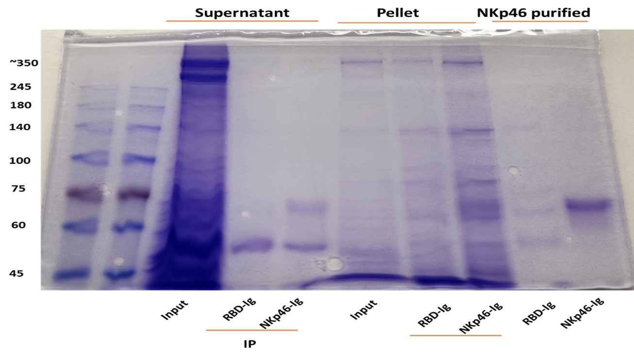
Author response image 2. NKp46 immunoprecipitation with Fusobacterium nucleatum (ATCC 23726) lysates. The resulting lysates of supernatant and pellet of Fusobacterium were immunoprecipitated (IP) with 2.5 μg of Control fusion protein (RBD-Ig) or with NKp46-Ig. 2.5 μg of purified fusion proteins were also run on gel.
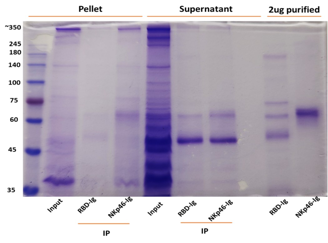
(2) Figure 2: Binding Specificity and Bacterial Strains
A CEACAM1-Ig control should be included in all binding experiments to distinguish between specific and non-specific Ig interactions. There is differential Ig binding between strains ATCC 23726 and 10953. The authors should quantify RadD expression in each strain to determine if the difference in binding is due to variation in RadD levels.
No significant difference in mCEACAM-1-Ig binding was observed across multiple independent experiments. Author response image 3 shows a representative histogram showing mCEACAM-1-Ig binding to F. nucleatum ATCC 23726 and F. polymorphum ATCC 10953. Comparable binding levels were detected in both bacterial species (upper histogram). Similarly, NKp46-Ig and Ncr1-Ig fusion proteins exhibited comparable binding patterns (lower histogram). It is currently not possible to quantify RadD expression directly, as no anti-RadD antibody is available.
Author response image 3. CEACAM-1 Ig binding to Fusobacterium ATCC 23726 and ATCC 10953. Upper histograms show staining with secondary antibody alone (gray) compared to CEACAM-1 Ig (black line). Lower histograms show binding of NKp46 and Ncr1 fusion proteins to the two Fusobacterium strains. Gray represent secondary antibody controls.
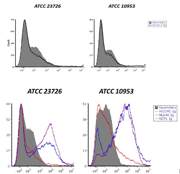
(3) Figure 3: Flow Cytometry Inconsistencies and Missing Controls
What do the FITC-negative, Ig-negative events represent? The authors should clarify whether these are background signals, bacterial aggregates, or debris.
We now present the gating strategy used in these experiments (Author response image 4). Fusion negative Ig samples were the bacterial samples stained only with the secondary antibody APC (anti-human AF647). The TITC-negative represent unlabeled bacteria.
Author response image 4. Gating strategy for FITC-labeled Fusobacterium stained with fusion proteins. Bacteria were first gated as shown in the left panel. The gated population was then further analyzed in the right plot: the lower-left quadrant represents bacterial debris, the upper-left quadrant corresponds to FITC-stained bacteria only, and the upper-right quadrant shows bacteria double-positive for FITC and APC, indicating binding of the fusion proteins.
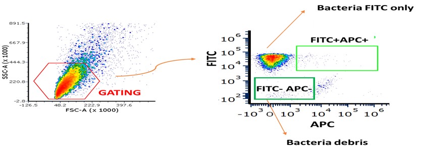
Panel B, CEACAM1-Ig binding appears markedly increased compared to WT bacteria. The reason for this enhancement should be discussed-does it reflect upregulation of the bacterial ligand or an artifact of overexpression? Fluorescence compensation should be carefully reviewed for the NKp46/NCR1-Ig binding assays to ensure that the signals are not due to spectral overlap or nonspecific binding. Importantly, binding experiments using the FadI/RadD double knockout strain are missing and should be included. This control is essential.
We don’t know why expression of CEACAM1-Ig binding is increased. Indeed, it will be nice to have the FadI/RadD double knockout strain which we currently don’t have.
In Panel E, the basis for calculating fold-change in MFI is unclear. Please indicate the reference condition to which the change is normalized.
The mean fluorescence intensity (MFI) fold change was calculated by dividing the MFI obtained from staining with the fusion proteins by the MFI of the corresponding secondary antibody control (bacteria incubated without fusion proteins).
(4) Figure 4: Binding Inhibition and Receptor Sensitivity
Panel A lacks representative FACS plots and is currently difficult to interpret.
Fusobacteria binding to CEACAM-1, NKp46, and NCR1 fusion proteins was tested in the presence of 5 and 10 mM L-arginine (Author response image 5). L-arginine inhibited the binding of NKp46-Ig and NCR1-Ig, whereas no effect was observed on CEACAM-1-Ig binding.
Author response image 5. Fusobacterium binding inhibition by L-Arginine. The figure shows the binding of CEACAM1-Ig (left panel), NKp46-Ig (middle panel), and Ncr1-Ig (right panel) in the presence of 0 mM (black), 5 mM (red), and 10 mM (blue) L-arginine.
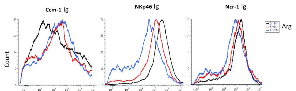
Differences in the sensitivity of human vs. mouse NKp46 to arginine inhibition should be discussed, given species differences in receptor-ligand interactions.
Ncr1, the murine orthologue of human NKp46, shares approximately 58% sequence identity with its human counterpart (1). The observed differences in arginine-mediated inhibition of bacterial binding between mouse and human NKp46 might stem from structural differences or distinct posttranslational modifications, such as glycosylation. Indeed, prediction algorithms combined with high-performance liquid chromatography analysis revealed that Ncr1 possesses two putative novel O-glycosylation sites, of which only one is conserved in humans (2).
References
(1) Biassoni R., Pessino A., Bottino C., Pende D., Moretta L., Moretta A. The murine homologue of the human NKp46, a triggering receptor involved in the induction of natural cytotoxicity. Eur J Immunol. 1999 Mar; 29(3).
(2) Glasner A., Roth Z., Varvak A., Miletic A., Isaacson B., Bar-On Y., Jonjić S., Khalaila I., Mandelboim O. Identification of putative novel O-glycosylations in the NK killer receptor Ncr1 essential for its activity. Cell Discov. 2015 Dec 22; 1:15036.
What are the inhibition results using F. nucleatum strains deficient in FadI?
The inhibition pattern observed in the F. nucleatum ΔFadI mutant was comparable to that of the wild-type strain (Author response image 6). When cultured under identical conditions and exposed to increasing concentrations of arginine (0, 5, and 10 mM), the F. nucleatum ΔFadI strain also demonstrated a dose-dependent reduction in binding to NKp46 and Ncr1.
Author response image 6. Arginine inhibition of NKp46-Ig and Ncr1-Ig binding in F. nucleatum ΔFadI. Histograms show NKp46-Ig (A, C) and Ncr1-Ig (B, D) binding to F. nucleatum ATCC10953 ΔFadI (A and B) and to F. nucleatum ATCC23726 ΔFadI (A and B) following exposure to 5 mM and 10 mM L-Arginine. Panels (E) and (F) display the mean fluorescence intensity (MFI) quantification corresponding to (A and B) and (C and D), respectively.
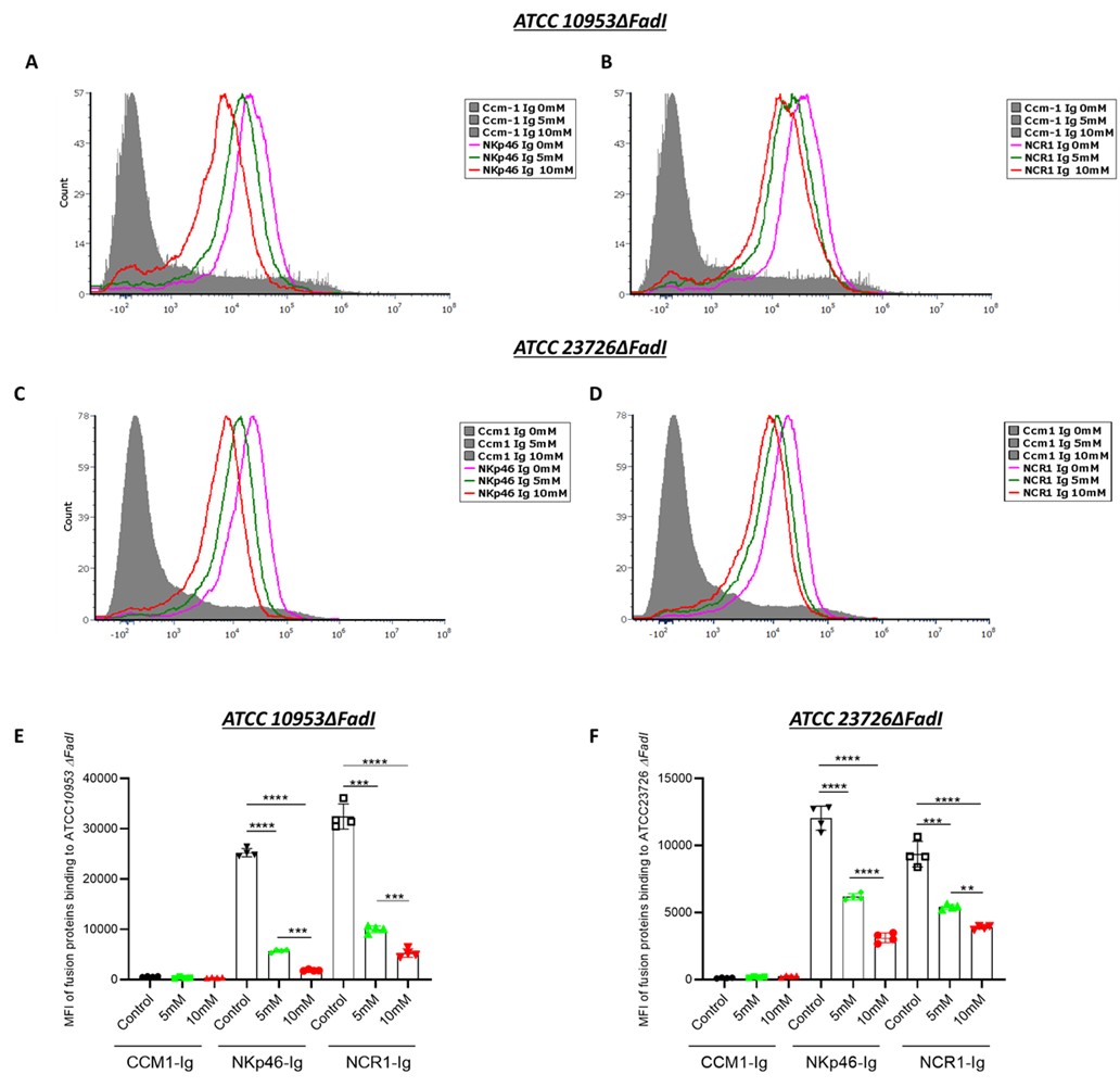
In Panel B, CEACAM1-Ig and RadD-deficient bacteria must be included as negative controls for binding specificity upon anti-NKp46 blocking.
We appreciate the request to include CEACAM1-Ig and RadD-deficient bacteria as negative controls for specificity under anti-NKp46 blocking. We don’t not think it is necessary since the 02 antibody is specific for NKp46, we used other anti0NKp46 antibodies that did not block the interaction and an irrelevant antibofy, we showed that arginine produced a dose-dependent reduction in NKp46/Ncr1 binding, consistent with an arginine-inhibitable RadD interaction already shown in our manuscript (Fig. 4A). The ΔRadD strains we used already demonstrate loss of NKp46/Ncr1 binding and loss of NK-boosting activity (Figs. 3, 5). Collectively, these data establish that NKp46/Ncr1 recognition of a high-molecular-weight ligand consistent with RadD is specific and functionally relevant.
Figure 5: Functional NK Activation and Tumor Killing
In Panels B and C, the key control condition (NK cells + anti-NKp46, without bacteria) is missing. This is needed to evaluate if NKp46 recognition is involved in tumor killing. The authors should explicitly test whether pre-incubation of NK cells with bacteria enhances their anti-tumor activity.
No significant difference in NK cell cytotoxicity was observed between untreated NK cells and NK cells incubated with anti-NKp46 antibody in the absence of bacteria. Therefore, the NK + anti-NKp46 (O2) group was included as an additional control alongside the other experimental conditions shown in Figures 5b and 5c, and is presented in Author response image 7 below.
Author response image 7. NK cytotoxicity against breast cancer cell lines. NK cell cytotoxicity against T47D (left) and MCF7 (right) breast cancer cell lines. This experiment follows the format of Figure 5b and 5c, with the addition of the NK cells + O2 antibody group. No significant differences were observed when values were normalized to NK cells alone.
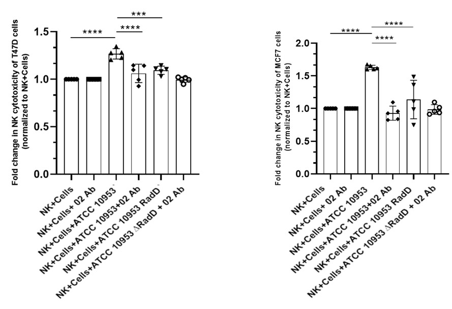
Could bacteria induce stress signals in tumor cells that sensitize them to NK killing? This distinction is critical.
It remains unclear whether the bacteria induce stress-related signals in tumor cells that render them more susceptible to NK cell–mediated cytotoxicity.
(6) Figure 5D: Mechanism of Peripheral Activation
It is suggested that contact between bacteria and NK cells in the periphery leads to their activation. Can the authors confirm whether this pre-activation leads to enhanced killing of tumor targets, or if bacteria-tumor co-localization is required? The literature indicates that F. nucleatum localizes intracellularly within tumor cells. If so, how is RadD accessible to NKp46 on infiltrating NK cells?
We do not expect that pre-activation of NK cells with bacteria would enhance their tumor-killing capacity. In fact, when NK cells were co-incubated with bacteria, we occasionally observed NK cell death. Although F. nucleatum can reside intracellularly, bacterial entry requires prior adhesion to tumor cells. At this stage—before internalization—the bacteria are accessible for recognition and binding by NK cells.
(8) Figure 5E and In Vivo Relevance
Surprisingly, F. nucleatum infection is associated with increased tumor burden. Does this reflect an immunosuppressive effect? Are NK cells inhibited or exhausted in infected mice (TGIT, SIGLEC7...)? If NK cell activation leads to reduced tumor control in the infected context, the role of RadD-induced activation needs further explanation. RadD-deficient bacteria, which do not activate NK cells, result in even poorer tumor control. This paradox needs to be addressed: how can NK activation impair tumor control while its absence also reduces tumor control?
Siglec-7 lacks a direct orthologue in mice, and neither mouse TIGIT nor CEACAM1 bind F. nucleatum. The increased tumor burden observed in infected mice may therefore result from bacterial interference with immune cell infiltration and accumulation within the tumor microenvironment (Parhi, L., Alon-Maimon, T., Sol, A. et al. Breast cancer colonization by Fusobacterium nucleatum accelerates tumor growth and metastatic progression. Nat Commun 11, 3259 (2020)). Consequently, the NK cells that do reach the tumor site can recognize and kill F. nucleatum–bearing tumor cells through RadD–NKp46 interactions. In the absence of RadD, this recognition is impaired, leading to reduced NK-mediated cytotoxicity and increased tumor growth.
(9) NKp46-Deficient Mice: Inconsistencies
In Ncr1⁻/⁻ mice, infection with WT or RadD-deficient F. nucleatum has no impact on tumor burden. This suggests that NKp46 is dispensable in this context and casts doubt on the physiological relevance of the proposed mechanism. This contradiction should be discussed more thoroughly.
Ncr1 is also directly involved in mediating NK cell–dependent killing of tumor cells, even in the absence of bacterial infection. Therefore, in Ncr1-deficient mice, F. nucleatum has no additional effect on tumor progression (Glasner, A., Ghadially, H., Gur, C., Stanietsky, N., Tsukerman, P., Enk, J., Mandelboim, O. Recognition and prevention of tumor metastasis by the NK receptor NKp46/NCR1. J Immunol. 2012).
Reviewer #2 (Public review):
Weaknesses:
(1) A previous study by this group (PMID: 38952680) demonstrated that RadD of F. nucleatum binds to NK cells via Siglec-7, thereby diminishing their cytotoxic potential. They further proposed that the RadD-Siglec-7 interaction could act as an immune evasion mechanism exploited by tumor cells. In contrast, the present study reports that RadD of F. nucleatum can also bind to the activating receptor NKp46 on NK cells, thereby enhancing their cytotoxic function.
Siglec-7 lacks a direct orthologue in mice, and neither mouse TIGIT nor CEACAM1 bind F. nucleatum. In contrast, NKp46 and its murine homologue, Ncr1, both recognize and bind the bacterium.
While F. nucleatum-mediated tumor progression has been documented in breast and colon cancers, the current study proposes an NK-activating role for F. nucleatum in HNSC. However, it remains unclear whether tumor-infiltrating NK cells in HNSC exhibit differential expression of NKp46 compared to Siglec-7. Furthermore, heterogeneity within the NK cell compartment, particularly in the relative abundance of NKp46⁺ versus Siglec-7⁺ subsets, may differ substantially among breast, colon, and HNSC tumors. Such differences could have been readily investigated using publicly available single-cell datasets. A deeper understanding of this subset heterogeneity in NK cells would better explain why F. nucleatum is passively associated with a favorable prognosis in HNSC but correlates with poor outcomes in breast and colon cancers.
Currently, there are no publicly available single-cell datasets suitable for characterizing NK cell heterogeneity in the context of F. nucleatum infection—particularly regarding the expression of Siglec-7, NKp46, or CEACAM1 and their potential association with poor clinical outcomes in breast, head and neck squamous cell carcinoma (HNSC), or colorectal cancer (CRC). Furthermore, no RNA-seq datasets are available for breast cancer cases specifically associated with F. nucleatum infection and poor prognosis. Therefore, we analyzed bulk RNA expression datasets for Siglec-7 and CEACAM1 and evaluated their associations with HNSC and CRC using the same patient databases utilized in our manuscript (Author response image 8). No significant differences in Siglec-7 expression were detected between HNSC and CRC samples (Author response image 8A). Although CEACAM1 mRNA levels did not differ between F. nucleatum–positive and –negative cases within either cancer type, its overall expression was higher in CRC compared to HNSC (Author response image 8B).
Author response image 8. Siglec7 and Ceacam1 expression and the prognostic effect of F. nucleatum in a tumor-type-specific manner. Comparison of Siglec7 (A) and Ceacam1 (B) expression across HNSC and CRC tumors. Log₂ expression levels of NKp46 mRNA were compared across HNSC and CRC cohorts, stratified by F. nucleatum positive and negative. Results were analyzed by one-way ANOVA with Bonferroni post hoc correction.
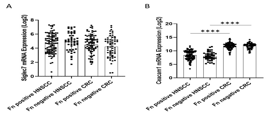
(2) The in vivo tumor data (Figure 5D-F) appear to contradict the authors' claims. Specifically, Figure 5E suggests that WT mice engrafted with AT3 breast tumors and inoculated with WT F. nucleatum exhibited an even greater tumor burden compared to mice not inoculated with F. nucleatum, indicating a tumor-promoting effect. This finding conflicts with the interpretation presented in both the results and discussion sections.
Siglec-7 lacks a direct orthologue in mice, and neither mouse TIGIT nor CEACAM1 bind F. nucleatum. The increased tumor burden observed in infected mice may therefore result from bacterial interference with immune cell infiltration and accumulation within the tumor microenvironment (Parhi, L., Alon-Maimon, T., Sol, A. et al. Breast cancer colonization by Fusobacterium nucleatum accelerates tumor growth and metastatic progression. Nat Commun 11, 3259 (2020)). Consequently, the NK cells that do reach the tumor site can recognize and kill F. nucleatum–bearing tumor cells through RadD–NKp46 interactions. In the absence of RadD, this recognition is impaired, leading to reduced NK-mediated cytotoxicity and increased tumor growth.
(3) Although the authors acknowledge that F. nucleatum may have tumor context-specific roles in regulating NK cell responses, it is unclear why they chose a breast cancer model in which F. nucleatum has been reported to promote tumor growth. A more appropriate choice would have been the well-established preclinical oral cancer model, such as the 4-nitroquinoline 1-oxide (4NQO)-induced oral cancer model in C57BL/6 mice, which would more directly relate to HNSC biology.
The tumor model we employed is, to date, the only model in which F. nucleatum has been shown to exert a measurable effect, which is why we selected it for our study (Parhi, L., Alon-Maimon, T., Sol, A. et al. Breast cancer colonization by Fusobacterium nucleatum accelerates tumor growth and metastatic progression. Nat Commun. 2020; 11: 3259). We have not tested the 4-nitroquinoline-1-oxide (4NQO)–induced oral cancer model, and we are uncertain whether its use would be ethically justified.
(4) Since RadD of F. nucleatum can bind to both Siglec-7 and NKp46 on NK cells, exerting opposing functional effects, the expression profiles of both receptors on intratumoral NK cells should be evaluated. This would clarify the balance between activating and inhibitory signals in the tumor microenvironment and provide a more mechanistic explanation for the observed tumor context-dependent outcomes.
This question was answered in Author response image 8 above.
Lo que más me llamó la atención de la lectura fue la comparación entre la desconfianza de Sócrates hacia la escritura y las críticas actuales hacia la inteligencia artificial. Me pareció muy interesante cómo el autor muestra que, aunque una tecnología pueda generar temor o resistencia, finalmente termina transformando la manera en que pensamos y vivimos, tal como ocurrió con la escritura o las redes sociales. La frase que más me impactó fue: “Si absolutamente todos adoptáramos su uso en todas las áreas de la vida, pronto nadie tendría habilidades.” Me hizo reflexionar sobre la dependencia que estamos desarrollando hacia la inteligencia artificial y sobre el riesgo de perder la capacidad de aprender y crear por nosotros mismos. Creo que el texto podría mejorar si el autor profundizara un poco más en las posibles formas de integrar la IA sin perder el valor del aprendizaje humano, por ejemplo, mostrando ejemplos positivos de cómo esta tecnología puede complementar nuestras capacidades en lugar de reemplazarlas. También sería interesante incluir una perspectiva más global, considerando cómo distintos contextos culturales enfrentan la adopción de la IA.
Author response:
The following is the authors’ response to the original reviews.
Reviewer #1 (Public review):
Summary:
This is an interesting study on the role of FGF signaling in the induction of primitive streak-like cells (PS-LC) in human 2D-gastruloids. The authors use a previously characterized standard culture that generates a ring of PSLCs (TBXT+) and correlate this with pERK staining. A requirement for FGF signaling in TBXT induction is demonstrated via pharmacological inhibition of MEK and FGFR activity. A second set of culture conditions (with no exogenous FGFs) suggests that endogenous FGFs are required for pERK and TBXT induction. The authors then characterize, via scRNA-seq, various components of the FGF pathway (genes for ligands, receptors, ERK regulators, and HSPG regulation). They go on to characterize the pFGFR1, receptor isoforms, and polarized localization of this receptor. Finally, they perform FGF4 inhibition and use a cell line with a limited FGF17 inactivation (heterozygous null) and show that loss of these FGFs reduces PS-LC and derivative cell types.
Strengths:
(1) As the authors point out, the role of FGF signaling in gastrulation is less well understood than other signaling pathways. Hence this is a valuable contribution to that field.
(2) The FGF4 and FGF17 loss-of-function experiments in Figure 5 are very intriguing. This is especially so given the intriguing observation that these FGFs appear to be dominating in this model of human gastrulation, in contrast to what FGFs dominate in mice, chicks, and frogs.
(3) In general this paper is valuable as a further development of the Human gastruloid system and the role of FGF signaling in the induction of PS-CLs. The wide net that the authors cast in characterizing the FGF ligand gene, receptor isoforms, and downstream components provides a foundation for future work. As the authors write near the beginning of the Discussion "Many questions remain."
We thank the reviewer for these positive comments.
Weaknesses:
(1) FGFs are cell survival factors in various aspects of development. The authors fail to address cell death due to loss of FGF signaling in their experiments. For example, in Figure 1E (which requires statistical analysis) and 1G (the bottom FGFRi row), there appears to be a significant amount of cell loss. Is this due to cell death? The authors should address the question of whether the role of FGF/ERK signaling is to keep the cells alive.
Indeed, FGF also strongly affects cell survival and it is an interesting question to what extent this depends on ERK. Our manuscript focuses instead on the role of FGF/ERK signaling in cell fate patterning. As mentioned in our discussion, figure 1de show that doxycycline induced pERK leads to more TBXT+ cells than the control without restoring cell number, suggesting the role of FGF in controlling cell number is independent of the requirement for FGF/ERK in PS-LC differrentiation. To further support this, we have added data showing low doses of MEKi are sufficient to inhibit differentiation without affecting cell number (Supp. Fig. 1i).
To address the reviewers question regarding the cause of cell loss, we now stained for BrdU and cleaved Cas3 to assess proliferation and apoptosis in the presence and absence of MEK and FGFR inhibition (new Supp. Fig.
1ef). This shows that the effect of these inhibitors on cell number is primarily due to a reduction in proliferation. We have also included statistical analysis in Fig.1e.
(2) Regarding the sparse cells in 1G, is there a reduction in cell number only with FGFRi and not MEKi? Is this reproducible? Gattiglio et al (Development, 2023, PMID: 37530863) present data supporting a "community effect" in the FGF-induced mesoderm differentiation of mouse embryonic stem cells. Could a community effect be at play in this human system (especially given the images in the bottom row of 1G)? If the authors don't address this experimentally they should at least address the ideas in Gattoglio et al.
Indeed, FGFRi reproducibly affects cell number more than MEKi, in line with the fact that pathways other than MAPK/ERK downstream of FGF (e.g. PI3K) play important roles in cell survival and growth. However, we think the lack of differentiation in MEKi and FGFRi in Fig.1g cannot be attributed to a loss of cells combined with a community effect. This is because without FGFRi or MEKi cells efficiently differentiate to primitive streak at much lower densities than those originally shown, consistent with the data we discuss in response to (1) arguing against a primarily indirect effect of FGF on PS-LC differentiation through cell density. In the context of directed differentiation (rather than 2D gastruloids), we have now shown in a controlled manner that the effect of MEKi and FGFRi does not depend on a community effect by repeating the experiment in Fig.1g while adjusting cell seeding densities to obtain similar final cell densities in all three conditions (new Fig.1g, new Supp Fig.1g). Furthermore we have included new data showing extremely sparse cells without MEKi or FGFRi still differentiate without problems (new Supp Fig 1h). We have also include Gattoglio et al in our revised discussion.
(3) Do the FGF4 and FGF17 LOF experiments in Figure 5 affect cell numbers like FGFRi in Figure 1?
We did not observe major changes in cell number in the FGF4 and FGF17 loss of function experiments. This is in line with our observation that low levels of ERK signaling are sufficient to maintain proliferation (new Supp. Fig. 1i), and the fact that low levels of ERK signaling are maintained in the absence of FGF4 and FGF17 (Fig.5), likely by FGF2 (Fig. 2). In contrast, FGFRi treatment in Fig.1 leads to a nearly complete loss of FGF signaling (ERK and other pathways) that has a dramatic effect on cell number.
Why examine PS-LC induction only in FGF17 heterozygous cells and not homozygous FGF17 nulls?
We were unable to obtain homozygous FGF17 nulls, it is not clear if there is a reason for this. In the absence of homozygous nulls, we have now further corroborated our findings with additional knockdown data (described in response to other comments below).
(4) The idea that FGF8 plays a dominant role during gastrulation of other species but not humans is so intriguing it warrants deeper testing. The authors dismiss FGF8 because its mRNA "...levels always remained low." (line 363) as well as the data published in Zhai et al (PMID: 36517595) and Tyser et al (PMID: 34789876). But there are cases in mouse development where a gene was expressed at levels so low, that it might be dismissed, and yet LOF experiments revealed it played a role or even was required in a developmental process. The authors should consider FGF8 inhibition or inactivation to explore its potential role, despite its low levels of expression.
We thank the reviewer for this suggestion. We have now analyzed the role of FGF8 using FISH to visualize its expression and siRNA to understand its function (Fig.5d,f,h; Supp.Fig.5e,g,6e). We found that FGF8 expression is higher earlier in differentiation, preceding most expression of TBXT. Our scRNA-seq only analyzed samples at 42h so did not capture this. Furthermore, FGF8 expression localized inside the PS-like ring rather than coinciding with it like FGF4. Surprisingly, FGF8 knockdown led to an increase in primitive streak-like differentiation, suggesting it may counteract FGF4. The results are shown in the revised Fig. 5 and Supplemental Fig. 5. While this certainly merits further investigation, understanding the role of FGF8 in more detail is beyond the scope of the current work.
(5) Redundancy is a common feature in FGF genetics. What is the effect of inhibiting FGF4 in FGF17 LOF cells?
Further siRNA and shRNA experiments showed that FGF17 knockdown had a much smaller effect than FGF4 knockdown on expression of primitive streak markers (Fig.5i, Supp.Fig.6f-i) but that FGF17 knockdown did lead to a complete loss of the mesoderm marker TBX6 (Fig.5j, Supp.Fig.6j). A double knockdown of FGF4+FGF17 looked similar to FGF4 alone (Supp.Fig.6k). Thus, we now think the more likely scenario is that FGF17 is downstream of FGF4-dependent PS-differentiation and although this may have a positive feedback effect whereby this FGF17 can then enhance further PS-differentiation, which we previously interpreted as partial redundancy, the primary role of FGF17 may be later, in mesoderm differentiation.
(6) I suggest stating that the authors take more caution in describing FGF gradients. For example, in one Results heading they write "Endogenous FGF4 and FGF17 gradients underly the ERK activity pattern.", implying an FGF protein gradient. However, they only present data for FGF mRNA , not protein. This issue would be clarified if they used proper nomenclature for gene, mRNA (italics), and protein (no italics) throughout the paper.
Thank you for the suggestion. We have edited the paper to more clearly distinguish protein and mRNA. We do think our data provide substantial indirect evidence for a protein gradient which is what the results heading is meant to convey. Receptor activation is high where ERK activity is high (Fig.3), and receptor activation is limited by ligands, since creating a scratch to let exogenous FGF reach the basal side of cells in the center leads to receptor activation (Fig.4). This strongly suggests ERK activity reflects an FGF protein gradient.
Reviewer #2 (Public review):
Summary:
The role of FGFs in embryonic development and stem cell differentiation has remained unclear due to its complexity. In this study, the authors utilized a 2D human stem cell-based gastrulation model to investigate the functions of FGFs. They discovered that FGF-dependent ERK activity is closely linked to the emergence of primitive streak cells. Importantly, this 2D model effectively illustrates the spatial distribution of key signaling effectors and receptors by correlating these markers with cell fate markers, such as T and ISL1. Through inhibition and loss-of-function studies, they further corroborated the needs of FGF ligands. Their data shows that FGFR1 is the primary receptor, and FGF2/4/17 are the key ligands for primitive streak development, which aligns with observations in primate embryos. Additional experiments revealed that the reduction of FGF4 and FGF17 decreases ERK activity.
Strengths:
This study provides comprehensive data and improves our understanding of the role of FGF signaling in primate
primitive streak formation. The authors provide new insights related to the spatial localization of the key components of FGF signaling and attempt to reveal the temporal dynamics of the signal propagation and cell fate decision, which has been challenging.
Weaknesses:
Given the solid data, the work only partially clarifies the complex picture of FGF signaling, so details remain somewhat elusive. The findings lack a strong punchline, which may limit their broader impact.
We thank this reviewer for their valuable feedback and compliment on the solidity of our data. The punchline of our work is that FGF4 and FGF17-dependent ERK signaling plays a key role in differentiation of human PS-like cells and mesoderm, and that these are different FGFs than those thought to drive mouse gastrulation. A second key point is that like BMP and TGFβ signaling, FGF signaling is restricted to the basolateral sides of pluripotent stem cell colonies due to polarized receptor expression, which is crucial for understanding the response to exogenous ligands added to the cell medium. Indeed, many facets of FGF signaling remain to be investigated in the future, such as how FGF regulates and is regulated by other signals, which we will dedicate a different manuscript to.
Reviewer #3 (Public review):
Jo and colleagues set out to investigate the origins and functions of localized FGF/ERK signaling for the differentiation and spatial patterning of primitive streak fates of human embryonic stem cells in a well-established micropattern system. They demonstrate that endogenous FGF signaling is required for ERK activation in a ringdomain in the micropatterns, and that this localized signaling is directly required for differentiation and spatial patterning of specific cell types. Through high-resolution microscopy and transwell assays, they show that cells receive FGF signals through basally localized receptors. Finally, the authors find that there is a requirement for exogenous FGF2 to initiate primitive streak-like differentiation, but endogenous FGFs, especially FGF4 and FGF17, fully take over at later stages.
Even though some of the authors' findings - such as the localized expression of FGF ligands during gastrulation and the importance of FGF/ERK signaling for cell differentiation in the primitive streak - have been reported in model organisms before, this is one of the first studies to investigate the role of FGF signaling during primitive streak-like differentiation of human cells. In doing so, the paper reports a number of interesting and valuable observations, namely the basal localization of FGF receptors which mirrors that of BMP and Nodal receptors, as well as the existence of a positive feedback loop centered on FGF signaling that drives primitive-streak differentiation. The authors also perform a comparison of the role of different FGFs across species and try to assign specific functions to individual FGFs. In the absence of clean genetic loss-of-function cell lines, this part of the work remains less strong.
We thank the reviewer for emphasizing the value of our findings in a human model for gastrulation. We agree more loss-of-function experiments would provide further insight into the role of different FGFs. While we did not manage to create knockout cell lines, we have now performed both siRNA and shRNA knock-down of all FGF4, and FGF17 in two different hPSC lines, performed siRNA knockdown of FGF8, and also made a FGF4+FGF17 shRNA double knockdown cell lines to more completely test the functions of the individual FGFs (Fig.5, Supp.Fig.5,6). Our data suggest FGF17 may be downstream of FGF4 and primarily required for mesoderm differentiation while FGF8 appears to counteract FGF4. In doing this we have added a large amount of new data to the manuscript and we have removed the heterozygous knockout data in the first version of the manuscript which we felt added little to the new data. Further experiments are still needed to solidify our interpretation but those are beyond the scope of the current work.
Reviewer #1 (Recommendations for the authors):
(1) FGF2 is added to culture experiments (e.g. Figure 4), but the commercial source is not mentioned in Methods. For example, it could be added to "Supplementary Table 1: Cell signaling reagents."
We apologize for this oversight and have now added the information to Supplementary Table 1.
(2) Line 117-118: "For example, by controlling the expression of Wnt or Nodal which are both required for PS-like differentiation". It is clear what the authors mean, but this is not a complete sentence.
We edited this for clarity, it now reads: “First, is FGF/ERK signaling required directly for PS-like differentiation, or does it act indirectly? These possibilities are not mutually exclusive. For example, FGF/ERK could be required directly but also act indirectly by controlling Wnt or Nodal expression, as both Wnt and Nodal signaling are required for PS-like differentiation.”
(3) Line 246 "...found its spatial pattern to strongly resembles that of pERK..." either remove "to" or change "resembles" to "resemble"
Thank you for catching this. We removed “to”.
(4) Lines 391- 393 seem to be missing a word in the last phrase: "...with FGF17 more important continued differentiation to mesoderm and endoderm." Maybe "during" after the word "important"?
Thank you for catching this, indeed the word “during” was missing and we have now added it.
(5) Please define acronyms in Figure 3D (PS-LC was defined previously, but not others).
We apologize for the oversight, we have now defined the acronyms.
(6) The three blue lines in Figure 5B (right) are hard to discern (and I'm not colorblind). I suggest also using a variety of dotted lines in a subset of these FGFs.
Thanks you for the suggestion. We have now given all the FGFs colors that are more clearly distinct and made the TBXT and TBX6 lines dashed.
Reviewer #2 (Recommendations for the authors):
(1) The reviewer acknowledges that FGF signaling is complex, particularly when dynamics and its correlation with cell fates are considered. To improve the clarity of the findings, the authors are encouraged to provide an additional schematic figure that clearly delineates the main findings of this study.
Thank you for the suggestion. We have now added a summary figure (Fig.6) to our discussion, which we hope helps present our findings more clearly.
(2) The data suggest that FGF signaling may function differently in mice compared to primates, and their stem cell model aligns more closely with the latter. While the authors discuss this in the contents only based on sequencing data, it would be valuable to conduct some experiments with mouse embryos to validate the key differences.
It is unclear to us which experiments the reviewer has in mind. There is ample data on FGF expression in the mouse literature, as are many knockout phenotypes. Furthermore, verifying loss of function phenotypes (e.g. FGF17 knockout) in mouse is beyond our expertise.
(3) Heparan sulfate proteoglycan (HSPG) is mentioned as an important component of FGF signaling; however, the only data related to HSPG is single-cell sequencing results. The authors should consider performing immunostaining or other assays to validate HSPG expression and spatial distribution, similar to the approach they used for other signaling components.
Our scratch experiments in Fig. 4 strongly argue against HSPGs as being responsible for the spatial pattern of FGF receptor activation: after a scratch across the colony the response is strong all along the scratch as expected if presence of FGF (an FGF gradient) controls the level of activity. If HSPGs were limiting, FGF flowing in from the media show not be able to uniformly activate receptors around the scratch.
In addtion, we have now included an immunostain for HS in a newly added Supp. Fig. 4 which does not explain the observed pattern of ERK signaling.
(4) In the scratch experiment, particularly high PERK expression is observed at the edge of the scratch. The authors should provide an explanation for why this expression is significantly higher compared to the edges of the colony. Additionally, it would be interesting to investigate the fate of the cells with super high PERK expression.
We have now determined that adaptive response to FGF is the reason that the response around the scratch is initially much higher than in the ERK activity ring that overlaps with the primitive streak-like cells. We have added figures showing that although the intial response to FGF exposure after scratching is very high, the response around the scratch adapts to levels similar in those in the ERK ring over the course of 6 hours (Fig.4ij).
(5) For some of the key experiments, multiple cell lines should be used to ensure that the findings are reproducible and applicable across different human stem cell lines.
We have now checked FISH stainings and knockdown phenotypes for different FGFs in two different cell lines: ESI17 (hESC, XX) and PGP1 (hiPSC, XY). These results are shown in Supplementary Figures 6. We found all results to be consistent.
(6) Where applicable, the meaning of error bars needs to be more clearly presented, including details on the number of independent experiments or samples used.
Thank you for pointing this out. Where error bar definitions were missing we have now added them to the figure captions.
Reviewer #3 (Recommendations for the authors):
(1) The authors only analyze the ppERK ring in micropatterns of a single size. What was the motivation for the choice of this size? Can the authors how the ppERK ring is expected to depend on colony size?
Much smaller patterns lose the interior pluripotent regions while much larger patters have a much larger pluripotent region, which requires larger tilings to image without providing additional insight. The colony sizedependence of cell fate patterning was described in the paper that established the 2D gastruloids model (Warmflash Nat Methods 2014) and we later showed this due to a fixed length scale of the BMP and Nodal signaling gradients from the colony edge (Jo et al Elife 2022). We have now included data showing that the ERK patterns behaves similarly, with a fixed length scale of the pattern implying that in smaller colonies the ERK ring becomes a disc and the entire center of the colony has high ERK signaling (Supp Fig 1a).
(2) The scRNAseq is somewhat confusing - why do the two datasets not overlap in the PHATE representation? This is unexpected, because the two samples have been treated similarly, and the authors have integrated their data to iron out possible batch effects. This discrepancy should be discussed. The authors should also specify from which reference exactly the first dataset comes from.
The two datasets do overlap nicely, the same fates are well mixed in the same place and the gene expresison profiles for the integrated data (e.g., Fig.2e) look smooth, so we believe the integration is good, but different cell fates are represented to different degrees. In particular, sample 2 shows much more mesoderm differentiation making the mesoderm branch mostly orange. Occassionally samples differentiate faster or slower than average which we see here, and these samples were collected far apart in time. We do not believe this affects our conclusions, if anything, we think performing the analysis on two samples that differ this much should make the conclusions more robust.
(3) If find it intriguing that exogenous FGF2 is important early on for primitive streak-like differentiation, although the authors show that it does not reach the center of the colony. The authors may want to discuss this conundrum. Does the FGF2 effect propagate from the outside to the inside, or does it act at an early stage when the cells have not yet formed a tight epithelium on the micropattern?
The cells in the experiment in Fig. 5a were given 24h to epithelialize, so we we do believe it acts from the edge. We believe this may be due to FGF2 modulating the early BMP response on the edge and are working on a manuscript that further explores this pathway crosstalk.
(4) The authors' statement that FGF4 and FGF17 have partially redundant functions is not very strong, mainly because the study lacks a full FGF17 loss-of-function cell line. If the authors wanted to improve on this point, they could knock down FGF4 in the FGF17 heterozygous line, or produce a homozygous FGF17 KO line. If there are specific reasons why FGF17 homozygous lines cannot be produced, this could be interesting to discuss, too. Finally, I noticed that the methods list experiments with an FGF17 siRNA, but these are not shown in the manuscript.
We agree our evidence was previously not as strong as it could be. While there is no reason we know of why homozygous knockout lines cannot be produced, we failed to produce on. To strengthen our evidence we have therefore included substantial new knockdown data. We have now performed both siRNA and shRNA knockdown of all FGF4, and FGF17 in two different hPSC lines, performed siRNA knockdown of FGF8, and also made a FGF4+FGF17 shRNA double knockdown cell lines to more completely test the functions of the individual FGFs (Fig.5, Supp.Fig.5,6). These experiments showed that FGF17 knockdown had a much smaller effect than FGF4 knockdown on expression of primitive streak markers (Fig.5i, Supp.Fig.6f-i) but that FGF17 knockdown did lead to a complete loss of the mesoderm marker TBX6 (Fig.5j, Supp.Fig.6j). A double knockdown of FGF4+FGF17 looked similar to FGF4 alone (Supp.Fig.6k). Thus, we now think the more likely scenario is that FGF17 is downstream of FGF4-dependent PS-differentiation and although this may have a positive feedback effect whereby this FGF17 can then enhance further PS-differentiation, which we previously interpreted as partial redundancy, the primary role of FGF17 may be later, in mesoderm differentiation. Furthermore, our new data suggests FGF8 may counteract FGF4 and limit PS-like differentiation.
Minor
(5) Line 63: Reference(s) appear to be missing.
This whole paragraph summarizes the results of the references given on line 55, we have now repeated the relevant references where the reviewer indicated.
(6) Supplementary Figure 1a,b does not show ppERK, unlike stated in lines 102 - 104.
Indeed, the data described in lines 102-104 is shown in Fig.1a and we have removed the original Supplementary Figure 1ab since it did not provide relevant information.
(7) Line 201: It is not clear whether this is a new sequencing dataset, or if existing datasets have been reanalyzed.
We agree our description was unclear. We have edited the text, which now explicitly states that our analysis is based on one dataset we collected previously and a replicate that was newly collected and deposited on GEO for this manuscript.
(8) Figure 2f; Supplementary Figure 2b, c: The colors need to be explained in scale bars. How has this data been normalized to allow for comparison between very different sample types?
We have now added color bars indicating the scale for each of these figure panels. As the caption stated, the interspecies comparison was normalized within each species, so the highest FGF level for any FGF at any time within each species is normalized to one. We are thus comparing between species the relative expression of different FGFs within each species. Indeed there is no good way to compare absolute expression between species. For extra clarity we have expanded our description of the interspecies comparison analysis and normalization in the methods section.
(9) Line 232: Where is the expression of SEF shown?
It is shown in Fig. 2i, under the official gene name IL17RD.
(10) Supplementary Figure 4 seems to be missing.
Thank you for pointing this out. We have now added a supplementary Fig.4.
(11) Line 437: Citation needed.
We have included citations now.
(12) Line 439: A similar feedback loop has been proposed to operate during mesoderm differentiation in mouse ESC (pmid: 37530863 ). The authors may consider citing this work.
Thank you for the suggestion, we have now included this work in the discussion. The feedback loop proposed in that work involves FGF8, while we were trying to explain why FGF4 and not FGF8 appears to be conserved across species by invoking an FGF4 feedback loop. Thus, it becomes even harder to explain differences in FGF4 and FGF8 expression between human and mouse gastrulation.
(13) Supplementary Figure 6 is not described in the main text.
We have removed the original Supplementary Figure 6 and corresponding heterozygous knockout data in the main figure which we felt added little to the extensive knockdown data we now present. We did create a new Supplementary Figure 6 showing additional knockdown data which is described in the main tekst.
(14) Submission of sequencing data to GEO needs to be updated.
We have now made the GEO data public.
Reviewer #1 (Public review):
Jouary et al. present Megabouts, a Transformer-based classifier and Python toolbox for automated categorization of zebrafish movement bouts into 13 bout types. This is potentially a very useful tool for the zebrafish community. It is broadly applicable to a wide variety of behavioral paradigms and could help to unify behavioral quantification across labs. The overall implementation is technically sound and thoughtfully engineered. The choice of standard Transformer architecture is well-justified (e.g., it can handle long-term tracking data and process missing data, integrates posture and trajectory information over time, and shows robustness to variable frame rates and partial occlusion). The data augmentation strategies (e.g., downsampling, tail masking, and temporal jitter) are well designed to enhance cross-condition generalization. Thus, I very much support this work.
For the benefit of the end users of this tool, several clarifications and additional analyses would be helpful:
(1) What is the source and nature of the classification errors? The reported accuracy is <80% with trajectory data and still <90% with trajectory + tail data.
(1a) Is this due to model failure (is overfitting a concern? How unbiased were the test sets?), imperfections of the preprocessing step (how sensitive is this to noise in the input data?), or underlying ambiguity in the biological data (e.g., do some "errors" reflect intermediate patterns that don't map neatly onto the 13 discrete classes)?
(1b) A systematic error analysis would be helpful. Which classes are most often confused? Are errors systematic (e.g., slow swims vs. routine turns) or random?
(1c) Can confidence of classification be provided for each bout in the data? How would the authors recommend that the end user deal with misclassifications (e.g., by manual correction)?<br /> Overall, the end user would benefit greatly from more information on potential failure modes and their root causes.
(2) How well does the trained network generalize across labs and setups? To what extent have the authors tested this on datasets from other labs to determine how well the pretrained model transfers across datasets? Having tested the code provided by the authors on a short stretch of x-y zebrafish trajectory data obtained independently, the pipeline generates phantom movement annotations. The underlying cause is unclear.
(2a) One possibility is that preprocessing steps may be highly sensitive to slight noise in the x-y positional data, which leads to noise in the speed data. The neural net, in turn, classifies noise into movement annotations. It would be helpful if the authors could add Gaussian noise to the x-y trajectory data and then determine the extent to which the computational pipeline is robust to noise.
(2b) When testing the pipeline, some stationary periods are classified as movements. Which step of the pipeline gave rise to the issue is unclear. Thus, explicit cross-lab validation and robustness tests (e.g., adding Gaussian noise to trajectories) would strengthen the claims of this paper.
(2c) Lastly, given the potential issue of generalization across labs, it would be helpful to provide/outline the steps for users in different labs to retrain and fine-tune the model.
Créer un lien vers la page « Inscrivez-vous gratuitement »
C
Autoriser la connexion des utilisateurs ayant un mot de passe respectant les critères de sécurité
S
Reviewer #2 (Public review):
Summary:
The authors tested an interesting hypothesis that white flies and planthoppers independently evolved salivary proteins to dampen plant immunity by targeting a receptor-like protein.
Strengths:
The authors used a wide range of methods to dissect the function of the white fly protein BtRDP and identify its host target NtRLP4.
Weaknesses:
(1) Serious concerns about protein work.
I did not find the indicated protein bands for anti-BtRDP in Figures 1a and 1b in the original blot pictures shown in Figure S30. In Figure 1a, I can't get the point of showing an unspecific protein band with a size of ~190 kD as a loading control for a protein of ~ 30 kD.
The data discrepancy led me to check other Western blot pictures. Similarly, Figures 2d, 3b, 3d, and S15b (anti-Myc) do not correspond to the original blots shown. In addition, the anti-Myc blot in Figure 4i, all blot pictures in Figures 5b, 5h, and S19a appeared to be compressed vertically. These data raised concerns about the quality of the manuscript.
Blots shown in Figure 3d, 4f, 4g, and 4h appeared to be done at a different exposure rate compared to the complete blot shown in Figure S30. The undesirable connection between Western blot pictures shown in the figures and the original data might be due to the reduced quality of compressed figures during submission. Nevertheless, clarification will be necessary to support the strength of the data provided.
(2) Misinterpretation of data.
I am afraid the authors misunderstood pattern-triggered immunity through receptor-like proteins. It is true that several LRR-type RLPs constitutively associate with SOBIR1, and further recruit BAK1 or other SERKs upon ligand binding. One should not take it for granted that every RLP works this way. To test the hypothesis that NtRLP4 confers resistance to B.tabaci infestation, the author compared transcriptional profiles between an EV plant line and an RLP4 overexpression line. If I understood the methods and figure legends correctly, this was done without B. tabaci treatment. This experimental design is seriously flawed. To provide convincing genetic evidence, independent mutant lines (optionally independent overexpression lines) in combination with different treatments will be necessary. Otherwise, one can only conclude that overexpressing the RLP4 protein generated a nervous plant. In addition, ROS burst, but not H2O2 accumulation, is a common immune response in pattern-triggered immunity.
(3) Lack of logic coherence.
The written language needs substantial improvement. This impeded the readability of the work. More importantly, the logic throughout the manuscript appeared scattered. The choice of testing protein domains for protein-protein interactions, using plants overexpressing an insect protein to study its subcellular localization, switching back and forth between using proteins with signal peptides and without signal peptides, among others, lacks a clear explanation.
Reviewer #3 (Public review):
Summary:
In this study, Wang et al. investigate how herbivorous insects overcome plant receptor-mediated immunity by targeting plant receptor-like proteins. The authors identify two independently evolved salivary effectors, BtRDP in whiteflies and NlSP694 in brown planthoppers, that promote the degradation of plant RLP4 through the ubiquitin-dependent proteasome pathway. NtRLP4 from tobacco and OsRLP4 from rice are shown to confer resistance against herbivores by activating defense signaling, while BtRDP and NlSP694 suppress these defenses by destabilizing RLP4 proteins.
Strengths:
This work highlights a convergent evolutionary strategy in distinct insect lineages and advances our understanding of insect-plant coevolution at the molecular level.
Weaknesses:
(1) I found the naming of BtRDP and NlSP694 somewhat confusing. The authors defined BtRDP as "B. tabaci RLP-degrading protein," whereas NlSP694 appears to have been named after the last three digits of its GenBank accession number (MF278694, presumably). Is there a standard convention for naming newly identified proteins, for example, based on functional motifs or sequence characteristics? As it stands, the inconsistency makes it difficult for readers to clearly distinguish these proteins from those reported in other studies.
(2) Figure 2 and other figures. Transgenic experiments require at least two independent lines, because results from a single line may be confounded by position effects or unintended genomic alterations, and multiple lines provide stronger evidence for reproducibility and reliability.
(3) Figure 3e. Quantitative analysis of NtRLP4 was required. Additionally, since only one band was observed in oeRLP, were any tags included in the construct?
(4) Figure 4a. The RNAi effect appears to be well rescued in Line 1 but poorly in Line 2. Could the authors clarify the reason for this difference?
(5) ROS accumulation is shown for only a single leaf. A quantitative analysis of ROS accumulation across multiple samples would be necessary to support the conclusion. The same applies to Figure 16f.
(6) Figure 4f: NtRLP4 abundance was significantly reduced in oeBtRDP plants but not in oeBtRDP-SP. Although coexpression analysis suggests that BtRDP promotes NtRLP4 degradation in an ubiquitin-dependent manner, the reduced NtRLP4 levels may not result from a direct interaction between BtRDP and NtRLP4. It is possible that BtRDP influences other factors that indirectly affect NtRLP4 abundance. The authors should discuss this possibility.
(7) The statement in lines 335-336 that 'Overexpression of NtRLP4 or NtSOBIR1 enhances insect feeding, while silencing of either gene exerts the opposite effect' is not supported by the results shown in Figures S16-S19. The authors should revise this description to accurately reflect the data.
(8) BtRDP is reported to attach to the salivary sheath. Does the planthopper NlSP694 exhibit a similar secretion localization (e.g., attachment to the salivary sheath)? The authors should supplement this information or discuss the potential implications of any differences in secretion localization between BtRDP and NlSP694 for their respective modes of action.
Author response:
The following is the authors’ response to the previous reviews
Reviewer #1 (Public review):
Summary:
The manuscript characterizes a functional peptidergic system in the echinoderm Apostichopus japonicus that is related to the widely conserved family of calcitonin/diuretic hormone 31 (CT/DH31) peptides in bilaterian animals. In vitro analysis of receptor-ligand interactions, using multiple receptor activation assays, identifies three cognate receptors for two CT-like peptides in the sea cucumber, which stimulate cAMP, calcium, and ERK signaling. Only one of these receptors clusters within the family of calcitonin and calcitonin-like receptors (CTR/CLR) in bilaterian animals, whereas two other receptors cluster with invertebrate pigment dispersing factor receptors (PDFRs). In addition, this study sheds light on the expression and in vivo functions of CT-like peptides in A. japonicus, by quantitative real-time PCR, immunohistochemistry, pharmacological experiments on body wall muscle and intestine preparations, and peptide injection and RNAi knockdown experiments. This reveals a conserved function of CT-like peptides as muscle relaxants and growth regulators in A. japonicus.
Strengths:
This work combines both in vitro and in vivo functional assays to identify a CT-like peptidergic system in an economically relevant echinoderm species, the sea cucumber A. japonicus. A major strength of the study is that it identifies three G protein-coupled receptors for AjCT-like peptides, one related to the CTR/CLR family and two related to the PDFR family. A similar finding was previously reported for the CT-related peptide DH31 in Drosophila melanogaster that activates both CT-type and PDF-type receptors. Here, the authors expand this observation to a deuterostomian animal, which suggests that receptor promiscuity is a more general feature of the CT/DH31 peptide family and that CT/DH31-like peptides may activate both CT-type and PDF-type receptors in other animals as well.
Besides the identification of receptor-ligand pairs, the downstream signaling pathways of AjCT receptors have been characterized, revealing broad and in some cases receptor-specific effects on cAMP, calcium, and ERK signaling.
Functional characterization of the CT-related peptide system in heterologous cells is complemented with ex vivo and in vivo experiments. First, peptide injection and RNAi knockdown experiments establish transcriptional regulation of all three identified receptors in response to changing AjCT peptide levels. Second, ex vivo experiments reveal a conserved role for the two CT-like peptides as muscle relaxants, which have differential effects on body wall muscle and intestine preparations. Finally, peptide injection and knockdown experiments uncover a growth-promoting role for one CT-like peptide (AjCT2). Injection of AjCT2 at high concentration, or long-term knockdown of the AjCT precursor, affects diverse growth-related parameters including weight gain rate, specific growth rate, and transcript levels of growth-regulating transcription factors. The authors also reveal a growth-promoting function for the PDFR-like receptor AjPDFR2, suggesting that this receptor mediates the effects of AjCT2 on growth.
Weaknesses:
The authors present a more detailed phylogenetic analysis in the revised version, including a larger number of species. But some clusters in the analysis are not well supported because they have only low bootstrap values. This makes it difficult to interpret the clustering in some parts of the tree.
Thank you for the reviewer’s comments. In response, we have produced a new phylogenetic analysis using the maximum likelihood method. This was done by Nayeli Escudero Castelán and Kite Jones in the Elphick group at QMUL and therefore they have been added as co-authors of this paper. The new phylogenetic tree (Figure 2, line 206) includes broad taxonomic sampling of CT-type receptors and PDF-type receptors. CRH-type receptors, which are also members of the secretin-type GPCR sub-family, have been included as an outgroup to root the tree. In the previous version the much more distantly related vasopressin/oxytocin-type receptors, which are rhodopsin-type GPCRs, were included as an outgroup. Furthermore, VIP-type receptors were also included in the previous tree but these have been omitted from the new tree because VIP receptor orthologs only occur in vertebrates and therefore they are not representative of a bilaterian GPCR family. The new tree shows high bootstrap support for key clades, notably achieving a bootstrap value of 100 for a clade comprising both deuterostomian and protostomian PDF receptors. This provides important evidence that the A. japonicus PDF-type receptors characterised in this study (AjPDFR1, AjPDFR2) are co-orthologs of the PDF-type receptor that has been characterised previously in Drosophila. Similarly, there is strong bootstrap support (100) for a clade comprising CT/DH31-type receptors and, importantly, the CT-type receptor characterised in this study (AjCTR) is positioned in a branch of this clade that comprises deuterostomian CT-type receptors (with bootstrap support of 100). Details of methods employed to produce the new receptor tree are included in lines 727-739. The new phylogenetic tree is shown below and has been incorporated into the revised manuscript (Figure 2, line 206). The description of new phylogenetic tree has also been modified accordingly in the revised manuscript (line 169-183).
References:
Bauknecht P, Jékely G. Large-Scale Combinatorial Deorphanization of Platynereis Neuropeptide GPCRs. Cell reports, 2015, 12(4), 684–693. doi: 10.1016/j.celrep.2015.06.052.
Beets I, Zels S, Vandewyer E, Demeulemeester J, et al. System-wide mapping of peptide-GPCR interactions in C. elegans. Cell reports, 2023, 42(9), 113058. doi: 10.1016/j.celrep.2023.113058.
Cardoso J C, Mc Shane J C, Li Z, et al. Revisiting the evolution of Family B1 GPCRs and ligands: Insights from mollusca. Molecular and cellular endocrinology, 2024, 586, 112192. doi: 10.1016/j.mce.2024.112192.
Gorn A H, Lin H Y, Yamin M, et al. Cloning, characterization, and expression of a human calcitonin receptor from an ovarian carcinoma cell line. The Journal of clinical investigation, 1992, 90(5), 1726–1735. doi: 10.1172/JCI116046.
Huang T, Su J, Wang X, et al. Functional Analysis and Tissue-Specific Expression of Calcitonin and CGRP with RAMP-Modulated Receptors CTR and CLR in Chickens. Animals: an open access journal from MDPI, 2024, 14(7), 1058. doi: 10.3390/ani14071058.
Johnson E C, Shafer O T, Trigg J S, et al. A novel diuretic hormone receptor in Drosophila: evidence for conservation of CGRP signaling. Journal of Experimental Biology, 2005, 208(7): 1239-1246. doi: 10.1242/jeb.01529.
McLatchie L M, Fraser N J, Main M J, et al. RAMPs regulate the transport and ligand specificity of the calcitonin-receptor-like receptor. Nature, 1998, 393(6683): 333-339. doi: 10.1038/30666.
Schwartz J, Réalis-Doyelle E, Dubos M P, et al. Characterization of an evolutionarily conserved calcitonin signaling system in a lophotrochozoan, the Pacific oyster (Crassostrea gigas). Journal of Experimental Biology, 2019, 222(13): jeb201319. doi: 10.1242/jeb.201319.
Sekiguchi T, Kuwasako K, Ogasawara M, et al. Evidence for conservation of the calcitonin superfamily and activity-regulating mechanisms in the basal chordate Branchiostoma floridae: insights into the molecular and functional evolution in chordates. Journal of Biological Chemistry, 2016, 291(5): 2345-2356. doi: 10.1074/jbc.M115.664003.
Expression of CT-like peptides was investigated both at transcript and protein level, but insight into the expression of the three peptide receptors is limited. This makes it difficult to understand the mechanism underlying the (different) functions of the two CT-like peptides in vivo. The authors identify differences in signal transduction cascades activated by each peptide, which might underpin distinct functions, but these differences were established only in heterologous cells.
We appreciate the reviewer's insightful comments. Regarding expression of CT-like peptide receptors, we have quantitatively analyzed the mRNA expression levels of the three receptors in key tissues using qRT-PCR (Figure 6, line 319) and receptor expression exhibits significant tissue-specific differences. Combined with the heterologous expression assays and In vivo functional validation, we believe our findings have provided clear mechanistic insights into the functional divergence of the two CT-like peptides. Investigation of the expression of the three receptor proteins in A. japonicus would require generation of specific antibodies, which was beyond the scope of this study. Furthermore, immunohistochemical visualization of neuropeptide receptor expression in other invertebrates has not been reported widely, which likely reflects technical difficulties in generation of antibodies that can be used to specifically detect receptor proteins that are typically expressed a low level in comparison to the neuropeptides that act as their ligands.
We acknowledge that investigating signal transduction cascades in heterologous cells (rather than native A. japonicus cells) is a limitation. However, as a non-model organism, A. japonicus currently lacks established cell lines for such research. Therefore, using heterologous cells was the most feasible approach to examine the differential signaling cascades activated by the peptides through the three receptors. Importantly, our in vivo experiments demonstrated that long-term knockdown of either the AjCT precursor or AjPDFR2 resulted in similar and significant growth defects. The phenotypic consistency strongly suggests that AjCT2 and AjPDFR2 function within the same signaling pathway, with AjPDFR2 serving as the key receptor functionally activated by AjCT2.
The authors show overlapping phenotypes for a long-term knockdown of the AjCT precursor and the AjPDFR2 receptor, suggesting that the growth-regulating functions of AjCT2 are mediated by this receptor pathway. However, it remains unclear whether this mechanism underpins the growth-regulating function of AjCT2, until further in vivo evidence for this ligand-receptor interaction is presented. For example, the authors could investigate whether knockdown of AjPDFR2 attenuates the effects of AjCT2 peptide injection. In addition, a functional PDF system in this species remains uncharacterized, and a potential role of PDF-like peptides in growth regulation has not yet been investigated in A. japonicus. Therefore, it also remains unclear whether the ability of CT-like peptides to activate PDFRs is an evolutionary ancient property of this peptide family or whether this is an example of convergent evolution in some protostomian (Drosophila) and deuterostomian (sea cucumber) species.
Thank you for the reviewer’s insightful comments and constructive questions. We acknowledge the request for more direct evidence to demonstrate how AjCT2 functions in vivo through AjPDFR2. However, long-term knockdown of the AjCT precursor and AjPDFR2 both resulted in identical and significant growth defect phenotypes. The high phenotypic consistency, combined with the activation effect of AjCT2 on AjPDFR2 in heterologous cells, strongly suggests that they function within the same signaling pathway, with AjPDFR2 serving as the key receptor functionally activated by AjCT2. While exogenous peptide injection combined with receptor knockdown is a classic method for verifying receptor activation, phenotypic overlap itself is widely accepted in genetic research as robust evidence for pathway association (Shafer and Taghert, 2009; Van Sinay et al., 2017). A. japonicus is a non-model organism with a 3-month aestivation period in summer followed shortly by winter hibernation. During these periods, we are unable to conduct in vivo experiments. Any single experimental suggestion from reviewers could potentially require one more year of research and we have already conducted an additional year of research, in response to reviewer feedback, since submitting the original manuscript. We hope therefore that these challenges associated with working with aquatic invertebrate non-model organisms is recognized by the reviewers.
We fully agree that the functional PDF/PDFR system in A. japonicus and its potential role in growth regulation remain uncharacterized. Currently, the precursors of the PDF-type neuropeptide in echinoderms remain unidentified, which precludes clear pharmacological characterization of the two receptors. While further exploration of echinoderm PDF-type neuropeptides is still needed, our phylogenetic analysis-conducted using the maximum likelihood method with optimized parameters and rigorous sequence curation-demonstrates that the deuterostomian PDFRs (including AjPDFR1 and AjPDFR2) are positioned in a clade with the well-characterized protostomian PDFR clades with extremely high bootstrap support (value=100). Therefore, these two receptors in A. japonicus clearly belong to the PDF receptor family and our findings clearly indicate that the ability of CT-like peptides to activate PDFRs is either an evolutionarily ancient and conserved property or has arisen independently in different lineages. Details of methods employed to produce the new receptor tree are included in line 727-739. The new phylogenetic tree is shown below and has been incorporated into the revised manuscript (Figure 2, line 206). The description of new phylogenetic tree has also been modified accordingly in the revised manuscript (line 169-183).
References:
Bauknecht P, Jékely G. Large-Scale Combinatorial Deorphanization of Platynereis Neuropeptide GPCRs. Cell reports, 2015, 12(4), 684–693. doi: 10.1016/j.celrep.2015.06.052.
Beets I, Zels S, Vandewyer E, Demeulemeester J, et al. System-wide mapping of peptide-GPCR interactions in C. elegans. Cell reports, 2023, 42(9), 113058. doi: 10.1016/j.celrep.2023.113058.
Cardoso J C, Mc Shane J C, Li Z, et al. Revisiting the evolution of Family B1 GPCRs and ligands: Insights from mollusca. Molecular and cellular endocrinology, 2024, 586, 112192. doi: 10.1016/j.mce.2024.112192.
Gorn A H, Lin H Y, Yamin M, et al. Cloning, characterization, and expression of a human calcitonin receptor from an ovarian carcinoma cell line. The Journal of clinical investigation, 1992, 90(5), 1726–1735. doi: 10.1172/JCI116046.
Huang T, Su J, Wang X, et al. Functional Analysis and Tissue-Specific Expression of Calcitonin and CGRP with RAMP-Modulated Receptors CTR and CLR in Chickens. Animals: an open access journal from MDPI, 2024, 14(7), 1058. doi: 10.3390/ani14071058.
Johnson E C, Shafer O T, Trigg J S, et al. A novel diuretic hormone receptor in Drosophila: evidence for conservation of CGRP signaling. Journal of Experimental Biology, 2005, 208(7): 1239-1246. doi: 10.1242/jeb.01529.
McLatchie L M, Fraser N J, Main M J, et al. RAMPs regulate the transport and ligand specificity of the calcitonin-receptor-like receptor. Nature, 1998, 393(6683): 333-339. doi: 10.1038/30666.
Schwartz J, Réalis-Doyelle E, Dubos M P, et al. Characterization of an evolutionarily conserved calcitonin signaling system in a lophotrochozoan, the Pacific oyster (Crassostrea gigas). Journal of Experimental Biology, 2019, 222(13): jeb201319. doi: 10.1242/jeb.201319.
Sekiguchi T, Kuwasako K, Ogasawara M, et al. Evidence for conservation of the calcitonin superfamily and activity-regulating mechanisms in the basal chordate Branchiostoma floridae: insights into the molecular and functional evolution in chordates. Journal of Biological Chemistry, 2016, 291(5): 2345-2356. doi: 10.1074/jbc.M115.664003.
Shafer, O. T., & Taghert, P. H. (2009). RNA-interference knockdown of Drosophila pigment dispersing factor in neuronal subsets: the anatomical basis of a neuropeptide's circadian functions. PloS one, 4(12), e8298. doi: 10.1371/journal.pone.0008298.
Van Sinay, E., Mirabeau, O., Depuydt, G., Van Hiel, M. B., Peymen, K., Watteyne, J., Zels, S., Schoofs, L., & Beets, I. (2017). Evolutionarily conserved TRH neuropeptide pathway regulates growth in Caenorhabditis elegans. Proceedings of the National Academy of Sciences of the United States of America, 114(20), E4065–E4074. doi: 10.1073/pnas.1617392114.
Reviewer #2 (Public review):
Summary:
The authors show that A. japonicus calcitonins (AjCT1 and AjCT2) activate not only the calcitonin/calcitonin-like receptor, but they also activate the two "PDF receptors", ex vivo. They also explore secondary messenger pathways that are recruited following receptor activation. They determine the source of CT1 and CT2 using qPCR and in situ hybridization and finally test the effects of these peptides on tissue contractions, feeding and growth. This study provides solid evidence that CT1 and CT2 act as ligands for calcitonin receptors; however, evidence supporting cross-talk between CT peptides and "PDF receptors" is weak.
Strengths:
This is the first study to report pharmacological characterization of CT receptors in an echinoderm. Multiple lines of evidence in cell culture (receptor internalization and secondary messenger pathways) support this conclusion.
Weaknesses:
The authors claim that A. japonicus CTs activate "PDF" receptors and suggest that this cross-talk is evolutionary ancient since similar phenomenon also exists in the fly Drosophila melanogaster. These conclusions are not fully supported. The authors perform phylogenetic analysis to show that the two "PDF" receptors form an independent clade. The bootstrap support is quite low in a lot of instances, especially for the deuterostomian and protostomian PDFR clades which is below 30. With such low support, it is unclear if the clade comprising deuterostomian "PDFR" is in fact PDFRs and not another receptor type whose endogenous ligand (besides CT) remains to be discovered.
Thank you for the reviewer’s comments. In response, we have produced a new phylogenetic analysis using the maximum likelihood method. This was done by Nayeli Escudero Castelán and Kite Jones in the Elphick group at QMUL and therefore they have been added as co-authors of this paper. The new phylogenetic tree (Figure 2, line 206) includes broad taxonomic sampling of CT-type receptors and PDF-type receptors. CRH-type receptors, which are also members of the secretin-type GPCR sub-family, have been included as an outgroup to root the tree. In the previous version the much more distantly related vasopressin/oxytocin-type receptors, which are rhodopsin-type GPCRs, were included as an outgroup. Furthermore, VIP-type receptors were also included in the previous tree but these have been omitted from the new tree because VIP receptor orthologs only occur in vertebrates and therefore they are not representative of a bilaterian GPCR family. The new tree shows high bootstrap support for key clades, notably achieving a bootstrap value of 100 for a clade comprising both deuterostomian and protostomian PDF receptors. This provides important evidence that the A. japonicus PDF-type receptors characterized in this study (AjPDFR1, AjPDFR2) are co-orthologs of the PDF-type receptor that has been characterized previously in Drosophila. Similarly, there is strong bootstrap support (100) for a clade comprising CT/DH31-type receptors and, importantly, the CT-type receptor characterized in this study (AjCTR) is positioned in a branch of this clade that comprises deuterostomian CT-type receptors (with bootstrap support of 100). Details of methods employed to produce the new receptor tree are included in lines 727-739. The new phylogenetic tree is shown below and has been incorporated into the revised manuscript (Figure 2, line 206). The description of new phylogenetic tree has also been modified accordingly in the revised manuscript (line 169-183).
References:
Bauknecht P, Jékely G. Large-Scale Combinatorial Deorphanization of Platynereis Neuropeptide GPCRs. Cell reports, 2015, 12(4), 684–693. doi: 10.1016/j.celrep.2015.06.052.
Beets I, Zels S, Vandewyer E, Demeulemeester J, et al. System-wide mapping of peptide-GPCR interactions in C. elegans. Cell reports, 2023, 42(9), 113058. doi: 10.1016/j.celrep.2023.113058.
Cardoso J C, Mc Shane J C, Li Z, et al. Revisiting the evolution of Family B1 GPCRs and ligands: Insights from mollusca. Molecular and cellular endocrinology, 2024, 586, 112192. doi: 10.1016/j.mce.2024.112192.
Gorn A H, Lin H Y, Yamin M, et al. Cloning, characterization, and expression of a human calcitonin receptor from an ovarian carcinoma cell line. The Journal of clinical investigation, 1992, 90(5), 1726–1735. doi: 10.1172/JCI116046.
Huang T, Su J, Wang X, et al. Functional Analysis and Tissue-Specific Expression of Calcitonin and CGRP with RAMP-Modulated Receptors CTR and CLR in Chickens. Animals: an open access journal from MDPI, 2024, 14(7), 1058. doi: 10.3390/ani14071058.
Johnson E C, Shafer O T, Trigg J S, et al. A novel diuretic hormone receptor in Drosophila: evidence for conservation of CGRP signaling. Journal of Experimental Biology, 2005, 208(7): 1239-1246. doi: 10.1242/jeb.01529.
McLatchie L M, Fraser N J, Main M J, et al. RAMPs regulate the transport and ligand specificity of the calcitonin-receptor-like receptor. Nature, 1998, 393(6683): 333-339. doi: 10.1038/30666.
Schwartz J, Réalis-Doyelle E, Dubos M P, et al. Characterization of an evolutionarily conserved calcitonin signaling system in a lophotrochozoan, the Pacific oyster (Crassostrea gigas). Journal of Experimental Biology, 2019, 222(13): jeb201319. doi: 10.1242/jeb.201319.
Sekiguchi T, Kuwasako K, Ogasawara M, et al. Evidence for conservation of the calcitonin superfamily and activity-regulating mechanisms in the basal chordate Branchiostoma floridae: insights into the molecular and functional evolution in chordates. Journal of Biological Chemistry, 2016, 291(5): 2345-2356. doi: 10.1074/jbc.M115.664003.
Reviewer #2 (Recommendations for the authors):
Figure 1C: The bootstrap support is quite low in a lot of instances, especially for the deuterostomian and protostomian PDFR clades which is below 30. With such support, I would be hesitant to label the blue clade as deuterostomian PDFR for two reasons: 1) no members of this clade have been shown to be activated by a PDF-like substance and 2) the current study shows that these receptors are activated by CT-type peptides. Therefore, the phylogenetic analyses do not support the conclusions of this paper. What is the basis for calling these receptors PDFR and not CTR in light of weak phylogenetic support?
Thank you for the reviewer’s comments. In response, we have produced a new phylogenetic analysis using the maximum likelihood method. This was done by Nayeli Escudero Castelán and Kite Jones in the Elphick group at QMUL and therefore they have been added as co-authors of this paper. The new phylogenetic tree (Figure 2, line 206) includes broad taxonomic sampling of CT-type receptors and PDF-type receptors. CRH-type receptors, which are also members of the secretin-type GPCR sub-family, have been included as an outgroup to root the tree. In the previous version the much more distantly related vasopressin/oxytocin-type receptors, which are rhodopsin-type GPCRs, were included as an outgroup. Furthermore, VIP-type receptors were also included in the previous tree but these have been omitted from the new tree because VIP receptor orthologs only occur in vertebrates and therefore they are not representative of a bilaterian GPCR family. The new tree shows high bootstrap support for key clades, notably achieving a bootstrap value of 100 for a clade comprising both deuterostomian and protostomian PDF receptors. This provides important evidence that the A. japonicus PDF-type receptors characterized in this study (AjPDFR1, AjPDFR2) are co-orthologs of the PDF-type receptor that has been characterized previously in Drosophila. Similarly, there is strong bootstrap support (100) for a clade comprising CT/DH31-type receptors and, importantly, the CT-type receptor characterized in this study (AjCTR) is positioned in a branch of this clade that comprises deuterostomian CT-type receptors (with bootstrap support of 100). Details of methods employed to produce the new receptor tree are included in lines 727-739 The new phylogenetic tree is shown below and has been incorporated into the revised manuscript (Figure 2, line 206). The description of new phylogenetic tree has also been modified accordingly in the revised manuscript (line 169-183).
We agree with the reviewer that no members of the PDF-type receptor clade in deuterostomes have yet been shown to be activated by a PDF-like substance. That is because the precursors of the PDF-type neuropeptides in echinoderms remain unidentified so far, which precludes clear pharmacological characterization of these receptors within the deuterostomian PDFR clade. However, the new phylogenetic tree now provides strong support (bootstrap value = 100) for the clade comprising deuterostomian and protostomian PDFRs, confirming the classification of AjPDFR1 and AjPDFR2 as PDF-type receptors.
References:
Bauknecht P, Jékely G. Large-Scale Combinatorial Deorphanization of Platynereis Neuropeptide GPCRs. Cell reports, 2015, 12(4), 684–693. doi: 10.1016/j.celrep.2015.06.052.
Beets I, Zels S, Vandewyer E, Demeulemeester J, et al. System-wide mapping of peptide-GPCR interactions in C. elegans. Cell reports, 2023, 42(9), 113058. doi: 10.1016/j.celrep.2023.113058.
Cardoso J C, Mc Shane J C, Li Z, et al. Revisiting the evolution of Family B1 GPCRs and ligands: Insights from mollusca. Molecular and cellular endocrinology, 2024, 586, 112192. doi: 10.1016/j.mce.2024.112192.
Gorn A H, Lin H Y, Yamin M, et al. Cloning, characterization, and expression of a human calcitonin receptor from an ovarian carcinoma cell line. The Journal of clinical investigation, 1992, 90(5), 1726–1735. doi: 10.1172/JCI116046.
Huang T, Su J, Wang X, et al. Functional Analysis and Tissue-Specific Expression of Calcitonin and CGRP with RAMP-Modulated Receptors CTR and CLR in Chickens. Animals: an open access journal from MDPI, 2024, 14(7), 1058. doi: 10.3390/ani14071058.
Johnson E C, Shafer O T, Trigg J S, et al. A novel diuretic hormone receptor in Drosophila: evidence for conservation of CGRP signaling. Journal of Experimental Biology, 2005, 208(7): 1239-1246. doi: 10.1242/jeb.01529.
McLatchie L M, Fraser N J, Main M J, et al. RAMPs regulate the transport and ligand specificity of the calcitonin-receptor-like receptor. Nature, 1998, 393(6683): 333-339. doi: 10.1038/30666.
Schwartz J, Réalis-Doyelle E, Dubos M P, et al. Characterization of an evolutionarily conserved calcitonin signaling system in a lophotrochozoan, the Pacific oyster (Crassostrea gigas). Journal of Experimental Biology, 2019, 222(13): jeb201319. doi: 10.1242/jeb.201319.
Sekiguchi T, Kuwasako K, Ogasawara M, et al. Evidence for conservation of the calcitonin superfamily and activity-regulating mechanisms in the basal chordate Branchiostoma floridae: insights into the molecular and functional evolution in chordates. Journal of Biological Chemistry, 2016, 291(5): 2345-2356. doi: 10.1074/jbc.M115.664003.
The new results following AjCT and AjPDFR2 knockdown are a welcome addition. While this additional evidence supports the claim that AjCT could mediate its effects via AjPDFR2, this evidence does not show that AjCT acts as an endogenous ligand for PDFR in vivo. In combination with the weak phylogenetic analyses, I would recommend the authors to key down their claims that they have functionally characterized a PDFR (in the title and text).
Thank you for your insightful comments and we do understand the reviewer’s concern.
Regarding “the weak phylogenetic analyses”, as highlighted above, we have produced a new phylogenetic tree (Fig 2, line 206) that provides strong bootstrap support for the clade comprising deuterostome and protostome PDF-type receptors. For this reason, it is our opinion that inclusion of “pigment-dispersing factor-type receptors” in the title of the paper is appropriate. The details of phylogenetic analysis method were added in line 727-739, and the updated phylogenetic tree has been incorporated into the revised manuscript (Figure 2, line 206). The description of new phylogenetic tree has also been modified accordingly in the revised manuscript (line 169-183). Besides, long-term knockdown of the AjCT precursor and AjPDFR2 both resulted in identical and significant growth defect phenotypes. And the observation of phenotypic overlap is widely accepted in genetic research as strong evidence for pathway association (Shafer and Taghert, 2009; Van Sinay et al., 2017). This high degree of phenotypic consistency, coupled with our in vitro finding that AjCT2 specifically activates AjPDFR2, strongly supports the conclusion that AjCT2 and AjPDFR2 function within the same signaling pathway in vivo, with AjPDFR2 serving as the key receptor functionally activated by AjCT2.
References:
Shafer, O. T., & Taghert, P. H. (2009). RNA-interference knockdown of Drosophila pigment dispersing factor in neuronal subsets: the anatomical basis of a neuropeptide's circadian functions. PloS one, 4(12), e8298. doi: 10.1371/journal.pone.0008298.
Van Sinay, E., Mirabeau, O., Depuydt, G., Van Hiel, M. B., Peymen, K., Watteyne, J., Zels, S., Schoofs, L., & Beets, I. (2017). Evolutionarily conserved TRH neuropeptide pathway regulates growth in Caenorhabditis elegans. Proceedings of the National Academy of Sciences of the United States of America, 114(20), E4065–E4074. doi: 10.1073/pnas.1617392114.
Since there is no formal logic defining the use of "type" vs "like" vs "related", I would encourage the authors to use one term (of their choice) to avoid unnecessary confusion. Or another possibility is that these relationships are defined at some point in the manuscript so that it becomes clear to the reader.
Thank you for the reviewer’s comments. The “CT-related peptides” has defined in the Introduction (line 54-58). As per your suggestion, we have now defined both “CT-type peptides” and “CT-like peptides” in the Introduction (line 76-79). “CT-type peptides” are characterized by an N-terminal disulphide bridge, whereas “CT-like peptides” (diuretic hormone 31 (DH31)-type peptides) lack this feature. Additionally, in accordance with the definitions, we have corrected these three descriptions in the revised manuscript (line 80, 83, 88 for “CT-type peptides”) to ensure consistent and accurate usage of these terms.
"To provide in vivo evidence supporting CT-mediated activation of "PDF" receptors, we conducted the following experiments: Firstly, we confirmed that AjPDFR1 and AjPDFR2were the functional receptors of AjCT1and AjCT2 (Figure 2, 3 and 4). Secondly, injection of AjCT2 and siAjCTP1/2-1 in vivo induced corresponding changes in AjPDFR1and AjPDFR2expression levels in the intestine (Figure 8C, 9A, 9B and 9C)."
None of these experiments provide direct evidence that CT activates PDFR in vivo. The functional studies are indeed a welcome addition but they cannot discriminate between correlation and causation.
Thank you for the reviewer’s insightful comments. We agree that the functional studies do not constitute direct proof that CT’s activation of PDFR in vivo. However, we observed identical and significant growth defect phenotypes following long-term knockdown of the AjCT precursor and the AjPDFR2. This high degree of phenotypic congruence, combined with the established in vitro activation of AjPDFR2 by AjCT2, provides strong support for the conclusion that AjCT2 acts as the key endogenous ligand activating the AjPDFR2 signaling pathway in vivo. Importantly, such phenotypic overlap has been widely accepted in genetic research as strong evidence for functional pathway association (Shafer and Taghert, 2009; Van Sinay et al., 2017).
References:
Shafer, O. T., & Taghert, P. H. (2009). RNA-interference knockdown of Drosophila pigment dispersing factor in neuronal subsets: the anatomical basis of a neuropeptide's circadian functions. PloS one, 4(12), e8298. doi: 10.1371/journal.pone.0008298.
Van Sinay, E., Mirabeau, O., Depuydt, G., Van Hiel, M. B., Peymen, K., Watteyne, J., Zels, S., Schoofs, L., & Beets, I. (2017). Evolutionarily conserved TRH neuropeptide pathway regulates growth in Caenorhabditis elegans. Proceedings of the National Academy of Sciences of the United States of America, 114(20), E4065–E4074. doi: 10.1073/pnas.1617392114.
RRID:AB_2869702
DOI: 10.1038/s43856-025-01193-y
Resource: (BD Biosciences Cat# 565694, RRID:AB_2869702)
Curator: @scibot
SciCrunch record: RRID:AB_2869702